/


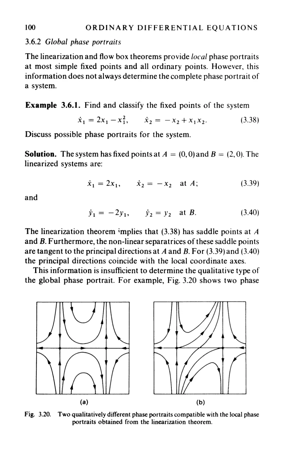
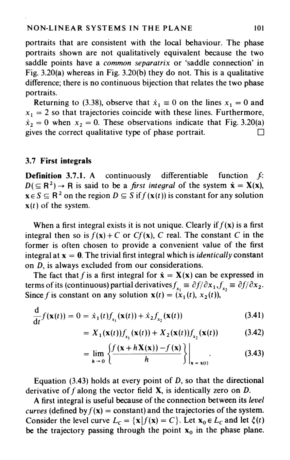


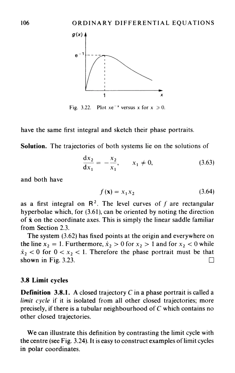


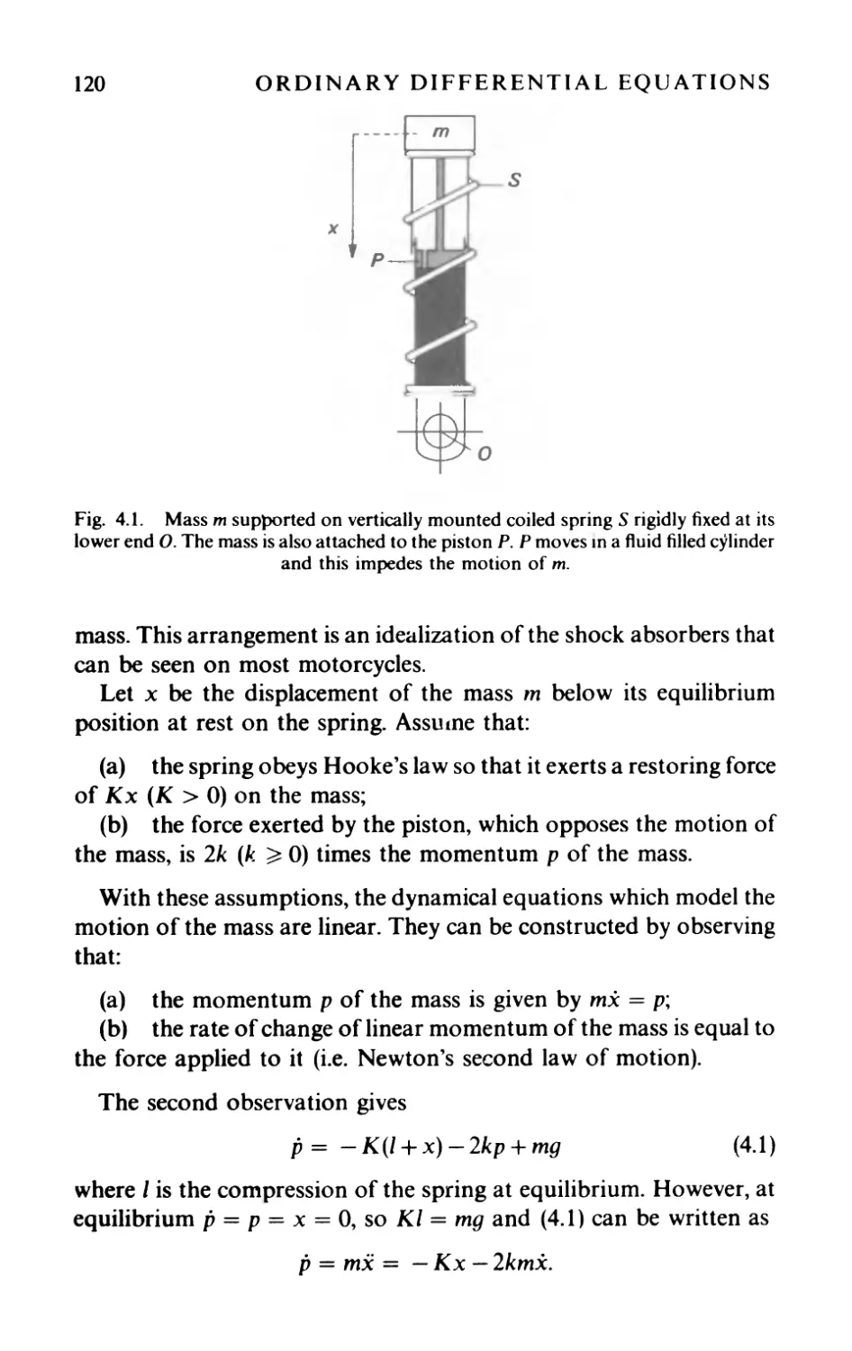


![5.6 A mathematical mode] of tumor growth](https://djvu.online/jpg/G/w/G/GwGYh3YdhuXUV/225.webp)


Автор: Arrowsmith D.K. Place C.M.
Теги: mathematics higher mathematics differential equations chapman and hall publisher
ISBN: 0-412-22600--6
Год: 1982


Текст
Ordinary
DifferentiaI
Equations
A qualitative approach with applications
D. K. ARROWSMITH
Queen Mary and Westfield College
University of London
C. M. PLACE
Previously of Westfield College
University of London
s
CHAPMAN AND HALL
LONDON · NEW YORK · TOKYO. MELBOURNE. MADRAS
UK
USA
JAPAN
AUSTRALIA
INDIA
Chapman and Hall, Il New Fetter Lane,
London EC4P 4EE
Chapman and Hall, 29 West 35th Street,
New York NY10001
Chapman and Hall Japan, Thomson Publishing Japan,
Hirakawacho Nemoto Building, 7F, 1-7-11 Hirakawa-cho,
Chiyoda-ku, Tokyo 102
Chapman and Hall Australia, Thomas Nelson Australia, 480
La Trobe Street, PO Box 4725, Melbourne 3000
Chapman and Hall India, R. Sheshadri, 32 Second Main Road,
CIT East, Madras 600 035
First edition 1982
Reprinted 1990
@ 1982 D. K. Arrowsmith and C. M. Place
Phototypeset by Macmillan India Ltd, Bangalore
Printed in Great Britain by J. W. Arrowsmith Ltd, Bristol
ISBN () 412 22600 6 (HB)
o 412 22610 3 (PB)
AlI rights reserved. No part of this publication may be
reproduced or transmitted, in any form or by any means,
electronic, mechanical, photocopying, recording or otherwisc,
or stored in any retrieval system of any nature, without the
written permission of the copyright holder and the publisher,
application for which shall be made to the publisher.
Library of Congress in Publication Data
Arrowsmith, D. K.
Ordinary differential equations.
(Chapman and Hall mathematics series)
Bibliography: p.
Includes index.
1. Differentiai equations. 1. Place, C. M.
II. Title. III. Series.
QA372.A74 515.3'52
ISBN 0-412-22600--6
ISBN 0-412-22610-3 (pbk.)
81-14003
AACR2
British Library Cataloguing in Publication Data
Arrowsmith, D. K.
Ordinary differential equations.-(Chapman and
Hall mathematics series)
1. Differentiai equations
1. Title Il. Place, C. M.
515.3'5 QA371
ISBN 0-412-22600-6
ISBN 0-412-22610-3 PbK
Preface
ln this book we present an introduction to the qualitative theory of
ordinary differential equations and its applications to the modelling
of time-dependent systems. The mathematical ideas involved consist
of a fascinating blend of calculus, algebra and geometry so that the
reader makes use of a variety of mathematical skills. Variety is also a
feature of the applications and aIl kinds of dynamical systems are
encountered from the more traditional mechanical and electrical
problems to models in ecology, economics and cancer research.
The text is primarily aimed at second year undergraduate students
and the reader is assumed to have completed first courses in Calculus
of Several Variables and Linear Algebra. Thus, a knowledge of
continuity, differentiability, level curves and critical points of func-
tions of two variables is assumed. Algebraic ideas such as bases,
linear transformations, eigenvalues and eigenvectors and similarity
are ta ken to be within the readers' experience but Jordan forms are
not. The relevant results in this last area are simply stated and
illustrated. Our approach throughout the text is to use examples,
wherever possible, to explain the significance of the theorems
introduced. We wish to show the reader what results are available and
how to use them. ln this way, we hope to provide not only the
knowledge necessary to construct and analyse the models but also to
stimulate interest in a deeper understanding of the mathematical
results themselves.
The book is divided into five chapters. Chapter 1 introduces the
VI
PREFACE
state space approach by considering differential equations involving
onlya single real variable. The elementary techniques from calculus
for the solution of such differential equations are treated in exercises
and attention is focused on the geometrical interpretation of the
solutions. Ideas such as autonomous equations, phase portraits and
qualitative equivalence are introduced in this setting. The chapter
goes on to consider how these ideas can be extended to systems of
difTerential equations and gives an overview ofwhat is to be studied in
later chapters. Chapter 2 deals with linear systems, with particular
emphasis on pairs of coupled differential equations. A self contained
treatment of the Jordan forms of 2 x 2 real matrices is given in order
to bring out the connection with the readers' own algebraic
experience. Chapter 3 contains a treatment of some basic results for
non-linear systems. The material has been chosen with second year
undergraduates particularly in mind. The linearization theorem is
introduced and the distinction between local and global analysis is
discussed. The chapter ends with a discussion of limit cycles and
Poincaré-Bendixson theory. ln Chapter 4, we illustrate the role of the
qualitative approach in modelling and in Chapter 5 we present a
selection of topics of a somewhat more advanced nature. This last
chapter is possibly more suitable to third year undergraduate
students, although the idea of a Liapunov function could be discussed
earlier. Each chapter is provided with exercises to consolidate the
ideas developed in the text and to encourage the reader to think
critically about what has been discussed. Hints to solutions are also
gIven.
Finally, we would like to thank Professors R. Brown and
M. P. Eastham and Drs J. D. Knowles and R. Smith for reading and
commenting on the manuscript. We are also grateful to Mrs G. A.
Place for her accurate typing of the manuscript and help with the
diagrams.
D. K. Arrowsmith
C. M. Place
Contents
Preface page v
J Introduction 1
1.1 Preliminary ideas 1
1.1.1 Existence and uniqueness 1
1.1.2 Geometrical representation 3
1.2 Autonomous equations 7
1.2. 1 Solution curves and the phase portrait 7
1.2.2 Phase portraits and dynamics 12
1.3 Autonomous systems in the plane 14
1.4 Construction of phase portraits in the plane 18
1.4.1 Use of calculus 19
1.4.2 Isoclines 23
1.5 Flows and evolution 25
Exercises 30
" Linear systems 39
M
2.1 Lînear changes of variable 39
2.2 Similarity types for 2 x 2 real matrices 42
2.3 Phase portraits for canonical systems in the plane 48
2.3. 1 Simple canonical systems 48
2.3.2 Non-simple canonical systems 52
2.4 Classification of simple linear phase portraits in the
plane 52
2.4.1 Phase portrait of a simple Iinear system 52
VUl CONTENTS
2.4.2 Types of canonical system and qualitative
equivalence 56
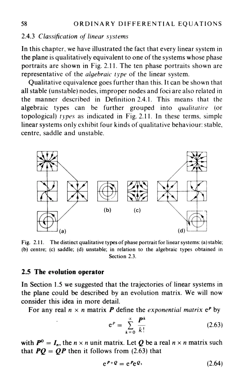
2.4.3 Classification of linear systems 58
2.5 The evolution operator 58
2.6 Affine systems 61
2.7 Linear systems of dimension greater than two 64
2.7.1 Three-dimensional systems 64
2.7.2 Four-dimensional systems 67
2.7.3 n-Dimensional systems 69
Exercises 70
3 Non-Iinear systems in the plane 79
3.1 Local and global behaviour 79
3.2 Linearization at a fixed point 82
3.3 The linearization theorem 85
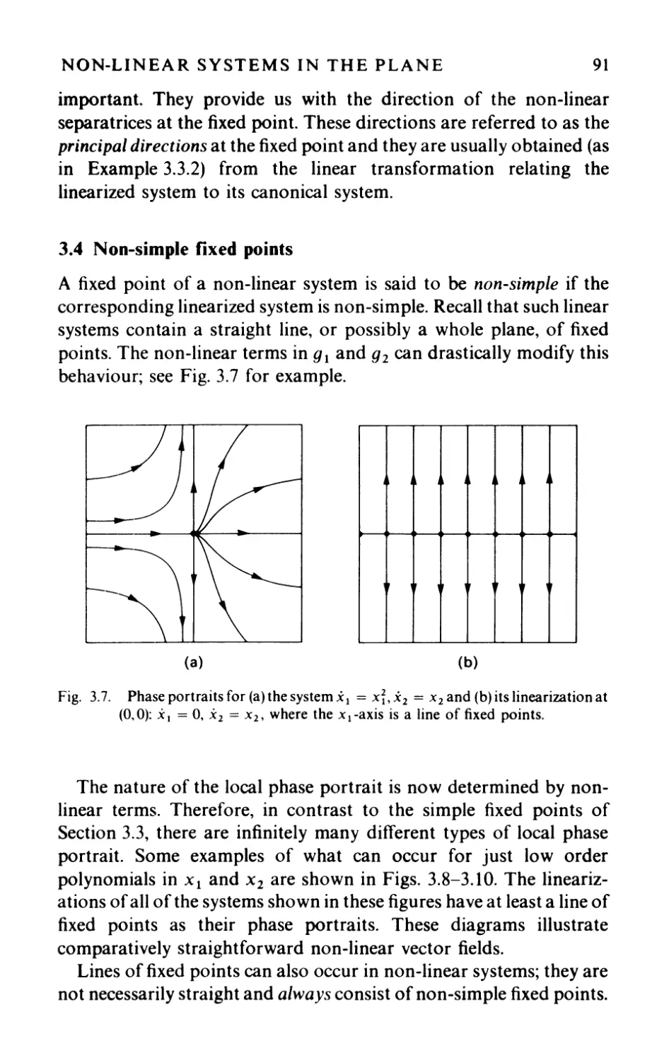
3.4 Non-simple fixed points 91
3.5 Stability of fixed points 93
3.6 Ordinary points and global behaviour 97
3.6.1 Ordinary points 97
3.6.2 Global phase portraits 100
3.7 First integrals 101
3.8 Limit cycles 106
3.9 Poincaré-Bendixson theory 109
Exercises 113
4 Applications 119
4.1 Linear models 119
4.1.1 A mechanical oscillator 119
4.1.2 Electrical circuits 125
4.1. 3 Economics 129
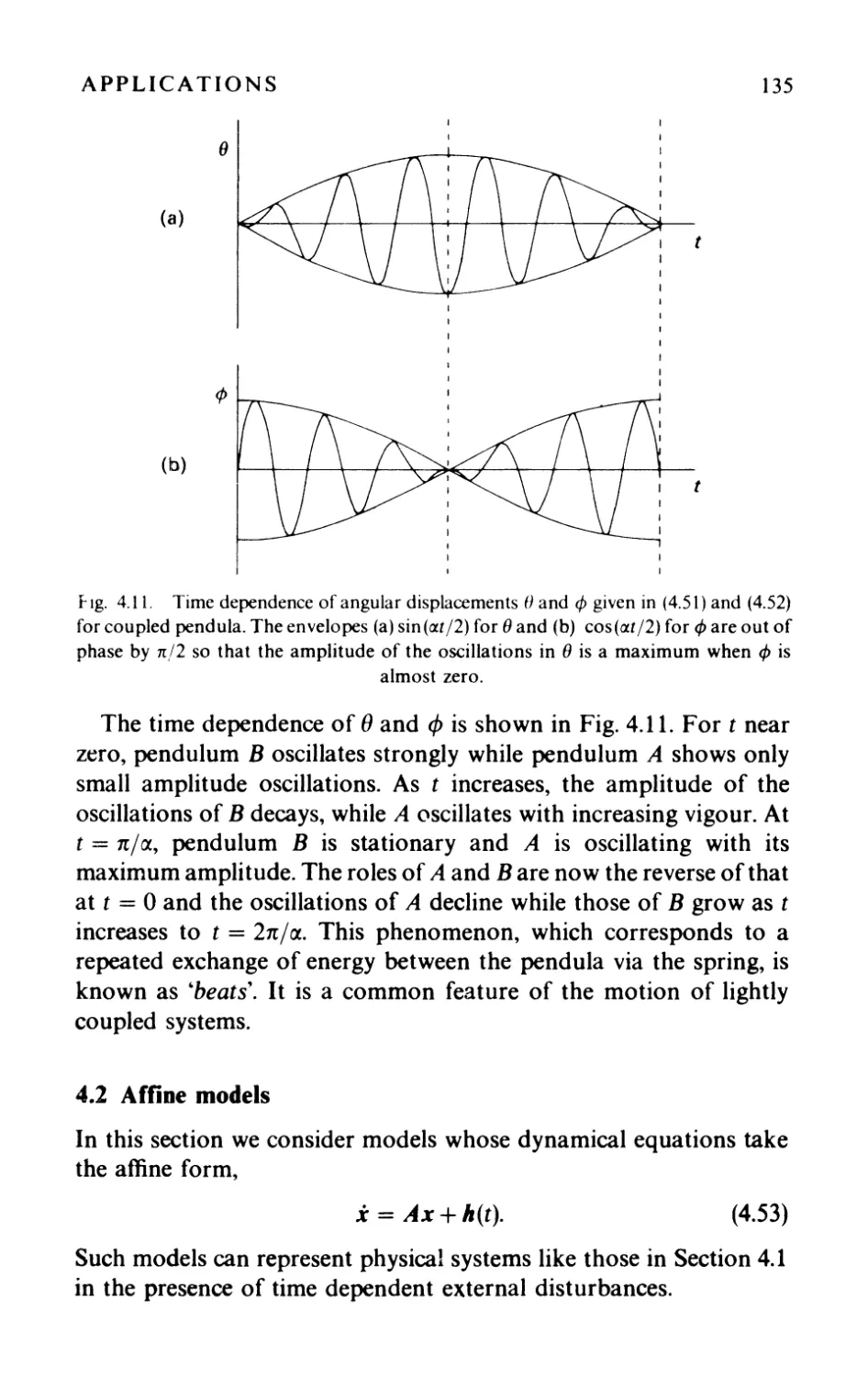
4.1.4 Coupled oscillators 131
4.2 Affine models 135
4.2.1 The forced harmonie oscillator 137
4.2.2 Resonance 137
4.3 Non-linear models 140
4.3.1 Competing species 140
4.3.2 V olterra-Lotka equations 144
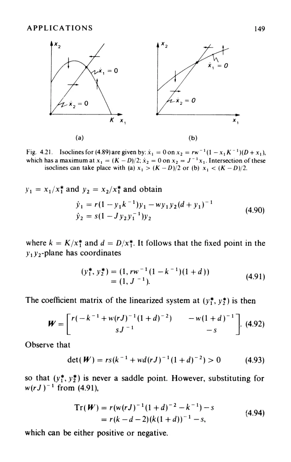
4.3.3 The Holling- Tanner model 147
4.4 Relaxation oscillations 151
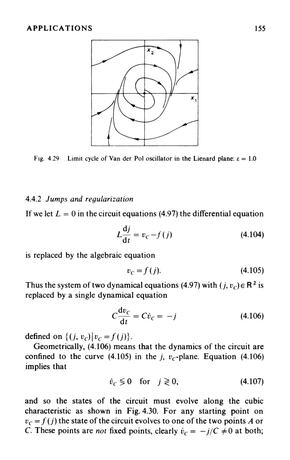
4.4.1 Van der Pol oscillator 151
4.4.2 lumps and regularization 155
CONTENTS lX
4.5 Piecewise modelling 159
4.5.1 The jump assumption and piecewise models 159
4.5.2 A limit cycle from linear equations 162
Exercises 166
5 Advanced techniques and applications 179
5.1 The Liénard equation 179
5.2 Regularization and some economic models 184
5.3 The Zeeman models of heartbeat and nerve impulse 190
5.4 Liapunov functions 198
5.4.1 Theory 198
5.4.2 A model of animal conjiict 204
5.5 Bifurcation of systems 210
5.5.1 Some simple examples 210
5.5.2 The Hopf bifurcation 212
5.5.3 An application of the Hopf' bifurcation theorem 214
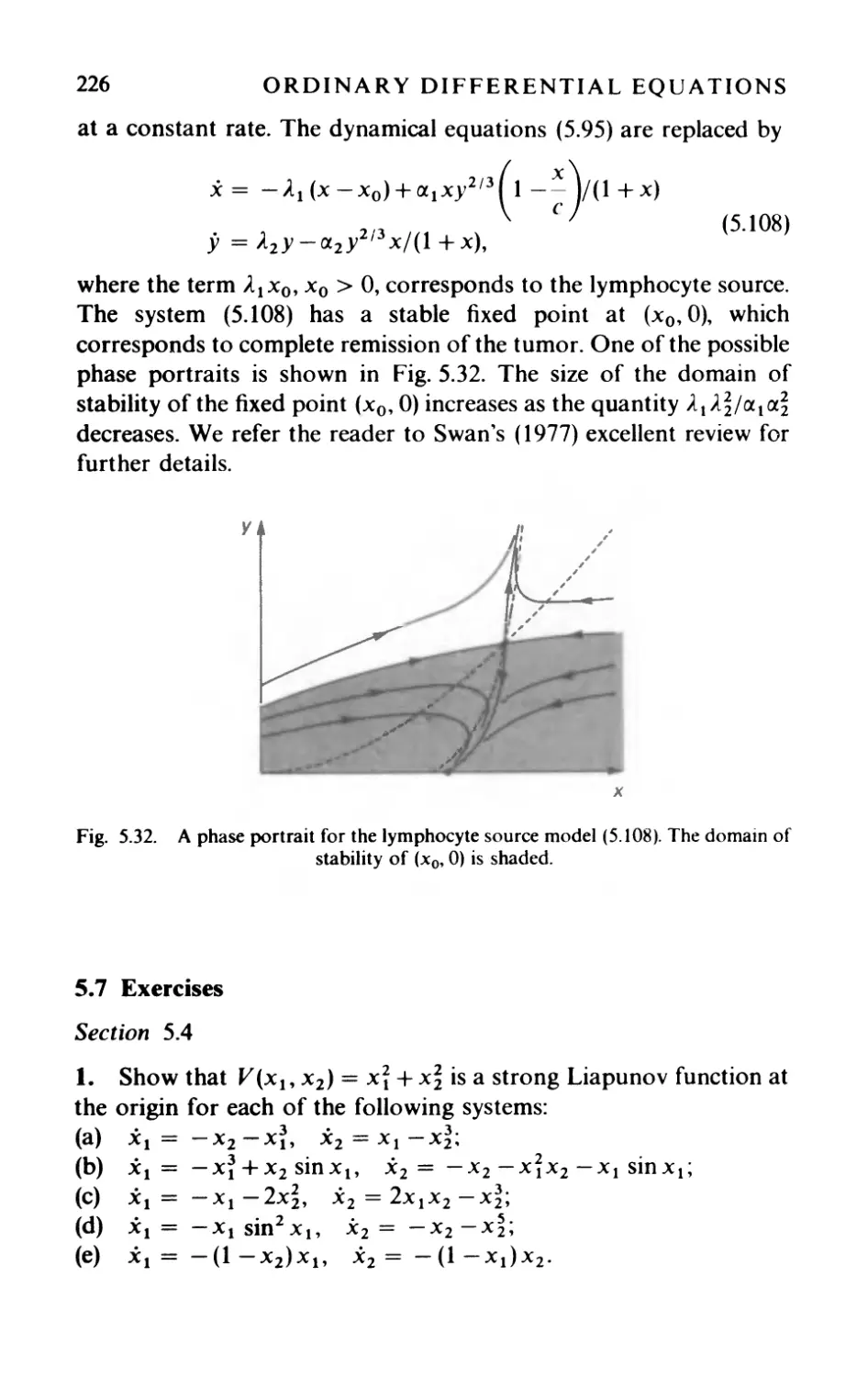
5.6 A mathematical mode] of tumor growth 216
5.6.1 C"onstruction of' the model 217
5.6.2 An analysis of" the dynamics 218
Exercises 226
Bibliography 230
Hints to exercises 232
Index 249
CHAPTER ONE
ln trod uction
ln this chapter we illustrate the qualitative approach to difTerential
equations and introduce some key ideas such as phase portraits and
qualitative equivalence.
101 Preliminary ideas
1.1.1 Existence and uniqueness
Definition 1.1.1. Let X (t, x) be a real valued function of the real
variables t and x, with domain D c R 2 . A function x(t), with t in some
interval 1 c R, which satisfies
dx
x(t) == - = X(t,x(t))
dt
(1.1)
is said to be a solution of the difTerential equation (1.1).
A necessary condition for x(t) to be a solution is that (t, x(t)) E D for
each tEl; so that D limits the domain and range of x(t). If x(t), with
domain l, is a solution to (1.1) then so is its restriction to any interval
J c 1. To prevent any confusion, we will always take 1 to be the largest
interval for which x(t) satisfies (1.1). Solutions with this property are
called maximal solutions. Thus, unless otherwise stated, we will use
the word 'solution' to mean 'maximal solution'. Consider the
following examples of (1.1) and their solutions; we give
x = X ( t, x),
D,
x (t ),
1
2
ORDINARY DIFFERENTIAL EQUATIONS
in each case (C and C' are real numbers):
(a) x=x-t, R 2 , l+t+Ce t , R;
(b) X=X2, R 2 , (C-t)-l, (-oo,C)
0, R
(C' - t)-l, (C', (0);
(c) x = -xlt, {(t, x)lt =1= O}, Cjt, (- 00,0)
C' It, (0, ex;);
(d) x = 2X I / 2 , {(t, x)lx O}, { O, (- 00, C)
(t - C)2, (C, (0)
0, R;
(e) x == 2xt, R 2 , Ce t2 , R;
(f) x == -xltanht, {(t,x)lt =1= O}, Cjsinht, (-00,0)
C' jsinh t, (0, oc).
The existence of solutions is determined by the properties of X. The
following proposition is stated without proof (Petrovski, 1966).
Proposition 1.1.1. If X is continuous in an open domain, D' c D,
then given any pair (to, Xo)E D', there exists a solution x(t), tE l, of
x = X(t, x) such that t o Eland x(to) = xo.
For example, consider
x = 21x11/2, (1.2)
where D = R 2 . Any pair (to, xo) with Xo 0 is given by (to, x(to))
when x(t) is the solution
{ O, tE(-OO,C)
x(t) = (t -C)2, tE (C, 00)
and C = t o - J Xo. A solution can similarly be found for pairs (to, xo)
when Xo < O.
Observe that Proposition 1.1.1 does not exclude the possibility that
x(t o ) = Xo for more than one solution x(t). For example, for (1.2)
infinitely many solutions x(t) satisfy x(to) = 0; namely every solution
of the form (1.3) for which C > t o and the solution x(t) = O.
The following proposition gives a sufficient condition for each pair
in D' to occur in one and only one solution of (1.1).
(1.3 )
Proposition 1.1.2. 1 f X and a xia x are con tin uous in an open
domain D' c D, then given any (to, xo) E D' there exists a unique
solution x(t) of x = X(t, x) such that x(t o ) = Xo.
INTRODUCTION
3
Notice that, while X = 21xll/2 is continuous on D (= R2) ôXlôx
(== Ixl-1/2 for x > 0 and -lxl-1/2 for x < 0) is continuous only on
D' == {(t, x) 1 x =1= O}; it is undefined for x == O. We have already
observed that the pair (to, 0), t o E R occurs in infinitely many solutions
of x = 21x11/2.
On the other hand, X(t, x) = x - t and ôXlôx = 1 are continuous
throughout the domain D = R 2 . Any (to, xo) occurs in one and only
one solution of x = x - t; namely
x(t) == 1 + t + Cet
(1.4 )
when C == (xo - t o - l)e -to.
Weaker sufficient conditions for existence and uniqueness do exist
(Petrovski, 1966). However, Propositions 1.1.1 and 1.1.2 illustrate the
kind of properties required for X (t, x).
1.1.2 Geometrical representation
A solution x(t) of x == X(t, x) is represented geometrically by the
graph of x(t). This graph defines a solution curve in the t, x-plane.
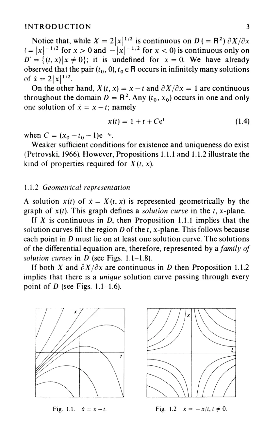
If X is continuous in D, then Proposition 1.1.1 implies that the
solution curves fill the region D of the t, x-plane. This follows because
each point in D must lie on at least one solution curve. The solutions
of the difTerential equation are, therefore, represented by a family of
solution curves in D (see Figs. 1.1-1.8).
Ifboth X and ôXlôx are continuous in D then Proposition 1.1.2
implies that there is a unique solution curve passing through every
point of D (see Figs. 1.1-1.6).
Fig. 1.1. x = x - t.
Fig. 1.2 x = - x/t, t =1= o.
x
t
Fig. 1.3. X = -llx.
Fig. 1.5. X = 2xt.
x
Fig. 1.7. X = J{l-x 2 ), Ixl 1,
Fig. 1.4. X = t(x 1 -1).
t
Fig. 1.6. X = - xltanh l, t =1= o.
Fig. 1.8. X = 2X 1/2 , X o.
INTRODUCTION
5
Observe that the families of solution curves in Figs. 1.2 and 1.6 bear
a marked resemblance to one another. Every solution curve in one
figure has a counterpart in the other; they are similar in shape, have
the same asymptotes, etc., but they are not identical curves. The
relationship between these two families of solution curves is an
example of what we calI qualitative equivalence (see Sections 1.3, 2.4
and 3.3). We say that the qualitative behaviour of the solution curves in
Fig. 1.2 is the same as those in Fig. 1.6.
Accurate plots of the solution curves are not always necessary to
obtain their qualitative behaviour; a sketch is often sufficient. We can
sometimes obtain a sketch of the family of solutions curves directly
from the ditTerential equation.
Example 1.1.1. Sketch the solution curves of the difTerential
eq ua tion
x==t+t/x
( 1.5)
în the region D of the t, x-plane where x =1= o.
Solution. We make the following observations.
(a) The difTerential equation gives the slope of the solution curves
at aIl points of the region D. Thus, in particular, the solution curves
cross the curve t + tlx = k, a constant, with slope k. This curve is
called the isocline of slope k. The set of isoclines, obtained by taking
difTerent real values for k, is a family of hyperbolae
t
x=- k '
-t
( 1.6)
with asymptotes x = -1 and t == k. A selection of these isoclines is
shown in Fig. 1.9.
(b) The sign of x determines where in D the solution curves are
conc ve and convex. If x > 0 ( < 0) then x is increasing (decreasing)
with t and the solution curve is said to be convex (concave). The region
D can therefore be divided into subsets on which the solution curves
are either concave or convex separated by boundaries where x = O.
For (1.5) we find
x = x- 3 (x + l)(x - t)(x + t)
(1. 7)
6
ORDINARY DIFFERENTIAL EQUATIONS
k=-3k=-1 k=1k=3
k=3
k = 1
k=O
k = -1
k = -2
k - -3
V -
k = -1
k=O
k = 1
k=2
k=O
Fig. 1.9. Selected isoclines for the equation x = t + tlx. The short line segnlents on
the isoclines have slope k and indicate how the solution curves cross them.
and D can be split up into regions P (x > 0) and N (x < 0) as shown in
Fig. 1.10.
(c) The isoclines are symmetrically placed relative to t == 0 and so
there must also be symmetry of the solution curves. The function
X(t, x) = t + tlx, satisfies X( - t, x) = - X(t, x) and thus if x(t} is a
solution to x = X (t, x) then so is x( - t) (see Exercise 1.5).
These three observations allow us to produce a sketch of the
solution curves for x = t+tlx(seeFig.l.11). NoticethatbothX(t,x)
= t + tlx and èX lèx = - tlx 2 are continuous on D = {(t, x) lx =1= O},
so there is a unique solution curve passing through each point
ofD. D
',+
"
", "-
',r
/
/
p
N
,
,
,
,
,
,
N
P "N" P
x = - 1 " "
u - - - -- : ,-/ -, J - - - - r - - - · :: : ,- - - - - - - -
" ,
,/ P "
,...../\ ",
/ l' "
/,,"" +- ",
Fig. 1.10. Regions of convexity (P) and
concavity (N) for solutions ofx = t + tlx.
Fig. 1.11. The solution curves of the
differential equation x = t + tlx in the
t, x-plane.
INTRODUCTION
7
It is possible to find the solutions of
x = t+t/x
( 1.8)
by separation of the variables (see Exercise 1.2). We obtain the
equation
x-Inlx+11 == tt 2 +C,
( 1.9)
C a constant, for the family of solution curves as weIl as the solution
x(t) = -1. However, to sketch the solution curves from (1.9) is less
straightforward than to use (1.8) itself.
The above discussion has introduced two important ideas:
1. that two difTerent difTerential equations can have solutions that
exhibit the same qualitative behaviour; and
2. that the qualitative behaviour of solutions is determined by
X (t, x).
We will now put these two ideas together and illustrate the
qualitative approach to difTerential equations for the special case of
equations of the form x = X (x). We shall see that such equations can
be classified into qualitatively equivalent types.
1.2 Autonomous equations
1.2.1 Solution curves and the phase portrait
A differential equation of the form
x = X(x),
X E S c R,
(D = R x S)
(1.10)
is said to be autonomous, because x is determined by x alone and so the
solutions are, as it were, self-governing.
The solutions of autonomous equations have the following
important property. If ç(t) is a solution of (1.10) with domain 1 and
range ç (1) then ,,(t) = ç (t + C), for any real C, is also a solution with
the sa me range, but with domain {t 1 t + C El}. This f ollows because
(t) = ç (t + C) = X ( ç (t + C)) = X (1] (t) ). ( 1.11 )
The solution curve x =:.. ç (t) is obtained by translating the solution
curve x = 1](t) by the amount C in the positive t-direction.
Furthermore ifthere exists a unique solution curve passing through
each point of the strip D' = R x ç(l) then ail solution curves on D' are
8
ORDINARY DIFFERENTIAL EQUATIONS
translations of x = ç (t). The domain Dis therefore divided into strips
where the solution curves are aIl obtained by shifting a single curve in
the t-direction (see Figs. 1.12-1.15). For example,
Fig. 1.12. x = x: strips D' consist of the
half planes x < 0 and x > o.
x
t
x==x
(1.12)
Fig. 1.13. x = t(x 1 - 1): strips D' =
R x ç (1) wit h ç (1) = ( - C(), - 1), ( - l, 1)
and (1, C()).
x
Tl
Fig. 1.14. Solution curves for x = x 3 . Fig. 1.15. Solution curves for x = x 2 .
has solutions:
ç(t) = et,
ç (t) = 0,
ç (t) = - et,
1 = R
,
1 = R
,
1 = R
,
ç(I) = (0, (0)
ç (1) -= {O}
ç(I) = ( - 00, 0).
(1.13)
(1.14)
( 1.15)
INTROD{)CTION
9
AlI the solution curves in the strip D' defined by XE (0, (0), tER are
translations of e'. Similarly, those in D' = {(t, x) 1 XE ( - 00, 0), tER}
are translations of e -'.
For families of solution curves related by translations in t, the
qualitative behaviour of the family of solutions is determined by that
of any individual member. The qualitative behaviour of such a sample
curve is determined by X (x). When X (x) =1= 0, then the solution is
either increasing or decreasing; when X (c) = 0 there is a solution
x(t) = c.
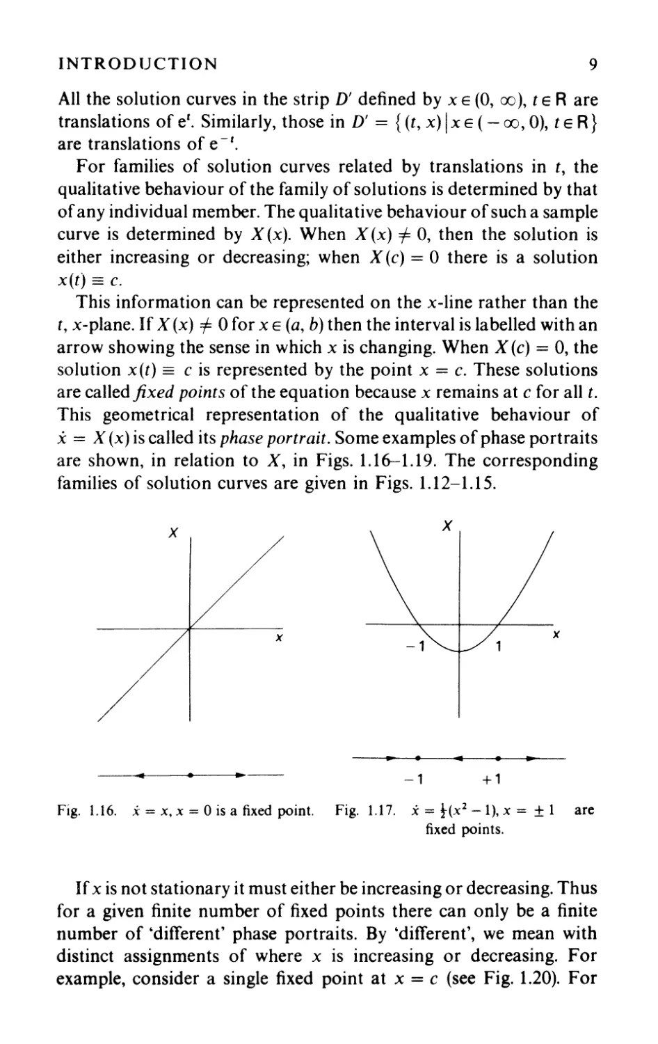
This information can be represented on the x-line rather than the
t, x-plane. If X (x) =1= 0 for x E (a, b) then the interval is labelled with an
arrow showing the sense in which x is changing. When X (c) = 0, the
solution x(t) = c is represented by the point x = c. These solutions
are called fixed points of the equation because x remains at c for aIl t.
This geometrical representation of the qualitative behaviour of
x = X (x) is called its phase portrait. Some examples of phase portraits
are shown, in relation to X, in Figs. 1.16-1.19. The corresponding
families of solution curves are given in Figs. 1.12-1.15.
/
.. .
4
. ..
...
.
..
-1
+1
Fig. 1.16. x = x, x = 0 is a fixed point. Fig. 1.17. x = t(x 2 -1), x = 1: 1 are
fixed poin ts.
If x is not stationary it must either be increasing or decreasing. Thus
for a given finite number of fixed points there can only be a finite
number of 'ditTerent' phase portraits. By 'ditTerent', we mean with
distinct assignments of where x is increasing or decreasing. For
example, consider a single fixed point at x = c (see Fig. 1.20). For
10
ORDINARY DIFFERENTIAL EQUATIONS
x
x
...
.
.
.
-.--
Fig. 1.18. X = x 3 , X = 0 is a fixed point. Fig. 1.19. x = x 2 , X = 0 is a fixed point.
c
. .
c
. . .
(a)
(b)
c c
. . - ---.-- ---
(c) ( d)
Fig. 1.20. The four possible phase portraits associated with a single fixed point. The
fixed point is described as an attractor in (a), a shunt in (b) and (c) and a repellor in (d).
x < c, X (x) must be either positive or negative and similarly for
x > c. Hence, one of the four phase portraits shown must occur. This
means that the qualitative behaviour of any autonomous difTerential
equation with one fixed point must correspond to one of the phase
portraits in Fig. 1.20 for some value of c. For example, x = x, X == x 3 ,
X = x - a, x = (x - a)3, X = sinh x, x = sinh(x - a) aIl correspond to
Fig. 1.20(d) for (' = 0 or Q. Of course, two difTerent equations, each
having one fixed point, that correspond to the same phase portrait in
Fig. 1.20(d) for c = 0 or a. Of cûurse, two difTerent equations, each
difTerential equations are qualitatively equivalent.
Now observe that the argument leading to Fig. 1.20 holds equally
weIl if the fixed point at x = c is one of many in a phase portrait. ln
other words, the qualitative behaviour of x in the neighbourhood of
an y fixed point must be one of those il1ustrated in Fig. 1.20(a)-(d). We
INTRODUCTION
Il
say that this behaviour determines the nature ofthefixed point and use
the terminology defined in the caption t,o Fig. 1.20 to describe this.
This is an important step because it implies that the phase portrait
of any auto no mous equation is determined completely by the nature
of its fixed points. We can make the following definition.
Definition 1.2.1. Two difTerential equations of the form x == X (x)
are qualitatively equivalent if they have the same number of fixed
points, of the same nature, arranged in the same order along the phase
line.
F or example, x = (x + 2)(x + 1) is qualitatively equivalent to
x = t(x 2 - 1). Both have two fixed points, one attractor and one
repellor, with the attractor occurring at the smaller value of x. The
equation x = - (x + 2)(x + 1) is not qualitatively equivalent to
x == t(x 2 -- 1) because the attractor and repellor occur in the reverse
order.
Example 1.2.1. Arrange the following difTerential equations ln
qualitatively equivalent groups:
(1) x == cosh x;
(4) x==cosx-1;
(7)
x == eX.
,
(2) x (x - a)2;
(5) x == coshx -1;
(8) x == sinh 2 (x - b).
(3) x == sin x;
(6) x == sin 2x;
Solution. Equations (1) and (7) have no fixed points; in both cases
X(x) > 0 for aIl x. They both have the phase portrait shown in
Fig. 1.21 (a) and are therefore qualitatively equivalent.
Equation (2) has a single shunt at x = a with X(x) 0 for aIl x.
Another equation with a single fixed point is (5); this has the same kind
C
..
.
..
(a)
(b)
C 2 C 1 Co c,
.. .........
C-2 C-1 Co C,
.. ......
(c)
(d)
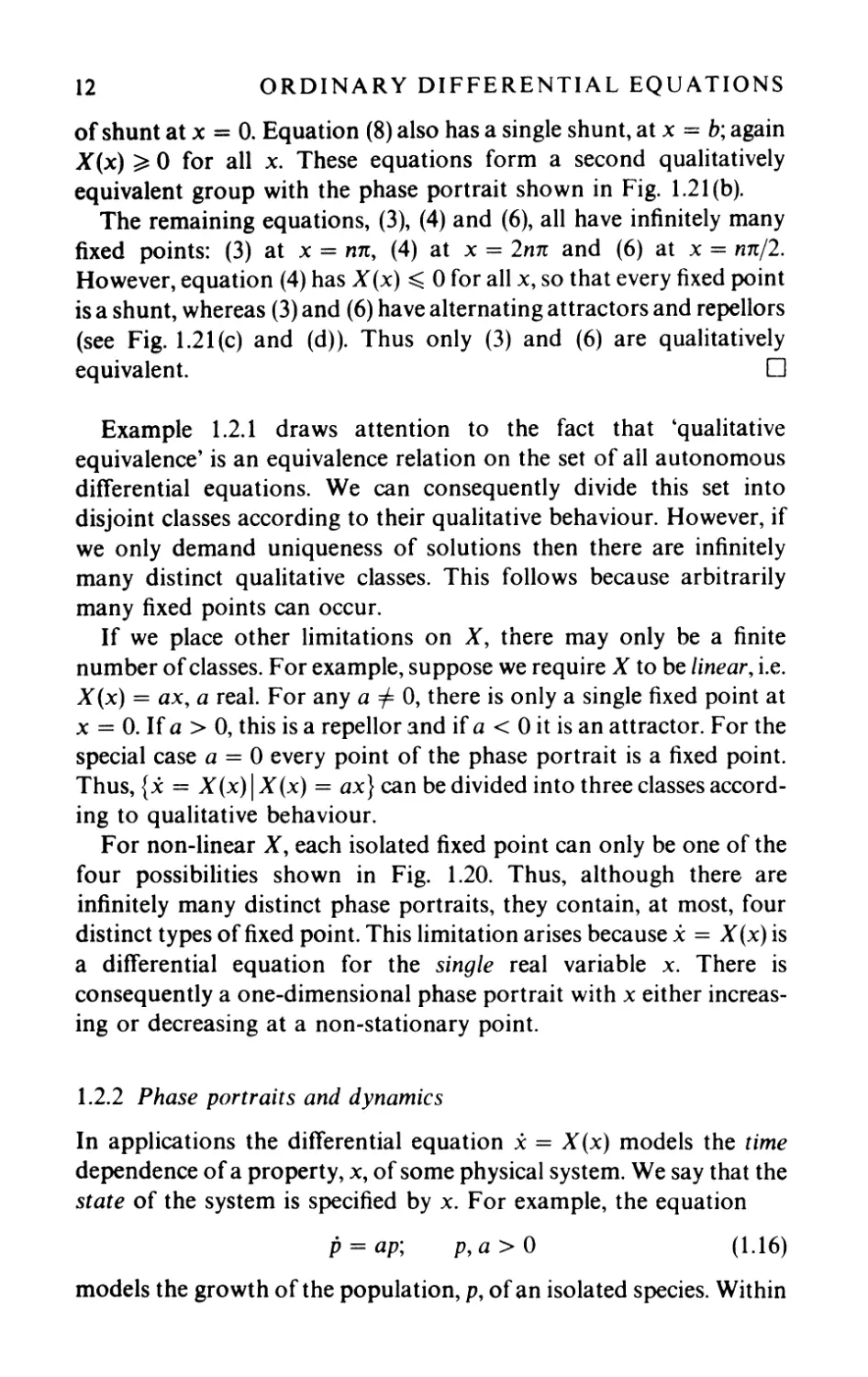
Fig. 1.21. Phase portraits for qualitatively equivalent groups in Example 1.2.1. ln
(b) c = a for (2),0 for (5) and b for (8). ln (c) (n = 2nrr for (4) and in (d) C n = nrr for (3)
and n1t/2 for (6).
12
OROINAR y OIFFERENTIAL EQU A TIONS
of shunt at x = O. Equation (8) also has a single shunt, at x = b; again
X(x) 0 for all x. These equations form a second qualitatively
equivalent group with the phase portrait shown in Fig. 1.21 (b).
The remaining equations, (3), (4) and (6), aIl have infinitely many
fixed points: (3) at x = nn, (4) at x = 2nn and (6) at x = nnl2.
However, equation (4) has X(x) 0 for aIl x, so that every fixed point
is a shunt, whereas (3) and (6) have alternating attractors and repeIlors
(see Fig. 1.21(c) and (d)). Thus only (3) and (6) are qualitatively
eq uivalen t. 0
Example 1.2.1 draws attention to the fact that 'qualitative
equivalence' is an equivalence relation on the set of aIl autonomous
difTerential equations. We can consequently divide this set into
disjoint classes according to their qualitative behaviour. However, if
we only demand uniqueness of solutions then there are infinitely
many distinct qualitative classes. This follows because arbitrarily
many fixed points can occur.
If we place other limitations on X, there may only be a finite
number of classes. For example, suppose we require X to be linear, i.e.
X(x) = ax, a real. For any a =1= 0, there is only a single fixed point at
x = O. If a > 0, this is a repellor and if a < 0 it is an attractor. For the
special case a = 0 every point of the phase portrait is a fixed point.
Thus, {x = X(x)IX(x) = ax} can bedivided into threeclassesaccord-
ing to qualitative behaviour.
For non-linear X, each isolated fixed point can only be one of the
four possibilities shown in Fig. 1.20. Thus, although there are
infinitely many distinct phase portraits, they contain, at most, four
distinct types offixed point. This limitation arises because x == X(x) is
a difTerential equation for the single real variable x. There is
consequentlya one-dimensional phase portrait with x either increas-
ing or decreasing at a non-stationary point.
1.2.2 Phase portraits and dynamics
ln applications the difTerential equation x = X (x) models the time
dependence of a property, x, of some physical system. We say that the
state of the system is specified by x. For example, the equation
p = ap; p, a > 0 (1.16)
models the growth of the population, p, of an isolated species. Within
INTRODUCTION
13
this model, the state of the species at time t is given by the number of
individuals, p(t), living at that time. Another example is Newton's law
of cooling. The temperature, T, of a body cooling in a draught of
temperature 't is given by
t = - a (T - 't),
a > O.
( 1.1 7)
Here the state of the body is taken to be determined by its
temperature.
We can represent the state x(to) of a model at any time t o by a point
on the phase line of x == X (x). As time increases, the state changes and
the phase point representing it moves along the line with velocity
i == X(x). Thus, the dynamics of the physical system are represented
by the motion of a phase point on the phase line.
The phase portrait records only the direction of the velocity of the
phase point and therefore represents the dynamics in a qualitative
way. Such qualitative information can be helpful when constructing
models. For example, consider the model (1.16) of an isolated
population. Observe that p > 0 for ail p > 0, the phase portrait, in
Fig. 1.22(a), shows that the population increases indefinitely. This
featurc is clearly unrealistic the environment in which the species live
must have limits and could not support an ever-increasing
population.
.. .
p=o
(a)
...... ...
P = 0 P = Pa
(b)
Fig. 1.22. Phase portraits for (a)p = apand(b)p = p(a-bp),Pe = ajb. ln bothcases,
we are interested only in the behaviour for non-negative populations (p 0). The
equation in (b) is known as the Logistic Law of population growth.
Let us suppose that the environment can support a population Pe,
then how could (1.16) be modified to take account ofthis? Obviously,
the indefinite increase of p should be interrupted. One possibility is to
introduce an attractor at Pe as shown in Fig. 1.22(b). This means that
populations greater than Pe decline, while populations less than Pe
increase. Finally, equilibrium is reached at P = Pe' The fixed point at
P == Pe, as weil as P == 0, requires a non-linear X(p) in (1.16). The form
p = p(a -bp)
( 1.18)
14
ORDINARY DIFFERENTIAL EQUATIONS
has the advantage of reducing to (1.16) when b = 0; otherwise
Pe = alb.
Of course, models of physical systems frequently involve more than
a single state variable. If we are to be able to use qualitative ideas in
modelling these systems, then we must examine autonomous cqua-
tions involving more than one variable.
1.3 Autonomous systems in the plane
Consider the difTerential equation
dx
x = dl == X(x)
(1.19)
where x = (x l, x 2 ) is a vector in R 2 . This equation is equivalent to the
system of two coupled equations
Xl == X 1 (x b X2),
.X 2 = X 2(X b x 2 ),
( 1.20)
where X(x) == (X 1 (x l, x 2 ), X 2 (x l, X2)), because x == (x b X2)' A
solution to (1.19) consists of a pair of functions (x 1 (t), X2 (t)), tEl c R,
which satisfy (1.20). ln general, both Xl (t) and x 2 (t) involve an
arbitrary constant so that there is a two-parameter family of
solutions.
The qualitative behaviour of this family is determined by how Xl
and X2 behave as t increases. Instead of simply indicating whether x is
increasing or decreasing on the phase line, we must indicate how x
behaves in the phase plane. The phase portrait is therefore a two-
dimensional figure and the qualitative behaviour is represented by a
family of curves, directed with increasing t, known as trajectories or
orbits.
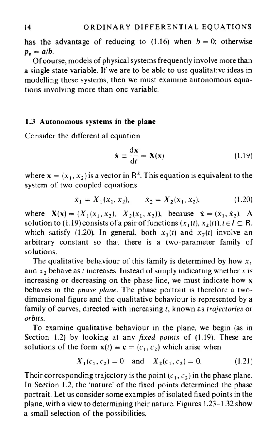
To examine qualitative behaviour in the plane, we begin (as in
Section 1.2) by looking at any fixed points of (1.19). These are
solutions of the form x(t) = C = (CI' C2) which arise when
X 1 (CI' C2) = 0 and X 2(C b C2) = O. (1.21)
Their corresponding tra jectory is the point (c l' C 2) in the phase plane.
ln Se tion 1.2, the 4. na ture' of the fixed points determined the phase
portrait. Let us consider some examples of isolated fixed points in the
plane, with a view to determining their nature. Figures 1.23--1.32 show
a small selection of the possibilities.
Fi g. 1. 2 3. X 1 = - XI' X 2 = - X 2 .
k:::
Flg.1.25. XI =X I ,X2= -X2.
Fig. 1.27. XI = -XI' X2 = -XI +X2.
Fig.1.24. XI = -X I ,X2= - 2X 2.
Fig. 1.26. XI = X2,X 2 = -XI.
Fig. 1.28. XI = 3x I +4X2,
X2= -3XI- 3x 2.
16
ORDINARY DIFFERENTIAL EQUATIONS
Fig. 1.29.
. . 2
Xl = Xl' X2 = X 2 .
Fig. 1.31. Xl = xf,x 2 = x2(2xI-X2)'
Consider Fig. 1.23; the system
Xl = -X b
J
Fig. 1.30.
. l'
Xl = X 2 , X 2 = Xl'
1
J
Fig. 1.32.
. . 2 l
Xl = -X I X2,X 2 = Xl +'\2
X 2 = - X2
(1.22 )
has a fixed point at (0, 0) and solutions
Xl(t) = Cie-t,
x 2 (t) == C 2e-t
( 1.23)
where CI' C 2 are real constants. Clearly, every member of the family
(1.23) satisfif S
X 2 (t) = K Xl (t),
(1.24 )
where K = C 21C l, for every t. Thus every member is associated with a
radial straight line in the Xl x 2 -plane. Equation (1.23) shows that, for
any choice of CI and C 2' 1 Xl (t) 1 and 1 X2 (t) 1 decrease as t increases and
approach zero as t -+ 00. This is indicated by the direction of the
INTRODUCTION
17
arrow on the trajectory; i.e. if (x 1 (t), X2 (t)) represents the value of x at t
then this phase point will move along the radial straight line towards
the origin as t increases. The directed straight line is sufficient to
describe this qualitative behaviour. ln Fig. 1.24,
X 2 = KXI,
which alters the shape of the trajectories. However, they are still aIl
directed towards the fixed point at the origin.
Figure 1.25 shows another possibility: here as t increases, 1 Xl (t) 1
decreases but Ix 2 (t)1 increases. ln fact, Xl = -Xl' X2 == X2 has
solutions
Xl(t) = Cle-r,
el' c 2 real; so that
X 2 (t) == C 2 et,
( 1.25)
K -1
X 2 == Xl'
( 1.26)
with K == CI C 2- ln this case, only two special trajectories approach
the fixed point at (0, 0), the remainder ail turn a way sooner or later
and 1 x 2 1 CIJ as 1 X II O. This qualitative behaviour is obviously
quite difTerent from that in Figs. 1.23 and 1.24.
ln Fig. 1.26 the trajectories close on themselves so that the same set
of points in the phase plane recur time and time again as t increases. ln
Section 1.4, we show that the system
Xl == X2,
X2 == - Xl
( 1.27)
has solutions
X 1 (t) == C 1 cos ( - t + C 2 ),
1 t follows that
X2(t) == CI sin( - t + C 2)' (1.28)
2 2 C 2
X I +X 2 = 1
( 1.29)
and the trajectories are a family of concentric circles centred on the
fixed point at (0, 0). This obviously corresponds to yet another kind of
qualitative behaviour. The fact that Xl (t) and X2 (t) are periodic with
the sa me period is reflected in the closed trajectories.
These examples show that qualitatively ditTerent solutions,
(x 1 (t), X 2 (t)), lead to trajectories with difTerent geometrical properties.
The problem of recognizing ditTerent types offixed point becomes one
of recognizing distinct' geometrical configurations of trajectories. As
18
ORDINARY DIFFERENTIAL EQUATIONS
in Section 1.2, we must decide what we mean by 'distinct' and there is
an element of choice in the criteria that we set.
For example, in Figs. 1.23 and 1.24 aIl the trajectories are directed
toward the origin. It would be reasonable to argue that this is
the dominant qualitative feature and that the difTerences in shape of
the trajectories are unimportant. We would then say that the nature
of the fixed point at (0, 0) was the same in both cases. Of course, its
nature would be completely changed if we replaced Xl by - X 1 and x 2
by - x 2 . Under these circumstances aIl trajectories would be directed
away from the origin (see Exercise 1.22) corresponding to quite
ditTerent qualitative behaviour of the solutions.
Let us compare Figs. 1.25 and 1.27. Are the fixed points of the same
nature? ln both cases Ixl(t)1 tends to zero while IX2(t)1 becomes
infinite and only two special trajectories approach the fixed point
itself. Yes, we would argue, they are the same. If the orientation of the
trajectories is reversed in these examples is the nature of the fixed
point changed as in our previous example? Orientation reversaI
would mean that the roles of x 1 and X 2 were interchanged. However
the features which distinguish Figs. 1.25 and 1.27 from the remaining
ten diagrams still persist and we conclude that the nature of the fixed
point does not change. Similarly, we would say that Figs. 1.26, 1.28
and their counterparts with orientation reversed aIl had the same kind
of fixed point at the origin.
The intuitive approach used in discussing the above examples is
sufficient for us to recognize that seven distinct types offixed point are
illustrated in Figs. 1.23-1.32. ln fact, there are infinitely many
qualitatively difTerent planar phase portraits containing a single fixed
point. Some examples of phase portraits with more than one isolated
fixed point are shown in Figs. 1.33-1.36. As can be seen, it is not
difficult to produce complicated families of trajectories.
1.4 Construction of phase portraits in the plane
Methods of obtaining information about the trajectories associated
with systems like
X 1 = X 1 (x 1 , X 2 );
X 2 = X 2 (x l' X 2 ),
(X h X2)ES C R 2
are straightforward extensions of ideas used to obtain solutions in
Section 1.1.
INTRODUCTION
Fig. 1.33. Phase portrait for Xl = Xl
(a -bX2)' X 2 = -X 2 (c -dxd with a, b, c,
d > O. There are fixed points at (0, 0) and
(cid, a/b) in the phase plane.
Fig. 1.35. Phase portrait for Xl = (2
-Xl - 2X 2)X I , X 2 = (2 -2x I -X2)X2' Fi-
xed points occur at (0,0), (2,0), (0,2) and
(!, i).
19
Fig. 1.34. Phase portrait for Xl =
-xI[1-3x /3(1-xd/(1 +xd], X2
2/3 ) . 0 F .
= X2 -3X I X 2 /(1 +X 1 , Xl> X 2 . 1-
xed points occur at (0, 0) and (t, 1).
Fig. 1.36. Phase portrait for Xl
= sin Xl' X 2 = - sin X2. Fixed points
occur at (n1t, m1t); n, m integers.
1.4.1 (Jse of ca/cu/us
ln Section 1.3, we were able to obtain the trajectories shown in
Figs. 1.23-1.25 by solving the system equations separately. This was
possible because Xl depended only on Xl and x 2 only on X2' A system
in which each equation contains one, and only one, variable is said to
be decoupled. This is not usually the case and if calculus is to be used in
this way, new variables must be found which bring about this
isolation of the variables.
20
ORDINARY DIFFERENTIAL EQUATIONS
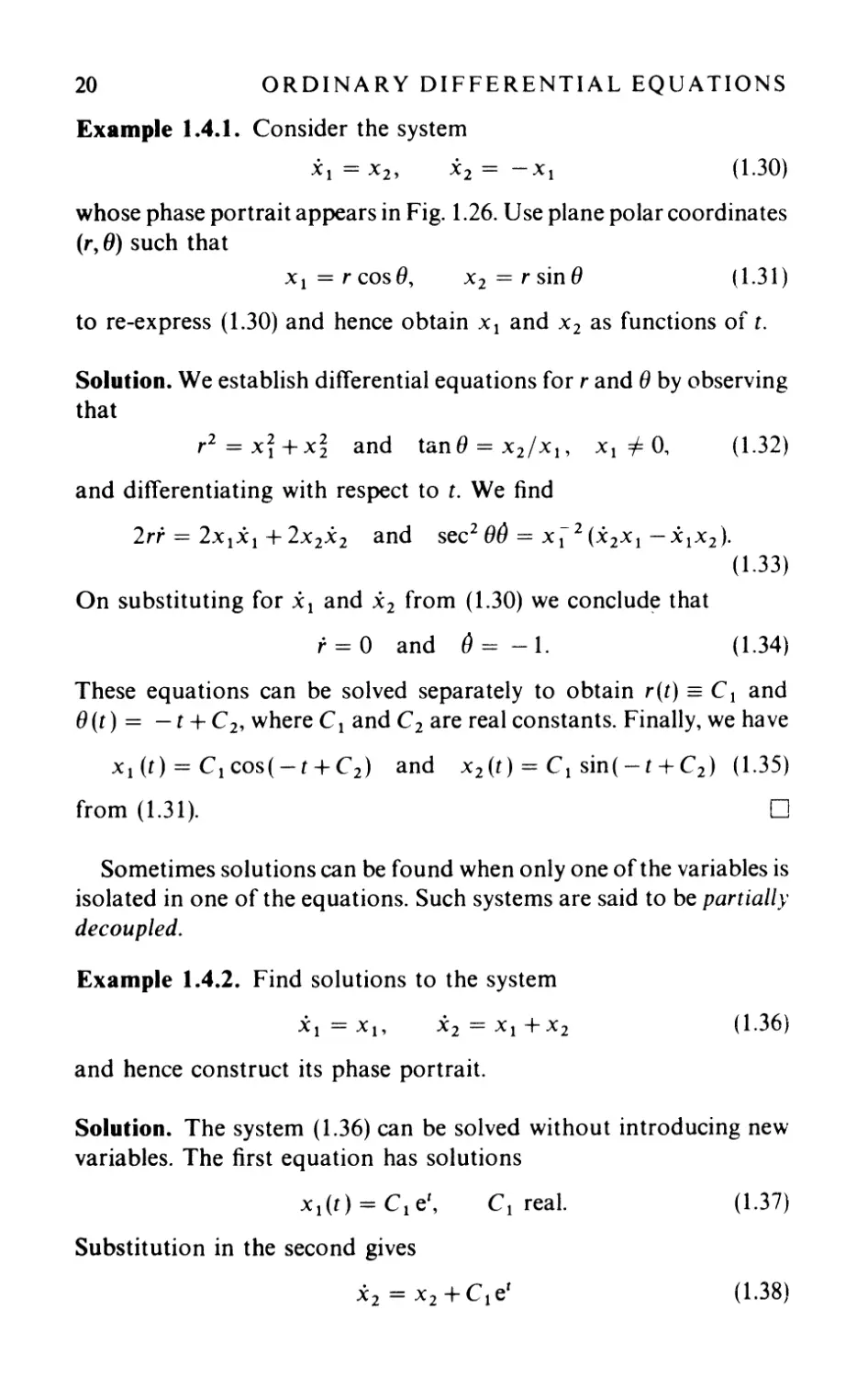
Example 1.4.1. Consider the system
Xl = X2,
X 2 = -Xl
( 1.30)
whose phase portrait appears in Fig. 1.26. Use plane polar coordinates
(r,O) such that
Xl = r cos 0,
X 2 = r sin 0
(1.31 )
to re-express (1.30) and hence obtain Xl and X 2 as functions of t.
Solution. We establish difTerential equations for rand () by observing
that
r 2 = xi + x and tan () = x2Ix!, Xl =1= 0, (1.32)
and difTerentiating with respect to t. We find
2rr = 2X I X I + 2X2X2 and sec 2 OÔ = X 2 (X2XI -X I X 2 ).
(1.33)
On substituting for Xl and X2 from (1.30) we conclud that
r = 0 and Ô = - 1.
(1.34 )
These equations can be solved separately to obtain r(t) = CI and
() (t) = - t + C 2' where el and C 2 are real constants. Finally, we have
Xl(t) = ClcoS(-t+C 2 ) and x 2 (t) = CI sin(-t+C 2 ) (1.35)
from (1.31). D
Sometimes solutions can be found when only one of the variables is
isolated in one of the equations. Such systems are said to be partial/y
decoupled.
Example 1.4.2. Find solutions to the system
Xl = X b
X 2 =X I +X 2
(1.36 )
and hence construct its phase portrait.
Solution. The system (1.36) can be solved without introducing new
variables. The first equation has solutions
X 1 (t) = Clet,
Substitution in the second gives
X 2 = X 2 + Clet
C 1 real.
(1.37)
( 1.38)
INTRODUCTION
21
which in turn has solutions
X 2 (t) = e' (C 1 t + C 2 )
( 1.39)
(see Exercise 1.1).
To construct the phase portrait examine (1.37) and (1.39) and note:
(a) For CI = K > 0, Xl (t) strictly increases through aIl positive
values as t increases through ( - 00, (0).
(b) For CI =K>O, X2(t)-+0 as t-+ -00; X2(t)<0 for Clt
+ C 2 < 0; X 2 (t) = 0 for C l t + C 2 = 0 and x 2 (t) -+ 00 as t -+ 00.
(c) For CI = 0, we obtain the solution
Xl (t) = 0,
X 2 (t) = C 2 et.
( 1. 40)
(d) For C l = - K < 0, both Xl (t) and X2 (t) assume precisely
minus one times the values on a trajectory in (a) and (b) above.
Notice also that the turning point in X2, implied in (b), is given more
precisely in (1.36) where x 2 = 0 when X 2 = - Xl' Furthermore,
the symn1etry described in (d) is also apparent in (1.36) because
this system is invariant under the transformation Xl -+ -Xb
X 2 -+ - X2 (see Exercise 1.26). Finally, we sketch the phase portrait
in Fig. 1.37. D
Fig. 1.37. Phase portrait for the system Xl = Xl' X2 = Xl + X 2 . The dashed line is
X 2 = - Xl where X 2 = O. The origin is a fixed point.
ln Section 1.3, we sometimes found it advantageous to eliminate
t between Xt(t) and X2(t) and obtain a non-parametric form for the
22
ORDINARY DIFFERENTIAL EQUATIONS
trajectories. These equations can often be found directly by solving
dX 2 x 2
dX I Xl
X 2 (Xb X 2)
X I (X I ,X 2 )
(1.41 )
Example 1.4.3. Consider the system
Xl = X2,
X 2 = Xl'
( 1.42)
Use dx 2 1 dx 1 to determine the nature of the trajectories and hence
construct the phase portrait for the system.
Solution. For the system (1.42) we have
dX 2
dX I
Xl
X 2 =1= 0,
(1.43 )
,
X2
which has solutions satisfying
2 2 C
Xl - X 2 = ,
(1.44)
CreaI. This family of hyperbolae is easily sketched and their
orientation as trajectories is given by (1.42). For example, note that
both Xl' X 2 > 0 implies that both Xl (t) and X 2 (t) increase with t. This
pro vides directions for aIl the trajectories in X 2 > - XI' Similarly,
XI' X 2 < 0 means Xl' X 2 < 0 and gives orientation to the trajectories in
x 2 < - Xl' Thus the phase portrait is as shown in Fig. 1.38. 0
Fig. 1.38. Phase portrait for XI = X 2, X 2 = X 1. The origin is a fixed point and the
trajectories are hyperbolae.
INTRODUCTION
23
1.4.2 Isoclines
As in Section t.l, it may be necessary to construct a phase portrait
when calculus fails to give tractable solutions. This can be done by
extending the method of isoclines to the plane. The vector valued
function or vector field X: S R 2 now gives X at each point of the
plane where X is defined. For qualitative purposes it is usually
sufficient to record the direction of X (x). This is constant on the
isoclines of (1.41). The zeroes and divergences of dX2/dxI are of
particular interest and such lines will be referred to as the 'x 2 = 0' or
'x 1 = 0' -isoclines respectively.
If a unique solution x (t) of
x = X(x),
XES and with x(to) = Xo
( 1.45)
exists for any Xo E Sand t o E R, then each point of S lies on one, and
only one, trajectory. AlI of the examples presented thus far ln
Sections 1.3 and 1.4 have been of this kind. Furthermore, when non-
uniqueness occurs, it is frequently confined to lines in the domain S. It
is only in the neighbourhood of such lines that the behaviour of the
trajectories is not immediately apparent from X (x).
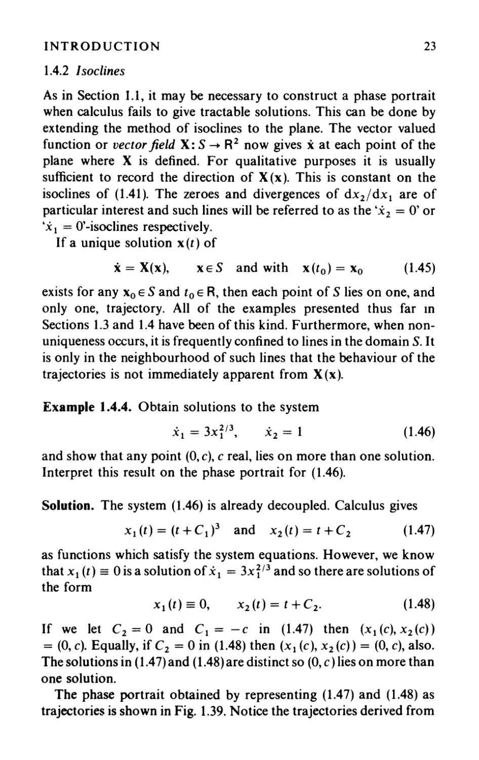
Example 1.4.4. Obtain solutions to the system
Xl = 3xî/ 3 ,
X2 = 1
( 1.46 )
and show that any point (0, c), creaI, lies on more than one solution.
Interpret this result on the phase portrait for (1.46).
Solution. The system (1.46) is already decoupled. Calculus gives
xl(t) = (t+C I )3 and X2(t) = t+C 2 (1.47)
as functions which satisfy the system equations. However, we know
that Xl (t) = 0 is a solution of X 1 = 3xî/ 3 and so there are solutions of
the form
Xl (t) = 0, X 2 (t) = t + C 2' ( 1.48)
If we let C 2 = 0 and CI = - c in (1.47) then (Xl (c), X2 (c))
= (0, c). Equally, if C 2 = 0 in (1.48) then (Xl (c), X2 (c)) = (0, c), also.
The solutions in (1.47) and (1.48) are distinct so (0, c) lies on more than
one solution.
The phase portrait obtained by representing (1.47) and (1.48) as
trajectories is shown in Fig. 1.39. Notice the trajectories derived from
24 ORDINAR Y DIFFERENTIAL EQU A TIONS
Fig. 1.39. Phase portrait for Xl = 3xi/ 3 , X2 = 1. There is no fixed point for this
system and trajectories touch the x2-axis.
(1.47) all touch the x2-axis. This is itself a trajectory, oriented as
shown, corresponding to (1.48). It is no longer clear what '\Te should
mean by a single trajectory because
{ (t -a)3,
Xl (t) = 0,
(t-b)3,
also satisfies (1.46).
t<a
a t b,
t > b,
X2 = t + C
(1.49)
D
ln the remainder of this book we will be concerned only with
systems that have unique solutions. However, (cf. Section 1.1.1) a
useful sufficient condition for existence and uniqueness of solutions
to x = X (x) is that X be continuously difTerentiable.
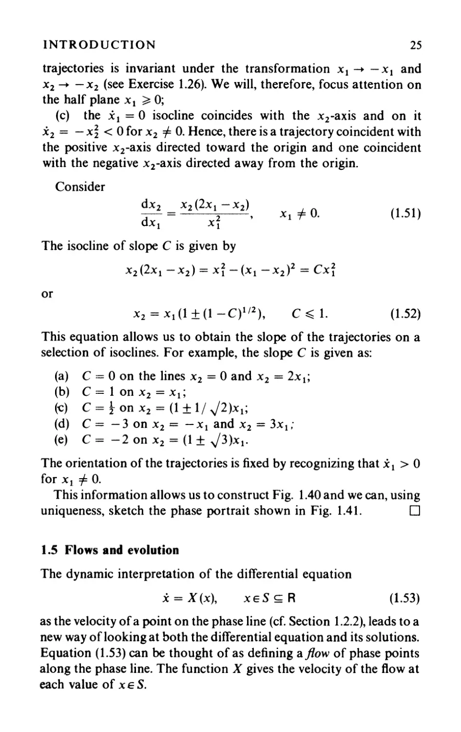
Example 1.4.5. Sketch the phase portrait for the system
· 2
Xl = X b
X2 = X 2 (2x I - X2)
( 1.50)
without using calcul us to determine the trajectories.
Solution. Examine (1.50) and note the following features:
(a) there is a single fixed point at the origin of the Xl x2-plane;
(b) the vector field X(x) = (xi, X2(2xI -X2), corresponding to
(1.50), satisfies X (x) = X ( - x). This means that the shape of the
INTRODUCTION
25
trajectories is invariant under the transformation Xl -+ - X 1 and
X2 -+ - X2 (see Exercise 1.26). We will, therefore, focus attention on
the half plane x t 0;
(c) the Xl = 0 isocline coincides with the X2-axis and on it
X2 = - x < 0 for X2 =1= O. Renee, there is a trajectory coincident with
the positive X2-axis directed toward the origin and one coincident
with the negative X2-axis directed away from the origin.
Consider
dX2
dX I
X2 (2x I - X2)
xi
Xl =1= o.
(1.51 )
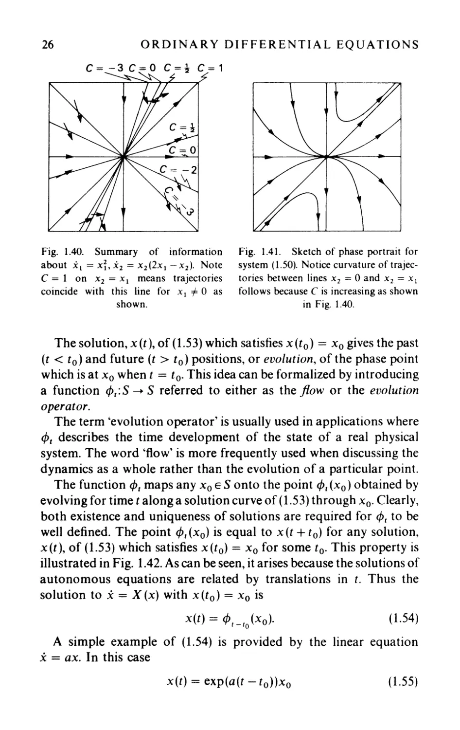
The isocline of slope C is given by
x2(2x t -X2) = xi -(Xl -X2)2 = cxi
or
X 2 = Xl (1 + (1 _C)I/2),
C 1.
( 1.52)
This equation allows us to obtain the slope of the trajectories on a
selection of isoclines. For example, the slope C is given as:
(a) C = 0 on the lines X2 = 0 and X2 = 2x l ;
(b) C == 1 on x 2 = Xl;
('C) C = t on X2 = (1 + 11 J2)x l ;
(d) C = -3 on X2 = -Xl and X2 = 3XI;
(e) C = -2 on X2 = (1 + J3)xt.
The orientation of the trajectories is fixed by recognizing that Xl> 0
for Xl =1= O.
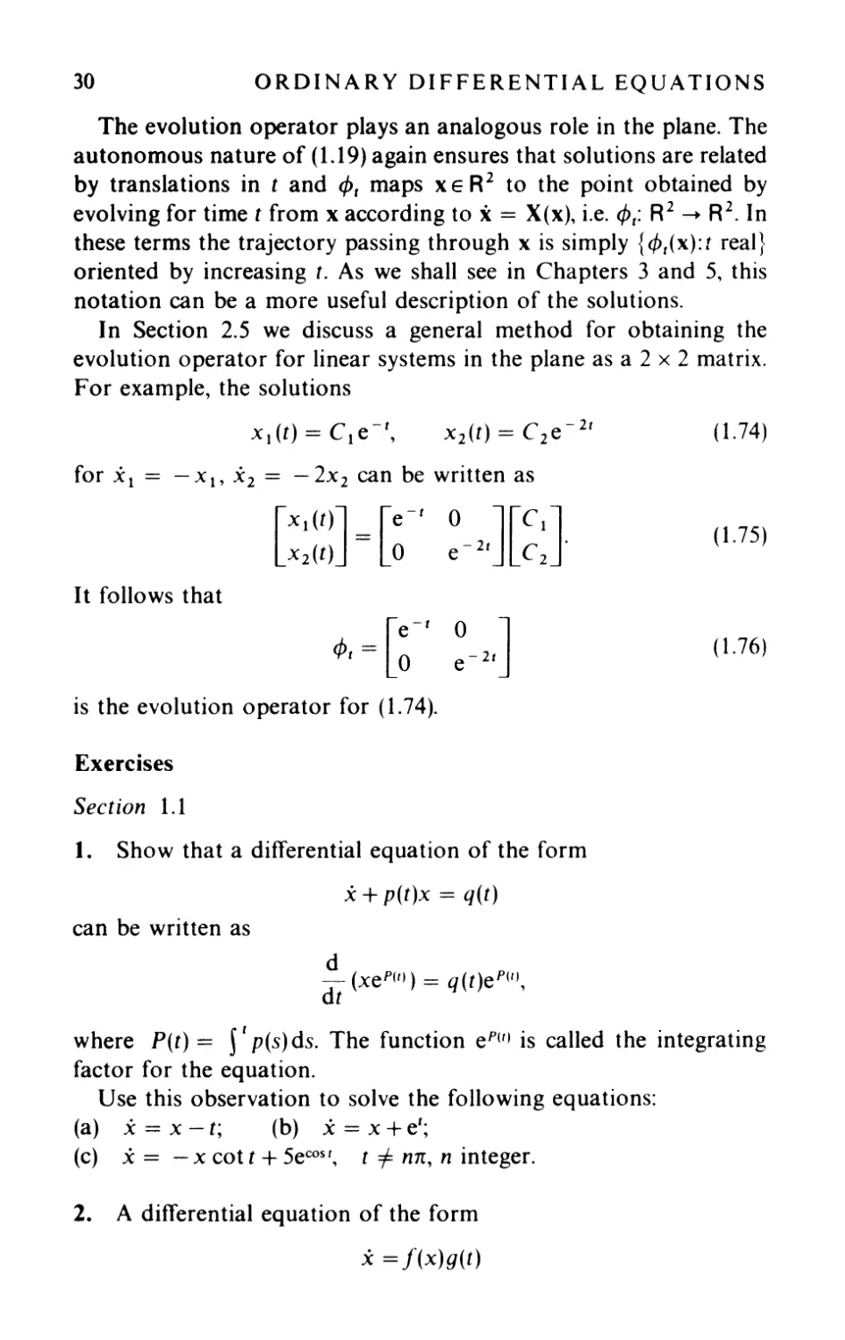
This information allows us to construct Fig. 1.40 and we can, using
uniqueness, sketch the phase portrait shown in Fig. 1.41. 0
1.5 Flows and evolution
The dynamic interpretation of the difTerential equation
x = X (x),
xeS c R
(1.53)
as the velocity of a point on the phase line (cf. Section 1.2.2), leads to a
new way of looking at both the difTerential equation and its solutions.
Equation (1.53) can be thought of as defining aflow of phase points
along the phase line. The function X gives the velocity of the ftow at
each value of XE S.
26
ORDINARY DIFFERENTIAL EQUATIONS
Fig. 1.40. Summary of information
about XI = xL X 2 = x2(2x I -X2). Note
C = 1 on X 2 = XI means trajectories
coincide with this line for XI =1= 0 as
shown.
Fig. 1.41. Sketch of phase portrait for
system (1.50). Notice curvature of trajec-
tories between lines Xl = 0 and Xl = XI
follows because C is increasing as shown
in Fig. 1.40.
The solution, x (t), of (1.53) which satisfies x (to) = Xo gives the past
(t < t o ) and future (t > t o ) positions, or evolution, of the phase point
which is at Xo when t = t o . This idea can be formalized by introducing
a function <Pt: S S referred to either as the flow or the evolution
operator.
The term 'evolution operator' is usually used in applications where
<Pt describes the time development of the state of a real physical
system. The word 'flow' is more frequently used when discussing the
dynamics as a whole rather than the evolution of a particular point.
The function <Pt maps any Xo E S onto the point <Pt (xo) obtained by
evolving for time t along a solu tion curve of (1.53) through Xo. Clearly,
both existence and uniqueness of solutions are required for <Pt to be
weIl defined. The point <Pt (xo) is equal to x (t + t o ) for any solution,
x(t), of (1.53) which satisfies x(to) = Xo for some t o . This property is
illustrated in Fig. 1.42. As can be seen, it arises because the solutions of
autonomous equations are related by translations in t. Thus the
solution to x = X (x) with x (t o ) = Xo is
x(t) = <Pt-to(x o ). (1.54)
A simple example of (1.54) is provided by the linear equation
x = ax. 1 n this case
x(t) = exp(a(t - to))xo
( 1.55)
INTRODUCTION
27
-- --------- x = Xo
Fig. 1.42. Solution curves for x = 1(x 1 - 1). Observe that the solutions ç(t) and 1](t)
sa t i s f y ç (t d = ,., ( ( 2) = X 0' and ç (t + (d = ,., (t + t 1) = 4> r ( X 0), tER.
so that l/J( _( is simply multiplication by exp(a(t - t o )). However, it is
only for lin ar equations that the evolution operator takes this simple
form. ln fact, knowing l/Jt is equivalent to having solved (1.53) and so
finding it is of comparable difficulty.
The flow l/Jt has simple properties which follow directly from its
definition. U niqueness conditions ensure that
l/Js+t(X) == l/Js(l/Jt(x));
s, tER
( 1.56)
providing both sides exist. ln particular,
l/Jt(l/J -t(x)) = l/J -t(l/Jt(x)) = l/Jo(x) = x
( 1.57)
and so
l/J t- 1 == l/J - t.
( 1.58)
For the flow in (1.55) the equalities (1.56) and (1.58) follow
immediately from the properties of the exponential function.
However, these relations are not always so apparent.
Example 1.5.1. Find the evolution operator l/Jt for the equation
x = x-x 2 .
( 1.59)
Verify (1.56) for this example.
28
ORDINARY DIFFERENTIAL EQUATIONS
Solution. The solutions to (1.59) satisfy
f x du x
= ln = t + C
u - u 2 X - 1
for x =1= 0 or 1. This relation can be rearranged to give
( 1. 60 )
x
= Ke t
x-l
with K = + e C , and thus
x(t) = Ke t j(Ke t - 1).
( 1.61 )
If we let x = Xo at t = 0, then (1.61) implies K == xo/(xo - 1)
and so
x(t) = 1>t(xo) = xoetj(xoe t - Xo + 1) (1.62)
for t real and Xo =1= 0 or 1. The points x = 0 and 1 were excluded in
(1.60) because the integral is not defined for intervals including them.
However, we see from (1.59) that they are the fixed points of the
equation, which means that
1>t (0) = 0 and 1>t (1) = 1,
(1.63)
for aIl tER. The form for 1>t is given in (1.62) has precisely these
properties and we can take
1>t(x) = xe t j(xe t - x + 1)
( 1. 64 )
for ail real x and t.
To check the basic property (1.56) of the evolution operator,
observe
1>S(1)t(x)) = 1>s(x I )
( 1.65)
where Xl = 1>t(x). Thus
1> s( 1> t (x)) = X 1 eS j (x 1 eS - x 1 + 1)
( 1. 66 )
with
Xl = xe t j (xe t - x + 1).
Substituting (1.67) into (1.66) gives
1>s(1)r(x)) = xes+tj(xe s + t -x + 1) = 1>s+t(x).
(1.67)
(1.68) D
INTRODUCTION
29
ln Section 1.1, we saw that solutions of x = X(x) may not be
defined for aIl real t. The following exalnple illustrates how this is
reflected in the domain of definition of 1>,(x).
Example 1.5.2. Find the evolution operator 1>, for the equation
x = x 2
( 1.69)
and give the intervals of t on which it is defined for each real x.
Solution. Solutions to (1.69) satisfy
I x
u- 2 du = -x- l = t+C
(1. 70)
where C is a constant, in any interval which does not contain x = O. If
x = Xo when t = 0, then C = - Xo 1 and we obtain
x(t) == xo/(1 - xot),
=1= -1
t Xo.
(1.71)
ln terms of the evolution operator, (1.71) means that
1>,(x) = x/(l - xt)
(1. 72)
for any non-zero x. As in Example 1.5.1, 1>,(x) given in (1.72) is also
valid at x == 0; i.e.
1>,(0) = 0 for aIl real t,
(1.73)
as required by the fixed point at x = 0 in (1.69). Thus (1. 72) is valid for
aIl real x. However, 1>,(x) is not defined for aIl t; consider, for example,
t == x - 1 in (1. 72). ln fact, the interval in t for which 1>,(x) is defined is
determined by x as foIlows:
(a) x > 0: the entire evolution of x is given by (1.72) for - 00 < t
< x - 1 .
,
(b) x == 0: (1.73) shows that 1>,(0) is defined for - 00 < t < 00;
(c) x < 0: (1.72) again describes the evolution of x but with x- l
< t < 00.
ln case (a), 1>,(x) increases from arbitrarily smaIl, positive values at
large negative t; through x at t = 0 and tends to infinity as t x - 1.
Similarly, in case (c) 1>,lx) takes arbitrarily large, negative values for t
close to x - 1; as t increases, x increases strictly and approaches zero as
t 00 (cf. Fig. 1.15). 0
30
ORDINARY DIFFERENTIAL EQUATIONS
The evolution operator plays an analogous role in the plane. The
autonomous nature of (1.19) again ensures that solutions are related
by translations in t and l/J, maps XE R 2 to the point obtained by
evolving for time t from x according to x = X(x), i.e. l/J,: R 2 R 2 . ln
these terms the trajectory passing through x is simply {4>,(x): t real}
oriented by increasing t. As we shall see in Chapters 3 and 5, this
notation can be a more useful description of the solutions.
ln Section 2.5 we discuss a general method for obtaining the
evolution operator for linear systems in the plane as a 2 x 2 matrix.
For example, the solutions
Xl (t) = el e-',
X2(t) = C 2 e- 2 ,
(1. 74)
for Xl = -X b x 2 = -2X2 can be written as
[ X 1 (t ) J = [ e - , 0 J [ c 1 J .
X2(t) 0 e- 21 C 2
(1.75)
1 t follows that
t = [ -I -2tJ
is the evolution operator for (1.74).
(1. 76)
Exercises
Section 1.1
1. Show that a difTerential equation of the form
X + p(t)x == q(t)
can be wri t ten as
d
dt (xeP(t)) == q(t)eP(t),
where P(t) = l' p(s) ds. The function eP(t) is called the integrating
factor for the equation.
Use this observation to solve the following equations:
(a) X = X - t; (b) x == X + e';
(c) x = - X cot t + 5ecos t , t =1= n1t, n integer.
2. A difTerential equation of the form
x = f(x)g(t)
INTRODUCTION
31
is said to be separable, because the solution passing through the point
(t o , xo) of the t, x plane satisfies
f x du f I
f u = g(s)ds,
XO ( ) to
provided these integrals exist. The variables x and tare separated in
this relation. Use this result to find solutions to:
(a) x = xt; (b) x = -x/t, t =1= 0;
(c) x = - t/x, x =1= 0; (d) x = - x/tanh t, t =1= o.
3. A difTerential equation of the form
M(t, x) + N(t, x)x = 0
is said to be exact if there is a function F(t, x) with continuous second
partial derivatives such that aF/at = M(t, x) and aF/ox = N(t, x).
Show that a necessary condition for such a function to exist is that
aM
ax
aN
-
ot
and that any solution to the difTerential equation satisfies
F(t, x) = constant.
Show that
x
- + [ln (xt) + 1 Jx = 0,
t
is an exact difTerential equation. Find F(t, x) and plot several solution
curves.
t, x > 0
4. Use the calculus to find solutions for the following difTerential
equations:
(a) .,x = x 2 ; (b) x = îx 3 ;
(c) X = î(x 2 -1); (d) x = 3x 2/3 ;
(e) x = / (1 - x 2 ), 1 x 1 1; (f) x = 2x 1 1 2 , X O.
Equations (e) and (f) are defined on the closed domains
D = {(t, x) Ilxl 1} and D = {(t, x)1 x O}, respectively. Prop-
osition 1.1.1 ensures existence of solutions on the open domains
D' = {(t, x)llxl < 1} and D' = {t, x)lx > O} for these examples. Do
the solutions you have found exist on the boundary of D?
32
ORDINARY DIFFERENTIAL EQUATIONS
s. Show how to construct infinitely many solutions, satisfying the
initial condition x(O) = 0, for the differential equations given in
Exercise 1.4 (d) and (f). Can the same be done for the equation in
Exercise 1.4 (e) subject to the condition (a) x(O) = 1, (b) x(O) = -1?
Explain your answer.
6. Suppose the differential equation x = X(t, x) has the property
X(t, x) = X( - t, - x). Prove that if x = ç(t) is a solution then so is
x = - ç( - t). Find similar results on the symmetry of solutions when:
(a) X(t, x) = - X( - t, x); (b) X(t, x) = - X(t, - x). Which of these
symmetries appear in Figs. 1.1-l.8?
7. A difTerential equation of the form
x = h(t, x)
(1 )
is said to be homogeneous if h(t, x) satisfies h((Xt, (Xx) = h(t, x) for aIl
non-zero real ex. Show that the isoclines of such an equation are always
straight lines through the origin of the t, x-plane.
Use this result to sketch the solution curves of
x = exit
,
t =1= O.
(2)
Show that the change of variable x = ut allows (1) to be written as a
separable equation (Exercise 1.2) for u when t =1= O. Does this result
help to obtain the family of solution curves for (2)?
8. Sketch the family of solutions of the difTerential equation
x = ax -bx 2 ,
x > 0,
a and b > O.
Obtain the sketch directly from the difTerential equation itself. Prove
that x is increasing for 0 < x < a/2b and decreasing for a/2b < x
< alb. How does this result influence your sketches? How does x
behave for alb < x < oo?
9. Show that the substitution y == x - l, x =1= 0 allows
x = ax - bx 2
to be written as a difTerential equation for y with the form described in
Exercise 1.1. Solve this equation and show that
x(t) = aXo/{ bxo + (a - bxo) exp( - a(t - t o ))},
INTRODUCTION
33
where x(t o } = Xo. Verify that the sketches obtained in Exercise 1.8
agree with this result. Can you identify any new qualitative features of
the solutions which are not apparent from the original differential
equation?
10. Sketch the solution curves of the differential equations:
(a) x = x 2 - t 2 - 1; (b) x = t - tlx, x =1= 0;
(c) x = (2t + x)/(t - 2x), t =1= 2x; (d) x = x 2 + t 2 ;
by using isoclines and the regions of convexity and concavity.
Il. Obtain isoclines and sketch the family of solutions for the
following difTerential equations without finding x as a function of t.
(a) x = x + t; (b) x = x 3 - x;
(c) X = xt 2 ; (d) x = x ln x, x > 0;
(e) x = sinh x; (f) x = t(x + 1)/(t 2 + 1).
What geometrical feature do the isoclines of (b), (d) and (e) have in
common? Finally, verify your results using çalculus.
Section 1.2
12. Find the fixed points of the following autonomous differential
equations:
(a) x = x + 1; (b) x = x - x 3 ; (c) X = sinh(x 2 );
d) x = x 4 -x 3 -2x 2 ; (e) x = x 2 + 1.
Determine the nature (attractor, repellor or shunt) of each fixed point
and hence construct the phase portrait of each equation.
13. Which differential equations, in the following list, have the same
phase portrait?
(a) x = sinhx; (b) x = ax, a> 0; (c) X = { xln1xl, x =1= 0
o x = O .
, ,
(d) x = sin x; (e) x = x 3 - x; (f) x = tanh x.
Explain, in your own words, the significance of two differential
equations having the same phase portrait.
14. Consider the parameter dependent differential equation
x = (x - À)(x 2 - À), À real.
Find aIl possible phase portraits that could occur for this equation
together with the intervals of À in which they occur.
34
ORDINARY DIFFERENTIAL EQUATIONS
15. How many distinct qualitative types of phase portrait can occur
on the phase line for a differential equation with three fixed points?
What is the formula for the number of distinct phase portraits in the
general case with n fixed points?
16. Show that the phase portrait of
x = (a -x)(b -x}
is qualitatively the same as that of
y = y(y - c)
for aIl real a, b, c; a =1= b, c =1= O. Show, however, that a transformation.
y = kx + 1, which takes the first equation into the second, exists if and
only if c = b - a or a - b.
17. Consider the difTerential equation
x == x 3 + ax - b.
Show that there is a curve C in the a, b-plane which separa tes this
plane into two regions A and B such that: if (a, b) E A the phase
portrait consists of a single repellor and if (a, b) E Bit has two repellors
separated by an attractor. Let a < 0 be fixed; describe the change in
configuration of the fixed points as b varies from - CfJ to oc.
18. A substance y is formed in a chemical reaction between
substances r:x and p. ln the reaction each gram of y is produced by the
combination of p grams of r:x and q = 1 - p grams of /3. The rate of
formation of y at any instant of time, t, is equal to the product of the
masses of r:x and p that remain uncombined at that instant. If a grams
of r:x and b grams of pare brought together at t = 0, show that the
differential equation governing the mass, x(t), of y present at time t
> 0 is
x = (a - px)(b - qx).
Assume alp > b/q and construct the phase portrait for this equation.
What is the maximum amount of y that can possibly be produced in
this experiment?
Section 1.3
19. Find the fixed points of the following systems of differential
INTRODUCTION
35
equations in the plane:
(a) Xl = Xl (a - bX2)
x 2 = -X2(C -dx l )
a, b, c, d > 0;
(c) Xl == X 2
X 2 == x 2 (1 -xi) -Xl;
(e) Xl == sin Xl
X 2 == cos X2"
(b) Xl = X2
. "
X 2 = - sIn Xl;
(d) Xl = xI(2 -Xl -2X2)
x 2 = x2(2 - 2XI - X 2 );
20. Sketch the following parametrized families of curves in the
plane:
(a) (X b X2) == (acost,asint); (b) (X I ,X 2 ) == (a cos t, 2asint);
(c) (x b x 2 ) = (ae t , be- 2t); (d) (xJ, X2) == (ae t + be-t, ae t - be- t );
(e) (Xl' X 2 ) = (ae t + be 2t , be 2t );
where a, bER. Find the systems of difTerential equations in the plane
for which these curves form the phase portrait.
21. U se the sketches obtained in Exercise 1.20, to arrange the
families of curves (a}-(e) in groups with the same type offixed point at
the origin of the X 1 X 2 -plane.
22. Consider the phase portrait of the system
X 1 == X 1 (x l, X 2 ),
Show that the system
YI == - X 1 (y 1 , Y 2 ),
X 2 = X 2 (X l, X 2 ).
(1)
Y 2 = - X 2 (y l, Y 2)
has trajectories with the same shape but with the reverse orientation
to those of (1). Verify your result by obtaining solutions for:
(a) Xl = Xl (b) Xl = Xl
X 2 = X 2; X 2 = 2x 2
and comparing with Figs. 1.23 and 1.24.
Section 1.4
23. Use the change of variable
Xl = YI + Y2,
X 2 =YI-Y2
to decouple the pair of differential equations
Xl = X2,
X2 = Xl'
36
ORDINARY DIFFERENTIAL EQUATIONS
Hence construct the phase portrait for the system.
24. Show that a solution of the system of differential equations
Xl = -2x.,
X 2 = Xl - 2X 2
satisfying Xl (0) = 1, X2 (0) = 2 is given by
x l (t)=e- 2 " X 2 (t) = e- 2 '(t+2).
Prove that this solution is unique.
25. Consider the system of non-linear first-order differential
equations
Xl = -X 2 +x l (l-xî -x ),
X2==XI+X2(1-xî-x ). (1)
U se the change of variables Xl = r cos 8, X 2 = r sin (J to show that (1)
is equivalent to the system
;- = r (1 - r 2 ),
ë = 1.
(2)
Solve (2) with initial conditions r(O) == ro and 8(0) = (Jo to obtain
r(t) = ro/[r5 + (1 -r5)e- 2 ,]1/2, (J(t) = t + 0 0 ,
26. (a) Suppose the autonomous system
x = X(x)
(1 )
is invariant under the transformation x -+ - X. Sho\\' that if ç(t)
satisfies (1) then so does ,,(t) = - c;(t).
(b) Suppose, instead, that X satisfies X(x) = X( - x). Show, in this
case, that if c;(t) is a solution to (1) then ,,(t) = -ç( -t) is also a
solution.
Illustrate the relations obtained in (a) and (b) by examining typical
trajectories c;(t) and ,,(t) for:
(i) Xl = Xl' X 2 = Xl +X 2 ; (ii)
. 2
Xl == Xl'
. 4
X2 == x 2 .
27. (a) Consider the non-autonomous equation
X = X (t, x)
( 1 )
discussed in Section 1.1. Use the substitution Xl = t, X2 = X to show
that (1) is equivalent to the autonomous system
Xl = 1,
X 2 = X (x l' X 2)'
INTRODUCTION
37
(b) Use the substitution Xl == X, X 2 == X to show that any second-
order equation x = F(x, x) is equivalent to the autonomous system
Xl == X2,
X 2 = F(x l , x 2 ).
Use these observations to convert the following equations into
equivalent first order autonomous systems:
(i) x == x - t; (ii) x == xt; (iii) x + sin x == 0;
(iv) x + 2ax + bx = 0; (v) x + f(x)x + g(x) = O.
Show that (b) is not a unique procedure by verifying that Xl = X2
- J xI f(u) du, X2 == - g(x 1) gives alternative systems for (iv) and (v).
28. Reduce the following sets of equations to a system of auto-
nomous first-order equations in an appropriate number of variables:
(a) x + X = 1, Y + Y + y = 0; (b) x + t = x, y + y3 = t;
(c) x + tx + 1 == 0, y + t 2 x2 + X + y = O.
29. Use the method of isoclines to sketch the phase portraits of the
following systems:
(a) Xl = Xl +X2, X 2 = xi; (b) Xl == X , X 2 == Xl -X ;
(c) Xl == ln Xl; X 2 == X2, Xl> O.
30. The following systems of differential equations in the plane aIl
have a single fixed point. Find the fixed point and use the method of
isoclines to determine which systems do not have closed orbits in their
phase portraits.
(a) Xl == X 2 - 1
X 2 = - (X 1 - 2);
Confirm your results
dX2/dx 1 == x 2 1x l'
(b) Xl == Xl +X 2 (c) Xl = Xl -X2
X 2 = Xl; X 2 = Xl +X2'
using calculus to find the solutions of
31. Consider the difTerential equation
x + X2 + X = o.
(1)
Use Exercise 1.27 (b) to convert it to first-order form. Show that the
isocline of slope k
k = {(Xl' X2)I X 2 = kx l }
is a parabola with vertex (k 2 /4, - k12) and that these vertices
themselves lie on a parabola x = X l' Use the substitution x = w
to solve for X 2 as a function of X 1 and hence sketch the phase portrait
of (1).
38
ORDINARY DIFFERENTIAL EQUATIONS
Section 1.5
32. Show that the evolution operator of the difTerential equation
x = x - x 3 f r x > 1 is given by
<Pt(x) = xe t 1 .J (x 2 e 2 ' - x 2 + 1).
Check that <Ps(<pt(x)) = <Ps+,(x).
33. Find the evolution operators of the difTerential equations:
(a) x = tanhx; (b) x = x ln x, x > o.
34. Find the evolution operators of the following systems:
(a) Xl = Xl' X 2 = Xl -X2; (b) Xl = XIX2, X 2 = X .
Give the intervals of time for which each operator is defined and verify
that <P, +s(x) = <p,(<Ps(x)) provided t, sand t + s belong to the same
interval of definition.
35. Let <Pt describe a ftow in the plane. Dra w phase portraits with at
most two fixed points that satisfy each of the constraints given below:
(a) lim,_ 00 <P,(x) = 0 for aIl points x of the plane;
(b) there is a point Xo such that lim,_ 00 <p,(x o ) = lim,_+ - cc 4>,(x o )
= 0;
(c) limt_ - 00 4>,(x) = 0 for aIl points x of the plane;
(d) there is a trajectory through Xo such that lim,_ oocP,(x o ) = 0 and a
trajectory through x such that lim,_ - 00 cP,(x ) = o.
36. Given the differential equation X = xt, X, t 0, prove that the
evolution of the point Xo at t = t o does not depend only on Xo and
t - t o as in the autonomous case by showing that
,l,. ( t t X ) = X e(C - Co)(C + co)/2
0/ , 0, 0 0 .
CHAPTER TWO
Linear systems
A system x = X(x), where x is a vector in Rn, is called a linear system of
dimension n, if X: Rn --+ Rn is a linear mapping. We will show that only
a finite number of qualitatively ditferent phase portraits can arise for
linear systems. To do this we will first consider how such a system is
atfected by a linear change of variables.
2.1 Linear changes of varia ble
If the mapping X: Rn--+ Rn, where Rn = {(Xl'." ,Xn)lxiER,
i = 1, . . . , n}, is linear, then it can be written in the matrix form
[ X 1 (x l' . '.' , X n)
X (X) = .
X n (X l' . . . , X n)
ail
a ln
Xl
(2.1 )
a nl
a nn
X n
Correspondingly, x = X(X) becomes
x = X(X) = Ax,
(2.2)
where A is the coefficient matrix. Each component Xi(i = 1, . . . , n) of
i is a linear function of the variables Xl' . . . , Xn' These variables are,
of course, simply the coordinates of x = (x l, . . . , x n ) relative to the
natural basis in Rn (i.e. {eJi = l, where ei = (0, . . . , 0, 1, 0, . . . , 0)
with 1 in the ith position). Thus
n
X = L Xi e i and
i = 1
n
X (x) = L Xi (x)e i .
i = 1
(2.3 )
40
ORDINARY DIFFERENTIAL EQUATIONS
ln order to make a change of variables we must express each
xi(i = 1, . . . , n) as a function of the new variables. We consider the
effect on (2.2), of making a linear change of variable,
n
Xi = L mij Yj (i = 1, . . . , n) or x = My (2.4)
j = 1
where mij is a real constant for aIl i and j. Of course, there must be a
unique set of new variables (y l, . . . , y n) corresponding to a given set
of old ones (x l, . . . , x n ), and vice versa. This means that (2.4) must be
a bijection and therefore M is a non-singular matrix. 1 t follows that
the columns m;, i = 1, . . . , n, of Mare linearly independent.
Equation (2.4) implies
n
X = l Yi mi'
i = 1
(2.5)
and we recognize YI' . . . , Yn as the coordinates of x E Rn relative to
the new basis {mi} i = l'
1 t is easy to express (2.2) in terms of the new variables; we find
x = My = AMy
(2.6)
so tha t
y = By,
(2.7)
with
B= M-IAM.
(2.8)
Thus the coefficient matrix B of the transformed system is similar
to A.
Example 2.1.1. The system
Xl = X2,
X 2 = Xl
(2.9)
is transformed into the decoupled system
YI = Yb
Y2 = - Y2
(2.1 0)
by the change of variable
Xl = Yl + Y2;
X2 = YI - Y2'
(2.11 )
Use this result to illustrate (2.8).
LINEAR SYSTEMS
41
Solution. Expressing these systems of equations in matrix form we
o btain
[ I J = [ 0 1 J[ XI J , [ XI J = [ 1 1 J[ YI J and
X 2 1 0 X2 x 2 1 - 1 Y2
[;:J = [ - J[ :l
Thus
A _ [ 0 1 J
- 1 0 '
M = [ _ ] and B = [ - l
Observe that AM = M B so that (2.8) is satisfied.
D
Example 2.1.2. Find the matrix representation of the linear system
Xl = X 1 + 2x 2,
X 2 = 2X2
(2.12)
under the change of variables
Xl = YI + 2Y2,
X 2 = Y2'
(2.13 )
What is the basis for which Yb Y2 are the corresponding
coordinates?
Solution. The change of variables (2.13) can be written in the form
[::J = [ J[ :J
(2.14 )
so that
M = [ ]
The system (2.12) has the matrix form
x = [ Jx = Ax. (2.16)
(2.15)
Equations (2.7) and (2.8) give
B=M-1AM=[ J and y=By (2.17)
as the required matrix representation.
42
ORDINARY DIFFERENTIAL EQUATIONS
The basis with coordinates YI' Y2 is given by the columns of M in
(2.15), that is {(1, 0), (2, 1)}. D
Similarity is an equivalence relation on the set of n x n real matrices
(see Exercise 2.2) and it follows that this set can be disjointly
decomposed into equ valence cr similarity classes. For any two
matrices A and B in the same similarity class, the solutions of the
systems x = Ax and y = By are related by x == My if M - 1 AM == B.
Thus, if one such system can be solved, solutions can be obtained for
each member of the class.
ln Section 1.4.1, we saw that decoupled or partially decoupled
systems could be solved easily and we are led to consider whether each
similarity class contains at least one correspondingly simple (e.g.
diagonal or triangular) member. The answer to this algebraic problem
is known and we will illustrate it for n = 2 in the next section.
2.2 Similarity types for 2 x 2 real matrices
For each positive integer n.. there are infinitely many similarity classes
of n x n real matrices. These similarity classes can be grouped into just
finitely many types. ln the following proposition we give these types
for n = 2.
Proposition 2.2.1. Let A be a real 2 x 2 matrix, then there is a real,
non-singular matrix M such that J = M -1 A.. is one of the types:
(a) [ I l ,11 > ,12; (b) [ o ol
A 2 (2.18)
[ o ol [ - l
(c) (d) f3>0
where ,10, À., ,12' cx, f3 are real numbers.
The matrix J is said to be the Jordan form of A. The eigenvalues of
the matrix A (and J) are the values of À for which
PA (À) = ,12 - tr(A),1 + det(A) = O.
(2.19)
Here tr(A) = ail + a22 is the trace of A and det(A) = ail a22
- a 12 a21 is its determinant. Thus the eigenvalues of A are
,11 = !(tr(A) + J ) and ,12 = !(tr(A) - J ) (2.20)
LINEAR SYSTEMS
with
43
6. = (tr(A))2 - 4 det(A).
(2.21 )
It is the nature of the eigenvalues: real distinct ( > 0), real equal
( = 0) and complex ( < 0) that determine the type of the Jordan
form J of A.
(a) Real distinct eigenvalues ( > 0)
The eigenvectors u., U2 of A are given by
Au. == A.u.
1 ,"
(i = 1, 2)
(2.22)
with Ab À 2 , Al > A2, the distinct eigenvalues. Let
M = [UI : U2]
be the matrix with the eigenvectors u., U2 as columns. Then
AM=[Au l : AU2]=[AIUI : A2u2]= MJ (2.24)
(2.23)
where
J = [ I
J .
A 2
For distinct eigenvalues the eigenvectors UI and U2 are linearly
independent and therefore M is non-singular. Thus
M- 1 AM = J = [ I J. (2.25)
(b) Equal eigenvalues ( = 0)
Equation (2.20) gives Al = A2 = t tr (A) = Ao, and we must consider
the following possibilities.
(i) A is diagonal
[ A o 0 J
A = = Ao 1
o Ao
which is (2.18(b)). ln this case for any non-singular matrix M,
M - 1 AM = A. Therefore the matrix A is only similar to itself and
hence is in a similarity class of its own.
(2.26)
(ii) A is not diagonal
ln this case, since Al = A 2 = Ao, rank(A - Ao/) = 1 and there are not
two linearly independent eigenvectors. Let Uo be an eigenvector of A.
44
ORDINARY DIFFERENTIAL EQUATIONS
If we take "'1 = 110 and choose m2 so that M = [uo : m2] is a non-
singular matrix,
AM = [À.ollo : Am2] = M[ÀOel ; M- I Am2]' (2.27)
where el is the first column of 1.
The matrices A and M - 1 AM have the same eigenvalues, and so
M-IAM= [ À o C J
o Ào
(2.28)
for some non-zero C. However, the simple modification of M to
[ 1 0 ]
M-M
1 - 0 C- l
(2.29)
results in
M-IAM= [ À O 1 J
1 1 0 Ào
which is (2.18(c)).
(c) Comp/ex eigenvalues (A < 0)
We can write ÀI = ex + ip and À 2 = ex - ip, where ex = t tr(A) and
p = + t J ( - A). We wish to show that there is a non-singular matrix
M = [ml j m2], such that M - 1 AM is given by (2.18(d)), or equiva-
lently that
[ a - J.
AM = M fJ v.
(2.30)
Partitioning M into its columns, we obtain
[Ami i Am2] = [exml + 13m2 : - pmi + exm2]
or
[(A - exl)m l - plm2 : {3lm l + (A - exl)m2] = [0 : 0]. (2.31)
This matrix equation can be written as four homogeneous linear
equations for the unknown elements of M, i.e.
t Ûa !-i -A- :J t=:1 = t j . (2.32)
LINEAR SYSTEMS
45
To solve these equations, let P be the coefficient matrix in (2.32)
and let
fA-aIl PI l
Q = [- p ; - a/J ·
(2.33)
Now observe that
PQ = t ; -!- : j (2.34)
where PA (À) = À 2 - 2 À + ( 2 + P2) is the characteristic polynomial
of A. The Cayley-Hamilton theorem (Hartley and Hawkes, 1970)
states that PA (A) = 0 (see Exercise 2.7) and we conclude that
PQ = 0,
(2.35)
the 4 x 4 null matrix. Thus, the columns of Q must be solutions to
(2.32). The first column of Q gives
[ a Il -
M=
a21
- l
(2.36)
Note that the discriminant L\ of PA (À) = 0 can be written
L\ = (a Il - a22)2 + 4a 12a21'
(2.37)
If L\ < 0 then al2a21 =1= 0 and hence a21 =1= o. Further, {3 = + t
J ( - L\) =1= 0 and we conclude that det(M) = Pa21 =1= O. Thus, (2.36)
provides a non-singular matrix M such that M- I AM is given by
(2.18(d) ).
Any given 2 x 2 real matrix A falls into one, and only one, of the
cases set out above (see Exercise 2.6) and Proposition 2.2.1 is justified.
Let us consider some simple illustrations of this result.
Example 2.2.1. Fînd the Jordan forms of each of the following
matrices:
(a) G l
(b) [_ l
[ 3 - 1 J
(c) 1 l'
Solution. The pairs of eigenvalues of the matrices (a}-(c) are (À b À 2 )
= (1 + J2,1 - J2), (3 + i, 3 - i) and (2,2) respectively. Thus, the
46
ORDINARY DIFFERENTIAL EQUATIONS
Jordan forms are
(a) [ ' J=[1+0J2 1- 0 J2J
(b) [; - J = [ - ]
(c) [ o J = [ J
respectively. Notice (2.18 (c)) is chosen for (2.38 (c)) above because the
original matrix is non-diagonal. 0
(2.38)
Example 2.2.2. Find a matrix M which converts each of the matrices
in Example 2.2.1 into their appropriate Jordan forms.
Solution. Matrix (a) has real distinct eigenvalues and so the columns
of M can be taken as the two corresponding eigenvectors. The
eigenvector UI == [ U II J satisfies [A - (1 + J2)IJu l = 0 which im-
U21
plies only that Ull J2 = 2U2'o We can take ", = [ f2} Similarly,
[ - 12 J
"2 corresponding to À 2 = 1 - J2 can be taken as 0 Thus
M = [ 2
- 12J and M-'[
2 J M= [ 1+J2 0 J .
1 0 1 - J2_
Matrix (b) has complex conjugate eigenvalues 3 + i, 3 - i and
Equation (2.36) gives an explicit form for M. ln this case, we find
[ -1
M=
-2
- J
and verify that
[- JM=M[ - J
Finally, matrix (c) has equal eigenvalues and a single eigenvector
LINEAR SYSTEMS 47
[: ] obtained by solving
{[ -: J -2[ J}[ :::J = [ J.
This gives the first column of M. Provided the second column is
chosen to make M non-singular, matrix (c) can be reduced to upper
triangular form. For example, let
M=[
-1 J .
o '
this is a simple choice which makes det( M) == 1, then
M-l[ - JM = [ - J.
This is not the Jordan form given in (2.38), however, ifwe replace Mby
Ml as suggested in (2.29), i.e.
MI = M[ - J = [ J
The result J = [ J is achieved.
D
We will discuss the Jordan forms of matrices with dimension
greater than two in Section 2.7, but first let us examine the significance
of the above results for linear sys ems in the plane. We can summarize
the situation as follows:
(a) every two dimensional linear system
x = Ax
(2.39)
can be transfofmed into an equivalent canonical system
y = Jy,
where J == M- I AM is the Jordan form of A and
(2.40)
x = My;
(2.41 )
(b) the Jordan matrix J must belong to one of the four types given
in the Proposition 2.2.1.
48
ORDINARY DIFFERENTIAL EQUATIONS
We can now find solutions to any system like (2.39) by solving the
corresponding canonical system (2.40) for y and using (2.41) to find x.
2.3 Phase portraits for canonical systems in the plane
A linear system x = Ax is said to be simple if the matrix A is non-
singular, (i.e. det A =1= 0 and A has non-zero eigenvalues). The only
solution to
Ax = 0
(2.42)
is then x = 0 and the system has a single isolated fixed point at the
origin of the phase plane. The canonical system corresponding to a
simple linear system is also simple because the eigenvalues of A and J
are the same.
2.3.1 Simple canonical systems
(a) Real, distinct eigenvalues
ln this case J is given by (2.18(a)) with ÀI and À 2 non-zero. Thus
YI = ÀIy.,
and hence
YI (t) = CI e ÀIC ,
Y2 = À 2 Y2
(2.43 )
Y2(t) = C 2 e À2C ,
(2.44 )
where CI' C 2 are real constants.
If À 1 and À 2 have the same sign phase portraits like those in Fig. 2.1
arise. The fixed point at the origin of the YI Y2-plane is said to be a
(a)
(b)
Fig. 2.1. Real distinct eigenvalues of the same sign give rise to nodes: (a) unstable
0-1 > ).2 > 0); (b) stable ().2 < ).1 < 0).
LINEAR SYSTEMS
49
node. When all the trajectories are oriented towards (away from) the
origin the node is said to be stable (unstable). The shape of the
trajectories is determined by the ratio y = À. 2 1 À. I . Notice that (2.43)
and (2.44) give
dY2 K (y- 1)
- = YI ,
dYI
where K = yC 2IC'i. Therefore, as YI -+ 0
dY2 { O, if Y > 1
d YI -+ 00, if Y < 1 .
(2.45)
(2.46 )
Y2
Fig. 2.2. Real eigenvalues of opposite sign (À. 2 < 0 < À. 1 ) give rise to saddle poInts.
If À. I and À. 2 have opposite signs, the phase portrait in Fig. 2.2 occurs.
The coordinate axes (excluding the origin) are the unions of special
trajectories, called separatrices. These are the only trajectories that are
radial straight lines. A particular coordinate axis contains a pair of
separatrices (remember the origin is a trajectory in its own right)
which are directed towards (away from) the origin if the correspond-
ing eigenvalue is negative (positive). The remaining trajectories have
the separatrices as asymptotes; first approaching the fixed point as t
increases from - 00, passing through a point of closest approach and
finally moving away again. ln this case the origin is said to be a saddle
point.
50
ORDINARY DIFFERENTIAL EQUATIONS
(b) Equal eigenvalues
If J is diagonal, the canonical system has solutions given by (2.44) with
À. 1 = À. 2 = AO =1= 0.Thus(2.18(b))correspondstoaspecialnode,called
a star (stable if Ao < 0; unstable if Ao > 0), in which the non-trivial
trajectories are aIl radial straight lines (see Fig. 2.3).
If J is not diagonal (i.e. (2.18(c))) then we must consider
YI = AOYI + Y2,
(a)
Y2 = AOY2;
AO =1= O.
(2.47)
// 1
//
4 1
1
(b)
Fig. 2.3. Equal eigenvalues (À,1 = À,2 = À,o) give rise to star nodes: (a) unstable;
(b) stable; when A is diagonal.
This system has solutions
YI (t) = (C 1 + t C 2 ) e Àot ;
Y2 (t) = C 2 e,{ot
(2.48)
and phase portraits like those in Fig. 2.4 are obtained (sec
Example 1.4.2).
The origin is said to be an improper node (stable Ao < 0; unstable
AO > 0). The line on which the trajectories change direction is the
locus of extreme values for y l' This is given by the YI = 0 isocline,
namely
Y2 = - AOYI'
(2.49 )
(c) Complex eigenvalues
The Jordan matrix is given by (2.18(d)) so the canonical system is
YI == YI - f3Y2; Y2 = f3YI + Y2' (2.50)
LINEAR SYSTEMS
V
L-
(a)
51
(b)
Fig. 2.4. When A is not diagonal, equal eigenvalues indicate that the origin is an
lmproper node: (a) unstable (Â o > 0); (b) stable (Â o < 0).
This kind of system can be solved by introducing plane polar
coordinates such that YI == r cos 0, Y2 == r sin O. We obtain, as ln
Example 1.4.1,
with solutions
r == (1.r,
r ( t) == r 0 e cxt ,
()={3
O(t) = {3t + 0 0 ,
Typical phase portraits are shown in Fig. 2.5.
_- ---1
(a)
(b)
(2.51 )
(2.52)
(c)
Fig. 2.5. Complex eigenvalues give rise to (a) unstable foci (tX > 0), (b) centres (tX = 0)
and (c) stable foci (tX < 0).
If (1. =1= 0 the origin is said to be a focus (stable if (1. < 0; unstable if
ex > 0). The phase portrait is often said to consist of an attracting
52
ORDINARY DIFFERENTIAL EQUATIONS
(lX < 0) or repelling (lX > 0) spiral. The parameter P > 0 determines the
angular speed of description of the spiral.
When ex = 0, the origin is said to be a centre and the phase portrait
consists of a continuum of concentric circles. This is the only non-
trivial way in which recurrent or periodic behaviour occurs in linear
systems. Every point (excluding the origin) in the phase plane recurs at
intervals of T = 2rcl p. The coordinates are periodic in t with this
period, i.e.,
YI = ro cos (pt + (Jo), Y2 = ro sin (pt + (Jo). (2.53)
The other (trivial) form of recurrence that occurs in simple linear
systems is the fixed point. ln a sense, the fixed point is the ultimate in
recurrence; it recurs instantaneously with period zero.
2.3.2 Non-simple canonical systems
A linear system x = Ax is non-simple if A is singular (i.e. det A = 0
and at least one of the eigenvalues of A is zero). 1 t follows that there
are non-trivial solutions to Ax = 0 and the system has fixed points
other than x = O. For linear systems in the plane, there are only two
possibilities: either the rank of A is one; or A is null. ln the first ca .
there is a line of fixed points passing through the origin; in the second,
every point in the plane is a fixed point. Of course, the rank of J is
equal to the rank of A, so that the canonical systems exhibit
corresponding non-simple behaviour. Figure 2.6 shows two examples
when J has rank one.
We shall, in the remainder ofthis chapter, focus attention on simple
linear systems. These systems play a key role in understanding the
nature of the fixed points in non-linear systems (see Section 3.3).
The results obtained in this section are summarized in Fig. 2.7;
where each type of phase portrait is associated with a set of points in
the tr(A )-det(A) plane. Each point of this plane corresponds to a
particular pair of eigenvalues for A and therefore to a particular
canonical system.
2.4 Classification of simple linear phase portraits in the plane
2.4.1 Phase portrait of a simple linear system
The phase portrait ofany linear system x = Ax can be obtained from
that of its canonical form y = Jy by applying the transformation
1 Y2
-
-
Y,
-
(a)
Fig. 2.6. (a)
Y 2
-
-
-
- -
- Y,
- -
-
-
-
-
-
(b)
[ Yt ] [ 0 1 ][ Yt ] .
Y2 = 0 0 Y2' 1.e. À,o = O.
Every point on the Yt-axis is a fixed point; cf. the À,o -+ 0 limit of Fig. 2.4(a).
(b)
[ Yt ] [ 1 0 l[ Yt ] .
Y2 = 0 0..... Y2 ' 1.e. À,t = 1,À,2 = O.
Every point on the Y2-axis is a fixed point; cf. the À,2 -+ 0 limit of Fig. 2.1 (a).
det (A )
tr (A )
Fig. 2.7. Summary of how the phase portraits of the systems .t = Ax depend on the
trace and determinant of A.
54
ORDINARY DIFFERENTIAL EQUATIONS
x = My. Let us consider how the phase portrait is changed under this
transformation. For example, the canonical system
YI = YI;
Y2 = - Y2
(2.54)
has the phase portrait shown in Fig. 2.8(a). Figure 2.8(b)-(f) shows
the phase portraits for some linear systems that have (2.54) as their
canonical system.
As noted in (2.6) the variables YI and Y2 are the coordinates of x
relative to the basis {ml, m 2 } obtained from the columns of M. Thus
the Y 1- and Y2- axes are represented by straight lines, through
the origin of the x l x2-plane, in the directions of ml and m2
respectively.
The directions defined by ml and m2 are ca lIed the principal
directions at the origin. The mapping is a bijection so every point of
the YIY2-plane is uniquely represented in the xlx2-plane and vice
versa. Furthermore, x is a continuous function of y, so that
trajectories map onto trajectories. Orientation of the trajectories is
also preserved. ln particular, the directions of the separatrices in the
X 1 x2-plane are given by the eigenvectors of A.
These properties of the linear transformation x = My are sufficient
to ensure that, although the phase portrait is distorted, the origin is
still a saddle point. The phase portraits in Fig. 2.8(a}-(f) are typical of
ail systems x = Ax for which A has eigenvalues + 1 and - 1; they aIl
have saddle points at the origin. ln other words, linear transfor-
mations preserve the qualitative behaviour of the solutions.
Example 2.4.1. Sketch the phase portrait of the system
YI = 2YI,
Y2 = Y2,
(2.55)
and the corresponding phase portraits in the Xl x2-plane where
Xl = YI + Y2,
X 2 = YI + 2Y2,
(2.56)
and
Xl = YI'
X2 = - YI + Y2
(2.57)
respectively.
Solution. The phase portrait of system (2.55) is sketched in
Fig. 2.9(a).
Observe that the change of variables given by (2.56) and (2.57) can
CA CA
.. ...- .. --
B
H
D
F
B
H
\ (( r1
EG
(a)
H 8
nl1
EG
(b)
HB
G A
E C
1 \I( 1
F D
(c)
G
E
G
'"
E
H
/.J4 8
Cd)
E G H 8
' ,
F A
D C
(e)
Fig. 2.8. EfTect of various Iinear transformations x = My on the phase portrait of the
canonical system .i'i = YI' }'2 = - J'2.
(a) Canonlcal system }'I = YI; }'2 = - Y2"
(b) M = [ J. (e) M = [ J.
(d) M = G J. (e) M = [: -: J-
(f) M = [ _ J-
..,
56
ORDINARY DIFFERENTIAL EQUATIONS
(a)
Y 2 Y,
(b)
Y 2
y,
(c)
Fig. 2.9. The phase portraits of the canonical system (2.55) in the YI' y1-plane [(a)]
and in the Xl' x 2 -plane defined by (2.56) and (2.57) [(b) and (c) respectively].
be written in the matrix form x = My with
M = [ J and [- J
respectively. The basis for which YI and Y2 are coordinates is
{(l, 1), (1, 2)} for (2.56) and {(l, -1), (0, 1)} for (2.57). The YI and Yz-
coordinate directions are shown in the x l x 2 -plane in Fig. 2.9(b) and
(c) along with the correspondingly transformed phase portrait from
Fig. 2.9(a). D
2.4.2 Types of canonical system and qualitative equivalence
Two Jordan matrices with different eigenvalues are not similar and so
their solutions cannot be related by a linear transformation. However,
the fixed point at the origin of every simple canonical system is one of
a small number of possibilities; namely a node, a focus, a saddle, etc.
How are these phase portraits related?
Consider, for example, the canonical systems
YI = œYI - /3Y2,
œ, /3 > 0 and
Y2 = /3YI + œY2,
(2.58 )
il = Zl -Z2,
i 2 = Zl +Z2'
(2.59 )
Their phase portraits are both unstable foci (see Fig. 2.10).
The trajectories are given by
r = r Oeal ,
() = /3t+(}o
(2.60 )
LINEAR SYSTEMS
57
(a)
(b)
Fig. 2.10. Relation between phase portraits of canonical systems: (a) YI Yl-plane:
trajectory through (ro,Oo) of the system (2.60); (b) Zlzl-plane: trajectory through
(Ro, 4>0) of the system (2.6:
and
R = Roe t ,
</> = t + </>0'
(2.61)
respectively, where (r, (J) and (R, </» are polar coordinates in the YtY2-
and Z lZ2-planes. The trajectory passing through (ro, (Jo) ro =1= 0, in the
YI' Y2-plane can be mapped onto the trajectory passing through
(Ro, </>0) in the zlz2-plane by the transformation
( r ) l/a.
R = Ro - ,
ro
This transformation allows the phase portrait in Fig. 2.10 (a) to be
mapped-trajectory by trajectory-onto that in Fig. 2.10 (b). The
transformation in (2.62) is a bijection; it is continuous; it preserves the
orientation of the trajectories. However, it does not map the YtY2-
plane onto the ztz2-plane in a linear way, unless œ = p = 1.
ln Sections 2.4.1 and 2.4.2 we have examined more closely the
relationship between systems with the same qualitative behaviour (see
also Exercise 2.17). We are led to make the intuitive ideas of
Section 1.3 more precise in the following definition.
(J - (Jo
4> = P + 4>0.
(2.62)
Definition 2.4.1. Two systems of first-order differential equations
are said to be qualitatively equivalent if there is a continuous bijection
which maps the phase portrait of one onto that of the other in such a
way as to preserve the orientation of the trajectories.
58
ORDINARY DIFFERENTIAL EQlJATIONS
2.4.3 Classification of linear systems
ln this chapter we have iIlustrated the fact that every linear system in
the plane is qualitatively equivalent to one of the systems whose phase
portraits are shown in Fig. 2.11. The ten phase portraits shown are
representative of the algebraic type of the linear system.
Qualitative equivalence goes further than this. 1 t can be shown that
aIl stable (unstable) nodes, improper nodes and foci are also related in
the manner described in Definition 2.4.1. This means that the
algebraic types can be further grouped into qualitath'c (or
topological) types as indicated in Fig. 2.11. ln these terms, simple
linear systems only exhibit four kinds of qualitative behaviour: stable,
centre, saddle and unstable.
(b) (c)
mm
Fig. 2.11. The distinct qualitative types of phase portrait for linear systems: (a) stable;
(b) centre; (c) sadd le; (d) unstable; in relation to the algebraic types obtained in
Section 2.3.
2.5 The evolution operator
ln Section 1.5 we suggested that the trajectories of linear systems in
the plane could be described by an evolution matrix. We will now
consider this idea in more detail.
For any real n x n matrix P define the exponential matrix e P by
ex pk
e P = l - (2.63)
k=O k!
with po = ln, the n x n unit matrix. Let Q be a real n x n matrix such
that PQ = QP then it foIlows from (2.63) that
e P + Q = ePe Q ,
(2.64 )
LINEAR SYSTEMS
59
(see Exercise 2.24). This result allows us to conclude that
ePe- P = e-Pe P = eO = 1
n'
(2.65)
so t ha t
(eP)-1 = e- p .
(2.66 )
If we let P == At and difTerentiate (2.63) with respect to t, we find
d
dt (e At ) = Ae At == eAtA.
(2.67)
This means that
d
-,,- (e-Atx) = e-Ati -e-AtAx = e-At(i -Ax) = O. (2.68)
at
If we are given x(to) = Xo, then integrating (2.68) from t o to t, gives
e-Atx(t) = e-Atoxo
(2.69)
and hence
X ( t ) = eA(t -to) X = ( x )
o 'P t - to 0,
(2.70)
by (2.66). Thus, matrix multiplication by eA(t -to) gives the evolution of
the phase point which is at Xo when t = t o . It follows that e At is the
evolution operator for the linear system x = Ax.
Of course, in order to make use of (2.70) we must kno w eA(t - to). For
simple canonical systems in the plane we can write down e Jt from the
solutions given in Section 2.3.1. We find:
e Jt == [ e,tlt 0 J for J = [ 21 J
o e À2t 0 2
(including 2 1 = 2 2 == 2 0 ) from (2.44);
e /t = e [ J for J = [ LJ
(2.71 )
(2.72)
from (2.48); and
[ COS pt - sin pt J · [ a - P J
e Jt = e C (( lor J =
sin pt cos pt p a
from (2.52). These results can also be obtained directly from (2.63) (see
Exercise 2.25).
(2.73)
60
ORDINARY DIFFERENTIAL EQUATIONS
Equations (2.71 }-(2. 73) can be used to obtain e AI for any non-
singular 2 x 2 matrix A by exploiting the relation between A and its
Jordan form J. Recall,
x(t) = My(t) == MeJ1y(0) = (Me Jt M- I )x(O), (2.74)
so tha t
e At = Me Jt M - 1.
(2.75)
While this gives us an understandable way of obtaining e AI it is not
always convenient in practice. An alternative way is to adapt a general
method of Sylvester (Barnett, 1975) for finding functions of matrices.
We consider the method for n = 2.
Let the 2 x 2 real matrix A have two distinct real or complex
eigenvalues À., À 2 . Define the (possibly complex) matrices QI' Q2 by
Q _ A - À 2 l
1- À I -À 2 '
Q _ A-À Il
2 -
À 2 - ÀI
(2.76)
and observe that A = ÀI QI + À 2 Q2' It can be shown that QI Q2
= Q2 QI = 0, Qi == QI and Q = Q2 (see Exercise 2.26) and there-
fore
A k = (À 1 QI + À 2 Q2)k = À QI + À Q2 (2.77)
for any positive integer k. Thus
00 00
e AI _ Akt k _ ( À tk À tk )
- 6 k! - 6 k! QI + k! Q2
k=O k=O
= e).l'QI + e).2 t Q2'
(2.78)
When the eigenvalues À., À 2 of A are equal, define Q = A - Àol,
where ÀI = Â 2 = Ào. ln this case Q2 = 0 and
A k = (Àol+Qt = À I+kÀ -IQ,
because Qk = 0 for k 2. Thus
(2.79)
00
I ( À k kÀk-l )
e AI = 1 + 0 Q t k
k! k!
k=O
= e.J.ot(1 + t (A - Ào 1)).
(2.80)
LINEAR SYSTEMS
Example 2.5.1. Find e At where
A=[_ J
by (a) the method of reducing to canonical form, and (b) the use of
formula (2.78) or (2.80).
61
(2.81 )
Solution. (a) The eigenvalues of A are both Ào = 2. An eigenvector
. . [ 1 ]
"oIS glven by "0 = 1 . Let
M = [
-I J
o '
(2.82)
then
M-IAM= [ 2 1 ] = J'
02'
(2.83)
the required Jordan matrix. The exponential matrix
el' = e 2 , [ ]
by (2.72), and (2.75) gives
e-4' = Me/'M- 1 = e 2 'C
-I J[ 1 t J[ 0 1 ]
o 0 1 -1 1
(2.84 )
= e 2t [ 1-=-/ 1: rI
(b) The eigenvalues of A have been calculated in (a). Substituting
for A and ;'0 == 2 in (2.80), we obtain
e-4( = e2'fl+t{[_ J-{ J}}
= e 2 {1-=-/ 1: rI
(2.85)
D
2.6 Affine systems
ln this section we consider systems where the vector field X is of the
62
ORDINARY DIFFERENTIAL EQUATIONS
form
X(x)=Ax+h
(2.86)
where "E Rn. The mapping X is said to be affine. 1 n the strict algebraic
sense Ax + Il is a non-linear function of x but it is clearly closely
related to linear functions. ln fact, systems x = X(x) with X given by
(2.86) are frequently ca lIed non-homogeneous linear systems as
opposed to the homogeneous linear system x = Ax.
The change of variable
x = y - Xo,
(2.87)
where Xo is a solution ofAx o = Il, if one exists; allows (2.86) to be
written as
Y(y) = X(y - xo) = A(y - xo) + h = Ay. (2.88)
ln such cases, the change of variable (2.87) allows the affine system
x = Ax + h
(2.89 )
to be written as the linear system
y = Ay.
(2.90 )
However, what if Il is not in the image of A or if h in (2.89) is replaced
by a time dependent vector lI(t)? Non-autonomous systems of the
latter form frequently occur in practical problems (see Section 4.2).
The evolution operator provides a solution to both of these
difficul ties.
The procedure is a matrix equivalent of the integrating factor
method' used in Exercise 1.1. M ultiply (2.89) throughout by e - At and
rearrange as
d
-(e-ACx) = e-Ach(t).
dt
(2.91)
Here the evolution operator acts as a matrix integrating factor'.
Suppose we are given x (t o ) = Xo, then integrating (2.91) frolTl Co to t
glves
e-Atx(t)-e-ACOxO = f ' e-Ash(s)ds.
Co
Since eAte -Ac = 1 we can solve for x(t); thus
x(t) = XCF(t) + xp,(t),
(2.92)
LINEAR SYSTEMS
63
where
XCF(t) = eA(C-Co)xo
(2.93)
and
XPI(t) == e Ac f r e-A<h(s)ds.
(0
(2.94 )
Equation (2.92) gives the general solution to the affine system (2.89),
whether or not h depends on t.
The first term XCF(t) is the solution of the linear system x = Ax
which satisfies the initial condition XCF(t O ) == Xo. 1 t corresponds to the
complenlentary junction of traditional treatments of second-order,
non-homogeneous linear equations. The second term, xPI(t), gives a
general expression for the particular integral' of such treatments. It is
easy to verify that xPI(t) satisfies (2.89) and that xpl(O) = 0, so that x(t)
in (2.92) satisfies both (2.89) and x(to) == Xo.
Example 2.6.1. Consider the second-order equation
x + 2x + 2x == u(t).
(2.95)
Write this equation as a first-order system and obtain a general
expression for the solution which satisfies x(O) == x(O) == o.
Solution. Let Xl == x and Xl = X, then (2.95) becomes
Xl == X2,
x 2 == -2x l -2X2 + u(t).
(2.96 )
ln matrix notation, (2.96) takes the form x == Ax + h(t) with
.A == [ 0 1 J and
-2 -2
h(t) = [ 0 J .
u(t)
(2.97)
The matrix .4 has cigenvalues Âl == - 1 + i, Â 2 == - 1 - i and (2.78)
glves
{ e it [ 1 + i
e A ( == e -1 -
2; -2
1 J -it [l .
e -1
- 1 + ; 2; - 2
_ 11 _ J}
1 [ COS t + sin t sin t J
e Ac == e-
- 2 sin t cos t - sin t .
(2.98)
The initial condition given corresponds to x(O) == 0, so XCF(t) = 0 in
64
ORDINAR Y DIFFERENTIAL EQUATIONS
(2.92) and x(t) = xPI(t), which is
e _t [ cos t 2 +.sin t sin t . J r' e' U(S) [ - sin J ds. (2.99)
- sIn t cos t - sIn t J a cos S + sIn s
Hence
Xl (t) = x{t) = e -, {sin t l' e'u(s) cos S ds
- cos t l' e'u(s) sin s dS}.
(2. J (0) [J
2.7 Linear systems of dimension greater than two
2.7.1 Three-dimensional systems
The real Jordan forms for 3 x 3 matrices are
o 0 ?] [ -{3 ] ,
À,l ex
0 A 2 0 À,l
[ o 1 ] and [ o 1 ]
À,o À,a (2.101)
0 À,l 0 À,a
where ex, {3, À,o, À,l' À,2 ar real (Hirsch and Smale, 1974). Observe that
ail, except the last form, in (2.101) can be partitioned in diagonal
blocks of dimension 1 and 2. For example, consider
1
ex -{3 1 0
1
Y = Jy with J = {3 ex: 0
- - --------
o 0: À,l
1
(2.102)
where À,l < ex < 0, {3 > O. The diagonal block structure ensures that
the Y3-equation is decoupled from the other two. ln fact, (2.102) is
equivalent to the two systems
[;:J = [; - J[ J,
(2.103)
Y3 = À,IY3'
(2.104)
LINEAR SYSTEMS
65
This decoupling allows us to construct the qualitative features of the
three-dimensional phase portrait.
Equation (2.103) shows that the projection of the trajectories onto
a plane of constant Y3 is a stable (a < 0) focus; the attracting spiral
being described in an anticlockwise sense (f3 > 0). Since ÀI < 0, 1 Y3(t) 1
decreases exponentially with increasing t. A typical trajectory of
(2.102) passing through (a, b, c) at t == 0, with ail three coordinates
non-zero, is shown in Fig. 2.12. The spiral in the constant Y3 projec-
tion is drawn out into a kind ofheIix with decreasing radius and pitch.
Y 3
Y,
Fig. 2.12. The trajectory of (2.1 02) passing through (a, b, c). Each trajectory lies in a
surface of the form Y3 = K (yi + y ),{1/2(X.
Returning to (2.101), the Jordan form that is not amenable to block
decomposition corresponds to a system j = Jy that can be solved by
finding e Jt . The evolution operator can be obtained by using the
expansion (2.63); observe
ÀO 1
J = L o
0 ] [ a 0 0 ] [ 0
1 = 0 Àa 0 + 0
Àa 0 0 Àa 0
J = D + C.
1 0 J
o 1
o 0
(2.105)
As in Exercise 2.24, DC = CD and (2.64) reduces the problem to one
of finding e Ct . ln this case,
C 3 = 0 and e O = 1+ tC+ tt 2 C 2
1 t t t 2 ]
and e Jt = e J.ol 0 1 t .
001
(2.106)
66 ORDINARY DIFFERENTIAL EQUATIONS
Ex.mple 2.7.1. Sketch the trajectory which satisfies x(O) = (0, b, c);
b., c > 0., for the system
x = lx,
(2.107)
where J is given by (2.105) with Ào > O.
Solution. Observe that the projection of (2.107) onto the x2x3-plane,
l.e.
[ 2 J = [ À o 1 J[ X2 J
x 3 0 Ào x 3
is independent of Xl' This means that each trajectory of (2.107) can be
projected onto one of the trajectories of(2.108) in the x2x3-plane. The
system (2.108) has an unstable (Ào > 0) improper node at X 2 == X3 == 0
and so its trajectories are like those in Fig. 2.13.
(2.108)
Fig. 2.13. Projections of the trajectories of system (2.1 07) onto the x 2 x 3 -plane are
given by the phase portrait of (2.109), which has an unstable improper node at the
origin. The line X3 = - À-OX2, where x 2 = 0, is shown dashed.
Let l/Jt denote the evolution operator for (2.107), then it follows that
the trajectory {l/Jt (0, b, c) 1 tER} lies on the surface S generated by
translating the trajectory,
[:: : J=eÀ&[ J[:J
(2.109)
of (2.108), in the xl-direction (see Fig. 2.14). Notice that (2.109) is the
LINEAR SYSTEMS
67
x,
Fig. 2.14. The surface S containing the trajectory {4>,(O, b, c) 1 tER} of (2.107),
obtained by translating the curve given by (2.109) in the xl-direction.
X2x3-projection of
1 t t t J [ O
4>,(0, b, c) = e'ot J
(2.110)
(cf. e Jt in (2.106)).
Now consider the Xl x2-projection of the required trajectory. The
system equations (2.107) give Xl = 0 for X 2 = - À-ox 1 and X2 = 0 for
X 3 = - À-OX2' The latter plane intersects Sin its fold line (see Fig. 2.13).
The Xl x2-projection of the fold is the line X2 = K, where K is
the value of X2 for which X2 = 0 in (2.109). We can then sketch the
xlx2-projection shown in Fig. 2.15.
Finally we can show the required trajectory on S (see
Fig. 2.16). 0
2.7.2 F our-dimensional systems
The Jordan forms J of 4 x 4 real matrices can be grouped as follows:
(a) [-i+ l (2.111)
À-o 1 0 10
1
(b) o À.o 1 : 0 (2.112)
1
o 0 À-o 1 0
__ _ ___ __L__
0 0 0 ; À- 1
1
68
ORDINARY DIFFERENTIAL EQUATIONS
X 2
x = K
2
------- -------
x, > 0
x, = 0
.....-'t C
x,
A
x, < 0
1
B
Fig. 2.15. Projection of {4>,(O, b, c) 1 tER} onto x., x2-plane. A, Band C label points
of the projection where Xl = 0 or X2 = O. The turning point at X2 = K coincides with
the fold in S shown in Fig. 2.14.
x 2
x,
Fig. 2.16. The trajectory {4>, (0, b, c) 1 tER} of (2.107). The extreme points at A, Band
C are those shown in Fig. 2.15. The curve (2.1 09) in the x 2, X 3 -plane is shown dashed.
and
,1,0 1 0 0
(c) 0 ,1,0 1 0 (2.113)
0 0 ,1,0 1
0 0 0 ,1,0
LINEAR SYSTEMS
69
ln (a) the submatrices Band C are 2 x 2 Jordan matrices and 0 is the
2 x 2 null matrix. ln (b) and (c) ,1,0' ,1,1 are real numbers.
The matrices in both (a) and (b) allow y == Jy to be split into
subsystems of lower dimension. We have for (a)
[ J = B[:J and G:J = e[::J
(2.114)
and for (b)
[ ill f:o 1
J = l o
!J
and
X 4 = Â I X 4 .
(2.115)
The solution curves of aIl these subsystems have already been
discussed.
The only new system we have to consider is one with a coefficient
matrix of type (c). The trajectories for this system can be found by
extending the method used to obtain (2.106). We find
1 t tt 2 t3
, 4J ) ,0 1 t tt 2 (2.116)
x (t J = t (x o == e.A.ol 0 0 1 t Xo.
0 0 0 1
Thus it is conceptually no more difficult to find solutions for the
canonical systems when n == 4 than it is for n == 2 and 3.
2.7.3 n-Dinlensional systems
The pattern ofblock decomposition which we have illustrated for the
Jordan forms of 3 x 3 and 4 x 4 real matrices extends to arbitrary n.
This means that the corresponding canonical systems y = Jy, with
J = M - 1 AM, decouple into subsystems. These subsystems may
have:
dimension 1
Y .. == À. } "
1 1 1 ,
À i real;
or dimension 2
[ Yi J [ ex - f3 J[ Yi J
Yi+l - f3 ex Yi+l'
f3 > 0, ex real;
70
ORDINARY DIFFERENTIAL EQUATIONS
or dimension j, with 2 j n
Yi À 1 0 0 V.
- 1
0 À 1
0 )" real.
À 1
ri + j - 1 0 0 0 À Yi + j - 1
However, as we have seen for n = 3 and 4, solutions can be found for
aIl of these subsystems and we conclude any canonical system can be
solved. Of course, this means that the solutions of alllinear systems
i = Ax can also be found by using x == My.
Exercises
Sections 2.1 and 2.2
1. Indicate the efTect of each of the following linear transformations
of the xlx2-plane by shading the image of the square S == i (Xl' X2)1
o Xl, X2 1}:
(a) [ J (b) [= - J (c) [= J (d) [; - J.
U se the images of the square to help to sketch the images of the
following sets:
(a) the circle xI + x = 1; (b) the curve XIX 2 == 1, XJ, X 2 > O.
2. Prove that the relation "" on pairs A, B or real n x n matrices
given by
A "" B B == M - 1 A M,
where M is a non-singular matrix, is an equivalence relation.
Furthermore, show that all the matrices in any given equivalence class
have the same eigenvalues. Group the following systems under this
equivalence on their coefficient matrices:
(a) x = [ ]x;
(b) x = [ ]x;
LINEAR SYSTEMS 71
X=L -2J (d) . [-4 2JX'
(c) x' x=
-6 ' -4 5 '
(e) X = [ 2}. (f) X = [ }.
1 '
3. Show that each of the following systems can be transformed into
a canonical system by the given change of variable:
(a) XI == 4x 1 +X2, X2 == -Xl + 2X 2'
YI == 2x 1 + X 2, Y 2 == Xl + X 2;
(b) Xl == 12x 1 + 4x 2, X 2 == - 26x 1 - 8x 2,
YI == 2XI + X2, Y2 == 3XI + X2;
(c) Xl == 10X l + 2X2, X2 == - 28x I - 5X 2,
YI == 7Xl + 2X2, Y2 == 4x I + X2'
Write down the coefficient matrices A of each of the above systems,
the Jordan forms J and the change of variable matrices M. Check that
J =:: M - 1 AMis satisfied.
4. For each matrix A given below
[- J
[ 41 - 29 J
58 -:41'
[-: -;J
find its Jordan form J and a matrix M that satisfies
J = M- I AM.
5. What is the efTect on the system
Xl = -7x I - 4X 2 -6x 3
x 2 = -3x I -2x 2 -3x 3
X3 = 3x I +2x 2 + 2X 3
of the change of variables YI = Xl + 2X 3'Y2 = X2,Y3 = Xl +x3?How
does the introduction of these new variables help to investigate the
solution curves of the system?
6. Prove that no two difTerent 2 x 2 Jordan matrices are similar.
Hence prove that there is one and only one Jordan matrix similar to
any given 2 x 2 real matrix.'
72
ORDINARY DIFFERENTIAL EQUATIONS
7. Find the characteristic equations of the matrices
[ J
[- J
[ 8 - 4 J
6 - 3 '
and illustrate the Cayley-Hamilton theorem for each matrix.
Section 2.3
8. Find the solution curves x (t) satisfying x == Ax subject to
x (0) = Xo, where the matrix A is taken to be each of the Inatrices in
Exercise 2.4.
9. Sketch phase portraits for the linear system
[ :J=A[::J
when A is given by:
(a) [ l (b) [-1 0]- (c) [- l
02'
(d) [ l (e) [ l (f) [- - l
(g) [- } (h) [ - } (i) [ }
(j) [ - J.
10. Indicate the effect of the linear transformation
[ :J = e J[::J
on each of the systems in Exercise 2.9 by sketching each phase portrait
in the Yt Y2-plane.
Il. Find the 2 x 2 matrix A such that the system
x = Ax
LINEAR SYSTEMS
73
has a solution curve
_ l e -t (cos t + 2 sin t) J
x (t) - - t .
e cost
12. Let
. [ -1 -I J
x= x
2 -4
and y = Xl + 3X2' For this situation the system is said to be
'observable' if by knowing y (t) the solution curve x (t) can be derived.
Prove that the system is observable when y (t) = 4e - 2t by finding x (0).
Section 2.4
13. Locate each of the following linear systems in the Tr-Det plane
and hence state their phase portrait type:
(a) Xl = 2x I + X2, x 2 = Xl + 2x 2 ;
(b) Xl = 2x I + X2, X 2 = Xl - 3x 2 ;
(c) Xl = Xl -4x 2 , X 2 = 2x I -X2;
(d) Xl = 2x 2 , :X2 == - 3x I - X2,
(e) Xl = -x l +8x 2 , X 2 = -2x l +7x 2 .
14. Express the system
x l =-7x l +3x 2 ,
X 2 = -8x I + 3X 2
in coordinates Yb Y2 relative to the basis { (1, 2), (3, 4)}. Hence sketch
the phase portrait of the system in the X 1 X 2 -plane.
15. Let x (t) be a trajectory of the linear system x = Ax and suppose
limt_oox(t) = O. Use the continuity of the linear transformation y
= Nx, where N is a non-singular matrix, to show that the trajectory
y(t) = Nx(t) of the system
y = NAN-Iy
also sa tisfies the property
Ii m t _ 00 y(t) = o.
Hence prove that if x = Ax has a fixed point which is a stable node,
improper node or focus then so has the system y = NAN- I y.
74
ORDINARY DIFFERENTIAL EQUATIONS
16. Find a corresponding result to that of Exercise 2.15 when a
trajectory x(t) of the system x = Ax satisfies limt - 'x x(t) == O. Use
both results to prove that if the system x = Ax has a saddle point at
the origin then so does the system y = NA N - 1 y.
17. Show that there is a linear mapping of the family of curves
X2 = Cx onto the family of curves Y2 = C' y ' (Il, Il' constant) if and
only if Il = Il' or Il = 1/ Il'. Hence show tha t there is a linear ma pping
of the trajectories of
. ,
Xl = AIX.,
X 2 = À 2 X 2,
 1 )¥ 2 =1= 0,
onto the phase portrait of the system
YI == VIYI,
Y2 == V 2 Y2
if and only if À1/À2 = VI/V 1 or ÀI/Àl = V 2 /V I .
18. Show that there is a real positive number k such that the
continuous bijection of the plane
YI == Xl
{ x , X 2 0
Y2 =
- ( - X2)k, X2 < 0
maps the trajectories of the node Xl -= ÀIX" X 2 == À2X2 onto the
trajectories of the star node YI = £y., Y2 = £Y2, £ = + 1 or - 1,
preserving orientation.
19. Show that the results developed in Exercise 2.18 can be used to
find a mapping which maps trajectories of any saddle point onto the
trajectories of the saddle Xl = Xl' X 2 = - X 2.
20. Sketch the phase portrait of the system
Xl = 2x 1 + Xl'
X2 = 3X2
and the phase portraits obtained by
(a) reflection in the x l-axis;
(b) a half turn in the X 1 X 2 - plane;
(c) an anticlockwise rotation of n/2;
(d) interchanging the axes X 1 and X2'
LINEAR SYSTEMS
75
State transforming matrices for each of the cases above and find the
transformed system equations. Check that each of the phase portraits
you have obtained corresponds to the appropriate transformed
system.
Section 2.5
21. Calculate e At for the following matrices A:
(a) [ J,
(d) [= _ ], (e)
(b) [ l
[ -4 1 ]
-1 -2 '
(c) [ ;J,
22. Calculate e At when A is equal to:
[ 2 3
(a)
- 7 J [ 2 4 J
- 8 ; (b) - 2 6 .
Use the results to calculate e At when A equals:
-7 l 2 -7 0 0
3 -8 0 0
(c) -8 (d)
0 0 2 4
0 0 0 -2 6
23. Re-order the variables of the system
2 0 1 0
0 -5 0 9
x= 0 0 2 o x
0 -4 0 8
so that the coefficient matrix takes the same form as that in Exercise
2.22(d). Hence, or otherwise, find the trajectory passing through
(2, 1, 0, 1) at t = 1.
24. Prove that if P and Q are n x n commuting matrices then P'Qs
= QJ P' for r, s non-negative integers.
76
ORDINARY DIFFERENTIAL EQUATIONS
Hence show by induction on n, or otherwise, that
n n n
l (P:!Q)k = (I ; )( l !k )
k=O
k=O
k=O
and deduce
e P + Q = ePe Q .
25. Use (2.63) to evaluate e At when:
(a) A = [ o ;J by writing A = À-oi + C where C = [ l
(b) A =[; - J by writing A = (XI + pD, where
D=[ -1J
o .
26. Write down the characteristic equation of a 2 x 2 matrix A. Use
the Cayley-Hamilton theorem to obtain an expression for A 2 in terms
of A and 1. Use this result to prove that if À I , À 2 (À I =1= Â 2 ) are the
eigenvalues of A, then
{ A - ÀI/ } { A - À-2I = 0
À 2 -À I À I -À 2 J '
and
{ A - ÀI/ } 2 = { A - ÀI/ }
À 2 -À I À 2 -À I
(c.f. Section 2.5).
27. Let A be a 3 x 3 real matrix with eigenvalues ÀI = À 2 = À3
( = Ào). Show that
e At = eÀol (1 + tQ + tt 2 Q2)
where Q = A - ÀoI. Generalize this result to n x n matrices.
LINEAR SYSTEMS
77
Section 2.6
28. Find, where possible, a change of variables which converts each
affine system into an equivalent linear system.
(a) Xl == Xl +x 2 +2, x 2 = Xl +2X 2 + 3;
(b) Xl = X2 + 1, x 2 = 3;
(c) Xl = 2x I - 3x 2 + 1, x 2 = 6x I - 9X2;
(d) Xl = 2x I -X 2 + 1, X2 = 6x I + 3X2;
(e) Xl == 2x 1 + X 2 + 1, X 2 = Xl + X 3' X 3 = X 2 + X 3 + 2;
(f) Xl = Xl +x 2 +x 3 +1, x 2 = -X2, x 3 = Xl +X3+ 1 .
For those affine systems equivalent to a linear system, state their
alge braic type.
29. Find the solution curve (Xl (t), X2(t)) which satisfies
Xl = Xl + X2 + 1,
X2 = Xl + X2
subject to the initial condition Xl (0) = a, X2 (0) = b.
30. When the non-singular change of variables x = My, x,y E Rn,
is applied to the affine system x = Ax + h, what is the transformed
system? Hence show, when n = 2, that every affine system can be
changed to an affine system with a Jordan coefficient matrix. ln the
case when A has two real distinct eigenvalues show that the system x
== Ax + h(t) can be decoupled.
Is it possible to change an affine system to a linear system by a linear
transformation?
31. Sketch phase portraits of the affine systems
(a) x l =2x 2 +1, X2= -x l +l (b) X I =x l +2, x 2 =3.
Section 2.7
32. Show that the system
Xl = -3x I + 10x2
X 2 = - 2x I + 5x 2
X 3 = -2x I +2x 2 + 3X 3
can be transformed into
YI = aYI -bY2
Y2 = bYI + aY2
Y3 = CY3
78
ORDINAR Y DIFFERENTIAL EQUATIONS
where a, band c are constants. What are their values? Find a matrix M
of the form
[rI m l 2 J
m22
m 32
such tha t
x = My.
What form does the phase portrait take when projected onto the YIY2-
plane and the Y3-axis respectively? Make a sketch of some trajectories
of the transformed system.
33. Find a solution curve of the system
Xl = Xl +2X 2 +X3
X 2 = x 2 + 2X3
X 3 = 2x 3
which satisfies Xl (0) = X2(0) = 0 and X3(0) = 1.
34. Find the form of the solution curves of the systems x = Ax,
XE R 4 , where A equals:
À 1 0 0 rx -{3 0 0 rx -f3 0 0
(a) o À 1 0 (b) {3 rx 0 0 (c) {3 rx 0 0
o 0 À 1 0 o À 1 ' 0 o y -b .
000 À 0 o 0 À 0 o £5 }'
35. Consider the six-dimensional system
Xl 2 0 000 0 Xl
X2 o 0 -1000 X2
X3 o 1 o 000 X3
- o 0 o 100
X 4 X 4
XS o 0 o 0 1 1 Xs
X6 o 0 000 1 X6
Divide the system into subsystems and describe the phase portrait
behaviour of each subsystem.
CHAPTER THREE
Non-linear
systems in the
plane
ln this chapter we consider the phase portraits of systems x = X(x),
XE S c R 2 , where X is a continuously difTerentiable, non-linear
function. ln contrast to Sections 1.2 and 2.3 these phase portraits are
not always determined by the nature of the fixed points of the system.
3.1 Local and global behaviour
Definition 3.1.1. A neighbourhood, N, of a point Xo E R 2 is a subset
of R 2 containing a disc {x Il x - Xo 1 < r} for some r > O.
Definition 3.1.2. The part of the phase portrait of a system that
occurs in a neighbourhood N ofxo is called the restriction of the phase
portrait to N.
These definitions are illustrated in Fig. 3.1 using a simple linear
system.
When analysing non-linear systems, we often consider a restriction
of the complete or global phase portrait to a neighbourhood ofxo that
is as small as we please (see Section 3.3). Such a restriction will be
referred to as the local phase portrait at xo.
Consider the restriction of a simple linear system to a neigh-
bourhood N of the origin. There is a neighbourhood N' C N such
that the restriction of this phase portrait to N' is qualitatively
equivalent to the global phase portrait of the simple linear system
itself. That is, there is a continuous bijection between N' and R 2 which
80
ORDINARY DIFFERENTIAL EQUATIONS
(a)
(b)
d
/
b
Fig. 3.1. (a) Phase portrait for Xl =
-Xh Xl = -2x l . (b) Restriction of (a)
to N = {x Il x 1 < a}, a > 0, of the fixed
point at (0, 0). (c) Restriction of (a) to
N={xla<xl<b. c<xl<d} a,b,
c, d > 0, of point Xo where x =1= O. A disc
radius r > 0 centred on Xo is shown
shaded.
Xo
(c)
maps the phase portrait restricted to N' onto the complete phase
portrait. This result is illustrated for a centre in Fig. 3.2. The
neighbourhood N is taken to be {(Xl' x2)la < Xl < b, c < X2 < d;
a, c < 0; b, d < O}. Let N' be the set of (Xl' X2) lying inside the critical
trajectory T shown in Fig. 3.2(b). Every trajectory in the global phase
portrait (Fig. 3.2(a» has a counterpart in its restriction to N'and vice
versa. If we consider the restriction of the stable node shown in
Fig. 3.1 (b), then again the result holds but in this case with N' = N.
This qualitative equivalence of the phase portrait and its re-
strictions is what we really mean by saying that the phase portrait of a
&imple linear system is determined by th 'nature' of its fixed point. ln
other words, the local phase portrait at the origin is qualitatively
equivalent to the global phase portrait of the system.
Non-linear systems can have more than one fixed point and we can
often obtain the local phase portraits at aU of them. However, as
Fig. 3.3 shows, local phase portraits do not always determine the
NON-LINEAR SYSTEMS lN THE PLANE
81
(a)
- - --,
1 .
1
.
1
.
.
.. _ _ _ _ _ _J
(c)
(a)
c T
a
N
d
(b)
Fig. 3.2. (a) Phase portraIt for Xl
= 3x I +4x 2 , x 2 =- -3x I -- 3x 2 . (b) Re-
striction of (a) to N = {(Xl' x 2 )la < Xl
< b, c < X 2 < d; a, d < 0; b, c > O}. The
critical trajectory 1 is shown dashed.
lC) Restriction to nelghbourhood
N' (shaded) = {xix inside T}. This re-
stnction IS qualitatively equivalent
to fa).
(c)
Fig. 3.3. Qualitatively different global phase portraits consistent with given local
behaviour at three fixed points.
T
Ir
(b)
global phase portrait. The figure shows three qualitatively different
global phase portraits, each containing three fixed points. The local
phase portraits at the fixed points are the same in ail three diagrams.
82
ORDINARY DIFFERENTIAL EQUATIONS
These phase portraits are realized by the non-linear system
Xl = - (Xx 2 + Xl (1 - xi - x ) - X 2 (x i + x )
X 2 = (Xx 1 + x 2 (1 - xi - x ) + x t (x i + x ) + p
for certain choices of the pair ((X, f3).
Figure 3.3(c) also illustrates another global feature of non-Iinear
phase portraits which is not revealed by a study of fixed points. The
isolated closed orbit around one of the fixed points is called a limil
cycle. The detection of limit cycles requires a global approach (see
Section 3.9).
The treatment of non-linear systems, therefore, involves techniques
relating to both local and global behaviour. The former are discussed
in Sections 3.2--3.6.1 inclusive, while the latter are dealt with in
Sections 3.6.2-3.9.
(3.1)
3.2 Linearization at a fixed point
We begin by examining non-linear systems with a fixed point at the
origin of their phase plane.
Definition 3.2.1. Suppose the system y == Y(y) can be written in the
form
YI = aYI +bY2+YICVl,Y2)
}'2 = CYI + dY2 + Y2(Yb Y2),
where [gi(Yb Y2)/r] --+ 0 as r = (yi + y )1/2 --+ O. The linear system
YI = aYI + bY2, Y2 == CYt + dY2 (3.3)
(3.2)
is said to be the linearization (or linearized system) of (3.2) at the origin.
The components of the linear vector field in (3.3) are said to form the
linear part of Y.
Example 3.2.1. Find the linearizations of the following systems:
(a) YI == YI + yi + YIY ' Y2 = Y2 + y /2;
(b) YI = yi, Y2 = Y2 + Y2 sin YI
(c) YI = yi e Y2 , }'2 = Y2 (e) 1 - 1).
Solution. For each system, we tabulate the real numbers a, b, c, d and
the functions gl and g2 below. The functions gi (i = 1, 2) are given in
NON-LINEAR SYSTEMS lN THE PLANE
83
polar coordinates so that the requirement
Lim r _ o [gi(Y l, Y2 )/r] = 0,
can be checked.
i = 1, 2,
(3.4 )
System a b c d gt g2
(a) 1 0 0 1 ,2(COS 2 8 +, cos 8 sin 2 8) ,3/2 sin3/28
(b) 0 0 0 1 ,3 cos 3 8 , sin 8 sin(, cos 8)
(c) 0 0 0 0 ,2 cos 2 8e rsmo r sin (}(r cos () +
12 2() )
+ 2r cos +...
Hence, the linearizations are:
(a) YI == Yb
(b) }'l == 0,
(c) }'l == 0,
Y2 = Y2;
Y2 == Y2;
Y2 == O.
D
Definition 3.2.1 can be applied at fixed points which do not occur at
the origin by introducing local coordinates. Suppose (ç, YI) is a fixed
point of the non-linear system x = X(x), x = (x l' X2)' The variables
YI = Xl - ç,
Y2 = X2 - YI
(3.5)
are a set of Cartesian coordinates for the phase plane with their origin
at (Xb Xl) == (ç, YI). They are said to be local coordinates at (ç, YI). It
follows that
}'i = Xi = Xi(YI + ç, Y2 + YI),
i = 1, 2,
(3.6)
where Xl' X 2 are the component functions of X. If we define
(Yb Y2) = Xi(YI + ç, Y2 + YI),
(3.7)
(3.6) becomes
Yi= (YI'Y2)'
i = 1, 2 or y = Y(y).
(3.8)
The system in (3.8) has the fixed point of interest at the origin of its
phase plane and Definition 3.2.1 can be applied.
Example 3.2.2. Show that the system
Xl = e X1 + X2 -x2,
X2= -X I +XIX2
(3.9)
84
ORDINARY DIFFERENTIAL EQUATIONS
has only one fixed point. Find the linearization of (3.9) at this point.
Solution. The fixed points of the system satisfy
e XI +X2 - X2 == 0 (3.10)
and
X 1 (X 2 -1) = O. (3.11)
Equation (3.11) is satisfied only by Xl == 0 or X2 = 1. If Xl == 0, (3.10)
becomes e X2 == X2 which has no real solution (e X2 > X2, for aIl real X2)
and there is no fixed point with Xl = O. If x 2 == 1, f3.1 0) gives
e XI + 1 = 1 which has only one real solution, Xl == - 1. Thus (x b xz)
== ( - 1, 1) is the only fixed point of (3.9).
To find the linearized system at (- 1, 1), introduce local coor-
dinates YI == Xl + 1 and Y2 = X 2 -1. We find
YI == e j1 + V2 - Y2 -1,
Y2 == - Y2 + YIY2'
(3.12)
This can be written in the form (3.2), by using the power series
expansion of e jl + 2;
. == + { (YI + Y2f + (YI + Y2)3 + . . . }
YI YI 2! 3! (3.13)
Y2 = - Y2 + YIY2'
Finally, we recognize the linearization as
YI = YI'
Y2 = - Y2'
(3.14) D
Example 3.2.2 suggests a systematic way of obtaining linearizations
by utilizing Taylor expansions. If the component functions
Xi(X I , X2) (i = 1,2) are continuously ditTerentiable in some neigh-
bourhood of the point (ç, YJ) then for each i
ax.
X i (XI,X2) == Xi(ç,YJ)+(x l -ç) (ç,YJ)
uX I
ax.
+ (X2 - YJ) (ç, YJ) + Ri(X I , X2)' (3.15)
uX2
The remainder functions Ri(x l, X2) satisfy
Lim r _ o [Ri(x l, X2)/r] = 0,
(3.16)
NON-LINEAR SYSTEMS lN THE PLANE
85
where r = {(x - ç)2 + (y _1])2 } 1/2. If (ç, 1]) is a fixed point of x = X(x),
then Xi(ç, 1]) = 0 (i = 1, 2) and on introducing local coordinates (3.5),
we obtain
. oX l oX l
y 1 == YI ---;-- (ç, 1]) + y 2 ---;-- (ç, 1]) + R 1 (y 1 + ç, y 2 + 1])
uX 1 uX 2
. ax 2 ax 2 (3.17)
y 2 == Y 1 ---;-- ( ç, 1]) + y 2 ---;-- ( ç, 1]) + R 2 (y 1 + ç, y 2 + 1]).
uX I uX2
Equation (3.16) ensures that (3.17) is in the form (3.2) with gi(Yb Y2)
= R.(Yl + ç, Y2 + 1]) (i = 1,2) and the linearization at (ç, 1]) is given by
a OXI b = OXI OX2 d == oX 2
ox 1 ' OX2' C = oX I ' ox 2 ' (3.18)
aIl evaluated at (ç, 1]). Thus in matrix form the linearization is y == Ay,
where
oX I oX I
- -
A== oX I OX2 (3.19)
oX 2 oX 2
- -
oX I OX2 (Xl, x2) = (ç,',)
Example 3.2.3. Obtain the linearization of (3.9) by using the Taylor
expansion of X 1 and X 2 about ( - 1, 1).
Solution. Recall
Xl (Xl' X2) = eXI +x2 - X2,
X 2 (X b X2) = -X I +X I X2'
The matrix A in (3.19) is
A = [ ex! +X2 ex! +X2 -I J = [ 1 0 J .
-1+X2 Xl (xl,x2)=(-I,I) 0-1
Therefore the linearization at (-1,1) is
YI = Yb
Y2 = - Y2;
in agreement with (3.14).
D
303 Tbe linearization tbeorem
This theorem relates the phase portrait of a non-linear system in the
neighbourhood of a fixed point to that of its linearization.
86
ORDINAR Y DIFFERENTIAL EQUATIONS
Definition 3.3.1. A fixed point at the origin of a non-linear system
y = Y(y), y ES C R 2 , is said to be simple if its linearized system is
simple.
This definition ex tends the idea of simplicity (see Section 2.3) to the
fixed points of non-linear systems. 1 t can be used when the fixed point
of interest is not at the origin by introducing local coordinates as in
Section 3.2.
Tbeorem 3.3.1 (Linearization Theorem). Let the non-linear
system
Sr = Y(y)
(3.20)
have a simple fixed point at y = O. Then, in a neighbourhood of the
origin the phase portraits of the system and its linearization
are qualitatively equivalent provided the linearized system is not a
centre.
This important theorem is not proved in this book. The interested
reader may consult Hartman (1964) if a proof is desired.
The linearization theorem is the basis of one of the main
methods - 'linear stability analysis' - of investigating non-linear
systems. However, it is easy to confuse the theorem and the techniques
so that the significance of the theorem is not appreciated.
For example, one might, mistakenly, argue that the definition of the
linearized system implies that, in a sufficiently small neighbourhood
of the origin, the linear part of the vector field Y quantitatively
approximates Y itself; and so their qualitative behaviour will
obviously be the same. This is not a valid argument as the case
when the linearization is a centre (excluded in the theorem) clearly
shows.
Example 3.3.1. Show that the two systems
. ( 2 2 )
Xl = -X2+ X I Xl +X2,
. ( 2 2 )
X2 = Xl +X2 Xl +X2
(3.21 )
and
Xl = -X2-XI(xî+x ),
. ( 2 2 )
X2 = Xl -X2 Xl +X2
(3.22)
both have the same linearized systems at the origin, but that their
phase portraits are qualitatively difTerent.
NON-LINEAR SYSTEMS lN THE PLANE
87
Solution. Both systems (3.21) and (3.22) are already in the form (3.2),
since both
lim [x 1 (xî + x )/r] and lim [x 2 (xî + x )/r]
r-O r-O
are zero. Thus both systems have the linearization
Xl = -X2,
X 2 = Xl
(3.23)
which has a centre at Xl = x 2 = O. However, in polar coordinates
(3.21) becomes
f = r 3
,
0= + 1
(3.24 )
while (3.22) gives
r = - r 3
,
0= +1.
(3.25)
Equation (3.24) shows that f > 0 for aIl r > 0 and so the trajectories of
(3.21) spiral outwards as t increases. On the other hand, (3.25) has
f < 0 for aIl r > 0 and the trajectories of (3.22) spiral inwards (see
Fig. 3.4). Thus (3.21) shows unstable behaviour while (3.22) is stable,
i.e. they are qualitatively ditTerent. However, sufficiently close to the
origin the vector fields of both (3.21) and (3.22) are quantitatively
approximated, to whatever accuracy we choose, by the linear vector
field in (3.23). D
(a)
(b)
(c)
Fig. 3.4. Phase portraits for systems (a) (3.21); (b) (3.22) and (c) their linearization
(3.23).
Example 3.3.1 shows that the quantitative proximity of Y and its
Iinear part does not guarantee qualitative equivalence of the non-
Iinear system and its Iinearization. The content of the linearization
88
ORDINAR Y DIFFERENTIAI.. EQUATIONS
theorem is that the centre is the only exception. That is, provided
the eigenvalues of the linearized system have non-zero real part, the
phase portraits of the non-linear system and its linearization are
qualitatively equivalent in a neighbourhood of the fixed point. Such
fixed points are said to be hyperbolic. Some examples are shown in
Fig. 3.5.
Observe that the qualitative equivalence is not confined to the
ultimate classification of stable, sadd le, unstable of Fig. 2.11. ln fact,
within the stable or unstable categories, nodes, improper nodes and
foci in the linearization are preserved in the phase portrait of the non-
linear system. We can therefore refer to the non-linear fixed points as
no des, foci, etc. when their linearizations are of that type.
This general property of hyperbolic fixed points arises from the
special character of the continuous bijection involved in the qualitat-
ive equivalence. The mapping must reflect the quantitative agreement
between Y and its linear part near the fixed point. On small enough
neighbourhoods it must, in some sense, be close to the identity. This
property of the continuous bijection alloY/s us to deduce some more
information from the linearized system.
A separatrix is a trajectory which approaches, or leaves, a fixed
point tangent to a fixed radial direction. It follows that the tangents to
the separatrices of the linearized system at the fixed point are also the
tangents to the non-linear separatrices.
Example 3.3.2. Use the linearization theorem to determine the local
phase portrait of the system
Xl = Xl +4X2 +e xl -1,
X 2 = -X2 -X2 ex1
(3.26)
at the origin.
Solution. The component functions of the vector field in (3.26) are
twice differentiable and so (3.19) is applicable. We obtain
A=
o
-;- (Xl + 4X2 + e X1 -1)
uX I
o
- (-X2 -X2 ex1 )
oX I
o
-;- (Xl + 4X2 + eXI - 1)
uX 2
o
- (-X2 -X2 ex1 )
OX2 _ (Xl,X2)=(O,O)
(3.27)
(8)
(c)
(8)
(b)
(d)
(f)
Fig. 3.5. Non-linear phase portraits and their linearizations at the origin: (a) non-
linear system Xl = sin x., X2 = -sinx2; (b) linearized system for (a) Xl = Xl'
X2 = - X2' a saddle point; (c) non-linear system Xl = Xl - xt X2 = X2 + x:; (d) lin-
earized system for (c) Xl = X"X2 = X2, an uns table star node; (e) non-linear system
Xl = !(x 1 + X2) + xi, X 2 !(3x 2 Xl); (f) linearized system for (e) Xl = !(X 1 + X2),
x 2 = !(3x 2 - Xl)' Ali these fixed points are hyperbolic.
90
ORDINAR Y DIFFERENTIAL EQUATIONS
Renee the linearization is
Xl = 2x I + 4X 2'
X2 = - 2X 2'
(3.28)
whieh is a simple linear system with a saddle point at the origin
(det A < 0).
The directions of the separatrices are given by the eigenvectors (1,0)
and (1, -1) of A. The corresponding eigenvalues are + 2 (unstable)
and - 2 (stable), respectively. Therefore, the unstable separatrices lie
on the line X2 = 0 while the stable ones lie on X2 = - Xl (see
Fig. 3.6(b)).
For (3.26), there is a neighbourhood of the origin in which the non-
linear separatrices are as sho\\"n in Fig. 3.6(a). This follows because, on
the line X2 = -x}, dX2/dxl -1 when Xl O. 0
(a)
(b)
Fig. 3.6. Phase portraits for (a) the non-linear system (3.26) and (b) its linearized
system (3.28). Notice that the x l-axis is the unstable separatrix for both systems because
both (3.26) and (3.28) imply X2 = 0 when X2 = o. The stable separatrices of (3.26) and
(3.28), however, only become tangential at the fixed point.
Further examples of the tangential relation between separatrices in
non-linear systems and their linearizations appear in Fig. 3.5. The star
node in items (e) and (d) of this figure is particularly interesting
because every trajectory of both linear and non-linear systems îs a
separatrix. Thus every non-linear trajectory ultimately becomes
tangential to its radial counterpart in the linearized system.
Our examples show that in analysing non-linear systems it is the
directions of the straight line separatrices in the linearization that are
NON-LINE AR SYSTEMS lN THE PLANE
91
important. They pro vide us with the direction of the non-linear
separatrices at the fixed point. These directions are referred to as the
principal directions at the fixed point and they are usuaIly obtained (as
in Example 3.3.2) from the linear transformation relating the
Iinearized system to its canonical system.
3.4 Non-simple fixed points
A fixed point of a non-Iinear system is said to be non-simple if the
corresponding linearized system is non-simple. Recall that such linear
systems contain a straight line, or possibly a whole plane, of fixed
points. The non-linear terms in gland g2 can drastically modify this
behaviour; see Fig. 3.7 for example.
-
(a)
. . .
r , , r ,
(b)
Fig. 3.7. Phase portraits for (a) the systern Xl = XI,X2 = x2and (b)itslinearizationat
(0,0): XI = 0, X 2 = X 2, where the Xl -axis is a line of fixed points.
The nature of the local phase portrait is now determined by non-
linear terms. Therefore, in contrast to the simple fixed points of
Section 3.3, there are infinitely many difTerent types of local phase
portrait. Some examples of what can occur for just low order
polynomials in x 1 and x 2 are shown in Figs. 3.8-3.10. The lineariz-
ations of aIl of the systems shown in these figures have at least a line of
fixed points as their phase portraits. These diagrams illustrate
comparatively straightforward non-linear vector fields.
Lines of fixed points can also occur in non-linear systems; they are
not necessarily straight and always consist of non-simple fixed points.
Fig. 3.8. Xl = xdx I + 2X2)' X2 = x2(2x I + X2); linearization Xl = 0, X2 = o.
Fig. 3.9. Xl = XdXI - 2X 2)' X2 = -x2(2x I -X2); linearization Xl = 0, X2 = 0
Fig. 3.10. Xl = -xt x 2 = Xl +X ; linearization Xl = 0, X 2 == Xl.
NON-LINEAR SYSTEMS lN THE PLANE
93
Consider the system
. 2
Xl = Xl -X 2 ,
X2 = X2(X I -X ),
(3.29)
for example. The fixed points of (3.29) lie on the parabola x = X l' A
typical fixed point (k 2 , k), k real, has linearization y = Ay, where
A = [
-2k J
- 2k 2 .
(3.30)
Clearly, det (A) = 0 for aIl k and so the fixed points are aIl non-simple.
The phase portrait for (3.29) is shown in Fig. 3.11.
Fig.3.11. The phase portrait for thesystern XI = XI-X ,X2 = x2(x 1 -xDwithnon-
simple fixed points on the parabola x = XI.
ln view of the above observations, it is not sUiprising that there is
no detailed classification of non-simple fixed points. However, the
following definitions of stability (which apply to both simple and
non-simple fixed points) do pro vide a coarse classification of quali-
tative behaviour.
3.5 Stability of fixed points
1 t can be shown that the local phase portrait in the neighbourhood of
any fixed point falls into one, and only one, of three stability types:
asymptotically stable neutraIly stable or unstable.
Definition 3.5.1. A fixed point Xo of the system i == X(x) is said to be
asymptotically stable if there is a neighbourhood N of Xo such that
94
ORDINARY DIFFERENTIAL EQlJATIONS
every trajectory passing through N approaches Xo as t tends to
in6nity.
This is the type of stability encountered in connection with the
node, improper node and focus in Section 2.3. Obviously,
Definition 3.5.1 can be applied to simple, non-linear fixed points via
the linearized system. For example, the non-linear system
. 3
Xl = -Xl +X 2 -X.,
. 2
X2= -X I -X 2 +X 2
(3.31 )
has an asymptoticaIly stable fixed point at the origin. This follows
because the linearized system
X I =-X I +X 2 ,
X2 = -Xl -X2
(3.32)
has eigenvalues - 1 + i, so that the origin is a stable focus. The
existence of a neighbourhood of the kind required by Definition 3.5.1,
in the phase plane of the system (3.31), is then assured by the
linearization theorem.
Definition 3.5.1 can also be applied to non-simple, non-linear fixed
points. For example, the non-linear system
2
Xl = -X I X2,
2
X2 = -X2 X I
(3.33 )
has a non-simple fixed point at the origin. ln polar coordinates,
however,
;- = -2xîx /r < 0
for any (x l, X 2) in the phase plane. Thus, aIl trajectories approach the
origin as t -+ 00, so that Definition 3.5.1 is satisfied with N = R 2.
The second type of stability is weaker than asymptotic stability.
Definition 3.5.2. A fixed point Xo of the system i = X(x) is said to be
stable if, for every neighbourhood N of Xo, there is a smaller
neighbourhood N' c N of Xo such that every trajectory which passes
through N' remains in N as t increases.
Observe that every asymptotically stable fixed point is stable by
taking N' = N. However, the converse is not true.
Example 3.5.1. Show that the system
Xl = X2,
X2 = - x
( 3.34 )
is stable at the origin but not asymptotically stable.
NON-LINEAR SYSTEMS lN THE PLANE
95
Solution. The fixed point at the origin of (3.34) is non-simple (the
linearized system is Xl = X2, X2 = 0) so that the linearization theorem
does not pro vide a local phase portrait. However, the shape of the
trajectories is given by
dX2
dX 1
which has solutions satisfying
txt+x = C,
X
X2
(3.35)
(3.36)
where C is a real constant. The phase portrait is shown in Fig. 3.12.
Fig. 3.12. Phase portrait for the system (3.34). Trajectories satisfy t xi + x = c.
Orientation given by Xl> 0 for x 2 > o.
None of the trajeetories approaeh the origin as t -+ 00, so the fixed
point is not asymptotically stable. HO\\o'ever, as Fig. 3.13 shows, for
every dise N centred on the origin, there is a smaller dise N' such that
every trajectory passing through N' remains in N. Thus the origin is
stable. D
Definition 3.5.3. A fixed point of the system x = X(x) which is
stable but not asymptotically stable is said to be neutrally stable.
There are many examples of neutrally stable fixed points similar to
Example 3.5.1. For instance, the non-trivial fixed point of the
Volterra-Lotka equations
Xl = Xl (a - bX2)'
X2 = -X2(C -dXI)'
(3.37)
96
ORDINARY DIFFERENTIAL EQ"UATIONS
1 N I
" >
,
IN' 1
Fig. 3.13. Typical neighbourhoods N and N' (shaded) of DefinitIon 35.2. Observe aIl
trajectories passing through N' remain in N.
a, b, c, d > 0 is neutrally stable. The phase portrait for these equations
was given in Fig. 1.33. Neutral stability of the fixed point at (cid, alb)
follows from the existence of neighbourhoods N and N' satisfying
Definition 3.5.2 as indicated in Fig. 3.14. Clearly, the fixed point is not
asymptotically stable.
Fig. 3.14. Typical neighbourhoods N and Nf for the Volterra-Lotka equations
showing neutral stability.
Another example is the non-simple linear fixed point shown in
Fig. 3.15. The particular fixed point A is not asymptotically stable
because there are trajectories passing through N (see Fig. 3.15) which
do not approach A as 1 -+ 00. However, with N' = N.. every trajectory
passing through N' remains in N; so A is stable.
NON-LINEAR SYSTEMS lN THE PLANE
97
N=N'
Fig. 3.] 5. Neutra) stability of the system Xl = 0, X 2 = - X 2 at A follows with
N = N'.
Definition 3.5.4. A fixed point of the system x = X (x) which is not
stable is said to be unstable.
This means that there is a neighbourhood N of the fixed point such
that for every neighbourhood N' c N there is at least one trajectory
which passes through N'and does not remain in N. For example, the
sadd le point is unstable because there is a separatrix, containing
points arbitrarily close to the origin, which escapes to infinity with
. .
Increaslng t.
Example 3.5.2. What are the stability types of the simple linear fixed
points obtained in Section 2.3.
Solution. (a) Stable node, improper node and focus are such that all
trajectories approach the origin as t -+ 00. Thus Definition 3.5.1 is
satisfied with N = R 2 and these fixed points are asymptotically stable.
(b) The centre is not asymptotically stable but it is stable. This
follows from Definition 3.5.2 with N' = N = {(x 1 ,x2)1 (x
+X )1/2 < £, e> O}. Thus the centre is neutrally stable.
(c) The unstable node, improper node, focus and saddle point are
aIl unstable in the sense of Definition 3.5.4. 0
3.6 Ordinary points and global behaviour
3.6.1 Ordinary points
Any point in the phase plane of the system i = X(x) which is not a
fixed point is said to be an ordinary point. Thus, if Xo is an ordinary
98
ORDINARY DIFFERENTIAL EQUATIONS
point then X (xo) =1= 0 and, by the continuity of X, there is a
neighbourhood of Xo containing only ordinary points. This means
that the local phase portrait at an ordinary point has no fixed points.
There is an important result concerning the qualitative equivalence of
such local phase portraits - the flow box theorem (Hirsch and Smale,
1974).
Consider the local phase portraits at a typical ordinary point Xo
shown in Figs. 3.16-3.19. ln each case, a special neighbourhood ofx o ,
called a ftow box, is shown. The trajectories of the system enter at one
end and ftow out through the other; no trajectories leave through the
sides. For each phase portrait shown, we can find new coordinates for
the plane such that the local phase portrait in the flow box looks like
the one shown in Fig. 3.16. For example, in Fig. 3.17 we take polar
coordinates (r, 8). ln the r, 8-plane the circles (r = constant) become
straight lines parallel to the 8 = 0 axis and the radial lines
(8 = constant) become straight lines parallel to the r = 0 axis. Thus,
the phase portrait in the ftow box in Fig. 3.17 is, in the r, O-plane, the
same as Fig. 3.16.
A' B
Xo
D C
. 1 1 " Il
Fig. 3.16. System Xl = 0, X2 = 1 with Fig. 3.17. System Xl = - X2, X2 = Xl.
typical ftow box. ln polar coordinates this gives ; = 0,
f} = 1.
For Fig. 3.18, the trajectories in the neighbourhood of Xo lie on
hyperbolae XIX2 = K > O. If we introduce variables YI = X I X2 and
Y2 = lnx i then the ftow box is bounded by the coordinate lines
YI = constant and Y2 = constant and in the YIY2-plane the local
phase portrait again looks like Fig. 3.16.
NON-LINEAR SYSTEMS lN THE PLANE
99
Fig. 3.18. System Xl = Xl' X2 = -X2. The variables YI = XIX2 and Y2 = ln X.,
Xl > 0, satisfy YI = 0, Y2 = 1.
Fig. 3.19. The ftow box theorem guarantees the existence of coordinates which
transform the local phase portrait at Xo into the form shown in Fig. 3.16.
Tbeorem 3.6.1 (Flow Box Tbeorem). ln a sufficiently small neigh-
bourhood of an ordinary point Xo of the system x = X(x) there is a
difTerentiable change of coordinates y = y(x) such that y = (0, 1).
The ftow box theorem guarantees the existence of new coordinates
with the above property, at least in some neigh ourhood of any
ordinary point of any system. Thus, local phase portraits at ordinary
points are all qualitatively equivalent.
100
ORDINARY DIFFERENTIAL EQUATIONS
3.6.2 Global phase portraits
The linearization and flow box theorems pro vide local phase portraits
at most simple fixed points and aIl ordinary points. However, this
information does not always determine the complete phase portrait of
a system.
Example 3.6.1. Find and classify the fixed points of the system
. 2 2
Xl = Xl -Xl'
X 2 == -X2+ X I X 2.
(3.38)
Discuss possible phase portraits for the system.
Solution. The system has fixed points at A == (0,0) and B == (2,0). The
linearized systems are:
Xl = 2x b X2 = -X2 at A. (3.39)
,
and
YI = -2y., Y2 == Y2 at B. ( 3.40)
The linearization theorem ;mplies that (3.38) has saddle points at A
and B. Furthermore, the non-linear separatrices of these saddle points
are tangent to the principal directions at A and B. For (3.39) and (3.40)
the principal directions coincide with the local coordinate axes.
This information is insufficient to determine the qualitative type of
the global phase portrait. For example, Fig. 3.20 shows two phase
(a)
(b)
Fig. 3.20. Two qualitatively different phase portraits compatible with the local phase
portraits obtained from the linearization theorem.
NON-LINEAR SYSTEMS lN THE PLANE
101
portraits that are consistent with the local behaviour. The phase
portraits shown are not qualitatively equivalent because the two
saddle points have a common separatrix or 'saddle connection' in
Fig. 3.20(a) whereas in Fig. 3.20(b) they do not. This is a qualitative
difference; there is no continuous bijection that relates the two phase
portrai ts.
Returning to (3.38), observe that Xl = 0 on the lines Xl = 0 and
Xl = 2 so that trajectories coincide with these lines. Furthermore,
X2 = 0 when X 2 = O. These observations indicate that Fig.3.20(a)
gives the correct qualitative type of phase portrait. D
3.7 First integrals
Definition 3.7.1. A continuously differentiable function f:
D( c R2) -+ R is said to be a first integral of the system x = X(x),
XE S R 2 on the region D c S iff (x(t)) is constant for any solution
x(t) of the system.
When a first integral exists it is not unique. Clearly if f(x) is a first
integral then so is f(x) + C or Cf(x), CreaI. The constant C in the
former is often chosen to provide a convenient value of the first
integral at x = O. The trivial first integral which is identically constant
on D, is always excluded from our considerations.
The fact thatfis a first integral for x = X(x) can be expressed in
terms ofits (continuous) partial derivativesf = ofl oXI,f = of/ OX2'
Xl x2
Sincefis constant on any solution x(t) = (Xl (t), X2(t)),
d
- d f(x(t)) = 0 = Xl (t)f (x(t)) + x2f (x(t))
t Xl x2
= XI(x(t»f (x(t»+X2(x(t»f (x(t»
xl x2
= 1 . { f(X+hX(X)-f(X) }
lm h .
h - 0 x = x(r)
(3.41 )
(3.42)
(3.43)
Equation (3.43) holds at every point of D, so that the directional
derivative of f along the vector field X, is identically zero on D.
A first integral is useful because of the connection between its level
curves (defined by f(x) = constant) and the trajectories of the system.
Consider the level curve Le = {xlf(x) = C}. Let Xo E Le and let ç(t)
be the trajectory passing through the point Xo in the phase plane.
102 ORDINAR Y DIFFERENTIAL EQUATIONS
Since f is first integral, f(ç(t» is constant and f(Ç(l» = f(x o ) = C.
Therefore, the trajectory passing through Xo lies in Le.
Whenfis a first integral.. it is constant on every trajectory in D. Thus
every trajectory is part of some level curve off Hence each level curve
is a union of trajectories. Uniqueness of the solutions to x = X (x)
ensures that this union is disjoint.
The first integral is so named because it is usually obtained from a
single integration of the differential equation
dX 2
dX I
X 2 (X I ,X 2 )
X I (X I ,X2)'
(X., X 2 )E D' c S.
(3.44)
If the solutions of this equation satisfy
f(x l , x 2 ) = c,
(3.45)
wheref: D' -+ R, thenf is first integral ofi = X(x) on D'. This follows
by .jifferentiating (3.45),
df dX2
- d = 0 =f x, +- d fX2'
Xl Xl
substituting from (3.44) and multiplying by X 1 (X., X2) to obtain
(3.42). Of course, Xl cannot vanish on D'or (3.44) would not define
dX2/dxt. However, zeroes of X 1 present no such problem in (3.42).
Thus, iff (x) is continuously differentiable on a larger set D ::> D'and
(3.42) is satisfied there, then f is a first integral of i = X(x) on D.
Definition 3.7.2. A system that has a first integral on the whole of
the plane (i.e. D = R 2) is said to be conservative.
Example 3.7.1. Show that the system
Xl = -X2,
X2 = Xl
(3.46 )
is conservative, while the system
Xl = Xl'
X 2 = X2
(3.47)
is not.
Solution. The difTerential equation (3.44) gives
dX2
dX I
Xl
X2 f 0
(3.48)
,
X2
NON-LINEAR SYSTEMS lN THE PLANE
103
which has solutions satisfying
xi + x = c,
X2 =1= 0,
(3.49)
where C is a positive constant. However, (3.42) with
f (x) = xi + x (3.50)
is satisfied for ail (x b x 2 ) E R 2. Thus (3.50) is a first integral of the
system (3.46) on the whole plane and so (3.46) is a conservative system.
Now consider (3.47); the difTerential equation
dX2
dX I
X2
Xl =1= 0
(3.51 )
,
Xl
has solutions
X2 = CX I
(3.52)
with CreaI. ln this case (3.42) is satisfied by
f(x) = x2lx l ,
Xl =1= 0
(3.53)
so that D' is R 2 less the X2-axis.
There is no way in which the domain D'off can be enlarged upon.
The only continuous function which is:
(a) defined on the whole Xl X2 -plane;
(b) constant on every trajectory of (3.47) (i.e. on every radial line in
the plane and at the origin itself);
is identically constant. This follows because on any radial line we can
easily find a sequence of points {Xi} 1 such that lim i _ 00 Xi = O.
Thus, by continuity,f(xi) = f(O) for aIl i andftakes the same value at
aIl points of aIl radial lines. ln other words, (a) and (b) are only
satisfied by a function which is constant throughout R 2. Thus, there is
no first integral on R 2 and (3.47) is not a conservative system. 0
Conservative systems play an important part in mechanical
problems. The equations of motion of such systems can be con-
structed from their Hamiltonian. For example, a particle moving in
one ditnension, with position coordinate x, momentum p and
Hamiltonian H (x, p) has equations of motion
. oH(x,p)
x=
op
. oH(x,p)
p= -
ox
(3.54)
104
ORDINARY DIFFERENTIAL EQUATIONS
Here H (x, p) is a first integral for (3.54) because
aH aH d
x-+p-=-H = O
ox op dt
(cf. (3.42)) and H remains constant along the trajectories. ln other
words, H is a conserved quantity or constant of the motion.
Example 3.7.2. Find the Hamiltonian H of the system
x = p,
p = - x + x 3
(3.55)
and sketch its phase portrait.
Solution. The difTerential equation
dp
dx
-x+x 3
p=!=O
(3.56)
p
has solutions on the plane less the x-axis which satisfy
x 2 -îx 4 +p2 = C,
(3.57)
where C is a constant. Equation (3.42) shows that this is a first integral
on the who le of the plane and H (x, p) = x 2 - t x 4 + p2 .
The level curves of the first integral are unions of trajectories of
(3.55), so we can obtain the global phase portrait for the system by
sketching the level curves of H (x, p). These curves are shown in
Fig. 3.21 (a) and the phase portrait in Fig. 3.21 (b). D
We can show that a given level curve is a union of several
trajectories by considering LI /2 = {x 1 x 2 - tx4 + p2 = î} for H (x, p).
This set of points is shown as a heavy line in Fig. 3.21 (a). ln
Fig. 3.21 (b), it is made up from eight trajectories.
Notice also that the linearization of (3.55) at the origin is a centre, so
that the linearization theorem could not provide a local phase portrait
there. ln fact, first integrals are one of the main ways of detecting
centres in non-linear systems.
Example 3.7.3. Show that the fixed point of the system
Xl = Xl -XIX2,
X2= -X2+ X I X 2
(3.58)
at (1, 1) is a centre.
NON-LINEAR SYSTEMS lN THE PLANE 105
(a) (b)
Fig. 3.21. (a) Level curves of H (x, p) = x 2 - t x 4 + p2. L 1/2 is marked by a heavy line.
(b) Trajectories of (3.55). The orientations are determined by notlng that .X > 0 for
p > 0 and x < 0 for p < o.
Solution. The difTerential equation
dX 2
dX l
-X 2 +X I X 2
Xl -X l X 2
Xl =1= X I X 2 '
(3.59)
is separable, with solutions satisfying
g(Xl)g(X2) = K,
(3.60 )
where g (x) = xe - x and K is a positive constant. The function g is
shown in Fig. 3.22 Îor X 0; it has a single maximum at X = 1 where
g(l) = e - l. It follows that (x b X2) = (1, 1) is a maximum of the first
integral g(x l )g(x 2 ). This means that there is a neighbourhood of(l, 1)
in which the level curves of g(XI)g(X2) are c/osed. Since, these
level curves coincide with trajectories, we conclude that (1, 1) is a
centre. D
1 t is important to realize that first integrals do not give solutions
x(t) for a system; rather they provide the shapô of the trajectories.
Example 3.7.4. Show that the systems
Xl = Xl'
X2 = - X2
(3.61)
and
Xl == Xl (1 - X 2),
X 2 = - X2 (1 - X2)
(3.62)
106
ORDINARY DIFFERENTIAL EQUATIONS
g(x)
1
x
Fig. 3.22. Plot xe - x vers us x for x o.
have the same first integral and sketch their phase portraits.
Solution. The trajectories of both systems lie on the solutions of
dX2
dX I
X 2
Xl
Xl =1= 0,
(3.63)
and both have
f (x) = Xl X2
( 3 .64 )
as a first integral on R 2. The level curves of.f are rectangular
hyperbolae which, for (3.61), can be oriented by noting the direction
of x on the coordinate axes. This is simply the linear saddle familiar
from Section 2.3.
The system (3.62) has fixed points at the origin and everywhere on
the line X 2 = 1. Furthermore, X2 > 0 for X2 > 1 and for X 2 < 0 while
X2 < 0 for 0 < X2 < 1. Therefore the phase portrait must be that
shown in Fig. 3.23. D
3.8 Limit cycles
Definition 3.8.1. A closed trajectory C in a phase portrait is called a
limit cycle if it is isolated from aIl other closed trajectories; more
precisely, if there is a tubular neighbourhood of C which contains no
other closed trajectories.
We can illustrate this definition by contrasting the limit cycle with
the centre (see Fig. 3.24). It is easy to construct examples oflimit cycles
in polar coordinates.
NON-LINEAR SYSTEMS lN THE PLANE
107
Fig. 3.23. Phase portrait for system (3.62). This system has the same first integral as
the linear saddle.
,
\
'\.
'"
"-
'-
,
\
,
......
\
,
"
"
" \
\ \
\ ,
....
.....
(a)
(b)
Fig. 3.24. Illustration of a tubular nelghbourhood, here taken as a clfcular annulus
(shaded). ()bserve that for a centre, shown in (a), c10sed orbits are not isolated. ln (b),
however, the Iimit cycle is the only c10sed orbit in the tubular neighbourhood.
Example 3.8.1. Show that the system
Xl == -X2+XI[1-(xi+x )1/2],
X2 = XI + x2[1 - (xi + X )1 '2]
bas a limit cycle given by xi + x = 1.
(3.65)
Solution. ln polar coordinates XI = r cos e, X2 = r sin e, (3.65)
becomes
;=r(l-r),
{} = 1.
( 3.66 )
108
ORDINARY DIFFERENTIAL EQUATIONS
Clearly, r(t) = 1 and O(t) = t is a solution giving a closed trajectory
consisting of the circle xI + x = 1 traversed in an anticlockwise sense
at constant angular speed {} = 1. For 0 < r < 1, f is positive and
trajectories in this region spiral outwards (recall {} = 1) towards r == 1.
However, r > 1, gives f < 0 and trajectories must spiral inwards as t
increases. The phase portrait is qualitatively equivalent to that shown
in Fig. 3.24(b) with a limit cycle given by xI + x = 1. D
Limit cycles do not aIl behave in the sa me way as the one in
Example 3.8.1. There are three types:
(a) the stable (or attracting) limit cycle, where trajectories spiral
into the closed orbit from both sides as t --+ 00, i.e. as in Fig. 3.24(b):
(b) the unstable (or repelling) limit cycle, where trajectories spiral
away from the closed orbit on both sides as t --+ 00;
(c) the semi-stable limit cycle where the trajectories spiral towards
the closed trajectory from one side and spiral away from it on the other.
Example 3.8.2. Find the limit cycles in the following systems and
give their types:
(a) f = r(r -1)(r -2), ë = 1;
(b) r = r (r - 1)2, (j = 1.
(3.67)
(3.68)
Solution
(a) There are closed trajectories given by
r(t) = 1, 0 = t and r(t) = 2, () = t. (3.69)
Furthermore
{ > 0, 0 < r < 1
r < 0, 1 < r < 2
> 0, r > 2
The system therefore has two circular limit cycles: one stable (r = 1)
and one unstable (r = 2).
(b) System (3.68) has a single circular limit cycie of radius one.
However, f is positive for 0 < r < 1 and r > 1, so the limit cycle is
semistable. 0
(3.70)
Limit cycles are not always circular and are, therefore, not always
revealed by simply changing to polar coordinates. For example,
NON-LINEAR SYSTEMS lN THE PLANE
109
consider the 'Van der Pol' eq uation
x-x(l-x 2 )+x = 0
with its equivalent first-order system
X I =X2, X2=X2(I-xI)-x l .
ln polar coordinates this becomes
f = r sin 2 0(1 - r 2 cos 2 0)
{} = -1 +cosO sinO(I-r 2 cos 2 0).
These equations do not give any immediate insight into the nature
of the phase portrait which contains a unique attracting limit cycle
(see Sections 4.3 and 5.1). ln fact, the problem of detecting limit cycles
in non-linear systems can be a difficult one which we will now examine
more closely.
(3.71 )
(3.72)
(3.73)
3.9 Poincaré-Bendixson theory
What are the characteristics of phase portraits with limit cycles? For
example, a stable limit cycle requires the existence of a tubular
neighbourhood such that aIl trajectories cross its boundary and tend
towards the limit cycle as t 00. Suppose there is an annular region,
in the phase plane, with the property that aIl trajectories, that cross its
boundary, enter the region. Is this sufficient to ensure that a limit cycle
occurs in the annulus? Figure 3.25 shows that the answer to this
question is no; a saddle and anode can produce trajectories with the
Fig. 3.25. Phase portrait for the system f = r( 1 - r), 8 = sin 8.
110
ORDINARY DIFFERENTIAL EQUATIONS
properties described. However, the theory to be discussed in this
section is a development of this approach. We begin by stating the
main theorem without proof (Hirsch and Smale, 1974).
Tbeorem 3.9.1. Suppose the trajectory <p,(x o ) of the system
i = X(x), with flow <p" is contained in a bounded region D of the
phase plane for t O. Then as t --., 00 the points <p,(x o ) must either:
(a) tend to a fixed point; or
(b) spiral towards a limit cycle of the system.
The following property of a phase portrait allows us to obtain a
definite result for limit cycles.
Definition 3.9.1. Given the system i = X(x) with flow <p,; a subset
D c R 2 is said to be a positively invariant set for the system if,
for every point Xo of D, the trajectory <p, (x o ) remains in D for aIl
positive t.
Theorem 3.9.1 then has the following useful corollary.
Corollary. If the region D is a closed, bounded, positively invariant
set for the system and there are no fixed points in D, then there must be
a limit cycle in D.
Example 3.9.1. Show that the phase portrait of
x-x(I-3x 2 -2x 2 )+x = 0
has a limit cycle.
Solution_ The corresponding first-order system is
Xl = X2, X2 = - Xl + x 2 (1 - 3xI - 2x ), (3.74)
which becomes
;. = r sin 2 0(1 - 3r 2 cos 2 0 - 2r 2 sin 2 0) (3.75)
{} = -1 + t sin 20(1 - 3r 2 cos 2 0 - 2r 2 sin 2 0) (3.76)
in polar coordinates. Observe:
(a) Equation (3.75) with r = t gives
;. = tsin20(1-tcos20) 0
(3.77)
NON-LINEAR SYSTEMS lN THE PLANE
III
with equality only at (J = 0 and 'Tt. Thus, {xl r > t} IS positively
invarian t;
(b) Equation (3.75) also implies that
;. r sin 2 6(1 - 2r 2 ).
Thus for r = 1/ J2, ;. 0 with equality only at (J = 0 and 'Tt. Thus,
{xlr < 1/ J2} is positively invariant.
Now (a) and (b) imply that the annular region {x 1 t < r < 11 J2} is
positively invariant and, since the only fixed point of (3.74) is at the
origin, we conclude there is a limit cycle in the annulus D
The following result gives a condition for there to be no limit cycle
in a region D.
Theorem 3.9.2. Let D be a simply connected region of the phase
plane in which the vector field X(x) = (X 1 (X., X2), X 2 (X b X2)) has the
property tha t
eX 1 eX 2
-+-
eX I eX 2
is of constant sign. Then the system x = X(x) has no closed
trajectories wholly contained in D.
It will be sufficient for our purpose to recognize that a simply
connected region of the plane is a region with no 'ho les' in it (see
Fig. 3.26). The theorem follows from Green's theorem in the plane
which may be stated as follows:
(3.78)
Let the real valued functions P(x l , X2) and Q(x b X2) have
continuous first partial derivatives in a simply connected region of
(a)
(b)
(c)
(d)
Fig. 3.26. The shaded regions in (a) and (h) have no 4holes' and are simply eonneeted.
Those in (e) and (d) have 4holes. and are not simply eonneeted.
112
ORDINARY DIFFERENTIAL EQUATIONS
the Xlx2-plane bounded by a simple closed curve . Then
i Pdx) +Q dX 2 = IL ( : - : )dXldX2' (3.79)
where f'jindicates integration along ((j in an antic10ckwise direction.
To prove Theorem 3.9.2 assume that a limit cycle C of period T
exists for the system. Let P = - X 2' Q = X 1 in (3.79) and obtain
fX)dX 2 -X 2 dx) = I: (X)x 2 -X 2 xddt
(= 0)
(3.80)
If ( eXI eX2 )
= !N OX) + OX2 dx) dx 2 (+- 0).
(3.81 )
Equation (3.80) follows because C is a solution curve, while (3.81)
follows from (3.78). Hence, the closed trajectory C cannot exist.
Example 3.9.2. Prove that if the system
Xl = -X2+XI(1-xi-x ),
X 2 = Xl +x2(I-XI -x )+K,
(3.82)
where K is a constant, has a closed trajectory, then it will either:
(a) encircle the origin; or
(b) intersect the circle xi + x = t.
Solution. The quantity
eX 1 eX 2 2 2
+ = 2-4(x l +x 2 )
uX I uX2
(3.83)
is positive inside the circle xi + x = t and negative outside it. Thus,
any closed trajectory cannot be wholly contained in the simply
connected region {(Xl' X2) 1 xi + x < t}. Therefore, if a closed
trajectory exists it is either contained in { (x l, X2) 1 xi + x > t } or it
will intersect xi + x == 1. If the ciosed orbit is contained in
{ (x 1 ,X2) 1 xi + x > t } then it must encircle the origin, otherwise it
will contain a region of constant negative sign of (3.83). 0
NON-LINEAR SYSTEMS lN THE PLANE
113
Exercises
Sections 3.1-3.3
1. Use the method of isoclines to sketch the global phase portraits of
the following systems:
(a) Xl = XIX2, X2 = ln Xl, Xl > 0;
(b) Xl = 4x I (X2 -1), X2 = X2 (Xl + xi);
( ) . . 2 2
C X I =X I X2, X2=X 2 -X I ,
2. Show that the mapping (x l, X2) -+ (f(r) cos O,f(r) sin 0), where
Xl = r cos 0, X 2 = r sin 0 and f(r) = tan(nrI2ro), is a continuous
bijection of N = {(X I ,x2)lr < ro} onto R 2. Does the bijection map
the set of concentric circles on 0 in N onto the set of concentric circles
on 0 in R 2? What property of local phase portraits oflinear systems in
the plane does this result illustrate?
3. Sketch the local phase portraits of the fixed points in Figs. 3.5(a),
3.21(b) and 3.25.
4. Find the linearizations of the following systems, at the tixed
points indicated, by:
(a) introducjng local coordinates at the fixed point;
(b) using Taylor's theorem.
(i) Xl = Xl +xlx /(1 +Xi)l, X2 = 2x I -3X2' (0,0);
(ii) Xl = xi + sin X 2 -1, x 2 = sinh (Xl -1), (1, 0);
( "' ) ' 2 . (1 ) ( -1/2 1)
III x l =x l -e X2 , X 2 =X2 +X2, e ,-.
State the preferred method (if one exists) for each system.
5. Use the linearization theorem to classify, where possible, the fixed
points of the systems:
(a) Xl = x -3x I +2, X2 = xi -x ;
(b) X 1 X 2, X 2 = - Xl + X ;
(c) Xl == sin(x i + X2), X 2 = X2;
(d) Xl = Xl -X 2 -ex., X 2 = Xl -x 2 -1;
(e) x I = -X2+XI+XIX2, X2=XI-X2-X ;
(f) Xl == X2, X2 = -(1 +xi+xt)x 2 -Xl;
() . - 3 4 . - 2 2
g X I --X 2 +X I X2-, X2- X 2- X I'
6. Linearize the system
Xl = -X 2 ,
. 5
X2=X I -X I
114
ORDINAR Y DIFFERENTIAL EQU A TIONS
at the origin and classify the fixed point of the linearized system. Show
that the trajectories of the non-linear system lie on the family of
curves
xi +X -x1/3 = C,
where C is a constant. Sketch these curves to show that the non-linear
system and its linearization have qualitatively equivalent local phase
portraits at the origin. Why could this conclusion not be deduced
from the linearization theorem?
7. Find the principal directions of the fixed points at the origin of
the following systems:
(a) Xl = e X \ +X2 -1, x 2 = X 2 ;
(b) Xl = - sin Xl + X2, X2 = sin X2;
(c) Xl = ln (Xl + X 2 + 1), x 2 = tX I + Xi2, Xl + X2 > -1;
and use them to sketch local phase portraits.
Sections 3.4-3.6
8. Find the family of solution curves which satisfy
dX 2
dX I
X - x
2x 1 X 2 '
Xl' X 2 =1= 0,
by making the substitution x = u. Sketch the family of solutions and
hence or otherwise sketch the local phase portrait of the non-simple
fixed point of
Xl = 2x 1 X 2,
. 2 3
X 2 = X 2 -Xl'
9. Are the phase portraits of the systems Xl = xle x1 ,x2 = X2ex1 and
Xl = Xl' X2 = X2 qualitatively equivalent? If so, state the continuous
bijection which exhibits the equivalence.
10. Show that the 'straight line' separatrices at the non-simple fixed
point of
Xl = x2(3xi - x ),
satisfy X 2 = kx 1 where
X2 = Xl (xi - 3x )
k 2 (3 - k 2 ) = 1 - 3k 2 .
NON-LINEAR SYSTEMS lN THE PLANE
115
Hence, or otherwise, find these separatrices and by using isoclines
sketch the phase portrait.
Il. Show that the system
. 2 3
Xl = Xl -X 2 ,
. 2 ( 2 3 )
X2 = Xl Xl -X2
has a line of fixed points. Furthermore, show that every fixed point on
the line is non-simple. Can this conclusion be reached by using the
linearization theorem?
Is the above conclusion true for any system with a line of fixed
poin ts?
12. Give an argument to show that a fixed point surrounded by a
continuum of closed curves is stable, but not asymptotically stable.
13. Show that the non-linear change of coordinates
3
YI = Xl + X 2 ,
_ + 2
Y2 - X 2 X 2
satisfies the requirements of the flow box theorem for the system
3X2
. 2
X - -
1 - 1 + 2x 2 '
. 1
X 2 =
1 + 2x 2
in the neighbourhood of any point (x l' X2) with X 2 =1= - t.
14. Prove that the following systems have no fixed points
(a) Xl = e XJ + X2 , X2 = Xl + X2;
(b) Xl = Xl + X 2 + 2, X 2 = Xl + X 2 + 1;
(c) i 1 = X 2 + 2x , X 2 = 1 + x
and sketch their phase portraits.
15. Sketch phase portraits consistent with the following
information:
(a) two fixed points, a saddle and a stable node;
(b) three fixed points, one saddle and two stable nodes.
16. Find the local phase portraits at each of the fixed points of the
system
Xl = xl(l-xI),
X2 = X2'
116
ORDINARY DIFFERENTIAL EQUATIONS
Use these results to suggest a global phase portrait. Check whether
your suggestion is correct by using the method of isoclines.
Section 3.7
17. Find first integrals of the following systems together with their
domains of definition.
(a) Xl = X2, X2 = xi + 1;
(b) Xl = Xl (X 2 + 1), X 2 = - X 2 (x 1 + 1);
(c ) Xl = sec X., X 2 = - X , lx II < Tt /2;
(d) Xl = Xl (x l e x2 - cos X 2 ), X2 = sin X2 - 2x l e x2 .
18. Find a first integral of the system
. 3 3
Xl = X I X 2 - Xl'
. 2 6 2 4
X 2 =X2- X I X2+ X I
using the substitution X 2 == uxi. Sketch the phase portrait.
19. How do the phase portraits of the two systems
Xl = X 1 (x - Xl), X 2 = - X2 (x - Xl)
Xl = X., X 2 = -X2
differ?
20. Find a first integral of the system
Xl = XIX2,
X 2 = ln Xl'
Xl> 1
in the regioa indicated. Henee, or otherwise, sketch the phase portrait.
21. Find first integrals for the linear systems x = Jx, where J = 2
x 2 Jordan matrix of node, centre and focus type. State maximal
regions on which these first integrals exist.
Is a system which has an asymptotically stable fixed point ever
conservative?
22. Find a Hamiltonian H for a particle moving along a straight line
subject to
x = - x + exx 2 ,
ex > 0, where X is the displaeement. Sketch the level curves of the
NON-LINEAR SYSTEMS lN THE PLANE
117
Hamiltonian H in the phase plane. Indicate the regions of the phase
plane that contain trajectories which give non-oscillatory motion.
Sections 3.8- 3.9
23. Sketch phase portraits consistent with the following
information:
(a) an unstable limit cycle and three fixed points, one saddle and two
stable nodes;
(b) a stable focus and two limit cycles, one stable and one unstable.
24. For each of the following systems show that the indicated region
R is positively invariant:
(a) Xl = 2XIX2, x 2 = x , R = {(XI,X2)lx2 O};
(b) Xl = - ŒX I + X2, X2 = (fJ - Œ) X2; Œ, fJ constant,
R = {(X"X2)IX 2 = fJXI};
(c) X I = -XI+X2+XI(xî+x ), X2= -XI-X2+X2(xî+x ),
R = {(XI,x2)lxî + X < l};
(d) Xl = X 1 (X - Xl)' X 2 = - X 2 (X - Xl)' R = {(X., X 2) 1 Xl> x }.
25. Find closed trajectories of the following differential equations:
(a) x+(2x 2 +x 4 -1)x+x 3 =0; (b) x+(X 2 +x 2 -4)x=0;
(c) X + (2X2 + X4 -1)x 3 = O.
26. Show that the polar form of the non-linear system
Xl = -X2 +xl(l-xf -x ),
is given by
X2 = Xl +x2(1-xî -x )
f = r(1 - r 2 ),
B = 1.
Solve this equation subject to the initial conditions r(O) = ro, 0(0) = 0 0
at t = 0 to obtain
r(t) = ro/(r + (1 - r )e - 2t)1 /2.
Plot the graph of r(t) against t for
(a) 0 < ro < 1, (b) ro = 1, (c) ro > 1,
and obtain the phase portrait of the system. Can the phase portrait be
sketched more easily from the polar differential equation?
118
ORDINARY DIFFERENTIAL EQUATIONS
27. Prove that there exists a region R = {(x l, X2) 1 xi + x r 2 }
such that aIl trajectories of the system
Xl = -wx 2 +x t (1-xi -x ),
X2 = wX I +x2(1-xi -x )-F,
where W and F are constants, eventually enter R. Show that the system
has a limit cycle when F = O.
28. Prove that the system
Xl = 1 -X I X2,
x 2 = Xl
has no limit cycles.
29. Consider the system
x 1 = - W X 2 + Xl (1 - xi - x ) - X 2 (x i + x ),
X2 = wX I + x2(1 -xi -x ) + Xl (xi + x ) - F,
where W and F are constants. Prove that if the system has a limit cycle
such that aIl of its points are at a distance greater than 11 J2 from the
origin, then the limit cycle must encircle the origin.
30. Suppose that the region R = {(x l, x 2 ) 1 Xl' X 2 > O} is positively
invariant for the system Xl = X 1 (x l, X2), X2 = X 2 (x b x 2 ) and that
Xl So forx2 -xi+3xI+l
x 2 50 forx2 XI'
respectively. Assuming that there are no closed orbits in R prove that
the unique fixed point in R is asymptotically stable.
CHAPTER FOUR
Applications
The results of Chapters 2 and 3 play an important role in the
construction and analysis of models of real time-dependent systems.
ln this chapter, we illustrate these applications by presenting a
number of models from several difTerent areas of study.
ln each model the vector x(t) gives the state of the system at time t
(cf. Section 1.2.2). The time-development of the states is governed by
the dynamical equations (or equations of motion) x = X(x) and the
qualitative behaviour of the evolution of the states is given by the
corresponding phase portrait.
4.1 Linear models
A model is said to be linear if it has linear dynamical equations.
As we have seen in Chapter 2, such equations only show certain
kinds of qualitative behaviour. For example, in the plane the
qualitative behaviour is confined to the classification given in
Section 2.4.
4.1.1 A mechanical oscillator
Consider a mass m supported on a vertically mounted spring as shown
in Fig. 4.1. The mass is constrained to move only along the axis of the
spring. The mass is also attached to a piston that moves in a cylinder
of ftuid contained in the spring. The piston resists any motion of the
120
ORDINARY DIFFERENTIAL EQUATIONS
m-EJ
_ S
)(
p-
..
.0
Fig. 4.1. Mass m suptx>rted on vertically mounted coiled spring S rigidly fixed at its
lower end O. The mass is also attached to the piston P. P moves ln a fluid filled cylinder
and this impedes the motion of m.
masse This arrangement is an idealization of the shock absorbers that
can be seen on most motorcycles.
Let x be the displacement of the mass ln below its equilibrium
position at rest on the spring. Assutne that:
(a) the spring obeys Hooke's law so that it exerts a restoring force
of Kx (K > 0) on the mass;
(b) the force exerted by the piston, which opposes the motion of
the mass, is 2k (k 0) times the momentum p of the mass.
With these assumptions, the dynamical equations which model the
motion of the mass are linear. They can be constructed by observing
that:
(a) the momentum p of the mass is given by mx = p;
(b) the rate of change of linear momentum of the mass is equal to
the force applied to it (i.e. Newton's second law of motion).
The second observation gives
fi = -K(l+x)-2kp+mg
(4.1 )
where 1 is the compression of the spring at equilibrium. However, at
equilibrium fi = p = x = 0, so KI = mg and (4.1) can be written as
fi = mi = - Kx - 2kmx.
APPLICA TIONS
121
Thus, the position of the mass satisfies the ljnear second-order
equation
x + 2kx + w x = 0, (4.2)
where w = Kim> 0 and k O. An equivalent first-order system is
given by putting Xl = X and X 2 = x (cf. Exercise 1.28) to obtain
Xl = X2;
X 2 = -W XI - 2kX 2'
(4.3 )
The linear system (4.3) has coefficient matrix
[ 0 1 J
A = 2 '
- W û - 2k
with Tr(A) = - 2k 0 and det(A) = w > O. It follows that the fixed
point at the origin of the phase portrait of (4.3) is always stable
(asymptotically for k > 0). As Fig. 4.2 shows, or each fixed value of
w (i.e. the spring constant K), the phase portrait passes through the
sequence: centre, foci, improper nodes, no des; as k increases through
the interval 0 k < 00.
(4.4)
det (A) = w
.. Foci
"0..
Nodes Q!
(')
(1)
:t
ro+
..
(1)
en
.- - - - - - - - -
K
w 2 =-
o m
Tr(A) = - 2k
o
Fig. 4.2. Quadrant of the Tr(A) - det(A) plane reached by A in (4.4). Tr(A) 0
implies that ail phase portraits are stable (cf. Fig. 2.7).
Each of the above types of phase portrait corresponds to
a qualitatively difTerent motion of the mass m. There are four
cases:
122
ORDINARY DIFFERENTIAL EQUATIONS
(a) k = 0
Tr(A) = 0 and the eigenvalues of A are ÀI = - À 2 == ÎWo. The
corresponding canonical system y = Jy has solution (2.53) with
p = Wo and x = Ax has trajectories
(Xl (t), X2(t)) = (R cos(wot + 0), - woR sin(wot + 0)), (4.5)
(see Exercise 4.1). Notice that for this problcm X 2 (t) = Xl (t). The
phase portrait is therefore as shown in Fig. 4.3. The relationship
between the oscillations in X 1 and the trajectories is also illustrated in
this figure.
t X 2
x(t 3 )
x,
t
x, (0)
x(t 2 )
x,
x (t, )
1
(a)
(b)
Fig. 4.3. (a) Phase portrait for XI = X2, X2 = - wôx I consists of a continuum of
concentric ellipses. The trajectory (4.5) through x(O) = (R cos (), - Wo R sin ()) cor-
responds to the oscillations in XI shown in (b).
The motion of the mass consequently consists of persistent
oscillations of both position ana velocity with the same period
To = 2nlw o . The mass is said to execute free (no external applied
forces), undamped (k = 0) oscillations at the natural frequency
Wo = Kim of the system.
(b) 0 < k < Wo
The eigenvalues of A are now - k + i(w6 - k2)1 12 and (2.52) implies
that
Xt(t) = Re-kt cos(pt + 0)
where f3 = (W _k2)1/2 (see Exercise 4.1).
(4.6)
APPLICA TIONS
123
The motion is, therefore, modified in two ways:
(a) the amplitude of the oscillation decays with increasing t; and
(b) the period of the oscillations is T = 2nl/3 > To.
The system is said to undergo damped, free oscillations. These
oscillations, and the corresponding phase portrait, are shown in
Fig. 4.4.
x 2 +
x (t 3)
x,
x (t 2)
X(t4)
X,
x(O)
t
x (t, )
(a)
(b)
Fig. 4.4. Phase portrait, (a), and XI (t) versus t, (b), for XI = X2, X2 = - w5 X 1 - 2kx2,
o < k < Wo. The phase portrait is a stable focus and the envelope of the
oscillations - shown dashed in (b) - is Re - kt.
(c) k = W o
As k -+ (V o _ the period T = 2n/(w6 - k2)1 /2 increases indefinitely and
finally at k = Wo the oscillations disappear. The eigenvalues of A are
real and both equal to - k. We have reached the line of stable
improper nodes in Fig. 4.2. The system is said to be critically damped,
in so much as the oscillations of the underdamped (0 < k < (Vo) system
have just disappeared.
ln this case we have from (2.48)
x (t) = e - kt (a + b t, b - k (a + b t ) )
(4.7)
with a, bER (see Exercise 4.1). The motion of the mass depends on the
initial conditions as the phase portrait in Fig. 4.5(a) shows.
Suppose the mass is projected with velocity x 2 = - So
(speed So > 0) from Xl = Xo > O. The phase portrait shows that if
124
ORDINARY DIFFERENTIAL EQUATIONS
slope = -kx
0
x \,
, '. ,
'. ,
,
"' (2)
"
"
x,
-- t
(a)
(b)
Fig. 4.5. (a) Phase portrait for Xl = X2, X 2 = - k 2 Xl - 2kx2: the ongln is an
improper node. The trajectory through A gives Xl (t) shown by curve (1) in (b), while the
trajectory through B gives that shown in curve (2).
50 > kxo (e.g. point A in Fig. 4.5(a)) then the mass overshoots the
equilibrium position once and then approaches Xl = O. If 50 < kxo
(e.g. point B) then no overshoot occurs. The two kinds of behaviour of
Xl are illustrated in Fig. 4.5(b).
(d) k > W o
The eigenvalues of A are no longer equal, but both are negative
(i.e. ÂI == - k + (k 2 - W6)1 /2, Â 2 = - k - (k 2 - W6)1/2) and so the
origin is a stable node. It can be shown that
Xl (t) = ae;.\l + be;'2 1 ,
X2(t) == x 1 (t)
(4.8)
and the phase portraits look like those in Fig. 4.6.
As k 00, À,l 0 and À,2 - 00 so the principal directions at the
fixed point move to coincide with the coordinate axes as indicated in
Fig. 4.6. The trajectories steepen and the speed, 1 x 2 1, decreases rapidly
from large values while the mass moves through a relatively short
distance. The area of the plane from which overshoot can occur
diminishes and the system is said to be overdamped.
The difTerent motions of the mass described in (a}-(d) are easily
recognizable in the context of vehicle suspensions. The overdamped
case would be a "very hard' suspension transmitting shocks almost
APPLICA TIONS
(a)
125
(b)
Fig. 4.6. Phase portraits for Xl = X2, X2 = - W X 1 - 2kx2 with (a) k = kt> W o ; (b) k
= k 2 > kt > W o . The principal directions are given by (1, Àd, (1, À 2 ) (see Exercise 4.2).
directly to the vehicle. The highly underdamped case would allow the
vehicle to "wallow'. These situations would both be unsatisfactory.
The critically damped case, with at most one overshoot, would
obviously be most reasonable. Indeed, this is usually the case as the
reader may verify on the suspension of any motor cycle or car.
The equations (4.2) or (4.3) are arguably the most frequently used
linear dynamical equations. They appear in models of aIl kinds oftime
dependent systems (see Sections 4.1.2 and 4.1.3). Their solutions are
characterized by trigonometric (or harmonic) oscillations, which are
damped when k > O. As a result (4.2) and (4.3) are known as the
damped harmonie oscillator equations.
4.1.2 Electrical circuits
Electrical circuit theory is a rich source of both linear and non-linear
dynamical equations. We will briefly review the background for
readers who are not familiar with the subject.
An electrical circuit is a collection of 'circuit elements' connected in
a network of closed loops. The notation for some typical circuit
elements is given in Fig. 4.7, along with the units in which they are
measured.
Differences in electrical potential (measured in volts) cause charge
to move through a circuit. This flow of charge is called a current, j
(measured in amperes). We can think of an electrical circuit as a set of
126
ORDINARY DIFFERENTIAL EQUATIONS
--ANv- --1 -111 --@-
Resistor Inductor Capacitor Battery Generator
( ohms)
R
(henrys)
L
(farads)
C
(volts) (volts)
E E(t)
Fig. 4.7. The values R, Land C of the resistor, inductor and capacitor are always non-
negative (unless otherwise stated) and independent of t. Batteries and generators are
sources of electrical potential difTerence.
'nodes' or 'terminaIs' with circuit elements connected between them. If
a circuit element is connected between node n and node m of a circuit
we associate with it:
(a) a potential difTerence or voltage v nm ;
(b) a current inm.
The voltage V nm is the potential difTerence between node n and node
m, so that V nm = - V mn . Equally inm measures the flow of charge from n
to m and therefore jnm = - imn.
The currents and voltages associated with the elements in a circuit
are related in a number of ways. The potential difTerences satisfy
Kirchhoff's voltage law:
The sum of the potential difTerences around any closed loop in
a circuit is zero; (4.9)
and the currents satisfy Kirchhoff's current law:
The sum of the currents flowing into anode is equal to the SUffi
of the currents flowing out of il. (4.10)
Apart from these fundamentallaws, the current flowing through a
resistor, inductor or capacitor is related to the voltage across it. 1 f a
resistor is connected between nodes n and m then
V nm = Jnm R .
(4.11 )
This is Ohm's law and such a resistor is said to be ohmic. More
generally, the relationship is non-linear with
V nm = j"(jnm)'
(4.12)
Unless otherwise stated we will assume (4.11) to be valid.
The inductor and capacitor pro vide relationships involving time
derivatives which, in turn, lead to dynamic equations. With the
APPLICA TIONS
127
notation defined in Fig. 4.8, these relations are:
dj (4.13)
v = L dt ;
and
dv
C - = j. (4.14 )
dt
L
c
--1
n
m
J
n
m
J
(a)
(b)
Flg. 4.8. ]n (4.13) and (4.14),} =-Jnm and r =- rnm the potential difTerence is taken in
the direction of j.
Example 4.1.1. Find the dynamical equations of the LCR circuit
shown in Fig. 4.9. Show that, with Xl = V 23 and X2 == V 2 3, these
equations can be written in the form (4.3).
2
3
1
L
Fig. 4.9. The 'series' LC R circuit.
Solution. KirchhofT's current law is already satisfied by assigning a
current, j, to the single closed loop as shown; while the voltage la w
128
ORDINARY DIFFERENTIAL EQUATIONS
implies
VI2+V23+V31 =0.
The circuit element relations give
Vl2 = }R,
(4.15)
(4.16)
d}
v 31 =L dt
(4.1 7)
and
dV 23 .
C-==j.
dt
Substituting (4.15) and (4.16) into (4.17) and writing V23 - v gives
(4.18)
dv j
dt C'
d} R. v
- = --j --.
dt L L
(4.19)
Let Xl = v and X2 = V = }IC and (4.19) becomes
Xl = X 2 ,
X 2 = -W6 X I- 2kx 2'
(4.20)
with w = II LC > 0 and 2k = RI L O. Equation (4.20) is precisely
the same system as (4.3) for the mechanical oscillator. D
The fact that (4.20) and (4.3) are the same means that the series LC R
circuit is an electrical analogue of the mechanical oscillator. The
potential difTerence v (= Xl) across the capacitor behaves in exactly
the same way with time as the displacement of the mass on the spring.
Clearly, (4.20) implies
v+2kv+W6v = 0
(4.21)
which is exactly the same as (4.2).
The phase portraits in Fig. 4.3-4.6 can be re-interpreted in terms of
Xl = v and X 2 = jlC. For given Land C, the capacitor voltage may:
oscillate without damping (R = 0); execute damped oscillations
[0 < R < 2(LIC)1 /2]; be critically damped [R = 2(L/C)1 /2] or over-
damped [R > 2(LIC)1 /2 J.
Observe that the sign of } determines the sense in which charge
ftows around the circuit. If} > 0, the flow is clockwise; if} < 0 the flow
is counterclockwise (cf. Fig. 4.9). Consider the case when R = 0, for
APPLICA TIONS
129
example, and suppose v(O) = Vo > 0, )(0) = O. Equation (4.5) implies
that
( j(t) ) ( ( t ) Vo . ( t ))
v(t),C- = vocos J(LC) , - J(LC) sm J(LC) . (4.22)
Charge flows around the circuit in a counter-clockwise sense until
t == 11: J (LC), when
v(n J (LC)) = - Vo and j(n J (LC)) = O. (4.23)
As t increases further, v(t) increases andj(t) becomes positive. Charge
now flows around the circuit in a clockwise sense until t = 2n J (LC)
when
v(2n J (LC)) = Va and j(2n J (LC)) = O.
(4.24)
The state of the circuit is now the same as it was at t = 0 and the
oscillations continue. This behaviour is easily recognized in the
elliptical trajectories of Fig. 4.3(a).
4.1.3 Economics
An economy is said to be closed if aIl its output is either consumed or
invested within the economy itself. There are no exports, imports or
external injections of capital. Thus, if Y, C and 1 are, respectively, the
output, consumption and investment for a closed economy at time t,
then Y = C + 1. When external capital injections, such as government
expenditure G, are included the economy is no longer closed and
output is increased so that
y = C + 1 + G.
( 4.25)
Furthermore, consumption increases with output; we take
C = dY = (1 - s)Y,
( 4.26)
where d, s > 0 are, respectively, the marginal propensities to consume
and to save (see Hayes, 1975).
Let us consider an economy which operates with a constant level of
government spending Go. At any particular time t, the economy is
subject to a demand D(t) which measures the desired level of
130
ORDINARY DIFFERENTIAL EQUATIONS
consumption and investment. The aim is to balance the economy so
that output matches demand, i.e. D(t) = Y(t). However, in practice
output is unable to respond instantaneously to demand. There is a
response time, t, associated with development of new plant, etc.
To achieve balance in the presence of lags we must plan ahead and
adjust output to meet predicted demand, by taking
D(t) = (1 - s)Y(t - t) + I(t) + Go.
( 4.27)
ln (4.27) we have assumed that investment does not change sig-
nificantly during the period t 50 that 1 (t -7:) = 1 (t). If we now take
Y(t - 7:) = Y(t) - 7:Y(t) + O( 7: 2 ),
(4.28)
we see that (4.27) means that balance is achieved to first order in r
provided
(1 - s)7:Y(t) = - sY(t) + 1 (t) + Go,
(4.29)
for every real t.
Although 1 (t) does not change significantly in periods of order 7:; it
is not a constant. Investment will respond to trends in output. One
plausible investment policy - the 'accelerator principle' - claims that
I(t) = aY(t), a > 0, is suitable. Time lags in implementing investment
decisions prevent this relation from being satisfied, however, we
always move towards this ideal if we take
i (t) = b(aY(t) - 1 (t)),
b > o.
(4.30)
Equations (4.29) and (4.30) are the basis of the dynamics of the
economy. They can be cast into more familiar form by difTerentiating
(4.29) to obtain
(1 -s)7:Y + sY = i = b(aY - 1).
(4.31 )
Substituting for 1 from (4.29) finally gives
(1 - s)ty + (s - ba + (1 - s)7:b)y + sby = 0, (4.32)
where y = y - (Gois). Thus the output y, relative to Gois, satisfies (4.2)
with
k = (s - ba + (1 - s)tb)/27:(1 - s) and w = sbl7:(l - s) > O. (4.33)
APPLICA TIONS
131
When k is non-negative, the phase plane analysis of Section 4.1.1
applies, with suitable re-interpretation, to the output of the economy.
ln particular, the oscillations in Y (about Gois) correspond to the
'booms' and "depressions' experienced by many economies.
A new feature in this model is that the "damping constant', k, given
in (4.33) can be negative. This means that the equivalent first-order
system
Xl == X2,
X 2 = -W6 X I +21k1X2
(4.34)
has an unstable fixed point at the orlgln of its phase plane. It
has the qualitative behaviour characteristic of the positive quadrant
of the Tr(A)-det(A) plane given in Fig. 2.7. Under such circum-
stances, the peaks of the booms increase with l; as do the depths of the
depressions. External intervention is then necessary to prevent output
from eventually reaching zero.
4.1.4 Coupled oscillators
The decoupling oflinear systems with dimension> 2 into subsystems
of lower dimension (see Section 2.7) is the basis of the treatment of
several models involving interacting oscillators. Small oscillations are
usually assumed in order to ensure that the dynamical equations are
linear.
Consider two identical simple pendula connected by a light spring
as illustrated in Fig. 4.10. We will examine the motion ofthis system in
the vertical plane through 00'.
The dynamical equations can be obtained from the components of
force perpendicular to the pendula rods. For small oscillations we
obtain
ii g )J
u = --O--(O-<jJ)
a a
(4.35)
.. g )J
<jJ = --<jJ+-(O-<jJ).
a a
If the unit of time is chosen so that t J (g 1 a) is replaced by t and we
take
Xl = 0,
.
X2 = 0,
X 3 = <jJ and X 4 = cP,
( 4.36)
132
OROINARY OIFFERENTIAL EQUATIONS
o
0'
m
m
A
B
Fig. 4.10. Two identical pendula, A and B, of length a are suspended at points 0 and
0' and connected by a spring of naturallength 1 = 00' and spring constant mÀ. The
angles of deftection from the vertical are () and 4> as shown.
(4.35) can be written as the first-order linear system,
Xl = X2,
X3 = X4,
X 2 = - Xl - (1 (X 1 - X 3 ),
X 4 = - X3 + (1(X I - X3),
(4.37)
where (X = À1Ig > O.
The system (4.37) can be decoupled into two-dimensional sub-
systems by the linear change of variable
,
Xl = Xl + X3,
,
X 3 = Xl -X3,
,
X 2 = X2 +X4,
,
X 4 = X2 -X4.
(4.38 )
The transformed system has coefficient matrix
1
o 1: 0 0
1
-1 0: 0 0
-------1--- -- -- ---
00: 0 1
o 0: - (1 + 2(1) 0
(4.39)
The diagonal blocks correspond to a pair of undamped harmonic
oscillators, one with Wo = 1 and the other with Wo = J (1 + 2(1). Of
course, (4.39) is not a Jordan form; a further change
,
Xl = YI'
,
X3 = Y3,
,
X2= -Y2,
X = - J(1 + 2(1)Y4,
(4.40)
APPLICA TIONS
133
is necessary to obtain the canonical system y = Jy with
o -1: 0 0
1
1 0 1 0 0
J = - - - -- - - --:- - - - - - - - - - - - - - - - - - - -. (4.41)
o 0 1 0 - J (1 + 2(1)
1
o 0: J (1 + 2(1) 0
The solutions of (4.37) are linear combinations of those of y = Jy
and a number of interesting features appear for difTerent initial
conditions. For example:
(a) () = 4J = 0, 0 = cb == {J
Equations (4.36), (4.38) and (4.40) imply that YI = Y3 = Y4 = 0 and
Y2 - 2v at t = 0; therefore (cf. (2.53)),
YI == 2vsin(t),
Y2 = - 2v cos(t),
Y3 = Y4 = O. (4.42)
Transformation back to the natural variables gives
f:) = v sin(t),
cP = v sin (t).
(4.43)
Thus f:) = 4J and the pendula oscillate in phase with period 2n; the
spring remains unstretched at aIl times;
(b) f:) = cP = 0, ë = - ci> = v
ln this case, we find
2v . /
YI = Y2 = 0, Y3 = J sm( v (1 + 2cx)t)
(1 + 2cx) (4.44)
-2v
Y4 = J (1 + 2cx) cos( J (1 + 2cx)t)
and
(} = - 4J = J (1 : 2cx) sin ( J (1 + 2cx)t) (4.45)
so that the pendula oscillate with period 2nl J (1 + 2(1) and a phase
difference of n. They are always symmetrically placed relative to the
vertical bisecting 00'.
These two special forms of oscillation are called the normal modes
of the cou pied pendula. They correspond to the solutions of the
134
ORDINARY DIFFERENTIAL EQUATIONS
canonical system (4.41) in which oscillations take place in one of the
subsystems while the other has solutions which are identically zero. ln
(a) one normal coordinate YI = f:) + cP oscillates while the other
Y3 = f:) - cP = O. ln (b) these roles are reversed and YI = O.
Another kind of motion is obtained if the initial conditions are
f:) = cP = 0 = 0 and 4> = v when t = 0, so that YI (0) = Y3 (0) = 0,
Y2 (0) = - v and Y4(O) = vi J (1 + 2a). ln this case,
Yt = v sin(t) and Y3 = J - v 2 sint J (1 + 2a)/) (4.46)
(1 + a)
so tha t
f:) = { sin t _ sin( J (1 + 2a)t) }
2 ( ) J (1 + 2a)
rh _ { . sin( J (1 + 2a)t) }
'1' - 2 sm(t) + V (1 + 2a)
(4.47)
Suppose, now, that the spring constant À is sufficiently small for
o < a 1, so that the coupling is light. Since
. ) sin(fJt). . fJ ( 1 ) . fJ
sm(t + p = sm(t) + sm( t) + p -1 sm( t)
for any fJ, we can uniformly approximate f:) and cP in (4.47) by
(4.48)
() = {sin(t) - sint J (1 + 2a)t)}
cP = { sin (t) + sin ( J (1 + 2a) t ) } ,
2
(4.49)
incurring, at worst, an error of magnitude
1 2
1 - J (1 + 2a) = a + O(a ).
( 4.50)
Finally, (4.49) can be approximated by
f:) -=- - v cos (t) sin (at 12)
(4.51 )
and
cjJ -=- v sin (t) cos ((Xt 12).
(4.52)
APPLICA TIONS
135
o
t
(a)
<P
t
(b)
f-lg. 4.11. Time dependence of angular displacements 0 and 4> given in (4.51) and (4.52)
for coupled pendula. The envelopes (a) sin(atj2) for () and (b) cos(atj2) for <1> are out of
phase by 1[/2 so that the amplitude of the oscillations in () is a maximum when <1> is
almost zero.
The time dependence of f:) and cP is shown in Fig. 4.11. For t near
zero, pendulum B oscillates strongly while pendulum A shows only
small amplitude oscillations. As t increases, the amplitude of the
oscillations of B decays, while A oscillates with increasing vigour. At
t = nia, pendulum B is stationary and A is oscillating with its
maximum amplitude. The roles of A and B are now the reverse ofthat
at t = 0 and the oscillations of A decline while those of B grow as t
increases to t = 2nlrx. This phenomenon, which corresponds to a
repeated exchange of energy between the pendula via the spring, is
known as 'beats'. It is a common feature of the motion of lightly
coupled systems.
4.2 Affine models
ln this section we consider models whose dynamical equations take
the affine f orm,
i = Ax + h(t).
(4.53)
Such models can represent physical systems like those in Section 4.1
in the presence of time dependent external disturbances.
136
ORDIN AR Y DI FFER ENTIAL EQUATIONS
2
1
3
4
Fig. 4.12. Introduction of the generator as shown above replaces the linear
dynamical equations (4.20) by an affine form.
The source of the disturbance or forcing term, h(t), depends on the
physical system being modelled. For example, if the mass on
the spring in Section 4.1.1 is subjected to an externally applied
downward force F(t) per unit mass, (4.3) becomes
Xl = X2,
x 2 = -ro xl-2kx2+F(t)
( 4.54 )
and
h(t) = [F t)J.
(4.55)
Similarly, the inclusion of a generator in the LCR circuit of Section
4.1.2 (see Fig. 4.12) leads to
h(t) = [ E(t LC J.
(4.56)
Let us consider the efTect of a periodic forcing term
[ 0 J
h(t) =
ho eos rot
(4.57)
on the damped harmonie oseillator discussed ln Section 4.1.1
and 4.1.2.
APPLIC'A TIONS
137
4.2.1 The forced harmonie oscillator
Equation (2.92) gives
x(t) = eA1xo + e A1 t e - ASh(s)ds (4.58)
for the solution of (4.53) which satisfies the initial condition
x(O) == Xo. For h(t) given by (4.57), the integral in (4.58) can be
evaluated by using the matrix equival nt of integration by parts (see
Exercise 4.12). The result is
(w 2 1+A2) t e-A'h(s)ds = Ah(O)-e-A1{h(t)+Ah(t)}. (4.59)
Thus
x(t) = xT(t) + xs(t),
( 4.60)
where
xT(t) = eAt{xo + (w 2 1 + A 2 )-1 Ah(O)}
xs(t) = - (w 2 l + A 2 )-1 {h(t) + Ah(t)}.
The 4first term xT(t) in (4.60) is a particular solution of the free
(undisturbed) harmonie osciIlator;
x = Ax with A = [- ô - kJ. (4.61)
ln Section 4.1.1, we observed that the fixed point at the origin of (4.61)
is asymptotically stable for aIl k > 0, so xT(t) --. 0 as t --. 00. We say
that xT(t) is the transient part of the solution. The second term, xs(t), in
(4.60) is persistent and is. said to represent the steady state solution;
this remains after the 'transients' have died away.
4.2.2 Resonance
This phenomenon occurs when the frequency, w, of the forcing terra is
near a special frequency determined by Wo and k. To see how this
cornes about we must examine xs(t) more closely.
It is straightforward to show that
2 2 [ w 2 - W6 - 2k J
w 1 + A = 2k 2 2 2 4k 2 '
Wo w -wo+
( 4.62)
138
ORDI ARY DIFFERENTIAL EQUATIONS
and observe that
det(w 2 1 + A2) = (w 2 - W )2 + 4k 2 w 2
=f= 0 for k > 0;
(4.63 )
so an inverse exists. This is given by
2 2 1 1 [ w 2 - w + 4k 2
(w 1 + A )- =
(w 2 - W )2 + 4k 2 w 2 - 2kw
+2k ]
w 2 - w .
(4.64)
Finally we can conclude that
xs(t) = [ XSl(t) J
x S2 ( t )
ho [ (w - ( 2 ) coswt + 2kw sin wt J
= (w2-wôf+4k2w2 2kw 2 coswt-(wÔ-w 2 )wsinwt .(4.65)
Observe X S2 (t) = .x Sl (t), as indeed it must since x(t) --. xs(t) as t --. 00;
so let us examine X Sl (t) alone. This is simply a linear combination of
cos wt and sin wt and it can therefore be written as
X S1 (t) = G(w)cos(wt - t1 (w))
( 4.66)
where
ho
G(w) = [(w2 -WÔ)2 +4k2w2r/2
(4.67)
and
-i l 2kw ]
'1 ( w) = tan 2 2 '
wo-w
For a given physical system (i.e. fixed Wo
maximum at W = W R given by
W R = (w - 2k2)1 /2
provided w > 2k 2 . What is more,
G(w R ) = ho/2k(w - k2)1 /2
( 4.68)
and k), G(w) has a
(4.69)
(4.70)
and G(wR)/h o -+ 00 as k --. O. This means that if the physical system is
sufficiently iightly damped, then the amplitude, G(w R ), of the response
is large, compared with that of the forcing term, ho (see Fig. 4.13). The
APPLICA TIONS
139
G(c.o)
G (c.oR ) - - - - - - - - -
2
ho/w
1 1
1 1
G (WR )
1
WR wR Wo
1 2
Fig. 4.13. Plots of G (w) vers us w for: (a) k = ko where w < 2k ; (b) k = kt where
w6 > 2kf: maximum at wR I < Wo; (c) k = k 2 < kt with maximum at WR where
wR I < wR 2 < Wo. Observe the sharpening and shift of the maxima as k decrkses.
system is said to resonate with the disturbance and ro R is called the
resonant frequenc y.
Resonances do have very important applications particularly in
electronics where tuning devices are in common use. We can illustrate
this idea by considering the series LCR circuit shown in Fig. 4.12 with
E(t) = Eo cos rot. We have already observed in (4.20) and (4.56) that
for this case
ro = IILC,
2k = RI Land h(t) = [ 0 J .
(Eoi LC) cos rot
(4.71)
The current flowing through the circuit in the steady state is CXS2(t),
l.e.
j(t):= -CroG(w) sin (rot -'1(w)) = jo cos(wt + [n/2 -'1(w)]). (4.72)
This has amplitude
Eoro
jo = CwG(w) = L{ [w 2 _ (1/ LC)]2 + (R 2 / L2)W 2 }1!2
Eo
{R 2 + [roL - (1/roC)]2}1/2'
(4.73)
The ratio Z = Eoljo is called the impedance of the circuit; so for the
140
ORDINARY DIFFERENTIAL EQUATIONS
series LC R circuit
Z = {R 2 +[wL-(1/wC)]2}1/2
(4.74)
ln this case the resonant frequency is given by
1 2
wRL-- C =O or w R =I/LC.
W R
(4.75)
At this frequency the impedance of the circuit is a minimum (= R)
and for frequencies in this neighbourhood the impedance is small if R
is small. For other frequencies the impedance increases with their
separation from w R and the amplitudes of the associated currents
would be correspondingly smaller. The circuit is said to be selective,
favouring response in the neighbourhood of W R'
If, for example, the capacitance C can be varied then the resonant
frequency can be changed. It is then possible to tune the circuit to
provide strong current response at a desired frequency.
4.3 Non-linear models
ln spite of the simplicity and undoubted success oflinear models, they
do have limitations. For example, the qualitative behaviour of a linear
model in the plane must be one of a finite number of types. Linear
models c n have only one isolated fixed point; they can only produce
persistent oscillations of a harmonic (or trigonometric) kind; such
oscillations always corne from centres in their phase portraits, etc. If
the qualitative behaviour of the physical system to be modelled is not
consistent with these limitations then a linear model will be
inadeq ua te.
ln this section, we consider some problems from population
dynamics and electrical circuit theory for which non-linear models are
req uired.
4.3.1 Competing species
Two similar species of animal compete with each other in an
environment where their common food supply is limited. There are
APPLICA TIONS
141
several possible outcomes to this competition:
(a) species 1 survives and species 2 becomes extinct;
(b) species 2 survives and species 1 becomes extinct;
(c) the two species coexist;
(d) both species become extinct.
Each ofthese outcomes can be represented by an equilibrium state of
the populations x 1 and X2 of the two species. The difTerential
equations used to model the dynamics of x 1 and X2 are therefore
required to have four isolated fixed points.
Consider the following non-linear dynamical equations:
Xl == (a-bx l - aX 2)XJ,
X2 = (c - VX 1 - dX2)x2, (4.76)
where a b, c, d, a, v > O. Observe that the per capita growth rate xllx l
== (a - bx 1 - aX2) consists of three terms: the growth rate, a, of the
isolated population; the 'intra'-species competition, - bx 1 (cf. Section
1.2.2); and the 'inter'-species competition, - aX2' A similar in-
terpretation can be given for the terms c, -dx2 and - vX I in x21x2'
A necessary condition for coexistence of the two species is that
(4.76) has a fixed point with both populations greater than zero. Such
a fixed point can only arise in (4.76) if the linear equations
bX I +ax 2 = a,
VX I +dX2 = c
(4.77)
have a solution. We will assume that (4.77) has a unique solution in the
positive quadrant of the Xl X2 -plane. The fixed point is then given by
( ad -ac bc -av )
bd - va' bd - va '
(4.78)
where either:
bd < va with ad < ac and bc < av;
(4.79)
or
bd > va with ad > ac and bc > av.
(4.80)
The geornetrical significance of these inequalities is illustrated in
Fig. 4.14.
We will now consider the dynamics of Xl and X2 when (4.79) is
satisfied; some other possibilities are dealt with in Exercise 4.16. We
begin by examining the linearizations at the four fixed points. Let each
142
ORDINARY DIFFERENTIAL EQUATIONS
a/a
X 2
a/a
cid
cid
c/v
a/b x,
ajb CjV
--.
x,
(a)
(b)
Fig.4.14. Geometrical significance of (a) (4.79) and (b) (4.80). The fixed points of
(4.76) are denoted by .
linearized system be denoted by y = Wy, where y are local COOf-
dinates at the tixed point, then each fixed point and its corresponding
W are given by:
(0,0), [ l
(0, cid), [a-aC/d cl
- veld
(alb,O), [ a -aa/b J
e - val b '
(4.81 )
(4.82)
(4.83)
lac -ad av -be )
\ va-bd ' va-bd '
1 [ b(ae-ad)
bd - va v(av - bc)
a(ac - ad) J
d (a v - bc)
(4.84)
The fixed points are aIl simple and their nature is determined by the
eigenvalues of W. For (4.81) these are a > 0 and e > 0 and, by the
linearization theorem, the origin is an unstable node. The eigenvalues
of W in (4.82) are also given by inspection, since W is triangular, but
both are negative (cf. (4.79)). The same is true of (4.83) and in both
cases the linearization theorem aIlows us to conclude that these fixed
points are stable nodes or improper nodes (note that a - ae/d = - c
or e - valb = - a is possible). Finally, the fixed point (4.84) is a sadd le
APPLICA TIONS
143
point, because
d _ (uc - ad)(av - bc) 0
et( W) - bd < ,
- vu
( 4.85)
by (4.79), and the eigenvalues of W must have opposite sign (cf.
Fig. 2.7).
It is now apparent that coexistence is extremely unlikely in this
model since only the two stable separatrices approach the sadd le
point as t --. 00. The fixed points at (0, cid) and (alb, 0) are stable and
correspond, respectively, to either species 1 or species 2 becoming
extinct. The origin is an unstable node so there is no possibility of
both populations vanishing since aIl trajectories move away from this
point. Assuming that aIl initial states in the positive quadrant are
equally likely, then by far the most likely outcome of the competition
is that one or other of the species will die out. This result agrees with
the .Law of Competitive Exclusion'; namely, that when situations of
this competitive kind occur in nature one or other of the species
involved becomes extinct.
Further details of the evolution of the two species can be obtained
by sketching the phase portrait for the mode!. Observe that the
straight lines given in (4.77) are respectively the Xl = 0 and x 2 = 0
isoclines. The sense of the vector field ((a -bx I -UX2)XI, (c -VX I
- dX2)X2) can be obtained by recognizing that Xl and X2 take positive
and negative values as shown in Fig. 4.15. This information, along
cid
ala
clv ajb x,
Fig. 4.15. The signs of XI and x 2 given by (4.76) in the positive quadrant of the
x 1 x rplane. The notation is as follows: L means .x 1, X 2 > 0; r is Xl> 0,
X 2 < 0; is XI < 0, X 2 > 0 and. is Xl' X 2 < o.
144
ORDINARY DIFFERENTIAL EQUATIONS
cid
a/a
Cjv
ajb
x,
Fig. 4.16. Phase portrait for the competing species model (4.76) with bd < 'G,
ad < GC, bc < av.
with the nature of the fixed points, is sufficient to construct a sketch of
the phase portrait shown in Fig. 4.16.
Details such as whether trajectories leave the origin tangential to
the Xl- or X2-axis depend upon actual values of the eigenvalues. For
instance, in Fig. 4.16 we have assumed c < a so that trajectories are
drawn tangential to the X2-axis. Further such detail is dealt with in
Exercise 4.15.
4.3.2 V olterra- Lotka equations
The most general oscillatory form that can arlse from linear
dynamical equations in the plane is
Xl (t) = RI cos(pt + ( 1 ),
X 2 (t) = R 2 cos (pt + ( 2 ), (4.86)
corresponding to elliptical closed orbits in the phase portrait. These
harmonic oscillations in (4.86) are very symmetric and, while Ri and (Ji
(i = 1, 2) allow variation of amplitude and shift of origin, their shape
remains unchanged.
ln population dynamics, there are many examples of populations
exhibiting oscillatory behaviour. However, these oscillations are
markedly difTerent from harmonic forms and non-linear dynamical
equations are required to model them. The Volterra-Lotka equations
are a particularly well-known example.
Consider a two species model in which one species is a predator that
APPLICA TIONS
145
preys upon the other. Let Xl and X2 be the populations of prey and
predator, respectively, and assume that there is no competition
between individuals in either species. The per capita growth rate
xl/xl of prey is taken as a - bx 2 , a, b > 0; a is the growth rate in the
absence of predators and - bX2 allows for losses due to their
presence. The predator population would decline in the absence
of their food supply (i.e. the prey), so when Xl = 0, x21x 2 = - c,
c > O. However, successful hunting ofTsets this decline and we take
x21x2 = -c+dx l , d > 0, when Xl> O. Thus
Xl = (a -bx 2 )X b
X 2 == (-c +dx I )X2,
(4.87)
where a, b, c, d > O. These are the Volterra-Lotka equations.
The system (4.87) has two fixed points (0, 0) and (cid, alb). The
former is a saddle point with separatrices which coincide with the Xl -
and x 2 -axes; the latter being stable. The linearization at the non-trivial
fixed pOÎJJt, (cid, alb), is a centre and therefore the linearization
theorem is unable to determine its nature.
The system (4.87) has a first integral
!(X b X2) = x e-Jxlx e-h\2 =g(xdh(X2) (4.88)
(cf. Example 3.7.3). The functions g(x l ) and h(X2) have the same form;
each is positive for ail arguments in (0, (0) and has a single maximum
in this interval. These functions are plotted for typical values of their
parameters in Fig. 4.17.
The maxima occur at Xl = cjd and X2 = ajb, respectively, and thus
j'(X., X2) has a maximum of g(cld)h(alb) at (X., X2) = (cid, alb). The
9(Cld) ------
h(ajb) - --
x
ajb Cid
Fig. 4.17. Graphs of g(x) and h (x) for a = 4.0, b = 2.5, c = 2.0 and d = 1.0. Maxima
occur at x = cjd and x = ajb, respectively.
146
ORDINAR Y DIFFERENTIAL EQUATIONS
level curves of f(xt, X2) are therefore closed paths surrounding
(cid, alb). The trajectories of (4.87) coincide with these curves and
clearly (cid, alb) is a centre.
The functions g(x l ) and h(X2) are not symmetric about their
extreme points and consequently the closed trajectories are certainly
not ellipses. The sharp rise followed by slower fall shown by both 9
and h (see Fig. 4.17) means that the trajectories take the form shown in
Fig. 4.18.
X 2
o
X 1
Fig. 4.18. Phase portrait for the Volterra-Lotka equations Xl = (a -bX2)XI,
x 2 = (-c + dxdx 2 with a = 4.0, b = 2.5, c = 2.0, d = 1.0.
The non-elliptic form of the trajectories of the non-linear centre is
reftected in the non-harmonie nature of the oscillations in the
populations (see Fig.4.19).
t
Fig. 4.19. Oscillations in x 1 and x 2 obtained from the phase portrait in Fig. 4.18.
APPLICA TIONS
4.3.3 The Rolling-Tanner model
Although persistent non-harmonic oscillations in dynamical variables
can be modelled by systems with centres in their phase portraits, the
stability of such oscillations to perturbations of the model is suspect.
We saw in Section 4.1 that the centre for the harmonic oscillator was
destroyed by even the weakest of damping forces; becoming a focus.
The same is true of the simple pendulum (see Exercise 4.25). Similarly,
suppose the Volterra-Lotka equations (4.87) are modified to include
the additional efTects of competition within the species. The resulting
system no longer has a centre in its phase portrait (see Exercise 4.17)
and the population oscillations decay. This tendency to be very easily
destroyed is inherent in the make-up of centres. They are said to lack
structural stabilit y.
An alternative way for persistent oscillations to occur in non-linear
systems is by the presence of a stable limit cycle in their phase portraits
(cf. Section 3.8). The limit cycle is structurally stable and is con-
sequently a 'more permanent' feature of a phase portrait; it is not
likely to disappear as a result of relatively small perturbations of the
mode!. Models that are insensitive to perturbations are said to be
robust. Since most models are idealizations which focus attention on
certain central variables and interactions, this kind of stability is very
important.
The two-species prey-predator problem is obviously an idealiz-
ation of the kind mentioned above and the V olterra- Lotka model is
not robust. It is therefore questionable whether (4.87) contains the
true mechanism for population oscillations.
A model which pro vides structurally stable population oscillations
for the prey-predator problem is the Holling- Tanner mode!. The
dynamical equations are
147
Xl = r (1 - X 1 K - 1 )x 1 - W X 1 X 2 (D + Xl) - 1
X 2 == S (1 - J x 2 X Il )x 2
(4.89)
with r,s,K,D,J > O.
The rate of growth of prey Xl is the difTerence of two terms:
(a) r(l-x I K- I )x 1 , which gives the growth of the prey popu-
lation in the absence of predators. This includes competition between
pre y for some limiting resource (see Section 1.2.2);
(b) wx 1 X2 (D + Xl) - l, which describes the efTect of the predators.
148
ORDINARY DIFFERENTIAL EQUATIONS
To explain the form of (b) it is convenient to think of the efTect of
predators on Xl in terms of a predation rate. This is the number of prey
killed per predator per unit time. ln (4.87) the predation rate is bx l'
This means that the number of prey killed per predator per unit time
increases indefinitely with pre y population.
A more reasonable assumption is that there is an upper limit to the
predation rate, e.g. when the predator's appetite is satisfied. This is
taken into account in (b) where the predation rate is wx 1 (D + x d - 1
(see Fig. 4.20).
-----------------------------------
WX,
D+ x,
x,
Fig. 4.20. The predation rate for the Holling- Tanner mode!. The slope at Xl = 0 is
w/ D and the saturation value is w.
The rate of growth of the predator population, x 2 , is obtained by
viewing the prey as a scarce resource. We will assume that the number
of prey required to support one predator is J. Thus if the prey
population is Xl it can support no more than x 1/ J predators. We can
ensure that the predator population does not exceed its environmen-
tallimits by taking (cf. (1.18))
X 2 = X 2 ( S - : X 2 ).
This is the equation given in (4.89).
The Xl = 0 and x 2 = 0 isoclines of (4.89) are shown in Fig. 4.21. As
can be seen, there is a fixed point with x 1 and X2 both greater than
zero; at (X., x 2 ) = (xf, x!), say. To determine the nature ofthis fixed
point it is convenient to scale the variables in (4.89) by xf. We take
APPLICA TIONS
149
....-x = 0
2
K X,
x,
(a)
(b)
Fig. 4.2 L Isoclines for (4.89) are given by: XI = 0 on x 2 = rw - 1 (1 - XI K - 1 )(D + x d,
which has a maximum at XI = (K - D)/2 X2 = 0 on X2 = J - 1 X l' Intersection of these
isoclines can take place with (a) XI> (K - D )/2 or (b) XI < (K - D )/2.
YI == xl/xi and Y2 = x21xT and obtain
YI = r(1-y l k- I )YI-WYIY2(d+YI)-1
Y2 = s(1-JY2Yl l )Y2
(4.90)
where k = K/x! and d = D/x!. It follows that the fixed point in the
YIY2-plane has coordinates
(y i, yi) = (1, rw - 1 (1 - k - 1 ) (1 + d ) )
= (1, J - 1 ).
(4.91 )
The coefficient matrix of the linearized system at (yi, yi) is then
[ r( _k-l +w(rJ)-I(l +d)-2)
w=
sJ -1
-W(l_ d)-l J (4.92)
Observe that
det( W) = rs(k- l +wd(rJ)-I(1 +d)-2) > 0 (4.93)
so that (yi, y!) is never a saddle point. However, substituting for
w(r J ) - 1 from (4.91),
Tr(W) = r(w(rJ)-I(1 +d)-2 -k-l)-s
= r(k -d -2)(k(1 +d))-l -s,
which can be either positive or negative.
(4.94)
150
OROINARY DIFFERENTIAL EQUATIONS
Let 4>, be the evolution operator for (4.90) and consider l/J,(k, 0 +)
for t > O. As Fig. 4.22 shows, this trajectory must move around the
fixed point and intersect the Xl = 0 isocline at A. The set S enclosed by
this trajectory and the part of the Xl = 0 isocline between A and (k, 0)
is positively invariant.
Y21 t
Y2
.
.J
S J
A
, 0
r
A
r
L
L
k Y,
k Y,
(a)
(b)
Fig. 4.22. Positively invariant sets S contalning the fixed point (yr, y!), bounded by
the trajectory {tP,(k, 0 + ) 1 t > O} and part of the XI = 0 isocline: (a) xT > (K - D )/2
(b) xT < (K - D)/2.
Y,
Fig. 4.23. Phase portrait for (4.90) with r = 1.0, s = 0.2. k = 7.0. d = 1.0: showing the
stable limit cycle of the Holling- Tanner model.
If Tr( W) > 0, so that (y t, y!) is an uns table fixed point then the
linearization theorem ensures that there is a neighbourhood N of
(yT, y!) in S such that S\N is positively invariant. However, there are
no fixed points in S\N and by the corollary to Theorem 3.9.1 this set
APPLICA TIONS
151
must contain a closed orbit. Thus for those sets of parameters
(r.. s, k, d) for which
r(k -d -2)
s<
k(l +d) ..
the phase portrait of (4.90) contains a stable limit cycle (see Fig. 4.23).
ln Exercise 4.19, it is shown that this can only occur if (y t, y!) lies to
the left of the peak in the Xl = 0 isocline. Thus the phase portrait
corresponding to Fig. 4.22(a) has no limit cycle; (y t, y!) is simply a
stable focus.
(4.95)
4.4 Relaxation oscillations
4.4.1 Van der Pol oscillator
Consider the modification of the series LC R circuit shown in
Fig. 4.24. Suppose that the 'black box' B is a circuit element (or
c
8
Fig. 4.24. A modification of the series LC R circuit.
collection of circuit elements) with a voltage-current relationship like
that shown in Fig. 4.25(a). The black box is said to be a non-linear
resistor with the cubic characteristic,
V B = f(j B) = jB(tj; - 1).
(4.96 )
Let VL' v B and - V c be the potential difTerences across the elements
in Fig. 4.24 in the direction of the currenl j. The dynamical equations
for the circuit are
d'
L d = ve-fU);
dv c
C- = -J,
dt
( 4.97)
where we have used Kirchhoff's voltage law to eliminate v L' Now let
152
ORDINARY DIFFERENTIAL EQUATIONS
. .
J nm = J B
IB
n
V nm = V B
m
(a)
(b)
Fig. 4.25. The voltage--<;urrent 'characteristic' (a) of the black box in Fig. 4.24. With
the notatIon ln (b) L'B = ((.lB) : IB( j1- 1).
L -Ir t, XI =j, Xl == v c , LIC == t], to obtain
Xl == X 2 -.F (x 1 ),
x 2 = -1JXl.
(4.98 )
The system (4.98) has a fixed point at Xl == X 2 == 0 and the isoclines
shown in Fig. 4.26.
X 2
x,
Fig. 4.26. Isoclines for (4.98): il = 0 on X2 =f(xd; .x l = 0 on Xrax s. The sense of
the vector field is shown for small '1.
Suppose !10W that is so small (L small compared with C) that X 2
can be neglected, relative to Xl' at aIl points of the phase plane that are
not in the immediate neighbourhood of the Xl == 0 isocline. This
means that the vector field (x 2 - f (x 1), - X 1) is directed essentially
APPLICA TIONS
153
horizontally in Fig. 4.26 except near the curve
xi
X 2 =!(X I )=--X I .
3
It follows that the phase portrait must be as shown in Fig. 4.27. As can
be seen, aIl initial values of (x l, X2) lead to trajectories which home in
on the limit cycle ABCD at the first opportunity. At points away from
the cubic (4.99) Xl is comparatively large so that the phase point
moves rapidly to the neighbourhood of the characteristic and slowly
follows it.
( 4.99)
Fig. 4.27. Phase portrait for (4.98) when 17 o. AlI trajectories rapidly home in on the
limit cycle ABCD.
The fast movement on AB, CD and the slow movement on BC, DA
leads to an almost discontinuous' wave form for the persistent
oscillations of the current Xl (t) (see Fig. 4.28). Oscillations of this kind
are called relaxation oscillations.
The system (4.98) does not only have a limit cycle when " --. O. For
example, when " = 1 it is a special case of the Van der Pol equation
x + [;(x 2 -l)x + x = 0,
[; > 0,
(4.100)
when [; = 1. This equation has the form
x+g(x)x+h(x) = 0
(4.101)
154 ORDINARY DIFFERENTIAL EQUATIONS
x,
B B B
C C C
F
t
A A A
D D D
Fig. 4.28. Relaxation oscillations from the trajectory starting at F in Fig. 4.27.
Sections marked CD and AB are almost vertical corresponding to rapid motIon
between these points in the phase plane.
which is equivalent to the system
f X)
Xl = X2 - g (u)du;
X2 = -h(x l )
(4.102)
(cf. Exercise 1.27). Equations of the form (4.101) are sometimes called
Liénard equations (see Section 5.1) and the coordinates in (4.102) are
said to define the Liénard plane. The Liénard representation of the Van
der Pol equation is
Xl =x2-e( f -Xl}
X 2 = -Xl
(4.103)
which is (4.98) when e = " = 1.
The Van der Pol equation can be thought of as an extension of the
harmonic oscillator equation (4.2). The difTerence is that it has a non-
linear damping coefficient, e(x 2 -1), instead of the constant 2k in
(4.2).
The Van der Pol oscillator has a unique stable limit cycle for aIl
values of e. When e -+ 00, this limit cycle takes the shape shown in
Fig. 4.27 and relaxation oscillations result (see Exercise 4.28).
When e -+ 0, the limit cycle is approximately circular with radius
two (see Exercise 4.27). As e increases from zero the limit cycle
distorts smoothly from one of these extremes to the other (see
Fig. 4.29).
APPLICA TIONS
155
Flg. 4.29 Limit cycle of Van der Pol oscillator in the Lienard plane: t: = 1.0
4.4.2 J umps and regularization
If we let L = 0 in the circuit equations (4.97) the difTerential equation
dO
L d = vc-f(j)
(4.104)
is replaced by the algebraic equation
ve=f(j).
(4.105)
Thus the system of two dynamical equations (4.97) with (j, v e ) E R 2 is
replaced by a single dynamical equation
dV e .
Cd( = CV e = - }
( 4.106)
defined on {(j, v e ) 1 v e = f (j)}.
Geometrically, (4.106) means that the dynamics of the circuit are
confined to the curve (4.105) in the j, ve-plane. Equation (4.106)
implies that
V e 0 for j 0,
(4.107)
and so the states of the circuit must evolve along the cubic
characteristic as shown in Fig. 4.30. For any starting point on
V e = f (j) the state of the circuit evolves to one of the two points A or
C. These points are not fixed points, clearly v e = - j jC =1= 0 at both;
156
ORDINARY DIFFERENTIAL EQUATIONS
A
-': t. - . ....
o
fie >0
..,....... - -.........
Fig. 4.30. Equation (4.107) means thal v( is increasing for 1 < 0 and
decreasing for j > O. Thus, for any initial point on r( = f(j). the state of the circuit
evolves elther to pOint A or to point C.
however they are special in that
d j . ( d f ) - 1
- = -J c-
dl dj
is undefined (since dfldj vanishes).
Without the analysis of (4.97) given in Section 4.4.1, we would have
difficulty in deciding what happens when A or C is reached. As it is, we
can reasonably assume that j changes disconcinuously; instan-
taneously 'jumping' to B or D, respectively, while V c remains constant.
Thus, relaxation oscillations occur in j (t), but the changes are now
genuinely discontinuous.
When a constrained system of dynamical equations is asymptoti-
cally related to an unconstrained system of higher dimension, the
unconstrained system is called the regularization of the constrained
one. Thus, (4.97) is the regularization of (4.106).
Sometimes constrained dynamical equations and assumptions of
'jumps' in the variables occur in the natural formulation of a model. ln
such cases, the regularization can represent a refinement of the model.
We can illustrate this by the following example involving an electrical
circuit containing a 'neon tube'.
A neon tube, or "neon', is essentially a glass envelope containing an
inert gas (neon) which is fitted with two electrodes. As the potential
difTerence between these electrodes is increased from zero, no current
(4.108)
APPLICA TIONS
157
flows until a threshold voltage VI is reached. At this voltage the tube
suddenly conducts (the inert gas ionizes) and the current jumps to a
non-zero value. Thereafter the current increases essentially linearly
with increasing voltage. This is the portion 0 --+ A --+ B --+ E of the
voltage-current characteristic for the neon shown in Fig. 4.31.
VN E
v, A ----- ----
V 2 D ----4---...:..t.
o
lN
Flg. 4.31. An Ideahsed voltage current characterrstic of a neon-tube. Observe the
slmtlanty bctwecn thlS and the CUblC characteristic; both are folded curves.
When the potential difTerence is reduced from its value at E,
however, the tube does not stop conducting when voltage VI is
reached. Instead, the current continues to decrease with voltage until
V2 ( < VI) is reached; here the current falls sharply to zero. This is the
path E --+ B --+ C --+ D on Fig. 4.31. This behaviour is completely
reproducible if the voltage is again increased.
There is also physical evidence for a section of characteristic
connecting C and A, shown dotted in Fig. 4.31. This does not appear
in the simple steady voltage experiment described above and need not
concern us greatly here. However, it does help to emphasize the
folded' nature of the neon characteristic.
Example 4.4.1. Show that the dynamics of the circuit shown in
Fig. 4.32 are governed by a constrained dynamical equation describ-
ing the time dependence of the voltage, v c , across the capacitor.
Suppose that a small inductor, L, is introduced between nodes 2
and 3 in the figure, what efTect does this have on the dynamical
equations?
158
ORDINARY DIFFERENTIAL EQUATIONS
2
1
3
4
Fig. 4.32. A rudimentary time-base circuit (see Section 4.5.1).
Solution. Let V l2 = v, , V l3 = vcand V 34 = V R then, with the notation
given in Fig. 4.32, we have
vR+vc=&=jR+v c
(4.109)
and
v c = V N = f (i),
(4.110)
where f (i) is the voltage urrent characteristic of the neon tube.
Furthermore,
CV c = j - i.
Thus the behaviour of the circuit is determined by
tf -v
CV c = R c - i with V c = f (i),
(4.111)
(4.112)
which is a constrained dynamical equation.
If the inductor, L, is introduced between nodes 2 and 3,
Equation (4.110) becomes
v L = VC-v N ,
(4.113)
where v L = V23' It then follows that the constraint V c = f (i) is replaced
by the new dynamical equation
di
L d t = v c - f (i).
(4.114)
APPLICA TIONS
159
This equation, along with the difTerential equation in (4.112), forms an
unconstrained system which is the regularization of (4.112). 0
Jumps are built into the dynamics of the capacitor voltage in
Example 4.4.1 by the characteristic of the neon. Suppose, V c is initially
zero; the battery, &'1 charges the capacitor, C, through the resistor, R.
The voltage across the neon tube, v N , is equal to V c . The current, i,
through the neon is zero until V N == V c = VI (0 -... D -... A on Fig. 4.31)
when the neon conducts (i.e. there is a jump in i). Provided R is
sufficiently large, the neon represents a low resistance path and the
capacitor discharges through it. This means that V c faIls, however, the
neon continues to conduct until V c = V N = V2 when i jumps back to
zero (B -... C -... Don Fig. 4.31). The battery then charges the capacitor
again. The jumps arise because V c must be equal to f (i).
The small ind uctance, L, changes aIl this. The d ynamics are defined
on the whole i, vc-plane and the jumps are smoothed out as ABCD in
Fig. 4.31 becomes a limit cycle.
4.5 Piecewise modelling
ln Section 4.4 we have considered models in which the dynamical
equations are constrained by functional relationships between the
dynamical variables. Another, apparently different type of constraint,
arises in models which involve difTerent dynamical equations in
certain intervals of time or regions of the dynamical variables. Such
models can often be thought of as being constructed in pieces and
frequently give rise to piecewise continuous or piecewise differen-
tiable time.-dependences in the variables.
4.5.1 The jump assumption and piecewise models
At first sight these models might appear to be completely separate
from the models with constraints considered in Section 4.4. However,
this is not always the case, as the foIlowing example shows.
Example 4.5.1. Show that the constrained dynamical equation
(4.112), i.e.
&-v
C . c. h
V c = - 1 wit
R
v c = f (i)
160
ORDINARY DIFFERENTIAL EQUATIONS
obtained in Example 4.4.1, is equivalent to a model involving two
different dynamical equations in different intervals of time.
Refer to the neon tube characteristic shown in Fig. 4.31 and assume
that on CE V N = rI",. Use the dynamical equations you have
developed to find oscillatory solutions for vc(t) if V c == V2 and i == 0
when t == O.
Solution. Consider the significance of the jump assumption as-
sociated with the dynamics of (4.112). If the portion CE of the
characteristic shown in Fig. 4.31 is given by
j \ = cjJ (v \ ),
then the jump assumption implies that
. f o, on OA
1-
-t cjJ(v(), on CE.
Thus, when the state of the circuit corresponds ta a point on 0 A the
dynamical equation is
(4.115)
(4.116)
tC-v
C . (
v( ==
R
(4.117)
However, when the state corresponds to a point on CE, the dynamica!
equation is
tC-v
CV c = ( - cjJ(v( ).
R
(4.118)
If vc(O) == V2 and i(O) == 0, the initial state of the system is at D on
o A and the dynamics are given by (4.1 17). This is a linear (strictly
affine) equation with solution
v ( (t) = & [1 - ex p ( - t / CR) ] + v 2 ex P ( -- t / CR).
(4.119)
The voltage V c = V N therefore increases towards &.
!
For oscillations to take place we require & > VI, so that after time
Tb say, the neon begins to conduct. The state of the circuit jumps to
BE CE and the dynamical equation switches to (4.118). If we take
cjJ(v c ) = vc/r, then (4.118) becomes
. v( tC
v( + CR == CR '
where R - 1 = R - 1 + r - 1. This linear difTerential equation has
(4.120)
APPLICA TIONS
161
solution
8 R - -
V c = - [1 - exp( - 't/CR)] + VI exp( - 't/CR)
R
(4.121)
w here 't = t - Tl .
For oscillations to occur & RI R must be smaller than v 2 so that V c
now falls as t increases, finally reaching V 2 at 't = T 2 , say (see Fig. 4.33).
.At this voltage the neon stops conducting and the state jumps again to
D where (4.117) takes over again and V c rises once more. D
V c
t ----------------------------------
v,
Tl I T2
t
Flg. 4.33. Non-linear 'saw-tooth' oscillations obtained from the linear differential
equations (4.117) and (4.118)
The voltage across the capacitor in Example 4.5.1 increases to V2 at
a rate determined by R (see (4.119)) and relaxes' back to VI in a way
determined by R (see (4.121)). If R r, R r and the relaxation
takes place much more rapidly than the growth of V c . If T 2 is
sufficiently small compared with Tl the return to V2 is essentially
instantaneous. Furthermore if VI - V2 is small enough compared with
8, V c is essentially linear for the rise from V2 to VI'
These are just the properties required for the time base of an
oscilloscope. The x-plates are connected across the capacitor and the
signal to be displayed is applied across the y-plates. The electron beam
is therefore dra wn steadily across the screen and returned rapidly to
162
ORDINARY DIFFERENTIAL EQUATIONS
its starting point, once in every cycle. Synchronization of the period of
V c and the signal allows the latter to be displayed as a stationary wave
forme
This example is particularly interesting because the non-harmonic,
saw-tooth oscillations are clearly a non-linear phenomenon and yet
they are mode lied successfully by using the essentially linear difTeren-
tial equations (4.117) and (4.118) in the appropriate time intervals.
The two types of solution are joined continuously at t = Tl, t = Tl
+ T 2 , etc., although the slope V c is discontinuous at these points. This
discontinuity arises because of the jumps which take place in the
phase plane shown in Fig. 4.31. The equations (4.117) and (4.118) are
defined on the separated sets DA and BC of this figure and it is this
separation which gives rise to the jumps and hence the discontinuity
of v c .
4.5.2 A limit cycle Jrom linear equations
There are many models in which non-linear phenomena are
constructed by piecing together linear dynamical equations. Perhaps
the most intriguing example of this kind is the construction of a limit
cycle from two damped, harmonic oscillator equations (Andronov
and Chaikin, 1949).
The system is defined by
.. 2k . 2 2
x+ x+wox = wog,
x + 2kx + w x = 0,
x>O
x O
(4.122)
(4.123)
where g is a real constant. We have already examined the possible
solutions to (4.123) in Section 4.1. For our purpose here it will be
necessary to assume that 0 < k < Wo so that the system undergoes
damped, free oscillations of the form
x (t) = Re - kt cos (P t + (J)
(4.124)
1
where p = (w - k2)1 /2. ln the phase plane defined by Xl = x, x 2 := X
the phase portrait has a fixed point at (0, 0) which is a stable focus.
The solutions to (4.122) are easily obtained from the same
information by recognizing that this equation can be written as
y + 2ky + w y = 0 (4.125)
with y = x - g. It follows that (4.122) has solutions of the form
x(t) = g + Re -let cos (pt + (J) (4.126)
.APPLICA TIONS
163
and its phase portrait in the x l x2-plane has a stable focus at (g, 0).
ln order to show that the system defined by (4.122) and (4.123) has a
limit cycle in its phase portrait, we will first prove that a closed
trajectory can be found. Let us suppose that at some time t = t 1 the
phase point is at (x 1 (t 1), 0), with Xl (t 1) > 0; it moves according to
(4.123) and spirals about the origin. At time t 1 + ni {3 it again
encounters the Xl -axis on the other side of the origin (i.e. it follows the
segment oftrajectory from P to Qin the lower half plane ofFig. 4.34).
Equation (4.124) gives
XI(t l ) = Rexp( -ktl)cos({3t l +8) (4.127)
and
X1(t 1 + ; ) = Rex p [ -k(t 1 + ; ) JcOS(pt 1 +1£+8)
- -ReXP(-ktdex p ( - k; ) cos (pt 1 +8).
(4.128)
Thus
X1(t 1 + ; ) = - pxdtd
with p = exp( - knl {3) < 1.
(4.129)
x 2
f
Q:(x, (t, +1t/fJ), 0)
(g, 0) P: (x, (t, ), 0) N x,
Fig. 4.34. The phase plane of the system defined by (4.122) and (4.123) with Xl = x
and x 2 = X. The trajectory evolving from (x 1 (t 1), 0) is shown. For x 2 0, this
trajectory spirals about (O. 0); for x 2 > 0 it spirals about (g, 0).
164
ORDINARY DIFFERENTIAL EQlJATIONS
For t > t 1 + n/ P the phase point moves into the upper half plane in
Fig.4.34 and its motion is governed by (4.122). It consequently
executes part of a spiral centred on (g, 0), until at t = t 1 + 2n/ {3 the
positive xl-axis is encountered at N. Equation (4.126) gives
X1(t 1 + ; )-g = R ex p [ -k(t 1 + ; )J cos (pt 1 +1t+ÎJ}
and
Xt(tt + 2; )_g = - R ex p [ -k(tt + ; ) }cOS(Pt l +1t+ÎJ}.
(4.130)
Thus, using (4.129) we have
Xl(tt + 2; )_g = -[ -pxdtd-g]p. (4.131)
If a closed trajectory exists, there must be a value of x 1 (t 1) such that
N coincides with P. This will be so provided there is a positive solution
to (4.131) with Xl (t l + 2nl(3) = Xl (t 1 ). It is easily seen that there is
only one such solution, namely
( ) 9 (c)
Xl t 1 = = Xl'
I-p
Consequently there is a single closed trajectory.
We may confirm that the closed orbit is an attracting limit cycle by
arguing as follows. Consider the trajectory starting from an arbitrary
point in the Xl x2-plane and let Xl =1= x\C) be the X l-coordinate of its
first intersection with the positive x l-axis. Equation (4.131) then
implies that the Xl -coordinates of intersections with the positive
xl-axis are given by the sequence
( 4.132)
{X l, 9 (1 + p) + p2 Xl' 9 (1 + P + p2 + p3) + p4 Xl' . . . ,
(1 2 2m-l ) 2m- }
9 + P + p + . . . + p + p X.,... ,
(4.133)
where m is the number of complete revolutions of the trajectory about
the origin. Since p < 1 the limit of the sequence (4.133) exists and is
eq ual to the sum of the geometric series
00 9
9 L pi = = x\C).
i=O I-p
(4.134 )
APPLICA TIONS
165
Thus aIl trajectories 'home in' on the closed one and we conclude that
the system has a unique, attracting limit cycle.
Example 4.5.2. Consider the electrical circuit shown in Fig. 4.35
(Andronov and Chaikin, 1949). There are two unfamiliar circuit
elements involved here. The triode valve, T, consists of an evacuated
glass envelope with three electrodes which are connected to nodes 1,2
and 3 of the network. When a potential difTerence is applied between
node 2 and node 1 a current flows through the triode however the
magnitude of this current is a function, f say, of the potential
difTerence between node 3 and node 1. This function is called the
mutual characteristic ofT. Taking currents) and i as shown to satisfy
KirchhofT's current law, we have
i+)=f(V31)'
(4.135)
4
r-- ------- "'\
1 1
t r --.--" 1
1 1 1
21 R t
+ 1
3 1 1
T 1 c
L' L 1
1 1
1 , M 4 j
1 l'
l_ _ '1 1
--- --- -;..../
5
Fig. 4.35. An electrical circuit which pro vides a realization of the dynamical
equations (4.122) and (4.123).
The origin of V 31 involves the second new circuit element. This is the
mutual inductance, M. This consists of two coils L and L' wound
together; a change of current, i, in L produces a potential difTerence of
1 di/dt across L', i.e.
V 31 = M di/dt,
(4.136)
where M is a posItIve constant. Find the dynamical equation
governing the current through the resistor R.
166
ORDINARY DIFFERENTIAL EQUATIONS
Solution. If v L' v R, V c are the potential differences across the
corresponding elements, in the direction of the currents i and j, then
Kirchhoff's voltage law and the properties of L, C and R give
VL+VR=V c ;
di
L dt = v L;
dv c
C- =j'
dt '
V R = iR. (4.137)
Equations (4.135) and (4.136) imply
( di )
i + j = f M dt '
while (4.137) gives
dv c j dV L dV R d 2 i di
-=-=-+-=L-+R-.
dt C dt dt dt 2 dt
Thus
d 2 i R di i 1 ( di )
dt 2 + L dt + LC = L f M dt .
(4.138) 0
Now suppose f (v) is simply a step function, Le.
{ 0, v 0
f(v) = IoIC, v > 0'
then, defining 2k = RI L and w = 11 LC, we have
d 2 i 2k di 2. { W lo, di/dt > 0
-+ -+W 1 = .
dt 2 dt 0 0, dildt 0
We conclude therefore that the triode valve with a discontinuous
:nutual characteristic can pro vide a realization of the dynamical
equations (4.122) and (4.123).
(4.139)
Exercises
Section 4.1
1. For the harmonie oscillator equations
Xl = X2, x 2 = -W5 X I - 2kx 2,
write down the canonical system y = Jy when
(a) k = 0, (b) 0 < k < Wo, (c) k = wo, (d) k > Wo,
APPLICA TIONS
167
and its solutions. Without finding the transformation matrix M
explicitly, show that the solutions in the x b x 2 variables take the
form given in Equations (4.5}-(4.8).
2. Sketch the phase portrait for the canonical system y = Jy
corresponding to the critically damped harmonic oscillator
Xl = X2,
X 2 = - k2X I - 2kx 2'
Show that x = My where
M - [ 1 0 J
-k 1
and write down the principal directions at the orlgln. Use these
directions and the method of isoclines to sketch the phase portrait in
the Xl X2 -plane. Is this the same as Fig. 4.5(a)?
3. Consider an overdamped harmonic oscillator
Xl == X2,
. - 2 2k
X 2 = - ..J)OXI - X2,
k > wo.
Write down the canonical system y = Jy. Find the principal direc-
tions at the origin and investigate their behaviour as k --+ 00. Show
that for large k the trajectories in the Xl X2 -plane are essentially
vertical except near to the Xl -axis.
4. Consider a circuit with three elements, an inductor L, capacitor C
and a linear resistor R connected in parallel between two nodes. Show
that current through the inductor satisfies a damped harmonic
oscillator equation. Identify the damping k and natural frequency wo.
Assuming Land Rare fixed, find a condition on C for the inductor
current to execute damped oscillations.
5. Consider the circuit shown below.
2
1
3
168
Suppose that
ORDINARY DIFFERENTIAL EQUi\TIONS
{ O,
V l3 = E(t) =
Eo,
t O
t > O.
Show that the current flowing through the resistor R at time t > 0 is
Eo
j R = - (1 - e - Rt/ L ).
R
6. An electrical circuit consists of a capacitor C and a linear resistor
R joined in parallel between two nodes. Prove that the potential
difTerence across the resistor decays exponentially to zero regardless
of its initial value.
7. A model for price adjustment in relation to stock level is given as
follows. The rate of change of stock (q) is assumed to be proportional
to the difTerence between supply (s) and demand (u), i.e.
q = k (s - u), k > O.
The rate of change of price (p) is takcn to be proportional to the
amount by which stock falls short of a given level qo and so
p= -m(q-qo), m>O.
If both sand u are assumed to be affine functions of p, find a second
order differential equation for p. Show that if u > s when p == 1 and
ds du .
dp > dp ' then the pnee oscillates with time.
8. A cell population consists of 2-chromosome and 4-chromosome
cells. The dynamics of the population are modelled by
b = (À - J.1)D,
il = J.1D + vU,
where D and U are the numbers of 2- and 4-chromosome cells,
respectively. Assume that D = Do and U = U 0 at t = 0 and find the
proportion of 2-chromosome cells present in the population as a
function of t. Show that this tends to a saturation level independent of
Do and U 0 providing À > J.1 + v.
9. The motion of a particle P moving in the plane with coordinates x
APPLICATIONS
169
and y is governed by the differential equations
x == - w 2 X
,
y == - y.
Plot the parametrized curve (x (t), y (t)) in the xy-plane when x (0)
== 0, i(O) = 1, y(O) = 1, y(O) = 0 for w == 1,2,3. [These dynamical
equations are realized in the biharmonic oscillator (Arnold, 1978).]
10. Three springs (each of naturallength 1 and spring constant k)
and two masses, m, are arranged as shown below on a smooth
horizontal table. The ends A and B are held fixed and the masses are
displaced along the line of the springs and released.
A
m
m
8
--- 1 --+
--
Let x 1 and X2, respectively, be the displacements (measured in the
same sense) of the masses from their equilibrium positions. Show that
the equations of motion of the masses are
mX I = k( - 2x I + X2),
mX2 = k (Xl - 2x 2 ).
Write these equations in the matrix form i = Ax, where x = [::J
and find a linear change of variables, x = My, such that y = Dy with
D diagonal. Hence, find normal coordinates and describe the normal
modes of oscillation of the two masses.
Section 4.2
110 ln a simple model of a national economy, j = 1 - (XC, ë =
f3 (1 - C - G), where 1 is the national income, C is the rate of consumer
spending and G is the rate of government expenditure. The model is
restricted to its natural domain 1 0, C 0, G 0 and the constants
a and p satisfy 1 < a < 00, 1 P < 00.
(a) Show that if the rate of government expenditure G = Go, a
constant, then there is an equilibrium state. Classify the equilibrium
state when p = 1 and show that then the economy oscillates.
(b) Assume government expenditure is related to the national
income by the rule G = Go + kl, where k > O. Find the upper bound A
170
ORDINARY DIFFERENTIAL EQUATIONS
on k for which an equilibrium state exists in the natural domain ofthis
mode!. Describe both the position and the behaviour of this state for
/3 > 1, as k tends to the critical value A.
12. Suppose U(s) and V(s) are matrices with elements uij(s) and
v ij (s) (i, j = 1, . . . , n). Verify the relation
d dU d V .
- d (UV)=- d V+U-=U(s)V(s)+U(s)V(s)
s s ds
and show that
I U(s)V(s)ds = [U(s)V(s)] - I U(s)V(s)ds. (1)
Let
f I [ 0 J
P = e- As ds
o cos(ws)
and
f I [ 0 J
Q = e - As ds
o sin ( ws ) .
Use (1) to obtain:
(a) wp = e - Al [ . 0 ] + AQ;
sIn (wt )
(b) wQ = { -e- As [ 0 J} ' -AP.
cos (ws) 0
Hence show that
(W 2 1+A2)P=A [ O J +e- At {[ .0 J -A [ 0 J}
1 w sln(wt) cos(wt)
and obtain Equation (4.59).
13. Consider the electrical circuit shown below, where u (t) is an
'input' voltage applied at A and y (t) is the corresponding 'output'
voltage measured across the smaller capacitor at B.
APPLICA TIONS 171
A R 2R B
T l e 1 f
u(t) le Y(t)
1 2 1
1 l
Obtain the dynamical equation
R 2 C 2 y(t) + tRCy(t) + y(t) = u(t)
and derive the equivalent first-order system
dX I
d! = X2,
dX 2 5
-== -X I - 2 X 2 +U(RC!)
d!
where RC! = t and Xl = y. Hence show that the steady-state output
of the circuit is given by
2 i '
ys(t) = 3RC [e(S-C)/2RC -e 2 (s-C)/RC]u(s)ds
Co
for any initial values of y (to) and y (to).
14. Consider the electrical circuit shown below.
J
A
L '2
Eocoswt rv C
R
. B
Obtain difTerential equatiops for the currents il and i 2 and hence find
their steady-state values. Calculate the amplitude, Jo, of the current J.
Show that the impedance Z ( = EoIJo) of the LCR circuit between A
and B is given by
LIC
Z=
[ R 2 + (w L - 11 wC) ] 1 / 2 '
172
ORDINARY DIFFERENTIAL EQUATIONS
where R is small compared with wL. Sketch Z as a function of w and
obtain the resonant frequency of the circuit.
Section 4.3
15. Investigate the nature of the fixed points of the competing
species model
Xl = (2 -Xl - 2X 2)X I ,
X2 = (2 - 2X I -X2)X2
and indicate their position, together with the Xl = 0, X 2 = 0 isoclines,
in the Xl x2-plane. Find the principal directions at the fixed points,
sketch the phase portrait and interpret it in terms of species
behaviour.
16. Examine the behaviour of the fixed points of the competing
species model
Xl = (1 -Xl -X2)X"
X 2 = (v -X2 -4v 2 XI)X2,
Xl' X 2 > 0,
as v varies through positive values. Show that changes in the number
and the nature of the fixed points occur at v = ! and v = 1. Sketch
typical phase portraits for v in the intervals (0, :), (1, 1) and (l, 00).
17. Consider the prey-predator equations with 'logistic' corrections
Xl = Xl (1 - X 2 - (XX 1 ),
XJ.= -x2(1-xI+ exX 2),
where 0 (X < 1. Show that, at the non-trivial fixed point, the centre
that exists for (X = 0 changes into a stable focus for 0 < ex < 1.
Sketch the phase portrait.
18. Let (x 1 (t), X2 (t)) be a periodic solution of the prey-predator
equations
Xl = Xl (a - bX2)'
X2 = -x2(C- dx I)'
Define the average value, Xi' of Xi by
Xi = r xi(t)dt
where T is the period of the solution. Show that Xl = cid and
X2 = alb.
APPLICA TIONS
173
Suppose the dynamical equations are modified by the addition
of 'harvesting' terms, - £Xi (£ > 0), to Xi for i = 1,2. Such terms
correspond, for example, to the efTects of fishing on fish populations
or chemical sprays on insect populations. What efTect do these
harvesting terms have on the average populations, x 1 and X2?
19. Show that the fixed point (1, J -1) of the HoIling- Tanner model
(4.90) is stable if the Y2 = 0 isocline intersects the parabola YI = 0 to
the right of its peak. Hence show that if a phase portrait for this model
contains only one limit cycle, which is stable, then the Y2 = 0 isocline
must intersect the parabola to the left of its peak.
20. An age-dependent population model is given by
p == - J.1(P)P + B,
i3 = [y -J.1(P)]B, y > 0,
where P is the total population and B is the birth rate. Prove that
B = y P is a union of trajectories for aIl choices of the function J.1(P).
Investigate the phase portrait when J.1(P) = b + cP where b < 0 and c
> O. Show that for aIl positive initial values of the variables, both
population and birth rate stabilize at non-zero values.
21. Find a first integral for the general epidemic model
x = -2xy,
Y = 2xy - y,
where x is the number of susceptibles and y is the number of
infectives, suitably scaled. Hence, or otherwise, sketch the phase
portrait in the region x, y O. Show that the number of infectives
reaches a peak of
Co -!(1 + ln 2)
when x == !, where Co is the total number of susceptibles and infectives
when x == 1. How does the epidemic evolve?
22. ln Exercise 4.21, suppose the stock of susceptibles is being added
to at a constant rate so that
x = - 2xy + 1,
Y.= 2xy - y.
Show that the new system has a stable fixed point in the region x, y
> O. What are the implications for the development of this epidemic?
174
ORDINARY DIFFERENTIAL EQUATIONS
23. The system
S = -rIS,
J == rIS -"II,
R=l-S-I
(r, y > 0) models how a disease, which confers permanent immunity,
spreads through a population. Let S,land R be the fractions of the
population which are, respectively, susceptible, infected and immune.
Define a = rl'Y and assume initial values S = So, 1 = 10 and R = O.
Prove that:
(a) if aS o 1, then 1 (t) decreases to zero;
(b) if aSo> 1, then I(t) increases to a maximum value of
1 - (1 + In(aSo))la and then decreases to zero.
Show that in both (a) and (b) the population S (t) approaches S Las
t 00, where S L is the unique root of the equation S L
= (lia) ln (SLISo) + 1 in the interval (0, lia).
24. A simple model of the molecular control mechanism in cells
involves the quantity X of messenger ribonucleic acid and the
quantity Y of a related enzyme. The dynamical equations are given by
x = a -b
A+kY'
y = lI.X - {3,
a > bA,
where A, k, a, b, lI., {3 are positive constants. Prove that both X and Y
exhibit persistent oscillations in time.
25. Investigate the fixed points of the equations of motion
. . 2 .
Xl = X2, X 2 = - W o sIn Xl
\
of the simple pendulum where w == g/l. Here, q is the acceleration
due to gravit y and 1 is the length of the pendulum. Find a first integral
and sketch the phase portrait. Suppose a damping term - 2kx 2 ,
k > 0, is added to X2' Find the nature of the fixed points of the damped
system when k is small and sketch its phase portrait.
Interpret both of the above phase portraits in terms of the motions
of the pendulum.
26. The behaviour of a simple disc dynamo is governed by the
system
x = - J.1X + xy,
y = l-vy-x2;
J.1, v > 0,
where x is the output current of the dynamo and y is the angular
APPLICA TIONS
175
velocity of the rotating dise. Prove that for J.1v > 1 there is one stable
fixed point A at (0, v- 1 ) but for J.1V < 1, A becomes a sadd le point and
stable fixed points occur at ( + J (1 - J.1v), J.1).
Section 4.4
27. Verify that the system
Xl = X2,
X 2 = - Xl - £(xI -1)x2'
£ 0,
(1)
is equivalent to:
(a) the Van der Pol equation £ > 0;
(b) the undamped harmonie oscillator when £ = o.
Obtain a system equivalent to (1) in polar coordinates, where
Xl = rcos 0 and X2 == r sin e, and derive an expression for drlde.
Assume £ is small compared with unit y and suppose the trajectory
passing through (r, 0) = (r 0' 0) evolves to (r l, - 21t). Show that
Ar = ri -r o = f" erosin2e(1-r cos2e)de
to first order in £. Evaluate this integral and explain why the result
implies the existence of a stable limit cycle with approximate radius 2.
28. (a) Show that the Van der Pol equation is obtained by
differentiating the Rayleigh equation,
x+£(tx 3 -x)+x = 0,
with respect to time and setting y = x. Show also that the two
equations can be represented by the same first-order system.
(b) Consider the Liénard representation
. ( 1 3 )
X I =X 2 -£j"X I -X I ,
X2 = -Xl
of the Van der Pol equation. Show that the dependence of the
characteristic on the parameter £ can be removed by rescaling the
variable X 2 and letting X 2 = £w. Sketch the phase portrait of the Van
der Pol oscillator in the Xl w-plane as £ -+ 00.
29. Let a resistor R, with a current-voltage characteristic of j =
v 3 - V, be connected to an inductor L to form a single loop. With
the notation in the figure, show that the dynamics of the circuit are
176
ORDINARY DIFFERENTIAL EQUATIONS
R
L
VL
IL
given by
djL
L- = V L
dt
i". 3
IOr}L=vL-v L ,
Regularize this circuit by introducing a small capacitor in an
appropriate way and deduce that the regularized dynamical equations
can oscillate.
Section 4.5
30. A model for a population which becomes susceptible to
epidemics is constructed as follows. The population is originally
governed by
p = ap-b p 2
(1)
and grows. to a certain value Q < alb. At this population the epidemic
strikes and the population is governed by
jJ = Ap - B p 2
(2)
where Q > AI B. The population falls to the value q, where AI B < q
< alb, at which point the epidemic ceases and the population is again
controlled by (1) and so on. Sketch curves in the [rt plane to illustrate
the fluctuations in population with time. Show the time Tl for the
population to increase from q to Q is given by
Tl = !ln [ Q(a -bq) J .
a q(a-bQ)
Find the time T 2 taken for the population to fall from Q to q under
influence of (2) and ded uce the period of a typical population cycle.
APPLICA TIONS
177
31. A model of a trade cycle is given by
y -ljJ(Y) + kY + Y = 0,
o < k < 2,
where Y is the output. The function cp satisfies cp(O) = 0,
cp(x) -+ L as x -+ 00 and cp(x) -+ - M as x -+ - CIJ,
where M is the scrapping rate of existing stock and L is the net
amount of capital-goods trade over and above M. If the function ljJ is
idealized to be
cp(O) == 0;
cp(y) = L, Y > 0;
cp(y) == -M, Y < 0,
sketch the phase portrait of the difTerential equation. Show that the
output Y (t), regardless of its initial value, eventually oscillates with a
1i.xed amplitude and period.
32. A model of economic growth is given by Y + 2Y + Y = G (t),
where Y(t) is the output and G (t) is government spending. The
function G (t) has the form G (t) == 0, 0 t < 1 and G (t) = Go, t 1.
Show that there exists an output curve YI (t) with the following
fea t ures:
ta) YI (0) == 0;
(b) YI (t) increases for tE [0, 1] to a maxImum value Go where
YI ( 1) == 0;
(c) YI (t) = Go, t 1.
Investigate the long-term efTect on the output Y (t) if, with the same
initial conditions ((a) and (b)) as for YI (t), the onset of government
spending occurs at a time later than t = 1.
33. Consider a block of mass m whose motion on a horizontal
conveyor belt is constrained by a light spring as shown below.
m
v
o
VO
178
ORDINARY DIFFERENTIAL EQUATIONS
Suppose the helt is driven at a constant speed Vo and let x(t) be the
extension of the spring at time t. The frictional force F exerted on the
block by the helt is taken to be
{ Fo,
F=
- F 0, x > Vo,
x < V o
i.e. 'dry' or 'Coulomb' friction.
Show that the equation of motion of the block is
mx + kx = - F
and sketch the phase portrait in the xx-plane. Describe the possible
motions of the block.
CHAPTER FIVE
Advanced
techniques and
applications
ln this final chapter we present a selection of theoretical items and
recent models which indicate how the basic ideas of the earlier
chapters can be developed. Our aim is to fi.ll some theoretical gaps and
to stimulate interest in current applications.
5.1 The Liénard equation
ln this section we prove that the system
. 3
Xl = X 2 -Xl +X I ,
X 2 = -Xl
(5.1 )
has a unique attracting limit cycle. The method of proof also works
for systems of the form
Xl =X 2 -G(X 1 ),
.
X2 = -h(x l ),
(5.2)
for which G(Xl) behaves in a similar way (see Theorem 5.1.2) to the
cubic characteristic X -Xl and h(Xl) is odd. Such systems cor-
respond to the second-order equations
x+g(x)x+h(x) = 0,
g(x) = dG(x)/dx,
(5.3)
which are called Liénard equations. For example, the Van der Pol
equation
x+e(x 2 -l)x+x = 0,
e > 0,
(5.4 )
180
ORDINARY DIFFERENTIAL EQUATIONS
has the cubic characteristic G (x 1) = [; (t xi - Xl); and hence a unique
attracting Ii mit cycle, for any value of [; > O.
Theorem 5.1.1. The phase portrait of the system
. 3
Xl = X 2 - Xl + Xl'
X2 = -Xl
(5.5)
consists of a unique attracting limit cycle surrounding an unstable
focus at the origin.
Proof. The proof is carried out in two parts.
(a) We prove that aIl trajectories spiral around the orIgIne
Consider the trajectory through the point Xo on the positive x 2-axis
(labelled P in Fig. 5.1). At P, Xl > 0 and X2 = 0 and so the trajectory
4>t (xo) (4) is taken to be the flow of system (5.5)) enters the region
Xl > 0 for t > O. For Xl > 0, x 2 < 0 and so the trajectory curves
downwards to some point Q (= 4>tQ (x o ) ) on the Xl = 0 isocline. As t
increases through IQ the trajectory enters a region for which Xl < 0
and x 2 < O. Hence the trajectory intersects the dx 2 /dx I == 1 isocline
at the point R(= 4> t R(XO))' For l > t R the trajectory enters the region
X2 < xi - 2x 1 where dx 2 /dx 1 < 1. Thus the straight line of slope 1
through R bounds the trajectory below. ln the region X2 < xi - 2x 1
both x 1 and X2 are negative and so the trajectory through P meets the
negative X2-axis at S.
Observe that the system (5.5) is unchanged under the reflectiol1 in
the origin (X., X2) -+ (-Xb -X2)' Thus the trajectory through S is
just the reflection in the origin of the trajectory through the point S.
on the positive X2-axis where OS. = OS (see Fig. 5.1). We conclude
that the trajectory through a point P on the positive X2-axis spirals
clockwise around the origin to intersect the positive X2-axis
repeatedly.
(b) The second part of the proof consists of showing that there is
one and only one trajectory which closes to form a stable limit cycle.
Suppose A is a point on the positive X2-axis. Let A' be the first
point of return of the trajectory through A to the positive X2 -axis. Let
DA' = a' and define the function f: R + -+ R by f(a) = a' - a. Note
that the trajectory through A will be closed (periodic) if and only if
f{a) = 0, that is when A = A'. The mapfjust gives the signed change
in the radial distance r for a complete revolution.
ADV ANCED TECHNIQUES AND APPLICATIONS 181
Fig. 5.1. The isoclines .x 1 = 0, X 2 = 0, dx 2/dx 1 = 1 and the trajectories through P
and S * where OS * = os.
1 f r denotes radial distance in the x l x 2 - plane then r r == x 1 Xl
+ Xz X z and for system (5.1)
rr == xi (1 -xi).
(5.6)
Let
I CI I CI
(Po, Pl) = rrdt = XI(l-XI)dt.
Co Co
(5.7)
Then ( Po., Pl) is proportional to the change in r Z (t) on a solution
curve x(t} { = (Xl (t),X2(t))} between Po when t = t o and Pl when t
== t l' Let x (t), x. (t) be the solutions corresponding to trajectories
through the points A and Al where OA < OA I (see Fig. 5.2), Suppose
dx 2 = 1
dX 1
1
1
1
1
L-z..X = 1
1 1
1
. 0 1
x 2 = ,
Fig. 5.2. Trajectories passing through A and A 1 on the positive x2-axis and their
points of intersection with the line Xl = 1.
182
ORDINARY DIFFERENTIAL EQUATIONS
the two trajectories intersect the negative X2-axis at D and Dl
respectively. We will show that
(A l,Dl) < (A,D).
(5.8)
The solution curves are split into three segments (see Fig. 5.2):
(a) AB and Al BI
The change
A(A, B) = f':ol xdtf[l -xdt)2]dt = l
xf(l-xf)
3 dXh
X2- X I+ X I
(5.9)
using dxl/dt = X2 - x + Xl' Similarly
f i xf(l -xi)
A(A.,BI)= * 3 dx l .
o X 2 -- Xl + Xl
However for XIE[0,l],x!>X2>X -XI where (X.,X2) and
(X., x!) are points of the curves AB and Al BI respectively and so
(5.10)
A(A b BI) < A(A, B).
(5.11 )
(b) BC and BIC I
The segments BC and BI C 1 can be parametrized by X2 as functions
Xl = X 1 (x 2) and Xl = xT (X2) (see Fig. 5.3). With the notation in
Fig. 5.3,
A(B, C) = f: : XI (x2)2[1 - XI (X2)2]dt
= - f: X I (X2)[X I (X2f -1] dx 2' (5.12)
x,
C 1
Fig. 5.3. The segments BC and BI CI of the two solution curves through A and A l'
ADV ANCED TECHNIQUES AND APPLICATIONS 183
using x 2 = -Xl' The change (Bb CI) is given by the same
expression as (5.12) with Xl (X 2 ) replaced by X!( 2) together with an
interval of integration [C., b l J. For any fixed X 2 E [c, b J, X!(X2)
> Xl (X2) 1 and so
x!(x2)[x!(x 2 )2-1J XI(X2)[XI(X2)2_1J O. (5.13)
Thus noting the minus sign in (5.12)
(BI CI) < (B, C). (5.14)
(c) CD and C IDI
Similar considerations to those in case (a) imply
(C l' Dl) < (C, D). (5.15)
Adding the three inequalities obtained above we conclude
( Al' Dl) < ( A, D). ( 5 .16 )
The symmetry of the Liénard equation (5.5) allows us to deduce
that in the region Xl < 0, the radial change in the outer' curve is also
less than that of the inner' curve. Therefore, if A' and A are the return
points on the positive x 2-axis of the trajectories through A and Al'
then
(AI' A ) < (A, A').
It follows thatjïs a decreasing function, i.e. if 0 < a < al thenf(a l )
< j'(a). The function j' also has the properties:
1. The origin of system (5.5) is an unstable focus (by the
linearization theorem) and so f(a) is positive for a small when the point
A is close to the origin.
2. For large a, j'(a) is negative. As a increases the trajectory
through A to D is displaced to the right in Fig. 5.2 because a = 0 A.
Both the interval of integration and the integrand of (5.12) therefore,
strictly increase with a. It follows that (B, C), and hence (A, A'),
tend to - IX) as a -+ ex).
3. The function f is continuous because solution curves depend
continuously on their initial points over finite intervals of the
variable t.
Therefore, there exists ao E R such thatf(ao) = 0 and so there is a
closed trajectory through the point Ao on the positive X2-axis where
o Ao = Qo. Furthermore, the trajectories on either side approach the
closed trajectory as t -+ Cf:; since f(a) 0 for a ao. 0
184
ORDINARY DIFFERENTIAL EQUATIONS
We can now examine the generalized Van der Pol equation (5.3).
The hypotheses in Theorem 5.1.2 on the functions G(x), h(x)
generalize the important aspects of the corresponding coefficient
functions in (5.4). These enable the existence of an attracting limit
cycle to be proved by the same methods as in Theorem 5.1.1.
Tbeorem 5.1.2. The phase portrait of the equation
x+g(x)x+h(x) = 0
(5] 7)
where:
(a) G(x) = f: g(u)du is an even function which is zero only at
x = 0 and x = + J.1, J.1 > 0;
(b) G (x) -+ 00 as x -+ 00 monotonically for x > J.1;
(c) h(x) is an odd function and h(x) > 0 for x > 0;
consists of a unique attracting limit cycle surrounding an unstable
focus at the origin.
With these conditions satisfied Equation (5.3) is known as a
Liénard equation. This result provides sufficient but not necessary
conditions for the limit cycle behaviour to occur.
5.2 Regularization and some economic models
The idea that constrained dynamical equations can sometimes be
regularized (see Section 4.4) has not escaped the notice of mathemati-
cal model-makers. ln this section we describe an interesting sequence
of models of business cycles constructed by Good win (1951). A crude
mode l, involving constraints and jump assumptions, is first developed
in order to capture the essentially non-linear nature of the problem.
Mechanisms leading to regularization of the dynamical equations are
then introduced as refinements; culminating in a Rayleigh-like
equation (see Exercise 4.28) in the final mode!. This process of refine-
ment is instructive from the stand point of modelling and it is particu..
larly interesting to see how the 4ofolded characteristic' is engineered.
We are to be concerned with models of an economy with a view to
accounting for fluctuations corresponding to the 'booms' and
'depressions' that have occurred in many national economies. Let us
begin by introducing the variables involved and some basic re-
lationships between them.
ADV ANCED TECHNIQUES AND APPLICATIONS 185
At any time t, the economy is taken to have 'capital stock', K
consisting of plant, machinery, etc. which is changing at a rate j( equal
to the net investmentjdeterioration at that time. The economy has an
'income' [rom its 'output' Yand a 'consumption' C. These quantities
are takcn to be related by
c = a.Y + p (5.18)
Y = C + K, (5.19)
where r:x and pare real constants such that r:x <. 1 and p < C.
Equation (5.18) states that the consumption of the economy depends
on its output in a linear way. Equation (5.19) implies that output is
either consumed or invested. Further, the capital stock, K, is assumed
to be controlled by a desire to maintain it at a level proportional to the
output. Thus if R is the capital stock requl:. .ent at time t then
R = yY
(5.20)
where y E R.
(a) Model 1
1 t is now possible to suggest a way in which cycles in the economy can
occur. The basic equations (5.18) and (5.19) imply
f3+ K
Y= .
1-r:x
(5.21 )
It follows that periodic behaviour in Y (and K) can be generated by
oscillations in investment, K. These oscillations, in turn, arise from the
desire to make K equal to R, the desired level of capital stock.
Let us assume a rather extreme investment policy and suppose that
. K 1 > 0, K < R
K = 0, K = R
- K 2 < 0, K > R
(5.22)
where K., K2 are independent of t. This corresponds to maximum
investment if capital stock is less than that desired and zero
investment (i.e. stock deteriorates at rate K 2 ) if the desired level is
exceeded. Normally, we would expect the rate at which plant can be
created by maximum investment to be greater than its rate ofremoval
by deterioration and obsolescence, i.e.
KI> K2'
(5.23)
186 OROIN AR y OIFFERENTIAL EQUATIONS
Equations (5.20)-(5.22) imply
{ RI = y(P + KI)/(1 - ex), K < R
R = Ra = yP/(1 - ex), K == R
R 2 = y(P - K2)/(1 - ex), K > R.
(5.24)
Let R 2 < K < RI so that R == RI at t == O. Investment is therefore
equal to KI> 0, K increases and Y remains constant, as shown in
Fig. 5.4, until K == R 1- Here R changes to Ra since K = R; now
K = RI > R == Ra so R switches straight through to R 2 - Thus,
efTectively R changes instantaneously from RI to R 2 and K changes
from KI to - K 2 - The output Y faIls discontinuously at this same
instant by (5.21). Now K decreases until K == R 2 A similar argument
shows that R switches to RI so that K = R 2 < R == RI and k.
becomes KI> 0 again. Capital stock, K, again rises to RI and the cycle
is complete. Thus K and Y undergo oscillations as shown in Fig. 5.4.
K, Y
R,
R 2 ---------- ----------
t
Fig. 5.4. Osillations in K (-) and Y (-) with time for a stop-go investment policy.
The connection with the jump model of Section 4.4 cr.n be
emphasized by representing the dynamics in the KK-plane (see
Fig. 5.5). The dynamics are confined to the line segments BC and DA.
where, respectively, K = KI and K = - K2' The jumps from A to B
and C to D correspond to the discontinuities in Y shown in Fig. 5.4.
As a mathematical description of a business cycle, this first model
has some success. During periods of investm nt, output is high and
the economy booms. When investment is zero output is low and the
economy is in a depression. However, the model also has many
ADVANCED TECHNIQUES AND APPLICATIONS 187
K
8 C
K . - . , ... 1
,
1 1
1 1
1
1 1
. t
1 Ro : R 1
R 21
1 K
- 1\:2 - - 1
A D
Fig. 5.5. Phase plane representation of the state of the economy. Jumps are
represented by dashed lines.
weaknesses. For instance, discontinuous changes in investment and
immediate response by output to investment (implied by (5.21)) are
unrealistic. Further, KI> K 2 implies that the de pressions are long
compared with the booms; this is not what is observed. There is no
growth of the economy since output, capital stock, etc. aIl repeatedly
return to previously held values.
Space does not permit us to deal with aIl of these points in detail;
here our aim is to develop the connection with our earlier discussion.
We will therefore look at only two items:
1. the response of output to investment;
2. discontinuous changes in investment.
(b) Model 2
ln dealing with item 1 it is apparent that we must modify (5.21) in such
a way that discontinuous changes in Y do not result, even if
discontinuous changes in K should occur. This can be achieved by
replacing (5.21) by
1 ..
y == - (P + K - E Y)
l-Ll
(5.25)
where E is a positive constant.
It is easily shown that the new term introduces a lag in the output
response. Observe that (5.25) implies
EY+(I-Ll)Y= !3+K I ,
EY + (1 -Ll)Y = !3 - K2,
K<R
K > R.
(5.26)
(5.27)
188
ORDINARY DIFFERENTIAL EQ1JATIONS
Now suppose a depression ends at t == t 1 and that there is an
instantaneous switch [rom (5.27) to (5.26) then the solution of the
latter equation shows that during the subsequent boom
P + KI { [ Ll - 1 J } [ Ll - 1 J
y (t) == 1 _ Ll 1 - ex p [; (t - t d + y (t 1 ) ex P ---;-- (t -- t 1) .
(5.28 )
1 t follows that Y does not increase instantaneously to (P + K 1)/ (1 - (J.);
rather it approaches this value as t -+ 00. Of course, from the practical
point of view, the time ta ken for Y(t) to approach this limit to any
given tolerance is completely controlled by the parameter [;. Similarly
(5.27) 'smooths' the discontinuous fall of Y (see Fig. 5.4) at the end of a
boom.
Having assured ourselves that the output response lags behind
changes in investment, we must turn our attention to item (2) and
remove the discontinuous changes in investment. We must ainl to
soften the sudden change from K == KI to K == - K 2 (and vice versa)
when K becomes equal to R.
To do this, we will consider the part of the investment that is
induced by a change in output. This cornes [rom our desire to keep the
capital stock K == R == yY, the capital stock requirement. ,\ change in
y produces a change in Rand this requires a change in K (i.e. i<.. =1= 0) if
K == R is to be maintained. Clearly if we were completely successful in
our desires we should have K == yi'. Unfortunately, we know this
cannot be true for aIl Y E R because K has an upper limit of KI and a
lower limit of - K 2'
We, therefore, suggest that K == t/J (Y) where t/J (Y) is shown in
Fig. 5.6. For sufficiently small Y investment is able to keep pace with
requirements and K == y y is maintained. Finally investment reaches
its extreme value and capital stock fails to satisfy requirements.
This argument means that K should be written
K == L+t/J(Y)
(5.29)
where t/J (Y) is the induced investment and L represents other non-
induced investment contributions. Thus (5.25) should be replaced by
1 [ . . ]
y == P + L + t/J (Y) - [; y .
l-Ll
The function t/J (Y) - [; y can be seen in Fig. 5.6 when [; < y its 'folded'
or 'cubic-like' shape is clearly apparent.
(5.30)
ADV ANCED TECHNIQUES AND APPLICATIONS 189
. 1
Y I
1
K, u_uu,L
t/J cr )
t/J(Y)-t;'f
"
,
"
."
y
Fig. 5.6. Induced investment t/J (Y) is approximated by the ideal )'Y for Y near zero but
is ultimately limited by KI and - K 2. The functions t;Y and t/J (Y) - t;Y are also shown.
Observe the folded nature of the latter.
To obtain a plot of Y against Y we must shift t/1(Y) - eY, in Fig. 5.6,
upwards by p + Land scale by (1 - lX). Provided p + L is sufficiently
large we obtain a plot of the form shown in Fig. 5.7. This curve, along
with a jump assumption completely determines the behaviour of this
second model.
y
Fig. 5.7. Phase plane representation of Model 2. The dynamics are confined to the
folded characteristic.
Ail states of the modellie on the curve and the sign of Y determines
where Y is increasing or decreasing. Thus the state of the system must
move in the direction of the arrows. The point (P + L, 0) is con-
190
ORDINARY DIFFERENTIAL EQUATIONS
sequently a repelling fixed point of the system. Points C and A are
candidates for a jump assumption by analogy with Fig. 4.30. Assum-
ing jumps A to Band C to D, we obtain relaxation oscillations in Y.
(c) Model 3
The jump assumption can be removed by n10ving to a two-
dimensional system with a limit cycle. This can be obtained by
recognizing that there is a lag between the decision to make an
investment and the actual appearance of the investment outlays. This
means that the induced investment at time t is actually determined by
:Y (t - 0), where e is the implementation lag, rather than Y (t).
We, therefore, replace (5.30) by
£:Y(t) + (1 -ex)Y(t)-tjJ(Y(t -0)) = {3+ L (5.31)
or putting T == t - 0,
£:Y(T + 0) + (1 - ex)Y(T + 0) - tjJ(Y(T)) == P + L. (5.32)
Expanding in powers of 0 and retaining only first-order terms we find
£eY(T) + [£+ (l-ex)O]:Y(T) -tjJ(Y(T)) + (1 -ex)Y(T) == {3+ L.
(5.33)
If we assume {3 + L is constant and take y = y - ({3 + L )/(1 - ex),
(5.33) can be written in the homogeneous form
£0 y + [£ + (1 - ex)O] y - tjJ (S' ) + (1 - ex) y = O.
Finally, Goodwin takes x == J[ (1 - Cl)/£O]y, t == J[ (1 - ex)/£O]T and
X (x) = {[ £ + (1 - Cl)O] x - tjJ (x) } / J [ (1 - ex )£0]
to obtain the form
x + X (x) + x == o. (5.34 )
When [£ + (1 - Cl)O] < }', X(i) is a .cubic-like' function, (5.34) is a
Rayleigh-like equation and a stable limit cycle occurs. Figure 5.8
shows the phase portrait of (5.34) for typical values of the parameters.
5.3 The Zeeman models of heartbeat and nerve impulse
These models (Zeeman, 1973) are examples of the geometrical
approach to modelling with difTerential equations. They are
ADV ANCED TECHNIQUES AND APPLICA TïONS 191
Fig. 5J . Phase portrait for (5.34) when £ = 0.5, e = 1.0, r1. = 0.6, }' = 2.0, KI = 9.0
x 10 9 , "- 2 = 3.0 x 10 9 . Details of the ongin of these numerical values are given in
CJoodwln (1951).
constructed from a purely qualitative description of the dynamics of
the biologlcal mechanisms. The particular difTerential equations
chosen are merely the 'simplest' ones having the required dynamics.
There are no specific conditions imposed on their form by any
mechanisms whereby the dynamics arise. Only a variety of qualitative
features of phase portraits are invoked in order to produce a
mathematical description of the heartbeat and nerve impulse. This is
in direct contrast to the modelling procedure in Section 5.6 where
assumptions about the mechanisms involved completely determine
the form of the dynamical equations.
The heart is predominantly in one of two states; relaxed (diastole)
or contracted (systole). Briefly, in response to an electrochemical
trigger each muscle fibre contracts rapidly, remains contracted for a
short period and then relaxes rapidly to its stable relaxed state and so
on. ln contrast, nerve impulses have difTerent dynamic behaviour. The
part of the nerve cell which transmits messages is the axon. The
operative quantity here is the electrochemically stimulated potential
between the inside and outside of the axon. ln the absence of stimuli
the axon potential remains at a constant rest potential. When a
message is being transmitted the axon potential changes sharply and
then returns slowly to its rest potential.
These actions have three qualitative features in common and they
form the basis of the models. They are:
192
ORDINARY DIFFERENTIAL EQUATIONS
(a) the existence of a stable equilibrium, to which the system
returns periodically;
(b) a mechanism for triggering the action; and
(c) a return to equilibrium after the action is completed.
ln this context the main difTerence between the heartbeat and nerve
impulse results from the way in which item (c) takes place.
To construct a model of heartbeat with the above qualities we need
to be clear about their interpretation in terms of phase portrait
behaviour. Property (a) is interpreted as a stable fixed point in the
phase portrait. Property (b) assumes there is a device for periodically
moving the state of the system from the fixed point to some other state
point. The trajectory through this nearby threshold' state then
executes the fast action followed by the fast return to equilibrium as
required in (c). To show how this can be done we discuss a sequence of
models of increasing complexity.
We will use Zeeman's (1973 ) notation and consider
x = - Àx,
b == -b
(5.35)
where À is much larger than 1 (see Fig. 5.9). AlI trajectories other than
those on the b-axis are almost parallel to the principal direction of
- Â., the fast eigenvalue, and eventually move in a direction closely
parallel to the principal direction of the slow eigenvalue - 1. The
equations x = - Àx, b = - b are called the fast and slow equations
x
, Il "
'- '- '-"-- J J
".-- "" "'"""" b
. . .
Fig. 5.9. The stable node of the system (5.35) with fast (- À) and slow (- 1)
eigenvalues.
ADV ANCED TECHNIQUES AND APPLICATIONS 193
respectively. Another example of this type of behaviour is
£x = X - b,
b=x
(5.36)
where £ is positive and much smaller than 1. The eigenvalues are
approximately 1/£ and 1 and the principal directions are approxi-
mately along b = 0 and b = (1 - £)x. The fast equation is £x = X - b as
this contains the small term £ which gives the fast eigenvalue 1/£. The
phase portrait of system (5.36) is sketched in Fig. 5.10. As in the
previous example the fast and slow movements are almost parallel to
the principal directions of the node.
Fig. 5.10. The stable node £x = x - b, '6 = x with fast movement parallel to the x-axis
and slow movement close to b = (1 - £)x.
Now consider the system
£x = x - x 3 - b
,
b=x
(5.37)
for £ positive and small compared to 1. Equation (5.37) can be
regarded as a modification of (5.36) with the linear term x replaced by
the cubic function x - x 3 . ln fact the linearization of (5.37) at the fixed
point (0, 0) is just (5.36). The x = 0 isocline for the non-linear system
(5.37) is now a cubic curve b = x - x 3 as illustrated in Fig. 5.11. The
fast movement is almost parallel to the x-direction and the slow
movement occurs close to the characteristic curve b = x - x 3 . System
(5.37) is of Liénard type as discussed in Sections 4.4 and 5.1. The shape
of the limit cycle and some neighbouring trajectories are sketched in
Fig. 5.11.
194
ORDINARY DIFFERENTIAL EQUATIONS
Fig. 5.11. The phase portrait of the Lienard system £x = x - x 3 - b, 6 = x, where
O<£ 1.
Zeeman (1973) makes the adjustment
. 3 b b
EX == X - X - , = X - Xo
(5.38)
to the Liénard system (5.37) to obtain a model ofheartbeat. The value
of Xo is taken to be greater than 1/ J3, the value of X at A in Fig. 5.12.
The system (5.38) then has a unique fixed point E = (x o , bo), where
b o = Xo - X6, on the upper fold of the characteristic b == x - X3. The
linearization of (5.38) at E is
[ J = [1-13X - J[; J
and theref ore E is stable.
x= jJ
b
Fig. 5.12. The phase portrait of i:X = x - x 3 - b, 6 = x - xo, where 0 < f; 1.
ADV ANCED TECHNIQUES AND APPLICATIONS 195
The variable x is interpreted as the length of a muscle fibre and b is
an electrochemical controi. The trigger mechanism moves the heart
muscle from its equilibrium state E to the nearby state A (see
Fig. 5.12). The muscle fibre then contracts rapidly as x decreases along
the trajectory from A to B. A rapid relaxation of the muscle fibre
occurs on the segment CD of the trajectory before returning to its
relaxed state E. This behaviour is then repeated periodically by the
action of the trigger to mimic the behaviour of the muscle fibres in a
beating heart.
To obtain the slow return involved in a nerve impulse a model in R 3
is required. The need for a higher dimensional system of differential
equations can be seen as follows. The fast action of a modellike (5.38)
arises from a folded characteristic curve. This essentially means that if
there is a periodic orbit there must be a second fold and, consequently,
a fast return. The introduction of a further dimension avoids this
difficulty because the return does not have to take place in the vicinity
of a fold. We are led, therefore, to models involving a characteristic
surface in R 3.
The folded surface M around which the dyna.mics are constructed
is given in (x, a, b )-space by
x 3 +ax+b=0, (5.39)
(see Fig. 5.13).
Fig. 5.13. The folded surface x 3 + ax + b = O.
196
ORDINAR Y DIFFERENTIAL EQUATIONS
To see why Equation (5.39) gives the surface depicted here, it is
instructive to consider various a == constant planes in R 3 and see how
the surface M intersects these planes as a increases from negative
values through zero to positive values. For a == constant, the equation
x 3 + ax + b = 0 is a cubic curve in the x, b-coordinates. Figure 5.14
illustrates how the fold in the surface for a < 0 disappears for a > O.
x
x
x
x
x
b
b
b
b
b
0= -2
0=-1
0=0
0=1
0=2
Fig. 5.14. Various a = constant sections of the surface M.
Differentiai equations which model fast action with slow return are
given by
£X == - (x 3 + ax + b )
a == - 2x - 2a
,
b == -a-1
( 5.40)
where £ is a small positive constant. As usual the fast equation gives
large values of x for points not close to the surface M. This will give
rise to fast movement in the x-direction in Fig. 5.16. For the slow
return we shaH see that the equations enable movement from the
bottom sheet to the top sheet of M with no abrupt changes in any of
the variables.
There is a unique fixed point E for system (5.40) at x == 1, a = -1,
b == 0 on the surface M with linearization
] t 2/£ - 11£ - 1/ J[ X
a == -2 -2 0 a
b 0 -lOb
This linear system has eigenvalues î( -1 + i .J3) and - 2/£, to the first
order in £, and so E is a stable fixed point. The fast eigenvalue gives
rapid contraction towards E in the x-direction at points away from
the surface M whilst the slow eigenvalues give spiralling towards E in
the vicinity of M. A sketch of the phase portrait of (5.40) viewed from
(5.41)
ADV ANCED TECHNIQUES A ND APPLICATIONS 197
above M is given in Fig. 5.15, the line OF being the top fold of the
surface M.
Fig. 5.15. A sketch of the phase portrait of (5.40) near to the surface M as viewed from
a point on the positive x-axis.
With the help of Fig. 5.16, we can now describe the 'fast
action-slow return' dynamic of system (5.40). We assume that the
triggering process entails b increasing from zero at the equilibrium
point E to some b c 2/(3 J3) while x and a remain constant. The
constraint on b c ensures that the point A = (1, -1, b c ) is to the right
of the fold line OF (see Fig. 5.16). The dynamic given by (5.40) quickly
Fig. 5.16. The essential features of the dynamic on M.
198
OROINARY DIFFERENTIAL EQUATIONS
changes x from 1 at A to the x-value at B which is almost vertically
below A on the lower sheet of M. The trajectory through B then lies
close to M and this ensures its relatively slow return to the top sheet
before spiralling into E. The who le cycle can then be repeated.
To model the nerve impulse the variables x, Q, b have to be suitably
interpreted. During the transmission of a nerve impulse the ability of
sodium ions to conduct through the cell undergoes a substantial and
rapid increase and so sodium conductance is associated with - x
(recall x decreases rapidly). The trigger for this abrupt change was
taken to be a small change in b. If b is taken to represent the potential
across the cell membranes then a small increase in this potential is the
nerve impulse triggering mechanism. Finally, the variable a represents
potassium conductance. After the action, the conductance: of potas-
sium ions does appear to follow changes consistent with the trajectory
through B. A slow rise in a is followed by a slow fall to equilibrium at
a == - 1, as the trajectory from A to E swings around O.
5.4 Liapunov functions
5.4.1 Theor y
ln Chapter 3 the main tool for discussing the behaviour of a non-
linear system at one of its fixed po nts was the linearization theorem.
The theorem gave conclusive results only when the fixed points were
simple and not of centre type. However, in Section 3.5 it \vas shown
how to categorize aIl fixed points into three types: asymptotically
stable, neutrally stable and unstable. This section discusses a method
for detecting these types of stability.
For example, suppose we wish to investigate the nature of the fixed
point at the origin of the system
3
Xl = -X b
3
X l == -Xl'
(5.42)
The linearization theorem is of no use here as the linearized system is
clearly non-simple. However, we can show that the origin is asympto-
tically stable by examining how the function V(x l , Xl) == xi + x
changes along the trajectories of (5.42).
Let x(t) = (x 1 (t), X2(t)) be any solution curve of system (5.42),
then
av av
V(x(t)) = _ a Xl + -Xl = - 2(xi + xi).
Xl aX2
(5.43 )
AD\' ANCED TECHNIQUES AND APPLICATIONS 199
Therefore, V(x(t» is negative at aIl points other than the origin of the
x., x2-plane and so V(x(t») decreases as t increases. This means that
the phase point x(t) moves towards the origin with increasing t. ln
fact, V(x(t» < 0 for x(t) f 0 implies that V(x(t)) -+ 0 as T -+ 00 and
hence x(t) -+ 0 as t -+ 00. Thus, the origin is an asymptotically stable
fixed point of system (5.42).
The above example is a simple illustration of the use of a Liapunov
function. To develop this idea we will need the following definitions.
Definition 5.4.1. A real-valued function V: N c R 2 -+ R, where N is
a neighbourhood of 0 E R 2, is said to be positive (negative) definite in N
if V(x) > 0 (V(x) < 0) for xEN\{O} and V(O) = o.
Definition 5.4.2. A real-valued function V: N c R 2 -+ R, where N is
a neighbourhood of 0 E R 2, is said to be positive (negative) semi-
definite in N if V(x) 0 (V(x) 0) for XE N\ {O} and V(O) = o.
Definition 5.4.3. The derivative of V: N c R 2 -+ R along a para-
meterized curve given by x(t) = (Xl (t), X2(t») is defined by
. a V ( x ( t )) a V ( x ( t )
V (x (t )) = a Xl (t) + a x 2 (t ). ( 544)
Xl X2
The function V(x b x 2 ) = xi + x used in the introductory
example is positive definite on R 2 . This function is typical of the
positive definite functions used in this section. Any continuously
difTerentiable, positive definite function V has a continuum of closed
level curves around the origine Of course, such curves are not
necessarily circular (see Fig. 5.17). However, provided Vis negative on
X 2
x,
Fig. 5.17. The level curves V(X., X2) = C of the positive definite function V(X., X2)
= Xl -log(1 + xd + x for C = 0.5, 1.0, 1.5.
200
ORDINARY DIFFERENTIAL EQUATIONS
a trajectory, then that trajectory must still move towards the origin,
because V is decreasing. Observe that for any system x = X(x),
V(x(t» = ( :; Xl + : Xl)
is a function of x 1 and X2 only and, for this reason, it is often denoted
by V(x).
(5.45)
Theorem 5.4.1 (Liapunov stability theorem). Suppose the system
x = X(x), XE S c R 2 has a fixed point at the origin. If there exists
a real-valued function V in a neighbourhood N of the origin such
that:
(a) the partial derivatives 0 V/ox b 0 V/OX2 exist and are
continuous;
(b) V is positive definite;
(c) V is negative semi-definite;
then the origin is a stable fixed point of the system.
If (c) is replaced by the stronger condition
(Cf) V is negative definite,
then the origin is an asymptotically stable fixed point.
Proof. Properties (a) and (b) imply that the level curves of / form a
continuum of closed curves around the origin. Thus, there is a positive
k such that NI == {x 1 V(x) < k} is a neighbourhood of the origin
contained in N. If Xo EN 1\ {O}, then V(l/J,(x o )) 0, for aIl t 0, by
(c) and V(l/J,(xo)) is a decreasing function of t. Therefore, V(l/J,(x o ))
< k, for aIl t 0, and N 1 is a positively invariant set. Consequently,
by Definition 3.5.2 the fixed point is stable.
For case (Cf) we obtain the asymptotic stability of the origin by the
following argument. The function V (l/J, (xo)) is decreasing and
bounded below by zero so that it must tend to a limit as t 00. It
follows that lim V(l/J,(x o )) = 0 but, when V is negative definite, this
,-(X)
can only occur if l/J,(x o ) 0 as t 00.
D
Definition 5.4.4. A function V satisfying hypotheses (a), (b) and (c)
of Theorem 5.4.1 is called a weak Liapunov junction. If (c) is replaced
by (Cf) then V is a strong Liapunov junction.
ADV ANCED TECHNIQUES A ND APPLICATIONS 201
Example 5.4.1. Prove that the function
v( ) 2 ,2 2 4
YbY2 = YI + }IY2 + Y2,
(y b Y 2 ) E R 2
( 5.46)
IS a strong Liapunov function for the system
Xl = 1 - 3x 1 + 3xI + 2x - xi - 2x 1 x
X2 = X2 -2X I X 2 +xîx 2 -x ,
(5.47)
at the fixed point (1, 0).
Solution. On introducing local coordinates Yb Y2 at (1, 0), (5.47)
becomes
. 3 2 2
YI == - YI - YI Y2,
. 2 3
Y2 = YI Y2 - Y2'
(5.48)
The function V in (5.46) is positive definite and
. oV oV
V(Yb Y2) = _ 0 YI + _ 0 Y2
YI Y2
= (2YI + 2YI Y )( - yi - 2YI Y ) +
(2y; Y2 + 4y )(y; Y2 - Y )
= -2y1-4y;y -2yîy1-4y
is negative definite. Therefore, v, is a strong Liapunov function for
(5.47). D
Example 5.4.2. Investigate the stability of the second-order
equation
x + X3 + x == 0
(5.49)
at the origin of its phase plane.
Solution. 1 f Xl = x and x 2 = X, then
Xl = X2,
X 2 = -XI-X
( 5.50)
is the first-order system of (5.49). The derivative of the function
V(Xb X2) = xi +X along the trajectories of (5.50) is
. 4
V(XI, X2) = - 2x 2
and so V is only negative semi-definite. Hence by Theorem 5.4.1 the
origin is a stable fixed point of system (5.50). D
202
ORDINAR Y DIFFERENTIAL EQUATIONS
ln fact, asymptotic stability can be deduced for systems having a
weak Liapunov function similar to that in Example 5.4.2. Observe
that V(x) only fails to be negative away froID the origin on the line
X2 == O. On this line the components of the vector field given by (5.50)
are Xl == 0, X2 == - Xl' Thus, ail trajectories (except the origin) cross
the line X2 == 0 and Vis only momentarily zero. At ail other points in
the plane it is negative. U nder these circumstances the following
theorem gives asymptotic stability.
Tbeorem 5.4.2. If there exists a weak Liapunov function J/ for the
system x == X (x) in a neighbourhood of an isolated fixed point at the
origin, then providing V(x) does not vanish identically on any
trajectory, other than the fixed point itself, the origin is asymptotically
stable.
Proof. Let V be defined on some neighbourhood N of the origin.
Then by the same argument as in the proof of Theorem 5.4.1 there is a
positively invariant neighbourhood NI == {x 1 V(x) < k } of the origin
contained in N. Theorem 3.9.1 states that the trajectory through any
Xo ENI either tends to a fixed point (at the origin) or spirals towards a
closed orbit as t -+ 00. If the latter occurs then limt _ 00 V(cPt(x o )) == 0
and the continuity of V implies V(x) == 0 for all points x of the closed
orbit. Thus V vanishes identically on the closed orbit contrary to
hypothesis. We conclude that limt _ 00 cPt(x o ) == 0 and the origin is
asymptotically stable. D
Example 5.4.3. Show that all trajectories of the system
Xl == X2,
X 2 == -Xl -(1-xI)X2
(5.51)
passing through points (X., X2), with xi + x < 1, tend to the origin
with increasing t.
Solution. The function V(X., X2) == xi + x is a weak Liapunov
function in the region xi + x < 1 (V(XI' X2) == - 2x (1 -xf)).
The function V vanishes only on the lines X2 == 0 and Xl == + 1.
However, there are no trajectories of (5.51) which lie on these lines
because on X2 == 0, X2 = -Xl =1= 0 and on Xl == + 1, Xl == X2 =1= O.
Therefore, by Theorem 5.4.2, the origin is asymptotically stable.
Moreover the arguments used to prove Theorem 5.4.2 show that any
trajectory cPt(x o ), 1 Xo 1 < 1, has the property limt _ 00 cPt(x o ) == O. D
ADV ANCED TECHNIQUES AND APPLICA TIONS 203
The fact that the origin is an asymptotically stable fixed point of
system (5.51) can he deduced by using the linearization theorem.
However, the above solution provides an explicit 'domain of stability'
N = { (x b x2)1 xi + X < 1}. AlI trajectories through points of N
approach the origin as t increases. The linearization theorem gives the
existence of a domain of stability but no indication of its size.
Theorem 5.4.3. Suppose the system x = X(x) has a fixed point
at the origin. If a real-valued, continuous function V exists such
that:
(a) the domain of V contains N = { x Il x 1 r} for some
r > O'
,
(b) there are points arbitrarily close to the origin at which V is
posi ti ve:
(c) V is positive definite; and
(d) V (0) == 0,
then the origin is unstable.
Proof. We show that for every point Xo in N, with V (x o ) > 0, the
trajectory <Pt (x o ) leaves N for sufficiently large positive t. Dy
hypothesis, such points can be chosen arbitrarily close to the origin
and therefore the origin is unstable.
Given r b such that 0 < ri < r, there is a point Xo =1= 0, with 1 Xo 1
< ri and V (xo) > O. The function V is positive definite in N and so
V(<pt(xo)) is an increasing function of t. Therefore, the trajectory
<Pt(x o ) does not approach the origin as t increases. Hence V(<pt(xo))
will be bounded away from zero, i.e. there exists a positive K such that
V(<pt(xo)) K for aIl positive t. If we assume the trajectory <Pt(xo)
remains in N, then
V(<pt(x o )) - V(xo) Kt,
(5.52)
for aIl positive t and V(<pt(x o )) becomes arbitrarily large in N. This
contradicts the hypothesis that V is a continuorls function defined
on the closed and bounded set N. Thus the trajectory <Pt(x o ) must
lea ve N as t increases. D
Example 5.4.4. Show that the system"
. 2
Xl == X.,
. 2 2
X 2 = X 2 -X I X2
(5.53)
204
ORDINARY DIFFERENTIAL EQUATIONS
is unstable at the origin by using the function
V(x l , X2) ==exxI + {3xIx 2 + YXIX + bx ,
for a suitable choice of constants ex, {3, y, b.
(5.54 )
Solution. The derivative of Valong the trajectories of system (5.53) is
. 4 {3 3
V(x., X2) == 3exx I + X I X2
+ (2{3 - y)xI x + (4y - 3b)x 1 x
+ 6bx1. (5.55)
Observe that if we choose ex == t, {3 == 4, Y == 2, b == 1- then the various
terms of V can be grouped together to form
V (X., x 2 ) == xi + 4x i X 2 + 6x I x + 4x 1 x + 8 x1
== (x 1 + X2)4 + 7 xi (5.56)
which is clearly positive definite. The function V is given by
V( ) 1 3 4 2 2 2 4 3
x., X2 == 3 X I + X 1 X 2 + X 1 X 2 + 3X2'
( 5.57)
This function has the property that V(X., X2) == txi when X2 == 0,
and so points arbitrarily close to the origin on the Xl -axis can be
found for which V is positive. It follows that the origin is an unstabJe
fixed point by Theorem 5.4.3. 0
5.4.2 A model of animal conjlict
Suppose we wish to model the ritualized conflicts which occur within
a species when, for example, there is competition for mates, terri tory
or dominance. Conflict occurs when two individuals confront one
another and we will suppose that it consists ofthree possible elements:
(a) display;
(b) escalation of a fight; or
(c) running away.
The population to be mode lIed is taken to consist of individuals
who respond to confrontation in one of a finite number of ways.
Suppose that each individual adopts one of the strategies given in the
following table.
An individual playing strategy i against an opponent playing j
receives a 'pay-off' aij- This pay-off is taken to be related to the
individuals capability to reproduce (i.e. the greater the pay-ofT, the
ADV ANCED TECHNIQUES AND APPLICA TIONS 205
Index Strategy Initial Tactic if opponent
tactic escalates
- - -- -- --- - - ----------
1 Hawk (H) escalate escalate
2 Dove (0) display run away
3 Bully (B) escalate run away
greater the number of otT-spring). Assuming that only pure strategies
are played (i.e. an individual is always true to type and always plays
the same strategy) and that individuals breed true (i.e. otT-spring play
the same strategies as their parent), the model is able to determine the
evolution of the three sections of the population.
Let Xi be the proportion of the population playing strategy i. 1 t
follows that
3
L Xi == 1
i = 1
(5.58)
and
XL 0,
i == 1, 2, 3.
( 5.59)
The pay-otT to an individual playing i against the rest of the
population is
'a..x. == ( Ax ) .
L} } P
j
( 5 . 60)
where A 1S the pay-ofT matrix'. The average pay-otT to an individual is
Lxi(Ax)i = x T Ax.
(5.61)
The advantage' of playing i is therefore
(AX)i- XTAx .
( 5.62)
The per capita growth rate of the section of the population playing i
is taken to be proportional to this advantage. A suitable choice of
units of time then gives
Xi = xi((Ax)i -x T Ax),
(5.63 )
206
ORDINARY DIFFERENTIAL EQUATIONS
i = 1, 2, 3. These equations only represent the state of the population
for points in R 3 which satisfy (5.58) and (5.59), i.e. on the region, â, in
Fig. 5.18.
X 3
1 B
x 2
D
1
a
H
1
x,
Fig. 5.18. The dynamics of the animal conflict model (5.63) are confined to
={(X.,X2,X3)II =lXi=1, Xi O, i=1.2.3}. This is the plane triangular
'constraint surface' BDH.
We can obtain a pay-ofT matrix by awarding scores, at each
confrontation, according to: win == 6, lose == 0, injury == - 10, time
wasted == - 1. The actual values chosen here are not importan ; it is
their signs and the order of their magnitudes that are significant. A
hawk meeting a dove or a bully simply wins so a l 2 == a l 3 == 6. Iftwo
hawks meet they fight until one is injured. Each hawk has an equal
probability of winning and so the expected gain is î(6 -10) == -2
= a Il. A dove meeting either a ha wk or a bully loses so that a21 == a23
= 0, but two doves continue to display for some time before one gives
up. Thus a22 = (6 + 0) -1 = 2. Finally, bullies lose against hawks
(a31 = 0), win against doves (a32 == 6) and have a 50% chance of
winning against bullies [a33 == î (6 + 0) == 3 J. Thus
L -2 6
A= 020'.
063
(5.64)
1 t is also useful to note that the advantage of a strategy is
unchanged by the addition ofa constant to a column of A. Thus A can
be simplified by reducing its diagonal elements to zero by such
ADV ANCED TECHNIQUES AND APPLICA TIONS 207
column changes without changing the dynamical equation (5.63).
Therefore we take
4
A = 2 0
2 4
- J .
( 5.65)
The dynamical equations (5.63) are, in fact, only part of a more
substantial model described by Zeeman (1979); his paper gives a clear
account of the model and its dynamics. Our purpose here is merely to
draw the readers' attention to models of this kind and, at the same
time, to illustrate the value of the Liapunov approach when domains
of stability are required.
Example 5.4.5. Show that the dynamical equations (5.63), with A
given by (5.65), have a fixed point at (Xb X2, x 3 ) == (t, 0, t). Use the
function
V(x) == X /5 X /5,
( 5.66)
to show that this fixed point is asymptotically stable, with do main of
stability
A == { (x h X2, x 3 )lx l + X2 + X3 == 1; X b X2, X3 > O}.
Find the remaining fixed points of (5.63), determine their nature
and sketch the phase portrait on â. What happens to a population
consisting entirely of ha wks and doves if a mutant bully appears?
Solution. To check that x == (!, O,!) is a fixed point of (5.63) we note
that xTAx == 5(t)(t) == . For i == 1 and 3 (AX)i == and hence
Xl == X 3 == O. When i == 2, x 2 == 0 since X2 = O.
We show that the point (t, 0, t) is asymptotically stable on A by
using an argument of the Liapunov type. The level surfaces
V(X., X2, X3), cut the X2 == 0 plane in hyperbolae and are invariant
under translation parallel to the X2-axis. A sketch is given in Fig. 5.19.
The triangular surface â intersects these level surfaces in a system of
curves illustrated in Fig. 5.20.
208
ORDINARY DIFFERENTIAL EQUATIONS
x,
Fig. 5.19. The level surfaces of V(X}7 X2, X3) = xf/s X /S are generated by translating
the hyperbolae X 3 = Cx 1 3 / 2 , C constant, in the xl-direction.
H
D
Fig. 5.20. The level curves of V = X /S X /S on A obtained by intersecting the level
surfaces of V with A. V takes its unique maximum value on at Q so that C 3 > C 2
> CI'
On A the derivative of Valong the trajectories of (5.63) is
· ( 3i 1 2i3 )
V(x) = V(x) -+-
5x 1 5X3
= V(x)[ (t, 0, t)Ax - x T Ax]
- V(x)[(1-x 1 -X3)(¥-X 1 -X3)
+ 5(x 1 - t)2] (5.67)
AD V ANCED TECHNIQUES AND APPLICA TIONS 209
Hence, V (x) is positive for x E A. and V increases along trajectories, of
(5.63) as t increases.
Using a similar argument to that given in Theorem 5.4.1, we can
conclude that along any trajectory in A the function V increases to its
maximum at Q (whereas V decreases to a minimum in the proof of
Theorem 5.4.1). Thus ail trajectories in Li approach Q as t increases. It
also follows that A is a subset of the domain of stability of Q and
therefore cannot contain any fixed points. Ali the fixed points of (5.63)
therefore appear on the boundary of L\. On HB (X2 == 0), the
equations Xl == 0, X 3 == 0 are given by Xl (3X3 - 5x l x 3 ) == 0 and
X3 (2x I - 5XIX3) == 0, respectively. Thus, besides Q, there are fixed
points at H == (1,0,0) and B == (0,0,1). Similarly, on BD (Xl == 0) and
HD (X3 == 0) we find that D == (0, 1, 0) and P == (i-, t, 0) are the only
other fixed points on L\.
We can obtain the behaviour of the trajectories on the boundary of
L\ by observing that:
(a) on HB, Xl > 0 for Xl < t and Xl < 0 for Xl > t;
(b) on BD, x 3 > 0;
(c) on HD, X2 > 0 for X2 < t and x 2 < 0 for X2 > t.
Finally, we obtain the phase portrait shown in Fig. 5.21.
8
H
p
o
Fig. 5.21. The phase portrait on A of system (5.63) with A given by (5.65).
Suppose a mutant bully appears in a population consisting
originally of only hawks and doves. The population mix is represen-
ted by a phase point in A. near to H D. Since ail trajectories in A
210
ORDINARY DIFFERENTIAL EQUATIONS
approach Q as t increases, we conclude that the state of the population
evolves to x = (t, 0, t) where the doves become extinct. 0
s.s Bifurcation of systems
5.5.1 Some simple examples
Dynamical equations frequently involve parameters or 'constants' as
well as the dynamical variables. For example:
(a) the per capita growth rate, a, in the population equation
x == ax'
,
(5.68)
(b) the natural frequency, wo, and damping constant k in the
harmonic oscillator
x + 2kx + w x == 0;
(c) the quantity E in the Van der Pol equation
x + E (x 2 - l)x + x == 0;
are aIl 'parameters'.
The bifurcation of a differential equation is concerned with changes
in the qualitative behaviour ofits phase portrait as a parameter (or set
of parameters) varies. For example, (5.68) has an attractor at x == 0 if
a < 0 and a repeIlor if a > O. As a increases through zero, the
solutions change from decreasing to increasing functions of t. This
difTerential equation is said to have a bifurcation point at a .= O.
Similarly the system
X 1 == J.1X b
X2 == -X2,
(5.69)
where J.1 E R undergoes a bifurcation at J.1 == O. Here qualitatively
different phase portraits arise for J.1 < 0, J.1 == 0 and J.1 > 0, as shown in
Fig. 5.22.
For an y J.1 < 0 the phase portrait is a stable node; for J.1 = 0 it is the
phase portrait of a non-simple fixed point (cf. Fig. 2.6(b)); and for any
JI. > 0, the phase portrait is a saddle.
Example 5.5.1. Find the different qualitative types of phase portrait
obtained for the one-parameter system
. ( 2 2 )
Xl == Jl.x 1 - X 2 - X 1 Xl + x 2 ,
. ( 2 2 )
X 2 = Xl + J.1x 2 - X 2 Xl + x 2
(5.70)
as JI. increases from - 00 to + 00.
ADV ANCED TECHNIQUES AND APPLICATIONS 211
(a)
Ir 1
1
(b)
(c)
Fig. 5.22. Phase portraits of the parametrized system Xl = J..LX b X2 = - X2:
(a) Ji < 0; (b) Ji = 0; (c) Ji > o.
Solution. The system (5.70) can be simplified by transforming to
coordinates r, 8 to obtain
;- == r(J.1- r 2 ),
0==1.
(5.71 )
For Il < 0, r == Owhen f == 0; otherwise r < O. Thus for ail negative J.1 the
phase portraits are attracting spirals. When J.1 == 0, f == - r 3 and so the
phase portrait is still an attracting spiral. The spiralling trajectories
are weakly pitched (the linearized system is a centre when
Il == 0). However, for J.1 > 0, the origin is unstable because ;- > 0 when
o < r < J J.1. The functions r(t) = J J.1, 8(t) == t are solutions of (5.71)
and so the circle r == J J.1 forms a closed orbit. For r > J J.1, ;- < 0 and
therefore the closed orbit is a stable limit cycle with trajectories
spiralling in from both sides.
The distinct qualitative types of phase portrait are shown in
Fig. 5.23 and we conclude that the system (5.70) undergoes a bifur-
cation at J.1 == O. 0
X 2
x,
(a)
X 2
(b)
X 2
(c)
Fig. 5.23. Phase portraits of the parametrized system (5.70): (a) Ji < 0; (b) J..L = 0;
(c) Ji > O.
212
ORDINARY DIFFERENTIAL EQUATIONS
Observe that the eigenvalues of the linearization of (5.70) at 0 are
JI. + i and become purely imaginary at the bifurcation point J.1 == O. For
JI. > 0 a limit cycle exists which graduaIly grows in size away from the
fixed point as 11 increases. This is an example of the Hop! bifurcation
and we now give sufficient conditions for a limit cycle to appear in this
way.
5.5.2 The Hop! bifurcation
Theorem 5.5.1. Suppose the parameterized system
Xl == X 1 (x b X 2, J.1),
X2 == X 2 (x b X2, J.1)
(5.72)
has a fixed point at the origin for aIl values of the real parameter J.1.
Furthermore suppose the eigenvalues of the linearized system,
ÀI (J.1) and À 2 (J.1), are purely imaginary when J.1 == J.10' If the real
part of the eigenvalues Re[À I (J.1)] {== Re[À2(J.1)]}, satisfies
(d/dJ.1){Re[À I (J.1)]}I Jl =Jlo> 0 and the origin is an asymptotically
stable fixed point when J.1 == J.10, then:
(a) J.1 == 110 is a bifurcation point of the system;
(b) for J.1 E (J.1b J.10), some J.11 < J.10, the origin is a stable focus;
(c) for J.1 E (J.10, J.12)' some J.12 > J.10, the origin is an unstable focus
surrounded by a stable limit cycle, whose size increases with J.1.
The Hopf bifurcation is characterized by a stability change of
the fixed point accompanied by the creation of a limit cycle.
Theorem 5.5.1 gives explicit conditions for such a bifurcation to occur
at J.1 == 110' The mathematics required to prove the theorem is beyond
the scope of this book (see Marsden and McCracken, 1976). ln
contrast, the techniques required to apply the theorem have been
discussed alread y.
Example 5.5.2. Prove that the parameterized system
Xl == J.1XI - 2X2 - 2XI (xi + X )2
. 2 ( 2 2 ) 2
X 2 == Xl - J.1x 2 - X 2 Xl + x 2 ,
(5.73)
undergoes a Hopf bifurcation at the origin when J.1 = O.
Solution. The origin is a fixed point of the system for aIl Jl. The
ADV ANCED TECHNIQUES AND APPLICATIONS 213
Jinearized equations are
Xl = JlXl - 2X2,
X2 = 2x 1 + J.1 X 2;
(5.74)
with eigenvalues À,1 (Jl), À,2(P) = Jl + 2i and so when Jl = 0, Â. 1 (0), Â. 2 (0)
= + 2i and (d/dJ.1){Re[,1,l (Jl)]}I#l =0 = 1 > 0 as required.
The system (5.73) with J.1 = 0 has a strong Liapunov function
V(x 1 , X2)= xi + X
with
V(X b X2) = -2(2xi+x )(xî+x )2
(5.75)
80 that the origin is asymptotically stable. Therefore by Theorem 5.5.1
the system bifurcates to give a stable limit cycle surrounding the origin
for some interval of positive Jl. 0
When a strong Liapunov function cannot be found, it can be
difficult to check that the origin is asymptotically stable, when J.1 is at
the bifurcation point Jlo' The linearization theorem can never
determine the nature of this non-linear fixed point, because the
linearized system is always a centre. There is, however, an index which
may still determine the stability at Jl = Jlo. This index is calculated by
the following procedure:
(a) find the linearization i' = Ax of system (5.72) at the origin of
coordinates when Jl = Jlo;
(b) find a non-singular matrix M such that
M- 1 AM= [ 0 Iwol J ( 5.76 )
-1 Wo 1 0 '
where the eigenvalues of A are + iwo;
(c) transform the system Xl = Xl (Xb X2, J.10), X 2 = X 2(X b X2, J.10)
by the change of variables x = My into YI = YI (Yb Y2),
.V2 = Y 2 (Yb Y2);
(d) calculate
1 = 1 Wo 1 (Y 111 + Y1 2 2 + Yi 12 + Y 2 2)
+ (Y lYi 1 - Y l Y i2 + Yi lYi2
+ 2Yi2 -Y 2Y12 -Y 2 2) (5.77)
where
ï a 2 Y i i a 3 Y i
Yj" = a a (0, 0) and Yj'" = a a a (0, 0).
Yj y" Yj y" y,
If the index 1 is negative, then the origin is asymptotically stable.
214
ORDINARY DIFFERENTIAL EQUATIONS
Example 5.5.3. Show that the equation
x + (X2 - J.1)x + 2x + X3 == 0
(5.78)
has a bifurcation point at J.1 == 0 and is oscillatory for some J.1 > O.
Solution. The corresponding first-order system is
Xl == X2,
X 2 == - (xi - J.1)X2 - 2x I - xi
(5.79)
which has a fixed point at the origin. The eigenvalues of the
linearization are given by À == [J.1 + J (J.12 - 8) ]/2; at J.1 == 0 they are
purely imaginary and (d/dJ.1)[Re(Â.)]I = 0 == t. The linearization of
(5.79) is
[ 1 J == [ 0 1 J [ X 1 J
X 2 - 2 J.1 X2
( 5.80)
and so the coefficient matrix is not in the form required to calculate
the index 1.
The matrix M = [ ] has the property
l [ 0 1 J [ 0 J2 ]
M -2 0 M = - 2 0
as required in (b) above. The change of variable x == My converts
system (5.79) with J.1 == 0 into
YI == J2Y2, Y2 == - J2YI - yiY2 - YI/ J2, (5.81)
and 1 can now be calculated to be - 2 J2.
Thus as J.1 increases through 0 system (5.79) bifurcates to a stable
limit cycle surrounding an unstable fixed point at the origin. The
system (5.79) is the phase plane representation of the equation (5.78)
and the existence of a closed orbit implies that x(t) is oscillatory for
some J.1 > 0 D
5.5.3 An application o}' the Hop! bifurcation theorem
Lefever and N icolis (1971) discuss a simple model of oscillatory
phenomena in chemical systems.
ADV ANCED TECHNIQUES AND APPLICATIONS 215
They consider the set of chemical reactions
A X
B+X Y+D
2X+Y 3X
X E
( 5.82)
where the inverse reactions are neglected and the initial and final
product concentrations A, B, D, E are assumed constant.
The resulting chemical kinetic equations are
x = a - (b + l)X + X 2 y,
y = bX - X 2 y
,
(5.83)
for some positive parameters a and b. There is a unique fixed point P
at (ci, b/a). The linearization of (5.83) at P has coefficient matrix
[ 2XY - b - 1
b - 2XY
X2 J [ b - 1
- X 2 (a,b/a) - - b
a 2 J
2 .
-a
(5.84 )
The determinant of this matrix is a 2 and so the stability of P is
determined by the trace. The fixed point is stable for a 2 + 1 > band
unstable for a 2 + 1 < b.
To use the Hopf bifurcation theorem we introduce local coor-
dinates Xl = X - a, X2 = y - b/a to obtain
. 2 b 2 2
Xl = (b - l)x 1 + a X 2 + 2ax 1 X 2 + - Xl + X 1 X 2
a
2 b 2 2
X2 = -bx I -a X 2 -2aX I X2 --Xl -X I X2'
a
( 5.85)
We now interpret (5.85) as a system parameterized by b with a
remaining fixed. The real part of the eigenvalues is t(b - a 2 -1) for
(a _1)2 < b < (a + 1)2 and so
[t(b -a 2 -1)] = t
db
at the bifurcation value b = a 2 + 1.
Ali that needs to be checked now is the stability of (5.85) when
b = a 2 + 1. The matrix
M = [ a2 0 J
_a 2 a
216
ORDINARY DIFFERENTIAL EQUATIONS
sa tisfies
M-l[b bl _:22JM=[_ J (5.86)
and the transformation x = My converts (5.85) into
YI = aY2+(I-a 2 )aYî+2a 2 YIY2 -a 4 y:+a 3 yiY2
,
Y2 = -aYl'
(5.87)
The stability index (5.77) can now be calculated and, since only Yf Il
and YflYf2 are non-zero, 1 = -2a s -4a 3 . It follows that system
(5.83) bifurcates to an attracting limit cycle surrounding P as b
increases through the critical value 1 + a 2 . An example of a typical
phase portrait is given in Fig. 5>24.
y
x
Fig. 5.24. The limit cycle of system (5.83) when a = 1, b = 3.
5.6 A matbematical model of tumor growth
ln recent years the bifurcation of ditTerential equations has attracted
much theoretical interest and provided new scope in mathematical
models. ln this section, we consider a model which illustrates this
point particularly weIl. It concerns the way in which an animal's
immune system responds to foreign tissue, in this case a tumor. The
model (Rescigno and De Lisi, 1977) is described at length in a survey
by Swan (1977); we only sketch the background here.
ADV ANCED TECHNIQUES AND APPLICATIONS 217
5.6.1 Construction of the model
Tumor cells contain substances (antigens) which cause an immune
response in the host animal. This consists of the production of cells
(lymphocytes) which attack and destroy the tumor cells.
The following variables are involved in the model (in each case they
refer to the size of the cell population described):
(a) L - free lymphocytes on the tumor surface;
(b) C - tumor cells in and on the tumor;
(c) Cs-tumor cells on the surface of the tumor;
(d) C -- tumor cells on the surface of the tumor not bound by
lymphocytes;
(e) C f- tumor cells in and on the tumor not bound by
lymphocytes.
1 t follows immediately from these definitions that
C = Cf - C + Cs.
The tumor is assumed to be spherical at all times, so that
( 5.88)
Cs = Kt C 2 / 3 ,
(5.89)
where KI is constant, and interactions take place only on the surface
of the tumor. Not all tumor cells are susceptible to attack and
destruction by lymphocytes and only a proportion of free tumor cell-
free lymphocyte interactions result in binding. An equilibrium
relation
Cs- C = K 2 C L,
( 5.90)
where K 2 is constant, is assumed between the numbers of free and
bound lymphocytes, so that (5.88) and (5.89) imply that
Cf = C-K t K 2 LC 2 / 3 /(1 +K 2 L)
(5.91 )
and
C = K t C 2 / 3 /(1 +K 2 L).
(5.92)
This means that Land C can be taken as the basic variables of the
model.
The specific growth rate, LI L, of the free lymphocyte population is
218
ORDINARY DIFFERENTIAL EQUATIONS
assumed to consist of two terms:
(a) a constant death rate À,l;
(b) a stimulation rate (X'l C (1 - LI LM)'
Item (b) shows that, while for small L the stimulation of free
lymphocytes increases linearly with C, there is a maximum population
LM at which the stimulation rate becomes zero. Thus, L satisfies
L = -À, l L+(X'l C L(1-LIL M ).
(5.93)
The growth rate of the tumor cell population C is given by
ë = À,2C f - a. L. (5.94)
The first term in (5.94) describes the growth of tumor cells unaffected
by lymphocytes, while the second takes account of free tumor cell-free
lymphocyte interactions on the tumor surface.
On substituting for C and Cf from (5.91) and (5.92), equations
(5.93) and (5.94) can be written as
x
x = -À,lx+a. l xy 2 / 3 (1--)/(1 +x)
c
y = À,2Y - a.2 X y 2 / 3 1(1 + x),
(5.95)
where
x = K 2 L,
c = K 2 L M ,
y = K 2 C
and À,b À,2, a. l , a.2 are positive parameters. Since x and y are popu-
lations they must be non-negative, but x cannot exceed c because L is
bounded above by LM'
We now turn to the qualitative implications of the dynamical
equations (5.95) and characterize the various phase portraits that can
occur, together with their associated parameter ranges.
5.6.2 An analysis of the dynamics
It can be seen at once that the system (5.95) has a sadd le point at the
origin, for aIl values of the parameters, by the linearization theorem.
The positive x- and y-axes are trajectories of the system and form the
separa trices of the saddle.
To investigate the non-trivial fixed points, however, we write (5.95)
in the form
x = xf(x, y),
y = y2/3 g(x, y),
( 5.96)
ADVANCED TECHNIQUES AND APPLICATIONS 219
where
x
f(x, y) = - ÂI + (Xl y2/3 (1 - - )1(1 + x) (5.97)
e
and
g(x, y) = Â 2y l/3 - (X2x/(1 + x).
The fixed point equations
(5.98)
f(x, y) = 0,
g(x, y) == 0
gIve
2/3 ÂI ( 1 + x ) ( (X2 X ) 2
Y = 1 - ( xie) == Â 2 1 + x '
so that the x-coordinates of the non-trivial fixed points satisfy
x 2 (1 - (xie)) ÂIÂ
t/f(x) = (1 + )3 = .
X (XI(X2
(5.99)
The function tjJ(x) has a unique global maximum at x* = 2c/(c + 3),
with tjJ(x*) = 4e 2 /27(e + 1)2. Now define
ÂIÂ 4e 2
J.1 ----
l-(XI(X 27(c+1)2'
when it follows that (5.99) has:
(a) no real roots for J.11 > 0;
(b) exactly one root at x = x* for J.11 = 0; and
(c) exactly two roots, x1 and x!, where 0 < x1 < 2e/(e + 3) < x!
< c, when J.11 < O.
(5.100)
Geometrically, (a}--(c) correspond to the curves f(x, y) = 0 and
g (x.. y) = 0 having the intersections shown in Fig. 5.25.
We now consider the phase portraits for each of these situations.
(a) J.11 > 0
There are no non-trivial fixed points. Recalling that the origin is a
saddle point, the signs of x and y are sufficient to construct a sketch of
the phase portrait (see Fig. 5.26).
Observe that y -+ 00 as t -+ 00, for aIl initial states of the
populations. This corresponds to uncontrolled growth of the tumor.
220
ORDINARY DIFFERENTIAL EQUATIONS
y
1
1
1
1
1
g = 0:
1
1
1
.
c x
r
x*
c x
x; c x
Fig. 5.25. The equation f{x, y) = 0 defines a curve which is concave and has
asymptote x = c, while the curve g(x, y) = 0 has asymptote y = ((X2/ À,2)3. The possible
configurations of these curves are shown: (a) III > 0; (b) J.11 = 0; (c) III < O.
y
Fig. 5.26. Phase portrait for (5.95) with 111 > O. Ali trajectories approach x = c
asymptotically as t --. 00.
'"
'"
'"
'"
"
l "
/
..
/1
/
"
"
,
"
,
,
,
"
/
"
,/ .
1
1
--1
1
1
(b) J.11 = 0
There is a single non-trivial fixed point (x*, y*), where x* = 2c/
(c + 3). The coefficient matrix of the linearized system is
,
""
c x
w _ [ xfx
- y2/3 gx
xfy J
2/3 '
Y gy (x., y.)
(5.101)
since f{x*, y*) = g (x*, y*) = O. We have used the notation
j . = of
x - ,
ox
of
!; = -,
oy
og
gx = - and
ox
og
gy = -.
oy
ADV ANCED TECHNIQUES AND APPLICATIONS 221
It follows that
det (W) = x* y*2/3 (lxg y - hgx) 1 (x*, y*). (5.102)
However, as Fig. 5.25(b) shows, when J.11 = 0 the slopes of the curves
f(x, y) = 0 and g(x, y) = 0 are the same at (x*, y*). This implies that
lx gx
h (x*, y*) gy (x*, y*)
(5.103)
so that det ( W) == O. Thus (x*, y*) is a non-simple fixed point and
linear analysis cannot determine its nature.
We will return to the problem of the precise nature of the fixed
point (x*, y") later on. However, the global behaviour of the phase
portrait for J.11 == 0 is clearly such that uncontrolled tumor growth
occurs for the majority of initial states (the area of the domain of
stability of (x*, y*) is finite).
(c) J.11 < 0
ln this case, there are two non-trivial fixed points, Pl = (xT ,yT) and
P 2 == (x!, yi) with 0 < x! < x* < x! < c and x* = 2c/(c+3).
If W i (i == 1, 2) is the coefficient matrix of the linearization at
(xi, yi), then (5.97), (5.98) and (5.102) give
det(WJ={(X1A.2Xy2/3( -C-3);3C(1+X)2} . .
(X"y,)
(5.104)
Thus, det (W I ) is positive and det( W 2 ) is negative. We can immediately
conclude that P 2 is a saddle point, but the stability of Plis determined
by tr(W I ). 'fhe matrix (5.101), evaluated at (xT, yT), gives
tr( W 1 ) = (xix + y2/3 gy) 1 (xT, yT)
= À2 { 1_3 ( )( 1+C ) x } ,(5.105)
3 À 2 e (1 + x)(l -xie) xT
= " (xT)
where (5.97) has been used to eliminate y. The function x {(1 +x)
(l-xle)} -1 is strictly increasing on (0, e) and therefore, 17(X) is a
strictly decreasing function of x on (0, x*) (recall 0 < x* < c). There
are several possibilities for tr( W 1 ) = 17(xt) as shown in Fig. 5.27.
Observe that ,,(x*) 0 implies that 17 (xt) > 0, for any xT, (curves
(a) and (b)) whereas if" (x*) < 0 then" (xt) may be positive (curve (c)),
222
ORDINAR Y DIFFERENTIAL EQlJA TIONS
P7(x)
x
c)
Fig. 5.27. Possible forms for P7(x) versus x. Observe tr( W t ) = P7(xn IS positive for
(a}-(c), zero for (d) and negative for (e).
zero (curve (d)) or negative (curve (e)). We can express this result
in terms of the parameters of the model in the following way. When
x = x* = 2c/(c+3),
(x*) = 2 {1 - GJ C( C:l ) )}
which is zero (i.e. curve (b) in Fig. 5.27) if ÀI/ À 2 = (c + 1)/2(c + 3).
Now define
(5.106)
ÀI (c+l)
J.12 = - -
)'2 2(c+3)
when it follows that if:
(a) J.12 0 then ,,(x*) 0 and tr ( W I ) == ,,(x!) > 0 and hence Pl
is unstable;
(b) J.12 > 0 then sign of tr ( W I ) is not determined.
When J.12 > 0, we can say that " (x) moves through the sequence of
curves (c), (d) and (e) in Fig. 5.27 as J.12 increases from zero.
Correspondingly, the sign of tr ( W I ) = ,,(x!) is positive, zero and
then negative. Thus, as J.12 increases through (0, (0) (with J.11 constant)
the fixed point Pl changes from being unstable at J.12 = 0 to being
stable at sufficiently large J.12.
We summarize the results obtained above in Fig. 5.28. The
JlIJl2-plane is shown, divided into three major regions: A, where the
only fixed point is at the origin; B, where Plis uns table; and C, where
ADVANCED TECHNIQUES AND APPLICATIONS 223
,, ,
....{
. j
'"
"
.: -
"\.
" J- C:
,,-{C\ " A
No non
ttNial
fixed
points
-"""- 8 ,?:':...
:"'_. ' . 't .A.J'-' :' _
Fig. 5.28. Summary of results of hnear
stability analysis of (5.95). The nature of
the fixed pOInts on 11. = 0 and the boun-
dary betwcen Band C are not revealed by
this analysis.
Flg. 5.29. Summary of global analysls
of (5.107). The fi.}lrplane is divided into
four reglons A', B'., B 2 , C'in which the
phase portraits are as shown ln Fig. 5.30.
Plis stable. We have not determined the shape of the boundary
between Band C in the figure and so it is shown schematically as a
broken straight line.
'The local behaviour shown ln Fig. 5.28 is qualitatively equivalent to
that of the simpler two parameter system,
. ( - 2 )
X == - J.11 + y ,
j' = - (x + J.12 y + y2),
(5.107)
investigated by Takens (1974). The major features of the global
analysis of (5.107), are summarized in Figs. 5.29 and 5.30. Observe
that the local phase portraits at the fixed points are the same in
Fig. 5.30(b) and (c). Thus, from the point ofview of local behaviour B;
and B; are equivalent and we can identify A with A', B with
B f = B; u B; and C with C'.
The relationship between (5.95) and (5.107) extends beyond local
behaviour; in fact, every global phase portrait presented by Swan
(1977) for (5.95) has a qualitatively equivalent counterpart in Takens'
treatment of (5.107). Of course, this does not prove that (5.95) and
(5.107) are qualitatively equivalent" since Swan's treatment does not
exhaust the global phase portraits of (5.95). However, such an
equivalence is certainly a real possibility.
The conjecture that (5.95) and (5.107) are qualitatively equivalent
has important repercussions for (5.95) itself. Takens has given a
complete global analysis of (5.107) and this could be used as a guide in
the analysis of (5.95). For example, we would suggest that the
224
ORDINARY DIFFERENTIAL EQUATIONS
(a)
(b)
(c)
(d)
Fig. 5.30. Phase portraits for (5.107) when ("i11,/12) belongs to: (a) C'; (b) B ; (c) B'I;
(d) A'.
boundary between C and B in Fig. 5.28 is a Hopf bifurcation, as is the
boundary between C' and B' in Fig. 5.29. Remember, the linearization
of (5.95) has purely imaginary eigenvalues on the CB-boundary
(tr ( W 1 ) = 0) and there is a sharp change in stability of Pl' These are
the 'symptoms' of a Hopf bifurcation. A limit cycle consistent with
this surmise appears in Swan's treatment.
There is no mention in Swan's work of the bifurcation correspond-
ing to the B;B -boundary in Fig. 5.29, but the conjecture of quali-
tative equivalence would imply its existence. As J.12 decreases, at fixed
J.11 < 0, we would expect a limit cycle to be created at the
BC-boundary by a Hopf bifurcation and then to expand until it
reaches the sadd le point P 2' A further bifurcation would then occur
ADVANCED TECHNIQUES AND APPLICATIONS 225
and the bounded oscillations, arising from initial states within the
cycle, would turn into uncontrolled growth of the tumor (see
Fig. 5.30(c)).
Finally, qualitative equivalence of (5.95) and (5.107) would allow us
to discuss the nature of the fixed points of (5.95) at J.11 = O. Takens'
classification con tains ail such 'degenerate' cases for (5.107). For
example, when J.11 = J.12 = 0, the non-simple fixed point of (5.107) has
the phase portrait shown in Fig. 5.31. This is qualitatively equivalent
to the phase portrait for the non-trivial fixed point (x*, y*) of (5.95)
given by Swan.
Fig. 5.31. The non-simple fixed point of (5.107) with Jil = Ji2 = o.
The four phase portraits shown in Fig. 5.30 are ail found for (5.95),
at corresponding values of (J.11, J.12)' and they form the basis of Swan's
discussion. As can be seen, uncontrolled growth is the dominant
feature. ln the parameter space, pairs (J.1I, J.12) belonging to A and
much of B give rise to phase portraits like those in Fig. 5.30(d) and (c)
in which almost every trajectory corresponds ultimately to un-
controlled growth. For the remaining set of (J.1I, J.12)' where phase
portraits like Fig. 5.30(a) and (b) arise, uncontrolled growth still
occurs, unless the initial state of the populations belongs to limited
areas of the x y-plane.
A key idea is, then, to find realistic ways in which these domains of
stability can be enlarged. For example, Rescigno and De Lisi (1977)
consider the existence of a source of lymphocytes entering the system
226
ORDINARY DIFFERENTIAL EQUATIONS
at a constant rate. The dynamical equations (5.95) are replaced by
x = - À-.(x - xo) + IXIXy2/3 (1 - ; );(1 + x)
y = À,2Y - a2y 2 / 3 x/(l + x),
(5.1 08)
where the term À,l Xo, Xo > 0, corresponds to the lymphocyte source.
The system (5.108) has a stable fixed point at (xo,O), which
corresponds to complete remission of the tumor. One of the possible
phase portraits is shown in Fig. 5.32. The size of the domain of
stability of the fixed point (xo, 0) increases as the quantity À 1 À /at a
decreases. We refer the reader to Swan's (1977) excellent review for
further details.
y
,
,
,
,
,
,
,
,
;;
,.
" ,-- 1
i'
,,'
x
Fig. 5.32. A phase portrait for the lymphocyte source model (5.108). The domain of
stability of (xo, 0) is shaded.
5.7 Exercises
Section 5.4
1. Show that V(x l , X2) = xi + x is a strong Liapunov function at
the origin for each of the following systems:
(a) Xl = -X2 -x:, x 2 = Xl -X ;
(b) Xl = -X:+X2 sin x., X2 = -X2 -XI X 2 -Xl sin Xl;
(c) Xl = -Xl -2x , x 2 = 2X I X 2 -x ;
(d) Xl = -Xl sin 2 X., X2 = -X2 -X ;
(e) Xl = -(1-X2)X I ' X2 = -(1-X I )X2.
ADV ANCED TECHNIQUES AND APPLICA TIONS 227
2. Find domains of stability at the origin for each of the systems
given in Exercise 5.1.
3. Show that V (x l, X2) = xi + X is a weak Liapunov function for
the following systems at the origin:
(a) Xl == X2, X 2 = -Xl -x (1-xi)2;
(b) . - 2' _ 2 .
Xl - -Xl +X2, X 2 - -X I X 2 -Xl'
( ) ' 3. 2
C Xl == -X., X2 = -X I X2;
(d) . 2 2, 2 3
Xl == -Xl + X I X 2 ' X2 == -X I X2'
Which of these systems are asymptotically stable?
4. Prove that if V is a strong Liapunov function for x = - X (x), in a
neighbourhood of the origin, then i = X (x) has an unstable fixed
point at the origin. Use this result to show that the systems:
( ) ' 3, 3.
a XI==X I , X2==X2,
(b) Xl == sin Xl' X 2 = sin X 2;
(c) Xl == - X + 2xî sin Xl' X2 = X2 sin 2 X2;
are unstable at the origin.
50 Prove that the difTerential equations
(a) x+x-x3/3+x == 0; (b) x+xsin(x 2 )+x = 0;
(c) x + x + X3 = 0; (d) x + X3 + X3 = 0,
have asymptotically stable zero solutions X (t) = o.
6. Prove that V (x l, X 2 ) = axi + 2bx 1 X 2 + ex is positive definite if
and only if a > 0 and ae > b 2 . Hence or otherwise prove that
Xl == X2,
X 2 = -XI-X2-(XI+2x2)(x -I)
is asymptotically stable at the origin by considering the reglon
1 x21 < 1. Find a do main of stability.
7. Find domains of stability for the following systems by using the
appropriate Liapunov function:
(a) -Xl = X 2 -Xl (1 -xi -x ) (xi + x + 1)
X2 = -xl-x2(1-xi-x )(xi+x +1);
(b) . . 3 5
Xl = X2, X2 == -X2 +X2 -Xl'
8. Use V(X I ,X2) = (x l /a)2 + (X2/b)2 to show that the system
Xl=xl(xl-a), X 2 =X2(x 2 -b), a,b>O,
228
ORDINARY DIFFERENTIAL EQUATIONS
has an asymptotically stable origin. Show that ail trajectories tend to
the origin as t -. 00 in the region
xi x
-;;+17<1.
9. Given the system
Xl == X2,
. 3
X 2 ==X 2 -X I
show that a positive definite function of the form
V(x b X2) == axt + bxi + CX I X 2 + dx
can be chosen such that V (x b x 2 ) is also positive definite. Hence
ded uce tha t the origin is unstable.
10. Show that the origin of the system
. 2 2
Xl == X 2 -Xl'
X2 == 2X I X 2
is unstable by using
V(X., X2) == 3XIX - x .
11. Show that the fixed point at the origin of the system
. 4
Xl == Xl'
. 2 2 2 2
X 2 == X IX 2 - X 2
is unstable by using the funcrion
V(x l , X2) == aX I + pX 2
for a suitable choice of the constants a and p.
Verify the instability at the fixed point by examining the behaviour
of the separatrices.
Section 5.5
12. State the distinct qualitative types of phase portraits obtained as
the parameter J.1 varies from - 00 to + 00 in the systems:
(a) f == - r 2 (r + J.1), 0 == 1; (b ) f == J.1r (r + J.1) 2 , 0 == 1;
(c) f == , (/l-r) (/l-2r), 0 == 1; (d) f == , (/l_,2), 0 == 1;
(e) f == ,2 J.1, 0 == J.1; (f) f == r 2 , 0 == 1 -- J.12 .
13. Use the stability index to deduce that the following systems are
ADV ANCED TECHNIQUES AND APPLICA TIONS 229
asymptotically stable at the origin:
(a) Xl == X2 -X +XIX , X2 == -Xl -XIX ;
(b) x t ==x 2 -xisinx., X2==-XI+XIX2+2xi;
(c) XI=X2-xi+2xIX2+X , X2==-XI+XIX2+X ,
14. Prove that ail the following one-parameter systems undergo
Hopf bifurcations at J.1 == 0 such that a stable limit cycle surrounds the
origin for J.1 > 0:
( ) ' 3' 2
a Xl == X 2 - Xl' X 2 == - Xl + J.1X 2 - X 1 X 2 ;
(b) Xl = J.1X 1 -+- X 2 - X cos X., X 2 == - Xl + J1X 2 ;
() . 2 2 2' 2
C Xl = J.1X 1 + X 2 + J.1X 1 - X 1 - X 1 X 2' X 2 == - Xl + X 2 .
15. Show that Rayleigh's equation
x + X3 - J1X + X == 0
undergoes a Hopf bifurcation at J.1 == O. Describe the phase portra;ts
near and at J1 == O.
16. Prove that the fixed point at the origin of the system
x 1 == (J.1 - 3) X 1 + (5 + 2 J1) X 2 - 2 (x 1 - X 2 ) 3
X 2 == -2x I + (3 + J.1)X2 - (Xl -X2)3
has purely imaginary eigenvalues when J.1 == O. Find new coordinates
YI' Y2 so that when J.1 == 0 the linearized part of the system has the
correct form for checking stability. Hence or otherwise show that the
system undergoes a Hopf bifurcation to stable limit cycles as J.1
increases through O.
17. Prove that the one-parameter system
Xl == - J.1X 1 - X 2,
. 3
X 2 ==X I +X 2
undergoes a Hopf bifurcation at J.1 == 0 to unstable limit cycles
surrounding a stable focus for J.1 > O.
Bibliography
Books
Andronov, A. A. and Chaikin, C. E. (1949), Theory of Oscillations,
Princeton University Press, Princeton, NJ.
Arnold, V. 1. (1973), Ordinary Differentiai Equations, M.I.T. Press,
Cambridge, MA.
Arnold, V. 1. (1978), Mathematical Methods of' Classical Mechanics,
Graduate Texts in Mathematics, Vol. 60, Springer- Verlag, New
York, NY.
Barnett, S. (1975), Introduction to Mathematical Control Theory,
O. U.P., Oxford.
Braun, M. (1975), Differentiai Equations and Their Applications: an
Introduction to Applied Mathematics, Applied Mathematical
Sciences, Vol. 15, Springer-Verlag, New York, NY.
Haberman, R. (1977), M athematical M odels, Prentice-Hall, Engle-
wood ClifTs, NJ.
Hartman, P. (1964), Ordinary Differentiai Equations, Wiley, New
York, NY.
Hartley, B. and Hawkes, T. O. (1970), Rings, Modules and Linear
Algebra, Chapman and Hall, London.
Hirsch, M. W. and Smale, S. (1974), Differentiai Equations, Dynamical
Systems and Linear Algebra, Academic Press, London.
Hayes, P. (1975), Mathematical Methods in the Social and Managerial
Sciences, Wiley, New York, NY.
BIBLIOGRAPHY
231
Jordan, D. W. and Smith, P. (1977), N on-linear Ordinary Differentiai
Equatio s, Clarendon Press, Oxford.
Marsden, J. E. and McCracken, M. (1976), The Hopf Bifurcation and
its Applications, Applied Mathematical Sciences, Vol. 19, Springer-
Verlag, New York, NY.
May, R. M. (1974), Stability and Complexity in Model Ecosystems,
Monographs in Population Biology, Princeton University Press,
Princeton, NJ.
Maynard-Smith, J. (1974), Models in Ecology, C.U.P., London.
Petrovski,I. G. (1966), Ordinary Differentiai Equations, Prentice-Hall,
Englewood Cliffs, NJ.
Pieliou, E. C. (1977), Mathematical Ecology, Wiley, New York, NY.
Swan, G. W. (1977), Some Current Mathematical Topics in Cancer
Research, Xerox University Microfilms, Ann Arbor, Michigan, MI.
Takens, F. (1974), Applications of Global Analysis l, Comm. Math.
Inst. Rijksuniversitiet Utrecht, 3.
Papers
GoodwÎn R. M. (1951), The non-linear accelerator and the persis-
tence of business cycles, Econ., 19, 1-17.
Lefever, R. and Nicolis, G. (1971), Chemical instabilities and sus-
tained oscillations, J. Theor. Biol., 30, 267-284.
Rescigno, A. and De Lisi, C. (1977), Immune surveillance and neo-
plasia II, Bull. Math. Biol., 39, 487-497.
Swan, G. W. (1979), Immunological surveillance and neoplastic
development, Rocky Mountain J. Math., 9, 143-148.
Tanner, J. T. (1968), The stability and intrinsic growth rate of prey
and predator populations, Eco/., 56, 855-867.
Zeeman, E. C. (1973), Dijj"erential Equations j'or the Heartbeat and
N erve 1 mpulse, Salvador Symposium on Dynamical Systems,
Acaden1Îc Press, 683 -741.
Zeeman, E. C. (1979), Population Dynamics from Game Theory, Int.
Conf. Global Theory of Dynamical Systems, Northwestern
University, Evanston, IL.
Hin ts to
.
eXerClSeS
Cbapter 1
1. (a) x=l+t+Ce'.
(b) x = te' + Ce'.
(c) x = - 5e cost cosec t + C cosec t, (n - 1)1t < t < n1t,
n integer.
2. (a) x = Ce t2/2 , x > o.
x = C' e t2 12 , x < O.
x = o.
(b) x = C It, t < O.
x=C'lt, t>O.
(c) x= J(C-t 2 ), -JC<t< JC.
x= -J(C'-t 2 ), -JC'<t< JC'.
C
(d) x = . h ' t < O.
SIn t
C'
x = sinh t ' t > O.
3. F (t, x) = x ln (tx).
1
4. (a) x = C _ t ' t < C.
1
x = t > C'.
C' - t '
x = O.
HINTS TO EXERCISES
233
(b) x == (C-t)-1/2, t < C. x == _(C' _t)-1!2, t < C'.
x = O.
(c) x == (1 + Ce')/(1 - Ce'), x < - 1, t > -ln C, CE R + .
X == (I-C / e')/(1 +C'e'), -1 < x < 1, -00 < t < 00,
C' E R + .
X == (1 + Ce ')/(1 - Ce '), x > 1, t < -ln C, C E R +.
x = -l. x = l.
(d) x == (t - C)3, t < C; x = 0, C t C';
x == (t -C / )3, C' < t.
x == (t - C)3 , t < C; x = 0, C t.
x = 0, t < C; x == (t - C)3 , C t.
x = O.
(e) x = -1, t < C-n/2;
x == sin (t -C), C -n/2 t C + n/2;
x = 1, t > C+n/2.
x = l. x = -l.
(f) x = 0, t C; x == (t - C)2, t > C.
x = O.
Yes for both (e) and (f)
5. 4(d) x == (t -C)3, t C;
x = 0, t > C,
satisfies x(O) == 0 for aIl negative C.
4(f) x = 0, t < C;
x == (t - C)2, t > C,
satisfies x(O) == 0 for aIl positive C.
{ - 1, t < C - n/2
4(e) x == sin (t - C), C -n/2 t C + nl2 satisfies x(O) == + 1
1, t > C+n/2
for C < -n/2 and x(O) == - 1 for C > n/2.
6. (a) ç( - t) is a solution.
(b) - ç (t) is a solution.
7. If C == h (to, xo) then C == h (ext o , exxo), V ex =t= O.
Substituting u == x/t in x == e X /' results in f x du = log t + C;
eU - u
the integral cannot be evaluated using elementary calculus.
d
8. x == x dx (x) == (a - 2bx)x(a - bx) gives the regions of concavity
and convexity in the tx-plane.
234
ORDINARY DIFFERENTIAL EQUATIONS
b
9. y= -ay+b; y=-+Ce- a ,.
a
Il. (b), (d) and (e) are autonomous equations; the isoclines are
x = constant lines.
12. (a) 1 (R); (b) - 1 (A), O(R), 1 (A); (c) O(S); (d) - 1 (A),
0(5), 2(R); (e) none
[(A) = attractor, (5) = shunt, (R) = repellor.]
13. {(a), (b), (f)}, { (c), (e)}, { (d)}.
14. À 0 -4.. ; À > 0 (À =t= 1) 4.........- ;
À= 1 . ...- .
15. 16; 2" + 1 .
16. Y == y(y - c) transforms to ki = (kx + 1) (kx + (1- c)); k == 1 and
1 - c = - a, 1 = - b or 1 - c = - b, 1 == - a.
17. Let y = X3 + ax - b. The numbers of real roots of y == 0 arc
determined by:
dy
a > 0 => dx > 0 => one root;
a < 0 => y = - 2a J( - ) - b } ' = + 2a J( - ) - b.
max 3 3 ' mm 3 3 '
(i) Y max < 0 => 1 root;
(ii) y mm > 0 => 1 root;
(iii) y max > 0 > y mm => 3 roots.
18. blq.
19. (a) (0,0), (cid, alb); (b) (nn,O), n integer; (c) (0,0);
(d) (0, 0), (2,0), (0, 2), (2/3,2/3); (e) (nn, (2m + 1)nI2),
n, m in tegers.
(a) Xl = -X2, x 2 = Xl;
(c) il == X., X 2 = - 2X2;
(e) rX I = Xl + X2, X 2 = 2X2.
{ (a), (b)}, {( c), (d)}, {( e) }
Both systems satisfy the same difTerential equation
dX2 X 2 (Xl' X 2 )
-
dX I X I (X})X2)
y = YI' Y2 = - Y2'
Assume another solution (X'I (t), Xl (t)) and consider the differ-
1 ,
ences Xl - Xl' X 2 - X 2 .
See Exercise 1.9.
20.
21.
22.
23.
24.
25.
(b) Xl == - t X 2, X 2 = 2x 1 ;
(d) Xl == X2, X2 == Xl;
26.
30.
31.
32.
33.
34.
36.
HINTS TO EXERCISES
235
Invariance of the system equations under x -+ - x means that
- x == X( - x). Thus X(x) == - X( - x) (see Exercise 1.6).
(a) The isoclines are aIl straight lines passing through the point
(2, 1). Moreover the slope is always perpendicular to the
isocline (closed orbits exist).
(b) Locate the regions of constant x}) X2 sign and consider
trajectory directions (no closed orbits).
(c) The isoclines are radial and the tangents to the trajectories
make acute angles with outward direction (no closed orbits).
Slope k-isocline satisfies kX2 + x == - Xl' Solutions:
e2Xl(x +x I -t) == C.
X2
__ == Ce 2t
1 _x 2
(a) ljJI(X) == sinh -1 (el sinh X); (b) ljJI(X) == x(e').
elx (0) X (0)
(a) xl(t) = e'xl(O), x 2 (t) = +e-'[x 2 (0)- 1 2 J, ail t.
1
(b) x 2 (t) = [ 0 J ; substitute in XI = X I X 2 '
1/x 2 () -t
1 1
t<--, t>-.
x 2 (0) x 2 (0)
( X ) t2 t5
For X > 0 ln - == - - - uSln g initial conditions. For
o , Xo 2 2
Xo == 0, x = o.
Chapter 2
2. {(a) L {(b), (f)}, { (c), (d)}, { e } .
3. J, M = [ J.[- - 1 J [2 -2J [-1 - J
2 ' 2 2' 3
[3 0J [-1 - J.
o 2' 4
J, M = [ J[ J[ - 1 J [41 -lJ
4. o ' 58 o '
[31J[-2 - 1/3 J
o 3' 3 o .
236
ORDINARY DIFFERENTIAL EQUATIONS
5. Yt == - Yh Y2 = -2Y2 -3Y3' Y3 == -2Y2 -4Y3'
6. Similar matrices have the same eigenvalues. Check that the
Jordan matrices in Proposition 2.2.1 are determined uniquely by
their eigenvalues for types (a) and (b). Are [ J and [ J
similar?
8. Use Exercise 2.4 to obtain canonical systems, solve these and use
x == My.
Il. Xl == -lXI +i X 2'X2 == -tX I -t X 2'
12. Xt(t) == (2e- 2f -e- 3f )xI(0)+ (e- 3f -e- 2f )x2(0);
X2(t) == (2e- 2f -2e- 3f)X I (0) + (_e- 2f + 2e- 3f)X2(0).
Put YI == 4e- 2f == Xl + 3X2' Compare coefficients of e- 2f and
e - 3f and obtain simultaneous equations for Xl (0) and
X2 (0) [x 1 (0) == X2 (0) == 1 J.
13. (a) unstable node; (b) saddle; (c) centre; (d) stable focus;
(e) unstable improper node.
14. Xl == YI + 3Y2, X2 == 2YI + 4Y2; YI == - YI' Y2 == - 3Y2'
15. Linear transformations are continuous and so
lim (N x (t )) == N ( lim x (t ) ) .
f-oo f-oo
lim y(t) == lim Nx(t) == N ( lim X(t) ) == NO == O.
f-oo f-OO f-oo
If'i '= Ax has a stable fixed point at 0, then lim x(t) = 0 for ail
f - 00
trajectories x(t) and so lim y(t) = 0 for ail trajectories of
f-oo
y=NAN-ty.
16. If y(t) == Nx(t), then Hm y(t) == lim Nx(t) == O. If 0 is a
f- -00 f--OO
saddle point then there exist two trajectories x(t) and x'(t) such
that lim x(t) = lim x' (t) = O. The corresponding trajectories
f-oo f--OO
y(t) = N x(t), y' (t) = N x' (t) satisfy lim y(t) = lim y'(t) == O.
f-oo f-oo
The saddle is the only fixed point of linear systems with this
property.
17. The linear transformation must preserve straight lines and so
HINTS TO EXERCISES
237
either YI == ax., Y2 == dX2 or YI == bX2, Y2 == CXI' Then consider
C'a#J'
Y2 == C'yr' => X2 == - x ' => J.1 == J.1';
d
C' b#J' 1
Y2 = C'y ' =>X 2 == - x ' => J.1 == -.
C J.1'
Consider J.1 == À 2 IÀ I ,J.1' == v 2 lv l -
18. If À 2 k == À I , then YI == ÀIYI, Y2 = À I Y2 which is qualitatively
equivalent to YI == EYI, Y2 == EY2 with E == sgn (À I ).
20. (a) [ - J (b) [- - J (c) [
(d) [ J.
[ e 21 0 J [ el 2e' (e' - 1 ) J
21. (a) 0 e31; (b) 0 e21 ;
(c) e; [ :J+ e;'[ _; -;J
(d) [ J2 cos pt
J2 -2 sin pt
sin pt J
p == 2 J 2;
J2cospt'
(e e - 31 [ 1 - t t J .
) -t l+t
-1 [ 7
22. (a) e _
4 3
= J+ e 51 [= J
(b) e 41 [ COS 2t sin 2t 2 sin 2.t J .
- sIn 2t cos 2t + sIn 2t
23. Let YI == X I ,Y2 = X3,Y3 == X2,Y4 == X4'
24. (P+Q)k = Î. 1 pIQk-l.
k ! 1 = 0 l! (k - l)!
25. (a) C 2 == 0; e At == e).ot (1 + tC).
-I J .
o '
238
ORDINARY DIFFERENTIAL EQUATIONS
(b) e!1.t/==e(J.t/;
ex, ( 1)" x ( 1)"
e fJtD == l ---, (fJt)2n / + L --, ({Jt)2n + 2 D,
n=O (2n). n=O (2n+ 1).
D=[ - J.
26. The characteristic equation of A is
). 2 - (À 1 + À 2)À + ) 1 À 2 = 0
where ).1' À 2 are the eigenvalues. The Cayley-Hamilton
Theorem states
A 2 - (À 1 + À 2 ) A + À 1 ).2/ == 0
( 1 )
and so
(A - Àl /)(A - À 2 /) = O.
Calculate (A - ).1 /)2 by expanding and then substituting for A 2
from (1).
27. Show e Ar == e;'o(. e Q1 and Q3 == O. Use (2.63).
[ n - 1 Qn - 1 J
e AI = e"ol 1 + tQ + . . . + (nn-":l)! .
28. (a) )'1 == Xl + l'Y2 == X2 + 1; (d) YI == Xl +k, )'2 == Xl -};
(e) YI == Xl -1/3, Y2 == X2 + 5/3, Y3 == X 3 + 1/3.
29. x(t) = [!(a-b)+i t { - J+ [!e21(a+/J)-*(l-e21)]r: J.
30. If x == My, then Ii == Ax + h transforms to
y (t) == M - 1 A My (t) + M - 1 h (t).
If A has real distinct eigenvalues )I.b )1.2 choose matrix M such
that
M- 1 AM = [ 1 ) J.
31.
32.
No; if h (t) ¥= 0 then M - 1 h (t) ¥- O.
(a) Convert to linear system; (b) use isoclines.
For example,
M= l
_ 1
-2 0
- 1 0 and a == 1, b == 2, c == 3.
-1 1
Unstable foc us in the YI Y2-plane. Repellor on the Y3-axis.
HINTS TO EXERCISES
239
33. Xl == 5e 2t - (4t + 5)e t , X2 == 2e 2t - 2et X3 == e 2t .
34. e Al == :
t 2 t 3
1 t 2
6
(a) e).t t 2
0 1 t
2
0 0 1 t
0 0 0 1
[ cos pt - sin pt J
e CXC 0
sin {3t cos pt
(b) - - - - - - - -
0 [1 J
e AC 0
[ COS {3t - sin pt J
e CXC
sin pt cos pt
o
(c)
------ -------------------
o
1
: .,c [ cos bt
1 el
: sin bt
1
- sin b t J
cos bt
35. Subsystems are formed from the following subsets of
coordinates: {Xl}, {X2, X3}, {x 4 }, {X s' x 6 } and are respectively a
repellor, centre, repellor and unstable improper no de.
Chapter 3
2. Let YI == j'(r) cos (J, Y2 == f(r) sin (J. Show the circle xi + x == r
maps onto the circle yi + yi == j'(r). The result illustrates the
qualitative equivalence of the global phase portrait and the local
phase portrait at the origin.
4. ( i) J' 1 == Y 2, J' 2 == 2 Y 1 - 3 Y 2
(ii) YI == 2YI + Y2, Y2 == YI;
(iii) }' 1 == 2e - î Y 1 - e - 1 Y 2' Y 2 == - y 2'
5. (a) (1, -1), sadd le; (1,1), stable node; (2, - 2), unstable focus;
(2, 2), saddle.
(b) ( + 1, 0), saddle; (0, 0), centre;
(c) (n11r,O), unstable improper node (m even), saddle (m odd);
(d) (0, - 1), stable focus;
240 OROINAR y OIFFERENTIAL EQUA TIONS
(e) (0, 0), non-simple; (2, - 2), saddle;
(f) (0, 0), stable focus;
(g) (-1, -1), stable focus; (4,4), unstable focus.
dX2 Xl -xi. 2 2 6
6. Solve - d == . The functtonf(xl' X2) == 3(x l + X2) -Xl
Xl -X2
has a minimum at the origin and so locally the level curves off
are closed. The Linearization Theorem is not applicable because
the linearization is a centre.
7. (a) (1,0); (b) (1,2), (1,0); (c) (J2, 1), (- J2, 1).
du 3. x
8. Xl - d == u - Xl' U == ex 1 - -.
Xl 2
9. Yes; the identity map suffices for qualitative equivalence. Both
. f dX2 X 2 d h h . fi d .
systems satls y - == - an bot ave a unIque xe pOInt at
dx 1 Xl
the origin.
10. If a trajectory lies on the line X 2 == kx., then d dX 2 == k.
Xl
II. The line of fixed points is xi == x . The linearization at the fixed
point (k 3 , k 2 ), k real, is
[ 2k 3 - 3k 4 J
2k 9 - 3k lO .
Yes, assume the fixed point is simple and use linearization
theorem to obtain a contradiction; Yes.
12. Let N be the neighbourhood of a fixed point with boundary
given by a closed trajectory. Then Xo E N satisfies 4>t (xo) EN for
aIl t 0 and hence the fixed point is stable. Given Xo E N\ {O},
Xo == 4JT(X O ) for some positive T, since every trajectory in N is
periodic, and so l/Jt(x o ) + 0 as t -+ 00.
13. YI == Xl + 3X X2 == 0'Y2 == X2 + 2X2X2 == 1. YI' Y2 aredifTerenti-
able functions of X 1 and X2; inverse transformations
3 -1+J(1+4Y2)
Xl == YI - X 2 and X 2 ==
2
are difTerentiable functions of YI and Y2 providing Y2 > - k
(this condition is necessarily satisfied if Y2 == X2 + x ).
16. (- 1, 0) saddle; (0, 0) unstable node; (1, 0) saddle. Observe that
the lines Xl == 0, + 1 and X2 == 0 are aIl unions of trajectories.
HINTS TO EXERCISES
241
3 2
Xl X2 _ 2.
17. (a) -3+ XI -2' D - R ,
(b) Xl + ln 1 XII + x 2 + ln 1 x 21, D == { (X b X 2) 1 x 1 X 2 =t= O};
1 .
(c) --- - SIn Xl' D == { (x}) X 2 ) Il xII < n12, X2 =1= O};
X2
(d) xîe X2 - x 1 sin X2, D == R 2.
du -(u 2 -1)
18. - d - = (3 ;(x 1 -X2) = C(x 1 +x2)2.Introducenewcoor-
Xl Xl - u)
di na tes YI == Xl + X2 and Y2 == Xl - X2 and plot curves for C
== 0, + 1, + 2, + 3.
19. The trajectories of both systems lie on the solutions of the
difTerential equation d dX2 = - X2 . The first system has a line of
Xl Xl
fixed points (Xl == X ) whereas the second system has a saddle
point at the origin.
20. x = (ln XI)2 + C.
21. J = [ I J, (X2/ X I)À,/,\ D = R 2 \ {X2- axis }
J [ 0 - P J 2 2 D R 2
== po' Xl + X2, == .
22.
24.
J = [; - J re- œO / fJ , P =1= 0 D = R 2 \{0}.
Let the trajectory x(t) tend to a fixed point Xo as t --+ 00. A first
integral f satisfies f(x(t)) == f(xo), by continuity of f If Xo is
asymptotically stable then f(x) == f(xo) for ail x in some
neighbourhood of Xo.
X 2 (XX 3
H = ix + i - -f, centre at (0, 0), saddle at (a- 1, 0).
(a) Let X2(0) 0; then x 2 0 implies X2(t) X2(0) for ail
positive t;
(b) For X 2 = PX l' Xl == (P - (X)x I and x 2 == (P - a)x2' Thus X2
== p.i l ;
(c) ln polar coordinates f == - r(1 - r 2 ) and hence f < 0 for r
< l'
,
(d) The trajectories lie on the family of hyperbolae Xl X2 = C.
Show that the boundary of the indicated region is a parabola
of fixed points.
242
25.
26.
27.
28.
29.
30.
ORDINARY DIFFERENTIAL EQUATIONS
(a) 2X2 +x 4 == 1; (b) X2 +x 2 == 5; (c) 2X2 +x 4 == 2.
Yeso
If ris the radial distance,;- == r( 1 - r 2 ) - F sin G. When F == 0, the
limi t cycle is gi ven by r = 1.
The system has no fixed points. If there exists at least one limit
cycle choose a region R bounded by such a trajectory which
contains no other limit cycles. Use Poincare-Bendixson theory
to obtain a contradiction by showing a fixed point should exist
in R.
oX 1 oX 2
- + - == 2 - 4(xi + x ). A limit cycle either intersects
oX I OX2
xi + x == t or contains this curve in its bounded region.
Locate the subregions of R of constant sign in x 1 and i 2 .
Consider the behaviour of the trajectories through the points on
the parabola Xl == - xi + 3x 1 + 1, and show that they spiral in
an anticlockwise sense about the fixed point.
Chapter 4
3. The principal directions are (1, À 1)' (1, À 2 ) where À l' À 2 (À 1 > )w2)
are the eigenvalue . Show that as k -+ OCJ, ÀI -+ 0 and À 2 --+ - OC.
d 2 i 1 di 1
4. dt 2 + CRdt + CL i == O.
djR .
L dt + RJR == Eo.
6. C dvc == v c .
dt R
D kDo
U +D (k+J1.)Do+(kUo-J1.Do)e-kt ' k = A-V-J1..
5.
8.
D k
-+-- as t -+ 00.
U+D k+J.1
9 1 .
. x == - sIn wt, y == cos t.
w
10. M== [ 1 I J D== [ -k/m 0 J
1 - 1 ' 0 - 3k/m .
Normal modes: YI = 0, the particles undergo oscillations that
are symmetric relative to the mid-point of AB; Y2 = 0, oscil-
lations occur with particles fixed at a distance 1 apart.
HINTS TO EXERCISES
243
Il. (a) The equilibrium state is ( a.G o , Go ) ; introduce local
a-1 a-1
coordinates and use Trace-Det classification.
(b Th . l ' b . . ( aGo Go )
) e eqUl 1 Tlum state IS [ k ]' [ k ]
a(l- )-1 a(l- )-1
with k < a - lia (== A). The stable equilibrium point moves
off to infinity as k -+ A.
13 A == [ 0
-1
1 J 1 [ 4e - tr - e -2r 2e - tr - 2e -2r J
e"h - -
- 5/2' - 3 - 2e - tr + 2e - 2r - e - tr + 4e - 2r .
14 The steady state solutions are:
Eo
',= -..1 2 2 2 cos(wt - cM, where tan cP = wL/ R;
(R + w L )
il == -EoCwsinwt.
The current il + i 2 has amplitude
E C [ R 2 +( wL- C y J
15 The fixed points are at (a) (0, 0), unstable node; (b) (2,0), stable
improper node; (c) (0, 2), stable improper no de; (d) (2/3, 213),
saddle. The principal directions are (a) (1,0) and (0,1); (b) (1,0);
(c) (0, 1); (d) (1, 1) and (1, -1).
16. The fixed points occur at 0 == (0,0), A == (0, v), B == (1, 0) and
C == ((1-v)/(1-4v 2 ), v(1-4v)/(1-4v 2 )) and depend on vas
follows:
A: { saddle 0 < v < 1
stab1e node v > 1
{ saddle v < *
B:
stable node v > *'
{ stable node v < *
C:
saddle v > 1
(C is not in the first quadrant for * < v < 1)
0: unstable node v > O.
17. Fixed points at 0 == (0 1 0), A == (0, -lia), B == (lia, 0),
C == ( 1 +a. 2 , 1 - ) . Linearization at Chas trace -2a/(1 +a 2 ),
l+a 1+(X
'\
determinant (1 - (X2)/(1 + (X2) and hence L\ < O.
18.
20.
21.
22.
23.
24.
244
ORDINARY DIFFERENTIAL EQUATIONS
19.
Xl = IT xldt = IT ( + :: )dt = .
i X2 (T) dx
== 0, since X2 (0) == X2 (T).
X2(O) X 2
X2 == alb.
With harvesting Xl == Xl [(a - £) - bX2]'
X2 == -X2[(c+£)- dx I],
_ c+£ _ a-£
Xl ==d,X2 ==b'
f k - d h . h .
The peak 0 the parabola occurs at YI == 2 w lC IS greater
than 1. Use this to deduce that Tr( W) (see (4.94)) is negative.
A phase portrait with just one (stable) limit cycle must contain
an unstable fixed point.
B == yP when B == yP.
For J.1(P) == b + cP, fixed points are: 0 == (0, 0), unstable node; S
( y -b y(y -b) )
== ( - blc, 0), saddle; T == c ' c ' stable node or
focus. The fixed point Thas the positive quadrant as a domain of
stability.
Y == - X + t ln X - Co (orientation is given by X decreasing for
x, y > 0). The number of susceptibles (x) decreases and
the infectives (y) increase to a maximum before decreasing to
zero.
The fixed point (t, 1) is a stable focus. The epidemic sustains a
non-zero number of infectives.
1
1 == 1-S+-log(SISo) (at t == 0, Io+So == 1, Ro == 0).
a
(a) aSo 1, then aS (t) < 1 for aIl positive t (5' < 0).
Hence J == yI (aS -1) is negative and J == 0 if and only if
1 == O.
(b) aS o > 1, S decreases and so let t == t o satisfy aS (to) == 1.
Then J is positive for t < t o and negative for t > t o .
Note S == SL when 1 == O. To show that SL is unique, prove that 1
is an increasing function of S in (0, 11 a) where 1 (0) < 0 and
I(1/a) > o.
A first integral is f(X l, Y2) == h(X) + g(Y) where h(X) == !a.X"2
25.
26.
27.
28.
29.
30.
31.
32.
HINTS TO EXERCISES
245
- pX and g(Y) == bY - ln (A + kY). The functions h (X) and
k
g(Y) both have global minima for positive values of X and Y
respecti vel y.
2
A first integral isf(x b X2) = x 22 + w (1 - cos x d. The linearized
system at the fixed points (2nn, 0), n integer, is a centre and at the
fixed points ((2n + 1 )n, 0), n integer, is a saddle.
At the fixed point (0, v- 1), eigenvalues are - Ji +!, - v; at the
v
fixed point ( + J (1 - J.1 v), J.1), the trace is - v and the de-
terminant is 2(1 - J.1v).
r; == XIX I +X2X2; r 2 (j == X I X 2 -X2XI; ; == £rosin 2 0(I-r5
cos 2 0) + 0(£2); () == -1 + £(r cos 2 0 -1) + 0(£2). r == £ nr o(1
- r5/ 4 ).
r > 0, r 0 < 2, r < 0, r 0 > 2, to first order in £ and so r == 0
for ro == 2.
(a) Obtain the second order equations in x and y given by the
system x == y -£(tx 3 -x), y == -x.
X
(b) If X2 == £w, then Xl == £(w - txi + Xl), cO == - . As
£
£ -+ 00, X 1 -+ 00 except near w == t xi - Xl'
Introduce a capacitor C in parallel; the circuit equations become
dvc . 3 dj
C dl == J L - V c + v c , L dt == - V c . The system equations are of
Liénard type and hence the circuit oscillates.
TI== f Q dp T 2 = f q dp
q (ap-b p 2)' Q (Ap-B p 2f
The population cycle has period Tl + T 2 .
Obtain the system equations
y + kY + y == L (Y > 0),
y + kY + y == - M (Y < 0).
Use the substitution Y' == Y - L in both equations to draw an
analogy with the system considered in Section 4.5.2.
YI (t) == Gote l -r, 0 t < 1, YI (t) == Go, t 1. The general
solution of the difTerential equation for t > 1 is Y (t) == (At
+ B)e- r + Go, where A and B are constants. Regardless of the
choice of A and B, Y(t) -+ Go as t -+ 00.
246
Cbapter 5
1. (d) V(X., X2) == -2xf(sin X I )2 - 2x - 2x is negative definite
when xf + x < n 2 .
(e) V(X., X2) == -2xf(1 - X2) - 2x (1 - Xl) is negative definite
when xi + x < 1.
2. The domain of stability is R 2 for (a), (b) and (c) and { (x b X2)
1 xf + x < r 2 } where r == n for (d) and r == 1 for (e).
3. Asymptotically stable: (a) and (b).
Neutrally stable: (c) and (d).
4. The system x == - X(x) has an asymptotically stable fixed point
ORDINARY DIFFERENTIAL EQUATIONS
at the origin. Let Xo be such that lim 4>r (xo) == O. Choose a
r-+oo
neighbourhood N of 0 not containing Xo. The trajectory
through Xo of the system x == X(x) satisfies lim 4>r(xo) == O.
r-+-rx
Use this property to show that the origin is unstable. Use the
function V (x l, X2) == xi + x in (a) to (c).
5.. Use the function V (X., X2) == xi + x in (a) and (b) and
V(X., X2) == xt + 2x in (c) and (d).
6. If V is positive definite then V (1,0) is positive and so a is
positive; also
V(X\>X2) = a(x! + X2r +(c- ba2 )x
and th us a and c - b 2 la are positive. Try a == 5, b == 1, c == 2; then
( X2 ) 2 9 2
V(X.,X2) == 5 Xl +5 +5X2'
For V(X., x 2 ) < 9/5, x < 1 and so there is a domain ofstability
defined by 25xi + 10X I X2 + 10x < 9.
7. (a) V(X., x 2 ) == xf + x , V(x l , X2) == - 2r 2 (1 - r 2 )(1 + r 2 ); xi
+ x < 1.
(b) V (Xl' x 2 ) == x + 3x , V == - x (1 - x ); x + 3x < 3.
. 2xf 2x . . .,
V(x b X2) == 7 (Xl -a)+V(x 2 -b) IS negatlve definlte for
8.
9.
xf x
a2 + b 2 < 1.
V( ) - 1 4 1 2 2
X., X2 - 2 X I +-2 X l -X I X2 + X2
Theorem 5.4.3.
satisfies the hypotheses of
· 2 2 2
V(Xl, X2) = 3(x l + X2) .
V(X}) X2) = Xl - X2'
One separatrix is X2 = 0 where Xl = xt. Thus the phase portrait
on the X l-axis is a shunt and so the fixed poillt is unstable.
(a) J.1 < 0: unstable focus, stable limit cycle at r == - J.1;
J.1 0: stable focus.
(b) Ji. < 0: stable focus, semi-stable limit cycle at r == - Ji.;
Ji. == 0: cen tre;
Ji. > 0: unstable focus,
(c) J.1 0: unstable focus;
Il > 0: unstable focus, stable limit cycle at r == J.1/2 and
unstable limit cycle at r == J.1.
(d) J1 0: stable focus;
J1 > 0: unstable focus surrounded by a stable limit cycle at r
== J J.1.
(e) Il < 0: stable focus (clockwise);
Il == 0: plane of fixed points;
Il > 0: unstable focus (anti-clockwise).
(f) 1 J.11 < 1 : unstable focus (anti-clockwise);
1 J.11 == 1 : unstable star node;
1 Ji. 1 > 1 : unstable focus (clockwise).
(a) 1 == - 4; (b) 1 == - 2; (c) 1 == - 2.
Let Xl == X2, X2 == - Xl + J.lX2 - x . The system bifurcates from
a stable fixed point to stable limit cycles surrounding an unstable
fixed point as Ji. passes through O.
[ 1 - 2 J
Use x == y to obtain YI == J.1YI + Y2, Y2 == - YI + J.1Y2
1 -1
3
- Y2'
17. Consider the system which has trajectories with reverse
orientation. Show that this system undergoes a Hopf bifur-
cation to stable limit cycles at Ji. == O.
to.
Il.
12.
13.
15.
16.
HINTS TO EXERCISES
247
Accelerator principle in economics,
130
Affine system, 61, 135
Aigebraic type, 58
Animal conflict model, 204
Asymptotic stability, 93, 200, 212
Attractor, 10
Autonomous equations, 7, 14
Battery, 126
Beats, 135
Bifurcation, 210
Business cycle, 184
Canonical system, 47
Capacitor, 126
Capital stock, 185
Centre, 52
Characteristic
of a resistor, 151
folded, 184, 188
surface, 195
Chemical oscillator, 214
Competing species, 140
Competitive exclusion, 143
Complementary function, 63
Concave function, 5
ConservaÜve system, 102
Index
Convex function, 5
Coupled pendu la, 13 1
Critical damping, 123
Decoupled system, 19, 65
Derivative
direction al, 101
along a curve, 199
Domain of stability, 203
Dynamics, 12
Dynamical equations, 119
Economic model
linear, 129
non-linear, 184
Electrical charge, 125, 128
Electrical circuit theory, 125
Electrical current 125, 126
Electrical potential, 125
Evolution operator, 26, 58
Exact differential equation, 31
Existence of solutions, 2, 23, 24
Exponential matrix, 58
Fixed point
for .\"= X(x), 9, II
forx=X(x),14
hyperbolic, 88
isolated, 12, 14, 18
249
250
ORDINARY DIFFERENTIAL EQUATIONS
non-simple, 52, 91
simple, 48, 86
stable, 94, 200
unstable, 97, 203
First integral, 101
Flow, 25, 110, 180, 200, 203
Flow box theorem, 99
F ocus
linear, 51
non-linear, 88
Force, 120
Forcing terms, 136
Generator, 126
Global phase portrait, 79, 223
Green's Theorem, III
Hamiltonian, 103
Harmonic oscillator
free, 122
forced, 137
overdamped, 124
second order form, 121, 128, 130
underdamped, 123
Heartbeat model, 190
Holling-Tanner model, 147
Homogeneous differential
equation, 32
Hopf Bifurcation, 212, 224
Hopf Bifurcation Theorem, 212
Impedance, 139
Improper node
linear, 50
non-linear, 88
Induced investment, 188
Inductor, 126
Integrating factor, 30
Isocline, 5, 23
Jordan form
2 x 2, 42
3 x 3, 64
4 x 4, 67
n x n, 69
Jump assumption, 156, 187, 189
Kirchhoff La\vs, 126
Level curve, 101
Level surface, 207
Liapunov function
strong, 200
weak, 200
Liapunov Stability Theorem, 200
Liénard equation, 154, 179, 184
Liénard plane, 154
Limit cycle, 82, 106
criterion for non-existence, 111
in modelling, 147
seml-stable, 108
stable, 108
unstable, 108
Linear change of variable, 40
Linear differential cquation.
.\- = X( x), 12
Linear mapping, 39, 54
Linear system, 39
algebraic type, 58
classification of, 58
coefficient matrix of, 39
homogeneous, 62
qualitative (topological) type, 58
non-hon10geneous, 62
non-simple, 52
simple, 48
Linearization, 82
Linearized system, 82
Linear part, 82
Linearization Theorem, 86
Local coordinates, 83
Local phase portrait, 79
Logistic La\\-', 13
Maximal solution,
Momentum, 120
Mutual charactcristic, 165
Mutual inductance, 165
Natural frequency, 122
Negative definite, 199
Negative semi-definite, 199
Neighbourhood, 79
INDEX
Nerve impulse, 190
Newton
la w of cooling, 13
second la w of motion, 120
Node
linear, 49
non-linear, 88
Non-autonomous equation, 36, 38
Normal modes, 133
Normal coordinates, 134
Ohms law, 126
Orbit, 14
Ordinary point, 97
Partially decouplcd system, 20
Particular integral, 63
Partitioned matrices, 44, 45, 64,
67, 69
application of, 132
Periodic behaviour, 52
Phase line, 13
Phase plane, 14
Phase point, 13, 17
Phase portrait
construction of, 19
one dimension, 9
qualitative type of, 58
restriction of. 79
two dimensions, 14
Piecewise modelling, 159
Poincaré- Bendixson Theorem, 110
Polar coordinates, 20
Positive definite, 199
Positive semi-definite, 199
Positively invariant set, 110
Predation rate, 148
Prey-predator problem, 145, 147
Principal dIrections, 54, 91
Qualitative behaviour
for .\:= X'(x), 5, 10
for x=.: X(x), 14, 18
Qualitative equivalence, 5, 10, Il,
18, 57
Rayleigh equation, 184, 190, 229
25
Recurrent behaviour, 52
Regularization, 156, 184
Relaxation oscillations, 153
Repellor, 10
Resistor, 126
Resonance, 137
Resonant frequency, 139
Robust system, 147
Sadd le connection, 101
Sadd le point
linear, 49
non-linear, 88
Sawtooth oscillations, 161
Separable difTerential equation, 31
Separation of variables, 7, 3 1
Separatrix, 49, 88
Shunt, 10
Similar matrices, 40
Similarity classes, 42
Similarity types, 42
Simple pendulum, 174
Simply connected region, 111
Solution curve, 3
Solution
for .x-=X(x), 1
for x = X(x), 14
steady state, 137
transient, 137
Spiral attractingjrepelling, 51
Stability
asymptotic, 93
neutral, 95
structural, 147
Star node
linear, 50
non-linear, 88
State of a dynamical system, 12,
119
Symmetry, 6, 32, 36, 183
Taylor expansion, 84
Time base, 161
Time lags, 187, 190
Trajectory, 14
Transients, 137
Triode valve, 165
252
ORDINARY DIFFERENTIAL EQUATIONS
Tumor growth, 2 16
U niqueness
one dimension, 2
two dimensions, 23, 24
Van der Pol equation, 109, 153,
179
Vector field, 23
linear part of, 82
Voltage, 126
V olterra- Lotka equations, 144
structural instability, 172