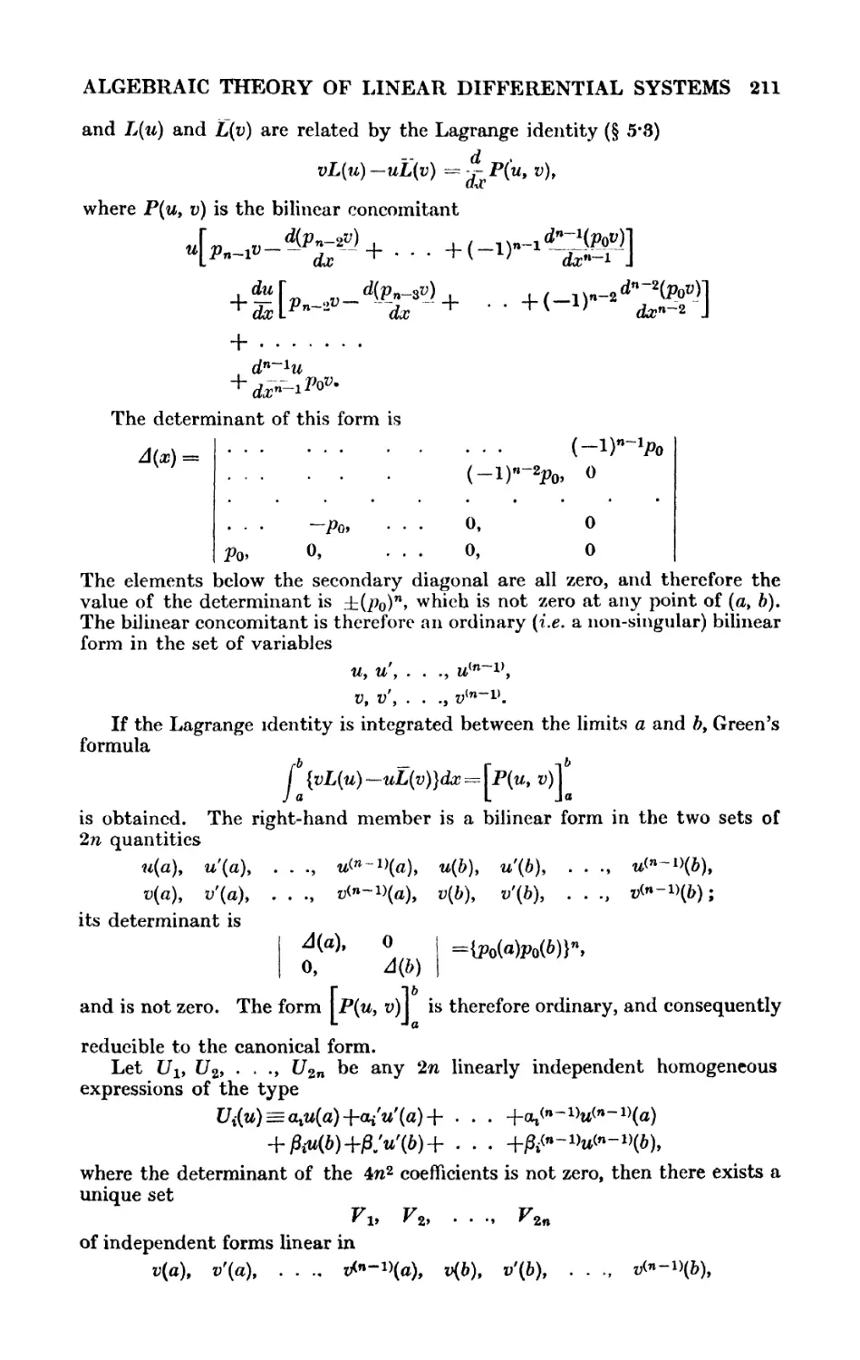
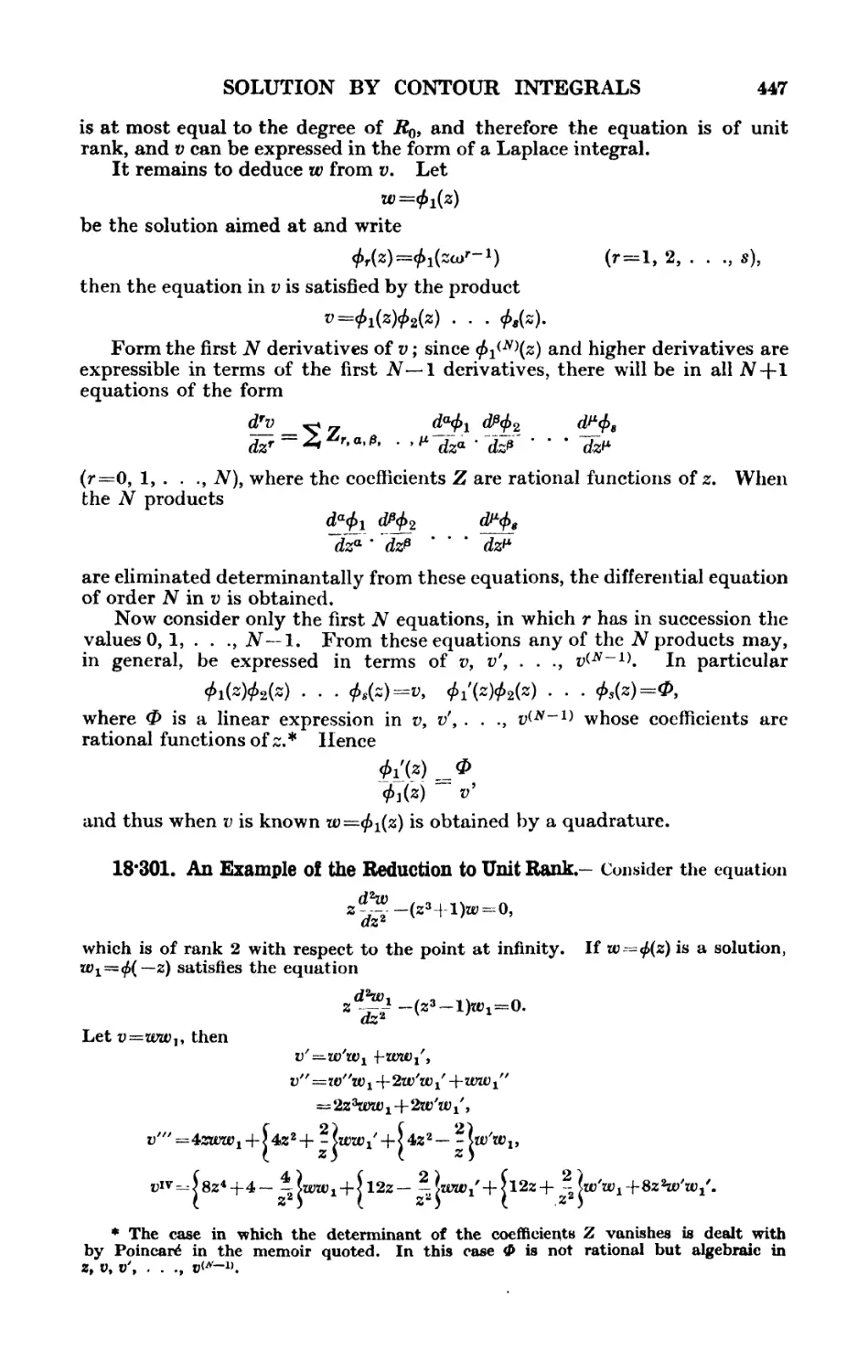
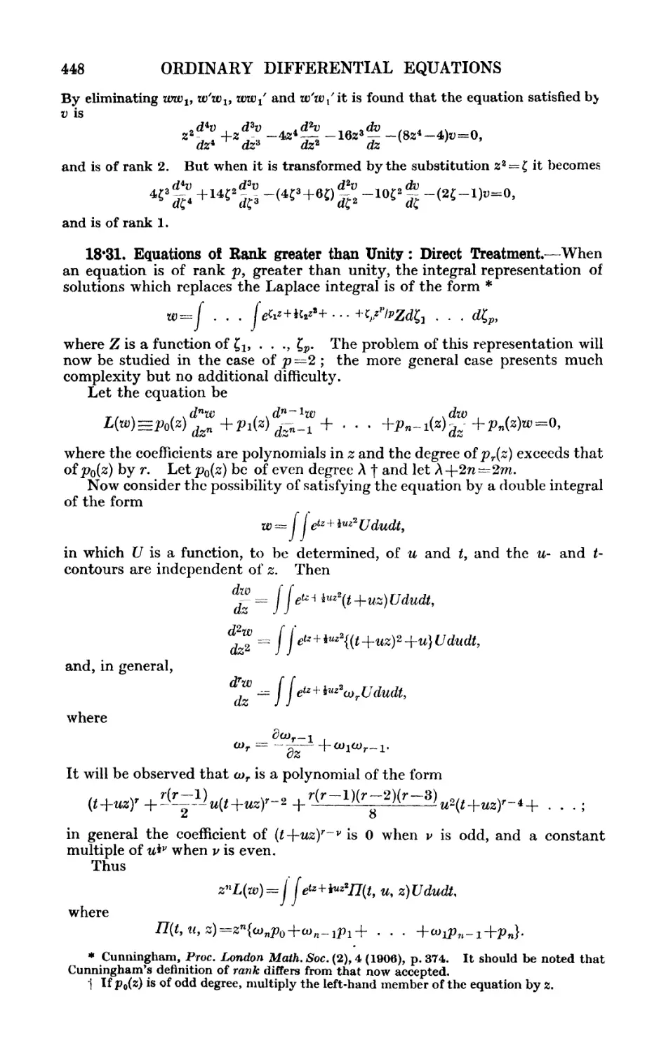
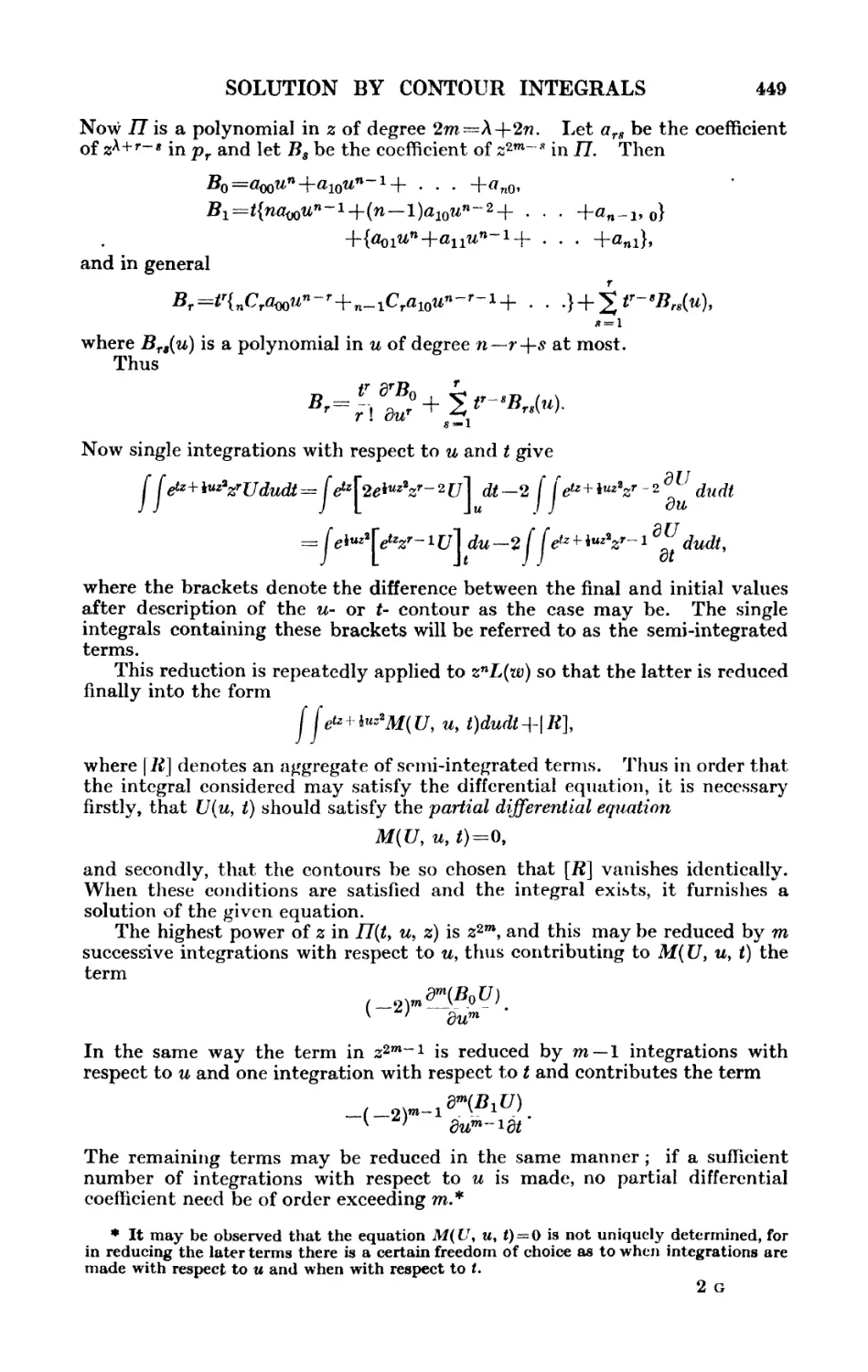
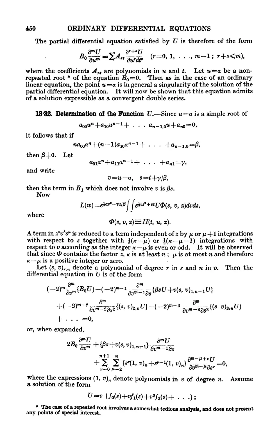
/


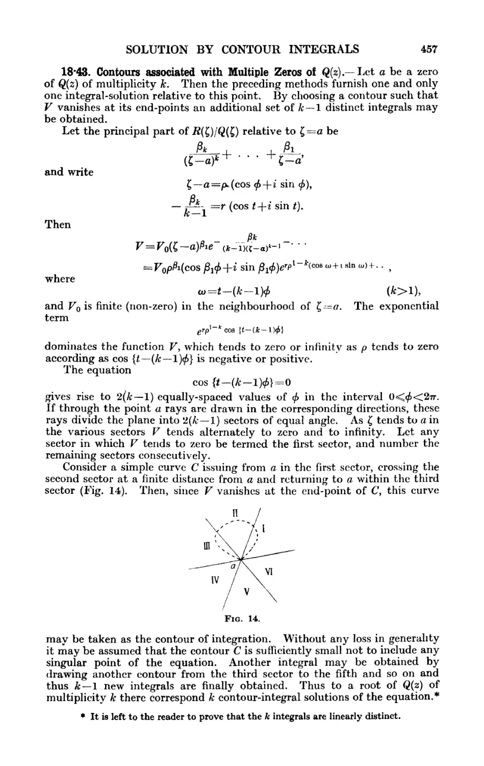
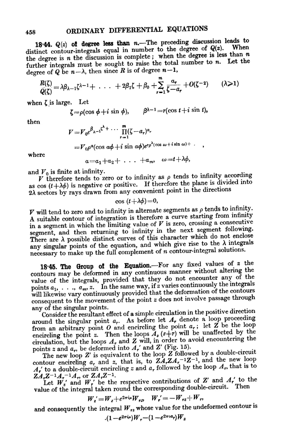


Текст
PREFACE
In accordance with the tradition which allows an author to make his preface
serve rather as an epilogue, I submit that my aim has been to introduce the
student into the field of Ordinary Differential Equations, and thereafter to
guide him to this or that standpoint from which he may sec the outlines
of unexplored territory. Naturally, I have not covered the whole domain
of the subject, but have chosen a path which I myself have followed and
found interesting. If the reader would pause at any point where I have
hurried on, or if he would branch off into other tracks, he may seek
guidance in the footnotes. In the earlier stages I ask for little outside
knowledge, but for later developments I do assume a growing familiarity
with other branches of Analysis.
For some time I have felt the need for a treatise on Differential Equations
whose scope would embrace not merely that body of theory which may now
be regarded as classical, but which would cover, in some aspects at least,
the main developments which have taken place in the last quarter of a
century. During this period, no comprehensive treatise on the subject has
been published in England, and very little work in this particular field has
been carried out; while, on the other hand, both on the Continent and in
America investigations of deep interest and fundamental importance have
been recorded. The reason for this neglect of an important branch of
Analysis is that England has but one school of Pure Mathematics, which
implies a high development in certain fields and a comparative neglect of
others. To spread the energies of this school over the whole domain of
Pure Mathematics would be to scatter and weaken its forces; consequently
its interests, which were at no time particularly devoted to the subject of
Differential Equations, have now turned more definitely into other channels,
and that subject is denied the cultivation which its importance deserves.
The resources of those more fortunate countries, in which several schools
of the first rank flourish, are adequate to deal with all branches of
Mathematics. For this reason, and because of more favourable traditions,
the subject of Differential Equations has not elsewhere met with the neglect
which it has suffered in England.
In a branch of Mathematics with a long history behind it, the prospective
investigator must undergo a severer apprenticeship than in a field more
recently opened. This applies in particular to the branch of Analysis which
lies before us, a branch in which the average worker cannot be certain of
winning an early prize. Nevertheless, the beginner who has taken the pains
to acquire a sound knowledge of the broad outlines of the subject will find
manifold opportunities for original work in a special branch. For instance,
I may draw attention to the need for an intensive study of the groups of
functions defined by classes of linear equations which have a number of
salient features in common.
Were I to acknowledge the whole extent of my indebtedness to others,
I should transfer to this point the bibliography which appears as an appendix.
But passing over those to whom I am indebted through their published
work, I f^ei it my duty, a* it is my privilege, to mention two names in
vi PREFACE
particular. To the late Professor George Chrystal I owe my introduction
to the subject; to Professor E. T. Whittaker my initiation into research
and many acts of kind encouragement. And also I owe to a short period of
study spent in Paris, a renewal of my interest in the subject and a clarifying
of the ideas which had been dulled by war-time stagnation.
In compiling this treatise, I was favoured with the constant assistance
of Mr. B. M. Wilson, who read the greater part of the manuscript and criticised
it with helpful candour. The task of proof-correction had hardly begun
when I was appointed to my Chair in the Egyptian University at Cairo,
and had at once to prepare for the uprooting from my native country and
transplanting to a new land. Unassisted I could have done no more than
merely glance through the proof-sheets, but Mr. S. F. Grace kindly took the
load from my shoulders and read and rc-rcad the proofs, These two former
colleagues of mine have rendered me services for which I now declare myself
deeply grateful. My acknowledgments arc also due to those examining
authorities who have kindly allowed me to make use of their published
questions; it was my intention to add largely to the examples when the
proof stage was reached, but the circumstances already mentioned made
this impossible. And lastly, I venture to record my appreciation of the
consideration which the publishers, Messrs. Longmans, Green and Co., never
failed to show, a courtesy in harmony with the traditions of two hundred
years.
If this book is in no other respect worthy of remark, I can claim for it
the honour of being the first to be launched into the world by a member of
the Staff of the newly-founded Egyptian University. In all humility I
trust that it will be a not unworthy forerunner of an increasing stream of
published work bearing the name of the Institution which a small band of
enthusiasts hopes soon to make a vigorous outpost of scientific enquiry.
E. L. INCE.
Hkltopolir,
December, 1920.
CONTENTS
PART 1
D1EEERENTJAL EQUATIONS IN THE HEAL DOMAIN
Oil Wi'KK l*A<ii:
1. Introductory 3
II. Elementary Methods of Integration , 10
-111. The Existence and Nature of Solutions of Ordinary Differential
Equations 02
IV. Continuous Transformation-Groups 93
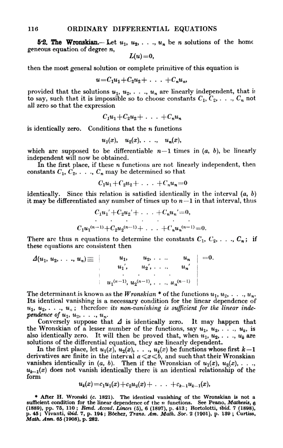
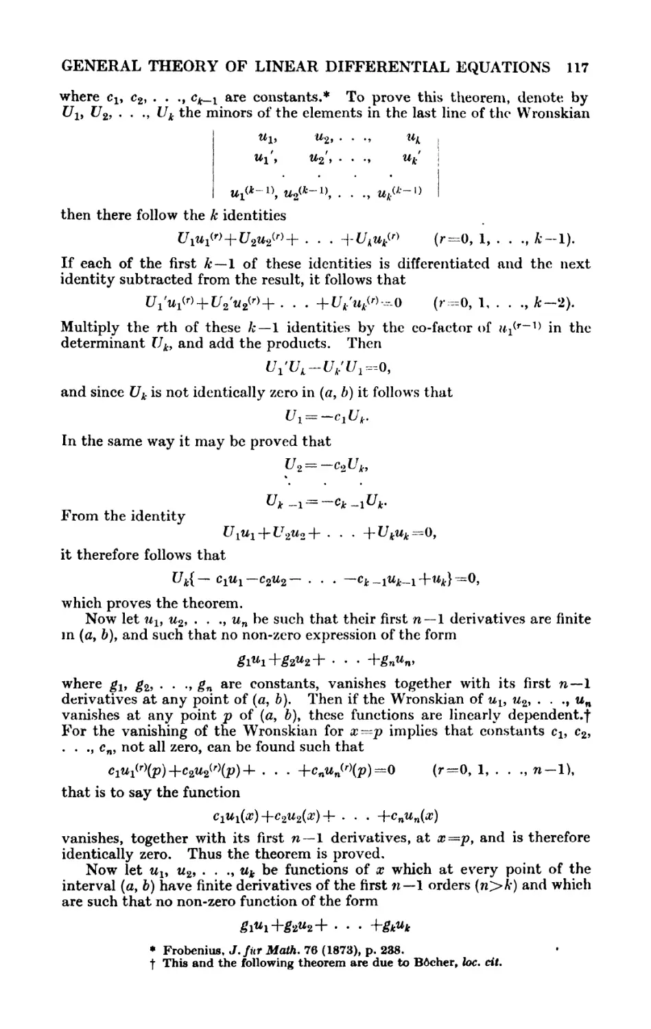
V. The Ueneral Theory of Line\r Differential Equations . . . 114
VI. Linear Equations with Constant Coefficients 133
A
VII. The Solution of Linear Differential Equations in an Infinite
Form 158
VIII. The Solution of Linear Differential Equations by Definite
Integrals 180
IX. The Algebraic Theory of Linear Differential Systems . . . 204
X. The Sturmian Theory and its Later Developments 223
XL Further Developments in the Theory of Boundary Problems . 254
PART II
DIFFERENTIAL EQUATIONS IN THE COMPLEX DOMAIN
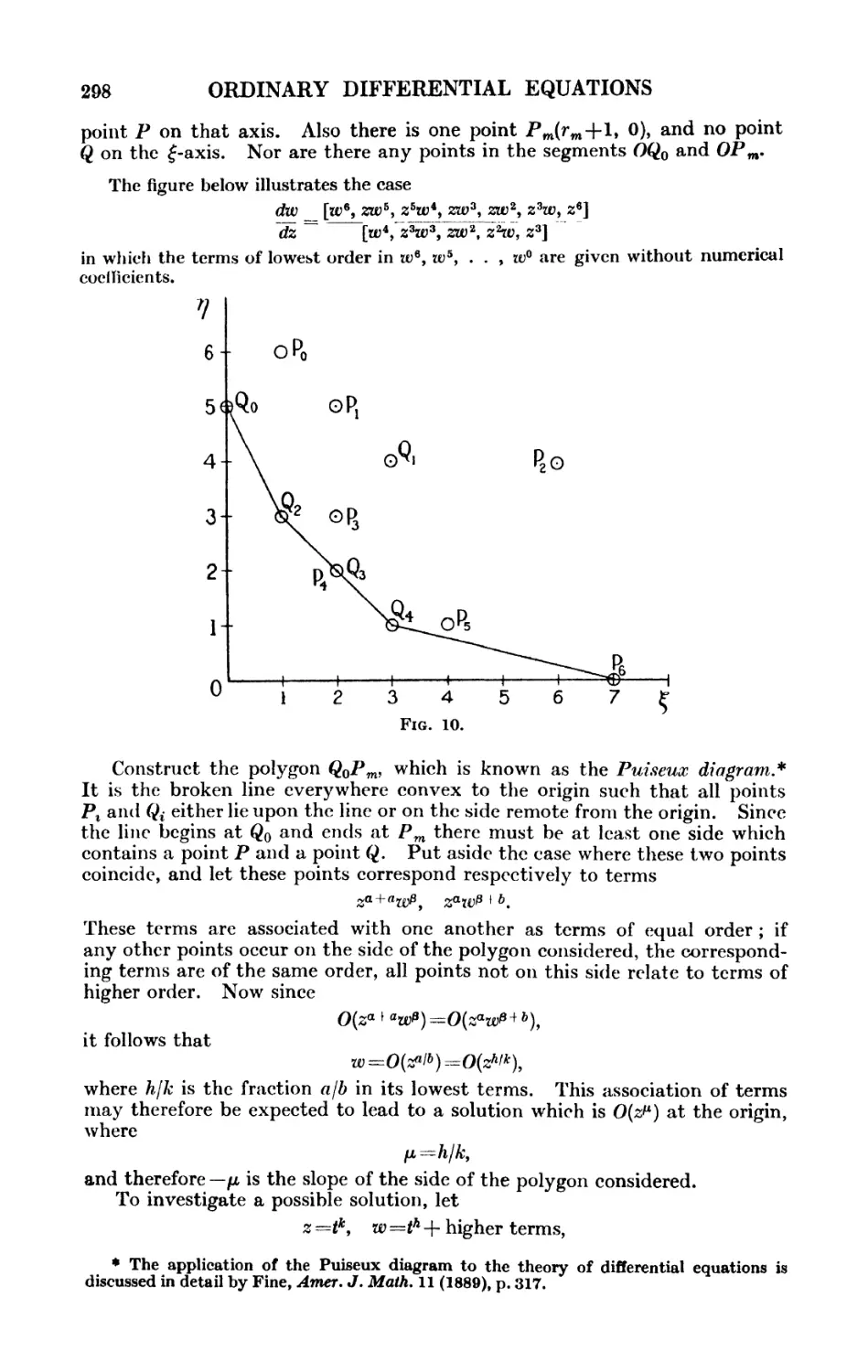
XII. Existence Theorems in the Complex Domain 281
XIII. Equations of the First Order but not of the First Degree . 304
XIV. Non-Linear Equations of Higher Order 317
XV. Linear Equations in the Complex Domain 356
XVI. The Solution of Linear Differential Equations in Series . . 396
XVII. Equations with Irregular Singular Points 417
XVIII. The Solution of Linear Differential Equations by Methods of
Contour Integration 438
XIX. Systems of Linear Equations of the First Order 469
XX. Classification of Linear Differential Equations of the Second
Order with Rational. Coefficients 494
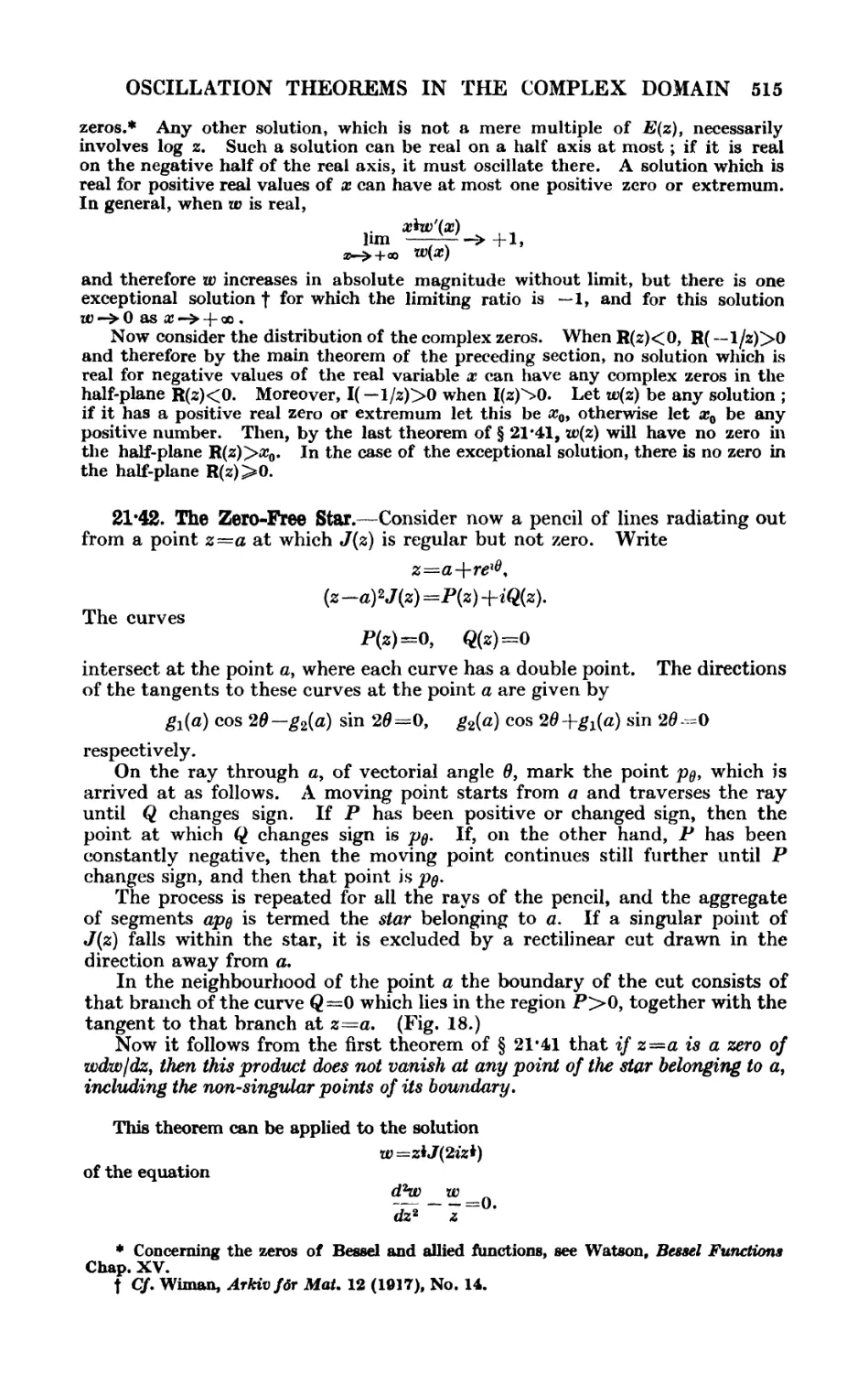
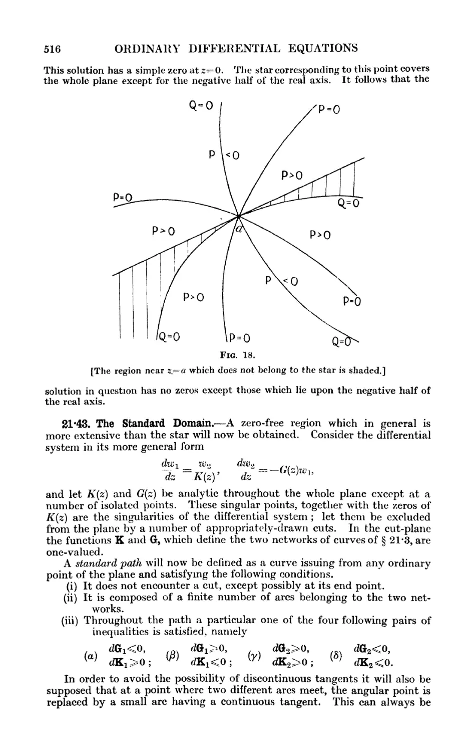
tXI. Oscillation Theorems in the Complex Domain 508
vn
viii CONTENTS
APPENDICES
A1TBND1X I'AUK
A. Historical Note on Formal Methods of Integration .... 529
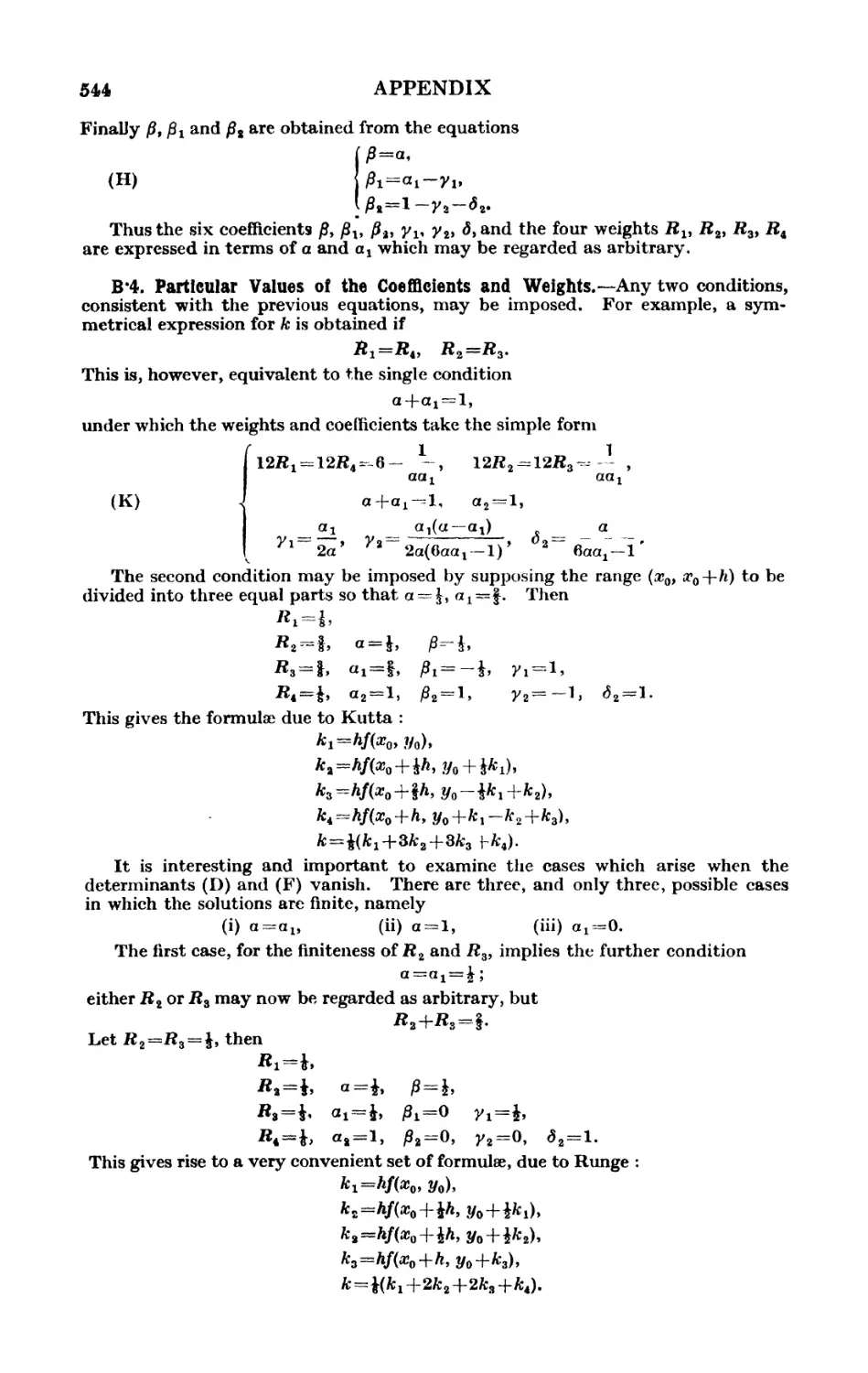
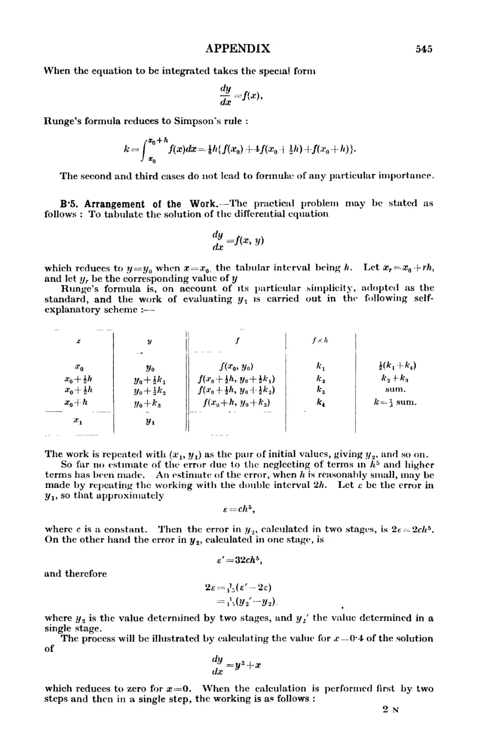
B. Numerical Integration of Ordinary Differential Equations . 540
C. List of Journals Quoted in Footnotes to the Text ... 548
D. Bibliography 551
Index of Authors 553
General Index 555
PART I
DIFFERENTIAL EQUATIONS IN THE REAL DOMAIN
CHAPTER I
INTRODUCTORY -
1/1. Definitions.—The term oequatio differentialis or differential equation
was first used by Leibniz in 1676 to denote a relationship between the
differentials dx and dy of two variables x and y* Such a relationship, in
general, explicitly involves the variables x and y together with other symbols
a, 6, c, ... which represent constants.
This restricted use of the term was soon abandoned ; differential equations
are now understood to include any algebraical or transcendental equalities
which involve either differentials or differential coefficients. It is to be under-
understood, however, that the differential equation is not an identity-!
Differential equations are classified, in the first place, according to the
number of variables which they involve. An ordinary differential equation
expresses a relation between an independent variable, a dependent variable
and one or more differential coefficients of the dependent with respect to
the independent variable. A partial differential equation involves one
dependent and two or more independent variables, together with partial
differential coefficients of the dependent with respect to the independent
variables. A total differential equation contains two or more dependent
variables together with their differentials or differential coefficients with
respect to a single independent variable which may, or may not, enter
explicitly into the equation.
The order of a differential equation is the order of the highest differential
coefficient which is involved. When an equation is polynomial in all the
differential coefficients involved, the power to which the highest differential
coefficient is raised is known as the degree of the equation. When, in an
ordinary or partial differential equation, the dependent variable and its
derivatives occur io the first degree only, and not as higher powers or products,
the equation is said to be linear. The coefficients of a linear equation are
therefore either constants or functions of the independent variable or variables.
Thus, for example,
is an ordinary linear equation of the second order ;
is an ordinary non-linear equation of the first order and the first degree ;
♦ A historical account of the early developments of this branch of mathematics^ will
be found in Appendix A.
f An example of a differential identity is :
\dy)
this is, in fact, equivalent to :
dx dy
3
ORDINARY DIFFERENTIAL EQUATIONS
is an ordinary equation of the second order which when rationalised by squaring
both members is of the second degree ;
3z dz___
X3x y3y
is a linear partial differential equation of the first order in two independent variables ;
32V 32V d2V _Q
is a linear partial differential equation of the second order in three independent
variables ;
OlZ O2Z / OlZ \2
3x2'3y2 \dxdy I
is a non-linear partial differential equation of the second order and the second
degree in two independent variables ;
udx -f vdy -f- wdz—0,
where w, v, and w are functions of a;, y and 2, is a total differential equation of the first
order and the first degree, and
x2dx2-\- 2xydxdy -f y 2dy 2—z Mz2=0
is a total differential equation of the first order and the second degree.
In the case of a total differential equation anyone of the variables mayT5e regarded
as independent and the remainder as dependent, thus, taking x as independent
variable, the equation
udx -f- vdy -f wdz=0
may be written
or an auxiliary variable t may be introduced and the original variables regarded as
functions of t, thus
dx , dy , dz ,.
1-2. Genesis of an Ordinary Differential Equation.—Consider an equation
(A) f(x, y, cl9 c2, . . ., cn)=0,
in which x and y are variables and cl9 c2, . . ., cn are arbitrary and independent
constants. This equation serves to determine i/asa function of x ; strictly
speaking, an n-fold infinity of functions is so determined, each function
corresponding to a particular set of values attributed to cl5 c2, . . ., cn.
Now an ordinary differential equation can be formed which is satisfied by
every one of these functions, as follows.
Let the given equation be differentiated n times in succession, with respect
to x, then n new equations are obtained, namely,
y
8xdyy ^dy*y +dy
'%+■■■ +ly-
8xn ' ' 8y
where
J{
dx'
INTRODUCTORY 5
Each equation is manifestly distinct from those which precede it; •
from the aggregate of w+1 equations the n arbitrary constants Ci, c2, . . ., cn
can be eliminated by algebraical processes, and the eliminant is the differential
equation of order n :
F(x, y, y\ y\ . . ., y<»>)=o.
It is clear from the very manner in which this differential equation was
formed that it is satisfied by every function y=<f)(x) defined by the relation
(A). This relation is termed the primitive of the differential equation, and
every function y—<f>(£) which satisfies the differential equation is known as a
solutio7i.-\ A solution which involves a number of essentially distinct arbitrary
constants equal to the order of the equation is known as the general solution.%
That this terminology is justified, will be seen when in Chapter III. it is proved
that one solution of an equation of order n and one only can always be found
to satisfy, for a specified value of x, n distinct conditions of a particular type.
The possibility of satisfying these n conditions depends upon the existence of
a solution containing n arbitrary constants. The general solution is thus
essentially the same as the primitive of the differential equation.
It has been assumed that the primitive actually contains n distinct constants
cl9 c2, . . ., cn. If there are only apparently n constants, that is to say if two or
more constants can be replaced by a single constant without essentially modifying
the primitive, then the order of the resulting differential equation will be less than
n. For instance, suppose that the primitive is given in the form
f[x, y, <f>(a, b)}=0,
then it apparently depends upon two constants a and b, but in reality upon one
constant only, namely c = (/)(a, b). In this case the resulting differential equation
is of the first and not of the second order.
Again, if the primitive is reducible, that is to say iff(x, y, cl9 . . ., cn) breaks up
into two factors, each of which contains y, the order of the resulting differential
equation may be less than n. For if neither factor contains all the n constants,
then each factor will give rise to a differential equation of order less than n, and
it may occur that these two differential equations are identical, or that one of them
admits of all the solutions of the other, and therefore is satisfied by the primitive
itself. Thus let the primitive be
y2 —(a-f b)xy-\-abx2=O ;
it is reducible and equivalent to the two equations
y~ax—O, y—bx~O,
each of which, and therefore the primitive itself, satisfies the differential equation
y-xy' = O.
1*201. The Differential Equation o! a Family o! Coniocal Conies.—Consider
the equation
where a and b are definite constants, and A an arbitrary parameter which can
assume all real values. This equation represents a family of confocal conies. The
* Needless to say, it is assumed that all the partial differential coefficients of / exist,
and that ~ is not identically zero.
"* t Originally the terms integral (James Bernoulli, 1689) and particular integral (Euler,
Inst. Calc. Int. 1768) were used. The use of the word solution dates back to Lagrange
A774), and, mainly through the influence of Poincar^, it has become established. The
term particular integral is now used only in a very restricted sense, cf. Chap. VI. infra,
I Formerly known as the complete integral or complete integral equation {wquatio integralis
completa, Euler). The term integral equation has now an utterly different meaning (cf.
§ 3*2, infra)y and its use in any other connection should be abandoned. %
6 ORDINARY DIFFERENTIAL EQUATIONS
differential equation of which it is the primitive is obtained by eliminating A between
it and the derived equation
From the primitive and the derived equation it is found that
and, eliminating A,
and therefore the required differential equation is
it is of the first order and the second degree.
When an equation is of the first order it is customary to represent the derivative
y' by the symbol p. Thus the differential equation of the family of confocal conies
may be written :
1/21. Formation of Partial Differential Equations through the Elimination of
Arbitrary Constants.—Let xl9 x2, • - ., xm be independent variables, and let
s, the dependent variable, be denned by the equation
where c-±, c& . . ., cn are n arbitrary constants. To this equation may be
adjoined the m equations obtained by differentiating partially with respect
to each of the variables xl9 x2, . . ., xm in succession, namely,
1
If m^n, "sufficient equations are now available to eliminate the constants
clf c2, • • ., cn. If ra<n the \m(m+\) second derived equations are also
adjoined ; they are of the forms
0s 32/ /0a y 8/
a^z' aa;
(r, 5=1, 2, . . ., m;
This process is continued until enough equations have been obtained to
enable the elimination to be carried out. In general, when this stage has
been reached, there will be more equations available than there are constants
to eliminate and therefore the primitive may lead not to one partial differ-
differential equation but to a system of simultaneous partial differential equations.
1*211. The Partial Differential Equations of all Planes and of all Spheres.—
As a first example let the primitive be the equation
' z—ax+by+c,
in which a, 6, c are arbitrary constants. By a proper choice of these constants, the
equation can be made to represent any plane in space except a plane parallel to the
z-axis. The first derived equations are :
dz dz ,
dx ' 3y ~°'
These are not sufficient to eliminate a, b, and c, and therefore the second derived
equations are taken, namely,
d2z d2z dH_
* u' dxdy ' dy*
INTRODUCTORY 7
They are free of arbitrary constants, and are therefore the differential equations
required. It is customary to write
_dz _dz _d*z __#jL . ^2z
p~~dx* q~~ dy' r~dx^ S~3xdy> dy*
Thus any plane in space which is not parallel to the z-axis satisfies simultaneously
the three equations
r=0, s=0, t=0.
In the second place, consider the equation satisfied by the most general sphere;
it is
where a, b, c and r are arbitrary constants. The first derived equations are
(x-a)+(z-~c)p=O, (y-b)+(z-c)q=O,
and the second derived equations are
pq+(z-c)s=O9
l+q2-r(z-c)t=O.
When z —c is eliminated, the required equations are obtained, namely,
r s t
Thus there are two distinct equations. Let A be the value of each of the members of
the equations, then
\(rt-s)=l+p+q>0.
Consequemly, if the spheres considered are real, the additional condition
rt>s2
must be satisfied.
1-22. A Property of Jacobians.—It will now be shown that the natural
primitive of a single partial differential equation is a relation into which
enter arbitrary functions of the variables. The investigation which leads up
to this result depends upon a property of functional determinants or
Jacobians.
Let ul9 u2i . . •> um be functions of the independent variables xlt x2, . • •»
xni and consider the set of partial differential coefficients arranged in order
thus :
du1 dux dui
' ' ' dx
n
du2
dz2' ' ' "' dxn
Then the determinant of order p whose elements are the elements common to
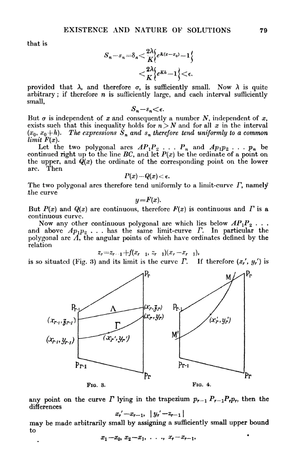
p rows and p columns of the above scheme is known as a Jacobian.* Let
all the different possible Jacobians be constructed, then if a Jacobian of
order pt say
tin? dup
dxp
is not zero for a chosen set of values x1~^1, . . ., xn — fn, but if every Jacobian
of order p+1 is identically zero, then the functions ulf u2i . . ., up are
* Scott and Mathews, Theory of Determinants, Chap. XIII.
8
ORDINARY DIFFERENTIAL EQUATIONS
independent, but the remaining Junctions up+i, . . ., um are expressible in
terms ojul9 . . ., up.
Suppose that, for values ofa^, . . ., xn in the neighbourhood of £ls . . ., fn,
the functions %, . . ., up are not independent, but that there exists an
identical relationship,
<f>(u^ . . ., up)—0.
Then the equations
are satisfied identically, and therefore
d(u, . . ., wp)
d(f>
dup
dup
' dxp
du
o,
dx
p
du
p
0
identically in the neighbourhood of fj, . . ., fn, which is contrary to the
hypothesis. Consequently, the first part of the theorem, nan^^, that
nls . . ., Up are independent, is true.
In Wp+i, . . ., um let the variables #!, . . ., xp, xv+\, . . ., xn be replaced
by the new set of independent variables ux, . . ., up, xp+i, . . ., xn. It will
now be shown that if ur is any of the functions %+i, . . ., um, and x8 any one
of the variables xp+i, . . ., xni then ur is explicitly independent of xi9 that is
Let
dx8
Um—
and let xx, . . ., xp be replaced by their expressions in terms of the new
independent variables ul9 . . ., up, xp+li . . ., xni then differentiating both
sides of each equation with respect to cc8y
0
i ,
r • • •
dx
p
p
r
dx,'
dxY dxs
.,..., m).
The eliminant of ^
dx,
p
dx8
is
dx8 dx8'
dfr.tepidjjL
dxp dx8 dx/
9 dx8
'p' &X8
fa_dUr
p dxg
—0
INTRODUCTORY
9
or
But since, by hypothesis,
*KU__' • ; fp, fr)
dix^i,
it follows that
C'liZ/J, • • •, Xn^ il
,, . . ., xp)
0
Consequently each of the functions «p + i, . . ., um is expressible in terms
of the functions ul9 . . ., up alone, as was to be proved.
1*23. Formation of a Partial Differential Equation through the Elimination
ol an Arbitrary Function.—Let the dependent variable z be related to the
independent variables acl9 . . ., xn by an equation of the form
F(ul9 u.z, . . ., un)=0,
where F is an arbitrary function of its arguments uXi u2, . . ., un which, in
turn, are given functions of xXi . . ., xn and z. When for z is substituted its
value in terms of xl9 . . ., xni the equation becomes an identity. If therefore
Drug repi^ents the partial derivative of u8 with respect to ^r when z has been
m
replaced^y its value, then
But
. . ., JJnun
dus du8 dz
+
and therefore the partial differential equation satisfied by z is
jx dz
+
dz ' dx^ ' ' "' dxn
dui dux d
dx
n
5WM ^Wn a,
' *' dx
n
dun dz
"dz ' dx
0.
n
1 231. The Differential Equation of a Surface of Revolution.- The equation
F(z, *3+.V2)=0
represents a surface of revolution whose axis coincides with the z-axis. In the
notation of the preceding section,
and therefore z satisfies the partial differential equation
dz dz
'dx dy
2a?, 2y
~~
or
dz _
X'~- =0.
d
^ dz dz
dx dy
Conversely, this equation is satisfied by
where <f> is an arbitrary function of its argument, and is therefore the differential
equation of all surfaces of revolution which have the common axis a? =0, «/=C\
10 ORDINARY DIFFERENTIAL EQUATIONS
1-232. Enter's Theorem on Homogeneous Functions.—Let
z = </>(%, y),
where <f>(x, y) is a homogeneous function of x and y of degree n. Then, since <j>(x. y)
can be written in the form
it follows that
In the notation of § 1'23,
F(uu w2/-
and therefore z satisfies the partial differential equation
%dz x_n<k
dx X dy
and this equation reduces to
dz , dz
dx * dy
Similarly, if u is a homogeneous function of the three variables #,T7 and z, of
degree n,
du , du y du
x+y+Z
This theorem can be extended to any number of variables.
1*24. Formation of a Total Differential Equation in Three Variables.—The
equation
<f>(xy y, z)=c
represents a family of surfaces, and it will be supposed that to each value of
c corresponds one, and only one, surface of the family. Now let (<r, yy z) be a
point on a particular surface and (x+8x, y+hy, z+Sz) a neighbouring point
on the same surface, then
<f>(z+Sx, y+Sy, z-\-8z)—(f>(x, y, z)=0.
Assuming that the partial derivatives
d<f> def) d(j>
'dx' dy' dz
exist and are continuous, this equation may be written in the form
where €i, e%, e3-»0, as Sx, Sy, Sz->0.
Now let ely e2 and e3 be made zero and let dx, dy and dz be written for 5a?,
8y and 8z respectively. Then there results the total differential equation
which has been derived from the primitive by a consistent and logical process.
If the three partial derivatives have a common factor /a, and if
INTRODUCTORY 11
then if the factor /x is removed, the equation takes the form
Pdx+Qdy+Rdz=O.
That there is no inconsistency in the above use of the differentials dxt etc., may
be verified by considering a particular equation in two variables, namely,
y -f(x) = c.
The above process gives rise to the total differential equation
dy-f'(x)dx=O,
and thus the quotient of the differentials dy, dx is in fact the differential coefficient
dyjdx.
Example.—The primitive
=c
gives rise to the total differential equation
2 2 22 2z+x+y
W dz~~~ '
which, after multiplication by (a?+yJ, becomes
—zz)dx+(x2 —z2)dy+Bz -\-x -\-y)(x ~\-y)dz =0.
1*8. The Solutions of an Ordinary Differential Equation.—When an
ordinary inferential equation is known to have been derived by the process
of elimination from a primitive containing n arbitrary constants, it is evident
that it admits of a solution dependent upon n arbitrary constants. But
since it is not evident that any ordinary differential equation of order n can
be derived from such a primitive, it does not follow that if the differential
equation is given a priori it possesses a general solution which depends upon
n arbitrary constants. In the formation of a differential equation from a
given primitive it is necessary to assume certain conditions of differentiability
and continuity of derivatives. Likewise in the inverse problem of inte-
integration, or proceeding from a given differential equation to its primitive,
corresponding conditions must be assumed to be satisfied. From the purely
theoretical point of view the first problem which arises is that of obtaining a
set of conditions, as simple as possible, which when satisfied ensure the
existence of a solution. This problem will be considered in Chapter III..
where an existence theorem, which for the moment is assumed, will be proved,
namely, that when a set of conditions of a comprehensive nature is satisfied
an equation of order n does admit of a unique solution dependent upon n
arbitrary initial conditions. From this theorem it follows that the most
general solution of an ordinary equation of order n involves n, and only n,
arbitrary constants.
It must not, however, be concluded that no solution exists which is not
a mere particular case of the general solution. To make this point clear,
consider the differential equation obtained by eliminating the constant c
from between the primitive,
</>(x, y, c)=0,
and the derived equation,
The derived equation in general involves c; let the primitive be solved
for c and let this value of c be substituted in the derived equation. The
derived equation then becomes the differential equation
12 ORDINARY DIFFERENTIAL EQUATIONS
where the brackets indicate the fact of the elimination of c. In its total
form, this equation can be written
Now let x, y and c vary simultaneously, then
dy
When c is eliminated as before this equation becomes
and therefore, in view of the previous equation,
Idc
Jdc.
There are thus two alternatives : either c is a constant, which leads back
to the primitive,
or else
ldc\ =0*
The latter relation between x and y may or may not be a solution of the
differential equation ; if it is a solution, and is not a particular case of the
general solution, it is known as a singular solution.
Consider, for instance, the primitive
where c is an arbitrary, and a a definite, constant. The derived equation is
cdy—xdx^Q,
which, on eliminating c, becomes the differential equation
The total differential equation obtained by varying x, y and c simultaneously is
(c -{- y)dc -f cdy — xdx—0
or, on eliminating c,
(x* +y* -a2)idc -\-[-y+(x2 ~\ -y2-a~)i]dy-xdx=O.
Thus, apart from the general solution there exists the singular solution,
which obviously satisfies the differential equation.
A differential equation of the first order may be regarded as being but
one stage removed from its primitive. An equation of higher order is more
remote from its primitive and therefore its integration is in general a step-by-
step process in which the order is successively reduced, each reduction of the
order by unity being accompanied by the introduction of an arbitrary
constant. When the given equation is of order n, and by a process of
integration an equation of order n — 1 involving an arbitrary constant is
obtained, the latter is known as the^r.?/ integral of the given equation.
Thus when the given equation is
where/(t/) is independent of a?, the equation becomes integrable when both members
are multiplied by 2y', thus
Y =2f(y)y\
INTRODUCTORY 13
and its first integral is
where c is the arbitrary constant of integration.
1*4. Geometrical Significance of the Solutions of an Ordinary Differential
Equation of the First Order.—Since the primitive of an ordinary differential
equation of the first order is a relation between the two variables x and y
and a parameter c, the differential equation is said to represent a one-
parameter family of plane curves. Each curve of the family is said to be
an integral-curve of the differential equation.
Let the equation be
t
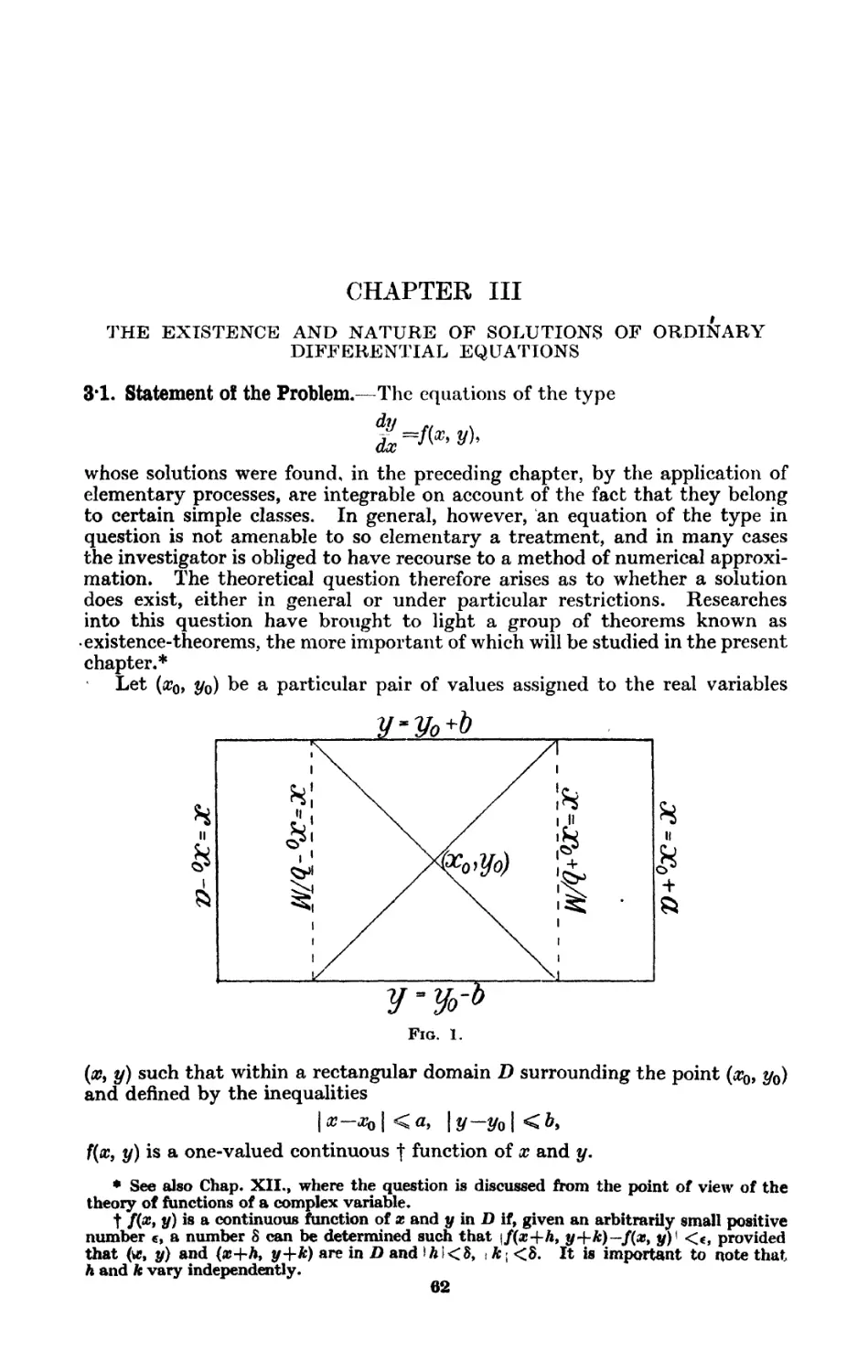
let D be a domain in the (<r, ?/)-plane throughout which f(x9 y) is single-
valued and continuous, and let (x0, y0) be a point lying in the interior of D.
Then the equation associates with (xOi y0) the corresponding value of dyjdx,
say pOi and thus defines a line-element * (x0, y0, p0) issuing from the point
(xo> 2/o)- Choose an adjacent point (xlt yi) on this line-element and construct
the line-element (xl9 yx, px). By continuing this process a broken line is
obtained which may be regarded as an approximation to the integral-curve
which jMtfses through (x0, y0).
This method of approximating to the integral-curves of a differential equation
is illustrated in a striking manner by the iron filings method of mapping out the
lines of force due to a bar magnet. Iron filings are dusted over a thin card placed
horizontally and immediately above the magnet. Each iron filing becomes
magnetised and tends to set itself in the direction of the resultant force at its
mid-point, and if the arrangement of the filings is aided by gently tapping the
card, the filings will distribute themselves approximately along the lines of force.
Thus each individual filing acts as a line-element through its mid-point.
Let the bar magnet consist of two unit poles of opposite polarity situated at A
and B and let P be any point on the card. Then if the co-ordinates of A, B and P
are respectively (—a, 0), (a, 0), (x, y), if r and s are respectively the lengths of AP
and BP, and if X, Y are the components of the magnetic intensity at P,
i s3 r6 s3
ri s3 r6 s
The direction of the resultant force at P is
dx X
y
x-\-a
r3—s3
and this is the differential equation of the lines of force. Its solution is
x+a x~a
r s
— const.
By giving appropriate values to the constant the field of force may be mapped out.
The integral-curves are the lines of force approximated to by the iron filings.
Since it has been assumed that/(#, y) is continuous and one-valued at
every point of Z>, through every point there will pass one and only one
integral-curve. Outside D there may be points at which/(.r, y) ceases to be
continuous or single-valued ; at such points, which are known as singular
points, the behaviour of the integral-curves may be exceptional.
♦ The line-element may be denned with sufficient accuracy as the line which joins
the points (a?0, i/0) and {xo + Sx, y9+$y) where 8a; and By are small and b/b
14 ORDINARY DIFFERENTIAL EQUATIONS
Similarly, if an equation of the second order can be written in the form
where f(x, y9 y') is continuous and single-valued for a certain range of values
of its arguments, the value of y' at the point (x0, yQ) can be chosen arbitrarily
within certain limits, and thus through the point (x0, y0) passes a one-fold
infinity of integral-curves. The general solution involves two arbitrary
constants, and therefore the aggregate of integral-curves forms a two-
parameter family.
In general the integral-curves of an ordinary equation of order n form an
n-paramcter family, and through each non-singular point there passes in
general an (n—l)-fold infinity of integral-curves.
1*5. Simultaneous Systems of Ordinary Differential Equations,—Problems
occasionally arise which lead not to a single differential equation but to a
system of simultaneous equations in one independent and several dependent
variables. Thus, for instance, suppose that
<f>(x9 y, z, cl9 c2) =0,
ifs(x9 y, z9 cl9 c2) =0
are two equations in x9 y, z each containing the two arbitrary constants
cl9 c2. Then between these two equations and the pair of equations obtained
by differentiating with respect to x, the constants cx and c2 can be qjjpiinated
and there results a pair of simultaneous ordinary differential equations of
the first order,
<P(x9y9y'9z9z')=O,
It is possible, by introducing a sufficient number of new variables, to
replace either a single equation of any order, or any system of simultaneous
equations, by a simultaneous system such that each equation contains a
single differential coefficient of the first order. This theorem will be proved
in the most important case, namely that where the equation to be considered
is of the form *
In this case new variables yl9 y2, . . ., yn are introduced such that
dx ~y* dx ~y*' ' ' " dx -yn'
where yx =y. These equations, together with
dtt
-^ =F(x, yl9 tj2i . . ., yn),
form a system of n simultaneous equations, each of the first order, equivalent
to the original equation. In particular it is evident that if the original
equation is linear, the equations of the equivalent system are likewise linear.
Miscellaneous Examples.
1. Find the ordinary differential equations, satisfied by the following primitives :
(i) y=Axm+BaP ; (vi) y=xn(A+B log x) ;
(ii) y^Aenx+Be™; (vii) y=emx(A + Bx);
(iii) y—A cos nx+B sin nx; (viii) y=(A+ Bx) cos nx+(C-\-Dx) sin nx ;
(iv) y^e^iA cos nx+B sin nx); (ix) t/=ewu;{(,4+lta) cos nx+(C+Dx) sin nx} ;
(v) y=*A cosh (xjA); (x) y=*Ax cos (n/x+B),
where A, B, C, D are arbitrary constants and m and n are fixed constants.
* D'Alembert, Hist. Acad. Berlin, 4 A748), p. 289.
2. Prove that if
INTRODUCTORY 15
y
B cx+d
then
and that if a+cf=O, then
B/-*)i/"=2t/(l+i/')- [Math. Tripos I. 1911.]
3. Prove that if y8-Qax*+x*=0, then
Show that the curve given by the above equation is everywhere concave to the a?-axis,
and that there is a point of inflexion where x=8a. [Math. Tripos I. 1912.]
4. Show that if
then
Hence prove by Maclaurin's theorem that the value of y which vanishes when x==0 and
is such that its 5th differential coefficient is unity when # — 0 is
k9 /. LMath. Tripos I. 1915.]
5. Show that the differential equation of all circles in one and the same plane is
6. Any conic section wliich has not an asymptote parallel to the i/-axis may be written
in the form
{y — ax — ftJ=ax*+26a;+c.
Hence show that the differential equation of all such conic sections is
dx3\\dx*!
or
dx* dx*dx^J\ dx*J dx*
In particular, show that the differential equation of all coplanar parabohe is
or
/ePy\* d*y d*y
7. Verify that if
then
d*z ^ d2z d%z d*z = / dlz V
dxdy dydx' dx2'dy2 ~ \dxdy) '
8. Prove the following extension of Euler's theorem : If/ is a function homogeneous
and of degree m in xlt xt and homogeneous and of degree n in yl9 yz then
df\ ( d d
+X
9. Prove that if the family of integral-curves of the linear differential equation of the
first order
is cut by the line x=g, the tangents at the points of intersection are concurrent.
For curves satisfying the equation
dy—y=— -
dx x~~ x*'
prove that for varying £ the locus of the point of concurrence is a straight line. '
CHAPTER II
ELEMENTARY METHODS OF INTEGRATION
2-1. Exact Equations of the First Order and o! the First Degree.—An ordinary
differential equation of the first order and of the first degree may be
expressed in the form of a total differential equation,
Pdx+Qdy=O,
where P and Q are functions of x and y and do not involve p. If the
differential Pdx^-Qdy is immediately, that is without multiplication by any
factor, expressible in the form du, where u is a function of x and y, it is said
to be exact.
If the equation
Pdx+Qdy=O
is exact and its primitive is *
u=c,
the two expressions for du, namely,
Pdx+Qdy and -— dx + — dy
if
must be identical, that is,
a?
Then
(A) —
K ' dy dx y
d2u
provided that the equivalent expression —— is continuous. The condition
of integrability (A) is therefore necessary. It remains to show that the
condition is sufficient, that is to say, if it is satisfied the equation is exact
and its primitive can be found by a quadrature.
Let u(x, y) be defined by
w=J P(x,y)dx+<f>(y)y
where xQ is an arbitrary constant, and <f>(y) is a function of y alone which,
for the moment, is also arbitrary. Then u~c will be a primitive of
Pdx+Qdy=O
if
dx '
The first condition is satisfied ; the second determines <f>(y) thus :
* Throughout this Chapter the letter c or C generally denotes a constant of integration.
Any other use of these letters will be evident from the context.
16
ELEMENTARY METHODS OF INTEGRATION 17
and therefore
cv
where y0 is arbitrary.
The condition is therefore sufficient, for the equation is exact and has the
primitive
fy
P(z, y)dcc+ I Q(xOy y)dy=c.
o J Vo
The constants x0 and y0 may be chosen as is convenient, there are not, in
all, three arbitrary constants but only one, for a change in x0 or in z/0 is
equivalent to adding a constant to the left-hand member of the primitive.
This is obvious as far as yQ is concerned, and as regards x0, it is a consequence
of the condition of integrability.
As an example, consider the equation
, 2u~\-x
The condition of integrability is satisfied. The primitive therefore is
It is evidently an advantage to take xQ—Q ; as the second integral then involves
log 2/> 2/o may be taken to be 1. Thus
that is
wliich reduces to
(Jx + 2 1 ";==c,
Jox*+y'A Jl y
log (a!a+#3)-arc tan - +2 log y=c,
(x24-y2)— arc tan —c.
y
2*11. Separation o£ Variables.—A particular instance of an exact equation
occurs when P is a function of x alone and Q a function of y alone. In this
case X may be written for P and Y for Q. The equation
Xdx + Ydy
is then said to have separated variables. Its primitive is
fXdx+fYdy=c.
When the equation is such that P can be factorised into a function X of
x alone and Yt a function of y alone, and Q can similarly be factorised into
Xi and F, the variables are said to be separable, for the equation
(I) XY^
may be written in the separated form
(II) y
It must be noticed, however, that a number of solutions are lost in the
c
18 ORDINARY DIFFERENTIAL EQUATIONS
division of the equation by XiY\. If, for example, x—a is a root of the
equation Xx~0, it would furnish a solution of the equation (I) but not
necessarily of the equation (II).
Example.—
The variables are separable thus :
dx + y
x y2-]
Integrating :
#2-f-log a?2-f log (y2 — 1)— c
or if c=log C,
x2
In addition a?—0, y = l, y=—l are real solutions of the given equation. The two
latter, but not the former are included in the general solution.
2*12. Homogeneous Equations.—If P and Q are homogeneous functions
of x and y of the same degree ?i, the equation is reducible by the sub-
substitution * y~vx to one whose variables are separable. For
P(x, y) =xnP(\, v), P(oc, y)=xnQ(l, v)9
and therefore
becomes
{P(l, v)+vQ(l, v)}cLx+xQ(l, v)dv=--0
or
dv dx
(f>(v) x
where
The solution is
f dv , c
Example.—
Let y=vx, then
(u4 +v)dx -A —2v*Krdv=0
or
dx 1— 2vz
dv
X V-\-V
4
\v 1 +ir
whence
log x =log v —log A +u3) -flog c
or
a?(l-f v3)=cv.
Thus the primitive is
a?3-f yz=cxy.
When the equation
Pdx+Qdy=0
is both homogeneous and exact, it is immediately integrable without the
* This device was first used by Leibniz in 1691.
ELEMENTARY METHODS OF INTEGRATION 19
introduction of a quadrature, provided that its degree of homogeneity n is
not -i-l. Its primitive is, in fact,
Px+Qy-=c.
For let u=Px+Qy, then
du 3P 8Q
r+X +y
by Euler's theorem (§ 1*232), and similarly
Consequently
du = -- dx + — du
dx by J
=--(n+l)(Pdx+Qdy)9
and therefore
Hence if n =f= 1, the primitive is
Px+Qy=c.
Example.—-
x(x2+3y2)dx i-y(y~-\-3x2)dy=0.
Solution: #4-f 6a?2*/2-f yi~c.
When n — —1 the integration in general involves a quadrature. It is a
noteworthy fact that the homogeneous equation
Pdx+Qdy
Px+Qy
is exact, for the condition of intcgrability, namely
Jy\Px+Qy/ dl\Px+Qy )'
reduces to
dP , dP\ j dQ , dQ\
which is true, by Euler's theorem, since P and Q are homogeneous and of
the same degree. Thus any homogeneous equation may be made exact by
introducing the integrating factor lj(Px + Qy). The degree of homogeneity
of this exact equation is, however, 1, so that the integration of a
homogeneous equation in general involves a quadrature.
An equation of the type
dx V ax-\-by-\~c /
in which A, B, C, a, b, c are constants such that Ab—aB=^O, may be brought
into the homogeneous form by a linear transformation of the variables, for
let
where f, 77 are new variables and h, k are constants such that
v Ah+Bk+C=O9
— 0.
20 ORDINARY DIFFERENTIAL EQUATIONS
The equation becomes
d£ Kag+brjJ9
so that F is a homogeneous function of £, rj of degree zero. The constants
h9 k are determinate since Ab— aB^=0.
When Ab—aB=0, let rj be a new dependent variable defined by
then
^1+F
dx a \ ay] +c /
The variables are now separable.
Example.—
The substitution
reduces the equation to
It is now homogeneous ; the transformation rj~v£ changes it into
or
(JL
\v-
v-1 ' v + 1
whence
where c is the constant of integration, that is
The primitive therefore is
2#13. Linear Equations of the First Order.—The most general linear
equation of the first order is of the type
where <f> and ip are functions of x alone. Consider first of all the homogeneous
linear equation *
Its variables are separable, thus :
and the solution is
y—
where c is a constant.
Now substitute in the non-homogeneous equation, the expression
* The term homogeneous is applied to a linear equation when it ciAitains no term inde-
independent of y and the derivatives of y. This usage of the term is to be distinguished from
that of the preceding section in which an equation (in general non-linear) was said tc e
homogeneous when P and Q were homogeneous functions of x and y of the same degr<
There should be no confusion between the two usages of the term.
ELEMENTARY METHODS OF INTEGRATION 21
in which v, a function of x, has replaced the constant c. The equation
becomes
e
ax
whence
The solution of the general linear equation is therefore
and involves two quadratures.
The method here adopted of finding the solution of an equation by
regarding the parameter, or constant of integration c of the solution of a
simpler equation, as variable, and so determining it that the more general
equation is satisfied, is a particular case of what is known as the method of
variation of parameters. *
It is to be noted that the general solution of the linear equation is linearly
dependent upon the constant of integration C. Conversely the differential
equation obtained by eliminating C between any equation
and the derived equation
is linear.
If any particular solution of the linear equation is known, the general
solution may be obtained by one quadrature. For let yx be a solution, then
the relation
is satisfied identically. By means of this relation, ip can be eliminated from
the given equation, which becomes
The equation is now homogeneous in y—yi> and has the solution
where C is the constant of integration.
If two distinct particular solutions are known, the general solution may
be expressed directly in terms of them. For it is known that the general
solution has the form
y=Cj(x)+g(x)9
and any two particular solutions yx and t/2 are obtained by assigning definite
values Ci and C2 to the arbitrary constant C, thus
and therefore
Examples.—(i) y'—ay—ew* (a and m constants,
The solution of the homogeneous equation
y'-ay=O
* Vide § 5*23. The application of the method to the linear equation of the first order
is due to John Bernoulli, Ada Erud., 1697, p. 113, but the solution by quadratures was
known to Leibniz several years earlier.
22 ORDINARY DIFFERENTIAL EQUATIONS
is y^cefi*. In the original equation, let
y
where v is a function of x, then
or
Thus the general solution is
Solution:
Solution :
Solution :
(ii)
(iii)
(iv)
V-C +
2a
y=C(x*
y' cos
»=c
m-
L/C1**
-\-xe
x+:
COS
~a
?/ sin a; = 1
a?-fsin x.
2*14. The Equations of Bernoulli and Jacobi.—The equation
in which <f> and tp are functions of x alone, is known as the Bernoulli equation**
It may be brought into the linear form by a change of dependent variable.
Let
then
dz ., x dy
dx v v dx
and thus if the given equation is written in the form
it becomes
dz
and is linear in z.
The Jacobi equation^
in which the coefficients a, 6, c are constants, is closely connected with
the Bernoulli equation. Make the substitution
where a, jS are constants to be determined so as to make the coefficients of
XdY — YdXy dY and dX separately homogeneous in X and Y. When this
substitution is made, the equation is so arranged that the coefficient of
XdY—YdX is homogeneous and of the first degree, thus
xX +c{Y){XdY - YdX)
* James Bernoulli, Ada Erud. 1695, p. 553 [Opera 1, p. 663]. The method of
?olution was discovered by Leibniz, Ada Erud, 1696, p. 145 [Math. Werke 5, p. 829].
t J fiir Math. 24 A842), p. 1 [Ges. Werke, 4, p. 256]. See also the Darboux equation,
t 2*21, infra.
ELEMENTARY METHODS OF INTEGRATION 23
where
Ar^ar+b^+CrP (r=l, 2, 3).
The coefficients of dY and dX also become homogeneous if a and /3 are so
chosen that
A<i—aAi=O,
or, more symmetrically, if
Ai~X> Ao—aX.
that is if
(A) a1—X+b1a+Cjfi=a2+(h—^)
Thus A is determined by the cubic equation
—0,
! a3t b3, c3—A
and when A is so determined, a and /3 are then the solutions of any two
of the consistent equations (A).
The equation may now be written* in the form
The substitution Y~Xu brings it into the form of a Bernoulli equation,
where ZJX and U% are functions of u alone.
It will be shown in a later section (§ 2*21) that if the three roots of the
equation in A are A1? A2, A3 and arc distinct,* the general solution of the Jacobi
equation is
i ~ A2 ™ const.
where U, V, W are linear expressions in x and y.
2*15. The Riccati Equation.—The equation
in which ifj, cf> and % are functions of x, is known as the generalised Riccati
equation.^ It is distinguished from the previous equations of this chapter
in that it is not, in general, integrable by quadratures. It therefore defines
a family of transcendental functions which are essentially distinct from the
elementary transcendents. J
When any particular solution y~i/x is known, the general solution may
be obtained by means of two successive quadratures. Let
* The case in which they are not distinct is discussed by Serret, Cede. Diff. et Int. 2, p. 431.
> f Riccati, ActaErud. Supply VIII. A724), p. 73, investigated the equation y'-\-ay2—bxmy
with which his name is usually associated. The generalised equation was studied by
dVflembert, vide infra, § 12-51.
J The elementary transcendents are functions which can be derived from algebraic
functions by integration, and the inverses of such functions. Thus the logarithmic function
is defined as / x~~1dx; its inverse is the exponential function. From the exponential
'^notion the trigonometrical and the hyperbolic functions are derived by rational processes,
d such functions as the error-function by integration.
24 ORDINARY DIFFERENTIAL EQUATIONS
then the equation becomes
and since y=yi is a solution, it reduces to
dx
This is a case of the Bernoulli equation ; it is reduced to the linear form by
the substitution
z—lju.
from which the theorem stated follows immediately.
Let yl9 y2, y3 be three distinct particular solutions of the Riccati equation
and y its general solution. Then
1 1 1
y -2/i 2/2 ~yi
satisfy one and the same linear equation, and consequently
where C is a constant. When u, % and u2 are replaced by their expressions
in terms of y, yx and y% this relation may be written
2/
This formula shows that the general solution of the Riccati equation is
expressible rationally in terms of any three distinct particular solutions, and
also that the anharmonic ratio of any four solutions is constant. It also
shows that the general solution is a rational function of the constant of
integration. Conversely any function of the type
whereZ^/2,/3,/4 are given functions of x and C an arbitrary constant, satisfies
a Riccati equation, as may easily be proved by eliminating C between the
expressions for y and the derived expression for y'.
When if; is identically zero, the Riccati equation reduces to the linear
equation ; when ip is not zero, the equation may be transformed into a linear
equation of the second order. Let v be a new dependent variable defined by
2/=
then the equation becomes
where
The substitution
v=u'ju
now brings the equation into the proposed form, namely,
ELEMENTARY METHODS OF INTEGRATION 25
In particular, the original equation of Riccati, namely,
where a and b are constants, becomes *
dx2
2*16. The Euler Equation.—An important type of equation with separated
variables is the following: f
dx ,dy
X* "•" F* '
in which
X=aox* -\-aiX* -\-a2x2
Y=
Consider first of all the particular equation
dx dy
one solution is J
are sin ,/
but the equation has also the solution
xV(i ~y2)+yV(i -a?2)=c.
Since, as will be proved in Chapter III., the differential equation has but
one distinct solution, the two solutions must be related to one another in a
definite way. This relation is expressed by the equation
C=J{c)
Now let
ir—sin u, 7/=sin v,
then
sin u cos v-\-sin v cos u—f(c)
-/(u+w).
Let v=0, then
sin u=f(u)
and therefore
sin u cos u+sin v cos w=sin (w+^)«
Thus the addition formula for the sine-function is established.
In the same way, the differential equation
dy ^Q
A -y2f(l -fc2j/2)*
has the solution
arg sn x +arg sn y=c,
* The solution of this equation may be expressed in terms of Bessel functions
(§ 7-31).
f Euler, Inst. Calc. Int., 1, Chaps. V., VI.
(x
i The function arc sin x is defined as / A—t2)~~bdt: sin x is defined as the inverse of
arc sin a?, so that sin 0=0 ; and cos x is defined as A—sin2a;)* with the condition that
cos 0=1. No further properties of the trigonometrical functions are assumed.
26 ORDINARY DIFFERENTIAL EQUATIONS
where arg sn x is the inverse Jacobian elliptic function* defined by
[* dt
argsn a^j
Let
w, y=snv,
then
A second and equivalent solution may be found as follows. By definition
and therefore
d2x
—
Similarly
from which it follows that
d-
Hence
d2y d-x
x V
du2 __ / dy dx\ 2k2xy
dy dx
ft .. ., qj
du du
This equation is immediately integrable ; the solution is
dod
(du dod\
x^ ~~V^-)=const. +log A — k'
or
that is
sn u sn'a+sn v sn'u=f(c)(l —k2 sn2wsn2t;).
By putting v=0 it is found that/(w)=snw, and therefore
, . snwsn'^+sn vsn'u
sn(u+v)= 1_ft,m8usn8p •
This is the addition formula for the Jacobian elliptic function snw.
The same process of integration may be applied to the general Euler
equation.f In particular it may be noted that when Oq=0 a linear transfor-
transformation brings the equation into the form
dx dy
-f — 2 =0.
♦ Whittaker and Watson, Modern Analysis, Chap. XXII.
t Cayley, Elliptic Functions, Chap. XIV.
ELEMENTARY METHODS OF INTEGRATION 27
If ^(z) is the Weierstrassian elliptic function denned by
(
and x— ^(u), y — ^(v), the general solution of the equation is
w-fu-c.
An equivalent general solution is
It may thus be shown that the addition-formula for the ^-function is
2-2. The Integrating Factor.—Let
Pdx+Qdy=O
be a differential equation which is not exact. The theoretical method of
integrating such an equation is to find a function fi(x, y) such that the
expression
fjL(Pdx+Qdy)
is a total differential du. When fi has been found the problem reduces to
a mere quadrature.
The main question which arises is as to whether or not integrating factors
exist. It will be proved that on the assumption that the equation itself
has one and only one solution,* which depends upon one arbitrary constant,
there exists an infinity of integrating factors.
Let the general solution be written in the form
<f>(x, y) =c,
where c is the arbitrary constant. Then, taking the differential,
or, as it may be written,
Since, therefore,
is the general solution of
Pdx+Qdy=O,
the relation
P~~Q
must hold identically, whence it follows that a function fi exists such that
Consequently
that is to say an integrating factor /jl exists.
Let F(^) be any function of <f>, then the expression
is exact. If, therefore, /x. is any integrating factor, giving rise to the solu-
solution <j>=c, then fiF(<f>) is an integrating factor. Since F(<f>) is an arbitrary-
function of <f>, there exists an infinity of integrating factors.
* This assumption will be justified in the following chapter.
28 ORDINARY DIFFERENTIAL EQUATIONS
Since the equation
fi{Pdx+Qdy)=O
is exact, the integrating factor satisfies the relation
=
dy dx
or
Thus \i satisfies a partial differential equation of the first order. In general,
therefore, the direet evaluation of \i depends upon an equation of a more
advanced character than the ordinary linear equation under consideration.
It is, however, to be noted that any particular solution, and not necessarily
the general solution of the partial differential equation is sufficient to furnish
an integrating factor. Moreover, in many particular cases, the partial
differential equation has an obvious solution which gives the required inte-
integrating factor.
As an instance, suppose that \i is a function of x alone, then
_ l/dPdQ\
\ )
It is therefore necessary that the right-hand member of this equation
should be independent of y. When this is the case, \i is at once obtainable
by a quadrature. Now suppose also that Q is unity, then P must be a linear
function of y. The equation is therefore of the form
where p and q are functions of x alone. The equation is therefore linear ;
the integrating factor, determined by the equation
da
is
(cf. § 2*13).
An example of an equation in which an integrating factor can readily be
obtained is
axdy+pydx +xmyn(axdy -\-bytlx) =0.
Consider first of all the expression axdy -f- ftydx; an integrating factor is
and since
xp ~^ijo.-\(axdy + pydx) =
the more general expression
is also an integrating factor. In the same way
is an integrating factor for xmyn{axdy-\-bydx). If, therefore, 0 and F can be so
determined that
an integrating factor for the original equation will have been obtained. Let
0to=*r9
then xkyP will be an integrating factor if
ELEMENTARY METHODS OF INTEGRATION 29
These equations determine p and r, and consequently A and /u if only afi—6a=j=O.
If, on the other hand, a—kat b—kp, the original equation is
A +kcemyn)(axdy -f fiydx) =0.
The integrating factor is now
2*21. The Darboux Equation.—A type of equation which was investigated
by Darboux is the following : *
—Ldy +Mdx +N(xdy —ydx) =0.
where L, M, N are polynomials in x and y of maximum degree m.
It will be shown that when a certain number of particular solutions of
the form
/(*,«/) =o,
in which f(x, y) is an irreducible polynomial, are known, the equation may be
integrated.
Let the general solution be
u(x, i/)=const.
then the given equation is equivalent to
du du
dx+ dy=O,
dx dy a
and therefore
T du , --du ../ du , du\ _.
L +Af---M«- +y 1=0.
dx dy \ dx dy>
Replace x by - , y by -, where z is a third independent variable, then ul -, - )
Z Z \Z Z /
is a homogeneous rational function of x, y, z of degree zero, and by Euler's
Theorem (§ 1*232)
du , du , du
x _ -\-y - ~\-z - =0.
dx u dy dz
Moreover w -, - ) satisfies the relation
\z z/
A(u) = L +M- +ZV -=0,
dx dy dz
in which L, My N are homogeneous polynomials in x, y, z of degree m.
The theory depends on the fact that if
u(xy 2/)= const.
is a solution of the given equation, ui-, -\ is homogeneous and of degree
\ z z '
zero, and satisfies the relation A(u)=0. The converse is clearly also true.
Now let
be any particular solution, where f(x, y) is an irreducible polynomial of degree
hy and let
g(x, y, z)=z»f(?, I).
* Bull. Sc. Math. B), 2 A878), p. 72.
80 ORDINARY DIFFERENTIAL EQUATIONS
Then, since g is homogeneous and of degree k,
dg dg , dg ,
dy ' dz
since /=0 is a solution. This relation may be written in the form
since A(g) is a polynomial of degree m+h—l and g is a polynomial of degree
ht K is a polynomial of degree m—1.
The operator ^4 has the property that if F is any function of u, v, w, . . .,
where ti, v, w, . . . are themselves functions of x, y, z,
Let
be particular solutions of the given equation, where / (xf y) is an irreducible
polynomial of degree hr. Let
and consider the function
u{x, yiz)=U (gr) ar>
where al9 a2, . . ., ar are constants to be determined. Now
where Kr is, for every value of r, a polynomial of degree m—1. Also w(tT, t/, z)
is a polynomial in x, y, z of degree ^1a1+A2«2+ • • • +^^. If u(x, y, z)
is to furnish the required solution when 2=1, it must be a polynomial in
x, y9 z of degree zero, and must satisfy the relation A(u)=09 whence
Each polynomial ^Tr contains at most ^ m(m+l) terms, so that the last
equation, being an identity in x, y, z, is equivalent to not more than £ m(m+l)
relations between the constants ai, a2, . . ., ap. There are? therefore, in all,
at most
equations between the p unknown constants a. Suitable values can there-
fore be given to these constants if the number p exceeds the number of
equations, that is if
ELEMENTARY METHODS OF INTEGRATION 81
If, therefore, Jra(m+l)+2 particular solutions are known, the general
solution can be obtained without quadratures.
If p—\m(m+1)+1 and the discriminant of the equations is zero, the
same result holds. Let p=£m(m+l)+l and let the discriminant be not
zero. In this case, let the constants be determined by the equations
V \TT . LIT dL 3M dN
K1a1+K2a2+ . . . +K
There are now £m(m+l)+l non-homogeneous equations which determine
the constants a. This determination of the constants gives rise to a function
u(x, y, z) such that
du , du , du
dx
dx dy 8z \dx dy
between t
dz
du
Eliminate between these equations, then
dz ^
But since N is homogeneous and of degree m,
qh?/ Q +Z7T
dx J dy dz
and therefore, eliminating — ,
oz
8L , 8M 8N 8N
Let 2=1, then u(x, y) satisfies the equation
But this is precisely the condition that u(x, y) should be an integrating factor
for the equation
—Ldy -\-Mdx +N(xdy —ydx) =0.
If, therefore, |m(m+1)+1 particular solutions are known, an integrating
factor can be obtained.
To return to the Jacobi equation (§ 2*14),
In this case m — 1. The equation will have a solution of the linear form
~ const.
+(<*i*+b1x+C}y)
where A is a constant and f '=ax +Py+yz. This leads to three equations between
a, p, y, A, namely,
y(fli-A)+aa2+j8a,=O, yfci+a^-AHjS&s-O, >*!-f <w2+£(<:,-A)=0,
whence x
ax—a, a2» a3
bv b2 — \, 63
Cit cti C3—A
82 ORDINARY DIFFERENTIAL EQUATIONS
It will be assumed that this equation has three distinct roots, Ax, A2, A3, to which
correspond three values of/, namely, G, V9 W. Then
will be the general solution, when z is made equal to unity, if
ifj+k=O,
A^'-f A2</-f A3&=0.
It is sufficient to take i~\2 — A3, i = A3 — Al9 k — \1 — \2. The general solution
is therefore
2*3. Orthogonal Trajectories.—The equation
<t>(x, y, c)=0,
in which c is a parameter, represents a family of plane curves. To this family
of curves there is related a second family, namely, the family of orthogonal
trajectories or curves which cut every curve of the given family at right angles.
To return to the instance given in § 1*4, the first family of curves may be
considered as the lines of force due to a given plane magnetic or electrostatic
distribution. The family of orthogonal trajectories will then represent
the equipotential lines in the given plane.
Let
F(x, y,p)=O
be the differential equation of the given family of curves ; it determines the
gradient p of any curve of the family which passes through the point (x, y).
The gradient m of the orthogonal curve through (x, y) is connected with p
by the relation
pm=~ 1,
and consequently the differential equation of the family of orthogonal tra-
trajectories is
Since the differential equation of the given family is obtained by elimi-
eliminating c between the two equations
' dx xrdy '
the differential equation of the orthogonal trajectories arises through the
elimination of c between the equations
» 0.
d
0, p
r dx dy
Examples.—(i) The family of parabolas,
y2—4,cx,
where c is a parameter, are integral-curves of the differential equation
2xp=-y.
The differential equation of the orthogonal trajectories is therefore
and the trajectories themselves are the curves
they compose a family of similar ellipses whose axes lie along the co-ordinate axes.
ELEMENTARY METHODS OF INTEGRATION 33
(ii) The family of confocal conies,
where A is the parameter, are integral-curves of the differential equation
(x -\-py)(y ~px)-\-(a2 —b2)p=O.
This equation is unaltered by the substitution of —p~1 for p. The family is there-
therefore self-orthogonal.
2*31. Oblique Trajectories.—An oblique trajectory is a curve which cuts
the curves of a family at a given angle. Let the given angle be arc tan m.
Then if p and m are respectively the gradients of a curve of the given family
and the trajectory at a point where they intersect,
p—m
w = - .
1 ~{-mp
If the differential equation of the given family is
F{x, y9p)=O,
that of the family of oblique trajectories will be
tA p—m \ ^
\ \-\~mp'
Example.—Consider the family of concentric circles,
their differential equation is
x
The family of curves which cut the circles at the angle arc tan m is therefore
1 +mp
or
(mx +y)p -\-x -~my~O.
This equation is homogeneous : its solution is
log V"(;z2-f?/2)+?rcarctan - -const.
x
In polar co-ordinates, the equation of the trajectories is
the curves are therefore equiangular spirals.
2*32. Conformal Representation of a Surface on a Plane.—Another
important application of differential equations of the first order is to the
conformal representation of an algebraic surface upon a plane. The real
quadratic form
dS* =Edu* +2Fdudv +Gdv* {EG-F2^--0)
represents an element of surface. Since it is essentially positive, its linear
factors,
adu~\-bdv, a'du+b'dv
are such that a and b are, in general, complex functions of u and v, and
a' and b' are respectively the conjugate complex functions.
Let fi(u9 v) be an integrating factor for adu+bdv, then the conjugate [i
will be an integrating factor for a'du+b'dv. If
fi{adu +bdv) =-dVy fi'(a'du +b'dv) =dV
then V and V will be conjugate complexes, and
D
34 ORDINARY DIFFERENTIAL EQUATIONS
Define x and y as new variables by the equations
V=x-\-iy, V'—x—iy
and let
A*=/*/*',
then
Thus the surface (u, v) is conformally represented on the plane (<r, 2/).*
Example.—Consider the representation of the sphere
dS*^a2du*+a* sin2u dv2
on the plane.
dJS2~a2(du~'\~i sinw dv)(du—i sinu dv)
—a2 sin2w(cosecw du -{-idv)(cosecu du —idv)
Let
cosecw du—dy, dv—dx,
that is
?/=log tan \u, x~v.
Then
dS*^±a2 seeh2?/ {dx2+dy2).
This correspondence between the sphere and the plane is Mercator's projection f
Meridians on the sphere are represented by lines parallel to the ?/-axis in the plane,
and parallels of latitude by lines parallel to the #-axis. The whole sphere is
represented by that strip of the plane which lies between x= —n and x — -J-tt. Any
straight line in the plane represents a loxodrome on the sphere, that is a curve which
cuts all the meridians at a constant angle.
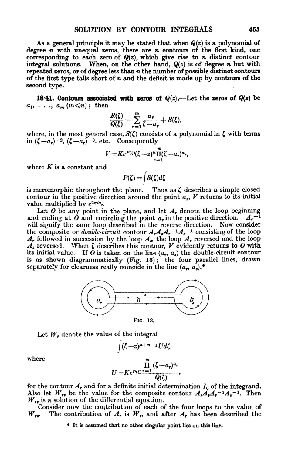
2*4. Equations of the First Order but not of the First Degree.—An
equation of the first order and of degree m may be written
where Plf . . ., Pm are functions of x and y. Theoretically, the equation
may be brought into the factorised form,
where pl9 p2, . . . , pm are functions of x and y.
Let
0r(#, V, Cr) =0
be the general solution of the equation
du
dx
it will also be a solution of the given equation. Conversely if
&(x, y, C)=0
is a solution of the given equation, it must satisfy one or other of the equations
Pr '
-pr=0 (r=l,2, . . . .m).
♦ For the general theory of conformal representation) see Forsyth, Theory of Functions,
Chap. XIX.
■f Gerhard Kremer {latine Mercator) published his map of the world in 1538. The
underlying mathematical principles were first explained by Edward Wright in 1594.
ELEMENTARY METHODS OF INTEGRATION 35
It follows that every solution of (A) will be included in the solution
VlVl*'> i/» CW2VX> #> c) * * • rml^J Z/» CJ—v,
which is therefore the general solution. The one arbitrary constant c is
sufficient for complete generality, for a particular solution is obtained
explicitly by solving one or other of the equations
(f>r(x9 y, c)=0,
in which c has any numerical value.
Example.— ( - 1 -
\dx,i
In the factorised form the equation is
dy
{:
dx
the two factors give rise to solutions
«/=sinh (c±x)
respectively, where c is a constant. The general solution therefore is
= 4(C—cosh 2a?),
where C — cosh 2c.
2*41. Geometrical Treatment.—The theory of the differential equation
may also be approached from a geometrical point of view. Replace ' by z
and regard z as the third rectangular co-ordinate in space. Then the equation
F(x,y,z)=O
represents a surface S.
Let
y=<f>(x)
be any solution of the differential equation, then the pair of equations
y=</>{x)9 z=<f>'(x)
represents a space-curve F which, since
F{x, <f>{x), f (x)} ~--0
identically, lies upon the surface S. There is not a solution of the differ-
differential equation corresponding to every curve which lies on S9 but only to
those curves at all points of which the differential relation
dy—zdx—O
is satisfied.
Let
x=x(t)9 y=y(t), z=z{t)
be the parametric representation of a curve F upon S lor which the relation
dy—zdx=O
is satisfied. The projection of F upon the (x9 t/)-plane Will be the curve C
x=x(t)9 y=
or
36 ORDINARY DIFFERENTIAL EQUATIONS
Since at all points of the curve F the equation
becomes
F{x, <f>(x), 4>'(x)}=0,
the curve C, or
y=<f>(x)
is an integral-curve of the equation
Let the parametric representation of the surface S be
x=f(u, v), y^g(u, v), z=h(u, v),
then the relation
dy — zdx=O
becomes
or, say,
dv
du
Any solution of this differential equation is a relation between u and v
which defines a curve F on the surface S sueh that the projection of this
curve on the (#, t/)-plane is an integral-curve of the differential equation.
Consider, as an example, an equation which can be written in the form
y-g(x, jp)=O.
The corresponding surface S is then representable parametrically as
and the relation dy~zdz~Q becomes
p + dP
Z -k{x'p) ■
This is a differential equation of the form
Z
let its general solution be
Then the integral-curves are the projeetions on the (x, ?/)-plane of the intersection
of the surface
with the family of cylindrical surfaces
l(Xj z> c)=0.
The general solution of the given equation is therefore obtained by eliminating p
between the two equations
2*42. Equations in which x or y does not explicitly occur.—When an
equation of either of the forms
F(x,p)=O9 F(yiP)=O
can be solved for p, the equation can be integrated by quadratures. On
the other hand it may occur that the equation is more readily soluble for
x (or y as the case may be) in terms of jp. Let
ELEMENTARY METHODS OF INTEGRATION 37
be the solution, then, on differentiating with respeet to y,
f(p)
p -J (P> dy'
whence y ^c -) fpf(p)dp
say. Then the equations
may be regarded as a parametric representation of the solution, which is
obtained explicitly by eliminating p between the two equations.
If the equation does not involve x, it is solved for y and then differentiated
with respect to x. The solution is then obtained in the parametric form
?y
where
More generally, it may be possible to express the equation
F(x, p) -0
parametrieally in the form
x=u(t), p=v(t),
then, on differentiating the former with respeet to t,
whence
The solution is then obtained by eliminating t between the expressions for
x and y. The equation
if expressible in the form
y=u(t),
is solved by eliminating t between
y~u(t) and x=c{\ }J
J v(t)
Example.—Consider the equation
p*—p2-\-y2~0.
It may be represented parametrieally as
y = t~P, p-=l~t2.
Differentiate the first equation with respect to /, then
dx
whence
n-3^2 , t-\
J 1-t2 SM-1
Thus x and y are expressed in terms of the parameter t.
2*43. Equations homogeneous in x and y.—An equation which is homo
geneous and of degree m in x and y may be written
xmF(- ,
x
38 ORDINARY DIFFERENTIAL EQUATIONS
If it is soluble for p, equations of the type
already considered (§ 2*12) will arise. This case, therefore, presents no new
features of interest. Consider, however, the case in which the equation is
soluble for - ; thus
X
or
Differentiate this equation with respect to x, then
Let p be taken as dependent variable, then in this equation the variables are
separable, and it has the solution
lo* exf
or, say,
The simultaneous equations
y=xf{p), cx-=
furnish the general solution of the equation.
Example.— y — yp2 -f 2px.
Solve for x, thus
differentiate with respect to «/, then
2 ( \ \dp
p p * J\p2^ )dy
or
dp p
y
whence
py^c.
Eliminating p from the original equation gives the required solution
2*44. Equations linear in x and y.—A general type of equation whose
solution can be obtained in a parametric form by differentiation is the
following: *
y=
The derived equation is
* The equations appear to have been integrated by John Bernoulli before the year 1694.
Its singular solutions were studied by d'Alembert, Hist. Acad. Berlin 4 A748), p. 275.
ELEMENTARY METHODS OF INTEGRATION 39
if x is regarded as dependent variable, and p as independent variable the
equation may, when p— <f>(p)^O, be written
dp p-<f(p) p~<f>(p)
and is then a linear equation in the ordinary sense. Its solution in general
involves two quadratures ; let it be
then x may be eliminated from the original equation, giving an expression
for y in the form
The general solution is thus expressed parametrically in terms of/?.
Consider now those particular values of p, say pi, p2, . . . , for which
p-<f>(p)=~-O;
for those values of p,
y ~-U.
ax
Thus there arises a certain set of isolated integral curves such as
They are straight lines such that .if an integral curve of the general family
meets one of them, it will have, in general, an inflexion at the common point.
The straight lines furnish an example of singular solutions, that is of solutions
of the equation which are not included in the general family of integral
curves, and not obtainable from the general solution by attributing a special
value to the constant of integration.
Example. — y ■= 2px —p2.
The derived equation is
dx
whence, if/?=j=0,
dx 2x
— -f- -
dP P
The solution of this linear equation is
X=p* + 3P'
which, combined with the original equation, gives the required solution.
On the other hand, when p—0, there is a solution
2#45. The Clairaut Equation.—The Clairaut equation,*
is not included in the class of equations studied in the preceding section
because, in the notation of that section,
identically, and therefore the method adopted fails.
The derived equation is
* Hist. Acad. Paris A734), p. 209.
40 ORDINARY DIFFERENTIAL EQUATIONS
it can be satisfied either by p—c, a constant, or by
The first possibility, p=c, leads to the general solution
y=cx+ip{c).
The second possibility leads to a particular solution obtained by eliminating
p between the two equations
y=px+i//{p), z+ifj'(p)=0.
It contains no arbitrary constant, and is not a particular case of the general
solution ; it is therefore a singular solution.
Now the envelope of the family of straight lines
is obtained by eliminating c between this equation and
and is identical with the curve furnished by the singular solution. In the
case of the Clairaut equation, therefore, the singular solution represents the
envelope of the family of integral-curves.
Conversely, the family of tangents to a curve
satisfies an equation of the Clairaut form, for if
y=ax+p
is a tangent, then
ax+P=f(x)9 a~-=f(x).
The elimination of x between these equations gives rise to a relation
J3=0(o),
and since, on the tangent, a=p, the tangents satisfy the equation
Example.— y=px-\ \/p.
Differentiating,
whence either p=c, giving the general solution
y
or else
The singular solution is found by eliminating p between
p2-~l/x and y —px +1 /p
and is
t/2— 4x.
2*5. The Principle of Duality.—There exists a certain transformation,
due to Legendre, by which a dual relationship can be set up between one
equation of the first order and another of the same order. Let X and Y
be new variables defined by the relations
X =p, Y =xp —*/,
and let
dY
dX'
ELEMENTARY METHODS OF INTEGRATION 41
Now, assuming that ~- 4=0,
~dp, dY=xdp-\-pdx—dy
=xdp,
and therefore
P^x.
Also
y =xp — Y
Thus the transformation
X=p, Y—xp—y
is equivalent to
x=l\ y=XP-Y.
They are therefore reciprocally related to one another.*
IJy means of this substitution, either of the equations
F(x9 7/, p)=0, F(P, XP-Y, X)^0
may be transformed into the other, and in this sense a dual relationship
exists between them. When one of the equations is integrable, the other
may be integrated by purely algebraical processes.
For instance, let
<f>(X, Y)=o
be a solution of the second equation, then on differentiating with respect
to X,
dx hdY
Now X, F, P may be eliminated between these two equations and
x=P, y=XP-Y,
thus giving a solution of the equation
F(x, y,p)=0.
In particular, an equation of the form
<P(xp —y) =-=xW{p)
would become
<P(Y)=PW(X).
The variables X and Y are now separable, and the equation is integrable
by quadratures.
Example.— (y—px)x~~y.
The transformed equation is
p
Y+X'
it is homogeneous, and has the solution,
log Y — — == const.
Differentiate with respect to X, then
P Y-XP
— — • —\jt
Y Y2
* If {xt y) and (X, Y) are regarded as points in the plane of the variables w, v, the
locus of (a?, y) is the polar reciprocal of the locus of (AT, Y) with respect to the parabola
m8—2v, and conversely. *
42 ORDINARY DIFFERENTIAL EQUATIONS
whence
Y-XP_y
P x
and consequently
X ^l-1-!
Y~~P x
Hence the solution of the original equation is
/ y\ 1
log 1 — '-)-—- = const.
\ X> X
or
y~cxe1Jx.
dp
Note.—In the case of the Clairaut equation the condition that —- =|=0 is violated
(XX
for the general solution ; this method therefore leads only to the singular solution.
2*6. Equations o! Higher Order than the First.—The simplest of all
differential equations of general order n is the following:
Its integration is simply the process of n-ple integration and may be carried
out in successive stages as follows. Let x0 be a constant, chosen at random,
then
^0
-X .-I
dxj dx
t/=j dxj dx ... | f(x)dx+C0Kjj2i\\ + ■ ■ ■ +C«-i'
where Co, t\< . . ., Cn-.x are arbitrary constants.
The multiple integral may, however, be replaced by a single integral.
Let
then
dY 1 ,•*
whence, finally,
JnV
Y is therefore a solution of the equation which, together with its first (n—1)
derivatives vanishes when x=xQ. It is therefore identified with the multiple
integral. The general solution of the equation is therefore
ELEMENTARY METHODS OF INTEGRATION 43
Apart from this simple case, and the case of linear equations with constant
coefficients, which will be dealt with in Chapter VI., there are but few equations
of order higher than the first which yield to an elementary treatment. In a
number of very special cases, however, the order of an equation can be
lowered by means of a suitable transformation of the variables, combined
with one or more quadratures. The main cases of this kind which can arise
will be dealt with in the three following sections.
2*61. Equations which do not explicitly involve the Dependent Variable.-
Consider the equation
/ d*y d*+ty dny\
\'da*'da*+19 ' ' "dxn) '
in which y and its first k—\ derivatives do not appear. The transformation
dky
_
dxk
reduces the equation to an equation in v of order n—k. If this equation can
be integrated and its solution is a— v(x), it only remains to integrate the
equation
which is of the type dealt with in the preceding section.
More generally, however, the reduced equation has a solution of the
form
<f)(x, v)=0,
which is not readily soluble for v. For the method to be practicable it is
necessary to express x and v in terms of a parameter t, thus
yW ^v(t), x—x(t).
Then
dtf*- U=v(t)dx =v(t)x'(t)dt,
which, on integration, gives y^k~l\ The process is repeated, A; times in all,
until the explicit solution is reached.
An important particular case is that of equations of the form
such equations are integrable by quadratures.
2*62. Equations which do not explicitly involve the Independent Variable.—
When an equation has the form
dy d^y dny \
'•' ' ' "'• dxn)~ '
its order may be reduced to n—1 by a change of variables. Let y be taken
as a new independent variable, and p as the dependent variable. The
formulae by means of which this transformation is effected are
dy __ dhj _ dip d?y _ B/ dp
V V ~~P dy\P
dx* ~~P dy\P dy )'
The given equation is thus reduced to one of the form
dp dn-1p\ .
$)=0
44 ORDINARY DIFFERENTIAL EQUATIONS
Let it be supposed that this equation can be integrated, and that its solution
is expressible in the parametric form
where / and g are functions of the auxiliary variable t, and depend also on
n~l constants of integration. Then x is obtained, in terms of t, by a
quadrature, thus:
f V
lf'(t)dt
In particular, an equation of the second order, which does not explicitly
involve x, namely
is transformed into the equation
which is of the first order.
An equation of the form
dxn
is reduced, by the substitution
dn~2y
—^ =v
dxn~2
to
dx*
If -j- -~p, this last equation becomes
whence
and therefore
a>=f{c+ff{v)dv}-*dv.
In order that y may be obtained, v must be expressed in terms of x ;
the solution is then completed by n—2 quadratures.
2#63. Equations exhibiting a Homogeneity of Form.—Two classes of
equations will be discussed, the first class being that of equations which are
homogeneous in y, y\ y", . . ., ?/*>, and which may also involve x explicitly.
An equation of this class may, if ?n is the degree of homogeneity, be written
ymF(x, y-, y\ . . .,
v y y y '
Let u be a new dependent variable, defined by the relation
ELEMENTARY METHODS OF INTEGRATION 45
then
and in general
where Un is a polynomial in u, uf u^1). The change of dependent
variable from y to u therefore reduces the order of the equation from n to
n—1.
The second class includes those equations which are homogeneous in
y, xy\ x2y", . . ., xntfn>> and do not otherwise involve x. Let
be the typical equation. Change the independent variable by the sub-
substitution
x—e\
then
dx~~dt' dx*~~dF dt9 ' ' '
and, in general,
dry d(d ,\ , d \
dxr dt^dt ' dt r /J
y ( ,
dxr dt^dt ' dt
Thus the transformed equation is of the form
dy dly
and does not explicitly involve x. It thus comes under the heading of
§ 2*62.
An equation which comes under the last class, but which can be integrated by
a simpler method is the following : *
The derived equation is simply
where FJy F2, F^ are the partial derivatives of F with respect to its first, second, and
third arguments respectively. It is satisfied by «/'" = 0, or
where A, B, C are arbitrary constants. This will be the general solution of the
original equation provided that
F(C\ B
2*7. Simultaneous Systems in Three Variables.—Before the general theory
of the integration of simultaneous systems of differential equations is
attacked, it will be convenient to dispose of a simple case in which the equa-
equations are integrable by the methods which were detailed in the earlier sections
of the chapter.
Consider the system
dx dy __ dz
, 7] and I are, in general, functions of x, y and z. A very special, but
* Dixon, Phil. Trans. R. S. (A) 186 A894), p. 563. The generalisation to any order
is obvious. See also Raffy, Bull. Soc. Math. France, 25 A897), p. 71.
46 ORDINARY DIFFERENTIAL EQUATIONS
important case is that in which £ and 77 are independent of z. In this case
the equation
dx dy
involves only x and y ; it will be supposed that this equation can be integrated
and that its solution is
&(x, y, a)=0,
where a is the constant of integration. Let this equation be solved for y,
thus
y=(f>(xf a),
and let fx and £1 be what f and £ become when y is replaced therein by
<f>(x, a). Then the equation
dx dz
does not involve y. Its solution will be of the form
@(x, z9 a, j3)=0,
where j8 is the constant of integration. Now let a be eliminated between the
two solutions
&(x, y, a)=0, 8(x, z, a, j8)=0;
the solutions then take the form
&(x, y, a)=0, W(x9 y, z,
2*701. Integration of a Simultaneous Linear System with Constant Co
efficients,—The system
dx dy dz
where
=a3x+b^y+c3z -f d3,
is not of the form dealt with in the preceding section. It can, however, be dealt
with in a similar manner after a linear transformation of the variables has been
made. To simplify the working a new variable t is introduced such that
dx dy dz dt
then, whatever constants l,m,n may be,
dt Idx+mdy+ndz
Let /, m, n be so chosen that
la1 -\-ma2 -f naz
lb1-{-mb2 +nbz ~mp9
lcx-{-mc2i-nc3=np,
then
dt __ d(lx-\-my+nz)
t ~ p(lx+my-\-nz-{-ry
where rp=ld1-\-md2-\-ndz. This choice of Z, w, n is possible if p is a root of the
equation
ELEMENTARY METHODS OF INTEGRATION 47
Let the roots of this equation, supposed distinct be . , , , and let the corre-
Ax A2 \3
sponding values of /, w, n, r be
lv miy ni9 r{ (i = l, 2, 3),
then
dt _
t "
whence
t =
The solution of the system is therefore
C1(^+m17/+n1z+r1)Ai^C2(/2aj+ra22/+w2z^
and contains three constants of integration, C\, C2, C3, of which two are arbitrary.
2-71. The Equivalent Partial Differential Equation.—Let x and y be
regarded as independent variables, and z as a dependent variable. Let
p and q be the partial derivatives of z with respect to x and ?/ respectively,
then
is a linear partial differential equation of the first order and is known as
the Lagrange linear equation. If
is a solution of the equation, then
tor all values of x9 y. This solution represents a surface, known as an integral-
surface of the partial differential equation. Since the direction cosines of
the normal to a surface z~f(x, y) are proportional to
dl df _i
do; 3y
the differential equation expresses a distinguishing property of the tangent
plane to the integral-surface.
Now consider the system of simultaneous ordinary differential equations
dx dtf dz
and let its solutions be solved for the constants of integration, thus
u(x9 y, z)=a, v(x9 y, z)=0.
These solutions represent a two-parameter family of curves in space, which
are known as the characteristics of the system. If £, 77, $ exist and are one-
valued at a point (x0, y0, z0), and at least one of them is not zero at (x0) t/0, z0),
one and only one characteristic passes through that point.
It will now be shown that the characteristics of the simultaneous differ-
differential system bear an intimate relationship to the integral-surface of the
partial differential equation. In the first place it will be proved that, if an
integral-surface passes through (xQ, yQ, Zq), it contains the characteristic through
that point. Let the integral surface through (x0, y0, Zq) be
and, supposing that £ does not vanish at (#0, t/0> *o)> consider the differential
equation
dx
48 ORDINARY DIFFERENTIAL EQUATIONS
in which z has been replaced by f(x, y). The equation defines y as a
function of x and is therefore the differential equation of a family of cylinders
whose generators are parallel to the axis of z. The cylinder through (#0, y0, 0)
intersects the integral-surface in a curve through (x0, ?/0, z0). Along this
curve
dx dy __ pdx+qdy dz
£ ~ V " pf+W ~~ £ '
The curve so defined is therefore a characteristic, and the theorem is proved.
An immediate consequence of this theorem is the fact that every integral
surface is a locus of characteristics. In particular if any non-characteristic
curve in space is drawn, the characteristics which pass through the points
of this curve build up an integral-surface.
In the second place, the converse of this theorem will be shown to be
true, namely, that in general every surface which arises as a locus of character-
characteristic curves is an integral-surface of the partial differential equation* The
tangent line to the characteristic at any arbitrary point (x0, i/0, z0) is
x—Xq = y ~-y0 ^z —z0
£o Vo Co
where £0, rj0, £0 are the values of f, 77, £ at (x0, y0, z0). The equation of the
tangent plane at (x0, y0, Zq) to the surface which envelopes the characteristics
will be
where pa and qa are respectively the values of ^, — on the surface at
y
(xQ, y0, Zq). Since the characteristic lies in the surface, the tangent line lies
in the tangent plane, and therefore
But (x0,7/0, z0) is any point on the surface ; the latter is therefore an integral-
surface of the partial differential equation
2*72. Formation of the Integral-Surface.—The aggregate of character-
characteristics form a two-parameter family or congruence of curves. Just as a plane
curve is formed by selecting, according to a definite law, a one-fold infinity
of the two-fold infinity of points in a plane, so an integral-surface is formed
by selecting a one-fold infinity of curves of the congruence. Let
u(x, \u z)^a, v(x9 y, z)=p
be the aggregate of characteristics from which a one-fold infinity is chosen
by setting up a relationship between a and /?, say
fi(a, j8)=0.
The equation to the integral-surface is therefore
Q(u, v)=0,
and this equation, in which the function Q is arbitrary, is the general solution
of the partial differential equation.
In the theory of ordinary differential equations of the first order, it is
often required to find that integral-curve which passes through a given
point of the plane. The corresponding problem in the case of partial
♦ The exceptional case arises when the surface has a tangent plane parallel to the
2-axis, for then p and q become infinite and the proof fails.
ELEMENTARY METHODS OF INTEGRATION 49
differential equation is to find that inteorral-surfaee whieh passes through a
given (non-characteristie) base-curve in space. This problem, in its general
form, is known as Cauchy's problem.
Let
</>(x, y, 3)=0.
represent the base-curve, and let
u(x, y, s)=a, v{x, y, z
be the characteristics. If, between these four equations, jc, ?/, z are eliminated,
there remains a relation between a and p which expresses the eondition that
the characteristics and the base-curve have points in common. Let this
relation be
#(afj8)=O,
then
0(u, v) —0
is the required integral-surface.
Example. Consider the partial differential equation
(a/ -bz)— -\-(az —cx)-t-- — bx—uy.
ox ay
The subsidiary differential system is
dx dy dz
cy—bz az—cx bx -ay
This system is equivalent to
( a dx -\-bdy -f cdz=0,
\xdx \-ydy-\-zdz- 0,
and therefore the equations of the characteristics are
ax \-by \-cz- a,
•«2 I ,»2 I ~2 O
wht'rc a iind fi are arbitrary constants. The characteristics arc the intersections
of all spheres whose centre is at the origin with all planes whieh are parallel to the
straight line
x y z
A) ~ = r =-~9
a b c
that is to say, they are the aggregate of circles whose planes are perpendicular to,
and whose centres lie on, this line.
The integral-surfaces have the equation
and are surfaces of revolution which have the line (/) as axes of symmetry.
Now consider that particular integral-surface which contains the y-axis ; it
is built up of those characteristic curves whieh pass through the «/-axis. The
characteristics are those for which a and ft are such that the equations
ax+by-l-cz — a, a?2+//2-Hzar-A ar=O, z—0
are consistent. The condition that they are consistent is obtained by eliminating
y from
and therefore is
The required integral-surface is
or
2-f Vabxy -j -2bcyz+2cazx=0.
50 ORDINARY DIFFERENTIAL EQUATIONS
2*73. The Homogeneous Linear Partial Differential Equation.—When £ is
identically zero, the equation has the so-called homogeneous form
The equations of the characteristics then become
dx _dy dz
The last equation gives at once
z— a,
and therefore the characteristics are plane curves whose planes are perpen-
perpendicular to the 2-axis.
The most important case is that in which £ and 77 are independent of z;
the equation of the characteristics is then
z=a,
and the equation of the integral-surface may be written in the form
z
Now consider the equation
where £, 77, £ are functions of x, y, z and do not involve /. If
where c is a constant, is a solution of the partial differential equation, then
= -/- dx + %dy + dJ-dz - 0,
and therefore/(cT, y, z)~ c is a solution of the simultaneous system
dx _dy _ dz
The converse is also true, for if
u(x, y, z)=a
is any solution of the simultaneous system, then
du du du
d+d+
and therefore
du . ydu
Let
v(x, y, z)=
be a second, and distinct, solution of the simultaneous system ; it will also
be a solution of the partial differential equation, so that
dv , ydv
+^0
If any other solution
w(x, y, z) =y
exists, then
dw dw r dw
ELEMENTARY METHODS OF INTEGRATION
51
and, eliminating f, 77,
, i\ w) __ dn du
d(x, y, z) —
dv dv dv
da*9 dy' d
dzv dzv dw
cKv ' by ' dz
identically. Consequently xv is a function of u and v,* and therefore the
partial differential equation admits of two and only two distinct solutions.
From the three equations
u(x,y,z)^a, v(jc, y,z)-P, u\d\ y, z) y,
two of the variables, say x and ?/, may be eliminated, rind the eliminant can
be expressed in the form
zv=(f>(u, v, z).
Now
_c'(m, 1/, rt') r(/*, i\ <f>)J)(u, v, z)
a((?;, //, z) c)(u9 z\ z) d(,r, y, z)
The first determinant on the riffht is simply ^ , the second is ,) ' . The
dz c%iv, y)
second of these is not zero, since u and v are supposed to be independent.
Consequently
z
that is to say, <f> is explicitly independent of z, or in other words iv is a
function of u and v alone.
The general solution of the partial differential equation
is therefore
Q(u, v) —const.,
where Q is an arbitrary function of its arguments, and
u --a, v-~f$
are any two independent solutions of the subsidiary system
dy dz
v C
The extension to the case of n variables is obvious. An exceptional case
occurs when £, 77, £ have a common factor ; the result of equating this factor
to zero provides a special solution of the partial differential equation which
may or may not be included in the general solution.
As an example consider the equation
+
The subsidiary system
by
dx dy dz
52 ORDINARY DIFFERENTIAL EQUATIONS
has the two distinct solutions
— z:== a., :rr=Bt
X XZ
The general solution is
Qi - 9 ) = const.
\x xz I
2*8. Total Differential Equations.—An algebraic equation in three
variables, of the form
where c is a constant, leads to the total differential equation
^dx^dy+fdz
dx dy * ' dz
If „- , _- , ,/ have a common factor u, and if
dx dy dz
dy ^ dz
the total differential equation may be written in the form
Pdx+Qdy+Rdz^-O.
On the other hand, if P, Q, and K are arbitrarily-assigned functions of
x, y, z, the total differential equation does not necessarily correspond to
a primitive of the form
For if such a primitive exists, /*, Q, R are respectively proportional to the
three partial differential coefficients of a function <j)(x, y, z), which is not in
general true. The problem therefore arises, to iind a neeessary and sufficient
condition that a given total differential equation should be integrable, that
is to say, derived from a primitive of the form considered.
It is first of all necessary that functions <f>(x, y, z) and jjl(x, y9 z) exist such
that the conditions
dx dy dz
are satisfied. Then *
dydx
that is
\sp_m p
\dy dx) dx dy'
and similarly
dit} dfi a?
dR dP> dp. dp
{dx " dz]' 8z da'
* It is, of course, assumed that the change of order of differentiation is valid,
ELEMENTARY METHODS OF INTEGRATION 53
The unknown fx is eliminated from these three equations by multiplying
respectively by R, /\ Q and adding. The resulting equation
dz\ +Hl8y
is a necessary condition for integrability.*
It is obvious from the above demonstration, and may easily be verified
independently, that if A is a function of x, yy z and
P3 =\P, Qi --AQ, Rl =-
the condition for integrability is satisfied by Pl9 Q1? /?j.
It will now be proved that the condition of integrability is a sufficient
condition, that is to say, whcjijtjjsatisfledj there exists_a solution involving
an arbitrary constant. The prooFmcid'entally furnishes aTrnethod of obtain-
in oTTu*" solution when the condition for integrability is satisfied.
Let one of the variables be, for the moment, regarded as a constant. If
the variable chosen is z, the equation reduces to
where P and Q are to be regarded as funetions of x and y into whieh z enters
as a parameter. This equation has a solution
ti(x, y, z) — const,
where, if A(,r, y, z) is the integrating factor,
but, of course, it does not follow that
du
dz "
Let
du
= dz
then since, by hypothesis,
( dz dy ) ( dx dz ) t dy
it follows that
dS du dS du
dx (hj dxj dx
This relation is not satisfied in virtue of
u(x, y, z)~ const.,
it is therefore an identity. Consequently S and u, regarded as functions of
x and y arc functionally dependent upon one another. The functional
relationship between them, however, involves also the third variable z9 and
thus 6T is expressible in terms of u and z alone.
Now
+Qdy +Rdz)- ^dx +d™dy+ ^dz +Sdz
ex oy c z
~du-\-Sdz.
* Euler, 7ns/. Calc. Int. 3 A770), p. 1.
54 ORDINARY DIFFERENTIAL EQUATIONS
- The original equation is therefore equivalent to
du-{-Sdz=O;
let fi(u, z) be an integrating factor, then
\n(Pdx+Qdy+Rdz) =ii(du+Sdz)
is an exact differential di/f. The primitive is
tfs(u, z) =o ;
and if u is replaced by its expression in x, y, z the primitive takes the form
<j>(x. y, z) =c.
Similarly it may be proved that a necessary and sufficient condition that
the equation in n variables
should have a primitive of the form
is that the set of equations
X^ (dXv dXrf ft
^A J +AAl ^ "^ 5
(A, /x, v=l, 2, . . ., n),
are satisfied simultaneously and identically. The total number of such
equations is \n(n—l)(n-~2); of these |(w—l)(n—2) are independent.
•
The main lines upon which the integration proceeds is illustrated by the
following example :
yz(y -f z)dx+zx(z Jrx)dy+xy(x +y)dz ==0.
In this case
P=yz(y+z), Q=zx(z+x), R=xy(x+y).
and the condition for integrability is satisfied.
* When z is regarded as a constant the equation reduces to
yz(y+z)dx +zx(z+x)dy=0,
and this reduced equation has the solution
__ (z+x)(z-\-y)
Now
du _ z(z-\-y)
\J*X> Us U
du z(z-\-x)
so that
Also
XU* ^,2>ti2 ">
x±y __2z+x+y ^ _%x+y+z
xy xy xy
and therefore
X(Pdx+Qdy +Rdz)=du - 2 ^-^ dz.
2
ELEMENTARY METHODS OF INTEGRATION 55
An integrating factor is pi =z-8, and
The primitive therefore is
z* ~~
or, replacing u by its expression in terms of x9 y, z,
xyz "~C#
2*81. Geometrical Interpretation.—When R is not zero, the total
differential equation may be written
P.- Q
or
dz=Udx+Vdy.
Since
the total differential equation is equivalent to the two simultaneous partial
differential equations
p = U(x9 y, z)9 q=V(x9 y9 z).
The equation of the tangent planq at (afo, yOi Zq) to the integral-surface which
passes through (#0, y0, z$) is therefore^
where G0 and Fo are respectively the values of U and V at (oto, y0, q)
The problem of integration is therefore equivalent to finding a surface
such that the direction cosines of its normal at every point (cc9 y9 z) are
proportional to
V(x, y9 z)9 V{x, y, z)9 —1. ^
This problem is, in general, insoluble; in order that it may be soluble the
condition for integrability, which reduces to
+FaB+Z
dy "r dz dx^ dzf
must be satisfied.
The general solution of each of the partial differential equations
dy~
represents a family of surfaces, such that through every curve in space there
passes, in general, one and only one surface of each family.* Their common
solution represents a family of space-curves
xy yy z) =a, v(at, y, z) =K,
depending upon the two parameters a and jS, and such that through each
point in space then passes one and only one integral-curve.
An integral-surface of the total differential equation cuts every curve of
* This depends upon the fact that a partial differential equation possesses, in general,
a unique solution satisfying assigned initial conditions. The truth of the underlying
existence-theorem is assumed. •
56 ORDINARY DIFFERENTIAL EQUATIONS
this family orthogonally, that is the tangent plane at any point P of an
integral-surface must contain the normals at P of the two surfaces u—a,
v=p which pass through P. Hence
du du du
+
dv dv dv
+
These two equations determine
P = U{ob, y, z), q=V(x, y, z).
These are consistent if, and only if
dy ~ dx9
that is, if the condition for integrability
dV .vdU dV dV
dy "*■ dz 3x ^ dz
is satisfied.
2*82. Mayer's Method of Integration.—The method of integration
developed in § 2*8 depends upon the integration of two successive differential
equations in two variables. In Mayer's method * only one integration is
necessary. Let (#0> 2/o) be any chosen pair of values of (x, y) and let Zq be
an arbitrary value of z such that the four differential coefficients
du
dy ' dz1 dec ' dz
exist and are continuous in the neighbourhood of (x0, y0, Zq). Then if the
equation is integrable, its solution will be completely determined by the
initial value Zq. The value of z at (x, y) can therefore be obtained by following
the variation of z from its initial value Zq as a point P moves in a straight
line in the (x, i/)-plane from (x0, y0) to (x, y).
There is no loss in generality in supposing that the point (x0, y0) is the
origin, and this will be assumed. On the straight line joining the origin to
( )
where k is constant. The equation therefore becomes
where Ui and Fj are what U and F become when y is replaced by kx. This
equation, in the two variables x and z, has a solution of the form
<f>(x, z, *c)= const,
or, since z~Zq when x—0,
<f>(X, Z, K)=0(O, Zq, K).
On replacing k by yjx, the solution
<f>(x, *, yjx) =<f>@, Zq, yjx)
is obtained in a form which indicates its dependence upon the arbitrary con-
constant Zq.
* Math. Ann., 5 A872), p. 448.
ELEMENTARY METHODS OF INTEGRATION 57
Example —Consider the equation
1+yz x(z-x)
dz = —-2- dx + -1-:—fly;
1+xy l+xy
bhe coefficients of dx and dy are continuous in the neighbourhood of a?=0t t/=0,
2~20, and so are their partial differential coefficients.
Let
then the equation reduces to
dz 2kx 1 —kx*
dx " Z +
it is now linear, and has the solution
The solution of the given equation is therefore
2*83. Pfafl's Problem.—When the condition for integrability is not
satisfied, the total differential equation is not derivable from a single primitive.
On this account such an equation was at one time regarded as meaningless.*
Further consideration, however, brought to light * the fact that the total
differential equation is equivalent to a pair of algebraic equations f known
as its integral equivalents. In general, when the equations for integrability
are not all satisfied, a total differential equation in 2n or 2n—1 variables
is equivalent to a system of not more than n algebraic equations.} The
problem of determining the integral equivalents of any given total differential
equation is known as Pfaff's Problem. A sketch of the method of procedure,
in the case of three variables, will now be given.§
The first step consists in showing that the differential expression
Pdx+Qdy+Rdz
can be reduced to the form (JL t
d +d
where u, v, w are functions of #, y, z. The two forms are identical if
p + q + R+
Let
dz dy9 * dx dz' dy
then
p, _dv dw _ dv dw
~8'd ~d' dz9
dw __dv dw_
dx'dz dz'dx9
dx'dy'
♦ Euler, Inst. Cak. Int., 3 A770), p. 5.
f Monge, Mhn, Acad. Sc. Paris A784), p. 535.
t Pfeff, Abh. Akad. Wiss. Berlin A814), p. 76.
§ An extended treatment in the general case is given in Forsyth, Theory of Differential
'Equations, Part I., and in Goursat, Lemons sur le ProbUme de Pfaff* *
58 ORDINARY DIFFERENTIAL EQUATIONS
It follows that
-
Thus v and w are solutions of one and the same linear partial differential
equation ; the equivalent simultaneous system is
dx __ dy __ dz
Let
a(x, yy s)=const., /?(#, y, 2)=const.
be two independent solutions of the simultaneous system, then v and w are
functions of a and /?.
Now return to the variable u; since
it follows that
p'£+q%+R'^=pp>+qq>+RR>-
But the condition
pp>+QQ>+RR'=0
is the condition for integrability; since it is supposed not to be satisfied,
u does not satisfy the same partial differential equation as v and w.
Now w may be any function of a and j8 ; for simplicity let
zv=a.
Then if the relation
a(x, y,
where a is a constant, is set up between the variables x, y, z, the differential
form Pdx+Qdy-\-Rdz reduces to duy and therefore becomes a perfect
differential. Thus the relation a(x9 y, 2)= a is used to express any variable,
say z, and its differential dz in terms of the other two variables and their
differentials, and when these expressions are substituted for z and dz in
Pdx+Qdy+Rdz, the latter becomes a total differential d$(x, y, a). When
a is replaced by a(x, y, z) this differential becomes du. Thus u is obtained,
and since u and w are known, v may be deduced algebraically from any one
of the equations (A). The total differential equation
Pdx+Qdy+Rdz=O
is thus reduced to the canonical form
du+vdw=0.
The canonical equation may be satisfied in various ways, as follows :
(i) t4=const«, t£j=const» (ii) w=const., u=0.
More generally, if \fs(u> w) is any arbitrary function of u and w, an integral
equivalent is
(iii)
(iii) includes (ii) but not (i). In each case, the integral equivalent consists
of a pair of algebraic equations.
ELEMENTARY METHODS OF INTEGRATION 50
As an example, consider the equation
ydx -\-zdy +xdz=0.
In this case
P=y
and thus
that is, the condition for integrability is not satisfied.
The simultaneous system is
dx=dy=dz;
one solution is
a = aj—-t/=a.
Let w—a, and eliminate x from the given equation, which becomes
(y+z)dy+(y+a)dz=O.
This reduced equation is immediately integrable and its solution is
<f> = iy2+yz+az=const.
When a is replaced by re—y, <j> becomes u, thus
Finally v is obtained as follows :
dw du
dx9
that is
v=y—z.
Thus
ydx -\-zdy +xdz—du-\- vdw,
where
u = %y2+xy, v=y—z, w=x—y.
Integral equivalents are therefore
(i) i2/2+aJ2== const., oj—t/=const.,
(ii) Jy2+a?z=const.,, y— z=0»
Other integral equivalents are obtained by permuting x, y, z, cyclically.
2*84. Reduction of an Integrable Equation to Canonical Form.—The
foregoing reduction to canonical form may equally well be performed in
the case of an integrable equation, but since, in this case,
PP'+QQ'+RR''=o,
identically, u satisfies the same partial differential equation as v and w
and therefore u, v and w are functions of a and j3.
It follows that
du+vdw =Ada +Bdfi,
where A and B are functions of a and f$ alone. When a and j3 have been
determined, A and B are derivable algebraically from any two of the three
consistent equations,
^ R=A~+B£.
by* Adz^ dz
Thus the total differential equation is transformed into an ordinary equation
in the two variables a and £.
60 ORDINARY DIFFERENTIAL EQUATIONS
This leads to a practical method of solving an integrable equation, as is shown
by the following example (cf. § 2*8):
yz(y -\-z)dx -\-zx(z -\-x)dy -f xy(x -\-y)dz=0.
Here
V=2y(x—z)9 R'=2z(y--x)t
and the condition for integrability is satisfied. The simultaneous system
dx dy dz
—z) z(y—x)
is equivalent to
dx dy dz
w it y
Jb If <t
and has the solution
a~ x-\-y+z—const., fi = xyz—const.
Thus the given equation reduces to
Ada~\-Bdp=0,
where
yz(y+z)=A+Byz,
zx(z-\-x)=A-\-Bzx>
xy(x+y)==-A+Bxy.
Hence
that is to say, the equation becomes
adfi—pda=09
and has the solution
a=x+y+z
p xyz
Miscellaneous Examples.
1. Integrate the following equations :
(i) A— a?a)*diu+(l— y*)ldy=0 ; (xiii) xp—ay—xn;
(ii) #(l+ya)*(fe-f t/(l+a?2)*%==0 ; (xiv) xp—y^x2 sin x ;
(iii) {x*-\-2xy—y2)dx—{x*—2xy—yz)dy~O ; (xv) p-\-2xy=sxe~"x ;
(iv) (y2— xyfdx+ix*— xy)dy=0 ; (xvi) P sin x cos x— y-=
(v) x*ydx+(x*—y*)dy~0 ; (xvii) (y1 —
(vi) (x+y)dx-Bx-y-l)dy=0 ; (xviU) (y-
(vii) (x+2y+l)dx-Bx+4>y+a)dy=0; (xix)
(viii) Bx*+6xy+y2)dx+(Sx*+2xy+4y')dy=*0; (xx) __
(ix) (a;s4-j/a)ate-ha!3/<iy=O ; (xxi) yp*+2px—y~Q ;
(x) (l+aja)p+ary=l; (xxf?) y~(a
(xi) p+y tan aj=sin 2a?; (xxiii) (aH
(xii) p+y cos aj^c*^ ; (xxiv) y—
2. Determine n so that the equation
is exact.
8. Show that the equation
an1 integrating factor which is a function of xy*, and solve the equation.
ELEMENTARY METHODS OF INTEGRATION 61
4. Show that cos x cos y is an integrating factor for
Ba? tan y sec x+y% sec y)dx+By tan a? sec y+x% sec x)dy
and integrate the resulting product. [Edinburgh, 1915*]
5. From the relation
derive the differential equation
where ct=sAC(Bt—At), Deduce the addition theorem for the hyperbolic cosine.
6. Verify that a solution of
dx dy
is x*y*+2axy(x+y)+a*(x-y)t—4(x+y)+4fa=0,
where a is an arbitrary constant. In what way is this result connected with the theory of
elliptic functions ?
7. Find the curves for which
(i) The subnormal is constant and equal to 2a ;
(ii) The subtangent is equal to twice the abscissa at the point of contact;
(iii) The perpendicular from the origin upon the tangent is equal to the abscissa at
the point of contact;
(iv) The subtangent is the arithmetical mean of the abscissa and the ordinate ;
(v) The intercept of the normal upon the a>axis is equal to the radius vector ;
(vi) The intercept of the tangent upon the y-axis is equal to the radius vector.
8. P is a point (a?, y) on a plane curve, C is the corresponding centre of curvature, and
T the point in which the tangent at P meets the aj-axis. If the line drawn through T
parallel to the y-axis bisects PC prove that
and hence prove that the curve is a cycloid. [Paris, 1914.]
9. Prove that every curve whose ordinate, considered as a function of its abscissa,
satisfies the differential equation
where a is a constant, has the following property. If // is the foot of the perpendicular
from the origin O upon the tangent at any point P of the curve and Q Is the foot of the
perpendicular from // upon OPt then P lies upon the circle of centre O and radius a.
Change the variables by the substitution
a?=r cos 0, y—r sin 6
and integrate the equation thus obtained. IParis, 1917.J
CHAPTER III
THE EXISTENCE AND NATURE OF SOLUTIONS OF ORDINARY
DIFFERENTIAL EQUATIONS
8*1. Statement of the Problem.—The equations of the type
whose solutions were found, in the preceding chapter, by the application of
elementary processes, are integrable on account of the fact that they belong
to certain simple classes. In general, however, an equation of the type in
question is not amenable to so elementary a treatment, and in many cases
the investigator is obliged to have recourse to a method of numerical approxi-
approximation. The theoretical question therefore arises as to whether a solution
does exist, either in general or under particular restrictions. Researches
into this question have brought to light a group of theorems known as
•existence-theorems, the more important of which will be studied in the present
chapter.*
Let (o?o, Vo) be a particular pair of values assigned to the real variables
H
1 \
V \
°i • \
w /
% /
\ /
i /
I /
/ i
/ ;*
\ i
Fio. 1.
(poy y) such that within a rectangular domain D surrounding the point (#0, y0)
and defined by the inequalities
| x—Xq I < a, I y— y0 \ < b,
f(x, y) is a one-valued continuous j function of x and i/.
♦ See also Chap. XII., where the question is discussed from the point of view of the
theory of functions of a complex variable.
t f(x> V)is a continuous function of x and y in D if, given an arbitrarily small positive
number «, a number 8 can be determined such that \f(x+h, y+k)—/(#, y)' <«t, provided
that («, y) and (x+h, y+k) are in D and !fc!<8, (A?; <5. It is important to note that
h and k vary independently.
62
EXISTENCE AND NATURE OF SOLUTIONS 68
Let M be the upper bound of \f(x, y) | in D and let h be the smaller of a
and b/M. If A<a, the more stringent restriction
x—Xq I < h
is imposed upon x. (Fig. 1.)
Yet another condition must be satisfied by f(xy y)y namely that, if (a?, y)
and (x9 Y) be two points within Z), of the same abscissa, then
\f(x,Y)-f{x,y)\<K\(Y-y)\,
where K is a constant. This is known as the Lipschitz condition*
Then, these conditions being satisfied, there exists a unique continuous
function of x9 say y{x), defined for all values of x such that \x— xo\<Ch, which
satisfies the differential equation and reduces to t/0 when x—Xq.
Two entirely distinct proofs of this existence theorem will now be given,
known respectively as the Method of Successive Approximations and the
Cauchy-Lipschitz Method.
3*2. The Method of Successive Approximations^—Suppose for the
moment that a solution y(x) is known, which reduces to y0 when x=Xq ;
this solution evidently satisfies the relation
f{U Vi{t)}dt.
0
This relation is, in reality, an integral equationy% involving the dependent
variable under the integral sign. Let the function y(x) be now regarded as
unknown ; the integral equation may then be solved by a method of successive
approximation in the following manner.
Let x lie in the interval § (a?0, x0 -\-h) and consider the sequence of functions
yi(x)> y%{x)> • • * » yn(x) defined as follows :
rx
xQ
%
i f{t, yn-i{t)}dt.
J *0
It will now be proved
(a) that, as n increases indefinitely, the sequence of functions yn(x)
tends to a limit which is a continuous function of xt
(b) that the limit-function satisfies the differential equation, and
(c) that the solution thus denned assumes the value y0 when a?=a?0 and
is the only continuous solution which does so.
* It will be seen, as the theory develops, that it is only necessary that the Lipschitz
condition should hold in the smaller region \x—x9\<h, y—y0 \<M \x—a?0|.
f This method, though probably known to Cauchy, appears to have been first published
by Liouville, J. de Math. A) 2 A838), p. 19 ; A) 3 A838), p. 565, who applied it to the case
of the homogeneous linear equation of the second order. Extensions to the linear equation
of order n are given by Caque, J. de Math. B) 9 A864), p. 185; Fuchs, Annali di Mat.
B) 4 A870), p. 36 [Ges. Werke, I. p. 295]; and Peano, Math. Ann. 32 A888), p. 450. In
its most general form it has been developed by Picard, J. de Math. D) 9 A893), p. 217;
Traiti d*Analyse, 2, p. 801; Bnd ed.) 2, p. 840; and Bdcher, Am. J. Math, 2* A902),
p. 311.
t Bocher, Introduction to the Theory of Integral Equations; Whittaker and Watfon,
Modern Analysis, Chap. XJ.
§ This restriction is a matter of convenience, not of necessity, and will shortly be
removed.
64 ORDINARY DIFFERENTIAL EQUATIONS
In the first place, it will be proved by induction that, when x lies in the
interval considered, \yn(x)~t/0|^&- Suppose then that | yn-i(x)~Vo I ^ *
it follows that | f{t, yn-\(t)} \ ^M, and consequently
\f{Uy*-i{t)}\dt
But evidently
it is therefore true that
fnW-tfa\
for all values of n. It follows that f{x9 yn{x)} ^M when xo<x<C,xQ-\-h.
It will now be proved, in a similar way, that
n!
For suppose it to be true that, when xo^x
n-l
then
< I* I/ft »»-lW)-/ft Vn-2(t)} | *
•" Xn
by the Lipschitz condition, so that
n\
But the inequality is clearly true when w=l, it is therefore true for all values
of n. In the same way it can be proved to hold when xo~h^x^x0, it is
therefore true for \x— «z0 | ^ h.
It follows that the series
00
is absolutely and uniformly convergent when j *zr—o:o | <& and moreover
each term is a continuous function of x. But
n
consequently the limit-function
2/(a?)=lim yn(x)
exists and is a continuums function of x in the interval (xo~-ht
c ♦ Bromwich, Theory of Infinite Series, § 45.
EXISTENCE AND NATURE OF SOLUTIONS 65
Now if it is true that
lim yn{x)=y0+\im f/fttti-i
=i/0+ f lim /{*, y,-
it will follow that y(x) is a solution of the integral equation
f{t,y(t)}dt.
That the inversion of the order of integration and procedure to the limit
is legitimate may be proved as follows :
f [fi*. y(t))-f{t, yn-i(t)W\<K f Iy(t)-yn-!(t)| dt
xQ J r0
where €n is independent of x and tends to zero as n tends to infinity.
The function f{t, y(t)} is continuous in the interval a^—A
consequently
dy{x) _d r*
dx -)
The limit-function y(x) therefore satisfies the differential equation; it also
reduces to y0 when x assumes the value x0.
It remains to prove that this solution y(x) is unique. Suppose Y(x) to
be a solution distinct from y(x)9 satisfying the initial condition Y(xQ)=y09
and continuous in an interval (xo> Xq+W) where h'<Jt and h' is such that the
condition
\Y(x)-yo\<b
is satisfied for this interval. Then, since Y(x) is a solution of the given equa-
equation, it satisfies the integral equation
jXJ{t, Y(t)}dtf
and consequently
Y(x)-yn(x)= I* [/ft F(*)}-/{*, yn^(t))]dt.
J XQ
Let n=l, then
Y(x)-yi(x)= f [fit, Y(t)}-f{t, yo}]dt,
and it follows from the Lipschitz condition that
\Y(x)-y1(x)\<Kb(x-x0).
Similarly, when n=2,
Y(t))-fit, Vl (t)})dt
<K(*\Y[t)-yi{t)\dt
tx
J X*
66 ORDINARY DIFFERENTIAL EQUATIONS
and in general
I Y(x) —yn(x) \<~ nt
whence
Y(x) = lim yn(x) =y(x)
for all values of x in the interval (x0, xo+h')t and therefore the new solution
is identical with the old. There is therefore one and only one continuous
solution of the differential equation which satisfies the initial conditions.
3*21. Observations on the Method of Successive Approximation.—The
two main assumptions which were made regarding the behaviour of the
function f(x, y) in the domain D, namely the assumption of continuity and
that of the Lipschitz condition are quite independent of one another. The
question arises as to the necessity of these assumptions ; it is therefore well
to look a little more closely into them and to enquire whether or not they
may be unduly restrictive.
In the first place, it will be seen that the continuity of f(x, y) is not
necessary for the existence of a continuous solution ; in fact all that the
previous investigation demands is that f(x, y) be bounded, and that all
integrals of the type
f{uyn{t)}\dt
exist. In particular, f(x, y) may admit of a limited number of finite dis-
discontinuities.*
Thus, for instance, the differential equation
dy
~ =r-y(l ~2x) when
dx
™ yBx — 1) when
admits of a continuous solution satisfying the initial condition // — I when x = l.
This solution is
y=ez~*2 when x\
—cx2-~x when i
and the solution is valid for all real values of x, moreover it is unique.
On the other hand, the Lipschitz condition, or a condition of a similar
character, must be imposed in order to ensure the uniqueness of the solution.
It is not difficult to construct an equation for which the Lipschitz condition
is not satisfied, and which admits of more than one continuous solution
fulfilling the initial conditions.f
Thus, for instance, in the equation
the Lipschitz condition is violated in any region which includes the line y=0. The
* These may be discrete points or lines parallel to the t/-axis ; any other lines of dis-
discontinuity imply a violation of the Lipschitz condition throughout an interval of finite
dimensions. Mie, Math. Ann. 43 A898), p. 553, has shown that solutions exist whenever
f(x, y) is continuous in y and discontinuous but integrable (in Riemann's sense) with
respect to x.
t Peano, Math. Ann. 87 A890), p. 182; Mie, loc. cit., ante; Perron, Math. Ann.
76 (lfrlS), p. 471.
EXISTENCE AND NATURE OF SOLUTIONS 67
equation admits of two real continuous solutions satisfying the initial conditions
#=0, y=0, viz.
A°) 2/=0,
B°) y=\x* whenaj^O,
= — Jo?2 when a?<0.
Another example is given by the equation
where
4xy
f(x, y) — - — - when # and y are not both zero,
x*+y*
= o when #=?/=0.
It is easily proved that f(x, y) is a continuous function of x and y. On the
other hand
J{x, Y) -fix, y) | = 4 1~
and therefore the Lipschitz condition is not satisfied throughout any region con-
containing the origin.
The ^equation admits of the solution
c being an arbitrary real constant, and thus there is an infinity of solutions
satisfying the initial conditions x~0f y—0.
The question has been placed on a firm basis by Osgood,* who proved
that, if /(#, y) be continuous in the neighbourhood of (xOf y0), there exists
in general a one-fold infinity of solutions satisfying the initial conditions.
These solutions lie entirely within the area bounded by two extremal solutions
A necessary and sufficient condition that there be a unique solution is that
Y-i(x) and Y2(x) be identical. This is the case when the Lipschitz condition
is satisfied, but it is also true when the Lipschitz condition is replaced by one
or other of the less restrictive conditions
\f(x, Y)-f(x, y)\<K1\ Y-y | log
fix, Y)-f(x, y)\<K2\ Y-y \ log { y^ log log
in which Kx, K2, . . . are constants.
The constant K which occurs in the Lipschitz condition determines, fof
any given value of x, the rapidity with which the comparison series
A nl
converges, and therefore gives an indication of the utility of the series
n
r-l
as an approximation to the limit-function y(x). Thus if R were small,
* Monatih. Math. Pkys. 9 A808), p. 881.
68 ORDINARY DIFFERENTIAL EQUATIONS
yn(x) would tend to the limit y(x) more rapidly than if K were large. Now
in most cases occurring in practice K is the upper bound of
dy
in the domain D. To make use of this fact, consider the family of curves
M y)=c,
for all values of the constant C. The typical curve of this family is such that
it intersects each integral curve in a point at which the gradient of the latter
curve is C. For this reason the curves are known as the isoclinal lines.* Let
the isoclinal lines be plotted for a succession of discrete equally-spaced (e.g.
integral) values of C\ and let a line be drawn parallel to the g/-axis. Then
the intervals along this line in which the points of intersection with the
isoclinal lines are densely packed correspond to large values of K, whereas
those intervals in which the intersections are more widely spaced correspond
to smaller values of A^. This brings out the fact that the regions in which
the method of successive approximations may most successfully be applied
as a practical method of computation are those in which the isoclinal lines
tend to run more or less parallel to the ?/-axis.f
The method of successive approximations leads to a solution which was
shown to converge in the interval \x—xo\<^h, where h is the least of a and
b/M. But, as was remarked in passing, the assumption originally made that
certain conditions are satisfied throughout the region \x— iro|<a, \y—«/0| <i>
was unnecessarily restrictive. If a region \x— #0|</e, \y— y$\ <M|#—xo\
can be found such that /(#, y) satisfies the necessary conditions in that region,
and M is the upper bound of \f(x, y)\, then k will certainly not be less, and
may quite conceivably be greater, than h. Several writers have succeeded
in thus extending the range in which the solution can be proved to converge,{
but no general method of determining the exact boundaries of the interval
of convergence has yet been discovered.
3*22. Variation of the Initial Conditions.—Let the given initial condition
that y=y0 when x=x0 be replaced by the new condition j/—yo+f] when x—Xq9
where («r0, yo+rj) is a point within the domain D such that \rj | <S. Then, in
place of the sequence of functions
as denned in § 3*2, there now arises the sequence
x)9 Y2(x), . . . , Yn(x),
denned as follows :
Yi{*)=Vo-hl+f /ft
J H
Y2(x)=y0+V+f /ft
f f{t, Yn
* The term is due to Chrystal, see Wedderburn, Proc. Roy. Soc. Edin. 24 A902), p. 400.
t Practical methods of approximate computation based upon the method of suc-
successive approximations have been devised by Sevenni, Rend. 1st. Lombard. B) 91 A898),
pp. ear, 950; Cotton, C. R. Acad. Sc. Paris, 140 A905), p. 494; 141 A905), p. 177;
146 A908), pp. 274, 510; Math. Ann. 31 A908), p. 107.
t Ljndelof, C. R. Acad. Sc. Paris, 118 A894), p. 454 ; J. de Math. D) 10 A894), p. 117.
See Picard, TraiU d*Analyse, 3, p. 88 ; Bnd ed.) 2, p. 340 ; and also § 3*41 below.
EXISTENCE AND NATURE OF SOLUTIONS 69
The existence and uniqueness of the solution
1
then follow as before. Now
\Y1(x)-y1(x)\<8+\j* [f{t,
<8+K8\x-xo\,
I Y2(x)-y2(x) | < 8+ \jX [/{*, FaWWfr </i (t)}dt I
<8+K8\x-x0
and, by induction,
\Yn(x)-yn(x)\<8+K8\x-x0\ + . . . + ~K«8 \ x-x0 ln
so that, in the limit,
Consequently, when \x — #0| <&, the solution is uniformly continuous in the
initial value y0. To bring out this fact, it may be written in either of the
forms
y(x, y0) and y(x— x0, y0).
Moreover,
n(v> 2/0)
1
<l+K\x-zo\ + . . . +—.Kn\x-z0\n,
1
and consequently
<\+K\x-xa\ + . . .
n\
from which it may be deduced that the series
*(>r' yo)-yn-i(x>yo)}
is absolutely and uniformly convergent. Therefore y(x> y0) is uniformly
differentiate with respect to y0 when \x— xo\ <^.
A proof proceeding on similar lines to the above shows that if the
differential equation involves a parameter A, that is to say if
where f(xt y; X) is single-valued and continuous and satisfies the- Lipchitz
condition uniformly in D when yIx<A<yl2, then the solution depends
continuously upon A, and in fact is uniformly differentiate with respect to
A when \x— xo\<Ji.
3*23. Singular Points.—A singular point may be denned as a point of
the (x, t/)-plane at which one or other of the conditions necessary for the
establishment of the existence theorem ceases to hold. In fact if for the
initial value-pair (x0, y0) the solution
(a) is discontinuous, (b) is not unique, or (c) does not exist,
then the point (x0, y0) is a singular point of the equation. As illustrations
of the diverse ways in which the solutions of an equation may behave at or
in the neighbourhood of a singular point, the following examples may be
taken.
70 ORDINARY DIFFERENTIAL EQUATIONS
dii y
A°) -£■=■■-.
v f dx x
The conditions requisite for the existence of a unique and continuous solution
are fulfilled except in the neighbourhood of x~0. The solution corresponding to
the initial value-pair (a?0, yQ) is
when aJo=f=O. If x0—0 and y^ft, the solution reduces to
x=0.
The only exceptional case is when xo~yo—0 ; the only singular point in the finite
part of the (x, y)-plane is the origin. Now every integral-curve passes through the
origin, which is a node of the integral-curves.
B°) -ji^m--
y ' dx x
In this case also, the only singular point is the origin. To any other point
(xOi y0) corresponds the solution
y=
The family of integral curves corresponding to all possible values of (#0, ^o) touch
the #-axis at the origin if m>l and the y-axis at the origin if l)<m<l. Thus if
w>0, every integral-curve passes through the origin.
On the other hand, if m<0, say m= — p, the solution is
The family of integral-curves is asymptotic to the x- and i/-axes. The degenerate
curve
passes through the origin, but no other integral-curve does so. The origin is a
saddle-point, for in its neighbourhood the integral-curves resemble the contour
lines around a mountain pass.
dx x
The origin is the only singular point; to any other point (xQ, y0) corresponds
the solution
x
0
X
X
0
The origin is a node of the integral-curves.
D0)
y
The solution is, in general,
No real integral-curve, except the degenerate curve x*-\-y2=0 passes through the
origin, which is a focal point.
dx x—y
This equation is most effectively dealt with by means of a transformation to
polar co-ordinates
#=r cos 6, y—r sin 8.
It then becomes
dr
dO *
the integral-curves are the family of logarithmic spirals
EXISTENCE AND NATURE OF SOLUTIONS 71
One curve of the family goes through each point of the plane except the origin. No
integral-curve passes through the origin, which is a focal point of every curve
of the family.
It will be noticed that all these examples are particular cases of the general
form
dy ax+by
dx~~ cx+dyy
which may be integrated by the method of § 2*12. It will be found that, from
the point of view of the behaviour of the integral-curves in the neighbourhood
of the origin, the equation is of one or other of three main types according as
I. (b-c)*+4ad>0f
II. (b-c)*+4ad<0,
III. (b—cJ+4ad=0
In Case I the origin is a node of ad—6c<0, and a saddle-point if ad—bc>0; in
Case II. the origin is a focal point, and in Case III. a node.
^3*3. Extension of the Method of Successive Approximation to a System of
Equations of the First Order.—Let the system of equations be
2/2, • • •, 2/
dy<>
dx
then, under conditions which will be stated, there exists a unique set of con-
continuous solutions of this system of equations which assume given values y-^,
2/2° • • • 2/m° when x=x0. A bare outline of the proof will be given; the
method follows exactly on the lines of the preceding section.
The functions fl9 /2, . . . fm are supposed to be single-valued and con-
continuous in their m-fl arguments when these arguments are restricted to
lie in the domain D defined by
| x-Xq I <a, | #1-t/i° | < bly . . ., | tjm~ym° \ < bm.
Let the greatest of the upper bounds of fl9 /2, . . ., fm in this domain be
M; if h is the least of a, bxjM9 . . ., bJM, let x be further restricted, if
necessary, by the condition | x—x0 \ <h.
The Lipschitz condition to be imposed is
|/r(*,Fifra> . . .,YJ-fr(xfyl9y2, . . ., ym) \ <KY \ Y, -yi \ +K2\ Y%
+ . . - +Km\Ym-y
for r=l, 2, . . ., m.
Now define the functions y}n (x)f y2n (a?), . . ., ymn (x) by the relations
yrn(x)=yr°+ I fr[t, yin~l (t)9 y2n'1 @, • • - Vm71'1 (OR
then it can be proved by induction that
and the existence, continuity, and uniqueness of the set of solutions follow
immediately.
Since the differential equation of order m
dy
-f(
72 ORDINARY DIFFERENTIAL EQUATIONS
is equivalent to the set of m equations of the first order
' ' ' " dx
it follows that if / is continuous and satisfies a Lipschitz condition in a
domain Z), the equation admits of a unique continuous solution which, together
with its first m—1 derivatives, which are also continuous, will assume an
arbitrary set of initial conditions for the initial value x —x0.
3-31. Application to a System of Linear Equations.— Consider the set of m
linear equations
di/
fa=pnyi+Pi2y2+ • • • -bw/m+n- (*=i,2, . . .,m),
in which the coefficients pt3 and rt are continuous functions of x in the
interval a<#<&. The right-hand member of the equation is therefore
continuous for all values of t/a, j/2, . . ., ym when x lies in the interval (a, b).
No further restrictions are necessary ; the set of continuous solutions
yi{a), y*(x), . . .,ym(x)
exists and is unique in the interval (a, b).
If, moreover, the coefficients are continuous for all positive and negative
values of x, then the set of solutions will be continuous for all real values
of x. This is the case, for instance, when all the functions p^ and rt are
polynomials in x.
Suppose now that the coefficients pv and r^ in addition to being con-
continuous functions of x in (a, 6), are analytic * functions of a parameter A in
a domain A. The moduli | p%J | are therefore bounded ; let K (a number
independent of A) be their upper bound.
Now the integrals such as
> \)+n(t)}dt
are continuous in x and analytic in A. Also
| y«{x, A)-»»-!(*, A)
Thus the comparison of the series
with the power series
n
shows that the functions yxn(x, A) tend respectively to their limits y^x. A)
uniformly in (x9 A), when a<#<6 and A is in A, Consequently the solutions
yt(x, A) are continuous in x and analytic in A. In particular, if the coefficients
♦ It is inexpedient to restrict the discussion to real values of A, as it so frequently
happens that imaginary or complex values have to be considered. Let A, then, be a com-
complex number restricted to such a region A of the Argand diagram (or A-plane) that the
coefficients are analytic in A, that is to say, they are single-valued, continuous, and admit
of a unique derivative (i.e. a derivative independent of the direction of approach), at each
point of the domain A.
EXISTENCE AND NATURE OF SOLUTIONS 78
are integral functions (or polynomials) of A, the solutions yx{x, A) will them-
themselves be integral functions of A, and may be written in. the form
yt(x, X)=ui0+uaX+ . . . +uir\r+ . . .
(i=-l, 2, . . ., m)
uniformly convergent for all values of A when a<#<6. If the initial con-
conditions do not themselves involve the parameter A, u^ must alone satisfy
the appropriate initial conditions, whilst each u^ (j>0) reduces to zero for
the initial value of x.
Frequently a convenient method of obtaining a series-solution of an
equation, or set of equations, involving a parameter A is to assume a solution
of this form and then to proceed by a method of undetermined coeflicients.*
3*32. The Existence Theorem for a Linear Differential Equation of Order n.—
It has already been pointed out (§ 1*5) that the linear differential equation
is equivalent to the system of n linear equations of the first order
[dy
dx ~~yii dx j2' ' * " dx Jn~li
dx po(x) po(cc)y po(x)
It follows from the preceding section that if po{x), Pi(x), . . ., pn(x) and
T(x) are continuous functions of x in the interval a<x<J) and Pq(x) does not
vanish at any point of that interval, the differential equation admits of a unique
solution which, together with its first (w— 1) derivatives, is continuous in (a,b)
and satisfies the following initial conditions :
where x0 is a point of (a, b).
A direct proof of this theorem will now be given, but in order to abbre-
abbreviate the work, it will be restricted to the equation of the second order
dy
associated with the initial conditions
where c is an internal point of the interval (a, b) in which p, q and r are
continuous.
As a preliminary, consider the equation
a solution which satisfies the initial conditions is
= C(z~t)v(t)dt+y'(x-c)+y,
J c
and this solution is unique.
Let yo(x) be any continuous function of x such that yQ\x) is also con-
continuous in (a, b), and form the equation
=r(x)-qyo(x)-pyo'(x).
* See Poincare", Lea Miihodes nouveUes de la Micanique cileste, I., Chap. II.
74 ORDINARY DIFFERENTIAL EQUATIONS
Let y~y\{x) be the solution of this equation which satisfies the initial
conditions */i(c)—y, y1'(c)~y'9 and form the equation
dx* ^
of which the solution which satisfies the initial condition will be denoted
by y%{x).
By proceeding in this way, a sequence of functions
continuous and differentiate in (a, b) and such that
is obtained. It will now be proved that this sequence has a limit, and that
the limit function is the solution required. Write
then
d2un{x)
and since
it follows that
f x ~t)dt,
c
rX
.' C
The coefficients p(x) and q(x) are finite in (a, b), so that
I p(x) I +1 q(x) I < ^
also, a number A exists such that
Let L be the greater of 1 and b— a. Then it follows by induction that
un(x), ^ /m ^, j
and | !*„'(#) | satisfies the same inequality.
The series
and
are therefore absolutely and uniformly convergent in (a, b). Consequently
y(x) =lim yn(x), yn'{x) =lim yn'{x)
exist and are continuous in (a, b). Now
q(x)y(x) +p(x)y'(x) =q(x)yQ(x) +p(x)yQ\x) + ^ {q(x)un(x) +p(x)un'(x)}
M
since the series which represents y"(x) is uniformly convergent in {a, b).
Tl\e limit-function y(x) therefore satisfies the differential equation ; it
EXISTENCE AND NATURE OF SOLUTIONS 75
"emains to show that it is the only solution which fulfils all the conditions
specified.
Suppose that two such solutions y(x) and Y(x) exist, and let
Then v(x) would satisfy the homogeneous differential equation
together with the initial conditions
a(c)=0, t/(c)=O.
Now this is impossible, for if v^x) and vz(x) are any two distinct solu-
solutions of the homogeneous equation, then
^i(^){^2» +p(v)v2(x) +q(x)v(x)} -v^x^vSix) +p{x)vi(x) +q(x)v1(x)} =0,
whence
^{v^v^x) -v^v^x)} +P(x){v1(x)v2'(x) -v^xp^x)} =0,
a linear differential equation of the first order whose general solution is
p(x)dx
where C is a constant determined by the initial values of v^x), i>2(#)> vi(®)*
v2'{£c). This is known as the Abel identity.*
Now let Vx(x) be the solution which satisfies the initial conditions
then C=0 and
vi(x)vz{x) —v2(x)vi(as) =0
identically.
If Vi(x) is not identically zero, this identity may be written
=
v2(x)
which implies that v2(x) is a constant multiple of v^x), or that the solutions
vx(x) and v2(x) are not distinct. This contradiction proves that vx(x) is identi-
identically zero, and therefore the solution y(x) is unique.
If the coefficients p{x). q{x) and r(x) depend upon a real parameter A, and
are continuous for all values of x in (a, b) when A ranges between Ax and
A%, then y(x) can be proved to depend continuously upon A when A lies within
a closed interval interior to (Aly A%). For it is sufficient to assign such a
value to the number M that the inequality
q(x)\<M
holds for all values of A in (Aly A2). Then the subsequent inequalities
prove the uniform convergence of the series
and of its derivative for all values of x in aKx*£b and for any closed interval
of A in (Al9 A2). The existence and uniform continuity of the limit-func-
limit-functions y(x) and y'(x) follow immediately. By a slight change of wording the
theorem may be extended to cover the case of a complex parameter A.
3*4. The Cauchy-Lipschitz Method,—This method of proving the existence
of solutions of a differential equation or system of equations is essentially
* Abel, J.fiir Math. 2 A827), p. 22 [CEuvres complies A889) 1, p. 08: A881) 1, p. 251].
76
ORDINARY DIFFERENTIAL EQUATIONS
distinct from the method of successive approximations. It is in reality a
refinement of the primitive existence theorem invented by Cauchy.*
Let (xq, i/0) be the initial pair of values to be satisfied by the solution of
dx
dividing the interval (x0, x) into n subdivisions
such that
consider the sequence t/0, yl9 y%y . . ., yn~^ yn defined as follows
2/2 =2/14-/(^1,
Then the sum
offers a close analogy to the sum which leads to Cauchy's definition of the
definite integral. This sum will now be generalised in a way which exhibits
the closest possible analogy with the more general Riemann definition.!
Consider the triangle ABC (Fig. 2) formed by the three straight lines
Y=yo+M(X-xo), Y=yo-M(X-~xo),
B
Y
Fig. 2.
♦ The original method was developed by Cauchy in his lectures at the ficole poly-
technique between the years 1820 and 1830 ; it is summarised in a memoir, Sur Vintegration
des Equations diffirentielUs, lithographed Prague, 1835, reprinted Exercises dTAnalysey
1840, p. 827 [CSuvres completes, B) 11, p. 899]. In a fuller form, it was preserved by
Cauchy's pupil, l'abtje* Moigno, Lemons de calcul, 2 A844), pp. 385, 513. The essence of
the method, however, goes back to Euler, lnst. Cole. Int. 1 A768), p. 493. The improve-
improvement due to Lipschitz was given in Bull. Sc. Math. 10 A876), p. 149.
t This generalisation is due to Goursat, Cours d? Analyse, 2 Bnd ed.), p. 375. A generali-
generalisation on different lines is given by Cotton, Ada Math. 31 A908), p. 107.
EXISTENCE AND NATURE OF SOLUTIONS 77
where h is as defined in § 8*2. Then if a continuous integral-curve passing
through the vertex A exists, this curve will lie below AB and above AC>
because for any x such that x^^x^x^+h the gradient of the integral-curve
is less than that of AB and greater than that of AC, Now let the triangle
be divided up into strips by the lines X=Xj9 X=x2, . . ., X=x9 parallel to
BC. The first of these strips is the triangle AbyCi> the second the trapezium
&& an(l SO On*
In the triangle Ab1c1 let the upper and lower bounds of /(#, y) be 3^ and
then
—M<m1<M1<M.
Let P1 and px be the points on the line X=x^ whose ordinates are
respectively Fx =?/0+iW1(«r1 — x$) and yi=yo-\-m1(x1—xo). Draw PiQ2 and
PiQz parallel to AB and AC respectively, to meet the line -Y— x2 in Q2 an(i
q2. LetM2 and m2 be the upper and lower bounds of f(x, y) in the trapezium
j91P1Q25r2» then since this trapezium lies entirely within the trapezium c^>ib2c2
it follows that —M</rn2<M2<M* Let P2 and P2 De points on the line
X =x2 of ordinates Y2 = Y1-\-M2(x2 —#1) and ^/2=2/i+m2(i2?2~"^i) respectively.
The process is continued from one trapezium to the next until points Pn
and pn on the X—x are reached, whose ordinates are
Yn^Yn-i+M^x-x^j) and yn=yn-1+mn(x-xn-.1).
Thus two polygonal arcs APXP2 . . . Pn and Apip2 . . . pn are defined
and lie entirely within the angle CAB,
The sums
. . . +Mn(x-xn-1)
and
are exactly analogous to the sums Sn and 5n in the classical Riemann theory
of integration.* To take full advantage of the analogy, Sn will be written
for Yn and sn for yn. If, then, Sv and sv are the corresponding sums
arising from a new mode of subdivision of the same range (xQ, x) into v
intervals,
Sn>sv; Sp>sn.
As the number, n or v, of subdivisions increases by the addition of new
points of subdivision, the existing points being retained, Sn and Sv do not
increase, nor do sn and sv decrease. Let the lower bound of Sn and the
upper bound of sn be Y and y respectively, then
Now
and each of the three bracketed terms is positive or zero. If, therefore, it
is proved that, as n->oo ,
S„-
it will follow that
since Y and y are independent of n. Hence
lim Sn and lim 8n
will both exist and will be equal.
* For a full explanation of the steps which are here merely outlined, see Whjttaker
and Watson, Modem Analysis, § 4*11.
78 ORDINARY DIFFERENTIAL EQUATIONS
It is therefore sufficient to prove that, € being assigned, N can be deter-
determined such that
^n"~5n<^€ when w>JV.
This is true if, in ABC,
(i) /(#, y) is a uniformly continuous function of x, i.e. given A, arbitrarily
small, a number a, independent of x and y, may be found such that
\f(xf, y)—f{xn> y) | <A when | x'—x" | <cr.
It will be supposed that the subdivision of (x0, x) has been carried so far
that the length of every interval xr-iXr is less than ex.
(ii) The Lipschitz condition,
\f(x,y')-f(x,y")\<K\y'-y"\,
is satisfied for all pairs of points in the triangle ABC which lie on lines
parallel to BC.
In any given mode of subdivision with a pre-assigned value of A, let
then
But
r-mr=f(xrf9 yr')-f{xr\ yr")
r\ yr')-f{xr\ yr'
where (a?r\ y/) and (#/, yr") are the co-ordinates of two particular points in
the trapezium pr-iPr~iQrQr- Hence
Mr-mr<\+K\yr'~~yr"\.
But
and therefore
Let the intervals be taken so small that
2MK(xr-xr^
for r=l, 2, . . ., n, then
Mr—mr<2\+K8r_lf
whence
and therefore
2A
K
Consequently
A
EXISTENCE AND NATURE OF SOLUTIONS
79
that is
s.
<
2A(
K
provided that A, and therefore cr, is sufficiently small. Now X is quite
arbitrary; if therefore n is suflieiently large, and each interval suffieiently
small,
But a is independent of x and consequently a number AT, independent of cc9
exists such that this inequality holds for n>iV and for all x in the interval
(a;0, xo+h). The expressions Sn and sn therefore tend uniformly to a common
limit F(x).
Let the two polygonal ares APXP^ . . . Pn and Apip% . . . pn be
continued right up to the line BC, and let P(x) be the ordinate of a point on
the upper, and Q(x) the ordinate of the corresponding point on the lower
arc. Then
P(x)-Q(x)<e.
The two polygonal arcs therefore tend uniformly to a limit-curve F, namely
.the curve
But P(x) and Q(x) are continuous, therefore F(x) is continuous and F is a
continuous curve.
Now any other continuous polygonal arc which lies below APXP2 • • .
and above Apxp2 . . . has the same limit-curve F. In particular the
polygonal arc A, the angular points of which have ordinates denned by the
relation
Zr=Zr-l+/(aV 1' Zr l)(xr ~^r l),
is so situated (Fig. 3) and its limit is the curve F. If therefore (xr\ yr') is
(xr-n$r-i}
Fig. 3.
Fig. 4.
any point on the curve F lying in the trapezium pr^1 Pr-xPrpr) then the
differences
may be made arbitrarily small by assigning a sufficiently small upper bound
to
80 ORDINARY DIFFERENTIAL EQUATIONS
and therefore
r'. Vr')—f(Vr-l> *r-l)|
may be made arbitrarily small. Consequently the gradient of F at (x\ y')
is f(x\ y') and therefore F is an integral-curve of the differential equation.
Moreover F passes through the point (xq, y0). Thus the limit-function
y=F(x)
is a solution of the differential equation and satisfies the initial conditions.
The integral-curve F is the only continuous integral-curve which passes
through the point A. For if another such integral-curve existed, the sub-
subdivision of the interval (x0, xo~\-h) could be carried to such a degree of fine-
fineness that this integral-curve would pass across one or other of the polygonal
arcs corresponding to this mode of subdivision. Suppose, for instance, that
it crosses the arc Pr__l Pr at the point M, and let M' be the point in which it
cuts pr^.1Pr^1 (Fig. 4). Then the gradient of the chord M'M is equal to the
gradient of the curve at a point (xr\ yr') of the arc M'M. But the gradient
of the integral-curve at (xrr, yr') is /(#/, yrr) which is by definition less than
the gradient of Pr—\ Pr> thus leading to a contradiction.
Consequently there exists one and only one continuous solution of the
differential equation which satisfies the initial conditions.
3*41. Extended Range of the Cauchy-Lipschitz Method.—The method of
successive approximation and the Cauchy-Lipschitz method lead to a demon-
demonstration of the existence and uniqueness of a continuous solution in the
minimum interval (x0, x0 -\-h). The ideal method would be one which leads
to a solution which converges uniformly throughout any greater interval
(#o> #b+&) m which the solution, defined by the assigned initial conditions,
is continuous. The advantage of the Cauchy-Lipschitz method is that it
does actually furnish a solution which converges in a maximum interval.
To show that such is the case, let
be the solution such that ?/o—^(^o)* Let S be the strip bounded by the two
straight lines
x—x0, x=xo-\-k9
and by the parallel curves
y=F(x)-r}, y=F(x)+V
where 77 is an arbitrarily small positive number. It will be supposed that
k is such that F(x) is continuous in (x0, xo-\-k) and that 17 is so small that a
Lipschitz condition is satisfied by f(xt y) throughout S.
Let the interval (xOi xo-\-k) be subdivided by points whose abscissae, in
increasing order, are
Xq9 X\, . . ., Xn—1, Xn9
where
let
be the corresponding ordinates of the integral-curve F, and let
y0, Zit . . ., zn—i, zn
be the corresponding angular points of the polygonal line A defined by the
recurrence formulae
with Zo=yo (Fig. S).
EXISTENCE AND NATURE OF SOLUTIONS 81
It will now be proved that if the subdivision of the interval {x^y x0 -\-k) is
sufficiently fine, then the polygonal line A will be wholly within the strip
S> and if dj.— [ ^—t/r |, then dr<e where e is arbitrarily small. Let it be
supposed that the angular points up to and including the point )
are within the strip S. Then, by the mean-value theorem,
where (xr\ yr') is a point of F lying between the points (xr—lf y^—i) and
(n 2/r).
Consequently
But
f(xr_l9 Zr^-fix/, yr')=
and by the Lipschitz condition, since (xr_l9 2f_i), (#r-i> 2/r-i) are both in St
Also since /(a?, e/) is continuous in S> it is a continuous function of x along F>
and therefore, if A is arbitrarily assigned, a may be chosen sufficiently small
that
Thus if the sub-interval (xrf ^r_!) is sufficiently small,
dr<dr_1+(xr-xr_1)BX+Kdr^1),
whence, as in the preceding section,
8r<4£
A.
If, therefore, A is so chosen that
then it follows by induction that
d
n
that is to say all the angular points of A lie within the strip S.
Let A' denote the polygonal line formed by joining the successive points
of abscissae xOi xlt . . ., xn of the integral-curve F; let P(x) be the ordinate
of any point of A and Q(x) be the ordinate of the corresponding point of A'.
Then, if the difference between the greatest and least values of F(x) in each
sub-interval (xr__l9 xr) is less than £
Now 77 is arbitrary ; let i7<^€, then
and since
P(x) -F(x) =
it follows that, throughout the interval (x0,
I P(x)-F(x) I
Thus if the equation possesses a solution
y=F(x)
continuous in the interval (x0, xo+k), and e is an arbitrary positive number, the
Cauchy-Lipschitz method will, for a sufficient fineness of subdivision of the
interval, define a function P(x) such that
I P(x)-F(x) I <€
for
xo<x<ao+k.
Q
82 ORDINARY DIFFERENTIAL EQUATIONS
3*5. Discussion o! the Existence Theorem for an Equation not of the First
Degree.—Consider a differential equation of the form
- y. t)=°-
dx
in which F is a polynomial in -f , and is single-valued in x and y. Let
dec
(x0, yQ) be any initial pair of values of (x, y). Then if the equation
has a non-repeated root p~Po when x=x0, y=yo, it will have one and only
one root
which reduces to p0 when x=x0, y~yo, and j{x, y) will be single-valued in
the neighbourhood of (x0, y0).
Now if f(xy y) is continuous and satisfies a Lipschitz condition throughout
a rectangle surrounding the point (xOf yQ), the equation
will possess a unique solution, continuous for values of x sufficiently near to
x0, and satisfying the assigned initial conditions. This solution clearly
satisfies the original equation for the same range of values of x, and thus in
this case the problem presents no new features.
On the other hand, when the given equation
F(x,y,p)=O
has a multiple root p—p0 for x=x0, «/=2/0, then p is a non-uniform function
of (x, y) in any domain including the point (<r0, y0) and therefore the existenee
theorem is not applicable.
jf p=ip0 is a root of multiplicity ft at (xOi y0), then
3F _ __ a^jijP _ d^F
so that if
the equation F(x, y, p)=Q takes the form
3F dF dF PP
dx0 dy0 dp^ ft!
Let
then
tJ> dy dY dYx
Po+p=P-=P+
and therefore
dX'
Since X and P> are small, Yi is of a higher order than X. Thus, retaining
only terms of lowest order,
from which, with the assumption that
dF . dF
EXISTENCE AND NATURE OF SOLUTIONS 83
it follows that
where Zisa constant, not zero, whence
where Kx depends upon K and \i and is not zero. Thus wlien the equations
„ BF d* !F dW . BF
Of , — 0,..., ^=0, ~*0
simultaneously satisfied for
the solution which assumes the value y0 when x—x0 is, in the neighbourhood of
( )> of the form
w a function having /jl values which become equal when x
The most general case in which F~0, Fp~0 are satisfied simultaneously
is when .F=0 has a double root p=p0 for x~jt0, y^y& and therefore /Lt==2.
In this case the solution is of the form
and therefore in the most general case the integral-curve has a cusp at (xOi y0),
3*51. The ^-discriminant and its locus.—A triad (x0, y0, p0) for which
is said to be a singular line-element. The corresponding pair of values
(^o> Vo) must satisfy the equation obtained by eliminating p between
F(x, y, p) =0, Fp(x, y, p) =0.
The eliminant * is termed the p-discriminant f of the differential equation
and is denoted by
ApF(x, y, p);
the curve which the equation
JpF(x,y,p)=0
in general defines is known as the p-discriminant locus.
Assuming for the moment that #0=0, yo=^0u the differential equation
can be written
where the coefficients are developable in series of ascending integral powers
of x and y, and since F(x, y, p) is to be of the second order in p—po when
x=0, y=0, C70 and Ui must be of the forms
Then the approximation to the ^-discriminant at the origin is p =pQ or
♦ It should be observed that in the process of elimination no variable factor is to be
discarded. The use of a general method such as Sylvester's dialytic method of elimination
(Scott and Mathews, Theory of Determinants, Chap. X., § 10) is therefore to be recommended.
f For references, see § 3*6.
84
ORDINARY DIFFERENTIAL EQUATIONS
But the integral curve has the equation
and is therefore not, in general, tangential to the p-discriminant locus (Fig. 5).
In general the p-discriminant locus is the locus of cusps on the integral-curves
of the differential equation.
\
Fig. 5
[The p-discrirninant is the broken line, the integral-curve which meets the
p-discriminant at the origin is the full line.]
At a point on the ^-discriminant locus, the equation
F{x, y, p) =o
has at least two equal roots in p. This is in general owing to the presence
of a cusp of an integral-curve at the point in question. When more than
two roots in p become equal, there is in general a multiple point with coin-
coincident tangents. The preceding theorem thus becomes still more general
if the term locus of cusps is understood to mean locus of multiple points with
coincident tangents.
But the p-discriminant locus is not necessarily only a locus of cusps,
because equal roots in p may occur through circumstances other than the
presence of a cusp. The most important case of all is when consecutive
members of the family of integral-curves have the same tangent, that is to
say at points on the envelope of the family of integral-curves. The p-
discriminant therefore includes the envelope in all cases in which an envelope
exists. Moreover, the envelope is an integral-curve, for the line-elements of
the envelope coincide with the line-elements of the integral-curves at the
points of contact, and thus the envelope is built up of continuous line-
elements which satisfy the differential equation. But the line-elements on
the ^-discriminant are, by definition, singular ; the envelope is therefore said
to be a singular integral-curve. An example of an envelope singular solution
has been met with in the Clairaut equation (§ 2*44).
A singular integral-curve is not, however, necessarily an envelope; the
exceptional case arises when the singular integral-curve touches every
member of the family of integral-curves at a point which is the same for
all curves. In this case the singular integral-curve is a member of the
general family of integral-curves and is obtained by assigning a particular
value to the parameter of the family. It is generally known as a particular
curve.
As an example, consider the equation
Ba? -pJ +x(y ~x)zBx -p) -(y -x*)* =0,
EXISTENCE AND NATURE OF SOLUTIONS 85
whose general solution is y—x2 -\ .
1-f-ca?
The p-discriminant of the equation, as well as the c-discriminant of its solution,
contain the factor y—x2f and yet the curve y~x2 is not an envelope. In fact this
curve does not have any finite point in common with any integral-curve for which
1. It is therefore a particular curve, and corresponds to c=0.
There remains one other possibility, namely that two non-consecutive
integral-curves have the same tangent at a point on the p-discriminant locus.
Such a point is said to be a tac-point; the locus of tae-points is a tac-locus.
In general the common tangent to the integral-curves is not a tangent to
the jp-discriminant locus, and therefore the tac-locus, like the cusp-locus, is
not, except in very special cases, an integral-curve of the differential equation.
3*52. The c-discriminant.—When the differential equation can be in-
integrated, and its solution is
the envelope, if it exists, is given by the o-discriminant equation
Ac0(xt y, c)=0,
obtained by eliminating c between the two equations
*=0, f=0.
OC
But, as will now be proved, the c-discriminant does not furnish the envelope
alone.
Let the equations 0—0, <t>c=0 be solved for x and y, thus giving the
c-discriminant in the parametric form
x=<f>{c), y=i/t(c),
then the direction of tangent at any point of the c-discriminant locus is
Since
dx dy y
the tangent at any point of the integral-curve c=c0 has the direction
y>
dx 7 " dy
Let (xq, y0) be the co-ordinates of a point of intersection of the two curves
and if the functions <f> and *ft are many-valued let them be so determined
that
Then the parametric equations
x=<f>(c)9 y=
represent a branch of the c-discriminant locus through (x0, y0).
Now at any point of the c-discriminant locus
a* dx 8& ty^
^ dy'dc~~ '
86 ORDINARY DIFFERENTIAL EQUATIONS
and therefore, at (#0, y0),
Thus the integral-curve through (ccOf y0) and the c-discriminant locus have a
common tangent unless
that is to say, unless the integral-curve has a singular point at («r0, ?/o)-
Thus the branch of the c-discriminant locus through (cc0, y0) is either an
envelope or a locus of singular points. In general the c-discriminant locus
breaks up into two distinct parts, of which one furnishes the envelope, whilst
the other furnishes the locus or loci of singular points. In the most general
case the singular points are cusps and nodes, so that the c-discriminant locus
includes the cusp- and node-loci. As in the example of the preceding section,
a particular curve may also be included. The c-discriminant and ^-dis-
^-discriminant loci, therefore, have in common the envelope and cusp-locus and
possibly also a particular curve.
It is not always possible to obtain the explicit general solution of an
equation and therefore it is necessary to investigate criteria for the dis-
discrimination of the various curves which may occur in the /^-discriminant
locus without having recourse to the solution. These criteria will be obtained
after the foregoing discussion has been illustrated by examples.
3*521. Examples of Discriminant-loci.—
(i) The curves of the family
where c is the parameter of the family and a and fi are constants (/$>a>0), are
integral-curves of the differential equation
4p2x(x -a)(x -p) ^{3a?2 -2(a -\-
The /^-discriminant equation is
and the c-discriminant equation is
x(x~ a
The three lines
x—0, x—a,
are common to both discriminant loci, each line touches every member of the
family, and therefore the three lines form the envelope. The remaining part of
the p-discriminant locus breaks up into two pairs of coincident straight lines
These are tac-loci ; the former is the locus of imaginary, and the latter of real,
points of contact of non-consecutive curves of the family.
(ii) Now let £ = a>0 ; the differential equation of the family
(y -f cJ -- x(x—aJ
is
The /^-discriminant equation is
and the c-discriminant equation is
x(x— aJ=0.
The common ocus x—0 is the envelope. The ^-discriminant locus also contains
EXISTENCE AND NATURE OF SOLUTIONS 87
the line a?=*Ja which is the tac-locus, and the e-discriminant locus contains the
line a?=a which is the nocie locus.
(iii) Finally, let £=a=0 ; the differential equation of the family
is
The p-discriminant locus is x—0 and the c-discriminant locus is aja=O. Every
member of the family of integral-curves has a cusp on the y-axis, which is therefore
a cusp-locus.
3*6. Singular Solutions.—When a continuous succession of singular
line-elements build up an integral-curve of the equation, that integral-curve
is singular, and the corresponding solution is known as a singular solution.*
Since singular line-elements exist, by definition, only at points on the p-dis-
criminant locus, a singular integral-curve must be a branch of the jp-dis-
criminant locus.
To obtain the direction of the tangent at any point of the ^-discriminant
locus, differentiate the equation
F(x,y,p)=O
with respect to x, thus
3F 3F dy 8F dp
dx dy dx dp dx~
But at any point on the p-discriminant locus
^0
dp '
and therefore the direction of the tangent is given by
8F BF dy
dx *
But since the tangent to the p-discriminant locus now coincides with the
tangent to an integral-curve,
dy
p
and therefore a necessary condition for the existence of a singular solution is
that the three equations
*>> y> P) =0,
dF(x, y, p)
dp
8F(x, y, p) 3F(x, y, p)
~ dx +P~ dy -°
should be satisfied simultaneously for a continuous set of values of (#, y).
* The first examples of singular solutions were given by Brook Taylor in 1715 (see
Appendix A). The earlier attempts at a systematic treatment of the subject, such as
Lagrange, Mim. Acad. Sc. Berlin, 1774 [CEuvres, 4, p. 5]; De Morgan, Trans. Camb. Phil.
Soc. 9 A851), p. 107 ; Darboux, C. R. Acad. Sc. Paris, 70 A870), p. 1331 ; 71, p. 267 ;
Bull. Sc. Math. 4, A873), p. 158 ; Mansion, Bull. Acad. Sc. Belg. 34 A872), p. 149 ; Cayley,
Mess. Math. 2 A873), p. 6 ; 0 A877), p. 23 [Coll. Math. Papers, 8, p. 529 ; 10, p. 19] ;
Glaisher, ibid. 12 A882), p. 1 ; Hamburger, J.Jhr Math. 112 A893), p. 205, are not altogether
satisfactory. The first complete direct treatment of the p-discriminant is due to Chrystal,
Trans. Hoy. Soc. Edin. 38 A896), p. 803. Other noteworthy papers are : Hill, Proc.
London Math. Soc. A) 19 A888), p. 561; 22 A891), p. 216; Hudson, ibid. 33 A901), p. 380 ;
Petrovitch, Math. Ann. 50 A898), p. 108. See also Bateman, Differential Equations,
Chap. IV. The theory has been extended to equations with transcendental coefficients
by Hill, Proc. London Math. Soc. B) 17 A918), p. 149.
88 ORDINARY DIFFERENTIAL EQUATIONS
Conversely suppose that the equations
d\ ~ '
dF(x, y, X) 6F(x, y^\)
dx i"A ~% ~ '
where A is a parameter, represent a curve. Then by differentiating the first
equation and simplifying the derived equation by means of the second, the
direction, p, of the tangent at any point of the curve is given by
=0,
dx ^P By
and therefore, in view of the third equation,
Consequently, if Fy is not zero at all points of the curve,
and therefore the curve is an integral-curve of the differential equation
F(x,y
Thus the conditions
F=0, Fp=0, Fx+pFy=0,
together with the condition Fy^0, are sufficient for the existence of a singular
solution.*
8*61* Conditions lor a Tac-locus.—It was seen in § 35 that if
dF dF
+
Tx +P by
at all but a finite number of points of a branch of the ^-discriminant locus,
that branch is a cusp-locus or locus of multiple points. At any point at which
dF
two distinct integral-curves touch one another. If, in the notation of the
preceding section, X^=p, the integral-curves do not touch, and therefore are
both distinct from, the p-discriminant locus, or in other words a tac-point
occurs. Necessary conditions for a tac-point are therefore
OF OF
0 °
which implies that at a tac-point a double-point of the ^-discriminant locus
occurs.
In order that the p-discriminant may furnish a tac-locus it is necessary
that every point of some particular branch should be a double-point, which
is impossible unless that branch is a double-line. The ^-discriminant must
therefore contain (as in § 3*521, (i) and (ii)) a squared factor, which, equated
to zero, gives the equation of the tac-locus.
It follows that a necessary condition that the p-discriminant should furnish
a tac-locus is that the four equations
F(x,y,p)=0, Fp=0, Fx=0, Fy=0
should be satisfied for a continuous set of values of (x, y).
♦ The examples of § 8-521 show that an envelope may exist when JFy=O.
EXISTENCE AND NATURE OF SOLUTIONS 89
Since these equations are satisfied at every point of a tac-locus
Fppdp +Fpx<te +Fpydy =0,
F^dp +Fxxfa +Fxydy =0,
Fpydp +Fxydx +Fyydy =0,
and thus the condition for a tac-locus becomes
Fpz, Fvy =0.
•£ xxi ^xy
J? 1? T?
r py> rxy> ryy
3*611. A Deduction from the Symmetry of the Condition for a Tac-locus.—
It appears from the symmetry of the conditions for a tac-locus that if the p-dis-
criminant of the equation F(x, y, p)~0 furnishes a tac-locus, the same is true, in
general, with regard to the equations
F(y, aj,p)=O, i^r,p,7/)-0, F(y,p, x)=0, F(p, x, y) =0, F(p9 y, «)=0.
In particular cases, however, the tac-locus may reduce to a tac-point.
Consider, for example, the equation *
F(x, y, p)~(x2-a2)p2-2xyp—x2^0.
The conditions for a tac-locus are
xp2—yp—x~O9 arp=O, (x2— a2)p— xy—O,
whence
a?=0, y^y, p^=0.
The tac-locus is x=0. In the case of the equation
F(y> x> P) = (yz-a2)p2-2xyp -t/a-0,
the conditions are
x=x, i/=-0, p=- 0,
and the tac-locus is y=0. But in the equation
F(x,py y)~(x2-a2)yi-2xpy-x2=0,
the conditions are
aJ=O, i/=0, p-^p,
and there is no tac-locus, but a tac-point at the origin.
3'62. The Locus of Inflexions.—An integral-curve may be regarded
either as the locus of its points or as the envelope of its tangents. Now
the analytical conditions for a cusp, in point-co-ordinates, are formally iden-
identical with the analytical conditions for an inflexion in line-co-ordinates. Since,
therefore, the family of integral-curves has in general a cusp-locus, it will
have, in general, also an inflexion locus.
Since
BF , 8F 3F dp n
dx ^ 2*r dp dx
and at an inflexion -- =0, the inflexion locus is furnished by the p-eliminant
of the equations
In the general case 7\ is finite on the inflexion locus. But
ax*
dF dtp
* Glaisher, Mess. Math, 12 A882), p. 6.
90 ORDINARY DIFFERENTIAL EQUATIONS
and therefore It is necessary that
3'7. Discussion of a Special Differential Equation.—The equation
F(x> y9 p) = ay +px2 +yxp +p2 =0
will now be considered.* It will first of all be proved that when the equation
has an envelope singular-solution, its integral-curves are algebraic. When
the equation is solved for p,
Let y—vx2, so that
and, assuming that a=f=O, write
u2 = y2 —4j8 —4ar;.
The equation is now rational, and its variables are separable, thus
udu dx
u2 x
The conditions Fp~0, Fx+pFy=0, for a singular solution, are respectively
yx +2p =0, 2fix +yp +pa =0,
whence, eliminating p,
With this condition the equation in u and x is reduced to
du dx
- — -j- — =0,
M±a X
and has the general solution
x(u ±a) =const.,
or
ax ± V( —ayx2 — 4at/) — c,
where c is the parameter of the family of integral-curves. In its rationalised
form the solution is
(ax—cJ +a(yx2 +4y) ^=0;
and the integral-curves constitute a family of parabola?, whose envelope is
the parabola
Thus, when there exists an envelope singular-solution, the integral-
curves are algebraic. The converse is not, however, true. In order to obtain
a condition that the general solution be algebraic, express the equation in
the form
udu dx
(u — ~A)(u—fi) x ~
where
(u—X)(u—/x) =u2 ±au — ay —y2 +4/3.
Let
* This equation is effectively the first approximation in the neighbourhood of the origin t
to the equation F(x, y, p) — 0t when the axes are so chosen that an integral-curve touches
the g-axis at the origin. The investigation here reproduced is due to Chrystal, Trans.
Roy. Soc. Edin. 38 A896), p. 818,
EXISTENCE AND NATURE OF SOLUTIONS 91
then
a2—A;=4(—ay—y2
that is
The solution now is
± . +1) log (u— A)—( ± f ~1 ) log (w—/it)+log x-~log c2,
VA: / V Vk 3
whence
where
Thus, assuming that a, £ and y are rational numbers, a necessary and suffi
cient condition that the general solution be algebraic is that k, or
(a+2yJ-16j8,
be the square of a rational number.
But when this condition is satisfied, the condition for an envelope singular
solution, namely
is not necessarily satisfied. On the other hand, when this condition is
satisfied,
and the general solution is algebraic.
The equation
has an algebraic primitive, namely,
i!2 ha?/J- 0.
The c- and /^-discriminants are effectively yz and y respectively. The negative
half of the z/-axis is a locus of real cusps. There is no true envelope because the
point of ultimate intersection of consecutive curves is the same, namely the origin,
for all curves of the family.
Miscellaneous Examplpis.
1. Modify the method of successive approximations so as to prove the following existence
theorem. If xQ, yQi a, bt and K have the meanings attributed to them in § .'3'J, but M
now signifies the upper bound of | f(x, y0) J for values of x in the interval {x0, #0-f-a), then
there exists a unique solution of the equation
which reduces to y0 when x~xQ and is continuous in the interval (a?0, a?0-f p)> where p is
the smaller of the two numbers a and K l lop; A -f KbM l).
[Liudelof,./. dc Math, (i) 10 A891), p. 117.]
2. Investigate the behaviour, near the origin, of solutions of
(i)y'=y*; (ii)
(V) xy'+y*=0i (vi) x*y'-\-y^x.
92 ORDINARY DIFFERENTIAL EQUATIONS
3. Discuss the p- and c-discriminants of the equations :
(i) 3xy=2px*-2p*> Primitive: Cy-f 2c)*=4ca!8;
(ii) j?8—4xyp-^8yt=0t Primitive: y—c(x —cJ;
(iii) xp2—2yp-j-4#=0, Primitive : cy—c*x%+1 ;
(iv) />2B—3y)a=4(l-y), Primitive: t/2-t/3=(#-c)*;
(v) t/p2-4arp+t/=0, Primitive: yfl-3aj*2/4-f 2ca<3t/l-8a!*)-f ^==0;
(vi) 8p3a;==t/A2p*-9), Primitive: 3c2/2=(a;+cK.
4. Integrate the equation (t/+p#J=4a!2p and discuss the discriminants.
5. Show that the equation
represents a family of conies touching the four sides of a square.
6. Let <£(#, y, c)=0 be a general family of integral-curves. Then <£(#, y, z)=0 repre
sents a surface, and the c-discriminant locus is the orthogonal projection on the (x, y)
plane of the curve of intersection of the two surfaces
By considering the section of <£~0 by a plane parallel to the z-axis, prove that in general
where 22-^0 is the envelope, iV=0 is the node-locus and C=0 is the cusp-locus.
[Cayley, Hill, Hudson ; see Salmon, Higher Plane Curves, 3rd ed., p. 54.]
7. Show that the locus of inflexions on the orthogonal trajectories of F(x, y, p)=0
is a branch of the curve
F(*> V, P)=0, pFx-Fy=0.
Discuss the case in which this curve has a branch in common with
F(xtytp)=Qt Fx+pFv^0. [Chrystal.]
8. Show that an irreducible differential equation of the first order, polynomial in a?, y
and p, whose degree in x, y and p collectively does not exceed the second, can have no
tac-locus. [Chrystal.]
CHAPTER IV
CONTINUOUS TRANSFORMATION-GROUPS
4-1. Lie's Theory of Differential Equations.—The earliest researches in the
subject of differential equations were devoted to the problem of integra-
integration in the crude sense, that is to say to finding devices by which particular
equations or classes of equations could be forced to yield up their solutions
directly, or be reduced to a more tractable form. The next stage was the
investigation of existence theorems, which served as criteria to settle, in a
rigorous manner, the question of the existence of solutions of those equations
which were not found to be integrable by elementary methods. Thus on
the one hand, there exists a number of apparently disconnected methods
of integration, each adapted only to one particular class of equations, whilst
on the other hand, the existence theorems show that, except possibly for
certain very unnatural equations, every equation has one or more solutions.
This heterogeneous mass of knowledge was co-ordinated in a very striking
way by means of the theory of continuous groups.* The older methods of
integration were shown to depend upon one general principle, which in its
turn proved to be a powerful instrument for breaking new ground. In the
following sections this co-ordinating method will be explained in its simplest
aspects and with reference only to equations of the first order in one inde-
independent and one dependent variable.
4-11. The Transformation-Group of One Parameter.—Consider a trans-
transformation
(T) x1=-cf>(x, y)f y1=i//(aif y)9
by means of which the point (x, y) is transferred to the new position (x\9 y{)
in the same plane and referred to the same pair of rectangular axes. If the
equations which represent the transformation are solved for x and y in terms
of xx and yl9 thus
x--=0(xl9 yx)9 y=y(xlt 2/i),
they represent the inverse transformation (T{), namely the operation of
transferring the point (xl9 y±) back to its original position (x, y). The result
of performing the transformations T and T1 in succession, in either order, is
the identical transformation
Now consider the aggregate of the transformations included in the family
=#B» y; «)> yi=#B, y;
* Klein and Lie, Math. Ann. 4 A871), p. 80; Lie, Forhand. Vi&.-Selsk. Chrisiiania
A874), p. 198 ; A875), p. 1 ; Math. Ann. 9 A876), p. 245 ; 11 A877), p. 464 ; 24 A884),
p. 537 ; 25 A885), p. 71 [Lie's Ges. Abhandlungen, iii. iv.] See also Lie-Scheffers, Vorle~
sungen tiber Differentialglelchungen mit Bekannten Infinitesimalen Transformational A891)
and Page, Ordinary Differential Equations A896).
98
94 ORDINARY DIFFERENTIAL EQUATIONS
where a is a parameter which can vary continuously over a given range
Any particular transformation of the family is obtained by assigning a parti-
particular value to a. Now, in general, the result of applying two successive
transformations of the family is not identical with the result of applying
a third transformation of the family, for in general a$ cannot be found such
that
4>{x, y; fl3)=^W*. y; ai)> $(*, y
or in particular, taking
<j> (x, y; a)^a—xy ip(x, y;
it is not true that a3 can be so chosen that for all values of x,
a3 — #—a2—(a2 —x).
When, however, any two successive transformations of the family are
equivalent to a single transformation of the family, the transformations
are said to form a finite continuous group. It will be assumed that every
group considered contains the inverse of each of its transformations, and
therefore also the identical transformation. Since the transformations
which form the group depend upon a single parameter a, the group will be
referred to as a Gx or group of one parameter.
4*111. Examples of Gx.—
(a) The group of translations parallel to the a?-axis
x^x + a, yx=-y.
The result of performing in succession the transformations of parameters ax
and a 2 is
++, yx=y,
and is the transformation of parameter ax+a2. The inverse, of the transformation
of parameter ax is
its parameter is — ax
(b) The group of rotations about the origin
xx—x cos a—y sin a, yx=x sin a+y cos a.
The result of performing successive transformations of parameters a1 and a2 is
x1—(x cos a2—y sin a2) cos a1—(x sin a2-\-y cos a2) sin ax
^x cos i
=(x cos az—y sin a2) sin ax-\-(x sin a2-\-y cos a2) cos a1
=x sin (ax-\-a2)+y cos (a1+«2).
and is the transformation of parameter al +aa. The inverse of the transformation
of parameter ax is
xx=x cos ax-{-y sin alf yx = —x sin ax-\-y cos ax ;
its parameter is ~av
(c) The group
x1=ax, yx=a*y.
The transformations of parameters ax and a2 applied in succession are equivalent
to the transformation of parameter axa%. The inverse of the transformation of
parameter ax is the transformation of parameter ljav
412. Infinitesimal Transformations.—Let oq be that value of the para-
parameter a which corresponds to the identical transformation, so that
y y; ao)=tf, ip(x, y;
* It will be assumed that <£ and ^ are differentiablc with respect to a in the given ran^e.
CONTINUOUS TRANSFORMATION-GROUPS 95
then if e is small, the transformation
cTi-^r, y ; «0 -f-e), ?/i^-0(^ y; ao-\-€)
will be such that xx differs only inliiutcsimally from x. and t/] from y. This
transformation therefore differs only innnitesimally from the identical trans-
transformation, and is said to be an infinitesimal transformation. It will now
be shown that every G± contains an infinitesimal transformation.*
Let a be any fixed value of the parameter a, and /3 the parameter of
the corresponding inverse transformation. Thus
. y; <*)* yr-${x> y;
Let 8^ be small, and consider the transformation
-=<f>{<f>{xyy\ a), ^(A',f/; a); £+&}« y' ^*p{<j>{d\ tj; a), 0(^\ ?/; a);
By the mean-value theorem, if d± and 0^ arc positive and less than unity,
^ a);
y; a), fl*. tf; a);
!, «/; a) 8/,
£, y; a), ^r(j:, t/; a); £}+ rir dB 8t
, y; a
where |(^, ?/; a), ^(.r, ?/ ; a) do not in general vanish identically and are
independent of 8t if terms of the second and higher orders are neglected.
These equations represent an infinitesimal transformation. Every Gx in
two variables contains therefore an infinitesimal transformation ; the
method is evidently applicable to the case of any number of variables, with
the same result.
Geometrically, this infinitesimal transformation represents a small dis-
displacement of length
in the direction 6 where
cos O-g/Vi^+r)*), sin e^
Two transformation groups are said to be similar when they can be
derived from one another by a change of variables and parameter. It will
be shown that every 6\ in two variables is similar to the group of transla-
translations. To prove this theorem, write the equations of the infinitesimal trans-
transformation in the form
8x = g(x, y)8t, Sy =rj(x, y)8t,
then the finite equations of the group are found by integrating the equations
dx = dy
£(*» y) v(x> y)
The solutions are expressible in the form
Fi{*,y)=Clf F2{x, y)=C2+t,
where C2 and C2 are constants. Let J=0 correspond to the identical trans-
transformation, then
^(^i, 0i)=-Fi(.*, y\ *\{vi> yi)=*\(x> y)+t>
Let u=F1(x9 y), v~F2(x, y) be taken as new variables, then
* It will be proved later that no GT, contains more than one infinitesimal transformation.
96 ORDINARY DIFFERENTIAL EQUATIONS
Thus the given group has been reduced to the group of translations. It
is clear that this group has one and only one infinitesimal transformation,
namely 8u=0, 8v~8t, Since £ and rj are uniquely determined in terms of
u and v it follows that the original G± has only one infinitesimal transformation.
4*121. Examples.—(a) The identical transformation of the rotation group
defined by
xt=x cos a—y sin a, yx=x sin a-\y cos a
is given by a=0. The infinitesimal transformation is therefore
x1=x cos dt—y sin dt, yx—x sin di-\-y cos dt.
or to the first order of small quantities
x1—x—ydt, yx~y-\-xdt.
This transformation represents a rotation, in the positive sense, through the
small angle St.
(b) The equations
define a group ; the identical transformation corresponds to a — 1. The infinitesimal
transformation therefore is
or, to the first order of small quantities,
To reduce the group to the translation group it is necessary to solve the equations
dy
Him
x 2y
whence
The required new variables are therefore
u—y/x2, v=logx.
4*13. Notation lor an Infinitesimal Transformation,—Consider the variation
undergone by any given function /(#, y) when the variables x, y are subjected
to the infinitesimal transformation
9 y)8t,
The change in the value of f(oc, y) is :
, y)
retaining only small quantities of the first order. Conversely, if the increment
$f(%> y)ls known, which a given function f(x> y) assumes under the infinitesimal
transformation of a Glt then t*(x. y) and rj(xt y) are known and therefore the
infinitesimal transformation itself is known. Thus the infinitesimal trans-
transformation is completely represented by the symbol
CONTINUOUS TRANSFORMATION-GROUPS 97
Thus, for example, the symbol
, Of
— y-zr +*z~
dx dy
represents the infinitesimal rotation
xx^x— ydt, yi~
In particular
Ux = ((x, tj), Uy=7i(x, y),
so that
S + Vy.
ex dy
It is obvious that if in a Gl operating on variables x, y> these variables are
replaced by x', y\ where x\ y' are any functions of x, y, the group property
is maintained. Now since
df(x',yj=df(x', y') M df(x', y') £f_
dx dx' dx dy' dx'
x\ y') df(x\ y') dx'
dy dx' dy + dy' dy'
it follows that
df by'\ , , , ,A df dx' , df di/
Now, let the finite equations of the Gx be
x1 -=<f>{x9 y ; t)9 yx =0(a?, y ; t),
and let ^~0 give the identical transformation. The function j(jrly yx) may be
regarded as a function of a;, y and t; regard x and y as fixed and let the function
be expanded as a Maclaurin series in t, thus
where
Jo L dt J L
«-o
Consequently the expansion of f(xlt yx) is
where Unf symbolises the result of operating n times in succession on f(x, y)
by the operator
n
98 ORDINARY DIFFERENTIAL EQUATIONS
In particular,
t2
and these are the finite equations of the group. It may easily be verified that,
regarding x and y as fixed numbers to which xx and yx reduce when 2=0, these
equations furnish the solution of the simultaneous system
i, V\\ w(x*i, Vi)
V'ijLf I \ X* £7 X /
The infinitesimal transformation therefore defines the group, which may
therefore be spoken of as the group Uf.
4'131. Examples of the Deduction of the Finite Equations from the Infini-
Infinitesimal Transformation.—
(a) Given the infinitesimal transformation
to find the corresponding Gx. It may be verified that
TJx =-—!/,
J2x=^-x, U2y=-y,
=y, Uzy——x,
Thus U is a cyclic operation of period 4, with respect to x and y. It follows that
t t2" t3 t*
1 ir 2! 3r^4!
/ tz t* \ / t fA
~x cos t—y sin £,
=1/4- T.x - ~y - ~,-}x + y y -f
/ t t3 \ / <2
—x sin f-f 2/ cos *•
Thus the corresponding G2 is the rotation-group.
F) In the same way, if
it is found that
tf t2 t3
+
If el is replaced by the new parameter a, the equations become
x1=axi y1=ayt
and define the group of uniform magnifications.
CONTINUOUS TRANSFORMATION-GROUPS 99
4*2. Functions Invariant under a Given Group.—As before, let the finite
equations of the group,
xx =<i>(x, y; t), yi^if*(x,y;t),
be such that the identical transformation corresponds to t =0, and let
denote the infinitesimal transformation of the group.
A function Q(x, y) is said to be invariant if, when xl9 yl are derived from
a?, y by operations of the given group,
for all values of t.
Now the expansion of i2(xlf y^) in powers of t may be written in the form
If, therefore, Q(x, y) is invariant under the group, this expression must be
equal to ii(xt y) for all values of t in a given range. For this it is necessary
and sufficient that UQ should be identically zero, that is,
dQ „
ox dy
The function z=Q(x, y) is therefore a solution of the partial differential
equation
6z „
and consequently,
Q(x, t/)=constant
is a solution of the equivalent ordinary differential equation
dx
Since this equation has one, and only one, solution depending upon a
single arbitrary constant, it follows that every G1 in two variables has one
and only one independent invariant. In other words, there exists one
invariant in terms of which all other invariants may be expressed.
4*201. The Invariants of the Group of Rotations.—The infinitesimal trans-
transformation of the Gi of rotations is
dy
The equation to determine Q is
f
y or
and has the solution x% -\-y2=const. Hence
It is, of course, geometrically evident that circles whose centres are at the origin
are invariant under the gTOup. To verify this'fact analytically, note that the finite
equations of the group are
a?1=oicos t—ysint, y1—xaint+ycoat.
Then
sin t-\-y cos t)%
100 ORDINARY DIFFERENTIAL EQUATIONS
whatever value t may have. The invariance of x* -ft/2 is therefore established.
Any other invariant under the group must be a function of xZjry2, and conversely,
any function of x2+y2 is invariant under the group.
4*21. Invariant Points, Curves and Families o! Curves.—If, for any point
in the (xf t/)-plane, £(#, y) and r}(x9 y) are both zero, that point is a fixed point
under the infinitesimal transformation
and is consequently fixed under all transformations of the group. Such
points are said to be absolutely invariant under the group.
A point (x0, y0) which is not invariant under the group is transferred, by
the infinitesimal transformation, into a neighbouring point (xo-\-8x, 8)
such that
If the infinitesimal transformation is repeated indefinitely, the point P,
originally situated at {x0, t/0), will trace out a curve which will be one of the
integral-curves of the equation
The family of integral-curves
is such that each curve is invariant under the group.
But a family of curves may also be invariant in the sense that each curve
is transformed into another curve of the same family by the operations of the
group. Thus the family of curves may be invariant as a whole although the
individual curves of the family are not invariant under the group. Let
(x, t/)=const.
be such a family of curves. If, under any transformation of the group,
(x, y) becomes (xly yx), then
Q{xlt y1)=QOiist.
must represent the same family of curves. But
and therefore, if the two families of curves
Q(xl9 ^1)=const., Q(x9 y) —const,
are identical, the expression
must be a constant for every fixed value of ty that is, for every curve of the
family
C7£f=const.
Thus a necessary and sufficient condition that Q(xy y) —const, should represent
a family of curves invariant, as a whole, under the group, is that W2=const.
should represent the same family of curves, that is UU should be a certain
function of fi, say F(fl). When F(Q) is zero, the individual curves of the
family are invariant curves.
CONTINUOUS TRANSFORMATION-GROUPS 101
Thus, for instance, under the rotation group
xx —x cos t —y sin t, yx —y cos t -\-x sin /,
y
the family of straight lines - — a
x
becomes - — 8,
x
where a and ft are the parameters of the families. But
V cos t 4- x sin t y / w2\
a?! a; cos < — </ sin < a; V x2
y
If the family - =a is invariant, the family
*/ i/3\ a
x x*/
X"
must be identical with it. This is, in fact, the case ; the parameters o and y being
connected by the relation
Now
-, UQ=-y \-x-
This is the form which the condition UQ - F(Q) takes in this case.
4*3. Extension to n Variables.—The G1 in n variables xl9 x2> • • •> ^n
defined by the transformations
may be proved as above to admit of, and to be equivalent to, a unique
infinitesimal transformation
6 a; |
Let i be the parameter of the group such that the infinitesimal transforma-
transformation is
jrl'=xi + (l(a!1, x2< - • <> *Pn^ ('' 1» 2, . . ., w),
then if ^(^2, <r2, • • •> crn) is a function which can be differentiated any
number of times with respect to its arguments,
Let (xly cc2> • • •» ^n) ^e considered as the co-ordinates of a point in space
of n dimensions, and t as a parameter independent of these co-ordinates; t
may, for instance, be regarded as a measure of time. As t varies, the point
(xi\ x2\ . . ., xnr) describes a trajectory starting from the point (xly x2, . .., xn).
Every trajectory is evidently an invariant curve under the group.
As before, a necessary and sufficient condition that Q(X\9 a?2, . . ., xn)
should be an invariant function is that UQ be identically zero. A curve
■Q—0 is a trajectory and therefore an invariant curve if UU~Q. The family
of curves
is, as a family, invariant if UQ is a definite function of Q above.
Lastly, an equation
is invariant if UQ is zero, whether identically or by virtue of the equation
102 ORDINARY DIFFERENTIAL EQUATIONS
£=0. In the former case the equation Q— a is invariant, and in the latter
case not invariant, for all values of the constant a.
Examples of invariant equations are as follows :
(a) the equation £ = #2-f t/2—c2—0, where c is any constant, is invariant
under the rotation-gTOup, for
ox cy
(b) the equation Q = y —a?=0 is invariant under the group
for
On the other hand, the equation y— a?+c=O, where c is any constant not zero,
is not invariant under the group.
4*4. Determination of all Equations which admit of a given Group.—
An equation is said to admit of a given group when it is invariant under that
group. Let the group be
X2y . . ., X
Let
be an equation which admits of the group so that UH=O. It will be supposed
that Q is not a factor common to all of the functions £l9 . . ., £n; let f n, for
instance, be not zero when £2—0. Then if
=0, and therefore 43 is invariant under the group Vf.
Let ylt y2 Z/n—i ^e an independent set of solutions of the partial
differential equation
F/=0;
since they are also solutions of Uf=0 they are functions of the original
variables x\9 x%9 . . ., xn. Now adjoin to yi9 y2f . . ., yn—\ the function xn ;
the functions of the set thus formed are also independent, for if not there
would be a relation of the form
and therefore xn would be a solution of the linear partial differential
equation F/=0, which is manifestly untrue.
On the other hand xly x2, . . ., #n_i are expressible in terms of the n vari-
variables yl9 y2, . . ., yn-i an^ ^n« When this change of variables is effected
let the invariant equation Q =0 become
Apparently W involves xn ; in reality it does not. For if a is any constant,
CONTINUOUS TRANSFORMATION-GROUPS 103
Since V^[yx, j/2» • • •. J/n-i» a) >s identically zero and rTV(«/lf t/2> . . ., (/n_i, •»„
is zero either identically or because of the equation W- 0, it follows that
=0,
dx
n
that is to say, W is effectively independent of a'n. Thus W and consequently
Si is expressible in terms of yl9 y2i . . ., yn~\ alone.
Thus if the equation Si—0 is invariant, Si must be expressible in terms of
the n—\ independent solutions of the partial differential equation Uf—O. In
other words, every invariant equation Q-=0 is a particular integral of the
equation Uf=Q.
In particular, if u and v are two independent solutions of the equation
the most general equation, invariant under the group Uf has the form
S2(u, v)--=0,
or the equivalent form
v—F(u)=0.
This result is the foundation upon which most of the following work will be
based.
4*5. The Extended Group.- Let
a?i=0(a?, y ; a) y^i/ifa y ; a)
define a Gx in two variables. Consider the differential coefficient p as a third
variable which under the group becomes p} where
dx d<f)
4- v
dx ^ by1
Let a and ft be two particular values of a, such that
X1-=(j>(x9 y ; a), yl.- -t/»(/r, ?y ; a),
X2,=<t>(xi, yi ; p)y Uti~=rlls(x\i ?Ji * P)*
then the resultant transformation
Xo~ (b(x, y ; y), u<>---ijj(xi y ; y)
is the result of eliminating xx> yl between the equations of the two component
transformations. In the same way,
__ #(*, y ; y)
is the result of eliminating y1 between
and
, y; a)
Thus in general the transformations
acting on the line-element (a?, ?/, jp), form a group. This group is known as the
extended group of the given group.
104 ORDINARY DIFFERENTIAL EQUATIONS
The finite equations of the given group may be developed in the form
_ t
and hence
Vi =
, */, p) + . • •
When £(#, y> £>) is thus defined, the infinitesimal transformation of the
extended group is
The group can be further extended in a similar way by considering as new
variables the higher differential coefficients y", . . ., y^n)
4*6. Integration of a Differential Equation of the First Order in Two
Variables.—It has been proved (§2*1) that an exact differential equation of
the first order in two variables is immediately integrable by means of a
quadrature. When an equation is not exact, the first step towards its integra-
integration is the determination of an integrating factor by means of which the
equation is made exact. It will now be shown that when an equation is
invariant under a known group, an integrating factor may, at least theoreti-
theoretically, be found, and the equation integrated by a quadrature.
Let it be supposed, then, that the differential equation
n*> y, p) =0
is invariant under the extended group
dp
derived from
-s dx^ 'dy
Then the necessary and sufficient condition for this invariant property is
satisfied, namely ihat U'F is zero either per se or in virtue of the equation
It is proposed to determine, and to integrate, the most general differential
equation which admits of the given group U'f. The problem is therefore to
determine two independent solutions of the partial differential equation
and this, in turn, depends upon finding two distinct solutions of the simul-
simultaneous system
dx _ dy __ dp
CONTINUOUS TRANSFORMATION-GROUPS 105
Let u—a be the solution of
dx __ dy
then since £ and rj are independent of p, u is independent of p. Let v—fl be
a solution of
dx dy dp
distinct from u =a ; v must necessarily involve p. Then i{H(it) is an arbitrary
function of u, f—v—H(u) satisfies the partial differential equation CJ'/— 0,
that is
Uf{v-H{u)}--=0.
Consequently,
v—H(u)--=0
is the most general ordinary differential equation of the first order invariant
under U'.
It will now be shown that, when u is known, v can be determined by
a quadrature. It has been proved that any group is reducible to a translation
group. Let the change of variables from (x, y) to (xl9 yx) reduce Vf to the
group of translations parallel to the ^/1-axis, namely U^f. Then
from which it follows that
Thus xlf y1 are determined as functions of x9 y by the equations
+ r)o ( + rii
dx ^V dy y * dx ±V fiy
The first equation has the solution
x1-=u(xf y),
the second equation is equivalent to the simultaneous system
dx dy dyx
One solution of this system is
u(xy
if this solution is used to eliminate x from the equation
dy ~~ V(X' y)'
yx is obtainable, in terms of x and a, by a quadrature. By eliminating a, y}
is obtained in terms of x and y. Thus the necessary change of variables has
been found.
It is easily verified that U^f, the extended group of Utf, is identical with
Uif itself. The most general equation invariant under U^f is found by solving
the simultaneous system
0 1 0 '
Since two solutions of this system are
=const., px =const.,
106 ORDINARY DIFFERENTIAL EQUATIONS
the most general invariant differential equation of the first order may be
written in the form
and is integrable by quadratures. In the original variables this equation
has the form
But since x1 =u, p1 is necessarily a function of v alone, and since H is arbitrary
there is no loss of generality in taking px —v.
Thus when one solution of the equation
dx
is known, the most general differential equation of the first order invariant
under the group Uf~£~ -f-^j- can be constructed, and this equation is in-
if
tegrable by quadratures.
4*61, Integration of a Differential Equation invariant under Gx.—Let the
given differential equation be
dx __ dy
PWy)=Q(*> yY
and let
<f)(x, tj)=c
be its solution. Then (j>(x, y) is an integral of the partial differential equation
dx dy
It will be assumed that, for at least one value of c, the integral-curve <f>(x, y) —c
is not invariant under the group. As a family, however, the integral curves
are invariant, so that
where F(<j>) is a definite function of <f> not identically zero. Now if <P is a
function of (f> alone, the family of curves &~C is identical wTith the family
<f>=c. Let
then
Thus 0 is an integral of the two partial differential equations
8<P
from which it is found that
80 _ -Q
CONTINUOUS TRANSFORMATION-GROUPS 107
and therefore
= —-dx +-w- dy
dx dy J
_ Pdy-Qdx
Consequently - is an integrating factor for the differential equation
The solution of the equation
dx dy
is therefore
where K is a constant.
When every individual integral-curve is invariant under the group,
U<f> is identically zero, that is
and therefore
The infinitesimal transformation then takes the form
and conversely, when it is of this form it docs not furnish an integrating factor
of the equation
Such an integrating factor is said to be trivial with respect to the equation
in questioii.
4*62. Differential Equations of the First Order invariant under a Translation
Group.—It is now proposed to investigate the most general differential
equations which are invariant under particular groups of an elementary
character. To begin with consider the G1 of translations parallel to the
07-axis,
In this case the extended group U'f is identical with Uf. The simultaneous
system to be considered is therefore
dx dy dp
1^0 ~ 0 ;
it possesses the solutions
t/=const., p — const.
The most general differential equation invariant under the group is therefore
where F is arbitrary.
Similarly, the most general equation invariant under
108 ORDINARY DIFFERENTIAL EQUATIONS
is
p=F(x).
In these two cases the variables are separable.
The general translation group is
~a 3x b dy'
where a and b are constants. U'f is again identical with Uf. The simul-
simultaneous system is
adx = — bdy = -^,
and hence the most general differential equation invariant under the group is
p=F(ax+by).
It is integrated by taking ax-{-by as a new dependent variable.
4*63. Differential Equations o! the First Order invariant under the Affine
Group.*—
In this case £—x, ??=O, £ = —P> and hence the extended group is
The simultaneous system
dx dy dp
X 0 — p
has solutions
.rp—const, y— const.
The most general equation which admits of the group is therefore
Similarly it is found that the general differential equation which admits
of the affine group
is
In both cases the variables are separable.
4-64. Differential Equations of the First Order invariant under the Magnifica-
Magnification Group, f—
Uf=xd/+y8/
J dx
* An affine transformation is a protective collineation which transforms the Euclidean
plane into itself. It preserves the parallelism of straight lines and may be represented by
xL~ax+by + c, yl=a'x+b'y+c'. {ab'—a'&=J=O).
An affine group is a group of such transformations, and is a one-parameter group if a, b, c,
a\ b'> c' are functions of a single parameter (Euler, 1748 ; Klein, Erlanger Programm, 1872).
t Or group of perspective transformations.
CONTINUOUS TRANSFORMATION-GROUPS 109
Here p -=0, and U'f is identical with Uf. The simultaneous system
dx ___ dy _ ri/>
a? = y ~~ 0
has solutions
j?=const., '-—const.
The invariant differential equation of general form is therefore
it is of the type known as homogeneous (§ 2*12).
If the equation is written in the form
it has for integrating factor the reciprocal of
Example. — (y4—2x*y)dx f (x4 — 2xy
The integrating factor is the reciprocal of
Now
The solution therefore is
or
x3-\-y3~cxy.
Consider now the more general group
a dx b dy
The extended group is
ab *dp'
The simultaneous system
adx __ bdy __ abdp
x y (a—b)p
has the solutions
--l
where a and j3 are constants. The typical invariant differential equation is
therefore
Particular examples are:
or pf
(i) Uf x~—y~\ Equation: xdy =F(xy)ydx,
ex cy
Integrating factor : xy.
110 ORDINARY DIFFERENTIAL EQUATIONS
df df /y'2\
(ii) Uf~ 2x -- -fy- ; Equation : ydy^Fl -
ex ex ^ x
Integrating factor : —
(iii) 17/—a? -[-2?/ ** ; Equation: rft/=^
dx ' dx \
Integrating factor :
Similar types :
(iv) Uf^ „ + ~ • o ; Equation : p -- - -f a-jpfu
Integrating factor: dx/xF(- ).
.(v) Uf—x^+xy^ Equation: ajp-
Integrating factor : dx/x2F[ - ).
4*65. Differential Equations of the First Order invariant under the Rotation
Group.—
The extended group is
The first equation of the simultaneous system
dx __dy _ dp
—y a? 1 +p*
has the solution
where a is a constant. The last equation may therefore be written
dy __ dp
its solution is
arc sm - — arc tan p =8,
a r '
where j8 is a second constant. This solution is equivalent to
arc tan ~t,~?-~ ot — arc tan »=
yB2)
or to
2/
arc tan - —arc tan p=f$
x
and therefore may be written
y
v
—— = tan p.
CONTINUOUS TRANSFORMATION-GROUPS 111
The most general differential equation which admits of the group is therefore
When this equation is written in the form
(x -yF)dy -(*/ +xF)dx=0,
it admits of the integrating factor
Similar examples are:
(i) Uf=yf; Equation: *P-~y = F(y),
ox p
or {x-F(y)}dy—ydx^Q%
Integrating factor : — .
(ii) UfE=x--; Equation : xp — y-F(x)i
vy
or xdy—{y+F(x)}dx—Q%
Integrating factor : — .
X"
4*66. Differential Equations o£ the First Order invariant under the Group.—
dy
The extended group is
The simultaneous system is virtually
dx dy dp
one solution is
X =af
where a is a constant. In view of this solution the last equation becomes
dy dp
whence
p-y<f>(a)=p,
where )8 is a second constant. The invariant equation is therefore
v —uWp) =*W>
that is, the general linear equation of the first order. When it is written
in the form
dy-{y<f>(x)+F(x)}dx=r-09
it has the integrating factor
4*7. Integral-Curves which are Invariant under a Group of the Equation.—
The family of integral-curves is invariant, as a whole, under any group which
the differential equation admits, but unless the group is trivial all individual
112 ORDINARY DIFFERENTIAL EQUATIONS
curves of the family are not invariant under the group. It may, however,
occur that particular integral-curves are invariant, and it is important to
note the special properties which these curves enjoy.
If
is a differential equation invariant under the group
and if any integral-curve is invariant under the group its gradient at any
point (x, y) will be rjjg. Hence any such integral-curve is found by substi-
substituting rjl£ for p in the differential equation itself; all such curves, if any
exist, are included in the equation
But this equation may include curves which are invariant under the group
and have equations which are solutions of the differential equation, but are
not particular integral-curves. An instance arises when the integral-curves
have an envelope ; the envelope itself is invariant under the group which
transforms the family of integral-curves into itself, has an equation which
satisfies the differential equation, but is not in general a particular integral-
curve. The equation of such a curve is a singular solution of the differential
equation.
Example.—The differential equation
pA
admits of the group
dy
If a singular solution exists, it is obtained by replacing Sy/x for p in the dif-
differential equation, which becomes
whence either y~0 or 27t/=4a:3.
The general solution of the equation is
y=
and thus 2/=0 is a particular solution. On the other hand, 27y=4x3 is an envelope
singular solution.
Miscellaneous ExamplEvS.
1. Find the general differential equations of the first order invariant under the groups :
df
V
and determine the corresponding integrating factors.
2. Show that each of the equations
(i) 2xyp+x-y*=:Q ; (iv) |)»-
(ii) ocp— y~xm=0 ; (v) p*—4y(arp — 2t/J=0 j
(in) t/-f.r/>-;c4pa=O; (vi) p*+2x*p — teiy=0
admits of a group of the form
ax+by.
dx dy
Integrate the equations and examine them for singular solutions.
CONTINUOUS TRANSFORMATION-GROUPS 113
3. Show that if
df df df df
by ' dy'
a/ a/
is the n times extended group of Uf=E£—\-v—, then
dx dy
ax cLc
4. Prove that if u — a, v=f3y w — y(a>f},y constants) are distinct solutions of the system
( rj i)
such that u involves only x and y, v involves y' but not y", and w involves y'\ then the
most general differential equation of the second order invariant under the twice extended
group
df df df df
is of the form
W) = 0(U, V),
where 0 is an arbitrary function of its arguments.
Show that there is no loss of generality in taking w == dvjdu, and that therefore the
second order equation w=<P(ut v) is equivalent to the first order equation
do
an
Verify this theorem in the case of the following groups and corresponding invariant
differential equations, and in each case show how a first integral may be obtained :
y"=F(y,y');
(ii) H/zz^, y"=F(xty');
dy
(iii) Uf~ J! xy"-y'F{yt xy');
ox
(iv) Vf = yQ9 y"=yF(xty'ly);
°y
(v) 17/= x(-+y^ xy- =F(y/xt t/') ;
dx dy
[Page, Ordinary Differential Equations, Chap. IX.]
CHAPTER V
THE GENERAL THEORY OF LINEAR DIFFERENTIAL EQUATIONS
6'1. Properties o! a Linear Differential Operator.— The most general linear
differential equation is of the type
dnij d** ^7/ du
which may be written symbolically as *
(A) L(f/) = fe,D»+p1Z>«-i+ • • • +Pn-1D+p,,}y=r(x).
It will be assumed that the coefficients p0, pl9 . . . , pn, and the function
r(x) are continuous one-valued functions of x throughout an interval a<£r<&,
and that p0 does not vanish at any point of that interval. Then the funda-
fundamental existence theorem of § 3 proves that there exists a unique continuous
solution y{x) which assumes a given value y0 at a point orQ within (a, b), and
whose first n- 1 derivatives are continuous and assume respectively the values
The expression
4
is known as a linear differential operator of order n. The differential equation
(B) L(tt)=O
is said to be the homogeneous equation corresponding to (A). It is so called
because L(u) is a homogeneous linear form in u, u\ . . . , w<n>. It is also
known as the reduced equation.
The following elementary theorems bring out clearly the nature of the
operator L:
I. // u~Ui is a solution of the homogeneous equation (B), then u=Cui
is also a solution, where C is any arbitrary constant.
This follows from the fact that
1
For then,
r-0
n
=C
II. If u~ult «2, . . . » um are m solutions of the homogeneous equation (B),
then u=C1«1+C2W2+ • • • -\-Cmum ^s a solution, where Cl9 C2, . . . , Cm are
arbitrary constants.
* The notion of a symbplic operator has been traced back to Brisson, ./. iiV. Polyt.
A) Cah. 14 A808), p. 197. Its use was extended by Cauchy.
114
GENERAL THEORY OF LINEAR DIFFERENTIAL EQUATIONS 115
This follows in a similar way from the fact that
D'{C1u1+C2,u2+ . . . +Cmum}=C1D'u1+C2D'u2+ . . . +CmD'un.
If n linearly-distinct solutions ult u2, . . ., un, of the homogeneous equation
are known,* then the solution
w(^)=C1w1+C2w2+ . . . +Cnun,
containing n arbitrary constants, is the complete primitive of the homo-
homogeneous equation. The constants Ctf C2, . . ., Cn maybe chosen, and in one
way only, so that
(C) u(xo)=yOf Uf(x0)--=y0\ . . .,
III. Let y=yo{%) be any solution of the non-homogeneous equation (A),
then if u(x) is the complete primitive of (B), y—y^{x)-\-u(x) will be tlie most
general solution of (A), f
Since the operator Dr is distributive, L is distributive, that is to say,
L{yo(x) +w(#)} =L{yo{x)} +L{u(x)} =r(x),
for
Uy*(x)} =r(x), L{u(x)} =0.
But the solution
involves n arbitrary constants ; it is therefore the most general solution of (A).
If u(x) is chosen so as to satisfy the conditions (C), and yo(x) is such that
which is possible provided that r(x) is not identically zero, then the solution
y
also satisfies the conditions
This general solution of (A) may be considered as consisting of two parts,
viz.
A°). The complete primitive of the corresponding homogeneous equation,
which is of the form
u(x)=C1ul+C2u2+ . . . +Cnwn,
containing n arbitrary constants—this is known as the Complementary
Function,
B°). The Particular Integral, which is any particular solution of (A),
and contains no arbitrary constant. It may, for definiteness, be that solution
of (A) which, together with its first n—1 derivatives, vanishes at a point x0
in the interval (a, &).
Thus, for instance, if the equation considered is
Z
then the complementary function is A cos x+B sin x, in which A and JB are arbi-
arbitrary constants; the particular integral may be taken as y=-x. The general
solution is therefore
y=A cos x-\-B sin x+x.
Any special solution is obtained by assigning to A and B definite numerical values.
* Conditions for linear independence follow in § 5*2.
t d'Alembert, Misc. Taur., 8 A762-65), p. 381.
116 ORDINARY DIFFERENTIAL EQUATIONS
5*2. The Wronskian.— Let ul9 u2, . . ., un be n solutions of the home
geneous equation of degree n,
L(u) =0,
then the most general solution or complete primitive of this equation is
u=Clu1+C2u2 + . . . +Cnun9
provided that the solutions ul9 u2, - • ., un are linearly independent, that is
to say, such that it is impossible so to choose constants Cl9 C2, . . ., Cn not
all zero so that the expression
C1u1+C2u2+ . . . +Cnun
is identically zero. Conditions that the n functions
ux(x), u2(x), . . ., un(x),
which are supposed to be differentiate n—l times in (a, b), be linearly
independent will now be obtained.
In the first place, if these n functions are not linearly independent, then
constants Cl9 C2, . . ., Cn may be determined so that
C1u1+C2u2+ . . . +Cnttn=O
identically. Since this relation is satisfied identically in the interval (a, b)
it may be differentiated any number of times up to n—l in that interval, thus
There are thus n equations to determine the constants C1? C2, . . ., Cn; if
these equations are consistent then
A(UV U2i . . ., Un)~ | ul> U2> - • " un
» ?^2 » • • •» Wn
=0.
The determinant.is known as the Wronskian * of the functions ul9 uly . . ., un.
Its identical vanishing is a necessary condition for the linear dependence of
ul9 u2i . . ., un ; therefore its non-vanishing is sufficient for the linear inde-
independence of Ui, Uny . . ., un.
Conversely suppose that A is identically zero. It may happen that
the Wronskian of a lesser number of the functions, say w2, u2, . . ., %, is
also identically zero. It will then be proved that, when ulf u2, . . ., % are
solutions of the differential equation, they are linearly dependent.
In the first place, let Ui(x), %(#), . . ., uk{x) be functions whose first &—1
derivatives are finite in the interval a<a?<6, and such that their Wronskian
vanishes identically in (a, b). Then if the Wronskian of u^x), u2(x), . . .,
uk-i{x) d°es n°t vanish identically there is an identical relationship of the
form
uk(x)=c1u1(x)+c2u.1{x)+ . . .
* After H. Wronski (c. 1821). The identical vanishing of the Wronskian is not a
sufficient condition for the linear dependence of the n functions. See Peano, Mathesis, 6
A889), pp. 75, 110 ; Rend. Accad. Lincet E), 6 A897), p. 413; Bortolotti, ibid. 7 A898),
p. 45; Vivanti, ibid. 7, p. 194; Bochex, Trans. Am. Math. Soc. 2 A901), p. 189; Curtiss,
Math. Arm. 65 A908), p. 282.
GENERAL THEORY OF LINEAR DIFFERENTIAL EQUATIONS 117
where cx, c2, . . ., ck_l are constants.* To prove this theorem, denote, by
U U2, . . ., Uk the minors of the elements in the last line of the Wronskian
then there follow the k identities
Ulwlw + U<lu^+ . . . +Uku^r) (r-0, 1, . . ., k-l).
If each of the first k—1 of these identities is differentiated and the next
identity subtracted from the result, it follows that
)--0 (r--=0, 1, . . ., A—2).
Multiply the rth of these k—1 identities by the co-factor of m^* in the
determinant Uk9 and add the products. Then
and since Uk is not identically zero in (a, b) it follows that
In the same way it may be proved that
Uk -i"=~ck_iUk.
From the identity
Ulul + U2u2 + . . . +Ukuk=O,
it therefore follows that
— CxWi— c2u2— . . . —ck_i%-
which proves the theorem.
Now let wlf i^2» •••>**„ be such that their first n—1 derivatives are finite
in (a, 6), and such that no non-zero expression of the form
where gl9 g2, . . ., gn are constants, vanishes together with its first ft—1
derivatives at any point of (a, h). Then if the Wronskian of wl9 m2, . . ., Mn
vanishes at any point p of (a, 6), these functions are linearly dependent.!
For the vanishing of the Wronskian for x~p implies that constants cl5 c2,
. . ., cni not all zero, can be found such that
=O (r=0, 1, . . ., n
that is to say the function
c1ul(x)+c2u2(x)+ . . . -\-cnun(x)
vanishes, together with its first n—1 derivatives, at x=p, and is therefore
identically zero. Thus the theorem is proved.
Now let Uu u29 . . ., uk be functions of x which at every point of the
interval (a, b) have finite derivatives of the first n— 1 orders (n>k) and which
are such that no non-zero function of the form
♦ Frobenius, J.fiir Math. 76 A873), p. 238.
f This and the following theorem are due to Bocher, loc. cit.
118 ORDINARY DIFFERENTIAL EQUATIONS
(where gi9 g29 . . ., gk are constants) vanishes together with its first n~ 1
derivatives at any point of (a, b). Then if the Wronskian of ul9 u2i • . ., uk
vanishes identically, the functions are linearly dependent.
To prove this theorem, consider first the case in which the Wronskian of
ul9 u2i - - ., %-i does not vanish identically in (a9 b). Let p be a point of the
interval in which it does not vanish. Then since the Wronskian is continuous,
it will not vanish in the immediate neighbourhood of p, and from what has
already been proved it follows that constants clt c2i . . ., ck will exist such
that the function
• • • +ckuk
is zero in the neighbourhood of p. The first n—1 derivatives of this function
therefore also vanish in the neighbourhood of p9 and thus, by hypothesis,
the function must be identically zero.
Now consider the general case, and let the Wronskian of uXi u2i . . ., um
vanish identically (l<m<&), whilst that of ult u2y . . ., wwi_i does not vanish
identically in (a, b). Then it follows that ux, %, . . ., um are linearly
dependent and the theorem is proved.
These theorems may now be applied to the solutions
u^x), u2{x)9 . • ., un(x)
of the differential equation. Since any solution which, together with its
first n—1 derivatives, vanishes at any point of the interval (a, b) is identically
zero, it follows that:
I. If the Wronskian of ul9 u2, . . ., un vanishes at any point of (a, b) these
n solutions are linearly dependent.
II. // the Wronskian of the k solutions ult w2, • • •* uk (k<Cn) vanishes
identically in (a, b), these k solutions are linearly dependent.
If vlKv2, . . •, vn are derived from %, u2, . . ., un by the linear transforma-
transformation
^l, % . . ., n),
then it is easily verified that
% . . ., vn)-AA(ul9
where A is the determinant \ars\. Consequently A(vl9 v2, . . .. vn)
is not zero, and therefore v1% v2, . . ., vn are linearly independent provided
A°) that the determinant A is not zero, that is to say, the transformation is
ordinary, B°) that u^ u2, . . ., un are linearly independent.
Let t«i, u2f . . ., un be n linearly independent solutions of the equation
L(u)=O9
then the Wronskian A(ux, u2y . . ., un) is expressible in a simple form which
will now be obtained. In the first place,
&A
U2i . . ., Un
\ u
n
for all the other determinants which arise in the differentiation have two
rows alike, and therefore vanish. Then since
GENERAL THEORY OF LINEAR DIFFERENTIAL EQUATIONS 119
it follows, after a slight reduction, that
A,
dx p0
or
P-'dz:
where Jo *s the value to which A reduces when x~x0. This relation is
known-as the Abel identity (cf. § 3-32).
This shows that if po(x) does not vanish in the interval (a, b), then if A
vanishes at x0, A will be identically zero. If Ao is not zero, then A will not be
zero except at a singular point, that is to say, at a point in which pi/p0 becomes
infinite. Such points are excluded by the supposition that the coefficients
in L(u) are continuous ami p0 does not vanish in (a, b).
5*21. Fundamental Sets of Solutions.—Any linearly independent set of
n solutions u2, u2. . . ., un of the equation
L{u)=O
is said to form a fundamental set or fundamental system.* Conversely, the
condition that any given set of n solutions should be a fundamental set is
that the Wronskian of the n solutions is not zero. The general solution of
the equation will be f
u=C1u1+C2u2+ • • . +Cnun,
which cannot vanish identically unless the constants Clf C2, . . . Cn be all
zero.
There is clearly an infinite number of possible fundamental sets of solu-
solutions, but one particular set is of importance on account of its simplicity.
Let Ui(x) be such that
and define ur(x)t where r=2, 3, . . ., n, as that particular solution which
satisfies the initial conditions
u(x0)
Then w1(tr), u2(x), . . ., un(x) form a fundamental set; the value of their
Wronskian when x = x0 is unity.
The unique solution of
L(u) =0
which satisfies the initial conditions
is
u(x)=y0ul(x)+yo'u2(x)+ . . .
Any fundamental set of solutions
x), u2(x), . . ., un(x)
* The term fundamental system is due to Fuchs, J. fur Math. 66 A866), p. 126 [Ges.
Math. Werke, 1, p. 165].
f Lagrange, Misc. Taur., 3 A762-65), p. 181 {(Etwres, I, p. 473].
120 ORDINARY DIFFERENTIAL EQUATIONS
may be re-written in the form
and in general
where
. . .
_
r dxlV dxiv dx ' ' '
Now the homogeneous differential-equation which has as a fundamental
set of solutions the n functions
is obtained by eliminating the n arbitrary constants C from between the n-\-\
equations
'=C1tt1/+C2M2/+ . . . -\-Cnun\
and is therefore
At Ui, u2, . . ., un)~0,
where Zl is the Wronskian of u, ulf u2, . . ., t/n. In its development, the
coefficient of u^ will be J(wlf w2» • • •> wn) which is not zero since ui9 u2i
. . ., un form a fundamental set.
It is convenient to write
, u2, . ., un)
9 . . ., un)
so that the coefficient of u^n) in L(u) is unity.
Then the equation is
dn'hi du
where pT—~Ar\A
and Jr is obtained from A by replacing ux{t)"r) by W!(rt), w2(/'~r)^y W2(r?)
so on.
In order to express the operator L as the product of n operators of the
first order, write
Ar =^A{ui, u2, . . ., ur).
Then*
An > An_x <h\ An
By repeating the reduction it is found that
ft
wjhere each differential operator acts on all that follows it.
* The essential step that UrAr-x = Uf_, J / — Wr-.XA r is proved by partially expanding
the determinants.
GENERAL THEORY OF LINEAR DIFFERENTIAL EQUATIONS 121
When the fundamental system is taken in the form
ux-=--vv u2 -ViJVodx Un—Vxlvvf . . . jvn{dx)n-l9
the equation becomes *
d d d d u
__ # • _ ._ • i|
dx vndx vn^\dx ' ' ' v2dx v1
Symbolically, the equation L(u)~O may be written in the form f
-0,
where the symbol L{ represents the operator D—aln in which
d
This follows from the fact that
A% d/A%^iZ\ dz d , A,
At-i dw\ Ah ' dx dz
It is to be noted that the order in which the factors G>~al) occur
must in general be preserved, for it is not true that for any two suffixes
i and /
~-at).
In other words, the faetors of the differential operator are not in general
permutable.
5*22. Depression o! the Order of an Equation.- If r independent solu-
solutions of the equation of order w,
are known, then the order of the equation may be reduced to n—r. For let
be the known solutions, and let
d ( Vi\
vx-^u, v»=-r\ -I, v* =
d ( vi\ _. d{\ d (u^
dx<v2
and so on as before. Then since the equation is known to be ultimately
of the form
d d d d d u
dx v^dx ' v,4-idx vrdx
n
it may be written as
where
/ . . d d d u
(A) v — , • 3-• . . . •—jr'~~
v ' vrdx vr_idx v2dx
and P is a linear operator of order n —r.
If any solution of P(v)—0 is obtainable, the corresponding value of u
may be obtained directly from (A) by r quadratures.
♦ Frobenius, J.fur Math. 76 A873), p. 264 ; 77 A874), p. 256.
t Floquet, Ann. £c. Norm. B) 8 A879), suppl. p. 49.
122 ORDINARY DIFFERENTIAL EQUATIONS
The actual way of carrying out the process may be illustrated by the case
of the equation of the second degree
<B> 2*
Suppose that one solution of this equation is known ; let it be denoted
by yx and write
y
Then
yifudx +2yx 'u +ylvf +p{yi 'judx +yxu] +qy1fudx =0,
and this reduces to
yiu'+By1'+py1)u=0.
This is a linear equation of the first order in u whose solution is
and therefore the two distinct solutions of (B) are
yi and
5*23. Solution of the Non-homogeneous Equation,- Consider now the
general equation
(A) UV)=W,
it being supposed that a fundamental set of solutions Ui(x), u2(x), • . •, un(x)
of the reduced equation
L(u)=0,
are known.
Then the general solution of the reduced equation is
u=C1u1+C2u2+ . . . +Cnun,
in which Ci, C2i . . ., Cn are arbitrary constants. Now just as in the case of
linear equations of the first order (§ 2*13), so here also the method of variation of
parameters * can be applied to determine the general solution of the equation
under consideration. Let
y=V1u1+V2u2t+ . . . +Vnun,
in which Vly V2i . . ., Vn are undetermined functions of xy be assumed to
satisfy the equation (A). The problem is to determine the functions V
explicitly. Since the differential equation itself is equivalent to a single
relation between the functions V and r(x)f it is clear that n— 1 other relations
may be set up provided only that these relations are consistent with one
another. The set of n— 1 relations which will actually be chosen is
1'u1+VJut+ . . . +Vn'un=0,
V1'u1'+V2'u2'+ . . .
As a consequence of these relations.it follows that
y'=V1u1'+Vi.u2'+ . . . +Vnun',
y"=VlUl"+ViU2"+ . . . +Vnun",
* Lagrange, Nouo. Mim. Acad. Berlin, 6 A774), p. 201 ; 6 A776), p. 190 [CEuores, 4,
pp. 9, 150].
GENERAL THEORY OF LINEAR DIFFERENTIAL EQUATIONS 128
whilst
Thus the expression
satisfies the differential equation
in which the coefficient of j^B> is supposed to be unity, provided that
(C)
Since the solutions v>i(x), u2(x), . . ., un(x) form a fundamental set the
n equations in (B) and (C) are sufficient to determine Vx\ V2t • • .» Vn'
uniquely in terms of ul9 u2, . . ., un and r(x). Then Vlf V2i . . ., Vn are
obtained by quadratures.
In particular, if the equation is of the second degree,
V1 = — \ A ~S~L t r(x)dcc, V2 = ^7-" , r(x)dx,
where A(ui, u2) is the Wronskian of wx and u2.
5'3. The Adjoint Equation.—The conception of an integrating factor,
which plays so important a part in the theory of linear equations of the
first order, may be brought into use in the theory of linear equations of
higher order, and leads to results of supreme importance. Let
,., T. , dnu , dn~lu t du
(A) L() = + + +
and let a function v be supposed to exist sucli that vL(u)dx is a perfect
differential. Then the formula
dx
applied to vL(u) in its extended form gives
(B) vL(u)=
dx
I
where
The differential expression L(x>) is said to be adjoint to L(u), and the
equation
124 ORDINARY DIFFERENTIAL EQUATIONS
is the adjoint equation * corresponding to
L(u)=O.
The relation (B) may be expressed in the form
vL(u) -uL(v) =
and is known as the Lagrange identity. The expression^ P(u, v), which is
linear and homogeneous in
u, u', . . .,
as well as in
vt v\ . . .,
is known as the bilinear concomitant.
In order that v may be an integrating factor for L(u) it is necessary and
sufficient that v should satisfy the adjoint equation L(u)=O. If v is taken
to be a solution of this equation, then the equation
reduces to the linear equation of order n—1,
P{u, v)=C,
where C is an arbitrary constant.
If r distinct solutions of the adjoint equation are known, for example,
then there will be the r distinct equations
P(u, vx)=.Cl9 P(u, u2)=C2, . .
each of order n—1. Between these r equations, the r—1 quantities ti(rt~1),
u(n—2)f ^ u(n_r+1) may \ye eliminated ; the eliminant will be a linear
equation of order n—r whose coefficients involve the r arbitrary constants
Ci> ^2» • • •> Cr. In particular, if r—n all the derivatives ti<n~^, u(n-2>, . . ., u1
may be eliminated ; and the result is an explicit expression of u in terms of
vi> V2> • - •> vn and Cv C2,. . ., Cn. In other words, the equation is then
completely integrable.
It will now be proved that the relation between L(u) and L(v) is a reciprocal
one, that is to say if L(v) be adjoint to L(u), then L(u) is adjoint to L(v).
For if not, let L^u) be adjoint to L(v) Then there exists a function Pi(u, v)
such that
— d
vLx{u) ~uL(v) = ^
But
and therefore
Now Pifw, u)—P(w, v) is homogeneous and linear in v, v', . . ., i^n—!>. But
v{Zr1(u) ■—L(w)} does not involve a<n> and therefore the coefficient of i^-D in
P(u, v)—Pi(w, w) is zero. The argument may be repeated, and proves that
♦•Lagrange Misc. Taut. 3 A762-65), p. 179 [ORuvres, 1, p. 471]. The term adjoint is
due to Fuchs, J./Hr Math. 76 A873), p. 188 [Ges. Math. Werke, 1, p. 422].
GENERAL THEORY OF LINEAR DIFFERENTIAL EQUATIONS 125
Pi(u, v)—P(u, v) is identically zero, and therefore that Lj(u) is identical
with L(u).
When an equation is identical with its adjoint it is said to be self-adjoint. ^
Now let L(u) be factorised after the manner of the preceding section,
thus let
d d d u
= —-=- - • . . . • .
vn + 1d*r vndx v±dx Vi
Then since J*
f T. . 7 v d d d u
/ ^n+i vndx vn xdx v2dx
d d
vn
d v \( d d d u
• II _ _ . . .
dx vn\i ^vndx vn^idx ' ' ' v2dx i\
\1
d v V d d d u
ndx vn + i^vn + idx vn-%dx ' ' ' v2dx ^
[/ d d v V d d d u
ji • — • ii . . ._.
J^dx vndx vn + i'\vn \dx vt,^2dx ' ' ' v2dx v}
and so on ; if
v d d d u
1 111 3^)==
Vni-i vndx vn. xdx ' ' ' v2dx l>
/ d v Xr d d d u\
^vndx vn^i^vn xdx vn ^x ' ' ' v2&r v^
... )
v4dx vndx vn {.\^
d . d . . d -y )u
odx V3dx Vndx Vn + i'Vi
and
d d v
..... •
v2dx vndx vn f i
then
vL(u)
In particular, if the expression L(u) is self-adjoint, then
Vn f 1 =
Thus if L(u)= 0 is a self-adjoint linear differential equation of even order 2m.
it may be written as J
d d d d d d u
vxdx v2dx ' ' ' vmdx vm + idx vmdx
* An early example of a self-adjoint equation is given by Jacobi, J.fUr Math. 17 A837),
p. 71 [Werke, 4, p. 44], who proved that when the order is 2m the operator is of the form PPf
where P and P are adjoint operators of order m. See also Jacobi, J. fur Math. 82 A846),
p. 189 (Werke, 2, p. 127], Hesse, ibid. 54 A857), p. 280.
t Frobenius, J.fUr Math. 76 A873), p. 264 ; Thome", ibid. 76, p. 277. See also Frobenius
ibid. 77 A874), p. 257 ; 80 A875), p. 328.
Frobenius, ibid. 85 A878), p. 192.
126 ORDINARY DIFFERENTIAL EQUATIONS
or
where P is the differential operator
d d d
v2dx ' ' vmdx
and P is its adjoint.
Similarly, if the equation L(u) =0 is self-adjoint, and of odd order 2m— 1,
it may be written as *
d d d d d u
vxdx v2dx ' ' ' vmdx vmdx ' ' v2dx Vj
or
where P is the operator
dd d
. . . —
vxdx v2dx * ' ' vm-[
and P is its adjoint.
5*4. Solutions common to two Linear Differential Equations.- If it is
known, a priori, that the equation
L(u)=Of
of order n, has solutions in common with another homogeneous linear equa-
equation, of lower order, then the order of the first equation may be depressed,
even though the common solutions may not explicitly be given. Let
L=p0D»+plD»-1+ . . . +pn-1D+pn9
and let
. . . +qm-iD+qm
be an operator of order m, less than w. Consider a third operator
. . . +rB_w_1Z)+rfl_w,
in which the coefficients r are to be determined in such a manner as to depress
the order of the operator
as far as possible. By choosing the coefficients r so as to satisfy the relations
Pi =
-m-l)qof +qi}+ro{l(n--m)(n--m--l)qof'+(n--m)qx/+q2}i
m)
it is possible to clear the operator L—RxLi of terms in D, jDw+1, . , .,
Now these relations are sufficient to determine in succession r0, rl9 . . ., rn_
and when these coefficients have been so determined, the operator L—R1L1
is reduced to the order m—1 at most.
It should be noticed, in passing, that the functions r are derived from the
functions p and q by the rational processes of addition, subtraction, multipli-
♦ Darboux, Thiorie des Surfaces, 2, p. 127.
GENERAL THEORY OF LINEAR DIFFERENTIAL EQUATIONS 127
cation, division, and differentiation. If, therefore, the coefficients of L and Lx
are rational functions of x, then so also are the coefficients of Rx.
Thus
where L2 is an operator similar to L and Lx but of order not exceeding m—I.
Consider the case in which the equations
L(t*)= 0, £,!(*)=()
have a solution in common. Then this solution will also satisfy the equation
L2(t*)=O.
If every solution of L1(t<)=0 were a solution of L(w)=0, and L2 were not
identically zero, the equation L2(t*)=O, whose order is at most m—1, would
be satisfied by the m solutions of L^teJ — O. which is impossible. £2 would
therefore be identically zero, and L would be decomposable into the product
R^i. The converse is also true.
Suppose, on the other hand, that L1(m)=0 has solutions which do not
belong to 7>(w)=0, then L2 would not be identically zero. Then operators
R2 and L3, where the order of L3 is less than that of L2, exist, such that
and so on until, finally,
In this last equation Lv+\ is cither identically zero, or else an operator
of order zero, for in any other circumstance the process could be advanced
a stage further.
In the first case, every solution of Lv(uH is a solution of L,,_i(w)=0,
and therefore also of
Ly_2(tt)=0, . . ., L1(w)=(), L(u)—Q.
Then
L2 +L
+Rs)L3+(R1R2+l)Lt
and thus L has been decomposed by rational processes into the product of
two operators.
If, therefore, the change of dependent variable
v—Lv(u)
is made, the equation L(u) -0 becomes
where R is an operator of order n—k> if k is the order ot"Lv.
Let v — V be the most general solution (involving n ~k arbitrary constants)
of R(u) =0, then the general solution of
L(u) —0
is obtained by solving completely the non-homogeneous equation
this solution will contain, in all, n arbitrary constants.
In the second case, Lv + i is either a function of x or a constant, not zero,
which shows that
have no common solution, not identically zero.
128 ORDINARY DIFFERENTIAL EQUATIONS
When an equation with rational coefficients has no solution in common
with any other equation of lower order than itself, whose coefficients are
also rational, it is said to be irreducible. This idea may be extended very
considerably by appealing to the concept of a field of rationality. The
independent variable x and certain irrational or transcendental functions
of x are taken as the elements or base of a field [R], Then any function
which is derived by rational processes * from these elements is said to be
rational in the field [R], If an equation whose coefficients are rational in
[R] has no solution in common with an equation of lower order, whose
coefficients are also rational in [R], that equation is said to be irreducible
in the field [R].
5*5. Permutable Linear Operators.— Any differential equation of the type
may be expressed in a factonsed form as
{D+a2{x)}{D+a1{x)}y=O9
for it is only necessary to determine the functions ax and a2 by the equations
ax(x) +a2{x) =2p, ax(x)a2(x) +a1'(x) =q.
which may, at least theoretically, be solved. | The given equation is there-
therefore satisfied by the general solution of
{D+ai{x)}y=O,
but not, except in a very special case, by the general solution of
It will be satisfied by the general solution of the latter equation as well as
by that of the former if, and only if, the two operators
D +a1(aj) and D-\-a2(x)
are permutable or commutative, that is to say if
{D +a1(x)}{D +a2(x)}u ^={D +a2(x)}{D +ax{x )}u,
whatever differentiable function u may be. A necessary and sufficient
condition that the operators be commutative is that
a2'{x)=a1'(x)
or
a2(x)=ai(x)-\-A,
where A is an arbitrary constant. The differential equation is therefore
of the form
(P+A)Py=O,
where P represents the operator D+ax(x). Also, the equation
where a is an arbitrary constant, may be factorised into
(D+p-a)(D+p+a)y=O,
and is completely integrable.
* The rational processes include differentiation.
t Cayley, Quart. J. Math. 21 A886), p. 331. [Coll. Math. Papers, 12, p. 403.]
GENERAL THEORY OF LINEAR DIFFERENTIAL EQUATIONS 129
It is not difficult to prove that the operator
D +a(x)
is permutable with the operator of the second order
D*+2pD+q
when, and only when, the latter is expressible in the form
where Ax and A2 are constants. In general, if P and Q are operators of orders
m and n respectively, P and Q, are commutative if
• • • {D+a(x)+Am},
l} . . . {D+a{x)+Am+n}9
but this condition, though clearly sufficient, is far from necessary. Thus,
for instance, the operators
and
are commutative, but cannot be expressed in the above product-form.
This at once suggests the problem of determining a necessary and sufficient
condition that two operators P and'Q be permutable, when these two operators
are not themselves expressible as polynomials in a differential operator R
of lower order.
5*51. The Condition for Permutability.*—Let P and Q be linear operators
of orders m and n, then if P and Q arc permutable, and h is an arbitrary
constant
Consequently, if
is a fundamental set of solutions of the equation
(A) P(y)-hy=O,
then
Qtii), «»a)» • • •> «(»»)
are likewise solutions of (A), and there exist relations of the form
. . +a2mym,
Q(ym)mly1+m2yz\ . . . -\-ammym.
Now let
then
provided that k and the constants c satisfy the equations
kcr=arlc1+ar2ci+ . . . +armcm (r=l, 2, . . ., m).
In order that these equations may be consistent it is necessary that k be
determinea by the relation
ky #i2» • • •»
a2,2—*9 • • »i
• »••••
aml> am2* • • •» atnm
* BurchnaU and Chaundy, Proc. London Math. Soc. B) 21 A022), p. 420.
130 ORDINARY DIFFERENTIAL EQUATIONS
Thus corresponding to each h there exist m values of the constant k (not
necessarily all distinct) such that the equations
(A) P(y)-hy=0,
(B) Q(y)-ky=0
have a common solution.
Similarly, corresponding to each k of (B) there exist n values of h in (A)
such that (A) and (B) have a common solution. Thus, when (A) and (B)
have a common solution, h and k are related by an algebraic equation
F{h,k)=0,
of degree n in h and m in k. This expression may be obtained explicitly
by eliminating
between the m-\-n equations
P(y)-hy=0,
DP(y) -hy' =0, DQ(y) -Icy' =0,
Now since
P{y)-hy=o,
it follows that
F(P,
and therefore y is a solution of the equation
L{y) = F(P,Q)y=0,
which is of order run.
Now let the numbers
be all distinct, and let
V V V
J 1* •* 2> • • •? ■* r
be common solutions of
for these values of h and corresponding values of k. These functions
Yj, F2, . . ., Yr are linearly distinct, for if there existed an identical relation
of the type
C1F1+C,F2+ . . .
then by operation on the left-hand member of this identity by P, P2,. . .,
further relations
are obtained. But these relations are inconsistent unless Clt C2. . . ., Cr
are all zero. This is true no matter how many distinct numbers h are
chosen.
Thus there exists an unlimited set of linearly distinct functions Ylt F2, .. .
all of which satisfy the equation
F(Pt Q)t/=O.
GENERAL THEORY OF LINEAR DIFFERENTIAL EQUATIONS 131
But the order of this equation is mn, and therefore it cannot possess more
than mn linearly distinct solutions. It follows that
F(P, Q)=o
identically.
This leads to the fundamental theorem that if P and Q are permutable
operators of orders m and n respectively, they satisfy identically an algebraic
relation of the form
of degree n in P and of degree n\ in Q.
Thus, for instance, if
P = D2~2x~2
Q
then
P3
and the equations
have common solutions if
Miscellaneous Examples.
1. If the equation ^ + P^r +
dx* ax
is transformed by the substitution e=Q(£) into
prove that J2PQ + ~)Q^ ={*pq + ^
Hence integrate the equation
§ + y = 0.
2. Verify that x* and x~% are solutions of
and obtain a particular integral of
6
8. Integrate the equation
given that the reduced equation has a particular solution of the form y—x*.
4. Prove that any homogeneous self-adjoint equation of order 2m may be written in
the form
Investigate the corresponding theorem for the equation of order 2m-f-l.
[Bertand, Hesse.]
132 ORDINARY DIFFERENTIAL EQUATIONS
5. Prove that if the general solution u=u(x) of the equation
d%u
is known for all values of h, and that any particular solution for the particular value
is u =/(#), then the general solution of the equation
[Darboox, C. R. Acad. Sc. Paris, 94 A882),
p. 1456; Tkiorie des Surfaces, II. p. 210.J
6. By considering, as the initial equation,
= hu.
dx*
with /i1=0, integrate the equation
By repeating the process, integrate
where w is an integer. [Darboux.]
7. By considering the same initial equation, but taking h1 = — 1, integrate
d*y nn{m-l) n(n-l)
*y nn{m-l) n(n-l) \
a;2 I sin" a? "*" "cos1 a "^ r
where m and n are integers. [Darboux.]
CHAPTER VI
LINEAR EQUATIONS WITH CONSTANT COEFFICIENTS
6*1. The Linear Operator with Constant Coefficients.—The homogeneous
linear differential equation with constant coefficients
was the first equation of a general type to be completely solved.* But
apart from its historical interest, the equation has important practical
applications and is of theoretical interest because of the simplicity of its
general solution. The corresponding non-homogeneous equation f
has also many important applications.
It is assumed that JQ is not zero ; the remaining coefficients may or may
not be zero. Equation (A), which may be written as
has an operator which may be factorised thus :
AdD-aMD-at) . . . (D-aw).
But now flj, a2> • * •> an are constants, namely the roots of the algebraic
equation
(C) AQZ"
and therefore the factors
D—a1? D—
are permutable. It follows that the given homogeneous equation is satisfied
by the solution of each of n equations of the first order, namely,
6*11. Solution ol the Homogeneous Equation.—Let yr be the general
solution of
♦ It appears that the solution was known to Euler and to Daniel Bernoulli about the
year 1739. The first published account was given by Euler, Misc. Berol. 7 A743), p. 193 ;
see also Inst. Calc. Int. 2, p. 375.
t D'Alembert, Misc. Taur. 3 A762-65), p. 381.
I The symbolic notation F{D) is due to Cauchy, see Exercises math. 2 A827), p. 159
[CEuvres {2) 7, p. 198].
133
134 ORDINARY DIFFERENTIAL EQUATIONS
then
and therefore the general solution of (A) is
where Clt C2, . . ., Cn are arbitrary constants. It has been tacitly assumed
that aXi a2, . . ., an are unequal; the case in which the algebraic equation (C)
has equal roots will be set aside for the moment.
Now let it be assumed that the coefficients Aq, Av . . .,, An are real
numbers, so that alt . . ., an are either real or conjugate imaginaries. The
preceding solution is, as it stands, appropriate to the case in which a^ . . ., an
are real, but requires a slight modification when one or more pairs of conjugate
complex quantities are included. For instance, let ar and a8 be conjugate
complex numbers, say
«r
Then the terms
may be written as
fix+i sin px)+Cs(cos px-i sin
' cos fe+C/ sin j&r},
where
The number of arbitrary constants therefore remains as before.
As an example, consider the equation
d3y dhj du
dxz dx2 dx
The roots of
are
3, -2-ft, -2-t,
and therefore the general solution is
cos x-\-Cz sin x).
6*12. Repeated Factors.— Now let the operator
A0D»+A1D»-i+ . . . +An-1D+An
have a repeated factor, for example, the factor
(D-a)*.
Then the general solution of
(D-a)ty=O
will be included in the general solution of (A). One solution corresponding
to this factor is known, namely,
y,
where C is a constant; to determine all the general solution, the method of
variation of parameters is applied. Write
where v is a function to be detennined, then
LINEAR EQUATIONS WITH CONSTANT COEFFICIENTS 185
Consequently y^eP^v is a solution of
provided that v is a solution of
and hence v is an arbitrary polynomial in x of degree p—1. Thus the solution
required is
and contains, as it theoretically must contain, p arbitrary constants.
Lastly, if two conjugate imaginaries occur, each in a factor repeated p
times, for example,
the solution which corresponds will be of the form
y=(C1+C2x+. . . +CpxP~1)eax cospx+(Ci +C2'x+ . . .
with the correct number, 2p, of arbitrary constants.
For example, the general solution of
d*y
is y=z(C1 + C2x) cos aj-j-(C3-f C4#) sin x.
6*13. The Complementary Function.—The complementary function of
any linear equation has been defined as the general solution of the corre-
corresponding homogeneous equation. Now that all possible cases which may
arise when the coefficients are constants have been discussed, it is important
to determine whether or not the solution obtained is the most general solution.
Consider, first of all, the case in which
and the numbers au a2f . . ., an, which may be real or complex, are distinct.
In this case, if
. . . +an,
the value of the Wronskian of the solution is
#2, 0,%, . . ., an
and cannot be zero since di^Oj. The n functions
. . .,
are therefore linearly distinct, and
is the general solution.
186 ORDINARY DIFFERENTIAL EQUATIONS
In the next place consider the extreme case in*/which the numbers a are
all equal. Then
If, for any particular values of the constants C, y is identically zero, then
C1-\-C2x-\- . . . +Cnxn~l will be identically zero, which is impossible unless
Ci~C2 — • • • =Cn—0. In this case also the solution is general.
In any other case the solution would be of the form
where Plt P2, . . ., Pm are polynomials in x, and the numbers a1} alf . . ., am
are distinct. It will be shown that a function of this kind cannot be identically
zero unless the polynomials P are themselves identically zero. Assume then
that
P1eaiz+P2ea*x+ . . .
identically. Let
then the identity may be written
Let /*! be the degree of the polynomial Pl9 then if the identity is differentiated
rx +1 times it takes the form
where Q2, . . ., Qm are polynomials whose degrees are the same as the
degrees of P2, . . ., Pm respectively and the numbers b%, . . ., bm are unequal.
If this process is continued, a stage is arrived at in which
identically, where Rm is a polynomial whose degree is equal to that of Pm.
Hence Rm must vanish identically, which is impossible. If follows that
is not identically zero.
The investigation of the complementary function may therefore be
regarded as complete.
6-14. The Case of Repeated Factors regarded as a Limiting Case.—A very
powerful method of attacking the case in which the operator
A(>D«+A1D*-i+ . . . +An-1D+AH
has a repeated factor is due to d'Alembert.* As the scope of the method
extends beyond the case in which the coefficients are constants, it will be
convenient to suppose for the moment that the equation is of the form
n
where p0> plt . . .. pn depend upon certain parameters
and possibly also upon x. Let f(x, r) be a function which for certain values
♦ Hist. Acad. Berlin 1748, p. 283.
LINEAR EQUATIONS WITH CONSTANT COEFFICIENTS 137
of r, depending upon the parameters al9 a2, . . ., aM, satisfies the equation.
Let
be such a set of values of r, so chosen that functions
f(x, ri), /(#, r2), . . ., /(ar, r,)
are in general distinct. The functions are thus a set of v particular solutions
of the equation. For particular values of al9 a2, . . ., a^, however, two or
more of the quantities r, say rx and r2, and the corresponding functions
f(xf Tij and f(x, r2) become equal, and therefore the number of solutions of
the equation represented by the functions f(x, r) is reduced. In such a case,
however, the limiting value of
when that limit exists, is a solution of the equation. But this limit is
*, r)l
The case in which rl9 r2 and r3 become equal may be treated in the same
way. The function
• • / Q / 1 ic*^. fO; ;lcC« *9l /V^* ' 1 J
satisfies the equation, and if its limit exists, this limit, namely
L,-
is a solution of the equation.
In general if, for particular values of the parameters al5 a2, ♦ . ., a^,
the equation has the /jl solutions
8f(x'
Consider, as an example, the equation
replace it by the more general equation
The latter equation, when ct2=(=j32, has the general solution
y—Ax cos ax-\-A2 cos fix-\-A3 sin cur-}-^l4 sin fix.
When a=£=l this solution ceases to be general, and reduces to
y — Ci cos x-\-Cz sin x.
But the functions
—, cos ax = —# sm a;, I — sin ax —x cos a?
\_da Ja=»i L^ct Ja=i
are particular solutions not obtainable by attributing particular values toC1 and C8«
The general solution of the given equation is thus
cos aj+(C34-C4aj) sin a;.
138 ORDINARY DIFFERENTIAL EQUATIONS
6*2. Discussion of the Non-Homogeneous Equation.—The determination
of a particular integral of the non-homogeneous equation depends upon the
properties of operators inverse to D, D—a, etc., for the problem really
amounts to attributing a value to the expression *
The operator inverse to D is D'1 and is the operation of simple indefinite
integration ; similarly D~p is the operation of p-ple integration. A signifi-
significance must now be given to the operators (D—a)~l and (D—a)~p where a
is a non-zero constant.
In order to make these operators as definite as possible, it will be
stipulated that the arbitrary element which they introduce is to be
discarded. Just as the operation D introduces an arbitrary additive
constant, and, more generally, the operation D* introduces an arbitrary
element Cx+C^x-^- . . . +C^xp~~19 so also (D—a)~~l brings in an arbitrary
element Ce**9 and (D—a)-* introduces eax(C1+C2x + . . . +C>p-i). These
expressions are already accounted for by the complementary function ; they
are therefore discarded in determining the particular integral.
When f(x) is a function of a simple type the effect of operating upon
f(oc) by (D— a)-i or by (Z>—a)-* is as follows :
1°. Let
f(cc) -~ekx, k a constant.
Operating upon both sides of the identity
by (k— a)~(D— a) gives
{D -a)~W=(* - a
provided that k^pa ; this exceptional case is treated below.
Similarly
* . . . {k-ap)ekx,
provided that ax> . . ., ap are distinct from A;. In particular
(D-a)-p(*x={k -a)-*e**.
Thus if F(D) is a polynomial in D such that F(k)^ 0, then
where F~*(P) is the operator inverse to F(D).
2°. Let
In the identity
where X is an arbitrary function of x9 write
(D+k-a)X=<f>(x)y
then
(D-a)<**(D+k-a)-i<f>(x) =ek*<f>(x),
and hence
(D -a
♦ Lobatto, Thiorie des caracUristiques (Amsterdam, 18S7); Boole, Comb. Math. J.,
2 A841), p. 114.
LINEAR EQUATIONS WITH CONSTANT COEFFICIENTS 189
Similarly it may be proved that in general
(D -ax)-i . . . (D-a
or
In particular, taking A:=a1~a2= . . . —ap=a9 <£(«r)=l, it follows that
xp
and thus the exceptional case left over from above is accounted for.
3°. Let
/(#)~sin ax.
If F(D) is an even polynomial in D, write F(D)=$(D*) so that 0AJ) is a
polynomial in D2. Then
<P(D2) sin ax=0(— a2) sin
and hence
. sin ax
In the most general case, the polynomial F(D) is not even; if it has an
even polynomial factor G(D), let F(D)^-G(D)H(D). Then
sin a^ = ^"^ sin
J^(-Z))
~ G(D)H(D)H( -D)
Now G(D)H(D)H( —D) is an even polynomial in D and may be written
thus
( )
sm a# = -~ sm
and thus F~1(/>) sin ax and similarly jF*(Z)) cos ax may be evaluated provided
that K(-a*)fO.
By combining this case with the previous case, particular integrals of
the form
F~1(D)ekz sin ace, F~1(D)ehz cos ax
may be evaluated.
Example.—
CZJ-f-2D-8)y=5 cos x.
A particular integral is
5
__ _ 5L8i) 2 t??^i8L -
(8/JT2^-8)CO^-2i-8) °°S *
5(8Da-2D-8)
9/)*-52/J-f64
5CD2-2D-8)
cos a;
cos x
9+52+64
-8)-2i>} cos a?=^B sin a?-ll cos a?).
140 ORDINARY DIFFERENTIAL EQUATIONS
4°. Let f(x) = xn.
Then
(D—a)xn = nxn~l —axn,
a a
x f
a2 a2 a
• •••••<
n(n—1) . .8.2 n! n(n—1) . . .3.2
)
Hence, by addition,
and consequently
n n
This result is the same as would have been obtained by formally expanding
the operator (D—a)" in ascending powers of D and performing the differentia-
differentiations. It follows that if X is a polynomial in oc of degree n,
F-*(D)X=(ao+a*D+ . • . +anD»)X,
where
ao+a1D+ . . . +anDn
is the expansion of F~1(D) to n+1 terms.
The inverse differential operator F~1(D) may be decomposed into partial
fractions in precisely the same way as the reciprocal of a polynomial, for if
this process is formally carried out, the resulting expression will be reduced
to unity by the operator F(D). Consequently the material which has been
accumulated is sufficient to determine the particular integral in cases where
the function f(x) is a sum of terms or products of terms of the form
a?n, ekx, sin ax and cos ax. Sine and cosine terms may equally well be dealt
with by expressing them in the exponential form.
6*21. Determination of a Particular Integral by Quadratures.—If the
function f(x) is such that f(x) and e~axf(x) are integrable, a particular integral
may be determined by quadratures. Suppose in the first place that F(D)
has no repeated factors. Then jP~1(Z>) can be decomposed into simple
partial fractions thus
A particular integral is then
r-l
LINEAR EQUATIONS WITH CONSTANT COEFFICIENTS 141
The lower limit of integration may be arbitrarily fixed, for the term which
proceeds from a constant lower limit of integration is a constant multiple
of e?*r£y and is therefore included in the Complementary Function.
Consider now the case in which F(D) contains the factor (D—a)p. The
j art of the expression of /<Wl(D) in partial fractions which corresponds to
Uiis repeated factor is
4- JL
and the corresponding contribution to the particular integral is
rX ft .-
*i !■■■!
Example.—
dx2'
The Complementary Function is Ae2x -\-Be~-2x ; the Particular Integral may be
written as
The lower limits of integration are so chosen as to make the particular integral as
simple as possible. By integration by parts it is found that
6#3. The Euler Linear Equation.—The equation of the type
in which Ao, Ax . . ., An are constants, is known as the Euler equation.*
It may be transformed into a linear equation with constant coeflicients
by means of the substitution x—ef, for
dy dy
where D now signifies -y, and similarly
az
_dy _D(D
and thus the equation is brought into the form
and may be solved by the foregoing methods.
* Its general solution was, however, known to John Bernoulli at least as early as the
year 1700. Euler's work on the equation was done about the year 1740, published
Jnst. Calc. Int. A769), 2, p. 483. Later work was done by Cauchy; see also Malms ten,
J. fur Math. 89 A850), p. 99.
142 ORDINARY DIFFERENTIAL EQUATIONS
A simple factor (D—a) of the operator F(D) leads to a term in the Com
plementary Function of the form
whilst a repeated factor (D—aY leads to
y=eaz(C1+C2z+ . . .
{
Cp(log x
This solution should be particularly noted. It might equally well have been
arrived at by the application of d'Alembert's method. For since y—x° is a
solution of the homogeneous equation, corresponding to a p-ple factor in
Ida" )a«a tda
s
a—a
are also solutions of the homogeneous equation.
In the same way, equations of the type *
r—0
where a, 6, ^4r are constants and a=j=O can be dealt with by the substitution
A particular integral of the non-homogeneous equation may be obtained
by quadratures in a manner analogous to that adopted in the case of the
equation with constant coefficients.
d
Let & denote the operator x ~r-, then since
the operator
may be written
F$ A$\$ . . . +A'n_1&+An,
and F(&) may be decomposed into permutable linear factors as follows
Now
m
so that
If therefore a is such that F(a)=O,
is a solution of the homogeneous equation
♦ Lagrange, Misc. Tawr. 8 A762-66), p. 190 [CEuores, 1, p* 481].
f Notethatif aj=e2,^=a?^- and D=^, then *~Z).
1 d» dz
LINEAR EQUATIONS WITH CONSTANT COEFFICIENTS 143
Also if X is a function of «r,
and in general,
from which it follows that
Write <f>(x) for F(&+[j,)X and operate on both sides of this identity by F~1(&)f
then
When F(d>) has no repeated factors, the inverse operator F~1{d>) may be
decomposed into simple partial fractions thus
rl
for ^cLr(&—ar)~1 is reduced to unity by the direct operator F(&). A par-
particular solution of the non-homogeneous equation is therefore
*
If F(&) has a repeated factor, say (&— a)v, the corresponding part of the
partial fraction representation of F-x(&) will be of the form
The corresponding terms in the particular integral are
r-l
Example.—
dy
dx
This may be written
The complementary function is
144 ORDINARY DIFFERENTIAL EQUATIONS
The particular integral is
-1 log x
tr1 log t dt={x log xJ.
6 4. Systems of Simultaneous Linear Equations with Constant Go-
efficients.—It was remarked in a previous section (§ 1*5) that a single linear
differential equation may be replaced by a system of simultaneous equations
each of lower order than n, and in particular by a system of n simultaneous
equations of the first order. The converse question now suggests itself,
namely, given a system of simultaneous linear equations, is this system
equivalent to a single linear equation, in the sense that the general solution
of the system contains the same number of arbitrary constants as does the
complete solution of the simultaneous system ? This question will now be
discussed with the assumption that the equations considered have constant
coefficients.* Such equations appear in many dynamical problems ; their
importance is therefore both practical and theoretical.
The germ of the problem to be considered can be made clear by con-
considering a system of three homogeneous linear equations between three
dependent variables, namely,
Fsl(D)y1+F32(D)y2+FS3(D)y3=0,
where Fr8(D) are polynomials in the operator Z), with constant coefficients,
and the independent variable is x.
The variable ?/3 may be eliminated from these equations by first of all
operating on the first by F2^(D), and on the second by F1Z(D) and sub-
subtracting, and then by operating on the second by F33(D), and on the third
by F2z(D) and subtracting. Then y% may be eliminated in the same way
between the resulting two equations, leaving an equation in yx only. This
process is identical with that of algebraic elimination, and is formally carried
out as if the operators Fr8 (D) were constants. The result is therefore
Fn(D), F13(D)
F22(D), F<a(D)
1 Fai(D), F3%(D), FS3(D)
or, say,
F(D)yi=O.
This equation exists if F(D) is not identically zero, that is to say when
the three equations of the given set are really distinct from one another. In
the same way
O, F(D)y3=Q.
F(D) may be a constant, in which case the only possible solution is
2/1 =V% =2/3=0.
* The original discussion of the problem, by Jacobi, J. fur Math. 60 A865), p. 297
[Ges Werke 5, p. 193], was defective ; a rigorous investigation into the equivalence of two
systems of simultaneous linear equations was made by Chrystal, Trans. Roy. Soc. Edin.
38 A895), p. 163. The account here given is based upon Chrystal's memoir.
LINEAR EQUATIONS WITH CONSTANT COEFFICIENTS 145
or in other words the equations are inconsistent, but in general F(D) is a
polynomial in D ; let its degree be m. Let the factors of F(D) be
an suppose that a1? a2, . . ., am are all distinct. Then the solution of
F(D)y1 =-0 will be
and similarly the solutions of F(D)y2=0 and F(D)y3=0 will be
respectively. In all 3ra constants enter into these solutions, but these
constants are not all independent. For since yl9 y2, y3 must satisfy the given
system, the constants are connected by the relations
ClrF21(ar)+C2rF22(ar)+C3rF23(ar)=0,
ClrF31(ar) + C2rF32(ar)+C3rF33(ar)=0,
= l, 2, ... m), and if these equations are sufficient to determine all the
ratios Clr : (J2r: C3r, the number of constants is effectively reduced to m.
But although it is true that the order of the system, whiqh is equal to the
number of independent constants in its general solution, is always the same
as the order of the characteristic determinant F(D), the assumptions which
have been made are not always valid. The difficulty arises from the fact
that even when yl9 y2, y3 form a general solution of the system, it may
happen that no one of the functions y^y y2,2/3 satisfies the characteristic equation
F{D)y=0.
A rigorous proof of the theorem that the order oj the system is equal to the
order of the characteristic equation will now be given ; the first step consists in
establishing a necessary and sufficient condition for the equivalence of two
systems of linear equations, not necessarily homogeneous with constant
coefficients.
The following example is illustrative. Consider the system :
2=z,
V~
Its characteristic determinant reduces to a constant, the natural inference from
which is that the solution of the system involves no arbitrary constants. Consider
the derived system :
DU-(D*
This system reduces to
-y2=l-2ex,
whence
This is a solution of the given system. The investigation which follows shows
that when the determinant of the multiplier system, which is here
1, —j
D, -
is a constant, the given system and the derived system are equivalent, and have the
same general solution. In this case, therefore, the general solution has no arbitrary
constants.
146 ORDINARY DIFFERENTIAL EQUATIONS
6*41. Conditions for the Equivalence of Two Systems of Linear Equations.
Let
/
(r=l, 2, . . ., m),
Gn(D)y1+Gr2(D)y2+ . . . +Grn(D)yn=gr(x)
(r=l, 2, . . ., w),
be two systems of linear equations in the n dependent variables
where n^m. The m equations of each set are supposed to be linearly
distinct, and the operators F(D) and G(D) are polynomials in D with constant
coefficients. These systems may be written respectively
(U) ux=o9 r/2=o, . . ., um=o,
(V) ^=0, F2-0, . . ., F^O.
The system (V) is said to be derived from the system (U) when every
solution of (U) satisfies (V). When this is the case, any equation of (V) can
be obtained by operating upon the equations of (U) by polynomials in D
and adding the results together. Thus
. . . +8lmUm,
The set of operators 8r8 is known as the multiplier system by means of
which the system (V) is derived from the system (U), and the determinant
is its modulus. A cannot be zero since the equations of (V) are linearly
independent.
If, when (V) is derived from (U), every solution of (V) satisfies (U), the
systems are said to be equivalent. It will now be proved that a necessary
and sufficient condition that the two systems be equivalent is that the modulus
is a constant.
Let
. . .. Alm
be the reciprocal of J, then Ul9 . . ., Um are expressed in terms of
follows : *
. . . +AmmVm.
Hence every solution of (V) satisfies the system
AU1=09 . . ., AUm=0.
If, therefore, A is a constant, every solution of (V) satisfies (U). The
condition stated is therefore sufficient. To prove that it is necessary, suppose
that the system (U) is derived from the system (V). Then there will exist a
set of polynomials in D, say 8fr89 such that
. . . +8\mVm,
* See Scott and Mathews, Theory of Determinants, Chaps. VI. and XI.
LINEAR EQUATIONS WITH CONSTANT COEFFICIENTS 147
By substituting the values of Fx, . . ., Vm in terms of Uly . . ., Um it is
found that
. . . +8lmUm)+ . . . +8'rm(8ml*71 + . . . +8mmUm)
(r—1, 2, . . ., m).
But Ux, . . ., Um are linearly independent, and therefore
• • • +8'rm8mr==l.
There are, for each value of r, m equations to determine 8'rl, . . ., 8'rm ;
their solution is
and, therefore, if A' is the modulus of the multiplier system 8'
wim
JA + ~Am
• • • •
"lm> • • •» ^mm
But both J and A' are polynomials in £>. The identity
cannot therefore be satisfied unless A and A' are both independent of Z),
that is to say A and J' are constants. The condition is therefore necessary
as well as sufficient.
6*42. An Alternative Form of the Equivalence Conditions.—The above
form of the equivalence theorem explicitly involves the multiplier system ; a
second form of the theorem, and one which does not require the direct
calculation of the multiplier system can be derived as follows. Since
Ur = Frl(D)yi+ . . . +Frn(D)yn-fT(x)
and
Vr = Grl{D)yi+ . . . +Grn(D)yn-gr{x),
and since
. . . +8rmU
m,
it follows, on equating the operators on yl9 . . ., yn and writing Fr8 and
Gr8 in short for Fr8 (D) and Grs (D), that
rl± lnT • • • \urmz
mm
From these equations it follows that
rn, . . ., Gln, gi \ — A /Fll9 . . ., Fln,fx
*)-(■"■■)
Sm x mlf ' ' •' x mm J m
rml* • • •> "mn» Sm ^ ml* • • •' ^ mm Jm
in the sense that every determinant * of order m whose columns are columns
of the first matrix is equal to the corresponding determinant of the second
matrix, multiplied by the constant A. This condition is both necessary and
sufficient for the equivalence of the systems.
* It must be noted that in evaluating determinants containing f(x) and g(x) the operators
F and G are multiplied by, and do not operate on, f(x) and g(x). Thus a typical term of
the expansion of a determinant of the first matrix is g,(aj) G2l GM G42 . . . and not
G G G ()
148
ORDINARY DIFFERENTIAL EQUATIONS
In particular, if there are as many equations as dependent variables,
namely n, then
G
n>
G
In
G
. G
nn
/<n, . . ., t
• « •
F , F
In
nn
Therefore a necessary and sufficient condition that two homogeneous systems
of n equations in n dependent variables be equivalent is that the determinants of
the operators of the two systems are constant multiples of one another. This
condition is also necessary when the two systems are non-homogeneous ;
the remaining conditions requisite for a sufficient set of conditions are easily
supplied.
6*5. Reduction of a System of Linear Equations to the Equivalent Diagonal
System.—A system of linear equations of the forms
r12(Z%2+ffls(J%3+ . . . +Hln(D)yn=h1(x),
■ • ■ +H2n(.D)yn=hi{x),
. . . +»*,(/%,, =As(«).
Hnn(D)yn=hn{x),
in which the first equation involves yl9 the second equation involves y2 but
does not involve yi9 the third equation involves ys but not y1 or z/2 and so on,
until the last involves yn only is called a Diagonal System. The operators
^n(^)> ^22(^)> • • •> Hnn(D) are known as its diagonal coefficients. Each
dependent variable is associated with one, and only one, diagonal coefficient;
the mode of this association is known as the diagonal order.
It will now be proved that every determinate system of linear equations with
constant coefficients can be reduced to an equivalent diagonal system in which the
dependent variables have any assigned diagonal order. For definiteness it will
be supposed that the diagonal order is that of increasing suffixes, as in the
scheme above.
As a preliminary lemma it will be proved that if
• • • +Fi»(D)y.-f1(w)=*,
are two equations both containing any particular dependent variable, say yl9
they can be replaced by an equivalent pair of equations, one of which' does
not contain yx. If such an equivalent pair exists, it will be of the form
where L, M, L\ M' are polynomials in D with constant coefficients such tha.t
LM'-L'M
is a constant. Let F be the highest common factor of Fn(D) and F21(D),
then
and 4> and W are polynomials in D having no common factor. Let
then there will be no term in y1 in
tUx+MU2.
LINEAR EQUATIONS WITH CONSTANT COEFFICIENTS 149
But since L and M are relatively prime with respect to Z), two polynomials in
D, namely L' and M'f can be determined * so that
LM'-L'M
s a constant, not zero. The lemma is therefore established.
Now let the given system be
£/i—0, . . ., Z7n=0,
so arranged that any equations which do not contain yx are placed at the
end of the system. Let Ur~0 be the last equation which contains yl9 then
6rr_1=0 and Ur—Q can be replaced by an equivalent pair of equations
JJ'r-i =0 and U'r—0 of which the second does not contain yx. Similarly
C7r_2=:O and C7'r_1= 0 can be replaced by the equivalent pair Z7'r_2™0 and
t/%_1=0 of which the second does not involve yv This process may be
repeated until an equivalent system, say,
7i=0, . . ., Vn~0
is reached in which the V1 alone involves yv V\ itself must involve yl9 since
the original system is determinate. Then setting Vj —0 aside, the remaining
system
r2=o, . . ., vn=o,
which involves all of the remaining variables y2, • • • 2/n> ^s dealt with in
the same way with respect to t/2» and reduced to a system
in which Wz alone involves y2. The process is repeated, until finally the
diagonal system is reached.
6 501. Example o! a Reduction to a Diagonal System.—Consider the homo-
homogeneous system
By means of the multiplier system
the last two equations may be replaced by an equivalent pair of equations, one of
which does not contain yl9 and thus the system becomes
-y2+(D* -:
Next by operating on the first two equations of this equivalent set by the multiplier
system
/ —1, D \
( 1
\ —1, Z)-f 1 '
the set of equations becomes
Lastly, by applying the multiplier system
/ 0, 1 \
to the last pair of equations, the diagonal system is obtained, namely
The last equation is easily solved for i/8, the second and first equations then give,
in turn, y2 and yx,
♦ Chrystal, Algebra, i., Chap. VI., § 11.
]$0 ORDINARY DIFFERENTIAL EQUATIONS
651. Properties of a Diagonal System. Proof of the Fundamental Theorem.
—Let U1=0t . . ., L7W—0, be a system in the diagonal form; its de-
determinant is clearly the product of its diagonal coefficients. This product
is therefore equal to, or a constant multiple of, the determinant of any other
system to which the diagonal system is equivalent.
Now a diagonal system can be solved by a continued application of the
methods given in the earlier sections of this chapter for the solution of single
linear equations with constant coefficients. Let wr be the degree in D of
the diagonal coefficient of yr. The last equation of the system gives a
general value for yn, with a definite number wn of arbitrary constants. If
this value for yn is substituted in the last equation but one, and that equation
solved for yn-i> a number o>n_1 of additional arbitrary constants are intro-
introduced. The process is repeated; in general the expression for yr will introduce
wr new arbitrary constants in addition to some or all of the arbitrary constants
which enter into the equation for yr owing to the fact that that equation
may involve the expressions for yr+lf . . ., yn previously obtained.
Since the cor constants introduced by the process of integrating the
equation for yr are essentially new constants, altogether distinct from the
constants which t/r+i, . . ., yn involve, the general solution of the system
involves o>1+<o2+ . . • +^n constants, none of which are superfluous.
The total number of distinct arbitrary constants which occur in the complete
solution of the system is therefore equal to the degree of its determinant.
From this follows the main theorem which it was the aim of this investiga-
investigation to establish, namely, that the order of any determinate system of linear
equations with constant coefficients is equal to the order of its characteristic
equation.
6-52. Equivalent Diagonal Systems.—Let Lr+l9 . . ., Ln be polynomials
in D with constant coefficients, then any set of solutions of t/r+2 —0,..., Un —0
will satisfy the equation
If, therefore, an expression of the form Lr+1f7r4 1-\- . . .-\-LnUn is added to
the left-hand member of any equation Ur-=0, the modified system will have
all the solutions of the old system. But in the resulting system the diagonal
coefficients are precisely those of the original system. The equivalence of a
diagonal system is consequently not affected by this process, but on the other
hand a gain in simplicity may be attained.
Thus when the diagonal order of the dependent variables is assigned,
the diagonal coefficients are uniquely determined, but the non-diagonal
coefficients are not so determined. Moreover, the diagonal coefficient of
any variable is uniquely determined if the aggregate of the variables which
follow in the diagonal order is known. Thus let the variable yr be followed,
in any order, by the n—r variables t/r+i, . . ., yn. Let the diagonal co-
coefficient of yr and the succeeding variables be
in one order and
r> & r + l> • • •» A n
in another order. Then since the two systems are equivalent,
KrKr+1 . . . Kn=KfrKfr+1 . . . K'n*
Bui in the two cases the last n—r equations, between the variables
yr+i9 . . ., yn, form equivalent systems, and therefore
n=K'r+1 . . . K'n>
LINEAR EQUATIONS WITH CONSTANT COEFFICIENTS 151
whence it follows that
r,
that is to say, the diagonal coefficient of yr is unaltered if the aggregate of
variables which follow yr is unchanged.
In the complete solution let yr involve vT arbitrary constants, then if
the diagonal system is so arranged that yr occurs in the last equation, the
diagonal coefficient of yr will be of degree vr in D. Now let the system be
transformed so that yr occurs as the diagonal term in the last equation but
one. Then, since in the complete solution yT still involves vr arbitrary
constants, the degree of the diagonal coefficient of yr will not exceed vr; in
fact it may be less than vr by the degree of the diagonal coefficient of the last
equation of the system. The degree of the diagonal coefficient of yr may be
diminished still further by so transforming the system that yr occurs in the
diagonal term of the last equation but two, and so on. Thus the diagonal
coefficient for any given variable is least when that variable occurs first in
diagonal order; it may increase but cannot diminish as the variable advances
in diagonal order, and is greatest when the variable is last in diagonal order.
When the variable is last in diagonal order, the degree of its diagonal
coefficient is equal to the total number of arbitrary constants in the complete
expression for that variable; when the variable is first in diagonal order,
the degree of its diagonal coefficients is equal to the number of arbitrary
constants which enter into it but not into any other variable. The diagonal
coefficients in these two extreme cases are therefore important; a set of
rules for calculating the diagonal coefficients of any particular variable will
therefore be given, when that variable occupies the first or the last place in
diagonal order.
Let
(U) U1=0f *72=0, . . ., t7M=0,
where
Ur=Friyi+ . . . +Frnyn-fr(x),
be the given system, and let
(V) V^O, V2=0, . . ., Fn=0,
where
Vr=Hrryr+ . . . +Hrnyn-hr(x),
be an equivalent diagonal system. Let
Oiiy • • •» "ln\ /" 11> • • •» O lr»\
. •) , ( • • )
Til* * * "> Wfl 111* " " *> tttl
nn ° nl» • • •> ° nn
be the multiplier systems which transform (U) into (V) and (V) into (U)
respectively, then, since
it follows by comparing coefficients of yx that
and since
. . . +8'rnVn (r=l,2, . . ., «),
it follows similarly that
Frl=»'rlHn (r=l, 2, . . ., n).
Hence Hn must be a common factor in D of
and the highest common factor of these quantities must be a divisor of
Consequently, apart from a constant multiplier, Hn must be the highest
152
ORDINARY DIFFERENTIAL EQUATIONS
common factor of FJly . . ., Fnl. This is the rule for calculating the
diagonal coefficient of t/x when y1 is first in diagonal order. If yr were to be
first in diagonal order, its diagonal coefficient would then be a constant
multiple of the highest common factor yr of
F-, F
The rule for calculating Hnn, that is to say the diagonal coefficient of yn,
when yn is last in diagonal order, is as follows. Since
it follows by comparing the coefficients of yl9 . . ., t/n_i, yn that
Let Grt be the co-factor of Frk in the characteristic determinant
r*
s . . ., F
nl
let jTw be the highest common factor of Gln, . . ., Gnn9 and let
Si ft' T"» Si Sir T"»
Therefore
where A is denned by the relation
nnnn9
and since G^'in, . . ., 6r'nn are relatively prime, A is either a constant or a
polynomial in D.
Now since the two systems are equivalent, the modulus
8n, . . ., 8ln
s«i, • • ., sMB
must be a constant. But this determinant clearly has the factor A, therefore
A is a constant. Hence
XF
FnnGnn) =--„- .
l n
More generally, when t/r is last in diagonal order, its diagonal coefficient is a
constant multiple of Firri where F is the characteristic determinant of the
system and Fr is the highest common factor of
si fy
^lr> • • •» "wr*
and Gmr is the minor of Fmr in the characteristic determinant.
Finally, the differential equations which determine yl9 . . ., yn separately
are
n
w
n
But it is to be noted that although this set of equations fully determines each
• • • Vn ye*> considered as a system, it is not necessarily equivalent to
LINEAR EQUATIONS WITH CONSTANT COEFFICIENTS 153
the given system. For the aggregate of the arbitrary constants in the
solutions of this set of equations may, and in general does, exceed the order
of the given system.
6*53. Simple Diagonal Systems : Prime Systems.—It may happen that
of the total number of dependent variables, certain variables are wholly
determined by non-differential equations, and therefore involve no arbitrary
constants. If this is the case, it may be supposed that the variables in question
are removed from the system by being replaced wherever they occur, by
their actual values. The system then involves no dependent variable which
can be determined without integrating a differential equation.
Suppose that in a solution thus restricted there occurs only one differential
equation. This equation must be the last equation of the system, for
otherwise the last dependent variable in diagonal order would be determined
by a non-differential equation. Let the last variable be yn9 then yn is deter-
determined by the equation,
whose order is equal to the order of the system, so that the expression for
yn involves all the arbitrary constants of the complete solution of the
system. The remaining diagonal coefficients /7n_It„..•,, . . ., 11 n are
constants; the corresponding dependent variables yn -i, . . ., i)\ depend
upon some or all of the constants which enter into the expression for yny
but do not involve any other arbitrary constants than these. Such a system
is known as a Simple Diagonal System. Conditions in which a given system
is reducible to a simple diagonal system will now be investigated.
If F is the determinant of the given system, then
and since the operations by which J/^, //22, . . ., Hnn are obtained from the
coefficients of the original system are rational operations, it follows that Hn,
H22> • . ., Hnn are rational in the operator coefficients Fr8 of the original
system. If therefore F has no factor of lower order in D than F itself, which
is a polynomial in the coefficients FrBi then //u> . . ., H^-i, n -i must reduce
to constants, and the equivalent diagonal system is simple.
As before, let Grs denote the co-factor of Fr8 in the characteristic deter-
determinant F. Consider the matrix
(G'n, . . ., Gln\
.1
P Pi
and suppose that the constituents of any one column, say the rth, are re-
relatively prime. Then, in the notation of the previous section, Fr is a con-
constant, and consequently if yr is taken as the dependent variable last in order
in the equivalent diagonal system, the coefficient of yr in the last equation
of the diagonal system is a constant multiple of F itself. The diagonal
system thus obtained is simple. Thus, for every prime column in the reciprocal
matrix of a given system an equivalent simple diagonal system can be formed
in which the corresponding variable is last in diagonal order.
In particular, if every column of the reciprocal matrix is prime, then
every equivalent diagonal system will be simple and the expression for each
dependent variable will contain all the arbitrary constants.
A system every column of whocc characteristic determinant is prime is
known as a prime system. Any given system may be transformed into a
prime system, for if yr is the highest common factor of Flr> . . ., Fnr, it
is only necessary to introduce new dependent variables uXy u2) . . ., uni where
154 ORDINARY DIFFERENTIAL EQUATIONS
The characteristic property of a prime system is that, in any equivalent
diagonal system, the first equation is non-differential.
The homogeneous system
+ (D-l)jfc=O,
(D- l)yi+Dy2+Dih=0
is reduced, by the transformation
u1=(D-l)y1, u2=
into the prime system
u1-\-u2 -\-Du2 =0.
This is the system whose reduction to equivalent diagonal form was effected in
§ 6-501.
Example.—
The characteristic determinant is
2D-2 , D3~ D+2
D3-f3D2 + 5D-l, -3D2-
and the characteristic equation is
The reciprocal matrix is
/-3D2—4D+1, -JD3— 3D2-5D + 1\
\-l>3-f£>-2 , 2D — 2 )'
its columns are both prime. Thus, in any equivalent diagonal system the first
equation is non-differential, and as there are only two equations in the system,
the system is therefore simple. The multiplier system
c
L M \
D3+3D2-\-5D-l, -2D+2J
wiU transform the given system into an equivalent diagonal system in which y2
is last in diagonal order provided that L and M are so chosen that
is a constant.
L and M are readily determined as follows : let
then, eliminating D3,
D*u-2v= -$Di-10D+2.
Next, eliminating Da between the expressions for D2u — 2v and u,
(Z>a-KZ))w-2i>= -18JD+2,
and finally, eliminating D between this expression and the expression for u.
(D2-f4Z)+9)w-2u=-16.
Thus, suitable values for L and M are
Z,=D2+4D+9, M=-2.
The required multiplier system
/ D2+4D-\-9 , -2 \
\D*+3D%+5D-lf -2D+2/
reduces the given system to the equivalent diagonal system.
LINEAR EQUATIONS WITH CONSTANT COEFFICIENTS 155
The general solution of the equation for y2 is
Since the equation for yx is non-differential, the expression for t/j is
cos x + C6 sin x —
6-6. Behaviour at Infinity of Solutions of a Linear Differential System with
bounded Coefficients.—It is convenient at this stage to enlarge the scope of the
investigation in order to consider the behaviour, for large values of the
independent variable, of solutions of systems whose coefficients are not
necessarily constant, but are bounded.*
The following lemma will be assumed. Let f(x) be a function which is
finite when #0<;r<oo, and let Aj and A2 be two real numbers such that e*ixf(x)
tends to zero and ektxf(x) does not tend to zero as x-><*>. Then there will
exist in the interval (A1? A2) a number Aq<A2 such that, if e is a small positive
number, e^xo~^xf(x) tends to zero and c^Ko ^e)xj{x) to infinity as
Similarly, if
are functions denned in the range (xOi oo) and Xx and A2 are such that each
product eKixjr(x) tends to zero, whereas the products eK*xfr(x) do not all tend
to zero as #-><x>, then there will exist a number Ao such that A1<A0<A2 and
such that each product e^o~()rfr(x) tends to zero, but one at least of the pro-
products e(xo+*)xfr(x) is unbounded. The number Ao is said to be characteristic
for the system of functions in question.
Now consider the system
dx
. . . +a2ny
n>
where all the coefficients a are real functions of x, bounded in the range
where A is an arbitrary real number, then
SJijy
. . . +a2nvn,
dvn
av+av+ . . . +(ann-\)vn.
When these equations are multiplied respectively by vl9 v2, . . . vm and then
added together the resulting equation is
* Liapounov, Comm. Math. Soc. Kharkov A892); Ann. Fac. Sc. Toulouse B), 9 A908).
t This theorem is proved by repeated subdivision of the interval (Alf A2).
156 ORDINARY DIFFERENTIAL EQUATIONS
Now, if A is sufficiently large, the quadratic form which stands on the
right-hand side of this equation is definite and negative, and therefore, if for
A a sufficiently large positive number a is taken,
for all values of x in the interval (a?0, oo). Thus, the positive function
v12+v22> + . • • +vn2 diminishes as x increases, and therefore I?!, v2, . . *>vn
are severally bounded. It follows that
a% 11 p-~OLX
are bounded in the interval #0<#<qo, and it is obvious that a can be so
chosen that the limiting value of each product is zero
Similarly if A ——j8, where j8 is a sufficiently large positive number,
and therefore the limiting value of i;12+i>22+ • • •" +u«2 *s no^ zero.
Consequently, one at least of
does not tend to zero as
It follows, therefore, that any system of solutions
not identically zero admits of a characteristic number Aq.
An immediate consequence of this theorem is that there exists a real
number k such that
yxeKX,
tend simultaneously to zero as #
The corresponding theorem in the case of the single linear differential
equation of order n is that if the coefficients pr in the equation
dv
n
are bounded in the interval @, oo), there exists a number k such that, if y is any
solution of the equation,
, y e , . . ., y^ 'e
all tend to zero as
Miscellaneous Examples.
1. Integrate the following equations :
-V= cosh x ; (iv)
(v) ^ +4y=e* sin 2a cos x ; (vi) ^ +20 +«/=sin x ;
(vui)
LINEAR EQUATIONS WITH CONSTANT COEFFICIENTS 157
2. Find the solution of
which satisBes the conditions
y— ~ =0 when x=0, y= ^- =0 when x—l
dx a dx*
8. Prove that a particular solution of the equation
is
(* (*
y=ztn sin mx I f(x)cos mx dx—m cos mx I f(x) sin mx dx.
Jo Jo
[Fourier.]
4. Integrate the systems
i)
(ii) g
5. Solve the system
d2x
^ -Sx -
subject to the condition that, when <=0,
6. Integrate the system
d2x d2y n d2x , dhj
[Edinburgh, 1009.]
7. Reduce to diagonal systems and integrate
(ii)
where D^7.
at
CHAPTER VII
THE SOLUTION OF LINEAR DIFFERENTIAL EQUATIONS IN AN
INFINITE FORM
7*1. Failure of the Elementary Methods.—Apart from equations with
constant coefficients, and such equations as can be derived therefrom by a
change of the independent variable, there is no known type of linear equation
of general order n which can be fully and explicitly integrated in terms of
elementary functions. When an equation arises which can not be reduced
to one or other of the general types discussed in Chapter VI., it is almost
invariably the case that the solution has to be expressed in an infinite form,
that is to say as an infinite series, an infinite continued fraction, or a definite
integral. Thus, in the great majority of cases, equations which arise out of
problems of applied mathematics and which are not reducible to equations
with constant coefficients, have as their solutions new transcendental
functions. It may, perhaps, be not without profit to emphasise the fact that
transcendental functions may be divided into two classes, namely those
which, like the Bessel functions, are solutions of ordinary differential equa-
equations, and those which, like the Riemann-Zeta function, do not satisfy any
ordinary differential equation of finite order.
The present chapter will deal in the main with the process of expressing
the solution of linear differential equations as infinite series ; continued
fractions will briefly be mentioned, and the problem of expressing solutions
in the form of definite integrals will be postponed to the following chapter.
It was proved in Chapter III. that if the coefficients of the equation
are all finite, one-valued and continuous throughout an interval
the only singular points which can occur within that interval are the zeros
of the leading coefficient Pq(x). All other points of the interval are ordinary
points.
From the point of view of the problem of developing the solutions of the
equation as infinite series, the distinction between ordinary and singular
points is fundamental. The following sections aim at making clear the
distinction between solutions relative to an ordinary point and those appro-
appropriate to a singular point,
7-2. Solutions relative to an Ordinary Point—The fundamental existence
theorems show that if Xq is a non-singular point of the differential equation,
then there exists a unique solution y(x) such that y(x) and its first n—1
derivatives assume a set of arbitrarily-assigned values,
when x—Xq, and such that y(x) may be developed as a Taylor's series con-
convergent in a certain interval (xQ~h, xo-{-h). It has also been seen that if
158
SOLUTION OF LINEAR DIFFERENTIAL EQUATIONS 159
Y\{x), Y2(x) Yn(x) are the particular solutions defined by the con-
conditions
then
y(*)=y0Y1(<€)+y0'Y1(x)+ . . . +yo{n~1]Yn{x).
Thus, in order to arrive at either the general solution of the equation,
or a particular solution satisfying pre-assigned conditions, it is sufficient to
have derived the n fundamental solutions Y^x), Y2(x), . . ., Yn(x).
It is characteristic of Fr+1(a?) that its leading term is (x—xo)rjr\ and that
no terms in (x— #o)r+1> (# — #o)r+2> • • •» (#~~iCb)n~1 are present. In practice,
however, it is more convenient to take the coefficient of the leading term to
be unity and to endeavour to satisfy the equation by series of the form
={x— xo)r{l+arl(x— xo) + • . • -\-arv(x — xQ)v
Since
the Wronskian of the set of solutions yi(x), y%(x)> * • •» yn(%) does not vanish ;
the set is therefore fundamental.
The actual method of solution as carried out in practice is to substitute
the series in the left-hand member of the differential equation, to arrange the
resulting expression in ascending powers of x —x0 and then to equate to zero
the coefficients of successive powers of x—x0. There results a set of linear
algebraic relations between the coefficients arl, ar2, . . . arv, . . ., known as
the recurrence-relations ; thus the coefficients are determined by algebraical
processes.
7*201. The Weber Equation.—In the case of the Weber equation *
the point x—0 is an ordinary point and the two fimdamental solutions may be
expressed in ascending series of powers of x. But it is more advantageous to make
the preliminary transformation
when the new dependent variable is found to satisfy the equation
d2v dv
- _ — x -~ -f nv — 0.
dx2 dx
Now assume the solution
the two fundamental solutions vx and v2 are obtained by assigning the initial con-
conditions
(i) ao=l, aj^O, (ii) a0=0, a^l.
The recurrence-relation which the coefficients must satisfy is
(r+l)(r+2)or+2=(r-n)ar, (r=0,1,2, . . .
• Weber, Math. Ann. 1 A869), p. 29. The equation in v was previously studied by
Hermite, C. R. Acad. Sc. Paris, 58 A864), pp. 93, 266 [(Euvres II., p. 293J. The
functions denned by the equation were standardised by Whittaker, Proc. London Math.
Soc. A) 85 A908), p. 417. See also Whittaker and Watson, Modern Analysis, §§ 16*5-
16*7.
160 ORDINARY DIFFERENTIAL EQUATIONS
and
thus
n 7
n — l
3!
*(n—2) „ i
f 5!
<
2)(w-4)
(n-l)i
(w-
7!
The ordinary tests show that these series converge for all finite values of x .
7*21. Solutions relative to a Singular Point. Let the point ,r0, which for
the purposes of the argument will be taken to be the origin, be not an ordinary
point. Then a natural hypothesis to make is that there is nevertheless a
solution of the form
though perhaps in this case r may not be a positive integer.
To investigate the possible existence of such solutions, substitute the
series for y in L(y) and equate to zero the coefficient of the dominant term,
namely the term of lowest degree in x. This coefficient will be either indepen-
independent of r or a polynomial P(r) in r whose degree will not exceed the order of
the equation.* In the former case no solution of the type in question exists,
and the singularity, x=0, is said to be irregular. In the latter case, if P(r)
is of degree n, the singularity is said to be regular ; if the degree of P(r) is
less than n the singularity is again said to be irregular. For the present the
singularity will be assumed to be regular ; then the equation
which is known as the indicia! equation, will have n roots some or all of which
may be equal. If, for the moment, the equation is reduced to the form
dy
then in order that P(r) may be of degree n it is necessary and sufficient that f
pr —O(x~r) (r 1, 2, . . ., n).
The roots of the indicial equation are known as the exponents relative to
the singular point in question. It will now be stated as a general principle,
which will be proved at a later stage writh the aid of the theory of the complex
variable,J that if the exponents are distinct, and no two of them differ by
an integer, then there are n linearly-distinct solutions of the type con-
contemplated. If, on the other hand, two or more of the exponents are equal,
or differ by an integer, then the number of solutions of the type in question
in general falls short of n, and the remaining solutions of a fundamental set
are of a less simple character.
7*22. The Point at Infinity as a Regular Singular Point.—The question
as to whether any finite singularity is regular or irregular can be settled
almost at a glance ; the nature of the point at infinity can be determined
with little extra trouble. The transformation
x=z~x
carries the point at infinity to the origin, and the criteria for an ordinary
* It is obvious that P(r) will be independent of the coefficients alf an . . ., and will
involve a0 as a multiplicative factor.
f The ordo-symbol O(x ~r) will frequently be used in the following pages. -Its definition
is as follows: if a function/(,r) is such that as x—>() (or oo), | xTj(x) j <^ A, where K is a positive
number independent of x or zero, then f(x) is said to be oftheorder of x —ror f(x)~O(x-r).
tt will generally be clear from the context whether the limiting process is for x—>0 or for
#■-> oo. If lim | xrf{x) 1 =0 the state of affairs is indicated by writing f(x) = o(x — r).
A rigorous proof that pr = 0(x~r) is a necessary and suflicient condition for a regular
singularity will be given later (§ 15 3).
See Chap. XV.
SOLUTION OF LINEAR DIFFERENTIAL EQUATIONS 161
point, a regular singularity, and an irregular singularity may then be applied
directly.
Consider the equation of the second order
when transformed by the substitution x—z~1 it becomes
* idz^^ y~~
z
If the original equation has an ordinary point at infinity, the transformed
equation will have an ordinary point at the origin, and therefore the
conditions
2
z
,2
must hold as z->0. The corresponding conditions for the original equation
are that
as
The conditions for a regular singularity are
2
as z->0, that is
as x-><& . Let
q(x)=qoP-2+O(x-*),
then the indicial equation relative to the singularity 2—0 will be
r*+(l-po)r+qo=O.
+(po)qo
Let its roots be a and j8. Ther, in the general case, when a and ft are
unequal and do not differ by an integer, there will exist two solutions of the
original equation, relative to the singularity # = oc , namely,
and these developments will converge for sufficiently large values of | x |. It
is to be noted that the exponents relative to the point at infinity are a, /3
and not —a, —/3.
The foregoing general principles will now be illustrated by considering
an equation of particular importance, known as the hypergeometric equation.
7*28. The Hypergeometric Equation. —The hypergeometric equation *
* Gauss, Comm. Gott.s2 A813) [Werke, 3, pp. 123, 2071. A detailed study of the
hypergeometric function, with references, is given in Whit taker and Watson, Modern
Analysis, Chap. XIV.
M
162 ORDINARY DIFFERENTIAL EQUATIONS
has three singular points, namely, #=0, a?=l, and x—oo . The exponents
relative to x=0 are 0 and 1—y, those relative to x=l are 0 and y— a— p,
and those relative to #=oo are a and p. To express this fact the most general
solution of the equation is written in the symbolic form,
0 oo 1
y=P 0 a 0 #
[l—y p y—a—K
and the entity which stands on the right-hand side of this relation is
known as the Riemann P-function.*
The solution relative to the singularity «r=0 and exponent 0 is develop-
developable in the series
& I °("+l)(<*+2)j3(j3+l)(j3+2);r!,
2\.y(y+l)X +' " 3!.y(r+T)(y+2)
and is denoted by F(a, P ; y ; x). It may be verified that the series con-
converges when | a?|<l for all finite values of a and j8, and for all finite values
of y except negative integer values, and diverges when |a?|>l. If a, j8
and y are real, the series converges when #=1 if y>a+j8, and diverges if
y <a-)-j8; it converges when x = — 1 if y+l>a+/3, and diverges if y+1 <a-}-£.
Now consider the solution relative to the singularity x~~0, with exponent
1 —y ; assuming the series-solution
y=
it. is found that
for v=0, 1, 2, . . ., with ao=1- Thus
y=xi~yF(a-y+l, 0-y+l ; 2-y;
It may be found in the same way that two solutions appropriate to the
singularity a?=l are
y=F(a,P; a+j8—y+1; 1-tf),
y={l-x)y-*-f*F{y-a, y-P; y-a-jB+1 ; l-«),
and that two solutions appropriate to the point at infinity are
y==x-aF(a, a-y+1 ; a
The interval of convergence for the series in 1 — x is 0<#<2, and for the
series in x it is | x |>1. Thus six solutions have been obtained ; f since not
more than two solutions are linearly distinct, linear relations must exist
between them. An example of this linear relationship will now be given.
7*231. Linear Relationship between the Series-Solutions.—it will first of all
be proved that, when y>a 4-£, and y is not a negative integer,
Since, when 0<aj<l, 2?(a, £ ; y; x) satisfies the identity
{y-(*+p+l)x}F'(a,P; y; x)=apF(a, p ; y; x) -x(l -x)F"(a, p; y ; x),
and since, as may be verified from the series itself, F* (a, p ; y ; 1) is finite, it follows
that
(; y; l)=a0F(a,0; y; 1).
• Riemann, Abh. Oes. Wiss. Gdtt. 7 AB57) [Math. Werke, 2nd ed, p 67].
t Kummer, J. fur Math. 15 A886), pp. 89, 127. See also Whittaker and Watson,
we, cit.
SOLUTION OF LINEAR DIFFERENTIAL EQUATIONS 168
It may also be verified by comparing the coefficients of like terms that
F(*,p; y + 1; x)-F(a,fi; y; x)= ~--^-F(a + l, p+l ; y+2 ; x)
y{y i)
= -~F'(a9fi; y+1; x).
and therefore
F(a9fi; y + 1; 1)-F(a,p; y; 1)= --2<"(a,/?; y+1; 1)
y
y(y-a
Consequently
5 y; 1) = (?~ ^^l-'fa, )8 ; y + 1; 1).
@)
By repeated use of this formula it is found that
x y ; 1) = lim H rXV «Ir ^'^ y+W; X) "
But, by a well-known theorem,* the limiting value of the infinite product is
r{y-*)r(y-fi)'
and since
F(a9fi; y + n; ) + f
where Un is a convergent series and is positive and decreases as n increases,
limF(a,p; y+n; 1)=1,
and the theorem is proved.
Now, since any solution is linearly expressible in terms of two independent
solutions, there will be an identical relationship of the form
F(a9fi; y; x)=*AF(a9fi; a+p-y+l; l-x)
+B(l-x)y~«-pF(y-a,y-p; y-a-fi + 1 ; 1 -x)9
where A and B are constants to be determined.
In order that all series may converge throughout the common interval
it is assumed that f
Then, putting in succession x — l and x—09 it is found that
F(a, fi; y; l)=A,
l=AF(a,P; a+0-y + l; l)+BF(y-a, y-fi ; y-a-fi+l; 1).
From these two equations the values of A and B are obtained. The resulting
relationship is
7*232. The Case of Integral Exponent-Difference.—The two solutions appro-
appropriate to the singularity x—0, namely,
yi=F(a,p; y; x)t yt=*i-yF(o-y+l, j8-y + l ; 2-y; a),
are distinct when the exponent-difference 1—y is not zero or a negative integer.
When y = l, the two solutions become identical ; when y =2, 3, 4, . . ., the solution
* Whittaker and Watson, Modern Analysis, § 1213.
f This severe restriction is not essential to the result, it is merely inherent to the method
followed.
164 ORDINARY DIFFERENTIAL EQUATIONS
y2 becomes illusory through the vanishing of the denominator in the coefficients
of an infinite number of terms of the series. Nevertheless, the solution y2 can be
made significant when y —m, a positive integer, by multiplying it by an appropriate
constant factor. Consider the solution
B—y) . . . (m — y) . (m—1) !
This solution remains finite when y is made equal to m, the first m — 1 terms of
the series-development vanish and there remains the solution
Thus, when y is a positive integer or zero the two solutions y1a.nd y2 are effectively
the same. The general method * of obtaining another solution which is essentially
distinct from the one considered will be investigated in a later chapter (Chapter XVI)
A simple example which illustrates the general case is the following:
Consider the equation
the origin is a regular singular point to which corresponds the indicial equation
whose roots are equal. One solution is obtainable directly, namely,
1/ x2 x* \
y = xH 1 -f — -f o + . . . 1 ;
1/1 V 42 42.82 /
the second solution is now arrived at by making the substitution
where v is a new dependent variable. The equation for v, namely
2/iU//-f2t/1V=O.
has the solution
dx
v =i {y>)}» =y
-lx + O(x*)}dx = log x
The second solution y2 is therefore of the form
2/2 ^Vi. log x-x^{^x2+O(x
Thus the logarithmic case arises, just as it arose in similar circumstances in
the case of the Euler equation (§ 6*3).
7*34. The Legendre Equation.—The differential equation
known as the Legendre equation, is of great importance in physical problems;
its solutions are known as Legendre Functions.f The equation has regular
singularities at the points ^1 and at infinity, and is denned by the scheme
r-i
~r% 1
A* _™ *~9 J
1
(
or by the equivalent scheme
y=P
0
0
0
0
0
00
n+1
—n
00
n+1
—n
+1
0 x
0
1
0
* See Lindelof, Ada Soc. Sc. Fenn. 19 A898), p. 15.
t Legendre, M&rn. Acad. Sc. Paris, 10 A785); see Whittaker and Watson, Modern
Analysis, Chap. XV.
SOLUTION OF LINEAR DIFFERENTIAL EQUATIONS 165
The most manageable expansion for the solution is that which proceeds
in descending powers of x, and is therefore appropriate to the singularity at
infinity. It may easily be verified that the equation is satisfied by the two
series
~xn *("-l) -■— , n(n-l)(n-2)(n-8)
2.Bn+3) ' 2.4.Bn+3)Bn+5)
both of which are convergent when | x | >1.
In the first place, let n be an integer ; moreover, as no further essential
restriction is thereby introduced, n will be regarded as a positive integer.*
Then the solution yx is a polynomial of degree n and after multiplication by
the factor
Bn)!
2n(n !J
will be denoted by Pn(x). This particular choice of multiplying faetor is
made so that, for all values of n, /*n(l)~ 1. The polynomials so defined are
known as the Legendre Polynomials ; they play the central part in the theory
of Spherical Harmonics.
The first six Legendre polynomials arc •
It may be proved directly that if n is a positive integer,
This result is known as the Rodrigues formula.
Now consider the second series y2 ; since this series does not terminate
when n> —1 there is no point in restricting n to be an integer. This series-
solution, when multiplied by the faetor *
is denoted by Qn(#). It may be verified, by comparing the series y2 with
the hypergeometric series in x~'2 that, when
The function Qn(a?), thus defined, may be taken as one standard solution
of the Legendre equation, and is known as the Legendre function of the second
kind.
The series y1 ceases to be essentially distinct from y2 when 2n assumes the
value —1 or any positive odd integral value, and is therefore unsuitable as a
standard solution. Now it follows immediately from the second of the
* In general, n being real, it is sufficient to consider values of n such that n > — |.
t On account of the duplication-formula for the Gamma-function, namely,
222~1rB)r (z+i)=7t*r B2)
this multiplier can be written 2«{.T(n-fl)}*/TBn-f2), and when n is a positive integer,
has the value
The reason for this choice will appear later.
166 ORDINARY DIFFERENTIAL EQUATIONS
two schemes by which the Legendre equation may be defined that the
hypergeometric series
F(n+1, -n; 1; \~\x)
satisfies the Legendre equation and assumes the value 1 when x=l. More-
Moreover it is a polynomial when n is a positive integer and since, when n>0,
only one solution, namely Pn(#), is a polynomial, it follows that
Pn(x)=F(n+l9 -n; 1; $-$*).
There is no value of n for which this solution ceases to be significant;
it is therefore taken as standard. As the hypergeometric function has only
been defined as a series, convergent when — l<i-i#<l, it follows that
when n is- not an integer the series-development of Pn(x) is only valid in the
range —Jt<a?<3. Thus the series-solutions Pn(x) and Qn(x) have the
common range of validity 1<#<3.*
7*241. The Second Solution when n is an Integer.—Since the exponents
relative to the singularities x — ±\ are equal, it is to be expected that the companion
solution to y~Pn(x) is of a form which involves logarithmic terms. Let
y=uPn(x)~v
be assumed as a tentative solution, then
{A -x*)u" -2xu'}Pn(x)+2A -x*)u'Pn'(x) -{A -a?2)u" -2xv' +n(n +l)v] =0.
Let u be so chosen that
A— x2)u"~- 2xu"=0
or
The choice of the number —1 as the constant of integration is made so as to facilitate
the subsequent identification of the solution which will be obtained. Then
1 .
u = - log
2 s x-1
and v is determined by the equation
A -x*)v"-2xv'+n(n+l)v=2Pn'(x).
Now it may be verified directly that
Pn'(x) -Pn_a'(»)=Bn -
and therefore
the last term of the series is SP^x) or P0(x) according as n is even or odd. Conse-
Consequently v is to be determined by the equation
r-l
where N=±%n or i(n-f 1) according as n is even or odd. But a particular solution
of the equation
is
2n-4r+3
and consequently
N
^n~%r+
♦ Extended ranges of validity are obtainable by expressing the solutions in the form of
definite integrals..
SOLUTION OF LINEAR DIFFERENTIAL EQUATIONS 167
Thus the solution sought for is
the last term is
•■■$•■
according as n is even or odd. The solution is obviously valid for all values of x
such that | x | >1.
Let the solution obtained be denoted, for the moment, by Sn(x), then since
Pn(x) and Qn(x) are distinct solutions,
Sn(x)=APn(x)+BQn(x),
where A and B are constants. Now for large values of | x |,
and since
1+ar 111
=.-- - -f -f
1 - - a? a? 3a?J 5a?5
Sn(x) is at most O(xn~1). Consequently ^4 ~0 and
Thus
is a mere multiple of Qn(x).
= lPn(x) log l+\ - Rn(x),
where^i?n(a?) is a polynomial of degree n —1. Divide both sides of the equation
by Pn(x) and differentiate with respect to x, then
where Tn(x) is a polynomial of degree 2n — 2 at most.
Now since
it is found, by multiplying the first equation by Qn(x) and the second by Pn(x) and
subtracting, that
whence, by integration,
where C is a constant to be determined. Now, since the leading terms in Pn(x)
and Qn(x) are respectively
Bn)l n 2w(
2«(!)aa; an B
it is found that C=l. Therefore
or
dx(.Pn{x)
168 ORDINARY DIFFERENTIAL EQUATIONS
Thus it follows that
B 1 Tn(x)
\-x* {Pn(x)}*9
or
Let x — 1, then, since Pn(l) = l and Tw(l) is finite, it follows that B=l
Consequently
In particular,
5 *Og , ^ciV^j — o*' 1«JK - — A >
aj) log
^ - §z2 + f.
37 — A X J.
7*3. The Point at Infinity as an Irregular Singular Point.—Equations
whose solutions are irregular at infinity are of frequent occurrence; linear
equations with constant coefficients furnish a case in point. To study the
behaviour of solutions of such equations for numerically large values of x
is therefore a problem of some importance, a problem, however, which cannot
be fully treated except with the aid of the theory of functions of a complex
variable.*
It is, however, possible to give some rather crude indications of the
behaviour of solutions which are irregular at infinity, which, crude as they
are, will be found to be not without value in their applications.
Consider the equation of the second order,
in which at least one of the conditions for a regular singularity at infinity,
namely,
p(x)=O(x~i), q(x)=O(x 2)
as a?->«, is violated. It will be supposed that the coefficients p{x) and
q(x) can be developed as series of descending powers of xt thus
then since the point at infinity is irregular, one or both of the inequalities
must be satisfied.
Now consider the possibility of satisfying the equation by a function
which, for large values of zc, is of the form
where P(x) is a polynomial in x and v(x)—O(l) as #->ao . Let Xxv be the
leading term in P(x), then on substituting the above expression in the
equation and extracting the dominant part of each term it is found that
A2l/2#2»'- 2 +p0AKt*+a-1 +qotfi =0.
Thus v is given by
v=a+l or 2v=j3+2,
whichever furnishes the greater value of v. Thus 2v is a positive integer,
for simplicity it will be supposed that v is a positive integer also.
Then a solution of the form
♦ See Chaps. XVII.-XIX.
SOLUTION OF LINEAR DIFFERENTIAL EQUATIONS
is assumed, where
and the constants A, /a, . . . , m% or, al9 a2, . . . determined in succession.
When a solution of this type exists, it is said to be normal and of rank
v. Unfortunately, however, when the series v(x) does not terminate, it
diverges in general, and therefbre the solution is illusory. Nevertheless
it can be shown that the series, though divergent, is asymptotic?* and
therefore is of value in practical computation. It will now be shown, by
an application of the process of successive approximation, how it is that the
divergent series are of practical value, and an illustration will be taken from
the theory of Bessel functions.
7*31. Asymptotic Development of Solutions.— Consider the linear equation
of the second order
g-»«*+**->.
in which p and q are real and finite at infinity ; let p and q be developed in
the convergent scries
The substitution y=e^v transforms the equation into
if A is a root of the equation
the constant term in the coefficient of v disappears and the equation takes the
form
Now let
V—X^U,
then if
the term in x in the coefficient of v disappears.
dv
The leading term in the coefficient of , is m0 and is real if A is real. It
ax
will be supposed that m0 is negative,! then multiplication of the independent
variable by the positive number ( — tuo)~1 replaces m0 by —1.
The equation thus becomes
b2
a solution will be found which assumes the value 77 when x — • + qo . Let
uY =7} and define the sequence of functions (uu) by the relations
1
dx* dx " Ix "^ar*1 ' ' Ux
dx* dx~
* Whittaker and Watson, Modern Analysis, Chap. VIII.
* The case in which wQ is positive and that in which X is imaginary may be left to the
reader. An example of the latter circumstance is given in the following section.
170 ORDINARY DIFFERENTIAL EQUATIONS
Then*
where ax, a2, . . ., j32, j83, . . . are expressible in terms of als a2i . • .,
&2> > • • ••
It follows that
Let it be supposed that | un-1—un-2 | is bounded for x>a, and that its upper
bound is Mn^l. Then | wn— un-1 \ is bounded in the same range and its upper
bound Mn satisfies the inequality
B1(
where K is a constant, independent of n. Now M2 is bounded for sufficiently
large values of x; consequently the inequality holds for all values of n.
It follows by comparison that the series
u=u1+(u2—u1)+ . . . +(wn— un-1)+ . . .
is convergent for sufficiently large values of x. Moreover its sum is a solution
of the differential equation in
Now
xm '
where €j->0 as a;-»ao .
Similarly
and finally, if
where €„_!-»() as
Consequently,
i j: 1
x +a* "*" * * ' ^^
♦ The solution of
which reduces to q when »= +oo is
provided that the integral exists.
dx* dx~ J{X)
SOLUTION OF LINEAR DIFFERENTIAL EQUATIONS 171
where €->0 as #-><» . On the other hand
H
where H is a constant, for sufficiently large values of- x.
It follows that
V^ x ^x* + ' ' ' +a*-i 7 a*»
where yn->0 as a?->oo .
Consequently the given differential equation admits of a solution of the
form
X X2 X" Xn
The series ^Crx~r may terminate, in which case the representation is exact.
But when the series does not terminate, it in general diverges.* Never-
Nevertheless if m is fixed, and Sm denotes the sum of the series
X rim
fi
then if € is arbitrarily small,
for sufficiently large values of | x I. Consequently the series furnishes an
asymptotic representation of the solution, and the sign of equality is replaced
by the sign of asymptotic equivalence, thus :
-± + ... 4- "
7*32. The Bessel Equation.—When n is not an integer, the Bessel equation f
dx2 ] dx
is satisfied by the two distinct solutions
where
w^ = 2wr(w+l)r~2~2.lM^^ ' ' '
When n is an integer these two solutions cease to be independent. The
second solution, when n is an integer, is of the logarithmic type.J
Now consider solutions appropriate to the irregular singularity at infinity. §
The substitution
removes the second term from the equation, which becomes
This can be verified by considering the simple equation
f Bessel, Abh. Akad. Wxm. Berlin, 1824, p. 84. An account of the early history of
this and allied equations is given by Watson, Bessel Functions, Chap. I.
X This solution will be given explicitly in a later section (§ 16*82).
§ For a complete discussion of the problem, see Watson, Bessel Functions, Chap. VII.
172 ORDINARY DIFFERENTIAL EQUATIONS
For large values of | a? | this equation becomes effectively u"+u—09 which
suggests the substitution *
The equation now becomes
u=e%xv.
This equation is formally satisfied by a series of descending powers of x>
namely
izZL2.• _(i-^)(fw) .
22 2 !a:2 "r
22 . 2 !. a:2 r 2» . 3 ! .
2*.4 I. x*
This series is divergent for all values of x, but it is of asymptotic type.
In fact, if | a? | is large, the earlier terms diminish rapidly with increasing rank,
and as will be seen later the series furnishes a valuable method for computing
Jn(x) when x is large.
By combining the series obtained with that obtained by changing i
into —i two asymptotic relations are obtained, namely
yi ~ x~t(U cos x + V sin x),
2/2 ~ x~l(U sin x — V cos x),
where U and V stand respectively for the even and odd series
2
and
J-n* _(J-»*)(£-
2a? 23.3! .a?»
The connection between the function J0(x) and the corresponding asym-
asymptotic series may be derived from the relation,f
ttJ0(x) — I cos (x cos d)dd.
J o
Let
J0(x) =Ayx +By29
then as #->oo
lim x*J0(x)=A cos x-\B sin ai,
lim «r*J0'(a;) = — A sin <r+Z? cos a?.
Thus
A = lim aj*{J0(#) cos x—J0'(x) sin #
= lim — 1 {cos x cos (a? cos 6) + sin # cos d sin (# cos
77 J o
a?* r*
IT
Tcos Ba? sin2£0) cosHOdO
Jo
+ lim — I cos Ba; cos4<9) si
Let
\/{2x) sin J^=^,
* For an alternative method of procedure when n =0, see Stokes, Trans. Camb. Phil.
Soc. 9 A850), p. 182 ; [Math, and Phys, Papers, 2, p. 850].
f An equivalent relation will be established in the following chapter, § 8*22.
SOLUTION OF LINEAR DIFFERENTIAL EQUATIONS 178
then
lim - / cos Boo sinHd) cosHOdB - lim — f 1 - £- ) cos 6*d6
TTjo " 7T J 0 V 2X/
The second integral has the same limit and therefore
Similarly #=77—*, and thus
I2.32.52.72
12 12.32.52
7*321. Use of the Asymptotic Series in Numerical Calculations.—The value
of the asymptotic series may be illustrated by computing particular values of
J0(x). If the ascending series
_ . , , #2 x' xQ x9 x10
ov / 2" 2e 28.32 210.32.4a 212.32.42.5a " ' '
is used to evaluate J0B). and the last term taken is that in xu, the value
J0B) =0-223 890 779 14
correct to eleven places is obtained. But if a? ^6, and terms up to and including
that in x*° are taken, the value obtained is
J0F) =0-15067,
which is correct to four places only ; in fact the last term used has the value 0*00026
which affects the fourth decimal place. Thus for even comparatively small values
of x the ascending series is useless for practical calculations.
Now consider the asymptotic representation of «70F); it is found that
Ji(G)=— {(sin 6+cos 6)U + (sin 6- cos G)V}$
V Cji)
where
12.32 12.32.52.72 12.32.52.72.92.112
~1~2«2!.62+ 212.4!.64 "~~ 218.6!.66 " " '
= 1-0-00195+0*00009-0-00001+ . . .
=0-99812,
and
l2^ 12.32.52 1^.32.^2
-gTfl ~2».81.6s + ~" 218.Ti
= 0-02083 -0-00084+0-00003
= 0-02052.
Since 271—6=0*28318, it is found from Bureau's tables that
sin 6= —0-2794.1, cos 6=0-96017,
and therefore
JoF) =0-23033 @67948 -0*02544)
=0-15064,
correct to five places of decimals. Thus by the use of the asymptotic series a more
correct result is obtained with far less labour than in using the convergent ascending
series.
7 322. The Large Zeros of the Bessel Functions.—it may be proved, as in
§ 7-32, that
/ 2 \i
Jn(x) ~( — ) {Un cos (x —\nn ~ln) + Vn sin (j? — inn — \n)}9
\71X/
174 ORDINARY DIFFERENTIAL EQUATIONS
where
W <*4 —— ___^ • • • •
2x
If, therefore, £ is a zero of Jn(x), $ is given by the relation
cot {£ — \nn—\ii) ~
Consequently if £ is a zero of large absolute value and n is not very large, £ is
approximately given by the equation
cot (£ — \nn — \n) =0,
or
where m is large.*
An immediate consequence of this result is that the large zeros of consecutive
Bessel functions separate one another,t that is between two consecutive large
zeros of Jn(x) lies one and only one zero of Jn + i(#).
7*323. Further Illustration of the Use of an Asymptotic Series.—The
differential equation
dy , 1
ax x
is formally satisfied by the series
1 LI ?_! nl
x + x* + x*+ ' ' ' +0»+1+ " • '
but the series is obviously divergent for all values of x.
Now the equation possesses the particular integral
y=e-*\ x-
J -oo
which is convergent when x is negative.
By repeated integration by parts it is found that
[* f , 1 1! 2! n\
e-x x~1e*dx = -+ —+ - + . . . +—-+#
J-oo XX2 XZ Xn+X
where
Now when a?<0,
(
J
-00
I Rn I < (" + !) I «"x I a?—*»—a I r
J —
e*dx
oo
Consequently the error committed in taking the first n terms of the series is
numerically less than the (n-fl)th term. The series is therefore asymptotic and
may be used for computing the integral.
The function denned by the integral
rx e,x
— dx
-oo *
is known as the exponential-integral function and is denoted by Ei(x).
* The method is due to Stokes, Trans. Camb. Phil. Soc. 9 A850), p. 184 ; [Math, and
Phys. Papers, 2, p. 852]. For its full development see Watson, Bessel Functions, § 15*58.
f This theorem is in fact true of all the zeros. The general problem of the distribution
of the zeros of solution of a linear differential equation of the second order is treated in
Chap. X.
SOLUTION OF LINEAR DIFFERENTIAL EQUATIONS 175
7*4. Equations with Periodic Coefficients; the Mathieu Equation.
When the coefficients of a differential equation are one-valued, continuous,
and periodic, say with period n, the general solution does not necessarily
also possess the period n. In fact the equation may not, and in general does
not, admit of such a periodic solution.
Thus the equation
du
+(<*+& cos 2x)y =0
(IX
has no periodic solution unless a—0, and although the equation
has always a periodic general solution, the period is not n unless n is an even integer.
The consideration of the general case will be deferred to a later chapter,*
but a particular equation which has some important applications, namely
the Mathieu equation f
will be considered. This equation has no finite singular points and therefore
its solutions are valid for all finite values of x. Moreover if G(x) is a solution
which is neither even nor odd, then G( —x) is a distinct solution and
is an even solution, not identically zero, and
is an odd solution, not identically zero. Thus it is sufficient to consider only
even or odd solutions. Now if the equation possessed two distinct even
solutions, a solution satisfying the initial conditions
y@) =0, W@)=l
would not exist, which is in contradiction to the fact that the origin is an
ordinary point. Thus two distinct even solutions; and likewise two distinct
odd solutions, cannot exist. Thus one fundamental solution is even and
the other odd.
Now assume that an even periodic solution with period 2n exists, and
admits of the development J
00
x)==%cr cos Br+l)x.
By substituting this series in the equation and equating the coefficients of
like terms, a set of recurrence-relations connecting the coefficients cr is
obtained, namely
(a -l-e)co-dc1=O9
{Br+lJ-a}cr+(9(cr+1+cr_1)=O (r=-l, 2, 8, . . .)•
* See Chap. XV.
f Mathieu, J. de Math. B) 18 A868), p. 146; Whittaker and Watson, Modern Analysis,
Chap. XIX.; Humbert, Fonctiona de LamS et Fonctions de Mathieu.
X The differential equation has no finite singular point, and therefore (§§ 882, 12-22)
its solution has no finite singularity, and the development converges for all values of x.
See also Whittaker and Watson, Modern Analysis, § 9*11.
176
ORDINARY DIFFERENTIAL EQUATIONS
Now these equations must be consistent; the condition for their consistency is
a, 0)= a-1-0, -0, 0, 0, ... =0.
Uy (X *J y ~~~Uy \Jy • • •
0, —0, a—25, —0, ...
0, 0, —0, a—49, . . .
Thus, in order that a periodic solution of the type considered may exist,
the constant a must have one of the values determined by the determinantal
equation *
A(a, 0)=O.
These values of a are known as the characteristic values ; when a has been
determined, the coefficients cr may be obtained from the recurrence-relations,
and are determined uniquely, apart from a constant ^actor.
Let an be that root of the determinantal equation which reduces to n2
when 0=0. Then it may be verified that f
ax =1
2(^=1) +°<>
It may also be verified that if a=a2n-\-1 and cn = l,
n^5, 7, 9,
. ).
Cn-r
8w
Bn—r)\6r
22rr!Bwjl
0
+0@'+1),
which, at least for small values of | 0 |, confirms the convergence of the series
In the same way, a solution of the type
exists, where a is a root of the determinantal equation
A(at— 0)=-O.
The recurrence-relations from which the coefficients c'r are determined are
V-i)-O (r==l, 2, 3, . . . ).
There also exist, for appropriate values of a, solutions of period tt, of the form
00
Ce(#) = 2, Cr cos
r=0
oo
— ^ C'r Sm
♦ As it stands, the determinant is not convergent; it may, however, be made absolutely
convergent by multiplying each row by an appropriate factor. See Whittaker and Watson,
Modern Analysis, § 2-81.
f The verification is most easily affected by expressing a and C0(x) as ascending series
in $ and determining the first two or three coefficients*
SOLUTION OF LINEAR DIFFERENTIAL EQUATIONS 177
The recurrence-relations in these eases are respectively
0,
, 0 H) (/--I, 2. 3, . . \
0,
(lr2-a)c',+0(c'r[v\-c'r 0-0, (r - 2, 3, K . . . ).
Thus there are four distinct types of solution of the Mathieu equation,
having a period 77 or 2tt ; these solutions, multiplied by appropriate factors,
are known as the Mathien Functions, The Mathieu Function which reduces
to cos inx when 6 0 and in which the eoellicicnt of cos tux is unity is denoted
by cem(x). Similarly the function which reduces to sin )/tx when # -0 and
in which the coefficient of sin /nx is unity is denoted by $eln(<v)- Thus
celn, ^x) is of type C0(x)y
cc»n(x) is of type Ce(jc)9
5^n(tc) is of type *y
7*41. The Non-Existence 0! Simultaneous Periodic Solutions. Let a
be such that Mathieu's equation has a periodic solution of type Co(<v). Then
the question arises as to whether in any circumstances the second solution,
and therefore the general solution, can be periodic. Since if y{ and //2 arc
distinct solutions of the equation,
U y ()
and therefore
dii.> din ,
?/i ; — y.> ', constant,
it follows that if y{ is of type Co (a1), //^ is of type So (x) and not of type Se (x).
If the equation admits both ol' a solution Co (x) and of a solution So (x) the
equations
(a— I+0)c'o—6c'
=0,
(r—1, 2, .3, . . .) must be satisfied simultaneously. It will be shown that
this is impossible.
From the first two equations it is found, on eliminating a, that
or
%> ci
6
Similarly the last two equations give
or
Cr9 Cr + l -= I Cr_!, Cr
C n C r + 1 < ' C r 1> C
whence, for all values of r,
cril
C'r
178 ORDINARY DIFFERENTIAL EQUATIONS
But if c0 is zero and 6 is not zero, the remaining coefficients cn are zero and the
solution is identically zero. Therefore c0 is not zero, and similarly c'o
is not zero. But in order that the series may converge it is necessary that
as
which leads to a contradiction. Thus, except when 6—0, solutions of types
C0(x) and S0(x) cannot exist simultaneously. In the same way it may be
proved that solutions of types Ce(x) and Se(x) do not co-exist.
7*42. The Nature of the Second Solution;—It has thus been proved that
if one solution yx has the period tt, or 2tt, the second solution z/2 is definitely
aperiodic. An indication of the general character of this second solution
will now be given. Since
where C is a constant,
dx
Now let
QO
=C0(x)= 2cr cos
then
00
and since yx is not zero when x=0,
00
— ^,gr c°s 2ro?.
The last series is convergent at least for sufficiently small values of x.
Consequently
j
00 W 00
cos Bf+l)a?}!
r-0
where since y2 is known not to be periodic, g0 is not zero, and therefore, with
an appropriate choice of C\
where S0'(x) is a series of the same type as S0(x).
Thus y%(x) is not periodic, but quasi-periodic, and
y2(x +2tt) =y2{x) +2iTtj1(x).
The nature of the second solution, when the first solution is of type S0(x)9
Ce{x\ Se(x) may be investigated in the same way.*
7 5. A connexion between Differential Equations and Continued Fractions.—
The particular method of dealing with differential equations which will now
be outlined has the advantage that it is direct and not so artificial as the
method of solution in series. It suffers on the other hand that it is applicable
only to linear equations of the second order and admits of no obvious extension
to equations of higher order.f
The equation to be considered may, without loss in generality, be assumed
to be of the form
* The general solution when a is not a characteristic number may be exhibited in a
variety of forms. See, for example, Whittaker, Proc. Edin. Math. Soc. 32 A914), p. 75.
f The method was originally applied by Euler to the Riccati differential equation.
SOLUTION OF LINEAR DIFFERENTIAL EQUATIONS 179
where Qo and Px are functions of x. The equation is differentiated and
becomes
where
" 2~l
This process is repeated indefinitely, and a set of relations
is obtained, where /i—], U, 8, . . . , and
.._Qn.1+/V
Then
0
where
Pn
It is therefore natural to consider the continued fraction *
1 Pi Po P
if it terminates it will represent the logarithmic (Jeijiyative of a solution of
the equation ; if it does not terminate the problemoi its convergence arises.
This question is settled by the following theorem, which is fundamental in
the theory of continued fractions.! 27?*? continued fraction (A) converges
and has the value y'jy if y j 0 and (i) Pn->iJ, Qn-^Q as n->» , (ii) the roots px
and p2 of the equation p* - Qp -\-P are of unequal modulus, and (iii) if \ p» \ < | pi |
then
i
provided that | p2 | =j= 0.
When | p^ | =0 the last condition is replaced by the condition that the
limit is finite.
7*501. An example of a terminating Continued Fraction.—in the ease of
the equation
x , 1 „
where m is a positive integer, the derived equations are
♦ A similar continued fraction may frequently be obtained by integrating instead of
differentiating.
f A proof of this theorem will be found in Perron, Die Lehre von den KeltenbrUchen, % 57.
180 ORDINARY DIFFERENTIAL EQUATIONS
It follows that
yr m m — 1 m—2 1
y ~~ x -f x -f x ~\~ ' ' ' -\- x'
Since the continued fraction terminates, it may explicitly be evaluated by cal
culating its successive convergents,* and it is found that
where
n!
ar~~2rr\(n-2r)V
Thus, as may be verified directly, the equation has the polynomial solution
7-51. The Function, iF2(a; y ; a?) and the associated Continued Fraction.
The function f
where
(a)r=a(a+l) . . . (a+r —1),
is a solution of the equation
when y is not an integer an independent second solution is
a-y + l ; 2-y ; x).
The series terminates when a is zero or a negative integer ; this case is of
no new interest and will be put aside. When the series is multiplied by
ljr{y) its coefficients are always finite, and the function vanishes only when
y— a as well as a is zero or a negative integer. This case also will be excluded.
Now let
v
" i\y)
then
a-f-n a+w
All the derivatives F<w) cannot vanish, for if F(w + X> and F(m+2) were to vanish
when x=x0, it would follow from the above relation that Y^m\ F^*, and
finally Y itself would vanish when x—x$. Thus Y would vanish identically,
which except in the excluded cases is not true.
It may be verified directly that
Y'(a ; y ; tf)=aF(a+l ; y+l ; x),
* Chrystal, Algebra, II., Chap. XXXIV.
f This function was first considered by Kummer, J. fur Math. 15 A836), p. 189 ; the
notation is due to Barnes, Trans. Cathb. Phil. Soc. 20 A906), p. 253. The confluent hyper-
geometric functions are closefy allied; in Whittaker's notation
see Whittaker and Watson, Modern Analysis, Chap. XVI. The Bessel functions are
particular cases, in fact
SOLUTION OF LINEAR DIFFERENTIAL EQUATIONS 181
and in general,
W(a; y; x)=(a)nY(a + n; y+n; x)
Let m be a positive integer such that
m >
then, if n^m,
a~\-n
y+n
<
n+]a\
n-\y\
n-\-m
and, a fortiori, if r>l
Consequently,
<
a+n+r
/i
pi
(a)
m
r(y+m)
. . . (a 4/1-I)
(y-fm) . . . (y + n — 1)
. 4.1-W ]
and therefore | F<tt) \lln is finite. Rut the equation for p is
2!
and p2^=
follows that the continued fraction *
X
a
a;
or
a
a
a + l
y
4
a42
(a+2)tr
y—a
converges and has the value
^{logjF^a; y;
for all values of x for which the latter function is finite.
The hypergeometrie equation may be treated in a somewhat similar way, but
the results obtained are by no means as simple as in the above case. The main
result is that, for real values of a?, the continued fraction
4
f-
r)x( 1 —x)
"2fT"
converges to the value log F(a, ft \ y\ x) when J!<i, and to the value
(IX
d
dx
log F(a, fi; at ft-y + l ; 1 -x) when ar>J.t
* Perron, Kewrf. Circ. Mat. Palermo, 29 A910), p. 124.
t Ince, Proc. London Math. Soc. B), 18 A919), p 230.
182 ORDINARY DIFFERENTIAL EQUATIONS
7-511. Continued Fractions and Legendre Functions.—it may be verified
that, if yn is a Legendre function Qn(x) of degree w,*
(n+2)ynf2-Bn4-3)a^w+1+(n-r-l)yn=0 (n=0, 1, 2, 3, . . .),
These recurrence relations lead to the infinite continued fraction
1 1^ 22 W
the convergence and significance of which will now be investigated.
Since, as n->» ,
2/1-J-3 n + 2
>2
the equation in p is
and
The continued fraction will therefore converge and have the value y0 if
l
lini \yn\«< ~_
Now, since
and therefore |
1
iim I QB(j-) \n = -— .
Thus when
1
or at least when \x\ >1, y0 can be identified with Q0(x), and therefore
1 12 22 3^
— *)X ' ~ i JC
Now (§ 7*241), since
log '
x — 1
=Pn(x)QQ(x)-Rn(,v),
where Rn is a polynomial of degree 71 — 1,
It follows that the convcrgcuts of the continued fraction for Qv(x) are
This result furnishes a practical method of evaluating the polynomials Kn
* These recurrence-relations are also satisfied by yn = Pn(x) except the first, which is
evidently not satisfied.
t Bromwieh, Infinite Series, Appendix I., p. 421.
SOLUTION OF LINEAR DIFFERENTIAL EQUATIONS 183
MlSCEIXANEOUS EXAMPLES.
1. Find a series which satisfies the differential equation
Prove from the differential equation that if/(m) is the solution which reduces to unity \>hcn
x—0 then, for all values of x,
2, Show that the function
n ( \ —
satisfies the equation
jc dx
■■I/ - - when n is an even positive integer
n
when n is an odd positive integer
[Kdmbnrgh, 1D12.J
3. Find two independent series of ascending powers of x which satisfy the differential
equation
Show that the equation is also satisfied by an asymptotic expansion of the form
where ^ — -jiV and v is a series of descending powers of x .
Edinburgh, 1914.]
4. Show that the following functions satisfy the hypcrpeomrhic equation
(i) A -jt)V -a -p/.'(y-a, y -/3 ; y ; a-),
(n) tu1-y(l-tT)y a /J/'(l-a, l-]8; 2-y; j").
Transform the equation by taking in succession as new independent variables
and write down four soluiions in eacli of the new variables. Show thiit the aggregate of
twenty-four solutions may be grouped into six classes, such that the mcmbris of each class
arc equal or are constant multiples of one another. [Kunimri. j
5. Prove that, when m is a positive integer and — 1 > , the associated liCgcndre
equation
i . . -. m2 |
is satisfied by the associated Legendre functions
Obtain and identify descending series which satisfy the equation.
<}. Show that if CV^a?) is the coeHieient of hv in the expansion of A— 2xh [-h*)~ll in
ascending powers of ht then ^ V^(*c) satisfies the differential equation
dhj B^^1).c dij v(v i-2/i)
and express C\-fl(jc) as an associated Legcndre function.
7. Show that the differential equation for GV*(#) is defined by the scheme
1 « 1 ,
0 ^
0 r-f 2/a
fi —v
0
184 ORDINARY DIFFERENTIAL EQUATIONS
8. Prove that the differential equation
is satisfied by a function 3l\(a, /?, y; 0, c; a;) whose series development is
9. Prove that, when n is not an integer,
d i.J-n{x)\ —2 sin
da: I Jn(x) ) 7rx{Jn(x)}*'
8^ [Lommel.]
TTX
10. Show that when n is half an odd integer, the Bessel equation admits of solution in
a finite form, and that
Ji(x) — ( — ) sin x.
\ttxJ
and obtain the general solution in each case.
11. Show that the general solution of the equation
may be written in the form
12. Show that the equation
d* ( m(m + l)\ _Q
is integrable in terms of Bessel functions, and that, when m is a positive integer, it admits
of the following general solution :
w here A and B are arbitrary constants.
13. Find ascending and descending (asymptotic) series-solutions for the confluent
hypergeometric equation
and show that, when fc=0, a solution is
14. Show that if Wu,m(x) is a solution of the confluent hypergeometric equation, the
function
satisfies the Weber equation
dht
Solutions of this equation are known as the Wcber-Hermite or parabolic-cylinder functions
and are denoted by Dn(x). Verify the asymptotic relationship
, n(n —l)(n—2)(n—3)
Dn(x) ~ e-i,V{l-
and show tbat D-n- i(i«) is an independent solution.
SOLUTION OF LINEAR DIFFERENTIAL EQUATIONS 185
15. By considering the differential equation
ay=-xy'+y",
show that when a]>0, xj>0,
a a + 1 a-f2 a + 3 J 0
Jo
x
16. Show that the substitution y—exu transforms the equation
into
and hence prove that
ax (a-j-l)a; (a+2)x
y-X-h y-#-f-l +y-*
~a)x (y-a--l)x (y — a— 2)x
17. Show that, if Dn(x) is the Weber-Hermite function,
Dn{x) n n — V n-'Z
Dn(x) ~~ x — x — x — * " *
and that
D'-n-^ix) n + l n + 2 n-f3
D~n-i(ix) x — x — x
I Perron 1
CHAPTER VIII
THE SOLUTION OF LINEAR DIFFERENTIAL EQUATIONS BY
DEFINITE INTEGRALS
8'1. The General Principle.—The object which is now in view is to obtain
a definite integral of the form
(A) y{x)^\*K{xyt)v{t)dt,
wherein x enters as a parameter, to satisfy the given linear differential equation
(B) i«(»)=0.
There are three distinct elements in the definite integral which have to be
chosen as circumstances demand, namely :
A) the function K(x, t), which will be known as the nucleus of the definite
integral,
(ii) the function v(t),
(iii) the limits of integration, a and /?.
Now let it be supposed that the nucleus K{x> t) can be found to satisfy
a partial differential equation of the form *
(C) Lx{K)=Mt{K),
where Mt is a linear differential operator involving only t and ^ .
Then, if it is permissible to apply the operator Lx to the definite integral
J a
= f Mt{K{x, t)}v(t)dt.
J a
LetMj be the operator adjoint toikf(, then from the Lagrange identity (§ 5*3)
which is here of the form
it follows that
v(t)Mt{K(z, t))-K(x, t)Mt{v(t)} = 8tP{K, v),
f K(x, t)M,{v)cU+\p{K, v}T"
J a >- J£—a
In order that the integral (A) may be a solution of the equation (JJ), the
right-hand member of this last equation must be zero. Such is the case if,
in the first place, v(t) is a solution of the equation
* Bateman, Trans. Comb. Phil. Soc. 21 A909), p. 171.
f This assumption will be made throughout the present chapter.
} The bilinear concomitant P{K, v} here involves g as a parameter.
186
SOLUTION BY DEFINITE INTEGRALS 187
and secondly, if the limits of integration are so chosen that
P{K, v}]tmm* =0
[
identically.
This method admits of considerable generalisation. Thus, for instance,
let it be supposed, not that the nucleus K(x, t) satisfies the partial differential
equation (C), but merely that two functions K(x, t) and k(x, t) can be found
such that
L
then
f
and it is now necessary to find the function v(t) and the ihpnits of integration
a and /3 as before. ^\
8*2. The Laplace Transformation.—If, in the operator L^ach coefficient
is of degree m at most, and the operator itself is of order ny /^)piay be written
in the extended form
in which the coefficients ar8 are constants.
Consider, together with LXi the operator
n m
then
L
for each member of ^this identity is
n to
Consequently the equation
is satisfied by the definite integral
(C)
provided that v(t) satisfies the differential equation
(D) Mt(v)=0,
and tliat the limits of integration are so chosen that
\p{e*\ v}] "" =0
identically.
The equation (D) is known as the Laplace-transform of Lx(y)=0, and
as the nucleus of the transformation from v(t) into y(x). The success of the
method as a means of obtaining an explicit solution of the given equation
depends primarily upon the readiness with which a solution of (D) is obtain-
obtainable. In the particular and very special case in which m=l, that is to say,
when the coefficients of the given equation are linear in x, the Laplace-
transform is a linear equation of the first order and may therefore be integrated
by quadratures.*
* See Example 1, p. 201.
188 ORDINARY DIFFERENTIAL EQUATIONS
An important reciprocal relationship * exists between the equations
Lx(y)=^® and M«(u) =0, namely, that the former is the Laplace-transform of
the latter, the nucleus of the transformation being e XK This follows at once
from the identity
Lx(e *')=
Since
n*. m
if r
it is sufficient to prove that
~1}
dt* '
and this is true since each member of the equation is equal to
It follows that, if y and 8 are appropriately chosen,
(E) \\
\
I y
is a solution of (I)). The relationship between (C) and (E) furnishes an
example of the inversion of a definite integral, that is to say the determination
of an unknown function v(t) in the integrand, so that the definite integral
may represent the function y(p) which is now supposed to be known.
8*201. Example illustrating the Laplace Transformation. Let
dy
then
Mt(u)
-f q-2)t)v.
it*.
and
rMf(w)-wAft(;y)=dj
The equation il/e(u)^-0 possesses the solution
and therefore an integral of the type
J a
will satisfy the equation Lx(y)^-{) provided that a and /? can be so chosen that
T
L
identically.
* Petzval, Integration der linearen Differcntialgleichungen, 1 (Vienna, 1851), p. 472.
SOLUTION BY DEFINITE INTEGRALS 189
It is convenient to write — t for t. Then tlie integral
y{jc) - I e-rHP-\l -/)'' -hit
■ a
satisfies Lx{y) —0 if a and /J arc such that
[
vanishes identically. Appropriate pairs of values are
(i)
(")
(in)
(iv)
(v)
a
a
a
a
a
-o,
-o,
— ■ QC ,
"-- - GO ,
£ x>
p -1
(^>o,
(-i>0,
(.r<(),
*/>o),
y>><>),
7>0),
y»o),
*/>o).
Thus required values of a and £ exist in all cases except when p and </ are both
negative. In particular when />, q and a? arc all positive, the general solution of
Lx(y)=0 can he written
ri
y=A\ e
Jo
where ^4 and B are arbitrary constants.
8*21. Determination of the Limits of Integration. The equation AI(v) o,
which serves to determine v(t), is of order m ; its general solution is of the form
where vls jy2, • . ., vm form a fundamental set of solutions and the constants
Cl9 C2, . . ., Cw are arbitrary. These constants and the limits of integration
a and j8 have to be so determined that the expression
[
vanishes identically.
Now it will be seen from the form of the bilinear concomitant (§ 5\*3)
that it is sufficient to determine the constants C\, . . ., Cm9 a and j8 so that
v(t), v'(t)f . . ., u<m "^(O
vanish when £ —a and t=f$. Such cannot be the case unless a and /3 arc singular
points of 3/(u)=0. But if a and j3 are singular points, and a solution v(t)
exists such that the exponent relative to each of these points is greater than
m—1, the bilinear concomitant vanishes at a and at j8 and therefore the
limits of integration may be taken to be a and /?. This case is of practical
importance, and is illustrated by the example of the preceding section.
Every distinct pair of limits, if distinct pairs exist, leads to a distinct
particular solution of the equation. In some cases a sufficient number of
definite integrals is available to build up the general solution, in others
only a partial solution is attained.
8-22. Definite-Integral Expressions for the Bessel Functions. -A function
which may be taken, instead of e?* as the nucleus of a definite integral is
Now the two functions e^xt and e~^Tt may be expanded respectively in
ascending powers of xt and xt'1 which con verge absolutely for all values of a? and
190 ORDINARY DIFFERENTIAL EQUATIONS
all non-zero values of t. The double series which represents their product
therefore converges for the same values of x and t, and is as follows :
When w>0, the coefficient of V is obtained by selecting those terms of the
double series, for which r it j-.v. These terms form a singly infinite series,
namely.
where Jw('t') is the liessel function of order n. Similarly, the coefficient of
r" is (-l)»JR(^). Thus
Now let t £<0, and this relation becomes
CO 00
m ~ t w = 1
By separating real and imaginary parts, the following two expressions are
obtained :
cos (x sin 0)~JQ(x)-\-2 ^ Jzm{x) cos 2;
OO
sin (j; sin 0)=-2 >, J2m~iW s*n Bw—1H.
By changing 0 into hrr—d it follows that
oc
cos (x cos 0)---Jo(a;)+2 V (--l)mJ»m(x) cos
sin (# cos 0)- 2 2 (-IJ^ + ^m-iW cos (-w-
From the first of these four relations it follows that
cos (x sin 0) cos nS dd~-7rJn(x) when n is even,
*
~0 when n is odd,
and from the second it follows that
/ sin (x sin 0) sin nddB -irJn(x) when n is odd,
-0 when n is even.
By addition it follows that when n is any positive integer, or zero,
I cos (n6—x sin 6)dO~7rJn(x).
J o
Thus the ordinary Bcssel function with integer sulfix is expressed as a definite
integral.*
8*3. The Nucleus K(x— t).—Consider the possibility of satisfying a linear
differential equation of the Laplace type
* Ik-ssd, Abh. Alcud. )) m. Uerlw, 1821, p. :u.
SOLUTION BY DEFINITE INTEGRALS 191
by a definite integral of the form *
y(x) = K{x—t)v(t)dt.
J a
It is clear that K(x—t) will satisfy a partial differential equation of the
form
j
provided that K(z)t regarded as a function of the single variable z} satisfies
the ordinary linear equation
If, therefore, v(t) is a solution of the equation
the left-hand member of which is the adjoint expression of the right-hand
member of (A), and if the limits of integration can be suitably chosen, the
given equation has a solution expressible as a definite integral of the specified
type.
8*31. The Euler Transformation. A frequently-occurring instance of a
nucleus of the type studied in the preceding section is
K(x-t)={x-t)~v~K
The transformation of which (x— t)~~v~1 is the nucleus is adaptable to any
linear differential equation in which the coefficient of ?/<r> is a polynomial in
x of degree r. Such an equation may always be written in the form
+)G •(T\y
1.2 ho[X)dx"~*
or
where
In these expressions Gr is a polynomial of degree n —r and jjl is a constant.
It is supposed that the jp+1 polynomials Go . . . Gp suffice.
Now, writing — y=n+/jt in the nucleus K(x—t),
n — r
♦ CaUler, Bull. Sc. Math. 34 A800), p. 26; see also Mellin, Ada Soc. Sc. Fenn. 21
A896), No. 6.
192 ORDINARY DIFFERENTIAL EQUATIONS
and therefore
where
A
Now if
then
■ ■ ■
r—l
where
Consequently
where C=AjB.
If, therefore,
7 a
then
a
a
and now, as in the general case, v(t) has to be chosen so that the integrand is a
perfect differential, and thereafter the limits of integration have to be fixed.
The determination of v(t) involves the solution of the equation
Mt(v) -0,
which is known as the Euler-transform of Lx(?/)—0. When p~l the Euler
transform is a linear equation of the first order, and v(t) can then be deter-
determined explicitly.*
8*311. An Example of the Euler Transformation.—Take, as an illustration.
the case of the Legendre equation (§ 7**J4),
In the notation of the preceding section,
These relations are satisfied by
G1{x)=
provided that
fi=n — l or fx~—n—2,
* The full discussion involves the use of the complex variable and is postponed to
§ 18-4.
SOLUTION BY DEFINITE INTEGRALS 198
So in this case p = 1, and the equation Mt(u) =0 becomes
du
The adjoint equation is
dv
and has the solution v(t)=(l—t2)-t*-2.
The limits of integration a and /3 arc to be so chosen that
[
(a>—
identically. When fi — — n — 2, w + l>0 and |«r| >l this condition is satisfied be-
betaking a=—l, j8= +1. Hence the definite integral
r+i
x)=
J ~\
y{x)=\ (x~t)-n-\l-t2)ndt
J ~\
satisfies the Legendre equation. In fact, if Qn(x) is the Legendre function of the
second kind,*
8-32. The Laplace Integrals.-—It is possible, by modifying the path of
integration, to obtain an integral expression for the Legendre function
Pn(x) similar to that which in the preceding example was stated to represent
Qn(x). Tins cannot, however, be carried out without making use of the
complex variable, and will be postponed to a later chapter.t In view of the
importance of the Legendre polynomials, however, it is well at this point to
interpolate a simple method by which they may be expressed as definite
integrals.
Consider that branch of the function
which has the value +1 when h=0. When | h \ is less than the smaller of
| x-\-(x2— 1)* | and | x— {x2- — 1)* |, the function can be expanded as a power
series in h, namely
P0(x)+hP1(x)+h*l>2(x
where Pq(x), Pi{x), P%(x), . . . are polynomials in x which will be proved to
be the Legendre polynomials.
Now the equation
has a root
_^ 1 —\/(l'
h
which reduces to x when h=0 and which, when | h \ is sufficiently small, is
developable in the form of the series
00 hn /dnv v
It is easily verified that
dv dv
* Whittaker and Watson, Modern Analysis, § 15-3.
t § 18-5.
194 ORDINARY DIFFERENTIAL EQUATIONS
and that if <f>(v) is any function of v,
d (,, ,dv
Let it be supposed that, for a certain integral value of n,
a«» a-i p a*>
dhn dxn~H2nK ' dxy
then
a^ a-
dh
Thus, since the relation holds when w=l, it holds for all values of n.
Now let ft=O, so that v— x, then
and consequently,
Thus
dv
dx
and therefore
and Pn(a?) is identified, on account of the Rodrigues formula (§ 7*21), with the
Legendre polynomial.
Now since, when | 6 | < | a |,
rir dx 77
cos x
it follows that
00 1
hx~h^(x2—l) cost
This integral is absolutely and uniformly convergent for sufficiently small
values of | h |; by developing the integrand as a series of ascending powers
of h and comparing the coefficients of hn it is found that
1 fv
77 J q
-1) cos
This is the Laplace integral for the Legendre polynomial Pn(x); the choice
of the determination of \/(x2—l) is immaterial.
SOLUTION BY DEFINITE INTEGRALS 195
Similar integrals are
,00
Jo
Pnm(x) =v ^ A ~ \--±—J {«+(a/oj2-1) cos t}n cos m* dt,
7T Jo
Qnm(x)=:(—l)mn(n-l) . . . (n—m + 1) I {cc+\/(x2—1) cosh ^}~n~1 cosh ml dU
Jo
8-4. The Mellin Transformation.—Definite integral solutions in which the
nucleus is a function of the product xt have been exhaustively studied by
Mellin.* Such solutions may be obtained when the differential equation in
question is of the form
(A) Lx{y) = x»f(x %)y+G(x ^)y =0.
Let H be any polynomial of its argument and K(z) any solution of the
ordinary differential equation
then K{oct) satisfies the partial differential equation
or
LxK=MtK.
The integral
y=[ K{xt)v{t)dt
J a
satisfies (A) provided that v(t) is a solution of
Mt(v)=-Q,
where Mt is the operator adjoint to Mtt and provided that appropriate
limits of integration a and /3 are taken.
8*41. Application of the Mellin Transformation to the Hypergeometrie
Equation.—The example taken for illustration will be the hypergeometrie
equation
(A) x(l -*)g +{c-(a+b+l)x}d£ -<%=0
which, after multiplication by x, may be written in the form
Let
+(>
where the constant e is arbitrary. Then the partial differential equation
* Ada Soc. Sc. Fenn. 21 A896), No. 6, p. 80.
196 ORDINARY DIFFERENTIAL EQUATIONS
is satisfied by K(xt) provided that u=K(z) is a solution of
du
Now the equation
Mt{v) =o
is satisfied by
ty c
and limits of integration are to be determined so that
vanishes identically. Ifw=F(a, &; e; xt) this condition is satisfied when
a=0, j8—1 provided that e>0, c>e. Under these conditions, then
x)=[ F{a,b; e; xt)te ^(l—t)e
J o
satisfies (A). Now
ab r{e)r(c-~e)
But these initial conditions determine the unique solution
and consequently
F(a,b; e; xt)tG~i(l-t)c~e ldt^- K)r;\ } F(a, b; c; x).
In particular, let e=b, then since
(a, 6; b;
it follows that
bbmr^^Cfb),b; c; x)
o ^ (€)
provided that fe>0. c>&.
842. Derivation of the Definite Integral from the Hypergeometric Series.
By making use of the properties of the. Gamma and Beta functions it is a
simple matter to transform the series expression for the hypergeomctric
function into the equivalent definite integral. Since
6F+1) . . . F+r-l) = 7TF+r)/7TF).
c; )
I\c)il\b) ^a(a+l) . . . (a+r-1) I\b+r) t
SOLUTION BY DEFINITE INTEGRALS 197
Now
Jo
provided that the real parts of b-\-r and c—b are positive, and therefore
The inversion of the order of summation and integration which has been
made is valid so long as the hypergeometric series remains uniformly con-
convergent, that is to say if \x\ <p<l. Nevertheless the definite integral
representation of the function is valid for all values of x, but to compensate
for this increase of validity, restrictions have been imposed upon h and c.
It is possible to alter the path of integration in such a way that the
integral constitutes an independent solution of the differential equation.
8*5. Solution by Double Integrals.- In many cases in which attempts to
satisfy a given linear differential equation by a definite integral of the type
(8*1, A) fail, it is possible to solve the problem by means of a multiple integral.
For instance, a method such as that based upon the Laplace transformation
is practically useless unless the transformed equation is of the first order and
the equation to be solved restricted accordingly. In the present section a
method of expressing the solution of a differential equation by a double
integral will be outlined, and in the following section a particular example
will be treated in detail.
Let Lx(y)~O be the given differential equation, and let it be supposed
that a function K(x ; s, t) can be found such that
(A) L£K(x; s,t)=M8ttK{x; s, I),
where M8t t is a partial differential operator of the second order of the type
(B) ^dl
where a, 2>, c and d are functions of s and t. Such relations as these can as
a rule only be arrived at tentatively; no general method for setting them up
is known.
Now consider the double integral
(C) y(x)=ffK(x ; s9 t)w(s9 t)dsdt,
where both the function w(s, t) and the domain of integration are at present
unspecified. Then, assuming the validity of differentiation under the integral
sign a sufficient number of times with respect to x,
; $, t)w{$, t)dsdt
f/M8t tK(x ; sf t)w(s9 t)dsdt.
198 ORDINARY DIFFERENTIAL EQUATIONS
But, by integration by parts,
LM8s
I jbwfsdsdt =[fbwKdt]-j
f few ft dsdt = [fcwKds] - jJK ^ dsdt,
and therefore
Lxy{x)=JfK{x; s9 t)M8tt(w)dsdt+\P{K9 w}\,
where
is the partial differential operator adjoint to (B), and P{K, w) is an expression
analogous to the bilinear concomitant which may easily be written out
in full.
In the first place, then, w(s, t) is to be determined as a solution of the
partial differential equation
(E)
Thus the solution of the problem appears to depend, and in fact may depend
upon an appeal to a higher branch of analysis, namely the theory of partial
differential equations. But in most cases of practical importance w(s9 t) has
the particular form u(s)v(t), and the single partial equation (E) is replaced by
a pair of ordinary equations each of the first order:
du , r, rt dv
+00
where a and j3 are functions of .s* only, and y and 8 functions of / only.
In the second place, zv(s, t) having been determined, it remains to choose
a domain of integration such that the integral in (C) exists and the expression
[P{K, w}] vanishes identically.
8-501. Example of Solution by a Double Integral,- Consider the equation
It does not yield to treatment by the simple Laplace transformation because the
first coefficient is of the second degree. It can, however, be solved by a double
integral whose nucleus is e**1, a form suggested by Laplace's nucleus e%t. In this
case
Is +
The multiplier w(st t) therefore satisfies the differential equation
and it is sufficient to write w(s, t)—u(s)v(t)t where
du
~ —(a—l)u=s2u,
as
whence
SOLUTION BY DEFINITE INTEGRALS 199
and
dv
whence
The domain of integration may be taken to be the quadrant a?>0 t/>0 provided
only that a and b are numbers whose real parts are positive.
It follows that
-oo -oo
-oo -oo
Jo io
and similarly that
Jo J o
are solutions of the given equation.
8 502. Connection of the Double Integral with the Solutions in Series.—The
double integrals which satisfy the differential equation of the previous section may
readily be derived from the series solution by making use of the property of the
Gamma function that *
A pair of series solutions, even and odd functions of x respectively, is
2! 4>!
, a(a+2)(a+4).&F + 2)F+)
+ _ x
x + . . .,
-f
yaarf«f _;«+
o! 5 1
where the law of formation of the coefficients is sufficiently obvious.
Then
=2*-\a-hb( [ e-K*l+it)sa>-Ht>-1 cosh(xst)dsdt
J o J o
and in the same way it may be proved that
oc roo
C^1 sinh(xst)dsdt.
roc roo
The series Yt and Y2 converge for any values of a and b when |#|<1 ; the
corresponding integrals exist for all values of x when the real parts of a and b are
TOO
* It will be remembered that T(z)= e~uuz~1du
Jo
oo
'~~xdtt writing u«
2l~*{
200 ORDINARY DIFFERENTIAL EQUATIONS
positive. Thus the increase in the range of validity of the expression for the
solution is gained at the expense of a restriction on the parameters a and b.
8*6. Periodic Transformations. It will now be supposed that, in the
integral
(A) y(x) - f K{x, t)v(t)dt,
J
a
the nucleus K(x, t) satisfies the partial differential equation
(B) Lx(K)=Lt(K).
Then, if the differentiation under the integral sign is valid, and if A is an
arbitrary constant,
= f {LlK)+AK}v{t)dl
J
a
a
a
Thus if, for any choice of the constant A, the function v(t) satisfies the
differential equation
(C) Lt(v)+AvM),
and the limits of integration arc chosen so that the integrated part is identi-
identically zero, the definite integral will satisfy the equation
(D) L,{y)+Ay~0
for the same value of A.
The solution of an equation such as (C) or (D) is often, as was seen in
§ 7*4, a twofold process involving not merely the formal determination
of a function which satisfies the equation together with a set of initial con-
conditions relative to a specified point, but also the determination of the constant
A so that other conditions may be satisfied. Such conditions might be
introduced, for instance, by supposing that the solution is purely periodic
with a given period, or lias a zero at a point other than that to which the
initial conditions refer.
It will be supposed then, that such conditions are imposed upon the
solution of (C), that such a solution can exist only for a set of discrete values
of Ay and when it exists is uniquely determined apart from an arbitrary
constant multiplier. Precisely the same set of conditions will be imposed
upon the nucleus K(x, t) regarded as a function of the single variable x
with Us a parameter.* Then clearly, if the relation vr(t), so determined,
corresponds to the characteristic value Ari then
yr{x)=\ K(x, t)vr(t)dt
J a
satisfies (D) for the parameter Ar and satisfies all the initial conditions which
were imposed upon vr(t). But yr(x) is, under these restrictions, unique, that
is to say, a mere multiple of vr(x). If vT(x) ~\ryr(x), then yr{x) satisfies the
homogeneous integral equation f
y(x) -A ( K(x, t)y{t)dt9
J a
when A has the characteristic value Ar
* The possibility of determining K(x, t) to satisfy the imposed conditions identically
in t is assumed.
f Bateman, Proc. London Math. Soc. B), 4 A907), pp. 90, 461; Trans. Camb. Phil. Soc.
21 A909), p. 187 ; Ince, Proc. Roy. Soc. Edin. 42 A922), p. 43.
SOLUTION BY DEFINITE INTEGRALS 201
8*601. Example ol Solution by an Integral Equation.--Let the given equation
be
L d{ ^ {A- p(m~n)x I p-x^y 0,
} ^
ax
where m, n andp are constants and m^O. n ,0. For certain discrete characteristic
values of A there exists a solution, unique apart from a constant nuiltipher, which
is Unite in the neighbourhood of the singular points x—±l. The nucleus K(a\ /)
whieli satisfies the equation LX(K)~ £{(/£) and is finite, for all vahies of / except
t—-±lf in the neighbourhood of x=--±l, is #'-"(l-| t)m~ l(l -t)n~l. Now
et
ct tit
If v(t) is finite in the neighbourhood of / — ±1, the expression in square brackets
will vanish at those points provided ?*>(), w>0. Consequently solutions of the
&iven equation will satisfy the integral equation
-A / eJ)rt(l -] /)>" lA —t)n li
MlSCKLLAN HOUS l^XAMl'i.I'S^
1. Show that the differential equation
0,
where </> and »/r are polynomials with constant eoellicients, is satisfied by
y / e
J &
where x@ is» the rccijirocal of </>(/), and a and K aie so choncii Midi I'oi all values of ,r.
■]" -
Jtt
2. l^xprcss the general solution oi"
h!>(t)x(t)dt
in integral form (i) for positive, and (n) for negative values of j?. [lVtzvaL]
3. Show that the most general solution of
where a is a constant, is
o
where o>w < 1- 1, and the constants Ar are connected by the single relation
4. Prove that the equation
lias the particular solution
y= I sin
J <>
and that the equation
202 ORDINARY DIFFERENTIAL EQUATIONS
has the particular solution
r
= I
J
O
when #>(). What modification is required when a?<0 ?
Derive the general solution of each equation. [Petzval.]
5. Show that the equation
has the solution, finite at the origin,
y~ \ cos (x cos 8 +a log cot \8)dt>
J 0
when a is real. fSharpe, Mess. Math, x.]
6. Prove that
is satisfied by
y^l A— t2)m-lcos Xtdt,
J —1
and deduce the series-development of this solution.
7. Prove that, in the notation of Chapter VII., Example 8,
3F2K ft y ; 8, e ; x)
A0)
o./o
and thus express the general solution of the 3F8-«kquation in terms of double integrals.
8. Prove that a particular integral of
is
y= I I f(stx)sai-1tai~1dsdt,
J QJ 0
and obtain the corresponding result for the equation of order n:
9. Prove that, if Pm{^) is a Legendre polynomial, and Qm(x) the corresponding Legendre
function of the second kind,
and deduce, by induction, that if m and n are positive integers and
Pn(x)Qm(x) = | / £C_( dt.
10. Find the differential equation of the fourth order satisfied by
l\{x)Pm{x), Pn(x)Qm(x)y Pm(n)Qn(x), Qm(x)Qn(x)
and show that it is transformed into itself by the Euler transformation
Obtain a general type of equation of order n invariant under this transformation.
11. Show that the relation
f{x) = [*K(x-t)<f>(t)dt,
J 0
may be replaced by the three relations
u(s) = ( e-stK(t)dty v(s) = ( e~st<f>(t)dt,
Jo Jo
*00
u(s)v(s) = I e-stf(t)dt. [Bore!.]
0
SOLUTION BY DEFINITE INTEGRALS 203
Hence prove that, if Jn(x) is a Bessel function
[Bateman.J
0
12. Show that the nucleus K(xt) satisfies the partial differential equation
dx1 \ dx)) } V dt ' V dt'S
if u = K{s) is a solution of
d\ ( d\l -
ds) \ ds'S
and that there is then a transformation depending upon the nucleus K(xt) from
d \ / d \i
dx' \ dx 'S
to the adjoint equation of
C / d\ / d \)
V dt' \ dtf)
Hence prove that
where x is positive and n is real and greater than — J. [Hateman.]
CHAPTER IX
THE ALGEBRAIC THEORY OF LINEAR DIFFERENTIAL SYSTEMS
9*1. Definition of a Linear Differential System. - The linear differential
equation
taken together with one or more supplementary conditions which are to be
satisfied, for particular values of x, by y and its first (n—1) derivatives, is
said to form a linear differential system. The simplest set of supplementary
conditions is that which was postulated for the fundamental existence
theorem (§ 3*32), viz. :
Vo> Vo'i - • •» 2/o(w~1) being n pre-assigned constants. The existence theorem
reveals the fact that, when x0 is an ordinary point of the equation, the
system has one and only one solution. This particular set of supplementary
conditions provides what is known as a one-point boundary problem,, since a
solution of the differential equation has to be found which satisfies the
initial conditions at one specified point. Such a problem, then, has one and
only one solution provided that the number of independent conditions is
equal to the order of the equation.
In a two-point boundary problem the differential system is composed of
the differential equation and a number of supplementary linear conditions
of the form
in which the numbers a, j8 and y are given constants, and (a, b) is a definite
range of variation of x. It will be supposed that pi linearly-independent
supplementary conditions of this type are assigned ; since there cannot be
more than 2n independent linear relations between the 'In quantities
y(a), y'(a), . . ., y«~»(a), y(b), y
it follows that m<2rc.
The system will be written in brief as
\t(y)yt (=l, 2, . ., m).
Intimately related to the given system is the completely homogeneous
system
(U%(y)=O (z=l, 2, . . ., m).
Tliis is known as the reduced system.
In the case of the reduced system, there are clearly two possibilities to
consider:
consider:
204
ALGEBRAIC THEORY OF LINEAR DIFFERENTIAL SYSTEMS 205
(i) The system may possess no solution which is not identically zero ;
the system is then said to be incoitipatible.
(ii) The system may have k( <w) linearly independent solutions
Then the general solution of the reduced system may be written
and depends upon the /»• arbitrary constants tj, i\z ck. The system is
said, in this case, to be h-ply compatible ; A* is called the index of compatibility.
Similarly, in the non-homogeneous system there arise two eases :
(i) The system may admit of no solution at all, which implies that no
solution of the equation L(y)~-r(x) can be found which satisfies the m
boundary conditions LJl(y)—yli.
(ii) The system may be satisfied by a particular solution ;/0(.r). Then
if the index of the reduced system is A\ the general solution of the non-
homogeneous system is
where c1i/1(a;)+C22/2(ir)~|-~ . . . -ff/?//^) is the general solution of the reduced
system. It bears a close analogy to the complementary function (§ 51) of
the linear differential equation, when the latter is unrestricted by boundary
conditions.
The present chapter will be devoted to the general question of the com-
compatibility or incompatibility of a linear differential system, and will show the
very close resemblance which exists between the theory of linear differential
systems on the one hand, and the theory of simultaneous linear algebraic
equations on the other.
92. Analogy with the Theory of a System of Linear Algebraic Equations.
A linear differential system may be regarded as the limiting ease1 of a
system of M linear algebraic equations involving N variables, when, in the
limit, M and .V tend to infinity. For simplicity, the analogy will, in the
first place, be developed for the ease of a linear differential system of the
second order,
X) dx
It will be supposed that po{x), p^{x), p^(x) and r(x) are continuous
functions of the real variable x throughout the closed interval a<.x<Jj. Let
this interval be divided into .v equal parts by the points
'^0' '*Jh '^2' • • •» tEgy
where a?0=a, Xg-^b, and let
Then the differential equation may be regarded as the limiting form of the
difference equation *
Ahh y Ay,
Ax- l)l\Xv' Ax
when, in the limit, Ax ten-Is to zero. As it stands, this difference equation
holds for v -0, 1, 2, . . ., s- ~*2. In virtue of the expressions for Ayv and
* Porter, Ann. of Math. B), ii A902), p. 55, proved that the passage to the limit from
the difference equation to the differential equation maybe made with complete rigour.
206 ORDINARY DIFFERENTIAL EQUATIONS
it may be written, after both members have been multiplied by
in the form
Povyp+PiMp+i+P2vyv+2=R» (*—o, i» 2, . . ., 5—
There are thus s— 1 equations connecting the 5+1 unknown quantities
In the same way, each boundary condition
a<y(a) +ai'y'{a) +&y(b) +Pt'y'(b) =y,
may be expressed as the limiting form of
which, in turn, may be written as
and so each boundary condition is equivalent to a linear difference equation
connecting y0, yl9 ys_l9 and y8.
The ideas here involved are clearly quite general; thus a linear differential
equation of order n, whose coefficients are continuous in (a, 6), may be
regarded as the limiting case of a family of difference equations of the type
Ptoyv+P\vyV + l+ ' • • +PnMv+n=Rv (v=0, 1, 2, . . ., S—n)
where, as before, s is the number of equal segments into which the interval
(a, b) has been subdivided. Each boundary condition, whether it relates to
one, to two, or to several, points of (a, />), also leads to an equation of pre-
precisely the same type ; if there are ?n boundary conditions, there will be, in
all, $-\-m~w+1 equations between the s-\-l unknown quantities
In order to emphasise the analogy which is thus seen to exist between
linear differential systems and systems of linear algebraic equations, it is
necessary to record the main properties which the latter are known to
possess.*
9-21. Properties o£ a Linear Algebraic System.—Consider the set of M
simultaneous linear equations
between the N variables Xx, X2, . . ., Xy. Two cases may arise
(i) The system may admit of no solution except
^j==^\_2=^= . . . =A^=0 >
that is, the system may be incompatible.
(ii) There may be several, say k, sets of solutions :
X\u X%i9 . . ., Xyu
These relations are said to be linearly independent if it is impossible to
determine constants c, which are not all zero, such that the N equations
0,
♦ See B6cher> Introduction to Higher Algebra, Chap. IV.
ALGEBRAIC THEORY OF LINEAR DIFFERENTIAL SYSTEMS 207
are satisfied simultaneously. When the A' sets of solutions are in faet linearly
independent, then on account of homogeneity of the system, the general
solution is
in which cl5 c2, . • ., cAare arbitrary constants. The system is, in this case,
/c-ply compatible.
The index of compatibility, /r, of the given system is determined by the
following theorem : If p is the order of the non-zero determinant of highest
order which can be extracted from the matrix
I
then k^=N—p. The number p is called the rank of the matrix (A).
Consider now the non-homogeneous system of equations
^2 "I" • • '
and with it the augmented matrix
(«11> «12j • • •> aLN> bl \
A.
The rank of (B) is at least equal to that of {A) ; a necessary and sufficient
condition that the non-homogeneous system of equations be compatible is
that the rank of (B) .should be exactly equal to that of (,/). lu this case, jf
is any particular solution of the non-homogeneous system, then the general
solution is
9*22. Determination of the Index of a Linear Differential System. Let
£» 2/2> • • •> Un De a fundamental set of solutions of the homogeneous linear
differential equation
L{y) -0,
The question as to whether or not this equation is compatible with the m
homogeneous linear boundary conditions
Ut(y)-=0 (i-1,2, . . ., m)
is equivalent to the problem of investigating the possibility of determining
the constants clt c2, . . ., cn in the general solution
in such a way that the boundary conditions are satisfied. Everything there-
208 ORDINARY DIFFERENTIAL EQUATIONS
fore depends upon the compatibility or incompatibility of the system of m
simultaneous equations
. . . +cnU1(yn)=0,
CiUm(y1)+c<iUm(y2)+ . . .
and therefore upon the rank of the matrix
If the rank of this matrix is p, there will be n~p linearly independent sets
of values of cl9 c2, . . ., cn and corresponding to each of these sets of values
there will be one solution of the differential equation which satisfies the
boundary conditions. The index of the differential system is therefore
k~n —p. Consequently, a necessary and sufficient condition that the given
system should be k-ply compatible is that the rank of the matrix (U) is n—k.
In particular, if the rank of the matrix is n (which implies the condition
that m>n), the system will be incompatible.
Consider now the non-homogeneous system
* Ul{y)-=yl (i=h 2. . ., m).
If yl9 y2, . . ., yn form, as before, a fundamental set of solutions of the
homogeneous equation, and if y0 is a particular solution of the non-homo-
non-homogeneous equation, then the general solution of the latter will be
In order that the boundary conditions of the non-homogeneous system may
be satisfied, it must be possible to determine the constants c1? c2, .... cn
from the equations
CiU1(y1)+c2U1(y2)+ • • •
. . . +cnUm(yn)^ym-Um(y0)
The possibility of so doing depends upon the rank of the augmented matrix
-£Myo) \
I.
ym—un(yQy
A necessary and sufficient condition that the non-homogeneous system should
be compatible is that the rank of the matrix (U1) is equal to the rank of the
matrix (U). If p is the common rank of the matrices, the general solution of
each system will depend upon n—p arbitrary constants.
As an important corollary it follows that when m<Cn a necessary and
sufficient condition that a non-homogeneous system should have a solution is
that the corresponding reduced system is (n—m)-ply compatible; when m—n
the condition is that ilie reduced system is incompatible.
9*3. Properties of a Bilinear Form.—The expression
ALGEBRAIC THEORY OF LINEAR DIFFERENTIAL SYSTEMS 209
is said to be a bilinear form in the two sets of N variables
for the reason that the coefficient of each x is a linear function of the variables
y and conversely. A distinction has to be made between the cases when the
determinant
#21 °22
A. —
which is known as the determinant of the form, is or is not zero respectively.
In the former case the bilinear form is said to be singulary in the latter it is
said to be ordinary. It will here be assumed that the form considered is
ordinary.
Let the variables xi9 x2, • • •> xn be replaced by a new set of N variables
Xl9 X2, - • •, X$ by means of the substitution
such that the determinant
is not zero. Since C=^=0 the substitution is reversible, that is to say the
variables X are uniquely determinate in terms of the variables x. The
bilinear form is then expressible as
N N
I c=> 1 j c= 1
and the corresponding determinant is
\ckj\
* .
The form therefore remains ordinary after the substitution has been made.
Now let the variables yx, y2, - . ., yN be replaced by the set Yi, Y2, F
by means of the ordinary substitution
. . . +dlNyN,
The form is thus reduced to
X1F1
which may be regarded as the canonical representation of an ordinary bilinear
form. This reduction may be carried out in an infinite number of ways
because the variables a?i, x2, . . ., Xy may be transformed into the new set
Xlf X2, . . ., Xn by any linear substitution whose determinant is not zero.
But once the new set of variables Xi9 X2, . . ., X^ has been determined,
the corresponding set Fx, F2, * . ., F^ is unique.
Consider then what change is introduced into the set of variables F in
consequence of a change in one or more of the variables X. In the first
place suppose that to
, A2,
210 ORDINARY DIFFERENTIAL EQUATIONS
correspond respectively
■*1» -*2> • • •» *Af> *M+V • • -i * jY»
LetXj, ^l2> • • •> -^m remain unchanged; let Zjf-f. l5 . . ., X.y be replaced
by the new variables X'M+1, , . ., JfV which are such that
form a linearly independent system, and, further, let
Y i, 5^ 2> • • •> * My Y M + 1> • • •> * ^
be the corresponding system. Then
Since X^ X2, . . ., 1^, J£'m+1, • • •» ^'jv are linearly independent quanti-
quantities derived from the variables xi9 x2, . . ., #jv by a substitution whose
determinant is not zero, it follows that a unique set of values of xl9
can be found such that
Then, if for these values of X\9 x%, . . ., xr9 Xm + i, Xm+2> • • •> %n become
respectively Am+i, -Am-yz, • • •» ^iv> it follows that
^Jtf + 2+ • • •
In the same way F/j/f2, • • •♦ Y'n are expressible as linear combinations of
The quantities Y\, F'2, . . ., Y'm may be dealt with in a similar way.
In particular, let that set of values of Xi, x2, • • ., x^ be determined for
which
and for this set of values let Xm+\9 • • * ^jv become
respectively. Then
. . .,
and similar expressions are found for F'2, . . ., Y'm>
9*31. Adjoint Differential Systems.—The theory of the bilinear form,
which was outlined in the previous section, finds an important application
in the development of the conception of an adjoint pair of linear differential
systems.* Let
dnu , dn~1u , , du
be a linear differential expression, in which it is assumed that the coefficients
Pi are continuous functions of the real variable x for a<^x<ib9 that the first
n—i derivatives of pi exist and are continuous, and that p0 does not vanish
at any point of the closed interval (a, b).^
Then the adjoint differential expression is
... %
dx
♦ A special pair of adjoint differential systems is given by Liouville, J. de Math. 3
A838), p. 604. Mason, Trans. Am. Math. Soc. 7 A906), p. 337, deals with systems of the
second order. Birkhoff, ibid. 9 A908), p. 373, and Bocher, ibid. 14 A913), p. 403, tieat
the general question. Extensions to systems of differential equations have been made
by Bounitzky, J. de Math. F), 5 A909), p. 65, and Bocher, he. cit.
| This implies that the equation has no singular points within the interval (a, b) or
at its end-points.
ALGEBRAIC THEORY OF LINEAR DIFFERENTIAL SYSTEMS 211
and L(u) and L(v) are related by the Lagrange identity (§ 5*3)
vL(u) —uL(v) — -.- P(u, v),
where P(u, v) is the bilinear concomitant
dx
du
+
The determinant of this form is
. . .
(-1
o,
o,
(-1)"
)«-2Po, 0
0
0
0,
The elements below the secondary diagonal are all zero, and therefore the
value of the determinant is zb(/>0)w> which is not zero at any point of (a, ft).
The bilinear concomitant is therefore an ordinary (i.e. a non-singular) bilinear
form in the set of variables
III) VL f . • .) U/ y
v, v\ . . ., v{n~v.
If the Lagrange identity is integrated between the limits a and b, Green's
formula
f {vL(u)~-uL(v)}dx^\P(ut »)]
is obtained. The right-hand member is a bilinear form in the two sets of
2n quantities
w(a), u\a)y . . ., u<n~»(a), u(b), u'(b), . . .,
v(a), v\a), . . ., o(»-«(a), v(b)9 v'(b), . . .,
its determinant is
0
{Po(a)Po(l>)}n,
0, A(b)
and is not zero. The form P(u, v) is therefore ordinary, and consequently
L ja
reducible to the canonical form.
Let Ul9 C72> • • ., U%n be any 2n linearly independent homogeneous
expressions of the type
where the determinant of the 4n2 coefficients is not zero, then there exists
unique set
*V * 2> • • •» 'In
of independent forms linear in
v(a), v\a) ^-D(a), v(b), v'{b), . . ., v<*
212 ORDINARY DIFFERENTIAL EQUATIONS
such that
\^ . . . +U2nVv
Consequently Green's formula may be written
. . . +V2nV1.
a
If £7], U2, . . -, Um remain unchanged, whilst a different choice of
Um+1, . . ., U2n is made, F1? F2, • . ., F2n_TO will change into a new set
V'i> V'2, . . ., F'2n_m whieh are linear combinations of Vl9 V2i . . ., F2n_ro.
Thus Vi9 V2, • . -, V^n-m depend in reality upon Ui, U%, . . ., Um only.
The system
S L(v)=O,
{ Vl{v)^O (i=l, 2, . . ., 2n-?n)
is said to be the adjoint of
( L(u) =0,
\ Ul{u)^=0 (i = l, 2, . . ., m).
The symmetry of the formulae brings out the fact that, conversely, the
second system is the adjoint of the first.
When a homogeneous linear differential system is regarded as the analogy of
the set of equations
= 0,
the adjoint equation is the corresponding analogy of
9*32. A Property of the Solutions of a A>ply Compatible System.—The forms
Um+l9 . . ., Uzn are restricted only by the condition that
Ui, U& . . . Umi Um+i, . . ., U2n
are linearly independent. They have, however, the important property
that if Ui, u2, . . ., uk form a linearly independent set of solutions of the
ft-ply compatible system
L(u) =0,
Ut(u)=0 (z=l, 2, .... m),
then
tfi(t*i)» ^*(«*2)» • • •» ^iiuk) (t=m+l, . . ., 2m)
are linearly independent.
For if not, then constants Ci,.c2> • • •» cfc can ^e found so that
• • >m+CkUk)
u2)+ . . . +ckUl(uk)=0
(i=m-\-l9 . . ., 2n).
But
t/^CiMx +c2w2 + . . . -fcjfeWjfc)=O (i=l, 2, . . ., m).
and hence
where t=l, 2, . . ., 2n, and u~CiU1-\-c2u2-\~ . . . +ckuk.
These 2n independent homogeneous equations involve the 2n quantities
u(a) u<»-»(a), u(b), u
ALGEBRAIC THEORY OF LINEAR DIFFERENTIAL SYSTEMS 213
since the determinant of the 4/i2 coefficients is not zero, these equations are not
satisfied unless each of these quantities is zero. This, however, is impossible,
since then u would vanish identically. The theorem is therefore established.
9*33. The Case in which the Number of independent Boundary Conditions is
equal to the Order of the Equation.—The case m=n is of considerable im-
importance, and is of rather greater simplicity than the more general case.
In this case, it will be proved that the index of compatibility of a homo-
homogeneous differential system is equal to the index of the adjoint system.
Let the given system be
L(u) =-0
£7,A0=0. (i---l, 52, . ., n).
Let k be its index, and let ulf u2* . , uk be a set of linearly independent
solutions. The adjoint system is
-0 (i -1, 2, . ., n).
Let Vj, v29 . . ., vn be a fundamental set of solutions of the equation
L{v)=0;
then Green's formula
rb
reduces to
Un+1(u)Vn(v1) +
Un+i(u)Vn(vn)+ . . •
where u denotes any solution of the set %, w2, . . ., uk.
This set of equations, regarded as equations to determine Un + i9 . . ., U2n
has the k solutions
Un-\ i(m,), • • ., U2n(u%) {i=l,'2, . . ., k),
and these solutions, in virtue of the lemma of the preceding section, are
linearly independent. Consequently the rank of the matrix
• • • • • I
V (o ) VUv V
, . . ., v1(vny
is n—k at most. But this is precisely the matrix which determines the
index of the adjoint system. If the index of the adjoint system is k\ the
rank of this matrix is n—k'9 and hence
n—k'<n—k>
or
But if in this reasoning the two systems are interchanged it would follow
that &>&', whence finally k'=h as /was to be proved.
If the restriction m — n is removed, the more general form of the theorem is
that k'—k+m— n. The proof follows on the same general lines. It is first estab-
established that k'^>k+m—n. From the reciprocity between the system and its
adjoint, it is deduced thatk'^,k'-\-Bn—m)—ntork'<'k-\-m—nl whence the theorem
follows.
9*34. The Non-homogeneous System.—Let the given complete system be
(A) * L{u) ^
K } ( U{u)^y (i-l,2 n),
214 ORDINARY DIFFERENTIAL EQUATIONS
then a necessary and sufficient condition that this system may have a solution
is that every solution v of the homogeneous adjoint system
(i(*)=O,
\ Vx{v)=O <i=l, 2, . . ., n)
satisfies the relation
(C) (bvrdx=yiV2n(v)+ . . . +YnVn+1(v).
J
Let k be the index of the homogeneous system (B); if k=0 the theorem
follows from § 9*22, it will therefore be supposed that A;>0, and that
vly v2, . . ., vk form a linearly independent set of solutions.
If the given complete system has a solution u* let v be any solution of
the system (B). Then if u and v so defined are substituted in Green's formula,
equation (C) follows immediately. The condition is therefore necessary.
In order to prove the condition sufficient, let Uq be any solution of the
equation
then Green's theorem leads to the relation
-b
vrdx=^U1(u0)V2n(v) + . . . +ZJn(u0)Vn+1(v),
a
where v denotes any solution of the system (B).
By subtraction from (C), it follows that
(D) {U1(uQ)-y1}V2n{v)+ . . . +{Un(uX))-yn}Vn+1(v
Now let lA-i, u9. . . ., ww be a fundamental system of solutions of the homo-
geneous equation
then, by Green's theorem,
U1(u1)V2n(v)+ ■ ■ ■ +Un(ul)Vnil(v)=O,
(E)
Thus there are in all n-\-\ linear homogeneous equations in the n unknowns
Vzn(v)> • * •» Vn+i(v)> and they are satisfied by the k solutions
Fn G) \ V t It) \ in 1 9 h\
£d ft \ v f 7 7 /i ] JL, \ §> / \ * 7 * f
which, by § 9*32, are linearly independent. The rank of the matrix of the
set of n+1 equations (D, E) is therefore at most n—k, but it cannot be less
than n—k since the rank of the matrix of the n equations (E) is exactly n~k.
The rank of both matrices is therefore n~k9 from which it follows that the
given complete system has a solution.
When m=f=n the theorem is that a necessary and sufficient condition that the
complete system
L(u) =r,
Ui(u) = yt (i—Iy 2, . . ., m)
should have a solution is that every solution v of the homogeneous adjoint system
L(v) -0,
Vt{v)=0 (i = l, 2, . . ., 2n~m)
satisfies the relation
vrdx=y1Vin(v)+ . . .
a
The case n^m, k=n —m is disposed of by reference to § 9*22; the proof then follows
on the above lines.
ALGEBRAIC THEORY OF LINEAR DIFFERENTIAL SYSTEMS 215
9 4. The self-adjoint Linear Differential System of the Second Order.
Let
du
be a homogeneous linear differential expression of the second order. The
adjoint expression is
dv
A necessary and sufficient condition that L(u) be identical in form with its
adjoint L(v) is clearly
Po^Pi-
The expression may then be written
d( du\
In its general form, L(u) is not self-adjoint, but the expression
eJ po /v(u)=: , \C Pq , I \~ eJ p<> u
i^o ttii: - ajr y Po
is self-adjoint. Since, therefore, any equation of the second order can be
made self-adjoint by multiplying throughout by an appropriate factor (which
does not vanish or become infinite in (a, b) if the assumptions of § 9'ttl are
maintained), there is no loss in generality in regarding as the general equation
of the second order the self-adjoint equation
d (.
which is known as the Sturm equation. In this case, let
du
then, if u and v are any two functions of x whose first and .second
derivatives are continuous in (a, h),
d f / du dv
and hence the bilinear concomitant is
/ du dv
Green's formula reduces, in this case, to the simple form
*b r /
In particular, if L(w)=O, L(v)—O9 it reduces to Abel's formula
K(b){v{b)u\b)~u{b)v\b)}^K{a){v{a)u\a)-~u(a)v'(a)},
Consider, then, the homogeneous differential system
u) =a,u(a) -(-o2m(/j) +a3u'(a) -\atu'(h) —0,
I V2{u)
216 ORDINARY DIFFERENTIAL EQUATIONS
where it is supposed that Ui and U2 are linearly independent. This con-
condition implies that, of the six determinants $y~aj8j— a^ contained in the
matrix
/cii, a2, 03, a4\
£i> £2* &> A'
not all are zero.
Suppose, in the first place, that 5124rU» then let C73 and t/4 be taken in
such a way that Ul9 U2, Uz and t/4 are linearly independent. For instance,
let
Uz{u)=u\a), CT4(«0 =«'(*).
then if w and 0 are any functions of x such that L(u) and L(u) are continuous
in (a, b)9
that is
-u(b)v'(b)} -K(a){v{a)u'(a) ~u{a)v'{a)}
+u'(a)V2+u'(b)V1.
A comparison of the coefficients of u(a), u(b)9 u'(a) and u'(b) gives rise to the
four equations
From these equations Fj, F2, F3 and F4 may be obtained explicitly, viz.
d) =K(b)v(b) + i
a)f'(a
o12
In order that the given system may be self-adjoint, it is necessary and
sufficient that V^v) and V2(v) should each be a linear combination of U^v)
and U2(v), Since v(a) does not enter into F1? V1 may be obtained by
eliminating v(a) between Ui(v) and U2(v). Hence V1 is a multiple of
and thus
K(b)v(b) + 1 {SlzK(b)v'(a) +8uK(b)v'(b)}.
If this expression is compared with the previous expression for Vx it is seen
that the condition sought for is that
Precisely the same condition is obtained by expressing the fact that V2(v)
is essentially the eliminant of v(b) between U^v) and U2{v). Thus the
218 ORDINARY DIFFERENTIAL EQUATIONS
and the condition that the system may be self-adjoint becomes
In particular, the system involving the so-called periodic boundary
conditions
\y(a)=y(b)9
is self-adjoint provided that
k(a)=k{b).
9*5. Differential Systems which involve a Parameter. The Characteristic
Numbers.— It frequently happens that, in the homogeneous differential
system of order n
*=1, 2, . . ., n\
the coefficients in the differential equation, and possibly those in the boundary
conditions, depend upon a parameter A. A case in point was met with in
the preceding section. The capital question here is to determine those
particular values of A for which the system becomes compatible. Such
values are known as the characteristic numbers of the system, the solutions
which correspond to them are termed the characteristic functions. A later
chapter (Chap. XI.) will be devoted to a closer study of the characteristic
functions; the present section serves as a link between the theory which was
expounded in the preceding pages and that which will be developed subse-
subsequently.
Let t/i, y2j . . ., yn be a fundamental set of real solutions of the equation
these are to be regarded as functions of the real variable-pair (xy A), and as
such are continuous functions * of (x, A), and possess derivatives with respect
to x up to and including the (w —l)th order, which are likewise continuous
functions of (x, A) when a<#<& and A lies in a certain interval, say (A^ A2).
The condition for compatibility is that
Ux(yn)
• • •» Un(yn)
which may be written
=0,
It will be assumed that the coefficients in Ux are continuous functions of
A, then F(X) will be continuous in the interval (/I,, yl2). This equation is
known as the characteristic equation of the system, its roots are the character-
characteristic numbers. For values of A which lie in the open interval Ai<\<A2y
the roots of the characteristic equation are isolated ; f the end points Ax
and A2 may, however, be the limit points of an infinite number of roots.
The characteristic equation is independent of the fundamental set of
solutions chosen, for the effect of replacing yt by YX9 where
Y%=cny1+Ct£y2+ . . . +cinyn (i"=l, 2, . . ., n),
is to multiply the left-hand member of the characteristic equation by the
♦ For a definition of a continuous function of two real variables, see footnote to
§ 3'1. That ylt yti . . ., yn and their first (n — 1) derivatives with respect to x are continuous
functions of (a;, A) follows from the existence theorems of §§ 8*31, 3*32.
t See § 9*6>n/ra.
218 ORDINARY DIFFERENTIAL EQUATIONS
and the condition that the system may be self-adjoint becomes
In particular, the system involving the so-called periodic boundary
conditions
\y{a)=y{b),
\y'(a)=y'{b)
is self-ad joint provided that
k(a)=k(b).
9*5. Differential Systems which involve a Parameter. The Characteristic
Numbers.— It frequently happens that, in the homogeneous differential
system of order n
j
\Ux(y)=O (i-l,2, . . ., n\
the coefficients in the differential equation, and possibly those in the boundary
conditions, depend upon a parameter A. A case in point was met with in
the preceding section. The capital question here is to determine those
particular values of A for which the system becomes compatible. Such
values are known as the characteristic numbers of the system, the solutions
which correspond to them are termed the characteristic functions. A later
chapter (Chap. XI.) will be devoted to a closer study of the characteristic
functions; the present section serves as a link between the theory which was
expounded in the preceding pages and that which will be developed subse-
subsequently.
Let ylf y2, . . ., ?/„ be a fundamental set of real solutions of the equation
these are to be regarded as functions of the real variable-pair (x, A), and as
such are continuous functions * of (t?:, A), and possess derivatives with respect
to x up to and including the (n—l)th order, which are likewise continuous
functions of (#, A) when «<#<& and A lies in a certain interval, say (A^ yl2).
The condition for compatibility is that
=0,
Unfa), . . ., Un(yn)
which may be written
F(\)=0.
It will be assumed that the coefficients in Ut are continuous functions of
A, then F(X) will be continuous in the interval (A^, A^). This equation is
known as the characteristic equation of the system, its roots are the character-
characteristic numbers. For values of A which lie in the open interval /11<A</12,
the roots of the characteristic equation are isolated ; f the end points Ax
and A2 may, however, be the limit points of an infinite number of roots.
The characteristic equation is independent of the fundamental set of
solutions chosen, for the effect of replacing y% by Yv where
Y%=cny1+cl3y2+ . . . +cinyn (i=l, 2, . . ., n),
is to multiply the left-hand member of the characteristic equation by the
♦ For a definition of a continuous function of two real variables, see footnote to
§ 3* 1. That ylf yv . . ., yn and their first (n — 1) derivatives with respect to x are continuous
functions of (a;, A) follows from the existence theorems of §§ 8*31, 3*32.
t See § 9'Qjnfra.
ALGEBRAIC THEORY OF LINEAR DIFFERENTIAL SYSTEMS 219
determinant | c;;-1 which is not zero since Ylr F2, . . ., Yn form a funda-
fundamental set.*
By definition, each characteristic number Af renders the system com-
compatible ; the system will then have a certain index of compatibility, say &*.
Furthermore A$, regarded as a root of the characteristic equation, is of a
certain multiplicity m$. Now wi may be unequal to kt> but in all cases,
(It will be remembered that /rt<w). To establish this inequality, it will be
sufficient to prove that, if A is any characteristic number, and & its index,
Now 2^r>(A) is obtained by writing down a number of determinants, each
of which contains at least (n—r) columns of F(X) unaltered, the remaining
columns being derived by differentiation from the corresponding columns
of F( A). Let each of these determinants be developed, by Laplace's formula,!
in terms of the minors contained in the n—r undifferentiatcd columns.
Since the index of A is k, all determinants of order greater than or equal to
n— /c+1 extracted from the matrix (Vt(yj)) are zero. That is to say each
term in the development of F'^(\) will be zero, or
-0,
provided that r<& —1. Therefore the root A is of multiplicity A' at least, as
was to be proved.
9*6. The Effect of Small Variations in the Coefficients of a Linear Differential
System.—The supposition that the coefficients of the linear differential system
(A}
Ux(y) 0 (*'---l, 2, . . ., n),
depend upon a parameter A raises the question as to how a change in the
value of A will influence the compatibility of the system. In particular, it is
important to determine whether an arbitrarily small variation in A will raise,
lower or leave unaltered the index of the system when it is known that for a
given value of A, say Ay, the system is ft-ply compatible. In its broader
aspect, this question is settled by the following theorem.J
Theorem I.—The index of the system, is not raised by any variation of the
coefficients which is uniformly sufficiently small.§
The index of the system for the characteristic number Ao being kt there
exists within the matrix
■ • • • • a • •»*■
Un(yJ
at least one determinant of order n—k which is not zero when A Xq (§ 9*22).
Let Aq be given a small variation, then if a number 8 (independent of x) exists
such that, consequent on this variation, every coefficient in L(y) and in
Ut(y) changes by an amount not greater in absolute magnitude than 5, the,
* The coefficients cl} may be functions of A, but then the set V,, V2, . . ., Yn ceases
to be fundamental for any values of A for which | cy- j =0. The difficulty is overcome by
stipulating that ylt ys, . . ., t/w form a fundamental set for all values of A in (Alt /12).
t Scott and Mathcws, Theory of Determinants, p. 80.
t The present discussion is due to Bocher, Bull, Am. Math. Soc. 21 A914), p. 1.
§ That is to say, corresponding to each characteristic number Ao, a number S exists,
such that in each coefficient of L(y) is, in absolute magnitude, less than h for all values
of x in (a. b). The variation of every coefficient in TJ%{y) is similarly less, in absolute
magnitude, than h.
220 ORDINARY DIFFERENTIAL EQUATIONS
variation in the value of the determinant will be comparable with §. Thus
a sufficiently small variation in Aq will not reduce the determinant to zero,
which proves the theorem.
On the other hand, all determinants of order n— ife+1 extracted from the
matrix are zero when A=Aq. It is at least extremely probable that a small
variation given to \ would alter the value of at least one of these determinants,
which would mean that the index had fallen below k. Without going into
the question in its fullest aspect, an important case will be taken up, and it
will be proved that by a uniformly sufficiently small variation in one coefficient
alone, namely the coefficient of y in L(y), the index may be reduced to zero.
The proof depends upon three preliminary lemmas.
Lemma I.—Let yo(x) bejiny particular solution of the given system corre-
corresponding to the characteristic number Aq. Then there exists a function y(x, A),
continuous in (x, A), which satisfies the system (A) for values of A in an interval
A including Aq, and which reduces to yo(x) when A = Aq.
To make matters definite, let it be supposed that the determinant which
does not vanish, when A=Ao, is that formed by the first (n—k) rows and
columns of the matrix (U). Then any solution of L(y)—0 which satisfies
the first (n—k) boundary conditions will also satisfy the remaining k con-
conditions.
Such a solution is given by
(B) y{xyX)
• • • +CkUn-k(yn)
The identical vanishing of this determinant, were it possible, would express
a linear relationship between the fundamental solutions yu y2, . • ., yn.
Since this is contrary to hypothesis, the determinant is not identically zero.
Consequently, the formula (B) represents a solution of the given system, and,
being dependent upon k arbitrary constants, is its general solution.
Suppose now that there exists an interval A, containing Aq, such that the
system remains of index k for all values of A within A, Then A may be
taken sufficiently small to ensure that the (n—/e)-rowed determinant which
does not vanish for Aq, is not zero for any value of A in A. Consequently (B)
is the general solution of the system for all values of A in A, and is a con-
continuous function of (a?, A), provided that the c% are determined as constants
or as continuous functions of A.
Lemma II.—Let u(x) be a real solution of the system
,r, L(u)=gu,
LJt\uj—\j {i — i, 49 . . ., nj,
where g is a continuous function of x, and v(x) a real solution of the system
adjoint to (A)
then
rb
(E) gu(x)v(x)dx=O.
V%(v)=Q (i-=l, 2, . . ., n),
a
This lemma is a consequence of Green's Theorem.*
* For details of the proof, refer to the more general case of § 10»7 infra.
ALGEBRAIC THEORY OF LINEAR DIFFERENTIAL SYSTEMS 221
Lemma III.—// the given system (A) is compatible and of index &>1, and
if an arbitrarily small positive number e is assigned, there exists a continuous
real function g(x) such that 0<g(#)<e for which the index of the system (C) is
less than k.
Let y(x) be a solution of the system (A) when A=Ao, and let v(x) be a
solution of (D) for the same value of A. Neither y(x) nor v(x) can have an
infinite number of zeros in (a, b).* Consequently a point c can be found in
(a, b) at which the product y(x)v(x) is not zero. Moreover, since y(x)v(x) is a
continuous function of x, the point c can be included in an interval {a', b')
within which y(x)v(x) does not vanish. Now define <f> as a continuous real
function of x which is zero outside (a', b') and positive, but less than e, for
a'<#<&'. From this definition, it follows that
fb
I <f>y(x)v(x)dx=f=G.
J a \
Define g by the relation V
where k is a constant and 0<k<1. Then, from (E),
(j)u(x)v(x)dx-~O.
a
Let it be assumed, for the moment, that Lemma III. is false. Then for
0<k<1, the system (C) is at least k-ply compatible, whereas, by virtue of
Theorem I., its index cannot exceed A; for suliiciently small values of k. Let
k then be restricted to values sufficiently small to ensure that the index of
(C) is precisely k. Then, by Lemma I., u(x) is a continuous function of
(x, k) which approaches y{x) uniformly as k approaches zero through positive
values, consequently
rb rb
I / / V / \ J I //\/\7
I ft\1ll 'Y>\tyl ■T' * "nn **■ I fT\1l( I" 1711 T> 1/7 T>
I UJWldb iuydbJUhJL^? I QjuydjfU\di>jfJLdL
J a J a
uniformly as k -> 0. But this is impossible since the first integral is zero
for all values of k, whereas the second integral is not zero This contradiction
demonstrates the truth of Lemma III.
From it follows :
Theorem II.—// a positive number e is arbitrarily assigned, there exists a
continuous real function g(x) such that 0^g(a?)<e for which the system (C) is
incompatible. The function g(x) may be \hosen as zero except in an arbitrarily
small sub-interval of (a, b).
The function g which was denned in Ihe proof of Lemma III. lowers the
index of the system (C) by at least uniw. If the index is not then zero,
the process may be repeated by defining 1 function g\{x) such that 0<^1<e,
which is everywhere zero except in an interval {a", b") which does not overlap
the interval (a', b'). Then the index of tne system
Ul(u)=0 (i=l, 2, . . ., n)
is at least one unit lower than that of (C) and therefore at least two units
lower than that of (A). By continuing the process, the index may be reduced
to zero. Theorem II. is therefore true.
If to the function g(x), which renders the system (C) incompatible, there
is added a sufficiently small function of x which is positive, but not zero, at
* If y(x)% for instance, had an infinite number of zeros in (a, ft), these zeros would have
a limit point, say c, in (a,b). Then y(c)—y'(c)— . . . =t/(n--l)(c)=0, which is impossible
unless y{x) is identically zero. See § 10*2, infra.
222 ORDINARY DIFFERENTIAL EQUATIONS
all points in (a, b), then, by Theorem I., the system remains incompatible.
This consideration leads to a new theorem as follows :
Theorem III.—// a positive number c be arbitrarily assigned, a continuous
real function g{x) such that 0<g(#)<e exists for which the system (C) is incom*
patible.
Miscellaneous Examples.
1. Show that the system
{axy(a) + a2y(b) + a&'(a) + a,y'(b) = A,
I
is self-ad joint if
f
/
J
a
2. Prove that if c is an arbitrary positive number and xv . . ., Xy are arbitrarily
assigned points in (a, b), there exists a real continuous function g(x) which vanishes and
changes sign at each of the points #,, but vanishes at no other point of (a, b)t which
satisfies the condition | (g(x)) J < €, and which is such that the system
| Hu)=gu,
\Ui(u) — Q A=1, 2, . . ., n)
is incompatible.
CHAPTER X
THE STURMIAN THEORY AND ITS LATER DEVELOPMENTS
Purpose
in the main, with equations of the type
in which K and G are, throughout the closed interval a<#<6, continuous
real functions of the real variable x* K does not vanish, and may therefore
be assumed to be positive, and has a continuous first derivative throughout
the interval.
The fundamental existence theorem (§ 3*32) has established the fact that
this equation has one and only one continuous solution with a continuous
derivative which satisfies the initial conditions
y(p) =yo> y'(c) =y i»
where c is any point of the closed interval (a, b). But valuable as the exist-
existence theorem is from the theoretical point of view, it supplies little or no
information as to the nature of the solution whose existence it demonstrates.
It is important from the point of view of physical applications, and not
without theoretical interest, to determine the number of zeros which the
solution has in the interval (a, b). This problem was first attacked by
Sturm; * the theory based upon his work may now be regarded as classical.
The two Theorems of Comparison, which form the core of the present chapter,
are fundamental, and serve as the basis of a considerable body of further
investigation.
10*2. The Separation Theorem.—No continuous solution of the equation
can have an infinite number of zeros in (a, b) without being identically zero.
For if there were an infinite number of zeros, these zeros would, by the
Bolzano-Weierstrass theorem,t have at least one limit-point c. Then, not
only t/(c)=O, but also y\c)=0. For
y(c+h)=y(c)+hy'(c+0h) (O<0<1)
and, since c is a limit-point of zeros, h may be taken so small that
y(c+h)=O9
and therefore
y'(c+eh)=0,
* J. de Math, 1 A886), p. 106. The most complete account of the theory and its
% modern development is that given in the monograph by Bdcher: Lemons 8ur les mtthgdes
de Sturm (Paris, 1917). See also the paper by the same author in the Proceedings, Fifth
International Congress (Cambridge, 1912), I. p. 168.
f Whittaker and Watson, Modem Analyns, § 2-21.
228
224 ORDINARY DIFFERENTIAL EQUATIONS
from which, on account of the continuity of y'(x), it follows that
y
But the system
has no solution not identically zero. This proves the theorem, which may be
extended to the linear homogeneous equation of order n.
Now let yi and y2 be any two real linearly-distinct solutions of the
differential equation. It will be supposed that yx vanishes at least twice
in (a, b); let x± and x2 be two consecutive zeros of y1 in that interval. Then
y2 vanishes at least once in the open interval Xi<&<.Xo.
In the first place t/2 cannot vanish at Xi or at x2, for y2 would then be a
mere multiple of yx. Suppose then that y2 does not vanish at any point of
(xlf x2). Now, the function yi/yo is continuous and has a continuous deri-
derivative throughout the interval a?1<^<cT2, and vanishes at its end-points.
Its derivative must therefore vanish at not less than one internal point of
the interval. But
dx\y2) y2*
a fraction whose numerator is the Wronskian of y± and «/a and therefore
cannot vanish at any point of (xx, x2). This contradiction proves that y2
must have at least one zero between x1 and x2. It cannot have more than one
such zero, for if it had two, then y± would have a zero between them, and
Xi and x2 would not be consecutive zeros of y±. The theorem which has thus
been proved may be restated as follows : the zeros of two real linearly-distinct
solutions of a linear differential equation of the second order separate one another.
This theorem does not hold if the solutions are not real. Thus, in the equation
y*+y=-o,
the roots of the real solutions
yx—&in x, y2 --- cos x
separate one another. More generally the roots of any two real solutions
y1=A sin x-\~B eos x, y%~C sin x^-D cos x
separate one another provided that AD—BC^i), winch is merely the condition
that these two solutions are linearly independent. But the imaginary solution
s x-\-i sin x
has no zero in any interval of the real variable x>
10-3. Sturm's Fundamental Theorem.—If there are two functions of x,
say yx and y2i defined and continuous in the interval (a, b), and if in this
interval y2 has more zeros than yl9 then y2 is said to oscillate more rapidly
than yx. Thus, for instance, if m and n are positive integers and w>n,
cos mx oscillates more rapidly than cos nx in the interval @, tt) for the
former has m, and the latter n zeros in that interval. The separation
theorem of the previous paragraph may be stated roughly as follows : the
zeros of all solutions of a given differential equation oscillate equally
rapidly, by which it is implied that the number of zeros of any solution in
an interval (a, /?) lying in (a, b) cannot exceed the number of zeros of any,
independent solution in the same interval by more than one. If, in any
interval, a solution has not more than one zero, it is said to be non-oscillatory
in that interval.
THE STURMIAN THEORY AND ITS LATER DEVELOPMENTS 225
The theorem to which this and the succeeding paragraph are devoted
asserts that if the solutions of
oscillate in the interval (a, b), they will oscillate more rapidly when K and
G are diminished. In the first place, the theorem will be proved when G
alone diminishes, K remaining unchanged.
Let u be a solution of
dSKdu
K
and v a solution of
fJAfj<?,., =0,
dx\ dx)
where G^G2 throughout (a, 6), but GX^G2 at all points of the interval.
By multiplying the first equation throughout by v, and the second by w,
and subtracting, it is found that
£ {K(ufv-uv')} =(GX -GJuv,
whence
(Gi~G2)uvdx9
a particular case of Green's formula.
Let the limits of integration xx and Xo be taken +o be consecutive zeros
of u ; suppose that v has no zero in the interval xx<Cx<ix2. With no loss in
generality u and v may be regarded as positive within that interval. The
right-hand member of the above equation is then definitely positive. On
the left-hand side u is zero at xx and at x^9 u{ is positive at xx and negative
at x2, and v is positive at both limits. The left-hand member is, therefore,
negative, which leads to a contradiction. Hence v vanishes at least once
between xx and x2.
In particular, if u and v are both zero at xly the theorem shows that r;
vanishes again before the consecutive zero of u appears. Thus v oscillates
more rapidly than u.
For instance, the solutions of
oscillate more rapidly than those of
provided that ?n>w.
10*31. The Modification due to Picone.^—The more general theorem which
compares the rapidity of the oscillation of the solutions of the two differential
equations
rr dU
dx
wherein
d i dv i
ixl dx)
may be attacked by means of the extended formula
{Kyu'v-Ktfw'Y* = jZ\G1~G2)uvdx+ ^{K^K^u'v'dx,
Q
226 ORDINARY DIFFERENTIAL EQUATIONS
but a difficulty arises through the presence of the product u'v' in the second
integral. This difficulty was overcome by Picone,* who replaced the above
formula by a similar one obtained as follows :
{(d -G2)uv +(Ki -K2)u'v'} +K1u'^-(K1 +K2)uu'
Then
which is known as the Picone formula.
Let x1 and x2 be consecutive zeros of w, and suppose that v is not zero
at any point of the closed interval a?1<#<#2« Then the right-hand member
of the Picone formula is positive (apart from the exceptional case mentioned
below) and the left-hand member is zero. This contradiction proves that
v has at least one zero in the interval (xl9 cc2).
The theorem also holds if v is zero at one or both of cc± and cc2 ; a slight
modification of the form of the left-hand member of the Picone formula is all
that is necessary. Suppose, for instance, that v vanishes at xl9 then the
indeterminate quantity u/v must be replaced by its limiting value u'jv',
which is determinate since u' and vf are not zero at points where u and v
respectively vanish. Consequently,
lim ^-(K^v-K^uv')]=[(K1-K2)uu'\x^Xi
= 0.
Thus, whether v is zero at x1 and #2 or no*> *ne left-hand side of the Picone
formula is zero, and the right-hand side positive, a contradiction which
leads to the conclusion that v has at least one zero in the open interval
If in any finite part of the interval (a?x, x2) 6r1>Gf2, then the first term of the
right-hand member of the Picone formula is positive and not zero. The only con-
conceivable case in which the right-hand member could become zero is when G1~G2
throughout the interval (xlt #2), and K1=K2 in part of the interval, whilst in the
remainder of the interval u'—O (which implies G1~0 in that range). The first and
second integrals are then zero, the third is zero if v is proportional to w. The essence
of the exception lies in the fact that if, in any part of (xl9 x2), G is identically zero,
then, within that range, K can be changed in any continuous way without increasing
the oscillation of solution which is constant in that range. This exceptional case
may be met by imposing the condition that Gt and G2 are not both identically zero
in any finite part of (a, b).
10*32. Conditions that the Solutions of an Equation may be Oscillatory or
Non-oscillatory.—The coefficients K and G in the equation
* Ann. Scuota Norm. Pisa, 11 A009), p. 1.
THE STURMIAN THEORY AND ITS LATER DEVELOPMENTS 227
being supposed to be continuous and bounded in the interval «<#<£, let
the upper bounds of K and G in this interval be K and G and their lower
bounds k and g respectively. Thus, throughout (a,
K>K>k>o,
As a first comparison equation, consider
<»>
which may be written
Then the solutions of equation (A) do not oscillate more rapidly in (a, b)
than the solutions of (B). The latter equation is (as its alternative form
shows) immediately integrable ; its solutions are as follows :
1°. If g >0, there is the exponential solution exp{y'(g/k)«}, which has no
zero in (a, b). Similarly, if g=0, the comparison solution may be taken as
unity. Hence, if g>0 the solutions of (B) are non-oscillatory. This leads
to the conclusion that if Gf>0 throughout the interval (a, b), the solutions of
the given equation (A) are non-oscillatory.
2°. If g<0, there is the oscillatory solution sin {<\/( —g/k)#}; the interval
between its consecutive zeros, or between consecutive zeros of any other
solution of the comparison equation, is tt\/{ — k/g). If, therefore,
no solution of the given equation can have more than one zero in the interval
(a, b). Consequently, the solutions of (A) are non-oscillatory provided that
Now consider, as a second comparison equation,
or
-u 77=0 •
then the solutions of (A) oscillate at least as rapidly as those of (C). Let
G be negative ; then the solutions of (C) are oscillatory, and the interval
between consecutive zeros of any solution is tt\/(— K/G). It follows that
a sufficient condition that the solutions of the given equation (A) should have
at least m zeros in (a, b) is that
^( /— a,
or
In particular, a sufficient condition that the equation (A) should possess
a solution which oscillates in (a, b) is that
^ (b-a)*'
10*33. Application to the Sturm-Liouville Equation.—-The equation
£
228 4 ORDINARY DIFFERENTIAL EQUATIONS
is typical of a large class of equations which arise in problems of mathematical
physics.* The oscillatory or non-oscillatory character of its solutions, and,
in the oscillatory case, the number of zeros in an interval (a, b)9 are questions
of considerable interest to the physicist.
If &>0 andg>0, which is the case in many physical problems, the equation
can be regarded as a particular case of
with
jSl. = /£, 6r=/
In this case an increment in A leaves k unaltered, but diminishes G and
therefore increases the rapidity of the oscillation.
Another, and apparently distinct, case is that in which A:>0, 1^0 and g
changes sign within the interval (a, b). This case may, however, be brought
under the general type by writing
r
If | A | increases whilst A remains continually of one sign, both K and G
dimmish in general. If I is identically zero, K diminishes but G is un-
unchanged. In either case an increment in | A | produces a more rapid
oscillation of the solution.
10*4. The First Comparison Theorem.—This theorem aims at comparing
the distribution of the zeros of the solution u(x) of the equation
which satisfies the initial conditions
w(«)=aj, u'(a) a/,
with the distribution of the zeros of the solution v(x) of
d < „ dv \
Ao , f —GoV—0
which satisfies the conditions
v(a) =-a2, z
when, throughout the interval (a, b)9
K1^K2>09 Gx>G2.
The following assumptions are made :
1°. aj and a^ are not both zero, nor are <x2 and a2 .
2°. If 0^4=0, then
K{) K 2@H.2
which implies that |
3°. The identity Gx = G2 = 0 is not satisfied in any finite part of (a, b).
Then Sturm's first comparison theorem states that if u(x) has m zeros
in the interval a<x<J>, then v(x) has at least m zeros in the same interval, and
the i th. zero of v(x) is le^s than the i th. zero of u(x).
Let xl9 #2» • • • 9 xm De ^ne zeros of u(x) which lie in (a, b); if these
zeros are so enumerated that
then Sturm's fundamental theorem shows that between each pair of consecu-
* See § 9-41
THE STURMIAN THEORY AND ITS LATER DEVELOPMENTS 220
tive zeros j\ and xt ( A there lies at least one zero of v(x). The comparison
theorem follows at once if it can he proved that at least one zero of r(ii') lies
between a and xx.
If n(x) has also a zero at the end-point an that is to say, if aj—0, then
v(x) certainly has a zero between a and xx ; it will therefore be supposed
that clj^O. Then, since v(a)~a2^0, the Picone formula
uiKi-KzDl = {G1-G,)u-klr.+ (K.-K.^i'-dx
™ v Ja .' a J a
A2 .,
may be applied. The right-hand member is positive; if the left-hand
member is evaluated, on the supposition that v lias no zero in (a, <r3), it is
found to reduce to
which is negative or zero in virtue of the second assumption. Tins contra-
contradiction proves that there is at least one zero of v(x) between a and xx. The
theorem is therefore true.
If the zeros of the solution of the differential system
d S K dlJ
dx t dx> ^
//(n)-a, t/(a)—a'
are marked in order on the line .i/J, where .1 is the point ,r «, and /i is x — b
(a<Cb), then the effect of diminishing K and 6\ but leaving a and a invariant,
is to cause all the roots to move in the direction from H towards ./. When
A' and G dimmish continuously,* a stage may arrive when a new zero enters
the segment AJJ. This new zero will lirst appear m the segment t at B ;
a further diminution of A' and G will cause the zero to enter into the
segment and to travel towards xi.
10*41. The Second Comparison Theorem. Let c be any interior point
of the interval (a, b) which is not a zero of u(x) or of i'(.r), then in the open
interval (a, c), v(x) has by the first comparison theorem at least as many
zeros as u(x). The second comparison theorem states that if c is such that
u{x) and %\x) have the same number of zeros in the interval a-<.x<^ct then
K£c)v\c)
u(c) v(c)
Let xL be the zero next before c ; it is necessarily a zero of u(x) and not
of v(x), for between a and xh there lie not less than i (and by supposition
exactly i) zeros of v(x). Then the Picone formula, taken between the
limits xt and c shows that
This gives at once the desired inequality. If u(x) and v(x) had no zero in
* This process may most easily be affected by supposing A' and G to depend upon an
auxiliary parameter A, as in the Sturm-Liouvflle equation.
| The boundary conditions preclude the possibility of a new zero entering at A ; binee
the solution is continuous and vanes continuously with K and A> any new zero appearing
at an interior point of (a, b) would appear as a double zero, which is contrary to the
supposition that K does not vanish m (a, b). Any new zero which appears, therefore,
enters the segment at fi.
280 ORDINARY DIFFERENTIAL EQUATIONS
(a, c), the theorem would be proved in a similar manner by considering the
Picone formula taken between the limits a and c.
Thus, in the system
(A)
y(a)=a9 y'(a)=a\
the effect of continuously diminishing K and G is to cause the value of
K(x)y'(x)ly{x) at any Pom^ °f (a> ^)> which was not originally a zero of
y(x)9 to diminish until that point becomes a zero of y(cc).
It may be noted that the comparison theorems which have been proved
for the system (A) hold equally well in the case of the system
ly(a)=pa9 y
where p is any constant. For if y(x) is the solution of (A), then py(x) will
be the solution of (B). The truth of the remark is now obvious. But if
p is regarded as arbitrary, then (B) is equivalent to the system
a'y(a)-ay'(a)=09
in which the two non-homogeneous boundary conditions have been replaced
by one homogeneous condition. Since the solution of (C) is py{x)9 the
two comparison theorems hold in the case of the completely homogeneous
system (C).
10*5. Boundary Problems in One Dimension.—By a boundary problem
in its general sense is meant the question as to whether a given dfferential
equation possesses or does not possess solutions which satisfy certain boun-
boundary, or end-point, conditions, and assuming that such solutions exist,
to determine their functional nature and to investigate those modifications
which arise through variations either in the differentia] equation itself, or
in the assigned boundary conditions.
A boundary problem in one dimension is that aspect of the general problem
which arises when the equation is an ordinary differential equation, in par-
particular an ordinary linear equation, and the boundary conditions are relations
which hold between the values of the solution and its successive derivatives
for particular values of the independent variable x. The fundamental
existence theorems of Chapter III. are in reality solutions of one-point
boundary problems, for the initial conditions are such as refer to a single point
a?0. In the following pages a wider aspect of the problem will be taken up,
namely the two-point boundary problem, in which the boundary conditions
relate to the two-end points of the interval a<#<&.
It will be supposed that the coefficients in the differential equation, and
possibly also those which enter into the boundary conditions, depend upon
a parameter A. Thus it will be supposed that in
d
dxt
K and G are continuous functions of (x9 A) when a<#<6, Ax <A</12, that
K is positive and is uniformly differentiable with respect to x9 its derived
function being continuous in (a, h).* The coefficients in the boundary
conditions are also assumed to be continuous functions of A when Ax <A</J2.
♦ It may happen that K has only an /2-derivative at a and an L-derivative at 6.
THE STURMIAN THEORY AND ITS LATER DEVELOPMENTS 281
The questions which arise are now of two categories :
1°. Questions of Existence,—For what values of A docs a solution exist
which satisfies all the conditions of the problem ?
2°. Questions of Oscillation.—When a solution exists* how many zeros
does it possess in the interval (a, b) ?
For the one-point boundary problem, the first question is answered by
the fundamental existence theorem, which states that for every value of A
in (Ax, A>i) a solution exists, and is a continuous function of (r, A). The
second question is then answered, in part at least, by the theorems which
have been developed in this chapter. These theorems will now be developed
and expanded in such a way that they become applicable to the more delicate
two-point problem.*
10*6. Sturm's Oscillation Theorems. The differential system whieh fur-
furnishes the simplest type of two-point boundary problem is the following,
known as a Sturmian system :
The particular boundary conditions which are here imposed are of a very
special type, for each is, in itself, a one-point boundary condition. The
equation, taken together with the first condition* has one and only one distinct
solution, say y — Y(jr9 A). The association of this solution with the second
boundary condition furnishes the characteristic equation
F(X)=p'Y(b, X)+p¥'(b, A)-=0,
whose roots are the characteristic numbers.
It will be supposed that K and G are real mono tonic decreasing functions
of A, and, in accordance with the provisions of § 10*31, that G is not identically
zero in any finite sub-interval of (a, b). The upper bounds G and K, and the
lower bounds g and k are continuous monotonic decreasing functions of A
in the interval (A}, A2).
It was seen in § 1032 that if, for any particular value of A, the equation
L(y)=0
is such that
G mhr-
then, for that value of A, the equation admits of a real solution, satisfying
the boundary condition
and having at least m zeros in the interval (ctt b). Now suppose that the
further condition that
—G/K-> -+ x as A -> A2
is imposed; it will be proved that the solution in question can be caused to
have any number of zeros, however great, in (a, b) by taking A sufficiently
near to Ao. The coefficients a and a may be functions of A, in which case
it will be supposed that K(a)a'Ja is a monotonic decreasing function of A.
♦ The oscillation theorem which immediately follows occurs in the famous paper by
Sturm, already quoted, J. de Math, 1 A830), p. 106. The boundary conditions are there,
however, of a very special type. The investigation was brought to successive degrees
of completion by Mason, Trans. Am. Math. Soc. 7 A906), p. #37; B6cher, C. R. Acad. Sc.
Paris, 140 A905), p. 928 ; Birkhoff, Tram, Am. Math. Soc. 10 A909), p. 259.
232 ORDINARY DIFFERENTIAL EQUATIONS
Let A be caused to increase from a number arbitrarily close to A\% and
suppose that the solution considered has initially ? zeros in the open interval
a<x<b. As A increases, the number of zeros increases, and each zero tends
to move in the direction of the end-point a. Consequently, for a certain
value of A, say A—/xt, the solution will acquire an additional zero, which
appears at the end-point b and then travels, as A increases, towards a. For
the value A=/xl+1 another zero appears, and so on. Thus, there exists a
sequence of numbers
which have the limit-point A2, and which arc such that when
the equation admits of a unique solution which has exactly m+1 zeros in
(a, b)9 and which satisfies the first boundary condition.
Moreover, it was seen, by the second comparison theorem, that when A
varies from ixm to fim + i, the expression
K{b)y'{b)ly{b)
is a monotonic decreasing function of A. It must necessarily decrease from
00 to —qo because when A—/lito and A— fim M, y(b)~O, but y
Tne effect of imposing the second boundary condition
in addition to the first will now be considered. The coefficients f} and j
may be functions of A ; it will be supposed that j3 is not identically zero,*
and that
is a monotonic decreasing function of A.
Since K(b)y'(b)/y(b) is a function which, as A increases from fim to /xm+lt
steadily decreases from +qo to — x , and since —K(b)f}'/fi steadily increases
in the same interval, there must be a single value of A between /nm and fim + i
for which these two expressions become equal, that is to say, for which the
second boundary condition is satisfied as well as the first For this value
of A, say Am+l5 the system is compatible ; it admits of a solution which has
precisely wi+1 zeros in the interval a<x<b. The results which have been
obtained so far may in part be summed up as :
Theoukm I. The system, (A) has an infinite number of real characteristic
numbers which have no limit point but A%. For each integer mr^i there
exists one and only one characteristic number Am+1, to which corresponds
a solution having m+1 zeros in the open interval (a, b).
In order to obtain a degree of precision which is lacking in this theorem
as it stands, a further assumption is made, namely that
—g/k~> — x as A-*/^.
Since k is positive for all relevant values of x and A, this implies that, in the
neighbourhood of A^ g is positive.
Consider, then, as a comparison equation
which may be written
where
for values of A sufficiently near to
♦ The case j8=~:0 may be dismissed at once ; the second boundary condition reduces
to y(b)=Q, the characteristic numbers are therefore j*i, ^ 1 i,
. .
THE STURMIAN THEORY AND ITS LATER DEVELOPMENTS 283
Let u(x) be that solution of (B) which satisfies the initial conditions
(C) u(a)~a, w'(a)—a\
then
For sufficiently large values of s, that is to say for values of A sufficiently
near to A^ u(x) approximates to a cosh s(x—a) and therefore has no zeros.
Now let y{x) be the solution of the original equation
which satisfies the conditions (C).
Then the conditions of the first comparison theorem, viz.
are satisfied. Consequently y(x) has no more zeros for a<x<b than u(x)t
and therefore, for values of A sufficiently near to A}, y(x) has no zeros in
(a, b). It follows that i— 0.
It may now be proved that there exists one and only one characteristic
number Xq in the interval (Alt /xq). Since, for values of A in that interval,
y(x) and u(x) have no zeros for a<.x<b, it follows from the second comparison
theorem "that
K(b)y\b) ku'F)
y(b) * ~u(b) '
But as A->/l1, s-> + oo and therefore
and since k>0,
Consequently, as A increases from /l^to /xy, K(b)y'(b)jy(b) steadily
decreases from +x to — cc . The system has therefore one characteristic
number, and one only, in the interval (Alt /x,}). The sum total of these
results is contained in the main theorem of oscillation :
Theorem II.—The real characteristic numbers of the system (A) may be
arranged in increasing order of magnitude and may be denoted by
\)i A1? A2, . . ., Anii .
if the corresponding characteristic functions are
then ym will have exactly m zeros in tlie interval a
The supposition that
lim {-
upon which Theorem II. depends, was made for the express purpose of ensuring
that the characteristic number Aq should exist. This condition, though
sufficient, is very far from being necessary for the existence of Aq ; its chief
importance lies in its practical applicability. Another set of conditions,
sufficient to ensure the existence of Ao and of some utility in later work is
as follows.
Up to the present it has been supposed that K, G, a, a', /3 and /?' are defined
in the open interval Ax<A<A2 ; it will now be supposed that the interval
is closed at its left-hand end-point, that is to say that A± belongs to the
interval. Let
> G\9 ctlf a/,
284 ORDINARY DIFFERENTIAL EQUATIONS
be the values of the corresponding quantities when A—Al9 and suppose that
but that d! and a/ are not both zero, nor are & and /3X'-
Now consider the comparison system
t d
(C)
the differential equation may be written as
in which
Suppose for the moment that 5>0, then the solution of the comparison
system may be taken as
w(a?)=a1 cosh s(x — a) -f- — sinh 5@;—a),
6'
90 that u(x) is definitely positive or definitely negative for x>a.
Now if v(x) is the solution of the system
(D)
=0,
in which .Kj and Gx represent K and G when A—/lx, the first comparison
theorem states that v(x) can have no more zeros in (a, b) than w(#) has ; it
therefore has no zeros in (a, b), in other words i=0. For a certain value of
A greater than Alf namely A—/xq, the solution y(x) of
(which reduces to v(x) when X^-Ax) will have a zero at x=b. Since neither
w{a?) nor y{x) has a zero in {a, b) when /11<A<C/l/.o, the second comparison
theorem may be applied ; it shows that
y(b) > u(b) '
when /11<A</Lto. The right-hand member of the inequality may be calcu-
calculated directly ; it is readily found to be positive, from which it follows that the
left-hand member is also positive. Thus the expression
K(b)y'(b)Iy(b),
which assumes the value 7iT1F)u/(fe)/y(fe) when A=Al9 steadily diminishes
from a value greater than zero to negative infinity as A increases from A
to fXQ. Since
steadily increases from a negative value when X—Al9 a point must come at
which the two expressions become equal, and for that value of A, say A
y(x) satisfies also the second boundary condition
There is, therefore, a characteristic number Aq in the interval (Ai$ f
distinct from Ax and jxq (except when £=0, in which case Aq^jiq) such that
the system (A) has a solution which has no zeros in the interval a<x<b.
The special case s=0 may now be considered very briefly. The solution
THE STURMIAN THEORY AND ITS LATER DEVELOPMENTS 235
u(x) is here a linear function of the argument x - a. Furthermore u(x) is
definitely positive or negative in (a, b) and ku'(b)Ju(b) is in general positive
but may be zero. Thus, as before, the characteristic number Aq exists but
may, in a special case, coincide with Av This case arises when
ai =
but in no other circumstances. Hence follows :
Theorem III.—Under the assumption that
the system (A) has an infinite set of real characteristic numbers
Aq, Aj, A2, . . ., Am, . . .,
to which correspond the characteristic functions
ym has exactly m zeros in the interval a<x<b. The least characteristic
number Xq is distinct from A\ except in the case
1061. Application to the Sturm-Liouville System.—The group of
theorems now known as the oscillation theorems were first proved by
Sturm * in the case of the system
a'y(a) —ay'{a) =0,
which has already been met with.|
In this case it will be supposed that k, g and I are real continuous functions
of x when a<#<&, are independent of A and arc such that /c>0, £>0. The
coefficients a, a', j8 and /?' are also independent of A. Since G^l—\g steadily
decreases, or at most remains constant for any value of x in (a, b) as A increases
from A1~— x to /t2 —-|-°°, the conditions which were imposed in the
course of the proof of Theorem II. (§ 10*6) are satisfied. In .particular
+00,
as A-> +x • Consequently tiiere exists an infinite set of real characteristic
numbers Aq, Xly A2, . . ., ivhich have no limit-point except A---f-<*> ; if the
corresponding characteristic functions are y0, yl9 y2, . . ., then ym has exactly
m zeros in the interval a<.x<.b.
If the additional conditions
Z>0, aa'>0, $S'>0
for A~0 are imposed, then A\ may be taken to be zero. In this case, when
A=0,
and the characteristic numbers are all positive. This case is important from
the physical point of view.
Now consider the case in which /c>0, />0 and g changes sign in the
interval (a, b). The problem may be attacked by precisely the same device
as that which was adopted in § 10*33. Rewrite the equation as
di k dy) 1—X&
dx\\X\dx] \X\y '
* J.de Math. 1 A886), pp. 189, 148. t §9 9'41, 10*33.
236 ORDINARY DIFFERENTIAL EQUATIONS
it is now of the general type considered in § 10*6 if
k I
K= . n , G = , . , -g when A>0,
K= .k.n G^ , ~ +g when A<0.
II II
In either ease, K and G steadily diminish as | A | increases ; if the conditions
aa'>0, fifi'^O are also satisfied,
a'k(a) fS'k(b)
and
steadily diminish as | A | increases. Up to the present point the required
conditions are satisfied, but if it is noted that, since g changes sign in (a, b),
G>0 and K>0,
it is seen that
—G/K-> — oo
as | A | —> qo .
Thus the conditions of Theorem I. (§ 10*6) are not satisi^ed ; it does not, how-
however, follow that the theorem is false in the case now considered. On the
contrary, since g changes sign in (a, b) a sub-interval (a\ b') can be found in
which
in the case A>0,
in the case A<0.
In either case, values of A may be taken suflieiently large in absolute value
to make it certain that G<0 in (a\ b'). Consequently the required condition
that
as | A | -> oo is fulfilled in the interval (a', b'). Thus A may be taken sufficiently
great to ensure that the solution of the system
oscillates in (a\ b') and a fortiori in (a, b). The number of zeros in (a, b) may
be increased indefinitely by taking A suflieiently large.
But on the other hand the solution of the system
d^ ,du
dx{ dx
a'y(a)-ayf(a)=O
(which is the case A=0) has no zero in (a, b) if I >0 except possibly in the case
Z^O, when one zero may exist.
Let it be supposed that
l>09 aa'>0,
and let the special case
which requires special treatment,* be excluded. Then the methods by
which Theorem III, (§ 10*6) was proved may be utilised here to demonstrate
the existence of characteristic numbers to which correspond characteristic
functions having 0, 1, 2, . . ., m, . . . zeros in (a, b). The only real
difference is that the case A<0 separates itself from the case A>0 so that
♦ Such a treatment is given by Picone, Ann. Scwtla Norm, Pisa, 11 A909), p. 39;
B6cher, Bull. Am, Math. Soc. 21 A914), p. 0.
THE STURMIAN THEORY AND ITS LATER DEVELOPMENTS 237
there is an infinite set of negative characteristic numbers with the limit-point
A = — oo as well as an infinite set of positive characteristic numbers with
the limit-point A = + °° . The oscillation theorem now reads as follows : *
// g changes sign in (a, b), and
Z>0, aa'>0, $3'>0,
there exists an infinite set of real characteristic numbers which have the limit-
points + qo and — ac . If the positive and negative characteristic numbers
are arranged each in order of increasing numerical value, and are denoted by
\+ X+ A+ A+
o ' l » 2 ' • • "> m' *
and the corresponding characteristic functions by
y2/yy
2/~~ II U ... //,...,
then y ' a?id ?/ have exactly m zeros in tJie interval a<x<b.
10 7. The Orthogonal Property o! Characteristic Functions and its Conse-
Consequences.—Consider the differential system
/ 4 x -r / s % __ dnu dn hi du , , , x ,
(A) L{u)-\-\gllzzzPo , n I /;Ij n-i I ' • • iPn 1 i "T~(^n+A^)W "">
f/^0 0 (? 1,2, . . ., n),
in which the coefficients pQ, pu . . ., pn-i, pn, g in the differential equation
and the coefficients which enter into the expressions Ut(u) are independent
of the parameter A. The adjoint system is
Vt(v)=-0 G=1, 2, . . ., n).
Let the system (A) admit of at least two characteristic numbers, say A, and
Aj, and let the corresponding characteristic functions be Mt and Uj. Then
the system (B) is compatible for At and A7; let the characteristic functions
be vt and vJt
Now Green's formula
... +u2nv1
a
(§ 9*31) holds whatever u and v may be. Let u ~wt and v^vp then the right-
hand member vanishes since
Consequently
•b
a
which reduces to
a
* Sanlievici, Ann. fie. Norm. C) 26 A009), p. 19 ; Piconc, he. cit. ; Richardson,
Math. Ann. 68 A910), p. 279.
238 ORDINARY DIFFERENTIAL EQUATIONS
and since Xt and A; are distinct
-b
a
In particular when the system (A) is self-adjoint,
rb
\ gutUjdx=O
J a
A set of functions
which are such that, the function g being assigned,
• b
a
are said to be orthogonal with respect to the function g; if, in addition,
ib
a
then each function ut may be multiplied by a constant so that
fb
gufdx^-l,
J a
when so adjusted the functions are said to be normal. The characteristic
functions of the system (A), when the latter is self-adjoint, therefore form an
orthogonal set. In certain cases, and in particular when g>0, they can also
be normalised.
From this orthogonal property follows the important theorem that
if g>0 throughout the interval (a, b), the characteristic numbers are all real.
For suppose that A^cr+iV is a complex characteristic number, then since
the coefficients of the system are all real, among the remaining characteristic
numbers is the number conjugate to A;, say A,—a—it. If the characteristic
function U{ is s-\-it, then u0 will be its conjugate s—it. Then
rb
a J a
which cannot be zero unless s = t = O. Thus when g>0, the assumption of
the existence of complex characteristic numbers leads to a contradiction,
which proves the theorem. The condition g>0 may be replaced by the
less stringent condition g>0 provided that the equality docs not hold at all
points of any finite sub-interval of (a, b).
10*71. Application to Sturm-Liouville Systems,~The preceding investiga-
investigation is immediately applicable to the Sturm-Liouville system,
(A)
a'y(a)— ay'{a)=0,
if g is of one sign throughout the interval (a, b), every characteristic number
is real.*
If, on the other hand, g changes sign in (a, b)9 then all the characteristic
numbers may be proved to be real provided that the conditions
k^>0, 1^0, cui'^O, pj3'^0
hold (cf. § 10*61). Let it be supposed, for the moment, that Aj is a complex
♦ This theorem can be traced back to Poisson, Bull. Soc. Philomath. Paris, 1826, p. 145.
THE STURMIAN THEORY AND ITS LATER DEVELOPMENTS 289
characteristic number, say a-\-ir ; the corresponding characteristic function
t/i will be complex, say s+it. Then the equation
is satisfied identically. The real and imaginary parts, equated separately
to zero, give respectively
From these equations it follows that
rb r ib fb
a L Ja Ja
J a J a
Now
[k(ss'+tt')]
by virtue of the restrictions
/c>0, aa'>0.
also
rb
a
since A;>0 in (a, b)> and s' and t' are not identically zero ; * and finally
a
-/:
The contradiction which evidently follows proves that no complex or
imaginary characteristic number can exist in the case under consideration.
In this case also it may be proved that, if yt be any characteristic function,
a
Let \ be the characteristic number to which y^ corresponds, then
If this identity is multiplied through by yx and integrated between the
limits a and b, it gives rise to the relation
f (bly*dx+ fky
a J a J a L Ja
The first term in the right-hand member is positive or zero, the second is
definitely positive and the third is positive or zero. Hence
<0 if
♦ s'—t'—O would imply (a-\-ir)g — l^^Ot and therefore Tg ^ 0 ; since t+0,
contrary to the supposition that g changes sign in (a, 6).
240 ORDINARY DIFFERENTIAL EQUATIONS
In the notation of § 10*51, the characteristic functions y+ and yx may
be multiplied by appropriate real constants so that
a
{&) =0,
Now consider the more general system : *
(JLS)
(cf. § 9*41). It is supposed that at least two of the ratios
al ^2 a_A ^4
Pi' /V Ps' Pa
are unequal. If
^ a2 __ a4
* ^2 A'
the system reduces to (A). This particular ease is rejeeted as having been
dealt with ; in any other ease the boundary conditions are reducible to
(O
It will be supposed that the condition
that the system may be self-adjoint, is satislicd.
Now the relation
\k(ss' \ tt')T - (''fr(*'2H-*'2)eto- lbZ(.v
which is a necessary consequence of the supposition that the system (B)
admits of a complex characteristic number, is violated when /i>0, />(), il
a
that is to say, if
k(a)s(a)s'(a) —k(b)s(b)s'{b)
k(a)t(a)t\a)-k(b)t(b)t\b) >0.
It follows from (C) that these two inequalities arc satisfied if
where g—s(b), r)—s'(b), or g---t(b), i]=t'(b). By means of (D) this inequality
reduces to
which may also be written
<2\im
Y1Y2
The condition (C) implies that yiy./— YiYi>® > ^ follows that the above
inequalities are satisfied when both yi'yz^O and yiy2^~0.
The system (B) then admits of none but real characteristic numbers.
♦ Mason, Trans, Am. Math. Soc. 7 A906), p. 337.
THE STURMIAN THEORY AND ITS LATER DEVELOPMENTS 241
These conditions are satisfied in a very important ease, namely that of
the periodic boundary conditions,
y(a)=y(b), y\a)-y\b).
Thus if &>0, />0 and k(a)=k(b), the characteristic numbers of the system
are all real.
10-72. The Index and Multiplicity of the Characteristic Numbers. — Consider
again the simple Sturm-Liouville system :
a'y(a) —ay'(a) =0,
PW)+/¥(*) -«•
If, for any particular value of A, the index of the system were 2, then the
most general solution of the equation would satisfy the lirst boundary-
condition, which is clearly impossible. The index of the system, for each
characteristic number, is therefore unity.
Let y(oc9 A) be the solution of the differential equation which satisfies the
first boundary-condition. Then the second boundary-condition imposed
upon y(x, A) gives the characteristic equation, viz.
Let At be a characteristic number, and y(x, XL) the corresponding characteristic
function, then
lk
,K>U
By eliminating I between these equations and then integrating the clirninant
between the limits a and b, there is obtained the relation
b [b
+(At-A) gy(jc,\)y(x,\)dx--o,
a J a
which, in view of the fact that y(x, A) and y(x, At) both satisfy the first
boundary-condition, while y(x, Al) satisfies also the second boundary-condi-
boundary-condition, reduces to
Now as
F(X)l(X-X1)^Ff(\) since
y(x, X)->y(x, \)
uniformly because y(x, A) is an integral function of A. Consequently in the
limit,
x, \)}*dx^k(b)y'{b, XJFW).
If j8'=)?0, the left-hand member of the equation is not zero. It follows
that F'{XX)^O> that is to say, A> is a simple root of the characteristic equation.
If j8' ~0, a modification of the method leads to the same result with the
possible exception of the case in which g changes sign in (a, b)t I is identi-
identically zero, and a'~j8'=O. In that case the characteristic numbers may
occur as double roots of the characteristic equation.
242
ORDINARY DIFFERENTIAL EQUATIONS
(A)
K
10*8. Periodic Boundary Conditions.—The system which will now be
considered is the following : *
dij
dx
y(a)=y(b),
y'(o)=y'{b)9
in which the condition that the system be self-adjoint, viz. K(a)~K(b), is
satisfied. It includes, as a most important particular case, that in which
K and G are periodic functions, with period (b— a), but in reality it goes far
beyond this case.
It is, as before, assumed that K and G are continuous functions of
(x, A) when a<#<6, A1<.h<A2, and that both decrease.as A increases.
The slightly more stringent restriction that
3G
is also made ; this does not exclude the most important of all cases, the
Sturm-Liouville case where G—J—Ag, g>0. It is also assumed that
lirn
— — oo
lim
X=At
G
K
Let yx (oc, A) and y2(x> A) be two fundamental solutions of the differential
equation chosen so as to satisfy the initial conditions
yx(a, A)=l, y2(a, A)=0,
then, by Abel's formula (§ 9*4),
(B) yi(b, X)Vi'(b, X) -y2(b, X)yi'(b, X) =K(a)/K(b) =1.
a relation satisfied identically for all values of A.
The characteristic equation is
-0,
or
-y\{b, A), y*(a, A) - y2(b, A)
'(a, A) -yx(b, A),
-Vz (b, A)
=0,
which, by virtue of the above identity (B), reduces to
(C) F(X) = yi(b,X)+y2'(b,X)-2^0.
A number A such that F(\)~0, but not all the elements of the characteristic
determinant are zero, is said to be a simple characteristic number. If all
these elements are zero, then there will exist two linearly independent solutions
of the system (A). Such a value of A, for which
yi(b, A)=l,
is said to be a double characteristic number.
The immediate problem is to prove that, under the conditions stated, the
characteristic equation admits, as its roots, of an infinite set of real character-
♦ Tzitz&ca, C. #. Acad. Sc. Paris, 140 A905), p. 223; B6cher, ibid. p. 928 ; Mason,
ibid. p. 1086 ; Math. Ann. 58 A904), p. 528 ; Trans. Am. Math. Soc. 7 A906), p. 837. See
also Picard, Traiti d?Analyse, 3 Ast ed.), p. 140 ; Bnd ed.), p. 188. Extensions to the
general self-adjoint linear system of the second order have been made by Birkhoff, Trans.
Am. Math. Soc. 10 A909), p. 259 ; and Ettlinger, ibid. 19 A918), p. 79 ; 22 A921), p. 186.
THE STURMIAN THEORY AND ITS LATER DEVELOPMENTS 243
istic numbers.* This problem is attacked, in an indirect manner, by studying
the sign of F(A) for certain values of A corresponding to which the solutions
of L(y)=O have certain ascertainable properties.
In the first place, let A=/n$ be a characteristic number of the system
L(u)=Ot
This system is of the Sturmian type, in fact it is the particular case of the
Sturmian system (§ 10*6, A) in which a—/3~0. It has therefore an infinite
number of characteristic numbers /it (i>l) such that each of the corresponding
characteristic functions ut (x) has, in the interval f a<ix<b, a number of zeros
equal to the suffix i.
The characteristic numbers jjLh of (D) are not in general, but in particular
cases may be, roots of the characteristic equation (C). Now uv(x) may be
identified with y%(x, /**)• Since in this case
the identity (B) reduces to
and hence
Consequently
7^(Ja1)>° when yx(b9 /it)>0 but -f=l,
or when y%{b, /xt)>0 but -f-1,
F{fi%)=0 when yx(b9 pl)=y2t(bt /^)=l,
F(fit)<0 when yx(b9 /xt) or yz'(h9 /*l)<0.
Now since yt\a, (jlJ^I and y2(b, m)==y2{a9 ^,)--0, ^'F, /t,) is positive or
negative according to whether y%(x, /xt) has an even or an odd number of
zeros in the interval a<aj<6. Therefore, when i is even, F(fjLt)^0 and
consequently /xfc may be a root of the characteristic equation (C), and when
i is odd, F(/xl)<0 J and jut is not a root of (C).
The sign of F(X) at the points /xa, /x2, /x3, . . . may be exhibited graphically
as follows :
= A, JUL,
-t—
<o zo <o zo -••
Fio. 0.
The characteristic equation F(X)-=0 has therefore an even number of roots §
in each interval (fii, /x3), (/x3, /x5), . . ., thus it is seen that there exists an
infinite set of real characteristic numbers of the system (A).
In the second place consider the system
(E)
♦ The methods of the preceding section may be employed to prove that in a very large
class of cases, the system has no complex characteristic numbers.
f The first end-point a is included, but the second end-point b is excluded because
u(b) — n(a); there is no characteristic number fi0 since each ut(x) has a zero when x—a.
% A very slight modification of the argument shows that F(n£ < — 4 when i is odd.
§ A possible double root is counted twice.
244 ORDINARY DIFFERENTIAL EQUATIONS
it admits of an infinite set of characteristic numbers vt(i>0) such that each
characteristic function vt(x) has i zeros in the interval a <x<b. By identifying
v%{x) with yi(x> vh) it is found, as before, that
Consequently
F(vi)>0 when yx(by vt)>0 but =f=l,
F(v%)=0 when yx(b, v%)=l9
F(v%)<0 when yx(b, v%)<0.
Now yx(x, vh) lias an even or an odd number of zeros in a<x<b according
as i is even or odd. Since yx(at vt) ~1 it follows that y^b, vx) is positive or
negative according to whether / is even or odd. Therefore, when i is even,
F(vl)>0 and vx may be a root of the characteristic equation (C), and when /
is odd, F(y^)<J& and vx is not a root of (C).
The sign of F(X) therefore runs as follows :
k= A, v0 v{ v2 v3 ■ ■ • A
2
-I , 1 »-
F(\) so <o zo <o • • •
Fig. 7.
F(X) has thus an even number of roots in each interval (Al9 vY), (vly
.... Now it is clear that
because an increase in the number of zeros in a<x<b implies an increase in
the value of A. But, on the other hand, nothing can be said as to the relative
magnitudes of /n, and vx. Supposing, merely for purposes of illustration, that
/xl<j/t, the change in the sign of F(X) may be exhibited thus :
^o >o <o <o
Fig. 8.
It has thus been proved that, under the conditions stated, there exists at
least one characteristic number for the system (A) in each interval (fit) /il+i),
The next step is to show that there is only one characteristic number for
the system (A) in each interval (/xt, /nH x) or (vlt vl + x). In order to do so it
will be suilieient to prove that F'(X) has tlie same sign at every root of F(x) —0
which occurs in any such interval. Since ascending and descending nodes
must succeed one another in the graph of a continuous function, the result
will then follow immediately. To simplify the working it will now be
assumed that K(x) is independent of A. Now
and therefore
i(b, A) i>y2'(b, A)
ex + ex
Let m(iI\ A) be tlxe unique solution of the system
u(a)—a, u'(a)— a',
THE STURMIAN THEORY AND ITS LATER DEVELOPMENTS 245
in which a and a are real numbers, independent of A. Then clearly r
CA
satisfies the non-homogeneous equation
xKdX M
But the corresponding homogeneous equation
dx{ dxKdX M 3X "" M "*
is known to possess the fundamental pair of solutions
dv dv
^ V/i(^ A), ,)A --i/^(,r, A),
q r\ J
d J
q J
from which --r- and ^J _ ) are to be derived by the method of variation of
parameters (§ 5*23), thus *
and
T
Therefore, taking ,r--/> and ?/ //t in the expression for . it is found that
'1 /
J J it i i
1 /
and taking ,r= & and u n.> in the expression for J , J it is similarly found
that
'" c)X~ K(a)Ia ~~JX '/2( ' A)J//l( ' )//2 ( J }~/y'^ ' )/yi ( ' } S
It follows that
-/2(/A A)//|2(/' A) H//2'(/'' A) //l(ft) A)l/yi(^' A)//^' A)
6G .
Since K(a)>() and r. <(), the sign of F'(X) is of)posite to that of the
quadratic form
in which £—y\(t, A), 'q~-y2(t, A). The discriminant of this form is
l?/2'(&. A) -j/,F, A)|*-|-i»2(A, A)fy,'(A, A)
whieh, by virtue of Abel's formula,
yi(b, k)!h'(b, \)-y2(b, \)yi\b, A) = l,
reduces to
\y*V>. A)+y/,F, A)|8-4,
and tlicrcforc, for those values of A for which the characteristic equation
, A) +»/2'(A, A) ,,2
* It is to bo remembered that ri(at A) -a, u'(a> A) a' for all values of A, and therefore
dA
246 ORDINARY DIFFERENTIAL EQUATIONS
is satisfied, the discriminant is zero. For such values of A, the quadratic
form may be written as
Now at a simple characteristic value of A
cannot both be zero. It follows therefore that JF"(A) is not zero and its sign
is that of y\(by A) or —y^b, A). Consequently F(X) changes sign at a simple
characteristic value of A.
When, for any particular value of A,
Abel's formula reduces to
and it then follows from the characteristic equation
yi(b, A) +yt'(b, A) =2
that
Vl(b, A)=y2'F, A)=l.
The value of A in question is therefore a double characteristic number and for
such a value
Now it may be proved, by a method similar to that adopted in finding F'(X),
that
Since y1 and y2 are independent solutions of the differential equation, and
s and / are independent variables,
yi(s, A)#2(<, X)-y2{s, X)y1(tf A)
is not identically zero. Consequently F"(X) is negative for a double cha-
characteristic value of A, and therefore, in the neighbourhood of a double characteristic
number, F(X) preserves a constant negative sign.
Now since F(X) is negative at /x2rn-i and at /x2m+i and is positive or
zero at /x2m, there must exist at least two simple characteristic numbers Xp
and Xq, or one double characteristic number Xp~Xqi in the double interval
) tnat
No double characteristic * number can lie in this interval except at j2nr
If then there are additional eharacteristic numbers in (/z2m-i, ^2™) they must
be simple, and even in number. But for these values of A, F'(X) is of opposite
sign to ?/2F, A) which is impossible since «/2F, A) does not change sign at any
interior point of the interval. Thus there are no characteristic numbers
other than A^ and A^ in the double interval (/xgm-i* Msm + i)- In tne same
way it may be proved that there are only two characteristic numbers in the
double interval (i^m-i. ^w+i) >' obviously these characteristic numbers are
X
and Xq, and therefore
It follows immediately that no characteristic number can lie in the open
interval ()Lc2m, y2m) or m ^ne closed interval (/X2m + i» ^2m + i)* ^n the same
THE STURMIAN THEORY AND ITS LATER DEVELOPMENTS 247
way it may be proved that F(A)>0 in the interval Ai<\<vo, and therefore
no characteristic number lies in that interval.
Since Xp and Xq are interior points of the double interval (fe.2m-i, fJ>2m + i)i
the corresponding characteristic functions yp and yq cannot have less than
2m—1 nor more than 2m+1 zeros in the interval a<d'<&. But, on account
of the periodic boundary conditions, the number of zeros in that interval
must be even. Consequently yv and yq both have precisely 2m zeros in the
interval a<#<&.
Let the interval (Ax, v0) be denoted by (k0), and the intervals (/zj, vx),
(fjL2, v%)> ... by (kx), (k2), . . . (Fig. 9). Then no characteristic number
can be an interior point of any interval (/ct). On the other hand, between
any two consecutive intervals (k%) and (k{m) there lies one and only one
characteristic number ; * let it be denoted by At and let yt(x) be the corre-
corresponding characteristic function. Then yo(x) does not vanish in the interval
a<#<&, yi(x) and y<i{x) vanish twice, y^(x) and ?/4(^) vanish four times, and
so on. This leads to the following Oscillation Theorem,:
There exists for the system (A) an infinite set of characteristic nunibers
\)> Ax, A2, . . ., At, . . . such that, if the corresponding characteristic functions
are denoted by */0, ?/lf y2, . . ., «/t, . . ., then y% has an even number of zeros
in the interval #<#</>, namely i or i-\-l zeros.
A, (/Q
Fig. 9.
10*81. Equations with Periodic Coefficients. The most important appli-
application of the theory of systems with periodic boundary conditions is to the
case in which the coeilicicnts of the differential equation are periodic functions
of x with a period commensurable with (b-a). In particular, let K and G be
even periodic functions, with period tt, and let the boundary conditions be
then it will follow from the differential equation that if yt is any characteristic
function, #t<r)(--7r)=--y,(r)Gr), and therefore every characteristic function will
be purely periodic and of period 2tt. «
It is convenient to define the fundamental solutions y\{x, A) and y^(x, A)
thus :
A)=O, y2@,
, A)=0, y2'@,
then yi(x, A) will be an even, and y2(z* A) an odd, function of x. For if
yx{x, A), for instance, were not even, then yx(x, A) yx{-x, A) would be a
solution of the equation, vanishing, together with its first derivative for
x ^0, which is impossible.
If, for any value of A, y^ — TT, A)--0, then yx(x, A) would have an even
number of zeros in the interval — 7r<x<7r, which would violate the condition
y'(—7r)=y'GT), and consequently that value of A would not be characteristic.
For any other value of A, y\{x, A) satisfies the condition
The further condition
* The modification of this statement when double characteristic numbers occur is
obvious.
248 ORDINARY DIFFERENTIAL EQUATIONS
is satisfied when A—i>2m» Similarly, for all relevant values of A, y%{x, A)
satisfies the condition
and also satisfies the condition
when A=/n2m. In this case, therefore, A^ is to be identified with i^ when i
is even, and with /x^+i when i is odd.
An interesting and important extension of this case is to periodic solutions
of the second kind ; that is to say y(ir) and y'(ir) are not equal to, but arc
merely proportional to y(—7r) and y'(—7r). The two linear boundary con-
conditions are now replaced by a single quadratic boundary condition, viz.
y( -v)y'Gr) —y'( -^)y(^) =o.
The problem is essentially that dealt with in a later chapter under the name
of the Floquet Theory. The system will there be seen always to have one
solution, and in general, for all values of A, to have two linearly independent
solutions.
10*9. Klein's Oscillation Theorem.—An example of an oscillation theorem
will now be given, whose scope far outreaches that of the theorems due to
Sturm. It gives an indication of the lines upon which further generalisations
of the problem have proceeded.
Consider the equation known as the Lame equation,*
L +_J_ + -1 #»_ Ax+B f/==0
e1 x~e2 x—e^Sdx (^x—e{){x—e^){x—e^) '
in which 51<^2<^3. Let two closed intervals (ax, Z^), (%, b2) be taken, such
that each lies wholly within one or other of the open intervals (ex, e2), (e2, e^),
F3,00 ), but not both within the same interval. In this way the continuity
of the coefficients of the differential equation is ensured in each of the intervals
(au &i)» (a2» ^2)* The constants A and B are to be regarded as parameters ;
the problem which is suggested by physical considerations is, if possible, so
to determine A and B that the equation possesses, at the same time, a
solution yx which satisfies certain boundary conditions relative to (a3,
and a, solution */2 which satisfies other boundary conditions relative to (a2,
Or, more particularly, it may be required to determine A and B such that the
equation admits of a solution y^ which vanishes at at and 6X and has m^
zeros between aa and bl9 and also admits of a solution y2 which vanishes at
a2 and b% and has ra2 zeros between mx and ?n2. This was the problem actually
discussed by Klein ; f his method of attack forms the basis of the rather
more general theory which will now be discussed.
In the differential equation
let G be of the form
being thus dependent upon n-f-1 parameters. Further, let there be n-j-1
closed intervals
♦ See Whittaker and Watson, Modern Analysis Crd ed.), Chap. XXIII.
t Math. Ann. 18 A881), p. 410 ; Gott. Nach. A890), p. 91; [Ges. Math. Abh.y 2, pp. 512,
540]; Bocher, Bull. Am. Math. Soc. 4 A898), p. 295 ; 5 A899), p. 365. The case of a pair
of equations of the second order with two parameters is treated by Richardson, Trans.
Am. Math. Soc. 13 A912), p. 22 ; Math. Ann. 73 A912), p. 289.
THE STURMIAN THEORY AND ITS LATER DEVELOPMENTS 249
where
n,
. . . <an<b,
such that Kt I and g are continuous and g>0 for values of x lying in any of
these intervals.*
The problem now set is to investigate the possibility of determining
Aq, Ax, . . . An in such a manner that n +1 particular solutions of the equation
can be found, say yOi yx, . . ., yn, where yr satisfies the pair of boundary
conditions
)-pryrf(br)=O (r-0, 1, . . ., n),
and has an assigned number of zeros, say mr, in (aM /;r).
The oscillation theorem which provides a complete solution of the problem
stated is as follows : There exists an infinite set of simultaneous characteristic
numbers (Aq, A1s . . ., An), such that to each particular set there corresponds
a set of characteristic functions. If (w-f-1) positive integers or zeros (w0,
mi, . . ., mn) are assigned, then the characteristic numbers (A^, A^ . . ., Xn)
can be chosen, in one way only, so that in each interval ar<x<.br, the correspond-
corresponding characteristic function yr has precisely mr zeros.
The theorem is proved by induction ; it is certainly true when n — 0,
for then it reduces to the older oscillation theorem of § 10*0. Let it be
supposed that the theorem is true up to and including the case of n para-
parameters ; it will then be proved to be true for the case of n 4 1 parameters.
Now if G is rewritten in the form
and the parameter Xn is, for the moment, iixed, then G may be regarded as
dependent upon the n parameters Aq, Ai5 . . , An . t. Now the hypothesis
is that these n constants may be chosen in one way, and m one way only,
so that the characteristic functions ?/0, yx, . . ., yn- x exist such that each
satisfies its peculiar boundary conditions, and each has an assigned number
of zeros in the corresponding interval. The n characteristic numbers \y
A1? . . . , An _x so determined naturally depend upon An, and therefore, if
Aq, Au . . ., \n -i are expressed in terms of An, G may now be regarded as a
function of a; and of the single parameter An. If Sturm's oscillation theorem
can be applied to the equation
so as to demonstrate the existence of a solution yn having mn zeros in the
interval an<ix<bn9 the theorem is proved. It is therefore imperative to
make certain that G {x, An) is such that the conditions requisite for the
validity of the oscillation theorem are satisfied.
In the first place, it will be proved that G (x, Xn) is a continuous function
of (#, An) for values of x which lie in the interval (an, bn). Now if An' is any
fixed value of the parameter An, the difference
G(x,\n)-G(x,\n')
must vanish for at least one value of x in each interval ar<,r<6r (r<n—1),
for if this difference were constantly of one sign in any interval (ar, br) then
yr(x, Xn) would, by the comparison theorem, oscillate more (or less) rapidly
than yr(x, An'), which contradicts the fact that yr has exactly mr zeros in (ar, br).
Hence there is at least one point xr in each interval (art bT) such that
r, AM')
♦ Nothing is assumed as to the nature of Kt I and g, for values of x which do not lie in
one or other of these intervals; in fact, in the case of the Lame* equation, the coefficients
become infinite for certain values of a? (viz. ex, t%% e3) outside the intervals chosen.
250 ORDINARY DIFFERENTIAL EQUATIONS
But
. . . +(K'-K)*n}g(x)
t
Thus when x lies in (an, bn)
|<?(a?,All)-G(®>AJI')|<|An/-All||6n-ao||6I,-o1| . . . \bn~an^\\g{x)
from which the continuity of G(xt Xn) follows. Also
x— xr>0 (r=0, 1, . .' ., n— 1),
when x lies in (an, bn), and consequently
<0
for an <#<&„. More precisely,
go as
ao as An-> — oo .
The conditions requisite for Sturm's oscillation theorem are therefore satisfied.
Consequently there exists one and only one characteristic number An such
that yn admits of exactly mn zeros in the interval an<.x<bn. The induction
is now complete, and the theorem proved.
The characteristic numbers which have been under consideration are real.
As in Sturm's case, the question arises as to whether or not there may also
exist complex characteristic numbers, and as before the assumption of the
existence of complex characteristic numbers leads to a contradiction.
Let Aq, A!, . . ., An be a set of simultaneous characteristic numbers, to
which corresponds the set of characteristic functions Uq, tii . . ., un. If,
as is supposed, at least one of Ao, A1? . . ., An is a complex number, while
all other coefficients in the differential equation and in the boundary con-
conditions are real, then the differential system admits as a set of charac-
characteristic numbers the set ^ p^ . . ., fxn> conjugate to Ao, Xl9 . . ., An,
together with the set of characteristic functions vOi vl9 . . ., vn conjugate
to Uq, u^ . . ., un. Then
(r=0, 1, . . ., ft).
On eliminating I between the two equations and integrating the eliminant
between the limits ar and br the following set of equations is obtained:
rbf
(r=0, 1, . . ., w).
The (n-fl) numbers Ar—/xr are not all zero; let it be-supposed, in the
first place, that no one of them is zero. Then there are n+1 equations
between the (n+l) quantities (Ar—/xr); the condition that these equations
should be consistent is that (C)
J «o J an
THE STURMIAN THEORY AND ITS LATER DEVELOPMENTS 251
where
xn) =
1, Xq, . . ., Xq
1, xXi . . .,
1, X
n>
If p of the quantities Ar-~/xr vanish (which implies that the corresponding
numbers Ar are real) there will be n-\-l equations between the n — p+1
remaining quantities. The condition for their consistence is expressible as
a number of equations of the form (C), in each of which the order of the
multiple integral is n—p-\-\t The remainder of the argument is essentially
the same in all cases.
When n=0 the formula (C) reduces to
b
I guvdx—O.
Now in (C),
A{x0, . . ., xn)>0 since oro<x1< . . . <xn>
gr(xr)>0,
wr(#r)ur(#r)>0 since ur and vr are conjugate quantities.
The integral therefore cannot be zero, a contradiction which proves the
non-existence of complex or imaginary characteristic numbers.
The theory can be extended, without any real difficulty, to the case of
an equation in which
Q=^l^-Xogo—\1gl— . . . _\ngn.
In the multiple integral, the product
A(xOt . . . , xn)g(x0) . . . g{xn)
is replaced by the determinant
The non-existence of complex characteristic numbers is assured if
gi> - - •? gn are s^ch that the determinant maintains a fixed sign when
Miscellaneous Examples.
1. Prove that the Wronskian of k linearly independent solutions of a linear differential
equation of order n^>k cannot have an infinite number of zeros in any interval (a, b) in
which the coefficients are continuous.
[Bdcher, Bull. Am. Math. Soc. 8 A901), p. 53.]
2. Let y be any solution of
and 4>t and fa be functions of x which, with their first derivatives, are continuous in the
interval (a, o). Let
then if {^lt <j>t) does not vanish in (a, &), <P cannot vanish more than a finite number of
times there, and 0 and <P' do not both vanish at any point of (a, b).
[Bocher, Trans. Am. Math. Soc. 2.A901), p. 480.]
252 ORDINARY DIFFERENTIAL EQUATIONS
3. If jf/j and y2 arc distinct solutions of the equation of B), and if
then between any two consecutive zeros of 01? there lies one and only one zero of 02.
[Bocher, ibid. 3 A002), p. 214.
4. Let «/>! and 02 be functions of the same nature as <f>l and <£2, and let
0
then if neither of
vanishes in (//, b), then in any portion of (a, b) in which V does not vanish, 0 cannot vanish
more than once,
[Bocher, ibid., 2 A901), p. 430-1
5, If none of the functions
vanish in («,/;), then hetwecn I wo consecutive zeros of 0 lies one and only one root of V
and rjcc vi rsa.
| Bocher, i&iVZ., p. 431.1
(». If to the conditions of E) is added 1hc condition thai Jr/»,, </>2} and {</r,, »//2] arc of
opposite sign, then neither 0 nor W vanishes more than once in (a, b), and if one of these
functions vanishes, the other does not. Consider the special ease »//,__!, ifj2 — 0.
[Bocher, ibid. p. Mi.|
7. Let ^j and x2 be similar to (f>1 and </>2, and le(
0 0,i/-<£
then if none of the six functions
vanish in (aJ>), if the last three have the same sign, and if the product of all six; is negative,
then between any root of <P and a larger root of X lies a root of W, between any
root of W and a larger root of 0 lies a root of X, and between any root of X
and a largei root of W lies a root, of 0.
I Hoeher, ibid. p. 432 ; in a special ease, Sturm, J. dr Math. I A83(j), p. lO.-J.
S. Jf, throughout the interval (a, b)
then the zeros of 7, >/', t/" follow one another cyclically in that order if /y"'J>0, and in the
reverse order if A' '0.
9. The positive zeros of the Bcssel functions ./,,(a'), Jn , ,(,*■), Jn , ,(,e) follow one another
cyclically 111 that oider 11" /#_ - 1, and in the reverse order if n * 1.
IBocher. ihilL Am. Maih. Soc. A897), p. 2<>7 ; lor. cit. ante, p. V.M.]
10. J^or a system
--Ma\!
where
j«) (i~l, 2),
and A', (/, a,, /?,, y,, <^ depend upon A, let the following conditions for (a ' .r
be nnposc<l namely:
(Aj) K and ^#' arc continuous and A' 0 for all values of (jc. A) considered ;
(AtI) K and (i do not increase as A increases, and for any A there exists a value of jc for
which A' or A actually decreases ;
(Am) the eight eoelneients a(, . . . , 8( are continuous real functions of A in the interval
considered and
(A1V) either j3j is identically zero or a,//3, does not increase as A increases, and either 8,
is identically zero or y,/8, does not increase with A ;
(B) the conditions which will ensure the correctness of Sturm's oscillation theorem for
the system
B) ^
0 ;
THE STURMIAX TIIE0HYAX1) ITS LATER DEVELOPMENTS 25:5
0.
«n Pi i 7n «i
Let */0(ii\ A) and ?/1(al, A) denote the two hneaily nidependent solutions of the differential
equation satisfying the conditions
^)l 1> '<il</i(«)J 0,
then the eharaeteristie equation for the system A) is
*XA) ^'il!/o(^A)] | A/Ji/,^ A)J 2-0,
and tluie exists one and only one eharaeteristie nuinbei between <'\ ery pan of ehaiaelei ist ie
nunibeis of tlie Stumuan system B). ll/i,0,/xx, . . . aie the oidered eii.uaetei isl ie inimheis
of the system B) and Ao> At, . . . those of the s\stein (I), aeeonnt W\\\<^ taken of their
inultipheity, tlien the following eases are possible :
l«i- ^r ,Mo "Ao ;'jxx ; A^ "/t2 A, /io A, .... M,,
I/,. /Ijl'A,,- /i0 A, 'ji^'Ao /t2 A
,
The conditions for these eases are respectivcly
Irt. MAUoih* A0)J>0, /-(.I, i c) 0,
lb. MMb, Ao)| 0, /'(/1,-htKO,
ILa. A/if/ZoCA A,,)] 0, /'X/lt fc) 4),
II/;. A/.IVoCA An)K<), i'(At HO 0.
The ehaiaeteristie function eoi icsponclin^ to tiie eliaiactcristic number \)t will have /> 2,
^ 1, p} ]> \ \ or p f 12 zeros in the mter\al « '\r- fo.
[Kttlinger, Trans. Am Math. Soc. li) (HI8), p. 7!) ; 22 A921), p. i;w.
CHAPTER XI
FURTHER DEVELOPMENTS IN THE THEORY OF BOUNDARY
PROBLEMS
11-1. Green's Functions in One Dimension.—The most powerful instru-
instrument for carrying the theory of boundary problems beyond the stage to which
it was brought in the previous chapter is the so-called Green's function, which
will now be defined.* Consider the completely-homogeneous linear differential
system:
(T, x dnu dn~^u du
(A) \L(u)=P°dx-+P^^+ ■ ■ ■ +P»-idx
JJi(u)=O (i'=l, 2, . . ., n).
It will be supposed that this system is incompatible, that is to say,.it admits
of no solution, not identically zero, which together with its first n—1 deriva-
derivatives, is continuous throughout the interval (a, b). But though (A) possesses
no solution in this strict sense, there possibly exists a function which formally
satisfies the system but violates, at least in part, the conditions of continuity.
Such is a Green's Function G(x, £) which
A°) is continuous and possesses continuous derivatives of orders up to
and including (n— 2) when a<#<6,
B°) is such that its derivative of order (n—1) is discontinuous at a point f
within (a, b), the discontinuity being an upward jump of amount l/po(£),
C°) formally satisfies the system at all points of (a, b) except £.
It will first of all be proved that such a function G(x, £) actually does
exist, and, moreover, is unique. Let
u>i(x), u2(x), . . ., un(x)
be a fundamental set of solutions of the equation
then, since G(x, £) satisfies the equation in the interval a<«<^, it must be
expressible in the form
G(x, $) =alu1(x) +d2U2(x) -f . . . +anun{x)
in that interval; similarly it must be expressible as
G(xy €)=b1u1(x)+b2u2(x)+ . . . +bnun(x)
in the interval £<#<&. But G(x, £) and its first (n—2) derivatives are
continuous at £, and therefore
. . . +bnun(€)}=0,
=0,
♦ Bdcher, Bull. Am. Math. Soc. 7 A901), p. 297; Hilbert, GrundzUge einer allgemeinen
Theorie der linearen lntegralgleichungen, vii-ix.
254
DEVELOPMENTS IN THEORY OF BOUNDARY PROBLEMS 255
The discontinuity in G*"^, £), when £=£, gives rise to the equation
These equations may be written
. . . +cnun(£) -0,
where
cf=&f—«i (<^=1, 2 /i).
The discriminant of these n equations is the value of the Wronskian of
ux(x),u2(x)f . . ., un(x) when x — t; ; it is not zero since the n solutions chosen
form a fundamental set. Consequently the numbers c1? c2, • • •* cn mav
determined uniquely.
Thus far the boundary conditions in (A) have not been utilised. Let
where the terms relative to the end-point a are grouped under At, and those
relative to b under Bt. Then, taking into consideration the fact that the
representation of G in (a, £) differs from that in (£, b)> it is seen that
Ul(G)=a1Al(u1)+a2Al(u2)+ . . . +anAt(un)
+blBl(u1)+b2Bl(u2)+ . . . +MK1-0,
which may be rewritten as
b1lj\(u1)+b2Ul(u2)+ . . . +bnUl(un)=c1Ai(u1)+c2At(u2)+ . . . +cnAl(un)
(i- -1, 2, . . ., n).
The determinant | Ut(Uj) \ is not zero since the n boundary conditions are
linearly independent and the system is incompatible. The equations are
therefore sufficient to determine blt b2f . . ., bn uniquely in terms of the
known quantities f j, ca, ■ . ., cn and the coeflicicnts of Ut.
Thus the coefficients ah and bl are determined uniquely; G(x, £) is
therefore unique. Also G(x9 |) and its first (w—2) derivatives are continuous
in (a, b), whilst the next derivative has the discontinuity postulated, viz.
Now let H(x, |) denote the corresponding Green's function for the
adjoint system
Vt(v)=0 (i = l, 2, . . ., n).
Let the interval (a, b) be divided up into three parts (a, £x), (£j, f2)> (£%>
and consider the two Green's functions
Then Green's formula
fc . r V
{vL(u)+uL(v)}dx = P(ut v)
I Ja
*
may be applied, with the proviso that the range of integration is regarded as
f.
256 ORDINARY DIFFERENTIAL EQUATIONS
the limiting case of the aggregate of the three ranges (a, £1 —e), (£i +€,£2 —*),
(^2+^> &) when c tends to zero. In each of these ranges,
L(G)=O, L(H)=O,
and therefore
Urn \P(Gf H)]h~* + lim \P(Gt ff)f'"* + Jim \p(G, H)t =0.
I la L J^+e L Jf2+«
Since, by virtue of the boundary conditions,
P(G,H)=O
when x~a and when x =b, this relation reduces to
lim \P(G, //)fA + 6 •+ lim \P(G9 H)]**** -= 0.
L i L J
im \P(G9
L
On referring back to §9*81, it is seen that the only discontinuous term in
P(G, H) is
and therefore
%^\ l^ f ["] =0,
[dn~
and since
it follows that
This formula has been proved when ^2>£i> ^ maY equally well be proved
when ^2^£i- Consequently, if a? and £ are any two points in (a, b),
H(v9 i)=G(£, x),
or in other words, the Green',s function of the adjoint system (B) is G(£9 os).
Furthermore, if the given system is self-adjoint, the Green's function is
symmetrical, that is to say,
Since the Green's function of a given system is unique, the converse
follows, namely that if the Green's function of a given system is symmetrical,
the system is self-adjoint*
11*11. Solution o! the Non-Homogeneous System.—It is known that, since
the homogeneous system
Uu) =0,
Ux{u)=0 (i=l, 2, . . ., n)
is incompatible, any non-homogeneous system corresponding to it, and in
particular the system
V ^ lU(yH (t=l,2, . . ., n)
admits of one, and only one, solution. When the Green's function G(x9 £)
of (A) is known, an explicit solution of (B) can immediately be obtained,
namely,
For
cxv
DEVELOPMENTS IN THEORY OF BOUNDARY PROBLEMS 257
dn~2G(x £)
and since —. -n_'2 - is uniformly continuous in {a, b) it follows that
. n_2
But the integrand is now discontinuous at £~<r, and therefore
r
Ja
and therefore
L{y)
f
a
since L(G)--Q. The differential equation of (B) is therefore satisfied.
Since Ut(y) involves no derivatives of y of higher order than (w-1) it
follows that
f
f
J a
-0 (/ = 1, 2, . . ., n),
since Ul(O)=0. Thus the boundary conditions are also satisfied. The
expression (C) is therefore the sohition of the system (B).
The solution of the more general non-homogeneous system
may now be obtained in a very simple way. Let 6f,(.r) be the unique solution
of the system
o
then it may immediately be verified that the solution of A3) is
Let ux(x) and M2(^) be linearly distinct solutions of the equation
d2u du
and consider the function
F(«, f) 4u(*)+ll«(*)±
where the positive sign is taken when a<#<£, and the negative sign when
F(x, £) is continuous in (a, b); its differential coefficient has the finite discontinuity
l//?0(£) when x — I but is elsewhere continuous. The third term is independent of
the solutions ux(x) and u2(x) chosen. F(x, £) is therefore of the nature of a Green's
function, and by a choice of the constants A and B so that F(x, £) satisfies assigned
boundary conditions, becomes the Green's function of that system.
s
258
ORDINARY DIFFERENTIAL EQUATIONS
Examples.—
A°)
[dhi
dx2
= 0,
(*>£).
B°)
d*u
=,4 cosh nx+B sinh wa?di — sinh n(£ —
£7i
sinh n# sinh n(|— 1)
n sinh n
sinh n£ sinh n(x— 1)
n sinh n
C°)
t*(O)=u(l),
J?(ar, f)—-4 cos na?+B sin nx^z — sin n(|—«),
G(x, $) == ~J cot - cos n(£ —a?) +sin n \ f —a; | [.
This last example shows that, when the system becomes compatible, i.e. when
n—2k7t, where k is an integer, the Green's function becomes infinite.
11*12. The Green's Function of a System involving a Parameter.—-The
preceding investigation shows that when A is not a characteristic number of
the system
{L{u)-\-\u~ r(tc),
lUt(u)=0 (i=l, 2, . . ., n),
a unique Green's function G(cr, £ ; A) exists, and the solution of the system is
a
Similarly the solution of the adjoint system
iL(v) -\-\v =r(x)9
i=l, 2, . . ., n)
is
As an important corollary it follows that if A; is a characteristic number
which renders the homogeneous system
(L(m)+Am—0,
iC7<(it)=0 (i=l, 2, . . ., n)
singly-compatible, and if v^x) is the corresponding characteristic function,
then
DEVELOPMENTS IN THEORY OF BOUNDARY PROBLEMS 259
This result follows immediately from the fact that the differential equation
admits of the solution u%(x).
If Vi(x)> V2ix)y • • •» Vn{x) form a linearly independent set of solutions of
the homogeneous equation
L(u)+Au=O,
the explicit form of G(x, £ ; A) may be written down,* namely
. £; A)
where
•>
Uniyx), Vn(ya),
Un(yn), Un(g)
• . ., Ux(yn)
.),
and
Un(yt)
V2(x), ■ ■
• • • i
the positive or negative sign being taken according as x< or
The existence theorem of § 3*31 shows that if L(u), r{x) and U%(u) are
independent of A, the solutions yi(x)t 2/2(#)> • • •» yn(x)are integral functions
of A. It follows that G(x, £ ; A) is an analytic function of A for all values of
A except the zeros of A(\), that is, for all values of A except the characteristic
numbers.t The form which G(x, £; A) assumes in the neighbourhood of a
simple characteristic number A$ which occurs as a simple zero of Zl(A) will
now be determined.
If A(X) has the simple zero Al, the Green's function may be written
G(x,i; X^
&J
e. A),
where Gi(x9 £ ; A) is analytic at A=At-.
Now
* Birkhoff, Trans. Am, Math. Soc. 9 A908), p. 377. It is assumed that the coefficient
of t*(") in L(u) is unity.
f In fact, G(xt £ ; A) is a meromorphic function of A.
260 ORDINARY DIFFERENTIAL EQUATIONS
In the expansion of the determinant for N(x, f; Al), the coefficient of g(x, f; ^)
is zero. Consequently N(x, f; \) and its first n derivatives with respect to
x and £ are continuous functions of (x> g) for a<a;<6, a<£<b. Moreover,
£; A) satisfies the system
Ut(u)=O (i=l, 2, . . ., n)
for all values of A, and therefore R(x, £), regarded as a function of x, satisfies
this system for the characteristic number At. This characteristic number is
simple, and therefore R(x, f) is of the form
where ut{x) is the characteristic function corresponding to \, and C\ depends
upon f only. But regarded as a function of f, R(x, f) satisfies the system
= l, 2,
for the characteristic number At; C4 is therefore of the form
where ct is a constant. Hence
R(x,
and it remains to determine the constant ct.
Now
is analytic in A if A is sufficiently near to \, and is continuous in x and
since both G and R are continuous in a? and £ ; also
lim {(A-AJG(*, f ; AJ-c^^Wflj -0.
A->At
It follows that
AA)/V;( | AKdJdf^f (|)(f)rff 0.
But
J a
which is not identically zero, and therefore
a
The following theorem has thus been established : // A — \ is a simple root
of the characteristic equation, the Green's function has the form
. +R{X>
J a
where
a
and R(x, i;; A) is regular in the neighbourhood of
If all the characteristic numbers A^ whose moduli are less than a number A
are simple roots of the characteristic equation, then
G(x, ^, A) =2 - U^)V^1— +E(z, (; A),
. (A-A,) «4(£H
J a
DEVELOPMENTS IN THEORY OF BOUNDARY PROBLEMS 261
where E(x, £; A) does not become infinite for any value of A such that
|A|4
||
Since u^x) and vt(x) satisfy homogeneous systems, they may be normalised
so that
J a
and then
11*2. The Relationship between a Linear Differential System and an
Integral Equation.—Any non-homogeneous linear differential system "with
boundary conditions equal in number to n> the order of the equation, may be
written in the form
y /=.l, 2, . . ., n),
and, moreover, the main theorem of § 9*G shows that when the system is given,
g(x) may be so chosen that the homogeneous system
B L(u) =0,
Ux(u)=0
is incompatible. It does not follow that (A) has a unique solution, or in fact
any solution at all. Let it be assumed, however, for the moment, that (A)
has a solution !J\(x). Then the system
L(y) =g{x
has a unique solution, and this solution is yi(x). As in § 11*11, /yL(«i) satisfies
the relation
■ ■ ■ +Y»GH{x),
a
where G(x, £) is the Green's function of the system (B).
But now ij(x) occurs under the integral sign ; the relation has therefore
taken the form of an integral equation, of which G(x, £) is the nucleus.
Write
K(xt £)=
a
expressions wliich, theoretically at least, are regarded as known. Then the
integral equation which would be satisfied by a solution of (A) is
(C) \
J a
which is known as a Fredholm equation of the second kind.*
It has thus been proved that any solution of the differential system (A),
supposed compatible, satisfies Die integral equation (C).
Conversely if y^{x) is a solution of (C), then
satisfies the system
♦ Whittaker and Watson, Modern Analysis, § 11*2.
262 ORDINARY DIFFERENTIAL EQUATIONS
But, in the integral equation, y(x) =y%{x); the differential system therefore
admits of the solution y2(x), that is to say, any solution of the integral equation
(C) satisfies the differential system (A).
These two theorems are included in the general statement that the
differential system and the integral equation are equivalent to one another.
In particular, if A is not a characteristic number of the system
Ut(u)=0 (i=ly 2, . . ., n),
in which L(u) and Ui(u) are independent of A, then the system
(»=1,2, . . ., n)
is equivalent to the integral equation
(F) y(x)+\f G(x,
J a
where
= ("G(x,
a
G(x, £) is, as before, the Green's function of the system (B); let F(<v, £ ; A)
be the Green's function of the system
(G)
Vt(v)=O (* = 1, 2, . . ., n),
adjoint to (D). Then by applying Green's formula
rb _ r -tb
{vL(u)—uL(v)}dx—\P(u, v)\ ,
a L Ja
it is found, as in § 11*1, that
(H) \\G{xt iJIXx, f£; X)dx
J a
[/fn-l^-i^ + f
The function F(x, f; A) which enters into this relation is known as the
resolvent function of the nucleus G(x, £), for now the integral equation (F)
and therefore the differential system (E) have solutions explicitly given by
(I)
a
as is seen by substituting this expression in (F) and making use of (H).
But since the characteristic numbers of the system (G) are the poles of
its Green's function F(x, g ; A), and since the poles of F(x, £ ; A) are precisely
the characteristic numbers of the homogeneous integral equation
(J) \
it follows that this integral equation is equivalent to the system (D), and in
the same way the adjoint integral equation
(K) v(x)+\f G(£, x)v(g)d$=O
J a
is equivalent to the adjoint system (G).
If the solutions of the system (D) are denoted by U{(x), and those of (G)
DEVELOPMENTS IN THEORY OF BOUNDARY PROBLEMS 268
by t>t(*r),. then it is known from the theory of adjoint integral equations that
the systems u^x), Vi(x) are biorthogonal, that is to say,
f.
The systems may also be normalised, so that
rb
tLl(x)vt(x)dx==l.
r
Then G(x, £), regarded as the nucleus of the homogeneous integral equation
(J) may be developed thus :
where \iy A2, . . ., An are arranged in order of increasing modulus and
E(x, £) is a nucleus which has no characteristic numbers of modulus less
than | Xn | . This agrees with the development in the preceding section.
When the given differential system is self-adjoint, and therefore the
Green's function is symmetrical, the results of the well-developed theory of
integral equations with symmetrical nuclei can be taken over bodily. Thus,
for instance, the theorems that at least one characteristic number exists, and
that there can be no imaginary characteristic numbers are true for self-
adjoint differential systems.
Moreover, it may be shown that when the given system is of the form (D)
the Green's function is closed, that is to say, there exists no continuous
function <f>(x) such that
J
identically. In such a case there always exists an infinite set of characteristic
numbers.
11-8. Application of the Method ol Successive Approximations.—The
demonstration of the existence theorems of Chapter III. by means of the
method of successive approximations is equivalent to the theoretical solution
of a one-point boundary problem. By a modification of the method the two-
point problem may also be approached.* This new aspect of the problem is
valuable because it brings out very clearly the part played by the character-
characteristic numbers.
The differential system may be written in a variety of ways as
=M(y)+r(x),
in which parts of the differential expression and of the boundary expressions
have been transferred to the right-hand members of the equations. Thus
L(y) is a differential expression of order n, and M(y) a differential expression
of order lower than n ; Ut(y) and V%(y) are linear forms in
irfo), y'(a), . . .,' j/C-i)(a), y(b), y'(b) tf<—»(ft).
The coefficient of y^n\x) in L(y) will be taken to be unity, the remaining
coefficients in L(y) and those of M(y) will be supposed to be continuous in
(a, 6).
Now the given system may, by § 9*6, be so written in the form (A) that the
system
/ ' \ux{u)=O (i=l, 2, . . ., n)
is incompatible.
* Liouville, J. de Math. 5 A840), p. 856.
264 ORDINARY DIFFERENTIAL EQUATIONS
Now let y0 be a function of x such that M(y0) is continuous in (a, b) and
the expressions F\(?/o) are finite. Then since (B) is incompatible, a system
of functions
yx(x)9 y%(x\ . . ., yr[x\ . . .
is determined uniquely by the recurrence-relations
i=l,2, . . ., n).
In fact, if G(x, £) is the Green's function of the system (B),
so that if
then
(C)
a
where the functions Gt(x) are as defined in § 11*11.
The question now at issue is whether or not the process converges, that
is to say whether or not the series
^1+^2 + • • • +^r+ • • •
and the first n— 1 derived series obtained by term-by-term differentiation
converge uniformly in the interval («, b). It will be seen that the question
is now by no means as simple as it was in the case of the one-point boundary
problem.
Let A be a number at least equal to the greatest of the upper bounds of
x fl I 8G
\G%(x)\, \Gi'(x)\y . . ., | Gt<»-«(a?) |, (i=l, 2, ...,«
in the interval (a, b).
Let F(x) be the sum of the moduli of the coefficients of M(v) and Q the
sum of the moduli of the coefficients of all the n expressions Vt(v). Also
let cor be the greatest of the upper bounds of
I 7) I I 7) ' I I 7) (n~ 1)
in (a, b). Then
rb
«
for all values of x in (a, b), or
where
=( F(t)dt+Q.
Ja
The process therefore converges if AB<1. Now it will be seen that A
depends only on the coefficients of L(v) and Ut(v) and on r(x) and yt, and
B depends only upon the coefficients of M(v) and^Ft(t;). If, therefore, M(v)
and Vi(v) can be chosen so that AB is sufficiently small, the process will
converge.
The most satisfactory way of attacking the problem is to consider the
auxiliary system
1 '
DEVELOPMENTS IN THEORY OF BOUNDARY PROBLEMS 265
where
This system reduces to the original system (A) when A—1.
Let yi(x) be chosen so as to satisfy the system
Uj)^ (i=l, 2, . . ., n),
and let
be denned by successive approximation in (I)). Then y\{x) will be
independent of A and yr(,v) will be a polynomial in A of degree r—1. In the
limit this polynomial becomes a power series in A which will presumably
converge for sufficiently small values of | A |. The point at issue is
whether or not it converges for A=l.
To settle this question, consider for the moment a system of a more
general character than (D), namely
in which t(x) and the coefficients of L(re>) are analytic functions of A throughout
a given domain, and are uniformly continuous functions of x in (a, b).
Similarly f}% and the coefficients of U,(w) are analytic functions of A in the
given domain.
The formal expression of the solution of this system is
*/i, • ., yn „ A
in which zv0 is a solution of the equation
and f/b . . ., yn are linearly-independent solutions of
Now since wQi yl9 . . ., yn are solutions of equations whose coefficients arc
analytic in A and uniformly continuous in or, the two determinants which
figure in the expression for w(cr) are themselves analytic in A and uniformly
continuous in x. Hence w(x) is also analytic in A and uniformly continuous
in cr except for those values of A for which the determinant in the denominator
vanishes, that is to say, except for characteristic values of A.
This result may now be applied to the system (D) to the effect that the
power scries in A which represents the limiting value of //r(,f) converges in any
circle whose centre lies at the point A^O and which does not contain any
characteristic number of the system
*Ut{u)-=\Vi{u) (/-I, 2, . . ., w).
It follows that the method of successive approximations as applied to the
system (A) will converge if the system (F) has no characteristic number of
modulus less than or equal to unity.
A much more precise result can now be obtained. Let A^ Ax, be a
characteristic number of the homogeneous system corresponding to (E).
Then (A—AT) will be a factor of the denominator of w(x) and the multiplicity
266 ORDINARY DIFFERENTIAL EQUATIONS
of this factor will be at least equal to the index of Aj. If it so happens that
(A—Aj) is also a factor of the numerator of the same multiplicity as in the
denominator, then the solution w(x) will exist even for the characteristic
number Xv This will occur, for instance, when the multiplicity of Ax is
equal to its index ft, and the non-homogeneous system (E) has a solution
when A=Ai. For then every minor of order n—k which can be extracted
from the numerator of w(x) will be zero when A=AX, and therefore the
numerator, as well as the denominator, will contain the factor (A—Ax) repeated
exactly k times. Thus w(x) will remain analytic when A—A^
Applied to the system (D) this result proves that the process will converge
when | A | < 1 provided that if any characteristic numbers of (F) lie within or on
the circumference of the circle I A | =1, the index of each such characteristic number
is equal to its multiplicity ana that for each such characteristic number the system
(D) is compatible.
11*31. Conditions for the Compatibility of a Non-Homogeneous System for
Characteristic Values of the Parameter.—When, as in the case of any con-
consistent one-point boundary problem, there exist no characteristic numbers,
the method of successive approximations certainly converges for all values
of the parameter for which the coefficients of the equation remain continuous.
On the other hand, the system corresponding to a two-point boundary
problem has, in general, characteristic numbers, and in order that the
method of successive approximation may be applicable, it is necessary that
the system should remain compatible at least for those characteristic numbers
whose moduli do not exceed a certain magnitude. Necessary and sufficient
conditions for the existence of solutions of a non-homogeneous system for a
characteristic value of the parameter are known.* In the present section
such conditions will be given in the case of the self-ad joint system of the
second order
(A)
( U2(y)^ply(a)+p2ij(b)+^f(a)
All coefficients which occur in the system are supposed to be analytic
functions of the parameter A in a given domain, Kt G and R are further
supposed to be uniformly continuous functions of x in (a, b). The condition
that the system may be self-adjoint is that
(B)
where
Let ux(x) and u2(x) be solutions of
such that
(C)
then the general solution of the equation
IS
rx r
y —c^ +c2t/2 +wi / KRu2dx +u21
.'a J x
* Such conditions are given in the case of equations of the second order by Mason,
Trans. Am. Math. Soc. 7 A906), p. 387 ; and in the case of equations of higher order by
Dini, Ann. di Mat. C), 12 A906), p. 243.
DEVELOPMENTS IN THEORY OF BOUNDARY PROBLEMS 267
The constants cx and c2 are determined by imposing the boundary conditions
thus :
fb
a
'b
fb
=B—{fiiu2(a) +PsU2'(a)} / KRuxdx
J a
(b)}l KRu2dx,
J a
J a
(b)} I KRu2dx.
J a
Everything depends upon the determinant
U2(u2)
Values of A for which A is not zero are not characteristic numbers ; the
given system is then compatible. The purpose of the present investigation
is to discover what conditions must be imposed upon R, A and B in order
that when A is zero, the system may admit of a solution. Two cases arise:
A°) The minors of A are not all zero.
The reduced system is now singly-compatible ; it admits of one and only
one independent solution. Let u^x) be this solution, then
but t/i(tz2) and U^(u2) are not both zero.
A necessary and sufficient condition that the system (A) should be
compatible is that
— Uf>(u2)\A— {a1u2(a)-i oisU2'(a)}j KRu1€kc—{a2Ui(b)-]-aiUi'(b)}I
fb
In the left-hand member, the coefficient of I KRu2dx may be written
J a
a) +azul'(a
'(b)u2(b) —u2 (b)ux{b)}
K(a) K(b)
so that the condition becomes
(D) U^uAB-fau^a) +p3u2'(a)} f KRuxda]
—1/2(%) A —{diU^a) +azU2'{a)} / KRu-^dx ==0.
/ a
Now
S2lUl(b) +?aiu1/(a
=0,
for the left-hand members of these equations are of the form
where *=1, 2, 3, 4 respectively.
268 ORDINARY DIFFERENTIAL EQUATIONS
By means of the relations (H), (C) and (E) it may be verified that
+^
B3K(b)Ul(b)} -U^^R^u^a) +azK(b)ih(b)} =0,
(F
0.
Now Ui(u2) and C^^) are not both zero; they may therefore be
eliminated between (D) and any one of the four equations of (F). Thus
the eliminant of (D) and the first equation of (F) is
— p2K(a)u1'{a)+piK(b)u1\b)}\A—{alu2(a)+atiu2i'(a)}
j
a
which reduces to
a
Moreover, the process may be reversed, that is to say, the eliminant so
obtained and the first equation of (F) lead back to (D), except when
a2K(a)ui(a) +*1K(b)u1'{b) =0,
that is to say, except when 812—0 or when ui(a)=Ui(b)—Q. In the latter
case, both u^(a) and ux(b) must be distinct from zero, and therefore the first
and second equations of (E) show that 612—0, which is thus the only excep-
exceptional case* The equations obtained by eliminating Ui(u2) and U2(u2)
between (D) and the four equations (F) are respectively
{a2B--^2A)K{a)ulr{a)+{alB-^lA)K{b)ul\b)+h12
(G)
(atB-pAA)K(a)u1'(a)'-(alB-p1A)K(b)u1(b)
a
a
a
a
Any one of these is equivalent to the condition (D) provided that the corre-
corresponding determinant 812, 843, 82s or &u ^s no^ zero Now if any three of
these determinants are zero, then all determinants 8i; are zero, which is
impossible, since the expressions Ui(n) and U2(u) are independent. Hence
at least two of the equations (G) are significant.
Hence a necessary and sufficient condition that the system (A) be compatible
when the corresponding reduced systein has only one distinct solution Ui is
that A, B and R should satisfy one or other of the relations (G) zvith non-zero
determinant 8ir
When A and B are both zero, the condition is that
B°) The minors of A are all zero.
The reduced system is now doubly-compatible and admits of the two
solutions ux{x) and u2{x). The equations (E) still hold, but there is now also
DEVELOPMENTS tN THEORY OF BOUNDARY PROBLEMS 269
a precisely similar set of equations in w2. Suppose for the moment that
S13— 0, then, by (B), 824 — 0. The first equation in (E) becomes
821u1(b)+8nu1'(b)=Of
and similarly
But, by (C),
K{b){ih 'FI*2F) -u2'(b)Ul(b)} =l,
and therefore
821=8^~-O.
Similarly
All determinants are thus zero, which is impossible ; it follows that 613 and
824 are not zero.
Since
B) =0,
necessary and sufficient conditions for the existence of a solution of the
system (A) are that
fb
KRuxdx —{a2Ui(b)-\-aiUi'(b)} I
> a J a
rb fb
a
fb
J a
These equations are equivalent to
fb
a)u2'(a)+8ls
J a
b
(Y~) 3 4 \ T^T i \ / \ I / 1} Q 4 \ Xf i \ // v i o j
(H)
a
Other equations of the same tyjoc may be found, but only two are independent.
A necessary and, sufficient condition that the system (A) may be compatible
when the corresponding reduced system has two linearly distinct solutions ux
and u2 is that A, B and R should satisfy one or other of the relations (II).
When A and B are zero, R must satisfy the relations
b
-0, / KRu2dx=0.
J a J a
11*32. Development of the Solution of a Non-Homogeneous System.—
Consider the particular system *
where /c, g9 I and p(x) are continuous, and k does not vanish when a
Let Ui and u2 be a fundamental pair of solutions of the liomogeneous equation
such that
) = l, u1'(a)=0,
2(a)=0, uz'(a)--=--\.
♦ Kneser, Math. Ann. 58 A004), p. 109.
270 ORDINARY DIFFERENTIAL EQUATIONS
Then the general solution of the differential equation in (A) is
rx rz
x) u2{t)p(t)dt—u2{x)
J a J a
where Ci and C2 are arbitrary constants. Each of the four terms which
f A
i 2 y
enter into this expression is an integral function of A when a
The boundary conditions of (A) lead to the relations
Cjj —hC\ =0,
'(&) +HUl(b)} f u2(t)p(t)dt~{uz'(b) +Hu2(b)} f Ul(t)p{t)dt=O,
J a J a
which determine Cj and C2. Thus
y^w(x, A)/J(A),
where w(xt A) is, for all values of x in (a, b), an integral function of A, and
J(A), the characteristic determinant, is an integral function of A alone.
Let At be a characteristic number of the homogeneous system
[ d
dx\ dxS s
(B) ] dx\ dxS
v\a) -hv(a) =v'(b) +Hv(b) -=0,
and let i\{x) be the corresponding characteristic function. Then since this
system is simply-compatible, a necessary and sufficient condition that the
non-homogeneous system may have a solution when A=At is that
rb
(C) I k(x)p(x)v%(x)dx^0.
J a
If this condition is satisfied, the function w(x, X)IA(X) will be finite
when \=\. Let it be supposed that the condition is satisfied by all charac-
characteristic functions
then w(xy A)/J(A) will be finite when A assumes any of the values
that is to say, it is finite for all values of A for which A vanishes. Conse-
Consequently, when (C) is satisfied for all integral values of i, y{x) is an integral
function of A and may be developed, when <2<£T<6, in the convergent series
y(x) =a0 +axX+ . . . +anAn-f . . .
in which the coefficients oq, al9 . . ., an, . . . may be determined by the
method of successive approximations.
The Asymptotic Development of Characteristic Numbers and Functions.
In the Sturm-Liouville equation
it will be supposed that, throughout the interval a<a?<6, the functions
k, g and I are continuous and Jc and g do not vanish, that k possesses a con-
continuous derivative, and that gk has a continuous second derivative. Then if
the following transformations are made
where K is the constant
DEVELOPMENTS IN THEORY OF BOUNDARY PROBLEMS 271
the equation assumes the normal form
where
and d(z) and <j>(z) are respectively (gk)* and Ijg, expressed as functions of z.
The interval «<#<& becomes 0<2<tt. Throughout this interval q(z) is
continuous ; for the present no further restrictions are necessary,* but later
work requires also the existence and continuity of the first two derivatives
of q(z).
The boundary conditions are not altered in form by the transformation ;
thev will be supposed to be
where the constants h and H are real.
If now the equation is written as
d2u
its general solution may be expressed symbolically as
^A cos pz-\-B sin pz+(D2 -\- p2)~1q(z)u{z)
1 fz
—A cos pz+B sin pz-\-~ \ sin p(x—t)q(t)u(t)dt.
PJo
The differential system as it stands is homogeneous ; to make its solution
quite definite, the first boundary condition will be replaced by the non-
homogeneous conditions
u@)=l ; m'(O)=A.
The constants A and B are then uniquely determined, f and
h 1 rz
u(z)~=cos pz-\-- sin pz+ -I sin p(z—t)q(t)u(t)dt.
P PJ o
The fundamental existence theorem affirms that | u(z) \ is bounded in
@, tt). Let M be its upper bound, then
Since | u(z) | is continuous in the closed interval 0<a:<7T, it attains its upper
bound, and therefore
whence
for all values of p greater than a fixed positive number.
If now the second boundary condition is applied, it is found that p is
determined by the equation
tan Tip = p,,
p—f
♦ These restrictions may be considerably lightened by adopting the methods of Dixon,
Phil. Trans. R. S. (A) 211 A911), p. 411.
f The relation thus obtained is interesting historically as being the first recorded
instance of an integral equation of the first kind, Liouville, J. de Math. 2 A887), p. 24.
272 ORDINARY DIFFERENTIAL EQUATIONS
where
P =h + // + / ) cos pt sin pt \q{t)u(t)dt,
J o ' P *
Hh f"{ II )
p' = 1_ I I sin pt -|— cos p£ \q(t)u(t)dt.
p •> o' /> 3
Since
in @, tt), it follows that | P \ and | P' \ are both less than finite numbers
independent of p.
The development will now be carried a step further.* Since u(t) is of
the form
cos pt + r ,
p
where a(p, t) is bounded,
w(;s)=cos pz\l ( sin pt(cos />/ + -~- - )q(t)dt\
1 PJo x P )
+sin p2[- + - f cos p*(cos
(p j v
and therefore
- f cos p*(
pj o v
where
f q(t)dt.
Jo
It is now easy to verify that
p
where
("q(t)dt.
Jo
The characteristic equation now becomes
and therefore, for sufliciently large values of p
or
where c is independent of n. This expression incidentally furnishes a new
proof of the theorem that there exists an infinite set of characteristic
numbers.
Now
cos pnz^cos nz{\JrO{n~2')}— sin ?iz {czn^1 +0(n~2)},
sin pnz=sin nz{l~\-0{n 2)}+cos nz
and therefore the characteristic function corresponding to pn is
* Hobson, Proc. London Math. Soc. B) 6 A008), p. 374.
DEVELOPMENTS IN THEORY OF BOUNDARY PROBLEMS 273
where
Let the characteristic function be normalised, and then denoted by vn(z)y
thus
vn(z)--=(?) cos n
This is the asymptotic expression for the characteristic lunctions; it is of
particular utility in computing the characteristic functions Cor large values
of n. The expression may be carried to any desired degree of approxima-
approximation.*
Two exceptional cases deserve mention, namely A°) when either h or //
is infinite, B°) when both h and // are infinite.f In the first case, at one of
the end-points, but not at the other, w-(.r) is zero ; then
In the second case, u(x) vanishes at both end-points, and
11*5. The Sturm-Liouville Development ol an Arbitrary Function.—Let
uo(x), ux(x), . . ., un(j'), . . .
be the set of normalised characteristic functions of the system
corresponding respectively to the characteristic numbers
Po> Ply • • •> Pn> ■ ' '
where, as in § 11*4,
r\ - — *yi 1 _ /^ y> ""™ JL I — w§( syi ~ m l
I ,f —™ / (/ I O * v I \_^ I f v I •
It will first be shown that this set of characteristic functions is closed,
that is to say, if p(x) is any function continuous in @, tt) and if
(B) {" p(x)un(x)dx=0
J o
for all values of n, then
p(x)=0
identically.J
Consider the system
(C)
»'@) —hv@) =v'(n) +Hv(tt) =0.
When p is not a characteristic number, this system has a unique solution
which may be expressed in the form of the infinite series
* Horn, Math. Ann. 52 A899), pp. 271, 340 ; Schlesinger, ibid. 63 A907), p. 277 •
Birkhoff, Trans. Am. Math. Soc. 9 A908), pp. 219, 373 ; Blumenthal, Archiv d. Math, u
Phys. C), 19 A912), p. 136.
f Kneser, Math. Ann. 58 A904), p. 136.
t Ibid., p. 113.
T
274 ORDINARY DIFFERENTIAL EQUATIONS
where v0, vl9 . . ., vn, . . . satisfy the equations
From these equations it is easily verified that
I Jo {v™Vn~~
L
Now the left-hand member of this relation reduces to
which is zero on account of the boundary conditions. Hence
/ vm + ivn-1dx=rvmvndx.
Jo Jo
The common value of these integrals therefore depends only upon the sum
of the suffixes ; it will be denoted by Wm+n. Now
J o
which cannot be negative for any real values of a and j8, and therefore
considering a^O, j3—0 in turn,
Moreover, since the quadratic form in a, j8 is ptositive,
and therefore W2m is either zero for all values of m or always positive.
Suppose that W0>0, then
w0<w2< ' ' ' <w2m
Now it follows from § 11*31 that if the system (C) has a solution Vn(x)
h
when p— p%
^ p(x)Vn{x)dx=O,
•7T
0
and conversely. Moreover it was proved in § 11*32 that if this relation holds
for all integral values of w, the system (C) has a solution v(cc) for all values
of p, and this solution, by the fundamental existence theorem, is represented
by the series (D) which then converges for all values of p and for all values
of x in @, tt). Consequently the development
"IT
0
is finite for all values of p, which is impossible in view of the inequalities (E).
It therefore follows that
DEVELOPMENTS IN THEORY OF BOUNDARY PROBLEMS 275
Consequently
vo—Q and p(x) -0
identically in (a, b).
Now let f(x) be an arbitrary function of the real variable x. The theory
of Fourier series suggests that it may be possible to develop f(x) as an infinite
series of normal functions, thus
(#) +c1u1(x) + . . . +cnun(x)+ . . .
If this development is possible, then on account of the orthogonal properties
of the functions un(%), it is easily found that
"
f(t)un{t)dt,
o
so that the coefficients cn are determined uniquely.
The two main questions which arise are
A°) whether the series
0
converges uniformly in @, tt) or not,
B°) when the sqries converges, whether it converges to the value f(x) or
to some other limit. These questions will be dealt with in the succeeding
sections.
11*51. The Convergence of the Development.—In the first place, a very
special function <f>(x) will be dealt with, which is continuous and has con-
continuous first and second derivatives in @, 77). Consider the series *
00 rrt
2r()| <f>(t)ur(t)dt.
r = l J 0
Now
<j>{t)ur{t)dt
Jopr*-q(t) di*
[d>(l)ur (t) dt v@ ^l71" Z*71
Pr —9a V dttpr^1—SaO^-iO « 0
on integrating by parts ; in view of the boundary conditions this reduces to
Wo)Mr(o) r d( J(t) r\« _ r-
Pr2~q@) ^1 A>dtlp^-q(t)S\o Jo
Now since <f>(t) is continuous and has continuous first and second derivatives,
and the same hypothesis has been made with regard to q(t), it is clear that
and p
P
are bounded for sufficiently large values of p, say p>pv, and for all values
of t in @, it). Hence
where the constants Ar are finite for all values of r. The series is therefore
* Kneser, Math. Ann. 53 A904), p. 121.
276 ORDINARY DIFFERENTIAL EQUATIONS
absolutely and uniformly convergent in the interval 0<#<77. The sum of
the series
CO z7"
(A)
ro
is therefore a continuous function of x in @, 77) ; let it be denoted by ift(x).
'then since tcrm-by-term integration of the series for ip(x)un(x) is justified
by its uniform convergence,
rtt QO rTT rTT
\ i/j(x)un(x)dx-S \ ur(x)un(x)dx ur(t)<j>(t)dt
J 0 rry ° J °
= fun(t)<f>(t)dt,
J 0
on account of the orthogonality of the functions un(x). Thus it is seen that
{ifj(x) — <f)(x)}un(x)dx -0,
7
0
for all values of n, and therefore
identically in @,77). The series (A) therefore converges absolutely and uniformly
in the interval 0<#<tt, and in that interval its value is f{x).
11*52. Comparison of the Sturm-Liouville Development with the Fourier
Cosine Development.—It will now be supposed that f(x) is a continuous
function of the real variable x in @, tt) ; no further restrictions will be put
upon it. Let sn(x) be the sum of the first (w+1) terms of the Sturm-Liouville
development, thus
•it
r-0
The behaviour of sn(x) as n tends to infinity will now be investigated.*
The Fourier cosine development is a particular case of the above ; the
differential system to which the normal set of orthogonal functions
(
corresponds is
) > I ) cos
7T' \/
p
v'@)=v'(ir)=r0.
It will now be shown that the Sturm-Liouville development of f(x)
behaves in all respects exactly like the Fourier cosine development. Let
then if
r a 200 )
crn(x)~ I f(t)\- -\— V cos rx cos rtidt,
.'o t77 ^r^i j
&n(x, t)—Sur(x)ur(t)—\—|- -V cos rx cos m,
^n ITT TT^. )
r^Q \ r—1 J
it follows that
^ >n(x, t)f(t)dL
o
♦ Haar, Math. Ann. 69 A910), p. 339; Mercer, Phil. Trans.R.S. (A) 211 A910), p. 111.
DEVELOPMENTS IN THEORY OF BOUNDARY PROBLEMS 277
By means of this relation will be proved the remarkable theorem that
uniformly as n->oo . The proof depends upon two lemmas.
Lemma I.—There exists an absolute constant M such that
\&n(x,t)\<M
for all values of n.
On account of the asymptotic form of ur(x) it is easily seen that
2
ur(x)ur(t) cos rx cos rt
TT
) W(t) i t +fi() t i } - +o( 2
( - ) W(t) cos rx sin rt +fi(x) cos rt sin rx}
Since the sums of the scries
sin Hx+t) , £ sin r(x—t)
and > v '
r r
r = 1 r -1
arc bounded, and fi(x) is bounded in @, tt), the lemma follows.
Lemma II.—// cf>(x) is continuous in @, tt) and has continuous first and
second derivatives in that interval, then
<"TT
0n(a\ t)<f>(t)dt->0
o
uniformly in @, tt) as w->qo .
For if gn(x) and hn(x) rcj)resent the first n + 1 terms of the Sturm-Liouville
and the cosine developments of <f>(x) respectively, then
gn(x) -hn(x) =- $n(x9 t)<f>(t)dt.
J o
But gn(x) and hn(x) both approach <j)(x) uniformly, which proves the lemma.
The main theorem may now be attacked.
Since f(x) is continuous in @, tt), a sequence of continuous functions
having continuous first and second derivatives can be formed which tends to
f(x) uniformly in @, tt). These functions may, for example, be polynomials
of degree equal to the suffix.* Then
9 t)<f>m{t)dt.
Jo Jo
Since cf>m approaches f uniformly, m may be chosen such that for all values
of t in @, tt)
where M is the absolute constant of Lemma I. Then m having been so
chosen, n may by Lemma II. be taken sufficiently large to make the absolute
value of the second integral less than ^€. Consequently
| Sn(x) -On{x) I < €
uniformly for sufficiently large values of n. This proves the theorem :
The Sturm-LiouvHie development of any continuous function j\x) converge*
or diverges at any point of the interval @, tt) according as the cosine development
converges or diverges at that point. It converges uniformly in any sub-interval
* Weierstrass, Math. Werke, 3, p. 1.
278 ORDINARY DIFFERENTIAL EQUATIONS
of @, tt) when and only when the cosine series converges uniformly in thai sub-
interval.
This result is of far-reaching importance because it implies that the
enormous volume of work which has been done concerning convergence or
divergence of the Fourier development of an arbitrary continuous function
applies with merely verbal changes to any Sturm-Liouville development of
that function, when the conditions of continuity and differentiability which
have been imposed upon the coefficients k, g and I are satisfied.*
But more lies in the theorem than appears on the surface. Thus let
Sn(x) be the arithmetic mean of
so(x)y s^x), . . ., sn(x)9
and let £n(x) be the arithmetic mean of
Then from the fact that
uniformly as n->», it follows immediately that
uniformly. Now the cosine development of a continuous function is always
uniformly summable by the method of arithmetic means.f Consequently
the Sturm-Liouville development is summable (C.I).
♦ It is also supposed that the constants h and // in the boundary conditions are real
and finite.
t Feje>, Math. Ann. 58 A904), p. 59.
PART II
DIFFERENTIAL EQUATIONS IN THE COMPLEX
DOMAIN
CHAPTER XII
EXISTENCE THEOREMS IN THE COMPLEX DOMAIN
12. General Statement.—The purpose of the present chapter is to extend
the work of Chapter III. concerning the existence and nature of solutions
of differential equations with one real independent variable to equations
with a complex independent variable. In the iirst place a single equation
of the first order
dw
will be considered.
In order that the equation may have a meaning, . must exist, that is to
az
say zv is to be an analytic function of z. Let/(£, zv) be an analytic function *
of the two variables z and zv. With this assumption, the Method of Successive
Approximations (§ 8*2) can be applied with merely verbal alterations. The
main theorem may be stated as follows : f
The differential equation admits of a unique solution zv w(z), which is
analytic within the circle \ z—z0 | - hy and which reduces to wQ when z —z{).
The Cauchy-Lipschitz method can also be extended so as to be applicable
to the complex domain.J ]$ut perhaps the method most appropriate to the
complex domain is that known as the Method of Limits,§ to which the
following section is devoted.
* By Cauchy's definition,/(z, w) is an analytic function of z and w in a domain D if
(i) /(z, w) is a continuous function of 2 and w in 1) ; and (ii) , botli exist at every point
of 1). This definition implies the Rienmnn conditions that if z-~x-f-1?/, wj- u-\ iu, /(z. xv)
~P(x, yf u, v) -\-iQ(ji\ y, u, v), then /' and Q are differential)le, in I), with respect to their
four real arguments and their first partial differential coefficients arc continuous and satisfy
the equations
dP dQ dP DQ dP dQ dP dQ
dx dy ' dy dx ' du dv' dv dit '
(See Picard, Traiti dWnalyse, 2, Chap. IX.)
The condition of analytieity when the variables are complex, replaces the condition
that, when the variables are real,/ is continuous and satisfies a Lipsehitz condition. The
fact that, when/(z, w) is analytic, ^ is bounded takes the place of the Lipschitz condition
in the proof of the existence theorems.
f The number h is here defined precisely as in § «'M. I*ainlev6, Hull. Soc. Math. France.
27 A890), p. 152, has shown that, in certain cases, the radius of conveigenee may exceed h,
I Painlev^, C. R. Acad. Sc. Pans, 128 A899), p. 150."), and Pieard, ibid. p. VMV.i; Ann.
fie. Norm. C), 21 A904), p. 56, have shown that the method leads to convergent develop-
developments representing the solution throughout the domain in which it is analytic.
§ Cauchy, C. R. Acad. Sc. Paris, 9-11, 14, 15, 23 A839-40) passim, (Euvres A), 1-7,
10 ; simplified by Briot and Bouquet, C. R. 30, 39, 40 A853-55), passim ; ./. fie. Polyt.
A) cah. 36 A850), pp. 85, 131. The method was apparently independently discovered
by Weierstrass, Math. Werke, 1, pp. 67, 75 (dated 1842); J. fur Math. 51 A856), p. 1,
[Math. Werke, 1, p. 153]. Weierstrass' treatment was simplified by Koenigsberger,
J. fur Math. 104 A889), p. 174 ; Lehrbuch, p. 25. Sec also Briot and Bouquet, Thiorie
des Fonctions Elliptiques, p. 325.
281
282 ORDINARY DIFFERENTIAL EQUATIONS
12*2. The Method of Limits.—In the equation
dw
Tz
the function f(z, w) is supposed to be analytic in the neighbourhood of
(*b> wo)' There is, however, no loss in generality in supposing z and w to be
written in place of z —Zq and w — wQ respectively ; which amounts to assuming
that zo=wQ~O. The conditions of the problem may therefore be re-stated
as follows :
Let f(z, w) be analytic when z and w remain respectively within circles
C and F, of radii a and b, drawn about the origin of the z- and wj-planes.
Further let f(z, w) be continuous on the circumferences C and F. In these
conditions \f(z, w) | is bounded within this domain ; letM be its upper bound.
Thus
when
By repeated differentiation in the equation, the successive differential
coefficients
d2w d3w drw
dz29 dz*' ' ' " ~~
are found, thus
__df df dw
~dz dw' ^
d*w _ d2f a2/ dw d2f/dw\2 df dhv
+ dzdw' dz+ dwAdz) ~^~'T
and it is to be noted that these expressions are formed by theyoperations of
addition and multiplication only. With the relation
as the starting point, these relations determine in succession the values of the
coefficients in the Maclaurin series
__/ dw \ z / d2w\ z2 / drw \ z*
It is clear that the series for w, so defined, formally satisfies the differential
equation ; the essential point is to prove that it converges for sufficiently
small values of z.
To this end let the Maclaurin development o(f(z, w) in the neighbourhood
of z—w—Q be
where
But*
0
and hence
M
♦ Picard, Traite <T Analyse, 2 Ast ed.), p. 239; Bnd ed.), p. 259.
EXISTENCE THEOREMS IN THE COMPLEX DOMAIN 288
from which it follows that, if
for all positive integral or zero values of p and q. But
F(z,w)=
and therefore, if
is the solution of
dK =F(z, JV)
which reduces to zero when z — 0, then
(drW\ (drw\
\ dz /q \ dz o
for the successive terms ( , ) are formed from the coefficients
by precisely the same law of addition and multiplication as that by which
(dTw\ /dp+gf\
the terms I -=— were derived from the coefficients ' J l
The series for JV is therefore a dominant series for the function w, that is
to say the Maclaurin series for w converges absolutely and uniformly within
any circle concentric with and interior to the circle of convergence of the
series for JV. But an explicit expression for the radius of convergence of
the scries for JV can easily be found, for if the differential equation
, =F{z, W)
dz
is written in the form
W\dW M
b) dz ~x_5'
a
the variables are separate, and the solution which reduces to zero when 2—0
is readily found to be *
The radius of convergence p is therefore determined by the equation
or
and therefore the series formally obtained converges absolutely and uniformly
within any circle | z | —p — e, where 0<€<p, and is in consequence a solution
♦ The principal value of the radical is taken, i.e. that which becomes +1 when z=0.
284 ORDINARY DIFFERENTIAL EQUATIONS
of the differential equation.* Since the coefficients in the Maclaurin series
for w are obtained in a definite manner by operations of addition and
multiplication, and since the Maclaurin development of an analytic function
is unique, the equation admits of one and only one solution which satisfies
the assigned conditions.
12-21. Extension to Systems ol Equations.—The method of limits can be
extended so as to apply to the system of m equations of the first order,
Again, without loss of generality, the initial conditions may be taken to be
such that zvx—ii\> - ... =~zvm—O as z=0. Let the functions /ls /2, . . ., fm
be analytic in the domain | z | <a, \ tv-^ | <&, | w2 | <&, . . ., | wm | </>, and let
M be the upper bound of the set fl9 /2, . . ., fm in this domain. Then
the dominant functions may be taken as the appropriate solutions of the
equations
dW*> dWm M
T
The functions W\, IF2, . . ., \Vm are all zero, when z-0, and are therefore
all equal. The set may therefore be replaced by a single dominant function
W which satislies the equation
dW M
--Y1—7)
or, taking into account the initial conditions,
Y---b-hl\
and therefore the radius of convergence is
( - b
p=a\l—c (™ +
1222. An Existence Theorem for the Linear Differential Equation of
Order n.—In view of the very great importance, theoretical and practical,
of ordinary linear equations, an independent proof of the existence of solutions
satisfying assigned initial conditions for z~z0 will now be given.f The
analogy with the theory as it is in the case of an equation, or system
of equations, of the first order will be clear.
Let
d1lw . y v dn~'xzv . . . > div
* It may be noted that the radius of convergence of the series obtained by the Method
of Limits is less than that obtained by the Method of Successive Approximations. Note
Jilso that, withiu the circle <z -p, |ra>|<&; the original hypotheses are therefore not
ild b h li
violated by the solution.
t Fuchs, J.fur Math. 66, A866) p. 121 ; [Math. Werke, 1, p. 159J.
EXISTENCE THEOREMS IN THE COMPLEX DOMAIN 285
be a homogeneous linear differential equation of order n, in which the
coefficients pi(z), , . ., pn(z) are analytic throughout a domain D in the
2-plane. In the Taylor series
r=-0r>
in which z0 and z arc in D, let the coefficients zrt^fa), or the corresponding
coefficients cr, be so determined that the series formally satislies the
differential equation. The n initial values
are to be assigned arbitrarily ; the succeeding values
may be determined from the differential equation as it stands and from the
equations obtained by its successive differentiation with respect to z. Thus
the constants zrtr)fa) or cr may be determined uniquely ; since they are
determined from the initial values by processes of addition and multiplication
only, they remain finite so long as the initial values are themselves finite.
Let the recurrence-relations which determine :i/')(c0) be
r
^(r)(~o) - 2 dr9wtr-»fa) (C n).
The coefticients pv(z) are bounded throughout the circular domain
| z—Zq | <# which is supposed to lie entirely within D; let the upper bound
of | pv (z)\ on the circle F or | z—Zq \ —-a be Mv. Then since
1 drv (s)
where pW is the value of • . when z--Zq9 it follows by the Cauchy
r! dzr
integral theorem that
1 f pv{z)dz
1 v 27riJ i (z --ZuY { l
M,
ar
Hence if Pv(z) is defined by the equation
a
then \pv{z) | <| Pv(z) \ within the circle F and on its circumference.
Now consider the differential equation
JnW fJn-iW (IW
i() + +iV()
dz" =ilB) 5^-i + ' • ' +iVl(s) dz
let it be satisfied by the Taylor scries
whichissuchthatC0~|c0|, Cx | cx\, . . ., Cn-i-=|cB_i|. Let the recurrence
relation determining W^fa) be
»=■!
286
ORDINARY DIFFERENTIAL EQUATIONS
Since the coefficients of the expansion of Pv(z) are positive real numbers, and
since Br8 is derived from those coefficients and from Co, Ci, . . ., Cn-i by
addition and multiplication, Br8 is a positive real number, and
whence it follows by induction that
and hence
The circle of convergence of the dominant series ^Cr(z—Zq)t may be
found without difficulty ; in fact it will be shown to be \z — 2o|=a. Write
z— zq=o£9 then the differential equation which determines W(z) becomes
^ +Mna"W;
tne following recurrence relation
n
= ]j; (n+r—
if it is satisfied by the power series
must hold
{n+r)\
But in order that Vyr£r may be formally identical with ^Cr(z— Zq)',
yfr=arCf (when r=0, 1, 2, . . ., n—l). It follows by induction that yr>0
for all r.
Hence
where ^n+r_2>0. Now Mi is not restricted except by the condition that
I Pi(z)\ *^Mi on the circle F ; letMi De chosen so large thatMi<2>w, then
for all values of r, and consequently
when s>2. Now
whence
lim -
y-n+r =
Hence the series 2vr£r converges when | £ |<1, and therefore the dominant
series is convergent when \z—Zq \<.a. Consequently the differential equation
admits of a solution which satisfies the specified initial conditions when
z=Zq, and which is expressible as a power series which is absolutely and
uniformly convergent within any circle with Zq as centre in which the
coefficients Pi(z), . . ., pn(z) are analytic.
12*3. Analytical Continuation of the Solution ; Singular Points.—The
method of limits shows that there exists a solution
-zQ)r
W(z -zq) =^
of the differential equation
dw
EXISTENCE THEOREMS IN THE COMPLEX DOMAIN 287
which is analytic throughout the domain | z— Zq |</>, where
SinceM is the upper bound of |/(z, w)\ in the domain [2—£o|<tf, |rc —
it is clear thatM in general depends upon the choice of Zq and w0.
Now the solution obtained is the only analytic solution which corre-
corresponds to the initial value-pair (zq, w0). But there still remains the question
as to whether or not there may exist non-analytic solutions which satisfy
the initial conditions. This question has been completely answered in the
negative ; * for the purposes of the work which follows it will be sufficient
to show that there can be no solution, satisfying the initial conditions, which
proceeds as a series of other than positive integral powers of z—Zg.'f In this
case the conclusion is obvious, for if the series involved negative or fractional
powers of the variable, then on and after a certain order the differential
coefficients would become infinite when z—Zq. But the values of yo(r> as
obtained from the differential equation and its successive derivatives are
necessarily finite, which leads to a contradiction.
In the statement that only one solution corresponds to the initial value-
pair (#0, w0), the supposition is implied that these values are actually attained.
Let it now be supposed merely that w-^Wq as z->Zq along a definite simple
curve C in the z-plane. Since the path described is a simple curve, given
e>0, it is possible to find a point zx on the curve such that
and it is also supposed that there exists 8>0 such that
\w— wo\<8 when \z— 2o|<e.
Let W be the analytic solution, and let W\W be supposed to be a dis-
distinct solution satisfying the modified initial conditions. Then
W->0 as z->Zq along C.
Now
', W),
where F represents a series which converges when z is a point on C such
that 12— 20|<<z, and when
| W-wQ\ <&, | W+W-wQ | <6.
Assuming that W =f 0,
fdfy f
log FF= / ,_ =1 Fd2?,
and if \z— So|<a, |F| has an upper boundM so that
|/cF<fc|<M/e|d2|
where I is the length of the path considered. On the other hand, since
W->0 as z->Zq, the value of
' Fdz\
1/,
c
may be made indefinitely great by carrying the corresponding integration
* Briot and Bouquet, J, tic. Polyt. A), cah. 36 A856), p. 183; Picard, TraiU & Analyst,
2, p. 314; Bnd ed.), 2, p. 857 ; Painlev4, Legons sur la thiorie analytique des Equations
diffirenHelles (Stockholm, 1805), p. 394.
t Hamburger, J.fur Math. 112 A803), p. 211.
288 ORDINARY DIFFERENTIAL EQUATIONS
along C sufficiently close to Zq, This leads to a contradiction provided
that I is finite,* and consequently there does not exist a solution of the kind
postulated, other than the original analytic solution.
Let Zi be a point within the circle \z—zo\—p, then all the coefficients in
the series
W1(z-z1)=W(z1-zo)+W'(z1-zo)(z-zl)+ . . . +W('Hz1-z0){Z~Z^ + . . .
can be determined, and are finite, and the series W^z—Zi) has a radius of
convergence at least equal to p — \zx~Zq\. In the sector common to their
circles of convergence W\(z—z{) and W(z—z0) are formally identical.
Wi(z—Zi) is therefore, at all points at which it is analytic, a solution of the
differential equation, and is the only solution which reduces to the value
W(z1~zQ) when z=Zi. If f(z, w) is analytic within and continuous on the
boundary of the domain \z— 3i|=ai, \w— Wi|— bj, and if Mi is the upper
bound of \f(z, w)\ within this domain, the function W^z—Zi) is analytic
throughout the domain |j3 —^x| </o2 where
If p]>p — \zi~zo\, the circle of convergence of Wi(z—Zi) will extend
beyond the circle of convergence of W(z~z0); this in general will be the case.f
Let z2 be a point within the circle of convergence of Wi(z—z{)9 though not
necessarily within the circle of convergence of W(z—Zq), then the series
is formally identical with W^z—z^ in the region common to their circles of
convergence and therefore satisfies the differential equation. It is therefore
an analytic continuation of the solution W(z—Zq).
The process may be repeated a finite number of times, giving in succession
the solutions
W±{z~~i)> W2(z—z2), • • ., Wk(z-zk\
which are analytic continuations of the solution W(z— z0).
The series-solution W(z—z0) together with all the series obtained by
analytical continuation defines a function F(z ; Zq, w0) in which the initial
values So, w0 appear as parameters. This function is analytic at all points
of the domain J D defined by the aggregate of the circles of convergence of
w, wl9 w2f . . ., wk.
If z-=-2 is a point such that for the value-pair z~ £, w—F(£, ; Zq, w0) the
function f(z, zv) is not analytic, then this point £ is not an internal
point of the domain D. Such points, together with the points for which
F(t, ; z0, w0) becomes infinite, and possibly the point at infinity are the
singular points of the differential equation. These singular points will
now be studied more closely.
12§4. Initial Values for which f(z, w) is Infinite.—It has been seen that if
f(z, w) is uniform and continuous in the neighbourhood of (zq, w0), then w
* For discussions of the case when I is infinite (for example, when C is a curve
encircling z spirally) see Painleve\ LeQons, p. 19 ; Young, Proc. London Math. Soc. A), 34
A902), p. 234.
f Picard, Bull. Sc. Math. B), 12 A888), p. 148 ; Traiti $Analyse, 2, p. 311 ; Bnd ed.),
2, p. 351. A representation valid throughout the whole of the domain in which an analytic
solution exists can be obtained by replacing the Taylor series by series of the polynomials
of Mittag-Leffler, C. R. Acad. Sc. Paris, 128 A899), p. 1212.
X But not (unless the domain is simply connected) necessarily analytic throughout
the domain D. For instance, the function log z is analytic at every point of the domain
0<8<||<J, but is not analytic throughout this domain.
EXISTENCE THEOREMS IN tHE COMPLEX DOMAIN 289
may be expressed as a convergent power series in (z— Zq). In other words,
if (zq, Wo) is an ordinary point of the function f(z, w) it is also an ordinary
point of the solution w—F(z ; zOi w0). On the other hand, there will in
general be points for which the conditions of uniformity and continuity
imposed upon f(z, w) are not fulfilled ; in the first place it will be supposed
that f(z, w) becomes infinite at (^, rc0), but in such manner that the reciprocal
l/f(z, w) is analytic in the neighbourhood of this value-pair. In this case
1
in which the coefficients A0(z), A1(z),^l2l(z)y . . . arc themselves developable
in series of ascending powers of z —z0, and A0(zq) ~0*
It will be assumed * that not all of the coefficients A(z) are zero when
z=z0 ; for defmiteness it will be supposed that
A0(z0)=A1(z0) = . . . =Jj._1C6)--=0, Ak(zo)^O.
The differential equation may now be written in the form
dz _ 1_
dw ~~f(z, wY
in which z is regarded as the dependent, and w as the independent variable.
The method of limits may be applied to it; since the successive differential
coefficients
dz d2z dkz
dw9 dw2' ' ' *' divk
dk]z
are zero for z^Zn, w~Wn, whereas . , , is not zero, the equation admits
dwk (l
of a unique solution whose development is
in which c04=0. It follows that w - zvQ can be expressed as a series of powers
1 S l }
of the (k-\-l)ple valued function (^—^o)^^1* l-e- ^ tlo-PiU^—2b)* + 1(>
where Pj denotes a power-series whose leading term i^» of the first degree
in the argument. There are therefore Ar + 1 solutions which satisfy the
initial conditions ; and the point ~0 is a branch point around which these
solutions are permutable.
In particular, let the differential equation be
dw g(z, w) *
dz ~~ h(z, w)'
in which g(z, w) and h(z, w) are polynomials in w whose coefficients are
analytic functions of z; let the degree of li(z, w) be n. Let z0 be such that the
equations g(z0, w)=~0 and h(zQ, tw)—0 have no common root, then to Zq corre-
correspond n values of w0 such that to each of these initial value-pairs B0, w0)
there corresponds a set of solutions having a branch point at z0. If the point
Zq is supposed to describe a curve in the £-plane, such that for no pomt Zq
on this curve do the equations gfa, w)—0, hfa, w)— 0 have a common root,
then every point of such a curve is a branch point for one or more sets of
solutions. The branch points may therefore be regarded as movable
singularities. On the other hand, any other singularities which may appear,
* If all these coefficients vanish when z—zQ, it is possible to write
m»> =Giz)giz> w)'
where g(z, xv) is analytic near B,,, w0), and C{z) is a function of z only which vanishes when
z -=z0. The point z0 is then a singular point of the equation. See §§ 12(i, 12*61.
u
290 ORDINARY DIFFERENTIAL EQUATIONS
and in particular any essential singularities, arise through the coefficients of
the polynomials g(z, w) and h(z, w) ceasing to be analytic. Since this occurs
quite independently of w, such singularities are fixed * as to their position
in the 2-plane.
12-41. Values ol z for which the Function F(z; zq9 w0) becomes Infinite.—
Let zx be a value of z for which the solution
w=F(z; Zo, wQ)
becomes infinite ; the mode in which F(z; Zq, w0) becomes infinite will now
be investigated, certain assumptions being made as to the behaviour of
f(zy w) when z— zlt w = <x>.
Write w—W~1t so that the differential equation appears as
dW
=.<f>{z, W), say.
In the first place assume <f>(z, W) to be analytic in the neighbourhood of
z=zl9 W — 0. The initial value-pair (zl9 0) thus relates to an ordinary point
of W, and the corresponding development of W is
W={z-z{f{co+c1(z--zx)+c2(z-z1)* + . . .
in which A; is a positive integer (not zero). Consequently
that is to say the solution w=F(z ; Zq, w0) has a pole of order k at z—zx or
tA)
Now let </>(z, W) become infinite at (zls 0), but in such a way that ll</>(z, W)
is analytic in the neighbourhood of that value-pair. Then (as in § 12*4)
there exists a set of solutions which permute among themselves around the
branch point z ~zx thus
and consequently
or
W=P_i1(Z--Z1
and therefore zx is both an infinity and a branch point for the solution
w=F(z; 2q, w0). The fixed singular points of the two types met with in
this section are collectively termed regular.
125. Fixed and Movable Singular Points.—In this section f(z, zv) will be
restricted to be a rational function of w9 say
s, w)
' h(z, w)'
where
g{z,w)=po(z)+p1(z)w+ . . . +pm(z)wm,
h(z,w)=qo(z)+q1(z)w+ . . . +qn{z)wn.
Then any singularities of solutions of the differential equation, which do not
fall into one or other of the classes discussed in the two preceding sections,
♦ What is here said concerning the fixity of essential singularities refers only to an
equation of the first order ; it is not true in the case of equations of higher order than the
first.
EXISTENCE THEOREMS IN THE COMPLEX DOMAIN 291
can only arise for discrete values of z ; in other words they are independent
of the initial value of the dependent variable w. Such singularities may
arise at the point z=zlf where
(a) zx is a singular point for any of the coellicients * p and qt
dw w
e.g. - =
* dz
Solution: w =
(b) zx is such that h(zl9 w) is identically zero,
dw w
e.g. =
dz
_ 1
Solution : w = Ce z~zi.
The preceding example also illustrates this case.
(c) z1is such that the equations
g(zlt w)=0, h(zlt w)=0
are satisfied simultaneously by particular values f of w.
dw w-\-sin (z—Z})
e.g» —— — .
QZ Z —2>j
Here g=h=Q when z=zlf w=0.
Solution: w — (z—z1)\ - * dt.
Ja (^ 2i)
Now let W=w~l and
5, W~
hx(z, W) >
this fraction being reduced to its lowest terms in W. Singularities may then
arise at z^z} in the cases
(d) z1 is such that hx(zy w) is identically zero,
(e) zx is such that the equations
are satisfied simultaneously by particular values of W.
The point at infinity is also examined for singularity by transforming
the differential equation by the substitution z^~l and testing the point
£—0 in the light of the above investigation.
The singular points which then arise are known as the Fixed or Intrinsic
Singular Points of the Differential Equation ; they can be determined
a priori by inspection of the function f(z, w). Let each of those fixed singular
points which lie in the finite part of the plane be surrounded by a small circle,
such that no two circles intersect and let each circle be joined to the point
at infinity by a rectilinear cut, in such a way that no two cuts intersect.
In this way a simply-connected region R is defined in the 2-plane, such
that at every point of the surface, every solution F(z ; 20, w0) is regular.
Now let zx be an interior point of the region R, and let it be supposed that
* It is assumed that if any such singular point can be eliminated by multiplying g(z, w)
and h{zy w) by an appropriate function of z, it has been so removed.
f The equations cannot be satisfied simultaneously for a continuous sequence of values
of w without g and h having a common factor in z, such a factor is supposed to have been
removed. The singular values zx are obtained by eliminating w between g(z, w)~0 and
h(z, w)=Q.
292 ORDINARY DIFFERENTIAL EQUATIONS
as the variable z tends to the value zl9 F(z ; z0, w0) tends to a limiting value,
finite or infinite ; let
F(z ; 2o> wo)->w1 as z->zv
The following cases may then arise:
1°. If f(z, w) is analytic in the neighbourhood of (z^ Wi) then F(z ; z0, w0)
is analytic in the neighbourhood of the point zx, which is an ordinary point
of the equation.
2°. If w1 is infinite, but (f)(z, w) analytic in the neighbourhood of (zl9 0),
then, as was seen in § 12* 41, F(z; 20, w0) has a pole at the point zx, which is
a regular singularity of the equation.
3°. If Wi is finite, but/^j, wx) is infinite, then, since the coefficients p or q
are analytic in the neighbourhood of zl9 h(zi, Wj) must be zero. But the
possibility of g(zi, XV]) being also zero cannot arise in the region R. Hence
l//(z, w) is analytic in the neighbourhood of (zlt Wj), and therefore zl is a
branch point of F(z ; z0, zv0) and a regular singular point of the equation.
4°. If, wx is infinite, and <f>(z, w) also infinite in tihe neighbourhood of
(zi, 0), ll<f)(z, w) is analytic near (zx, 0). Then Zi is adi infinity and branch
point of F(z ; z0, w0) and a regular .singular point of tnc equation.
The only possibility which remains is that as £j3*r*4s to Zj, F(z ; z0, w0)
may not tend to any definite limit. It will be shown that this is impossible.*
Let a moving point start from z0 and describe a simple curve C in the
region R. Suppose ^i to be the first point encountered at which there is
any doubt as to the existence of a limiting value of F(z; ~0, w0). Then let
the roots of the equation h(zi, w)—0 be a>l9 . . .,xwni multiple roots being
enumerated once only.
and define a region A in
Let 8 be an arbitrarily small positive numbe^^ . . o
the w-plane as the aggregate of the points which satisfy the inequalities
w—
Now suppose that as z approaches z^ F(z\ z0, zvQ) assumes values corresponding
to points lying ultimately within A. Then a positive" number e exists such
that for every point z of C\ for which | z ~Zi \ < €, on* or other of the inequalities
\w— a)]
is satisfied. Hut F(z ; ~0, w0) varies continuously as z moves on C from
z0 to z1 and therefore only one of these inequtiirHes can be satisfied. Hence
w assumes one or other of the definite values (v-Jjh^., wn, oo , when z=z1.
The alternative supposition is that as z approaches zlf the values of
w—F(z ; Zq, w0) ultimately correspond to points lying outside the circles J.
Then a number y exists such that when \z—^t\<.y, |/i(-> w)\ has a positive
lower bound, and therefore |/(£, w)\ is bounded. Now let z be a point of C
such that \zi—£|<{y then whatever number W is associated with z, the
series-solution of the differential equation corresponding to the initial values
z—z. w=w has a radius of convergence not lessJ than some definite number
/z., provided only that w lies outside the circles A. Choose then a point z-±
on C whose distance from z} is less than the smaller of \i and IS, and let the
value Wi associated with it be w1=--F(Zi; £0, w0P Then the circle of conver-
convergence of development of z as a power series in z—zl includes the point z±
and therefore the function F(z ; Zq, w0) is analytic at Zi.
Thus in all cases rv=F(z; j^0, zvQ) tends to a definite limit, finite or infinite
at every interior point of the region R. A singularity arises at zx only for
particular values of w, which depend in their turn upon (zq, w0). A change
in (^o, w0) will in general move the singularity from z± to another point of the
2-plane. Any point of the s-plane may be a singularity of one or more
♦ Painlev^, Ann. Fac. Sc. Toulouse A888), p. 38 ; Lemons, p. 32 ; Picard, TraiU
<TAnalyse, 2 Bnd ed.), p. 370.
EXISTENCE THEOREMS IN THE COMPLEX DOMAIN 293
solutions of the equation. Take the point zk for instance, and let wk be any
root of the equation h(zk, w)—Q. Then if g(zk, wk)^0t a singularity arises
for z=zk, w=wk. Such singularities, which move in the s-plane as the
initial values are varied are known as Movable or Parametric Singularities.*
The theorem proved in the preceding paragraph is equivalent to the state-
statement that there eannot be, when the equation is of the first order and first
degree, any movable essential singularities.
As an example consider the equation
div z
j + =0,
dz w
in which case g(z9w)=—z9 h(z, w)=w. The solution which corresponds to the
initial pair of values (z09 w0) is
or
The singularity, in this case a branch point, arises when h(z, ie)=w—0. Any
point zk can be made a singular point by choosing z0 and xv0 such that
In conclusion it is to be noted that whereas the movable singularities of
an equation of the lirst order are regular and not essential singularities,
this is not generally true of equations of higher order than the first.
12*51. The Generalised Riccati Equation.—It was seen in the previous
section that singularities of solutions of the equation
dz JX ' h(zy iv)
fall into two categories :
(a) The fixed singular points, which arc points in the s-plane whose
positions are independent of the initial values.
(b) The movable singular points, which depend upon the initial values,
and move over the z-planc as the initial conditions are varied. The movable
singularities may be either poles or branch points.
The question now arises as to what restrictions must be imposed upon
f(z9 w) if no solutions with movable branch points are to be possible. Let
z0 be any point of the z-plane which is not one of the fixed singular points.
Then it is necessary that there should be no value of w for which the equation
is satisfied. But this equation always has roots unless h(z0, w) is inde-
independent of w. Sinee Zq is any non-singular point of the z-planc it follows
that h(z, w) is a function of z only. In other words, f(z9 w) is a polynomial
in w>, say
f(zf rv)=
For a similar reason,
must be a polynomial in W, and consequently it is necessary that
identically.
* Hamburger, J. fvr Math. 83 A877), p. 185 ; Fuchs, Sitz. A/sad. Wise. Berlin, 32
A884), p. 699 [Math. Werke, 2, p. 355].
294 ORDINARY DIFFERENTIAL EQUATIONS
The differential equation is therefore necessarily of the form
and the condition that it be of this form is easily seen to be sufficient for the
non-appearance of movable branch points. The equation thus obtained is
the generalised Riccati Equation; * when p%(z) is identically zero, it reduces
to the linear equation.
The condition that the equation should be completely dissociated from
movable branch points leads to an important conclusion as to the form of the
general solution. Let Zq and z be two points in the region R (§ 12*5); they can
be joined by a simple curve which does not pass through any branch point.
Let w0 be the initial value of the dependent variable chosen to correspond to
Zq, and let w be the value at z obtained by analytical continuation through
the medium of a finite number of circles which in the aggregate completely
enclose the path Zqz\ Through all the steps of this continuation the solution
or its reciprocal remains an analytic function of w0, and the final value of
w is an analytic function of w0. Whatever value, finite or infinite, w0 may
have, w is uniquely determined, for the region R is completely free from branch
points. Hence Wi regarded as a function of w0 is one-valued, analytic, and
devoid of singularities other than poles, and is therefore a rational function
of w0.
But the process may be reversed, w being considered as an arbitrary
initial value and w0 the value derived from it by analytical continuation ;
w0 is thus a rational function of w. This rational one-to-one correspondence
between w and w0 can only be if w is a linear fractional function of w0, i.e.
Awo+B
W~Cw0+D>
where A, B, C9 and D are functions of z.
It follows from the properties of the anharmonic ratio that if wx, w2 and
w3 are any three particular solutions of the Rieeati equation, then the
general solution is expressible in the form
W —
_
w—w2
where A is a constant.
An alternative method of finding the general solution is as follows. The
equations
are consistent if
w/, 1, wj, w2
This condition is equivalent to
whence the result follows.
♦ d'Alembert, Hist. Acad. Berlin, 19 A763), p. 242; Liouville, J. tic. Polyt. can. 22
A888), p. 1 ; J. de Math. 6 A841), p. 1. The particular case to which the name of Riccati
is more commonly attached has been studied in § 2* 15.
EXISTENCE THEOREMS IN THE COMPLEX DOMAIN 295
12*52. Reduction to a Linear Equation of the Second Order.—If p2(z)
is identically zero, the Riccati equation degenerates into a linear equation of
the first order. Set this case aside, and write
u'
then the Riccati equation becomes
I j
JJ_ w[ _ _P\ W
p2u +f2\ u) + (p2)«" u ~Po p2 u
and reduces to the homogeneous linear equation of the second order
Conversely the equation of the second order
d2u , __, .du
is transformed by the substitution
into the Riccati equation
The theory of the Riccati equation is therefore equivalent to the theory of
the homogeneous linear equation of the second order.
The general solution of the linear equation is of the form
and therefore the general solution of the Riccati equation is
C1ul\z)+C2u2\z)
P2^){CiUi(z)+C2u2(z)}'
Example.—Deduce that the movable singularities of the Riccati equation are
all poles.
12#6. Initial Values for which f(z, w) is indeterminate.— The equation of
Briot and Bouquet,*
dw
zj
az
is characterised by the fact that for the pair of initial values z=w=O the
differential coefficient, being of the form 0/0, is indeterminate. The question
of interest is whether or not there may exist one or more solutions, analytic
in the neighbourhood of 2—0, and reducing to zero when z=0.
Let the series
w(z)^=clz-\-c2zi-\- . . . +cnzn+ . . .
be supposed formally to satisfy the differential equation, then its successive
coefficients are determined by the relations
B
(n
* J. £c. Polyt. cah. 36 A856), p. 161. See Picard, TraiU (TAnalyse, 3, Chap. II.
296 ORDINARY DIFFERENTIAL EQUATIONS
in which Pn is a polynomial in its arguments, whose coefficients are positive
integers. Thus the successive coefficients cI? c2, . • ., cn . . . may be
calculated, provided that A is not a positive integer. The series w(z) then
represents a solution of the differential equation if it converges for
sufficiently small values of \z\. That the series does actually converge may
be proved by an adaptation of the method of limits, as follows.
Since n — A is supposed not to be zero, a number B can be found such
that | n—A | >J5 for all values of n. Let the series
converge within the domain \z\—r, \w\=R, and let it be bounded on the
frontier of the domain ; let M be the upper bound of its modulus on the
frontier. Then the function
77T -M(l + ^
is a dominant function for this series.
Consider that root of the quadratic equation
BW=0(z, W),
which is zero when z is zero ; it may be developed as a Maclaurin series
W=Clz+C2z2+ . . . +Cnzn+ . . .,
which has a finite, non-zero radius of convergence.
The coefficients of this series are successively determined by the relations
BC 2~
where the polynomial Pn is formally the same as that which determines
(ft—A)cn. Consequently, since
B<\n~A|; -410>
it follows, by induction, that
Cn>\cn
Thus when A is not a positive integer, the equation admits of a solution,
analytic in the neighbourhood of ^—0, which vanishes when z is zero. This
analytic solution may easily be proved to be unique.*
In the case when A—1, no analytic solution can exist unless a10—0.
When this is the ease, c1 may be chosen arbitrarily, and the remaining
coefficients determined. In the same way, if A —rc>l, there exists an
analytic solution if, and only if, there is a certain algebraic relation between
the coefficients ar8, where r+^<w. Thus, when A ~2, this relation is
#20—anaio Jrao2aio2 — 0*
In the case A=n, the coefficient cn is arbitrary.
♦ Briot and Bouquet proved that when the real part of A is negative, there exists none
but the analytic solution so long as z tends to zero along a path of finite length which
does not wind an infinite number of times around the origin. On the other hand, when
the real part of A is positive, the equation admits of an infinite number of non-analytic
solutions which reduce to zero when z is zero. Representations of these non-analytic
solutions have been given by Picard, C. R. Acad. Sc. Paris, 87 A878), pp.480, 748; Bull.
Soc. Math. France, 12 A888), p. 48, and Poincare*, J. Jfc. Polyt. cah. 45 A878), p. 13;
J. dc Math. C), 7 A881), p. 375 ; 8 A882), p. 251; D), 1 A885), p. 167.
EXISTENCE THEOREMS IN THE COMPLEX DOMAIN 297
As an example consider the simple case,
dw
z -^ Xw—az.
dz
The general solution is
a ifA=f=l,
w z
1 X
w=az log z+Cz if A = 1,
where C is an arbitrary constant.
12-61. The Generalised Problem of Briot and Bouquet; the First Reduced
Type.—The problem of the previous section will now be generalised and
restated as follows. It is required to investigate the existence of solutions
of the equations
dz
which vanish when 2=0, where *
£@, 0)=/i@, 0)=0.
It is assumed that g(z, iv) and h(z9 w) may be expanded as convergent ascend-
ascending double series in z and w near the origin, and also that neither g nor h is
divisible by any power of z or w.
In g(z, w) let the term involving w to the lowest power and not multiplied
by a power of z be that in wm. Then let
z7! be the lowest power of z which multiplies wm~19
»
and zTm the lowest power of z which has a constant coefficient.
Both wm and zTm must exist, for g is not divisible by any power of z or tv9 but
any of the other terms mentioned may be absent.
The numbers rl9 r2, . . ., rm are positive integers, not zero. If all the
terms of higher order than those corresponding to these indices are omitted,
g(z, w) is reduced to a polynomial in z and w.
Similarly h(z, zv) involves terms such as
the first and last of which must exist, together with terms of higher order.
The problem in hand is that of investigating the possibility of a solution
which is O(zfi) at the origin. The equation (A) itself may be written in the
form
h(z9 w)z %- ~zg(z, w).
Now construct a diagram similar to the classical Newton's diagram, repre-
representing any term z^wV be the point whose Cartesian co-ordinates are (f, rj).
Let the points Px represent the various terms of zg(z, w) and the points Q>
represent the terms of h(z, w)z -=" which, for the purposes of the diagram is
CLZ
regarded as equivalent to wh(z, w). f
Among these points there is one point Qo(°> n+l) on tne ^-axis and no
♦ Briot and Bouquet, C. R. Acad. Sc. Patis, 39 A854), p. 368; J. tic. Polyt. cah. 36
A856), p. 133 ; Poincare, loc. at. ante ; J. de Math. D), 2 A886), p. 151.
t Note that since w = 0(zP) it follows that
298
ORDINARY DIFFERENTIAL EQUATIONS
point P on that axis. Also there is one point Pm(rw+1» 0), and no point
Q on the |-axis. Nor are there any points in the segments OQ0 and OPm.
The figure below illustrates the case
, ZW
, 2MJ2, Z3H?, Z6]
dz ~ [w4y zhv3, zw2, zhv, z3]
in which the terms of lowest order in w*, w5, . . , zv° are given without numerical
coefficients.
Construct the polygon Q0Pm, which is known as the Puiseux diagram.*
It is the broken line everywhere convex to the origin such that all points
Px and Qi either lie upon the line or on the side remote from the origin. Since
the line begins at Qo and ends at Pm there must be at least one side which
contains a point P and a point Q. Put aside the case where these two points
coincide, and let these points correspond respectively to terms
These terms are associated with one another as terms of equal order ; if
any other points occur on the side of the polygon considered, the correspond-
corresponding terms are of the same order, all points not on this side relate to terms of
higher order. Now since
it follows that
where h/k is the fraction ajb in its lowest terms. This association of terms
may therefore be expected to lead to a solution which is O(z^) at the origin,
where
and therefore — fx is the slope of the side of the polygon considered.
To investigate a possible solution, let
z =tk, w =th + higher terms,
♦ The application of the Puiseux diagram to the theory of differential equations is
discussed in detail by Fine, Amer. J. Math. 11 A880), p. 317.
EXISTENCE THEOREMS IN THE COMPLEX DOMAIN 299
then
■* -""*'■
and if
zg(ziw)=O(tN)>
then
h(z,w)=O(t*-h).
Thus if
where u is 0A) at the origin, then
zg(z, H>)=W0+^+1t7i+higher terms,
h(z, w)=tN-hVo+tN-h + iJ^+higher terms,
where U$, U^ . . ., Fo> ^i» • • • are polynomials in u.
The equation (A) then reduces to
(B)
and if
where tiQ^Q, the roots of
give the initial values
Equation (B) may be written
~ =F(u)+(kU1-huV1)t+ . .
To avoid complications, assume in the hrst pJacc that u=Uq is a simple
root of the equation F(u) =0 ; then
where
F'(«o)*O.
Assume also that
Vq^O when u—
and write
Then
du _ (u
or
dv
t-r: =Xv+at +higher terms,
dv
where v —u—u§ and A=j=O. The equation is now said to be of the First Reduced
Type, and is of the form studied in the preceding section. Thus, apart from
the exceptional case where A is a positive integer, the original equation has
a solution
where 'Ph(zllk) denotes a power-series in zllk whose leading term is of degree A.
Suppose now that u—Uq is a multiple root of F(u)—0, so that F'()
then if, as before, u=Uq is not a root of F0=0,
du _ (kU1-huF1)t+ . . .
dt
300 ORDINARY DIFFERENTIAL EQUATIONS
or if v=u—Uq,
t~r —aJ+terms of the second and higher orders.
This is merely the particular case of the First Reduced Type where A —0,
and calls for no special remark.
12*62. The Second Reduced Type.— Consider now the case in which u0
is a common zero of F(u) and of Fo, so that both
F'(uq)=0 and Oq^O.
If, as before, v=u— uo> the equation assumes the form
dv_a'v+p't+ . . .
dt ~ av+fit+ . . . '
where a, j8, a', 8' are constants, any or all of which may be zero.* The right-
hand member has still an indeterminate form at the origin. An examination
of the polygon corresponding to this case leads to the tentative assumption
that the first approximation to a solution at the origin is
a'v+P't=0.
Write therefore (assuming that a'4=0)
and the equation becomes
t2 1} = -T
dt a p —ajS
a
Then if a'j8—aj8'=j=0, the equation is reduced to the new form
.~dvi
^A^i+a^+higher terms.
If, on the other hand, a'j8—a/P —0, the right-hand member is still indeter-
indeterminate at the origin. The process is then repeated and either leads to an
equation of the form
/3 2 _\v%-\-at-^higher terms
or to one in which the right-hand member is of the form 0/0 at the origin.
In the latter case, the reduction is continued. It can be proved that after
a finite number of reductions, the right-hand member ceases to be indeter-
.minate at the origin, and thus an equation of the form
tm i i m —Xv^at-\-higher terms,
where m is a positive integer >1 is arrived at. This is the Second Reduced
T
The origin is, in general, an essential singular point of the equation of
the Second Reduced Type, for if A=j=O, m>l, the equation cannot be satisfied
by an ascending series of powers of t in which the leading term is tp. If
* Necessary but not sufficient conditions for the existence of this case are that the
side of the polygon considered contains (*a) at least two points P and two points Q, or
(b) no points P, or (c) no points Q.
t For a study of the behaviour of solutions this equation in the neighbourhood of the
origin, see Bendixson, Ofv. Vet.-Akad. Stockholm, 55A898), pp.61), 139,171 ; Horn, J. fur
Math. 118 A897), p. 207; 119 A898), pp. 196, 267; Math. Ann. 51 A898), pp. 846, 360.
A further generalisation is due to Perron, Math. Ann. 75 A914), p. 256.
EXISTENCE THEOREMS IN THE COMPLEX DOMAIN 301
A4=0, 7/z—l, the equation can formally be satisfied by a Maclaurin series,
which, however, diverges for all values of t.
For instance, the equation
has the formal solution
(hv
-- hv - z
00
n -1 A"
which obviously converges only if z~0.
12-63. Special Cases of the Reduced Forms of the Equation.—(i) The
equation
m t , div
~dz
is of the Second Reduced Type. But it is also a linear equation and can
therefore be integrated by quadratures. Its solution is
If A—0 the integral is algebraic, but in the general ease, A f 0, there is an
essential singularity at the origin.
is a ease of the Rieeati equation. The polygon eorresponding to this equation
(Fig. 11) has two sides, PiQ0 and Q0P0.
Fig. h.
In the side PiQo, w2 is associated with zwy which suggests a solution
rc?== O(z) at the origin. Let
IV— ZU,
then the equation becomes
-
d
The equation which determines Uq is
F(u)=Pu2— u=0y
and has the non-zero root u^ - 1//3.
302 ORDINARY DIFFERENTIAL EQUATIONS
Then if u=v+l/p,
dz
which is that case of the Briot and Bouquet equation where A—1. It has
no analytic solution unless a—0. To find the nature of the solution, if any,
near z =0, write the equation in the form
which is a Riceati equation in v/z. Now transform it into a linear equation
of the second order by writing
z"
It then assumes the very simple form
and this equation has the two distinct solutions
and
where WQ is a power series in z.
Thus W\ alone leads to a solution of the Riceati equation, and this
solution is
a2i32
z2
(
which is indeed an analytic solution of the equation but it does not satisfy
the initial conditions z—w—0.
Since the side PiQ0 has failed to reveal an analytic solution, the side
QqP0 is now tried. It associates zw with z3 and suggests a solution
w=0(z2) at the origin. Let
W=Z2U,
then
z
dz
In this case
and therefore u$ = |a. Write
then the equation becomes
dv
and is a Briot and Bouquet equation of the first type, with A = — 2. There
is here no complication ; there exists an analytic solution
and therefore there is one solution of the original equation which is analytic
in the neighbourhood of the origin, and assumes the value zero there, namely,
EXISTENCE THEOREMS IN THE COMPLEX DOMAIN 803
Miscellaneous Examples.
1. In the equation
£ P(z, w)
dz ~Q&r™V
let
P(z, w)=az+ba>-\- . . . , Q{z, w)—
and let A = Aj/Aa, where A1 and A, are the roots of the equation
—A, 0 =0.
a , b — X
Prove that if neither A nor I/A is a positive integer, or if A is not a negative real number,
two particular solutions exist analytic near 2=0, w—0 and are of the forms
17B, lv)~gZ+hW+ . . . =0, FB, O>)==y2 + /ctt> + . . . =0,
where gK— hy =±=0, and that the general solution is
U(z,w)=clV(z,w)]\
where c is an arbitrary constant.
[Poincare".]
2. When, in the notation of the preceding question, A or I/A is a positive integer, prove
that there exists in general one and only one analytic solution such that w=0 when 2=0.
Let this solution be V(z, w), then the general solution is of the form
S(z, w)
^ +h tog V{*> w)=const.,
where S(z, w) is analytic in the neighbourhood of z—0, «j=0. The number h depends
upon the earlier coefficients a, 6, . . . , a, ft, . . . in P and Q. Discuss the particular
case A—U.
[Poincare', Bendixson, Horn.]
3. If A is a negatiyc real number, two particular analytic solutions exist such that
w=0 when 2=0, but the general solution is not of the form specified in Ex. 1. Transform
the equation into one of a similar type in which a = l,£=0, a=0, b = \, and writing
zw~ A=pl—A, w=
prove that the general solution admits of the development
. . . = const.,
u
where A2t ASt . . . are analytic near it=0, and the series converges when j p |<8, |
where G is arbitrary and 8 depends upon G and tends to zero as G tends to infinity.
[Bendixson.]
CHAPTER XIII
EQUATIONS OF THE FIRST ORDER BUT NOT OF THE FIRST
DEGREE
13-1. Specification of the Equations Considered.—In the differential
equations which are now to be dealt with, the differential coefficient is not
defined explicitly in terms of z and u\ but is related implicitly * to z and w,
thus
Hdw \
Of this general class of equations only those equations in which the left-hand
member is a polynomial in w and will be considered. Writing
dzv
V= dz'
it is then possible to express F(z, w, p) in the form
A0(z, w)pm+Ai{z9 w)jJm-1+ . . . +Am.1(z, w)p+Am(z, w),
where the functions A(z, w) are assumed to be polynomials in w9 whose
coefficients are analytic functions of z. It is now further supposed that
the above expression is irreducible, that is to say not decomposable into
factors of the same analytical character as itself.
The main* problem is to determine necessary and sufficient conditions
for the absence of movable branch points,*)" and thus to obtain generalisations
of the Riccati equation.
Let D(z, w) be the p-discriminant of the equation
F(z,iv,p)-Q;
it is a polynomial in w, whose coefficients are analytic functions of z.
A number of values of z are excluded from the following discussion,
namely those for which
(a) D(z, w)~0 independently of w,
(b) Ao(z, w)^0 independently of w,
(c) the coefficients A possess singular points for general values of w,
(d) the roots of D(z, w)=0, regarded as an equation in w, have singular
points.
All these values of z arc fixed, and depend only upon the coefficients A.
They correspond to singular points fixed in the s-plane. Henceforward
Zq will be considered as an initial value of z distinct from one of the singular
♦ A knowledge of the elementary properties of implicit algebraic functions will be
assumed.
t Fuchs, Sitz, Akad. Wiss. Berlin, 32 A884), p. 099 [Math. Werke, 2, p. 355J.
304
EQUATIONS OF THE FIRST ORDER 305
values enumera f ed ; let wQ be the corresponding initial value of w. Then
there are four distinct cases to consider, according as
(i) D(zo, wo)±O, Ao(zOi
ii (
(ii) D(zo9 a<o)+O, A0{z0, wo)=Oi
(hi) D(ssq, wo)=O, Aq(zq, woL=°>
(iv) D(zo, wo)=O, A0(z0, ivo)=--O.
These four cases will now be considered in detail.
13*2. Case (i).—When neither D(z, zv) nor A0(z, \v) is zero for z—Zq, w=w09
it follows from the theory of algebraic functions that the equation
(A) F(z,w,p)=0
determines, in the neighbourhood of (;r0, w0), m distinct 'uiiti vnlu- of /;.
Let w assume the fixed value wQ, then the equation
F(z9
will have p distinct roots which are analytic in the neighbourhood of
Let these roots be
then in the neighbourhood of (z0, w0) m expressions of the form
p=tBi+Ctto (iv-u\))+C\W(w-w0)*+ . . . (i=l,2, . . ., m)
exist. Since mi and the coefficients Ch arc analytic in the neighbourhood of
Sq, these expressions may be written as
(B) p=m%™+Pt(z-Zo, w-w0) (/-I, 2, . . ., m),
where mf® is the value of w% when z~z0, and Pt denotes a double series which
converges for sufficiently small values of |£--So| and |w—tt»0|, and vanishes
when z—zOi w=w0. Thus the original equation (A) is replaced by the set
of m distinct equations (B), each of which is known to possess one and only
one analytic solution which reduces to w0 when z---z0. The equation (A)
has therefore m distinct analytic solutions which satisfy the initial con-
conditions. Nor has it any other solution.
13B3. Case (ii).—When A0(z0, u>o)=-=O but D(z{), tt;0)-f 0, the equation (A)
determines m values of p, one of which becomes infinite at (zg, w{)). There
cannot be two values of p which thus become infinite, for this would neces-
necessitate Ai(zq, «jo)~0 and D(z0, wo)-—Q. So there arc ?n — l distinct expressions
for p, analytic in the neighbourhood of (£0, w0), and these lead to a set of in — 1
solutions of the equation which satisfy the initial conditions.
To investigate that root which becomes infinite at (£0, w0), let
dz =,1
dw p'
then the equation
F(z, w, P- i)--0
has a root
P=P(Z—ZO, W-
vanishing at, and analytic in the neighbourhood of (zq, w0). This equation
has a solution
— w0),
where r<2 since
- =^0, when w=w0.
dw
306 ORDINARY DIFFERENTIAL EQUATIONS
The solution of (A) corresponding to the value of p which becomes infinite
for (zq, w0) is therefore
Thus Case (ii) always leads to a solution which has a branch point at Zq,
i.e. a movable branch point. This leads to the first necessary condition for
the absence of movable branch points, namely :
The equation A0(z9 w)~0 has no solution w~^(z) such that D(z, ro)=(=0.
13*4. Case (iii).—The left-hand member of the algebraic equation
D(z, w)=0
is a polynomial in zo with coefficients which are analytic in z. Let w — r)(z)
satisfy this algebraic equation, then r)(z) ceases to be analytic only at the
singular points of D(z, w) and possibly at a limited number of other points.
Let these points, which are fixed, be excluded in what follows.
The equation
has at least one multiple root in p. say p ~--m ; let it be of multiplicity A. On
the other hand, for general values of u\ the equation
F(z9 w, p)^0
has m distinct roots. Let those roots which become equal to one another
and to w when w-~rj be
pl9 p2, . . ., pK.
Let z be fixed for the moment and let iv describe a small circuit around
the point 77 corresponding to the value of z chosen. On the completion of
this .circuit, p± returns cither to its initial value or to one of the values
jj2, . . ., pA. After a(<A) complete circuits have been described, pl returns
to its initial value. Let the sequence of values assumed by pl during this
process be
Pi> 2>2> - - •» Pa, Pi ;
this sequence is said to form a cycle of order a.
Thus pXi regarded as a function of w9 has a branch point of order a — 1
at w —77 ; write
then pi becomes a uniform function of W. Hut px m when rv^rj, and is
bounded when w is in the neighbourhood of rj. Therefore p1 is developable
in the Maclaurin series
00
whose coefficients depend upon z, and which converges when z takes non-
singular values and W is sufficiently small. Let ck be the first of the coefficients
whieh does not vanish identically, then
k jfc + l
a
and thus w—r}(z) satisfies the differential equation
d{w—rj(z)} _ d-q / u~_i_ n*^1
HZ HZ
13*41. Condition lor the Absence of Branch Points in Case (ii).- -In the
particular case a—1, the right-hand member of this equation is analytic
(except for isolated points) in z and in w~rj(z); the equation then has an
EQUATIONS, OF THE FIRST ORDER 307
analytic solution. If, however, a>l, the right-hand member is non-uniform
and then p is said to have a branched value. Consider first the case in which
fin
identically. The isolated values of z for which m and ~ are equal are
&z
excluded. Let
then if, as before,
w—T)(z) = Wa9 (a>2)
dW
and the right-hand member of this equation is analytic for sufficiently small
values of z —Zq and W. Consequently
" — — Wa~1 + higher terms,
dW O
and this equation has a unique analytic solution of the form
On inverting? this becomes
and the original equation has a solution
w-
Thus there is a parametric branch point whenever the equation
dz
is not satisfied identically. A necessary condition for the absence of para-
parametric branch points is therefore:
If p—tBi, m2, • • • are multiple roots of F(z, rj, p)=0, and correspond to
branched valites of p, then
dr)
identically.
Consider further the condition that
dr)
dz
308 ORDINARY DIFFERENTIAL EQUATIONS
identically. The equation now becomes
dz
One solution is obvious, namely W ~ 0 or
It is the Singular Solution of the equation, which has arisen as a root of the
^-discriminant.
There may possibly be other solutions ; this possibility will be considered
(a) when a—1>A\ (b) a —1<A\
When a — 1>A;, let a — l=rk-\-r; the equation may be divided out by Wk
and becomes
dW
aWr , ~c^0>+terins in W and (z—z0),
where r>l and c^0)=}=0 when £0 is not one of the fixed singular points of
the equation. Thus
dW "" c^o) ^'+Wgher terms.
an equation having the analytic solution
which in turn leads to
and thus the solution of the original equation is
P
and since r>l this solution always has a movable branch point.
Alternatively, when a — 1 <'h\ let
k =a-\-s — 1 (,y; 0).
After division by Wa~l the equation becomes
dW
a ~c^°W* f higher terms.
In this ease , is an analytic function of W and z — z0, and therefore there
is an analytic solution
If A'>0, an obvious solution is W —0, and by the fundamental existence
theorem it is the only solution reducing to zero when £~£0- Thus the
singular solution
is the only solution when s>0.
If 5=0, there exists the analytic solution
and therefore the solution of the original equation is
which has not a branch point at z~Zq.
Thus the condition A:>a—1 is necessary for the absence of movable branch
points.
EQUATIONS OF THE FIRST ORDER 309
13*5. Case (iv).—In this case w=rj(z) is a solution common to the two
equations
D{z, w)=0, A0[z, w)=0,
and the equation
F{z,7)9p)=0
has a multiple infinite root. Of the roots plt p2, . . ., pK of
F{z9w9p)=O9
which become infinite when w=r)(z), let pl9 p2, . . ., pa form a cycle of order
a(>l); then pl9 for instance, will be expressible in the form
Jc 1 2
where the coefficients c depend upon z and A: is a positive integer which has
been so chosen that c0 is not identically zero. As before, it is supposed that
Zq is such that
Let
so that the equation becomes
dW
or
dW
a
7o> ^ a X "t~higher terms.
Since k-{-a —1>0 this equation has a unique analytic solution
whence, by inversion,
and therefore
Since /c>0, this solution has a movable branch point, and this is true
even when a = l, and the expression for px is one-valued.
Hence a further necessary condition for the absence of movable branch points
is that Aq(z, w) and D(z, w) should have no common factor of the form w—r)(z).
The conditions thus obtained may be summed up as follows : Necessary
conditions for the non-appearance of movable branch points are :
(A) The coefficient A0(z, w) is independent of w and therefore reduces to
a function of z alone or to a constant (§§ 13*3, 13*5). The equation may then
be divided throughout by Ao and takes the form
pm+*l>i(z, w)pm~1+ . . * +&»-!(*, w)p+*f>m(*> w)=0,
in which the coefficients ip are polynomials in w9 and analytic, except for
isolated singular points, in z.
A3) // w=7](z) is a root of D(z9 w)=09 and p=m(z) is a multiple root of
F(z, y), p)—Q9 such that the corresponding root of F(z> w9 p)=09 regarded as a
function ofw—rj(z) is branched, then (§ 13*41)
310 ORDINARY DIFFERENTIAL EQUATIONS
(C) // the order of any branch is a, so that the equation is effectively of the form
d k
dz iw —n(z)} =ck{w -*?(*)}«
then(% 18-41) A:>a—1.
13*6. The Dependent Variable initially Infinite.—To consider the possi-
possibility of the dependent variable becoming infinite at a branch point, let it
be assumed that
wj->oo as
Make the substitution
so that
W->0 as
and write
then the equation becomes
In order that the coefficient of each power of P may be rational in W> the
coefficient of Pm being unity, it is necessary (and sufficient) that tpi(z, w)>
*p2(z> w)> • • •» *AmB> w) should be of degrees 2, 4, . . ., 2m at most in w.
When m=l, and this condition is satisfied, the equation simply reduces to
the Riccati equation.
Thus condition (A) of the previous section must be supplemented by
(A') ifjr(z, w) is at most of degree 2r in w.
Now let D'(z, W) be the P-discriminant of the transformed equation. If
the discriminant D(z9 w) of the original equation has a factor w —r)(z), then
D'(zy W) will have a corresponding factor W —\jii)(z)9 and therefore, if con-
conditions (B) and (C) are satisfied for the original equation, they are satisfied for
the transformed equation. But, in addition to such factors, the discriminant
D'(z, W) may also contain W as a factor. More exactly, when condition
(A') is satisfied, D(z, zv) is at most of degree 2m(?n—l) in w, but may be of a
lower degree, say 2m(ni—\)—s. D'(z, W) will then contain the factor W8.
This last case has to be considered apart, and gives rise to special con-
conditions for the absence of movable branch points.* If P, as deduced from
the transformed equation and regarded as a function of W9 has a branch
point corresponding to W=09 then (condition B) P=0 when W=0. It
follows that W must be a factor of the term W2miftm(z, W~l). But since W
is also a factor of the discriminant, it must also be a factor of the preceding
coefficient W2m-2tfsm-i(z, W).
It then follows, as in § 13*41, that the equation, when solved for P, gives
k
p z=ck(°)Wa +higher terms,
* The necessity for the special treatment of this case was first pointed out by Hill and
Berry, Proc. London Math. Soc. B), 9 A910), p. 231. These writers give the equation
I dz I
where m and r are positive integers prime to one another and r<jn as an instance of the
necessity of special conditions. The equation satisfies conditions (A), (A'), (B), (C), but,
as the solution
r )~m(r
m
shows, it has a movable branch point, for which w is infinite.
EQUATIONS OF THE FIRST ORDER 811
being a constant, not zero. In order that this expression for P may
give rise to a solution which has not a movable branch point it is necessary
that
Ar>a—1.
The two new conditions which have been obtained may be formulated
as follows :
(B') // Die equation is transformed by the substitution w=W~1, and W is a
factor of the discriminant of the transformed equation, then if P is a many-
valued function of W,W must be a factor of the last two coefficients in the trans-
transformed equation,
(C) // the order of a branch is a so that the equation is effectively of the form
dW k
then /b>a—1.
The conditions (A), (B), (C) and the supplementary conditions (A'), (B'),
(C) are necessary, and are clearly also sufficient for the non-appearance of
movable branch points.
By adopting a line of argument not essentially different from that applied
in § 12*5 to the case of the equation of the first degree, it is not difficult to
prove that solutions of the equation
pm+ti(z, w)pm~1+ . . . +0m_i(*, w)p+i/fm(z, w)=0
have no movable essential singularities.* This is true whether the equation
has movable branch points or not.
13-7. Equations into which z does not enter explicitly.—Consider the
case in which the equation is of the form f
p^+A1(w)pm-^ . . . +Am-1(w)p+Am(w) =■-(>,
in which the coefficients A arc polynomials in w with constant coefficients
and the polynomial Ar is of degree not exceeding 2r. Further, let the
equation be such that its solutions have no movable branch points.
Now, except possibly for the point at infinity, the equation admits of no
fixed singular points, for such singular points are singularities of the co-
coefficients Ay and these coefficients are independent of z.
Let w=(f>(z) be any solution of the equation, then since the equation is
unaltered by writing z~\-c for z, where c is an arbitrary constant,
is a solution. Since it contains an arbitrary constant it is the general solution.
Since, therefore, all solutions of the equation are free from branch points
and essential singularities in the finite part of the z-plane, such solutions
partake of the nature of rational functions. Consequently any solution,
continued analytically from a point z$ along any closed simple curve in the
s-plane, returns to its initial value at Zq, and therefore the point at infinity
cannot be a branch point. It may, however, be an essential singular point.
In the ease of the Riccati equation, when z does not appear explicitly, the
equation may be integrated by elementary methods. Let the equation be
dw
2
7 aQ+al
ctz
where aOi al9 a2 are constants ; the variables may be separated, thus
dw
/try
♦ Painleve\ Lemons, p. 56.
f Briot and Bouquet, J. £c, Polyt, A) cah. 36 A856), p. 199.
312 ORDINARY DIFFERENTIAL EQUATIONS
Let px and p., be the zeros of azw2-{-alw-i-aQ, then if />2=
dw
whence
z)?
1
C being an arbitrary constant in each case.
13*8. Binomial Equations of Degree m.—Consider now the class of
equations included in the type *
\J\) JJ \ ^±\^, IV) — U,
which is assumed to be irreducible. It is to be supposed that the conditions
for the absence of movable branch points are all fulfilled. In particular,
A(z, w) must be a polynomial of degree 2m at most ; suppose for the moment
that its degree is less than 2m, and that it is not exactly divisible by w.
Write zv=W~x9 then the equation becomes
but here the term W2mA(z9 W~l) is of degree 2m in W. On the other hand,
if A(z, w) is of lower degree than 2m in re and contains the factor w, let a be
such that w—a is not a factor. Then, by writing w—a W x and proceeding
as before, an equation is obtained which does contain W~m. There is thus
no loss of generality in supposing that A(z, w) is exactly of degree 2m in w.
Since (A) has equal roots if, and only if, A(z, w)--0, the jo-discriminant
is effectively A(z, «>). Let w—rj(z) be a factor of A(z, w)> then/j=O is a root of
First let the corresponding root of (A) be branched when w-—r](z). Then by
condition B (§ 13*5), which here reduces to
^0
dz -0>
rj(z) is a mere constant.
Secondly, suppose that the corresponding root of' A(z, w) is not branched.
Then A(z, w) contains cither {zv—y](z)}2M or {w— r)(z)}m as a factor.
If {w— 7j(z)}2m is a factor, the equation becomes
pm +K(z){w —r)(z)}2m -0
and is reducible, contrary to supposition. If {w~r)(z)}m is a factor and the
remaining factor can be written as k(z){tv~^i(^)}m, the equation is again
reducible. Hence if {w-~r)(z)}m is a factor, any other factor w—tj^z) can
only occur to a degree less than m, from which it follows that the value of p
corresponding to zv — rj^z) is branched and therefore rj^z) is a mere constant.
Consider first of all the case in which A(z, w) does not contain a factor
{w— r)(z)}m. The equation may then be written in the form
p
where at is a constant, and
* Briot and Bouquet, Fonctions Elliptiques, p. 388 ; for the simpler type pm=f(w), sec
Briot and Bouquet, C. R. Acad. Sc. Paris, 40 A855), p. 3A2.
EQUATIONS OF THE FIRST ORDER 313
and p may be developed in a series in which the leading term is
c(z)(w— ax)Mm.
Let jAilm be reduced to its lowest terms and written A^/c^, then, by condition
C (§ 13-5),
A
or
-'>
since at>2. Hence
/Lif > \m.
Thus the problem of finding all possible types of binomial equations of
the form
I*.
is that of finding sets of rational numbers ~ such that
m
m
But since
i
any fraction — which is less than unity is of the form where a>2.
J m J a
There are six cases to consider, in which the equation is of a degree higher
than the first, and irreducible.
Type I.—There is one factor whose exponent fix exceeds m. Let the
remaining exponents (none of which can exceed m) be
..
then mil— )+ . . . -\~m{ I -
whence
r-K X l
+ +
a2 a
r
since al9 a2, . . ., ar are integers greater than unity. Hence r—1, and thus
the only possibility is that of two factors whose exponents are m + 1 and
m—1 respectively. The equation then is
I. pm +K(z)(w -ax)w+ !(r£J ~a2)m~ i =-0,
where m is any positive integer.
Type II.—Let [i1=m, then if the remaining exponents are as before,
m\ 1 ) + . . . -{-mi 1 — ) —w,
whence
7*—1= {-- [- , . . -f-
a a2 ar
Here arise two possibilities r=l and r=2. If r=l the equation reduces to
one of the first degree, viz.
p +K(z)(w
314 ORDINARY DIFFERENTIAL EQUATIONS
But ifr =2,
whence ax r=a2=2. The exponents are therefore ra, £m, Jm, and the equation
is reducible unless ra=2. Thus the only irreducible equation of this type is
II. pZ+Kiz^w-arfiw-a^w-a^^Q.
Types III.-VI.—All the exponents are now less than ra. The only sets
a \
of numbers of the form whose sum is 2 are:
a .
2» 2» 2» 2» 3» 3» 3 » 4> 4> 2 > 6> 3» 2*
These give rise respectively to the four types of equation :
III. p2 +K(z)(w—a1)(w —a2)(w —a$)(w—aA) =0,
IV. p* +K(z)(w-a1J(w -a2J(w -03J =0,
V. p* +K(z)(w -a^i w -a2)*(w -03J =0,
VI. jc>6 +K(z)(w -avf(w -a2)*(w -a^Y =0,
where, in all cases, a1? a2} a3> a4 are distinct constants.
Now return to the case in which the factor {w— rj(z)}m occurs. The
equation can be written
pm +K(z){w -
and as before the condition
must hold. But since, in this case, ^<m, 2^—w, the only possibility
is that of two exponents ^ and fi2 such that
But the equation is now reducible unless m—2. The only possible equation
of this type is therefore
p2 +K(z){w -i){z)¥{w -a2)(w -a3) -0,
where a2=f=«3- This is a generalisation of Type II., to which it degenerates
when t)(z) becomes a constant alt distinct from a2 and 03.
These six types (including under Type II. its generalised form) exhaust
all those cases in which the binomial equation
pm+A(z, w)=0,
where m>l and A{z, w) is exactly of degree 2m in w, have solutions free from
movable branch points.
Corresponding to each of the six main types of equation are equations
in which w occurs to a lower degree than 2m. Such equations are obtained
by the substitution W^={w—ax)~'1, where w—a^ occurs as a factor in A(zt w).
It may be verified that the following list of equations so derived is exhaustive.
The type given is the main type from which the new equations are derived.
Type I. pm+K(z)(w-a)m-i^0,
pm+K{z)(w— a)w + i=0.
Type II. p* +K(z)(w -a^w-a^) -0,
p2 +K(z)(w -a^iw -a2) -0.
Type III. p*+K(z)(w—ax){w— a2)(w— a3)=0.
Type IV. pZ+KizXw-a^w-a^^O.
Type V. p* +K(z)(w -a{)Hw -a2K =0,
p* +K{z)(w —a^(w -a2J = 0.
Type VI. p*+K(z){w
p* +K(z)(w -
p« +K(z)(w —a^lw -a2K =0.
EQUATIONS OF THE FIRST ORDER 815
13*81. Integration of the six Types of Binomial Equations.— The equation
of Type I. may be written in the form
pm—{A(z)}m(w —
Let
w—a2i
then the equation is transformed into
dz m
and therefore its general integral is
w—a2/
Consider now the most general equation of Type II., which may be
written as
Let
W—CI2
then the equation becomes
|- ±lA(z)[a1-r}(z)-{a2-1(z)}t*],
which is a case of the Riccati equation.
In the case where rj(z) is a mere constant, say rj, let
the equation is then reduced to
and, so far as t is concerned, its integration involves only elementary quadra-
quadratures.
The integration of the four remaining types involves the introduction of
elliptic functions. In these types there is no loss of generality in replacing
K(z) by ■—1, for since each equation is of the form
dz
the substitution
leaves terms in w unchanged. Nor is there any loss in considering, not the
main equation of any type, but any equivalent equation.
Thus the equation
(duo \^
dz) ^w-a
can be taken to illustrate Type III.
Type IV. may be represented by
Let
dw
816 ORDINARY DIFFERENTIAL EQUATIONS
then, by differentiation,
or
Type V. may be represented by
Let w=t2+a1> then this equation reduces to
Type VI. may be represented by
/dw\Q .
\dz) ^(w~~
Let w=/8+alf then this equation reduces to
Thus in every case the equation is reducible to one of the form
where P$(t) represents a cubic function of /. This differential equation is
integrable only by means of elliptic functions.*
By a linear transformation, this equation may be brought into the form
whence ^^(z+a, g2i ga), where a is an arbitrary constant.
* Whittaker and Watson, Modern Analysis, § 20 22.
CHAPTER XIV
N0N-L1NEAK EQUATIONS OF HIGHER ORDER
14-1. Statement of the Problem.— The study of the uniform functions
defined by differential equations of the first order, certain aspects of which
were treated in the preceding two chapters, may be regarded as fairly com-
complete, and docs not present any very serious analytical difficulties. The
comparative simplicity of this investigation is accounted for, at least in the
case of equations which involve;? and rr rationally, by the absence of movable
essential singularities. In the case of equations of the second and higher
orders, even of a very simple form, movable essential singularities may arise,
and add greatly to the difficulty of the problem.
To take a simple case, the equation
dhv i divy 2w -1
dz- \iiz ) ' wa-hl
has the general solution
7V - tan {log (Az -B)]t
where A and B arc arbitrary constants.
As z tends to BjA, either in an arbitrary manner, or along any special path, w
tends to no limit, finite or iniinitc. In fact an infinite number of distinct branches
of the function spring from the point B/'A, winch is both a branch point and an
essential singularity. As this point depends upon the constants of integration,
it is a movable singular point.
The problem thus arises of determining whether or not equations of the
form
nit)
(A) --F{z. w, p)
exist, where F is rational in /;, algebraic in w, and analytic; m z, which have
all their critical points (that is their branch points and essential singularities)
fixed.*
An obvious extension is to the more general equation of the second
order
F(z, W,p, (
but this generalisation is not at present of any great interest.
* Picard, C. R. Acad. Sc. Pans, 104 A887), p. 41 ; 110 A890), p. 877 ; J. de Math.
D), 5 A889), p. 263 ; Ada Math. 17 A89.3), p. 297 ; Painieve, C\ It, \\i\ A893), pp. 88,
173, 362, 566; 117 A893), pp. 211, 611, 686; 126 A898), pp. 1185, 1329, 1697; 127
A898), pp. 541, 945; 129A899), pp. 750,949; 133 A901), p. 910; Bull. Sac. Math. Franc»,
28 A900), p. 201 ; Ada Math. 25 A902), p. 1 ; Gambier, C. IU 142 A900), pp. 266, 1403,
1497 ; 143 A906), p. 741 ; 144 A907), pp. 827, 962 ; Ada Math. 33 A910), p. 1.
317
318 ORDINARY DIFFERENTIAL EQUATIONS
1411. The General Solution as a Function of the Constants of Integration.
—In the case of equations of the second order, it is important to dis-
distinguish between the various modes in which the constants of integration
may enter into the solution. The fundamental existence theorems show
that when the critical points are fixed, and z is a non-critical point, the
solution is completely and uniquely specified by the knowledge of the values
w0 and w0' which the dependent variable w and its first derivative w' assume
at the point zq. The solution may thus be regarded as a function of w0
and wof whose coefficients are functions of z —z0.
Three cases may arise, as follows :
(i) The solution may be an algebraic, or in particular a rational, function
of w0 and Wq or of an equivalent pair of constants of integration ; thus, for
instance, the equation
w" +3a>w' -f-w3 =q(z)
has the general solution w — u'/u, where u is a general solution of the linear
equation of the third order
u'"=q(z)u.
Since u is of the form
where wl9 u2, % form a fundamental system for the linear equation, and
Ai, A2, A3 are arbitrary constants, the general solution of the equation in
w is
+Bu2
and is a rational function of the two constants of integration, B and C.
(ii) The general solution is not an algebraic function of two constants of
integration, but nevertheless the equation admits of a first integral which
involves a constant of integration algebraically. In this case the general
solution is said to be a semi-transcendental function of the constants of
integration. Thus the first integral of
w" -\-2ww' —q(z)
is
w' +w2 —fq(z)dz +A,
and depends linearly upon the constant A, The general solution is therefore
a semi-transcendental function of A and the second constant of integration.
(iii) Neither (i) nor (ii) is true. The general solution is in this case said
to be an essentially-transcendental function of the two constants of integration.
Only those equations which come into the last category can be regarded
as sources of new transcendental functions, that is to say of functions distinct
from the transcendental functions defined by equations of the first order with
algebraic coefficients.
14'12, Outline of the Method of Procedure.-—The equation (A) may be
replaced by the system
(dw
~dz ^P'
or, more generally, by a system of the form
(B)
j —zv. \
NON-LINEAR EQUATIONS OF HIGHER ORDER 319
It is convenient to suppose, for the moment, that H and K are functions
of a parameter a, whieh are analytic in a throughout a domain D of which
a—0 is an interior point. The following lemma will be found to be of import-
importance in all that follows. // the general solution of the differential system is
uniform in zfor all values of a in D except (possibly) a=0, then it will be uniform
also for a~0.
For let w(z, a), u(z, a) be that pair of solutions of the system which
corresponds to the initial conditions
Z-^Zq, W- K'o, U—
Let C be a closed contour in the jz-plane, beginning and ending at z0, on which
wo(z) and Uq(z) are analytic, where
wo(z)=w(z, 0), Un(z)=u(z, 0).
Then if the functions w(z, a) and u(z, a) are developed as scries of ascending
powers of the parameter a, thus
w(z, a)~
u(z, a)=
these series will converge for values of z on C and for sufficiently small values
of | a |. Let wv(z) increase by kv as z describes the circuit (\ then
00
for 0<| a | <ao, and consequently
for all v. It follows that wo(,z), zv^z), . . ., and in a similar manner
tii(z), . . . are uniform.*
The method to be adopted breaks up into two distinct stages. First
of all a set of necessary conditions for the absence of movable critical points
is obtained. Then a comprehensive set of equations which satisfy these
necessary conditions is derived, and it is shown, by direct integration or
otherwise, that the general solutions of these equations arc free from movable
critical points, thus proving the sufficiency of the conditions. In order to
obtain the set of necessary conditions, a parameter a is introduced into the
system (\l) in such a way that the new system has the same iixed critical
points as (E) and, in addition, is integrable when a- 0. The functions
wo(z), Wi(z), . . ., ?4)(z), ?*](£), . . . arc determined by quadratures ; the
conditions that their critical points arc all fixed »re necessary conditions for
the absence of movable critical points in the given system.
Let
be a pole of one or both of the functions H(zq, u'o, u), K(z0, w0, u). There
is no loss in generality in supposing g(z, w) to be identically zero, since
u—g(z, w) could be replaced by a new variable V. This being the case, the
system (B) may be written as
dw
um , =H0(z, w)+uH1(z9 w)-\- . . .,
du
z9
du
unj- =K0(z, w)+uK1(
where one at least of the numbers m, n is greater than zero.
♦ It would be sufficient to know that a?(z, a), u(z, a) ure uniform in z for an infinite
sequence alf a2, . . . of values of a, having a=0 as a limit point.
320
ORDINARY DIFFERENTIAL EQUATIONS
First suppose that ra<n+l, where n is greater than zero, and introduce
the parameter a by writing
um
then the system becomes
dW
dZ ~
dU _
dZ ""
.Except possibly when a—0, this new system has fixed critical points when
those of (B) are fixed. When a—0, it becomes
TjmdW ^jt („ „. x rrndU
and this system has a solution of the form
where A is an arbitrary constant. The solution of the system when a=0
has therefore a movable branch point, and in consequence of the lemma
cannot have fixed critical points when a=f-O. The system (B) therefore has
solutions which have movable critical points when m<?t-|-l.
Suppose, on the other hand, that wi>w+l. It is sufficient to suppose
that ??i=n-f-l, allowing at the same time the hypothesis that K0(z, w) and
possibly others of the functions K(z, zv) may be identically zero. Write
=zo+amZ,
then the system becomes
if
the system reduces, when a^O, to
, w)=k{w),
lIm
<dz
This new system may be integrated by quadratures ; in order that the
original system may have no movable c: itical points, it is necessary that the
branch points of the solutions of this reduced system should be fixed.
This condition, when applied to all the poles of H(zy w, u) and K(z, w, u)
of the form u=g(z, w) or w—h(z), and to the values u — oo and w = oo , gives
a set of conditions which are necessary for the non-appearance of movable
branch points in the general solution. The same process must also be
applied to any values u—g(z), w=h(z) which render H or K indeterminate,
as well as to the singular points of H and K, should any occur.
14*2. Application of the Method.—Consider the equation
(C)
NON-LINEAR EQUATIONS OF HIGHER ORDER
321
where R is a rational function of w and p, with coefficients analytic in z. It is
to be supposed that R is irreducible and therefore expressible in the form
H(z, iv, 2>) =
P(z, w, p)
Q(z,u,,Py
where P and Q are polynomials in p with no common factor.
The equation is equivalent to the system
dw
dz
[/z R(Zi Wyph
In this case m is zero ; if R were to have a pole p — g(z9 tv), the condition
m>n + l could not be satisfied. Hence if no movable critical point is to
appear, R can have no such pole, and must be a polynomial in p ; let it be of
degree q.
But (C) is also equivalent to the system
(dw
dz
u
du
dz
= —u(*R(z, w, u-l)--R0(z, 7v)+uR1(z,
In this case m—1, n=q—2, and thus the inequality m~^n-\-\ leads to the
condition that q is at most 2. Consequently, if the general solution of (C)
has no movable critical points, it is necessary that it should be of the form
(D)
fcw
w)p"-\-M(z, w)pJrN{z, iv)>
in which L, M and AT are rational functions of w, with coefficients analytic
in z.
Now let
z- zo-\-aZ> zv—aW,
then (D) is equivalent to a system which reduces, when a—0, to
fdW 1
dZ ~~u9
du
jiZ ^~
and this system is equivalent, in turn, to the equation
(dW\*
It is thus necessary, in the first place, to determine explicitly those equa-
equations of the form
(E)
whose solutions have only fixed branch points.
14*21. The First Necessary Condition for the Absence of Movable Critical
Points.—The first step is to show that the function l(w) has only simple poles ;
let w=Wi be a pole of order r. Since this pole may be made to coincide with
Y
822
ORDINARY DIFFERENTIAL EQUATIONS
the origin by a translation, which does not alter the form of the equation,
may be taken to be zero. The equation is then equivalent to the system
dw __
dz
where A; is a constant. Write
then the system becomes
w—aW, p=arP,
(dW ^
dz
dP
~— =
dz
When arranged in ascending powers of a, the solution of this system is
ii__.
where
k(z+C)
0(a),
C——Zq —
Pok'
and r>l. Thus when r>l the critical points are certainly not fixed.
When r=l, the system becomes
dz
dP^
, dz ""
when a=0, this system has the solution
-* when
or W=eAz+B when k=l9
and this solution has a movable branch point except when
ft l
n
or
where n is an integer, positive or negative.
Now the equation
may be integrated once ; the first integral is
At any pole, w=wl9 l(w) is to have a principal part of the form
l
and therefore contributes a factor (w— w^) »i to the expression ^<w^. Let
v be the least common denominator of the exponents of all such factors, then if
(F) pv
NON-LINEAR EQUATIONS OF HIGHER ORDER 323
</>(w) will be a function having no singularities other than poles in the finite
part of the plane. The transformation iv = W~ l shows that it has, at most,
a pole at infinity and is therefore a rational function. Thus the problem
is made to depend upon the question of determining those equations of type
(F) whose solutions are free from movable branch points ; this question was
disposed of in § 13*8. Now (F), on differentiation, becomes identified with
(E)if
it \
v<p(w)
and thus the knowledge of the types of equation (F) which have no movable
branch points leads to the conclusion that l(w) must be either identically
zero, or of one of the following types :
Type I. v=m, l(w) = - + -
J^ ' m(w— a±) m(w—do)
„ III v^l /(«,)=-
III. v^l, /(«,)=-*- + l + * + *
v zv — a1
IV. ^=3, l(zv) = *
w
„ , () + +
wci w—a2 w—
„ V. , () + +
w— iii w—Uz w~~a3
„ VI. »-G, l(w)= * +
The constants ax, #2> rt3> a4 may have any values, any one of which may be
infinite, and are not necessarily all unequal. Type II. is omitted, as for the
present purpose it may be regarded as a degenerate case of Type III.
The manner in which l(zv) arose from L(z< zv) leads to the conclusion that
a necessary condition that solutions oj the equation
,7
z, w)p+N(z, w)
may be free from movable critical points is that L (c, zv) should be identically
zero or else belong to one or other of the five main types enumerated above, where
> a4 ar€ now t° oc regarded as junctions oj z.
14 22. The Second Necessary Condition for the Absence o! Movable Critical
Points.—The next step taken is to show that the poles of M(z, zv) and
N(z, w)9 regarded as functions of w, are simple, and are included among
the poles of L(z, iv). Let w=h(z) be a pole of order ; of M(z, zv) and a pole
of order k of N(z, zv). Since the substitution W — zv —h(z), while not essentially
altering the form of the equation, changes the pole m question into W~Q,
it may be assumed that h(z) is identically zero. The equation may then be
written in the expanded form
where, if z#— 0 is a pole of L(z, zv), n is a positive or negative integer distinct
from 0 or 1 ; if w= 0 is not a pole of L(z, zv), then w —1.
Make the following transformation :
zv^aW, z=Zo+a3Z, if A;<2j-1,
or w^aW, «=ao+a*<* + 1>Z, if
dW
and write P = -^ , Mo ^M^), No =N(z0).
324
Then
ORDINARY DIFFERENTIAL EQUATIONS
dZ*
Ph
if
^ k>2j-l,
The third of these equations effectively contains the other two wher
a =0, on the supposition that MQ or iV0 may be zero. Now the equation
in which, whenM0=0, 2j—1 is to be regarded as a symbol standing for the
positive integer k, and therefore 2j is an integer not less than 2, may be
replaced by the system
rdW W_
du
j-}+Mou+Nou^
IV
dZ _
KdW~
Now assume, in the first place, that jf>l, then since n is an integer, j
TV
Moreover, Mo and No are not both zero, from which it follows that the equation
has at least one non-zero root, say w=--%, a constant. Then u~u1 is a par-
particular solution of the first equation of the above system. But the second
equation of the system, which becomes
dZ
has then (since J>1) a solution with a movable branch point, and conse-
consequently the general solution is not free from movable branch points. Thus
the possibility j>l, and similarly the possibility /O>1, must be ruled out.
Thus if M{z, w) and N(zs w) have poles w -^h(z), these poles are simple.
Now assume j=k—n~l, that is to say, suppose that W^=0 is a simple
pole of M(z, w), or of N(z, zv), or of both, but not a pole of L(z, w). Then the
reduced equation is
dW__M0P+N0
dZ* W " '
and is equivalent to the system
[dWl
dZ~u9
du _ u(Mq+Nou)
dZ~ W '
This system in turn becomes, on replacing u by aw, Z by aZ,
dZ
du
au
W
NON-LINEAR EQUATIONS OF HIGHER ORDER 825
when solved for W and u in series of ascending powers of a, with coefficients
which are functions of Z, it has the solution
«o
u =«o -aMo«o2 log ( Wo +Z ~Z°)+O(a*), if M0+0,
or M=Mo_a2iVoWo3log(»'0+?-Zo)+0(aS), ifAfo=O.
Here the solution has a movable critical point, so that the only possibility
which remains is that expressed by
that is to say zv ~h(z) can only be a pole of M(z, w) or of N(z, w) if it is
also a pole of L(z, zv). Thus the poles of M(z, zv) and N(zt w) are simple,
and arc included among the poles of L(z, w).
Now, on referring back to the Types I.-VI., it will be seen that L(z> zv) can
be written in the form Jy— (, where D(z, zv) is at most of the fourth degree
in w, and \(z, zv) is at least one degree lower than D. M and N can therefore
be expressed in the forms
> W)
9 w) == J:; ;, N(z, w) =--
where /x and i^are polynomials in w whose maximum degree is to be determined.
Let D(z, w) be of degree 8 in w.
In equation (D) write w-^W*1, then that equation becomes
/dW\2 HIV
, W -i))W-\ I ) +M(z, W i) '
az
If the numbers a which occur in the expressions for L(z> w) in Types I.-VI.
are all finite, then {2W—L(z, W-i)}W-* will be finite (or zero) at W=0. Con-
Consequently W=0 cannot be a pole oi'M(z, W~l)oroi W2N{z, W~x), from which
it follows that the degree of [n(z, zv) in w is at most S, and that of v(z, w) at most
8 +2. If, on the other hand, L(z, w) is either identically zero or of a degenerate
type, in which one of the numbers «j, a2, a& U\ has been made infinite,
then W — 0 is a simple pole of {2W —L(z, W 1)}W~2, and therefore may be a
simple pole of M(z, W~1) and of W'2N(z, W -1). In this case (jl(z, w) and
v(z, w) are of degrees not exceeding 8 +1 and S+3 respectively.
Thus, in general terms, the second necessary condition for the absence of
movable critical points is that if D(z, w) is the least common denominator of the
partial fractions in L(z, w) and is of degree 8 in w, then M(z, w) and N(z, w)
are respectively expressible in the forms
fifato) v(z,w)
D(z, wY D(z~wY
where fj, and v are polynomials in w of degrees not exceeding 8 f-1 and 8+3.
14-3. Reduction to Standard Form.—It has been seen that if the solutions
of an equation of the second order have no movable critical points, the
equation is necessarily of the form
mv d2w Jdw\2 . _-, .dw xr/ .
(D) -=L(z, w){^) +M(z, w)dz f N(z, w),
where L(z, w) is either identically zero, or of one of the five main types
826 ORDINARY DIFFERENTIAL EQUATIONS
enumerated in § 14*21. To simplify the form of L(z, w) make one or othei
of the following transformations :
1
(i) If L(z, w) has only one pole, w~aXi write
——-
W
(ii) If L(z, w) has two poles, o>—alf a2, write W—
(iii) If L(z, w) has three poles, w=al5 a2, a^, or four poles, w=ai, a2, a^, a4,
write *
The equation is then transformed into one of the type
+B(z, ») -^ +C(z, W)9
in which A(z> W) has one of the following eight distinct forms :
1. U, 11. — ,
y 1
iii. —j^ (m an integer greater than unity),
_^ .. 2
V1* ilw^wiv VUm
...1A
Of these forms iii. arises from Type I. ; ii., iv. and viii. from Type III.;
v. from Type IV. ; vi. from Type V. ; and vii. from Type VI.
In viii.
This quantity may be a constant, or it may depend upon z. In the latter
case it is taken as a new independent variable Z.
14*31. Case i.—In Case i. L(z, w) is identically zero; the second set of
necessary conditions (§ 14*22) shows that the equation is of the form
={A(z)w+B(z)} d£
But nothing has been found which would immediately settle the question
as to whether solutions of this equation are, or are not, free from movable
critical points. In fact, the conditions which have been found are necessary,
but by no means sufficient. The investigation has thus to be continued to a
further stage, though without any essential alteration in the method.
W
Let «j = —
a
then the equation becomes
* In the case of Type V. it is more convenient to write
a%—at w—at'
NON-LINEAR EQUATIONS OF HIGHER ORDER
827
and, when a =0, this equation is equivalent to the system
dZ~~~uT '
where 00=^B0), co—C(zq). When Cq—O, the reduced equation
W__ wdW
has the first integral
where y is the constant of integration ; its general solution is uniform. Let
co=f=O, then if W is replaced by W{-~c(z)}~*, c(z) is replaced by —1 ; it may
therefore be supposed, with no loss of generality, that co = —1. The system
may now be written
fdW
dZ~
u
du
dZ
=(u-h){u-k)W,
where
Write
then if h~k the system becomes
dZ
dv
dZ
and this system has the solution
v=c2— ac22h log
where cx and c2 are constants of integration. But this solution has a movable
critical point; the supposition h—k must be rejected.
On the other hand, if h=\=k, the system becomes
dZ
and now the solution is
h
The movable singular point Z~cx will be a branch point unless 2—/i2 is an
integer n, positive or negative (but not zero since h2 =2 implies the rejected
possibility h~k). Thus
328 ORDINARY DIFFERENTIAL EQUATIONS
and similarly
and therefore
The only three distinct possibilities are
i. 2— n=l, 2—n'=4,
ii. 2— n = —1, 2—n' = -4,
iii. 2—rc^-2, 2-rc' = -2,
and these correspond respectively to
ii. h~
iii. /i=
in each case either all the upper signs, or all the lower signs are to be taken.
The case ^ = +3 is deducible from the case Oo = —3 by reversing the sign
of w1 and is therefore not distinct from the latter case ; in ii. the transforma-
transformation w—±_iwx results in changing C(z) from —1 to +1 and in changing Oq
into —1. Now since Zq is arbitrary, any relation such as
aQ=A(zQ) = '~ 3
holds for all values of Zq, and thus A(z) is constant.
When A =0, C=f=O, if W is replaced by Wy/B/C), C is replaced by 2 ; if
^={=0, C=0, and W is replaced by —2W/A, A is replaced by —2.
To sum up, if in Case i. the general solution of the equation is free from
movable, critical points, it is necessary that the equation should be
reducible, by a substitution of the form
to an equation in which A(z) and C(z) have the pairs of constant values given
in the table :
(a) A=0, C=0. (b) A = -2, C=0.
(c) J--3, C = -l. (d) A = -l9 C=l.
(e) .4=0, C=2.
The more general transformation
does not alter the main features of equation (G), which becomes
dZ
where dashes denote differentiation with respect to z. Particular forms of
this transformation will be of use in the sections which follow.
14*311. Sub-Case i(a).—When A = C=0, let A, ft and v be chosen to satisfy the
relations
2Du— *
NON-LINEAR EQUATIONS OF HIGHER ORDER 329
When D is identically zero, the equation is linear ; this simple case will be put aside
and D supposed not to be identically zero. Then A, <f> and p are determined by
quadratures, and the transformation
brings the equation into the form
where S(z) is expressible in terms of B, D, E and F.
To determine whether the solutions of this equation arc free from movable
critical points or not, let
where a is an arbitrary constant. Then
du2
This equation in V has a solution which may be developed in ascending powers of
a, thus
where
IV* -12wr = U\ &r)(a) (r - 0, 1, 2, 8).
r\
When r>4 the recurrence equation is more complicated; fortunately it will be
sufficient to proceed only as far as r~ 2. . ^ <* >
The first integral of V^*?*7*I,,''|L\
iT = 6i>a s \s cT XT
is a* \
h ^sT V
where h is the constant of integration. The general solution is therefore
where A: is the second constant of integration.
Now consider the homogeneous equation
vr" — l2^(u -k, 0,
its general solution is
where Cl and C2 arc constants of integration. The non-homogeneous equation
v/-12f(u-k, 0, h)vr--U\s<r\a) (r=-0, 1, 2, 3)
can now be integrated by the method of Variation of Parameters ; its general
solution is
vr=U
where
| {f () +f (u-fc)}.
Now
«_*)= -L- +o«i»-ft)«},
-*)+2 P(u
330
ORDINARY DIFFERENTIAL EQUATIONS
and therefore, on integrating to obtain U1 and U2> a term in log (u—k) will appear
when r=2. It follows that if the solution is to be free from movable critical points,
But a is arbitrary, and therefore
♦S"(Z)=O,
from which it follows that S(Z) is of the linear form pZ-\-q.
Thus if solutions of the equation of sub-case (a) are free from movable critical
points, the equation is reducible to the form
dz*
By trivial changes in the variables, this equation may be brought into one or other
of the three standard forms
(i) ._ =6m;2 (whenp~g=0),
CVZt
(ii)
(iii)
(when p =0,
CtZ "
Of these forms, the first two may be integrated by elliptic functions, giving
respectively the uniform solutions
where h and /c are arbitrary constants. The solutions are thus semi-transcendental
functions of the constants of integration ; they have no movable critical points,
but do have movable poles. The third equation is not integrable in terms of
elementary functions, algebraic or transcendental ; * its general solution is in fact
an essentially transcendental function of two constants. It is therefore to be
regarded as denning a new type of transcendent, which is, in fact, free from movable
critical points. The study of this equation will be taken up, in greater detail, in
§ 14-41.
14*312. Sub-Case i(b).—When
The equation then takes the form
-2 and C=0, let A = l, 9?=z and
dz
dW
Let
dz
- +Q(Z)W*+S(Z).
then the equation becomes
d^w dw
dz2 dz
and in this form may be satisfied by
where
\
From' these relations it follows that
0
* That is, the exponential, circular and elliptic functions. In future the term classical
transcendents will be used to signify the class of elementary transcendents and trans-
transcendents denned by linear differential equations.
NON-LINEAR EQUATIONS OF HIGHER ORDER 881
where a and c are arbitrary constants, and
But
1
and since wQ* possesses a double pole, the twofold integration which the expression
for wx involves will lead to a logarithmic term, depending upon a unless P(Zo) — <
for all values of z0, that is P(z) and Q(z) must be identically equal.
The equation is thus reduced to
d2^ dw
dz2 dz
It is now integrable, its first integral is
dw
~dz
where
This first integral is of the Riccati type, the singular points of the function u are
fixed, and therefore the general solution has fixed critical points.
An equivalent form of the equation is
dz
for this equation has also the first integral
dw . 2
dz
where
w = W-iq, u^{q
The general solution is a semi-transcendental function of the constants of
integration.
14*313. Sub-Case i(C).—When ^=^3, C=-l, the typical equation whose
general solution has only fixed critical points is
The general solution is
W = -l du
u dZ'
where u (Z) is the general solution of the linear equation of the third order
it is therefore a rational function of the constants of integration.
14-314. Sub-case i(d).—When A = -1, c=i, let
then the equation takes the form
<L!L =-W — +W*+P(Z)\3™ +W2\+R(Z)W+S(Z).
dZ2 dZ I dZ )
Solutions free from movable critical points arise in five distinct instances, as follows
1° R(z)=P'(z)-2P2(z),
The equation may be written
dho dw
dz2 ~~ dz
832 ORDINARY DIFFERENTIAL EQUATIONS
its solution is arrived at by the following steps, let
u
then
where dashes denote differentiation with respect to z. By writing
w = 4>'(z)W, Z=<f>(z),
where
<t>"=P(z)<f>,
the equation is brought into the standard form
d2W dW
- q{z) R(z) -
The equation may be written
dw . „ .
>w :
its solution is obtained as follows, let
V(*u>-l*u+K) = 2V3 V{9(Z)} iK an arbitrury instant),
then
u'
w= - - .
u — 1
If
o
where
the equation is brought into the standard form
dW
, R(z)=P'(z)-2P'l(z) - 12q2(z), S(z)= ~24q3(z)
The equation may be written
dhv dw „ (r/(z) ) i dw
( (
3
( q(z) ) { dz
to integrate it. let
where J5C is an arbitrary constant, then
By the substitution
w
where
the equation is brought into the standard form
°> l)W+V2f'(Z, 0, 1).
4o p( ■._ 2q(z) 242 „, 12
P{z) () S(z)
NON-LINEAR EQUATIONS OF HIGHER ORDER 333
where
and either e=O and k^I or else e = l and k is arbitrary. The equation
dhv dw , , 2q(z) C dw . 2) 24z 12
= — «> ho?3— —-<3 -4-W?2> W +
dz2 dz^ ff'(*)l <& i q(z) q(z)
is integrated as follows, let
u' 1
(it arbitrary),
then ^^w'-l
By means of the transformation
W^wy/^-sz-a), Z- f(Zt e, a)
the equation is brought into the standard form
where q(z) is the new transcendental function which satisfies the differential equation
The solution of the equation
d2w dw , , , _ . v , «,« // \
— — w -\-wz — V2q(z)w-\~\2q'(z)
dz
is
u'{z)-q'(z)
MB) -^B) '
where u(z) is any solution of
u"=6u2-{-z
distinct from q(z).
Thus every equation wliich comes under sub-class i(d) and has its general solution
free from movable critical points is reducible to the standard form
dW
dZ* = "W IZ
where either
(a) q is zero,
or (£) q is a constant, not zero,
or (y and d) q(z) satisfies the equation
q'^Qq^n (tj=Oot1),
or (e) q(z) satisfies the equation
In (a)— F) the solution is a semi-transcendental, and in (e) an essentially
transeendental function of the constants of integration.
14*315. Sub-case i(e).—In this case A=0,C=2; suppose, in the first place, that
B is also zero, and let
A
then the equation becomes
d2W
If R(z) and S(z) are constants, say j8 and y, the equation is at once integrable in
terms of elliptic functions. If R(z) is not a constant, then for the absence of movable
critical points it is necessary that
R(z)=z+pf S(z) = y,
where ft and y are again constants. The transformation
334 ORDINARY DIFFERENTIAL EQUATIONS
then brings the equation into the standard form
<12W
This equation is not integrable in terms of the elementary transcendental functions :
its general solution, nevertheless, can be shown to be free from movable critical
points.
If B is not zero, then the only admissible case is found to be
dhv dw
— ^-Sq()
The transformation
W =
reduces the equation to the standard form
d2W
dZ* ~
14*316. Canonical Equations of Type I.—To sum up, the following set of ten
equations may be regarded as canonical equations of the type characterised by
L(z, w) ef. 0.
d2W
L
d*W dW dW
2W+«z>
dW dW
VII. - =2FF». VIII. ~ =2»F3+i8PF + y. IX.
d2W dW
aZz aZ
In V. and VI. q(Z) is arbitrary, in X. q(Z) is as defined in § 14-314.
14*32. Case ii.—The equation is, in the present case, necessarily of the
form
d*w Itdw)? { C{z)\dw
D(z)w*+E{z)w*+F(z)w+ G(z) +
Let
then the equation becomes
and this is equivalent, when a—0, to the system
dZ
When do=O, the solutions of this system are uniform ; if do=f °> ^ may
NON-LINEAR EQUATIONS OF HIGHER ORDER 335
proved, as in § 14*31 that the only possibility is Oq^O. It follows that either
A(z) or D(z) is identically zero. Similarly it may be proved, by writing
and proceeding as before, that either C(z) or H(z) is identically zero.
14*321. Canonical Equations Of Type II.—1°. When A-^C=O there are three
canonical equations.
dZ* W\ dZ
First integral r
where K is an arbitrary constant. The integration may be completed by the use
of elliptic functions.
or, if Z=ez,
d2W 1 /dW \2
"*T = h< * )
This equation is not integrable in terms of the classical transcendents.
2°. When A=^=0, C=J=O, there is one canonical equation.
The first integral is of the Riccati type :
where K is an arbitrary constant.
3°. Where -4=0, C=f=O there are two canonical equations.
dm i/dw\ \ *w d
xv> d~& = wKdz )+w-'dz +r{Z)W ~wdz
The first integral is
dW r'(Z) J
+)\w+1\ =
\
where K is an arbitrary constant.
d2W 1 /dW\* 1 dW
XVL
The first integral is
The case ^4^=0, C=0 is deducible from the preceding by writing l/W for W.
The general solution of each canonical equation is a semi-transcendental function
of the constants of integration, with the exception of equations XIII. and XIII1.
which are irreducible.
336 ORDINARY DIFFERENTIAL EQUATIONS
14*33. Case iii.—The equation is of the form
d*w m—l(dw\2( . C(z)\dw
-rr,-= ( y J +)A{z)w-\-B(z) + --K-
dz- ?nw y dz' t w )dz
* -f F(z)w + G{z) +
Let
w==a-1W, z=z0 faZ, A(zQ)=a09
then the equation becomes
dZ* = mW \ dZ t +a°W dZ
The treatment of § 11*61 may be applied here, but an alternative procedure
is as follows. Let
dZ
then, when a—0, the equation reduces to
2
u" m ' v u
m-f-1 Q * m+\
vi m
But if the critical points are to be fixed, the right-hand member of this
equation must, when decomposed into partial fractions, be of one or other
of the eight forms enumerated in § 1 V3, W being, of course, replaced by u.
This leads to several distinct possibilities, namely,
(a) if in is unrestricted, then either
(i) both A(z) and D(z) are identically zero, or
>
(b) when m—2, either
(i) A(z)=Q, identically, /J(s)-f=O, or
(ii) Y)(s) =
(c) when m^-3,
(d) when m -5
By writing w-—l/v9 the original equation is transformed into
mv \dz' t v )dz
-II(z)v* -G(z)v* -F(z)v -E(z)
It follows that
(a) if m is unrestricted, then either
(i) both C(z) and H(z) arc identically zero, or
(u)
(Z>) when 7^—2, either
(i) both C(z) and H(z) are identically zero, or
(ii) C(z)-0, identically, //(s)=J=O.
Consider, in particular, the case in which A(z) and D(z) are both identically
zero, then if the equation is first transformed by writing
eQ^E(z0),
NON-LINEAR EQUATIONS OF HIGHER ORDER 387
and a is then made zero, the equation becomes
~ mW\dZ) ^° '
An evident possibility is that E(z) is also identically zero. When E(z) f
it may be proved, as in §14*22, that the only possibilities are ra=2, m=4, and
m = — 4. In the same way, if C(z) and H(z) are both identically zero, then
either G(z) is identically zero or m=4.
This discussion limits the number of cases to be considered.* By con-
continuing the investigation it is found that the equations whose solutions are
free from movable critical points are of the canonical forms enumerated in
the following sub-section.
14*331. Canonical Equations o! Type m.—
1°. When A,CyD and // are identically zero, there are seven canonical equations.
d*W m-l{dW\*
~ mW\dZ)m
The general solution W—(KyZ+K^f* is rational in the constants oi integration
x and K2.
d2W 1 /
XVIII. aw _±_BL\
dZ* 2W\dZ)
First integral :
xix d*w
XIX-
First integral :
dW 1 /d
XX. - - -[
dZ* 2W\dZ
Equivalent to
a particular case of equation IX.
3 /dW\2
— I I
Equivalent to
f2 1 d\% 3m3
Equivalent to
rxxxm ^
(XXXII.) dZ*2ttUzJ 2u
* There are fourteen cases to be discussed of which nine are essentially distinct. The
discussion is, in its complete form, due to Gambier, C. R. Acad. Sc. Paris, 142 A906),
pp. 1403, 1497 ; the previous discussion by Painleve* was not exhaustive.
Z
388 ORDINARY DIFFERENTIAL EQUATIONS
Equivalent to
dZ* 2u\dZj + 2 +T+ {U ~
a particular case of equation XXX.
2°. When C and H are identically zero, and (m-f2)*D-fm-42=0, there are two
canonical equations.
\dZ ) +qW dZ
Solution :
_ 3 /dW\2 SWdW
VL* ~ 4
Solution :
W
— * u—r
where u = t'/t, t being the general solution of the linear equation
3°. When A and D are identically zero, and (to— 2)iH+mCt=0, there is one
canonical equation.
dW _ 3 (dW\* 6q' dW „
XXVL 'dZ* -W\m) +w'dZ +3W +129W1^
where
^=6g2, or g"=6g2 + £, or / =
Solution :
where
v-
and
Q^6Qa or Q" = 6Qa-hi, or Q"=:
as the case may be, but Qjr/.
Other equations in which A and D are identically zero are particular cases of
the following :
4°. When m is unrestricted, and (m-2JH-fmC2=0 there is one equation.*
Its general form is
mW\dZ) +{JW+<I) mWjdZ
+
where /, <j> and y are definite rational functions of two arbitrary analytic functions
q(Z) and r(Z) and of their derivatives. In the particular case m=2, the canonical
equation is
and its solution is
where
* This difficult case was studied in special detail and solved by Gambier, Ada Math.
83 A910), p. 51.
NON-LINEAR EQUATIONS OF HIGHER ORDER 889
On differentiation, this last equation becomes linear, and of the fourth order
ulv=2Fu"+F'u'-u.
Thus, when m=2, the general solution is a rational function of the constants of
integration.
5°. When w=2, D~\A and C identically zero, there is one equation.*
XXVIII. <™ = XJdWJ -(W-
dZ* 2W\dZj K
+3(9'+WW-
in which q and r are determined as follows. Let Vx and F8 be any two solutions
of either
, or u"=6u2-f£, or v"=
then
Solution :
where F satisfies the same equation as F3 and F2. When V\ and F2 are made
equal,f
V ' — V '
g-lim--2-- * r=0.
6°. When m = 2, A and C identically zero, D not identically zero, there are three
canonical equations.
dZ* 2W\dZ) ^ 2
First integral :
xxx-
First integral
dW\2
Z )
«Z
XXXI.
Not integrable in terms of classical transcendents.
7°. When w=2? A, C and D identically zero, // not identically zero, there are
three canonical equations.
d*W 1 /dWy 1
First integral:
/rfw\a
XXXIII.
* This case also was given special notice by Gambier, ibid. p. 49*
■f V depends in general upon two parameters, say a and /?, and may be written V(Z, a, p).
Vx is obtained by giving a and f$ the special values ax and j31 and
where A and ^ are constants whose ratio is arbitrary.
340
ORDINARY DIFFERENTIAL EQUATIONS
First integral:
( Y
Solution :
where
(IX.) F"=2F3+ZF-2a-£.
8°. When n=3, D=|<42, H——3C2 there is one canonical equation.*
xxxv"
where, if 2«3-f #w-j-r represents either 2m3 or 2u3+aM-f jS or 2w3+Zw
Solution :
where F is any solution of
9°. When n = 5, D=5^42, //— — gC2, there is one canonical equation.
where
and F2 being solutions of
Solution :
=6F [S
(A?==0, i or Z).
F being the general solution of F"=6F+>S\
14*34. Canonical Equations of Type IV.—In Case iv. there are four
canonical equations.
xxxvn
xxxvii.
First integral :
Solution :
-^
♦ For details of this case, see Gambier, t'tod. p. 32.
f Gambier, C. R. Acad. Sc. Paris, 143 A906), p. 741.
NON-LINEAR EQUATIONS OF HIGHER ORDER 841
First integral:
xxxix
dw (W-iw p
2W + W-1 ^dZ) Z'dZ + Z*
Not integrable in terms of the classical transcendents.
where
Method of integration : let
aW__2u
then u is given by the Riccati equation
u
where
t;/=2(^— r)v.
It may be noted that if s and t are not both zero,
v' __ s' V
V S t'
and therefore v==Kst.
14*35. Canonical Equations o! Type V.—In Case v. there are two
canonical equations.*
d*W 2fl . 1 \(i
\\dzr
First integral:
&W XI 1 )/dFF
Solution :
2W=l+V'{KlZ+K2, 0, -1).
VTTT d*W 2A
XLIL
s - q)
where
E
E
♦ Gambier, C. ft. 144 A907), p. 827.
842 ORDINARY DIFFERENTIAL EQUATIONS
and Vi is any solution of the equation
in which C, D, and E are all zero (Equation XXIX.), or are all constants
(Equation XXX.) or C=Z, D=Z*-a, E=p (Equation XXXI.). If V is
the general solution of this equation, then *
14*86. Canonical Equations of Type VL—In Case vi. there are five
canonical equations.f
First integral :
Solution :
Solution :
where
$ - ^y~ +k\u(\-u?).
W W-\SdZ
where
r 2 V 1 ^ 2 r 1
H^2B'+AB, K=2C+AC,
in which Fi and F2 are any two solutions of the equation
V=2V*+SV+T
(Equation VII., VIII., or IX.). If V is the general solution of this equation,
_r JL)dW
Hi
+ W(W_i)|BFFl)() ++
where
H=2(F1'+F1*)+o,
♦ For the complete discussion of this case see Gambier, Ada Math. 83 A910), p. 88.
t Gambier, C. R. 144 A907), p. 962.
NON-LINEAR EQUATIONS OF HIGHER ORDER 848
in which V\ is any solution of
(VIII.) V*=2V*+aV+p.
If V is the general solution of this equation, and
F'~Fi'
■*■ y_y
then
3T2
XLVII &WX1 ±\<W\ H'i 3 ]dW
)
where
in which Fi is any solution of
(IX.) F//=2F3+ZF+a.
The integration proceeds on the lines indicated under XLVI.
14*87. Canonical Equations (rf Type VII.—In Case vii. the equation is:
where
in which
and Fj, F2, F3 are any three particular solutions of
Solution :
=1 _l 2
where
(X.)
14*88. Canonical Equations Of Type VTO.— There are two typical equa-
equations in Case viii., in the first of which 77 is a constant, say a, and in the
second of which rj =Z.
0w_m 1 1 ](dw
* Gambier, C. R. 144 A907), p. 962 ; Ada Math. 83 A910), p. 45.
t /Wd. 143 A906), p. 741.
844 ORDINARY DIFFERENTIAL EQUATIONS
First integral:
The general solution is expressible in terms of elliptic functions.
t
r
flZ y(Z-l) (8-
2Z2(z-iJ
This equation is not, in general, integrable in terms of the classical tran-
transcendents. When a=£=y=8=0 it may be integrated as follows. Let
A(u, Z) be the elliptic function defined by
i0
u
and let 2cox and 2to2 be its periods, which are functions of Z. Then the
general solution of the equation is
where K1 and K2 are arbitrary constants.*
14*39. General Conclusion.—The repeated application of the conditions
necessary for the absence of movable critical points has thus led, by a
process of exhaustion, to fifty types of the equation
-*{dW w z)
dZ* v dZ
in which F is rational in W and in W\ and analytic in Z. Of these
fifty types all but six are integrable in terms of known functions and the
general solution is found in each of these cases to be free from movable
critical points. This latter fact is true in the remaining six cases; the
lines upon which the demonstration proceeds will be indicated in later
sections (§§ 14*41 et seq.). Thus when the restrictions stated are imposed
upon F, the aggregate of conditions is sufficient as well as necessary. The
fifty canonical types which have been enumerated may be generalised by
the transformation
p(z)w+q(z)
where I, m, p, q and <f> are analytic functions of z, and the new types obtained
contain all the equations of the second order, rational in w and w', whose
general solutions have fixed critical points.
But when the equation is algebraic in w, and is not reducible to an
equivalent equation in which w appears rationally, the state of affairs is
altogether different. This is clearly shown by the following example : f
/dw\
l/dw
2
/
It is not difficult to prove that the general solution of this equation has
no algebraic singularities other than poles; with rather greater difficulty
it can be proved that any solution, which tends to a determinate value
when z tends to z0 along any path, is analytic or has a pole at zQ. But it
♦ In its general form Equation L. was first discovered by R. Fuchs, C. R. Acad. Sc.
Paris, 141 A905), p.555. The integration, when a, j8, y and 8 are zero, is due to Painleve'.
Painlev£, Bull. Soc. Math. France, 28 A900), p. 230.
NON-LINEAR EQUATIONS OF HIGHER ORDER 345
does not follow that the solution is meromorphic throughout the s-plane.
In fact the general solution is
u> —sn{A log (Az- B)} (mod A*),
where A and B are arbitrary constants. The point z^=B/A is an essential
singularity of the solution : as z tends to B\A along any definite path,
w tends to no limit whatsoever.
This example shows clearly why it is that the necessary conditions may
not be sufficient, and consequently why each of the fifty canonical types
obtained in the foregoing sections has to be examined separately in order
that the absence of movable critical points may be confirmed.
14*4. The Painlevg Transcendents.—The most interesting of the fifty
types enumerated are those which are irreducible * and serve to define new
transcendents. These irreducible equations are those numbered IV., IX.,
XIII., XXXI., XXXIX. and L., six types in all. It is convenient to tabulate
and renumber them, thus :
(i)
dHv A 1 \(dw\2 1 dw (iv--l)~i Q\ yrv 8zv(w
U + S ~z d~z+ ** r^+l+T^^^
The new transeendentaNunctions defined by these equations are
the Painleve Transcendents, f The solutions of (i), (ii), and (iii) have
known as
no branch
points, and are therefore unilfc^rm functions of z. If, in (iv) and (v), the inde-
independent variable is changecJLJby the transformation z--■£*, the solutions are
uniform functions of z. ftutw equation (vi) the points z - 0, z —1 and z — qo are
critical points. •~-£^J
Equation (vi) contai/isT^ reality, the first five equations, which may be
derived from it by a process of coalescence. J As it can be proved that the
solutions of (i) are indeed new transcendents, it follows that the solutions of
the remaining five equations cannot (except possibly for special values of
a> j8, y and 8) be expressible in terms of the classical transcendental functions
alone.
This process of step-by-step degeneration may be carried out as follows :
In (vi) replace z by 1-fez, <5 by -, y by V -~, and let t->0. The limiting
form of the equation is (v).
* By irreducible is meant not replaceable by a simpler equation or combination of
simpler equations.
t Only the first three types were discovered by Painleve, the last three were subse-
subsequently added by Gambier.
% Painleve, C. R. Acad. Sc. Paris, 143 A900), p. 1111. The solutions of (vi.) in the
neighbourhood of a singular point were studied by Gamier, C. R. 162A010), p. f)H9 ; 16&
), pp. 8, 118.
846 ORDINARY DIFFERENTIAL EQUATIONS
B B a
In (v) replace w by 1 +ew, ft by — ~2, a by —2 -f - > ? by ye and d by <5e. In the
£ Eh
limit, when e -> 0, the equation becomes (iii).
Similarly in (v) replace w by eu>V2> 2 by 1 +ezV2> a by „> 7 DV j an(* ^
2e4 c4
/I *S \
by —( — -f — )• In the limit equation (iv) arises.
In (iii) replace z by 1 +e2z, a) by 1 +2ezv, y by — , <5 by ~--,aby — — .
1 2fl
by — + 7- In tne limit the equation becomes (ii).
2e* e3
£Z 1 2 1
Similarly (ii) may be obtained from (iv) by replacing z by . — - , w by 2rew -f- — >
1 1
a by — - — a, B by — — and taking the limit.
2e6 2£1-
6 14
Finally, in (ii) replace z by e22— — , w by ew-f- —, a by , and in the limit
e ' e f,
the equation degenerates into (i).
14*41. The First Painlevg Transcendent: Freedom from Movable Branch
Points.—The equation
satisfied by the first Painlcvc transcendent, will now be studied in greater
detail. It will first of all be proved that its general solution is free from
movable critical points.* The principle of the method is applicable to the
five equations which define the remaining transcendents.
The first step is to show that the equation admits of solutions possessing
movable poles, but not movable branch points. In the neighbourhood of
any arbitrary point Zq, the equation is satisfied by the series
where h is the second arbitrary parameter ; this series may also be written
in the form
On eliminating z—Zq between the latter series, and that for w't namely,
and writing w=v~2, it is found that
where €= ±1. Transform equation (i) by writing
w = v~~2'9 w'~ — 2xr-3 — \zv
* Painlev^, Bull. Soc. Math. France, 28 A900), p. 227 ; C. R. Acad. Sc. Paris, 185
A902), pp. 411, 641, 757, 1020.
t Alternatively, the transformation
may be made
NON-LINEAR EQUATIONS OF HIGHER ORDER 347
the equation then becomes the system
(dv
(ia)
du
This system has a unique solution which is analytic in the neighbourhood
of Zq and satisfies the initial conditions u~Uq, v=0 when z=Zq. The corre-
corresponding solution w(z) has a pole at Zq and the constant h is equal to \u$.
Thus the general solution has a movable pole at any arbitrary point Zq.
No solution can have an algebraic branch point at any point zlf for if A(z —Zi)f
is the dominant term of a solution having an algebraic singularity at ziy r is
necessarily —2, and then the solution is analytic in the neighbourhood of
14*42. Freedom from Movable Essential Singularities. It has now to be
shown that no solution of equation (i) can have a movable essential singularity
in the finite part of the plane.* With this end in view, a number of pre-
preliminary theorems, relating to special solutions of (i) will first be proved.
Let w(z) be the particular solution which assumes the finite value wOi while
zv'(z) assumes the finite value zv0', when z~ z0. This solution is analytic in
the neighbourhood of zQ ; let F be the greatest circle whose centre is at Sq,
within which w(z) has no singularities other than poles. If the radius of F
is infinite, the solution has no essential singularity except possibly at infinity,
so that the theorem is proved. If the radius of F were finite, f hen on the
circumference of F there would be an essential singularity of w(z). It will
be shown that this hypothesis is untenable.
Let the supposed essential singularity occur at z -a, and let M be the
upper bound of | ti)(z) | and | w'(z) | as z tends to a along the radius z^a.
Assume first of all that the solution w(z) is such that M is finite. Then if z}
is a point on the radius, and w(s1)=w;1, w'(zi) —w{9 and e is arbitrary,
| w—Wi | *^A, | w' —Wi | <vi, when | z- Sj | <Te,
where A is finite. Now (i) can be written as the system
f dw __ ,
dz '
dw' _
dz
and the right-hand member of eaeh equation of this system is finite for all
finite values of z, w and w\ By the fundamental existence theorem (§ 12*2),
there will exist a solution zv(z), satisfying the assigned initial conditions with
respect to zlf which will be analytic throughout the circle | z— zx \ ~=€. The
solution will thus be analytic at a, contrary to hypothesis. It must, there-
therefore, be supposed that if a is an essential singularity, | w(z) | is not bounded
on ZqU.
It will now be shown that, if w(z) is any particular solution of (i) such that
| w(z) | is not bounded on ZqO9 the point a is a pole of 1^B;) provided that there
exists a set of points zx on the radius, having a as their limit-point, such that
| w(z) | is unbounded, but, for a particular sign of ^ojS, | u(z{) |<C, where C
is a fixed number.
Returning to the transformation
* The necessity for this discussion is illustrated by the examples in §§ 141, 14*30.
348 ORDINARY DIFFERENTIAL EQUATIONS
which is equivalent either to
or to
where w=v~2, it is seen that, if it) is a solution having a pole at the point a,
then, in the neighbourhood of a, one determination of u is such that
Now, from the assumption that, for one of the determinations of u>
u(zi) \<C> it follows that one or other of the expressions
will, when z=rzJy be of modulus less than C. Suppose, for definiteness, that
the first of these expressions satisfies this condition. As before, let (i) be
transformed by the substitution
w' = —2v~s — \zv
the resulting system (ui) will have a solution u(z), v(z) such that u, v assume
assigned initial values uu v1 when z=zv Then, if € is arbitrary,
| u ~ui | < K, | v—Vi | < K, when | z~zx | < e, | z1— a | <e,
where K is finite, from which it follows, by the fundamental existence theorem
that u(z) and v(z) are analytic throughout the circle | z —a \ = e. Conse-
Consequently w(z) has a pole at a.
It is possible to find any number of functions U(z) having the same pro-
property as u(z), namely that if, for points z1 on ZqCL, having a as their limit-
point, | U(z1) | is bounded whenever | w(zx) \ is unbounded, then w(z) has a
pole at a. One sueh function may be constructed as follows, and has the
advantage of being a rational expression in z, w9 w''.
The two-valued function
u --wl(zvf -f- -o w~x) -\-2wZ+\zw
is such that if w has a pole at z0> one of the two determinations of u assumes
the arbitrary value 7h when z=Zq. Whichever determination is the correct
one, u satisfies the equation
{w' + \w~ 1 ~ w*B + \zw~z — uw~3)}{rv' -f- \w~l +^^B + \zw~2 — uw~~3)} =0.
The left-hand member of this equation, when expanded, is free from
fractional powers of w arid may be written
w'
w |
w
where the omitted terms involve w~l, w~2 and w~3 but not w'. Let
w'
w
then on substituting for w the series
it is found that
U(z)^. -28h+O{(z-zQ)*}.
The fact that U'(z0) =0 would introduce apparent complications into the
later work. To avoid this difficulty, let
then in the neighbourhood of 2^,
4w(z)+z+0(k>~1),
NON-LINEAR EQUATIONS OF HIGHER ORDER 849
where u(z) is that determination of u which is finite at Zq. Since m'(s<)) =0,
Let Zi be any value of z for which | w | is unbounded, but. | V | bounded,
the corresponding value of w' is either root of the equation
~2zw ~\-z —- V.
But since the corresponding value of u is determined by
and therefore |mBi)| is bounded.
It follows that if there exists a set of points zx on the radius j^a, having
a as their limit-point, and such that |k>B?i)| is unbounded, but |FB])| is
bounded, then, for one determination of u(z)y \u{Z])\ will be bounded, and
consequently w(z) will have a pole at a.
14*421. The Main Proof in the Case when \w\ has a positive Lower Bound.—
An important restriction will now be imposed, and removed at a later stage, namely
that if w(z) is a solution having an essential singularity at «, then for all points on
the radius zoa, |h>(z)|>p, a positive number. Then there must be a set of points
zx on the radius, such that | V(zx) | is unbounded. For if | w(Zj) | and | F^) | were both
bounded, then, by the definition of F, |w'(zi)| would be bounded and zv(z) would
be analytic at a. If, on the other hand, |F(Zi)| were bounded, but | ?^(Zi) | un-
unbounded, then, by the concluding theorem of the preceding section, iv(z) would
have a pole at a. Thus if a is an essential singular point, a set of points zx for
which \V(zx) | is unbounded, certainly exists.
It will now be proved that, as a consequence of this result, another set of points
z2, having a as a limit-point, exists such that | F(z2)| is arbitrarily small. For con-
consider the expression
V __ 2w'w"^-tv-1?*)" —w-W1 — V2iv2w' — 2zw'—2w +1
V w'2
w(ww'z-\-w' —4w"—2zw2 ~\-zw)'
If \W\ were bounded on the radius zoa, \ V \ would be bounded, even for the
set of points zlt which is not true. Thus a set of points z2 arbitrarily close to a,
must exist such that | W(z2) \ is unbounded. Moreover \zv(z2) I is also unbounded.
For if \w(z2) | and |ft>'(z2) I are bounded then | V(z2) [ is arbitrarily small and tv(z) is
analytic at a ; if | w(z2)\ is bounded,and | ^'(^2) I unbounded, then | W{z2) | would be
bounded, contrary to hypothesis.
Now if wf is eliminated between the expressions for V and Wy it is found that
and since, for the set of points z2, having the limit-point a, | w(z2)\ and | ^(z2)| are
unbounded, | V(z2) \ is arbitrarily small. It follows from the conclusion of the
preceding section that w(z) has a pole for z~a.
The case in which. w(z) tends to a unique limit g as 2 approaches a along the
radius can be dismissed at once, for the preceding investigation is not altered except
in the non-essential point that in the expression for V, the term w'jw is replaced by
w'\{w ~g). In particular, the proof holds good if | w(z) |, instead of having a positive
lower bound, had the limit zero when z — a.
The choice of the radius zoa as the line of approach to a is not an essential part
of the proof; any curve of finite length, ending at a, no point of which, with the
assumed exception of a, is an essential singularity of w(z)y would serve equally well.
14*422. Discussion of the Case in which the Lower Bound of | w(z) \ is
zero.—All possible hypotheses have now been disposed of except one, namely that
there exists, on the radius zoa, a set of points zx having the limit-point a, such
850
ORDINARY DIFFERENTIAL EQUATIONS
that | o^Zi) |<p, and another set of points z2, also having the limit-point a, such
that |u?(z2) |>p. It will be shown that, even in this case, a is a pole of w(z).
Let Xly Aa, ... be a sequence of non-overlapping segments of the radius zoa,
at the end points of which \to(z) |=/>, and within which | w(z)\<p ; let ll9 l2i . . . be
the lengths of these segments. The existence of the set of points z2 implies that the
number of intervals A is infinite. It will be shown that every segment Xv can be
replaced by a curved segment AVi of length Lv, where 1 <CLv/lv<.3n along which
\w(z) \—p and such that, in the region between Xp and Av, w(z) is analytic.
When z is regarded as dependent, and w as independent, variable, equation (i)
becomes
d2z <*™™
(ib)
dw
dz
Let Zv be an end-point of Xv and let Wv be the corresponding value of w(z), so that
] Wv\—p. Let z(w) be the solution of (ib) such that
~(W \ — Z z'lW \ — Z '
If Zy ~0 this solution is merely z—Zv ; it does not involve w and therefore corre-
corresponds to no solution w(z) of (i). It may therefore be supposed that ^'(W^^O.
But if e is a positive number less than J, a number r can be found such that, when
then
where S is analytic in w and Zvf and
As z describes the segment Av, w will describe a curve Cv in the w-plane ; this
curve Cv will lie within a certain circle Fv described about the point w ^0 with radius
p ; the initial and final values of w will correspond to points on the circumference
of Fv. Let Sv denote the length of Cv. On the radius zQa, let
z—a+re
%a,
where a is constant. Then
// v d
z'(w)
dw
ds
ds =
0
dr
ds
dst
where the path of integration is the curve Cv. Since
dr\
it follows that
\
Now let w describe the smaller arc of Fv between the end points of Cv. let av be
the length of this arc and kv the length of its chord. Then
But
dr
da
\
Jo
S,
that is
and consequently
Since z'(w) is analytic and not zero within the circle Fv and on its circumference,
w(z) will be free from poles in the region between the curve Av and the segment
Av. But w(z) can have no singularities but poles in this region, and therefore Xv
can be deformed into Av without meeting any singular point of w(z). Thus, if
each segment Xv is replaced by the corresponding arc AVy there is formed a path
A, leading from zQ to a, composed of an infinite number of arcs, whose total length
does not exceed 3nRt where R is the length of the radius zoa. For all points of the
path At
w(z) I > p,
NON-LINEAR EQUATIONS OF HIGHER ORDER 851
and at its end-point a w(z) is supposed to have an essential singularity. But the
discussion of the previous section shows that this is impossible, and therefore,
finally, w(z) has no essential singularity at any finite point of the z-plane.
14*43. Representation of the Transcendent as the Quotient of two Integral
Functions.—Let w(z) be the first Painleve transcendent, then since
if
it follows that
dm
dz
and 7j(z) satisfies the equation
Since the only singular points of w(z) are poles at which the development
takes the form
the only singularities of 77B) are simple poles. Let
then £B) is uniform, for although J-qdz is infinitely many-valued, its values
differ by additive multiples of 2tti. But £C) has no poles, it is therefore an
integral function of 2.
Thus w(z) can be expressed in the form
W £2 '
and both numerator and denominator of this expression are integral functions
of z.
14*44. The Arbitrary Constants which enter into the Transcendent.—It
will be shown that the transcendent is an essentially transcendental function
of the two constants of integration. In the first place, it cannot be a rational
function of two parameters, for, if it were, the solution of the equation
d2w
obtained from (i) by replacing z by az and w by a~2w> would also be rational
in the constants of integration. But, when a=0, the solution
is not rational in p and y ; it is therefore not rational in its parameters when
40
Suppose then that u>(z) were a semi-transcendental function of the con-
constants of integration. Then (i) would admit of a first integral, polynomial
in w and w\ say
P(z> w,w') = w'™+Qx(z, w)w'm~i+ . . . +Qm-1{z9w)w'+Qm{z,w9)=O.
Since the solution of this first integral, that is the transcendent itself, is
free from movable branch-points, <& is a polynomial in w of degree not exceed-
exceeding 2i. Replace z by z^+az, w by a~2w and w' by a~3w', then
P(z, w, u>')=a-kP0{w9 w')+O(aT*+i) (*>8m),
352 ORDINARY DIFFERENTIAL EQUATIONS
where P0(w9 w') is a homogeneous polynomial in y/w\ \/w. But Pq=O
is a first integral of the equation
zv"
and therefore Po is of the form
where K and j are constants. It is easily verified that
and that, in consequence, Qm(z, w) is of degree \m in w.
Now t£?(z) admits of movable poles, and in the neighbourhood of such a
pole there is a relation of the form (§ 14*41)
(where h is a constant), in which the integral and fractional powers of w have
been disposed on opposite sides of the equation. For large values of w9
every root w' of the equation
P(z, w, w')-^0
must be expressible in this form, and therefore
j
P(z, w, w')^
which is impossible, since the right-hand member is not a polynomial in w.
Consequently the first Painleve transcendent is an essentialUj'transcendental
function of two parameters.
Yet it might be supposed that equation (i) could possess particular solu-
solutions which are either algebraic or expressible in terms of the classical trans-
transcendents. If the solution w(z) were algebraic, it would be developable, for
large values of | z | as a series
If v were negative or zero, w and w' would be finite for £-=oo5 and therefore the
equation would not be satisfied. If v>0, v must be an integer on account
of the term z in the equation, but when v is a positive integer, the term z2v
introduced by the term w2 in the equation, is uncompensated, and the equation
cannot be satisfied. Consequently w(z) is transcendental.
Suppose that w(z) is a classical transcendent, then it must satisfy an
algebraic differential equation distinct from (i). By eliminating the higher
differential coefficients between (i) and equations derived from it, on the one
hand, and the new equation, on the other, an equation of the form
P(Z9 W9 Z£/)=0
is arrived at, in which P is a polynomial in w and w'. But it has just been
shown that this is impossible, and therefore no 'particular solution exists
which reduces to a known function.
14*45. The Asymptotic Relationship between the First Painlev6 Trans-
Transcendent and the Weierstrassian Elliptic Function.- -Although the first Painleve
transcendent is an essentially new function, yet it is, in a certain sense,
NON-LINEAR EQUATIONS OF HIGHER ORDER 353
asymptotic to the elliptic ^-function.* This property is somewhat analogous
to the property of the Bessel function Jn(z) that, when | z | is large, f
( 2 \*
Jn(z)~{ ) cos (z — \n-n-\n).
77/u
The equation
dzl
is not essentially different, when /* —1, from the equation satisfied by the
transcendent. Make the transformation
Z ^n
Z A
then the equation becomes
d2W *>il dW
dZ* (n+*)Z'dZ
This last equation may be compared with
— 6F2 — G
an equation whose general solution is
:
where /? and y are constants of integration. This comparison suggests that,
for large values of | Z |,
and that, if ^(s) is the Painleve transcendent,
j
This question was thoroughly investigated by Boutroux, who determined
the region wherein the asymptotic relation, for determinate values of /J and
y, was valid.
[For details of the proof, the reader is referred to the papers quoted.]
In conclusion, a theorem due to Painleve may be stated : the equation
zv(z) A
has an infinite number of roots for any value of the constant A.
14*5.—Equations of the Second Order, algebraic in w.—The general
problem of finding necessary and suilicicnt conditions that the general
solution of
/ dw\
{)
should be free from movable critical points, when F is rational in p, algebraie
in w, and analytic in z, demands a knowledge of the theory of algebraic
functions.}:
* Boutroux, Ann. tic. Norm. C), 30 A913), p. 255; 31 A914), p. 99. The second
Painlev^ transcendent (Equation li, § 14#4) is asymptotically related to the Jacobian
elliptic function sn(z).
t Whittaker and Watson, Modern Analysis, § 17-5 ; Watson, Bessel Functions, § 7-1.
{ The essential point is that when the equation is expressed, as is always possible,
in the form
where 0 is rational in w, u and p, and iv and u arc connected by the relation
H(z, w, u) — Q,
in which H is a polynomial in w and u whose coefficients are analytic functions of 2, the
genus of the relation //-=0 is 0 or 1. When the genus is 0, the equation is reducible to
one or other of the fifty types already enumerated ; when the genus is 1, the equation
belongs to one of the three new classes.
2 A
854
ORDINARY DIFFERENTIAL EQUATIONS
Apart from the types already enumerated, there are three, and only
three types of equation whose critical points are fixed. They are as follows :
This equation is equivalent to the system
dw /f
its solution is therefore a semi-transcendental function of the constants of
integration. By a change of variables the system may be reduced to
dW
dZ
dU
dZ
-o,
and is therefore equivalent to
(§ 14*38, equation XLIX.).
JA
dz* ~~2\
w w — 1 w —
r+JLi J_^»
z z—1 w—zSdz
— z)
+q(zW{w{w-\)(w-z)Y
The general solution is an essentially-transcendental function of two con-
constants ; it may be arrived at as follows : Let Ux(z) be any solution of
2z—\ ,
U ; —U
u
42B—1)
let A(u, z) be defined by the inversion of
dw
0
r.
— l)(w— z)}
nt
and let 2wi9 2cu2 be its periods. Then the general solution of the equation
considered is
where Kx and K2 are the constants of integration. Thus the equation does
not lead to any new type of transcendental function.
in )/dw\2 . , Aw
m)
dz*
dz/
—g2w—gs))\
+r(z
in which 2co is any period of ^(w, g2, g3). The equation is equivalent to the
system
( dw
_ =
—
NON-LINEAR EQUATIONS OF HIGHER ORDER 855
its solution is thus a semi-transcendental function of the constants of
integration. The system may be transformed into
JZ
— TT2
dZ~w '
and therefore the original equation is equivalent to
which is the simplest equation of this particular type.
Another question now arises, but cannot be dealt with in full here, namely
whether or not it is possible, when the general solution of an equation is free
from movable critical points, to have a singular solution whose critical points
are not fixed.*
The following example shows that this may actually happen :
The general solution of the equation
is
w=A tan (A*z+B),
a singular solution is
where /4, B and C are arbitrary constants.
14*6. Equations of the Third and Higher Orders.- The principle of
Painleve's a-method, which enabled a complete discussion of equations of
the second order to be carried out, may be applied to the discussion of
equations of the third and higher orders.f
As before the method naturally divides itself into two stages, the deter-
determination of conditions which are necessary for the absence of movable
critical points, and the subsequent proof of the sufficiency of these conditions.
There is no difficulty whatever in extending the method for the determination
of the necessary conditions, but the difficulty of proving that these conditions
are sufficient increases with the order of the equations discussed.
♦ Chazy, C. R. Acad. Sc. Pans, 148 A909), p. 157.
f Painlev6, Bull. Soc. Math. France, 28 A900), p. 252 ; Chazy, C. R. Acad. Sc. Paris, 145
A907), p. 305, 1263 ; 149 A909), p. 563 ; 150 A910), p. 456 ; 151 A910), p. 203 ; 155
A912), p. 132 ; Acta Math. 34 A911)» P- 317- Gamier, C. R. 145 A907), p. 308 ; 147
A908), p. 915 ; Ann. $c. Norm. (8), 29 A912), p. 1.
CHAPTER XV
LINEAR EQUATIONS IN THE COMPLEX DOMAIN
15*1. The a priori Knowledge of the Singular Points.- It will be con-
convenient to begin this present chapter by recalling a number of established
theorems relating to the homogeneous linear equation of order n
Let z0 be any point in the neighbourhood of which the n coefficients are
analytic. Then, by the existence theorem of § 12*22, there exists a unique
solution, such that this solution and its first n — 1 derivatives assume any
arbitrarily-assigned values when z—Zq. This solution is expressible as a
power series in z— z0, which converges at least within the circle whose centre
is z0 and whose circumference passes through that singular point of the
coefficients which lies nearest to z0. In other words, the singularities of the
solutions can be none other than the singularities of the equation, and
therefore movable singularities, even movable poles, cannot arise when the
equation is linear.
Again, the general theory of the linear equation with real coefficients, as
expounded in Chapter V., may be transferred to the complex domain when
obvious verbal changes in the investigation have been made. In particular,
if
TO,, 7£>2, . . ., Wn
are n distinct solutions, forming a fundamental set, the Wronskian
cannot vanish when z—Zq. Since
0
where Ao is the value of A when z -~z0) and the path of integration is restricted
to lie within the region containing ~0 within which pi(z) is analytic, it is
clear that A cannot vanish at any point except possibly a singular point
of px(z).
The point at infinity is or is not a singular point, according as the
coefficients of the equation obtained by the substitution
followed by a reduction to the form (A) have or have not singularities at the
origin.
Thus the singular points can immediately be found by mere inspection of
the equation. For any non-singular point a fundamental set of n distinct
solutions can be found; the question now at issue is to determine whether
there also exists a fundamental set of solutions relative to any given singular
point, and having demonstrated the existence of these solutions, to investi-
356
LINEAR EQUATIONS IN THE COMPLEX DOMAIN 857
gate their behaviour in the neighbourhood of the singular point. This
investigation leads to what is known as the Fuchsian Theory of lineal1
differential equations.*
15-2. Closed Circuits enclosing Singular Points.—Let the coefficients of
the equation (A) be one-valued and have only isolated singular points. Let
wu w2, . . ., wn
be a fundamental set of solutions and let Zq be any ordinary (i e. non-singular)
point of the equation. A simple closed circuit y is drawn, beginning and
ending at Zq, not passing through any singular point, but possibly enclosing
one or more singular points in its interior. Let Wl9 JF2, . . Wn be what
Wi, w2, . . ., wn respectively become after the variable z has described the
circuit y in the positive direction. The determination of W^ W2, • • ., Wn
may be carried out by the process of analytical continuation in a finite
number of steps.f
Since the coefficients pi(z), ^(-X • • •* Pn(z) are unaltered by the
description of this circuit, the equation as a whole is unchanged, that is to
say, the functions
JFj, W2, . . ., Wn
are solutions of (A); they may therefore be expressed linearly in terms of
the fundamental system wl9 w2, . . ., wn9 thus
(B)
where the coefficients a are numerical constants.
At any point z on the contour,
'n.
f
,w2i . . ., wn)=Joexpf— /
J
the integral being described from Zq to z along that branch of the contour
which has the interior of the contour on its left-hand side. Let Ax be the
value of the Wronskian after a complete description of the circuit y, then
exp {-j
=--e 2WI*J
where R denotes the sum of the residues of pi(z) at the poles which lie within
the contour. Thus
A{Wl9 W2, . . ., Wn)
is not zero at z=Zq9 and since, at any ordinary point z9
, W2, . . ., Wn form a fundamental set of solutions.
It may be remarked in passing that
_A(W1, W2, . . ., Wn)
A{wx, w2, . • •, wn)
* Riemann (Posthumous Fragment dated 1857), Ges. Werke Bnd ed.), p. 879 ; Fuchs,
J.f&r Math. 66 A866), p. 121 ; 68 A868), p. 354 [Ges. Werke, 1, pp. 159, 205].
f If the length of the circuit is lt and the distance of any singular point from any point
of the circuit is greater than d, the number of steps required will not be greater than N
where N is the integer next above l/2d.
358 ORDINARY DIFFERENTIAL EQUATIONS
Now that these preliminary results are established, it is possible to
determine constants Ax, A2, . . ., An such that the particular solution
becomes su after the circuit has been completely described once, where s is a
numerical constant. For let u become U after description of the circuit,
then
(/=A1^L+A2^2+ . . . +XnWrr
so that, if U--su,
n
s{X1w1+X2w2 + . . . +Xnwn)=^Xr(arlw1+ar2w2 + . . . +arnwn).
"nr
This relation is to hold identically, and therefore
(r = l, 2,. . ., n).
When the undetermined constants Ar are eliminated from this set of simul-
simultaneous equations, the equation to be satisfied by s is found, namely,
a~\ 1 O« ftoi, . . . .. CLrt'i «J.
11 ' til.' ' 11X.
a22~S9 - • •• ^W2
This determinantal equation is known as the characteristic equation of the
system chosen. It cannot have a zero root as otherwise | ar81 would be
zero, contrary to the hypothesis that the system chosen is fundamental.
To any value of s which satisfies the characteristic equation corresponds a
set of constants Aj, A2, . . ., An whose ratios may be evaluated from
equations (C). These lead to a solution u determinate apart from a constant
factor, which becomes su after the point z has completely described the
circuit y.
The characteristic equation is invariant, that is to say. it is independent
of the initial choice of a fundamental system. For let
be a fundamental system distinct from that originally chosen ; it must be
linearly related to the former one, thus
'ft'
where the coefficients cr8 are constants such that | crs | =j= 0. Suppose that,
after the circuit has been described, the solutions vly v.Zi , . ., vn become
respectively Vl9 V2, . . ., Fn, then
V1=A11v1+A12vz+ . . . +Alnvny
V2~-
where | Ars |=(=0. Hence
n
£ . . . +CtnWn).
LINEAR EQUATIONS IN THE COMPLEX DOMAIN 859
But also
. . . +crnWn
#-1
Thus, by comparison of the coefficient of wiy
A
=l, 2
Now, by virtue of these relations, the product *
anl
a2
n,
. . ., a
nn
and the product
'nn
An—s, j.
1» -^*22—*^> • • •»
are exactly equal. It follows that
• • •> anl
•nn
identically with respect to s.
15 21. Non-Repeated Roots of the Characteristic Equation.—In the first
place, let the characteristic equation have n unequal roots sx, s2, . . ., sn.
Then there exist n solutions ul9 w2, • . •, un which, after the circuit has
been once described, become Uly U2, . . ., t/n respectively, where
TT TT TT
# / - O^fli m I ^ —— O—.tf / —. ml • O 41
v-/ i —oi t**!, v-/ g — 2* • * *t ti — b ft*
The solutions ul9 w2, . . ., un are fully equivalent to the original set, and
form a fundamental system.
Consider in particular the case where the contour encloses one singular
point only,f say z=£, and consider the multiform function (z—Qp. After
one complete circuit has been described, this function becomes e'Wp(z—t
Let pk be chosen so that
then the function
will return to its initial value after the description of a complete circuit about
£; in other words <f>(z—Q is a uniform function of z in the domain of the
point £.
Moreover pk is undetermined, in the sense that it may be replaced by
where m is any positive integer. If pk can be so determined that
♦ For the rule for multiplying together two determinants of the same order, see Scott
and Mathews, Theory of Determinants, Chap. V.
f The contour might now conveniently be taken to be the circle |z—£|=jR where,
if Zj is the nearest singular point to {, ft is any number less than | z, — {|.
360 ORDINARY DIFFERENTIAL EQUATIONS
<f>k(O) is finite, but not zero, the solution is said to be regular. A regular
solution is therefore one which is expressible in the form
where
#2-0=0A) as
The index pk is known as the kth exponent relative to the regular singular
point 2=£»
If pk cannot be determined in this way, <f>k(z—Q (and therefore uk) has
an essential singularity * at z=£, ; the solution is then said to be irregular.
This occurs, for instance, when
15 22. The Case of Repeated Roots.- Suppose now that the characteristic
equation has repeated roots, for instance let the root s\ be repeated m times,
$2 repeated m2 times and so on until the enumeration of the roots is com-
complete. Then
It will now be proved f that, corresponding to any root ,v of multiplicity m,
there exists a sub-set of /i(<m) linearly distinct solutions
which become respectively, after the circuit has been described,
svl9 >
The remaining solutions Vp+1, vH,+2, . . .,vm give rise toother sub-sets with
the same multiplier s. In other words, what has to be proved is that the
set of n linear transformations (§ 15*2, B) may be replaced by the aggregate
of a number of sub-sets of which
is typical, Vi, v2i . . ., v^ being linear combinations of w^ w29 . . ., wn.
This will be proved by induction, the first step being to assume it true with
regard to an (n—l)-fold system, and to deduce from this assumption its
truth in the case of an w-fold system.
Let or be any root of the characteristic equation ; then there exists a
solution v such that
V- ov.
Of the solutions wls w2i . . ., wn, at least n— 1 are linearly independent of
v; let them be w2, . . ., wn. After the circuit has been described they
become W2, • • -, Wn respectively, where
(C)
I Wn^bnv-\-bn2w2
But .9 , o , . . , 0
from v hich it follows that
-2, 3, . . ., 7
J-2, 3, . . ., 7
* £ is also said to be a point of indeterruination.
f Fuchs, J. fur Math. 66 A866), p. 186 [Ges. Werke, 1, p. 174] ; Hamburger, J. fur
Math. 70A873), p. 121.
LINEAR EQUATIONS IN THE COMPLEX DOMAIN 361
Write
then
' W2=b22w.2 + . . . +b2nwn,
(C)
Wn'=bn2w2+ . . . +bnnwn
is a set of linear transformations on n — 1 symbols, with non-zero determinant.
It follows from the assumption made, that w2 ivn may be replaced by
linear combinations of these symbols, say
U\, U2, . . ., Un^i,
which become Ui, U2 Un'-i after description of the circuit.
Then the system (C) is transformed into
together with other similar sub-sets giving in all n— 1 e(][uations. But if the
transformation which changes zu2, • • -> wn in^° wi> • • •» lln~i 1S applied
to the system (C) instead of to the system (C), the former system will
become
\-kpV,
where kx, A\2, . . ., k^ are definite constants depending upon certain of the
fi
coefiicients br. Now write
where A1? A2 AM are arbitrary constants. Let the quantities vu r2, . . ., v^
thus defined become F1? F2, . . ., F/x. when wj, n2, . . .. up become
^i» ^2' • • •> Up* so that
Then
^Fr--.v(t;rH-?V-i) f{/r,-(a-.v)Ar-f,vArM}r (r 2, ij /x).
In the first place, let cr^=s, then Ab A2, . ■ ., AM may be chosen so that
the eoellieient of v is zero in each case. Then the set of substitutions
assumes the canonical form
In the second place, let a =-.<?, then if A?!—0, A,, A2, . . . A^-, may be chosen
to make the coefficient of v disappear, and the set of substitutions again
assumes the canonical form as above. On the other hand, if k^O, v may
be replaced by svjki throughout and Als A2, . . ., ^ix~\ chosen so as to make
the coefiicients of v, in all equations but the first, vanish. The canonical set
of substitutions then becomes
There may also arise two or more sets of substitutions (C") with the
same factor* #~a. They may be reduced, by proper choice of the
constant, A, to
V2--=s(v2+v1), . . .. Vii—
n m ii'v, F/x4 2-^(^4 2+^/x n), • • - Vv
etc., and it is assumed that A^O, ki^O, .... As before, by replacing v
* No special treatment is required when there are several sets of substitutions with
:i factor $=^o, as the reduction of each set to canonical form is irnjncduite. The only
case which calls for special mention is the one treated, where « —a, fcl4=()i ^l'^0* etc>
362 ORDINARY DIFFERENTIAL EQUATIONS
by sv/kv kx is replaced by $, and the first set, taken together with the sub-
substitution V—sv becomes canonical. In the second set, write
then
which is of canonical form. The remaining sub-sets, if there are any, are
dealt with in the same way. Thus the first part of the theorem is proved,
namely that if a set of n—1 substitutions can be reduced to canonical form,
a set of n substitutions can similarly be reduced. But when n=\ the theorem
is obviously true, in fact trivial; it is therefore true generally.
15*23. Solutions of a Canonical Sub-Set.—It has thus been proved that
corresponding to an m-ple root s of the characteristic equation there exists a
set of m solutions,
which may be arranged in sub-sets so that, if the solutions become
V V V
r 1> r 2> • • •» r m
when the circuit has been described,
V1=svli
Consider the first sub-set, supposing as before that the contour encloses
only one singular point s=£. The nature of the /x. solutions which compose
this sub-set will now be examined.
As before
where
and <f>i(z—£) is uniform in the domain of the point £.
Now
that is to say, i^Ah *s a quasi-periodic function of z—£. But the function
—. log (z—J) has the same quasi-periodicity, for after a circuit described in
the positive sense around the point £, -—. log (z—5) becomes —. log (z— £)+1.
Consequently the difference
returns to its initial value after the circuit has been described, and therefore
where ^1B—{) is uniform in the domain of £. Hence
Vl^-W^Uz-V) log (*-
where
LINEAR EQUATIONS IN THE COMPLEX DOMAIN 868
Now make the substitution
and let
Then as the variable z describes a simple circuit, in the positive direction
around the point £, t increases to /+!> and thus the functions uri regarded as
functions of t, satisfy the quasi-periodic relations
ur(t+l)=ur(t)+ur^(t) (r>2).
These relations can be satisfied by taking %(*)—1, U2(t)=tt &nd in general by
taking ur(t) to be the polynomial
C^t-l) ...(*- -r+2).
The constant Cr has to satisfy the relation
and thus
Thus a particular solution of the functional equation satisfied by ur(t) has
been found. Denote this solution by 6r(t), so that
t(t-l) . . . (t-r+2)
VAt)--
and consider the function
where each function x(t) is such that
x
Then
T
and therefore,
wr(<)=©rW (r=2, 8, ...,
is a general solution of the system of relations
Now referring back to the variable z, it will be seen that the functions
vl9 v2y . . ., Vp are of the following forms :
Vt = B -
in which ^r is written in short for
where the same determination of the logarithm is taken throughout, and
the functions <f>r(z—5) are uniform in the neighbourhood of the point £.
The remaining sub-sets having the same multiplier s may be treated in
precisely the same way. Thus in general, when s is a repeated root of the
364 ORDINARY DIFFERENTIAL EQUATIONS
characteristic equation, terms having logarithmic factors enter into the
general solution. This case is frequently spoken of as the logarithmic case
(see § 6*3).
Example.—The equation
has the two linearly-independent solutions
w1— 2*, w2=z± log
If z describes a circuit in the positive direction around the origin, these solutions
become respectively,
Wl=— £* = — w19 W2= —
The characteristic equation is therefore
1-s, 0
■2rrt, -1-5
=0,
or
Any solution of the form
is said to be regular 9* when the point £ is an ordinary point or pole of the
functions 0. If all the n solutions relative to the point £ are regular, £ is said
to be a regular singular point of the equation. If any one of the funetions <j>
has an essential singularity at £, the point £ is said to be an irregular singular
point of the equation.
15-24. Alternative Method of Obtaining the Solutions of a Canonical Set—
Starting from the solution
write
then V12 satisfies a homogeneous linear equation of order n—\, which has at
least one uniform solution ; let this uniform solution be v12. The corre-
corresponding characteristic equation is of degree n—1, for one root s has dropped
out and the canonical sub-set
V1=svli V2=s(v2+v1), • • - JV=s(*
is now replaced by
V12=sv12, Vls=
Now write
and repeat the process. In this way there arises a set of /i solutions corre-
corresponding to the canonical sub-set, namely (cf. § 5*21),
*V=01/012/023 • • • A-LrW (r=2,3, . . ., ft),
in which v12, f2s» • • •> 0r-i, r are all one-valued in the domain of £. Since
these functions are one-valued, vr must necessarily be of the form
where tr=\og (z—Q and ^ is a constant multiple of fa.
♦ ThonuS, J./i4r MflK/i. 75 A873), p. 266.
LINEAR EQUATIONS IN THE COMPLEX DOMAIN 865
15*3. A Necessary Condition for a Regular Singularity.—The preceding
theory is of great theoretical importance in that it reveals the character of the
general solution of an equation relative to any of its singular points, but it
contributes little towards the more difficult problem of determining the
explicit form of the general solution. In fact a point has now been reached
where it is practically impossible to proceed further without imposing some
convenient restrictions upon the equation or upon its solutions. The path
to take is pointed out very clearly by the following theorem.*
A necessary and sufficient condition that the point z—t, should be a regular
singular point of the equation
dnw . .dn-1w . .dw
is that
pr(z)=(z-i)-TP(z) (r=l,2, . . ., n),
where P(z) is analytic in the neighbourhood of £.
There is no loss in generality in supposing the point £ to be the origin.
The necessity of the condition relative to z =0 will first be proved. It has
been seen that there always exists a solution
«>i =zP<f>(z)>
where <f>(z) is uniform in the domain of the origin, and assuming this solution
to be regular, ^@)=(=0. Now let
w=Wifvdz
be a solution of the equation, then v will satisfy a differential equation of the
form
and if w is to be a regular solution, v must be regular. But the coefficients q
are expressible in terms of w-i and the coefficients p, thus
Take first of all the simple case n=l ; the equation
dw
dz
has the solution
and if this solution is to be regular it will be necessary for p1 to have the form
z~xfi{z)> where fx(z) is analytic near the origin. Next proceed to the case
n=2. The equation in i; will be of the first order arid consequently near the
origin,
91(Z) =
Also
!
dz
Hence, as before, px(z) is of the form
♦ Fuchs, J.filr Math. 66 A866), p. 148 ; 68 A868), p. 358; Tannery, Ann. tc. Norm.
B), 4 A875), p. 135.
866 ORDINARY DIFFERENTIAL EQUATIONS
where/j(a) is analytic in the neighbourhood of the origin. But
and since, near the origin,
I-£
w dz
p2 is of the form z~2f2(z), where f2(z) is analytic in the neighbourhood of z=0.
The proof is now completed by induction. The theorem is supposed true
for an equation of order n—1, thus in the equation for v, it is assumed that
qr(z)=z-rgr(z) (r=l, 2, . . ., ra-1),
where gr(z) is analytic at the origin. Then it follows immediately from the
expressions for the coefficients p that
pr(z)=z~%(z) (r=l, 2, . . ., n-1),
/r(z) being analytic at the origin. It therefore remains only to prove that
pr(z) is of this form when r=n. But this follows at once from the equation
dn~1w1
The condition stated is therefore necessary.
A proof of the sufficiency of this condition could be supplied by proving
that when the condition is satisfied, convergent expressions for the n solutions
of the equation can be obtained explicitly. This proof will be given at the
beginning of the next chapter ; in the meanwhile an independent and some-
somewhat more general proof of sufficiency will be outlined.
15 31. Sufficiency of the Condition for a Regular Singular Point.—It has
now to be proved that if, in the equation
all the functions P(z) are analytic in the neighbourhood of the origin, the
equation possesses a fundamental set of n solutions regular at the origin.
Now the equation may be replaced by the system
~ = A1(z)w1+A2(z)w2+ . . . +An(z)wn,
where Ai(z\ . . ., An(z) are linear combinations of Pi(z), . . ., Pn(z) with
constant coefficients, and are therefore analytic near z=0.
It is convenient to consider, in place of the above system, the more
general system
Z
. . . +Alnwn>
dwn M , . , . A
z j_ — An\W}-\-An2wn-\- . . . -j-Annwi
LINEAR EQUATIONS IN THE COMPLEX DOMAIN 867
wherein all the coefficients A are analytic in the neighbourhood of the origin.
It will first of all be proved that, when a certain restriction (to be removed
later) is imposed, there exists a set of solutions of this system, regular at the
origin and also free from logarithmic terms> namely,
w2=zru2, . . ♦, wn=zru
n>
where r is a certain constant, and ult w2, . . ., un are all analytic at the origin.
The constant r may be so chosen that if Cj, c2> . . ., cn are the values of
ult u2, . . ., un when z=0, at least one of the numbers c is not zero. Let
ar8 be the value of ArB when 2=0, then by substituting wx, w2, . . ., wn in the
system and equating to zero the coefficient of zr in each equation, the following
set of relations is found :
(an-r)c1+a12c2 + . . . +alncn =0,
— r)c2+ • ' • +a2ncn =0.
. . . +(ann-r)cn=0.
By eliminating the unknown coefficients cr from this system the indicia!
equation or equation to determine r is found, namely,
a\i—r> rti2» • • •» ain —0;
anl> an2> ' ' -J ann r
let its roots, which may not all be distinct, be denoted by
rn'
.T .. TTr nr TJ/ ... x. dw1 dw2
Now if W,, Wo, . . ., Wn are written tor z——, z , ,
az as
spectively, the system under consideration is
. . . +alnwn+0(zy w),
. . . +a2nwn+O(z,w),
z
dwn
n
re-
where O(z, w) is written in brief for linear expressions in wl9 w2, . . ,wn whose
coefficients are analytic functions of z which vanish at the origin. Apart
from the terms O(z9 w), this set of linear substitutions is quite analogous to
that which arose in § 15-2 although its source is completely different. Let
the terms 0(z, w) be ignored for the moment, then wXi w2, . . ., wn may be
replaced by linear combinations of these quantities, namely i>3, v2t . . ., vni
such that the system becomes, when the roots of the indicial equation are all
unequal,
V V2=r2v2, . . ., Vn=rnvn.
By performing exactly the same reduction on the system when the terms
O(z, w) are present, the system considered may be replaced by
Vi=r1v1+0{z9 v),
Vn=rnvn+0(z, v).
If, on the other hand, the roots of the indicial equation are not all distinct,
368 ORDINARY DIFFERENTIAL EQUATIONS
the system may be replaced by the aggregate of a number of sub-systems
such as
V1=r1v1+O(z9 v), VM.1=r2vfi+1+O(z9 v)9
V2=r1(v2+v1)+O(z, v)9 F/M-a-rgOv+a+xy H1)+0(z, v)9
z9 v)9
and so forth. As the latter case includes the former, only the latter will be
considered. Transform the system by writing
v1=sf^1(z)9 v2=zri(fJ(zI . . ., vn=zri<f>n(z),
then since Vi,V2i . . -,Vn are the same linear combinations of Wl9W2> . . -,Wn
as Vi, v2, . . ., vn are of wv ?e>2, . . ., wn9 it follows that
1 ~ dzy ' ' *' n ~~~ dz '
The system therefore becomes
Z ^
Since the terms O(z, <f)) can be found explicitly, and are linear In
f <£2< • • ., <t>n with cocllicients analytic in z and vanishing at the origin, the
functions <f> can be determined from the equations, as power series in z, by a
method of successive approximation. It can be seen almost immediately
that </>i(s), . . ., <f>fi-i(z) must be zero when z --0, whereas ^@) may have any
arbitrary value a. Thus, for instance, if 0/x_1(O) were not zero, (f>p(z) would
involve a logarithmic term, contrary to hypothesis. If r2—r3 is a positive
integer, say in, then in general the process of determining successive coefficients
in the expansion of <f>^^ ±(z) breaks down at the term in zm, for then there is
nothing to balance the term in zm proceeding from the term 0(z, cf>). Thus,
for the development of all the functions cf> as power series in z to be possible,
it is necessary to restrict rk—r1 to be not a positive integer (though it may be*
zero) for any value of k. This is the restriction mentioned earlier in this
section. When this restrictive condition is satisfied, it is possible to deter-
determine all the coeilicients in the series developments of the functions cf>. It
only remains to prove that these developments converge for sufficiently
small values of \z\. An outline of one possible method of proving this con-
convergence is as follows.
Let e be the numerical difference between r2 — r^ and the nearest positive
integer, and consider the system of ordinary linear equations.
LINEAR EQUATIONS IN THE COMPLEX DOMAIN 869
in which Ql9 Q2> • • •? Qn are linear expressions in *plt «/r2, . . ., iftn whose
coefficients, vanishing at the origin, are dominant functions for the corres-
corresponding coefficients in the terms 0(zf <j>) of the system in <f>l9 cf>2, . . ., <f>n.
But this present system may be solved for the functions \p in series of ascending
powers of z with positive coefficients, and these series converge for sufficiently
small values of | z \. If the coefficient of the leading term in the series for
each of the functions ip is the modulus of the leading term in the series for the
corresponding function <f>, the moduli of the remaining coefficients in the
series for the functions <f> will be at most equal to the corresponding coefficients
in the series for the functions 0. The series for the functions <f> therefore
converge absolutely and uniformly within a definite circle whose centre is at
the origin.
It follows that the system of n linear differential equations of the first order
possesses the set of regular solutions
wn—zrmu,
where u\9 u%, . . ., un are analytic in the neighbourhood of z^O, and r1 is a root
of the indicial equation such that the difference
7k~~rii
where rk is any other root of the indicial equation, is not a positive integer.
When no two of the roots of the indicial equations differ by an integer,
the system possesses n distinct sets of solutions of the above type.
In the case of the single equation of order n, to which the system is equiva-
equivalent, the indicial equation is
W«+Pi(O)[r]f,_1+ . . . +PB-1(O)r+Pfl(O)=O,
where [rjn — r(r — 1) . . . (r—n+1). If the roots of this equation are
the differential equation will possess a solution
w =zrkuk(z)
corresponding to each root rk9 where uk(z) is analytic near z=0 and uk@)=^0,
provided that none of the differences
n—rk, r2-rk, . . ., rn-rk
are positive integers, though one or more of these differences may possibly
be zero.
15*311. The Logarithmic Case.—To complete the proof of the sufficiency of
Fuehs' conditions, it is now necessary to admit the possibility of the roots of the
indicial equation differing by an integer. Let the roots
differ from one another by integers, and from all other roots by numbers other than
integers. Let
The solution
wl-=zriul(z)
corresponding to rx exists in consequence of the work of the previous section. Let
be a solution, then (§ 15*3) v satisfies an equation of order n — 1 satisfying Fuchs'
conditions with respect to 2=0. But since
d/ w \
the roots of the characteristic equation relative to the equation in v are
rf 1 «• Iff 1 <!*., f 1
2 1 ' 3 * 1 ■*■ > •••« r" 1 9
and of these the first /u—-1 are negative integers.
2 B
370 ORDINARY DIFFERENTIAL EQUATIONS
Since rt^r3, there will be a solution
where 0(z) is analytic near the origin and ^@)=|=0. Consequently there exists the
solution
which, multiplied if necessary by a constant factor, reduces in general * to
W2^=ZT1{U1(Z) l0g
The process may be repeated, giving in general
= 2, 3, . . .,
where the functions u(z) are all analytic in the neighbourhood of s—0. The
remaining groups of indices are treated in the same way and the proof of the
sufficiency of the condition is complete.
15*4. Equations of Fuchsian Type.—An equation of Fuchsian type is one
in which every singular point, including the point at infinity, is a regular
singularity. Let there be v regular singular points
in the finite part of the plane. It is an immediate consequence of the theorem
of Fuchs that the coefficient pm(z) will be of the form
where, since there are no other singular points in the finite part of the z-plane,
Pm(z) is an integral function of z.
Now consider the behaviour of these coefficients at infinity ; if the equation
is to have a regular singularity at infinity, the point at infinity must be at
most a pole of the function pm(z). Consequently, Pm(z) is a polynomial in
z, and pm(z) is expressible in the form
where P^ is a constant f and Qm is a polynomial whose maximum degree is
to be determined. On the other hand pm(z) admits of the development
convergent for sufficiently large values of | z \ ; let
be assumed to be a solution of the equation, regular at infinity. The exponent
r is determined by the indicial equation relative to the point at infinity; if
there are to be n distinct regular solutions this indicial equation must not
degenerate to an order lower than n. Since, therefore, the indicial equation
arises by equating to zero the terms of highest order in z, it must involve the
term of highest order in w<n> which is O(zr~n), and no other term can be of an
order greater than this. But the dominant term arising out of pm(z)w{m) is
O(++) and therefore
w<—m.
It follows that
at most, when m>l, and that Qx is identically zero.
There remains the question as to what degree of definiteness is introduced
♦ In the very particular case in which the series development of if>(z) does not involve
the term 2^1 ~rt no logarithmic term appears in wt.
t Pms() ()(
LINEAR EQUATIONS IN THE COMPLEX DOMAIN 371
into the equation by the knowledge of the n exponents which correspond to
each singular point. Consider the singularity z—a4; if the regular solution
is assumed, the indicial equation is found to be
n
Consequently, if the exponents
a«l> a«2> • • •> asn
relative to a8, are pre-assigned, the constants Pm8 are uniquely determined,
thus
n
jfc = l
n n
* i/-i
and so on.
Now suppose that the leading term in Qm(z) is Amzrnv~m~vi so that for
large values of z,
If a solution of the type
is assumed, the corresponding indicial equation is found to be
The exponents relative to the point at infinity are defined as the roots of this
equation in a with their signs changed.
If the exponents are 8l9 82, . . ., Sn then, since Ai=O,
s = 1
But
and therefore
that is, the sum of all the exponents is constant. Thus if there are v~\-l
singular points (including the point at infinity) there are n(v-{-1) exponents
with one relation between them. The coefficient pm(z) contains m(v—1)+1
constants, namely the v constants Pm9 and the mv—m—v+1 coefficients of
the polynomial Qm(z). Thus the equation contains, in all,
distinct constants, of which w(v+l)—1 are accounted for by the exponents.
There remain
\(n—l)(nv— n— 2)
arbitrary constants.
372 ORDINARY DIFFERENTIAL EQUATIONS
The n solutions corresponding to each of the v+1 singular points are
grouped together under one symbol known as the Riemann P-function * :
. . . OLV 00
• . . . z
aln . . . ayn, 8n
which indicates the location of the singular points, and the exponents relative
to each singularity.
155. A Glass of Equations whose general Solution is Uniform.—Consider
the equation
dnw . . . dn~hv . . . . dw
it will be assumed
(a) that the coefficients are polynomials in z and that the degree of po(z)
is not less than that of any other coefficient;
(b) that the singular points which lie in the finite part of the s-plane are
regular ; the point at infinity may or may not be regular ;
(c) that the general solution of the equation is uniform.
In order that (c) may be true, it is necessary, in the first place, that the
exponents relative to every singular point be integral, and in the second place
that no logarithmic terms appear in the solution.
It will now be proved that, when these conditions are fulfilled, the general
solution of the equation is of the form
where Cx, C2, . . ., Cn are the constants of integration, Xl9 A2, . . ., An are
definite constants which need not be all unequal, and the functions R(z) are
rational, f
Let the finite singular points be al9 a2, . . ., a^, and let the least negative
exponent relative to a9 be a8; if the exponents corresponding to a8 are all
positive, let a, be zero. Then the change of dependent variable
w1~(z—a1)ai . . . (z— av)avw
transforms the equation into one in which all the exponents relative to the
finite singularities are positive integers or zero ; let the transformed equation
be
dn
This equation has the properties (a), (b) and (c) specified for the original
equation.
Now let
then there arises an equation in which the coefficient of w% is
A"ft(»)+A"-1g1B;)+ . . . +Xqn- x(z) +qn(z)9
and A can be so chosen as to make the coefficient of the highest power of z
zero. The equation may then be written
♦ Riemann, Abh. Ges. Wiss. G6H., 7 A857), p. 8 [Math. Werke Bnd ed.), p. 67]
Cf. § 7-23.
| Halphen, C. R. Acad. Sc. Paris, 101 A885), p. 1238.
LINEAR EQUATIONS IN THE COMPLEX DOMAIN 373
in which, if Qq(z) is of degree m in zy Qn{z) is at most of degree ra—1 and the
remaining coefficients are of degrees not exceeding m.
Now
where y0 is a constant. The sum of the exponents relative to a8 is
Now these exponents are unequal positive integers, their sum is therefore not
less than
0 + 1+2+ . . . +(n—l) = $n(n —1).
Consequently y% is zero or a negative integer, and therefore
Suppose, for the moment, that Qn(z) is not identically zero ; it will be shown
that a finite chain of transformations can be set up which leads to an equation
in which the term corresponding to Qn(z) is identically zero. Let
1 dz
then
fa rf2n 2
Differentiate with respect to z, obtaining the equation
and then eliminate w2 between the last two equations. The eliminant is
... =0,
and is an equation of the same type as that in w2* Let Sr be the number which,
in this equation, replaces the number S in the equation in w2 ; S' is the
coefficient of z~1 in the expansion in descending powers of z of
«b(») «o(*} '<&(*) '
and this coefficient is m in Qof(z)IQ0(z)i S in Qi(z)/Q0(z) and is not greater than
m—1 in Qn'(z)/Qn(z). Consequently,
The process may be repeated, provided that the coefficient of Wx in the
above equation is not zero, by finding the equation in W2 where
dz '
a number S" is obtained such that
S">S+2,
and so on. The process must, however, terminate, because the numbers
S'f S", . . . are negative integers. Thus there will come a stage at which the
coefficient of the dependent variable
874 ORDINARY DIFFERENTIAL EQUATIONS
is zero. The equation then has the solution
Wp= constant,
and therefore w2 is a polynomial in z of degree p. Thus, since
—a^i . . . (z—av)av*
there exists a solution
w=eXzR(z)
of the given equation, where R(z) is a rational function of z.
To complete the proof it is necessary to show that there are distinct solu-
solutions of this type equal in number to the order of the equation. This will be
assumed when the order is n—1 and then proved for an equation of order n.
The given equation possesses one solution of the type considered, let it be
and write
The new dependent variable satisfies an equation of order n—1 and this
equation will be of precisely the same type as that in w. It therefore has a
solution
u=ex*R(z),
where R(z) is a rational function of z ; let
w =w1 JeXzR(z)dz.
Now, since w is to be uniform, the integral
JekzR(z)dz
can introduce no logarithmic terms ; it must therefore be of the form
where TR(z) is rational in z. The n-~ 1 independent solutions u(z) therefore
lead to n—1 solutions
wr=ekrzRr(z) (r=2, 3, . . ., n),
which together with Wi form a set of n independent solutions of the given
equation. Since the theorem is true when n=l, it is true always.
The converse of this theorem is also true, namely, that if e*i*Ri(z)9
e^&R^z), . . ., ex*zRn(z) are linearly distinct, these n functions satisfy a
differential equation of order n, with polynomial coefficients, such that the
dnw
degree of the coefficient of t-^ is not less than the degree of any other co-
dz
efficient in the equation. Consider, in the first place, the single function
where P and Q are polynomials in 2. Then
and therefore the coefficient of w is a polynomial of degree not exceeding
that of the coefficient of -5- .
dz
d^^
Now suppose that for an equation of degree n~ 1 the coefficient of
is a polynomial of degree not less than that of the remaining coefficients.
LINEAR EQUATIONS IN THE COMPLEX DOMAIN 375
The n functions
satisfy a differential equation
whose coefficients are polynomials in z multiplied by exponentials. If
dW
dz
there arises an equation of order n—\ in u whose solutions are
dz\ Rx(z)y • ' - dz
each of which is of the type eKzR(z). By reason of the'assumption made, the
exponential factors in Qo{z), • . •, Qn-i(z) cancel out, and the degree of Qo(z)
is at most equal to that of the remaining coefficients. Now make the
substitution
zv=eki*R1(z)W,
then the equation satisfied by w is of order n and is of the type specified. In
dntx)
particular the degree of the coefficient of ^n is at least as great as that of
cvz
the other coefficients. The converse theorem is therefore proved.
This investigation gives a clue to the nature of the solutions when the point
at infinity is a point of indetermination of a simple character.
15 6. Equations whose Coefficients are Doubly-Periodic Functions.—
Another class of equations whose general solution, when uniform, is expressible
in terms of known functions is revealed by the following theorem.* When
the coefficients of a homogeneous linear differential equation are doubly-periodic
functions of the independent variable, the equation possesses a fundamental set
of solutions which> if uniform, are in general doubly-periodic functions of the
second kind.
Let the differential equation be
dnw dn-i*£> dw
and let the coefficients p(z) be doubly-periodic functions with the periods
2o> and 2a/. It will also be assumed that the number of singular points in
a period-parallelogram is finite, and that the general solution of the equation
is uniform, for which it is necessary that the exponents relative to every
singular point should be unequal integers.
Let Wi(z), w2(z), . . ., wn(z) be a fundamental set of solutions of the
equation. Then
zv2(z+2w), . . ., wn(z+2w)
will also be solutions forming a fundamental set, and there arises a set of n
linear relations
wr(z+2ot))=arlw1(z)+ . . . +arnwn(z) (r=l, 2, . . ., n).
♦ Hermite, C. R. Acad. Sc. Paris, 85-94 A877-82) passim [(Euvres, 3, p. 266]; Picard,
C. R. 89 A879), p. 140 ; 90 A880), p. 128 ; J.fUr Math. 90 A881), p. 281. Mittag-Leffler,
C. R. 90 A880), p. 299 ; Floquet, C. R. 98 A884), pp. 38, 82 ; Ann. £c. Norm. (8), 1 A884),
pp. 181, 405.
876 ORDINARY DIFFERENTIAL EQUATIONS
By following a line of reasoning very similar to that used in § 15'2 it can
be proved that there is at least one solution Ui(z) such that
where s is a numerical constant. Now consider the other period ; the
functions
are all solutions of the equation. Since the equation has only n distinct
solutions, there will be a number m (<n), such that w1(z+2ma)') is expressible
as the linear combination
b1u1(z)+b2u1(z+2wf) + . . . +bmUi{z+2(m-l)w'}9
and supposing m to be the least integer for which this is true, the constant b1
is not zero.
Let
u1(z+2co')=u2(z)f
then
um(z+2ojf )=^b1u1(z)+b2u2i(z)-\r . . , +bnum(z),
and Ui(z), u2(z), . . ., um(z) are linearly distinct, and
ur(z+2o})= sur(z) (f=l9 2, . . ., m).
The existence of the above set of transformations shows that there is at least
one function v(z) which is a linear combination of u^z), . . ., um(z) such that
v(z+2<o')=s'v(z)9
where s' is a constant.
Consequently the equation has a solution w=v(z) such that
v(z-{-2co)—sv(z)f v(z+2a>')~$'v(z),
in other words v(z) is a doubly-periodic function of the second kind, or a
quasi-doubly-periodic function.
In the general case, when the characteristic equation corresponding to
the substitution of z-\-2to (or 2+2a/) for z has n distinct roots, the equation
will have a set of n fundamental solutions each of which has a quasi-periodicity
of this nature.
In any case, an analytic expression of the general solution can be arrived
at. Let
be any quasi-periodic solution of the given equation, and write
Then W will be a uniform solution of an equation of order n—1. On account
of the fact that <f>i(z)/</>(z) and its successive derivatives are purely periodic,
the coefficients of this equation, after division throughout by {<t>(z)}n, will be
purely periodic. This equation in turn has a quasi-periodic solution <f>2(z)
and therefore
w2=(f>1(z)f(f>2(z)dz
is a solution of the original equation. This process may be continued, and
the n distinct solutions
w2 =
are obtained.
LINEAR EQUATIONS IN THE COMPLEX DOMAIN 377
15*61. The Explicit Form of the Solution.—Let
w=<f>(z)
be a solution of the equation, such that
<f>(z+2co)=s<j>(z)i
Consider the function
where A and a are constants, and a(z) is the Weierstrassian cr-function.*
Then
and therefore the quotient <f>(z)/ip(z) will be doubly-periodic if
2Aco—2r/a=log s,
Since it is known that f
' — orq' = \ it i 4=^0,
these equations determine A and a in terms of cu, to', 17, rj\ log s and log s'.
Thus
where p(z) is an elliptic function.
New restrict the equation to the second order ; when the roots of both
characteristic equations are unequal, both solutions are doubly-periodic
functions of the second kind. Let the two solutions be <f>i(z) and <j>^{z) and
consider first of all the case in which both characteristic equations have
double roots ; suppose
If £'=0, <f>i(z) and faiz) are doubly-periodic functions of the second kind ; let
2'={=0, then <f>i(z) is expressible in the form obtained above. Also if
X(z)
then
+2ci')=xW+7
Compare this with the function
AZ(z)+Bz,
* Whittaker and Watson, Modern Analysis, § 20-42. It may here be noted that
o{z) o(z)
where 17 and 77' are constants. Also
d
az
so that
f Whittaker and Watson, loc. tit. § 20*411.
378 ORDINARY DIFFERENTIAL EQUATIONS
which increases by 2Ar}+2Bw when z increases by 2eo, and by 2Arjr +22W
when z increases by 2eo'. Thus if
Arj +Ba> == 0, Aq +Bo>' = ~,
the function
will be a doubly-periodic function of z. In this case therefore
where fiiB) is an elliptic function and A and B are definite constants. On
the other hand, let
+2u>) =
These are consistent since <f>{(z+2u))+2a)'}=<f>{(z+2a)')-{-2oj}. Now ^()
is a doubly-periodic function of the second kind as before, but in this case
X(z+2co) =x(z) + 1 xB +2w') =() + J
and the constants -4 and B have to be determined by the equations
t t'
At] +Boj = —, ^tj' +5w' = --,.
The form of (f>2(z) is, however, as before.
The equation of the third order may be treated similarly ; the only case
needing special discussion is that in which the characteristic equation has a
triple root. In that case <f>i(z) and 02(^) are °f ^ne forms given ; the third
solution <£(;s) will be found to involve terms in
**, *{(«) and {*(*).
In general, if the characteristic equation has an m-ple root, there will be
solutions involving z and Z,(z) up to the (m— l)th power. This corresponds
to the logarithmic case in an equation of Fuchsian type.
15*62. The Lame Equation.- In the equation of Lame,*
-{h+n(n+l)f(z)}w==0t
where n is a positive integer and h a constant, the singular points are the
origin and its congruent points 2ma)-\-2m'aj'. The exponents relative to any
singular point are — n and w+1. The Fuchsian theory makes clear the
existence of one uniform solution, namely
where W(z) is analytic in the domain of the point 2moj+2m'a/ and not zero
at that point. The difference of the exponents is 2n+l, and since this is a
positive integer, the possibility of the second solution w2(z) containing a
logarithmic term has to be considered. But since
v>2(*)wi(*) —Wxiz^'iz) =0,
♦ Whittaker and Wat*on, Modern Analysis (8rd ed.), Chap. XXIII. The Jacobian
form of the equation, namely
is obtained by the transformations
a sn'tt-—rj}
w
LINEAR EQUATIONS IN THE COMPLEX DOMAIN 879
the% second solution is
dz
iv2(z)=Cwl(z)j
where C is a constant. But 1/{w1B)}2 is easily seen to be an even function
of z; its residues relative to the origin and congruent points are zero, and
therefore a logarithmic term cannot arise. In particular, let n=l, so that
the equation is
Introduce a parameter a, connected with h by means of the transcendental
equation
Then the equation has the solutions
aiz+a) 9YI v a(z —a)
and these solutions are in general distinct. If, however, h is equal
to ei, e2 or ez> the solutions are not distinct. For example, if h is equal to elf
a becomes equal to oI and the two solutions which in general are distinct now
both reduce in effect to
=£ i J.
GB)
When h=ex the second solution may be obtained by means of a quadrature,
but it is more convenient to arrive at it by a limiting process, supposing, in
the first place, that h is not equal to elt but differs only infinitesimal!y from
it. Then the equation
has the roots a=oI=te, where e is infinitesimal. Consider the function
where
This function is a solution of the equation ; its limit will be the second solu
tion tt>2 required.
Now
and therefore
Also
and thus
W2 differs from Wt only in the sign of e. Finally
380 ORDINARY DIFFERENTIAL EQUATIONS
It will be noted that the solution in general is not doubly-periodic, but
consists of a doubly-periodic function multiplied by an exponential factor.
Thus when a has one of the characteristic values w1} 6u2or a>8, the first solution
is periodic, but the second solution is not periodic.
The two independent solutions of the Lame" equation
d2w
—
may also be expressed in the forms
15*63. Equations with Doubly-Periodic Coefficients such that the Ratio of
any two Solutions is Uniform.—As before, let the equation be
dnw
dzn
and let the coefficients be doubly-periodic functions with periods 2co and 2a/.
It will now be supposed that although the general solution is not uniform,
nevertheless the ratio of any two particular solutions is a uniform function
of z. It will be shown that this case can be reduced to that in which the
general solution is uniform.*
Let «! be a singular point; the exponents relative to this singularity
must differ by integers. Let
be the exponents, arranged in increasing order of magnitude so that en, £12,
are positive integers. Let a± be the residue of Pi(z) relative to the pole z=
Then the sum of the roots of the indicial equation relative to ax is
\n(n—\) — al9
and this is equal to the sum of the exponents, that is to
n-l
Now let there be k singular points
in one and the same period-parallelogram, then
But ^ar, the sum of the residues relative to the poles within a period
parallelogram, is zero, and consequently
n(vi+v2+ . . . +vk)
is an integer. Let in be the least integer for which
is an integer and consider the function
Since
Jz+2mco\
* Halphen, Mhm. Acad. Sc. Paris B) 28 A884) [CEuvres, 3, p. 55].
LINEAR EQUATIONS IN THE COMPLEX DOMAIN 381
It follows that the logarithmic derivative of |J>(s+ 2ma>) exceeds the loga-
logarithmic derivative of p(s) by
2mrj^v —2rjXjm,
which is zero. The same is true with regard to the period 2mcof. Thus the
function f$'(z)j$(z) is a doubly-periodic function with periods 2?ncj, 2ma>f.
Now make the substitution
then the equation in W has coefficients which are doubly-periodic with the
periods 2mw, 2maj'. But in this equation the exponents relative to each
singular point are positive integers. The equation therefore has one uniform
solution. But since the ratio of any two solutions of the equation in w is
uniform, the same is true of the solutions of the equation in W. Conse-
Consequently the general solution of the equation in W is uniform, which was the
theorem to be proved.
15*7. Equations with Simply-Periodic Coefficients,—In the equation
dnw dn~lw dw
+^) + +()
let the coefficients be uniform purely-periodic functions of 2 with period 2a>,
devoid of any singularities but poles in the finite part of the 2-plane. There
is no loss in generality in supposing w to be a positive real number. The
theory of equations of this type is very similar to that of equations with
doubly-periodic coefficients, by which it appears to have been suggested,
and is generally known as the Floguet Theory *
Let Wi(z), Woiz), . . ., wn(z) be a fundamental set of solutions of the
equation. Then Wi(z-\-2oj), W2(zJr2co), . . ., wn(z-\-2(x)) likewise satisfy the
equations, and therefore there exists a set of linear relations
wr(z+2a))=arlw1(z)+ar2iw2(z)-\- . . . +arnwn(z) (r^l, 2, . . ., n)
and, as in § 152, the determinant | ar8 | is not zero.
The problem of determining a solution u(z) such that
u(z-\-2w)~ su(z)
is equivalent to that of reducing the above set of linear relations to its
canonical form, which in turn depends upon the characteristic equation
an—s,
*'
anl>
If this equation has n distinct roots sl9 s2> . . ., sn, then a fundamental set
of n solutions u^z), u2(z), . . ., un(z) can be found such that
U1(z+2o))=s1u1(z)y . . ., un(z+2a))=^snun(z).
If, on the other hand, s± is a repeated root, there will be a sub-set of
solutions ux{z\ . - ., Up(z) such that
u2(z -\-2oj) =
and possibly other sub-sets of a similar nature.
♦ Floquet, Ann. &c. Norm. B) 13 A883), p. 47.
382 ORDINARY DIFFERENTIAL EQUATIONS
Consider the analytic expression of the solutions in these two cases. In
either case there is at least one solution Ui{z) such that
Now
and therefore
will be a purely periodic function, with period 2o>, provided a is so chosen that
A number a satisfying the equation
e2au)^sri
for any particular value of r is called a characteristic exponent; its imaginary
part is ambiguous in that any integral multiple of ni/a) may be added to it.
The real part of a,, on the other hand, is perfectly definite, and pla}rs an
important part in the theory.
Thus, when the n roots of the characteristic equation are distinct, there
exists a linearly independent set of u solutions u1{z)9 u2(z)f . . ., un(z) such that
ur(z)=e**f>r(z),
where ar is a characteristic exponent corresponding to sr and <f>r(z) is a purely
periodic function with period 2cu.
Now consider the case where Sj is a repeated root. By writing
the canonical sub-set is reduced to
v1(z+2<o)=v1{z)9
v2(z +2co) =V
Thus
_ Vj[z)
v1(z+2oj) "»i(s) '
and therefore
v2(z) z
v-i(z) 2<x>
is a purely periodic function of z, with period 2o>. In general, it may be
proved, precisely as in § 15*28, that if
z(z~2ot}) • • •
then
U2(Z) =
• •••••
) +PV-
(i/=2, 3, . . ., jjl),
where <^i(z), ^2C) • • •» ^B) are purely periodic, with period 2<o.
15'71. Tlie Characteristic Exponents.—When the characteristic exponent
a is a pure imaginary, the corresponding solution remains finite as z tends to
infinity along the real axis. On the other hand, if the real part of a is not
zero, the modulus of the term e** becomes infinite either for z=-|-oo or for
LINEAR EQUATIONS IN THE COMPLEX DOMAIN 388
z = — oo . In the former case the solution is said to be stable, in the latter,
unstable.
The problem of determining the characteristic exponents is in general
a very difficult one.* The theory which has been outlined, and which reveals
the functional character of the general solution, does not provide a practical
method for obtaining the solution explicitly. The problem has therefore
to be attacked indirectly, as follows.
Consider the equation of the second order
where p(z) is a function having the real period 2o>, which is analytic throughout
a strip—^<|/<7;, including the real axis in its interior. The characteristic
equation is, in this case, of the form
s*-As+1=0,
where A is a constant depending only upon the function p(z). Let f(z) and
g(z) be two solutions of the equation such that
/@) = l, /@)=0,
5@) =0, *'@)=l,
and let
f(z +2co) -=a1j{z)+a12g(z)9
g(z +2co) =a21f(z) +a22g(z),
so that
g\z +2co) =a21f(z) +a22g'{z).
By writing z=09 it is seen that
and since the characteristic equation is
it follows that
Now consider, instead of the original equation, the equation
it possesses solutions
f(zt A)=
g{z, A)=
such that the functions fn(z) and gn(z) are zero at z—0, and the series are
convergent for all values of A when z lies within the parallel strip enclosing
the axis of reals.
Now the functions fn(z) and gn(z) satisfy the relations
* Liapounov, Ann. Fac. Sc. Totri. B), 9 A907), pp. 208-469 [originally published
in Russian, Kharkov, 1892]. Poincar£, Les M&thodes nouvelles de la Micanique ctleste, 1,
Chap. IV.; Horn, Z. Math. Phys. 48 A908), p. 400.
384 ORDINARY DIFFERENTIAL EQUATIONS
and therefore fn(z) and gn(z) may be evaluated from the equations
O-'O
with the initial conditions
/o() &()
When the functions/„(«), gn(s) have been found, A may be made equal to
unity ; it then follows that
In the first place, suppose that p(z) is positive for all real values of z,
then the functions fn(z)f gn(z) and gn{z) are all positive when z>0. It
follows that A>2, and consequently that the roots of the characteristic
equation are real. The characteristic exponents may be taken to be real,
and therefore any solution is unstable. For a stable solution it is therefore
necessary that p(z) be negative for some real values of z.*
15*72. Hill's Equation.—Suppose now that p(z) is an even periodic
function of period tt. The equation may be written in the form
jo +{0o+20i cos 2s+*202 cos 4z+ . . . }w—0,
CLZ
p(z) being replaced by the equivalent Fourier-cosine series. It will be assumed
that this series converges absolutely and uniformly throughout a parallel
strip enclosing the real axis.
Assume a solution
00
r = — oo
then, on substituting in the equation it is found that the coemcierrts br
satisfy the recurrence-relations
00
V — — 00
for all integral values of r. By dividing this relation throughout by (a+2nJ
and then eliminating the coefficients b, the characteristic exponent a is found
to satisfy the convergent determinantal equation
(ia+4J—0n —01 —0? ~~ 0^ —0^
n » ... v/«
-V 42--0o' 42-0o'
(/a+2J-0o -01 * ~h -03
22__^0' 22~0O, ' 22-0o' 22-0O'
/i /i /i"n\2 /) ft f)
— c7q "o "o "o ^0
/J ZJ £\ Inn *>\2 d fi
O i^ -i- \ / v X
22-0oJ 22-0/ 22 -0O J 22-0oJ
~03 r02_ _z^i_ (ia-4)8-00
42-0oJ 42-0oJ 42-0O'
• ••• • « •• • •
♦ It was shown by Liapounov (loc. ciU) that if p(z) is negative for all real values of 2
and 2o> I p(z)dz is in absolute magnitude not greater than 4, | A |< and the roots of
Jo
the characteristic equation are conjugate complex numbers, of modulus unity.
LINEAR EQUATIONS IN THE COMPLEX DOMAIN 885
The problem now takes on a two-fold aspect: either the constants $ may
all be given explicitly, and it is required to determine a to correspond, or
else the problem may be to find what relation must exist between the con-
constants 6 in order that a may be zero, and the solution purely periodic with
period tt.
The first aspect of the problem is at once soluble, for writing Hill's deter-
minantal equation in the form
it is found that *
and therefore a is a root of the transcendental equation
sin2 (£7raz'HJ@) sin* (^V^o)-
The second aspect of the problem reduces to determining a relation between
the constants 0 so that
J@)=0.
15'8, Analogies with the Puchsian Theory,—An equation, such as that
of Hill, may be brought into the form
(V
v-0
by writing /=^cos z. This is an equation with regular singularities at t=^ ±1,
the exponents being, in each case, 0 and J, and an irregular singular point at
infinity. By considering the equation in this algebraic form, from the point
of view of the Fuchsian theory, certain interesting properties are brought
into view.|
The fundamental solutions relative to t = +1 may be written
od
X
in each case the series converges within the circle | 1 —t j =2 ; in the second
case \/(l — t) is initially positive when —l<£<-fl. Since the equation is
unchanged when t is replaced by —t, the solutions relative to the singular
point £ = —1 are
Fx(l+t) and JP2A +0,
the series now being convergent within the circle | 1 +t \ =2. Within the
region common to both circles of convergence,
F1(l-0=a^i(l+0+i3*1a(H 0.
F2(l -t) =^A +t) +8F2A +t),
where a, j8, y and 8 are constants. Also
Fi(l +t) =aF1(l -t) -H9F2A -t)
=(a* +Py)F1(l +t) +p(a+8)F2(l +t)t
F2(l +t) =yF1(l -t) +8F2(l -t)
* Hill, Ada Math 8 A886); see Whittaker and Watson, Modern Analysis, § 19-42.
f Poole, Proc. London Math. Soc. B), 20 A922), p. 374.
2 c
886 ORDINARY DIFFERENTIAL EQUATIONS
and these relations must be satisfied identically, for otherwise 2^A +t) and
JP2A +t) would be linearly related. Hence
a2+jSy=j8y+S2=l> jB(a+8)=y(a+8)=O,
and there are only two possibilities, namely, either
(i) a=8=±l, ]8=0, y=0,
or (ii) a =—5, j8y=l—a2.
Consider first the possibility a =8 = +1, j8=y=O. Then
and this relation holds in the common region of convergence of the series,
and therefore it certainly holds near the origin. But the origin is an ordinary
point of the equation, so that there cannot be two distinct even solutions
both valid near t=0. This first hypothesis must therefore be rejected. The
hypothesis a=8 = —1, j8=y— 0 similarly implies the existence of two distinct
odd solutions, valid at the origin, and must likewise be rejected. Thus
there only remains the hypothesis a = —8, ffy—1— a2, which, however,
admits of a multitude of particular cases. The following are the more
important:
(a) Let a= —8— ±1, j8~0, so that
F1(l-t)=±F1(l+t)
when 11 ±t |<2. This is a solution, even if a = +l> odd if a ——1, having
no singularity in the finite part of the plane. The substitution t=cosz
expresses it when a=+l as a series of cosines of even multiples of z, and
when a = — 1 as a series of odd multiples of z.
(b) Leta=— 8=±1, y=0, so that
F2(l-t)=±F2(l+t)
when 11±2|<2. The solution is the product of y/(l—t2) and an integral
function of t, for it changes sign when t describes a small circuit about t = +1
or about t— — 1. This integral function is even if 8 — +1, and odd if 8= — 1.
By writing tf=cos z the solution becomes, when 8—+1 a series of even
multiples of z, and when 8~ —1 a series of sines of odd multiples of z.
(c) Let a =8=0, J3y=l. Then
F2(l -t) = ^
when 11 ±t |<2. The solutions may be written
Fx(l -t) = V(l +*#(*). *2A -')
where <^(/) is an integral function of t. By writing tf=cos z, they are trans-
transformed into
F± =cos izf(z), F2 -=sin ^/(tt —z),
where/(z) is a series of cosines of integral multiples of 2, converging throughout
the finite part of the z-plane. Thus the equation admits of two independent
solutions having the period 4tt.
15-81. The Existence of Periodic Solutions in General.- The existence
of solutions of period 4tt which has just been proved raises the question of
the possibility of the existence of solutions of period 2nt7T where m is any
positive integer.
Consider the circuit illustrated in the figure, which is in the. form of a
LINEAR EQUATIONS IN THE COMPLEX DOMAIN 887
loop enclosing the two singular points t—±l. Start at the point A with
the two solutions
. »A=F2(l-t),
Fig. 12.
and proceed along the cut AB. At B the solutions become
wB =aFx(l +t) +pF2(l +*), vB =yF1(l +t) +8F2
The effect of describing the circle BC is to change the sign of F2i
unchanged in sign, so that
uc =aFi(l +*) —pF2(l +*), vq =yFx(l +t) —8F2
Next describe the cut CD ; at D the solutions become
uI>=(a2-py)F1(l-t)+p(a+8)Fz(l-t),
remaining
Lastly, after describing the circuit DA the solutions become
But, as before
and therefore
where
Now let
W =au -\-bv
be a solution such that
au+bv =s( au + bv),
then the equation which determines s is
2a2—1—s, 2ay
—2ap,
2a2-
=0
or
Ba2 —1 — sJ +4a2(l —a2) =0.
This equation reduces to
s2 +2s(l -2a2) +1=0.
If a2>l this equation gives rise to two real and distinct values of s ;
leading to two solutions W\ and W2, which become respectively snWi and
s~~nW2 after n circuits have been described. These solutions are not periodic.
On the other hand, if a2<l the roots of the equation in s are conjugate
complex numbers of modulus unity. Suppose, in the first place, that $m=l
where m is a positive integer. Then
and
2a2—1= cos
2rn
m *
Solutions which return to their initial values after m circuits thus arise ;
in terms of the variable z they are
888 ORDINARY DIFFERENTIAL EQUATIONS
where f(z) is a function of period 2tt, finite for all finite values of z. These
solutions are of period 2mir. If, on the other hand, s is not a complex root
of unity the solutions will be of the form
where 6 is an irrational number. The solutions are not now periodic ; they
are, however, stable.
15*9. Linear Substitutions.—Consider a simple closed contour in the
2-plane, denned in terms of the vectorial angle 6 by the equation
z=<f>F),
where </>@) is a one-valued periodic function of 0. It will be supposed that
the contour does not pass through any singular point. Now any solution of
the differential equation '
dnw , dn~lw dw
may be developed, by the method of successive approximations, as a series
which converges for all values of the real variable 0. Let
be a fundamental set of solutions, and assuming that the coefficients of the
equation are one-valued,
W1@+27T), W2@+277), . . ., WnF+27T)
is also a fundamental set. Consequently
w1@+27r)=anw1F)+a12W2@)+• . +alnwnF),
. . . -f <22nwn(
wn@ +27r)=anlzvl(d)+an2w2(d)+ . . . +annwn@),
where the coefficients a are constants, with of course a non-vanishing deter-
determinant, which can be evaluated from n sets of n equations of which the follow-
following is typical :
wr@+27T)=arlw1(e)+ar2w2F)+ . . . +arnwn@),
wrfF+2iT)=arlw1'(e)+ar2w2'@)-i- . . . +arnwn'(d),
Thus the linear substitutions undergone by a set of fundamental solutions
when z describes a simple closed circuit may be considered as known.
In particular, suppose that the coefficients of the equation are rational
functions of z, which when decomposed into partial fractions are of the form
Then it follows from the general existence theorems that if the coefficients
Ai1c are regarded as parameters in the equation the solutions ^i(^), w2(z), . . .,
wn(z) are integral functions of these parameters and therefore, the coefficients
ar8 in the set of linear substitutions are meromorphic functions of these para-
parameters.*
♦ Further developments depend to a great extent upon the theory of the invariants
of the general linear differential equation. See Hamburger, J. fur Math. 83 A877),
p. 198; Poincare^ Ada Math. 4 A883), p. 212; Mittag-Leffler, Ada Math. 15 A890),
p. 1 ; von Koch, ibid. 16 A892), p. 217.
LINEAR EQUATIONS IN THE COMPLEX DOMAIN 889
15*91. The Group of a Linear Differential Equation.—It will be assumed
that the coefficients of the equation are uniform in z and that there are only
a finite number of singular points. Then the effect of causing z to describe
a closed circuit not passing through any singular point is that of a linear
substitution S which transforms wlf w2, . • ., wn respectively into
a11tvl+anw2+ . . . +alnwn,
a21rv1—a22w2 + . . . +a2nwn,
where the determinant of the constants ars is not zero.
Let S' be the linear substitution corresponding to a circuit distinct from
the first. Then the result of performing the second circuit followed by the
first is a substitution of the same general form, namely the product S'S.
This is in general distinct from the substitution SS'.
Now any circuit in the s-plane enclosing a number of singularities is
equivalent to a succession of closed circuits or loops described in a definite
order and such that each loop encircles one and only one singular point.
Let there be m singular points alt a2, . . ., am and let Sr be the simple
substitution which arises from a circulation around the point ar in the positive
direction. Then *Sr-1 is the inverse substitution due to the same circulation
made in the negative direction. Any arbitrary substitution can thus be
decomposed into a succession of simple substitutions of the form
• • •
where A, /i, . . ., &, p are positive or negative integers, and Spr denotes
Sr described | p | times in the positive or negative direction according as p
is positive or negative.
The aggregate of these substitutions is known as the group of the
equation.*
The group has been defined with reference to a particular fundamental
set of solutions. Now consider a second fundamental set; it is derived
from the first set by a definite substitution 27. Then if S is any substitution
carried out on the iirst set, E~lSE is a substitution carried out on the second
set. Clearly if the substitutions S form a group the substitutions Z}~lSE
will also form a group and these groups will be intimately related to one
another,
15*92. The Riemann Problem.—The following classical problem f will
serve as an illustration of the general theory of linear differential equations.
It is proposed to determine a function
a
a
a'
b
Qf
c
y
y
z
which satisfies the following conditions :
(i) It is uniform and continuous throughout the whole plane except at
the singular points a, b9 c.
* More specifically it is known as the monodromic group of the equation to distinguish
it from a more extensive group known as the rationality group. It may be noted that a
set of linear substitutions forms a group if the set contains (a) the identical substitution,
(b) the inverse of each substitution, (c) the product of any two substitutions.
f Riemann, Abh. Ges. Wiss. GoU. 7 A857), p. 8; [Math, Werke Bnd ed.), p. 67].
890 ORDINARY DIFFERENTIAL EQUATIONS
(ii) Between any three determinations Pl9 P2, P8 of this function there
exists a linear relation
C1P1+C2P2+C3P3=O,
where cXt c% and c3 are constants.
(iii) In the neighbourhood of the point a there are two distinct
determinations:
(z-a)«Mz), {z-a)a'Mz),
where f\(z) and/2B) are analytic in the neighbourhood of z=a and not zero
at a. Similarly in the neighbourhood of x=b there are two determinations :
~ u)Hbl\*/> \z ur &2V*7>
and in the neighbourhood of 2=c there are also two determinations:
Let Pa and P2 be any two linearly distinct determinations of the required
function. Then since any other determination is linearly dependent upon
P2 and P2, the required function will satisfy the differential equation of the
second order
d2w dw
dz* '
P "
P "
^2 >
dz9
p '
p '
^2 >
W
Pi
P%
which may be written
d2w , dw
+
where
Pt" P2T/'
q
Consider the behaviour of the function ^ in the neighbourhood of the
singular point z=a. Let
P1 =(z -a)«/i(«), P2
then it is found that
I—a—a'
where roB?) is analytic in the neighbourhood of z=a. It follows that
1-a-a' , l-
where w(z) is analytic everywhere. Now since the P-function is analytic at
infinity it is necessary that, for large values of | z |,
But
and since u(z)=0(l) it is necessary that u(z)=0 and therefore
^ z-a ^ 2-6 » z-c
where
LINEAR EQUATIONS IN THE COMPLEX DOMAIN 391
In the same way it is found that in the neighbourhood of a
and therefore q may be written
* (z-a)* ^(z-b)* ^(z-c)* * z-a ^z-b ^z-c'
where A, B9 C are finite for all finite values of z. It is more convenient,
however, to adopt the equivalent expression
q~~(z-a)(z-b)(z-c)\z-a+z-b+z-cy
where L, M and N are finite for all finite values of z.
But since the point at infinity is an ordinary point, for large values of | z |»
£(*) =0C-*),
and therefore L, M, N are constants, and it may easily be verified that
L =aa'(a — b)(a — c),
M=pp'(b-c)(b-a),
N =yy'(c—a)(c —b).
Thus Riemann's P-function satisfies the differential equation,*
d2w -*1—a—a\ dw ~ aa'(a—b)(a—c)t w __
Z za dz ^ za (z a)(z b^z^) ~
dz2 Z z—a dz ^ z—a (z— a)(z—
This equation is known as the generalised hypergeometric equation ; when
a—Q9 b=l9 c = cc,f a'=/3'=0, it becomes the ordinary hypergeometric
equation
/]2,iff) Hit)
^ a£ -yy'w=0.
The solutions of the generalised hypergeometric equation thus furnish
the required functions. In order that they may be of the form postulated
it is only necessary that no one of the exponent differences
should be an integer ; otherwise logarithmic terms would enter into one
or other of the solutions.
15-98. The Group of the Hypergeometric Equation.—Let Pa and Pa>
be the two solutions appropriate respectively to the exponents a and a at the
singularity a, P$ and Pp those relative to the singularity b, and Py and Py
those relative to the singularity c. Let F be any closed simple curve, for
example the circle which passes through the points a, b and c. Then within
F the sht solutions are analytic and there exist between them relations such as
Pa —AyPy
Pa> ==A' yPy
wherein the coefficients A are constants. These constants are not all inde-
independent ;. there exist relations between them which will now be determined.
Since the point at infinity is an ordinary point, a circuit in the positive
♦ First obtained by Papperitz, Math. Ann. 25 A885), p. 218. In Riemann's exposition,
simplifications were introduced which led to the ordinary hypergeometric equation,
t z—c is replaced by 1/z.
392 ORDINARY DIFFERENTIAL EQUATIONS
direction around the point c is equivalent to a circuit in the negative direction
around the two points a and b. The third of the above relations shows that
the effect of the first circuit is to change Pa into
whilst the first relation shows that the second circuit changes Pa into
e
Consequently
and similarly
But
On eliminating Py, Py, Pfi, P^ between these four relations it is found that
Ay _ Ap m e-ma sin (a+ft+y'Or __ Ap' m e~™a sin
ATy~~ A~t e-™* sin (a'+£+y> ~ A'/ e~™' sin (a+$'+y')tt9
Ay __ Ap m e~nla sin (a+ft+yOr _ Afi' m e~ma sin
(+j+y) A/ sin
Thus any one of the ratios
-^3 A$' Ay Ay'
A'p9 A'ft* A'y' A'y>
is a known multiple of the others. The four relations given are consistent if
sin (a+jS'+y'O7** sin (a'+jS+y'V __ sin (a+/3'+y)tt . sin (a'
sin (a-f-j8+y'Or. sin (a'+zS'+y')^ ~~sin (a'+j3'+y)^ • sin (a
which is satisfied in virtue of the relation
In order to determine the group of the equation it is sufficient to consider
the substitutions which any pair of fundamental solutions, for example
Pa and Pa', undergoes when the point z describes a circuit around each of two
singular points, a and b for example. The description of a circuit round a
in the positive sense transforms Pa and Pa* respectively into
and similarly when a positive circuit round b is completed, Pa and Pa> respec-
respectively become
A
But since
where
'•
the final forms which Pa and Pa> take after description of the circuit round b
may be expressed in terms of Pa and Pa> as follows :
Pa+
A7-!
'_A ^a H A^A : a'
LINEAR EQUATIONS IN THE COMPLEX DOMAIN 898
To obtain a more symmetrical expression, let
u=(A'-A)Pa, v=Pa.,
then if Sa is the operation of describing a positive circuit around a,
Sau =e2"iau, Sav=e2"ia'v,
and if S& is the similar operation with regard to b
Sbu =&■ \ ft
u
where
- K _ sin (a+ft'+y>.sin (a'+jB+y>
~T ~sin (a'+j8'+y>. sin (a+j8+y>'
The two substitutions Sa and £& may be regarded as the fundamental
substitutions of the group ; any other substitution is compounded of integral
powers of Sa and
If it is postulated that all the solutions of the equation are algebraic functions
of z, and are therefore the roots of an algebraic equation, then each solution can
have but a finite number of values at each singular point. Consequently the
number of distinct substitutions is finite and the group is a finite group. It is
evident that a necessary condition for the finiteness of the group is that
a, a', j8,
are all rational numbers.
When the equation is reduced to its normal form by removing the term in
dw
— by means of the substitution
dz
^£J
it becomes
C-OrI H
where
There are fifteen different cases in which an algebraic solution is possible ; the
values which Alf Aa, A8 may assume are as follows : *
I.
III.
V.
VII.
IX.
XI.
XIII.
XV.
1/2
2/3
2/3
2/5
1/2
2/5
4/5
3/5
1/2
1/3
l/4
1/3
2/5
2/5
1/5
2/5
1/n
1/3
1/4
1/3
1/5
2/5
1/5
1/8
II.
IV.
VI.
VIII.
X.
XII.
XIV.
1/2
1/2
1/2
2/3
3/5
2/3
1/2
1/3
1/3
1/3
1/5
1/3
1/3
2/5
1/3
1/4
1/5
1/5
1/5
1/5
1/3
[For a detailed discussion of linear equations of the second order whose general
solutions are algebraic, and for practical methods of constructing such solutions,
see Forsyth, Theory of Differential Equations, Vol. 4, pp. 176-190.]
♦ Schwarz, J. filr Math. 75 A872), p. 298 ; Cayley, Trans. Cam . Phil. Soc. 18 A881),
p. 5 [Coll. Math. Papers, 11, p. 148]; Klein, Math. Ann. 11 A877), p. 115 ; 12, p. 167
[Ges. Math. Abhand. 2, pp. 302, 307] ; Vorlesungen liber da$ Ikosaeder, p. 115.
894
ORDINARY DIFFERENTIAL EQUATIONS
Miscellaneous Examples.
1. Prove that if w satisfies the algebraic equation
whose coefficients are polynomials in z, then w satisfies a linear differential equation of
order n—1, whose coefficients are rational functions of z.
2. If u is any function of z, and
prove that
u'Jdz ~9u
3. Prove that the differential equation of the scheme
in which
is
10 1 a
0 0 0
1-A 1-/Z V
A-f-/z— v—a — t—0,
a z
T
z(z-l)(z-a)
where q is an arbitrary constant. If the solution relative to the singular point 2=0 with
exponent 0 is denoted by
W(a, q; a, t, A, /* ; 2)
show that there are in general eight possible solutions of the form
w=za(z-lf(z-a)YW(at q ; <r't t', A', p ; z).
[When a—I, g=l, or when a=0, g=0, the equation degenerates into the hyper-
geometric equation. A set of 64 solutions can be constructed analogous to the set of
24 solutions of the hypergeometric equation. See Heun, Math. Ann., 83 A889), pp. 161,
180.]
4. The equation
is transformed by the substitution
into
d*w
dw
w — W. exp (—
where
[This is known as the normal form of the equation. Equations which have the same
normal form are equivalent, and / is their invariant.]
If z is a function of s, the expression
where dashes denote differentiation with respect to 3, is known as the Schwarzian derivative.
Let tt^ and wn be two distinct solutions of the above equation in wt and let s=w1lwt.
Then
Prove that, for a change of independent variable from 2 to Z,
)
LINEAR EQUATIONS IN THE COMPLEX DOMAIN 895
5. Prove that, for the hypergeometric equation
Hi M id M V^i-i'i
where y, /*, v depend upon a, 0, y.
[For the connection of this result with the construction of algebraic solutions, see
Forsyth, Theory of Differential Equations, Vol. 4, pp. 182-184.]
6. When the Lame* equation with n = l is expressed in the Jacobian form
its general solution is
where dn2a~r)—k*.
Discuss the particular cases
1, k\ [Hermite.]
7. Show that, when n is a positive integer, the Lame* equation
has, for appropriate values of h, solutions of the forms
(i) w^Pm (n=2m),
(ii) w = [{f(z)-eK}{f(z)-efX}]iPm-i (n=2m)t
(iii) w = [f(z)-eK]Pm-i (n=2m-l),
(iv) w = f(z)Pm-2, (»=2m-l),
where Pr denotes a polynomial of degree r in ^(z), and ek, e are any two of the con-
constants elf e2i e3.
Investigate the corresponding solutions of the Jacobian form of the Lame* equation.
8. Integrate the equation
(A-hl) /x(u-fl)<in22 v( v + l)/c
sn22 ' cna2 dnz2
[Darboux.]
9. Find the linear differential equation whose solutions are the products of solutions
of the equation
5?
and explain why it is of the third order. [Lindemann.]
10. Show that the equation
dxv
has two particular solutions the product of which is a single-valued transcendental function
F(z)f and show that these solutions are
- {FB) }
* •
where c is a determinate constant. In what circumstances are these two particular
solutions coincident ?
[Math. Tripos, II. 1898.]
CHAPTER XVI
SOLUTION OF LINEAR DIFFERENTIAL EQUATIONS IN SERIES
16*1. The Method ol Frobenius.—It was shown in the preceding chapter
(§ 15*3) that if all the solutions of a linear differential equation are regular in
the neighbourhood of a singular point, the coefficients of the equation are
subject to certain definite restrictions. Thus, if the singular point in question
is the origin, the equation may be written in the form
in which Px(z\ . . ., Pn(z) are analytic throughout the neighbourhood of
2—0. In this case it is possible to obtain an explicit development of the
n fundamental solutions relative to the singularity at the origin, and inci-
incidentally to prove that these developments are convergent for sufficiently
small values of | z |.*
16*11. The Formal Solution.- Set up a series
(co4=O),
v-0
in which the number p and the coefficients ' „ are so to be determined that
W is a solution of the differential equation. Let the differential equation be
represented symbolically as
then
LW(z, P) = ^
=V<V*p+v/(*> p+v)9
where/(z, p+v) represents the expression
in which [p-f-^]n is written fo* (p+v)(p+v — 1) . . . (p+v—n-fl). Now
let f(z9 p-\-v), which is an analytic function of z in the neighbourhood of
2=0, be developed as a power series in z, thus
f(z,
then
00
Now if
LW(z, p)=0,
♦ Frobenius, J. fur Math. 70 A873), p. 214. Modifications of the original exposition
are due to Forsyth, Differential Equations, Vol. 4, pp. 78-97.
396
SOLUTION OF LINEAR EQUATIONS IN SERIES 897
the coefficient of each separate power of z must be zero. There thus arises
the set of recurrence-relations :
and so on.
Since c0 is not zero, the first equation of the set, viz.
that is to say the indieial equation, determines ?? values of p which may,
or may not, be distinct. If one of these values is so chosen that/0(/3+v)=j=0
for any positive integral value of v, then the recurrence-relations determine
the constants cv uniquely, thus
where
h(p+v-l), /2(p+v-2), . . ., fv Up+1), /v(p)
>+v — 1), /i(/3+v—2), . . , fv-*(p+l), /„_
0 , f(\(p-\-v—2), . . ., fv- ^(p-f 1), fv-o(p)
o , o , . . ., Mp+i)
Assuming for the moment the convergence of the series W(z, p) for each
particular value of p chosen, it is seen that, if the n roots of the indieial
equation are distinct and no two of them differ by an integer, to each p
corresponds a determinate sequence of coefficients cv, and altogether n
distinct solutions, forming a fundamental system, are obtained.
If the n indices are not such that no two of them differ by an integer,
they may be arranged in order in distinct sets,
P0> Pi y - •» Pa~l,
Pat Pa+V • • •>
in such manner that the numbers in each set differ only by integers, and are
so arranged that their real parts form a non-increasing sequence. The
first member only of each set gives rise to a solution of the type just dis-
discussed, since, for instance, any member pa+k °f the set pa . . . pp~i is either
equal to pa or is less than pa by a positive integer. In the iirst case, the
solution corresponding to pa+k ls formally identical with that proceeding
from pa ; in the second case, the solution corresponding to pa ^.k is nugatory
owing to the violation of the condition fo(p+v)=^Q, when v~pa— pa + k»
The difficulty in the second case could be removed by replacing the
initial constant cQ by cofo(pa+/t+^); a series is then obtained in which all the
coefficients cv are finite, but it will be seen that the first v terms vanish and the
series differs from that corresponding to pa only by a constant multiplier, and
is therefore not a distinct solution.
1612. Modification of the Formal Method of Solution. In order to
obtain the material from which all the solutions corresponding to each set
may be deduced it is necessary to modify the preceding method as follows.
Let a be a parameter whose variation is restricted to a circle drawn
898 ORDINARY DIFFERENTIAL EQUATIONS
round a root of/0(p)=0 with radius sufficiently small to exclude all other
roots.* Assume the series
v-0
in which c0 is arbitrary, and cv is in general determined as a function of a
by the recurrence-relations ,
in which the functional operators /0, fl9 . . . /„, . . . are as previously
defined. Then
in virtue of the recurrence relations. The previous solution is now obtained
by taking o =/>, where p is an appropriate solution of/0(a)=0. '
16*2« The Convergence of the Development.—Let F be the radius of the
largest circle, with its centre at the origin, within which all of the functions
Pi(z), ^2B), • • •, Pn{z) are analytic. Then the series
and the series
f'(z, %
A
obtained by differentiating the former term-by-term with respect to z9 are
convergent for |2|<JT. Let M(a-\-v) be the upper bound of \f(zf or+v)|
on the circle \z\=R = r—€, where e is an arbitrarily small positive number.
Then, by Cauchy's integral theorem,
whence
1 M(a+v) D M(a+v)
and
|/A+i(a+i/)|<M(a+v)B-^ (A=0, 1, 2,
Since a is restricted to vary in the neighbourhood of the roots of/0(a)=d
and since the number of such roots is finite, a positive integer N may be
chosen that/(a+^+l)=}=0 when */>2V. This being the case,
Af{+)+f(+—1)+ • • •
and if each term is replaced by its modulus/
i—pjyj {|^| |/i(«t+O| +|C-,_ i| |/2(ff+v—1)| + . . . +\co\\fv+1(a)\}
=CV+1 say.
* /o(p)—° i* *n algebraic equation in p of degree n ; its roots are therefore isolated,
and each root, a multiple root being reckoned once only, can be surrounded by a circle
of non-zero radius which excludes all other roots.
SOLUTION OF LINEAR EQUATIONS IN SERIES 899
Then as a consequence of this definition of Cr+i,
_ \
V+1~\
and since | cv |<CW it follows that
Cv+1 M(<7+v)
<
Let positive numbers Av be chosen to satisfy the recurrence relation
_l
and such that Ay^=Cy, then
Now
/(a, cr+v)-[cr+v]n+[a+^]n_1P1(z)+ . . . +Pn(z),
whence
i.e. /(z, cr+^) is a polynomial in a-\-v of degree n—1 whose coefficients
depend upon z only. Consequently
M(a+i/)=Max|/f(», a+v)\
where
and therefore, given v0, a number K9 independent of <r, exists, such that
when v>v0. Similarly, since /o(^+^) is a polynomial in ct+v of degree n,
a number -STj, independent of a, exists, such that
Hence, as
M(u+v)
and
both uniformly with respect to a, from which it follows that
uniformly with respect to cr.
Hence * the power-series
has 12 as its radius of convergence, and therefore, since
\cn\<A
the radius of convergence of the series
n,
is not less than R. Since An is independent of a, the convergence is uniform
in o.
" ♦ Bromwich, Theory of Infinite Series, { 84.
400 ORDINARY DIFFERENTIAL EQUATIONS
16'3. The Solutions corresponding to a Set of Indices.—Consider one of the
sets of indices, for instance the set *
P0> Pv • • •> pa-i
which is so arranged that, if *<A, pK—p\ is a positive integer or zero. Since
these indices are not necessarily equal to one another, they may be divided
into sub-sets such that the members of each sub-set are equal to one another.
Thus suppose po=pi= . . . =p%-i to correspond to a root of/0(a)=0 of
multiplicity i; Pi~pi+i= . . . —pj-i to correspond to a root of multi-
multiplicity j—i; Pj—pj+i— - - - ~Pk-i to correspond to a root of multiplicity
k—j, and so on until the set is exhausted.
In order to avoid any of the coefficients cVi as determined by the recur-
recurrence relations of § 16-12, becoming infinite, c0 is replaced by
where cj=p0— pa-i> which amounts to multiplying the series for W(z, a)
throughout by /(a). Then
W(z, cr)=f(a)W(z, a)
00
v 0
and is finite when a is restricted to vary in the neighbourhood of any one
of pOf pl9 . . ., pa-1- Also
LW(z, <T
where F(a) is written for the product/0(ct)/0(ct+1) . . . f0(o-{-to).
Now in F(a)9 the factor fo(a) is of degree i in (a—p0), of degree j—i in
(a—pi), of degree k—j in (a- pj) and so on. No other factor contains
(a— po)f but/0(a-f po-~Pi) is of degree i in (a— p%). Similarly (a—pj) appears
as a factor of degree j—i in fo(cr+p%—pj) and as a factor of degree i in
fo(v+Po— Px)- Tnus *V) is of degree i in (a— p0), of degree j in {a—pi), of
degree k in (o—pj) and so on.
When a lies in a certain domain in the cr-plane containing the point p^,
where p^ is an index of the set under consideration, the coefficients cv are
analytic (in fact rational) functions of a. When also | z | <JR, the series Sc^zv
is a uniformly convergent series of analytic functions of a and can therefore
be differentiated any number of times with respect to a. Furthermore the
d8
operators L and — are permutable. Hence
for s=0, 1, 2, . . ., m—1, where m is the degree of F(a) in (cr~pM), and
consequently for any one of these values of s
t a)]
is a solution of the differential equation.
Now
00
* Each index is written a number of times equal to the multiplicity of the corresponding
root of /0(a)=0.
SOLUTION OF LINEAR EQUATIONS IN SERIES 401
where gv(a) =cv/1(or), and therefore
% log z%gv^-^{a)z-+ . . . +(log z)>
-=wt(z> a) +s log z «>,_1B, a) + . . . +(log z)*U)i(z, a),
where wr(z, a) is written for
Consider the index p0 of the first sub-set. In this case gv(p0)=cvf(p0)
is finite or zero for all values of v and go(po)^Q- Thus there arises the sub-set
of i solutions
=w0(z, Po),
W1=w0(zi p0) log
W2=w0(z, p0) (log z)*+2w1(z, p0) log z+zv^z,
The presence of the term woB» Po) (l°g 2)^a ^n ^r shows that the i solutions
are linearly distinct.
Next consider the index pi of the second sub-set. Here gv(pi) is zero to
the order i when v=0,1, 2, . . ., pQ—pl~l1 and iinite or zero when
Hence
when 5=0, 1, 2, . . ., z—1. The leading significant term in W(z, a) is there-
therefore of degree cj+Po —pi m 2> that is to say of degree px when cr—pi.
The solutions corresponding to the sub-set of index i have been com-
completely enumerated; they are Wo> Wly . . ., W^^ Since the solution
is free from logarithmic terms, it is a constant multiple of WQy and in general,
when 5<i—1,
is a linear combination of the solutions Wo, Wl9 . . . W6.
There remain the j—i solutions
where s=i, i-\-l, . . ., j—1. These solutions form the sub-set
. . . +tv%(z, p
in which wr(z, pt), when r<i—1, is a linear combination of zvo(z, p0), w^z, pQ),
. . ., wr(z, p0). The term Wi(z> p^ is not identically zero for
The remaining members of the sub-set of index i involve w%(zt p{) multiplied
2 d
402 ORDINARY DIFFERENTIAL EQUATIONS
by a logarithmic factor, thus W%+r involves the term w^z, p<)(log z)r»
The members of the sub-set are therefore linearly independent of one another ;
it will be proved in the next section that they are also linearly independent
of the members of the first sub-set.
In the same way it may be proved that the sub-set of index j furnishes
k—j solutions which are given by
[£{*■ WL
l> = 0 Q Pi
where s—j, j+lt . . ., k—1, and so on until the complete set of indices
Po* Ph • • *> Pa-1 nas been exhausted.
Similarly the set of indices
Pa> Pa + lt • • •> Pp-1
is divided into sub-sets of equal indices and dealt with in the same way.
Thus finally an aggregate of n solutions of the equation is obtained ; it
remains to prove that they form a fundamental system.
1631. Proof of the Linear Independence of the Solutions.—Consider the
solutions which correspond to a particular set of indices, for example the set
po, />!, . . ., pa-i, and suppose that these solutions are connected by the
linear relation
A0W0+A1W1 + • • • +4,-i»P«-i=0.
Arrange the left-hand member in descending powers of log z9 then the aggre-
aggregate of terms which are of the highest degree k in log z must vanish identically,
thus
AfWr+ . . . +AgW8=0.
But each of Wr, . . ., Wg proceeds from a distinct sub-set; they therefore
correspond to different indices. The coefficient of the term of highest index
must therefore vanish, likewise the coefficient of the term of second highest
index and so on. Thus finally
The expression AqWq+AiWx + . . . -\-Aa-lWa-1 is now of degree
A;—1 in log z, the aggregate of terms involving (log z)* are now equated
to zero ; each coefficient which enters into these terms is then proved to be
zero. The process is continued until finally it is proved that
The solutions of any particular set are therefore linearly independent of-
one another.
Now consider the aggregate of the solutions
and suppose that a linear relationship of the form
exists. The aggregate of the terms of highest degree k in log z must vanish
identically thus
(ArWf+ . . . +A9W9)+{AiWt+ . . . +AUWU)+ ... =0,
where the terms bracketed together are of the same set. Let the multi-
multipliers of these sets, corresponding to a circuit of the point z around the origin,
be dlt 02» • • • • Then after A circuits
Bx\ArWr+ . . . +A,Wt)+d2*(AtWt+ . . . +AUWU)+ . . .=0.
SOLUTION OF LINEAR EQUATIONS IN SERIES 403
Since Q^O^ . . ., these equations, for A=0, 1, 2, . . ., are inconsistent
unless
ArWr + . . . +AsW8=;0, AtWt+ . . . +AuWu=0, . . .
which has been proved impossible unless
A A A A (\
Now deal with the terms of degree k —1 in log z; the coefficients they
involve are likewise proved to be zero. The process is continued until
finally it is proved that
A A A ft
jli^,—^^2— ... —**~n — "•
The n solutions are therefore linearly independent and form a fundamental
system.
16*32. Application to the Bessel Equation.—Take the Bessel equation in
the form *
or symbolically, Lw—0. Then if
W(z,
it is found that
provided that
The roots of the indicial equation
a2— n2=0
are ±n ; when n is not an integer the corresponding solutions are distinct.
The solutions are, in fact, Jn(z) and «7_nB), where
FM-V
fTo2n
The first exceptional case to consider is that in which n is zero. In this
case Jn(z) and J-n(z) coincide in the one function
22. 4,2. 62
Since a~0 is a double root of the indicial equation the second solution is
log
where
Now let n be a positive integer ; the solution
w=Jn(z)
is the one and only solution free from logarithms. The function J-n(a) has
now no meaning, because the coefficients, on and after the coefficient of z2n,
* This application is due to Forsyth, Differential Equations, Vol. 4, p. 101.
404 ORDINARY DIFFERENTIAL EQUATIONS
become infinite through the occurrence of the factor (a+2nJ—n2 in the
denominator. Write
so that
2j2n-2
2— n2
wl 1 — I —
L (a-'-2n+2J-n2 ^{(a+2n+2J-na}{(cr+2n+4J-n2} * * J
When a=—n, wl becomes zero, and w2 reduces to a multiple of Jn(z). The
second solution is obtained from
,. dw
hm —.
Let
hm x = Wlf hm — -^ =
then
n-l
2, (w;1)(n+2) - • •
The term
which occurs in PF2, is a constant multiple of Jn(z) and can be discarded
altogether. Let
2—
c^_--
so that
then that part of the solution w = W71 + W72 which remains is
and this may be taken as the second solution of the Bessel equation. It
differs only by a constant multiple of Jn(z) from Hankel's function * Yn(z).
16*33. Conditions that all Solutions relative to a particular Index may be free
from Logarithms.—The first solution corresponding to a set of indices, such
as the solution Wo of § 16*8, is free from logarithms ; the subsequent solutions
of the first sub-set certainly involves logarithmic terms. In general the
leading solution of the second sub-set, the solution Wit for instance, also
involves logarithms, but in particular cases may not do so, whereas the
remaining solutions of the second sub-set must involve logarithms. It is
♦ Whittaker and Watson, Modern Analysis, § 17-61 ; Watson, Bessel Functions, § 8*52.
SOLUTION OF LINEAR EQUATIONS IN SERIES 405
likewise true that for every sub-set after the first, the only solution which
may not involve logarithms is the leading solution of that sub-set.
Consider any set of indices
so arranged that
is a positive integer for [a>k. A set of conditions which are necessary and
sufficient for the absence of logarithmic terms from every solution Wp
corresponding to the index p^ will now be investigated.*
In the first place, pp. must be a simple root of the indicial equation, for
a multiple root always introduces logarithmic terms. Moreover, since every
index pK whose suffix k is less than /x exceeds p^ by a positive integer, any
solution of the form
where bl9 . . ., bp are arbitrary constants, is a solution of index pp. Conse-
Consequently the solutions Wo, Wl9 . . ., Wp-1 must be free from logarithms. It
is therefore necessary that the indices pl9 p%, . . ., pp should be distinct.
Now
In order therefore that Wp may be free from logarithms it is necessary and
sufficient that
for .9=0, 1, 2, . . ., fx—1 and for all values of v. Consequently gv(a) must
contain the factor (a —pp)*1 for all values of v.
But
. - ^H (a)
2) . . . fo(a+v) ""^
and since go{cr)=CQf{a)i go(a) contains the factor (o—ppY- A necessary and
sufficient condition is therefore that Hv(pn) should be finite or zero for all
values of v. Now the recurrence relations for gv(a) and therefore those for
Hv(a) are the same as those for cv, namely,
where HQ(c)=l. If therefore H^pp), //2(/v)> • • •» ^-i(P/*) are finite,
will be finite unless v is such that p^+v is a root of the indicial equation
which occurs when v assumes one or other of the increasing positive integers
PiL-i—Pn> Pn-2—Pp - - •> Po—Pn*
When v=pii-1—pii, the factor/0(cr+v) in the denominator of Hv(a) has a
simple zero o—pp and no other factor vanishes. Consequently it is necessary
that
when v—pp-i—p, and sufficient that Fv(o) should vanish to the first order
when a—pp.
* Frobenius, loc. cit.t p. 224.
406 ORDINARY DIFFERENTIAL EQUATIONS
When J>=Pu-2"-/V two factors m tne denominator of Hv(a) have simple
zeros for a=ptl, namely
It is therefore necessary and sufficient that for this particular value of v
Fv(a) should vanish to the second order when cr=pn, or
=0 when „=,„_,-,»,,
When v=pii-^—pii three factors in the denominator of Hv(a) have simple
zeros for a—p^ namely,
and
and therefore for this value of v9 Fv(a) must vanish to the third order when
a—p^. Therefore it is necessary and sufficient that
F{pil)=0 \] =0 \
L w Jc-p^ L <?a^ Jc=p/x
where v=p/x_3— /y
In the same way, wnen v=p r — p^ r factors in the denominator of
Hv(a) have simple zeros for a—pp, and therefore Fv{a) must vanish to order
r when a=p^. The last condition is that, when v=po~~P/x» ^Vfa) must vanish
to order /u, for cr=Pfi.
But it has been assumed that the solutions relative to pl9 p2, . . ., p^-i
are free from logarithms. The number of conditions to be satisfied is
respectively 1, 2, . . ., /x — 1 which together with the /x conditions relating
particularly to p^, itself make up an aggregate of £/z(//,+l) conditions which
are necessary and sufficient for all solutions relative to the index pp to be
free from logarithms.
16*4. Real and Apparent Singularities.—The singularities of solutions of
a linear differential equation are necessarily singularities of the equation, but
the converse is not always true. In general when the point z=a satisfies
the conditions for a regular singularity, some, if not all, of the solutions
involve negative or fractional powers of (z—a) and possibly also powers of
log (z— a). In these cases the singularity is said to be real. But it may
happen in special circumstances that every solution is analytic at z=a, in
which case the singularity is said to be apparent. A set of conditions,
sufficient to ensure that the singularity is only apparent will now be derived.*
Let the equation be written in the form
iM dw , *»(*! y,,_0
)«-i dz ^(z-a)" *
where Px(z), . . ., Pn(z) are analytic at z=a. Let the point z=a be an
apparent singularity, so that each solution of the fundamental set
is an analytic function of z—a in the neighbourhood of the singularity.
Let
Wn
♦ Fuchs, J.ftir Math. 68 A868), p. 878.
SOLUTION OF LINEAR EQUATIONS IN SERIES 407
and let Ar(z) be the determinant derived from J by replacing it>1<n~r),
. . ., wn(n~r) respectively by w^n\ . . ., wn^nK Then
Pr(z) Ar(z)
A(z)>
but for at least one value of r, Pr(z) does not contain the factor (z—a)r and
therefore, for that value of r, Ar(a)/A(a) is infinite. But Ar(z) is analytic
for z=a and therefore
Now
1 dA(z) _ Pt(z)
A(z) dz z—a
z—a dz
where G(z—a) is analytic near z=a and therefore
where A is a constant. But A(z) is analytic at z—a and therefore P\{a) must
be a negative integer.
The indicial equation relative to z— a is
The roots of this equation must be positive integers, and must be unequal,
for equal roots necessarily lead to logarithmic terms. The least root may
of course be zero. The condition that the exponents are positive integers
includes the condition that Pi(a) is a negative integer ; the latter may be
regarded as a preliminary test, when it is not satisfied the singularity is
undoubtedly real.
Finally, a set of conditions sufficient to ensure that no logarithmic terms
appear must be imposed. Let the roots of the indicial equation, arranged
in descending order of magnitude be p0, pl9 . . ., pn_i. The sqlution with
the exponent p0 certainly does not involve logarithms. One condition
suffices to ensure that every solution with the exponent p1 is free from
logarithms, two further conditions are sufficient for the exponent p2* and so
on until finally n—1 further conditions suffice for the exponent pn_i. Thus
in all
1+2+ . • • +(n-l)=£n(n-l)
conditions suffice to ensure the absence of logarithmic terms from the general
solution.
The conditions that the exponents are positive integers or zero and that
no logarithmic terms appear ensure that the singularity is apparent.
16*401. An Example illustrating the Conditions for an Apparent Singularity.
—The equation
z^ D2 + A*)^
dz2 dz
contains two parameters A, k. It will be shown that when certain relations exist
between these parameters the singularity z = 0 is only apparent.*
Assuming, as in the general method, that
00
it is found that
L(w)=co(a-4)(<J-l)z<r,
* Foreyth, Differential Equations, Vol. 4, p. 119. Note that P1(a)=—4, a negative
integer, and therefore the singularity may be apparent.
408 ORDINARY DIFFERENTIAL EQUATIONS
provided that the coefficients cv satisfy the recurrence relations
(a+v-4,)(o+v-l)cv={\(o+i>-l)+K}cv-v
The exponents />0=4 and p2=l are positive integers ; corresponding to the greater
exponent there is a solution analytic at z=0, namely w—cQu, where
u=z*{lH-t^z-fy222+ . . .
and
_4A + k 5A-+-*
yv~ 1.4 *2.5 '
The solution corresponding to the smaller exponent pY = \ will, in general,
involve logarithms. In order that it may be free from logarithms one condition
must be imposed. Since po—p1—3, the necessary and sufficient condition is that
-F8(l)=0. Now
iind therefore the necessary and sufficient conditions reduce to
Thus there are three possibilities:
(i) k=t— A when the relevant solution is w=z,
(ii) k=-2A „ „ „ w=z-tiXz2,
(iii) k=-3X „ „ „ w=z + Xz2+i\2z*.
In these cases, and these only, is the origin an apparent singularity.
16*5. The Peano-Baker Method of Solution.—The solution of a linear
differential equation obtained in the form of an infinite series by the Frobenius
or a similar method, is, from the practical point of view, quite satisfactory.
But from the theoretical point of view it suffers from the disadvantage of
being valid only within the circle of convergence which, in general, covers
but an insignificant part of the plane of the independent variable. The
method * which will now be expounded is of great theoretical interest in
that it leads to an analytic expression for the general solution, which is
valid almost throughout the whole plane. As an offset against this extended
region of validity, it would appear that the convergence of the development
is slow,f and that therefore the method is not adaptable to computation.
Consider the system of n simultaneous linear equations
l ++ . . . +uinwn (i=l, 2, . . ., n),
where the coefficients u^ are functions of z. The point Zq will be supposed
not to be a singular point of any of the coefficients. Consider the Mittag-
Leffler star J bounded by non-intersecting straight lines drawn from every
singular point of the coefficients to infinity. For definiteness these barriers
may be taken to be the continuations of the radii vectores drawn from the
point Zq to the singular points. It will be supposed that the coefficients u^
are analytic throughout the star.
Now the system of n linear equations may be represented symbolically as
dw
-r=uwy
dz
* Peano, Math. Ann. 82 A888), p. 455 ; Baker, Proc. London Math, Soc. 84 A902),
p. 854 ; 85 A902), p. 334 ; B), 2 A904), p. 298 (giving a historical summary) ; Phil.
Trans. R. S. (A), 21,6 A915), p. 155. See also Bdcher, Am. J. Math. 24 A902), p. 311.
t Milne, Proc. Edin. Math. Soc. 84 A915), p. 41.
X Mittag-Leffler, C R Acad. Sc. Paris, 128 A889), p. 1212.
SOLUTION OF LINEAR EQUATIONS IN SERIES 409
where u represents, not a single function of z, but the square matrix
Cll» • • •> wln\
)
«-nl> • • •» Unn'
and w represents the aggregate (wl9 w2> . . ., wn)-
The symbol Qi* will be defined as representing the matrix obtained by
integrating every element of the matrix u from Zq to z along a path which
does not encounter any of the barriers of the star. The symbol uQu denotes
the matrix obtained by multiplying the matrix u into the integrated matrix
Qu.* Q(uQu) is written QuQu, and so on.
Now form the series of matrices
Q(u)=l+Qu+QuQu+QuQuQu+ . . .;
its sum is a matrix. It will be proved that the elements of the matrix Q(u)
converge absolutely and uniformly throughout any finite domain D contain-
containing Zq and lying wholly within the Mittag-Leffler star. In the domain D the
functions n}j are bounded; let Mxj be such that
for all points of Dt and let M be such that
for all values of i and j. Let
Cz
the path of integration being a simple curve lying wholly within Z>. Let
be any particular point on the path (zq, 2), sx the length of the path (
and s that of the whole path (zq, z). Then
. . . +Mln)ds1
0
<nM2 [
J 0
and, in particular,
Similarly,
. . . +Min)ds1
/
J 0
\
o!
♦ The product of two square matrices i/~ (ut}) and u~(Uy) of the same order n is
formed according to the law uv = (utlv1j-j- . . . -\-UinPnj)t and is in general distinct from.wu.
The sum of the two matrices u and v is the matrix (
The symbol 1, regarded as a matrix, represents
A, 0, . . ., 0v
0, 1, . . ., Oj
0, 0, . . ., 1/
410 ORDINARY DIFFERENTIAL EQUATIONS
and so on indefinitely- But u^^(z) is the (hj)^ element of the matrix Qu,
^2\z) that of the matrix QuQu9 etc. Consequently the series
is a dominant series for every clement of the matrix Q(u)9 and therefore the
elements of Q{u) are series which are absolutely and uniformly convergent
throughout the domain D. Hence if
w=(l+Qu-\-QuQu+ . . .)wOf
where w0 denotes the aggregate of arbitrary initial values (zc^0, w20, . . ., w>n°),
then, by term-by-term differentiation,
, =^u(l+Qu+QuQu+ . . .)wQ
and therefore
iv=Q(u)wQ
is a solution of the system of linear equations which converges through-
throughout any region lying wholly within the star, and which is such that
( • • *i wn) reduces to (iVi°, w2°> . . ., wn°) when 2=20.
16*51. Properties of Q(u).—Let QXJ be the typical element of Q(u); if
w
where W denotes the aggregate
t W2, . . . Wn),
then
wh=Q%1Wx+ . . . +QlnWn,
and
dz ~~dz Wl+ ' ' ' + dz~Wn+Ul1 <k'+ ' ' ' +Uln~
When translated back into matrix symbolism, this result becomes
dw S d n \ n div
dW
Q(u) [
Li
dz
Now let Q-^u) be the matrix inverse to Q(u), that is to say, the matrix
which is such that
Q-i(u)£}(u)=Q(u)£i-i(u) =1.
It will now be proved that, if u and i; are square matrices each of n2 elements,
Q(n+v)=Q(u)Q{Q-l(u)vQ{u)},
provided that the determinant of the matrix Q(u) is not zero.
For consider the system of linear differential equations
dw
and in it make the change of dependent variables
w
or, what is the same thing,
SOLUTION OF LINEAR EQUATIONS IN SERIES 411
Then
and thus
(u-\-v)w~uw-\-Q(u) v -,
that is
(M)dz
or
AW
dz
Consequently
=Q(u)Q{Q-
But on the other hand
which, in view of the known uniqueness of the solutions of a system with
given initial values, proves th^ theorem.
It is not difficult to calculate the determinant A of Q(u); in fact
. . . +unn)dz.
For since Qx) represents the typical element of Q(u), the equations
dzQ(u)-^uQ(u),
when written out in full, are of the form
'dz' =Ul
Now -rr- can be written as the sum of n determinants, each of which is
dz
obtained by differentiating all the elements of one particular column of A.
By using the above expression for the derivative of Qtj it is easily seen that
d A . , \ /i
from which the result follows at once.
In particular, if
A is independent of 2, and in fact A = 1.
16 k52. Conversion o! a Linear Equation of Order n into a Linear System.
—A linear differential equation of order n may be expressed as a system of
n simultaneous equations of the first order in an infinity of ways. There is,
however, one method which is particularly adapted to the matrix notation,
as follows :
Let the given equation be written in the form
dz ■"+>£'"t- "V"
412 ORDINARY DIFFERENTIAL EQUATIONS
and write
, dw . . d2w
WX=W, W2=
then
dz </>1y dz <f>1 (f>2' dz \(fI <f>2' 3
Thus if Hm~ V '-J-, the equation is equivalent to the system
dw
— = uzv,
dz
where u represents the matrix
) , x , 0 , 0 , . . ., 0 , 0
?i
U } Jti. J_j ~j5 U , . . . , \J y \J
0 , 0 , #2> ,,..., 0 , 0
0 , 0 , 0 , 0 , . . ., Hn
T* V V V P P
<pn (f>n <pn d>n <pn
The following cases are those of greatest interest :
(a) The functions P and <f> are polynomials, and no one of the functions
<f> has a multiple factor. The linear system then has the form
where V is a matrix each of whose elements is a polynomial in z, z—as is a
factor of one or more of the functions <f> and As is a matrix of constants.
For example,
(z+l)zhv'"— {(a2-\-b2)z+a2}z2w" -{(a^b^z+ajzw' — {(a+b)z+a)w=O
leads to the equivalent system
l>«, a-,, ao+2' xo, 6i, Oo'
(b) The functions P and <£ are as above, and
For example,
w
w ----- w + ' ' to
A) 2(IJ
-1) 22B-l)-
leads to
SOLUTION OF LINEAR EQUATIONS IN SERIES 418
(c) The functions P are polynomials, <f>1=(f>2= . . . =0n_1=l and <f>n
is a polynomial without multiple roots. The functions H are then all zero.
Thus
r "V A ) f N )
leads to
dz (V ,V+ff ^n Xr)z~arSWt
(d) The functions P are analytic functions of zf and each of the functions
<f> is either unity or &—a, where4 a is not a singular point of the functions P.
For instance let the equation be
where p0, /?!» . . ., pn-i are constants, and QOi Qlt . . ., Qn-i are functions
developable about the origin in positive integral powers of z. The equivalent
system is
dz
0
0
o ,
o ,
o,
1,
1,
o,
o,
1,
2 ,
0 , .
0, .
1 ,
. ., 0
. ., 0
. .. 0
■ , ■ ,/
m • * * m r* H ~~ X I
^2, />3
16*53. Particular Examples.—In the first place, consider the single
equation of the first order
dw
dz
In this case it may easily be verified that
QuQu = i
(Qw), QvQuQu =
and so on. Thus the solution is
w—Wq exp Qu9
which is identical with the solution obtained by elementary methods.
Now consider the linear equation of the second order
this equation is equivalent to the system
(dw dw'\ /0,
where w' — -r-. It may be verified that, if the initial value of z is taken
dz J
to be zero,
414 ORDINARY DIFFERENTIAL EQUATIONS
and so on. Thus the general solution is
w=wQW1+wQ'W1,
where W1 and fF2 are given by the series
and (w;0, wor) are the values of (w, w') when 2=0. It will be observed that
Q2v, Q2vz, Q?vQ2vt Q2vQ2vz vanish to orders 2, 3, 4, 5 when z=0.
As a particular instance, consider the Bessel equation
dhv dw
2 dz
Write
z
where c is arbitrary ; then the equation becomes
— = (m-ce*>)w.
In this case,
These series are convergent for all values of t; when rearranged in powers of t,
they agree with the expressions for the solutions obtained by direct calculation of
the coefficients.
Lastly, consider the linear system
and suppose that a new variable s can J>e found so that log (z—cr) is a uniform
analytic function of s9 for a certain range of values of s and for r=l, 2,
... a. Then every solution of the linear system is a one-valued function
of s.
Let
so that
—W(s), say.
Thus the system is
'()[A+AV+ +AW]+ 2 C^/() J»
SOLUTION OF LINEAR EQUATIONS IN SERIES 415
The terms
uds, QuQu= I uds I uds, . . .
are all uniform analytic functions of s ; the solution
w=Q(u)wo=(l+Qu+QuQu+ . . .)w0
is also analytic in the neighbourhood of s.
For instance, the Bessel equation may be written as the system
dw f /0, 0\ , 1/0 ,
its solution is expressible as a one-valued function of the new variable%=log z*
The scope of the matrix method is very wide, but its successful application
demands a knowledge of theorems in the calculus ot matrices which cannot
be given here. There is, however, a simple application of some theoretical
importance which will be outlined in the following section.
16-54. Application to an Equation with Periodic Coefficients.—Consider
the equation
™?+ («*+¥> =o,
where n is an integer, and W a periodic function of z.
Write
X = \exnx\ mw J, Y=\e-%nt\ -j- + mw I
* \dz / 2 \dz r
then
i
3
dz 2n
dz 2n v ;
If t=2iz9 £,—eT9 the system can be written
In particular, let n=l, W=±a cos Az+46 cos /cz, then
~(Z, F)=(ap+^)(X, F),
where p, q denote the matrices
_^1; J).
The solution
where
is absolutely and uniformly convergent for all values of z.
[For further developments of this application of the method, and in particular
for a discussion of the stability of solutions of the linear differential equation of
the second order with periodic coefficients, the reader is referred to Baker's Phil.
Trans, memoir already quoted.]
416 ORDINARY DIFFERENTIAL EQUATIONS
Miscellaneous Examples.
1. Solve in series of ascending powers of z
d*w dw
(i 42 - + 2-~
dz* dz
dho dw
(ii) B«+*»)-— --T- -6*ie=0.
az1 dz
2. Find the complete solution of the hypergeometric equation
d*w * dw
{3)} -aj8tt>=0
dz2 dz
(i) when y—1 ; (ii) when y is a negative integer.
3. Show that the equation
d*w d*w dhv dw
3 +( + f3)afA4h+ + + ) ()
Z +(p + <y + Tf3JfA4pha+T + pa+<TT + rp)z (zpar)
az* az* aza az
is satisfied by the function
a
^.(a ; p, a, r ; 2) = 1 + Z+
par 2
and find the remaining solutions relative to the singularity 2=0.
When a=r, xFz(a ; p ; a, r ; z) reduces to <>Ft(p, a ; z) ; prove that this function
satisfies the equation
d*tv dhc chv
dz8 dz1 dz
Establish the relationship between the two equations. [Pochhammer.]
4. Show that every solution of the following equations, relative to the singularity at
the origin is free from logarithms:
dzw dw 2
_j_ ii>=0,
z*
dhv { dw )
(ii) zB-za)-^ -(»»-4«+2H(l-») —+w =0.
az2 ( az )
5. Prove that the origin is an apparent singularity of the equation
d2tv dw
z— -A+z)— +2(l-*)wM>.
dz2 dz
CHAPTER XVII
EQUATIONS WITH IRREGULAR SINGULAR POINTS
17. The Possible Existence of Regular Solutions.—The theorems which were
established in the two preceding chapters show that, when the point z0 is a
regular singularity, the functional nature of the fundamental set of solutions
appropriate to z0 is known. Moreover, each solution of the set can be
developed in series of ascending powers of z~Zq, whose coefficients are deter-
determined in succession by a system of recurrence-relations.
Let it now be supposed that, in the neighbourhood of Zq, every coefficient of
/A, ,, ,—dnw .dn~lw .dn~2w dw
(A) LH+() +() + +()
is analytic, but that one at least of the coefficients pr(z) has a pole at z0 of
order exceeding the suffix r. Then since the condition for a regular singu-
singularity is violated, not all of the n solutions appropriate to the point z0 will be
regular. The problem which now arises is whether any of these solutions can
be regular, and if so to obtain analytic expressions for them.*
Let mX) m2i . . ., a?n be the orders of the poles which plt p2, . . ., pn
respectively have at z$, and consider the numbers
of which, by hypothesis, at least one exceeds n. Let gn-\ be the greatest of
these numbers, excluding wn, and suppose that the equation has a regular
solution
where ^@L=0, then by substituting this solution in the equation
lidnu
it will be seen that pn(z) will have a pole at z0 of order not exceeding gn-\.
Thus a necessary condition for the existence of a regular solution is that
17*11. A necessary Condition for the Existence of n—r Regular Solutions.
—The previous theorem will now be generalised. Let gr be the greatest
of the r numbers
—1, w2+n—2, . . ., mr~\-n—r;
then if there are n—r regular solutions, the remaining numbers
will all be less than gr. A proof by induction will be adopted ; let the theorem
be supposed to be true when the order of the equation is n—1, it will then be
proved true when the order of the equation is n.
* Thom^ J.fur Math. 74 A872), p. 193 ; 75 A873), p. 265 ; 76 A873), p. 278.
417 2 E
418 ORDINARY DIFFERENTIAL EQUATIONS
Let the equation be subjected to the transformation
w=w1(z)jvdzi
where
is a regular solution of (A), then v will satisfy an equation of the form
dv
and, on the supposition that (A) has n—r regular solutions, (B) will have
n—r—\ regular solutions. Let
0*1
be the order of the pole at Zq in ql9 q2, . . ., <]n-i respectively.
Now qs(z) may be expressed explicitly as follows :
C
and therefore
or,<gr+$—-w E — 1, 2, . . ., r).
Thus each of the numbers
cr1+(w—1)—-1, G2+(n—l)—2, . . ., <jr+(n—l)—r.
is at most equal to gr-~ 1.
The assumption made is that when equation (B) has n— r— 1 regular
solutions, the remaining numbers
are also at most equal to gr—1. Then, referring back to the expression for
qs, it will be seen in succession that
and consequently that each of the numbers
is at most equal to ^r. It then follows, as in the last section, that mn is also
at most equal to gr.
Now the theorem is true in the case of an equation of order r+1 which
has one solution regular at ^; it is therefore true for an equation of order
r+2 having two regular solutions, and therefore, finally, for an equation of
order n having n—r solutions regular at Zq.
From this theorem a very important corollary can be deduced, as
follows. Let g be the greatest of the numbers
mni
and let r be the least integer for which
then the equation will have at most n—r distinct solutions regular at Zq, For
if it had a greater number, n—s, of independent solutions, regular at Zq,
then, since s<r, each of the s numbers
tffx+n—1, . . ., m8-\-n~s
is at most equal to a number h, itself less than g. But as there are now
supposed to be n —s regular solutions, each of the remaining numbers
V3g+1-\-n—6' — 1, . . ., Wn
is at most equal to h. In particular
vjr+n— r<h<g,
contrary to hypothesis. The theorem is therefore true.
EQUATIONS WITH IRREGULAR SINGULAR POINTS 419
The number r is known as the Class * of the singular point Zq. When
all the solutions appropriate to Zq are regular, each of the numbers
~0) is less than or equal to n. In this case, therefore, r is zero.
When r>l, the number of distinct solutions regular at Zq has been proved
at most equal to n—r, but may fall short of this upper bound.
Thus, in the equation
9dhjo , dw
dz2 dz
where a and b are constants (a=j=O), ar1 = a72=2, and, considering the singularity
at the origin,
o^+w—1=8, ora-fra-2=2.
Consequently
g=3, r=l,
and therefore there is at most one solution, regular at the origin. It is easily seen
that if this regular solution exists, its development is
w=AQ+Alz+A0* + . . . -\-Amz™+ . . .,
where
But lim ] AmjtxjAm \ = oo , and therefore the series does not converge for any value of
z except 2=0. Thus in this case no solution, regular at the origin, exists.
17*2. The Indicia! Equation.—For simplicity, let the singular point Zq
be the origin. In place of (A) consider the equivalent equation
where L1=^L. Now L1 may be written in the form
**Qo(z)D«+**-iQ1{z)D»-*+ . . . +zQn-l(z)D+Qn(z),
where
=1> 2, . . ., n).
The functions Q are analytic in the neighbourhood of the origin ; from
the definitions of g and r it follows that, when 2=0 is not a regular singularity,
QO(O)=Q1(O)= . . . =Qr_1@)=0,
and the remaining coefficients Q are finite or zero at the origin.
Let it be assumed that there exists a solution regular at the origin, say
then the coefficient of the term in zP proceeding from
zn~
will be
and will vanish when v<x but not when v—r. Since zP is the lowest power
of z which occurs in L1(jxj), p must satisfy the indicial equation
Qr(O)[p]n_r+ ... =0,
where the omitted terms are of lower degree in p than the term written.
The degree of the indicial equation is therefore n—r, which confirms the
♦ The accepted term is Characteristic Index, but the terms " characteristic " and
" index " are already sufficiently overworked. The excess of the number n—r over the
actual number of regular solutions could conveniently be called the Deficiency.
420 ORDINARY DIFFERENTIAL EQUATIONS
theorem already proved, that there eannot be more than n ~ r distinct regular
solutions.
In particular, when n— r the indieial equation becomes
Thus when the left-hand member of the indieial equation is independent
of p there can be no regular solution.
17*21. Reducibility of an Equation which has Regular Solutions.—Let it
be supposed that the equation (A) has k distinct solutions which are regular
at the singular point z=0. These solutions form a fundamental set for an
equation of order k whose coefficients satisfy Fuchs' conditions with respect
to the origin. Let this equation be
where the coefficient of Dk in Af is unity, and write Mi —z*M. Then
where R1 is a differential operator of order n — k formed as indicated in § 5*4.
Since the coefficients of both Li andM] are finite or zero at the origin, and
are analytic in the neighbourhood of the origin, the same is true of the
coefficients of 11^. Consequently the equation L^tv)—®, and the equivalent
equation L(w)-=0, are reducible if one or more regular solutions exist.
Now the equation
which, from the definition of g, is not an identity, is the indieial equation
of L1(zv)=0 or of L(zv) ~0 with respect to the singularity z— 0. Let
where the summation begins, in eacli case, with A=0, then since
/o(p)=O, go(p)=--O
are the indieial equations of L(zt))— 0 andM(w)-0, neither fo(p) nor go(p) is
identically zero. Now
Thus
and therefore
a set of relations which determine, in turn, the polynomials /^(p),
/(), .... In particular
which proves that h^(p) is not identically zero.
When the polynomials h\{p) have been evaluated, Rx can be determined
EQUATIONS WITH IRREGULAR SINGULAR POINTS 421
explicitly, as follows : The degrees of the polynomials f\(p) have the upper
bound n, which is attained ; those of g\(p) have the upper bound k, which is
also attained. The upper bound of the degrees of h\(p) will therefore be
n—k, and will be attained. Let n—k~m, then since
h(z,
h(zy p) is expressible in the form
TO — 1
r=0
where the coefficients u(z) are determined by the formula
slus(z)=[Arh(z, /o)]p-o.
where
Ah(z, p)=h(z, p+l)—h(z, p),
AVi(z, p)=Ah(z,
Hence
z, p)zP
and therefore Rt is the operator
zmum(z)Dm + . . . +zul(z)D+u0(z).
Now /o(p) is of degree n—r in p and go(p) °^ degree k. Hence h()(p) is of
degree n—r—k. Thus since //0(p)=0 is the indieial equation of /21(w)==0,
the degree of this indieial equation is the number by which the degree of the
indieial equation of LGej)— 0 exceeds the number of regular solutions. In
particular, if R1(w)=O has no indieial equation, L(w)—O has precisely n—r
regular solutions.*
17'3. Proof of the general Non-Existence of Regular Solutions.—In § 1711
it was shown by an example that even when the equation L(w)--0 possesses
an indieial equation for the singularity z=0, the corresponding formal develop-
development of the solution may diverge for all values of \z\. This phenomenon
is in no way exceptional, in fact the exceptional case is for a regular solution
to exist at all.
Consider, as before, the modified equation ,
then, if th^re exists a regular solution
p will be determined by the indieial equation
/o(p)=O.
By equating to zero the coefficients of successive powers of z in
the following set of recurrence-relations is obtained :
and these recurrence-relations determine cls c2, • • •> cv> • • • when c0 is given
(ef. § 16-11).
♦ Floquet, Ann, £c. Norm. B), 8 A879), suppl. p. 63.
422 ORDINARY DIFFERENTIAL EQUATIONS
Now the essential difference between the present case, and the case,
treated in the preceding chapter, in which all solutions are regular at the
origin, is that fo(p) is not of degree n but only of degree n —r in p. On the
other hand, among the functions fv(p) there are some whose degree is n ; the
first of these is/^_n(p).
If the process of evaluating the coefficients cv terminates, so that the
expression for w contains only a finite number of terms, then the expression
so found is a solution regular at the origin. In general, however, the series
does not terminate ; in this case it will be shown to diverge.
For certain values of k, for example k —g —n,
lim
= QO
fo(p+v)
for the numerator is of degree n, and the denominator of lower degree, in v.
Thus, in order that the recurrence-relation
, cy-2/2(p+"—2) , , cofv(p)
~r I~TTTTTa ~~r * • • i
may be satisfied, it is necessary, in general, that
lim
the series therefore diverges.
17'4. The Adjoint Equation.—When the indicial equation relative to an
irregular singularity is of degree n—r, there cannot be more than n—r regular
solutions. But since the number of regular solutions may fall short of the
maximum, it is expedient to find a criterion for ascertaining whether or not
the possible number of regular solutions is attained. This required criterion
can be obtained by means of the adjoint equation.*
Let L1 be the differential operator adjoint to L^ In the Lagrange identity
(§ 5-3)
— d
vL^u) -uL^v) =r.j-JP(u, v)},
let u—zp, v=z~p~v~1, where p is arbitrary, but v an integer, then
d
Now P(zp, z~P~v~l) is free from terms in zP ; from the assumption made
concerning the coeificients of the operator L it follows that P has at the origin
no singularity other than a pole. Consequently no term in z"x can exist in
z-p~v
As before, let
L
and now let
The coefficient of z'1 in z~p~v~1L1(zp) is f (p) and that of z~x in
z 'Liiz-P-*-1) is <f>v(— p— v—1), hence
and similarly,
* Thom£, J./ar. Math. 75 A878), p. 276 ; Frobenius, ibid, 80 A875), p. 320.
EQUATIONS WITH IRREGULAR SINGULAR POINTS 423
An immediate consequence is that the degrees of the two indicial equations
fp®* relating to L^u)—®, and tf>Q(p)=O^ relating to L1(»)=0, are equal.
Let this degree be n—r, then the class r is the same for both equations. In
particular if one of L1(w)=O and Li(v)~O has all or no solutions regular at a
singular point, the same is true of the other.
It will now be supposed that Li(u)=O actually has n— r solutions regular
at the origin. Then
where Mi(u) —0 is the equation satisfied by the n — r regular solutions, and
Rx is an operator of order r. But if JRj and M\ are the adjoint operators of Rx
and Mi respectively,
Now the indicial equations, relative to the origin, of both Lx and M\ are of
degree n—r. Consequently the equation B^(u)=O has no indicial equation.
If, therefore, the equation L(v)~O has n—r regular solutions, it is necessary
that the adjoint equation L(u)=O should be satisfied by all the solutions of an
equation JR(w)=O, of order r, which has no indicial equation.
But this condition is also sufficient, for when it is satisfied the equation
Ri(u)= 0, adjoint to i2x(i;)=O, has also no indicial equation. Consequently
the order of the equation M1(u)=0 is equal to the degree of its indicial equa-
equation relative to the singularity considered, and all the solutions of Mi(u)~0
are regular at the origin. The equation L-^ti) —0 therefore has n—r solutions
regular at the origin.
Thus a necessary and sufficient condition that an equation of order n should
have n—r solutions regular at a singular point at which the indicial equation
is of degree n—r, is that the adjoint equation should be satisfied by all the solutions
of an equation of order r, which has no indicial equation at the singular point
in question.
When regular solutions exist, explicit expressions for them may be
obtained by solving the set of recurrence-relations given in § 17*3. Any cases
in which roots of the indicial equation are repeated, or differ from one another
by integers, can be treated by applying the general method of § 16*3.
17'5. Normal Solutions.—The next problem which arises is that of obtain-
obtaining, if possible, developments to represent those solutions which are not
regular at a singular point. The case of an equation of the first order for
which the origin is an irregular singular point will serve as an introduction
to the more general case. Consider, then, the equation
in which
h
where <f*(z) is analytic in the neighbourhood of the origin, and <£@)=0.
The general solution is
where A is an arbitrary constant,
and
dz.
*(z)=exp f^
424 ORDINARY DIFFERENTIAL EQUATIONS
If the solution is written as
then v(z) is the solution (regular at the origin) of the equation
The essential singularity of the solution is thus due to the presence of the
factor e^z\ which is known as the determining factor of the solution. When
a solution of this form exists it is known as a normal solution* ; the number
p is the exponent,
17*51. Equations in which the Point at Infinity is an Irregular Singularity.—
—In equations arising out of physical problems, when a point is an irregular
singularity, that point is almost invariably the point at infinity. It is
therefore expedient to suppose that any particular singular point, say Zq,
has been transferred to infinity by the substitution
z= -A .
Z—Zo
No loss in generality, and an appreciable gain in ease of manipulation results
from this transformation.
Consider, then, the equation
dnw .d11-1™ dtv
in which the coefficients are developable in series of descending integral powers
of z, thus
If, as is supposed, the point at infinity is an irregular singular point,
v for at least one value of v. Suppose that
Kv+v<Kr-\-r when v<r,
when
then the degree of the indicial equation relative to the point at infinity will
be n —r, and r will be the class of the singularity.
It will now be shown that a necessary condition for the existence of a
normal solution is that A'v>0 for at least one value of v. When a solution,
normal at infinity, exists, it is of the form,
where Q(z) is a determinate polynomial in z and u(z) is of the form
Let
Am
u eQ—t eQ
so that
t0—1, ti=Q'
and, in general,
If Q(z) is a polynomial of degree s9 then at infinity
tm=O(znu-m).
* Thom4, J.fur Math. 95 A883), p. 75.
EQUATIONS WITH IRREGULAR SINGULAR POINTS 425
Let the equation satisfied by u(z) be
dnu .dn-iu , , , sdu
then it may be verified that
qv=pv+(n—v+l)t1pv-1+n-.v+2Czt2pv-2+ . . . +nCvt
and in particular
Now if a normal solution exists, it will be possible to determine Q so that
the equation in u has at least one solution regular at infinity. This con-
condition limits the degree of the dominant term in qn. The degrees of the
dominant terms of the components of qv are, in order
Kv, Kv-1+$ — 1, AV_2+2s— 2, . . ., v(s—1)
and therefore, when the polynomial Q is of degree s, but otherwise arbitrary,
the degree of the leading term in qv exceeds that of the leading term in qv-\
by at least s—1. In general, therefore, the dominant term in qn will not be
less than the dominant term of any other coefficient qv. The equation in
u will therefore have no indicial equation, and consequently no regular
solution, at infinity.
Thus when a normal solution exists, it must be possible, by a proper
choice of the degree of Q(z) and of its coefficients, to make the degree of the
dominant term in qn at least one unit lower than the degree of the dominant
term in qn~i, in which case only can the equation in u have a solution regular
at infinity. In order that this may be possible, it is necessary that no one of
the numbers
Kn, Kn-i+s-l, AV2+2(*-l), • • •> n(s-l)
should exceed all the rest, that is, of the numbers/
Kn-n(s-l), /^-(n-lXs-l), AV2-(m-2)(*-1), • — 0
the two greatest should be equal. Let g be the greatest of the numbers
then it is necessary that
Kv—v(s—l)>Q
for some value of v, from whieh it follows that
But since the solution is normal, and not regular,* 6>1, and therefore
It follows that Av>0 for at least one value of v.
For instance, the equation
—0
has no solution, normal at infinity, because K1~K2 — —1, and therefore g= —
17#52. Calculation of the Determining Factor.—The degree, s, of the
polynomial Q(z) is thus limited by the inequality
When g is a positive integer or zero, it is clearly admissible to take s
because, in that case,
Kv=v(s-1)
* Note also that, when the point at infinity is an irregular singularity,
for at least one value of v, so that £>—1.
426 ORDINARY DIFFERENTIAL EQUATIONS
for at least one value of v> and for all other values of v
and therefore, of the numbers
Kni Kn-i+s-l, Kn-2+2(s-l) n(*-l),
the number n(s -1) is equal to at least one other, and greater than the
remaining, numbers ol the set.
Now the class has been denned as the number r such that
Kv-\-v<Kr+r when v<r9
Kv+v<,Kr+r when v>r,
and thus, when *>>r,
Kr+{n-r){s-l)>Kv+(n-v){s-\)+s{v-r)
>Kv+{n-v){s-\).
Consequently the equality
Kv+(n-v)(s -l)=
or
which is certainly true for at least one value of v, namely r, can only hold
when v<r, and therefore
Kv<,ug when v<r,
Kv=vg when v=^r,
Kv<vg when v>r.
Let m be the least value of v for which Kv—vg, then
and
Kv+(n—v)(s—l)<ng when v<?n or v>r.
The terms of highest order in qjz) arc therefore
*n> tn~mPm> • • •' ^n—rPr'
But
whereas
and therefore the dominant expression in ^n(s;) is
Let
then since
the condition for the vanishing of the term of highest order in qn(z) is
A/+am0A/-m+ . . . +ar0=0.
There are therefore at most r distinct values of the constant A8. When
a value of A8 has been obtained, the remaining constants A9-ly . . ., Ax
can be calculated in succession. Thus, when .<?=g+l the determining factor
can be determined in one or more ways.
The assumption that s=g+l is necessary when g—0, but when g is a
positive fraction, and in general also when g is a positive integer, integral
values of s less than g+1 will be admissible. To obtain the admissible
EQUATIONS WITH IRREGULAR SINGULAR POINTS 427
values of 5, use is made of the Puiseux diagram * which is constructed as
follows. The points whose Cartesian coordinates (x, y) are
@, r), {Kl9 r-1), . . ., (Kr9 0),
are plotted, and a vector line is drawn through the point @, r) in the first
quadrant and parallel to the #-axis. This vector is rotated about @, r) in
the clockwise direction until it encounters one or more of the other points.
It is then rotated in the same direction about that one of these points which
is most remote from @, r) until it meets other points, and so on until it
passes through the point (Kr, 0). A polygonal line joining @, r) to (Kr, 0)
is thus formed such that none of the points lie, in the ordinary sense, above
or to the right of that line.
Consider any one rectilinear segment of the line, and suppose, for instance,
that it passes through the points
(Ka, r-a), . . ., (KT9 r—t),
and let it make the angle 6 with the negative direction of the //-axis. If
/1—tan 0, points on this segment satisfy the equation
where C is constant, and therefore
Ka+n(r— or)-- . . . =A'T+/x(r—t),
and if (Kv, r—v) is a point not on the segment
If, therefore, /x is a positive integer or zero, an admissible value of ft will be
and there will be as many admissible values of s as there are distinct recti-
rectilinear segments in the polygonal line, for which jjl is a positive integer or zero.
When an admissible value of .<? has been obtained, the method of deriving
the polynomial Q(z) proceeds on the same lines as before. The next step is
to obtain the differential equation in w, and to ascertain whether or not it
has solutions regular at infinity, for it is only when u(z) is regular at infinity
that a normal solution w(z) can be said to exist. The existence of the de-
determining factor eQ(z) is not of itself suilicicnt for the existence of n normal
solution ; the convergence of the series in u(z) is also necessary, and this,
as has been seen, is exceptional. When, however, a normal solution exists,
it is said to be of. grade s, where s is the degree of the polynomial Q(z). The
rank of an equation, relative to the singular point considered, is the number
h where
A -=£ + 1.
When h is an integer, h may be equal to s, but in general
When the polynomial Q(z) has been determined, the next step is to
obtain the indicial equation satisfied by p. When this equation has equal
roots, or roots which differ from one another by integers, there may exist,
in addition to a normal solution free from logarithmic terms, solutions of
the form
in which the functions <f>(z) are analytic at infinity.
17*58. Subnormal Solutions.—For any rectilinear segment of the Puiseux
diagram, the inclination /x is a rational fraction. In order to construct any
♦ Cf. § 12-61.
428 ORDINARY DIFFERENTIAL EQUATIONS
normal solutions which may exist, any zero or positive integral values of /x
may be selected; non-integral values have to be discarded. These, however,
are not altogether useless, for they may lead to solutions of a new type,
known as subnormal solutions.*
Let the rational fraction /x, expressed in its lowest terms, be l/k, and trans-
transform the equation by writing
Then the Puiseux diagram of the transformed equation will possess a reeti-
linear segment inclined at an angle 8' to the negative direction of the y-axis,
where
tan 8'=l.
If I is a positive integer, the transformed equation may possess a normal
solution ; if it docs, the determining factor Q(£) will be a polynomial in £
of degree s, where
Thus the original equation may possess a solution of normal type in the
variable zllk; such a solution is said to be subnormal, Obviouslv, if one
subnormal solution in zllk exists, there will be & —1 other subnormal solutions
of the same type. These solutions are said to form an aggregate of sub-
subnormal solutions.
For example, the equation
dhv dw A 5
z ---j-2 ---—- + - —
dz2 dz D 16z
has two subnormal solutions. Its general solution is
w=Ae^*{z-*--z-t} i-Be- */*{z-
where A and B are arbitrary constants.
When the determining factor Q(zllk) is of degree s in zllk9 the subnormal
solution is said to be of grade sjk ; in this case
Thus when a normal or subnormal solution exists, its grade does not exceed
the rank of the equation.
17*54. Rank of the Equation satisfied by a given Fundamental Set of
Normal and Subnormal Functions. Let
be n functions of normal or subnormal type arranged so that, if their grades
aie respectively y^ y2, • • • •» 7n> then
jf';>y1;>y2i> . . . i>yn.
Then the differential equation of order n satisfied by these functions will be
of rank h not exceeding /*, with respect to the singular point at infinity.*)* Let
A =
wl9
tt>2', . . ., Wn
be the Wronskian of the n given functions; it is assumed that A is not
* Fabry, Thkse (Faculty des Sciences, Paris, 1885).
t Poincare. Ada Math, 8 A886), p. 305.
EQUATIONS WITH IRREGULAR SINGULAR POINTS 429
identically zero. Let Ar be the determinant obtained from A by replacing
Wl(n-r) by to1(»>, aJi»-r> by k\>(>i> and so on. Then, if
the differential equation satisfied by zvl9 w2, . . ., wn will be
dnw . dn"hv . . dw
dz"
+ *1 dz
0.
The rank of this equation depends upon the order of the coefficients pr at
infinity. Now from
it follows that
where *f>^v is analytic, and not zero, at infinity. Now
• • •-
When the determinants are expanded according to the elements of the
n—r-\-lth row (which is the only row in which the determinants differ),
pr takes the form
6 f } 6 TJ -a" i
7/ *
The functions L^, . . , Un are analytic at inlinity, and it will be supposed
that the numbers ah . . , an have been so chosen that 17 j, . . , IIn are not
zero at infinity.
If, therefore,
m
\),
r(yn— 1)+ an— a
7rt,
r(yn-1),
Kr will be the greatest of the numbers
r(y1--l)-\-a1~-am, . . ., r(y
which are in turn not less than
r(yr-l), . . ., r
and of these the greatest is r(y2- 1).
Thus, for all values of r,
and therefore
When all of the given functions are normal functions, they arc uniform
in z, and consequently the coeilicients pr arc also uniform in z. Consider
the case in which, among the functions Wi(z), . . ., wn(z), there occurs an
aggregate of subnormal functions. Thus suppose, for definitencss, that
mj1B), . . .,zt'jt (z) form an aggregate of subnormal solutions. Then if Z,—zk
they may be written as
where W2, W2, . . Wk are normal functions of £. But they may also be
arranged in such an order that
where a>*=l.
430 ORDINARY DIFFERENTIAL EQUATIONS
From this it follows that the effect of replacing z1'* by wz1!* is to leave pr
unaltered. That is to say, pr is uniform in z. The same is clearly also true
when two or more aggregates of subnormal solutions are present.
Consequently a set of n functions which are normal or subnormal and of
grade equal to or less than F satisfies a differential equation of order n and rank
h not greater than JP, with uniform coefficients, provided that when a subnormal
function is present, the remaining members of the corresponding aggregate are
likewise present.
It follows from this theorem that when an equation L(w>)—0, having
uniform coefficients, possesses normal or subnormal solutions, it is reducible.
For any number of the normal solutions, or of aggregates of the subnormal
solutions will satisfy an equation
with uniform coefficients. If this equation has, as may be supposed, no
solutions other than those which satisfy L(w) =0, the latter equation can be
written in the form
RM(w)=0
and is therefore reducible.
17*6. Hamburger Equations.—No general set of explicit conditions is
known which is sufficient to ensure that an equation of order n should admit
of a normal solution. Only in one or two particular cases are explicit sets
of conditions known ; of these cases the most important is that of an equation
of order n which is such that
(i) there are two and only two singular points, namely x=0 and x = <x>,
(ii) the origin is a regular singularity,
(iii) the point at infinity is an essential singularity for every solution.*
The equation may be written in the form
dnw . n . d"-1™ . l dw
where pXi p2, • • ., pn are necessarily integral functions of z ; for simplicity
it will be assumed that they are polynomials in z.
Now since the origin is a regular singular point, there exists at least one
solution of the form
where V(z) is a power series convergent within any arbitrarily large circle
|z|==i2, and F@L=0. This solution can be obtained by the methods of
Chapter XVI.
A set of conditions will now be found sufficient to ensure that this solution
is normal with respect to the singular point at infinity. Since any solution,
normal at infinity is of the form
w
where Q(z) is the polynomial
and U(z) is analytic throughout any region which does not include the origin,
and does not vanish at infinity, it follows that
where, for large values of | z |, U'IU—0(z~2). But
w
* Hamburger, J.fnr Math. 108 A888), p. 238.
EQUATIONS WITH IRREGULAR SINGULAR POINTS 481
and therefore V'/V must be developable as a series of descending powers of
z containing only a finite number of positive integral powers of z. In order
that this may be possible it is necessary that V should have only a finite
number of zeros within any circle | z \ —R however large ; let V have k zeros
apart from zeros at the essential singularity 2 = 00 . Then, by Weierstrass'
theorem,
where P(z) is a polynomial in z of degree k and g(z) is an integral function
of z. Hence
and consequently g(z) on the one hand is a polynomial in z and U(z) on the
other is a polynomial in z; also
cr -p+k.
Now let
w' ^ ip
w
where
"
then
{
w V zv ' dz w
to" (w\* ,d{w'
V ' dz w
where
In general
zv
where
PK v«-\-O(z~*).
Substitute for w'/zv, w"jw9 . . ., w^jw in the differential equation, then
the resulting equation
is an identity. Now the positive integer ^ has not been restricted ; let it
betaken so large that each of the polynomials z^n~K^pK (k--1, 2, . . ., n— 1)
is at most of degree us, and let
K8
»»o
Now the determining factor is
Q{z)=\* z*-*v
J 0
and since
PK=.-v*+O(z
v(z) is obtained by taking the first s terms of a root of the equation
In particular the equation which determines cto, the leading term in v, is
it will be supposed that a^ is a simple root of this equation.
432 ORDINARY DIFFERENTIAL EQUATIONS
17*61. Conditions for a Normal Solution.—Let
then if w is a normal solution, the equation satisfied by u will admit of at
least one regular solution. Now
dzK
where vK is identical with vK in the terms in z°, z, . . .» z~*+l. Conse
quently
K—\) y '
with u0 —*> ^i^^j and therefore the differential equation for u is
or, as it may be written,
V
v\(n— r—v)
with po—!••
The coefficient of w in the differential equation is
But since v is obtained by taking the s leading terms of a root of the equation
71
and since the 5 leading terms of vn-r and vn~r agree, it follows that the s
highest terms in the coefficient of u, namely the terms in zns, . . ., js(»i)i
must vanish, and therefore
where, since v is known, 60 is a known constant.
du
Likewise the coefficient of z =- in the differential equation is
71-1
r-0
but since oq is assumed to be a simple root of the equation
71
it follows that
71-1
Consequently the leading term in the coefficient of z~r, that is to say the
CLZ
term in ^w~1>» does not vanish identically, and therefore the coefficient oi
2 ■=- is of the form
where, since u is known, -q0 is a known constant which is not zero.
EQUATIONS WITH IRREGULAR SINGULAR POINTS 433
Now if u=zaU(z), where U(z) is a polynomial in 3-1, a must satisfy the
indicial equation
But a=p-\-kt where k is a positive integer or zero, and p satisfies the indicial
equation
It follows that a necessary condition for the existence of a normal solution is
that the equation
regarded as an equation in k, should have at least one root which is a positive
integer or zero.
Let it be supposed that this condition is satisfied and that k is the corre-
corresponding value of k. Then
u=za(c0-}-c1z-1-\- . . .
• • • +cozK).
When this expression is substituted in the differential equation for u, the set
of recurrence-relations
cK_ 2/(p +2) +cK - iGx{p +2) +cKG2(p +2) -0,
* • • •
where Gl9 Go, . . . are polynomials in their arguments, must be satisfied
by the coefficients cK, cK-i, . . .. The first equation is satisfied indepen-
independently of cK ; when the value of cK is assigned the succeeding k equations
determine cK~\9 . . ., c0. In all there are s(n—1) recurrence-relations of
which k-\-l have been used ; the remaining equations must now be satisfied
identically in virtue of the determined values of cK, . . ., c0. When the
aggregate of these relations is satisfied a normal solution exists.
If the equation
A(ai))=0
has more than one simple root, in respect to which all the requisite conditions
are satisfied„ there will be a corresponding number of normal solutions of
the differential equation. The possibility of the existence of n normal
solutions will now be investigated. Let pl9 /32, . . ., /3n be the n distinct
roots of ^4(ao)=O, and let
Then if normal solutions exist, they will be of the form
where Ur(z) is polynomial in z~1; if kt is its degree, then
where pl9 p2 . . ., pn are the roots of l{p)=0. Now
n n
^r— Kr) =2^
= ln(n — 1)— a10,
and Vaf can be evaluated as follows.
2 f
434
ORDINARY DIFFERENTIAL EQUATIONS
Let A be the Wronskian of the solutions
is no loss of generality in writing
wn9 then since there
n9
■ •
the first approximation to A is
and more exactly
where
A -^
On the other hand,
A=;
Thus it is found that
> • • > •*■
• • •
n~l ft n
-1
= —al0.
Also
1).
But since A:j, . . ., kn are positive integers, this equation is impossible. Thus
if the numbers jSj, . . ., /3n are unequal and the numbers aj . . . , <jn are
unequal, and if the numbers a are associated with n distinct roots of the
equation I(p) —0, the differential equation cannot have n normal solutions.
On the other hand, if the numbers a are not unequal, or if each a is not
associated with a distinct py the equation
n
n
is no longer true, and the theorem is in default. It can in fact be shown by
examples that in these cases n normal solutions may possibly exist.
Now consider the case in which a^ is a multiple root of the equation
then 170=0 ; since
must be finite, it is necessary for the existence of a normal solution thai
0O=:O. When the factor «(»-!)«-1 has been removed, the differential equatior
has the form
'"" .=0
EQUATIONS WITH IRREGULAR SINGULAR POINTS 485
and in general the coefficient of s" "*" is 0(«<1->''«+1). Thus the indicial
(IZ
equation is
6i+'0i°+<sQv(<r—1)=0 when s=l,
or
61-{-7j1a—0 when s>l.
A set of conditions sufficient to ensure the existence of a normal solution is
obtained by continuing the investigation on the same lines as before.*
It may happen that a zero value for v is obtained so that Q(z) disappears.
This would happen if the solution under consideration were regular; when
this is the case the solution is developed by the methods of Chapter XVI. Ifv
however, the solution is found not to be regular, the possibility that it is of subnormal
type (§ 17*53) must then be considered.
17'62. The Hamburger Equation of the Second Order.—Consider the
equation
d~m
02-
the origin is a regular singular point relative to which the indicial equation is
It will be assumed that the regular solution has only a Unite number of zeros
in the finite part of the plane, and that the normal solution
exists, where
Q(sHa°Z'+ . . . +af_,z.
Then the equation for u is
w"+2QV+(Q"+Q'*- a-2bz * -cz
in order that this equation may admit of the solution
M^l-fc^-M"^""^ • • • )
it is necessary that
s —1, a^-^a, Oqct ~b.
The coefficients cr satisfy the recurrence-relations
G —1)—c,
(j—r)—c}cr-x (r=2, 3, 4, . . .);
if the series Tcrz~r did not terminate, it would diverge for all values of |
and the solution would be illusory. Let the series terminate with cKz~K; then
It is therefore necessary that the equation
should, either for 0^= +\/a or f°r <*<) — ~Va» nave a ro°t * which is a positive
integer or zero, and this condition is manifestly sufficient for the existence of
one normal solution.
Additional conditions are necessary to ensure the existence of two normal
solutions. If the two values of cr, namely
* Gunther, J. fur Math, 105 A889), p. 1.
486 ORDINARY DIFFERENTIAL EQUATIONS
are not zero, and if they are associated with distinct values of />, thus
then
which is impossible since kx and k2 are positive integers or zero.
If, on the other hand,
ax =a2 =0,
that is to say, if b=Q, and if the equation
k(k+1}— c
has a positive integral root, there will exist two normal solutions
1+ . . . +cKz~«)t
—clz-l+ . . . ±cKz~K).
Again, if ax and ct2 are unequal, but are associated with the same value
of p so that
then since
—0,
x and 2<r2 must be integers, that is 2b/\/a must be an integer. Also
and therefore 2p1 is a negative integer, not zero. But
that is 4c+1 is the square of an integer, not zero. These conditions are
necessary and sufficient for the existence of two normal solutions.
Miscellaneous Examples.
1. Prove that the equation
dw
+2A-2)— -w;=0
dz
has two solutions normal at infinity and obtain them.
2. Prove that the equations
(ii) 2«(z»+6) - + («»-}-12)( 32-- + 3— -2% )=0
dz8 \ dza d? /
d!!; dw di£)
(hi) z*Bz+l) --- +B224-92+5)a---- +(-223-h322+62-f4) - -f(-2*a
Cf2* a2a ds
have each three solutions normal at infinity and obtain them.
8. Prove that the equation
dhv dw
42* 4-8*
dza
has one solution normal at infinity.
EQUATIONS WITH IRREGULAR SINGULAR POINTS 487
4. Prove that the equation
dhc a dw
dz% z dz
has two solutions normal at infinity if a is an integer or zero.
5. Prove that the equation
dhc
dz* "
has a normal solution if the quadratic equation
b \
has a positive integral or zero root for either value of Va« Consider also the two cases:
(i) both roots are integers for the same value of -y/a ; (ii) the equation has a positive
integral root for both values of \^a.
6. Prove that the equation
dhv dw
dz2 ^ dz
possesses two solutions of subnormal type at infinity if 2/* is an odd integer.
7. Prove that the equation
d2w
dz2
has two solutions of subnormal type at infinity. Express them in terms of the solutions
regular at the origin.
8. Prove that the equation
pdhv
z - -=w
dz3
possesses three solutions of subnormal type at infinity when
and n is an integer not divisible by 3. Obtain them. [Halphen.]
CHAPTER XVIII
THE SOLUTION OF LINEAR DIFFERENTIAL EQUATIONS BY
METHODS OF CONTOUR INTEGRATION
18*1. Extension of the Scope of the Laplace Transformation.—The general
principle of the Laplace transformation was explained in an earlier section
(§ 8*1) of this treatise. Let
n to
0
be a differential operator in z, whose coefficients are polynomials in z of degree
m at most. Then the equation
is satisfied by
W[Z) =
IC
where the function v (£) and the contour of integration C are defined as follows.
In the first place let M% be the differential operator
n m
8=0
and letMc be its adjoint. Then v(Q must satisfy the differential equation
whose order is equal to the degree of the polynomial coefficients in the operator
L. Secondly, the contour C is to be so chosen that, if P{ez^9 v} is the bilinear
concomitant of the transformation, then
=0
\c
identically.
The advantage of replacing a definite integral by a contour integral lies
partly in the increased liberty in the choice of a path of integration which
is thereby gained. But this in itself would not justify a separate discussion
of the expression of solutions of differential equations in terms of contour
integrals. The real reason why this discussion is now taken up again is that
the contour integral provides a powerful instrument for investigating those
solutions which are irregular at infinity, and whose developments in series
diverge, and are therefore illusory. The nature of the coefficients in the
equation Lz(w)=O shows that the point at infinity is an irregular singular
point; by means of contour integral expressions for the solutions of the equa-
equation, the behaviour of the solutions in the neighbourhood of the singularity
may be investigated.
18*11. Equations whose Coefficients are of the First Degree.—In the case
in which the coefficients of the given equation are of the first degree, the
488
SOLUTION BY CONTOUR INTEGRALS 439
equation satisfied by v(Q is of the first degree, and therefore completely
soluble. Let the given equation be
Then u(£) will satisfy an equation of the form
where P(£) and Q(£) are polynomials of degree n ; * this equation may be
written as
— — r= [A \ f f
f- . . .
where al9 . . ., an are the zeros of P(£), and are supposed, for the moment,
to be distinct. Then
The bilinear concomitant is found to be
and therefore the contour integral
f
J
c
will satisfy the given differential equation provided that the contour C (which
must be independent of z) is so chosen that
identically with respect to z.
Let the real parts of X1 and A2 be greater than —1, then
will be a solution of the equation if the integration is taken over any simple
curve of finite length joining ax to a2, but remaining always at a finite distance
from any point ar for which the real part of the index 1 -\-Xr is negative or
zero.
If the real parts of Xlt . . ., Xn are all greater than — 1, there will be n- 1,
but no more, distinct integrals of the above type, each of which satisfies the
given equation.
Now consider the case in which the numbers A arc unrestricted. For
simplicity, each of the points aj, . . ., an will be considered to be at a finite
distance from the origin. Then the contour will be that formed by the
aggregate of four loops described in succession such that each loop begins
and ends at the origin and encloses one and only one singular point. For
instance, let the first loop pass round ax in the positive direction, the second
round a2 in the positive direction, the third round aa in the negative direction,
and the fourth round a2 in the negative direction. The function
returns to its initial value after this circuit has been described and therefore
the contour is appropriate. In this way w —1 distinct integrals may be
formed, which satisfy the given equation.
* Note that P(Q is a constant multiple of ao£n+ai£n"""l~ • • • +fln-i£ + On ; in order
that P(£) may not be of lower degree than n it will be supposed that rto=j=°* ^ne P°*nt
infinity is then an irregular singularity for w of rank unity.
440 ORDINARY DIFFERENTIAL EQUATIONS
A set of n distinct contour integrals which satisfy the equation cannot be
obtained without some restriction on z. Suppose, for instance, that
then a suitable contour is described when the point £ moves from —cc along
the line drawn through ax parallel to the real axis until it reaches a distance
r from al9 describes a circle about ax in the negative direction, and then
retraces its rectilinear path. It is of course supposed that every point on
the loop is at a finite distance from a2, . . ., an. In general, n integrals of
this type will exist.
18*12. Discussion of the Integral when R(z) is large.—Consider the
integral
I
for large values of H(z). There is no loss in generality in taking /a to be zero,
which amounts to replacing 2+/x by z9 nor in taking ax to be zero which
amounts to replacing £ — ax by £ and putting aside the factor ea\z which will
subsequently be restored. The contour is then composed of the three
following parts :
(i) the real axis from — oo to — r,
(ii) the circle y of radius r described in the negative direction about the
origin, and
(iii) the real axis from — r to —oo .
Let 11, 12, /3 be the respective contributions of these three paths to the
integral. Now when £ is real, and £< — r a positive number k can be found
such that
and therefore, when R(z)>k
/—r /> — r{z—k)
\h\< ea.?
Consequently
/i-^0 as
and similarly
J0 as
There remains the integral 72, taken round the circle y of arbitrarily
small radius r. The first part of the integrand may be expanded thus :
where Ao, A\y . . ., Am are constants. LetM be the upper bound of
«-<*,)*. . . . (i-an)K
when |J| <r. Then there wilJ be a positive number p such that
\A0\<M, \A1\<Mp9 . . .,
and consequently
f
l—rp
Now
= f {A>+A^+ . . . +Am(r)&ie#dl+[
Jy J
the problem is to determine the behaviour of J2 as R(z) *> -\- oo . No
essential point will, however, be lost by restricting z to be real.
SOLUTION BY CONTOUR INTEGRALS 441
Consider the integral
Y
where z is large and real; let z£ = —t, then the integral becomes
f (-
where k is a circle of radius rz described in the positive direction about the
origin in the <-plane, and the value of the integral therefore is *
sin
This quantity is finite except when p is a positive integer.
Consequently, as 2-> + oo along the real axis,
(
J
f
sin
— 1 2 m)
J y
and
/
ftl
since r can be so chosen that r/><l. Hence
except when Ax is a positive integer.
The factor ea\z was temporarily discarded, on restoring this factor it is
seen that the integral considered approaches the limit
where K^ is finite and not zero, as z approaches +00 along the real axis.
18*13. Existence o! n linearly Distinct Integrals.—Let it be supposed that
the numbers
•» a
n
are arranged so that their real parts form a decreasing sequence. In order
that the loop corresponding to each point a may be drawn, it is necessary to
suppose that the imaginary parts of these numbers are all unequal. When
that is the case there will be an integral corresponding to each a ; let these
integrals be respectively
3X7],
These integrals are linearly distinct, for if this were not the case, there would
be an identical relation of the form
C1w1+C2w2+ .
But as z-> + oo ,
lim *
lim v
=0 (i/=2, 8, . . . , n),
since the real part of aa —av is positive.f Consequently the relation cannot
hold unless Cx =0. In the same way C2, . . ., Cn are zero, and therefore no
such linear relation exists.
* Whittaker and Watson, Modern Analysis, % 12-22.
f When the real parts of any two or more successive numbers a are equal the theorem
is still true, but the proof of this fact is much more difficult.
442 ORDINARY DIFFERENTIAL EQUATIONS
18*14. The Case in which P(£) has Repeated Linear Factors.—This case
will be illustrated by considering the effect of two of the numbers a, say
and a2, becoming equal. In this case
A 4. *i_ 4.-A-4. 4-"
• IY „ \9 * Y ~ ' " * * *
u 4 4 4
AY—r*1^ Y „ • IY „ \9 * Y ~
so that
In order to obtain the full complement of integrals, two distinct contours
relative to the point a! must be obtainable. One suitable contour is the loop
which has been discussed ; the real interest of this case lies in the second
contour. It has been seen that when aj and a2 are distinct there exists a
suitable contour which enlaces these two points and does not proceed to
infinity. The contour which now provides the second integral relative to
the point a2 is in reality a limiting case of the contour enlacing the two
points ax and a2 which now coincide.
In the present case the bilinear concomitant is
An appropriate contour would be a closed curve starting from a! in a certain
direction and returning to aj with a different direction. In other words
it would be a contour whose gradient is discontinuous at aj. Moreover, it
must be such that as £ approaches alt in either of these directions, the bi-
bilinear concomitant must tend to zero.
Let
so that
k
then
e c-
-—-
C p
Now p->0 as £-»ai. In order, therefore, that this exponential factor may
tend to zero as £ approaches al9 it is necessary that cos (cf> — /2) should be
positive or that
Thus all possible directions of approach to g^ will lie on one side of the
straight line drawn through ax in the direction jS.
18*15. The Equation with Constant Coefficients.—When the method of
Laplace is applied to the equation
dnw ' dn~lw , dw
in which the coefficients a are constant, it appears to break down. For it
the equation is satisfied by an integral such as
c
f
J
the condition to be satisfied is simply that
identically, where
SOLUTION BY CONTOUR INTEGRALS 448
Thus there is no differential equation to be satisfied by v(£); the only
condition to be fulfilled is that the function
should be analytic in a region of the £-plane. The contour C may then be
taken to be in that region.
Consider, for example, the case in which £ —a is a root of multiplicity m
of the characteristic equation
and let the contour C enclose this root, but no other root of the equation.
Choose /{£) so that
where \jf(t) is analytic within C; the constants A depend on the choice of
/(£) and are therefore arbitrary.
Then
w==
When this integral is evaluated, w is found to be of the form (cf. § 612)
18*2. Discussion of the Laplace Transformation in the more general Case.
—The restriction that the coefficients of the differential equation are of the
first degree will now be abandoned. Let the equation be
in which P0(z) is a polynomial in z of degree p, and the remaining coefficients
are polynomials of degrees not exceeding p.* Let
Then if
. , n).
c
J c
By repeated integration by parts it may be verified that
• •
Consequently
• The rank of the singular point at infinity is therefore at most unity.
444 ORDINARY DIFFERENTIAL EQUATIONS
where i? is a series of terms of the form
d*(t,rv) ($=0> 1, 2, . . ., p—1\
** dg~ \r=0, 1, 2, . . ., n r
whose coefficients are polynomials in z alone.
Thus it the integral W is a solution of the given differential equation it
is necessary that v(z) should satisfy the differential equation
• • • —— \/»
Consequently the determination of a contour integral which satisfies the
given differential equation depends upon (i) the solution of the associated
equation of order p, and (ii) the determination of the contour C so that [R]
is zero identically in z. It will now be proved that n distinct integrals of
the type considered do in fact exist,*
Let a1? a2, . . .^ an be the roots of the equation
0i
then i=alf a2, . . ., an are the singular points of the differential equation
fn v. Now each of these singular points is regular and, moreover, relative
to each singularity ar there are n—1 solutions which are analytic in the
neighbourhood of that singularity and one non-analytic solution of the form
where <f>r(£,) is analytic near ar. Consider this non-analytic solution v. Let
z tend to infinity along a straight line I drawn in the negative direction
parallel to the axis of reals. Then, by an unimportant modification of the
theorem of Liapounov (§ 6*6) it follows that a positive number jjl exists
such that
tend to zero as R(£)-> — <x>. The same is evidently true, whatever v may be,
with regard to
dir dl^
If, therefore, R(^) is positive and sufficiently large and the contour C is
a loop beginning and ending at the point at infinity on the line I and encircling
the point ar, [R] will vanish independently of z.
Thus there will exist n integrals
such that the integral Wr corresponds to the point ar. Moreover, as in § 18*2,
it follows that when Als . . ., An are not positive integers
WV-°i*8*i + i, . . ., Wne~anzzK+l
tend to non-zero limits as z approaches +oo along the real axis. Thus the earlier
discussion virtually also covers the more general case.
18*21. Asymptotic Representations.—The contour integrals obtained in
the preceding section lead directly to asymptotic representations of the
solutions which they represent.f It follows as in § 18*12 that if W represents
the typical contour integral
i.
e*K
* Poincar^, Am. J. Math. 7 A885), p. 217.
t Poincar^, Ada Math. 8 A886), p.l295.J grf
SOLUTION BY CONTOUR INTEGRALS 445
then
f {A0+A1t>+ . . .
Along the rectilinear parts of the contour the integral itself, and the product
of the integral by any arbitrary power of z, tend to zero as RB)-> + oo.
The important part of the contour is the small circle y encircling the origin
in the negative direction. Now if r is a positive integer,
and
J y
where K is independent of z.
Let
Bm=vi sin
then
zm(Wt
as z -> oo along the real axis. Consequently eazz~^~~1Sm is an asymptotic
representation of the integral W, that is
, AmI\X+m+l)
The asymptotic series is formally identical with the series obtained in
examining the equation for the presence of a normal solution. Thus when
the normal series does not terminate and furnish a normal solution it furnishes
an asymptotic representation of a solution.
In the preceding investigation it has been supposed that z tended to
infinity along the real axis. This is a restriction adopted merely for the sake
of simplicity ; there is no essential difference in the case in which z tends to
infinity along any ray of definite argument. The series Sm cannot be an
asymptotic representation of the same function We~~azz^ + 1 for all values of the
argument, for if
were to tend uniformly to zero for sufficiently large values of | z\,
would be analytic, and the series representation would converge, which,
at least in the general case, is untrue. What actually happens is that as arg z
increases, the solution which Sm asymptotically represents changes abruptly.
Thus when a solution is developed asymptotically it is essential to specify the
limits of arg z between which the representation is valid.*
18*3. Equations of Rank greater than Unity : Indirect Treatment.— In the
preceding sections an explicit solution of equations of rank unity was
obtained by means of the Laplace integral. The restriction that the rank
should not exceed unity is essential; when the equation is of rank greater
than unity the method breaks down entirely. It will now be shown that an
equation of grade s greater than unity can be replaced by an equation of unit
grade and rank which in turn lends itself to treatment by the Laplace integral.f
A more direct method of procedure will be given in a later section.
♦ See the example of § 18*61 below and compare §§ 19-5, 19-6.
t Poincar^, Ada Math. 8 A886), p. 328, originated the method and discussed in detail
the case of an equation of grade 2. Horn, Acta Math. 23 A900), p. 171, continued the
discussion in the case of an equation of the second order and of rank p.
t § 18*81 ; see also §§ 19-41, 19*42.
446 ORDINARY DIFFERENTIAL EQUATIONS
Let the equation be
d»w &-iw dw
P° d£= +Pl ~d^=i + ■ ■ • +*—1 dz +F»w-°>
in which the coefficients are polynomials in z ; let Pr be of degree Kr. Then
if the equation possesses solutions which are normal and of grade s at infinity,
Kr<K0+r(s-l)
and the sign of equality holds at least once for r>l.
Let
wt(z), w2(z), . . ., wn(z)
be n independent normaJ solutions and let
Form all possible products, each of s factors, such as
where the suffixes a, j8, . . ., /x. may assume any of the values 1, 2, . . ., n.
The number N of distinct products is n8, and the products satisfy a differ-
differential equation of the type
dv
whose coefficients are polynomials in z. Now v is a normal solution of grade
s, and therefore, if 6r is the degree of Qr,
dr<dQ+r(s-l).
If z is replaced by toz, co2z, . . ., or ca8^'1z, the products v are permuted
among themselves and therefore the equation remains unaltered.
Thus a number m can be found such that
Qt{z)=zm-'qT{z?) (r=0, 1, . . ., N),
where qT(?f) is a polynomial in s*. The equation in v may therefore be written
d 7j dv
N + +{8)
drv
Now let 2*=£, then zr -7-- is a linear expression in
rdrv idr-lv
4 dzr'
with constant coefficients. The equation therefore becomes
jfd^v d»-iV dv
d£** dZx-71 ' ' '
where the coefficients are polynomials in £.
If r\r is the degree of qr in z*,
and therefore
Now the degree of Br is the degree of the highest term in
and in general is the greatest of the numbers
that is N+tjq. Consequently the degree of each of the coefficients R^, . . .s
SOLUTION BY CONTOUR INTEGRALS 447
is at most equal to the degree of ROt and therefore the equation is of unit
rank, and v can be expressed in the form of a Laplace integral.
It remains to deduce w from v. Let
be the solution aimed at and write
<£rB)=<£i(sco'---1) (r=l, 2, . . ., s\
then the equation in v is satisfied by the product
Form the first N derivatives of v; since (^^^(z) and higher derivatives are
expressible in terms of the first JV— 1 derivatives, there will be in all iV+1
equations of the form
7 ^ !h
r'a'0' ■ ^ dz« -dz^" mmm
(r=0, 1, . . ., N), where the coefficients Z are rational functions of z. When
the N products
da<f>x
are eliminated determinantally from these equations, the differential equation
of order N in v is obtained.
Now consider only the first N equations, in which r has in succession the
values 0, 1, . . ., JV—1. From these equations any of the JV products may,
in general, be expressed in terms of v, v', . . ., pC^-1). In particular
where 0 is a linear expression in v9 v\. . ., i;^-*) whose coefficients are
rational functions of z.* Hence
and thus when v is known w=^>1B) is obtained by a quadrature.
18*301. An Example of the Reduction to Unit Rank.- Consider the equation
dhv
which is of rank 2 with respect to the point at infinity. If w = <j>(z) is a solution,
w1~<f)(—z) satisfies the equation
Let v—wwj, then
i/—w'w
v"=iv"w1+2w'w1' -\~zvwi
* The case in which the determinant of the coefficients Z vanishes is dealt with
by Poincar^ in the memoir quoted. In this case <P is not rational but algebraic in
zt v, v\ . . ., <*
448
ORDINARY DIFFERENTIAL EQUATIONS
By eliminating wwv ai'mj, wwi and w'Wx'it is found that the equation satisfied
v is
** *» *? * _(te«-4)«,=0,
and is of rank 2. But when it is transformed by the substitution 22 = £ it becomes
and is of rank 1.
18*31. Equations of Rank greater than Unity: Direct Treatment.—When
an equation is of rank p, greater than unity, the integral representation of
solutions which replaces the Laplace integral is of the form *
w
where Z is a function of £l9 . . ., t,p. The problem of this representation will
now be studied in the case of p—2 ; the more general case presents much
complexity but no additional difficulty.
Let the equation be
dnw , d"™ dw
L(w)=pQ{z) +{) + +()
where the coefficients are polynomials in z and the degree of pr{z) exceeds that
oipQ(z) by r. Let pQ(z) be of even degree A | and let A+2n=2m.
Now consider the possibility of satisfying the equation by a double integral
of the form
in which U is a function, to be determined, of u and t, and the u- and t
contours are independent of z. Then
n l«*\t+uz)Ududt,
,/2w,
and, in general,
where
It will be observed that <or is a polynomial of the form
7M
is 0 when v is odd, and a constant
, u% z)Ududt
in general the coefficient of
multiple of u*v when v is even.
Thus
where
* Cunningham, Proc. London Math. Soc. B), 4 A906), p. 374. It should be noted that
Cunningham's definition of rank differs from that now accepted.
1 If po(z) is of odd degree, multiply the left-hand member of the equation by 2.
SOLUTION BY CONTOUR INTEGRALS 449
Now II is a polynomial in z of degree 2m— \-\-2n. Let ar8 be the coefficient
of zA+r-« m ^ ancj jet B8 be the coefficient of z*m~■* in J7. Then
and in general
where Brs(u) is a polynomial in w of degree ft—r+s at most.
Thus
Now single integrations with respect to u and 2 give
r-2U] dt-2 f />+i^V -2 aLdndt
f f
u j j du
eu
tzzr-1 c/i du_2 r fe
tz 4!v1
where the brackets denote the difference between the final and initial values
after description of the u- or t- contour as the case may be. The single
integrals containing these brackets will be referred to as the semi-integrated
terms.
This reduction is repeatedly applied to znL(w) so that the latter is reduced
finally into the form
uy t)dudt +\ R],
where \R] denotes an aggregate of semi-integrated terms. Thus in order that
the integral considered may satisfy the differential equation, it is necessary
firstly, that U(u, t) should satisfy the partial differential equation
M(U, uy
and secondly, that the contours be so chosen that [R] vanishes identically.
When these conditions are satisfied and the integral exists, it furnishes a
solution of the given equation.
The highest power of z in IJ(ty ut z) is 22m, and this may be reduced by m
successive integrations with respect to u, thus contributing to M(U, u, t) the
term
du
m
In the same way the term in z2™ is reduced by m-1 integrations with
respect to u and one integration with respect to t and contributes the term
The remaining terms may be reduced in the same manner ; if a sufficient
number of integrations with respect to u is made, no partial differential
coefficient need be of order exceeding m.*
♦ It may be observed that the equation M{Uy w, t) — Q is not uniquely determined, for
in reducing the later terms there is a certain freedom of choice as to when integrations are
made with respect to u and when with respect to t.
2 G
450 ORDINARY DIFFERENTIAL EQUATIONS
The partial differential equation satisfied by U is therefore of the form
dr+8U
where the coefficients Ar9 are polynomials in u and t. Let u~a be a non-
repeated root * of the equation B0=0. Then as in the case of an ordinary
linear equation, the point u==a is in general a singularity of the solution of the
partial differential equation. It will now be shown that this equation admits
of a solution expressible as a convergent double series.
18*32. Determination of the Function U.—Since w=a is a simple root of
a0Oun+a10un~1+ . . . aw-
it follows that if
then 04=0. Let
a0lan+a11an-1+ . . .
and write
V =u —a, s =t +y/j3,
then the term in Bx which does not involve v is f$$.
Now
^e^-r'Ipf J eiv**+°*U&(s, i>, z)dvds,
where
0(s, v,z)^n(t9 utz).
A term in 2*uV is reduced to a term independent of z by //, or /x+1 integrations
with respect to s together with £(/c— yi) or \(k—/x—1) integrations with
respect to v according as the integer k —/jl is even or odd. It will be observed
that since 0 contains the factor z, k is at least n ; /x is at most n and therefore
k —[i is a positive integer or zero.
Let (s, r)r>n denote a polynomial of degree r in s and n in v. Then the
differential equation in U is of the form
+ . . . =0,
or, when expanded,
where the expressions A, r)n denote polynomials in v of degree n. Assume
a solution of the form
♦ The case of a repeated root involves a somewhat tedious analysis, and does not present
any points of special interest.
SOLUTION BY CONTOUR INTEGRALS 451
then if [p]m=p0>—1) • . . (p—m+1), the functions / satisfy the recurrence-
relations
+(<*>*+4>)
where Oq, flj, blf c0, ... are constants which occur in the differential equation.
The first recurrence-relation reduces to
and is satisfied by
where
The second recurrence-relation then takes the form
where A-y and A2 are definite constants (dependent upon a). Consequently,
and, in general,
where gr^) is a polynomial in s of degree r.
It will now be proved that the formal solution
is convergent within any finite circle J v I ~y for all values of I 6* | greater than
a fixed positive number s0. There will be no loss of generality in assuming
that jp = O, a=0, for the form of the series ^gr(s) is the same in all cases.
For simplicity let s-l—t, then the partial differential equation for U becomes
Its solution may be developed as the series
U=l+vg1(t)+ . . . +v'gr(t)+ . . .,
whose coefficients gr(t) are polynomials determined by relations of the form
(h) Jfc-0
where a^ and ^a* are constants.
If polynomials <f>r(t) are defined by the relations
1
(A)ft-O
with ^»0=^0=l, the coefficients of <f>r(t) will be the moduli of the corresponding
coefficients of gr(t) and therefore
452
ORDINARY DIFFERENTIAL EQUATIONS
for all values of t. Consider also the sequence of functions ijjr{t)~c1tr, where
■tdt
r-l
dt
+2rifjr
the coefficients cr are positive if co=l. If 11 | > 1 and if
then
dth
dth
— n 1 r i \
Therefore, by induction, for all values of r and for \t\ > 1,
\ > \gr\-
But iftr~crtr and <£r is a polynomial of degree r with positive coefficients and
therefore
dth
for h—1, 2, . . ., r, and therefore
eft*
Now consider the expression
it satisfies a partial differential equation of the form
in which P^(^) is a power series in v which converges within the circle
| v | ~8, where 8 is the modulus of the zero of B0(v) nearest the origin. Con-
Consequently, if vt—Z,, F(£) satisfies an ordinary" differential equation of the form
where Qr is developable as a power series in £ which converges for
and therefore the series V converges for |£l<8£, that is for | v |
It follows that the series
| £
converges absolutely and|uniformly if | v \ <S and if 11 \ is finite and greater than
unity. But since the coefficients gr(t) are polynomials in t, the series converges
also when |/|<1.
The function U(v, s) is thus represented by a double series which converges
for all non-zero values of s, including $--<x>, and for |vj<8. It remains to
prove that contours in the s- and a-planes can be assigned such that the
double integral exists and the semi-integrated part [R] vanishes.
18*33. Completion of the Proof.—The series for V satisfies a linear partial
differential equation whose coefficients P^.(u) can be developed as power
series in (v —c), where c is not a zero of B0(v). Its solutions may similarly be
developed and will converge within the circle \v— c\=rj, where rj is the
distance from c of the nearest zero of B0(v). From this remark it follows that
V admits of an analytic continuation throughout any closed region in the
SOLUTION BY CONTOUR INTEGRALS 458
a-plane which contains no zero of B0(v). The same is true of the differential
coefficients of V with respect to v and t.*
But when 11|>1, the coefficients in the development of V are dominant
functions for those in the development of U and therefore U and its derivatives
admit in the same way of an analytic continuation.
Now by considering the source of the coefficients Phk(v) m *ne partial
differential equation for V it will be seen that these coefficients, and
therefore also the coefficients Qr(£, t) in the ordinary equation for V are
bounded for u~ao . It follows that, if \i |>1, a number A can be found
such that as v tends to infinity in a definite direction,
and therefore
Thus if l<|2|o and if v tends to infinity in such a manner that J&(vz2)
is positive,
But since U is an absolutely convergent series of positive powers of t, the
restriction 1<£ can be removed and the result is true for 0<£<r. Under the
same conditions
Consequently if |a*|>.90=t~, as | v
and similarly as | * j—>oo
provided that ultimately,
Thus it is always possible to find contours in the v- and .v-planes, encircling
the points ^ — 0 and «—0 and extending to infinity in appropriate directions
such that the double integral
exists and such that the semi-integrated term | R] vanishes at the* infinite
limits of integration.
The double integral
toy ( I
^s -l)+v*g2(s-l)+ . . ,}dvds
is therefore a solution of the given differential equation of rank 2. Setting
aside the exponential factor, the integral solution consists of terms such as
k I \dvds
(h --1,2, . . .; k < h).
Let the contours in the £- and 77-planes be loops each encircling the origin
and proceeding to infinity along the negative real axis. Then the term
considered is seen to be a constant multiple of
* The proof would be on the Jines of § 123.
454 ORDINARY DIFFERENTIAL EQUATIONS
that is of
^+^) 2-2»n+a0/^-2A + * + 2 (fc^l, . . ., h)
Hence
where P(z) may formally be developed as an ascending series in ar*1. But
since an infinite number of the coefficients
JV+fc+i)
increase without limit as A-»0, the series will in general diverge. Thus
unless P(z~1) terminates, the development will not furnish a valid solution
of the equation. It may, however, be proved that it does furnish an
asymptotic representation of the solution.
18'4. Integrals of Jordan and Pochhammer.— The Euler transformation
(§ 8*81) furnishes a powerful method of discussing equations of the type
i-2
—0
where Q(z) and R(z) are polynomials such that one of Q(z) and zR(z) is of
degree n, whilst the degree of the other does not exceed n.
The complete discussion of the contour integrals which arise out of this
transformation is due to Jordan and Pochhammer; * by considering the
various possible contours of integration it is possible, in general, to obtain
n distinct particular solutions which together compose the general solution.
The integral to be considered is
where U is a function of £ alone, determined by the Euler-transform
namely,
Then
L{JV(z)}=l dV,
J c
where
and the contour C has to be so chosen that
c
independently of z. This condition will be satisfied if either
(i) C is a closed contour such that the initial and final values of V are the
same,
or (ii) C is a curvilinear arc such that V vanishes at its end-points.
♦ Jordan, Cours <TAnalyse, 8 (8rd ed. 1915), p. 251 ; Pochhammer, Math. Ann. 85
A889), pp. 470, 495 ; 87 A890), p. 500. Further applications of the method were made
by Hobson, Phil. Trans. Boy. Soc. (A) 187 A896), p. 498.
SOLUTION BY CONTOUR INTEGRALS 455
As a general principle it may be stated that when Q(z) is a polynomial of
degree n with unequal zeros, there are n contours of the first kind, one
corresponding to each zero of Q(z), which give rise to n distinct contour
integral solutions. When, on the other hand, Q(z) is of degree n but with
repeated zeros, or of degree less than n the number of possible distinct contours
of the first type falls short of n and the deficit is made up by contours of the
second type.
18*41. Contours associated with zeros of Q(z).—Let the zeros of Q(z) be
ai> •••>«*» (wt<n); then
where, in the most general case, S(£) consists of a polynomial in £ with terms
in (£— ar)~2, (£ — ar)~3, etc. Consequently
m
where K is a constant and
is meromorphic throughout the plane. Thus as £ describes a simple closed
contour in the positive direction around the point ar, V returns to its initial
value multiplied by e27riar.
Let 0 be any point in the plane, and let Ar denote the loop beginning
and ending at 0 and encircling the point ar in the positive direction. Ar~l
will signify the same loop described in the reverse direction. Now consider
the composite or double-circuit contour ArA9Ar~lA9~1 consisting of the loop
Ar followed in succession by the loop A& the loop Ar reversed and the loop
At reversed. When £ describes this contour, V evidently returns to O with
its initial value. If O is taken on the line (ar, a8) the double-circuit contour
is as shown diagrammatically (Fig. 13); the four parallel lines, drawn
separately for clearness really coincide in the line (ar, a,).*
0
Fig. 13.
Let Wr denote the value of the integral
where
m
for the contour Ar and for a definite initial determination Jo of the integrand.
Also let Wrs be the value for the composite contour ArA9Ar-~1Ai~l. Then
Wrs is a solution of the differential equation.
Consider now the contribution of each of the four loops to the value of
Wr9. The contribution of Ar is Wr9 and after Af has been described the
♦ It is assumed that no other singular point lies on this line.
456 ORDINARY DIFFERENTIAL EQUATIONS
final value of the integrand is e2niarlo. This is the initial value for the loop
A9 which therefore contributes the amount e27TiarW8 to the value of Wr8 and
leaves the integrand with the value ^27ri<ar+a«J0. Now if the loop Ar~x were
described with the initial value e27riarlo assigned to the integrand, the con-
contribution would be — Wt and the final value of the integrand would be Jo.
But actually the integrand has, with regard to this loop, the initial value
tf2wt<ar+a,)j0. t^e contribution to the value of Wrs is therefore — e^ia.Wr
and the final value of the integrand is e2nia*I0. Lastly, the loop Af1 con-
contributes the amount — W8 to the value of Wn and the integrand returns to
its initial value Jo.
The four loops together therefore give
Wrt=(l -e*™.)WT-{\ -e*™r)Wg.
Thus
and it may readily be verified that
A — e^iat)Wr8^{\ -e^iar)W8t+(l —e2ma.)Wrt.
A similar contour with respect to the points ar, z may be constructed ;
let Wrz be the value of the integral for this contour. Then
and therefore all integrals of the type Wr8 may be expressed linearly in
terms of the integrals Wrz. Consequently there are not more than m
linearly distinct integrals of the type in question.
18*42. The Case ol Integral Residues.—When any of the residues ar in
QQ is an integer, the method fails. Thus let
where k is an integer. Then in the relation
e2mar—l is zero and Wr is identically zero since the integrand is analytic
throughout the contour Ar. Consequently Wrz is identically zero, and the
number of distinct integrals of the type considered falls short of m. In this
case the missing integral is supplied by the following device.
In the integral Wrz replace ar by ft-f-e, where € is a small quantity ; then
the integral Wrz will not vanish. It is clearly legitimate to expand the
integrand in powers of €, and since [fFr*]e-o—0 the development is
W =t\^
fl L de
The differential equation is satisfied by
W \<*w 1
lim = I
tncO
where Wr is the form which the integral WT takes when the term (^—a
is replaced by
When, for any reason the number of distinct integrals falls below w,
this method may be employed to furnish integrals to bring the total number
up to m.
SOLUTION BY CONTOUR INTEGRALS 457
18*43. Contours associated with Multiple Zeros o! Q(z).— Let a be a zero
of Q(z) of multiplicity k. Then the preceding methods furnish one and only
one integral-solution relative to this point. By choosing a contour such that
V vanishes at its end-points an additional set of A;—1 distinct integrals may
be obtained.
Let the principal part of #(£)/Q(£) relative to £—a be
and write
—a=p*(cos <j>-\-i sin <f>),
— =££- =r (cos t+i sin t).
k—l v
Then
0*
Sin K«th\eTP' A*(C08 w +1 sin
where
cu=<—(A; —
and Vo is finite (non-zero) in the neighbourhood of £—». The exponential
term
dominates the function V, which tends to zero or infinity as p tends to zero
according as cos {t—(k—1)<£} is negative or positive.
The equation
cos {t— (k—1)^}=0
gives rise to 2(k—1) equally-spaced values of (f> in the interval ()<(£<2?r.
If through the point a rays are drawn in the corresponding directions, these
rays divide the plane into 2(/t —1) sectors of equal angle. As £ tends to a in
the various sectors V tends alternately to zero and to infinity. Let any
sector in which V tends to zero be termed the first sector, and number the
remaining sectors consecutively.
Consider a simple curve C issuing from a in the first sector, crossing the
second sector at a finite distance from a and returning to a within the third
sector (Fig. 14). Then, since V vanishes at the end-point of C, this curve
n
Fig. 14.
may be taken as the contour of integration. Without any loss in generality
it may be assumed that the contour C is sufficiently small not to include any
singular point of the equation. Another integral may be obtained by
drawing another contour from the third sector to the fifth and so on and
thus k—1 new integrals are finally obtained. Thus to a root of Q(z) of
multiplicity k there correspond k contour-integral solutions of the equation.*
♦ It is left to the reader to prove that the k integrals are linearly distinct.
458 ORDINARY DIFFERENTIAL EQUATIONS
18*44. Q(z) of degree less than n.—The preceding discussion leads to
distinct contour-integrals equal in number to the degree of Q(z). When
the degree is n the discussion is complete; when the degree is less than n
further integrals must be sought to raise the total number to n. Let the
degree of Q be n—A, then since R is of degree n—1,
when £ is large. Let
£—p(cos <[>-\-i sin (f>), p^~~1=r(cos t-\-i sin t)9
then
=F0pa(cos axj>-\-i sin axf>)eTP (cosw+
where
a=a1+a2+ . . . +am» OJ"Z
and Fo is finite at infinity.
F therefore tends to zero or to infinity as p tends to infinity according
as cos (t+X<f>) is negative or positive. If therefore the plane is divided into
2A sectors by rays drawn from any convenient point in the directions
cos (£~{-A<p)=O,
V will tend to zero and to infinity in alternate segments as p tends to infinity.
A suitable contour of integration is therefore a curve starting from infinity
in a segment in which the limiting value of F is zero, crossing a consecutive
segment, and then returning to infinity in the next segment following.
There are A possible distinct curves of this character which do not enclose
any singular points of the equation, and which give rise to the A integrals
necessary to make up the full complement of n contour-integral solutions.
18*45. The Group o! the Equation.—For any fixed values of z the
contours may be deformed in any continuous manner without altering the
value of the integrals, prqvided that they do not encounter any of the
points ax, . . ., am,z. In the same way, if z varies continuously the integrals
will likewise vary continuously provided that the deformation of the contours
consequent to the movement of the point z does not involve passage through
any of the singular points.
Consider the resultant effect of a simple circulation in the positive direction
around the singular point ar. As before let Ar denote a loop proceeding
from an arbitrary point O and encircling the point ar; let Z be the loop
encircling the point z. Then the loops As (^=f=r) wu** be unaffected by the
circulation, but the loops Ar and Z will, in order to avoid encountering the
points z and ar, be deformed into Ar' and Z' (Fig. 15).
The new loop Z' is equivalent to the loop Z followed by a double-circuit
contour encircling ar and z, that is, to ZArZAr~^Z~x> and the new loop
Arf to a double-circuit encircling z and ar followed by the loop Ar> that is to
ZArZ~1Ar~1Ar, or ZArZ~1.
Let Wt' and Wr' be the respective contributions of Z' and Ar' to the
value of the integral taken round the corresponding double-circuit. Then
and consequently the integral Wrt whose value for the undeformed contour is
.A -e2"*) Wr-A -
SOLUTION BY CONTOUR INTEGRALS
459
is transformed into
r' -A -
ri
On the other hand, since the loop A8 is unaffected, the integral Wfl is
transformed into
Now consider the effect on the integrals of § 18-43 of a circulation around
the multiple zero a. The contours are simple closed curves beginning and
ending at a and may be made arbitrarily small. Consequently a circulation
of z around a has no effect upon this contour. The only effect is that which
is due to the presence of the factor (£ — z)P in the integrand, for as z encircles
the point a it also encircles the point £ on the contour. The effect of the
Fig. 15.
circulation therefore is to multiply the integral by the factor e2nl*. The
integrals of this type relative to multiple zeros other than a are unaffected
by a circulation around a.
Finally, the effect of a circulation in the positive direction including all
the singular points is to multiply the integrals of § 18*44 by the same factor
Thus the fundamental substitutions of the group of the equation are
known and therefore the group itself is known.
18*46. Recurrence-Relations and Contiguous Functions.—In order to
emphasise the dependence of the integral-solution upon the parameters
ai, . . ., am9 jjl it may be written in the form
W(alf . . ., am, ijl ; z).
In particular, let Q(z) be of degree n and let the roots of Q(z)=O be unequal,
then
W(al9 . . ., an, /a; z)= (£ —
where C is such that the initial and final values of the integrand are equal.
By differentiation under the integral sign it is found that
By substituting this expression, with «c=l, 2, . . ., n, in the differential
460 ORDINARY DIFFERENTIAL EQUATIONS
equation a linear relation with polynomial coefficients between the w+1
functions
W(al9 . . ., an9 /x ; z)9 W(au . . ., an9 /x—1 ; z), . . ., W(al9 . . ., an, fi—n; z)
is obtained.
Again, since
it follows that
a2, . . ., an,
+(z—a)W(al9 a2, . . ., an,
By considering all possible formulae of these types it may be seen that all
the functions
where jpl9 . . ., jpn, </ are integers or zero, may be expressed as linear com-
combinations, with polynomial coefficients, in terms of any n of these functions,
as for instance,
W(al9 . . ., an, fi — l ;*),.. ., W(al9 . . ., an, p—n; 2).
These relations are the recurrence-relations between the functions.
When one of the parameters is increased by unity and another diminished
by unity a contiguous function * is produced. The relations which involve
contiguous functions are particularly simple, thus by eliminating the function
W(al9 . , ., an, ft—1 ; z) between
a2, . . ., an, /x—1 ; z) = W(al9 a2, . . ., a
and
n,
an, /z—
a2, . . ., an, /x ;
+B)^@!, . . ., an, /x—1 ; s),
it is found that
(z—a2)*P(<*i+l, «2, . . ., an, ^u,—1; z)_B—^JW^fax, a2+l, . . ., an, /x—1;
=(fl!—a2)FF(a1, a2, . . ., an, /x ; 2).
Other sets of recurrence-relations may be derived from formulae similar to
where W=W(al9 . . ., an,/x ;
18*47. Contour-Integral Solutions of the Riemann P-Equation.—If, in
the equation of the Riemann P-function (§ 15*93) the transformation
w=(z—a)a(z —b)P(z —c)Yu
is made, the resulting equation is
where
Q(z)=(z-a)(z-b)(z-c),
* Riemann, Gott. Abh. 7 A857); [Math. Werke, p. 67].
SOLUTION BY CONTOUR INTEGRALS 461
In this case
If, therefore, C is a double-loop contour encircling any two of the points
a, b, c, the integral
multiplied by the factor (z — a)a(z—b)P(z—c)v represents a Riemann P-
function.
In particular, let the double-loop contour encircle the points b and c.
Let z lie in a circle F whose centre is a and which does not include either of
the points /; and c, then the contour C may be deformed, if necessary, so as
to be wholly outside F. Then, for all points £ on C
| z — a |< | £ — a |.
Let
| arg(z— a) |<tt,
also let arg (a —b) and arg (a— c) have their principal values, and let arg (£ —a),
arg(£ — b) and arg(£ — c) be similarly made definite when £ is at the initial
point 0. Then if argB—b)9 argB— c) and arg(£—2) are so denned that
they reduce respectively to arg (a—ft), arg (a— c), arg(£— a) when
(z-e)v=(a-e)y\l+yX~+ . . .},
and the series on the right converge absolutely and uniformly for all z in
and on P and for all £ on C.
If, therefore, P(a) is that RiemannP-function which admits of the develop-
development
then the integral solution *
■(& + , c + , &-, c-)
0
represents P^a) multiplied by the factor
.' 0
In the same way the solutions P<a'>, P^>, P<£'>, P(V)f P(>") may be
expressed as double-circuit integrals.!
* 18*471. The Periods of an Abelian Integral.—When the indices fll, . . ., an, v
are rational real numbers, the indefinite integral
is an Abelian integral. Its value for a closed contour such that the integrand returns
♦ The manner of writing this integral indicates the order and sense in which the loops
composing the contour are described.
t The exceptional cases in which a—a', /? — /?' or y — y' are integers or zero require
the special treatment of § 18*42.
462 ORDINARY DIFFERENTIAL EQUATIONS
to its initial value is a period of the integral. From what has gone before it is not
difficult to deduce the fact that the periods, which are functions of z, satisfy a
linear differential equation with coefficients which are polynomial in z.
Consider in particular the elliptic integral
/(I -*2)A -kHz)dt
and let I be one of its periods. Then if
and in the notation of the previous sections,
and therefore w satisfies the hypergeometric equation
dw
In fact, if K and jK' are the quarter-periods of the Jacobian elliptic function
then*
18*5. The Legendre Function Pn(z),—A result obtained in an earlier
section (§ 8-811) may now be restated in the following terms. The contour
integral
c
furnishes a solution of the Legendre equation
dw
+n(n+l)a>=Of
provided that the contour C is such that the expression
resumes its initial value after the contour has been described.
Let A be a point on the real axis to the right of £=1 f and at ^4 let
arg(£-l)=arg(£+lHO; | arg (J-z) |<tt.
Now if 5 starts from ^, describes a positive loop around the point £=1 and
returns to A, the expression (£— 2)-»-2(£2__i)n+1 assumes its initial value
multiplied by e2m(n+i); if a similar loop is made round £=2, the expression
returns to its initial value multiplied by e2ni^~n^2K If therefore the two
loops are described, or what is the same thing if the contour of integration
begins and ends at A and encircles £=l and £=3 in the positive direction,
but does not encircle £== — 1, the contoui integral is a solution of the Legendre
equation for all values of n.
Thus the contour integral %
2m J A
is a Legendre function, and since when n is a positive integer and z—1 it
reduces to unity, it may consistently be represented by the symbol Pn(z)
which, when n is a positive integer, represents the Legendre polynomials.
♦ Whittaker and Watson, Modern Analysis, § 22*8, et seq.
f If z is real and greater than unity, A must be to the right of £~z.
Schlftfli, Uber die zwei Heine*schen Kugdfunctiontn, Bern, 1881.
SOLUTION BY CONTOUR INTEGRALS 468
The contours C and C (Fig. 16) both satisfy the requisite conditions, but
the one cannot be transformed into the other without encountering the
singular point £= — 1. Thus when n is not an integer, Pn(z) will not be a
Fm. 16.
single-valued function of z. To render the function single-valued a cut
along the real axis from —1 to — x must be made in both the £- and the
2-planes. Throughout the cut 2-plane the function Pn(z) is analytic.
18*51. The Legendre Function Qn(z).—The contour which leads to the
Legendre function of the second kind Qn(z) is described as follows.* Let
z be not a real number lying in the interval (—1, +1) and describe an ellipse
with the points ±1 as foci such that z lies outside the ellipse. Then from A,
the right-hand extremity of the major axis, describe a figure-of-eight contour
C encircling the point +1 clockwise and the point —1 counter-clockwise, and
lying within the ellipse (Fig. 17). Then the expression (£ — z)"n~2(t>2—l)n+1
Fig. 17.
returns to its initial value as £ returns to the starting point A after having
described the contour.
Let | arg z | <tt, let I arg B—£) | -» arg z as £ -> 0 on the contour, and at
A let arg (£ -1) =arg (£ +1) =0. Then
4i sin W7r.
is a solution of the Legendre equation valid when n is not an integer, and is
analytic throughout the z-plane cut along the real axis from 1 to — 00 .
Now let R (w-f l)>0 and consider the contour as composed of:
(i) a small circle described around +1 in the negative direction,
(ii) a small circle described around —1 in the positive direction,
(iii) the lines (+1, -l)and(-l, +1).
Since R(n+l)>0 the contributions of (i) and (ii) tend to zero as thedimensions
of the circles diminish.
The contribution of the line (+1, —1) is
> —n-rrt
2n+2 sin n
♦ Whittaker and Watson, Modern Analysis, § 15-8.
464 ORDINARY DIFFERENTIAL EQUATIONS
and that of the line (—1, +1) is
pMTl f -f 1
2n+2 sin mrJ _i
and the two contributions taken together gives
This formula is valid when R(w+l)>0 and covers the case in which n is a
positive integer or zero (cf. § 8*311). If the integrand is expanded as a power-
series in z the series for Qn(z) is obtained (§ 7).
18*6. The Confluent Hypergeometric Functions.—The equation of the
confluent hypergeometric functions of Whittaker * is derived from the
Riemann P-equation, which is effectively the hypergeometric equation, by
the following limiting process. In the equation of the P-f unction
0 oo c
w=P i+m —c c—k z
\—m 0 k
let c->x, then the equation becomes
*w2
The substitution
reduces this equation to its normal form, the confluent hypergeometric equation
The limiting form of the contour integrals which represent the above
P-function suggests that this equation is satisfied by an integral of the form
f /
(
J cx
for a proper choice of the contour C
It is readily found that this integral is a solution of the confluent hyper-
hypergeometric equation if
and this condition is satisfied if the contour is a simple loop proceeding from
infinity in a direction asymptotic to the positive real axis, encircling the origin
in the positive direction but not encircling the point £ = —z, and returning to
infinity on the positive real axis.
Thestandard solution of the confluent hypergeometric equation is defined as
where, to make matters perfectly definite, it is supposed that arg z has its
principal value, that | arg(—£) |<tt and that arg(l+J/^-^o as £->0 along
a simple path inside the contour. The confluent hypergeometric function
Wk$ m{%) is then analytic throughout the plane, cut along the negative real
axis.
The above definition of Wkt m(z) ceases to be valid when, and only when
♦ Whittaker and Watson, Modern Analysis, Chap. XVI.
SOLUTION BY CONTOUR INTEGRALS 4C5
7n—k + \ is a positive integer. But when R(m —k + J) >0 the contour integral
may be transformed, as was done in the last paragraph, into the definite
integral
k °
_ \k\-
which is also valid when ?n—k-\-l is a positive integer.
The function W-kt7n(—z) is also a solution of the given equation valid
when | arg (— z) | <tt. But since, in their respective regions of validity,
, / ~\ P\z( ^
the ratio of these two solutions is not a constant and therefore, taken together
they form a fundamental set.
18*61. The Asymptotic Expansion of Wk%m(z). — In order to derive the
asymptotic expansion from the contour integral for Wk m(z) use is made of
the formula *
where
and \—k-\-?n — l.
Then by substituting this series in the contour integral for W^t m(z) and
integrating term-by-tcrm it is found that the (r-\- l)th term in the expansion is
Y .
and since
this reduces to
that is to
{m2_(/(;_iJ}{w2_(*__D2} . . . {TO2_(*_r + Jm
r!
When w is so large that R(n—^-j-m-— J)>-0, the remainder term may be
expressed as the definite integral
Now suppose that A=/c+^—i is real, that |s|>l and that |arg2 | <?r— a,
where a>0. Then
1+22-11<1 +i when R(z)>0,
\1+tz~1 \>sin a when R(z)<0,
and consequently, in either case, if p — \ A | and r=a\tz~1\,
«t> ,< m^ A(A—1) . . . (A-n) /1+* V fr n/, , vfl,
#n*, 2 < -^ '——.—> 1\~-) \ un(l+u)pdu
1 v '' n! vsm a/ Jo
jA(A—1) . . . (A—
n\
t n
z
n+l
* See Jacobi (Diss. Berlin, 1825), Ges. Werke, 3, pp. 1-44.
2h
466 ORDINARY DIFFERENTIAL EQUATIONS
Therefore when \z |>1 the remainder term is in absolute magnitude less than
A cosectol*!-"-1! [ A4-*JP*w-*+n+te-W*|,
Jo
where A is independent of z, and since the integral converges, the remainder
term is of the order of
cosecpa z~n~~1i
and in particular, when a>ao>O, it is of the order of z**1-1.
Therefore for | z | >1 and | arg z | <7T—a<7r,
If A:—^ ±m is a positive integer, the series terminates and therefore furnishes
an exact representation of the function.
18*7. The Bessel Functions.—The Bessel functions of integral order n
may be defined * (cf. § 8*22) as the coefficient of £n in the Laurent expansion
c-1). Consequently
where the contour is any simple closed curve encircling the origin in the
positive direction.
The substitution t,—2tjz transforms the integral into
the contour is again any closed curve encircling the origin in the positive
direction, and may conveniently be taken to be the circle |*|=1 described
counter-clockwise.
Now consider how the contour must be modified in order that the integral
for Jn(z) may, for any value of n, satisfy the Bessel equation
nd2w , dw
2+
It is an easy matter to verify that the contour C must be such that
identically in z. When n is an integer, the function t~n~^ exp(t—z2j4tt)
resumes its initial value after £ has described the circle |$|=1, but when n
is not an integer, this function is not one-valued on the circle. A suitable
contour is one in which t~n~l exp (t—z2/4t) vanishes at the end-points and
this is furnished by a loop beginning at a great distance along the negative
real axis, encircling the origin positively, and returning to its starting point.
Thus for all values of n, Jn(z) is defined by the integral
where arg 2 has its principal value and | arg 11 <tt on the contour.
The function thus defined is analytic for all values of z and admits of the
series development
* Schlomilch, Z. Math. Phys. 2 A857), p. 137.
SOLUTION BY CONTOUR INTEGRALS 467
The contour integral may, for all values of n, be transformed into a definite
integral where \sLTgz\<$7r* The formula
holds for all values of n when | arg z \<ln. Let the contour be taken to be
the circle |£ |=1 joined to the point at infinity by a double line lying along the
negative real axis.
The contribution of the circle is (writing £ =
and the contribution of the lines (— oo, —1) and (—1, — ») together give,
when £ is replaced by ie**1 in the first and by ie in the second,
00
QOS
"—i)l
In the latter integral write t =e^9 and then, taking the two integrals together,
-z sin 6)dS n I £-«0-«sinh
When n is a positive integer the second integral disappears and the result
reduces to that of § 8 22.
Miscellaneous Examples.
1. Transform the Schlafli integral (§ 18-5) into the Laplace integral
1 [IT
- I {24-B2 —1)* COS
Wo
[Whittaker and Watson, Modern Analysis, § 15*23.]
Transform the corresponding integral for Qn(z) into
/•CO
Qn(z)= / {z + (z* — l)* cosh 6}-n~1d0.
Jo
[Ibid. § 15-33.]
2. Prove that the associated Legendre equation
d*w dw C m2
—22 \-ln(n + l)
dzz dz \ 1—za
is satisfied by
2niri
and transform the last expression into
. , . (n+m)
; 1 — m ; £~
\m /"(I +, z + )
J A
* JO
3. Show that the Weber-Hermite equation
d*w
is satisfied by the* function
that
-!)^ cos ^}wcos m(j>d<j>.
* Schlafli, Math. Ann. 3 A871), p. 148. A similar result which holds when
was given by Sonine, ibid. 16 A880), p. 14.
468 ORDINARY DIFFERENTIAL EQUATIONS
and that when n is a positive integer
dn / \
1* (*
[Whittaker and Watson, Modern Analysis, § 16*5.]
4. Prove that
" r(y)
provided that | arg (— z) | <7r and the contour is in general parallel to the imaginary axis
but is curved where necessary to ensure that the poles of r(£-f a).T(£-f j9) lie to the left and
the poles of T( -£) lie to the right of the path.
[Barnes, Proc. London Math. Soc. B), 6 A908), p. 141.]
5. Prove that when | arg z \ <7r
00i
— 00,
and that this expression is a definition of Wk, m(z) when 77< | argz
[Barnes.]
6. From the last result deduce that, when | arg z\ < %ir,
where
—k
n )
I Whittaker and Watson, Modern Analysis, § 16*41.]
7. Prove that
and deduce the asymptotic expansion for Jn(z).
8. Prove that
where C is a figure-of-eight contour encircling £^1 in the positive and £=—1 in the
negative directions. Deduce that when R(n ^)
2 [h
j (Z) = n I sin 2n6 cos (z cos 8)d6.
[Hankcl, Ma//i. 4rcH. 1 A869), p. 467.]
9. Prove that when n is an integer,
yw(z)-lini
0
\2z
is a second solution of the Bessel equation, and deduce its asymptotic expansion.
[Hankel; Whittaker and Watson, Modern Analysis, § 17'6.]
CHAPTER XIX
SYSTEMS OF LINEAR EQUATIONS OF THE FIRST ORDER
19-1. Equivalent Singular Points.—In the system of n linear differential
equations of the first order
=l 2
2,
. . ., n),
it will be supposed that the coefficients prs(z) are analytic functions of the
independent variable z, and have no singularities but poles even at infinity.
Any finite point is an ordinary point of the system if the coeilicients are
analytic at that point; the point at infinity is an ordinary point if
as z-><x>. In studying the behaviour of the solutions at a singular point, it
is a convenience, and no restriction, to transfer that point to infinity.
Outside a circle |2|^=i£, which includes all the finite singular points of the
equation, the coefficients may be expanded in scries of descending powers
of z. If q is the greatest exponent of the leading term in any of these expan-
expansions, the number g+1 is. consistently with the previous definition, termed
the rank of the singular point at infinity. Thus when <y< — 2, the point
at infinity is an ordinary point; when q~—1 it is a regular singular point.
Let g>0 and consider the possibility of satisfying the system of equations
by a set of formal solutions of the normal type
r
where
Bzq
Then if
p
a is determined by the characteristic equation
where
When q=— 1, this same equation determines the exponent a in the regular
solution
The nature of the formal solutions depends upon whether the roots
of the characteristic equation are equal or unequal and, when q= — 1, differ
or do not differ by integers. But in any case, the fundamental existence
theorem implies that there exists a set of n linearly independent solutions
469
470 ORDINARY DIFFERENTIAL EQUATIONS
such that each element wr(8) is analytic for \z\>/?, and the general solution
may be expressed as a linear combination of these solutions, thus
Now by any linear transformation of the form
n
(r=l, 2, . . ., n),
where the coefficients ar8(z) are analytic at infinity and such that the deter
minant
is not zero for z = x, the given linear differential system is transformed into
a system of the same form, namely
dwr JL , s_
^~ =1, 2, . . ., ft).
The coefficients of this transformed equation are explicitly given by the
formula
n n i
Prs(z)—^aTk(z)pki{z)ais(z)—Zark(z)^ajc8(z) (r, 5=1, 2, . . ., ft),
where {dr8(z)} is the matrix of functions inverse to the matrix {arg(z)}9 that
is to say such that
n
When the transformation is such that the coefficients are not only analytic
at infinity but also satisfy the relations
ars(z)=8rs for 2 = 00,
the original and the transformed systems are said to have an equivalent
singular point at infinity. Since the inverse transformation has also this
special property at infinity, the relation of equivalence is reciprocal. More-
Moreover, since the product of two such transformations is also of this special
form, the relation is transitive.
It is clear from the formulae which express the coefficients pr8(z) in terms
of the coefficients prs(z) that the rank of the transformed system cannot
exceed that of the original system. But since the relation of equivalence
is reciprocal, the converse is also true, and therefore the rank of all systems
having an equivalent singular point is the same.
The conception of equivalent singular points suggests the problem of deter-
determining the simplest possible system which is equivalent, at infinity, to the
given system. This problem is solved in the general case by a theorem
which will be proved in the following section, namely that every system of
n linear differential equations\ with a singular point of rank q~\-l at infinity
is equivalent at infinity to a canonical system of the form
.-=2^*)^. (r=l, 2, . . .,ft),
dz
in which the coefficients Pr8(z) are polynomials of degree not exceeding g+1.*
* This theorem is due to Birkhoff, Trans. Am. Math. Soc. 10 A909), p. 486. The
simpler and more general proof here reproduced is also due to Birkhoff, Math. Ann. 74
A918), p. 134.
SYSTEMS OF LINEAR EQUATIONS 471
Consider, for a moment, the implication of this theorem when the point
at infinity is regular, and the roots ax, a2, . . ., an of the characteristic equa-
equation are unequal and do not differ by integers. The canonical system is then,
in its simplest form,
dW1 dWn
ZaW *^a
It is soluble and has the fundamental set of n solutions
o, . . ., wn<»=o,
Consequently the original equation has the fundamental set of solutions
»!<*>, . . ., wn<»> (*=1, 2, . . .,
where n
=zas ar3(z).
This is, in fact, the fundamental existence theorem for a regular singular
point; in the same way the solutions of the canonical system lead to solu-
solutions of the original system when the point at infinity is an irregular
singularity.
19*2. Reduction to a Canonical System.—The proof of the theorem
enunciated in the preceding section depends upon a lemma in the theory of
analytic functions which will be stated, without proof, in the following
terms : *
Let {lrs(z)} be any matrix of functions, single-valued and analytic for |s|>/?,
but not necessarily analytic for z=oc , and such that the determinant of this matrix
does not vanish for \z)^»R. Then there exists a matrix {ar8(z)} of functions
analytic at infinity and reducing at infinity to the unit matrix (Sr8)9 and also a
matrix {er8(z)} of integral functions, whose determinant is nowhere zero in the
finite plane, such that
M
where klf k2f . . ., kn are integers.
The significance of the lemma may be illustrated by considering a single function
l(z) and taking R so large that l(z) does not vanish for | z j >B. Then log l(z) is
analytic for | z | >/2, but not single-valued. But after a positive circuit around
z = co , log l(z) becomes
log l(z) —2nki9
where k is an integer. Consequently
log l(z) —k log 2
is both analytic and single-valued for | z \ ]>JK, and its expansion as a Laurent series
shows it to be of the form
A(z)+E(z),
where A(z) is analytic at infinity and A( oo)=0, and E(z) is an integral function. Let
a(z)= exp A(z)9 e(z)=exp E(z),
then
* For a proof based upon the theory of linear integral equations see Birkhoff, Bull.
Am. Math. Soc. 18 A911), p, 64 ; Math. Ann. 74 A913), p. 122, A proof in matrix notation
of an equivalent theorem is given by Birkhoff in Trans. Am. Math. Soc. 10 A909), p. 438,
and generalised in Proc. Am. Acad. 49 A913), p. 521. These theorems are included in
more general theorems by Hilbert, Oott. Nach. 1905, p. 807, and Plemelj, Monatsh. Math.
Phys. 19 A908), p. 211.
472 ORDINARY DIFFERENTIAL EQUATIONS
where a(z) is analytic at infinity and a(oo)==l, e(z) is an integral function and k is
an integer.
Now let z describe in the negative sense a simple closed curve C, enclosing
the circle |z|=i? within which lie all the finite singularities of the system.
This curve is equivalent to a circuit described in the positive sense about
the point at infinity. Since every finite point outside the circle | z \ =# is
an ordinary point of the system, there exists at any point of the curve C, a
fundamental set of n solutions
each element of which is analytic at all points of C. The elements of these
solutions are not, however, single-valued, and thus when z has described a
complete circuit along the curve C, the solutions are transformed into a new
fundamental set
The two sets of solutions are connected by linear relations
or in matrix notation
where (cr(s)) is a matrix of constants of non-zero determinant.
In the general case, that is to say, when the roots pr> p2, • . ., pn °f the
equation
|cr<*>-8f,p|=0
are unequal,* the initial fundamental set of solutions may be so chosen
that the matrix (<v(<s)) has the simple form (8r8ps). Thus the substitution
relative to a circuit in the positive direction around z = oo is
Now let Aj, A2, . . ., An be numbers which satisfy the equations
i
=1, 2, . . ., n).
These equations leave A1? A2, . . ., An undetermined to the extent of additive
integers. For any chosen determination of X8 let
then each function lrs(z) is single-valued - and analytic for |z|>j? and the
determinant of these functions has the value
where c is a constant, and is not zero for | z \ >.
The matrix of functions {lr8{z)} thus satisfies the conditions of the lemma
and can therefore be decomposed into the product of matrices
Let
♦ Strictly speaking, it is not necessary to assume the inequality of Pl, Pif . . ., Pn;
the correct assumption to make is that the elementary divisors of the matrix (c/'> — $t8p)
are distinct. Vide Kowalewski, Determinantentheorie, Chap. XIII.
SYSTEMS OF LINEAR EQUATIONS 473
then with the functions ars(z) so defined, the transformation
connects each particular set
of solutions of the original equation
} r %
P ~ '1, 2, . . ., n)
a~ si
with the corresponding set
WA*) W (*>
of solutions of the transformed equation
H
(r=l,2 n).
The w2 equations satisfied by the elements Wr(^ may be combined into
the matrix equation
whence, if {^Fr(s>} x is the matrix inverse to
Now
and therefore
Also
f •—
az S I a,
where the functions /r,(s) are integral functions. Consc<jucntly
Since the determinant |/r,,(-)| is nowhere zero in the finite plane, the matrix
{^7«(-)}~J is a matrix of integral functions. Consequently each function
zprs(z)
is an integral function.
But since the rank of the singular point at infinity is q-\~ 1,
as 2->oc . Thus :pr,B) is an integral function which has a pole of order
gf+1 at most at infinity and is therefore a polynomial of degree not greater
than <7+l.
The given system is therefore equivalent at infinity to the canonical system
n
(r=l, 3, . . ., n),
where the coefficients Prs(z) are polynomials of degree <7 + l at most.
The canonical system may be still further simplified by a substitution of
the form
% (r=l, 2, • • ., n).
474 ORDINARY DIFFERENTIAL EQUATIONS
In particular, when the roots als a2, . . ., an of the characteristic equation
are unequal, the constants crs may be so chosen that the polynomials Pr8{z)
are of the form *
When the polynomials Pr8(z) are thus simplified the system is said to be
in the standard canonical form,
1921. Modification of the Proof in the Degenerate Case.—To illustrate
how the argument is modified in the degenerate case in which two or more
of the multipliers p, corresponding to a positive circuit around the point at
infinity, are equal, consider the particular case px =/o2. ^» as *n ^ ^
case, there is a fundamental set of solutions such that
for s=l9 2, . . ., n, no modification is necessary. When this is not the
case,f a fundamental set of solutions exists such that (cf. § 15*22) for r=l,
p *=3, 4, . . ., n).
As before, let
A8= . log p8 (*=1, S9 . . ., n),
and write
log z[9
~39 4, . . ., n).
In this way there is defined a matrix {lr8(z)} of functions which arc single
valued and analytic for | z | >Ii and whose determinant
is not zero for | z \ >
Then, as before, the transformation
changes the given system into an equivalent canonical system
AW n
* -j=2PrMW, (r-1, 2, . . ., n),
in which the coefficients Prb(z) are polynomials of maximum degree
and which has the fundamental set of solutions
(WrW jpr<«>) (f=i, 2, . . ., n),
* The coefficients crs are such that the operations
new col. r=cn (col. l)-f- . . . +Cm (col. n) (r = l, 2, . . ., n)
transforms the determinant \arx — Srsa\ into I 8M(ar — a) | . The corresponding theorem
when alt o2, . . ., aw are not all distinct may be supplied by the reader.
f That is to say, when the elementary divisors of the matrix (cr(») — $rttp) corresponding
to Px — Pi are equal.
SYSTEMS OF LINEAR EQUATIONS 475
where
z) log z[,
E=3, 4, . . ., n).
As before {lr6(z)} is a matrix of integral functions whose determinant docs
not vanish anywhere in the finite plane and &l5 . . ., kn arc integers.
The standard canonical form is reached as before.
Cases of further degeneracy may be disposed of in the same manner ; and
thus the possibility of reduction to the canonical form is established in all
cases.
1922. A simple Example of the Reduction to Standard Canonical Form.—
Consider the linear differential equation of the second order *
d2w , , .dw
in which p(z) and q(z) are analytic for | z | >K and, at infinity,
In the most general case the point at infinity is an irregular singularity of
rank unity. If b1 and b2 are the roots of the quadratic equation
+poqo
and are distinct, and if the constant c is properly chosen, the change of
variables
z=(b2 —bi)z, w=ehizzc~~
will transform the given equation into an equation of the same form but with
It will therefore be supposed that j){z) and q(z) are of these forms.
Now if v—z -, the single equation of the second order may be replaced
by the pair of equations of the first order
dw v dv , ( 1
A pair of solutions wl9 w2 of the original equation can always be found such
that if the point z describes a positive circuit about the point at infinity, then
either
or
The first case will be dealt with in detail ; the modifications which the
second case involves will be indicated subsequently.
Thus the linear system admits of the solutions
where the exponents \l9 A2 satisfy the equations
and are thus arbitrary as to additive integers, and the functions ln(z),
♦ Birkhoff, Trans. Am. Math. Soc. 14 A913), p. 462.
476 ORDINARY DIFFERENTIAL EQUATIONS
l2i(z) and I22(z) are single-valued and analytic for | z | >22. Moreover the
determinant has the value
and is not zero for | z |
In order to carry out explicitly the reduction to canonical form, it is
convenient to restate the lemma of § 19*2 for the particular case n=2, as
follows : Let lu(z), Zi2(£), hiiz), ^22B) oe functions single-valued and analytic
for I z I >22 (but not necessarily analytic at infinity), and such that their deter-
determinant hi{z)l22{z)—ll2(z)l2i(z) does not vanish for \z\ >#. Then there exist
a set of functions au(z), a12(z)i #21B)* #22B) analytic at infinity and reducing
respectively fo 1,0,0, 1 at infinity, and a set of integral functions eu(z), e12(z),
e2\{z)'> e2<i{z) whose determinant does not vanish at any point in the finite plane,
such that
In(z)^{au(z)ell(z)+a12(z)e21(z)}zki9
where k1 and ko are integers.
Now four functions Zn(z), l\o(z), /2iB)» ^22(^)> satisfying these conditions,
have been defined by means of the relations
w2
v2
and their definition depends upon the actual choice of X1 and A2. By properly
choosing these exponents, the integers kx and k2 can be made zero, and it will
be supposed that this definite choice of Aj and A2 has been made.
Now make the transformation
zv=a11(z)W+a12(z)V9 v=a21(z)W+a2»(z)V;
then the transformed system is
flW (IV
dz ^PuizW+PuWV, Tz =P.u(z)W+P.Z2(z)V,
where
J
and the determinant
is not identically zero.
Since, at infinity,
these expressions admit of developments of the form
where r and 5 are constants whose values will be determined later.
SYSTEMS OF LINEAR EQUATIONS 477
The solutions of the transformed system are
on substituting these expressions in the first equation of the transformed
system it is found that
e(x)+
Since en(z)> e^z), e2i(z)> e2%(z) are integral functions and their determinant
is not zero for any finite value of z, the functions Pn(z) and Piz(z) are analytic
throughout the finite plane except for a possible simple pole at the origin.
By considering the second equation of the transformed system it may be
proved that the same is true with regard to the functions P9-i(z) and P<>Jz).
But the four functions P7S(z) are analytic at inlinity ; they are therefore
linear in z~1. Thus the terms 0(z~2) in the developments of these functions
disappear and the transformed system has the simple canonical form *
dW dV
z-T =rV, z-.- —sW+iz+l— pi)V.
This leads to the theorem : // w(z) is a solution of the equation
d2w . t ,dw
(
where
then w(z) and zw'(z) may be represented in the forms
dw(z) z dW
, z -—-' =a2l{z)W+a22{z)-' - ,
where W is a particular solution of
dz* ^l ^ z) dz z<
and an(z), a12(z), «2iB)> a22(s) are analytic at infinity and reduce when z = cc
to 1, 0, 0, 1 respectively.^
The constants r and s will now be identified. The origin is a regular
singular point of the transformed equation with exponents Ax and A2.
But the indicial equation relative to this singularity is
and therefore
Ai+^2—I—Ply AiAg — —rs-
In the exceptional case when
=PlW2 +Wlt
* The system is integrable by quadratures when either r or 8 is zero.
t When r=0 it is necessary to replace
2 dW , .. z dW
-' ~r by lim • —-.
r dz r-^oi* dz
478 ORDINARY DIFFERENTIAL EQUATIONS
the functions lu(z), f^OO* hi(z)> hz(z) are defined, so as to satisfy the
conditions of the lemma,, by means of the relations
log Z\f
vl=zw1'=zxil21{z), v2=zw2' =zfy22(z) + 2^--^2i(») log zj,
where
and Aj is so determined that, in the lemma. k1=0. The argument then
proceeds on the main lines as before, and ends with precisely the same
theorem.
19*3. Formal Solutions.—It will now be supposed that all the roots,
ai» • • •> an °f tne characteristic equation of the given system are unequal
and that £>0. The equivalent standard canonical system is therefore
n
(r=l, 2, . . ., n),
aZ 8 = l
where
Then for each value of s there will arise a formal solution
rr 1 x 1 ? .... rr n — x
of the normal type in which
n
where
and jjl8 is so chosen that the constant B88 is not zero. To make the formal
solutions definite, B8S will be given the value unity.
By direct substitution it may be verified that
and that
The remaining coefficients are then determined in the order
The determinant of the formal solutions is
where
D=\Bn\=l.
The formal determinant therefore does not vanish identically.
Since solutions of the original system
dwr ^ . .
= 2 P(*)w (*1, 2, . . ., n)
SYSTEMS OF LINEAR EQUATIONS 479
are connected with the solutions of the canonical system by the relations
where each function art(z) is analytic at infinity and reduces to 8rt for z — <x>,
it follows that the system admits of precisely n formal solutions
w^SJ'), . . ., wn=SnM (.9=1, 2, . . ., n),
in which
where Q8(z) is the same polynomial as for the canonical system, and Ar8(z)
is a series of descending powers of z and has the value 8r8 for z = qo .
19*4. Solution of the Standard Canonical System of Bank Unity by Laplace
Integrals.-—When q=Q the standard canonical system is of the form
The formal solutions
Wx=Txi*\ . . ., Wn=Tn(*) E=1,2, . . ., n)
are given by expressions such as
where
and
Now consider the possibility of satisfying the system by the set of Laplace
integrals
j (r = l, 2, . . ., n).
By direct substitution in the differential system it is found that the condition
to be satisfied is
8 = 1 J J
= l, 2 , n).
Consequently the functions vi(C,)9 v2(Q, . . ., un@ must satisfy the Laplace
transformed system
480 ORDINARY DIFFERENTIAL EQUATIONS
and the corresponding contour of integration must be such that every one
of the terms
[«*{<;-a,K({) I (r=l,2, . ... ft)
vanishes identically in ;s.
Now the Laplace transformed system has regular singular points at
£=<!!, a2, . . ., an and at infinity. The exponents relative to ^=a8 are
all zero except one which has the value
It will, for the moment, be supposed that this exponent is not a negative
integer. Then the corresponding solutions of the transformed system,
namely
=(£—a«) *** Vi(<f)(C~a*)» • • •» ^n{s)"(C~a
where the functions </>r<iS)(£—aiV) arc analytic in the neighbourhood of £ — ag,
lead to a set of integral solutions if the corresponding contour is a loop Cs
from infinity in the £-plane along a suitable ray, encircling the point ar in
the negative direction, and returning to infinity along the ray. The con-
conditions which must be imposed upon the ray arc that it does not meet any
singular point other than as, and that R{z(£— as)} is negative along the ray.
Then a set of solutions is represented by the formulae
■==1, 2, . . ., n).
To each finite singular point as corresponds a set of solutions, that is n sets
in all.
When — jxs—1 is a positive integer, the contour degenerates into a
rectilinear path extending in an appropriate direction from <xA. to infinity.
When —[As — 1 is a negative integer or zero, the logarithmic case arises but
does not present any special difficulty. Thus each set of integrals
• •?
W <s>
represents a solution of the standard canonical system of rank unity, which is
valid in certain sectors of the z-plane.
19*41. Solution of the System of Rank Two.—It will now be shown that
the foregoing process may be modified and extended so as to cover systems
of rank greater than unity. Consider first of all the system of rank two
HIV
The formal solutions are
W1=T1^\ . . ., Wn=Tn(°) E=1, 2, . . ., n),
where
r
and
SYSTEMS OF LINEAR EQUATIONS 481
Now in this case the Laplace integral is replaced by an integral of more
general form, namely
Wr^\ez\vr{i{t>)-\-zvn(t>)}dt> (r=l, 2, . . ., n).
When this expression for Wr is substituted in the system of equations it is
found that
n
/* a
J
or, transferring the terms which involve z2 from the left-hand to the right
hand member,
(
X {pr.@) +P,.AM (e^v^Qdt, + £ P
i J i
rs«»z
n
a,) d°^£) j dt, -zfe*\ vn@ +B^ -a,)
The integrals on the two sides of this equation cancel one another if the
2n functions v,o(£) and vrl(£) satisfy the 2n simultaneous equations
n
The finite singular points of this system are £=^als ^a2, . . ., \an ;
they are not regular but irregular singularities of rank unity. The point
at infinity is a regular singularity. If, in the original system, the trans-
transformation
Wr=e-PmzWr (r=-l> 2, . . ., n)
were made, the effect would be to replace prr(^1) by prrA)~ftm throughout;
in particular pmm{1) would be reduced to zero.
Now the system of equations by which ur0(£) and vrl(£) are defined may
be written
(r—1, 2, . . ., n).
The singularity £ — \am is irregular when poles of the second order at
Jaw occur in the coefficients of the system, and this can only happen if
But since by the transformation just mentioned pmm{1) may
2 i
482 ORDINARY DIFFERENTIAL EQUATIONS
be reduced to zero, that transformation renders the singularity at £—
regular. It will be supposed that this transformation has been effected.
The exponents relative to the regular singularity £=£aw are all zero
except two, which are
Hence there exists a solution of the system in v^Q and vrl(Q which i& of
the form
where <f>ro(m)(£—lam) and <£ri(m)(£—'i*1™) are analytic in the neighbourhood
Each individual singularity £=£a, is dealt with separately, and is made
regular by the appropriate transformation. To each singularity £—£<x,
corresponds the set of 2n functions
The corresponding contour Cs is a loop-circuit encircling the point £
in the negative sense and proceeding to infinity along a ray such that
R{2(£J)} is negative. Then £acA ^ of integrals
(r=l, 2, . . ., n) represents a solution of the standard canonical system of
rank two.
The case in which the exponent — £(//,,+1) is an integer is easily disposed
of; the other exponent ~i(/A,+2), which is then not an integer, simply
takes its place.
19*42. Solution of the System o! general Bank 9+1.—In the general
case the formal solutions are given by
where
The generalised Laplace integrals
satisfy the system of rank q-{-l if
exp(&«+<)
i-i
n
#-1
4
(f=1, 2, . . ., 1
All integral powers of a up to &+1 are involved. By equating to zero the
aggregate of terms in z and zv+Q+1 for v=0, 1, . . ., g, a set of q+l
SYSTEMS OF LINEAR EQUATIONS 488
equations in the q+1 unknown functions *Vo(£)> 2ri(£)> • • •> vrq(O 1
obtained. The typical equation is (after the factor z vhas been suppressed):
f
But since, by integration by parts,
each of the q -f1 equations is found to be satisfied, for an appropriate choice
of the contour, if the functions
*Vo(O> »ri(£)» • • •> vrq(Q (r = h 2, . . ., n)
satisfy the set of n(g+l) transformed equations
where r=l, 2, . . ., n; ^=0, 1, . . ., q.
Thus, taking in succession v—q, q—l, . . ., 0, the complete set of trans-
transformed equations may be written :
t
AH ^-g-
n
In each equation r=l, 2, . . ., n.
The finite singularities of this system are
and are irregular singularities of rank q at most. The point at infinity is
regular. The transformation
has, for fixed m, the effect of changing
P
respectively into
for r=l, 2, . . ., n. The equations for i;^,, vn, . . ., urtf then have a regular
singular point * at S=aw/(^+l), relative to which all n(q+l) exponents are
* For a proof of this fact see Birkhoff, Trans. Am. Math. Soc. 10, p. 460. The statement
concerning the exponents admits of an indirect proof by the principle of continuity ; no
direct proof appears to be known.
484 ORDINARY DIFFERENTIAL EQUATIONS
zero except £+1, namely,
and a solution of the form
exists, where the functions ^r^(m) are analytic near {,=am/(q-\-l).
Thus if C8 is a loop-circuit about £ =a,/(g+1) such that E[a?+i{£ —at/(q+1)}]
is negative along its ray, each set of integrals
() K)
represents a solution of the standard canonical system of rank q.
If (/i,+l)/@+l) is an integer, it may be replaced by anyone of the other
(non-integer) exponents. The sectors in which this integral representation
of the solution is valid will be specified more particularly in the following
section.
19*5. Asymptotic Representations.—In the integral representation of
make, for each s, the substitution
then
f
WtoWW elt
where Fs is a loop-circuit enlacing the point /=0. Then by a suitable
modification of the reasoning of § 18*21 it may be proved, on expanding the
integrand, that if arg z=<j> is a ray for which
there will be a sector for which arg z^<f> is an interior ray, and for which
z
where em->0 for all m as 2->co . So far as the first m+1 terms are concerned,
this development coincides with the formal solution Tr^s\ Thus Wr^s) is
asymptotically represented by Tr(s) along the ray arg z=<f> or symbolically
Wf (*) ^ T (fi) (aver ~ rk\
rr r <* ±r ^arg *—</>;.
The ray in the £-plane along which the loop-circuit Cg proceeds to infinity
is such that Rzq + 1{^> — a8/(q+l)} is negative; subject to this condition it
may vary so long as it does not pass through any finite singular point other
than 5=^/(^+1). It is not difficult to determine the exact sectors in the
2-plane for which the corresponding formulas are valid, and this is the question
which will now be considered.
In all there are N—n{n—l)(g+l) rays for which
R{(a, — at)z«+1} =-0 (*+*),
and these rays are given by the formula
tan (<7+lH=cot arg (a.—a-).
Assuming that these rays are distinct, let them be denoted, in increasing
angular order, by
arg 3=t1, t2,
let
SYSTEMS OF LINEAR EQUATIONS 485
As the point z passes from any sector (tw_3, Tm) into the consecutive
sector (tot, Tm+1), the real part of a particular one of the differences (a8~at)z?+1
changes from positive to negative. Let this particular difference be denoted
by
(a,
TO Irt
Consider any one of the g+1 values of m for which Tm— s, and let rm'
be the ray next in increasing angular order to rm on which the real part of
another difference, say
for which tm'—s, changes from positive to negative. Then the argument of
the loop circuit C9 is intermediate between the consecutive pair of arguments
arg (a* ~a*)> ar8 (asm>—a«)
tn ^ tn
and B,[zq+1{C—aSil(q'\-l)}] remains negative for
The integrals
WAS) W (8) W (8)
furnish a set of q-{-l solutions of the canonical system, fixed by assigning the
sector in which the ray of the loop circuit Cs is to lie. Each set is valid for any
one of the g+1 corresponding sections
For every ray arg 3— <f> which lies within any one of these sectors, there exists
a fundamental set of solutions
W^W^K FF2 = FF2W, , . . ., Wn = Wn(*) (s = h 2, . • ., n)
such that
The corresponding theorem for the original system * is that there exist
solutions tvi, w2, . . ., wn such that
wr~SrM (r = l, 2, . . ., n)
within any given sector
196. Characterisation of the Solutions in the Neighbourhood of Infinity.—
The solutions of the canonical system arc characterised by the following
theorem : There exist N—n(n— l)(q-\-l) fundamental sets of solutions of the
standard canonical system, namely
W, <*> Wo <*> W (!)
rr lm > " 2m» •> • * •» rr nm '
(m = l, 2, . . ., iV)
W, (n)
(n) ^/ (n)
anrf finally
* This theorem generalises a result given by Horn, J.fUr Math. 138 A907), p. 19.
486 ORDINARY DIFFERENTIAL EQUATIONS
The present section will be devoted to a proof of this theorem.*
By virtue of the theorem in the preceding section it is possible to divide
the jz-plane into a finite number of closed abutting sectors a in each of which
there exists a fundamental set of solutions
such that, in the sector considered,
The sectors may be chosen so that the rays arg z=rm are internal rays
and so that at most one ray lies within each sector. Now if a is a sector not
containing any ray r, every solution of the canonical system of equations
will have a definite asymptotic representation throughout cr. For the general
solution is
. . . +cnWT(»> (r=l, 2, . . ., w),
and this leads to the asymptotic relationship
Wr~c1TrM+c2TrW+ . . . +cBrr(B>-
For large values of \z\ the relative magnitudes of the terms of this
expression are respectively the relative magnitudes of
and the relative order of magnitude does not change except at the rays
arg z=rl9 t2, . . ., rNi
and therefore does not alter in any sector a not containing a ray t. Let it
be supposed that, for the sector under consideration, the suffixes 1, 2, . . ., n
are so chosen that
and let
Then for the sector a
wT
But since consecutive sectors abut on one another, every solution
W%> . . ., Wn has the same asymptotic representation in successive sectors
until a sector which contains a ray t is reached. Thus if the sector a and
consecutive sectors up to and including that which contains the ray rw+i
are amalgamated into a single sector am it follows that there exists a funda-
fundamental set of solutions
Wxl'\ Wp\ . . ., WnW (*=1, 2, . . ., n)
such that throughout the sector am
wr - zy*>.
Now consider the character of the general solution
wx, w2, .... wm
in the sector orm. As the point z crosses the ray arg z—rm, the order of
magnitude of R{Q,J;s)} and R{Qtm(z)} is inverted, and moreover
,J)} {Qtm
<0 (arg z>rm).
Suppose that on the initial bounding ray of the sector <jm
, . . ., R(ans«+i)
♦ The solutions referred to in this theorem are not, in general, the integral solutions
of §§ 19-4-19-42; the Laplace integral solutions retain their asymptotic form throughout
maximum sectors ; the sectors of the present theorem are minimum sectors.
SYSTEMS OF LINEAR EQUATIONS 487
are in descending order of magnitude. Then as z crosses the ray arg 2=r
two particular consecutive terms say
tn»
will change their relative order. But the general solution
Wr=c1Wr<»+c2Wrm+ . . . +cnWrW (r=l, 2, . . ., n)
will nevertheless preserve its asymptotic form unless
When this is the case the solution is of the asymptotic form
Wr ~ ckTr«»
on the initial bounding ray, and of the asymptotic form
on the terminal boundary ray of the sector crm.
If, however, two particular solutions Wrand Wrr can be found such that,
on the initial bounding ray of am
Wr ~ ckTrV<\ W; ~ c'k + 1Tr(*+V (r=l, 2, . . ., n),
then a linear combination Wr-\-AWrf of these solutions can be chosen which
will preserve its asymptotic form throughout the sector am. For since
it is only necessary to assign to A the value —
Now let
Wn<>\ W21<*\. . ., Wnl™ (*=1, 2, . . ., n)
be any fundamental set of solutions such that, in the sector cri,
Each of the n distinct solutions of the set will preserve its asymptotic form
throughout the consecutive sector cr2 except possibly the solution
but when this exceptional case does arise,* a constant Ax can be so chosen
that the solution
preserves its asymptotic form
2Y«i>, T2<h\ . . ., TnW
throughout the sector a2. Therefore the new fundamental set of solutions
where
preserves its asymptotic form throughout the sector <r2-
In the same way fundamental sets of solutions
E = 1, Z9 . . ., 71)
are determined in succession, which respectively preserve their asymptotic
• It is important to note that this exceptional case arises only when H(a8lifl+ l) changes
its order relative to the other expressions R(a«w + i) and goes into a lower rank.
488 ORDINARY DIFFERENTIAL EQUATIONS
forms throughout the sectors cr3, . . ., o$. From the last set the same
process leads to a new set
which preserves its asymptotic character throughout the sector o^. It now
remains to prove that a choice of the initial fundamental set of solutions
made be made so that
. (r, *=1, 2, . . ., n).
The first step is to show that the final fundamental set of solutions is
entirely independent of the choice of the initial set
Wu{g)9 Wof\ . . ., Wnl^ (*=1, 2, . . ., n).
Let
Unu\ U2l(*\ . . ., UnlW (*=1, 2, . . ., n)
be a new initial set of fundamental solutions ; let
OW0, U2J'\ . . ., UnJ°> {s=l, 2, . . , n ; ro=2, 3, . . ., N)
be the successive fundamental sets derived therefrom, and let the constant
which corresponds to A m be denoted by Bm.
In the sector (t!, t2) let
then since R(at^ + 1) is the expression of lowest order there can be but one
solution asymptotic in (t15 t2) to
and therefore
J7ri<*)=Wfl0> (r=l, 2, . . ., n).
Now every two of the expressions R(asz'z hl) become equal 2(^+1) times
as z describes a complete circuit about the origin ; if they become equal on
the ray arg z—t\ they also become equal on the rays
K.TT
(#c=lf2, . . .,
and nowhere else. Consequently in the sector
7T
where v—\n(n—1), every two of the expressions R(a^ + 1) become equal
on one and only one ray. In particular, as arg z increases from rx to tv,
R(at^+1) steadily increases and finally surpasses all the remaining expres-
expressions R(a^+1), and therefore
Thus since
£7flw
it follows that
tj @ — 117 (t) lr — \ 2 n\
for m<v.
Now since, in (t^, t2), R(a^+1) is second in increasing order of magni
tude, there will be a relation of the form
Url^=Wr^+cW^ (r=l, 2 n),
and from this there follows the relation *
* Note that R(ajZ?+J) cannot fall below R(ctgZ«+ x) except for
SYSTEMS OF LINEAR EQUATIONS 489
for m=2, 3, . . ., 0, where 6 is the value of m for which the magnitude of
R( falls below that of R(ol^+1). Now since
t e+
Urt$ + 1
the relation
may be written
In the sector (tq, tq + 1)9 R(als<7fl)>R(aJ2*+1), and since it has been proved
that
it follows that
Bd=Ad—c,
and consequently that
But for m=0+l, 0+2, . . ., v, the order of R(ay^ f*) does not fall below
that of any other expression R(ag2(?+1) and therefore
form=0+l, 0+2, . . ., v.
In the same wav a relation of the form
urm rr rm i ^rr rm ]lirrrm
holds for successive values of in. The constants c and d in this relation
alter their values only for values of m such that the relative order of the
three expressions
is changed at the ray arg s—rw. If the first expression, which is initially
lowest in order, increases over the second, the value of d may change ; when
the second increases over the third, c becomes zero ; when the first increases
over the third, d becomes zero. Thus if 0' is the value of m for which the
first expression increases over the third,
TJ (fc)--w (A) (r—1 2 n)
for m=0'+l, 0'+2, . . ., v.
By continuing the argument on these lines it may be proved that on
and after a fixed value of m O, the relation
holds for every value of s. In particular the final fundamental system
^i,*-U(s), ^^r + i^ tfn,JVi-i(lS) (*===!, 2, . . ., n)
is identical with the system
0ri,jr+:L(-\ W2iN+1<*\ . . ., FF^^ + xW (*-l, 2, . . ., n).
The final fundamental system is therefore independent of the choice of
the initial fundamental system, provided, of course, that the initial choice
is consistent with the conditions of the theorem. Let the initial system be
defined in terms of the invariant final system by the relations
Wrl^=e~2^Wr>N + 1^ (r, *=1, 2, . . ., n).
This definition is self-consistent for, since TrW is multiplied by the factor
£27"^* when the point z has described a complete positive circuit about the
point at infinity, the asymptotic relationship
holds for the sector (rx, r2).
490 ORDINARY DIFFERENTIAL EQUATIONS
Thus the theorem proposed has been completely proved. Its extension
to the original system is immediate and may be formulated as follows :
There exist N=n(n—l)(q+l) fundamental solutions of the system
dwr ^ / v / , n \
j — 2* Prs\z)wsi v—L> £> ' ' •> ni
dz ~*+
whose rank at infinity is q, namely
(m=l, 2, . . ., N)
such that if the formal fundamental solution is
8An) SJn) g (n)
N fundamental solutions are linked up by the relations
r
where, for m—N,
Any set of functions wfm(8) which satisfies all these conditions furnishes
a solution of the differential system. The theorem is therefore said to give a
complete characterisation of the solutions of the system with reference to the
point at infinity.
The constants which determine the nature of the standard canonical
system are known as the characteristic constants and fall into two classes.
The exponential constants are the #+1 constants a89flM, . . ., A, of each
polynomial Q,(z) and the exponents jjl8 ; altogether they are n(q-\-2) in
number and are independent of one another. The transformation constants
Aly A%, . . ., AN are not all independent, for n—1 of them may be disposed
of by the transformation
Wr=crWr (r=l, 2, . . ., n),
where the constants cr are properly chosen. The number of essential cha-
characteristic constants is therefore
The coefficients in the standard canonical system involve, in all,
n2(q+l)-\-n constants which may be reduced to n2(q-\-l)-\-l by multiplying
Wi, W2, . . ., Wn by suitable constants. In the general case the number
of constants in the equation cannot further be reduced ; these constants are
therefore said to be the irreducible constants of the system. Since the
number of characteristic constants and the number of irreducible constants
is the same, it follows that the characteristic constants are not connected by any
necessary relation.
19 7. The Generalised Riemann Problem.—The Riemann problem which,
in its original form (§ 15-92), referred to three singular points, all of which
were regular, has been generalised by Birkhoff in the following terms : To
SYSTEMS OF LTNEAR EQUATIONS 491
construct a system of n liiiear differential equations with prescribed singular
points
of respective rank
and with a given monodromic group, the characteristic constants being assigned
for each singular point.
To show that the problem thus postulated is self-consistent consider the
simultaneous system of equations
n c m
r \
dz \ ff^ X
=!. 2, ■
which is the most general equation whose singular pojnts zl9 z%, . . ., zm, oo
are of the prescribed ranks ql9 q2, . . ., qm, qm+i- The number of arbitrary
constants Ar8M and Br9k to be disposed of is
r w + 1
Now let
wx<*\ a»2<»), . . ., wnw (*=1, 2, . . ., n)
be a fundamental set of solutions fixed by assigning the condition that at
some particular ordinary point a,
the group of this particular fundamental set will be regarded as assigned.
Now the monodromic group possesses m fundamental substitutions, one
corresponding to each finite singular point.* Each substitution is defined
by a matrix of n2 constants, and therefore the group involves, altogether,
mn2 arbitrary constants.
The characteristic constants relative to the singularity z^ are n2(gj.-f-l)-f-l
in number, in all there are
m
characteristic constants. But the exponents fx are determined both by the
group and by the characteristic constants, and are n(m-{~l) in number.
Thus between the constants of the group and the characteristic constants
there are n(m+l) relations.
Finally a correspondence must be set up, at each singular point, between
the chosen fundamental set of solutions and the canonical fundamental sets
defined by the theorem of § 19'6. This correspondence is determined by
the group (which fixes the exponents at each singularity) except for n multi-
multiplicative constants. Thus n—1 additional conditions are imposed at each
singularity ; in all (n—l)(m+l) further conditions.
The total number of conditions to be satisfied is therefore
w+l
* If Slt StJ . . ., Sm are these substitutions, and #m f 1 is the substitution corre-
corresponding to z=oo 9 then
where 1 is the identical substitution.
492 ORDINARY DIFFERENTIAL EQUATIONS
and is equal to the number of constants to be disposed of. The problem is
therefore self-consistent.
The problem thus formulated was virtually solved by Birkhoff (Proc.
Am. Acad. 49 A913), p. 536). When obvious conditions of consistency are
satisfied, either a solution of the problem as stated, or a solution of the
problem modified by replacing the exponents pl9 . . ., /aw relative to any
one of the singular points by /z^A^, . . .. /xn+A;r,, where kx, . . ., kn are
integers, will exist.
Miscellaneous Examples.
[These examples are all taken from Birkhoff, Trans. Am. Math, Soc. 14 A913), pp.
462-476.]
1. The system
z— -
has the formal solutions
_ z dS\(z)
r dz
r dz '
where, if Ax-f A2 = l— pl9 A^ ——rs,
1.2
2. Let
then if p1=^=lt pz^l neither r nor s is zero and the formal solutions diverge. If pi =
either r or s may be taken to be zero and at least one of the formal solutions terminates.
The two formal solutions are, when r=0
w-x. ^—
and when s~0
W—rezz Pul-\- h +•••}■» V—ezzL pi-
K z z2 J
When both the formal series terminate both r and s may be taken to be zero.
3. By determining the formal solutions sx(z) and s2(z) of the equation
d*w dw
where
and using the formal solutions S^z), S2(z), show that the coefficients in the transformation
can be developed in power series in z when r=|=0.
SYSTEMS OF LINEAR EQUATIONS 493
4. Two linearly independent solutions of the equation of Ex. 3 may be represented
in the form
c%
i = l, 2),
where Ai(z) and Bx{z) are analytic at infinity and reduce to 1 and 0 respectively for z= oo.
This representation breaks down when one or other of px and p% reduces to zero, when it
may be replaced by one of the following :
w,=
5. If the multipliers p1 and pa are distinct from one another and from unity the
coefficients in the Laurent series
00 CO
}S= — 00 V = — 00
in which two particular linearly independent solutions of the equation of Ex. 3 may be
expanded have the form
. • • (* = 1, 2),
where
1
. . . (At
ana av and bv are numbers such that | av \ 1lvt \bv\ [lv are finite for all values of v.
6. If px and p2 are distinct from one another and from unity and if \jt(z) is analytic at
infinity, then for every solution W(z) of the equation
d2W ( Pi\dW rs
dz2 I z S dz z~2
there is a relation of the form
dW{z)
dz '
where a(z) and b(z) are analytic at infinity.
CHAPTER XX
CLASSIFICATION OF LINEAR DIFFERENTIAL EQUATIONS OF THE
SECOND ORDER WITH RATIONAL COEFFICIENTS
20*1. The Necessity tor a Systematic Classification.—The foundations of the
abstract theory of ordinary linear differential equations are firmly placed
upon the classical theorems which assert the existence and specify the
nature of solutions in the neighbourhood of an ordinary point. The nature
of the solutions in the neighbourhood of a regular singularity is known with
equal exactitude, and the behaviour of solutions with regard to irregular
singular points has been revealed. On the other hand, the information
available regarding the functions defined by particular equations or classes
of equations is very scanty. Apart from simple equations, whose solutions
are elementary functions, the only equation which has been exhaustively
studied is the hypergeometric equation in its general form or under a particular
guise such as the Legendre equation, that of Bessel or that of Weber or the
equation of the confluent hypergeometric functions. The equations of
Mathieu and of Lame have been studied to some extent, but the knowledge
of the functions defined by these equations is, even now, far from complete.
It would thus seem desirable that the study of linear differential equations
should be resumed from a point of view intermediate between the most
general on the one hand and the highly particularised on the other. In this
intermediate aspect, any given equation appears as the common member of
a number of specific classes whose salient properties it possesses. Thus what
is inherent and essential in any given equation is readily discriminated from
what is purely accidental.
In the present chapter a systematic classification of linear differential
equations with rational coefficients is carried out by grouping the equations
into types according to the number and the nature of their singular points.
This classification is of value in that it not only indicates those properties
which are common to the members of a particular class, but also suggests
the existence of relationships between the individual members of one class
and the corresponding members of another.
This systematisation was suggested by the discovery of Klein and B6cher *
that the chief linear differential equations which arise out of problems of
mathematical physics can be derived from a single equation with five distinct
regular singular points in which the difference between the two exponents
relative to each singular point is J. The coalescence of two such singular
points produces a regular singularity whose exponent-difference is arbitrary ;
the coalescence of three or more in one point generates an irregular singularity.
Every linear differential equation of the second order with rational
coefficients has associated with it a definite number of regular and irregular
♦ Klein, VorUsungen fiber lineare DifferenticUgleichungen der zweiten Ordnung A894),
p. 40 ; Bocher, Uber die Reihenentwickelungen der Potentialtheorie A894), p. 193.
494
CLASSIFICATION OF LINEAR DIFFERENTIAL EQUATIONS 495
singular points. By regarding each of these singularities as generated by
the confluence of the appropriate number of regular singularities with
exponent-difference £, it is possible to consider the equation as derived3
by definite processes, from one of a standard set of equations. The whole
ground can be covered in this way, and those characteristic features which
may be attributed to the presence of certain singularities of a certain definite
type may be brought to light.
20*2. The Confluence of Singular Points.—It is convenient to introduce
a term signifying a regular singular point with exponent-difference £; such
a singular point will be called elementary. When a regular singular point
is not so qualified, it is to be assumed that the exponent-difference is arbitrary.
The most general equation which has p elementary singularities, situated
at the points
ai9 a2, . . ., ap_i,oo
is (§ 15-4)
where the exponents relative to a, are c^. and 0,+^. Since the exponents
relative to the singular point at infinity also differ by J,
A -
The constant Ap-Z is therefore definite; the remaining p — 3 constants
Ao, Al9 . . ., Ap-± are, on the other hand, entirely arbitrary.
Now suppose that two of the elementary singularities are caused to
coalesce ; thus let a2t=ax. Then the indicial equation relative to the singular
point z=ai becomes
p2~2(a1+a2)p+a1(a1+i)+a2(a2+i)+A=09
where
—a4) . . . P
The exponent-difference relative to the singularity z—ai is now dependent
upon A, that is upon the arbitrary constants Ao, . . ., ^-4, and is therefore
arbitrary if />>4. The singularity, however, remains regular.
If the coalescence is not between ax and a2 but between say ap-1 and go ,
let the arbitrary constants AQ> . . ., AP-^ be such that
lim -A.^-,4' . . ., Hm ^zi=_^
where A'Q, . . ., -^'p-* are finite but otherwise arbitrary; since AP-% is neces-
necessarily finite,
lim —E—* =0.
Then the equation takes the form
r-l
and the singular point at infinity is regular but, since ArP-^ is arbitrary, with
arbitrary exponent-difference.
Again, suppose that any q elementary singular points coalesce, then if
496
ORDINARY DIFFERENTIAL EQUATIONS
g, the resulting singularity does not admit of an indicial equation and is
consequently an irregular singularity.
The nature of an irregular singular point depends entirely upon the
number of elementary singularities by whose coalescence it was generated.
An irregular singularity generated by the coalescence of three elementary
singularities will be said to be of the first species, and in general an irregular
singularity of the r-th species will be denned as one which arises out of the
coalescence of r+2 elementary singularities. It is evident that the order
in which the singularities coalesce has no influence upon the nature of the
resulting singularity.
20*21. Standard Forms : Transformations.—By multiplying the depen-
dependent variable by an appropriate factor it is possible, without altering the
exponent-difference, to give to one exponent at any regular singular point
any chosen value. Thus if the equation with dependent variable u has an
elementary singularity ar with exponents a,, and ar+J the transformation
u—(z—ar)arv
gives rise to an equation in v with a singularity at ar with exponents 0 and J.
More generally if the equation in u is denned by the scheme
u
a
m
a2
• # •
a
m
00
*
where the asterisks denote that the point at infinity is any singularity, regular
or irregular, the transformation
m
ar)
ar
leads to the equation
QC
0 0
2 2
0
$
Z
in which the nature of the singularity at infinity has not been altered.
Thus there is no loss in generality in taking as the standard equation
with p elementary singularities alt a2, . . ., #p-i, oo the following
dz*
dz
where, since the point at infinity is also elementary,
16
This equation is known as the generalised Lame equation. There is
occasionally an advantage in taking the exponents at the finite singularities
to be £ and J, for then the equation assumes its normal form
r-l
where
CLASSIFICATION OF LINEAR DIFFERENTIAL EQUATIONS 497
There are two algebraic transformations in the independent variable
which will occasionally be made. The projective transformation
a}—ax z—ak
transforms the singular points alf a$, and ak into 0, I and oo respectively,
without altering the exponents relative to these points.* Thus there is no
loss in generality in fixing three singularities at the three points 0, 1, oo ; if
there are more than three singularities the distribution of the remainder is
arbitrary.
Next in importance is the quadratic transformation
with two fixed points 0 and go . An elementary singularity at either of these
two points becomes an ordinary point, a regular singularity remains regular,
and an irregular singularity has its species doubled. A singularity at any
other point z~a is replaced by two precisely similar singularities at z' — ±.y/a
and thus in general complicates the equation.
Finally, transcendental transformations are used to reduce the equation
to a known form, e.g. to the Mathieu equation. Their general effect is to
replace a number of elementary singularities by an irregular singularity of
transfinite species.
20*22. The Formula of an Equation : the Irreducible Constants.—Any
given equation is, in the first place, characterised by
(a) the number a of its elementary singularities,
(j8) the number b of its non-elementary regular singularities,
(y) the number c of its essential singularities of all species.
In the second place the c irregular singularities may be subdivided into
(i) c1 singularities of the first species,
(ii) c% '* »« second ,,
(iii) c3 „ ,, third „ ,
and so on. The equation will then be said to have the formula f
Lg"§ #1 /*"* f* /^* I
Equations which have the same formula may differ from one another
firstly as to the actual location of the singular points, secondly as to the
actual exponents relative to the regular singularities, and thirdly as to certain
arbitrary constants. An equation, whose formula is given, is determinate
except as to these three variants, the arbitrary nature of which introduces
three categories of constants Into the equation. Of the constants in the
first category, which determine the position of the singularities, all but three
must be regarded as arbitrary. Secondly, to each non-elementary regular
singularity corresponds an arbitrary constant which represents the exponent-
difference. These arbitrary constants, together with the constants of the
third category, are the irreducible constants of the general equation with the
given formula. Thus the first equation of § 20*2 whose formula is [p, 0, 0]
hasp— 1 constants of the first category (al9 a2, . . ., aP-i)9 which are reducible
to p~3 ; it has p—1 constants of the second category (al5 a2, . . ., ctp~i)
all of which are removable, and p—S arbitrary constants of the third
category (A0,Alt . . ., Ap-4). It has thus in all 2/? — 6 irreducible constants.
The coalescence of singularities is a process affecting the constants of the
* Alternatively a transformation into +1, — 1, oo is occasionally used.
f When c=0 the formula [a, 6, 0] is used. When there is only one irregular singularity
the formula is shortened to [a, b, 1J, where 8 is the species.
2 K
498
ORDINARY DIFFERENTIAL EQUATIONS
first category alone ; each individual coalescence of two singular points
diminishes the number of irreducible constants by one and only one provided
that at least three singularities remain. When, however, the number of
distinct singularities is reduced to two @ and oo ), a transformation z' =Cz,
where C is a constant properly chosen, can be applied which reduces one of
the constants in the third category to a predetermined numerical value. If
now further coalescence takes place, and but one singularity (at oo ) remains,
a linear transformation can be applied which again diminishes the number
of constants in the third category by unity. Hence the equation [p, 0, 0]
and all others derived from it by coalescence have at most 2p-~6 and at
least p— 5 irreducible constants.
20*221. The Number of Distinct Types of Equation which can be derived
from the Equation [p, 0, 0].— It may easily be verified that the number of distinct
types of equation, having only regular singularities, which can be derived from the
equation [p, 0, 0] is ip or \{p — 1) according as p is even or odd. Any such equation
is in fact of type [/?—2r, r, 0].
Similarly the number of types of equation possessing one irregular singularity
of the first species is ip — 1 or \{p — 1) according as p is even or odd. More generally
the total number of types of equation having one irregular singular point of any
possible species is
when p is even, or
-3) + . . .
when p is odd. The typical equations having two or more irregular singularities
may be enumerated in the same way.
If each regular singularity is counted once or twice according as the exponent-
difference is J or arbitrary, and each irregular singularity of the rth species is counted
r+2 times, the sum of the numbers thus obtained will be p. Conversely the
number N of distinct types of equations which may be derived from the equation
[p, 0, 0] is the same as the number of partitions of the integer p into any number
of integral parts each less than p. The results are summarised, for particular
values of p, in the following table in which JVr denotes the number of distinct types
of equation with r irregular singularities and N the total number theoretically
possible. The equation [p, 0, 0] itself is not included.
N
2
2
5
2
4
G
6
3
6
1
10
7
3
9
2
•—
14
8
9
4
12
5
21
4
16
8
1
29
20*3. Equations derived from the Equation with four Elementary Singu-
Singularities*—The equations which have two or three elementary, and no
other singularities are trivial; the present section deals with the equation
having four elementary singularities and its coalescent cases.
Let the four elementary singularities be z=aX9 a2, 03, 00; since the sum
of the eight exponents is 2, the exponents relative to each singularity can be
chosen to be 0 and £. Ax is then zero and the standard form of [4, 0, 0] can
therefore be taken as
—ax z—dz
dz2
(z~a1)(z—a2)(z—az)
CLASSIFICATION OF LINEAR DIFFERENTIAL EQUATIONS 499
There are two irreducible constants, namely — and AQ. The equation is
a particular case of the Lame equation and is of no importance in itself.
Now let the singular point z~a% coalesce with the singular point at
infinity, and let
lim A0/as~n2.
If the points ax and a2 are transferred to —1 and +1 respectively, the
equation becomes [2, 1,0]:
d2w ( I \ \dw n*_
and contains one irreducible constant, n. It is the equation of the Gegenbauer
function * Cn°(z).
If a% -> 00 and also a2 -> a,\ -> 0, and n2 is as before, the equation becomes
[0, 2, 0] :
, ldw_n
cfe2 zdz z
with one irreducible constant, n. Multiplication of the dependent variable
by zn reduces the equation to its standard form :
l—2ndw
z dz
The equation [1, 0, 1] is obtained by the coalescence of a% and Og with 00 ,
producing at infinity an irregular singularity of the first species. Let ax -> 0.
Since Ao is arbitrary, it may be so chosen that
lim A0la2a2 = —m2,
where m is finite. This gives rise to the equation :
\dw m2
dz2 z dz z
The constant m2 is not irreducible ; if the independent variable is multiplied
by m*~2 the equation reduces to its standard form :
III. d%? 4J dJ? _ *? =0.
dz2 z dz z
Finally let
a3 -> a* -> ax —> oo
and let
lim A0la1a2a%=m2i
then the equation has an irregular singularity of the second species at
infinity and is
d2w 2 A
dz2
The constant m2 is removable, and therefore the standard form of [0, 0, 0,
or [0, 0, 12] is
Tir dW
IV. -w=0.
dz2
Thus there can be derived from [4, 0, 0] the four types :
I.
II.
2, 1, 0] with one irreducible constant,
;o, 2, 0] „ one „ „ . ,
III. [1, 0, 1] „ no
IV. TO, 0, 0, 1] „ no
99 >>
It may be noted that the quadratic transformation changes III. into IV. in
accordance with § 20-21.
♦ Whittaker and Watson, Modern Analysis, § 15*8.
500 ORDINARY DIFFERENTIAL EQUATIONS
20*31. Equations derived from the Equation with Five Elementary Singu
larities.—The standard form of [5, 0, 0] is
A-
+
and contains four irreducible constants.
Let a4 -> 0 and let
lim A0/a/i=lh9 lim
Then the equation which arises is [3, 1,0]:
J
— a2 z—a^Sdz 4>(z—a1)(z—a2)(z—as)
and has three irreducible constants, — % h and n. It is the Lame equation
aa
in its algebraic form.*
Now in I. let a2 -> «3 -» 1, «i -» 0, then equation [1, 2, 0] arises in the form :
'd&^lz^ZlSdz 42B-1J '
and contains two irreducible constants.
It is transformed by the quadratic substitution z ~x2 into the Associated
Legendre equation :
Ha.
Equation Ila. has the formula [0, 3, 0J but is particularised in that the exponents
at z = — 1 are the same as those at z = -j-1. It has only two irreducible constants
whereas the general equation of type [0, 3, 0] has three (Equation III. of the following
section).
The first of the two possible equations having the point at infinity as an
irregular singularity of the first species is obtained by the process :
lim ^4
Thus the typical equation [2, 0, 1] is :
IN d2w 4J* 4- * idw a+k2z ™-n
and contains two irreducible constants. By means of the transcendental
substitution z=cos2# it is transformed into the Mathieu equation
d2w
Ilia. 2 +(a+k2 co$2x)w=0.
Now let
ai ~^ a2 "^ ^> a3->a4 —> go ,
lim AQ\aza^^\n2, lim
then there arises the equation
.Idw n2 +k2z
—u —
2
* Whittaker and Watson, Modern Analysis,, § 23*4,
CLASSIFICATION OF LINEAR DIFFERENTIAL EQUATIONS 501
The constant k is removable by multiplying the independent variable by
—k~2 ; thus the typical equation [0, 1, 1] is
d2w . 1 dw . z—n2
=0
and involves one irreducible constant. The quadratic transformation z—x2
reduces it to the Bessel equation :
IVa. x2 ~~ +x~~ +{x2 -n*)w =0.
ax1 dec '
The Bessel equation is a particular case of [0, 1, 0, 1], the general case of which
involves two arbitrary constants (Equation VIII. of the following section).
An irregular singularity at infinity of the second species is obtained by the
operations
a2 "~> as -> a4 "^ °° 9 «i "^ 0.
The equation [1, 0, 0, 1] or [1, 0, 12] thus generated reduces to
V. z
and contains one irreducible constant. Under the transformation z—x2
this equation becomes the Weber equation :
Va.
which has the formula [0, 0, 14] (Equation X. of the following section).
Lastly, if ax -> a2 -> % -> a4 -> oo , the equation [0, 0, 13] arises, which
may be reduced to the standard form :
and contains no irreducible constant.
Equation VI. is transformed by the substitutions
w=zty9 z — (^ar)l
into a particular case of the Bessel equation, namely
Thus the six types of equation which can be derived, by coalescence of
singularities, from the equation [5, 0, 0] are as follows :
I. [3, 1, 0] with three irreducible constants,
II. [1, 2, 0] „ two
III. [2, 0, 1] „ two
IV. [0, 1, 1] „ one
V. [1, 0, 12] „ one
VI. [0, 0, 13] „ no
20*32. Equations derived from the Equation with six Elementary Singu-
Singularities.—It is convenient to take [6, 0, 0] in its most general form :
d2w
dz2
n
where
r-l r-1
502 ORDINARY DIFFERENTIAL EQUATIONS
There are six irreducible constants, namely Aq, Al9 A2 and the anharmonic
ratios of three tetrads of the numbers al9 a2i . . ., a5.
Let a5 -> oo and let
lim A0/a6 = — JC0, lim A1ja^ = —\Cli lim A2/a5=in(n+l) ;
also let a1=a2=a3=a4=0. Then the equation which arises is [4, 1, 0] :
This equation is a generalised form of the Lam6 equation ; it has four ele-
elementary singularities and a regular singularity at infinity with exponent-
difference n+|, and involves five irreducible constants.
The next equation [2, 2, 0] is obtained from I. by the operations
aj m-> 0, a2 —> % —> a, a4 —> 1
and is of the form :
dz
with four irreducible constants a, Co, Cl9 n.
Let a=/c~2 and make the transformation 2=sn2(ir, k), then with a little
manipulation the equation may be brought into the form : *
\y=0.
Equation [0, 3, 0] is most conveniently obtained directly from [6,0, 0].
Let ax-> a2-> 0, a3-> a4-> 1, a5-> qo , and let Co, C1? and w be as above. The
four exponents al9 a2, a3, a4 may be assigned in any arbitrary manner ; there
remain three irreducible constants, let them be a, )8, y defined as follows :
y— a— £=2(a3+a4),
0=a9(a8+J)+a4(a4+i)+i{C0+2C1-n(n+l)},
afi=-i(C0+Cl).
The equation then reduces to the ordinary hypergeometric equation :
III. <l-z)^S +fr-(«+j3+lJ}~ -o/3w=0.
The equation [3, 0, 1] is obtained by the operations
ai~>0, a2—>a, a3->l, a4->a6-> oo,
lim-40/a4a6=JC0, lim ^41/a4a5=JC1, lim A
Let
a1=a2 =0.3=0,
and the equation becomes :
IV dW + (* + _*_ + J_ 1dw + Co±?C.lz±.C^ w =o
with four irreducible constants. If a—k~2 and 2=sn2 (x, k) the equation
becomes
This equation is thus an extension of the Lam£ equation.
♦ Hermite, J. /Ur Math. 89 A880), p. 9 [(Euvres, 4, p. 8] ; Darboux, C. R. Acad. Sc.
Paris, 94 A882), p. 1645.
CLASSIFICATION OF LINEAR DIFFERENTIAL EQUATIONS 503
The equation [1, 1, 1] is a confluent case of IV. It is, however, more
convenient to derive it from [6, 0, 0] as follows. Let %->a5->oo and let Co,
Ci and C2 be as above. Let ax->0 with ^=0 and let a2r>(hm^'^* forming
a regular singularity with exponents 0 and r. The conditions for this are
r=2(a2+a3),
The equation then assumes the form :
lz+z-l)dz Mz-l) '
V
where a=C0, k2 = —2C2 ; it has three irreducible constants. The substitution
2i=cos2 x transforms it into the Associated Mathieu equation : *
dw dw
Va- tt +(x ~2r)cot x *r +(a+k2t cos2
The equation [0, 0, 2] having two irregular singularities of the first
species, the one at the origin and the other at infinity, arises as follows.
Let a4->a5-> <x> and let Co, Ct and C2 be as before. Let a1-»a2->%->0 with
ai—J> a2— 0> a3=0. Then the equation becomes :
There are only two irreducible constants ; if the independent variable is
multiplied by an appropriate constant, the equation can be reduced to its
standard form :
VI. ,
The transcendental substitution z=e2lx now transforms it into the Mathieu
equation :
Two equations for which the point at infinity is an irregular singularity
of the second species are obtainable. In the first place, let
and let
lim A0/asaia6 = — JC0, lim A1(aza^ab= — lClt lim A2llasa4ta6 = — JC2.
Let ax->0, a2->l with a1=a2~0. There arises the equation [2, 0, 12] :
VII. d% C| j \dw CQ+2Clz+2C2z*
dzi^lz^zlSdz^' 4z(zl) '
which contains three irreducible constants. The transformation z— cos2 x
followed by a modification of the constants brings the equation into the
form |
Vila. ^ +{a— (n+l)l cos 2x+%l2 cos
CLX
Secondly> let a3->a4->a6->oc as in the previous case, and let
with a1=a2=£. If Co^=— J— 4m2 the exponents relative to z=0 are
* Ince, Proc. Edin. Math. Soc. 41 A923), p. 94.
f This equation was first obtained by Whittaker, Proc. Edin. Math. Soc. 33 A014),
p. 22, by confluence from [2, 2, 0]. It was investigated in detail by Ince, Proc. London
Math. Soc. B), 28 A024), p. 56 : ibid. B), 25 A926), p. 58; for its physical significance
see Ince, Proc. Roy. Soc. Edin. 45 A925), p. 106.
504 ORDINARY DIFFERENTIAL EQUATIONS
and \-\-m. No loss of generality is involved in taking Cj.—2/r, C2=^
The equation is now reduced to its standard form :
VTII
VIII.
dz* > L * ' z ' *2
and involves two irreducible constants. It is the equation of the confluent
hypergeometric functions * Wk>m(z).
Let a2->a'3->a4r>a5m~>'x> an(l ^ct «i->0 with €^=0. If
the equation becomes [1, 0, 13] :
d2w . 1 dzv , C0+2C1z+2C2zZ
Iz dz
The equation has only two irreducible constants, CQ2jC1 and C0z/C2. The
quadratic transformation z=x2 brings it into the form :
IXa.
which is a particular case of [0, 0, 16].
Finally, let all the elementary singularities coalesce in the point at infinity,
then the equation fO, 0, 14] which arises can easily be reduced to the Weber
equation :
X.
It involves one irreducible constant.
Thus the ten distinct equations which arise out of the equation [6, 0, 0]
by coalescence of its singularities are : f
I. [4, 1, 0] with five irreducible constants,
II. [2, 2, 0] „ four
III. [0, 3, 0] „ three
IV. [3, 0, 1] „ four
V. [1, 1, 1] „ three
VI. [0, 0, 2J „ two
VII. [2, 0, 12] „ three
VIII. [0, 1, 12] „ two
IX. [1,0, VI » two
X. [0, 0, 14] „ one
1J
•>•>
20*4. Constants-in-Excess.—It may be noted that in the set of equations
derived from [0, 0, 0] the number of irreducible constants is equal to the
number of singularities ; in the set derived from [5, 0, 0] the number of
singularities exceeds the number of irreducible constants by unity. In
general the number of irreducible constants in an equation derived from
[p, 0, 0] exceeds the number of singularities by p—6. It is interesting to
inquire how these constants are to be accounted for.
The typical equation [p, 0, 0] involves altogether 2p—6 irreducible con-
constants, of which £>—3 are accounted for by the arbitrary position of p—3
singularities, and ^—3 remain unspecified. Similarly in the equation
[p, q, 0] there are p+q- 3 arbitrary constants which are not accounted for by
the positions of the singular points or by the arbitrary exponent-differences
relative to the q regular singularities. These constants are termed the
constants-in-excess.
* Whittaker, Bull. Am. Math. Soc. 10 A003), p. 125 ; Whittaker and Watson, Modern
Analysis, Chap. XVI. It is essentially equivalent to the Hamburger equation, § 17*62.
f The types I., IV., V. and IX. have not yet been investigated in detail.
CLASSIFICATION OF LINEAR DIFFERENTIAL EQUATIONS 505
Now consider the class of equations which have one irregular singularity
of the first species. Any such equation [p, q,l] may be regarded as generated
from \jp -f-l, q +1, 0] by coalescence of an elementary with a regular singularity.
In this process one constant is lost, but it is not a constant-in-excess. There-
Therefore [/>, q, 1] has the same number of constants-in-excess as [p+1, #+1, 0],
namely jp-f-y—1. Similarly by considering [p, q, 12] to be derived from
[p, q+2, 0] by the coalescence of two regular singularities it may be proved
that the number of constants-in-excess in [p, q, 12] is p-j-q—1. In general
the equation [p, q, \8] has 2p-\-3q~\~s~3 irreducible constants, of which
p-\-q—2 are accounted for by the arbitrary positions of that number of
singularities, q are accounted for by the exponent differences relative to the
q regular singularities, and s by the constants in the determining factor
relative to the irregular singularity. There remain p-\-q—1 constants-in-
excess.
The constants-in-excess are involved in the group of the equation; by a
proper choice of these constants the group may be simplified. An example
is furnished by the Mathieu equation (§ 20*31, Ilia.), in which the constant A*
occurs in the determining factor relative to the irregular singularity at infinity,*
and the constant a is the constant-in-excess.
20*5. Sequences of Equations with Regular Singularities.—The equations
of formulae
[3, 1, 0], [4, 1, 0], . . ., [p, 1, 0], ...
form an important sequence. The first is the Lame equation
i \dw n(n+l)z+h
z-ar) dz » ™
'-* 4>Yl (z—ar)
T ~— 1
Only one of the constants ar is reducible; there is therefore no loss in
generality in supposing that the singularities are so disposed that
Let z be transformed by the substitution
so that z~ p (x), and the equation becomes
-{h+n(n
The generalised Lame equation is
* \dw
4 n (z-o,)
with p— 2 constants-in-excess, namely Ao, A^ . , ., Av-.^. Under the
transformation
x^\\ n (t~ar)\ dt
the equation becomes
d*w +{A0+A1z+ . . . +^_2^-2}w^0.
* Ince, Proc. Roy. Soc. Edin. 46 A926), p. 386.
506 ORDINARY DIFFERENTIAL EQUATIONS
Another important set of Fuchsian equations is the set having p singu-
singularities. The distinct types are
[p, 0, 0], [p-1, 1,0], . . ., [0,p, 0],
and each equation has p— 8 constants in excess. The equations p=S are
equations of the Riemann P-function ; the equations p =4 are the Lam6
equation, and the associated equations derived from the Lame equation by
generalising its elementary singularities. The equations forp=5, 6, 7, . . .
have not yet been studied.
20*51. Sequences of Equations with one Irregular Singularity.—The Weber
equation [0, 0, 141
may be regarded as a particular case of [0, 0, lp]:
dz*
which has p —3 irreducible constants.
It was seen that the equation [1, 0, 12] (§ 20*31, V.) is transformed by the
quadratic substitution into [0,0,14]. Now the more general equation [1,0, lr]
is
with r—1 irreducible constants. It is transformed by the substitution z—x2
into
and now has the formula [0, 0, l2r]- But it is not the typical equation of that
formula since it contains only r—1 instead of the full number 2r—3 of
irreducible constants. The sequence of equations [1, 0, lr] can therefore be
ignored ; they are effectively included in the sequence [0, 0, \v\
The equation [0, 1, lx] is transformed by the quadratic substitution into
BessePs equation which is a particular case of [0, 1, 12], the confluent hyper-
geometric equation. Similarly, the more general equation [0, 1, lp]:
with p irreducible constants, is transformed by the substitution z=x2 into
which is a particular case of [0, 1, 12JJ.
20*52. Equations with Periodic Coefficients.—Just as the equation [2, 0, l]
is transformed by the substitution 3=cos2a; into the Mathieu equation, so
also is the more general equation [2, 0, lp]:
4»(*-l)
with p-\-\ irreducible constants, transformed into
-\-{AQ-\-A & cos2 x-\- . . . -\-Av cos2** x}w =0,
CLASSIFICATION OF LINEAR DIFFERENTIAL EQUATIONS 507
which may be written in the form
d2w
j~2 +{©o+20i cos 2x + . . .
and is virtually the equation of G. W. Hill in the Lunar Theory. When
p—1 it reduces to the Mathieu equation, when p—2 to Equation Vila.
of § 20*32 ; no particular properties of equations for which p>2 are known.
If the two elementary singularities 3—0 and 2=1 of [2, 0, lP] are caused
to coalesce in the origin, the equation becomes [0, 1, lp].
The Lam£ equation may be generalised in a somewhat similar manner
by replacing the regular singular point at infinity by an irregular singularity
of species p—1. The equation [3, 0, l^-i] is
_ . -*_+ * ]dw i KMi*+ ■ ■ ■ +a&\
a za za> dz I 4B a)(za){z a) )
]dw i K-Mi*+ ■ ■ ■ +a&*\
> dz I 4B — a1)(z—a2){z— a3) )
dz2 Iz—a,! z~-a2
with p+2 irreducible constants. If aj—0, a2=&~2, 03=1, the substitution
z~sn2(cc9 k) brings the equation into the form
d2w
By means of the operations
[3, 0, lj>-il becomes [2, 0, lp] and the generalised Lame equation degenerates
into the Hill equation.
20*6. Asymptotic Behaviour of Solutions at an Irregular Singularity.—
Since any equation which has an irregular singular point at infinity of odd
species can be converted by the quadratic transformation into an equation
with a singularity of even species, it will be sufficient to consider the latter
type. The equation [0, 0, I2p\ may be written
d2w
where m=j=0. If a normal solution exists, the determining factor is of the
form
and therefore the equation is of rank p. The same is true even when other
singularities are present.
Miscellaneous Examples.
1. Find conditions sufficient to ensure that [2, 0, 12] should possess a normal solution.
Kxamine the possibility of two normal solutions. Express the results in terms of Equation
Vila. (§ 20-32).
2. Illustrate in tabular form the statement that equation [2, 0, la] bear the same
relation to [2, 0, 1J as [0, 1, la] bears to [0, 1, 1^.
3. Write down the formulae of the 14 typical equations which can be derived from
[7, 0, 0].
CHAPTER XXI
OSCILLATION THEOREMS IN THE COMPLEX DOMAIN
21*1. Statement of the Problem.—In Chapters X. and XI. a series of theorems
was developed, whose aim was to specify the number and the distribution of
the real zeros of functions of the Sturm-Liouville type. The complex zeros
of such particular functions as the hypergeometric function, Bessel functions *
and Legendre functions f have been investigated by modern writers, but
until quite recently no general theorems covering the whole field of Sturm-
Lionville functions were known. This gap was filled up by Hille,J who,
in turn, applied his results to such well-known functions as those of Legendre §
and Mathieu. || Hille's methods will be expounded in the present chapter,
and illustrated by the special example of the equation
d2w w
da* ~ z '
whose solutions may be expressed in terms of Bessel functions of the first
order.
The method depends upon the study of certain integral equalities, known
as the Green's transforms, which are derived from the differential equation
of the problem. The behaviour of the zeros of a particular solution of the
equation is reflected in the behaviour of the corresponding Green's transform.
It will be found that there exist certain regions of the plane of the complex
independent variable, known as zero-free regions, throughout which the
particular solution does not vanish. In the more important cases, the zero-
free regions will be found to extend over the greater part of the plane,
thus confining the zeros of the solution to a comparatively small region.
21*2. The Green's Transform.—In the self-adjoint linear differential
equation of the second order,
it will be supposed that K(z) and G(z) are analytic in a domain D throughout
which K(z) does not vanish. If
♦ See especially Hurwitz, Math. Ann. 33 A889), p. 246.
t Hille, Arkivfar Mat. 18 A918), No. 17.
t Arkiv for Mat. 16 A921), No. 17 ; Bull. Am. Math. Soc. 28 A922), pp. 261, 462 ;
Trans. Am. Math. Soc. 23 A922), p. 350.
§ Arkiv for Mat. 17 A922), No. 22.
|| Proc. London Math. Soc. B), 23 A924), p. 185.
508
OSCILLATION THEOREMS IN THE COMPLEX DOMAIN 509
the single equation (A) is replaced by the pair of simultaneous equations of
the first order
(B) i f
J dw2
The first equation of this system is also true if each term is replaced by its
conjugate, thus
It follows that
w2dw1 -\-w1dw2 -=w2tv2dz/K(z)
and, on integrating between limits z1 and z2, and assuming that every point
on the path of integration lies in D,
ft*
wi\2G(z)dz=0.
This equation is known as the Green's transform of the given equation ; it
plays a part in the investigation of the complex zeros analogous to that
played by the original Green's formula in the case of the real variable.
Let
dzjK(z) =dK^dK1 +idK2,
~\Zo /'z« I vt) 12 ft*
lzt J zx K(z) J zx
r
K29 Gi, G2 being real, then the Green's transform becomes
z% i Wl |
and when the real and imaginary parts are separated,
(E)
J J
f'
21*21. Invariance of the Green's Transform.—Let Z be a new independent
variable, defined by the relation
dz =f(Z)dZ,
where/(Z) is any analytic function. In the new variable, the system B1*2, B)
becomes
dw1 =w2dZ/k(Z), dw2 = —g(Z)w1dZy
where
If
dZlk(Z)=dtt, g(Z)dZ=dC
then the Green's transform becomes
Z% rZ
||2flft
~\ZZ rZ% rZz
WjwJ - |w2|2«flft + /
•* Z-^ J Z-^ J Z-^
as (C) above, and therefore the Green's transform is invariant under a trans-
transformation of the independent variable.
510 ORDINARY DIFFERENTIAL EQUATIONS
Three special cases of the transformation deserve special mention.
(i) Let Z=K(«) and write J(Z)=G(z)K(z),
then the differential equation and the Green's transform become respectively
' - f' | a>21HZ + [*' | wx |*J(Z)dZ =0.
, J Zt J Zx
(ii) Let Z=G(z) and write H(Z)=G{z)K(z), then
(iii) To obtain a symmetrical form, let
then
21*3. Selection of an appropriate Path of Integration.—The path of
integration (zx, z2) has not yet been specified ; by choosing the path to be
such that one or other of the conditions
^O, BK2=O,
is satisfied, the formulae B1*2, E), derived from the Green's transform, may
be simplified.
The curves Ki--const., K2=const. are mutually-orthogonal families of
curves in the £-plane, and will be known as the K-net. In the particular
case K—l, the K-net consists of the network of straight lines parallel to
the x- and t/-axes. Similarly the curves Gi=const., G2=const. constitute
a pair of mutually-orthogonal families, known as the G-net.
Now consider the G-net,* and write
G(*) =&(»)+&(*).
where gi and g2 are real. Let J be a region of the z-plane for which G(z) is
meromorphic, and let a be an interior point of J for which G(a)=^0. Through
a there passes one and only one curve of each family Gi=const., G2=«const.
The slopes of these two curves at a are respectively
Thus the curves of the family Gi=const. have tangents parallel to the
#-axis at points where they meet the curve giB)=0, and tangents parallel
to the f/-axis at points where they meet the curve go{z)—0. The reverse is
true in the case of the family G2=const.
* Since the K-net becomes trivial in the most important case, namely K = l, it is
advantageous to concentrate on the G-net. The corresponding results for the K-net
will be stated at the end of the section.
OSCILLATION THEOREMS IN THE COMPLEX DOMAIN 511
The only exceptional points of A are zeros and poles of G(z). In the first
place let 2 =a be a zero of multiplicity k. Then, if
G{z) =ak(z -<z)* +0{(z -a)*+ *},
Write
z—a
then, separating real and imaginary parts,
cos
sin
Thus through the point z=a there pass A:+l curves of each of the families
G1=const., G2—const. The curves of the two families alternate with one
another and consecutive tangents intersect at the constant angle 7r/(A;+l).
In the second place, let z=a be a pole of order k, where /r>l. If
G(z)=ak(z-a)~k+O{(z~aI-k}>
and if it is assumed that the term in (z— a) is absent from the expansion of
G(z), then
f G(z)dz=y+i8~
.' rC — JL
where y+ld is the complex constant of integration. It follows that
1 ~k cos
-=y ^ r
f G(z)dz=8+ jA^1-* sin {(k-~\)d~<f>}+O(r2~k).
Since, under the assumption made, Gx and G2 involve no logarithmic
terms, every curve of either family which has points in the neighbourhood
of z=a actually passes through z—a. The curves in question which belong
to the Gi-family are tangent to the lines
arg (z-aH
and those of the G2-family are tangent to the lines
*rg(z-a)={<f>+v7r}l(k-l),
where, in each case, *>=(), 1, 2, . . ., k—2.
Lastly, consider the case in which z—a is a simple pole of G(z), and let
Then
( G(z)dz=y+i8+a1 log {z—a
and, if ^—a+ifi,
=Rf G(z)dz=y+a\ogr-P0-\-O(r),
log r+ad+O(r).
When a=|=0, j8=f=O, the point z—a is a spiral point for the curves of both families;
when a=f=O, j8=0, the curves of the Gi-family near z—a are approximately
512 ORDINARY DIFFERENTIAL EQUATIONS
circular ovals enclosing this point, and those of the G2-family have the point
z—a for a point of ramification of infinite order. When a=0, ^=f=^> ^ne reverse
is true.
The corresponding results in the case of the K-net are as follows. When
z=a is a pole of K(z), the K-net behaves at the point a as the G-net behaved
when 2=a was a zero of G(z). Similarly the behaviour of the K-net when
z—a is a zero of K(z) of order greater than unity, or of order unity, is similar
to that of the G-net when 2—a is a pole, of the same order, of G(z).
21*31. Special Case : G(z) a Polynomial.—The case in which G(z) is a
polynomial of degree n is of prime importance ; let
G(z)^=A0(z—a1)vi(z—a2)v^ . . . (z—am)vm {v1+v2+ . . . +vm=n),
then the following deductions may be made from the theory of the preceding
section. Any general curve of either of the G-families which does not pass
through any of the points aXi a2f . . ., am has no multiple points in the
2-plane. On the other hand one curve of each family has a multiple point
of order vk-\-l at a*., and therefore there are at most m singular curves of each
family.
Every curve intersects the line at infinity in n+1 distinct points, but
these intersections are the same for all curves of the same family. The
asymptotes of all the curves are real and distinct and intersect in one point,
namely the point
n
If arg A0=<f>Q, the asymptotic directions of the Gi-curves arc
n+1
and those of the G2-curves are
krr— <
where k=0, 1, . . ., n. The asymptotes of each family therefore make
equal angles with one another, and bisect the angles between the asymptotes
of the other family.
Qti(z) and G2B) are functions harmonic throughout the finite part of the
z-plane. Therefore they can have neither maxima nor minima for any
finite value of £.* It follows that a G-curve cannot begin or end at a finite
point, nor can a G-curve be closed. Thus a path can be drawn from infinity
to any chosen point in the s-plane without crossing the curve in question.
21*4 Zero-Free Intervals on the Real Axis.—Let x± and x2 (i2)
two arbitrary points of any interval (a, b) of the real axis throughout which
J(z) is analytic, then if w is any solution of the equation
(A)
and
w=wly w'=w2,
the formulae deduced from the Green's transform become
(B) R w^z \ - \H I w2 \*dx+ fZgx(x)\ w1 |2<£r=
L J*i J *i J x1
(C) if^i^l^ + (*'&(*)I o>i \*dz=0.
L J*i J xx
* Forsyth, Theory of Functions, p. 475, IV.
OSCILLATION THEOREMS IN THE COMPLEX DOMAIN 513
It will now be proved that if throughout the interval (a, b) eitlver Rt/(;&)<0
or U(z) does not change sign, then there can be at most one zero of wdivjdz in that
interval.
For let there be more zeros than one in the interval, and let cc1 and x2 be
consecutive zeros. Then, in equation (B), [wi*^] 2 1S zero, whereas if
£!(#)<() the sum of the remaining two terms is definitely negative. Again in
the second equation (C), [^1^2] 2 *s zero, whereas if g2(x) is of one sign and
1
vanishes only at discrete points, the second term is not zero. Thus under
either hypothesis the supposition that there is more than one zero leads to a
contradiction, which proves the theorem. As a corollary it follows that two
necessary conditions for oscillation in an interval of the real axis free from
singular points arc that
(a) B>J(z)>0,
(b) U(z) changes sign or vanishes identically.
The above theorem will require modification if any singular point occurs
within or at an end-point of the interval (a9 b). To take a particular instance,
let z~a be a regular singular point of (A) with exponents A2 and A2 (X1+A2=1).
Assume also that R^^^ and let w~-Wi be the solution corresponding to the
exponent Ax. Then since z~a is at most a pole of order 2 for J(z), the
integrals in (B) and (C) are finite provided that no singular point other than
z=a occurs in (a, b). If, then, the conditions previously imposed upon
J(z) hold, and if also w^w^-^O as z->ay then wlw2 will not vanish in the
interval a<x<.b.
21*41* Zero-Free Regions.—Let zxz2 be any rectilinear segment in the
z-plane along which J(z) is analytic. Write
then 0 is constant along the segment chosen. If w(z) is any solution of
equation B1*4, A), the Green's transform becomes
dri0 Jo dr Jo1
Let
dw
W dr ==
gi(z) cos 20—g2Oz) sin 20=P(z, B),
gt(z) cos 26+gx(z) sin 20=Q(z9 8),
where fl9 f2, P and Q are real, and separate the real and imaginary parts of
the Green's transform. Then
fi(r)-fi(O)-f
J o
dw
dr
• r
dr+ P(z, 0)| w
o
o
A line of reasoning similar to that followed in the previous section now leads
to the following theorem.
There is at most one zero of wdw/dz on the segment zxz2 provided that along
that segment either
(i) P(z, 0)<O, or (ii) Q(z9 0) does not change sign.
j in addition to (i), /i@)>0, or if, in addition to (ii), /2@) has the opposite
2 l
514 ORDINARY DIFFERENTIAL EQUATIONS
sign to that which Q(z, 6) hew on the segment* then the product wdwjdz lias no zero
at all on the segment.
This theorem will now be modified in such a way as to lead to a lemma
which, in its turn, provides an important theorem on the distribution of the
complex zeros. Consider the pencil of parallel lines (I)
in which Zq is regarded as a variable parameter. Let T be a simply-connected
region in the z-plane throughout which J(z) is analytic, and which is such that
every line of the pencil which cuts the boundary cuts it in two points. Two
lines of the pencil each meet the boundary in coincident points ; let these
points be a and j8. The boundary is thus divided into two distinct arcs, one
of which will be regarded as the locus of Zq and termed the arc C. Then there
follows the lemma.
There is at most one zero of wdwjdz on that part of each line I which lies
within T, provided that throughout T either
(i) P(zy 0)<O, or (ii) Q(z, 0)+O.
//, in addition to (i), R{wdwjdr}>0 along C, or if, in addition to (ii) l{wdw/dr}
has along C the opposite sign to that which Q.(zt 6) has throughout T, then wdw/dz
has no zero in T.
Now let C be a segment of the real axis, let w(z) be real for all points of C,
and let Q~\tt. Then
This leads to the important theorem which follows.
// w(z) is a solution which is real on a segment {a, b) of the real axis; if,
further, T is a region symmetrically situated with respect to the real axis, and such
that every line perpendicular to the real axis which cuts the region cuts its
boundary in two points and meets (a, b) in an interior point; and if finally
R{J(z)}>0 throughout 2\ then w(z) can have no complex zero or extremurn *
in T.
In the statement of this theorem the words real axis may be replaced by
imaginary axis and the condition R{J(s)}>0 by R(J(s)}<0.
If the equation considered is o)*+id=0 and w(z) is taken to be sin z, the above
theorem shows that sin z and cos z have no complex zeros.
The following theorem and a similar theorem for the imaginary axis may
be deduced in a similar manner.
Let the region T be as before, and let w(z) be a solution, real on ilie segment
(a, b) and such that in (a, b) wdwjdz has a fixed sign; let l{J(z)} have this sign
throughout that part of the region T which lies above the real awis, then w(z) can
have no complex zero or extremum in T.
21*411. Application.—Consider the differential equation
dhv w
=0 :
dz2 z
it has a regular singular point at the origin with exponents 0 and 1, and an irregular
singularity at infinity. One solution is finite at the origin, and this solution may
be written as E(z)=izU1Biz^)i where J1 is the Bessel function of order 1. This
solution is real for all real values of z, and has an infinite number of real negative
* An extremum (point for which w'(z)—0) corresponds in the theory of the complex
variable to a stationary point in the theory of the real variable.
OSCILLATION THEOREMS IN THE COMPLEX DOMAIN 515
zeros.* Any other solution, which is not a mere multiple of E(z), necessarily
involves log z. Such a solution can be real on a half axis at most; if it is real
on the negative half of the real axis, it must oscillate there. A solution which is
real for positive real values of x can have at most one positive zero or extrenium.
In general, when w is real,
lim A'
and therefore w increases in absolute magnitude without limit, but there is one
exceptional solution f for which the limiting ratio is —1, and for this solution
Now consider the distribution of the complex zeros. When R(z)<0, R( —l/z)>0
and therefore by the main theorem of the preceding section, no solution which is
real for negative values of the real variable x can have any complex zeros in the
half-plane R(z)<0. Moreover, I( —1/2)>0 when 1B)^0. Let w(z) be any solution ;
if it has a positive real zero or extremum let this be #0> otherwise let a?0 be any
positive number. Then, by the last theorem of § 21*41, w(z) will have no zero in
the half-plane R(s)>#0. In the case of the exceptional solution, there is no zero in
the half-plane R(z)>0.
21*42. The Zero-Free Star.—Consider now a pencil of lines radiating out
from a point z=a at which J(z) is regular but not zero. Write
(z-a)*J(z)=P(z)+iQ(z).
The curves
P(a)=0, Q(s)=O
intersect at the point a, where each curve has a double point. The directions
of the tangents to these curves at the point a are given by
gx(a) cos 26—g2(a) sin 20=0, g2(a) cos 20-f-#1(a) sin 20--0
respectively.
On the ray through a, of vectorial angle 0, mark the point pg, which is
arrived at as follows. A moving point starts from a and traverses the ray
until Q changes sign. If P has been positive or changed sign, then the
point at which Q changes sign is p$. If, on the other hand, P has been
constantly negative, then the moving point continues still further until P
changes sign, and then that point is p$.
The process is repeated for all the rays of the pencil, and the aggregate
of segments ap$ is termed the star belonging to a. If a singular point of
J(z) falls within the star, it is excluded by a rectilinear cut drawn in the
direction away from a.
In the neighbourhood of the point a the boundary of the cut consists of
that branch of the curve Q==0 which lies in the region P>0, together with the
tangent to that branch at z=a. (Fig. 18.)
Now it follows from the first theorem of § 21*41 that if z—a is a zero of
wdtvjdz, then this product does not vanish at any point of the star belonging to a,
including the non-singular points of its boundary.
This theorem can be applied to the solution
w =zMBi
of the equation
dhv w
* Concerning the zeros of Bessel and allied functions, see Watson, Bessel Functions
Chap. XV.
f Cf. Wiman, Arkivfdr Mat. 12 A917), No. 14.
516
ORDINARY DIFFERENTIAL EQUATIONS
This solution has a simple zero at z—0. The star corresponding to this point covers
the whole plane except for the negative half of the real axis. It follows that the
Fig. 18.
[The region near z.— a which docs not belong to the star is shaded.]
solution in question has no zeros except those which lie upon the negative half of
the real axis.
21#43. The Standard Domain.—A zero-free region which in general is
more extensive than the star will now be obtained. Consider the differential
system in its more general form
and let K(z) and G(z) be analytic throughout the whole plane except at a
number of isolated points. These singular points, together with the zeros of
K(z) are the singularities of the differential system ; let them be excluded
from the plane by a number of appropriately-drawn cuts. In the cut-plane
the functions K and G, which define the two networks of curves of § 21-3, are
one-valued.
A standard path will now be defined as a curve issuing from any ordinary
point of the plane and satisfying the following conditions.
(i) It does not encounter a cut, except possibly at its end point.
(ii) It is composed of a finite number of arcs belonging to the two net-
networks.
(iii) Throughout the path a particular one of the four following pairs of
inequalities is satisfied, namely
dGi<0, B dGi>0, <2G2>0, <2G2<0,
In order to avoid the possibility of discontinuous tangents it will also be
supposed that at a point where two different arcs meet, the angular point is
replaced by a small arc having a continuous tangent. This can always be
OSCILLATION THEOREMS IN THE COMPLEX DOMAIN 517
carried out in such a way that the characteristic pair of inequalities of the
curve is not violated.
Now let the point a be such that, if W(z) = w1(z)w^(z\ then W(a)=O. If
b is any other point on a standard path issuing from a, then it follows
immediately from the equalities
I6 /b rb
-/ /
/
a J a J a
) a J a
that W(z) will have no zero except a on the standard path.
If the aggregate of standard paths issuing from the point a is called the
standard domain of a, then follows the theorem. // W(a)—O, W(z) has no
zero, other than z =a, in the standard domain of a.
Similarly there may be constructed the standard paths of all the points
of a continuous curve C upon which the variation of the sign of K(z)wi(z)wz(z)
is known. The aggregate of these standard paths is known as the standard
domain of C with respect to the solution considered.
21*431. Example o! a Standard Domain.—In the case of the equation
dho w
—0
dz2 z
it is found that
K(z)---z, G(z)=-log 2.
To make G(z) single-valued, the plane is cut along the negative half of the real axis.
Now, if z—rel0t the standard curves are made up of arcs of the networks of
curves
x~const., ?/=== const. ; r~ const., 0~const.,
and the four characteristic pairs of inequalities arc effectively
dy<0.
Let there be a solution such that W(xo) — O. where x0 is a point on the negative half
of the real axis. Then standard curves issuing from xQ can be made to cover the
following regions.
When (a) is satisfied the region is R(-)>#0> j z\ >| x0 |.
There is no region in which (/3) is satisfied.
When (y) is satisfied, the region is I(z)>0.
When (S) is satisfied, the region is I(z)<().
Thus the standard domain covers the whole of the plane with the exception of that
part of the real axis for which R(z)<|a;oj, and it follows that no solution of the
equation considered which has a negative real zero z~-x0 has a complex zero or a
real zero |
21*5. Asymptotic Distribution ol the Zeros.— The theorems which have
been developed in the preceding sections have as their aim a more or less
complete solution of the problem of determining extensive regions of the
£-plane which are free from zeros of a particular solution of the differential
equation in question. A complementary problem will now be taken up,
namely to investigate the distribution of the zeros in the neighbourhood of
an irregular singular point.*
* Similar problems have been studied in connection with the Painlev^ transcendents
by Boutroux, Ann. £c. Norm. C), 30 A913), p. 255 ; C), 31 A914), p. 99, and in connection
with the solutions of linear differential equations by Gamier, J. de Math. (8), 2 A919),
p. 99.
518 ORDINARY DIFFERENTIAL EQUATIONS
The differential equation
is transformed, by the change of independent variable
into
where
It may also be written in the form
(C)
where
F(Z)=dz{log
The change of dependent variable
W=y/{S(Z))w
now transforms the equation into
(D)
where
The new variable Z, regarded as a function of z, is infinitely many-valued.
It will be assumed that Z may be so determined that <£(Z) is analytic through-
throughout an infinite region A of the Z-plane having the following properties :
(Al) A is simply connected and smooth.
(A2) Every line parallel to the real axis cuts the boundary F of the
region (i) in a line segment, or (ii) in a point, or (iii) not at all.
(A3) A lies wholly within a sector
-7r+8<argZ<7r-8, \Z\>R0>0.
A region which satisfies these conditions is said to be of type A. When /"*
is cut by every parallel to the real axis the region is said to be of type Aa,
otherwise it is of type Ab. The conditions A ensure that A contains a strip
Aq of finite width defined by inequalities such as
R{Z)>A>R0, BX>I(Z)>B2.
It is also assumed that at every point of J, <P(Z) satisfies the condition
where M and v are positive numbers.
It follows from the existence-theorems that any solution W(Z) of (D) is
bounded in the strip Ao. Consider the expression
j sin (T~ZH(T) W(T)dTy
where W0(Z) is a solution of
OSCILLATION THEOREMS IN THE COMPLEX DOMAIN 519
and the path of integration is parallel to the real axis. It is found that
and therefore, if /(Z) is a solution of the integral equation
(E) /(Z)=*F0(Z) + fsin (T-Z)$(T)f(T)dT,
J z
z
then /(Z) is also a solution of the differential equation (D). In this sense
(E) may be spoken of as the equivalent integral equation*
21*51* Discussion of the Integral Equation.—Before considering the
integral equation itself, it is necessary to obtain an expression for the upper
bound of the integral
(F)
where /x is real and
where z is not a negative real number, and the path of integration is parallel
to the real axis. Let
then
-CO J
Now
\v+<M\-il=(l+2v cos
When |0|<7r, the second factor may be expanded as a series in vftl-) vJ;
the resulting series for \v-\-el^\~^ is uniformly convergent for 0<z;<oo . By
integrating this series term-by-term, employing the formula
/0
it is found that
and consequently f
♦ It is a singular integral equation of the Volterra type. The following discussion
of the integral equation is due to Hille, Trans. Am. Math. Soc. 26 A024), p. 241.
+ In particular, I(re^; 2) = —7—..
1 rsm 9
520 ORDINARY DIFFERENTIAL EQUATIONS
Now it may be proved that,* when O<|0|O,
i; sin* |0) = -F{ji.-1,1; ifi+i; cos* i
Since each of the two hypergeometrie functions in this equation has a
positive sum when /tx>l, 0<| 0|<77-, it follows that
sin
Now the hypergeometrie function in the expression for I(re 0; fx) increases
with |0| when O<|0|<tt, and therefore if ||
(/x-i)r(i>")
On the other hand, if £n-< | d |<tt,
Now when ^>/iO>l, the expression
is bounded, let its upper bound be C Then finally,
(G)
where, if z—x-\-iy,
R~ | z | when 0<| arg 2?
/^ = |^| when |77-<larg
Now consider the integral equation
sin (T~~ZH(T) W(T)dT,
z
and write
K(Z, T)=sin
It will be shown, by a method of successive approximation, that a solu-
solution of the integral equation exists. Define the sequence of functions
WX{Z) Wn(Z)9 . . . where
(Z9 T)W0(T)dT9
z
and, in general,
f
n(Z) = W0(Z)+fK(Z, T)Wn-x(T)dT (n=l, 2, 3, . . .)•
Then
n(Z)=rK(Z, T){Wn(T)-Wn^(T)}dT.
J Z
* The proof follows from the formula (§ 7-231) expressing F(a, j?; y; a?) in terms of
F(a,P; a + 0-y+l ; 1 -x) and A -a)V-°-0F(y-a, y-M ; y-a-^ + l ; l-a;)andfrom
the fact that F(a, i? ; a ; a?) = (l-a;)-^.
OSCILLATION THEOREMS IN THE COMPLEX DOMAIN 521
Let L be the upper bound of | W0(Z) | in Jo; since T— Z is real on the path
of integration,
Now let it be supposed that for some value of n
then
n L r MdT
/ CM Y
that is, the inequality holds for the next value of n. But since
\W1(Z)-W0(Z)\< K(Z9 T)WQ(T)dT
J z
°° MLdT
CML
the inequality holds for n=l, and the proof by induction follows.
Consequently Wn{Z) converges uniformly in Ao to a limit-function W(Z)
which is analytic throughout Ao and satisfies the integral equation. More-
Moreover W(Z) is the only bounded solution of the integral equation, for if a
second bounded solution existed, the difference D(Z) would satisfy the
homogeneous integral equation
D(Z) = f K{Z, T)D(T)dT.
J z
Let Aa be that part of Ao for which R(Z)>a, where a is to be determined,
then it may be verified that, if fxa is the upper bound of | D(Z) | in Aa, then
CM
Thus if a is so chosen that av~>CM\v^, this inequality will lead to a contra-
contradiction unless fJia—O, which proves that D(Z) must be identically zero.
The proof holds for any strip of type Ao which A may contain. It
follows that the integral equation possesses, in that part of A which lies in
the half-plane R(Z)>0, a unique analytic solution. Now consider the half-
plane R(Z)<0, and let b be an arbitrarily large positive number. Then a
positive number Mh exists such that, in A,
The only modification necessary to complete the proof in this case is that
due to the altered form of the inequality (G). It follows that a unique
solution also exists in that part of A which lies on the negative side of the
imaginary axis provided that
R(Z)>— b, \l(Z)\>p.
Let D be a part of A in which I(Z) is bounded, R(Z) is bounded below,
and | I(Z) \>p when R(Z)<0. Let A be the upper bound of | W(Z) | in D
522 ORDINARY DIFFERENTIAL EQUATIONS
and let 2i=#i+m/i be a point at which this upper bound is attained, then
if L is the upper bound of | W0(Z) | in Dy
where
l| when
when
Now if D is so chosen that R1v>2CM/^9 then A <2L and
where J?=| Z I or | Y | according as X>0 or
It is not difficult to obtain similar equalities which are valid in that part
of A in which I(Z)>J?2' For the integral equation
r K+(Z, T)W+(T)dT9
J z
in which
WO^(Z)=^ZWO{Z), K+(Zt T)=e*z-WK(Z, T),
is satisfied by
and it may be proved that | JF+(Z) | is bounded for l(Z)>B2. ^Y an
appropriate choice of B2i the upper bound of | W+(Z) \ in the region con-
considered may be made less than twice the upper bound L+ of | W0+(Z) \ in that
region. It follows that
where R is as before. An analogous formula may be obtained for that part
of A for which l(Z)<Bv
On account of these inequalities W(Z) is said to be asymptotic to W0(Z);
in the same wa}r it may be proved that W\Z) is asymptotic to W'0(Z).
21*52. Truncated Solutions.—Now let W^Z) be the solution asymptotic
to eiZ. Then the integral equation
is satisfied by U(Z)=e~^zWi(Z). From this integral equation it may be
shown * that WX{Z) is analytic in the sector
—tt+€< arg Z<27r+e, | z \>p,
and that
where | ©i(Z) | is bounded in the sector. Similarly, if W2(Z) is the solution
asymptotic to e~iZ,
e
It follows from these formulae that Wi(Z) and W2(Z) have no zeros out-
outside a sufficiently large circle ; they are said to be truncated in A. The
same is true of the derivatives WX'(Z) and W2'(Z).
Now when the region A is of type Aa> in which case every line parallel
♦ For a proof valid when v = l, see Hille, Proc. London Math. Soc. 23 A924), § 2-24.
OSCILLATION THEOREMS IN THE COMPLEX DOMAIN 523
to the real axis intersects the boundary, WY(Z) and W2(Z) are the only
solutions truncated in A, For any other solution may be written in the
form
W(Z) ^Cx W1(Z)+C2W2(Z)
and is asymptotic to
z
Without any loss of generality W0(Z) may be assumed to be sin (Z — a);
its zeros are then an=a+W7r. Now since the region is of type Aa, the strip
Ao may be so chosen as to contain all the zeros of W0(Z) on and after a
certain value of n, say JV0. Let the parts of A which lie above and below
Ao be denoted by Ax and A _! respectively. Then, in Jo,
W(Z) = sin
in Au
eizW{Z)=eiz sin
and in
()=e-rf sin
In each case, in A\,
when
where L\ denotes the upper bound of | && sin (Z — a) | in A\.
Now let Fn be the circle of small radius € surrounding the point an, then
on F
2
I sin (Z—a) |> -e,
1 ' 7T
and if
then
7T
This proves that sin (Z —a) is the dominant term for W(Z) on any circle Fn
which lies in A and without the circle | Z | —y.
Let A + be that part of J which lies outside the circle | Z | = y. Then
within each circle /^ in J+ lies one and only one zero of W(Z)* Let J* be
what remains of A + when the interior of each circle Fn in A+ is removed.
Then W(Z) has no zero in A*. In the same manner it may be proved that
the zeros of W(Z) in A + lie one within each of the circles
where aw'=a-|-£7r.
Thus the zeros of W(Z) and W'(Z) may be denoted respectively by An
and ^4'n where
lim (An— aw)=0, lim (J'M—a'n)=0,
and the set of points ^4W is said to form a string of zeros of the oscillatory
solution Wn(Z). The two truncated solutions, and these only, have no
string of zeros.
* Cf. Rouchl, J. £c. Polyt. cah. 30 A862), p. 217.
524 ORDINARY DIFFERENTIAL EQUATIONS
Where the region A is of type Ab, an infinite number of solutions exist
which are truncated in A, namely those which are asymptotic to a function
W0(Z) whose zeros lie outside of A. On the, other hand if. on and after a
certain value of n. the set of points an=a-\-mr lies in A> a solution can be
constructed whose string of zeros is approximated by (an), and this solution
is asymptotic to W0(Z)=^C sin (Z—a).
Thus whatever be the type of the region, a solution can always be found
whose zeros approximate to the set (a~\-mr) if this set ultimately lies in A.
To indicate the dependence of the zeros upon a, write An(a) instead of An
and W(Zf a) for W{Z). The question now arises as to how An(a) varies with
a. Let a ==cr -\-ir and assigning to r the constant value r0, let a vary from
a0 to vo+tt. Then An(a) describes a continuous curve between the points
An(aQ), where cLo~vo-\-ir0, and yjn + 1(ao). As a continues to increase, An(a)
describes a curve joining the zeros of the string and approaching its asymptote
I(Z)=r0. This curve is called the zero-curve of the differential equation. It
is evident that through every point in A+ there passes one and only one
zero-curve.
21*53. Distribution ol Zeros in the z-plane.—The foregoing results are
referred back to the z-plane by means of the substitution
G(z)
This substitution sets up a conformal transformation between the Z- and the
2-plane. The simply connected domain A on the Z-plane will transform
into a simply-connected, but in general overlapping domain D in the z-plane ;
the transformed domain lies in the most general case upon an infinitcly-
many leaved Riemann surface. Any solution w(z) is analytic throughout the
domain D9 but on the boundary of this domain there may be one or more
singular points corresponding to z = oo .
The results which have been obtained concerning the distribution of zeros
upon the Z-plane may now be re-stated in regard to the z-plane. The circle
| Z | — y corresponds to a curve dividing the region D into two parts; let
I) f be the part corresponding to A +. The points an become points an and
the circles Fn become closed contours Cn enclosing the points an. D* is
defined to be that part of D+ which is left when the interior of the contours
Cn are removed. If, on and after a certain value of n the points an all lie in
J, the corresponding points an will lie in D. To the solution W(Z, a) corre-
corresponds the solution w(z, a), where
iv(z,a) ~{S(Z)}-*W{Z9a)9
and one and only one zero of w(z, a) lies within each of the contours Cn in D±
whereas no zero at all lies in D*.
The zero-curves in the Z-plane are represented by zero-curves (I on the
Riemann surface which are asymptotic to the curves
Through every point a in D passes one and only one zero-curve G(#). Let
the points an be marked upon (I(«) in the direction of increasing values of
R(Z), where
and the path of integration is the curve C(a). Then there exists a solution
w(z, a) such that its zeros An can be so ordered that
lim (An-an)^O.
OSCILLATION THEOREMS IN THE COMPLEX DOMAIN 525
Consider two circles Ex and 272 drawn in the Z-plane with radii RL and R2
respectively where R<{>R{>R, and suppose for simplicity that each of these
circles cuts jH, the boundary of A, in two and only two points. In the 2-plane
the circular arcs Ul and £2 transform into curves S1 and Sz which, together
with the transformed portions of F enclosed between L\ and U2 form a
curvilinear quadrilateral \D]. This quadrilateral is cut by G(a) in two points,
say z1 on S1 and z2 on So. Then the number of zeros of w(z, a) in [l)\ is
given by the formula
where the path of integration lies along (£(a) and —1<0< +1.
Similar results may be obtained with regard to w'(z, a) by considering
the formula
in which the first factor alone is relevant.
21*54. Equations with Polynomial Coefficients.—A definite and important
example is provided by the case in which K(z) and G(z) are polynomials in
z' let
In order that the point at infinity may be an irregular singular point it
will be supposed that£>&—1 ; let m—g-—k-\-2 so that
Since
Zis in general an Abelian integral of the third kind. For large values of' z, Z
has the form
7I
log
in which the logarithmic term occurs only if ?n is an even number. Con-
Conversely
where ^ is a double series of ascending powers of Z~m and log Z, which is
convergent for sufficiently large values of" | Z [.
Again, since
it follows that
and therefore
where ^ is a double series of the same type as above.
Similarly
and therefore <£(Z) satisfies a condition B with *>=1 in any region outside a
526 ORDINARY DIFFERENTIAL EQUATIONS
sufficiently large circle | Z | =jB in which arg Z is bounded. Let A be the
region
\Z\>R, R(Z)>0.
For a sufficiently large value of R this region is conformally ^represented on
the z-plane by a sectorial region D^ in which
±{B(i-l)n-eo}-d< arg *< ?■ {B,t+l)ir-0o}+8,
Ifti lib
where 8 is a small positive number, 60 is arg gQ, and fi has the value 0, 1. . . .,
or m—1 corresponding to the chosen determination of Zl>m.
If z ~rel&, the asymptotic zero curves in the s-plane are of the form
r*m sin |(m0+0o)+ lower terms—const.,
and their asymptotic directions are
0u= l BU7T-6Q).
r m
The solution w(z9 a) is not, in general, one-valued in the neighbourhood
of infinity, but if 2) represents that part of the Riemann surface of log z which
lies outside a sufficiently large circle, w(z, a) is one-valued on H). The zeros of
w(z9 a) thus form m strings which are asymptotic to the directions dp in each
leaf of 2). If N(r) denotes the number of zeros in a string within the circle
| z | =r then as r->oo,
The results of § 21*52 show that there are two solutions which are trun-
truncated in the direction dp, from which it follows that the total number of
truncated solutions does not exceed 2m. It will now be shown that the
actual number of truncated solutions is m.
Consider the region A' whose boundary is the large circular arc
| Z |=«, -$7r+8< arg Z<Jtt-8,
and the tangents drawn to the extremities of this arc and extending to
infinity in the half plane I(Z)<0. The region thus defined is of type A, and
in it <P(Z) satisfies a condition B. Let W^Z) and W2(Z) be the truncated
solutions asymptotic to elZ and e~iZ respectively. Now WX(Z) is asymptotic
to elZ in the more extended region
—7r< arg Z<2tt,
and, as may be seen by considering a region symmetrical to A' with respect
to the imaginary axis, W2(Z) is asymptotic to e*12 in the more extended region
arg
If therefore | I(Z) |->oo ,
in the upper half of A\
JF2(Z)->0 in the lower half of A',
and in view of the properties of the integral equation satisfied by W{Z),
these conditions suffice uniquely to determine Wi(Z) and W2(Z) respectively.
In the 2-plane there are m distinct regions D''^ which correspond to A
and D'fi is such that
0/i_1+€< arg2<^+1— e (/x=0, 1, . . ., m-~ 1).
Consecutive regions D'^ and Df(l+1 have a common part namely a region
where
arg 2<^+1—€.
OSCILLATION THEOREMS IN THE COMPLEX DOMAIN 527
Now there is one solution truncated in D'p which tends to zero in Up and a
solution truncated in D'p+l which also tends to zero in Up. But as only one
such solution can tend to zero in Up, the two solutions in question must be
identical. The number of truncated solutions thus reduces to m ; that this
number is actually attained may be seen by considering the equation
If Wp(z) is the solution which tends to zero in Up, this solution is truncated
in the adjacent directions Op and 0p + l9 and moreover, it preserves the same
asymptotic representation in the three adjacent regions Up-ly Up and
Up+1.
Miscellaneous Examples.
1. Prove the formula
I2
X(z)
2. Considering the dynamical system
|w,|J
dhf
where g1 and g2 are functions of t, employ the results of § 21*4 to prove that a particle
starting from the origin at time tl with a given velocity will continue to move away from
the origin so long as gi(t)<^0 and the sign of g2{t) remains unchanged. •
3. Extend the results of §§ 21*4, 21*41 to the general self-adjoint equation of the second
order.
4. Let F(z) be real and positive when z is real and greater than xlf analytic throughout
a region Z> including the real axis for H(z)>xlt and such that either
or I{*X«)}={=0
in D ; let W(z) be a solution of
dhv
—
dz*
such that W(z)—>0 as z—>qo in D along a parallel to the real axis, then under very general
assumptions, W(z) has no zero nor extremum in D.
5. Construct the standard domain for a solution of
d*w w
-^.q
dzz z
which has a complex zero z—a+ib.
6. Prove that when 0{Z) is analytic and satisfies a condition B in the half-plane V,
I(Z)>JBa, every solution is asymptotic to one sine-function in y+, the extreme right-hand
part of the region, and asymptotic to another sine-function in y~,the extreme left-hand
part of the region. Discuss the zeros of this solution.
7. Given the function sin (Z —a), there exsts one solution W ^(Z) asymptotic to it in Y +,
and another solution W—(Z) asymptotic to it in Y—. But if t =I(a) is large, there exists a
solution W(Z) asymptotic to sin (Z — a) throughout Y, and the strings in Y + and Y— join into
a single string. There are no zeros above this string and only a finite number of zeros in
Y below it.
528 ORDINARY DIFFERENTIAL EQUATIONS
8. The asymptotic zero-curves of the equation
dhv w
=0
dz2 z
are parabolas with focus at the origin and the negative real axis as axis. Work out the
distribution of the zeros in the neighbourhood of the asymptotic parabola.
9. The general solution of the equation
dho
in which G(z) is a polynomial in z, can be represented in the form
w>=a>x(z) —Aw;a(z),
where to^z) and w2(z) are linearly independent solutions and A is a complex parameter.
Show that a necessary and sufficient condition that the solution be truncated is that A is
one of the asymptotic values of the meromorphic function \(z)=w1(z)/w2(z).
[Note.—A number a is said to be an asymptotic value of an integral or meromorphic
function/(z) if there is a simple curve tending to infinity along which /(z)«->a.]
APPENDIX A
HISTORICAL NOTE ON FORMAL METHODS OF INTEGRATION
A'l. Differential Equations to the End of the Seventeenth Century.—The early
history of a branch of mathematics which has enjoyed two and a half centuries of
vigorous life naturally tends more and more to be masked by the density of its
later growth. Yet our hazy knowledge of the birth and infancy of the science of
differential equations condenses upon a remarkable date, the eleventh day of
November, 1675, when Leibniz first set down on paper the equation
fydy=
thereby not merely solving a simple differential equation, which was, in itself a
trivial matter, but what was an act of great moment, forging a powerful tool; the
integral sign.
The early history of the infinitesimal calculus abounds in instances of problems
solved through the agency of what were virtually differential equations ; it is even
true to say that the problem of integration, which may be regarded as the solution
of the simplest of all types of differential equations, was a practical problem even
in the middle of the sixteenth century. Particular cases of the inverse problem
of tangents, that is the problem of determining a curve whose tangents are sub-
subjected to a particular law, were successfully dealt with before the invention of the
calculus.*
But the historical value of a science depends not upon the number of par-
particular phenomena it can present but rather upon the power it has of coordinating
diverse facts and subjecting them to one simple code.
A*ll. Newton and Leibniz.—Thus it was that the first step of moment was
that which Newton took when he classified differential equations of the first order,
then known as fluxional equations, into three classes.f
The first class was composed of those equations in which two fluxions x and y
and one fluent x or y, are related, as for example,
(i) r =/(*); (ii) | -f(y),
X X
or as they would to-day be written
(i) dl -A.).
The second class embraced those equations which involve two fluxions and two
fluents thus
X
The third class was made up of equations which involve more than two fluxions ;
these are now known as partial differential equations.
Newton's general method was to develop the right-hand member of the equation
• For example, by Isaac Barrow A630-1677).
f Methodus Fluocionum et serierum inftnitarum, written about the year 1671, published
in 1736 [Opuscula, 1744, Vol. I. p. 66].
529 2 M
580 APPENDIX
in powers of the fluents and to assume as a solution an infinite series whose co-
coefficients were to be determined in succession. For example, if the equation to be
solved was
x
a solution of the form
was assumed. Then
H =A1+2A2x+3Azx2+ • •
x
and by substituting in the equation it was found that
It was noted that Ao could be chosen in an arbitrary manner, and it was con-
concluded that the equation possessed an infinite number of particular solutions. Yet
the real significance of this fact that the general solution of an equation of the first
order depends upon an arbitrary constant remained hidden until the middle of
the eighteenth century. Newton did, however, observe that any solution of the
equation
remains a solution after the addition thereto of an arbitrary polynomial of degree
n-1.*
One of the earliest discoveries in the integral calculus was that the integral of
a given function could only in very special cases be finitely expressed in terms of
known functions. So is it also in the theory of differential equations. That any
particular equation should be integrable in a finite form is to be regarded as a
happy accident; in the general case the investigator has to fall back, as in the
example just quoted, upon solutions expressed in infinite series whose coefficients
are determined by recurrence-formulae.
The general statement of the problem of integrating a given differential equation
was first formulated by Newton in the following anagram : f
6a, 2c, d9 ae, 13e, 2/, 7i, 3/, 9n, 4o, 4q, 2r, 4s, 8t9 12r, a?,
which was subsequently deciphered thus : Data aequatione quotcumque fluentes
quantitates involvente, fluxiones invenire et vice versa. Two methods of solution are
stated in a second anagram which when unravelled runs as follows : Una methodus
consistit in extractione fluentis quantitatis ex aequatione simul involvente fluxionem
ejus ; altera tantum in assumptione seriei pro quantitate qualibet incognita, ex qua
cetera commode derivari possint, et in collatione terminorum komologorum aequationis
resultantis ad eruendos terminos assumptae seriei.
The inverse problem of tangents led Leibniz on to many important develop-
developments. Thus, in 1691, he implicitly discovered the method of separation of variables
by proving that a differential equation of the form
is integrable by quadratures.% A year later he made known the method of inte-
integrating the homogeneous differential equation of the first order, and not long after-
afterwards reduced to quadratures the problem of integrating a linear equation of the
first order.
To Leibniz is due the modern differential notation and the use of the sign of
integration. The notorious controversy § which centres round Newton and Leibniz
had the effect of depriving English mathematicians of the use of this powerful
♦ Tractatus de quadratura curvarum, written about 1676, published for the first time as
an appendix to the Opticks A704) [Opuscula, 1744, Vol. I. p. 244].
t It occurs in a letter to Leibniz (through the intermediary of Oldenburg) dated the
26th October, 1676.
X This theorem was communicated to Huygens towards the end of the year 1691,
Briefzvechsel von Leibniz, 1, p. 680.
§ See Gibson, Proc. Edin. Math. Soc. 14 A806), p. 148.
APPENDIX 581
system of notation, and for more than a century England was barren, whereas the
Continent flourished in the field of analysis.
A*12. The Elder Bernoullis.—In May, 1690, James Bernoulli published his
solution of the problem of the isochrone,* of which a solution had already been
given by Leibniz. This problem leads to the differential equation
In this form the equation expresses the equality of two differentials from which,
in the words ergo et horum Iniegralia aequuntur, Bernoulli concludes the equality
of the integrals of the two members of the equation and uses the word integral for
the first time on record. From this beginning also sprang the idea of obtaining the
equation of a curve which has a kinematical or a dynamical definition by expressing
the mode of its description in the guise of a differential equation and integrating
this equation under certain initial conditions. Instances of such curves are the
spira mirabilis or logarithmic spiral, the elastica and the Jemniscate.
To John Bernoulli (a younger brother of James) is due the term and the
explicit process of seperatio indeterminatarum or separation of variables, f But it
was noticed that in one particular yet important case this process broke down ; for
although the variables in the equation
axdy—ydx~0
are separable, yet the equation could not be integrated by this particular method.
The reason was that the differential dxjx had not at that time been integrated ;
in fact Bernoulli, assuming that the formula
holds when p — — 1, comes to the conclusion neutrius habetur integrale. In this par-
particular instance the difficulty was overcome by the introduction of the integrating
factor J ya~ ljx2 which brings the equation into the form ^
.A V J
when it is immediately integrable and has the solution r £, \ -Ji A +*
A ^
=--6, ^ jv \> «.
a;
where b is any constant. rC X
In the same year, however, the true interpretation of Jdx/x as log x became
known,§ and the scope of the method of separation of variables was vastly
extended.
The equation known as the Bernoulli equation,
ady—ypdx-\- bifqdx,
in which a and b are constants, and p and q are functions of x alone, was proposed
for solution by James Bernoulli in December, 1695.|| As was pointed out by
Leibniz ^f it may be reduced to a linear equation by taking yl~n as the dependent
variable. John Bernoulli chose a different line of attack, making use of the process
♦ Acta Erud. May, 1690 [Opera, 1, p. 421].
f Acta Erud., November, 1694 ; given in a letter to Leibniz, May 9, 1694.
X From a letter to Huygens dated 14/24 June, 1687, it appears that Fatio de Duillier
applied this process to the equation Qxdy—2ydz—0. No earlier instance of an integrating
factor seems to be known.
§ It may have been known to Nicolaus Mercator (N. Kaufmann) in 1668. It was
certainly known to Leibniz, through the problem of the quadrature of the hyperbola,
in 1694. Napier's Mirifici Logarithmorum Canonis Descriptio was published in 1614, some
fifty years before the invention of the infinitesimal calculus.
|! Acta Erud. A695), p. 558 [Opera I. p. 663].
H Acta Erud. A696), p. 145.
532 APPENDIX
by which the homogeneous equation was reduced to an integrable form; he made
the substitution
y—mz, dy—mdz-\-zdm,
where m and z are new variables, and thus obtained the relation
amdz +azdm =mzpdxJrbmnznqdx.
The fact that one unknown y has been replaced by two unknown m and z intro-
introduces an element of choice which is exercised in writing
amdz—mzpdx,
whence
adz .
— —pdx.
z
This auxiliary equation can be integrated, giving z as a function of x. Then in the
remaining equation
azdm =^
the variables are separable ; the equation can be integrated and thus m and there-
therefore y are explicitly found in terms of x.
A*2. The Early Years of the Eighteenth Century.—By the end of the seven-
seventeenth century practically all the known elementary methods of solving equations
of the first order had been brought to light. The problem of determining the
orthogonal trajectories of a one-parameter family of curves was solved by John
Bernoulli in 1698 ; the problem of oblique trajectories presented no further
difficulties.
The early years of the eighteenth century are remarkable for a number of
problems which led to differential equations of the second or third orders. In
1696 James Bernoulli formulated the isopcrimetric problem, or the problem of
determining curves of a given perimeter which shall under given conditions,
enclose a maximum area. Five years later he published his solution,* which
depends upon a differential equation of the third order.
Attention was now turned to trajectories in a general sense and in particular to
trajectories defined by the knowledge of how the curvature varies from point to
point; these gave rise to differential equations of the second order. Thus, for
example, John Bernoulli, in a letter to Leibniz dated May 20, 1716, discussed
an equation which would now be written
dx2 x2
and stated that it gave rise to three types of curves, parabolac, hyperbolae and a
class of curves of the third order.f
A1. Riccati and the Younger Bernoullis.—An Italian mathematician, Count
Jacopo Riccati, was destined to play an important part in furthering the theory
of differential equations. In investigating those curves whose radii of curvature
were dependent solely upon the corresponding ordinates, he was led to a differential
equation of the general form
that is to say to an equation explicitly involving y. y' and yff but not x. By
regarding y as an independent variable and p or y' as the dependent variable, and
making use of the relationship
«/ —p
y
* Ada Erud., May, 1701 [Opera 2, p. 895].
t The general solution may be written
y~ a
where a and b are constants of integration. When b — 0 the curves are parabolse, when
a — » they are rectangular hyperbolae, in other cases they are of the third order.
APPENDIX 588
Riccati brought the equation into the form *
and thus reduced it from the second order in y to the first order in p.
The particular equation to which the name of Riccati is attached was first
exhibited in the form |
mdq du u%
dx dx q
Before the equation can be dealt with some restrictive hypothesis as to u or q
must be made. Riccati chose to suppose that q was a power of x, say xn> and
thus reduced the equation to the form
nxm+n~1-^ — +u2x~n.
dx
The problem now became one of choosing values of n such that the equation could
be integrated, if possible, in a finite form.
This problem attracted the attention of the Bernoulli family. Following
immediately upon Riccati1 s paper is a note by Daniel Bernoulli, who claimed that
he and three of his kinsmen had independently discovered the value of n by means
of which the variables became separable.f What these solutions may have been
is not known ; Daniel Bernoulli concealed his own solution under the form of an
anagram which has not yet been deciphered. §
Daniel Bernoulli published the conditions under which the equation, written
in a form equivalent to
dx
is intcgrable in a finite form, namely that rn must be of the form — 4>k/Bk + 1)
where A; is a positive integer.
A*3. Euler.—The next important advance was made by Euler, who proposed
and solved the problem of reducing a particular class of equations of the second
order to equations of the first order.^[ The germ of Euler1 s method lies in replacing
x and y by new variables v and t by the substitution
where a is a constant subsequently to be determined. In modern symbolism the
formulae of transformation are
The idea of the method is to choose a, if possible, in such a way that no exponential
terms shall appear in the transformed equation, which implies a certain degree of
* Giornale de1 Letterati d'Italia, 11 A712). The device by which the lowering of the
order is effected had already been used by James Bernoulli.
f Ada Erud. Supp. 8 A723), pp. 6^-73. The equation arose as the result of reducing
the equation xmd2x—d*y-\-dy2 to the first order through the substitution dx/dy—q/ut where
u and q are, in the first place, supposed to depend upon x and y.
% Ibid, p. 74 : PraescriMt frater meus, se illud solvixse ; sed praeter ilium alii quoque
existunt solutores, solutionem enim eruerunt Pater et Patruelis Nicolaus Bernoulli pariter
ac egomet. Daniel was the second son of John Bernoulli; Nicholas the younger was his
elder brother, and Nicholas the elder his cousin.
§ The anagram is reproduced in Watson, Bessel Functions, p. 2.
|| Exercitationesquaedammathematicae (Venice, 1724), pp. 77-80; AdaErud,t November,
1725, pp. 473-475.
Comm. Acad. Petrop. 3 A728), pp. 124-137.
584 APPENDIX
homogeneity in the original equation. Thus consider, as a particular instance, the
equation
=axm>
\axy axa
which is transformed into
a-Pe(n+p-pa-
The exponential term cancels out if
n-\-p— 1
m-\-p
and with this choice of a the equation takes the form
dv ) \dv2 do m+p ) \ m-\-p
It is now simpler than the original equation in the sense that the independent
variable v is not explicitly involved ; let v be replaced by a new variable z defined
by the relation
dv _
di~Zi
then the equation is reduced to the first order in z and t. Several types of equations
of order higher than the second may be reduced to a lower order by similar methods.
The fundamental conception of an integrating factor is also due to Euler,*
for although instances of its use in the integration of a differential equation of
the first order had already been given, Euler went further and set up classes of
equations which admit of integrating factors of given types. He also proved that
if two distinct integrating factors of any equation of the first order can be found,
then their ratio is a solution of the equation. In the development of the theory
of the integrating factor an important part was played by Clairaut.f
A'4. Linear Equations.—With a letter from Euler to John Bernoulli, dated
September 15, 1739, begins the general treatment of the homogeneous linear
differential equation with constant coefficients.J It appears from Bernoulli's
replies that before the year 1700 he had studied the differential equation
He first multiplied it throughout by the factor xPy then defining z by the relation
1 dy
dx * p+l dx
and making use of the formulae
ax
~ +b(p+l)(p+2)x*y>
ax
etc.. he transformed the equation into one of the form
^+cx^t
dx dx2
Now a depends upon p, and p may be so chosen as to reduce a to zero, by which
means the order of the equation is reduced by unity. This process of reduction
can be repeated as often as is necessary.
* Comm. Acad. Petrop. 7 A734), p. 168 ; Novi Comm. Acad. Petrop. 8 A760), p. 8.
t Hist. Acad. Paris, 1739, p. 425 ; 1740, p. 293.
j Bibl. Math. C), 6 A905), p. 87. On the discovery of the general solution of this
equation, see Enestrdm, Bibl. Math. B), 11 A897), p. 43.
APPENDIX 585
Euler's method of dealing with the linear equation with constant coefficients
was as follows.* If y~u is any solution of the differential equation
CtPy DO* Nd»y
!+ f . . . +,_,
dx dx~ dx2 dxn
then y=au is a solution, where a is any constant. Moreover, if n particular solu-
solutions (valorcs particuliares) y—u, y—v, . . . are obtainable, then the complete
or general solution (aequatio integralis completa) of the differential equation will be
where a, 0, . . . are constants.
Now if the root z~- of the algebraic equation of the first degree q— pz—O
satisfies the algebraic equation of the na degree,
A+Bz+Cz* + . . . -f2Vzn=0,
qx
then the solution y—aeP of the differential equation
will satisfy the differential equation of order n. Thus there are as many particular
solutions of this form as there are distinct real linear factors in
The complication introduced by a multiple factor (q —pz)k is met by the substitution
y=ev u,
whereby a particular solution involving k constants is found :
qx
When a pair of complex linear factors arise they are united in a real quadratic
factor p — qz-\-rz2 or
n
p—2zVpr cos <}>-\-rz2, where cos </>— —j■---•
To this factor corresponds the differential equation
0=py—2zVpr cos <f><S +ritM..
dx dz%
The transformation
reduces the equation to
dhi
T dx*
which is of the form
dx*
an equation which had already been solved.f Repeated quadratic factors were
next dealt with and the discussion of the homogeneous linear equation with
constant coefficients was complete.
Buler next turned his attention to the non-homogeneous linear equation
* Published in Misc. Berol. 7 A743), pp. 193-242.
t Euler, lnquisitio physica in caiisam fluxus ac refluxus maris, 1740. Daniel Bernoulli
had solved it independently, Comm. Acad. Petrop, 18 A741), p. 5.
586 APPENDIX
a particular case of which, namely
he had also discussed in 1740. The method now adopted was that of a successive
reduction of the order of the equation by the aid of integrating factors of the
form eaxdx. Thus, in the case of the equation of the second order,
ea*Xdx =
\eAydx+eBdy+e\
I dx J
By differentiating and comparing like terms it is found that
B' = C, A'=B-aC=~, whence A-Ba + Ca2=0.
a
Thus a, A' and B' are found, and the equation is reduced to an equation of the same
form as before, but of lower order, namely
B'dy
dx
TO
An integrating factor for this equation is e&xdx where a-\-p = —, and therefore a
and fl are the two roots of A —Ba-{-Ca2=0.
, In the case of the equation of order n, there are n integrating factors of the
type eaXdx, by means of which the equation is reduced in order step by step and
finally integrated. The complications due to equal or complex roots of the
equation in a were also disposed of by Euler.
To Euler is also due the process of integrating by series equations which were
not integrable in a finite form. Thus, for example, he integrated the equation *
dx*
in the form
V • / C
)sin
^
—kx 2 (Axm-Cxs™+ . . . )cos
A'41. Lagrange and Laplace.—The problem of determining an integrating
factor for the general linear equation
where L, M, N. . . ., T are functions of t, led Lagrange to the conception of the
adjoint equation.f If the equation is multiplied throughout by zdt, where 2 is a
function of t, then the equation can be integrated once if z is a solution of the adjoint
equation
d.Mz d*.Nz
dt +
In this way Lagrange solved the equation J
where A, B, C, . . ., h and k are constants and T is a function of t. He formed
* Novi Comm. Acad. Petrop. 9 A762/63), p. 298. It is virtually the Bessel equation.
t Misc. Taur. 3 A762/5), pp. 179-186 [CEuvres, 1, pp. 471-478]. See also Euler,
Novi Comm. Acad. Petrop. 10 A764), p. 134.
t Ibid. pp. 190, 199 [(Euvres, 1, pp. 481-490].
APPENDIX 587
the adjoint equation and assumed that it was satisfied by z~(k+kt)r. The
index r was then found to satisfy the equation
... =0.
Lagrange also proved * that the general solution of a homogeneous linear
equation of order n is of the form
?/=c1t/1-fc2i/2+ . . . +cnyn,
where yu yif . . ., yn are a set of linearly independent solutions and cltct cn
are arbitrary constants.
Laplace generalised Lagrange's methods | by considering not a single integrating
factor but a system of multipliers. In the equation
where X, H, H'', . . . are functions of xs Laplace made the substitution
where a> and T were functions of x to be determined. The equation then became
where
a,G,(n-i)=//(«-l),
(IX
* • • • •
dco
ca+a> -{-co — -f- . . . = H.
dx
The first n — 1 equations determine a/, co" ... in terms of a)^H\H", .... The
last equation then becomes an equation of order n — \ for a>; the equation for T
is also of order n — 1. Thus the given equation of order n has been replaced by
a pair of equations of order n— 1, which are not, in general, linear. If, however,
n — 1 particular solutions of the equations in a> and in T are known, the general solu-
solution of the linear equation in y can be obtained by quadratures.
In particular, if the given equation is of the second order :
dx
then w is determined by the Riccati equation
do) Hid aJ
1
let p and f$' be two independent solutions. T is determined by a similar equation,
let two solutions be T and T'. Then the given equation has the general solution
y=e
Lagrange also discovered in its general form the method of variation of para-
parameters X by means of which, if a linear equation can be solved when the term
* Ibid. p. 181 [CEuvres, 1, p. 478].
f Misc. Taur. 4 A766/9), p. 173.
X Nouv. Mtm. Acad. Berlin, 5 A774), p. 201 ; 6 A775), p. 190 [(Euvres, 4, pp. 9, 159].
The method had been used by Euler in 1739 in his investigations on the equation
V
dx*
It was also known to Daniel Bernoulli (Comm. Acad. Petrop. 18 A741), p. 5).
538 APPENDIX
independent of y and its derivatives is made zero, its solution when that term
is restored can be obtained by quadratures.
On the basis of Lagrange's work d'Alembert considered the conditions under
which the order of a linear differential equation could be lowered.* D'Alembert
also derived a special method of dealing with the exceptional cases of the solutions
of linear equations with constant coefficients, and initiated the study of linear
differential systems,f His main work lies, however, in the field of partial differential
equations.
A*5. Singular Solutions.—Singular solutions were discovered in a rather sur-
surprising manner Brook Taylor % set out to discover the solution of a certain
differential equation which, in modern symbolism, would be written
He made the substitution
where u and v were new variables, and A and # constants to be determined, and so
transformed the equation into
dv duV-
dx dx)
In this equation there are three elements whose choice is unrestricted, namely A,
and v ; u is then the new dependent variable.
Firstly let
then, after division by (l-\-x2J. the equation becomes
)
Now let A= — 2, # = 1 and the equation reduces to
( duY * , •>
I 9l»W v?71 I zzz 4*71 41i*
V dx)
that is
du »/rfw\a_
r +z>(:r )
dx \dx/
or, since v—1-fa?2,
dn /du\2 ,
u2— 2xu-~ +»( - ) =1.
dx \dx/
Now, if this equation is differentiated with respect to x9 the derived equation is
d2u/ du \
2---(»---BH
dx2\ dx
and breaks up into two equations namely
dHi du
dx2 dx
du
The first gives —- =a, a constant; when this value is substituted in the
dx
differential equation for u> the latter degenerates into the algebraic equation
(u~ax)i=l—a\
The general solution of the original equation is therefore
_ 1L l2
V= u* ^
♦ Misc. Taur. 3 A762/5), p. 381.
t Hist. Acad. Berlin, 4 A748), p. 283.
X Methodus Incrementorum A715), p. 26.
APPENDIX 589
The second equation,
du
dx
taken in conjunction with
du
u2~2#m~- +v( T
dx \dx
gives
_ 2x*u*
1 =u2— —— -f-
V V
or
v=u2(v— x2)—u2,
and therefore
v
This is truly a solution of the original equation, but it cannot be derived from the
general solution by attributing a particular value to a. It is therefore a singular
solution.
Nearly twenty years later Clairaut published his researches ♦ on the class of
equations with which his name is now associated. Here, also, the general and the
singular solutions were arrived at by differentiation and elimination, and the fact
that the singular solution was not included in the general solution was made clear.
Geometrically the general solution represents a one-parameter family of straight-
lines ; the singular solution represents their envelope. Closely allied to the work
of Clairaut are the researches of d'Alembert f on the more general class of equations
of the form
A*6. The Equations of Mathematical Physics.—The history of formal methods
of integration practically ends at the middle of the eighteenth century. In con-
conclusion it remains but to mention the Laplace partial differential equation J
This and allied equations associated with various types of boundary conditions led
to the ordinary differential equations, such as those of Legendre and Bessel which
together with the hypergeometric equation suggested much of the modern analytical
theory. As the power of analytical methods grew, the problem of formal integra-
integration dropped into comparative insignificance in comparison with the wider problems
of the existence and validity of solutions.
♦ Hist. Acad. Paris, 1784, pp. 196-215.
t Hist. Acad. Berlin, 4 A748), pp. 275-291.
J Hist. Acad. Paris, 1787, p. 252.
APPENDIX B
NUMERICAL INTEGRATION OF ORDINARY DIFFERENTIAL
EQUATIONS
B*l. The Principle of the Method.—Of all ordinary differential equations of the
first order only certain very special types admit of explicit integration, and when an
equation which is not of one or other of these types arises in a practical problem
the investigator has to fall back upon purely numerical methods of approximating
to the required solution.
It will be supposed that the equation to be considered has been reduced to the
first degree, and can therefore be expressed in the form
It will also be supposed that the initial pair of values («r0, yo)is not singular with
respect to the equation, and that, therefore, a solution exists which can be developed
in the Taylor series,
where
yy
and h is sufficiently small.
Now the coefficients in the Taylor scries may be calculated as follows:
dx2 dx J dy
+2f
2 J
+2f +P +(
dx2 J dxdy J dy2 ^dx
but the increasing complexity of these expressions renders the process impracticable.
The actual method adopted in practice * is an adaptation of Gauss' method of
numerical integration.! Four numbers ku k2, k3, k4, are denned as follows :
^hf(x09 y0),
♦ In its original form the method is due to Runge, Math. Ann. 46 A895), p. 167 ; later
modifications are due, among others to Kutta, Z. Math. Phys. 46 A901), p. 435. A
detailed exposition of this and other methods is given by Runge and Konig, Numeriches
Rechnung A924), Chap. X.
f Whittaker and Robinson, Calculus of Observations A924), p. 159.
540
APPENDIX 541
where the nine constants a, /?, , . ., <52, and four weights Rlf JR2, JR3, Ht are to be
determined so that the expression
agrees with the Taylor series up to and including the term in /*4.
B*2. Equations connecting the Constants.—The expressions k2, kst k± are
developed in powers of h by making use of the Taylor expansion in two variables
where
Thus, to evaluate k2t let
d
where /0=/(a;0, y0), then
3 d ( d d
ah \-Bk1-—=h[ a \-Bf0
dx H ldy V dx H/Od
and therefore
To evaluate k3, let
pi
ox oy
then
d 8 / d d\ d
h+(pk k) /(+5/j + fr
o
and therefore
where
. .j]
Lastly, to evaluate &4, let
then
^, + |ya(AtVo)fe5t(A3^
-^
and therefore
[
+h*(ysplf+dtpif)DJv + . - -I .
642
APPENDIX
Now k itself has the development
where
and this development is to agree, as far as the terms in A;4 inclusive, with that of
whatever may be the function f(x, y).
Now, to the order in question there are eight terms in the development of A; :
if each of these terms is equated to the corresponding term in the development of
R1k1-]~ . . . -\-R4kA the following eight relations must hold :
+^
+RtDJ
4 I
R,yi62DJ = ^
These equations are homogeneous in the operators D19 D2i D39 D with constant
coefficients. These operators must therefore bear a constant ratio to one another
which can only be the case if
and consequently
D1=aD9
In view of these relations the eight equations assume a form independent of the
function /(re, y), namely
(A)
R2a
J,
Thus between the thirteen unknowns il,, . . ., Rt, a E2 there are eleven
equations, so that two further consistent relations may be set up between the
unknowns.
APPENDIX
548
B*3. Determination of the Constants*—To the fourth of the equations (A), add
the second multiplied by aa8 and the third multiplied by — (a-faa), then
(B)
From the fifth and seventh equations it follows that
(C)
and from the fifth and sixth :
6
a
6
When R4 is eliminated between this equation and the eighth of the set (A), it is
found that
and, substituting this expression in (C),
R2al(a-a1)(a2-a1)^Ba-l)(^ -j).
Finally, comparing this equation with (B),
aa,
3
whence
a a,
2 ~~ 3
act*— a.
Now it is clear from the eighth of the equations (A) that a cannot be zero,
it therefore follows that
The same equation shows that Rx cannot be zero, and it is now evident from
equation (C) that Rz cannot be zero.
The first four equations of the set (A) determine Rv R2, jB3, JR4 uniquely in terms
of a and ax provided that their determinant, which, since a2~l, has the value
does not vanish. The values found are
(E)
2a!—1
2 —
^aia^- a)(l -a)'
l-2a
7«\) '
12A-0X1-0^)
The fifth, sixth and seventh of equations (A) now determine yl9 y2 and S2 in
terms of a and a1 provided that their determinant
(F)
does not vanish. The values obtained are
zr3
2o(i-~2oj'
2a(a1-a){6aa1-4.(a
544
APPENDIX
FinalJy 0, fix and f$2 are obtained from the equations
(H)
Thus the six coefficients /?, /Ja, /Ja, y2, y2, <5,and the four weights Rx, R2i R3> Rt
are expressed in terms of a and al which may be regarded as arbitrary.
B*4. Particular Values of the Coefficients and Weights.—Any two conditions,
consistent with the previous equations, may be imposed. For example, a sym-
symmetrical expression for k is obtained if
This is, however, equivalent to the single condition
under which the weights and coefficients take the simple form
(K)
aal
a-f-ax —1, a
aa
2a
2aFaa1 —1)' 2
The second condition may be imposed by supposing the range (xQ> ocQ-{-h) to be
divided into three equal parts so that a — J, <*!—§. Then
This gives the formulae due to Kutta :
It is interesting and important to examine the cases which arise when the
determinants (D) and (F) vanish. There are three, and only three, possible cases
in which the solutions are finite, namely
(i) a^ctj, (ii) a = l, (iii) a^O.
The first case, for the finiteness of JB2 and R39 implies the further condition
either Rt or i?3 may now be regarded as arbitrary, but
Let iJ2=K3 = J, then
This gives rise to a very convenient set of formulae, due to Runge
ot t/0),
),
APPENDIX
545
When the equation to be integrated takes the special form
dy
Runge's formula reduces to Simpson's rule :
= / f(x)dx^
J x0
The second and third cases do not lead to formula? of any particular importance.
B'5. Arrangement of the Work.—The practical problem may be stated as
follows : To tabulate the solution of the differential equation
dx
=f(x> y)
which reduces to y~y0 when x^xQj the tabular interval being h. Let xr=---xQ-\-rh,
and let yr be the corresponding value of y
Runge's formula is, on account of its particular simplicity, adopted as the
standard, and the work of evaluating yx is carried out in the following self-
explanatory scheme :-—
x.
y
Vo
Vx
/
fo» 2/o)
k
k4
\%
sum.
k=-}x sum.
The work is repeated with (xl9 yx) as the pair of initial values, giving ?/2, and so on.
So far no estimate of the error due to the neglecting of terms m h5 and higher
terms has been made. An estimate of the error, when h is reasonably small, may be
made by repeating the working with the double interval 2h. Let c be the error in
ylt so that approximately
e =
where c is a constant. Then the error in ?/2, calculated in two stages, is 2e=~2ch&.
On the other hand the error in yz, calculated in one stage, is
and therefore
2e
2c)
where y2 is the value determined by two stages, and ?// the value determined in a
single stage.
The process will be illustrated by calculating the value for x-~0*4 of the solution
of
dx
which reduces to zero for x—0. When the calculation is performed first by two
steps and then in a single step, the working is as follows :
2 N
546
Tabular Interval
X
0
01
01
0-2
0*2
oa
0-3
0*4
0-4
: ft=0-2.
y
0
0
•010000
•020020
020020
040060
050180
080524
080524
APPENDIX
/
0
•100000
•100100
•200401
•200401
•301605
•302518
•400484
hf
0
020000
020020
040080
•040080
•060321
000504
•081207
020040
040020
•060060
020020
•060688
120825
•181513
060504
Tabular Interval: ft=0*4
1
0
02
0*2
0-4
0-4
V
0
0
•040000
080640
080647
/
0
•200000
•201600
•406503
hf
0
•080000
•080640
•162601
081301
160640
•241941
•080647
The difference between the two determinations is -000125, which points to an
error of roughly 000008 in the first determination. The errors are both in excess,
and therefore the corrected value is
0-080516.
It may easily be verified that the solution in question may be developed as
follows :
and that the true value oft/, for x—0*4, is
00805161 . . ..
B#6. Extension to Systems of Equations.—The foregoing processes of numerical
integration may be extended to systems of any number of equations of the first
order, and therefore to equations of order higher than the first. For a system of
two equations
if the initial conditions are that
y=!/o»
* when a;=
APPENDIX 547
then Runge's formulae for the increments A: and / which y0 and z0 receive when ,r0
is increased by h are
.Vo
Examples for Solution.
1. Given the differential equation
dx y+x*
with* the initial conditions .ro — O, i/q-1, tabulate y for x — 0*2, 0*4, . . ., 1*2 to six places of
decimals. [The accurate solution
X £t
gives t/ = 1*1678417 when a? — 1*2.]
2. For the above range of values, and initial conditions tabulate the solution of
1 2
[When x = 1#2 the value of y correct to seven places of decimals is 0*5387*334. This example
is treated in detail in Runge-Konig, Numerisches Rechnvng,]
3. The equation of the Bessel functions of order zero
is equivalent to the system
dy z dz _
rfj; x dx
and the solution
f/=J0(a;)
corresponds to the initial conditions
#0=0, ^o^1* 20=0.
Tabulate J0(x), to five places of decimals, at intervals of 0*2 from #=0 to
APPENDIX C
LIST OF JOURNALS QUOTED IN FOOTNOTES TO THE TEXT
[For fuller information concerning these Journals, and for a list of the libraries in
which they may be found, the Catalogue of Current Mathematical Journals, etc.,
published by the Mathematical Association, may be consulted.]
Abh. Akad. Wiss. Berlin .
Abh. Ges. Wiss. Gott.
Ada Erud.
Ada Enid. SuppL .
Ada Math.
Ada Soc. Sc. Fenn. .
Am. J. Math. .
Ann. di Mat.
Ann. Ec. Norm.
Ann. Fac. Sc. Toulouse .
Ann. of Math. .
Ann. Scuola Norm. Pisa .
Archiv d. Math. u. Phys.
Archiv for Math.
Arkiv for Mat. .
Bibl. Math.
Bull. Am. Math. Soc.
Bull. Acad. Sc. Btlg.
Bull. Sc. Math. .
Bull. Soc. Math. France .
Bull. Soc. Philomath. Paris
Camb. Math. J.
Comm* Acad, Petrop,
Abhandlungen der koniglichen Akademie der
Wissenschaften in Berlin.
Abhandlungen der koniglichen Gesellschaft
der Wissenschaften zu Gottingen [continua-
[continuation of Comm. Gott.].
Acta Eruditorum ptiblicata Lipsiae.
Acta Eruditorum quae Lipsiae publicantur
Supplementa.
Acta Mathematica, Stockholm.
Acta Societatis Scientiartim Fcnnicse, Hel-
singfors.
The American Journal of Mathematics,
Baltimore, Md.
Annali di Matematica pura ed applicata,
Rome and Milan.
Annales scientifiques de Ti^cole Normale
supe>ieure, Paris.
Annales de la Faculte des Sciences de
Toulouse.
Annals of Mathematics, Princeton, N.J.
. Annali della R. Scuola Normale superiore di
Pisa.
. Archiv der Mathematik und Physik (Gruncrt's
Archiv), Greifswald and Leipzig.
Archiv for Mathematik og Naturvidenskab,
Christiania (Oslo).
Arkiv for Matematik, Astronomi och Fysik,
Stockholm.
Bibliotheca Mathematica, Stockholm and
Leipzig.
Bulletin of the American Mathematical
Society, Lancaster, Pa., and New York.
Bulletins de PAcademie royale des Sciences
de Belgique, Brussels.
Bulletin des Sciences mathematiques, Paris.
Bulletin de la Societe math£matique de
France, Paris.
. Bulletin de la Societ6 philomathique de Paris.
. The Cambridge Mathematical Journal.
. Commentarii Academiae Scientiarum Im-
perialis Petropolitanae [Continued as
Novi Comm.].
548
APPENDIX
549
Comm. GotL
m •
Comm. Math. Soc. Kharkov
C.R. Acad. Sc. Paris.
Forhand. Vid.-Selsk. Christiania
GotL Nach.
Hist. Acad. Berlin
Hist. Acad. Paris
Commentarn Societatis Regia? Seientiarum
Gottingensis. [Continued successively as
Novi Commentarii, Commentationes and
Commentationes recentiores.l
Communications and Proceedings of the
Mathematical Society of the Imperial
University of Kharkov.
Comptes Rendus hebdomadaircs des Seances
de PAcademic des Sciences, Paris.
Forhandlinger i Videnskabs-Selskabet i
Christiania (Oslo).
Nachrichten von der koniffliehcn Gesellsclmft
der Wissenschaften zu Gottingen.
Histoire de VAcademic royale des Sciences et
des Belles-Lett res de Berlin.
Histoire de I'Academie royale des Sciences,
Paris.
J. de Math.
J. Ec. Polyt.
.7. fur Math.
Math. Ann.
Mathesis
Mem. Acad. Sc. Paris
Mess. Math.
Misc. Berol.
Misc. Taur.
Monatsh. Math. Phys.
Journal de Matheinatiqucs purcs et appliquecs
(Liouvillc), Paris.
Journal de V l^eole Polyteehnique, Paris.
[Reference is made to the Cahier, each of
which is separately paged. The number
of cahicrs to the volume is irregular.]
Journal fur die reine und angewandte Mathe-
matik (Crellc's Journal), Berlin.
Mathematische Annalen, Leipzig.
Mathesis, Recucil Mathematique, Gand and
Paris.
Mcmoires de I'Academie des Sciences de
l'lnstitut de France ; since 1805, Memoires
prcsentes par divers savants ....
The Messenger of Mathematics, London and
Cambridge.
Miscellanea Kcrolinensia, Berlin.
Miscellanea Taurinensia, Turin.
Monatshcfte fur Mathcmatik und Physik.
Vienna.
Nouv. Mem. Acad. Berlin
m •
Ofv. Vet.-Akad. Stockholm
Phil Trans. R.S. .
Proc. Am. Acad.
Proc. Camb. PhiL Soc.
Proc. Edin. Math. Soc.
Proc. London Math. Soc.
Proc. Roy. Soc. Edin.
Nouveaux Me moires de T Academic royale des
Sciences et Belles-Lett res,- Berlin. [Con-
[Continuation of Hist. Acad. Berlin.]
Ofversigt af Kongliga Vetenskaps-Akademicns
Forhandlingar, Stockholm.
Philosophical Transactions of the Royal
Society of London.
Proceedings of the American Academy of
Arts and Sciences, Boston, Mass.
Proceedings of the Cambridge Philosophical
Society.
Proceedings of the Edinburgh Mathematical
Society.
Proceedings of the London Mathematical
Society.
Proceedings of the Royal Society of Edinburgh.
550 APPENDIX
Quart, J. Math, .... The Quarterly Journal of Pure and Applied
Mathematics, London.
Rend. Accad. Lined .... Atti della R. Accademia dei Lincei, Rendi-
conti, Rome.
Rend. Circ. Mat. Palermo . . Rendiconti del Circolo Matematico di Palermo.
Rend. 1st. Lombard Reale Istituto Lombardo di Scienze e Lettere.
Rendiconti, Milan.
Sitz. Akad. Wiss. Berlin . . . Sitzungsberichte der koniglichen preussischen
Akademie der Wissenschaften, Berlin.
Trans. Am. Math. Soc. . . . Transactions of the American Mathematical
Society, Lancaster, Pa. and New York.
Trans, Comb. Phil. Soc. . . . Transactions of the Cambridge Philosophical
Society.
Trans, Roy. Soc. Edin. . . . Transactions of the Royal Society of Edin-
Edinburgh.
Z. Math. Phys Zeitschrift fur Mathematik und Physik,
Leipzig.
APPENDIX D
BIBLIOGRAPHY
f. Treatises.
A) Forsyth, A. R., Theory of Differential Equations, Cambridge, 1900-1902, six
volumes, of which the first four deal with ordinary differential equations,
namely :
Vol. I. Exact Equations and Pfaff's Problem.
Vols. II., III. Ordinary Equations, not Linear.
Vol. IV. Ordinary Linear Equations.
B) Craig, T., Treatise on Linear Differential Equations, New York, 1889.
C) Page, J. M., Ordinary Differential Equations, with an Introduction to Lie\s
Theory of Groups of One Parameter, London, 1897.
D) Bateman, H., Differential Equations, London, 1918.
E) Goursat. E., Cours d'Analyse mathematique, Paris, Tome II. Dth ed. 1924)
and Tome III. Crd ed. 1922).
Ea) A Course in Mathematical Analysis, translated by E. R. Hendrick and
O. Dunkel, Vol. II., part 2, Boston, 1917.
F) Jordan, C, Cours eTAnalyse de VEcole Poly technique. Paris, Tome III. Crd
ed. 1915).
G) Picard, E., TraiU $Analyse, Paris, Tome II. Crd ed. 1920), Tome III. Bnd
ed. 1908).
(8) Schlesinger, L., Einfuhung in die Theorie der Differentialgleichungen auf
funktiontheoretischer Grundlagc, Berlin and Leipzig Crd ed. 1922 ; a
revised version of Sammlung Schubert XIII.).
(9) Schlesinger, L., Handbuch der Theorie der linearen Differentialgleichungen,
Leipzig, Band 1.1895, Band II,. 1897, Band II2.1898.
A0) Schlesinger, L., Vorlesungen uber lineare Differentialgleichungen, Leipzig and
Berlin, 1908.
A1) Koenigsberger, L., Lehrbuch der Theorie der Differentialgleichungen, Leipzig,
1889.
A2) Heffter, L., Einlettung in die Theorie der linearen Differentialgleichungen mil
einer unabhdngigen Variabeln, Leipzig, 1894.
A8) Horn, J., Gewohnliche Differentialgleichungen beliebiger Ordnung, Leipzig,
1905 (Sammlung Schubert L.).
A4) Bieberbach, L., Tfieorie der Differentialgleichungen, Berlin, 1928.
551
552 APPENDIX
II. Monographs.
A) Enzyklopddie der Mathematischen Wissenschaften, Leipzig :
II. A 4a. Painlev6, P., Gewohnliche Differentialgleichungen ; Exisienz
der Lbsungen, 1900.
II. A 4b. Vessiot, E., Gewohnliche Differentialgleichungen ; Elementare
Integrationsmethoden, 1900.
[These are reproduced, in an improved form, in the Encyclopedic des
Sciences mathematiques, Paris and Leipzig, Tome II. vol. 3, fasc. 1, 1910.]
II. A 7a. B6cher, M., Randwertaufgaben bei gewohnlichen Differential-
Differentialgleichungen, 1900.
II. B 5. Hilb, E., Lineare Differentialgleichungen im komplexen Gebiet,
1915.
II. B 6. Hilb, E., Nichtlineare Differentialgleichungen, 1921.
III. D 8. Liebmann, H., Geometrische Theorie der Differentialgleichungen,
1916.
B) Klein, F., JJber lineare Differentialgleichungen derzweiten Ordnung. Gottingen,
1914 (autographed ; a printed edition is said to be in preparation).
* •
C) Boeher, M., Uber die Reihenentwickelungen der Potentialtheorie, Leipzig,
1894.
D) Painleve, P., Lecons sur la theorie analytique des equations diffe'rentielles,
professe'es a Stockholm, Paris, 1897 (lithographed).
E) Boutroux, P., Lecons sur les fonctions de'finies par les {quations difftrentielles de
premier ordre, Paris, 1908.
F) Bocher, M., Lemons sur les methodes de Sturm dans la theorie des equations
diffe'rentielles linraires et leurs devefoppements modernes, Paris, 1917.
[Several monographs in preparation for the Series: Memorial des Sciences
matiques deal with various aspects of the theory of ordinary differential equations.]
INDEX OF AUTHORS
[As a rule no reference is made to authors of current text-books quoted in the text.]
Abel, N. II., 75, 119
Alembert, J. le Rond d\ 14, 23, 38, 115,
133, 136, 294, 538, 539
Baker, H. F., 408
Barnes, E. W., 180, 468
Barrow, I., 529
Bateman, II., 186, 200, 203
Bcndixson, I., 800, 803
Bernoulli, Daniel, 133, 533, 535, 537
Bernoulli, James, 5, 22, 531-532
Bernoulli, John, 21, 38, 141, 531-533
Bernoulli, Nicholas, 533
Bernoulli, Nicholas II., 533
Berry, A., see Hill, M. J. M.
Bertrand. J., 131
Bessel, F. W., 171, 190
Birkhoff, G. D., 210, 231, 242, 259, 470,
471, 475, 483,492
Blumenthal, O., 273
Bdcher, M.?63, 116, 117, 210, 219, 223, 231,
236, 242, 248, 251, 252, 254, 408, 494
Boole, G., 138
Borel, E., 202
Bortolotti, E., 116
Bounitzky, E., 210
Bouquet, see Briot
Boutroux, P., 353, 517
Briot, C. A. A., and Bouquet, J. C, 281,
287, 295, 296, 297, 311, 312
Brisson, B., 114
Burchnall, J. L., and Chaundy, T. W.,
129
Cailler, C, 191
Caque", J., 63
Cauchy, A. L., 49, 63, 75, 76, 114, 133, 141,
281
Cayley, A., 87, 92, 128, 393
Chaundy, see Burchnall
Chazy, J., 355
Chrystal, G., 68, 87, 90, 92, 144
Clairaut, A. C, 39, 84, 534, 539
Cotton, E., 68, 76
Cunningham, E., 448
Curtiss, D. R., 116
D'Alembert, see Alembert
Darboux, G., 29, 87, 132, 395
Dini, U., 266
Dixon, A. C, 45, 271
Duillier, see Fatio
Enestrom, G., 534
Ettlinger, H J , 242, 253
Euler, L., 5, 10, 25, 53, 57, 76, 108, 133,
141, 178, 191, 533-537
Fabry, C. E., 428
Fatio de Duillier, N., 531
Fejer, L., 278
Ferrers, N. M., 183
Fine, H. B., 298
Floquet, G., 121, 375, 381, 421
Forsyth, A. R., 396, 403, 407
Fourier, J., 157
Frobenius, G., 117, 121, 125, 396, 405, 422
Fuchs, I,., 63, 119, 124, 284, 293, 304, 357,
360, 365, 406
Fuchs, R., 344
Gambier, B., 317, 337-313
Gamier, R., 345, 355, 517
Gauss, C. F., 161
Gibson, G. A., 530
Glaisher, J. W. L., 87, 89
Giinther, N., 435
Haar, A., 276
Halphen, G. H., 15, 372, 380, 437
Hamburger, M., 87, 287, 293, 360, 388, 480
Hankel, II., 468
Hermite, C, 159, 375, 395
Hesse, L. O., 125, 131
Heun, K., 394
Hilbert, D., 254, 471
Hill, G. W., 384
Hill, M. J. M., 87, 92
Hill, M. J. M., and Berry, A., 310
Hille, E., 508, 519, 522
Hobson, E. W., 272, 454
Horn, J., 273, 300, 303, 383, 445, 485
Hudson, R. W. H. T., 87, 92
Hurwitz, A., 508
Ince, E. L., 181, 200, 508, 505
Jacobi, C. G. J., 22, 125, 144, 465
Kauffmann, N., 531
Klein, F., 93, 108, 248, 393, 494
Kneser, A., 269, 273, 275
Koch, H. von, 388
Koenigsberger, L,, 281
Kremer, G., 34
553
554
INDEX OF AUTHORS
Kummer, £. E., 162, 180, 183
Kutta, W., 540
Lagrange, J. L., 87, 119,122,124,142,187,
536-588
Lame*, G., 248, 378
Laplace, P. S., 187, 198, 587, 539
Legendre, A. M., 40, 164
Leibniz, G. W., 8, 18, 21, 22, 529-531
Liapounov, A., 155, 883-884
Lie, S., 93
Lindeldf, E., 68, 91, 164
Lindemann, C. L. F., 395
Liouville, J., 63, 210, 263, 271, 294
Lipschitz, R., 63, 75, 76
Lobatto, R., 138
Lommel, E., 184
Malmsten, C. J., 141
Mansion, P., 87
Mason, M., 210, 231, 240, 242, 2G0
Mathieu, E., 175
Mayer, A., 56
Mellin, H., 191, 195
Mercator, see Kauffmann, N., Kremer, G.
Mercer, J., 276
Mie, G., 66
Milne, A., 408
Mittag-JLeffler, G., 288, 375, 388, 408
Moigno, F. N. M., 76
Monge, G., 57
Morgan, A. de, 87
Napier, J., 531
Newton, I., 529-530
Osgood, W. F., 67
Painleve\ P., 281, 287, 292, 311, 817, 344-
346, 853, 355
Papperitz, E., 891
Peano, G., 68, 66, 116, 408
Perron, O., 66,181,185, 300
Petrovitch, M., 87
Petzval, J., 188, 201
Pfaff, J. F., 57
Picard, E., 63, 281, 288, 296, 317, 875
Picone, M., 226, 236-287
Pleraelj, J., 471
Pochhammer, L., 416, 455
Poincare\ H., 5, 73, 296, 297, 303, 388, 428,
444, 445, 447
Poisson, S. D., 238
Poole, E. G. C, 385
Porter, M. B., 205
Raffy, L., 45
Riccati, J. F., 23, 25, 294, 532
Richardson, R, G. D., 237, 248
Riemann, G. F. B., 76, 162, 281, 857, 872,
389, 460
Rodrigues, O., 165
Rouche, E., 528
Runge, C, 540
Sanlievici, S. M., 287
Schlafli, L., 462, 467
Schlesinger, L., 273
Sehlomilch, O., 466
Schwarz, H. A., 393
Serret, J. A., 23
Severini, C, 68
Sharpe, F. R., 202
Sonine, N. J., 467
Stokes, G. G., 172, 17*
Sturm, J. C. F., 228, 231, 235, 252
Tannery, J., 365
Taylor, B., 87, 538
Thome, L. W., 125, 364, 417, 422, 424
Tzitze"ica, G., 242
Vivanti, G., 11H
Weber, H., 159, 184
Wedderburn, J. H. M., 68
Weierstrass, K., 277, 281
Whittaker, E. T., 159, 178, 503-504
Wiman, A., 515
Wright, E., 34
Wronski, H., 116
Young, W. H., 288
GENERAL INDEX
[Numbers refer to pages; those in italics relate to special samples. ]
Abellan integral, equation satisfied by
periods of, 461
Abel Identity, 75, 119, 215, 242
Addition formulae for circular, hyperbolic,
and elliptic functions, 25, 61
Adjoint equation, 128, 131 ; reciprocity
with original equation, 124 ; composition
of, 125 ; criterion for number of regular
solutions, 422
Adjoint systems, 210 ; self-adjoint systems
of the second order, 215. See also
Sturm-Liouville systems.
Analytical continuation of solutions, 286
Asymptotic development of solutions of linear
equations, 169 ; of Bessel functions, 171,
468; use of, in numerical calculations, 173;
of parabolic-cylinder functions, 184 ; of
characteristic numbers and functions, 270;
of first Painleve" transcendent, 352;
derived from Laplace integral, 444 ; of
confluent hypergeometrie functions, 465 ;
of solutions of a system of linear equa-
equations, 484
Asymptotic distribution of zeros of solutions.
515-527
Bernoulli equation, 22, 531
Bessel equation, 171, 184, 501; general
solution, 403
Bessel functions, definite integrals for Jn(je)t
190, 203 ; contour integrals, 466, 468
Bilinear concomitant, 124 ; proved to be an
ordinary bilinear form, 211
Bilinear form, properties of, 208
Binomial equations, 312; integration of
the six types, 315
Boundary conditions, 204; of adjoint
system, 212; of self-adjoint system of
the second order, 216 ; of Sturm-Liou-
Sturm-Liouville system, 217; 285, 238 ; periodic, 218,
241-242
Boundary problems, 204, 230 ; with peri-
periodic conditions, 242
Bounded coefficients, systems of linear
equations with, 155
Branch points, movable or parametric, 289,
293 ; conditions for absence of, 306-811,
322, 846
Brlot and Bouquet, equation of, 295;
generalised, 297
Canonical form of total equation, 58
Canonical sets of substitutions, 361
Canonical system of linear equations, 471
Cauony-Llpschitz method, 75-80 ; extended
range of, 80
c-dlscrimlnant and its locus, 85, 92
Characteristic determinant and equation of a
system of linear equations with constant
coefficients, 144; of the general linear
equation, 358 ; of a system of linear
equations, 469
Characteristic exponents of an equation with
periodic coefficients, 382
Characteristic functions, 218, 238, 235, 237 ;
orthogonal property, 238 ; of a system
with periodic boundary conditions, 247 ;
in Klein's oscillation theorem, 249 ;
asymptotic development, 270; closed,
273
Characteristic numbers, 218, 220, 232, 238,
285, 237, 247, 249, 253, 260 ; reality of,
238, 240 ; index and multiplicity of, 241 ;
asymptotic development, 270
Characteristic values of the parameter in
Mathieu equation, 170 ; in a non-
homogeneous equation, 266
Characteristics of a simultaneous linear
system, 47, 49, 50
Clairaut equation, 39, 539
Class of a singularity, 419
Comparison theorem, Sturm's first, 228 ;
second, 229
Compatibility, index of, 205, 207
Complementary function, 115 ; of the linear
equation with constant coefficients, 185 ;
of the Euler linear equation, 142
Confluence of singular points, 495
Conformal representation, 38
Conies, differential equations of families of,
5, 15, 32
Constant coefficients, linear equation with,
133, 5(J4-536 ; the complementary
function, 135 ; particular integrals, 188 ;
application of the Laplace method to,
442 ; systems of linear equations with,
46, 144-155
Constants-in-excess, 504
Contiguous functions, 459
Continued fractions, representation of
logarithmic derivatives of solutions by,
178 ; terminating, 179 ; connexion with
the function ,2^ (a ; y ; x), 180; with
the Legendre functions, 182; other
examples, 184-185
Continuity in initial values, 69
Convergence of series-solutions, 64, 72, 74,
266, 283, 286, 898
Critical points, movable, necessary con-
conditions for the absence of, 821-825. See
also Branch points.
D'Alembert's method in the theory of linear
equations, 136, 538
Darboux equation, 29
Degree, 3; equations not of the first, 34,
82, 304-316
555
556
GENERAL INDEX
Determining factor of a normal solution,
424 ; calculation, of, 425
Diagonal systems, 148, 150, 157 ; simple,
153
Doubly-periodic coefficients, equations
having, 375-381. See also Lame*
equation.
Duality, principle of, 40
Equivalence of simultaneous linear systems
with constant coefficients, 146. See also
Diagonal systems.
Essentially-transcendental functions, 318
Euler equation (total), 25, 61
Euler linear equation, 141, 534
Euler's theorem on homogeneous functions,
10 ; extended, 15
Euler transformation, 191, 202
Exact equation, 16,19
Existence theorems, 62-81, 91, 281-286
Exponents (indices) relative to a singular
point, 160, 360 ; differing by integers,
163, 369; solutions corresponding "to sets
or sub-sets of, 362, 364, 400
Floquet theory, 381-384; application to
Hill's equation, 384
Formula of an equation, 497
Frobenius, method of, 396-403 ; application
to the Bessel equation, 403
Fuchsian theory, 356-370; analogies of
Floquet theory with, 385
Fuchsian type, equations of, 370
Fundamental set (system) of solutions of a
linear equation, 119,159, 403 ; of solutions
of a system of linear equations, 469
Gegenbauer function Cn°(z), equation of the,
499
Geometrical significance of solutions of an
ordinary differential equation, 13, 35 ;
of a total differential equation, 55
Grade of normal or subnormal solution,
427-428
Green's formula, 211, 215, 225, 255
Green's function, 254, 258 ; of a system
involving a parameter, 258-263
Green's transform, 508 ; invariance of, 509
Group, continuous transformation, 93-113 ;
equations which admit of, 102 ; extended
group, 103
Group, monodromic, 389 ; of the hyper-
geometric equation, 391 ; derived from
contour-integral solution, 458
Hamburger equations, 430-436 ; conditions
for normal solution, 432
Hill's equation, 384, 507
Homogeneous equations, of the first order,
18, 37 ; of higher order, 44
Homogeneous functions. See Euler's
theorem.
Homogeneous (reduced) linear equations, 20,
114, 133
Hypergeometric equation, 161, 181, 183,
394, 416, 502; solution by definite
integrals, 195 ; confluent hypergeometric
equation, 464,468,504; generalised hyper-
hypergeometric equation, 391 ; other equations
of similar type, 180, 184, 198, 202,
394. See also Bessel equation, Legendre
equation.
Index of compatibility, 205 ; determination
of, 207 ; of adjoint system, 213 ; effect
of small variations on, 219
Indicial equation, 160, 367, 369, 371, 397,
419
Infinitesimal transformations, 94 ; notation,
96. See also Groups, continuous trans-
transformation.
Infinity, singular point at, 160,168, 291, 353,
356, 371, 424, 430, 469, 495, 507
Inflexions, locus of, 89
Initial values (initial conditions), 62, 71,
73, 115, 119; variation of, 68 ; singular,
288-290, 304. See also Boundary con-
conditions.
Integrability, condition of, 16, 19, 53, 58
Integral-curve, 13, 15, 32, 33, 36, 40, 55 ;
cusp on, 83 ; singular, 84 ; particular, 81;
algebraic, 90
Integral equation, 63, 200, 261, 519
Integral equivalents, in PfafTs problem, 57
Integral, first, 12
Integrals, solution by, single, 186-197, 201-
203 ; double, 197-199 ; contour, 438-468
Integral-surface, 47, as a locus of cha-
characteristic curves, 48
Integrating factor, 19, 27, 60, 531, 534-537
Invariant of a linear equation of the second
order, 394
Irreducible constants, 490, 497
Irreducible equations, 128, 304
Jacobians, 7
Jacobi equation, 22, 31
Jordan and Pochhammer, integrals of, 454
Klein's oscillation theorem, 248
Lagrange identity, 124
Lam6 equation, 248, 378, 395, 500, 505 ;
extended, 502 ; generalised, 496, 502, 507
Laplace integrals, for the Legendre functions,
193-195, 467 ; solution of standard
canonical system by, 479
Laplace transformation, 187-189, 438-444
Legendre equation, 164, 192, 462;
associated equation, 183, 500
Legendre functions, Pn(x)and Qn(#), series
for, 165 ; continued fractions and, 182 ;
definite integrals, 192-195, 202, 464 ;
contour integrals, 462-464 ; associated
functions, 183, 195
Legendre polynomials, 135, 193
Limits, method of, 282
Linear differential equation, 3, 534-538; of
the first order, 20 ; of order n (existence
of solution), 73, 284. See also under the
names of special equations, Boundary
problems, Singularities, etc.
Linear differential systems. See Systems,
linear differential
Linear independence of solutions of a linear
equation, 402 See also Fundamental set
GENERAL INDEX
557
Linear substitutions, 118, 209, 357-362, 388,
470
Linear systems. See Systems, simultaneous
linear.
Line-element, 13 ; singular, 83
Lipschitz condition, 63, 67, 71
Logarithmic case, 164, 364, 369
Logarithms, conditions for freedom from,
404
Mathieu equation, 175, 500, 503, 508 ; non-
existence of simultaneous periodic solu-
solutions, 177 ; associated equation, 503
Mathieu functions cen{x) and sen(x), 177
Matrix solution of a simultaneous linear
system. See Peano-Baker method.
Mayer's method of integrating total differ-
differential equations, 56
Mellin transformation, 195 ; application to
the hypergeometric equation, 195
Mercator's projection, 34
Non-homogeneous linear equation, solution of,
122 ; with constant coefficients, 138, 535
Non-homogeneous linear systems, compati-
compatibility I of, 214, 266; development oi
solution, 269
Non-linear equations of the second and
higher orders, 317-355
Normal solutions, 423-427, 436-437, 469,
478 ; of the Hamburger equation, 432-
436
Numerical integration of equations, 540-547
Operators, linear differential, 114; factori-
factorisation, 120; adjoint, 125 ; permutable,
128 ; with constant coefficients, 133
Order, 3 ; integrable equations of highei
thun first, 42; depression of, 121
Ordinary differential equation, 3 ; genesis
of, 4; solutions of, 11 ; geometrical
significance, 13.
Orthogonal property of characteristic func-
functions, 237, 263.
Oscillation of solutions, 224 ; conditions for,
227
Oscillation theorems, Sturm's, 231-237 ;
Klein's, 248 ; other forms, 252-253
Painlev6 transcendents, 345 ; freedom from
movable critical points, 346-351 ; asymp-
asymptotic relationship with elliptic functions,
352
Partial differential equation, 3 ; formation
of, 6, 9 ; equivalent to simultaneous
linear system, 47 ; homogeneous linear,
50; satisfied by functions invariant
under a given group, 99
Peano-Baker method in the theory of
simultaneous linear systems, 408
p-discriminant and its locus, 83, 92, 304,
308
Periodic boundary conditions, differential
systems with, 242-248
Periodic coefficients, equations having. See
Doubly-periodic coefficients, Simply-
periodic coefficients.
Periodic solutions, existence of, 386
Periodic transformations, 200
PermutAble linear operators, 128, 133
Pfaff's problem, 57-60
Picone formula, 226
Planes, partial differential equations of, 6
Prime systems, 153
Primitive, 5
Puiseux diagram, 298, 301, 427
Quadratures, determination of particular
integral by, 122, 140
Rank of an equation or system of equations,
427-430, 469; equations of unit rank,
443 ; reduction of rank, 445 ; equations
of higher rank, direct treatment, 448 ;
solution of standard canonical system of
rank unity by Laplace integrals, 479 ;
solution of system of rank two, 480 ;
solution of system of general rank, 482
Recurrence-relations, between coefficients
in the series-solution of a linear differ-
differential equation, 397, 421, 433 ; between
contiguous functions, 460
Reducibility of an equation having solutions
in common with another equation, 126 ;
of an equation having regular singu-
singularities, 420
Regular singularity. See under Singularity.
Regular solutions of a linear differential
equation, 364 ; of a system of linear
equations, 369 ; development in series,
396 ; possible existence of, at an irregular
singularity, 417 ; general non-existence
of, 421 u^ y
SUccati equation, 23, 293, 311, 315, 335,
341 533
Riemann P-function, 162, 389 ; its differ-
differential equation, 391 ; contour-integral
solutions of the equation, 460 ; extended
P-function, 496
Riemann problem, 389 ; generalised, 490
Schwarzian derivative; 394
Self-adjoint. See Adjoint equation, Adjoint
systems.
Semi-transcendental functions, 318
Separation of variables, 17, 530-531
Separation theorem, Sturm's, 223
Simply - periodic coefficients, equations
having, 175, 247, 381, 415, 506. See also
Hill's equation, Mathieu equation.
Singular points (singularities), 13, 69, 160,
286; fixed and movable, 290 ; closed
circuits enclosing, 357, 885 ; regular
(conditions for), 161, 365-369 ; real and
apparent, 406, 416 ; irregular, 168, 417-
437 ; equivalent, 469 ; elementary, 495 ;
confluence 495; species of irregular, 496.
See also Branch points, Critical points,
Infinity.
Singular solutions, 12, 87, 112, 308,355, 538
Solutions, 3. See also Fundamental set,
Normal solutions, Regular solutions,
Singular solutions, Subnormal solutions.
Spheres, partial differential equations of, 6
558
GENERAL INDEX
Standard Domain, zero-free, 516
Sturm-Liouvllle development of an arbitrary
function, 273; convergence of, 275;
comparison with Fourier cosine develop-
development, 276.
Sturm-Liouvllle systems, 217, 227, 235,238,
241, 270
Sturm's fundamental theorem, 224. See also
Comparison theorem, Oscillation theorems,
Separation theorem.
Subnormal solutions, 427, 437
Successive approximations, method of, 63-
75, 91, 263
Surfaces of revolution, partial differential
equation of, 9
Systems, simultaneous linear algebraic, 205
Systems of differential equations, simul-
simultaneous, 14, 45 ; existence of solutions,
71, 284, 408 ; conversion of linear
equation into, 78, 411 ; equivalent
singular point of, 469 ; formal solutions,
478 ; characterisation of solutions at
infinity, 485. See qIso under Bounded
coefficients, Constant coefficients.
Systems, linear differential, 204 ; determina-
determination of index, 207 ; adjoint, 210 ; non-
homogeneous, 213, 260; self-adjoint of
second order, 215 ; involving a para-
parameter, 218 ; effect of small variations in
coefficients, 219. See also Sturm-Liouville
systems.
Tae-polnt and tac-locus, 85, 88
Total differential equations, 3, 16; forma-
formation of, 10; integrability, .'2; geo-
geometrical interpretation, 55; Mayer's
method, 56 ; PfafPs problem, 57;
canonical form, 59
Trajectories, orthogonal, 32, 92, 532;
oblique, 33
Transformation-groups. See Groups, con-
continuous transformation.
Transformations, 496; protective and
quadratic, 497. See also Linear substitu-
substitutions.
Truncated solutions, 522
Uniform solutions, class of equations having,
372
Variables, equations not involving one of,
36, 43, 311 ; equations linear in, 38
Variation of parameters, 21, 122, 245
Weber equation, 159, 501, 506
Wronsklan, 116; Abel formula, 119 ;
value after description of closed circuit,
357
Zero-free intervals, 512
Zero-free regions, 513; star, 515. See also
Standard Domain.
Zeros. See under Sturm's fundamental
theorem.
THE