THE UMBRAL
CALCULUS
STEVEN ROMAN
D'/Hlrlmml of Mathtmatics
California Stolt Unrwrsity
Ful/'rlon. California
1984

ACADEMIC PRESS, INC.
(Harcourt Brace Jovanovich. Publishers)
Orlando San Diego San Francisco New York London
Toronto Montreal Sidney Tokyo São Paulo

COPYRIGHT @ ]984, BY ACADEMIC PRESS. INC
ALL RIGHTS RESERVED.
NO PART OF THIS PUBLICATION MAY BE REPRODUCED OR
TltANSMITTED IN ANY FORM OR BY ANY MEANS, ELECTRONIC
OR MECHANICAL. INCLUDING PHOTOCOPY, RECORDING. OR ANY
INFORMATION STORAGE AND RETRIEVAL SYSTEM, WITHOUT
PERMISSION IN WRITING FROM THE PUBLISHER.
ACADEMIC PRESS. INC.
Orlando. Florida 32887
United KÎllgdom Edition published by
ACADEMIC PRESS. INC. (LONDON) LTD.
24/28 Oval Road. London NWt 7bx
Library of Congres Cataloging in Publication Data
Roman. Steven
The umbral 'ah:ulu.
(Pure and applied m.llhcmatk ; )
Includes bibliographical references and index
I. Calculus. I. Title. II. Serie' Pure and
applied mathematiçs (Acadcmk Prcs) ;
QA3 P8 IQA303] 510 (5151 83-11940
ISI3N 0-12-594380-6
PRINTFD IN THE UNIT[D STATES OF AMERICA
84 8S 86 87
9876S4321

To Donna and to my parents

CONTENTS
Preface
ix
Chapter I
INTRODUCTION
I. A Definition of the Classical Umbra! Calculus
2. Preliminaries
I
3
Chapter 2 SHEFFER SEQUENCES
1. Thc Umbral Algebra
2. Linear Operators
3. Sheffer Sequences
4. Associated Sequcnces
S. Appell Sequences
6. A Few Examples
6
12
17
2S
26
28
Chapter 3 OPERATORS AND THEIR ADJOINTS
I. Continuous Operators on p. 32
2. Automorphisms and Derivations on p. 33
3. Adjoints 34
4. Umbral Operators and Umbral Composition 37
5. Sheffer Operators and Umbral Composition 42
6. Umbral Shifts and the Recurrence Formula for
Associated Sequences 4S
7. Shcffer Shifts and the Recurrence Formula for Sheffer Sequences 49
8. Thc Transfcr Formulas 50
Chapter 4 EXAMPLES
I. Associated Sequences
2. Appell Sequences
3. Sheffer Sequcnces
4. Other Sheffer Sequences
53
86
107
125
vII

viü
CONTENTS
Chapter 5 TOPICS
I. The Connection Constants Problcm and Duplication Formulas 131
2. The Lagrange Inversion Formula 138
3. Cross Sequences and Steffensen Sequences 140
4. Operational Formulas 144
S. Inverse Relations 147
6. Sheffer Sequence Solutions to Recurrence Relations 156
7. Binomial Convolution 160
Chapter 6 NONCLASSICAL UMBRAL CALCULI
I. Introduction 162
2. The Principal Results 162
3. A Particular Delta Series and the Gcgenbauer Polynomials 166
4. The q-Umbral Calculus 174
REFERENCES 183
Index 189

PREFACE
This monograph is intended to be an elementary introduction to the
modem umbral calculus. Since we have in mind the largest possible audi.
ence, the only prerequisite is an acquaintance with the basic notions of
algebra, and perhaps a dose of applied mathematics (such as differential
equations) to help put the theory in some mathematical perspective.
The title of this work really should have been The Modern Classical
Umbral Calculus. Within the past few years many, indeed infinitely many,
distinct umbral calculi have begun to be studied. Actually, the existence of
distinct umbra! calculi was recognized in a vague way as early as the 1930s
but seems to have remained largely ignored until the past decade.
In any case, we shall occupy the vast majority of our time in studying one
particular umbra! calculus-the one that dates back to the 1850s and that
has received the attention (both good and bad) of mathematicians up to the
present time. For this, we use the term classical umbra! calculus. Only in the
last chapter do we glimpse the newer, much less well established, nonclassi-
cal umbra! calculi.
The classical umbra! calculus, as it was from 1850 to about 1970, con-
sisted primarily of a symbolic technique for the manipulation of sequences,
whose mathematical rigor left much to be desired. To drive this point home
one need only look at Eric Temple Bell's unsuccessful attempt (in 1940) to
convince the mathematical community to accept the umbral calcuhls as a
legitimate mathematical tool. (Even now some are still trying to achieve Eric
Temple Bell's original goal,) This old-style umbral calculus was, however,
useful in deriving certain mathematical results; but unfortunately these
results had to be verified by a different, more rigorous method.
In the 1970s Gian-Carlo Rota, a mathematician with a superlative talent
for handling just this sort of situation, began to construct a completely
rigorous foundation for the theory-one that was based on the relatively
Ix

x
PREFACE
modem ideas of a linear functional, a linear operator, and an adjoint. In
1977, the author was fortunate enough to join in on this development.
It is this modem classical umbra! calculus that is the subject of the present
monograph.
Perusal of the table of contents will give the reader an idea of the
organization of the book; but let us make a few remarks in this regard. A
choice had to be made between the present organization of Chapters 2-4
and the altemati ve of integrating these chapters by applying each new aspect
of the theory to a running list of examples. We feel that the alternative
approach has a tendency to minimize the effect of the theory, making it
difficult to see just what the umbra! calculus can do in a specific instance. On
the other hand, we recognize that it can be difficult to remain motivated in
the face of a large dose of theory, untempered by any examples. For this
reason, we have included at the end of Chapter 2 a very brief discussion of
some of the more accessible examples. Chapter 4 contains a more complete
discussion of these and other examples. Let us emphasize, however, that we
do not intend this book to be a treatise on any particular polynomial
sequence, nor do we make any claims concerning the originality of the
formulas contained herein. While Chapter 2 contains the definition and
general properties of the principal object of study - the Sheffer sequence-
it is Chapter 3 that really goes to the heart of the modem umbra! method. In
Chapter 6 we touch on some of the nonclassical umbra! calculi, but only
enough to whet the appetite for, it is hoped, a sequel to this volume.
Before we begin, we should like to express our gratitude to Professor
Gian-Carlo Rota. His help and encouragement have proved invaluable over
the years.

CHAPTER I
INTRODUCTION
I. A DEFINmON OF THE CLASSICAL UMBRAL CALCULUS
Sequences of polynomials playa fundamental role in applied mathematics.
Such sequences can be described in various ways, for example,
(I) by orthogonality conditions:
r P.(x)p",(x)w(x) dx = ð.,,,,,
where w(x) is a weight function and 15.... = 0 or I according as n #= m or n = m;
(2) as solutions to differential equations: for instance, the Hermite
polynomials H,,(x) satisfy the second-order linear differential equation
y" - 2xy' + 2ny = 0;
(3) by generating functions: for instance, the Bernoulli polynomials
B,,<<)(x) are characterized by
( t ) << "" B1Æ)(X)
- e"'= Ltt.
e' - 1 t-O k! '
(4) by recurrence relations: as an example, the exponential polynomials
4>.(x) satisfy
</>" + 1 (x) = x(</>.(x) + 4>(x));
(5) by operational formulas: for example, the Laguerre polynomials
L):'(x) satisfy
L)(x) = x- 2 e"D.e-"x.+<<
(some put n! L)(x) on the left).

2
I. INTRODUCTION
One of the simplest classes of polynomial sequences, yet still large enough
to include many important instances, is the class of Sheffer sequences (also
known, in a slightly different form, as sequences of Sheffer A-type zero or
poweroids). This class may be defined in many ways, most commonly by a
generating function and, as Sheffer himself did, by a differential recurrence
relation. Although we shall not adopt either of these means of definition, let us
point out now that a sequence s.(x) is a Sheffer sequence if and only if its
generating function has the form
f Sk(X) t k = A(t)e"B{I),
k-O k!
where
A(t) = Ao + A1t + A 2 t 2 +...
(A o "# 0)
and
B(t) = Bit + B 2 t 2 +...
(B. "# 0).
The Sheffer class contains such important sequences as those formed by
(1) the Hermite polynomials, which play an important role in applied
mathematics and physics (such as Brownian motion and the Schrödingerwave
equation);
(2) the Laguerre polynomials, which also play a key role in applied
mathematics and physics (they are involved in solutions to the wave equation
of the hydrogen atom);
(3) the Bernoulli polynomials, which find applications, for example, in
number theory (evaluation of the Hurwitz zeta function, a generalization of
the famous Riemann zeta function);
(4) the Abel polynomials, which have a connection with geometric
probability (the random placement of nonoverlapping arcs on a circle);
(5) the central factorial polynomials, which play a role in the inter-
polation of functions.
Now to the point at hand. The modern classical umbral calculus can be
described as a systematic study of the class of Sheffer sequences, made by
employing the simplest techniques of modern algebra.
More explicitly, if P is the algebra of polynomials in a single variable, the
set p. of all linear functionals on P is usually thought of as a vector space
(under pointwise operations). However, it is well known that a linear func-
tional on P can be identified with a formal power series. In fact, there is a one-
to-one correspondence between linear functionals on P and formal power
series in a single variable. For example, we may associate to each linear

2. PRELIMINARIF.8
3
functional L the power series Lt"'zoL(x")t"/kL But the set of formal power
series is usually given the structure of an algebra (under formal addition and
multiplication). This algebra structure, the additive part of which "agrees"
with the vector space structure on p., can be "transferred" to p.. The algebra
so obtained is called the umbral algebra, and the umbral calculus is the study of
this algebra.
As a first step in this direction, since p. now has the structure of an algebra,
we may consider, for two linear functionals Land M, the geometric sequence
M, ML, ML 2 , ML J ,.... Then under mild conditions on Land M. the
equations
ML"(s.(x)) = n1 <5.,1:
for n, k  0 uniquely determine a sequence s.(x) of polynomials which turns
out to be of Sheffer type, and, conversely, for any sequence s.(x) of Sheffer type
there are linear functionals Land M for which the above equations hold. Thus
we may characterize the class of Sheffer sequences by means of the umbral
algebra. The resulting interplay between the umbral algebra and the algebra of
polynomials allows for the natural development of some powerful adjointness
properties wherein lies the real strength of the theory.
The umbral calculus is, to be sure, formal mathematics. By this we mean
that limiting processes, such as the convergence of infinite series, play no role.
Formal mathematics, much of which comes under the headings of com-
binatorics, the calculus of finite differences, the theory of special functions, and
formal solutions to differential equations., is., in the opinion of some, staging a
comeback after many years of neglect. It is our hope that the present work will
aid in this comeback.
2. PRELIMINARIES
Since formal power series playa predominant role in the umbral calculus,
we should set down some basic facts concerning their use. The simple proofs
either can be supplied by the reader or can be gleaned from other sources, such
as the paper of Niven [I].
Let C be a field of characteristic zero. Let  be the set of all formal power
series in the variable t over C. Thus an element of  has the form
'"
f(t) = L a"l"
I:zO
(1.2.1)
for a" in C. Two formal power series are equal if and only if the coefficients of

4
I. INTRODUCTION
like powers of 1 are equal. It is well known that if addition and multiplica-
tion are defined formally,
00 00 00
L a_t- + L b_t- = L {a_ + b_)t.
=o _=0 -o
( f. a_t )( f b"t- ) = f. ( t aþ_j ) tl;,
=o o =o J=O
then  is an algebra (with no zero divisors).
The order o(f(t)) of a power series f(t) is the smallest integer k for which
the coefficient of tl; does not vanish. We take o(f(t)) = + 00 if f(t) = O. It is
easy to see that
o{f{t)g{t)) = o(l(t)) + o{g(t)
o(f(t) + g(t))  min{o(f(t)), o{g(t))}.
The series f(t) has a multiplicative inverse, denoted by f(t)-I or 1/ f(t), if
and only if o(f{t)) = O. We shall then say that f(t) is invertible.
Let f_(t) be a sequence in F and suppose o{};.(t)) - 00 as k - 00. Then for
any series
00
g{t) = L b_t-
1;=0
we may fonn the new series
ac
L b,,};.(t)
-o
that is a well-defined formal power series in t. In particular. if f_(t) = f(tY', with
o(.f(t))  I, then the composition of g(t) with f(t) is
00
g(f(t)) = L b1f(tY'.
_=0
It is clear that o(g{f(I))) = o(g(t))o(f(t)).
_ If o(f(t)) = I, then theformal power series f{t) hasacompositionalinverse
f{t) satisfying f(J(I)) = 1(f(t)) = I. A series f(t) for which 0(f{1)) = 1 wiU be
called a delta series. The sequence f(t)- of powers of a delta series forms a
pseudobasis for . That is, for any series g(t) in  there exists a unique
sequence of constants al; for which
00
g{t) = L a1f(tY'.
I;O
If f(t) has the form (1.2.1), the formal derivative of f(l) with respect to t is
00
è,f(t) = L ka"t"-l.
"=1

2. PRELIMINARIES
5
We shall also use the notation f'(t} for ð,f(t}.
We use the notation
ð".k = {
if n = k,
if n  k
for the Kronecker delta function. There is a variety of notations for the lower
(or falling) factorial x(x - 1)'" (x - n + 1). We shall use the notations
(x). = xIx - l)"'(x - n + I}
and
Xl") = xIx + 1)"'(x + n - 1),
which are the usual ones in combinatorics and are also used in the calculus
of finite differences. (Another common notation in the calculus of finite
differences is Xl") = x(x - I}'" (x - n + 1), and in the theory of special
functions one sees (x). = xIx + 1)'" (x + n - I}.)
We abbreviate the expression Section k of Chapter n as Section n.k.
References to the bibliography will be made simply by using the author's last
name and the citation number, as in Riordan [1].

CHAPTER 2
SHEFFER SEQUENCES
I. THE UMBRAL ALGEBRA
Let P be the algebra of polynomials in the single variable x over the field C
of characteristic zero. Let P" be the vector space of all linear functionals on P.
We use the notation
(L I p(x)),
borrowed from physics, to denote the action of a linear functional L on a
polynomial p(x), and we recall that the vector space operations on P" are
defined by
(L + Mlp(x)) = (Llp(x)) + (Mjp(x))
and
<cLlp(x)) = c(LIp(x))
for any constant c in C. Since a linear functional is uniquely determined by its
action on a basis, L is uniquely determined by the sequence of constants
(L I x").
As in Chapter I, we let  denote the algebra of formal power series in the
variable t over the field C. The formal power series
'" a
f(t) = L 2:t k
Ic=ok!
defines a linear functional on P by setting
(f(t) I x") = a.
6
(2,1.1)
(2.1.2)

l. THE UMBRAL ALGEBRA
7
for all n  O. In particular,
(t k I x) = n! ð.k'
Actually, any linear functional L in p. has the form (2.1.1). For if
fdt) = f (Llx t ) t k , (2.1.3)
tO k!
then from (2.1.2) we get
(fL(t) I x") = (L I x"),
and so as linear functionals L = fL(t).
Theorem 2.1.1 The map L -+ fL(t) is a vector space isomorphism from p.
onto .
Proof Since L = M if and only if (L I) = (M I) for all k  0, which
holds if and only if fL(t) = fM(t), the map is bijective. But we also have
r () _ f (L+ Mlxk) t
JL+M t - L... k ' t
t=o .
 (Llx") :xl (Mlx k )
= I:-t"+ 2: tIc
,,o k! to k!
= fL(t) + fM(t),
and, similarly,
!cL(t) = CfL(t).
Thus our map is a vector space isomorphism.
We shall obscure the isomorphism of Theorem 2.1.1 by thinking of linear
functionals on P as formal power Sliries in t, using (2,1.2) and (2.1.3) as our guiding
light. Henceforth, IF will denote both the algebra of formal power series in t
and the vector space of all linear functionals on p, and so an element f(t) of fF
will be thought of as both a formal power series and a linear functional It is
important to keep in mind that two elements f(t) and get) of IF are equal as
fonnal power series if and only if they are equal as linear functionals. This
follows directly from (2.1.2) and the corresponding definitions of equality.
Thus we have automatically defined an algebra structure on the vector
space of aU linear functionats on P, namely, the algebra of format power series.
We shall call  the umbral algebra.
Let us give an example. For yin C the evaluationfunctionalis defined to be
the power series el. From (2.1.2) we have
(eYlI x) = y",

8
2. SHEFFER SEQUENCES
and so
(e 1f I p(x)) == p(y)
(2.1.4)
for all p(x) in P, which explains the name. If e ZI is evaluation at z, then
e11eZl = e(1+ Z It,
and so the product of evaluation at y with evaluation at z is evaluation at y + z.
Notice that for all f(t) in 9'
f(t) = f <f(t)!X1) t 1
1=0 k!
(2.1.5)
and for all polynomials p(x)
p( ) =  (t 1 Ip(x)) t
x L... k ' x.
t"o .
(2.1.6)
Let us consider some simple consequences of the results so far.
Proposition 2.1.2 If f(t) and g(t) are in fF, then
<f(t)g(t) I x") = Jl)(f(t)lxt><g(t)!x..-t>.
Proof If we write both f(t) and get) in the form of (2.1.5), then the formal
product is
f(t)g(t) == ..lJl)(f(t)lxt><g(t)lx.d) )  .
By applying both sides of this, as linear functionals, to x. and using (2.1.2), we
get the desired result.
It is easy to extend this result (by induction) to the product of several linear
functionals.
Proposition 2.1.3 If fl(t),.. .,f..(t) are in.1', then
<fl(e)'" f..(t)lx") = LC,..,iJ<fI(t)IX")"'<f",(t)lxl_),
where the sum is over all i l ,..., i", such that i l + ... + i", = n.
Proposition 2,1.4 If o(f(t)) > degp(x), then <f(t) I p(x)) == O.
Proof This follows easily from (2.1.2) since <f(t) I x.) == 0 whenever
o(f(t)) > n.

I. THE UMBRAL ALGEBRA
9
Proposition 2.1.5 If O(h(t)) = k for all k  0, then
(Jo ad.(t)/P(X)) = Jo a.<f.(t) I p(x))
for all p(x) in P, the second sum being a finite one.
Proof Suppose that deg p(x) = d. Then
(Jo a.h(t) I P(X)) = (Jo a.h(t) + .=tl atf.(t)/p(X))
= (Jo a.h(t) I p(x) )
d
= L a.(h(t)l p(x))
.o
'"
= L a.(h(t) I p(x)).
.=0
Proposition 2.1.6 If o(f.(t)) = k for all k  0 and if
(f,.(t) I p(x)) = (!t(t)lq(x))
for all k, then p(x) = q(x).
Proof Since the sequence !t(t) forms a pseudobasis for IF, for all n  0 there
exist constants a.,. for which t" = 2.-ac.. o a...h(t). Thus
'"
<t"lp(x)) = L a...(h(t)!P(x))
.-0
'"
= L a.Jc(h(t) I q(x))
.=0
= (t"jq(x))
and so (2.1.6) shows that p(x) = q(x).
Proposition 2.1.6 implies that if o(h(t)) = k and (h(t)lP(x)) = 0 for all
k  0, then p(x) = o.
Proposition 2.1.7 If degp.(x) = k for all k  0 and if
(f(t)l P.(x)) = (g(t) I P.(x) >
for all k, then f(t) = g(t).
Proof For each 11  0 there exist constants a... for which
.
x" = L a".kpk(X).
k=O

10
2. SHEFFER SEQUENCES
Thus
M
(J(t) I X) = L a",.<f(t)l P.(x) >
.=0
M
= L a"..<g(t)lPk(X))
.-0
= <g(t)l x M ),
and so (2.1.5) shows that f(t) = g(t),
Proposition 2.1.7 implies that if degp.(x) = k and <f(t) I P.(x)) = 0 for all
k  0, then f(t) = O.
The reader may have noticed that for any polynomial p(x)
<t.1 p(x)) = plk)(O).
In words, the linear functional t. is the kth derivative evaluated at O. The
multiplicative identity to is simply evaluation at O.
When we are considering a delta series f(t) in IF as a linear functional We
will refer to it as a delta functional. Similarly, when we are considering an
invertible series as a linear functional, we use the term invertible functional.
Proposition 2.1.8 The series f(t) is a delta functional if and only if
<f(t)ll) = 0 and (J(t)lx) "Í' O.
Proof This follows directly from the definition of delta series and (2.1.5).
Proposition 2.1.9 The series f(t) is an invertible functional if and only if
<f(t) 11) "Í' O.
Let us now give our first umbral result.
Theorem 2.1.10 If f(t) is in . then
<I(t) I xp(x)) = <òr!(t) I p(x))
for all polynomials p(x).
Proof By linearity we need only verify this for p(x) = x M . But if
 a. k
f(t) = .o k! t ,
then
<ò,f(t)l x M ) = (JI (k k I)! t.-II x M ) = a"'1
= / f ak t. l xM+I ) = (J(t)lx'x).
\k-O k!

I. THE UMBRAL ALGEBRA
11
The following simple result will be used frequently.
Proposition 2.1.11 For any f(t) in F and p(x) in P,
(f(t)lp(ax)) = (f(at)jp(x))
for all constants a in C.
Proof Taking f(t) = t. and p(x) = x\ we have
<t"l(ax)k) = ain!ð",i = a"n!ð".i = ((at)" I Xi).
This may be extended by linearity to all f(t) and p(x).
We conclude this section with a few examples of linear functionals that will
appear in the sequel.
Example 1. The evaluation functional is the invertible functional e,t and we
have
(e"lp(x)) = p(y).
Example 2. The forward difference functional is the delta functional eY' - 1
and
(e" - 11 p(x)) = p(y) - p(O).
Example j, The Abel functional is the delta functional teY'. We have
(te"'x.) = ( f l ti:+I I X" ) = ny"-I,
k=O k!
and so
(te>' p(x)) = p'(y).
Example 4. The invertible functional (I - t) -I satisfies
<(l - t)-llx") = (J/IX") = n!.
It is associated with the Laguerre polynomials. Since
n! = fo" u"e-Wdu,
we get the integral representation
<(I - W1Ip(x)) = f: p(u)e-wdu.
Example 5. The functional f(t) that satisfies
(f(t)lp(x)) = f>(U)dU

12
2. SHEFFER SEQUENCES
for all polynomials p(x) can be determined from (2.1.5) to be
 (f(t)lx t ) oc yhl e,t - I
f(t) = L tt = L tl< = -.
1<-0 k! t-o(k + 1)! t
Its inverse r/(e,t - I) is associated with the Bernoulli polynomials. In fact, the
numbers
B = (t/(e' - 1)1x Ø )
are known as the Bernoulli numbers. We shall have more to say about this in
Chapter 4.
Example 6. The invertible functional (I + e")/2 satisfies
(0 + e Fl )j21 p(x)) = (P(O) + p(y))j2.
Its inverse 2/(1 + e") is associated with the Euler polynomials, also discussed
in Chapter 4.
2. UNEAR OPERATORS
Let us begin this section by doing something that may seem, at first, to lead
to some confusion. Namely, we use the notation tt for the kth derivative
operator on P, that is,
ttxø = { (n)txø-t, k  n,
0, k > n,
where (n)t = n(n - I)... (n - k + I). With this notation, any power series
 a
f(t) = L ....!tt
..=ok!
(2,2.1 )
is a linear operator on P defined by
f(t)x = f. ( n ) atx. -to (2.2.2)
1<=0 k
Notice that we use juxtaposition f(t)p(x) to denote the action of the operator
f(t) on the polynomial p(x).
Thus an element of IF plays three roles in the umbral calculus-it is a
formal power series, a linear functional. and a linear operator. A little
familiarity should remove any discomfort that may be felt by the use of this
trinity, and the notational difference between
<f(t) I p(x)) and f(t)p(x)
will make the particular role of f(t) clear.

2. LINEAR OPERATORS
13
As with linear functionals, we note that two elements f(t) and g(t) in  are
equal as formal power series if and only if they are equal as linear operators.
(To see the "if" part, take successively n = 0, 1,2,... in (2.2.2).)
Since (t'tj)x = t H jx ft = t'(tjx), we conclude that
[f(t)g(l)]p(X) = f(t)[g(t)p(x)]
(2.2,3)
for all f(t)andg(t)in and p(x) in P,and so we may write f(t)g(t)p(x) without
ambiguity. Equation (2.2.3) shows that the product in  is also the com-
position of operators. We remark that
f(t)g(t)p(x) = g(t)f(t)p(x)
for all fIt) and g(t) in .F and pIx) in P.
The operator to is, of course, the identity operator.
When we think of a delta (or invertible) series as an operator, we shall refer
to it as a delta (or invertible) operator.
Let us consider the operator analogs of Propositions 2.1.4-2.1.7. Since the
proofs are also analogous, we shall omit them.
Proposition 2.2.1 If o(J(t)) > degp(x), then f(t)p(x) = O.
Proposition 2.2,2 If o(h(t)) = k for all k  0, then
[Jo adA(t)}(X) = Jo aAUA(t)P(X)]
for all p(x) in P, the second sum being a finite one.
Proposition 2.2.3 If O(fA(t)) = kfor all k  o and if f,(t)p(x) = fA(t)q(X) for all
k, then pIX) = q(x).
Proposition 2.2.4 If deg PA(X) = k for all k  0 and if f(r)PA(x) = g(t )PA(X) for
all k, then f(t) = g(t).
We now come to the key relationship between the functional f(t) and the
operator fIt).
Theorem 2.2.5 If f(t) and g(t) are in!f/, then
(J(t)g(t)lp(x)) = (g(t)lf(t)p(x))
for all polynomials p(x).
Proof Writing f(t} and g(t) in the form
f(t) = f (f(t) I x") t A ,
'=0 k!
y(t) = t <g(t)lx") tt
k-O k!

14
2. SHEFFER SEQUENCES
and using (2.2.2), we get
(g(t)1 f(t)x") = \g(t)\ttl:)(f(t)lxt)x.- t )
= tt/:)<f(t) I xt)<g(t) I x.- t ).
which, according to Proposition 2.1.2, gives the desired result.
Incidentally, consideration of Theorems 2.UO and 2.2.5 points out the
advantages of the notation (L I p(x)).
From Theorem 2.2.5 we see that
(f(t) I p(x)) = (to I f(t)p(x)).
In words, applying the functional f(t) to p(x) is the same as applying the
operator f(t) and then evaluating at x :; O.
Let us consider the operator versions of the examples of Section l.
I. The operator e yr satisfies
eFtx" = f y: t 1 x. = t ( n ) ytX"-t = (x + y).,
t-o k. 1=0 k
and so
e"'p(x) = p(x + y).
For this reason e yt is called a translation operator.
2. The forward difference operator eyt - 1 satisfies
(e'" - l)p(x) = p(x + y) - p(x).
3. The Abel operator is the delta operator teY', and we have
teyrp(x) = tp(x + y) ::; p'(x + y).
4. The operator (l - W I satisfies
7;)
(I - t)-l x. = L (n)tx"-t.
1-0
Since
r'" (x + u)"e-udu = r"' [ t ( n ) X"-t u 1 J e- u du
Jo Jo 1=0 k
· ( n ) ·
::; L k! X"-l ::; L (n)lx.-1
1=0 k t-O
= f. t 1 x. ::;(I_t)-IX.,
1=0

2. LINEAR OPERA TORS
IS
we have
(I - W 1 p(X) = f; p(x + u)e-wdu.
5. The operator (e 1f - l)/t is easily seen to satisfy
e,l - I 1 "+1
-x. = u"du
t x '
and so
e'l - 1 1 "+1
-p(x) = p(u)du.
t "
6. The operator (1 + e 11 )/2 is given by
1 + e 1t p( ) = p(x) + p(x + y)
2 x 2 .
Unlike the case for linear functionals, not all linear operators on P take the
form of a power series in fF. For example, since deg f(t)p(x) s; deg p(x) for any
f(t) in fF, the linear operator multiplication by x,
p(x) -+ xp(x),
cannot have the form f(t) for any series in fF. We devote the remainder of
this section to various characterizations of the operators in fF. As a point
of semantics, we shall say that a linear operator T on P has the form get) if
Tp(x) = g(t)p(x) for all polynomials p(x).
First we require a lemma,
Lemma 26 Let f(t) be a delta operator and let T be a linear operator on P
that commutes with f(t), that is,
f(t)[Tp(x)] = T[f(t)p(x)]
for all polynomials p(x). Then deg Tp(x) S; deg p(x) for all p(x).
Proof If the conclusion did not hold, there would exist an integer m  0
such that deg Tx'"  m + l. Now, since o([(t)) = I, it is clear that
degf(t)p(x) = degp(x) - I
whenever degp(x) > O. Thus we have
0= Tf(t)"'+lX" = f(t)"'+lTx""# O.
This contradiction establishes the lemma.
Theorem 2.2.7 A linear operator Ton P has the form get) if and only if it
commutes with the derivative operator, that is, if and only if
T[tp(x)] = t[Tp(x)]
for all polynomials p(x).

16
2. SHEFFER SEQUENCES
Proof If T has the form g(t), then it commutes with all operators in F. For
the converse, let
( ) _ f (tOITx t ) t
g t - L.. k ' t .
t=o .
Then
00 (to I Tx t ) · ( n )
g(t)x" = L tt x . = L (to I Txt)x"-t.
t-O k! t-O k
But, using Theorem 2.2.5, we see that
k'
(to I Tx t ) = -:(t o I Tt.-tx")
n!
k!
= _(to I t,,-tTx")
n!
k!
= ,(t"- 1 1 Tx"),
n.
and so
g(t)x. = t <t,,-1 I Tx") x.-1
t-O (n - k)!
_ t (t 1 I Tx") x t = Tx"
- 1=0 k! .
Thus T has the form g(t) and the proof is complete.
Corollary 2.2.8 A linear operator Ton P has the form g(t) if and only if it
commutes with any delta operator.
Proof If T has the form g(t), then it commutes with any operator in Y.
Conversely, suppose that Tf(t) = f(t)T for some delta operator f(t). Then
there exist constants at such that
00
t = L atf(tt
t=o
Using Lemma 2.2.6, we have
"
Ttx" = T L atf(t'fx"
t=O
= t atf(t)1Tx" = tTx.
t=O
and so we may invoke Theorem 2.2.7 to conclude the proof.

3. SHEfFER SEQUENCES
17
Corollary 22.9 A linear operator Ton P is of the form get) if and only if it
commutes with any translation operator eFt.
Proof This follows from Corollary 2.2.8 and the fact that T commutes with
eFt if and only if it commutes with the delta operator eFt - 1.
 SHEFFER SEQUENCES
By a sequence sw(x) of polynomials we shall always imply that
deg sw(x) = n.
Theorem 2.3.1 Let f(t) be a delta series and let get) be an invertible series.
Then there exists a unique sequence sw(x) of polynomials satisfying the
orthogonality conditions
<g(t)f(t).' s,,(x)) = n! <5",.
(2.3.1 )
for all n, k  O.
Proof The uniqueness follows from Proposition 2.1.6. For the existence, if
we set sw(x) = I.;_oaw,Jx} and g(t)f(t). = I.:":.bi.i with b u # 0, then (2.3.1)
becomes
n! ð",i = I.f. b i ,/ I .f aW,}xJ )
\.=. J=O
00 "
= I. I. b../a".J(tll x})
I=.}=O
"
=  b . . a _ 1 '1
t... "'.& ".1..
i=i
Taking k = n, one obtains
a".w = l/b".w'
By successively taking k = n, n - 1,...,0, we obtain a triangular system of
equations that can be solved for a..k'
We say that the sequence sw(x) in (2.3.1) is the Sheffer sequence for the pair
(g(t),J(t)), or that sIlex) is Sheffer for (g(t f(t)). Notice that get) must be
invertible and f(t) must be a delta series.
There are two types of Sheffer sequences that deserve special con-
sideration. The Sheffer sequence for (I, f(t)) is the as.çociated sequence for f(t),
and sw(x) is associated to f(t). The Sheffer sequence for (g(t), t) is the Appell
sequence for get), and sw(x) is Appell for g(t). Incidentally, the term Appell
sequence appears in the literature, but usually with a slightly different

18
2. SHEFFER SEQUENCES
meaning; s.(x) is Appell in our sense if and only if s.(x)jn! is Appell according
to these other sources. For convenience, in the next two sections we refor-
mulate the results of this section for these two special cases.
Since (tt I x.) = n! ð.,h the sequence P.(x) = x. is associated to the delta
functional f(t) = c.
The next two results are among the most useful in the umbral calculus. The
first one shows how to express any power series in terms of the geometric
sequence g(t)f(t)k.
Theorem 2.3.2 (The Expansion Theorem) Let s.(x) be Shefferfor (g(t ),/(t)).
Then for any h(c) in 
h(t) = f (h(t)lst(x)) g(t)f(t)t.
k=O k!
Proof The expansion theorem follows from Proposition 2.1.7 since
/ f (h(t) I Sk(X)) g(t)f(t)k l s.(X) ) = f (h(t)lsk(X)) (g(t)f(t)tls.(x))
\t-O k! t-O k!
= (h(t)ls.(x)).
The polynomial analog of the expansion theorem shows how to express an
arbitrary polynomial as a linear combination of polynomials from a Sheffer
sequence.
Theorem 2.3.3 (The Polynomial Expansion Theorem) Let s.(x) be Sheffer
for (g(t),f(t)). Then for any polynomial p(x) we have
p( ) =  (g(t)f(t)t I p(x)) ( )
x t.- k ' Sk X .
k.,O .
Proof Applying g(t)f(t) to either side of this equation gives the same result
(g(t)f(t)k I p(x)). Hence Proposition 2.1.6 completes the proof.
It is our intention now to characterize Sheffer sequences in several ways.
We begin with the generating function.
Theorem 2.3.4 The sequence s.(x) is Sheffer for (g(t). f(t)) if and only if
--l-e,/(I) = f Sk(Y) tt (2.3.2)
gU(t)) t-O k!
for all y in C, where f(t) is the compositional inverse of f(t).
Proof If s.(x) is Sheffer for (g(c), f(t) then by the expansion theorem
e,t = f (e'" I St(x)) g(t)f(t)k = f Sk(Y) g(t)f(t)k.
k-O k! k-O k!

3. SHEFFER SEQUENCES
19
Thus
....!....e Jt = f s.(y) f(t)k
get) k=O k!
and finally
e)f(1) = f s.(y) t k .
g(f(t)) k-O k!
For the converse, suppose that (2.3.2) holds. Then if ,.(x) is Sheffer for
(g(t f(t)), we have
f '.(y) t k = -!.-eJ!I') = f. Sk(Y) t k ,
.=0 k! g{f(t)) .-0 k!
and so 'key) = s.(y) for all y in C, which implies that 'k(X) = Sk(X),
If we allow the use of formal power series in the two variables x and t, we
could write (2.3.2) as
-!- e "f(11 =  Sk(X) t k . 3
L- k (2.3. )
g(f(t)) kO!
While this is the usual form for a generating function, it has a small drawback
in the present context, namely, when we think of x and t as formal variables
they commute, but when we think of t as a linear operator they do not, for t
acts on polynomials in x. This is not a serious problem and when we use (2.3.3)
it is with the tacit understanding that t is nothing but a formal variable.
Some caution must be exercised with the term Sheffer sequence when
consulting the literature. F or example, sequences of A-type zero are character-
ized by ShetTer as sequences u.(x) that have a generating function of the form
ao
A(t)e"B(r) = L Uk(X)t k ,
k-O
where o{A(t)) = 0 and o{B(t)) = 1. Thus s.(x) is a ShetTer sequence if and only
if .s.(x)/n! is a sequence of Sheffer A-type zero. As we have already noted, the
same remark applies to Appell sequences.
Incidentally, sequences of ShetTer A-type zero are called poweroids by
Steffensen [1] and sequences of generalized Appell type by the Bateman
Manuscript Project (Erdelyi [I]), although in Boas and Buck [I] the latter
term is used for a more general set of polynomial sequences.
The generating function leads us to a representation for ShetTer sequences.
Theorem 2.3.5 The sequence s.(x) is Sheffer for (g(t),f(t)) if and only if
· I -
s.(x) = Jo k! <g(f(t)tlf(t)kix')xk. (2.3.4)

20
2. SHEFFER SEQUENCES
Proof Applying the right side of (2.3.2) to x" gives
/ f Sk(Y) k I . ) ( )
\kO""""j(!t X == s. y,
and applying the left side to x. gives
(g(1(tW le']1111 x.) == (Jo :! ),k g (1(tW l f(t)k I X")
· 1 - -
== L ,(g(f(t)tlf(t)klx.)y k .
k-ok.
Since this holds for all y in C, the result follows.
Equation (2.3.4) is called the conjugate representation for s.(x).
Theorem 2.3.6 The sequence s,,(x) is Sheffer for (g(t),f(t)) if and only if
g(t)s.(x) is the associated sequence for f(t).
Proof This follows directly from Theorem 2.2.5 and the definitions since
<f(t)k I g(t)s,,(x)) == (g(t)f(t)k I s.(x)) == n! 15".1<'
Theorem 2.3.6 says that each associated sequence gives rise to a class of
Sheffer sequences, one sequence for each invertible operator get) in 9'.
We next give an operator characterization of Sheffer sequences.
Theorem 2.3.7 A sequence s,,(x) is Sheffer for (g(t), f(t)), for some invertible
g(t), if and only if
f(t)s,,(x) = ns"-l (x)
(2.3.5)
for all n  O.
Proof If s,,(x) is Sheffer for (g(t), f(t)), then
(g(t)f(t)k I f(t)s,,(x)) == (g(t)f(t)H II s,,(x))
= n! ð",HI
== n(n -l)!ð,,-u
= (g(t)f(t)k, ns" _I (x)),
and so f(t)s,,(x) = ns._ 1 (x). Conversely, suppose that (2.3.5) holds and let P.(x)
be associated to f(t). We define a linear operator Ton P by
Ts,,(x) = P.(x).
This operator is well defined and invertible since both s,,(x) and p,,(x)
form a basis for P. Then, since the first part of this proof shows that

3. SHEFFER SEQUENCES
21
f(t)Pø(x) = nPØ-1 (x), we have
Tf(t)sø(x) = nTs ø _ 1 (x)
= npØ-l(x)
= f(t)Pø(x)
= f(t)Tsø(x),
and so Tf(t) = f(t)T. From Corollary 2.2.8 we deduce the existence of an
invertible series g(t) for which g(t)sø(x) = Pø(x), The result follows from
Theorem 2.3.6.
From Theorems 2.3.6 and 2.3.7 we get a formula for the action of an op-
erator in !F on a Sheffer sequence.
Theorem 2.3.8 Let sø(x) be Shefferfor(g(t),f(t)) and let Pø(x) be associated to
fIt). Then for any hIt) in,
h(t)s,,(x) = JJ)(h(t)IS'(X))Pø-,(X)'
Proof By the expansion theorem
hIt) = f (h(t)lsit(x)) g(t)f(t)'.
it=O k!
Applying each side of this equation, as an operator, to s,,(x) gives
h(t)sø(x) = Jo (h(t),(X)) g(t)f(t)its,,(x)
= Jo() (h(t) I s,(x))g(t)sø_'(x)
= ittG) (h(t) I s,(X))P"_i(X),
We turn now to an algebraic characterization of Sheffer sequences that
generalÎ7.es the binomial formula.
Theorem 2.3.9 (The Sheffer Identity) A sequence sø(x) IS Sheffer for
(g(t), f(t) for some invertible g(t), if and only if
s,,(x + y) = ,t(:)p,(Y)S.-i(X)
fl' all Y in C, where P.(x) is associated to f(t).

22 2. SHEFFER SEQUENCES
Proof Suppose that .ft(x) is Sheffer for (g(t),f(t)). By the expansion theorem
e" == f p,,(y) f(r)k,
"-0 k!
and applying both sides of this equation to s.(x) gives
s,,(x + y) = e)"sft(x)
"" f p,,(y) f(t)ks.(x)
"-0 k!
"" Jo()p,,(y)s.-,,(X).
For the converse, suppose that the sequence s.(x) satisfies the Sheffer identity,
where P.(x) is associated to f(t). We define a linear operator Ton P by
Ts,,(x) == p.(x).
Then according to Theorem 2.3.6 it suffices to prove that T has the form get) in
. The first part of this proof shows that p,,(x) satisfies the Sheffer identity and
so
e"Tsft(x) = e)p,,(x)
== p.(x + y)
== Jl)p"(Y)Pft-"(X)
"" T Jl)Pt(Y)S,,-,,(X)
== TSft(x + y)
== Te"s.(x).
Thereforee"T == TeFl and Corollary 2.2.9 shows that Thas the form get) in Y.
This concludes the proof.
Incidentally, by interchanging x and y in the Sheffer identity and setting
y==O,weget
Sft(x) == "t()s" _t(O)p,,(x).
Thus, given a sequence P.(x) associated to f(t), each Sheffer sequence s.(x) that
uses f(t) as its delta functional is uniquely determined by the sequence of
constant terms Sft(O), Moreover, any sequence of constants a" for which ao "Í' 0

3. SHEFFER SEQUENCES
23
gives rise in this way to a Sheffer sequence, using f(t) as its delta functional. To
see this, suppose that a. is such a sequence of constants and define ....(x) by
sþ:) = i. (k n ) an-kPkC{),
k-O .
Then since ao "# 0, s.(x) is a sequence and
f(t)s.(x) = f(t) J/)a.-kPk(X)
= 1tG)ka n - k p 1 - dx)
= '\tl( = ;)a.-l-(-I)Pk-dX)
.-l ( I )
= 11 kO 11  a.-1-kPk(X)
=nsn_l(x).
By Theorem 2.3.7 the sequence sn(x) is Sheffer for (g(t),f(t)) for some g(t).
An important property of Sheffer sequences is their performance with
respect to multiplication in F. One might wish to compare the next result with
Proposition 2. t .2.
Theorem 2.3.10 Let s.(x) be Sheffer for (g(t),f(t)) and let p.(x) be associated
lo f(t) Then for any h(t) and I(t) in.1' we have
(h(l)l(l) I s.(x)) = Jl)(h(t)ISk(X))(I(t)IP.-k(X)).
Proof According to Theorem 2.3.8
(h(t)/(t) I s.(x)) = (/(1) I h(t)s.(x))
= (((t)IJl)(h(t)lSk(X))P.-k(X))
= J/) (h(t)l Sk(X)) (l(t) I P.-k(X)).
We conclude this section with an illustration of how nicely umbral results
can marry to produce useful formulas that are general enough to apply to all
Sheffer sequences.

24
2. SHEFFER SEQUENCES
We wish to determine the coefficients a", in the expansion
,,+1
xS,,(x) = L a",t.t(x),
t=O
where s,,(x) is a Sheffer sequence. If s,,(x) is Sheffer for (g(t),f(t) then by the
polynomial expansion theorem
. ( ) _ "1 (g(t)f(t)tlxs,,(x)) . ( )
xs" x - L k ' s X.
t=O .
By Theorems 2.1.10, 2.2.5, and 2.3.7 we deduce that
(g(t)f(t)t I xS,,(x)) = (<:,y(r)f(t)k Is,,(x))
= <g'(t)f(t)t + kg(t)f(t)t-If'(t) I s,,(x))
= <g'(t)l f(r)s,,(x))
+ k(g(r)f'(r)l f(t) - IS,,(X))
= (n)<g'(t) I S,,-t(x))
+ k(n)k-I <g(t)f'(t) I S,,-H I(X)).
Thus we obtain the following expansion formula, which we shall use in
Chapter 4.
Theorem 2.3.11 If s,,(x) is Sheffer for (g(r), f(t)), then
xs,,(x) = :t:[ G)(y'(t) I S"_k(X)) + (k : I) (g(t)f'(t) I s,,_ k+ I(X)) }t(X),
where we take (j) = 0 if j < 0 or j > m.
It is also worth singling out a formula for 5(X) in terms of Sk(X),
Theorem 2.3.12 If s,,(x) is Sheffer for (g(t), J (t)) and p,,(x) is associated to f(t),
then
"-I ( n )
s(x) = tO k <t I p,,_(x))St(x).
Proof By the polynomial expansion theorem
' ( ) _ ".ç.1 (g(t)f(t)t I ts,,(x)) ( )
s" x - L k ' 5k X
t=O .
_ ".ç.' (t I g(t)f(r)s,,(x)) ( )
- L k ' 5t X
-o .
= :t:(:)(tIP,,-t(X))St(X).

4. ASSOCIATED SEQUENCES
25
4. ASSOCIATED SEQUENCES
We reformulate the results of the previous section for associated se-
quences. One should take special note of Theorem 2.4.5.
Theorem 2.4.1 (The Expansion Theorem) Let P.(x) be associated to f(t).
Then for any hIt) in .'F
hIt) = i (h(t) I k(X)) f(t)k.
k=O k.
Theorem 2,4.2 (The Polynomial Expansion Theorem) Let P.(x) be asso-
ciatcd to f(t). Then for any polynomial p(x) we have
( ) _  (f(t)klp(x)) ( )
p x - L.. k ' Pk X .
kO .
Theorem 2.4.3 The sequence P.(x) is associated to f(t) if and only if
ey/(r) = f Pk(Y) t k
k-O k!
for all y in C.
Theorem 2.4.4 The sequence P.(x) is associated to f(t) if and only if
( ) _ i- (l(t)kl x .) k
P. x - L.. k ' x .
k=! .
This is the conjugate representation for associated sequences.
The operator characterization of associated sequences adds a new feature.
Theorem 2.4.S The sequence P.(x) is associated to fIt) if and only if
(i) (to I P.(x)) = 15.. 0 ,
(ii) f(t)p.(x) = np._.(x).
Proof Suppose that P.(x) is associated to f(t). Then (f(t)k I P.(x)) = n! 15...,
and setting k = 0 gives (i). Part (ii) follows from Theorem 2.3.7. Conversely, if
Ii) and (ii) hold. then
<f(t)k I P.(x)) = (to I f(t)kp.(X))
= (to I (n)kP.-k(X))
= (n)k ð.- k . o = n! ð.. k .
One should notice that (i) is equivalent to Po (x) = I and P.(O) = 0 for n > O.

26 2. SHEFFER SEQUENCES
Theorem 2.4.6 If Pn(x) is associated to f(t), then for any h(r) in fF
h(t)p.(x) = .tG)<h(t)IP.(X))P.-t(X).
Theorem 2,4.7 (The Binomial Identity) The sequence P.(x) is an associated
sequence if and only if
p.(x + y) = .t(:)Pt(Y)P.-k(X)
for all y in C.
A sequence P.(x) that satisfies the binomial identity is known as a sequence
of binomial type. According to Theorem 2.4.7, a sequence is an associated
sequence if and only if it is of binomial type.
Theorem 2.4.8 If p.(x) is associated to f(t), then
xP.(x) = :t:(k  1)<f'(t)IP.-hl(X))Pk(X).
Theorem 2.4.9 If Pn(x) is an associated sequence, then
.-1 ( n )
p(x) = kO k <t I P.-t(X))Pk(X).
5. APPELL SEQUENCES
Let us recast the results of Section 3 for Appell sequences. Recall that our
Appell sequences may differ from others in the literature by a factor of n!. The
last result of this section has not appeared previously.
Theorem 2.5.1 (The Expansion Theorem) Let s.(x) be the Appell sequence
for get). Then for any h(t) in Y
h(t) = f <h(t) I St(x)) g(t)tt.
k=O k!
Theorem 2.5.2 (The Polynomial Expansion Theorem) Let s.(x) be Appell
for get). Then for any polynomial p(x) we have
( ) =  <get) I p(t)(x)) . ( x )
P x L.. k ' St,
k;,:O .
where p1kJ(X) = tkp(x) is the kth derivative of p(x).

5. APPELL SEQUENCES
27
Theorem 2.5.3 The sequence s.(x) is Appell for g(t) if and only if
eYI = f Sk(Y) t k
g(l) k=O k!
for all y in C.
Theorem 2.5.4 The sequence s.(x) is Appell for g(t) if and only if
s.(x) = t ( n ) <Y(I)_11 X"-k)Xk.
k=O k
This is the conjugate representation for Appell sequences.
Theorem 2.5.5 The sequence s,,(x) is Appell for g(t) if and only if
s.(x) = g(t)-IX..
Theorem 2.5.6 The sequence s,,(x) is Appell for g(t) if and only if
ts"(x) = ns._ dx),
that is,
s(x) = 115" _ I (x).
It is common in the literature to find that Appell sequences are defined by the
condition u(x) = U._I(X). Then n! u.(x) is Appell in our sense.
Theorem 2.5.7 Let s.(x) be Appell for g(t). Then for any h(t) in Y
h(t) s,,(x) = t ( n ) <h(t) I Sk(X))x"-k.
k=O k
Theorem 2.5.8 (The Appell Identity) The sequence s.(x) is an Appell se-
quence if and only if
s.(x + y) = kt().k(Y)X"-t.
Theorem 2.5.9 If s,,(x) is Appell for g(t), then
xs.(x) = S.+I(X) + J/:) <g'(t) I S._k(X>)St(x).
Theorem 2.5.10 (The Multiplication Theorem) If s"(x) is the Appell se-
quence for g(t), then for any constant IX >F 0
" Y(I)
S,,(IXX) = IX g(t/IX) s.(x)
for all n  O.

28
2. SHEFFER SEQUENCES
Proof First we recall that, according to Proposition 2.1.11. for any f(t) and
p(x)
<f(t) I p(x)) = <f(t/oc) I p(.:xx)).
Then we have
(t k I y(t/.:x)s.(ocx)) = <.:xktkg(t)l sþ))
= ockn! ð.. k
= oc.n! ð.. k
= <t k I.:x"g(t)sþ)).
and so
g(t/a)s.(.:xx) = .:x"g(t)s.(x),
from which the result follows.
6. A FEW EXAMPLES
For reasons outlined in the Preface, we pause briefly to discuss a few
examples of Sheffer sequences. No proofs or derivations will be given here and
for convenience all results will be repeated in Chapter 4.
Although it may seem from the coming discussion that in some cases the
determination of the Sheffer sequence for a given pair of linear functionals is
oblique, in the next chapter we shall obtain fonnulas for the explicit com-
putation of these sequences.
One may wish to refer to the examples of linear functionals at the end of
Section 2.1 and the corresponding examples of operators in Section 2.2.
Example 1. The sequence p.(x) = x. is, of course, associated to the delta
functional f(t) = t. The generating function
'" Xk
L _t k = eX'
k=O k!
and the binomial identity
(x + y)" = t ( n ) xky.-k
k-O k
should come as no surprise.
Example 2. The lower factorial polynomials
(x). = x(x - l)"'(x - n + 1),

6. A FEW EXAMPLES
29
also called the falling factorial or binomial polynomials, are associated to the
forward difference functional
f(t) = e' - 1.
This can easily be seen from Theorem 2.4.5.
The generating function is
f (X)4 t k = exlOJ(I +r),
k=0 k!
which is equivalent to the binomial expansion
.t(:}. = (I + W.
The binomial identity is
(x + y). = 4t()<xMY)"-k'
which can be rewritten as
( X + Y ) _ t ( x ) ( y )
n - k-O k n - k .
This is known as Vandennonde's convolution formula.
EXllmple 3, The Abel polynomials
A,,(x;a) = x(x - an)"-I
arc associated to the Abel functional
f(t) = teM.
This can readily be verified from Theorem 2.4.5.
The generating function is
ot ( k) k - I
 X X - a k _ xli'!
t.- k ' t - e .
4=0 .
Incidentally, if we differentiate with respect to x, we obtain
 k(x - a)(x - ak)k-t 4 _ f - ( ) x](r)
t.- k t - te .
4=0 !
Setting x = 0 gives
'X) (_a)kk 4 - 1 _
JI (k _ I)! t k = f(t).

30
2. SHEFFER SEQUENCES
The binomial identity in this setting is
(x + y)(x + y - an).-I = f. ( n ) xy(X - ak)k-I(y - a(n - k)).-k-I,
t=O k
which is a formula due to Abel.
Example 4. The Hermite polynomials H.('() form the Appell sequence for
g(t) = e" 2.
By Theorem 3.5.5 we ha ve
"to ( I ) k I
H.(x)=e-I"2x'=kO -2 k! t 2k X.
= L ( _ ) k (nhk X.-k.
kO 2 k!
The generating function is
t Hk(x) t k = e-"12 e X' = e X '-{"/2).
k=O k!
The Appell identity (Theorem 2.5.8) is
Hþ + y) = kt/) Ht(X)y.-k
Some care must be exercised here since the term Hermite polynomial is
frequently used for the sequence s.(x) satisfying
f St(x) = e 2x '-".
twO k!
This sequence is not exactly Appell, but it is Sheffer for (e"i 4 , t/2).
In Chapter 4 we discuss the more general Hermite polynomials H')(x) of
variance \I.
Example 5. The Bernoulli polynomials B.(x) form the Appell sequence for
g(t) = (e' - l)/t.
Theorem 2.5.5 gives us
B.(x) = (t/(e' - l))x'.
The generating function is
f Bt(x) tt = ,!--e x ,.
k=O k! e - I

6. A FEW EXAMPLl:S
31
Taking x = 0, we have
f Bk(O) t 1 = 
1 = 0 k! e' - 1"
The numbers B.(O) are known as the Bernoulli numbers.
In Chapter 4 we discuss the more general Bernoulli polynomials m')(x) of
order (x.
Example 6. The Laguerre polynomials LI(x) of order IX (sometimes known
as the generalized Laguerre polynomials) form the Sheffer sequence for
y(t)=(I-W.- I ,
f(l) = t/(t - 1).
The sequence L - I) is associated to f(l) = t/(I - 1).
From the formulas of the next chapter we shall easily compute that
L'I(X) = t n! (  + n ) ( _X)1.
k-ok! n-k
The generating function is
 L')(x) I k = I "'1(1- II
kO k! (I - 1)2+ Ie.
The Sheffer identity is
L'I(x + y) = Jl)L')(X)L-=-)(Y),
Many interesting properties of the Laguerre polynomials follow by
umbral methods from the fact that 1(1) = f(I).
Once again, some care ml&st be exercised with the tenn Laguerre
polynomials, for in the literature they are frequently defined as L21(x)ín!. Also,
ror reasons related to orthogonality, the condition (X > - I is sometimes
invoked. Needless to say, we shall disregard this constraint.

CHAPTER 3
OPERATORS AND THEIR ADJOINTS
1. CONTINUOUS OPERATORS ON p.
In this and the next two sections, we shall let p. denote the umbral algebra,
which we have been denoting by .1'. This will conform to standard usage and
should not be misleading since, for the time being, we shall be concerned with
the vector space structure of the umbral algebra only.
Linear operators defined on the umbral algebra p. play an important role
in the umbral calculus. An indispensible property of such an operator T is that
it pass under infinite sums, that is,
'" ...
T L akft(t) = L a k Tft(t)
k = 0 k =0
(3.1.1 )
whenever L"'-o akft(t) exists, which, as we have remarked, is precisely when
Q(jk(t)) -+ oc as k -+ oc. But in order for (3.1.1) to be meaningful, the right side
must also exist, that is, o(Tfk(t)) -+ 00 as k -+ 00. Thus a necessary condition
for T to have the property expressed in (3.1.1) is that
o(Tf..(t)) -+ oc whenever o(ft(t)) -+ 00. (3.1.2)
This turns out to be sufficient as well.
Theorem 3.1.1 If T is a linear operator on p. satisfying (3.1.2), then
'" "-
T L akj(t) = L Uk Tfk(t)
kO k=O
for all sequences ft(t) for which o(.ft(t)) -+ 00 as k -+ 00.
32

2. AUTOMORPHISMS AND DERIV A nONS ON 1>*
33
Proof Suppose that o(};.(t)) -+ oc. For any polynomial p(x) and any m  0
we have
( T Jo aklk(t) I P(X)) = ( T .to akÜt) I P(X)) + ( T k t 1 adk(t) I p(x) ).
(3.1.3)
Now o(};.(t)) -+ 00 implies that o[L"'..",... I akJ,.(t)] -+ oc as m -+ oc, and so by
(3.1.2) we haveo[TL;ÆIII+ 1 adk(t)] -+ oc as m -+ 00. Thus we may take m large
enough so that the second term on the right of (3.1.3) vanishes and so that
o(1:t;.(t)) > degp(x) for k > m. Then
(T Jo adk(t)[ P(x)) = (T Jo adk Ip(X))
= (Jo ak TJ,.(t) I P(X))
= (o ak TÜt) I P(X)).
This proves the theorem.
We shall say that a linear operator T on P" is continuous if it has the
property expressed in (3.1.2).
Actually, it is possible to define a topology on P* by specifying that the
cquencc J,.(t) converges to f(t) if, for any n  0, there exists an integer k. such
that if k> k., then fk(t) and f(t) agree in the first n terms; in symbols,
<fk(t) I xl> = <f(t) I xl> for O::s; j ::S; n - I. It can be shown that this makes P*
into a topological vector space. Clearly, the sequence fk(t) converges to 0 if and
only if o(J,.(t)) -+ 00 as k -+ 00. Now a linear operator T is continuous if and
only jf TJ,.(t) converges to 0 whenever ft(t) converges to O. In other words, Tis
continuous if and only if it satifies (3.1.2). Since we shall not require any
topological notions other than continuity, we take (3.1.2) as the definition.
2. AUTOMORPHISMS AND DERIVATIONS ON P*
Let us recall that a linear operator Ton p* is an algebra morphism if it
preserves the product on P*,
T[f(t)g(t)] = Tf(t)Tg(t).
If in addition T is bijective, then it is said to be an automorphism of P*.
Theorem 3,2.1 If T is an automorphism of p., then T preserves order, that is,
o(Tf(t)) = o{f(t))
for all f(t) in p..

34
3. OPERA TORS AND THEIR ADJOINT'S
Proof First we observe that Tf(!) is invertible if and only if f(t) is invertible.
For if f(/)-1 exists, then Tf(t)T{f(W 1 ) = T(f(t)f(t)-I = T1 = l. Hence
Tf(r) is invertible, with inverse T(f(t) -I). The converse follows in a similar
manner, using the automorphism T - I. In terms of order we have shown that
o(Tf(t)) = 0 if and only if o(f(t)) = O. In particular then, o(Tt)  l. But if
o(Tt) > 1, then there would be nog(t) in p* for which Tg(t) = t. For any g(t)in
p* can be written in the form get) = go + tgl(t), and then Tg(t) = Yo +
T(tgl(t)) # t because o(Ttgdt)) = o(TtTg1(t))  o(Tt) > 1. Thus, since T
is surjective, we must have o(Tt) = l. This implies that o(Tt k ) = k for all
k  O. Finally, if O(f(t)) = k, then f(t) = tkg(t), where o(g(t)) = 0, and so
o(Tf(t)) = o(TtkTg(t)) = o(Tt k ) + o{Ty(t)) = k.
Corollary 3.2.2 Any automorphism of p* is continuous.
As a consequence, we remark that any automorphism of p* is uniquely
determined by its value on any delta functional, in particular by its value on t.
A linear operator ê on p* is a derivation on p* if
ê[f(t)g(t)] = f(t) ðg(t) + g(t) êf(t)
for all f(t) and g(t) in P*.
Theorem 3.2.3 If ð is a surjective derivation on p., then èc = 0 for all
constants c in C and o(èf(t)) = k - 1 whenever o(f(!)) = k  1.
Proof Firstweobservethatòl = ðl 2 = èl + ðl,andsoòl = O.Thusèc = 0
for any constant c. Now any g(t) in p. has the fonn get) = Yo + tgl(t). Hence
òg(t) = tðgl(t) + gdt)ðt, and since o{tvgl(t))  I, the fact that ð is surjec-
tive implies o(òt) = O. Finally, if o(f(t)) = k  I, then f(t) = tkg(t),where
o(g(r)) = 0, and so o{ê((t)) = o{t k èg(t) + ktk-Ig(t) èt) = k - 1.
Corollary 3.2.4 Any sUijective derivation of p* is continuous.
3. ADJOINTS
If i. is a linear operator on P, its adjoint is the linear operator i.* on p*
defined, for each f(t) in P*, by the condition
<i.*f(t)lp(x)> = <f(t) I i.p(x))
(3.3.1 )
for all polynomials p(x).
For example, since (((t)g(r) I p(x)) = (g(t)if(t)p(x)>, we see that the
adjoint of the operator i. = f(t) is the operator multiplication by f(!). That is,
f(t)*g(t) = f(t)g(t)
for all y(t) in p..

3. ADJOINTS
3S
It follows easily from (3.3.1) that
(i. + 1l)* = i.* + 1l*,
(d)* = cì. *,
(). c 1l)* = 1l* <, i.*,
(). -1)* = (i.*)-l,
( 3.3.2)
Î. invertible.
Thus the adjoint map, which sends a linear operator i. on Pto its adjoint i.*
on P*, is a linear transformation from the vector space of all linear operators
on P to the vector space of all linear operators on P*. Furthermore, if i..* = 0,
then (f(t) I i.p(x)) = 0 for all f(t) in p* and all p(x) in P. Thus i. = 0 and the
adjoint map is injective. In the next theorem we determine its range.
Theorem 3.3.1 A linear operator Ton p. is the adjoint of a linear operator i.
on P if and only if T is continuous.
Proof Suppose first that T = i.* for some operator i. on P, and let
o(lt(t)) -+ oc.
Then for all /I  0 there exists an integer k n such that k > k. implies
o(It(t)) > degi.x J for all 0  j  n. Thus if k > k ð . we have (TIt(t) I xl) =
(Jk(t)l i.x J ) = 0 for 0  j  II, that is, o(Tfk(t)) > n. Thus o(Tfk(t)) -+ 00
and T is continuous. Conversely, suppose that T is continuous. We define a
linear operator i. on P by
. ð _ " (Ttklx ð ) k
I..X -.t.... k ' x,
k;!:O .
the sum being a finite one since o(Tt k ) > II for k large. Then
(i..*tMlx") = (tMIi..x")
= L (Ttklx ð ) (tMlx k )
k;!:O k!
= (TtMlx ð ),
and so i.*t'" = Tt'" for all m  O. Since both Î.* and T are continuous,
i.*f(t) = TJ(t)
for all f(t) in p.. Thus T = ì.* and the proof is complete.
In summary, we have established the following theorem.
Theorem 3.3.2 The adjoint map (Fig. 3.1), which sends a linear operator on P
to its adjoint i.* on p., is a vector space isomorphism from the vector space of

36
3. OPERA TORS AND THEIR ADJOINTS
Linear operators on P Linear operaton on p.
FIGURE 3.1 Thc adjoin! map of Thcorcm 3.3.2.
all linear operators on P onto the vector space of all continuous linear
operators on p..
Since both automorphisms and derivations on P are continuous, we may
augment Fig. 3.1 as shown in Fig. 3.2.
The linear operators on P that fill in the upper left-hand box in Fig. 3.2 are
known as umbral operators and those that fill in the lower left. hand box are
known as umbral shifts. We shall study these important operators in Sections 4
and 6, but first let us attend to one more result.
Linear operators on P
Linear operators on p.
FIGURE 3.2

4. UMBRAL OPERA TORS AND UMBRAL COMPOSITION
37
If Tis a linear operator on P"', then it too has an adjoint T"', defined on p**
by
(T*I/>)f(t) = I/>(Tf(t))
for alII/> in p** and f(t) in P*.
Let us recall that while the vector spaces P and p** are not isomorphic,
there is a vector space isomorphism (J, from Pinto P"'''', defined by
((Jp(x))f(t) = (f(t)lp(x))
for all f(t) in P'" and p(x) in P. The isomorphism e is known as the canonical
isomorphism. It is common to identify the image e(p) of the canonical
isomorphism with the space P of polynomials, in other words, to think of a
polynomial p(x) as a linear functional on P*, where p(x)f(t) = <f(t) I p(x)).
If T is a linear operator on P*, it is natural to wonder whether the adjoint
T*: p** -- p** maps "polynomials" in P" to "polynomials" in P**; that is,
whether T*(J(P) c (J(P). The answeris given in the next theorem. Notice that it
is in terms of the original operator T.
Theorem 3.3.3 Let Thea linear operator on P*. Then the adjoint T* satisfies
T*(J(P) c (J(P) if and only if T is continuous.
Proof Assume first that T*(J(P) c (J(P) and let o(.Ii(t))-- 00. Then 0-lT*(Jx l
is in P for all j  0, and for all II  0 there exists an integer k" such that k > k"
ìmplies (T*Oxl)!t(t) = (JiJt) I 0 - 1 T*Ox J ) = 0 for O:s j :S n. Thus k > k"
implies (Tft(t)l xl) = ((Jxl)(Tft(t)) = (T*(Jxl)ft(t) = 0 for 0 :S j :S II, that is,
o(Tft(t)) > II. Hence T is continuous. For the converse, assume that T is
continuous. Then T = i.* for some operator Î.. on P. We have
(p(Jp(x))!(t)) = (i..**(Jp(x))f(t)
= (Op(x)){i.*f(t))
= (ì.*f(t)lp(x))
= <f(t) I ì.p(x))
= ((Ji.p(x))f(t),
and so T"'(Jp(x) = Oi.p(x) and T*e = (J).. Hence PO(P) = Oì.(P) c (J(P) and
the proof is complete.
4. UMBRAL OPERATORS AND UMBRAL COMPOSITION
We return to the notation.F for the umbral algebra.
Let P.(x) be the associated sequence for !(t). Then the linear operator ì. on
P, defined by
..
i.x. = P.(x),

38
3. OPERATORS AND THEIR ADJOINTS
is called the umbra I operator for p.(x) or for f(t). To indicate the dependence of
i. on f(t) we may use the notation )'1'
Incidentally, in the next section we shall study Sheffer operators, which are
linear operators i.: x. -+ s.(x), where s.(x) is an arbitrary Sheffer sequence.
Since degp.(x) = n, it is clear that an umbral operator is a bijection.
It is our intention in this sectíon to characterize umbral operators by
means of their adjoints.
According to Theorem 3.3.1, the adjoint of an umbral operator is
continuous. Much more is true, however, since, if i. f : x. -+ P.(x) is an umbral
operator, then
(i.jf(t)tl x .) = (f(t)t I i.fx")
= <f(t)k I P.(x))
= n! ð.,k
= (t k I x"),
and so
ì.j f(t)k = tt
for all k  O. The continuity of i.j then implies that
).jg(l(t)) = get)
for all get) in Y. In particular, if we take g(t) = j(t)t, then
).i tk = j(t)k,
which leads to
i.1g(t) = g(1(t))
for all get) in :F, In words, the operator i.j is substitution by J(t),
From (3.4.1) it follows that
i.1g(t)h(t) = g(Ï(t))h(J(t)) = i.jg(t)i.jh(t),
(3.4.1 )
and so i.1 is an automorphism of P. It is a pleasant fact that this characterizes
umbral operators.
Theorem 3.4.1 A linear operator ). on P is an umbral operator if and only if
its adjoint).* is an automorphism of Y. Moreover, if i. f is an umbral operator,
then
).jg(l) = g(/(t))
for all get) in :F. In particular, i., f(t) = t.

4. UMBRAL OPERA TORS AND UMBRAL COMPOSITION
39
Proof We have already seen that the adjoint of an umbral operator is an
automorphism of.<F satisfying (3.4.1). For the converse, suppose that ).* is an
automorphism of . It follows from Theorem 3.2.1 and the fact that i.* is a
bijection that there exists a unique delta series [(t) for which i.*f(t) = t. If Pn(x)
is associated to J(t), then
<f(t) I Î.x n ) = (i.*J(t) I x")
= <t I x n )
=n!ð d
= <f(t) I Pn(x)),
and so i.xn = Pn(x), Therefore i. is an umbral operator and the proof is
complete.
Corollary 3.2.2 and Theorems 3.3.1 and 3.4.1 imply that any automor-
phism of .<F is indeed the adjoint of an umbral operator. Thus we have the
following result.
lbeorem 3.4.2 The adjoint map, which sends a linear operator on P to its
adjoint i.* on, is a bijection between the set of all umbral operators on P and
the set of all automorphisms of .
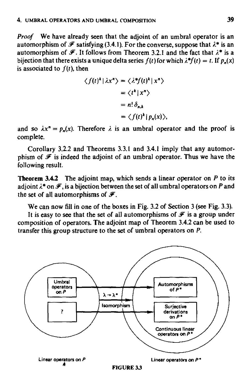
We can now fill in one of the boxes in Fig. 3.2 of Section 3 (see Fig. 3.3).
It is easy to see that the set of all automorphisms of  is a group under
composition of operators. The adjoint map of Theorem 3.4.2 can be used to
transfer this group structure to the set of umbral operators on P.
Linear operators on P
A
Linear operators on P'
FIGURE 3.3

40
3. OPERA TORS AND THEIR ADJOINTS
Theorem 3.4.3 The set of all umbral operators on P is a group under'
composition. In fact,
i' f 0 i., = ;"'f' i.ï 1 = i'l' (3.4.2)
Proof We give two proofs of the first part of this theorem. The first one uses
Theorem 3.4.2. Let i.. and J.I be umbral operators. Then V. 0 Jl)* = Jl* 0 i.* is the
composition of two automorphisms of !F and so is an automorphism of .
Thus by Theorem 3.4.2 the map i.. 0 Jl is an umbral operator. Similarly, since
(i. -1)* = ().*)- J is an automorphism of .1', the map i. - I is also an umbral
operator. Thus the umbral operators form a group under composition. The
second proof is more direct and establishes (3.4.2) but is less elegant. We have
from (3.4.1)
(i'f 0 i.,)*h(t) = i.: 0 i.j h(l)
= i.:h(J(t))
= h(Ï(g(t)))
= h(( g" f )(t))
= i.: fh(t),
so ()'J 0 i. f )* = i':'f and i' f c jo = i'g'J' Similarly,
(i.ï 1 )*h(t) = (À.j)-Ih(t) = h(f(l)) = Åjh(t),
and so i.i J = i.j.
Coronary 3.4.4 An umbral operator maps associated sequences to associated
sequences.
Proof Let P.(x) be an associated sequence and let i. be an umbral operator.
Then if Jl: x" - P.(x) is the umbral operator for p,,(x), we have i.p,,(x) = À 0 JlX".
But i. 0 J.I is an umbral operator and so i.p.(x) is an associated sequence.
Corollary 3.4.5 If p,,(x) and q.(x) are associated sequences and (X: p,,(x) -
q.(x) is a linear operator, then (X is an umbral operator.
Proof Let i.: x' - P.(x) and Jl: x. - q.(x) be umbral operators. Then
Jl 0 i.. -I P.(x) = q.(x) = (XP.(x), and so (X = Jl 0 i. - J is an umbral operator.
Let us see what effect Theorem 3.4.3 has on the corresponding associated
sequences. According to the definition of umbral operator, the sequence i'fI JX.
is associated to the delta functional y(f(t)). But if we write
Î.J:x. - P.(x),
.
'." () _'" k
I.,. X -q" X - L. q..k X ,
k-O

4. UMBRAL OPERATORS AND UMBRAL COMPOSmON
41
then
"
Å.,'fX. = i' f 0 i.,x" = i.fq"(x) = L q",kPk(X). (3.4.3)
k=O
In general, if p,,(x) and q"(x) = L:- 0 q".kXk are sequences of polynomials, we
define the umbral composition of q"(x) with p"(x) to be the sequence
.
q.(p(x)} = L q".kPk(X).
k=O
Thus (3.4.3) may be written as
i.gofx" = q"(p(x)).
(3.4.4)
Theorem 3.4.6 The set of associated sequences is a group under umbral
composition. In particular, if P.(x) is associated to f(t) and q,,(x) is associated
to g(t), then q.(p(x)) is associated to gU(t)). The identity under umbral
composition is the sequence x" and the inverse of the sequence p"(x) is the
associated sequence for J(t).
Proof The second statement follows directly from (3.4.4). It is clear that the
sequence x" is the identity under umbral composition. Setting g(t) = l(t) in
(3.4.4) gives
x. = Î.J<fx" = q"(p(x)
and o i.lx" = q"(x) is the inverse of p,,(x). But i./x" is the associated sequence
for [(t).
We close this section with a formula for the action of an automorphism
of ..
Theorem 3.4.7 Let i. be an umbral operator on P. Then as operators on P we
have
i.*g(t) = Î, -Ig(t)i.
for any operator g(t) in:F.
Proof For any f(t) in  and p(x) in p.
(J(t)I(i.*g(t))p(x)) = (J(t)(}.*g(t))lp(x))
= (i. *[g(t)().*)-'f(t)] I p(x))
= (g(t)().*)-'f(t)1 Î.p(x))
= (p. -1)*f(t) I g(t)Â.p(x))
= (f(t) I Â. -lg(t)J.p(x)),
f

42
3. OPERA TORS AND THEIR ADJOINTS
and so i.*g(t)p(X) :; i. - tg(r)i.p(x). Thus as operators on P we have
i.*g(t) = ). -lg(t)L
In view of the fact that i.jg(t) = o(1(t)). we get the following useful
corollary.
Corollary 3.4.8 For any umbral operator i' f we have
Î. f 0 g(1(t)) = g(r)c i' f
(3.4.5)
for all g(t) in F.
5. SHEFFER OPERATORS AND UMBRAL COMPOSITION
Let s(x) be the Sheffer sequence for (g(t) f(t)). Then the linear operator J.
on P defined by
Î.X = s.(x)
is called the Sheffer operator for S,.(x) or for (g(t),f(t)). To indicate the
dependence of i. on g(t) and f(t) we may write Åø.f or Î.g(f).f(1)" Clearly, Sheffer
operators are bijective.
Since. if s(x) is Sheffer for (g(t), f(t)). then p.(x) = g(t)s(x) is associated to
f(t we see that
).,,fx. == s.(x)
= g(t) - I p.(x)
== g(t) - 1 i.fx.,
and so
i.,,f = g(t)-l i. f . (3.5.1)
This makes the theory of Sheffer operators a corollary of the theory of umbral
operators. In particular, since Î.;,f = i.j(g(t)-l)*, we have
i';,fh(t) = g(J(t)t Ih(J(t))
(3.5.2)
for all h(t) in IF.
Theorem 3.4.1 and Eq. (3.5.1) immediately give a characterization of
Sheffer operators by their adjoints.
Theorem 3.5.1 A linear operator Å on P is a Sheffer operator if and only if its
adjoint i.* has the form of multiplication by an invertible series g(t) -1 followed
by an automorphism )., of IF. Moreover, if ;.* has this form, then Å = i'(I,f' In
fact, any operator on !F that is of this form is the adjoint of a Sheffer operator.

5. SHEFFER OPERA TORS AND UMBRAL COMPOSITION
43
Let us consider the composition of Sheffer operators. If ).,)'/(I) and ).11(1),1111
are Sheffer operators, then by (3.5.2)
(J'g(tl.f(l) 0 i.It(J).I(I))*U(l) = ì.tl.I(I' 0 Å.:ì,)./(,)u(t)
= i,,'.l(rIg{1(t W 1 u{1(t ) )
= h(Ï(t)t 19{1(Ï(t))t IU(Ï(Ï(t)))
= (h 0 /)((1 c f)(t)t Ig((I 0 /)(tW IU((I o.t )(t))
= ì.f(lHg(')"lf(lllu(t)
for all u(t) in :?, and so
Å.,c,.. fit) 0 )'Io(J), 1(,) = ì'g(I)(f(m.l(f(t)I'
We also have by (3.5.1)
(ì.'(t:./(I))*U(t) = [i'Î(,I)og(t)]*u(t)
= g(t)*(ì.id))*u(t)
= g(t)i.j(,)u(t)
= g(t)u(f(t))
= (go Ï)(f(t))u(f(t))
= ì./lt1J - I J(t) u( t)
for all u(t) in ff, and so
. - 1 .
1.,(11. fl'J = 1'g(J(I))" , J(I)'
We have proved the following theorem,
Theorem 3.5.2 The set of all Sheffer operators is a group under composition.
I n fact,
i'g(')' f{11 <> i.(J).I(J) = i'g(tJ(f(III.I(f(m'
--I -
1.,(11. fIt) = 1'g(J(lII- '. J(r)"
(3.5.3)
Corollary 3.5.3 A Sheffer operator maps Sheffer sequences to Sheffer
sequences.
Proof Let s.{x) be a Sheffer sequence and let i. be a Sheffer operator. Then if
Jl" x" -+ SIl(X) is the Sheffer operatorfor s.(x), we have ),SII(X) = i. 0 /-IX". But i. 'J1
is a Sheffer operator, and so ì.sll(x) is a Sheffer sequence.
Corollary 3.5.4 If.s.(x) and rll(x) are Sheffer sequences and 01:: SII(X) -+ r.(x) is a
linear operator, then at: is a Sheffer operator.

44
3. OPERATORS AND THEIR ADJOINTS
Proof Let ì.: x ft - Sft(x) and J1: x ft - r ft(x) be Sheffer operators. Then
J1 c). - 1 Sft(X) = rft(x) = :xs.(x) and so (X = J1 0 ì. - 1 is a Sheffer operator.
Now we come to the behavior of Sheffer sequences under umbral
composition.
Theorem 3.5.5 The set of Sheffer sequences is a group under umbral com-
position. In particular, if Sft(x) is Sheffer for (g(t), f(t)} and r.(x) is Sheffer for
(h(t),/(t)}, then r..(s(x)) is Sheffer for (g(t)h(f(t)),l(f(t))). The identity under
umbral composition is the sequence x ft and the inverse of the sequence Sft(x) is
the Sheffer sequence for (g(f(t)) - 1, J(t)).
Proof From (3.5.3) we have
rn(s(x)) = ì'g(f).f(Or.(x)
_.. .. It
- I'g(.,. f(., ' l'h('I./(.)x
. n
= l'gll)h(f(r)I./(f(l)Ix ,
and this proves the second statement of the theorem. The third statement is
clear. To prove the last statement we observe that rft(s(x)) = x ft if and only if
)'r(')h(f(r))./(f('U is the identity, which is true if and only if
g(t)h(f(t)) = I,
/(f(t)} = t.
Solving these equations shows that r.(x) is Sheffer for
(h(t),l(t)) = (g(Ï(tw 1, J(t)).
We summarize some of the previous results in a useful fonn in the next
theorem.
Theorem 3.5.6 If Sft(x) is Sheffer for (g(t).f(t) then for all series h(t) and
polynomials q(x)
(h(t) I q(s(x))) = (g(J(tW th(f(t)} I q(x)).
In particular,
(h(t) I sø(x)) = (g(J(t)}-lh(!(t))1 x").
If pft(x) is associated to f(t), then
(h(t)lq(p(x))) = (h(f(t))lq(x))
and
(h(t) I Pft(x)) = (h(f(t)) I x").

6. UMBRAL SHIFTS
45
6. UMBRAL SHIFTS AND THE RECURRENCE FORMULA FOR
ASSOCIATED SEQUENCES
Let p,,(x) be the associated sequence for f(t). Then the linear operator 0 on
P defined by
9p,,(x) = p" + I (x)
is called the umbral shift for p,,(x) or for f(t). We use the notation () f to indicate
the dependence on f(t).
In the next section we shall study the more general Sheffer shift
0: s,,(x) -+ S" + t (x)
for s,,(x) an arbitrary Sheffer sequence.
Since degp.(x) = n, we see that an umbral shift is injective, but it is not
surjective.
We proceed to characterize umbral shifts by means of their adjoints. If
Of:P"(x).... P.+ I(X) is an umbral shift, we have
(8if(t)k I P.(x)) = (f(t)kI9 f P,,(x))
= (J(t)klp.+t(x))
= (n + I)! 15,,+ I.k
= kn! ðn.k+ 1
= (kj(t)k-ljPn(X))
for all k  0, and so
8if(t)k = kf(t)k-I.
By the expansion theorem any get) in .? can be written in the form
(3.6.1 )
:x>
g(l) = I ad(t)k,
kO
and the continuity of OJ implies
:x>
Ojg(t) = I kad(t)k-t.
kO
Also, we have
Oif(t)k}(t)i = Ojf(t)Hi
= (k + j)f(t)k + j- 1
=jf(l)kJ(t)i- t + kf(t)k-t/(t)i
= f(l)k()j f(t)i + f(t)J(J1 f(l)k.

46
3. OPERATORS AND THEIR ADJOINTS
From this and the continuity of 01 we get
Ojg(t)h(t) = g(t)O'jh(t) + h(t)81g(t)
for all g(t) and h(l) in $'.
Thus OJ is a surjective derivation on . In view of (3.6.1), the map 81
is actually the derivative with respect to f(r), which we denote by ð l . That is,
8i = 0-. Once again we have a characterization.
Theorem 3.6.1 A linear operator 0 on P is an umbral shift if and only if its
adjoint 0* is a surjective derivation on IF. Moreover, if 8 1 is an umbral shift,
then 8j = 0- is the derivative with respect to f(t),
01f(t)k = kf(t)k-l
for all k  O. In particular, OJ f(t) = I.
Proof We have already established one half of this theorem. Suppose now
that 0* is a surjective derivation on:F. It follows from Theorem 3.2.3 that there
exists a delta functional f(t) for which O*f(l) = 1. If pþ) is associated to f(l),
then
(J(t)kiOp,,(x)) = (O*f(t)klp,,(x))
= <kf(t)k- 1 0*f(l) I p,,(x))
= <kf(1)k- 1 Ip.(x))
= (n + 1)115,,+ I.k
= <f(t)klp.H(x)),
and so 8p.(x) = P.+ l(X) and () is the umbral shift for f(I).
r
Corollary 3.2.4, along with Theorems 3.3.1 and 3.6. I, implies that any
surjective derivation on ;y: is the adjoint of an umbral shift.
Theorem 3.6,2 The adjoint map, which sends a linear operator 0 on P to its
adjoint operator ø* on !7, is a bijection between the set of all umbral shifts on
P and the set of all surjective derivations on .F.
We can now fill in the remaining box of our original diagram (see Fig. 3.4).
Unlike the case for automorphisms, the set of surjective derivations on /Ii
does not form a group under composition. In casting about for some structure,
we recall a well-known fact that almost every student of elementary calculus
fails to learn, namely, any two derivations are related by a formula known as
the chain rule!
Theorem 3,6.3 (The Chain Rule) Let ûf and è, be surjective derivations on
.'F. Then
è, = (<Î,f(t)) 0-.

6. UMBRAL SHIFTS
47
Linear operators on P
linear operators on P*
FIGURE 3.4
Proof We have
vgf(t)* = kf(t)k-I Ogf(t) = (ogf(t))od(t)k
for all k  0 and the result follows by continuity.
Corollary 3,6,4 If of and Og are surjective derivations on IF, then
 ) 1
vgf(t = ofy(t) '
The correspondence of Theorem 3.6.2 can be used to translate the chain
rule into a relationship between umbral shifts.
Theorem 3,6.5 Let ()j and Og be umbral shifts. Then
8f = 8g 0 (ofy(t)).
Proof According to the chain rule, we have
OJ = (0-y(t))8:,
and so
(h(t) 18fp(x)) = <8jh(t) I p(x))
= <(û j g{t))9:h(t) I p(x))
= <O:h(t)l(èjy(t)}p(x))
= (h(t)l9 q o (ð j y(t)}p(x))
for all h(t) in IF and p(x) in P. Thus (JJ = 9g 0 (ðfg(t)).

48
3. OPERA TORS AND THEIR ADJOINTS
Taking g(t) = t in Theorem 3.6.5 and observing that O,xn = x n +', that is,
the operator Og is multiplication by x, we get a very useful formula for Of'
Of = X ôft = x(è,J(tW' = x(f'(t)t '.
Applying this to the associated sequence for f(t) leads to the following
recurrence formulas.
Corollary 3.6.6 (The Recurrence Formulas) If p.(x) is associated to f(t),
then
(i) Pn+' (x) = x[f'(t)] - 1 p"(x) and
(ii) Pn+l(x) = xÄAJ(t)]'x"
for all n  O.
Proof The first formula has been proved. For the second we use Corol-
lary 3.4.8,
Pn + I (x) = x[f'(t)] - 1 i.fx"
= xi.f[f'(f(t))] -I x"
= xi.f[f(t)]'x".
Incidentally, the second form of the recurrence formula can be written as
Å.fx n + 1 = x.À.f[J(t)]'xn,
which is equivalent to the commutation rule
i.fx = Úf[f(t)]',
We can now derive a formula for surjective derivations on.
Theorem 3.6.7 Let 0 be an umbral shift. Then as operators on p we have
O*g(t) = g(t)9 - Og(t)
(3. 6.2)
for all operators g(t) in :F.
Proof For any f(t) in  and p(x) in P we have
<f(t) I (O*g(t)}p(x)) = (f(I)(O*g(t)) I p(x))
= <O*f(t)g(t) - g(tW*f(t)Jp(x))
= < O*f(t)g(t)l p(x)) - (g(t)O*f(t) I p(x))
= <f(t) I g(t)9p(x)) - <f(t) IOq(t)p(x))
= <f(t) I [g(t)8 - Og(t)]p(x)),
from which the desired conclusion follows.

7. SHEFFER SHIFTS
49
When Ø: x" -+ x"+ I is the umbral shift for p"(x) = x", the map (}* is at and
(3.6.2) becomes
g'(t) = g(t)x - xg(t),
(3.6.3)
where both sides are considered as operators on P. The right side of this
equation is known as the Pincherle derivative of the operator g(t).
7. SHEFFER SHIFfS AND THE RECURRENCE FORMULA
FOR SHEFFER SEQUENCES
Let s,,(x) be the Sheffer sequence for (g(t), fIt)). The linear operator () on P
defined by
8s"(x) = s,,+ I (x) (3.7.1)
is called the Sheffer shift for s,,(x) or for (g(t), f(t)). We also use the notation Of.g'
Since degs,,(x) = n, a Sheffer shift is injective, but it is not surjective.
If sþ) is Sheffer for (g(t), f(t)), then p"(x) = g(t)s,,(x) is associated to f(t).
and so (3.7.1) becomes
8 g ./g(t)-l p "(X) = g(t)-lp"+t(X).
Thus
8 g ./ = g(t) - 18 f g(t),
where Of is the umbral shift for f(t). Using Theorems 3.6.6 and 3.6,7 and the
chain rule, we get
8g,f = g(t)-I(}Jg(r)
= g(W t[g(t)OJ - 8jg(t)]
= 8J - g(t) - I ôJftlg(t)
= Of - g(t)-I èJui ð,g(t)
= xU'(t)] -I - g(t)-I[F(t)] - Ig'(t)
[ 9'(1) ] I
= x - g(l) FUr
We have proved the following result.
Theorem 3,7.1 If 8 g ,f is a Sheffer shift, then
o = [ X - g'(t) J 
1 fI.f g(t) F(tr
This gives a recurrence formula for Sheffer sequences.

so
3. OPERA TORS AND THEIR ADJOINTS
Corollary 3.7,2 (The Recurrence Formula for Sheffer Sequences) If s.(x) is
Sheffer for (g(t),J(t)}, then
[ g'(t) ] 1
s,,+ dx) = x - g(t) f'(t) s.(x).
8. THE TRANSFER FORMULAS
We next derive two powerful formulas for the computation of an asso-
ciated sequence from its delta functional. These formulas, together with
Theorem 2.3.6, can be used to compute Sheffer sequences.
Theorem 3.8.1 (The Transfer Formulas) If P.(x) is the associated sequence
for f(t), then
(i) p"(x) = f'(t) (ft) ) -,,-I x" and
(ii) P.(x) = x (ft)r . x.- I
for all n  O.
Proof For convenience we set g(t) = f(t)/t. Then g(t) is invertible. Actually,
the right sides of (i) and (ii) can be shown to be equal, using (3.6.3),
!,(t)g(t)-"-I x. = [tg(t)]'y(t) -.-1 x.
= gUf "x. + tg'(t)g(t)-"-I x"
= g(t)-"x" + ng'(t)g(t)-.-Ix.- I
= g(t)-"x" - [g(t)-"]'x.- I
= g(r)-"x" - [g(W"x - xg(W"]x.- 1
= xg(t)-"x.- I .
To prove (i) we verify the two conditions of Theorem 2.4.5 for the sequence
q"(x) = f'(t)g(t)-.-I x.. For the first condition, when n  1, the fourth
equality above and Theorem 2.1.10 give
(to I q"(x)) = (to I j'(t)g(W,,-1 x")
= (tOlg(W.x" - [g(tr.]'x"-')
= (g(t)-.Ix.) - ([g(0-"],lx.- 1 )
= (g(t)-.x") - (g(t)-"Ix.)
=0.

8. THE TRANSFER FORMULAS
51
If n = 0, then (to I q.(x)) = I, and so <to I q.(x)) = ð.. o ' For the second
condition
f(t)q.(x) = f(t)!,(t)g(t)-.-'x.
= rg(t)f'(t)g(t) -. IX.
= n!'(t)g(W.x.- 1
= nq._ 1 (x).
Thus q.(x) is associated to f(t) and the proof is complete.
The next corollary gives a formula that directly relates any two associated
sequences.
Corollary 3.8.2 Let P.(x) be associated to f(t) and let q.(x) be associated to
get). Then for n  I,
q.(x) = x( ;:;: )"x-1p.(X).
[We remark that f(t)fg(t) is the invertible element of fF defined by
[f(t)ft] [g(t)ft] -I and that since P.(O) = o for n  1, the expression X-I P.(x) is
indeed a polynomial.]
Proof By the first transfer formula we have
(f(t)ft).x-Ip.(x) = x.- t = (g(t)ft).x-Iq.(x),
and the result follows by solving for q.(x).
We conclude this section with a rather useful result.
Theorem 3.8.3 If s.(x) is Sheffer for (g(t), f(t) then
rn(x) = sþ + ,% + ßn)
is Sheffer for
(g(t)e -t( I - g;) .e-P1(t)).
Proof The sequence r.(x) is Sheffer for the delta functional e- P 1(t) since
e-P'l(t)r.(x) = e-P1(t)e(+P.Jls.(x)
= nel+P.-Plls._ d x )
.
Now suppose that r.(x) is Shetferfor(h(t), e - P1(r)). Corollary 3.8.2 implies that
= nr._.(x).

52
3. OPERATORS AND THEIR ADJOINT
the associated sequence for e - J1'f(t) is
q.(x) = xe,s.'x-1p.(x)
x
= x + ßn P.(x + ßn)
= e/l.' ( x ßn ) P.(x),
and so
( X - ßn )
h(t)s,,(x + (1. + ßn) = e,slll ---;- P.(x)
or
h(t)s.(x) = e-<<. e ßn )p.(X)
= e-(l - ßnx-I)p,,(x).
By the recurrence fonnula, P.(x) = x [f'(t)] - 1 P. _I (x), and so
h(t)s.(x) = e-Æl[p.(x) - ßn(f'(tW1p.-I(x)]
= e-"[p.(x) - ßf(t)(f'(t)t Ip.(x)]
= e- Æl ( I - 7tD p.(X)
- " ( I ßf(t) ) ( ) ( )
= e - f'(t) g t s. x
This gives the desired result.

CHAPTER 4-
EXAMPLES
In this chapter we discuss some important examples of Sheffer sequences.
(t is not our intention here to give a treatise on any polynomial sequence, but
rather to give enough examples of umbral techniques to al\ow the interested
reader to continue on his own. In the next chapter we shall develop additional
umbral techniques and apply them to the examples of this chapter.
Our primary source for the definitions of special polynomial sequences is
the Bateman Manuscript Project (Erdelyi [1]), and we remind the reader of
the remarks made in this regard following Theorem 2.3.4, We shall keep the
reader informed of any discrepancies, albeit they are only minor, between our
definitions and those of our sources.
In the hope of achieving greater clarity each example is divided into five
parts, whose defining Jines are by no means precise:
definitions,
the generating function and the Sheffer identity,
recurrence relations and operational formulas,
expansions, and
miscellaneous results.
t. ASSOCIATED SEQUENCES
For ease of reference we list the key results. Let the sequence p,,(x) be
associated to f(t).
Generating function
f Pk(X) t k = e X / fll .
1<-0 k!
53

54
Binomial identity
P.(x + Y) = ktG)Pk(X)P.-k(Y)'
Theorem 2.4.5
(to I Pn(X)) = 15.,0,
f(tjPn(x) = IIpn-1 (x).
Recurrence formulas
P.+t!x) = X[f'(t)r1pn(X),
P. + 1 (x) = xi-rE!(t)]' x n .
Transfer formulas
( ) ( f(t) ) -. .-1
P. x = x t x ,
P.(x) = f'(tj( ft) ) -.-1 x.,
Expansion theorem
g(t) = f (g(t)lpk(X)) f(tt
k=O k!
Polynomial expansion theorem
( ) _ ,, (f(t)klp(x)) ( )
p x - L... k ' P. X.
kO .
Theorem 3.5.6
(g(t)lq(p(x))) = (g(l(t))lq(x)),
(g(t) I P.(X)) = (g(l(t)) I x.).
Theorem 2.4,8
.+I ( II )
XP.(X) = JI k _ 1 (f'(t) I P.-H I(X))Pk(X)
or
.+ I ( II ) _
XP.(x) = JI k _ 1 (f'(f(t))IX.-H1)Pk(X),
4. EXAMPLES

1. ASSOCIATED SEQUENCF-S
55
Theorem 2.4.9
.-I ( n )
p(X) = tO k (t I P.-t(X))Pt(X)
or
p(x) = :t:()(l(t)lx.-t)Pt(X).
Conjugate representation
(x) = f (l(t)t I x.) t
P. L. k ' x .
t-l .
Proposition 2.1. I 1
(g(t)lp(ax)) = (g(at)lp(x)).
Theorem 2.1.10
(g(t)lxp(x)) = (ð,g(t)lp(x)).
1.1. The Sequence X-
The sequence P.(x) = x. is. of course, associated to f(t) = t. The results in
this case present no surprise and we list them quickly. The generating function
IS
00 Xk
L -t k = e''',
k=ok!
and the binomial identity is
(x + yr = t ( n ) xky.-k.
k=O k
The expansion theorem is
get) = f (g(t)lx k ) t k ,
k=O k!
which for g(t) = eY' is Taylor's expansion
eY' = kt(i)t k .
Applying this to p(x) gives
p(x + y) = L ( Y ) p1t)(X).
tO k

56
4. EXAMPLES
1.2. The Lower Fadorial Polynomials
DEFINmONS
Let us consider the forward difference functional
f(t) = eM - 1
for a i' O. We note that
r(t) = ae"',
f<t) = a- 1 10g(1 + t).
The associated sequence for f(t) is easily determined by using Theorem 3.5.6,
PM(Y) = (eY11 PM(X))
= (eY](I)lx M )
"" (e F "-' 10g(1 + c)lx M )
_ <(I + t)y/a I x M )
= (.o(Yia)ttlxn)
= ()..
Thus
PM(X) = ()a = ( - I}"( - n + I).
These are the lower factorial polynomials, also known as the falling factorial or
binomial polynomials.
The first form of the recurrence formula would have worked as well to
determine the sequence Pø(x
PM+l(X) = X[f'(t)]-lpM(X)
= a-1xe-"'Pø(x)
x
= -P (x - a
a ø
and since Po(x) = I, we are lead to Pn(x) = (x/a)M'
For ease of expression we couch some of the following results for a = I,
although it is really no more difficult to obtain them for arbitrary values of
a i' O.

I. ASSOCIATED SEQUENCES
57
We express (x). in powers of x by
( ) = f <tI(X),,) 
X. t... k ' x.
=o .
The coefficients in this expression are known as the Stirling numbers of the
first kind,
1 
s(n, k) = k! (t I (x),,).
Thus
"
(x). = L s(n, k)x.
kO
We shall discuss these important numbers later in this example and in the next
one.
GENERATING FUNCTION AND SHEFFER IDENTITY
The generating function for (x)" is
f (x) t = exlDJ(1 +t),
-o k!
which can be written in the familiar form
Jl:)t k = (l + t)"'.
The binomial identity is
(x + y). = tl:)XlcY'-'
which can also be written as
( X + Y ) = t ( x )( Y )
n lc-O k n - k .
This is known as the Vandermonde convolution formula.
RECURRENCE RELATIONS AND OPERATIONAL FORMULAS
Theorem 2.4.5 gives the formula
t ( I
e - I)(x)" = n(x)"_,,

58
4. EXAMPLES
which can be written as
(x + 1)" - (x)" = II(X)"_I'
The second form of the recurrence formula is
(x)"+t = xJ..f[f(t)]'x"
= x).f(t + t)-I x"
"
= xJ. f L (- Wtkx"
k-O
.
= x L (-I)k(nMx)._k
k=O
"
= x L (- tr-k(n)"_k(x)k'
k-O
EXPANSIONS
The expansion theorem is
get) = kt (g(t) I;/a)k> (e'" - t)k.
Taking get) = e,t we get the beautiful formula
eFt = f ( y/a ) (e llt - l)k.
k=O k
This is actually Newton's forward difference interpolation formula. If we use
the notation
P:p(x) -+ p(x + y),
A,,: p(x) -+ p(x + a) - p(x)
for the translation and forward difference operators, it takes the more familiar
form
p = f. ( y/a ) A:.
k=O k
Setting f(t) = t'" in the expansion theorem gives
t'" = f (t'" I (x/a)k> (eat _ l)k
t-O k!
<LJ ,
= L k '", s(k,m)(e'" - l)k.
k=O .a

1. AssoÇlA TED SEQUENCES
59
By applying this to a polynomial p(x) and observing that
((eO' - Wlp(x)) = t (  ) (-I)'-)<ejolIP(x))
)O )
= t (  ) (-l)'-)p(ja),
)=0 )
we obtain a classical formula for numerical differentiation,
(4.1.1 )
m! · ( k ) .
pC""(O) = L k ' ", s(k,m) L . (-1)'-J p (ja).
'2:0 .a )=0 )
Expanding the functional (e'" - 1)/t in terms of the forward difference
gìves
e,t - 1 = f ((e" - lIlt I(x),) (e' _ 1)'.
t '=0 k!
If we apply this to a polynomial p(x), we get
r' p(u)du = L ((e" - O/t I (x).) (e' - l)'p(x).
Jo '2:0 k!
This is known as Gregory's formula (Jordan [1, p. 284]). It was discovered by
Gregory in 1670 and is reported to be the earliest formula of numerical
integration. We shall discuss the coefficients of this expansion when we come
to the Bernoulli polynomials of the second kind in Section 3.
The polynomial expansion theorem is
p(x) = I ((e lll - 1)'1 p(x)) (  ) ,
'2: 0 k! a k
and, using (4.1.1), this becomes
(4.1.2)
p(x) = I ( x k /a ) L (  ) ( -1)'-)p(ja).
k2:0 )-0 )
If we take a = 1 and p(x) = x" in (4.1.2), we obtain
" ((e' - 1)'1 x")
x. = I x'.
'-0 k!
These coefficients are known as the Stirling numbers of the second kind,
1
S(n, k) = k! ((e' - 1)' I x"),

60
4. EXAMPLES
Thus
.
x' = L S(n,k)(X)i'
i-O
(4.1.3)
We shall say more about these numbers later, butfor now we notice that (4.1.1)
gives
8(11, k) =..!.. t (  ) ( _1)i - i".
k! j=O J
Again, by the polynomial expansion theorem
(  b) = t k l , ((e'" - WI(X/b).) (  ) .
II A-O. a A
From Theorem 3.5.6 we get
<(e'" - l)il(x/b).) = ([elalb)1oI11 +rþ - I]ilx')
= ((I + tr lb - I]A I x'),
and, using Proposition 2.1.3, we have
((eM _ I)i I (x/b).)
= L ( . n . ) ((I+t)a/b_llxil)"'((I+Wlb_llxik)
i,+ "'+ik-II 11,...,li
( n )( a ) ( a )
= L - '''-
;1+' +Ik-. i.,...,i. b I, b Ik'
IJ>O
Either of these forms can be substituted into the above expansion.
According to Theorem 24.8,
x(). = :t:C: l)(f'(t)l(x/a)'-Hl)()A
= :t:C: l)<ae"'j(x/a)'-Hl)()i
= a J:(k: l)cl).-Hl()..
and since (1).. = <5... 0 + <5...1> we get
X (  ) = a (  ) + an (  ) .
a II a .+ 1 a .

I. ASSOCIATED SEQUENCES
61
Theorem 2.4.9 provides a formula for the derivative of the lower factorial
polynomials,
ft -1 ( n )
t(X). = Jo k (- Ir-k(n - k - I)! (x)..
MISCELLANEOUS RESULTS
Let us explore some of the properties of the Stirling numbers, using umbral
methods. A great deal has been written about these numbers, and they have
important combinatorial significance which we cannot discuss here. The
interested reader might wish to consult Comtet [1] or Riordan [2,3].
As to the Stirling numbers of the first kind
I k
s(n, k) = k! (t I (x),,),
let us apply t.' k! to both sides of the recurrence
x(x). = (x)" + 1 + n(x)ft.
Using Theorem 2.1.10, we get
1 ( . ( ) ) 1 .-1
k! r Ix x. = (k _ I)! (r I(x)ft> = s(n,k - 1)
and
1 .
k! (t I (x)ft + 1 + n(x)ft) = s(n + 1, k) + ns(n, k),
and so
s(n + l,k) = s(n,k - I) - ns(n,k).
This recurrence, together with the initial conditions
s(n,O) = 0,
s(O, k) = 0,
s(O,O) = 0,
enables one to compute the numbers s(n, k).
Applying ttjk! to the formula obtained from the second form of the
recurrence formula gives
n > 0,
k > 0,
ft
s(n+ l,k)= L(-I)"-)(n)ft_)s(j,k-l).
)-0
The conjugate representation for (x)" is
· " 1
(x)ft = L k , <[log(l + tWlx")x.,
t-o .

62
4. EXAMPLES
and so
1
5(n, k) = k! ([log(1 + t)]k, x.).
From Proposition 2.1.3 we then get
s(n, k) = ! I, + "lkZ.C"..' iJ (log(1 + t) I Xl!) ... (log(1 + t) I Xl.)
1 ( ) ( . ' ) ( . ' )
=- L n (-Irk  ... 
k!/,+. .+/.=" i"...,i k i 1 i k
I}>O
=(_l),,-k n ! L 
k! 1,+ . +[k=./1..'l k
I}>O
When the binomial identity for (x). is written out and the coefficients of like
powers of x and yare compared, one obtains
C  j)S(n,i + j) = ktO(:)S(k,i)S(n - k,j).
Turning to the Stirling numbers of the second kind, we have already
remarked that
S(I1, k) = k 1 , .t (  ) ( -1).-1..
. )-0 }
Proposition 2.1.3 gives, as we have seen,
I
S(n,k) = k! ((e' - l)klx.)
- k! 1,+ 1.=.Cl,..,iJ.
I}>O
Finally, for k  I and n  I, we have from Theorem 2.1.10
I
S(n,k) = k! ((e ' - I)klx.)
I (e'(e' _ 1)k- 1 1 x.-I)
(k - I)!
I ((e'-l)klx.-I)+ t ((e'_I)k-llx"-I)
(k - l)! (k - I)!
= kS(n - I,k) + S(n - I,k - I).

J. ASSOCIATED SEQUENCF.8
63
From the initial conditions
S(n,O) = 0,
S(O, k) = O.
S(O, 0) = I,
n>O,
k > 0,
one can compute the numbers S(n, k).
We shall discuss the connection between the Stirling numbers of the first
and second kind in the next example.
The multinomial version of Theorem 2.3.10 and Eq. (4.1.1) lead to
.f (  ) (-l).-jp.(ja)=. L. ( . n . ) Pi,(a)...PI.(a) (4.1.4)
)=0 } .,+ '+'.-. 'I'''.''.
1)>0
for any associated sequence. This specializes to give some interesting
combinatorial identities. For example, if we take P.(x) = (bx/a)., this becomes
t (  ) (_1).-j ( bj ) = L (  ) ... (  ) .
j=O } n 1,+: +i.=. '. 't
1)>0
Incidentally, the backward difference functional
f(t) = l-e- Ø
satisfying
<f(t)l p(x) > p(O) - p(a)
and' f(t)p(x) = p(x) - p(x - a)
is associated to the sequence of rising factorial polynomials
(r) = ()( + l)-"( + n - I).
All of the above results have analogs for the rising factorial sequence, and we
shall not give them here except to mention that the role of the Stirling numbers
of the first kind s(n,k) is taken by their absolute values Is(n.,k)l, which are
known as the signless Stirling numbers of the first kind, that is,
.
x'.) = L I s(n, k)l x t .
t=o
1.3. The Exponential Polynomials
DEFINITIONS
Let us consider the delta functional
f
f(t) = logO + t).

64
4. EXAMPLES
Since Ï(t) = e' - I is the forward difference, Theorem 3.4.6 implies that the
associated sequence for f(t) is inverse to the lower factorial sequence under
umbral composition. Equation (4.1.3) gives us the sequence
"
<<p,,(x) = L S(n, k)x t .
t=o
These are called the exponential polynomials.
GENERA TING FUNCTION AND SHEFFER IDENTITY
The generating function for the exponential polynomials is
f <<Pt(x) c t = e"('" - 1)
t=O k!
and the binomial identity is
ø,,(x + y) = tt()øt(X)ø.-t(y).
RECURRENCE RELATIONS AND OPERATIONAL FORMULAS
The recurrence formula is
<<P,,+l(X) = x [f'(t)r 1 <<P.(x) = x(1 + t)<<p,,(x) = x(<<p,,(x) + <<p(x)).
From this we also get the operational formula
ø,,(x) = [x(1 + t)]"l.
But
e-"(xt)e"x" "" e-"x(e"x" + ne"x,,-l) = x(I + r)x",
and so, as operators,
x(1 + t) = e -"(xt)e".
This gives the operational formula
<<p,,(x) = e-"(xt)"e".
The second form of the recurrence formula is
ø/l+ 1 (x) = xi.f[Ï(t)]'x"
= xÎ..fe' x"
= xlAx + I)"
= x tt()øt(X).
(4.1.5)

I. ASSOCIATED SEQUENCES
65
From Theorem 2.4.5 we obtain
ntþ,,_ I (x) T= log (I + t)tþ,,(x)
00 ( 1 ) 1+1
= L - t 1 tþ,,(x)
1 I k
" ( 1 ) 1+1
= L - tþ"I(X).
1=1 k
EXPANSIONS
The expansion theorem is
g(t) = f (g(t)l (Þt(X)) [log(1 + t)]".
"-0 k!
For g(t) = e)1t we get a formula for the exponential function in terms of the
logarithm,
e" = f (Þt(Y) [log(1 + t)]t.
1-0 k!
Sincef'(j(t)) = I/{I + (e t - I)) = e- I , Theorem 2.4.8 gives the expression
xtþ,,(x) = :t:(k: 1)<-t)"-t+ltþt(X).
Theorem 2.4.9 is
.-l ( n ) "-I ( n )
tþ(x) = L k (e' - II x,,-t)tþ..(x) = L k tþ..(x).
t=O t=o
MISCELLANEOUS RESULTS
If We set p,,(x) = (X)"' then tþ,,{p(x)) = x" isjust (4.1.3). But we also have
p,,{tþ(x)) = x".
Writing
x" = e- X f (k)" x"
t=O k!
(we are extending ourselves here a bit in writing this, but it can easily be
justified), we have
p,,(tþ(x)) = e- X f p,,(k) x".
"-0 k!

66
4. EXAMPLES
Thus for any polynomial p(x),
p(tþ(x)) = e- r f p(k) x k .
k"O k!
If we take p(x) = x., then
'" k.
4>.(x) = e- r I k , x\
k"O .
which is known as Dobinski's formula.
Let us turn again to the Stirling numbers. When the binomial identity for
if>.(x) is written out and the coefficients of like powers of x and yare compared,
one obtains
( i + j ) · ( n )
i S(n, i + j) = Jo k S(k, i)S(n - k, j).
Since
(t i l4>.(x)) = j! S(k,j
applying t i to the recurrence (4.1.5) gives
j!S(n + I,j) = (tJlx kt()4>.(X))
= (jtj-ll.tl)4>k(X))
= kt()j! S(k,j - I)
or
S(n + I,j) = .tl)S(k,j - I).
Applying t i to the expansion of x4>.(x) gives, after dividing by j!,
S(n,j-I)= :t:(k: 1)<-I).-H1S(k,j).
The umbral composition if>.(p(x)) = x., where P.(x) = (x)., is equivalent to
.
x. = I S(n,k)(X)k
4:=0
. k
= I S(n. k) I s(k,j)x i
k-O J"O
= f f S(n, k)s(k,j)x J ,
j-Ok-j

I. ASSOCIATED SEQUENCF.5
67
and comparing coefficients of x J gives
.
ð.,J == L S(n, k)s(k,j).
à-j
If we let i.:x" ..... (x). be the umbral operator for (x)"' then
(x). = Ä - 1 0 i.(x).
= t s(n,k)À -I oÃx à
à=O
.
= L s(n, k)Ä - I(X)à
à=O
" à
= L s(n, k) L s(k,j)tþþ)
à-l j-O
II à t
= I s(n, k) L s(k,n S(j, i)x i
à=O j-O 1-0
II " à
= ILL s(n, k)s(k,j)S(j, i)x i ,
i=Ok-lj-O
and so
" à
s(n, i) = I L s(n, k)s(k,j)S(j, i).
à-lj=O
Many more properties of the Stirling numbers can be obtained by similar
umbral methods.
1.4. The Gould Polynomials and the
Central Factorial Polynomials
DEfiNITIONS
We generalize the forward difference functional by setting
!(t) = eøt(e b ' - I),
where b #; O.
Using Corollary 3.8.2 to relate the associated sequence for !(t) to the lower
factorial sequence, we have
( x ) x ( X - an )
q.(x) = xe-."x- I - = - - .
b" x-an b .
.
These are the Gould polynomials, which we denote by G,,(x; a, b).

68
4. EXAMPLES
In case a = - b/2 we get the central difference series
ð(r) = e btl2 _ e- btI2 ,
which satisfies
(ð/>(t)lp{x)) = p(b/2) - p(-b/2)
and
ð(t)p(x) = p(x + tb) - p(x - tb).
This series plays an important role in interpolation theory (Steffensen [2]).
The associated sequence for ðt(r) is formed by the central factorial poly-
nomials
x l -] = GII(x; -1/2,1) = x(x + tll - )).-1'
GENERATING FUNCTION AND SHEFFER IDENTITY
The generating function for the Gould polynomials is
f Gt(x;a,b) tt = rJ(t).
k-O k!
By differentiating with respect to x and setting x = 0 we get
f - ( ) =  G(O;a,b) k
r L. k ' r ,
k-l .
where f(t) = e"'(e'" - 1). Let us compute G(O;a,b) by umbral techniques,
G(O; a, b) = (t I Gt(x; a, b))
= \fl x  ak(x  ak) )
= \to\ x  ak(X  ak) )
= \e-.krl())
=\e-.t'I(-I)k_)
=  \ e - (Hø)I I (\ _ )
1 < -(b+at" I . t-1 >
=b e I.X
(equation l"on,'nues)

1. ASSOCIATED SEQUENCF.5
69
= !U.e-(U..l)t I Xl-I>
b
= !(e-(Uø1: Ib - 1 I oal 1+,) I Xl-I>
b
I
= _ < (I + n- (b +Alllb I Xl - I >
b
=! f ( -<b  ak)/b ) <t J1 X 1 - 1 >
b j=O )
= (-(  alk)/b}k - I)!.
Thus we obtain
l(t) = f ! ( -(b + ak)/b ) .
l=lb k-l k
The bìnomial identity is a generalized Vandermonde convolution,
x + Y ( (x + y - an)/b )
x + y - all II
= f. -=-- y ( (x - ak)/b )( (Y - a(n - k))/a ) .
1=ox-aky-a(lI-k) k n-k
(4.1.6)
Such convolutions play an important role in combinatorics (Riordan [2]).
RECURRENCE RELATIONS AND OPERATIONAL FORMULAS
Equation (4.1.6) can be used in connection with the recurrence formula to
give the recurrence
G.+i(x;a,b) = XÀ. j l(t)'x.
.  l ( -(b + ak)/b ) 1-1 .
= XJ'j '-- - b k ) t X
"=1 -
. +11 ( -(b + ak)/b )
= x Jl b k _ I (11)"-1 G.- H dx;a,b).
For the central factorial polynomials, the first form of the recurrence
formula is
Xl. + 1] = x [f'(t )] - i xl.]
= 2x[e'/2 + e-,/2]-lx l . 1
= XJ.L(t)-lx l . l ,
(4.1.7)

70
4. EXAMPLES
where (t) is the averaging operator
( ) ( ) p(x + 1/2) + p(x - 1/2)
tpx= 2 .
Theorem 2.4.5 is
{x + 1/2/"1 - {x - 1/2)'"] = nx'" - II.
EXPANSIONS
The expansion theorem can be used to derive various classical inter-
polation formulas, such as those of Gauss, Stirling, Bessel, and Everett. We
shall give only a brief sampling, referring the reader to Steffensen [2, Article
18] for more details.
The expansion theorem gives
0(. ylkl
e Y ' = kO ",ðl(t1',
and so
1 "-' 1 y1t] + ( _ y)'k J 0(. yl2t]
- 2 (eyf + e- Y ') =  k ' 2 ðl(l)k =  (2k) , ð l (c)2k. (4.1.8)
k-O . k-O .
We wish to differentiate this with respect to ðdt). Using the chain rule
(fheorem 3.6.3), we have
èðll,.(e,t + e-yf) = Ôð,l'lt ò,(e Y ' + e- Y ')
= [è,ðdt)r I ê,(e" + e-yf)
= (t}-Iy(e" - e-"),
and so
I '" [2t]
-(c)-ly{eYI-e-Y')=L y ðdl)2t-1
2 k_d2k - I)!
00 y[2H 21
= Jo {2k + 1), ð l (I)2HI.
Thus we have
1 z [U+
_(e't - e- Y ') = L y (I)ðl(t)2k+t.
2 t=o{2k + 1)!
Adding this to (4.1.8) gives Stirling's formula
 [ [UI (2k +21/ ' ]
e"::; L L-ð (t)2k + y } (t)ð (t)2H 1 .
k-O (2k)! I (2k + 1)! I

\. ASSOCIATED SEQUENCES
71
As another example, the expansion theorem gives
p(t)-lf(l) = t (p(t)-lf(l)lx ltJ ) ð 1 (l)t
t-O k!
for any series f(t), and so from (4.1.7) we deduce that
f(t) = tt <f(t)lx;+llfX) p(l)ð 1 (t)t.
Setting f(t) = e', we obtain a formula of Steffensen [1, p. 362]
.., ylHllfy
e Yf = L k' p(t)ðt(t)t.
t-O .
MISCELLANEOUS RESULTS
Riordan [2. p. 212] gives a discussion of the numbers t(n, k) and T(n, k)
defined by
M
X(M) = L t(n, k)x t
k:O
and
ft
XM = L T(n, k)X 1kJ .
t-O
Note the analogy with the Stirling numbers. We leave it to the interested
reader to obtain results analogous to those obtained earlier for the Stirling
numbers.
We conclude this example with an amusing application of Proposition
2.1.3. If Pft(x) is an associated sequence, We have
([eD/(e b / - l)]klpft(x)) = ((e b ' -l)tlpft(x + ak)>
= Î (  ) ( _l)t- jpft(bj + ak).
j:O J
On the other hand, by Proposition 2.1,3,
([eØl(e b / - l)]t I pft(x))
= L ( . n . ) <ea'(ebt-l)IPi,(x))oo.(e'''(ebl-l)IPi.(X))
iJ+ -+1,,-11 'J,...,lt
:::: L f ( . n . ) [pi,(a + b) - PI.(a)]'.' [PI.(a + b) - Plk(a)],
1.+ .+I.:M 11....,lt

72
4. EXAMPLES
and so
t (  ) ( _1)'- Jpn(bj + ak)
j=O }
=. L. ( . n . ) [Pi,(a + b) - p;.(a)] ... [Pi.(a + b) - pi.(a)].
_.+ .. +t,,=,. ll,...,lt
Takingpn(x) = x", a = 1 and a + b = -I, we get
t (  ) ( -l)'-J(k - 2j).
J-O }
= L. ( . n . ) [(_1)i l _ l ]"'[(_1)I'-I]
f I + .. +.. =. 11>"" I,
= (-2)' L ( . n . ) .
11 +. . +i,,-.. '1,...,11:
I j odd
Except for the factor (- 2)', the right side counts the number of ways of
distributing n balls into k boxes, subject to the condition that each box receive
an odd number of balls!
1.5. The Abel Polynomials
DEFINITIONS
The associated sequence for the Abel functional
f(t) = re øt
(a  0)
can be determined from the transfer formula to be
An(x; a) == x( ft)) -.X.-I
== xe-""x.- I
= x(x - an).-l.
These are the Abel polynomials.
GENERATING FUNCTION AND SHEFFER IDENTITY
The generating function for the Abel polynomials is
00 ( k) ' - I
 X X - a '_ ,,1(1)
L.. k ' t - e ,
k=O .

I. ASSOCIATED SEQUENCES
73
where f(t) = te M . Differentiating with respect to x and setting x = 0 give
co ( ak ) -l
1<t) = 2: - t.
= 1 k!
The binomial identity in this case is
(x + y)(x + y - an).-l = Jl:)xy(X - ak)-l(y - a(n - k)),,-k-I.
There are a host of identities of this form, and Riordan [2, p. 18] gi yes a
thorough account. For example, one of Abel's generalizations of the binomial
formula is [Riordan 2, p. 18, Eq. (13)]
x-lex + y - na)" = Jl}x - ak)k-l(y - a(n - k)),,-t. (4.1.9)
Since
tetl'(x - an)" == ne"'(x - an),,-l = n(x - a(n _ 1))"-1,
we see that the sequence s.(x) = (x - an)" is nothing but a Sheffer sequence
for the Abel functional f(t) = te'" and that (4.1.9) is nothing but the Sheffer
identity for s"(x).
RECURRENCE RELATIONS AND OPERATIONAL FORMULAS
The recurrence formula for Abel polynomials is
Aø+l(x;a) == x[f'(t)]-lA,,(x;a)
= x(1 + at)-l e -"'A.(x;a)
= x(1 + at)-lA"(x - a;a)
= x t atAt)(x - a;o),
k-O
and the second form gives
A"+l(x;a) = xÃAl(t)]'x.
co ( -ak ) -l
= xlf 2: tt- 1 x.
k=l (k-I)!
= x :t:(k  1)< - ak)k- I A.-t+ 1 (x; a).
Theorem 2.4.5 is the simple equation
.
A;(x + o;a) = nA._ 1 (x;a).

74
4. EXAMPLES
EXPANSIONS
The expansion theorem is
get) = f (g(t) I x(x - ak)t -I) ttest'.
t=o k!
Taking get) = e", we get
00 ( ak ) t-I
el' = L y Y - tteøkl,
t=o k!
and for any polynomial
( k)t - I
p(x + Y) = L y y - a p1t)(x + ak).
tO k!
Taking get) = c" in the expansion theorem and observing that for k  n  1
(c"lx(x - ak)t-I)= (nt"-II(x - aW-I)
= n t t 1 ( k  1 ) ( _ak)t-l-J(c"-II xi)
i=O }
= n(k - l),,-I( _ak)t-",
we have
t"= f n(k 1)1I (_ak)t-"ttest,.
t=" k.
Applying this to a polynomial p(x) gives a formula for p("I(O) in terms of
p(t)(ak),
p(al(O) = L n(k - 1)"-1 ( -aW-IIp(tJ(ak).
tall k!
The polynomial expansion theorem is
( ) ,, (tteØottlp(x)) ( k \o\- I
px = L.. xx-a I
taO k!
or
(t)(ak)
p(x) = L  k l x(x - ak)t-I.
tO .
Taking, for instance, p(x) = x' gives
x. = f. ( " ) (ak)a-tX(x - ak)t-I.
t=1 k

1. ASSOClA TED SEQUENCES
75
This shows that the inverse, under umbral composition, of the Abel sequence
An(x;a) is the sequence
q.(x) = .tl:)(akr-kxk.
This sequence is associated to Jet) -= r:.I( -ak)k-Ittjk!.
Theorem 2.4.8 is
.+I ( n )
xA.(x;a) -= Jl k _ 1 <(I + at)eGIIA._HI(x;a))Ak(x;a)
"+I ( n )
-= JI k - I (A.- H1 (a;a) + a ð".k)Ak(X; a)
"+I ( n )
= a JI k -I ([ -a(n - k)]"- k + ð".k)Ak(x; a).
Theorem 2.4.9 is
"-I ( n )
A(x;a)= Jo k <tjA.._k(x;a))Ak(x;a)
"-I ( n )
-= kO k [-a(n-k)],,-t-1Ak(x;a).
1.6. The Mittag-Leffter Polynomials
DEFINITIONS
We next consider the delta series
e ' - I
f(t) -= -
e ' + I
and note that
2e '
f'(t) = (e ' + W
- ( I + t )
f(t) = log I _ l .
Let us denote the associated sequence for f(t) by M,,(x). We call the M,,(x)
Mittag- Leffler polynomials (Bateman [1], Erdelyi [1, Vol. 3, p. 248]). It should
be noted that both the aforementioned sources define the Mittag-Leffler
polynomials as M..(x)jn!.

76
4. EXAMPLES
We obtain a nice expression for the Mittag-Leffler polynomials by using
Theorem 3.5.6,
M,,(y) = (e"l M,,(x))
= (exP(YIOg G  :) )Ix-)
=( G:f lx-)
= \ (I + 1  t ) ' I x.)
= Jlr)2 k \ (1  t). jx-)
= Jl)2k(n).((l - t)-klx.-)
= t(n2nMn - 1),,_.,
and so
- ( n )( n - 1 )
M,,(x) = Jo k n _ k 2x)..
GENERATING FUNCTION AND SHEFFER IDENTITY
The generating function for the Mittag-Leffler polynomials is
f M.(x) t. = ( 1 + t ) ".
.-0 k! 1 - t
These polynomials were used by Mittag-Leffler in the study of the integrals
and invariants of linear homogeneous differential equations, wherein he used
the conformal mapping
w = ((1 + z)j(l - z))"
for x constant. They were also used by Pidduck (see Bateman [I]) to study the
propagatìon of a disturbance in a fluid acted on by gravity,
The binomial identity is
M,,(x + y) = .t(:)M.(X)M_-.(y).

1. ASSOCIATED SEQUENCES
RECURRENCE RELATIONS AND OPERATIONAL FORMULAS
Theorem 2.4.5 is
e' - 1
.----- 1 M.(x) = nM._t(x),
e +
which is equivalent to
(e' - I)M.(x) = n(e' + l)M.- t (x)
or
M.(x + I) - M.(x) = n[M._ 1 (x + I) + M.-dx)]'
The recurrence formula is
M.+ 1 (x) = x[f'(t)]-lM.(x)
= txe-'(e t + l)lM.(x)
= 1x(e' + 2 + e-')M.(x)
= tx[M.(x + 1) + 2M.(x) + M.(x - I)],
and the second form gives the recurrence
M.+1(x) = x)'f[Ï(t))'x.
= x;.A2/(1 - t 2 ))x.
oc
= 2xÀ. f L t 2k x.
t=O
= 2x L (nht M .-2t.
*o
EXPANSIONS
The expansion theorem for the Mittag-Leffler polynomials is
g(t) == f (g(t)l Mt(X)) ( e: - 1 ) *,
*-0 k! e + 1
and since (g(t)1 M*(x)) = (g(f(t))lx t ),
g(t) = Jo ! (9(IOg G  : ) )Ix t ) (::: : r
For g(t) = e" we get
co [ k ( k )( k - I ) J( e' - l ) k
eytf= to JO j k _ j 2 J (Y)J e' + 1 .

78
4. EXAMPLES
Since J'{l(t)) = (1 - ( 2 )/2, Theorem 2.4.8 yields
xM"(x) = "f ( n ) / 1 - t 2 I x.-t+l ) Mt(X)
k= I k - 1 \ 2
1
:::::: 2[M"+I(x) - n(n - I)M._dx)].
Theorem 2.4.9 gives
· -I ( n )
M(x) :::::: Jo k (r I M,,-t(x))Mk(x),
and since
"-k ( n - k )( n - k - 1 )
(tIM"_t(x)):::::: L. k . 2 i (tl(x)J)
J=O J n - - J
.-"' ( n - k )( n - k - I )
= - L. . (-2)J(j-l)!,
i-I} n - k - J
we get
M(x) = - "f [ "f ( n k)( n  k )( n - k k - I. ) (- 2)J(j - l)! J Mt(x).
1<=0 j= I J n - - J
1.7. The Bessel Polynomials
DEFINITIONS
Krall and Frink [I] made a study of the polynomials
· (n + k)! ( x ) 1<
y,,(x) :::::: Jo (n - k)! k! '2 '
which are called Bessel polynomials in view of their connection with Bessel
functions. The y.(x) satisfy the differential equation
xZ y" + (2x + 2)y' + n(n + I)y = 0,
and their derivatives form an orthogonal sequence of polynomials. Krall and
Frink also discuss applications of these polynomials to spherical waves.
Carlitz [2] defined a related set of polynomials
P.(x):::::: x"y"_I(l/x)
and gave many of their properties. Now, by the transfer formula, the
associated sequence for
f(t) = t - t 2 /2

I. ASSOCIATED SEQUJiNCES
is
x (ft) ) -"X.-I == X( 1 - ) -.X.-1
. -I ( -n )( I ) k
== XL -- (n - t)k X .- t - t
k.O k 2
,,-I (n - 1 + k)! ( I ) t
- L X,,-k
-ko(n-I-k)!k! 2
= x.Y"_I().
Thus
p,,(x) = X"y,,-{Ð
· (2n - k - I)! ( l ) "-t k
- L - x
- k=dk - I)!(n - k)! 2
is associated to f(t) == t - (2/2.
GENERATING FUNCTION AND SHEFFER IDENTITY
The generating function for P.(x) is
f Pt(x) t k == eX!1 -(I - 21)1,2]
.=0 k!
and the binomial identity is
p,,(x + y) = J/:)Pk(X)P,,-t(Y),
which translates into (provided we set Y _ t (x) = I)
(x + Y)"Y"-I C  y ) == .t()Xky"-kYt_I()Y._._{}
RECURRENCE RELATIONS AND OPERATIONAL FORMULAS
According to Theorem 2.4.5, we have
(t - (t 2 /2))p,,(x) = np"_ ,(x)
or
p;(x) - 2p(x) + 2np. _ I (x) = o.

80
The recurrence formula gives
P,,+I(X) = x[f'(t)]-Ip.(x)
"" x(l - tj-lp,,(X)
"
= x L pi)(X)
i-O
as well as
p,,(x) = (l - t {"+ I (x) ,
x
or, by performing the indicated derivative and simplifying,
(x + l)p,,+I(x) - XP+I(X) - x 2 p,,(x) = O.
From the second form of the recurrence formula we obtain
PH I (x) =::: Û,[](t)]'x.
=::: x).,(l - 2t)- 1/2 x.
= xÎ., J/ - /2} -2)t(n)tx.-i
= x t ( n ) [1'3"'(2k - 3)(2k - l)]x.- t .
t=O k
EXPANSIONS
The polynomial expansion theorem is
p( ) =  <(t - t 2 ;2)tl p (x)) ( )
x L.. k ' Pt x .
k..O .
But
<(t - t 2 f2}"lp(x)) = <(I - t/2)tl p (t'(X))
= t (  )( - ) j<tJIP(k)(X)>
j=O J 2
= .f (  )( - ) j p(i+ jJ(O).
)=0 J 2
and so
p(x) = JoLt ;! GX -Djpct+J)(O)}.(X).
4. EXAMPLES

I. AS&X:IA TED SEQUENCES
Taking p(x) = x. gives
. ( k ) n! ( 1 ) .-"
x = L k k ' -- 2 p,,(x).
"""11 n - .
Theorem 2.4.8 gives
xP.(x) = J:(k  1)<(1- t)lp,,-Ul(X))P,,(x)
.+1 ( n )[ (2n-2k)! ( I ) .-" ]
= "?1 k - I 0",.+1 - (n - k)! 2 p,,(x)
= P.. dx) - "t/k : l Y: = r GY-"P"(X).
Theorem 2.4.9 yields
p(x) = :tX)(tIP.-"(X))P"(X)
_ .-I ( n ) (2n - 2k - 2)! ( 1 ) .-"-1
- Jo k (n - k - I)! "2 p,,(x).
Let us also expand XI p,,(X) as
1 .+2<(t - t I /2)"lx 2 p,,(x))
X P.(x) = "f:o k! p,,(x),
Now
<(t - ( 2 /2)"lx 2 p,,(x))
= <ð:[(t - ( 2 /2)"] I p,,(x))
= <k(k - I)(t - (2/2)-2(1- t)2 - k(t - ( 2 /2)"-llp.(x))
= k(k - 1)(n)"_2(O - t)2Ip"_U2(X)) - k!Ot."+1
=k(k-l)(n)"_2((1-[I-(1-2t)1 / 2])2Ix"-U2)-k!0".
= k(k - l)(n),,_ 2 (l - 2t Ix,,-t+2) - k! 15".,,+1
= k(k - l)(n)"_2(Ot..+2 - 2o",..d - k!O".II+l
= k! 0.'''+2 - (2n + l)k! Ok,,,+ I'
and so
x 2 p,,(x) = PII+2(X) - (2n + 1)P.+1(X)
or
P,,+I(x) = (2n - I)p.(x) + X 2 P"_I(X).

82
4. EXAMPLES
1.8. The Bell Polynomials
DEFINITIONS
Let us consider a somewhat different type of example. Let K be a field of
characteristic zero and let Xl' xz.... be a sequence of independent variables.
We take the field C to be K with the variables Xi adjoined,
C = K(xI' X2'" .).
The generic delta series is the series
) x.
g(t = t1 k! t ,
and
(g(t) I x') -- X.
for alln  1.
Let b.(X;XI'X2'...) denote the associated sequence for get). the com-
positional inverse of the generic delta functional, and set
.
b.(X;X t ,X2'''') -- L B...'(X I 'X2....)X..
1-0
The sequence b.(x; X I' X 2" . .) is the generic associated sequence. so named since
any associated sequence is but a special case of b.(x; XI' X2"") for an appro-
priate choice of the variables X.. We shall see some examples in the subsection
on miscellaneous results.
Results obtained for the sequence b.(X;XI'X2....) are therefore generic
results that apply to all associated sequences. The same is true for the generic
coefficients B...(x I' X2,., .).
The conjugate representation provides an explicit formula for the coeffi-
cients B".'(XI'X2....)'
I
B.. 1 (X I ,X2,"') = k! <g(t)'lx")
- k!/,+ i.=.C....,iJ<g(t)lxl,)...<g(t)lxi')
( n )
, L . . Xil"' X i .
k. I , + +1.0:. '1'"'' I.
iJ>O
_ n! ( xI ) h ( X2 ) h...
- L "'1... 1" 1" .
j,+il+ =11:11.12. I. 2.
], + 2), +.. . ="

I. ASSOCIATED SEQUENCES
83
The B... t (X 1 ,X 2 ,...) are known as the Bell polynomials (Comtet [I. p. 133J),
and they have important combinatorial significance.
GENERATING FUNCTION AND SHEFFER IDENTITY
The generating function for b,,(x;x 1 , X2....) is
 b t (X;X1'X2....) k _ ,, (  X k k )
1... r - e 1... -t .
t:o k! t-1 k!
The binomial identity is
b.(x + Y;X 1 ,X2"") = kt/)bt(X;Xl>X2....)b,,-t(Y;Xl>X2""),
which is equivalent to the following identity for the coefficients,
( i + J ) · ( n )
i B.. i + j (XJ,X 2 ....) = tO k .i(XI'X2'...)B,,-k.J(XI'X2'...).
(4.1.10)
This generie result shows that a sequenee
"
p,,(x) = L a..tx t
k-O
is an associated sequence if and only if the coefficients a.. t satisfy
c: l)a"i+ j = kt(:)at,ia"-k,J'
Taking ì = t and 1 = I - I in (4.1.10), we get the reeurrence formula
IB.,,(X I 'X 2 ....) = tt1(:)Xt B .-u- dXJ, X 2....).
RECURRENCE RELATIONS AND OPERATIONAL FORMULAS
The second form of the recurrence formula is
b,,(X;X1,X2'''') = XÀ,[g(r)]'x" 1
_ . f XJ j-1 ,,-1_ . " ( n-I ) .-j
- X)" .1... ( . I)' t X - XA., L . 1 XJX
):1}- . jal }-
" ( n-I )
· = XL. 1 xþ.-j(X;X1'X2....).
j-1 J-

84
4. EXAMPLES
Applying t k to both sides gives the recurrence
.-1 ( n-l )
B..k(Xl,Xl,''') =)" . X._jBj.k_ dx 1 ,X2,''')'
J-1"'-l }
MISCELLANEOUS RESULTS
Other identities involving the Bell polynomials follow easily by umbral
methods. For example, setting
(gl(t)lx.> = x.+l/(n + I)
for n  1 and (gl(t) I x o > = 0, we have
g(t) = t(Xl + gl(t)).
(4.1.11)
Hence
g(t)k = i (  ) -Jgl(t)Jtk. (4.1.12)
J-O )
From (4.1.11) we see that (gl (t)k I x.> = k! B., k(Xl/2, X3/3, .. .), and so apply-
ing (4.1.12) to x. gives the identity
B.,t(Xl.Xl,''') = Jo (n _ k)k _ j)! x1- JB._k.J (X; , X3 3 ,...).
If we adjoin additional variables Yl' Yl,' .. to C and set
(h(t) I x.> = x. + Y.
for n  1 and (h(t)lx o > = 0, then the associated sequence for h(t) is
b.(X;Xl + Yl,X2 + Y2'''')' Now
(h(t)k I x.> = ([g(t) + (h(t) - g(t))]k I x.>
= .t (  ) (9(t)JIX.)((h(t) - g(tW-Jlx.),
}=o }
whence we obtain
k
B.,k(Xl + Yl,X 2 + Y2,"') = L B.. J (Xl'X2....)B.. k - J (Yh Y2"")'
j-O
Let us consider some special cases of the Bell polynomials. If we set
Xk = 1
for all k  I. then the generic functional becomes
co 1
g(t) = L k ' tk = e' - 1,
k=l .

I. ASSOCIATED SEQUENCES
85
and so
b.(x; 1. I,. . .) = t/Þ.(x),
where t/Þ.(x) are the exponential polynomials. Thus
8.....(1,1,...) = S(n, k)
are the Stirling numbers of the second kind.
If we take
x... = (-l),t-I(k - I)!
for all k  I, then
g(t) = JI( _I),t-I (k! I)! tt = 10g(I + t),
and so
g(t) = (x)..
Thus
8.. t (0!, -1!,2!, -3!,...) = s(n,k)
are the Stirling numbers of the first kind.
If we take
x... = ka'" - 1
for all k  I, then
00 a,t - 1
g(t) = JI (k _ I)! t i = te",
which is the Abel functional. As we saw in the subsection on expansions in
Section 1.5, the associated sequence for g(t) is
b.(x; 1,2a,3a 2 ,...) = tt/}akrtxt.
Thus
8.....(1,2a,3a 2 ,...) = ()<ak).-,t.
For a = 1 these numbers are known as the idempotent numbers (Comtet
[I, p. 91]).
Finally, let us take
Xi = k!

86
4. EXAMPLES
for all k  1. Then
00 t
get) = L t = -
= 1 I - t
and
_ t
get) = -.
I + t
The transfer formula gives us the associated sequence for g(t),
bll(x; I !,2!,3!,...) = x(1 + WX,,-I
"-1 ( " )
= X t k (n - I)x"-I-
" ( n - l ) n! 1
- L -x
- t= 1 k - I k! .
Thus
B ( , 2 ' 3 ' ) ( n - I ) n!
",t I., ., .,... = k _ I kr
These are the Lah numbers (Comtet [l, p. 156]). We shall encounter them
again in connection with the Laguerre polynomials.
2. APPELL SEQUENCES
For ease of reference we list the key results. Let SII(X) be Appell for get).
Generating function
f St(X) (1 = ....!...-e>:t.
=o k! get)
Appell identity
SII(X + y) = tG)Sl(Y)X"-t.
Theorem 2.5.5
SII(X) = g(t)-I X ".
Theorem 2.5.6
tsII(x) "" nS"_1 (x).
Recurrence formula
( y'(t) )
S"+I(X)= x- get) SIlex).

2. APPELL SEQUENCES
87
Expansion theorem
h( ) = f (h(t)lSi(X)) ( ) t
t '-- k ' 9 t t .
k-O .
Polynomial expansion theorem
( ) _  (g(t) I tip(X)) ( )
p x - '-- k ' St x .
t"o .
Theorem 3.5.6
(h(t) I q(s(x))) = (g(t)-lh(t)lq(x)>,
(h(t) I s.(x)) = (g(t)-lh(t)lx.).
Theorem 2.5.9
xs.(x) = s.+.(x) + itO()(g'(t)lS.-I<(X))Si(X)
or
xs.(x) = s.....(x) + tt()<g'(t)/g(t)l X.-I<)Si(X).
Conjugate representation
s.(x) = f ( n ) (g(t)- I I X.-t>Xi.
1<=0 k
Multiplication theorem
g(t)
s.(ax) = 'J!' get/a) s.(x) (rx .,. 0).
Proposition 21.11
(h(t)lp(ax)) = (h(at)lp(x)).
Theorem 2.Ll 0
(h(t)lxp(x)) = (è,h(t) I p(x)).
2.1. The Hermite Polynomials
DEFINmONS
The Hermite polynomials H'I(X) of variance v form the Appell sequence
for
g(t) = e v ,212.
The case v = 1 is the most familiar, and we write H.J(x) = H.(x).

88
4. EXAMPLES
Theorem 2.5.5 easily gives an explicit expression for the Hermite poly-
nomials.
00 ( -V ) * I
H'I(x) = e-"' /2 X. = L - -t 2 "X.
*o 2 k!
[] ( - V ) " (nh" _
= L - -x. U
i-O 2 k! .
From this we deduce that
1P,.Y'(x) = v./2H.(xlvI/2).
Incidentally, the operator e"'/2 satisfies, for V > 0,
e Yl '/2 p (x) =  f '" e-W2/2Yp(x + u)du
(21tv) I 12 -00
and has been called the Weierstrass operator.
GENERATING FUNCTION AND SHEFFER IDENTITY
The generating function for the Hermit polynomials is
00 H(Y) ( )
L t" = e""-"'/2.
i-O k!
It should be noted that many sources, including Erdelyi [I, Vol. 2, p. 192],
define the Hermite polynomials by means of the generating function
 ui(x) .. _ 2"'-Y"
L k ' t - e .
/;-0 .
According to this definition, the sequence k! u..(x) is Sheffer, but it is not Appell,
for the delta functional is f(t) = t12. In any case, since
u.(x) = 2"121P,.Y)(2 1/2 x),
the discrepancy in the definitions is only minor (even though it is a major
nuisance).
The Appell identity in this case is
H')(x + y) = itl)HY)(Y)X"-t,
and applying e- II "/2 gives the appealing identity
m'+I')(x + y) = ..t/)H1:')(Y)H::..(X). (4.2.1)

2. APPELL SEQUENCES
89
Taking J.l = - v gives
(x + y)" = kt(:)m'l(x)H1(Y),
We shall say more about identities of the form (4.2.1) when we discuss cross
sequences in Chapter 5.
RECURRENCE RELATIONS AND OPERATIONAL FORMULAS
Since H')(x) is Appell, we have
tH.)(x) = nH. 1 (x).
The recurrence fonnula is
m'ì 1 (x) = (x - vt)H')(x)
= xH.)(x) - vnHY 1 (x).
(4.2.2)
Applying the operator t to both sides and recalling that tx - xt is the identity
[Eq (3.6.3)], we get
(n + 1)H:,')(x) = tH.L 1 (x)
= txH')(x) - vt 2 H')(x)
= xtH.)(x) + H.I(X) - vt 2 HY)(x),
which simplifies to
vt 2 H')(x) - xtH'I(x) + nH')(x) = o.
This is the familiar second-order differential equation for the Hermite poly-
nomials.
One easily sees, by taking p(x) = x", that
(x - vt)p(x) = _e x >12'(vt)e- x >/h p (x),
and so by iterating the first equation in (4.2.2) we get the classical Rodrigues
formula
H')(x) = (-I)"e.IC>/2'(vWe-..>/2'.
EXPANSIONS
The polynomial expansion theorem is
f p(x) = L (e""/2 ikp(X)> H')(x).
tO .

90
4. EXAMPLES
If we take p(x) = x, then
x = L ( n ) (e VI112 I x - t > Hj.V)(x).
tO k
For n = 2m,
(eV12121 x 2 ",-t) = f (  ) j <t2J I x 2 "'-t)
j=O 2 )1
{ (  ) "'-1 (2m - 2/)!
= 2 (m - I)!
o
for k = 2/,
for k odd,
and so
z.. =  ( 2m ) (2m - 2/)! (  ) "'-'HIV) ( )
x If-O 21 (m _ I)! 2 21 X.
For n :::: 2m + 1,
oo ( v ) iI
(e.. 212 Ix 2 "'+I-k) =.L - 1( t2j lx 2 ",+I-k)
}=o 2 J.
{(  ) "-1 (2m - 2/)!
= 2 (m - /)!
o
for k = 21 + 1.
for keven,
and so
2...+1 = .ç. ( 2m + 1 ) (2m-2/)! (  ) "'-IJ{<.') ( )
x I 21 + 1 (m _ I)! 2 21 + 1 X .
One of the nicest properties of the Hermite polynomials is expressed in the
next lemma.
Lemma 4.2.1 For any polynomial p(x),
(e 1212 I Ha(x)p(x)) = (taeI112Ip(x))
for all n  O.
Proof We verify this for p(x) = x" by induction on m. If m = 0, then
<e,1/ Z I H.(x)) = ð.. o = (c.eI112IxO)
for all n  0, Suppose that for alii  m
<e,2121 H.(x)x ' ) = (ce,2/21 Xl)
for all n ;::: O. Then we show that this also holds for 1 = m + 1. Now

2. APPELL SEQUENCES
91
(e,2 12 1 Hn(x)x'" + 1 ) = (ð,e,2121 H.(x)x"')
= (te,2!21 H.(x)x"')
= (e,2!21 tH.(x)x"')
= (1f2!2I nH._ 1 (x)X" + mH.(x)x"'-l)
= (nt.- 1 e,212Ix"') + (mt.e,2!2Ix"-1)
= (nt.- 1 e'2!2 + t.+ le,2!2 Ix"')
= (ò,t.e,2 12 / X"')
= (t.e'2!2Ix"'+1)
for all n  O. This completes the proof.
This lemma is most effective when used with the polynomial expansion
theorem. If p(x) is any polynomial, then
p(x)H..(x) = L k \ (e,2!21 tkp(x)H..(x))Hk(x).
kO .
From the Leibniz formula and the lemma we have
<e,2!21 tkp(x)H..(x)) = (e'2!2IJJ;)rJ p (X)t k - lH",(X))
= (e'2!2IJo G) (m)k-ÆtJP(x)]H..-uÞ) )
= t (  ) (m)k_J<e'2!21 [tJp(x)]H"'_k+Þ))
j=O 1
= t ( ) (m)k_j<t"'-l<+le'2!21 tjp(x))
j=0\1
= t (  ) (mh_j<e'2f21 t"'-H2jp(X)),
J=O )
and so, for any polynomial p(x),
p(x)H",(x) = L [ t (k m . )  I (e,2121 t..-1<+2J p (X)) ] H k (X). (4.2.3)
k2:0 j-O - ) ).
In particular, if sn(x) is an Appell sequence and we take p(x) = s.(x). then
t",-I<+ 2 1 S .(X) = (n)"'-k +21s.-",+k-2j(X)
.
= (nMn - j)"'-k+JS.-"'+k-2).X),

92
4. EXAMPLES
and so
s.(x)H..(x) = L [ t (k m . ) (  ) (n- j)",_Uj(e,2/2Is._"'H_2j(X)) ] Ht(X).
tò!:O j-O - ) J
In case S.(X) = HII(x),
(e,2/ 2 IH ._IIIH_2j(X)) = ð.-rnH-2j.O
= ð ll -..+ t . 2j ,
and so for n  m,
.+m ( n )( m )
H.(x)H",(x) = L . k _ . (n - j)! H,,(x).
t=.-.. J )
2j=II-_+t
This can be put into a more familiar form by observing that n - m + k is even
if and only if n + m - k is even, and so we may set n + m - k = 2/. Then
2j = n - m + k = 2n - 2/, and so j = n - I. Also. k - j = m - I and we have
H.(x)H..(x) = rtl)(7}! H.+..- 2 /(x).
This well-known formula goes back to 1918.
MISCELLANEOUS RESULTS
The umbral composition of Hermite polynomials is relatively simple,
HVI(H(I'I(x)) = e - 1',2/2 HV)(x)
= e - jUl/2e - v, 212 X.
= e-(.+,,),2/ 2 x "
= Jr,,' + jt)(x).
In particular,
HII(H(x)} = Jr,,2)(X) = 2"/ 2 H.(x/2 1 / 2 ).
For JÅ;:: -v we get
mV1(W-')(x)) = HO)(x) = x.,
and so HV)(x) and H- V'(x) are inverses under umbral composition. This nice
behavior with respect to umbral composition is certainly not unique to the
Hermite polynomials. and we shall speak briefly about this when we discuss
cross sequences in Chapter 5.

2, APPELL SEQUENCES
93
We conclude with the multiplication theorem,
HIY)(a.X) = IX. get) HIY)(X)
· g(t/IX) ·
= lX.e(l-"-'IYI211H')(x)
== IX. H':'.')(x),
which, of course, follows directly from the explicit expression of HY)(x).
2.2. The Bernoulli Polynomials
DEFINITIONS
The Bernoulli polynomials B'."')(x) of order a form the Appell sequence for
( e' l ) ø
gel) == 
(a #; 0).
We recall from Chapter 2 that
( e t  l !p(X)) == L p(u)du
and
e' -I f "+1
-p(x) == p(u)du.
t "
The polynomials H,,1)(x) == B.(x) are by far the most common. The interested
reader may consult Milne-Thomson [1] for a discussion of the higher order
Bernoulli polynomials from a classical point of view.
It follows from Theorem 2.5,5 that
B"')(x) = C'  I r x.,
and so
c'  I r Bø)(x) = Bø+b)(x).
A simple expression for the Bernoulli polynomials in terms of the lower
factorials can be obtained from the polynomial expansion theorem,
B ( ) _ f ((e ' - l)tl B.(x)) ( )
.x - L.. k' Xt.
f t=O .

94
4. EXAMPLES
Since for k 2= 1
((e'-l)kIB.(x)) "" ((e t - Wl e ,  1 xn)
=((e'-I)k-1Inx.-l)
""n(k-l)!S(n-l,k-l),
we have
n n
B.(x) "" B.(O) + l kS(n - I,k - l)(x)k'
GENERATING FUNCTION AND SHEFFER IDENTITY
The generating function of the Bernoulli polynomials is
00 Bløl(X) k ( t ) "..,
L - k l t = ---,--- 1 e.
k-O. e -
Setting x = 0 gives the expansion
( t ) ø x. BL")(O) k
e' - 1 = Jo t ,
where the numbers B")(O) are the well-known Bernoulli numbers.
The Appell identity is
B"I(x + y) = Jl:) B")(Y)X.-k.
Applying [r/(e' - IW, we have
Bo+b.(X + y) = Jl:)Blø)(X)Bb!k(Y).
and for a + b = 0
(x + y)" = Jl)Blø)(X)B(y).
Setting y = 0 in the Appell identity, we get
ß<.øl(x) = Jl:)Bø!k(O)Xk.
RECURRENCE RELATIONS AND OPERATIONAL FORMULAS
Since Bø)(x) is Appell,
tBI(X) = nBø! dx).
(4.2.4)

2. APPELL SEQUENCES
Next we observe that
(e' - I)B")(x) = (e' - I) (  ) "x.
e' - 1
= (  ) "-ltX.
e' - I
= nB"_-l"(X),
which may be written as
B:.")(x + I) = B")(x) + nB"--ll(x).
In particular,
(e' - I)B.(x) = IIX.- 1
or
B,,(x + t) = B.(x) + nx.- 1 .
Also.
J:' B"I(u) du = ( e" t- I I B")(X))
= l eY' - l l (el_ I)BI.,+II(X) )
\ t II + I .+1
= II  1 (e" - I I e'  t B':++ll(X))
= II l (e>"-II B :."ll(x))
=  l [B::ll(Y) - B"ll(O)].
11+
The recurrence formula is
Jr..,1 ( x ) = ( X _ gl(r) ) B(AI ( x )
.+ 1 g(t).
_ [ _ ( 1 + t - e' ) ] (AI
- X a I + t(e' _ I) B. (x).
9S
(4.2.5)
(4.2.6)

96
4. EXAMPLES
Applying t to both sides and recalling that tx - xt is the identity, we get
[ 1 + t - e' ]
(n + I)Bøl(X) = xt + I - at - a e' _ I Bø)(x)
t
= (x - a)tBøl(x) + B.)(x) + aB.I(x) - a e' _ 1 Bø)(x)
= n(x - a)B. I (x) + B.)(x) + aB"I(x) - aBØ + !I(x),
and so
BØ+ l)(x) = (I - )B"I(X) + n( - 1 )w"ø I (x), (4.27)
which expresses the Bernoulli polynomials of order a + I in terms of those of
order a (for a #; 0).
By the transfer formula the associated sequence for the delta series
( e t 1 ) G
f(t) = ----r- t
is
p"(x) = X (f;t)) -"X"-I
= X (  ) ""X"-I
e' - 1
= xB)tCx).
But if a = 1, then f(t) "" e' - 1 is the forward difference, and so we have
(x)" = xB"!. I (x),
which gives
w... I (x) = X-I (x)" = (x - 1)"-1'
Applying l,,-i-I, for k  n - I, we obtain the operational formula
B (.) ( ) - k! "-i-I e 1)
k X -(n_l)!t x- "-I'
(4.2.8)
EXPANSIONS
The expansion theorem is
_ '" (h(t) I BlØ)(x)) ( e' - I ) G k
h(t) - Jo k! t t .

2. APPELL SEQUENCES
97
Taking h(t) = e", we obtain the famous Euler-Maclaurin expansion,
00 Bj,øl(y) ( e' - I ) "
e"= L- - ro.
k-O k! t
Applying this to a polynomial p(x) gives, for a = 1,
(y) I ". I
p(x + y) = L  p(kl(U) duo
k2:0 k. "
Recalling the expansion of t'" in powers of the forward difference, we have
'" = f <t"'l(x/a)k> ( III _ I ) k = f  (k ) ( elll - l ) k k
t L. k ' e L. , ... S ,m t .
k=.... k=...k. a t
Applying this to B"'(X) gives
" m l · (n)m l
(a) _  ---..:..... (,,-k) _  -.: (,,-kl
(n)",B._",(x) - kf-",k!a",s(k,m)(n)kB"-k (x) - kf-", k a",s(k,m)B__ k (x).
Since for any m  0
e' - 1 00 I
-- L t"-'"
t - k=",(k - m + I)! '
we have
t'" = J", (k _  + 1)/er  I ) t k .
Applying this to x" gives
( ) --... f (n)k B ( )
n ",x = f. (k _ I) ' ,,-Ie X.
Ic-'" m + .
For m = I this is the well-known formula
nx,,-I = Ictl(:)B_-Ic(X).
MISCELLANEOUS RESULTS
The multiplication theorem is
B,,(ax) = IX" gtj) B,,(x)
_ ,,_I e' - 1 )
- O!  I B.(x .
e -

98
4. EXAMPLES
Now if  = m is a positive integer, then
e' - 1
Ba(mx) = m a - 1 '/01 Ba(x)
e - 1
..- I
= m a - I 2: etll"'Ba(x)
k=O
..-1 ( k )
= m a - 1 2: B" x + - ,
1<=0 m
which is the classical multiplication theorem for Bernoulli polynomials.
From Proposition 2.1.11 we see that
\ e- I Y( _t)tl BG)( -X)) = \ e'  I Ytt I BøJ(X)) = n! ða,t,
and so the sequence
s.(x) = Bø)( - x)
is Sheffer for
((Tr -t).
Therefore, since p.(x) = (- x)" is associated to f(t) = - t,
B")( -x) = ( 1 _t e-' )"( -x)"
= e/U (  ) "( -x)"
e'- I
= ( - 1 )"e'" B::,I(X)
= (-1)" B"I(X + a).
This is known as the complementary argument theorem.
Let us discuss briefly the Bernoulli numbers. Taking x = 0 in (4.2.6) gives
B.)(l) = B"J(O) + nB"_-ll(O).
Taking x = 0 in (4.2.7), with a replaced by a-I, gives
B"J(O) = (I - a : 1 )B"-I)(O) - nB"':I1J(O).
Combining these two formulas, we obtain
m"I(l) = (I - a  I ) B. - 1)(0).

2. APPELL SEQUENCES
99
The operational formula (4.2.8) is equivalent to
n'
t"'(x) = . B("_+ IJ(X + 1)
" (" - m)! " ",
for m  1. This leads to a connection between the Bernoulli numbers and the
Stirling numbers of the first kind,
1
s(n., m) = ,(tIll I (x),,)
m.
I
= ,(to I t"'(x)")
m.
= (:)BII_+":J(l)
( " - I ) (II) 0 )
= m - I B,,_..( .
Thus
 ( n - 1 ) (It) 0) k
(x)" = '-- I B,,-t( X.
k=O m-
We may connect the Bernoulli numbers to the Stirling numbers of the
second kind as follows:
S(n.,k) = :, ((e l - l)klx")
= ! \(rltkX")
= (:)\t o I (h) -\It-t)
_ ( " )B (-tl ( O )
- k "-t ,
and so
x" = kt()B(O)(X)t.
One of the most appealing aspects of the Bernoulli numbers is their
connection with the partial sums of the harmonic series. If we let
I I 1
h" = 1 + 2" + "3 + ... + ñ'

100
4. EXAMPLES
then since
Xl.+l) = X(X + I)(x + 2)..'(x + II)
=n!x(x+ I)(+ 1)"'(;+ I).
we have
h. = ( '; I ! X(o+I)),
But Po(x) = x(.' is associated to the backward difference functional
f(t) = 1 - e-',
as can easily be seen by the recurrence formula. Thus the transfer formula gives
( ,2 1 1 ( 1 - e-' ) -O-l . )
h = - -x - x
" 2 n! t
1 ( I ( , ) 0+ 1 " )
=- , - x
n! I-e-'
= ! (tl (), r+l (e'  1 )"+\")
1
= ,<, I e(II+ IItB"+ 1)(X))
n.
= <e(.+ 1)' I tB(II+ lI(x))
n! II
_ 1 B(,,+I) ( t)
- (n _ 1)! II-I n + .
Using the complementary argument theorem, we finally get
! ... !_(_l)"-1 (0+1)
1 + 2 + + n - (n _ I)! B._ 1 (0).
2.3. The Euler Polynomials
DEFINITIONS
The Euler polynomials E.)(x) of order a form the Appell sequence for
( e' + 1 ) "
g(t) = ----r-
(a :# 0).

2. APPELL SEQUENCES
101
The properties of the Euler polynomials are similar in spirit to those of the
Bernoulli polynomials. We write El)(X) = E.(x).
It follows from Theorem 2.5.5 that
E(Q)(x) = (  ) "x.
· e' + 1 '
and so
(  ) b E(Ø) ( x ) = E(Q+b) ( X )
e' + I. · .
Since
( e t  I r = ( 1/ ( I + e t  I) r = Jl a)( e' ; I r
we have the expression
E")(x) = .f. ( -.a ) 2 1i et - I)ix..
J=O )
From Theorem 2.3.8 we get
(4.2.9)
· 1
(e' - I)ix. = L -((e'- l)ilx")x.- i
tzok!
. j! . ,,-t
= L k ' S(k,j)x ,
t-O .
and so
EoI)(X) = t [ f ( -.a ) k j ; 2 1ß (k,j) J x"-t.
t-o i-O ) .
Equation (4.2.9) gives another formula for E")(x). Since
(4.2.10)
"
x. = L S(n, k)(x)",
i-O
we have
"
(e t - I}lx" = L S(II, k)(k)Þ)i_ i'
i-i
and so
" or ( -a ) I
EQ)(x) = .L L. . 2 i k )ß(II,k)(x)t-i'
. }-01=) )
This is known as the Newton expansion of the Euler polynomials.

102
4. EXAMPLES
Since P.(x) = (x - aI2)" is Appell for the series e GI / 2 , the expansion of
EQ)(x) in terms of p"(x) is
· ( eQl/2tt l E(Q) ( x )) ( a ) 1
E(GI(X) = L II X - -
" 1-0 k! 2
= 1tl:)<e Qtl2 I EQ1(X)>( x - y
= t ( n ) El") (  )( x_ ) "-1.
=o k 2 2
The numbers 2" E")(aI2) are known as the Euler numbers, in contradistinction
to the Bernoulli case. (This terminology is due to Nörlund.)
GENERATING FUNCTION AND SHEfFER IDENTITY
The generating function for the Euler polynomials is
co ElQI(X) ( 2 ) G
L-c t = - eX'
1=0 k! e' + I .
Incidentally, if we set a = t, t ::::: 2iu, and x = 0, we get
"" 2 1 E 1 (O). 1 2 .
L - kl (IU)::::: 21. I ::::: I -Itanu,
=o. e +
and if we set a = I, t = 2iu, and x = t. then
 2 1 E 1 (t) . t 2 i. 2
1f-O --"k!(IU) = e 21 . + 1 e = el. + e-I. = secu.
For this reason the numbers 2 t EG)(O) and 2 1 Etm are known as the tangent
and secant coefficients, respectively.
The Appell identity is
EG)(x + y) = tl)ElQ)(y)XII-.
and as before we have
E+"I(X + y) = Jl)ElQ)(Y)Et(X)
and
(x + y)" = Jl)Ei")(Y)E:(X).

2. APPELL SEQUF.NCES
103
Setting y = 0 in the Appell identity gives
E::"(x) = Jo()EQk(O)Xk.
RECURRENCE RELATIONS AND OPERATIONAL FORMULAS
Since EQI(x) is Appell,
tEQ'(x) = nE::' I (x).
Further, we have
(e' + 1)E(Q)(x) = (e' + I) ( 2- ) Q x"
· e' + I
= 2 C,  I Y-Ix. = 2EQ-I)(X),
and so
E::)(x + I) = 2EQ-I'(X) - E::)(x).
(4.2.11)
Next we have
J: E"I(U) du = ( e" t- I I EØ)(X))
= ( e,r - 1 1 tE(Ø) ( X) )
t n + I .+1
1
= n + 1 (e Y ' - II E"L 1 (x) >
=  I [EØL(y) - EQL,(O)].
n+
The recurrence formula is
E(ØL(x) = ( X - g'(t) ) EIQI(X) = ( X -  ) E(Q)(X)
" y(t) " e' + I ·
a
= xE::'(x) - 2EØ+l)(x + I)
or
a
2EQ+1)(x 1- 1)= xE::')(x) - EØ)(x) - EØìdx).

104
4. EXAMPI
Combining this with (4.2.11), we get the recurrence
EO+l)(x) = EL + 2( 1 - )EQ)(X).
EXPANSIONS
The expansion theorem is
_ oc (h(t) I ELO)(x)) ( e t + 1 ) 0 k
h(t) - Jo k! 2 t .
Taking her) = e", we get Hoole's summation formula
QC E CQ )( y) ( e t + I ) 0
e yt = L  - t k .
k=O k! 2
Applying this to p(x) for a = I gives
ElQJ(x) p(k)(l) + pCkl(O)
p(x+y)= L - k ' 2 .
k<<O '
Since for m  0
, I f ( .. I ) k-'"
e + = "f- m uk''''+(k_m)! t ,
we have
till = kt(ð".", + (k  m)! ) (et  t )rk.
Applying this to x. gives
(n)",x.-" = J..(ð k ... + (k  m)!)<i k E.-k(x),
and for m = I
._1 f ( t ) (n)k
nx = k1 ð u + (k _ I)! TE.-,,(x).
Theorem 2.5.9 gives us
· ( n ) I a ( e l + 1 ) Q - I I )
xEQI(X) = EQìl(X) + Jo k \2 e '  EØ.(x) ElQ)(x)
= EQL(x) + J/)E.-.(l)EQJ(X)'

2. APPELL SEQUENCES
103
MISCELLANEOUS RESULTS
The multiplication theorem is
1 + e'
E,.(ax) = IX"- l t/ E,,(x).
+e
If  = 2m + 1 is a positive odd integer, then
2111 1 _ [ _etl(2111+ 1) ] 2111+ I
" [ rl(2... + 11] _
/:"0 -e - t _ [_e'/(2111+ II]
1+ e'
1 + e,/(2111+ I)'
and so
2111
E,,((2m + I)x) = " L (_I)ekll(2'" + IIE,,(x)
aO
= IX" r ( -I)E,, ( X +  ) .
O 2m+1
For  = 2m a positive integer we must be a bit more enterprising and write
1+ e'
E,,(2mx) = (2m)" 1 t12", E,.(x)
+e
1
= 2(2m)" 1 112", x"
+e
= -2(2m)" C 1+ I"' ) (el  l)n  I xft+ I
2 (2m r ( 1 - e' )
= -n+1 1 +e'/2", Bft+I(x)
2(2m)" 2"f" I [ tI2"' ] " 8 ( )
=-- L.... -e ,,+I X
n + I o
2(2m)" 2", - I  ( k )
= -- I L (-I) Bft+l x + 2m .
n + -o
Setting m = 1 gives a nice formula connecting the Euler polynomials with the
Bernoulli polynomials,
E,,(2,) = - : [B"+I(X)-B"+I(x+ÐJ.

106
4. EXAMPLES
By the multiplication theorem for Bernoul\i polynomials
B.+I( x + Ð = ;" B o + d2x) - B.+ I(X),
and so
E,,(2x) =  1 [BO+l(2x) - 2"+ I B.+ I(X)].
n+
Since E")( - x) is Sheffer for
(( e-'2+ 1 J.-t).
we have
E"'( -x) = C_,2+ I Y( -x)"
= (-l)"e.u (  ) "x"
1 + e'
= (-I)"EG)(x + a),
which is the complementary argument theorem for the Euler polynomials.
By the transfer fonnula the associated sequence for the delta series
e- al/2 (e' + l)"
f(t) = 2" t
= {coshT
IS
P.(x) = x (ft) ) -"X.-I
( 2 ) ""
= xe"",/2 _ X,,-l
e' + I
= xe""'12 E")I (x)
= XE"\( x + a 2 n).
This fact can be used to derive additional properties of the Euler polynomials.

3. SHEFFER SEQUENCES
107
3. SHEFFER SEQUENCES
For ease of reference we list the key results. Let s.(x) be Sheffer for
(g(t),f(t)).
Generating function
f s.(x) t. = --!-e"I(I).
.-0 k! g(J(t))
Sheffer identity
s.(x + y) = Jl)Sk(X)P.-k(Y)'
Theorem 2.3.6
s.(x) = g(t)-l p .(X).
Theorem 2.3.7
f(t )s.(x) = ns. _ I (x).
Recurrence formula
( g'(t) ) 1
s.+1(x)= x- g(t) j'(t) S.(X)'
Expansion theorem
h(t) = f (h(t)lSk(X)) g(t)f(t)k.
k=O k!
Polynomial expansion theorem
( ) _  (g(t)f(t)kl p(x)) ( )
P x - L.. k ' s. X.
k..O .
Theorem 3.5.6
(h(t) I q(s(x))) = (g(J(t)r I h(!(t)) I q(x)),
<h(t) I s.(x)) = (g(J<tjf Ih(J(t)) I x.).
Theorem 2.3.11
.+ I [( n )
xs.(x) = Jo k (g'(t)ls._.(x))
+ (k  t)<g(t)!'(t)ls.-u I(X)) }d X ).

108
4. EXAMPLES
Theorem 2.3.12
"-I ( n )
S(X) = Jo k (t I p"-t(X))Sk(X)
or
S(X) = :t:()(l(t)lx.-k)Sk(X)'
Conjugate representation
· 1 - - k
s.(x) = kO k! (g(J(tW Y(t)t I x")x .
Proposition 2.1.11
(h(t)lp(ax)) = (h(at)lp(x)).
Theorem 2.1.1 0
(h(t) I xp(x) > = (ô,h(t) I p(x)).
3.1. The Laguerre Polynomials
DEfiNITIONS
The Laguerre polynomials L<<I(X) of order ex form the Sheffer sequence for
the pair
g(t) = (l - t)-2-1,
f(t) = tl(t - 1).
Evidentally, the sequence L-I)(X) = L.(x) is associated to the delta series
f(t). However, the polynomials LO}(x) are generally known as the (simple)
Laguerre polynomials.
Once again there is some variation in the definition of Laguerre poly-
nomials. Many sources, including Erdelyi [1], take the Laguerre polyno-
mials to be L"}(x)/n!.
We note that
f'(t) = -1/(1 - t)2
and /(t) = tl(t - 1) = f(t).
From Theorem 2.3.6 we see that
L<<)(x) = (1 - t)<<+ 1 L.(x),
and so
(I - t)' L.}(x) = L.+'I(X).
(4.3.1)

3. SHEFFER SEQUENCES
109
The transfer formula gives an explicit expression for the sequence L,,(x),
L,,(x) = f'(t) (1t) ) -"-IX"
= -(I - t)2(t - W+lx"
= ( - 1)"(1 - t)" - I x"
"-I ( I )
= (-I)" L n - (-I)"t"x"
"=0 k
"-I ( I )
= L n - (-I)"-"(n)"x"-"
"=0 k
= t ( n - I ) n' (-x)".
. = I k - 1 k!
Incidentally, the coefficients of (- x)t are the Lah numbers B".t(l!, 2!, 3!,...)
that we encountered in Section 1.8.
From this and (4.3.1) we get
L")(x) = (1 - t)''' + I L,,(x)
= (-1)"(1 + t)"+Ox"
= t ( n + lX ) n! (_X)"
tO n - k k!
It is worth noting separately that
L"I(X) = (-1)"(1 - t)"+"x".
To derive the classical Rodrigues formula we observe that, as operators,
1 - t = -e"te-".
and so
(1 - t)" = (-l)"e"t"e -".
Furthermore, it is easy to see that
x-"(I - t)"x"+" = (1 - t)"+"x",
and so
L")(x) = (-1)"(1 - t)"hX"
= (-I)"x-"O - t)"X"h
f
= x-"e"t"x-"e"+".

110
4. EXAMPLES
GENERATING FUNCTION AND SHEFFER IDENTITY
The generating function for the Laguerre polynomials is
<X V)(x)
I lk = (I - t)-.-teII(r-!).
t=o k!
The Sheffer identity is
")(X + y) = Jl)L"(Y)L'-k(X).
Applying (1 - l)Þ+1 gives
LH/I+ l)(X + y) = ktl)L"(Y)L:!'k(X)'
RECURRENCE RELATIONS AND OPERATIONAL FORMULAS
Theorem 2.3.7 is
t
- L(II) ( X ) = nV" ( x )
t - 1 · .-1'
(4.3.2)
which is equivalent to
lL)(x) = ntL.!.l(X) - nL.!.I(X)
and to
t L'(X) = - nL._\1)(x).
The recurrence formula is
V") ( ) _ ( B'(t) ) 1 L() ( )
.+ 1 X - X - g(t) f'(t) " x
= -[x - (a + 1)(1 -t)-I](1- t)2L.)(x)
= (Xl - x + IX + 1)(1 - I)L.)(x)
= (Xl - x + !X + 1)L"+ !)(x).
From this we see that
L.",(x) = (Xl - X + IX + 1)(')L+")(x),
and if m = 0, we have a formula of Carlitz,
L.'(x) = (Xl - X + IX + 1)(.)1.
From (4.3.2) and the recurrence formula we easily obtain the familiar
second-order differential equation for the Laguerre polynomials, Writing
(4.3.3)

3. SHEFFER SEQUENCES
111
(4.3.2) as
(1 - t)L.I(x) = -(1/n)tLI(x)
and substituting into (4.3.3), where n + I has been replaced by n, we get
L)(x) = -(I/II)(xt - x + IX + 1)tL)(x),
which simplifies to
(xt 2 + (IX + 1 - x)t + n]L.)(x) = O.
EXPANSIONS
Theorem 2.3.1 1 is
.+ I [( n )
xLa)(x) = Jo k (g'(t)l Lai(X))
+ (k : 1) (g(t)/,(t)l L.H 1 (x)) ]L.)(X).
But
(g'(t) I L::)(x)) = (IX + 1)(0 - t) -a- 21 L'(x)) = (O! + 1)(t I L- 2'(X))
( m-2 )
= (IX + I) m m! = (IX + 1)(<>...0 - 15",.1)
and
<q(t)j'(t)I)(x)) = (-(1- t)-2-JIL)(x)) = -(rIL-J)(x))
= _(m: 3)m! = -(15"',0 - 215",.1 + 2<5... 2 ),
Thus
xL)(x) = :t[()(1X + 1)(15..1< - ð.- u )
+ (k: 1)<-<>.+1.1< + 2<>..1< - 2ð._l.k)]Lr)(X)
= - Cll, (x) + (IX + I + 2n)LCI)(x)
-(n(1X + 1) + n(n - 1))L dx),
which is the recurrence
f
L.ll (x) - (2n + <X + 1 - x).)(x) + 11(11 + IX)L 1 (x) = O.

112
4. EXAMPLES
Theorem 2.3.12 gives
tLJ(x) = :t:(:)(t I LM_k(X))LL<<J(x)
· - I ( n ) " - I n I
= - L k (n - k)! LL 2 1(x) = - L k ; LL"'(x).
k"'O k"'O .
The polynomial expansion theorem is
p(x) = kO :! ((l - t) -<<-l C  I Y I P(X)) LL<<J(x).
Let us set p(x) = xtL:,"l(x). Then, since
\(1 - W'-I C  l rIX1L2)(X))
= ((-l)k(l - t)-<<-l-ktklxtL'I(X))
= <(-I)k(l- t)-.-I-kkt k - I
+ (_I)k(!X+ I +k)(I-t)-<<-2-ktkltL<<)(x))
=(k(l-W2-I C l r
- (!X + I + k)(1 - W<<-l C  1 y+ II L<<I(X))
= kn! ð".k - (IX + I + k)n! ð..k+ I
= nn! ð".k - (IX + n)n! ð._ I.k'
we have
xt L)(x) = nL<<)(x) - n(2 + n)L:: 1 (x).
This is just a small sample of the many formulas involving the Laguerre
polynomials which can easily be obtained by umbral methods.
MISCELLANEOUS RESULTS
Let us discuss briefly the umbral composition of Laguerre polynomials. To
compute L21(L'Ø)(X)) we employ Theorem 3.5.5, where
(g(t),f(r)) = ((I - n-Ø-I,t/(t - I))
and
(h(t), l(t)) = ((I - 0- <<-', t/(t - I)).

3. SHEfFER SEQUENCES
113
Then, according to this theorem, LCJ)(V'I(X)) is Sheffer for
(g(r)h(f(r)),l(f(r))) = ((I - t)CJ-',t),
and so
L:,CJ)(V')(x)) = (I - t)'-CJ x . = (-l)"L--")(x).
If we set a = p, then
L:,CJ)(L(CJ'(x)) = x.,
which shows that the Laguerre polynomials are self-inverse under umbral
composition.
If we let
s")(x) = (1 - n-"x.,
then
SA)(X) = (-l)"L-),-")(x)
and
LCJ)(V')(x)) = sCJ-')(x). (4.3.4)
Furthermore, since s),I(x) is Sheffer for ((I - t)A,t), another application of
Theorem 3.5.5 shows that SAI(LÚ<)(x)) is Sheffer for ((1 - t)- A-I' -1, t/(t - I)).
Thus
SA)(V,.)(X)) = L:,H,.)(X). (4.3.5)
Combining (4.3.4) and (4.3.5), we obtain Rota's umbral composition law for
Laguerre polynomials as
LCJ"(L(")(L(CJJ)(. . . (L(CJk)(X))" .)))
= { L.'-"+CJJ-" +....)(x).
SÆI-3:l+23-' -Ic}(X),
k odd,
k even.
3.2. The Bernoulli Polynomials of the Second Kind
DEFINITIONS
The Bernoulli polynomials b,,(x) of the second kind form the Sheffer
sequence for
t
g(t) = .- 1 '
e -
f
fer) = e' - I.

114
4. EXAMPLES
We recall that
e' - 1 f "+ 1
-p(x) = p(u)du
t "
and
\T!P(X)) = J: p(u)du.
Jordan [I] makes a study of these polynomials, but he defines them as b(x)/n!.
Theorem 2.36 is
e' - 1
b(x) = -(x).
t
f "+1
=" (u).du.
Also,
tb.(x) = (e' - l)(x)" = n(x)-1>
and from this we get
b(x) - b.(O) = n J: (u). - 1 duo
(4.3.6)
Theorem 2.3.7 is
(e ' - t)b.(x) = nb._I(x)
or
bþ + I) = b,,(x) + nb._ dx).
Setting x = 0 gives
b.(l) = b.(O) + nb._ 1 (0).
If we combine this with (4.3.6), we get
b.(O) = J: (u). duo
Let us call the numbers
b.(O) = ((e' - I)/tl(x).)
the Bernoulli numbers of the second kind.

3. SHEFFER SEQUENCES
liS
In order to expand b.(x) in powers of x", we observe that for k  1
I k 1 / k I e' - 1 )
k' (t I b,,(x)) = k! \ t ----r-(x)"
1
= k! (tk-II (e' - l)(x),,)
= ;, <t k - l l(x),,_l)
n
= -s ( n - I k - I )
k ' ,
(4.3.7)
where s(n, k) are the Stirling numbers of the first kind. Thus
" 1 " n
b,,(x) = ko k! <tklb,,(x))x k = b,,(O) + JI ks(n - 1,k - l)x k
(ef. the corresponding formula for Bernoulli polynomials in the subsectìon on
definitions of Section 2.2).
Next we compute g b,,(x) dx by using the formula for ìntegration by parts,
which is easily seen to be
e' - 1 I ( e t - I ) '
-=e-t-.
t t
Then
I b,,(x)dx = ( e'  I I b,,(x))
= (e t _ t( e l  l} ]b.(X))
= b.(I) - (( )'I n(x),,_.)
= b,,(l) - n( e r  I !X(X),,_I)
= b,,(I) - n( e l  I !(X)" + (n - I)(X)._I)
= b,,(I) - nb.(O) - n(n - 1)b._ 1 (0)
= (I - n)b"(O) + n(2 - n)b. _ 1 (0).
f
(4.3.8)

116
GENERATING FUNCTION AND SHEFFER IDENTITY
The generating function for b.(x) is
 b,,(x) " t JC
L. - k l t = I (1 ) (1 + t) .
1:-0. og + t
If x = 0, we have the expansion
f b,,(O) t" = t
"=0 k! log(1 + t)
The Sheffer identity is
b.(x + y) = "t()b,,(Y)(X).-t.
Taking y = 0 gives
b.(x) = Jl)b"(O)(X).-,,.
Applying t to this yields
(tlb.(x)) = JoG)b,,(O)(tl(X)o-,,)
or, since for n  1
(tlb,,(x)) = (t O ln(x)"_l) = ð".l
and
<t I (x)._,,) = (-lr-"-l(n - k - I)!,
we have
,,-I (-I)"
ð.. 1 = "f:o k! (n _ k) b,,(O).
From this one can compute the numbers b,,(O).
EXPANSIONS
The expansion theorem is
h(t) = f <h(t)lbt(x)) t t (e ' _ 1)1.
1-0 k! e - 1
Taking h(t) = 1 and multiplying by (e ' - 1)/t, we get
e' - I = f bt(O) (e ' _ 1)t.
t "-0 k!

3. SHEFFER SEQUENCES
117
This is Gregory's formula, encountered in the subsection on expansions in
Section 1.2, where we pointed out that Gregory discovered this formula in
\670 and that it was reportedly the first formula for numerical integration.
Applying Gregory's formula to b.(x) gives another expression for
Já b.(x)dx,
f b.(x)dx = ( e'  I J b.(x) )
= it b() ((e r - Wlb.(x))
= Jl)b1(O)b.-i(O).
The polynomial expansion theorem is
p(x) = L k I, / ,!- l (e' - 1 )l j P(X) ) b 1 (X).
1O . \e -
If we replace p(x) by [ee' - I)jt]p(x), we obtain a formula for the integral of a
polynomial in terms of its differences at 0,
i x + 1 e ' - I I
p(u)du = -p(x) == L - k ' ((e' - 1)11p(x))b i Jx).
x t 10 .
Let us next expand b.(x) in terms of the Bernoulli polynomials (of the first
kind) B.(x). Using (4.3.7) and (4.3,8), we have
b.(x) = t k l , / e ' - I t 1 1 b.(X) ) Bl(X)
1-0 . \ t
= ( e l  I lb.(X)) + (e ' - Ilb.(x))B1(x)
· I
+ J2 k, ((e'-I)t1-llb.(x))Bk(X)
== (I - n)b,,(O) + n(2 - n)b. -1 (0) + nb,,_ 1 (O)B I (x)
f n 1 1
+ k2 k! (t - Ib.- I (x))B 1 (x)
== (I - n)b,,(O) + n(2 - n)b. -I (0) + nb,,_ 1 (0)B 1 (x)
" n(n - I)
 J2 k (k _ I) s(n - 2,k - 2)(x).

118
4. EXAMPL
We may expand B.(x) in terms of b.(x) by
B.(x) = Jo ! ( e'  1 (e' - l)k I BÞ))bþ).
In order to evaluate (t/(e' - 1)1 B.(x)) we require the analog of integration b
parts for the operator tj(e' - 1). which is
t ( t ) '
- = 1 - t - (e' - I) - .
e' - I e' - 1
Then
(I-d B.(X)) = (I - t - (e' - l) C,  I)' I B.(x))
= (1 - t I B.(x)) - ( (e'  1 ) '1 (e' - I)B.(X))
= B.(O) - nB. - ,(0) - ( (e'  1)' I nx. - , )
= B.(O) - nB. - ,(0) - ( e'  I I nx. )
= B.(O) - nB. _ ,(0) - nB.(O)
= (I - n)B.(O) - nB._,(O).
Hence
B.(x) = (l - n)B.(O) - nB._,(O) + (tIB.(x))b1(x)
· I
+ L k ' (t(e' - W-11 B.(x))bk(x)
k-2 .
= (I - n)B.(O) - nB._,(O) + nB._,(0)b1(x)
+ f k n, ((e l - l)k- 2 1(e' - I)B._1(x))bk(x)
k-2 .
= (1 - n)B.(O) - nB._,(O) + nB._, (0)b 1 (x)
+ J2 n(nk l) ((e' - l)k- 2 Ix.- 2 )b k (x)
= (I - /I)B.(O) - nB._,(O) + nB._t(O)b,(x)
· n(n - I)
+ .f: 2 k(k _ 1) S(n - 2, k - 2)b k (x).

3. SHEFFER SEQUENCES
119
MISCELLANEOUS RESULTS
Symmetry in the Bernoulli polynomials of the second kind is easily
detected by observing that, according to Proposition 2.1.11, the sequence
h.( - x) is Sheffer for
(-tf(e' - 1),e-' - I).
Now
((e -, - l)k I (- 1)8x(.)) = (- W-k(O - e-t)k I x(.))
= (-l).-k n ! ð.,k = n! ð.. k ,
and so ( -I)" Xl.) is associated to e -, - l. Thus
e- I - 1
b.( -x) = (-l).x(.)
( . Ie' - I ( 1)
;::: -1)e------r- x + n - .
;::: (-I).e-Ibþ + n - 1)
= (-I).b.(x + n - 2).
Replacing x by 1 -!n + x, we get
b.(tn - I - x) = (-I).b.C1'n - 1 + x).
3.3. The Poisson-Charlier polynomials
DEFINITIONS
The Poisson-Charlier polynomials c.(x;a) form the Sheffer sequence for
g(t) = elO(e'-n,
J(t) = aCe' - 1)
for a oF O. These polynomials are discussed by Jordan [1, p. 473], Erdelyi [1,
Vol. 2, p. 226], and Szegö (I, p. 34]. They derive their importance from the fact
that, for a > 0, they are orthogonal with respect to the Poisson distribution;
that is,
X>
L j(k)c.(k;a)c",(k;a) = a-.n! ð.,,,,,
.-0
where j(k) is the Poisson density
f j(k) = (a k /k!)e- Ø
for k = 0, 1, 2, .. . .

no
4. EXAMPLES
Since
(ak(e' - l)kl a -"(x)") = ak-"((e l - l)kl(x),,)
= n! ð".k'
we see that the associated sequence for f(t) is p,,(x) = a - "(x)". Thus from
Theorem 2.3.6 we obtain
c"(x;a) = g(t) - I p"(x)
= a-"e-Ø(-II(x)"
-" f (-a)" ( . l) k ( )
=a L..-e- x
k=O k! "
= a-" kt()< -a)"(x)"-k
= t ( n ) (_l)"-ka-k(X)".
kO k
Recalling that (Ii I (X)k) = j! s(k,j), we get the explicit expression
( . ) _ f (rllc"(x;a)) i
e" x,a - L.. ., x
i-O J.
= t t ( n k) (-l)"-"a-k/ I (X)k ) xl
i - 0 k - 0 \J .
= t [ t (k n ) ( -l)" -"a -"s(k, j) ] xl.
}=O "-0
It is interesting to note that
a-"L"-")(a)=a-" t ( x ) n! (_a)"
"O n - k k!
= a-" "tG)< -a)"-"(x)"
= c.(x;a),
where L)(x) are the Laguerre polynomials.
GENERATING FUNCDON AND SHEFFER IDENTITY
The generating function for the Poisson-Charlier polynomials is
 c.(x;a). -' (1 I ) "
L.. -l = e + - .
k-O k! a

3. SHEFFER SEQUENCES
121
The Sheffer identity is
c.(x + y;a) = it(:)ai-.Ci(y;a)(X).-i'
RECURRENCE RELATIONS AND OPERATIONAL FORMULAS
Theorem 2.3.7 is
aCe' - l)c,,(x;a) = nC,,_I(x;a),
which is the recurrence
ac.(x + l;a) - aC,,(x;a) - nc._1(x;a) = O. (4.3.9)
The recurrence formula is
( gl(r) ) 1
c.+I(x;a) = x - get) f'(t) c.(x;a)
1
= (x - ae')tc,,(x;a)
ae
= a-1xc.(x - l;a) - c.(x;a)
or
aC,,+I(x;a) + ac.(x;a) - xC,,(x - l;a) = O.
(4.3.10)
If we solve for C,,_I (x; a) in (4.3.9) and substitute into (4.3.10), where n is
replaced by n - 1, we get
ac,,(x + l;a) + (n - a - x)c.(x;a) + xc.(x - l;a) = O.
EXPANSIONS
Referring to Theorem 2.3.11, we have
(g'(t)lc._,,(x;a)) = (ae'e*'-I) I C"-i(X; a))
= <ae'lai-.(x),,_i)
= ai-II + I (I ),,_ i
= a i -"+1(ð",i + ð.- I . i )
and
(g(t)f't1)!C.-HI(x;a)) = <ae'eGte'-I)lc,,_HI(x;a))
= ai-"(ðll+ I.i + ð",i)'

122
4. EXAMPLES
Thus
"+ l [( n )
xc"(x;a) = tf:o k at-"+I(ð".t + ð..- u )
+ C: l)a k -"(ð"+1.k + ð".k)}k(X;a)
= ac,,+dx;a) + (a + n)c"(x;a) + nC"_l(x;a)
or
ac,,+dx;a) + (a + n - x)c"(x;a) + nC"_l(X;a) = O.
According to Theorem 2.3.12,
"-I ( n )
c(x;a) = kf.o k (tlak-"(x)"_t)ck(x;a)
"-l ( n )
= Jo k a k -"( _l)"-t-l(n - k - 1)1 ct(x;a).
MISCELLANEOUS RESULTS
An interesting feature of the Poisson-Charlier sequence is its inverse
under umbral composition. Theorem 3.5.5 implies that this inverse s"(x) is
Sheffer for
(g(f(t))-l,J(t)) = (e-r,IOg(t +)).
Proposition 2.1.11 tells us that the associated sequence for 10g(1 + tfa) is
(Max), where cþ"(x) are the exponential polynomials. Thus
s"(x) = e1q,,,(ax) = cþ"(a(x + I)),
and so
c,,(tþ(x)) = ((x - a)fa)".
Recalling a formula in the subsection on miscellaneous results of Section 1.3,
_ (X) p(k)
p( tþ(x)) = e "L - k ' x\
k-O .
which is valid for any polynomial p(x), and letting p(x) = c,,(x;a), we have
00 x" ( X - a ) "
L c,,(k;a)- k l e-x = - .
It-O . a

3. SHEFFER SEQUENCES
123
3.4. The Actuarial Polynomials
DEFINITIONS
The polynomials a)(x Sheffer for
get) = (I - t)-',
f(t) = 10g(1 - t),
are known as the actuarial polynomials, since they were introduced in con-
nection with problems of actuarial mathematics. They are discussed briefly
in Erdelyi [1, Vol. 3, p. 254] and Boas and Buck [l, p. 42].
Since the associated sequence for f(t) = log(1 - t) is p(x) = eM - x),
where (I>a(x) are the exponential polynomials, we have
a)(x) = (I - t)'CÞ.( -x)
= f ( ß k) (-J)ktkcþ.(-X)= f. ( ß k) cþk)(-X). (4.3.11)
k=O k=O
Also,
(I - l)la)(x) = a:!+A)(x). (4.3.12)
Expanding tþkl( - x) and substituting into (4.3.11), we get the explicit ex-
pression
a)(x) = Jl) t" S(n,j)(j).( _X)J-k
· [ "-1 ( 1 + k ) ]
= L L k (ß)"S(n, 1 + k) (-x)'.
'-0 IIaO
GENERATING FUNCTION AND SHEFFER IDENTITY
The generating function for al(x) is
x. aC/l)(x)
L  k ' tk = exp[ßl + x(1 - e')].
k-O .
Thc Sheffer identity is
a:!l(x + y) = ktG)a'(y)tþ.-k( -x),
and applying (l - t)Á gives
tl:!+Á)(x + y) = kt(:)al(y)a::2k(X).

124
4. EXAMPLES
RECURRENCE RELATIONS AND OPERATIONAL FORMULAS
Letting;. = I in (4.3.12), we obtain the formula
a -I- u(x) = a)(x) - ta:fJ(x).
The recurrence formula is
a<PL(x) = ( X - g'(t) ) a(tI)(x)
 get) r(t) 
= -(x-ß(l-t)-l)(l-t)a)(x)
= (xt - x + ß)a)(x),
(4.3.13)
and so
a:f'(x) = (xt - x + ß) I
(cf. the corresponding formula for Laguerre polynomials in the subsection on
recurrence relations and operational formulas of Section 3.1). Using (4.3.12),
we have
aldx)= -(x-ß(I-t)-I)(I-t)a:f'(x)
= -xa:f+l'(x) + ßa)(x),
EXPANSIONS
For use in Theorem 2.3.11 we compute
(g'(t) I a:f!.k(x)) = (ß(1 - W,-ll a!.k(x))
= ßa-=-I(O)
and
(g(t)f'(t) I a!.H dx) = (-(I - 0-,-11 a!.H I(X))
= -a:'+l(O).
Therefore,
xa:f)(x) = :t:[ ()ßa:i'(O) - (k  l)a:l)+I(O)}LIII(x).
Theorem 2.3.12 is
 -l ( n ) . -l ( n )
ta:!)(x) = L (I - e'l x. - k > aLII)(x) = - L a)(x).
k=O k k-O k
Combining the last result with (4.3.13) gives the recurrence
a+U(x) = Jl)aLII)(x).

4. OTHER SHEFFER SEQUENCES
12S
MISCELLANEOUS RESULTS
Let us conclude with an umbral composition. The sequence a:!'( - x) is
Shefferfor((I + t)-II, log (I + 1)) according to Proposition 2.1.1 1. By Theorem
3.5.5 the inverse, under umbra I composition, of a:!'( - x) is the Sheffer
sequence s"(x) for
(ell', e' - I),
and so
S,,(x) = e-"(x)..
Thus
 (k)
S,,(8(/I)( -x)) = x. = e- x L -.-!!x k
kO k!
_ x "- (e kl I e/l's.(x)) k
= e L k l x ,
1-0 .
and so for any polynomial p(x) we have
( (ÞI ( )) _ -x f (ek'J ell'p(x)) 1
p a -x - e L... k ' x
k-O .
_ -x f p(k + If) k
-e L... , X.
k=O k.
Taking p(x) = x", we have shown (Whittaker and Watson [I, p. 336]) that
111) ( ) _ - x f (k + ß)" 1
a" -x - e L... k ' X.
1=0 .
4. OTHER SHEFFER SEQUENCES
We conclude this chapter by mentioning some additional examples of
Sheffer sequences.
4.1. The Meixner Polynomials of rhe First Kind
These polynomials form the Sheffer sequence for
g(r) = (  ) /I,
1- ee'
f 1- e'
f(t) = 1 ,
(' -e

126
4. EXAMPLES
for c # l. The generating function is
f m(x;ß,c) t = ( I -  ) x(l - O-x- l1 .
. 0 k! c
Meixner has shown that this sequence of polynomials satisfies the familiar
three-term recurrence relation
S,,+ 1 (x) = (x - b,,)s,,(x) - d"s" - 1 (X),
So(x) = I, which characterizes orthogonal polynomial sequences (Chihara [I,
p. 175], Erdelyi [1, Vol. 2, p. 225]). We shall discuss this recurrence relation in
the next chapter. Incidentally, the Krawtchouk polynomials, which are
orthogonal with respect to the binomial distribution, are a special case of the
Meixner polynomials of the first kind (Erdelyi [I, Vol. 2, p. 224], Szegö [1,
p.35]).
4.2. The Meixner Polynomials of the Second Kind
These polynomials are Sheffer for
g(t) = [(I + ðf(t))2 + f(t)2]/2,
t
f(t) = tan 1 + & '
and so the generating function is
f M k (x;ð,'1) t k "" [(t + &)2 + t2r/2exp [ xtan-I (  )J .
k=O k! I + ðt
Like the Meixner polynomials of the first kind, these polynomials form an
orthogonal sequence (Chihara [I, p. 179]). We mention them again in this
connection in the next chapter.
4,3, The Pidduck Polynomials
These polynomials are Sheffer for
2
g(t) = ...-- 1 '
e -
e' - I
f(t) = e' + I '

4. OTHER SHEFFER SEQUENCES
127
and the generating function is
f P1(X) t 1 = (I _ tJ-l ( .!2.!. ) ".
1=0 k! 1 - r
We recall that the associated sequence for f(t) is formed by the Mittag-Leffler
polynomials M.(x), and so
P,,(x) = !(e' + I)M,,(x).
Bateman [I], Erdelyi [1, Yol. 3, p. 248], and Boas and Buck [I, p. 38] discuss
the Pidduck polynomials.
4.4, The Narumi Polynomials
The Narumi polynomials form the Sheffer sequence for
( e l 1 ) a
get) = ----c- '
f(t) = e' - l.
The generating function is
<<> S1(X) 1 ( t ) a "
L - k l t = I (1 ) (I + t) .
1=0. og + t
The Narumi polynomials are mentioned in Boas and Bu.::k [1, p. 37] and
Erdclyi [I. Yol. 3, p. 258, Eq. (3)].
4.5. The Boole Polynomials
These form the Sheffer sequence for
g(r) = I + eAt,
f(t) = e' - l.
Thus the generating function is
f S1(X) t 1 = [I + (1 + t)Á] -1(1 + tV.
1=0 k!
Jordan [I] and Boas and Buck [I, p. 37] discuss these polynomials. Actually,
Jordan gives a detailed discussion of the polynomials n' r,,(x), where r,,(x) is
Sheffer for
1+ e'
f g(t)=,
f(t) = e' - I.

128
4. EXAMPLES
4.6. The Peters Polynomials
These are a generalization of the Boole polynomials, being Sheffer for
g(t) = (I - e A ')",
f(t) = e' - 1.
Thus
(X) s (x)
L tk = [1 + (l + t)i.] -1'(1 + tY.
k=O k!
They are mentioned in Boas and Buck [I, p. 37].
4,7. TIle Squared Hermite Polynomials
According to Erdelyi [1, Vol. 3, p. 250], if Hø(x) are the Hermite poly-
nomials (by our definition, not that of Erdelyi), then
f [Hk(xI/2)] 2 t k = (1 _ t 2 )- 1/2 e*/(t+,)].
k=O k!
Thus the squared Hermite polynomials [H.(x 1/2)] 2 form the Sheffer sequence
for
g(t) = (1 - 2t)1 / 2/(1 - t),
f(t) = t/O - t).
See also Boas and Buck [I, p. 41].
4.8. The Stirling Polynomials
The Stirling polynomials Sø(x) form the Sheffer sequence for (g(t)'f(t)
where
g(t) = e-',
1<t) = 10g C _t e _,).
The generating function is therefore
co Sk(X) t k = (  ) "+1
kO k! 1 - e-/
(cr. Erdelyi [1, Vol. 3, p. 257]).

4. OTHER SHEFFER SEQUENCES
129
The Stirling polynomials may be connected to the Stirling numbers as
follows. By Theorem 3.5.6 and Proposition 2.1.11 we have
S.(m) = <e""IS,,(x)) = <g(J(t)t l e "'/(I) I x">
=\(r+llx.)
= (-I)"\(h)"'+ll x .).
Now, if m is an integer and m  11, then
S,,(m) = (-1)"\ (e l  1 )"'+ljx") = (-I)"B"'+I)(O)
(-w
= (:) s(m+ I,m-n+ 1),
where B-+ U(x) are the Bernoulli polynomials, s(m + I, m - n + I) are the
Stirling numbers of the first kind, and the last equality follows from a result
obtained in the subsection on miscellaneous results of Section 2.2.
If m is a negative integer, then
S,,(m) = (- w( e'  1 ) ---II X")
=(_l)./ (  ) -"'-l l t-"'-1 1 X"-_-I )
\ t (n - m - 1)-"'-1
= (-l)"/(e'-l)-"'-l j 1 X.-"'-I )
\ (n-m-l)_"'_1
(-1)"n! < -...-I I ,j., ( ))
(n _ m _ I)! t Y'.-...-I X
( -1)"n!
(n _ m _ 1), S(n - m - 1, - m - 1),
where S(n - m - I, - m - I) are the Stirling numbers of the second kind.
4.9. The Mahler Polynomials
Mahler introduced the polynomials s,,(x), associated to f(t), where
4 _
f(t) = 1 + t - e ' ,

130
4. EXAMPLF.5
for the investigation of the zeros of the incomplete gamma function (Erdelyi
[I, Vol. 3, p. 254]). The generating function is
f Sk(X) tl: = e X (1 +r-t"I.
1:=0 k!
4.10. Polynomials Related to the Hermite Polynomials
The associated sequence for f(t), where
f<t) = t - !t 2 - log(l + t) = -tt 3 + *(4 - ...
is related to the Hermite polynomials and was introduced for the study of the
asymptotic properties of the Hermite polynomials {Erdelyi [1, Vol. 3, p. 256]).
The generating function is
f SI:(x) tl: = (I + n- x e-<u-'>/2I.
1:=0 k!
4.11. Polynomials Related to Hyperbolic Differential Equations
The Sheffer sequence for
g(l) = (I + t)-C,
f(t) = 1-(1 +W 2
has been applied to the theory of hyperbolic differential equations (Erdelyi [1,
Vol. 3, pp. 251-258]). The generating function is
f SI:() tl: = (1 + t)-Xe xu -'>/2I.
k=O k.
4.12. TIle Mott Polynomials
Mott has considered the associated sequence for
[(t) = - 2t/( I - (2)
in connection with problems in the theory of electrons (Erdelyí [1, Vol. 3,
p. 251]). The generating function is
'X: s,(x) , _ ( [ (1 - (2)1/2 - I J)
L k ' ( - exp x .
1:=0 . t

CHAPTER 5
TOPICS
In this chapter we discuss some topics to which umbra) methods can be
fruitfully applied. We shall consider only enough examples in each case to give
an indication of the success of the method. The sections of this chapter may be
read independently of each other.
I. THE CONNECTION CONSTANTS PROBLEM AND
DUPLICA TlON FORMULAS
The connection constants problem consists in determining the connection
constants Cn.i in the expression
.
s.(x) = I Cn.ir,,(X),
k=O
(5.1.1)
where sn(x) and r.(x) are sequences of polynomials. Umbral methods give an
easy solution to this problem when the sequences involved are Sheffer.
Let sn(x) be Sheffer for (g(t),f(t)) and let ,.(x) be Sheffer for (h(t),l(t)). In
(5. t.l) we recognize an umbral composition
s.(x) = i'II(,).I(I) t Cn.i X ".
i=O
131

132
5. TOPICS
and so from Theorem 3.5.2 we deduce that
.
t,,(x) = L C",kXt
t=O
= ).,t III)S.(X)
= )'h(,L"')'j(r).,(lþx.
= Å.It(T(t))rl!l)'jll).,(I)X.
, .
= 1.ø<f(I))(T(rn- 1,J(f(')JX .
Thus the sequence
.
t.(X) "" L c..,x'
tO
is Sheffer for the pair
( g(t)) ,J(T(t)) ) .
h( I(t))
This is one form of our solution. To get an explicit expression for the con-
nection constants we use (3.5.2),
I t
c".t = k! (t 1 t,,(x))
1 ( '. ' I . )
= k! j., 1T('IT(I)I-I./IT(,))t x
= ..!../ h((t)) /(J(tW I x. ) .
k! \g(J(t))
A duplication formula is a formula of the form
"
r.(ax) = L c..,r,(x),
t=o
where a is a nonzero constant.
When r,,(x) is a Sheffer sequence, this is a special case of the connection
constants problem, for if r,,(x) is Sheffer for (h(t),/(t) then, according to
Proposition 2.1.11,
(h(a-1r)/(a-1t)'lr.(ax)) = (h(t)/(t)k I r.(x))
= n! ð.. k
and so r,,(ax) is Sheffer for (h(a - I t  i(a - 1 t)). Thus we see that
"
I,,(X) = L c..t Xk
k-O

l. CONNECTION CONSTANTS PROBLEM AND DUPLICATION FORMULAS 133
is Sheffer for
( h(a- 1 nt)) l(a-q(t)) )
h(I(t)) ,
and
1 jh(ant)) - 4 1  )
C.4 = k! \ h{ì(t)) I(al(t)) x .
Let us give some examples.
Example 1 Consider the formula
"
(x)" = L C II . 4 X(III,
4=0
where X(III == x(x + I)'" (x + n - I) is associated to the backward difference
I - e-'. We have
get) = I,
h(t) = I,
f(t) = e' - I,
I(t) = 1 - e- r ,
and so t.(x) is Sheffer for
( gm t )) r t ) = ( I - )
h(nt)),J{ ()) 't - I .
Tbus
t,,(X) = L( - x),
where L.(x) are the Laguerre polynomials. In particular,
· ( n - I ) n! 4
t.(x) = JI k _ t k! x
and
(X)" = f. ( n - t ) n! X(.I.
4=1 k-I k!
Example 2 Consider the formula
.
x[,,] = L C".4(X)4'
4=0
Tbe central factorials are Sheffer for
get) = I,
J(t) = e,/2 - e- r !2,
and the lower factorials are Sheffer for
I
h(t) = I,
I(t) = e' - I.

134
5. TOPICS
Thus the sequence t(x) is Sheffer for
(I, (l +t t)I!2 }
By the transfer formula
t(x) = x(1 + t).!2 x.- 1
 ( n/2 )
= kO k (n - l)kx-k
= t ( n/2 k) (n - l)_kxk,
k=O n-
and so
II f ( n/2 )
x = '- k (n - 1)..-k(X)k'
k=O n-
Extunple j Consider next

L)(x) = L t:.,kcl>k( -x),
k-O
where 4)(x) are the Laguerre polynomials and cI>(x) are the exponential
polynomials. Here we have
get) = (l - t)--1,
f(t) = t/(t - 1)
and
h(t) = I,
Thus t(x) is Sheffer for
let) = log(l - t).
(e-'+I)1, I - e-')
and so
t(x) = e'+I)1(x)'.)
= (x + IX + 1 )'.)

= L Is(n,j)I(x + IX + 1))
)=0
(Comtet [1, p. 213])
= f [ i Is(n,j)I ( J k ' ) (IX + l ))-k ] Xk,
k=O }=k
where s(n,j) are the Stirling numbers of the first kind. Thus we have
LI(X) = t [ t ( J k ' ) Is(n,j)I(IX + l )J-k ] cI>k( -x).
kO J=k

I. CONNECTION CONSTANTS PROBLEM AND DUPLICATION FORMULAS 135
For IX = - 1 we get
"
Lþ) = L Is(n, k)1 tJ>t( - x).
t-O
Example 4 Consider
"
Hv,(x) = L cftotHl"'(x),
teO
where HV'(x) are the Hermite polynomials of variance v. Here we have
get) = e vtl / 2 , f(t) = t,
h(t) = e Å1l / 2 , let) = t.
Thus t.(x) is Sheffer for
(e(V- M1l/2, t)
and
t.(x) = e(A - v)"/2 x"
= L ( ;1. - v ) J (b X"-2j
1,,0 2 )!
L ( ). - V ) (,,-t)/2 (n),,-t t
= tO --r- (!(n - k))! x,
,,-.even
and so
" ( ' ) (,,-t)/2 ( )
(v) ,. - v n ,,- t (A)
H" (x) = Jo --r- (t<n _ k))! Ht (x).
,,-keveft
Example 5 Let us consider
"
E,,(x) = L c..tBt(x),
t=O
where E,,(x) are the Euler polynomials and B,,(x) are the Bernoulli polynomials.
Here
get) = (e' + 1)/2,
h(t) = (e ' - I)/t,
and so t"(x) is Sheffer for
f(t) = t,
let) = t,
.
( t e' + 1 )
e' _ l --y-,t .

136
5.
Hence
e' - I 2 e' - I
t(x)=--x.=-E(x )
· t e' + It.
e t - I 1 1,
=-- l tE.+I(x)=- I (e -l)E.+dx)
t n+ n+
=  l (et + I - 2)E.+ I(X) =  l (x.+t - E.+ 1 (x))
n+ n+
· ( n+l ) -2
= L k - I E.+l-k(O)xk,
k&O n +
and so
· ( n+l ) -2
E.(x) = L k _ 1 EH1-k(O)(X).
k-O n +
Exømple 6 Consider
,
c.(x; b) = L C..kCk(X; a),
t-o
where c,(x;a) are the Poisson-Charlier polynomials. In this case
get) = eble'-II, f(t) = beet - 1),
h(t) = ea(r' - 11, let) = aCe' - I),
and so t,(x) is Sheffer for
(t(b l .-I", t).
Therefore
t.(x) = ()"e(l-bl.)lx.
= (i)"(x + t -)"
( a ) ' · ( n )( b ) "-t k
= - L 1-- x
b k=O k a
and
( a ) " ' ( n )( b ) ,-t
c.(x; b) = b kO k I -;; ck(x;a).

1. CONNECTION CONSTANTS PROBLEM AND DUPLICATION FORMULAS 137
Exømple 7 Consider the duplication formula for Hermite polynomials,
"
H('#' ( ax ) - '" c H(vÞ ( x )
. - '- II.." .
1:=0
We have
h(t) = exp(vt 2 f2),
I(t) = t,
and so
1
c".1: = k, <exp[(a 2 - l)w 2 f2]a"t"jx")
= (:)al:(ex p [(a 2 - l)vt 2 f2] Ix"-")
(( )( ) 1.-1:'/2 1
n  (a2 _ 1)(.-I:Þ/2 a l: ,
= k 2 H(n - k))!
0,
n - keven,
n - k odd.
Thus
. ( )( ) (11-1:'12 I
Hv)(ax) = I n  (a 2 - l)(.-1:' /2 al: Hl'Þ(x).
"=0 k 2 (t<n - k))!
lI-teYCD
Example 8 Consider the duplication formula for Laguerre polynomials,
"
L)(ax) = I cII."L.)(x).
1:=0
We have
h(t)=(I-t}-.-I,
l(t) = If(t - 1),
and so
1/ -.-1 ( at ) " 1 " )
C II ." = k! \ (at - I + I) at _ I + I x
"
= ((at - t + 1)-.-I-"t" I x.)
k!
= (:)al:([(a - I)t + Ira-i-I: I x.-I:)
= (:)aI:JK -oc -j 1- k)<a - l)J(tJlx.-")
= ( n ) al:( _ I)"-I: ( -oc - 1 - k ) = ( n + oc ) n' al:(I _ a)"-..
k n - k n - k k!

138
5. TOPICS
Thus we obtain
 ( n + a ) n!
L<<)(ax) = I -at(l - a)'dL<<)(x).
t=O n - k k!
Eømple 9 Let us obtain the coefficients in
M(i) = tt C,tMt(x).
where M.(x) are the Mittag-Leffler polynomials. Recall that M(x) are
associated to
I(t) = (e' - l)j(e' + I)
and that
t) = 10g((1 + t)j(t - t)).
Thus the sequence t.(x) is associated to
1 ( 2ì t ) _((1 + t)j(t - t))2 - 1
() - ((I + t)j(1 - t))2 + I
_ (l + t)2 - (I - t)2 _ 2t
- (1 + t)2 + (I - t)2 - 1 + t 2 '
By the transfer formula,
( I + ( 2 ) .
t,,(x) = x  X"-l
1 " ( n )
=lix L t 2k x"-1
2 t=o k
= ;. to()<n - Ihtx-2t,
and so
M,,(i) = ;. to()<n - IhtM.- 2t (x).
1. THE LAGRANGE INVERSION FORMULA
The Lagrange inversion formula is a formula for the compositional in verst
of a delta series. Actually, the most common version of the Lagrange formula

2. THE LAGRANGE INVERSION FORMULA
139
is more general and there are variants. A concise treatment from the classical
point of view, with references, can be found in Comtet [1]
Let get) be any formal power series and let f(t) be a delta series.
The LAgrange I nversion Formula The coefficient of t N in g(J(t) t multiplied by
n, equals the coefficient of t N -1 in g'(t)(f(t)ftt.. In the symbols of the umbral
calculus,
(g(l(t)) I x N ) = \ g'(t) (ft)) -, X.-l).
Hermite's Version (If the LAgrange Inversion Formula The coefficient of t. in
tg(J(t))/ J(t)f'(Ï(t)) equals the coefficient of t N in g(t)(f(t)ftt lt . In symbols,
/ tg(l() I xlt ) = / g(t) ( f(t) ) -. I X It ) .
\f(t)f'(f(t)) \ t
When get) = t, the Lagrange fonnula reduces to
<J(t) I x.) = \ (ft) ) -Itj X N - I ),
a formula for the compositional inverse of f(t).
Notice that the key feature of these formulas, indeed of any variant of the
Lagrange formula, is the presence of l(t) on one side and its absence on the
other.
There have been many different proofs of these fonnulas, many of which
assume that the power series involved are convergent and represent functions
analytic in a disk (for an example see Whittaker and Watson [1]). Cauchy's
theorem is frequently invoked. But, as Henrici [1] points out, the essential
character of the Lagrange formula is purely formal.
Using umbral methods, the proof of the Lagrange inversion fonnula and
its variants reduces to a simple computation. From the second form of the
transfer formula we have
<g(l(t))lx lt ) = <).jg(t)/x.>
= (g(t) I )'fx lt )
= (g(l)! x(f(t)ft)-.x.- 1 )
= (g'(t)l(f(t)ft)-.x N - 1 )
= <g'(t)(f(t)fttlt'x"- l ).
4

140
5. TOP1CS
It is hard to imagine a simpler proof. Moreover, from this proof we see how to
obtain variants of the formula. Using the first form of the transfer formula, we
get
(g(!(t))lx n ) = (g(t)!),/x.)
= (g(t)If'(t)(f(t)/tt. xn )
= (g(t)f'(t)(f(t)/tt.-1Ix.).
Thus we have another version of Lagrange's formula.
A Third Variant of the Lagrange Inversion Formula The coefficient of t. in
g(Ï(t)) equals the coefficient of t. in g(t)f'(t)(f(t)/tt n - I . In symbols,
(g(!(t)) I x n ) = (g(t)f'(t >(ft) ) -n-I\ xn).
If we replace g(t) by g(t)f(t)jtf'(t) we obtain Hermite's variant.
3. CROSS SEQUENCES AND STEFFENSEN SEQUENCES
The reader may have observed that many of the examples of the previous
chapter share a common property. Namely, they have the form
SÅI(x) = h(t)Ås.(x),
where sn(x) is a Sheffer sequence, h(t) is invertible, and;' ranges over the real
numbers. The sequence sÅ)(x) is known as the Steffensen sequence for h(t) and
s.(x) of index ).. In case sn(x) is an associated sequence, then sÁ)(x) is known as
the cross sequence for h(t) and s.(x) of index Ä.. If sn(x) = x., then SÅI(X) =
h(t)Åx. is the Appell cross sequence for h(t) of index Ä..
For example, the Hermite, Bernoulli (of the first kind), and Euler poly-
nomials form Appell cross sequences. The Poisson-Charlier and actuarial
polynomials form cross sequences, and the Laguerre polynomials form a Stef-
fensen seq uence.
Of course, any Sheffer sequence sn(x) generates, in a natural way, a crOSS
sequence. For if sn(x) is Sheffer for (g(t),J(t)) and P.(x) is associated to f(t).
then
s.(x) = g(W I P.(x),

3. CROSS SEQUENCES AND STEFFENSEN SEQUENCES
141
and so
S"I(X) = g(t)J.pþ)
is a cross sequence for which
S-II(X) = sþ).
The theory of Steffensen sequences per se has not been well developed (but
see Rota el al. [I], and J. W. Brown [I]). We shall present here only a few
results.
Theorem 5.3,) A sequence p")(x) is a crOSS sequence if and only if
p:,'-+/I)(x + y) = Jl)pi")(Y)P::.(X) (5.3.1)
for all n  0, all Y in C, and all real numbers). and Jl.
Proof Let p)(x) = h(t)"p,,(x) be a cross sequence. If p,,(x) is associated to
f(1), then f(t)p"J(x) = np" 1 (x), and so for each ;. the sequence p")(x) is
Sheffer and
p")(x + y) = kt()pi")(Y)p,,-.(X).
Applying h(W to this equation gives (5.3.1). Conversely, if (5.3.1) holds,
then taking /.l = 0 shows that pJ.)(x) is Sheffer, say for (h..(t), f(t)}. Thus
pÁ.(x) = h..(W 1 p,,(x). Now
<h..(W I hp(t)- II p,,(x)) = Jl) <h..(t)-I J Pk(X)) <h/l(t)-ll p" _.(x))
= t ( n ) pi".(O)P::'k(O)
kED k
= pH p)(O)
= <hH/I(t)-llp,,(x)),
and so hJ.(t)h/l(t) = h.<+p(t), which implies that h..(t) = h(t)A. Thus
pÁ)(x) = h(t)Ap,,(X)
s a cross sequence.
beorem 5.3.2 A sequence SA)(X) is a Steffensen sequence if and only if
sJ.+/lJ(x + y) = ktG)siÁ)(x)P::k(Y) (5.3.2)
or some cross sequence p:/,'(x).
4

142
5. TOPICS
Proof If SAI(X) is a Steffensen sequence, then SAI(X) = g(t)-I p)(x), where
pAI(x) is a cross seq uence. Applying g( t) - 1 to (5.3.1) with x and y interchanged,
we get (5.3.2). For the converse, taking Jl = 0 in (5.3.2), we deduce the existence,
for each Î", of an operator YA(t) for which g;.(t)s;')(x) = p;')(x). Then
gA+jI(r)-1 pA+"I(x + y) = sA+,,)(x + y)
= it/)siAI(X)P!i(Y)
· ( n ) .
= g;,(t)-I iO k pi A )(x)p::'2 i (y)
= g;,(t)-Ip'+/I)(x + y),
and so gH,,(t) = g;,(t), which implies that g;,(t) = go(t). Thus
S.l.I(X) = 90(W 1 p;')(x)
is a Steffensen sequence.
The umbral composition of Appell cross sequences is very simple.
Theorem 5.3.3 If p;')(x) is an Appell cross sequence, then
pA)(p(/I)(x)) = pH,,)(X).
Proof This follows from the fact that the umbral operator for p;')(x) is h(t)J..
We conclude this section with some more exotic results.
Theorem 5.3.4 If s')(x) = h(t);'s.(x) is a Steffensen sequence, where s.(x) is
Sheffer for (g(t), f(t) then the sequence
sø.)(x)
is Sheffer for
( ( h(r) -1(t))' h(t)"g(t  h(t) - Øf(t) ) .
f'(t)
Proof First we observe that
h(W1(t)s".I(X) = h(t)-Øf(t)h(t)""s,,(x)
= nh(W,,,-l)s._I(x)
= nsØïØ)(x).

3. CROSS SEQUENCES AND STEFFENSEN SEQUENCES
143
Also, if Pa(x) = g(t)sþ) is associated to f(t), then
(h(tj;(t))' h(t)Øg(t)s"")(x) = (h(tj((t))' h(t)"(H IIp.(x)
= (h(t)- Øf(t))' h(t),,(a + I '(t) ( f(t) ) - a-I x"
r(t) t
= (h(t)-Øf(t)),( h(t) "f(t) ) -a- 1 x",
which, by the transfer formula, is the associated sequence for h(t)-"f(t). This
concludes the proof.
Theorem 5.3.5 It sÀ)(x) = h(t)À(f'(t)] -I p,,(x) is a Steffensen sequence, where
pAx) is associated to f(t), then the sequence
XSII (x)
for n 2 1, is associated to h(t)-"f(t).
Proof By the transfer formula and the recurrence formula we see that the
associated sequence for h(t)-"f(t) is
x e(t)"f(t) ) -If x" - 1 = Xh(t),,"( ft) ) -a X"-I
= xh(tt"x- I x (ft) ) -"x lf - 1
= xh(t)".x - 1 p"(X)
= xh(c)""x - 1 x [f'(t)r 1 P,,_I (X)
= xh(t)"" [f'(t)r I P"_I (X)
= XSø'. (X).
Appell cross sequences fit the requirements of this theorem with f(t) = t.
Corollary 5.3.6 If sÀ)(x) = h(t)"x" is an Appell cross sequence, then
XSll (x)
is associated to h(t)-Øt.
Corollary 5.3.7 If S"I(X) = h(t)À[f'(t)] - 1 p,,(x) is a Steffensen sequence,
where P.(x) is associated to f(t), then
(x + l)s::)l(x + y) = kt()xysi"II(X)SØ;l(Y),

144
5. TOPICS
4. OPERATIONAL FORMULAS
In this section we present a simple umbral technique for deriving opera-
tional formulas. A well-known example of an operational formula is
N
(xt)N = L S(n, k)x.t\
.-0
(5.4.1)
where t is the derivative operator and S(n,k) are the Stirling numbers of the
second kind. Many formulas of this type are obtained by catch-as-catch-can
methods and then proved by induction. The umbral approach gives a sys-
tematic method for generating sueh formulas.
Let SN(X) be Sheffer for (g(t), f(t)}. Suppose that Q. is a sequence of linear
operators on P for which
Q.Sft(x) = ,.(n)sN+,,(x),
where rN(x) is Sheffer for(h(t), I(t)) and Jl is an integer. Suppose further that Tis
an operator on P for which
Ts.(x) = u(n)sN+Ä(x),
where u(x) is a polynomial and;. is an integer. We wish to expand T in terms of
the operators Q..
By the polynomial expansion theorem,
1
u(x) = L - k ' (h(t)l(t). I u(x))r,,(x).
.o .
If 8: Sft(x) -+ S. + 1 (x) is the Sheffer shift for s.(x) and if Jl  min{O, ;.}, then
1
TSft(x) = L - k ' (h(t)/(t)" I u(x)),.(n)sN+l(X)
.,,0 .
= 8 l -,. L k \ (h(t)l(t). I u(x))r,,(n)s.+,.(x)
.,,0 .
= 8;'-,. L k \ <h(t)l(t)" I u(x))Q"Sft(x),
",,0 .
and so the desired expansion is
1
T = 8 A -,. L - k (h(t)l(t)" I u(x))Q".
",,0 !
(5.4.2)
We have not taken the most general approach to deriving a formula of the
type (5.4.2). In Roman [9] we consider more general operators Q", where r .(x)

4. OPERATIONAL FORMULAS
145
may not be Sheffer. However, to avoid details that tend to obscure the main
idea, we shall confine ourselves here even to the case Ä. == II == O.
Theorem 5,4.1 Let s.(x) be Sheffer for (g(t), f(t)} and let r,,(x) be Sheffer for
(h(t),/(t)}. Then if Qk and T are operators defined by
Q.s.(x) == r.(n)s,,(x), Ts,,(x) == u(n)s,,(x),
where u(x) is a polynomial, we have
I
T == L k ' (h(l)/(t).1 u(x))Q..
.<!:o .
Let us consider a simple example. If we take
Q. == (j.f(t)k,
then
Q.s,,(x) == 9 t f(t)t s ,,(x) == (n)ks.(x),
where, of course, if k > n, then (n)k == O. Thus
r,,(x) == (x).,
h(l) == I,
I(t) == e ' - I,
and so we have
1
T == L ,((e ' - 0.' u(x))e(t)k.
t"ok.
Taking
T == [Of(t)]"',
we have
Ts.(x) == [9f(l)]'"S,,(x) = n'"s,,(x),
and so
u(x) == x"'.
Thus we obtain the operational formula
[O[(t)]'" == Ï ((et - l)k'x"')9 t f(t)k
k=ok!
or, since (II k!) ((e ' - l)k I x'" > == S(m, k) are the Stirling numbers of the second
kind,
'"
f [Of(t)]"' = L S(m, k)(Jtf(r)k.
1=0
(5.4.3)

146
5. TOPICS
Here (): s(x) -+ s.+ I (x) is the Sheffer shift for s.(x), which is Sheffer for a pair
whose delta series is f(I).
Let us give some instances of (5.4.3).
Extulfple 1 Let s.(x) = (x - a)., which is Sheffer for (e"', t). By Theorem 3.7.1,
( g'(t) ) I
() = x - get) ['(t) = x - a,
and (5.4.3) becomes
IN
[(x - a)t]"' = L S(m,k)(x - a)ttt,
t-o
which, for a = 0, is (5.4.1).
Extulfple2 Let s(x)=(xla)(xl(a+ l))"'(x/(a+n-l) which is asso-
ciated to the backward difference f(t) = 1 - e -"', Then
() = x[f'(I)]-1 = a- 1 xe 4ll ,
and so we get
"'
[a-'x(e 4ll - I)]"' = L S(m,k)a-i(xe"')t(I - e-"f)i.
t=O
Using the notation
A" = e'" - 1,
V" = I - e- 4II ,
E"= e411
for the forward difference, backward difference, and translation operators, we
have
"'
(x A,,)'" = L S(m, k)a"'-t(xE")t V:.
t=o
Extulfple j Let s.(x) = H')(x) be the Hermite polynomials. Then
g'(t)
(J = x - - = x + VI,
g(t)
and so we get
[(x + vt)t]'" = f S(m,k)(x + vt)kt k .
k-O
Other examples of Theorem 5.4.1 are just as easily obtained.

5. INVERSE RELATIONS
147
5. INVERSE RELATIONS
An inverse relation is a pair of equations of the form
.
Y. = L a.,kxk'
t-O
.
X.= L b..tYt.
t=O
where x. and Y. are variables. One of the simplest examples of an inverse
relation is
(5.5.1 )
Y. = ttl)Xk'
X. = Jo(-l).-k(:)Yt.
There Îs a vast literature on inverse relations, and Riordan [2] devotes no less
than 85 pages to the subject.
The relations (5.5.1) are equivalent to a single orthogonality relation,
obtained by substitution,
.
ð.. J = L a..tbt,j
t-j
(5.5.2)
From our point of view, we observe that if s.(x) and ,.(x) are sequences of
polynomials for which
.
r,,(x) = L a..tst(x)
t-o
and
.
s.(x) = L b..k't(x),
k=O
then a... and b. o . satisfy (5.5.2), and so also (5.5.1).
Now suppose that sþ) is Sheffer for (g(t), f(t)) and '.(x) is Sheffer for
(h(t), I(t)}. Then by the polynomial expansion theorem
( ) _ f (h(t)l(t)kls.(x)> ( )
s. x - '- k ' rt x
k=O .
and
r ( x ) = f (g(t)f(t)tlr.(x)> ( )
. '- k ' s. x .
t-o .

148
5. TOPICS
This gives the inverse pair
_  (h(t)l(t)'1 s.(x))
Y. - L- k ' x,.
k=O .
_  (g(t)f(t)/r I ,.(x))
x. - L- k ' Yk'
/r=0 .
Actually, this pair can be simplified somewhat. For if PII(X) is associated to f(t)
and q.(x) is associated to I(t), then
. I
y" = Jo k! (g(t)-I h(t)l(t)kl PII(X) )x/r'
· I
X. = Jo k! (h(t)- 1 g(t)f(t)/r I q,,(x)) Yk'
Since g(t) and h(t) are arbitrary (invertible) series, we have proved the fol-
lowing result.
11teorem 5.5.1 Let P.(x) be associated to f(t) and let q.(x) be associated to
I(t). Then for any invertible series h(t) we have the inverse pair
_  <h(t)l(t)klp,,(x))
Y. - L. k ' X/r,
t=o .
_  <h(t)-lf(t)klq.(x))
x. - L- k ' Yt'
t=o .
In case f(t) = I(t), this theorem can be simplified.
Corollary 5.5.2 Let p,,(x) be an associated sequence. Then for any invertible
h(t) we have the inverse pair
Y" = tt()(h(t)IP"-k(X))X"
x" = Jl:) <h(t)-II P,,-t(x)) Yt.
Corollary 5.5.3 Let P.(x) be an associated sequence. Then for any constant y
we have
Y. = Jl)p.-t(Y)X"
x. = J/)P.-t( - Y)Yt.

5. INVERSE RELATIONS
149
Let us give a few examples.
Exømple 1 If p.(x) = x., we get
Y. = J/:)y.-kXb
XII = J/)< - Y)"-.Yk'
Exømple 2 If P.(x) = (x)., then we have
Y. = J/)<Y).-kXk'
X. = .t/} - Y).-kYk'
Exømple j If p.(x) = G.(x; a; b) are the Gould polynomials, we get
Y. = t Y ( Y - a(n - k) ) x..
l<=oY - a(n - k) b .-a
" Y ( -y-a(n-k) )
x. = L ( b Yk'
k=OY + a n - k) .-1<
Exømpte" The Fibonacci numbers F. can be defined by the generating
function
<C 1
L Fl<t k = 2 .
k-O 1 - t - t
If P.(x) is the associated sequence for which
f P.:Cx) t k = (I - t - t 2 ) -",
k=O k!
then, for x = I, we get
Pa(l) _ F.
k! - k
and, for x = -I, we get
Po(-I)=l,
pl(-l)= -I,
P2( - t) = -2,
PI<( -I) = 0, k > 2.
4

150
5. TOPICS
Thus, taking y = - I in Corollary 5.5.3, we get the inverse pair
y" = x" - nX._l - n(n - l)x"-2'
" n!
X. = L k ' F.-tYt.
t=O .
Replacing x" by x.ln! and y" by y.ln! gives
y,,=X,,-X,,_I-X._2'
.
x" = L F,,-Ir.Yt-
1r.=0
Next, let us take h(t) = u(t)/(t)A in Corollary 5.5.2, giving
Y. = ttl)(U(t)ISA.!.t(X)>XIr.>
x. = t.tl) (u(t)-ll s::'(x)> Yt.,
where sÀ)(x) = /(t)Ap.(X) is, in the language of Section 3, a cross sequence.
Taking u(t) = e Y ', we get
_ f ( n ) (A)
y" - tO k S,,-t(Y)XIr.>
(5.5,3)
f ( n ) (-A)
x. = t..f-o k s.-d - Y)Yt.
We continue the examples.
Exømple 5 Let SAI(x) = H:/)(x) be the Hermite polynomials. Then
Y. = ttG)HA.!.t(Y)Xt.,
X. = Jl)H::'1)( - Y)Yt.
Since
(( _Â. ) (,,-t J /2 (n - k)!
Hi..!.t(O) ="""2 (1(n - k))! '
0,
n - keven,
n - k odd,

5. INVERSE RELATIONS
151
we get the inverse pair
" ( n )( Î. ) (.-k)l2 (n - k)!
y" = kO k -2 (!(n _ k))! x,
n-1even
= " ( n ) (  ) (. -k)l2 (n - k)!
x. Jo k 2 H(n _ k))! Yi'
tt-keveft
Example 6 If s")(x) = BÀ)(x) are the Bernoulli polynomials, we have
y" = t(:)Bj,.I.k(Y)Xh
x. = Jl)B-::i'(-Y)Yi'
for Å = I and Y = 0, since
B(-::1I(0) = I e' - I I X"-k ) = 1
"k \ t n-k+I'
we have
y" = kt(:)B,,-k(O)X k ,
x" = Jl:) n _  + I Yk'
Example 7 The Laguerre polynomials satisfy
LÀ)(x) = (I - t) H1 L,,(x),
and so jf we set u(t) = e '/ (1 - t) and Sll(X) = (I - t)l L.(x) in (5.5.3), we get
f ( n ) (1)
y" = if-O k L:;-k(Y)Xk'
X. = ktl)L-::i-2J( - Y)Yk'
Example 8 Recalling that the Laguerre polynomials are self-inverse, that is,
LÅJ(L(À)(x)) = x".
.

152
5. TOPICS
we get the orthogonality relation
x. = t n: ( À. + n ) ( -l)t Lli.'(x)
k=ok. ).+k
= t n; (  + n ) (_l)" t ; (  +  ) ( -1)JxJ
k=ok. I. + k )-0). A. +)
_ f f n! ( Î' + n )( i. + k ) "+ J ".
- L.. L.. - ( - 1) x J
J=Ot-jj! Î. + k ;. + j ,
which gives the inverse pair
· n! ( À. + n ) t
Y. = L k ' . k (-1) x'"
11:-0 . I. +
· n! ( À.+n ) "
x. = Jo k! ;. + k (-1) Yt.
Let us consider a somewhat more delicate corollary of Theorem 5.5.1.
Namely, we take
f(t) = e"'u(t)
and
let) = e"u(t).
where u(t) is a delta series and a -# b. Then Theorem 5.5.1 gives the inverse pair
whose coefficients are
1
k! (h(t)ebiru(t)tlp.(x)),
1
"I (h(t)-Iea"'u(t)" I q.(x)).
k.
This is equivalent to the pair of coefficients
I
k! (h(t)e1b-aji' l [e"'u(t)]"P.(x)).
1
k! (h(t)-I e1a-b)/c, I [e"u(t)]"q.(x)),
which in turn is equivalent to
() (h(t)e1b-a)t, I P._,,(x)),
() (h(t)-Ie(a-b).t' I q._,,(x))

5. INVERSE RELATIONS
IS3
or
(:) <h(t) I P._(x + (b - a)k)),
(:)<h(I)-llq._k(X + (a - b)k)).
Now if u.(x) is associated to u(t), then, according to Corollary 3.8.2,
p.(x) = x (e:lt)r x-Iu.(X)
= xe-""'x-1u.(x)
(5.5.4)
x
= -u.(x - an),
x- an
and, similarly,
X
q.(x) = - b u.(x - bn).
x- n
Putting this into (5.5.4) gives the following result.
Corollary 5,4 Let u.(x) be an associated sequence. Then for any invertible
h(t) we have the inverse pair
· ( n ) / I x + (b - a)k )
Y. = k?O k \ h(t) x _ an + bk U._k(X - an + bk) Xh
· ( n ) / _ l j x+(a-b)k )
x. = k?O k \ h(t) x _ bn + ak U.-k(X - bn + ak) Yk'
Corollary S.s Let u.(x) be an associated sequence. Then for any constant Y
we have
· ( n ) y + (b - a)k
Y. = I k bk U.-k(Y - an + bk)Xb
k=O Y - an +
· ( n ) - Y + (a - b)k
x.= I k b k U.-k(-y-bn+ak)Yk'
k=O - Y - n + a
Let us consider some examples of Corollary 5.5.5.
Example 9 If we take u.(x) = (x). and a = 0, we get
Y. = Jl:)<y + bk).-kXb
4 f ( n ) y + bk
.IC.= kO k y+bn (-Y-bn).-kh,

154
5. TOPICS
and when b = 0,
" n! ( Y )
Y"=to k! n-k Xto
" n! ( - y )
x"=to k! n-k Yt.
Exømple 10 If we take u,,(x) = (x)" and b = -I, we get
" n! Y - (a + l)k ( y - an - k )
y" = I - k x",
t=o k! y - an - k n -
_ f n! -y+(a+ l )k ( -y+n+ak )
x" - L. k ' k k Yt,
1<=0 . - Y + n + a n -
which is equivalent to a class of inverse relations given by Gould (Riordan [2,
p. 50, Eq. (7)]).
Riordan [2, pp. 92-99] also gives four inverse relations associated with the
name of Abel. If we take u,,(x) = x" in Corollary 5.5.5, we have
y" = Jl}y + (b - a)k)(y - an + bkr- t - 1 x".
x" = t ( n ) ( - y + (a - b)k)( - Y - bn + akr- t - 1 y".
t=o k
Example 11 If a = b = -I, we get
f ( n ) ( k) ,,-t-l
y" = tf-o k y Y + n - Xt>
x" = ttG}-y)(-y + n - k),,-t-l yto
which is Riordan's first Abel inverse relation.
Exømple 12 If a = 0 and b = -1, we have
y" = .tl)(y - k),,-t xt ,
x" = .tl)( - y + k)(y + n),,-t-l YI<,
which is Riordan's third Abel inverse relation.

5. INVERSE RELATIONS
155
Exampk 13 If a = -I and b = I, we get
Y. == Jl}y + 2k)(y + n + krr.-1X.,
x. == Jl:} - Y - 2k)(-y - n - krt-IYt,
which is Riordan's fourth Abel inverse relation.
To obtain Riordan's second Abel inverse relation, it is more instructive to
invert one of the two relations rather than to prove that the given pair of
relations are inverse to each other. In fact, we can generalize a bit and consider
the problem of inverting the relation
Y. = r.t(}y + IX + fJ(n - k))'HXt. (5.5.5)
(When ac = 0 and ß == I, we get the first equation of Riordan's pair.) If we set
s.(x) = (x + ex + ßn)-,
then, according to Theorem 3.8.3, s.(x) is Sheffer for
(e -<<t(l - ßt), te - ").
Thus
s.(x) == e'"'(1 - ßt)-IA.(x; -fJ),
where A.(x; -fJ) == x(x + fJnf-l are the Abel polynomials. Now (5.5.5) can be
wri tten as
Y. = Jl)<e1'e,",(l - fJt)-11 A._r.(x; -ß))xr.,
and by Corollary 5.5.2 its inverse is
x. = Jl)<e-,te-"'(l - ßI)1 A.-r.(x; -ß))y,..
It is straightforward to compute that
(I - ßt)A..(x; -ß) = (I - ßt)x(x + ßm)"-l == (x 2 - ß2 m )(X + ßm)"-2,
and thus we get the inverse pair
Y. == ,.tl}y + IX + ß(n - k))"-"xr.,
x. = ,.t/:)[(Y + ex)2 - ß2(n - k)][ -y - IX + ß(n - k)].-r.-2yr..

156
5. TOPICS
Setting ex = 0 and ß = 1, we get Riordan's second Abel inverse relation
y" = t(:)<Y + n - k),,-t xtf
X" = Jl)<y2 - n + k)( - y + n - k)"--2Yt.
The examples in this section are only a small sampling of the power of
Theorem 5.5.1.
6. SHEFFER SEQUENCE SOLUTIONS TO
RECURRENCE RELA nONS
The umbral calculus can be used to determine the Sheffer sequence
solutions to certain recurrence relations. One of the most important nontrivial
examples is that of the familiar three term recurrence
S,,+l(X) = (x - b,,)s,,(x) - d"S"_l(X) (5.6.1)
for n  0, with so(x) = I and L 1 (x) = 0, which is known to characterize
polynomial sequences that are orthogonal with respect to a moment func-
tional. For details on orthogonality we refer the reader to Chihara [1].
The Sheffer sequence solutions to (5.6.1) were first determined by Meixner
[1] in 1934 and then by Sheffer [I], using a different method, in 1939. The
modern umbral method gives a very elementary solution to this and other
recurrence relations.
The basic idea is that a Sheffer sequence satisfies a certain recurrence
relation if and only if its associated pair of linear functionals satisfies a certain
pair of formal differential equations.
Theorem 5.6.1 Let h(t) be an invertible series and let I(t) be any series. Then
the recurrence relation
III
s,,+,(x) = [xh(t) + I(t)]s,,(x) + I n!c..,]s.._þ) (5.6.2)
]=0
for n  0, with St(x) = 0 for k < 0, has a solution s,,(x), which is Sheffer for
(get), f(t) if and only if
(i) Q{g(t)) = o,o(f(t)) = 1,
(ii) c Hj ,] = (l/k!)(kc J + I.] - (k - l)cj.J) for k  1,
(iii) r(t) = (l/h(t))[1 - I7=0(c j + I.J - Cj.j)f(ty+ 1], and
(iv) (g'(t)/g(t)) = -(I/h(t)}[I(t) + I7=oc j . j f(t)J].

6. SHEFFER SEQUENCE SOLUTIONS TO RECURRENCE RELATIONS
1.57
Proof Equation (5.6.2) holds for s.(x), Sheffer for (g(t), f(t)}, if and only if it
holds when g(t)f(t)" is applied to both sides, for all k  O. Now
(g(t)f(t)" I s.+1(x)) = (n + I)! ð.+ u
= (kg(t)f(t'f-'Is.(x)),
<g(t)f(t)" I [xh(t) + l(t)]s.(x)) = ([h(t)ô, + l(t)]g(t)f(t)" I s.(x)),
and
(g(t)f(t)" I n! c..js._ j(x)) = n! cn.jk! ð..._ j
= (k!cU).)g(t)f(t)HJls.(x)),
which holds even for n - j < O. Thus (5.6.2) holds for s.(x), Sheffer for
(g(t), f(t)}, if and only if
'"
kg(t)f(t)"- I = [h(t) ð, + l(t)]g(t)f(t)" + L k! Ck+ j,jg(t)f(t)U i
j=O
for all k  0, along with o(g(t)) = 0 and o(J(t)) = J. Taking the indicated
derivative and canceling a factor f(t)" - I give
kg(t) = h(t)g'(t)f(t) + kh(t)g(t)f'(t) + I(t)g(t)f(t)
'"
+ L k!c u j,jg(t)f(t)j+ 1
j=O
(5.6.3)
for all k  O. For k = 0 this is
'"
0= h(t)g'(t)f(t) + l(t)g(t)f(t) + L c).jg(t)f(t)i+ 1 . (5.6.4)
j=O
By canceling a factor f(t) and rearranging, we get (iv). Thus (5.6.2) holds if and
only if (i), (5.6.4), and (5.6.3) hold.
Next we subtract (5.6.4) from (5.6.3), cancel a factor g(t), and rearrange to
get
'" 1
h(t)f'(t) = I - Jo k (k!c u i.i - Cj,j)f(t)j+ 1 (5.6.5)
for all k > O. Thus (5.6.2) is equivalent to (i), (5.6.4), and (5.6.5) for all k > O. But
(5.6.5) has a solution f(t) for all k > 0 if and only if it has a solution when
k =; I, which gives (iii), and
(l/k)(k! C H i.i - c j . i ) = C 1 + i.j - ci.i
for all k > 0, which 1.Ïves (ii). Thus (5.6.2) is equivalent to (i)-(iv) and the proof
is complete.

158
5. TOPICS
Condition (ii) is subject to separation of variables and can be solved in a
variety of cases. Once f(t) is determined, (iv) can be solved and, since
(g(r)lso(x)) = 1, we get
g(r) = SOX) exp ( - f[/(t) + Jt CJ,Jf(t)J] h:t) dr} (5.6.6)
We may also obtain differential equations for f(t) and g(1(tW I, for use in
determining the generating function for the solution sn(x), Condition (iii) is
equivalent to
[f(t)]' [ '" +I J -I
h(1(t)) = I - Jf.o(C J + I.J - Cj.)t J ,
and from this and (5.6.6) we get
1 _ ( ) (f I(f(t)) + Lj=ocJ,jt J dr)
----=-- - So x exp '" j+ 1 .
g(f(t)) 1 - Lj-o(cj+ l.j - Cj,j)t
(5.6.7)
(5.6.8)
Corollary 5.6.2 The recurrence relation (5.6.2) has a solution sn(x), which is
Sheffer for (g(t), f(t) if and only if Eqs. (i), (ii), (5.6.7), and (5.6.8) hold.
Let us give two simple examples.
Exømple 1 The recurrence relation
S'+l(X) = xs.(x) - YS(x),
with so(x) = 1, is well known to characterize the Hermite polynomials.
Pretending ignorance of this fact and referring to Theorem 5.6.1, we have
h(t) = 1,
and so (iii) and (iv) give
f'(t) = 1
I(t) = - yt,
C".t = 0,
and
g'(t)/g(t) = yt.
Hence
f(r) = t
and
g(t) = ev"/2,
which is indeed the pair for the Hermite polynomials.
Example 2 For the recurrence
s" + 1 (x) = (2n + oc + I - x)s,,(x) - n(n + oc)s. -1 (x)
with so(x) = 1, we have
Co.o = 0,
h(l) = -1, l(t) = oc + 1,
2
c.,o = (n _ I)! (n > 0),
m = I,
n+oc
C.. 1 = - (n - I)! '

6. SHEFFER SEQUENCE SOLUTIONS TO RECURRENCE RELATIONS
159
Thus (iii) is
f'(t) = -(I + f(tW,
and so
f(t) = I/(t - 1)
and (iv) is
g'(t) = (0( + 1)(f(t) _ 1) = 0( + 1 ,
g(t) t - 1
and so
g(t) =(1 -1)-<<-1,
reminding us that the Laguerre polynomials satisfy this recurrence.
From these examples the reader should have no difficulty solving other
recurrence relations (whose solutions are not known in advance).
Finally, let us consider (5.6.1), which is only a little less trivial than the
preceding examples. In this case we have
h(t) = 1,
l(t) = 0,
m==2,
b ø
c..o = -,'
n.
d.
Cø.1 = - n! '
Equation (ii) gives, for j == 0 and then j = 1,
b k = k(b l - b o ) + b o
and
d UI = (k + 1)[k(d 2 /2 - d.) + d l ].
Equations (5.6.7) and (5.6.8) are
- f dt
f)= 2
1 + (b l - bo)t + (d 2 /2 - dl)t
and
I f -bo-dlt
----=-- = exp 2 dt.
g(f(t)) I + (b l - bo)t + (d 2 /2 - dl)t
These two integrals are routinely evaluated by elementary techniques and
we omit the details. Suffice it to say that one obtains, as Sheffer did, four cases,
depending on whether the denominator I + (b l - bo)t + (d 2 /2 - d l )t 2 is
constant, linear, quadratic with distinct roots, or quadratic with confluent
roots. Meixner considers five cases according to whether the denominator is
constant, linear, or <;6adratic with negative discriminant, zero discriminant, or

160
5. TOPICS
positive discriminant. Chihara [I, p. 164] gives the explicit solutions, which
are in terms of the Hermite, Laguerre, Poisson-Charlier, and Meixner (of both
kinds) polynomials (see also Erdelyi [I, Vol. 3, p. 273]).
The technique used in the proof of Theorem 5.6.1 works for types of
recurrence relations other than the one given in that theorem. Thus if the
reader has a particular recurrence relation he wishes to solve for Sheffer
sequence solutions, this approach might prove useful.
7. BINOMIAL CONVOLUTION
We know that if f(t) and g(t) are delta series, then so is f(g(t)). Theorem
3.4.6 gives us the relationship between the associated sequences for f(t), g(t)
and f(g(O).
Now if f(t) and g(t) are delta series satisfying 1'(0) + g'(O) #- 0, then
f(t) + g(t) is also a delta series. In this section we briefly consider the relation-
ship between the associated sequences for f(t),g(t), and f(t) + g(t).
Theorem 5.7.1 Let P.(x) be a ssociated t of(t) and let q.(x) be associated to
g(t). If 1'(0) + g'(O) -# 0, thenf(t) + g(t) is a delta series whose associated
sequence is
r.(x) = Jl)Pi(X)q.-i(X).
Proof This follows from
ex(J(I) + ,(1)) = e"J(I) e",(I)
= f Pi(X) t i f qi(X) fi
i=O k! i-O k!
cc [ · ( n ) ] t.
= L L k Pi(X)q.-i(X) "
.=0 i=o n.
We call the sequence r.(x) in Theorem 5.7.1 the binomial convolution of
P.(x) and q.(x), and write
P.(x)oq.(x) = it/)Pi(X)q.-i(X).
If we introduce the notation P.(x) for the inverse, under umbral com-
position, of P.(x), then Theorem 5.7.1 has the following corollary.
Corollary 5.7.2 Let P.(x) be associated to f(t) and let q.(x) be associated
to g(t). If 1'(0) + g'(O) -# 0, then the delta series f(t) + g(t) has associated'

7. BINOMIAL CONVOLUTION
161
sequence
Pø(X) 0 qø ( x),
Theorem 5.7.1 can easily be extended to arbitrary Sheffer sequences,
although the notation is a bit cumbersome.
Theorem 5.7.3 Let s(x) be Sheffer for (g(t),f(t)) and let Tø(X) be Sheffer for
(h(t),/(t)}. If ['(0) + g'(O) #- 0, then the binomial convolution
sø(x) 0 Tø(X) = J/:)St(X) 0 rø-t(x)
is the Sheffer sequ ence for
(g(f(f(t) + g(t)))h(f(f(t) + 1(t))), f(t) + T(t)
In the Appell case Theorem 5.7.3 is a bit more manageable.
Corollary 5.7.4 Let s(x) be Appell for get) and let rø(x) be Appell for h(t).
Then the binomial convolution
s.(x) c rø(x) = tt( :)St(x)r. -t(x)
is Sheffer for
(g(t/2)h(t/2), t/2).
Thus
S.(X) 0 r.(x) = 2 Ø g(t/2)-1 h(t/2) -I x ø .
As a simple example, the Bernoulli polynomials B")(x) are Appell for
(e' - It/t a and the Euler polynomials Ea)(x) are Appell foree' + 1)"/2 a . Thus
B (a) ( ) 0 E (GI ( ) _ 2 Ø ( t/2 ) Q (  ) Q ø
ø X . X - e'!2 _ 1 e'!2 + 1 x
= 2 -(e'  I r x
= 2' a)(x).
That is,
tt()B1a)(X)Eak(X) = 2ØB")(x).
-I

CHAPTER 6
NONCLASSICAL UMBRAL CALCULI
I. INTRODUCTION
In this chapter we shall discuss briefly the nonclassical umbral calculi. It i
our intention to give only an introduction to the theory. For a more detailed
discussion we refer the reader to Roman [6-8, 10].
Let CII be a sequence of nonzero constants. If n! is replaced by C r
throughout the preceding theory, then virtually all of the results remain true
mutatis mutandis. In this way each sequence c" gives rise to a distinct umbra]
calculus.
Actually, Ward [2] seems to have been the first to suggest such a
generalization (of the calculus of finite differences) in 1936, but the idea
remained relatively undeveloped until quite recently, perhaps due to a feeling
that it was mainly generalization for its own sake. Our purpose here is to
indicate that this is not the case.
In the next section we list the principal results. In Section 3 we discuss
a particular delta series, which for certain values of c" gives rise to the
Gegenbauer and Chebyshev polynomials. In the final section we discuss a
particular nonclassical umbral calculus, which is known as the q-umbral
calculus. Sections 3 and 4 are independent of each other.
2. THE PRINCIPAL RESULTS
In this section we consider the effect of replacing n! by c. in the preceding
theory. Since this chapter is intended only to be isagogic, we merely give a
summary of the main results. In most cases the proofs follow lines identitical
to those of the classical case, and for these we refer the reader to Roman
[6-8, 10].
J62

2. THE PRINCIPAL RESULTS
163
Let c" be a fixed sequence of nonzero constants. Then we may map the
algebra' of all formal power series in t isomorphically onto the vector space
p. of all linear functionals on P, in a manner completely analogous to that of
Section 2.1, by setting
(tt I x") = c.b.,t.
Again we obscure this isomorphism and think of' as the algebra of all linear
functionals on P. If
00
f(t) = L att t ,
t-o
then we have
(f(t)! x') = c.a".
If we define the continuous operator (1. on IF by
CT.t' = (C./C"_I)t.- 1 ,
then Theorem 2.1.1 0 has the following analog.
Theorem 6.1.1 If f(t) is in IF, then
<f(t) I xp(x)) = ((1rf(t)lp(x))
for all polynomials p(x).
The evaluation functional is
00 yk
Eþ) = L _tt,
t-O c"
which is the analog of the exponential series for the c,,-umbral calculus. As one
might expect, this series lies at the heart of the theory. We have
(t)t) I p(x)) = p(y)
for all polynomials p(x).
With regard to linear operators, it is clear that the statement of Theo-
rem 2.2.5,
(f(t)g(t)l p(x)) = (f(t) I g(t)p(x)),
is all but indispensable. Guided by this requirement, we are forced, quite
willingly, to adopt the definition
ttx' = (c.!c._t)x.- t
and, more generally,
00 . C
J(t)x' = L a"t"x' = L ----!!.....-a"x.-".
t-O "=OC,,-t

164
6. NONCLASSICAL UMBRAL CALCULI
The operator &,(t) satisfies
· C
&,(t)x. = L y.-kXk,
k-OCiC.-i
this sum being the analog of (x + y).. In fact, following old-style umbral
notation, one would write this sum as (x + y).,
A sequence of polynomials s.(x) is Sheffer for the pair (g(t), f(t)) if
(g(t)f(t)i I s.(x)) = c.ð.. i
for all n, k  O. As usual we require that o(g(t)) = 0 and o{J(t)) = l. Associated
and Appell sequences are defined as expected, that is, with g(t) = I and
f(t) = t, respectively. All of the principal results of Section 2.3 have analogs
for this definition.
Theorem 6.1.2 (The Expansion Theorem) Let s.(x) be Sheffer for
(g(t),J(t)). Then for any h(t) in F,
h(t) = f (h(t)lsi(x)) g(t)f(t)i.
i=O Ci
Theorem 6,2.3 (The Polynomial Expansion Theorem) Let s.(x) be Sheffer
for (g(t),J(t)). Then for any polynomial p(x),
( ) _  (g(t)f(t)k,p(X)) ( )
pX-L. SiX.
iO Ci
Theorem 6.2.4 The sequence s.(x) is Sheffer for (g(t),f(t)) if and only if
---!-e,(J(t)) = f Sk(Y) t i
g{J(t)) k-O C.
for all constants y in c.
Boas and Buck [I], in their work on polynomial expansions of analytic
functions, define a sequence of polynomials to be of generalized Appell type if
it has the above generating function, but without the factor lick on the right
Theorem 6.2.5 (The Conjugate Representation) The sequence s.(x) is
Sheffer for (g(t), f(t)) if and only if
· (g(l(t))-lJ<t)i, x.) i
s.(x) = LX.
i - 0 C k
Theorem 6.2.6 The sequence s.(x) is Sheffer for (g(t),J(t)) if and only if
g(t)s.(x) is the associated sequence for f(t).

2. THE PRINCIPAL RESULTS
165
Theorem 6.27 A sequence sn(x) is Sheffer for (g(t),f(t) for some invertible
g(t), if and only if
f(t)s.(x) = ..2... S ._ I (x).
C._I
Theorem 6.28 (The Sheffer Identity) A sequence s.(x) IS Sheffer for
(g(t),f(t)), fo:' some invertible g(t), if and only if
· C
t,{t)s.(x) = I -!!-Pt(Y)Sn-t(X)
t-OCtCn-t
for all constants y, where P.(x) is associated to f(t).
If P.(x) is the associated sequence for f(t) in the c.-umbral calculus, then
the transfer operator for Pn(x), or for f(t), is the operator defined by
).: x. ... P.(x).
In the classical case, a transfer operator is an umbral operator. Sheffer
operators are defined in an analogous manner. As before, the adjoint map is a
bijection between the set of all transfer operators on P and the set of all
automorphisms of IF (Theorem 3.4.2).
The theory of umbral shifts takes on a slight complication in the non-
classical case. Let P.(x) be associated to f(t). In order to preserve the
characterization of umbral shifts given in Theorem 3.6.1, we must take the
umbral shift OJI') to be
(n + l)c.
Of(II:P.(x)- Pn+I(X),
C.+ 1
Of course, in the classical case, for which C n = n!, we get the classical umbral
shift of Section 3.6. Thus 0 is the umbral shift for f(t) if and only if O. is the
derivation ÒJIII on .'F. Notice that
0 ,. (n + I)c. .+1
,.x - X
c.+ 1
is the analog of multiplication by x. It is interesting to observe that
O,tx n = ..2...O,X.-1 = nx.,
C.-I
and so
(J,t = xD,
where D is the ordinary derivative.
We still have a v'ry useful recurrence formula.

166
6. NONCLASSICAL UMBRAL CALCULI
Theorem 6.2.9 (The Recurrence Formula) If s"(x) is Sheffer for (y(t), f(t)
then
C"+I ( Y'(t) ) 1
(n+ l)s"+I(x)=---c,:- 8,- g(l) f'(l) slI(x),
Finally, we mention the transfer formulas.
Theorem 6.2.10 If p"(x) is associated to f(t), then
(i) p,,(x) = r(1 >( ft) r" -1 x" and
(ii) p,,(x) = e, ( f(t) ) -"X"-I (n > 0).
nC"_1 t
3. A PARTICULAR DELTA SERIES AND THE
GEGENBAUER POLYNOMIALS
In this section we briefly discuss the delta series
f(t)= -l .
This will lead us eventually to the Gegenbauer and Chebyshev polynomials.
We begin by observing that
-t
f(t) = 1  2 '
+ v J -- t
- -2I
f(t) = 1 + t2 '
f'(t) = f(t) .
t
Also, since
[  ( IX + 2j - I ) IX ]
(1 + )-% = 2- 1 + 11 j _ 1 j4i 1
(see, for example, Rainville [I, p. 70]), we have
f(t)A = (_2)-k [ t k + f ( k  2j - 1 ) -!5-tZ1U J .
lE I J - 1 ]4 1
(6.3.1)
(6.3.2)

3. A PARTICULAR DELTA SERIES AND THE GEGENBAUER POLYNOMIALS 167
The associated sequence p(x) for f(t) has the generating function
f Pk(X) t k =8... ( -2(2 ) '
 - 0 Ck I + t
An explicit expression for p(x) comes from the conjugate representation
 I (( -2t ) k l )
p(x) = L - _ I 2 x x k .
k=OCk + t
But
( (. 2:2 YI x) = (-2) Jl k) <l2J+k I x")
k ( _ k )
= (_2)k L . C"ð.2J+
J=O J
= { (-2)-2JCj; n)c",
0,
k = n - 2j,
n - k odd,
and so
pþ) = Ir l ( 2 j -: n ) (_2X)-2j.
j=O J C-2j
We shall concentrate mostly on re<:urrence formulas in this brief dis-
cussion, but let us give one example of the polynomial expansion theorem,
namely,
 f <f(t)klx) ( )
x = t... Pt x ,
k=O C k
which, from (6.3.2), is
[ ( n - I ) n - 2j c ]
x = (-2)-" p"(x) + L . I --:------.!...-P-2j(X) .
j;d J- J C-2J
Let us turn to some recurrence formulas. Theorem 6.2.7 implies that
JI=lT -I _
p"(x) - P. _ 1 (x),
1 C-1
which is equivalent to
 PII(X) = 2..t P. _ 1 (x) + P.(x).
c.- 1
(6.3.3)

168
6. NONCLASSICAL UMBRAL CALCULI
But also,
-t c
P..(X) = ---..!.....P.-I(X).
I + V I - t 2 C.-I
which, for n replaced by n + I, is equivalent to
Jl-=tf P.(x) = _.s...tp,,+ dx) - p,,(x),
c.+ I
Equating these two expressions for  p,,(x) gives the recurrence
C. C" ( ( )
-tP.+I(x)+-tP,,_lx)+2p.x =0.
C.-+-I c.- 1
(6.3.4)
We remark that (6.3.4) holds for any Sheffer sequence that uses J(t) as its delta
series.
The recurrence formula for p,,(x) is
('. + 1 I
(n + l)p,... I(X) = --z;-O, f'(l) P,,(x)
_ c. + 1 t Jl-=tf
- c" 0, f(t) P.(x).
Writing P.(x) = (c"lc,,+ dJ(t)p,,+ I (x), substituting into the above equation,
and replacing n + I by n give
np,,(x) = 9,lJl-=tf p,,(x).
Employing (6.3.3), we obtain
np,,(x) = O,t (  t p" _ 1 (x) + P,,(X) ) ,
C.-l
and recalling that Oft = xD, we have
c"
(xD - n)p,,(x) + -xDtp,,_ dx) = O.
C,,_I
( 6.3.S)
Equations (6.3.4) and (6.3.5) can be used to derive an operator equation
involving p,,(x) only. First, we observe that
t8,-8,t=1.
Multiplying by t on the right and replacing O,L by xD, we get
lxD - xDt = t.
(6.3.6)

3. A PARTICULAR DELTA SERIES AND TIlE GEGENBAUER POLYNOMIALS 169
(Of course, this could easily be verified directly.) Applying xD to (6.3.4), we get
C. ) c.
-xDtp.+dx + -xDtp._I(x) + 2xDp.(x) = O.
C.+ 1 c.- 1
We then solve for (c./c._ I )xDtp._I (x) in (6.3.5) and substitute to get
c.
-xDtP.+ dx) + (xD + n)p.(x) = O.
c.+ I
If (xD - n) is applied to this, we obtain
íxD(xD - n)tp.+ I(X) + (xD - n){xD + n)p.(x) = 0,
C.+I
and using (6.3.6 we have
xDt(xD - n - I )P.+ I (x) + (xD - n)(xD + n)p.(x) = O.
c.+ I
Again, using (6.3.5), but with n replaced by n + I, we get
_(XDt)2 p .(X) + (xD - n)(xD + n)p.(x) = 0
or
[(XDt)2 - (XD)2 + n 2 ]p.(x) = O.
Finally, since
(XDt)2 = xDtxDt = xD(xDt + t)t = xD(xD + 1)(2,
we have
[xD(xD + 1)(2 - (XD)2 + n 2 ]p.(x) = O.
(6.3.7)
Now let us consider the Sheffer sequence s::"(x) for the pair
g(t) = ( p ) ",
1+ I-t
f(t) = Jf=l2 - I .
(
In the language of Section 5.3
( 1+  ) "
s::'J(x) = "';2 1 - I P.(x)
4
is a cross sequence.

170
6. NONCLASSICAL UMBRAL CALCULI
It is easy to see that
g(f(t)) = (I + t 2 )I',
and so the generating function for s::')(x) is
f s)(x) t = (I + ( 2 )-I'&,, ( -2t2 ) ' (6.3.8)
k=O Ck 1 + t
To obtain the conjugate representation we observe that
(g(l(t}t Il(t)k Ix") = ((_2)kt k (1 + t 2 )-k-l'lx")
C
= (-2)((1 + t2)--lIlx"-k)
C"-k
= (_2)k2- f ( -k.- JJ ) <t 2J1 X"-k)
C.-k J=O ]
= { ( -2)"- 2J C "C j - jn - JJ). k = n - 2j,
0, n - k odd.
Hence
S::'I(X) = 'f ( 2 j -  - JJ ) ( _ 2xt- 2j.
k=O ] C.-2j
According to (6.3.1),
g(t)f(t)k = 2"(-t)k(1 + Jï=l2)-II- k
= (_ 2)k [ tk + f ( JÅ +  + 2j - I ) JÅ.+ .k t2j+t ] ,
j=1 )-1 )4 J
and, after a few simple manipulations, we arrive at the expansion of x. in terms
of s::')(x),
(-2)"x. = s::')(x) + I'fJ ( JJ -: n - I ) C. JJ + n. - 2j S::2Þ)'
j= I ) - I c._ 2j )
Let us turn to recurrence formulas. We recall that (6.3.4) holds for s)(x),
C C
---!...ts::'! I (x) + ts::' I(X) + 2s::')(x) = O. (6.3.9:
C. + I C. - I
The recurrence formula is
III) _ C. + 1 ( _ g'(t) )  (Il) ( )
(n+ l)s"+I(x)- e" 8, g(t) ['(t)s. x.

3. A PARTICULAR DELTA SERIES AND mE GEGENBAUER POLYNOMIALS 171
Now
g'(t) = _ J-ltf'(t)
get)
and
f(t) 
f'(t) =t y l-t.
and so
c + I ( 1 )
(n + I)s! dx) =  O' f'(t) + J-lt s)(x)
_ D f(t) .(/1' ( ) e. + 1 (/I' ( )
- ut f'(t) SO+1 X +J-lts. x
r;----;r C + 1
= ortv' I - t 2 s::'! 1 (x) + .....!.-J.lts'(x).
c.
Replacing n + 1 by n and using (6.3.3), which holds for s'(x). we have
e
ns:t"(x) = O,ts:t'/(x) + J-lts:t'21(x)
C._ t
= XD ( ts21(X) + s):')(X) ) +J.lts:!,21(x),
C.-1 C.-I
which is
e
(xD - n)s):"(x) + --!...(xD + J.l)ts!. 1 (x) = O.
C,,_I
(6.3.10)
Again, we can use (6.3.9) and (6.3.10) to obtain an operator equation for
s):')(x). First. we apply (xD + J-l) to (6.3.9),
(xD + J-l)ts):' dx) + ..5!....(xD + J-l)ts2 dx) + 2(xD + J.l)s:!"(x) = O.
e.+1 C,,_I
Substituting into (6.3.10), we have, after collecting like terms,
...2...(xD + J-l)ts! dx) + (xD + n + 2J.l)s::"(x) = o.
c.. 1
Applying (xD - n) to this and using (xD - n)t = t(xD - n - I), we get
e
(xD + J-l)t(xLC n - I)S::'!l(X) + (xD - n)(xD + n + 2J-l)s:!')(x) = O.
e o + 1

172
6. NONCLASSICAL UMBRAL CALCULI
Using (6.3.10), with n replaced by n + 1, gives
[((xD + Jl)t)2 - (xD - n)(xD + n + 2Jl)].::'I(x) = o.
Finally, from (6.3.6) we have
[(xD + Jl)(xD + Jl + 1)t 2 - (xD - n)(xD + n + 2Jl)]s)(x) = O. (6.3.11)
Let us now specialize the sequence Cft. The case Cft = n! is the classical one,
and we shall not discuss it except to remind the reader of the example given in
4.12, at the end of Section 4 of Chapter 4. Let us take
Cft = II (  Å ).
where), is not a negative integer. Then
e" n
C._I -;" - n + 1
and
n _
tx ft = x" I,
-À - n + 1
from which it follows that
t = -(À + XD)-ID.
Actually, the motivation for choosing e" as we did is that
e,(t) = f ( -;' ) lt k = (1 + yt)-Â.
k:O k
We consider first p,,(x). The generating function is
Jl Á)Pk(X)tk = (1 - I t(2 )-Â
= (I + (2).1(1 - 2xt + (2)-.1.
(The reader may begin to notice a Gegenbauer flavor here.)
The conjugate representation is
(i.)p,,(X) = C =i;JCj 7 n}_2X),,-2 J .
Dividing (6.3.4) by c. gives
(n\}p"+I(X) + (n -=:"I)tP.-I(X) + 2( ;.)P..(X) = O.

3. A PARTICULAR DELTA SERIES AND THE GEGENBAUER POLYNOMIALS 173
Since -(i. + xD)t = D, we get
(n ll)DPN+dX) + (n -=!'I)DPø-I(X) - 2( l)(). + xD)Pø(x) = 0, (6.3.12)
which hold also for any Sheffer sequence using f(t) as its delta series.
Equation (6.3.5) is, after dividing by C ø and applying -(). + xD),
( ;}XD + Ä)(xD - n)Pø(x) - (n -="ÂI )XD 2 Pn_1 (x) = O.
Finally, since D(i. + XD)-I = (Â + I + XD)-I D, Eq. (6.3.7) is
[xD(xD + l)(xD + i.)-I(xD + i. + 1)-1 D 2 - (xD)z + nZ]po(x) = O.
Next, let us consider the sequence s'(x) for the above choice of CO' The
generating function is (6.3.8),
f ( -l ) sr'(x)t k = (1 + tZ)l-II(l - 2xt + t 2 )-1.
k-O k
Thus if Jl = Å, the polynomials
Cl)(X) = ( l)Sll(X)
are the Gegenbauer polynomials (Erdelyi [I, Vol. 2, p. 177]). Taking Jl =
i. = 1, we get the Chebyshev polynomials of the second kind. The Cheby-
shev polynomials of the first kind are Sheffer for a different get).
The conjugate representation is
( -Â ) s::"(X) = I'fJ ( 2 j -  - Jl )( -Ä . ) ( _2x)Ø-ZJ,
n k=O} n - 2}
and for Jl = l we get
(o/zl ( _I ) k;'(Ø-}1
C(1)(X) = L . (2X).-2 J
o kÆoj!(n - 2j)! ,
which is a well-known expression for the Gegenbauer polynomials (Erdelyi [I,
Yol. 2, p. 175]).
Our example of the polynomial expansion theorem is
( -;' ) (-2X)" = s::"(x) + I'fJ ( Jl -: n - 1 )( -).. . ) Jl + n. - 2j S::'2J(X).
n J 1 J - 1 n - 2} }
Let us turn to the recurrence formulas. Equation (6.3.9) is
(n )'I )DS::' 1 (x) + (n -=..\ )DS::' I (x) - 2( ;.)(). + xD)s::"(x) = o.

174
6. NONCLASSICAL UMBRAL CALCULI
When jl = i., we get
DC I (x) + DCÅ.!.I (x) - 2(l + xD)CÅ)(x) = 0,
which is also a well-known formula for the Gegenbauer polynomials (Erdelyi
[I, Vol. 2, p. 176]).
Equation (6.3.10) is
( -i. ) ( -), )
n' (xD + J.)(xD - n)s)(x) - n _ 'I (xD + jl)DS.!.l (x) = O.
In the Gegenbauer case, since jl = )" we may apply (xD + ).)-1 to get
(n - xD)CÅ)(x) + DCl.!.1 (x) = O.
Finally, Eq. (6.3.11) is
[(xD + jl)(xD + jl + 1)(xD + l)-ID(xD + ;rlD
- (xD - n)(xD + n - 2jl)]s)(x) = 0,
and since D(xD + ).)-1 = (xD + ;, + I)-I D, we get
[(xD + jl)(xD + jl + 1)(xD + i.)-l(xD +;, + 1)- I D 2
- (xD - n)(xD + n - 2jl)]s)(x) = O.
In the Gegenbauer case, when jl = À, we get
[D 2 - (xD - n)(xD + n - 2À)]C:f)(x) = 0
or, using (XD)2 = x 2 D 2 + xD,
[(I - x 2 )D2 - (1 + 2;')D + n(n + 2l)]C1)(X) = 0,
which is the well-known differential equation for the Gegenbauer poly-
nomials.
In this section we have shown that the Gegenbauer polynomials fit nicely
into the umbral catalog, There are indeed other important polynomial
sequences that share this property, but further discussion would be inappro-
priate here. For a short discussion of the Jacobi polynomials we refer the
reader to Roman [6].
4. THE Il-UMBRAL CALCULUS
One of the most interesting of the nonclassical umbral calculi is defined by
setting
(I _ q)(1 _ q2)'''(1 _ q")
ell = (I _ q)" '

4. THE q-UMBRAL CALCULUS
17.5
where q "" 1. This is the q-umbraI calcu/us. We have
 = 1 - q-
"" - 1 1 - q
and
1 "
tx-=X"-1
I-q
x. - (qx)-
x-qx
and so
tp(x) = p(x) - p(qx) .
x - qx
The operator t is known as the q-derivative, although some use this term for the
operator (1 - q)t.
The q-binomial coefficient is
()4
-
CkC"-k
(1 - q),..(1 - q-)
-(1-q)"'(I- q l<)(I-q)"'(I-q"-I<)'
This is also known as the Gaussian coefficient and has important com-
binatorial significance. In Goldman and Rota [1] it is shown that when q is a
prime power, <:>4 is the number of vector subspaces of dimension k of a vector
space of dimension n over the finite field GF[q].
We also have
& (t) = '" ((I - q)yt)1<
y I<f:o (l-q)...(l-ql<)
and
&,(t)x" = Ì. ( n ) lx"-I<.
k=O k 4
It is very easy to see that
) &,(1) - 6 r (qt)
Y&y(t =
r - qt
or
&r(qt) = (I - (1 - q)yt)&þ).
Recalling that 0-,: r" -+ (C,,/C"_I )t" -I, we have
f
o-,J(t) = ((r) - f(qt) .
t - qt

176
6. NONCLASSICAL UMBRAL CALCULI
The q-derivative operator t, and so also (J" satisfies a q-Leibniz formula
(J(J(t)g(t)) = t ( n k ) q-kl.-k)U:f(t)U:-kg(qkt).
k-O q
For an umbral proof of this see Roman [6].
As Andrews [I] has observed, the series &þ) can be expressed as an infinite
product
( t )  I
&1 - = n 
I - q j=O I - qJt
that is valid for Iql < I and It I < 1/(1 - q).
Many of the combinatorial properties of the q-binomial coefficients can be
derived easily by umbral means. We observe first that
()q
=
CkC.-k
t
= -(&I(t) I tkx.)
Ck
= (&1 (t) :: Ix. ).
From this we obtain Some of the simplest properties of m., for example,
()q = (&I(t) :: Ix.)
= Ck-I /&I(t) tk-1 I tx. )
c k \ Ck - 1
Ck-I C. ( n-l ) l -qn ( n-l )
=---C;:- C n - I k-t q= t_qt k-l q'
and, by using the q-Leibniz formula,
(:). = (Cdt) :: \xn)
= ( u,&dt) :: Ix. - 1 )
( tk - 1 k t k I )
= &1(t)- + &1(t)L x.- I
Ck-I C k
= ( n - I ) k ( n - I )
k-I +q k .
q q

4. THE q-UMBRAL CALCULUS
177
Let US give a somewhat more delicate example. I t is easy to see, by using the
q-Leibniz formula, that
O',eþ) = Y&y(t)
and
0",6y(t)&=(t) = (y + z - (I - q)yzt)&}(t)&=(r).
Then
Jl;)/AzR- A = \&At)IJl)/AX"-.)
= (&At) 1 &y(t)x")
= (cy(t)&.(t) I x")
= <O',&y(t)&.(t) 1 X"-I)
= <(y + z - (l - q)yzt)&y(t)&=(t) I X"-l >
= (y + z) "f ( n - I ) Y.Z"-I-.
A-O k f
_ (1 - q"-l)yz "f ( n - 2 ) iz"-2-k.
A-O k "
Now if we take y = z = I, then
f ( m ) /Z"-k - Ï ( m )
.-0 k f - .o k f
is the total number of subspaces, of all dimensions, of a vector space of
dimension m over the field GF[q]. Denoting this by G.., we have the recurrence
formula
G,,=2G"_I-(1-q"-I)G"_2'
Taking y = -I and z = I, we obtain, for the alternating sum
A.. = t (-I)A ( m k ) ,
A-O "
the recurrence
A,,=(I-q"-I)A"_2'
Combinatorial considerations aside, the q-umbral calculus. and other
related umbral calculi, plays a definite role in the theory of basic hypergeo-
metric series and hence in the theory of numbers. However, this is not the place
to enter into a geneial discussion, and we refer the reader to Slater [I] and to
Hardy and Wright [l] for the q-analog of the hypergeometric series.

178
6. NONCLASSICAL UMBRAL CALCULI
We shall content ourselves with a brief discussion of two important Sheffer
sequences, namely, the Appell sequences for &,(t) and &,(t)-I.
Let us use the notation
s(X) = [x]".
for the Appell sequence for
g(t) == &,(t).
In order to determine [x]p we first observe that
[y],..+1 = (&,(t)! [X],,+I)
= c.+l ð .+1.0
=0,
and so we may set
[x])',. + I = (x - y)r.(x).
The q-Leibniz formula gives
CH I ð.+ 1.k+ I = <8,(t)t H II [x],.o+ t >
= <8,(t)t H 'I(x - y)r.(x))
= <(0', - Y)&it)tHllr(x)>
= c H I <&,(qt)tt I r.(x)),
Ck
and since &,(qt) = &,,(t), we get
<8 q ,{t)ttl r ..(x)) == ctð.,t.
Thus r,,(x) = [x]q,,11 and
[x],..+ I = (x - y)[x]q,,,
which leads to
[x]". = (x - y)(x - qy)'.'(x - q.-t y ).
The generating function for [x],... is
f. [x]"t tt = &x(t) .
.-0 Ct &,(t)
Setting x = 0 and observing that
[O]"k = (- y)ti),

4. THE q-UMBRAL CALCULUS
179
we have
1 :x> (- y). ( . )
-= L-qZl..
6y(l) .=0 c.
This gives an explicit expression for [x]""'
[x]"" = 6,l) x"
= t (- y). i)t.x"
.=0 c.
= t ( n ) (_ y),,-kq<,,:zk)X k .
k80 k q
Incidentally, in view of the expression
6%( 1  q ) = 6 1 C  q )
00 t
= }1 1 - qJ zt '
which holds for Iql < 1 and It I < 1/(1 - q), the generating function becomes,
after replacing t by t/(1 - q),
 [x],.. k !-t oo I - qiYl
'- -t -
.=0 C. - 8 1 - qi z (
Using the notation of basic hypergeometric series (Slater [1]),
c,,(l - q)" = (q;q)"
and
[x]y," = x"(;q):
this becomes
fI I - qiYl = f (Y/X;q)k (Xl).
i-O 1 - qJzl .=0 (q;q).
= 14>0[y/x;q;Xl],
which is Heine's theorem (Slater [I, p. 92]).
Since [x],." is Appell, we have
l[X],." = [X]""-l'
("-I

180
6. NONCLASSICAL UMBRAL CALCULI
and since t is the q-derivative, we obtain
'[x],. - [qx]". _  [ ]
- X y._1
X - qx C_I
or
[X]F. - [qx],...= (1 - q.)x[x]Y,_I'
From the polynomial expansion theorem we get
. _ f Ú,(t)tkl x.) [ ]
x - l.J x,..
k = 0 c.
f ( n ) -k ]
=.f.. k Y [x ,..'
k-O q
The Appell sequence for
g(t) = B,(W 1
is
H.(x;y) = B,(t)X. = t ( n k ) y"-kX.,
k-O q
which is the q-analog of (x + y).. The polynomials H,,(x; 1) are known,
however, as the q-Hermite polynomials. (One reason for this is that the
polynomials H,,(x;y) have some algebraic properties that are analogous to
those of the Hermite polynomials; for example,
H(x; l)H..(x; I) = ktl)J)/.(t - q)kx.HhI_Zk(X; 1);
for another reason see Allaway [2].)
The generating function for the q-Hermite polynomial is
f H.(x;y) t k = By(t)Bx(t),
.-0 c.
and if Iql < 1 and It I < 1/(1 - q),
'" H.(X;Y) ( t ) . 00 I
L-- -0
k=0 C. \ - q - j=o(1 - qjyt)(\ - qjxt}"
The fact that H.(x;y) is inverse to [x],... under umbral composition can be
expressed as
· ( n ) ( -. )
x. = L (- y)"-.q Z Hk(x; y).
.-0 k q

4. THE q-UMBRAL CALCULUS
181
Since H.(x;y) is Appell, we have
c"
lH.(x;y) = -H._ dx;y),
C.-I
\",hich is equivalent to
H,,(x;y) - H.(qx;y) = (1 - q.)XH._l(X;Y),
Finally, from the polynomial expansion theorem we have
H( ' ) = " l(By(n-lt"lxH,,(x;Y)) H( . )
x . x,y i... "x,y .
"-a c"
But by the q-Leibniz formula
(By(t)-l t" I xH.(x; y)> = <O'tBy(t)-l t" I H.(x; Y))
= / ey(l)-I t,,-I - (qt)"ye,<qt)-l l H,,(x;y) )
\C"_I
 c"O"..+l - y(By(t)-lt"IH.(qx;y)),
and so
,,+ 1 1
xH.(x;y) = L -(C"O"..H - Y(By(t)-lt"IH,,(qx;y)))H,,(x;y)
,,=ocl:
.+ 1 I
 H.+1(x;y) - y I -(e,(t)-lt"IH.(qx;y))H,,(x;y)
I:=OC"
 H'+I(x;y) - yH.(qx;y)
or
H.+ l(X;Y) = xH,,(x;y) + yH,,(qx; y).
We have scratched only the surface of the q-umbral calculus in briefly
discussing these two Appell sequences. For a somewhat more detailed dis-
cussion along these lines we refer the reader to Roman [6, 10].
There have been several works on the subject of the q-umbral calculus in
the past decade. Andrews [1] was the first to make a detailed study. However,
his theory differs from the one we have just outlined. For example, the role of
the Sheffer identity
ey(t)s,,(x)  t (k n ) s,,(x)Pn-"(y)
1:-0 q
is taken by the identity
., s,,(xy) = t (k n ) s,,(x)y"p,,_,,(y).
II-a q

181
6. NONCLASSICAL UMBRAL CALCULI
Without going into any detail, it happens that Andrews' theory is actually the
theory of Appell sequences in a whole class of umbral calculi, all of which are
related to the q-umbral calculus. This has opened up a study of the rela-
tionship among the various related umbral calculi. For example, the umbral
calculus defined by setting
c - -(Ð (l - q)"'(l - q")
II - q (I _ q)"
or, more generally,
I (I - q)'''(l - q")
CII = [a]Y,1I (I _ q)"
has strong ties to the q-umbral calculus.
The study of these relationships has barely begun and promises to be quite
fruitful (Roman [10]).

REFERENCES
This list contains those references used in the text as well as a few others. It
is intended only as a guide to further study of the umbral calculus and not as a
bibliography on Sheffer sequences.
Allaway, W. R.
[I) Extcnsions of Sheffcr polynomial sels, SIAM J Math. AMI. 10 (1979),38-48.
[2] Some propertics of Ihe q-Hcrmile polynomials, Canad. J. Marh. 32 (1980). 686-694.
[3] A comparison of two umbral algebras, J. Math. AIUÚ. Appl. M (1982), 197-235
Allaway, W. R., and Yucn. K. W.
[]] Ring isomorphisms for the family of Eulcrian diffcrential operators, J. M arh. Anal. Appl.
77 (1980), 245-263.
AI-Salam. W. A.
[I] q-Appell polynomials, Ann. Mat. Pwa Appl. 57 (1967), 31-46.
AI-Salam. W. A and Ismail, M. E. H.
[I] Somc operational formulas, J. Math Anal. Appl. 51 (1975). 208-218.
AI-Salam, W A., and Verma, A.
[I] General1zcd Sheffer polynomials, Duke Math. J. 37 (]970). 361-365.
Andrews, G. E.
[I] On thc foundations of combinatonaltheory V, Eulcrian differential operators, Stud. Appl.
Marh, 50(1971). 345-375
Bateman, H.
[I] Thc polynomial of Mittag-Leffer, Proc. Nar. Acad. Sci U.S.A. 26(1940). 491-496.
BeIl,E.T
[I] Postulational bases for the umbral calculus, Amer. J. Math. 62 (1940). 717-724.
Boas, R. P., and Buck. R. C
[I) "Polynomial Expansions of Ana]ytic Functions," Academic Press, New York, 1964
Boolc. G.
[I] "Calculus of Finile Diffcrences," Chclsea, Bronx, Ncw York. 1970.
Brown, J. W.
[I] A note on genesa]izcd Appell polynomials, Amer. Math. Monthly 75 (1968).
[2] Generalized Appell connection sequences n. J. Marh. Anal. Appl. 50 (1975). 458-464
183

184
REFERENCES
[3] On orthogonal shelTer sequences. GIQ.. Mar Ser.l/lIO, 30 (1975). 63-67.
[4] Steffensen sequences satisfying a certain composition law, J. Math. Allal Appl. 81 (1981),
48-62.
Brown, J. W  and Goldberg, J. L
[]] Generalized Appell connection sequences, J. M arh Anal Appl. 46 (1974), 242-248.
Brown, J. W., and Kuezma. M.
[I] Selr-inverse Sheffer sequences, SIAM J. Math. Anal. 7 (1976). 723-728.
Brown, J W and Roman, S.
[I] Inverse relations ror certain ShelTer sequences, SIAM J. Math Anal. IZ (1981). ]86-195.
Brown, R B
[I] Sequences oUunctions or binomial type, Discrete Math 6 (1973). 313-331
Burchnall, J L
[I] The Bessel polynomials, Callad. J. Math 3 (1951),62-68.
Carlitz, L.
[1] Some polynomials related to thela runctions, Ann Mat Pura Appl (4) 41 (1955). 359- 373.
[2] A note on the Bessel polynomials, Duke Math J 24(1957).151-162.
Chak, A. M
[I] An extension or a class or polynomials I, Ri Mar. Univ. Parma (2) IZ (1971), 47-55.
Chak, A. M and Agarwal, A. K
[I] An eXlension or a class of polynomials II, SIAM J. Math. Anal. 2 (1971),352-355.
Chak, A. M , and Srivastava, H. M.
[I] An extension of a class of polynomials III, Riv. Mat. Univ. Parma (3) 1 (1973),11-18
Chihara, T. S.
[I] An Introduction to Orthogonal Polynomials, Gordon & Breach, New York, 1978.
Cigler, J
[I] Some remarks on Rota's umbral calculus, lndag. Math. 40(1978),27-42
[2] Opcratormelhoden rür q-Identitåten, Monalilh. Marh 88 (1979), 87-105
[3] Opcratormelhoden rür q-Idenlilåten II; q-Laguerrc-Polynomc, Monatsh Math. 91
(1981),105-117.
[4] Operatormethoden fur q-Identitåten III Umbrale Inversion und die Lagrangesche'
Formal, A.rh. Math. 35(1980). 533-543
Comtet, L
[I] Advanccd Combinatorics," Reidel, Boston. 1974.
Erdelyi, A. (cd.)
[I] Highcr Transcendental Functions, The Bateman Manuscript Project, Vols I-III.
McGraw-Hili, New York, 1953.
Fillmore, J. P., and Williamson, S G.
[1] A linear algebra setting ror the Mullin-Rota theory or polynomials or binomial type,
Linear and Multilinear Algebra 1 (1973).67-80
Freeman, J M
[I] New solutions to the RotaíMullin problem or connection constants, Proc. Sourheastern
Con} Combinatorls Graph Theory Camput ,9th, Bo<a Raton, /978, pp. 301-305
Garsia, A.
[I] An exposé or the Mullin-Rota theory or polynomials or binomial type, Linear and
Multilinear Algebra 1 (1973), 47-65.
Garsia, A. and Joni, S. A.
[I] A new expression ror umbra] operalors and power senes inversion. Proc Amer. Math. Soc.
64(1977),179-185.

REFERENCES
185
Goldman, J., and Rota, G -C
[I] The number of subspaces of a vector space,ln Reccnt Progress in Combinatorics  (W. T.
Tuite, ed). Academic Press, New York. 1969.
[2] On the foundalions of combinalorial theory IV: Finile vector spaces and Eulerian
generaling functions, Stud Appl. Math. 49. (1970). 239-258
Gould. H. W.
[I] A $Cries transformation for finding convolution identilies, Duke Math J 21 (1961).193-
202.
[2] A new convolution formula and some new orthogonal relations for inversion of series.
Duke Math. J. Z9 (1962). 393-404.
Guinand, A
[I] The umbral method: A survey of elementary mnemonic and manipulative U5CS, Amer
Math. Monthly 86(1979). 187-195.
Hardy, G. H., and Wright. E M.
[I] "An Introduction to Ihe Theory of Numbers," Oxford Univ. Press, London and New
York,1979.
Henrici, P.
[I] An algebraic proof of the Lagrange-Burmann formula, J Math. Anal. Appl 8 (1964).
218-224
Ihrig, E c.. and Ismail. M. E. H.
[I] On an umbral calculus, Proc. Southeastern Con[. Combinalortcs.. Graph Theory Comput.,
10th, Boca Raton, 1979, pp. 523-528.
[2] A q-umbral calculus, J Math. Anal. Appl. 84 (1981), 178-207
Ismail, M E. H.
[I] Polynomials of binomial type and approximalion theory. J. Approx. Theory 13 (1978),
177-186.
Joni, S. A.
[I] Lagrange inversion in higher dunensions and umbra] operators, Linear and Multilinear
Algebra6(1978).1l1-121.
[2] Expansion formulas I: A general method, J. Math. Anal. Appl. 81 (1981). 364-377.
[3] Expansion formulas II. Variations on a theme, J. Math. Anal Appl. 81(1981),1-13.
Joni, S. A., and Rota, G.-C
[I] "Umbra] Calculus and Hopf A]gebras, Amer. Math. Soc., Providence, Rhode Island.
]978.
Jordan, C.
[I] "Calculus of Finite D1fferences, Chelsea, Bronx, New York, 1965
Krall, H. L, and Frink, O.
[I] A new class of orthogonal polynomials: The Bessel polynomials, Trans. Amer. Math. Sac
(1948),IOO-I]5.
Krouse, D, and Olive, G
[I] Binomial functions wilh the Stirling property, J. Math. Anal. Appl. 83 (1981), 110-
126.
Labelle, G.
[1] Sur l'inversion ell'itcration continue de $Cries formelles, European J Combin. I (2). (1980),
113-138
Meixner, J
[I] Orthogonale Polynømsystem mitlinern besondtren Gestalt der eryengenden Funklion,
J.LondonMadSac.9(1934),613

186
REFERENCES
Milne-Thomson, L. M
(I] "The Calculus of Finite Differences," Chelsea. Bronx, New York, 1960.
Morris, R. A.
[I] Frobenius endomorphisms in the umbral calculus, Stud. Appl. Math. 62 (1980), 85-92
Mullin, R., and Rota, G.-C
[I] On the foundations of combinatorial theory III' Theory of binomial enumerations, in
"Graph Theory and Its Applications" (8. Hams, ed.), Academic Press, New York, 1970
Niederhausen, H.
(1] Sheffer polynomials for computing exact Kolmogorov-Smimov and Renyi type distri-
butions, Tech Rep. No.6, M I.T., Cambridge, Massachusetts, 1979.
Niven, I
[I] Formal power series, Amer. Marh Monthly 76 (1969), 871-889.
Olive, G.
[I] The b-transform, J Marh. Anal Appl. 60 (1977),755-778
[2] Binomial functions and combinatorial mathematics, J Math. Anal. Appl.70 (1979), 460-
473
[3] A combinatorial approach to generalized powers, J. Math. Anal. Appl. 74 (198O), 270-285.
Rainville, E.
[I] "Special functions, Chelsea, Bronx, New York, 1960
Reiner, D. L.
[I] Sequences of polynomials of fractional binomial type, Linear and Multilinear Algebra 5
(1977), 175-179.
[2] The combinatorics of polynomial sequences, Srud. Appl Math. !IS (1978), 95-1 ] 7
[3] Eulerian binomial type revisiled, Srud. Appl. Marh. 64 (1981), 89-93.
Riordan, 1.
[I] Inverse relations and combinatorial identities, Amer. Math. Monthly 71 (1964), 485-498.
[2] kCombinatorialldentities, Wiley, New York, 1968.
[3] kAn Introduction to Combinatorial Analysis," Pnnccton Univ. Press, Pnnceton, New
Jersey, 1980.
Roman, S
[I] The algebra of formal series, Ado. In Math. 31 (1979), 309-339; Erratum 35 (198O), 274.)
[2] The algebra of formal series II: Sheffer sequences, J. Math. Anal. Appl. 74 (1980), 120-
143
[3] The algebra of formal senes III: Several variables, J. Approx. Theory 26 (1979),340-381.
[4] The formula of Faá di Bruno, Amer Math Monthly 87 (1980),805-809.
[5] Polynomials, power senes and interpolation, J. Math. Anal. Appl. 80 (1981), 333-371.
(6] The theory of Ihe umbral calculus I, J Math Anal. Appl. 87 (1982),58-11 S.
[7] The theory of the umbraJ calculus II, J. Marh. Anal. Appl. 89 (1982),290-314.
[8] The theory of the umbral calculus III, J. Math. Anal Appl to appear.
[9] Operational formulas, Linear and Mulrilinear Algebra 11 (1982), 1-20.
[10] More on the umbral calculus, with emphasis on the q-umbral calculus, J. Math. AMI.
Appl., to appear
Roman, S., and Rota, G.-C
[I] The umbral calculus, Ado. in Math. 27 (1978), 95-188.
ROla, G.-C.
[I] kFinite Operator Calculus," Academic Press. New York, 1975
Rola, G.-C, Kahancr, D, and Odlyzko, A
[I] On the foundations of combinatorial theory VIII: Finite operator calculus, J. Math. Anal.
Appl. 42 (1973), 684-760.

REFERENCES
187
Sheffer, I M.
[I] Some properties of polynomial sets of type zero, Duke Math. J. 5 (1939), 590-622
[2] Note on Appell polynomials, 8ull. Arner Malh. Soc. 51 (1945), 739-744.
Shohat, J.
[I] The relalion of the classical orthogonal polynomials to the polynomials of Appell, Amer
J Math 511 (1936),453-464.
Slater, L. J.
[I] "Generalized Hypergeometric Funclions," Cambndge Univ. Press, London and New
York, 1966.
Steffensen, J. F
[I] The poweroid, an extension of the mathematical notion of power, Acta Math. 73 (l94n
333-336.
[2] "Interpolation," Chelsea, Bronx, New York, 1950
Szegö, G.
[I] "Orthogonal Polynomials," Amer Math Soc., Providence, Rhode Island, 1978.
Ward, M.
[I] A certain class of polynomials, Ann. of Math 31 (1930),43-51.
[2] A calculus of sequences, Amer. J Math 511 (1936),255-266
Whittaker, E. T.. and Watsoll, G N.
[I] "A Course of Modern Analysis," Cambridge Univ. Press, London and New York, 1978.
Yang, K.-W.
[I] Integration in the umbral calculus, J. Math. Anal. Appl 74 (1980),200-211.
Zeilberger, D
[I] Some comments on Rota's umbral calcu]us, J. Math. Anal. App/ 74 (1980). 456-463.

A
Abel function, II. 72, 85
Abel operator, 14
Abel polynomials. 72 -75
binomial identity, 73
e"pansion theorem. 74
generating function, 72
inverse under umbral composition, 75
transfer formula, 72
Actuarial polynomials. 123-125, ]40
generating function. 123
recurrence rdation, 124
Sheffer identity, 123
umbral composition. 125
Adjoint, oflinear operator on p. 34
AppeU cross sequence, 140
Appell identity. 27, see also specific
polynomial sequence
Appell sequence, 17,26-28. 164
Appell identity, 27
conjugate representation. 27
e"pansion of xs.(x), 27
c"panSlon theom, 26
generating function, 27
multiplication theorem, 27
polynomial e"pansion theorem, 26
Associated sequence(s). 17.25-26,48.
50-51.164
action of operator h(t) on, 26
binomial identity, 26
conjugate representation, 25
c"pansion of fT.(x). 26
e"pansion of xp.<x). 26
generating function. 5
INDEX
operator charactenzation of, 25
polynomial e"pansion theorem. 25
recurrence formulas. 48
relationship between. 5 I
transfer formulas, SO
Automorphisms of p., 33-36, 38
ø
Backward difference functional, 63
Bell po]ynomials. 82- 86
connection with
Abel function, 85
e"ponential polynomials, 85
idempotent numbers, 85
Laguerre polynomials, 86
Lab numbers, 86
Stirling numbers, 85
Bernoulli numbers. 12, 94,
98-100
connection with
harmonic series, 99-100
Stirling numbers, 99
Bernoulli numbers of second kind, 114
Bernoulli polynomials, 12,
93-100,105.117-118,129.135,140.
151
Appell identity, 94
complementary argument theorem. 100
connection with
Bernoulli polynomials of second kind,
117. 118
Euler polynomials. 105. 135
lower factonal polynomials. 93
Stirling polynomials. 129
189

]90
Eulcr-Maclaurin cxpansion, 97
cxpansion theorcm, 96
generating function, 94
multinomial theorem, 97
polynomial cxpansion theorem, 93
reçurrcnce formula, 95
transfer formula, 96, 100
Bernoulli polynomials of second kind,
113-119
connection with Bernoulli polynomials,
117-118
cxpansion theorem, 116
generating function. 116
Gregory's formula, 117
polynomial c)(pansion theorem, 117
Shcffer idcntity, 116
symmctry of, 119
Bessel polynomials, 78-82
binomial identity, 79
gencrating function, 79
polynomial cxpansion theorcm. 80
reçurrcnce formula, 80
transfer fonnula, 78-79
Binomia] convolution, 160-] 61
Binomia] identity, 26, see also Sheffer
identity
Binomial type:, sequence of. 26
Boole polynomials, 127
Boolc's summation formula, 104
c
(",3
Central difference senes. 68. see also Gould
polynomia]s
Chebyshev poIynomia]s, 162, 166. 173
Complementary argumcnt theorem
for Bernoulli polynomials. 100
for Euler polynomials, 106
Conjugatc representation, see also specific
polynomial sequence
of Appel] sequences. 27
of associated sequences. 25
of Sheffer sequences, 20
Connection constants problem, 131-138
Cross sequences. 140
D
Delta functional. J 0
Delta operator, 13
INDEX
Delta series, 4
generic, 82
Derivations on p., 34
chain rule for. 46
Dobinski's formula. 66
Duplication formu1as. 132. 137 -138
for Hermite polynomials, 137
for Laguerre polynomials. 137
for Mittag-Lefßer polynomials, 138
E
Euler numbers. 102
Euler polynomials. 12, 100-106, 135-136,
161
Appell identity, 102
Boole's summation formula. 104
complementary argument theorem, 106
connection with Bernoulli polynomials,
105,135-136
e)(pansion theorem, 104
generating function. 102
multiplication theorem, 105
Newton's expansion of. 101
recurrence formula, ]03
Evaluation functional, 7, II, 163
Expansion theorem
for associated sequences, 25
for Appell sequences, 26
for Sheffer sequences, 18. 164
E)(ponential polynomials, 63-67, 85
binomial identity, 64
connection with
actuarial polynomials, 123
Laguerre polynomials, 134
Poisson-Charlier polynomials, 122
Dobinski's formula, 66
expansion theorem. 65
generating function, 64
reçurrcnce formula. 64
F
F, 3. 7,12
Falling factonal polynomials, see Lower
factonal polynomials
Fibonacci numbers, 149
Formal power series. 3-4
Forward difference functional. II. 56
Forward difference operator. 14

INDEX
G
Gaussian coefficient, see q-Umbral calculus
Gegenbauerpolynomials, 162, 166, 173
Generating function, see a/so specific
polynomial sequence
for Appell sequences, 27
for associated sequences, 25
for Sheffer sequences, 18 - 19
Generalized Appell type, ]9, 164
Genenc associated sequence, 82-84, see
a/.m Bell polynomials
binomial identity, 83
conjul!í!te representation, 82
generating function, 83
rtturrence formula, 83-84
Gould polynomials, 67 - 72, 149
binomial identity, 69
expansion theorem, 70
generating function. 68
reçurrence formula, 69
Stirling's formula, 70
Vandennonde's convolution formula, 69
Gregory's formula. 59. 117
H
Heine's Theorem, see q-Umbral calculus
Hermite polynomials, 87-93. 135, 137, 140.
ISO, 158
Appel] identity, 88
classìcal Rodrigues formula, 89
duplication formula, 137
generating function, 88
mu]tiplication theorem, 93
polynomial expansion theorem, 89-90
q-Hermite polynomials, see q-Umbral
calculus
recurrence formula, 89
reçurrence relation for, 158
squared Hermite polynomials, 128
umbral composition of, 92
Weierstrass operator, 88
Idempotent numbers, 85
Integration by parts, 118
Inverse relations, 147 -156
Invertible functional, 10
Invertible operator, I:.
191
K
Krawtchouk polynomials, 126
L
Lagrange inversion formula, 138 - 140
Laguerre polynomials, 11,108-113, 120,
133-134,137,140,151,158-159
classical Rodngues formula, 109
connection with
exponential polynomials, 134
Poisson -Otarlier polynomials, 120
duplication formula, 137
generating function, 110
Lah numbers, 109
polynomial expansion theorem, 112
recurrence formula, 110
recurrence relation for, 158 - 159
second order differential equation for,
110-111
Sheffer identity, 110
transfer formula. 109
umbraI composition of, 112-113
Lah numbers, 86, 109
Linear operator, continuous, 33
Lower factorial polynomials, 56-63
binomial identity, 57
conjugate representation. 61-62
expansion theorem, 58
generating function, 57
Gregory's formula. 59
Newton's forward difference interpolation
formula. 58
polynomial e)(pansion theorem, 59
reçurrence formula. 56, 58
Vandermonde convolution formula, 57
M
Mahler polynomials. 129-130
Mei)(ner polynomials of first kind, J 2S -126
Mei)(ner polynomials of second kind, 126
Mittag-Lefller polynomials, 75 - 77, 138
binomial identity, 76
duplication formula, 138
expansion theorem, 77
generating function, 76
recurrence formula, 77
Mott polynomials. 130

192
Mu]tiplication theorem, 27, 93,97-98, 105
for Bernoulli polynomials, 97 - 98
for Euler polynomials, 105
for Hennite polynomials, 93
N
Narumi polynomials, 127
Newton's forward difference polynomials, 58
o
Operational formulas, 144- 147
Orthogonal polynomials, three term
recurrence relation for, 156, 159- 160
p
P.6
Peters polynomia]s. 128
Pidduck polynomials, 126-127
Pincherele denvative, 49
Poisson-Charlier polynomials, I] 9-123,
136,140
connc:ction with Laguerre polynomials,
120
generating function, 120
recurrence formula, 121
Sheffer identity, 121
umbraI composition of, 122
Poisson distribution, 119
Polynomial expansion theorem, see also
specific polynomial sequence
for Appell sequences, 26
for associated sequences. 25
for Sheffer sequences, 18, 164
Poweroid, ] 9
Q
q-Binomial coefficient, see q-Umbral calculus
q-Derivative, see q-Umbral calculus
q-Hermite polynomials, see q-Umbral
calculus
q-Leibniz formula, see q-Umbral calculus
q-Umbral calculus, 174-182
Gaussian coefficients, 175
Heine's theorem. 179
q-binomial coefficients, 175-177
q-dcrivative, 175
INDEX
q-Hermite polynomials, 180-181
generating function, 180
inverse under umbral composition, ISO
polynomial expansion theorem, 181
q-Leibniz formula, 176
R
Recurrence formulas
for associated sequences, 48
for Sheffer sequences, 50. 166
Rising factorial polynomials, 63
s
Sheffer identity, 21, see alo specific
polynomial sequences
Sheffer operato 42-44
adjoint of. 42
group of. 43
Sheffer sequence, 17-24, 164-165
action of operator of form h(t) on, 21
charactenzation by Sheffer Identity, 2],
165
conjugate representation of, 19-20, 164
expansion of s,,(x). 24
expansion of xs,,(x). 24
expanSÌon theorem, 18, 164
generating function, 18-19, 164
operator charactenzation of, 20, 165
peñormance with respect to multiplication
in umbraI algebra, 23
polynomial expansion theory, 18, 164
recurrence formulas, 50
Sheffer shift. 49 - 50
Signless Stirling numbers of first kind, 63
Squared Hennite polynomials, 128
Steffensen sequences, 140-143
Stirling's formula, 70
Stirling numbers of first kind, 57-59,
6] -62,66-67,85,99,115. 129, 134
connection with Stirling polynomials, 129
signless. 63
Stirling numbers of second kind. 59-60,
62-64,66-67,85,99, 129, 144
connection with Stirling polynomials, 129
Stirling polynomials, 128-129
connection with
Bernoulli polynomials, 129
Stirling numbe 129
generating function, 128

INDEX
T
Transfer fonnulas, SO, 166
Transfer operator, 165
Translation operator, 14
u
Umbra! algebra, 7
Umbral compoSition, 41
Umbra! operator. 37 -42, see also Transfer
operator
193
adjoint of, 38
group of. 40
Umbral shifì(s), 45-49. 165
adjoint of. 46
formula for, 48
relationship between, 47
V
Vandennonde convolution fonnula. 57, 69

Pure and Applied Mathematics
A Series of Monographs and Textbooks
Editors aemuel Ellenberg end Hymen a...
Columbia Univeraity, New York
RECENT TITLES
CARL 1.. DJ;;VlTo. Functional Analysis
MICBIJ;;L HAZEWINKlt.. Formal Groups and Applications
SIGURDUR Hi:LGASON. Differential Geometry, Lie Groups, and Symmetric Spaces
ROBERT B. B UacKEL. An IntroductiDII to Oassical Complex Analysis: Volume I
JOSEPH J. ROTMAN. An Introduction to Homological Algebra
C. TRUESDELL ^,D R. G. MI.NcAsn;a. Fundamentals of Maxwell's Kinetic Theory of a
Simple Monatomic Gas; Treated as a Branch of Rational Mechanics
BARRY SIMON. Functional Integration and Quantum Physics
GRZEOOiIZ ROZEN BERG AND ARTO SALOMAA. The Mathematical Theory of L Systems
DAVID KINDE1U.EHUR and GUIDO STAMPACCHIA. An Introduction to Variational Inequat-
hies and Their Applications
H. SEIFERT AND W. THRELFALL. A Textbook of Topology; H. SEIFERT. Topology of
3-Dimensional Fibered Spaces
LoUIS HALLE ROWEN. Poly nominal Identities in Ring Theory
DONALD W. KAHN. Introduction to Global Analysis
DRAoos M. CVETKOVIC, MICHAEL DooB, AND HORST SACHS. Spectra of Graphs
ROBERT M. YOUNG. An IntroductiDII to Nonhannonic Fourier Series
MICHAEL C. IRWIN. Smooth Dynamical Systems
JOHN B. GARNETT. Bounded Analytic Functions
EDUAIlD PRuGOvEéKI. QuantlDD Mechanics in Hilbert Space, Second Edition
M. SCOTt' OSBORNE AND GARTH WARNER. The Theory of Eisenstein Systems
K. A. ZHJ;;VLAKOV. A. M. SLIN'KO, 1. P. SHESTAKOV, AND A. 1. SHDtSHOV. Translated
by HARRY SHITH. Rings That Are Nearly Associative
J UN DIEUDONNÉ. A Panorama of Pure Mathematics; Translated by I. MacdonaJd
JOSEPH G. RoSENSTEIN. Linear Orderings
AVRAHAK FUNTuCH AND RIclIAItD SAEKs. System Theory: A Hilbert Space Approach
ULF GRENANDER. Mathematical Experiments on the Computer
HOWAIlD OSBORN. Vector Bundles: Volume I, Foundations and Stiefel-Whitney Classes
K. P. S. BHASKARA RAn AXD M. BHASXARA RAo. Theory of Charges
RICHAIlD V. KADlSON AND JOHZ-: R. RINGROSE. Fundamentals of thc Theory of
Operator Algebras. Volume I
EDWARD B. MANouxrAN. Renormalization
BARRETT O'NEILL. Semi-Riemannian Geometry: With Applications to Relativity
LARRY C. GRO\'E. Algebra
E. J. MCSHANE. Unified Integration
STEVEN RoMAN. The Umbral Calculus
IN PREPARATION
ROBERT B. BURCKEL. An Introduction to Oassical Complex Analysis: Volume 2

RICHAlID V. KADISON AND JOHN R. RINGRDSE. Fundamentals of the 'Ibeory of
Operator Algebras, Volume II
A. P. MORSE. A Theol y of Sets. Second Edition
JOHN W. MORGAN .\D HUíA" BASS (Eds.). The Smith Conjecture
SIGURDUR HELG,'SO. Groups and Geometric Analysis, Volume I: Radon Transforms
Invariant Differential Operators, and Spherical Function