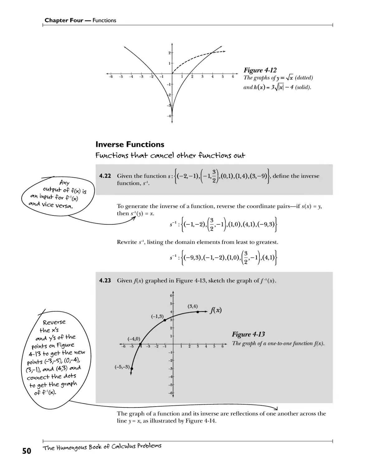
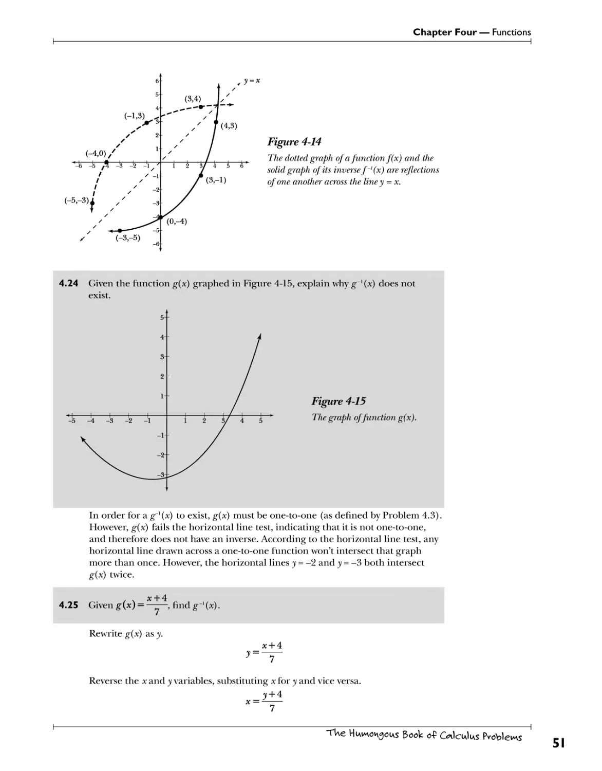
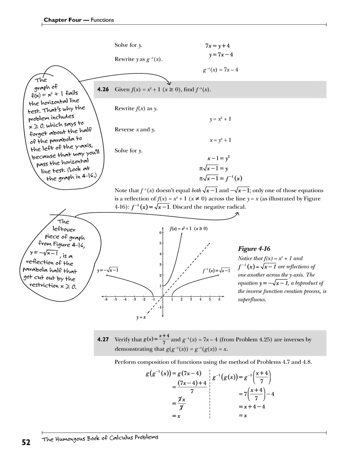
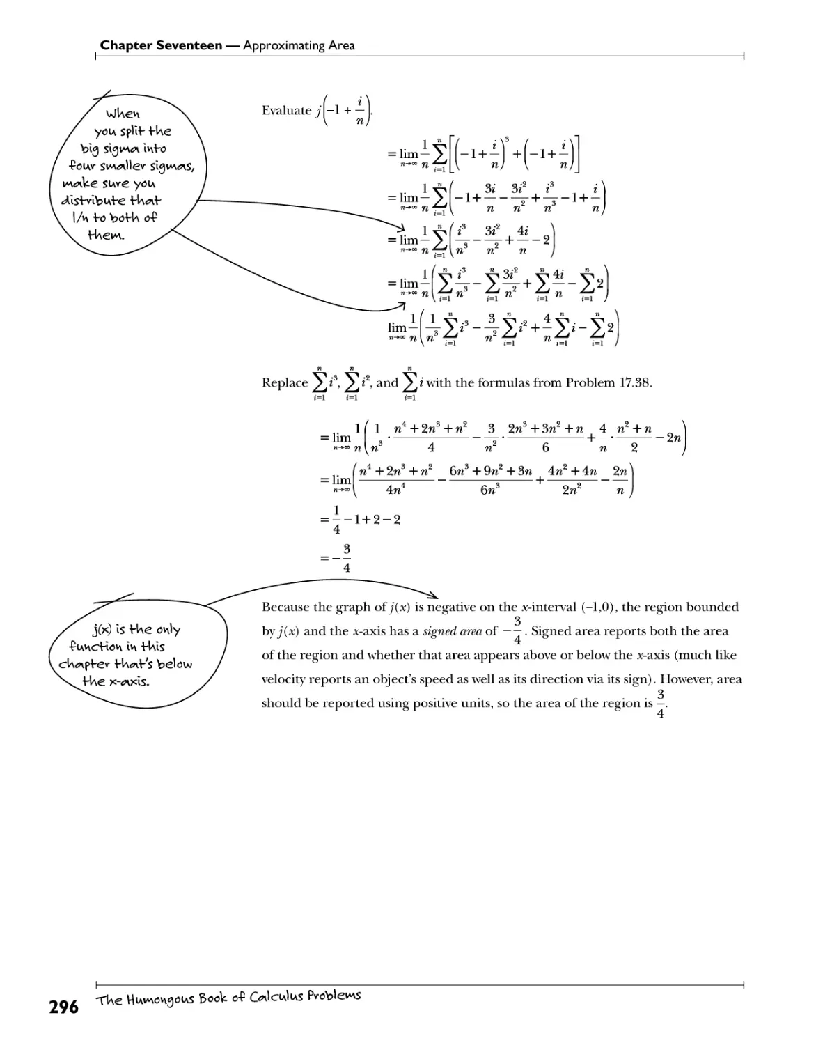
/


Автор: Kelley M.
Теги: mathematics mathematical physics calculus problems alpha publisher math for children
Год: 2006


Текст
1, 00 s pr lems i h om e si e s I i ■ s
fir A t - ajir o>i sof -I lus I
$0 * *
v> <*
>\
?
w
vv&
yvj. Klc e 11 y
, *
• •?
uM
VA
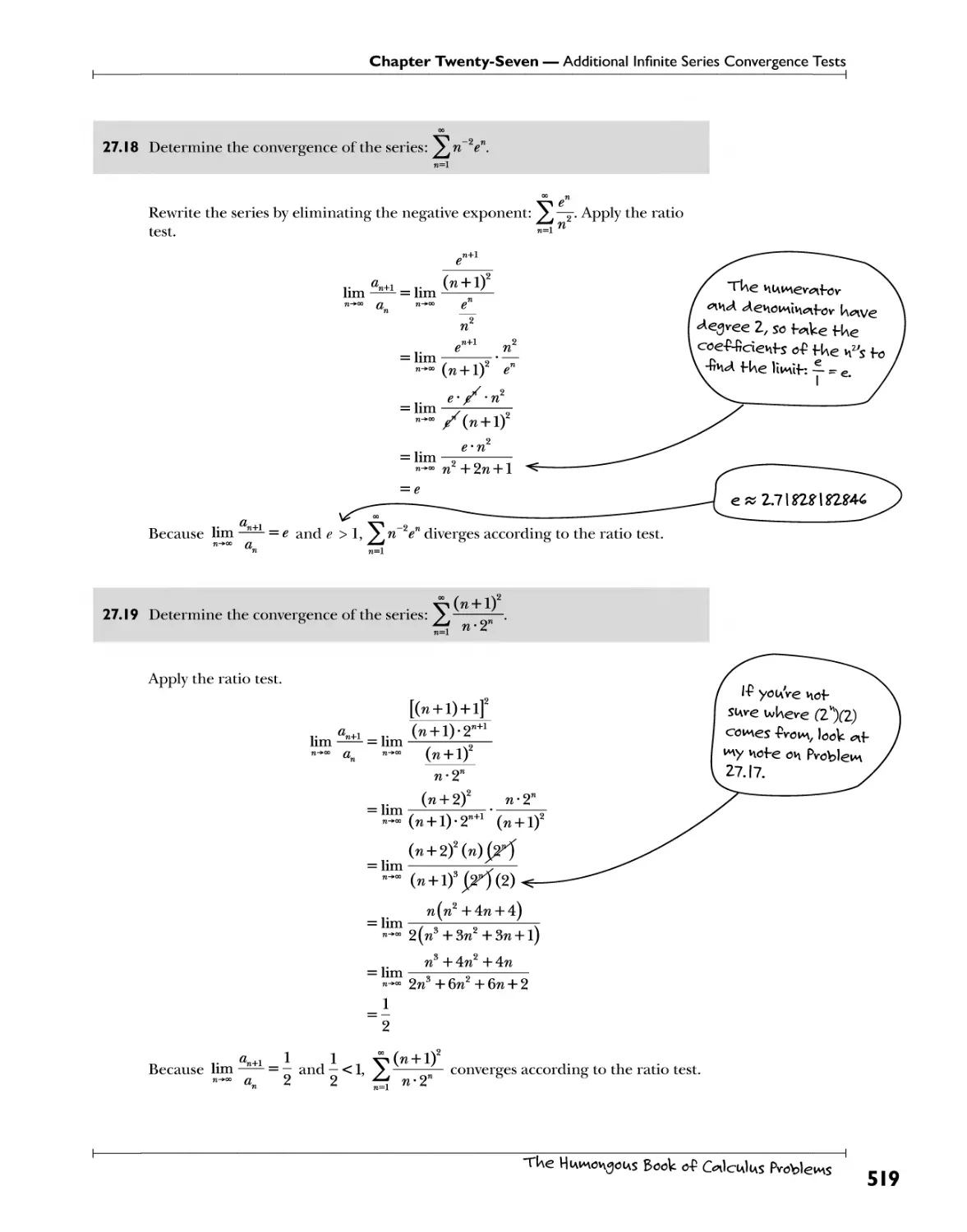
W. MIcIa 11 y
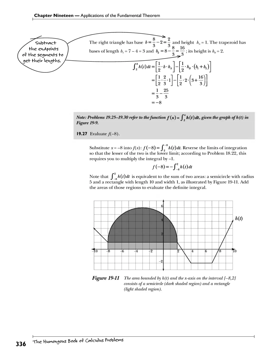
i U *
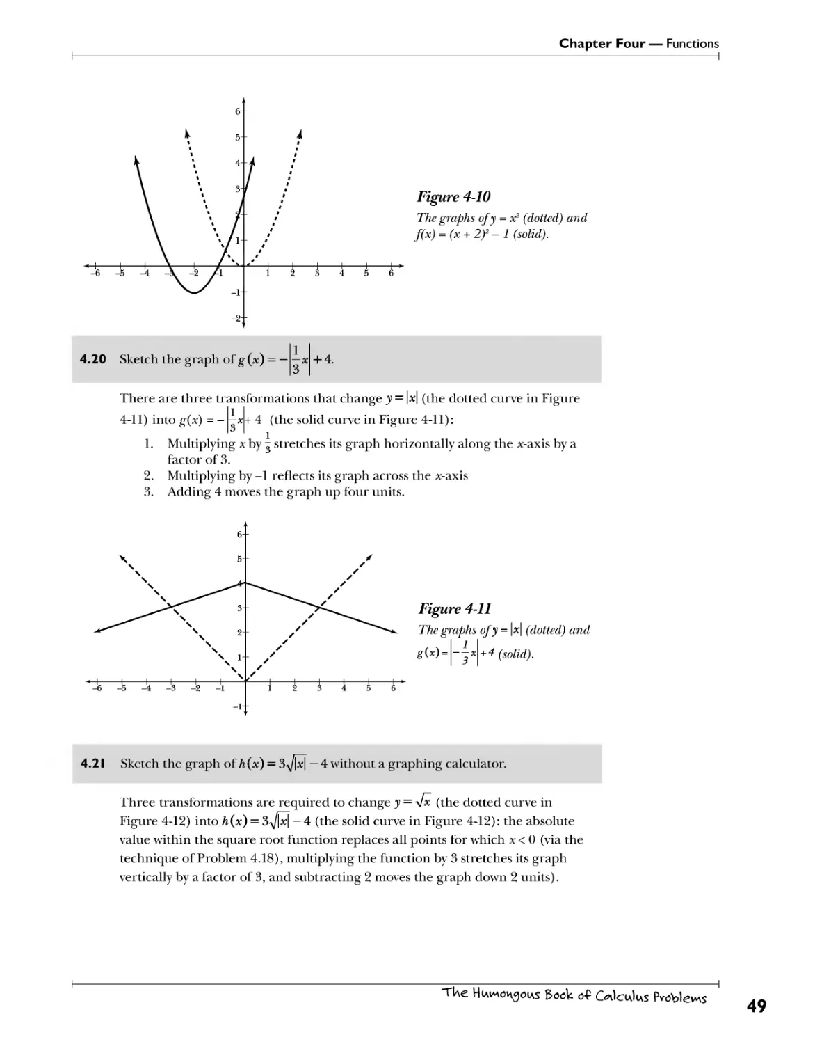
A niomturr< i lVn"LLin %r hl|j {LYA) In
ALPHA BOOKS
Published by the Penguin Group
Penguin Group (USA) Inc., 375 Hudson Street, New York, New York 10014, U.S.A.
Penguin Group (Canada), 10 Alcorn Avenue, Toronto, Ontario, Canada M4V 3B2 (a division of
Pearson Penguin Canada Inc.)
Penguin Books Ltd, 80 Strand, London WC2R ORL, England
Penguin Ireland, 25 St Stephen's Green, Dublin 2, Ireland (a division of Penguin Books Ltd)
Penguin Group (Australia), 250 Camberwell Road, Camberwell, Victoria 3124, Australia (a division of
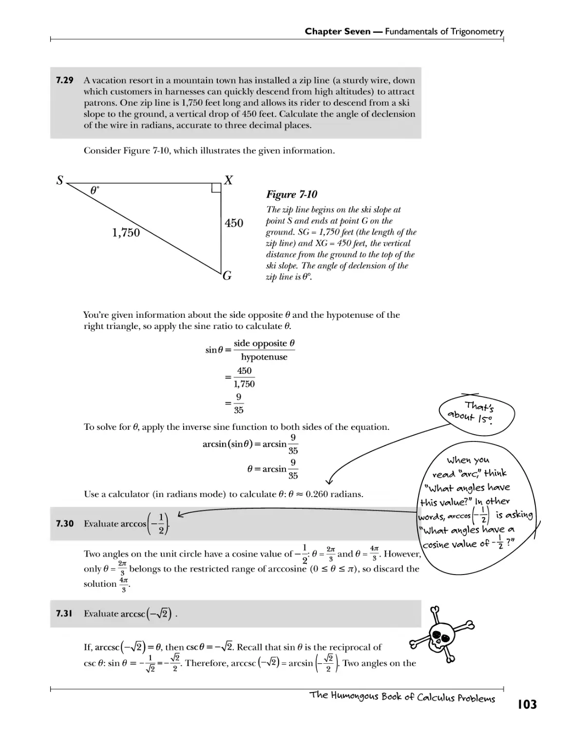
Pearson Australia Group Pty Ltd)
Penguin Books India Pvt Ltd, 11 Community Centre, Panchsheel Park, New Delhi—110 017, India
Penguin Group (NZ), cnr Airborne and Rosedale Roads, Albany, Auckland 1310, New Zealand (a
division of Pearson New Zealand Ltd)
Penguin Books (South Africa) (Pty) Ltd, 24 Sturdee Avenue, Rosebank, Johannesburg 2196, South
Africa
Penguin Books Ltd, Registered Offices: 80 Strand, London WC2R ORL, England
Copyright © 2006 by W. Michael Kelley
All rights reserved. No part of this book shall be reproduced, stored in a retrieval system, or
transmitted by any means, electronic, mechanical, photocopying, recording, or otherwise, without
written permission from the publisher. No patent liability is assumed with respect to the use of
the information contained herein. Although every precaution has been taken in the preparation
of this book, the publisher and authors assume no responsibility for errors or omissions. Neither
is any liability assumed for damages resulting from the use of information contained herein. For
information, address Alpha Books, 800 East 96th Street, Indianapolis, IN 46240.
International Standard Book Number: 978-1-59257-512-1
Library of Congress Catalog Card Number: 2006930703
08 07 06 8 7 6 5 4 3 2 1
Interpretation of the printing code: The rightmost number of the first series of numbers is the year of
the book's printing; the rightmost number of the second series of numbers is the number of the book's
printing. For example, a printing code of 06-1 shows that the first printing occurred in 2006.
Printed in the United States of America
Note: This publication contains the opinions and ideas of its author. It is intended to provide helpful
and informative material on the subject matter covered. It is sold with the understanding that the
author and publisher are not engaged in rendering professional services in the book. If the reader
requires personal assistance or advice, a competent professional should be consulted.
The author and publisher specifically disclaim any responsibility for any liability, loss, or risk, personal
or otherwise, which is incurred as a consequence, directly or indirectly, of the use and application of
any of the contents of this book.
Most Alpha books are available at special quantity discounts for bulk purchases for sales promotions,
premiums, fund-raising, or educational use. Special books, or book excerpts, can also be created to fit
specific needs.
For details, write: Special Markets, Alpha Books, 375 Hudson Street, New York, NY 10014.
Contents
Introduction ix
Chapter 1: Linear Equations and Inequalities *<*>>«"« «*if*Uw0 * h> H\e -first- powev j
Linear Geometry Cv-eoiHvig, g^^P^i*^/ <**<* »*\e<nsuvivi<j lines «nn<A line segwenf s 2
Linear Inequalities and Interval Notation... &&)%?. *fM*). ?&X h*'!?.f?!^J^?«?.^.^f^«t?. 5
AfooZttte VoZw* Equations and Inequalities 5.?!y«.*™. #M.*£.the..&?.e..<??..^.e 5
^sterns of Equations and Inequalities f^f\ ???.^?^??A^* 11
Chapter 2: Polynomials Because you oWf K^nve exponenfs o-P I -Povevev 15
Exponential and Radical Expressions ?.<*?&* f*£. *$**?$. ™*?. 16
Operations on Polynomial Expressions.. A^'.^^f.^.^\?]y>.^..*?}.*?. ?°)y*?™*)?. 18
Factoring Polynomials ^.ftt!fe^!&Y&^X™=e??. 21
Solving Quadratic Equations EfW?}t™J?. ftak. h*Y<?. * hlghS?*: .?.f f.^.^t<??.l. 23
Chapter 3: Rational Expressions FV^cHons, -Pactions, <*vvA ^ove -Pv^cHows 27
Adding' and Subtracting Rational Expressions . R?^^.«:.^A?^.«^V^.^^!^t?.,:T.. 25
Multiplying and Dividing Rational Expressions.. X^hWS.T.efSX. ^V!^3. fT.f^'??*'.«?. «fJ?X.. 30
Solving Rational Equations ... .tf$£ 5.°.^e?. <^.!**!t}rJ!£*K?* 33
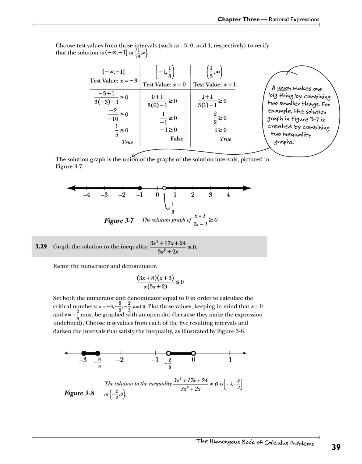
Polynomial and Rational Inequalities.. .Crit^l .^W&ST?. ^r.«?f*K SfR .YP.W *!$?$>&. K*<? 35
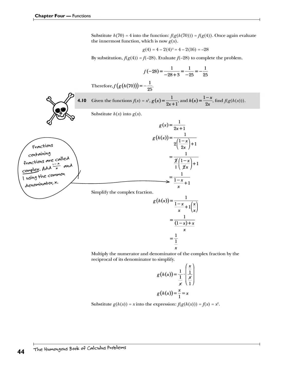
Chapter 4: Functions N<5Vw y^' sWf seei*3 ^) *n °vev H\e pWe 41
Combining Functions P?. .the. .*?.*?]. &.7< *'.:tl £ .f!W3.!e^. .l*t?. 5*5b.<#*?: 42
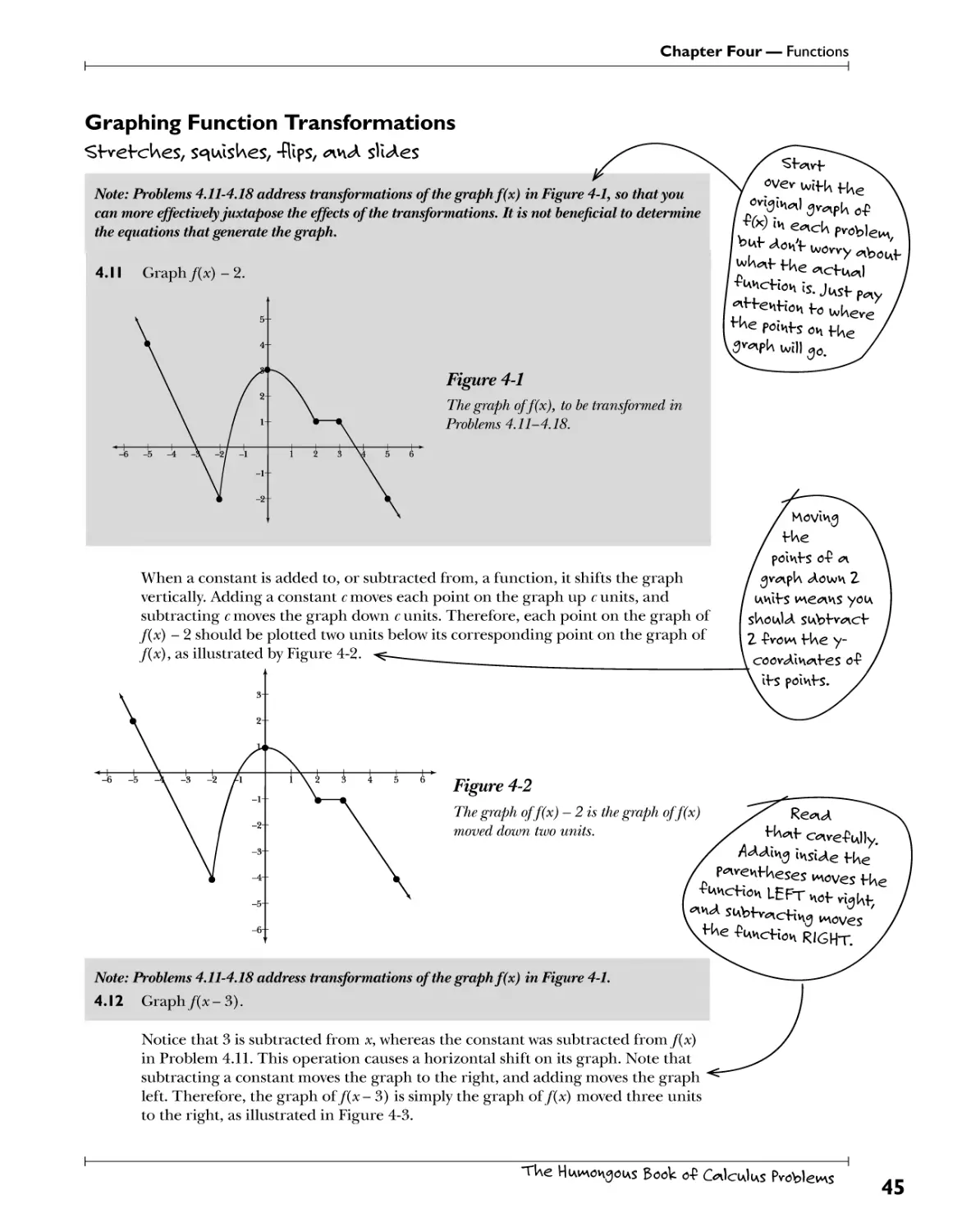
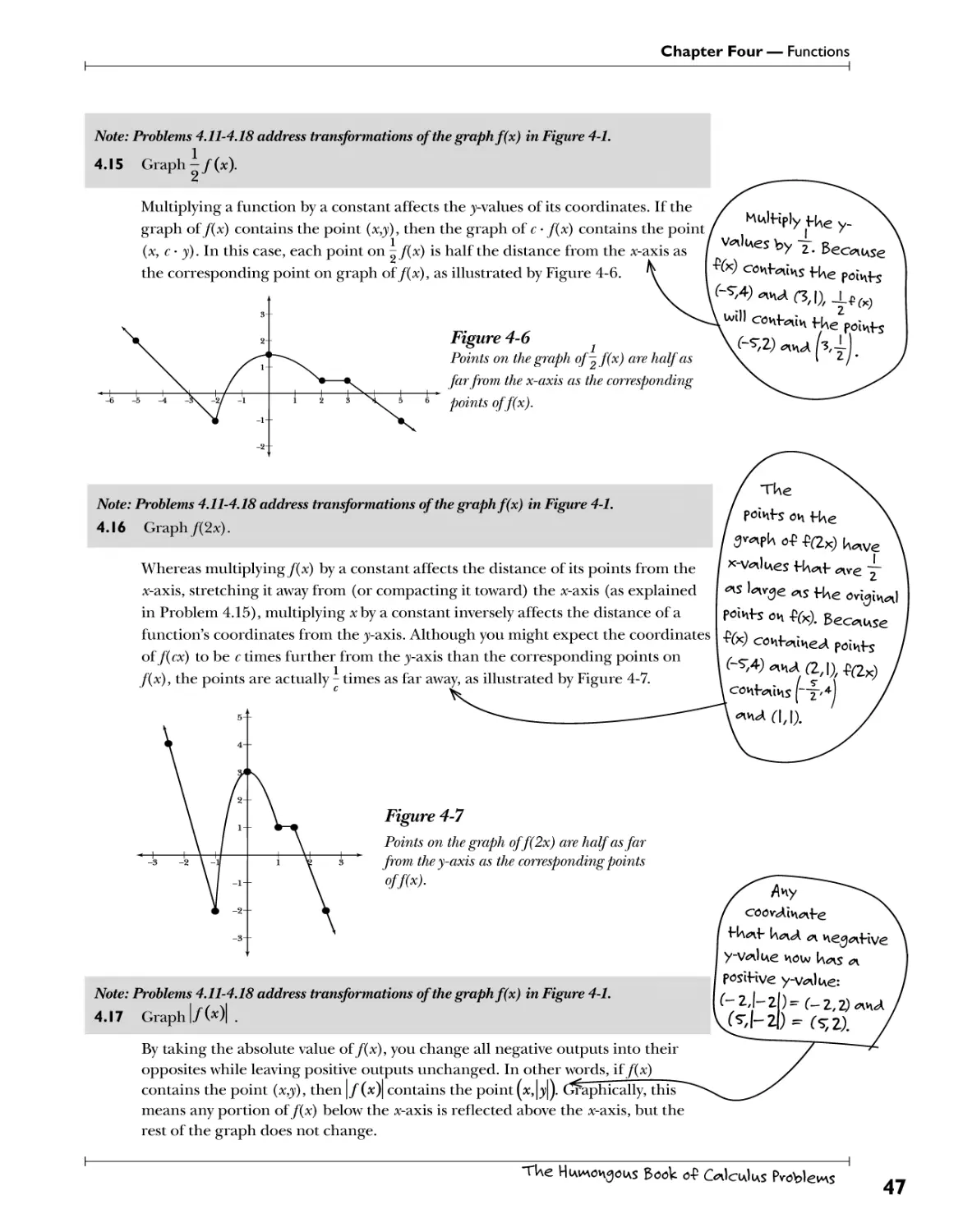
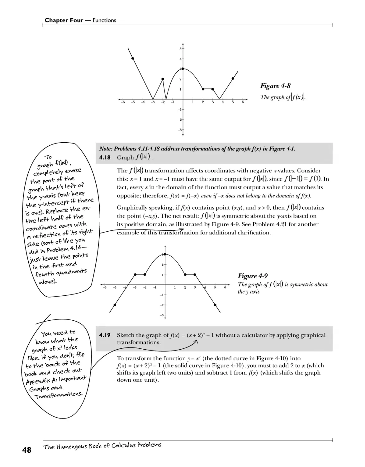
Graphing Function Transformations fk$*7$>&t. ^^Kes, flips, W slUes 45
Inverse Functions f.W}?.f}?V. .**** £**«:! ftyfrT. £V*£™??. *£ 50
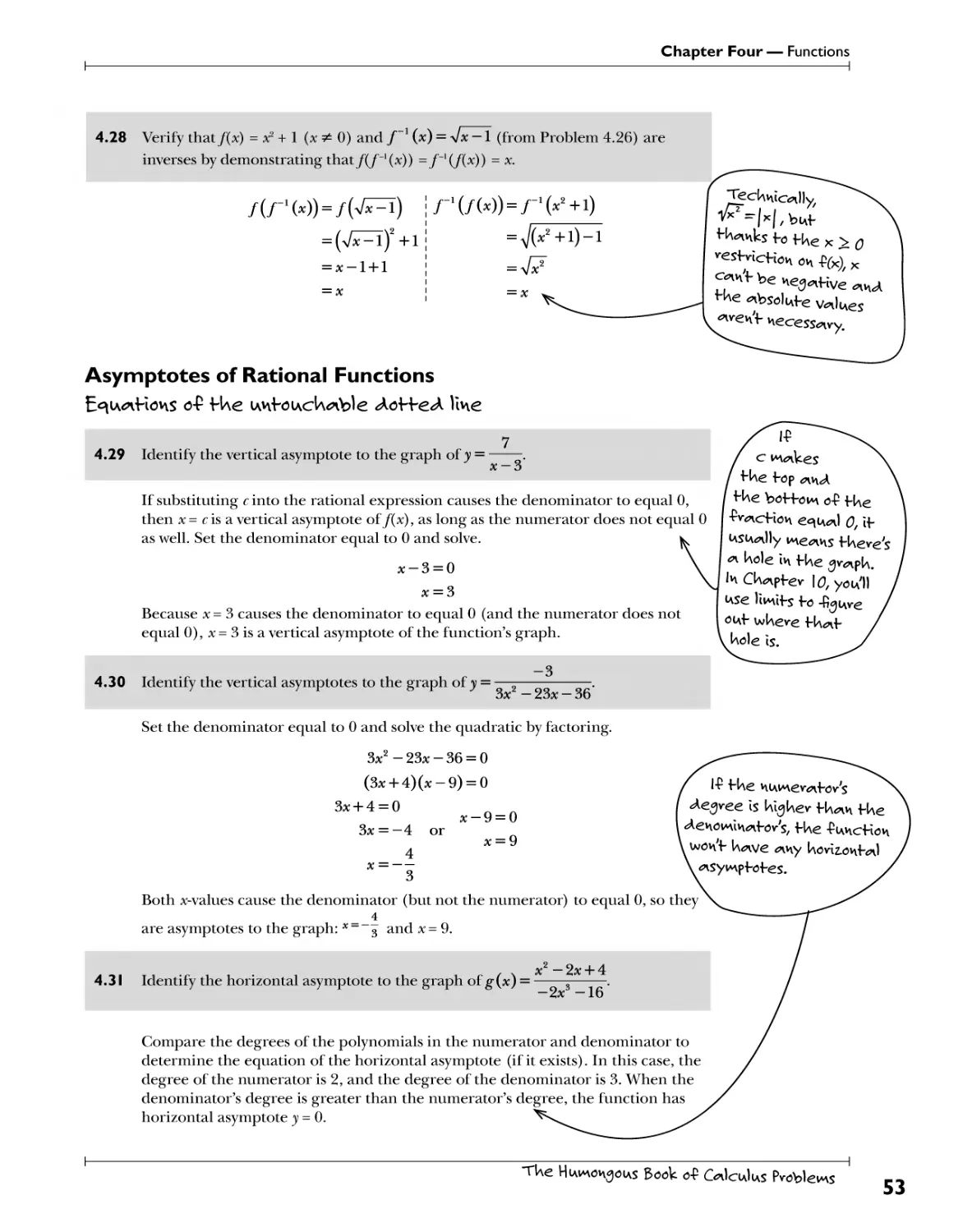
Asymptotes of Rational Functions... .EfW^^?.?.-?.^. W^!*£h*V)S.f*?.tt£.4. .%e 53
TUe HuiAA6v\3<3us Book o-P Calculus Problems
ill
Table of Contents
Chapter 5: Logarithmic and Exponential Functions FwicKovvs UVe log3 x, 1^ >c, 4*, <*}\A e* 57
Exploring Exponential and Logarithmic Functions tf <?W.<?$£ .<*'.'. fckp.SS .poiw<?y3 55
Natural Exponential and Logarithmic Functions . Bases .of. .e,.<wA .ctavh^e. o.f .b#is.e.f ow^ta. 62
Properties of Logarithms £tfpfW<*Wg /W.4. #afci$ W*g .'.04 £?spyje$#PA& 63
Solving Exponential and Logarithmic Equations. Exponents, £v.n<A .logs .c*wael .e#.ch .pB\<?r. P.^h... 66
Chapter 6: Conic Sections P^nv^boW, clvcles, ellipses, *nh<A Uype^boW 69
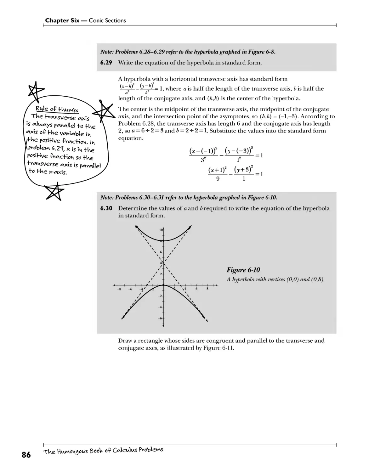
Parabolas .Ox^ph$.P.^.^^^r^Hc.^fi^^Hp.n$ 70
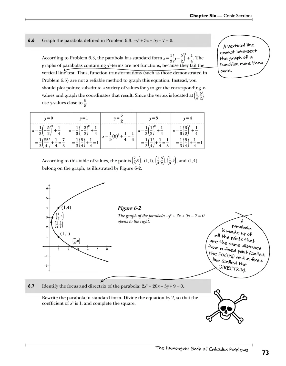
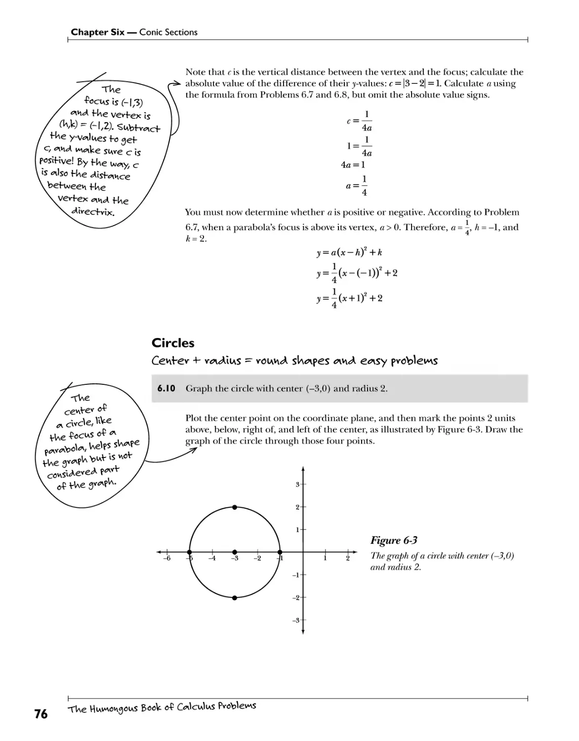
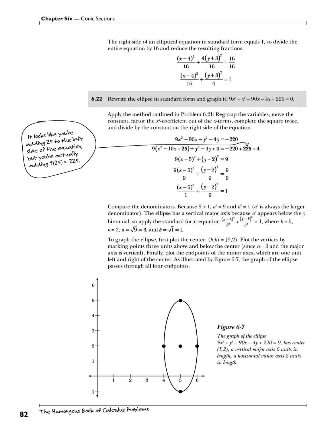
Circles .CenVev.+r.Y-^^ms.fr.Y'PMh^.s^p.es. ^.n^.e^sy.py.o.b.l.ev^s 76
Ellipses f^?.Y.Vy.°.^.f.^.!?.V^!?! 79
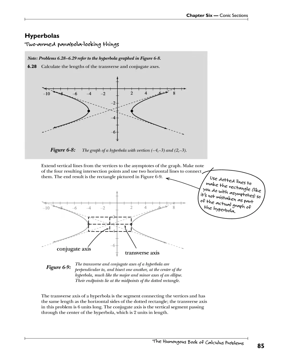
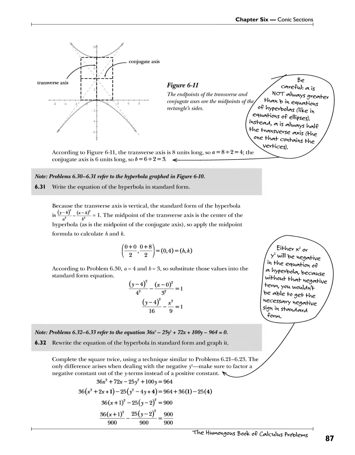
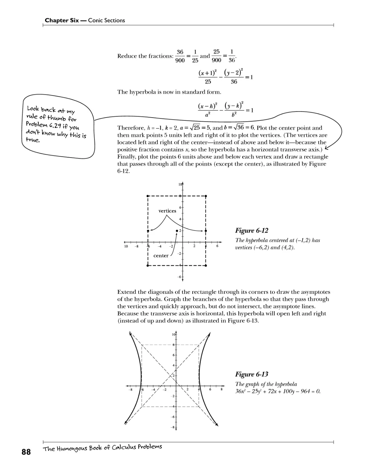
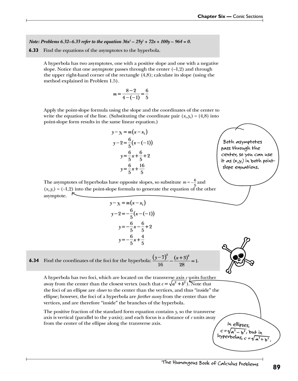
Hyperbolas Twa-.ww£^.p.^v^ 55
Chapter 7: Fundamentals of Trigonometry l^ecf sine, cosing, ^^ f^mgenf info fUe ml* 91
Measuring Angles £5*^)?<M?3^ 92
Angfe Relationships C?.^!?!^ 93
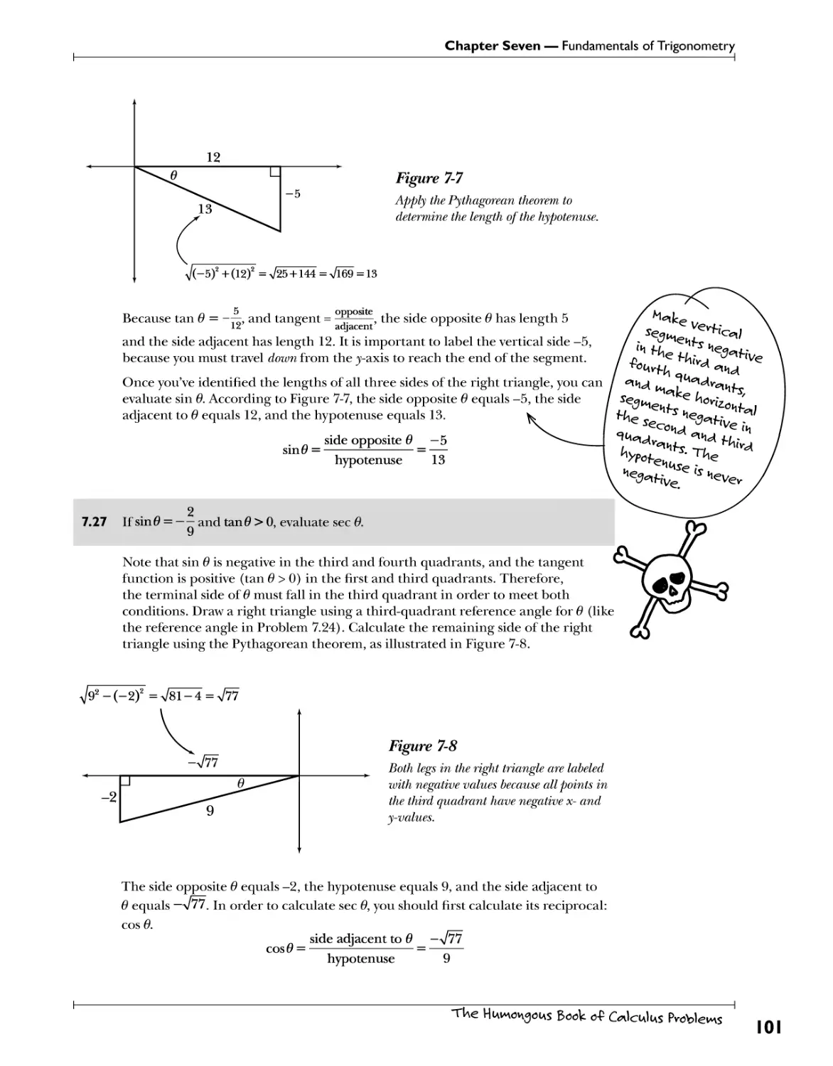
Evaluating Trigonometric Functions $3^. frl*Ml?. fr». ^.^.r^y.?.^.?. 5Wa'« 95
to^ Trigonometric Functions 1WV* **}#!*?&. /?V^. ?.V*T!*t: /W.fftS!??.f.°.r.f\£^3?. 702
T/w e^^Ho^s *** Ue^Hf y pvoo£s
Chapter 8: Trigonometric Graphs, Identities, and Equations J 105
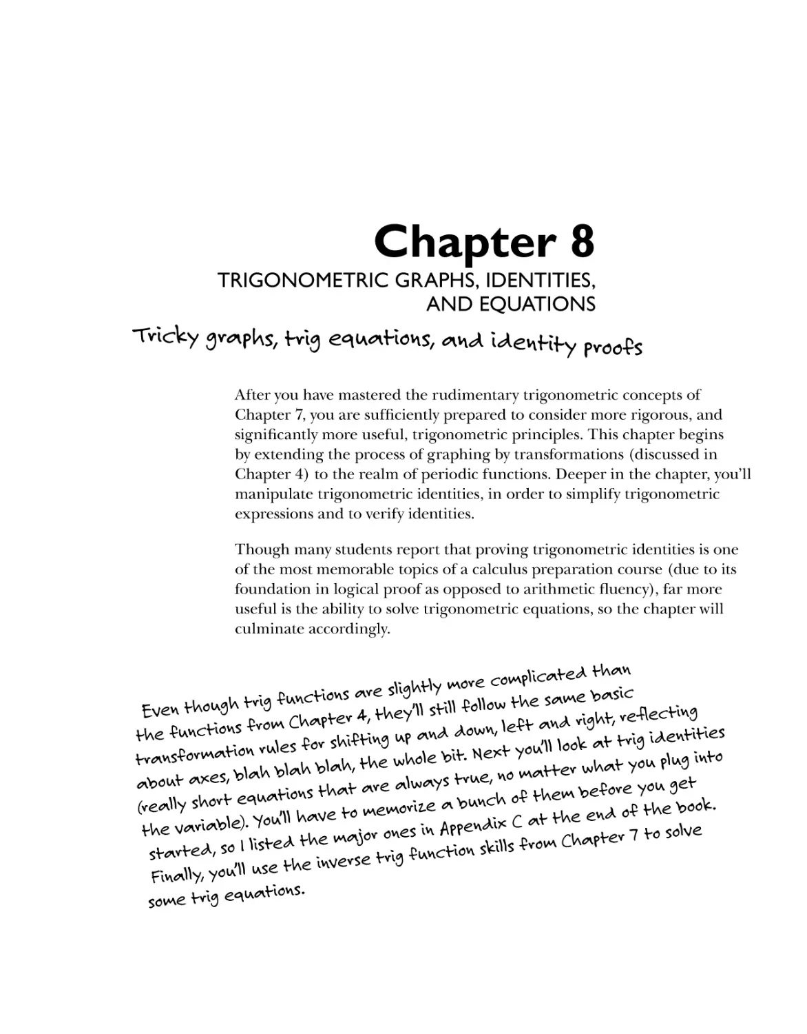
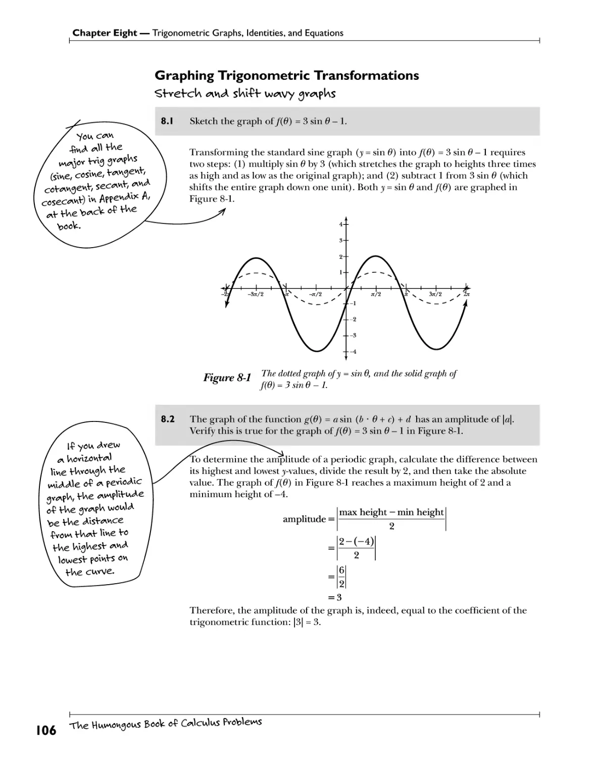
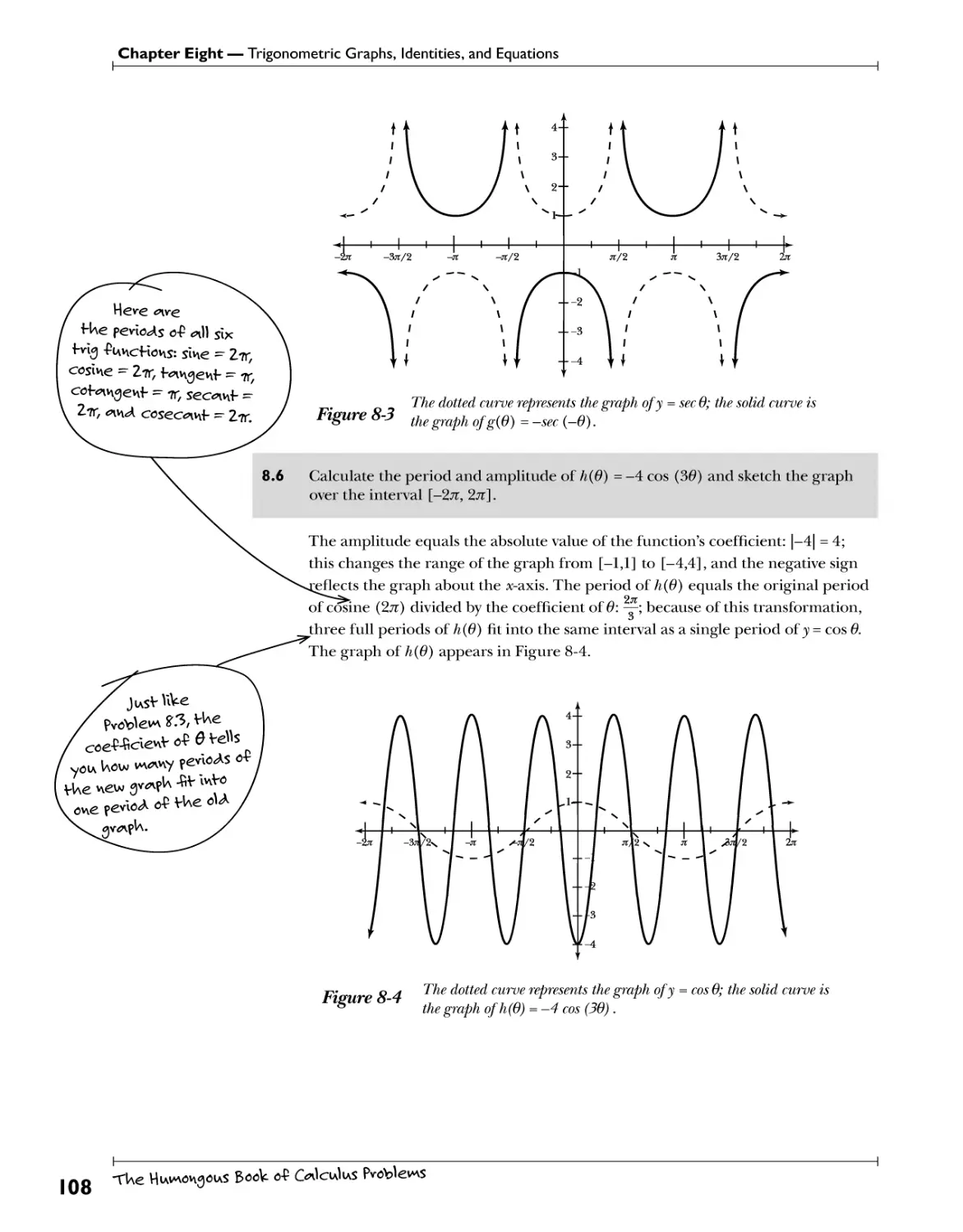
Graphing Trigonometric Transformations $ty.?fc£v. 5^4. $bV? .t .V^Y.y.3.^fh? 706
Applying Trigonometric Identities ^f.%.^.P.^ 770
Solving Trigonometric Equations .?.?!Y£.7.?T.y. .lAs.t?.?V^.?."?.*. 775
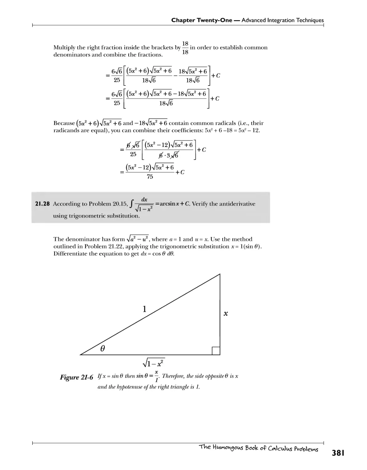
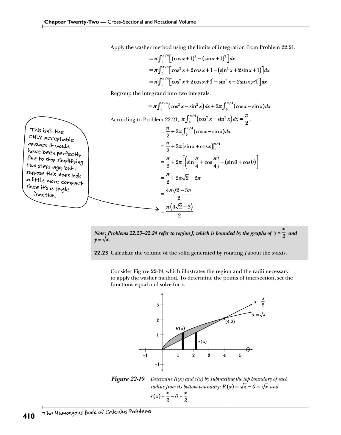
Chapter 9: Investigating Limits wU*f UeI3^ <*oes W\€ -Pi^cHoh intbid f 0 ve*cW? 123
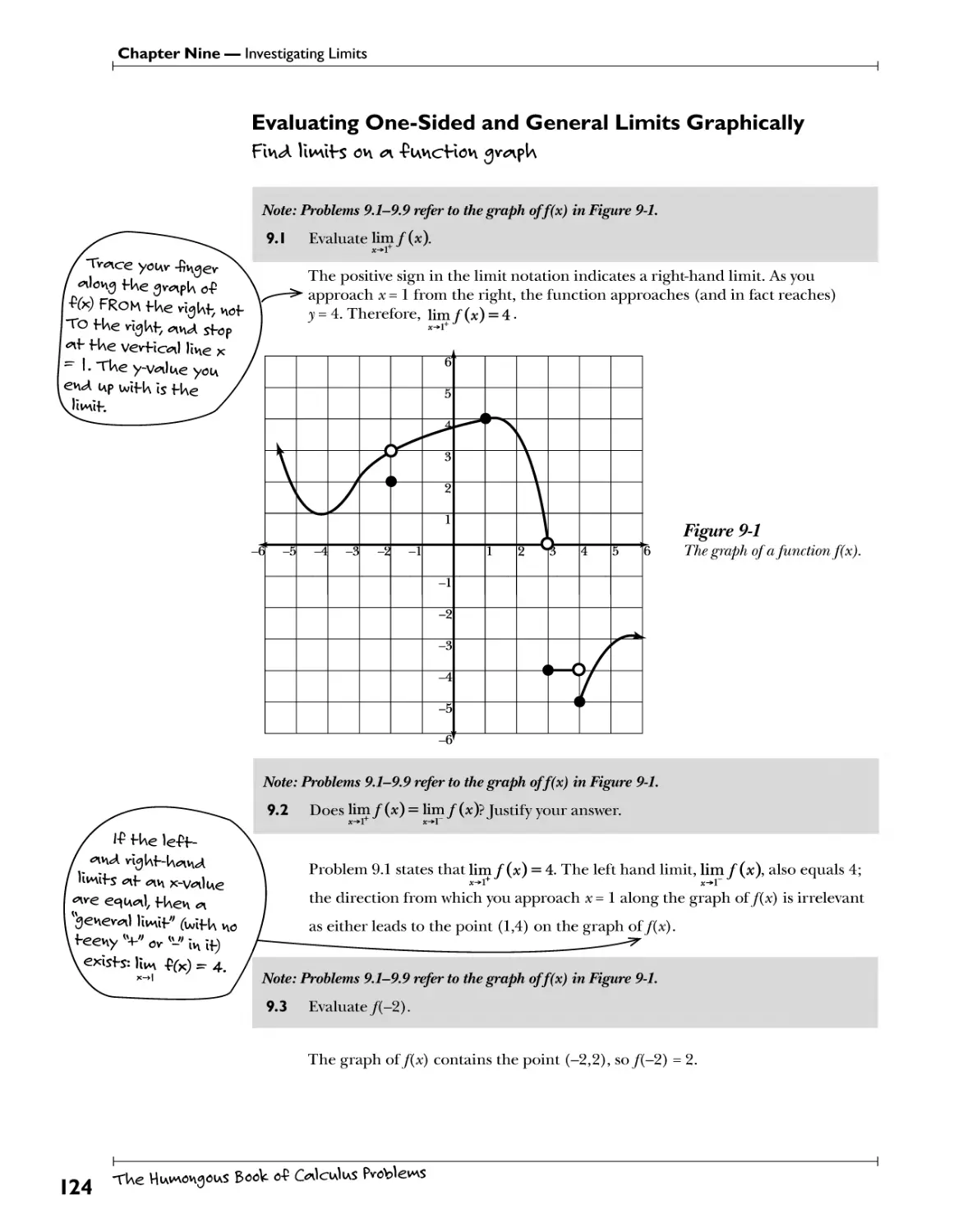
Evaluating One-Sided and General Limits Gra^z^^.... f 1^. .,}!^>h?.9.^.f^.f.^9.^?^ .3.v.^eh.... i2^
Limits and Infinity W.^.h*^ 729
Formal Definition of the Limit.... %?$?*:*€)*:*. f ™Y>1?!*? .?>r£ .*<? .f W\ *t *!> 734
Chapter 10: Evaluating Limits OlcuUte Wifs wifUoiAf * gv^pk 0.p fUe *uhcHoh 137
Substitution Method ^l^^Y^l^S^S^.f^^ 755
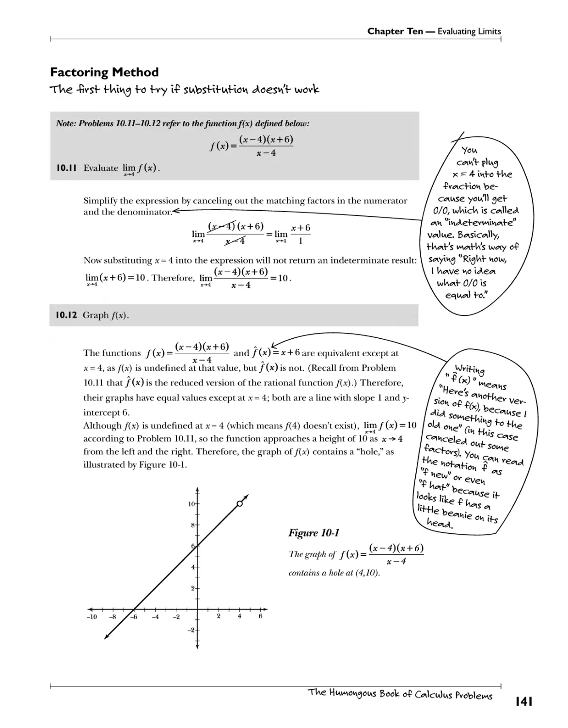
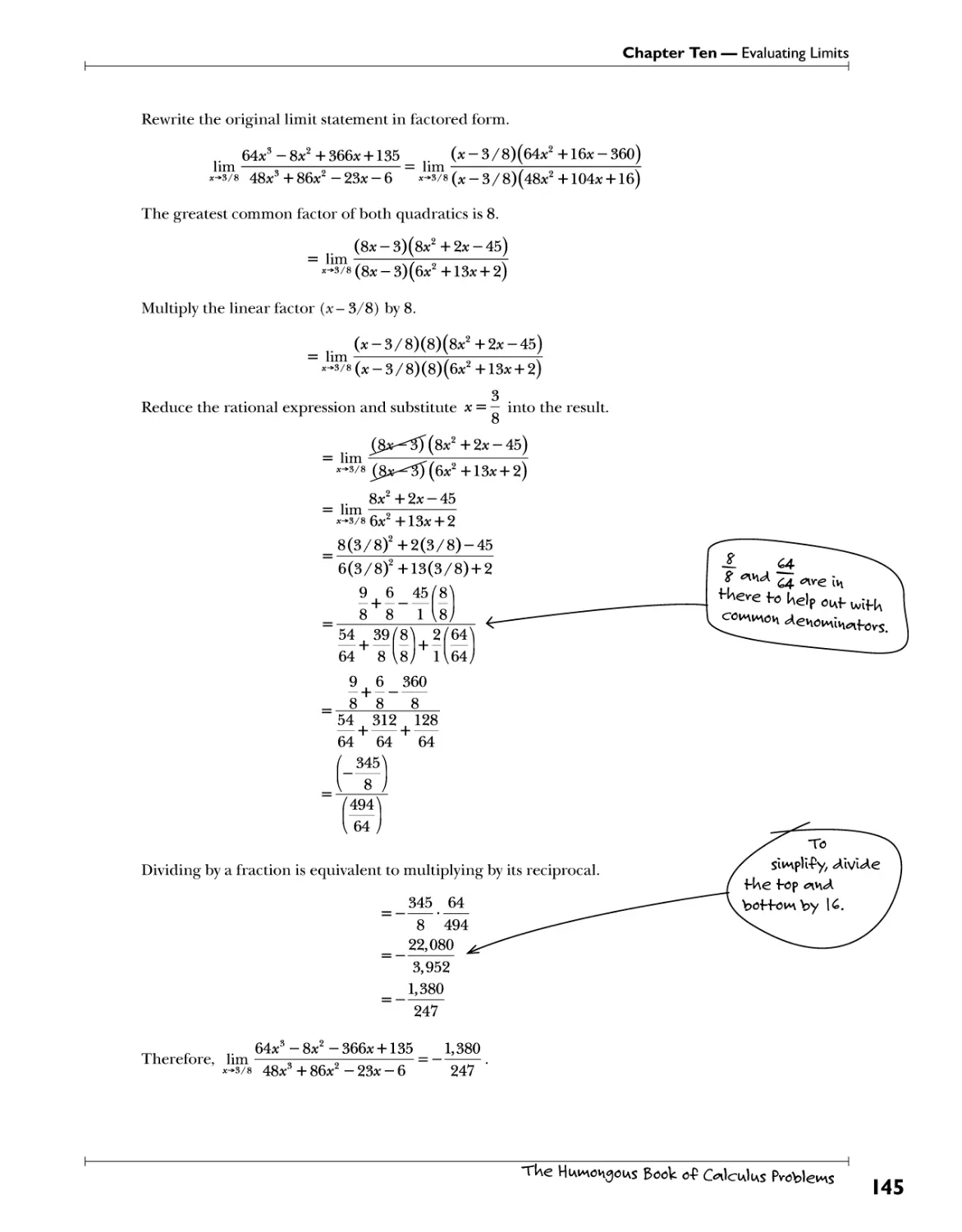
Factoring Method .Th?. ."?.v[?h ."fyl^S. .t?. .^T^ A"?. ?^Yj?t?h^rV??\ .^.<?^?y\'h .^yH 747
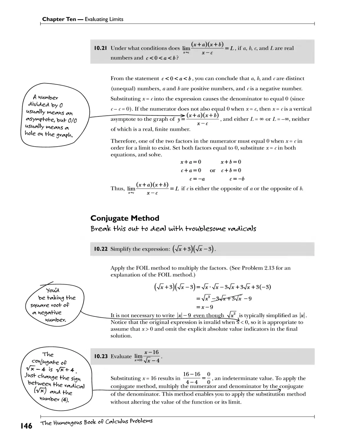
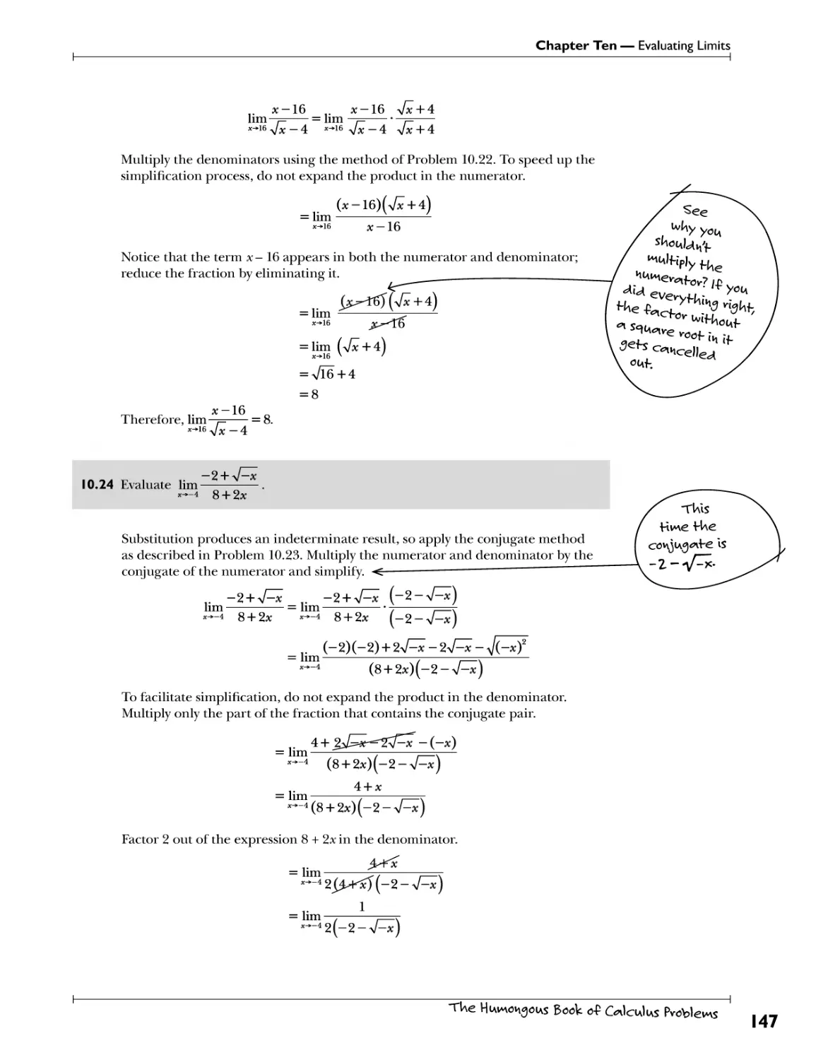
Conjugate Method P.^f^f: .Vhl?.9.^. .t?. .4.?^!.VylVb.tTC^Yll??/?^.!?.^.^rf!1!? 746
%aaZLzmzYT/^or^ 749
TUe HiAvnov\goiAS Book o-P G*1oa1ias Problems
Table of Contents
Chapter 11: Continuity and the Difference Quotient UnW^ble 3^PUs 151
Continuity .V^W. ^^>?.^T?. T*7. "P.^f7.^1?.^ .f^^"?.^.^ff. fT.f:?^ti^*0.^.s. 152
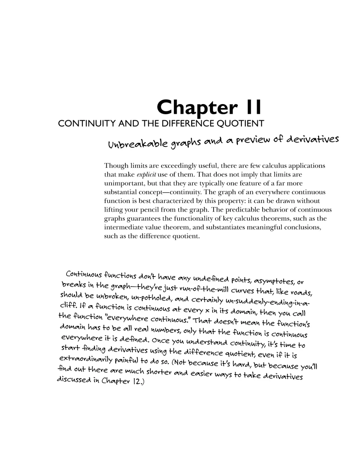
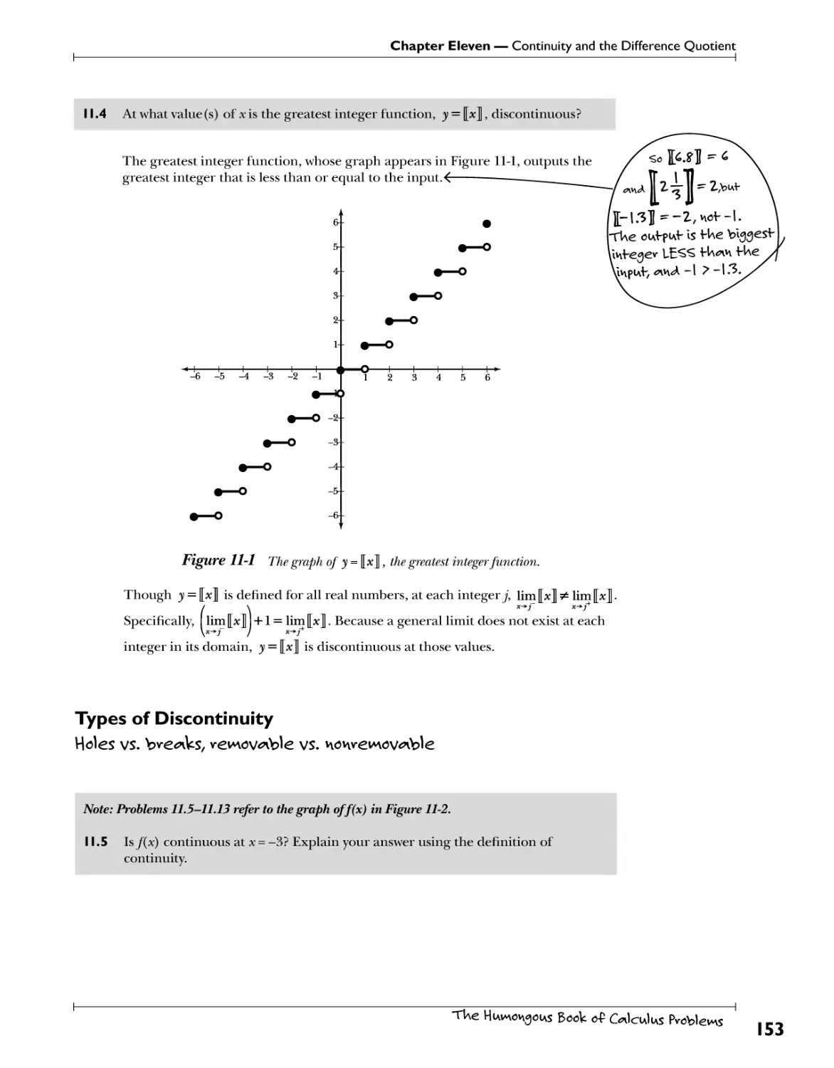
Types ofDiscontinutty.M^^^ 153
The Difference Quotient ^..^^ 163
Differentiability ^\^?.?.f^ 166
Chapter 12: Basic Differentiation Methods -The 4W Ue^vy kiffevs £ov -fiw^lwg ^eviv^Hves 169
Trigonometric, Logarithmic, and Exponential Derivatives tt£W#cU-S .Vhs$S .£oyW*!ftf 7 70
77^ Power Rule fJyv^l'y .?* .?h?y.t£ vtfr. £<?y. ^.f eyey^if^yvs. h^yvs?. )!lV.?. ** 172
The Product and Quotient Rules..M?f?y<?*hl*£?. £^>£ti?*?.t^h *\v.?.^Hp!i?.4.*T.4Ws4e4 775
77^ Chain Rule P!l£k?y<?y\tf^^ 179
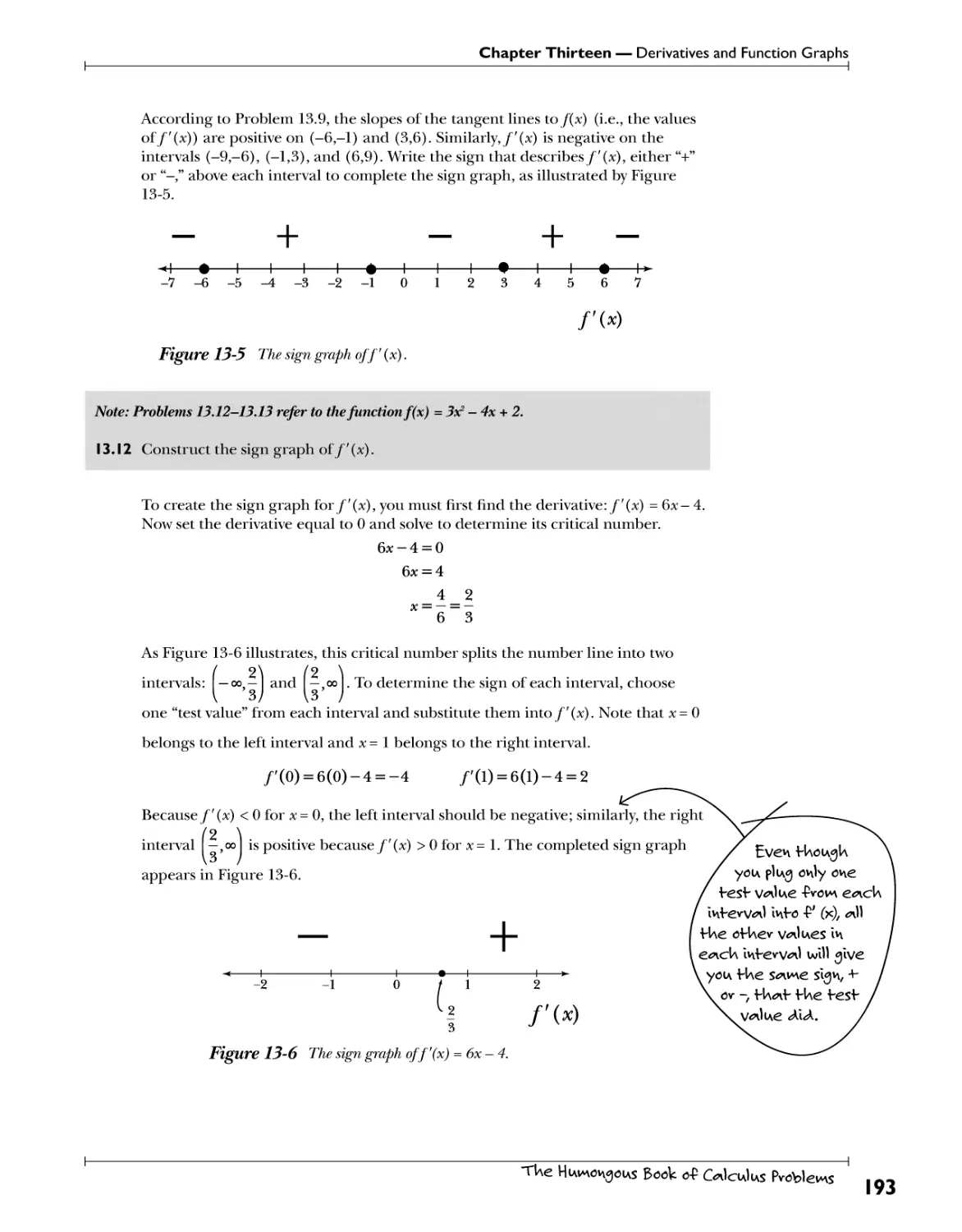
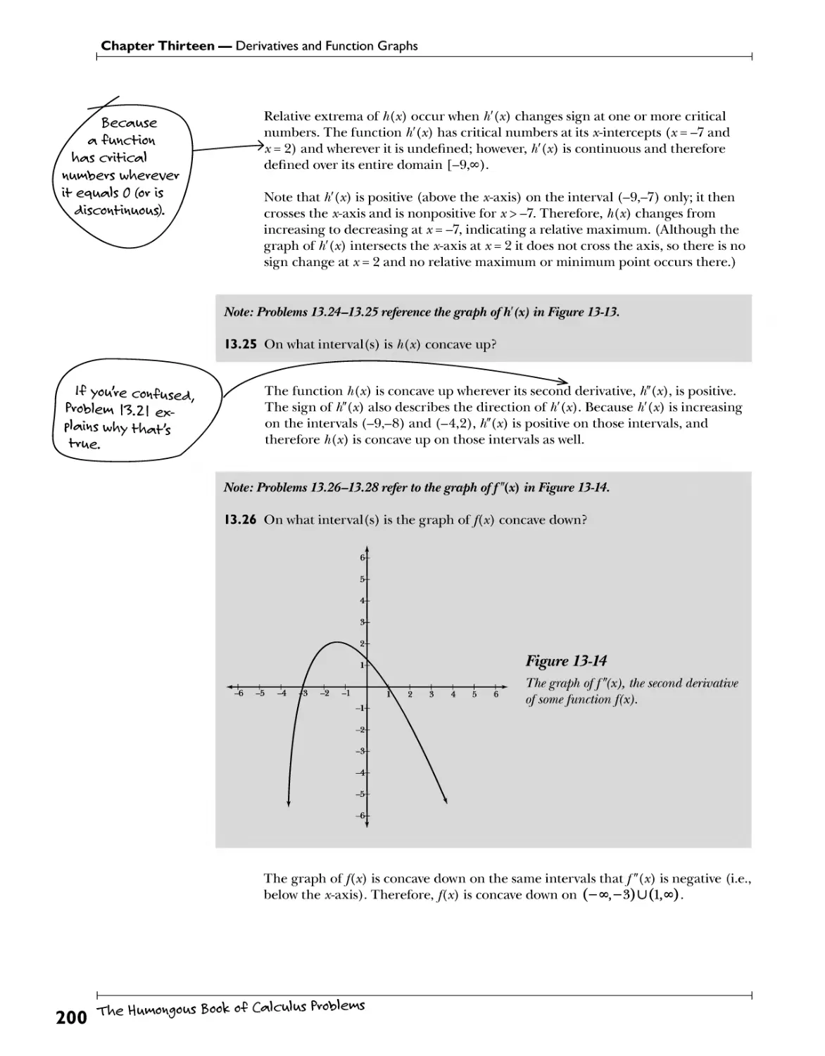
Chapter 13: Derivatives and Function Graphs ^<* *W* ^ ^eviv^Hves fell you ^bo^f gv^Ws jg7
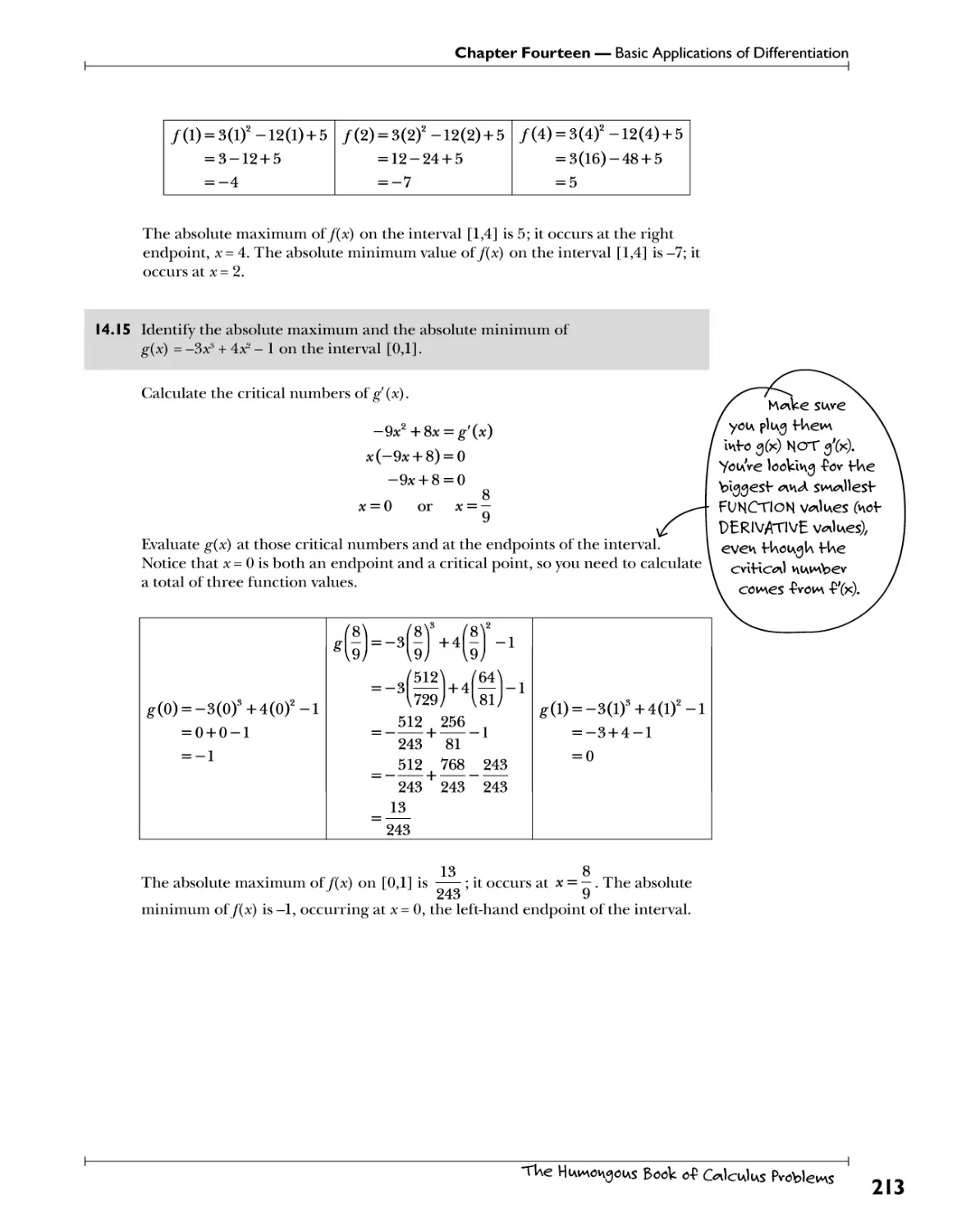
Critical Numbers N.^beys VW; ^r.^.^?..Vf\33]^.3^f^. 188
Signs of the First Derivative U?^.W\33]^. 3?*?^?. fc. 5*?texW*?. i^ncHon. ^jyecHon 797
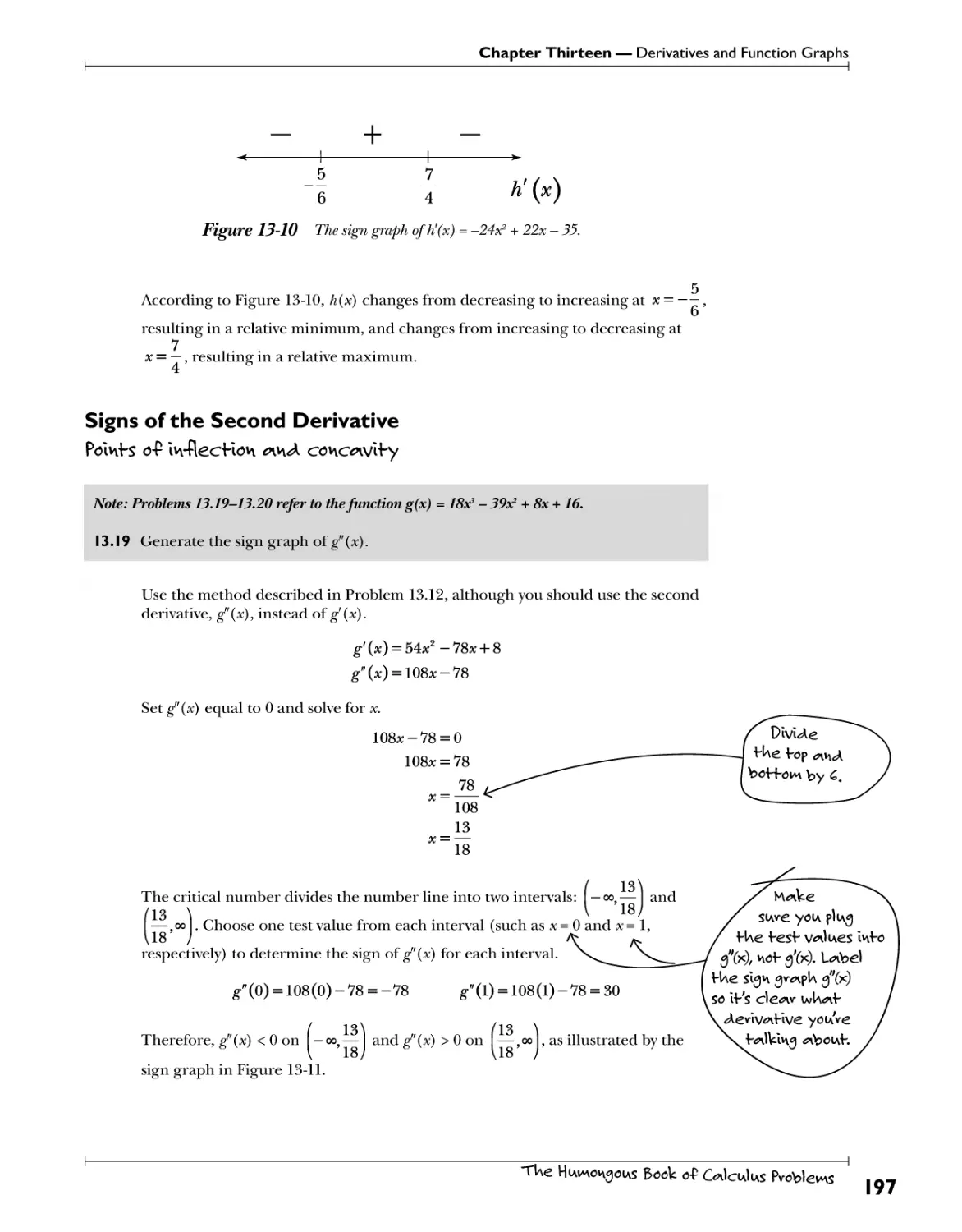
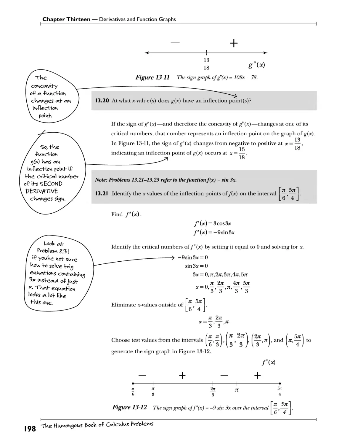
Szgrcs 0/ J/m? Second Derivative ftw.ts. rf.^^cHpH. *ww*. c<?h«\Yihy 797
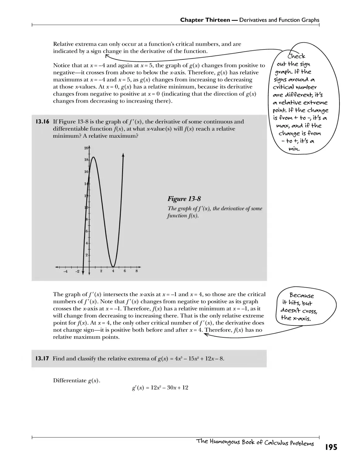
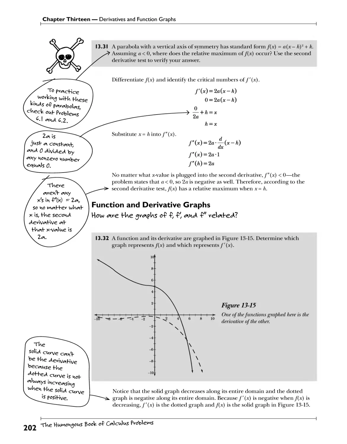
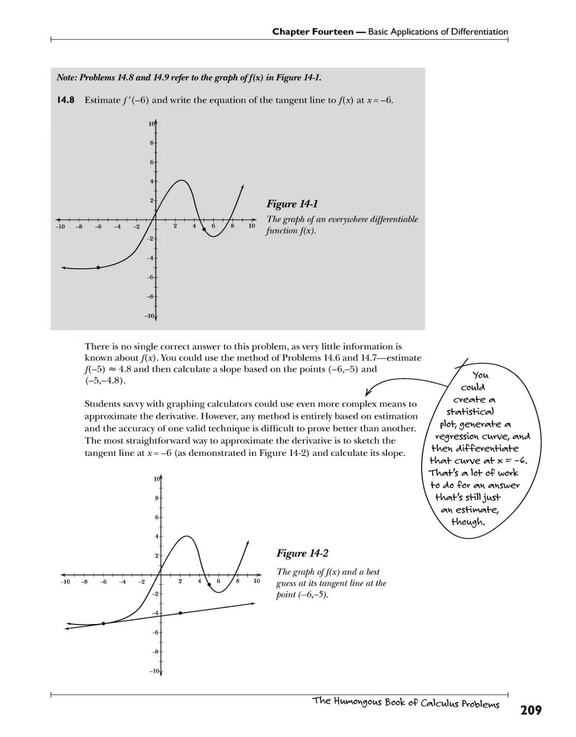
Function and Derivative Graphs H?W. -we f Ue ^pJas 0* .£ .-P^yuA £" veUte<A? 202
Chapter 14: Basic Applications of Differentiation P^ youv <Aeviv<nHves skills fo use 205
Equations of Tangent Lines.. Pp.l.nt.<?ft fc*>»€*GY± /terlYfltlYS .T.e/^<*Hon o-P W^e*f. 206
The Extreme Value Theorem ^?tt.*Wf#i^ 277
Newton's Method ....%)*>?)$.^yJV.^t'iY.??.£^y\/*PPy£*^/*t£.h^<?.f.?.^?.?.?."?.^.^^?'.^^^ 274
L'HopitaVs Rule Fi^J!lW^ 275
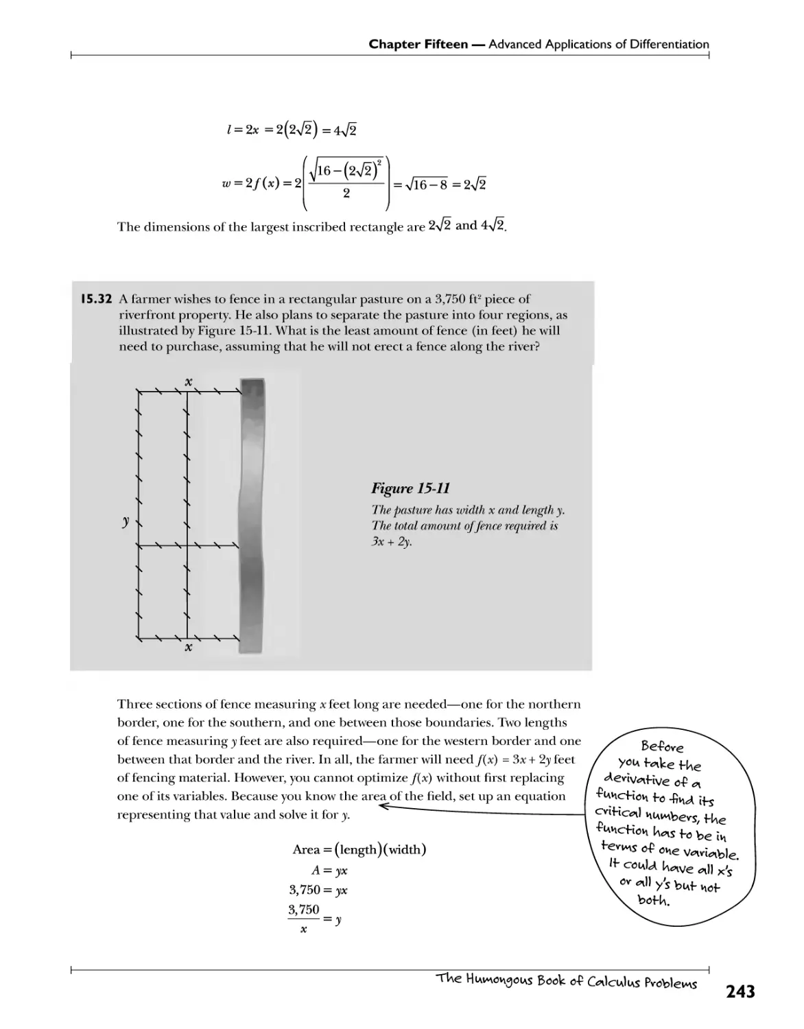
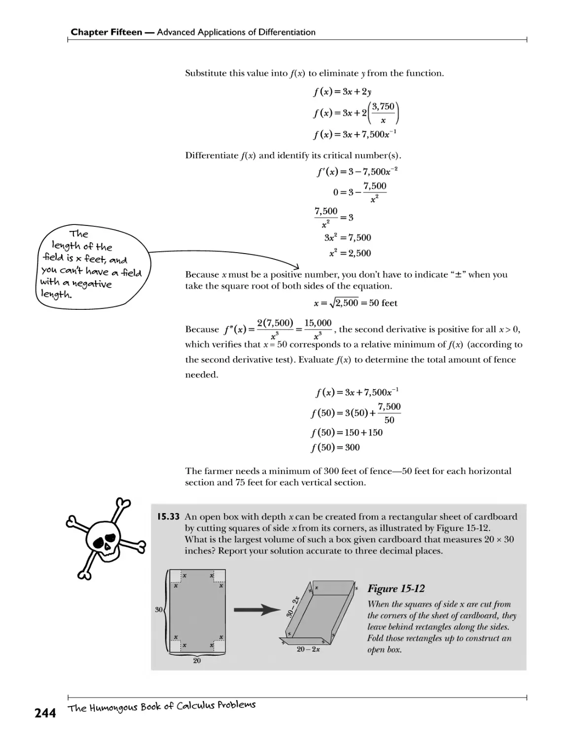
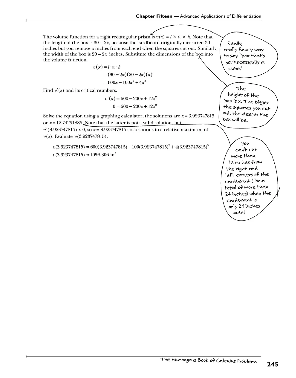
Chapter 15: Advanced Applications of Differentiation -tvicfcy W- ^fevesf^g use* 223
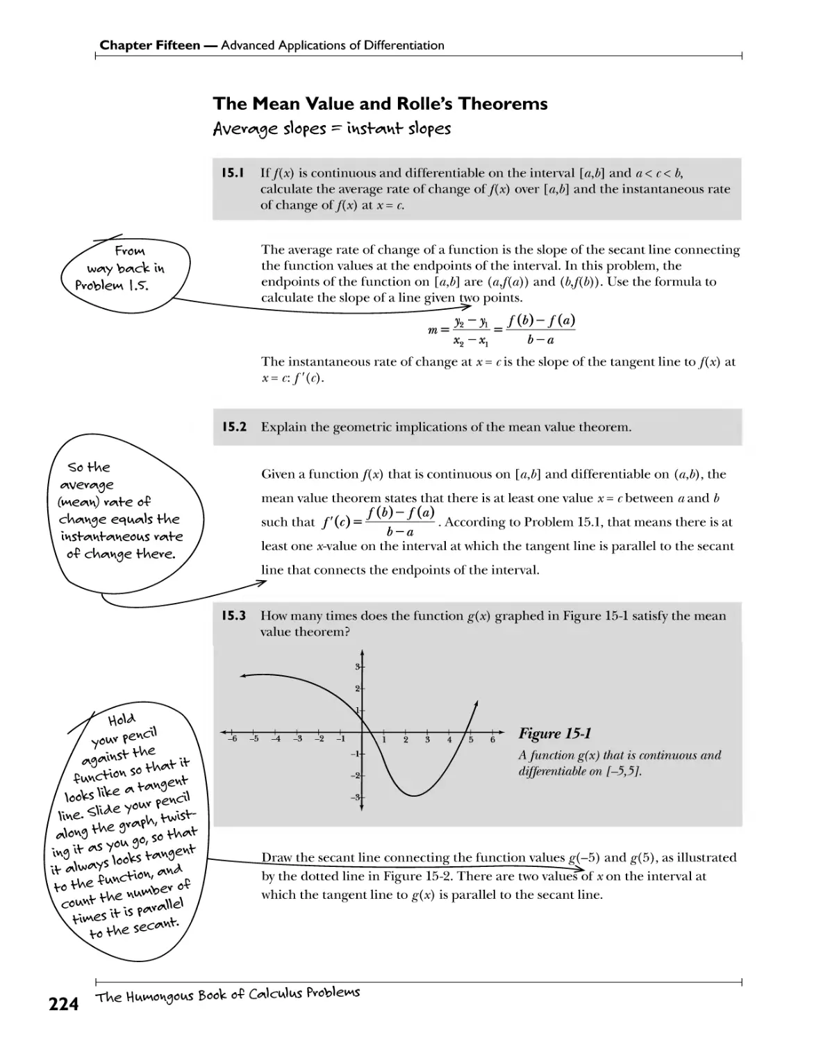
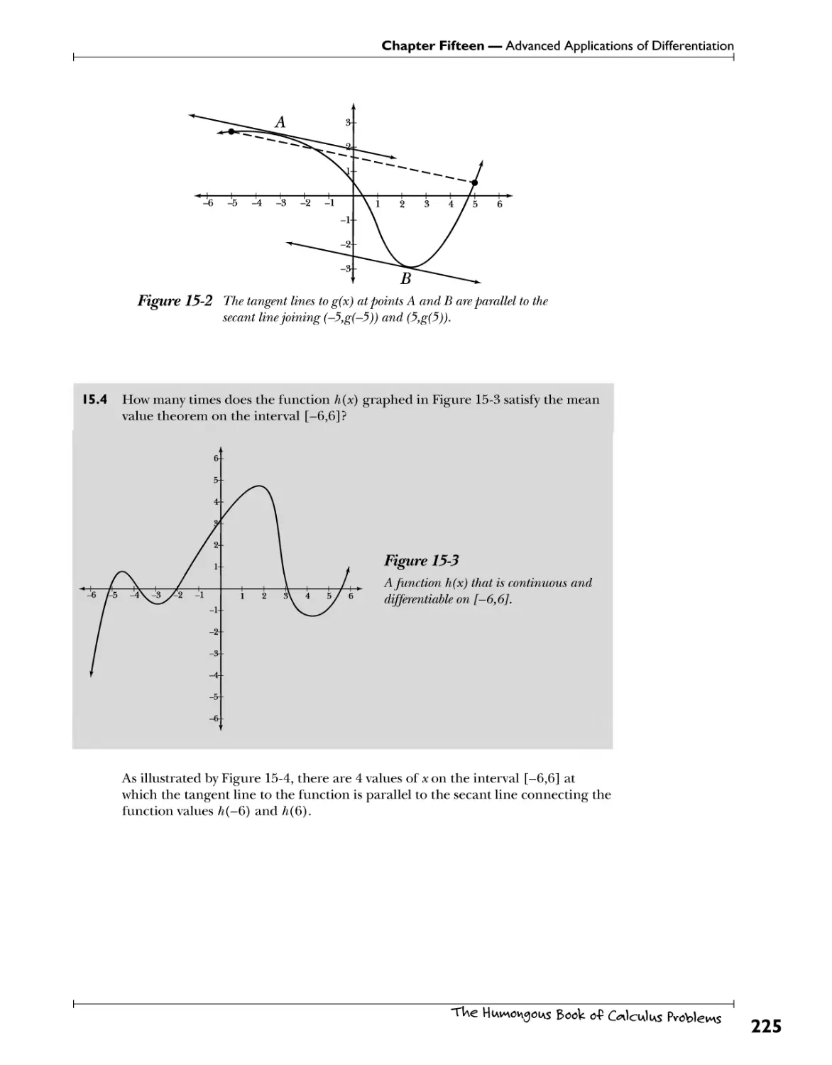
77h? Afean Vato and Rolles Theorems Average.slopes~\y$kwfr..$\<>T&. 224
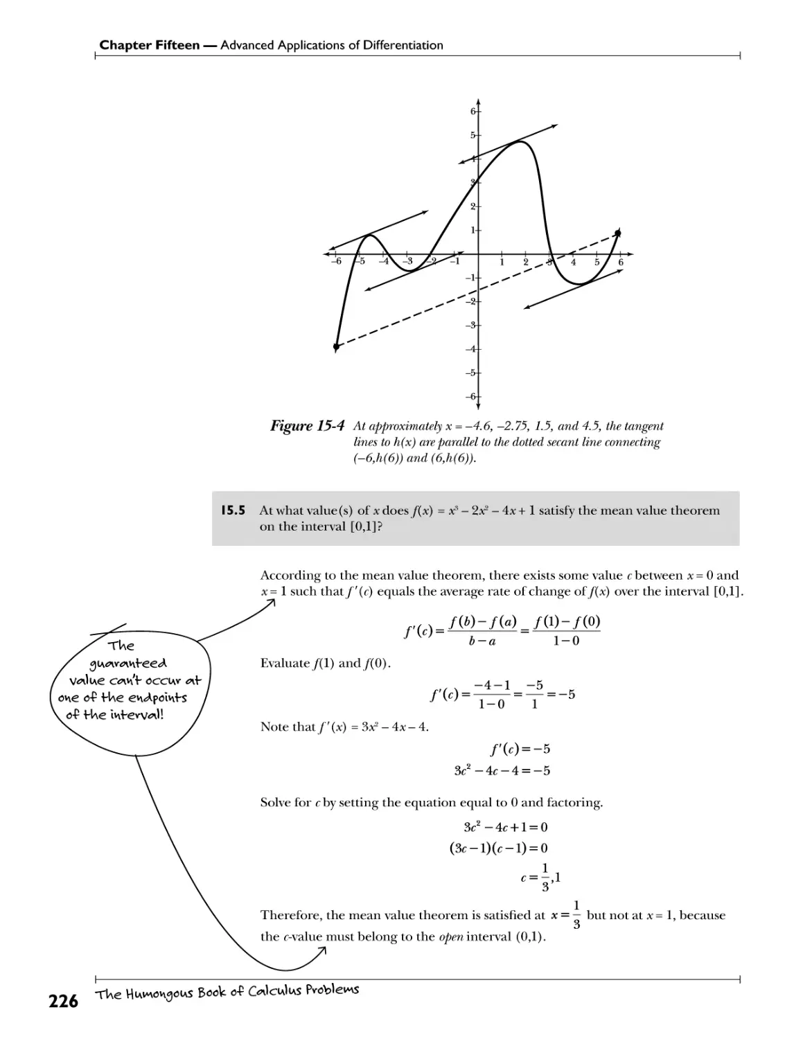
Rectilinear Motion ?<*$Y±9y±tXdoQ\yJm .W^.^ff^gr^hW. ^WfThW?. 229
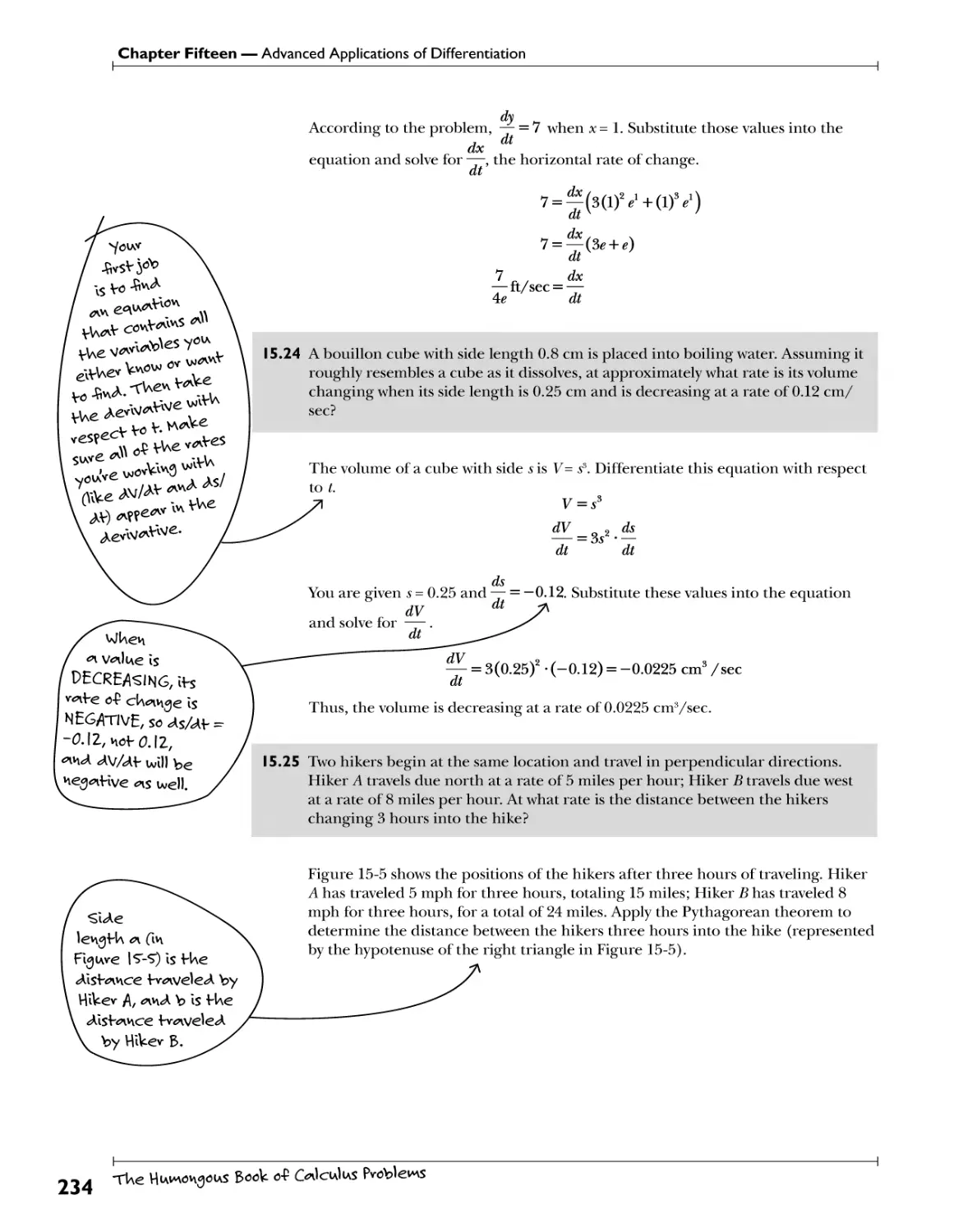
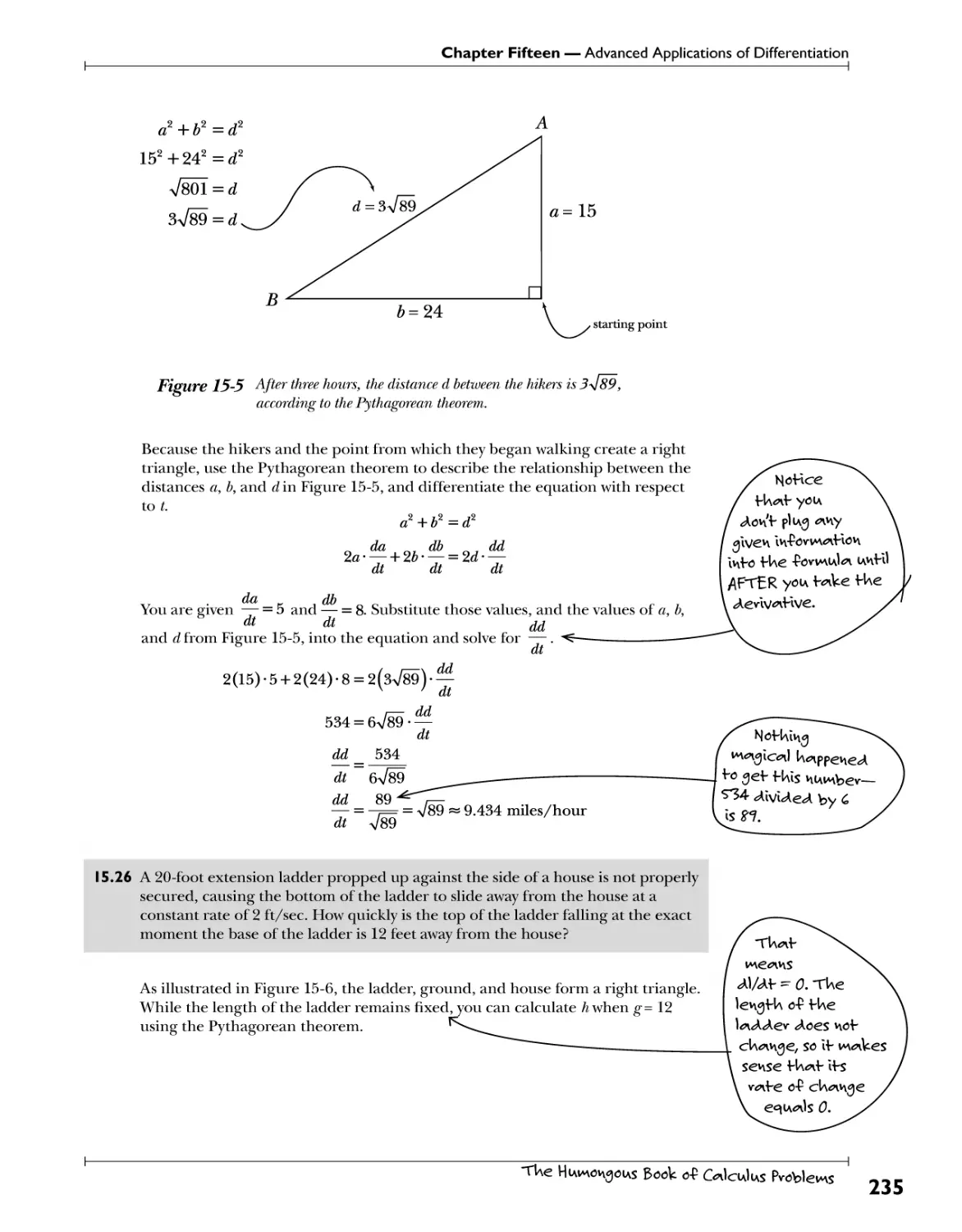
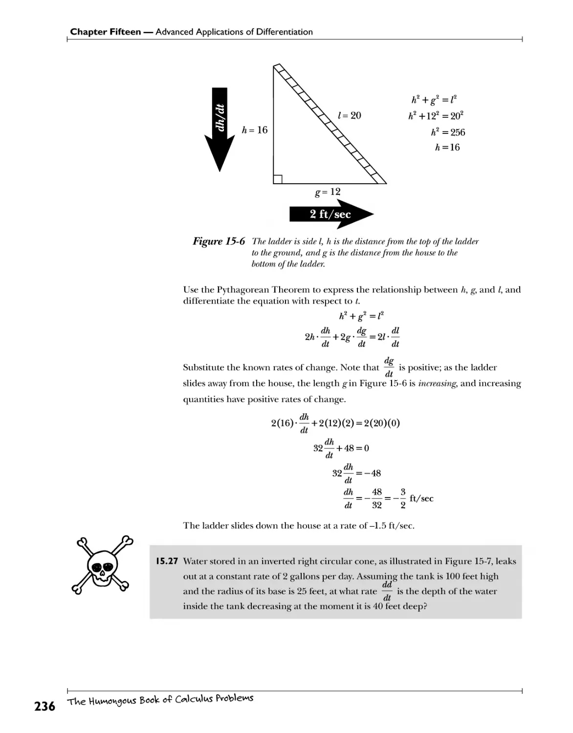
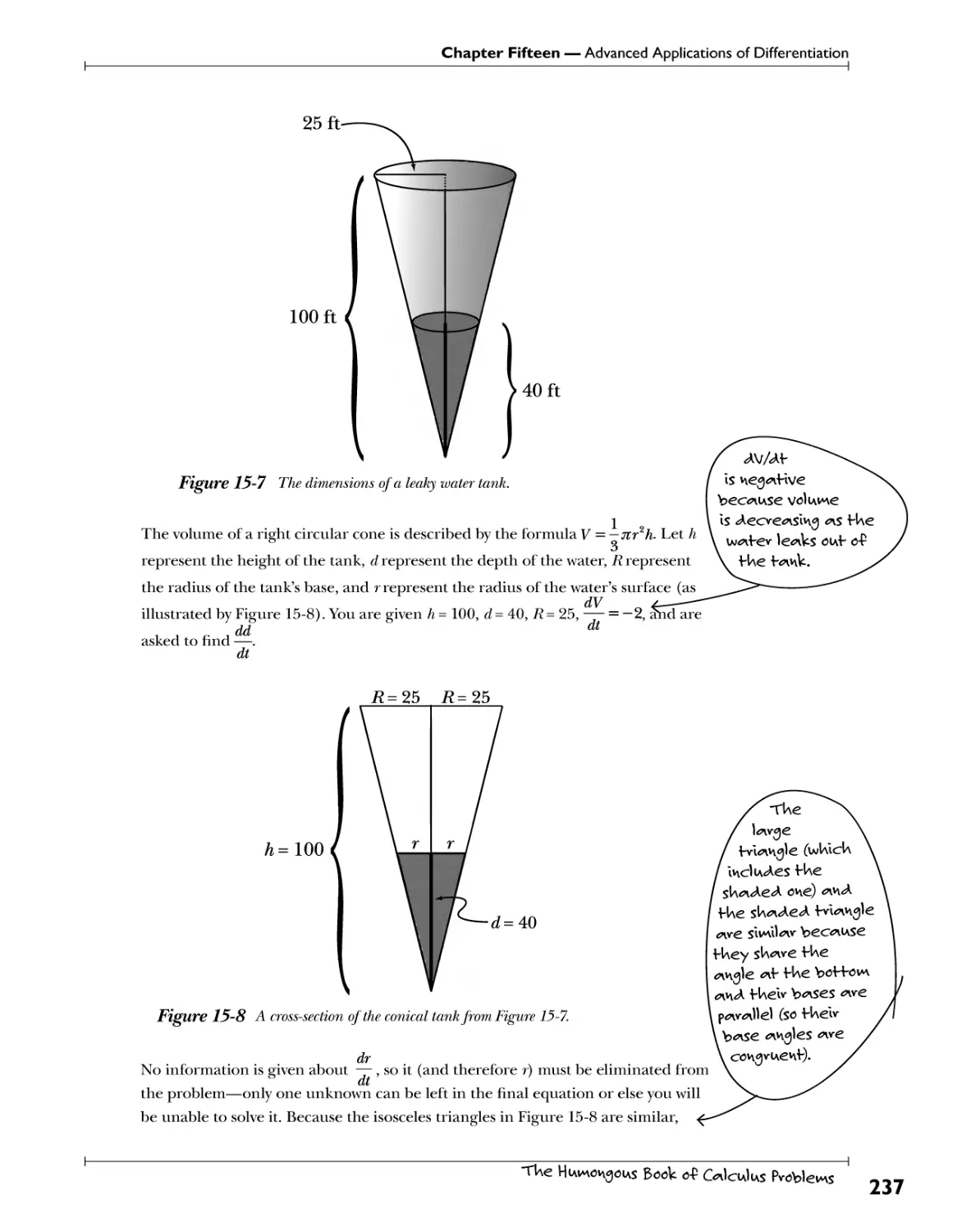
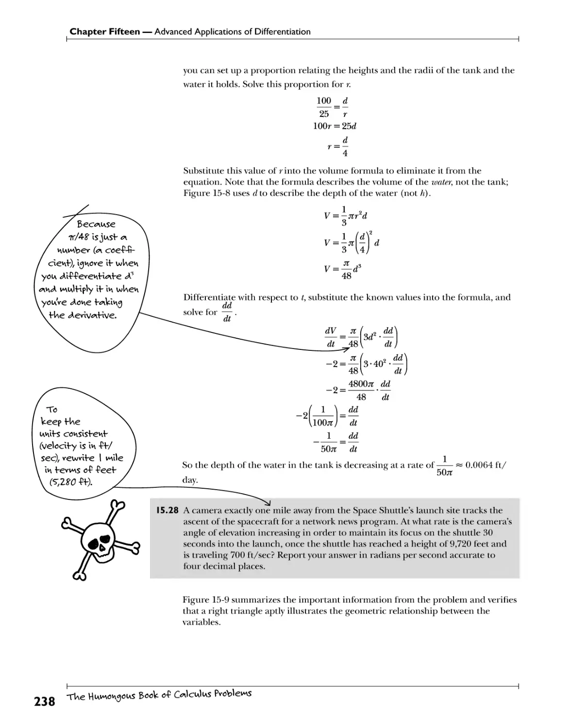
Related Rates T>3 ^Vf!? .?!*h b?.1^. .^l^V.'y .Vb£ .Y^.v.1.^)?!?.? .£^.^3?. .^ .^ .f JWr-ti??1. 233
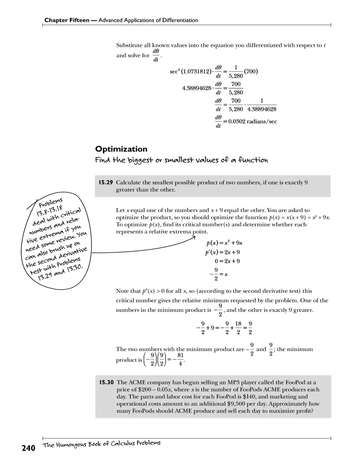
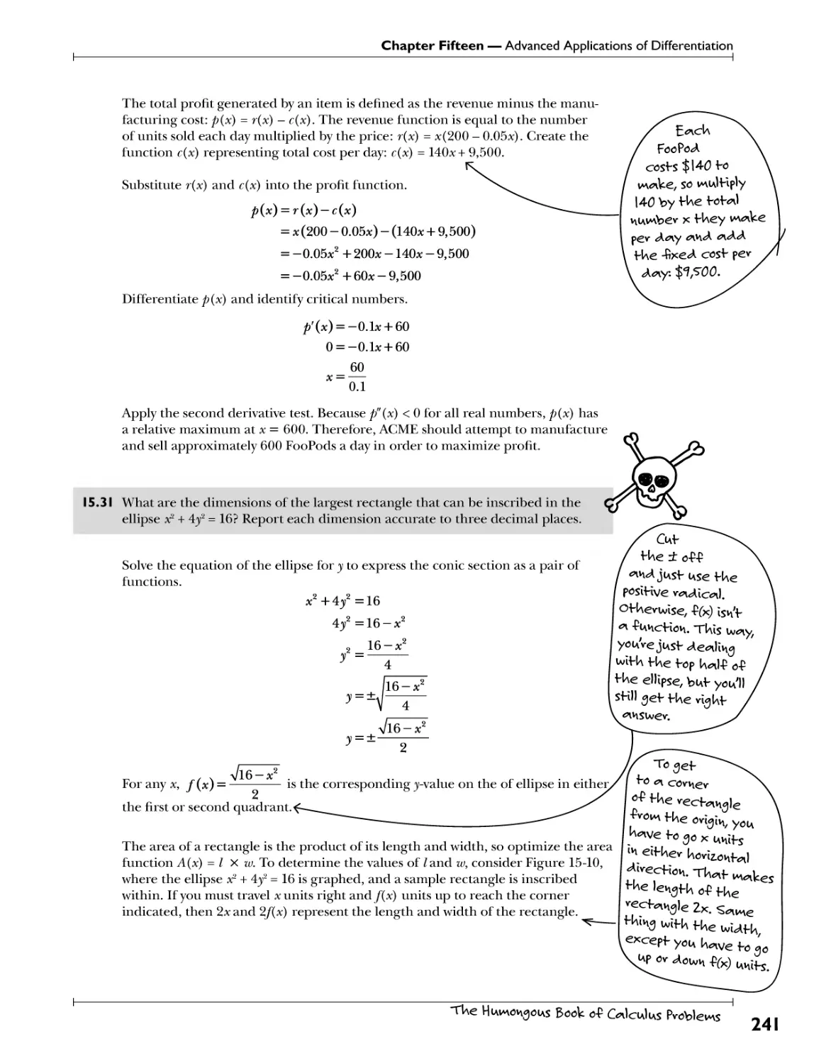
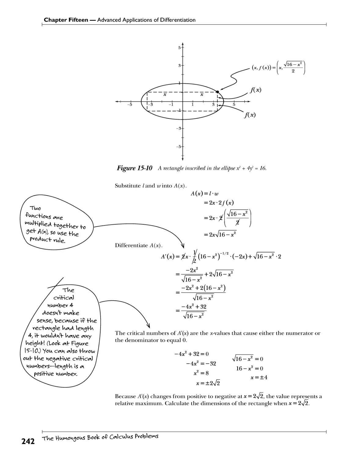
Optimization f}^. .^.?. )?!33 £?h £y. ?.v^^ll??.^ .Yf*! !*?.? .?£ ,?i .f.L>y\(r.^.(?y\ 240
Chapter 16: Additional Differentiation Techniques Yef move w*>* f0 <AU4>eve*H*fe 247
Implicit Differentiation Ess.?*t^ 248
Logarithmic Differentiation....^^ 255
Differentiating Inverse Trigonometric Functions .?-<?\L>?^ .Vh?. 5f.^T^Vf>t'.iy.?. ?."? .Vf>^.!. .^f. f^1.^.^ .s.?5? .z. ?:... 260
Differentiating Inverse Functions ^h?^. ^.^^?^3. ^^.t^Y .^?A 262
TUe HiAvnoHgoiAS Book o-P G*1cia1ias Pvobleiws
Table of Contents
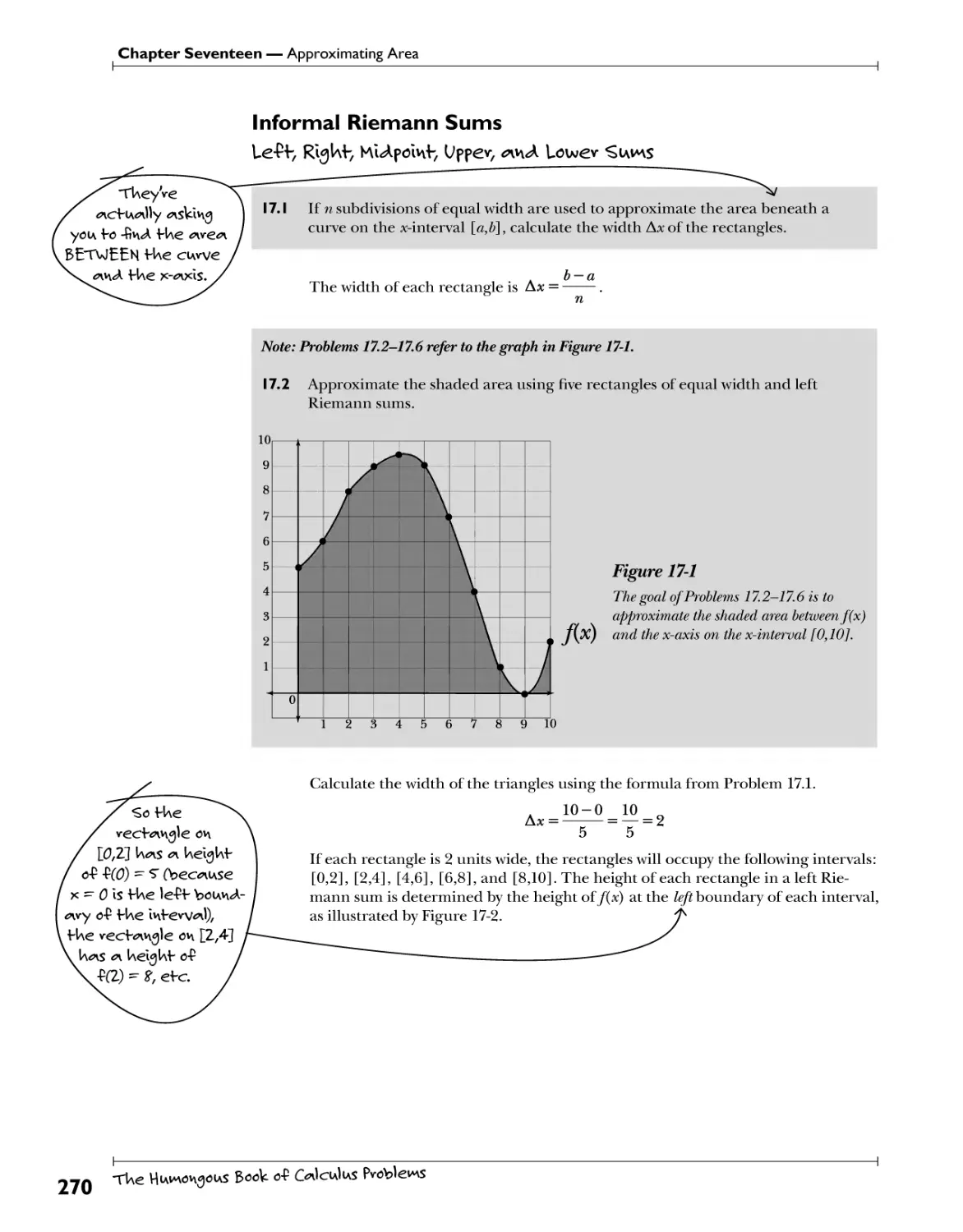
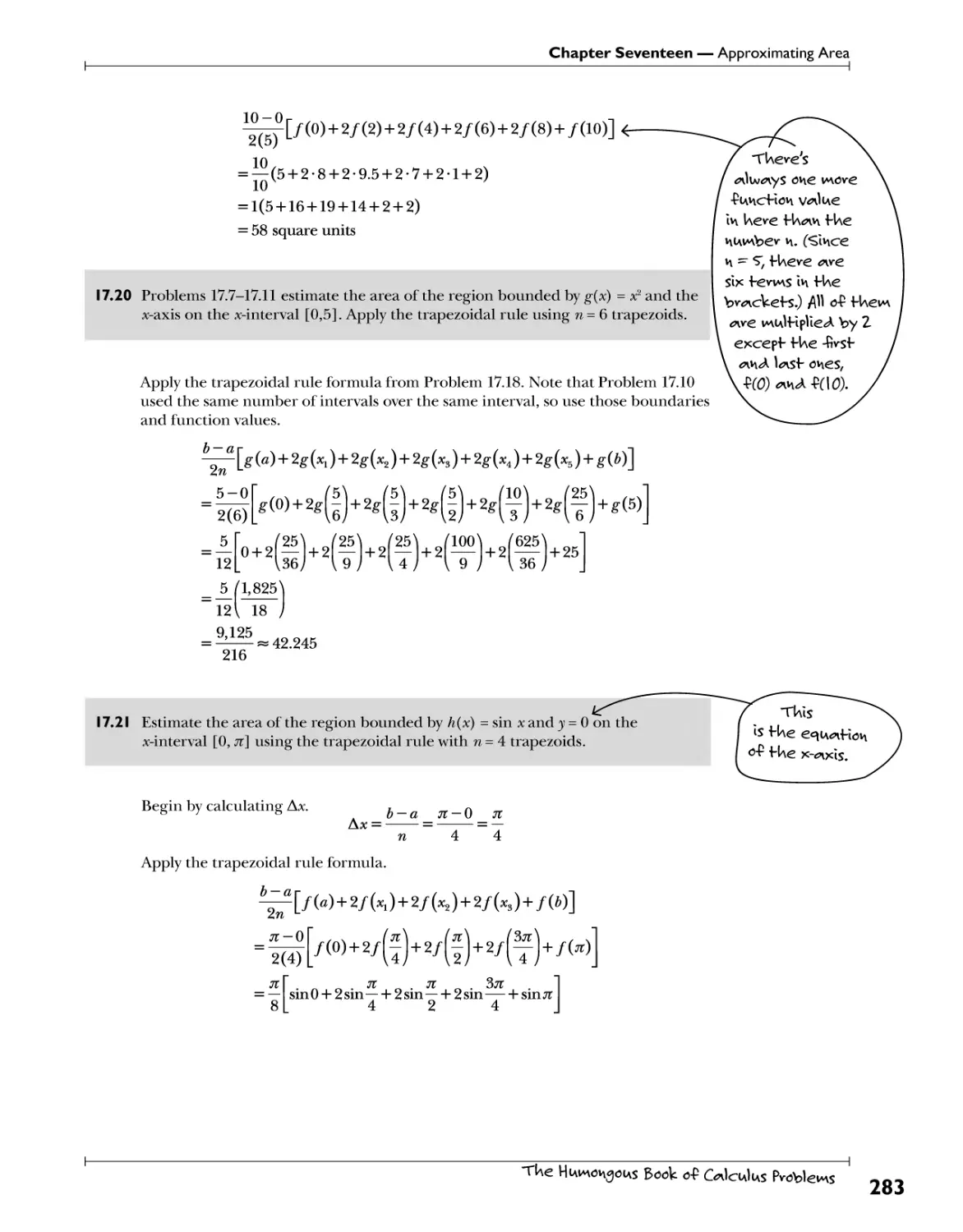
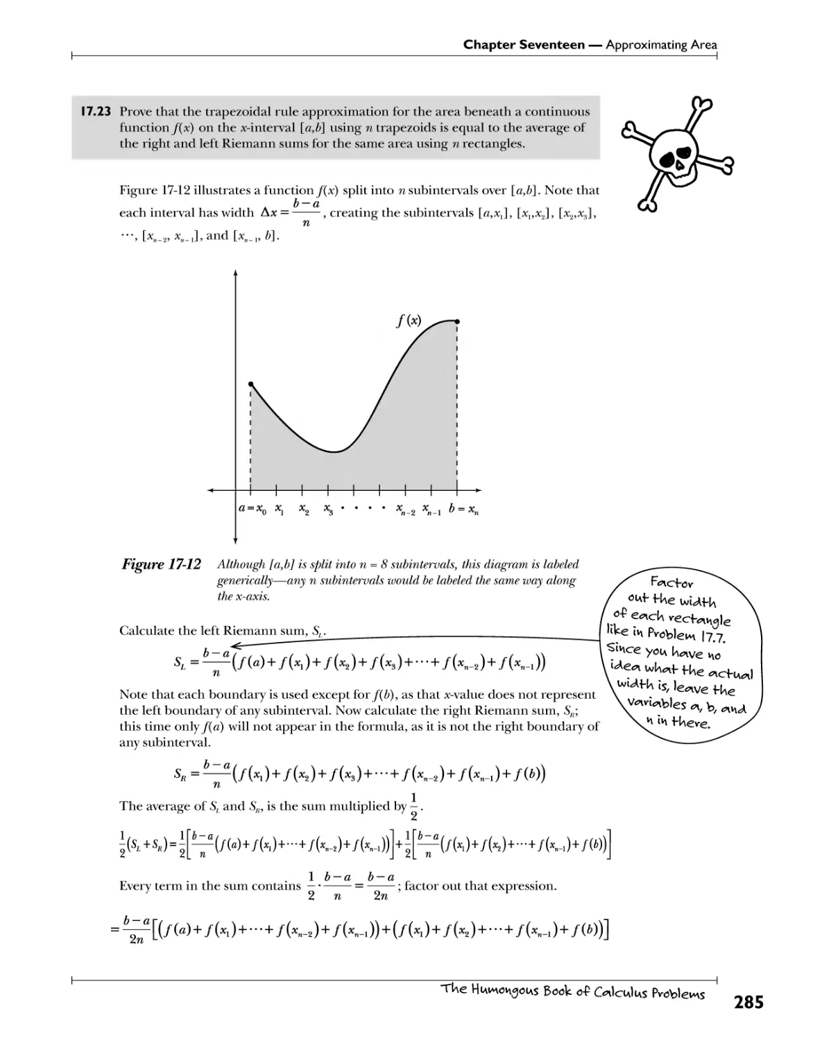
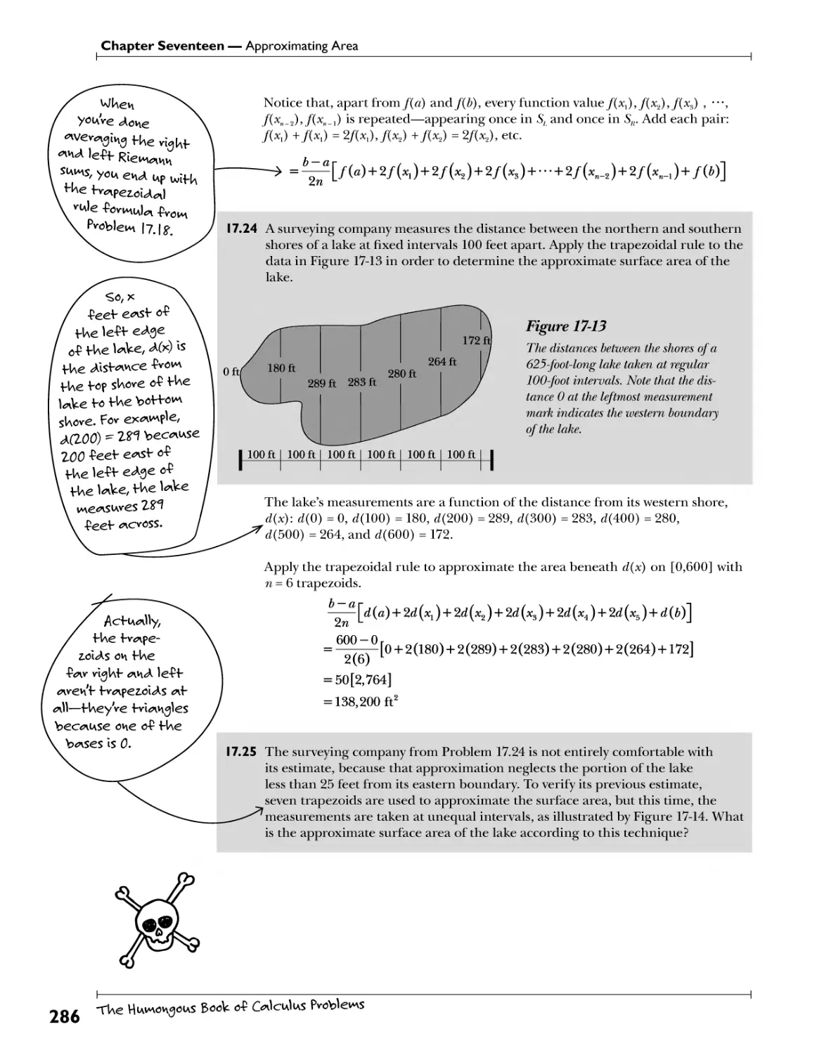
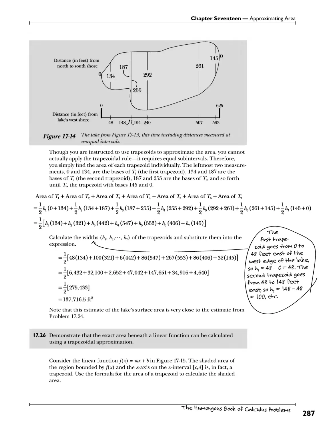
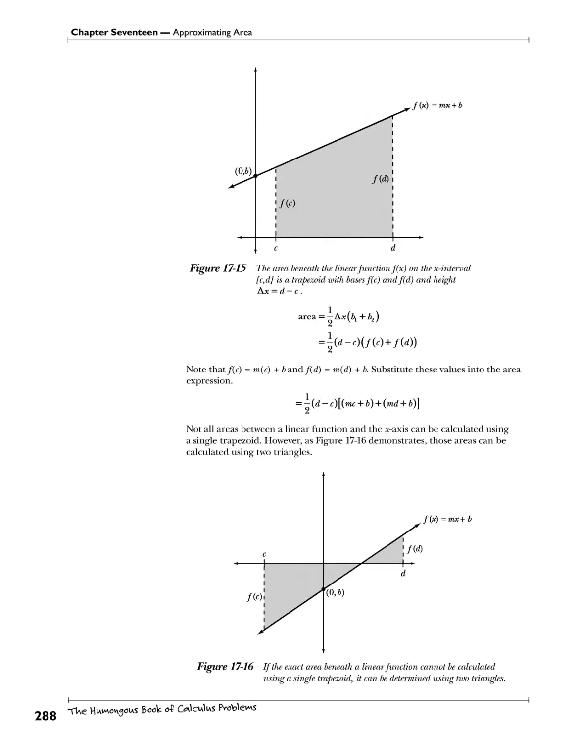
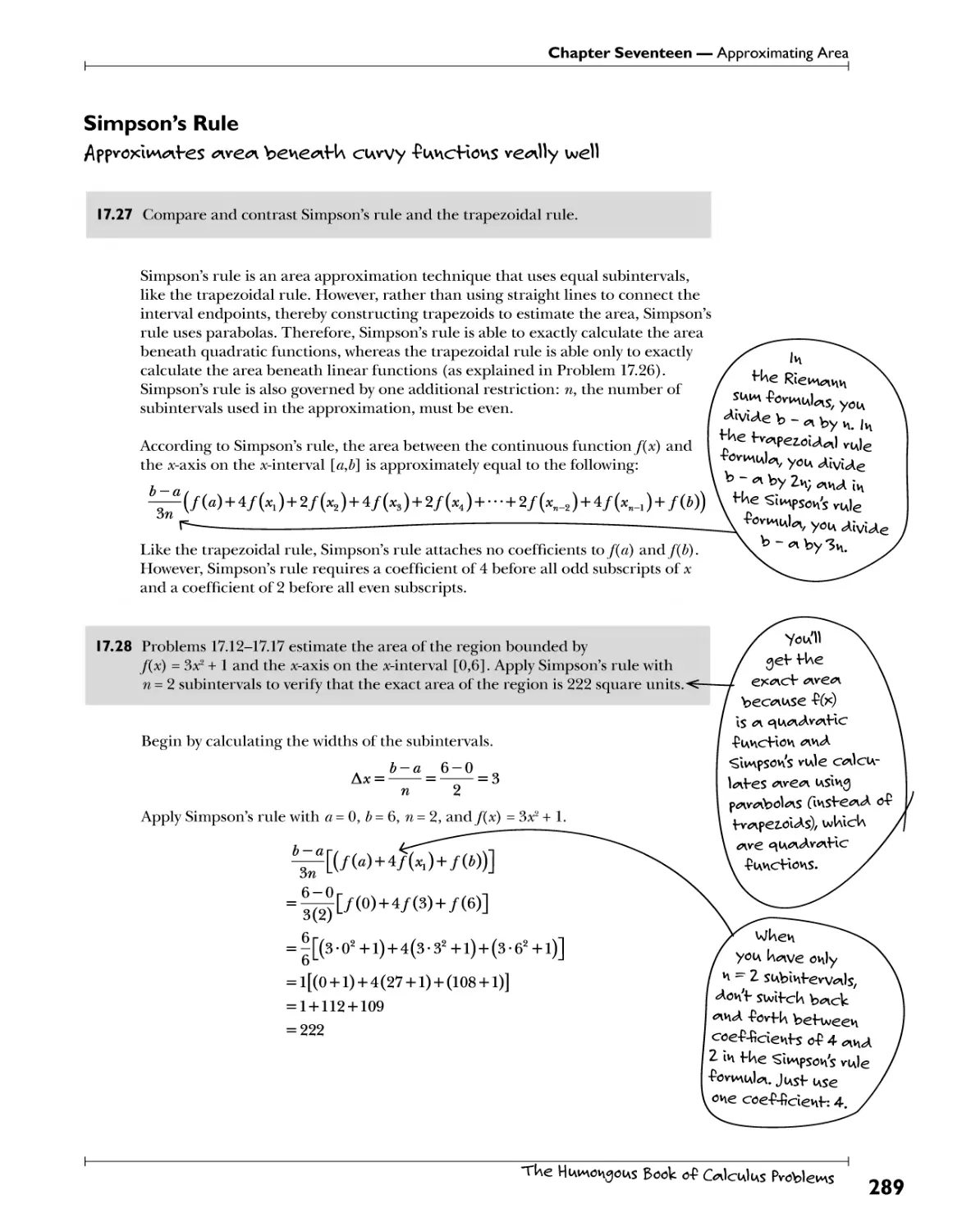
Chapter 17: Approximating Area EsHiM^ite fUe we** beHween <* cuorve <nv\<A fWe x-<ws 269
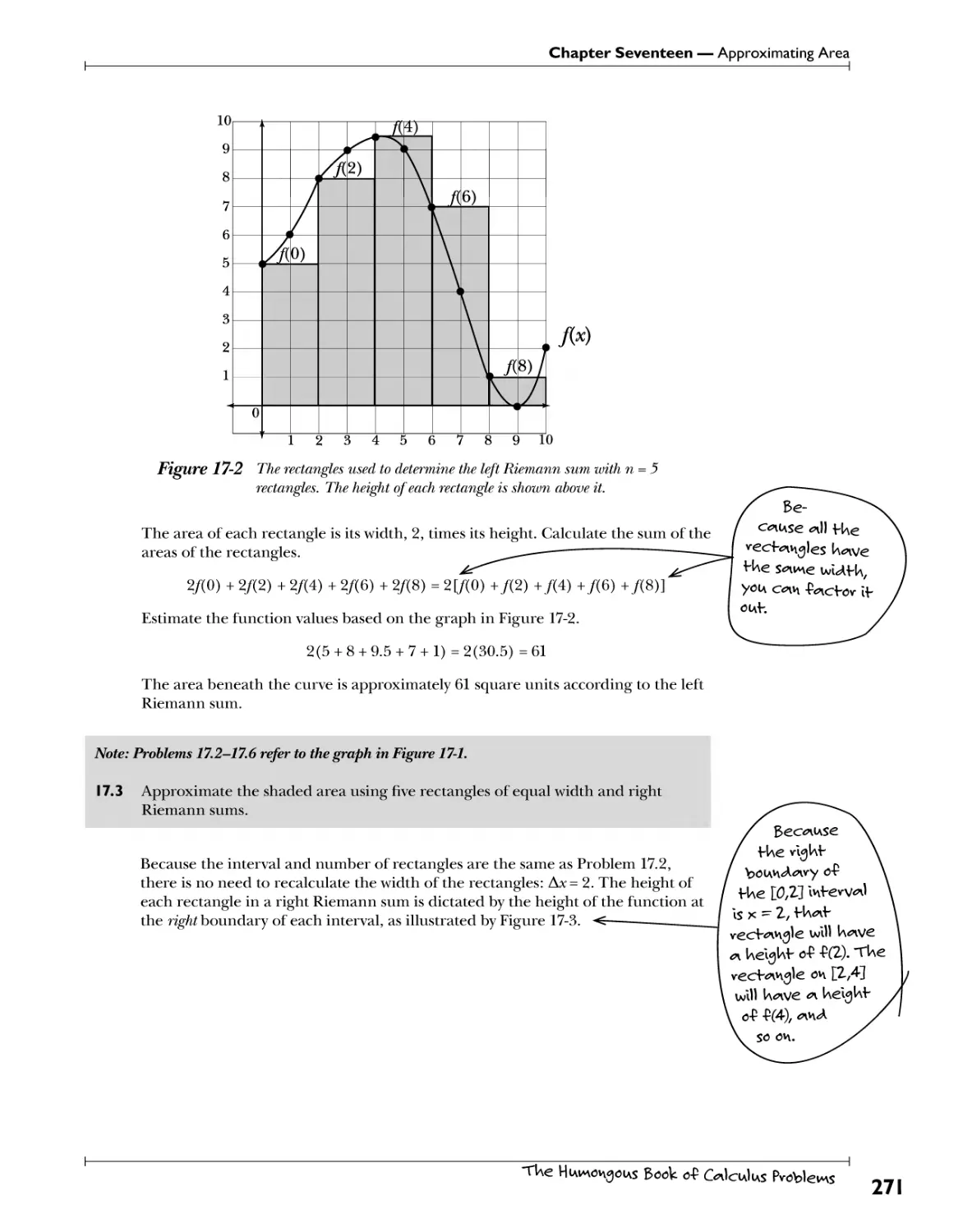
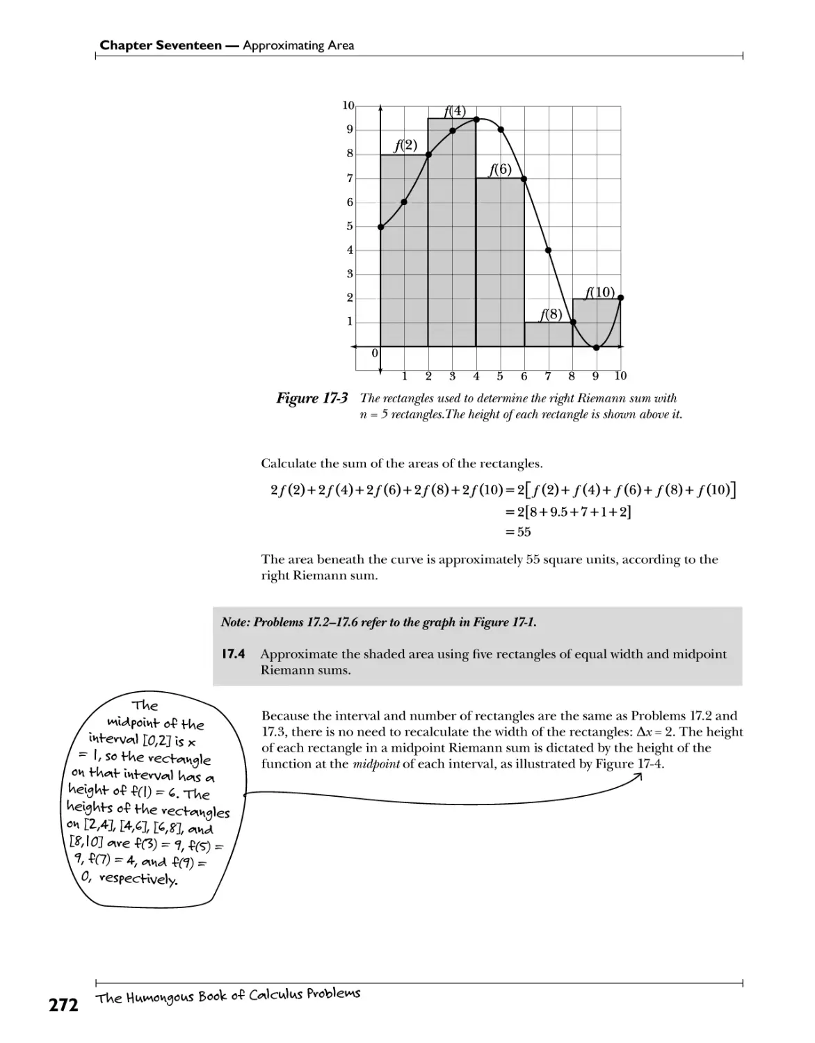
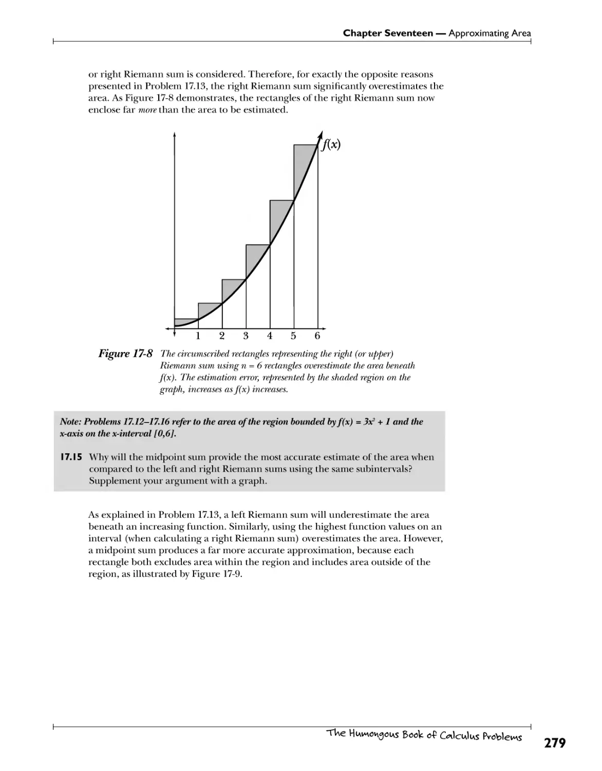
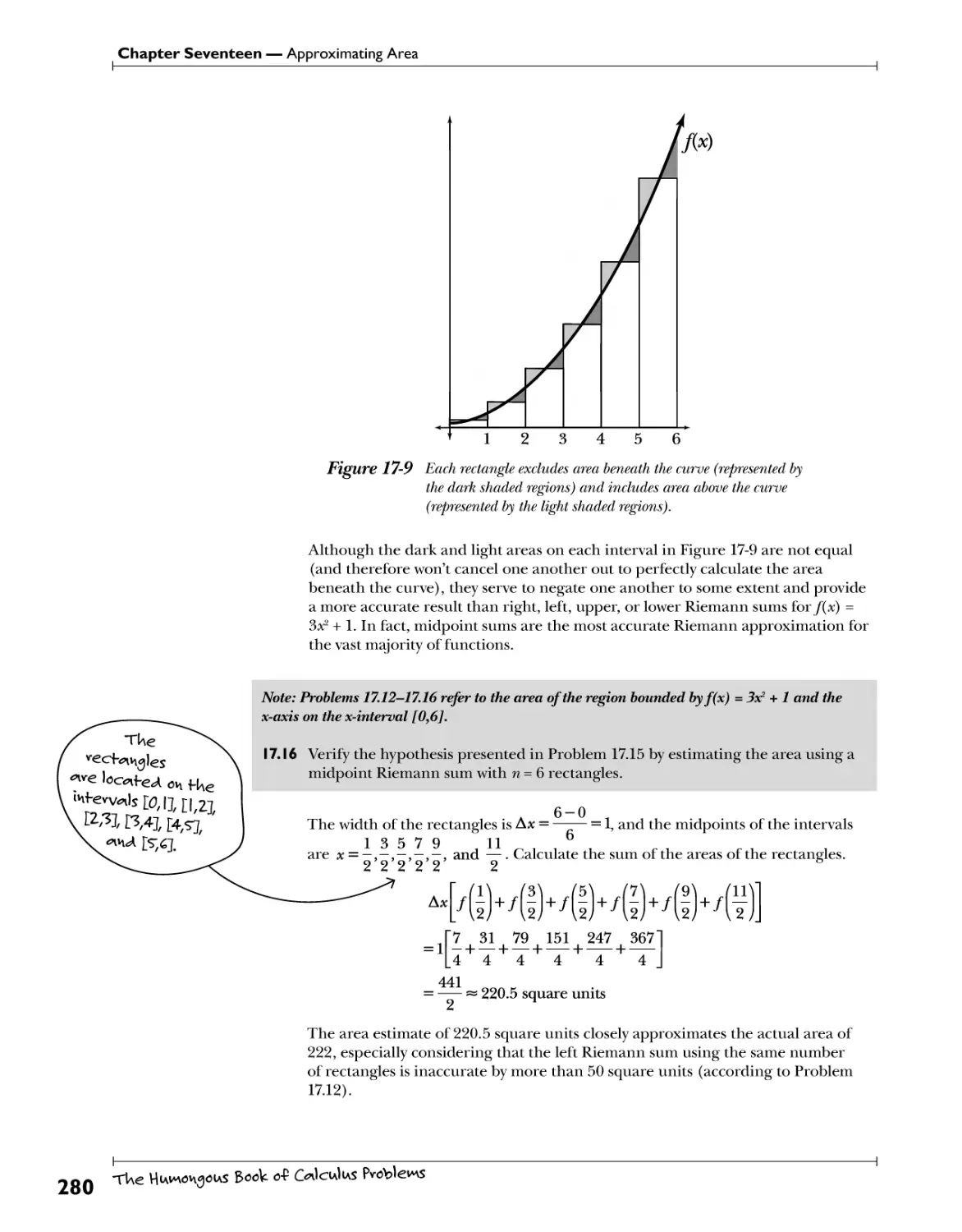
Informal Riemann Sums irSffc.rJa^/.W^KWfc.ttf P€r*/W.4. ]?*?/. .?V^>? 270
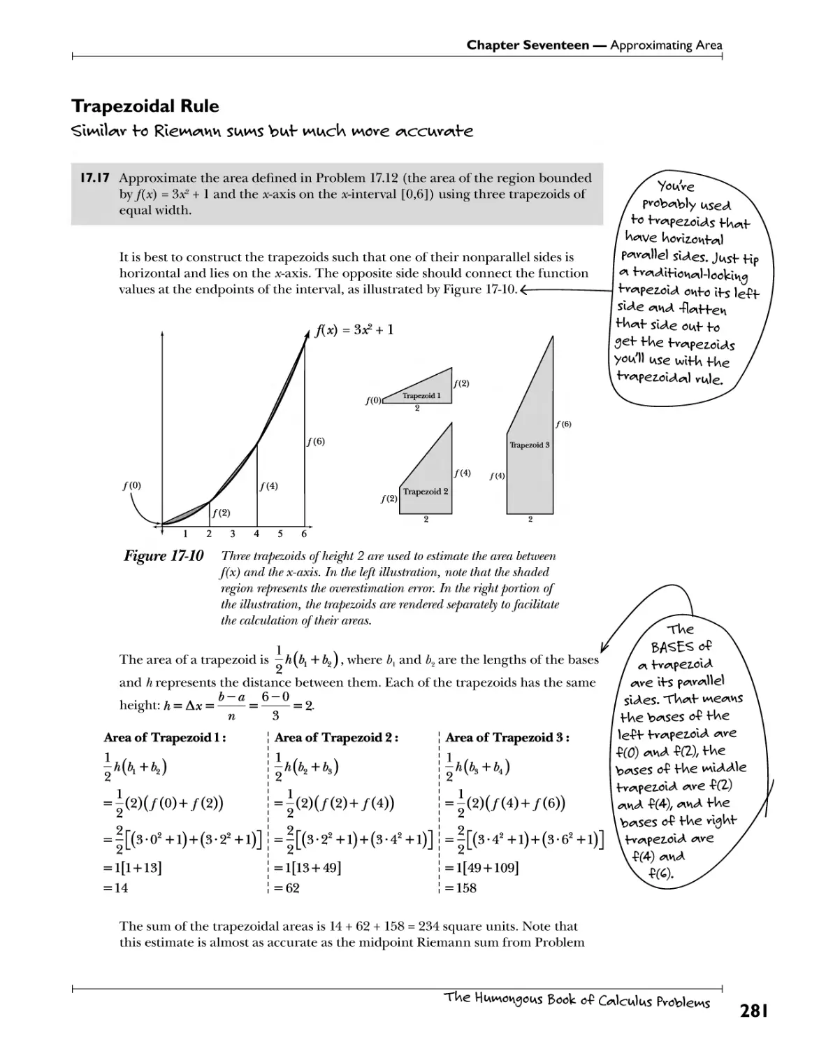
Trapezoidal Rule ^}y^)fSf. .t°. Kif^fS^y. ?.^.? .Vl^ .^>f*£^\ *^?.v".?. 5*££^Cf*b? 257
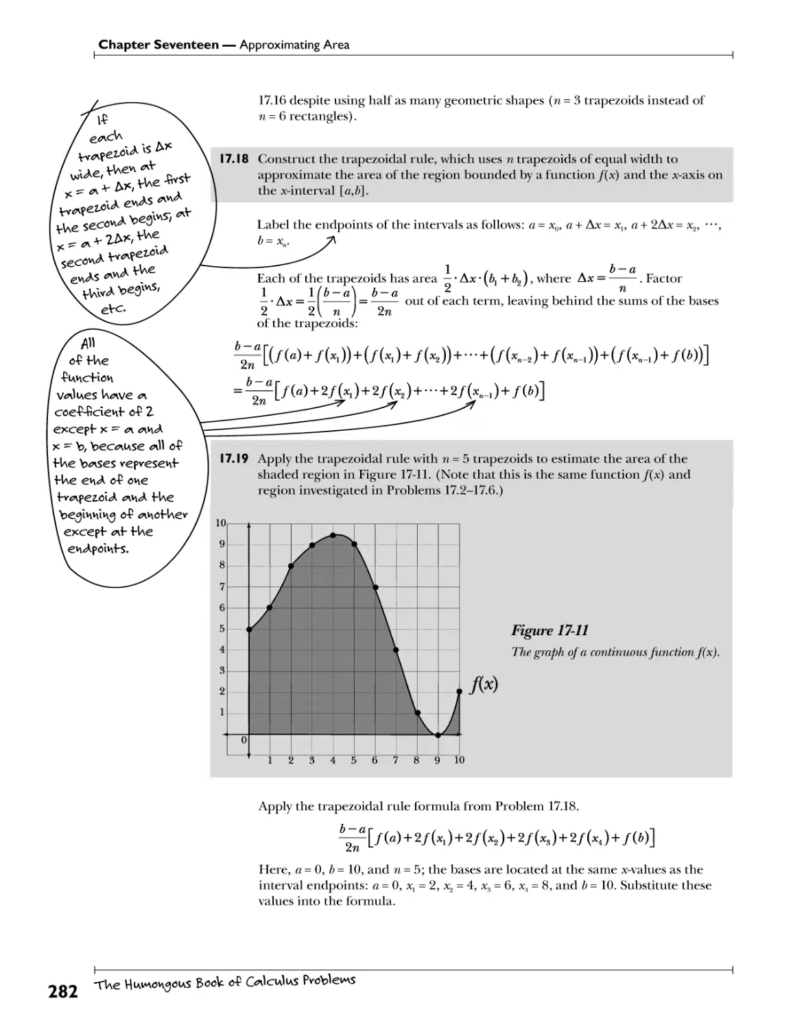
Simpson's Rule .^f.pyp.^^.^.t?.?.^^^.^^^^.^..^YYY.£^£hW£?€&))y..V0'.?)! 259
Formal Riemann Sums V?!V}? .V?f>!V*:.t?? -f?^ .YJ?^.^i"? .?^h 291
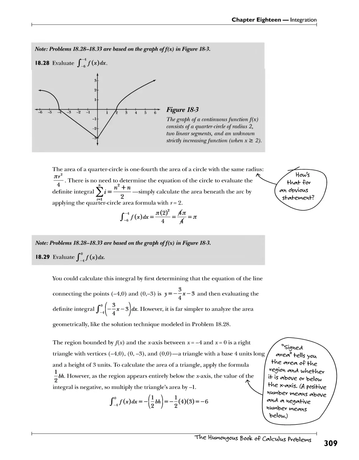
Chapter 18: Integration Now fUe <AevIv<nHve's nof W\e ^swev, If's fUe c\i\esHov\ 297
Pow*t Rule for Integration .. .A44.!. t°. ^.<?. Stf?.1^ .^.4. «#vUe by .W\e ^ew powev- 295
Tvig Wfegv-^ls look v\oW\Iv\g like Wig <AevIv*nHves
Integrating Trigonometric and Exponential Functions 301
The Fundamental Theorem of Calculus IntegraVwh .<?&A "?£& .<**€. c)?.se)y. vg\^rg<A 303
Substitution of Variables ^V^y.^)^.Vf^^!^}9^ 313
Chapter 19: Applications of the Fundamental Theorem TUW3S fo Ac wIfU ^e-fi^lfe \wVe3 3ig
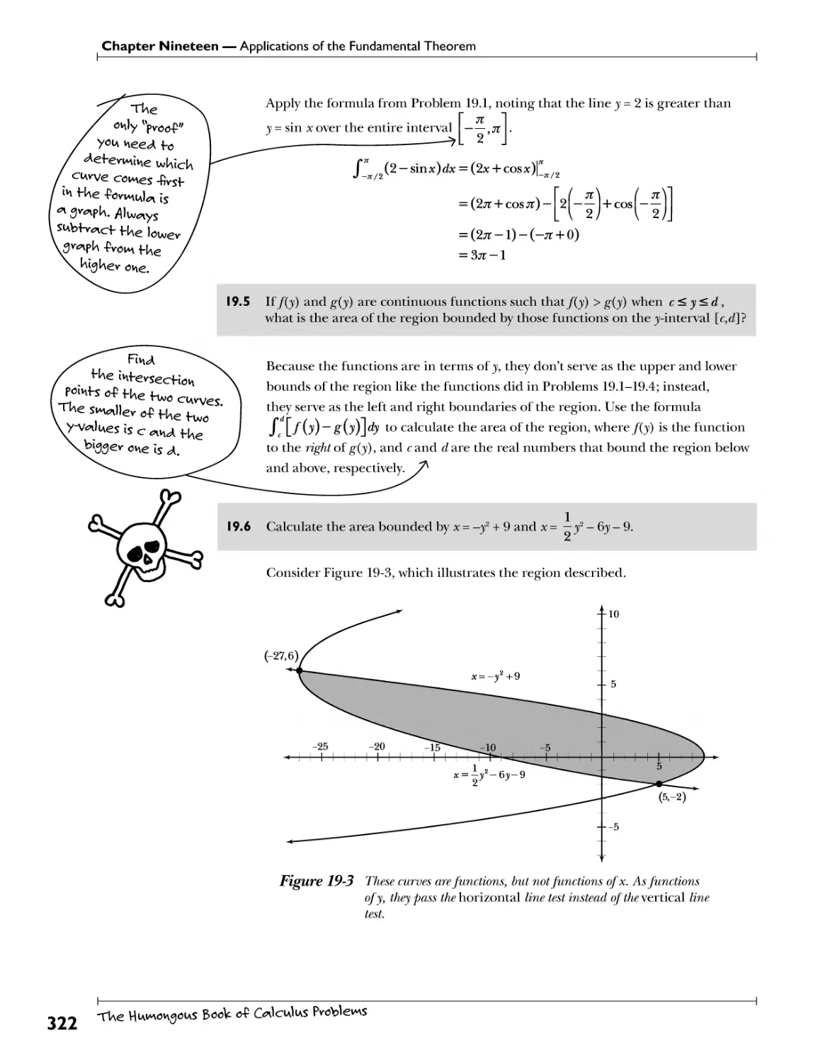
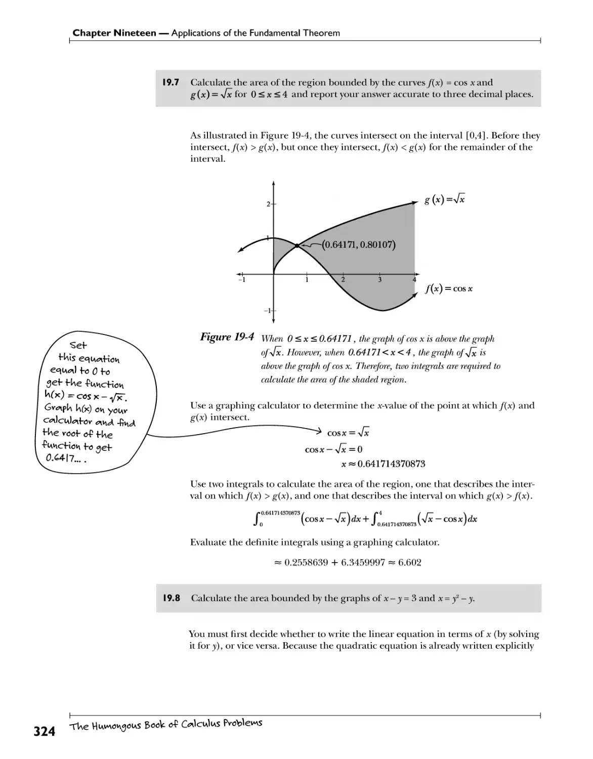
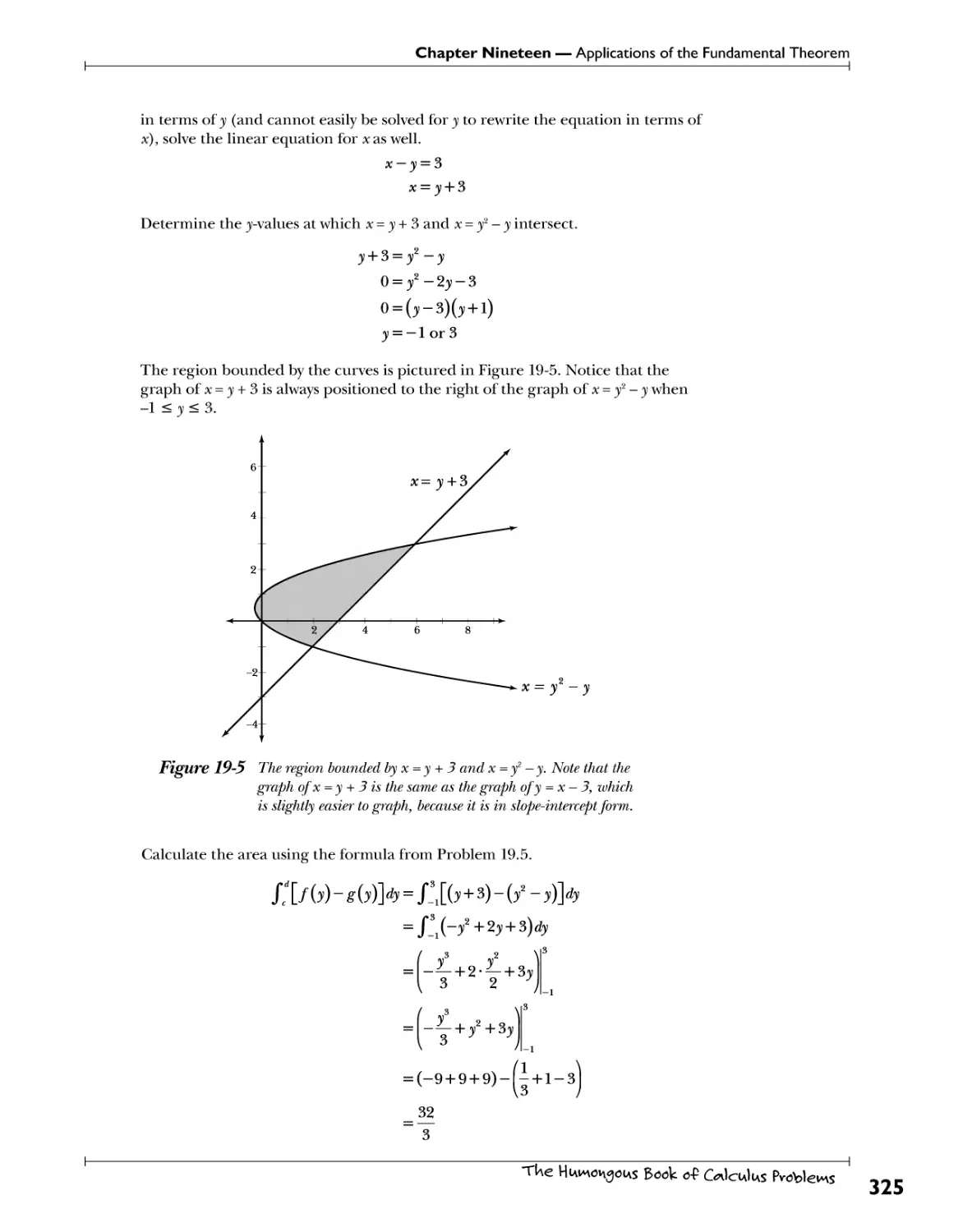
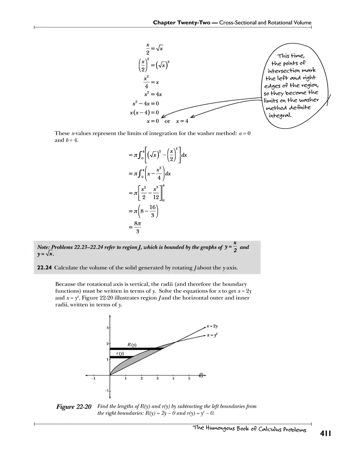
Calculating the Area Between Two Curves l*sb?*f*.?:?^ 320
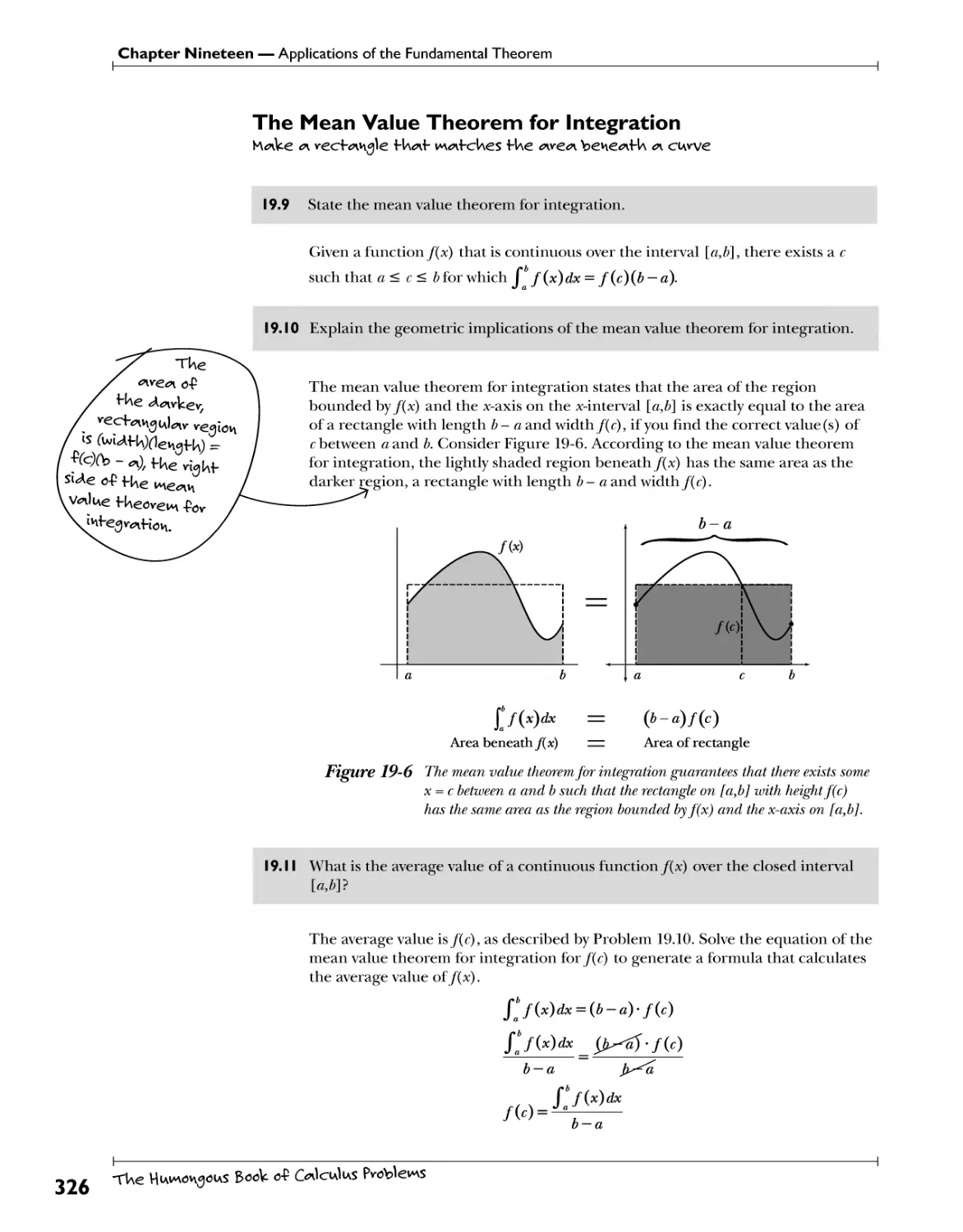
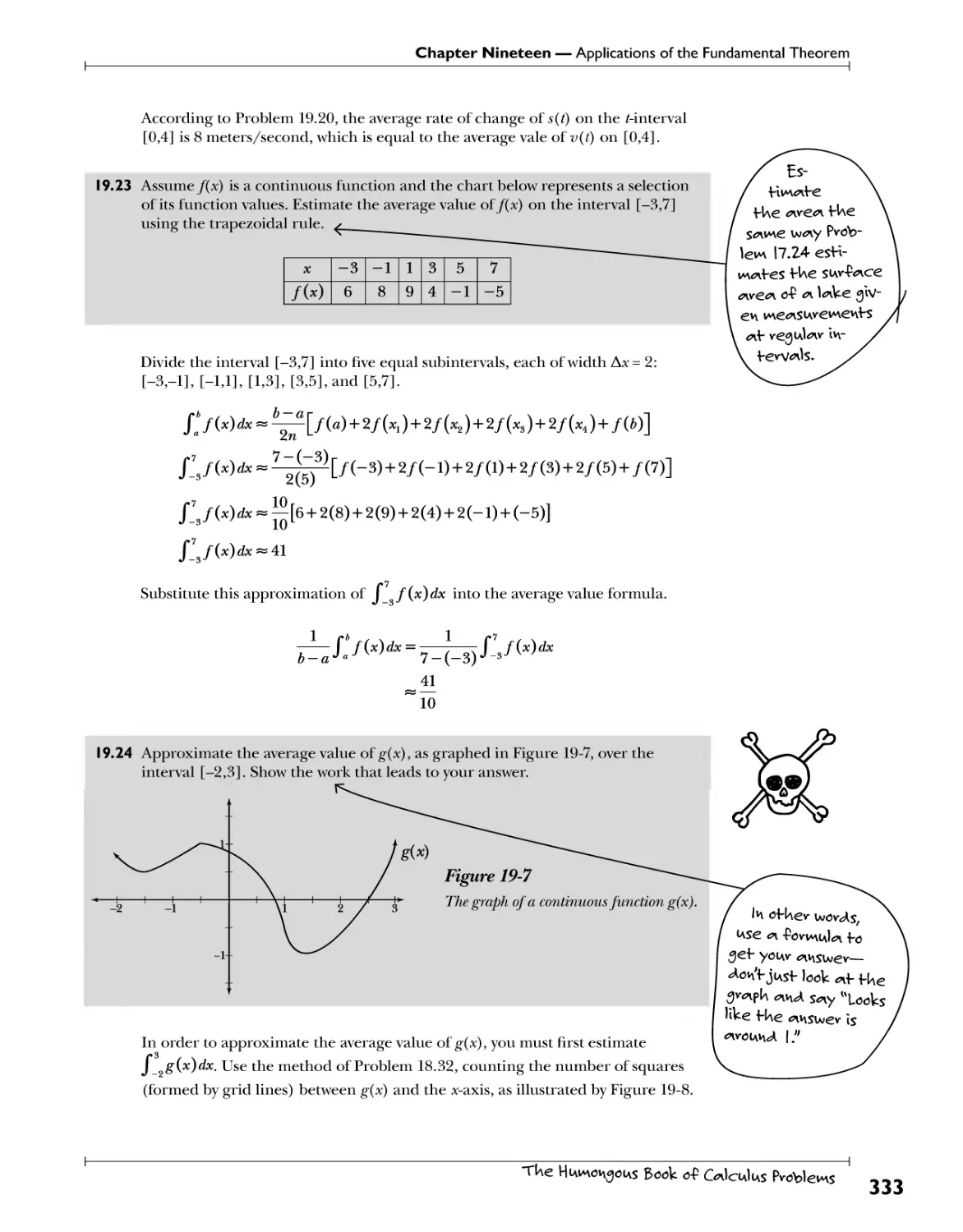
The Mean Value Theorem for Integration .S?f*fM*!fV:^^^^
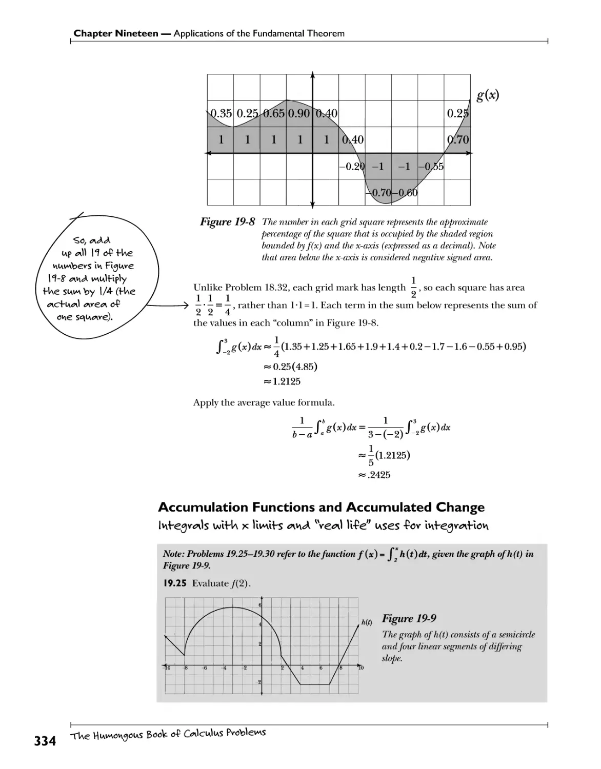
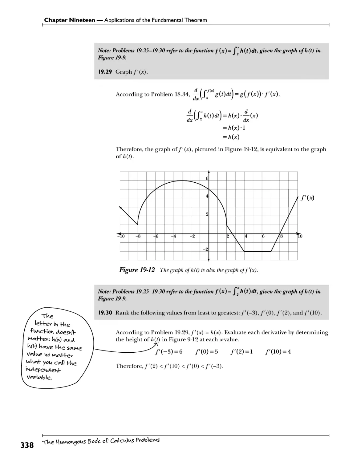
Accumulation Functions and Accumulated Change.. i?Af3Y*l$ Wfck* Jittlt?. WA !V.<?<*1 .Hfe'!.^.s.es 334
Chapter 20: Integrating Rational Expressions FwcHovis Iv\sl<Ae fUe Infegv^l 343
Separation ^Jr? .?!*?. )?!3. .^3'.Y. ^f^f; t??.^. iwt°. ?.v^^ll?y< )$??. .^3'.Y. ?.*>£? 344
Long Division V}S)^.)?.^?^.y9^^3r^^ 347
Applying Inverse Trigonometric Functions.. VSTY .^??M.^. ?.V},.Y. !* £€#?*?. f^?.^?h^>9?.?.. 350
Completing the Square ??*.fl^^*tf£?.4?.W.>?<?lw.^4.*<? v<w*V?)€S.W.YfiX 353
Partial Fractions A $<&&/.*?&. *?. .Vy.?.^}:.^?.^.^. ^f>£ti0*?. 357
Chapter 21: Advanced Integration Techniques EveH ^0ve <"*ys ^ -R*uA integwts 363
Integration by Parts !t'?JAV£±^?.f:^ 364
Trigonometric Substitution.... V.?1.^ A4?*t*£« 5^.^^. lltt:1^. r>ab^ .t.v.l^.v}3} ^. ^^ar.^^?. 368
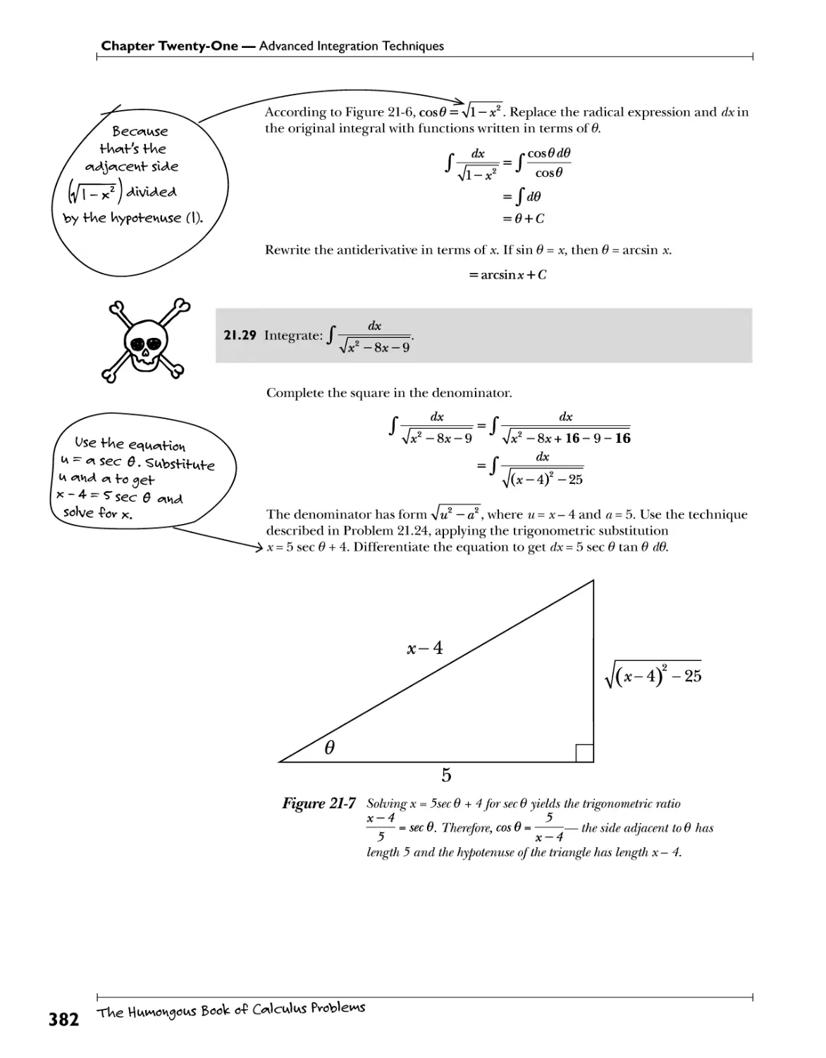
Improper Integrals ^3^3. .^?P*?. *?y^f.t?.^ !*£. ^f.^.^f.^fjr!?.? 353
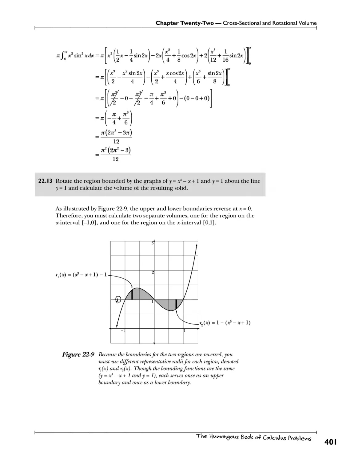
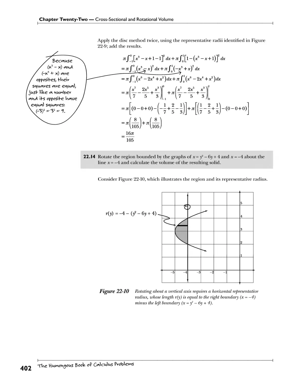
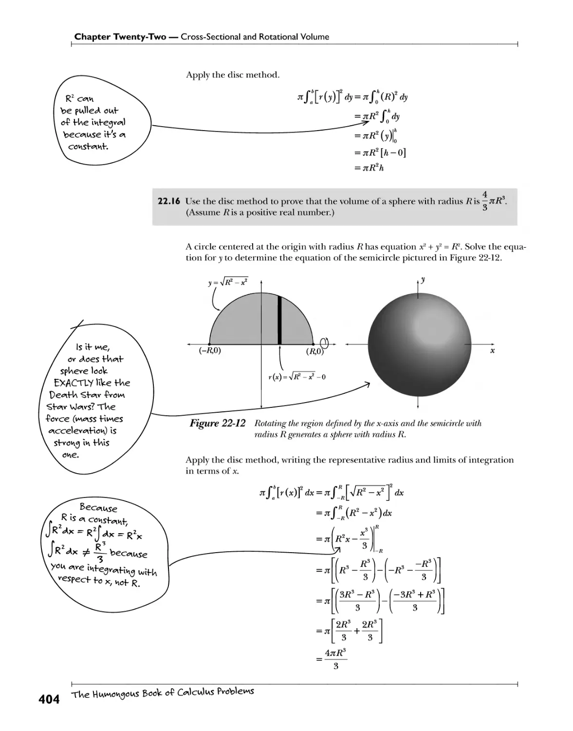
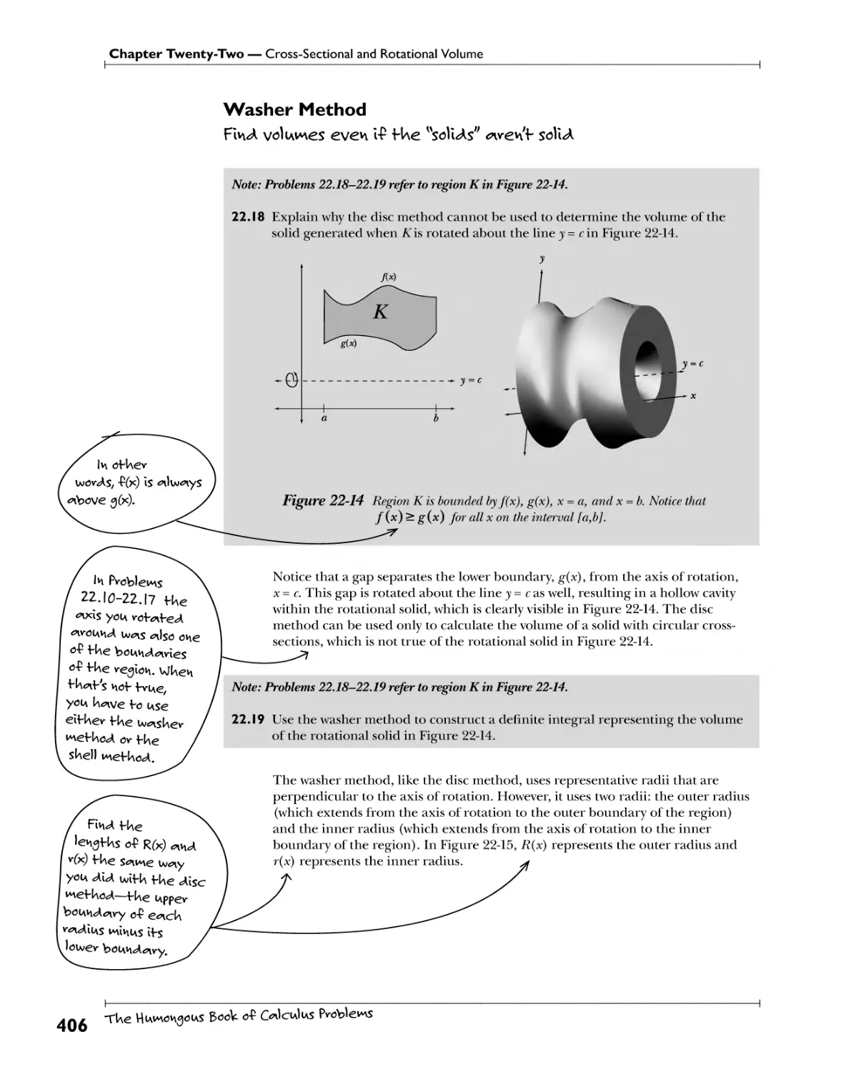
Chapter 22: Cross-Sectional and Rotational Volume^ ?^ 0H y°^ *U^ "v VU* ^389
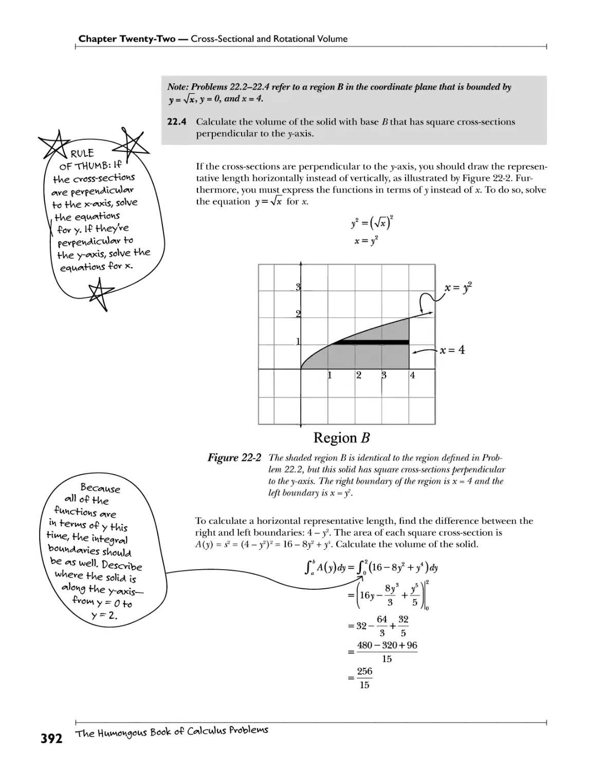
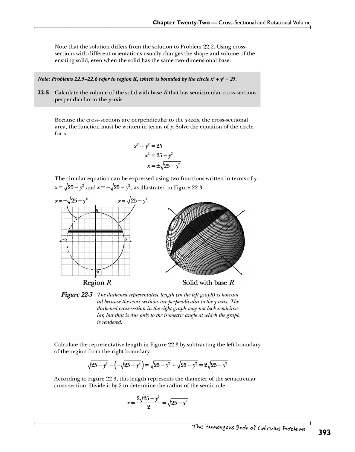
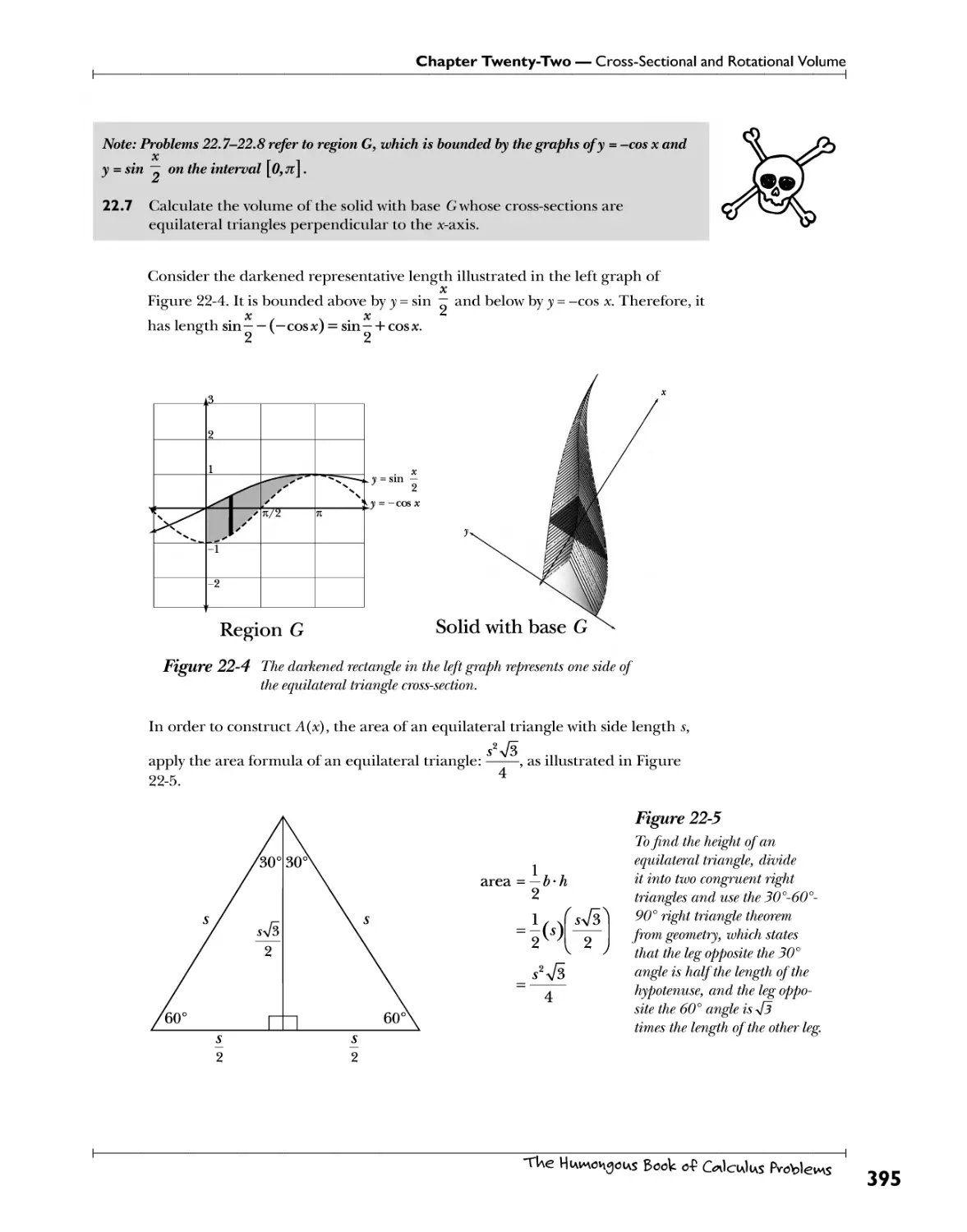
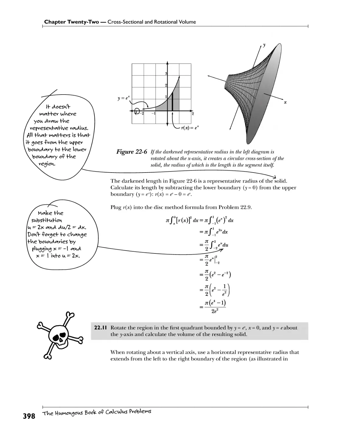
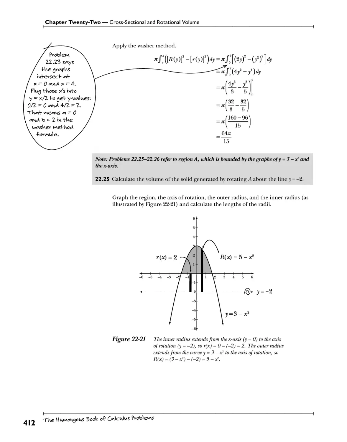
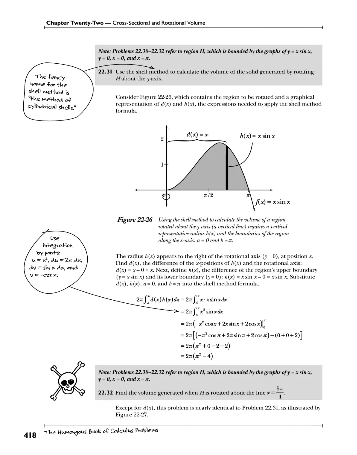
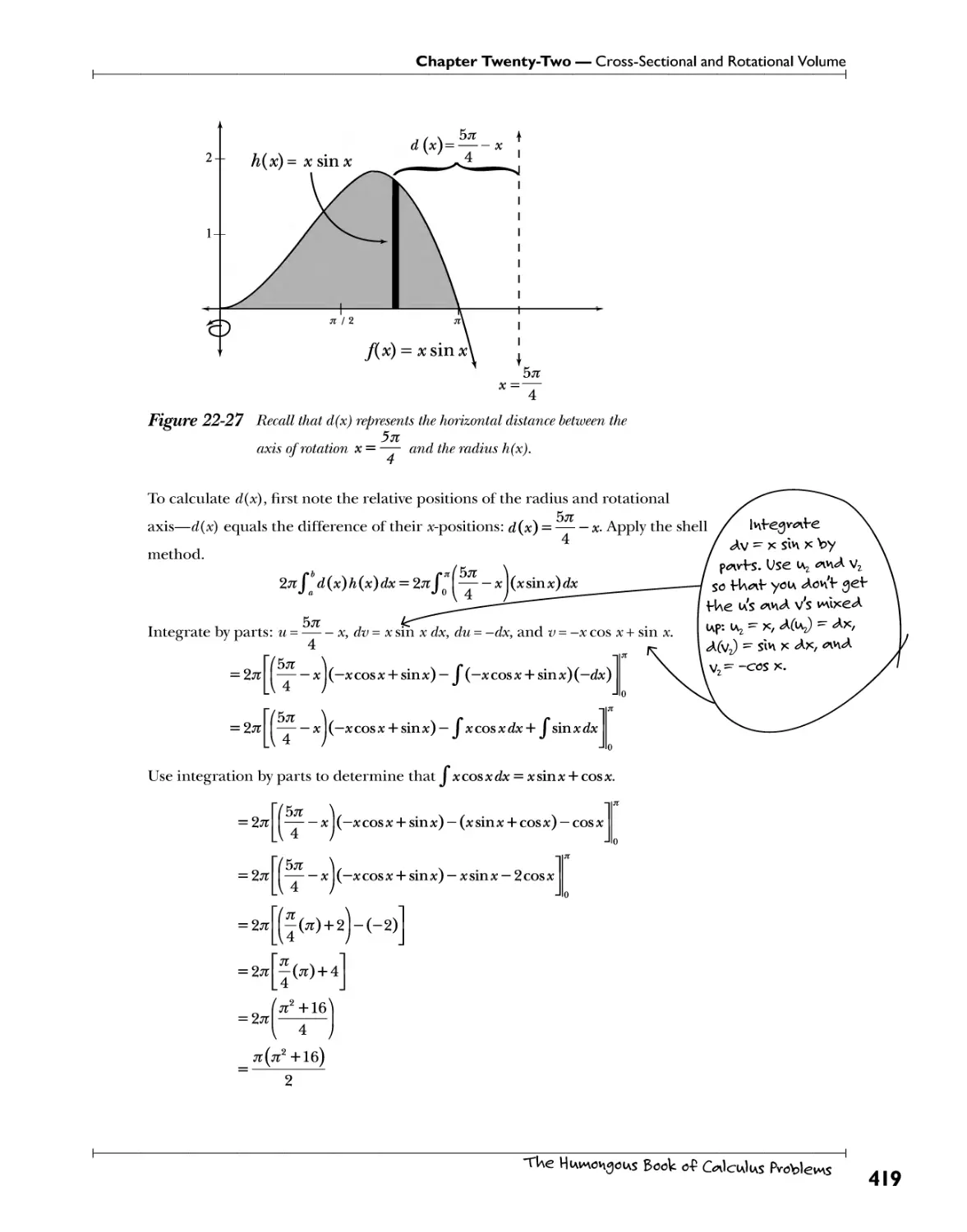
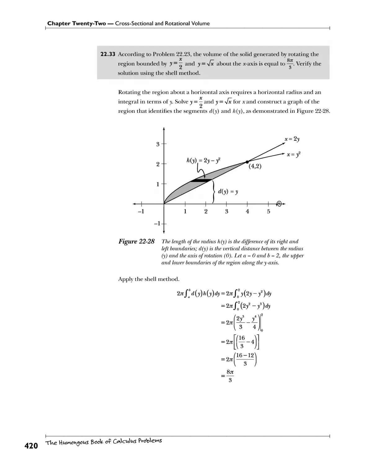
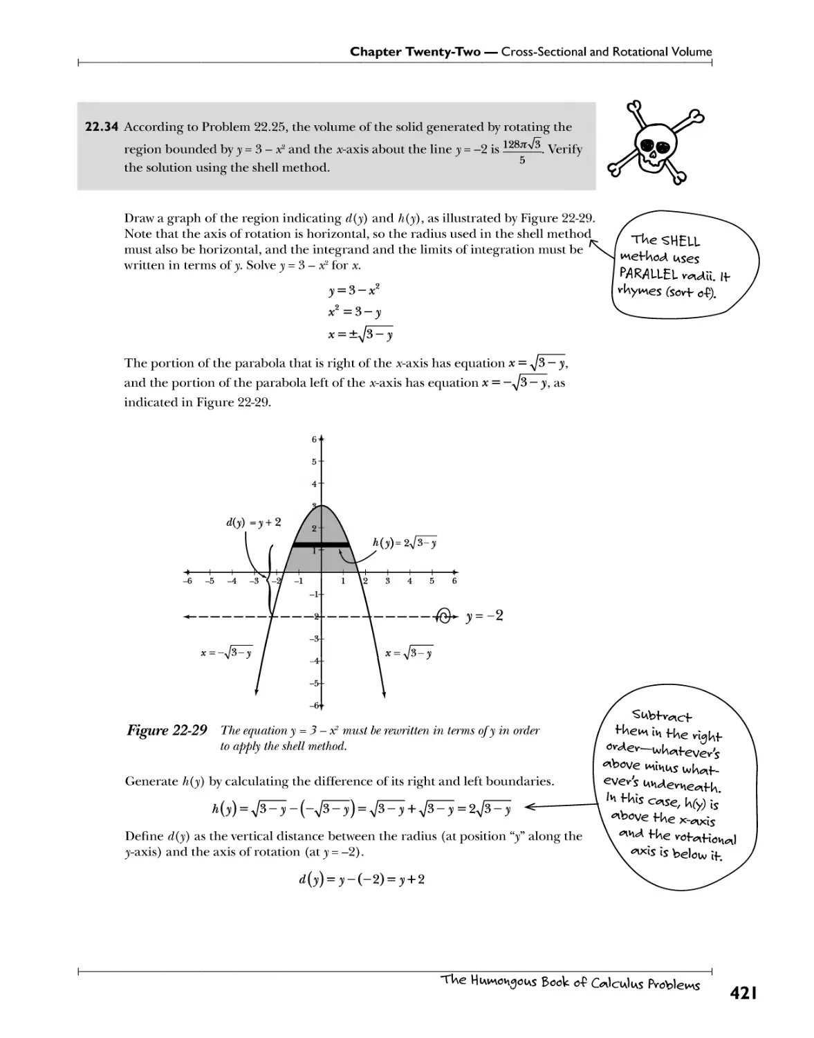
Volume of a Solid with Known Cross-Sections .Cvs+: .^^ A^M An^.el^^^^.^sn^. ^r^^^^r.^ ±K0A^.ln?^.^v^.. 390
Disc Method Qydgs. *?£. Jrh?. j^^su??*T-P?.??\\0i?. f?T?-??"?S^*ri?}l? 397
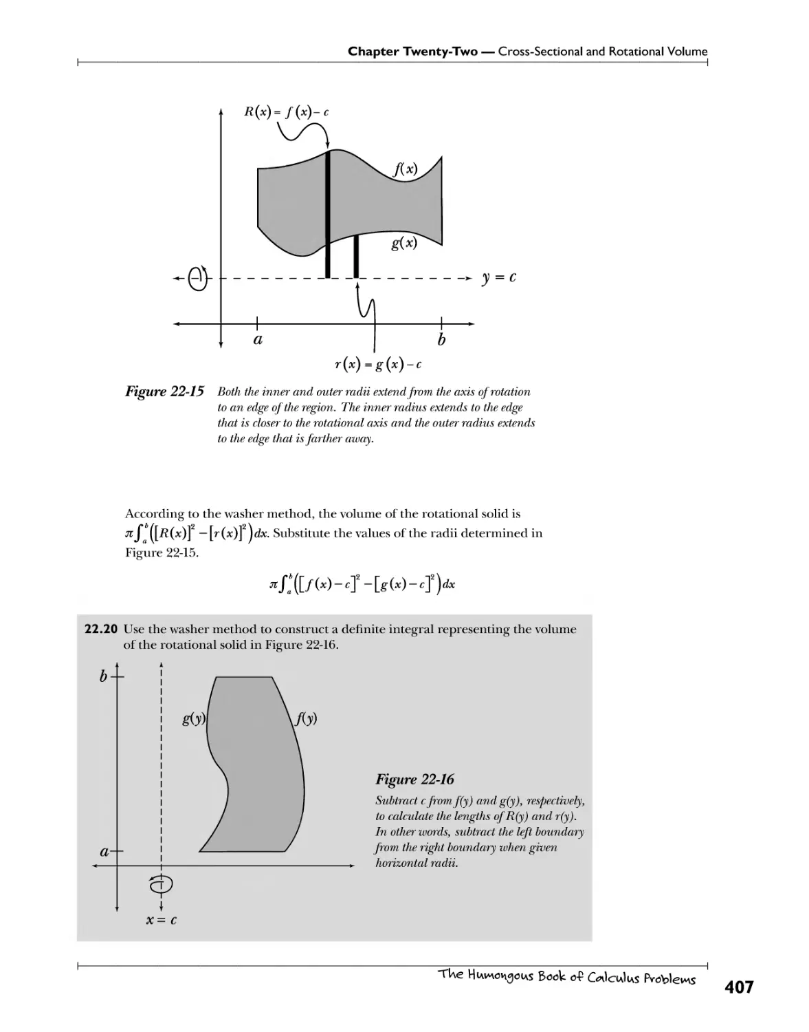
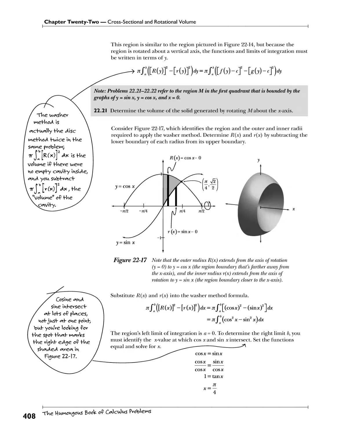
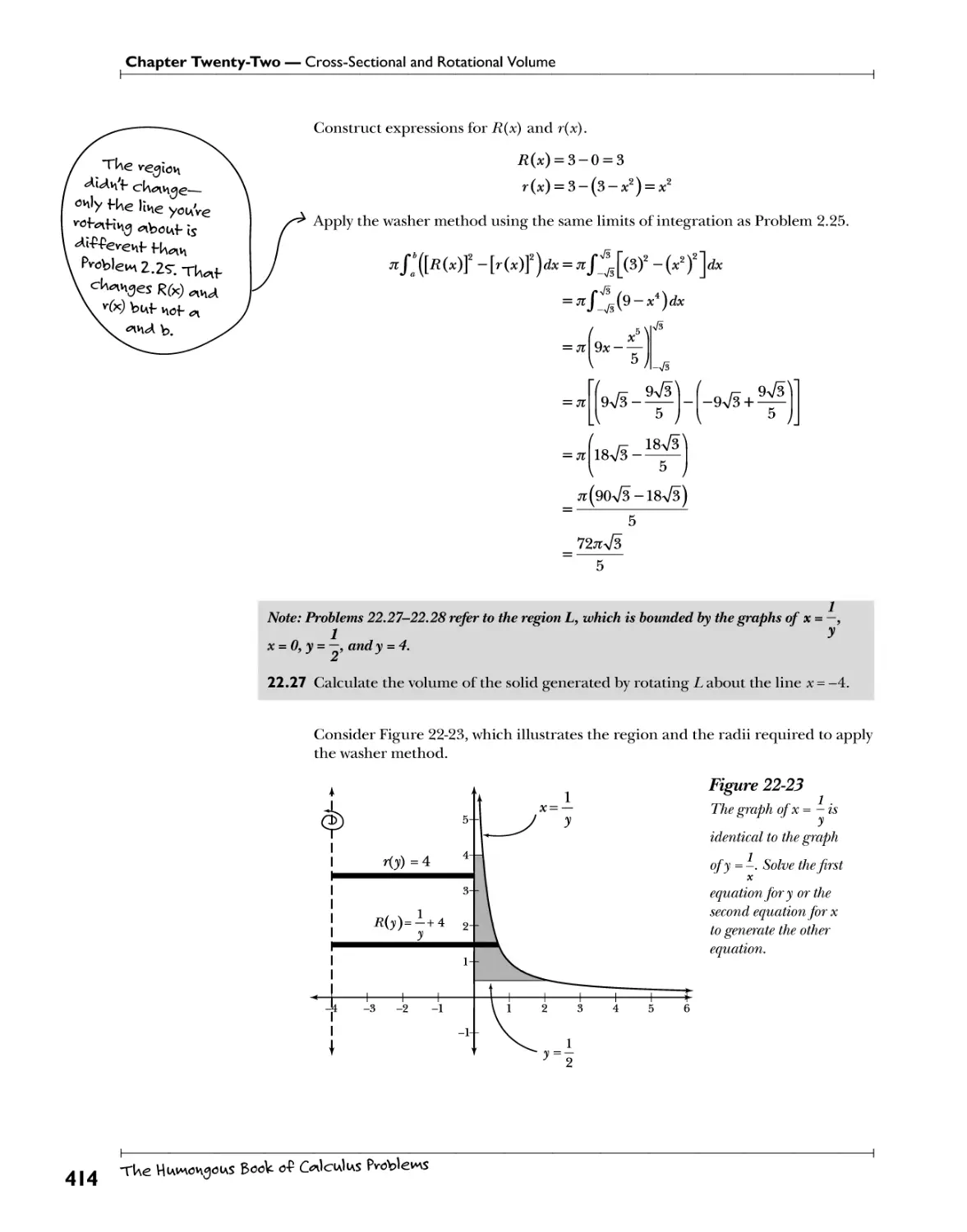
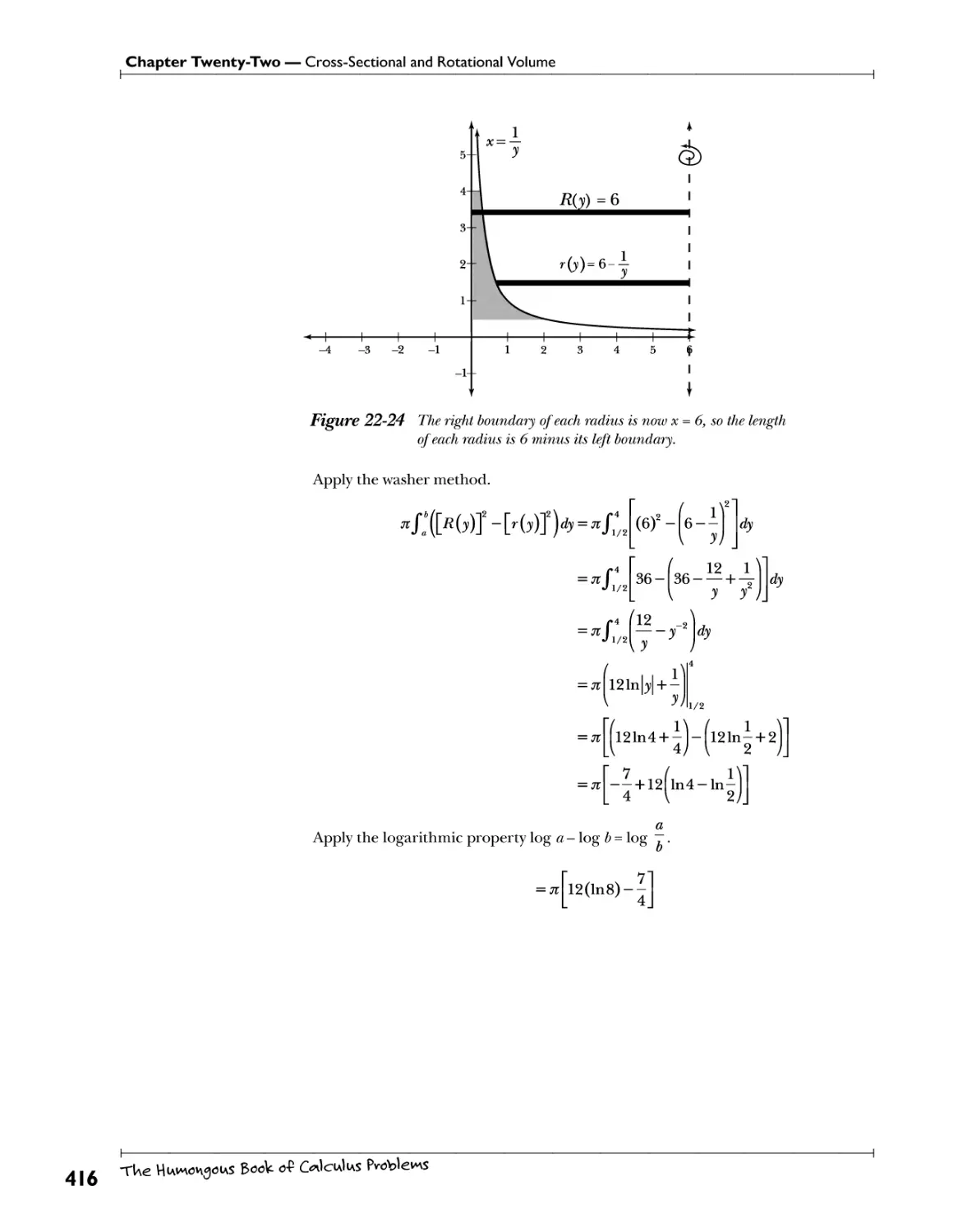
Washer Method P*i*. Y?! Wtt£5.£Yi?!* A"?.h^.??P.'.^.s.w **?*!t.5?.)}f* 406
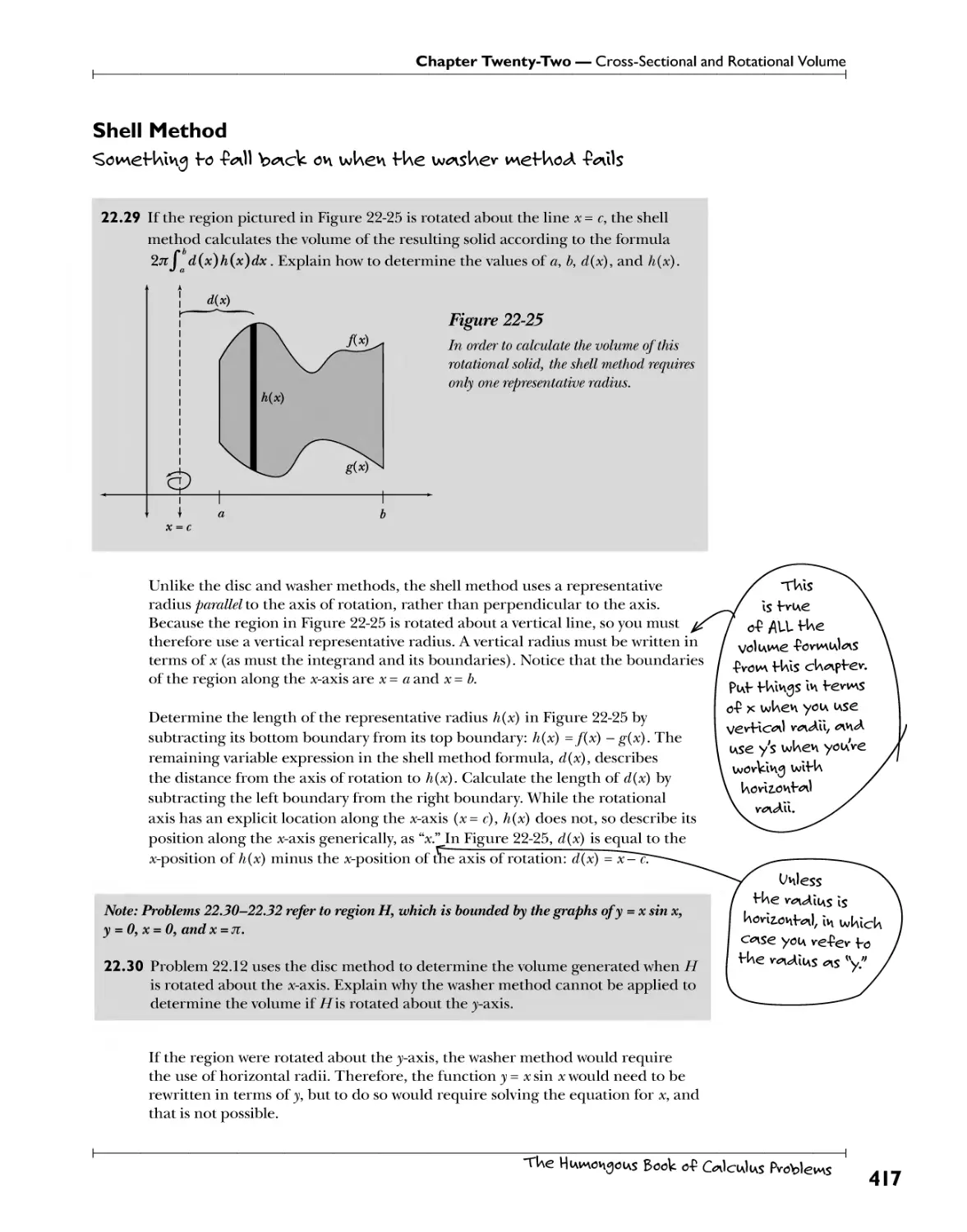
Shell Method ^owef UIv\g f 0 -knll b^nck ov\ wUev\ f We iw^nsUev weW\o<A -(Wis ^7
TUe HiAvnov\goiAS Book o-P C^IciaIias Problems
Table of Contents
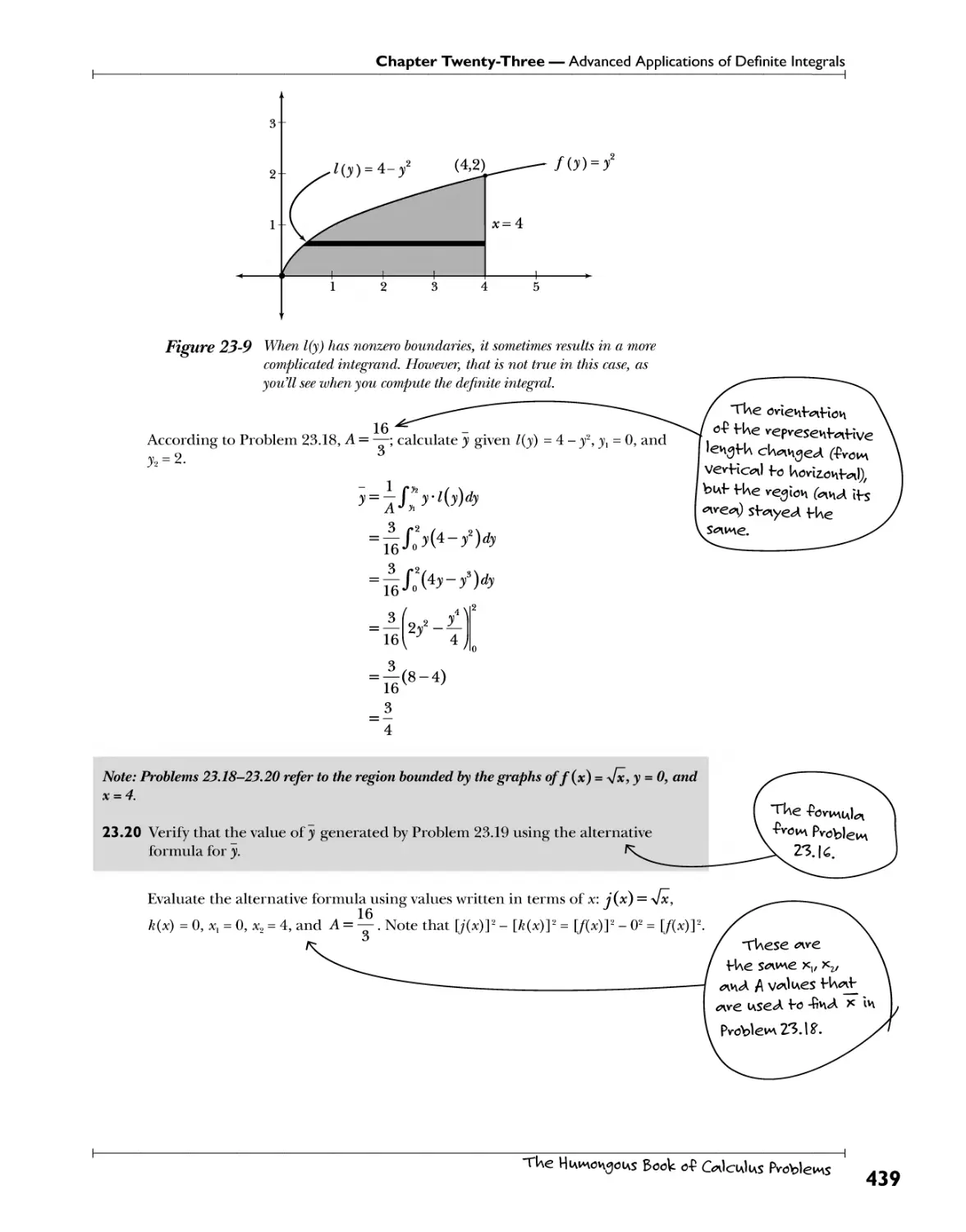
Chapter 23: Advanced Applications of Definite Integrals <£$*<* ?v 423
Arc Length ^ow "^ lS ^ ^vovvv P01V^ ^ ^° P01V^ & *dov\<j <n ciwvy vo<n<A? ^4
Surface Area ^Sf^?.^y^ h^.^ ^.^Hl^ ?."?.f^.T?.^T?>t>.0.\>f>! ?.0J}f^ 427
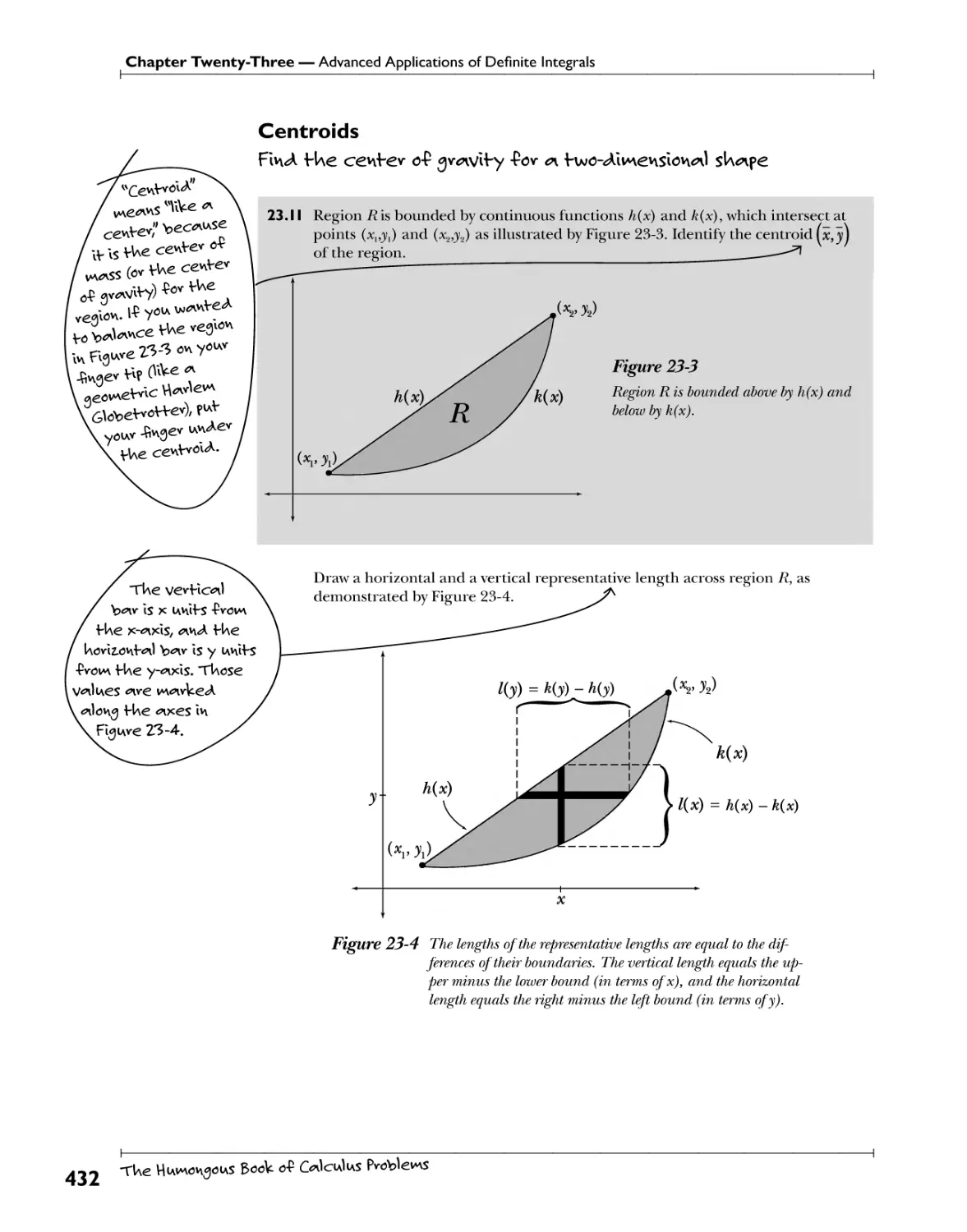
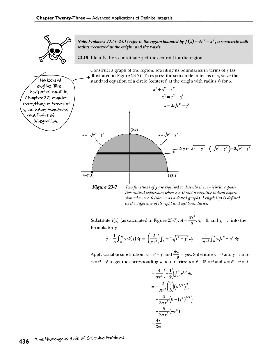
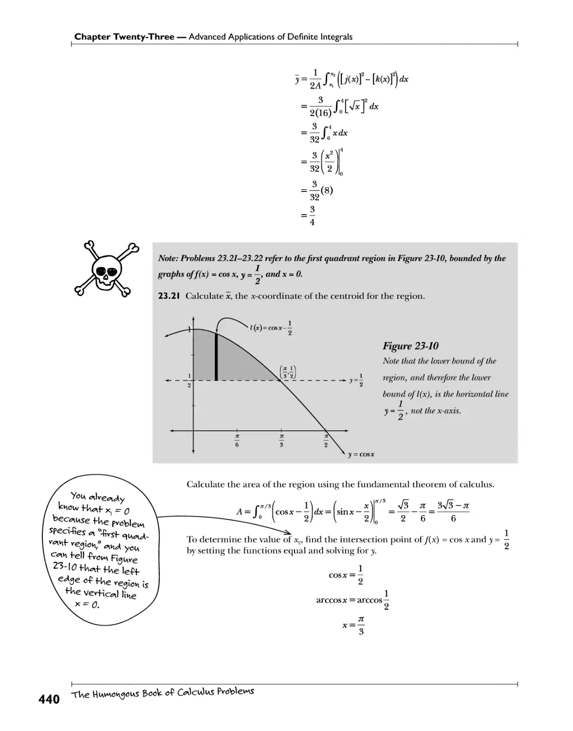
Centroids P.^.4. .th?. 5r£y\fr?.v ?."?.S.^VlhV. ?.°T. £\ .tW?r^^\?.^?!?^l .?h^\P? 432
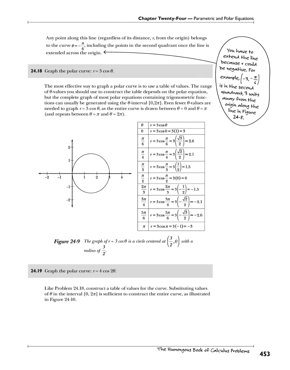
Chapter 24: Parametric and Polar Equations WWHv\g e^iA<*Hov\s wlfUoi\f x <w<A y 443
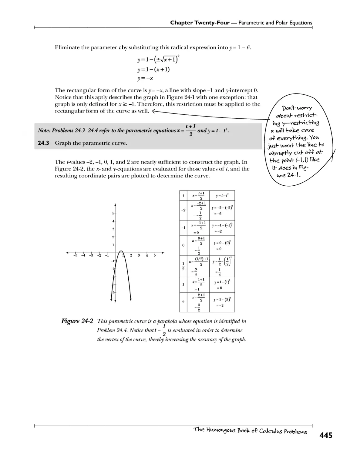
Parametric Equations Like *ey?)}*y\°w\es >yy.Boston.IWboy-, just ?a<A t 444
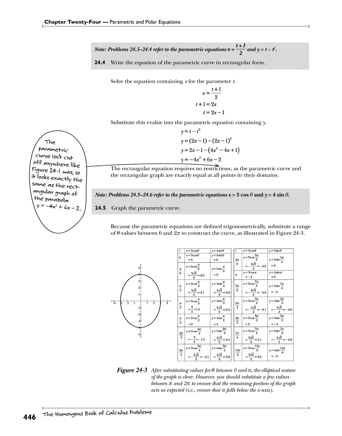
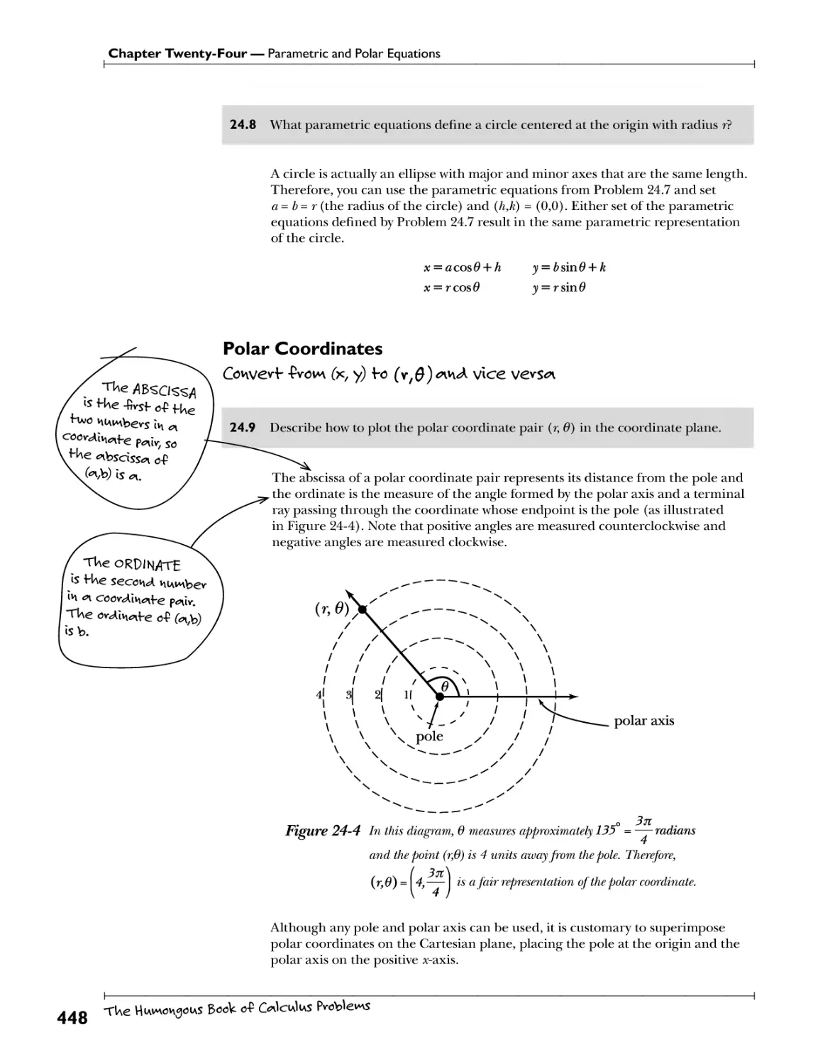
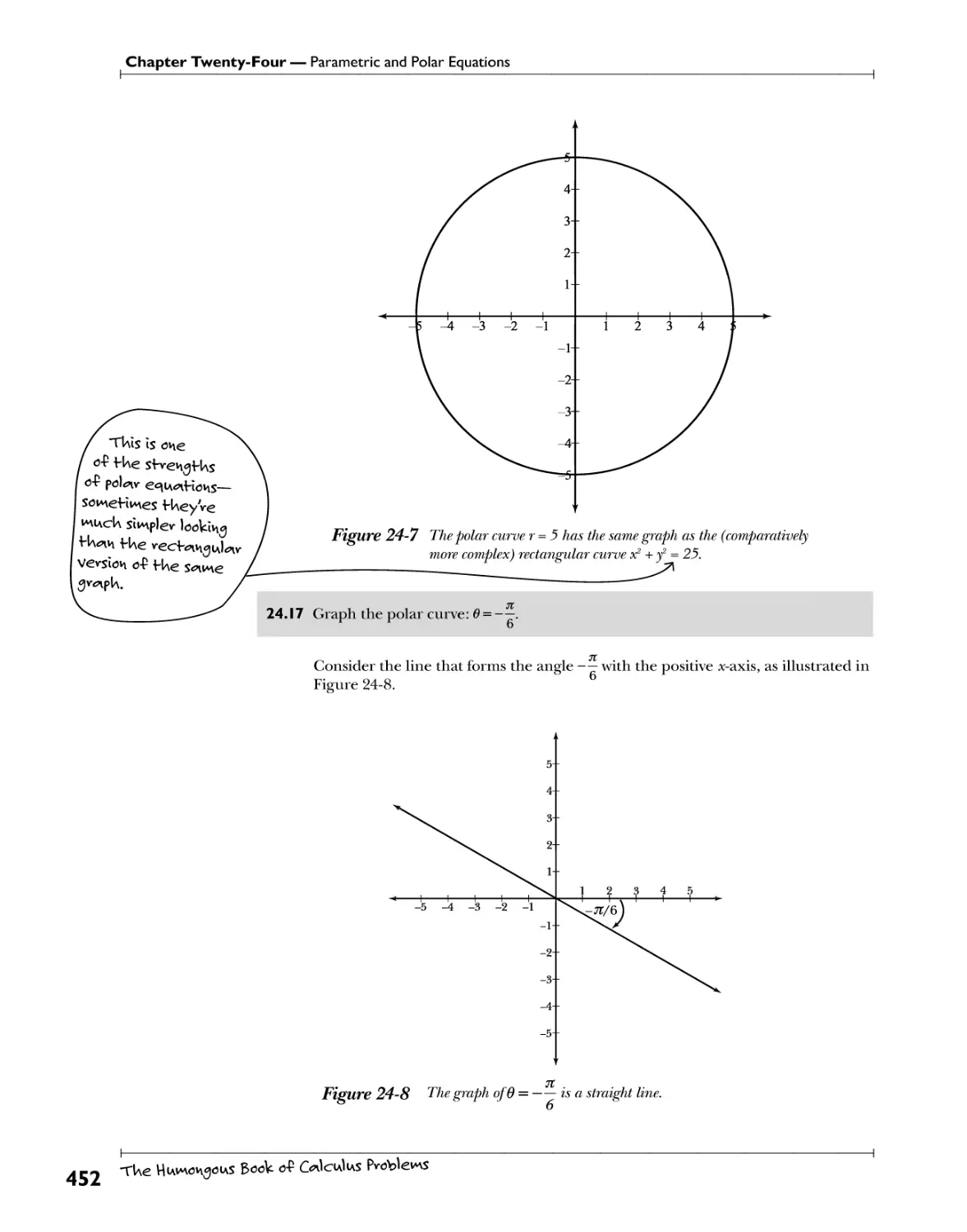
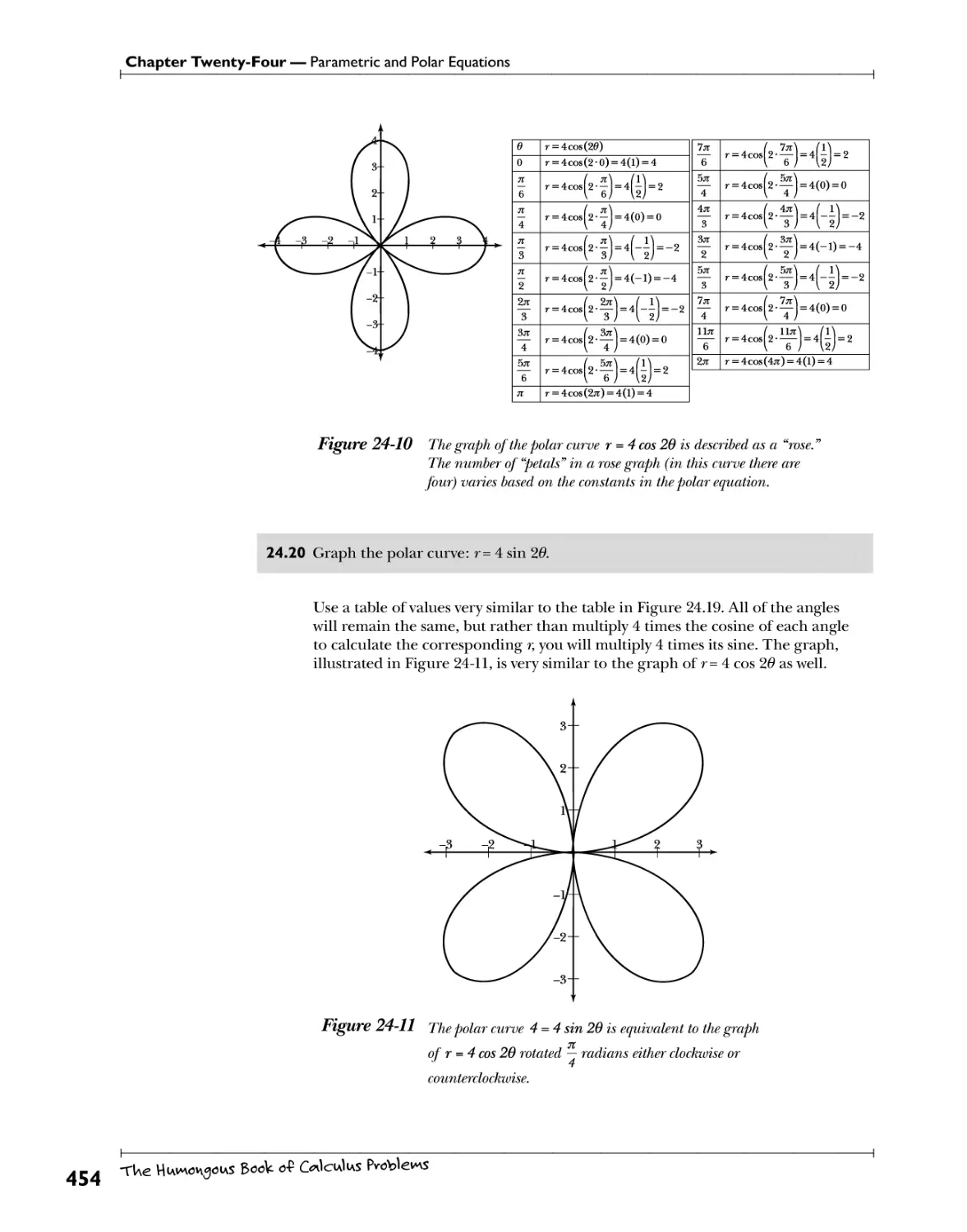
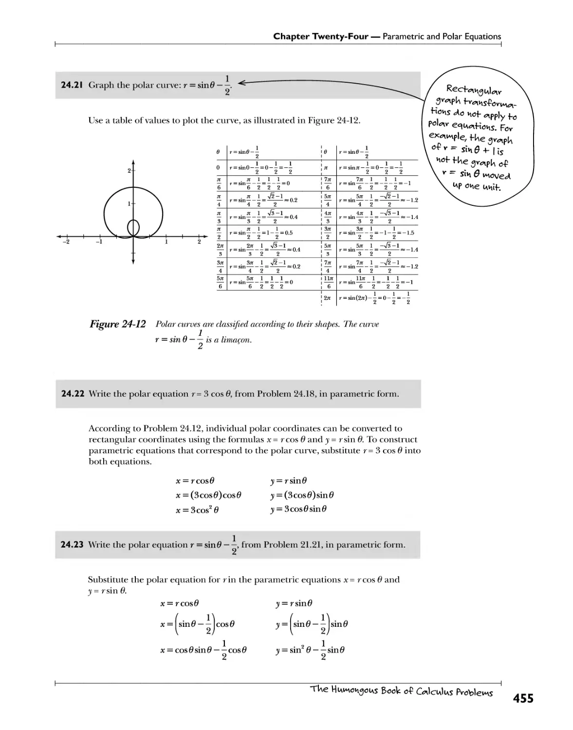
Polar Coordinates 9?^f^ 448
Graphing Polar Curves £^P^3.^^ 457
■ 1 \ a »-££evev\H<*Hov\ f vlcks
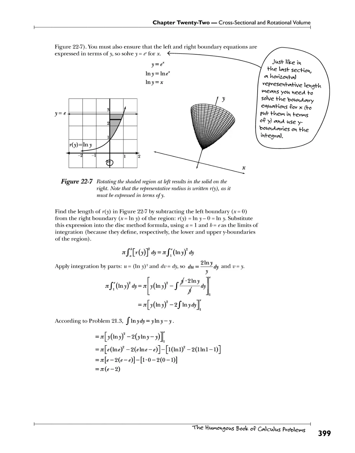
Applications of Parametric and Polar Differentiation T«K\?h * .*£* .^3.??.^?.?!^. ™ 45^
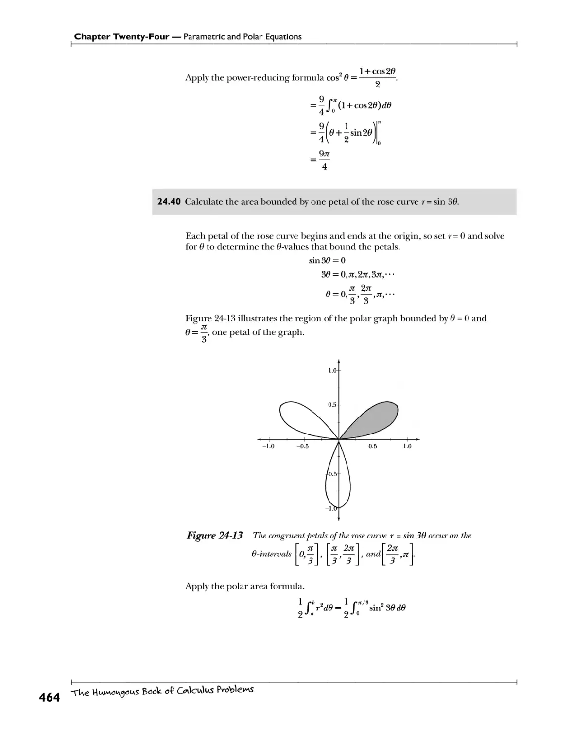
Applications of Parametric and Polar Integration f ?.?.4. th?. /*°3. .??!*?. .^a.^l* *?.<?! 4^2
Chapter 25: Differential Equations E<*u*Hohs tU*t contain * <Aeviv*Hve 467
Separation of Variables .^F^^.^.X1?. f>^. 4*'?. i^^.*'?. 5^.^?. 468
Exponential Growth and Decay... .W!^\ f>. ?tt*\«$?*'s .^fTO £.!?.?™f ?:#?**! .t°. *?.?!*? 473
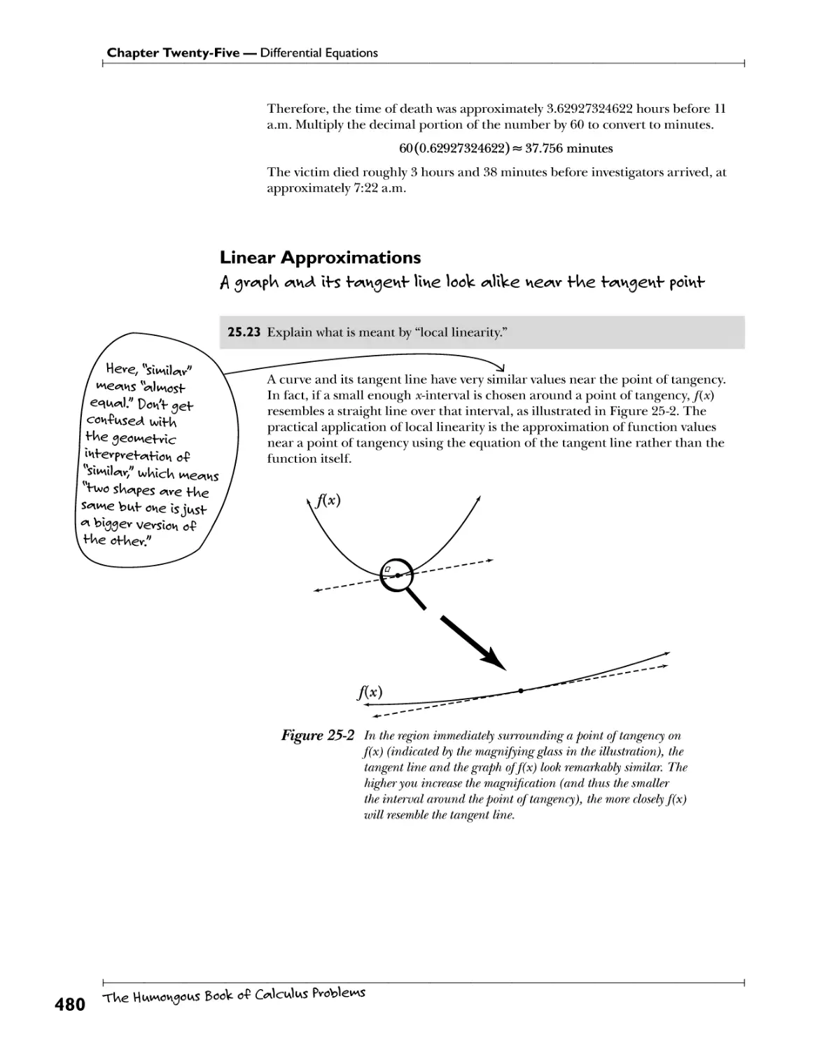
Linear Approximations A 3V?>PJ* *M4 At?. .^3?.^ .I1*?. *?*^hVtt?.? .'.<??):. * !?£ /*'.%?. 450
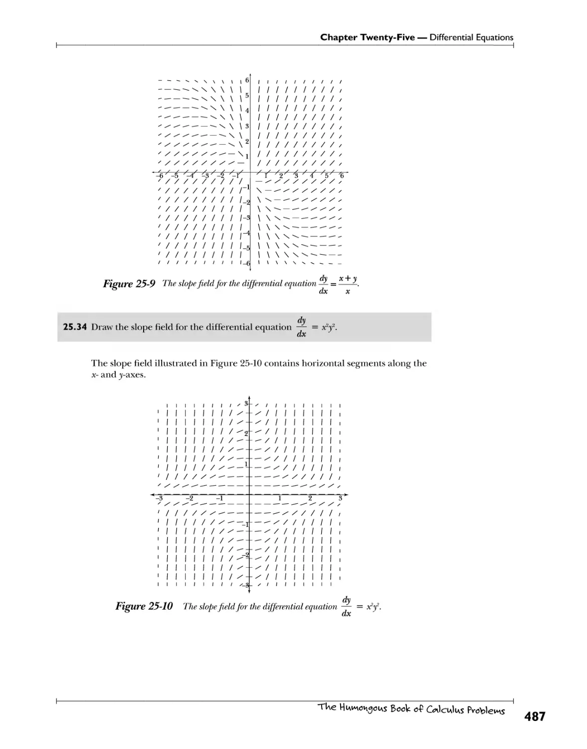
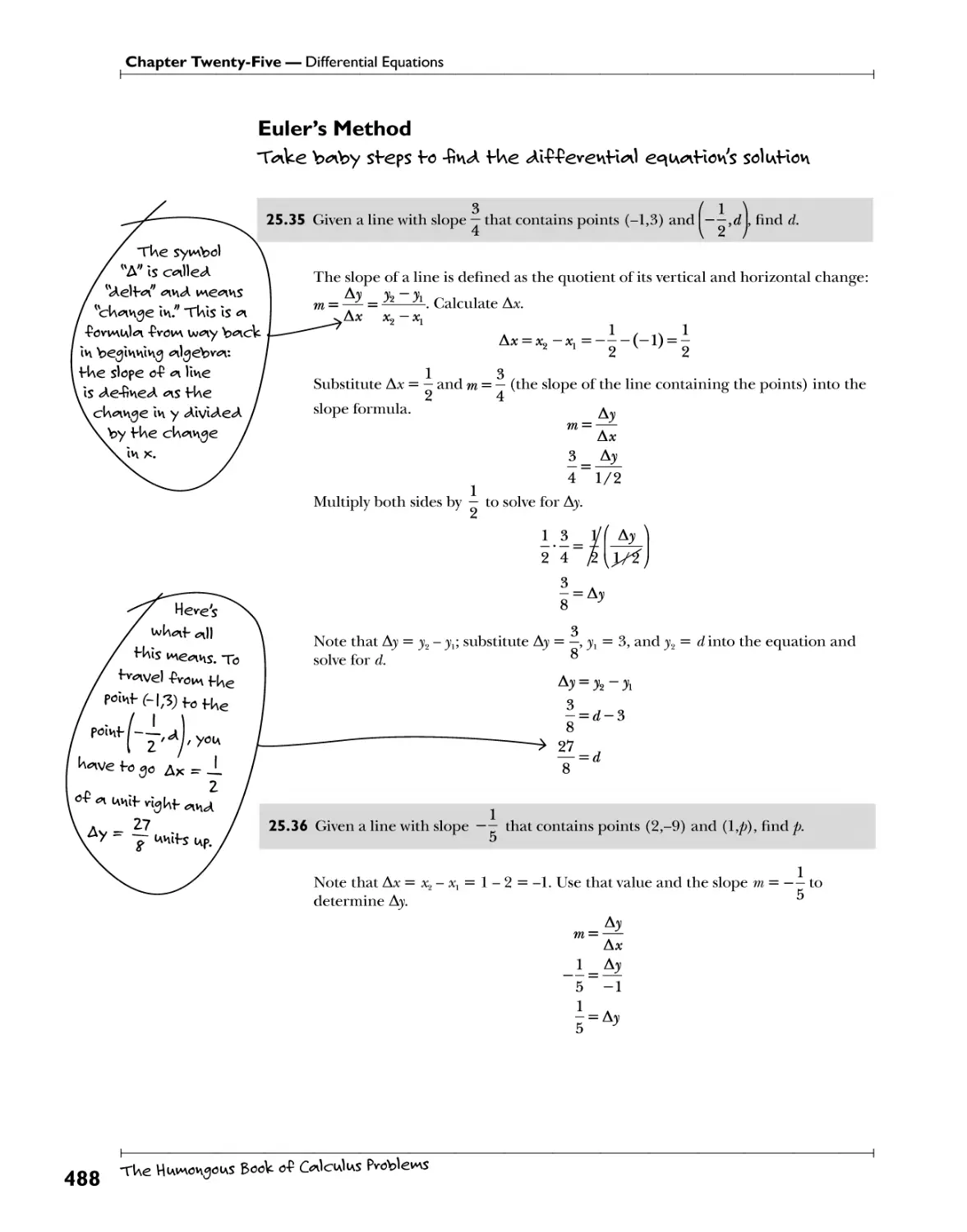
Slope Fields TUey look like iwlv\<A p^ittewvs oh <a iwe^ntUev vn^np ^^>2
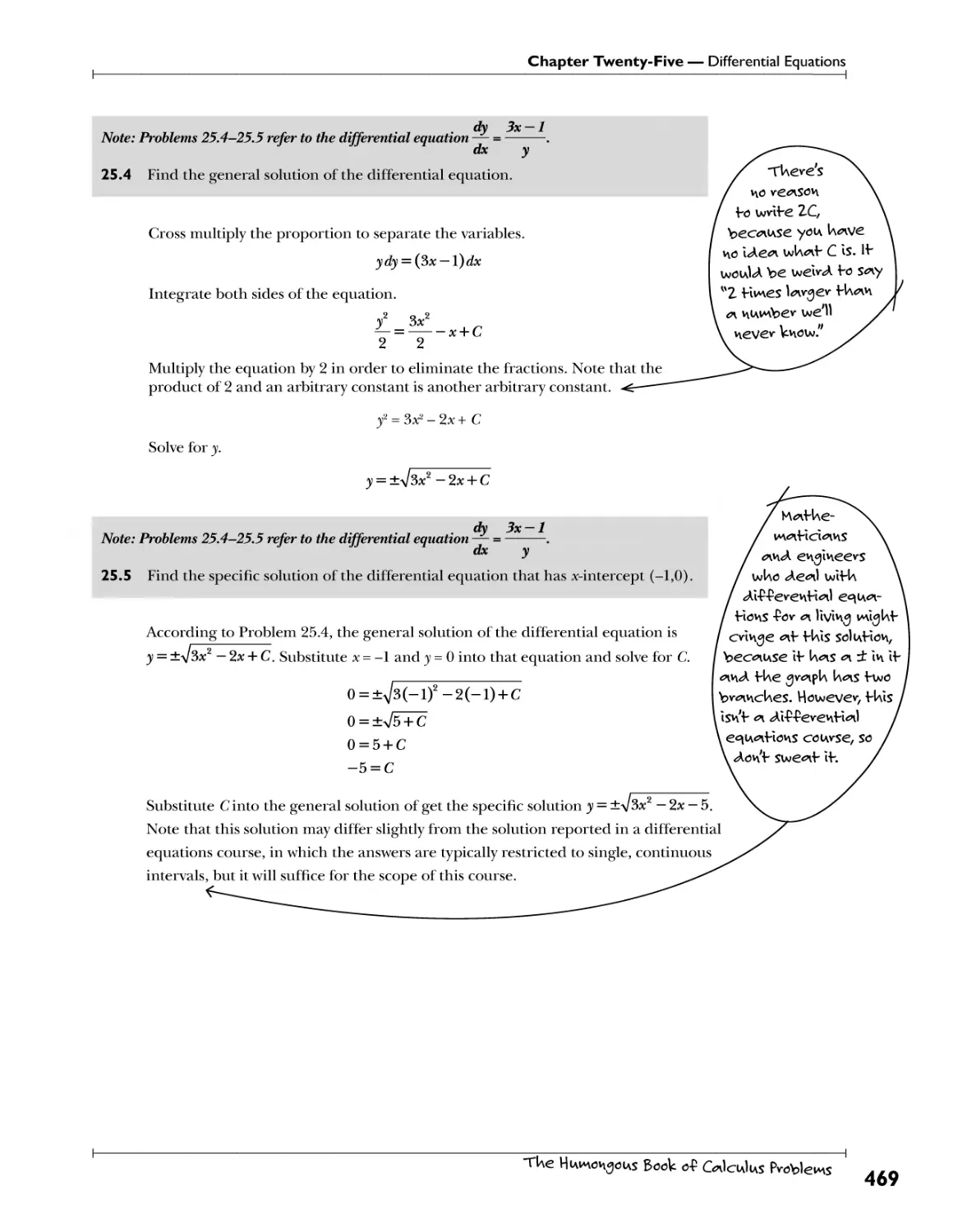
Eulers Method "^ke b^nby steps to -fiv\<A tUe <Al-P-Pevev\H*0 erudition's solution ^gg
^1 . o/. ™ • 0 10 • wl^f's ^a'i€v tU*in one Wctlon? ln-finltdy va<w/
Chapter 2b: Basic Sequences and Series 495
Sequences and Convergence P.°. A1*?. ?.f .^^V.?^ >M??y. .^!?r!r.t:^Xy?. fl?!1^: 496
Sm'ss and Basic Convergence T^fa. .^i^1. .,}?*:f^t5?.^f?!^.*:^.^.*^r!^. .^y^a?^?. ^.?V 498
Telescoping Series and ^-Series ... $°Y>. Y°. h?>!Y*l?.^.??.?. £f*srt^?P.°.t ?£*£? 502
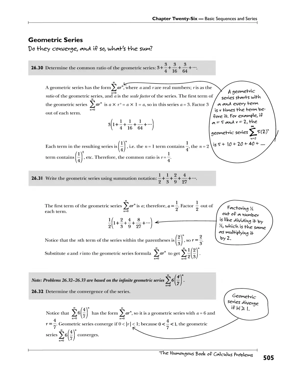
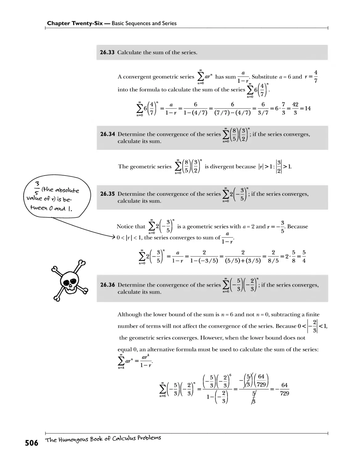
Geometric Series P.?.*^X«^^^ 505
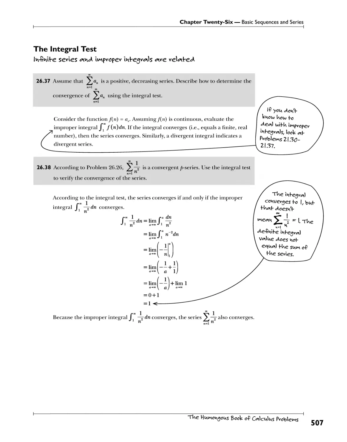
The Integral Test In-finlt e sevles <?w<A Iwpvopev Integv^ds we vel<?it e<A ^7
Chapter 27: Additional Infinite Series Convergence Tests Fov *se wIfU ^Uer l*fil*c $^ 511
Comparison Test Paving sevles we bl^ev t U^in bl^ <nn<A st^unllev t U^in st^unll J72
Lz'mzY Comparison Test SST!?.? .fyf* .9.°.weft?. 0* ^Ivevge by .ftfSoo^Hoh 574
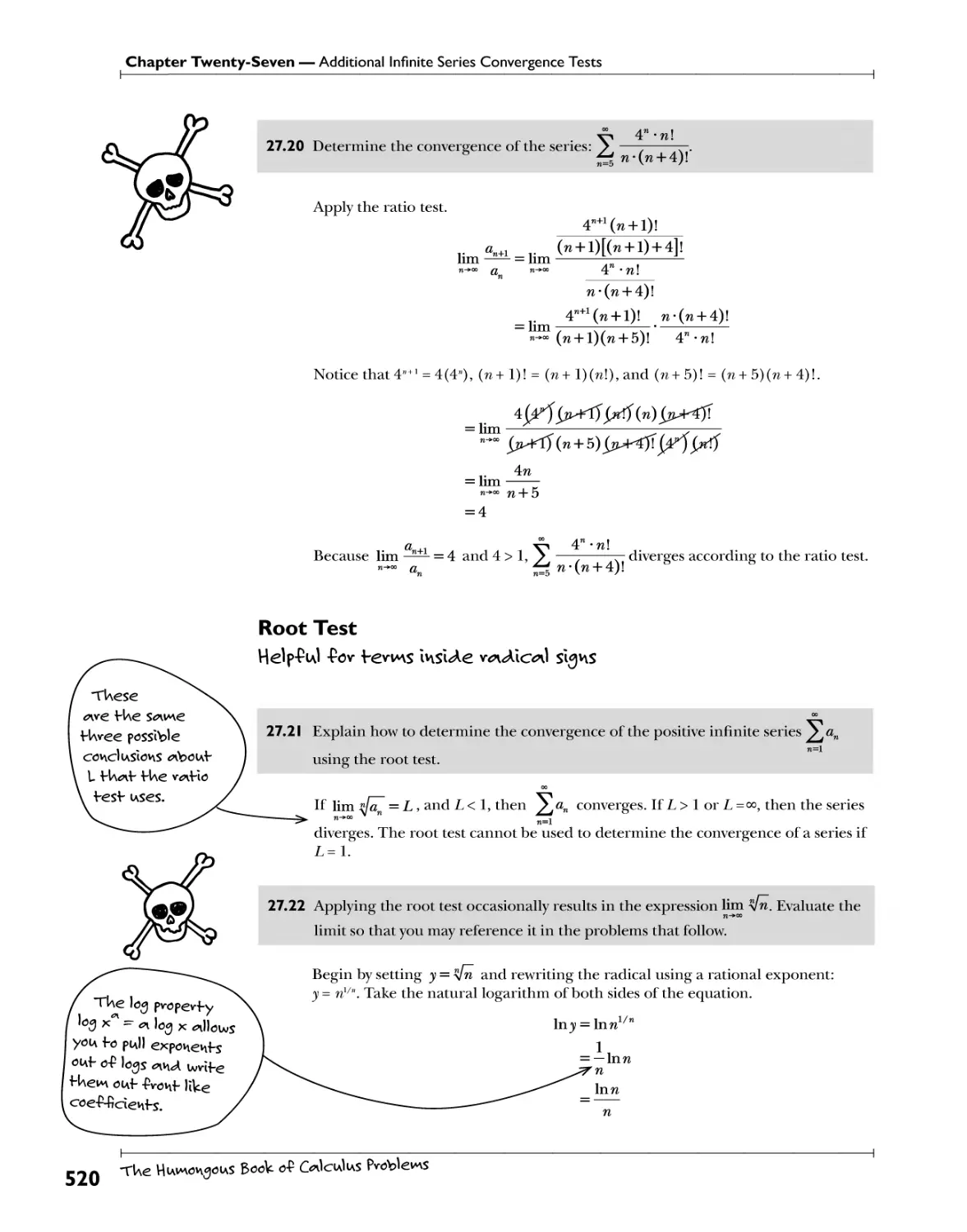
Ratio Test Cowpwe nelgUbov-ln^ fewns o-P *n sevles J77
d / t / Help-Pul -Pov tevws Inside v*i<Alc*il signs _
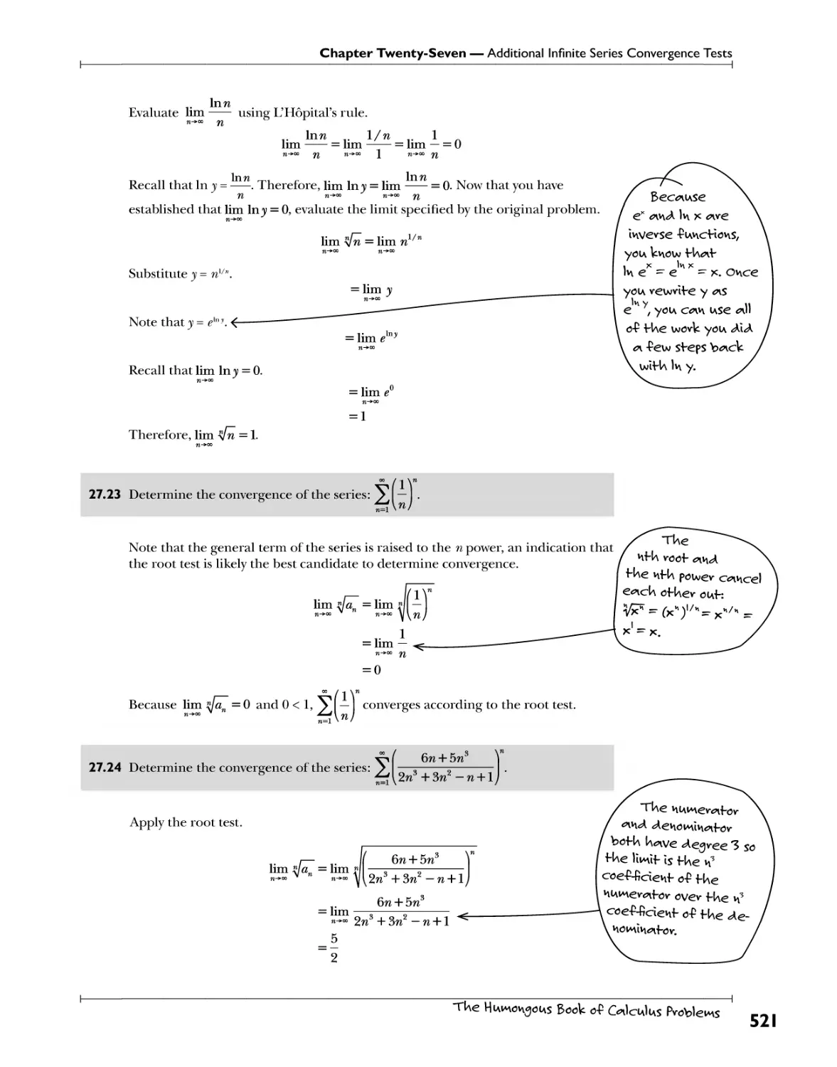
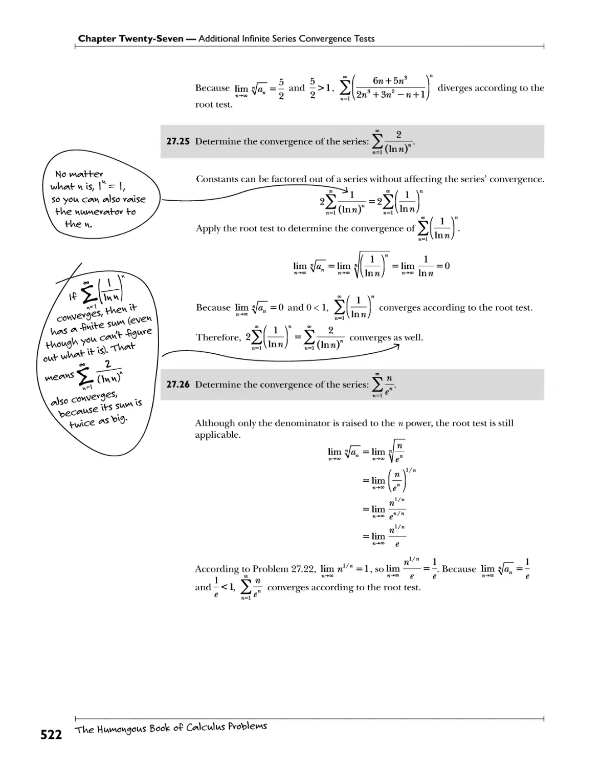
Alternating Series Test and Absolute Convergence...^'T^t-lf.?^r3^?.h^yi?-^^Sf^*^4?.-*^r!r^T 524
TUe HiAvnongoiAS Book o-P Calculus Pvobleiws
VII
Chapter 28: Advanced Infinite Series %evles fI^ contain x's 529
Power Series f!liV^M .^tSyMf^l? .°9. .9?w?.,r3.,?.vy~,r. 530
Taylor and Maclaurin Series *$?*?. .thf* *ef!*»*Y*tSi**^!.Y.^?.? 535
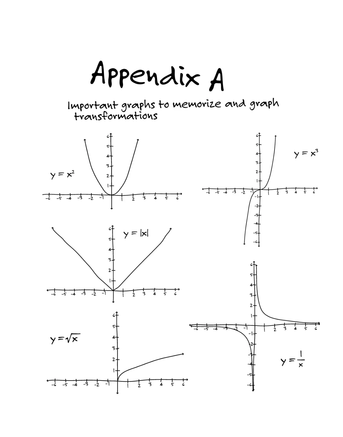
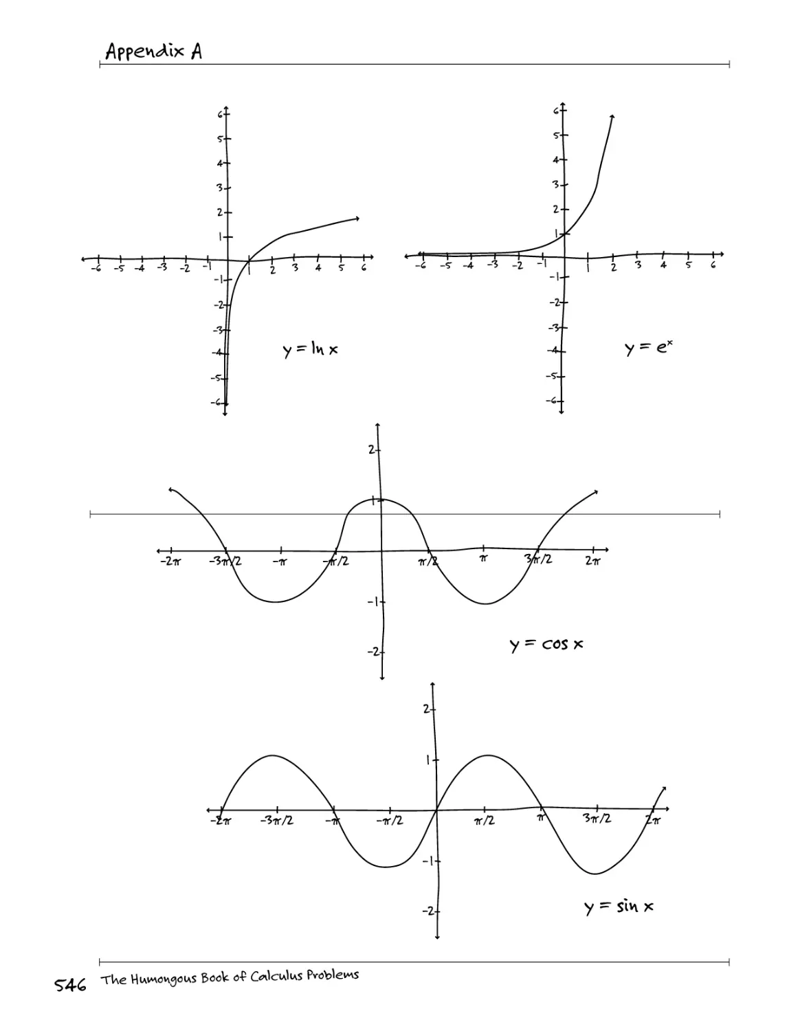
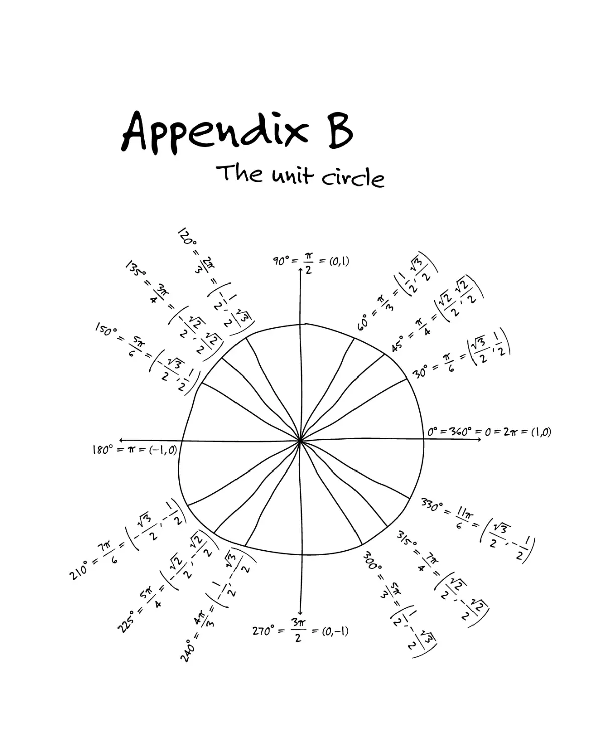
Appendix fr. IvnporUnf Gv^pUs fo vne*\onz.e <*kA 6™*pU -C«nvvs£owiHons ^4^
AppevUlx 3: Tke ChH. CWde ^|
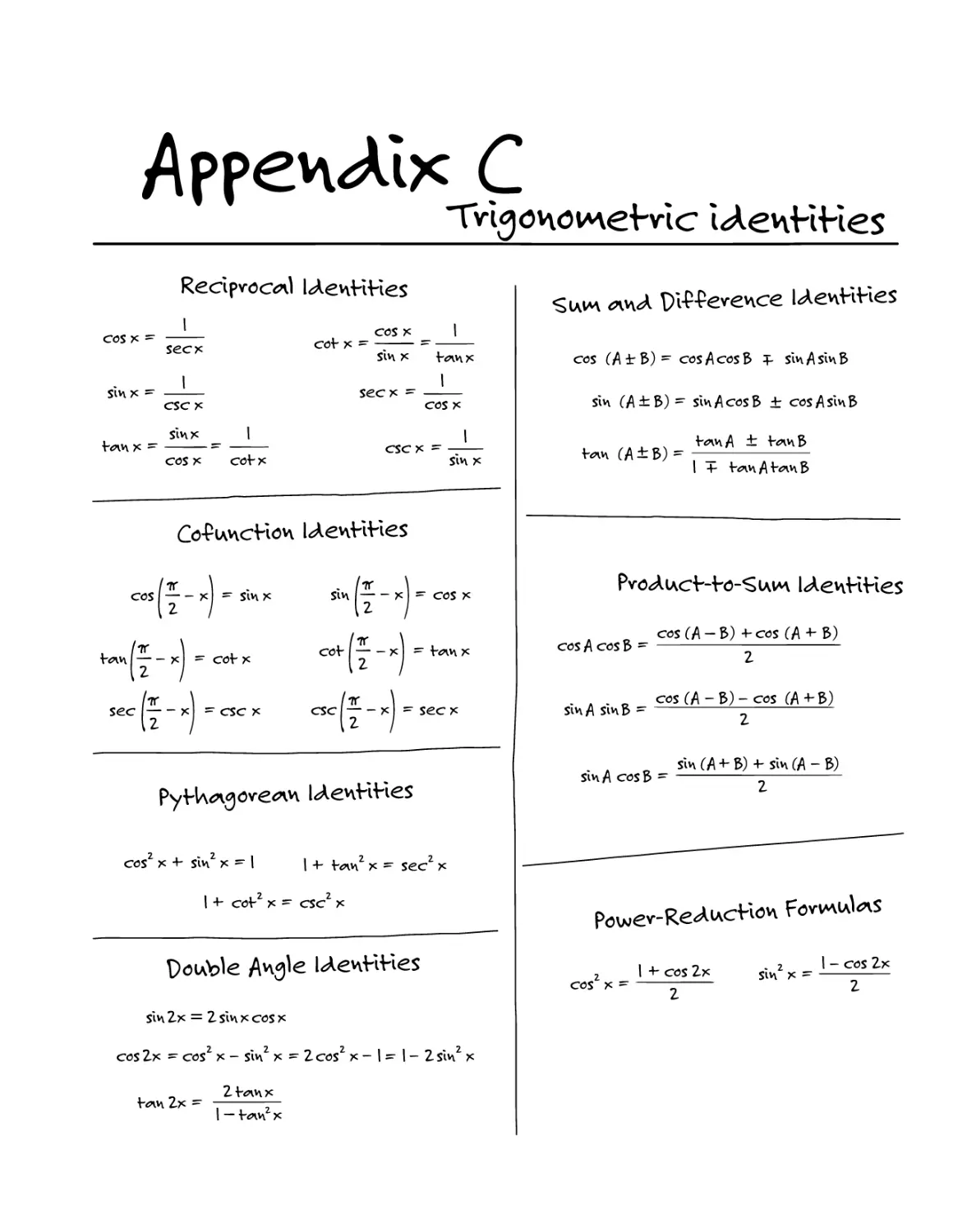
^ppevvAix O Tvl^onowefvlc l^enHHes ST5
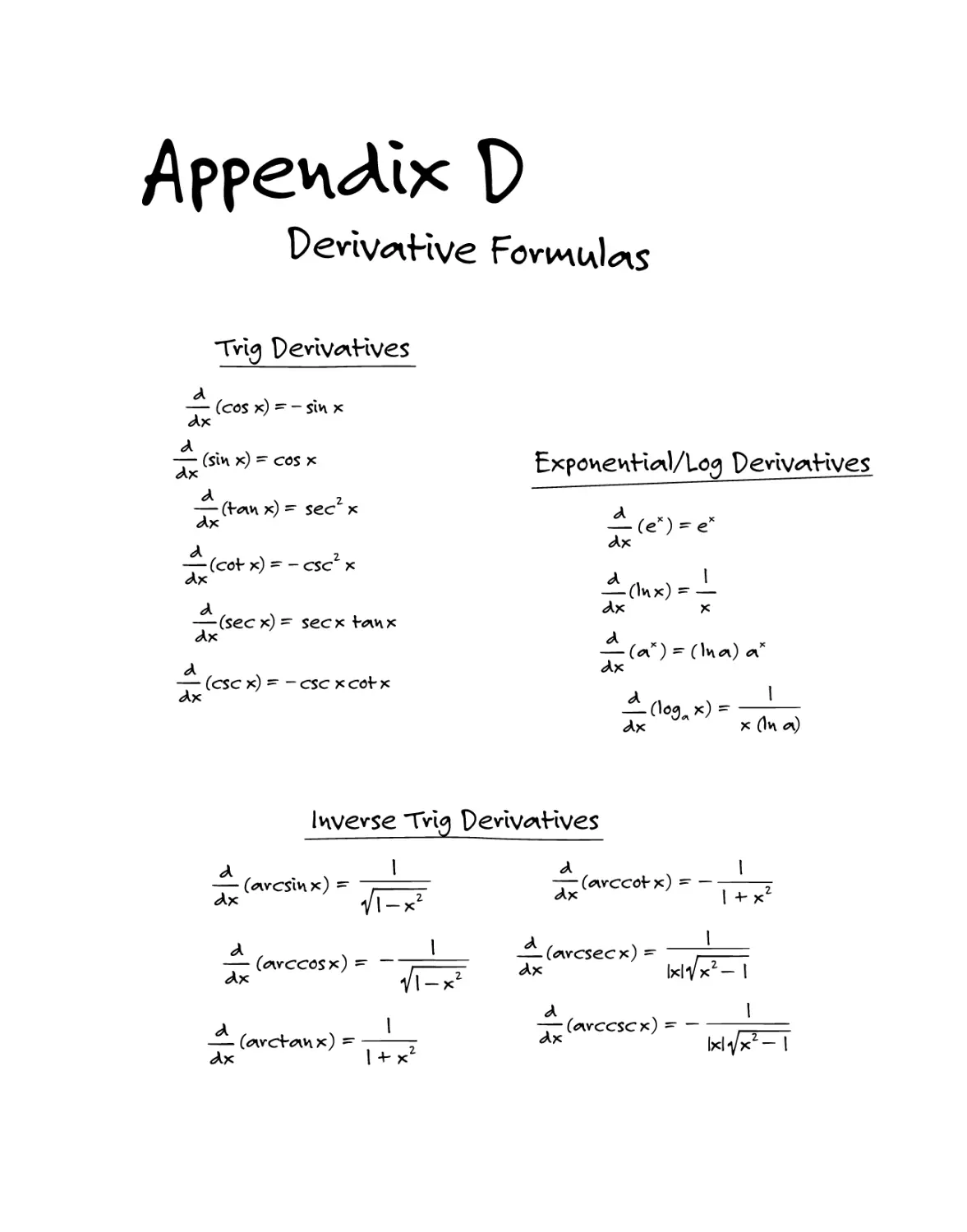
Appendix D: Deviv*Hve Fon^Us S5T
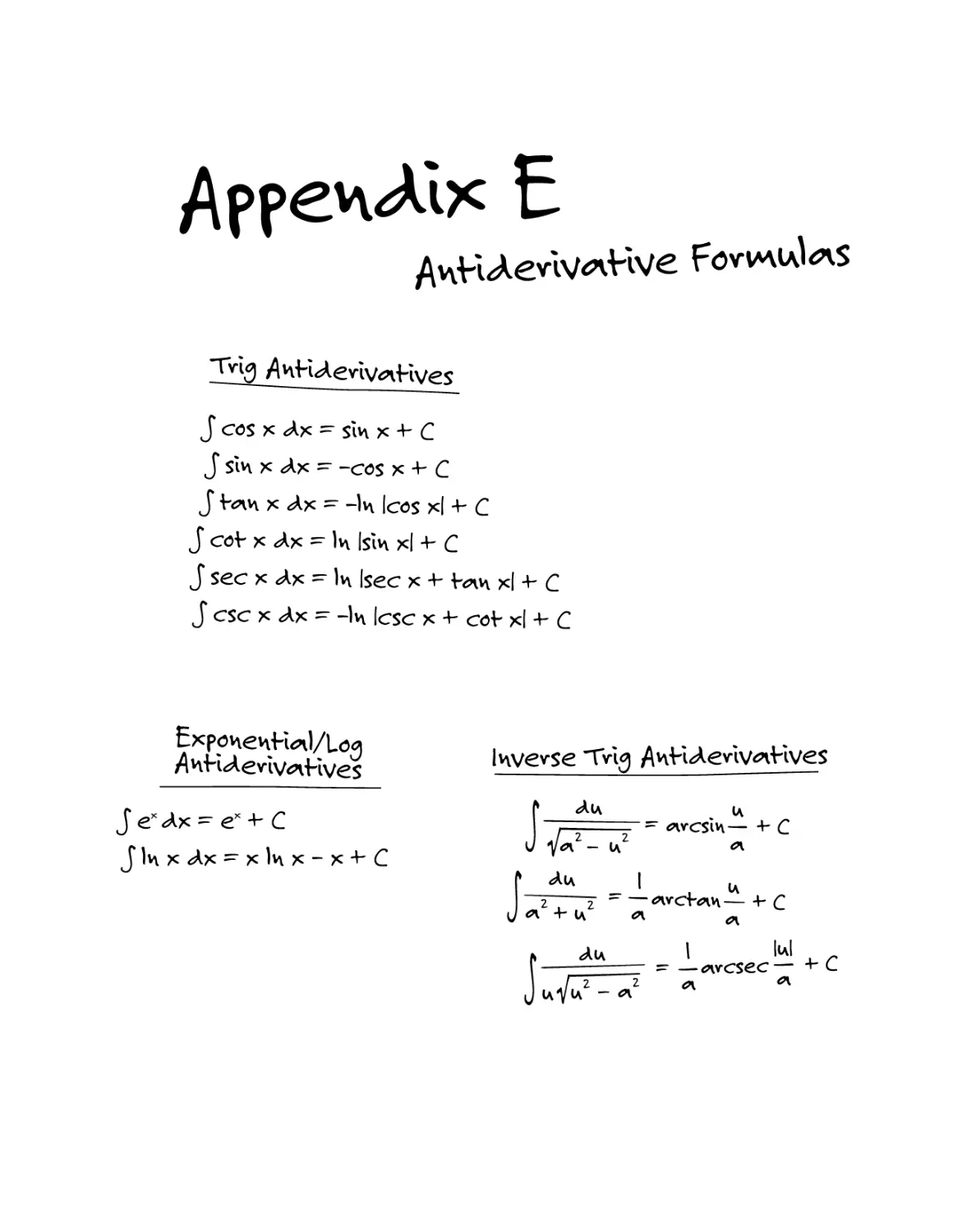
Appendix £: /WH-Deviv*iKve Formulas ST7
Index 559
TUe Hwwov^ous B00V o-P Calculus PvobWs
lv\fvo<AiAcHov\
f\ye you In c\ calculus cl^iss? Yes? TUen you NEED Hus book. Heme's wUy:
F^cf #1: TUe besf w^y fo le^vrn calculus Is by working ouf calculus problems.
TUeve's ho denying If. l-P you coul<A -figure f UIs cl^iss ouf jusf by vexing f Ue fexfbooV.
ov f^V-Ing goo<A nof es Iv\ cl^iss, everybody woul<A p^ss wlf U -flying cc\cys. Un-Povfun^fely,
f Ue U^ivsU f vuf U Is f U^f you U^ve fo buckle <Aown *?w<A wovk problems ouf unfll youv
-fingevs we nut*\b.
F^icf #2: Mosf fe*fbooks only fell you WHAT fUe ^nswevs fo fUelv pv^cflce problems
ewe buf v\of How fo Ac fUew!
^uve youv f exfbook t*\^y U^ve 17ST problems -Pov every foplc, buf mosf o-P fUew only
give you fUe ^nswevs. TU^f vne^ins I-P you <Aon'f gef fUe ^nswev vlgUf youVe fof^lly
scvewe<A! knowing youVe wvong Is ho Uelp ^f ^ill I-P you <Aon'f Wow WHY youVe wvong.
M^f U fexfbooks slf ov\ ^ Uuge f Uvone like fUe Gve^f <xaA Tewlble ot <xaA sc\y,
^Nope, Wy ^g^In," <xaA we Ac. over <xaA ever. f\>\A we Veep gefHng fUe pvoblew
wvong. WU^if c\ <AelIgUf-Pul w^y fo lewn! (Lef's v\of even gef Iv\fo wUy fUey only fell
you fUe ^nswevs fo fUe cAA problems. \)oes fU^f we^n fUe book's ^cf u^l A^THoR
A\A\\\- even -Peel like working ouf f Ue even c\\esl)
F^cf #3: Even wUen t*\^f U books Wy fo sUow you fUe sfeps -Pov c\ pvoblew, fUey Ac c\
lousy job.
Wc\\rU people love fo skip sfeps. You'll be -Pollowlng *>dong -fine wlf U ^n exptan^flon
cvaA f Uen <*)] o-P c\ si\AAe*\ BAM, youVe losf. You'll f UInU fo youvsel-P, lxHow A\A f Uey
Ac fU^f?" cy lxWUeve fUe Ueck AXA f U^f 42 ccv\e -Pvovn? If w^sn'f f Ueve Iv\ fUe l^isf
sfep!" WUy Ac ^ilmosf ^ill o-P fUese books c\$$w\e fU^if Iv\ cvAev fo wovV ouf ^i pvoblevn
ov\ p^vje ZOO, ycK\A beffev Wow p^vjes 1 fUvougU Iff HVe fUe b^icV o-P youv U^v\^?
You <Aov\'f w^v\f fo spev\^ fUe vesf o-P youv H-Pe ov\ UomewovV! You jusf w^inf fo Wow
wUy you Veep gefflv\g c\ neg^iflve numbev wUev\ youVe c^lcul^iflv\g fUe vnlv\lmuvn
cosf o-P bullying c\ pool wUose lengf U Is -Pouv flmes f Ue sut*\ o-P If s <Aepf U plus f Ue
v^fe ^if wUIcU fUe w^fev Is le^Vlv\g ouf o-P c\ W^Iv\ fU^f le-Pf CUIc^igo ^if 4:00
c\y\. W^vellv\g A\\e wesf ^if f Ue $c\v\e s?eeA c<*y\>c\\ Is Aec<?\y\y\g.
F^icf ^4: Re^i^Iv\g Hsf s o-P -P^icf s Is -Pun -Pov c\ wUUe, buf f Uev\ If gef s oU. Lef ;s cuf fo
f Ue c\r\c\$e.
Jusf ^ibouf every single Y\>\A o-P calculus pvoblew you coul^A possibly vuv\ Info Is In
Ueve—^-Pfev ^ill, fUIs book Is HUMONGoU^! l-P c\ fUous^in^ problems ^vren'f e^cKK^A,
TUe HiAvno^oiAS Book o-P C^IciaIias Pvoblewvs
IX
Introduction
f Uen you've gof sowe Y\y\A o-P cwty rn^if U Uungev, my -CVievu*, *in<A lU
seek pvo-Pession^O Uelp. TUis pv^cfice book w^is goo<A *if -fivsf, buf fo
m^iVe if GREAT, l wenf^fUvougU <*>\A wovVie^ ouf ^)) f Ue problems *w<a!
fooV- nofes in f Ue margins wUen I fUougUf somef Uing w^s con-Pusing
ov \\eeAeA c\ lif fie move e*pl*\n^fion. I ^lso <Avew liffie skulls ne*f fo
f Ue U^iv^esf problems, so youU Wow nof fo -CVe^U ouf i-P f Uey weve foo
cU^llenging. A-Pfev *ill,i-P you've wooing ov\ ^ pvoblem <xaA youVe foHnlly
sf umpe<A, isv\'f if beffev fo Wow fU*if f Ue problem is 'SUPPOSED fo be
U*wA? If's ve^ssunng, ^f le^sf -Pov me.
I f UinU you'll be ple^s^infly suvpvise<A by Uow Ae\-<*\\eA f Ue ^nswev
e*pW^fiov\s ewe., <*>\A I Uope you'll -fin<A my liffle nofes Uelp-Pul *dong f Ue
w^iy. C^ill me cv^ay, buf I f UinU f U^if people wUo WANT fo lewrn c^\\co]^s
£*}\A <we willing fo spen<A fUe fime billing f Ueiv w^y f UvougU pv^cfice
problems s\\oia\<A *icfu^lly be ^ible fo -figuve fUe problems ouf <xaA lewrn
c\S fUey go, buf f U^f's jusf my 2<£.
Goo<A lucV c\\\A m^Ve suve fo cowe visif my websife ^if www.c^dculus-Uelp.com.
l-P you -Peel so inclined, Avo? me *w em^ul <?v\A give me youv 2£. (Nof lif evilly,
fUougU—ve^l pennies clog up fUe Infevnef pipes.)
—Mike kelley
TUis book is -Pov my -P^imily, wUoU love <*>\A suppovf me wUef Uev I wvof e ridiculously
long m^ifU books ov nof. Fov my wi-Pe, Us*, wUose gvip on sonify is -fivm wUen mine
sf^ivfs fo buckle, I couUn'f possibly love you wove f U*w I Ao. Fov my sw^sUbucWing
piv^fe so\ Nick, wUo I Uope will confinue fo e^A fUe m^jonfy o-P Uis se^e^ces wif U
Ve U^w^ies" even wUen Ue's nof 3 ^nymove. f\}\A £ov my be^ufi-Pul fwin givls Enn *w<A
<Swf*v wUo jusf s*iU fUeiv -fivsf wov<A: "sUoes." I U^ve ^ sinking -Peeling I'll be Uewring
f U^if \noyA c\ lof in f Ue nof-f oo-^isf^nf -Puf uve.
^peci^il fU^inVs fo Mike ^^in^evs, \^ao Uelpe^. fuvn my i^e^i ^ibouf ^ m^vke^-up book
o-P c<*\ciaWs pvoblems info ^ verify, ^n^. fo my e^ifoys ^ue ^WicVl^n^ <?\\\A Ginny
Munvoe, \jMo wovV U^iv^ fo Veep we -P^om looking silly.
TUis book is in memovy o-P Joe, vMo ^sseA -Pvom ^as in 200&. B^cV \»he\\ I wvofe
TUe Complefe Uiof's Gui^e fo Calculus, Joe foU me Cm ^ fUicV Long IsUn^ -Povmev
f vucVev ^iccenf) f U^f if 'A be ^ K\owe vun." Wif U sincevif y unm^f cUe^ by anyone
I U^ive evev mef, Uis simple \noyAs o-P encouv^gemenf me^inf so \a\iacI\ fo me *is ^
sfvuggling new ^vuf Uov. TU^inVs, Joe. You weve vigUf.
TUe HiA^ongoiAS BooV o-P GnlciOiAS Problems
Chapter I
LINEAR EQUATIONS AND INEQUALITIES
A proper and rigorous understanding of linear equations and their standard
forms, linear segments and the associated algorithms, systems of multiple
linear equations, and linear inequalities is an essential prerequisite for the
study of calculus. Though the majority of calculus students are familiar with
the topics in this chapter, mere familiarity is insufficient. In order to succeed
in the more advanced topics of the chapters that follow, student mastery of
these foundational skills and concepts must be ensured.
^ ^ *« ~ ** ;^:sr^::T^ -
^ ****** «* *« ^x^ ^ ^ ^*
*a VWe >e«3H« «*A ^PomVs »^*L ^ ^ * ^ o«ce
^^£^' — — "* - "" ~
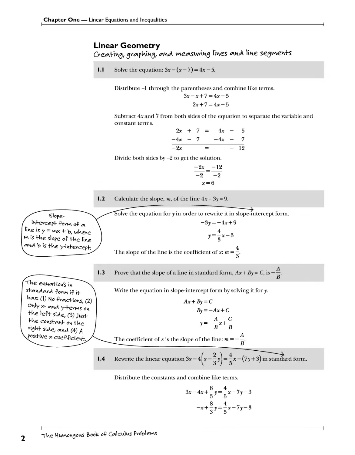
Chapter One — Linear Equations and Inequalities
Linear Geometry
Gre^Hvvj, ^v^pUivvj, <*>\A we^isu/ivig lines <w\A line se^v^enfs
I. I Solve the equation: Sx — (x — 7) = 4x — 5.
Distribute -1 through the parentheses and combine like terms.
3x-x + 7 = 4x-5
2* + 7 = 4*-5
Subtract 4x and 7 from both sides of the equation to separate the variable and
constant terms.
2x + 7 = 4x - 5
-4x - 7 -4x - 7
-2x = - 12
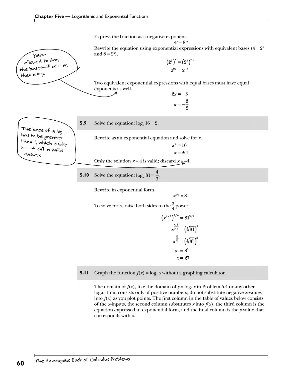
Divide both sides by -2 to get the solution.
-2x = -12
-2 " -2
# = 6
1.2 Calculate the slope, m, of the line 4x- 3y = 9.
^lope-
Iv\fevcepf .(W* o-P <n
W is y ^ ^x 4- b, wkeve
»* Is H\€ slope o-P H\€ l^e
**uA b Is H\e y-iwf evcepf.
Solve the equation for 31 in order to rewrite it in slope-intercept form.
—3_y = -4* + 9
4 o
■y = —x —3
' 3
4
The slope of the line is the coefficient of x: m = —.
Tke €^ca*iHoh's iv\
sf*ivv<Aw<^ -Povtn i-P if
^s: fl) No ^WKohs, ^
only x- <w y-fevlns oh
W\e cov^f^f oh fKe
right- sUe, ^^ (4) A
^siHve x-coe-P-fideHf.
1.3 Prove that the slope of a line in standard form, Ax + By = C, is -
Write the equation in slope-intercept form by solving it for y.
Ax + By = C
By = -Ax + C
A C
y = x-\—
J B B
B
The coefficient of x is the slope of the line: m ■
B
IA Rewrite the linear equation 3x — 4\x y\ = —x — (7y + 3) in standard form.
\ 3 ; 5
Distribute the constants and combine like terms.
Sx — Ax + — y = — x — ly — 3
3^5 y
8 4 M a
—x-\—y = — x — ly — 3
TWe HiAwvongoiAS Book o-P Oleics Problems
Chapter One — Linear Equations and Inequalities
Multiply by 15, the least common denominator, to eliminate fractions.
-15x +40y=12x- 105y - 45
Separate the variable and constant terms.
-27x + U5y = -45
27x-U5y = 45
1.5 Write the equation of the line passing through the points (-3,-8) and (-6,2) in
slope-intercept form.
MiOHply f We
enHve e^iunHon
by —I so Hwvf
f We *-coe-P-ficienf
Is posIHve. Of's <n
ve^iAlvevnenf o-P
Calculate the slope of the line.
m =
3fe-*= 2-(-8) =10
^2 — *i —6 —(—3) —3
Substitute the slope into the slope-intercept formula (y= mx+ b) for m, replace x
and y using one of the coordinate pairs, and solve for b.
y = mx + b
-8 = -—(-3) +6
3 V '
-8 = 10 + &
6 = -18
Substitute m and b into the slope-intercept formula.
3; = mx + b
■y = # — 18
y 3
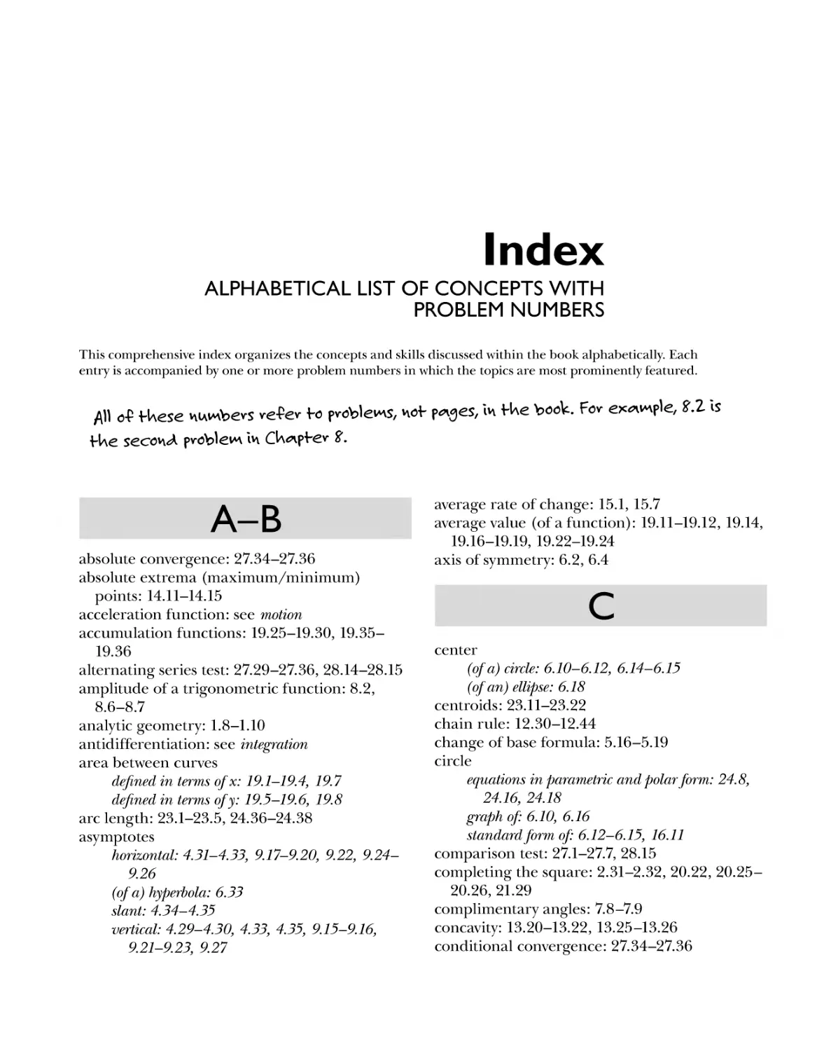
1.6 Calculate the x- and ^-intercepts of 3x- 4y = -6 and use them to graph the line.
To calculate the x-intercept, substitute 0 for y and solve for x. Similarly, substitute
0 for x to calculate the ^-intercept.
3(0) - 4j> = -6 3* - 4(0) = -6
-4y = -6 3# = -6
3 x = -2
Therefore, the graph of 3x - 4y = -6 intersects the x-axis at (-2,0) and the y-axis at
l°'2 L as illustrated by Figure 1-1.
TUe HiAwov^oiAS Book o-P C^IciaIias Problems
Chapter One — Linear Equations and Inequalities
Figure 1-1
The graph of 3x - 4y = -6 with its x- and
y-intercepts identified.
Assume that line p contains the point (-3,1) and is parallel to x - 4y = 1. Write
the equation of pin slope-intercept form.
Calculate the slope of x - 4y = 1 using the method of Problem 1.3.
__A_ ]__].
m~ B~ -4~4
Plug this slope and the coordinates (xx,yx) = (-3,1) into the point-sKpe formula.
y — yx =m(x — x^
■y — 1 = —^ + —
Solve for y to express the equation in slope-intercept form.
1 7
y = — x + -
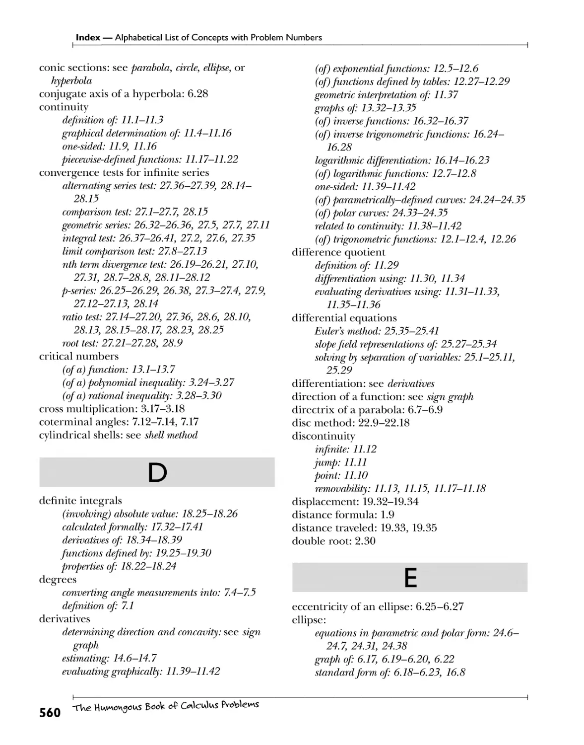
: Problems 1.8-1.10 refer to parallelogram ABCD in Figure 1-2.
1.8. According to a basic Euclidean geometry theorem, the diagonals of a
parallelogram bisect each other. Demonstrate this theorem for parallelogram
ABCD.
C= (11,4)
Figure 1-2
Parallelogram ABCD.
Calculate the midpoints of AC and ED; the diagonals bisect one another if and
only if those midpoints are equal.
TWe HiAwvongoiAS B00V o-P GnlcudiAS Problems
Chapter One — Linear Equations and Inequalities
Midpoint of AC:
2 + 11 1 + 4W13 5
2 '2
Midpoint of BD:
7 + 6 l + 4\ /IS 5
2 '2
Note: Problems 1.8-1.10 refer to parallelogram ABCD in Figure 1-2.
1.9 Prove that ABCD is a rhombus by verifying that its sides are congruent.
Apply the distance formula four times, once for each side.
AB = ^(7-2)2+(l-l)2 £C = V(ll-7)2+(4-l)2
= V25 + 0 =Vl6 + 9
= 5 =5
CD = V(6 - ll)2 + (4-4)2 AD = ^(6-2)2+(4-l)2
= V25 + 0 =Vl6 + 9
= 5 =5
Tke
P^f s 6c|/V|)
Note: Problems 1.8-1.10 refer to parallelogram ABCD in Figure 1-2.
1. 10 Prove that ABCD is a rhombus by verifying that its diagonals are perpendicular
to one another.
Calculate the slopes of the diagonals using the slope formula from Problem 1.5.
— 4-1 — 4-1
Slope of AC: ml= ——- Slope of BD: m2
11-2
1
6-7
ml
m2 = -
The diagonals are negative reciprocals, so the line segments are perpendicular.
lines k^ive ec^l
slopes. Tke slopes
o-P pevPeiwUclA|^v
lines we ^reciprocals
o-P one ^iHof kev <*vu
^*ive opposife signs.
Linear Inequalities and Interval Notation
GccJhye e^u^O sl^n, Uello p^venf\\eses <*y\A hv*\cYe\r$
1. 11 Write the expression x > -4 using interval notation.
An interval is defined by the two values that bound an inequality statement,
the lower followed by the upper bound. You must indicate whether or not each
endpoint is included in the interval. (A bracket next to an endpoint signifies
inclusion, and a parenthesis indicates exclusion.)
Any number greater than or equal to -4 makes this statement true; -4 is the lower
bound and must be included. The upper bound is infinity. Therefore, x > -4 is
written [-4,oo).
Always i\se
p^nvenf Ueses
fo oo wUev\ iwvIHng
Infevv^Os. Yoia
oWf WWe"
soweHung fU^nf's
v\of <a -finif e, ve^nl
niAwbev.
TUe Hiawov^oias Book o-P C^IciaIias Problems
Chapter One — Linear Equations and Inequalities
12 Write the expression x < 10 using interval notation.
The upper bound is 10 and should be excluded (since 10 is not less than 10).
Any number less than 10 makes this statement true; there are infinitely many
such values in the negative direction, so the lower bound is -oo. Therefore, the
inequality statement is written (-oo?10).
1.13 Write the expression 6 > x > -1 using interval notation.
The lower bound must always precede the upper bound, regardless of how the
expression is written: (-1,6].
1.14 Write the solution to the inequality using interval notation: 4x - 2 > x + 13.
Separate variables and constants, then divide by the coefficient of x.
4*-*>13 + 2
3*>15
x>5
Write the solution in interval notation: (5,oo).
1.15 Write the solution to the inequality using interval notation:
3(2x-l) -5 < 10x+19.
l-P yoiA wtdHply ov
<Al\/i<Ae bofU suAes o-P <*}\
iv\e^iA*nlif y by <a v\eg*nHve
v\iMA\bev> vevevse H\e
iv\e^iA*nlify sign. |v\ fUIs
onse, < becomes >.
Distribute the constant, combine like terms, and isolate x on the left side of the
equation.
6*-3-5<10* + 19
6k-8<10k + 19
-4* < 27
^ 27
Dividing by a negative constant fundamentally changes the inequality: x > .
Write the solution in interval notation:
[-?-).
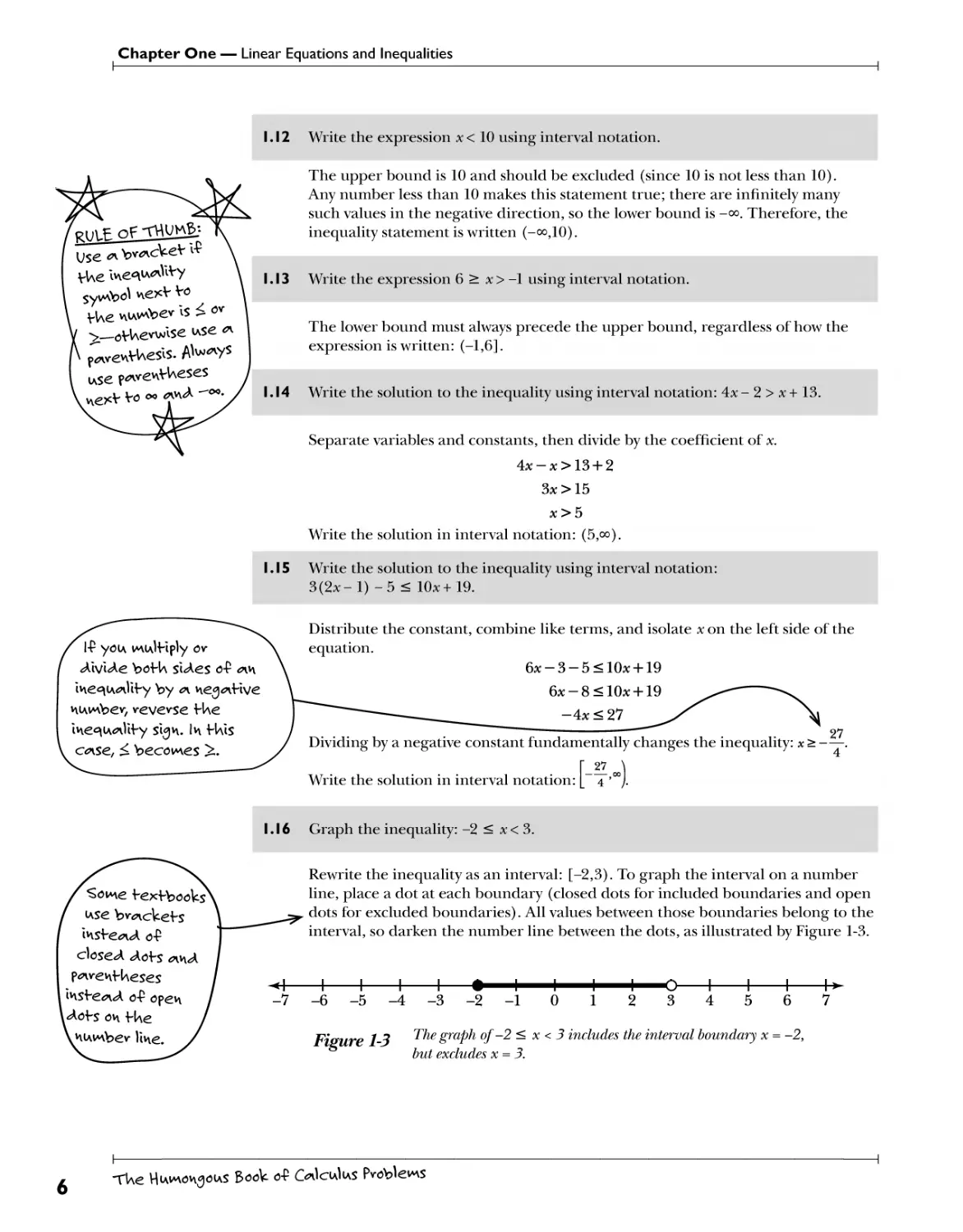
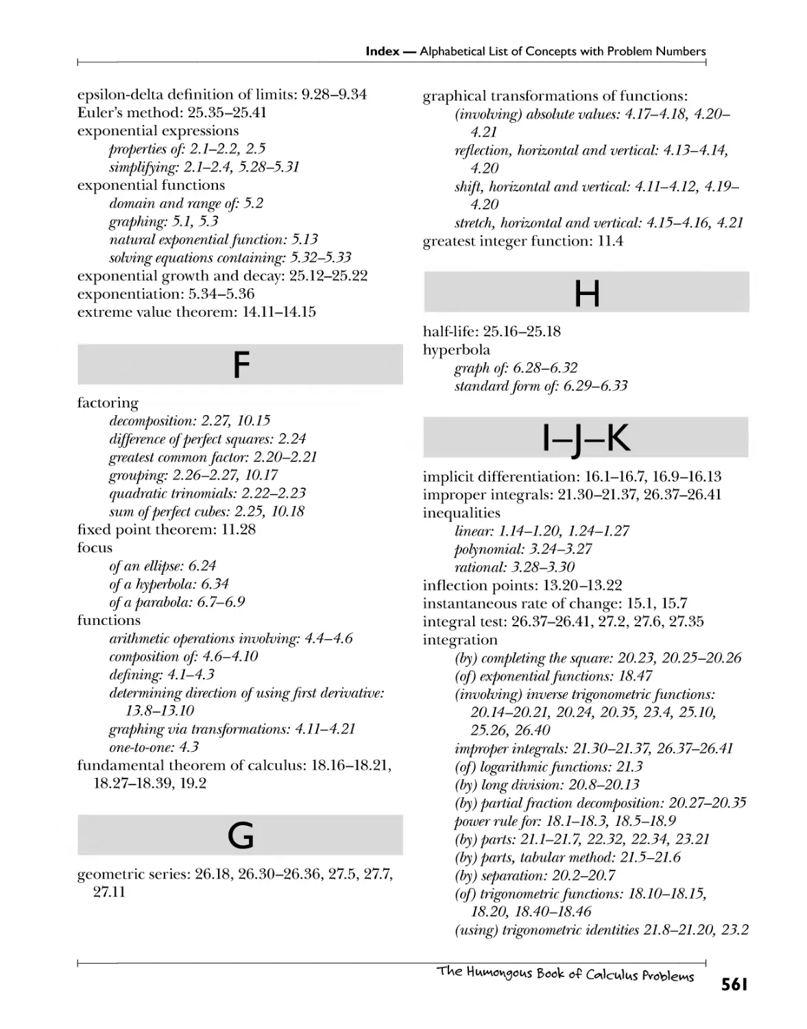
1.16 Graph the inequality: -2 ^ x< 3.
use bv^nckef s
msfe<*A o-P
closed Ao\*s *t\A
p^nv-ev\fUeses
iv\sfe^n^ o-P open
v\iAvnbev llv\e.
Rewrite the inequality as an interval: [-2,3). To graph the interval on a number
line, place a dot at each boundary (closed dots for included boundaries and open
dots for excluded boundaries). All values between those boundaries belong to the
interval, so darken the number line between the dots, as illustrated by Figure 1-3.
-h-
M I I I I 1 I I I I 0 I I I—
-7-6-5-4-3-2-10 1 2 3 4 5 6
Fifmre 7-5 ^e SraP^ °f~2— x < 3 includes the interval boundary x = -2,
but excludes x = 3.
TWe HiAwvongoiAS BooV o-P GnlcudiAS Problems
Chapter One — Linear Equations and Inequalities
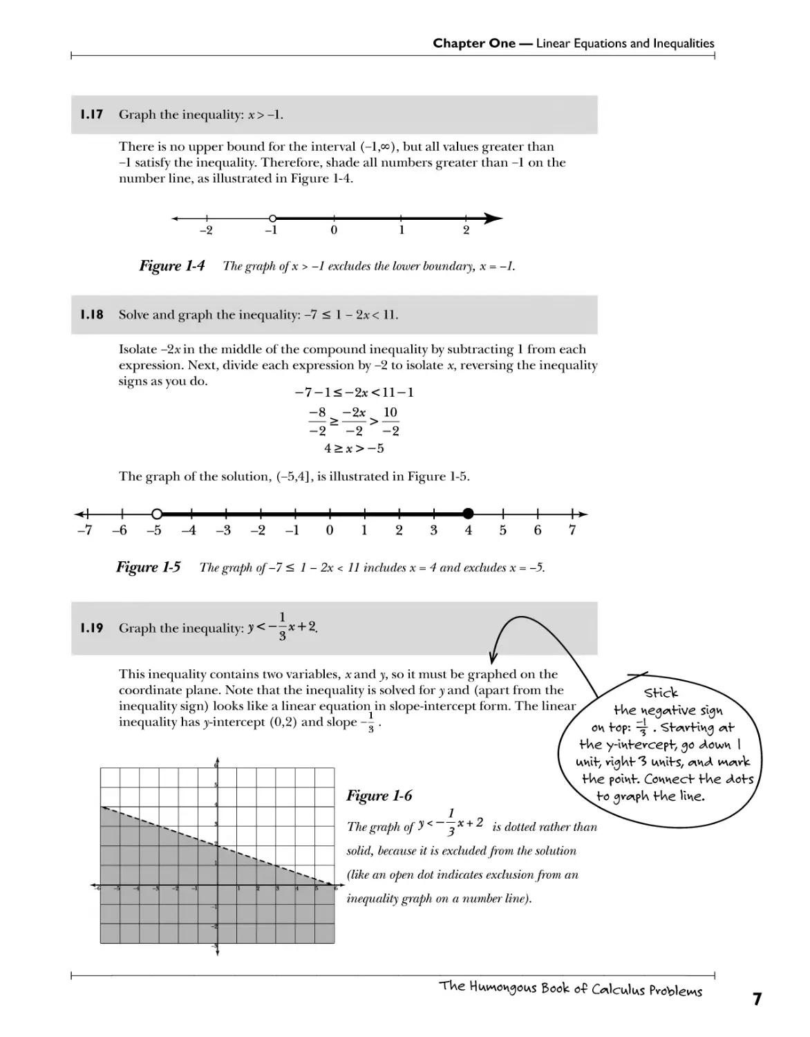
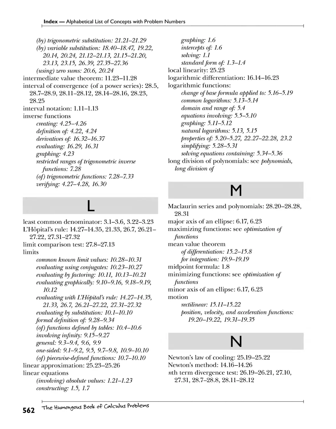
1.17 Graph the inequality: x> -1.
There is no upper bound for the interval (-l,oo)? but all values greater than
-1 satisfy the inequality. Therefore, shade all numbers greater than -1 on the
number line, as illustrated in Figure 1-4.
Figure 1-4 The graph ofx>-l excludes the lower boundary, x = -1.
1.18 Solve and graph the inequality: -7 < 1 - 2x< 11.
Isolate -2x in the middle of the compound inequality by subtracting 1 from each
expression. Next, divide each expression by -2 to isolate x, reversing the inequality
signs as you do.
-7-l<-2*<ll-l
-8 -2x 10
— > > —
-2 -2 -2
4>x>-5
The graph of the solution, (-5,4], is illustrated in Figure 1-5.
+
+
+
+
+
■h
+
■h
+
-7 -6 -5 -4 -3 -2 -1
Figure 1-5 The graph of -7 < 1 - 2x < 11 includes x = 4 and excludes x = -5.
+►
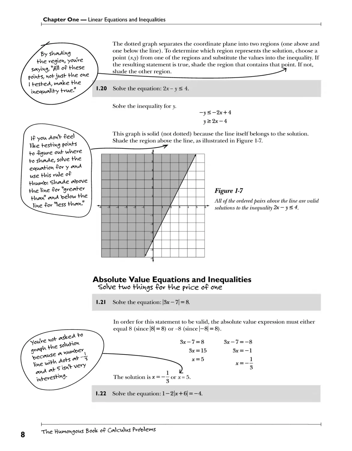
1.19 Graph the inequality: y < ~ ~ x + 2.
This inequality contains two variables, x and y, so it must be graphed on the
coordinate plane. Note that the inequality is solved for y and (apart from the
inequality sign) looks like a linear equation in slope-intercept form. The linear
inequality has ^-intercept (0,2) and slope -- .
a
a
*^t 1
|**»»i I I i I I I I I
—————r t^-—————
J I^^L,
n n n i ^ F F r F r
——————H——————
l
i
Figure 1-6
The graph of yK d
solid, because it is excluded from the solution
-x + 2
is dotted rather than
(like an open dot indicates exclusion from an
inequality graph on a number line).
TUe HiAwov^oiAS Book o-P C^IciaIias Problems
Chapter One — Linear Equations and Inequalities
3y sW^lng
f We veglon, youVe
folHfS/Hofjusf f We one
I f esf e<A, i*vnUe f We
The dotted graph separates the coordinate plane into two regions (one above and
one below the line). To determine which region represents the solution, choose a
point (x,y) from one of the regions and substitute the values into the inequality. If
the resulting statement is true, shade the region that contains that point. If not,
shade the other region.
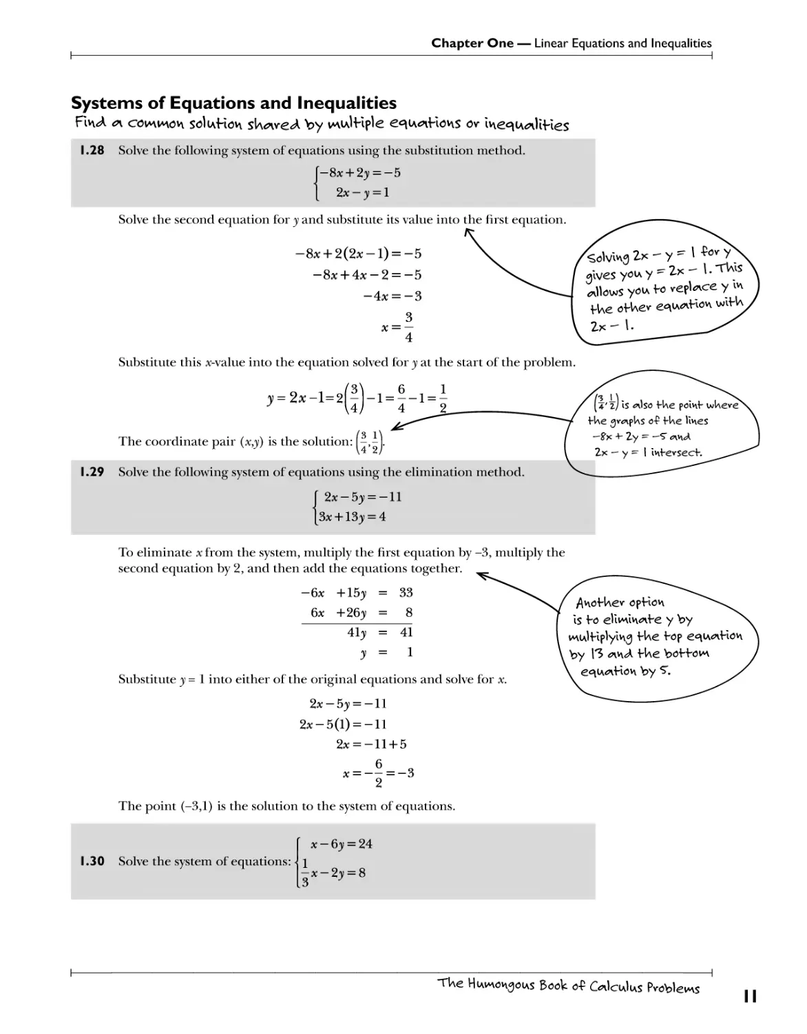
.20 Solve the equation: 2x - y < 4.
Solve the inequality for y.
l£ you <Wf "fed
UVe fesHvvg polvvfs
fo -figure oi*f \»Weve
to sW^e, solve ¥ We
e<^<*Hov\ -Pov y <*vv^
use fWls v^le o-P
f Ww*\Y>: €W*uAe <*Y>ove
fWe Vine -Pov v9ve^fev
f W<w" <**u* Y>eW VWe
line -Pov "less Hvw."
-);<-2tf + 4
3; > 2^c - 4
This graph is solid (not dotted) because the line itself belongs to the solution.
Shade the region above the line, as illustrated in Figure 1-7.
Figure 1-7
All of the ordered pairs above the line are valid
solutions to the inequality 2x — y<4.
lwVevesV^3-
Absolute Value Equations and Inequalities
^olve f wo f Uin^s -Pov H\e pvlce o-P one
1.21 Solve the equation: |3# — 7| = 8.
In order for this statement to be valid, the absolute value expression must either
equal 8 (since |8| = 8) or -8 (since |-8| = 8).
1
The solution is # = or x = 5.
3
1.22 Solve the equation: 1 - 2|* + 6| = -4.
3*-7 =
3x =
-1
_1
3
8
TWe HiAwvongoiAS Book o-P Oleics Problems
Chapter One — Linear Equations and Inequalities
Isolate the absolute value expression on the left side of the equation
-2|* + 6| = -5
|* + 6| =
Apply the technique described in Problem 1.21.
4-fi 5
x + o = —
= 5_12
X~2 2
x + 6 = —
1.23 Solve the equation: 9 - 3\x + 2| = 15.
Isolate the absolute value expression on the left side of the equation.
-3|k + 2| = 6
|* + 2| = -2
This equation has no solution. ^
1.24 Solve the inequality: \x — 5| < 1.
Absolve values
^nliw^nys pvo<Ai\ce
<a poslHve HiAvnbev, so
f Ueve's ho iw^ny soweHung
In ^nbsoliAfe values onn
e^iA^nl -2.
The solution to the absolute value inequality \x + a\ < b, where a and b are real
numbers (and b > 0), is equivalent to the solution of the compound inequality
-b< x+ a<b. ^ ^ M _
-i<*-5<:
Solve the inequality using the method described in Problem 1.18.
-l+5<*<l+5
4<x<6
The solution, in interval notation, is (4,6).
1.25 Graph the solution to the inequality: 2\x — 7| — 5 < — 1.
Dvop H\e
Inedibility b^nv-s,
stick *n w^nt cUing
ine^iunlit y sign oh tUe
le-Pt, *w<A then p^f fUe
opposite o-P tUe vigUt
si<Ae on tUe le-Pt
si<Ae.
Isolate the absolute value expression on the left side of the inequality.
2|*-7|<-l + 5
2|*-7| 4
—! -< —
2 2
|*-7|<2
Create a compound inequality (as explained in Problem 1.24) and solve.
-2 <x-7 <2
-2+7 <x <2+7
5 <x <9
The solution, [5,9], is graphed in Figure 1-8.
TUe HiAwov^oiAS Book o-P C^IciaIias Problems
Chapter One — Linear Equations and Inequalities
10
11
The solution graph of2\x — 7\ — 5 < — l is a closed interval
figure l-o because both endpoints (x = 5 and x = 9) are included.
1.26 Solve the inequality: \2x + 5| > 3.
Rewrite an inequality of form \ax + b\ > c as two new inequalities, ax+ b > c and
ax+ b < -c, and solve. The union of the solutions is equivalent to the solution of
the original inequality.
2* + 5>3 2* + 5<-3
2*>-2 or 2*<-8
x>—1 x<—4
The solution, in interval notation, is (°°,-4] or [-l,oo). The word "or" does not
imply that either interval by itself is an acceptable answer, but rather that both
intervals together (and therefore all values from both intervals) constitute the
solution.
.27 Solve the inequality and graph the solution: 2 — 3|# + l|<— 5.
To soWe c\
y oy > <*Y>soli*fe
sef *? H*o iweciUAUHes
wlfWoi*f *Y>so1i*fe v^lue
Y**vs. one wiW w*ck
fke o/igivv^O ivie«VA*0*y.
TV\e ofWev looVs fhe
swe on f We le-Pf sUe,
V>uf VWe vMMA\bev ok fWe^
vlgUf Is vveg^iHve <*vu*
f We !vie^u*0tt7 sign isy
vevevse<A.
Isolate the absolute value expression on the left side of the inequality.
-3|* + l|<-7
7
|* + 1|>-
1 ' 3
Dividing by -3 reverses the inequality sign; apply the solution method outlined in
Problem 1.26.
n 7 7
x+l>- x+l<
3 3
or
4 10
x>— x<
3 3
The solution is l-00>—H or I-,00!. Graph both intervals on the same number line to
generate the graph of 2 — S\x +1| < — 5, as illustrated by Figure 1-9.
10
-*-
-0+-
-hO-h
-1 0 1
All real numbers satisfy the inequality 2 — 3\x + l\<—5, except
Figure 1-9 \ w 4\
those on the interval] ,—
L 3 3.
10
TWe HiAwvongoiAS Book o-P Oleics Problems
Chapter One — Linear Equations and Inequalities
Systems of Equations and Inequalities
Fiv^A c\ co\a\\a\o\\ soIiaHoh sWweA by wulHple €^ia^iHov\s ov ivve^iu^iUHes
1.28 Solve the following system of equations using the substitution method.
{-8x + 2y = -5
( 2x - y = 1
Solve the second equation for y and substitute its value into the first equation.
-8* + 2(2*-l) = -5
-8* + 4a:-2 = -5
-4x = -3
3
# = —
4
Substitute this x-value into the equation solved for y at the start of the problem.
jr = 2*-l=2(f)-l = |-l = |
The coordinate pair (x,y) is the solution: (-,-).
1.29 Solve the following system of equations using the elimination method.
2x-5y = -ll
3x + 13y = 4
To eliminate x from the system, multiply the first equation by -3, multiply the
second equation by 2, and then add the equations together.
-6x +15y = 33
6x +26y = 8
41y = 41
y = 1
Substitute y=l into either of the original equations and solve for x.
2x-5y = -ll
2*-5(1) = -11
2* = -ll + 5
6
x = — = -3
2
The point (-3,1) is the solution to the system of equations.
Anof Uev opHon
Is f o eliwivunfe y by
muOHplying fUe fop e^u^nHon
by 13 <nn<A f Ue bof fow
e^iA^nHoH by ST.
1.30 Solve the system of equations:
x - 6y = 24
-k-23; = 8
3 J
TUe HiAvno^oiAS Book o-P C^IciaIias Problems
II
Chapter One — Linear Equations and Inequalities
^ec*** vUe coe^e*v
'Even f WougW
f We e^iA^Hons In
^epev^enf" sysf e^s
g\r<npWs we e*<ncf1y
fWe swe. No w<nffev
wW<nf x you P^9 "IV*°
fWe e^i^Hons, youll
gef f We s<we y, so
f Wey inf ev-secf *nf
iH-fiv\if ely w^iny
polnf s *vn<A W^nve
iv\-fiv\If ely w^iny
^coiA\^ov\ solutions.
1.31
plus is f We slope sWovfcuf
I -PovmuU -fVom problem 1.3.
Use the substitution technique, as the first equation is easily solved for x:
x = 6y + 24.
|(6, + 24)-2, = 8
2)> + 8-2); = 8
8 = 8
The end result is a true statement (8 = 8), but no variables remain. This indicates
that the equations of the system are multiples of each other (dividing the first
equation by 2 results in the second equation); the system is therefore dependent
and possesses infinitely many solutions.
Determine the real number value of k in the system of equations below that
makes the system indeterminate.
x — 6y = —13
4x — ky = 1
An indeterminate system of equations has no solution. Consider this geometric
explanation: If the solution to a system of equations is the point(s) at which the
graphs of its equations intersect, then an indeterminate system has no solution
because the graphs of the linear equations do not intersect. The slope of the first
11 4 4
line is <; = -, and the slope of the second line is = -. Set the slopes equal to
create parallel lines, and solve for k.
-k
k~ 6
Cross multiply to solve the proportion.
4-6 = /rl
24 = &
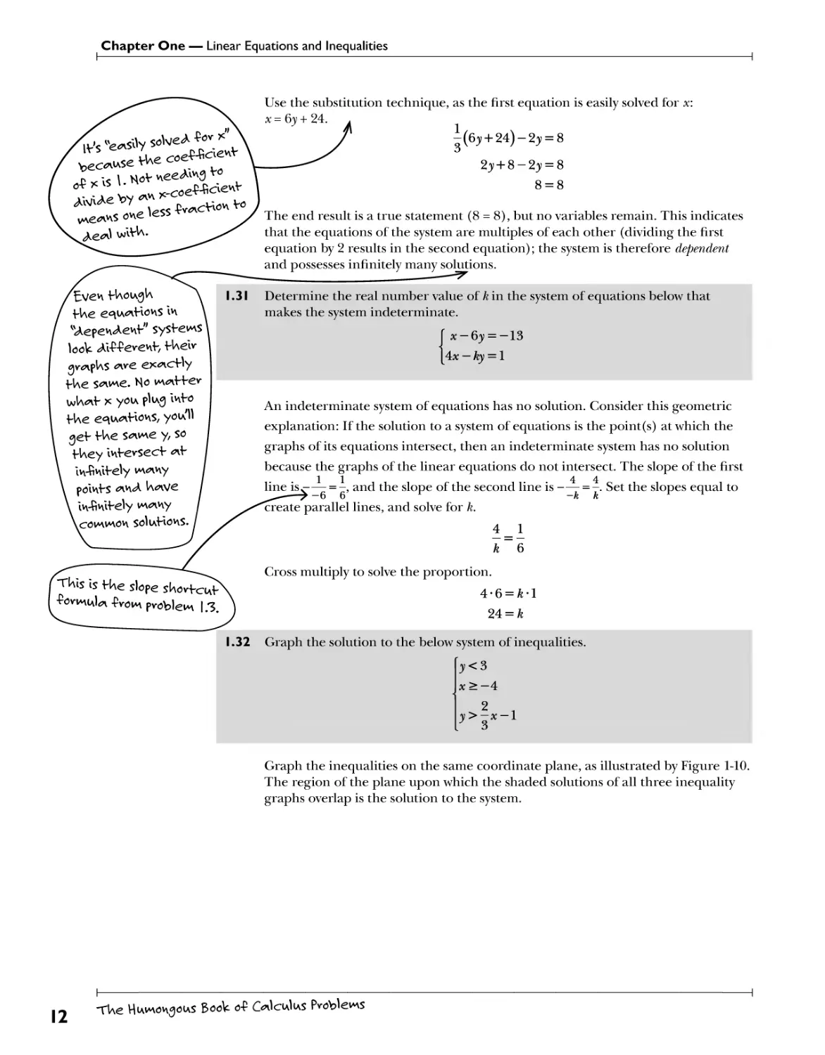
1.32 Graph the solution to the below system of inequalities.
\y<3
x>-4
y>—x — 1
y 3
Graph the inequalities on the same coordinate plane, as illustrated by Figure 1-10.
The region of the plane upon which the shaded solutions of all three inequality
graphs overlap is the solution to the system.
12
TUe Humorous BooV o-P Codecs Pvoble^s
Chapter One — Linear Equations and Inequalities
-a-
-A
i' I i I h AJ
Figure 1-10
The solution to a system of inequalities is a
two-dimensional shaded region. Note that
y = 3 is a horizontal line 3 units above the
and x = -4 is a vertical line four
units left of the y-axis.
1.33 Solve the following system of equations.
\$x + 2y-z = 0
5x — y — 8z = 9
x + 4y-3z = -22
Solve the first equation for z: z = 3x + 2> Use this expression to replace z in the
other two equations of the system.
x + 4y-3z = -22
x + 4y-3(3x + 2y) = -22
x + 4y-9x-6y = -22
-Sx-2y = -22
—4x — y = —ll
You're left with a system of two equations in two variables:
5x — y — 8z = 9
5x-y-8(3x + 2y) = 9
bx — y — 24* — 16y = 9
-19ai-17); = 9
[-19* -17 y = 9
-4x- y = -ll
Solve this system using substitution. (Solve the second equation for y to get
y = -4x +11 and substitute that expression into the other equation.)
-19*-17(-4* + ll) = 9
-19ai + 68ai-187 = 9
49* = 196
* = 4
Plug x= 4 into the equation you previously solved for y.
y = —4x + ll
y = -4(4) + ll
y = —5
Plug x= 4 and y = -b into the equation previously solved for z.
z = $x + 2y
z = 3(4) + 2(-5)
z = 2
The solution to the system of equations is (x,y,z) =(4,-5,2).
You
\ ^s e^HoH
\ ^y2.
TUe HiAwov^oiAS Book o-P C^IciaIias Problems
13
Chapter 2
POLYNOMIALS
Eec^iASe you cw'f W e*pon€Kf s *P | -Povevev
The usefulness of the exponential properties and algorithms taught in an
elementary algebra course does not expire at the final exam. In fact, they are
essential to the study of polynomials, one of the building blocks of calculus.
Polynomials, though simple in structure, can possess quite complex graphs,
and are so versatile that even the most fundamental differentiation and
integration techniques (the power rules for differentiation and integration)
are defined in terms of polynomials. This chapter affords you the opportunity
to review polynomials and properties of the exponents they contain.
Ewe-h will PUy „ key vole Ufer iH c^,cwl
o^uto m, TKe w* ^ iwpovW c<nlcwlws I ae^XrL
W * «M* H«* by woAfcs H„^k „„ «« ^s hit
Chapter Two — Polynomials
pvopevfy IsjiAsf ^
-tWcy iw^ny f o s*ny
f U^nf you c^nv\ <*AA ov
wiOflply f Ulv\gs lv\ <wy
ovAex, <*}\A If iwov\'f
cU*nv\ge fUe
» - Cl)Cl) ■
Exponential and Radical Expressions
Powers *vn<A s^u^e >rooH
2.1 Simplify the expression: x^fx^y6^8.
Apply the commutative property of multiplication to rewrite the expression by
grouping like variables together.
x2x^x9y3y6y8
Recall the algebraic axiom concerning the product of exponential expressions
with equivalent bases: xf1^ = xf1+h.
JA ^2+4+9^3+6+8 = tfSyll
10 6 3 8
w x y z
Simplify the expression: 2 4 7 10.
If the product of two exponential expressions with the same base requires you to
add the exponents (as demonstrated in Problem 2.1), then the quotient is equal to
the difference of the exponents
^10-2^6-4^3-7^-10 = ft/^-4^2
Rewrite the expression to eliminate the negative exponents.
~~ 8 2
W X
2.3 Simplify the expression:. g
4x
£owefWing fo <a
neg^nfive powev
sUouU be wove<A f o
f We opposlf e pwf o-P
f We -fWcflon. oy\ce
if's wove^A, cW^nnge
f We powev b^ncV f cj
poslflve.
The entire rational expression is raised to a negative exponent, so take the
reciprocal of the fraction.
x 4x
Square each factor. If a factor is already raised to a power, such as y3, multiply that
power by 2.
72y5(2) _49y6
4V ~16*2
2.4 Simplify the expression:
. (*"¥)3
(3xy~5)
Raise the numerator to the third power and the denominator to the -2 power.
x(-2)(V(3)
-6 18
x y
3-vy-5)(-2) 3-vv°
Eliminate the negative exponents.
svy 9«2y8
*V°
*y°
Simplify using the method outlined in Problem 2.2.
r\ 2-6 18-10 r\ -4 8 *V
9# 3; = 9# y =——
16
TUe Humourous B00V o-P CoOcutas Pvoble^s
Chapter Two — Polynomials
2.5 Prove that x° = 1.
K-"
The multiplicative inverse property of algebra states that any nonzero real
number times its reciprocal equals 1. Therefore, if x* is a real number and is
multiplied by its reciprocal, the result must be 1.
a 1 ,
x = 1
xa
Rewrite the fraction using a negative exponent.
(a8) (x~a) = 1
The expressions have the same base, so calculate the product by adding the
exponents.
xa~a=l
0—1
X = 1
2.6 Simplify the expression
:J72x~l
V.
Because the expression is a square root (with an unwritten, implied index of 2),
rewrite the factors in terms of perfect squares. ^
yJS6'2'X2'X2'X'y4'y4 =^62'2'(x2f'X'(y4f
Each perfect square can be removed from the radical: 6x y y/2x.
2.7 Explain why the expression ^x2y should be simplified as \x\ ^Jy, rather than x^Jy.
Consider the effect of these values in the original expression: x = -2, y = 5.
Simplify the result.
V20=A/475=V22-5=2>/5
Now test the expressions \*\yfy <md*yfy by substituting x = -2 and y = 5.
xj~y = -2^/5 \x\ Jj = |-2| JE = 2>/5
Notice that only \x\ yjy gives the correct result.
2.8 Simplify the expression: %J—8x7y5z2.
The index of the radical is 3, so rewrite the factors of the radicand as perfect
cubes and remove those perfect cubes from beneath the radical sign.
^(-2)3-(*2)3-*-(;y)S2-22 = (-2*2^
xy2z2
There's no need to include absolute value bars (as discussed in Problem 2.7)
because the index of the expression is odd.
Vis Is
<a}\ Iwpovf^vnf
viAle: 1-P you've gof
<*y\A h Is even,
siiMpU-Py If ^s M , nof
jiASf *. Fov instance,
ym<Alcw\<A
is iwlwvf yoiA
c^Ol iwU^nf's
i\v\<Aevv\e*nf U H\e
TUe HiAwov^oiAS Book o-P C^IciaIias Problems
17
Chapter Two — Polynomials
Simplify the expression: yjll2xy — ^J28xy.
<>o you
c^s^pU*yz^-Wy
Although 112xy - 28 xy = 84xy, the answer is not ^84xy; such an answer violates
numerous arithmetic rules. Terms containing radicals may be combined only via
addition or subtraction if the corresponding radicands match exactly. Notice that
simplifying the individual radicals in the expression produces such radicands.
^112^ -^28^ = ^16-7-xy-^4-7-xy
= ^42'7-xy-j22-7'xy
= 4^7xy - 2^7xy
= 2^
2.10 Rewrite 2502/3 as a radical expression and simplify.
A quantity raised to a rational exponent can be rewritten as a radical expression:
2502/s =(^/250)2 =(^/l25T2)2 =(^i)* = (5^f =25^/4
L Swot v~ • .
VogeVUev.
Operations on Polynomial Expressions
How f o 4-, -, x, *wU * polynomials
2.11 Simplify the expression: 3 (x2 - bxy + 6/) - 5 (x2 + 4ry - 1).
Distribute 3 through the first set of parentheses and -5 through the second set.
Sx2 - 15xy + 18/ -5x2- 20xy + 5
Combine like terms to simplify.
(3a2 - 5x2) + 18/ + (-15xy - 20xy) +5 = -2X2 - 35xy + 18/ + 5
Convention dictates that variables should be written in decreasing order of
exponential power. If two terms have the same power (in the above expression,
f, and xy are raised to the second power), write the variables in alphabetical
order.
2.12 Simplify the following expression.
-2x2(y-4) +x(x+6) -4(Sx-y) +7f(x+l) + 6y(y-9) -3(y + 5x)
Distribute the constants.
-2x*y + 8x? + x2 + 6x-12x+ 4y + 7xy2 + 7f + 6/ - 54^ -3y- 15x
Combine like terms.
-2x2y + 7xf + 9^ + 13/ - 21x - 53^
2.13 Find the product and simplify: (3; — 1) (2^ + 3).
Use the FOIL method to multiply pairs of binomials. "FOIL" is a technique
requiring you to multiply pairs of terms and add all of the results; its name is an
18
TUe Humorous BooV o-P Codecs Pvoble^s
Chapter Two — Polynomials
acronym describing those pairs: first (the first terms in each binomial, in this
example, y and 2y), outside (the terms at the outer edges of the product, y and 3),
inside (the terms in the middle of the product, -1 and 2y), and last (the last term
in each binomial, -1 and 3).
y(2y) + y(3) + (-l)(2y) + (-l)(3)
= 2y2 + 3); - 2y - 3
= 2y2 + y - 3
2.14 Find the product and simplify: (a- 3b)2.
Rewrite the squared binomial as a product and multiply using the FOIL method.
(a - 3b) (a - 3b)
= a-a + a(-3b) + (-36) (a) + (-36) (-36)
= a2 -3ab-3ab + 9b2
^> vV\e VewAS
= «2-6^ + %2
2.15 Find the product and simplify: (2x - y)(x+ by-1).
The FOIL method is useful only when multiplying exactly two binomials. In order
to multiply two polynomials containing any number of terms, multiply each term
in the left polynomial by each term in the right polynomial, one at a time, and / |H of Uev iwOwAs,
add the results.
2x(x) + 2x(by) + 2x(-1) + (-y) (x) + (-y) (by) + (-y) (-1)
= 2x2 +10 xy — 2x — xy — by2 + y
= 2x2 + 9xy — by2—2x + y
2.16 Evaluate the quotient using polynomial long division:
2xs - bx2 + 9x -1
x + 3
sf*nvf wif U 2* 4\y\A
vniAlHply If by evev-y f ewn
In fUe vigUf polynomial:
<nn<A 2*(-|) - -2*. Now
vepe^nf f Ue process, f UIs
Hme iwlf U -y.
Prepare the polynomials for long division: x + 3 is the divisor and 2x3 - 5^ + 9x - 8
the numerator is the dividend. ^~
x + 3
What value, when multiplied by x (the first term of the divisor) results in 2x3, the
first term of the dividend? The only such value is 2x2\ (x) (2X2) = 2x3. Write that
value above its like term in the dividend.
2x2
* + 3)2*3 -bx2 +9ai-8
Multiply each term in the divisor by 2x*, and write the opposite of each result
beneath its like term in the dividend.
2x2
5C + 3J 2xs - bx2 + 9* - 8
-2xs - Ox2
The
Is IvisuAe f [\e
division symbol,
<a>\A H\e ^lylsov Is
oi\fsI<Ae.
TUe HiAvno^oiAS Book o-P C^IciaIias Problems
19
Chapter Two — Polynomials
Combine like terms. Then copy the third term of the divisor next to the results.
/& HviS
point) Zy?
^Is^nppe^v-s. TWe
enHve purpose o-P fWe
steps le^uAing W> ^°
fWis wowenf v^^s t-o
Zy? f o If s opposite
so H\*f tt- g^s
You c*m
r cWecY fke ww€v by
r ^UlHplyiMg Hl€ ^lAOHe^f
**uA f ke AlvlsoY wA f ken
1 #x2- lk4-42)6c4-3)
y- 134. you skouU gef
2*2
a; +
3) 2x3
bxf + 9a; - 8
-2a;3 - 6a;2
-liar + 9a;
Repeat the process, this time identifying the value that (when multiplied by x) will
result in the first term of the new expression: -llx2. Place that value, -llx, above
the dividend, multiply it by the terms of the divisor, record the opposites of those
results, combine like terms, and copy the final term of the divisor (-8).
2a;2- 11*
* + 3J 2x
•s-5x2+ 9a;-8
-2a;3 - 6x2
-11a;2 + 9*
11a;2 + 33a;
42a;-8
The process repeats once more, this time with the value 42 above the divisor, since
x • 42 = 42x.
2a;2 - 11a; + 42
a;+ 3) 2a;3- 5a;2 + 9a; ^8~
-2a;3- 6x2
-11a;2 + 9a;
llx2 + 33x
42a;
-42a;
- 8
-126
-134
Jfvo^^fo3.TV\e
^ev\o\A\lv\^fov sVlps
H*o tevv*s,Y>eo*iAse
The remainder is -134, and should be added to the quotient, 2x2 - llx + 42, as the
numerator of a fraction whose denominator is the divisor: 2a;2 — 1 la; + 42 —
134
ai + 3'
2.17 Evaluate the quotient using polynomial long division: (x4 + 6x - 2) -f (x2 + 3).
Use the method described in Problem 2.16, but when setting up the division
problem, ensure that every power of x is included from the highest power to a
constant. Use a coefficient of 0 for missing terms.
^ s£ + Oa; - 3
+ 0a; + 3^
) x4
-xA
+ 0a;3
-Oa;3
Oa;3
Oa;3
+ Oa;2 + 6a; -
-3*2
— 3a;2 + 6a;
+ Oa;2 + Oa;
— 3a;2 + 6a; -
-2
-2
3a;2 + 0a; + 9
The solution is a;2 — 3 +
6a;+ 7
a;2 +3'
6a;+ 7
20
TWe HiAwvongoiAS Book o-P Oleics Problems
Chapter Two — Polynomials
2.18 Calculate (3x* + 10x- 8) -r- (x+4) using synthetic division.
List the coefficients of the dividend, and place the opposite of the divisor's constant
in a box to the left. Leave some space below that and draw a horizontal line.
F4l 3 10 -8
Copy the first constant (3) below the horizontal line, multiply it by the boxed
constant (-4), and record the result (-12) in the next column, below the number
10. Add the numbers in that column (10 - 12 = -2) and record the result beneath
the line.
" '3 10-8
-12
3 -2
Repeat the process; multiply the new constant (-2) by the boxed constant (-4).
Record the result (8) in the next column and, once again, add the numbers in
that column.
ED 3 10-8
-12 8
<\y\ce 6c 4- 4)
<Aivi<Ae<A evenly Info
-V4- IO*-?frUe
vet^unlvvAev iv^ns 0),
fc 4- 4) is e\ -tWrf ov o-P
3^4- 10*-?.
3-2 0
The numbers below the horizontal line are the coefficients of the quotient. Note
that the degree of the quotient is always one less than the degree of the dividend
(so this quotient is linear), and the rightmost number below the horizontal line
(in this case 0) is the remainder. The solution is Sx- 2.
2.19 Calculate (4x3 - llx2 - 1) -5- (x-3) using synthetic division.
List the coefficients and the opposite of the divisor's constant as demonstrated
in Problem 2.18, but notice that the dividend contains no x-term. Just like long
division, synthetic division requires you to insert a 0 coefficient for missing terms.
| 4 -11 0 -1
12 3 9
1 3 8
The quotient is 4x2 + x + 3 +
x-S'
Factoring Polynomials
Reverse f Ue wtOHpUc^Hon access
2.20 Factor the expression: 18^5 - 9xy3.
Both terms can be divided evenly by 9, x, and f (i.e. there will be no remainder).
Therefore, the greatest common factor is 9xf. Factor the expression by writing
TUe HiAwov^oiAS Book o-P C^IciaIias Problems
21
Chapter Two — Polynomials
the greatest common factor followed by the quotients of each term divided by that
factor. ,
\ 9xys 9xys
= 9xys (2xy2 -1)
2.21 Factor the expression: 2lxby9z6 - 15x4y2z11 + 36x*y3z.
The greatest common factor is 3x4y2z. Use that value to factor the expression,
applying the method outlined in Problem 2.20.
4 a (2lx5y9z6 15x4y2z11 36x8fz
6XyZ\ o^,2„ aM4„2. + Sx4fz
3x*fz Sx4y2z
= Sx4y2z(7xy7z5 -5z10 + 12x4y)
.22 Factor the expression: x2 + 13x + 40.
To factor a trinomial of the form x2 + ax + b, find two numbers \ and k2 such that
-^hx + k2 = a and \ • k2 = b. The factors of the polynomial will be (x + kj and (x + &2).
In this case, \ = 5 and &2 = 8, since 5 + 8 = 13 and 5(8) = 40, so the factored form
of the polynomial is (x + 5) (x + 8).
2.23 Factor the expression x2 - 7x- 18.
Determine kx and k2 as directed in Problem 2.22. Note that the constant (-18) is
negative so \ and k2 have opposite signs. (The product of two numbers with the
same sign is always positive.) Additionally, the x-coefficient is -7, which means the
larger of the two numbers must be negative: kx = -9 and k2 = 2, as -9 + 2 = -7 and
(-9) (2) = -18. The factored form of the polynomial is (x-9)(x+2).
701a cc\\\ <*\so -fWrf ov
\pev-Pecf cubes: *? - y5 ~
.(x-yX^ + xy + y1)-
2.24 Factor the expression: x2 - 49.
This expression is the difference of perfect squares (x2 = x • x and 49 = 7 • 7). Note
that «2 - b2 is factored (« + b) (a - b), so the factored form of the polynomial is
(x+7)(x-7).
2.25 Factor the expression: 8a3 + 125b3.
This expression is the sum of perfect cubes: 8a3 = (2a)3 and \25b3 = (5b)3. Much
like a difference of perfect squares follows a distinct factoring pattern, so does the
sum of perfect cubes: x3 + y3 = (x + y) (x2 - xy + y2). To apply the formula, set x=2a
and y = 5b. .
x + y = (x-\- y)(x — xy + y2)
(2a)3 + (56)3 = (2a + 56) ((2a)2 - (2a) (5b) + (5fc)2)
8as +12563 = (2« + 5b) (4a2 -10ab + 25b2)
22
TWe HiAwvongoiAS BooV o-P Oleics Problems
Chapter Two — Polynomials
2.26 Factor the expression: 4x3 - 20x2 - 3x + 15.
A polynomial containing four terms from which no common denominator can be
extracted is often factored by grouping. Use parentheses to split the polynomial
into the sum of two binomials, one containing the first two terms and one
containing the remaining two terms.
(4x3-20^) + (-3*+15) <r-
Factor the greatest common factor out of each quantity.
= 4x2(x-5)-S(x-5)
Both terms now have a common factor: (x-5). Factor out that binomial; the first
term is left with 4^ and the second term is left with -3.
= (a-5) (4a*-3)
2.27 Factor the expression by decomposition: 6^ + 7x- 24.
The coefficient of the x2-term in this trinomial does not equal 1, so the
method described in Problems 2.22 and 2.23 is invalid and you should factor
by decomposition. To factor the expression ax2 + bx + c (when a ^ 1), you once
again seek two constants (kx and k2), but in this case those numbers meet slightly
different criteria.
b and (kx) (k2) = ac
With some experimentation you'll determine that kx
Replace the x-coefficient with kx + k2.
6x2 +7x-
= 6x2 + (16 ■
= 6x2 + 16#
24
-9)x-
-9x-
16 and k2 = -9
-24
24
Factor by grouping, as explained in Problem 2.26.
= (6*2 + 16k) + (-9x- 24)
= 2x(3x + 8) - 3(3* + 8)
= (3* + 8) (2x - 3)
°"\<k
\A M
~l44.
Solving Quadratic Equations
2.28 Solve the equation by factoring: 4^ + 4x = 15.
Subtract 15 from both sides of the equation, so that the polynomial equals 0.
4x2 + 4x-15 = 0
Factor by decomposition, as explained in Problem 2.27.
4k2 +(10-6)^-15 = 0
4x2 +10^-6^-15 = 0
2k(2k + 5)-3(2k + 5) = 0
(2x - 3) (2x + 5) = 0
TUe HiAwov^oiAS Book o-P C^IciaIias Problems
23
Chapter Two — Polynomials
Set each factor equal to 0, creating two separate equations to be solved.
Use f We
sepw^nfe f We
^Hsv^evs, because
^ovjc^y,^! solve
f We e^u^iHoH.
The solution is x =
2x - 3 = 0
2* = 3
\ 3
\ k = —
\ 2
5 ^ 3
— or x = —.
2 2
or
2k + 5 = 0
2* = -5
5
x = —
2
2.29 Solve the equation using the quadratic formula: bx2 = 3x- 6.
Begin by setting the equation equal to 0.
5^-3x+6 = 0
Apply the quadratic formula to solve the equation.
-^=-(-3)±V(-3)2-4(5)(6)
2(5)
_3±V9-120
10
_3±V-111
10
In order to simplify a square root with a negative radicand, recall that i = v—1.
3±V-lll_3±V(-l)(Hl)_3±z\/m
10
10
10
e^iA^vHon W^ns <a
double yoo\- iwWen f We
s^nvne voof ^nppe^nvs
Hwlce. Fov example,
fc_3X>c-3)-0W*s
w^nfcWing SoIiaHohS:
* ~ 3 ov * ~ 3.
Therefore, there are two imaginary solutions to the quadratic equation:
3 + zVlTT
3-zVlll
10
10
2.30 Find the value of k such that the quadratic equation 6(^ + 2x) = k(2x- 1) + bx2
has the double root x = 3.
Simplify and set the equation equal to 0.
6x2 +12x = 2kx-k + bx2
(6k2 -5k2) + (12k-2kx) + k = 0
Factor x2 out of the first quantity and factor x out of the second.
k2(6-5) + k(12-2&) + & = 0
k2 + k(12 - 2k) + k = 0
Notice that (x- 3) (x- 3) =0 is another quadratic equation whose solution is the
double root x = 3. Set the equivalent expressions equal to one another.
k2 + k(12 - 2k) + k = (x - 3) (x - 3)
k2 + k(12 - 2k) + k = x2 - 6x + 9
24
TWe HiAwvongoiAS Book *P Oleics Problems
Chapter Two — Polynomials
Quadratics are equal only if the coefficients of their corresponding terms are
equal. The constant of the left quadratic is k, whereas the constant of the right
quadratic is 9. Therefore, k = 9. (Substituting k = 9 into (12 - 2k) results in -6, so
the coefficients of the x-terms in both polynomials will be equal as well.)
2.31 Solve the equation by completing the square: x2 - 14x +3 = 0.
Unlike the methods of factoring and the quadratic formula, you should not set
the equation equal to 0, but instead, isolate the constant on the right side of the
equation.
x2-Ux = -3
Calculate one half of the x-coefficient and square it: (-14) -=- 2 = -7, and
(_7)2 = 49 Add the result to both sides of the equation.
^-14x+49 = -3 + 49
This creates a perfect square on the left side of the equation.
(* - 7) (* - 7) = 46
(*-7)2=46
Take the square root of both sides of the equation and solve for x.
J(x-7f=±j46
*-7 = ±a/46
* = 7±V46
2.32 Solve the equation by completing the square: 4^ - 20x +7 = 0.
2<r.
7-[s h«te o-p
f he x-,
^e-P-Bcienf
<*y\A
2rr-_L
Htf'f
Note that you cannot complete the square unless the coefficient of the ^-term is 1.
Although that was true in Problem 2.31, it is not true here. Divide everything by
the coefficient of x2, and then use the method described in Problem 2.31.
4k^_20k 7_0
4 4 +4~4
7
x2 — 5x + — = 0
i/V kJi/V
x — 5x-\ = 1
x-- =-
\x--\ =±A
<a -Pv^ncHon
eUwln^nf es f We
wJXcoAs -Pvow Ifs
fop <nn<A boffow o-P f We
-P^ncHon by f We v*uAic*d
youVe frying f o gef vi<A o-P:
Rationalize the expression to get the equivalent solution x = — ±
TWe HiAvnongoiAS Book o-P C^IciaIias Problems
25
Chapter 3
RATIONAL EXPRESSIONS
Fv^cHons, -Pv^cHons, <*>\<k wove -Pv^cHons
During a course of review, rational expressions are the natural successors
of polynomial expressions for myriad reasons. For one, the most common
rational expressions are merely polynomial quotients. Additionally, rational
expressions (like polynomial expressions) are restricted under the binary
operations of addition and subtraction, but face far fewer restrictions if
products or quotients are calculated. It is, therefore, logical to investigate how
the skills already applied to linear and polynomial expressions (in Chapter 2)
extend to rational expressions.
A „to<J expression, like <* «.Ko*>0 wnteev, «>* « *"«*«>*• °*
co^e, yo* f^V ** ^ - «We »* <* We''* y0"V ^ **
WKo*s-Hvey o. V>e pveH-y Y~A h> wovk »f K especunlly Op
it- ««es fo «^«3 W s***™^. »M* o* H* «"* y«9 VUe
„»« *«**-** Is ^e «osf *Wto* «*« «*-* «««*** «h*
wWw*ely, it's wu«lly t-Ke -fivst- tVwg yo« We fo *>. ««"«'
„ll » yo* «Wt- <~W *«* H*,gs fpsertier, wKy even V>ot-Uev tewing
U„w t-o wWIKply ov <MvUe IW?) TWs cWl-ev will gel- yon Wk
w Vo spee^i w*K *v*cHow, Kelp yo* solve compile*** W*.ov>*l
e^Hons, *a «/ «** *«*WJ «e<,^«Hes Wi* *»*■ <"*
.wyHrog HVe VKe me W<«« *ww CWI-ev I).
Chapter Three — Rational Expressions
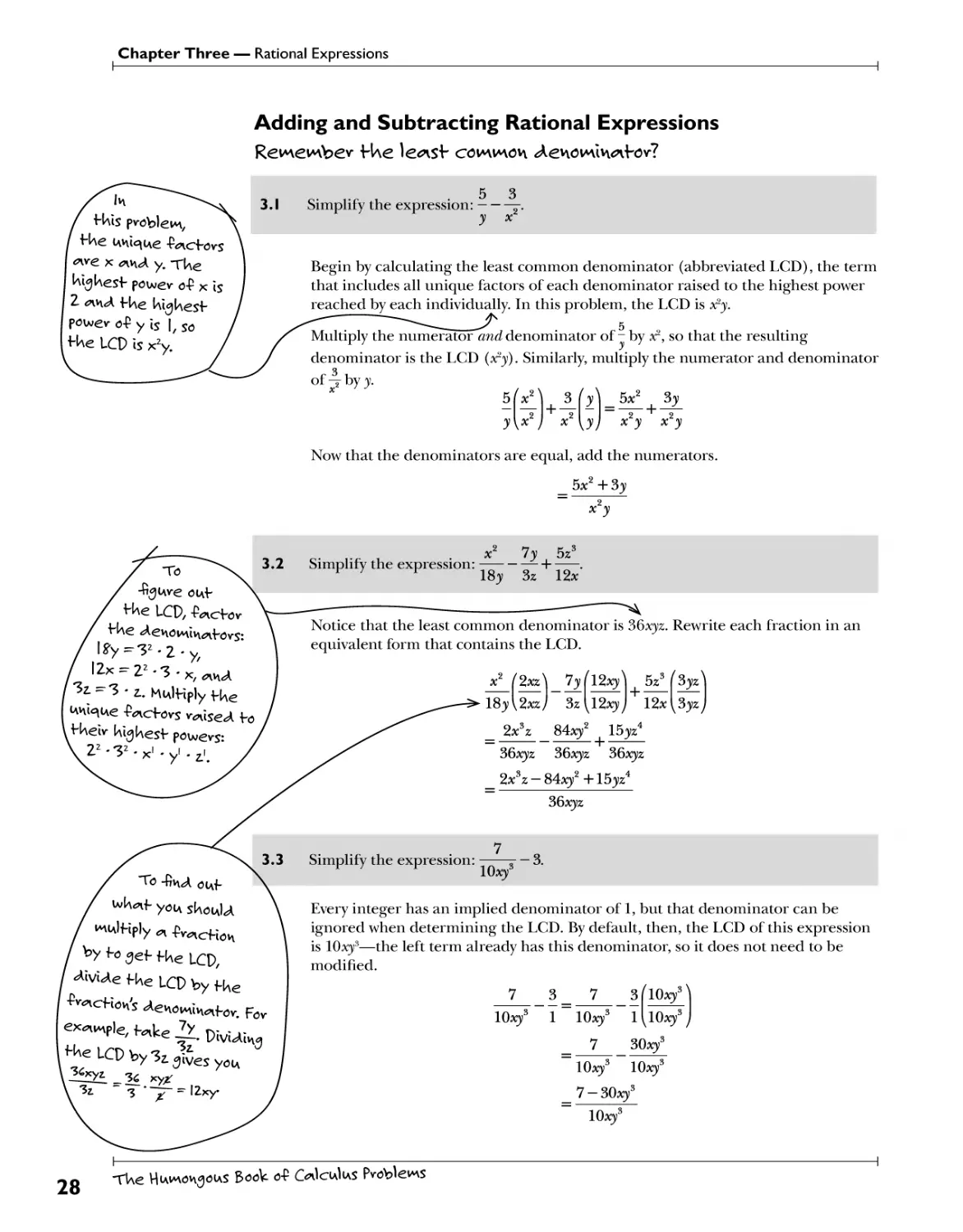
Adding and Subtracting Rational Expressions
^vv-e x o\y\A y. Tke
UigUesf powev o-P *
powev o-P y is I, so
iH\eLO)isx2y.
is
5 3
Simplify the expression: -
3; x
Begin by calculating the least common denominator (abbreviated LCD), the term
that includes all unique factors of each denominator raised to the highest power
reached by each individually. In this problem, the LCD is x2y.
Multiply the numerator and denominator of - by x2, so that the resulting
denominator is the LCD (x*y). Similarly, multiply the numerator and denominator
of J by >
x2) x2
= ^ +
33;
x y x y
Now that the denominators are equal, add the numerators.
_ 5x2 + 33;
x2y
Simplify the expression:
18j>
7y 5z3
- —+ .
3z 12^c
Notice that the least common denominator is 36xyz. Rewrite each fraction in an
equivalent form that contains the LCD.
x2 (2xz\ 7y(\2xy\ 5z3 (Syz\
18y\2xz) Sz{l2xy) 12x{syz)
2x\
S4xy2 15yz4
S6xyz 36xyz 36xyz
_2xsz-84xy2+15yz4
S6xyz
Simplify the expression:
* W you skouU
iMUlKply <* -P^cHoh
by f0 3€f f^€ Lc^
^ivU€ f ke LCD by f We
lOxy*
Every integer has an implied denominator of 1, but that denominator can be
ignored when determining the LCD. By default, then, the LCD of this expression
is 10ry3—the left term already has this denominator, so it does not need to be
modified.
lOtff
10xys
7
S(l0xy3
l^lOary3
30xys
I0xys 10xys
7-S0xys
10xys
28
TWe HiAwvongoiAS B00V o-P Oleics Problems
Chapter Three — Rational Expressions
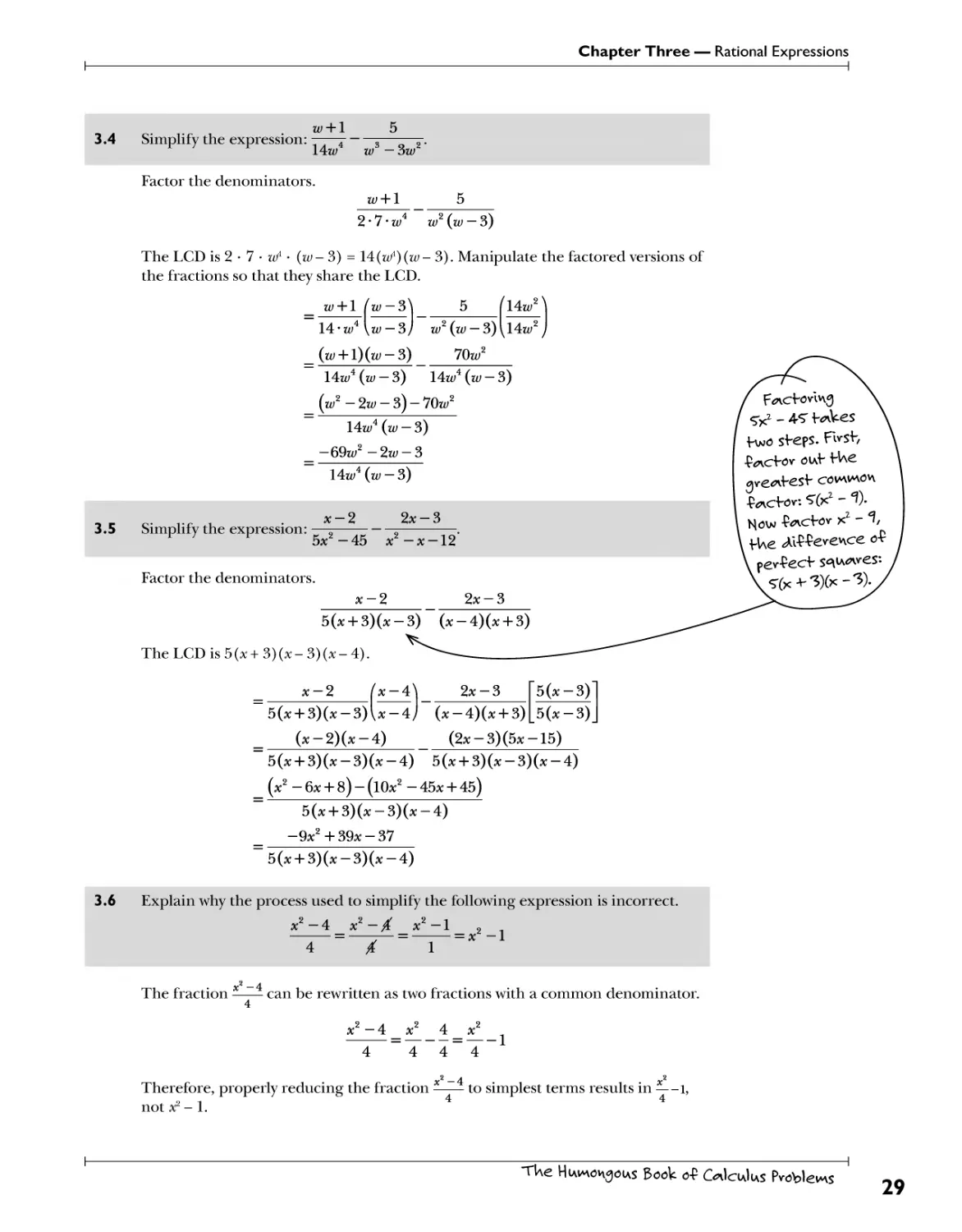
3.4 Simplify the expression:
Factor the denominators.
W/ + 1
14a/4
5
w3-$w*
w + 1
2-7-
!(a;-3)
The LCD is 2 • 7 • wA • (w- 3) = 14(w4)(w- 3). Manipulate the factored versions of
the fractions so that they share the LCD.
; + l
a;-hi I w
i
14a/
14 • w4 U - 3/ a;2 (a; - 3) \Uw*
(a; + l)(a;-3) 70a;2
14a;4 (a;-3) 14a;4 (a;-3)
(a;2-2a;-3)-70a;2
14a;4 (a;-3)
-69a;2-2a;-3
14a;4 (a; —3)
3.5 Simplify the expression:
x-2
2x-3
5af-45 af-*-12
Factor the denominators.
x-2
2x-3
5(x + 3)0 - 3) (x - 4)0 + 3)
The LCD is 5(x+ S)(x- S)(x- 4).
x-2
x — 4
5(x + 3)(x-3)U-4/ 0-4)0 + 3)
2*-3
5Q-3)
50-3)
0-2)0-4)
(2*-3) (5*-15)
50 + 3)0-3)0-4) 50 + 3)0-3)0-4)
(x2 - 6x + 8) - (l(k2 - 45* + 45)
50 + 3)0-3)0-4)
-9*2+39*-37
50 + 3)0-3)0-4)
3.6 Explain why the process used to simplify the following expression is incorrect.
= x2-l
iK T! iK /I iK -L a
/
1
The fraction
^-4
can be rewritten as two fractions with a common denominator.
x — 4 * 4 x
4 4 4
Therefore, properly reducing the fraction to simplest terms results in — -i,
not x2 -1.
TUe HiAvno^oiAS Book o-P C^IciaIias Problems
29
Chapter Three — Rational Expressions
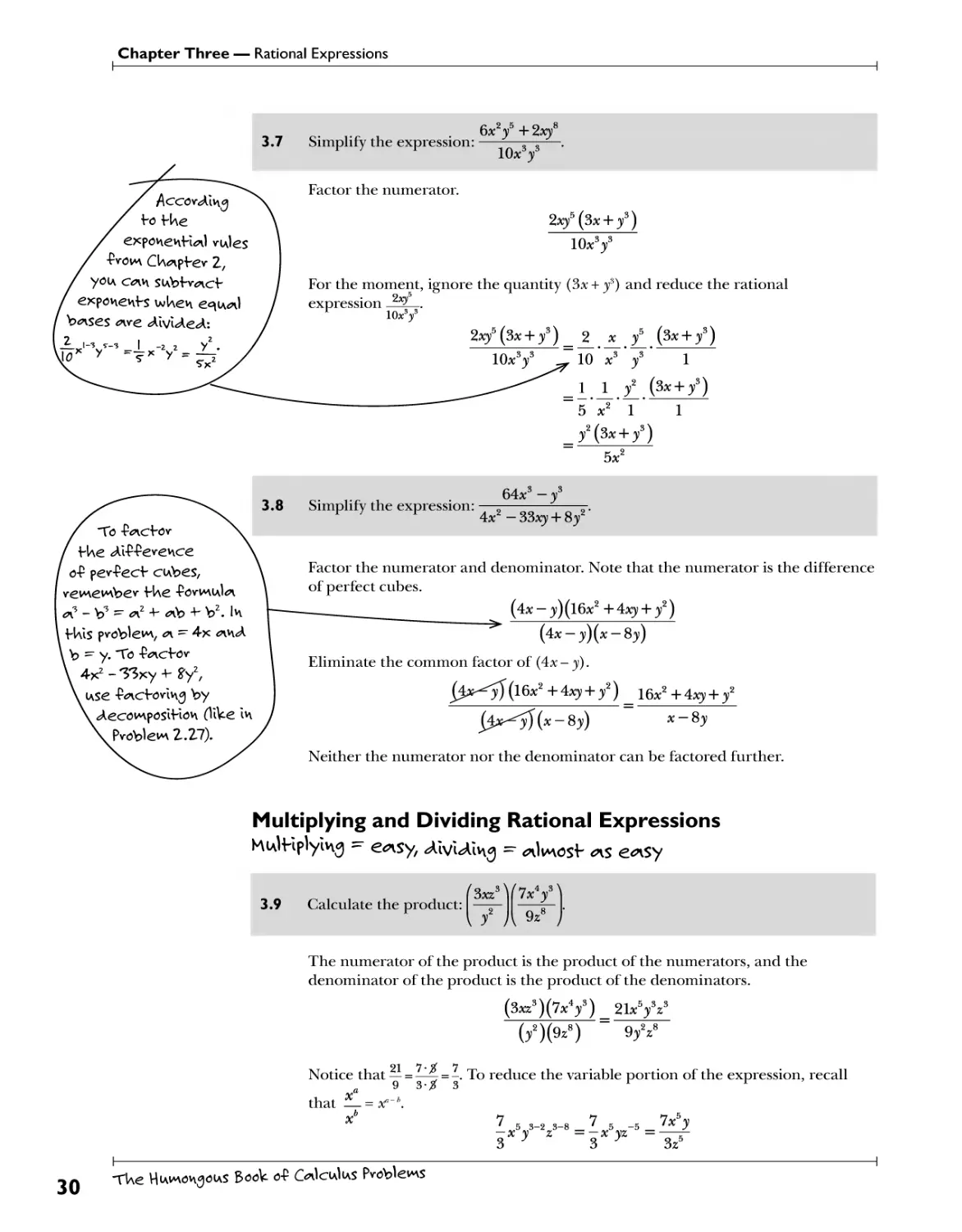
3.7 Simplify the expression:
Factor the numerator.
To -fWrf ov
f We <AI-P-Pevence
o-P pev-Pecf cubes,
vewewbev H\e -PovuaiaI^i
I ^ - b3 ~ <n2 4- <nb 4- b2. Iw
l b - y. To -fWrf ov
use -P^icf o/ivvg by
<AecowposlHov\ (llVe in
Problem Z.Z7).
6*2j>5+2*y8
10*Y
2*y5(3* + /)
For the moment, ignore the quantity (3x + y3) and reduce the rational
2xy5
expression
10*y
2xyB(3x + y*) 2 x y5 (3* + /)
io*y
10 xs ys 1
1 1 y2 (Sx + y*)
5 ' x2 ' 1 '
/(3x + /)
1
5*2
Simplify the expression:
64*3-/
4^-33^ + 8/
Factor the numerator and denominator. Note that the numerator is the difference
of perfect cubes.
(4x - y) (l6x2 + 4xy + y2)
[4x — y)[x — Sy)
Eliminate the common factor of (4x - y).
(£x^yj(l6x2+4:xy + y2) _16x2+4xy +y2
(4&^yj(x-8y) ^-Sy
Neither the numerator nor the denominator can be factored further.
Multiplying and Dividing Rational Expressions
3.9 Calculate the product:
3xz*)(7x4y-
9z8
The numerator of the product is the product of the numerators, and the
denominator of the product is the product of the denominators.
(3xz3)(7x4f) _21x5ysz3
(/)(*•)
9/z8
21 7 • 3f 7
Notice that — = —^ = -. To reduce the variable portion of the expression, recall
9 3-£ 3
that
: tf-
' 5 3-2 3-8 '5-5 'X J
— xy z =—xyz = —r-
3 y 3 y 3z5
30
TWe HiAwvongoiAS Book o-P Oleics Problems
Chapter Three — Rational Expressions
(33*V V 5w7 \
3.10 Calculate the product: — r-r- .
F { 10w5 All*9/J
Before you multiply the numerators together, it's helpful to reduce the
coefficients. Any factor in either numerator can be reduced using any factor in
either denominator:
11 1 10 2
7.2 5
3 1 W X y O 7_3 2_9 5_2 O 4 _7 3
a q o =—^ * y =—wx y =
1 2 a/VY 2 ' 2 3
3w y
2x7
(Sx2\S /W'
3.11 Calculate the product:
Before multiplying, raise each fraction to the power indicated.
33*2'3Y61(-2)/(-2)>|
27xV
' 36); V
3*6z
"17"
You couU <?dso
iv\fevpvef f Ue ^e^^Hve
lv\ ot-Uev \»oyAs, vewnfe
^ <*Wf U^nve fo mess
yWlf U lof S 0-P H€3*HV€
vexpov\ev\fs Ufev.
3.12 Calculate the product:
*-lY2*-5
4*y J\ * + 6
Apply the FOIL method when multiplying the numerators.
(*-l)(2*-5)_ 2*2-7* + 5
4xy2 (x + 6) 4x2y2 + 24xy2
3* 6* — 9
3.13 Calculate the quotient: — -=- .
H 4 10
'h of kev tvovJls,
^€cipvoc^lo-Px/;So^^C
The quotient --s-- (where # and d are nonzero real numbers) is equivalent to
b d
r(;P
3*
10
30*
4j\6x-9) 24*-36
To reduce the fraction, factor the denominator.
30* 0-5-x
12(2*-3) JBT - 2 - (2jc — 3)
5*
~2(2*-3)
TUe HiAvno^oiAS Book o-P C^IciaIias Problems
31
Chapter Three — Rational Expressions
3.14 Calculate the following quotient and write the answer in simplest form.
3*2 -lLc + 10 3*2-2*-5
x2-49
x2 — 6# — 7
Factor the polynomials and rewrite the quotient as a product (as explained in
Problem 3.13).
(3x-5)(x-2) . (3x-5)(x + l) _(3x-5)(x-2) Qc-7)Qc + 1)
(* + 7)(*-7) ' (*-7)(* + l) " (* + 7)(*-7) "(3*-5)(* + l)
_(3x-5)(x-2)(x-7)(x + l)
~(* + 7)(*-7)(3*-5)(* + l)
Eliminate any binomial factors that appear in both the numerator and
denominator.
gx^(x-2)£p^rf&#tf _x-2
(x + 7)(jc^^(£x^(j*^ ~ x + 7
3.15 Calculate the following quotient and write the answer in simplest form.
x3+8 m 8x + 16
0 + 8)3 ' *2+16* + 64
Division
ccv\es bePove
f o f [\e ovAev o-P
,opev*nHov\s.
Notice that x5 + 8 is a perfect cube (which should be factored according to the
formula in Problem 2.25) and x2 + 16x + 64 is a perfect square (because it has two
equivalent factors).
{x + 2){x2- 2x + 4) ^8(k + 2)
(k + 8)3 ' (k + 8)2
Convert this quotient into a product and simplify.
^Qc + 2)(*2-2* + 4) (x + 8)2
(* + 8)3 "8(* + 2)
i^A^) (x2 - 2x + 4) (^^)(^^)
(^$j(^$j{x + 8)(8)^K^
_x2 -2x + ±
8k + 64
3.16 Write the following expression in simplest form.
x 16#2 4#2+l(k
- + -
x-2 * + 4 4*2+13ai-12
Begin by calculating the quotient. Rewrite the quotient as a multiplication
problem and factor.
32
TUe Humorous BooV o-P Codecs Pvoble^s
Chapter Three — Rational Expressions
Calculate the sum.
* 16*' 4*'+13*-12
x-2 * + 4 4*2+10*
x 16*2 (4*-3)(* + 4)
x-2 * + 4 2*(2* + 5)
x 8'2'X'X'(4x-3)(jL*rf
-x (2* + 5) + (32*2 - 24*) (* - 2)
(*-2)(2* + 5)
(-2*2 - 5*) + (32*3 - 64*2 - 24*2 + 48*)
2*2+*-10
32*3-90*2+43*
2*2+*-10
Solving Rational Equations
Were cc\^es cress wtOHpUc^Hon
4 _ *
3.17 Find all solutions to the proportion: 3^ — jo
Cross multiply and solve for *.
Therefore, * = -4 or 4.
2*-7_2*-l
3.18 Find all solutions to the proportion: , •> — _ o .
Cross multiply and solve for *.
(2* - 7)(* - 2) = (* + 6)(2* -1)
2*2-ll* + 14 = 2*2+ll*-6
2*2-2*2-ll*-ll* = -14-6
-22* = -20
_20_10
*~22~11
MulHply
f We le-Pf
^iHpKe^byfken.kf
HiAtnev^fov * «- ^
becomes
fc~ ^
*i<* =■ be.
TUe IWov^oiAS Book o-P C^IciaIias Problems
33
Chapter Three — Rational Expressions
2 x — 4
3.19 Find all solutions to the equation: = 0.
x + 3 4
Transform the equation into a proportion by adding -— to both sides of the
equation.
2 x-4
x + 3 4
Cross multiply to eliminate the fractions.
2(4) = (* + 3)(*-4)
= K2-K-12
Apply the factoring method to solve the quadratic equation.
*2-*-20 = 0
(*-5)(* + 4) = 0
-4 or 5
+ 5 = 0-
20 Find all solutions to the equation:
af+2* + 3
Create a proportion and cross multiply.
x2+2x + 3 -5
~T
x2+2x + 3 = -5x
x2 +7ai + 3 = 0
ij fctij *7 4- /s*7
According to the quadratic formula, the solutions are x = and .
Simplify the left side of the equation.
3.21 Find all solutions to the equation:
so you'll be *ble fo
cycss tnulflply.
2* + l
-3 =
# + 5
4 3/2x + l\s + 5
4-3(2* + l)_* + 5
2^c + l *
4-6*-3 * + 5
2# + l x
—6a;+ 1 _ x + 5
2x + 1 #
Cross multiply and solve using the quadratic formula.
(-6* + l)(*) = (2* + l)(* + 5)
-6ai2+ai = 2tf2+lltf + 5
0 = 8af+10* + 5
The solution is x =
-5±Wl5
34
TWe HiAwvongoiAS BooV o-P Oleics Problems
Chapter Three — Rational Expressions
3.22 Solve the equation in Problem 3.21 again
L*
x + 5
but this time
\2x + \ x ,
eliminate the fractions by multiplying the entire equation by its least common
denominator. Verify that you get the same solutions.
The denominators of the terms, from left to right, are (2x + 1), 1, and x; the least
common denominator is x(2x + 1). Multiply each term of the equation by that / ^Hfive e^u f*
,f y°«* ^ f his.
2x + ]
4x£x^f) 3x(2x + l)_/(2x + l)(x + 5)
•prfi 1 /
4x-6x2 -3x = 2x2 + llx + 5
0 = 8x2+10x + 5
This matches the quadratic equation from Problem 3.21, so it will have identical
solutions.
3
3.23 Find all solutions to the equation:—-% , 2
Factor the denominators.
1
5 3 _ 1
{x-tf x*~x(x-2)
The least common denominator of all three terms is x2{x- 2)2. Multiply each term
by the LCD to eliminate the fractions.
-5x2£^<f s/(x-2f _X-x-(j^2l(x-2)
i^^f
J
x£*^T
-5x2+3(x-2)2 =x(x-2)
-5x2 + 3(x2 - 4x + 4) = x2 - 2x
-5x2 + 3x2 -12* +12 = x2 - 2x
-3x2 -10*+ 12 = 0
According to the quadratic formula, the solutions are x = —
5-V61 , 5 + V61
and —.
Polynomial and Rational Inequalities
CvIHc^d v\t\vMb€v*s bve^vk t\p yoiw v\i\i*\bev line
3.24 Write the solution to the inequality using interval notation: (x — 3)(2x +1) < 0.
Calculate the inequality's critical numbers.
*-3 = 0
x = 3
2* + l = 0
TUe HiAvno^oiAS Book o-P C^IciaIias Problems
35
Chapter Three — Rational Expressions
Draw a number line with these points marked; they split the number line into
three intervals: — «>,— I, —,31, and (3,oo)? as illustrated by Figure 3-1.
Figure 3-1 The critical numbers of(x — 3)(2x + 1) < 0 are x = and x = 3.
The solution to the inequality may be any combination of those three intervals. To
determine which belong to the solution, pick a value from each (called the "test
value" of the interval) and plug them into the original inequality.
1
00
2
Test Value: x = —l
(-l-3)(2(-l) + l)<0
(-4)(-l)<0
5<0
False
1
,3
Test Value: x = 0
(0-3)(2(0) + l)<0
(-3)(1)<0
-3<0
True
(3,oo)
Test Value: x = 5
(5-3)(2(5) + l)<0
(2)(11)<0
22<0
False
Only values from the interval I—,3] make the inequality true, so that is the final
solution to the inequality. Note that * = -- and x = 3 are excluded from the solution
because the critical numbers are excluded from the graph in Figure 3-1.
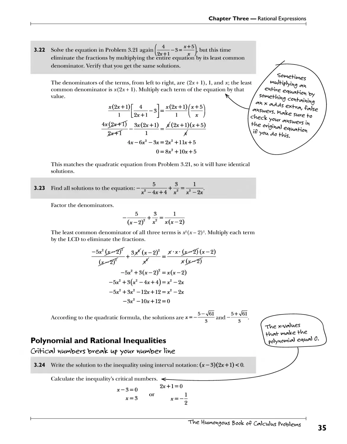
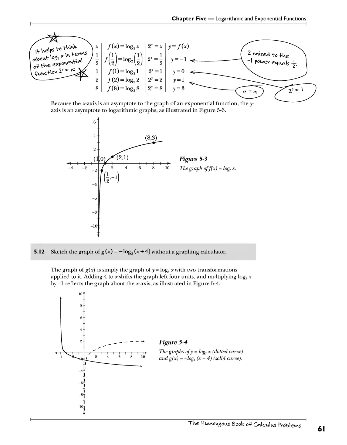
3.25 Graph the solution to the inequality: x2 + x > 2 .
Move all the terms to the left side of the inequality and factor.
*2+*-2>0
(* + 2)(*-l)>0
The critical numbers for this inequality are x = -2 and x=l. Graph both on a
number line using solid dots, as illustrated by Figure 3-2.
-4-3-2-101234
Figure 3-2 The critical numbers ofx2 +x>2 are x = -2 and x = 1.
The number line is split into three intervals: (— °°,—2], [—2,1], and [l,00). Choose
one test value from each interval (such as x = -5, x = 0, and x=2, respectively) and
plug each into the inequality to determine the solution.
36
TUe Humorous BooV o-P Codecs Pvoble^s
Chapter Three — Rational Expressions
It is more expedient to substitute into the factored version of the polynomial, as
the arithmetic is simpler.
(-°°,-2]
Test Value: x = — 5
(-5 + 2)(-5-l)>0
(-3)(-6)>0
18>0
True
[-2,1]
Test Value: x = 0
(0 + 2)(0-l)>0
(2)(-l)>0
-2>0
False
[i,«0
Test Value: x = 2
(2 + 2)(2-l)>0
(4)(1)>0
4>0
True
The solution is (—°°,—2] or [l,00); graph both intervals on the same number line, as
illustrated in Figure 3-3.
■N
■N
4-
4-
■N
■N
-4-3-2-10 1 2 3
Figure 3-3 The solution graph ofx* + x> 2.
3.26 Graph the solution to the inequality: 2x — 3x — 8 < 0.
Use
Y>™*cVeVs
since VWeyVe
3v^?Ue^ <*s soVa
<AoVs,VMV<*WyS
use f^venVUeses
o w^VVev
3±V73
Calculate the critical numbers via the quadratic formula: x = —-—. Use a
calculator to determine approximate decimal values for the critical numbers:
o 1*19. 9. _i_ 1*1%
—-— « -1.386 and —-— « 2.886. Choose test values (such as x — —2^, x — 0, and x = 4)
to verify that the solution is —-—,—-—, as graphed in Figure 3-4.
3-J73
3 + a/73
H OH-
-4
-3 -2 -1
Figure 3-4 The solution graph of2x2 — 3x — 8 <0.
3.27 Graph the solution to the inequality: 16#2 - 24# + 9 > 0.
Factor the quadratic and note that this polynomial has a double root (because the
polynomial is a perfect square).
(4k-3)(4k-3)>0
3
The only critical number is * = -; graphing that value results in two possible
interval solutions (as illustrated by Figure 3-5): I
and
TUe H wrongous Book o-P Calculus Pvoble^s
37
Chapter Three — Rational Expressions
-4 -3 -2 -1
3-
4
Figure 3-5 ^e on^ cr^ca^ number ofl6x2 — 24x + 9>0 isx
3_
4'
y^U^il (? is ^
Neither interval is a solution to the inequality; verify using the test values x = 0 and
x = 1—both make the inequality false.
Test value x = 0
(4(0)-3)(4(0)-3)<0
(-3)(-3)<0
9<0
False
Test value x = 1
(4(l)-3)(4(l)-3)<0
(1)(1)<0
1<0
False
Therefore, the only solution to the inequality is the solid dot x = — in Figure 3-5.
3.28 Write the solution to the inequality using interval notation:
x + 1
3*-±
>0 .
Critical numbers are x-values that cause an expression to equal 0 or x-values that
cause an expression to be undefined. Whereas polynomial inequalities do not
address the latter case, rational inequalities do.
Ensure that the rational expression alone appears on the left side of the inequality
and that 0 appears on the right side. Set the numerator and denominator equal to
0 and solve the resulting equations.
* + l = 0
x = — 1
or
3k -1 = 0
1
Plot those critical numbers on the number line, as illustrated in Figure 3-6. Notice
that * ~ 3 is plotted with an open dot, even though the sign of the inequality is
">". Any critical number generated by setting the denominator equal to 0 must be
plotted as anopen dot, regardless of the inequality sign. Therefore, the possible
solution intervals are (— °°, — 1 ], -1,- ], and f -
+-0 h
-4 -3 -2
-1
u
X + l 1
Figure 3-6 ^he critical numbers of > 0 are x = -l and x = —. Of
those, only x = -l can be part of the solution.
38
TUe Humorous BooV o-P Codecs Pvoble^s
Chapter Three — Rational Expressions
Choose test values from those intervals (such as -3, 0, and 1, respectively) to verify
that the solution is (— °°, — 1] or (-,00).
(-00,-1]
Test Value: x — — 3
-3 + 1
R
Test Value: x = 0
0 + 1
1
— c
Test Value: x = 1
1 + 1
A t\vylovv vn^nkes ov\e
big f Uiv\^ by cowbiv\iv\g
fiwo sw^Olev Huv^s. Fov
e^c^vnple, f Ue solution
3^pU in FyiAve 3-7 is
cve^nfe^ by cowbivuv^
fiwo iv\ec\iA^nlify
3^^pUs.
The solution graph is the union of the graphs of the solution intervals, pictured in
Figure 3-7.
-*■
-4 -3 -2 -1
+-o^
v
x +1
Figure 3-7 The solution graph of > 0.
3.29 Graph the solution to the inequality:
3x2 +17x + 24
3x2+2x
<0.
Factor the numerator and denominator.
(3*+ 8)0+ 3)
x(3x + 2)
<0
Set both the numerator and denominator equal to 0 in order to calculate the
8 2
critical numbers: x = -3,—,--,and 0. Plot those values, keeping in mind that x = 0
2 3 3
and x = — must be graphed with an open dot (because they make the expression
undefined). Choose test values from each of the five resulting intervals and
darken the intervals that satisfy the inequality, as illustrated by Figure 3-8.
-3
-2
-1
0
The solution to the inequality
Figure 3-8 0r [- -, o\
3x2 +17x + 24
3x2 + 2x
<0is
TUe HiAwov^oiAS Book o-P C^IciaIias Problems
39
Chapter Three — Rational Expressions
you've 30V 0 on
VUe vigWr S^e o-P
VWe me^u^ViVy <*vi<A
* Sl^e -EWVlo* ok
VUe^e^V behove you
sV^vV looVmg £ov
3.30 Write the solution to the inequality using interval notation:
x + 2,
#-4
Subtract 3 from both sides of the inequality and then identify critical numbers.
K + 2
x-4
-3>0
x — 4 1 \# — 4
K + 2 3*-12
Simplify the left side of the inequality using the least common denominator x-4.
x + 2 3(x-4\ „
>0
>0
>0
>0
x—4 x—4
(x + 2)- (3x-12)
x-4
x-3x + 2 + 12
x-4
-2*+ 14
x-4
The critical numbers of the inequality are x = 4 and x = 7, so the possible solution
intervals are (—00,4), (4,7), and (7,00). Use test values from each interval to
determine that the solution is (4,7).
40
TUe Humorous BooV o-P Codecs Pvoble^s
Chapter 4
FUNCTIONS
Now you'll sWf seeing -Pfr) <*U over H\€ pUce
Whereas linear, polynomial, and rational equations are both useful and
ubiquitous in advanced mathematics, concise definitions of mathematical
relationships are essential once theory and proof are involved. That the
function automatically assures us of predictable behavior is a given, but that
you know how to manipulate such expressions is not, hence this chapter.
fUeyVe weN wovfU reviewing.
Chapter Four — Functions
VUe seV
Combining Functions
Do H\e iasia^O (+-,-, x, *w\<A -f-) ov plu^ }ey\ Info e^vcU ofUev
4.1 Is the relation s: {(-3,2), (4,1), (8,2)}, a function? Justify your answer.
Yes, s is a function because each member of thejdomain (-3, 4, and 8)
corresponds to exactly one member of the range (2, 1, and 2). In other words,
s(-3) = 2, 5(4) = 1, and 5(8) = 2. While it's true that s(-3) and 5(8) both have the
same output, that does not invalidate the function. Two inputs may have identical
outputs, as long as each input corresponds only to that output and no other.
4.2 Find real number values for m and n such that the following relation is not a
function.
p: {(-4,-1), (-2,7), (0,3), (m,n), (10,8)}
The relation p is not a function if any element of the domain has more than one
corresponding range element. Therefore, if m is equal to any other member of the
domain and n does not match that element's range element, p is not a function.
Any of the four following possibilities are viable solutions to this problem: m = -4
and n ^ -1; m = -2 and n ^ 7; m = 0 and n ^ 3; and m = 10 and n ^ 8.
4.3 Find a real number value for c that ensures the following relation is one-to-one.
j: {(-2,9), (-1,.), (0, -4), (1, -13), (2,-6)}
As discussed in Problems 4.1-4.2, no function may have an input element that
corresponds to two different output elements. If a function is one-to-one, the
reverse is also true—each element of the range corresponds to exactly one
domain element, so cmay be any real number except -13, -6, -4, or 9. No matter
what real number is substituted for c, j will be a function, but it will only be one-to-
one if those four values are avoided.
4.4 Given the functions/: {(-1,10), (3,5), (10,-6)} and g: {(-1, -4), (3,0), (10, -5)},
calculate (f+ g)(10).
Note that (/+ g)(10) = /(10) + g(10).
(/ + g)(10) = /(10) + g(10)
= (-6)+ (-5)
= -11
4.5 Given the functions/(x) = x2 + 4 and g(x) = (x+ 4)2, calculate (fg)(-2).
Note that (fg)(-2) =f(-2) • g(-2).
U)(-2) = /(-2)-g(-2)
= ((-2)2+4)-(-2 + 4)2
= (4 + 4)(2)2
= 8(4)
= 32
42
TWe HiAwvongoiAS B00V o-P Oleics Problems
Chapter Four— Functions
4.6 Given the functions f(x) = x+ 1 and g(x) = 6x* + 19x- 36, determine the domain
ofgW.
(f\ f(x\ x + l
— (*) = J-r\ = t~9———— is undefined whenever its denominator / -.-„
equals 0. Set g(x) = 0 and solve to identify those values, which must be excluded / f ectav\l<^€. e*F \a\to£
from the domain.
Factor the polynomial.
6x2 + 19x-36 = 0
(2* + 9)(3*-4) = 0
2* + 9 = 0 3k-4 = 0
# = —-
# =
The domain of — \(x) is all real numbers except x = and x = — .
\g) F 2 3
4.7 Given functions f(x) = x2 and g(x) = 2x + 5, find (f ° g)(x) and (g°/)(*).
4.8
The notation (/ ° g")(x) is read "/composed with gof x," and is equivalent
to/(g(x)). In other words, the function g(x) should be substituted into/(x).
Similarly, (g o f)(x) = g (/(*)).
(f°g)(*) = f(g(x))
= /(2* + 5)
= (2x + 5)2
= 4*2 + 20*+ 25
= g(**)
= 2(x2) + 5
= 2x2+5
Given functions f{x) = 4x and £(*) = ** ~12x + 36 ; nnd(/°g)(*) and
*» « even, f kevx
(/^)W=/(gW)
= /(x2-12* + 36)
= V*2-12x + 36
= V(^-6)2
= |# — 6|
(go/)(*) = g(/(*))
= (^)2-12^ + 36
= *-12^ + 36
1
4.9 Given the functions f(x) = , g(x) = x - 2x2, and h(x) = %Jx — 6, calculate
f(g(h(70))). X + S
Evaluate the innermost function.
h(70) = ^70^ = ^64=^ = 4
S Wf wif k ^^
**u* u,ovk yotAv u-^y
**»* fUe insUe 0uf.
^^fyoiA3€f^VOln
♦^P'^tWvestJt
info -P6c).
TUe H wrongous Book o-P Calculus Pvoble^s
43
Chapter Four — Functions
Substitute h(lQ) = 4 into the function: f{g{h(70))) = f(g(4)). Once again evaluate
the innermost function, which is now g{x).
g(4) = 4 - 2(4)2 = 4 - 2(16) = -28
By substitution, f(g(4)) = /(-28). Evaluate/(-28) to complete the problem.
1 1 1
/(-28) = -
-28 + 3 -25 25
Therefore,/(g(A(70))) = -^.
4.10 Given the functions f(x) = x2, gyx) = , and hyx) = , find f(g(h(x))).
\ usvvxg ^e K-
Substitute h(x) into g(x).
g(*) =
1
2k + 1
1
*(*<*» = 71^
-Psf)«
1
2(1-*
l
->."lz*+1
+1
Simplify the complex fraction.
*(*<*)) = iz^
+1
1
(1 — x) + x
X
1_
1
Multiply the numerator and denominator of the complex fraction by the
reciprocal of its denominator to simplify.
fx\
1
g(h(x)) = Y
X
x
X
g(h(x)) = - = x
Substitute g(h(x)) = xinto the expression: f(g(h(x))) =f(x) = x2.
44
TUe Humourous BooV o-P Codecs Pvoble^s
Chapter Four— Functions
Graphing Function Transformations
€WefcUes, s^ulsUes, -flips, <*kA slices
Note: Problems 4.11-4.18 address transformations of the graph f(x) in Figure 4-1, so that you
can more effectively juxtapose the effects of the transformations. It is not beneficial to determine
the equations that generate the graph.
4.11 Graph/(x)-2.
Figure 4-1
The graph off(x), to be transformed in
Problems 4.11-4.18.
When a constant is added to, or subtracted from, a function, it shifts the graph
vertically. Adding a constant c moves each point on the graph up c units, and
subtracting c moves the graph down c units. Therefore, each point on the graph of
f(x) - 2 should be plotted two units below its corresponding point on the graph of
f{x), as illustrated by Figure 4-2.
Figure 4-2
The graph off(x) - 2 is the graph off(x)
moved down two units.
*W <h ercW p.oble^
MWHoHis.Justp^
Moving
p0lv\f S 0-P 0\
gv^npU <Aoiw\ Z
i\v\If s vne^nHS yoiA
sUoiO<A siAbW^ncf
Z -{Vow f We y-
coowAIvunfes o-P
If s polnf s.
Re<*A
*W c^e-Pully.
AAAl^3 l^slAe fke
^cHoHLEFTHofw.kf
Jke ^hcKoh RIGHT.
Note: Problems 4.11-4.18 address transformations of the graph f(x) in Figure 4-1.
4.12 Graph f(x- 3).
Notice that 3 is subtracted from x, whereas the constant was subtracted from/(x)
in Problem 4.11. This operation causes a horizontal shift on its graph. Note that
subtracting a constant moves the graph to the right, and adding moves the graph
left. Therefore, the graph off(x- 3) is simply the graph off(x) moved three units
to the right, as illustrated in Figure 4-3.
TUe HiAvnongoiAS Book o-P C^IciaIias Problems
45
Chapter Four — Functions
engine) -fy*)
d*«pk covins
^e poihf s (-.2 -2)
Hv€ opposif€S 0.p
Figure 4-3
The graph off(x - 3) is the graph off(x)
moved three units to the right.
Note: Problems 4.11-4.18 address transformations of the graph f(x) in Figure 4-1.
4.13 Graph -f(x).
Multiplying a function by -1 reflects its graph across the x-axis. Iff(x) contains the
point (x,y), then -f{x), graphed in Figure 4-4, contains the point (x,-y).
-6
\ j, ^ Figure 4-4
The graph of-f(x) is the reflection off(x)
across the x-axis.
Note: Problems 4.11-4.18 address transformations of the graph f(x) in Figure 4-1.
AAA Graph f(-x).
Multiplying xby -1 reflects the graph of/(x) across the ^-axis; if/(x) contains the
point (x,y), then/(-x) contains the point (-x,y), as illustrated in Figure 4-5.
Figure 4-5
The graph off(-x) is the reflection off(x)
across the y-axis.
46
TUe Humorous BooV o-P Codecs Pvoble^s
Chapter Four— Functions
Note: Problems 4.11-4.18 address transformations of the graph f(x) in Figure 4-1.
4.15 Graph-/(*).
Multiplying a function by a constant affects the ^-values of its coordinates. If the
graph off(x) contains the point (x,y), then the graph of c • f(x) contains the point
(x, c - y). In this case, each point on -f{x) is half the distance from the x-axis as
the corresponding point on graph of/(x), as illustrated by Figure 4-6.
Figure 4-6
Points on the graph of~f(x) are half as
far from the x-axis as the corresponding
points off(x).
MulHply f h€ y.
values by T. Because
**) QJHf^Hj Use poiv^fs
Note: Problems 4.11-4.18 address transformations of the graph f(x) in Figure 4-1.
4.16 Graph f(2x).
Whereas multiplying f(x) by a constant affects the distance of its points from the
x-axis, stretching it away from (or compacting it toward) the x-axis (as explained
in Problem 4.15), multiplying xby a constant inversely affects the distance of a
function's coordinates from the ^-axis. Although you might expect the coordinates
of/(ex) to be c times further from the ^-axis than the corresponding points on
f{x), the points are actually - times as far away, as illustrated by Figure 4-7.
Figure 4-7
Points on the graph off(2x) are half as far
from they-axis as the corresponding points
affix).
Note: Problems 4.11-4.18 address transformations of the graph f(x) in Figure 4-1.
AM Graph 1/0*01 .
By taking the absolute value of/(x), you change all negative outputs into their
opposites while leaving positive outputs unchanged. In other words, iff(x)
contains the point (x,y), then |/(#)| contains the pointfx,|;y|j. Graphically, this
means any portion off(x) below the x-axis is reflected above the x-axis, but the
rest of the graph does not change.
The
poihf S oh f ke
poinfs on £6s). Bec^se
(-*<*> **A(l,\), fOj
conf^iHs (~T/4)
TUe H (wrongous BooW o-P Calculus Pvoble^s
47
Chapter Four — Functions
* oJ). Re?Uce VUe e,-
sUe(sovVo£UVeyo*
V * VUe -fivsV <W^
Figure 4-8
The graph of\f(x)\.
Note: Problems 4.11-4.18 address transformations of the graph f(x) in Figure 4-1.
4.18 Graph /(l*l) .
The /(M) transformation affects coordinates with negative x-values. Consider
this: x = 1 and x = -1 must have the same output for /(M), since /(|—1|) = /(l). In
fact, every x in the domain of the function must output a value that matches its
opposite; therefore, f(x) =f(-x) even if-x does not belong to the domain off(x).
Graphically speaking, if/(x) contains point (x,y), and x> 0, then /(M) contains
the point (-x,y). The net result: /(M) is symmetric about the ^-axis based on
its positive domain, as illustrated by Figure 4-9. See Problem 4.21 for another
example of this transformation for additional clarification.
Figure 4-9
The graph off{\x\) is symmetric about
the y-axis
You we,e,A Vo
, voVUeb^Vo-PVUe
Tv^vvS^ovvA^ViovvS.
-V^hV
4.19 Sketch the graph of/fa) = (* + 2)2 -
transformations.
1 without a calculator by applying graphical
To transform the function y = x2 (the dotted curve in Figure 4-10) into
f(x) = (x + 2)2 - 1 (the solid curve in Figure 4-10), you must to add 2 to x (which
shifts its graph left two units) and subtract 1 from/(x) (which shifts the graph
down one unit).
48
TUe Humorous BooV o-P Codecs Pvoble^s
Chapter Four— Functions
4.20 Sketch the graph of g(x) = —
+ 4.
Figure 4-10
The graphs ofy = x2 (dotted) and
f(x) = (x + 2)2-l (solid).
There are three transformations that change y = \x\ (the dotted curve in Figure
4-11) into g(x) = - \-xU- 4 (the solid curve in Figure 4-11):
|3 |
1. Multiplying x by - stretches its graph horizontally along the x-axis by a
factor of 3.
2. Multiplying by -1 reflects its graph across the x-axis
3. Adding 4 moves the graph up four units.
The graphs ofy = \x\ (dotted) and
' + 4 (solid).
4.21 Sketch the graph of h(x) = SyJ\x\ — 4 without a graphing calculator.
Three transformations are required to change y = y/x (the dotted curve in
Figure 4-12) into h(x) = 3^/|#| —4 (the solid curve in Figure 4-12): the absolute
value within the square root function replaces all points for which x < 0 (via the
technique of Problem 4.18), multiplying the function by 3 stretches its graph
vertically by a factor of 3, and subtracting 2 moves the graph down 2 units).
TUe HiAwov^oiAS Book o-P C^IciaIias Problems
Chapter Four — Functions
Figure 4-12
The graphs ofy = yfx (dotted)
andh(x) = 3yj\x\ — 4 (solid).
Inverse Functions
Fi\v\cHov\s H\*if cancel of Uev -PiahcHohs ouf
4.22 Given the function s :
function, srl.
(-2,-l),|-l,-|,(0,l),a4),(3,-9)
define the inverse
To generate the inverse of a function, reverse the coordinate pairs—if s(x) = y,
then s~l(y) = x.
-1:{(-l,-2),(|,-l),(l,0),(4,l),(-9,3)}
Rewrite s~l, listing the domain elements from least to greatest.
s~l:{(-9,3),(-l,-2),(l,0),(|,-l),(4,l)
4.23 Given f(x) graphed in Figure 4-13, sketch the graph of/_1(x).
(-5,-3)
-5f
-4
Figure 4-13
-tj—±—i—+—±—**■ The graph of a one-to-one function f(x).
The graph of a function and its inverse are reflections of one another across the
line y = x, as illustrated by Figure 4-14.
50
TUe Humorous BooV o-P Codecs Pvoble^s
Chapter Four— Functions
*y = x
(-5,-3)
Figure 4-14
The dotted graph of a function f(x) and the
solid graph of its inverse f~*(x) are reflections
of one another across the liney = x.
A.2A Given the function g(x) graphed in Figure 4-15, explain why g~l(x) does not
exist.
Figure 4-15
The graph of function g(x).
In order for a g~l(x) to exist, g(x) must be one-to-one (as defined by Problem 4.3).
However, g(x) fails the horizontal line test, indicating that it is not one-to-one,
and therefore does not have an inverse. According to the horizontal line test, any
horizontal line drawn across a one-to-one function won't intersect that graph
more than once. However, the horizontal lines y = -2 and y = S both intersect
g(x) twice.
x + 4
4.25 Given g(x) = ——, find g~l(x).
Rewrite g(x) as y.
x + 4
y = -
Reverse the x and y variables, substituting x for y and vice versa.
_y + 4
TUe HiAwov^oiAS Book o-P C^IciaIias Problems
51
Chapter Four — Functions
Solve for y.
Rewrite y as g~l (x).
7x = y + 4
y = 7x - 4
g-1^) = 7x-4
Given/(x) = ^ + 1 (x > 0), find/"1^).
Rewrite f(x) as 3;.
3;= a? + 1
Reverse x and y.
x = y2 + 1
Solve for 31.
x — l = y2
±y/x — l=y
±7^1 = f1 (x)
Note that/_1(x) doesn't equal both ^x — 1 and —y/x — 1; only one of those equations
is a reflection of/(x) = x2 + 1 (x ^ 0) across the line 31 = x (as illustrated by Figure
4-16): f~l (x) = ^lx — 1. Discard the negative radical.
Figure 4-16
Notice thatf(x) = x2 + 1 and
f'1 (x) = 4x — l are reflections of
one another across the y-axis. The
equation y = — yjx — 1, a byproduct of
the inverse function creation process, is
superfluous.
y = x
x-\- 4
4.27 Verify that g(x) = —-— and g~l{x) = 7x - 4 (from Problem 4.25) are inverses by
demonstrating that g(g~l(x)) = g~l(g(x)) = x.
Perform composition of functions using the method of Problems 4.7 and 4.8.
g(g~1(x)) = g('7x-4)
_(7*-4) + 4
7
~T
= x
<r-(«(«))-?-(£^1)
=#+4-4
= X
52
TUe Humourous B00V o-P Codecs Pvoble^s
Chapter Four— Functions
4.28 Verify that/(x) = x2 + 1 (x * 0) and/ 1 (x) = y/x-1 (from Problem 4.26) are
inverses by demonstrating that/(/_1(x)) =f~l(f(x)) = x.
/(r1w)=/(v^ri)
= (V^IT)2+i
= x
r1 (/(*))=r (**+!)
=V(*2+i)-i
=V7
= k
H^mks fo fke x > £
*^€ absolute values
Asymptotes of Rational Functions
E^L\^vHov\s o-P H\e unfoiAcWble AcVVeA line
4.29
7
Identify the vertical asymptote to the graph of y =
x — 3
If substituting c into the rational expression causes the denominator to equal 0,
then x = c is a vertical asymptote of f{x), as long as the numerator does not equal 0
as well. Set the denominator equal to 0 and solve. Wv
c tn^nkes
fhe fop <nv^
causes the denominator to equal 0, / ™e boffom o-P f[^e
k-3 = 0
k = 3
X = 6
Because x = 3 causes the denominator to equal 0 (and the numerator does not
equal 0), x= 3 is a vertical asymptote of the function's graph.
USlA<J
tale in f he ^v^pU
KCknpfev |0, you'll
use Kmif s f o -fi^e
ouf wkeve f U<nf
tale is.
4.30 Identify the vertical asymptotes to the graph of 3; =
-3
3k'-23*-36
Set the denominator equal to 0 and solve the quadratic by factoring.
3k2-23k-36 = 0
(3k + 4)(k-9) = 0
3k + 4 = 0
Sx = — 4 or
__4
3
k-9 = 0
k = 9
vuAwev^nfov's
^e^vee is higher fU<nn H\e
i ^HOlMlH^ifov's, fWe -PIAHCHOH
^woVf U^nve *wy UoWz.ov\f^l
^nsyvnpfofes.
Both x-values cause the denominator (but not the numerator) to equal 0, so they
__4
are asymptotes to the graph: * ~ 3 and x = 9.
4.31 Identify the horizontal asymptote to the graph of g(x) =
x2 - 2x + 4
-2k3-16'
Compare the degrees of the polynomials in the numerator and denominator to
determine the equation of the horizontal asymptote (if it exists). In this case, the
degree of the numerator is 2, and the degree of the denominator is 3. When the
denominator's degree is greater than the numerator's degree, the function has
horizontal asymptote y = 0.
TUe IWov^oias Book o-P C^IciaIias Problems
53
Chapter Four — Functions
Tke
coe-P-ficievrf-
JVigkesf pou>ev.
4.32 Identify the horizontal asymptote to the graph of h(x) =
(2k-3)(k + 6)
(4k-5)(-3k + 1)
Calculate the products in the numerator and denominator.
h(x) =
2af+9*-18
-12*r+19*-5
When the degrees of the numerator and denominator are equal, the graph of
the function will have horizontal asymptote y = -, where a and b are the leading
coefficients of the numerator and denominator, respectively.
2 _ 1
-12" 6
y =
^sympfofes
occiav only u,keh
H\e Aegvee o-P f Ke
HiAtnev^fov is one
_/;
To geV
/o-P V-Ue sWV
/^sy^fVoVe, seV *y -
L\e ^vision ves^V <**u*
w N 3aT-13* + 4
4.33 Determine the equations of all asymptotes to the graph of / (x) = g— .
The numerator and denominator have equal degrees, so the horizontal asymptote
is equal to the quotient of their leading coefficients, as explained in Problem 4.32.
y = \ = $
To determine the vertical asymptotes, factor the polynomials.
(3k-1)(k-4)
/(*) = ■
(x + 3)(x-3)
Set the factors of the denominator equal to 0 and solve to get x = S and x = 3.
Neither of those values causes the numerator to equal 0 as well, so both represent
vertical asymptotes. Therefore, the equations of the asymptotes tof(x) are x = -3,
x= 3, and y = 3.
4.34 Find the equation of the slant asymptote to the graph of g(x) =
2x -3x + 6
x + 1
The slant asymptote is the quotient of the rational function (omitting the
remainder). The divisor is a linear binomial, so synthetic division (the method
described in Problems 2.18 and 2.19) is the most efficient way to calculate the
quotient.
ES 2 -3 6
-2 5
2 -5 11
The equation of the slant asymptote is the quotient: y = 2x- 5.
5k3-30k2-4k + 24
4.35 Identify asymptotes to the graph of j(x) = -
x2 + 2x - 4
Because the degree of the numerator is exactly one greater than the degree of the
denominator, j(x) has one slant asymptote and no horizontal asymptotes. (Note
that a rational function may have only one slant asymptote or one horizontal
asymptote, but may have multiple vertical asymptotes.
54
TUe Humorous BooV o-P Codecs Pvoble^s
Chapter Four — Functions
To determine the slant asymptote, use polynomial long division, as outlined in
Problems 2.16 and 2.17.
bx -40
k2+2k-4J5k3 -30k2- 4k + 24
-5k3 - 10k2 + 20k
-40k2+16k+ 24
40k2 + 80k -160
96k-136
The slant asymptote toj(x) is y = bx- 40. To determine the vertical asymptotes of
j(x), set the denominator equal to 0 and solve using the quadratic formula.
k2+2k-4 = 0
-2±V22-4(l)(-4)
x =
2-1
= -2±V20
2
= -2±2^
2
= X(-i±Vs)
%
The function j(x) has three asymptotes: the slant asymptote y = bx- 40 and the
vertical asymptotes x = — 1 — V5 and x = — 1 + V5.
TUe Humorous Book o-P Calculus Problems
Chapter 5
LOGARITHMIC AND EXPONENTIAL
FUNCTIONS
Ft\v\cHov\s UVe lo^3 >c, lv\ >c, oCf cv\A e?
Chapters 1-4 provide the opportunity to sharpen your skills in all matters
concerning variable expressions raised to real number powers. This chapter
begins by investigating the reverse, expressions containing real numbers
raised to variable powers. Whereas exponential rules hold true despite this
reversal, new techniques must be mastered in order to properly manipulate
such expressions. Of course, one cannot discuss such an important function
without exploring its inverse, the logarithmic function.
-rtus ck<nPfe. Ae«\s wiHv e^enfUl WHohs, wkick look move like
3" fU *\ Tke problems -Peel very »venf wken * is fke ecpo^f
thsfe^l o-P fke b*se. Fov one Hu^ you'll nee,A some w*y o-P < Weli-
ouf x e^ponenf s » youVe eve. 3oin3 fo solve *r *, ^ fU<nf re^Sres
o^nf kmic Wcohs. 6oo<A news ^ W news: lo^ifkmic WHohs
fl-ke cwevses o* e^enfUl WHohs) .e*lly kelP you solve e^Hons *W
k<nve * lH fke e^poneHf, buf lo^ifkms b/^ wifk fkern fkeiv own sef o-P
pvopevhes <*\\A \ri*les.
Chapter Five — Logarithmic and Exponential Functions
Exploring Exponential and Logarithmic Functions
W<*y\\ess *01 H\ose powers
4H €XpOH€HH^il
. €^,s|*teHy<,Upiu,
\pou,er win €c|lA^| ^
Graph the function f(x) = 3X without a graphing calculator.
Employ the most basic of graphic techniques: substitute consecutive values of x
into/(x) and plot the resulting coordinate pair.
i
/(-l) = 3"1 =
/(0) = 3°=1
/(1) = 31=3
/(2) = 32=9
Because /(— 1) = — the point _1,_ belongs on the graph. Similarly, the graph of
f(x) includes the points (0,1), (1,3), and (2,9), as illustrated by Figure 5-1.
Figure 5-1
The graph off(x) = 3x
suve f o use
<a P^nv-enf Uesls,
v\of <a bv^ncVef,
Uev-e. TWe -PiahcHoh
e^u^ls 0, so you cWf^
Incite OlnfWe
Note that the x-axis is a horizontal asymptote of f(x). Although negative values of
x result in small/(x) values, 3X doesn't equal 0 for any x-value.
5.2 Identify the domain and range of the generic exponential function g(x) = ax
(assuming a is a real number and a > 1).
Any real number can be substituted for x, but the positive real number a raised
to any power (whether positive or negative) always results in a positive number.
Therefore, the domain is (-oo?oo) and the range is^0,oo).
5.3 Sketch the graph of y = 2~x - 1 without a graphing calculator.
The graph of any exponential function y = ax will pass through the points (0,1)
and (I,a) and have a horizontal asymptote of y = 0. Begin by graphing
y = 2X as illustrated by the dotted curve in Figure 5-2.
58
TUe Humorous BooV o-P Codecs Pvoble^s
Chapter Five — Logarithmic and Exponential Functions
Figure 5-2
The graphs ofy = 2X (dotted) and
y = 2~x - 1 (solid).
To graph y = 2~x - 1, perform two translations on the graph of y = 2X (as explained
in detail by Problems 4.11-4.21): Substituting -xfor x reflects the graph about the
3?-axis, and subtracting 1 moves the entire graph down one unit.
5.4 Determine the domain and range of the logarithmic function h(x) = log3 x.
Note that h(x) is the inverse function off(x)= 3X, as defined in Problem 5.1.
Therefore, the domain off(x) equals the range of h(x) and vice versa. You can
then conclude that the domain of h(x) is (0,oo) and its range is (-oo,oo).
5.5 Solve the equation: log10 x = 2.
Rewrite the logarithmic equation as an exponential equation and solve for x.
102=*
100 = *
5.6 Solve the equation: log4 x = -3.
Rewrite in exponential form and solve for x.
4~=x
■ = x
64
5.7 Solve the equation: log5 625 = x.
Rewrite the equation in exponential form: bx = 625. Note that 54 = 625, so x = 4.
5.8 Solve the equation: log4 ~ = x.
8
Rewrite as an exponential equation.
8
TUe HiAwov^oiAS Book o-P C^IciaIias Pvoblewvs
59
Chapter Five — Logarithmic and Exponential Functions
VUe b^ses-
Express the fraction as a negative exponent.
4* = 8-1
Rewrite the equation using exponential expressions with equivalent bases (4 = 22
and8 = 23).
(27= (ST
Two equivalent exponential expressions with equal bases must have equal
exponents as well.
2* = -3
*W I, u,kick is u,ky
5.9 Solve the equation: logx 16 = 2.
Rewrite as an exponential equation and solve for x.
*2=16
x = ±4
Only the solution x = 4 is valid; discard #3^-4.
5.10 Solve the equation: log^ 81 =
Rewrite in exponential form.
x4/3 = 81
To solve for x, raise both sides to the - power.
(*4'7/4=81!
13/4
--
*3'4=(V8l)
- / I— \3
^=33
* = 27
5.11 Graph the function/(x) = log2 x without a graphing calculator.
The domain of/(x), like the domain of y = log3 x in Problem 5.4 or any other
logarithm, consists only of positive numbers; do not substitute negative x-values
into/(x) as you plot points. The first column in the table of values below consists
of the x-inputs, the second column substitutes xinto/(x), the third column is the
equation expressed in exponential form, and the final column is the ^-value that
corresponds with x.
60
TUe Humorous BooV o-P Codecs Pvoble^s
Chapter Five — Logarithmic and Exponential Functions
VWv\V
^gyV\$
OUT ™yi \
y sr jc:
tf
1
2
1
2
8
/(*) = log2*
4i)-(i)
/(l) = log2l
/(2) = log22
/ (8) = log, 8
2y=x
Qy — —
2
2^=1
2^=2
2^=8
y = f(x)
y = -l
y = 0
y = i ,
;y = 3
Because the x-axis is an asymptote to the graph of an exponential function, the y-
axis is an asymptote to logarithmic graphs, as illustrated in Figure 5-3.
Figure 5-3
The graph off(x) = log2 x.
5.12 Sketch the graph of g(x) = — log3 (x + 4) without a graphing calculator.
The graph of g(x) is simply the graph of y = log3 xwith two transformations
applied to it. Adding 4 to x shifts the graph left four units, and multiplying log3 x
by -1 reflects the graph about the x-axis, as illustrated in Figure 5-4.
Figure 5-4
The graphs ofy = log3 x (dotted curve)
and g(x) = —log3 (x + 4) (solid curve).
TUe HiAwov^oiAS Book o-P C^IciaIias Pv-oblewvs
61
Chapter Five — Logarithmic and Exponential Functions
-TV\e
Vov.
Natural Exponential and Logarithmic Functions
Uv\wvlf f ev\ \>c\ses, Wises wlf U e, <*v\<A cU^v^e o£ b<*se -PovwiO^
5.13 Define the terms "common logarithm," "natural logarithm," and "natural
exponential function"; indicate the notation used for each.
The common logarithm has base 10 and is implied if no base is indicated:
log x = log10 x.
The natural logarithm has base e and is written In x: In x = loge x.
• The natural exponential function has base e and is written e.
5.14 Use a calculator to determine the value of log 19, accurate to five decimal places,
and interpret the answer.
<** Vlf Iay<x) log o-P
Note that log 19 = log1019, because unwritten logarithmic bases are understood
to be 10. Calculating log 19 is the equivalent of solving the equation log1019 = x,
which can be rewritten in exponential form: 10x:
log 19 « 1.27875, which means 10L27875 « 19.
19. According to the calculator,
5.15 Use a calculator to determine the value of In 19, accurate to five decimal places,
and interpret the result.
ttosV
cWV compute
logs VU^vV ^ov\V
U^vve c\ Y>*vse o-P
VUe cU^w\ge o-P Y>*vse
-PovvauU is so Wowvfy.
VUe log o-P VUe
Y>*\se goes i* VUe
^ev\ov^\lv\^vVov.
Note that In 19 = loge 19, as any logarithmic expression written "In" instead of
"log" is a natural logarithm and has an implied base of e. Calculating In 19 is
the equivalent of solving the equation loge 19 = x, which can be rewritten in
exponential form: & = 19. According to the calculator, In 19 ~ 2.94444, so
^2.94444 ~ i9 Because Euler's number, e, is approximately equal to 2.7182818, you
can also write 2.7182818294444 « 19.
5.16 Evaluate log3 25, accurate to four decimal places, using the change of base
formula and a calculator.
The change of base formula allows you to rewrite the expression loga b as -^— or
ln«"
log 25 _ In 25
log3 ~ ln3
1.3979400087 _ 3.2188758249
0.4771212547 ~ 1.0986122887
2.92994704... = 2.92994704...
Therefore, log3 25 ~ 2.9299. Note that there is no need to calculate the value
twice, as both calculation methods return the same value.
62
TUe Hw*\ov\goiAS bccY o-P OOculus PvoV>le»*\s
Chapter Five — Logarithmic and Exponential Functions
5.17 Evaluate log610, accurate to four decimal places, using the change of base
formula and a calculator.
Apply the change of base formula.
lnlO _ 2.302585093
ln6 ~ 1.791759469
«1.2851
5.18 Verify the solution to the equation in Problem 5.7 (log5 625 = x) using the
change of base formula and a calculator.
Apply the change of base formula.
log 625 _
log 5
log 62£
log 5
= x
log 625
— = 4 *<-
5.19 Verify the solution to the equation in Problem 5.8 log4 — = x\ using the change
of base formula and a calculator. ^ '
Apply the change of base formula.
l-Pyou
\v\c&
*??
o-P
log
ln« 3
ln4 2
^^AWUe,yo^9^
zn^ooxri ^ AOOOOooooo\^
*** use "«<****
Properties of Logarithms
E*p<*v\<Aiv\3 <*v\<A S^t\isUiv\g log e>cpveSSlov\S
5.20 Rewrite as a single logarithm: log2 x + log2 5 + log2 3;.
The sum of logarithms with equal bases is equal to the logarithm of the product:
loge b+ logec=loge (be).
log2 x + log2 5 + log2 y = log2 (5xy)
5.21 Rewrite as a single logarithm: log 3 - (log 9 + log x).
Rewrite the parenthetical expression, log 9 + log x, as log 9x (as explained in
Problem 5.20). Combine those first, according to the order of operations.
log 3 - (log 9 + log x) = log 3 - (log 9x)
TUe Humongous Book o-P Calculus Problems
63
Chapter Five — Logarithmic and Exponential Functions
l-P f wo logs
one log fU^if's
iMiOHptte^A, f Uen If
w<*kes sense H\<*f
fwo logs siAbW^icfe^A
I \>e.ccv\e. one log f U^f 's
<Alvi*Ae<A—f UeyVe
, ejzc\c\r opposif es o-P
one <?wof Uev.
The difference of two logs with equal bases is equal to the logarithm of the
b
quotient: log, b - log, c = log, -.
c
= log
9*
Reduce the fraction.
3x
5.22 Rewrite as a single logarithm: log 7 + log x - log 3 + log y - log z.
The <*v\swev
IsjusV^iW o-PVWe
log v*dues \A/vIVVev\ in
one JWcVion—<*H VWe
posiHve logs Oike log 7
<*n<A log y) en<A up in Vke
nuv^ev^iVov, <*n<A <*H VWe
neg^Vive ones Hog *5 <*n<A
-log z.) en^ up in VUe
v^enovAin^iVov.
Jusf like
(U;z4-u;z4-u;z^3u;z.
According to the order of operations, addition and subtraction should be
performed from left to right. Begin by rewriting log 7 + log x as a single logarithm.
log 7 + log x - log 3 + log y - log z = log 7x - log 3 + log y - log z
Again manipulate the two leftmost terms of the expression; rewrite log 7x- log 3
as a quotient using the logarithmic property discussed in Problem 5.21.
7x
= log 1- logy — logz
3
7x
Adding log— to log y results in a single log containing the product.
7xy
7xy
Finally, divide ~y by z, which is the equivalent of multiplying the fraction by the
reciprocal of z.
5.23 Verify that 3 In x = In x5 and, based upon your proof, extrapolate and prove an
equivalent conclusion for loga x" (if a and n are real numbers and a > 1).
Rewrite 3 In x as a sum.
->- 3 In x = In x + In x + In x
According to a logarithmic property (described in Problem 5.20), the sum of
logarithms with the same base is equal to the logarithm of their product.
31n# = \nx-\-\nx-\-\nx = \n(x- x- x) = \nxs
Therefore, 3 In x = x3. Expressed more generally, n \oga x = loga x". As justification,
recall that n \oga x can be rewritten as the sum of n terms (where each term is
logfl*).
n log, x = log, x + log, x + log, x H 1- log, x
total of n terms
64
TUe Hw*\ongoiAS 5ccY o-P Codecs PvoV>le»*\s
Chapter Five — Logarithmic and Exponential Functions
Rewrite the sum of the logarithms as a single logarithm of their products.
/ \
\ogax + logax + \ogax + -- + \ogax = \oga
(x)(x)(x)'--(x)
there are n
factors of x
= ^gaxn
total of n terms
Therefore, n \oga x = \oga x*.
5.24 Rewrite as a single logarithm: 5 log x - 2 log y + 4 log (x - y).
Rewrite the coefficients of the logarithms as the exponents of their arguments
according to the logarithmic property n \oga x = loga x", as explained in
Problem 5.23.
5 log x- 2 log y + 4 log (x- y) = log x5 - log f + log (x- y)A
The two leftmost logarithms are equivalent to a logarithmic quotient.
5
= \og^ + \og(x-y)
y
The sum of logarithmic expressions with equal bases is equal to the logarithm of
their product.
x5 (x — y)
= log- V "
5.25 Expand the logarithmic expression: In xy
Expanding a logarithmic expression requires you to apply logarithmic properties / ^0u «~~- ^
in order to rewrite a single logarithmic expression as multiple logarithmic / _ \q<x y ^ 3 ^'
expressions. Because xy2 is a product, rewrite the argument as the sum of two / . ovV-S 0V^V ^
logarithms with equal bases. / \>uV Vv\<* ^ve
In xy2 = In x + In y2
Recall that log x? = a log x, so In f = 2 In 31.
= In x + 2 In 31
5.26 Expand the logarithmic expression: log—.
5
Recall that log — = log a — log b.
logy = log/-log5
Substitute log f = 3 log y into the expression.
= 3 log y - log 5
TUe Humongous Book o-P Calculus Problems
65
Chapter Five — Logarithmic and Exponential Functions
5.27 Expand the logarithmic expression: log8
2x2
(x-yf
The logarithm of a quotient can be rewritten as the difference of two logarithms.
log82x2-log8 (x-y)3
The leftmost logarithm contains a product, which can be rewritten as the sum of
two logarithms.
= log8 2 + log8 x2 - log8 (x-y)3
Rewrite the exponents of the logarithmic arguments as the coefficients of their
respective logarithms.
= log8 2 + 2 log8 x- 3 log8 (x-y)
Solving Exponential and Logarithmic Equations
5.28 Simplify the expression: log4 43.
Apply the logarithmic property log X'= a log x, as described in Problem 5.23.
log443=31og44
Apply the change of base formula to the logarithm.
31og44 = s(j^j = 3(l) = 3
This result demonstrates a fundamental logarithmic fact: loga an = n.
5.29 Simplify the expression: 3log3*.
This expression is the result of the composition of functions f(g(x)), where
f(x) = 3X and g(x) = log3 x. Because f(x) and g(x) are inverse functions, they
cancel one another out, leaving behind only the argument of the inner function:
giog3* _ ^ EXp0nential and logarithmic functions with the same base (y = ax and
y = \oga x) are inverses of one another.
5.30 Simplify the expression: In (e4 • e,x).
Multiply the natural logarithmic expressions within the parentheses.
In (e4 • ebx) = In ebx+4
Notice that the expression In ebx+4 is a composition of inverse functions, because
In x and t have the same base. Therefore, the functions cancel one another out,
leaving behind only the argument of the inner function.
In e,x + 4 = 5x+4
66
TUe Hw*\ongoiAS 5ccY o-P Codecs PvoV>le»*\s
Chapter Five — Logarithmic and Exponential Functions
5.31 Simplify the expression: elnx~lny.
Rewrite the exponent using logarithmic properties. (The difference of two
logarithms with the same base is equal to a logarithmic quotient, as explained in
Problem 5.21.)
Jnx-iny _ ^ln (x/y)
The natural logarithmic and exponential functions are inverses of one another,
so only the argument of the inner functions remains when the functions are
composed.
Ux/y) _ *
5.32 Determine the exact solution to the equation: 2X = 9. / ^pjc&yj&e.
\c$z 1 is <**
To eliminate the exponential function 2X on the left side of the equation, apply its / *lvv^Vlovv^ vviAwtoev)
inverse function log2 x to both sides of the equation. / -, Ae<£\v*<d d&ces
wevev Vevwiv^Ve ov
,epe*vV, so <*vvyH\ivv9 sWovV^
o-P^iw^vviVdy^vvgVisV
Although you could use the change of base formula to approximate log2 9, the \ °"^ ^
problem specifically requests the exact answer. Therefore, you should not estimate \ uXr\C i <*
the solution: x = log2 9.
log22*=log29
x = log2 9
5.33 Determine the exact solution to the equation: 2 ■
-13.
Subtract 2 from both sides of the equation to isolate the exponential function,
then multiply the entire equation by -1.
-*5*=-15
e5x=15
To eliminate the natural exponential function, take the natural logarithm of both
sides of the equation.
In^=lnl5
5x = lnl5
lnl5
x =
5.34 Determine the exact solution to the equation: 5 + In (x + 3) = 7.
Isolate the logarithmic expression on the left side of the equation.
^—_^^^^ In (x+S) =2
Exponentiate the equation to eliminate the natural logarithm.
eHx+s)=e2
x + 3 = e2
x = e2 - 3
TUe Humorous Book o-P Calculus Problems
67
Chapter Five — Logarithmic and Exponential Functions
5.35 Determine the exact solution to the equation: log5 2x- log5 3 = log5 (4x- 19).
Apply logarithmic properties to rewrite log5 2x - log5 3 as a logarithmic quotient.
log5y = log5 (4*-19)
Exponentiate the equation to eliminate the logarithms.
^log5(2*/3) _ glog5(4x-19)
Because 5X and log5 x are inverse functions, they cancel one another out, leaving
behind only the arguments of the logarithms.
2x
= 4k-19
Solve for x.
2* = 3(4*-19)
2* = 12*-57
-10* = -57
57
x = —
10
5.36 Determine the exact solution to the equation: log x + log (x — 2) - 1 = 0.
Move the constant term to the right side of the equation.
logx + log(x — 2) = 1
The sum of two logarithms with equal bases equals the logarithm of their
product.
log [*(*:-2)] = 1
log(a:2-2a:) = l
Exponentiate the equation to eliminate the logarithmic function.
k2-2*: = 10
K2-2a:-10 = 0
Solve using the quadratic formula.
-(-2)±V(-2)2-4(l)(-10)
2(1)
Discard the invalid solution x = 1 — v 11 (logarithmic functions have a domain of
x > 0); the only valid solution to the equation is x = 1 +
68
TUe Hw*\ongoiAS 5ccY o-P Codecs PvoV>le»*\s
Chapter 6
CONIC SECTIONS
When a double-napped right circular cone is sliced by a plane, the
perimeter of the resulting cross section will be a circle, an ellipse, a
parabola, or a hyperbola. Hence, this family of four curves is known as the
conic sections. Like their graphs share a similar origin, the equations of
their standard forms share similar characteristics as well, though each has
unique distinguishing features.
This chapter explores the nuances of the equations that generate the conic
sections and investigates how the constants and variables in those equations
affect their graphs.
«* cafe* f™y«.' The ««f obvioW fe^ # „ vtmJM^
kou, f„ ^H,pMUfe w e^Hoi so «-'s e«sy fc, r„pk
Chapter Six — Conic Sections
Parabolas
6.1 Write the equation of the parabola in standard form and identify its vertex:
y = x2 + 6x - 4.
Add 4 to both sides of the equation so that the right side contains only x-terms.
y + 4 = x2 + 6x
Complete the square on the right side of the equation: take half of the x-
coefficient [-•6 = 3], square the result (32 = 9), and add that number (9) to both
sides of the equation.
3, + 4+9 = ^c2+6^ + 9
y + 13 = x2+6x + 9
Factor the trinomial.
y + 13 = (x + 3)(x + 3)
y + \$ = (x + $f
y= (x+3)2-13
The standard form of a parabola is y = a(x- h)2 + k, , so in this problem a=\,
h = -3, and k = -13. The vertex of a parabola in standard form is (h,k) = (-3,-13).
6.2 Write the equation of the parabola in standard form and identify its vertex and
axis of symmetry: y = 2x2 - 16x- 1.
Move the constant to the left side of the equation.
y + 1 = 2x2 - 16x
Complete the square on the right side of the equation. To do so, the coefficient
of the x2-term must be 1. Divide the entire equation by 2 (the ^-coefficient) to
accomplish this.
- + - = x2 - 8x
2 2
The square of half the x-coefficient is 16: —(—8) = —4, and (-4)2 = 16; add 16 to
both sides of the equation.
V 1
z + - + 16 = ^2-8^c + 16
2 2
Add the constants on the left side of the equation and factor the right side.
f + ^ + f = (*"4)(*-4)
3> + 33
= (x-4)2
70
TUe Hw*\ongoiAS 5ccY o-P OOculus PvoV>le»*\s
Chapter Six — Conic Sections
Multiply the entire equation by 2 to eliminate the fraction; solve for y.
f)
m=(D
~(*-4)2l
1
y + 33 = 2(x-4)2
y = 2(x
-4)2-33
The equation is now in standard form, y= a(x- h)2 + k; therefore, a = 2, h = 4, and
k = -33. The vertex of the parabola is (h,k) = (4,-33), and the axis of symmetry
is x = 4.
i*u<
VVwougVviVsvevVe^.
vevHc^O Vine * - K-
6.3 Write the equation of the parabola in standard form and identify its vertex:
-f + Sx+5y-7 = 0.
Notice that this equation (unlike Problems 6.1 and 6.2) contains a /-term rather
than an x2-term. Though the process is similar to those problems, the end result is
an equation solved for x (not y) with standard form x= a(y- k)2 + h.
Isolate the ^-terms on the right side of the equation.
Sx—7 = f — 5y
Complete the square.
Sx-
25
4
-7 + — =y2-
12*-
■28 25 ,
12*-3
■5y +
5
2
25
4
5
2
-= ,
Multiply both sides of the equation by 4 in order to eliminate the fraction; solve
for x.
//12*~3
= 4\y
I2x-S = 4\y--
12x = 4\y
+ 3
Multiply each term by — to isolate x.
$MUw
+
12
4
12lJ
-- +
12
1
x = —I ■»-
sr
-- +
OiVeVUisowe),VisVUe
0?FosiVe o-P VUe *w**>ev
lw jwewVWeses *o<u* U
is VUe covvsV^vvvV. The
vevVex is sVffl (U,V)—
VUose coor^ivv^vVes we
e**c*tyVUes*i"£fS
jwovboUs \wiVU *
VWew.
U\
The parabola is now in standard form, * = a(y - k)2 + /^, with a = — ,h = — , and
5 /1 5\ 3 4
k = — . The vertex of the parabola is (h,k) = I —,— . ^
TUe Humorous Book o-P Calculus Problems
71
Chapter Six — Conic Sections
6.4 Write the equation of the parabola in standard form and identify its vertex and
axis of symmetry: x— 9y2 + 18y + 6 = 0.
*»* h> see iP y<5tA
^^e,^rOHyou
- <?v 2
V"M*y
4-tf^r,
SIVAlV
l<*v.
This equation contains y2, so you should rewrite it in standard form
x = a(y- k)2 + A. Move all ^-terms to the right side of the equation.
x + 6 = 9/ - lSy
Divide all of the terms by 9 to ensure the coefficient of f is 1, so that you can
complete the square. Solve for x.
oc_ 6 _ 9/ 18y
9 9~~9 9~
x + 6
x + 6
k + 15
= y'-2y
+ l = y2-2y + l
=(y-if
9
x + 15 = 9(y-lf
K = 9(y-lf -15
This is the standard form of the parabola x= a(y- k)2 + h , where a = 9, h = -15,
and k = 1, so the vertex is (h,k) = (-15,1). A parabola written in terms of y has axis
of symmetry y = k, so the axis of symmetry of this parabola is y = 1.
Graph the parabola defined in Problem 6.1: y = x2 + 6x- 4.
According to Problem 6.1, the standard form of the parabola is y = (x + 3)2 - 13.
Graph the parabola by applying two basic transformations to the graph of
>y= x2. Adding 3 to x shifts the graph left 3 units, and subtracting 13 shifts the
graph down 13 units.
Figure 6-1
The dotted graph ofy = x2 and the solid
graph ofy = (x + 3f - 13. All parabolas
containing an x2-term either open upward
or downward, whereas parabolas written
in terms ofy either open left or right.
vertex = (-3,-13)
72
TUe Hw*\ongoiAS 5ccY o-P OOculus PvoV>le»*\s
Chapter Six — Conic Sections
6.6 Graph the parabola defined in Problem 6.3:-y2 + 3x+ 5y-7 = 0.
According to Problem 6.3, the parabola has standard form # = -U — +-. The
graphs of parabolas containing y2-terms are not functions, because they fail the
k.—"
vertical line test. Thus, function transformations (such as those demonstrated in
Problem 6.5) are not a reliable method to graph this equation. Instead, you
should plot points; substitute a variety of values for y to get the corresponding
revalues and graph the coordinates that result. Since the vertex is located at I-,-),
use ^-values close to -.
/\ vevVic^O Vine
VUe gv^pW o-P c\
-PiAvvctfovv wove VWowv
once.
y = 0
S\ V 4
=u^y=7-
3\4) 4 3
y = \
x4HK
=H9-y-=i
5
y=-2
k = -(0)2+- = -
3W 4 4
y = 3
*~lUJ +4
SU/ 4 3
3> = 4
SU/ 4
According to this table of values, the points I -,0J, (1,1), (wl* I3'3)' an<^ (1>4)
belong on the graph, as illustrated by Figure 6-2.
Figure 6-2
The graph of the parabola -f +
opens to the right.
6.7 Identify the focus and directrix of the parabola: 2x2 + 20x - 3y + 9 = 0.
Rewrite the parabola in standard form. Divide the equation by 2, so that the
coefficient of x2 is 1, and complete the square.
TUe Humorous Book o-P Calculus Problems
73
Chapter Six — Conic Sections
2x2 2(k_3); 9_0
2 2 2 2~2
2 2
3*v 9
^-- + 25 = K2+10a: + 25
2 2
3y 9 50 , KW .
-^-- + y = (* + 5)(* + 5)
3<y + 41 , .2
2 V '
3); + 41 = 2(a: + 5)2
3); = 2(a: + 5)2-41
y = -(x + 5)2- —
2 41
Standard form of the parabola is y = a(x - h)2 + k, so « = -, h = -5, and & = ——. In
order to determine the focus of the parabola, first define the constant c =
c =
1
4/2
1
8
2 .
It is important to note that a = -is positive, because that means the parabola's
focus is above its vertex and its directrix is below the vertex. Any such parabola
has focus (h,k+ c) and directrix y=k- c. Substitute the values of h, k, and cinto
those formulas.
Focus = (h,k + c)
I 3 8
= -5,-
= -5,"
-328 + 9
24
319
24
Directrix: y = k — c
41_3
3 8
328 9
24 24
337
24
y = -
y = -
y = .
74
Tke Hw"vongous Book o-P Calculus PvobWs
Chapter Six — Conic Sections
6.8 Identify the focus and directrix of the parabola: y2 + 3y + 5x+2 = 0.
Rewrite the parabola in standard form x = a(y- k)2 + h by completing the square.
-5x-2 = y2+3y
9 9
-5a:-2 + - = 'y2+3<y + -
4 y y 4
8 9
-5x V — = 1 *y H— II y +
4 4 r 2Y 2
1( 3 V 1
x = y + — H
5^ 2 J 20
1 1
Therefore, a — —, h = —, and k = ; calculate c.
5' 20 2
1
4a
=
1
(i)B)
=
1
(-!)
=
5
4
When the parabola contains a 3^-term and a < 0, the focus is left of its vertex
and the directrix is right of the vertex. Specifically, the focus is (h— c, k) and the
directrix is x = h + c.
Directrix: x = h + c
x =
X-
X-
1
= — +
20
1
= — +
20
26
"20
13
5
4
25
20
10
6.9 Write the equation of the parabola with focus (-1,3) and directrix y = 1 in
standard form.
As noted in Problem 6.7, a parabola that contains an x2-term has a horizontal
directrix. (A parabola with a y^-term has a vertical directrix, as demonstrated by
Problem 6.8.) Therefore, you should use standard form y = a(x- h)2 + k.
The vertex (h,k) of the parabola has the same x-value as the focus, so h = -1.
Furthermore, it is equidistant from the directrix and the focus; therefore, k is
the average of the ^-coordinate of the focus and the constant in the directrix
equation.
* =
3 + 1
TUe Humorous Book o-P Calculus Problems
75
Chapter Six — Conic Sections
Note that cis the vertical distance between the vertex and the focus; calculate the
absolute value of the difference of their ^-values: c = |3 — 2| = 1. Calculate a using
the formula from Problems 6.7 and 6.8, but omit the absolute value signs.
c = -
1 =
4a
J_
4a
4a = 1
1
You must now determine whether a is positive or negative. According to Problem
l
6.7, when a parabola's focus is above its vertex, a > 0. Therefore, a
k=2.
y = a(x — h) +k
y = ^(x + lf+2
h = -l, and
Circles
-the
cenVev o-P
VV\e £<^s °* *
cowsUeveA f**
0£ vV\e 9^?V\.
6.10 Graph the circle with center (-3,0) and radius 2.
Plot the center point on the coordinate plane, and then mark the points 2 units
above, below, right of, and left of the center, as illustrated by Figure 6-3. Draw the
graph of the circle through those four points.
Figure 6-3
The graph of a circle with center (-3,0)
and radius 2.
76
TUe Hw*\ongoiAS 5ccY o-P OOculus PvoV>le»*\s
Chapter Six — Conic Sections
6.11 If points A = (-4,1) and B = (6,-5) are the endpoints of line segment AB, such
that AB is a diameter of circle C, find the center and radius of C.
The center of the circle is located at the midpoint of the diameter, so apply the
midpoint formula (as described in Problem 1.8).
center =
-4 + 6 l + (-5)
2' 2
= (1,-2)
The radius is half the length of the diameter. Calculate the diameter's length
using the distance formula (as described in Problem 1.9) and divide the result
by 2.
J. AB V(6-(-4))*+(-5-l)' Vl02+(-6)2 M6 %M
radius = = = = = ——
2 2 2 2 %
- = V34
6.12 Identify the center and radius of the circle: (x + 9)2 + (y- l)2 = 16.
The standard form of a circle is (x- h)2 + (y - k)2 = r2, where (h,k) is the center of
the circle and ris the radius. In this example, (h,k) = (-9,1);-The radius is equal to
the square root of the constant on the right side of the equation.
r2=16
r = 4
Though r = -4 is a valid solution to the equation r2 = 16, it is not a valid radius; the
radius of a circle must be positive.
6.13 Rewrite the equation of the circle in standard form: x2 + y2 —4x + 12^ - 10 = 0.
Write the x-terms in descending order of degree, leaving empty space before
listing the ^-terms. (You will use this space to complete the square in the next
step.) Then write the ^-terms in descending order of degree (leaving space before
the equal sign). Move the constant by adding 10 to both sides of the equation.
x2-4x +/+12> =10
£-
Complete the square twice (once for the x-terms and once for the ^-terms), adding
both constants to the right side of the equation to maintain equality.
x2 - 4x + 4 + / +12y + 36 = 10 + 4 + 36
(*-2)(*-2) + (y + 6)(y + 6) = 50
(x-2)2+(y + 6f =50
*kA 34 f o H\e le-Pf sUe
o-P f Ue e^u^iHon In fUe
\Y>l*ivvV. Spof s ^y\A c\AA
^bofU o-P fUe^A fc
nlso.
V
TUe Humorous Book o-P Calculus Problems
77
Chapter Six — Conic Sections
6.14 Rewrite the equation of the circle in standard form: x2 + f + 7x - 2y + 6 = 0.
Use the method of Problem 6.13 (completing the square twice simultaneously) to
reach standard form.
49 49
x2+7x + — + /-2> + l = -6 + — + 1
(x+l)\(y-iy =
29
4
Recall that the standard form of a circle is (x— h)2 + (y - k)2 = r2; therefore, h = ~-
k=l, and r= J— = —^~. The center of the circle is --,l|, and the radius is ——.
6.15 Identify the center and radius of the circle: 2x2 + 10x+2y2 -7y + 12 = 0.
*\ve
In order to complete the square, the coefficients of the x2- and /-terms must be
1. Note that they are equal, so divide all terms in the equation by the shared
coefficient.
2x2 10* 2/ 7y 12 0
2 2 2 2 2 2
7
x2 +5x + y2 y + 6 = 0
Rewrite the equation in standard form by completing the square once for the x-
terms and again for the y-terms.
2 25 2 7 49 r 25 49
x2+5x + — +<y2--<y + — = -6 + — + —
4 y 2y 16 4 16
5V $\ ( 7Y ?\ 96 100 49
x+2 *+irri rir_i6+i6-+i6
5\* ( 7\* 53
fb3 y/bS
a i and the radius is J— = —-—.
^/ V lb 4
( $1
The center of the circle is I 2' 4
6.16 Graph the circle: bx2 - 30x + by2 + by + 40 = 0.
Rewrite the equation in standard form using the method outlined by Problem
6.15. Divide all terms of the equation by 5, the coefficient shared by the x2- and
/-terms.
x2 — 6x + y2 + y = —8
1 ~ ~ I
4
x2 -6x + 9+ y2+y + -=-8 + 9 + -
78
-rUe HuvAOwgous BooV o-P Calculus Pvoblev^s
Chapter Six — Conic Sections
The center of the circle is 3>~- and the radius is J- =—. Use a calculator to find
a decimal approximation of the radius "^"sal118 and graph using the method
outlined in Problem 6.10. The solution is illustrated in Figure 6-4.
Figure 6-4
The graph of the circle 5x* - 3 Ox + 5f + 5y + 40 = 0
is centered at\3,--\ .
Ellipses
f<*wcy \noyA -Pov "ov<k\s"
Note: Problems 6,17-6,18 refer to the ellipse graphed in Figure 6-5,
6.17 Calculate the lengths of the major and minor axes of the ellipse and identify the
vertices.
(-2,6)
(-2,-4)
Figure 6-5
The graph of an ellipse and the endpoints
of its major and minor axes.
The major axis of the ellipse has endpoints (-2,6) and (-2,-4). Its length,
therefore, is the distance between those points. Note that endpoints are on the
same vertical line (x = -2), so the distance between the points is the absolute value
of the difference of the ^-coordinates: |-4 - 6| = 10.
TUe Humorous Book o-P Calculus Problems
Chapter Six — Conic Sections
, V>uVVUeyVe vioV
<**A b SU/*ip pUceS:
Stick *i lAhAewxe^k
t+l€ VwUbl€ 6c 0>r y)
*we ^iv-€cHon ess «v€
«*tj<*r *i*is. In Problem
is vcv+tc^il, sc sHck
v^ble since f ke
y-^ixts is *\)so
The endpoints of the minor axis are (1,1) and (-5,1); its length is |-5 - 1| = 6, the
difference of the x-coordinates. Note that the major axis is always larger then the
minor axis of an ellipse, and only the endpoints of the major axis are considered
the vertices of the ellipse: (-2,6) and (-2,-4).
Note: Problems 6,17-6,18 refer to the ellipse graphed in Figure 6-5,
6.18 Write the equation of the ellipse in standard form.
rThe standard form of an ellipse with a vertical major axis is ^ ~2 ' + ^ 2 '
1,
where (h,k) is the center of the ellipse, a is half the length of the major axis, and b
is half the length of the minor axis. Apply the midpoint formula to the endpoints
of the major axis to determine the center of the ellipse.
^•^Mt-IH-**
Therefore, h = -2 and k=l. (Note that the midpoint of the minor axis also marks
the center of the ellipse—both midpoints are equal, because the center marks the
point at which the axes bisect one another.) According to Problem 6.17, the length
of the major axis is 10 and the length of the minor axis is 6, so« = 10-^2 = 5 and
6 = 6-^2 = 3. Plug h, k, a, and b into the standard form equation to generate the
equation of the ellipse.
(x-hf (y-kf
b2 a2
(x-(-2)f (y-lf
32 52
(* + 2)2 ,(^-1)2=1
9 25
Note: Problems 6,19-6,20 refer to the ellipse graphed in Figure 6-6,
6.19 Determine the values of a and b required to write the equation of the ellipse in
standard form.
Figure 6-6
The endpoints of the major and minor
axes of an ellipse.
The horizontal axis, connecting points I-3**] and P'o] ■>ls 8 units long; the vertical
axis, connecting points (1,-2) and (1,3), is 5 units long. Since 8 > 5, the horizontal
80
TUe Hw*\ongoiAS 5ccY o-P OOculus PvoV>le»*\s
Chapter Six — Conic Sections
axis is the major axis, and a is equal to half its length: a = 8 -=- 2 = 4. Similarly, b is
5
half the length of the remaining axis: b = -. -<
Note: Problems 6.19-6.20 refer to the ellipse graphed in Figure 6-6.
6.20 Write the equation of the ellipse in standard form.
Identify the center of the ellipse by calculating the midpoint of the major (or
minor) axis.
-3 + 5 1/2 + 1/2W2 1\ ( 1
2 ' 2 J U'aJ IN
1 5
Therefore, h=\ and & = -. According to Problem 6.19, a = 4 and # = -. Substitute
these values into the standard form of an ellipse with a horizontal major axis.
(x-hf , (y-kf
- + -
= 1
(x-lf (y-l/2f
42 (5/2)2
(*-l)2 ,(^-l/2)2=1
16 25/4
6.21 Write the equation of the ellipse in standard form: x2 + 4y* - 8x + 24^ +36 = 0.
TeckHiCcn||
-Usance ^
HAeceHfevf
btsfke^sf
'*«!€
*ihM
«efcft
V'
w« f^e s<*_ ,.."*«
^e^€S^e
,e*3«V
<*lsc
'pse is
<?i
civde.
Group the x- and 3>-terms together and move the constant to the right side of the
equation.
x2-8x+4/ + 243i = -36
Reaching standard form requires you to complete the square twice, in a process
similar to writing equations of circles in standard form (see Problems 6.13-6.16).
However, the x2- and ^-coefficients of an elliptical equation are usually unequal,.
so rather than dividing by a shared coefficient (like in Problems 6.14 and 6.15),
you factor out the leading coefficients. In this problem the coefficient of f does
not equal 1, so factor 4 out of the 3>-terms.
x2 - 8x + 4(/ + 6y) = -36
Complete the square for the x-terms, and work within the parentheses to complete
the square for the 3>-terms.
x2-8x + 16 + 4(y!+6)> + 9) = -36 + 16 + 4(9)
Although you add 9 to create the trinomial y2 + 6y + 9, that expression is multiplied
by 4, so you must add 4(9) = 36 to the right side of the equation in order to
maintain equality.
(x-4f+4(y + sf =-36 + 52
(x-4)2+4(3> + 3)2=16
TUe Huvnongous Book o-P Calculus Pvoblews
81
Chapter Six — Conic Sections
The right side of an elliptical equation in standard form equals 1, so divide the
entire equation by 16 and reduce the resulting fractions.
4(y + Sf _16
~16
(x-4)2
16
+ -
(x-4)2
16
+
16
= 1
6.22 Rewrite the ellipse in standard form and graph it: 9x2 + f - 90x - 4y + 220 = 0.
Apply the method outlined in Problem 6.21: Regroup the variables, move the
constant, factor the ^-coefficient out of the x-terms, complete the square twice,
and divide by the constant on the right side of the equation.
9x2 - 90* + / - 4y = -220
9(k2 -10k+ 25) + / -4); + 4 = -220 + 225 + 4
9(x-5)2+(y-2)2 =9
9(x-5f | (y-2f
(x-5)2
1
+
9
_9
~ 9
= 1
Compare the denominators. Because 9 > 1, a2 = 9 and b2 = 1 (a2 is always the larger
denominator). The ellipse has a vertical major axis because a2 appears below the y
binomial, so apply the standard form equation
(x
-hf , (y-kf
1, where h = 5,
To graph the ellipse, first plot the center: (h,k) = (5,2). Plot the vertices by
marking points three units above and below the center (since a = 3 and the major
axis is vertical). Finally, plot the endpoints of the minor axes, which are one unit
left and right of the center. As illustrated by Figure 6-7, the graph of the ellipse
passes through all four endpoints.
1 +
Figure 6-7
The graph of the ellipse
9x? + f - 90x - 4y + 220 = 0, has center
{5,2), a vertical major axis 6 units in
length, a horizontal minor axis 2 units
in length.
82
TUe Hw*\ongoiAS 5ccY o-P OOculus PvoV>le»*\s
Chapter Six — Conic Sections
6.23 Write the equation of the ellipse in standard form and identify the lengths of its
major and minor axes: x2 + 16/ + 32y +12 = 0.
Apply the technique described in Problem 6.21, but note that you do not have to
complete the square for the x2-term.
x2 +16/ +32y = -12
*2+16();2+2); + l) = -12 + 16(l)
x2+16(y + lf =4
**_ 16(^ + l)2^4
4 4 ~4
4 1
This equation is not yet in standard form because (y + l)2 has a coefficient of 4
and neither squared term has a coefficient in standard form. To remedy this,
write the reciprocal of the coefficient l-j in the denominator of the fraction that
contains it. ^
x2 , (j + 1)
4 1/4
= 1
In this equation, h = 0, k = -1, a = v4 = 2, and b = J- = -. The major axis has length
2^=2 (2) = 4, and the minor axis has length 2b = 2 I -1 = 1.
(x-6)2 (^ + ll)2
6.24 Find the coordinates of the foci of the ellipse — + — — = 1
25
Note that a2 = 25 and b2 = 16; substitute these values into the formula c — \la* — b2
to determine the distance between the center of the ellipse and either of its foci.
c = ^25-16
The center of the ellipse is (h,k) = (6,-11) and its major axis is horizontal, so the
foci are 3 units left and right of the center.
is VWe s*»*e
* vecifvoc^O (see
vA^vVes sewse VW^V
same *s <MvuAu*g
(h — c,k) and (/& + £,&)
(6-3,-11) and (6 + 3,-11)
(3,-11) and (9,-11)
TUe Humorous Book o-P Calculus Problems
83
Chapter Six — Conic Sections
eccentricity of the ellipse from Problem 6.24:
= 1.
The eccentricity of an ellipse is calculated according to the formula e = —, where
- ns—" a
b . According to Problem 6.24, c = 3 and a = 5.
a 5
Calculate the eccentricity of the ellipse accurate to three decimal places:
2 / .\2
(* + 7)*+(j-5)
18
= 1.
Substitute, a2 = 18 and b2 = 6 into c = va2 — b2.
Apply the eccentricity formula defined in Problem 6.25.
_ c _ 2S _ 2S (yfe) _ 2^ _ V6
\/l8 3^2^72) 6 3
Use a calculator or other computer computational tool to calculate the decimal
equivalent: e ~ 0.816.
6.27 Prove that an ellipse with eccentricity 0 is a circle.
c
If the eccentricity of an ellipse equals 0, then e = — = 0. In order for this fraction
to equal 0, its numerator must equal 0, so assume that c = yja2 —b2 =0. Solve the
equation for a and disregard negative values for a and b. (Because they represent
distance in the coordinate plane, a and b must be positive real numbers.)
a2-b2=0
a2=b2
a = b
If a and b are equal, then the major and minor axes have equal lengths and the
endpoints of the axes (as well as all other points on the ellipse) are equidistant
from the center; that distance is the radius of the circle.
84
TUe Hw*\ongoiAS 5ccY o-P OOculus PvoV>le»*\s
Chapter Six — Conic Sections
Hyperbolas
Two-wi*\e<A p^v^boWlcoking fUlvigs
Note: Problems 6,28-6,29 refer to the hyperbola graphed in Figure 6-8,
6.28 Calculate the lengths of the transverse and conjugate axes.
^Krt—I—I—I—I—I—I—I—l-
-6 -4 -2
-\ 1 1 1 1 1 Y-^\ !-►
-4+
-6
Figure 6-8: The graph of a hyperbola with vertices (-4,-3) and (2,-3).
Extend vertical lines from the vertices to the asymptotes of the graph. Make note
of the four resulting intersection points and use two horizontal lines to connect^
them. The end result is the rectangle pictured in Figure 6-9.
conjugate axis
+ transverse axis
The transverse and conjugate axes of a hyperbola are
o " * perpendicular to, and bisect one another, at the center of the
hyperbola, much like the major and minor axes of an ellipse.
Their endpoints lie at the midpoints of the dotted rectangle.
The transverse axis of a hyperbola is the segment connecting the vertices and has
the same length as the horizontal sides of the dotted rectangle; the transverse axis
in this problem is 6 units long. The conjugate axis is the vertical segment passing
through the center of the hyperbola, which is 2 units in length.
TUe Humorous Book o-P Calculus Problems
85
Chapter Six — Conic Sections
Note: Problems 6.28-6.29 refer to the hyperbola graphed in Figure 6-8.
6.29 Write the equation of the hyperbola in standard form.
Rule o-P f UuimVv
Is *ilu/*iys p^m||€] f0 f^e
*ixls o-P fUc vwUblc In
U-Ue posIHve 4WfIon. in
Arwbl€iM6.2%xisiHfU€
poslflve 4WfIon so fUe
I K*insve>rse ^Is Is p^lld
\ fo fUe x-enxls.
A hyperbola with a horizontal transverse axis has standard form
i^tJlZ^L i, where «is half the length of the transverse axis, Hs half the
a b
length of the conjugate axis, and (h,k) is the center of the hyperbola.
The center is the midpoint of the transverse axis, the midpoint of the conjugate
axis, and the intersection point of the asymptotes, so (h,k) = (-1,-3). According to
Problem 6.28, the transverse axis has length 6 and the conjugate axis has length
2, so« = 6-i-2 = 3 and £ = 2-^-2 = 1. Substitute the values into the standard form
equation.
(*-(-l))2 (^-(-3))2
= 1
32 l2
(* + l)2 b + 3)2=i
9 1
Note: Problems 6.30-6.31 refer to the hyperbola graphed in Figure 6-10.
6.30 Determine the values of a and b required to write the equation of the hyperbola
in standard form.
Figure 6-10
A hyperbola with vertices (0,0) and (0,8).
Draw a rectangle whose sides are congruent and parallel to the transverse and
conjugate axes, as illustrated by Figure 6-11.
86
TUe Hw*\ongoiAS 5ccY o-P OOculus PvoV>le»*\s
Chapter Six — Conic Sections
conjugate axis
transverse axis
Figure 6-11
The endpoints of the transverse and
conjugate axes are the midpoints of the/ » "^in p i^ eptunfion*
rectangle's sides. / °£ kypevboUs (Tike in
According to Figure 6-11, the transverse axis is 8 units long, so a = 8 -s- 2 = 4; the
conjugate axis is 6 units long, so b = 6 -5- 2 = 3. ^ ■
Note: Problems 630-631 refer to the hyperbola graphed in Figure 6-10,
6.31 Write the equation of the hyperbola in standard form.
Because the transverse axis is vertical, the standard form of the hyperbola
is (r^L_ («z*£ = l. The midpo int of the transverse axis is the center of the
a b
hyperbola (as is the midpoint of the conjugate axis), so apply the midpoint
formula to calculate h and k.
0 + 0 0 + 8
= (0,4) = (M)
According to Problem 6.30, a = 4 and b = 3, so substitute those values into the
standard form equation.
Q>-4)* (*-0)2
42 32
Qy-4)* *2=1
16 9
Note: Problems 6.32-6.33 refer to the equation 36x? - 25f + 72x + lOOy - 964 = 0.
6.32 Rewrite the equation of the hyperbola in standard form and graph it.
EH-kev x?
y2 will
OY
tnfke
"i
kypevboU, because
f ^ you feouUirt-
be^blefo3ef f^e
■P<3VI*\.
Complete the square twice, using a technique similar to Problems 6.21-6.23. The
only difference arises when dealing with the negative f—make sure to factor a
negative constant out of the ^-terms instead of a positive constant.
36x2 + 72x - 25/ +100? = 964
36(x2 + 2x +1) - 25(/ - 4y + 4) = 964 + 36(1) - 25(4)
36(x + l)2-25()>-2)2=900
36(x + l)2 25(y-2f 900
~900
900
900
TUe Huvnongous Book o-P Codculus Pvoblews
87
Chapter Six — Conic Sections
Look b*ick *if ^y
Pvoble^ 6.2? tf yotv
^H'fknowwkyfkisis
fvue.
, r • 36 1 , 25 1
Reduce the fractions: = — and = —.
900 25 900 36
(x+i)2 (y-tf
25 36
The hyperbola is now in standard form.
(x-hf (y-kf
= 1
Therefore, h = -l,k = 2,a = v25 = 5, and b = v36 = 6. Plot the center point and
then mark points 5 units left and right of it to plot the vertices. (The vertices are
located left and right of the center—instead of above and below it—because the
positive fraction contains x, so the hyperbola has a horizontal transverse axis.)
Finally, plot the points 6 units above and below each vertex and draw a rectangle
that passes through all of the points (except the center), as illustrated by Figure
6-12.
Figure 6-12
The hyperbola centered at (—1,2) has
vertices (-6,2) and (4,2).
Extend the diagonals of the rectangle through its corners to draw the asymptotes
of the hyperbola. Graph the branches of the hyperbola so that they pass through
the vertices and quickly approach, but do not intersect, the asymptote lines.
Because the transverse axis is horizontal, this hyperbola will open left and right
(instead of up and down) as illustrated in Figure 6-13.
Figure 6-13
The graph of the hyperbola
36X2 - 25f + 72x + lOOy - 964 = 0.
88
TUe Huwongous ?>ccY o-P OOculus P>roY>1ews
Chapter Six — Conic Sections
Note: Problems 632-6.33 refer to the equation 36y? - 25f + 72x + WOy - 964 = 0.
6.33 Find the equations of the asymptotes to the hyperbola.
A hyperbola has two asymptotes, one with a positive slope and one with a negative
slope. Notice that one asymptote passes through the center (-1,2) and through
the upper right-hand corner of the rectangle (4,8); calculate its slope (using the
method explained in Problem 1.5).
8-2 6
4-(-l) 5
Apply the point-slope formula using the slope and the coordinates of the center to
write the equation of the line. (Substituting the coordinate pair {xx,yx) = (4,8) into
point-slope form results in the same linear equation.)
y — yx = m{x — x^)
y-2 = ^(x-(-l))
6 6 rt
«v = -^H 1-2
6 16
The asymptotes of hyperbolas have opposite slopes, so substitute m = — and
(#i,3>i) = (-1,2) into the point-slope formula to generate the equation of the other
asymptote. ^
y — y1 = myx — x1)
,-2 = -|(*-(-i))
6 6 n
y = x h2
6 4
y = X + —
y 5 5
p^iss f UvougU f Ue
cenf er, so you cc\y\ use
If c\s (*„>,) in bofU poinf-
slope e^u^\Hov\s.
6.34 Find the coordinates of the foci for the hyperbola
(y-7f (* + 3)2
16
28
= 1.
A hyperbola has two foci, which are located on the transverse axis c units further
away from the center than the closest vertex (such that c = \la2 +b2). Wote that
the foci of an ellipse are closer to the center than the vertices, and thus "inside" the
ellipse; however, the foci of a hyperbola are farther away from the center than the
vertices, and are therefore "inside" the branches of the hyperbola.
The positive fraction of the standard form equation contains y, so the transverse
axis is vertical (parallel to the ^-axis); and each focus is a distance of c units away
from the center of the ellipse along the transverse axis.
TUe Humorous Book o-P Calculus Problems
89
Chapter Six — Conic Sections
Note that a2 = 16 and b2 = 28; calculate c.
c = Ja2+b2
The center of the ellipse is (h,k) = (-3,7). The major axis is vertical, so the foci are
located at the points (h,k - c) = (-3,7 - 2Vll) and (h,k + c) = (-3,7 + 2Vll).
90
TUe Huwongous B00V o-P OOculus Pvoble^s
Chapter 7
FUNDAMENTALS OF TRIGONOMETRY
Iv^jecf slv\e, cosine, <?*\A f^i^enf tt\fo fke wl*
The study of calculus combines the arithmetic rigor of algebraic concepts
with geometric and trigonometric postulates, theorems, and measurement
techniques to expand, more accurately define, and generalize skills that
are historically restrictive and unadaptable. Reacquainting yourself with
trigonometric concepts must precede such a laudable endeavor.
Ufs o-P calculus problems ve^uive Pviov M^e o-P Wi3ovvovnef vy. Nof
owly Ac you U*ve fo Wu, wU*f sine, cosine, **A f^enf we, buf
you *ee<A fo wa^mzc some o-P f UeW values (usm3 f Ue uw* ovcle),
uwAevsWi f Ueiv ^o^ms W ™w3es, W mwupuUfe Wi3 e^vess^s
using Uenfifies *vu* f Ueovems.
TVig Uelps you move beyond vevy sWicf rides In geomef vy—wif Uouf Wig, if's
Uw<A f0 -RvuA f Ue we* o-P * f/i^ngle unless you Uei« if s b*se w\<A UeigUf.
Besides, fvig expvessions we <n lof move infevesfing (ve<n<A: cowplic*fe<A)
f Uw\ Knew wU polynomial e>cpvessiovvs, so f Uey we o-Pfen beffev fools fo
mo^Ael veod-li-Pe sif uwions.
B*sic«nlly, calculus is vi-Pe wif U Wig, so mw-e suve you un<Aev-sfw\<A fUe
mw-en«nl iv\ f Uis wuA f Ue ne*f f\wo cU^npfevs, because wif Uouf f Uis
b*ckgvoun<A, you'll sfvuggle migUfily iv\ tafev- cU«npfe>rs once calculus Uifs iv\
-Pull -Povce.
Chapter Seven — Fundamentals of Trigonometry
Measuring Angles
Which is larger, mZA = 15° or m£B = 15 radians? Justify your answer.
^v.
Radians and degrees represent two different ways to measure angles. Consider
an angle whose initial and terminal side overlap after one full rotation, creating
(for all intents and purposes) a circle. It is fairly commonly known that a circle
measures 360°, but less commonly that the circle measures 2jz radians. Therefore,
one radian equals —— (approximately 57.296) degrees. Therefore, 15 radians
equals slightly more than 859°, and mZ_i?is greater than mZ_A.
7.2 Convert 270° into radians.
If's -fine to
u/vife — && youv
-fiv\<?0 tf\v\SU/€v—yOU
<Aov\'f U^ive f o
c\c\ru^illy iw/if € f Ue
To convert a degree measurement into radians, multiply it by
71
180'
270-
7t _270tc
180 " 180
_9<f-3-7Z
#f-2
= — radians
2
7.3 Convert 144° into radians.
Multiply the degree measurement by
144
by n
;180
n
180
=
144jt
180
26-4-n
$6-b
4:71
— radians
5
71
7.4 Convert — radians into decrees.
To convert a radian angle measurement into degrees, multiply it by
7t_ 180 _ 18Qjt
3 7t Stc
_60-X-/
= 60°
180
92
-rUe H wrongous Book o-P Calculus Pvoblev^s
Chapter Seven — Fundamentals of Trigonometry
7.5 Convert 4 radians into degrees, and express the answer accurate to three
decimal places.
Although this radian angle measurement does not contain "jt," you should still
180
apply the method from Problem 7.4—multiply by —.
180 /720
Jt
Jt
Use a calculator to determine the quotient: 4 radians ~ 229.183°
7.6 Convert 900° into revolutions.
To convert an angle measured in degrees into revolutions, divide by 360°.
900 >8tf-5 5
360 >8tf-2 2
revolutions
one civcuW loop,
^sc one vevoluHoh
7.7 Convert into revolutions. ^=~
4
To convert a radian angle into revolutions, divide it by 2Jt, or (to facilitate
simplification) multiply it by —.
27 Jt o 27 Jt 1 27-/ 27
'- 2Jt = = 7- = — revolutions
4 4 2jt 8-/ 8
Angle Relationships
»Me,
hof
^eMH.
*** book.
7.8 Calculate the complement of 0 = 34°.
Complementary angles expressed in degrees have a sum of 90°, so if a is the
complement of 0, then a + 0 = 90°. Substitute 0 = 34° into the equation and solve
for a.
a + 34° = 90°
a = 90°-34°
a = 56°
The complement of 0 = 34° is 56°.
7.9 Calculate the compliment of 6 =
4jt
~9~'
Complementary angles expressed in radians have a sum of —. Express this as an
equation such that a is the complement of 0.
TUe Humorous Book o-P Calculus Problems
93
Chapter Seven — Fundamentals of Trigonometry
4jt
—
9
x
+ a =
a =
a =
^
: —
2
n
:
2
9jt
:
18
4jt
■ —
9
%7t
18
a =
71
18
71 4:71
Therefore, — and —— are complementary angles.
7.10 Calculate the supplement of 0 = 125°
When expressed in degrees, an angle 0 and its supplement a have a sum of 180°
125° + a = 180°
a = 180° -125°
a = 55°
The supplement of 125° is 55°.
7.11 Calculate the supplement of 0 =
IIjt
17'
An angle 0 and its supplement a, when expressed in radians, have a sum of jr.
lbr
£0V vAOve in-Po, see
pvo^evA7.\^-
6jt
lljr
17
+ a = jr
lljr
a = 7i —
a =
a =
17
I7jt lljr
6jt
T7
Therefore, —— and —— are supplementary angles.
7.12 Identify the three smallest positive angles coterminal with 0 = -70°.
Coterminal angles share the same terminal ray, so consecutive coterminal angles
differ in magnitude by a single revolution, 360°. Add 360° to (or subtract 360°
from) an angle to generate a coterminal angle. f^
-70° + 360° = 290° 290° + 360° = 650° 650° + 360° = 1,010°
7.13 Identify the angle coterminal to 6 = 1,265° that belongs to the interval [0°, 360°).
Subtract 360° from the angle to identify a coterminal angle: 1,265° - 360° = 905°.
That coterminal angle is still too large for the interval [0°, 360°), so continue
subtracting 360° until the result is between the endpoints of the interval.
94
TUe Hw*\ongoiAS 5ccY o-P OOculus PvoV>le»*\s
Chapter Seven — Fundamentals of Trigonometry
905° - 360° = 545° 545° - 360° = 185°
The angle measuring 185° is coterminal with 1,265° and belongs to the
interval [0°, 360°).
7.14 Identify the three greatest negative angles coterminal with 0 =
In
Subtract one revolution (2jz) from the angle at a time until you get a negative
coterminal angle.
In _ In 4n _ Sn
~2~" n~~% 2~~T
^n _ ^n 4jt _ n
~2~" n~~% 2"~"i
Subtract 2n twice more to generate the second and third greatest negative
coterminal angles.
7t n 4:71 Bn
*7n 71 5jt 9jT
The three greatest negative coterminal angles to 6 = — are , , and .
o o o 9 9 9 9
Evaluating Trigonometric Functions
71
7.15 Evaluate sin — based on the unit circle.
Graph 6 = — in standard position on the same axes as a unit circle with center
(0,0); its terminal ray intersects the circle at (0,1). The ^-coordinate of the point
of intersection represents the sine value of 6 = — , so sin— = 1.
7tz
7.16 Evaluate cos —— based on the unit circle.
6
lit .
The terminal ray of 6 = — intersects the unit circle centered at the origin at the
point
V3 1
In
2 , 2 . The x-coordinate of the intersection point represents cos~7~, so
In yfs
cos— = .
6 2
7.17 Evaluate cos
H)
based on the unit circle.
The unit circle provides only cosine and sine values for angles on the interval
[0,2^r]. Add 2n to the angle in order to calculate a positive coterminal angle for
0 =
n
that belongs to the interval.
TUe Humorous Book o-P Calculus Problems
95
Chapter Seven — Fundamentals of Trigonometry
"of THUMB:
PoslHve angles
ewe. gv^ipUe^
coi\v\fev-
u clockwise -{Vow
I H\e *-<**is, <*v\<A
v\eg<*Hve angles
we gv<?if Ue<A
clockwise.
71 n 71 67V 5tV
+ 2jz = + — = —
3 3 3 3
It D7t
Because —r and ~r are coterminal angles, they have the same trigonometric
(71 \ 5jT
—- =cos—. According to the unit circle, cos
bit _ 1
T~2'
71
7.18 Verify the cosine and sine values of 0 = — reported by the unit circle.
Jt
Draw the angle 6 = — in standard position and a unit circle centered at (0,0) on
the same coordinate plane. Construct a right triangle, as illustrated by Figure 7-1.
Because two angles of the triangle are known (45° and 90°), subtract their sum
from 180° to calculate the remaining angle: 180° - (45° + 90°) = 45°.
10-&0-10 VWeovew
■Pvova geoweWy. l-P
<* vigWV Wiggle ^s
VWose angles, f hen
VUe sl^e opposlf e
VUe30° single is
W*0-P VWe lengVW o-P
VWe UypoVev\t\se, ^n^
VWe sUe of f osiVe
VWe £0° ^ngle is VT
Viwes <*s long c\s VWe
sUovVesV si^e.
Figure 7-1
The radian measurement o = — is
4
equivalent to 45°, so this right triangle
must be a 45-45-90 right triangle, whose
side lengths are governed by specific
geometric principles.
The hypotenuse of the right triangle is also a radius of the unit circle, so its length
is 1. According to the 45-45-90 right triangle theorem, the legs of the triangle are
-t= times as long as the hypotenuse, so multiply the hypotenuse length (1) by that
fraction to calculate the lengths of the legs of the right triangle in Figure 7-1.
1
1
V2 V2
Multiply the numerator and denominator of the fraction by to rationalize it.
V2
J*
This means you must travel — units right and — units up from the origin to
reach the point of intersection between the angle and the unit circle, and the
coordinates of the intersection point are —,——the same values reported by the
jx> . jx> \ I
unit circle for cos— and sin—.
4 4
96
TUe Hw*\ongoiAS 5ccY o-P OOculus PvoV>le»*\s
Chapter Seven — Fundamentals of Trigonometry
7.19 If an airborne kite 80 feet high is staked to the ground so that the fixed length of
string forms a 50° angle of elevation, how long is the string that tethers the kite?
Provide an answer accurate to three decimal places.
Consider Figure 7-2, which illustrates the situation described.
7.20
Figure 7-2
The kite is 80 feet high with a 50° angle
of elevation; x represents the length of
the string
Note that the known side length, 80, is opposite the known angle and the side to be
calculated is the hypotenuse of the right triangle. Of cosine, sine, and tangent, the
only trigonometric ratio that describes the relationship between a right triangle's
opposite side and hypotenuse is the sine. Substitute the known values and solve for x.
sin50° = —
*(sin50o) = 80
80
sin50°
Use a calculator to determine the quotient accurate to three decimal places:
x « 104.433 feet.
The f Uxee
hng y^ylcs ^Ye
cosine =r J^E^L
^ypofenuse,
Sine =■ _jW<*jte_
hypofeHiAse/ <W\A
fwiH^enf - _£PP£*fe_
l^-
A stationary submarine (located at point S in Figure 7-3) has received
intelligence indicating that a hostile submerged mine (point M) is located
directly below a buoy (point B), which is exactly 2,500 feet from their current
position. If the crew is instructed to fire a torpedo at a 9° angle of declension to
detonate it from a safe distance, how far will the torpedo travel before it impacts
the mine? Provide an answer accurate to three decimal places.
2500
Figure 7-3
The distance dfrom the submarine S to
the mine M can be calculated using a
trigonometric ratio.
You're given a side length that is adjacent to the given angle and asked to calculate
the length of the hypotenuse of the right triangle. You should apply the cosine
adjacent , , , n ,
ratio, since cosine = -— , and then solve for d.
hypotenuse
TUe Huvnongous Book o-P Calculus Pvoblews
97
Chapter Seven — Fundamentals of Trigonometry
cos 9° =
,0_ 2,500
d
d(cos9°) = 2,500
J 2,500
a =
cos 9°
d~ 2,531.163 feet
lbt
7.21 Evaluate cot based on the unit circle.
6
The tangent of an angle is equal to the quotient of its sine and cosine.
lbt _ sin(lljt/6)
6 cos(lljt/6)
Substitute the sine and cosine values from the unit circle.
tan-
lljt _-l/2
~ S/2
Simplify the complex fraction by multiplying its numerator and denominator by
the reciprocal of the denominator.
tan-
lljr
i A
2IV3
2 U
\/3
The cotangent of an angle is equal to the reciprocal of its tangent. Bvecause
lbr 1 lljt S rr
tan = —1=, cot = = —v3-
6 S 6 1
2n
7.22 Evaluate esc—- based on the unit circle.
The cosecant function is the reciprocal of the sine function.
2jz 1
esc — —
3 sin (2^/3)
. 2n S
According to the unit circle, sin—- — -—.
o 4
2ji 1
esc— =
3 sin(2jr/3) S/2
Multiply the numerator and denominator by the reciprocal of the denominator.
^/3=J_
1 Vs
1
1
\ 2 j
(2 \
2
98
TUe Hw*\ongoi*s 5ccY o-P Codecs PvoV>le»*\s
Chapter Seven — Fundamentals of Trigonometry
Therefore, esc — = —=. Multiply the numerator and denominator by V 3 to
s
2ji
rationalize the expression: esc — =
2>/3
3
7.23 Identify the reference angle for 0 = 140°
Every angle whose measure is greater than 90° has a corresponding reference
angle—an acute angle used to calculate its trigonometric values. Each
reference angle is formed by the terminal side of the angle and the x-axis, so the
reference angle of 0 = 140° is 40°, as illustrated by Figure 7-4.
terminal side of 6 = 140(
Figure 7-4
The reference angle for 6 = 140°
measures 40°.
As Figure 7-4 demonstrates, an obtuse angle 0 whose terminal side lies in the
second quadrant will have a supplementary reference angle a: a = 180° - 0. In this^
problem, a =180° - 140° = 40°.
hit
7.24 Identify the reference angle for 6 = —.
5ji
The terminal side of angle 6 = — lies in the third quadrant, so the reference
angle is the acute angle formed by its terminal side and the negative x-axis, as
illustrated by Figure 7-5.
terminal side of 6 = —-
4
Figure 7-5
5n
The reference angle for 6 = measures
7t 4
— radians.
4
TUe Humorous Book o-P Calculus Problems
99
Chapter Seven — Fundamentals of Trigonometry
«>fk
eWv
is
^e«
ivM-
f^'e 0
-^ees,
in
its ^e-P<
°r~0^
^ehc*
\*0C
As Figure 7-5 demonstrates, an angle 0 whose terminal side lies in the third
quadrant will have a reference angle a defined by the formula: a = 0 -n.
bjt 5jv 4jt jt
7.25 Identify the reference angle for
lljt
lbr,
The terminal side of angle 0 = —— lies in the fourth quadrant, so the reference
angle is the acute angle formed by its terminal side and the positive x-axis, as
illustrated by Figure 7-6.
kVUe
-fivsV €\w^y^y^r
cosine, sine, *ov*
V^wvgenV ewe. c&
posiHve. However,
slwe's^sofosiViveivv
VWe second €\wc\^r
positive iv\ VWe
VWWL, <W, cosine
is posiVive in Vhe
7.26
lbr
Figure 7-6
77^ reference angle foru = —— measures
Jt o
— radians.
6
terminal side of 6 =
lbr
As Figure 7-6 demonstrates, an angle 0 whose terminal side lies in the fourth
quadrant has the reference angle a = 2ji — 0.
a = 2jt-0 = 2n-
lljt \2n lljt
jt
5 Sjt
If tan0 = and — <6<2Jt , evaluate sin0 .
12 2
Angles whose tangents are negative have terminal sides that fall either in the
second or fourth quadrant, but this problem specifically identifies the fourth
quadrant's boundaries: — < 6 < 2n.
Draw a right triangle based on the fourth quadrant reference angle (like the
reference angle in Problem 7.25). Although angle 0 in Figure 7-7 is a reference
angle (and not the original 0 from the problem), it has the same trigonometric
values.
100
TUe Hw*\ongoiAS 5ccY o-P OOculus PvoV>le»*\s
Chapter Seven — Fundamentals of Trigonometry
Figure 7-7
Apply the Pythagorean theorem to
determine the length of the hypotenuse.
V(-5)2 + (12)2 = -v/25 +144 = >/l69 = 13
Because tan 0 = -7^, and tangent
opposite
the side opposite 0 has length 5
_5_
J2> — -& — adjacent'
and the side adjacent has length 12. It is important to label the vertical side -5,
because you must travel down from the ^-axis to reach the end of the segment.
Once you've identified the lengths of all three sides of the right triangle, you can
evaluate sin 0. According to Figure 7-7, the side opposite 0 equals -5, the side
adjacent to 0 equals 12, and the hypotenuse equals 13.
side opposite 6 —5
sin0 = = —
hypotenuse 13
7.27 If sin 6 = - — and tan 6 > 0, evaluate sec 0.
Note that sin 0 is negative in the third and fourth quadrants, and the tangent
function is positive (tan 0 > 0) in the first and third quadrants. Therefore,
the terminal side of 0 must fall in the third quadrant in order to meet both
conditions. Draw a right triangle using a third-quadrant reference angle for 0 (like
the reference angle in Problem 7.24). Calculate the remaining side of the right
triangle using the Pythagorean theorem, as illustrated in Figure 7-8.
-(-2)2 =^81^4= J77
Figure 7-8
Both legs in the right triangle are labeled
with negative values because all points in
the third quadrant have negative x- and
y-values.
The side opposite 0 equals -2, the hypotenuse equals 9, and the side adjacent to
0 equals In order to calculate sec 0, you should first calculate its reciprocal:
cos 0.
side adjacent to 6 _ —\/77
cos 6 =
hypotenuse
TUe Humorous Book o-P Calculus Problems
101
Chapter Seven — Fundamentals of Trigonometry
Take the reciprocal of cos 0 to calculate sec 0.
sec0 = —
Rationalize the denominator.
sec0 = —
V77
9 (J77) 9^If7
yl77[yf77 77
Inverse Trigonometric Functions
Iv\pi\f c\ v\iM^\bev <*y\A oi\f pi\f <*y\ <*y\$e, -Pov c\ c\\c\y\§e.
frrCC*c
*****
7.28 The function f(6) = sin 0 is not one-to-one. As evidence, consider 0j = — and
02 = ^; because/^) =/(02)=|*
output. How, then, can an inverse function exist?
AS
•<e.
1^***9*
*%$*
-; because /(0j) =f(62) = —, each input does not correspond to a unique
Only one-to-one functions may possess inverses but functions can be defined
creatively to ensure they pass the horizontal line test and thus have an inverse. In
it it
the case of y = sin x, restricting the domain to -— ^0^ — produces a graph upon
which any horizontal line drawn across the graph intersects it only once (see
Figure 7-9).
Figure 7-9
Restricting the domain ofy = sin x to
n n .
—-<u<— ensures that it passes the
2 2 ^
horizontal line test and is thus a one-to-
one function with an inverse.
Therefore, the inverse function of/(x), usually labeled f~l{x) = arcsin xor
7C 7C
/_1 (x) = sin-1 x, has a restricted rangeof-—<arcsin*< —
102
TUe Hw*\ongoiAS 5ccY o-P OOculus PvoV>le»*\s
Chapter Seven — Fundamentals of Trigonometry
7.29 A vacation resort in a mountain town has installed a zip line (a sturdy wire, down
which customers in harnesses can quickly descend from high altitudes) to attract
patrons. One zip line is 1,750 feet long and allows its rider to descend from a ski
slope to the ground, a vertical drop of 450 feet. Calculate the angle of declension
of the wire in radians, accurate to three decimal places.
Consider Figure 7-10, which illustrates the given information.
450
Figure 7-10
The zip line begins on the ski slope at
point S and ends at point G on the
ground. SG = 1,750 feet (the length of the
zip line) and XG = 450 feet, the vertical
distance from the ground to the top of the
ski slope. The angle of declension of the
zip line is 6°.
You're given information about the side opposite 0 and the hypotenuse of the
right triangle, so apply the sine ratio to calculate 0.
sin0 =
side opposite 6
hypotenuse
450
1,750
"35
To solve for 0, apply the inverse sine function to both sides of the equation.
9
arcsin (sin 0) = arcsin—
V ' 35
6 = arcsin
_9^
35
Use a calculator (in radians mode) to calculate 6:6 ~ 0.260 radians
7.3 0 Evaluate arccos I —
1 2n
Two angles on the unit circle have a cosine value of—: 6 = — and 6
\n 2 3
only 6 = ~r belongs to the restricted range of arccosine (0 < 6 < n), so discard the
solution —.
3
7.31 Evaluate arccsc(—v2j .
If, arccsc (-V2) = 6, then esc Recall that sin 6 is the reciprocal of
esc 6: sin 6 = —1= = ——. Therefore, arccsc (—V2) = arcsin . Two angles on the
TUe Humorous Book o-P Calculus Problems
103
Chapter Seven — Fundamentals of Trigonometry
6 =
*TT
*^y cofer\*\l^]
angles f l^f -fif
Because 0 =r —2*
« less Hi*in —2lf
7 /
Jt-'S f 00 Sm*ill -Po>r
you k^ve fo fh^ou,
tf ouf ^ * possible
^Hsu/ev.
unit circle have a sine value of——: 0 = — and 0 = —. Neither of those angles falls
2 4 4 &
( ji ji\ 'I ji
in the restricted range of arcsine \~^-6-^\ > but a coterminal angle of 0 = — will.
Subtract 2n from — to identify it.
7jz 7ji 8ji jt
Therefore, arccsc(—v2j = .
7.32 Evaluate arc tan 1.
Because tangent is defined as the quotient of sine and cosine, the only way angle 0
can have a tangent of 1 is if sin 0 = cos 0. Consider an angle 0 such that
cos 0 = sin 0 = c, where c is a real number. Evaluate tan 0.
. sin0 c
tan0 = = - = 1
COS0 C
There are only two angles on the unit circle whose cosine and sine values are
Jl /2 ^7T /?
equal: 0 = — (where cos 0 = sin 0 = —) and 0 = — (where cos 0 = sin 0 = -—). Of
those two solution candidates, only the first falls within the restricted range of
arctangent -
— <6< — I, so arctan 1
2 2/
Lo*sv^V
v»vr —
: $\v\ '
. ( . lln
7.3 3 Evaluate arcsin sin
I 6
Because 31 = arcsin 0 and 31 = sin 0 are inverse functions, you may be tempted to
lljr
report that they cancel one another out, leaving -— as the answer. Though they
are inverse functions, the restrictions placed upon them to ensure they are one-to-
one invalidate that approach.
— ^
Begin by evaluating the expression inside parentheses: sin-
l\jt
. . Ujz
arcsin sin
I 6
• ( X\
= arcsin —
~2
1 7ji IIji
Two angles on the unit circle have a sine value of --: 0 = — and 0 = ——, but
0 A 6 D
neither of those angles fall within the restricted range of arcsine (-—<0<—J.
lljr
Calculate a coterminal angle for 0 = —— to find a suitable angle, as demonstrated
in Problem 7.31.
Jt
~6
. ( . llJt\ n
Therefore, arcsin sin = .
I 6 J 6
lbr _ lbr Yin
~6 n~~6 6~
104
TUe Hw*\ongoiAS 5ccY o-P Codecs PvoV>le»*\s
Chapter 8
TRIGONOMETRIC GRAPHS, IDENTITIES,
AND EQUATIONS
Tricky graphs, Wig e^iW-ioKs, <**<k UenKfy Pv0o£s
After you have mastered the rudimentary trigonometric concepts of
Chapter 7, you are sufficiently prepared to consider more rigorous, and
significantly more useful, trigonometric principles. This chapter begins
by extending the process of graphing by transformations (discussed in
Chapter 4) to the realm of periodic functions. Deeper in the chapter, you'll
manipulate trigonometric identities, in order to simplify trigonometric
expressions and to verify identities.
Though many students report that proving trigonometric identities is one
of the most memorable topics of a calculus preparation course (due to its
foundation in logical proof as opposed to arithmetic fluency), far more
useful is the ability to solve trigonometric equations, so the chapter will
culminate accordingly.
EVe« *** ** *rT 7t$» *» ***• ^ *"■ rifled
sov*e Wig e<i^How.
Chapter Eight — Trigonometric Graphs, Identities, and Equations
Graphing Trigonometric Transformations
<SWe\-cl\ <*>\A sUi-Pf w^ivy gv^pUs
Sketch the graph of/(0) = 3 sin 0 - 1.
Transforming the standard sine graph (y = sin 0) into f(0) = 3 sin 0 - 1 requires
two steps: (1) multiply sin 0 by 3 (which stretches the graph to heights three times
as high and as low as the original graph); and (2) subtract 1 from 3 sin 0 (which
shifts the entire graph down one unit). Both y = sin 0 and/(0) are graphed in
Figure 8-1.
et o j The dotted graph ofy = sin 0, and the solid graph of
figure o-i f(0) = 3sin0_L
1-P yoi\ Ave,\»
8.2 The graph of the function g(6) = a sin (b • 0 + c) + d has an amplitude of \a\.
Verify this is true for the graph of f(6) = 3 sin 0 - 1 in Figure 8-1.
To determine the amplitude of a periodic graph, calculate the difference between
its highest and lowest ^-values, divide the result by 2, and then take the absolute
value. The graph off(0) in Figure 8-1 reaches a maximum height of 2 and a
minimum height of -4.
amplitude =
max height - min height
2-(-4)
Therefore, the amplitude of the graph is, indeed, equal to the coefficient of the
trigonometric function: |3| = 3.
106
TUe Hwwongous 5ccY o-P OOculus PvoV>le»*\s
Chapter Eight — Trigonometric Graphs, Identities, and Equations
8.3 Calculate the period off(0) = -5 sin (20 + 1) - 6.
To calculate the period of a periodic function, divide the period of the
untransformed function by the coefficient of the variable in the transformed
version. In this example, the untransformed function y = sin 0 has a period of 2n,
To calculate the period off(0) = -5 sin (20 + 1) - 6, divide 2tz by the coefficient
of 6>.
untransformed period
new period =
coefficient of 0
%
= 71
8.4 Sketch the graph of/(0)
tan|0
[ In order t
V order to transform the graph of y = tan 0 into f(0), you must subtract — from
the argument of the function (which results in a phase shift of — units to the
right). Then, take the absolute value of the result (which reflects any portion
of the graph for which y < 0 across the x-axis). Figure 8-2 contains both the
untransformed graph ofy = tan 0 and the graph of/(0)
Figure 8-2
The dotted curve represents the graph ofy = tan 0; the solid curve is
(71
8.5 Sketch the graph of g(0) = -sec (-0).
In order to transform the graph ofy = sec 0 into g(0), you first multiply the
argument of the function by -1, which reflects the graph across the ^-axis. Notice
that this has no effect on the graph, because it is symmetric about the ^-axis.
However, the second transformation will affect the graph—multiplying a function
by -1 reflects its graph across the x-axis. Figure 8-3 contains the untransformed
graph of y = sec 0 and the graph of g(0) = -sec (-0).
TUe Humorous Book o-P Calculus Problems
107
Chapter Eight — Trigonometric Graphs, Identities, and Equations
The dotted curve represents the graph ofy = sec 0; the solid curve is
Figure 8-3 the gmph 0jg^ = _sec ^_e)
Calculate the period and amplitude of h(6) = -4 cos (30) and sketch the graph
over the interval [-2jz, 2jz] .
The amplitude equals the absolute value of the function's coefficient: |-4| = 4;
this changes the range of the graph from [-1,1] to [-4,4], and the negative sign
eflects the graph about the x-axis. The period of h(0) equals the original period
2tz
because of this transformation,
of cosine (2ji) divided by the coefficient of 0:
three full periods of h(6) fit into the same interval as a single period of y = cos 0.
The graph of h(0) appears in Figure 8-4.
jy.- o a The dotted curve represents the graph ofy = cos 0; the solid curve is
° the graph ofh(O) = -4 cos (30) .
108 TUe HuvAOK9ouS BooV °* c^lculus pv0^e^s
Chapter Eight — Trigonometric Graphs, Identities, and Equations
8.7 The function f(0) = asin (b • 0) + c is graphed in Figure 8-5. Determine the
values of a, b, and c.
Figure 8-5 The graph off(6) = a sin (b • 0) + c
Use the formula from Problem 8.2 to calculate the amplitude.
amplitude =
max height — min height
7/2-1/2
This formula has one limitation—it cannot determine whether or not a should
be positive or negative. Note that y = sin 0 increases at 0 = 0 but f(0) decreases
there, indicating that the graph has been reflected across the x-axis. Therefore,
a< 0: a = --.
The period off(0) is larger than 2n (the period of y = sin 0). Specifically, one
period of the graph stretches from -2n to 2jz; calculate the difference of those
^-values and take the absolute value to determine the period off(0).
period = \2jz - (-2n)\ = |4jr| = An
Use this result and the formula from Problem 8.3 to determine the value of b.
untransformed period
v -3 .
c*ih move We SiHe
d*«?b 7r unif s )e^ (cy
yty l*sbe«A ot flipping
* <apsU€ ^ou,h Uf k ^
new period = -
coefficient of 6
2n
4jz = —
b
4jtb = 2n
2/
b =
4/
2
To determine the value of c, take the average of the maximum and minimum
values of the graph
Therefore, a = , b
2
TUe Humorous Book o-P Calculus Problems
109
Chapter Eight — Trigonometric Graphs, Identities, and Equations
Applying Trigonometric Identities
€it*\pU£y e*pvessiov\s <*>\A pvove i<Aev\HHes
8.8 Simplify the expression: cos(—0) - csc(—6).
Cosine is an even function, so cos(-0) = cos 0, but cosecant is odd, so
esc (-0) = -esc 0.
cos (—0)• esc (—0) = cos 0• (— esc 0)
The cosecant function is defined as the reciprocal of the sine function.
cos0 / 1
1 V sin0
COS0
sin0
= -cot0
Therefore, cos(—0) • csc(—6) = —cot6.
sin2 (jt/2- 6)
8.9 Simplify the expression:
sec
(-6)
Apply the cofunction identity sin [ — -0 ) = cos 0 to the numerator; the denominator
is equal to sec 0, as secant is an even function.
sin
(H.
cos2 e
sec(—6) sec0
cos26>
1/COS0
Reduce the complex fraction by multiplying its numerator and denominator by
cos 0, the reciprocal of the denominator.
cos20 /cos0\
1
Therefore,
1
COS0
= cos3 0
1
COS0
sin2 (jt /2-0)
. .—- = cos^ 0.
sec(-0)
8.10 Simplify the expression: cot | 0 • tan 0 |.
The argument of the cotangent function is the opposite of the argument in the
cofunction identities. To remedy this, factor -1 out of the argument.
cot| 0 -tan 0 | = cot
= cot
--&+•-
Jt
tan(|-0
'-(f-Hf-
.. q TUe Hw^ongoiAS 3ccY o* C*\cv]*s ?vc\>\ev+s
Chapter Eight — Trigonometric Graphs, Identities, and Equations
Since cotangent is an odd function cot (-a) = -cot a. In this case, a = 0.
=_cot||_6>j.lan||_e
The tangent and cotangent functions (of the same angle) are reciprocals.
cot|0--Vtan(--0| = -l
Rewrite cot 0 as the reciprocal of tan 0.
cot 0 + tan0 = + tan0
tan0
8.11 Simplify the expression: cot 0 + tan 0.
Add the terms together using common denominators.
1 tan0 tan0
- + -
tan0 1 tan0
1 tan2 0
- + -
tan0 tan0
l + tan20
tan0
According to a Pythagorean identity, 1 + tan2 0 = sec2 0.
_sec20
tan0
Dividing by a quantity is the equivalent of multiplying by its reciprocal; the
reciprocal of tan 0 is cot 0.
= sec20*cot0
Rewrite the expression in terms of sine and cosine and simplify.
1 cos0
1
cos20 sin0
£0tf#cos0sin0
1
cos 0 sin 0^
cos 0 sin 0
When
■Pv^cViovv leaves
VUe nuvAev^iVov (ov in
VUe ^evvovAivv^Vov, -Pov
VU*V v**Hrer), v^^Ve
suve you \wviVe I
(woV 0) in VUe
ewfVy Sf oV.
Therefore, cot 0 + tan 0 =
8.12 Simplify the expression: 1-3 sin2 0 + 2 sin4 0.
Factor the expression, just as you would factor 1 - 3x + 2x2 (in this case, x = sin2 0).
1 - 3 sin2 0 + 2 sin4 0 = (1 - sin2 0)(1 - 2sin2 0) ^
TUe Humorous Book o-P Calculus Problems
III
Chapter Eight — Trigonometric Graphs, Identities, and Equations
According to a Pythagorean identity, cos2 0 + sin2 0 = 1. If you subtract sin2 6 from
both sides of that identity, you get cos2 6 = 1— sin2 6; use that identify to replace
the left factor. According to a double angle identity, cos 26 = 1 - 2 sin2 6; use this
to replace the right factor with cos 26.
= (cos2 6) (cos 26)
Therefore, 1 - 3 sin2 6 + 2 sin4 6 = (cos2 6) (cos 26).
You C0\\\
**pUce cos 2* u-ifk
"J *P*wUk C you'll use
<*H+ereMf versions „.p
cos2*-(W^eveHf
1 problems.
8.13 Simplify the expression: cot 0 -5- — esc2 0.
Rewrite the quotient as a complex fraction in terms of sin 6 and cos 6.
cotO cos6
1 = sinfl
esc2 0 1
2 2sin20
Reduce the complex fraction using the method described in Problem 8.9.
COS0
sin0
1
2sin26>
'2sin20^
1
2 sin2 6>
. 1 )
2 cos 0 sin2 0
sin0 _ 2*cos0*sin0^siritf
^rT6
£kr#
= 2cos0sin0
According to a double-angle identity, 2 sin 0 cos 0 = sin 20. Therefore,
cot 0 ■*■ - esc2 0 = sin 20.
2
8.14 Factor and simplify the expression: cos4 0 - sin4 0.
Factor the difference of perfect squares.
cos4 0 - sin4 0 = (cos2 0 + sin2 0) (cos2 0 - sin2 0)
According to a Pythagorean identity, cos2 0 + sin2 0=1, and a double angle identity
states that cos 20 = cos2 0 - sin2 0. Substitute those values into the expression.
(1) (cos 20)
Therefore, cos4 0 - sin4 0 = cos 20.
8.15 Generate the identity cos2 0 + sin2 0 = 1 by examining an acute, positive angle 0
graphed in standard position and its terminal side's intersection point with the
unit circle.
Draw 0 and the unit circle described by the Problem, as illustrated by Figure 8-6.
An angle in standard position intersects the unit circle at the point (cos 0, sin 0).
Thus, the horizontal leg of the right triangle in Figure 8-6 has length cos 0 and
the vertical leg has length sin 0.
According to the Pythagorean theorem, the sum of the squares of a right
triangle's legs is equal to the square of its hypotenuse, so cos2 0 + sin2 0 = 1. It is
no coincidence that the identity is classified as a Pythagorean identity, as its proof
depends on the Pythagorean theorem.
112
TUe Hw*\ongous 5ccY o-P OOculus Pvo\>le»*\s
Chapter Eight — Trigonometric Graphs, Identities, and Equations
Figure 8-6
A right triangle created by the intersection
point ofO's terminal side and the unit circle.
8.16 Verify the sine double angle identity sin 20 = 2 sin 0 cos 0 using a sum or
difference identity.
The sum-to-product formula for sine is sin (a ± b) = sin a cos b ± cos a sin b.
Rewrite sin 20 as sin (0 + 0) and apply the sum formula for sine. (Note that
a = b = 0 in this example, but a and b need not be equal for the formula to apply.)
sin(0 + 0) = sin0cos0 + cos0sin0
= sin 0 cos 0 + sin 0 cos 0
= 2sin0cos0
5jt Btc 2tc it
8.17 Evaluate cos — without a calculator, given — = .
12 5 12 3 4
The only trigonometric values you are normally expected to memorize are those
on the unit circle, so — is a troublesome angle until you note that it is equal to
^77* 977* 77*
the difference of two unit circle angles: — = . Apply the cosine difference
formula for cosine: cos(«± b) = cos « cos £ + sin a sin b.
<Aou/n *T" sign me^ns
you sUouU u/Wfe fUe
opposite o-P f Ue V
sign e^vllev In fUe
■Povmulen.
5jt /2jt
cos — = cos
12
71
"i
71
271 71 .271.71
= cos — cos—I-sin — sin —
3 4 3 4
^-72
TUe Huvnongous Book o-P Calculus Pvoblews
113
Chapter Eight — Trigonometric Graphs, Identities, and Equations
V^lH
^u^ftOHS/Hof n>
iexp>resstoHs.
8.18 Verify the identity: 2 - cos2 0 - (1 - cos2 0) = 1.
Expand and simplify the expression.
2^edf1J - lj>e<5f1J = 1
2-1 = 1
1 = 1
By applying valid operations to the equation, you have demonstrated that the
equation 2 - cos2 0 - (1 - cos2 0) = 1 is equivalent to the equation 1 = 1. Because
the latter equation is always true, so is the former, regardless of the 0-value
substituted into the equation.
8.19 Verify the identity: tan 0 + tan3 0 =
!0
cot 6
Factor tan 0 out of the left side of the equation.
tan0(l + tan20) =
sec20
cot0
According to a Pythagorean identity, 1 + tan2 0 = sec2 0.
sec20
tan0(sec20) =
cot0
Cross multiply to eliminate fractions.
(tan 0) (sec2 0) (cot 0) = sec2 0
Note that cot 0 is the reciprocal of tan 0.
tarf# • sec2 0 -p = sec2 0
part
l-sec20 = sec20
8.20 Verify the identity: sin2 0 cos 0 = cos 0 - cos3 0.
The greatest common factor on the right side of the equation is cos 0.
sin2 0 cos 0 = cos 0(1 - cos2 0)
Subtract cos2 0 from both sides of the Pythagorean identity cos2 0 + sin2 0 = 1 to
generate an equally valid identity: sin2 0 = 1- cos2 0. Use this identity to replace
the parenthetical quantity on the right side of the equation.
sin2 0 cos 0 = cos 0(sin2 0)
Multiplication is commutative, so the identity is verified.
8.21 Verify the identify:
sin 20 - cos 0 (sin 0-1)
COS0
= sin0 + sec2 0 - tan2 0.
According to a Pythagorean identity, 1 + tan2 0 = sec2 0. Subtract tan2 0 from both
sides of that identity to generate an equally valid identity: 1 = sec2 0 - tan2 0; use it
to rewrite the right side of the identity.
.. a -rUe HwAongous BooV o£ C^culus Pvoblev^s
Chapter Eight — Trigonometric Graphs, Identities, and Equations
sin20-cos0(sin0-l)
COS0
= sin0 + l
Cross multiply to eliminate the fraction.
sin 20 - cos 0 (sin 0 -1) = cos 0 (sin 0 + 1)
sin 20 — cos 0 sin 0 + cos 0 = cos 0 sin 0 + cos 0
Isolate sin 20 by adding cos 0 sin 0 to, and subtracting cos 0 from, both sides of
the equation.
sin 20 = cos 0 sin 0 + cos 0 sin 0 + cos 0 — cos 0
sin20 = 2cos0sin0
Solving Trigonometric Equations
€olve -Pov THETA H\sfe*uA o£ *
8.22 Find all solutions to the equation 3 (sin 0 + 1) = sin 0 + 4 on the interval [0,2jt).
Distribute the constant and isolate sin 0 on the left side of the equation.
3sin0 + 3 = sin0 + 4
3sin0-sin0 = 4-3
2sin0 = l
sin 0 = —
2
You are instructed to identify all solutions on the interval [0,2ji); there are two
such angles whose sine value equals -: 0 = — and 0 = —. ^.
You ccv\
sfop u/ovklng c\s
soo\\ c\s you gef
sowef king f U^fs
^e-Bnlf dy Hue, like *i
I \>*\sic e^tunflon (0 - o)
\oy <nv\ uAenKfy (like
vsm20^2sln0cos01n
, f Uls problem).
This
P^oble^
Is
o,clefWk
St^v^Ueo-pl H0
^^HffkeyVe
8.23 Calculate the exact solution to the equation: ^cot0-l = O.
^
Isolate cot 0 on the left side of the equation.
^cot0 = l
cot0 =
J_
Solve for 0 by applying the inverse cotangent function.
1
arccot (cot 0) = arccot
s
0 = arccot —j=
s
In order to better understand the solution, multiply the numerator and
denominator by -. Recall that the cotangent is defined as the quotient of the
cosine and sine functions.
cos0 1/2
sin0 -s/3/2
TUe Humorous Book o-P Calculus Problems
115
Chapter Eight — Trigonometric Graphs, Identities, and Equations
l a/3
The only angle 0 with a cosine value of- and a sine value of— on the restricted
cotangent range of [0,jr] is 0 = —.
8.24 Find the general solution to the equation: 4 cos2 0-2 = 0.
Isolate cos2 0 on the left side of the equation.
4cos20 = 2
2ir ever ck^a ever
*fl*in (see P^ble*,
Z7r fo you* ke^fs
iH-fiiuf,
Rationalize the fraction and the constant will mirror unit circle values.
1 >/2 +n/2
V2 V2 2
List all the angles on one period of cosine, [0,2jz), whose cosine is either —
& 2
7t 3jl §7t 7jl
Indicate that these angles and all of their coterminal angles are valid solutions.
71 3jZ $71 7jZ
0 = — + 2kjt, 1- 2kjt, 1- 2kjt, 1- 2kjl, where k is an integer
4 4 4 4
8.25 Identify all the points at which the graphs off(0) = sin 0 and g(0) = esc 0
intersect.
Set the functions equal and use a reciprocal identity to rewrite esc 0.
sin0 = csc0
sin0 =
1
Since Y*uV<
10
supposes VoWAVt
^fOseA
Cross multiply and solve for 0.
sKoiaJA
iwduAe
coVevvAiv\*0
Aavv\e
sin2 0 = 1
wv^e!
o-P
We in
Vsin26>=±A/l
sin0 = ±l
0 = — + 2kjz, — + 2kjz
2 2
3tz
The functions intersect at 0 = — (where f(6) = g(0) = 1), 0 = — (where
f(6) = g(0) = -1), and the infinitely many coterminal angles:
(•••(-f4(-f-'H-f4(-f-')'(f''Hf-i)-(f'i)'(f-1)"
.. ^ TUe Hu^ongoiAS Book o£ Codecs Pvoble^s
Chapter Eight — Trigonometric Graphs, Identities, and Equations
8.26 Calculate the exact solution(s) to the equation: tan2 0 = tan 0.
Set the equation equal to 0 and factor.
tan20-tan0 = O
tan0(tan0-l) = O
Set each factor equal to 0 and solve the individual equations; ensure that you only
include solutions from the restricted range of arctangent, as the problem specifies
exact solutions.
tan0-l = O
tan0 = l
or 0 = arctanl
e = *
tan0 = O
0 = arctanO
0 = 0
The solutions to the equation are 0 = 0 or 0 =
71
8.27 Calculate the exact solution(s) to the equation: 3 cos2 0-10 cos 0 + 3 = 0.
Factor the expression and set each factor equal to 0.
(cos0-3)(3cos0-l) = O
3cos0-l = O
1
cos0-3 = O
cos 0 = 3 or
0 = arccos 3
cos 0 =
0 = arccos -
1
The domain of arccosine (which is also the range of cosine, its inverse function)
is [-1,1]; note that 3 does not belong to that interval, so 0 = arcccos 3 is an invalid
solution. However, -1 < - < 1, so 0 = arccos - ~ 1.231 is a valid solution.
8.28 Calculate the exact solution(s) to the equation 2 tan2 0 - tan 0-5 = 0, accurate
to three decimal places.
This equation cannot be factored, so apply the quadratic formula instead.
-(-l)±V(-l)2-4(2)(-5)
tan0 = —
2(2)
tan0 =
l±V5l
4
0 = arctan
m
arctan
1 + ^41
Use a calculator to evaluate the inverse tangent functions.
0 « arctan(-1.35078105935821) 0 « arctan (1.85078105935821)
0« -0.933 °r 0« 1.075
TUe Humorous Book o-P Calculus Problems
117
Chapter Eight — Trigonometric Graphs, Identities, and Equations
8.29 Calculate the exact solution(s) to the equation 3 sin2 0 = -3 sin 0 + 1, accurate to
three decimal places.
Set the equation equal to 0: 3 sin2 0 + 3 sin 0-1=0. Because the expression is not
factorable, solve using the quadratic formula.
sin0 =
-3±V9-4(3)(-l)
sin0 =
2(3)
-3±V21
0 = arcsin 0 = arcsin
( 6 I { 6 )
0 « arcsin(-1.26376261583) or 0 « arcsin (0.263762615826)
no solution 0 ~ 0.267
Note that arcsin (-1.26376261583) does not exist because the domain of
y = arcsin 0 is [-1,1] and -1.26376261583 < -1.
8.30 Identify all solution(s) to the equation tan 20 + ^fs = 0 on the interval ~7>^~ •
Notice that this equation contains the double angle 20 within the trigonometric
function. Begin by isolating the trigonometric expression.
tan20 = -^
It is sometimes helpful to divide the numerator and denominator of the constant
by g when solving equations involving tangent and cotangent.
1 1/2
^ sin0 1
As tan0 = identify the angle 0 such that cos 0 = — and sin 0 =
cos0 y S 2
2 '
20 = -
71
Because the coefficient of 0 is 2, you should list twice as many solutions. Whereas
(71 7t\
_¥'¥j' you snould include one
more—the smallest coterminal angle that's greater than the solution —r.
71 27t
\-Jt = —
3 3
List the original solution and its coterminal angle.
3 3
Multiply the entire equation by r to isolate 6 and thereby solve the equation.
1
(26) =
e = -
-limn
71 71
"6'"3
11« TUe Hu^ongoiAS Book o£ Otadus ?vc\>\ev+s
Chapter Eight — Trigonometric Graphs, Identities, and Equations
8.31 Identify all solution (s) to the equation 3 (sin 30 + 1) - 5 = - 2 on the interval
[0,2tt).
Isolate the trigonometric function on the left side of the equation.
3sin30 + 3-5 = -2
3sin30-2 = -2
3sin30 = O
sin30 = O
Identify all of the angles on the unit circle that have a sine value of 0.
30 = O,jt ^
Rather than two answers, list three times as many (because the coefficient of
0 is 3). Calculate two coterminal angles for 0 = 0 and two coterminal angles
for 0 = it.
30 = 0,it, 2n, 3jz, 4jz, bn
Do not be concerned that these answers are out of the interval dictated by the
problem; when you divide each by 3 to solve for 0, they are bounded correctly.
„ ^ jt 2n 4jt bn
0 = 0,—,—,ji, —,—
'3 3 3 3
8.32 Determine the general solution to the equation: tan2 0-4 sec 0 = -5.
Rewrite the equation in terms of a single trigonometric function. To accomplish
this, apply a Pythagorean identity: if 1 + tan2 0 = sec2 0, then tan2 0 = sec2 0-1.
(sec20-l)-4sec0 = -5
sec20-4sec0 + 4 = O
This Viwe e\AA 2/rr
Vo e^cW *wv91e since
VU^iV's VUe f es\oA o-P
sine.
Factor and solve for 0.
(sec0-2)(sec0-2) = O
sec0 = 2
Recall that secant and cosine are reciprocal functions.
cos 0 = —
2
Find all angles on [0,2jt), one period of cosine, and express the solution in
general form, as directed by the problem.
0 = — + 2kjz,— + 2kjz
3 3
TWts
procedure c^
***** so ^ke s^e
! you |>^ ¥€Ju|f
8.33 Determine the general solution to the equation: 1 - sin 0 = cos 0.
It is easier to rewrite an entire equation in terms of a single trigonometric
function when at least one of the functions is squared, because it allows you to
apply Pythagorean identities. To introduce squared functions, square both sides of
the equation.
TUe Humorous Book o-P Calculus Problems
119
Chapter Eight — Trigonometric Graphs, Identities, and Equations
(l-sin0)2=(cos0)2
l-2sin0 + sin20 = cos20
0 * 2Vrr ^e
?oslHve x-*>^/ oo^
r * 2Vrr we *W ^Ue
^es VkovV ew^ on
VWe negative *-***•
VUose ow^es *V
once.
According to a Pythagorean identity, cos2 0 + sin2 0 =1; therefore, cos2 0 = 1- sin2 0.
Use this identity to rewrite the entire equation in terms of sine.
1 - 2 sin 0 + sin2 0 = 1- sin2 0
Set the equation equal to 0, and solve by factoring.
2sin20-2sin0 = O
2sin0(sin0-l) = O
2sin0 = O sin0-l = O
sin0 = O or sin0 = l
0 = 0
0=*
2
71
The general solution is 0 = 0 + 2kjz, 0 = 7t + 2kjz, or 0 = —I- 2kjt. Condense the
* it
notation by combining the first two solutions: 0 = 0 + ktt or 0 = —I- 2k7t.
— ^ 2
( 7t\ 1
8.34 Identify all solution(s) to the equation sin 0 = — on the interval [0,2^r).
Apply the difference formula for sine described in Problem 8.16.
sin 0 = —
\ S) 2
• a n a • n !
sinflcos cos0sin— = —
3 3 2
sin0
COS0
s
1
2
Multiply the entire equation by 2 to eliminate fractions.
sin0-^cos0 = l
Separate the trigonometric expressions and square both sides of the equation.
(sin0)2=(^cos0 + l)2
sin2 0 = 3cos2 0 + 2^cos0 + l
Because a Pythagorean identity states that cos2 0 + sin2 0=1, you can conclude that
sin2 0 = 1- cos2 0. Use this identity to rewrite the equation in terms of cosine.
(l -cos2 0) = 3cos2 0 + 2^cos0 + l
120
-rUe Hwrongous Book o-P Calculus Pvoblev^s
Chapter Eight — Trigonometric Graphs, Identities, and Equations
Set the equation equal to 0 and solve by factoring.
4 cos 0 + 2^3 cos 6 = 0
2cos#(2cos0 + ^) = O
n „ „ 2cos0 + yfs=0
2cos0 = O
cosfl = 0 2cos^ = -V3
0-« or cos0 = -^
2 2
6
. . 7t 7 71
The solutions to the equation are 6 = — or —.
H 2 6
TUe HiA^ongoiAS Book o-P G*lctdtvs Problems
Chapter 9
INVESTIGATING LIMITS
WUovV UogM- Aoes <* *uhc«oh INTEND fo ve«cU7
The concept of limits, though typically presented to students prior to the
study of differentiation and integration, was the final component of calculus
theory to fall into place. Though the theory allowing the calculation of
instantaneous rates of change and the determination of area based upon
infinite series existed, they could gain no credibility without a rigorous
and systematic set of theorems concerning the existence and behavior
of infinitely small or infinitely large quantities. The modern (epsilon-
delta) definition of limits bears an undeniable, though less obfuscated,
resemblance to the breakthrough characterization of limits whose discovery
led to the establishment of calculus, and is a foundational concept for much
of theoretical mathematics—even courses of study to which calculus is
merely peripherally related.
•? 4) All H.^,4- u. u. ■ ,, w*eau* °* * *»»=+«»> wilwe, like in PTOvle«
If' I? , " "^ y"U C"H ** wke'e «* WKon INTENDS
curves ^ ^ ^ ^ 3eH K;cWy w,sh .& cowss ^ £ J*£
£ztz^ ^ ^— ***—^-~
Chapter Nine — Investigating Limits
Evaluating One-Sided and General Limits Graphically
Note: Problems 9,1-9,9 refer to the graph off(x) in Figure 9-1,
9.1 Evaluate lim / (x).
The positive sign in the limit notation indicates a right-hand limit. As you
approach x = 1 from the right, the function approaches (and in fact reaches)
y = 4. Therefore, lim/(a:) = 4.
JC-»1+
Figure 9-1
The graph of a function f(x).
Note: Problems 9,1-9,9 refer to the graph off(x) in Figure 9-1,
9.2 Does \imf(x) = lim / (#)? Justify your answer.
Problem 9.1 states that lim/(^c) = 4. The left hand limit, limf(x), also equals 4;
the direction from which you approach x = 1 along the graph off(x) is irrelevant
as either leads to the point (1,4) on the graph off(x).
Note: Problems 9,1-9,9 refer to the graph off(x) in Figure 9-1,
9.3 Evaluate/(-2).
The graph off(x) contains the point (-2,2), so/(-2) = 2.
124
TUe VWongoiAS 5ccY o-P Odculus PvoV>le»*\s
Chapter Nine — Investigating Limits
Note: Problems 9.1-9.9 refer to the graph off(x) in Figure 9-1.
9.4 Evaluate lim/(#).
x->—€
As x approaches -2 from the left and from the right, f(x) approaches 3. Therefore,
lim/(x) = 3.
Note: Problems 9.1-9.9 refer to the graph off(x) in Figure 9-1.
9.5 Determine the value of c that makes the statement true: lim/(#) = 0.
x->c
The statement requires you to identify the x-value at which the graph of f(x)
approaches 0 (i.e. the x-intercept) as you approach c from the left. The correct
answer is c = 3; the function approaches the point (3,0) as you approach x = 3
from the left.
TUlv\k
o-PH\e
■Puncf Ion <*s <*
vovkA. Even fUougU
's*i
WenjOv
pof Me In f Ue g^pU
<* (rl?>\ H^if'j sHI!
Is l€*uAIv\g, so fUe
Umlf exisf s *if
A/bte: Problems 9.1-9.9 refer to the graph off(x) in Figure 9-1.
9.6 Evaluate/(3).
Two coordinates of interest fall on the vertical line x= 3: (3,0) and (3,-4). Clearly,
/(3) cannot equal both 0 and -4, as that violates the fundamental definition of
a function (each input must correspond to exactly one output). Note that (3,-4)
is actually on the graph off(x), whereas (3,0) is essentially a "hole" in the curve.
Therefore,/(3) =-4.
Note: Problems 9.1-9.9 refer to the graph off(x) in Figure 9-1.
9.7 Evaluate lim / (x).
x:-»4
As you approach x = 4 from the left, the graph of f(x) approaches the point (4,-4),
so \imf(x) = — 4.
Note: Problems 9.1-9.9 refer to the graph off(x) in Figure 9-1.
9.8 Evaluate lim / (x).
jc-»4+
As you approach x = 4 from the right, the graph of the function approaches the
point (4,-5), so lim/(a:) = -5.
Note: Problems 9.1-9.9 refer to the graph off(x) in Figure 9-1.
9.9 Find two values of k such that the following statement is true:
\imf(x) ^ \imf(x).
x^>k x^>k+
So, Kim-P 6c) ^
*of ocisf, because
As demonstrated by Problems 9.7 and 9.8, the left- and right-hand limits of f(x)
as x approaches 4 are unequal; thus, k = 4. As for the other correct value of k,
notice that one-sided limits are unequal at x = 3: limf(x) = 0 but limf(x) = — 4.
Therefore, k = 3 or k = 4.
TUe Humorous Book o-P Calculus Problems
125
Chapter Nine — Investigating Limits
Note: Problems 9,10-9,11 reference the function g(x) defined below,
2x2 —x — 6
g(x) = :
x-2
9.10 Graph g(x) without using a graphing calculator.
Factor the numerator of the function.
(2* + 3)(*-2)
g(x) = -
x-2
Note that the numerator and denominator contain the same factor, but before
you eliminate it to reduce the fraction, take note of the domain restriction
dictated by the denominator: x ^ 2.
(2* + 3)^ltf
g(x) = -
g(x) = 2x + 3, \£x*2
The graph of y — -
2x —x — 6
x-2
(pictured in Figure 9-2) is simply the graph of
y = 2x + 3 with one difference—there is a hole in the graph when x=2, due to
the restriction x ^ 2.
Figure 9-2
The graph ofg(x) =
2x2
x-2
notice the hole at (2,7).
J£
you p)^ * - 2
info 2* 4- 3,fhe
s^?Ue<A vision _ „._,
Problems 10. Il-lo. is;
Afote; Problems 9,10-9,11 reference the function g(x) defined in Problem 9,10,
9.11 Evaluate lim g (x).
x:-»2
Substituting x = 2 into the function produced an indeterminite result: g(2) =
ih
0
(Note that zero divided by itself does not equal one.) However, you can determine
limg(x) based upon its graph in Figure 9-2. Although the function is not defined
when x = 2 (due to a hole in the graph), g(x) clearly approaches the same ^-value
from the left and from the right: y=7.
126
TUe VWongoiAS 5ccY o-P Odculus PvoV>le»*\s
Chapter Nine — Investigating Limits
9.12 Given the piecewise-defined function h(x) defined below, evaluate lim/fc(#) and
\imh(x).
h(x) =
xs, x<0
\]x, x>0
Consider the graph of h(x) in Figure 9-3. To generate this graph, first plot y = x3,
but only draw the portion of the graph for which x < 0—the portion of the graph
that is left of the ^-axis. Technically, this graph segment should end with an open
dot on the ^-axis, because x is less than but not equal to 0. Next, graph the function
y = y/x on the same coordinate plane. Because its domain exactly matches the
restricted domain assigned to it by h(x) (x >0), the graph appears in its entirety,
including a solid dot on the ^-axis because the restriction x >0 includes 0.
Figure 9-3
The graph of h (x) =
x3, x < 0
4x, x>0
As x approaches 0 from the left and the right, h(x) approaches y = 0. Therefore,
lim h (x) = lim h (x) = 0.
3C-»0 3C-»0+
9.13 Given the piecewise-defined function j(x) defined below, evaluate lim j(x) and
\imj(x).
|0>c + 3)2-4, x<-2
[-k + 5, x>-2
Calculate the one-sided limits as x approaches -2 by substituting x = -2 into both
j(x) =
d limit
of the rules that define j(x).
limy(^) = (-2 + 3)2-4
= 1-4
lim ;(*) =-(-2)+ 5
= 2 + 5
= 7
TUe Huvnongous Book o-P C^vIcuIias Pvoblews
127
Chapter Nine — Investigating Limits
9.14 Evaluate limM.
If x > 0, the graph of f{x) = — will look like Figure 9-4.
3+
2
o
-5 -4
-1
-1 +
y=l
Figure 9-4 The graph off (x) = — matches the graph ofy = 1 when x is a positive number.
Any positive number divided by itself is 1, so when x > 0,f(x) = 1, and it is clear
from the graph that lim/(^) = 1. However, if x < 0, the graph of f(x) looks like
Figure 9-5.
2+
-A
H h
<>
= -1
-3+
Figure 9-5 The graph of f(x) = — matches the graph ofy = -1 when x is a negative number.
A number divided by its opposite equals -1, so when x < 0, f(x) = -1 and
lim/(^) = X Because lim fix) ^ lim f (x), limM does not exist.
128
TUe VWongoiAS 5ccY o-P C*\cv)ias Pvoble^s
Chapter Nine — Investigating Limits
Limits and Infinity
9.15
Evaluate lim tan0 and lim tan0.
Consider the graph of y = tan 0 in Figure 9-6.
Figure 9-6
The graph ofy = tan d,
with asymptotes at 6 =
ifk is an odd integer.
kjt
J'
As 0 approaches — from the left, the tangent graph increases without bound, so
lim tan0 = oo. However, as 0 approaches — from the right, the function values
e^sn/2~ 2
decrease without bound, so lim tan0 = — oo. Note that a "limit" of oo or -oo is
0->3ji/2+
actually an indication that a real number limit does not exist and a justification for
the nonexistence of a limit/
9.16 Based on Problem 9.15, describe the relationship between infinite limits and
vertical asymptotes.
If \imf(x) = oo or \imf(x) = — oo (and c is a real number), then x = c is a vertical
x->c x->c
asymptote of f(x).
9.17 Evaluate lim ex~2 + 3.
Graph y = ex~2 + 3 by applying two transformations to the graph of y = ex:
a horizontal shift of 2 units to the right and a vertical shift of 3 units up, as
illustrated in Figure 9-7.
TUe Humorous Book o-P Calculus Problems
129
Chapter Nine — Investigating Limits
Figure 9-7
The graph ofy = e* +3.
The untransformed graph of y = e* has a horizontal asymptote of y = 0 (the x-axis),
so shifting the graph up 3 units results in a new horizontal asymptote of
y = 3. As 0 approaches -oo, the graph gets infinitely close to, but never intersects,
that asymptote. Therefore, lim ex~2 +3 = 3. Note that lim^*2 + 3 = oo? because the
k-»-oo x:-»oo
function increases without bound as x gets infinitely large.
9.18 Based on Problem 9.17, describe the relationship between limits at infinity and
horizontal asymptotes.
If lim/ (x) = c or lim f(x) = c (and c is a real number), then y = c is a horizontal
x-»oo x->— oo
asymptote off(x).
Note: Problems 9.19-9.21 refer to the graph ofg(x) in Figure 9-8.
9.19 Evaluate limg(x).
Figure 9-8
The graph of a function g(x) and its three
asymptotes.
130
TUe VWongoiAS Book o-P Odculus PvoV>le»*\s
Chapter Nine — Investigating Limits
As x increases infinitely, the function approaches the horizontal asymptote y = —S.
Therefore, \img(x) = — 3.
Note: Problems 9.19-9.21 refer to the graph ofg(x) in Figure 9-8.
9.20 Evaluate limp*(x).
jc-»-oo
As x becomes more and more negative, the function approaches the horizontal
asymptote y = b. Therefore, limg(x) = 5.
x-»oo
Note: Problems 9.19-9.21 refer to the graph ofg(x) in Figure 9-8.
9.21 Does lim g(x) exist? Justify your answer.
x-*—l
In order for a limit to exist, the corresponding one-sided limits must exist
and be equal. According to the graph of g(x), as x approaches -1 from both
the left and the right, the function values decrease without bound; therefore
lim g(x) = lim g(x) = — oo. Although the limits are the same, they do not represent
«-»-1 3C-»-1+
a finite limit (see Problem 9.15 for further explanation). Because g(x) does not
possess a finite limit at x = -1, lim g(x) does not exist.
x-*-l
9.22 Given a function f(x) such that lim/ (x) = oo or lim/(x) = — oo? how many unique
x^>k x^>k
values of k are possible? If lim/ (x) = c or lim f(x) = c, how many unique values
K-»oo x->— oo
of care possible?
According to Problem 9.16, if lim/(^c) = oo or lim/(^c) = — oo, then a vertical
asymptote of f(x) exists at x = k. The first part of the question, then, asks you to
determine how many unique vertical asymptotes a function can possess. There
are no limitations on this number—a graph could have an infinite number of
vertical asymptotes. In fact, four of the trigonometric graphs have infinitely many
vertical asymptotes; the graphs of y = tan 0 and y = sec 0 have vertical asymptotes
71 * Jt
at x = (where n is an odd integer), and the graphs of y = cot 0 and y = esc 0
have vertical asymptotes at y = rut, where n is an integer. Therefore, k may have an
.infinite number of unique values.
As for the second part of the question, if lim/ (x) = c or lim f(x) = c, then y = c is
jc-»oo x-*— oo
a horizontal asymptote of the function (according to Problem 9.18). A function
may have, at most, two horizontal asymptotes, one which the function approaches
as x gets infinitely positive, and one which it approaches in the negative direction./^
Therefore, chas a maximum of two unique values.
Kosf
-Puv\cHov\s
only U<*ve
one Uoviz.ov\f<?0
<*sywpf of e, i-P <*v\y.
Fov ivistwvce, v^iHovv^il
i -Puv\cHov\s U^ive f Ue
k c\y\A -oo (see
Pvoblew
7.2S).
TUe Humorous Book o-P Calculus Problems
131
Chapter Nine — Investigating Limits
1h Cknpfe>r |3/
Hl€
^e ouf
*Wfioh In ^ ^0ve
^Hso-P^env^ifives
number like -2 WW
*^-3.00001.
9.23
Evaluate lim
# + 6#-16
k + 3
Factor the numerator of the fraction.
lim
3C->-3+
(x + 8)(x-2)
x + 3
Any value that causes the denominator to equal 0 but not the numerator represents
a vertical asymptote of the function (see problem 4.29); in this problem such
a value exists: x = -3. According to Problem 9.16, the limit of a function, as x
approaches a vertical asymptote, either equals oo or -oo. The answer depends upon
the function and the direction from which x approaches the asymptote.
To determine whether the values of a rational function increases or decreases
without bound, substitute a value slightly larger than -3, such as x = —2.999, into
the function.
(x + 8)(* - 2) (-2.999 + 8)(-2.999 - 2)
lim
*—3+
x + 3
-2.999 + 3
_ (5.001)(-4.999)
0.001
« -24,999.998
As x approaches -3 from the right, the function values are becoming infinitely
*• tv, f r (* + 8)(*~2)
negative. Therelore, lim = — oo.
9.24 Evaluate lim-
2*2-5a: + 6
*-»°° —x —6x — x + 2
According to Problem 4.31, if the degree of a rational function's denominator is
greater than the degree of its numerator, the function has a horizontal asymptote
2K2-5a: + 6
of y = 0. Therefore, lim
*-* — x —6x — x + 2
= 0.
^Alvi^e f Ue coe-P-ficlenf s
{c\s * ^ippvo^icUes +oo
k <n\<k -oo.
9.25 Evaluate lim
5^-9* + !
*—°°5 —3# — 6#
According to Problem 4.32, if a rational function contains a numerator
and denominator of equal degree, the function has a horizontal asymptote
equal to the quotient of their leading coefficients. The leading coefficient of
the numerator is 5 and the leading coefficient of the denominator is -6, so
5^2 _ 9^ _|_ i 5^2 _ 9^ _|_ i 5
lim r- = lim = . (Rational functions have the same limit
*-*°° 5 — 3# — 6# *-*-°° 5 — Sx — 6x 6
as #->oo and #-»—oo.)
132
TUe VWongoiAS 5ccY o-P Odculus PvoV>le»*\s
Chapter Nine — Investigating Limits
Note: Problems 9,26-9,27 reference the function f(x) defined below. Note that a, b, c, d, and k
are real numbers.
/(*) =
(2x + a)(x-b)
(ex + d)(3x — k)
9.26 Evaluate lim/(^c).
Expand the products in the numerator and the denominator.
/(*)=
2x — 2bx + ax — ab
Sex2 — ckx + Sdx — dk
The degrees of the numerator and denominator are equal, so the limit at infinity
equals the quotient of the leading coefficients, as explained in Problem 9.25.
(Only compare the powers of x when determining the degree, because a, b, c, d,
and k are constants.)
2x2 — 2bx + ax — ab 2
lim
-*00 Sex — ckx + Sdx — dk Sc
Note: Problems 9,26-9,27 reference the function f(x) defined in Problem 9,26,
9.27 Identify all values of n such that lim/ (x) = oo or lim /(x) = — oo.
x->n x->n
An infinite limit indicates the presence of a vertical asymptote (see Problem 9.16)
To find values of x that make the denominator equal 0, set both factors of the
denominator equal to 0 and solve.
cx + d = 0 3^-^ = 0
ex = —d or Sx = k
d
c
k
*-v<*li\e w^iVes
f Ue v\uiA\ev^if ov
AND fhe ^AevvoiMivv^ifov
e^i\*il Of if usually
ia\€^\v\s f Ueve's c\ Uole
In f Ue gv-^ipU, nof <a
vevfic^O <*sywpfofe,
SO C\ IWlf Sf HI
e*lsf s f Ueve.
It is not sufficient merely to identify these x-values—you must also ensure they do
not, in turn, make the numerator 0 as well. Set the factors of the numerator equal
to 0 and solve.
2x + a = 0
2x = — a
or
x-b = 0
x = b
a
2
Therefore, lim f(x) = — oo or oo (it's not possible to determine which because
x-*—d/c
you don't know the signs of a, b, c, d, and k) and lim f(x) = — oo or oo ? as long as
x-+k/S
d k a
neither nor — equals — ~ or b.
TUe Humorous Book o-P Calculus Problems
133
Chapter Nine — Investigating Limits
Formal Definition of the Limit
9.28. The formal definition of limit contains the expression \f(x) — L\ < e. Interpret
this statement geometrically.
The absolute value of a difference is often used to describe the distance of
the quantities that are subtracted. Accordingly, the expression \f(x) — L\<e
states that the distance between a function f(x) and a constant L is less than the
constant^. You can also conclude that £ > 0, because £ is greater that a quantity
within absolute values (which must be nonnegative).
9.29. The formal definition of a limit contains the expression " 0<\x — a\<d •"
Interpret this expression geometrically.
**d* * getting d^ i*
Like the expression in Problem 9.28, this expression also describes a distance.
It states that the distance between x and the constant a is less than a constant
called d, which must be a positive number. Unlike Problem 9.25, the expression
explicitly states that the distance between x and a cannot equal 0, so x ^ a.
9.30. The formal definition of a limit (also called the epsilon-delta definition due to
the variables customarily assigned to it) states that \imf(x) = L if and only if for
each real number £ > 0 there exists a corresponding real number 6 > 0 such that
0 < \x- a\ < d implies that \f(x) — L\<e. Interpret this theorem geometrically.
The limit off(x), as x approaches a, is equal to L if the following requirement
is met: assuming the function f(x) and the limit L it approaches are within a
fixed distance £ of one another, x and the value a it approaches must be within a
corresponding fixed distance 6.
9.31. Calculate the value of 6 that corresponds to £ given lim (2x +1) = 13, according
to the definition of limits.
According to the definition of limits (stated in Problem 9.30), you must find d that
corresponds to £ given |/(#) — L\<e. Substitute f(x) and L into the expression.
|/(x)-L|<£
|(2x + l)-13|<£
|2x-12|<e
Your goal is to generate an expression for <5 that mimics the expression \x — 6| < <5
(since a = 6). Factor 2 out of the left side of the inequality and isolate the absolute
value expression.
134
TUe VWongoiAS 5ccY o-P Odculus PvoV>le»*\s
Chapter Nine — Investigating Limits
2|x-6|<£
|*-6|<-
Therefore, \x — 6| < —. Compare that result to the expression \x- 6| < d to conclude
that d = -.
2
x2-7x + 10
9.32 Calculate the value of o that corresponds to £ given lim = — 3,
r & x^2 x — 2
according to the definition of limits.
Substitute f(x) and Linto the £ expression in the limit definition.
\f(x)-L\<e
|x2-7x + 10
x-2
x2-7x + 10
x-2
-(-3)
+ 3
<£
<£
Simplify the expression on the left side of the inequality using the common
denominator x-2.
Factor and simplify.
\x-2\<e
By comparing the statements \x- 2\ <£ and \x- a\ <6, you can conclude that 6 = £
9.33 Identify a value of 6 that corresponds to £ = 0.0001, such that lim (15 — 4x) = — 9
according to the definition of limits.
Although the value of £ is specifically stated, begin this problem using the same
method described in Problems 9.31 and 9.32—substitute into the £ statement of
the limit definition.
TUe HiAtnon3oiAS Book oP G*1cia1ias Pvoblewvs
135
Chapter Nine — Investigating Limits
\f(x)-L\<e
1(15 -4x)- (-9)| < 0.0001
|24-4x|< 0.0001
Factor -4 out of the expression within the absolute value symbols; note that
factoring a negative number out of a difference reverses the order in which the
terms are subtracted.
|-4(-6 + *)|< 0.0001
|-4(*- 6)| < 0.0001
|-4|-|*-6|< 0.0001
4|*-6|< 0.0001
0.0001
\x — 6|
\x — 6|
< 0.000025
By comparing the statements \x- 6| < 0.000025 and \x- a\ < d, you can conclude
that 6 = 0.000025.
9.34 Identify a value of d (accurate to two decimal places) that corresponds to e = 0.01
given lim (x2 + 3) = 4, according to the definition of limits.
x-*-l
Substitute known values into the e expression of the limit definition.
\f(x)-L\<e
|(x2+3)-4|<0.01
|x2-l|<0.01
|* + l||*-l|<0.01
Unlike Problems 9.31-9.33, the expression on the left side of the inequality is not
immediately in the form \x- a\ < d. In order to reach this form, begin by assuming
that d < 1, which is reasonable because d should represent an extremely small
distance. If d < 1, then \x+ 1| < 1, which means that-1 < x+ 1 < 1. Subtract 2 from
each of those expressions to get -3 < x— 1 < -1. Therefore, \x- 1| < 3.
Your goal is to produce the expression \x- a\ (which equals \x + 1| because a = -1)
in the middle of the compound expression. Recall that \x- 1| < 3 and substitute 3
into the inequality.
|*-1||* + 1|<0.01
3|x + l|<0.01
0.01
|* + 1|<-
Therefore, 6 = -^— ~ 0.003.
136
TUe HiAvnongoiAS BooV o-P C^IciaIias Pvoblews
Chapter 10
EVALUATING LIMITS
c«Jcid*vwg n^ivs wivuouv « 9™ru ^ vUe who*
Though the formal definition of a limit provides the fundamental
foundation, it is highly impractical to apply epsilon-delta proofs in order to
verify that limits exist. In fact, one of the assumptions of such proofs is that
the limit is already known. In order to calculate the vast majority of basic
limits, you need only apply a few basic techniques or identify an elementary
limit theorem.
I* you W fo Ar^ <* <^Pk ^ every siv^le Wif you weve <*sVeA fo
onlcuUfe, if wouU 3ef oU Pv€ffy w, G^?^g c,,clAUfovs ^ ^
* lof e^ev, no*- only because fkey c*h r*Pk We., buf because f key
o*h *, vUiculously co^lic^W c.lcuUfio*s insf^fly. However you Jfr
<nWys be *»Kw fo use fke^ ok <^es «u fesf s ^ f kis vevy ^sok
BesUes, unless f ke limif is * ^„y obvioiAS HlAtMbev ^ 2 ov c^cuU^r
^mswers cm be lousy. Suve you couU -fiva ouf *W * Wfion's litMif
«^wi^Wy I3.22HS7, buf isn'f If bef fev fo Wow f k*f f ke W* is
tXACTV/ s/T cnsfe^ o-P fk*f newness sfvi^ o-P ^cWds? Decisis
«re 3o<^ 4W ckecki^ ^ WW€V/ blAf Hof so 3ooJl £ov f ke ^swev if sel£
Tkcs ck^pfev skows you w*ys fo -foa Wcfs f k*f *ve feckholo3y-4Vee
Chapter Ten — Evaluating Limits
Substitution Method
As e.c\sy <*s plugging *\ -Pov *
10.1 Evaluate lim (x2 - Sx + 2) •
Notice that substituting x = 4 into the expression results in a real, finite value,
which indicates that the substitution method is applicable.
lim(x2-3x + 2) = 42-3(4) + 2 = 16-12 + 2 = 6
x->4
10.2 Evaluate lim 3*
Substituting x = -1 into the expression results in a real, finite value.
Iim3"=3-1=-
*—i 3
10.3 Evaluate lim arc tan (In x).
Substitute x= ^into the expression In x. Note that In e= 1.
lim arctan(lnx) = arctan(lne)
= arctan(l)
According to Problem 7.32, arctanl = — so lim arctan(lnx) = —.
4 #-»« 4
Note; Problems 10,4-10,6 refer to the functions f(x) andg(x) as defined by the table:
X
/(*)
g(x)
-1
5
-7
0
-3
1
1
-1
3
2
0
-4
3
6
2
Table 10-1: Although only selected values of functions f(x) andg(x) are given, f(x) andg(x) are
continuous for all real numbers.
0.4 Evaluate lim[f(x)-Sg(x)).
The limit of a sum (or difference) is equal to the sum of the individual limits,
lim (/ 0) - Sg (x)) = lim / (*) - lim Sg (x)
138
TUe HiAtnongoiAS BooV o-P C^OcuJias Pvoblews
Chapter Ten — Evaluating Limits
The limit of a product is equal to the product of the limits.
= limf(x) — (lim3)(limg(x)l
x-*-l \x-*-l / \x-*-l /
= lim / (x) — 3 lim g (x)
x-*-l ^y x-*-l
Substituting -1 into the expression results in a real, finite value.
= /(-l)-Sg(-l)
= 5-3(-7)^
= 26
Note: Problems 10,4-10,6 refer to the functions f(x) andg(x) defined in Problem 10,4,
g(x)
10.5 Find the value of k for which lim—;—r does not exist.
If k = 2, calculating the limit requires you to divide by 0, which is not a valid
operation.
limS(*)_£(2)_-4
«*/(*) /(2) 0
—4 g(%)
The value is not a real, finite value, so lim—-— does not exist when x = k
0 ~k f(x)
Note: Problems 10,4-10,6 refer to the functions f(x) andg(x) defined in Problem 10,4.
10.6 Evaluate lim / (g (x)).
Note that g(3) =2; substitute this value into the expression.
]imf(g(x)) = f(g(S)) = f(2)
Therefore, lim/(g-(*)) = /(2) = 0.
Note: Problems 10,7-10,10 refer to the piecewise-defined function h(x) defined below:
h(x) =
4-x , x<-l
-10, x = -l
4-x3, -Kx<2
6 — 5x, x>2
10.7 Evaluate lim h(x).
According to the piecewise-defined function, the expression 4-x3 generates the / , ,
values of h(x) when x<-\. s.
lim h(x) = 4 - (-3)3 = 4 - (-27) = 31
x:-»-3
Tke HiAvnongo^ Book o-P Calculus Pvoblevns
139
Chapter Ten — Evaluating Limits
Note: Problems 10,7-10,10 refer to the piecewise-defined function h(x) defined in Problem 10,7,
10.8 Evaluate lim h (x).
y<5u plug iH x ^ _aw
>kefkivji
-I <r
x<r2
C^if^Ovy:
According to the piecewise-defined function, the expression 6 - 5x generates the
values of h(x) when x > 2.
lim /*(*) = 6-5(11) = 6-55 = -49
Note: Problems 10,7-10,10 refer to the piecewise-defined function h(x) defined in Problem 10,7,
10.9 Evaluate lim h(x).
Even though h{-\) = 10, that is not the limit as x approaches-1. If a limit exists at
x = -l, the left- and right-hand limits as x approaches -1 must be equal. Note that
h(x) is defined by the expression 4 - x3 as x approaches -1 from the left and the
- right, so substitute x = -1 into that expression to evaluate the limit.
limh(x)= lim h(x) = 4-(-lf =4 + 1 = 5
Note: Problems 10,7-10,10 refer to the piecewise-defined function h(x) defined in Problem 10,7,
10.10 Evaluate lim h(x).
x->2
The rule defining h(x) changes when x = 2. For inputs slightly less that x = 2, h(x)
is defined as 4 - x3. Substitute x = 2 into that expression; the result is the left-hand
limit as x approaches 2.
lim h (x) = 4 - (2)3 = 4 - 8 = - 4
x^2~
For inputs slightly greater than x=2, h(x) = 6 - 5x. Substitute x = 2 into that
expression to determine the limit as x approaches 2 from the right.
lim/*O) = 6-5(2) = 6-10 = -4
x^2+
Because the left- and right-hand limits are equal as x approaches 2, the general
limit exists: lim h(x) = -4.
x^2
140
Tke HiAvnov^ous &«<& <& Olculus Pvoblevns
Chapter Ten — Evaluating Limits
Factoring Method
TUe -fivsf f Uiv\<5 fo f vy 1-P subsHf t\Hov\ <Aoesv\'f wovV-
Note: Problems 10.11-10.12 refer to the function f(x) defined below:
(x-4)0 + 6)
/(*) = "
x-4
10.
Evaluate lim/(x).
x:-»4
Simplify the expression by canceling out the matching factors in the numerator
and the denominator.^
(j^fj(x + 6) x + 6
hm —p = lim
x^4 £^A x^4 1
YOlA
cw\'f plug
* ~ A Info H\e
■Pv^cHoh
because you'll gef
0/0, u/UlcU Is o*lle<A
v^lue. B^sionlly,
f U<*f's vn^f Ws u/<*y o-P
Now substituting x = 4 into the expression will not return an indeterminate result: \ Spying RigUf nou/,
I U^ve ho l<Ae<n
u/U<*f 0/0 is
e^u^l fo."
lim(x + 6) = 10 . Therefore, lim^ 4^x + 6^ = 10 .
x-4
10.12 Graph/(x).
The functions / (x) = and / (x) = x + 6 are equivalent
x — 4
x = 4, as/(x) is undefined at that value, but /(#) is not. (Recall from Problem
10.11 that f(x) is the reduced version of the rational function/(x).)
their graphs have equal values except at x = 4; both are a line with s
intercept 6.
Although f(x) is undefined at x= 4 (which means /(4) doesn't exist)
according to Problem 10.11, so the function approaches a height of
from the left and the right. Therefore, the graph off(x) contains a '
illustrated by Figure 10-1.
Figure 10-1
The graph of f(x) =
(x-4)(x + 6)
contains a hole at (4,10).
TUe IWongoiAS Book o-P G*1cia1ias Pvobletws
141
Chapter Ten — Evaluating Limits
10.13 Evaluate lim
4x - x2
*-o xc
Substituting x = 0 into the expression returns an indeterminate result. Factor the
numerator and reduce the fraction, thereby creating a new rational function for
which the substitution method is a valid approach.
4x - x
lim
x^O x"
Therefore, lim-
4x - x
x^O x
= lim-
= -1.
!(4x3-l)
= lim (4xs -1) = 4 (0)3 -1 = -1
10.14 Evaluate lim
x + 5x — 36
Factor the numerator, reduce the fraction, and evaluate the resulting limit using
substitution.
lim(»-4)(, + 9) = 1.m(»-4)>^ =94 = _13
x + 9 *■*-s ^¥9 *—s
10.15 Evaluate lim
-3/4 4X ~ 3
Factor the numerator, simplify, and apply the substitution method.
to(4*-8)(*-S)=^j^<fc-5)=Hm (2x_5)J2(»)_5) = 6_5 = ,
*-*/4 4X-3 *-3/4 ^^5 *-3/4 \ \4^ ,/ 4
Therefore, lim
x->3/4
8x2-26x + 15
4x-3
7
2
10.16 Evaluate lim
jc->1
7x2-l(bc + 3 2-7x
x —1
- + -
x + l
Notice that the substitution method fails only for the left expression. Recall that
the limit of a sum is equal to the sum of the individual limits.
,. (7x2-10x + 3 2-7aA ,. 7x2-10x + 3 t. 2-7x
lim 1 =hm 1-lim
*-»! \ X — 1 X +1 j *-»! X — 1 *-»! JC +1
Factor the left expression and substitute x = 1 into the right expression.
142
Tke HiAvnov^ous Book o-P Olculus Pvoblevns
Chapter Ten — Evaluating Limits
=1.m(7x-3)(x-l) + 2^7(l)
*-* x-1 (1) + 1
= Km(7*-3) + (-|)
= 7(1)-3
= 4--
,. ;7*2-10* + 3 2-7*^ 3
Therefore, hm 1 ,
*-H x-l x + l ) 2
,_ ,„ , t. ax + 3ax-4abx-12ab .
10.17 Evaluate hm given a 5* 0.
x->-3/« — ' °
«x + 3
Factor the numerator by grouping.
a2x2 + 3«x - 4a2 bx - \2ab
lim
*-»- 3/a
ax+ 3
= lim
*-»- 3/a
= lim (ax — 4ab)
x^-3/a
3
Substituting x = for x now results in a real, finite value
= y — 4ab
= -3-4ab
^ _ ,. a2x2 + 3ax-4a2bx-l2ab n A T
Theretore, hm = -3-4ab.
x^-3/a ax+ 3
10.18 Evaluate lim
*--2 x + 2
Factor the sum of perfect cubes in the numerator.
(x + 2)(x2-2x + 4)
lim
xs +8
= lim -
*^-2 x + 2 *^-2
(^K2j(x2-2x + 4)
= lim^- x—-z
*—2 ^K2
= lim (x2 - 2x + 4)
sc^-2 V '
= (-2)2-2(-2) + 4
= 12
TUe HiAtnon3oiAS Book o-P G*1cia1ias Pvobletws
143
Chapter Ten — Evaluating Limits
Therefore, lim-
x3+8
*—2 x + 2
= 12.
10.19 Evaluate lim
2x3-7x2-33x + 18
x2-9
0
Substituting x = -3 into the numerator and denominator results in —. Therefore,
6 0
-3 is a root of both functions (y = 2x? - 7x2 - 33x + 18 and y = x2 - 9). All functions
with a root of x = a must contain the factor (x - a). Therefore, (x — (—3)) = (x + 3)
is a factor of 2x? - 7x2 - 33x + 18. Use synthetic division to identify the remaining
two factors; factor the difference of perfect squares within the denominator.
^3J 2 -7 -33 18
-6 39 -18
2 -13
0
Factor the quotient: 2x2 - 13x + 6 = (2x- l)(x- 6).
t 2x3-7x2-33x + 18 ,. 0 + 3)(2x-l)0-6)
lim ^ = lim ; — -
*—s x2-9 *—s (x + S)(x-S)
Note that x + 3 is a factor of the numerator and the denominator, so it can be
eliminated.
(xJ^j(2x-l)(x-6)
= lim^— -^
^-3 ^-K3) (x - 3)
,. (2*-l)(*-6)
= lim
*-»-3 x - 3
Substituting x = -3 into the expression results in a real, finite value.
_ (2(-3)-l)(-3-6) = (-7)(-9) 63 = 21
-3-3 ~ -6 6 ~ 2
2x3-7x2-33x + 18 21
Therefore, lim
xz-9
°f spying *IW+ even
Hvi*ik <*bou+ usiv\g youv
onlcuUfov +o -Bguve ouf
H\is pvoblem, because
you'll 3ef <* A<*cw\<d
"\s\re<*A o-P <* -Pv^cHoh
<*v\<A 111 Uhou; you
couUn'f ^o if y>y
10.20 Calculate the exact value of lim
64x3-8^-366*+ 135
*-*/s 48^+86^-23^-6
Substituting x = — into the numerator and denominator produces the
8 o
indeterminate result — . Apply synthetic division.
64 -8 -366 135
24 6 -135
64 16 -360
0
48 86 -23
18 39
-6
6
48 104 16 0
144
TUe Huwongous BooV o-P Calculus Pvoble^s
Chapter Ten — Evaluating Limits
Rewrite the original limit statement in factored form.
lim
64x3 - 8x2 + 366* +135 . (x- 3/8)(64x2 +16* - 360)
- = lim
nm 1 ^ = nm -7 7
*-s/8 48x3+86x2-23x-6 *-*/8(a_3/8)(48*2 +104x + 16)
The greatest common factor of both quadratics is 8.
(8x-3)(8x2+2x-45)
= lim 77—; 7
«^/8 (sx - 3)(6x2 + 13* + 2)
Multiply the linear factor (x- 3/8) by 8.
(x-3/8)(8)(8x2+2x-45)
~,im8(x_3/8)(8)(6x2+13x + 2)
3
Reduce the rational expression and substitute x = — into the result.
(j&^(8x2+2x-Ab)
^3/8 (j&^(6x2 + 13* + 2)
= lim
8x2 + 2x - 45
^3/8 6x2+13x + 2
8(3/8)2+2(3/8)-45
6(3/8)2+13(3/8) + 2
9 6_45/8^
_8 + 8 1 U
54
64
39/8\ 2(64
+ 8 UJ+H64
9 6
- + -
8 8
360
54 312 128
64 64 64
345
8
494
~64
Dividing by a fraction is equivalent to multiplying by its reciprocal.
__345 64
8 494
22,080
3,952
1,380
247
1 U
To
sIiMplI-Py, <AlvI<Ae
fUe fop <*\\A
boffomby 16.
Therefore, lim
64x3 - 8x2 - 366* +135 1,380
*-*/s 48^ + 86*'- 23* - 6
247
TUe HiAinovtgoiAS Book o-P Calculus Problems
145
Chapter Ten — Evaluating Limits
(x H~ d){ x H~ b)
10.21 Under what conditions does lim = L, if a, b, c, and L are real
x — c
numbers and c<0<a<b?
^IvlAeA by 0
usually me^s ^v\
^sympfofe, buf 0/0
usually me^s <a
hole oh f Ue gv^pU.
From the statement c < 0 < a < b, you can conclude that a, b, and c are distinct
(unequal) numbers, a and # are positive numbers, and c is a negative number.
Substituting x = c into the expression causes the denominator to equal 0 (since
c - c = 0). If the numerator does not also equal 0 when x= c, then x = c is a vertical
->{x + a)(x + b) .
y = , and either L = oo or L = -oo? neither
asymptote to the graph of y-
of which is a real, finite number.
Therefore, one of the two factors in the numerator must equal 0 when x = c in
order for a limit to exist. Set both factors equal to 0, substitute x = c in both
equations, and solve.
x+a=0 x+b=Q
c + a = 0 or c + b = 0
c = —a c = —b
(x + a)(x + b)
Thus, lim = L if c is either the opposite of a or the opposite of b.
Conjugate Method
10.22 Simplify the expression: \Jx + 3j(v# — 3 J .
be faking H\e
s^iA^ve voof o-P
<* neg^Hve
WAwbev.
Apply the FOIL method to multiply the factors. (See Problem 2.13 for an
explanation of the FOIL method.)
(yfx +3)(sfx -S) = y[x •-six - 3s[x + 3s[x + 3(-3)
= 4^^4^TS^x -9
= x-9
It is not necessary to write \x\ — 9 even though yx^ is typically simplified as \x\
Notice that the original expression is invalid when x < 0, so it is appropriate to
assume that x > 0 and omit the explicit absolute value indicators in the final
solution.
Tke
V*~-4 is V^"-^4#
Jusf cW^e f ke /
10.23 Evaluate lim
x —16
16-16 0
Substituting x = 16 results in ——— = — , an indeterminate value. To apply the
conjugate method, multiply the numerator and denominator by the conjugate
of the denominator. This method enables you to apply the substitution method
without altering the value of the function or its limit.
146
Tke HiAvnov^ous &<*&■ <& Olculus Pvoblevns
Chapter Ten — Evaluating Limits
x —16 t. x —16 v# + 4
hm—1= = hm —j= -j=
*^16 yJx-4 x^16 yJX - 4 y]x+4
Multiply the denominators using the method of Problem 10.22. To speed up the
simplification process, do not expand the product in the numerator.
= lim
x->16
(x-16)(^ + 4)
x —16
Notice that the term x - 16 appears in both the numerator and denominator;
reduce the fraction by eliminating it.
x — 16
Therefore, lim—f= = 8.
*^16 yJX — 4
= lim
(j£^L&j(^Jx+4)
= lim (yfx+4)
= ^ + 4
10.24 Evaluate lim
-2 + 4Zx
*—4 S + 2x
Substitution produces an indeterminate result, so apply the conjugate method
as described in Problem 10.23. Multiply the numerator and denominator by the
conjugate of the numerator and simplify. *<
,. -2 + 4zx ,. -2 + 4zx (-2-V=^)
hm = hm -, ==r
*—4 8 + 2* -—4 8 + 2* (_2-V=^)
,. (-2)(-2) + 2yFx~-2yFx~-yl(-x)2
= hm t ==r
**-4 (8 + 2*)(-2-V-*)
To facilitate simplification, do not expand the product in the denominator.
Multiply only the part of the fraction that contains the conjugate pair.
t 4 + 2y[^t^2^x - (-x)
= hm t ==r—
*—4 (8 + 2*)(-2-V-*)
4 + x
= lim — , .—x
^-4(8 + 2x)(-2-^)
Factor 2 out of the expression 8 + 2x in the denominator.
^x
2^x){r2-4z^)
1
= lim
= lim
2{-2-y[^)
TUe HiAvnovtgoiAS Book oP G*1cia1ias Pvobletws
147
Chapter Ten — Evaluating Limits
Substitute x = —4 into the expression.
1
2(-2-a/4)
_l
8
Therefore, lim
-2 + y[Zx 1
—4 8 + 2x 8
x — 5
10.25 Evaluate lim .
*^5 x — 5
The conjugate method is not necessary to evaluate this limit. Instead, rewrite the
radical expression using a rational exponent.
x — 5 (x — 5)
lim . = = lim
/2
*^5 y/x-5 x^5 (x - 5)1
To calculate the quotient of exponential expressions with the same base, subtract
the powers.
= lim(x — 5)1 1 2 = lim(x — 5)1 2 = lim jx — 5
x-*5 x-»5 x-»5
Substitute x = 5 into the expression to calculate the limit.
lmWtf-5 = V5-5 = ^/0 = 0
v x — 6 — 1
10.26 Evaluate the limit: lim—
*-* 7 - x
Multiply the numerator and denominator by ^/x — 6 + 1, the conjugate of
V x — 6 — 1.
t. vx —6—1 t. vx —6—1 vx —6+1
lim— = hm-
*-* 7 - x
7 7-* Vx-6+1
r (*-6)-l
= hm , . r
-7(7-x)(Vx-6 + l)
= hm , . r
^7(7-x)(V*-6 + l)
Factor -1 out of the terms in the numerator to reverse their order. This allows you
to reduce the fraction.
= lim
= lim
-i
""Vx-6 + l
148
TUe HiAvnongoiAS BooV o-P C^OcuJias Pvoblews
Chapter Ten — Evaluating Limits
Apply the substitution method.
-1
-1
V7-6 + 1 ^ + 1
10.27 Evaluate the limit: lim
x-19
-19 5 - ^x + 6 '
Apply the conjugate method using the expression 5 + yfx + 6 .
x-19 ,. x-19 5 + Vx + 6
lim . = lim , ,
*-195 - V* + 6 *-195-V* + 6 5+V*+6
(x-19)(5 + V^ + 6)
= lim ;
^19 25-0 + 6)
(*-19)(5 + V* + 6)
= lim
x-19 19 - X
Factor -1 out of the denominator in order to reduce the fraction, as previously
demonstrated by Problem 10.26.
= lim
x->19
(j<^rfj(5 + Jx + 6)
^ -? J- = lim-(5 + yJx + 6) = -(5 + ^) = -lO
Special Limit Theorems
UiAAif -PoviaaiO^is yoi\ sUoul^A i*\ew<mz.e
r c
10.28 Evaluate lim—r- if c is a positive real number.
The degree of the denominator is 2, and the degree of the numerator is 0— / B^iSictfdly,
technically, c = c-x° = c • 1. According to Problem 4.31, when the degree of the I <wy -finlfe Waiav-
numerator is greater than the degree of the numerator, the limit at infinity equals 1 "Cr AtyiAeA by e\
0 ,. _f_ _ q ^ 1 UiAvnongoiAS ln-fintt-e
x2 \ Huv^bev e^iA^ls 0.
10.29 Evaluate lim-
i70
ixltiply the numerator and
sinx
A common limit formula states that lim = 1.
denominator by 7 in order to force the denominator to match the argument of
sin 76.
,. sin70 ,. sin70 7
lim = lim —
e-o 0 0-0 0 7
= lim
7 sin 70
76
only I-P * ^ppvo^cUes 0
<**uA f Ue v^lue WsUe
H\e sine -PuhcHovi
»^v^f cUes H\e
TUe HiAvnovtgoiAS Book oP G*1cia1ias Pvobletws
149
Chapter Ten — Evaluating Limits
The limit of a product is equal to the product of its limits.
,. sin70 .
Therefore, hm = 7.
0-0 0
,~ ^~ ^ , ,. cos80-l
10.30 Evaluate hm .
0-0 26
= (lim7)
lim-
xie
\e^o )\ e^o 70
= 7-1 = 7
Like Problem 10.29, this problem requires the knowledge of a common limit
cosx —1
formula: hm = 0. Again, your goal is to match the argument of the
trigonometric formula and the denominator of the expression. As the
denominator of the expression is far easier to manipulate than the argument of cosine,
force 20 to become 80 by multiplying the numerator and denominator by 4.
,. cos80-l 4 ,. 4(cos80-l)
hm = hm
e-o 26 4 0-0 80
:(ln8)
cos 80-1
= (lim 4)[ lim ^^—- | = 4-0 = 0
80
'h of hev \„oyAs,
you skouU eif [\ev
^\e\A^cvlze if.
^0 f Ue
e>cpov\ev\f K %
Is nof Inside fUe
lWif ^nywove—fUe
L Uwlf Is v^Ise^A f 0
f Vi<*Sr pou/ev o-P
In*.
Rewrite the function so that it more closely resembles a common limit:
( IV
lim 1 + — = e. According to exponential properties, an exponential expression
raised to a power is equal to the original base raised to the product of the powers:
[/(*)!' = [(/(*))*] • In this problem, f(x) = (l + -\ a = x, and b = In 8,:
. _./■_«* r . ..-iln8 V XI
, SO
lim 1 +
c(ln8)
= lim
1 + -
The power rule for limits states that lim/(x)° = I lim/(x) J .
X
lim 1 + -
*-°° \ x
As stated earlier, lim 1 + — = e.
lim 1 + -
*-°° v x
Because y = In x and y = & are inverse functions, ln(e*) = elnx = x. Therefore,
ln8 _ q
e = o.
150
Tke HiAvnongous 5ooV o-P Olculus Pvoblevns
Chapter II
CONTINUITY AND THE DIFFERENCE QUOTIENT
Though limits are exceedingly useful, there are few calculus applications
that make explicit use of them. That does not imply that limits are
unimportant, but that they are typically one feature of a far more
substantial concept—continuity. The graph of an everywhere continuous
function is best characterized by this property: it can be drawn without
lifting your pencil from the graph. The predictable behavior of continuous
graphs guarantees the functionality of key calculus theorems, such as the
intermediate value theorem, and substantiates meaningful conclusions,
such as the difference quotient.
IZuZ ^ *r»^*** ******** c*ve Z£n* Las.
H*e WHoh every***. „hHwows." tW ju»* ^ H,e WW
^isciASse^ ih Ck^pfev 12.) ve5
Chapter Eleven — Continuity and the Difference Quotient
/\ Wif
fells you u/U<nf
UeigUf c\ -PuncHon
INTEND^ fo ve^cW
l-P f Ue -PuncHon Is
confinuous, f U<*f
vne^HS nof only <AI<A
k f Ue -Puncfion infen<A
f o gef f Ueve, If
<ncf L\^lly gof
fUeve.
Continuity
UiAAif e*lsf s 4- -Pi\v\cHov\ <Ae-fiv\e<A - cov\Hv\i\oi\s
If/(-2) = 7, what other conditions must be met to ensure f(x) is continuous at
a = -2?
If/(#) is continuous at x = c, three conditions must be met:
(1) lim/(x) = Lj, such that Lx is a real number
x:-»c
(2) f(c) = L2, such that L2 is a real number
(3) A=^
Because /(-2) = 7, condition (2) is met. In order for/(#) to be continuous at
x = —2, the function must approach 7 as x approaches -2: Km f(x) = 7.
11.2 A function r(x) is defined by the set of ordered pair listed below. At which
value (s) in the domain of r(x) is the function continuous?
r(x):{(-2,6),(l,7),(4,6)}
A function defined as a finite set of discrete points is not continuous at any of
those points. In order to possess a limit at x = c (one of the qualifying conditions
for continuity at x = c), a function must approach the same value as x approaches
c from the left and from the right. It is impossible to approach c from either
direction, as the function is undefined immediately to the left and right of x = c,
and no finite number of points could remedy that.
11.3 Which of the following trigonometric functions are continuous?
y = cos 0, y = sin 0, y = tan 0, y = cot 0, y = sec 0, y = esc 0
TUls Is
Ulv\<A o-P ^ Kick
^uesfloh, unless you
vemembeveJl y^.
■Pt\V\cfIov\S
siAeveA <AIscov\fiw
i*ci\s <*f x-v^lues
youVe hof *01ou/e<A
fo
C0\\-
iv\.
This question is posed in a purposefully vague fashion. You may be tempted to
classify y = tan 0, y = cot 0, y = sec 0, and y = esc 0 as discontinuous because their
graphs contain vertical asymptotes. Not only do graphs lack function values
at vertical asymptotes, they also have infinite limits, so all the conditions of
continuity are violated.
However, it is only appropriate to judge a function's continuity over the interval
for which it is defined. The functions y = tan 0 and y = sec 0 are undefined at
kjt
x = — (when k is an odd integer), and y = cot 0 and y = esc 0 are undefined at
x = kjt (for any integer k). These, not coincidentally, are the x-values for which
the functions don't meet the requirements of continuity.
Therefore, the most appropriate answer is that each trigonometric function is
rcontinuous over its entire domain.
152
Tke HiAvnov^ous &<*&■ <& Olculus Pvoblevns
Chapter Eleven — Continuity and the Difference Quotient
11.4 At what value (s) of x is the greatest integer function, 3; = [[#], discontinuous?
The greatest integer function, whose graph appears in Figure 11-1, outputs the
greatest integer that is less than or equal to the input. ^
6j-
4
4+
3-
2-
1-
-*H 1 1 1 1 h-
-6 -5 -4 -3 -2 -1
-2-
-5f
-6f
■O 1 1 1 1 H*-
12 3 4 5 6
Figure 11-1 The graph of y = [[#], the greatest integer function.
Though y = [[#] is defined for all real numbers, at each integer j, limfx] ^ limfx]
lim [[# J +1 = lim [[#]. Because a general limit does not exist at each
x^j J x->j+
integer in its domain, 3; = [[#] is discontinuous at those values.
Types of Discontinuity
Holes vs. \>ve<*Ys, vewov^ble vs. v\ov\vevnov^ble
Note: Problems 11.5—11.13 refer to the graph off(x) in Figure 11-2.
11.5 lsf(x) continuous at x = -3? Explain your answer using the definition of
continuity.
TUe HiAtnon3oiAS Book oP G*1cia1ias Pvobletws
153
Chapter Eleven — Continuity and the Difference Quotient
Figure 11-2
The graph of a function f(x).
Because lim f(x)^ lim f(x), the general limit limf(x) does not exist. Even
x-»- 3 x-*- 3+ x-»- 3
though the function is defined at x = -3, the absence of a limit means that/(x) is
discontinuous there.
Note: Problems 11.5—11.13 refer to the graph off(x) in Figure 11-2.
6 lsf(x) continuous at x = -1? Explain your answer using the definition of
continuity.
■Puvicf ioh Hevev
mfevsecf s f he
^oesv\'f exisf.
Yes, /(x) is continuous at x = -1, as lim / (x) = / (— 1) = 1.
x-*-l
Note: Problems 11.5—11.13 refer to the graph off(x) in Figure 11-2.
7 lsf(x) continuous at x = 1? Explain your answer using the definition of
continuity.
No, f(x) is discontinuous at x= 1, because lim/(x) is not a finite number:
x:-»l
\imf(x) = oo and \imf(x) = - oo# Furthermore,/(l) is not in the domain of/fa).
Note; Problems 11.5—11.13 refer to the graph off(x) in Figure 11-2.
11.8 Is/(x) continuous at x = 4? Explain your answer using the definition of
continuity.
No,/(x) is not continuous at x = 4 because lim/(x) = 5 but/(4) = 0. The limit and
function value must be equal in order to classify f(x) continuous at x = 4.
154
Tke HiAvnov^ous &<*&■ ^ OdaAus Pvoblevns
Chapter Eleven — Continuity and the Difference Quotient
Note: Problems 11.5—11.13 refer to the graph off(x) in Figure 11-2.
11.9 At what value of x does the graph of f(x) exhibit one-sided continuity (i.e., the
graph is continuous only as you approach xfrom the left or from the right)?
The graph off(x) is continuous from the right at x = -3, because
limf(x) = /(— 3) = — 1. One-sided continuity differs from standard continuity in
that the general limit need not exist; it is sufficient that a one-sided limit at that
x-value exists and is equal to the function value.
Note: Problems 11.5—11.13 refer to the graph off(x) in Figure 11-2.
11.10 At what value of x does the graph off(x) exhibit point discontinuity?
If limf(x) exists but does not equal f(c),f(x) is said to demonstrate point discon-
x->c
tinuity at x = c. Whether or not f(c) actually exists is irrelevant. In Figure 11-2,
limf(x) = 5 but/(4) = 0, sof(x) exhibits point discontinuity at x = 4 (and still
would even if /(4) were undefined).
Note: Problems 11.5—11.13 refer to the graph off(x) in Figure 11-2.
11.11 At what value of x does the graph of f(x) exhibit jump discontinuity?
If limf(x) = Ly and lim/(x) = L2 (where Lx and L2 are real numbers)
x->c x->c+ ^ .
but 1^^ L^, then/(x) exhibits jump discontinuity at x= c. In Figure 11-2,
lim f(x) = 2 but lim f(x) = — 1, sof(x) exhibits jump discontinuity at x = -3.
11.12 At what value of x does the graph of f(x) exhibit infinite discontinuity?
If lim/ (x) = oo or limf(x) = — oo (i.e., when a function increases or decreases
x->c x->c
without bound near a vertical asymptote), f(x) is said to demonstrate infinite
discontinuity at x= c. In Figure 11-2, f(x) exhibits infinite discontinuity at x= 1.
Note: Problems 11.5—11.13 refer to the graph off(x) in Figure 11-2.
11.13 Classify each instance of discontinuity in the graph off(x) as either removable or
nonremovable.
Poinf
<AisconHnuify
U^ppens u/Uen c\
cuv-ve U^s c\ Uole
in if buf <Aoesn'f
w c\c\rL\^lly bve<nk info
f u/o <Ai-P-Pev-enf
pieces.
Think
o-P f Ue -Punc-
V^c\\ <*s c\ sUeu/^lk.
If's cc&eA >mP" Jlli-
confinuif y because
youU U^ve fo jump
"* * ~ -3 i-P you
u/<*nfeA fo sf<*y cv^
H\e sUeu/*0k.
^oi^e books
c*JI if ^ssenf^l
^isconfinuify"
iH*»uA o-P Vfinlfc
^sconfinuify/'buf
f key Ve f ke
Hung.
s^ime
Functions that are discontinuous despite the existence of a limit (i.e., functions
with point discontinuity) are said to be "removably discontinuous," because
redefining the function to correspond with the existing limit would, effectively,
"remove" the discontinuity from the function. The graph of f(x) possesses
TUe Huwongous Book o-P Calculus Pvobletws
155
Chapter Eleven — Continuity and the Difference Quotient
If
u/oiaU "-fill in
f Ue Me" <*f f Ue
polnf (4,S) on f Ue
removable discontinuity at x = 4, because replacing/(4) = 0 with/(4) = 5 would
make/(x) continuous at x= 4.
On the other hand, discontinuity caused by the nonexistence of a limit (i.e. jump
and infinite discontinuity) is classified as "nonremovable," as redefining a finite
number of points will not "remove" the discontinuity. Because no general limits
exist on the graph of/(#) at x = -3 and x = l,f(x) is nonremovably discontinuous
at those values.
Note: Problems 11.14—11.16 refer to the graph ofg(x) in Figure 11-3.
11.14 Identify the x-values at which g(x) is discontinuous, and classify each instance of
discontinuity as point, jump, or infinite.
Figure 11-3
The graph ofg(x) has horizontal
asymptote y = 2 and vertical asymptotes
x = -2 and x = 2.
The graph of g(x) exhibits infinite discontinuities at x = -2 and x=2, point
discontinuity at x = 0, and jump discontinuity at x = 3.
Note: Problems 11.14—11.16 refer to the graph ofg(x) in Figure 11-3.
11.15 At what value (s) of x is g(x) nonremovably discontinuous?
Because g(x) has no general limit as x approaches -2, 2, and 3, g(x) is
nonremovably discontinuous at those x-values.
Note: Problems 11.14—11.16 refer to the graph ofg(x) in Figure 11-3.
11.16 At what value (s) of x does g(x) exhibit one-sided continuity?
The function g(x) is continuous from the left at x = 3, because
limg(x) = g($) = -2.
—7 x->3
156
Tke HiAvnov^ous &«<& <& Odculus Pvoblevns
Chapter Eleven — Continuity and the Difference Quotient
11.17 Given the piecewise-defined function h(x) defined below, identify any value(s) of
x at which h(x) is discontinuous and describe the discontinuity exhibited.
h(x) =
6x + 2, x>-l
The function h(x) is comprised of two polynomial functions, y = 3x - x2 and
^- ■
y = 6x + 2, both of which are continuous over their entire domains. Therefore,
the only x-value at which h(x) could be discontinuous is x = -1, where the rule
defining h(x) changes from the quadratic to the linear equation.
In order for h(x) to be continuous at x = -1, the limit as x approaches -1 must exist
and it must be equal to h(-\). To determine if the limit exists, substitute -1 into
both formulas; if the results are equal, lim h(x) exists.
x-*-l
Substitute x = —l into Sx — x:
3(-l)-(-l)2=-3-(l) = -4
Substitute x = —l into 6x + 2:
6(-l) + 2 = -6 + 2 = -4
Therefore, lim h(x) = lim h(x) = — 4, so limh(x) = — 4. Notice, however, that
x^-r x->-i+ x-+-i
h(-\) is undefined. According to the definition of h(x), the quadratic rule
3; = Sx — x2 applies when x < -1 and the linear rule y = 6x +2 applies when x > -1.
No rule addresses the case of x =
tinuous at x = -1.
-1, so h(-\) does not exist, and h(x) is discon-
Because a limit exists for h(x) as x approaches -1, this is an example of point
discontinuity, which is removable. <
11.18 Given the piecewise-defined function f(x) defined below, identify any value (s) of
x at which f(x) is discontinuous and describe the discontinuity exhibited.
/(*) =
■ 5x + 3, x < 2
Polynomial,
Changing
one o-P H\e
iHe^iA^lify signs in
Ufc) U/OIaUA vn^Ve if
cohHhiaoias. Replacing
^ U/if U ^ Cv ? U/if U >
U(-|) - -4, U/UicU
u/oiaUA vn^Ve Ufc)
cohHhiaoias.
*3-12,
x>2
Notice that/(x) is comprised of two polynomial functions, both of which are
continuous over their entire domains; therefore, the only location at which f(x)
could be discontinuous is x= 2. Begin by evaluating/(2).
/(2) = (2)2-5(2) + 3 = 4-10 + 3 = -3
In order for/(x) to be continuous at x = 2, limf(x) must also equal -3. Use the
x:-»2
method described in Problem 11.17 (substituting x= 2 into both rules of the
function) to determine whether or not the limit exists as x approaches 2. Notice
that, by calculating/(2), you've already substituted xinto one of the functions.
Simply evaluate the remaining function at x = 2.
y = x
■12 = (2)3-12 = 8-12 = -4
TUe IWongoiAS Book o-P G*1cia1ias Pvobletws
157
Chapter Eleven — Continuity and the Difference Quotient
Even
<*s x ^ppvo^cUes
le-Pf-U^v^ liiMifs ^ve
FINITE, so Neve's *
jump ^Isco*iH*iuIf y.
INFINITE on«UeA
Wif s we ^ SigH
^lSCOV\Hv\Uify.
Therefore, lim/(x) = — 3 but lim/(x) = — 4. Because the left- and right-hand
jc-»2 jc-»2+
limits are unequal, the general limit lim/(x) does not exist and h(x) has a
x:-»2
nonremovable jump discontinuity at x= 2.
19 Determine the value of c that makes the piecewise-defined function g(x)
everywhere continuous.
^ \J2x — c, x<0
* W+l, x>0
The function g(x) is comprised of a radical expression and a quadratic expression,
both of which are continuous over their entire domains. Therefore, the only
location at which g(x) may be discontinuous is at x = 0. Begin by evaluating g(0).
g(0) = 3(0)2+l = 0 + l = l
This result represents both g(0) and limg(x), since y = 3x2 + 1 generates the
x:-»0+
function values for all x's to the right of x = 0). If g(x) is to be made continuous
at x = 0, the left-hand limit as x approaches 0 must equal the right-hand limit.
Calculate the left-hand limit by substituting x = 0 into yl2x-c.
TW
J ^h^ Hvey bofU e^u^l
H\e -PuhcHovi v^lue
because H\e fop vule
^ *
When c = -1, g(x) is continuous at every real number.
11.20 Calculate the value of k that makes h(0) continuous over the interval [ ,-
h(8) = \
71 711
71
2(tan0+l), 6<
4
tan(&0-l), 6>-
71
71 71
In order for h(0) to be continuous at x = , substituting x = into both
pieces of the piecewise-defined function should produce the same result.
2|tan|~j + lj = tanf*-[-||-l
158
Tke HiAvnongous 5ooV o-P Olculus Pvoblevns
Chapter Eleven — Continuity and the Difference Quotient
Solve for k.
■ ^i ~ l—kn _
2 tan | +2 = tan 1
2(-l) + 2 = tan(—-1
~kjt
0 = tan| 1
arctanO = arctan
0 = ^-1
4
4 = -kjt
-±=*
Jt
71 71
When k = , h(6) is continuous over I — ~>~
7t \ 2 2
r i-kn
11.21 Calculate the value of c that makes f(x) everywhere continuous.
[ln(3c-2x2), x<7
/(*) = «
ln(x + 2c),
x>7
Substitute x = 7 into the expressions and set them equal. This effectively forces
the left- and right-hand limits to be equal at x = 7, which in turn forces f(x) to be
continuous there.
ln(3<;-2-72) = ln(7 + 2<;)
ln(3c-98) = ln(7 + 2c)
Solve the equation for c. In order to eliminate the natural logarithmic functions,
exponentiate the equation using e. 4
^ln(3C-98) _ ^ln(7+2C)
3c-98 = 7 + 2c
c = l05
When c= 105, f(x) is continuous for all real numbers.
Look <*f
yot\Ve nof siwe u/U<?if
ov u/Uy yoiA i\se e.
.22 Calculate the values of a and b that make g(x), as defined below, everywhere
continuous.
\x2, x<—4
g(x) = iax + b, —4<x<5
k/x + 31, x>b
TUe HiAvnovtgoiAS Book oP G*1cia1ias Pvobletws
159
Chapter Eleven — Continuity and the Difference Quotient
Because
<*+ * - -4, yoiA
plug +lW-in+o +Ue
f \mc -PiahcHoh viOes
[+U<*+ conf*iin -4 In
In order to ensure that the functions y = x2 and y = ax + b have the same limit as x
approaches -4, substitute x = -4 into both and set them equal.
x2 = ax + b
(-4)2=a(-4) + b
\6 = -4a + b
The functions y = ax + b and y = v# + 31 must also have matching limits, as x
approaches 5.
ax-\-b = y/x + 31
a(5) + b = ^5 + 3l
5a + b = 6
You now know that -4a + b= 16 and 5a + b= 6. Solve the system of two equations in
two variables to calculate a and b. To solve the system using elimination, subtract
the equation -4a + b = 16 from 5a + b= 6.
5« + 6 = 6
4a - b = -16
9a
= -10
10
9
a = — -
Substitute «into either equation in the system to determine the corresponding
value of b.
5a + b = §
50
9
+ 6 = 6
+ 6 = 6
r 54 50
9 9
104
9
10 104
When a = and b = , p(x) is continuous over its entire domain.
9 9 6
11.23 Given a function f(x) that is continuous over the closed interval [a,b], what
conclusions can be drawn about d, if d is a real number in the closed interval
[f(a),f(b)]?
According to the intermediate value theorem, there must exist a
value cin the closed interval [a,b] such that/(c) = d.
11.24 Apply the intermediate value theorem to verify the following statement:
Given the function f (x) = x2, there exists some number c on the interval [—1,3], such that
f(c) = 5.9243186704.
160
TUe HiAtnongoiAS BooV o-P C^OcuJias Pvoblews
Chapter Eleven — Continuity and the Difference Quotient
You can only apply the intermediate value theorem to functions if they are
continuous over a specifically identified closed interval. In this case, f(x) = xl is a
polynomial function whose domain is all real numbers, so f(x) is continuous on
any closed interval, including the interval specified: [-1,3]. Once continuity is
assured, evaluate f(x) at the endpoints of the closed interval.
/(-D=(-D2=i
/(3) = (3)2=9
For any real number din the interval [1,9], the intermediate value theorem
guarantees that there exists a value c on [-1,3] for which f(c) = d. Notice that the
relatively absurd number 5.9243186704 falls on the interval [1,9], so some value c
on the interval [-1,3] exists such that f(c) = 5.9243186704.
In
ofUev
\nqvAs, you
cw\ plug <wy ve<?0
nuwbev- Info >cz <7sy\&
youVe stwe f o §e$r
c\ ve.*} nuwbev-
b^cV ouf.
11.25 A calculus student is adamant that the intermediate value theorem
is fundamentally flawed. Locate and explain the logical flaw in his
"counterexample" below.
The function g(x) = sec x is a trigonometric function, and like all
trigonometric functions, is continuous over its entire domain or any piece
of that domain, including [0,n]. If you evaluate the endpoints of the
interval, you see that sec 0 = 1 and sec it = -1. Therefore, according to the
intermediate value theorem, I can choose any number dfrom the interval
[-1,1], such as the number 0, and some other number c must exist in the
interval [0,n] such that sec c = 0. However, g(x) = sec x never equals 01
Therefore, the intermediate value theorem is not necessarily true, especially
in the case of trig functions. <
If
^ouU f^e
^'of o-Pgufsfo
W^fyouk^lSpvoveJl
* calculus f keovem
H^f'sbeehW<w
^ eons, ^on'f you
Although each trigonometric function is, indeed, continuous over its entire
domain, g(x) = sec x is not continuous over the entire interval [0,7t] —it is un-
_ Jt
defined at x — —. Therefore, the intermediate value theorem cannot be applied.
11.26 Use the intermediate value theorem to prove that the number ^/20 exists and
has a value greater than 2 but less than 3.
Given a function f(x) that's continuous on the closed interval [a,b], any number
d between f(a) and/(#) has a corresponding value c between «and b such that
f(c) = d (according to the intermediate value theorem). In this problem, f(x) = x3,
a= 2, b= 3,f(a) =f(2) = 8, and/(#) =/(3) = 27. Thus, for any value dyou choose in
the interval [8,27] (such as d= 20), there exists a corresponding cin the interval
[2,3] such that f{c) = 20 ( c = ^20). Because/(2) = 8 and/(3) = 27 (and neither of
them equal 20), v20 actually belongs to the interval (2,3) .
Problem <*sks
you f o shc\» f U<*f
m is gv-e^fev
f U^h 2 buf less
f U^h 3, so you U^ve
f o pvove f k*f f Ue
evuApoWf s <AoVf 3ive
you 10 u/Uev\ you
plug f Uem Inf o
■P6s).
TUe IWovtgous Book oP Calculus Pvobletws
161
Chapter Eleven — Continuity and the Difference Quotient
V<^ gof ouf o-P f Ke
P^Uf some pomf
*- ^,-P6c) 3<5f ouf o-P
f he v\eg^Hve.
.27 Use the intermediate value theorem to verify that h(x) = (x- 3)2 - 7 has a root
between x = 5 and x = 6.
Because &(5) = -3 and h(6) = 2, the intermediate value theorem guarantees
that d= 0 (which belongs to the interval [-3,2]) will correspond to some cin the
interval [5,6] such that h(c) = 0. In other words, there's some value c between x= 5
and x = 6 that makes the function equal 0, and is therefore a root of the function.
Note that this problem does not ask you to find c—the intermediate value
theorem is an existence theorem that merely guarantees the existence of c but falls
short of actually identifying it.
.28 If/(x) is continuous over the interval [0,1] such that/(0) and/(l) also belong to
the interval [0,1], prove that there exists some value cin [0,1] such that f(c) = c.
P*i
This
,-fixe<A
poiHf f keovem.
fUeyVe
nonneg^Hve
niAtnbevs, so fUeyVe
elf Uev posiHve ov
0, bt\f i-P elf Uev one
e^iA^ls 0, you've
<?0ve<?uAy pvOVeH
f U^f gfc) U^s ^ 0,
<?w<A H\e pvoo-P Is
<*Ve<?uAy ovev!
Your goal is to demonstrate that/(x) = x for some xin the interval [0,1], which is
the equivalent of demonstrating that/(x) - x= 0 for some xin [0,1]. To simplify
later calculations, write the difference as a new function, g(x) = f(x) — x, and
attempt to verify that g(x) has a root in [0,1].
Iff(x) is a continuous function over [0,1], then g(x) is continuous as well—the
difference of continuous functions is, itself, continuous—so you can apply the
intermediate value theorem. Begin by evaluating g(x) at the specified endpoints,
much like you evaluated h(b) and h(6) in Problem 11.27.
s(o) = /(o)-o
g(l)=f(l)-l
This warrants closer inspection. Remember that both/(0) and/(l) are between
0 and 1, so they're positive numbers. If/(0) is a positive number, then so is g(0),
because g(0) instructs you to subtract 0 from a positive number, which won't
change its value. On the other hand, g(l) must be a negative number. Remember,
/(l), like/(0), is a positive number less than 1, so/(l) - 1 must be a negative
number.
If g(0) > 0 and g(l) < 0, then you can choose d= 0, and according to the
intermediate value theorem, some cmust exist in [0,1] such that g(c) = 0.
Essentially, once you find function values that have different signs, you can
conclude that a continuous function must cross the x-axis somewhere between
those function values, thereby possessing a root between them as well. Therefore,
g(x) =f(x) - xhas a root in [0,1], and thus c = f(c).
162
Tke HiAvnov^ous &«<& <& Olculus Pvoblevns
Chapter Eleven — Continuity and the Difference Quotient
The Difference Quotient
TUe KS\o\\g to<*y" fo -fiv\<A fUe <Aenv<*Hve
11.29 Explain the relationship between differentiation and calculating limits.
Derivatives are indelibly tied to limits at the most foundational level—derivatives
are defined as limits of specific fractions called "difference quotients." The most
common difference quotient is a formula containing "Ax" (read "delta x") used to
calculate the general derivative f'{x) of a function f(x).
f(X)=lunf(x + Ax)-f(x)
In order to quickly evaluate a derivative for a specific x-value, a second version
of the difference quotient is sometimes employed, one which contains a constant
(like c in the formula below) representing the value at which you are evaluating
the derivative.
f(c) = Hm^Z/M
x^c x — C
Note: Problems 1130-1133 refer to the function f(x)= 7x?.
11.30 Use the definition of the derivative to find/'(x). <-
TUe
f Uvee wosf
co\*v\oy\ u/<?iys f o
Hve ewe. -Pfc), y'
c\\\& Ay/Ax.
Apply the general difference quotient, as described in Problem 11.29. To do so,
first substitute x+ Ax into/(x) = 7x2, then subtract f(x) = 7x2 from the result, and
finally divide by Ax.
f(x + Ax)-f(x)
Ax
/'(*)=EsJ
,. 7(x + Ax) -7x2
= hm
Ax^O Ax
Expand the expression (x + Ax)2. Note that Ax should be considered a single value,
not the product A • x . Therefore, (Ax) (Ax) = (Ax) , not A2x2.
7 (x2 + 2xAx + (Ax)2) - 7x2
= lim-
Ax->0
Ax
= lim
Ajc->0
= lim
Ajc-»0
frf + 14xAx + 7 (Ax)2 ^tif
Ax
14xAx + 7(Ax)2
Ax
Pull
H\e gve^fesf
CCV\V\C\\ -P^Cf Ov OUf
o-P
Evaluate the limit by factoring.
,. Ax(l4x + 7Ax)
= lim
A^>0 Ax
= lim(l4x + 7Ax)
Asc^O
jusf like u/e <AU b<*ck
WPvoblem 10.13 Oven
f Ueve u/eve^'f ^y
Wl^mgles I*i f Ue
pv-oblems yef.
TUe HiAtnovtgoiAS Book oP G*1cia1ias Pvobletws
163
Chapter Eleven — Continuity and the Difference Quotient
Substitute Ax = 0 into the expression to evaluate the limit.
= 14*+ 7(0)
= 14x
Therefore, if/(x) = 7x\ then/'(x) = 14x.
Note: Problems 1130-1133 refer to the function f(x)= Ix2.
31 Calculate/'(3).
According to Problem 11.30,/'(x) = 14x. To evaluate/'(3), substitute 3 into the
derivative function.
/'(3)=14(3)=42
^^
Note: Problems 1130-1133 refer to the function f(x)= Ix2.
11.32 Given a is a real number, calculate /' (a - 4).
Replace the xin the derivative formula with the quantity (a- 4).
/'(*) = 14*
/'(a-4) = 14(fl-4)
/'(a-4) = 14a-64
/'ike PvobleiM \\3\)/CY
\jiASf use
Note; Problems 1130-1133 refer to the function f(x)= Ix2.
11.33 Use the specific value difference quotient to calculate/'(3) and verify that the
solution matches the solution to Problem 11.31.
Substitute f(x) = 7x2 and c = 3 into the difference quotient.
(^-b* =fci +■ bX« - W^
/'(c) = lim-
x:-»c
/'(3) = lim
x — c
7x2-/(3)
= lim
7x2-7(S)2
*-s x - 3
7x2-63
= lim
*-s x - 3
Factor the numerator completely, including the difference of perfect squares that
arises once 7 is factored out of the quadratic expression.
164
Tke HiAvnov^ous &<*&■ <& Olculus Pvoblevns
Chapter Eleven — Continuity and the Difference Quotient
7(x2-9)
= lim-^ '-
*-* x - 3
7(x + S)U^£j
= lim -p
= Hm7(x + 3)
jc-»3
= 7(3 + 3)
= 42
Therefore,/'(3) = 42, a result that matches Problem 11.31.
Note: Problems 11.34-11.36 refer to the function g(x) = x2 - 5x + 9.
11.34 Use the definition of the derivative to find g' (x).
Apply the general difference quotient formula, as demonstrated by Problem
,/ x r g(x + Ax)-g(x)
p (x) = lim
6 V ' A*-0 AX
= lim-
Ax->0
[(x + Axf - 5 (x + Ax) + 9] -(x2 -5x + 9)
Ax
Simplify the expression, expanding (x + Ax)2 and distributing -5 and -1.
[x2 + 2xAx + (Axf - 5x - 5Ax + 9] - x2 + 5x - 9
= lim
A*^o Ax
,. ^^f + 2xAx + (Ax)2 ^5aH^5aT - 5 Axj^-^lf
= lim
Ax^O Ax
,. 2xAx + (Ax) -5Ax
= lim
a*^o Ax
Apply the factoring method to evaluate the limit.
/A^(2x +Ax-5)
fix
= lim:
Ajc-»0
= lim (2x + Ax - 5)
= 2x + 0-5
= 2x-5
If g{x) = x2 - bx + 9, then g (x) = 2x - 5.
Note: Problems 11.34-11.36 refer to the function g(x) = x2 - 5x + 9.
11.35 Evaluate g'(-2).
4f
^uoKcnf pvoblem,
^ese fwevAkeses
t *eeAs f0 t^ve Ax
^ *. l-P OHe 0-P yoUv
^-Gx HvC ^iSf ^e
.be-Pove you 3<5
oh.
Substitute x = -2 into the derivative function from Problem 11.34.
gr(x) = 2x —5
g'(-2) = 2(-2)-5
g'(-2) = -9
Tke HiAvnoh3o^ Book o-P Calculus Pvoblewws
165
Chapter Eleven — Continuity and the Difference Quotient
Note: Problems 1134-1136 refer to the function g(x) = x2 - 5x + 9.
11.36 Use the specific difference quotient to calculate g'(—2) and thereby verify the
solution to Problem 11.35.
*"* ** plug -2 info
Use the method described in Problem 11.33, this time using the function
g(x) = x2 - bx + 9 and the constant c = -2.
,/ x ,. g(x)~g(c)
g(c) = hm
x^c x — C
= lim
(x2-bx + 9)-g(-2)
x-{-2)
(x2 -5x + 9)-U-2f -5(-2) + 9]
= lim —^f ^
x + 2
(x2-bx + 9)- 4 + 10 + 9]
= lim^ '—-
*—2 x + 2
,. x2 — bx —14
= lim
*--2 x + 2
Use the factoring method to evaluate the limit.
,. (x-7)(x + 2)
= lim
*—2 x + 2
(x-7)(^K^
= lim -p
*—2 ^>k2
= lim (x - 7)
= -2-7
= -9
Therefore, if g(x) = x2 - bx + 9, then g'(-2) = -9, which matches the solution to
Problem 11.35.
Differentiability
WUev\ Aces c\ <Aenv<*Hve e*lsf?
11.37 The derivative describes what geometric characteristic of a function's graph?
The derivative of/(x) at x= c, written f'{c), is equal to the slope of the tangent line
to/(x) at the point (c,f(c)).
Di-P-Pevevt+Ubili+y
Implies COVtHhUi+y.
11.38 Describe the relationship between the continuity of a function and its
differentiability.
If a function is differentiable at x = c, it must also be continuous at x = c. The
converse is not true: a function continuous at x = c is not necessarily differentiable at
x = c. See Problem 11.41 for an example of a continuous but nondifferentiable
function.
166
TUe HiAtnongoiAS BooV o-P C^OcuJias Pvoblews
H
Chapter Eleven — Continuity and the Difference Quotient
Note: Problems 1139-11.42 refer to the graph off(x) in Figure 11-4.
11.39 Given lim fW~f(6> = \[m /W~/(6) = I does f (6) = - ? Why or why not?
Figure 11-4
The graph ofthe piecewise-defined
function f(x).
[4, x < 0
**+l, 0<*<2
f(x) = \ (l/2)* + 4, 2<*<4
(l/2)* + 4, 4<*<6
Lc2-(23/2)* + 40, x>6
The given left- and right-hand limits represent the left- and right-hand
derivatives of f(x) as x approaches 6. According to the information given,
,. f(x)-f(6) 1 , , . . ,
lim = — , so the derivative of y = x
23 1
x + 40 equals — whenx=6.
2 H 2
f(x)-f(6) 1 11
Additionally, lim = — , so the derivative of y = — x + 4 equals — at
x= 6.
Because/(x) is continuous at x= 6 (which is another matter entirely, but the
function is continuous because lim / (x) = lim / (x) = f (6) = 7) and the left- and
x:-»6 x:-»6+
right-hand derivatives are equal at x= 6,f(x) is differentiable at x= 6; specifically,
/f(6) = |-
Do
you vecogvtiz.e
H^e ^I^eveHce
^uoHehf ^VOlM
H\e ^eviV^Hves 0.p
^eUSffu,o pieces
<^es fW h^ve C iH
4, ov £ In Flgtwe
||-4),fUele-Pf-<*n<A
vlgUf-U^H^A lWlf S <*S
* ^ppvo^cUes c wiAsf
e^u^l -Pfc), <*n<A f Ue
le-Pf- <*n<A vigUf-
U^h^A <Aev-iv<*Hves
<*s x ^ppv
c wi\sf be
■caches
Note: Problems 11.39-11.42 refer to the graph off(x) in Figure 11-4.
11.40 Given lim f^~f^ = \im /(*)~/(4) = I ? does f (4) = - ? Why or why not?
*^4+ x —4 ^4- x — 4 2 2
TUe
^evIv^Hve o-P
<* Hv\e^v -PuhcHov\
is f Ue slope o-P
H\e Kv\e.
TUe HiAvnovtgoiAS Book o-P G*1cia1ias Pvobletws
167
Chapter Eleven — Continuity and the Difference Quotient
While the left- and right-hand derivatives of f(x) are equal as x approaches 4, f(x)
is discontinuous at x = 4. Though a limit exists I lim / (x) = 61, /(4) is undefined,
which results in point discontinuity. Therefore,/'(4) does not exist—in order for
a function to be differentiable at x = c, it must also be continuous at x = c (as stated
in Problem 11.38).
Note: Problems 1139-11.42 refer to the graph off(x) in Figure 11-4.
.41
Given lim
/W-/(2)_1 f(*)-/(2)
x-2
= — and lim -
2 x-r
x-2
= 4, evaluate f'(2).
Although f(x) is continuous at x= 2, the left- and right-hand derivatives are not
equal as x approaches 2. Therefore, f(x) is not differentiable at x= 2 and/'(2)
does not exist.
Note: Problems 11.39-11.42 refer to the graph off(x) in Figure 11-4.
11.42 Given lim/(x)~/(0) =0 and lim/(x)~/(0) = 0, evaluate /'(0).
x^o+ x — 0 x^o x — 0
Notice that/(x) is discontinuous as x approaches 0 because the right hand limit
\imf(x) = 1 does not equal the left-hand limit lim f(x)= f(0) = 4 . Although the
right- and left-hand derivatives off(x) are equal as x approaches 0, the right- and
left-hand limits of/(x) are unequal as x approaches 0, so/'(0) does not exist.
168
Tke HiAvnov^ous &<><&■ <& C^coivs Pvoblevns
Chapter 12
BASIC DIFFERENTIATION METHODS
Though conceptually gratifying and a fitting culmination of prior limit
evaluation techniques (most specifically the factoring method), calculating
derivatives by means of the difference quotient is, at best, prohibitively time-
consuming and, at worst, nontrivial. It behooves a student of calculus to
embrace procedural algorithms once an underlying concept is understood,
as the determination of derivatives is but one of the foundational skills to
be learned in this course. Undoubtedly, the investment of time required to
truly master archaic limit expressions is not proportional to the worth of
such an undertaking.
TUe Jitfe^e ,wKe* Is only 3«<* fev c*«Ui,3 €«y ^v„KveS
<W**« rf WHo«s M *Wf Hy^l, I* yo, Uve Kowble ^
cwrt-aws «11 f ke .wpOTta.Kf <Ae»iv«Hve femuUs.
Chapter Twelve — Basic Differentiation Methods
Trigonometric, Logarithmic, and Exponential Derivatives
Mevnonz.e specl-fic -PovwiO^s -Pov ±\<\ese -Pi\v\cHov\s
TUis
we^ns you
cw\ Ignove H\e
coe-P-ficlenf o-P c\
■PiahcHoh u/Uen yoiA
f tfike ^ ^Aenv^Hve.
Once yoiA -figiwe oi\f
L u/U^f H\e ^Aenv^Hve
vis, jt\sf iMtdHply
vIf by H\e
coe-P-ficienf.
12.1 Differentiate with respect to x: f(x) = sin x.
The derivative of the sine function, as well as the derivatives of the other five basic
trigonometric functions, are used throughout calculus and should be memorized:
f'(x) = cos x.
12.2 Differentiate with respect to x: y = 5 tan 0.
The derivative of a function multiplied by a constant is equal to the constant
multiplied by the derivative of the function.
£>•/<.)]-*•£[/«]
Multiply the derivative of tan 0 by 5.
*=5.-^(tane)
dO dOy '
= 5(sec20)
= 5sec20
12.3 Find the second derivative ofy = cos x, with respect to x.
Differentiate both sides of the equation with respect to x. (Note that the derivative
dy
of y with respect to y is written —.)
dx
dy
dx
= — sinx
dy d y
The derivative of — is written —r-. As explained in Problem 12.2, the derivative
dx dx
of (— l)-sinx is equal to (—1) (sinx).
dx
d*y_
dx2
=(-D
dy
dx
(sinx)
lty = cos x, then —f = — cos x.
dx
= (-l)[cosx]
170
Tke HiAvnongous 5ooV o-P Olculus Pvoblevns
Chapter Twelve — Basic Differentiation Methods
12.4 Differentiate with respect to 0: y = sec 0 - esc 0.
The derivative of a difference is equal to the difference of the derivatives. (The
same is true for the sum of derivatives, but is not true for the product or the
quotient of derivatives.)
— = — (sec 6) (esc 6)
= (sec 6 tan 6) — (— esc 6 cot 6)
= sec0tan0 + csc0cot0
12.5 Given g(x) = 4*, find g"(x).
The derivative of the exponential function ax is ax (ln«), the function itself times
the natural logarithm of its base.
£.'(*:) = (4*)ln4
g"(x) = (ln4).£(4")
= (ln4)-(4*-ln4)
= (ln4)2-4*
12.6 Differentiate with respect to x: y = 4^.
Recall that the derivative of an exponential function is the function itself times
the natural logarithm of its base.
dx dx
= 4(^-1)
= 4ex
d
This problem demonstrates an important differentiation formula: ~r\e) = e*\ & is
its own derivative.
12.7 Differentiate with respect to x: y = log7 x.
d , x 1
Note that —(log x) = —:—; the derivative of a logarithmic function is the
dx x-ma
reciprocal of the logarithmic argument — divided by the natural logarithm of
the base (In a). Therefore, —(log7 x) = , ^x
dxx ' x(ln7)
TUe HiAvnovtgoiAS Book oP G*1ci*1ias Pvobletws
171
Chapter Twelve — Basic Differentiation Methods
12.8 Differentiate with respect to x: h(x) = In x.
Apply the formula discussed in Problem 12.7.
Pull
i-ke expovtehf
f^ *, ^va i^uiHpjy
* by fke coe-P-Bdenf
ch- t-heve Is one).
Tke ^u, pou,ev win
be one less H^H
The Power Rule
/\ sUovfct\f -Pov <Ai-P£evev\H<*Hv\<5 *n
12.9 Differentiate with respect to x: y = hx?.
The power rule for differentiation provides a simple method of differentiating
a single variable (with or without a coefficient) that is raised to a power:
d-(axn) = (n-a)xn-\
H\e c\A
dy
dx
= (3-5)x3
= l5xz
one.
12.10 Differentiate with respect to x:f(x) = x9.
The expression x9 has an implied coefficient of 1, so the coefficient off'(x) is
9-1 = 9.
/'(x) = (9-l)x"
= 9x8
12.11 Differentiate with respect to x: g(x) = -6x 4.
Remember to subtract one from the exponent when applying the power rule,
even when the exponent is negative. In this problem, x will be raised to the
-4-1 = -5 power.
g'(x) = (-4)(-6)x-4-1
= 24x-5
24
172
Tke HiAvnov^ous Book o-P Olculus Pvoblevns
Chapter Twelve — Basic Differentiation Methods
12.12 Differentiate with respect to w: y = — .
w
Rewrite the function using a negative exponent. <-
neg^Hve
L e*ponenf s in c\
-fin*?0 <?WSU/ev.
Apply the power rule. Note that this function is written in terms of w, not x, so the
dy dy
derivative of y is — instead of —.
dw dx
dy
dw
(-l-6)i
= — 6w
12.13 Differentiate f(x) = 2 with respect to x.
Even though f(x) contains only a constant, it can be written with an x-term.
Because x° =
power rule.
1, multiplying 2 by x° does not change its value: f(x) = 2x°. Apply the
= 0, ifx^O
The domain off(x) is all real numbers, but the power rule cannot determine
the derivative when x = 0. Consider the graph off(x), the horizontal line y = 2.
Horizontal lines have a slope of 0 for all real numbers, sof'(x)—the slope of the
tangent line tof(x)—equals 0 for all real numbers, including x = 0.
12.14 Use the power rule to differentiate f(x) = -6xwith respect to x. Generalize the
solution to construct a corollary of the power rule concerning the derivatives of
linear terms.
Include the implied exponent of 1 when writing the function: f(x) = -6X1. Apply
the power rule.
/'(x) = l-(-6)x1"1
= -6x°
= -6 if X *0 <=
Therefore, the derivative of a linear function is the slope of the line. Although the
power rule leaves f'(x) undefined at x= 0 (because 0° ^ 1), the slope of the line
f(x) = -6x is -6 for all xs, including x = 0.
In
f Uese Kvo
pvoblews, H\e
po\A/ev viOe Uelps
yoiA -figiwe ot\f
f Ue <Aeviv<*Hve, bt\f
if sfopsji\sf sUovf
o-P giving yoi\ f Ue
whole ^nswev. In bof U
c<*ses, f Ue powev vide
oWf o*lci\l<*fe f Ue
Jleviv^iHve wUen
* - 0f so yot\ U^ve f o
vesovf f o looking <nf
f Ue <ncft\^l gv^pUs
o-P f Ue -Puncfions
<nn<A -figtwing oi\f
wU^f f Ue slope o-P
f Ue f<*ngenf line
is when * =" 0
TUe HiAvnongoiAS Book o-P G*1cia1ias Pvobletws
173
Chapter Twelve — Basic Differentiation Methods
12.15 Differentiate h(x) = axf+l with respect to x, assuming a is a real number.
Apply the power rule.
h'(x) = (a + lXfl)*^"1 = (a2 + a)xa
In
c<*se you
move In-Pow^iHon.
12.16 Differentiate with respect to x: y = v^2.
Rewrite the function using a rational exponent.
Apply the power rule.
2/3
' y = x
^ = (2.1|xe/s)-i
dx \3
2,23 1
Subtract 1 from the rational exponent: — — 1 = — — ~ = — — .
3 ODD
*=(l)x-v.
dx 13/
^e^Hs you sUouU
gef vU o-P f Ue
^ev\omiv\^fov.
1/3
3x
It is equally correct to write your solution as a radical:
dy
dx
. However,
rational solutions are usually presented in rationalized form.
1?/x2 2^/x2
3^ 3^ V*7 3^7 3x
12.17 Differentiate with respect to t: y =
VT
Recall that 2 is the implied radical index when no other index is specified.
Apply the power rule.
= r1/2
dt 2
__l .
■3/2
2i
3/2
174
Tke HiAvnongous 5ooV o-P Olculus Pvoblevns
Chapter Twelve — Basic Differentiation Methods
12.18 Differentiate with respect to x: f(x) = yfx I v#4 — V#3 ) •
Rewrite the radical expressions using rational exponents.
f(x) = x1/2(xi/!i-xs/7)
Distribute x1/2 through the parentheses.
= (x1/2)(x4/6)-(x1/2)(x3/7)
14
^
= x13/10 _ x13/14
The derivative of a difference is equal to the difference of the individual
derivatives. Calculate those derivatives using the power rule.
/'(*) = — (x13/10)- — (x13/14)
J W dxK ' dxy '
= M^US/IO)-! _l^.x(13/14)-l
10
14
= l£x(13/10)-(10/10) 1J x(13/14)-(14/14)
-1/14
10
10
IS
10 14*1/14
13
14:
13
14!
13
The Product and Quotient Rules
t)i-P-Pevev\fi<nfe -Piav\cHov\s fIvnf we multiplied ov <K\y\Ae.A
12.19 Differentiate with respect to 8: y = sin 6 cos ft
The derivative of a product must be calculated using the product rule, stated
below.
AAA fhe
exponent u,ken
you've i^lfiplyi^
2 ^ \4*U=U
-(/(*)• *(*)) = /(*)• *'(*)+*(*)• /'(*) *
To apply the product rule formula, set f(6) = sin 0, g(0) = cos 6,f (6) = cos ft and
^'(0)=-sin ft
Tke HiAvnoh3o^ Book o-P Calculus Pvoblevws
175
Chapter Twelve — Basic Differentiation Methods
12.20 Differentiate with respect to x: y = 2X cot x.
Apply the product rule, as described in Problem 12.19. To apply the product rule
formula, set/(x) = 2X and g(x) = cot x.
dy
dx
= fMg'(x) + g(x)f,(x)
= 2*(-csc2x) + cotx(2*-ln2)
= - T esc2 x + (In 2) T cot x
12.21 Differentiate with respect to x: f(x) = 2xV - 7xV + 10x^ - e.
Rather than differentiating each term separately, first factor & out of the
expression.
/ (x) = ex (2x3 - 7x2 +10* -1)
Now/(x) is written explicitly as the product of two functions: e* and
2x* - 7xl + 10x- 1. Apply the product rule.
f'(x) = e*.^(2xs-7x2+10x-l) + (2xs-7x2+10x-l)'—(ex)
J dxx ' v ' dxx '
= ex(bx2 -\±x + \$) + (2x* -7x2 +\Qx-\)(ex)
Distribute ^ through both quantities and simplify the expression by combining
like terms.
= 6x2ex - l±xex +10e* + 2*V - 7x2ex + \0xtf - ex
= 2xsex + (6x2ex - 7x2ex) + (- \4xe* + \0xe*) + (l0** - ex)
= 2xsex-x2ex-4xex+9ex
12.22 Problem 12.9 used the power rule to determine that — [5xs) = 15x2. Use the
dx
product rule to verify this result.
Interpret 5x3 as the product f(x)g(x), where f(x) = 5 and g(x) = x3.
d
dx
(f(x)g(x)) = f(x)g'(x) + g(x)f(x)
|(5,.)=(5).|(,>(,.).a(5)
= 15x2+0
= 15x2
176
Tke HiAvnongous 5ooV o-P Olculus Pvoblevns
Chapter Twelve — Basic Differentiation Methods
12.23 Differentiate with respect tor y =
cosx
Sx
f(x) / H\e boffoiM
The derivative of the quotient h(x) = —— is calculated according to the quotient / cr> • i ^
rule, denned below. £<*> / ,, *f. +Y*MrK<M»
<* Hie fop ^m^ fUe
h'(x) =
g(x)f'(x)-f(x)g'(x)
(g(x))
fop HtMes ft,e ^eviv^_
Hveo-Pf^eboffo^
To apply the quotient rule, set/(x) = cos x, g(x) = 3x, f'(x) = -sinx, and g'(x) = 3. \ *" ^vlAeA by f he
d d
Ci/X \ OX
cosx\_ dx
3*--(cos*)-(cos*)-(3*) 3x(-sinx)_cosx(3) _ -3*sin*-3cos*
9x2
dx
(oxf
9x2
Reduce the fraction by factoring -3 out of the numerator.
_ -X(*sinx + cosx) _ xsinx + cosx
" /-3x2 o~x~2
12.24 Differentiate with respect tor y =
lnx
Apply the quotient rule.
dy *•—(ln*)-(ln*)—(*)
dx
(*)2
*(-)-(ln*)(l)
lnx
x,
x2
1 —lnx
12.25 Differentiate with respect to x: f(x) =
x3-2x2-5x-12
4x2-9
Apply the quotient rule to set up the derivative and use the power rule to
differentiate the individual polynomials.
/'(*)=
(4x2 - 9)(3x2 - 4x - 5) - (xs - 2x2 - 5* - 12)(8x)
(4x2-9)2
12jc4 - 16x3 - 47jc2 + 36x + 45 - (8x4 - 16xs - 40jc2 - 96jc)
16x4-72x2+81
4x4-7x2+132x + 45
16x4-72x2+81
Tke HiAvnoh^o^ Book o-P Calculus Pvoblevws
177
Chapter Twelve — Basic Differentiation Methods
12.26 Verify the trigonometric derivative using the quotient rule: —— (tan0) = sec2 0.
du
TUeve
H\e ^lAoHenf vide—
As the problem implies, you must first rewrite tan 6 as a quotient.
d / /i\ d f sin0\
— (tan0) =—
ddK d6\cos6
Apply the quotient rule.
cos 0 • —— (sin 0) — sin 0 • —— (cos 0)
d6K J d6K J
(cos^)2
cos 0 (cos 0) — sin 0 (—sin 0)
" cos20
_ cos2 0 + sin2 0
cos20
According to a trigonometric identity, cos2 0 + sin2 0 = 1.
1
~cos20
= sec2 0
Note; Problems 12.27-12,29 refer to the functions f(x) andg(x) and their derivatives, f (x)
andg' (x). All four functions are differentiahle on (-oo?ooj and selected values are listed in the
table below.
X
/(*)
/'(*)
g(x)
g'(x)
-2
5
8
1
2
-1
9
1
2
3
0
0
6
-2
-2
-3
1
2
-1
5
12
2
-1
-3
6
1
3
-4
-9
-1
-6
12.27 Evaluate —(f(x)-5g(x)) atx=l.
The derivative off(x) isf'(x) and the derivative of—5g(x) is -5g'(x).
d
(/(*)-5g(*)) = /'(*)-5g'(*)
Substitute *r = 1 into the expression and use the aboveaable to determine that
/'(l)=-landg-'(l) = 12.
/'(l)-5g'(l) = (-l)-5(12)
= -1-60
= -61
178
Tke HiAvnongous 5ooV o-P Olculus Pvoblevns
Chapter Twelve — Basic Differentiation Methods
Note: Problems 12.27-12.29 reference the table of values provided in Problem 12.27.
12.28 Evaluate (fg)'(2).
This problem asks you to differentiate f(x) • g(x) and then substitute x = 2 into
your answer. You cannot simply multiply/'(2) by g'(2)—you must apply the
product rule.
U)'(2) = /(2)-g'(2) + g(2)-/'(2)
= (-l)(l) + (6)(-S)
= -19
Note: Problems 12.27-12.29 reference the table of values provided in Problem 12.27.
12.29 Evaluate
K
V
(-1).
As this derivative is the quotient of two functions, it requires the quotient rule.
i] ( 1) = /(-D-g,(-i)-g(-i)-/,(-i)
[/(-DJ
(9)(0)-3(1/2)
(9)2
-3/2 <
81
h*lS if S OU/H
^ev\oiMivt^f 0v. (13^2
^S ^ ^eHOlMlii^if ov
*P 2), move f I^tf
^^^UlKply if V^Hvc
^HOlMlii^fov- <>p f I^e
The Chain Rule
DI-P-Pevev\H^fe -Pi\v\cHov\s fU^if we plu^e^A Iv\fo -Pi\v\cHov\s
12.30 Assuming f(x) and g(x) are differentiable functions, differentiate f{g{x)) with
respect to x.
According to the chain rule, the derivative of the composition of functions f(g(x))
equals f'\g(x))' g'(x) . In other words, the derivative of the "outer function" f(x)
evaluated at the "inner" function g(x), which is then multiplied by the derivative
of the inner function gr(x).
TUe HiAtnovtgoiAS Book oP G*1cia1ias Pvobletws
179
Chapter Twelve — Basic Differentiation Methods
12.31 Differentiate y= (2x - 3)2 using the power rule and then verify the result using
the chain rule.
Rule o-P
f UuvAb: 1-P H\e
■Puv\cHov\ youVe
^i-P-Pevev\H^Hv\3 U<*s
sowefUmg besides
>c plugged info if, use
f Ue cWun viOe. Fov
e^wple, x2 ^oesWf
^ve^iuive fUe cWm
vule, buf <wyf Uing
else s^uwe^ \wiH, ^e
C5*)2, 6c ■*- 7)z, ^^
(f<W>c)z
Expand the polynomial using the FOIL method and differentiate.
3> = 4x2-12x + 9
£ = 8*-12
It is helpful to rewrite 3; = (2x — 3) as a composition of functions before
jdifferentiating it. The linear expression 2x- 3 is squared, so in essence, you're
substituting 2x - 3 into the function x2. The function being substituted is the
"inner" function, g(x) =2x-3, and the function it's substituted into is the "outer"
function, f(x) = x2. Note that f(g(x)) = f(2x - 3) = (2x - 3)2. Use the chain rule to
calculate the derivative off(g(x)).
dx
[f(g(*))]=f(g(*))'g'(*)
The derivative off(x) = (x)2 is f'(x) = 2(x); therefore, the derivative of
f{g(*j) = {g(xjf equals 2 (#(*)).
dx
[(2x-Sf] = 2(g(x))-g'(x)
Substitute g(x) = 2x - 3 and g' (x) = 2 into the expression.
—r(2x-3)2~| = 2(2x-3)-2 = (4x-6)-2 = 8x-12
dx1
The power and chain rules produce identical derivatives: —[/(g*(#))] = 8x —12-
dx1
TUis
jiASf vne^HS
veu/vif e If <ns
■P(g(&)). Yoia <Wf
U^ve fo <Ao f Uls
I-P yot\ t\v\^Aevsf^v\^A
u/U<?if's going oh, bt\f if
Uelps i-P f Ue clWm
viOe con-Puses
you.
12.32 Differentiate with respect to 0 and simplify the result: y = vsec0.
Rewrite the function using a rational exponent.
^ = (sec0)1/2
Because the function sec 0, not just the single variable 0, is raised to a power,
you must apply the chain rule. Rewrite the function, indicating the composition
-^ within explicitly. Note that the inner function is g(0) = sec 0 and the outer
function is f{6) =01/2.
y = f(g(o))
% = f'(g(°)>g'(°)
Differentiate/^) using the power rule: f'{6) = — 6~1/2.
180 Tke HlAVn<3H30lAS BooU ^ c*,cu,us P*»*>1«*s
Chapter Twelve — Basic Differentiation Methods
Substitute g(0) = sec 0 and g'(6) = sec 0 tan 0 into the chain rule formula.
^ = -(sec0)-1/2-(sec0tan0)
d6 2
sec 6 tan 6
2(sec0)
1/2
You can reduce the sec 0 factors by applying exponential properties:
(sec0) ( ^y-(i/2) / ^xi/2 I 7)
-r^- = (sec0) = (sec0) = Vsec0.
(sec0)
dty _ yfsecO -taxiO
~d6~ 2
12.33 Differentiate with respect to x: f(x) = ln(sin x).
Because a function is substituted into the natural logarithm function instead of
a single variable, you must apply the chain rule. Differentiate the outer function
In x, leaving the inner function sin x inside that derivative. Then multiply by the
derivative of the inner function.
/'(*)= -1 "
sinx dx
1
sinx
_ cosx
sinx
= cotx
(sinx)
(cosx)
^evIv^Hve o-P
f he H^fuv^l log
o-P somef ki*ig e^u^ls
I ^IvUe^ by fW
c<*se, fUe <Wef UWg"
12.34 Differentiate with respect to x: g(x) = e x+ .
Because the exponent of e is a function (4x +1), not a single variable like x, you
must apply the chain rule.
g>(x) = e^ (4x + l)
= e4x+1-4
= 4e4x+1
Rewewbev-
e* Is if s own
^AevIv^Hve, so f Ue
^Aenv^Hve o-P e f o
some pou/ev Cm f Uis
onse 4* 4- |) e^u^ls e
f o f U<*f pou/ev- f iwes
f Ue ^Aenv^Hve o-P
f U<nf pou/ev.
12.35 Differentiate with respect tor y = csc(e4*+1).
Apply the chain rule formula such that/(x) = esc x and g(x) = e
d;[/Gr(*))]=/'Gr(*))-*'(*)
dx
dx
X „ ( 4jc+1\~|_ „ / 4x+l\ „4.{Ax+1\ & (Ax+1\
— cscle ) =—cscle Jcotle ) (e )
The
^evIv^Hve o-P esc * Is
esc x cof *. M^ke suve fo]
subsHfufee^^'-PovxW
bofU esc x ^v\<A cof *.
TUe HiAvnovtgoiAS Book o-P G*1cia1ias Pvobletws
181
Chapter Twelve — Basic Differentiation Methods
According to Problem 12.34, — (e4x+1) = 4e4
dx
= -csc(ei*+1)cot(e4*+1)-4ei*+1
= -4^+1csc(^+1)cot(^+1)
12.36 Differentiate with respect to x: f\g{h(x))).
Begin by differentiating the outermost function, leaving everything "inside it"
alone, and then multiply by the derivative of the quantity "inside."
d:[f(g(h(x)))]=f'[g(h(x))]-±[g(h(x))]
dxv
dx
Notice that —I g(^(#))J als° requires the chain rule.
dx
jx[g(h(x))] = g'(h(x))-h'(x)
Therefore, J;[/(g(A (*)))] = /'!>(*(*))]• g'(h(x))■ h'(x).
12.37 Differentiate with respect to 6: j(6) = —3sin cos— .
TUev-e
ewe \ru/o
negative signs
In Ueve f U^f owe
sovf o-P V^ewA \rc see.
MiOHpUe^A f ogefUev,
posiHve.
Apply the method outlined in Problem 12.36; begin by differentiating the
outermost function.
.,/m o ( o\ * r el
/ I 0) = -3cos cos— • — cos—
7 W { 2) del 2 J
Differentiating cos— also requires the chain rule.
.i//A o ( 0\\ . 0 d (0
1 I 0) = — 3cos cos— • —sin —
7 V ' \ 2) L 2 M2
Note that - = -6 , so — -0 = -.
2 2 d0\2 ) 2
/(e) = -Scos^cos-j-M-sin-j--|
( °\
s cos —
\ V
3 . e)
= l2"sin2i|cos|
12.38 According to the quotient rule, —
dx
fix)
g(x)
g(x)f'(x)-f(x)g'(x)
{g(x)f
. Because
dividing and multiplying by a reciprocal are equivalent operations, generate the
quotient rule formula by differentiating / (x) —^—r with respect to x.
g(x)
182
TUe HiAvnongoiAS BooV o-P C^OcuJias Pvoblews
Chapter Twelve — Basic Differentiation Methods
Rewrite g(x) using a negative exponent.
g{x)
Apply the product rule.
In order to differentiate [g(x)]_1, you must apply the chain rule.
=/(*)
g'(x)
(g(x))
+[g(*)r •/'(*)
Rewrite the derivative, eliminating the negative exponent.
=/(*)
g'(x)
~(g(*)T
+
i
g(x)
fix)
f(x)g'(x) | f'(x)
(g(x)f g(x)
The least common denominator is (g(x))2.
f(x)g'(x) , /'(*). g(*)
(g(x)f g(x) g(x)
f(x)g(x) f(x)g(x)
(g(x)) (g(x))
According to the commutative property, you can reorder the terms.
= f'(x)g(x) f{x)g'{x)
{g(x)) {g(x))
= g(x)f(x)-f(x)g(x)
(g(x))
12.39 Differentiate with respect to x: f(x) = x3 cos 2x.
Because f(x) is the product of two functions, you must apply the product rule.
/' (x) = xs [cos 2x] + cos 2x (xs)
dx dx
Use the power rule to differentiate x* and the chain rule to differentiate cos 2x.
f (x) = xs • - sin 2x • 2 + (cos 2x) (Sx2)
= — 2x3 sin 2x + Sx2 cos 2x
TUe HiAvnovtgoiAS Book oP G*1cia1ias Pvobletws
183
Chapter Twelve — Basic Differentiation Methods
12.40 Verify the solution to Problem 12.39 by differentiating f(x) = x3 cos 2x using the
quotient rule.
You must first rewrite f(x) as a quotient—otherwise, the quotient rule won't apply.
To do so, utilize a reciprocal identity, rewriting cos 2x as
sec2x
f(x) = x3
1
sec2x
sec2x
Apply the quotient rule.
/'(*)=
sec 2x (x3) — xs (sec 2x)
dx dx
(sec2x)
sec2x • Sx2 — x3 • sec2xtan2x • 2
sec2 2x
Sx2 sec 2x — 2x3 sec 2x tan 2x
sec2 2x
Factor sec 2x out of the numerator and reduce the fraction.
, x see%x[3x2 -2x3 tan 2x]
/' (*) = ——^
s&dzx -sec2x
_ Sx2 -2x3tan2x
sec2x
Write the derivative as two separate fractions, each with denominator sec x.
/'(*) =
Sx2
2x tan2x
sec 2x sec 2x
Rewrite the function in terms of sine and cosine:
1
tan2x =
sin2x
cos2x
sec2x
= cos 2x and
f(x) = Sx
|-2x3tan2x
sec2x
= (3x2cos2x)-
= [3x2cos2x]-
= Sx2 cos2x — 2x3 sin2x
sec2x
3 sin2x f .
2x (cos2x)
cos2x
2x3 '$\x\2x£&g^x
z&^ix
12.41 Differentiate with respect to x: j(x) = I — Jinx.
Because j(x) is a product of functions, you must apply the product rule to
differentiate it.
184 TUe HiAinon3oiAS BooV o-P Olcidus Pvoblevns
Chapter Twelve — Basic Differentiation Methods
j'(x) = \^Yjx(lnx) + (lnx)
dfx
dx\e
*^ d I x \ \ — x
The derivative of ~ requires the quotient rule: — — = ——
(XX \(s I (5
f(x) =
+
(lnx)
1 — x
_l_ (lnx)(l-x)
" ex + ex
1 + lnx — xhix
12.42 Differentiate with respect to 0: y = (sin SO tan SO)12.
Apply the chain rule such that 012 is the "outer" function and sin SO tan SO is the
"inner" function.
\ = 12(sin30tan30)n ■ -^ (sin 30 tan 30)
dO dO
Apply the product rule to calculate —(sin SO tan SO) .
dO
= 12 (sin 30 tan 30)n
sin 30 • -^ (tan 30) + tan 30 • -^ (sin 30)
dO
dO
Differentiating tan 30 and sin 30 requires the chain rule.
= 12(sin30tan30)n
sin 30 • sec2 30 • -^ (SO) + tan 30 • cos 30 • -^ (SO)
dO dO
= 12(sin30tan30)n • [sin30• (sec2 30)• 3 + tan30• (cos30)• 3]
= 12(sin30tan30)n-(3 sin 30 sec2 30 + 3 tan 30 cos 30)
Note: Problems 12,43-12,44 reference the functions f(x) andg(x) and their derivatives, f' (x)
andg'(x). All four of the functions are continuous and differentiahle on (-oo?ooj? and a few of
their values are listed in the table below.
X
/(*)
/'(*)
g(x)
g'(x)
-2
5
8
1
2
-1
9
1
2
3
0
0
6
-2
-2
-3
1
2
-1
5
12
2
-1
-3
6
1
3
-4
-9
-1
-6
12.43 Evaluate (/°g)'(-2).
Tke HiAvnoh3o^ Book o-P Calculus Pvoblewws
185
Chapter Twelve — Basic Differentiation Methods
TUls is
jiASf H\e
cW>iiv\ viOe. Yot\Ve
<AI-P-Pevev\H<?iHv\g
H\e ot\fev -PiahcHoh -P,
leaving g ^nlone, <?w<A
f Uen wiOHplylng by
^■Pa-
Note that (/ o g)(x) = f(g(x)).
■^(/°g)'(-2) = /'(g(-2))-g'(-2)
According to the table, g(-2) = 1, so/'(g(-2)) = /'(l).
= f'(l)-g'(-2)
= (-D(2)
= -2
Note: Problems 12.43-12.44 reference the table of values provided in Problem 12.43.
12.44 If h(x) =
,/<*>
o-P e f o H\e -P6c)
powev Is e^ Hvnes H\e
^AevIv^Hve o-P H\e pou/ev,
■P'fr). TUe ^AevIv^Hve
^ o-P Vgfr)) l* I °vev gfr)
k Hvnes H\e ^AevIv^Hve
o-P H\e -PiahcHoh
yot\Ve logging:
In(gO))
, evaluate /^'(2) accurate to five decimal places.
Because h(x) is a quotient, you must apply the quotient rule.
A'(*) = -
cfcy
dxL
[ln(g(x))J
k Differentiating e^*' and ln(g*(x)) requires the chain rule.
ln(g(*))• /W • /'(*)- /W • ^ • *'(*)
/*'(*) =
Evaluate the derivative at x = 2.
|>U(*))]2
A'(2)=
ln(^(2))-^-/'(2)-^-^
[ln(^(2))]2
Evaluate the functions using the table of values from Problem 12.43.
(]n6)(.->)(-s)-(r')(f)
-31n6
e
(ln6)2
1
6e
(ln6)2
Use a calculator to determine that A'(2) » —0.63505.
186 Tke HlAVn<3H30lAS BooU ^ c*,cu,us P*»*>1«*s
Chapter 13
DERIVATIVES AND FUNCTION GRAPHS
WU*V si^s o£ <Ae*v*Hves Veil you ^bouf 3v*PUs
Once you've mastered the procedural skills required to differentiate, your
next objective is to explore uses and applications of derivatives. The
most rudimentary and immediately gratifying application is the
correspondence between a function's behavior and the signs of its first and
second derivatives. Specifically, this chapter investigates how the signs
off'(x) describe the direction of/(x) and how the signs of/"(x) describe
the concavity of/(x).
In «*WI, yoCII fee -fi^ ** ^ sec0^ Jiefiw|Kvej rf
rrr •:: ^cviK~' ^^ smi *•* ^*- * ** ^ **
foppe<A WP 1H H,e ,ev.ew secHon rf fke Yx**, !h Ou^er 3.
Chapter Thirteen — Derivatives and Function Graphs
Critical Numbers
Nuwbevs f U<*f bve^ik t\p wiggle gv^pUs
13.1 If «is a critical number off(x), evaluate /(«).
If «is a critical number of/(x), then either a is a zero of the function (meaning
f(a) = 0) or the function is discontinuous at a (meaning f(a) does not exist).
v\of Ulv\g yoiA
cw\ plug In -Pov *
■PiahcHoh i\n<Ae-fine<A,
HVe negatives inside
z.evoes in <Aenowi-
13.2 Identify the critical numbers of^ = 2x2-21x+27.
All polynomial functions, including this quadratic, are continuous over their
entire domains; the domain of this function is (-oo?co). Therefore, the only critical
numbers will be its roots. Identify those roots by setting y = 0 and solving the
equation.
2x2-21x + 27 = 0
(2*-3)0>c-9) = O
2x-3 = 0 Q n
x-9 = 0
3 or
x =— x = 9
2
The critical numbers of y = 2x2 - 21 x + 27 are x = — and x = 9.
y 2
13.3 Identify the critical numbers off(x) = xl cos x.
Note that/(x) is the product of two functions (one polynomial and one
trigonometric), both of which are continuous over their entire domains.
Furthermore, xl and cos xare both defined on (-oo?oo)? sof(x) is everywhere
continuous. Therefore, the only critical numbers of f(x) are its roots.
x2cosx = 0
x*=0
cosx = 0
V? = ±^ or kn l
x = —, k an odd integer
Therefore, f(x) has infinitely many critical numbers: x = 0 and
_ 5jz Sjz it it Sit 5it
188
Tke Huvnongous 5coV o-P Olculus Pvoblevns
Chapter Thirteen — Derivatives and Function Graphs
13.4 Identify the critical numbers of h(x) =
9x2+3(k + 25'
Zeroes of the numerator are roots of the function, and zeroes of the denominator
represent undefined values of h(x). In both cases, those x-values are critical
numbers, so set the numerator and denominator equal to 0 and solve.
x2-9
9x2+30x + 25
The numerator is a difference of perfect squares, and the denominator is, itself, a
perfect square. Factor both and set all three unique factors equal to 0. (No need
to set the repeated factor in the denominator equal to zero twice—you'll get the
same double root both times.)
x + 3 = 0
x = -S
(x + S)(x-S)
(3x + 5)(3x + 5)
x-3 = 0
= 0
or
x = S
or
3x + 5 = 0
Sx = -5
5
x = —
3
The critical numbers of h(x) are x = -3, x = — , and x = 3.
13.5 Identify the critical numbers of g(x) =
x — 1
lnx
Use the method described in Problem 13.4: Set the numerator and denominator
of a rational function equal to 0 and solve both equations to determine the critical
numbers.
x-l = 0
x = 1
or
lnx = 0
Jnx _ 0
e = e
o i
x = e =1
The only critical number of g(x) is x= 1. Certainly, x = 1 cannot be both a root and
an undefined value. (If x = 1 is a root then g(l) = 0, and 0 is a real number, not an
undefined value.) This problem represents an indeterminate case: g(l) = — .
Previous examples suggest that indeterminate values represent "holes" in the
function—point discontinuity at which a limit exists. Regardless, the function
is undefined (and therefore discontinuous) at this x-value, so x = 1 is a critical
number of g(x).
TUe HiAtnon3oiAS Book o-P G*1cia1ias Pvoblewvs
189
Chapter Thirteen — Derivatives and Function Graphs
13.6 Given the function f(x) = (x + 4) (2x- 9), create a new function f(x) such that
-/ x 9
f\x) has three critical numbers: x = -4, x = — , and x = 8, and is equivalent to
f(x) at all x * 8.
^ ^ i r • 2/ n (* + 4)(2*-9)(x-8) . lr
Consider the function f (x) = , the rational function
~ x[x — 8\ x — 8
defined such that /(#) = /(#) . Multiplying f(x) by will not change
its function values, since x - 8 divided by itself, like any nonzero quantity divided
by itself, equals 1, and f(x) • 1 = f(x) . However, the expression
x-8
x-8
does carry
with it one restriction: xcan no longer equal 8. Therefore, f(x) is equivalent to
f(x) for every real number x 5* 8, including matching critical numbers x = -4 and
9 ~, .
x = — . However, since f\x) is undefined at x = 8, that x-value is a critical number
unique to / (x) .
13.7 Identify the critical numbers of the function j(x), graphed in Figure 13-1.
Figure 13-1
The graph of a function j(x).
The critical numbers of a function are the values at which the function equals 0 or
is discontinuous. A function equals 0 at its roots, which are also the x-intercepts of
its graph. Because j(x) intersects the x-axis at x = -5, -3, and 4, those are critical
numbers ofj(x). A function is discontinuous at any holes, breaks, or vertical
asymptotes on the graph, soj(x) also has critical numbers x = -4, 1, and x= 2.
Therefore, j(x) has a total of six critical numbers: x = -5, -4, -3, 1, 2, and 4.
190
Tke Huvnov^ous &<><&■ <& Odculus Pvoblevns
Chapter Thirteen — Derivatives and Function Graphs
Signs of the First Derivative
Use wiggle gv^ipUs fo <Aefevi*\iv\e -Pi\v\cHov\ <AlvecHov\
Note: Problems 13.8-13.11 refer to the graph off(x) in Figure 13-2.
13.8 Sketch the tangent lines to f(x) at every integer value of x on the interval
[-8,8]. <
Figure 13-2
The graph of a function f(x) that's
continuous and differentiable over its
entire domain, (— oo?oo).
US, SO ,
onvePtdly. P^y
c\ose <nffenHon f o
H\e signs o-P H\e
twxgenf slopes. Do
This problem requires you to draw 17 tangent lines, all of which are illustrated in
Figure 13-3.
Figure 13-3 The tangent lines tof(x) at x = -8, -7, -6, •••_, 6, 7, 8.
TUe HiAt*\on3oiAS VooV o-P G*1cia1ias Pvobletws
191
Chapter Thirteen — Derivatives and Function Graphs
Note: Problems 13.8-13.11 refer to the graph off(x) in Figure 13-2.
13.9 On what intervals do the tangent lines drawn in Problem 13.8 have positive
slopes? What tangent lines have negative slopes? 0 slopes?
A line with a positive slope increases in height as x increases. In other words, as
you travel from left to right, a line with a positive slope heads in the positive y
direction. Notice that the tangent lines at x = -5, -4, -3, -2, 4, and 5 have positive
slopes.
Lines with negative slopes slant downward as you travel along the line from left
to right. In Problem 13.8, the tangent lines at x = -9, -8, -7, 0, 1, 2, 7, and 8 have
negative slopes. Horizontal lines have a slope of 0. Therefore, the tangent lines at
x = -6, -1, 3, and 6 have slopes equal to 0.
Note: Problems 13.8-13.11 refer to the graph off(x) in Figure 13-2.
13.10 Based on your answers to Problems 13.8 and 13.9, describe the relationship
between the direction off(x) and the sign of its derivative as you travel along the
x-axis from x = -9 to x = 9.
Recall that the derivative is defined as the slope of the tangent line to a curve.
Travel along the graph off(x) from left to right. Whenever f(x) is increasing
at an x-value, the tangent line at that x-value has a positive slope. On the other
hand, whenever f(x) is decreasing at an x-value, the slope of the tangent line
(i.e., derivative) is negative there. The slope of the tangent line tof(x) equals
0 at a relative maximum or a relative minimum, when the graph changes from
increasing to decreasing or from decreasing to increasing.
Note: Problems 13.8-13.11 refer to the graph off(x) in Figure 13-2.
13.11. Draw a sign graph for /' (x).
A sign graph is a number line that identifies the intervals upon which a function
is positive or negative. To construct one, begin by identifying the critical numbers
for the function. Remember, you are constructing the sign graph of f'(x), so
the critical numbers are the x-values at which the slope of the tangent line to the
graph, f'(x), equals 0: x = -6, -1, 3, and 6. (There are no values for which f'(x)
is undefined, as Figure 13-2 describes f(x) as everywhere differentiable.) Plot the
critical numbers as points on the sign graph, as illustrated by Figure 13-4.
-H # I I I I # I I I • I I • h-
-7-6-5-4-3-2-10 1 2 3 4 5 6 7
Figure 13-4 The four critical numbers off (x) split the number line into five
distinct intervals.
The critical numbers act as boundaries that define these intervals: (-9,-6),
(-6,-1), (-1,3), (3,6), and (6,9). The sign of a function can only change at one of
its critical numbers (though, at some critical numbers, the sign will not change).
TUe HiAwongoiAS BooV o-P C^OcuJias Pvoblews
■fVom lepf f0 Yi3^
WUev\evev youv
fUeve U^s c\ posIHve
slope. WUev\ youv
\Me slopes we
Heg^Hve.
Chapter Thirteen — Derivatives and Function Graphs
According to Problem 13.9, the slopes of the tangent lines tof(x) (i.e., the values
off'(x)) are positive on (-6,-1) and (3,6). Similarly,/'(x) is negative on the
intervals (-9,-6), (-1,3), and (6,9). Write the sign that describes/'(x), either "+"
or "-," above each interval to complete the sign graph, as illustrated by Figure
13-5.
+
+ -
-*f-
+►
-6
-A -3 -2 -1
Figure 13-5 The sign graph off' (x).
Note: Problems 13.12-13.13 refer to the function f(x) = 3k2 -4x + 2.
13.12 Construct the sign graph of /' (x).
To create the sign graph for/'(x), you must first find the derivative:/'(x) = 6x- 4.
Now set the derivative equal to 0 and solve to determine its critical number.
6x-4 = 0
6x = 4
= 4 = 2
6 3
As Figure 13-6 illustrates, this critical number splits the number line into two
intervals: [ — oo,— | and [ — ,oo . To determine the sign of each interval, choose
one "test value" from each interval and substitute them into/'(x). Note that x= 0
belongs to the left interval and x = 1 belongs to the right interval.
/'(0) = 6(0)-4 = -4 /'(l) = 6(1) -4 = 2
Because/'(x) < 0 for x = 0, the left interval should be negative; similarly, the right
f2
interval —,oo is positive because/'(x) > 0 for x=l. The completed sign graph
appears in Figure 13-6.
^L
+
(.'
/'<*)
Even f Uoia^U
yot\ plug only one
fesf v^lt\e -Pvovn e<*cl\
Iv\f evv^l Info £' fr)/ «*N
f Ue of Uev values in
e.c\c\s\ Infevv^d u/lll give
you f Ue sc\v\e. sign, •*-
f U<*f f Ue fesf
v^vlt\e <AuA.
Figure 13-6 The sign graph off'(x) = 6x-4.
TUe IWongoiAS Book oP G*1cia1ias Pvobletws
193
Chapter Thirteen — Derivatives and Function Graphs
Note: Problems 13.12-13.13 refer to the function f(x) = 3x* -4x + 2.
13.13 On what interval (s) isf(x) increasing?
According to Problem 13.11, f(x) is increasing whenever its derivative is positive.
Problem 13.12 indicates that/'(x) > 0 on the interval — ,oo |. Therefore,/(x) is
?,
increasing on the interval — ,oo |.
k of Uev \moyAs, H\e
Note: Problems 13.14-13.15 reference the graph ofg'(x) in Figure 13-7.
13.14 On what interval (s) is g(x) increasing?
Figure 13-7
The graph ofg'(x), the derivative of some
function g(x).
This question does not ask where the graph is increasing, as the graph represents
the derivative of g(x), not g(x) itself. Instead, note where the graph of gr(x) is
positive, as those intervals correspond to the intervals upon which g(x) increases.
Since gr(x) is positive on (— oo?—4)U(0,5), g(x) is increasing on those intervals.
Rel^Hve
exf vev\c\ we.
humps In <* -PuhcHoh
g*<*pk ReUHve m^x
poWfs we H\e UigUesf
pe^ks o-P moiAHf^uv^
<*y\A imIhIimuims owe
\rUe lowesf poWf $ o-P
valleys.
Note; Problems 13.14-13.15 reference the graph ofg'(x) in Figure 13-7.
13.15 Identify the relative extrema of g(x).
A function has a relative extreme point (i.e., a relative maximum or a relative
-> minimum) when a function changes direction. Consider this: if a function
changes from increasing to decreasing at x = a, then its graph will reach a peak at
x = a. While this may not represent the absolute maximum value of the function, it
is the highest function value reached by any x close to a.
194
Tke Huvnongous &<><&■ <& Olculus Pvoblevns
Chapter Thirteen — Derivatives and Function Graphs
Relative extrema can only occur at a function's critical numbers, and are
indicated by a sign change in the derivative of the function.
Notice that at x = -4 and again at x = 5, the graph of g(x) changes from positive to
negative—it crosses from above to below the x-axis. Therefore, g(x) has relative
maximums at x = -4 and x = 5, as g(x) changes from increasing to decreasing
at those x-values. At x = 0, g(x) has a relative minimum, because its derivative
changes from negative to positive at x = 0 (indicating that the direction of g(x)
changes from decreasing to increasing there).
13.16 If Figure 13-8 is the graph off'(x), the derivative of some continuous and
differentiable function/(x), at what x-value(s) will/(x) reach a relative
minimum? A relative maximum?
Figure 13-8
The graph off'(x), the derivative of some
function f(x).
signs <nvoi\v\<A c\
cvlflonl niAwbev
ewe. ^Al-P-Pevenf, If's
a\ vel^flve e>cfvevne
polnf. I-P f Ue cV,c\\\o^e.
Is -Pvovn 4- f o -, If's c\
v\c\n, c\\\& I-P f Ue
c^Ac\y\^e. Is -Pvovn
- f 0 4; If's C\
win.
The graph off'(x) intersects the x-axis at x = -1 and x = 4, so those are the critical
numbers off'(x). Note that/'(x) changes from negative to positive as its graph
crosses the x-axis at x = -1. Therefore, f(x) has a relative minimum at x = -1, as it
will change from decreasing to increasing there. That is the only relative extreme
point for/(x). At x = 4, the only other critical number off'(x), the derivative does
not change sign—it is positive both before and after x = 4. Therefore, f(x) has no
relative maximum points.
13.17 Find and classify the relative extrema of g(x) = 4^ - 15x2 + 12x - 8.
Differentiate g(x).
g'{x) = 12x2-30x+12
TUe HiAvnoH3oiAS Book o-P G*1cia1ias Pvobletws
195
Chapter Thirteen — Derivatives and Function Graphs
This derivative is defined for all real numbers, so its only critical numbers are its
roots. Set g'(x) = 0 and solve.
12x2-30x + 12 0
6
2x2-5x + 2 =
(2x-l)(x-
-2) =
X-
~6
= 0
= 0
1
2
Construct a sign graph for g'{x), as illustrated by Figure 13-9.
+
+
1
2
g'(x)
Because
f Ue sign o-P
■Pvovn posiHve f o
neg^Hve. TUe
opposif e U^ppens
<*f * ~ 2.
Figure 13-9 The sign graph ofg'(x) = 12k2 - 30x + 12.
According to the sign graph, g(x) changes from increasing to decreasing at x = —,
resulting in a relative maximum, and g(x) changes from decreasing to increasing
at x = 2, resulting in a relative minimum.
13.18 Find and classify the relative extrema of h(x) = -8x? + llx2 + 35x - 19.
Differentiate h(x).
ti(x) =-24x2 + 22x+35
This quadratic is defined for all real numbers, so its only critical points are its
roots. Set h' (x) = 0 and solve using the quadratic formula.
-24x2+22x + 35 = 0
x = -
-22±V222-4(-24)(35)
2(-24)
x = -
- 22 ±-A 844
-48
-22 ±62
-48
-84 40
x = or
-48 -48
7 5
x = — or
4 6
Construct a sign graph for h'{x), as illustrated by Figure 13-10.
196 TUe HiAinon3oiAS BooV o-P Olcidus Problems
Chapter Thirteen — Derivatives and Function Graphs
+
5
6
7
4
ti (x)
Figure 13-10 The sign graph ofh'(x) = -24x? + 22x - 35.
According to Figure 13-10, h(x) changes from decreasing to increasing at x = —
resulting in a relative minimum, and changes from increasing to decreasing at
7
x = —, resulting in a relative maximum.
4 S
Signs of the Second Derivative
PoIv\f s o-P Iv\-flecHov\ <*y\A cov\o*vify
Note: Problems 13.19-13.20 refer to the function g(x) = 18%? - 39%? + 8x + 16.
13.19 Generate the sign graph of g" (x).
Use the method described in Problem 13.12, although you should use the second
derivative, g"(x), instead of g'(x).
g'(x) = 54:x2 -78x + 8
g"(x) = 108x-78
Set g"(x) equal to 0 and solve for x.
108*-78 = 0
108* = 78
78
108
13
18
x = ■
The critical number divides the number line into two intervals:
13 I a
- oo? — I and
r13 \ v 18
[ —,oo . Choose one test value from each interval (such as x = 0 and x=l,
U8 '
respectively) to determine the sign of g"(x) for each interval.
g"(0) = 108(0)-78 = -78 g"(l) = 108(l)-78 = 30
Therefore, g"(x) < 0 on [ — oo?— and g"(x) > 0 on —,oo ], as illustrated by the
sign graph in Figure 13-11.
TUe HiAtnon3oiAS Book o-P G*1cia1ias Pvoblewvs
197
Chapter Thirteen — Derivatives and Function Graphs
+
TUe
conowify
o-P a\ -PiahcHoh
cV>c\\\§es <*f c\\\
in-flecfion
polnf.
^o, f Ue
■PiahcHoh
in-flecfion poinf l-P
f Ue oiflctfd HLwnbev
o-P if s SECOND
DERIVATIVE
cWwjes sign.
Look <*f
Problem £31
l-P you've nof suve
Uou; f o solve Wig
*?* iv\sfe<*<A o-Pjusf
x. TU^f e^u^f ion
looks <a lof like
f IaIs one.
13
18
Figure 13-11 The sign graph ofg"(x) = 108x - 78.
13.20 At what x-value(s) does g(x) have an inflection point(s)?
If the sign of g"(x)—and therefore the concavity of g"(x)—changes at one of its
critical numbers, that number represents an inflection point on the graph of g(x).
13
In Figure 13-11, the sign of g"(x) changes from negative to positive at x = —,
13 18
indicating an inflection point of g(x) occurs at x = —.
18
Note: Problems 13.21-13.23 refer to the function f(x) = sin 3x.
[jt 5jv\
—,— .
Find f"{x).
f'(x) = ScosSx
f"(x) = -9sin3x
Identify the critical numbers off"(x) by setting it equal to 0 and solving for x.
> -9sin3x = 0
sin3x = 0
Sx = 0, Jt, 2jt, Sjt, 4jt, bn
X =
5jt~
4 _
X-
jt 2jv 4jz bn
0,—, —, Jt, —, —
3 3 3 3
jt 2jt
= —,—,jt
3 3
Eliminate x-values outside of
Choose test values from the intervals —,— , —, , —,jt I, and I jt,:— I to
Ws) U 3 ) { 3 'J { 4
generate the sign graph in Figure 13-12.
bn\
/"(*)
+
+
n
2tt
3
Jt
5tz
4
Figure 13-12 The sign graph off"(x) = -9 sin 3x over the interval
jt 5jt
198
TUe HiAwongoiAS Book o-P C^OcuJias Pvoblews
Chapter Thirteen — Derivatives and Function Graphs
Because the sign of f"(x) changes at all three critical numbers, each represents
it 2jv
the location of an inflection point off(x): x = ~>~r>ft •
3 3
Note: Problems 13.21-13.23 refer to the function f(x) = sin 3x.
13.22 Based on the sign graph generated by Problem 13.21, indicate the intervals on
which f(x) is concave down.
A function is concave down on the same intervals its second derivative is negative.
According to Figure 13-12, f"(x) is negative on —,— and —,ji , sof(x) is
concave down on those intervals.
Note: Problems 13.21-13.23 refer to the function f(x) = sin 3x.
13.23 Based on the sign graph generated by Problem 13.21, indicate the intervals on
which f'{x) is increasing.
Although f"{x) is the second derivative of/(x), note that it is also the^r^
derivative oif'{x). Therefore, the sign oif"{x) also describes the direction of
(jt 2ji\
—,— and
l on i 3 3 '
\jt,— , sof'(x) must be increasing there.
Note: Problems 13.24-13.25 reference the graph ofh'(x) in Figure 13-13.
13.24 Identify the x-values at which the relative maximum(s) of h(x) occur.
Figure 13-13
4 6 8 ' io The graph ofh1(x), the first derivative
of some function h(x) defined on the
interval [-9,°°).
TUe HiAvnoH3oiAS Book o-P G*1cia1ias Pvoblewvs
199
Chapter Thirteen — Derivatives and Function Graphs
Because
c\ -PiahcHoh
HLwnbevs u/Uevevev-
If e^iA^ls 0 (bv Is
^IscohHhiaoias).
Relative extrema of h(x) occur when h! (x) changes sign at one or more critical
numbers. The function h! (x) has critical numbers at its x-intercepts (x = -7 and
'x = 2) and wherever it is undefined; however, h! (x) is continuous and therefore
defined over its entire domain [-9,oo).
Note that h! (x) is positive (above the x-axis) on the interval (-9,-7) only; it then
crosses the x-axis and is nonpositive for x> -7. Therefore, h(x) changes from
increasing to decreasing at x = -7, indicating a relative maximum. (Although the
graph of h! (x) intersects the x-axis at x = 2 it does not cross the axis, so there is no
sign change at x = 2 and no relative maximum or minimum point occurs there.)
Note: Problems 13.24-13.25 reference the graph ofh'(x) in Figure 13-13.
13.25 On what interval(s) is h(x) concave up?
i-P you've covvPuse^
Problem 13.2!
explains u/Uy f U<*f s
Wue.
The function h(x) is concave up wherever its second derivative, H'{x), is positive.
The sign of H'{x) also describes the direction of h'{x). Because ti(x) is increasing
on the intervals (-9,-8) and (-4,2), ti'(x) is positive on those intervals, and
therefore h(x) is concave up on those intervals as well.
Note: Problems 13.26-13.28 refer to the graph off"(x) in Figure 13-14.
13.26 On what interval(s) is the graph off(x) concave down?
Figure 13-14
The graph off"(x), the second derivative
of some function f(x).
The graph off(x) is concave down on the same intervals that/"(x) is negative (i.e..
below the x-axis). Therefore, f(x) is concave down on (— oo? — 3)U(l,°°).
200
Tke Huvnov^ous &<><&■ <& Odculus Pvoblevns
Chapter Thirteen — Derivatives and Function Graphs
Note: Problems 13.26-13.28 refer to the graph off"(x) in Figure 13-14.
13.27 Which is greater:/'(-2) or/'(0)?
Note that/"(x) is positive on the interval (-3,1), sof'(x) must be increasing
over the entire interval. Iff'(x) increases between x = -2 and x= 0, then
/'(-2) </'(0).<
Note: Problems 13.26-13.28 refer to the graph off"(x) in Figure 13-14.
13.28 Identify and classify the relative extrema of/'(x).
The relative extrema of a function can only occur at the critical numbers of its
derivative. The only critical numbers oif"{x) are its x-intercepts: x = -S and x=l.
Because/"(x) changes from negative to positive at x = -S,f'(x) changes from
decreasing to increasing, indicating a relative minimum. Additionally, f"{x)
changes from positive to negative at x= 1, sof'(x) changes from increasing to
decreasing there, indicating a relative maximum.
13.29 Describe how the second derivative test classifies the relative extrema of a
function g(x).
Plug a critical number of gr(x) into g"{x). If the result is positive, then the
critical number represents a relative minimum of g(x). If the result is negative, it
represents a relative maximum of g{x). If, however, the result is 0, no conclusion
can be drawn, and a sign graph must be used to determine the direction of g(x)
to the left and to the right of the critical number.
13.30 Identify the relative extrema of f(x) = x3 + xl - x + 9 and classify each using the
second derivative test.
You've
looking £CY f he
■PYx), u/UicU U^s <*
^evIv^Hve o-P £"£*).
Find the critical numbers of/'(x).
f'(x) = 3x2+2x-l
0 = 3x2+2x-l
O = (3x-l)0>c + l)
3*-l = 0
x + l = 0
x = - x = -l
3
Substitute those critical numbers into/"(x) = 6x+ 2.
f"[l) = 6[l) + 2 = 4 /"(-1) = 6(-1) + 2 = -4-
Because /" — > 0,/(x) has a relative minimum at x = — , according to the second
derivative test. Similarly,/(x) has a relative maximum at x = -1 because/"(-l) < 0.
vMAi^bevs youfll gef
Jlon'f iM^f f ex, only
wUef Uev f Uey ^w-e
posiHve ov negative.
TUe HiAvnoH3oiAS Book o-P G*1cia1ias Pvobletws
201
Chapter Thirteen — Derivatives and Function Graphs
13.31 A parabola with a vertical axis of symmetry has standard form/(x) = a(x - h)2 + k.
Assuming a < 0, where does the relative maximum of f(x) occur? Use the second
derivative test to verify your answer.
To pv^cfice
klva* ^ Pi^boUs,
check ouf Pvoblems
2<* Is
I <*H<A 0 <X\\jiAe.A by
Differentiate/(x) and identify the critical numbers of/'(x).
f'(x) = 2a(x-h)
TUeve
^ven'f ^v\y
sc no t*\<nf f ex u/U<?if
* Is, H\e seccy\A
Aev\v<*Sr\\je <nf
f U^f >c-v^lt\e Is
2*.
Tke
solU
cuvve cWf
fee f he ^env^Hve
because f he
A«*+eA curve Is H„f
^'^ys theve^sihg
"ken f he solu clAVVe
is poslflve.
_0_
2«
0 = 2a(x-h)
+ h — x
h — x
Substitute x= hintof"(x).
f"(x) = 2a (x-h)
dx
f"(x) = 2a-l
f"(h) = 2a
No matter what x-value is plugged into the second derivative, f"{x) < 0—the
problem states that a < 0, so 2a is negative as well. Therefore, according to the
second derivative test, f(x) has a relative maximum when x = h.
Function and Derivative Graphs
How we f Ue ^v^pUs o-P -P, -P' c\y\<k -P" vetaf e<A?
13.32 A function and its derivative are graphed in Figure 13-15. Determine which
graph represents f(x) and which represents f'{x).
Figure 13-15
h—i—!► One of the functions graphed here is the
derivative of the other.
Notice that the solid graph decreases along its entire domain and the dotted
graph is negative along its entire domain. Because f'{x) is negative when/(x) is
decreasing, f'{x) is the dotted graph and/(x) is the solid graph in Figure 13-15.
202
The Huvnongous &<><&■ <& Olculus Pvoblevns
Chapter Thirteen — Derivatives and Function Graphs
13.33 A function and its derivative are graphed in Figure 13-16. Determine which
graph represents g(x) and which represents g' (x).
/
Figure 13-16
h—i—i—i—^ One of the functions graphed here is the
c q in J J o a
8 10
derivative of the other.
The solid graph is g(x) and the dotted graph is g' (x). The solid graph reaches a
relative maximum at x = -7. Meanwhile, the dotted graph intersects the x-axis as
it changes from positive to negative at x = -7. Therefore, the relative maximum of
the solid graph is reflected by a critical number sign change in the dotted graph.
Similarly, the solid graph changes from decreasing to increasing at x = 2, and the
dotted graph again intersects the x-axis at x = 2, this time changing from negative
to positive to reflect the direction change of the solid graph.
13.34 A function and its second derivative are graphed in Figure 13-17. Determine
which graph represents h(x) and which represents H'(x).
TUls Hvne
yoiA U^ve f Ue
gv^pU o-P c\ -PiahcHoh
^y\A ifs SECOND
^AevIv^Hve.
Figure 13-17
One of the functions graphed here is the
second derivative of the other.
TUe HiAtnon3oiAS Book o-P G*1cia1ias Pvoblewvs
203
Chapter Thirteen — Derivatives and Function Graphs
The solid graph appears to be concave up on the interval (-3,3), but the dotted
graph is negative for those x-values. Therefore, the dotted graph cannot be the
second derivative of the solid graph, as intervals on which h(x) is concave up must
correspond to intervals on which H'(x) is positive. On the other hand, the dotted
graph appears to be concave down from roughly x = -2 to x = 2, and the solid
graph is negative for those x-values. Therefore, h(x) is the dotted graph and H'(x)
is the solid graph.
13.35 Match the functions j(x), j r(x), and7 "(x) with their graphs in Figure 13-18.
Figure 13-18
The graph of a function j(x) and its first
and second derivatives.
e^u^ls 0 u/Uev\evev f \^e
ft-Uick) -PuhcKoh U^s *
Each time the thick graph reaches a relative maximum or minimum, the dotted
t graph intersects the x-axis. Furthermore, each time the dotted graph reaches
a relative maximum or minimum value, the thin graph intersects the x-axis.
Therefore, the thick graph isj(x), the dotted graph is j r(x), and the thin graph is
j"(x).
204
Tke Huvnongous &<><&■ <& Olculus Pvoblevns
Chapter 14
BASIC APPLICATIONS OF DIFFERENTIATION
Puf youv Aeriv^Hves stills Vo use
Though a conceptual understanding of how a function and the signs
of its derivatives are illuminating and worthwhile, the concepts are
very rudimentary. In this chapter, you will progress beyond direction
and concavity, using derivatives to identify equations of tangent lines,
approximate roots, and evaluate difficult limits. The skills of Chapter 13
are not to be shelved, however, as you will apply them to the extreme value
theorem, and then again in Chapter 15 as you optimize functions.
!*2^Tz ^t^9 wW «« ****** o* „ *mhcK,h fell you
*dl Hwd- «K«^. However Meriv„f!ves «* be weJl *or Wore Jh«I
Ptoses, «u» h f Ws eWfer, you'll ** ouf Hw* Meriv„Kves JL Mwe
H«h f« es Wfe f ke roofs o* „ <Wfio„ like **) - *? - 4* I £+ ■ f
wktcu ^uses f0 be WW «a cWf be solved by «wpleH- fke'
*u~e or f ke *rt* WO* (because if's obviously „of « twWic
express), youll even use ^riwfives f0 ** li„ik «Jf ve«,wi^
speo-Bc Kicks b*ck in a^«r 10, buf will how be si^Wic^fly easier
Huwks fa sowefWh3 c«HeA U'HSpitwI's rule.
Chapter Fourteen — Basic Applications of Differentiation
Equations of Tangent Lines
Problems 14.1-14.2 refer to the function f(x) = -2x? + 5x- 9.
14.1 If line / is tangent to f(x) at x = -1, identify the point of tangency.
The point of tangency lies on the graph of/(x) when x = -l, so evaluate /(-l) to
find the corresponding ^-coordinate.
/(-l) = -2(-l)2+5(-l)-9
= -2(l)-5-9
= -16
The point of tangency is (-l,/(-l)) = (-1,-16).
Problems 14.1-14.2 refer to the function f(x) = -2x? + 5x- 9.
14.2 If line /is tangent to f(x) at x = -1, identify the slope of /.
Calculate the derivative off(x) using the power rule and evaluate f'{x) at x = -1
to determine the slope of the tangent line at the point identified in Problem 14.1:
(-1,-16).
f'(x) = -4x + 5
/'(-l) = -4(-l) + 5
/'(-I) = 9
The slope of tangent line / is 9.
14.3 Write the equation of the tangent line to some differentiable function g(x)
at x = a.
fUese values
info H\e -PovwiaW.
The point-slope formula is the most expedient way to determine the equation of
the tangent line. It requires two components: a slope m and a point \xl,yl) on the
line.
y — yx = m(<x — xl)
Begin by substituting the x-value a into g(x) to get the corresponding ^-value:
g{a). The point of tangency, (a, g{a)), is located on both the curve and the
tangent line. Substitute that point and gr(a), the derivative of g(x) when x= a, into
the point-slope formula. The result will be the equation of the tangent line to g(x)
at the point g{a).
y-g(a) = g'(a)(x-a)
It is customary to solve for y when writing the equation of a tangent line, although
it is not required.
y = g'(a)(x-a) + g(a)
206
TUe HiAtnongoiAS BooV o-P C^OcuJias Pvoblews
Chapter Fourteen — Basic Applications of Differentiation
14.4 Using the method outlined in Problem 14.3 (and the values generated by
Problems 14.1 and 14.2), write the equation of the line tangent to
f(x) = -2x2 + 5x - 9 at x = -1.
Substitute the point of tangency (x^yj = (-1,-16) and the slope of the tangent line
m = 9 into the point-slope formula.
y — yx = m{x — xx}
^_(_16) = 9(*-(-l))
y + l6 = 9(x + l)
3; + 16 = 9x + 9
y = 9x - 7
Solve the equation for y.
14.5 Determine the equation of the tangent line tof(x) = 3 cos 2x at x =
bn
Evaluate /
(%■
4f) = 3»H2 6
Differentiate f(x) using the chain rule
Evaluate f
'(t
/'(x) = 3-(-sin2x)-2 -*"
f'(x) = — 6 sin 2x
f
,(?U-
-6sin 2
5jz
= —bsin —
-{4
Tke HiM*AOvvgoiAS Book o-P Calculus Pvoblevns
207
Chapter Fourteen — Basic Applications of Differentiation
Substitute {xlfy1) = —,— and m = 3v3 into the point-slope formula.
y 2 6
3; = 3V3*+ —
y = S^Mx+:
Tke
"PuhcHoh IS
RE^IL NUMBERS, Hof
*l* These *ivejUSf
-We x-v^ilues *ua
^Wyoug€fu,keH
info g6c).
Note: Problems 14,6 -14,7 refer to a differentiable function g(x) defined for all real numbers,
and include the selected function values in the table below.
14.6 Estimate g'(4).
X
g(x)
3
9
3.7
11.6
4
12.3
5
3
5.15
-0.4
Not much information is given about g(x), so you must make the best use of
the limited values given. Remember that the derivative represents the slope
of the tangent line at a specific x-value. The best geometric approximation of
the tangent line at x = 4 is the secant line connecting the points (3.7, 11.6) and
(4,12.3), because x = 3.7 is closer to x = 4 than any other known x-value. Calculate
the slope of that secant line by dividing the difference of the ^-values by the
difference of the x-values.
12.3-11.6
*'(4)«
4-3.7
0.3
«2.3
Note: Problems 14,6 -14,7 refer to tables of values provided in Problem 14,6,
14.7 Estimate g'(5).
Use the same technique demonstrated in Problem 14.6. The closest x-value to
x = 5 is x = 5.15, so the best approximation of g'(5) is the slope of the secant line
passing through (5,3) and (5.15,-0.4).
gK ' 5.15-5
-3.4
0.15
= -22.6
208
Tke HiAvnov^ous £<*& <& Odculus Pvoblevns
Chapter Fourteen — Basic Applications of Differentiation
Note: Problems 14.8 and 14.9 refer to the graph off(x) in Figure 14-1.
14.8 Estimate/'(-6) and write the equation of the tangent line tof(x) at x = -6.
lof
Figure 14-1
The graph of an everywhere differentiable
function f(x).
There is no single correct answer to this problem, as very little information is
known about/(x). You could use the method of Problems 14.6 and 14.7—estimate
/(-5) ~ 4.8 and then calculate a slope based on the points (-6,-5) and
(-5,-4.8).
Students savvy with graphing calculators could use even more complex means to
approximate the derivative. However, any method is entirely based on estimation
and the accuracy of one valid technique is difficult to prove better than another.
The most straightforward way to approximate the derivative is to sketch the
tangent line at x = -6 (as demonstrated in Figure 14-2) and calculate its slope.
Figure 14-2
The graph off(x) and a best
guess at its tangent line at the
point (-6,-5).
YOlA
coiO^A
sf<?\HsHo?0
plof, genev^fe c\
vegvessioH ciwve, a\y\A
TU^f's c\ lof o-P wovV
\rc Ac -Pov o\y\ ^nswev
fU^f'ssHlljiASf
fUoiA^U.
TUe HiAvnoH3oiAS Book o-P C^IclOias Pvobletws
209
Chapter Fourteen — Basic Applications of Differentiation
TUis
Is H\e s^vne
-PovwiO^ -Pvow
|4.7: *v ^ yz~Vl
It appears that the tangent line drawn in Figure 14-2 passes through (2,-4), so
calculate the slope of the line using that coordinate and the point of tangency
(-6,-5).
(-5-(-4)
-6-2
1
8
Note: Problems 14.8 and 14.9 refer to the graph off(x) in Figure 14-1.
14.9 Estimate/' (5) and write the equation of the tangent line tof(x) at x = 5.
Draw a tangent line tof(x) at x = 5, as illustrated by Figure 14-3.
Figure 14-3
x | ^ The graph off(x) and a best
10 guess at its tangent line at the
point (5,-1).
The tangent line drawn appears to pass through (3,2); use that point and the
point of tangency (5,-1) to calculate the approximate derivative.
-1-2
m~-
5-3
3
2
14.10 The equation of the tangent line to/(x) = ax2 + bx- 3 at (-4,-31) is y = 9x- 5.
Determine the values of a and b.
You are given/(-4) = -31, so substitute those values into the function.
/(-4) = «(-4)2+6(-4)-3
-31 = 16^-46-3
-28 = 16a-46
210
TUe HiAinongoiAS BooV o-P OOciaIias Problems
Chapter Fourteen — Basic Applications of Differentiation
Differentiate f(x). Because a is a real number, you should treat it like any other
coefficient—take the derivative of x2 and multiply it by a.
f'(x) =2ax+ b ^
Note that the tangent line y = 9x- 5 has slope 9, so/'(-4) = 9.
/'(-4) = 2a(-4) + 6
g = Sa + b
You now have two equations, -28 = 16a - 4b and 9 = —8a + b, each containing two
unknowns (a and b). Solve the system of equations to determine the solution
One approach is to solve the second equation for b (b = 9 + 8 a) and substitute it
into the other equation.
-28 = 16a-46
-28 = 16a-4(9 +8a)
-28 = 16a-36-32a
8 =-16a
1
— = a
2
Substitute a into either equation of the system to determine the corresponding
value of b.
9 = -8« + £
9 = -8\--j + b
9 = 4 + 6
5 = b
l-P you \\eeA
v*€Vl€U; Solving
o-P e^u^iHov\s, I
^Pvoblems 1.2?-
Therefore, the equation off(x) with the correct values of a and b is
f(x) = —x2 + 5# —3.
The Extreme Value Theorem
Evevy £i\v\cHov\ [\<*s ifs UlgUs c\y\A lows
14.11 lff(x) is a continuous on the interval [a,b], what is guaranteed by the extreme
value theorem?
The extreme value theorem guarantees that/(x) possesses both an absolute
maximum and an absolute minimum on [a,b]. The absolute extrema are not
guaranteed to be unique, however. In other words, f(x) may reach its absolute
maximum or minimum value more than once on the interval, but it will not
surpass either.
of Uev \ajcyAs,
f Ueve's one
■PuhcHoh v^ilue
Half's UlgUev c\\\A
one -PuhcHoh v^ilue
f U*if's Wev fU^ih
f he of Uev -PuHcfIon
values oh f Ue
infevv^il.
TUe HiAtnon3oiAS Book o-P C^IclOias Pvobletws
211
Chapter Fourteen — Basic Applications of Differentiation
14.12 At what x-values can the absolute extrema guaranteed by the extreme value
theorem occur, given a function f(x) continuous on [a,b]?
-> Absolute extrema occur either at an endpoint or a relative extreme point on the
interval.
14.13 Identify the absolute maximum and the absolute minimum off(x), the function
graphed in Figure 14-4.
Figure 14-4
^ The graph off(x), which is continuous
6 on the interval [-4,6].
The highest ^-value reached by/(x), y = 5, occurs at x = 6, the right endpoint of the
interval; the lowest ^-value reached byf(x), y = -3, occurs at the critical number
x = -2.
14.14 Identify the absolute maximum and the absolute minimum off(x)
on the interval [1,4].
3x2- 12x+5
According to Problem 14.12, the absolute extrema occur at endpoints of the
interval or relative extreme points of f(x) (which must be located at critical
numbers off'(x)). Setf'(x) = 0 and solve for x to identify critical numbers off'(x).
f(x) = 6x-12
0 = 6*-12
12 = 6*
2 = x
The absolute extrema of/(x) could occur at x = 1 (an endpoint), x = 2 (a critical
number off'(x)) or x= 4 (an endpoint). Substitute each of those x-values into/(x)
and determine which generates the maximum and which generates the minimum
function value.
H
212
TUe HiAinongoiAS BooV o-P OOciaIias Problems
Chapter Fourteen — Basic Applications of Differentiation
/(l) = 3(l)2-12(l) + 5
= 3-12 + 5
= -4
/(2) = 3(2)2-12(2) + 5
= 12-24 + 5
= -7
/(4) = 3(4)2-12(4) + 5
= 3(16)-48+ 5
= 5
The absolute maximum off(x) on the interval [1,4] is 5; it occurs at the right
endpoint, x = 4. The absolute minimum value of/(x) on the interval [1,4] is -7; it
occurs at x= 2.
14.15 Identify the absolute maximum and the absolute minimum of
g(x) = -3x3 + 4x2 - 1 on the interval [0,1].
Calculate the critical numbers of gr(x).
-9x2 +Sx = g'(x)
*(-9a: + 8) = 0
-9* + 8 = 0
x = 0
8
or
x = -
9
Evaluate g(x) at those critical numbers and at the endpoints of the interval.
Notice that x = 0 is both an endpoint and a critical point, so you need to calculate
a total of three function values.
YoLwe
FUNCTION v*\Ws (no+
DERIVATIVE v*vWs),
even f Uoia^U +Ue
oiHctfd niAtnbev
cesses -Pvow -P'fc).
s(0) = -3(0)3+4(0)2-l
=0+0-1
= -1
■GMSMSr-'
512 256
243 81
512 768 243
243 243 243
_ 13
243
g(l) = -3(l)3+4(l)2-l
=-3+4-1
= 0
13 8
The absolute maximum of fix) on [0,1] is ; it occurs at x = — . The absolute
7W 243 9
minimum off(x) is -1, occurring at x = 0, the left-hand endpoint of the interval.
TUe HiAtnon3oiAS Book o-P C^IciaIias Pvobletws
213
Chapter Fourteen — Basic Applications of Differentiation
Newton's Method
/\ppvo>cii*\^fe fUe zeroes o-P c\ £i\v\cHov\
14.16 Identify the formula used in Newton's method and explain what is meant by an
"iterative" calculation.
<>cv\e
fe*fbooks
c*ill f Uis f Ue
Newfon-R^pUson
wefUo^A.
An iterative calculation is used to produce a sequence of values, one at a time, so
that each successive value is based on one or more of the values that precede it. It
requires an initial value (often called a "seed value"), which is substituted into a
formula to generate a new value, which is then substituted back into the formula,
and the process repeats. Newton's method approximates the roots of functions.
Based on some initial seed value #,, it generates x2 (a better approximation of the
root) based on the formula below.
Xn+\ Xn £,( \
You then substitute x2 into the formula to generate x3, substitute x3 to generate x4,
and repeat the process until the desired degree of accuracy is achieved,
Scsev f Ue
see A \j*\We Is
f o f l\e c\cYi**d
voof, f V\e -Pewev
f Ue if ev^iHons
venire A fo ve^cV\
*w ^cctw^f e
^Hswev.
Note: Problems 14.17-14.19 refer to the function f(x) = x2 - 3.
14.17 Perform one iteration of Newton's method to estimate a root of/(x) using a seed
value of x = 4.
Substitute xn = x1 = 4 into the formula for Newton's method to determine xn+1 = x2.
Note that/(4) = 42 - 3 = 13 and/'(4) = 2(4) = 8.
*A/o tf[/-i
/'OO
= ._13
*2 8
32-13
19
19
Therefore, x2 = — is closer to the positive root off(x) = x2 - 3 than the original
8
seed value xl = 4.
Note: Problems 14.17-14.19 refer to the function f(x) = x2 - 3.
14.18 Apply Newton's method using x2 from Problem 14.17 to generate x3. How
accurately does x3 estimate the root of f(x) = x2 - 3? Use a calculator to represent
the function and derivative values as decimals.
214
Tke HiAvnov^ous &«<& <& Odculus Pvoblevns
Chapter Fourteen — Basic Applications of Differentiation
19
Substitute n=2, n + 1 = 3, and x2 = — = 2.375 into the Newton's method formula.
8
3 /'(2.375)
= 2.375 -
= 2'375" AUK
4.75
= 1.81907894737
(2.375)2-3
2(2.375)
2.640625
In order to determine the accuracy of x3, subtract it the actual root, v3.
\J% -1.81907894737| « 0.08703
Therefore, x3has an accuracy of 0.08703.
Note: Problems 14,17-14,19 refer to the function f(x) = x2 - 3,
14.19 Calculate two iterations of Newton's method to estimate the root of/(x), this
time using a seed value of xA = 2. Determine the accuracy of x3.
Substitute x = 2 into Newton's method.
-o /(«)
/'(2)
= 1.75
You've
less f U^ih ov\e-
, Ifev^iHoHs.
Now calculate x3 given x2 = 1.75.
*A/Q tA'Q
= 1.75-
= 2-
f{*t)
/(1-75)
/'(1-75)
0.0625
3.5
= 1.98214285714
Determine the accuracy of x3 by subtracting it from the actual root,
1% -1.982142857141« 0.25009 <
\s-
Typically, seed values closer to the actual roots produce more accurate
approximations more quickly, but that is not always true. According to Problem
14.18, the seed value xx = 4 more accurately predicts the root than the seed value
xx = 3 from this problem, if two iterations of Newton's method are performed for
both.
TKe HiAvnongo^ Book o-P Calculus Pvoblews
215
Chapter Fourteen — Basic Applications of Differentiation
RULE
OF THUMB:
Keep <w £y^ ovx
e^cU Ifev^Hov\
<n\A v^^Ve suve H\e
^l-P-Pevev\ce bef ween
e^cU ^ <w<A f Ue
we dosev fogefUev
v\of, pick *\ bef f ev
sfwf ovev.
14.20 How do you apply Newton's method to a function with multiple roots?
If a function contains more than one root, approximate each separately, being
careful to choose a seed value that is as close as possible to the root you are
tracking each time. Note that/(x) = x2 - 3, the function in Problems 14.17-14.19,
has two roots: and . The seed values of x = 2 and x = 4 will, after multiple
iterations, tend toward the root x = v3 . In order to approximate the negative
root, you will need to choose a negative seed value, such as x^=-2.
14.21 What are the two most common reasons Newton's method fails to calculate a
root?
If the seed value xx is too far away from the root, Newton's method may fail to
locate it; each iteration will produce values that are farther and farther apart
(rather than closer and closer together, like in Problems 14.17-14.19).
Newton's method cannot estimate non-real roots. If a function (such as
h(x) = x2 + 3) does not intersect the x-axis, it has no real roots; Newton's method
cannot calculate imaginary roots.
14.22 Calculate x = v21 accurate to five decimal places.
JlASf
because
H\e voof s
o-P Ufc) ^w-e
Iw^igln^ivy, f U^f
<Aoesn'f vne^H
f UeyVe V^awA \rc -fin<A:
If you cube both sides of the equation and set it equal to 0, you create a function
g(x) whose root is v21.
x*=(mf
*3 =21
*3-21 = 0
Because the root of g(x) = x3 - 21 is the value you are seeking, apply Newton's
method to determine a decimal approximation. You're not given a seed value, so
you must choose an appropriate value for xY. Because v8 = 2 and ^/27 = 3 , v21
must be between 2 and 3. Furthermore, v21 will be closer to 3 than 2 (because 21
is closer to 27 than 8). As such, xx = 3 is an appropriate seed value.
*(3)
*2
= 3-
= 3-
= 3-
= 2.7
*'(s)
6
27
0.2
216
Tke HiAvnov^ous &«<& <& Odculus Pvoblevns
Chapter Fourteen — Basic Applications of Differentiation
Repeat the process until two consecutive iterations produce equal values for the
first 5 decimal places.
*3= 2.75905185...
*4 =2.75892418...
*. =2.75892417...
Because x4 and x5 have the required number of matching decimal places (in fact,
their first seven decimal places match), v21 « 2.75892 according to Newton's
method. ^ ■ .
14.23 The function g(0) = sin 30-2 cos 20 has two roots on the interval [0,3], one
approximately 0 = 0.5 radians and the other approximately 0 = 2.5 radians.
Calculate both roots accurate to five decimal places.
V^ilue o-P ^Zl is
only -Pouv ifev^Hohs,
Neuron's tnefUoM
^ilve^i^y U^wA if
vtgkf f o ? Mecim^l
plaices!
You must apply Newton's method twice, once with a seed value of 01 = 0.5, and
once with a seed value of 01 = 2.5. Differentiate g(0) using the chain rule.
gf (0) = cos (SO) • 3 - 2 (- sin 20) • 2
= 3cos30 + 4sin20
Calculate a sufficient number of iterations of Newton's method for each seed
value (i.e., until the first five decimal places of consecutive iterations match).
02=2.5
02 = 2.63258343
03 = 2.61814022
04 = 2.61799389
02=O.5
02 = 0.523227335
0^=0.523598676
04 = 0.523598775
stw€ yoiw
C*dctd*lfOv IS S€f IH
- In v^^AI^hs unless ^
>voblew specl-fic^lly
mentions <Aegv
05 = 2.61799387
The roots of g(0) = sin 30-2 cos 20 are approximately 0 = 0.52359 and
0 = 2.61799.
Note: Problems 14.24-14.25 refer to the function f (x) = —e x +4.
14.24 The graph of/(x) intersects the x-axis only once, near x= 2. Calculate the root of
f(x) accurate to seven decimal places.
Differentiate f(x)
f'(x) = -e
dx
(x1/2) = -e
-x(V*h*=-e*.-
1
Ji
2^ e 2*I/2 24~x
—e
4~x
Apply Newton's method, given f(x) = —e + 4, f'(x) = —f=-, and xl = 2.
2V*
x,=2
x,= 1.92212473
^=1.92181206
^=1.92181205
Therefore, the root of f(x) = —e + 4 is approximately x = 1.9218120.
TUe HiAvnoH3oiAS Book o-P C^IclOias Pvobletws
217
Chapter Fourteen — Basic Applications of Differentiation
Note: Problems 14.24-14.25 refer to the function f (x) = —e x +4.
14.25 Repeat Problem 14.24 using a seed value of xl = 1 to demonstrate that a seed
value further away from the root requires additional iterations of Newton's
method to reach the same degree of accuracy.
Use/(x) and/'(x) from Problem 14.24, but set x1 = 1.
x1 =1
x,= 1.94303552
*3= 1.92183480
x4 =1.92181205
*. =1.92181205
An additional iteration, x5, is required to reach the same degree of accuracy as
Problem 14.24.
14.26 Demonstrate that Newton's method fails to calculate the complex roots of
y = x4 - 2x2 + 2 by calculating the first six iterations of the seed value x1 = -2.
Plug/(x) = xA - 2x2 + 2,f'(x) = 4x3 - 4x, and xl = -2 into the Newton's method
formula. Calculate x2 through x7, as they represent the first six iterations.
x,=-2
x2 =-1.583
xs =-1.2406166
x4 =-0.75820114
x5 =-1.6739696
x6 =-1.3219531
x7= -0.92760393
The terms of the sequence {x19 x2, xs, x4, x5, x6, x7j increase and decrease
but never approach any real number limit. Furthermore, the iterations do not
estimate any of the function's roots more and more accurately, because the
difference of consecutive iterations is not decreasing.
L'Hopital's Rule
FH\<A UiaaU-s fU^if i\se<A fo be impossible
14.27 If lim
/(*)
f(x) f(x)
lim —^t , or lim—;—^ (where c is a real number) is indetermi-
*->o° g(x) ' x*-00 g(x) ' x^c g(x)
nate, how do you apply L'Hopital's rule to calculate the limit?
218
Tke HiAvnongous $ooV o-P Odculus Pvoblevns
Chapter Fourteen — Basic Applications of Differentiation
According to L'Hopital's rule, if a rational function has an indeterminate limit,
you can differentiate the numerator and denominator of the function without
f(x)
altering the value of the limit. For example, if lim———- is indeterminate, then
^m-^mt -zsM
14.28 According to Problem 10.18, lim
x6+S
solution.
*--2 x + 2
= 12. Use L'Hopital's rule to verify the
Don't-
use f Ue
^uoHenf vule!
Jusf f^vVe fUe
JLeviv^vHve o-P +Ue
i +Ue <Aeviv*iHve o-P
k +Ue Aey\cv\\}\0\\rov—
simple ^vs f Ia^vK
Substituting x = —2 into the rational function produces the indeterminate result
A. xs+8 (-2)3+8 -8 + 8 0
lim = ——- = = —
*—2 x + 2 (-2)+ 2 -2 + 2 0
0
Apply L'Hopital's rule by differentiating the numerator and the denominator:
— (x + 8) = Sx and —(x + 2) = 1. Replace each expression with its derivative.
dx dx
i • I O OX o
lim = lim = lim 3x
*—2 5C + 2 *--2 1 *—2
Substituting x = -2 no longer results in an indeterminate value.
lim Sx2 = 3(-2)2 = 3(4) = 12
x->-2
L'Hopital's rule generates the same limit as Problem 10.18.
14.29 According to Problem 10.13, lim ^ = — 1. Use L'Hopital's rule to verify the
solution.
Plus
you A\Av\\
k^ive fo U^ive H\e
*SiA\*\ o-P pev-Pecf
cubes" -P^ic+ovih3
■PovtnuU \A\e\*\0Ylze<A
like you <AU In
Pvoblem 10.1?.
Substituting x = 0 into the rational expression produces an indeterminate result.
Apply L'Hopital's rule.
t 4x5-x2 4(0)5-(0)2 0
lim 2 = —-^ = -
*-o x2 (0) 0
,. 4x5-x2 ,. 20a:4-2a
lim o = lim -
x->0 #
x^o 2a:
Unfortunately, substituting x = 0 into the new limit expression also produces an
indeterminate answer.
= 20(0)4 -2(0) = 0
2(0) " 0
There is no restriction on the number of times you may apply L'Hopital's rule, as
long as the limit produces an indeterminate value each time.
,. 20*4-2* ,. 80a:3-2 80(0)3-2 -2
lim = lim = = — = — 1
x-o 2x *-o 2 2 2
This solution matches Problem 10.13.
TUe Huv^oh3ous Book o-P Calculus Pvobletws
219
Chapter Fourteen — Basic Applications of Differentiation
x —19
14.30 According to Problem 10.27, lim- . = -10. Use L'Hopital's rule to verify
the solution.
o-P ." wUIcU
Substituting x = 19 into the rational expression produces an indeterminate result.
*-19 _ 19-19 0 0
™5-y/x~+6 ~5-^/l9T6~5-^/25 ~0
Apply L'Hopital's rule by differentiating the numerator and denominator
separately.
lim , = lim
1
-195-^+6 -".i^ + g)-!/*.!
= lim ; = lim(—2v# + 6)
x->19 1 x->19V '
2^ + 6
Substitute x = 19 into the new limit expression.
= -2V19 + 6 = -2V25 = -2(5) = -10
The solution matches Problem 10.27.
14.31 According to Problem 10.29, lim—-— = 7. Use L'Hopital's rule to verify the
solution.
Substituting 0 = 0 into the rational expression produces an indeterminate result.
sin 70 _ sin(7 • 0) _ sinO _ 0
0
lim-
0-0 0
0 0
Apply L'Hopital's Rule; use the chain rule to differentiate sin 70.
_. sin70 r cos(70)-7 r . . .
lim = lim = lim 7 cos 70
6>->0 0 e^° 1 0-*°
Substitute 0 = 0 into the limit expression.
= 7cos(7-0) = 7cos0 = 7(l) = 7
This matches the solution to Problem 10.29.
5^c2 —9^ + 1 5
14.32 According to Problem 9.25, lim ^ = . Use L'Hopital's rule to verify
the solution. „~5-S*-6* 6
Substituting x = oo produces an indeterminate result.
, 5(oo)2-9-00 + 1 oo
lim —T =
*-" 5-3oo-6(oo)4 -oo
Apply L'Hopital's rule.
,. bx*-9x + \ ,. 10*-9
lim ^ = lim -
x->°°5 — Sx — 6x2 *-*°°—3 —12x
220
Tke HiAvnongous $ooV o-P Odculus Pvoblevns
Chapter Fourteen — Basic Applications of Differentiation
Substituting x= oo still produces the indeterminate result , so apply
L'Hopital's rule again.
,. 10*-9 ,. 10 5
lim = lim =
*-»°°—3 —12x x->°° —12 6
This method is a much more mathematically satisfying technique than the process
used to reach the same result in Problem 9.25, which simply presented the limit
as a quotient of the leading coefficients of the numerator and denominator of the
rational function.
14.33 Evaluate lim
Sx2 + 8x + 4
*—2 -2 + x
Substituting x = -2 does not produce an indeterminate result, so you cannot apply
L'Hopital's rule. ^ ■ —
A 3*2+8a: + 4 3(-2)2 +8(-2) + 4 12-16 + 4 0 „
lim = ;— = = = 0
x^-2 -2 + x -2+ (-2) -4 -4
Therefore, lim-
3af + Sx + 4
*—2 -2 + x
= 0.
TvlcV
Yoia cw\ only
use L'HSpWs
vide VP Ha€ UiAif is
iH^Aef evWn^ife, so VP
you gof -4, you -Pell
-Pov f Ue WlcV.
14.34 Evaluate lim[(*3 + 5x2 -Sx-9)(e~ax)\.
Substituting x = oo into the expression produces an indeterminate result,
(oo* + 5oo2 _3oo_9)(«-fl-) = (°°)(^) = oo-0 ^
Rewrite the expression as a quotient so you can apply L'Hopital's rule.
limlV + 5x2 -Sx-9)(e-ax)l = lim^ + 5*' ~3*"9
You'll have to apply L'Hopital's rule three times before the limit finally ceases to
be indeterminate.
lim
xs+5x2-Sx-9 .. 3*2+lCbc-3
= lim-
*"*°° a• e
6*+ 10
= lim
*■+" a'{a-ea'*)
= lim t r = Hm
' a-a'{a-eax)
x^as-ea'x
Substitute x = oo into the expression.
lim-
3 a-x 3 a-oo
*H>00 « • 6? « • 6?
= 0
Any fixed value divided by a number that increases without bound has a limit of 0.
Because
€ f o *! gigantic
P<5^€v is, cks you
**uU expecf, ve^IIy
M^Kc, | MlvUeM by
fk^f3^HfHu^bev
* Wieldly 0. fsee
Problem 10.2?-JW
TUe HiAvnoH3oiAS Book o-P C^IclOias Pvobletws
221
Chapter Fourteen — Basic Applications of Differentiation
14.35 Evaluate Km x1/x.
x->oo
Substituting x = oo produces an indeterminate result.
lim^/x=oo1/°°=oo0
x->oo
If expressions in terms of x are raised to a powers in terms of x, it is often useful to
employ natural logarithms to rewrite the exponential expression. Begin by setting
the expression whose limit you are evaluating equal to y.
lim^1/x = lim 3; when y = x1/x
x->°° x->°°
For the moment, manipulate only the y equation. Begin by taking the natural
logarithm of both sides.
lny = \nx1/x
According to a property of logarithms that states log ax = x log a, you can extricate
the exponent from the logarithm and write it as the coefficient of the logarithmic
expression.
1 ln#
In 3; = — • mx =
Inoo 00
Notice that lim In3; = = — , so you should apply L'Hopital's rule.
x->oo 00 00
In x 1 / x 1
lim Iny = lim = lim = lim— = 0
tf-*00 tf-*00 X x_>0° 1 x_>0° X
Therefore, liming = 0. Exponentiate both sides of this equation using the natural
exponential function.
lim In y = 0
x->oo
Umehiy=e0
Recall that y = xl/x.
Iim3; = l
x->oo
222
Tke HiAvnwgous $ooV o-P Odculus Pvoblevns
Chapter 15
ADVANCED APPLICATIONS OF DIFFERENTIATION
-TVicVy but Xvfrerestiyy ^es £ov derivatives
In Chapter 14, you were presented with a variety of basic differentiation
applications, each of which represented either an extension of a previously
known concept (such as locating absolute versus relative maxima and
minima) or a streamlined approach to solving problems (such as Newton's
method to find real roots and L'Hopital's rule to calculate indeterminate
limits). In this chapter, you will explore uses of the derivative that extend
beyond prior knowledge. Interpreting the derivative not only as the slope of
a tangent line, but as an instantaneous rate of change, presents unique uses
and applications concerning not only functions and graphs, but the actual
mathematical modeling of physical phenomena.
■«* Wc^ rf ^3e is H,e slope rf „ ^ wWck 3 • £
*"«■* «*B o* clw,ge, taw* f keiv h^ent- lines We ^evenf fev
Ltt^ * Yow1'SW' to*k vke — -'- «—< ^ w
**, ^eve, yow1) wse ^^ ^ ^.wHves fo £ J^J
«,We «,ef„H,s c, pvojecHles fW ^ ^ ^ jew
"e tflje* » *™.le*v„W o* „ WKm, like B,e lowe* possible Jf
* ^WWng * p^MeV given *«*|)c vesfncHcs). fWclly, H*
^ CI" ^'^^ "" "^ "* ^ « «* ****** «-U
<* w«Hv tetaf on* sUe<* l,3U(- <,„ H,e «*«l w^U, t-oo.
Chapter Fifteen — Advanced Applications of Differentiation
The Mean Value and Rolle's Theorems
Avev^e slopes =■ bast-wif slopes
15.1 If/(x) is continuous and differentiable on the interval [a,b] and a< c< b,
calculate the average rate of change off(x) over [a,b] and the instantaneous rate
of change of f(x) at x = c.
The average rate of change of a function is the slope of the secant line connecting
the function values at the endpoints of the interval. In this problem, the
endpoints of the function on [a,b] are (a,f(a)) and (b,f(b)). Use the formula to
calculate the slope of a line given two points.
*-* f(b)-f{a)
m = =
The instantaneous rate of change at x = c is the slope of the tangent line to f(x) at
x= c: f (c).
15.2 Explain the geometric implications of the mean value theorem.
Given a function f(x) that is continuous on [a,b] and differentiable on (a,b), the
mean value theorem states that there is at least one value x = c between a and b
,, x f(b)-f(a)
such that / \c) = . According to Problem 15.1, that means there is at
b — a
least one x-value on the interval at which the tangent line is parallel to the secant
line that connects the endpoints of the interval.
WoU
vo*
15.3 How many times does the function g(x) graphed in Figure 15-1 satisfy the mean
value theorem?
_5 _4 _3 _2 -l
*" Figure 15-1
A function g(x) that is continuous and
differentiable on [-5,5].
_Draw the secant line connecting the function values g(—5) and g(5), as illustrated
by the dotted line in Figure 15-2. There are two values of x on the interval at
which the tangent line to g(x) is parallel to the secant line.
224
Tke HiAvnov^ous &«<& <& Odculus Pvoblevns
Chapter Fifteen — Advanced Applications of Differentiation
Figure 15-2 The tangent lines to g(x) at points A and B are parallel to the
secant line joining (—5,g(—5)) and (5,g(5)).
15.4 How many times does the function h(x) graphed in Figure 15-3 satisfy the mean
value theorem on the interval [-6,6]?
Figure 15-3
A function h(x) that is continuous and
differentiable on [-6,6].
As illustrated by Figure 15-4, there are 4 values of x on the interval [-6,6] at
which the tangent line to the function is parallel to the secant line connecting the
function values h(-6) and h(6).
TUe HiAtnon3oiAS Book o-P C^IciaIias Pvobletws
225
Chapter Fifteen — Advanced Applications of Differentiation
Figure 15-4 At approximately x = -4.6, -2.15, 1.5, and 4.5, the tangent
lines to h(x) are parallel to the dotted secant line connecting
(-6,h(6)) and (6,h(6)).
15.5 At what value (s) of x does f(x) = x3 - 2x2 - 4x + 1 satisfy the mean value theorem
on the interval [0,1]?
According to the mean value theorem, there exists some value c between x = 0 and
x= 1 such that/'(c) equals the average rate of change of/(x) over the interval [0,1].
/'(*)=
f(b)-f(a) _/(l)-/(0)
b — a
1-0
Evaluate/(l) and/(0).
-4-1 _k
f(c) = ^—- = — = -5
J v ' 1-0 1
Note that/'(x) = Z£ - 4x- 4.
f'(c) = -5
3c2-4c-4 = -5
Solve for c by setting the equation equal to 0 and factoring.
3c2-4c + l = 0
(3c-l)(c-l) = 0
3
1
Therefore, the mean value theorem is satisfied at x = — but not at x = 1, because
3
the c-value must belong to the open interval (0,1).
226
Tke HiAvnov^ous &«<& <& Odculus Pvoblevns
Chapter Fifteen — Advanced Applications of Differentiation
15.6 At what value (s) of x does the continuous and differentiable function
g(x) = ax2 + bx+ c satisfy the mean value theorem on the interval [0,#]?
Assume that a, b, and c are nonzero real numbers.
Use the method outlined in Problem 15.5—differentiate g(x) and set gr(x) equal
to the slope of the secant line connecting (0,g(0)) to (b,g(b)).
15.7
*'(*) =
2ax + b =
2ax + b =
2ax + b =
g(b)-g(0)
b-0
{ab2 +b2 +c)-(a-02 + b-0 + c)
b
ab* +b% + f^c
b
tf(ab + b)
2ax + b = ab + b
Solve for x.
2ax = ab + ]y^S
2ax = ab
_4'b
x~ 2-A
b
x = —
A policeman clocks a commuter's speed at 50 mph as he enters a tunnel whose
length is exactly 0.75 miles. A second officer measures the commuter's speed
at 45 mph as he exits the tunnel 43 seconds later and tickets the driver for
exceeding the posted speed limit of 50 mph. Use the mean value theorem to
justify the speeding charge levied by the officer, even though the driver was
neither exceeding the posted speed limit while entering nor while exiting the
tunnel.
Determine the average speed of the driver.
d = r-t <-
The distance traveled is the length of the tunnel (d= 0.75 miles), and it took the
driver 43 seconds to travel that distance. Convert t = 43 seconds into a consistent
unit of measurement and substitute d and t into the distance formula.
0.75 = r(—
U600;
Solve the equation for r, the driver's average rate of speed, in miles per hour.
(3600^
{ 43
(0.75) = r
62.791« r
TUis
Is ^v -PoviauO^i
W*vele<A i*udHpUe<A by
«AIstw\ce Is
me<*siAyeA In MILES
o*\A f Ue speeds we
*\e<*si\YeA In mi)es
pev HOUR, H\€ Hme
nee^s ^ be tne*isi*ve<A
in HOURS, HOf seco^s.
TUeve we CO secaxAs
ih *i miHufe <\\\A CO
^niHUfes In ^h Uouv, so
evevy second
is
60'CO 3C00
o-P ^ih Uouv.
TUe HiAvnoH3oiAS Book o-P C^IclOias Pvobletws
227
Chapter Fifteen — Advanced Applications of Differentiation
His
fop spee<A in
f Ue funnel w^s
pvob^vbly wiacU
■P^sfev fU^n £2.7
vnpU. Yoia Yw\n Ue w^s
living slowev f U^n
f U^f <nf f Ue beginning
c\\\A en<A o-P f Ue funnel,
so Ue vniAsf U^ve ^lso
^Aviven pvef f y -P^sf
inside f Uev-e f o
gef siacU c\ UigU
^vev^ge.
If the driver's average rate of change is 62.791 mph, then (according to the mean
value theorem) the driver's actual (instantaneous) speed was 62.791 mph at least
once inside the tunnel, which violates the posted speed limit.
15.8 Describe the difference between the mean value theorem and Rolle's theorem.
Both theorems guarantee the existence of a value con a function f(x) that's
continuous on [a,b] and differentiable on (a,b) such that a< c< b. Furthermore,
both guarantee that f'(c) = . However, Rolle's theorem has one
b — a
additional requirement: f(a) =f{b). When x = a and x = b have equivalent function
values, the slope of the secant line connecting (a,f(a)) and (b,f(b)) is = 0,
b — a
so f'{c) must equal 0 somewhere on (a,b).
^encis^cvlficAi
HUtnbevo-P^U^
fUev^e^^y
^ve^veUHVein^
"r * *eUHv€ min
15.9 Find the smallest positive value of b such that you can apply Rolle's theorem to
g(x) = xsin xon the interval [0,#]?
In order to apply Rolle's theorem to g(x), you must determine the value of x = b
such that g(0) = g{b). Because g(Q) = (0)(sin 0) = 0, set g(b) = 0 and solve.
g(b) = 0
bsinb = 0
0 is nof
c\ posifive ov c\
neg<?\five niwnbev-.
If's nei\f v^l like
^wifz.evl^n^A—
only voi\n<Aev-.
These
coe-P-Bcienfs
we vUicu)0US
f Key Mon'f uwri-
y0UKyiH3f03^pk
™s by luvu cv f 0
Ac ^yHvi*^ besUes
The expression on the left side of the equation is a product, so set each factor
equal to 0 and solve.
b = 0 or sin# = 0
b = kjt, k is an integer
You are asked to identify the smallest positive value of b, which corresponds to the
smallest positive value of k, k = 1. Therefore, b = 1 • Jt = Jt.
15.10 Verify that/(x) = 40x4 + 22x3 - 91 x2 - 58x + 15 has at least one horizontal tangent
line on the interval
L 4 5.
The endpoints of the given interval are also roots off(x) ,as/| = / — = ^.
,. 5\ 3125 1375 2275 145 ,K
/ = 1 1-15
J ' 4J 32 32 16 2
_ 3125-1375 -2275(2) +145(16) +15(32)
m = JL + J>2__91_58+15
J\5) 125 125 25 5
_ 8 + 22-91(5)-58(25) + 15(125)
32
125
32
125
= 0
228
TUe HiAvnongoiAS BooV o-P OOciaIias Pvoblews
Chapter Fifteen — Advanced Applications of Differentiation
Because f\ = y — = 0 , then f'(c) = 0 for some value c between and —
according to Rolle's theorem.
Rectilinear Motion
PosIHovi, velocity, <*>\A tercel e™?vHov\ £i\v\cHov\s
Note: Problems 15,11-15,17 refer to the path of a baseball thrown from an initial height of 5
feet above the ground with an initial velocity of 100 ft/sec. For the sake of simplicity, discount
the effect of wind resistance on the baseball,
15.11 Construct a function that models the height of the baseball, in feet, at t seconds.
The path of a projectile t seconds after its launch is modeled by the position
equation s(i) = 12 + v0 •1 + hQ, where a is acceleration due to gravity, v0 is the
initial velocity, and h0 is the initial height. Note that a is a constant value, 32 ft/
sec2, and the rest of the values are explicitly defined by the problem: v0 = 100 and
h0 = b.
s(t) = --t2+v0-t + h0
-32
5(0 = 12 + 100-J + 5
w 2
s(t) = -16t2 +100J + 5
I*
wef ev-s ewe.
i\seA Iv\sf e.c\A o-P
■Peef, +Uen
*\ ~ IS sn/sec1.
Note: Problems 15,11-15,17 refer to the path of a baseball thrown from an initial height of
5 feet above the ground with an initial velocity of 100 ft/sec,
15.12 How high is the baseball exactly one second after it is thrown?
The moment the baseball is thrown is considered £=0 seconds. Given s(t) as
defined in Problem 15.11, 5(1) is the height of the baseball one second after it is
thrown.
s(l) = -16(l)2+100(l) + 5
= -16 + 105
= 89 feet above the ground
UelgUf flg c^A
ihiH*J vdoci+y
USU<
uTi+U
fUem—fUeyVe f Ue
UeigUf o^A vdocif y
^ev\ f Ue b*il) Is
TUe HiAvnoH3oiAS Book o-P C^IclOias Pvobletws
229
Chapter Fifteen — Advanced Applications of Differentiation
Note: Problems 15,11-15,17 refer to the path of a baseball thrown from an initial height of 5
feet above the ground with an initial velocity of 100 ft/sec,
15.13 What is the velocity of the baseball at t = 1?
The velocity is the rate at which the position of the projectile changes. Thus, the
derivative of s(t), s'(t) = -32t+ 100 represents the baseball's velocity £ seconds after
it is thrown. Evaluate s'(l) to determine the velocity of the baseball at t= 1.
s'(t) = -32(1) + 100 = 68 ft/sec
Note: Problems 15.11-15.17 refer to the path of a baseball thrown from an initial height of 5
feet above the ground with an initial velocity of 100 ft/sec.
15.14 What is the acceleration of the baseball at t = 1?
The acceleration of an object is the rate at which its velocity changes. Therefore,
the derivative of the velocity function is the acceleration function: a(t) = v'(t)
(and the second derivative of the position function: a(t) = s"(t)). Notice that
a(t) = -32 ft/sec2; the only acceleration of the baseball is the acceleration due to
^ gravity.
Note: Problems 15.11-15.17 refer to the path of a baseball thrown from an initial height of 5
feet above the ground with an initial velocity of 100 ft/sec.
15.15 When will the baseball hit the ground? (Provide an answer in seconds that is
accurate to four decimal places.)
The baseball hits the ground when its height, s(t), equals 0. Set s(t) = 0 and solve
using the quadratic formula.
-16^+100^ + 5 = 0
_ -100±Vl0000-4(-16)(5)
'" 2(-16)
Use a calculator to evaluate the expression: t ~ -0.049606 or 6.299606. Discard
. ^ the negative answer and round to the correct number of decimal places. The
baseball hits the ground approximately 6.2996 seconds after it is thrown.
Note: Problems 15.11-15.17 refer to the path of a baseball thrown from an initial height of 5
feet above the ground with an initial velocity of 100 ft/sec.
15.16 When does the baseball reach its maximum height?
The maximum height of the baseball is also the relative maximum of the function
s{t). To determine the location of the relative maximum, find the critical number
ofs'(0-
TUe HiAinongoiAS BooV o-P OOciaIias Problems
If
sense-Povf ^ b^!!f0
secc^As bePoveyou
*ff~0iHHfepn>blen
wswevs involving
He3^HveH^eskouUbe
Chapter Fifteen — Advanced Applications of Differentiation
j'(0 = -32t + 100
0 = -32* + 100
-100 = -32*
_ 100 _ 25
l~ 32 " 8
25
Note that the critical number t = — produces a relative maximum according to
8
the second derivative test. Therefore, the baseball reaches its maximum height
25
t = — = 3.125 seconds after it is thrown.
Because
s"fr) - -32, Hve
Is neg^iHve no t*v?\ff ev
wU^f f Is. Acceding
fo Pvoblew 13.2% tW-
whites H\e o-IHctfO
HLwnbev ^ vel^Hve
vn^>cIvnL\vn.
Note: Problems 15,11-15,17 refer to the path of a baseball thrown from an initial height of 5
feet above the ground with an initial velocity of 100 ft/sec,
15.17 Assuming the baseball is thrown straight up, what is the maximum height it will
reach?
According to Problem 15.16, the baseball reaches its maximum height at t= 3.125
seconds. To determine the height of the ball at that moment, evaluate 5(3.125).
5(3.125) = -16(3.125)2 + 100(3.125) + 5 = 161.25 feet above ground
Note: Problems 15,18-15,22 refer to the path of a particle traveling right and left along
the x-axis. The position of the particle (in inches) after t seconds is given by the equation
s(t) = cos (In (t + 0,5)), Use a graphing calculator to solve equations and evaluate
derivatives as necessary in these problems. Assume that all angles are measured in radians,
15.18 Construct the velocity function, v(t),of the particle and use it to determine the
particle's speed at t = 3 seconds. Provide an answer accurate to three decimal
places.
The velocity function, v(t), of the particle is the derivative of its position function,
s(t).
1 _ sin(ln(f + 0.5))
s'(t) = i/(0 = - sin (in (f+ 0.5))-
£ + 0.5
£ + 0.5
Evaluate v(S) to determine the velocity at t= 3.
3.5
Therefore, the particle is traveling at a speed of approximately 0.271 inches/
second. The negative sign is omitted when measuring speed; it merely indicates
that the particle is traveling in a negative direction (in this case to the left).
Vse
vule fo -BhM
Ue <A€viv0iKv€.
Dl-PfcvenH^ife
cosine fo 3ef -sine,
leaving f Ue w\ev
-PuhcHoh 1h fr 4- OS)
*done, iMulKply by
Hvc <Aev-iv*iHve o-P
'h fr ■*- .*), u,UlcU Is
multiply by Hv€
^evlv^iflve o-P
fr ■*- -S), u,UlcU
Isjusf I.
^pee<A Is
Hvc absolute v*il-
ue o-P veloclf y—if s
*du/*iys posIHve.
TUe HiAtnongoiAS Book o-P C^IclOias Pvobletws
231
Chapter Fifteen — Advanced Applications of Differentiation
Note: Problems 15,18-15,22 refer to the path of a particle traveling right and left along the
x-axis whose position, in inches, at t seconds is given by the equation s(t) = cos (In (t + 0,5)),
15.19 Calculate the particle's acceleration at t= 6. Provide an answer accurate to four
decimal places.
pw+ide's
the UHif s
-CW velocif y.
you useM
The acceleration function of the particle is the derivative of the velocity function
generated in Problem 15.18. Use the quotient rule to differentiate v(t), and notice
that the chain rule is required to differentiate the numerator.
,. d( sin(ln() + 0.5))
avt) = —
V dt\ £ + 0.5
a(t) = -
(t + 0.5)|cos(ln(t + 0.5))-l —I] -sin (in (t + 0.5))
(* + 0.5)2
Evaluate t = 6.
(6.5)1 cos(ln 6.5) • P-j J - sin (In 6.5)
a(6) = ^ , ^61 '' « 0.0296218
(6.5)2
^
Therefore, the particle is accelerating at a rate of 0.0296 in/sec2 when £=6.
Note: Problems 15,18-15,22 refer to the path of a particle traveling right and left along the
x-axis whose position, in inches, at t seconds is given by the equation s(t) = cos (In (t + 0,5)),
WUen sfr)
is incve^sing,
vfr) is positive c\\\<k
H\e pwHcle is moving
fo fUe vigUf} wUen sfr)
i Is <Aecve*?\siv\g, vfr) is
neg^iHve <w<A fUe
pw+lcle is Ue^^Aing
lePf.
15.20 How many times does the particle change direction (assuming t> 0)?
The particle changes direction whenever its velocity changes from positive to
negative or vice versa. Notice that — is a critical number of v(t) because
sin(ln(* + 0.5)) 2
equals 0 at that lvalue.
t + 0.5
1
The graph of v(t) is above the x-axis, and therefore positive, when t < — ; v(t)
then crosses the x-axis only once, at t = — , so v'(t) < 0 when t > — . Therefore, the
particle changes direction once, at t = — .
Note: Problems 15,18-15,22 refer to the path of a particle traveling right and left along the
x-axis whose position, in inches, at t seconds is given by the equation s(t) = cos (In t + 0,5)),
15.21 When is the particle moving left?
The particle is moving left when v(t) < 0. According to Problem 15.20, v(t) < 0 on
the interval — ,oo . Therefore, the particle travels left when t > — .
232
Tke HiAvnov^ous &«<& <& Odculus Pvoblevns
Chapter Fifteen — Advanced Applications of Differentiation
Note: Problems 15,18-15,22 refer to the path of a particle traveling right and left along the
x-axis whose position, in inches, at t seconds is given by the equation s(t) = cos (In (t + 0,5)),
15.22 What is the total distance traveled by the particle from t = 0 seconds to t = 5
seconds? Provide an answer accurate to three decimal places.
Determine the position of the particle when £=0 and when t=5.
s(0) = cos(ln0.5) « 0.7692389 s(5) = cos(ln5.5) « -0.1335515
You must also find the position of the particle wherever its direction changes.
According to Problem 15.20, the particle changes direction at t= 0.5.
5(0.5) = cos (In 1) = cos 0 = 1 f^-
Yoia
sufeW^cf fUese
niwbevs c\\\A
s^y f Ue pwHcle
o.wzitfi - o.iamoAr
inches. TU*if's H\e
fof*0 DISPLACEMENT
, bef ween if s sf ^iv+ing
From t= 0 to t= 0.5 the particle travels right, from 0.7692389 units right of the
origin to 1 unit right of the origin. Calculate the absolute value of the difference
between those positions to find the distance the particle travels during that half
second.
|1- 0.7692389| = |-0.2307611| = 0.2307611
From t= 0.5 to t= 5 the particle travels left, from 1 one unit right of the origin
to a position of-0.1335515, which is 0.1335515 units left of the origin. Find the
absolute value of the difference between those positions to find the total distance
the particle travels from t= 0.5 to t= 5 seconds.
1-0.1335515-1| = |-1.1335515| = 1.1335515
Sum the individual distances to calculate the total distance traveled.
0.2307611 +1.1335515 = 1.3643126
The particle travels approximately 1.364 inches during the first 5 seconds.
<*>\A ending poinfs bt\f
nof necess^vily [\g\n
■P*l!
*icfi\*dly
W*ivele<A.
Related Rates
15.23 A particle travels from left to right along the graph of y = xV. Assuming its
dy
vertical rate of change is — = 7 ft/sec when x=l, what is its horizontal rate of
dt
change at that moment?
Take the derivative of the equation with respect to t using the product rule.
dt
dt
dt
dy dx( 2 3 v
— = —[ox e +x e 1
dt dtx '
The
^eviv^iHve
o-P xz uhWv
vespecf f 0 * is 2x,
buf fUe <Aeviv*ifive o-P
xz u;IHv vespecf f 0 f is
use Hie cWin vide; *uuA
i"Uen you f^Ue Wve
^eviv^ifive o-P *, H\e
■PuncHon %sUe" xz,
ifisnf I ^inymove—
TKe HiAvnongo^ Book o-P Calculus Pvoblews
233
Chapter Fifteen — Advanced Applications of Differentiation
*0
■fl
yOU
fVvvOW
OV W
j^vvvV
AvVe^v/AV<AwAA5/
4?
According to the problem, — = 7 when x = 1. Substitute those values into the
j dt
ax
equation and solve for —, the horizontal rate of change.
dx
7 = f(3(l)V+(l)V)
dt
dt
7 _ . dx
— ft/sec = —
4e dt
15.24 A bouillon cube with side length 0.8 cm is placed into boiling water. Assuming it
roughly resembles a cube as it dissolves, at approximately what rate is its volume
changing when its side length is 0.25 cm and is decreasing at a rate of 0.12 cm/
sec?
The volume of a cube with side s is V= s3. Differentiate this equation with respect
to t.
V = ss
dV n 9 ds
dt dt
WUen
^i v^ilue Is
DECREASING, its
I **Sre O-P cU^ihge IS
1 NEGATIVE, sc As/AV =r
'-ai2,Hof a 12,
[ o*\A A\j/AV trill he
i H€g*iHV€ *IS U;el).
You are given 5 = 0.25 and — = —0.12. Substitute these values into the equation
dV dt
and solve for — .
dt
— = 3(0.25)2 -(-0.12) = -0.0225 cm3 /sec
dt
Thus, the volume is decreasing at a rate of 0.0225 cm3/sec.
15.25 Two hikers begin at the same location and travel in perpendicular directions.
Hiker A travels due north at a rate of 5 miles per hour; Hiker B travels due west
at a rate of 8 miles per hour. At what rate is the distance between the hikers
changing 3 hours into the hike?
Figure 15-5 shows the positions of the hikers after three hours of traveling. Hiker
A has traveled 5 mph for three hours, totaling 15 miles; Hiker B has traveled 8
mph for three hours, for a total of 24 miles. Apply the Pythagorean theorem to
determine the distance between the hikers three hours into the hike (represented
by the hypotenuse of the right triangle in Figure 15-5).
234
Tke HiAvnov^ous &«<& <& Odculus Pvoblevns
Chapter Fifteen — Advanced Applications of Differentiation
a2+b*=d2
152+242=d2
yfS01=d
3^ = d
a=15
starting point
Figure 15-5 After three hours, the distance d between the hikers is 3y/89,
according to the Pythagorean theorem.
Because the hikers and the point from which they began walking create a right
triangle, use the Pythagorean theorem to describe the relationship between the
distances a, b, and din Figure 15-5, and differentiate the equation with respect
to t.
a2+b2=d2
_ da _, db _ , dd
2a- — + 2b' — = 2d' —
dt dt dt
da db
You are given — = 5 and — = 8. Substitute those values, and the values of a, b,
dt dt dd
and d from Figure 15-5, into the equation and solve for — . ^
dt
2(15)-5+ 2(24)-8 = 2(3^89)
dd
dt
534 = 6^89-
dd
dt
dd
dt
dd
dt
534
6^89
V§9
= V§9 « 9.434 miles/hour
HcHce
f U^f yoiA
<Aon'f plug <wy
Info fUe -Povi*uO<?\ iahHI
[ AFTER VolA *^e \rUe
NofUing
I f o gef f UiS HUlnv>ev—
S"54 MIvUeM by £
Is #7.
15.26 A 20-foot extension ladder propped up against the side of a house is not properly
secured, causing the bottom of the ladder to slide away from the house at a
constant rate of 2 ft/sec. How quickly is the top of the ladder falling at the exact
moment the base of the ladder is 12 feet away from the house?
As illustrated in Figure 15-6, the ladder, ground, and house form a right triangle
While the length of the ladder remains fixed, you can calculate hwhen g= 12
using the Pythagorean theorem.
TUe HiAtnongoiAS Book o-P C^IciaIias Pvobletws
235
Chapter Fifteen — Advanced Applications of Differentiation
h=16
h
\\l=20
g=12
2 ft/sec
h2+g2=l2
h2+122 = 202
A2 =256
h = 16
Figure 15-6 The ladder is side I, h is the distance from the top of the ladder
to the ground, and g is the distance from the house to the
bottom of the ladder.
Use the Pythagorean Theorem to express the relationship between h, g, and /, and
differentiate the equation with respect to t.
dt dt dt
dg
Substitute the known rates of change. Note that — is positive; as the ladder
dt
slides away from the house, the length gin Figure 15-6 is increasing, and increasing
quantities have positive rates of change.
2(16)-§ + 2(12)(2) = 2(20)(0)
at
32 —+ 48 = 0
dt
32^ = -48
dt
dh 48 3 r ,
— = = — ft/sec
dt 32 2
The ladder slides down the house at a rate of-1.5 ft/sec.
15.27 Water stored in an inverted right circular cone, as illustrated in Figure 15-7, leaks
out at a constant rate of 2 gallons per day. Assuming the tank is 100 feet high
dd
and the radius of its base is 25 feet, at what rate — is the depth of the water
dt r
inside the tank decreasing at the moment it is 40 feet deep?
236
Tke HiAvnov^ous &«<& <& Odculus Pvoblevns
Chapter Fifteen — Advanced Applications of Differentiation
25 ft
100
40 ft
Figure 15-7 The dimensions of a leaky water tank.
The volume of a right circular cone is described by the formula V = —Jtr2h. Let h
3
represent the height of the tank, d represent the depth of the water, R represent
the radius of the tank's base, and r represent the radius of the water's surface (as
dV z
illustrated by Figure 15-8). You are given h = 100, d = 40, R = 25, —— = — 2, and are
asked to find
dd
dt
dt
R=25 R=25
h=100
d=40
Figure 15-8 A cross-section of the conical tank from Figure 15-7.
dr
No information is given about — , so it (and therefore r) must be eliminated from
dt
the problem—only one unknown can be left in the final equation or else you will
be unable to solve it. Because the isosceles triangles in Figure 15-8 are similar,
Wangle (wUlcU
Indies fUe
sVi^AeA one) ^n<A
we sWiW because
f Uey sUwe f Ue
<*v\gle ^f fUe boffow
<*>\A f Ueiv b^vses we
p^iwllel (so f UeW
b^vse angles ^ve
cov\gvt\ev\f).
v
TKe HiAvnongo^ Book o-P Calculus Pvoblews
237
Chapter Fifteen — Advanced Applications of Differentiation
you can set up a proportion relating the heights and the radii of the tank and the
water it holds. Solve this proportion for r.
100 _ d
25 ~ r
100r = 25d
_d
Because
TrAS'isjlASf c\
niAwbev {a\ coe-P-fi-
clenf), Ignove If wUen
yoiA <Al-P-Pevev\H<?\f e <£
o\y\& wiOfiply If Ih wUen
yot\Ve <Aone f^Vmg
fUe ^Aevlv^flve.
Substitute this value of rinto the volume formula to eliminate it from the
equation. Note that the formula describes the volume of the water, not the tank;
Figure 15-8 uses d to describe the depth of the water (not h).
V = —ds
48
Differentiate with respect to t, substitute the known values into the formula, and
dd
solve for
dt
dV
dt 4S\
dd
dt
jt
481
dd
dt
-2 = -
4800jt dd
48 dt
-2
1
IOOjt
1
50jt
dd
dt
dd
dt
So the depth of the water in the tank is decreasing at a rate of
day.
50jt
0.0064 ft/
15.28 A camera exactly one mile away from the Space Shuttle's launch site tracks the
ascent of the spacecraft for a network news program. At what rate is the camera's
angle of elevation increasing in order to maintain its focus on the shuttle 30
seconds into the launch, once the shuttle has reached a height of 9,720 feet and
is traveling 700 ft/sec? Report your answer in radians per second accurate to
four decimal places.
Figure 15-9 summarizes the important information from the problem and verifies
that a right triangle aptly illustrates the geometric relationship between the
variables.
238
Tke HiAvnov^ous &«<& <& Odculus Pvoblevns
Chapter Fifteen — Advanced Applications of Differentiation
launch pad
d= 5,280 ft
Figure 15-9 The Space Shuttle S, the camera C, and the launch pad serve
as the vertices of a right triangle. The height h of the shuttle
varies over time, but the camera remains a fixed distance d
from the launch pad. The angle of elevation of the camera is 0.
Unlike Problems 15.25 and 15.26, the Pythagorean Theorem is not a good choice
of equation, because it does not include 0, the variable whose rate of change you
are directed to calculate. Therefore, you should apply the tangent trigonometric
ratio, as you are given the lengths of the sides opposite and adjacent to 0.
h
tan# =
5,280
Because d is constant throughout the launch, its value is used in the equation, but
h and 0 vary at different times t throughout the launch, so they are expressed as
variables. Differentiate this equation with respect to t.
sec26>
dO
dh
dt 5,280 dt
dh
You are given — = 700 . Calculate tan 0 exactly 30 seconds into the flight.
dt
tan# =
9,720
5,280
(9,720
6 = arctan
U,280
0~ 1.0731812
TUe HiAtnoHgoiAS Book o-P C^IciaIias Pvoblems
239
Chapter Fifteen — Advanced Applications of Differentiation
Substitute all known values into the equation you differentiated with respect to t
and solve for — .
dt
sec2 (1.0731812)
4.38894628-
dO _ 1
dt ~ 5,280
d6 700
(700)
dt 5,280
dO _ 700 1
dt ~ 5,280 " 4.38894628
dO
dt
= 0.0302 radians/sec
Optimization
FH\<A f Ue blggesf ov svn^llesf values o£ ^ £i\v\cHov\
15.29 Calculate the smallest possible product of two numbers, if one is exactly 9
greater than the other.
Let x equal one of the numbers and x + 9 equal the other. You are asked to
optimize the product, so you should optimize the function p(x) = x(x + 9) = x2 + 9x.
To optimize p(x), find its critical number(s) and determine whether each
represents a relative extrema point.
p(x) = x2 +9x
p'(x) = 2x + 9
0 = 2* + 9
9
Note that p"{x) > 0 for all x, so (according to the second derivative test) this
critical number gives the relative minimum requested by the problem. One of the
numbers in the minimum product is , and the other is exactly 9 greater.
9 „ 9 18 9
— + 9 = — + — = -
2 2 2 2
9 9
The two numbers with the minimum product are - — and —; the minimum
/ 9\19\ 81 F 2 2
product is I--II-
15.30 The ACME company has begun selling an MP3 player called the FooPod at a
price of $200 - 0.05x, where xis the number of FooPods ACME produces each
day. The parts and labor cost for each FooPod is $140, and marketing and
operational costs amount to an additional $9,500 per day. Approximately how
many FooPods should ACME produce and sell each day to maximize profit?
240
Tke HiAvnov^ous &«<& <& Odculus Pvoblevns
Chapter Fifteen — Advanced Applications of Differentiation
The total profit generated by an item is defined as the revenue minus the
manufacturing cost: p(x) = r(x) - c(x). The revenue function is equal to the number
of units sold each day multiplied by the price: r(x) = x(200 - 0.05x). Create the
function c(x) representing total cost per day: c(x) = 140x+ 9,500.
Substitute r(x) and c(x) into the profit function.
p(x) = r(x) — c(x)
= a: (200 - 0.05*) - (140* + 9,500)
= -0.05*2 + 200* -140* - 9,500
= -0.05*2 + 60* -9,500
Differentiate p(x) and identify critical numbers.
p'(x) = -0Ax + 60
0 = -0.1* + 60
60
x = —
0.1
Apply the second derivative test. Because p"{x) < 0 for all real numbers, p(x) has
a relative maximum at x = 600. Therefore, ACME should attempt to manufacture
and sell approximately 600 FooPods a day in order to maximize profit.
15.31 What are the dimensions of the largest rectangle that can be inscribed in the
ellipse x2 + 4y2 = 16? Report each dimension accurate to three decimal places.
Solve the equation of the ellipse for y to express the conic section as a pair of
functions.
x2+4y2 =16
4/=16-*2
Cuf
f Ue ± o-P-P
H\e
/ =
16 -xl
y = ±.
y = ±
16-*2
4
Vl6-*2
^H<AjUSf
posifive v^uAlc^l
[ of Uevu,lse, .p^) ;SH'f
<* -Puncfion. tUis u^y,
youVejusf Me^i)iH3
uTiWv fUe fop U^il-P o-P
H\e ellipse, buf you'll
sHll gef fUe vigUf
^iHStvev.
\ll6-x2
For any x, f (x) = is the corresponding ^-value on the of ellipse in either/
the first or second quadrant. ^
fo
To
<5-P f ke vecf^gK
■Pvom f he
Cvl9i\ you
The area of a rectangle is the product of its length and width, so optimize the area
function A(x) = I X w. To determine the values of /and w, consider Figure 15-10,
where the ellipse x2 + 4y* = 16 is graphed, and a sample rectangle is inscribed
within. If you must travel x units right and/(x) units up to reach the corner
indicated, then 2x and 2f(x) represent the length and width of the rectangle.
^cepfyotA^Vefo^
TKe HiAvnongo^ Book o-P Calculus Pvoblews
Chapter Fifteen — Advanced Applications of Differentiation
<Aoesv\'f iA\<?\ke
sev\se, because I-P +Ue
Ar, If woi\l<Ai\'f U^ve <wy
UelgUf! (Look <*Sr Flgtwe
I ^-10.) Voia cw\ ^Iso fUvow
ot\f f Ue Heg^Hve oifIc^O
HiAwbevs—lev\gf U Is <a
poslflve v\i\iA\bev
(x,f(x)) =
( Vi6-x2
2
Figure 15-10 A rectangle inscribed in the ellipse x2 + 4f = 16.
Substitute /and t^into A(x).
A(x) = l-w
= 2*-2/(*)
= 2*-/
t )
= 2Wl6-*2
A'(jc) = X*-|(16-*8)"1/8-(-2jc) + V16-jc8-2
-2*2
: + 2Vl6-^2
Vl6-*2
-2*2+2(l6-a:2)
Vl6-*2
-4*2+32
Vl6-*2
The critical numbers of A'(x) are the x-values that cause either the numerator or
the denominator to equal 0.
-4*2+32 = 0
-4*2 =-32
*2=8
a: = ±2V2
Vl6-*2 =0
16-k2=0
x = ±4
Because A'(x) changes from positive to negative at x = 2v2, the value represents a
relative maximum. Calculate the dimensions of the rectangle when x = 2V2.
242
Tke Hw*\ov\goiAS Book o-P Calculus Pvoblems
Chapter Fifteen — Advanced Applications of Differentiation
l = 2x =2(272) =4^2
w = 2f(x) = 2
= Vl6-8=2V2
The dimensions of the largest inscribed rectangle are 2V2 and 4^2.
15.32 A farmer wishes to fence in a rectangular pasture on a 3,750 ft2 piece of
riverfront property. He also plans to separate the pasture into four regions, as
illustrated by Figure 15-11. What is the least amount offence (in feet) he will
need to purchase, assuming that he will not erect a fence along the river?
Figure 15-11
The pasture has width x and length y.
The total amount offence required is
3x + 2y.
Three sections of fence measuring x feet long are needed—one for the northern
border, one for the southern, and one between those boundaries. Two lengths
of fence measuring y feet are also required—one for the western border and one
between that border and the river. In all, the farmer will need/(x) = 3x + 2y feet
of fencing material. However, you cannot optimize f(x) without first replacing
one of its variables. Because you know the area of the field, set up an equation
representing that value and solve it for y.
Area = (length) (width)
A = yx
3,750 = 3;*:
3,750
= y
BeP*
>V£
you Mce f he
^WHoh f0 -fiia Ifs
cWHcaI HUlnbevs, f he
^cRo* ^s f 0 he iH
^couU^Ve^„^
CY ^11 y's buf HOf
bofk
TUe HiAtnon3oiAS Book o-P Calculus Pvobletws
243
Chapter Fifteen — Advanced Applications of Differentiation
Substitute this value into f(x) to eliminate y from the function.
f(x) = $x + 2y
r, x 0 J3>750>
/(x) = 3x + 2p—
\ x
/(x) = 3x + 7,500x_1
Differentiate/(x) and identify its critical number(s).
/'(*) = 3-7,500*~8
0 = 3-^
7,500
2~ = 3
3*2 =7,500
*2 =2,500
Because x must be a positive number, you don't have to indicate "±" when you
take the square root of both sides of the equation.
x = ^2,500 = 50 feet
Because f"(x) =
2(7,500) 15,000
, the second derivative is positive for all x > 0,
which verifies that x = 50 corresponds to a relative minimum off(x) (according to
the second derivative test). Evaluate f(x) to determine the total amount offence
needed.
/(x) = 3x + 7,500x_1
7,500
/(50) = 3(50) +
/(50) = 150+ 150
/(50) = 300
50
The farmer needs a minimum of 300 feet offence—50 feet for each horizontal
section and 75 feet for each vertical section.
15.33 An open box with depth x can be created from a rectangular sheet of cardboard
by cutting squares of side xfrom its corners, as illustrated by Figure 15-12.
What is the largest volume of such a box given cardboard that measures 20 x 30
inches? Report your solution accurate to three decimal places.
/I
30/
X
X
X
X
20-2*
Figure 15-12
When the squares of side x are cut from
the corners of the sheet of cardboard, they
leave behind rectangles along the sides.
Fold those rectangles up to construct an
open box.
20
244
TUe HiAinongoiAS BooV o-P OOciaIias Problems
Chapter Fifteen — Advanced Applications of Differentiation
The volume function for a right rectangular prism is v(x) = I X w X h. Note that
the length of the box is 30 - 2x, because the cardboard originally measured 30
inches but you remove x inches from each end when the squares cut out. Similarly,
the width of the box is 20 - 2x inches. Substitute the dimensions of the box into
the volume function.
v(x) = l'wh
= (30-2*) (20-2*)(a:)
= 600*-100a:2 + 4*3
Find v' (x) and its critical numbers.
v'(x) = 600- 200* + 12a:2
0 = 600 - 200a: + 12a:2
Solve the equation using a graphing calculator; the solutions are x= 3.923747815
or x= 12.74291885l<Note that the latter is not a valid solution, but
*/'(3.923747815) < 0, so x= 3.923747815 corresponds to a relative maximum of
v(x). Evaluate ^(3.923747815).
t;(3.923747815)« 600(3.923747815) -100(3.923747815)2 + 4(3.923747815)3
t;(3.923747815)«1056.306 in3
Really,
verily -P^wry w^vy
s^y
f U*vf s
v\of v\ecess^vvlly c\
ciAhe:
UeigUf o-P f Ue
bo* Is *. TUe biggev
f he s^iA^wes you cuf
ouf, f Ue <Aeepev f ^e
box will be.
Voia
cw\f
ft
Iv\cUes
Cl\f
-Pvow
12
f Ue vigUf ^v\<A
le-Pf cow\evs o-P f Ue
cwvAbo^wvA 6Pov ^v
fof ^1 o-P wove f U^v\
24 Iv\cUes) wUev\ f Ue
cwvAbo^wvA Is
ov\ly 10 Iv\cUes
wl<Ael
v
Tke Hw*\ov\3oias Book o-P Calculus Pvoblei*vs
245
Chapter 16
ADDITIONAL DIFFERENTIATION TECHNIQUES
Yef wove w*ys ** ^l£PereviH*fe
Before concluding the comprehensive investigation of differentiation that
began in Chapter 11, a few advanced differentiation techniques still merit
mention. Although these methods will be required far less frequently than
the differentiation methods outlined in Chapter 12, in specific situations,
they represent the most fastidious and logical method for calculating
derivatives. As such, knowing when to apply these techniques is as essential
as knowing how to perform them.
w*k-<-key JMSf 9,ve yolA opHws ^ ^ ^ , ^
"Wble w»W H« weHMJU owe** !„ Hvis cl™Pf«, *
Chapter Sixteen — Additional Differentiation Techniques
Implicit Differentiation
Essev\H<*l wUev\ yoi\ cw\'f solve c\ £i\v\cHov\ -Pov y
16.1 Differentiate the expression with respect to x: x2 - 3y2 + 2x + y.
Technically, when you differentiate x2 with respect to x, you are applying the chain
rule. You first take the derivative of the "outer function" x2 to get 2x, leaving the
"inner function" x alone. Then you take the derivative of the inner function with
dx dx
respect tor —. For all practical purposes, — (like any nonzero number divided
dx dx
by itself) equals 1.
—(x2) = 2x2-1- — = 2*'-1 = 2*
dx dx
In other words, when an expression containing x is differentiated with respect
to x, the answer is no different than the derivatives calculated in Chapter 12.
Differentiate the other term in the expression containing x in a similar fashion.
When you differentiate an expression containing a variable other than x with
respect to x, the derivative will contain differentials. For instance, the derivative
dy
of y with respect to xis simply —. This term cannot be simplified or omitted,
dx dx
because unlike —, this quotient does not necessarily equal 1.
dx
To differentiate -Sy2, apply the chain rule.
A.
dx
dx dx
Combine the derivatives for each of the four terms in the expression, all of which
are calculated above.
— (x2-$y2+2x + y) = 2x-6y— + 2 + —
dx dx dx
16.2 Describe the difference between equations that are written explicitly in terms of x
and those that are written implicitly in terms of x.
Equations explicitly written in terms of x can be expressed in a single variable, x.
For instance, 3x2y - 7xy = 14 can be explicitly written as a function of x by solving
for y.
Sx2y-7xy = 14
y(Sx2 -7x) = 14
14
If an equation isn't written as a single equation in terms of x (i.e., the equation is
not solved for the other variable, usually y, as illustrated in the above example), it
248
Tke HiAvnov^ous &«<& <& Odculus Pvoblevns
Chapter Sixteen — Additional Differentiation Techniques
is implicitly expressed in terms of x. For instance, circles, hyperbolas, and ellipses
must be implicitly expressed in terms of x. Note that these conic sections are not
functions, and neither are the vast majority of implicitly defined functions.
16.3 Differentiate the product xy with respect to x.
Neither x nor y is a constant, so the product must be differentiated using the
product rule.
dy dx
= x 1-3;
dx dx
dy
= x 1-3;
dx
16.4 Given 25x2 + 8x - 16/ - 4y - 9 = 0, find ^-.
dx
Differentiate each term with respect to x.
50* + 8-32r — -4—= 0 <
dx dx
dy
Move all terms not containing — to the right side of the equation.
dx
-323;- — -4-^ = -50*-8
dx dx
dy
Factor out — and solve for it.
dx
dy
dx
(-323;-4) = -50*-8
dy _-5Cbc-8
dy _-2(25x+4)
dx~ -2{16y + 2)
dy = 25x+4
dx 16^+2
16.5 Given y = 9Jx~- 2^/7, find ^-.
dx
Rewrite the radical expressions using rational exponents.
y = 9x1/2-2ys/5
TUe HiAvnoH3oiAS Book o-P C^IclOias Pvobletws
249
Chapter Sixteen — Additional Differentiation Techniques
WUen
yoiA use f Ue
powev viOe, yoiA
sUbW^cf one -Pvow
f Ue powev. Because
H\e ovigin^d powev o-P y
Is 3/sr, f Ue new powev Is
— _|^— - —^_—
Rewvlfe I
using ^ cowwon
<Aenowin*?\fov fo gef
^ single -Pv<?\cHon
Ueve.
TUe
ARGUMENT o-P
*i Hig -PuncHon (bv
*iny -PuhcHoh -Pov Hv*if
im^h-€v) is u;U^ifevev's
' 3€Wv\g plugged Info If.
[ The ^ivgumeHf 0£
,ccs xy Is xy.
Differentiate each term with respect to x.
-1/2
dy „ i
dx 2
2/5.^
dx
-,§,-
dfy 9 /- 6 dfy
— = — v# i=—
dx 2 55/iy2 dx
dfy dy
Move all terms containing — to the left side of the equation and factor out —
dx
dx
dy 6 dy _ 9^[x
dx 55/y^ dx 2
9a/5c
\
1 + -
df(*S[7
( $47)
6
+ -
2
^ 9jx~
dy
Solve for —.
dx
dx(5£f 5£fj 2
rfy [5^/7 + 6^9^
dx( 5^/7 J 2
^)_9^f 5^/7 )
16.6 Given sin y - cos xy= x - y, find
2 W+eJ
dx 10^/7 + 12
The chain rule is required to differentiate both terms on the left side of the
equation. Once you differentiate each of the trigonometric functions
(momentarily leaving the argument unchanged), you must then multiply by the derivative
of the argument.
cosyfjy)-
-sin xy
£H =
1-
dy
dx
Note that —(xy) is calculated in Problem 16.3.
dx
Distribute sin xy.
dy . I dy \ dy
cosy 1- sinxy\ x V y =1
dx \ dx J dx
dy dy dy
cos y Vxsmxy 1- y sin xy = 1
dx dx dx
dy
Move terms containing — to the left side of the equation and all others to the
right side.
dy dy dy
cos y Vxsmxy 1 = 1 — ysinxy
dx dx dx
250
Tke HiAvnov^ous &«<& <& Odculus Pvoblevns
Chapter Sixteen — Additional Differentiation Techniques
dy
Factor out — and then solve for it.
dx
[cos 3; + xsinxy +1] = 1 — 3; sin #3;
1 — ysinxy
dy
dx
dy
dx cos y + x sinxy +1
d2y
16.7 Given ex + cos y = In y6, find 2 .
dx
Differentiate the equation with respect to x.
dy
Solve for —.
dx
dy 1 -
-sin 3;--- = —63; - —
dx y dx
e —sin y =
dx
dy 6 dy
ex -smy — = -
dx y dx
dy 6 dy
ex = sni3;—+—-
dx y dx
x (. &)dy
e = sin;y + - —
\^ yjdx
y -sin y 6\dy
yjdx
3; sin 3;+ 6 J dy
y J dx
e y
y sin y + 6
dy
dx
by w Ws ihsUe
^TH/IT^hcKoh-
^co^^HSysofhe
To find the second derivative, apply the quotient rule. Note that the derivatives of
the numerator and denominator each require the product rule—the numerator
contains the product of ^ and y, and the denominator contains the product of y
and sin y.
£2
dx2
^y_
dx2
Recall that -2- = -
2., (3;sin3; + 6) \e*y) ~ e*y (y sm y + 6)
dx
dx
(3; sin y + 6)
(3;siny + 6)\ex \- exy\ — exy\ ycosy— + siny —
coiam^oh ^Aenowivvnf ovs.
To isol^fe Ay/A*,
JHply bof U sl^Aes
y
£k
dtf
rfx
(3; sin y + 6)
^3;
^3;
dx2
dx 3>sin3; + 6
(3; sin 3;+ 6)
e2xy
y sin y + 6
+ **>
^3?2cos3; 0*3; sin 3;
'^sin3; + 6 3>sin3; + 6
(3; sin y + 6)
TUe HiAvnongoiAS Book o-P C^IclOias Pvobletws
251
Chapter Sixteen — Additional Differentiation Techniques
l-P yoiA nee<A \rc
vex/lew ellipses <*>\A
\ooY <*Sr Pvoblevns
£.l7-£.20.
Note: Problems 16,8-16,10 refer to an ellipse centered at the origin with a horizontal major
axis of length 16 and a major axis of length 12.
16.8 Write the equation of the ellipse, expressing each coefficient therein as an
integer.
If the major axis of the ellipse is 16 units long, then a = — = 8; similarly, b = 6.
Plug these values into the standard form equation of an ellipse with a horizontal
major axis. (Note that h = k = 0 since the ellipse is centered at the origin.)
(x-hf (y-kf
a2 b2
2 2
64 36
Multiply each term in the equation by the least common multiple: 576.
9x2 + 16/ = 576
Note: Problems 16,8-16,10 refer to an ellipse centered at the origin with a horizontal major
axis of length 16 and a major axis of length 12,
16.9 Differentiate the equation of the ellipse generated in Problem 16.8 with respect
to x.
Differentiate 36x2 + 64y2 = 2,304 with respect to x and solve for
dy
dx
18*+ 32;y— =
dx
dx
dy
dx
dy
dx
0
-18*
18*
323;
9x
16y
Note: Problems 16,8-16,10 refer to an ellipse centered at the origin with a horizontal major
axis of length 16 and a major axis of length 12,
16.10 Calculate the slopes of the tangent lines to the ellipse when x=l.
You first need to determine the points on the ellipse when x = 1. To do so,
substitute x = 1 into its equation and solve for y.
252
Tke HiAvnov^ous &«<& <& Odculus Pvoblevns
Chapter Sixteen — Additional Differentiation Techniques
9(l)2+16/=576
16/ = 567
/=±.
567
16
9V7
y = ±-
, 9^) ( 9V7
Therefore, the ellipse contains the points 1,—-— | and 11,—
4 ) \ '4
each point to determine the slope of the tangent line there.
IM'.-—1
\dx { 4 )\
dy
dx
dy
dx
dy
9(1)
4¥)
9
4(-9)V7
1 Jl
or
dx \ 4
dx 4s/7 " 28
dy
dx
dy
dx
dy
dx
9(1)
16
9V7
9
4(9)V7
1
4^7
or
28
dy
Evaluate — at
dx
Note: Problems 16.11-16.13 refer to a circle centered at the origin with radius r.
16.11 Identify the equation of the circle and differentiate it with respect to x.
v like <a
niAtnbev, since H\e
v<?uAii\s o-P <a civcle
The equation of a circle centered at (0,0) with radius r is x2 + f = t2. Differentiate I . , , ."
implicitly with respect to x.
2x + 2y— = 0
dx
*yf-
dx
dy
dx
dy
dx
-2x
-2x
2y
X
y
^Aenv^Hve o-P v1
\s0.
Note: Problems 16.11-16.13 refer to a circle centered at the origin with radius r.
16.12 Calculate the slopes of the tangent lines to the circle when x = c.
Use the method outlined in Problem 16.10—begin by substituting x= cinto the
equation to determine the points of tangency.
TUe HiAtnon3oiAS Book o-P C^IciaIias Pvobletws
253
Chapter Sixteen — Additional Differentiation Techniques
x + y = r
2 2 2
y =r —c
y = ±\lr2 - c2
Therefore, the circle passes through the points lc9— yr2 —c2 I and lc,yr2 — c2 I.
Substitute these points into the derivative calculated in Problem 16.11.
dy
— a
dx
dy
dx
dy
dx
dy
t(c,
= -
= -
-Vr2-
X
y
c
-sf7~-
c
■«■)
-c2
dy
— a
dx
dy
dx
dy
dx
tlc,Jr2 -
X
y
c
,l^~-
<°)
r2
dx Vr2 - c2
TUis
f o f Ue clvde <*k H\e
poinf
(c,-//^)
Note: Problems 16.11-16.13 refer to a circle centered at the origin with radius r.
16.13 Write the equation of the tangent line to the circle in the first quadrant given
rx= c.
According to Problem 16.12, the slope of the tangent line at point lc,\lr2 —c2) is
dy _ c
dx -viy — i
Use the point-slope formula to write the equation of the line.
y — y1 = m (x — x1)
-(x — c)
Rationalize the expression on the right side of the equation and solve for y.
cy/r
) — yjr2 —c2= —
c V r2 — c2
2 2
r —c
(x — c)
c4r2 - c2 ( . r~2 g
= 1 — (x-c) + \Jr — c
2 2
r —c
254
Tke HiAvnongous $ooV o-P Odculus Pvoblevns
Chapter Sixteen — Additional Differentiation Techniques
Logarithmic Differentiation
Use I03 pvopev+ies fo vn^iUe cowple* <Aevlv<*Hves e^islev
16.14 Given y= of, find
Take the natural logarithm of both sides of the equation.
In y = In x*
Using a property of logarithms (explained in Problem 5.23), In ab = b In a.
In y = x In x
Differentiate both sides of the equation with respect to x, applying the product
rule to differentiate x In x.
1 dy 1 t
y dx x
1 dy
dy
Solve for —.
dx
y dx
= l + ln#
— = y(l + lnx)
dx
The original problem states that y=xx,so substitute that value into the equation.
^- = xx{\ + \nx)
dx
— = xx+xxlnx
dx
My Hme
you vxeeA fo -BhM
H\e ^eviv^iHve o-P
pou,ev, Hw*fs ok Ae<*A
give*iu,*iy you sUouU
^se logwlfUmic
^I-P-Pevev\H^iHov\.
I-P youVe f^Vmg
H\e log o-P sowe-
f Ulng v^lse^A fo ^
powev, you cw\ pull
H\e powev ouf in -Pvonf
o-P H\e log ^s ^
coe-P-ficienf.
16.15 Given j> = 2x, find
dy
dx
Use the method described in Problem 16.14—take the natural logarithm of both
sides of the equation and use a logarithmic property to change the exponent 2x
into a coefficient.
In3; = ln2x2x
In3; = 2#ln2#
Differentiate with respect to x, applying the product rule to differentiate the right
side of the equation.
-■^ = 2x1— .2) + In2*(2)
y dx \2x J
1 dy
- = 2 + 21n2*
y dx
TUe Hutnongous Book o-P C*)c^s Pvobletws
255
Chapter Sixteen — Additional Differentiation Techniques
Problem is
«plidfly Ae^eA
ih fevtns o-P *. Suve
^uffke-PuHcHoH '
2*Z* COHf^lHS only *'S/
skouU ^!so cohfeiiH
only x's.
Solve for — and recall that y = 2x2x.
dx
16.16 Given y = x111 x, find
dy
dx
-^ = 3;(2 + 21n2tf)
dx
-^ = 2*2x(2 + 21n2a:)
dx
dy
dx
= 4*2x+4a:2xln2a:
Y<5L\ CW\
(In >c)(ln >c) <as
(In >c)z ^h^A use
f Ue powev viOe fc\n<A
clwn viOe) fo -fin<A H\e
.,. xi I 2. In*
.ZOn*; ' —- .
Take the natural logarithm of both sides of the equation, apply a logarithmic
dy
property to relocate the exponent, differentiate with respect to x, solve for —.
dx
and replace y in the final answer with xlnx, as defined by the problem.
\ny = \nxlnx
In 3; = (In*) (In x)
1 dy t 1 t 1
= ln^c 1- lna: • —
6&C \ # /
6fo_2*lnxln*:
CtiX/ X
16.17 Given 3; = 5* x5x, find
da:
Take the natural logarithm of both sides of the equation.
In y = In (5xx5x)
v Expand the logarithm on the right side of the equation using the logarithmic
property log ab = log a + log b.
In y = In bx + In x5x
Move the exponents using logarithmic properties.
In y = x In 5 + (5x) In x
256
Tke HiAvnov^ous Book o-P Odculus Pvoblevns
Chapter Sixteen — Additional Differentiation Techniques
Differentiate with respect to x. Note that In 5 is a constant, so the product rule is
not needed to differentiate x\n 5;Jipwever, it is needed to differentiate (5x)ln x.
1 dy 1
= mb + bx h51n^
y dx x
1 dy
y dx
dy
dx
dy
dx
= ln5 + 5 + 51n#
= y(ln5-\-5-\-5lnx)
= 5Vx(ln5 + 5 + 51n*)
^ince
^evIv^iHve o-P frXlh S
e^u^ils JH sr jUSf jjte
f Ue ^eWv^Hve o-P
16.18 Given
i ** « a dy
m x , find —.
dx
The right side of the equation already contains a logarithmic function, so apply
a logarithmic property to move its exponent. There is no need to take the
logarithm of both sides of the equation, and as such, this is not a true logarithmic
differentiation problem (although you do apply logarithmic properties).
y = e* • In x
Apply the product rule to differentiate with respect to x
-^U^.I + ^ln*
MX X
dy e* . x,
— = — + ex\nx
MX X
16.19 Given y = %]x9 In(x + 2), find
dy
dx
Tvick
P^oblei
^ilevf!
Hvis
you tveve
Tkey
"ih f o see i-P
Paying *iftenKoit ov
,033^g bof k suAcs o-P
Take the natural logarithm of both sides of the equation and rewrite the radical
expression using a rational exponent.
lnj = ln[(*9ln(* + 2))VS]
Apply a logarithmic property to move the exponent.
ln;y = -ln[x9ln(x + 2)]
Expand the natural logarithm of the product by expressing it as a sum of
logarithms.
In 3; = -[in*9 + In (In (a: + 2))]
3
ln3> =-In*9 +-ln(lnO>c + 2))
3 3
Use a logarithmic property to move the remaining exponent.
In 3; = - • 9 • In* + - ln(ln(a: + 2))
3 3
In y = 3 In* + -ln(ln(^c + 2))
3
sneaky.
Vev
TUls
fIwe you
use logwif UiaVic
JllP-PevenfunHon
nof because <?\n
* Is r<A\se.A f 0 <?\n *
powev buf because log
pvopevHes cw\ bve^k
f Uls /uAlculously ugly
e*pvession Info bife-
slz.e<A chunks.
TUe Hutnongous Book o-P Calculus Pvobletws
257
Chapter Sixteen — Additional Differentiation Techniques
o-P Win (x 4- 2)) is
I ovev wU^f's inside
Ha€ by log (In fr 4- 2))
o-P f U^f innev ^i\*inHfy
(l/6c 4- 2)) K\*es H\€
<AeviV*lHve 0-P >c 4- 2,
fUe ^i\^inHfy Inside
H\e Inside
-PiAncHon!
Differentiate with respect to x.
1 dy
y dx x 3 In (# + 2) # + 2
J-.dy_3 1
y dx~ x S(x + 2)(ln(x + 2))
dx J\x (3* + 6)(ln0x: + 2))
Substitute y = ^x9ln(x + 2) into the derivative.
rV*9m(*+2)(f+(Sx+6)(Jn(iB+2))
dy
dx
16.20 Given
dy
tan(5x- 1), find —.
dx
Take the natural logarithm of both sides of the equation and expand the
logarithm of the product into a sum.
In3; = ln[4x -e2x • tan(5* -1)]
In y = ln4x + lne2x + In (tan (5* -1))
Apply a logarithmic property to move the exponents.
In y = x In 4 + (2x) In e + In (tan (5x — 1))
In 3; = x ln4 + 2x(l) + In (tan (5* -1))
Differentiate with respect to x.
1 dy
= ln4 + 2 + 7 r
3; dx tan (5x —1)
• sec2(5x — 1)•5
1 dy , „ _ 5 sec2 (5x — 1)
^- = ln4 + 2 +
y dx
dy
dx
dy
dx
= y
ln4 + 2 +
tan(5x —1)
5 sec2 (5,
tan (5,
fix-1)1
x-1) J
= 4Vxtan(5x-l)
ln4 + 2 +
5sec2(5x — 1)
tan(5x —1)
(sec2 x)(loeA x6) dy
16.21 Given y = V / A ^4Q } , find —.
J (12x-7)19 dx
Take the natural logarithm of both sides of the equation.
(sec2x)(log4x6)
In y = In-
(12x-7Y
258
Tke HiAvnongous $ooV o-P Odculus Pvoblevns
Chapter Sixteen — Additional Differentiation Techniques
Expand the logarithm on the right side of the equation.
Iny = ln[(sec2 *)(log4 x6)] - ln(12* - 7)19
In 3; = In (sec2 x) + ln(log4 x6) - In (12* - 7)19
In y = 2 In (sec x) + In (61pg4 x) -19 In (12* - 7)
In y = 2 In (sec*) + ln6 + ln(log4 x) - 191n(12* - 7)
Differentiate each term with respect to x.
y dx sec x
1 dy _ 2>edxTtan#
y dx >edxf x(ln4)(log4x) YZx — 1
log4# #-ln4
1 19-12
-19-
1
12*-7
•12
dy
dx
= y
2tan# + -
228
Recall that y -
*(ln4)(log4a:) 12*-7
(sec2x)(log4x6)
(l2x-7)19 '
dy _ (sec2a:)(log4a:6)
~dx~ (12*-7)19
16.22 Given y = xx* /(x"4), find ^.
dx
2tan# +
228
*(ln4)(log4a:) 12*-7
TMs
Is c\ lof like
Pvoblevn ST. 27,
wUIcU *\sYs you
f0 -PiOly e*p<?\v\<A c\
, logwlf Uw. Review
H\*if pvoblew
i-P youVe
cov\-Pi\se<A.
The 6
goes in -Pvonf
*P 'og4 x because
x Is v<*\seA f0 H\e £fk
powev. j-p Hv€ wUole
expression )og4 * u,^s
v^ilse^ f 0 H\€ ^ pou,ev.
only f Uen wouU you
pull f Ue 6 ouf Ih
-tVoHf o-P )h(1o34 *).
TUe
^evlv^iflve o-P
Ih £ Is 0.
Apply logarithmic differentiation.
lny = lnx*2/(*-4)
ln^ =
x-4
lnx
Differentiate with respect to x; apply the product rule on the right side of the
equation.
1 dy x d
y dx x — 4dx
— (ln#) + ln#
d [ x
dx \ x — 4
Note that differentiating requires the quotient rule.
1 dy _ x2
y dx x — 4x
1 dy _ / - x
- + ln#
y dx /(x — 4)
dy
+ ln#
(*:-4)(2*:)-*:2(l)
(*-4)2
(x-4f
dx
= y
x (\nx)[x2 —Sx)
x-4
dx
(x-4Y
x (lna:)(a:2-8#)
x-4
(x-4Y
TUe HiAtnon3oiAS Book o-P C^IclOias Pvobletws
259
Chapter Sixteen — Additional Differentiation Techniques
3 dy
16.23 Given y = xx, find —.
dx
Apply logarithmic differentiation.
In y = lna:x
In y = xs ln#
y dx *" —
1 dy x rt 9,
- = — + Sarin*
y dx x
dy
dx
dy
dx
= y(x2 +Sx2 \nx)
= xx* (x2 +%x2\nx)
Differentiating Inverse Trigonometric Functions
'Ou\se f Ue <Aeviv*iHve o-P f ^m"1 * <Wf sec"2 *
16.24 Differentiate arcsin xwith respect to x.
mf o tnvevse sine.
Tken i^ulfiply Hvnf
The derivative of arcsin u, if w is a function of x, is
du
Vl-M2 <&
; in this instance,
—(arcsin x) = ■ (x)
rfx ^/i — x2 dx
1
VP7
i
Vl-x2
16.25 Differentiate arccos 4x3 with respect to x.
411
t*vig -PuhcHoh
we HsfeM in
Appeal* p.
Apply the arccosine differentiation formula.
d . x 1 du
— (arccos u) = —.
dx ^]i — u2 dx
d / 3X 1 d
— (arccos4a: J = —,
dx V1"^3)2 ^
12*2
(4,3)
— (arccos4^ ) = 1=
dxK ) ^/TT
16^b
260
TUe HiAinongoiAS BooV o-P OOciaIias Pvoblews
Chapter Sixteen — Additional Differentiation Techniques
16.26 Differentiate tan 1yea*x) with respect to x.
Apply the inverse tangent derivative formula.
d / x 1 du
— (arctanw) = ^
dx \ + u dx
-(tan"1 em)= } x2 • —(em)
dxy } l + (ecosx) dxy }
Use the chain rule to differentiate e™ *.
£(-.' «-)=IT^r(«"")(-sin«)
sin#-e
U ( -1 cosx\ Sil1^
— (tan Vosx) =
16.27 Differentiate In (arccot 2x) with respect to x.
Because this is a composite function, apply the chain rule.
— [in (arccot 2x)] = (arccot 2x)
dx arccot 2x dx
Apply the differentiation formula for the arccotangent function
—[in (arccot 2x)] =
dx \ arccot 2x
\ + {2xf
(l + 4x2) (arccot 2x)
\nx
16.28 Differentiate arcsec—^- with respect to x.
x
Apply the arcsecant differentiation formula.
d , v 1 du
— (arcsec u) = ,
dx \u\ylu2 -1 dx
d ( /lnx\\_ 1 d l\nx
dx\ \ x2 )) \inx\ lhnx\2 _ dx{ x2
^ RULE
oF THUMB:
»<ne*in H\e s^ime
twigcnf -PiahcHoh.
Don'f Ky ^H^
iMi-P-PevenH^ife twf1 *
* lASlng H\e Powev
Rule f 0gef -f*mzx
because f U^ifs
f Of^illy \wvov\g—f l^ _ I
is Hof ^ih exponent-,
cfmgenf,
only neg^Hve. A"
o-P H\e -PiahcHohs
*W- stwf wlf U Vo"
(cosine, cofmgenf,
o\y\& coseowf) U^ve
neg^Hve <Aenv<?\Hves,
<*t\A f Ue ^Aenv^Hves
o-P f Ueiv iwevse
-PiahcHohs fcwccoslne,
^vccof^HgeHf, <*>\A
<?wccosecw\f) we
neg^Hve ^s
well!
Simplify the complex fraction by combining the quantities within the square root
into a single fraction.
1 d /InaO
ln#
2
(ln^c)
x
1
y> CWC \ «\<
d /ln#
ln#
yj(lnxf-x4 dx\x
TUe HiAtnon3oiAS Book o-P C^IclOias Pvobletws
261
Chapter Sixteen — Additional Differentiation Techniques
Yoia
cw\'f s^iA^ve
<a niAtnbev 4\\\A
gef <a neg^Hve, sc
you <Aon'f nee<A \rc Veep
<Av<?\ggiv\g fUose <?\bsoli\fe
V^vlt\e \>ows wlfU yoiA.
Howevev, K * cw\ be
neg^Hve (wUen * Is
vbefweev\ 0 <w<A I) sc
yoiA nee<A fo le^ve
If s ^bsolt\f e
values on.
I <AIvI<Ae<A by
c\ -Pv^cHoh e^iA^ls
H\e veclpvoc^l o-P
Note that neither x2 nor \jx4 = \x2\ require absolute values, because x2 must be a
nonnegative number.
1 d (Inx)
\lnx\y](lnx) —x4 dx\ x
2 2
d (\nx
|lnx|^/(lnx) —x4 dxX
Eliminate the complex fraction.
|ln#|y(ln#) —:
d (\nx
dx\ x2
Note that the derivative has not yet fully been determined. Now that the rational
expression is in an acceptable format (i.e., it doesn't contain a complex fraction),
lnx
use the quotient rule to differentiate —^~.
/ 1 \
x2 lnx(2x)
|lnx|y(lnx) —:
(*2)
x — 2x\nx
\\nx\yj{\nx) —x
pC {x — 2x\wx)
y*^*|lnx|^/(lnx) —:
x — 2x\nx
|lnx|y(lnx) —x4
Differentiating Inverse Functions
FuhcHohs
<w\A f keiv
inverses vevevse
e^ick of he/s iHpiAf s
r ^ufH^s-info ^
^ufpufs some Humbev c
S^6c) OUf pUf s ^
16.29 Given f(x) = x3 + 4x- 2, use a graphing calculator to evaluate/1 (5) accurate to
three decimal places.
Identifying an equation for/_1(x) is not a trivial matter. If you attempt to reverse
x and y and solve for y (the technique used to determine inverse functions that
is outlined in Problems 4.25 and 4.26), you will find that the equation cannot be
solved for y easily. Therefore, you must use an alternate approach, one that will
allow you to evaluate the inverse function for real number values without actually
identifying the function f~l(x). Because f(x) and/_1(x) are inverse functions, given
/_1(5) = c, it follows that f(c) = 5. Set f(c) = 5 and solve for c.
cs+4c-2 = 5
262
TUe HiAinongoiAS BooV o-P OOciaIias Problems
Chapter Sixteen — Additional Differentiation Techniques
Set the equation equal to 0.
cs+4c-7 = 0
Graph the equation y = x3 + 4x - 7 on a graphing calculator and calculate the
x-intercept (i.e., the root or the zero); you should get x ~ 1.255. Therefore,
7(1.255) « 5, so/-1 (5) « 1.255.
Note: Problems 1630-1631 refer to the function g(x) = x5 + 9x* - x2 + 6x - 2.
16.30 Prove that g~l(x) exists.
Only one-to-one functions have inverses. Graphically, this means any horizontal
line drawn on the function may intersect it once, at most. Therefore, any function
that changes direction will fail the horizontal line test, as demonstrated in
Figure 16-1.
relative maximum
relative mimimum
Figure 16-1 The graph of a continuous function f(x) that fails the horizontal line test
because of its relative extrema. The dotted horizontal lines represent only
two of an infinite number of horizontal lines that intersect the graph of
f(x) more than once.
Because the graph of gr(x) = 5x4 + 27x2 - 2x + 6 falls entirely above the x-axis, gr(x)
is positive for all x and g(x) is strictly increasing. All monotone increasing
or decreasing functions possess inverses.
gy Vvonofone
■PiahcHoh ^lw^ys
cUssVfie<A VvicHy
TUe HiAvnoH3oiAS Book o-P C^IclOias Pvobletws
263
Chapter Sixteen — Additional Differentiation Techniques
Note: Problems 1630-1631 refer to the function g(x) = x5 + 9x? - x2 + 6x - 2.
16.31 Use a graphing calculator to evaluate g * — accurate to three decimal places.
6
Use the method described in Problem 16.29, which states that given g(c) = -,
6
17] 7
it follows that g'11-J = c. Substitute cinto g(x), set the equation equal to — subtract
7
- from both sides of the equation, and use technology to identify the
x-intercept of the resulting function.
7
c5+9cs-c2+6c-2 = -
c~ 0.434
Because g (0.434) « - , it follows that g'1I - I « 0.434.
16.32 If h(x) = 7x* + 9x+ 18, evaluate (h 1) (2) , the derivative of h 1 (x) with respect
to xwhen x=2.
This
^Aoesn'f ^ppe^v oi\+
o-P Hun aCw—Pvoblew
I £37 e*pWns wUeve
If comes -Pvow.
Given a function f(x), the derivative of its inverse, (/ ) (x) 9 is defined according
to the formula below.
* (r,)'w=7(7%j)
Substitute h(x) for f(x) and plug x= 2 into the formula.
<*">'<2)=^(ij)
Calculate h~l(2) using the technique described in Problems 16.29 and 16.31:
if /r1 (2) = c, it follows that h(c) = 2.
7cs+9c + lS = 2
7cs+9c + 16 = 0
c = -\
Substitute h~l (2) = — 1 into the inverse derivative formula.
1
(^)'(2) = T777i
A'(A-J(2)) A'(-l)
Differentiate A(x) and evaluate A'(-l).
fc'(x) = 21x2+9
fc'(-l) = 21(-l)2+9
A'(-l) = 30
264
Tke HiAvnongous $ooV o-P Odculus Pvoblevns
Chapter Sixteen — Additional Differentiation Techniques
Substitute ti(-l) = 30 into the inverse derivative formula.
1 1
(^y(2)=T7
h'{-\) 30
16.33 If/(x) = 5xy - x2 + x- 4, evaluate (/ ) (6) accurate to three decimal places.
Apply the method described in Problem 16.32.
^m-7TFm
If/-1 (6) = c, then f(c) =6.
5c9-c2+c-4 = 6
5c9-c2+c-10 = 0
c ~ 1.081107956 ^
Substitute/1 (6) ~ 1.081107956 into the inverse derivative formula.
(f-1V(6) =
u } w /'(1.081107956)
Differentiate f(x) and evaluate/'(1.081107956).
/'(x) = 45x8-2x + l
/'(1.081107956) « 82.8156861426
into the inve
(r)'(6)«:
Substitute/'(1.081107956) into the inverse derivative formula.
1
82.8156861426
(/_1)'(6) « 0.012
Even
Places, you skouUVf
VOUva ^ny ^eci^ls
c^cuUf0vc^Hspif^f
V<"a, «3v yeu Yis\, ^ )e$s
Note: Problems 1634-1635 reference a one-to-one function f(x) that is continuous and
differentiable for all real numbers. Selected values of the function and its derivative are listed
in the table below.
16.34 Evaluate (/_1)'(-2).
x
f(x)
/'(*)
-2
6
1
2
-1
2
-6
0
1
-1
1
-1
5
3
2
3
2
1
8
3
-2
3
4
Apply the formula for the derivative of an inverse function.
(rx 2) /(/-1(_2))
TKe HiAvnongoi^ Book o-P Calculus Pvoblews
265
Chapter Sixteen — Additional Differentiation Techniques
According to the table,/ 1(—2) = 3.
(r)'(-2)=^
/'(3)
According to the table, /'(3) = — —.
u ;v ; -3/4 3
Note; Problems 1634-1635 reference a one-to-one function f(x) that is continuous and
differentiable for all real numbers. Selected values of the function and its derivative are listed
in Problem 1634.
16.35 Evaluate (/_1)'(-1).
Apply the formula for the derivative of an inverse function.
(r1)(-D=/,(/-1(_1))
According to the table,/(l) = —1; therefore, f~A (—1) = 1.
According to the table, /'(l) = .
3
(r1)'(-D=
1 3
-5/3 5
16.36 Given the function k(x) graphed in Figure 16-2, estimate
Figure 16-2
^ The graph of a continuous, one-to-one
8 10 function k(x).
Apply the formula for the derivative of an inverse function.
^^=V^W)
266
Tke HiAvnov^ous &«<& <& Odculus Pvoblevns
Chapter Sixteen — Additional Differentiation Techniques
The function appears to have a root of x = -6; therefore, k~l(0) ~ -6.
V } W ft'(-6)
To approximate k'(-6), estimate the slope of the tangent line to k(x) at x = -6.
One acceptable way to do so is to calculate the slope of the secant line connecting
the points on k(x) that are one unit left and one unit right of x = -6: (-7,-1) and
fv.*—
^ 2> k(-5)-k(-7)
Wx) cresses
Hi€n kr«6) - o. Reverse
I H\e Humbevs f o gef
values -Pov Hv€ Iwevse
*'(-6)«
-5-(-7)
(l/2)-(-l)
-5 + 7
3/2
Substitute this value into the inverse derivative formula.
4
TUe
-I ^h^A M we
jiASf guesses.
TUeve's ho w^y
o-P UenH-Pying f Ue
*icHa*J poinf s oh f Ue
gv^pU, buf guessing is
oV^y because youVe
V ' w &'(-6) 3/4 :
16.37 Generate the formula for the derivative of an inverse function:
(r)w f{r(x)y
If/_1(x) is the inverse function of/(x), then/(f'1 (x)) = x. Differentiate both sides of
this equation with respect to x.
£[/(r <*))]=£<*)<-
dxL J dx
/'(r1(*))-(/-I)'(*)=i
Solve the equation for (/ ) (x) .
(r)w=/'Cr«)
Nou, i^ulKply by f ke
^eviV^HVe 0.p f ^
iHHev
10V\
■PuHcfi
10V\:
TUe HiAvnongoiAS Book o-P Calculus Pvobletws
267
Chapter 17
APPROXIMATING AREA
EsK***Ve VUe *re* Y>et\w€e*i * curve *vuA fUe *-<**is
The opposite of differentiation, a process appropriately titled "anti-
differentiation" or (more commonly) "integration," is accompanied by its
own robust set of theorems, rules, algorithms, and applications, all of which
are discussed in Chapters 18 through 23. This chapter describes different
ways to estimate the area between a function and the x-axis, beginning with
very informal rectangular approximation methods and culminating with
significantly more formal techniques. The actual connection bridging area
approximation to the process of antidifferentiation will be investigated in
Chapter 18.
^eyVe hoV so W «« yo* 3eV we> ^ «*«■ You «*y *«+ wo.^g WKy
^KeA * I eve* w«* Vo ~PP—Ve «** WW Mes «fc We o £**
LyVKW" lf's>* cWWs w.y o* s*y«3 "in 9e^Wy, y°» «.U o* **
Chapter Seventeen — Approximating Area
TUeyVe
<Ac\ri\*dly listing
BETWEEN H\e cuvve
Informal Riemann Sums
17.1 If n subdivisions of equal width are used to approximate the area beneath a
curve on the x-interval [a,b], calculate the width Ax of the rectangles.
The width of each rectangle is Ax =
b — a
Note: Problems 17.2-17.6 refer to the graph in Figure 17-1.
17.2 Approximate the shaded area using five rectangles of equal width and left
Riemann sums.
10
9
8
7
6
5
4
3
2
1
0
]
L 1
) \
\ 4 I
t
> e
-\
h
7 S
r—
1
\ s
—
i
r »
> 1
>
0
Figure 17-1
The goal of Problems 17.2-17.6 is to
approximate the shaded area between f(x)
i J\X) and the x-axis on the x-interval [0,10].
^o H\e
vecfw\gle on
[0,2] \a&& <a UelgUf
o-P -P(0) - sr (hec*i*se
* - 0 is H\e lePf boiAH^A-
^vy o-P f Ue Infevv^d),
fUe vecf^ngle on [2,4]
U^s ^ UelgUf o-P
-Pa) ^ *, €fc.
Calculate the width of the triangles using the formula from Problem 17.1.
10-0 10 n
Ax = = — = 2
5 5
If each rectangle is 2 units wide, the rectangles will occupy the following intervals:
[0,2], [2,4], [4,6], [6,8], and [8,10]. The height of each rectangle in a left
Riemann sum is determined by the height of f(x) at the left boundary of each interval,
as illustrated by Figure 17-2.
270
Tke HiAvnov^ous &«<& <& Odculus Pvoblevns
Chapter Seventeen — Approximating Area
LU
o
g
>-7
1
5
A
3
9
1
0
1
A
/
0)
A
s\
2)
r^^r
1 \
1
\
\
1
, .T>
\
\
\
*
^8)/[
M
/
1
!./(*)
10
Figure 17-2 The rectangles used to determine the left Riemann sum with n = 5
rectangles. The height of each rectangle is shown above it.
The area of each rectangle is its width, 2, times its height. Calculate the sum of the
areas of the rectangles.
2/(0) + 2/(2) + 2/(4) + 2/(6) + 2/(8) = 2[/(0) +/(2) +/(4) +/(6) +/(8)]
Estimate the function values based on the graph in Figure 17-2.
2(5 + 8 + 9.5 + 7 + 1) = 2(30.5) = 61
The area beneath the curve is approximately 61 square units according to the left
Riemann sum.
Note: Problems 17.2-17.6 refer to the graph in Figure 17-1.
17.3 Approximate the shaded area using five rectangles of equal width and right
Riemann sums.
Because the interval and number of rectangles are the same as Problem 17.2,
there is no need to recalculate the width of the rectangles: Ax = 2. The height of
each rectangle in a right Riemann sum is dictated by the height of the function at
the right boundary of each interval, as illustrated by Figure 17-3. *<-
Because *il) f Ue
vecf*iH3)es U^ive
you c*ih -P^cf cy If
ouf.
is *-
vecf^ngle will U^ve
*v UeigUf o-P -Pa). TUe
vecf^ngle oh [2,4]
will U^vve <* UeigUf
o-P -P(4), <*y\A
SO OH.
TUe HiAvnongoiAS Book o-P C^IciaIias Pvobletws
271
Chapter Seventeen — Approximating Area
10
o
g
7
Pi
A
3
9
1
i
0
M,
i
/
t
' ]
/
/
i :
ppn
/
2 !
^
r
5 '
"^
|
\
,/(p)\
1 £
) C
v
\
\
m\
> :
? *
yuou
V,
i
\ £
/
/
1
) 10
Figure 17-3 The rectangles used to determine the right Riemann sum with
n = 5 rectangles. The height of each rectangle is shown above it.
Calculate the sum of the areas of the rectangles.
2/(2)+ 2/(4)+ 2/(6)+ 2/(8) +2/(10) = 2[/(2) + /(4) + /(6) + /(8) + /(10)]
= 2[8 + 9.5 + 7 + l + 2]
= 55
The area beneath the curve is approximately 55 square units, according to the
right Riemann sum.
Note: Problems 17.2-17.6 refer to the graph in Figure 17-1.
17.4 Approximate the shaded area using five rectangles of equal width and midpoint
Riemann sums.
Because the interval and number of rectangles are the same as Problems 17.2 and
17.3, there is no need to recalculate the width of the rectangles: Ax= 2. The height
of each rectangle in a midpoint Riemann sum is dictated by the height of the
function at the midpoint of each interval, as illustrated by Figure 17-4.
272
Tke HiAvnongous $ooV o-P Odculus Pvoblevns
Chapter Seventeen — Approximating Area
10
9
8
7
6
5
4
3
2
1
0
m
* i
L \
m
i i
* <
i f
«5)
> t
\
\
\
> 5
/(7)
\
\
\
7 £
1
V,
1
5 £
A
/
9/
1
I 10
Figure 17-4 The rectangles used to determine the midpoint Riemann sum with n = 5
rectangles. Note that the rectangle on [8,10] has a height off(9) = 0, so
its area is 0 as well.
Calculate the sum of the areas of the rectangles.
2/(1)+ 2/(3)+ 2/(5)+ 2/(7) +2/(9) = 2[/(l) + /(S) + /(5) + /(7) + /(9)]
= 2[6 + 9 + 9 + 4 + 0]
= 56
The area beneath the curve is approximately 56 square units, according to the
midpoint Riemann sum.
Note: Problems 17,2-17,6 refer to the graph in Figure 17-1,
17.5 Approximate the shaded area using 10 rectangles of equal width and upper
Riemann sums.
Because the number of rectangles is n = 10, Ax= 1. The height of each rectangle
inanvUpper Riemann sum is the greatest function value in an interval.
Therefore, the rectangle on the interval [0,1] has a height of/(l) = 6 (the right end-
point of the interval), whereas the rectangle on [7,8] will have a height of/(7) = 4
(the left endpoint of the interval). Note that the heights defining the rectangles in
an upper Rieman sum need not occur at the endpoints of the interval, but in this
problem they do.
text-books
c*ill uppev SUln
TUe HiAtnon3oiAS Book o-P C^IciaIias Pvobletws
273
Chapter Seventeen — Approximating Area
123456789 10
Figure 17-5 The greatest function values for each interval occur at either
the left or right endpoint, but that is not necessarily true for all
functions. In fact, it only occurs when a function, likef(x),
does not change direction between intervals.
1—-,
m
m)
/
m
[M
[pi
>
L/(5)
\
\
'
ffi
\
\
\
'
p)
\
\
\
m
\
p-n,
A
Calculate the sum of the areas of the rectangles.
l-/(l) + l-/(2) + l-/(3) + l-/(4) + l./(4) + l./(5) + l-/(6) + l-/(7) + l-/(8) + l-/(10)
= 6 + 8 + 9 + 9.5 + 9.5 + 9 + 7 + 4 + 1 + 2
= 65
The shaded area measures approximately 65 square units, according to the upper
Riemann sum.
Riem^iHH sum
vec+^ingles we
%scvibe<A
vec+^iHgles."
Note: Problems 17.2-17.6 refer to the graph in Figure 17-1.
17.6 Approximate the shaded area using 10 rectangles of equal width and lower
^Riemann sums.
The height of each rectangle in a lower Riemann sum is the smallest function
value on the x-interval, as illustrated by Figure 17-6.
10
6
i
A0\
m
/
p)
my
m
m
pn
«8)
i
W\
23456789 10
Figure 17-6 The smallest function value over each interval defines the heights of
the rectangles in a lower Riemann sum. Though these values occur at
interval endpoints for this function, it is not necessarily true for all
functions for the reasons given in Figure 17-5.
274
Tke HiAvnov^ous &«<& <& Odculus Pvoblevns
Chapter Seventeen — Approximating Area
Calculate the sum of the areas of the rectangles.
l-/(0) + l-/(l) + l-/(2) + l-/(3) + l-/(5) + l-/(6) + l-/(7) + l-/(8) + l-/(9) + l-/(9)
=5+6+8+9+9+7+4+1+0+0
= 49
The area beneath the curve is approximately 49 square units, according to the
lower Riemann sum.
Note: Problems 17.7-17.11 refer to the area of the region bounded by the x-axis and the function
g(x) =x? on the x-interval [0,5].
17.7 Estimate the area using a right Riemann sum with n = 5 rectangles of equal
width.
Calculate the width of the rectangles using the formula from Problem 17.1.
b-a 5-0 5 ,
Ax = = = — = 1
n 5 5
The rectangles will occupy these intervals on the x-axis: [0,1], [1,2], [2,3], [3,4],
and [4,5]. The height of each rectangle will be determined by the function
values of the right boundaries of each interval: g(l), g(2), g(3), g(4), and g(5),
respectively. Calculate the sum of the areas of the rectangles.
A^(l) + g(2) + g(3) + g(4) + g(5)) = l[(l2) + (22) + (32) + (42) + (52)]
= 1(1 + 4 + 9 + 16 + 25)
= 55
According to the right Riemann sum, the area is approximately 55 square units.
Note: Problems 17.7-17.11 refer to the area of the region bounded by the x-axis and the function
g(x) =xon the x-interval [0,5].
17.8 Estimate the area using a left Riemann sum with n = 5 rectangles of equal width.
Use the same width from Problem 17.7: Ax = 1. When calculating left Riemann
sums, the height of each rectangle is dictated by the height of the function at the
left boundary of each rectangle. Calculate the sum of the areas of the rectangles.
Ax(g(0) + g(l) + g(2) + g(3) + g(4)) = l[0*+l*+2*+?+4*]
= 1 + 4 + 9 + 16
= 30
According to the left Riemann sum, the area is approximately 30 square units.
TKe HiAvnon3ouis Book o-P Calculus Problems
Chapter Seventeen — Approximating Area
Htunbev o-P
Pvoblems 17.7 ^
To
Hmes.
Note: Problems 17,7-17,11 refer to the area of the region bounded by the x-axis and the function
g(x) =x? on the x-interval [0,5],
17.9 Estimate the area using a midpoint Riemann sum with n = 4 rectangles of equal
width.
Determine the width of the rectangles.
b-a_5-0_5
4 ~4
A# = -
.The four rectangles will occupy these intervals: 0.— , —.— , —.— , —,5 .
f I 4j L4 2j L2 4 J L 4 ' J
Determine the midpoint of each interval by adding its boundaries and multiplying
Midpoint of 0,-
[5 51
Midpoint of —,—
-Io+5].If5
2\ 4) 2 4
-If5. *)-U!L ^|-I|1^
~2U + 2j~2U+ 4 i~2U
5
8
15
8
2U+ 4j~2U + 4 J_2^ 4 J_ 8
[5 151
-,—
Midpoint of pU =If«+5) = Ifl5 + aO)=lW = K
H 1.4 J 2U ) 2\4 4) 2\4) 8
Calculate the sum of the areas of the rectangles.
|_SW \S) 6\S) 6\S)] 4^64 64 64 64
5/2,100
4\ 64
2,625
64
« 41.016 square units
Note: Problems 17,7-17,11 refer to the area of the region bounded by the x-axis and the function
g(x) =x? on the x-interval [0,5],
17.10 Estimate the area using a lower Riemann sum with n = 6 rectangles of equal
width.
Calculate the width of the rectangles.
b-a _5-0 _5
6 ~6
Ax = -
276
Tke HiAvnongous $ooV o-P Odculus Pvoblevns
Chapter Seventeen — Approximating Area
The six rectangles will occupy these intervals: °>~ L ^' ^ L «' 9 ' 9'T '
[10 251 [25 1
—,— , and "7"»5 • Because g(x) is strictly increasing on [0,5], the lowest function
L 3 t) J |_ D J -^^ _ —
value in each interval occurs at the right boundary. Therefore, the lower Riemann
sum is equivalent to the left Riemann sum iorf(x) = x2. ,
5
6
.*(0)Mf)+4)+4)My)+*(?).
5/ 25 25 25 100 625
= -0 + — + —+ —+ +
6^ 36 9 4 9 36
5 /25 +100 + 225 + 400 + 625
6\ 36
6,875
216
~ 31.829 square units
Note: Problems 17,7-17,11 refer to the area of the region bounded by the x-axis and the function
g(x) =x? on the x-interval [0,5],
17.11 Estimate the area using an upper Riemann sum with n = 6 rectangles of equal
width.
Follow the same method as Problem 17.10, but instead of the lesser of the function
values, define the rectangle heights as the greater of the endpoints' function
values.
fKi)+*(f)+^(l)+*(f)+*(f)+^(5)
= 5/25 25 25 100 + 685 \
6^36 9 4 9 36 )
5 /25 +100 + 225 + 400 + 625 + 900
6\ 36
11,375
216
« 52.662 square units
Note: Problems 17,12-17,16 refer to the area of the region bounded byf(x) = 3x? + 1 and the
x-axis on the x-interval [0,6],
17.12 Estimate the area using a left Riemann sum with:
(a) n = 3 rectangles
(b) n = 6 rectangles
Which estimate more accurately approximates the correct area of 222 square
units?
6-0 0
When n = 3 rectangles are used, Ax = = 2; when n = 6 rectangles are used,
A 6-° 1
Ax = = 1.
6
TKe HiAvnon3ouis Book o-P Calculus Problems
Chapter Seventeen — Approximating Area
y°* we fo c^lcuUfe
be.
(a) Left Riemann sum with n = 3 rectangles:
A*[/(0) + /(2) + /(4)]
= 2(1 + 13 + 49)
\= 126 square units
(b) Left Riemann sum with n = 6 rectangles:
Ax[/(0) + /(l) + /(2) + /(S) + /(4) + /(5)]
= 1(1 + 4 + 13 + 28 + 49 + 76)
= 171 square units
Using n = 6 rectangles produces a more accurate result.
Note: Problems 17.12-17.16 refer to the area of the region bounded byf(x) = 3x? + 1 and the
x-axis on the x-interval [0,6].
17.13 Why is the area estimate in Problem 17.12 significantly less than the actual area?
The graph of/(x) = 3x2 + 1 is increasing on the interval [0,oo)? so the function
value at the right boundary of each interval is greater than that of the left
boundary. Furthermore, the magnitude by the right endpoint is greater increases
as x increases. Consider Figure 17-7, the graph off(x) and the n = 6 rectangles
used to estimate the left Riemann sum.
Figure 17-7 The estimation error, represented by the shaded region of the
graph, increases as x increases.
Above each inscribed rectangle, a large region beneath the curve is omitted,
causing the rectangles to underestimate the actual area beneath the curve.
Note: Problems 17.12-17.16 refer to the area of the region bounded byf(x) = 3x? + 1 and the
x-axis on the x-interval [0,6].
17.14 Describe the accuracy of a right Riemann sum using n = 6 subintervals of equal
width.
The greater the difference between a function's height at the left and right
boundaries of each interval, the greater the estimation error when only the left
278
Tke HiAvnov^ous &«<& <& Odculus Pvoblevns
Chapter Seventeen — Approximating Area
or right Riemann sum is considered. Therefore, for exactly the opposite reasons
presented in Problem 17.13, the right Riemann sum significantly overestimates the
area. As Figure 17-8 demonstrates, the rectangles of the right Riemann sum now
enclose far more than the area to be estimated.
Figure 17-8 The circumscribed rectangles representing the right (or upper)
Riemann sum using n = 6 rectangles overestimate the area beneath
f(x). The estimation error, represented by the shaded region on the
graph, increases asf(x) increases.
Note: Problems 17.12-17.16 refer to the area of the region bounded byf(x) = 3x? + 1 and the
x-axis on the x-interval [0,6],
17.15 Why will the midpoint sum provide the most accurate estimate of the area when
compared to the left and right Riemann sums using the same subintervals?
Supplement your argument with a graph.
As explained in Problem 17.13, a left Riemann sum will underestimate the area
beneath an increasing function. Similarly, using the highest function values on an
interval (when calculating a right Riemann sum) overestimates the area. However,
a midpoint sum produces a far more accurate approximation, because each
rectangle both excludes area within the region and includes area outside of the
region, as illustrated by Figure 17-9.
TUe HiAtnon3oiAS Book o-P C^IciaIias Pvobletws
279
Chapter Seventeen — Approximating Area
Figure 17-9 Each rectangle excludes area beneath the curve (represented by
the dark shaded regions) and includes area above the curve
(represented by the light shaded regions).
Although the dark and light areas on each interval in Figure 17-9 are not equal
(and therefore won't cancel one another out to perfectly calculate the area
beneath the curve), they serve to negate one another to some extent and provide
a more accurate result than right, left, upper, or lower Riemann sums for/(x) =
Sx2 + 1. In fact, midpoint sums are the most accurate Riemann approximation for
the vast majority of functions.
rectangles
we loc^ifeM 0H fke
l*J^ds [0,11 [1,21
<H)\A
Kq.
Note: Problems 17.12-17.16 refer to the area of the region bounded byf(x) = 3x? + 1 and the
x-axis on the x-interval [0,6],
17.16 Verify the hypothesis presented in Problem 17.15 by estimating the area using a
midpoint Riemann sum with n = 6 rectangles.
6-0 ^
The width of the rectangles is Ax = —-— = 1, and the midpoints of the intervals
13 5 7 9 11
are x = —, — , — , —, — , and — . Calculate the sum of the areas of the rectangles.
2 2 2 2 2 2 6
A«[/(i
«+Atj+'ilMiM!MT
31 79 151 247 367
+ — + — + + +
4 4 4 4 4
441
« 220.5 square units
The area estimate of 220.5 square units closely approximates the actual area of
222, especially considering that the left Riemann sum using the same number
of rectangles is inaccurate by more than 50 square units (according to Problem
17.12).
280
TUe HiAinongoiAS BooV o-P OOciaIias Problems
Chapter Seventeen — Approximating Area
Trapezoidal Rule
^IiaaUw fo RIevn^\v\v\ suws bi\f wvucU wove ^icctw^fe
17.17 Approximate the area defined in Problem 17.12 (the area of the region bounded
byf(x) = 3x2 + 1 and the x-axis on the x-interval [0,6]) using three trapezoids of
equal width.
It is best to construct the trapezoids such that one of their nonparallel sides is
horizontal and lies on the x-axis. The opposite side should connect the function
values at the endpoints of the interval, as illustrated by Figure 17-10. <
/(0)
/(*) = 3a? + 1
/(6)
/<4> /(4)
Trapezoid 3
/(6)
Figure 17-10 Three trapezoids of height 2 are used to estimate the area between
f(x) and the x-axis. In the left illustration, note that the shaded
region represents the overestimation error. In the right portion of
the illustration, the trapezoids are rendered separately to facilitate
the calculation of their areas.
The area of a trapezoid is — hybx + b2), where bx and b2 are the lengths of the bases
and h represents the distance between them. Each of the trapezoids has the same
i • i a b — a 6 — 0
height: h = Ax = = = %
Area of Trapezoid 1:
= ^(2)(/(0) + /(2))
= |[(3-02+l) + (3-22+l)]
= l[l + 13]
= 14
Area of Trapezoid 2:
h{b2+bs)
= i(2)(/(2) + /(4))
= |[(3-22+l) + (3-4*+l)]
= l[l3 + 49]
= 62
Area of Trapezoid 3:
= |(2)(/(4) + /(6))
= |[(3.42+l) + (3.62+l)]
= 1[49 + 109]
= 158
c\
f o K*ipez.oUs f W
W^ipez-oU onfo ifs le-Pf
sUe c*\A -fUffen
fU^f sUe ouf fo
gef f Ue K^P€Z.0us
you'll use u/if U f Ue
W^ipez-oU^l vule.
-Pft}) ^A -Pa), Hve
b^ises o-P H\e i^i^^le
W^ip€Z.oi^ we -P(Z)
The sum of the trapezoidal areas is 14 + 62 + 158 = 234 square units. Note that
this estimate is almost as accurate as the midpoint Riemann sum from Problem
TUe Humorous Book o-P Calculus Problems
281
Chapter Seventeen — Approximating Area
AW
o£H\e
CO€-P-fici€Hf 0-P 2
€>cc€pf K — c\ C\\\<k
>c - b, because ^ill o-P
H\e \>c\ses vepvesenf
f Ue €H^ o-P one
beginning o-P ^mof Uev
e*cepf **f H\e
€H^poIv\fS.
17.16 despite using half as many geometric shapes (n = 3 trapezoids instead of
n = 6 rectangles).
17.18 Construct the trapezoidal rule, which uses n trapezoids of equal width to
approximate the area of the region bounded by a function/(x) and the x-axis on
the x-interval [a,b].
Label the endpoints of the intervals as follows: a = x0, a + Ax = x19 a + 2 Ax = x2, • • *,
x„.
1
b — a
Each of the trapezoids has area — • Ax m{b1+b2), where Ax = . Factor
— • Ax = — = out of each term, leaving behind the sums of the bases
2 2\ n ) 2n 6
of the trapezoids:
*~fl[(/(«)+/W)+(/fe)^^
[f(a) + 2f{xl) + 2f{x2) + -- + 2f{xn_l) + f(b)\
2n
b — a
2n
17.19 Apply the trapezoidal rule with n = 5 trapezoids to estimate the area of the
shaded region in Figure 17-11. (Note that this is the same function/(x) and
region investigated in Problems 17.2-17.6.)
—^
—
[ o
—
' ]
—
L 5
<
I I
1 4 £
t
> e
-\-
h—
\
7 £
5 c
(
/
/
) 1
>
0
Figure 17-11
The graph of a continuous function f(x).
IM
Apply the trapezoidal rule formula from Problem 17.18.
b — a\
2n
'-[f(a) + 2f(x1) + 2f(x2) + 2f(x3) + 2f(xi) + f(b)]
Here, a = 0, b = 10, and n = 5; the bases are located at the same x-values as the
interval endpoints: a= 0, 8, and # = 10. Substitute these
values into the formula.
282
TUe HiAf-vov^ous Book o-P Calculus Pvoblet^s
Chapter Seventeen — Approximating Area
[/(0)+ 2/(2)+ 2/(4)+ 2/(6) +2/(8)+ /(10)]<
10-0
2(5)
= — (5 + 2-8 + 2-9.5 + 2-7 + 2-1 + 2)
10
= 1(5 + 16 + 19 + 14 + 2 + 2)
= 58 square units
17.20 Problems 17.7-17.11 estimate the area of the region bounded by g(x) = x2 and the
x-axis on the x-interval [0,5]. Apply the trapezoidal rule using n = 6 trapezoids.
Apply the trapezoidal rule formula from Problem 17.18. Note that Problem 17.10
used the same number of intervals over the same interval, so use those boundaries
and function values.
^[g(a) + 2g(xl) + 2g(x2) + 2g(x3) + 2g(x4) + 2g(x5) + g(b)]
5-0[
2(6) L
5
^(0) + 2g(|) + 2g(|) + 2g(|) + 2^(y) + 2g(f) + g(5)
MlMfMfMxMfH
12
5 /1,825\
12V 18 /
9,125
■PiahcHoh v*du€
In Ueve f U^in f Ue
HiAiA\bev v\. (<>\y\ce
h - % f Ueve ewe.
si* f€via\s in f Ue
bv^icVef s.) AN of H\ew
216
42.245
17.21 Estimate the area of the region bounded by h(x) = sin x and y = 0 on the
x-interval [0, Jt] using the trapezoidal rule with n = 4 trapezoids.
Begin by calculating Ax.
A# =
b — a Jt — 0 Jt
Apply the trapezoidal rule formula.
b — a
2n [f(a) + 2f(xl) + 2f(x,) + 2f(xs) + f(b)]
-or/(o)+2/g+2/(f)+2/(f)+/(,)
2(4)
Jt
8
Jt Jt Sjt
sinO + 2sin—I- 2sin—I- 2sin 1- sinjr
4 2 4
TUe Humorous Book o-P Calculus Problems
283
Chapter Seventeen — Approximating Area
Evaluate the sine function using the unit circle.
Jt
0 + |2-^) + (2-l) + l2-^I + 0
= f[V2 + 2 + V2]
_jt(2 + 2a/2)
~ 8
Reduce the fraction by factoring 2 out of the numerator.
X-4
17.22 Estimate the area of the region bounded byf(x) = —, y = 0, x=l and x = 11 using
x
six trapezoids of equal height. Report your answer accurate to three decimal
places.
Apply the trapezoidal rule; begin by calculating Ax.
11-1_10_5
~ 6 ~3
Ax = :
Add - to the lower boundary five times to generate the boundaries of the
trapezoids.
3 3 + 5_8 8 + 5_13 13 + 5 _ 18 18 + 5 23 23 + 5_28 28 + 533
~3' 3 ~3' 3 ~3' 3 "3"' 3 ~3' 3 ~3' 3 ~3~
Apply the trapezoidal rule.
j^[f(l) + 2f(xl) + 2f(x2) + 2f(x3) + 2f(xi) + 2f(x5) + f(U)]
= ll[/(1) + 2/(f) + 2/(f) + 2/(6) + 2/(f) + 2/(f) + /(11)
,^3^3 ^1^3 ^3 1
1 + 2-- + 2- —+ 2-- + 2* — + 2- — + —
8 13 6 23 28 11
,3616 3 1
1 + - + —+ - + — + — + —
4 13 3 23 14 11
It is neither useful nor valuable to combine these fractions using a common
denominator—use a graphing calculator to identify the decimal equivalent. The
area is approximately 2.592 square units.
284
TUe HiAf-vov^ous Book o-P OOculus ?vo\>\ev*s
Chapter Seventeen — Approximating Area
17.23 Prove that the trapezoidal rule approximation for the area beneath a continuous
function/(x) on the x-interval [a,b] using n trapezoids is equal to the average of
the right and left Riemann sums for the same area using n rectangles.
Figure 17-12 illustrates a function f(x) split into n subintervals over [a,b\. Note that
b — a
each interval has width Ax = , creating the subintervals [tf,xj, [x1?x2], [x2,x3],
[xn_2, xn_1], and [xn_1, b].
n-2 n-\ w ^n
Figure 17-12 Although [a,b] is split into n = 8 subintervals, this diagram is labeled
generically—any n subintervals would be labeled the same way along
the x-axis.
Calculate the left Riemann sum, SL.
b — a
sL=-
(/(«) + /(xl) + /(xi) + /(xil) + - + /(xll_8) + /(xll_1))
ouf f he
Ov
Note that each boundary is used except for f(b), as that x-value does not represent
the left boundary of any subinterval. Now calculate the right Riemann sum, SR;
this time only f(a) will not appear in the formula, as it is not the right boundary of
any subinterval.
SR=—{f(x1) + f{x2) + f(xs) + -~ + f{xn_2) + f(xn_1) + f(b))
"te »h Problem 17.7
The average of SL and SR, is the sum multiplied by —.
^(/(«)+/(^)+-+/k-2)+/(v1))]+^[^(/(^)+/(^)+-+/k-i)+/W)
1 b—a b—a
Every term in the sum contains = ; factor out that expression.
2 n
2n
b — a
2n
[(/(*) + /(*!) + --- + /(*^
TUe Humorous Book o-P Calculus Problems
285
Chapter Seventeen — Approximating Area
JiaOO) ^ Z« because
z.oI^s oh f Ue
•tW ngUf a\y\A le-Pf
^iven'f f v^ipez.oI^s **f
*?01—fUeyVe fn^mglcs
because one o-P H\e
b<*ses is 0.
Notice that, apart from f(a) and/(#), every function value f(xl),f(x2),f(x5) , •••,
f(xn_2),f(xn_1) is repeated—appearing once in SL and once in SR. Add each pair:
fix,) +f(xl) = 2f(xx),f(x2) + f(x2) = 2f(x2), etc.
---» =
b — a
~2n~
[/(«) + 2/(xl) + 2/(xi) + 2/(xi) + --- + 2/(xrf) + 2/(xll.1) + /(ft)]
17.24 A surveying company measures the distance between the northern and southern
shores of a lake at fixed intervals 100 feet apart. Apply the trapezoidal rule to the
data in Figure 17-13 in order to determine the approximate surface area of the
lake.
Figure 17-13
The distances between the shores of a
625-foot-long lake taken at regular
100-foot intervals. Note that the
distance 0 at the leftmost measurement
mark indicates the western boundary
of the lake.
The lake's measurements are a function of the distance from its western shore,
d(x): d(0) = 0, d(100) = 180, d(200) = 289, d(300) = 283, d(400) = 280,
d(500) = 264, and d(600) = 172.
Apply the trapezoidal rule to approximate the area beneath d(x) on [0,600] with
n = 6 trapezoids.
b — a\
2n
600-0
[d(a) + 2d(x1) + 2d(x2) + 2d(x5) + 2d(x4) + 2d(x5) + d(b)\
[0 + 2 (180)+ 2 (289)+ 2 (283)+ 2 (280)+ 2 (264)+ 172]
2(6)
= 50 [2,764]
= 138,200 ft
17.25 The surveying company from Problem 17.24 is not entirely comfortable with
its estimate, because that approximation neglects the portion of the lake
less than 25 feet from its eastern boundary. To verify its previous estimate,
seven trapezoids are used to approximate the surface area, but this time, the
measurements are taken at unequal intervals, as illustrated by Figure 17-14. What
is the approximate surface area of the lake according to this technique?
286
TUe HiAf-vov^ous Book o-P CoOcodus ?vo\>\ev*s
Chapter Seventeen — Approximating Area
Distance (in feet) from
north to south shore
Distance (in feet) from I
lake's west shore
154 240
Figure 17-14 The lake from Figure 17-13, this time including distances measured at
unequal intervals.
Though you are instructed to use trapezoids to approximate the area, you cannot
actually apply the trapezoidal rule—it requires equal subintervals. Therefore,
you simply find the area of each trapezoid individually. The leftmost two
measurements, 0 and 134, are the bases of XJ (the first trapezoid), 134 and 187 are the
bases of T2 (the second trapezoid), 187 and 255 are the bases of T3, and so forth
until T7, the trapezoid with bases 145 and 0.
Area of Tx + Area of T2 + Area of Ts + Area of T4 + Area of T5 + Area of T6 + Area of T7
= -hl (0 + 134) + -/^ (134 + 187) + -/*3(187 + 255) + -/*4(255 + 292) + -/*5(292 + 261) + -/*6 (261 + 145) + -/^ (145 + 0)
= -\jk (134) + h, (321) + hs (442) + \ (547) + \ (553) + \ (406) + K, (145)]
Calculate the widths (hl7 h2,---, h7) of the trapezoids and substitute them into the
expression.
1,
= -[48(134) + 100(321) + 6(442) + 86(547) + 267(553) + 86(406) + 32(145)]
= -[6,432 + 32,100 + 2,652 + 47,042 + 147,651 + 34,916 + 4,640]
2L
= -[275,433]
= 137,716.5 ft2
Note that this estimate of the lake's surface area is very close to the estimate from
Problem 17.24.
17.26 Demonstrate that the exact area beneath a linear function can be calculated
using a trapezoidal approximation.
Consider the linear function/(x) = mx + b in Figure 17-15. The shaded area of
the region bounded hy f(x) and the x-axis on the x-interval [c,d] is, in fact, a
trapezoid. Use the formula for the area of a trapezoid to calculate the shaded
area.
TUe HumoHgoiAS Book o-P Calculus Problems
287
Chapter Seventeen — Approximating Area
f(x) =mx + b
Figure 17-15 The area beneath the linear function f(x) on the x-interval
[c,d] is a trapezoid with bases f(c) andf(d) and height
Ax = d — c.
area = — Ax (pl+b2)
= \{d-c){f{c) + f{d))
Note that f(c) = m(c) + bandf(d) = m(d) + b. Substitute these values into the area
expression.
= - (d - c) [(mc + b) + (md + b)\
Not all areas between a linear function and the x-axis can be calculated using
a single trapezoid. However, as Figure 17-16 demonstrates, those areas can be
calculated using two triangles.
f(x) =mx+ b
Figure 17-16 If the exact area beneath a linear function cannot be calculated
using a single trapezoid, it can be determined using two triangles.
288
TUe HiAf-vov^ous Book o-P OOculus Pvoblet^s
Chapter Seventeen — Approximating Area
Simpson's Rule
Appvo>cii*\^fes cwe.c\ bev\e^f U ciwvy -Pi\v\cHov\s verily well
17.27 Compare and contrast Simpson's rule and the trapezoidal rule.
Simpson's rule is an area approximation technique that uses equal subintervals,
like the trapezoidal rule. However, rather than using straight lines to connect the
interval endpoints, thereby constructing trapezoids to estimate the area, Simpson's
rule uses parabolas. Therefore, Simpson's rule is able to exactly calculate the area
beneath quadratic functions, whereas the trapezoidal rule is able only to exactly
calculate the area beneath linear functions (as explained in Problem 17.26).
Simpson's rule is also governed by one additional restriction: n, the number of
subintervals used in the approximation, must be even.
According to Simpson's rule, the area between the continuous function f(x) and
the x-axis on the x-interval [a,b] is approximately equal to the following:
-(/(«) + 4/(*l) + 2/(xi) + 4/(xi) + 2/(x4) + --- + 2/(x^) + 4/(x^1) + /(ft))
3n
Like the trapezoidal rule, Simpson's rule attaches no coefficients tof(a) and/(#).
However, Simpson's rule requires a coefficient of 4 before all odd subscripts of x
and a coefficient of 2 before all even subscripts.
17.28 Problems 17.12-17.17 estimate the area of the region bounded by
f(x) = 3x2 + 1 and the x-axis on the x-interval [0,6]. Apply Simpson's rule with
n = 2 subintervals to verify that the exact area of the region is 222 square units.
Begin by calculating the widths of the subintervals.
b-a 6-0 a
Ax = = = 3
n 2
Apply Simpson's rule with a=0, b= 6, n=2, and/(#) = 3x2 + 1.
b — ax
Hie Rie***^
Hie H*p€10i^j v(j€
*> - * by 2h; ^A iH
Hie Simpson's vtj€
^^ you AWUe
b " c\ by 3h.
3n
6-0
[(/(«) + 4/(xl) + /(ft))]
[/(0) + 4/(S) + /(6)]
3(2)
= -[(3-02+l) + 4(3-32+l) + (3-62+l)]
= 1[(0 + 1) +4(27 + 1)+ (108 + 1)]
= 1 + 112 + 109
= 222
■Piav\cHov\ &}\A
Simpson's mle c*dcu-
l^ifes we.* using
pw*iY>ol*is (insfe*i<A o-P y
W^ipez-oi^s), wUicU
*?ive ^ia^i^v^iHc
£iav\cHov\s.
Wken
you k<?ive only
h - 2 sUbinfevv^ils,
^on'f su/ifck b^ick
<*n<A -Povf h bef u/een
coe-P-ficienf s o-P 4 <*ia
2 in f ke Simpson's vtde
-PovmuU. Jusf use
one coe-P-ficienf: 4.
Tke HiAtnongous Book o-P Calculus Problems
289
Chapter Seventeen — Approximating Area
H\e ci\vve Is
2-—Ifs wovkeJl ouf
In Pvoblem IS-.ZO.
Simpson's vule Aces^
give you fke e^cf
we* because sin *
is c\ fngoHomefvic,
•PiahcHoh.
17.29 Problem 17.20 estimates the area of the region bounded by g(x) = x2 and the
x-axis on the x-interval [0,5] using n = 6 subintervals. Apply Simpson's rule to
determine the exact area.
^[g(a) + 4g(x1) + 2g(x2) + 4g(x3) + 2g(x4) + 4g(x5) + g(b)]
;-0[,(0) + 4,(^) + 2,(f) + 4,(|) + 2,(f) + 4,(f) + ,(5)]
3(6)
_5_
18
HsMsmtM^msh.
= —[150]
18L J
750
~ 18
_125
3
17.30 Use Simpson's rule with n = 4 subintervals to estimate the area between the x-
axis and the function h(x) = sin x (as defined in Problem 17.21) on the x-interval
[0,tt].
Use the subinterval width and function values from Problem 17.21 as you apply
Simpson's rule.
-[h(a) + 4h(x1) + 2h(x2) + 4:h(x3) + h(bj\
jr"°[M0) + 4/}(|) + 2/}(|) + 4/J(^) + /}(^
3(4)
71
12
0 + 4|^] + 2(l) + 4(^| + 0
= ^(2^ + 2 + 2^)
_jr(2 + 4^)
~ 12
Factor 2 out of the numerator to reduce the fraction.
_/jr(l + 2V2)
_rc(l + 2V2)
This equals approximately 2.00456, which is very close to the exact answer of 2. By
comparison, the trapezoidal rule estimate from Problem 17.21 was approximately
1.89612.
290
TUe HiAf-vov^ous Book o-P CoOcodus Pvoblet^s
Chapter Seventeen — Approximating Area
17.31 Use Simpson's rule with n = 6 subintervals to estimate the area between the
x-axis and f(x) = — (as defined in Problem 17.22) on the x-interval [1,11].
x
Provide an answer accurate to three decimal places.
The intervals and function values match those listed in Problem 17.22; apply them
to Simpson's rule.
b — a
3n
[f(a) + 4f(x1) + 2f(x2) + 4f(x3) + 2f(x4) + 4f(x5) + f(b)]
3(6) [
18 L
/(l) + 4/[^] + 2/^) + 4/(6) + 2/(f) + 4/(|) + /(ll)
1
1 + 4-- + 2- —+ 4-- + 2- —+ 4- —+ —
13 6 23 28 11
5/362631
= -l + - + —+ - + — + - + —
9^ 2 13 3 23 7 11
« 2.449
Formal Riemann Sums
You'll w^v\f fo poke yoiw Vs oi\f
17.32 Describe how the Riemann sum 2^lf\ci)Axi is used to calculate area in the
coordinate plane when/(x) > 0.
This expression states that the approximate area beneath the continuous function
f(x) is equal to the sum of a series of rectangle areas. Each rectangle's area is
equal to the product of its length, f(ct), and its width, Axt. For instance, the area
of the third (i= 3) rectangle is f(c3) • Ax3, where Ax3 is the distance between the
endpoints of the interval on which the rectangle is constructed, and/(c3) is the
height of the function/(x) at some point x= c3on that interval.
17.33 Use a formal right Riemann sum with n = 4 subintervals of equal width
to estimate the area of the region bounded by the x-axis and the positive,
continuous function f(x) on the x-interval [a,b].
Calculate the width of the rectangles using the formula from Problem 17.1.
b — a
Ax =
n
Next, identify the boundaries of the four intervals. The leftmost interval has a left
bound of x = a and a right bound of a + Ax: [a,a + Ax]. The left boundary of the
second interval matches the right boundary of the first interval (a + Ax) and its
right boundary is Ax to the right:
(a + Ax) + Ax = a + 2Ax
If
<Aoesv\f
verily iaa^iH*€v
wU^f poinf yot\
pick on f Ue Inf ev-
v*0, because yotfll
be using ivv-fiviif ely
f Uiv\ vecfangles *v\A
*W o-P f Ue £iav\cHov\s
V^iWs will be vot\gWy
^
Tke HtvvnohgoiAS Book o-P Calculus Problems
291
Chapter Seventeen — Approximating Area
Therefore, the second interval is [a + Ax, a + 2 Ax]. Similarly, the remaining
intervals are [a + 2 Ax, a + 3Ax] and [a + 3Ax, b].
Each rectangle of the right Riemann sum has a width of Ax = and a height
n
equal to f(ct), if c{ is the right boundary of the zth interval. Calculate the sum of
the areas of the rectangles.
Ax • f(a + Ax) + Ax • f(a + 2Ax) + Ax • f(a + 3Ax) + Ax • f(a + 4Ax)
= Ax[/(« + Ax) + /(« + 2Ax) + /(« + 3Ax) + /(« + 4Ax)]
<*vU SO OH, <*ll fk€ ^y
Up f0 i - h, fk€ W€<n
A* ♦ £ (* 4- h A*), once
you've -Pouia *ill f hose
17.34 Use a formal right Riemann sum with n subintervals of equal width to estimate
the area of the region bounded by the x-axis and the positive, continuous
function/(x) on the x-interval [a,b\.
Note that Problem 17.33 asks you to perform the same task, but with a specific
number of subintervals (n = 4). This problem will therefore have a similar
answer, but instead of 4 function values added parenthetically, there should be n:
Ax[/(« + Ax) + /(a + 2Ax) + /(a + 3Ax) + --- + /(« + rcAx)] m
17.35 Write the solution to Problem 17.34 in sigma notation.
To indicate a sum of n terms, the limits of the summation are 1 and n. Use the
n
variable i to indicate the individual rectangles: yl Ax - f(a + z'Ax)J.
17.36 In order to exactly calculate the area between a function/(x) and the x-axis,
an infinite number of rectangles must be used. Explain how to indicate this for
Riemann sums written in sigma notation.
Apply the formula from Problem 17.35 and indicate an infinite number of
n
rectangles by allowing n to approach infinity: J™ y^ [Ax • f(a + iAx)].
No
- « ^ W yoiA XvUe
.vesiAlfisb^sic^llya
fVoble^ I a 2?.)
oh
17.37 Justify the sufficiency of a right Riemann sum (or in fact any other Riemann
sum) to exactly calculate a finite area using an infinite number of rectangles.
In order for an infinite number of rectangles to fit in a finite space, the width of
_b — a
the rectangles, Ax — ? must approach 0. If the rectangles have an
infinitely small width, the heights of the function beneath which you are
approximating the area will not change significantly on the subintervals.
292
TUe HiAf-vov^ous Book o-P CoOcodus Pvoblet^s
Chapter Seventeen — Approximating Area
Therefore, all of the function values on each subinterval are essentially the
same, and the right, left, midpoint, or any other Riemann sum will produce the
exact same value, the precise area between the function and the x-axis.
n n n n
17.38 Identify the values of the following expressions: 2^k, 2^i, 2^^ > an<^ Xz
i=\ i=\
Calculating area with formal Riemann sums often requires you to know the values
of these sums. It is helpful to memorize their values rather than to generate them
when they are needed. In fact, generating them is both trivial and irrelevant for
the scope of this exercise, and is therefore omitted. <
n n 2i n o 3 i o 2 ■ n 4 . o 3 i 2
2Jk = kn, ^i = ——, ^/ = ,and2/ = 7
17.39 According to Problem 17.29, the exact area of the region bounded by g(x) = x2
125
and the x-axis on the x-interval [0,5] is equal to square units. Verify
this value using a formal right Riemann sum (i.e., using infinite number of
rectangles).
Problem 17.36 states that the right Riemann sum using an infinite number of
n
rectangles is equal to lim^TAa: • g(a + iAx)j. To apply the formula, begin by
W_>0° i=\
calculating Ax.
b-a 5-0 5
f Uese is MUCH
HARDER H\*H
jlASf lA\€lA\0/lZ.iv\g
f Uei*\, so Ao\\\- even
bofUev -figiAvIng If
ouf unless you U^ive
c\ lof o-P flwe oh youv
V.c\\\te. TUe -fiv-sf
Ax = -
n n
Substitute Ax = — into the formal Riemann sum formula. Note that
n
g(a + iAx) = g(iAx) because a=0.
n n
lim / \Ax•g(iAx)\ = lim /
n \n
According to a summation property, /«• g(x) = a^jgW • ^~
5z
Substitute — into g(x)
= X2.
= lim
w->oo
= lim
n->co
= lim
[5 <£, (5i\~\
5.yf5?'fl
"5 vf25*2)"
In f kls problem,
SA Is c\ consf<?mf
(\ cV,cw\o^es A\w\^ f k€
problem buf h JLoesn'f).
Pull if ouf sUe fke
summ^fIon symbol.
TUe Humorous Book o-P Calculus Problems
293
Chapter Seventeen — Approximating Area
Again apply the summation property /^a•g(x) = a>2.g(x) to remove the
25
constant — from within the summation.
= lim
n-»oo
125 A,
= lim
n->co
n
Apply the ^ji formula from Problem 17.38.
i=\
125 2ns+3n2+n
= lim
w->oo
= lim
250ns 375rc2 125n
6n3
6n3
6n3
,. 250ns , 375w2 ,. 125w
= hm ;—h hm ;—h hm-
6n6
6n6
6n*
Evaluate each limit either by comparing the degrees of the numerator and
denominator or using L'Hopital's Rule.
:^ + 0 + 0 = ^
6 3
17.40 According to Problem 17.28, the exact area of the region bounded by
f(x) = 3x2 + 1 and the x-axis on the x-interval [0,6] is equal to 222 square units.
Verify this value by calculating the same area using a right Riemann sum and
an infinite number of rectangles.
Apply the techniques described in Problem 17.39. Begin by calculating Ax.
b—a 6—0 6 /a\/a\i
Ax = = = — and /(a + iAx) = fyiAx), because a = 0
n n n
Substitute Ax into the formal right Riemann sum formula.
i=l i=l L \
Apply the summation property that states 2^a' s(x) = a A,g(x) an<^ evaluate
=iim|^-y| '-■ A
w-»oo | on ^^
n f
A
i=\ L
n f
2
4!i
6
n-»»l ft
n->ool n
n
= lim|6
108i2
+ 1
+ 1
n
294
TUe HiAt^o^ous Book o-P CoOcodus ?vo\>\ev*s
Chapter Seventeen — Approximating Area
According to a summation property, /j(a + b)= X&+ /,&.
= lim
6(^108z2 ^» '
Distribute — through the parentheses.
n
= lim -> —=- + -> 1
v f6 108 ^».2 6 A
= lim -y z2+-> 1
w^00 I 72 72
n
According to Problem 17.38, ^V =
2rt +3n2+n
= lim
w->oo
648(2rc3+3rc2+n>\ 6/ .
— « +"(n)
n \ 6 ^72
and 2jl = (l)n = n.
= lim
n->oo
648,
6rc3
(2ns+3n2+n) + ^f\
= lim ^r(2ns +3n2 +n) + 6\
= lim
216rc3 324rc2 108rc
- + -
+ —^ + 6
= lim
. 216rc3 ,. 324rc:
+ lim-
+ lim—~—I- limb
Evaluate the first three limits by comparing the degrees of the numerator and
denominator or using L'Hopital's Rule. Note that lim 6 = 6.
= 216 + 0 + 0 + 6
= 222
17.41 Calculate the exact area of the region bounded hy j(x) = x? + x and the x-axis on
the x-interval [-1,0] using a formal right Riemann sum.
Determine the value of Ax.
1
Ax =
0-(-l)_0 + l_l
Substitute Ax = — into the formal right Riemann sum formula.
1
i-l + -
n V n
lim 2. \_^x' j (a + iAx)j = lim 2.
Tke HtvvnohgoiAS Book o-P Calculus Problems
295
Chapter Seventeen — Approximating Area
i n
= lim^-T
1^1
-i+- + -i+-
n \ n
3z 3z2 is
= hm- > -1 + T + ^"_1 + ~
n_>0°n ^f \ n n n n
^. lv^z3 3z2 4i 0
= hm-> l-r--i- + 2
Kv^3
„-„ *i LZi ^3 ^ *i2 ^ <n ^
n n
"-i-s^-iS^^-s^
n n
Replace 2^*, £t^> anc^ Zj*^ with the formulas from Problem 17.38.
i=l i=l
,. 1(1 rc4+2rc3+rc2 3 2n5+3n2+n 4 rc2+rc ^
= lim—I — ; ^ : 1 z 2w
»^°° n\n 4 w 6 w 2
, >4+2rc3+rc2 6rc3+9rc2+3rc 4n2+4n 2n
= lim —; —; +
n->oo
4n*
6n6
2n*
n
= --1 + 2-2
4
jfr) Is f Ue only
Because the graph ofj(x) is negative on the x-interval (-1,0), the region bounded
3
byj(x) and the x-axis has a signed area of — — . Signed area reports both the area
of the region and whether that area appears above or below the x-axis (much like
velocity reports an object's speed as well as its direction via its sign). However, area
3
should be reported using positive units, so the area of the region is —.
296
TUe Hw*\ongoiAS Book o-P CoOcidus PvoV>)ei*\s
Chapter 18
INTEGRATION
Now VUe ^eWwvHve's w* VKe «wswer, if $ Hie ^uesVww
In this chapter, you will apply the fundamental theorem of calculus, which
uses the antiderivative of a function in order to exactly calculate the area
bounded by that function and the x-axis. Antidifferentiation requires a
wider variety of techniques and algorithms than differentiation, so Chapters
18-24 are dedicated to thoroughly exploring antidifferentiation techniques
and their applications. At this, the onset of said exploration, the power
rule for integration, trigonometric, logarithmic, and exponential function
antiderivatives, and variable substitution are discussed.
-UtteeMWw Vec We5, you'll lew Wc wfcg^KeH fov .wWMWwfcf,
.'^ «-*«*«-»* o* like aw»*« 17, wWck e^ wif k Vke <WW
£ SSTzT". we" " Ri~ w R^ —k -* ^ 5^7
tuST t: l' , ""* WV V° ^ ^'!v~«v« **»«* WP, fUe Powev ,wle L
Chapter Eighteen — Integration
Iw
>u^e^
Power Rule for Integration
ADD I fo fUe e>cpov\ev\f c\y\A DIVIDE by fUe new powev
18.1 Given « and n are real numbers, determine the antiderivative: J ##w d#.
According to a property of integrals, Jaf(x)dx = a J f(x)dx.
ax11 dx = a J xndx
w*?v*g<
v VAUl
, 9eW **A
\0 Vo 3^
/X
xndx = + C. In other words,
increase the exponent by 1 and divide the term by the new exponent; the result
is the antiderivative. Additionally, you must add a constant of integration "+C"
to the expression to indicate the possible presence of a constant. Notice that
differentiating this expression with respect to xwill return the original integrand.
d
dx \ n +1
- + C =
d
1
dx \ n +1
+ C =
n + 1
^n + lja: = v
n + 1
= #
TUe INTEGRAND
Is f Ue expression
Inside H\e Infcgv^O
(befu/een f Ue Inf€gv*d
sign ^h<A f Ue
Because the derivative of any constant is 0, there is no way to determine what
constant, if any, was eliminated by differentiating, so "+ C" is used as a generic
/ax
xndx = 1- C.
18.2 Integrate the expression: J x8dx.
Add 1 to the exponent (8 + 1=9) and divide the expression by the new exponent:
/x8dx = -
v8+1 v9
—+c = —+c.
8 + 1 9
one C £*ick Infe^l
k<?is <* cov\sf *u\f o-P
Infegv^HoH, buf
f kose fu/o iahUhou/h
COHSf ^iHf S *wA Jl up f0
so\*\e of kev iahUhou/h
COi\Sfw\f you
Ubel C.
18.3 Integrate the expression: J [6x2 +9x)dx.
According to a property of integrals, J \_f(x)±g(x)]dx = J f(x)dx± J g(x)dx:
The integral of a sum or difference is equal to the sum or difference of the
individual integrals.
J [6x2 + 9x)dx = J 6x2dx + J 9xdx
= 6J x2dx + 9 J xdx
Apply the power rule for integration.
+ C
= 2xs+-x2+C
2
TUe HiA^ongoiAS Book o-P OIcuIias Pvoble^s
298
Chapter Eighteen — Integration
18.4 Integrate the expression: J
dx
Note that the integrand can be rewritten as J — dx —moving dx out of the
I —dx—r
1
expression to be integrated does not affect the result, as it is still multiplied by —
x
in both cases. However, the power rule for integration doesn't apply because it
gives an undefined result.
.1
/i r _-, x x
— dx=\x dx = \-C = VC
x J -1+1 0
Division by 0 is mathematically invalid, so an alternative to the power rule for
integration is needed in order to integrate. Recall that —(ln#) = — . Therefore,
I dx x
J — dx = \n\x\ + C The absolute value signs are required because the domain of
y = In xis (0,oo)? the positive real numbers.
18.5 Integrate the expression: J\lxsdx.
Rewrite the radical expression using rational exponents (as discussed in Problem
2.10).
Jylxsdx = Jxs/2dx
Apply the power rule for integration.
*!(3/2)+1
-+c
3/2 + 1
xs/2+2/2
3/2+2/2
- + c
-+c
5/2
Eliminate the complex fraction.
= -x5/2 + C
5
18.6 Integrate the expression: dx.
By applying an integral property, you can split the integrand into three separate
integrals, move the coefficient of each outside its integral, and rewrite the radical
expressions using rational exponents.
f(9x4 + l4x - tffxf^dx = f9x4dx + f7y[xdx + /(-5^<k)
= 9J x4dx + 7J yjxdx — 5J yjxsdx
= 9fx4dx + 7fx1/2dx - 5fxs/8dx
TUe HumoHgoiAS Book o-P Calculus Problems
299
Chapter Eighteen — Integration
Use
H*lfOYS: CZ/X) 4- I =-
y*+*/*=u/g.
Apply the power rule for integration.
4+1
= 9-
x
4 + 1
- + 7-
x
,(l/2)+l
-5-
x
(3/8)+l
3/2
= 9- — + 7--—
5 3/2
(l/2) + l (3/8) + l
11/8
+c
-5-
= |x5+7f,x
3/2
11/8
8
■5| — |x
Ul
+ C
,11/8 +c
5 3 11
^ *fac.
Note that ~r\ = . , ^ + . , ^ , so rewrite the integrand as two separate
integrals.
h(x)
h(x) h(x)
s
5x — 6x7
>6x7
-dx
dx= I —r dx — I -
J X J „
= J 5xl~4dx — J 6x ~4dx
= 5J x~sdx — 6J xsdx
Apply the power rule for integration.
+ c
= 5- x +C
2*2 2
/[ xs — x4 i
4 ^-
Rewrite the rational integrand as two separate integrals, as explained in
Problem 18.7.
3 _ 4
= J xs~4dx — J ldx
= J x~xdx — J dx
According to Problem 18.4, the antiderivative of — is In \x\ + C; the antiderivative
x
of 1 (which can be written ldx or simply dx) is x, because the derivative of x is 1.
= In \x\ - x+ C
300
TUe HiAf-vov^ous Book o-P CoOcodus ?vo\>\ev*s
Chapter Eighteen — Integration
18.9 Integrate the expression: J x2 [5 — yjxjdx.
Distribute x2 before applying the power rule for integration.
J x2 \5 — yjx)dx = J (5x2 —x2 mx1/2)dx
= f(5x2-x5/2)dx
= 5 J x2dx — J x5/2dx
3 7/2
= 5- — -^ + C
3 7/2
2
3 V
— _ 3 _ _ 7/2 _|_/°
~~ X X "I- L>
pO\A/€v vO
infegv-^iHon.
Justice fUe vecipvoc^il
^in^ imuJH ply if by
^
Integrating Trigonometric and Exponential Functions
Tvig oaf egwOs look v\ofUlv\^ like fvlg ^evlv^iHves
18.10 Integrate the expression: Jcosxdx.
Recall that the derivative of sin x (with respect to x) is cos x, so it follows that the f vv^ Ua^vV vol*
antiderivative of cos x (with respect to x) is sin x. I -r^^ .
Pf ._ U^U^e**^-
J cosxdx = sinx + C < |. c\u^\wg VUe Vvig
18.11 Integrate the expression: J (7 — sin#)d#.
Rewrite the integral as the difference of two distinct integrals.
J 7dx — J sinxdx
d
The antiderivative of 7 is 7x (because — (7x) = 7); the antiderivative of sin xis
y dX
-COS X. < . .
= 7x — (—cosx) + C
= 7x + cos x + C
TUe Humorous Book o-P Calculus Problems
301
Chapter Eighteen — Integration
/sin# + cos#
—; dx.
sin x cos x
Using
Hie -Pov^uUj
Rewrite the integrand as the sum of two rational expressions, as explained in
Problem 18.7.
/sin# + cos# r
sin#
sin x cos x
sin x cos x
dx+ \
cos#
-dx
sin x cos x
^ dx+ I — —pdx
$tf(x COS# $tf\X£J&£x
= I dx + I d#
J cosx J sin#
= J $ecxdx+ \ cscxdx
Antidifferentiate the trigonometric functions.
= m|sec# + tan#| + (—ln|csc# + cot#|) + C
= ln|sec# + tan#| — ln|csc# + cot#| + C
^ Apply the logarithmic property stating that log a - log b = log
sec# + tan#
a
1'
= ln
csc# + cot#
+ C
/6 + sin#
dx.
cos#
Rewrite the integrand as a sum of two fractions.
/6 + sin# /• 6 fsin^c
dx = I d# + I dx
cos# J cos# ** cos#
1
= 6f <fcc + f
sin#
-d#
cos#
cos#
sin^c
Note that = tan*.
cos#
= 6J secxdx + J tanxdx
= 61n|sec+ tan#| — ln|cos#| + C
> Apply logarithmic properties.
= ln(sec# + tan#) — ln|cos#| + C
, (sec# + tan#)
= In j : 1- C
|cos#|
Absolute values are not required in the numerator, as any quantity raised to an
even power will be nonnegative.
302
-rt\e Hw*vovvgous BooV <& CoOcidus PvoV>lei*\s
Chapter Eighteen — Integration
18.14 Integrate the expression: J 4(tanx) 1 dx.
Rewrite the expression without negative exponents.
|4(tan#) 1dx= |4 dx
J J tanx
r 1
= 4 I dx
J ton v
tanx
Note that = cot#.
tanx
= 4Jcotxdx
= 41n|sin^| + C
18.15 Integrate the expression: J vcos2 x + sin2 x dx.
According to a Pythagorean identity, cos2 x + sin2 x=l.
J Vcos2 x + sin2 x dx = J yj\dx
= J \dx
= x + C
The Fundamental Theorem of Calculus
Iv\fe^v^\Hov\ c\\\& cwe.c\ ewe. closely vel<*fe<A
18.16 According to the fundamental theorem of calculus, what is the area of the
region bounded by the nonnegative continuous function/(x) and the x-axis on
the x-interval [a,b] in terms of F(x), the antiderivative of/(x)?
The area of the region is equal to the definite integral
J / (x) dx = F (x)\a = F (b) — F (a). In other words, the area of the region is
the difference ofF(b) and F(a), the antiderivative off(x) evaluated at the
x-boundaries of the region.
18.17 Evaluate the definite integral: J xsdx.
Find the antiderivative of the integrand x* using the power rule for integration.
x4
I x3dx = \-C
J 4
,RULE
: THUMB:
DEFINITE
Vo f Ueiv inf egv-^il
signs c€&eA lTii*ifs o-P
infegv*iHov\.'' Because
1 f Uey vep vesenf Ha€
\-Puv\cHov\, f Ueiv v*Ws
<*ve ve*0 numbers, *\of
■PuncHovis confining
lVC" UVe VUe
INDEFINITE inf egvY?ds ^
i problems Ifr.l-l?.!*'.
TUe Humorous Book o-P Calculus Problems
303
Chapter Eighteen — Integration
Write the antiderivative (excluding "+C") with a vertical bar to its right and
copy the limits of integration. This conventional notation indicates that you will
evaluate the antiderivative at each boundary and then calculate the difference.
I x ax = —
Jo A
Before evaluating the antiderivative at x = 2 and x = 0, you may factor out any
constants.
=>t
Substitute x = 2 and x = 0 into the expression and then calculate the difference.
= Ir24-o4l
4L J
^(16)
= 4
You
<Wf HAVE
fo -tWrfov ouf 1/5
be-Pove you plug In
>c - sr ^v\^A >c - 0.
18.18 According to Problem 17.29, the exact area of the region bounded by g(x) = x2
125
and the x-axis on the x-interval [0,5] is . Verify the area using the funda-
3
mental theorem of calculus.
Jx2dx = —
0 9
125 _ 125
3 3
18.19 According to Problem 17.12, the exact area of the region bounded by
f(x) = 3x2 + 1 and the x-axis on the x-interval [0,6] is 222. Verify the area using
the fundamental theorem of calculus.
Jo6(3^2+l)^ = p^ + ^ = (*3+*)[
As you evaluate the antiderivative for x = 6 and x = 0, ensure that you substitute
those values into both x? and x.
(^3+^c)[=(63+6)-(03+0) = 216 + 6 = 222
fit
18.20 Evaluate the definite integral: J sinxdx.
The antiderivative of sin x is -cos x.
J smxdx = —cosx\^ = — (cosjz — cos0) = — (— 1 — 1) = 2
304
TUe HiAf-vov^ous Book o-P OOculus ?vo\>\ev*s
Chapter Eighteen — Integration
18.21 Evaluate the definite integral: J
11 dx
dx
/ax ,11
— = ln|#|.
'ii dx
/] — = (lnW)|"=ln|ll|-ln|l| = lnll-0 = lnll
18.22 Given a function f(x) that is continuous over the x-interval [a,b], prove that
Apply the fundamental theorem of calculus, denoting an antiderivative off(x) as
F(x).
J f(x)dx = — \ f(x)dx
F(x)\ba=-F(x)\ab
F(b)-F(a) = -(F(a)-F(b))
F(b) - F(a) = -F(a) + F(b)
F(b)- F(a) = F(b)- F(a)
Because F(b) - F(a) is always equal to itself, you can conclude that
18.23 Given a function/(x) that is continuous on the x-interval [a,b] and a real number
c such that a < c < b, prove the following statement.
J f(x)dx = J f(x)dx + J f(x)dx. ^
Let F(x) be an antiderivative off(x) and apply the fundamental theorem of
calculus.
J f(x)dx = J f(x)dx + J f(x)dx
F(X)\:=F(X)fa+F(X)\:
F(c)-F(a) = [F(b)-F(a)] + [F(c)-F(b)]
F(c)-F(a) = ptf-F(a) + F(c)^F<tf
F(c)-F(a) = F(c)-F(a)
cw\ vevevse
t-Ue IWiVs o-P
iv\fegv-^Hon on ewy
mfegv^O—jusV i*wke
suve t-o \-e»ke H\e
oppostt-e o-P f Ue
c*m bve^k tvP one
'Hfe3v*vl info f^e
»«* o-P f u,0 ^ ^^
K^Ho-PiHfe3^HoH
«Hfo s*vill€v cktvnks
'HSfe^^iHf€3^H
OHce-P^|f0?you3
™<2H ^3<n{H ,pv<)iAA ^
Tke HtvvnohgoiAS Book o-P Calculus Problems
305
Chapter Eighteen — Integration
18.24 Given the even function g(x) = 3x4 - 8x*, demonstrate that
f_sg(x)dx = 2/0 g(x)dx.
f_s(Sx4 -8x2)dx = 2/o3(3x4 -8x2)dx
3x5 8xs
3(3)5 8(3)M (3(-3)5 8(-3):
= 2
= 2
3x5 8xs
729 _ 216 W_ 729 216
5 3 J I 5 3
3(3)5 8(3)3) (3(0)5 8(0):
5 3
729 216
-(0-0)
729_216 729 216 _ /729 216
5 3 + 5 3~V5 3
729 729 216 216 _ 1,458 432
5 5 3 3 ~ 5 3
1,458 432 _ 1,458 432
5 3 ~ 5 3
18.25 Given h(x) = \x- 2| - 5, evaluate f h(x)dx.
Consider the graph of h(x) in Figure 18-1.
Figure 18-1 The function h(x) = \x — 2\— 5 is comprised of two lines:
h,(x) = —x — 3 and h2(x) = x - 7.
306
TUe HiAf-vov^ous Book o-P CoAciAos ?vo\>\ev*s
Chapter Eighteen — Integration
The function h(x) consists of two rays with endpoint (2, -5). Because x- 2 may
be either positive or negative, you can determine the equations of those rays by
multiplying (x- 2) by -1 and 1.
hl(x) = -l(x-2)~
hl(x) = -x + 2-5
\ (x) = —x — 3
h,(x) = l(x-2)-5
\ (x) = x — 2 — 5
\ (x) = x — 7
Notice that h{x) is defined by hx{x) =-x-S for all x on the interval (-oo,2), and is
defined by h2(x) = x- 7 for all x on the interval (2,00). Because the rule by which
the function is defined changes at x = 2, you must split the integral
that value. ^
J h(x)dx = J hl(x)dx + J h^^dx
J[[o(\x-2\-5)dx = J\Q(-x-S)dx + Jl°(x-7)di
Apply the fundamental theorem of calculus.
/\bso!i\fe
\}<Awes inside
U\fegvY?0s ^iv-e
Ue^i^^icUes. "To
Ve^iV- H\e ^ibsolufe
v^i1ia€ e^t\^Hov\ info
f Ue e^iA^Hons o-P
= ]~-3x
+ ly-7*
■B-H-fHH(f-")-M
= [-8-(-20)] + [-20-(-12)]
= -8^t2©^2Tf + 12
= 4
Iff-1 stv^^enly 3oes
>0 f<5 2/ "ivU ^fegv^fe
K6s)-Pvoim 2 f0 la
/*7 i
18.26 Evaluate J _ |#2 — 3x — 5\ dx accurate to three decimal places and show the work
that leads to your answer. ^~
Consider the graph of y = \x2 — 3x — 5\ in Figure 18-2.
Figure 18-2 The graph ofy = \x2 — Sx — 5|. Between its x-intercepts, where the
graph ofy = x2 - 3x- 5 is normally negative, this graph is reflected
above the x-axis and has equation y = -(x2 - 3x - 5), or
y = -x2 + 3x + 5.
TUe Humorous Book o-P Calculus Problems
307
Chapter Eighteen — Integration
Like Problem 18.25, the expression within the absolute value bars may either be
positive or negative. The graph is defined by y = x2 - 3x - 5 for all x less than the
left x-intercept and all x greater than the right x-intercept. However, between
those intercepts, the graph is defined by y = -(x2 - 3x- 5). Use the quadratic
formula to identify the x-intercepts.
Q /OQ Q _|_ /an
— « -1.1925824036 and ^=- « 4.1925824036
Rewrite the definite integral as the sum of three distinct definite integrals,
using the x-intercepts calculated above, that explicitly state when the function
y = \x2 — 3x — 5\ changes from y = x2 - Sx - 5 to y = - (x2 - Sx - 5).
/7 I 2 I
-4I I
/-1.1925824036 , „ \ f
\x — 3x — 5)dx + J
5x
3^
2
-1.1925824036
4.1925824036
1.1925824036
3 Q..2
3^
2
— yx2 — Sx — 5 J dx + J
5*|| +
-1.1925824036
4.1925824036
3 Q..2
(x2 — Sx — 5)dx
3^
2
■5*
4.1925824036
Evaluate the antiderivatives using a graphing calculator.
« 28.597482 - (-26.028297) + 28.597482
« 83.223
18.27 Let R represent the area bounded by the function f(x) = ^ and the x-axis
on the interval [0,1]. At what value k does the vertical line x = k split R into two
regions of equal area?
Begin by calculating i^via the fundamental theorem of calculus.
J'l 1 _ ^7^ M1 -i ^ M 71
-z dx = (arctan*) L = arctanl — arctanO = 0 = —
n+x2 v y|° l_X—-->4
If k splits R into two regions of the same area, the area of each of the smaller
regions is half the area of R. Calculate the area of the left region, which has x = 0
as a left bound and x = k as a right bound, and set it equal to half of R's area.
Jo*2+l 2\4
(arctan#)|0 =
arctanl — arctanO =
Jt
~8
jt
~8
arctanl = —
8
jt
k = tan - « 0.414
308
TUe HiA^ongoiAS ^ccY o-P OIcuIias Pvoble^s
Chapter Eighteen — Integration
Note: Problems 18.28-1833 are based on the graph off(x) in Figure 18-3.
18.28 Evaluate J' f(x)dx.
Figure 18-3
The graph of a continuous function f(x)
consists of a quarter-circle of radius 2,
two linear segments, and an unknown
strictly increasing function (when x > 2).
The area of a quarter-circle is one-fourth the area of a circle with the same radius:
Jtr
. There is no need to determine the equation of the circle to evaluate the
4 n 2 ,
i ^ • • i V* n +n
definite integral / i —
-simply calculate the area beneath the arc by
applying the quarter-circle area formula with r= 2.
Note: Problems 18.28-18.33 are based on the graph off(x) in Figure 18-3.
18.29 Evaluate J*° f{x)dx.
You could calculate this integral by first determining that the equation of the line
3
connecting the points (-4,0) and (0,-3) is y = x — 3 and then evaluating the
ro / 3 \
definite integral J x — S\dx. However, it is far simpler to analyze the area
geometrically, like the solution technique modeled in Problem 18.28.
The region bounded byf(x) and the x-axis between x = -4 and x = 0 is a right
triangle with vertices (-4,0), (0, -3), and (0,0)—a triangle with a base 4 units long / <we<?\f fells you
and a height of 3 units. To calculate the area of a triangle, apply the formula / ^vv-e^ of f he
1 vegioh c\\\A u/kef kev
-bh. However, as the region appears entirely below the x-axis, the value of the J If \$ ^bove ov V> 1
H\e jc-^is. (A posifive
Humbev me^Hs *ibove
<*>\A c\ neg^Hve
HiAinbev me^Hs
belou/.)
integral is negative, so multiply the triangle's area by -1.
£/(*)«** = -^fift) = -±(4)(S) =-6
Tke HtvvnohgoiAS Book o-P Calculus Problems
309
Chapter Eighteen — Integration
l-Pyou
H\e cwe.c\ using
f Ue <Ae-fmife iv\fegv^il
Acvl\- U^ive f o u/ovvy
^ibouf vevevsing signs ov
*wyf Uiv\g—you'll gef
fUe vigUf tflHSU/ev
^iL\foiA\^iHc^illy.
Note; Problems 18.28-18.33 are based on the graph off(x) in Figure 18-3.
18.30 Evaluate f°f (x)dx.
The region bounded by/(x) and the x-axis between x = 0 and x=2, like Problem
18.29, is a right triangle that lies below the x-axis.
i
fj(x)dx = -(^) = -|(2)(3) = -3
However, this integral is not the definite integral identified by the problem.
Notice that the limits of integration in J / (x) dx are reversed—the upper limit
appears at the bottom of the integral sign, and the lower limit appears at the top.
According to Problem 18.22, the final answer is not -3 but its opposite.
■ > f2f(x)dx = -fj(x)dx = -(-3) = 3
Note: Problems 18.28-18.33 are based on the graph off(x) in Figure 18-3.
18.31 Evaluate J f(x)dx.
bo* fU^if's s\\<*AeA
Ih, c\\\A cowevf
f U*?if fo e\ Ae.c\v\<d.
Fov ejc^wple, H\e
bo* b€f U/€€H * - 2
*?m<A >c - 3 Is tfibouf
£S^ sU^i^e^. you've
VoL\v\Hv\g bo*es"
UH^ev f Ue -PiahcHoh
*nv\<A e^icU bo*
COl\l\f S i?lS OH€
s^u^ive i\v\if.
Split the integral into two distinct definite integrals.
f J(x)dx = f 4f(x)dx + fQf(x)dx
According to Problem 18.29, J f(x)dx = —6; according to Problem 18.30,
fof(x)dx = -3.
Pj(x)dx = (-6) + (-3) = -9
Alternatively, you could calculate J f(x)dx by noting that the region bounded
by f(x) and the x-axis between x = -4 and x = 2 is a triangle with base 6 and height
3, so its area must be —bh = —(6) (3) = 9. Because the triangle appears entirely
beneath the x-axis, its signed area is -9.
Note: Problems 18.28-18.33 are based on the graph off(x) in Figure 18-3.
18.32 Estimate J f(x)dx.
No function is given that defines/(x) on the x-interval [2,6]. Though f(x)
resembles y = \lx — 2, that function does not accurately describe the graph. (For
example, ^/6 —2 = % but the graph appears to pass through the point (6,3), not
(6,2).) Therefore, you should estimate the area of the region by counting the
number of square units between f(x) and the x-axis, as illustrated in Figure 18-4.
310
TUe HiAf-vov^ous Book o-P OOculus ?vo\>\ev*s
Chapter Eighteen — Integration
1 j
1 5
<
I
ft
/0.65
^0.6
1
^6!3
1
1
0.85
1
1
Figure 18-4 Each grid square on the interval [2,6] is labeled according to what
percentage of it lies in the region bounded byf(x) and the x-axis. The
values within each square must be between 0 and 1, and a higher
number indicates that a larger percentage of the square lies within the
region.
The definite integral is approximately equal to the sum of the estimates in
Figure 18-4.
f*f(x)dx~ 0.65 + 0.6 + 1 + 0.3 + 1 + 1 + 0.85 + 1 + 1« 7.4
Note: Problems 18.28-18.33 are based on the graph off(x) in Figure 18-3.
18.33 Estimate J* f(x)dx.
Express the integral as the sum of the definite integrals calculated in Problems
18.28, 18.31, and 18.32.
f6f(x)dx = j6f(x)dx + f4f(x)dx + f2f(x)dx
«(*)+ (-9)+ (7.4)
« jt-1.6
«1.542
18.34 Complete the following statement based on the fundamental theorem of
calculus.
d_( /•/(*)
dxr
:(//"««*)-■
The derivative of a definite integral taken with respect to the variable in the
upper limit of integration (here, you differentiate with respect to xand/(x) is
written in terms of x), is equal to the integrand evaluated at the upper limit of
integration, g(f(x)), multiplied by the derivative of the upper limit of integration,
TUe HumoHgoiAS Book o-P Calculus Problems
Chapter Eighteen — Integration
'■P you've
<W-Pev€HfUKH3
the uppev lii^if 0.p'f ke
<Hfe3v^| h^s x's iH ;f/
«tuA f he loivev li^if'
,s Sov^ HiAmbe*> f he
<*env*f ive u,Jll be f he
■PiahcHoh JnsUe f he
Wpl^e^fj^
^e ^env^iHve o-P f he
^ppevliintf.
f'(x). Note that in order for this formula to apply, the lower limit of integration
must be a constant.
-» £(/fVw^)=^(/w)-/'w
18.35 Differentiate the definite integral: — \ -dt\.
5 MJe t )
Apply the formula from Problem 18.34; replace £in the integrand with the upper
limit of integration x4 and multiply by the derivative of x4.
[C-A-H^--^)--,i--l
_d_( r*4l
dx
'h ofhev
^<5^s, Ac if f _
J
^HKa€viv^five o-P |/f
^€H you p|Ug jH
t^en f^ike f ke
^eviv^fi
we.
Tke
<Aenv<?ifive o-P
,v* 6 is 0, because
•h * iSJlASf *i fa*$fy
^ecim^l-p^ckeJl)
/\ccov^Iv\g
fo pvoblew
r l#.22, vevevsing fUe
iWif s o-P Iv\fegv^ifloH
i ia\€^ihs you U^ive f o
, sfick ^i neg^iHve
sign ouf si^e f Ue
Hifegv^O.
f*4l
18.36 Verify the solution to Problem 18.35 by evaluating J -^ and differentiating
the result with respect to x.
Recall that f-dt = \n\t\ + C.
tf]dt = (ln\t\)(=lnx*-ln6
Absolute value symbols are not required, as neither x4 nor 6 is negative.
Differentiate with respect to x.
— (ln*4-ln6) = ^-4*3-0 =
4x3
The result, — , matches the solution presented in Problem 18.35.
x
d / /•siny \
18.37 Differentiate the definite integral: —M coswdwj.
Apply the formula from Problem 18.34.
— IJ _ cos wdw\ = cos (sin y) — (sin y) = cos (sin y) • cos y
dyy
dy
18.38 Differentiate: —[/!(/ -5 In y)dy\
dx i- e -I
Notice that the upper limit of integration is a constant and the lower limit is a
function, but the opposite must be true in order to apply the formula in Problem
18.34. Reverse the limits and multiply the definite integral by -1.
dx*-
=_A[/;V_51n^]
312
The HiAf-vov^ous Book o-P CoOcodus ?vo\>\ev*s
Chapter Eighteen — Integration
Substitute the upper limit of integration e2x into y2 - 5 In y and multiply by its
derivative.
= [(^)2-51n^].£(,-)
= [e4x-5(2x)][2e2x]
= 2e2x(e4x-10x)
18.39
Differentiate: — ( f ** 9b2db).
dx \J *-2 /
Both boundaries are functions of x, so you cannot apply the formula from
Problem 18.34, as it requires the lower boundary to be constant. Instead, use the
method described in Problem 18.36. Begin by calculating the definite integral.
f5* 9b2db =
J x-2
9b3
x-2
5x
= 3bs\
= 3(5*)3-3(*-2)3
= 3(l25*3)-3(*3-6*2+12*-8)
= 375*3 - 3*3 +18*2 - 36* + 24
= 372*3+18*2-36* + 24
Differentiate with respect to x.
d
dx
(372*3 +18*2 - 36* + 24) = 1,116*2 + 36* - 36
Therefore, — ( f ** 9b2db) = 1,116a:2 + 36* -
36.
Substitution of Variables
Usually o*11e<A u-subsHK\Hovi
18.40 Find the antiderivative J sin x cos x dx by performing the variable substitution
u = sin x.
Take the derivative of u = sin x using the chain rule: Differentiate the sine
function, leaving the inner function x alone, and then differentiate the inner
function x to get dx. 4r .
u = sin*
du = cosx-dx
Notice that cos x dx is in the original integral expression. Rewrite the original
integral given u = sin x and du = cos x dx.
J sin*cos*d* = J wdu
TUe Humorous Book o-P Calculus Problems
313
Chapter Eighteen — Integration
Integrate Judu using the power rule for integration.
/u2
w du = \-C
- 2
/u
sin x cos x dx cannot be \-C, because the original
integrand contained only functions in terms of x. However, earlier in the problem,
u was defined explicitly in terms of x: u = sin x.
sin2 x „
= + C
18.41 Find the antiderivative J sinxcos xdx by performing the variable substitution
u = cos x.
Use the technique described in Problem 18.40, this time setting u = cos x.
u = cos x
du = —smxdx
Note that -sin x dx does not appear in the original integral, but sinxdx does, so
solve the equation containing du for sin x dx by dividing both sides by -1.
du —sin xdx
^1~ ^1
—du = $mxdx
Rewrite the original integral in terms of u given u = cos x and -du = sin x dx.
J sin#cos#d# = J cos#sin#d# = J u(—du) = —J udu
Now that the entire integrand is written in terms of u, apply the power rule for
integration. Then write the antiderivative in terms of x, recalling that u = cos x.
C a u j^r cos * ■ ^
— I udu = hC = hC
J 2 2
8.42 Problems 18.40 and 18.41 integrate J sin#cos#d# but produce nonidentical
solutions. Verify that those are equivalent.
Note that each antiderivative has a constant of integration, they are labeled Q
and C2 (rather than labeling them both C) to indicate that those constants are
almost certainly not equal.
sin x
+ Q=-
cos2#
+ C9
314
TUe HiAwongoiAS KooY o-P C^ciaIias Pvoble^s
Chapter Eighteen — Integration
According to a Pythagorean identity, cos2 x + sin2 x=l; therefore, cos2 x = 1 - sin2 x.
sin2#
sin2#
(l — sin2 x)
+Q = - 2 ;+c2
sin2#
_ 1 sin x _
+ C, = — + + C9
2 i 2 2 2
sin2*
+c1 =
sin2x f 1 „
— + -- + G,
1-P
sth2 * 4Vom bof h
ts Wue -Pov «nl|
*y>
The sum of the constants on the right side of the equation is another unknown
constant: ■
r C>o — (_>o.
sin x _ sin x _
By generating the above statement, you have demonstrated that Problems 18.40
sin2 x
and 18.41 have identical solutions: the sum of and an unknown constant.
18.43 As indicated in Problem 18.14, jcotxdx = ln|sin*| + C. Verify the antiderivative
using variable substitution.
Recall that cot x is defined as the quotient of cos x and sin x.
• cos*
I cotxdx = I —
Let u = sin x and perform variable substitution.
Write the integral in terms of u.
• cos#
/au , i i „
— = ln|w| + C.
*du
/cos x /• cos xdx ndu
dx = I = I —
sin# J sin# J u
du
— =ln|w| + C = ln|sin#| + C
01
18.44 According to Problem 18.13, jtanxdx = -ln|cos#| + C. Verify the antiderivative
using variable substitution.
Use the method described in Problem 18.43.
r rsin^
I tanxdx = I dx
Tke HtvvnohgoiAS Book o-P Calculus Problems
315
Chapter Eighteen — Integration
Let u = cos x; therefore, du = -sin x dx and -du = sin x dx. Use these equality
statements to rewrite the integral in terms of u.
I
sin# fSinxdx n—du rdu * \ \ „
dx = I = I = — I — = — ln|tt| + C
cos# J cos# J u J u
The antiderivative in your solution should be written in terms of x: -In |cos x\ + C.
sinxdx
/sin
I—
cos x
Apply variable substitution; if u = cos x, then du = -sin x dx and — du = sinxdx.
/sinxdx p —du
i* , v — du
According to Problem 16.25, —(arccos w) = , .
dx Vl-w2
^
d
■ cos2 x
/—du ^
, = arccos u + C
^/l:^
= arccos (cos x) + C
Note that removing -1 from the integral, once it's written in terms of u, results in
an equivalent alternate solution.
/—du r du / x
I = —J j = —arcsinw + C = —arcsin(cos^) + C
^/^:^
^/^:^
18.46 Evaluate the definite integral: f tan2xdx-
oF THUMB:
l-P <* f vig -PuncHovv
(bv *wy of Uev
■Puv\cHov\ -Pov f U^if
iA\^if fev) conf<*iv\s
sowef Uing of Uev f U*in
,use u-subsHf uHon
f o iv\f egv-^if e. ^oi\v\<A
^ W\iW? If wovVs UUe
f Ue cU*un vule, wUicU
you use^ f o f*Ye
f Ue ^eviv^Hve o£ *i Jj
-Puv\cHov\ conf fining ^^
sowef Uing <;
fU^injusf
Although J tanxdx = — ln|cos*| + C, J tan2xdx ^ -ln|cos2*| + C.
Apply variable substitution using u = 2x. Differentiating that equation results
in du = 2dx, but 2dx does not appear in the original integral, so you must solve
du = 2dxfor dx, which does appear in the integral.
du = 2dx
du
— = dx
Rewrite the entire definite integral in terms of u, including the limits of
Jt Jt
integration. To write x = — — and x = — in terms of u, substitute them into the
equation describing the relationship between x and u for this problem: u = 2x.
316
TUe HiAf-vov^ous Book o-P CoOcodus ?vo\>\ev*s
Chapter Eighteen — Integration
Convert lower limit: x =
Convert upper limit: x =
u = 2x
Jt
U =
3
u = 2x
u = 2
jt
u = -
Rewrite J _ tan2xdx in terms of u by substituting in the new boundaries and
du
recalling that u = 2x and — = dx.
* 2
/ji/n fn/% du 1 rn/6
tan2xdx= I tanu = —• I tan u du
-n/% J -tt/3 2 2 _7r/3
According to Problem 18.44, an antiderivative of tan xis — ln|cos#| .
1 pn/%
/n/6 1 , . |x|7T/6 1
tanudu = —(In cos it) =
-7T/3 0V ' ''l-Tt/3 O
Apply the logarithmic property log a — logb = log
-
In
L
Jt
cos —
6
-In
/
cos
I
Jt\\
—
3 A
1 1
= —
J ^
.nlfj-.nl-
bl|)-,„(I
21n3
Therefore, f tan 2x dx = In V3.
18.47 Evaluate the definite integral: J 32xdx.
Let u = 32x. Recall that —(ax) = ax • In a. In order to differentiate u = 32x, you must
dx i
apply the chain rule; specifically, —d/ = d/ * In a • f'(x).
dx
W = 3
^ = 32*-ln3-2d*
^ = 32*-21n3-<k
du
TUe Humorous Book o-P Calculus Problems
317
Chapter Eighteen — Integration
Write the limits of integration in terms of u.
Convert lower limit: x = 1
Convert upper limit: x = 5
u = 5
u = S2(1)
u = 32
u = 9
-9?*
u = 3
u
= 32(5)
,10
^ = 59,049
du
du
Replace the entire integrand of I 32x dx with (because = 32xdx) and
^ 6 Jl 91r^ V 91r^ /
21n3
21n3
apply the limits of integration calculated above.
/>*"*=/t
59,049 <&/
21n3
The integrand, apart from du, is a constant and can be moved outside the
integral.
1 r> 59,049
_ 91r^ J9
The antiderivative of dw is u.
1 / v 159,049 1
21n3
21n3
21n3«
(59,049-9) =
du
59,040 /• 29,520 29,520
21n3
/ln3
In 3
318
TUe Huwovvgous bocY o-P Calculus Pvoble^s
Chapter 19
APPLICATIONS OF THE FUNDAMENTAL THEOREM
TWlv^s f o Ac wU-W definite inters
In Chapter 18 (and to some degree in Chapter 17), only one application of
integration has been explored: calculating the area of a region that is bounded
by a function and the x-axis. In this chapter, however, you will calculate
areas bounded above and below by functions. You will also investigate the
antidifferentiation version of the mean value theorem, motion problems, and
accumulation functions (functions defined as definite integrals).
you 11 wovlc wifU mVe^v^ls. J vwivo,
Chapter Nineteen — Applications of the Fundamental Theorem
Calculating the Area Between Two Curves
19.1 Given the functions f(x) and g(x), which are continuous on the interval [a,b]
such that/(x) > g(x) for all a<x<b, what integral expression represents the
area bounded byf(x) and g(x) on [a,b]?
As long as/(x) > g(x), i.e., the graph off(x) lies above the graph of g(x) on the
entire interval [a,b], the area of the region bounded byf(x) and g(x) is equal to
J |_/(*) — £"(*)J^* * ^^(x) >f(x) f°r an< x on tne interval [a,b], the area is equal
to fa[g(x)-f(x)]dx.
19.2 Explain why J f(x)dx represents the areabetween/(x) and the x-axis
(assuming f(x) is positive for all xon [a,b]) using the formula in Problem 19.1.
Write the equation of the x-axis as a function g(x) = 0. Because f(x) is positive
on the x-interval [a,b],f(x) > g(x) for all xon that interval. To determine
the area between f(x) and g(x), apply the formula from Problem 19.1:
la [/M " g(X)]dx = Sa [/M " 0]^ = la f (X) dX '
19.3 Calculate the area bounded by the curves y = 3x and y = x2 when x > 0.
Consider Figure 19-1, which illustrates the region described.
(3,9)
Figure 19-1 The curves y = 3x andy = x2 intersect at points (0,0) and (3,9).
320
TUe HiAf-vov^ous Book o-P CoOcodus Pvoblet^s
Chapter Nineteen — Applications of the Fundamental Theorem
Calculate the left and right boundaries of the shaded region—the x-values of the
points at which the curves intersect. Both equations are solved for y, so set them
equal to each another: 3x = x2. Solve the equation for x by setting it equal to 0 and
factoring. ^
x2-3x = 0
x(x-3) = 0
x = 0,3
Therefore, the graphs of y = 3x and y = x2 intersect when x = 0 or x = 3.
According to Figure 19-1, the graph of y = 3xis greater than (above) the graph
of y = x2 on the entire interval [0,3]. Apply the formula from Problem 19.1 to
determine the area of the region.
J \_f(x)~g(xY\dx = j \3x — x2)dx
9
Therefore, the area of the region bounded by y = 3x and y = x2, when x > 0, is —
square units.
you k^ive fo use
M*e x-v^iliAes o-P Hie
Po^fso-PiHf€vS€cHoH
for youv li^ifs 0£
infegv^HoH. I-P fhe
iHfegv^l coHf*uW
yslHSfe^/youklAS€
Hi€ y-v^ilues o-P f K€
^e in Problems 17.^
*^ I7.S).
jr
19.4 Calculate the area bounded by 31 = sin x, y = 2, x — — — , and x = Jt.
Consider Figure 19-2, which illustrates the region described.
Figure 19-2 The upper boundary of this region is y = 2; the lower bound is
y = sin x.
TUe Humorous Book o-P Calculus Problems
321
Chapter Nineteen — Applications of the Fundamental Theorem
only Voo-P"
you y\eeA f0
cuvve cci^es -fivsf
<* 3^pk A^^ys
^siAbf^cffkelowev
S^pk -PvOl^A f k€
kigkev one.
Apply the formula from Problem 19.1, noting that the line y = 2 is greater than
Jt
2 '
y = sin x over the entire interval
/(2 — sin#)da: = (2# + cosa:)r ,.
-7l/2 7T/Z
= (2jt + cosjt)-
a-f +„-f
= (2jz-1)-(-jz + 0)
= 3jz-1
19.5 If/(^y) and g(y) are continuous functions such that/(^) > g(y) when c< y<d,
what is the area of the region bounded by those functions on the ^-interval [c,d]?
ciwves.
P0iv\fs
\Tk€s^"^o-Pfkefu,o
s^ev- one is Jl.
Because the functions are in terms of y, they don't serve as the upper and lower
bounds of the region like the functions did in Problems 19.1-19.4; instead,
they serve as the left and right boundaries of the region. Use the formula
J l/v7 — ffWI^y to calculate the area of the region, where f(y) is the function
to the right of g(y), and cand dare the real numbers that bound the region below
and above, respectively.
19.6 Calculate the area bounded by x = -y2 + 9 and x= —y2-6y-9.
Consider Figure 19-3, which illustrates the region described.
(-27,6)
Figure 19-3 These curves are functions, but not functions ofx. As functions
ofy, they pass ^horizontal line test instead ofthe vertical line
test.
322
TUe HiAf-vov^ous Book o-P CoOcodus Pvoblet^s
Chapter Nineteen — Applications of the Fundamental Theorem
Calculate the ^-values at which the curves intersect by setting the functions
equal and solving for y. As explained in Problem 19.5, when calculating the area
between two functions written in terms of y, the limits of integration must be
^-values.
-y* +9 = -^ -6;y-9
0 = -/-6);-18
2 2
-(0) = -
3V ' 3
-/ -6y-18
0 = /-4j;-12
0 = (,-6)(, + 2)
y = — 2 or 6
The functions intersect when y = -2 or y = 6, as illustrated in Figure 19-4.
Therefore, in the formula J |_/(;y) — g"(^)J^y > c = -2 and d = 6. Note that the
graph of/()>) = -y2 + 9 is always right of the graph of g(y) = y2 — 6y — 9.
SXf(y)-g(y)yy = r_2[(-f+9)-[\f-6y-9
dy
-y2+9--y2+6y + 9
dy
-f +6^ + 18
dy
3 v3 -y2
^23 2 '
-^- + 3/+18j/
216
-8
= + 3(36)+ 108 + 12-36
= (-108 +108 +108) - (4 +12 - 36)
= 108-(-20)
= 128
^ubW^cf
vlgUf ia\Iv\L\S
le-Pf, v\0+ +0p lA\Iv\L\S
bof+ow, iwUev\ H\e
£l\v\cHov\S ^v€ Iv\
fevws o-P y.
I*
you
gof-IZ^yoiA
pi\+ H\e -Pi\v\c+Iov\s
Iv\ H\€ lwvov\g ovvAev
iwUev\ you sef i\p H\e
o-P regions boi\vvAe<A
by Hwo ciwves ^ive
ALWAYS posiHve.
TUe HiAiA\o^9oiAS Book o-P GtOclOias Problems
323
Chapter Nineteen — Applications of the Fundamental Theorem
19.7 Calculate the area of the region bounded by the curves f(x) = cos x and
g(x) = 4x for 0 < x < 4 and report your answer accurate to three decimal places.
As illustrated in Figure 19-4, the curves intersect on the interval [0,4]. Before they
intersect, f(x) > g(x), but once they intersect, f(x) < g(x) for the remainder of the
interval.
e^tu?il fo 0 fo
gef f ke -PuhcHoh
W\e voof o-P f ke
•PiahcHoh fo gef
0.6417...
g (x) =4x
/(*)=<
Figure 19-4 When 0<x<0.64171, the graph of cos x is above the graph
ofyfx. However, when 0.64171 < x < 4, the graph ofyfx is
above the graph of cos x. Therefore, two integrals are required to
calculate the area of the shaded region.
Use a graphing calculator to determine the x-value of the point at which f(x) and
g(x) intersect.
" ^ COSX = ^JX
cosx — w=0
x~ 0.641714370873
Use two integrals to calculate the area of the region, one that describes the
interval on which/(x) > g(x), and one that describes the interval on which g(x) >f(x).
J 0.641714370873 / i— \ /»4 / r— \
(C0S# — yjx)dx+ l \yJX—COSx)dx
0 V / J 0.641714370873 V /
Evaluate the definite integrals using a graphing calculator.
« 0.2558639 + 6.3459997 « 6.602
19.8 Calculate the area bounded by the graphs of x - y = 3 and x = f-y.
You must first decide whether to write the linear equation in terms of x (by solving
it for y), or vice versa. Because the quadratic equation is already written explicitly
324
TUe HiAf-vov^ous Book o-P CoOcodus ?vo\>\ev*s
Chapter Nineteen — Applications of the Fundamental Theorem
in terms of y (and cannot easily be solved for y to rewrite the equation in terms of
x), solve the linear equation for x as well.
x — y = 3
x = y + 3
Determine the ^-values at which x = y + 3 and x = y2 - y intersect.
y + 3 = y2 — y
o = G-s)(,+i)
y = — 1 or 3
The region bounded by the curves is pictured in Figure 19-5. Notice that the
graph of x = y + 3 is always positioned to the right of the graph of x = y2 - y when
-1 < y < 3.
x = y
Figure 19-5 The region bounded by x=y + 3 and x=f-y. Note that the
graph ofx=y + 3isthe same as the graph ofy = x - 3, which
is slightly easier to graph, because it is in slope-intercept form.
Calculate the area using the formula from Problem 19.5.
= fl1(-y2+2y+z)dy
-l4+2i+3y
- + / + Sy
1
= (-9 + 9 + 9)-[- + l-3
= 32
3
TUe HumoHgoiAS Book o-P Calculus Problems
325
Chapter Nineteen — Applications of the Fundamental Theorem
<wec\ o-P
[sUeo-Ptke^n
The Mean Value Theorem for Integration
K^iVe c\ vecfsingle f U^if v\c\\rcUes H\e ^ive^i bene^if U ^i ciwve
19.9 State the mean value theorem for integration.
Given a function/(x) that is continuous over the interval [a,b], there exists a c
such that a < c < b for which J / (#) dx = f (c) {b — a).
19.10 Explain the geometric implications of the mean value theorem for integration.
The mean value theorem for integration states that the area of the region
bounded by/(x) and the x-axis on the x-interval [a,b] is exactly equal to the area
of a rectangle with length b - a and width f(c), if you find the correct value (s) of
c between a and b. Consider Figure 19-6. According to the mean value theorem
for integration, the lightly shaded region beneath f(x) has the same area as the
darker region, a rectangle with length b - a and width f(c).
b- a
jj(x)dx
Area beneath f(x)
(b-a)f(c)
Area of rectangle
Figure 19-6 The mean value theorem for integration guarantees that there exists some
x = c between a and b such that the rectangle on [a,b] with height f(c)
has the same area as the region bounded byf(x) and the x-axis on [a,b].
19.11 What is the average value of a continuous function f(x) over the closed interval
The average value is f(c), as described by Problem 19.10. Solve the equation of the
mean value theorem for integration for f(c) to generate a formula that calculates
the average value off(x).
fbaf(x)dx = (b-a)-f(c)
fbmf(x)dx = fr^fi-f(c)
b — a J^a
faf(x)dx
f(c) =
b — a
326
TUe HiAf-vov^ous Book o-P CoOcodus Pvoblet^s
Chapter Nineteen — Applications of the Fundamental Theorem
The average value formula may also be written as a product rather than a fraction:
b — a%
Note: Problems 19,12-19,13 refer to the function f(x) = x2,
19.12 Calculate the average value of f(x) between x = 0 and x = 4.
Apply the average value formula generated in Problem 19.11.
|4
I f(x)dx = I x2dx = -\ — \\ =-\ 0
Note: Problems 19,12-19,13 refer to the function f(x) = x2,
19.13 At what value con the x-interval [0,4] does/(x) satisfy the mean value theorem
for integration?
According to Problem 19.12, the average value off{x) = x2 on [0,4] is — .
3
According to the mean value theorem for integration, there exists some c such
that 0 < c < 4 and f{c) = —. Substitute x= cintof(x).
f(c) = c*
16 .
■ = c
Solve for c.
*$-*
Recall that 0 < c < 4, so
4a/3
4 4a/3
c = ±-^ = ±
is not a valid value for c; therefore, c =
4^3
Some
people f vy
f o -fin^A f he
<*veY<*$e v<*liAe
by ^vev^ing f \^e
-PiahcHoh values.
Since -Pft)) - 0 *ua
0 4- |6=r |£*ua JlivUe
by2^-2-*)f0
gef <?m ^vev^ge v^ilue
°-P #. As you c*m see,
f k<?if <Aoes Not
<*lu/<?iys give you
f he nghf €?msu;ev!
Note; Problems 19,14-19,15 refer to the function g(x) = e2x,
19.14 Calculate the average value of g(x) on the x-interval [-1,1].
Apply the average value formula from Problem 19.11.
—£# (x)dx=^z^) f-/"dx
= -C e**dx
2 J-i
TUe Humorous Book o-P Calculus Problems
327
Chapter Nineteen — Applications of the Fundamental Theorem
■PiahcHohs -Peel
<AI-P£evev\f f U^ih <wy
of Uev lA-subsHf iaHoh.
WUen you subsfif ufe,
f Uev-e's usually ho ia Ih f Ue
iv\fegv^m^, because <Ai\
COHftfilHS WOSf, I-P HOf
*t01, o-P f Ue o/igiH^il
€>cpveSSiov\.
iv\€ IH f€vl
Hie kypevbolic sme
'* >0lA We ho Ue^
^W f ke keck
*W Visaing
<*Hv?ickeJl
fo
<*Wf
sm;
swe^f if.
Integrate the expression using substitution of variables: u = e2x and du = 2e2xdx.
du 9
Therefore, — = e dx. Translate the limits of integration in terms of u by
substituting them into u = e2x.
Lower limit (x = — 1): u = e2x = £2(_1) = e
Upper limit (x = 1): u = e2x = e2(1) = e2
Rewrite the definite integral in terms of u.
2 J -i 2 J« 2
1 r»2
Eliminate the negative exponent in the solution.
Note: Problems 19.14—19.15 refer to the function g(x) = e2*.
19.15 At what value c on the x-interval [-1,1] does g(x) satisfy the mean value theorem
for integration?
According to Problem 19.14, the average value of g(x) on the interval [-1,1] is
e4-l e4-l
5—. Therefore, there exists a value c such that -1 < c < 1 and p-(c) = 5—.
Substitute cand g(c) into g(x).
g(x) = e2x
e4-l „
4el
Take the natural logarithm of both sides of the equation to solve for c.
In
In
e4-l
4e*
e4-l
4e2
= m(e-)
= 2c
1M—
2 4e
4 1
328
TUe HiAt^o^ous Book o-P CoOcodus Pvoblet^s
Chapter Nineteen — Applications of the Fundamental Theorem
Expand and simplify the logarithmic expression.
ln(*4-l)-ln(4*2) = 2c
ln(*4-l)-(ln4 + ln*2) = 2c
ln(*4-l)-ln4-ln*2=2c
ln(*4-l)-ln4-2 = 2c
ln(e4-l)-ln4-2
= c
2
19.16 Calculate the average value of f(x) = — over the x-interval — ,2 .
oX \_2, J
Apply the average value formula.
I f[x)dx = ; r dx
,-nJaJX ' 9-1/9 W1/2^y
b — a%
2-(l/2)Jl/23*
1 1 p2 dx
1/2
dx
/ax , ,
— = 1ii|k| + C.
-§K-i)
According to a logarithmic property, a log b = log If. Therefore,
-l-ln- = lnf-| =ln2.
= -(ln2 + ln2)
9
= |(21n2)
41n2
you v^eeA
pv^cfice u/if k fKiS/
ckeck ouf Problems
s-2^-^.27. Remembev
f k*if 1h €- =r ^ 0H]y
H\e powev is le-Pf
because In <?m<A
e cancel e<*ck
of kev ouf.
Fivsf o-P
*?01, I ovev ^
■Pv^icfioH equals
f Ue vecipvoc^il, so
I 2-
— ^?.You«
*?01oU/e<A fo pL\11
coHsf^infs oufsi^e o-P
^ih Inf egv<*\ so f U^if's
u/Ueve fUe 1/5 comes
n 2 I 2
•Woiav. —* — ^—.
3 3 ^
Apply the logarithmic property a log # = log If again: 4 In 2 = In 24 = In 16.
Therefore, the average value of f(x) = — on the interval
ox
1
,2
lnl6
Tke Humorous Book o-P Calculus Problems
329
Chapter Nineteen — Applications of the Fundamental Theorem
l-P you vevevse
f Ue lWifs o-P
Iv\fegv^ifloH (su/IfcU
-Ar c\\\<k sr v\e>cf fo f Ue
Infegv^O sign), you U^ive
fo wiOflply If s v*du€ by
-I.TU^if's u/Uy-10
su^^enly fiw-Hs
Info 10.
Note: In Problems 19,17-19,19, assume that h(x) is a continuous function over the interval
[-4,5], If a and b are fixed real numbers such that -4 < a < b < 5, the following definite
integral statements are true,
f4h(x) = -22, j5ah(x) = 13, and j~4h(x) = 10
19.17 Calculate the average value of h(x) over the x-interval [-4,5].
Apply the average value formula from Problem 19.11.
5_(_4)/-4/*(*)6k = 9 J-4* ^dx
Although you are not given the value of f h(x)dx, you are given
T/>wir|?io)=-|
Note: Problems 19,17-19,19 refer to h(x), a, b, and the definite integrals described in Problem
19,17,
19.18 Calculate the average value of h(x) over the interval [-4,#].
Apply the average value formula.
J h(x)dx = J h(x)dx
b-(-4)J-4 x b + 4
According to the information given, J h(x) = —22.
1
b + 4
22
(-22)
b + 4
The average value of h(x) over [-4,#] is —
22
b + 4*
Note: Problems 19,17-19,19 refer to h(x), a, b, and the definite integrals described in Problem
19,17,
19.19 Calculate the average value of h(x) over the interval [a,b].
As the value of J h(x)dx is not explicitly given, you must calculate it before
applying the average value formula. Because -4 < a < b<b, you can expand
J h(x) into three definite integrals.
J h(x)dx = J h(x)dx +J h(x)dxdx-\-J h(x)dx
330
TUe HiAf-vov^ous Book o-P OOculus ?vo\>\ev*s
Chapter Nineteen — Applications of the Fundamental Theorem
Add J h(x)dx to both sides of the equation (indicated below by the underlined
expression).
J h(x)dx + J h(x)dx = J h(x)dx + J h(x)dx + J h(x)dx + J h(x)dx
Notice that J h(x)dx + J h(x)dx = J h(x)dx and
Jh(x)dx+ I h(x)dx= I h(x)dx.
a J b J a
J h(x)dx+\ h(x)dx = J h(x)dx +J h(x)dx
Substitute the known values of the definite integrals into the equation and solve
for I h(x)dx.
h
-10+ f h{x)dx = -22. + \5
-10+ fbh(x)dx = -9
•J a
/h(x)dx = l
a
Now that you have determined the value of J h(x)dx, calculate the average value
of h(x) on the interval [a,b\.
1 Cb / \ 1 /i\ 1
— I h\x)dx = (1) =
TUis is H\e
f ncVy p^iv-f
f U^if yot\ v*<xy v\of
lv*ve f UoiAjjUf o-P.
cve^f es hwo ^€-fivvif e
U\f egv-^ils \*TifU Wown
v<*Ws on H\e vigUf
sUe o-P f Ue
y
b — a
b — a
b — a
Note: Problems 19.20-19.22 refer to the position equation s(t), a sprinter's distance from
the starting line during the first 4 seconds of a race (measured in meters after t seconds have
elapsed), as defined below.
,\ 8t
s(t) =
W t-5
19.20 Use s(t) to determine the average velocity of the runner during the first four
seconds of the race.
TUe slope o-P
The average velocity of the runner is the average rate of change of position on the / ™€ rtfingen
interval, which equals the slope of the secant line connecting points (0, s(0)) and / ^° ™€ gv^ipto o+
(4,5(4)).
v =
avg
5(4)-5(0)
4-0
_8(4)J_
4-5 {
8(0)\
0-5J
4
-1
posiHon vepvesenf s
iv\sf^iv\f^iv\eoi\S
velocity, ^n^ f Ue slope
o-P f Ue secw\f line
f o posiHon vepvesenf s
^vevwje velocity. Look
= 8 meters/second
TUe Humorous Book o-P Calculus Problems
331
Chapter Nineteen — Applications of the Fundamental Theorem
Sef i
f-<T
Note: Problems 19.20-19.22 refer to the position equation s(t), a sprinter's distance from
the starting line during the first 4 seconds of a race (measured in meters after t seconds have
elapsed), which is defined in Problem 19.20.
19.21 Identify the function v(t) that models the velocity of the runner during the first
four seconds of the race.
Given a position equation s(t), the velocity equation is the derivative with respect
to t. Apply the quotient rule to differentiate.
, x dl 8t
v(t) = —\
w dt{ t-5
(t-5)(8)-(80(l)
-
L (*-5)2
8t-40-8t
(t~5f
40
«*m<A you'll gef
f<3 gef new iHfe3v^|
,'imifso-P-s-
<w\A -I
0-5f
Note; Problems 19.20-19.22 refer to the position equation s(t), a sprinter's distance from
the starting line during the first 4 seconds of a race (measured in meters after t seconds have
elapsed), which is defined in Problem 19.20.
19.22 Calculate the average value of v{t) from Problem 19.21 to demonstrate that the
average rate of change of s(t) is equal to the average value of v(t).
Apply the average value formula to v(t), such that a = 0 and b = 4.
Cv(t)dt
4-0Jo
A JO
40
(t~5f
7dt
Remove the constant from the integrand and apply variable substitution.
_ 40 p4 dt
~~ A Jo
= 10/_~V2dw
= 10
-1
= -10|-
= -10-1- -
= -10-
= 8 meters/second
332
TUe HiAf-vov^ous Book o-P CoOcodus ?vo\>\ev*s
Chapter Nineteen — Applications of the Fundamental Theorem
According to Problem 19.20, the average rate of change of s(t) on the ^-interval
[0,4] is 8 meters/second, which is equal to the average vale of v(t) on [0,4].
19.23 Assume f(x) is a continuous function and the chart below represents a selection
of its function values. Estimate the average value off(x) on the interval [-3,7]
using the trapezoidal rule. •
X
/(*)
-3
6
-1
8
1
9
3
4
5
-1
7
-5
Divide the interval [-3,7] into five equal subintervals, each of width Ax= 2:
[-3,-1], [-1,1], [1,3], [3,5], and [5,7].
fj(x)dx~^[f(a) + 2f(x1) + 2f{x2) + 2f{xs) + 2f(x4) + f(b)]
/_73/W^«^^[/(-3) + 2/(-l) + 2/(l) + 2/(3) + 2/(5) + /(7)]
/7s/(x)^«^[6 + 2(8) + 2(9) + 2(4) + 2(-l) + (-5)]
f_j(x)dx~ 41
Substitute this approximation of J f(x)dx into the average value formula.
— fafWdx = 7_^f_sf(x)dx
41
10
19.24 Approximate the average value of g(x), as graphed in Figure 19-7, over the
interval [-2,3]. Show the work that leads to your answer.
g(x)
Figure 19-7
The graph of a continuous function g(x).
In order to approximate the average value of g(x), you must first estimate
J _2g(x)dx. Use the method of Problem 18.32, counting the number of squares
(formed by grid lines) between g(x) and the x-axis, as illustrated by Figure 19-8.
Iv\ of kev \hoyAs,
use c\ -PovmuU f o
gef youv <?msu/ev—
^on'f jiASf look <*f f he
like H\e <?msu/ev is
^iv-oiah^ |."
TUe HumoHgoiAS Book o-P Calculus Problems
333
Chapter Nineteen — Applications of the Fundamental Theorem
Figure 19-8 The number in each grid square represents the approximate
percentage of the square that is occupied by the shaded region
bounded byf(x) and the x-axis (expressed as a decimal). Note
that area below the x-axis is considered negative signed area.
Unlike Problem 18.32, each grid mark has length — , so each square has area
111 2
> = —, rather than 1-1 = 1. Each term in the sum below represents the sum of
the values in each "column" in Figure 19-8.
J*2g(x)dx~ -(1.35 + 1.25 + 1.65 + 1.9 + 1.4 + 0.2-1.7 -1.6-0.55 + 0.95)
« 0.25(4.85)
«1.2125
Apply the average value formula.
— fbag(x)dx = , ,9vJ'_a2g(*)<fe
b — a*
3-(-2)«
«|(1.2125)
5
«.2425
Accumulation Functions and Accumulated Change
Iv\fe^v^ls wifU * UiAAifs ^h^A Ksve<*) U-Pe" y\ses -Pov Iv\fe^v^Hov\
Note: Problems 19.25-1930 refer to the function f (x) = J h(t)dt, given the graph ofh(t) in
Figure 19-9.
\m Figure 19-9
The graph ofh(t) consists of a semicircle
and four linear segments of differing
slope.
19.25
N
-jlo
\
-
; ]
y
8
Evaluate/(2).
"
6
4
2
6
4
2
2
^^
\
|2 \
4
6
8
fh
lo
334
TUe HiAt^o^ous Book o-P CoOcodus ?vo\>\ev*s
Chapter Nineteen — Applications of the Fundamental Theorem
Substitute x = 2 into f(x): /(2) = J h(t)dt. According to the property of definite
integrals that states J f(x)dx = 0,/(2) = 0.
Note: Problems 19,25-19,30 refer to the function f (x) = J h (t) dt, given the graph ofh(t) in
Figure 19-9,
19.26 Evaluate/(8).
Substitute x = 8 into/(x): /(8) = J h(t)dt. The function value at x = 8 is defined as
the area of the region bounded by h(t) and the x-axis between x = 2 and x = 8, as
illustrated by Figure 19-10.
T°
8
6
4
-2
6
4
?
-2
>
'
k
2
k.
h
\
\
\
4
6
8
<h
\o
h(t)
-,o
Figure 19-10 The area bounded by h(t) and the x-axis consists of a right
triangle with a positive signed area (dark shaded region) and a
trapezoid with a negative signed area (light shaded region).
-2-1 3
The line segment connecting (2,1) and (4,-2) has slope = — . Use the
3 1^
point-slope formula to get the equation of the line: y = —x + 4. Substitute y = 0
into the equation and solve for x to calculate the x-intercept.
3
0 = —x + 4
3)2 V3
8
x = ■
Calculate J h(t)dt by combining the areas of the shaded regions in Figure 19-10;
subtract the area of the trapezoid from the area of the triangle to account for its
position below the x-axis.
J h {t) dt = area of right triangle — area of trapezoid
TUe HumoHgoiAS Book o-P Calculus Problems
335
Chapter Nineteen — Applications of the Fundamental Theorem
o-P H\e segwenf s f o
gef f Uelv lengf Us.
8 ^2
The right triangle has base b = — — 2 = — and height hA = 1. The trapezoid has
i o 8 16
bases of length ^=7-4=3 and b2 =8 = — ; its height is hB = 2.
3 3
f2h(t)dt =
■M-B
-ri.».ii-[i.
1.2 3 J |_2
_1 25
~3 3
= -8
•V(^+&2)
«K)]
Note; Problems 19,25-19,30 refer to the function f (x) = J h(t)dt, given the graph ofh(t) in
Figure 19-9,
19.27 Evaluate/(-8).
Substitute x = -8 into/(x): /(—8) = J h(t)dt. Reverse the limits of integration
so that the lesser of the two is the lower limit; according to Problem 18.22, this
requires you to multiply the integral by -1.
f(-8) = -f_8h(t)dt
Note that J h(t)dt is equivalent to the sum of two areas: a semicircle with radius
5 and a rectangle with length 10 and width 1, as illustrated by Figure 19-11. Add
the areas of those regions to evaluate the definite integral.
T°
-
8
6
4
2
;
6
4
2
-2
5
2 \
4
6
8
1
h(t)
Figure 19-11 The area bounded by h(t) and the x-axis on the interval [-8,2]
consists of a semicircle (dark shaded region) and a rectangle
(light shaded region).
336
TUe HiAf-vov^ous Book o-P CoOcodus Pvoblet^s
Chapter Nineteen — Applications of the Fundamental Theorem
J h {t) dt = area of semicircle + area of rectangle
= \-Jtr2j + (l-w)
= ^(5)2+(10-l)
25jv
+ 10
2
25jt + 20
Recall that/(-8) = -J* h(t)dt, so /(-8) = -
25jt + 20
Be o^ive-Pcd—
f Wis is Hof f ke
-fih<?ll €?iHSU;ev. /\ -Pew
Sfeps *igo, you k<?uA
fo -flip-flop fke limifs
o-P iv\fegv^fioH, so
you'll neeJl fo
mulflply by -1.
Note: Problems 19,25-19,30 refer to the function f (x) = J h (t) d£, giz>ew the graph ofh(t) in
Figure 19-9,
19.28 Evaluate/(-10).
Substitute x = -10 into/(x) and reverse the limits of integration.
f(-10) = f~Wh(t)dt
fi-io)=-p_wh{t)dt
Rewrite J h(t)dt as a sum of two definite integrals.
/(-10) = -[/_"^A(t)* + /!8A(*)*]
Note that J _ h(t)dt equals the area of a trapezoid with bases of length 1 and 3
and height 2.
According to Problem 19.27, J h{t)dt = -
25^ + 20
/(-10) = -[f2h(t)dt + fsh(t)dt]
I" 257T + 20"
8 -25JT-20
2+ 2
-25^-12
2
25jt + 12
Dtsfvibufe
fUis -I HwougU
fUen dwvnge H\is
- sign "mfo
*n +- sigh.
Tke HtvvnohgoiAS Book o-P Calculus Problems
337
Chapter Nineteen — Applications of the Fundamental Theorem
Note: Problems 19,25-1930 refer to the function f (x) = j h(t)dt, given the graph ofh(t) in
Figure 19-9,
19.29 Graphf'(x).
According to Problem 18.34, — (J1^ g(t)dt] = g(f(x))- f(x).
dx \ a I
d_
dx
{$lh(t)dt) = h(x)'—(x)
= h(x)-l
= h(x)
Therefore, the graph off'(x), pictured in Figure 19-12, is equivalent to the graph
ofh(t).
Tlo
8
6
4
-2
6
4
2
-2
2 S
4
6
8
f /
' J
ho
/'(*)
Figure 19-12 The graph ofh(t) is also the graph off'(x).
V<*llA€ HO W<*ffev
wk^if you o*ll f ke
iH^epev\^ev\f
Note; Problems 19,25-1930 refer to the function f (x) = J h(t)dt, given the graph ofh(t) in
Figure 19-9,
19.30 Rank the following values from least to greatest:/'(-3),/'(0),/'(2), and/'(10).
According to Problem 19.29, f'(x) = h(x). Evaluate each derivative by determining
the height of h(t) in Figure 9-12 at each x-value.
/'(-3) = 6 /'(0) = 5 /'(2) = 1 /'(10) = 4
Therefore,/'(2) </'(10) </'(0) </'(-3).
338
TUe HiAt^o^ous Book o-P OOculus Pvoblet^s
Chapter Nineteen — Applications of the Fundamental Theorem
Note: Problems 1931-1935 discuss a particle moving back and forth along the x-axis with
velocity v(t) =-t2 + 9t- 20 (measured in meters per second after t seconds have elapsed) and
an initial position 3 feet left of the origin.
19.31 Identify the function s{t) that models the position of the particle at time £with
respect to the origin.
The derivative of a position function is its velocity function. Therefore, the
antiderivative of the velocity function is the position function.
s(t) = fv(t)dt
= f(-t2+9t-20)dt
ts 9t2 o
= + 20J + C
3 2
According to the information given, 5(0) = -3. Use this initial condition to
calculate C.
s(0)=_<|:+9M_20(0)+c
-3 = C
f 9r
Therefore, s(t) = + 20t - 3.
3 2
This me^Hs
s(0) - -3. I-P Hv€
pwHcte is le-Pf o-P
W\€ Origin if s position
is cohsuAeveJi
H€g^ifiV€.
WUen yot\
Wo\w OV\€ O-P
fUe v*iWs o-P ^in
^nH^env^Hve, yoi\
out- \wU^if C e^iA^'s.
€iA>sHfw\re f - 0 info
■Piav\cHov\, c
Note: Problems 1931-1935 discuss a particle moving back and forth along the x-axis with
velocity v(t) = -t2 + 9t- 20 (measured in meters per second after t seconds have elapsed) and
an initial position 3 feet left of the origin.
19.32 Calculate the total displacement of the particle from t = 0 to t = 4.
Displacement of the particle on the time interval [a,b] is defined as s(b) - s(a); in
this problem, a = 0 and b = 4.
5(6)-5(0) = 5(4)-5(0)
43 9(4)2
- — + ^L-20(4)-3
3 2
3 2
= -— + 72-80
3
(-3)
-64-24
88
The particle is — meters left of where it began at t = 4 seconds.
3
in DlS pMcE ^
*^ you weve iH \)at
PMCE be-Pov€.» if
coi*pW€S sf^K
\ o-P fke objecf-
Hw*fs if.
Tk^if <Aoesn'f
necess^inly me^vt
if hr€\ve)eA c\ fof^il
o-P ??/? wefevs
f lAougk. I-P f ke pwtide
cWiges ^ivecfioH
<*f *ill, if 11 f v^vel
Wf kev f Ia^h f h€
^ispl^cemenf
suggesfs.
TUe Humorous Book o-P Calculus Problems
339
Chapter Nineteen — Applications of the Fundamental Theorem
Note: Problems 19.31-1935 discuss a particle moving back and forth along the x-axis with
velocity v(t) = -t2 + 9t- 20 (measured in meters per second after t seconds have elapsed) and
an initial position 3 feet left of the origin.
19.33 Determine the total distance traveled by the particle on the time interval [0,4].
p^ivflde Aces
cU^mge <AivecHo*i ^f
f - 4> u/Uev-e If s velocif y
is 0. Even fUougU f Ue
sf oppe<A moving, if U^sn'f
^icf u^illy begun
fv^ivcVmg fUe ofUev
u/*?iy yef.
You must first identify any lvalues at which the particle changes direction,
indicated by a sign change in the velocity function. Use the technique
demonstrated in Problem 15.20, which begins by setting the velocity function
equal to 0 and solving the equation to locate critical numbers.
-t2 +9^-20 = 0
-l(-*2+9*-20) = -l(0)
t2 -9* + 20 = 0
(*-4)(*-5) = 0
t = 4,5
The particle changes direction at t = 4 seconds and again at t = 5 seconds, because
v(t) changes sign at both of those critical numbers. Neither critical number
^
affects the distance traveled by the particle from t = 0 to t = 4, because the particle
travels in only one direction during that time. Therefore, its displacement and
88
distance traveled are equivalent: — meters (according to Problem 19.32).
3
Note: Problems 19.31-19.35 discuss a particle moving back and forth along the x-axis with
velocity v(t) = -t2 + 9t- 20 (measured in meters per second after t seconds have elapsed) and
an initial position 3 feet left of the origin.
19.34 Determine the displacement of the particle on the time interval [3,7].
As explained in Problem 19.32, the displacement of the particle is the difference
of its positions at the endpoints of the specified ^-interval: 5(7) - s(3).
5(7)-5(3) =
-f+9f-20(7)-s]-[4+?f-20(S)-S
343 441 „ 1 T „ 81 „ 1
+ 140-3 - -9 + 60-3
.32 J L 2 J
-686 + 1,323-840-181 _ ["-18 + 81-120-61
__221 63
6 2
= _32
6
16
16
At t= 7 seconds, the particle is — meters left of its position when t= 3.
3
340
TUe HiAf-vov^ous Book o-P OOculus ?vo\>\ev*s
Chapter Nineteen — Applications of the Fundamental Theorem
Note: Problems 1931-1935 discuss a particle moving back and forth along the x-axis with
velocity v(t) = -t2 + 9t- 20 (measured in meters per second after t seconds have elapsed) and
an initial position 3 feet left of the origin,
19.35 What is the total distance traveled by the particle on the time interval [3,7]?
According to Problem 19.33, the particle changes direction at t= 4 and t=5.
Definite integrals of the velocity function calculate the total distance traveled, as
long as the particle travels only one direction between the limits of integration.
However, if the particle is moving left, the definite integral will be negative.
Therefore, to calculate the total distance traveled by the particle, take the
absolute value of each integral and add the results.
distance traveled = J v (t) dt + J v (t) dt + J v (t) dt\
5
6
+
1
—
6
+
14
3
17
3
17
The particle travels a total distance of — meters between t = 3 and t= 7. The
3 (5 14 11 \
particle travels left for most of that distance — H = — meters , traveling right
F i U 3 2 ;
only — of a meter, between t= 4 and t=b seconds.
Yoia Ao\\\-
use C - -3 u/Uen
Ve u/ovVmg u/lf U
<Ae-fiv\ife infegv^ils—
f ew\ o£ vfr) using
H\e pou/ev viOe -Pov
infegv^ifloH.
19.36 Seven hours after a community water tank is filled, monitoring equipment
reports that water is leaking from the tank at a rate of I (t) = A-
t + 4
1
3 * + l
gallons per hour (where t is the number of hours elapsed since the tank was last
filled). Calculate the total amount of water that leaked out of the tank during
those seven hours.
The definite integral J l(t)dt calculates the total volume of water that leaked out
of the tank between t= a and t= b. Unlike Problems 19.33 and 19.35, there is no
need to identify critical points or split the definite integral because l(t) > 0 for
all t. Evaluate J l{t)dt-
nil lt + 4 1 \ _ *7y/t + 4 r7 dt
V3Jo Jo* + l
I* >fr) is tke
rate f k^iV f he
U/<*fev's leaking <_,
^ ^g^Hve lfr) me*ms
w^fev is leaking
b*ick in, ^H^ f i^f
^oesn'f w<*ke <?my
sense.
TUe Humorous Book o-P Calculus Problems
341
Chapter Nineteen — Applications of the Fundamental Theorem
Apply variable substitution. In the first integral, u = t + 4 and du = dt. In the second
integral, v = t + 1 and dv = dt. As you write the integrands in terms of u and v,
remember to write the limits of integration in terms of u and v as well.
** use ia <*s Hv€
**jbef fer f o use f wo
l^^€Hfv^vi^bl€S
^pvobletM) i£ yoiAv€
1 pn
.1/5
dw
^•-(«3/2)|n
/;
8rfw
■Inw
= ^(ll3/2-43/2)-(ln8-lnl)
Note that 43/2 = (Sf = 8 and In 1 = 0.
2V3;
9
-(ll3/2-8)-ln8
« 8.884 gallons
342
TV\e HiAi*vov\goiAS BooV o-P OOculus Pvoblei*\s
Chapter 20
INTEGRATING RATIONAL EXPRESSIONS
Minor differences in a rational integrand require vastly different solution
methods. For instance, integrating a prime quadratic denominator paired with
a constant numerator typically requires you to complete the square. However, if
the same denominator is paired with a linear numerator, variable substitution
may be required. Furthermore, a numerator with degree two or higher will likely
involve long division before you are able to integrate the expression. All of these
methods are explored in detail. The chapter culminates with the integration by
partial fraction decomposition technique, a powerful and rigorous tool used to
express an integrand as the sum of fractions whose denominators are factors of
the original rational expression.
tor kHte tnefa ^ Vke u,„y S„ck « «uUi,j ^ slAbK<ncH „,e
Chapter Twenty — Integrating Rational Expressions
1-P f keve's
<?wA<AlHoi\ ov
t-ke Humev^fov,
you c*m u;nfe e^ick
f em ovev ^ copy o-P
fke ^ev\omlv\€?ifov ^mJi
<?uA<A (cy subK^icf)
f kose -Pv^cHohs.
You cWf splif
<*p<?ivf <?wA<Alfloi\ ov
subf v^vcHoh in f ke
^ev\omlv\€?ifov like
f k<?if, f kougk.
Separation
M^iUe ov\e big ugly -Pv^cHoh Iv\fo sw^llev, less ugly ov\es
« + # a b
20.1 Demonstrate that = — + — but
c c c
a a a
*- + -.
b + c b c
->l
a b
Notice that — + - have common denominator c. You may combine the numerators
c c _i_z.
a a a + b
of such fractions: — + — = . However, in order to combine the fractions in the
c b c
expression
tor be.
a a
- + -
, you must first rewrite the sum using the common denomina-
alc\ a(b\_ac + ab
b\c)c\b) be
a a a a a ac + ab
Therefore, ~r~ ^ 7 + — : instead, — + — = .
b + c be' be be
20.2 Integrate the expression: J
J\i CtiAi
dx.
Separate the rational expression into two rational expressions with a common
denominator.
i\ *JtA/
f* —dx= ff— -— dx
J v6 aX J \ 6 6 aX
y 4
/X rX
-jrdxSJ-jrdx
= J xsdx — 3 J x~2dx
Apply the power rule for integration.
4 -1
= — -3- — + C
4 -1
x4 3 ^
= —+ - + C
4 x
~* -. T 1 r vx +1 ,
20.3 Integrate the expression: J dx.
Separate the expression into two indefinite integrals containing integrands with
common denominators.
344
-rt\e HwA\ov\goiAS $ooV c£ Calculus Problems
Chapter Twenty — Integrating Rational Expressions
dx = I — dx + I — dx
/x1/2 r dx
dx + I —
= fx-1/2dx + f—
^/2
= -flnld + C
1/2 ' '
= 2x1/2+ln\x\ + C
** a t i • rcos2* ,
20.4 Integrate the expression: I —dx.
J cos x
Recall that cos 2x = 2 cos2 x-1. Use this identity to rewrite the numerator and
separate the integrand into the difference of two fractions.
/cos2# f2cos2# — 1
2—dx= I „ dx
cos x J cos x
= (2COS*Xdx-[—
dx
cos x
cos x
= j 2 dx — j sec2 x dx
= 2x — tanx + C
Diving
by Yz. \s
iA\L\1Hp!yiv\g by 2
by 2 is f Ue s<*we <*s
lAMAlHplying by J4).
DERIVATIVE o-P
^NTIDERIV^t/VE o-P
e4*-2
20.5 Integrate the expression: J———dx.
Rewrite the integrand as the difference of two rational expressions.
f^-^dx = fe-^dx-f
e4xdx
= jl'dx-2Je~4xdx
Integrate Je~4xdx using variable substitution: u = e~4x and du = -4e~4x dx, so
du -Ax j
-e dx.
4 r, , ~ r du
= Jdx + — J du
= x + — u + C
2
Tke HtvvnohgoiAS Book o-P Calculus Problems
345
Chapter Twenty — Integrating Rational Expressions
20.6 Integrate the expression: J
-2dx
ex-2
Add and subtract ex in the numerator.
Leaving
-2 Inside
f Ue iv\fegv^il
fmsf e^i^A o-P pL\1Viv\g
If ouf In -Pvonf o-P
f Ue Iv\fegv^il sign) iwlll
*icf u^Oly s^ive you
^i sfep ov f u/o In f UIs
pvoblew, buf €if Uev
u/*?iy you'll gef f Ue
dx = I dx
px — 9 ^ "
e*-2
e*-2
Separate the first two terms of the numerator from the third term, creating two
indefinite integrals.
= I dx+ I
J ex-2 J ex-2
3 ^2 ** ~
ex-2
= fdx-f
exdx
ex-2
Apply variable substitution to the remaining rational integrand: u = & - 2 and
du= & dx.
/pdu
dx— I —
J u
= x — ln|w| + C
= *-ln|**-2| + C
** -. T i • r V*_ 4 + x T
20.7 Integrate the expression: J :—dx.
x — 4
Rewrite the integrand as the sum of two rational expressions.
*y]x — 4+X f>yjx — 4 r X
dx= I dx+ I dx
x-4 J x-4 Jx-4
s:
•(*-4)
= I — -j— dx + I dx
J (x-4)1 J x-4
= f(x-4)~l/2dx + f^—dx
J J x-4
Apply the same variable substitution to both integrals: u = x- 4 and du = dx.
/-i/2 t rw + 4
u du + J du
= Ju~1/2du + J-ydu + J — du
,!/2
1/2
- + u + 4]n\u\ + C
= 2Vx-4 + (*-4) + 41n|*-4| + C
= 2^lx-4 + * + 41n|a:-4| + C-4
346
TUe HiA^ongoiAS ^ccY o-P OIcuIias Pvoble^s
Chapter Twenty — Integrating Rational Expressions
Note that C - 4 is another arbitrary constant. To indicate that the new arbitrary
constant is different than C as it appeared in the preceding steps, you can use a
new constant, such as K, but it is common to continue to refer to the arbitrary
constant as C, even if the value of C may change throughout the problem. Also
note that, according to the logarithmic property that states a log b = log ba,
4 In \x-4\ =ln (x-4)4.
= 2yJx-4+x + ln(x-4)4 +C
Long Division
Divide be-Pove you Iv\fe^v^fe
20.8 Under what circumstances is it beneficial to perform long division on a rational
integrand?
If the numerator and denominator of the rational expression are polynomials
such that the degree of the numerator is greater than or equal to the degree of
the denominator, it is often beneficial to perform long (or synthetic) division
before integrating.
-4 3
fa = 1- — + C. Verify the antiderivative
x 4 x
by performing long division on the integrand before integrating.
As the degree of the numerator is greater than or equal to the degree of the
denominator (9>6), you can apply long division.
5] ^9+0/+0^+0/+0^5-3^4+0^3+0^2+0^ + 0
Rewrite the rational integrand as the quotient that results from long division
q ax = J [x — 3x fax
= J x3dx — 3j x~2dx
4 -1
= — -3- — + C
4 -1
x
4 3
= —+ - + C
4 x
Tke HtvvnohgoiAS Book o-P Calculus Pvoblews
347
Chapter Twenty — Integrating Rational Expressions
Even
Haoia^Ia
fO-lOWUe evenly,
'ov\g division sHH
^>ps i-P f keve's *
ve^l^ey, <*s you'll
^^einpvoblewvAs
20.11-20.13.
™ .,* T , • r2*3-13*2-57* + 108
20.10 Integrate the expression: J dx.
Perform polynomial long division.
x2 —5x— 36
2*-3) 2*3-13*2-57* + 108
-2xs + 3*2
-10*2-57*
+ lO*2 - 15*
-72*+ 108
+ 72*-108
0
Rewrite the rational integrand as the quotient that results from long division.
r2x8-13x2-57x + 108 ,m }
J 9v_9 J \ /
2*-3
>c3 5#2
-36* + C
™ .. T 1 • r*3-8*2+3* + 16 J
20.11 Integrate the expression: J ^ ax.
Perform polynomial long division.
x-8
*2-0a:-2) *3-8*2+3* + 16
-x3+0x:2+2*:
-8*2+5a: + 16
+ 8*2 -0*-16
Note that the remainder is 5x: therefore,
5x + 0
* -8af+3*-4
*2-2
:=*-8+-
5x
^2
/
x-8x2+3x-4
xY^2
dx= l\x — 8 + —^ *fac
= J xdx — J 8 d# + J —^ *fac
= I # dx — 8 I d# + 5 I —^ dx
348
TUe HiA^ongoiAS Book o-P OIcuIias Pvoble^s
Chapter Twenty — Integrating Rational Expressions
The rightmost integral requires variable substitution: u = x2 - 2 and du = 2x dx, so
du _
~~ X U/J\i .
2
= I xdx — 8 I dx + 5 • — I —
J J 2J u
x2 5 . .
= 8x + — ln\u\ + C
2 2
= — - 8* + - In \x2 - 2| + C
2 2 ' '
r4* + 7
20.12 Integrate the expression: J — -dx.
Perform long division.
3*-l) 4x+ 7
-4# +
25
4*+ 7 4 25/3 4
Therefore, — r = ~ +1 r = — +"
25
3*-l 3 3*-l 3 3(3*-1)"
Put
f Ue division
syiAbol because
4x?"
/^i*-/
: +
25
3 3(3*-1)
dx
r4 T 25 r dx
J3 3J3x-l
6/*
/ax i -»v^ *
: u = 3x - 1 and / pvoblei*\
du = 3 <ix, so — = d#.
r4 25 1 rdu
= I - dx H I —
J 3 3 3J m
4 25
= — aH lnld + C
3 9 ' '
4 25
= -* + — ln|3*-l| + C <-
3 9 ' ' ^
you
USlHg
S€Pw^iHo^bufHv€u-
^bsfifuHoHis^liffle
3k-|
j
3x-|
Mx.
TUe Humorous Book o-P Codctvlcvs Problems
349
Chapter Twenty — Integrating Rational Expressions
20.13 Integrate the expression: J
x —6x +3x — x — 1
x +
dx.
Because the denominator is a linear binomial with leading coefficient 1, synthetic
division is preferable to long division.
^2J 1 -6 3 0-1 -1
-2 16 -38 76 -150
1 -8 19 -38 75 -151
Rewrite the integrand using the quotient resulting from synthetic division.
/
x5 — 6x4 + 3xs — x — 1
x + 2
dx= f|/-8*3+19*2-38* + 75 )dx
J{ x + 2)
= fx4dx - Sfxsdx +19 f x2dx - SSfxdx + 75 fdx -151J
x5 8*4 19*3 38*2 ^ 1K1 t . . „
5 4 3 2 ' '
v5 IQv3
2x4 + 19*2+75*-15Mn|* + 2| + C
5 3
dx
x + 2
Applying Inverse Trigonometric Functions
Vevy use-PiO, bt\f ov\ly Iv\ cevf^Iv\ clvctwnsf<w\ces
iK U/iK
dx
/x ax r ax
% can ^e integrated using variable substitution but J ;
J. "T" X J. "T" x
cannot.
-subsHf iaHoh, buf
t-v\^if ^oesn'f ia\€^ih
H\*if (A) you cw\f
Iv\fegv^fe if *?if <*\\
cy ($) i\-si\bsHf iaHoh
u/on'f be Involved. You
CAN infegvvTife If, c\\\A
usually iA-subsHf iaHoh
sfep, even i-P If's
Hof f Ue only
sfep.
If u = x2 + 1, the shared denominator, then du = 2x dx and — = xdx. Because
2
the derivative contains "x dx" the numerator of the fraction must contain this
/x ax
~ %
does contain the required x (as well as the dx, which appears in both integrals),
/dx
^ does not.
1-
V + xA
dx
20.15 Integrate the expression: J ;
1 du
According to Problem 16.26, —(arctanw) = r- . If u = x in that
du 1 + u dx
rational expression, it becomes
1
(x) = z w' 1. Therefore,
dx
l + (x) dx 1 + aT
/ax
= arctanx + C.
350
TUe HiAt^o^ous Book o-P CoOcodus Pvoblet^s
Chapter Twenty — Integrating Rational Expressions
/du
—^ j , where u is a function of x and
1 (u\ n
a is a real number, has an antiderivative of —arctan — + C.
a \a
20.16 Integrate the expression: J
6xdx
*4+16'
/du
—^ j , if a = 4 (because 42 = 16) and u = x2 (because
(x2)2 = x4). To integrate, apply variable substitution: u = x2 and du = 2x dx, so
du _
6xdx
/vx ax c
*4+16 ~J *4+16
» du/2
u2+a2
2J u2+a2 <r
According to Problem 20.15, J — =-arctan — + C .
a2 +u2 a
= 3--arctan(-] + C
a \aj
= —arctan — + C
4 [4 '
ias Inside
H\e ihvevse frig
Hifcgv^Os sUoiO<A
veiA\iv\^A you f o use
u-subsHHiHoH l-P u
e^iA^ils sowefUIv\g
of Uev f U*?m
jusf *.
Tke
ov^ev In f h€
^ev\omlv\€?if ov Jloesn'f
eciwalert, jusf like
^^-3^HJi3 4-sr
20.17 Integrate the expression: f—=
V5
£*d#
/du . /w\
i = arcsin — + C.
yU^u1 W
Let a = yjb (because a2 = (v5 J = 5 ) and w = ^ (because m2 = (e*)2 = e2x). Perform
variable substitution: if u = e*, then du= e* dx.
exdx
r e ax _ r
dw
^
« —w
= arcsin| — | + C
= arcsin| —j= +C
Rationalize the denominator to get the equivalent solution arcsin
in
{ 5 j
+ C.
is -PoviaMaU
(u/UlcU looks <
lof like f Ue wcsln *
Aey\v<*\r\\re. -PowmO^i
•Pvow Pvobtei* I £.24)
^oesn'f U^ive l/*i
1 ouf -tVoHf like f Ue
Pvoblei^ 20.1st.
TUe Humorous Book o-P Calculus Problems
351
Chapter Twenty — Integrating Rational Expressions
Use
f Ue ^vcsine
■PvoiA\Pvob1eiA\ 20.17
^ig^iiH, because Inside
H\e v^i^Ic^il you've
gof ^i HiAwbev- ia\Iv\l\s
^i v^iv-I^ible (**z - iaz). In
Pvoblew 20.1% you Ae*A
v iwlf U i\z - **z Inside
f Ue v^i^Ictfil.
20.18 Integrate the expression: J
d#
x^l — (ln#)
Tke
o-P f ke v^i^ic^l sign
in f ke <Aev\owii\<?if0v
o-P f ke ongln^l
problem ^Als^ppe^s
u/ken you vepl^ce
TUe u/owA
^venfUeHc^V'
jivsf ia\€^ihs *VUe
sf u-P-P Inside f Ue
p^venfUeses."
Apply the inverse trigonometric antiderivative j . =
dx va2 - u
du (u\ . ,
= arcsin —\ + C with
0=1, M = lnx, and du = —.
<^l-(hixf ^l-(lnxf x
= arcsin — +C
= arcsin (In x) + C
20.19 Integrate the expression: J —
cos Sx dx
sin3#>/sin2 (3x) — 2
/du 1 /|wh
—, = — arcsec — + C. Let
r~ du
a = y/2 and u = sin 3x. Therefore, du = 3 cos 3x dx and — = cos3#d#.
3
cosSxdx r du/S
/
sin 3x-y/sin2 (3x) - 2 W«2 — a2
6/W
3 wVw2 - a2
arcsec — + C
3 a ^aj
1 flsjn(3^\
arcsec f=— + C
3^
^
Rationalize the expressions to get the equivalent solution
72 (V2|sin(3*)p
- arcsec
+c.
20.20 Integrate the expression: J
X U/X
(arctan x2 + x4 arctan x2) ^arctan2 (#2) — 25
Factor arctan x2 out of the parenthetical quantity in the denominator.
f
arctan x2 (l + x4 ) Jarctan2 (#2) — 25
352
TUe HiAf-vov^ous Book o-P Calculus Pvoblet^s
Chapter Twenty — Integrating Rational Expressions
Apply the arcsecant trigonometric antiderivative such that a = 5, because
a2 = 52 = 25, and u = arctan x2, because u2 = (arctan x2)2 = arctan2 (x2). Differentiate
u = arctan x2 to determine du.
u = arctan x
1 d
I
xdx p du / 2
arctan x2 (l + x4 ) ^arctan2 {x2) - 25 u4u2 - a2
1 1
arcsec IJ—^ | -I- C
2 a [a
1 1 11 arctan x
arcsec
2 5 5
2|\
+c
Note that arctan x2 > 0 for all x, so the absolute values are unnecessary.
1 | arctan #2 |
= —arcsec ] + C
10
Completing the Square
for 0[\a<kAy<k\\cs <Aowv\ below c\y\A v\o v<w\<7fr>\es i\p fop
20.21 Integrate the expression: f
dx
(4*-l)2+9
Apply the inverse tangent antiderivative from Problem 20.15, such that a = 3 and
du
u = 4x - 1. Therefore, du = 4 dx and — = dx.
4
/
dx
du/4
(4*-iy+9 J ir+tf
=S
= arctan — + C
4 a \a)
\t\\ (Ax-\\ „
= - - arctan +C
4\SJ { 3 j
1 f4x-l\ „
= —arctan + C
12 I 3
Tke HtvvnohgoiAS Book o-P Calculus Problems
353
Chapter Twenty — Integrating Rational Expressions
Jusf like
iv\ Problem
f s^^e Vme Ye^))y
I ^e^s you^ ^uj^
| 0, U;kick U^'f
20.22 Complete the square in the denominator of the integrand: f
dx
af-8* + 20
Compute the square of one-half the x-coefficient: I — 8 • — J =16. Add and subtract
this value from the denominator. ^ '
r dx r dx
^ x2-8x + 20~-' x2-8x + 20 +
16-16
Reorder the terms in the denominator so that the 16 is grouped with the x-terms
and -16 is grouped with the constant.
_ r dx
~J (x2-8x + 16) + (20-16)
Factor the trinomial, which (as a result of the above arithmetic manipulation) will
be a perfect square. Combine the constants as well.
dx
=S
(x-4)2+4
20.23 Integrate the expression f
dx
(x-4)2+4
, generated by Problem 20.22.
Integrate using the method described by Problem 20.21, setting a = 2, u = x- 4,
and du = dx.
/dx p du
(x-4f+4
1
— — arctan — +C
a \a)
1 (x-4\ „
= —arctan + C
2 \ 2
20.24 Integrate f
X CLX
x2-8x + 20
Attempt to integrate using variable substitution: set u = x2 - 8x + 20 and
differentiate.
du = (2x — S)dx
du = 2(x — 4)dx
— = (x — 4)dx
In order to apply the variable substitution technique, the numerator must be
(x - 4) dx instead of x dx. Add and subtract 4 in the numerator.
-8x + 20
8x + 20
354
TUe HiAinongoiAS BooV o-P OOoaIias ?ro\>\e\*s
Chapter Twenty — Integrating Rational Expressions
Split the expression into the sum of two integrals, such that x—4 (the expression
required for variable substitution) is one of the numerators.
/x — 4 f 4dx
—^ dx+ I —^—
x-4
= {—9 dx + 4:{—9—
J x2-8x + 20 J x2-
*r-8* + 20
8x + 20
dw
Apply variable substitution to the first integral: u = x2 - 8x + 20 and — = (x — 4)dx,
as calculated above. The second integral is calculated in Problem 20.23.
= [/—1+kf-r-^ 1
|_J u J L J x2-8x + 20j
-In w + 4--arctan -
1.2 'J L 2 I 2 jj
4 • -arctan | + C
2 2
i /#—4^
= -m(x2-8x + 20) + 2arctan +C
dx
20.25 Integrate the expression: f—-—-
J2x2-4x + 14
In order to complete the square, the x2-term must have a coefficient of 1.
p dx p dx
J 2x2-4x + 14~J 2(x2-2x + 7)
_ 1 r dx
"2^ x2-2x + 7
Complete the square in the denominator and apply the inverse tangent
antiderivative.
_ 1 p dx
~2^ x2-2x + l + 7-l
_1 f dx
~2^ (x2-2x + l) + (7-l)
-/-
2J (x-l)'+6
Let« = v6, u = x- 1, and d?i = dx.
_1 /» dw
~~ o J
2J i/+«2
j. J_
2' S
1 1 (*-l^
arctanl —-j=^ \ + C
Rationalize the expression.
a/6 (^(x-l)^
arctan + (
12 I 6 J
*bove f We x-^iS/ So
TKe HiAvnongo^ Book o-P Calculus Problems
355
Chapter Twenty — Integrating Rational Expressions
because f Wis Is
C\f0,?ef ^V. to
Wfo/"3ouf o-PZ,
^vUe2by3:2/5./
13: |3A
>^-
^3 U>if h
HLwnbev Inside
f Ue pev-Pecf
s^L\^ive will ^ilw^iys be
U^l-P f Ue jc-coe-P-ficienf,
so H\e -P^icf ove^A -Povw
o-P f Uls ^ia^i^Av^iHc is
1 i \i
bdx
20.26 Integrate the expression: f—
OJ\i £,J\i i
13
The leading coefficient of the quadratic must be 1, so factor 3 out of each term in
the denominator.
p 5dx r bdx
J 3x2-2x + 13~J 3[x2-(2/3)x + 13/3]
_5 /• dx
"3^ x2-(2/3)x + 13/3
Compute the square of half of the x-coefficient.
IB
1
dx
3J [*2-(2/3)* + l/9] + (13/3-l/9)
dx
(x-l/Sf+SS/9
_5 r dx
"3J(*-l/3)2 +
/38 a/38
Apply the inverse trigonometric antiderivative formula such that J— = —— = a,
i V 9 3
u = x — — , and du = dx.
_ 5 r du
"3J l/+«2
5 1 M „
= arctan — + C
3 « \a)
1 [x-l/3\ „
-arctan —j= | + C
1 <XA^UX±± 1
3 V38/3 1,a/38/3
Eliminate the complex fractions by multiplying their numerators and
3
denominators by -
a/38'
5 3
3 ^38
arctan
5 (Sx-l\
a/38
arctan
VS8X* 3
+ C
+ C
\ a/38 J
Rationalize the expression to get the equivalent solution
W38
38
-arctan
V38(3x-1)
38
+ C.
356
TUe HiAvnongoiAS B00V o-P OOoaIias P^oblews
Chapter Twenty — Integrating Rational Expressions
Partial Fractions
A -P^incy w^iy f o bve^iV- <Aown big -Pv^icf ions
20.27 What is the final goal of partial fraction decomposition?
Problem
2032 explains
Ufk^if f his i»eiwA
The ultimate goal of partial fraction decomposition is to rewrite a single fraction I 'if fie ^U^li-Pyin^
as a sum of fractions whose denominators are factors (or powers of factors) of the
original fraction.
2x — 3
20.28 Perform partial fraction decomposition on the rational expression: — .
x -25
lAiKl f keK Ac^
\AjOYyy ^ibouf If.
Factor the denominator.
2x-S
2x-S
x2-25 (x + 5)(x-5)
The goal of partial fraction decomposition is to rewrite the expression as a sum of
fractions whose denominators are the factors of x2 - 25.
2x-S
A B
+ -
(x + 5)(x — 5) x + 5 x — 5
Eliminate all of the fractions in the equation by multiplying every term by the
least common denominator (x + 5) (x - 5).
(x + 5)(x-5)'
1
2x-S
(x + 5)(x-5)
(x + 5)(x-5)
A B
x+b x—5
(jLArf(j^tfj(2x-3) (^oj(x-b)A (x + 5)(j^tf)B
(jlA^)(j^?J
jjH^
&^1)
2x-S = (x-5)A + (x + 5)B
Distribute A and B.
2x- 3 = Ax- 5A + Bx+5B
Group like terms and factor x out of the variable terms.
2x-S = Ax + Bx-5A + 5B
2x-3 = x(A + B) + (-5A + 5B)
Tke
* "f S" <*}\A * - $-
h^ive Aegvee I.
The v\ume^f0>rs
We *i ae^>ree
<-Ws ex^cfly oHe
[ ***"» ft5L In of key
{ ^^fke^^ag
v values we ^
HUmbevs.
If the expressions on the right and left sides of the equation are equal, their
coefficients must be equal. The x-coefficient on the left side of the equation is
2, so the x-coefficient on the right side (A + B) must equal 2 as well: A + B = 2.
Similarly, the constant on the left (-3) must equal the constant on the right
(-5A + 5B): -5A + 5B = -3. In order to identify A and B, you must solve the system
of equations.
A + B = 2
-5A + 5B = -S
TUe HiAvnohgoiAS Book o-P G*1cia1ias P>robletws
357
Chapter Twenty — Integrating Rational Expressions
The system is quickly solved using substitution.
-5A + 5B = -S
-5(2-B) + 5B = -S
-lO + 5B + 5B = -3
105 = 7
10
Substitute B into either equation of the system to calculate A.
A + B = 2
A + —= 2
10
20_^
~10 10
A =
13
10
Substitute the values of A and B into the original decomposition equation.
2x-3
A B
+
13/10 7/10
13
+ -
(x + 5)(x — 5) x + b x — 5 x + b x — 5 10(x + 5) 10(x —5)
20.29 Verify the partial fraction decomposition from Problem 20.28 by demonstrating
2x-S _ 13 7
that(x + 5)(x-5)~10(x + 5) + 10(x-5)'
Eliminate the fractions by multiplying by the least common denominator:
10(*+5)(*-5).
10(x-5)(x + 5)l
1 J
r 7
|_10(x-5)J
10£pArf£p^(2x-$)_)rf'l$£p#tf(x-5) }tf-l(^oj{x + h)
10(2x-3) = 13(x-5) + 7(x + 5)
20x-30 = 13x-65 + 7a: + 35
20x-30 = 20x-30
y^i^)
This is a true statement, so the original statement—equating the fraction to its
partial fraction decomposition—is true as well.
358
Tke HiAvnongous 5ccY o-P Odculus Pvoblevns
Chapter Twenty — Integrating Rational Expressions
r 2x-S
20.30 Integrate the expression: J —^ dx, from Problem 20.28.
x —25
2x-S
According to Problem 20.28, —^
13
x2-25 10(x + 5) 10(x-5)
/—s—^= r
■25
;+/;
7dx
lSdx
10(* + 4) J 10(*-5)
13
_ io r dx 7 r dx
~K)J x + <
10J x-5
Integrate each expression using variable substitution: u = x + 4, v = x- 5, du = dx,
and dv = dx.
13 rdu 7 pdv
10J u 10 J v
13 7
= — lny + — lnld + C
10 ' ' 10 ' '
13 7
= —ln|x + 4| + —ln|x-5| + C
10 ' 10 ' '
There are alternate ways to write the solution if logarithmic properties are
applied, but the above solution is preferable, as it clearly identifies the partial
fractions from which it is derived and is unencumbered by unwieldy rational
exponents.
swe problem. Use
COH-PusiOVl#
rllx-15
20.31 Integrate the expression: J —~2—~~dx.
11*-15
Factor the denominator to ffet \ , . ,
decomposition on the integrand, as described by Problem 20.28.
- dx. Perform partial fraction
x(4x-S)
1
11*-15 A B
— 7 = — +
x(4x-S) x 4x-S
x(4x-S)
llx-15
x(4x-3)
_x 4x — 3 J
llx-15 = A(4x-S) + Bx
Ux-15 = 4Ax-3A + Bx
llx-15 = x(4A + B)-SA
Set the x-coefficients on both sides of the equation equal, and do the same for the
constants on both sides of the equation. This generates a system of equations.
4A + £ = 11
-3A = -15
TUe HiAvnohgoiAS Book o-P G*1cia1ias P>robletws
359
Chapter Twenty — Integrating Rational Expressions
Infegv^ife using
v^ivl^ble subsHf iaHoh:
ia - 4* - 3 £\v\<A <Ai\ - 4- ^A>c, so
Ak\/A ^ Aye. TU^if 's wUeve
H\e ^Aenowln^if ov 4
comes -Pvow I
v\e>cf sf ep.
Solve the second equation to get A = 5. Substitute A = 5 into the first equation to
calculate 5.
4A + £ = 11
4(5) + £ = ll
B = -9
Rewrite the integrand according to its partial fraction decomposition.
rllx-15 7 rA 7 r £
I —„ ax = I — ax + I
J 4x2 - Sx J x J 4x - 3
ox
= I — dx+ I ax
^x^r 4x - 3
= 51n|*|--ln|4*-3| + C
20.32 Perform partial fraction decomposition:
x
4x + 4x + l'
Factor the denominator to get (2x + l)(2x + 1) = (2x + l)2; 2x+ 1 is a repeated
factor of the quadratic. Therefore, the partial fraction decomposition must
include all natural number exponents of the repeated factor, up to and including
its original exponent (i.e., powers from 1 to n if the factor is raised to the n
power).
A B
As both x-coefficients must be equal, 2A = 1, so A = —. The constants on both sides
360
Tke HiAvnongous 5ccY o-P Odculus Pvoblevns
Chapter Twenty — Integrating Rational Expressions
/x
—^— -dx, from Problem 20.32.
According to Problem 20.32,
1
4x2+4x + l 2(2x + l) 2(2x + lf
dx r dx
r X _ r aX r aX
^ 4x2+4x + l X~ J 2(2x + l) J 2(2x + l):
(2x + l)!
_ 1 r dx 1 /» dx
~2^ 2x + l~2-' (2x + ^2
Integrate both expressions using variable substitution: u = 2x + 1 and du=2 dx, so
du
— = dx.
2
1 cdu/2 1 cdu/2
■j
s-
1 1 r du 1 1 r _2 7
= I I U du
2 2J u 2 2J
1, , , 1 u'1 „
= -ln\u\ + C
4 ' ' 4 -1
= -ln|2* + l| + + C
4 ' 4 2x + l
= ln|2x + l|| 1 |C
4 8x + 4
20.34 Perform partial fraction decomposition:
Factor the denominator.
2xs -5x2+6x-S
2xs -5x2+6x-3
x2 (x2 + 3)
Unlike the preceding partial fractions exercises, the factor x2 + 3 requires the
linear numerator Ax + B rather than a constant numerator. Note that x2 is
considered a repeated factor, so you must include a denominator of xl as well as
denominator of x2.
2xs -5x2+6x-3
- = — +
B Cx + D
/y> /y> \* —I— -
x2 (x2 + 3)
x2 (x2 + 3)
2x3 -5x2 +6x-3"|_ x2(x2 +3)fA ^B Cx-KDl
x2(x2+3) J" 1 L+x2+x2+3j
2x3 - 5x2 + 6x - 3 = Ax(x2 + 3) + fi(x2 + 3) + x2 (Cx + D)
2x3-5x2+6x-3 = Ax8+3Ax + £x2+3£ + Cx3+Z)x2
2x3-5x2+6x-3 = (A + C)x8+CB + I>)x2+3Ax + 3JB
, RULE
oF THUMB:
* We3vee |), fk
' / y<W use Hve
HU^e^f CY ^
TKe HiAvnongo^ £oo\l o-P Calculus Problems
361
Chapter Twenty — Integrating Rational Expressions
Match the coefficients of the terms on both sides of the equations; you can
immediately calculate A and B.
xs coefficients ! x2 coefficients
L
x coefficients i constants
i
A+C=2 ' B+D=-5
3A = 6 ! SB = -S
A = 2 ! B = -\
Substitute A = 2 into the equation A + C = 2 to determine that C = 0. Substitute
B = -1 into the equation B + D = -5 to determine that Z> = -4. Substitute A, B, C,
and D into the partial fraction decomposition equation.
2xs - 5x2 + 6x - 3 _ A B_ Cx + D
=!+^
1 (0)* + (-4)
2 *2+3
x2 + -
2—^—5 dx, from Problem 20.34.
According to Problem 20.34,
2x3-5x2+6a;-3
*A/ I ^-l*A/
2af-5x2+6x-3 2 1
«A/ I *^*A/
V V V —I— '
dx = J—dx — J—^dx — J
„ rdx r 9 , A r dx
= 2/--JV2^-4f^
x'+S
-dx
^ # * ( x \ ( x \
= 21nW---4yarctany + C
_,_ i | 1 4x ( x \
= 21n x H ^arctan —;= +C
Rationalize the expression to get an equivalent solution:
n . , 1 Ws (Ws^ „
2In* + arctan + C.
1 ' x 3 3
362
TUe HiAvnongoiAS BooV o-P OOoaIias P^oblews
Chapter 21
ADVANCED INTEGRATION TECHNIQUES
Eve* v^ove w*ys Vo W wVe^s-^sV be yoivr VMVO«y
Integration by parts, the first topic investigated in this chapter, is an extremely
useful tool, the importance of which cannot be overestimated. By comparison,
the remainder of the techniques discussed in this chapter (trigonometric
substitution and improper integration), are less universally useful. Like most
integration techniques, they are exceedingly useful in very specific situations,
but integration by parts is an excellent "tool of last resort" when other
integration techniques fail.
f! ?.t f ?r * eWovH-Tke u* **> ^^ ^-h^, ^uhsLw
Chapter Twenty-One — Advanced Integration Techniques
Yoia <Aon'f even
U^ive fo incline
VC" hec^^se H\e
original -PiahcHoh, L\v,
U^lS HO COV\StW\f. TUe
infegv^l ^ih^A f Ue
^ ^Aevlv^iHve b^isic^illy
cancel e^icU
^IHOf Uev OL\f.
Integration by Parts
If's like f Ue pvo^Aucf vule, buf -Pov Iv\fe^v^ls
21.1 The method of integration by parts states that J u dv = uv — J v du, given
differentiable functions u and v. Generate this formula by differentiating the
product uv.
Because u and v are functions, you must apply the product rule.
d(uv) = u • dv+ v • du
T *r
Integrate both sides of the equation.
Jd{uv) = J(u -dv + v du)
Jd(uv) = Ju dv + J v du
Note that J d{uv) = uv, because the antiderivative of a function's derivative equals
the function itself.
Solve the equation for J udv .
_^ uv = J udv + Jv du
uv — Jv du = Judv
Le^ve
o-P-P Hie 4-C
iA>kile you integrate,
0>r f kings COUU gef
«*essy. Jusf ve^e^oev
\ro ^iff^ick 4-C fo
i^en youVe ^e^iling
u>if k huAe-fiiaife
iv\fegv-^ils.
21.2 Integrate using the parts method: J xexdx.
Rewrite the integral as J u dv. This requires you to define u and dv using parts of
the integrand (hence the name "integration by parts"). It is most helpful to set
u equal to an easily differentiable quantity and dv equal to an easily integrable
quantity: u = x and dv = exdx. Therefore, du = dx and v = Jdv = Jex dx = ex.
Substitute these values into the formula from Problem 21.1.
Ju dv — uv — Jv du
J xexdx = xex — J exdx
= xex-ex+C
21.3 Integrate the expression: J In x dx.
Integrate by parts, setting u=\n x and dv = dx. Differentiate u and integrate dv to
determine du and v: du = d(lnx) = — and v = J dv = J dx = x.
J u dv = uv — J v du
Jinx dx = (lnx)(x) — J (x)\ —
= x\nx — J dx
= xlnx — x + C
364
Tke HiAvnongous 5ccY o-P Odculus Pvoblevns
Chapter Twenty-One — Advanced Integration Techniques
21.4 Integrate: J x2 sin x dx.
Neither x2 nor sin x is difficult to differentiate—this allows you additional
freedom to choose u and dv. Given this choice, however, you should set u equal
to the function that will eventually equal zero if it is differentiated repeatedly.
Therefore, u = x2, dv = sin x dx, du = d(x2) = 2x dx, and v= l dv= J sinx dx =
— cosx. Substitute these values into the integration by parts formula.
J udv = uv— l v du
J x2 sinxdx = [x2)(— cosx) — J (— cosx)(2x dx)
= —x2 cos x + 2 J x cos x dx
Integrating J xcosx dx again requires integration by parts. Set u = x and
dv = cos x dx; it follows that du = dx and v = sin x.
I udv = uv— l v du
l xcosx dx = xsinx — J sinx dx
= x sinx — (— cos x) + C
= xsinx + cosx + C
This is not the final answer. Rather, this is the value of J xcosx dx, part of the
original attempt to integrate by parts. Substitute this antiderivative into the
original integration by parts formula.
J x2 sinx dx = —x2 cosx + 2J xcosx dx
= —x2 cosx + 2(xsinx + cosx + C)
= —x2 cosx + 2xsinx + 2cosx + C
21.5 According to Problem 21.2, J xexdx = xex — ex + C. Verify this antiderivative using
the integration by parts tabular method.
The tabular method consists of a table with three columns. The first column
contains u and its subsequent derivatives, the second column contains dv and its
subsequent integrals, and the final column alternates between +1 and -1 (always
beginning with +1).
Use the same values for u and dv from Problem 21.2. Find consecutive derivatives
of u until the derivative equals 0 and list them vertically in the left column.
(The final number in the left column must be 0.) Fill the second column with a
corresponding number of antiderivatives. The right column should always have
one more row in it than the other two columns?
Jlenv^Hve o-P 2 Is 0.
C geVs vauJH-
cowsV^(yo-^
SrSSr
re***'""**™*
Vo
M
X
1
0
dv
e"
ex
e"
±1
+ 1
-1
+ 1
-1
TKe HiAvnongo^ Book o-P Calculus Problems
365
Chapter Twenty-One — Advanced Integration Techniques
Multiply each term in the left column with the other values along a downward
diagonal, as illustrated by Figure 21-1.
Don't-
-Povgef fo
*iJU VC" fo
f Ue en<A because
if's ^ih In^e-finlf e
Iv\fegv^il. To pv^icf ice
using iv\fegv^ifIon by
pwfs wifU DEFINITE
infegv^ils, cUecV- ot\f
PvoblevnsZZ.il,
wZZ.IZ,*in<AZZ3l
fUvOlA^U
ZZ33.
16
X
1
0
dt;
^
ex
ex
~±ri
+i
-i
+i
—
V
X
Figure 21-1 Starting with the first term in the u column, move down and to
the right, following the paths indicated by the arrows. Find the
product of the terms along the path. Then, move to the next term
in the u column (1) and multiply along a similar path. (There is
no need to begin a path at 0, as the product will be 0.) Finally,
add the products together.
Multiply along the paths in Figure 21-1 and add the results.
(x)(e")(l) + (l)(e")(-l) = xe" -e"
Therefore, J xexdx = xex —ex+C, which verifies the solution to Problem 21.2.
21.6 According to Problem 21.4, J x2 sinx dx = — x2 cosx + 2xsinx + 2cosx + C. Verify
this antiderivative using the integration by parts tabular method.
Construct a table (as explained in Problem 21.5) using the values of u and dv
defined by Problem 21.4: u = x2 and dv = sin x dx.
u
x2
2x
2
0
dv
sinx
— cosx
— sinx
cosx
±1
+ 1
-1
+ 1
-1
+ 1
Draw diagonal paths (as illustrated in Figure 21-2), calculate the product of the
terms on each, and compute the sum of those products.
366
Tke HiAvnongous 5ccY o-P Odculus Pvoblevns
Chapter Twenty-One — Advanced Integration Techniques
u
x2
2x
2
0
dv
sinai
—cosx
— sinai
cosa:
±1
+ 1
-1
+ 1
-1
+ 1
Figure 21-2 There are three nonzero terms in the u-column, so products
must be calculated along three paths (as indicated by the
arrows in the diagram).
j x2 sin x dx = (x2) (- cos x) (+1) + (2x) (- sin x) (-1) + (2) (cos x) (1) + C
= —x2cosx + 2xsinx + 2cosx + C
21.7 Integrate the expression: J e* sinx dx.
Integrate by parts, setting u = sin x and dv = e dx. Accordingly, du = cos x dx and
v = ex.
I udv = uv— l v du
Jex sinx dx = ex sinx — J e* cosx dx
Integrating J e* cosx dx also requires integration by parts. <■
J e* sinx dx = e* sinx — J e* cosx dx
Jex sinx dx = ex sinx — [e* cosx + J e* sinx dx)
J ex sinx dx = ex sinx — e* cosx — J e* sinx dx
Add J £* sinx dx to both sides of the equation.
Je* sinx dx + J e* sinx dx = e* sinx — £* cosx —JV
2\ ex sinx dx = £* (sinx — cosx)
/„ . 7 £* (sinx-cosx) _,
e sinxdx = 1- C
2
^yp^fSfdlsyoufW
TKe HiAvnongo^ Book o-P Calculus Problems
367
Chapter Twenty-One — Advanced Integration Techniques
Trigonometric Substitution
Uslv\^ i<Aev\HHes <*>\A Uffie n^Uf fvWigle ^Al^v^ws
21.8 Compute the definite integral: f tan2 xdx.
According to a Pythagorean trigonometric identity, 1 + tan2 x = sec2 x. Therefore,
tan2 x= sec2 x-1.
Jtan2xdx = f (sec2x — \)dx
= I sec2 xdx— I \dx
Jjt/4 J n/'4
(71 7t\ (71 71
tan tan— —
3 4) \S 4
Evaluate the tangent by rewriting it in terms of sine and cosine.
'sinjt/3 sinjt/^ In 7t)
cosjt/3 costz/4) \3 4
S/2 y[2/2\ (4ti 3tz
1/2 y[2/2) U2 12
= S-\--
12
1-PfUe
^ih^A sin * v^ilse^A f o
powers ^in<A only ONE
o-P fUose powevs is o<A<A,
Uev-e's wU^if fo <Ao: f^iVe
^i si
ngle
COS * ov SIH *
ot\f o-P f Ue o<A<A powev.
In f Uis c^ise, cos3 x is
^ H\e o<A<A powev, so
vewvlf e If ^is
(cos x)(cosz x).
21.9 Integrate the expression: J cos3 xsin2 xdx.
Given an integral containing cosa x and sin* x, where a and b are natural numbers,
a is odd, and Ms even, rewrite cosa xas (cos x)(cosal x).
J cos3 x sin2 xdx = J cosx • cos2 x • sin2 xdx
Apply the Pythagorean identity cos2 x = 1- sin2 x to rewrite the now even-powered
trigonometric expression.
= J cos x (l — sin2 x) sin2 x dx
= J cosxsin2 x(l — sin2 x)dx
Distribute cos x sin2 x.
= J (cosx sin2 x — cosx sin4 x)dx
= J cosx sin2 xdx — J cosx sin4 x dx
Integrating using variable substitution: u = sin x and d?i = cos x dx.
= J u2du — l u4du
3 5
3 5
1-3 1-5 i /^
= —sin x sin x + G
3 5
368
TUe HiAvnongoiAS Book o-P OOoaIias P^oblews
Chapter Twenty-One — Advanced Integration Techniques
21.10 Integrate: J cos8 x sin3 x dx.
Rewrite sin3 x as (sin x) (sin2 x).
This problem is very similar to Problem 21.9, except this time sin xis raised to an
odd power and cos x is raised to an even power. Do the same things to sin3 x that
Problem 21.9 did to cos3 x.
J cos8 xsin3 xdx = J cos8 x • sin2 x • sin xdx
= J cos8 x (l — cos2 x) sin x dx
= J cos8 x sinx(l — cos2 x)dx
= J cos8 x sinx dx — J cos10 x sinx dx
Use variable substitution to integrate both expressions: u = cos x and du = -sin x dx.
= —j u8du — (—J u10duJ
u9 u11 „
= + — + C
9 11
= —cos9 x-\ cos11 x + C
9 11
21.11 Integrate the expression: J sin2 xdx.
According to a double angle identity, cos 2x = 1 - 2 sin2 x. Therefore,
. o 1 — cos2x ^_
sin x = . ^~
r • 2 , fl-cos2x 7
J sin xdx = J dx
= —J (1 —cos2x)dx
1 f If
= — J ldx J cos2x dx
Powev
identifies
e<Ai\cing
?s UVe
f Uis one we use-PiO
when you've gof co-
! sine ov sine v<*\se.A \rc
even powers, eif Uev ^ill
by fUewselves (like in
J cos * <A>c) ov wiOH-
plie<A fogefUev (like
in] sin2 x cos4 x <A*).
dw
/aw
cos2x dx : u = 2x and d?i = 2dx, so — = dx.
= — fdx \cosudu
1 1
= — x sinw + C
2 4
= —x sin2x + C
2 4
TUe HiAvnongoiAS Book o-P C*0cia1ias P>robletv\s
369
Chapter Twenty-One — Advanced Integration Techniques
21.12 Integrate: J sin3 x dx.
Rewrite sin3 x as (sin x) (sin2 x).
J sin3 xdx = J sinx • sin2 x dx
= J sin x (l — cos2 x) dx
= J sinx dx — J sinxcos2 x dx
Use variable substitution to integrate J sin x cos2 xdx: u = cos x and du = -sin x dx.
= I sinx dx — l—I u2du)
3
= —cosx + —cos3x + C
21.13 Integrate: J sin4 x dx.
cosine cy sine
W if sd£ insUe ^
^ usually ye^iYes fke
1 — cos 2x
Apply the sin2 x power-reducing formula from Problem 21.11: sin2 x = .
J sin4 xdx = J (sin2x) dx
_ /»fl-2cos2*: + cos22*A
= —Ijldx — 2J cos2x dx + J cos2 2x dx)
Apply the power-reducing formula cos2 6 = to integrate J cos2 2xdx
- 2 ^^
iTr, 7 of o 7 rl + cos2(2x) 7 1
= - J \dx-2J cos2x dx + J —-dx
= — J Xdx — 2 J cos2xdx + — J (l + cos4x)dx
= — J ldx — 2 J cos2xdx + — f J dx + J cos4xdxJ
370
Tke HiAvnongous &00W o-P Odculus Pvoblevns
Chapter Twenty-One — Advanced Integration Techniques
Use variable substitution to integrate the trigonometric integrals: u = 2xand
du
= dx.
= —\ x — 2'— sin2x + — x + — sin4x \ + C
4L 2 2\ 4 )\
= —\ x — sin2x + — x + — sin4x \ + C
4|_ 2 8 J
-sin4x +C
8 J
—x — sin2x + - .
2 8
3 1 1
= — x sin 2x H sin 4x + C
8 4 32
21.14 Integrate using a product-to-sum identity: J cos x cos 2x dx.
* ii-i- „ ., cos (A -B) + cos (A + 5) , , A
Apply the identity cos A • cosB = such that A = x and
B=2x.
cosxcos2x =
cos (x — 2x) + cos (x + 2x)
cosx + cos3x
Substitute cosxcos2x = into the integrand.
/n _ f cosx + cos3x
cosxcos2xax = J 1 ax
1 f lr
= — I cosxdx + — I cos3xdx
Use variable substitution to integrate J cos Oi^C MX.
= — sin x H sin Sx + C
2 2 3
= — sinx + —sin3x + C
2 6
21.15 Identify an alternate solution to Problem 21.14 by applying a trigonometric
identity to integrate J cosxcos2xdx.
Apply the double angle identity cos 2x = 1 - 2 sin2 x.
J cosxcos2xdx = J cosx(l — 2sin2 x)dx
= jcosxdx — 2J cosxsin2 xdx
TUe HiAvnohgoiAS Book o-P G*1cia1ias Pro\>)e\HS
371
Chapter Twenty-One — Advanced Integration Techniques
Apply variable substitution to the second integral (u = sin x and du = cos x dx).
= J cosxdx — 2 J u2du
= sinx — 2 \-C
3
= sinx sin3 x + C
3
21.16 Integrate the expression: J 7xsinx2 sin4x2 dx.
a ii i r i . „ . „ cos(A-B)-cos(A + B)
Apply the product-to-sum formula sin A sin B = to rewrite
sin x2 sin (4x2).
J 7xsinx2 sin4x2 dx = J 7x
cos \x2 — 4x2) — cos \x2 + 4x2)
dx
>-7
= —J xl cos(— 3x2) — cos5x2 \dx
= —Jx [cos Sx2 — cos 5x2 ] dx
7 7
= — fxcos3x2dx I xcos5x2dx
Apply variable substitution to integrate.
= I cosudu I cosvdv
2 6J 2 10J
7 7
= —sin3x2 sin5x2 + C
12 20
21.17 Integrate the expression J sec2 xtanxdx using the variable substitution u= sec x.
Expand the sec2 x factor in the integrand.
J sec2 xtanxdx = J secx• secx• tanx dx
Differentiate ?i = sec x to get du = sec x tan x dx.
= l udu
2
1 2 ^
= —sec x + C
2
372
Tke HiAvnongous BooW o-P Odculus Pvoblevns
Chapter Twenty-One — Advanced Integration Techniques
21.18 Use the variable substitution u = tanx to integrate J sec2 xtanxdx and verify
the solution to Problem 21.17.
If u = tan x, then du = sec2 x dx.
I sec2 xtanxdx = J udu
2
= -tan2x + C
2
Set — tan2 x + C equal to — sec2 x + C and prove that the expressions are
equivalent. Multiply by 2 to eliminate the fractions. (Note that Cis an arbitrary
constant, so 2C= Cfor the purposes of the proof.) 4
-ten* x + C
] = 2 — sec2 x
L2
+ C
tan2 x + C = sec2 x + C
Apply the trigonometric identity tan2 x + 1 = sec2 x.
tan2 x+ C= (1 + tan2 x) + C
Note that 1 + C= Cfor the reasons described above. ^—
tan2 x + C = tan2 x + C
Because this statement is true, the statement — tan2 x + C = — sec2 x + C is true as
2 2
well, which verifies that the solutions to Problems 21.17 and 21.18 are equivalent.
21.19 Integrate the expression: J sec6 x tan4 x dx.
If an integrand consists of the product seca x tan& x, such that where a and b are
natural numbers and a is even, rewrite the integrand as (sec2 x)(sec2 x)
Keep a single sec2 x factor separate and rewrite the rest of it as (sec2 x) \ where n is
an even number. For example, you'd change sec12 x into (sec2 x) (sec10 x) and then
change sec10 x into (sec2 x)5.
J sec6 xtan4 xdx = J sec2 x - sec4 x - tan4 xdx
= J sec2 x (sec2 x) tan4 x dx
Apply the Pythagorean identity 1 + tan2 x = sec2 x to the sec2x factor that is raised
to the second power.
= J sec2x(l + tan2x) tan4 xdx
= J sec2 xtan4 x(l + 2tan2 x + tan4 x)dx
= J sec2 xtan4 xdx + 2J sec2 xtan6 xdx + J sec2 xtan8 xdx
HUmbev* plus I
e^u^ils so\A\e of her
Uv\kv\ou;Vi Hi^Vjev. j
h^ive ho uAe*\ tvky
talking like Hvis Is
■Puv\ buf, o^aly,
if is.
TUe HiAtnovtgoiAS Book o-P G*1cia1ias P>robletws
373
Chapter Twenty-One — Advanced Integration Techniques
Perform variable substitution using u = tan x and du = sec2 x dx.
= J u4du + 2 J u6du + J u8du
even powev, c\\\& fUen
i\se<A ^i Pyf U^igove^iH
l<AenHf y. In f Wis
pvoblevn, yoiA Uol<A oi\f
sec * f^ih >c, vewvlf e
f Ue vesf o-P f Ue
tw\genf s <xs (f*inz *)
fo some even powev,
^ih^A f Uen use H\e
PyfU^igove^in
l^AenHfy.
5 7 9
u ^ u u „
= —+ 2- — + —+ C
5 7 9
1 5 2 7 1 9 ^
= —tan x + —tan x + —tan x + C
5 7 9
21.20 Integrate the expression: J sec7 x tan5 xdx.
If an integrand consists of the product seca x tan& x, such that a and b are natural
numbers and b is odd, rewrite the integrand as (secxtanx)(secfl_1 xtan6-1 x). Note
that b-\ will be even (because Ms odd). Then rewrite tan^xas (sec2 x- 1)(&1)/2.
^
J sec7 xtan5 xdx = J (secxtanx)sec6 xtan4 xdx
= J (sec x tan x) sec6 x (sec2 x — l) dx
= J (sec x tan x) sec6 x (sec4 x — 2 sec2 x +1) dx
= J (sec x tan x) (sec10 x — 2 sec8 x + sec6 x) dx
Distribute sec x tan x through the quantity, and separate each term of the
integrand into individual integrals.
= J sec10 x (sec x tan x) dx — 2J sec8 x (sec x tan x) dx + J sec6 x (sec x tan x) dx
Perform variable substitution: u = sec x and d?i = sec x tan x dx.
= J w10dw - 2/ w8dw + J w6dw
= 2- —+ — + C
11 9 7
= — sec11 x sec9 x + — sec7 x + C
11 9 7
TUls vne^HS
yoiA sUoiaI^A ^Av^iw
f Ue vigUf Wangle
in H\e -fivsf ^lA^i^Av^inf,
wUlcU we^ins yoiA <Aon'f
U^ive fo wowy ^ibot\f
f Ue signs o-P H\e si^Aes
like in Pvoblevns 7.2£
^in<A 7.27.
x
21.21 Given sin 0 = —, draw a right triangle to determine the value of cos 0, assuming
n
o<e<-
'Recall that the sine ratio relates the side opposite an angle to the hypotenuse of
x
the right triangle. If sin 0 = ~ , the side opposite 0 is x and the hypotenuse of the
right triangle is 4. According to the Pythagorean theorem, the remaining side of
the triangle has length V16 — x2 .
374
Tke HiAvnongous 5ccY o-P Odculus Pvoblevns
Chapter Twenty-One — Advanced Integration Techniques
X
Vl6-^
Figure 21-3 Construct this right triangle to illustrate an acute angle 0
with opposite side x and hypotenuse 4; you can then use it to
evaluate other trigonometric functions of 6.
Recall that the cosine of an angle is the quotient of its adjacent side and the
Vl6-x2
hypotenuse of the triangle. Therefore, cos 0 = .
21.22 Integrate the expression: J V16 — x2dx.
by frig subsfi-
fuHon (Problems
21.22-21.2?) kelps you
^a >r€^l hUlMber ^.
This integral requires the technique of trigonometric substitution. The integrand
is of the form v a2 — u2, where a = 4 and u = x. Given radicals of this form, make
the trigonometric substitution u = a sin 0. Substitute u and a into the equation
x = 4 sin 0
x
Divide both sides of the equation by 4 to get — = sin 0, which is the equation from
Problem 21.21. Differentiate x= 4 sin 6.
dx = 4 cos 0 d6
Now to address the integral J VI6 — x2 dx. Rewrite the integrand as a
trigonometric function based on the triangle in Figure 21-3. According to Problem
V16 — x2 I r-
21.21, cos 0 = , so 4cos0 = Vl6 — x . (Note that the cosine ratio is chosen
4
so that the constant leg of the triangle, 4, is used rather than side x, to reduce the
number of variables involved.)
J V16 — x2dx = J4cos6dx
Replace fusing the derivative identified above: dx= 4 cos 0 d6.
= /(4cos6O(4cos0d0)
= 16/cos20d0
TUe HiAtnon3oiAS Book o-P G*1cia1ias Problems
375
Chapter Twenty-One — Advanced Integration Techniques
Integrate using a power-reducing formula (as demonstrated by Problem 21.11).
J 2
= —[fldd + fcos2Od0\
= 80 + 8--sin20 + C
2
Apply the double angle trigonometric identity sin 20 = 2 sin 0 cos 0.
= 80 + 4(2sin0cos0) + C
= 80 + 8sin0cos0 + C
You must now replace 0, sin 0, and cos 0 with expressions written in terms of x.
Recall that x = 4 sin 0. Solve for 0 using the inverse sine function.
x = 4sin0
x • a
— = sine/
arcsin| — \ = 0
Substitute the values of sin 0 and cos 0 identified above:
= sin 0 and
Vl6 - x2
cos 0 = . Substitute all of these values into the antiderivative.
80 + 8sin0cos0 + C = 8arcsin
Vl6-x2
= 8arcsin — + — Wl6 — x2 + C
+ C
21.23 Given sec 6 = —j=, draw a right triangle to determine the value of sin 9, assuming
o < e < -.
2
X v3 i—
If sec0 = —j= then cos0 = , so the side adjacent to 0 has length V3 , and the
V3 x
hypotenuse has length X7 as illustrated by Figure 21-4.
Figure 21-4
The cosine of an angle
is the quotient of its
adjacent side and the
hypotenuse, so
cos 6 = . According
to the Pythagorean
theorem, the opposite
side has length
4x2-3.
V7^3
376
TUe HiAinongoiAS BooV o-P OOoaIias P^oblews
Chapter Twenty-One — Advanced Integration Techniques
According to Figure 21-4, sin# =
the hypotenuse of the triangle.
yff
the quotient of the side opposite 0 and
21.24 Integrate: J dx.
This integral contains \ju2 — a2 (where u = x and a = ^fs ), and requires the
trigonometric substitution u = a sec 0.
x = V3sec0
s
= sec0
Note that (not coincidentally), the triangle in Figure 21-4 is based upon the
equation sec0 = —j=. Differentiate x = v3 sec 6.
dx = V3 sec0tan0d0
Rewrite the integrand using this derivative and the conclusion drawn by Problem
. „ Jx2-3
21.23: sin^ = .
you 3ef f Wis
^u^iHoh, you
^■Po^^iHoh Problem
^21.23 g^ve you
^bouf f he
/ — dx = Jsin6>(^ sec0tan0d6>)
= yfS f sin0 tan0d0
= Sf—Km6de
J cos 6
= J3f tan2 OdO
Apply the Pythagorean trigonometric identity tan2 0 = sec2 0-1.
= Jsf(sec26-l)d6
= J$[f sec2 OdO-fldO~]
= S[tene-e] + C
y/x2 -3 r
According to Figure 21-4, tan0 = 1=—. Solve the equation x = V3 sec 6 for 0 to
S
find an expression equivalent to 0.
: = V3sec0
^
= sec0
arcsec —^= I = 0
TUe Huv^oh3ous Book o-P Calculus P>robletws
377
Chapter Twenty-One — Advanced Integration Techniques
Write the antiderivative v3 [tan0 — 6] + C in terms of x.
~ylx2-3
S[ten6-e] + C = S
r- - — arcsec —j=
+c
Rationalize the expression.
= yjx2-S - ^arcsec -^ + C
yjx2-S - ^arcsec -— + C
(xS)
21.25 Construct an equivalent solution for Problem 21.24 by replacing the inverse
trigonometric function.
\i)is
The expression arcsec | —^ | is generated by solving the equation sec0 — -j= for 0.
Based on Figure 21-4, you can define 0 in terms of any other trigonometric ratio;
„ ylx2-S . n ylx2-S
for instance, tan# = j=— and sin a = . Solve the tangent equation
S
for a
6 = arctan
{ J5 J
This value of 0 is as valid as 0 = arcsec —j= from Problem 21.24, so substituting it
for 8 in the antiderivative V3 [tan0 — 6] + C results in an equivalent solution.
>/3[tan6»-6»] + C = V3
\lx2-3 (Jx2-s)
1= arctan
s
+c
= Vx2-3 - V3 arctan
s
+c
x-sjB
21.26 Given tan# = r , draw a right triangle to determine the value of sec 0,
V6
71
assuming 0 < 0 < —.
S 2
Recall that the tangent of an angle is the quotient of its opposite and adjacent
sides. Therefore, the side opposite 0 has length xv5 and the side adjacent to 0 has
length , as illustrated in Figure 21-5.
378
Tke HiAvnongous 5ccY o-P Odculus Pvoblevns
Chapter Twenty-One — Advanced Integration Techniques
Figure 21-5 Apply the Pythagorean theorem to calculate the length of the
missing side—in this case the hypotenuse.
According to Figure 21-5, cos# =
X CA/X
/X CLX
y/5x2 +
This integral contains Vu2 + a2 and requires the trigonometric substitution
u = a tan 0, where u = yl5x2 = xyj5 and a = v6.
u = atanO
xy[b = V6tan0
Xy[h
= tan0
This trigonometric expression is illustrated by Figure 21-5. Solve for x and
differentiate the equation.
a/6
dx =—j= sec2 6 d6
V5
_ V 5x2 +6 i- I—
According to Problem 21.26, sect* = j=—, so V6 sec0 = \jbx + 6. Substitute
this into the original integrand.
X LLX
X LLX
/• X U/X /•
S
Also substitute the values of x and dx generated above: x = —j=tanO and
dx = —j= sec2 8 dd.
TKe HiAvnongo^ booY <£ Calculus Problems
379
Chapter Twenty-One — Advanced Integration Techniques
Reumfe
u
s> +• c) *s
y^TTcf y,
V6sec0
V 6 sec 0
s^iwe iH Hv€ le-Pf -tWfo>r
c^ihcel ouf, *wa you ^oh'f
lA^lVe fo WOYyry ^bouf
^ibsolufe v^ilue signs
because SV 4- 6 is
^ilu/^iys posiHve.
6V6
25
6V6 ^ tan3 fljjec^ sec 0 dO
6V6tan5 OsccOdO
5(5)
/tan3 0sec6>d6>
The integrand is a product of tan 0 and sec 0 with the tangent function raised to
an odd power; use the method described in Problem 21.20 to integrate.
6V6
/ sec 0 tan 0 (tan2 0)d0
f secOt<mO(sec2 0 -l)d0
[/sec2 OsecOtenOdO - J sec 0 tan 0d0~]
25
6V6
25
6V6
The antiderivative of sec 0 tan 0 is sec 0. Use variable substitution on the left
integral: u = sec 0 and du = sec 0 tan 0 dO.
6V6
25
6V6
[JVdw- J*sec0tan0d#]
25
1
sec 6 —sec 6
+ C
Recall that sec 0 =
V5x2+6
6V6
l.fV5x2+6) V5x2+6
3f
+ C
25
6V6
25
1 (5x2+6)V5x2+6 V5x2+6
3 6V6 V6
(5x2 + 6) V5x2+6 V5x2+6
+ C
18V6
V^
+ C
380
TUe Huwvovigous BooV o-P Calculus P^oblews
Chapter Twenty-One — Advanced Integration Techniques
18
Multiply the right fraction inside the brackets by — in order to establish common
denominators and combine the fractions.
18
6a/6
25
6a/6
25
(5x2+6)V5x2+6 W5x2+6
18a/6 18a/6
(bx2 + 6)^5x2+6 - W5x2+6
18a/6
+ C
+ C
Because (5x2 + 6)v5x2 + 6 and — 18V5x2 + 6 contain common radicals (i.e., their
radicands are equal), you can combine their coefficients: 5x2 + 6 -18 = 5x2 - 12.
0^
25
(5x2-12)V5x2+6
(5x2-12)V5x2+6
+ C
75
+ C
dx
/ax
I =arcsinx + C. Verify the antiderivative
vl-#2
using trigonometric substitution.
The denominator has form v a2 — u2, where a = 1 and u = x. Use the method
outlined in Problem 21.22, applying the trigonometric substitution x= l(sin 0).
Differentiate the equation to get dx = cos 0 dO.
Figure 21-6 tfx = s^n ® ^fien s^n ® = ~ • Therefore, the side opposite 6 is x
and the hypotenuse of the right triangle is 1.
TUe HiAtnon3oiAS Book o-P G*1cia1ias Pro\>)e\HS
381
Chapter Twenty-One — Advanced Integration Techniques
According to Figure 21-6, cos — x . Replace the radical expression and dx in
the original integral with functions written in terms of 0.
• cos6 dO
dx
/ax r
J
cos6
= fde
= e+c
Rewrite the antiderivative in terms of x. If sin 6 = x, then 0 = arcsin x.
= arcsin x + C
dx
_ _ r ax
21.29 Integrate: J , =
yjx2 —Sx —
Complete the square in the denominator.
dx
I
=/
-/
dx
yjx2 - Sx - 9 yjx2 -8*+16-9- 16
dx
V(*-4)2-25
The denominator has form V u2
a , where u = x- 4 and a = 5. Use the technique
described in Problem 21.24, applying the trigonometric substitution
x = 5 sec 0 + 4. Differentiate the equation to get dx= 5 sec 0 tan 0 dft
Figure 21-7 Solving x = 5sec 0 + 4 for sec 0 yields the trigonometric ratio
x — 4 5
—-— = sec 6. Therefore, cos 6 = — the side adjacent to 0 has
length 5 and the hypotenuse of the triangle has length x - 4.
382
Tke HiAvno^ous 5ccY o-P Odculus Pvoblevns
Chapter Twenty-One — Advanced Integration Techniques
J( x — 4)2 — 25 i 9
Figure 21-7, tan0 = -^ ; therefore, 5tan0 = y](x -4)2 - 25.
According to
Rewrite the original integral in terms of 0.
S
dx
=1
5sec0tan0d0
V(x-4)2-25 J 5tan#
= Jsec6d6
= ln|sec0 + tan0| + C
„ x-4 „ yl(x-4f-25
Recall that sect? = —-— and tan0 = .
5 5
= ln
x-4 V(x-4)2-25
+ C
1
It is customary to factor — out of the expression and expand the perfect square
into its original form.
= In - \x - 4 + ylx2 - Sx - 91 + C
51 I
Expand the expression. <-
= In - + In \x - 4 + y}x2 - Sx - 91 + C
5 I I
Note that In— is a constant, so In— + C is merely another arbitrary constant
5 5
C. More rigorous treatment of the arbitrary constant is neither required nor
necessary.
= lnl* - 4 + ylx2 - Sx - 9| + C
Improper Integrals
TUe log
o-P sowefUlng
\rwo logs 0\AAe.A
fogef Uev-: log ^ib ^
log c\ 4- log b.
one
o-P H\e KiMifs o-P
Wfeg^fioH (bv- some
HUmbev-'
H\etn) cWf 1
bef u>eev\
be
plugged info f Ue
-PuncHon
21.30 What characteristics classify an integral as "improper"?
Two conditions characterize the vast majority of improper integrals: discontinuity
of the integrand on the closed interval defined by the limits of integration^ or the/
presence of an infinite limit of integration. ^
21.31 When is an improper integral considered "divergent"?
As discussed in Problem 21.32, improper integrals are evaluated by means of a
limit. If that limit does not equal a real number, then the corresponding integral
is described as "divergent."
iHfeg^ls Heea
bouva^ies, so i£ one
<>-Pfke Wsisooo^
*ke ivif eg^l is
^ufom^iHc^lly
impvopev.
TUe HiAvnohgoiAS Book o-P G*1cia1ias P>robletws
383
Chapter Twenty-One — Advanced Integration Techniques
sinddd converges; if it does, evaluate the integral.
to f Ue le-Pf o£ * - o
number). T^e Uff)e
-USf-fWH0f^H<Hl_
sin 00*0 is an improper integral because its upper limit of
integration is infinite. In order to evaluate the integral, replace the infinite limit
with constant a and find the limit of the integral as a approaches infinity.
f °°sin0d0 = limf Psinfldfl)
= lim(—cos0|!j)
= lim (—cos a — (—cos 0))
«-»oo
= lim(—cosfl + 1)
«-»oo
= —lim cos a + liml
«->oo «->oo
= —limcosfl + 1
«-»oo
Unfortunately, lim (—cos a +1) does not exist, because y = cos 0 oscillates infinitely
as a approaches infinity. The graph is periodic, and cycles through the interval
JiOO
sin0d0
diverges.
21.33 Determine whether or not J \x\xdx converges; if it does, evaluate the integral.
Although y = In x is continuous on the x-interval (0,oo) 9 it is not defined when
x = 0. Replace the invalid limit of integration with constant a and evaluate the
limit as a approaches 0 from the right.
& fio / /»io \
I \x\xdx = XmY\\ \x\xdx\
J 0 a-*o+ \J a J
According to Problem 21.3, the antiderivative of In xis xln x- x.
= lim (xlnx — x)\a
= lim[(101nl0-10)-(«ln«-«)]
«-»o
= lim(101nl0-10)-lim(«ln«) + lim«
«->o+ «->o+ «->o+
Whereas Iim(101nl0-10) = 101nl0-10 (the limit of any constant as a
«->o+
approaches any value is equal to the constant) and lim a = 0 (by substitution) you
«->o+
must apply L'Hopital's Rule to evaluate lim (a In a).
lim (a In a) = lim
a-»0+ a^0+ \/a
= lim
In a
«^o+ a
Differentiate the numerator and denominator individually.
= lim t-
384
TUe HiAvnongoiAS BooV o-P OOoaIias P^oblews
Chapter Twenty-One — Advanced Integration Techniques
Eliminate the complex fraction by multiplying the numerator and denominator
by -a2.
r l(-a2
lim(alna) = lim
«->o+ «->o+
a\ 1
a2( 1
= lim(—a)
«->0+
= 0
Substitute the values lim(lOlnlO-lO) = 101nl0-10, lima = 0,and
lim(alna) = 0 into the antiderivative.
«->o+
f lnxdx = lim(101nl0 —10) — lim(alna) + lima
J ° «->o+ «->o+ «->o+
= 101nl0-10-0 + 0
= 10(lnl0-l)
s^X
— converges; if it does, evaluate the integral.
The integral is improper due to the infinite upper integration limit. Replace oo
with a and evaluate the limit of the integral as a -> oo .
r^=iimfr^)
J i x «->«> yJi x J
= lim(ln|x|| J
= lim(ln|«| —lnl)
= limln|«| — limO
= limlnU
Because y = In a increases without bound as a approaches infinity, the integ
diverges.
-l dx
>7
21.35 Determine whether or not J^-i~ converges; if it does, evaluate the integral.
<a vevKc*! <*sy wpfof e,
so If Incv-e^ses u/if Ia-
OLvf bOUH^A <*S *
y
The integral is improper due to the infinite lower integration limit. Replace -oo
with a and evaluate the limit as a approaches -oo.
TUe HiAvnohgoiAS Book o-P G*1cia1ias Pro\>)e\HS
385
Chapter Twenty-One — Advanced Integration Techniques
/—=-= liml f x 2dx)
-00 „* a^._OQ\J a J
= lim—
= lim 1 + -
= lim 1 + lim —
«->—00 «->—00 ^
=1+0
=1
x3-i
/2 X — 1
— dx converges; if it does, evaluate the integral.
This integral is not improper because of its limits of integration, but because
the integrand is discontinuous at x = 1. Split the integral at the location of the
discontinuity.
3 1
*2 X —1
~ix6 -1
J<2 X — 1 flX—1 f 2 X — 1
dx= I dx+ I dx
0 x-1 Jo x-1 Jl x-1
Replace the invalid limits in the integrals with constants, and evaluate the limits
of each integral as the constant approaches 1 from the appropriate direction (i.e..
from the left in the left interval and from the right in the right integral).
= lim f dx +lim f dx\
«-r\Jo x-1 ) «-i+\J« x-1 )
Factor the rational expression:
>xs -1 _(x-l)(x2+x + l)
As long as x ^ 1, you
x—1 x—1
can eliminate the common factor x - 1 in the numerator and denominator:
-1
x — 1
= x2 + x +1. Because you are calculating the limit as a approaches (but does
not equal) 1, it is safe to assume that x ^ 1.
= liml"$* (x2 + x + l)dx\ + liml"f* (x2 + x + l)dx\
= lim
«->r
3 2
— + — + x
3 2
+ lim
«-i+
3 2 \
X X 1
— + — + x\
3 2 J
2"
a
,. Ia a ^ \ ,.
= hm — + — + a - 0 + lim
«-*- 13 2 ) «-i+
- + 2 + 2 - —+ —+ a
3 Ms 2
20
3
386
TUe HiAvnongoiAS B00V o-P OOoaIias P^oblews
Chapter Twenty-One — Advanced Integration Techniques
dx
21.37 Determine whether or not f °° converges; if it does, evaluate the integral.
J-°°l + x2
There are no x-values for which the integrand is discontinuous; however, neither
the upper nor the lower limit of integration is finite. You must split the integral
into the sum of two integrals and address each invalid boundary separately.
Because the integrand is defined for all real x, you can choose to split the integrals
at any real number. To simplify the ensuing calculations, it is advisable to use x = 0.
dx
dx
dx
/•°° dx ro dx /•«> aa
J-°°l + x2 ~J-°°l + x2 J° 1 + ,
,. ( r0 dx \ „ / rb dx
= lim I ^ + hm I s
«—°° \J a 1 + x ) *-» \J ° 1 + x
/dx
r = arctanx + C.
\ + x2
= lim (arctanxl ) + limfarctanxL )
= lim (arctanO — arctana) + lim(arctan# — arctanO)
«->—oo 6->oo
= lim arctanO — lim arctana + lim arctanO — lim arctanO
a-*— oo a-*— oo 6->oo 6->oo
71 71
Because lim tanx = oo, lim arctanx = —. Similarly, lim arctanx = because
x->Jt/2 a:-*00 2 x^~ °° 2
lim tanx = —co.
X~*~ Jt/2
=o-(-f)+(f)-o
= 71
TUe HiAvnohgoiAS Book o-P G*1cia1ias P>robletws
387
Chapter 22
CROSS-SECTIONAL AND ROTATIONAL VOLUME
PWse puf on yo^-D glasses **• ttvis Hi*e
This chapter modifies the technique of calculating the two-dimensional area of
a region (originally introduced in Chapters 18 and 19) to calculate the volume
of three-dimensional solids. As Riemann sums added infinitely many areas of
rectangular regions to determine the area of a region, the methods herein
calculate infinitely many cross-sectional areas of a solid to exactly calculate its
volume.
Even fUoia^U *nll o-P f Ue pvoblews m f UIs cU^npfev <Ae*nl wifU fUvee-<AIwev\sIov\<nl
-fi^iAves, v\ov\e o-P H\e -PovwiaW you'll use look wiacU <AI-P-Pevev\f f U<nv\ f Ue ov\es -Pvow
CU^ipfev I? ^vv\^A | ?. TU^f's because fUe^e *nve lofs o-P sneaky w^iys fo c^lcul^fe
f Ue vol owe o-P ^ sc\\A jusf by looking *nf Ifs cvoss-secHov\s—fUe l^iyevs yoowA <jef
I-P you sU^nve^A H\e solI<A <Aowv\ wif U f U*nf buj silver vne^if slicev H\ey U^ive *nf H\e
<AelI f U^vf f iavv\s 3i*nv\f boul<Aevs o-P vo^nsf bee-P mfo f Urn, s*nv\<AtoicU-ve*n<Ay slices.
TUe -fivsf sef o-P pvoblews <Ae*nls wif U solids f U<nf ^vow iApto<nv<A" -Pvovn *n ve^Iov\ ov\
fUe coov^Am^vfe pl^ihe, ^m^A H\e vesf o-P H\e pvoblews <Ae*nl wlfU solids cve^fe<A by
swlv\^iv\^ so\fi\e ve^Iov\ o-P fke coov<AIv\*nfe pl^me *nvoiAV\<A *nv\ *n>cls o-P vof^nHov\.
Chapter Twenty-Two — Cross-Sectional and Rotational Volume
Volume of a Solid with Known Cross-Sections
Cuf f Ue soU<A Iv\fo pieces <*>\A vne^suve ¥l\ose H\sfe,<*A
22.1 If a three-dimensional solid has cross-sections perpendicular to the x-axis along
the interval [a,b] whose areas are modeled by the function A(x), what is the
volume of the solid?
The volume of the solid will be J A(x)dx. This formula states that the three-
dimensional volume of a solid can be determined by slicing the solid into
infinitely many, infinitely thin cross-sectional slices, determining the volumes of
the cross-sections, and then calculating the sum.
Finding the formula for the cross-section's area is the trickiest part. Once you
figure that out, you just integrate like you've been doing since Chapter 17.
gooA \Ae*\
f o Ay<*\» o^ A*\yV
line cy trectwtgle
like Hvis, c^e f Ws
pev-peKuAicuUv- f 0 ^€
ccvyec\r <*>ds <*\\A
sKef ekes ^cycss
Hie
Note: Problems 22.2-22.4 refer to a region B in the coordinate plane that is bounded by
y = sx9 y = 0, andx = 4.
22.2 Calculate the volume of the solid with base B that has square cross-sections
perpendicular to the x-axis, as illustrated in Figure 22-1.
3
2
1
1
\
2
VI
V
3
\ 1
4 1
Region B
Solid with base B
Figure 22-1 The base of the solid (region B) determines the size of the solid's cross-sections. The
darkened rectangle on the left graph corresponds to the darkened square cross-
section on the right.
Consider the graph of Region .Bin Figure 22-1. The problem states that the solid
has square cross-sections, so visualize a square lying along the darkened rectangle
on the left, perpendicular to the x-axis and the printed page, growing upwards
from this book rather than lying flat against it. The sides of a square all have
the same length, so the square is as tall as the darkened rectangle is long. By
calculating the length of the rectangle, you are also determining the length of the
sides of the square cross-section.
The rectangle is bounded above by y = ^jx and below by y = 0. Therefore,
the length of the darkened rectangle in Figure 22-1 is y/x — 0 = Vx, the
390
Tke HiAvnov^ous &<*&■ °$ Odculus fVoY>1et*s
Chapter Twenty-Two — Cross-Sectional and Rotational Volume
upper boundary of the region minus the lower boundary. The square cross-
sections have side length s = f(x) = vx, so the area A(x) of those squares is s2:
A(x) = s2 = \Jx) = x.
Apply the formula from Problem 22.1 to determine the volume of the solid.
J A(x)dx=l xdx
=^
2
2
= 8
Note: Problems 22.2-22.4 refer to a region B in the coordinate plane that is bounded by
y = yfx, y = 0, and x = 4.
22.3 Calculate the volume of the solid with base B that has rectangular cross-sections
of height 3 that are perpendicular to the _y-axis.
The region is the same as Problem 22.2, as is the orientation of the cross-
sections (perpendicular to the x-axis), so you will use the representative length
calculated in Problem 22.2: yfx — 0 = yfx. In this problem, that length represents
one dimension of the rectangle; the other dimension of the rectangle is stated
explicitly—the rectangles have a fixed height of 3.
Construct a function that represents the area A(x) of the cross-sections; the area
of a rectangle is the product of its length and width.
A(x) = length • width = v# * 3
Apply the formula from Problem 22.1 to calculate the volume of the solid. Use the
integration limits from Problem 22.2, as the region and orientation of the cross-
sections are the same.
J A(x)dx = J S^Jxdx
= sf4x1/2dx
Jo
'Rep>resevif^HVe
•e^His o-P fte
oviFi3u>re22-L
„3/2
= 3-
3/2
3 V ;|°
= 2[43/2-0]
TUe HiAvnohgoiAS Book o-P G*1cl0ias Pvobletws
391
Chapter Twenty-Two — Cross-Sectional and Rotational Volume
Note: Problems 22.2-22 A refer to a region B in the coordinate plane that is bounded by
y = *Jx, y = 0, and x = 4.
22 A Calculate the volume of the solid with base B that has square cross-sections
perpendicular to the ^-axis.
If the cross-sections are perpendicular to the _y-axis, you should draw the
representative length horizontally instead of vertically, as illustrated by Figure 22-2.
Furthermore, you must express the functions in terms of y instead of x. To do so, solve
the equation y = ^jx for x.
={^f
x = y2
3
2
1
1
1
1
2
3
d
4 1
x = y2
x= 4
Region B
Figure 22-2 The shaded region B is identical to the region defined in
Problem 22.2, but this solid has square cross-sections perpendicular
to they-axis. The right boundary of the region is x = 4 and the
left boundary is x=f.
To calculate a horizontal representative length, find the difference between the
right and left boundaries: 4 - f. The area of each square cross-section is
(4 - fY = 16 - 8/ + /. Calculate the volume of the solid.
faA{y)dy = fo{!6-8 f+y4)dy
= \l6y-
8y3
+ '
= 52-°* + *
3 5
480-320 + 96
15
256
15
392
Tke HiAvnov^ous &<*&■ °$ Odculus fVoY>1et*s
Chapter Twenty-Two — Cross-Sectional and Rotational Volume
Note that the solution differs from the solution to Problem 22.2. Using cross-
sections with different orientations usually changes the shape and volume of the
ensuing solid, even when the solid has the same two-dimensional base.
Note: Problems 22.5-22.6 refer to region R, which is bounded by the circle x2 + f = 25.
22.5 Calculate the volume of the solid with base R that has semicircular cross-sections
perpendicular to the ^-axis.
Because the cross-sections are perpendicular to the _y-axis, the cross-sectional
area, the function must be written in terms of y. Solve the equation of the circle
for x.
x2+y2=25
x2=25-y2
x = ±yJ25-y*
The circular equation can be expressed using two functions written in terms of y:
x = <y/25 - y2 and x = --y/25 - y2, as illustrated in Figure 22-3.
x=-j&-
T *\T\ rvl>f
□?LMJJJJJ_T\0
pj I pi
i\ j v i\
r \~\ t r/1
v /
—— >———— t ————~a ——
v _i_i__ I /
smm
s
\ar
1^1
AM
s«
m
w
Region R
Solid with base R
Figure 22-3 The darkened representative length (in the left graph) is
horizontal because the cross-sections are perpendicular to they-axis. The
darkened cross-section in the right graph may not look
semicircular, but that is due only to the isometric angle at which the graph
is rendered.
Calculate the representative length in Figure 22-3 by subtracting the left boundary
of the region from the right boundary.
^25-/ -(-yl25-y2) = ^25-y2 + yJ25-y2 = 2yJ25-y2
According to Figure 22-3, this length represents the diameter of the semicircular
cross-section. Divide it by 2 to determine the radius of the semicircle.
.*&ez.&7
TKe HiAvnongoi*s 3oo\l o-P Calculus FVoblevns
393
Chapter Twenty-Two — Cross-Sectional and Rotational Volume
Yoia Aov[\r nee<A
\rc use ^ibsolufe
values \rc siwpli-Py fUis,
\ \>ec<*i\se f Ue v^i<Aii\s
o-P H\e sewicivcle
will ^ilw^iys be
posiHve.
Construct the cross-sectional area function, A (y), by substituting the radius into
the formula for the area of a semicircle.
Calculate the volume of the solid.
SAy)dy = ^5j25-/)dy
= -25,-
This
soluA Is o\ spkev-e
0-P v^i^iUS T cuf ih
M-P. Tke volume o-P f k^f
( spkeve Is
V * l$ lA^1'^''/ Note: Problems 22.5-22.6 refer to region R, which is bounded by the circle x2 + f = 25.
jtftW. x J s > y y
22.6 Calculate the volume of the solid with base R that has semicircular cross-sections
perpendicular to the x-axis. Are the volumes of this solids described Problems
22.5 and 22.6 equal? Why or why not?
250jt
Like
Pvoblew
22.£, f Wis sc\\A
is ^i UewispUeve
(?\ spUeve sliced
in U^il-P) o-P v^i^AiiAS
% jL\sf genev^ife^A in
^i sligUfly ^Ai-P-Pevenf
w^iy. No vn^iffev Uow
you vn^Ve f U^f
U^il-P-spUev-e, if
U^is H\e s^iwe
voliAine.
In order to calculate the representative length for this solid, you need to solve
the equation of the circle for y: y — x . Therefore, the upper boundary
of the circle is y = *s/25 — x2, and the lower boundary is y = —v 25 — x2. Compute
the representative length by subtracting the lower from the upper boundary:
V25-*2 -(-V25-x2) = yJ2b-x2 + ^25-x2 = 2^25-x2. This length
represents the diameter of the semicircle (as it did in Problem 22.6), so
r = = V25 — x2. Use the formula for the ;
2
A(x).
,r(V25-*2)2 _n
: area of a semicircle to construct
A(x) = =
= j(25-x2)
The upper and lower x-boundaries of integration mirror the upper and lower
^-boundaries from Problem 22.6 when you apply the volume formula.
J A(x)dx = — J*_ (25-x2)dx
The only difference between this integral and the integral in Problem 22.6 is
the variable used (x instead of y). The label used to represent a variable does not
affect the value of an integral, so — f (25 - x2) dx = — f (25 - y2) dy = •
394
Tke HiAvnov^ous &<*&■ °$ Odculus fVoY>1et*s
Chapter Twenty-Two — Cross-Sectional and Rotational Volume
Note: Problems 22.7-22.8 refer to region G, which is bounded by the graphs ofy = -cos x and
x • r l
y = sin - on the interval [0, n\.
22.7 Calculate the volume of the solid with base G whose cross-sections are
equilateral triangles perpendicular to the x-axis.
Consider the darkened representative length illustrated in the left graph of
x
Figure 22-4. It is bounded above by y = sin ~ and below by y = -cos x. Therefore, it
has length sin (—cosx) = sin— + cosx.
/
Region G
Solid with base G
Figure 22-4 The darkened rectangle in the left graph represents one side of
the equilateral triangle cross-section.
In order to construct A(x), the area of an equilateral triangle with side length s,
apply the area formula of an equilateral triangle:
22-5.
s2j3
as illustrated in Figure
s /
/60°
/30°
2
r
3o\
\ s
6o\
area =—b-h
2
2v j\
'VT
'Vs
Figure 22-5
To find the height of an
equilateral triangle, divide
it into two congruent right
triangles and use the 30°-60°-
90° right triangle theorem
from geometry, which states
that the leg opposite the 30°
angle is half the length of the
hypotenuse, and the leg
opposite the 60° angle is 43
times the length of the other leg
TUe HiAvnohgoiAS Book o-P G*1cia1ias Pvoblewvs
395
Chapter Twenty-Two — Cross-Sectional and Rotational Volume
t^e -fi>rsf
f kiv^ ^^ f ^
Vwi^ble subsKfuKon-
2l-lf)oiaHv€
+ COS X
Substitute 5 = sin— + cosx into the area formula to generate A(x).
a / \ s v3 -s/3 ( . x \ V3 ( . 2 x • x
A(x) = = — sin— + cosx =— sin —+ 2cosxsin—
W 4 4 I 2 ) 4\ 2 2
Calculate the volume of the solid.
A\x)dx = —J sin —+ 2cosxsin—+ cos x \dx
S r* . 9 x , .2^3
= I sin — daH I cosxsin — dx-\ I cos
4 Jo 2 4 Jo 2 4 Jo
Integrate using the techniques from Chapter 21.
cosx\ . 2V3 , r^/sinl^x/z) sinlx /2)^ >/3 /Wl cos2x
I I I Wa/j I I I I Wa/j I I I I
«a> U/tK
4 JoU 2 j 4 Jo{
) , -v/3 r*/l cos2x\ ,
\dx-\ I —H \dx
) 4 JoU 2 ^
S, . .,» X-s/3/ 2 3x „ x\r a/3/' 1 . „
= —(x — sinxlL H -7- —cos h2cos — H \x + — sin2x
8 "° 4-/1 3 2 2^|0 8 I 2
-(-HKw
= —I Jt + —
8 L J 4
_ nS />/3 W3
~~8~~/-3 ~~8~~
_6jt>/3-8>/3
24
^/(3jt-4)^
X-12
_(3jt-4)^
12
Jusf like If
tAl^AVf tn^ffev-
i^kick k^is f ke
levigf h ^vuA u,Uf h
o-P fke >recf^3le iH
Problem 223. youVe
jUSf going f 0 mulf lp]y
f kem f ogef kev> ^a
iv\ tnulf Ipllc^fion,
f ke ow^ev* <Aoesv\'f
^n^iffev.
Note: Problems 22.7-22.8 refer to region G, which is bounded by the graphs ofy = -cos x and
x • r l
y = sin - on the interval [0, n\.
22.8 Determine the volume of a solid with base G whose cross-sections are semi-
ellipses perpendicular to the x-axis with a fixed height of 2.
The area of an ellipse is nab, where a is half the length of the major axis and b
is half the length of the minor axis (for the purposes of this problem, it doesn't
Ttdb Jt
matter which is which). Therefore, a semiellipse has area = —ab.
You are given one dimension of the ellipse—the fixed height of 2 is the distance
from the center to the endpoint of one of the axes, so let a = 2. The representative
x
length sin— + cosx, as calculated in Problem 22.7, is the remaining axis of the
2 l( x \
ellipse. Divide it by 2, because b is half the length of the axis: b = —I sin — + cosx .
396
Tke HiAvnov^ous &<*&■ °$ Odculus fVoY>1et*s
Chapter Twenty-Two — Cross-Sectional and Rotational Volume
Generate the cross-sectional area function A(x) by substituting a and b into the
formula for the area of a semiellipse: — ab.
71
A(x) = —ab
2
= f<2)
1/ . x
— sin—+ cosx
2l 2
TCI . X
= —\ sin— + cosx
2\ 2
Calculate the volume of the solid.
*n 71
r
Jo
. x \ n
, sin— + cosx = —
21 2 ) 2
Jt
-2cos —+ sinx
2
= ^[0"(-2)]
= n
Disc Method
Cycles we H\e e^slesf possible cross-se.cWo\\s
22.9 Determine a general formula to calculate the volume of a solid whose circular
cross-sections are perpendicular to the x-axis from x= ato x= b.
According to Problem 22.1, the volume of the solid is J A(x)dx, where A(x) is the
area of the a cross-section. Because the cross-sections are circular, A(x) = Jt[r(x)]2
given radius r(x). Substitute this into the volume formula from Problem 22.1.
J A(x)dx = J ?z[r(x)] dx = Jtj [r(x)] dx
This formula is referred to as the disc method and is used to calculate the volume
of rotational solids. If the cross-sections of the solid are perpendicular to the
3?-axis, use the formula tcj Wyy)] dy£
l-P youVe
vof^iHng
woun^A o\
UovIz.onf^il line, Hus
Is H\e <AIsc v\eSrV.cA
-Povwul^i. K^iVe stwe
you Ay<*\» c\ vevHonl
vepv-esenf^iHve v^i^AIus
^in<A puf evevyf UIng
(Inducing
boun^AwIes) In
f ewns o-P *.
22.10 Rotate the region bounded by the graphs of y = &, y = 0, x -
the x-axis and calculate the volume of the resulting solid.
-1, and x= 1 about
Figure 22-6 illustrates the region described and the three-dimensional solid
created by rotating that shaded region about the x-axis.
Wken you
vo\ro\\re. ^iv-oun^A
^i ve>rHc^il line, use
f kls -Po\rinuU <mA
Ay<?\\» ^ kovIz.onf^il
^ep>resenf^Hve v^uAius
^\A puf eve>ryf king
In f ev-ms o-P y.
TUe Hutnongous Book o-P Calculus Pvobletws
397
Chapter Twenty-Two — Cross-Sectional and Rotational Volume
si\bsHK\Hov\
H\e boiAH^A^ivles by
* ^ I Info i\ - 2*.
t - ex
V
[Pi -
{V-2
-1
T
3
2
/
J
V-
1
12
-r(x) =
Figure 22-6 If the darkened representative radius in the left diagram is
rotated about the x-axis, it creates a circular cross-section of the
solid, the radius of which is the length is the segment itself
The darkened length in Figure 22-6 is a representative radius of the solid.
Calculate its length by subtracting the lower boundary (y = 0) from the upper
boundary (y = ex): r(x) = e* - 0 = ex.
Plug r(x) into the disc method formula from Problem 22.9.
JtJ [r(x)] dx = Jij (ex) dx
= nf e2xdx
71 t
= -(e2-e-2)
n
= -\e- --
1
2
n(e4-l)
2e*
22.11 Rotate the region in the first quadrant bounded by y = ex, x = 0, and y = e about
the ^-axis and calculate the volume of the resulting solid.
When rotating about a vertical axis, use a horizontal representative radius that
extends from the left to the right boundary of the region (as illustrated in
398
Tke HiAvnov^ous &<*&■ °$ Odculus Pwtelevns
Chapter Twenty-Two — Cross-Sectional and Rotational Volume
Figure 22-7). You must also ensure that the left and right boundary equations
_. i • *. r .. u.~ xc „„ ^
ri^uic z,z,-/;. iuu iiium ai^u ciimiic uiai uic icii
expressed in terms of y, so solve y = e* for x. <
y = e
are
y =
k
Hy)=
\ ~2
In y
-1
3
2
1
t
=7
/
)
*_
»
1
Figure 22-7 Rotating the shaded region at left results in the solid on the
right. Note that the representative radius is written r(y), as it
must be expressed in terms ofy.
Find the length of r(y) in Figure 22-7 by subtracting the left boundary (x = 0)
from the right boundary (x = In y) of the region: r(y) = In y - 0 = In y. Substitute
this expression into the disc method formula, using a = 1 and b = e as the limits of
integration (because they define, respectively, the lower and upper y-boundaries
of the region).
nfa[r Ml dy=nSKXnyf dy
2lny
Apply integration by parts: u = (In y)2 and dv = dy, so du = -dy and v = y.
Jtj (in y) dy = n
, y> r/'21n^
y\lny) -J—t—dy
= jt\y(lny) -2J In3^3;
According to Problem 21.3, J In y dy = y In y — y .
= Jt\y(lny) -2(yIny-y)\
= ji[e(lnef -2(e\ne-e)]-[l(lnlf -2(Unl-l)]
= n[e-2(e-e)] -[l-0 -2(0-1)]
= Jt(e-2)
TUe HiAvnohgoiAS Book o-P G*1cl0ias Pvobletws
399
Chapter Twenty-Two — Cross-Sectional and Rotational Volume
22.12 Rotate the region bounded by y = x sin x and the x-axis between x = 0 and x = it
about the x-axis and calculate the volume of the resulting solid.
Consider Figure 22-8, which illustrates the region, the representative radius, and
the three-dimensional solid of rotation.
RULE
OF THUMB:
R<n<Ati in fUe
JXsc v\e\McA we
fUe <ws o-P votoKon.
vevKc*) Vines, we
<Aesoribe<A using
*'s.
Figure 22-8 Using the disc method to calculate the volume generated by
rotating a region about the x-axis requires boundary functions
in terms ofx, limits of integration in terms ofx, and a vertical
representative radius.
Find r(x) by subtracting the lower boundary from the upper boundary:
r(x) = x sin x - 0 = x sin x.
jzJ [r(x)] dx = jzj (xsinx) dx
= n\ x2 sin2 xdx
Jo
Use the integration by parts tabular method, as described in Problems 21.5 and
21.6, to find the antiderivative.
u
x2
2x
2
0
dv
sin2 x
—x sin2x
2 4
x2 1 o
h—cos2x
4 8
xs 1 .
1 sin2x
12 16
±1
+ 1
-1
+ 1
-1
+ 1
400 Tke HiAvnongous 3ccV o-P Olccdus Problems
Chapter Twenty-Two — Cross-Sectional and Rotational Volume
n I x2 sin2 xdx = n
Jo
2(1 l.o)o*l o J* 1 • o
" ' — x sin2x — 2x\ h —cos2x +2 1 sin2x
8
12 16
= 71
= 71
xs x2sin2x| (xs xcos2x| (xs sin2x
T 4 )~\2+ 4 J + (~6~ + 8
TV/ n 71/ 71 71
, -0--/---+—+0
/2 /2 4 6
-(0-0 + 0)
71 71
_ jr(2jr3-3jr)
" 12
_jr2(2^2-3)
~ 12
22.13 Rotate the region bounded by the graphs of y = x3 - x + 1 and y = 1 about the line
31 = 1 and calculate the volume of the resulting solid.
As illustrated by Figure 22-9, the upper and lower boundaries reverse at x = 0.
Therefore, you must calculate two separate volumes, one for the region on the
x-interval [-1,0], and one for the region on the x-interval [0,1].
ri(x) = (*?-#+!)-!
(D
/
\l
-1
3
2
1
1
rAx) = 1 - (a? - x+ 1)
Figure 22-9 Because the boundaries for the two regions are reversed, you
must use different representative radii for each region, denoted
r2(x) and r2(x). Though the bounding functions are the same
(y = x3 - x + 1 and y = I), each serves once as an upper
boundary and once as a lower boundary.
TUe HiAvnohgoiAS Book o-P G*1cl0ias Pvobletws
401
Chapter Twenty-Two — Cross-Sectional and Rotational Volume
Apply the disc method twice, using the representative radii identified in Figure
22-9; add the results.
JtJ_ \_xs - x +1 -1] dx + JtJ [l - (xs - x +1)] dx
= JtJ {x^r x) dx + JtJ [—xs + x) dx
= Jtf°_i(x6-2x4 +x2)dx + Jtf1Q(x6 -2x4 +x2)dx
v' 9v v
+ Jt\ — + —
7 5 3
= jt
(0_o+0)-|-I+f-I'
+*[(H+i)-(°-°+o>]
= Jt\ \ + Jt\
\105J \105J
16 Jt
105
22.14 Rotate the region bounded by the graphs of x = y2 - 6y + 4 and x = -4 about the
line x = -4 and calculate the volume of the resulting solid.
Consider Figure 22-10, which illustrates the region and its representative radius.
r(y) = -4 - (/ - 63; + 4)
-5
t
r"~
V
-4
)
-3
-2
-1
1
1
. 1
5
4
3
2
1
1 1
Figure 22-10 Rotating about a vertical axis requires a horizontal representative
radius, whose length r(y) is equal to the right boundary (x = -4)
minus the left boundary (x =f - 6y + 4).
402
Tke HiAvnov^ous &<*&■ °$ Odculus fVoY>1et*s
Chapter Twenty-Two — Cross-Sectional and Rotational Volume
Substitute r(y) into the disc method formula, using y = 2 and y = 4 as the lower and
upper limits of integration, respectively. - ^
^/24[-4-(/-^+4)]2^
= nf2(y4 -12/ + 52/ -963; + 64)dy
-48/+643;
= 71
= 71
'-* 52/
[5 y 3
512 496
15 15
16jt
"l5"
22.15 Use the disc method to prove that the volume of a right circular cylinder with
radius i^and height h is JtR2h. (Assume R and h are positive real numbers.)
Consider the rectangular region in the first quadrant of the coordinate plane
bounded by x = 0, x = R, y = 0, and y = h, as illustrated by Figure 22.11. If this
region is rotated about the ^-axis, it produces a right circular cylinder with radius
R and height h.
r(y) =R-0
R
>*
Figure 22-11 Because you are rotating the shaded rectangular region about a
vertical axis, you must use a horizontal representative radius, r(y); its
length is the right boundary (x = R) minus the left boundary (x = 0).
The limits of integration must be in terms ofy as well: y = 0 andy = h.
TUe HiAvnohgoiAS Book o-P G*1cia1ias Pvoblewvs
403
Chapter Twenty-Two — Cross-Sectional and Rotational Volume
Apply the disc method.
*SXr(y)Jdy=*fh0(Rfdy
= nR2f*dy
= ?zR2[h-0]
= jtR2h
Because
22.16 Use the disc method to prove that the volume of a sphere with radius Ris ~^R
(Assume R is a positive real number.)
A circle centered at the origin with radius R has equation x2 + f = R2. Solve the
equation for y to determine the equation of the semicircle pictured in Figure 22-12.
R Ay: ^ -— because
^Specffo^HofR.
Figure 22-12 Rotating the region defined by the x-axis and the semicircle with
radius R generates a sphere with radius R.
Apply the disc method, writing the representative radius and limits of integration
in terms of x.
JtJ [r(x)] dx = Jtj \\lR2-x2 dx
= JifRR(R2 -x2)dx
= n\R x--
= n
= jt
= jt
R3
«-¥--*-*
-R3
3R-R*
2RS 2RS
3 3
-3/r+iT
4jvR6
404
TUe HiAvnongoiAS BooV o-P OOoaIias P^oblews
Chapter Twenty-Two — Cross-Sectional and Rotational Volume
22.17 Use the disc method to prove that the volume of a right circular cone with radius
i^and height h is — JtR2h. (Assume i^and h are nonzero real numbers.)
3
Consider the first quadrant region bounded by x = 0, y = 0, y = h, and the segment
with endpoints (0,0) and (R,h), as illustrated by Figure 22-13. Rotating this region
about the _y-axis generates a right circular cone with height h and radius R.
r(y)=—y-0
h
R
Figure 22-13 The linear equation serving as the region's right boundary must
be solved for x, because the disc method integrand and limits of
integration must be written in terms ofy when revolving around
a vertical axis.
h
The equation of the line connecting the origin and the point (R,h) is y = —x
Solve the equation for y.
y = —x
y R
R
— y = x
R „ R
Determine r(y), the length of the representative radius: —y — 0 = —y, and apply
the disc method.
h(R
*f.[rM] dy=*fon;y) dy
n
"-jjrhfQ
jtR2 y
tzR2 hs
hz \ 3
JiR2h
TUe HiAvnohgoiAS Book o-P C^IciaIias Pvoblewvs
405
Chapter Twenty-Two — Cross-Sectional and Rotational Volume
Washer Method
FH\<A volumes evev\ 1-P fUe Kxso\\Js" weiaf soU<A
Note: Problems 22.18-22.19 refer to region K in Figure 22-14.
22.18 Explain why the disc method cannot be used to determine the volume of the
solid generated when Kis rotated about the line y = cm Figure 22-14.
-®
y = c
-+ y = c
Figure 22-14 Region K is bounded byf(x), g(x), x = a, and x = b. Notice that
fix) > g(x) for all x on the interval [a,b].
Ih Problems
22.10-22.17 Hie
wcis you YoVnkeA
*\yoiAi\<A u;^is *ilso o\\e
o-P \rke bouv\<*Wies
o-P f ke Yeglo*. wken
fkeif's hof Hue,
you k^ive fo i*se
eif ke>r f ke u^ske^
*nef ko<A cy f ke
skell tnef ko<A.
Notice that a gap separates the lower boundary, g(x), from the axis of rotation,
x = c. This gap is rotated about the line y = c as well, resulting in a hollow cavity
within the rotational solid, which is clearly visible in Figure 22-14. The disc
method can be used only to calculate the volume of a solid with circular cross-
sections, which is not true of the rotational solid in Figure 22-14.
Note: Problems 22.18-22.19 refer to region K in Figure 22-14.
22.19 Use the washer method to construct a definite integral representing the volume
of the rotational solid in Figure 22-14.
The washer method, like the disc method, uses representative radii that are
perpendicular to the axis of rotation. However, it uses two radii: the outer radius
(which extends from the axis of rotation to the outer boundary of the region)
and the inner radius (which extends from the axis of rotation to the inner
boundary of the region). In Figure 22-15, R(x) represents the outer radius and
r(x) represents the inner radius.
406
Tke HiAvnov^ous &0<& °$ Odculus fVoY>1et*s
Chapter Twenty-Two — Cross-Sectional and Rotational Volume
R(x)=f(x)-c
■» y = c
r(x) = g(x)-c
Figure 22-15 Both the inner and outer radii extend from the axis of rotation
to an edge of the region. The inner radius extends to the edge
that is closer to the rotational axis and the outer radius extends
to the edge that is farther away.
According to the washer method, the volume of the rotational solid is
tcj \\R(x)\ — [r(x)\ jdx. Substitute the values of the radii determined in
Figure 22-15.
H5a ([/ (*) " Cf " [^ M " Cl ) dX
22.20 Use the washer method to construct a definite integral representing the volume
of the rotational solid in Figure 22-16.
T L
a-\-
Figure 22-16
Subtract cfromf(y) and g(y), respectively,
to calculate the lengths ofR(y) and r(y).
In other words, subtract the left boundary
from the right boundary when given
horizontal radii.
«P
x= c
TUe HiAvnohgoiAS Book o-P G*1cia1ias Pvoblewvs
407
Chapter Twenty-Two — Cross-Sectional and Rotational Volume
This region is similar to the region pictured in Figure 22-14, but because the
region is rotated about a vertical axis, the functions and limits of integration must
be written in terms of y.
wef \koA is
o\c\rchilly f Ue <Aisc
v\eSrW>& fwice in H\e
voliAine i-P fUeve weve
no evnpf y c^ivif y inside,
subW^icf
*f.'([>(>)T -M?)T)^=*f.*([/G>HT -k(>HT)«*y
Note: Problems 22,21-22,22 refer to the region M in the first quadrant that is bounded by the
graphs ofy = sin x,y = cos x, and x = 0,
22.21 Determine the volume of the solid generated by rotating M about the x-axis.
Consider Figure 22-17, which identifies the region and the outer and inner radii
required to apply the washer method. Determine R(x) and r(x) by subtracting the
lower boundary of each radius from its upper boundary.
y = cos x
R(x) = cos x- 0
y = sin x
Figure 22-17 Note that the outer radius R(x) extends from the axis of rotation
(y = 0) to y = cos x (the region boundary that's farther away from
the x-axis)f and the inner radius r(x) extends from the axis of
rotation toy = sin x (the region boundary closer to the x-axis).
Substitute R(x) and r(x) into the washer method formula.
Jtj MjR(#)] — [r(#)] )dx = jzj l(cosx) — (sinx) \dx
=*/*('
cos2x — sin2 x)dx
The region's left limit of integration is a = 0. To determine the right limit b, you
must identify the x-value at which cos x and sin x intersect. Set the functions
equal and solve for x.
cosx = sinx
cosx sinx
cosx cosx
l = tanx
71
X = "
408
Tke HiAvnongous 3ccV o-P Odculus Pvoblevns
Chapter Twenty-Two — Cross-Sectional and Rotational Volume
Substitute a and b into the integral.
= n J (cos2 x — sin2 x) dx
According to a double angle identity, cos 2x = cos2 x - sin2 x.
J'Jt/4
cos 2x dx
0
du
Apply variable substitution: u = 2x and — = dx.
1 rn/2 *~
= 7V— \ cos u du
9 Jo
71
(sintt)£
|w/2
Til . 71 .
= — sin sinO
2\ 2
DoVf
e^ick o-P f kem
iv\fo
Note: Problems 22,21-22,22 refer to the region M in the first quadrant that is bounded by the
graphs ofy = sin x,y = cos x, and x = 0,
22.22 Calculate the volume of the solid generated by rotating M about the line y = -l.
Like Problem 22.21, region Mis rotated about a horizontal axis. However, R(x)
and r(x) are different due to the different axis of rotation, as illustrated by Figure
22-18.
y = sin x
-0-.*=
Figure 22-18 The outer and inner radii are each exactly one unit longer
than the radii in Problem 22.21, because the axis of rotation is
exactly one unit further away from the region.
TUe HiAvnohgoiAS Book o-P G*1cl0ias Pvobletws
409
Chapter Twenty-Two — Cross-Sectional and Rotational Volume
Tkis isVf fk€
ONLY^ccepf^ble
«**»&. If u,ouU
We been pe^-Pecf ly
^sfeps^bufl
appose fkis^oes look
* KfH€ ^cve co^p^cf
*"*« if's * si^le
Apply the washer method using the limits of integration from Problem 22.21.
= jrj [(cosx + 1) — (sinx + 1) \dx
= Jtj [cos2 x + 2cosx +1 — (sin2 x + 2sinx + l)\dx
= Jtj [cos2 x + 2 cos xj/i — sin2 x — 2 sin xyij dx
Regroup the integrand into two integrals.
(cos x — sin x)dx + 2JtJ (cosx — sinxjdx
According to Problem 22.21, nj* (cos2 x - sin2 x)dx = — .
= —l"2jrj (cosx — smx)dx
jt
= —I- 2jt [sinx + cosx]|0
iw/4
71 r,
= — + 2Jt
2
sin— + cos— ] — (sinO + cosO)
= - + 2W2-2jt
2
_4jtyf2-Sjt
2
_7t(4yf2-S)
Note: Problems 22,23-22,24 refer to region J, which is bounded by the graphs of y = ~ and
y = yfx,
22.23 Calculate the volume of the solid generated by rotating/about the x-axis.
Consider Figure 22-19, which illustrates the region and the radii necessary
to apply the washer method. To determine the points of intersection, set the
functions equal and solve for x.
Figure 22-19 Determine R(x) and r(x) by subtracting the top boundary of each
radius from its bottom boundary: R(x) = y/x — 0 = y/x and
x
2"
r(x) = --0-
V ' 2
a - q TUe HiAwvongoiAS Book <* C*lcidus Problems
Chapter Twenty-Two — Cross-Sectional and Rotational Volume
[$-w
TUls Hwe,
f Ue polnf s o-P
lv\f ev-secHov\ wwV-
f Ue left- <*n<A ngUf
eJlges o-P f Ue region,
so f Uey become f Ue
\ HiMifs on fUe w^sUev
v Infegv^d.
These x-values represent the limits of integration for the washer method: a = 0
and 6=4.
Jo
W
dx
= JtJ \x \dx
= 71
X
T
X
12
= JT 8-
16
8jt
Note: Problems 22,23-22,24 refer to region J, which is bounded by the graphs of y = ~ and
y = yfx.
22.24 Calculate the volume of the solid generated by rotating/about the _y-axis.
Because the rotational axis is vertical, the radii (and therefore the boundary
functions) must be written in terms of y. Solve the equations for x to get x=2y
and x = y2. Figure 22-20 illustrates region /and the horizontal outer and inner
radii, written in terms of y.
Figure 22-20 Find the lengths ofR(y) and r(y) by subtracting the left boundaries from
the right boundaries: R(y) = 2y - 0 and r(y) =f - 0.
TUe HiAvnohgoiAS Book o-P G*1cl0ias Pvobletws
411
Chapter Twenty-Two — Cross-Sectional and Rotational Volume
22.23 s*iys
lv\f evsecf ^if
* — 0 <**\<k y^-Ar.
Plug fUose *'s info
y - */2 fo gef y-v^iWs:
0/2 ~ 0 *in<A 4/2 ~ 2.
TU^if we^ins ^i - 0
o\\\A \> - 2 in H\e
w^isUev vnef Uo<A
Apply the washer method.
*r>wr -[rwr)^=<N2 -(/)2]^
=OT/o(4>2-/)'*y
= n
(4/ /)
I 3 5j
-(f-f)
= jr
(160-96^
I 15 i
64jt
15
Note: Problems 22,25-22,26 refer to region A, which is bounded by the graphs ofy = 3 - x2 and
the x-axis,
22.25 Calculate the volume of the solid generated by rotating A about the line y = -2.
Graph the region, the axis of rotation, the outer radius, and the inner radius (as
illustrated by Figure 22-21) and calculate the lengths of the radii.
R(x) =5-x2
^ 7-—LJ.J—A ^ y = -2
Figure 22-21 The inner radius extends from the x-axis (y = 0) to the axis
of rotation (y = -2), so r(x) = 0 - (-2) = 2. The outer radius
extends from the curve y = 3 - x2 to the axis of rotation, so
R(x) = (3-x2)- (-2) = 5 - x2.
412
TUe HiAwongoiAS BooV o-P OOciaIias ?vc\>\e»*s
Chapter Twenty-Two — Cross-Sectional and Rotational Volume
Determine the limits of integration by setting the boundaries of the region equal
and solving for x.
S-x2=0
x2=S
x = ±S
Substitute R(x), r(x), a = — v3, and b into the washer method formula.
Jt£([R(x)f -[r{x)?)dx = nJ^[(5-*>)* -(2f]dx
= jtfSs(25-10x2 + x4 -4)dx
= jif_Sj_(x4 -10x2 +2l)dx
x5 10*s
= n\
5 3
+ 21*
-s
= 71
= 71
— - 1CK/3 +21a/3 - - — + 10a/3-21a/3
5 J
128W3
Note: Problems 22,25-22,26 refer to region A, which is bounded by the graphs ofy = 3 - x2 and
the x-axis,
22.26 Calculate the volume of the solid generated by rotating A about the line y = 3.
Consider Figure 22-22, which identifies the region to be rotated and the radii
necessary to apply the washer method.
R(x) = 3
r(x) = x?
Figure 22-22
The inner radius extends
from the axis of rotation
(y = 3) to the inner boundary
tGt y - ^ of the region (y = 3 - x2).
The outer radius extends
fromy = 3 toy = 0.
-&1
TUe HiAvnohgoiAS Book o-P G*1cl0ias Pvobletws
413
Chapter Twenty-Two — Cross-Sectional and Rotational Volume
<*>y Hie line youVe
Problem 2.2s-.T^f
ck^3es R6c)^a
■6c) buf vtof
^u\<A b.
^i
Construct expressions for R(x) and r(x).
#(x) = 3-0 = 3
r(x) = S-(S-x2) = x2
Apply the washer method using the same limits of integration as Problem 2.25.
w/*([«(*)f -[r(*)f )«fcc = jr/^[(3)2 -{x^]dx
= 7Cj r\9 — x)dx
= 7V\9x — -
s
-S
= 71
9V3_^_U/3 + ^
5
18^3
= »[l8>/3-
tt(9(W3-18^)
~ 5
Note: Problems 22.27—22.28 refer to the region L, which is bounded by the graphs of x = —,
i y
x = 0,y = —, andy = 4.
11.11 Calculate the volume of the solid generated by rotating L about the line x = -4.
Consider Figure 22-23, which illustrates the region and the radii required to apply
the washer method.
1 .
Figure 22-23
The graph ofx= —is
identical to the graph
ofy = -. Solve the first
X
equation for y or the
second equation for x
to generate the other
equation.
11 a TUe HiAWongoiAS BooV o-P C^OcuJias Problems
Chapter Twenty-Two — Cross-Sectional and Rotational Volume
Determine the lengths of the radii.
R(y) = --(-4) = ^ + 4
y y
r(y) = 0-(-4) = 4
Apply the washer method.
*J*([*toT-['to!)*-*/,
+ 4 -(4)2 \dy
1 8
. -5- + - + I6-I6MV
=*fL(y~2+8f1)dy
= Jt\ h 8 In hi
y
= 71
= 71
4 + 81n4J- l-2 + 81n|
2_Ij + 8(ln4-l„i]
o-P H\e Infegv^d
\>-Ar, \>ec<*i\se you
nee<A f o use y Uwlf s
o-P lv\fegv^iHoH wlf U
Apply the logarithmic property log a - log b = log —
= n
= 71
^ oh 4
- + 8 In
4 I 1/2
- + 81n8
Note: Problems 22,27-22,28 refer to the region L, which is bounded by the graphs of x = —,
i y
x = 0, y = —, andy = 4.
22.28 Calculate the volume of the solid generated by rotating L about the line x = 6.
The axis of rotation x = 6 is to the right of the region—unlike the axis of rotation
x = -4 in Problem 22.26, which was left of the region. Therefore, the region
boundary that was once closer to the rotational axis is now farther away, and vice
versa. The radii changes are reflected in Figure 2-24.
22.2£) so fUe Ui*ifs
o-P infegvtfiHon w£
f Ue s<»v\e. <*n<A you'll
sHll use UovIz.onf*d
TUe HiAvnohgoiAS Book o-P G*1cia1ias Pvobletws
415
Chapter Twenty-Two — Cross-Sectional and Rotational Volume
-«—I 1 1 h-
-4 -3 -2 -1
-1
\ 1 1 I I f
4 5 <p
I
♦
Figure 22-24 The right boundary of each radius is now x = 6, so the length
of each radius is 6 minus its left boundary.
'1/2
1/2
(6)2-[6-^
Apply the washer method.
=afm[f-y~*)dy
dy
12 1
36-136 + ^
y y
dy
H+-
\ y
= n 121n|j
[(121n4 + i)-(121n^ + 2)]
= 71
= 71
7 / 1
— + 12 ln4-ln-
4 I 2
Apply the logarithmic property log a - log b = log "7
[l2(ln8)-|]
= 71
11 # TUe HiAWongoiAS BooV o-P C^OcuJias Problems
Chapter Twenty-Two — Cross-Sectional and Rotational Volume
Shell Method
€owefUiv\<5 fo -P^ill \><*cY ov\ wUev\ H\e w^isUev wef Uo<A -CWIs
22.29 If the region pictured in Figure 22-25 is rotated about the line x = c, the shell
method calculates the volume of the resulting solid according to the formula
2jtJ d(x)h(x)dx . Explain how to determine the values of a, b, d(x), and h(x).
Figure 22-25
In order to calculate the volume of this
rotational solid, the shell method requires
only one representative radius.
Unlike the disc and washer methods, the shell method uses a representative
radius parallel to the axis of rotation, rather than perpendicular to the axis.
Because the region in Figure 22-25 is rotated about a vertical line, so you must
therefore use a vertical representative radius. A vertical radius must be written in
terms of x (as must the integrand and its boundaries). Notice that the boundaries
of the region along the x-axis are x = a and x = b.
Determine the length of the representative radius h(x) in Figure 22-25 by
subtracting its bottom boundary from its top boundary: h(x) =f(x) - g(x). The
remaining variable expression in the shell method formula, d(x), describes
the distance from the axis of rotation to h(x). Calculate the length of d(x) by
subtracting the left boundary from the right boundary. While the rotational
axis has an explicit location along the x-axis (x= c), h(x) does not, so describe its
position along the x-axis generically, as "x.'^In Figure 22-25, d(x) is equal to the
x-position of h(x) minus the x-position of the axis of rotation: d(x) = x-
Note: Problems 22,30-22,32 refer to region H, which is bounded by the graphs ofy = x sin x,
y = 0, x = 0, and x = Jt,
22.30 Problem 22.12 uses the disc method to determine the volume generated when H
is rotated about the x-axis. Explain why the washer method cannot be applied to
determine the volume if//is rotated about the ^-axis.
TUIs
Is Hue
o-P Alt Hve
volume -PowmO^is
-Pvow fUIs cU^pfev.
Puf f Ulngs In f ew*s
o-P yc \»[\&\ you use
vevHonl vtfuAII, *nn*A
use y's \»k&\ youVe
wovVlng wlf U
Uov-Iz.onf^vl
Vtfl^II.
Unless
H\e y£\<A\ias Is
ko\riz.onf*il, Ih Ufkick
c^ise you ve-Pev f o
H\e >r*uAius *is *y."
If the region were rotated about the ^-axis, the washer method would require
the use of horizontal radii. Therefore, the function y = x sin x would need to be
rewritten in terms of y, but to do so would require solving the equation for x, and
that is not possible.
TUe Hutnongous Book o-P Calculus Pvobletws
417
Chapter Twenty-Two — Cross-Sectional and Rotational Volume
Note: Problems 22,30-22,32 refer to region H, which is bounded by the graphs ofy = x sin x,
y = 0, x = 0, and x = Jt,
H^ime £oy f We
skdl mef V,cA is
%ke v\e\-V,cA o-P
cyllHanc^il sMls."
22.31 Use the shell method to calculate the volume of the solid generated by rotating
//about the ^-axis.
Consider Figure 22-26, which contains the region to be rotated and a graphical
representation of d(x) and h(x), the expressions needed to apply the shell method
formula.
h(x)= x sinx
f(x) = xsinx
Figure 22-26 Using the shell method to calculate the volume of a region
rotated about the y-axis (a vertical line) requires a vertical
representative radius h(x) and the boundaries of the region
along the x-axis: a = 0 and b =n.
The radius h(x) appears to the right of the rotational axis (y = 0), at position x.
Find d(x), the difference of the x-positions of h(x) and the rotational axis:
d(x) = x- 0 = x. Next, define h(x), the difference of the region's upper boundary
(y = x sin x) and its lower boundary (y = 0): h(x) = x sin x- 0 = x sin x. Substitute
d(x), h(x), a = 0, and b = it into the shell method formula.
2tcj d(x)h(x)dx = 27Cj x-xsmxdx
x sinxdx
o
= 2jt [—x2 cos x + 2x sin x + 2 cos x)\
= 2n [(-Jt2 cos n + 2jtsinjt + 2cos n) - (0 + 0 + 2)]
= 2jt(jt2 +0-2-2)
= 2Jt(jt2-4)
Note: Problems 22,30-22,32 refer to region H, which is bounded by the graphs ofy = x sin x,
y = 0, x = 0, and x = Jt,
22.32 Find the volume generated when His rotated about the line x = ——.
S 4
Except for d(x), this problem is nearly identical to Problem 22.31, as illustrated by
Figure 22-27.
i ■ o TUe HiAwvongoiAS BooV o-P C^OcuJias Problems
Chapter Twenty-Two — Cross-Sectional and Rotational Volume
Figure 22-27 Recall that d(x) represents the horizontal distance between the
5n
axis of rotation x = and the radius h(x).
To calculate d(x), first note the relative positions of the radius and rotational
axis—d(x) equals the difference of their x-positions: d(x) = x. Apply the shell
4
method.
2nj d(x)h(x)dx = 2nj x \(xsinx)dx
&7C ^
Integrate by parts: u = x, dv= x sin x
= 2n
= 2jv
T
x (—xcosx + sinx) — J (—xcosx + sinx)(—dx)
— x (—xcosx + sinx) — J xcosxdx+ l sinxdx
Use integration by parts to determine that J xcosxdx = xsinx + cosx.
= 2jv
4
5jt
x (—xcosx + sinx) — (xsinx + cosx) — cosx
= 2jt11 — — x ](—xcosx + sinx) — xsinx — 2cosx
= 2*[(^(*) + 2)-(-2)
= 2rc -(tt) + 4
= 2n
nz+16
~ 2
TKe HiAvnongo^ Book o-P Calculus Problems
419
Chapter Twenty-Two — Cross-Sectional and Rotational Volume
22.33 According to Problem 22.23, the volume of the solid generated by rotating the
x ,— gjp
region bounded by y = ~ and y = -Jx about the x-axis is equal to —. Verify the
Z 3
solution using the shell method.
Rotating the region about a horizontal axis requires a horizontal radius and an
x i—
integral in terms of y. Solve y = — and y = ^jx for x and construct a graph of the
region that identifies the segments d(y) and h(y), as demonstrated in Figure 22-28.
Figure 22-28 The length of the radius h(y) is the difference of its right and
left boundaries; d(y) is the vertical distance between the radius
(y) and the axis of rotation (0). Let a = 0 and b = 2, the upper
and lower boundaries of the region along they-axis.
Apply the shell method.
2nfad(y)h(y)dy = 2nfoy{2y - f)dy
= 2nfo{2f-yi)dy
= 271
= 2n
(?-*)
[(H
= 2jt
8jt
16-12
420
TUe HiAinongoiAS BooV o-P OOciaIias P^oblews
Chapter Twenty-Two — Cross-Sectional and Rotational Volume
22.34 According to Problem 22.25, the volume of the solid generated by rotating the
region bounded by y = 3 - x2 and the x-axis about the line y = -2 is . Verify
the solution using the shell method.
Draw a graph of the region indicating d(y) and h(y), as illustrated by Figure 22-29.
Note that the axis of rotation is horizontal, so the radius used in the shell method
must also be horizontal, and the integrand and the limits of integration must be
written in terms of y. Solve y = 3 - x2 for x.
y = S-x2
x2=S-y
x = ±^/3 - y
The portion of the parabola that is right of the x-axis has equation x = yJ3 — y,
and the portion of the parabola left of the x-axis has equation x = —^3 — y, as
indicated in Figure 22-29.
Tke SHELL
*nef V^cA i\ses
PARALLEL
A ^ y = -2
Figure 22-29 The equation y = 3 - x2 must be rewritten in terms ofy in order
to apply the shell method.
Generate h(y) by calculating the difference of its right and left boundaries.
Define d(y) as the vertical distance between the radius (at position "y" along the
3^-axis) and the axis of rotation (at y = -2).
d(y) = y-(-2) = y + 2
^ubfv^icf
iv\ f ^ vtgkf
-Ufk^fevev's
*ibove minus u,k*if-
"hove f ke x-^cis
wis is bdou, if.
TUe HiAvnohgoiAS Book o-P G*1cl0ias Pvobletws
421
Chapter Twenty-Two — Cross-Sectional and Rotational Volume
The boundaries of the region along the ^-axis are a = 0 and b = 3. Substitute a, b,
d(y), and h(y) into the shell method formula.
2nfad(y)h(y)dy = 2nfo(y + 2){2^~y)dy
= ^Js0(y+2){<feiry)dy
Integrate by parts: u = y + 2, dv = yfS — ydy , du = dy, and v = —\3~y) -
^+2)(-|)(3-,r-±(3-,y
:(3"f)]
= 4tt
= 4tt
0-
2|-|]33/2-^,
= 4;r(-32/2-31/2+ —-34/2-31/2
U 15
(2oS+nS\
($2-J?>\
= 4ji
I 5 )
128nS
All
TUe Hui*\ov\gous &00V. o-P Calculus Pvoblew^s
Chapter 23
ADVANCED APPLICATIONS OF DEFINITE INTEGRALS
Move problems mVoWivig \>o\**teA Infers
In the preceding chapters, definite integrals have been applied to the
calculation of area and volume, the identification of a function's average value, and the
measurement of accumulated change. Though the majority of definite integrals
are used toward one of those ends in an elementary calculus class, additional
applications of the definite integral abound. This chapter discusses a small and
diverse remnant of those applications: arc length, surface area of rotation, and
centroids.
tVl TZ*0*** *** we" ^^cwwes "* ^ "*«■* «* «k*
»e.H * fyP,c*l «laJM cW. HoweV£V/ ^ ^ J ' ^»
1^' fUe **** "^ «-* te«H««te like * i.dcUe TKese fopics
*«nf usually owe*/ in M*CU <*ePfk o* fc, ve,y ,Wg, M S0Me ,£ ^ J . 'Z
L ^ ; tvtsfe^vUe Hwe yow ^ --u ^ «* why ££
Chapter Twenty-Three — Advanced Applications of Definite Integrals
^ Arc Length
How -CW Is If -Pvovn po!v\f /\ fo po!v\f £> <do\\$ c\ cuvvy vo<?uA?
23.1 Given a continuous and differentiable function f{x), what is the length of/(x)
between points (a,f(a)) and (b,f(b))?
The length of the arc formed by f(x) between x = a and x = b is equal to
jt 3jt
23.2 Calculate the length of the function f(x) = ln(sinx) between x = — and x = —.
■PuvicfioH is f\^e
*>y i^W's i^sUe fke
k3- &we fkiH3 ^s
^esfkeaeWv^Hve
o-P f ke iitsUe.)
Differentiate/(x) with respect to x.
/ \x) = ~ cosx = — = cotx
sinx sinx
Apply the arc length formula from Problem 23.1.
fjl + [f'(x)jdx = J^yjl + cotxdx
According to a Pythagorean trigonometric identity, 1 + cot2 x = esc2 x.
= f Jcsc2xdx
J Jt/4 V
/Sjt/4
csc x ax
71/4
The antiderivative of csc x dx is -In |csc x + cot x\.
= — In csc x + cot x\
\Sjt/4
In
In
In
csc 1- cot —
4 4
-In
71 71
csc—I-cot—I
4 4
2->/2
V2
In
In
+ 1
2 + ^
V2
Apply the logarithmic property that states log a — log b = log ~,
= -ln
= -ln
= -ln
(2-^)/^
(2 + V2)/n/2
2-VfV V2
V2 jl,2 + V2
2-J>
2 + V2
424
Tke HiAvnongous 3ccV o-P Odculus Pvoblevns
Chapter Twenty-Three — Advanced Applications of Definite Integrals
Rationalize the denominator by multiplying the numerator and denominator by
2-V2.
-In
(2-V2)(2-a/2)
(2 + V2)(2-a/2)
-In
4-4^ + 2
4-2
1 ' * \3/2
23.3 Determine the length of £*(#) = — (4 — x) between x = 0 and x = 4.
3
Differentiate g(x) with respect to x.
g
'(x) = ---(4-x)1/2(-1) = --a/4^
3 2
Apply the arc length formula.
=/oVi+^(4_x)dx
0fi + l--dx
jo
= — I J 8 — xdx
Integrate using variable substitution: u = 8 - x and -du = dx.
=--f4«i/2d«
9 ^ 8
2 3V
= --(43/2-83/2)
= -i(8-W2)
_ 8(2^2-l)
~ 3
upside
^.own—f he bigger
HW*bev is su^enly
on f Ke \>o\+ov*.
V
TKe HiAvnongo^ Book o-P Calculus Problems
425
Chapter Twenty-Three — Advanced Applications of Definite Integrals
23.4 Verify that the circumference of a circle is 2nr.
To simplify the calculations, assume that the circle is centered at the origin—its
placement in the coordinate plane will not affect its circumference. Solve the
standard form equation of a circle with radius rfor y.
x2+y2 = r2
2 2 2
y =r — x
y = ±v r2 — x2
A circle is not a function, but it can be described by the pair of functions
r — x and y = —sr — x , each of which is the equation for a semicircle of
the same radius. Therefore, you can calculate the arc length of one semicircle,
f(x), and multiply the result by 2 in order to calculate the circumference of the
full circle. Differentiate f(x) = ylr — x with respect to x.
/'(*) = ^(r2-*2)-I/2(-2*) = T
Apply the arc length formula.
/:,R7^=/:,f(^=ji
= Jr1
dx
Set a-
x, and du = dx
= r (arcsinl — arcsin(— 1))
426
Tke HiAvnov^ous &<*&■ °$ Odculus Pwtelevns
Chapter Twenty-Three — Advanced Applications of Definite Integrals
If a semicircle with radius rhas arc length Jir, then a circle with radius rhas
circumference 2Jtr.
23.5 Approximate the length of h(x) = yfx between x = 1 and x = 4 using the
trapezoidal rule with n = 6 subdivisions and round the estimate to three decimal places.
Differentiate h(x) with respect to x.
W 2 2^
Apply the arc length formula.
dx
JlV iv ^
Use the trapezoidal rule to approximate the value of this integral. To clarify
( v /4X + 1 y_
notation, set k yx) = <' ~
r4 Ux +1 _4-l
■M 4* *~2(6)
4#
*(l) + 2*||j + 2*(2) + 2*f|j + 2*(3) + 2*(|j + *(4)
l-(f)-(¥)-
10
+ 2
'<s/3JT
+ 2
/210^ >/l7
14
+ -
» 3.1699645
You've
Surface Area
23.6 Rotate the curve defined by f(x) = yjx between x = 0 and x = 3 about the x-axis
and calculate the area of the surface generated.
Differentiate f(x) with respect to x.
f'M=r"*=^
YouVe
HOf v-of^iflvtg
*i *e<fio\\ like mosf
o-P fke problems W
Chapter 22. Wkevi
you ™f*ife ^ p'iece c£
<* g^pk, If crepes
<*K iv\-fivtlfely f k^
fk^ee-tAImevisiovi^]
suv-P^ice, Hof ^
soluA.
TUe HiAtnovtgous Book o-P Calculus Problems
427
Chapter Twenty-Three — Advanced Applications of Definite Integrals
The surface area generated by rotating the portion of f(x) between x = a and x = b
about the x-axis is equal to 2jtJ / (x) Jl + [/ (#)] dx. Substitute f(x) ,f'(x), a = 0,
and b = 3 into the formula.
2nfj(x)Jl + [/'(*)! dx = 2nfo^^ + \^=
= 2jz\ yfxJl-\ dx
. r3 r I4X + 1
= 2ji I ylxJ dx
Jo \ 4x
dx
-3 //(4* + l)
4/
= 2jtl-\f*<j4x + ldx
du
Apply variable substitution: u = 4x + 1 and du = 4dx, so —— = dx. Rewrite the limits
of integration in terms of u as well: 4(0) + 1 = 1 and 4(3) + 1 = 13.
f)(i)r«"^«
A J 1
(«"')[•
_£t 2
=—(l33/2-l3/2)
12 v ;
= £(l*/lS-l)
23.7 Find the area of the surface generated by revolving the portion of f(y) = —
between y = 0 and y = 2 about the ^-axis.
Differentiate f(y): /' (y) = — (3^ ) = y ; apply the surface area formula.
3
428
TUe Hw*ov»gous Book o-P OOculus fVoY>let*s
Chapter Twenty-Three — Advanced Applications of Definite Integrals
du 3
Apply variable substitution: u = 1 + y4, —— = y dy, a = 1, and b
= 17.
2jtH
3 U
2ji(2\ ,/9,i7
ft7u1/2du
12 V3
3/2
jr,
= _Q'73/2_ j3/2\
-f(i»Jir-i)
23.8 Prove that the surface area of a solid right circular cylinder is 2Jtr(r + &), if ris
the radius and h is the height of the cylinder.
As illustrated in Figure 23-1, revolving the region bounded by x = 0, y = 0, x = r, and
y = h about the _y-axis generates a solid right circular cylinder.
Area of
circular face
= TIT*
Figure 23-1 This is a solid of rotation, not a surface of rotation. Therefore, you
must account for the surface area of the cylinder's circular faces aty = 0
and y = h. Both circles have radius r, so each circle has area nr2.
The surface of the cylinder is (excluding the circular bases) generated by rotating
the portion of f(y) = r between y = 0 and y = h about the ^-axis. Apply the surface
area formula.
(Note that ris a constant, so f'(y) = 0.)
^Sj(y)^+[f'(y)ldy=2^/0AWi+(o)2 dy
= 2nf\dy
= 2nrf*dy
= (2Jtr)y\"o
= 2jzrh
Even fUougU
f Ueve <we ho y's oh
f Ue vlgUf s\Ae o-P f Ue
e^lA^lflOH, fWiS -PlAHCflOH
Is Ih ferv\s o-P y \>ec<*iAse
If Is solved -Pov x. If's
fUe e^u^ifloH o-P fUe
v vevfIc^il line x - r
wlf U -P(y) In plaice
\ O-P X.
TUe Hutnongous Book o-P Calculus Problems
429
Chapter Twenty-Three — Advanced Applications of Definite Integrals
As noted in Figure 23-1, the total surface area of the solid is the sum of the areas
of the top and bottom faces of the cylinder and the surface area of rotation.
Total surface area = area of top face + area of bottom face + rotational surface area
= 2nr2 + 2nrh
= 2jir(r + h)
+Jtr4
+2nrh
23.9 Prove that the surface area of a sphere with radius ris equal to 4jrr\
TUeve
Ueve, bi\f you
f^ike f Ue s^uwe
voof fo gef v, <?\\\A
f Uen wove If oi\f s!<Ae
f Ue v^i^AIc^il, because
If's ^l COHSf^IHf.
TUeve's ^ih v ouf
-Pvonf f U^if w^isn'f
f Ueve In f Ue
Usf sf ep.
According to Problem 22.16, you can generate a solid sphere by rotating the
region bounded by f(x) = vr2 — x2 and the x-axis about the x-axis. Therefore, you
determine its surface area by rotating / (x) = v r — x between x = -r and x = r
can
about the x-axis. Differentiate f(x) with respect to x.
* \Jr —x
Apply the surface area formula.
2Jtfa f (*)^1+[/'(*)]* dx = 2Jtfr ylr2-x2Jl +
= 2nf[ v r2 - x2 Jl + —^ j dx
= 2jl[r yjr2 -x2
J —r
dx
r —x + x
Recall that the product of two radical expressions with the same index is the root
of the product: v«v& = sab.
r r —x
= 2jtr fr
J~r\r" —x"
= 2Jtrjr \dx
= 2nr(x)\_r
= 2nr\r — (—r)]
= 2nr(2r)
= 4jtr2
dx
430
TUe HiAi^onaous 3ccV o-P OOculus frc\>\e\*s
Chapter Twenty-Three — Advanced Applications of Definite Integrals
23.10 Prove that the surface area of a solid right circular cone with radius rand height
h is equal to nr
As illustrated in Figure 23-2, rotating the first quadrant region bounded by x = 0,
y = h, and / (y) = ~TJ about the _y-axis results in a solid right circular cone with
radius r and height h.
3>
D"
(r,h)
h
Area of
circular face
Jtr'
Figure 23-2 Aside from the rotational surface area, this cone has a circular base
with radius r aty = h. The area of the circle, nr2, must be added to
the rotational surface area in order to calculate the total surface area
of the solid.
TUis
line passes
f UvougU f Ue
poinf s (0,0) <*>\A
(v>U), sc f Ue e^i\^i-
Woy\ o-P f Ue line Is
y -—*. Jt\sf like
f Ue <Aisc ^in<A w^isUev
wef\fliOAs, evevyf Uing
nee<As fo be in f en*\s
o-P y when you vo-
f^ife ^ibouf ^i
vevHc^il
Notice that f'{y) = , ; plug f(y),f'(y), a = 0, and # = h into the surface area
formula.
i+i- «
^ r/*/ r \ V&2 + r2 ,
=2jrJok^l—^^^
r-hir \yfh2+r4
v
<h'
=2jtfo\^y\^\' dy
4h2
+ r2
Because ~ and
* h
leaving behind only y dy.
are constants, they can be removed from the integrand,
-Hi
fyJh2+r2)Ck j 2nr4ti
J0ydy = n
2+r2 y2
2nr4h2+r2 (h2\ rr^ , 2
= Jtr\lh + r
As explained in Figure 23-2, add the area of the circular face.
Jtr^lh2 + r2 + Jtr2 = Jtrf r + v/*2 + r2 J
TUe HiAtnongoiAS Book o-P Calculus Problems
431
Chapter Twenty-Three — Advanced Applications of Definite Integrals
G^oY>eVv "
iv\
yOW
-fivxgev
uv\Aev
VV\e cev\J
VvolA.
Centroids
Flv\^A f Ue cev\fex o-P gv^vif y -Pov ^ f wo-<Aii*\ev\siovu?0 sU^ipe
23.11 Region i?is bounded by continuous functions h(x) and &(x), which intersect at
points (Xp^) and (x2/y2) as illustrated by Figure 23-3. Identify the centroid [x,yj
of the region. ~~
(*2> y2)
(xv yA
Figure 23-3
Region R is bounded above by h(x) and
below by k(x).
Draw a horizontal and a vertical representative length across region R, as
demonstrated by Figure 23-4.
Figure 23-4 The lengths of the representative lengths are equal to the
differences of their boundaries. The vertical length equals the
upper minus the lower bound (in terms ofx), and the horizontal
length equals the right minus the left bound (in terms ofy).
432
TUe HiM"von30US $ccV o£ OOculus PvobWs
Chapter Twenty-Three — Advanced Applications of Definite Integrals
Calculate the area of the region: A = J 2 \h(x) — k(x)]dx. This value serves as the
J x1
denominator in the centroid formula below.
fax-l(x)dx feyl(y)dy)
(x,y) =
-fbax'l(x)dx,-f*rl(y)dy
Note that l(x) represents the length of the representative vertical length (in terms
of x) in Figure 23-4—a length that stretches from the top of the region to the
bottom; a and b are the boundaries of the region along the x-axis. Therefore,
l(x) = h(x) -k(x), a = xl9 and b = x2. Similarly, l(y) is the length of the
representative horizontal length (in terms of y), and the boundaries of the region along
the ^-axis are equal to c and d. Therefore, l(y) = k(y) - h(y), c = y19 and d = y2.
Substitute these values into the centroid formula.
fe)-(ij:.[»w-»w]*i/;,[»w-*(,)]*'
23.12 Identify the centroid of a rectangle with width w and height h.
Construct a rectangle in the coordinate plane and draw representative horizontal
and vertical lengths, as illustrated in Figure 23-5.
(0,/0
(0,0)
y= h
Ky)
l(x)
(w,h)
x= w
(w,0)
Figure 23-5 The rectangular region is bounded by y = 0 (the x-axis), x = 0
(the y-axis), x = w, and y = h.
According to Figure 23-5, the length of the representative vertical length is
l(x) = h - 0; and the x-axis boundaries of the region are a = 0 and b = w. The
representative horizontal length is l(y) = w-0, and it has ^-axis boundaries c = 0
and d = h. Apply the centroid formula from Problem 23.11, noting that A = wh.
TUe HiAtnongoiAS Book o-P Calculus Problems
433
Chapter Twenty-Three — Advanced Applications of Definite Integrals
Ho gi^inf
stwpvlse Ueve.
polnf o-P ^i vecf^ingle
Is vlgUf in f Ue cenf ev
bofU Uoviz.ov\f^illy ^ih<A
vevHc^illy, wUeve if s
^Ai^igoH^ils bisecf
one ^iHof Uev.
Begin by calculating x, the x-coordinate of 1
the centroi
x = — \ 2xml(x)dx
1 /»w
= — 1 X-h-dx
whJo
Remove the constant h from the integrand.
_l(*n
^Uj
w
0
_ip)
4 2 J
w;
Now calculate jf, the ^-coordinate of the centroid.
The centroid of the rectangle is f x, y) = I —, — .
Note: Problems 23.13-23.17 refer to the region bounded by f (x) = y/r — x,a semicircle with
radius r centered at the origin, and the x-axis.
23.13 Identify the x-coordinate x of the centroid for the region.
The representative vertical length is bounded above by f(x) and below by y = 0
along the x-axis from x = -r to x = r, as illustrated by Figure 23-6. The area of a
Jtr2
semicircle with radius ris A = .
2
434
TUe HiAwongoiAS BooV o-P OOciaIias Pvoblews
Chapter Twenty-Three — Advanced Applications of Definite Integrals
f{x) = vr2 - x'
l(x)=Jr2-x2-0
Figure 23-6 The length l(x) equals the difference between its upper
boundary (the semicircle) and its lower boundary (the x-axis).
Apply the centroid formula for x.
x = — f 2x-l(x)dx
= —r- I x\j r2 — x2 dx
\nrl )J-r
du
Apply variable substitution: u = r2 - x2 and = xdx. Substitute x = -r and x = r
corresponding ^-boundaries: u= t2 - (-r)2 = 0 and
into u = t2 - x2 to get the
u- t2 - (r)2 = 0,
Note: Problems 23.13-23.17 refer to the region bounded by f (x) = yjr — x,a semicircle with
radius r centered at the origin, and the x-axis.
23.14 The functions that bound the region are even. Draw a conclusion concerning
the centroids of such regions and explain your answer.
If the boundary functions of a region are even, the graphs of those functions are
symmetric about the _y-axis. Therefore, the region is split by the _y-axis into two
regions of equal area. The balance point of the region, then, must lie along the
line x = 0 (the ^-axis), and x = 0.
This conclusion can be further generalized: if a region is symmetric about any
vertical line x = c, then x = c for that region. Similarly, if a region is symmetric
about any horizontal line y = k, then ~y = k.
o-P i*\fe$Y<*Wo\\
o-P *i <Ae-fivuf e
cover <wy <we<*
i-P you sWf o^A
sf op ^f f Ue s^ime
Iv\fegv^iHov\ IiiaaIV.
I-P -P6c) is ^ih even
■PiAHcHovt, f U^if
«*€*ins -Pf-*) =r ^
lv\ of Uev wov^s, i-P
oh f Ue gv-^ipU o-P
■P6c), f Uevi so is
TUe HiAtnongoiAS Book o-P Calculus Problems
435
Chapter Twenty-Three — Advanced Applications of Definite Integrals
lengf Us OWe
UovIz.ov\f^il v^i^AU in
CU^ipf ev ZZ) ve^iAive
evevyf Uiv\g in fevws o-P
vy, including -PiahcHohs
<w\A lWif s o-P
infegv^iHoH.
Note: Problems 23,13-23,11 refer to the region bounded by f(x) = Vr — x , a semicircle with
radius r centered at the origin, and the x-axis.
23.15 Identify the ^-coordinate 3S of the centroid for the region.
Construct a graph of the region, rewriting its boundaries in terms of y (as
> illustrated in Figure 23-7). To express the semicircle in terms of y, solve the
standard equation of a circle (centered at the origin with radius r) for x.
x2 + y2 = r2
222
x =r — y
x = ±^r2 — y2
x = -yjr - y ^ -
/
/
/
/
/
/
(-r,0)
(0,r)
1 12 2
^^^^^^ x=yjr -y
\
(no)
l(y)=^7-(-f^7)=2f^
Figure 23-7 Two functions ofy are required to describe the semicircle, a
positive radical expression when x > 0 and a negative radical
expression when x < 0 (shown as a dotted graph). Length l(y) is defined
as the difference of its right and left boundaries.
Jtr
Substitute l(y) (as calculated in Figure 23-7), A = , y^ = 0, and y2 = r into the
formula for ~y.
du
Apply variable substitution: u = r2 - y2 and = ydy. Substitute y = 0 and y = r into
u = t2 - y2 to get the corresponding ^-boundaries: u = r2 - 02 = r2 and u = r2 - r2 = 0.
--^(o-frT)
d-3)
4_
Sjtr2
4r
436
TUe HiAiA\ov\goiAS B00V o-P OOoaIias Pvoblews
Chapter Twenty-Three — Advanced Applications of Definite Integrals
Note: Problems 23.13-23.17 refer to the region bounded by f(x) = yjr2 — x2,a semicircle with
radius r centered at the origin, and the x-axis. ^
23.16 Verify that the alternative formula y = — J 21 [j(x)\ - [k(x)\ I dx, where j(x) is the
upper bound of the region and k(x) is the lower bound, returns the same value
for ~y as Problem 23.15.
The upper boundary of the region \sj(x) =f(x) and the lower bound is k(x) = 0.
Therefore, [j(x)]2 - [k(x)]2 = [f(x)]2-02 = [f(x)]2.
y =
ny^f]2 dx
2'Jtr
= —r- f (r2 — x2)dx
Jtr
If- x6
Jtr2[ 3
Jtr
1
-r3+-
2rd
jtr
1 (4rs
2r6
Jtr2\ 3
4r
Sjt
Even fUougU
V/fUesUovfcuf Ism
f ems o-P x, sc use Hve
litnlfs *is Problem
23.1^: ^i--v- ^vuA
Note: Problems 23.13-23.17 refer to the region bounded by f (x) = \Jr —x 9 a semicircle with
radius r centered at the origin, and the x-axis.
23.17 Explain the practical value of the alternative formula,
3; = —J 2 l[j(#)] - [k(x)\ \dx, as applied in Problem 23.16.
Calculating y by means of the alternative formula is usually more efficient than
the formula y = — J yl\y)dy, which requires c, d, and l(y) to be in terms of y.
As demonstrated in Problem 23.15, writing those values in terms of y requires you
to transform one equation into a pair of equations, calculate a new representative
length l(y), and rewrite the limits of integration in terms of y. On the other
hand, the alternative formula in Problem 23.16 used the same region boundary
equations as the formula for x in Problem 23.13, the same representative length
function l(x), and the same limits of integration, which is both expedient and
convenient. -<
Note: Problems 23.18-23.20 refer to the region bounded by the graphs off(x) = y/x, y = 0, and
x = 4.
Heme's ^Hof lv
™*g in f en* o-P y ?YC_
Uuces^U3,ylvif ,
UW's^-ficulf,^
\^possible, h> c*Jcu-
Ufe by k^uuA,
23.18 Identify x, the x-coordinate of the centroid for the region.
Graph the region and l(x) in order to calculate the representative vertical length,
as illustrated by Figure 23-8.
TUe HiAtnongoiAS Book o-P Calculus Problems
437
Chapter Twenty-Three — Advanced Applications of Definite Integrals
/ (#) = \x
I (x) = V# - 0
Figure 23-8 The length ofl(x) is defined as the difference of its upper and
lower bounds.
Calculate the area of the region using the fundamental theorem of calculus.
*4 r*dx= x„ „
3V 7|o 3
Jo v /Ioqv/^
16
Evaluate the formula for x given A = —, l(x) = y/x, xx = 0, and x2 = 4.
3
x = —J 2x-l(x)dx
I X\l X IA/X
16Jo V
= —fV/2dx
16Jo
= A. 2/ 5/2 XI4
16 5V /Ig
= —(32)
= 12
" 5
In of Uev
\noyAs, Aoy\\r use
f Ue sUov-f ci\f (UhHJ
PvobleiA\ 23.20,
f W\¥ is).
Note: Problems 23,18-23,20 refer to the region bounded by the graphs off(x) = yfx, y = 0, and
x = 4.
23.19 Calculate y, the ^-coordinate of the centroid for the region, using the formula
from Problem 23.11.
Graph the region and draw l(y) in order to calculate the representative horizontal
length, as illustrated by Figure 23-9.
438
TUe Hw*ov»gous $ccV o£ OOculus PvoY>let*s
Chapter Twenty-Three — Advanced Applications of Definite Integrals
l(y) = 4-y2 (4,2)
f(y) = y2
Figure 23-9 When l(y) has nonzero boundaries, it sometimes results in a more
complicated integrand. However, that is not true in this case, as
you'll see when you compute the definite integral.
According to Problem 23.18, A = —; calculate y given l(y) = 4:-y2,yl = 0, and
o 3
>2 = 2.
y = jf*ylb)dy
=^f0y(4-f)dy
=Y^fA4y-y3)dy
-U*-i
o-P fUe ^epvesev\f^Hve
buf f Ue vegloh (^<A If s
^ sf^iyea f Ue
= —(8-4)
16V '
_3
~4
Note: Problems 23,18-23,20 refer to the region bounded by the graphs of f(x) = yfx, y = 0, and
x = 4.
23.20 Verify that the value of y generated by Problem 23.19 using the alternative
formula for y.
Evaluate the alternative formula using values written in terms of x: j(x) = yjx,
k(x) =0,x, = 0, x2 = 4, and A = — . Note that [j(x)Y - [k(x)Y = [f(x)Y - 02 = [f(x)Y-
TUe HiAtnongoiAS Book o-P Calculus Problems
439
Chapter Twenty-Three — Advanced Applications of Definite Integrals
y=^x£1([j(x)f-[k(x)f)dx
/o[v*Gdx
2(16)
= — f xdx
32 Jo
32(2
= ^(8)
32
_3
~4
Note: Problems 23,21-23,22 refer to the first quadrant region in Figure 23-10, bounded by the
graphs off(x) = cos x, y = —, and x = 0,
23.21 Calculate x, the x-coordinate of the centroid for the region.
l(x)=cosx-
Figure 23-10
Note that the lower bound of the
region, and therefore the lower
bound ofl(x), is the horizontal line
1
■y = —, not the x-axis.
y 2'
y = cosx
You £>\)rea\A'
0
species ^"-fivsf^^.
23-l0B\*ifH\el€-Pf
ts
Calculate the area of the region using the fundamental theorem of calculus.
1:1/3 S n sS-n
A = f cosx \dx = sinx
To determine the value of x2, find the intersection point off(x) = cos x and 31 = —
by setting the functions equal and solving for y.
1
cos#
arccos#
X
=
—
2
arccos
~3
440
TUe HiAi^onaous &00W o-P OOculus PvobWs
Chapter Twenty-Three — Advanced Applications of Definite Integrals
Evaluate the formula for x, given A = , l(x) = cos# , xl = 0, and x2 = —
x = — I 2x- l(x)dx
6 p/3 ( 1),
= —1= I x cos# \dx
3a/3-
— I #cos# x\dx
-jtJo { 2 )
According to Problem 22.32, jxcosxdx = #sin# + cos#.
6
,- hcsin# + cos# —
JT/3
^.^ + I_^|_(0 + i_o)
3 2 2 4-91 v '
6 [ JTV 3 71 1
3^-jt( 6 36 2
6 f6W3-jr2-18
3^-jt( 36
6W3-jt2-18
6(3^ -n)
Note: Problems 23,21-23,22 refer to the first quadrant region bounded by the graphs of
f(x) = cos x, y = —, and x = 0,
23.22 Calculate ~y, the ^-coordinate of the centroid for the region.
S-JS—jt \ 1 ft
Substitute A = , j(x) = cos x, k(x) = —, xx = 0, and x2 = — into the alternative
_ 6 2 3
formula for ^.
6 r/3[7 \2 (1)*]
= —. ]= ; COS* — — \ dx\
= —j= I cos2*: \dx
TUe HumongoiAS 3cc\l o-P Calculus Problems
441
Chapter Twenty-Three — Advanced Applications of Definite Integrals
l + cos2fl_l cos 20
2 ~2 + 2
3^-jt|_
3^ + 2jt
442
TUe HtwongoiAS Book o-P OOoaIias Problems
Chapter 24
PARAMETRIC AND POLAR EQUATIONS
Although the study of elementary calculus focuses primarily on equations
and functions in rectangular form, a brief discussion of alternate graphical
representations is in order. Though parametric and polar forms of equations are
both worthy of in-depth study, this chapter will limit itself to differentiation and
integration skills already discussed in terms of rectangular equations, such as
calculating rates of change, measuring arc length, and calculating area.
:szr^rirfow ***** ^ ^ —< * ---
Chapter Twenty-Four — Parametric and Polar Equations
Parametric Equations
Like vevoli\Hov\^vies Ih $os\-o\\ H^vV>ov, jusf c\&& f
Note: Problems 24,1-24,2 refer to the parametric equations x = t2 - 1 andy = 1 -t2.
24.1 Graph the parametric curve.
To visualize the shape of a parametric curve, you must substitute a sufficient
number of ^-values into both parametric equations. There is no single number
of lvalues that is appropriate for every parametric problem, but in this case,
substituting integer values on the interval [-2,2] is sufficient to visualize the
curve. To begin, substitute t = -2 into both equations.
o-P f Ue p^iv^imef vie
cuvve Is f Ue y^^e.
o-P H\e x-e^iA^iHovt,
<*>\A f Ue v^mge o-P f Ue
pw^imefnc cuvve Is
H\e v^mge o-P f Ue
x = r -1
^ = (-2)2-l
* = 3
^ = 1-*2
^ = l-(-2)2
j> = -3
Therefore, the point (x/y) = (3,-3) is on the parametric curve. The graph in
Figure 24-1 is generated by substituting additional values of t into the parametric
equations and plotting the resulting coordinates. Note that the graph has domain
[-l,oo) and range (-°°,1]-
(-1,1)
-'5 -'4 -'3 -'2
t
t = -2
t = -\
t = 0
t = \
t=2
x=t2 -1
x=(-2f-l
= 3
*=(-l)2-l
= 0
x= (0)2-l
= -1
*=(l)2-l
= 0
*=(2)2-l
= 3
y = l-t2
y=l-(-2f
= -s
y=l-(-if
= 0
y=l-(0f
= 1
y=l-(if
0
^l-(2)2
= -3
Figure 24-1 The graph of the curve defined by the parametric equations x = t2 -1
and y = 1 -t2.
Note: Problems 24.1-24.2 refer to the parametric equations x = f - 1 andy = 1 -f.
24.2 Write the equation of the parametric curve in rectangular form.
Solve the equation x = f - 1 for t.
x = t2 -1
x + l = t2
±slx + l = t
AAA
TUe HiAwongoiAS BooV o-P OOciaIias Provens
Chapter Twenty-Four— Parametric and Polar Equations
Eliminate the parameter t by substituting this radical expression into y = 1 - t2.
y = l- (±Jx + l)
y = l-(x + l)
y = —x
The rectangular form of the curve is y = -x, a line with slope -1 and ^-intercept 0.
Notice that this aptly describes the graph in Figure 24-1 with one exception: that
graph is only defined for x > -1. Therefore, this restriction must be applied to the
rectangular form of the curve as well.
t + 1
Note: Problems 24 3-24 A refer to the parametric equations x = —— andy = t- t2.
24.3 Graph the parametric curve.
The lvalues -2, -1, 0, 1, and 2 are nearly sufficient to construct the graph. In
Figure 24-2, the x- and ^-equations are evaluated for those values of t, and the
resulting coordinate pairs are plotted to determine the curve.
t
-2
-1
0
1
2
1
2
_ t+1
2
x-~2+1
2
1
2
-1+1
2
= 0
0 + 1
2
_ 1
~2
(1/2)+1
x=- —
2
_ 3
~ 4
1+1
x=
2
= 1
2 + 1
x=
2
_ 3
~2
y = t-t2
y = -2-(-2f
= -6
^ = -l-(-l)2
= -2
^ = 0-(0)2
= 0
_ i
~4
^=1-(1)2
= 0
y-2-(2f
= -2
o-P evevyf Ulng. yew
<*ViApf1y ci\f o-P-P <*f
v
Figure 24-2 This parametric curve is a parabola whose equation is identified in
Problem 24.4. Notice thatt = — is evaluated in order to determine
2
the vertex of the curve, thereby increasing the accuracy of the graph.
TUe HiAtnongoiAS Book o-P Calculus Problems
445
Chapter Twenty-Four — Parametric and Polar Equations
t + 1
Note: Problems 24.3-24.4 refer to the parametric equations x = and y = t- f.
24.4 Write the equation of the parametric curve in rectangular form.
lf '^oks ex^cf ly h^
Solve the equation containing x for the parameter t.
t + 1
2
£ + 1 = 2*
* = 2* -1
Substitute this lvalue into the parametric equation containing y.
y = t-t2
y = (2x-l)-(2x-lf
y = 2x-l-(4x2 -4x + l)
y = -4x2 + 6*-2
The rectangular equation requires no restrictions, as the parametric curve and
the rectangular graph are exactly equal at all points in their domains.
Note: Problems 24.5-24.6 refer to the parametric equations x=3 cos 0 and y = 4 sin ft
24.5 Graph the parametric curve.
Because the parametric equations are defined trigonometrically, substitute a range
of ftvalues between 0 and 2n to construct the curve, as illustrated in Figure 24-3.
t
0
n
n
n
n
~2
2tt
3
3jt
4
a: = 3cos0
a; = 3cos0
= 3
x = 3cos—
6
2
a; = 3cos—
4
2
x = 3cos—
3
■!■"
x = 3cos—
2
= 0
. 2jt
x = 3cos—
3
x = 3cos—
_-M„-„
3> = 4sin0
3> = 4sin0
= 0
■y = 4sin—
3 6
= 2
3; = 4sin—
4>/2
2
■y = 4sin—
J 3
2 ^5
V = 4sin—
y 2
= 4
. . 2jt
■y = 4sin—
3 3
= ^~35
2 3-5
3; = 4sm—
*
5jr
~6~
jr
7jt
6
5jt
T
3tt
2
7jr
4
11/r
6
x = 3cos0
5jt
x = 3cos—
6
2
x = 3cos?r
= -3
x = 3cos—
5?r
x = 3cos——
4
2
_ 3jt
x = 3cos—
2
= 0
x = 3cos—
x = 3cos
3> = 4sin0
■y = 4sin—
' 6
= 2
3> = 4sin?r
= 0
7rc
■y = 4sin—
3 6
= -2
„ . 5?r
3; = 4sin—
2
j ■ 3jr
■y = 4sin—
3 2
= -4
. . In
3; = 4sm—
= ~|—2.8
> = 4sin—
= -2
Figure 24-3 After substituting values for 0 between 0 andn, the elliptical nature
of the graph is clear. However, you should substitute a few values
between n and 2n to ensure that the remaining portion of the graph
acts as expected (i.e., ensure that it falls below the x-axis).
446
TUe Hw*ov»gous $ccV o£ OOculus PvoY>let*s
Chapter Twenty-Four— Parametric and Polar Equations
Note: Problems 24.5-24.6 refer to the parametric equations x = 3 cos 6 and y = 4 sin ft
24.6 Write the equation of the parametric curve in rectangular form.
Solve the first parametric equation for cos 6 and the second for sin ft
x = 3cos6 y = 4sin0
y
x a
— = cos0
3
= sin0
The standard form of an ellipse with a horizontal major axis is
(x-hf (y-kf
- + -
(y-kf
Substitute these expressions into the Pythagorean identity cos2 6 + sin2 6 = 1.
(cos602+(sin(9)2=l
= 1
This is the equation of an ellipse (in standard form) that is centered at the origin,
has vertical major axis length 2V16 = 8 and horizontal minor axis of length
2a/9=6.
24.7 What parametric equations define an ellipse in standard form?
■ = 1, such that a is half the length of the major axis, b is half
ar b
the length of the minor axis, and (h,k) is the center of ellipse. According to
(^ _ fry
a Pythagorean identity, cos2 6 + sin2 6 = 1. Therefore, cos2 6 = 5— and
Solve the equations for x and y, respectively.
cos20 =
(x — h)
sin2 6 =
(x — h) = a2 cos2 6
^(x — h)2 =\Ja2cos26
x = acos6 + h
(y-kf =b2 sin2 6
yj(y-kf = V'b2 sin2 e
y = bsva.0 + k
(y-k)
ellipse bof k confcniH
• rf,re ^^ *»*
^bofkc^€S/fkesUiM
«l ;^ffk€^sffeviM
«\C -fivsf fevlA, jH f ke
The above parametric equations apply only if the major axis of the ellipse
is horizontal. If the major axis is vertical, reverse a and b in the parametric
equations: x = b cos 6 + h and y = a sin 6 + k.
TUe HiAtnongoiAS Book o-P Calculus Problems
447
Chapter Twenty-Four — Parametric and Polar Equations
24.8 What parametric equations define a circle centered at the origin with radius r?
A circle is actually an ellipse with major and minor axes that are the same length.
Therefore, you can use the parametric equations from Problem 24.7 and set
a = b= r (the radius of the circle) and (h,k) = (0,0). Either set of the parametric
equations defined by Problem 24.7 result in the same parametric representation
of the circle.
x = acos6 + h y = bsin6 + k
x = rcos0 y = rsin0
' T^ ABSCISSA
* Hvc -fivsf o-P f he
^e *ibsdss*i o-P
Polar Coordinates
Cowers -Pvowv fa, y) fo (y,&) c\y\A vice vers*
24.9 Describe how to plot the polar coordinate pair (r, 6) in the coordinate plane.
The abscissa of a polar coordinate pair represents its distance from the pole and
, the ordinate is the measure of the angle formed by the polar axis and a terminal
ray passing through the coordinate whose endpoint is the pole (as illustrated
in Figure 24-4). Note that positive angles are measured counterclockwise and
negative angles are measured clockwise.
TUe ORDINATE
isb.
4j 3| 2[ II
polar axis
\
\
/ /
/
/
o 3jT
Figure 24-4 In this diagram, 0 measures approximately 135 = —— radians
and the point (r,6) is 4 units away from the pole. Therefore,
(r,6) = 4, is a fair representation of the polar coordinate.
Although any pole and polar axis can be used, it is customary to superimpose
polar coordinates on the Cartesian plane, placing the pole at the origin and the
polar axis on the positive x-axis.
448
TUe HiM"von30US $ccV o£ OOculus PvobWs
Chapter Twenty-Four— Parametric and Polar Equations
24.
( n\ I In
24.10 Plot the polar coordinate pairs on the same plane: A = 1,— , B = 5, —
2 I 3
Refer to Figure 24-5 for the locations of A, B, C, and D in the coordinate plane—
as stated in Problem 24.9, the pole should be placed at the origin and the positive
x-axis serves as the polar axis. Note that C contains a negative angle, and D
contains a negative directed distance.
f Ue v<*y across Hv€ ovi-
line In Figuve ZS'-S), <*n<A
y
Figure 24-5 Positive angles are rotated counterclockwise from the positive x-axis and
negative angles rotate counterclockwise.
Unlike the Cartesian coordinate system, in which each point on the plane is
expressed by a unique coordinate pair, each point in the coordinate plane can
be represented by an infinite number of polar coordinate pairs. Find two polar
coordinate pairs that represent the same point on the plane as 12,— .
As illustrated by Figure 24-6, replacing — with a coterminal angle, such as — or
\\n
——, will not alter the location of the point; therefore, the polar coordinate pairs
( 1Sjl\ , (a -list) , . ,
12,-^-1 and 12,—— I represent the same point on the plane as the polar
coordinate 12,— I. You can identify yet another polar coordinate pair with the same
graph by adding Jt to 0 and multiplying rby -1. ^
"S**. 77T-
f^hce
3l\90=- ir
(-r,e + ,) = [-2,^ + ,) = [-2,7f)
TUe HumongoiAS 3oo\l o-P Calculus Problems
449
Chapter Twenty-Four — Parametric and Polar Equations
e =
In
=* =T
** \
\
^1
e =
■* \
n \
\%7l
i t
-i
=2f" "
Figure 24-6
The polar coordinate pairs 12,— L
2,-—I £m<i -2,-— all represent the
same point on the coordinate plane.
24.12 Convert the point (-3, n) from polar to rectangular coordinates.
Given (r, 6) = (-3, jt), apply the formulas x = rcos 0 and 31 = rsin 0.
# = — 3cos Jt 3; = —3sinjr
* = -3(-l) y = -3(0)
x=S y = 0
Therefore, the polar coordinate (-3, Jt) and the rectangular coordinate (3,0)
represent the same point in the Cartesian plane.
24.13
Convert the point 7,— from polar to rectangular coordinates.
7,— , apply the formulas x = r cos 0 and y = r sin 0.
4jt m . 4jt
* = 7cos— 3> = 7sin-^
# = —-
y = -
iS
( 7 7^3^ (
The rectangular coordinate pair —t and the polar coordinate pair 7,
represent the same point in the Cartesian plane.
4jz
3
450
TUe HiAwongoiAS B00V o-P OOoaIias Provens
Chapter Twenty-Four— Parametric and Polar Equations
24.14 Convert the point (4, -4) from rectangular to polar coordinates. ^~
Given (x,y) = (4, -4), apply the conversion formulas r = yjx2 + y2 and tan0 =J
■ = >/42+(-4)2 tan0 =
-4
r = V32
r = 4yf2
tan(9 = -l
e = -«
4
Neve's wove VWn
one cowecV ^inswev Vo
VUis fvoblew. UVs o-P fo-
W coo^ivx^Ves wll ovev-
coov^Ivx^iVe (4,-4).
Infinitely many angles have a tangent value of-1 and you can replace 6 = -— with
any of them, including 0 = , —, and —. However, the polar coordinate must be
located in the fourth quadrant to match the rectangular coordinate
(4, -4). Therefore, ris positive for all angles terminating in the fourth quadrant
and negative for all angles terminating in the second quadrant. Correct polar
coordinate representations of the rectangular coordinate pair (4,-4) include
"T
(^-j),(^^),(-4^f),and(-4V2,
24.15 Convert the point (-1,^3) from rectangular to polar coordinates.
Given (x, y) = y— 1, v3 j, apply the conversion formulas r = ^x2 + y2 and tan0 = —,
Note that f—1, v3 J is in the second quadrant, so the terminal side of 0 is in the
second quadrant (for r> 0) and in the fourth quadrant (for r< 0).
r T^ / /-\2 tan 0 = —V3
r = 2
Correct polar coordinate representations of the rectangular coordinate (-l,>/3)
i»d»4'TM2'fM-2-iM-2'?)-
Graphing Polar Curves
24.16 Graph the polar curve r= 5.
The curve consists of all the points 5 units away from the pole, regardless of the
angle 0. As convention dictates that the pole be placed at the origin, then this
curve is the collection of points exactly 5 units away from (0,0). In other words, its
graph is a circle centered at the origin with radius 5, as illustrated in Figure 24-7.
TUe HiAtnongoiAS Book o-P Calculus Problems
451
Chapter Twenty-Four — Parametric and Polar Equations
TUis
o-P pol,
is one
o\x
sKev\gfUs
«^iacU simpler looking
vevsiovt o-P f Ue s^ime
, gv-^ipU.
Figure 24-7 The polar curve r = 5 has the same graph as the (comparatively
more complex) rectangular curve x2 + f = 25.
24.17 Graph the polar curve: 6 = -
Consider the line that forms the angle -— with the positive x-axis, as illustrated in
Figure 24-8.
71
Figure 24-8 The graph of 6 = is a straight line.
452
TUe HiM"von30US $ccV o-P OOculus PvobWs
Chapter Twenty-Four— Parametric and Polar Equations
Any point along this line (regardless of its distance, r, from the origin) belongs
JC
to the curve 6 = —, including the points in the second quadrant once the line is
6
extended across the origin. ^
24.18 Graph the polar curve: r= 3 cos 0.
The most effective way to graph a polar curve is to use a table of values. The range
of ^-values you should use to construct the table depends on the polar equation,
but the complete graph of most polar equations containing trigonometric
functions can usually be generated using the ^-interval [0,2tt]. Even fewer ^-values are
needed to graph r = 3 cos 0, as the entire curve is drawn between 0 = 0 and 0 = n
(and repeats between 0 = n and 0 = 2n).
0
0
JC
~6
JC
4"
JC
3"
JC
~2
2n
3
Sjc
T
5jc
~6~
JC
r = 3 cos 6
r = 3cos0 = 3(l) = 3
r = 3cos^ = 3^1« 2.6
, = 3cosf = s(f)«2.1
r = 3cos- = 3|-1 = 1.5
3 \2)
r = 3cos- = 3(0) = 0
2 V
r = 3cos—= 3|--] = -1.5
3 { 2)
Sjc J V2)
r = 3cos— = 3 - —
4 ( 2j
«-2.1
6 { 2)
r = 3cosjr = 3(-l)=-3
be Heg^Hve. Fcv
example, /-3 -i)
« Jh Hvc second
Figure 24-9 The graph of 7
3
radius of —.
3 cos 6 is a circle centered at \—,0\ with a
24.19 Graph the polar curve: r= 4 cos 20.
Like Problem 24.18, construct a table of values for the curve. Substituting values
of 0 in the interval [0, 2ti\ is sufficient to construct the entire curve, as illustrated
in Figure 24-10.
TUe HiAtnongoiAS Book o-P Calculus Problems
453
Chapter Twenty-Four — Parametric and Polar Equations
0
0
n
6
~4
n
ji
~2
2ji
3
Sjz
T
5jz
~6~
n
r = 4cos(20)
r = 4cos(2-0) = 4(l) = 4
r = 4cos
r = 4cos
r = 4cos
r = 4cos
r = 4cos
r = 4cos
r = 4cos
H)
( Jl\
M
[-!)
( Jl\
I2'?)
(>•¥
2.^
4
2.5jr
I 6
/
= 4
\
l\_
2j =
= 2
= 4(0) = 0
/
= 4
\
_1
2
= -2
= 4(-l) = -4
\
= 4
/
\
= 4(o) = 0
/
\
= 4
/
UJ
= 2
r = 4cos(2^) = 4(l) = 4
7jt
6
5jt
T
4jz
3
3jt
2
5jt
3
In
4
6
\2jz
r = 4cos
r = 4cos
r = 4cos
r = 4cos
r = 4cos
r = 4cos
r = 4cos
{ 6 J
[2—1
I 4 ,
I 2 j
I 4,
( llJZ
2
I 6
= 4
l\
V
= 2
= 4(0) = 0
= 4
' 1
, 2
\
= -2
/
= 4(-l) = -4
-«H
\
= -2
/
= 4(0) = 0
\
= 4
/
(V
= 2
r = 4cos(4jz) = 4(1) = 4
Figure 24-10 The graph of the polar curve r = 4 cos 20 is described as a "rose."
The number of "petals" in a rose graph (in this curve there are
four) varies based on the constants in the polar equation.
24.20 Graph the polar curve: r= 4 sin 20.
Use a table of values very similar to the table in Figure 24.19. All of the angles
will remain the same, but rather than multiply 4 times the cosine of each angle
to calculate the corresponding r, you will multiply 4 times its sine. The graph,
illustrated in Figure 24-11, is very similar to the graph of r= 4 cos 20 as well.
Figure 24-11 The polar curve 4 = 4 sin 20 is equivalent to the graph
ji
of r = 4 cos 26 rotated — radians either clockwise or
counterclockwise.
454
TUe HiM"von30US $ccV o-P OOculus PvobWs
Chapter Twenty-Four— Parametric and Polar Equations
24.21 Graph the polar curve: r = sin0 .
Use a table of values to plot the curve, as illustrated in Figure 24
e
0
31
31
1
31
31
23Z
3
Sn
4
5n
~6~
r = sin0 "0
2 "
• « 1 « 1 1 !
r = sinO = 0 = ,3V
2 2 2 !
. 31 1 1 1 „ " 7^
r = sin = = 0 l —
6 2 2 2 i 6
. n 1 V2-1 no \$3i
r = sin— - - = —-— « 0.2 1 —-
4 2 2 ! 4
. 31 1 a/3-1 „ „ ! 431
r = sin = « 0.4 , —
3 2 2 ] 3
. 71 1 , 1 n K 13^
r = sin—--=l--=0.5 1 —-
2 2 2 1 2
2^r 1 V3-1 nA \*>7t
r = sin = «0.4 1 —
3 2 2 ! 3
. Stc 1 V2-1 \7tc
r = sin—--- = «0.2 —
4 2 2 | 4
. 5n 1 1 1 „ \\\tc
6 2 2 2 16
| 2:rc
r = sin0
2
1^1 1
r = sin;7r = 0 = —
2 2 2
. 7tc 1 11
r = sin = = — 1
6 2 2 2
. 53t 1 -V2-1
r = sin—--- = w-1.2
4 2 2
. 43C 1 -a/3-1
r = sin = « —1.4
3 2 2
r = siny-- = -l-- = -1.5
. $31 1 -V3-1
r = sin = «—1.4
3 2 2
. 7*r 1 -a/2-1
r = sin—--- = w-1.2
4 2 2
. ll^r 1 11
6 2 2 2
r = sin(2rc)-- = 0-- = --
Figure 24-12 Polar curves are classified according to their shapes. The curve
r = sin 0 is a limacon.
24.22 Write the polar equation r= 3 cos 0, from Problem 24.18, in parametric form.
According to Problem 24.12, individual polar coordinates can be converted to
rectangular coordinates using the formulas x = r cos 0 and y = r sin 0. To construct
parametric equations that correspond to the polar curve, substitute r= 3 cos 0 into
both equations.
x = rcos6
# = (3cos0)cos0
# = 3cos20
y = rsin6
y = (3cos6)sind
3> = 3cos0sin0
24.23 Write the polar equation r = sin0 , from Problem 21.21, in parametric form.
Substitute the polar equation for rin the parametric equations x= rcos 0 and
y=r sin 0.
x = rcos6 y = rsind
x = \ sin0 cos0
v
3> = |sin0 sin0
x = cos 6 sin0 cos 6
2
^sin 6 sin0
y 2
TUe HiAtnovtgoiAS Book o-P Calculus Problems
455
Chapter Twenty-Four — Parametric and Polar Equations
y«Pecffofj)
To gef f Ue
second ^Aenv^iHve,
-fiv-sf
<AivUe by H\e s<^
^ev\otniv\^fov- you
<AivuAe<A by Iv\ f Ue
-fiv-sf «Aeviv*iHve.
^IH^
s<w\e.
Applications of Parametric and Polar Differentiation
Te^icU c\ v\ew <Aog sowe o)<A <Ai-P£evev\H<*Hov\ Wicks
24.24 Given a curve defined by the parametric equations x = f(t) and 31 = g(t),
dy d2y
determine — and —£ , the first and second derivatives.
dx dx2
Apply the derivative formula for parametrically-defined curves.
dy _ dy/dt
' dx dx/dt
= g'(t)
fit)
Note that the second derivative of a parametrically-defined curve is not simply the
dy dx
derivative of — with respect to t—it is the quotient of that derivative and — .
(XX (XI
d_ldy_
> d2y _ dt\dx
dx2 dx^
dt
Recall that ^ = 44
dx f{f)
digit)
dt\fjt)
f(t)
t + 1
24.25 Given the curve defined by the parametric equations x = and y=t-t2
dy ^
(from Problem 24.3), calculate —.
dx
Differentiate each of the parametric equations with respect to the parameter t.
x = ~it + l) y = t-t2
dx__\ -l = \-2t
dt 2 *
According to Problem 24.24, the derivative of the curve is equal to the quotient of
dy/dt and dx/dt.
dy _ dy/dt
dx dx/dt
= l-2t
1/2
= 2(1-20
= 2-4*
456
TUe HiAwongoiAS B00V o-P OOciaIias Provens
Chapter Twenty-Four— Parametric and Polar Equations
24.26 Verify the solution to Problem 24.25 using the rectangular form of the
parametric curve and its derivative.
Problem 24.25 states that — = 2 — 4£. Rewrite the derivative in terms of x by
ax
i • u • • t + 1 r
solving the parametric equation x = for t.
t + 1
x =
dy
Substitute t into -f- = 2 - 4t.
ax
^ = 2-4(2*-l)
ax
dy _
dx
dy
dx
2-8* + 4
= -8*+ 6
According to Problem 24.4, the curve defined by the parametric equations
x = and y= t- f has rectangular form y = -4x2 + 6x- 2. Differentiate with
respect to x.
dy
dx
= -8* + 6
o-P f. TUe vesf jiASf
sUows HW- \rUe
e^iA^il, wUefUev yoi\
<Al-P-PevenH<*f e in
p^iv^iiA\ef vie ov
vecf<*ngi\W
-Povw.
y
The derivatives are equal, verifying the parametric derivative calculated in
Problem 24.25.
Note: Problems 24,27-24,29 refer to the curve defined by the parametric equations x = el and
y = cos 3t,
24.27 Calculate the slope of the curve when t=2.
dx t
Differentiate the parametric equations with respect to t: — — e and
dy . dt
— = —3 sin St; apply the parametric derivative formula.
dt
dy _ dy/dt _ — 3sin3£
dx dx/dt el
dy
Evaluate — when t=2.
dx
-3sin(3-2) 3sin6
TUe HiAtnovtgoiAS Book o-P Calculus Problems
457
Chapter Twenty-Four — Parametric and Polar Equations
Note: Problems 24.27-24.29 refer to the curve defined by the parametric equations x = et and
y = cos 3t.
To wvif e
o-P <*. line, you nee<A
o\ polnf frUe poinf
o-P f^iHgency) <*t\& c\
slope frUe ^AevIv^iHve
^if f U^if polnf,
c^ilciO^ife^A In fUe
l^isf pvoblew).
24.28 Write the equation of the tangent line to the curve when t=2.
Substitute t = 2 into the parametric equations to determine the point of tangency.
x = el = e2 y = cos St = cos 6
When t=2, the point of tangency on the curve is (e2, cos 6). According to Problem
3 sin 6
24.27, the slope of the tangent line at that point is —. Apply the point-slope
e
formula to generate the equation of the tangent line.
y — yx = m(x — xx)
3sin6/ 2x
y — cosb = ^—[x — e )
/3sin6\ a . „
y — cos6 = — —^— |# + 3sino
e
3 sin 6
# + 3sin6 + cos6
Note: Problems 24.27-24.29 refer to the curve defined by the parametric equations x = e* and
y = cos 3t.
24.29 Determine the second derivative of the curve.
Tkis -CWfioit
b«s ^WHohs In f he
^™*«h» (because
Vfkevf^^^bofk)/So
vyouve3offOUSefke
^uofievtf YlA\e
Apply the second derivative formula from Problem 24.24, substituting the values
of ^ and — from Problem 24.27.
dx dt
d Idy
d2y _ dt\dx
dx2 dx / dt
d /-3sin3£
Jt( ?
1_ d I-3sin3n
e% (-9cos(30) - (-3sin(30)(«f)
Se (- 3 cos (30 + sin (30)
3(sin(30-3cos(30)
458
TUe HiAiA\ongoiAS bccY o-P OOoaIias Pvoblews
Chapter Twenty-Four— Parametric and Polar Equations
Note: Problems 2430-2432 refer to the curve defined by the parametric equations x-6 cos 6
and y = 2 sin 6.
dy
24.30 Find —, the derivative of the curve, in terms of t.
dx
Apply the parametric derivative formula.
dy dy/dO 2cos0 1
— = = = cotu
dx dx/' dO — 6sin0 3
v^
Note: Problems 2430-2432 refer to the curve defined by the parametric equations x-6 cos 6
and y = 2 sin 6.
24.31 Rewrite the parametrically-defined curve in rectangular form and differentiate
with respect to xin order to verify the derivative in Problem 24.30.
Solve each parametric equation for the trigonometric function within.
x = 6cos0 y = 2sin0
x a
— = cos a
6
Square both sides of each equation.
— = cos 0
36
z = sin0
2
^ = sin20
4
Substitute into a Pythagorean trigonometric identity.
cos20 + sin20 = l
2 2
36 4
Now that the equation of the ellipse is in rectangular form, differentiate with
respect to x.
>>+M*)-°
y(dy\_ x
2\dxj~~lS
dy _ x | 2
dx 18\3>
dy x
dx 9y
Write the derivative in terms of 0, recalling that x = 6 cos 0 and y = 2 sin 0.
6cos0
dy
dx^ 9(2sin0) 18sin0 3
6cos0 1
= —cot0
■PovwiO^is Ih
Pvoblew 24.24
U<*ve \fs In H\ew,
buf yot\ cw\ cU^nge
f f o wU^if evev
p^iv^iiA\ef ex Is t\se^A
by f Ue pvoblew,
like ft
You U^ive
\rc use Iwplldf
^AI-P-PevenH^iHon.
Fov wove Uelp, look ^if
Pvoblew 16.?—If U^is ^i
vevy sWil^iv e^t\^iHov\
^ih^A ^AevIv^iHve.
TUe Humorous Book o-P Calculus Problems
459
Chapter Twenty-Four — Parametric and Polar Equations
Tke sine oyy\A
\«ve redirect, sc
UivUlug by sine is f ke
^Ulfiplyi^ by
cosec^iHf.
Note: Problems 2430-2432 refer to the curve defined by the parametric equations x = 6 cos 0
and y = 2sinOm
d2y
24.32 Find —j, the second derivative of the curve, in terms of 0.
dx
dy dx
Substitute the values of — and —- from Problem 24.30 into the parametric
(XX Q/\7
second derivative formula.
d ldy\ d I 1
dly _ d0\dx) _ dO
(-HJ
csc20
dx2 dx/dO — 6sin0 —6sin0 18
csc30
Replace v
wlf U Z sin & in f Ue
■PoviaMaI^iS * =^ v CCS &
c\\\A y ~ Ys\y\&, like in
Pvoblews Z4.ZZ <*>\A
Z4.Z3.
^CUeck
I ^Ippeviau C -Pov ^ nSf
/ o-P Wig UeviHHes.
Note: Problems 2433-2434 refer to the polar equation r -2 sin 0.
24.33 Differentiate the polar equation.
Express the polar equation parametrically and differentiate the parametric
equations with respect to 0.
x = rcos0 3? = rsin0
# = (2sin0)cos0 y = (2 sin 6) sin 6
x = 2sin0cos0 y = 2sin2 6
dy
Apply the parametric derivative formula. Note that — requires the chain rule
dx d6
and — requires the product rule.
du
dy dy/d6
4sin0-cos0
_ 2sin0cos0
dx dx/dO 2[sin0(-sin0) + cos0(cos0)] cos2 0-sin2 0
Replace the expressions using double angle trigonometric identities.
sin 20
cos 20
= tan 20
Note: Problems 2433-2434 refer to the polar equation r = 2 sin 0.
24.34 Find the second derivative of the polar equation.
dy dy
Substitute — and — from Problem 24.33 into the parametric second derivative
formula. dx d0
d (dy\ d
^_^Ui_^(tan2e)_2sec2
20
dx2 dx/dO cos 20 cos 20
= 2 sec3 20
460
TUe HiM"von30US $ccV o£ OOculus PvoY>let*s
Chapter Twenty-Four— Parametric and Polar Equations
24.35 Identify the equation of the tangent line to the polar curve r= sin 0 - cos 20 at
6 = —— and write the equation in rectangular form. 4:
Express the polar equation parametrically.
x = rcosO y = rsinO
= (sin 0 — cos 20) cos 0 = (sin 0 — cos 20) sin 0
= cos0sin0 - cos0cos20 = sin2 0 - cos20 • sin0
Determine the rectangular coordinates of the point of tangency by substituting
0 = — into the parametric equations.
# = cos — sin cos — cos— J~ sm A cos Q sm A
4 4 4 2 \ 4 y 2 4
•III
£
(o)
#N(#
1.
2
The point of tangency, shared by the tangent line and the polar curve, is ,-
Differentiate the parametric equations with respect to 0, using the product and
chain rules.
dx
~d0
= [cos 0 (cos 0) + sin 0 (- sin 0)] - [cos 0 (- 2 sin 20) + (cos 20) (- sin 0)]
= cos2 0 - sin2 0 + 2 cos 0 sin 20 + cos 20 sin 0
= cos 20 + 2 cos 0 sin 20 + cos 20 sin 0
— = 2 sin 0 cos 0 - [cos 20 cos 0 +sin 0(-2 sin 20)]
dO
= 2sin0cos0-cos0cos20 + 2sin0sin20
Apply the parametric derivative formula.
dy _ dy/dO _ 2sin0cos0-cos0cos20 + 2sin0sin20
dx dx/dO cos 20 + 2 cos 0 sin 20 + cos 20 sin 0
Evaluate the derivative at 0 = —.
^ double
| tells you f U^if
[cosz0-sihz0=T
cos 20.
2(V2/2)(-V2/2)-(-V2/2)(0) + 2(V2/2)(-l)
0 + 2(-V2/2)(-l) + (0)(V2/2)
V2 + 2
TUe HiAtnongoiAS Book o-P Calculus Problems
461
Chapter Twenty-Four — Parametric and Polar Equations
Apply the point-slope formula to write the equation of the tangent line, with
(*i>30 = (-2'c>)andm = —Y^'
y — yx = m(x — x1)
y 2~ 2 (* { 2
1 J2+1( 1
■y = \x + —
y 2 2 I 2
Applications of Parametric and Polar Integration
M^iybe sowe oaf egwOs wi^Uf <*lso lv\fevesf fUe v\ew <Aog
24.36 Calculate the length of the curve defined by the parametric equations x= In t
and y = -j between t = 1 and t = 3. Use a graphing calculator to evaluate the
definite integral and report the result accurate to three decimal places.
Tkis
Wa f0 c^lcuUfe
, by k^a-^sf pw^
Tkese
bomuAwies
ex^cfly one dvde. I-P
0 <^A A*, f ke rfvde
gef s a^u,^ f u,ice
1 fo^»f^f^omfke
3^PK beo ..
f ke civcles
^iuse
If a curve is defined by the parametric equations x = f(t) and y = g(t), the length of
the curve between x = a and x = b is equal to f J — + — I dt- Differentiate the
Ja\\dt) \dt)
parametric equations with respect to t.
dx d ,, x 1
— = —(lnO = -
dt dt t
dt dtK ' ts
Substitute the derivatives into the parametric arc length formula.
+
<dt,
*-s$h[-7i-s'>
3 1 4
2+-dt = fi
s *4+4
f
dt
s *4+4
Use a graphing calculator to determine that J J—-— dt ~ 1.470.
24.37 Prove that the circumference of a circle with radius ris equal to 2^rrby
calculating the arc length of a parametrically defined curve.
According to Problem 24.8, the parametric curve defined by x = r cos 0 and
y = rsin 0 is a circle centered at the origin with radius r (for ^-values between 0
and 2n). Differentiate the parametric equations.
dx
~d0
= — rsinO
dy
~d0
s<9
462
TUe HiAwongoiAS BooV o-P OOciaIias Provens
Chapter Twenty-Four— Parametric and Polar Equations
Apply the parametric arc length formula from Problem 24.36.
= C ^2 sin2 6+ r2 cos2 6 d6
J 0
= fo^r2 (sin2 6 +cos2 6) d6
According to a Pythagorean trigonometric identity, sin2 6 + cos2 6 = 1.
= f0"V0~)d6 = rf*d6 = r (C = r (2* - 0) = Inr
24.38 Construct a definite integral representing the circumference of an ellipse with
major axis length 2a and minor axis length 2b.
The orientation of the ellipse (i.e., whether its major axis is horizontal or vertical)
is irrelevant, as is the center of the ellipse. Assume the ellipse is centered at the
origin and has a horizontal major axis. According to Problem 24.7, the ellipse
is defined by the parametric equations x = a cos 0 and y = b sin 0 for 0 < 0 < 2ji.
Differentiate the parametric equations.
dx
= —asind
d6
Apply the parametric arc length formula.
dy
d6
= bcos0
= /*"\Ja2 sin2 0 + b2 cos2 6 d6
24.39 According to Problem 24.18, the graph of the polar equation r= 3 cos 0 is a
circle centered at | — ,01 with radius -, which has area —. Verify the area of the
circle by calculating the area bounded by the polar curve between
0 = 7t,
The area bounded by a polar curve is equal to — J r2d6. Note that a and b are the
bounding values of 0 stated by the problem: a = 0 and b = n.
-f"r2d6 = -r(5cos6fd6
2"
9
2"
= -f cos2 6d6
9 Jo
we v^nf f ev\ \ =" Sc
plug v^U^ifevev v e^u^ils
Wf0 f Ue Iv\feojv^xA yz.
tWf -Povgef H\e & in"
■fW- o-P f Ue ae-fihlf e
TUe HiAtnovtgoiAS Book o-P Calculus Problems
463
Chapter Twenty-Four — Parametric and Polar Equations
Apply the power-reducing formula cos2 0 =
1 + cos 20
= -f*(l + cos26)d6
= -[<9 + -sin20
_9jt
" 4
24.40 Calculate the area bounded by one petal of the rose curve r= sin 30.
Each petal of the rose curve begins and ends at the origin, so set r = 0 and solve
for 0 to determine the 0-values that bound the petals.
sin 30 = 0
30 = 0,ji,2ji,3ji,--
3 3
Figure 24-13 illustrates the region of the polar graph bounded by 0 = 0 and
Jt
0 = —, one petal of the graph.
3
Figure 24-13 The congruent petals of the rose curve r = sin 30 occur on the
0-intervals
0,
n
71 27t\
7'Tj'
and
2n
-,Jt
Apply the polar area formula.
-fVd0 = -r/Ssin830d0
9 J a 9 JO
464
TUe HiM"von30US $ccV o£ OOculus PvobWs
Chapter Twenty-Four— Parametric and Polar Equations
According to a power-reducing formula, J sin2 WdO = J dO.
1 rn/sl — cos 60
— - I du
2 J o g
= -J*/9(l-cos60)d0
= -|0--sin60
4l3 6
12
JT/3
RepUce 0
24.41 Calculate the area of the shaded region in Figure 24-14 bounded by the polar
curve r= 1 - 2 sin 0 and the axes of the Cartesian plane.
Figure 24-14
A portion of the region bounded by the
polar curve r= 1 — 2 sin 0.
The polar graph in Figure 24-14 is generated by plotting 0-values on the interval
[0,2jt]; calculate the values of 0 in that interval at which the polar curve intersects
the origin (i.e., where r= 0).
l-2sin0 = O
2sin0 = l
1.
2
sin0 = -
0 =
6' 6
Consider Figure 24-15, which illustrates different regions of the graph and the
angles, 0, that bound those regions. According to the diagram, the shaded region
TUe HiAtnovtgoiAS Book o-P Calculus Problems
465
Chapter Twenty-Four — Parametric and Polar Equations
in Figure 24-14 is equal to the area on the ^-interval
the ^-interval
[jc but
—,2n
minus the area on
0 =— to 0=7t
6
0=71 tO 0 =
0=^- to 0 = 2ti
Figure 24-15 Regions bounded by r= 1 - 2 sin 0 and varying 0-values on
the interval [0,2it).
- C" (l-2sindfdd-- r/6(l-2sindfdd
= -\V (l-4sin6> + 4sin26>)rf6)- f6,I/6(l-4sin0 + 4sin20)d0l
Apply a power-reducing formula to determine the antiderivative of 4 sin2 8.
= -[(0 + 4cos0 + 20-sin26>)£/2 -(0 + 4cos0 + 20-sin20)|*726]
= |[(30 + 4cos0 - sin20)|^/2 -(30 + 4cos0- sinae)^6]
(6tt + 4-0)-| —+ 0-0|-
3ji „ $S
— + 4-7T +
2 2
5rc_W| V|W3»r
2 2 + 2 II 2 +
jVrc 8 + 3n/3
2(~2 + 2
tt + 8 + 3n/3
466
TUe HiAi^onaous BooW o-P OOculus PvobWs
Chapter 25
DIFFERENTIAL EQUATIONS
While the study of differential equations is sufficiently complex that it requires
focused attention in a mathematician's coursework, it is both appropriate and
useful to introduce them once the concepts of differentiation and integration
are explored. This book limits its discussion to ordinary differential equations
(equations presented in terms of a single independent variable). Equations
whose solutions can be determined by means of the separation of variables
are presented, as are visualization and solution approximation techniques for
inseparable differential equations.
ew, W wk«e ^!v*KVes we «« ««« ^ iH „« f ^
Chapter Twenty-Five — Differential Equations
Separation of Variables
€epw<*fe fUe y's <*>\A Ay's -Pvow fUe *'s <*v\<A <A*'s
Note: Problems 25,1-25,2 refer to the differential equation — = 4x.
dx
25.1 Find the general solution of the differential equation.
TUe <Aenv^iHve
I TU<?if tn^ikes 2xz 4- £
' *i solt\Hov\ o-P f Ue
"^^
Multiply both sides of the equation by dxin order to separate the variables.
dy = 4x dx
Integrate both sides of the equation.
J dy = 41 xdx
x2
y = 4 + C
y 2
3> = 2*2+C
The family of curves represented by the equation y = 2x2 + C are solutions to the
differential equation — = 4x.
dx
dy
Note: Problems 25.1-25.2 refer to the differential equation — = 4x.
dx
25.2 Find the specific solution of the differential equation that contains the point
(-3,7).
^o f ke gev\-
^^ single e^fi^
Wv*if looks like y-2x2
plussotneHu^^o^^,,
«**e possible soIuHohs
iP^ble^2^.2^fsov;,y
1-ke one, specific
solufiovt "
Passes
poivtf
According to Problem 25.1, the general solution is y = 2x2 + C. Substitute the given
x- and ^-coordinates into the solution and solve for C.
y = 2x2+C
7 = 2(-3)2+C
7 = 18 + C
-11 = C
The specific solution of the differential equation is y = 2x2 - 11.
25.3 Describe the difference between a general solution of a differential equation
(such as Problem 25.1) and a specific solution (such as Problem 25.2).
The general solution of a differential equation is an infinitely large collection
of curves that are identical apart from the constant term in each function.
Graphically, the solutions to differential equations are equivalent, except for their
vertical positions in the coordinate plane. The specific solution of a differential
equation is the unique member of the family of solutions that passes through a
point identified by the problem, called the initial value.
468
TUe HiM"von30US $ccV o£ OOculus PvobWs
Chapter Twenty-Five — Differential Equations
dy 3x — l
Note: Problems 25.4-25.5 refer to the differential equation — = .
dx y
25.4 Find the general solution of the differential equation.
Cross multiply the proportion to separate the variables.
ydy = (Sx — l)dx
Integrate both sides of the equation.
Sx
— = x + C
2 2
Multiply the equation by 2 in order to eliminate the fractions. Note that the
product of 2 and an arbitrary constant is another arbitrary constant.
y2 = 3x2-2x + C
Solve for y.
i=±4$x?
■2x + C
dy 3x — l
Note: Problems 25.4-25.5 refer to the differential equation — = .
dx y
25.5 Find the specific solution of the differential equation that has x-intercept (-1,0).
According to Problem 25.4, the general solution of the differential equation is
y = ±\Sx —2x + C. Substitute x = -1 and y = 0 into that equation and solve for C.
0 = ±V3(-l)2-2(-l) + C
0 = ±>/5 + C
0 = 5 + C
-5 = C
TUeve's
v\0 ve^lSOH
fo wvif e ZC,
because yoi\ U^ive
no \Ae.e\ \tMe\\r C Is. If
wouO^A be welvvA f o s<*y
VZ flwes Wgev f U<*n
v\t\wbev we
K^ifUe-
w^iflcwns
<*n<A englneev-s
wUo <Ae^il wlf U
^Ai-P-Pevenfl^il e^i\^i-
flons -Pov ^i living wlgUf
cvinge ^if f Uls soluflon,
because If U^is ^i i In If
^in<A f Ue gv^ipU U^is fwo
benches. Howevev, f Uls
Isn'f ^i ^Ai-P-PevenfI^il
e^t\^ifIov\s cotw-se, so
<Aon'f swe^if If.
Substitute Cinto the general solution of get the specific solution y = ±\Sx —2x — 5.
Note that this solution may differ slightly from the solution reported in a differential
equations course, in which the answers are typically restricted to single, continuous
intervals, but it will suffice for the scope of this course.
TUe HiAtnovtgoiAS Book o-P Calculus Problems
469
Chapter Twenty-Five — Differential Equations
dy x
Note: Problems 25.6-25.8 refer to the differential equation — = —.
dx y
25.6 Describe the family of solutions of the differential equation.
Look ^if
Pvoblew £.2*7
l-P you y\ee.A Uelp
Sfc\\\Ac\yA -Povia\ 0-P
Cross multiply to separate the variables and antidifferentiate both sides of the
resulting equation.
ydy = xdx
J ydy = J xdx
2 2
2 2
Multiply the equation by 2 to eliminate fractions.
y2=x2+C
This solution represents a family of hyperbolas centered at the origin with
transverse and conjugate axes of equal length. To verify this, isolate the constant
and divide each term by C—the result is a hyperbola in standard form.
y~ x~ _ C
2 2
y *_ = 1
c c
dy x
Note: Problems 25.6-25.8 refer to the differential equation — = —.
dx y
25.7 Graph the specific solution of the differential equation that passes through the
point (-1,2).
Substitute x = -1 and y = 2 into the general solution identified by Problem 25.6.
¥
c
I.
c
A
x2
C
"I)2.
c
= 1
=1
4-1
= 1
C = S
Substitute C = 3 into the general solution of determine the specific solution
(illustrated in Figure 25-1) that contains the point (-1,2).
2 2
y *_=1
c c
2 2
y «_=1
3 3
470
TUe HiM"von30US $ccV o£ OOculus PvobWs
Chapter Twenty-Five — Differential Equations
(-1,2)
-*-± b h 1
5—*r
I k k 4 i &'
-6 -5 -4 -3
-1
2 2
V X
Figure 25-1 The hyperbola = 1 is centered at {0,0), has a vertical
transverse axis of length 2^13, has a horizontal conjugate axis
of length 2^13, and passes through the point (-1,2).
dy x
Note: Problems 25.6-25.8 refer to the differential equation — = —.
dx y
2 2
y x
25.8 Verify that = 1 is a solution of the differential equation by demon
3 3
strating that the derivative of the solution is the differential equation
Differentiate implicitly. <■
^ ■
2y dy 2x
3 dx 3 ~
2y dy 2x
3 dx 3
(0)
_2*( S)
~ 3 {2yj
dy 6x
dx 6y
dy
dx
X
y
TUe HumongoiAS 3cc\l o-P Calculus Problems
471
Chapter Twenty-Five — Differential Equations
25.9 Find the general solution of the differential equation: — = xy(x + 3).
dx
Divide both sides of the equation by y and multiply both sides by dx.
— = x(x + S)dx
y
dy
= yx2 +3x)dx
Integrate both sides of the equation.
• dy
f— = f(x2+3x)dx
v3 Qv2
Solve the equation for y by exponentiating both sides of the equation.
gm =^3/3)+(3x2/2)+C
_ (xs/s)+(Sx2/2)+C
i-P C IS <*>\
H\ev\ ec Is *wof Uev
^IgUf ^is u,ell keep
iwlfli^ fUe iahUo^h
v^ilue ^is C.
Apply the exponential property that states xa+b = xfx*. Rather than writing each
term in the exponential sum separately with base e, transform only the last
exponential term, C, into its own factor.
25.10 Find the general solution of the differential equation: — =
dy yex
dx elx+b
Divide both sides of the equation by y and multiply both sides by dx to separate
the variables.
dy
y
eZx+b
-dx
Integrate both sides of the equation and isolate In \y\. Use an inverse
trigonometric integration formula and variable substitution to antidifferentiate the right
side of the equation.
dy
y
rdy=r^_
ln|,| = -^arctan[^J + C
472
TUe HiAwongoiAS BooV o-P OOciaIias Pvoblews
Chapter Twenty-Five — Differential Equations
Exponentiate both sides of the equation to solve for y.
ln\y\ _ (l/A/5)arctan(e* /S)+C
. , (l/A/5)arctan(e*/A/5) c
\y\=eK ' v }%e
^ (l/^arctan^*/^)
Rationalize the exponent: y = Ce" J™^^ J
n
25.11 Identify/(x), given f"(x) = 2x- cos x,f'(jz) = 0, and /(0) = -
Integrate/"(x) with respect to xto get/'(x).
f'(x) = J (2x — cosx)dx = x2 —sinx + C
Substitute x = n into/'(x) and recall that/'(jr) = 0 to determine the value of C.
f'(jt) = Jt2 -sinjr + C
0 = jr2-0 + C
-jt2=C
Therefore,/'(x) = x2 - sin x-jf. Integrate/'(x) to find/(x).
f(x) = J (x2 —smx — n2)dx = \-cosx — ji2x + C
71
Recall that/(0) = -.
(0)S
/(0) = -^^ + cosO-jr2(0) + C
3
n
Any
coy\s\~<*y& b
o-P bx. Because
If s Infegv^il Is
= 1 + C
2
Therefore, f (x) = h cos x — Jt2x H 1.
J V ' 3 2
Exponential Growth and Decay
WUev\ c\ popi\l^Hov\;s cU^mge is pvopovHovu*! fo Ifs site
dy dy
25.12 Assume y is proportional to its rate of change —: — = km y (where k is a nonzero
dt dt
real number). Find the general solution of the differential equation.
Divide both sides of the equation by y and multiply both sides by dt to separate the
variables.
Tke
bibles
Vwi-
r^iH3 f 0
H\e ^eWv^ifive
<V<*H even f hough
Neve's ho f {H f he
^^u^iHoh. keep k
<5v\ f ke f sUe o-P
♦"te e^u^iHoit,
bemuse you'll evevif u_
*»y solve 4Wy^
iakjuU k^ve fo tnove
TUe HiAtnovtgous Book o-P C*)cu]ias Problems
473
Chapter Twenty-Five — Differential Equations
^ = kdt
y
f^ = kfdt
J y J
ln\y\ = kt + C
Exponentiate both sides of the equation.
em = /t+c
Apply an exponential property, as explained by Problem 25.9: ^t+c = &lec.
elnbl=ektec
y = Cekt
Expov\ev\H^il
f Ue biggev f Ue
popuUHovv f Ue
■P^isfex If gvou>s.
ExpovtevtH^il ^ec^iy Is
f Ue of Uev sUe o-P f Ue
coIv\—someflmes fUe
blggev somef Ulv\g
is, fUe -P^isf ev If
^ec^iys.
Note: Problems 25.13-25.15 refer to a scientific experiment, at the start of which a scientist
observes 125 bacterial colonies growing in the agar of a Petri dish. Exactly six hours later, the
number of colonies has grown to 190.
25.13 Construct a mathematical model that describes the number of bacterial colonies
present t hours after the start of the experiment, assuming exponential growth.
A population y experiences exponential growth if and only if y is proportional to
dy
—-. According to Problem 25.12, populations experiencing exponential growth are
dt
modeled by the equation y = Cekt, where C is the original population, t is elapsed
time, and y is the population after time t has elapsed. Determine the value of k
based upon the given information.
The original bacterial population is C= 125; and after £=6 hours, the population
has grown to y = 190. Substitute these values into the exponential growth
equation.
y = Cekt
190 = 125/(6)
= e
Isolate e6k on one side of the equation.
190
125
25
Take the natural logarithm of both sides of the equation and solve for k.
ln^ = ln,6*
25
38
In— = 6k
25
In (38/25) ,
= k
474
TUe HiM"von30US $ccV o£ OOculus PvobWs
Chapter Twenty-Five — Differential Equations
It is often useful to express k as a decimal: k ~ 0.06978505581. Therefore, t hours
after the experiment begins, there are approximately y = i25^00697850558lW bacterial
colonies in the Petri dish.
Note: Problems 25.13-25.15 refer to a scientific experiment, at the start of which a scientist
observes 125 bacterial colonies growing in the agar of a Petri dish. Exactly six hours later, the
number of colonies has grown to 190.
25.14 Approximately how many bacterial colonies will be present exactly one day after
the experiment begins? Round the answer to the nearest integer.
According to Problem 25.13, there are approximately y = 125£006978505581W colonies
t hours after the experiment begins. Substitute £=24 into the equation to
determine how many colonies are present after 24 hours (i.e., one day).
y = i25^°-06978505581(24) = 125*?1-67484133943 « 667.244
There are approximately 667 bacterial colonies exactly 24 hours after the
experiment begins.
1-P yoi\Ve
going fo ivvife
Don't round
<Aecim^ls <as youv
c^ilcul^if cy co\\\ give
yoi\. of UevuTise,
yoiw ^Hswevs
migUf be
ih^icciAv^ife.
Note: Problems 25.13-25.15 refer to a scientific experiment, at the start of which a scientist
observes 125 bacterial colonies growing in the agar of a Petri dish. Exactly six hours later, the
number of colonies has grown to 190.
25.15 Assuming that resources are not a limiting issue to growth, how many hours will
it take the total bacteria population to reach 20,000? Round the answer to the
nearest integer.
Apply the exponential growth model from Problem 25.13. Set y = 20,000 and
isolate the natural exponential expression.
20,000 = 125^006978505581W
20, 000 _ 0.06978505581(0
125
1 fif) = ^006978505581(0
Take the natural logarithm of both sides of the equation and solve for t.
lnl60 = ln^00697850558lW
lnl60 = 0.06978505581(0
ln!60
0.06978505581
72.726 «t
The number of bacteria colonies will reach 20,000 approximately 73 hours after
the experiment begins.
TUis
Is <*n
implicit- <*ssiwp-
Hon in *dl
exponential gvowfU
problems. l-P H\e
b<*cf evi<* evenft\<*Hy
s?<*ce (because fUe
population is \roe big
-Pov H\e PeWi <AisU),
\e exponential
vowfU wo^Ael
isn't- ^icct\-
v<*fe.
TUe Humongous Book o-P Calculus Problems
475
Chapter Twenty-Five — Differential Equations
Note: Problems 25.16-25.18 refer to the radioactive isotope Carbon-14, which has a half life of
5,730 years.
25.16 Given an initial mass M of Carbon-14, construct a function that models the
remaining mass of the isotope after t years have elapsed.
If an isotope has a half-life of h years, then every h years its mass is halved as
its isotopes gradually decay into stable "daughter" material. In this example,
the initial mass M of C-14 will decay to a mass of— after 5,730 years. Apply the
exponential decay formula and determine the value of k.
y = Cekt
M
= Mek(5'm)
Ml 2 \M
l
_ 5,730ft
In- = 5,730&
2
ln(l/2)
5,730
Use a calculator to estimate k: k ~ -0.000120968094. Substitute this value and
C= Minto the exponential decay formula.
Me
-0.000120968094(0
Note: Problems 25.16-25.18 refer to the radioactive isotope Carbon-14, which has a half-life of
5,730 years.
25.17 Given 300 grams of C-14, what is the remaining mass of the isotope after 250
years have elapsed? Report an answer accurate to three decimal places.
Substitute M= 300 and t= 250 into the function constructed in Problem 25.16 and
calculate y.
_ Qfvfv -0.000120968094(250)
y = 300^"0030242023585
y ~ 291.063 grams
476
TUe HiAwongoiAS BooV o-P OOciaIias Provens
Chapter Twenty-Five — Differential Equations
Note: Problems 25.16-25.18 refer to the radioactive isotope Carbon-14, which has a half life of
5,730 years.
25.18 Given TV grams of C-14, in approximately how many years will the mass decay to
one third its original measure? Round the answer to the nearest integer.
Apply the exponential decay model from Problem 25.16, such that M= TV and
•y = —. Solve for t.
J 3
_ *r -0.0001209680940)
_ -0.000120968094(0
N_
3
In- = -0.000120968094(0
ln(l/3)
-0.000120968094
t ~ 9,081.835 « 9,028 years
25.19 According to Newton's law of cooling, the rate at which an object cools is
proportional to the difference between its temperature Tand the temperature
of the ambient environment TA. Write a differential equation that expresses this
relationship.
T„e raK of cto„ge of ,-e „bje«, te„„ , f, *„d *e ~e
between its temperature and the ambient temperature is T- TA. Two values
are proportional if they are equal when one is multiplied by a constant of
proportionality k.
dT
TA)
25.20 Solve the differential equation in Problem 25.19 to generate a model for the
temperature of the object after time £has elapsed. Let T0be the temperature of
the object when t = 0.
The variables in this equation are Tand t; TA is constant. Separate them by
multiplying both sides of the equation by <i£and dividing both sides by T- TA.
dT
T-TA
-The lVw-
\ youVe ivxsUe, VUe w-
voow Vewpev<*Vwe.
TUe objecf
U^is f o cool Ao\n\\
-tW f Uls -Pov^iaU f o
Uu, o-p cooling,
*vPfev <*W) sc t U^is
^o be gve^ifev
= kdt
TUe HiAtnovtgoiAS Book o-P Calculus Problems
477
Chapter Twenty-Five — Differential Equations
As i*iy Hofe oh
PvobleiM2s-.|<?ex.
"^ is ^ilv^^yj p0S^
Hve, you aoVf Heea
^bsolufe v^lue
signs kev-e.
Integrate both sides of the equation and solve for T.
J rp 'T' J
\n\T-TA\ = kt + C
eMT-TA\ _ ekt+C
— nUnC
T = TA+Cekt
Recall that T= T0when t=0. Substitute these values into the equation and solve
for C.
T0=TA+Cem
To=TA+Ce0
T0=TA+C-l
T0-TA=C
Substitute C into the solution of the differential equation to generate the formula
for Newton's law of cooling: T = TA+(T0- TA)ekt.
25.21 An uninsulated cup of coffee cools from 185°F to 150°F exactly four minutes
after it is served. Assuming the coffee shop maintains a constant room
temperature of 75°F, how much additional time will it take for the coffee to cool
to 95°F? Report an answer accurate to three decimal places.
Apply Newton's law of cooling, substituting T0 = 185, TA= 75, t=4, and T= 150 into
the formula from Problem 25.20. Solve for k.
T--
150 =
150-75 =
75 _
no"
ln^ =
22
ln(15/22) _
= TA+(T0-
= 75 + (185-
= (110)«4*
= eik
= 4k
= h
■TAy
-75)/(4)
-0.095748063064 «*
Substitute k, TA, and T0 into the formula for Newton's law of cooling to complete
the model describing the temperature T of the coffee t minutes after it is served.
T = 75 + (185 - 75)e-0-«K748063064(()
rp _ hjr . i -t q -0.095748063064(0
478
TUe HiAi^onaous 3ccV o-P OOculus PvobWs
Chapter Twenty-Five — Differential Equations
Substitute T= 95 into the model and solve for t to determine when the coffee's
temperature will cool to 95°.
95 = 75 + 110^°-095748063064W
20
110
_ -0.095748063064(0
In— = -0.095748063064(0
t = -
ln(2/ll)
-0.095748063064
t« 17.805
Approximately 17.805 minutes after the coffee is served, its temperature is 95°F, so
the solution is 17.805 - 4 = 13.805 minutes. < ■
0(i\esVi&\ Is
kHuA o-P fvlcky.
If ^isks Uow
wucU ADDITIONAL
Hw€ (AFTER f Ue
■PoL\v-iA\Iv\t\fe cool
<Aown -Pvow IS'S0?
fo |S0°F)if f^ikes
f Ue co-P-Pee f o
cool <Aown fo
25.22 The housekeeping staff in a hotel discovers a corpse, the apparent victim of a
fatal overnight heart attack, and alerts the police. Investigators arrive at 11 a.m.
and note that the body's temperature is 81°F; by 12:30 p.m., the temperature
has dropped to 77°F. Noting that the thermostat in the room is set to maintain
a constant temperature of 67°F, and assuming that the victim's temperature was
98.6°F when he died, at what time (to the nearest minute) did the fatal heart
attack occur?
Apply Newton's law of cooling, such that T0 = 81, TA = 67, T= 77, and £=1.5 hours.
T = TA+(T0-TA)f
77 = 67 + (81-67y-5(S)
10 = 14e15(*)
ln? = 1.5A
7
ln(5/7)
1.5
-0.224314824414 « k
Substitute k into the original formula to construct a function that models the
temperature T of the corpse exactly t hours after 11 a.m.
T = 67 + (81-67)^0-224314824414W
= 67 + i4£-°-224314824414W
To determine the time of death, substitute T= 98.6 into the mathematical model
and solve for t.
98.6 = 67 + 14^a224314824414W
31.6 = i4^-°-224314824414W
31-Q _ -0.224314824414(0
14
In— = -0.224314824414(0
14
t =
ln(31.6/14)
-0.224314824414
f« -3.62927324622 <-
TUe pevsoH
<AIe<A be-Pov-e
11 <*.w., wUIcU
e*pWns H\e
negative ^inswev -Pov f.
ksfe.c\A o-P cot\v\Hv\3
Uoiavs AFTER 11 <*.w.,
coiAHf b^cVw^iv^As
y
TUe HumongoiAS KooY o-P Calculus Problems
479
Chapter Twenty-Five — Differential Equations
Therefore, the time of death was approximately 3.62927324622 hours before 11
a.m. Multiply the decimal portion of the number by 60 to convert to minutes.
60(0.62927324622) « 37.756 minutes
The victim died roughly 3 hours and 38 minutes before investigators arrived, at
approximately 7:22 a.m.
Linear Approximations
A gvY*pU c\y\<k ifs f^v\^ev\f Uv\e look <*\\Ye \\ew fUe f^mgevif polv\f
25.23 Explain what is meant by "local linearity."
H\e geomefnc
YiimiIw," u>UicU tne^ihs
%u/o slopes ^iv-e H\e
s^ime buf one Is jiASf
^i biggev vevsioH o-P
H\e of Uev."
A curve and its tangent line have very similar values near the point of tangency.
In fact, if a small enough x-interval is chosen around a point of tangency, f(x)
resembles a straight line over that interval, as illustrated in Figure 25-2. The
practical application of local linearity is the approximation of function values
near a point of tangency using the equation of the tangent line rather than the
function itself.
Figure 25-2 In the region immediately surrounding a point of tangency on
f(x) (indicated by the magnifying glass in the illustration), the
tangent line and the graph off(x) look remarkably similar. The
higher you increase the magnification (and thus the smaller
the interval around the point of tangency), the more closely f(x)
will resemble the tangent line.
480
TUe HiM"von30US $ccV o£ OOculus PvobWs
Chapter Twenty-Five — Differential Equations
25.24 Estimate Vl6.1 using a linear approximation.
According to Problem 25.23, the graph of f(x) = yfx and its tangent line have very
similar values near a point of tangency. Therefore, f(x) and the tangent line tof(x)
at x = 16 will have similar values at x = 16.1. Because f'(x) = — x~1/2 = —1=, the
! j 7 2 2^
slope of the tangent line to /(x) at x = 16 is —1= = —. The point of tangency is (x,
f(x)) = (l6,vl6j = (16,4). Plug those values into point-slope form to generate the
equation of the tangent line.
,-4 = -(*-16)
Substitute x = 16.1 into the equation of the tangent line to estimate Vl6.1.
,-4 = ^(16.1-16)
,-4 = |(0.1)
y sUo
y 80
y =
321
80
321
Therefore, ^/l6J « « 4.0125. Note that the actual value of Vl6.1 is
80
4.01248053..., so the approximation is quite accurate.
25.25 Estimate In 1.05 using a linear approximation.
Use the equation of the tangent line tof(x) = In xat x= 1 to approximate In 1.05.
Note that/'(x) = —, so the slope of the tangent line is 1; the point of tangency is
x
(1, In 1) = (1,0). Apply the point-slope formula.
y-0 = l(x-l)
y = x — l
Substitute x= 1.05 into the equation of the tangent line to approximate In 1.05.
, = 1.05-1 = 0.05
Therefore, In 1.05 « 0.05.
TUe HiAtnovtgoiAS Book o-P Calculus Problems
481
Chapter Twenty-Five — Differential Equations
25.26 Estimate arctan 0.85 using a linear approximation.
TUls i\gly
Nof ^i b^uA esflw^ife,
even f Uot\gU If's nof
pv-effy.
Because differentiable functions exhibit local linearity near a point of tangency,
f(x) = arctan x and the tangent line to/(x) at x = 1 should have similar values.
Differentiate f(x) and evaluate /' (1).
/'(*) = : X
/'(1) =
l + xz
1 1
i A
The point of tangency is (1, arctan 1) = 11,— I and the slope of the tangent line is
/'(l) = —• Apply the point-slope formula to write the equation of the tangent line.
■y = —(x — l)
Substitute x= 0.85 into the equation to approximate arctan 0.85.
J-f = f(0.85-l)
^ = i + ^-°-15)
_jt_ 1/ 15
3?_ 4 + 2l 100
_5Qjr-15
200
Slope Fields
TUey look like wiv\<A p^f few\s ov\ ^ we^if Uev i*\<np
25.27 Explain how to create a slope field.
Select a coordinate («,#) on the coordinate plane. Substitute x = a and y = b into
the differential equation to find the slope of the tangent line to the solution curve
that passes through (a,b) and draw a small line segment centered at (a,b) with
that slope. Continue this process at other points on the coordinate plane until you
can visualize the family of solution curves to the differential equation.
482
The HwvongoiAS 3ccV o-P OOculus Problem
Chapter Twenty-Five — Differential Equations
Note: Problems 25,28-25,29 refer to the differential equation — = 2x.
dx
25.28 Draw a slope field at the coordinates indicated in Figure 25-3.
-1
-2<
t—2—r
• •
Figure 25-3
When constructing the slope field for
dy
— = 2x, include segments passing through
each of these points.
All points on the _y-axis will have horizontal segments associated with them—if
dy
x= 0, then — = 2(0) = 0, regardless of the ^-value at each coordinate. In fact,
dx
every segment in this slope field has a slope equal to twice the x-value of the
coordinate at which it is centered.
TMf's
e^tu*Hov\ Is spying:
vUyM>c" frUe slope o-P
fUe f<*ngev\f line) "-"
\ as) v2x" frwo Hwes
, f Ue >c-v^1t\e).
\ \
\ \
\ \
\
\
\
~3~
/
/
/
\ \ \
\ \ \
\ \ \
■T~
-3i
/
/
/
d\i
Figure 25-4 The slope field for the differential equation — = 2x.
TUe HiAtnovtgoiAS Book o-P Calculus Problems
483
Chapter Twenty-Five — Differential Equations
Note: Problems 25.28-25.29 refer to the differential equation — = 2x.
25.29 Determine the specific solution of the differential equation that passes through
(1,1) and graph it on the same coordinate axes as the slope field.
Separate the variables and integrate both sides of the equation.
—jl/Mc =(2x)dx
dy = 2x dx
Jdy = 2Jxdx
x2
y = 2-j + C
y = x2 +C
Solve for Cwhen x = 1 and y=l.
1 = 12+C
C = 0
The specific solution is y = x2, illustrated in Figure 25-5.
This is f Ue s^ime
-tVom Problems 2S.7 €vu
\
\
\
\
4
\
\
\
\\
\
\
\
-%
\
\
\
\
\\
\
-l\
\
\
\
3-
2-
1-
-1-
-2-
-3-
/
//
/
/i
/
/
/
//
/
/
/
k
1
1
1
1
1
1
i
k
1
1
1
Figure 25-5 The graph ofy = x2 is the specific solution of the differential
dy
equation — = 2x that passes through the point (-1,1).
dx
Note: Problems 25.30-25.31 refer to the differential equation
25.30 Draw the slope field for the differential equation.
dy x
dx y
The solution in Figure 25-6 is generated by a computer; hand-drawn slope fields
typically contain fewer segments at more predictable coordinates. While your
slope field need not mirror the number of segments in Figure 25-6 or their
484
TUe HiM"von30US $ccV o-P OOculus PvobWs
Chapter Twenty-Five — Differential Equations
exact locations, it should contain a sufficient number of segments to accurately
visualize the solution.
\ \ \ \ w--
\ \ \ \ w-^^ —
\ \ \ \ \ w-~ —
\ \ \ \ \ w^ —
\ \ \ \ \ w^-
\ \ \ \ \ \ w-
\ \ \ \ \ \ \ \---
\ \ \ \ \ \ \ \^
II II \ WW
^ ^ ^ / / / /
—^^//////
—^///////
---// / / / / /
-////////
--////////
/////////
/////////
-6 -I
-3 -2 -1
III//
/////////
////////-
/ / / / / / s ^-~
/ / / / / //-- —
//////^^—"
/ / / / / ^ ^ ■—_
/ / / / ^ ^'
I 2~~
\ \ \ \
fTT77
^\ \ \ \ \ \ \ \
---\ \ \ \ \ \ \ \
-w \ \ \ \ \ \
^^w\\\\\
— — w \ \ \ \ \
——\w\\\\
.j| -^ W \ \ \ \
. w\ \ \
dy
Figure 25-6 The slope field for the differential equation — =
RULE
OF THUMB:
Vceep ^v^iiAjiHg
segwenfs fin *^
Hl you c^ih fv-e^icf
wU^if \rUe ne*f seg-
wenf will be wifUouf
<*cfu*0ty plugging in
^ f Ue HuvAbev-s. once
yougeffMf^eeV'
-Pov f Ue g^*p U, you've
enough
segwenfs.
dx x
Note: Problems 2530-2531 refer to the differential equation ~ = ~-
dy
25.31 Graph the specific solution = 1 of the differential equation — = - on the
3 3 O/X y
same coordinate plane as the slope field generated by Problem 25.30.
2 2
The graph of- = 1, illustrated in Figure 25-7, is a hyperbola with transverse
3 3 j—
and conjugate axes that are the same length: 2v3.
dy x
Figure 25-7 The slope field for the differential equation — — — and
the specific solution that passes through the point (-1,2):
9 9
?-- — = !
TUe HiAtnovtgoiAS Book o-P Calculus Problems
485
Chapter Twenty-Five — Differential Equations
25.32 Draw the slope field for the differential equation:
Vbu cvWf
e^iA^ifion easily,
because you c<Wf
s€p^feH,ev^b)es
^'^^^ slope-fi€U
c^n 3,ve you S0(^e
sense o-P u,^ffke
6^
:3^- x.
-tWdy o-P solufi
looks like.
tons
Notice that — = 0 for all points on the line y -
dx
Figure 25-8.
x; the slope field is illustrated in
i i i i i i i
I
I I
14 U k
i /it
/ /
_ '_4/ is
///////
//////
//////- \ V2|
11/// —\\ \
/ / / ^ - \ \ \ \-4
/ / / - \ \ \ \ \
/ / - \ \ \ \ \ \"^
/-\\\\\\V
-\\ \ \\ \ \ \
x \ \ \ \ \ \ \ \_e| \
//////// ^
////////-
III////-\
//////-\\
11// /-w \
/ ///-\\ \ \
///-\\ \ \ \
//-\\\\\
/-w \ \ \ \
-w \ \ \ \ \
iVA^
1.vXX
V^-Vs
I
4
\ \ \
\ \
\ \
\
\
\
\
\
I
I I I I I
Figure 25-8 The segments in the slope field for the differential equation
dy
-*- = y — x get steeper as the distance away from the liney = x
dx
gets larger.
^PPOffev^bev^liWe
Hlwev^fov o-P f ke
* +" y «n^$ f l^osg
<5pposifeHuiMbevSf03ef
25.33 Draw the slope field for the differential equation — = -.
IA/X X
The slope field is illustrated in Figure 25-9. Notice that — is undefined along
dy
the ^-axis (because x = 0 for all such points) and — = 0 (resulting in horizontal
slopes) for all points on the line y = -x.
^ne^iHs
*i slope o-P 0
z.ov\f^l
segmevtf 0H f^€
slope -fieU.
486
TUe HiAiA\ongoiAS Book o-P OOciaIias Pvoblews
Chapter Twenty-Five — Differential Equations
- - -
-.
-^^
' ^ ^
' / ^
' / /
^ ^ \ \ \ \ i 6
-^N\ \ \ \
*S \ \ \5
-W \ \4
>\ \ \
«. \ \3
^ ^ - \ \
/ s ^ - \ 2
'////s^- \x
'///////'—
'-6' -*>
' / /
' / /
' / /
' / /
' / /
/ / /
' / /
' / /
1 / /
iii
'_^ '-$' -$ '-Y
///////
////// r1
////// / 2
///////
///III /-3
/ / I I 1 1 \ A
i i / i i i r4
////// l_5
///////
////// l_6
///////
///////
///////
///////
///////
/ //////
III////
1 //////
///////
///////
' r '2' 's' 4
—- / / / / /
III
/ / I
/ / /
/ / /
/ / /
/ / /
/ / /
/ / /
/ / /
/ / /
'5' V
/ / s
\ ^ / / / / / s
\ \ — -^ ^ ^ / / / s
\\--^-/
\ \ \
\ \ \\
\ \ \ W--
\\\\\^-
1\\\\\-
I \ \ \ \ \ ^
^ / s
^ ^ y
^ ^ ^
— .—
- - -
dx x ~\~ x
Figure 25-9 The slope field for the differential equation — = -.
CLX X
dy
25.34 Draw the slope field for the differential equation — = x2y2.
dx
The slope field illustrated in Figure 25-10 contains horizontal segments along the
x- and ^-axes.
1 1
' / /
' / /
1 1 1
*-3
1 1 1
' / /
' / /
l l l
I I l l l / ' 3
1 1 1 1 1//-
1 111///-
1 1 / / / / "%
//////--
III// /--
/ / ////--
/ / / //--l
////-
-2 -1
/////--_!
/ / / / //--
III// / —
1111/ /--
111///^
1 1 1 1 / //-
1 1 1 1 1//-
i / i I / / /_§
- ' / / I i / i
-////III
-////III
-////Ml
--/ / / / / /
--/ //III
--// / / / /
—-/ / / / /
-/ / / /
1 2
—-/ / / / /
--// / / / /
---/ //III
--/ / 1 1 I I
-/ / / / / 1 1
-////III
-////III
_ / / i / / i i
i i i
/ / /
/ / /
/ / /
/ / /
3*
/ / /
/ / /
/ / ,
/ / ,
I I
Figure 25-10 The slope field for the differential equation — = x?f.
TUe HiAtnovtgoiAS Book o-P Calculus Problems
487
Chapter Twenty-Five — Differential Equations
Euler's Method
T^V-e b^iby sfeps fo -fiv\<A fUe <Al-P£evev\H<?d e^iA<*Hov\'s soli\Hov\
25.35 Given a line with slope — that contains points (-1,3) and ,d\, find d.
The slope of a line is defined as the quotient of its vertical and horizontal change:
m = — = ———. Calculate Ax.
Z-\<A> i/i/a *\ri
Ax = x2-xl=---(-l) = -
Substitute Ax = — and m = — (the slope of the line containing the points) into the
slope formula.
_ A3;
Ax
3 _ Ay
4~T/2
Multiply both sides by — to solve for A3;.
1 3_ V( Ay
2' ±~%\yri
■ = Ay
Note that Ay = y2-yx\ substitute Ay = —, yl = 3, and y2 = d into the equation and
solve for d.
Ay = y2-yi
3
8
27
8
= d-3
= d
25.36 Given a line with slope — — that contains points (2,-9) and (l,p), find/?.
Note that Ax = x2 - xx = 1 - 2 = -1. Use that value and the slope m = — to
determine A3;.
m = -
Ay
Ax
l_Ay
5~-l
1 A
- = A3;
488
TUe HiM*vongoiAS 3ccV o-P OOculus ?voh\e\»s
Chapter Twenty-Five — Differential Equations
Calculate p.
Ay = y2-yi
-9 = p
25.37 Describe the role of Euler's method in the investigation of elementary
differential equations.
Euler's method is used to approximate ^-values on the graphs of specific solutions
of differential equations, particularly when those specific solutions cannot be
determined easily. The technique is based upon the principle of local linearity,
and uses the equations of tangent lines near points of tangency (calculated at
fixed values of Ax) to approximate the values of the function to which the lines
are tangent.
25.38 Use Euler's method with two steps of width Ax = - to approximate 3; (4) i
dy x + y
and the point (3,0) belongs to the graph of the specific solution of the
dx x
differential equation.
Apply Euler's method twice because the problem calls for two steps of width
Ax = —. In order to reach x = 4 from x = 3 (the x-value of the known point on the
4-3 1
solution graph) in two steps, those steps must have width Ax = = —.
Step one: From point {3,0) to point (3 + Ax, 0 + Ay).
dy
Calculate — at the point (3,0) by substituting x = 3 and y = 0 into the differential
dx
equation.
dy _ x + y
dx
dy
dx
dy
dx
X
3 + 0
3
= 1
Therefore, the slope m of the tangent line to the solution graph is 1 when x = 3,
Use the method described in Problem 25.35 to determine A3;.
m -
1 =
1
2"
A3;
Ax
A3;
= T72
= A3;
l-P you cw\'f
^icf u^illy sep^i-
v^ife v^iv-I^ibles f 0
solve <* <Al-P-Pevenfi^il
e^i\^iHov\ Y>i\f know
f U^if fUe solufIon
conf^uns, lef's s^iy,
f Ue polnf (5A), fUen
you cw\ f^ike <a -fi*e<A
niAwbev o-P %^iby
sfeps" using Ay/A* f0
gi\ess wU^if of Uev
ne^ivby polnf s
on fUe soli\f Ion
TUe HumongoiAS Book o-P Calculus Problems
489
Chapter Twenty-Five — Differential Equations
Substitute Ax = Ay = — into the destination point (3 + Ax, 0 + A3;).
»+I.o+iU».I
2 2) \2 2
Begin at this point instead of (3,0) for the second and final step of width Ax =
(7 1\ (7 1 \
Step two: From point —, — to I — + Ax, — + A3; .
dy x + y 7 1
Evaluate— = —1 ~~J —
dx
1
wn
X
en x = — ana y = —.
2 J 2
dy _(7/2) + (l/2)
dx 7/2
dy _S/2
dx 7/2
dy _ 8
dx 7
Calculate the corresponding value of A3;.
A3;
m = —
Ax
8_ A3;
7~l/2
. - — i ov\^
Ax- I/? unifs 1^ fo
^3^ckSfeP/P)'u-;
fk€c^^fP<3;Hffy)
1 v^e-Pov^^H^So|ve
in-
Ax
Ay.
4 .
— = Ay
Substitute Ax and Ay into the coordinate — + Ax, — + Ay to determine y (4).
£ ■■ >
(4,^(4)) « (| + A*, | + A>j
/7 1 1 4
= - + -,- + -
U 2 2 7
-K
15
'14
Therefore, 3; (4)
15
14'
1
25.39 Use Euler's method with three steps of width Ax = — to approximate y(l) if
dy 3
>—- = xy and the 3;-intercept of the solution of the differential equation is (0,-2).
dx
Step one: From point (0,-2) to —, — 2 + Ay |.
490
TUe HiAi^onaous &00W o-P OOculus PvobWs
Chapter Twenty-Five — Differential Equations
dy
Calculate — when x = 0 and y = -2.
dx
£ = ^ = (0)(-2) = 0
Determine the value of Ay when Ax = — and m = 0.
y 3
A3;
m = -
Therefore, step one ends at the point _, — 2
Step two: From point —, — 2\ to\— , — 2 + Ay
dy 1
Calculate — when x = — and y = -2.
dx 3
2-*-(i)<-»~!
1 2
Determine the value of Ay when Ax = — and m = —.
J 3 3
m = -
A3;
_2_
3"
_2_
9"
Ax
A3;
= T73
= A3;
/2 2^ (2 20 \
Therefore, step two ends at the point —,—2 = — > •
12 20\ ( 20
Step three: From point —, to\l, + A3;
dy 2 20
Calculate — when x = — and y = .
dx 3^9
dy (2
— = xy = —
dx J \3
20
" 9
40
27
1 40
Determine the value of Ay when Ax = - and m = -.
y 3 27
_ A3;
Ax
40 _ A3;
~27~T73
40
81
= A3;
(20 40 \ / 220 \
1, = 1, and
The H wrongous Book o-P Calculus Problems
491
Chapter Twenty-Five — Differential Equations
25.40 Use Euler's method with three steps of width Ax = — to approximate ^(-2)
if — = — y and the point (-1,4) belongs to the graph of the solution of the
lA/X X
differential equation.
This is f ke
' ******/ solved ft* Ay
o*- «\e €^u*iH<jh by Ax
'y^3^Ay-^Ax). '
Step one: From point (—1,4) to\ —, 4 + A3; .
dx
endsatthepointJ--,4 + -j = J--,y
Step two: From point —, — to\ —, — + &y\.
When x = -l and y = 4, — = -5, so A3; = -5 (Ax) = -5 — I = -. Therefore, step
When # = and y = —, — =
3 J ?> dx 12
/ 5 17 77 W 5 281
ends at the point —, 1 = —,
v 3 3 36 3 36
( 5 281) ( n281 A\
Step three: From point I _ — > —rr I to I _ 2, —— + A3; I,
281 dy _ 1,513
77/ 1"\ 77
■, so A-y = — = —. Therefore, step two
y 121 S) 36 F
When x = — — and y = _ , , 10/,
3 ^ 36 dx 180
1,513/ 1\ 1,513
so A3; = —77^-1" I= ~T77T. Therefore,
180 V 37 540
• f „ 281 1,513\ / rt 1,432\ , , ON
step three ends at the point -2, + = _2,-—— and 31 (-2) ~
\ 36 540 / \ 135 /
1,432
135 '
1
■0'
25.41 Use Euler's method with three steps of width Ax = — to approximate y\ — J if
dy
— = xy and the point (1,0) belongs to the graph of the solution of the
differential equation.
Step one: From point (1,0) to\—,0 + Ay .
When x = 1 and -y = 0, — = 1° = 1, so A3; = —(Ax) = 1 — = —. Therefore, step
dx dx \4) 4
one ends at the point —,0 + —] = (—,—
492
-rUe HiM*vongoiAS 3ccV o-P C^culus ?voh\e\»s
Chapter Twenty-Five — Differential Equations
Step two: From point — f — to —, — + A3; I.
5 a 1 dy (5
When x = — and y = —, — = \ —
4 J 4 dx U
Therefore, step two ends at the point
• \3 l + t/5/4
Step three: From point —,
3 , 1 + VV4 dy /3^)/4 A (st^Ul) (3/2)(l+^)/4
When x = - and y = , -i = - , soAn= - — =
2 y 4 dx U/ UJ UJ 4
, (7) 1 + ^574 A l + V574 + (3/2)(l+VF7i)/4
and yhj ~ —i—+Ay i •
TUe H wrongous Book o-P Gnlculus Pvoble^s
493
Chapter 26
BASIC SEQUENCES AND SERIES
WUovV's uglier Hvw owe *WHow? IwWVely vn<nwy.
Two-semester calculus courses typically conclude with the investigation of
infinite series, with a specific focus on series that approximate nontrivial
function values. Since the advent of powerful, portable calculation technology,
the use of interpolation via printed tables of values has waned. However, the
technological tools are not merely storage vessels for said tables. Rather, they
implement infinite series approximation techniques similar to those described
in Chapter 28. However, before you can understand how such series are applied,
you must first understand the basic concepts surrounding infinite series.
C T ,s", t nWMbevs *MeA ***«■ ™ *»* «L Lt
Chapter Twenty-Six — Basic Sequences and Series
Sequences and Convergence
Do Usf s o-P v\i\i*\bevs Wow wUeve f UeyVe gobag?
26.1 List the first five terms of the sequence {rf + 1}.
Substitute n = 1 into the expression to generate the first term of the sequence,
n = 2 to generate the second term, and so forth, up to n = 5 to generate the fifth
term.
n
n2+l
1
12+1 = 2
2
22+l = 5
3
32+l = 10
4
42+l = 17
5
52+l = 26
The first five terms of the sequence are: 2, 5, 10, 17, and 26.
26.2 List the first six terms of the sequence
(-i)B
2n
The e*cU-
**W-ion potnf ;H
kev€ is oicR^||y ^
Jnchjvunl sign. TKe
^cfoW^I 0£ ^ iH.
«vc HiAinbev Hi^es
<*e less fk^H^.
fo l-fr<'veK<?ii*lp|e.
4!^Wf5)aXI)-24.
Substitute the integers between (and including) n = 1 and w = 6 into the
expression to generate the first six terms of the sequence.
n
(-ir1
In
1
(-D° 1
2(1) 2
2
(-iy_ i
2(2) 4
3
(-D2 _ 1
2(3) 6
4
(-D3_ 1
2(4) 8
5
(-1)4 _ 1
2(5) 10
6
(~1)5_ 1
2(6) 12
The first six terms of the sequence are: —, , —, , —, and .
H 2 4 6 8 10 12
26.3 Identify a4, the fourth term of the sequence
Note that a4 is the fourth term in the sequence; generate it by substituting n = 4
into the expression.
[3(4)1! 12! w
a4 = l-^- = —= 7,484,
64
400
26.4 Determine the general term of the sequence: 0, -1, -2, -3, -4, ....
Each term in the sequence is the opposite of exactly one less than its
corresponding rvalue: an = -(n-l). Therefore, the general term of the sequence is {1 - n}.
496
TUe HiM"von30US $ccV o-P OOculus PvobWs
Chapter Twenty-Six — Basic Sequences and Series
26.5 Determine the general term of the sequence: {anj =
* 11 7_ 17
'4' '16'16'64'*
Some denominators in the sequence are explicit powers of 2: 22 = 4, 24 = 16, and
26 = 64. In fact, all of the denominators are powers of 2; this is disguised by the
fact that the terms ax, a3, and ab have been reduced to lowest terms. Reinstate
the original, unsimplified denominator of a^ by multiplying its numerator and
(2\ 2
denominator by2:a1 = 1| — | = —. Similarly, reinstate the original denominators of
, and a5 so that each denominator is a consecutive power of 2: as = 1 —^ = — and
°5 =
12
16V2
14
32'
8
r i [2 5 8 11 14 17 1
K/-|2'4,8,16,32,64'" J
The numerator of the nXh term is exactly one less than three times n: 3(1) - 1
2, 3(2) - 1 = 5, 3(3) - 1 = 8, etc. Therefore, the general term of the sequence is
f3n-ll
m
26.6 Does the sequence
tell
[e'\
converge?
Ih of Uev
\»oy<ks, f*ike fUe
litnlf, <*s v\ ^ippv-o^icUes
W-fiiaify, o-P fUe se-
^uev\ce expression.
I l-P *i IliMlf exisf s, f Ue
sequence co\\\iex$e.s
fo f U^if limlf.
A sequence {aj converges to the real number L if and only if lim an = L. Apply
L'Hopital's rule to evaluate the limit.
lim—- = lim—- = lim —
According to Problem 10.28, the limit at infinity of a constant divided by an
infinitely large value (e" increases without bound as n approaches infinity) is 0:
lim—- = 0. Therefore, the sequence
»-*» en \en
in2
-1 —
converges to 0.
26.7 Does the sequence
[lnnj
converge?
UlA\lf IS
HuAefevWn^ife Cm
fUls o*se o*/<x>),
f^ike f Ue ^AevIv^iHve
o-P f Ue fop o\\\A boffcv\
o-P f Ue -Pv^icfIon f o gef
^l SllA\plev -Pv^icf lOH
l wifU ^ih e^u^il lWif
The sequence i
V n
Inn
■yjfl
converges if and only if lim exists. Apply L'Hopital's rule
> Inn
to evaluate the indeterminate limit.
«!/2
limine
= lim
2n
1/2
1_
n
TUe HiAtnovtgoiAS Book o-P Calculus Problems
497
Chapter Twenty-Six — Basic Sequences and Series
Multiply the numerator and denominator by n to eliminate the complex fraction.
— (-)
]im2^1 u; = lim " = limIB,-a/2) = Ilim^
» uJ
As n approaches infinity, 4n increases without bound: — limvn = oo. Therefore, the
r /_1 2^°°
sequence i \ is divergent.
26.8 Determine the convergence of the sequence:
4n2 -3n + 7
-2 + n-5n2
The sequence converges if and only if a limit exists as n approaches infinity.
Compare the degrees of the numerator and denominator to evaluate the limit, as
explained in Problem 9.25.
A. 4n2-Sn + 7 4
hm r- =
»-* — 2 + n — bn 5
The sequence converges to .
Series and Basic Convergence Tests
M
26.9 Evaluate the finite series: > —
The series ^ — is the sum of the first four terms of the sequence \
n=\
Al 1 1 1 1
£n 1 2 3 4
12 6 4 3
= — + — + — + —
12 12 12 12
= 25
12
498
TUe HiM"von30US $ccV o£ OOculus PvoY>let*s
Chapter Twenty-Six — Basic Sequences and Series
26.10 Evaluate the finite series: > cos —.
nn
^y nn *~
The series Xcos— is the sum of the first eight terms of the sequence icos
n=0 ^ I ^ .
V< nn On In 2n Sn 4n 5n 6n In
> COS = COS h COS h COS h COS h COS h COS h COS h COS
^^9 99992222
2 2 2 2 2
= l + 0 + (-l) + 0 + l + 0 + (-l) + 0
= 0
L T-ke seWes:
' *V +■ *V 4-
«v
26.11 Evaluate the finite series
ies:2
(n-l)l
The series
v(»-i)i.
is the sum of the first four terms of the sequence
n
^(n-1)1 (1-1)1 (2-1)! (3-1)! (4-1)!
^r Q - ° — ° — °
l"
,12 6
= 1 + - + - + —
4 9 16
133
" 72
Note: Problems 26.12-26.14 refer to the arithmetic series 3 + 6 + 9 +12+ 15+... + 267 + 270.
26.12 Express the series in sigma notation.
Factor the common difference out of each term.
3(1+2 + 3 + 4 + 5 + ... +89 + 90)
The first term of the series is 3(1), the second term is 3(2), etc.; therefore, the nth
term is 3n. There are 90 terms, so that is the upper bound for the summation:
2>
Note: Problems 26.12-26.14 refer to the arithmetic series 3 + 6 + 9 + 12 + 15 + ... + 267 + 270.
26.13 Calculate the sum of the series.
The sum of an arithmetic series consisting of n terms is equal to — (^ + an), where
ax is the first term of the series and an is the last term. In this series of n = 90 terms,
ax = 3 and an = a90 = 270.
n 90
-(«1+«„) = y(3 + 270) = 45(273) = 12,285
TUe HumongoiAS 3cc\l o-P Calculus Problems
499
Chapter Twenty-Six — Basic Sequences and Series
Note: Problems 26.12-26.14 refer to the arithmetic series 3 + 6 + 9 + 12 + 15 + ... + 267 + 270.
26.14 Justify the sum formula — \al-\-an) from Problem 26.13, using the arithmetic
90
series 2j^n as an example-
The sum of the first and last terms of the series is 273: 3 + 270 = 273. Similarly,
the sum of the second and second-to-last terms is 273 (6 + 267 = 273) and the
sum of the third and third-to-last terms is 273 (9 + 266 = 273). In fact, the series
consists of 45 pairs of numbers whose sum is 273. Therefore, the sum of the series
is (45) (273), which is equivalent to the arithmetic series sum formula for this
90
series:—(3 + 270).
26.15 Calculate the sum of the series: 2 + 7 + 12 + 17 + ... + 87 + 92.
Tke
se-
Slws « *W€ up o-P
senes, Hie sui^ 0.p Hv€
series, fk€ sui^ 0.p fke
-^U*reem»ihers,
k «*€ sum o-P f he -fi^sf
^ihM
SO OV\.
The common difference of this arithmetic series is d= 5. To determine the
number of terms in the series, apply the formula n = -2— hi, where a is the last
a
term of the series and ax is the first.
_5L-«L + 1 = 92Z2+1 = 90+1 =
d 5 5
Now apply the arithmetic series sum formula with n = 19, «, = 2, and a„ = 92.
26.16 Identify the first five terms of the sequence of partial sums for the infinite series
j>>(n-2).
71=1
The partial sum Sn is the sum of the first n terms of the series. A sequence of
partial sums, {SJ, is the sequence S19 S2, S3, S4, ••• .
S1=^/n(n-2) = l(l-2) = -l
71=1
2
^=5)w(n-2) = l(l-2) + 2(2-2) = -l + 2(0) = -l
71=1
00
Given the infinite series V«„ , notice that Sd = 5,<J_1 + ad.
S3=S2+3(3-2) = -l + 3(l) = 2
S4=S3+4(4-2) = 2 + 4(2) = 10
55=54+5(5-2) = 10 + 5(3) = 25
The first five terms of the sequence of partial sums are: —1, —1, 2, 10, and 25.
500
TUe Hw*vov\g<5iAS BooU o-P OOcoOus fVoY>let*s
Chapter Twenty-Six — Basic Sequences and Series
26.17 Identify the first five terms of the sequence of partial sums for the infinite series
'l\n
x*
Note that the first term in this series corresponds to n = 0, so the sequence of the
first five partial sums is S0, S19 S2, Ss, S4.
s°=2{\) =2'1=2
*-*«(i)4-iHi)'-f
26.18 Describe the relationship between the sequence of partial sums and the
convergence of an infinite series.
An infinite series converges if and only if the sequence of its partial sums
oo / -l\n
converges to a finite, real number. Consider the geometric series ^^ "* from
„ n=0 W/
242
Problem 26.17, which has a sum of 3. Notice that S4 = — » 2.987654, so the fifth
81
term of the sequence of partial sums already approximates the actual sum
relatively well. Each consecutive term of the sequence of partial sums (of which
there are infinitely many) will more and more closely approach 3. For example,
S10 « 2.99998306 and S15 ~ 2.999999930.
26.19 Explain why the series \ diverges, according to the nth term divergence
test. »=i n ~ 5
According to the nth term divergence test, if lim an ^ 0 , then the infinite series
2,an is divergent. -< _
Apply L'Hopital's rule to evaluate the limit as n approaches infinity.
3n ,. 3 „
lim = lim — = 3
The terms of the series approach 3; essentially, this series adds the number 3
infinitely many times, resulting in an infinitely large sum. Unless the nth term of a
series approaches 0, a series cannot converge, because only 0 has a finite sum when
added to itself infinitely many times.
P^vefW^SeWes
c<3Hvev3eS/ ^A iH
be *b\e ho help *f
*»•'. Hou-evev, if \s ^
Tke Humov\3<3us Book oP Calculus Problems
501
Chapter Twenty-Six — Basic Sequences and Series
"The HUiMev^fov.
ItH-fiHifelyUvge
\HUlMbevisWto*lly0
26.20 Why does the series /j
test?
(n + 2)I
n\
diverge, according to the nXh term divergence
Rewrite the numerator of the expression and reduce the fraction.
(w + 2)! (w + 2)(w + l),tff
n\
X<
= (rc + 2)(rc + l) = rc2 + 3rc + 2
Because lim (n2 + 3w + 2) ^ 0, the series diverges according to the Mh term
7l->00
divergence test.
26.21 Why does the series 2 H 1 1 1 1 1 1— diverge, according
7 234527 5 5
to the wth term divergence test?
Identify the nth term of the series (as demonstrated in Problems 26.4 and 26.5):
V . Apply the nth term divergence test and calculate the limit at infinity
using L'Hopital's rule.
lim
Vrc + 3
lim
(l/2)(n + 3)-1/2
1
lim
2V^ + 3
= 0
The nth term divergence test can conclude only that the series {aj diverges
if lim an ^ 0. However, that limit does equal 0 for this series, so the nth term
divergence test does not allow you to draw any conclusion whatsoever. In order
to determine the convergence of this series, you will have to apply one of the
convergence tests presented in Chapter 27.
Telescoping Series and p-Series
How fo l\<A\\<A)e \-Wese e^sy-fo-spof series
26.22 Describe the behavior of a telescoping series and explain how to calculate its
sum.
A telescoping series contains infinitely many pairs of opposite values, which have a
sum of 0. Although the series contains an infinite number of terms, all but a finite
number of those terms are eliminated by their corresponding opposites. The sum
of the series, therefore, is the sum of the remaining terms.
502
TUe Hw*vov\g<5iAS BooU o-P OOcoOus ?*o\>\ev*s
Chapter Twenty-Six — Basic Sequences and Series
26.23 Calculate the sum of the telescoping series: yl .
Expand the first five terms of the infinite series
1 1
±An n + lj V
2J + U 3J + U 4J + U 5J + U 67
Notice that the series contains pairs of opposite real numbers such as and —,
and —, etc. More specifically, every rational number in the series (except
for 1) has a corresponding opposite.
1 1
n 72 + 1
.1+I-IU i-lU i-iUi-i+-
2 2) \3 3) \4 4) \5 5
=1+0+0+0+0+-
Therefore, s \ = 1.
26.24 Calculate the sum of the telescoping series: / 7 .
Expand the first seven terms of the series. Note that n = 3 represents the first term
in the series, not n = 1.
if-—-W1-
» IUI_i + I-l + l-i + l-i + l-l + l-ll+.
5 U 6 U 7 \5 8 U 9 \7 loJ \8 11;
Except for —, —, and —, all of the rational numbers in the series have a
F 2 3 4
corresponding opposite.
if-—-)-
^U-l n + 2)
1 ^ l+-+-+1---V1---V \1-IV\l--V-
2 3 4 \5 5) \6 6) \7 7) \S S)
= - + - + - + 0 + 0 + 0 + 0 + -
2 3 4
13
~12
26.25 Define jfr-series and describe the conditions under which a jfr-series converges.
Positive infinite series of the form ^ —, where p is a positive real number, are
called jfr-series; they converge when p > 1 but diverge when 0 < p < 1.
TUe Humorous Book o-P Calculus Problems
503
Chapter Twenty-Six — Basic Sequences and Series
26.26 Determine the convergence of the series
00 -.
V» 1 v» 1
Because ^j~2~ nas f°rm ^~p~> ^ *s aP~ser^es witn P = 2- According to Problem
n=\U U ~ I
26.25, a jfr-series converges when jfr> 1, so ^~2~ is convergent.
You c^ih pull ^\ 26.27 Determine the convergence of the series: / %ri
6/5
jusf like y<3tA c^ptv||
^»beiMulHplie^b 3 ,
sum o£ <* series, buf
cohvei
"3ehce.
Rewrite the series, eliminating the negative exponent.
oo 1
71—1
V< 1 6 6 ,
Note that /, ~ttt is a ^-series with b — —\ the series is convergent because — > 1
^n6/s r r 5> 5 5
(as explained in Problem 26.25).
- -3V
^ sin
26.28 Determine the convergence of the series: > 1=
n=i 5 • yjns
Rewrite the series using rational exponents.
-i °° 2/3 1 °° 1 °° 1 °° 1
Iy^ = Iy^/3)-(3/4)=Iyn-vi2 = Iy i
71—1
5^«1/12
71—1
V 1 1
Note that ^ 1/12 *s a jb-series with p = —; the series is divergent because
0 < — < 1 (as explained in Problem 26.25).
26.29 For what values of a does the series /A Sa+2 converge?
71=1
00 -,
Y—
-™^ on
oo -.
Because ^ 3a+2 is a jfr-series with p = 3a + 2, it converges when jfr > 1.
p>\
3a + 2>l
3«>-l
1
a> —
3
V 1 1
The series y^ 3a+2 converges when a > —.
504
TUe HiM*vov\3<5us BooU o-P OOcuOus PvobWs
Chapter Twenty-Six — Basic Sequences and Series
Geometric Series
Do f Uey covw/ev^e, cw\A 1-P so, vM<*k's fUe siaw?
3 3 3
26.30 Determine the common ratio of the geometric series: 3 + — + —- + —■- +
ge
4 16 64
A geometric series has the forrnyflrn, where a and rare real numbers; ris as the
71=0
ratio of the geometric series, and a is the scale factor ofthe series. The first term of
the geometric series ^orn is a X r° = a X 1 = «, so in this series a = 3. Factor 3
71=0
out of each term.
S(1+I+J_+J_+.
4 16 64
1* 1
Each term in the resulting series is I — , i.e. the n = 1 term contains —, the n = 2
(1\* 1
term contains — , etc. Therefore, the common ratio is r=—.
Ur 4
112 4
26.31 Write the geometric series using summation notation: — H 1 1 1- •
5 5 2 3 9 27
°° -i -i
The first term of the geometric series y^ arn is «; therefore, a — —. Factor — out of
each term. n=0
1/ 2 4 8
- 1+-+-+—- + •
2\ 3 9 27
/2\» 2
Notice that the nth term of the series within the parentheses is I — J , so r = —.
00 °° 1 /9\w
Substitute a and rinto the geometric series formula 2^orn to get V~ — •
7i=0 n=0^\^/
^J4Y
Note: Problems 2632-2633 are based on the infinite geometric series > 61 — I .
71=0 V ' /
26.32 Determine the convergence of the series.
00 /4V °°
Notice that ^ 61 — J has the form ^ arn, so it is a geometric series with a = 6 and
^=0 ^ ' 71=0
4 4
r = —. Geometric series converge if 0 < \r \ < 1; because 0 < — < 1, the geometric
• Xv(4V ^
series > 6 — converges.
TUe HiAmon3ous Book o-P Calculus Problems
505
Chapter Twenty-Six — Basic Sequences and Series
26.33 Calculate the sum of the series.
00 A
V* n a ^
A convergent geometric series > ar has sum . Substitute a = 6 and r = —
n=0 oo / a \n
into the formula to calculate the sum of the series \ 6 — .
7 42
= 6-- = — = 14
-(4/7) (7/7)-(4/7) 3/7 3 3
26.34 Determine the convergence of the series Y^ — — ; if the series converges,
calculate its sum.
(H\e ^ibsolufe
v^ilue o-P y) is be
f u;eev\ 0 ^ihM I
The geometric series ^I — II — ] is divergent because |r| > 1:
>1.
oo ( 9.Y1
26.35 Determine the convergence of the series y2 — ; if the series converges,
calculate its sum. n=o \ ^'
Notice that /2 — — is a geometric series with a = 2 and r = —. Because
0 < \r | < 1, the series converges to sum of
1-
2>
3V
2 =2-- = 5
5) \-r l-(-3/5) (5/5) + (3/5) 8/5 8 4
26.36 Determine the convergence of the series yl — ; if the
calculate its sum. n=6 * '\ '
series converges,
Although the lower bound of the sum is n = 6 and not n = 0, subtracting a finite
I 2|
number of terms will not affect the convergence of the series. Because 0 < < 1,
the geometric series converges. However, when the lower bound does not
equal 0, an alternative formula must be used to calculate the sum of the series:
00
> ar = —
4i i-
ar
Z-IH-
3A 3
i-i
bJ(729
1- -
64
729
506
TUe Hw*vov\3<5iAS BooU o-P OOcoOus ?*o\>\ev*s
Chapter Twenty-Six — Basic Sequences and Series
The Integral Test
Iv\-fiv\Ife series <w\& Iwpvopev Iv\fegv<*)s we ve^<*\~eA
00
26.37 Assume that 2jan is a positive, decreasing series. Describe how to determine the
71=1
00
convergence of Vfln using the integral test.
Consider the functionary) = an. Assuming f(n) is continuous, evaluate the
improper integral J f(n)dn. If the integral converges (i.e., equals a finite, real
/ number), then the series converges. Similarly, a divergent integral indicates a
( divergent series.
00 -.
26.38 According to Problem 26.26, 2^~^ *s a convergent jb-series. Use the integral test
to verify the convergence of the series.
n
According to the integral test, the series converges if and only if the improper
/oo 1
—fdn converges.
1 /y]
/» 1 , ra dn
—jdn = hm\ —
n~2dn
Because the improper integral J —^dn converges, the series ^ — also converges.
TUe Humorous Book o-P Calculus Problems
507
Chapter Twenty-Six — Basic Sequences and Series
00 (\ V
26.39 Determine the convergence of the series /j
subsHf uHoh f o
mfeg^fe: u ^ ]H H
Apply the integral test by determining the convergence of the corresponding
improper integral.
'(lnw)
a(lnn)
ryEiu_dn=limryEiLLdn
J 1 n «->oo •* 1 n
= lim I u2du
a->oo •* 0
= lim
«->oo
/ 3
U
T
\na\
= lim
o /
(lna)3
3
/ oo (In rz)
an diverges, the infinite series
diverges as well.
26.40 Determine the convergence of the series:
8 + rc*
/oo dn
— ^.
/°° dn ra dn
5- = lim I 5-
arctan-
r-1 arctan—1= — arctanO
converges as well.
converges, the infinite series
00 -.
ies y
^8 + 7
508
TUe Hui*\ov\gous &00V o-P Calculus Pvoble^s
Chapter Twenty-Six — Basic Sequences and Series
,rc3+l
26.41 According to the nth term divergence test, the series 2\ %— diverges. Verify that
, n
71=1
conclusion using the integral test.
/» 71 +1
—I—dn.
/» ns +1 /-« ?23 +1
„— dn = hm I „— dn
1 n6 a-oo-'l ^
= lim
«-»oo
=52[/*(1+»-H
1
= lim
n —-
2ra2
■fe[('-^)-N]
= lim
2a3-!) 1
2«2 2
HlM
2<*3
2<*2
oo
because H\e
O-P fte
Meg^ee in H\e
^€HOtniv\^ifov.
= oo <
roo n +1 rin +1
Because the improper definite integral J —g—dw diverges, the series > —3—
diverges as well. n=1
TUe Humorous Book o-P Calculus Problems
509
Chapter 27
ADDITIONAL INFINITE SERIES CONVERGENCE TESTS
Fov use wlVU uglier ovfihtt-e series
Chapter 26 presented examples of simple infinite series that exhibited definitive
characteristics; however, the majority of series cannot be classified so easily.
This chapter presents an assortment of tests to supplement and enhance those
discussed in Chapter 26, significantly increasing the number and variety of
series for which you can determine convergence. Note that the majority of the
tests apply only to series consisting of positive terms, although the treatment of
negative terms is discussed in the last section of the chapter.
se,es, wWcU fc* ,ike |>, ^ wWcU ,ook ,;We £_, . fe)£
w^e >* «*oc* ... o* VUe ^ cWce. o,e ™H,e/o^ «u H* 5*-^, **
wk.ck is «seW only * y0M cw !vife3^e ^e ^^ ^ ^ ^ ^ ^
TU,s dw.Hw wi.l w^ y0lw Uwii0„ ^ ^^ ^ cowev9eiic£ f^ ^
we oh seto y0W coWe .coss Hw* ^ * de^ly w, ^ 0, ^ c„v
coveve^A so -fW.
Chapter Twenty-Seven — Additional Infinite Series Convergence Tests
Comparison Test
PvoviHg series we \>lggev f[\<aw \>lg c\y\A sw&ev f[\^w s\n&X\
l-P evevy ^
fU^ih (bv e^u^l f0) fi^^
COv>reSpOH^lH3 b f ev\K
O, ^b,, *2<; b2/€fc.)
*ih<A f Ue b's *w*U up f 0
<* -fihlf e Humbev, H\e *i's
tvill U^ive *i seller for
e^u^il) -fihife sum.
27.1 Describe how the comparison test determines the convergence or divergence of
an infinite series.
Given the positive, infinite series 2X an<^ 2X such that an < bn, the convergence
^of ^Jbn guarantees the convergence of 2X- Similarly, the divergence of 2X
guarantees the divergence of 2X-
00
27.2 Determine the convergence of the series using the comparison test: >
two
00 -.
Consider the comparison series y^ . Because the denominators of the
series are equal, comparing their corresponding values is a simple matter. Because
n 1
the numerator of 1 is greater than (or equal to) the numerator of each
00 00 -,
^ n V* 1
term of ^ is greater than or equal to the corresponding term of > -:
00 -. 00 j 00 -.
\r\ 1 x^ n ra an \^ 1
> ^ > . Because hm I = oo > m is divergent according to
00
^S n
the integral test. By comparison, £, 7 must diverge as well, as it is greater than
71=1
a divergent series. Note that the nth term divergence test gives the same result.
27.3 Determine the convergence of the series
00 -.
ies: / ,
Consider the comparison series
iesETT = E^7F-
^=0 \n n=o
The denominator of ,
is greater than the denominator of
1
ytf
, so each term of the series
00 -,
2^
„=o yjn5 + 7
^""—-.^v 00 00 -, 00 -,
less than the corresponding term of the series ^w~5/2 : X y = —X.~5/i"-
71=0 71=0 V^ +7 71=0 ^
Notice that /A~^j^ is a convergent jfr-series (since — > 1), so according to the
71=0n 2
00 -.
comparison test, ^ , also converges because its sum is less than or equal
„=ovn +7
to the sum of a convergent series.
512
TUe Hw*vov\3<5iAS BooU o-P OOcoOus fVoY>let*s
Chapter Twenty-Seven — Additional Infinite Series Convergence Tests
27.4 Determine the convergence of the series: >
i In ?2
ge
£ yfn'
Consider the comparison series ^ —j= — ^ ~^ . Because In n > 1 for all n > 3,
!Vw
00-. 00-| 00 -.
^ lnw ^ 1 xS 1
> —1= ^ > IT?- Note that ^ —[j^ is a divergent jfr-:
n=2 ^n n=2 n kt n=2 ^V,^- ■
be divergent according to the comparison test.
00 -.
27.5 Determine the convergence of the series: /,—j^-
series, so /J
2
Vlnn
—=- must also
^ v™
00 /I \n
Consider the geometric comparison series 2^an ~ Zj \~\ ' Although the first few
oo / -i \n n=l \ ' oo -.
terms of ^ — are smaller than the corresponding terms of 2.K = X~~vJT>tne
71=1 ^ ^ I 71=1 n
opposite is true for all n > 5, as illustrated by the table of values below.
n
«n
K
1
1 = 0.5
2
1
2
- = 0.25
4
^r~0-375
3
- = 0.125
8
4r« 0.149
4
— = 0.0625
16
-^ = 0.0625
5
— = 0.03125
32
\ » 0.02736
5^
6
— = 0.01563
64
-^ « 0.01241
6^
< 1). Because
^(1Y
Note that > — is a convergent geometric series (because 0 <
71=1 \2/
00 1 °° /1 \w °° 1
X~jT — X — > X~jT also converges, according to the comparison test.
n=l W n=l \2/ n=i 71
3rc+l
27.6 Determine the convergence of the series: > —s—
we *ilWe<A
cprespoH<AiH3 f e>rms o-P
fevms o-P ^V>H
evenf u^illy gef
bigger o^A ST^y bigger
A -Petv b^iM nipples
^oVf spoil f Ue
u>Uole busUd.
Apply the integral test to determine the convergence of the comparison series
00
2;"
'rc*+4
—s = hm I —9
1 rc2 + 4 «-» J x rc2 + 4
= lim
= lim
1 /*«2+4 dw~|
= lim(i[ln(»!+4)-ln5]
subsHf uHoh f o
inf eg^f e: u ^ Hz 4- 4
*ih<A Mu/2 =- h a^
TUe HiAtno^gous Book o-P Calculus Problems
513
Chapter Twenty-Seven — Additional Infinite Series Convergence Tests
3* + l
v^oxti ^ v x
Therefore, > —s 7 is greater than or equal to the divergent series > —s
v3* + l
> 2 ^^ diverges according to the comparison test.
ar+4
7"+2
27.7 Determine the convergence of the series: > —-
V?" vi/7 V
Consider the geometric comparison series > —- = > I — I , which diverges because
n=0 " n=(A"'
> 1. Because 7" + 2 > 7", it follows that > —— > > - , and >
^ 6 :^V6/ s 6
diverges according to the comparison test.
coi*\pwisov\
sevles Is
usually v\c\<ke.
up o-P f Ue ^Viggesf
p<*vf s" o-P <*H, f Ue
weve verily big. TUIs
Includes H\e UlgUesf
powevs o-P v\ <*v\<A
f UH\gs v<?use<A f o
Because
H\ey gef mucU
blggev f|^H f^€
gef s Uuge.
Limit Comparison Test
levies fU^if cowevge ov ^Alvev^e by *issoci*iHovi
27.8 Describe how to determine the convergence of a positive infinite series using the
limit comparison test.
Given the series 2X> create a comparison series ^Jbn for which you can determine
the convergence and compute limTL • If the limit is equal to a positive, real
number, then both series either converge or diverge. If the limit either equals 0 or
does not exist, the limit comparison test is inconclusive.
27.9 Determine the convergence of the series y^ —
1 *
ns-2n + 8'
As n approaches infinity, the highest exponents of n in the numerator and
denominator (2 and 3 respectively) are more influential than the surrounding
-terms. The comparison series ^Jbn need not include the leading coefficients of the
numerator and denominator (5 and 7 respectively).
00 00 2 00 00 -|
2».=2!r = 2»-'=2r
Now apply the limit comparison test by evaluating the limit, as n -*■ °o, of the
series' quotient.
5w2+9
lirrA = lim^3-2rc + 8
ra-»oo h ra-»oo 1
n —
n
514
TUe HiM*vov\3<5us BooU o-P OOcoOus ?vo\>\e\*s
Chapter Twenty-Seven — Additional Infinite Series Convergence Tests
Multiply the numerator and denominator by the reciprocal of the denominator to
eliminate the complex fraction.
= lim
5rc2+9
n hn +9n 5 ,
= hm -—= = - «r
»-» 7w -2w + 8 1 »-» 7w -2w + 8 7
o-P H\e v\uiA\ev^if ov
The limit exists, so both series either converge or diverge according to the limit / ^^ <Aev\oiA\ivu?ifov
f Uelv coe-P-ficiev\f s f o
gef fUe JWif <*s v\
^ippvo^icUes oo.
comparison test. Because 2,K = 2* ~ *s a divergent jfr-series, y^
diverges as well.
ff7rc3-2rc + 8
27.10 Determine the convergence of ^ ~r
n=\ V'
rc + 2
rr - 3n + 5
Construct the comparison series ^Jbn using the degrees of the numerator and the
denominator.
00 00 00 00 00
Apply the limit comparison test.
rc + 2
r ^2-3n + 5 r n + 2
hm -p= = hm
= lim-
rc + 2
n^%ln2-Sn + 5 */n »■*- ^3-3rc2+5rc
1
The degrees of the numerator and denominator are equal I v w =n = 11, so
the limit equals the quotient of the leading coefficients of the numerator and the
denominator.
rc + 2
lim
"~ ^3-3rc2+5rc 1
= 1 = 1
The limit exists, so both series either converge or diverge according to the limit
00
comparison test; because ^ yjn diverges according to the nth term divergence
X^ n + 2
test, > y must diverge as well.
27.11 Determine the convergence of the series: > .
71=1
Apply the limit comparison test using the geometric comparison series
an _|_ r«
v F+T ,. 3"+6 5W ,. (3-5r+6(5w) 15"+6(5")
hm — = hm = hm — — = hm
„-» 3^ »— 5n+l 371 »-» (3-5) +371 »— lB^+S71
5M
This Hme,
youVe v\of using
H\e UigUesf pou^s
o-P h f c m^ike f Ue
comp^vIsoH sevles
dike in Problems 27.7
^H^27.l^buf Hvc
H\e h pou>ev.
TUe HiAtnongous Book o-P Calculus Problems
515
Chapter Twenty-Seven — Additional Infinite Series Convergence Tests
15"+6(5") 1571
im = lim
»— 15n+T »— 1571
to the limit comparison test, ^ ——- converges because > I — I is a convergent
. . 1 %J l A -| \ %j J
nrPAm^trir cpnpc n—l n—l
As n approaches infinity, lim — = lim —— = 1. Therefore, according
w_>0° 15+3 w^°° 15
geometric series.
vc
6*
^
©^
w^
fitr*>
\6*
&•
00 -.
27.12 Determine the convergence of the series: } , ,
Apply the limit comparison test using the divergent jfr-series 2, ~T= = X ~U2-
1
v Vrc + l + Vrc + 2 v
lim ^ = lim
1
V72
= lim
V?2
»-- yJn + l+yln + 2 1 »— yJn + l + yln + 2
As v\ ^ppvo^cUes
Ivv-fivvlfy, l/v\ <*v\<A Z/v\
^ppvo^cU 0, because
<Al\/i<Alv\g <*v\y ve^ll
v\uiA\bev by <*v\ Ivv-fivvlfely
big v\uiA\bev gives you c\
wicvoscopionlly sw<*H
vesulf f U<*f 's
b^isic^illy 0.
Multiply the numerator and denominator by —j=.
^ .. 1
= lim
= lim
1
1
»-» /n 1 Jw 2 »-- L 1 C 2 Vl + O + Vl + 0 2
'- + -+J- + - Jl + -+J1 + -
n n \n n v ra v w
00 -.
The limit exists, so )i , , must diverge according to the limit
00 -.
comparison test because /A~/= diverges.
^
w + w
27.13 Determine the convergence of the series > , =
n=\sn + n +1
Construct a comparison series using the highest powers of the numerator and
denominator.
5/2
DO O/Z 1
E^=E"(5/2M8/3)=S-"1/6=Siw
Apply the limit comparison test.
Vi
72 + 72
lim
^8 + n6+i ,. Vn+rc5 n1/6
= lim
o!/6
— ^/n8+n6+l 1
^*l
Notethat^^^f^V^.
= lim
^
n + n
^/^7F ,. ^
= lim-
n4/3+n16/3
"-" >/n8+n6+l 1 BH'" %Jn8 + n6+l
516
TUe HiM*vov\3<5us BooU o-P OOcoOus fVoY>let*s
Chapter Twenty-Seven — Additional Infinite Series Convergence Tests
The degrees of the numerator and denominator are equal (Vw16/3 = (w1673)1
and yjn = nm), so the limit equals the quotient of the leading coefficients.
3/8
= lim .— =1
*-" yjn8
Because the limit exists and the comparison series is a divergent jfr-series,
4:
n + ri
> i = diverges according to the limit comparison test.
n=i V n8 + n6 +1
Ratio Test
27.14 Explain how to determine the convergence of the positive series ^ an using the
ratio test.
00
If lim —— = L, and L < 1, then 2^an converges. If L > 1 or L = oo? then the series
71 71=1
diverges. The ratio test cannot determine the convergence of a series if L = 1.
27.15 Demonstrate that the ratio test cannot be used to determine the convergence of
the series: X*—.
Evaluate lim —
lim 3-1= lim ^-
Multiply the numerator and denominator by the reciprocal of the denominator to
eliminate the complex fraction. ^
3 ^
-ItoW.S
7l->00 O
n
= lim
n-» n4 + 4n3 + 6n2 +4^ + 1
= 1
Meg^ee, so *AivUe
f k€ir coe-P-Bcienf s
t-o gef H\e lliMif:
l/l - I.
TUe HiAtnov^ous Book o-P Calculus Problems
517
Chapter Twenty-Seven — Additional Infinite Series Convergence Tests
OF THUMB:
TUe v<*Ho
f esf Is goo<A -Pov
sevles cov\f^i!v\Iv\g
fevws f U<*f will gef
UtMA\OV\got\S <*S v\
^ippvo^icUeS Iv\-fiv\If y.
levies covvf^ilvvlvvg
■P^icf <m*ds (like Iv\
f UIs pvoblew), v\'s
v<?use<A f o powevs, <*v\<A
f UIv\gs v<?use<A f o v\
powevs we $ooA
, c<*y\<foA<*\res -Pov
VhUe v<*Ho fesf.
According to Problem 27.14, the ratio test cannot be used to determine the
00
X"* a +1
convergence of the series > an when lim —— = 1.
rc->oo a
27.16 Determine the convergence of the series: /j
rc + 3
\
nl
Apply the ratio test.
(w + l) + 3
»-» (n + l)l n + 3
^*- (rc +1) j^ff (rc + 3)
rc + 4
n"-i» n2 +4n + 3
= 0 ^1
<Zn+1 X^ 72 + 3
Because lim = 0 and 0 < 1, the series > — converges according to the
M-»00 /7 -"» 'W 1
27.17 Determine the convergence of the series: y.
=i "•
Apply the ratio test.
Note that 3n+1 = T • 31 = 3 • 3n
371
(2 rc-*00
= lim
w!
3n+1 nl
»— (w + 1)! 371
3-/M 3
= lim—* ^—r = lim - = 0
i3n
Because lim -^ = 0 and 0 < 1, V-: converges according to the ratio test.
518
TUe Hwwwgow; BooV o-P Calculus Pvobte^s
Chapter Twenty-Seven — Additional Infinite Series Convergence Tests
27.18 Determine the convergence of the series: /w 2en.
71=1
00 n
Rewrite the series by eliminating the negative exponent: 2j~zm Apply tne ratio
test.
= lim
Because lim -^- = e and e >\,/ n 2en diverges according to the ratio test
71^00 a
Vi(n + 1)2
27.19 Determine the convergence of the series: > —
71=1 n ' *
Apply the ratio test.
[(n + l) + lf
»-.. ^ „-«» (w+1)
n-T
= lim
n-T
^(n + l)-2n+1 (rc + 1)2
(rc + 2)2(rc
= lim
— (rc + l)3J>^(2)
= lim
»— 2(rc3+3rc2+3rc + l)
w3 + 4n2 + 4w
= lim
n~^ 2ns+6n2+6n + 2
1
2
i i °° / i I \^
Because lim -5±J- = — and — < 1, > converges according to the ratio test.
"~ «„ 2 2 ti n-T 8 8
Tke Humov\3<3us Book o-P Calculus Problems
519
Chapter Twenty-Seven — Additional Infinite Series Convergence Tests
27.20 Determine the convergence of the series: s —;
4*-nl
(w + 4)!'
Apply the ratio test.
4"+1(w + l)!
7i->°° fl n^oo
= lim
4w-nl
w(w + 4)!
4n+1(rc + l)! n-(n + 4)I
»— (w + l)(w + 5)! 4n-nl
Notice that 4"+1 = 4(4"), (w+ 1)! = (w+ l)(w!),and (ra+5)! = (w + 5)(w + 4)!.
= lim
= lim
»-°° w + 5
= 4
^H<f (n + 5) (ji^^^^ntf
4n
«+1 v» 4n-rc!
Because lim —-— = 4 and 4 > 1, > —; — diverges according to the ratio test.
TUese
<*ve f Ue s<*we
f Uvee possible
conclusions <*bouf
L f U^if f Ue v^iHo
f esf uses.
The log pvopevf y
,03 ** ~ *i log x ^Hou,s
you fo pull exponenfs
ouf o-P logs *ih<A twif e
H\etn ouf -{Vonf lite
coe-P-Bcienfs.
Root Test
Help-PiO -Pov feviws uasuAe v*uAlc*0 signs
00
27.21 Explain how to determine the convergence of the positive infinite series /^
71=1
using the root test.
CO
If lim W«~ = L , and L < 1, then Vfln converges. If L > 1 or L = oo? then the series
diverges. The root test cannot be used to determine the convergence of a series if
L=l.
27.22 Applying the root test occasionally results in the expression lim yjn. Evaluate the
limit so that you may reference it in the problems that follow.
Begin by setting y = ^Jn and rewriting the radical using a rational exponent:
y = n1/n. Take the natural logarithm of both sides of the equation.
\ny = \nn1/n
520
TUe Huwov\gous bocY o-P C^ciA^s Pvoblews
Chapter Twenty-Seven — Additional Infinite Series Convergence Tests
Inn
Evaluate lim using L'Hopital's rule.
\nn ,. \/n 1
lim = lim = lim — = 0
Recall that In y = . Therefore, lim In 3; = lim = 0. Now that you have
established that lim In3; = 0, evaluate the limit specified by the original problem.
7l->00
lim 4r~i = lim n/n
Substitute y = n1/n.
Note that y= elny.<:
Recall that lim In 3; = 0.
7l->00
Therefore, lim yfn = 1.
= lim e°
7l->00
= 1
Iwevse -Puv\cHov\s,
you know f U<*f
iv\ e ~ e ~ *. ov\ce
you vewvlf e y c\s
e H y, you c*>\ wse. <*11
o-P f Ue \A/ovk you <&A
c\ -Pew sfeps b<*ck
\wlf U lv\ y.
00 / -. \n
m
27.23 Determine the convergence of the series
Note that the general term of the series is raised to the n power, an indication that
the root test is likely the best candidate to determine convergence.
lim ^ = lim W -
ra->oo * n->oo \\fl I
= lim — ^_
7l->00 n
= 0
00 /1 \n
Because lim wa = 0 and 0 < 1, \ — 1 converges according to the root test.
27.24 Determine the convergence of the series:
Apply the root test.
SUs+
6n + 5n
3n2-n + l
lim r/a~ = lim p|
6n + 5n
»-» \l2w +3w -w + 1
6w + 5ns
= lim
»-» 2rc3+3rc2-rc + l <H
5
2
TUe Humorous Book o-P Calculus Problems
521
Chapter Twenty-Seven — Additional Infinite Series Convergence Tests
6n + 5n
Because lim ? a = — and — > 1, > —-% z - diverges according to the
root test.
27.25 Determine the convergence of the series: /j
i=iOnn)n"
Constants can be factored out of a series without affecting the series' convergence.
1 V
00 ^* -1 °° / -1
00 / 1 \n
Apply the root test to determine the convergence of 2. •
lim tfa~n = lim W = lim = 0
n^cc * n^cc y\\im / n^cc Inn
r- f/n*
Because lim \\a = 0 and 0 < 1, > converses according to the root test.
Therefore, 2 } = s — converses as well.
£t\lnn) £i(lnrc)n ^
27.26 Determine the convergence of the series: yJ—.
Although only the denominator is raised to the n power, the root test is still
applicable.
Iim^ = limri4
7l-»00 ' 7l-»00 V g
= lim
ra-»oo \S"
\/n
l/n
= lim —-r~
n
= lim
7l-»00 £
1/71 "I "I
According to Problem 27.22, lim n1/n = 1, so lim = -. Because lim rm~ = -
and - < 1, > — converges according to the root test.
522
TUe HiM*vov\3<5us BooU o-P OOcoOus PvobWs
Chapter Twenty-Seven — Additional Infinite Series Convergence Tests
27.27 Determine the convergence of the series: y(2 + 3vwj .
Apply the root test.
lim W^~ = lim W(2 + 3^)"
= lim (2+ 3^)
= lim2 + 31im^
7l->00 n->00
According to Problem 27.22, lim yfn=1
= 2 + 3(1)
= 5
Because lim %Jan = 5 and 5 > 1, ^(2 + 3vw) diverges according to the root test.
00 /a \n
27.28 Determine the convergence of the series: /j 2n+1 .
£1 3
Apply the root test.
= hm
= lim
g2+(l/n)
1— ^* (4n)w
Because lim rm = oo, > +1 diverges according to the root test.
71=1
Tke Humov\3<3us Book o-P Calculus Problems
523
Chapter Twenty-Seven — Additional Infinite Series Convergence Tests
Alternating Series Test and Absolute Convergence
WU^if 1-P series U^ive v\eg^Hve fevws?
T^e f wo
we neg^Hve signs
w ^ipvx^ick 0 u,ken h
^ *es k^is fo be s^!!-
V €>r f k^ Wve ten*
be-Pove if.
27.29 What is the defining characteristic of an alternating series, and how is the
alternating series test used to determine convergence?
An alternating series contains both positive and negative terms; consecutive
terms have opposite signs. An alternating series usually contains -1
raised to a power of n to generate the positive and negative terms, for
00
example: y(—l)nn =—1 + 4 — 9 + 16 — 25 H . However, other functions,
71=1
such as sine and cosine, can generate terms of alternating sign as well:
^cos(wjr) 11111
> = 1 1 1 . According to the alternating series test, the
4f n + 1 2 3 4 5 6 s s
71—1
00
alternating series 2^an converges if two conditions are satisfied: lim |<zj = 0
71=1 ~ "~>0°
and k+il^kl-
3 9 27 81
Note: Problems 2730-2731 refer to the alternating series 1 1 1
J s 4 9 16 25
27.30 Write the series using summation notation.
Let a = 1, a> = — —, «« = —, etc. Notice that the numerator of each term is a
' 4 4 Q
°° (—~\\n 9J1
power of 3, and each denominator is a perfect square: 2\ $~-
^^ (n + 1)
3 9 27 81
Note: Problems 2730-2731 refer to the alternating series 1 1 1 .
4 9 16 25
27.31 Determine the convergence of the series.
In order to satisfy the alternating series test, two conditions must be satisfied.
371
First, lim \an\ must equal 0. Use L'Hopital's rule to evaluate lim —, from
»-- (n + 1)
lim
yi
,. (In3)3n ,. (In3r3n
*xAAA 2 =hm = hm = 00
n^oo n +2n + l »-»°° 2n + l »-»°° 2
The nth term does not approach 0 as n approaches infinity, so this series fails the
first condition of the alternating series test and diverges according to the nth term
divergence test.
524
TUe Hw*vov\3<5iAS BooU o-P OOcoOus ?vo\>\e\*s
Chapter Twenty-Seven — Additional Infinite Series Convergence Tests
„„nt . f, ,. . y(-D"ln(w-2)
27.32 Determine the convergence or the series: > .
n-2
Apply the alternating series test. First, ensure that lim \an \ = 0 using L'Hopital's
ra->oo
rule.
W->00 yi 2 W^00
1
rc->°° 92 — 2
Now expand the series to verify visually that \an+\ < \a\ (i.e., each term is less than
the term that precedes it).
»ln(rc-2) lnl ln2 ln3 ln4 ln5 ln6 ln7 ln8 ln9
- + + + + + + —— + +
23456789
^ u\\n — z) _ in
~ 0 + 0.3466 + 0.3662 + 0.3466 + 0.3219 + 0.2986 + 0.2780 + 0.2599 + 0.2441
Although a4 > a3 (0.3466 > 0) and «5 > aA (0.3662 > 0.3466), once n > 5, each term
is less than or equal to the term that precedes it. To more rigorously prove that the
terms of the series decrease, differentiate f(x) =
x-2
/'(*) =
(*-2)fe)-ln(X_2) 1-lnOc-
2)
(x-2f
(x-2Y
Note that/'(x) < 0 for all x > 3, so the function (and the terms of the series it
generates) is decreasing on that interval.
,(-!)" ln(»-2)
Because both conditions of the alternating series test are met, ^ -
converges.
n-2
buf fhere U*is fo be
so\A\e cuf-o-P-P polhf
OlVe h - s) tokeve
f U*if 's Hue cm\A
sf^iys Hue -Pov
f Ue vesh o-P f Ue
sevles.
27.33 The remainder Rn of an alternating series describes how accurately the partial
sum Sn reflects the actual sum of the series S: \Rn\ = \S — Sn\< \an+11. Use R6 to
identify an interval of values within which the sum of the series
,(-irin(rc-2).
n-2
is contained. Report the boundaries of the interval accurate
to three decimal places.
According to the given information, |jRg| < \a6+1\, so the partial sum S6
approximates the actual sum of the series with an error of a7. Begin by calculating S6, the
sum of the terms up to and including the n = 6 term. (Note that the series begins
with n = 3.) Use a calculator to approximate the sum.
s =(-l)3ln(3-2) t (-l)4ln(4-2) { (-l)5ln(5-2) { (-l)6ln(6-2)
3-2
4-2
5-2
6-2
__lnl In2_ln3 ln4
1 2 3 4
« 0.32694308433724
Tke Humov\3<3us Book o-P Calculus Problems
525
Chapter Twenty-Seven — Additional Infinite Series Convergence Tests
Now calculate a7.
= (-D7ln(7-2) = _ln5 ^_0.M188758248682
7-2 5
Vi(-l)"ln(»-2)
Therefore, the actual sum of > is no more than
n=5
a7 ~ 0.32188758248682 units greater or less than 56 « 0.32694308433724. Add a,
to and subtract «7 from S6 to generate an interval that contains the actual sum
.(-l)"ln(n-2)
=3
"2
n-2
(S6 - \a, | ,S6 +1«71) « (0.32694308433724 - 0.32188758248682,0.32694308433724 + 0.32188758248682)
« (0.005, 0.649)
00
27.34 What conclusions can be drawn if 2^an exhibits absolute convergence}
series <*ye
neg^Hve, because if
c^H3esev^yfhiH3iHf0
^f 10, >rOOf, ^H^
integral fesfs ^kick
^PP'y only f c posiHv€
sevies).
If ^JflJ converges, then ^<\ converges absolutely; there is no need to actually
71=1 71=1
00
test the convergence of ^ an in such cases—it is guaranteed. However, if
71=1
^JtfJ diverges, 2^an may still converge; if it does, 2^an exnioits conditional
71=1
convergence.
27.35 Determine whether / , the series defined in Problem 27.
w"2
converges absolutely or conditionally.
32,
TUe wUole
poiv\f o-P f esHv\g -Pov
<*bsolufe cowevgence
Is f o see l-P f Ue sevies
converges \*/Uev\ you f<*ke
fUe ^ibsolufe v^ilue o-P
evevy f eviA\. TU<*f's
\*/Uy yot\ <Avop f Ue
v\eg^\Hves.
Discard the factor (-1)" that causes the terms to alternate signs and apply the
/ooln(?2 —2)
dn.
71/ /L,
rooln(n-2) 7 _. r«ln(n-2) 7
I dn = lim I dn
J 3 n-2 «-oo J 3 n-2
Integrate using variable substitution: u = In (n - 2) and du =
dn
~n~^
= lim I udu
a->oo J 0
2|ln(«-2)\
= lim| —
10 J
v [ln(fl-2)r
= hm
«->oo 2
526
TUe HiM*vov\3<5us BooU o-P OOcoOus ?vo\>\e\*s
Chapter Twenty-Seven — Additional Infinite Series Convergence Tests
V>ln(n-2)
The series > — diverges according; to the integral test because
/oo\n(n — 2)
dn, diverges. Therefore,
v(-l)"ln(n-2)
n-2
3 n-2
does not converge absolutely. However, it does converge
conditionally, according to Problem 27.32.
i-iy-'r
27.36 Determine whether the series Xw 7— converges absolutely or conditionally.
Discard the factor that causes the terms of the series to alternate sign, (-1)"-1, and
test the resulting series for convergence using the ratio test.
,im^ = lim [<-»> + *]'
4n
n-»oo d n-*
= lim
(w + 4)!
4n+1 (n + 4)!
»— (w + 5)! 471
= lim
n-»oo ^ + 5
= 0
Because lim -^ = 0 and 0 < 1, / - — converges according to the ratio test.
»~ an ^(rc + 4)!
Therefore, x, — — converges absolutely.
TUe HiAtnov^ous Book o-P Calculus Problems
527
Chapter 28
ADVANCED INFINITE SERIES
levies VU^vV contain *'s
The final chapter of the book concerns infinite series that represent functions;
hence, the series that follow will contain a variable (usually x) in addition
to n. The exercises begin with power series; although a brief discussion
about the representation of known functions via power series will ensue, the
majority of the focus is paid to the determination of a radius and an interval of
convergence. Following that, Taylor and Maclaurin series are used to estimate
function values, methods more elaborate than linear approximations and
capable of providing more accurate approximations further from the x-values
about which they are centered.
"rtvs cU„pter ^ wiH, v^ee s?e^c cf seWes
pecrfc towte o* fowev Sev,es: T<,yl„v «* M.ncWwi., se/,es ^ h^
Chapter Twenty-Eight — Advanced Infinite Series
A pou>ev series
\N\t\eve if
is
ceHfe^eM,
Power Series
28.1 Write the power series using summation notation and identify the x-value about
which it is centered: 0 + - (x + 3) + - (x + 3)2 + - (x + 3)3 + • • •.
S0 51 ^7 (*+W
'Proven in PvobleiM
2SVS.
Let the first term be a0, the second term be a,, etc. Notice that the numerator of
each coefficient is n, and each denominator is n + 2. Furthermore, each term
oo
contains the quantity (x + 3) raised to the n power: > \x + 3) . When com-
!w + 2
pared to the general form of a power series centered about x= c,^an(x — c)n,
71=0
_ U
an — ~~z and c = —S; therefore, the power series is centered about x = —S.
28.2 Write the power series in summation notation and identify the x-value about
2 3 4
\* \* \*
i\ i\ i\
which it is centered: x-\ 1 h -—h •
4 8 16
Each term in this series contains x, so it is beneficial to begin the series with
1 instead of n = 0: >.—£• Note that the power series is centered at c = 0, as
Z^t n
71=1
(x- c)n = (x- 0)" = xn.
28.3 Prove that the power series ^0n (x ~ c)n converges at x = c.
Expand the power series.
00
y^an(x — c)n =a1(x — c) + a2 (x — c) + as (x — c) +a4(x — c) + •
To determine the convergence of a power series at a specific x-value, substitute it
into the series.
00
y^an(c — c)n =al(c — c) +a2(c — c) +as(c — c) +a4(c — c) H
71=1
= a1(0)1+«2(0)2+a3(0)3+a4(0)4+---
= 0 + 0 + 0 + 0 + ---
= 0
The series has finite sum 0, so it converges when x = c.
530
TUe Hw*vov\3<5iAS BooU o-P OOcoOus ?vo\>\e\*s
Chapter Twenty-Eight — Advanced Infinite Series
28.4 According to Problem 28.3, the power series 2^an (x~ ^ converges at x = c. On
what other intervals might the power series converge?
A power series converges on exactly one of the following sets of x-values: (1) x = c
only; (2) all real numbers: (-°°,oo); or (3) on the interval (c—r,c+r), where ris
the radius of convergence (i.e., \x- c \ < r).
28.5 What is the difference between the radius of convergence and the interval of
convergence of a power series?
If the power series ^ an (x — c)n has radius of convergence r, then the series
71=0
converges for xbetween c-r and c + r. However, you must test the endpoints
x = c - r and x = c + r individually to determine whether or not the series converges
at each.
Note: Problems 28.6-28.9 refer to the power series yl
n=0 V ^
28.6 Determine the radius of convergence for the series.
Apply the ratio test to determine where the series converges absolutely.
\n+l I
lim
7l->00
= lim
7l->00
= lim
7l-»00
= lim
7l->00
(!)""■(
4\»
U/ U/
xn+1 _ 4"
4n+1 ' xn
:lim
= lim
n-»oo
jyfwj>^
irlwirf
The value of the expression
is unaffected as n approaches infinity, so
lim
7l->00
. According to the ratio test, the series converges only if the limit is
less than 1:
< 1. Multiply both sides of the inequality to solve for x: \x\ < 4 . Note
that this expression has form \x-c\<rifc=0 and r= 4. Therefore, the series
oo / \n
2. \~ ~\ has radius of convergence 4.
TUe HiAmon3ous Book o-P Calculus Problems
531
Chapter Twenty-Eight — Advanced Infinite Series
Note: Problems 28.6-28.9 refer to the power series yj — —
n=0 V ^
28.7 Does the series converge at the left endpoint of its interval of convergence?
According to Problem 28.6, the left endpoint of the interval of convergence is
x = -4. Substitute that value into the power series.
n °° / A \n °°
71=0 \ ^ / n=0 \^r/ 71=0
The series diverges according to the nth term divergence test.
(-1) , (U'UlcU
senes f esf), *dl
f Ws lePf In fk€
senes is I, because
technically H)H^
' H) • TU^if me^iHs
1/ Hof 0, so H\e
series Aivevges.
Note: Problems 28.6-28.9 refer to the power series yl .
n=0\ 4)
28.8 Does the series converge at the right endpoint of its interval of convergence?
Substitute the right endpoint, x=4, into the series.
71=0 ^ ^ / 71=0
The alternating series diverges according to the nth term divergence test.
oo / \ n
Note: Problems 28.6-28.9 refer to the power series \ .
28.9 Identify the interval of convergence of the series and verify the answer using the
root test.
You c^ih
plug posiHve <*>\A
Heg^iHve x's info
f Uis f>o\»eY series, buf
H\e v^ifio ^ihM >roof
tesf s \»oyV only u,if U
posiHve f er\*\s, sc
you neeM ^ibsolufe
values.
According to Problems 28.7 and 28.8, the series diverges at both of its endpoints,
so the interval of convergence does not include either: (-4,4). Apply the root test
to determine whether the series converges absolutely.
lim n\
7l->00 A/
/ \n
I x\
—
1 ±1
= lim
71^00
X
4
According to the root test, the series converges only if the limit is less than 1.
<1
x\<4
Therefore, the radius of convergence is r= 4, which matches the radius of
convergence determined by Problem 28.6. You already know that the series
diverges at x = -4 and x = 4 (according to Problems 28.7 and 28.8), so the interval
of convergence is (-4,4).
53? TUe Huia\o*3ous ZooY o-P C^culus Pvoble^s
Chapter Twenty-Eight — Advanced Infinite Series
(2n)xn
Note: Problems 28.10-28.12 refer to the power series >
n=0 ^
28.10 Determine the radius of convergence of the series.
Apply the ratio test to determine where the series converges absolutely.
Note that lim
w + 1 1
n^co %n 3
According to the ratio test, the series converges only if the limit is less than 1.
<1
Multiply each side by 3 to solve for x.
\x <3
A power series has radius of convergence r about x = c given | x - c \ < r. In this
problem, c= 0 and r= 3, so the radius of convergence is 3, and the series converges
on the interval (c- r, c+ r) = (0 - 3, 0 + 3) = (-3,3).
Note: Problems 28.10-28.12 refer to the power series \ -—
n=0 3
28.11 Does the series converge at the left endpoint of its interval of convergence?
According to Problem 28.10, the left endpoint of the interval of convergence is
x = -3. Substitute x = -S into the power series to determine whether or not the
series converges.
y(2«)(-3)'
Tke Humov\3<3us Book o-P C<?i1cia1ias Problems
533
Chapter Twenty-Eight — Advanced Infinite Series
Note that (-S)"=(-l)"-S".
71=0 /O 71=0
This alternating series diverges according to the nth term divergence test:
yr\(2n)xn
lim 2n ^ 0. Therefore, > -—-— diverges at x = -3.
7l">00 £^ Q71 °
Note: Problems 28.10-28.12 refer to the power series \ -—-
n=0 -*
28.12 Does the series converge at the right endpoint of its interval of convergence?
Indicate the interval of convergence for the series.
Substitute x = 3 into the power series.
71=0 /> 71=0
00
The series diverges by the nth term divergence test. Because the series ^
diverges at x = -3 and x = 3, its interval of convergence is (-3,3). n=0
(2n)xn
Note: Problems 28.13-28.14 refer to the power series 2. 7—\ •
„=o n{2n)
28.13 Identify the radius of convergence for the series.
Use the ratio test to determine where the series converges absolutely.
lim
7l->00
an+l
a
n
= lim
71^00
(s + 2)w+1
(n + \)(T+l)
= lim
= lim
7l->00
= lim
71^00
= lim
71^00
Qc + 2)"
n(2")
(x + 2)n+1
»(2")
(n + l)(2n+1) (x + 2)n
(j^^f(x + 2)(n)^
n(x + 2)
2(» + l)
n
2n + 2
(x + 2)\
2^ + 2)1
534
TUe HiM*vov\3<5us BooU o-P OOcoOus ?vo\>\e\*s
Chapter Twenty-Eight — Advanced Infinite Series
According to the ratio test, the series converges if
of the inequality by 2 to reach the form | x - c | < r:
|x+ 2|< 2
(* + 2)
< 1. Multiply both sides
The power series is centered at c = -2 and has radius of convergence r= 2.
^(-l)n(x + 2)n
Note: Problems 28.13-28.14 refer to the power series > 7—r .
28.14 Identify the interval of convergence for the series.
f Ue opposife
o-P f Ue v\uiA\bev H\
c, since H\e -PowaiaJ^i
|*-c| < y C0V\f^iIv\S
The series converges on the open interval (c- ry c+ r) = (-4, 0) and may converge
at either (or both) of the endpoints as well. Substitute x = -4 and x = 0 into the
series.
i(-l)n(-4 + 2r v(-1)W(-2)ri
K2n) ti
v(-l)"(0 + 2)n
-2
(2")
= y(-l)"^
(-l)n(-l)n2n_v ^
"(2n) £ ni^j
(2")
= y(-l)"
-S^-£
00 -.
Substituting x = -4 into the power series results in ^ —, a divergent jfr-series;
substituting x = 0 results in a convergent alternating series (according to the
alternating series test). Therefore, the interval of convergence for
i(-l)B(* + 2)\
i{T)
is (-4,0].
{x + 4)n
^ \x-\-^)
28.15 Identify the interval of convergence for the power series: > —; —.
lim
n-»oo
Apply the ratio test to determine the radius of convergence
(x + 4)n+1 (n + l)(n + 5)"
(x + 4)n+1
[(n + l) + l][(n + l) + 5]
(x + 4f
(n + l)(n + 5)
= lim
n-»oo
(n + 2)(n + 6) (* + 4)"
(* + 4)"
= lim
n-»oo
n2 + 6n + 5
n2 + 8n + 12
(a;+ 4)
= |* + 4|
No m<?iH-ev iwK^f h iS/
you'll evu* up sch**wh<»
-i/So(--i)\-ir-i.
According to the ratio test, 2^~( W/ ^\ converges when \x + 4\ < 1. The series
is centered at c = -4, has radius of convergence r= 1, so it converges on the interval
(-5,-3). Substituting the endpoints of the interval into the series produces two
convergent series, as demonstrated on the next page.
TUe Humorous Book o-P Calculus Problems
535
Chapter Twenty-Eight — Advanced Infinite Series
y (-5 + 4)" =^> (-l)w
^(rc + l)(rc + 5)~^2+6rc + 5
Y (-3 + 4)* =y F ^y 1
^(rc + l)(rc + 5)~^2+6rc + 5~^2+6rc + !
Substituting x = -b results in a convergent alternating series, and substituting
x = -S produces another convergent series. Therefore, both endpoints should be
included in the interval of convergence: [-5,-3].
Vi3n(*-l)n
28.16 Identify the interval of convergence for the power series: > .
lim
Apply the ratio test to determine the radius of convergence.
3"+1(*-l)"+l1
(n + 1)!
T(x-l)n
= lim
n-»oo
3n+i(^-ir+i
n\
(n + 1)! T{x-\)n
= lim
n-»oo
y-3-j^rf(3c-i)-^f
(» + l)|*tfj>>f>-lf
= lim
n-»oo
S(x-l)
n + \
= 0
According to the ratio test, the series converges when this limit is less than 1.
V* (x + 4)n
Because the limit equals 0 for any real number x, > 7 —, r converges for
4 y £(n + l)(n + 5) 8
all real numbers: (-00, °°).
28.17 Identify the radius of convergence for the power series
^ nl(x — 3)w
ies: > — -5—.
Apply the ratio test to determine where the series converges absolutely.
(n + l)!(x-3)n+1 (n + 5)
,im K'+W =lim
nl(x-S)
{n + bf
(rc + 6)2 nl(x-S)n
= lim
{n + \){n + b)z
(n + 6f
(x-3)
The ratio test stipulates that the limit must be less than 1 in order for the series to
^ nl(x — 3)n
converge. Clearly, 00 > 1, so > — r^— diverges for all values of x except for the
£2 (n + 5)
center x= 3. The radius of convergence is r= 0.
536
TUe HiM*vov\3<5us BooU o-P OOcoOus ?vo\>\e\*s
Chapter Twenty-Eight — Advanced Infinite Series
2 3 4
\* \* \*
i\ t\ t\
28.18 The power series > — = l + x-\ 1 h — H generates the exact values of
F ^0nl 2! 3! 4! 6
the function f(x) = e*. Verify that the power series, like e*, is its own derivative.
Differentiate each term of the convergent power series with respect to x.
d_
dx
2 3 4
_^ tAf tAf tAf
l + * + — + — + — + •
2! 3! 4!
„ . 2* 3*2 4*3
= 0 + 1 + — + + + •
2! 3! 4!
= \ + x + -^— + jL1— + •
Ih of Uev
i^ov^s, you'll gef
H\e s^ime f Ulng I-P
you plug some
H-0
X-2! X-3!
2 3
= 1 + * + —+ —+ •
2! 3!
Notice that the derivative is equivalent to the original power series.
Pvoblew
Zfr.rS pvoves
fU^if H\Is powev
sevles Is cov\vevgev\+
-Pov <?01 ve^il
v\uiA\bevs.
28.19 The power series ^
(-iyv
generates the exact values of g(x) = sin x. What
Z& (2» + l)l
power series generates the values for the function h(x) = cos x?
d / . v
Because —(sinx) = cos#, you can differentiate the convergent power series
representing sin x to create the convergent power series representing cos x.
d l(-l)nx2n+1) (-l)n(2n-^l)x2n+1-1
dx[ (2rc + l)!
Write (2w +1)! as (2w + 1) [(2w + 1) - 1]! = (2w + 1) (2w)!.
= (-l)*(2rc + l)*2*
(2n + l)(2n)I
(2n)I
ViC-l)"*2"
Therefore, cos # = > —;—-—.
Tke Humov\3<3us Book o-P Calculus Problems
537
Chapter Twenty-Eight — Advanced Infinite Series
Taylor and Maclaurin Series
levies f U<*f <*ppvo>ciiA\<*fe -Puv\cHov\ values
28.20 Define the pth Maclaurin polynomial of a function/(x), assuming f(x) is
differentiable at least p times.
^ne^ihs
You
cw\ use
pvimes
fUvou^U
-Pov H\e -fVsf
p^iveHf Ueses -Pov
-Pouvf U Menv^iHves
The Maclaurin polynomial is defined as the first p terms of an infinite series.
~^/w(o) ._ f((),+f'(o)v+f"(o) f"(o) f^(o) /»(o)
> X —t\{j)-\ X-\ X H X H 1 1 3
^ n\ J v 1! 2! 3! 4! />!
28.21 What is the difference between the jfrth Maclaurin polynomial of a function f(x)
and the pxh Taylor polynomial?
A Taylor polynomial is also defined as the first p terms of an infinite series.
> ix — c) = f{c)-\ (x — c)-\ ix — c) H (x — c) H 1 ix — c)
^ n\ v y J w 1! v y 2! 3! />!
This is
Hof usually Kue—
only *i -Peu, -PuhcHohs
^env^iHves, *ih<A e* Is
one o-P f Uem.
Both the Maclaurin and Taylor series are power series of form /«„ (# — c)n,
ft*) (^) n=0
where an = —. However, Maclaurin series are always centered about c = 0,
whereas Taylor series can be centered about any real number c.
x2 x3 x4
X^\x xxx
Note: Problems 28.22-28.23 refer to the power series > — = l + x + — + — + 1 ,
^ ^ nf 2f 3f 4f
originally introduced in Problem 28.18. n=0
28.22 Demonstrate that the power series is actually the Maclaurin series for/(x) = ex,
The terms of a Maclaurin series have the form ^ xn; the nth term contains
^ n^
71=0 'l '
the nth derivative of f(x). Note that the nth derivative of e (with respect to x) is e.
e* = /(*) = /'(*) = /" (*) = /'"(*) = /4) (*) = -
Expand the first few terms of the Maclaurin series to verify that its terms
2 3 4
/y» /y /y
correspond with the terms of the series l + x-\ 1 1 1 .
_ 2! 3! 4!
4j( n\ 0! 1! 2! 3! 4!
0 0 0
ts n ts -i (5 a " a C/ A
=—x H x H x H x H x +•
0!'
1!
2! 3!
4!"
2 3 4
= 1 + - + — + — + — + •
1 2! 3! 4!
538
TUe HuiA\ov\gous Book o-P Calculus Pvoble^s
Chapter Twenty-Eight — Advanced Infinite Series
°° n Z 3 ■*
^ X XXX
Note: Problems 28.22-28.23 refer to the power series > — = l + x + — + — + 1 ,
-" nf 2f 3f 4f
originally introduced in Problem 28.18. n=0
28.23 Prove that the series converges for all real numbers.
lim
Apply the ratio test to determine the absolute convergence of the power series.
an+l
an
= lim
xn+1
xn
= lim
7l-*C0
xn+1 n\
(w + 1)!* xn
= lim
n-*oo
(n+i)j^jy^
= lim
^ + 1
= |0-*| = 0
According to the ratio test, the series converges when this limit is less than 1.
Because 0 < 1 for all x, the series converges for all real numbers.
^(-l)nx2n+1
Note: Problems 28.24-28.25 refer to the power series > —; —, originally introduced in
Problem 28.19. »=<> \2n + 1)!
28.24 Demonstrate that the power series is actually the Maclaurin series for g(x) = sin x.
Expand the first five terms of the series (n = 0 through n = 4) in order to discern a
pattern.
v(-iyvn+1
13 5 7 9
fyt fyt fyt fyt fyt
i\ i\ i\ i\ i\
^ (2rc + l)! 1! 3! 5! 7! 9!
Calculate derivatives of g(x) = sin x and evaluate each at x = 0.
g(x) = sin#
g(0) = sin0
= 0
g'(x) = cosx
g'(0) = cos0
= 1
g"(x) = —sinx
g"(0) = -sin0
= 0
g'"(x) = —cosx
g"'(0) = -cos0
= -1
g^(x) = sinx
g(4)(0) = sin0
= 0
g(5)(x) = cosx
g(5)(0) = cos0
= 1
Note that the derivative values repeat: 0, 1, 0, -1, 0, 1, 0, -1, .... Substitute the
values of g(x) and its derivatives into the Maclaurin series formula.
Y g(n) (o) _ *(o) 0 g'(o) g"(o) g'"(o) f* (o)
> X — X H X H X H X H X H
Zj
0!
1!
0,1 0 2 -1
= -•1 + — -x + — -x2 +—
1 1! 2! 3!
3!
x3+— xi +•
4!
4!
1! 3!
When n is even, the corresponding term of y.
v^'W-.
n\
xn equals 0. Expand the
series through the n = 9 term to verify that the terms match the power series
expanded at the outset of the problem.
3 5 7 9
*-* fyt fyt fyt
i\ i\ i\
■ ^(0) ^ *3 + __
' n\ 13! 5! 7! 9
Tke Humov\3<3us Book o-P Calculus Problems
539
Chapter Twenty-Eight — Advanced Infinite Series
o i*\i\lKplyii\a
gooA \Ae*\ fo u;vlfe
* t-his u;^iy because
if lef s you cancel
W\e -tWfov ouf u,ifU
Mev\omiv\^ifov.
^H4-3X2H4-2X2H4-|)!ij'
unrifihg 12! *is
[n2XIIX|0!).subf^cf
I -Pvoim e^icU -tWfov
1 ^is you go.
(2n-\
28.25 Prove that the series converges for all real numbers.
Note: Problems 28.24-28.25 refer to the power series X* - , originally introduced in
Problem 28.19. &o (2n + l)!
Apply the ratio test to determine the absolute convergence of the power series.
2(n+l)+l
lim
= lim
7l->00
lim
[2(n+ l) + l]!
(2rc + l)!
(2n + l)I
|(2n + 3)I x2n+1
Note that x2n+3 = (x2n+1)(x2) because (2w + 1) + 2 = 2n + 3.
<^(x2)(p^tf.
= lim
W->00
(2n + 3) (2n + 2) (gzHrf. (j£^
= lim
ra->oo
Note that lim
1
4rr+10n + 6
4rc2+10rc + 6
= 0, so lim
1
4rc2+10rc + 6
= 0 • x2 = 0. According to
the ratio test, the series converges when this limit is less than 1. Because 0 < 1 for
i(-l)V"+1
aii x, y
ti (2»+i)i
converges for all real numbers.
28.26 Write the sixth-degree Maclaurin polynomial for h(x) = cos x and verify that its
terms are generated by the series identified by Problem 28.19:
cos
* = 2
(-D"
M2n
Z& (2»)1 •
Differentiate h(x) = cos x six times and evaluate each derivative at x = 0.
h(x) = cosx ! /&(()) = cos0 = l
ft'Qc) = -sinx !^ A'(0) = -sinO = 0
h"(x) = -cosx\ A"(0) = -cos0 = -l
ft'"(x) = sinx,.^4 A'"(0) = sinO = 0
h(4) (x) = cos x j /*(4) (0) = cos 0 = 1
(5) (x) = -smxj> h(5) (0) = - sinO = 0
h^ (x) = -cos* ! h(6) (0) = -cosO = -1
540
TUe HuiA\ov\gous Book o-P Calculus Pvoble^s
Chapter Twenty-Eight — Advanced Infinite Series
71=0
Substitute h(0), ti(0), ti'(0), ••• , h{6)(0) into the Maclaurin polynomial formula.
^A«(0) „ h(0) A'(0) , A"(0) 2h'"(0) 3 fc(4)(0) 4 A(5)(0) B A«>(0)
w! 0! 1! 2! 3! 4! 5! 6!
1 t 0 -1 2 0 s 1 4 0 5 "I 6
1 1! 2! 3! 4! 5! 6!
2 4 6
«A* «A* «A*
^(-1)V
Expand the series > —/q a— to verify that its terms match those of the
£ (2nl)
Maclaurin series.
^^2(2) /-lY* 2(S)
,(-irx2n_(-i)°x° c-i)1^ (-i)2x2(2) <-i)v
tS (2n)! 0! (2-1)! (2-2)! (2-3)!
2 4 6
/)/* /)/* /)/*
_^ t\ t\ t\
= 1 +
2! 4! 6!
28.27 Given cos 0.2 « 0.98006657784124, estimate cos 0.2 using the second, fourth,
and sixth degree Maclaurin polynomials for h(x) = cos x to demonstrate that
the larger the degree of the approximating polynomial, the more accurate the
approximation.
According to Problem 28.26, the Maclaurin series for y = cos x is ^
n=o (2nl) •
The first two terms of the series constitute the second degree Maclaurin
polynomial. Add an additional term to create the fourth degree Maclaurin
polynomial and then another to create the sixth degree polynomial.
v(-i)"*
r
71=0
71=0
3 i
2'
71=0
271
„=o (2»0
\{-\fxin
n-o (2nl)
3 ,(-1)" x2"
=1-
X
2!^
„2
(2n!)
= 1- — + —
2! 4!
2 4
= 1- — + — --
2! 4! 6!
x
polyv\oiA\I^il vevsus H\e
v\uiA\bev o-P f evws If
U<*s vevsus H\e uppev
\\v\i\r o-P H\e suiama\^\Hov\
bev f UIs: c\ seco\\A
Aegvee K^icl^iiwlvv
polyv\oiA\i<?d e>\As
Substitute n = 0.2 into each polynomial to approximate cos (0.2).
1-^ = 0.98
1-
2!
(0.2)2+(0.2)4
1-
2! 4!
(0.2)2 (0.2)4 (0.2)6
2!
4!
6!
» 0.98006666666667
» 0.98006657777778
Although the second degree Maclaurin polynomial produces a fairly accurate
approximation of cos (0.2), the sixth degree polynomial generates an
approximation accurate to nine decimal places.
Tke Humov\3<3us Book o-P Calculus Problems
541
Chapter Twenty-Eight — Advanced Infinite Series
28.28 Approximate In (2.95) using a fourth degree Maclaurin polynomial, given
In 3 « 1.09861228867.
Maclaurin polynomials only provide accurate function approximations for
x-values very close to 0. Begin by constructing the function f(x) = In (3 - x).
Calculate the first four derivatives of In (3 - x) and evaluate each at x = 0.
f(x) = ln(3-x)
f'(x) = -(3-xT1=--]-
3 — X
1
/"(*)=-(s-*r=-
/"'oo=-2(3-*r=-
/<4>(x) = -6(3-x)"4=-
(3-x)2
2
(3-x)3
6
(3-x)4
Apply the Maclaurin series formula.
/(*)~5/
/(0) = ln(3-0) = ln3
1 1
3
1.
9
__2_
27
2
/'(o) = -
/"(o) = -
/'"(o) = -
/(4)(o) = -
3-0
1
(3-0)2
2
(3-0)3
6
(3-0)4 27
v/w«>) ,
/(o) 0j./'(o) l4./"(o) 2 , /'"(o) 3 , /(4)(Q) 4
-X H x H X H X H x
0!
In 3
1!
2!
3!
4!
2 3 4
~3~T8~8T~324
Approximate In (2.95) by substituting x= 0.05 and the given estimate of In 3 into
the Maclaurin polynomial.
/0c)«ln3-
/(0.05) «In 3-
2 3 4
/yi V V V
3 18 162 324
0.05 (0.05)2 (0.05)3 (0.05)4
3 18
>« 1.08180517061
81
324
542
TUe Hw*vov\3<5iAS BooU o-P OOcoOus ?*o\>\ev*s
Chapter Twenty-Eight — Advanced Infinite Series
Note: Problems 28.29-28.30 refer to the function f(x) = sin x.
28.29 Identify the fourth degree Taylor polynomial for/(x) centered at c =
3jt
Differentiate f(x) = sin xfour times and evaluate each derivative at c =
f(x) = sinx
~2
f'(x) = cosx
f"(x) = —sinx
f'"(x) = —cosx
/(4) (x) = sinx
Apply the Taylor series formula.
ix«2
4 An)
f\c)
(x — c)n
J3n\ . 3jt
f\— =sin— = -1
J{ 2 ) 2
/tlj—T-0
/"(t)—»T-0
r — = sin— = —l
J \ 2 ) 2
When
^y<5uplu3^iHfofke
'*€«V«Hv€S/buf|Wk€H
/(37T/2)V _ 3*r\° + (f'(tot/2)\( _ 3«V + f/"(&t/2)
r'(33f2))(--f)34/(4>(y/2))(--y
1\{ 2 2\{ 2 5l\ 2 4\{ 2
Stt
1/ 3tt
2l 2
1 / 3tt
24l 2
Note: Problems 28.29-28.30 refer to the function f(x) = sin x.
hn
28.30 Estimate sin— using the Taylor polynomial generated in Problem 28.29.
3
Compare the approximation to the actual value and identify two ways you could
5jt
better approximate sin— using a Taylor polynomial.
3
but
Substitute x = — into the polynomial generated in Problem 28.29.
3
hit
sin-
*2\3 2 J 241
bjt 3jz \
«-! +
1(10jv-9jv
2\ 6
3 2
10jv-9jv\4
«-! + -
lfjt
« -0.86605388341574
TUe HiAmon3ous Book o-P Calculus Problems
543
Chapter Twenty-Eight — Advanced Infinite Series
hit V3
Recall, from the unit circle, that sin— = « -0.86602540378443, so the
3 2
approximation is accurate to four decimal places. Increase the accuracy of the
approximation by increasing the degree of the Taylor polynomial or centering
the polynomial about a c-value closer to — than —.
1-P you Ac\\\-
-Peel like Ye\»Y\Kv\3
<* -PuhcHoh f o use ok
M^icUunn polynomial
dike you U*wA f0 Ac in
Problem 2^2*), ^se <*
T^iylov polyHotni^i) in-
sfe^uA, since you cw\
cenf ev if ^f ^Hy x.
v^ilue, nof jusf
28.31 Approximate In 2.95 using the fourth degree Taylor polynomial for/(x) = In x
centered about c = 3. Compare the results to the approximation generated by the
Maclaurin polynomial of equal degree calculated by Problem 28.28.
Differentiate f(x) = In xfour times and evaluate each derivative at c= 3.
f(x) = lnx
f'(x) = x-1=-
X
f{x) = -x-2=-\
X
f'"(x) = 2x-3=\
X
/<4'(x) = -6x-4=-4-
X
Apply the Taylor series formula.
. ^/(M)(3)
/(3) = ln3
/"(s) = -
1
/'"(S) =
27
rw=~=-^
81
27
lnx = ^
w!
-(x-3)"
/(3) 1 , /7'00
0!
1!
/"(S)
2!
a + |^^|(x-3) + |^|(x-3)2 + K-^ (x-3)3 + M-P (x-3)4
«lnS + -(x-3) — (x-3)2+—^— (x-3):
3 9-2! 27-3! 27-4!
«ln3 + -(*-3)- — (x-3)2+ — (x-3)3-— (x-3)4
3 18 162 648
'"'(3)V-3)^/(4)(3)
(x-3)4
3!
2
4!
Approximate In (2.95) by substituting x= 2.95 into the polynomial.
In2.95 «ln3 + -(2.95 - 3) - —(2.95 - 3)2 +—(2.95 - 3)3 ——(2.95 - 3)4
3V 18v ' 162 648v
«ln3--(0.05)- — (0.05)2 -— (0.05)3 — (0.05)4
3 18 81 324
This approximation is exactly equal to the approximation in Problem 28.28, so
the Taylor and Maclaurin polynomial estimates of In 2.95 are identical.
544
TUe Hw*vov\3<5iAS BooU o-P OOcoOus fVoY>let*s
<4ppevwU>c A
~-5-4 ~
j 1—1 T~ 1 n
1 2
3 4 ST 6
y^
1
Appeal* A
y - siv\ *
<-»/ TUe Hui*vov\goiAS Book o-P OOctOus Pvobte^s
Appeal* /\
y - \rc\>\ n
y ~ co\r x
TUe HiAinohgous Book o£ Calculus Pvoblei*vs ^7
Appeal* A
-Ztt --5-ir/Z
-v
-%n
-i4
-24
•nr/2
3if/2
y ~ sec x
y =■ esc *
<T^J? TUe Hw*vov\gow> VooV o-P Calculus Pvobte^s
Appeal* /\
How co^ewfrs K^ihs-Povwv ^ -PuHcHon gv^ipU
< \> <i \: sWeVcKes £(x) V\ovlz.ov\V«\My
I <c \> < 0: -PVifs £(x) ovev y-«ocls owA sWeVcWes iV Woviz.ov\VovNy
\><
-\-. Wps
J I ^^ 3 >
* ' £(\>X 4- c) 4- ^
i /
Abso^Ve v*W o£ Odx •*- c) erases gmpW W£V o-P y-<ws
i vepUces IV \w\VV\ re^ecViovv o-P £(*) across VV\e y-<ws
TUe HumovvgoiAS Book o-P Calculus Problems
S41
Append!* B
Tke uv\if cWc)e
V
NO
0°^'560o^0-2ir-(l/0)
Appendix C
Reclpvoc^d UenHHes
CCS X -
Siv\?c -
f^\V\?C =^
sec?c
1
CSC ?c
Slv\?c
COf X -
COS X |
Siv\ * f<*v\>c
I
sec*
ccs *
cos * cc\- *
CSC* -
Siv\ ?c
Co£uv\cHov\ Uev\HHes
COS I — - X | - siv\ ?c
sec *] - esc x
siv\ | * | - ccs x
COf I — - X — f<*v\ ?c
12
csc x - sec x
U
pyfU^igore^ivv Ue^HHes
COS X 4- Slv\ X - | | 4, ^^z ^ ~ secz ^
4- cof x — csc x
Double A^e Uev\HHes
Siv\ Zx = Z Siv\ ?c COS X
COSZ* ^ COS X - slv\ ?c ^ ZCOS X -
I - Z slv\ *
f <*v\ Zx -
Zf^W\?C
cos (/lirB)- cosAcosB +- sH\/\siv\&
s!v\ (7\±B) - s!v\/\cosB ± cosAs!v\B
twi G4±&)^
I 4- f<*v\/\f<*v\B
Pvo^Aucf-fo-^uv^v l^Aev\HHes
:osA
sin A
cosfc -
Siv\B ~
/> —^, 0
cos CA -
cos C/\ -
Slv\ ({■
■fc) 4-cos (A +
2
fc) - cos (A ■»-
2
l4-B)4-slnCA-
*)
B)
-B)
power-Re^ucHo^v Fo^iaUs
COS X -
4- ccs Zx
-.- z —
Siv\ >c -
COS Zx
Appendix t>
Denv^iHve Fomul*is
"TVI3 Devi\MHves
— (cos *; - - sm *
— csin *) - cos * Expov\ev\H<?d/Lo3 PevIv^Hves
— (W\x)- sec2x ^
A M x 2
<A>c
— (cof x) =• - csc x
<Ax <A 1
— (Hi*) -—
^ <Ax x
—(sec x; =• seen f^v\>c
<Ax ^
— (*i*) - (Hi*i) *i*
— (csc *; =• - csc x cof x
Inverse Trig Pe/iy^Hves
A . 1 —(wesec*) -
- («rCCOSK) = ~J= ^ wy^rT
& N 1 — (Wccsc*) - —
(wct-*lH>c) <** |>c|V>cZ-
Ax I 4- >c
Appeal* £
J CCS yc <A* - slv\ * 4- C
J Stv\ * Aye - -cos yc 4- Q
J h*v\ * <A* - -1v\ |c0S *| 4- Q
J COf * <A>c =■ lv\ Islvv >c| 4- C
J sec * Aye - W \sec * 4- fm >c| 4- Q
J csc ycAyc- -K lese * 4- cot- *| 4- C
E*p0H€HK*il/L03
J 1v\ ?c <A* -*lv\>c->c4-C
Iv\vevS€ T/13 MH<Aeviv^vHves
^.u
<AlA
l lA
Index
ALPHABETICAL LIST OF CONCEPTS WITH
PROBLEM NUMBERS
This comprehensive index organizes the concepts and skills discussed within the book alphabetically. Each
entry is accompanied by one or more problem numbers in which the topics are most prominently featured.
/\11 o-P k-We.se. y*»vb>eys reXex ¥o problems, *of p^es, in ¥Ue book. Fov e^mple, 2.'t
¥Ue secc\\A pvoblew i*v CU«npfev £.
A-B
absolute convergence: 27.34-27.36
absolute extrema (maximum/minimum)
points: 14.11-14.15
acceleration function: see motion
accumulation functions: 19.25-19.30, 19.35-
19.36
alternating series test: 27.29-27.36, 28.14-28.15
amplitude of a trigonometric function: 8.2,
8.6-8.7
analytic geometry: 1.8-1.10
antidifferentiation: see integration
area between curves
defined in terms ofx: 19.1-19.4, 19.7
defined in terms ofy: 19.5-19.6, 19.8
arc length: 23.1-23.5, 24.36-24.38
asymptotes
horizontal: 4.31-4.33, 9.17-9.20, 9.22, 9.24-
9.26
(of a) hyperbola: 6.33
slant: 4.34-4.35
vertical: 4.29-4.30, 4.33, 4.35, 9.15-9.16,
9.21-9.23, 9.27
average rate of change: 15.1, 15.7
average value (of a function): 19.11-19.12, 19.14,
19.16-19.19, 19.22-19.24
axis of symmetry: 6.2, 6.4
c
center
(of a) circle: 6.10-6.12, 6.14-6.15
(of an) ellipse: 6.18
centroids: 23.11-23.22
chain rule: 12.30-12.44
change of base formula: 5.16-5.19
circle
equations in parametric and polar form: 24.8,
24.16, 24.18
graph of: 6.10, 6.16
standard form of: 6.12-6.15, 16.11
comparison test: 27.1-27.7, 28.15
completing the square: 2.31-2.32, 20.22, 20.25-
20.26, 21.29
complimentary angles: 7.8-7.9
concavity: 13.20-13.22, 13.25-13.26
conditional convergence: 27.34-27.36
Index — Alphabetical List of Concepts with Problem Numbers
conic sections: see parabola, circle, ellipse, or
hyperbola
conjugate axis of a hyperbola: 6.28
continuity
definition of: 11.1-11.3
graphical determination of: 11.4-11.16
one-sided: 11.9, 11.16
piecewise-defined functions: 11.17-11.22
convergence tests for infinite series
alternating series test: 27.36-27.39, 28.14-
28.15
comparison test: 27.1-27.7, 28.15
geometric series: 26.32-26.36, 27.5, 27.7, 27.11
integral test: 26.37-26.41, 27.2, 27.6, 27.35
limit comparison test: 27.8-27.13
nth term divergence test: 26.19-26.21, 27.10,
27.31, 28.7-28.8, 28.11-28.12
p-series: 26.25-26.29, 26.38, 27.3-27.4, 27.9,
27.12-27.13, 28.14
ratio test: 27.14-27.20, 27.36, 28.6, 28.10,
28.13, 28.15-28.17, 28.23, 28.25
root test: 2721-2728, 28.9
critical numbers
(of a) function: 13.1-13.7
(of a) polynomial inequality: 3.24-3.27
(of a) rational inequality: 3.28-3.30
cross multiplication: 3.17-3.18
coterminal angles: 7.12-7.14, 7.17
cylindrical shells: see shell method
D
definite integrals
(involving) absolute value: 18.25-18.26
calculated formally: 17.32-1741
derivatives of: 18.34-18.39
functions defined by: 19.25-19.30
properties of: 18.22-18.24
degrees
converting angle measurements into: 7.4-7.5
definition of: 7.1
derivatives
determining direction and concavity: see sign
graph
estimating: 14.6-14.7
evaluating graphically: 11.39-11.42
(of) exponential functions: 12.5-12.6
(of) functions defined by tables: 12.27-12.29
geometric interpretation of: 11.37
graphs of: 13.32-13.35
(of) inverse functions: 16.32-16.37
(of) inverse trigonometric functions: 16.24-
16.28
logarithmic differentiation: 16.14-16.23
(of) logarithmic functions: 12.7-12.8
one-sided: 11.39-11.42
(of) parametrically-defined curves: 24.24-24.35
(of) polar curves: 24.33-24.35
related to continuity: 11.38-11.42
(of) trigonometric functions: 12.1-12.4, 12.26
difference quotient
definition of: 11.29
differentiation using: 11.30, 11.34
evaluating derivatives using: 11.31-11.33,
11.35-11.36
differential equations
Eulers method: 25.35-25.41
slope field representations of: 25.27-25.34
solving by separation of variables: 25.1-25.11,
25.29
differentiation: see derivatives
direction of a function: see sign graph
directrix of a parabola: 6.7-6.9
disc method: 22.9-22.18
discontinuity
infinite: 11.12
jump: 11.11
point: 11.10
removability: 11.13, 11.15, 11.17-11.18
displacement: 19.32-19.34
distance formula: 1.9
distance traveled: 19.33, 19.35
double root: 2.30
eccentricity of an ellipse: 6.25-6.27
ellipse:
equations in parametric and polar form: 24.6-
24.7, 24.31, 24.38
graph of: 6.17, 6.19-6.20, 6.22
standard form of: 6.18-6.23, 16.8
560
TUe Hw*vov\3<5iAS BooU o-P OOcoOus PvobWs
Index — Alphabetical List of Concepts with Problem Numbers
epsilon-delta definition of limits: 9.28-9.34
Euler's method: 25.35-25.41
exponential expressions
properties of: 2.1-2.2, 2.5
simplifying: 2.1-2.4, 5.28-5.31
exponential functions
domain and range of: 5.2
graphing: 5.1, 5.3
natural exponential function: 5.13
solving equations containing: 5.32-5.33
exponential growth and decay: 25.12-25.22
exponentiation: 5.34-5.36
extreme value theorem: 14.11-14.15
factoring
decomposition: 2.27, 10.15
difference of perfect squares: 2.24
greatest common factor: 2.20-2.21
grouping: 2.26-2.27, 10.17
quadratic trinomials: 2.22-2.23
sum of perfect cubes: 2.25, 10.18
fixed point theorem: 11.28
focus
of an ellipse: 6.24
of a hyperbola: 6.34
of a parabola: 6.7-6.9
functions
arithmetic operations involving: 4.4-4.6
composition of: 4.6-4.10
defining: 4.1-4.3
determining direction of using first derivative:
13.8-13.10
graphing via transformations: 4.11-4.21
one-to-one: 4.3
fundamental theorem of calculus: 18.16-18.21,
18.27-18.39, 19.2
geometric series: 26.18, 26.30-26.36, 27.5, 27.7,
27.11
graphical transformations of functions:
(involving) absolute values: 4.17-4.18, 4.20-
4.21
reflection, horizontal and vertical: 4.13-4.14,
4.20
shift, horizontal and vertical: 4.11-4.12, 4.19-
4.20
stretch, horizontal and vertical: 4.15-4.16, 4.21
greatest integer function: 11.4
H
half-life: 25.16-25.18
hyperbola
graph of: 6.28-6.32
standard form of: 6.29-6.33
l-J-K
implicit differentiation: 16.1-16.7, 16.9-16.13
improper integrals: 21.30-21.37, 26.37-26.41
inequalities
linear: 1.14-1.20, 1.24-1.27
polynomial: 3.24-3.27
rational: 3.28-3.30
inflection points: 13.20-13.22
instantaneous rate of change: 15.1, 15.7
integral test: 26.37-26.41, 27.2, 27.6, 27.35
integration
(by) completing the square: 20.23, 20.25-20.26
(of) exponential functions: 18.47
(involving) inverse trigonometric functions:
20.14-20.21, 20.24, 20.35, 23.4, 25.10,
25.26, 26.40
improper integrals: 21.30-21.37, 26.37-26.41
(of) logarithmic functions: 21.3
(by) long division: 20.8-20.13
(by) partial fraction decomposition: 20.27-20.35
power rule for: 18.1-18.3, 18.5-18.9
(by)parts: 21.1-21.7, 22.32, 22.34, 23.21
(by) parts, tabular method: 21.5-21.6
(by) separation: 20.2-20.7
(of) trigonometric functions: 18.10-18.15,
18.20, 18.40-18.46
(using) trigonometric identities 21.8-21.20, 23.2
TUe Humorous Book o-P Calculus Problems
561
Index — Alphabetical List of Concepts with Problem Numbers
(by) trigonometric substitution: 21.21-21.29
(by) variable substitution: 18.40-18.47, 19.22,
20.14, 20.24, 21.12-21.13, 21.15-21.20,
23.13, 23.15, 26.39, 27.35-27.36
(using) zero sums: 20.6, 20.24
intermediate value theorem: 11.23-11.28
interval of convergence (of a power series): 28.5,
28.7-28.9, 28.11-28.12, 28.14-28.16, 28.23,
28.25
interval notation: 1.11-1.13
inverse functions
creating: 4.25-4.26
definition of: 4.22, 4.24
derivatives of: 16.32-16.37
evaluating: 16.29, 16.31
graphing: 4.23
restricted ranges of trigonometric inverse
functions: 7.28
(of) trigonometric functions: 7.28-7.33
verifying: 4.27-4.28, 16.30
least common denominator: 3.1-3.6, 3.22-3.23
L'Hopital's rule: 14.27-14.35, 21.33, 26.7, 26.21-
27.22, 27.31-27.32
limit comparison test: 27.8-27.13
limits
common known limit values: 10.28-10.31
evaluating using conjugates: 10.23-10.27
evaluating by factoring: 10.11, 10.13-10.21
evaluating graphically: 9.10-9.16, 9.18-9.19,
10.12
evaluating with LHopitaVs rule: 14.27-14.35,
21.33, 26.7, 26.21-27.22, 27.31-27.32
evaluating by substitution: 10.1-10.10
formal definition of: 9.28-9.34
(of) functions defined by tables: 10.4-10.6
involving infinity: 9.15-9.27
general: 9.3-9.4, 9.6, 9.9
one-sided: 9.1-9.2, 9.5, 9.7-9.8, 10.9-10.10
(of) piecewise-defined functions: 10.7-10.10
linear approximation: 25.23-25.26
linear equations
(involving) absolute values: 1.21-1.23
constructing: 1.5, 1.7
graphing: 1.6
intercepts of: 1.6
solving: 1.1
standard form of: 1.3-1.4
local linearity: 25.23
logarithmic differentiation: 16.14-16.23
logarithmic functions:
change of base formula applied to: 5.16-5.19
common logarithms: 5.13-5.14
domain and range of: 5.4
equations involving: 5.5-5.10
graphing: 5.11-5.12
natural logarithms: 5.13, 5.15
properties of: 5.20-5.27, 22.27-22.28, 23.2
simplifying: 5.28-5.31
solving equations containing: 5.34-5.36
long division of polynomials: see polynomials,
long division of
M
Maclaurin series and polynomials: 28.20-28.28,
28.31
major axis of an ellipse: 6.17, 6.23
maximizing functions: see optimization of
functions
mean value theorem
of differentiation: 15.2-15.8
for integration: 19.9-19.19
midpoint formula: 1.8
minimizing functions: see optimization of
functions
minor axis of an ellipse: 6.17, 6.23
motion
rectilinear: 15.11-15.22
position, velocity, and acceleration functions:
19.20-19.22, 19.31-19.35
N
Newton's law of cooling: 25.19-25.22
Newton's method: 14.16-14.26
nth term divergence test: 26.19-26.21, 27.10,
27.31, 28.7-28.8, 28.11-28.12
562
TUe Hui*\ov\gous Y>ccY o-P Calculus Pvoblews
Index — Alphabetical List of Concepts with Problem Numbers
o-p
proportions, solving: 3.17-3.18
^-series: 26.25-26.29, 26.38, 27.3-27.4, 27.9,
27.12-27.13, 28.14
optimization of functions: 15.29-15.33
parabola
graphing: 6.5-6.6
standard form of: 6.1-6.4, 6.9
parametric equations
arc length of curves defined by: 24.36-24.38
converting to rectangular equations: 24.2, 24.4,
24.6
differentiating: 24.24-24.35
expressing in rectangular form: 24.7-24.8,
24.26, 24.31
graphs of: 24.1, 24.3, 24.5
period of a trigonometric function: 8.3, 8.6-8.7
phase shift of a trigonometric function: 8.4
polar coordinates: 24.9-24.15
polar curves
area of regions bounded by: 24.39, 24.41
differentiating equations of: 24.33-24.35
expressing in parametric form: 24.22-24.23,
24.33-24.35
graphs of: 24.16-24.21
polynomials
adding and subtracting: 2.11-2.12
factoring: see factoring
long division of: 2.16-2.17, 20.9-20.12
multiplying: 2.13-2.15, 10.22
position function: see motion
power rule for differentiation: 12.9-12.18
power rule for integration: 18.1-18.3, 18.5-18.9
power series
convergence of: 28.3-28.4, 28.23, 28.25
interval of convergence of: 28.5, 28.7-28.9,
28.11-28.12, 28.14-28.16, 28.23, 28.25
properties of: 28.1-28.2
radius of convergence of: 28.5-28.6, 28.10,
28.13, 28.15-28.17, 28.23, 28.25
representation of functions: 28.18-28.19,
28.22-28.31
product rule: 12.19-12.22, 12.28, 12.38-12.39,
12.41-12.42
Q
quadratic equations, solving
completing the square: 2.31-2.32
factoring method: 2.28
quadratic formula: 2.29
quotient rule: 12.23-12.26, 12.29, 12.38, 12.40-
12.41, 12.44, 27.32
R
radians
converting angle measurements into: 7.2-7.3
definition of: 7.1
radical expressions
combining: 2.9
expressing with rational exponents: 2.10
simplifying: 2.6-2.8
radius of a circle: 6.10-6.12, 6.14-6.15
radius of convergence (of a power series) 28.5-
28.6, 28.10, 28.13, 28.15-28.17, 28.23, 28.25
ratio test: 27.14-27.20, 27.36, 28.6, 28.10, 28.13,
28.15-28.17, 28.23, 28.25
rational equations, solving: 3.17-3.23
rational expressions
products of: 3.9-3.12
quotients of: 3.13-3.16
reducing: 3.7-3.8
sums and differences of: 3.1-3.6, 20.1
rectilinear motion: see motion
reference angles: 7.23-7.25
related rates: 15.23-15.28
relative extrema of a function: 13.15-13.18,
13.24, 13.28, 13.30-13.31
remainder of an alternating series: 27.33
revolutions, converting angle measurements
into: 7.6-7.7
Riemann sums
formal Riemann sums: 17.32-17.41
geometric interpretation of: 17.1, 17.13-17.15
informal Riemann sums: 17.1-17.16
TUe Humorous Book o-P Calculus Problems
563
Index — Alphabetical List of Concepts with Problem Numbers
left sum: 17.2, 17.8, 1712-17.13, 17.23
lower sum: 17.6, 17.10
midpoint sum: 17.4, 17.9, 17.15-17.16
right sum: 17.3, 17.7, 17.14, 17.23
upper sum: 17.5, 17.11
right triangle trigonometry: 7.19-7.20, 7.29
Rolle's theorem: 15.8-15.10
root test: 27.21-27.28, 28.9
rotational volume: see volume
s
second derivative test: 13.29-13.31
separation of variables: 25.1-25.2, 25.4, 25.6,
25.9-25.10, 25.29
sequences
convergence of: 26.6-26.8
(of) partial sums: 26.16-26.18
terms of: 26.1-26.5
series
evaluating finite: 26.9-26.15
geometric: 26.18, 26.30-26.36
p-series: 26.25-26.29
telescoping: 26.22-26.24
shell method: 22.29-22.34
sign graph
(of the) first derivative: 13.11-13.18, 13.23-
13.24, 13.27-13.28, 16.30
(of the) second derivative: 13.19-13.22, 13.25-
13.26
Simpson's rule: 17.27-17.31
slope: 1.2-1.3, 1.10, 25.35-25.36
slope fields: 25.27-25.34
slope-intercept form of a line: 1.5, 1.7
supplementary angles: 7.10-7.11
surface area (of rotation): 23.6-23.10
synthetic division: 2.18-2.19, 10.19-10.20, 20.13
systems of equations: 1.28-1.31
systems of inequalities: 1.32-1.33
T
Taylor series and polynomials: 28.21, 28.29-
28.31
telescoping series: 26.22-26.24
transverse axis of a hyperbola: 6.28
trapezoidal rule: 17.17-17.27, 19.23, 23.5
trigonometric equations, solving: 8.22-8.34
trigonometric functions and expressions
evaluating: 7.15-7.18, 7.21-7.22, 7.26-7.27
graphing: 8.1, 8.4-8.7
simplifying: 8.8-8.14
trigonometric identities
cofunction identities: 8.9-8.10
double angle identities: 8.12-8.14, 8.16, 8.21,
20.4, 21.15, 22.21
even/odd identities: 8.8-8.10
power-reducing: 21.11, 21.13, 22.7, 23.22
product-to-sum: 21.14, 21.16, 22.7
Pythagorean identities: 8.11-8.12, 8.14-8.15,
8.19, 8.20-8.21, 21.8-21.10, 21.12, 21.15,
21.18-21.20, 23.2
reciprocal identities: 8.8, 8.10-8.11, 8.19
sum and difference identities: 8.16-8.17
verifying: 8.16, 8.18-8.21
u-v
^-substitution: see variable substitution
unit circle: 7.15-7.18, 8.15
variable substitution: 18.40-18.47, 19.22, 20.14,
20.24, 21.12-21.13, 21.15-21.20, 23.13, 23.15,
26.39, 27.35-27.36
velocity function: see motion
vertex
(of an) ellipse: 6.17
(of a) hyperbola: 6.28
(of a) parabola: 6.1-6.4
volume, calculating
(using) disc method: 22.9-22.18
(using) shell method: 22.29-22.34
(using) washer method: 22.19-22.28, 22.30
(of a) solid with known cross-sections: 22.1-22.9
^
tangent lines, equations of: 14.1-14.10, 16.10,
16.13, 24.28, 24.35
564
TUe Hui*\ov\gous Y>ccY o-P Calculus Pvoblews
Index — Alphabetical List of Concepts with Problem Numbers
W-X-Y-Z
washer method: 22.19-22.28, 22.30
wiggle graph: see sign graph
TUe Humorous Book o-P Calculus Problems