/


Текст
CALCULUS
Fourth Edition
Michael Spivak
CALCULUS
Fourth Edition
Copyright © 1967, 1980, 1994, 2008 by Michael Spivak
All rights reserved
Library of Congress Catalog Card .Number 80-82517
Publish or Perish, Inc.
PMB 377, 1302 Waugh Drive,
Houston, Texas 77019
www.mathpop.com
Manufactured in the United States of America
ISBN 978-0-914098-91-1
Dedicated to the Memory of
PREFACE
I hold every man a debtor
to his profession,
from the which as men of course
doe seeks to recewe countenance and profit,
so ought they of duty to endeavour
themselves by way of amends,
to be a help and
ornament thereunto.
FRANCIS BACON
PREFACE TO THE FIRST EDITION
Every aspect of this book was influenced by the desire to present calculus not
merely as a prelude to but as the first real encounter with mathematics. Since
the foundations of analysis provided the arena in which modern modes of math-
ematical thinking developed, calculus ought to be the place in which to expect,
rather than avoid, the strengthening of insight with logic. In addition to devel-
oping the students’ intuition about the beautiful concepts of analysis, it is surely
equally important to persuade them that precision and rigor are neither deterrents
to intuition, nor ends in themselves, but the natural medium in which to formulate
and think about mathematical questions.
This goal implies a view of mathematics which, in a sense, the entire book
attempts to defend. No matter how well particular topics may be developed, the
goals of this book will be realized only if it succeeds as a whole. For this reason, it
would be of little value merely to list the topics covered, or to mention pedagogical
practices and other innovations. Even the cursory glance customarily bestowed on
new calculus texts will probably tell more than any such extended advertisement,
and teachers with strong feelings about particular aspects of calculus will know just
where to look to see if this book fulfills their requirements.
A few features clo require explicit comment, however. Of the twenty-nine chap-
ters in the book, two (starred) chapters are optional, and the three chapters com-
prising Part V have been included only for the benefit of those students who might
want to examine on their own a construction of the real numbers. Moreover, the
appendices to Chapters 3 and 11 also contain optional material.
The order of the remaining chapters is intentionally quite inflexible, since the
purpose of the book is to present calculus as the evolution of one idea, not as a
collection of “topics.” Since the most exciting concepts of calculus do not appear
until Part III, it should be pointed out that Parts I and II will probably require
less time than their length suggests—although the entire book covers a one-year
course, the chapters are not meant to be covered at any uniform rate. A rather
natural dividing point does occur between Parts II and III, so it is possible to
reach differentiation and integration even more quickly by treating Part II very
briefly, perhaps returning later for a more detailed treatment. This arrangement
corresponds to the traditional organization of most calculus courses, but I feel
that it will only diminish the value of the book for students who have seen a
small amount of calculus previously, and for bright students with a reasonable
background.
The problems have been designed with this particular audience in mind. They
range from straightforward, but not overly simple, exercises which develop basic
techniques and test understanding of concepts, to problems of considerable diffi-
culty and, I hope, of comparable interest. There are about 625 problems in all.
Those which emphasize manipulations usually contain many examples, numbered
viii Preface
with small Roman numerals, while small letters are used to label interrelated parts
in other problems. Some indication of relative difficulty is provided by a system of
starring and double starring, but there are so many criteria for judging difficulty,
and so many hints have been provided, especially for harder problems, that this
guide is not completely reliable. Many problems are so difficult, especially if the
hints are not consulted, that the best of students will probably have to attempt only
those which especially interest them; from the less difficult problems it should be
easy to select a portion which will keep a good class busy, but not frustrated. The
answer section contains solutions to about half the examples from an assortment
of problems that should provided a good test of technical competence. A separate
answer book contains the solutions of the other parts of these problems, and of all
the other problems as well. Finally, there is a Suggested Reading list, to which the
problems often refer, and a glossary of symbols.
I am grateful for the opportunity to mention the many people to whom I owe my
thanks. Jane Bjorkgren performed prodigious feats of typing that compensated for
my fitful production of the manuscript. Richard Serkey helped collect the material
which provides historical sidelights in the problems, and Richard Weiss supplied
the answers appearing in the back of the book. I am especially grateful to my
friends Michael Freeman, Jay Goldman, Anthony Phillips, and Robert Wells for
the care with which they read, and the relentlessness with which they criticized, a
preliminary version of the book. Needles to say, they are not responsible for the
deficiencies which remain, especially since I sometimes rejected suggestions which
would have made the book appear suitable for a larger group of students. I must
express my admiration for the editors and staff ofW A. Benjamin, Inc., who were
always eager to increase the appeal of the book, while recognizing the audience
for which it was intended.
The inadequacies which preliminary editions always involve were gallantly en-
dured by a rugged group of freshmen in the honors mathematics course at Brandeis
University during the academic year 1965-1966. About half of this course was
devoted to algebra and topology, while the other half covered calculus, with the
preliminary edition as the text. It is almost obligatory in such circumstances to
report that the preliminary version was a gratifying success. This is always safe—
after all, the class is unlikely to rise up in a body and protest publicly—but the
students themselves, it seems to me, deserve the right to assign credit for the thor-
oughness with which they absorbed an impressive amount of mathematics. I am
content to hope that some other students will be able to use the book to such good
purpose, and with such enthusiasm.
14 hitham, Massachusetts
February 1967
MICHAEL SPIVAK
PREFACE TO THE SECOND EDITION
I have often been told that the title of this book should really be something like “An
Introduction to Analysis,” because the book is usually used in courses where the
students have already learned the mechanical aspects of calculus—such courses are
standard in Europe, and they arc becoming more common in the United States.
After thirteen years it seems too late to change the title, but other changes, in
addition to the correction of numerous misprints and mistakes, seemed called for.
There are now separate Appendices for many topics that were previously slighted:
polar coordinates, uniform continuity, parameterized curves, Riemann sums, and
the use of integrals for evaluating lengths, volumes and surface areas. A few topics,
like manipulations with power series, have been discussed more thoroughly in the
text, and there are also more problems on these topics, while other topics, like
Newton’s method and the trapezoid rule and Simpson’s rule, have been developed
in the problems. There arc in all about 160 new problems, many of which are
intermediate in difficulty between the few routine problems at the beginning of
each chapter and the more difficult ones that occur later.
Most of the new problems are the work of Ted Shifrin. Frederick Gordon
pointed out several serious mistakes in the original problems, and supplied some
non-trivial corrections, as well as the neat proof of Theorem 12-2, which took
two Lemmas and two pages in the first edition. Joseph Lipman also told me
of this proof, together with the similar trick for the proof of the last theorem in
the Appendix to Chapter 11, which went unproved in the first edition. Roy O.
Davies told me the trick for Problem 11-66, which previously was proved only in
Problem 20-8 [21-8 in the third edition], and Marina Ratner suggested several
interesting problems, especially ones on uniform continuity and infinite series. To
all these people go my thanks, and the hope that in the process of fashioning the
new edition their contributions weren’t too badly botched.
MICHAEL SPIVAK
IX
PREFACE TO THE THIRD EDITION
The most significant change in this third edition is the inclusion оГ a new (starred)
Chapter 17 on planetary motion, in which calculus is employed for a substantial
physics problem.
In preparation for this, the old Appendix to Chapter 4 has been replaced by
three Appendices: the first two cover vectors and conic sections, while polar coor-
dinates are now deferred until the third Appendix, which also discusses the polar
coordinate equations of the conic sections. Moreover, the Appendix to Chapter 12
has been extended to treat vector operations on vector-valued curves.
Another large change is merely a rearrangement of old material: “The Cos-
mopolitan Integral,” previously a second Appendix to Chapter 13, is now an
Appendix to the chapter on “Integration in Elementary Terms” (previously Chap-
ter 18, now Chapter 19); moreover, those problems from that chapter which used
the material from that Appendix now appear as problems in the newly placed
Appendix.
A few other changes and renumbering of Problems result from corrections, and
elimination of incorrect problems.
I was both startled and somewhat dismayed when I realized that after allow-
ing 13 years to elapse between the first and second editions of the book, I have
allowed another 14 years to elapse before this third edition. During this time I
seem to have accumulated a not-so-short list of corrections, but no longer have
the original communications, and therefore cannot properly thank the various in-
dividuals involved (who by now have probably lost interest anyway). I have had
time to make only a few changes to the Suggested Reading, which after all these
years probably requires a complete revision; this will have to wait until the next
edition, which I hope to make in a more timely fashion.
MICHAEL SPIVAK
PREFACE TO THE FOURTH EDITION
Promises, promises! In the preface to the third edition I noted that it was 13 years
between the first and second editions, and then another 14 years before the third,
expressing the hope that the next edition would appear sooner. Well, here it is
another 14 years later before the fourth, and presumably final, edition.
Although small changes have been made to some material, especially in Chap-
ters 5 and 20, this edition differs mainly in the introduction of additional problems,
a complete update of the Suggested Reading, and the correction of numerous er-
rors. These have been brought to my attention over the years by, among others,
Nils von Barth; Philip Loewen; Fernando Mejias; Lance Miller, who provided a
long list, particularly for the answer book; and Michael Maltenfort, who provided
an amazingly extensive list of misprints, errors, and criticisms.
Most of all, however, I am indebted to my friend Ted Shifrin, who has been
using the book for the text in his renowned course at the University of Georgia
for all these years, and who prodded and helped me to finally make this needed
revision. I must also thank the students in his course this last academic year, who
served as guinea pigs for the new edition, resulting, in particular, in the current
proof in Problem 8-20 for the Rising Sun Lemma, far simpler than Reisz’s original
proof, or even the proof in [38] of the Suggested Reading, which itself has now
been updated considerably, again with great help from Ted.
MICHAEL SPIVAK
XI
CONTENTS
PREFACE vi
PART I Prologue
1 Basic Properties of Numbers 3
2 Numbers of Various Sorts 21
PART II Foundations
3 Functions 39
Appendix. Ordered Pairs 54
4 Graphs 56
Appendix 1. Vectors 75
Appendix 2. The Conic Sections 80
Appendix 3. Polar Coordinates 84
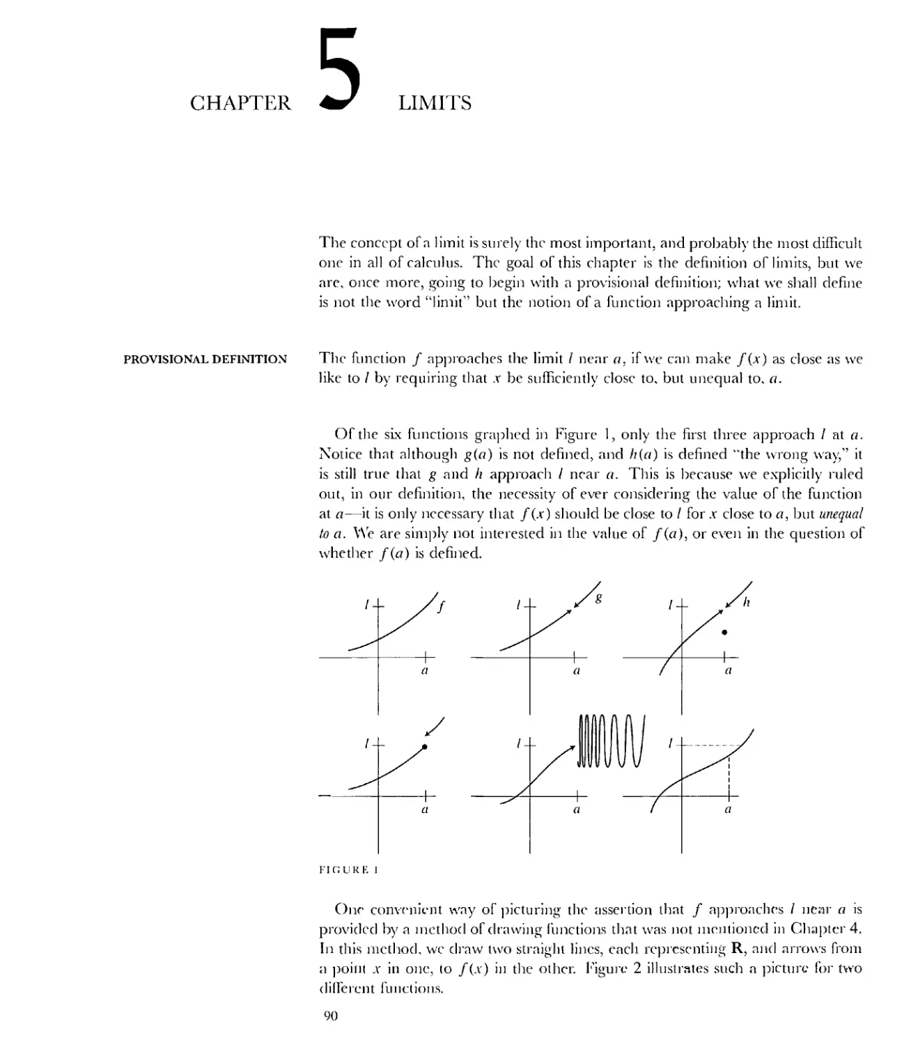
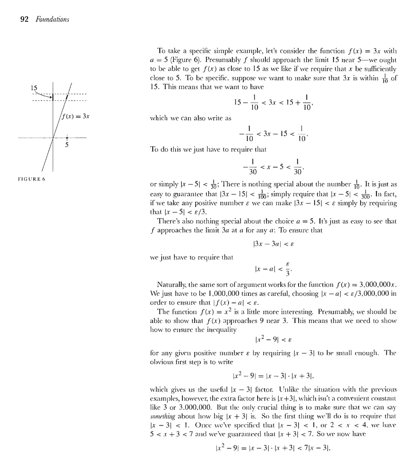
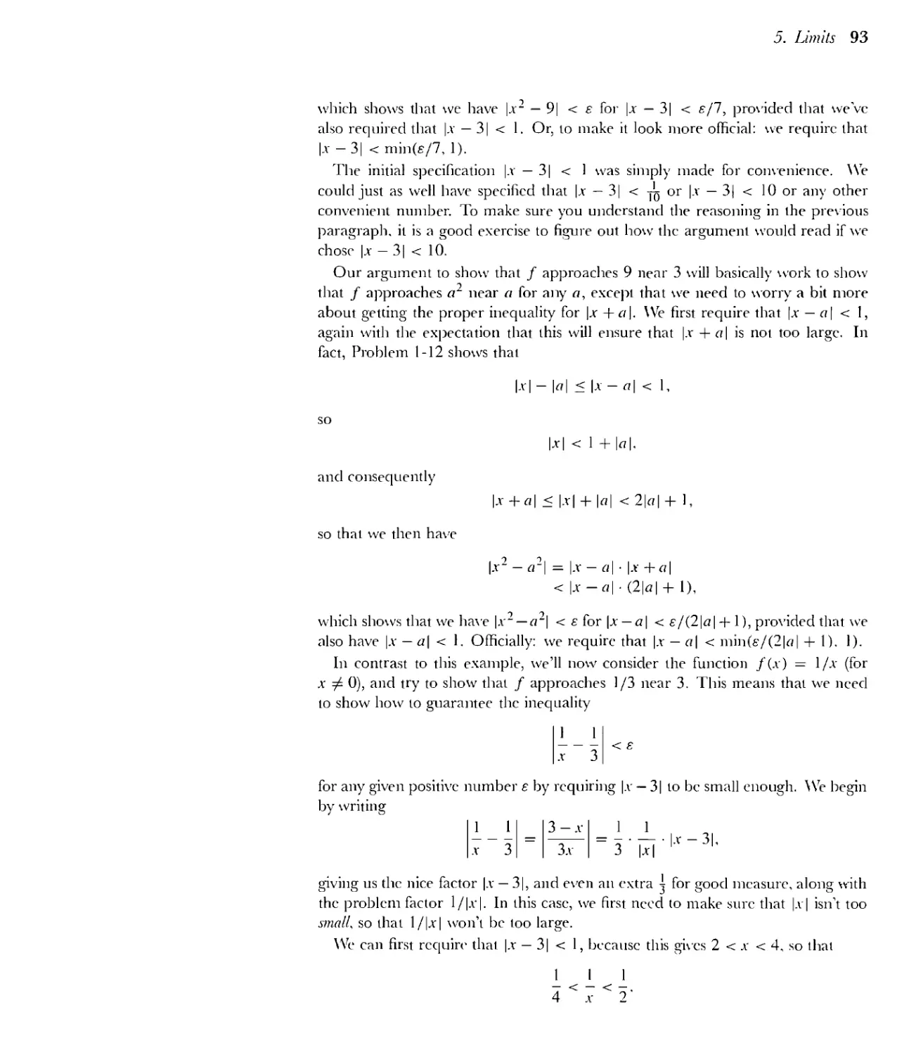
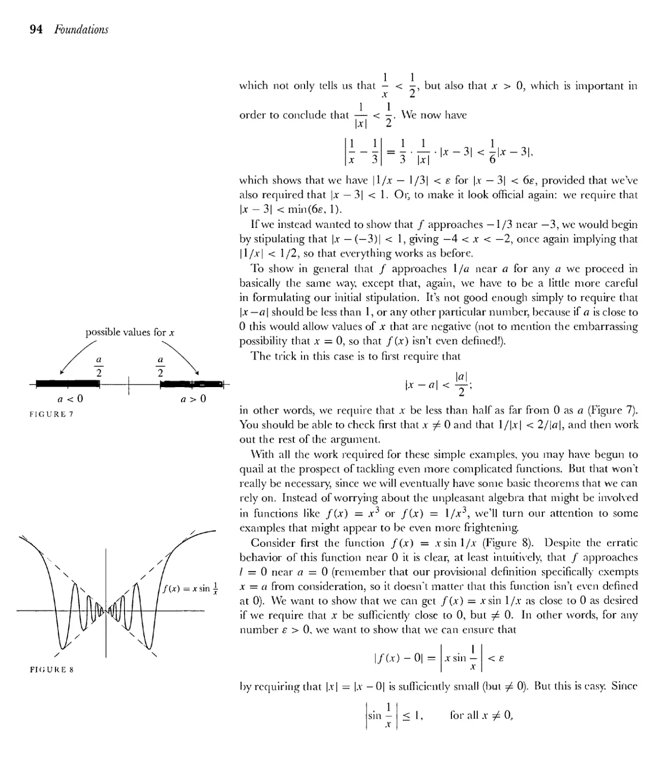
5 Limits 90
6 Continuous Functions 115
7 Three Hard Theorems 122
8 Least Upper Bounds 133
Appendix. Uniform Continuity 144
PART III Derivatives and Integrals
9 Derivatives 149
10 Differentiation 168
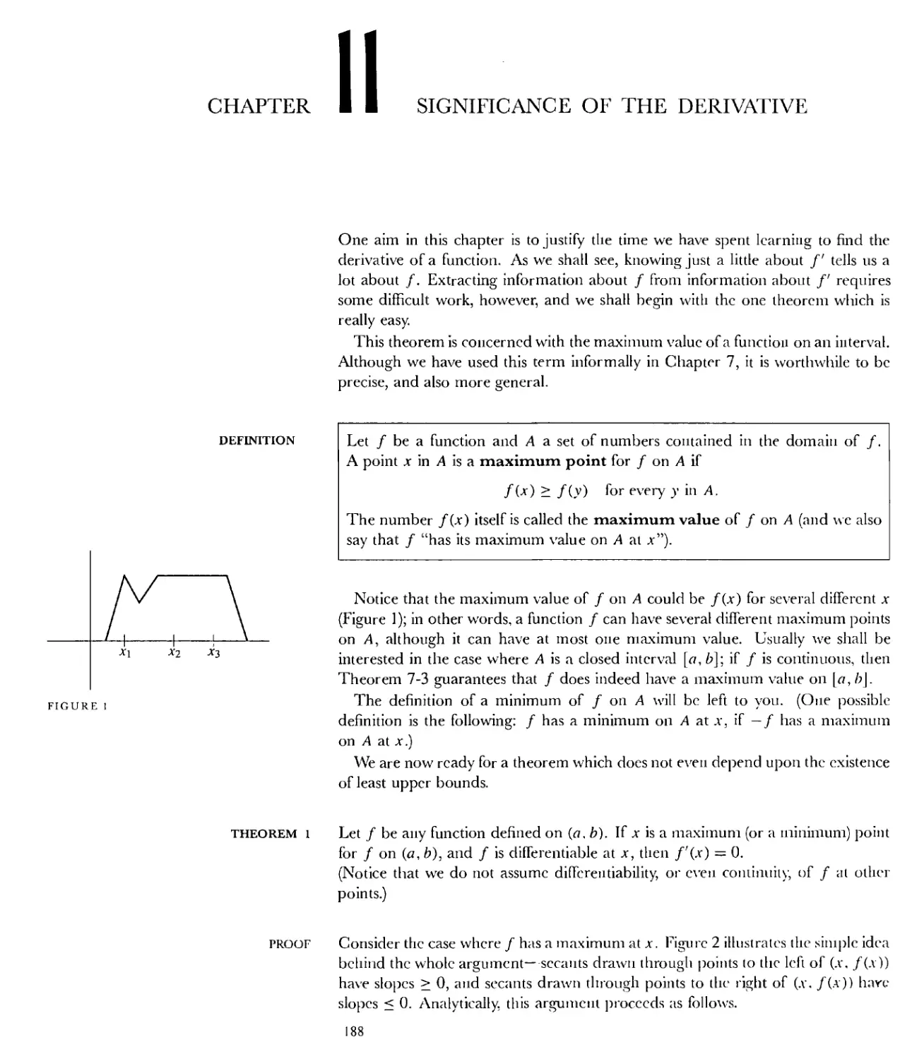
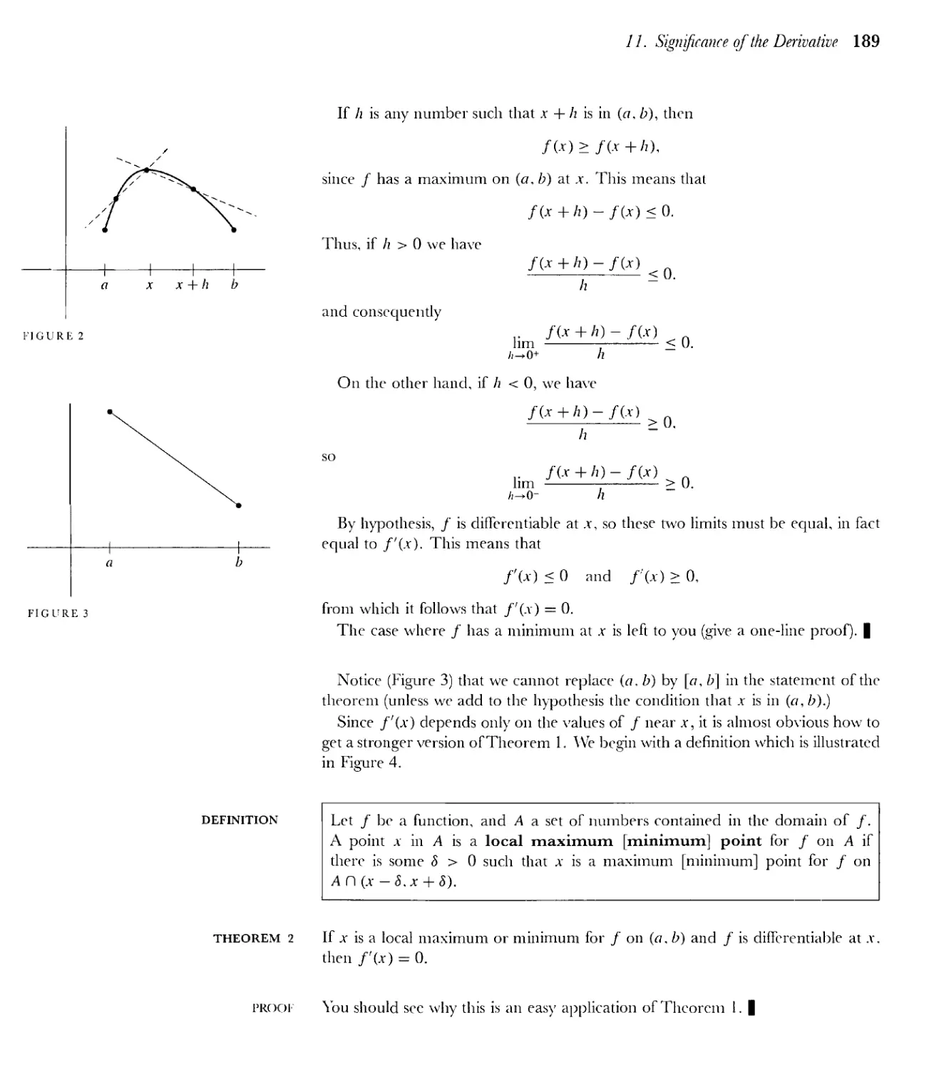
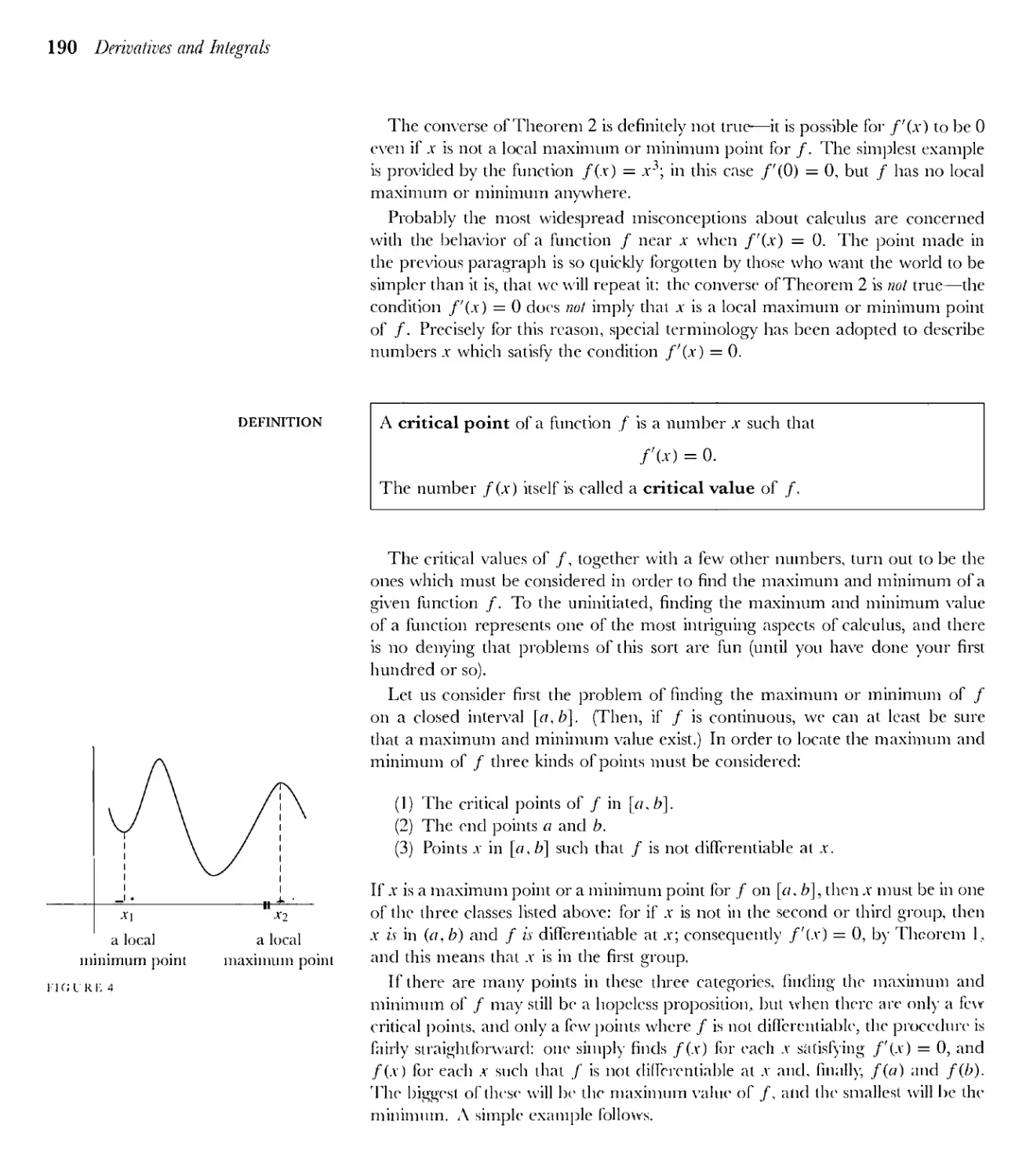
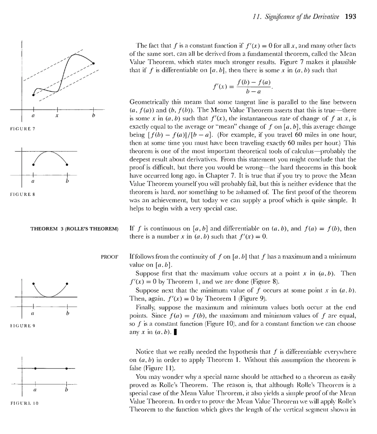
11 Significance of the Derivative 188
Appendix. Convexity and Concavity 219
12 Inverse Functions 230
Appendix. Parametric Representation of Curves 244
13 Integrals 253
Appendix. Riemann Sums 282
14 The Fundamental Theorem of Calculus 285
xiii
xiv Contents
15 The Trigonometric Functions 303
*16 7Г is Irrational 324
*17 Planetary Motion 330
18 The Logarithm and Exponential Functions 339
19 Integration in Elementary Terms 363
Appendix. The Cosmopolitan Integral 402
PART IV Infinite Sequences and Infinite Series
20 Approximation by Polynomial Functions 411
*21 e is Transcendental 442
22 Infinite Sequences 452
23 Infinite Series 471
24 Uniform Convergence and Power Series 499
25 Complex Numbers 526
26 Complex Functions 541
27 Complex Power Series 555
PARTY Epilogue
28 Fields 581
29 Construction of the Real Numbers 588
30 Uniqueness of the Real Numbers 601
Suggested Reading 609
Answers (to selected problems) 619
Glossary of Symbols 665
Index 669
CALCULUS
PART
о
PROLOGUE
To be conscious that
you are ignorant is a great step
to knowledge.
BENJAMIN DISRAELI
CHAPTER
BASIC PROPERTIES OF NUMBERS
The title of this chapter expresses in a few words the mathematical knowledge
required to read this book. In fact, this short chapter is simply an explanation of
what is meant by the “basic properties of numbers,” all of which—addition and
multiplication, subtraction and division, solutions of equations and inequalities,
factoring and other algebraic manipulations—are already familiar to us. Never-
theless, this chapter is not a review. Despite the familiarity of the subject, the
survey we are about to undertake will probably seem quite novel; it does not aim
to present an extended review of old material, but to condense this knowledge
into a few simple and obvious properties of numbers. Some may even seem too
obvious to mention, but a surprising number of diverse and important facts turn
out to be consequences of the ones we shall emphasize.
Of the twelve properties which we shall study in this chapter, the Erst nine are
concerned with the fundamental operations of addition and multiplication. For
the moment we consider only addition: this operation is performed on a pair
of numbers—the sum a + b exists for any two given numbers a and b (which
may possibly be the same number, of course). It might seem reasonable to regard
addition as an operation which can be performed on several numbers at once, and
consider the sum a\ + • • • + an of n numbers ai,... ,an as a basic concept. It is
more convenient, however, to consider addition of pairs of numbers only, and to
define other sums in terms of sums of this type. For the sum of three numbers
a, b, and c, this may be done in two different ways. One can first add b and c,
obtaining b + c, and then add a to this number, obtaining a + (b + c); or one can
first add a and b, and then add the sum a + b to c, obtaining (a + b) + c. Of
course, the two compound sums obtained are equal, and this fact is the very first
property we shall list:
(Pl) If a, b, and c are any numbers, then
a + (b + c) = (a + b) + c.
The statement of this property clearly renders a separate concept of the sum of
three numbers superfluous; we simply agree that a + b + c denotes the number
a + (b + c) = (a + b) + c. Addition of four numbers requires similar, though slightly
more involved, considerations. The symbol a + b + c + dis defined to mean
(1) ((a + b) + c) + d,
or (2) (a + (b + c)) + d,
or (3) a + ((fi + c) + d),
or (4) a + (b + (c + d)),
or (5) (a + fi) + (c + d).
3
4 Prologue
This definition is unambiguous since these numbers are all equal. Fortunately, this
fact need not be listed separately, since it follows from the property Pl already
listed. For example, we know from Pl that
(a + b) + c = a + (b + c),
and it follows immediately that (1) and (2) are equal. The equality of (2) and (3)
is a direct consequence of Pl, although this may not be apparent at first sight
(one must let b + c play the role of b in Pl, and d the role of c). The equalities
(3) — (4) — (5) are also simple to prove.
It is probably obvious that an appeal to PI will also suffice to prove the equality
of the 14 possible ways of summing five numbers, but it may not be so clear how we
can reasonably arrange a proof that this is so without actually listing these 14 sums.
Such a procedure is feasible, but would soon cease to be if we considered collections
of six, seven, or more numbers; it would be totally inadequate to prove the equality
of all possible sums of an arbitrary finite collection of numbers cq,.... an. This
fact may be taken for granted, but for those who would like to worry about the
proof (and it is worth worrying about once) a reasonable approach is outlined in
Problem 24. Henceforth, we shall usually make a tacit appeal to the results of this
problem and write sums r?i + • + an with a blithe disregard for the arrangement
of parentheses.
The number 0 has one property so important that we list it next:
(P2) If a is any number, then
a + 0 — 0 + u = u.
An important role is also played by 0 in the third property of our list:
(P3) For every number u, there is a number — a such that
a + (—«) = (—a) + a = 0.
Property P2 ought to represent a distinguishing characteristic of the number 0,
and it is comforting to note that we are already in a position to prove this. Indeed,
if a number x satisfies
a + x = a
for any one numbers, then л = 0 (and consequently this equation also holds for all
numbers a). The proof of this assertion involves nothing more than subtracting a
from both sides of the equation, in other words, adding — a to both sides; as the
following detailed proof shows, all three properties P1-P3 must be used to justify
this operation.
If a + г — a,
then (—a) + (a + .r) = (—a) + a = 0;
hence ((—«) + n) + a = 0:
hence 0+x = 0;
hence x = 0.
1. Basic Properties of.Numbers 5
As we have just hinted, it is convenient to regard subtraction as an operation
derived from addition: we consider a — b to be an abbreviation for a + (—b). It
is then possible to find the solution of certain simple equations by a series of steps
(each justified by Pl, P2, or P3) similar to the ones just presented for the equation
a + x = a. For example:
If x + 3 = 5,
then (x + 3) + (-3) = 5 + (-3);
hence x + (3 + (—3)) = 5 — 3 = 2;
hence x + 0 = 2;
hence x = 2.
Naturally, such elaborate solutions are of interest only until you become convinced
that they can always be supplied. In practice, it is usually just a waste of time to
solve an equation by indicating so explicitly the reliance on properties Pl, P2, and
P3 (or any of the further properties we shall list).
Only one other property' of addition remains to be listed. When considering the
sums of three numbers <?, b, and c, only two sums were mentioned: (<? + b) + c
and a + (/? + c). Actually, several other arrangements are obtained if the order of
a, b, and c is changed. That these sums are all equal depends on
(P4) If a and b are any numbers, then
a + b — b + a.
The statement of P4 is meant to emphasize that although the operation of ad-
dition of pairs of numbers might conceivably depend on the order of the two
numbers, in fact it does not. It is helpful to remember that not all operations are
so well behaved. For example, subtraction does not have this property': usually
a — b b — a. In passing we might ask just when a — b does equal b — a, and it
is amusing to discover how powerless we are if we rely only on properties P1-P4
to justify our manipulations. Algebra of the most elementary variety shows that
a — b = b — a only when a = b. Nevertheless, it is impossible to derive this fact
from properties PI-P4; it is instructive to examine the elementary algebra care-
fully and determine which step(s) cannot be justified by P1-P4. We will indeed
be able to justify all steps in detail when a few more properties are listed. Oddly
enough, however, the crucial property involves multiplication.
The basic properties of multiplication are fortunately so similar to those for ad-
dition that little comment will be needed; both the meaning and the consequences
should be clear. (As in elementary algebra, the product of a and b will be denoted
by a • b, or simply abb)
(P5) If <7, b, and c are any numbers, then
a • (b • c) = (a • b) c.
(P6) If a is any number, then
a • 1 = 1 • a = a.
6 Prologue
Moreover, 1 ф 0.
(The assertion that 1 0 may seem a strange fact to list, but we have to
list it, because there is no way it could possibly be proved on the basis of the
other properties listed—these properties would all hold if there were only one
number, namely, 0.)
(P7) For every' number а ф 0, there is a number n-1 such that
a a-1 = • a = 1.
(P8) If a and b are any numbers, then
a • b = b a.
One detail which deserves emphasis is the appearance of the condition а ф 0
in P7. This condition is quite necessary; since Q b — 0 for all numbers b, there is no
number 0-1 satisfying 0-0-1 = I. This restriction has an important consequence
for division. Just as subtraction was defined in terms of addition, so division is
defined in terms of multiplication: The symbol a/b means a • Z?-1. Since 0-1 is
meaningless, n/0 is also meaningless—division by 0 is always undefined.
Property P7 has two important consequences. If a • b = a • c, it does not
necessarily follow that b — c; for if a — 0, then both a - b and a c are 0, no matter
what b and c are. However, if а ф 0, then b = c; this can be deduced from P7 as
follows:
If a • b — a • c and a / 0,
then (« • b) — a~l (a c);
hence (n-1 a) b — (n-1 • a) • c;
hence 1 • b = 1 • c;
hence b = c.
It is also a consequence of P7 that if a • b — 0, then either a = 0 or b — 0. In fact,
if a b — 0 and а ф 0,
then бГ1 • (п • /?) = 0:
hence («-1 • a) • b — 0:
hence I • b — 0:
hence b — 0.
(It may happen that a = 0 and b = 0 are both true; this possibility is not excluded
when we say “either a — 0 or b = 0”; in mathematics “or” is always used in the
sense of “one or the other, or both.”)
This latter consequence of P7 is constantly used in the solution of equations.
Suppose, for example, that a number .v is known to satisfy
lx - l)(.r —2) = 0.
Then it follows (hat cither .v — 1 — 0 or л — 2 = 0; hence .v — I or .r — 2.
1. Basic Properties of Numbers 7
On the basis of the eight properties listed so far it is still possible to prove very
little. Listing the next property, which combines the operations of addition and
multiplication, will alter this situation drastically.
(P9) If a, b, and c are any numbers, then
a • (b + c) — a b + a • c.
(Notice that the equation (b + c) • a — b • a + c a is also true, by P8.)
As an example of the usefulness of P9 we will now determine just when a — b =
b — cr.
If
then
hence
hence
Consequently
and therefore
a —b = b — a.
(a — b) + b = (b — a) + b = b + (b — a);
a = b + b — a;
a + a — (b + b — «) + a — b + b.
a • (1 + 1) = b • (1 + 1),
a = b.
A second use of P9 is the justification of the assertion a • 0 - 0 which we have
already made, and even used in a proof on page 6 (can you find where?), This
fact was not listed as one of the basic properties, even though no proof was offered
when it was first mentioned. With Pl- P8 alone a proof was not possible, since the
number 0 appears only in P2 and P3, which concern addition, while the assertion
in question involves multiplication. With P9 the proof is simple, though perhaps
not obvious: We have
п-0 + д0 = «-(0 + 0)
= a -0:
as we have already noted, this immediately implies (by adding — (a -0) to both
sides) that «0 = 0.
A series of further consequences of P9 may help explain the somewhat myste-
rious rule that the product of two negative numbers is positive. To begin with,
we will establish the more easily acceptable assertion that (—a) • b = —(a b). To
prove this, note that
(—a) b + a b = [(—«) + a] b
= Qb
= 0.
It follows immediately (by adding — (a • b) to both sides) that (—fl) b = — (a b).
Now note that
(-a) • (-/?) 4- [-(a • Z?)J = (-a) • (—b) + (-a) • b
= (-«) • [(-/?) + b]
= (—a)-0
= 0.
8 Prologue
Consequently, adding (u b) to both sides, we obtain
(—a) (—b) — a b.
The fact that the product of two negative numbers is positive is thus a consequence
of P1-P9. In other words, if we want Pl to P9 to be true, the rule for the product of two
negative numbers is forced upon us.
The various consequences of P9 examined so far, although interesting and im-
portant, do not really indicate the significance of P9; after all, we could have listed
each of these properties separately. Actually, P9 is the justification for almost all
algebraic manipulations. For example, although we have shown how to solve the
equation
(x - l)(x -2) = 0,
we can hardly expect to be presented with an equation in this form. We are more
likely to be confronted with the equation
x2 - 3x + 2 = 0.
The “factorization” x2 — 3x + 2 = (x — l)(x — 2) is really a triple use of P9:
(x - 1) (x - 2) = X (X - 2) + (-1) (X - 2)
= x • x+ x (~2) + (-1) • x + (-1) • (-2)
= x2 + x [(—2) + (—1)] + 2
= x2 - 3x + 2.
A final illustration of the importance of P9 is the fact that this property is actually
used every time one multiplies arabic numerals. For example, the calculation
13
x24
~52
26
Tl2
is a concise arrangement for the following equations:
13-24= 13-(2- 10 + 4)
= 13-2- 10+ 13-4
= 26- 10 + 52.
(Note that moving 26 to the left in the above calculation is the same as writing
26 • 10.) The multiplication 13-4 = 52 uses P9 also:
13 -4 = (1 • 10 + 3) • 4
= 1-10-4 + 3-4
= 4- 10+ 12
= 4- 10+ 1 • 10 + 2
= (4+1)- 10+2
= 5 10 + 2
- 52.
1. Basic Properties of Numbers 9
The properties P1-P9 have descriptive names which are not essential to remem-
ber, but which are often convenient for reference. We will take this opportunity to
list properties P1-P9 together and indicate the names by which they are commonly
designated.
(Pl) (Associative law for addition) a + (b + c) = (« + b) + c.
(P2) (Existence of an additive identity) a + 0 = 0 + a = a.
(P3) (Existence of additive inverses) a + (—a) — (—a) + a — 0.
(P4) (Commutative law for addition) a + b — b + a.
(P5) (Associative law for multiplica- tion) a • (b c) = (a • b) • c.
(P6) (Existence of a multiplicative identity) a • 1 = 1 • a = a; 1^0.
(P7) (Existence of multiplicative inverses) a • « “1 = « “1 - a = 1, for a f 0
(P8) (Commutative law for multi- plication) a b = b a.
(P9) (Distributive law) a (b + c) = a • b + a • c.
The three basic properties of numbers which remain to be listed are concerned
with inequalities. Although inequalities occur rarely in elementary mathematics,
they play a prominent role in calculus. The two notions of inequality, a < b
(a is less than £>) and a > b (o is greater than Z?), are intimately related: a < b
means the same as b > a (thus 1 < 3 and 3 > 1 are merely two ways of writing
the same assertion). The numbers a satisfying a > 0 are called positive, while
those numbers a satisfying a < 0 are called negative. While positivity can thus
be defined in terms of <, it is possible to reverse the procedure: a < b can be
defined to mean that b — a is positive. In fact, it is convenient to consider the
collection of all positive numbers, denoted by P, as the basic concept, and state
all properties in terms of P:
(PIO) (Trichotomy law) For every number a, one and only one of the
following holds:
(i) « = 0,
(ii) a is in the collection P,
(iii) — a is in the collection P.
(Pl 1) (Closure under addition) If a and b arc in P, then a + b is in P.
(Pl 2) (Closure under multiplication) If a and b are in P, then a b is
in P.
10 Prologue
о
These three properties should be complemented with the following definitions:
a > b
a < b
a>b
a <b
if
if
if
if
a — b is in P;
b> a;
a > b or a = b\
a < b or a — b*
Note, in particular, that a > 0 if and only if a is in P.
All the familiar facts about inequalities, however elementary they may seem, are
consequences of PIO- Pl2. For example, if a and b are any two numbers, then
precisely one of the following holds:
(i) a — b = 0,
(ii) a — b is in the collection P,
(iii) — (n — b) = b — a is in the collection P.
Using the definitions just made, it follows that precisely one of the following holds:
(i) a = b,
(ii) a > b,
(iii) b > a.
A slightly more interesting fact results from the following manipulations. If
a < b, so that b — a is in P, then surely (b + c) — (a + c) is in P; thus, if a < b,
then a + c < b + c. Similarly, suppose a < b and b < c. Then
b — a is in P,
and c — b is in P,
so c — a = (c — b) + (b — a) is in P.
This shows that if a < b and b < c, then a < c. (The two inequalities a < b and
b < c are usually written in the abbreviated form a < b < c, which has the third
inequality a < c almost built in.)
The following assertion is somewhat less obvious: If a < 0 and b < 0, then
ab > 0. The only difficulty presented by the proof is the unraveling of definitions.
The symbol a < 0 means, by definition, 0 > a, which means 0 — a — —a is in P.
Similarly — b is in P, and consequently, by P12, (—a)(—b) = ab is in P. Thus
ab > 0.
The fact that ab > 0 if a > 0, b > 0 and also if a < 0, Z? < 0 has one
special consequence: a2 > 0 if a 0. Thus squares of nonzero numbers are
always positive, and in particular we have proved a result which might have seemed
sufficiently elementary to be included in our list of properties: 1 > 0 (since 1 = I2).
♦There is one slightly perplexing feature of the symbols > and <. 1'he statements
1 + I < 3
1 + I <2
arc both true, even though we know that < could be replaced by < in the first, and by = in the
second. This sort of thing is bound to occur when < is used w ith specific numbers; the usefulness
of the symbol is revealed by a statement like Theorem I— -here equality holds for some values of a
and h, while inequality holds for other values.
I. Basic Properties of Numbers 11
The fact that —a > 0 if a < 0 is the basis of a concept which will play an
extremely important role in this book. For any number a, we define the absolute
value |л| of a as follows:
a > 0
a < 0.
Note that |n| is always positive, except when a = 0. For example, we have | — 3| —
3, |7| = 7. |1 + 72 - 73| = 1 + 72- 73. and |1 + 72- 710| = 710- 72- 1.
In general, the most straightforward approach to any problem involving absolute
values requires treating several cases separately, since absolute values are defined
by cases to begin with. This approach may be used to prove the following very
important fact about absolute values.
THEOREM 1
For all numbers a and b, we have
l« + ^l < |fl| + |ft|.
PROOF
We will consider 4 cases:
(1) a > 0. b > 0;
(2) a > 0, b < 0;
(3) a < 0. b > 0;
(4) a < 0. b < 0.
In case (1) we also have a + b > 0, and the theorem is obvious; in fact,
|« + b\ = a + b = |n| + |Z?|,
so that in this case equality7 holds.
In case (4) we have a + b < 0, and again equality holds:
|n + b\ = -(a +b) = -a + (—b) = |«| + |Z>|.
In case (2), when a > 0 and b < 0, we must prove that
|a + b\ < a - b.
This case may therefore be divided into two subcases. If a + b > 0, then we must
prove that
a + b < a — b,
i.e., b < —b,
which is certainly true since b < 0 and hence — b > 0. On the other hand, if
a + b < 0, we must prove that
—a — b < a — b,
i.e., — a < a.
which is certainly true since a > 0 and hence —a < 0.
Finally, note that case (3) may be disposed of with no additional work, by apply-
ing case (2) with a and b interchanged. |
12 Prologue
Although this method of treating absolute values (separate consideration of var-
ious cases) is sometimes the only approach available, there are often simpler meth-
ods which may be used. In fact, it is possible to give a much shorter proof of
Theorem 1; this proof is motivated by the observation that
kd =
(Here, and throughout the book, \fx denotes the positive square root of x; this
symbol is defined only when x > 0.) We may now observe that
(|« + b |)2 = (n + Z?)2 — a2 + lab + Zt2
< л2 + 2|a| • |Z?| + b2
= |«|2 + 2|«| |Z?| + |Z?|2
= (l«l + |fi|)2-
From this we can conclude that |« + b\ < |a| + |Z?| because x2 < y2 implies .v < y,
provided that x and v are both nonnegative; a proof of this fact is left to the reader
(Problem 5).
One final observation may be made about the theorem we have just proved: a
close examination of either proof offered shows that
|a + Z?| = |o | + |&|
if a and b have the same sign (i.e., are both positive or both negative), or if one of
the two is 0, while
l« + b\ < |c?| + |Z>|
if a and b arc of opposite signs.
We will conclude this chapter with a subtle point, neglected until now, whose
inclusion is required in a conscientious survey of the properties of numbers. After
stating property P9, we proved that a — b = b — a implies a = b. The proof began
by establishing that
a • (1 + 1) = b (1 + 1),
from which we concluded that a = b. This result is obtained from the equation
a (1 + 1) = b-0 + 1) by dividing both sides by 1 + 1. Division by 0 should
be avoided scrupulously, and it must therefore be admitted that the validity of the
argument depends on knowing that 1 + 1 / 0. Problem 25 is designed to convince
you that this fact cannot possibly be proved from properties Pl- P9 alone! Once
PIO, Pl 1, and Pl2 are available, however, the proof is very’ simple: We have
already seen that 1 > 0; it follows that 1 + 1 > 0, and in particular 1 + 1/0.
This last demonstration has perhaps only strengthened your feeling that it is
absurd to bother proving such obvious facts, but an honest assessment of our
present situation will help justify serious consideration of such details. In this
chapter we have assumed that numbers are familiar objects, and that Pl- P12 arc
merely explicit statements of obvious, well-known properties of numbers. Il would
be difficult, however, to justify this assumption. Although one learns howto “work
with” numbers in school, just what numbers are, remains rather 'ague. A great
deal of this book is devoted to elucidating the concept of numbers, and by the encl
1. Basic Properties of Numbers 13
of the book we will have become quite well acquainted with them. But it will be
necessary to work with numbers throughout the book. It is therefore reasonable
to admit frankly that we do not yet thoroughly understand numbers; we may still
say that, in whatever way numbers are finally defined, they should certainly have
properties Pl Pl2.
Most of this chapter has been an attempt to present convincing evidence that
P1-P12 are indeed basic properties which we should assume in order to deduce
other familiar properties of numbers. Some of the problems (which indicate the
derivation of other facts about numbers from Pl-Pl2) are offered as further evi-
dence. It is still a crucial question whether Pl-Pl 2 actually account for all prop-
erties of numbers. As a matter of fact, we shall soon see that they do not. In the
next chapter the deficiencies of properties Pl-Pl2 will become quite clear, but
the proper means for correcting these deficiencies is not so easily discovered. The
crucial additional basic property of numbers which we are seeking is profound and
subtle, quite unlike P1-P12. The discovery of this crucial property will require all
the work of Part II of this book. In the remainder of Part I we will begin to see
why some additional property is required; in order to investigate this we will have
to consider a little more carefully what we mean by “numbers.”
PROBLEMS
1. Prove the following:
(i) If ax = a for some number a f 0, then x = 1.
(ii) x2 - y2 = (x - y)(x + y).
(iii) If x2 = y2, then x = у or x — —y.
(iv) x3 — y3 = (x — y)(x2 + xy + y2).
(v) x" — y" = (x — y)(x"~1 + x"“2y + • —H xy" 2 + y" ').
(vi) x3 + y3 = (x + y)(x2 — xy + y2). (There is a particularly easy way to
do this, using (iv), and it will show you how to find a factorization for
x" + y" whenever n is odd.)
2. What is wrong with the following “proof”? Let x = y. Then
(x +y)(x - y) = y(x - y),
X +y = y,
2y = y,
2=1.
3. Prove the following:
(i) aT = ^,X b.cfO.
b be
a c ad + be
(n) - H— =-----------, if b. d f 0.
14 Prologue
(iii) (ab) 1 = a lb !, if a, b / 0. (To do this you must remember the
defining property of (afe)-1.)
(iv) £^ = ^,ifh,d/0.
ba ab
(v) £ / if b, c, d 0.
b [ a be
a c .
(vi) If b, d / 0, then — — — if and only if ad = be. Also determine when
b d
a b
b a
4. Find all numbers x for which
(i) 4 —x<3 —2x.
(ii) 5 — x2 < 8.
(iii) 5 — x2 < —2.
(iv) (x — l)(x — 3) >0. (When is a product of two numbers positive?)
(v) x2 — 2x + 2 > 0.
(vi) x2 + x + 1 > 2.
(vii) x2 - x + 10 > 16.
(viii) x2 + x + 1 >0.
(ix) (x - 7r)(x + 5)(x — 3) > 0.
(x) (x-^2)(x-V2)>0.
(xi) 2х < 8.
(xii) x + 3х < 4.
, -л 1 1
(xin) - + ------> 0.
X 1 - X
(xiv) X * > 0.
5. Prove the following:
(i) If a < b and c < d, then a + c < b + d.
(ii) If a < b, then — b < —a.
(iii) If a < b and c > d, then a — c < b — d.
(iv) If a < b and c > 0, then ac < be.
(v) If a < b and c < 0, then ac > be.
(vi) If a > 1, then a2 > a.
(vii) If 0 < a < 1, then a2 < a.
(viii) If 0 < a < b and 0 < c < d, then ac < bd.
(ix) If 0 < a < b, then a2 < b2. (Use (viii).)
(x) If a, b > 0 and a2 < b2, then a < b. (Use (ix), backwards.)
6. (a) Prove that if 0 < x < y, then x" < yn, n = 1, 2, 3,....
(b) Prove that if x < у and n is odd, then x" < yn.
(c) Prove that if x" = yn and n is odd, then x = у.
(d) Prove that if xn = yn and n is even, then x = у or x = — y.
1. Basic Properties of Numbers 15
7. Prove that if 0 < a < b, then
Notice that the inequality -fab < (a + b)/2 holds for all a, b > 0. A gener-
alization of this fact occurs in Problem 2-22.
*8. Although the basic properties of inequalities were stated in terms of the col-
lection P of all positive numbers, and < was defined in terms of P, this
procedure can be reversed. Suppose that PIO Pl2 are replaced by
(P'10) For any numbers a and b one, and only one, of the
following holds:
(i) a = b,
(ii) a < b,
(iii) b < a.
(P'l 1) For any numbers a, b, and c, if a < b and b < c, then
a < c.
(P' 12) For any numbers a, b, and c, if a < b, then
a + c < b + c.
(P'13) For any numbers a, b, and c, if a < b and 0 < c, then
ac < be.
Show that P10-P12 can then be deduced as theorems.
9. Express each of the following with at least one less pair of absolute value
signs.
(i) |У2 + 7з - 75 + T7|.
(ii) |(|й + Z?| — |a| — |&|)|.
(iii) |(|a +b\ + |c| - \a +Z? + c|)|.
(iv) |x2 - 2xy + y2|.
(v) |(|V2 + 73| - |T5 - v/7|)|.
10. Express each of the following without absolute value signs, treating various
cases separately when necessary.
(i) |« + b\ - |fe|.
(ii) КИ - 1)|.
(iii) |x| - |x2|.
(iv) a - |(a - |o|)|.
11. Find all numbers x for which
(i) |x—3|=8.
(ii) |x - 3| < 8.
(iii) |x+4|<2.
(iv) |x — 11 + |x — 2| > 1.
(v) |.r-l| + |x + l| <2.
16 Prologue
(vi) |x- l| + |x + 1| < 1.
(vii) |x — 11 |x + 11 = 0.
(viii) |x - 11 • |x + 2| = 3.
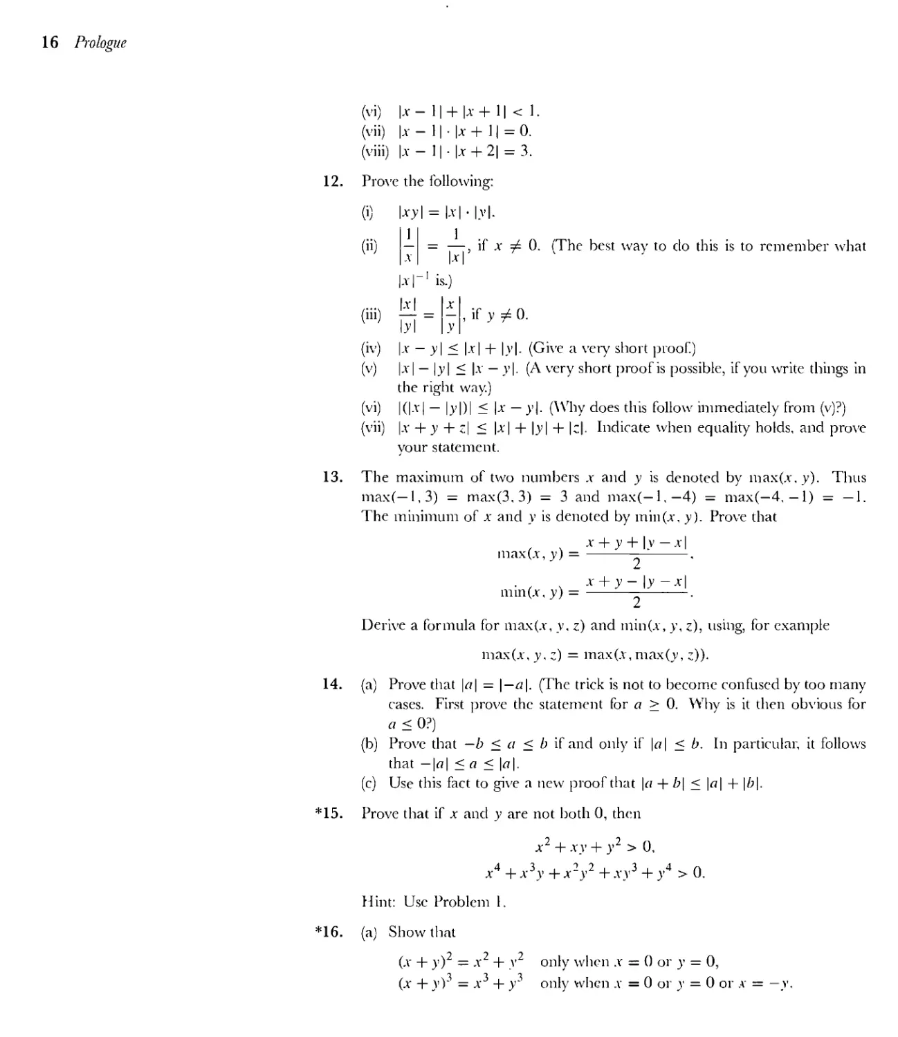
12. Prove the following:
— -—, if x 7= 0. (The best way to do this is to remember what
1У1 У
|x — y| < |x| + |y|. (Give a very short proof.)
|x | — |y| < |x — y|. (A very short proof is possible, if you write things in
the right way.)
|x + у + z| < |x| + |y| + |z|. Indicate when equality holds, and prove
your statement.
13. The maximum of two numbers x and у is denoted by max(x.y). Thus
max(—1,3) — max(3, 3) — 3 and max(— 1,— 4) — max(—4, — 1) — — 1.
The minimum of x and у is denoted by min(x, y). Prove that
x + y + |y-x|
max(x, y) = ------------.
z . * + У - 1У -x|
min(x, y) =-------------.
Derive a formula for max(x, y, z) and min(x, y, z), using, for example
max(x, y, z) = max(x, max(y, z)).
14. (a) Prove that |«| = |—a|. (The trick is not to become confused by too many
cases. First prove the statement for a > 0. Why is it then obvious for
a < 0?)
(b) Prove that — b < a < b if and only if |д| < b. In particular, it follows
that —|u| < a < |«|.
(c) Use this fact to give a new proof that |« + £»| < |«| + |Z?|.
*15. Prove that if x and у are not both 0, then
x2 + xy + y2 > 0,
X4 + x3y + x2y2 + xy3 + у4 > 0.
Hint: Use Problem 1.
*16. (a) Show that
(x + y)2 — x2 + y2 only when x = 0 or у — 0,
(x + y)3 — x3 + y3 only when x = 0 or у = 0 or x = — y.
1. Basic Properties of Numbers 17
(b) Using the fact that
x2 + lx у + у2 = (x + у)2 > 0.
show that 4x2 + 6xy + 4y2 > 0 unless x and у are both 0.
(c) Use part (b) to find out when (x + y)4 — x4 + y4.
(d) Find out when (x+y)5 = x5 + y5. Hint: From the assumption (x + y)5 —
x5+y5 you should be able to derive the equation x3+2x2y+ 2xy2 + y3 —
0, if xy Ф 0. This implies that (x + y)3 — x2y + xy2 — xy(x + y).
You should now be able to make a good guess as to when (x + y)" = x" + y";
the proof is contained in Problem 11-63.
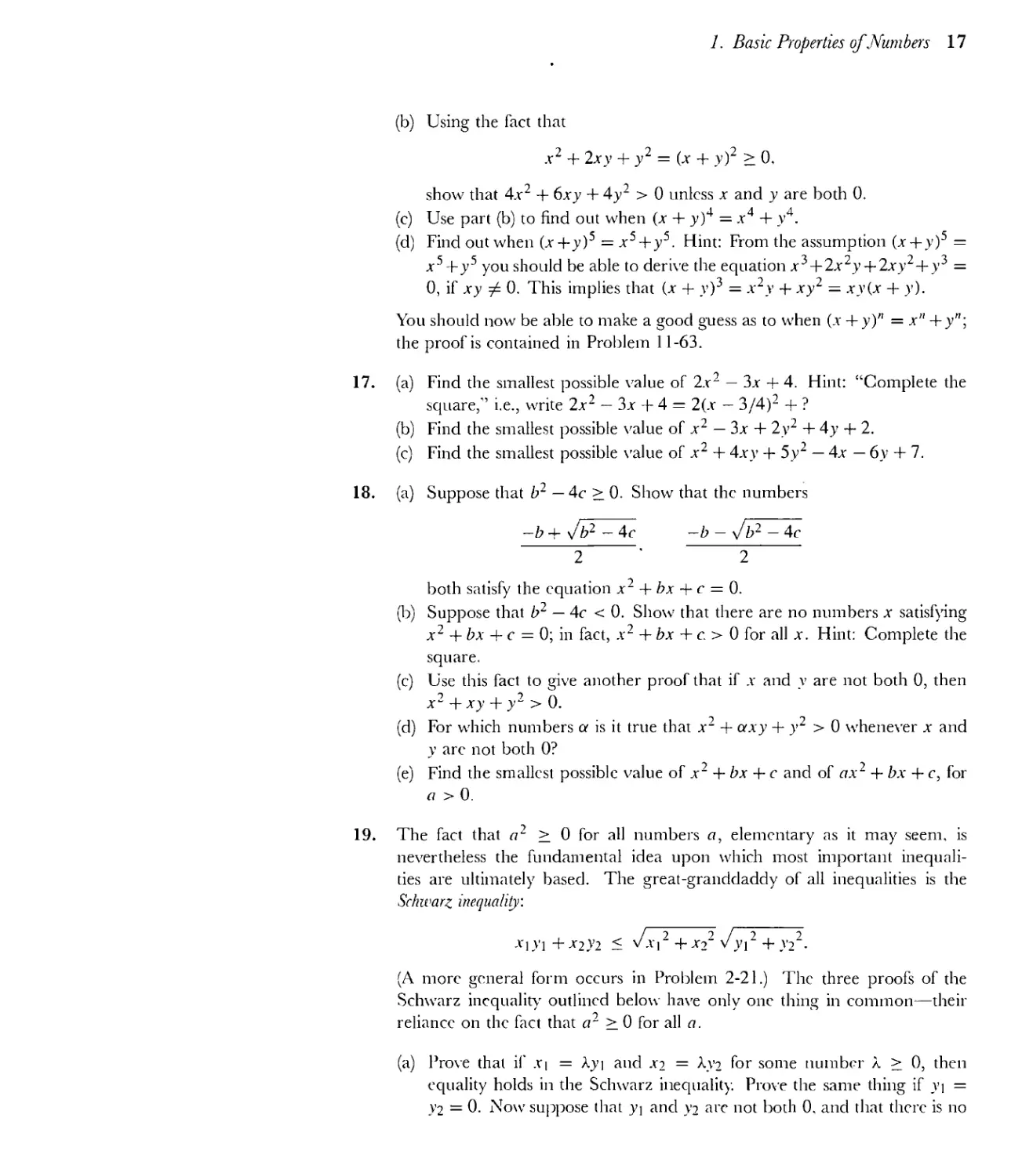
17. (a) Find the smallest possible value of 2x2 — 3x + 4. Hint: “Complete the
square,” i.e., write 2x2 — 3x + 4 — 2(x — 3/4)2 + ?
(b) Find the smallest possible value of x2 — 3x + 2y2 + 4 у + 2.
(c) Find the smallest possible value of x2 + 4xy + 5y2 — 4x — 6у + 7.
18. (a) Suppose that b2 — 4c > 0. Show that the numbers
—b + x/ b2- — 4c — b — — 4c
2 ' 2
both satisfy the equation x2 + bx + c = 0.
(b) Suppose that b2 — 4c < 0. Show that there are no numbers x satisfying
x2 + bx + c = 0; in fact, x2 + bx + c. > 0 for all x. Hint: Complete the
square.
(c) Use this fact to give another proof that if x and у are not both 0, then
x2 + xy + y2 > 0.
(d) For which numbers a is it true that x2 + axy + y2 > 0 whenever x and
у arc not both 0?
(e) Find the smallest possible value of x2 + bx + c and of ax2 + bx + c, for
a >0.
19. The fact that a2 > 0 for all numbers a, elementary as it may seem, is
nevertheless the fundamental idea upon which most important inequali-
ties are ultimately based. The great-granddaddy of all inequalities is the
Schwarz inequality.
, I 2 / S
Х1У1+Х2У2 < v.l| + X2 vyi + \’2 .
(A more general form occurs in Problem 2-21.) The three proofs of the
Schwarz inequality outlined below have only one thing in common—their
reliance on the fact that a~ > 0 for all a.
(a) Prove that if X| = Луч and xs = Лу2 for some number Л > 0, then
equality holds in the Schwarz inequality. Prove the same thing if yi =
y2 = 0. Now suppose that yq and ys are not both 0, and that there is no
18 Prologue
number A such that xi = Ayi and xt_ = k}’2- Then
0 < (Ayi - xi )2 + (Xyz-xi)2
= A2(yi2 + y22) - 2A(xi vi + x2y2) + (xi2 + x22).
Using Problem 18, complete the proof of the Schwarz inequality.
(b) Prove the Schwarz inequality by using 2xy < x2+y2 (how is this derived?)
with
- Xi , - y‘
Уи2 + -V22 \/yi2 + У22
first for i — 1 and then for i — 2.
(c) Prove the Schwarz inequality by first proving that
(Xi2 + X22)(yi2 + У22) = UlVl +X2V2)2 + (Х1У2 -Х2У1)2.
(d) Deduce, from each of these three proofs, that equality holds only when
У1 = У2 = 0 or when there is a number A > 0 such that xi = Ayi and
x2 = Ay 2.
In our later work, three facts about inequalities will be crucial. Although proofs
will be supplied at the appropriate point in the text, a personal assault on these
problems is infinitely more enlightening than a perusal of a completely worked-out
proof. The statements of these propositions involve some weird numbers, but their
basic message is very simple: if x is close enough to xq, and у is close enough to yo,
then x + y will be close to xq + уо, and xy will be close to Xgyo, and 1 /у will be close
to 1 /уд. The symbol “s” which appears in these propositions is the fifth letter of the
Greek alphabet (“epsilon”), and could just as well be replaced by a less intimidating
Roman letter; however, tradition has made the use of £ almost sacrosanct in the
contexts to which these theorems apply.
20. Prove that if
l-f -x0| < - and |y-y0| <
then
|(x +y)-(xo + yo)l <
|(x -y)-(xo-yo)l < £
*21. Prove that if
(e \ E
----------, 1 and |y — Vol < «-----------
2(|yol + D J 2(|x0|+ 1)
then |xy — xoyol < e.
(The notation “min” was defined in Problem 13, but the formula provided by
that problem is irrelevant at the moment; the first inequality in the hypothesis
just means that
Iх “ A'°l < o/i f',”i> and Iх “X()l < 1:
2(|yol + 1)
1. Basic Properties of Numbers 19
at one point in the argument you will need the first inequality, and at an-
other point you will need the second. One more word of advice: since the
hypotheses only provide information about л — xo and У ~ J’O, it is almost a
foregone conclusion that the proof will depend upon writing xy — xoyo in a
way that involves x — xq and у — yo.)
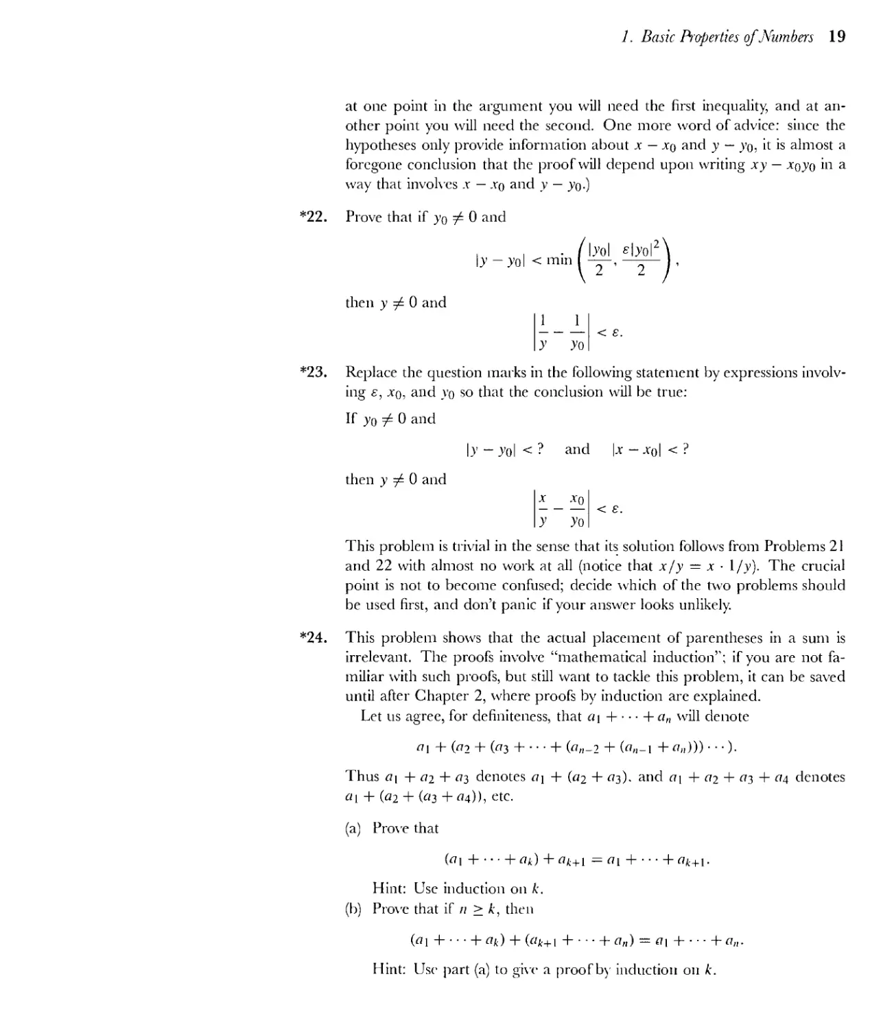
*22. Prove that if yo / 0 and
|y - y0| < min
b'ol g|yol2
2 ’ 2
then у 0 and
1 1
У У0
*23. Replace the question marks in the following statement by expressions involv-
ing s, xo, and yo so that the conclusion will be true:
If yo Ф 0 and
|y - y0| < ? and |x - x0| < ?
then у 7^ 0 and
x x0
-------< £.
У У0
This problem is trivial in the sense that its solution follows from Problems 21
and 22 with almost no work at all (notice that x/y — x 1/y). The crucial
point is not to become confused; decide which of the two problems should
be used first, and don’t panic if your answer looks unlikely.
*24. This problem shows that the actual placement of parentheses in a sum is
irrelevant. The proofs involve “mathematical induction”; if you are not fa-
miliar with such proofs, but still want to tackle this problem, it can be saved
until after Chapter 2, where proofs by induction are explained.
Let us agree, for definiteness, that a\ + • • + an will denote
«1 + («2 + («3 + • + («n-2 + (fln-i + «»))) •
Thus «1 + 02 + из denotes ai + («2 + «з). and «i + «2 + «3 + «4 denotes
«1 + (a2 + («3 +a4)), etc.
(a) Prove that
(cq + • • • + ak) + o^+1 — a i + • • • + flfc+i.
Hint: Use induction on к.
(b) Prove that if n > к, then
(a 1 + • • • + а^) + (Ok+1 + • • + an) — a 1 + •••+«„.
Hint: Use part (a) to give a proof by induction on к.
20 Prologue
(c) Let >y(ai,..., a*) be some sum formed from a\,... ,ak. Show that
5(«1, ...,ak) = <2i 4----------------------------\-ak.
Hint: There must be two sums s'(a\,and s"(a;+i,..., ak) such
that
5(<2i, ...,ak) =s'(a\, ...,ai) + sr’{ai+x, ...,ak).
25. Suppose that we interpret “number” to mean either 0 or 1, and + and • to
be the operations defined by the following two tables.
+ 0 1 0 1
0 0 1 0 0 0
1 1 0 1 0 1
Check that properties P1-P9 all hold, even though 1 + 1=0.
CHAPTER
2
Лш NUMBERS OF VARIOUS SORTS
In Chapter 1 we used the word “number” very loosely, despite our concern with
the basic properties of numbers. It will now be necessary to distinguish carefully
various kinds of numbers.
The simplest numbers are the “counting numbers”
1,2,3.....
The fundamental significance of this collection of numbers is emphasized by its
symbol N (for natural numbers). A brief glance at Pl Pl2 will show that our
basic properties of “numbers” do not apply to N—for example, P2 and P3 do not
make sense for N. From this point of view the system N has many deficiencies.
Nevertheless, N is sufficiently important to deserve several comments before we
consider larger collections of numbers.
The most basic property of N is the principle of “mathematical induction.”
Suppose P(.r) means that the property P holds for the number x. Then the prin-
ciple of mathematical induction states that P(x) is true for all natural numbers x
provided that
(1) P( 1) is true.
(2) Whenever P(k) is true, P(k + 1) is true.
Note that condition (2) merely asserts the truth of P(k+1) under the assumption
that P(k) is true; this suffices to ensure the truth of P(.r) for all x, if condition
(1) also holds. In fact, if P(l) is true, then it follows that P(2) is true (by using
(2) in the special case к — 1). Now, since P(2) is true it follows that P(3) is true
(using (2) in the special case к — 2). It is clear that each number will eventually be
reached by a series of steps of this sort, so that P(k) is true for all numbers k.
A favorite illustration of the reasoning behind mathematical induction envisions
an infinite line of people,
person number 1, person number 2, person number 3, ... .
If each person has been instructed to tell any secret he hears to the person behind
him (the one with the next largest number) and a secret is told to person number 1,
then clearly every person will eventually learn the secret. If P(x) is the assertion
that person number x will learn the secret, then the instructions given (to tell all
secrets learned to the next person) assures that condition (2) is true, and telling
the secret to person number 1 makes (1) true. The following example is a less
facetious use of mathematical induction. There is a useful and striking formula
which expresses the sum of the first n numbers in a simple way:
21
22 Prologue
! + •••+« =
n(n + 1)
2
To prove this formula, note first that it is clearly true for n = 1. Now assume that
for some natural number к we have
Then
k(k + 1)
1 + • • • + к + (к + 1) = —у + к + 1
k(k + \) + 2k + 2
~ 2
k2 + 3k + 2
“ 2
_ (k+ l)(fc + 2)
2
so the formula is also true for к + 1. By the principle of induction this proves
the formula for all natural numbers n. This particular example illustrates a phe-
nomenon that frequently occurs, especially in connection with formulas like the
one just proved. Although the proof by induction is often quite straightforward,
the method by which the formula was discovered remains a mystery. Problems 5
and 6 indicate how some formulas of this type may be derived.
The principle of mathematical induction may be formulated in an equivalent
way without speaking of “properties” of a number, a term which is sufficiently
vague to be eschewed in a mathematical discussion. A more precise formulation
states that if A is any collection (or “set”—a synonymous mathematical term) of
natural numbers and
(1) 1 is in A,
(2) к + 1 is in A whenever к is in A,
then A is the set of all natural numbers. It should be clear that this formulation
adequately replaces the less formal one given previously—we just consider the
set A of natural numbers .r which satisfy P(x). For example, suppose A is the set
of natural numbers n for which it is true that
n(n+l)
1-1----1- n = ------.
Our previous proof of this formula showed that A contains 1, and that к + 1 is
in A, if к is. It follows that A is the set of all natural numbers, i.e., that the formula
holds for all natural numbers n.
There is yet another rigorous formulation of the principle of mathematical in-
duction, which looks quite different. If A is any collection of natural numbers, it
2. Numbers of Various Sorts 23
is tempting to say that A must have a smallest member. Actually, this statement
can fail to be true in a rather subtle way. A particularly important set of natural
numbers is the collection A that contains no natural numbers at all, the “empty
collection” or “null set,”* denoted by 0. The null set 0 is a collection of natural
numbers that has no smallest member—in fact, it has no members at all. This
is the only possible exception, however; if A is a nonnull set of natural numbers,
then A has a least member. This “intuitively obvious” statement, known as the
“well-ordering principle,” can be proved from the principle of induction as follows.
Suppose that the set A has no least member. Let В be the set of natural numbers
a such that 1, • • •, и arc all not in A. Clearly 1 is in В (because if 1 were in A, then
A would have 1 as smallest member). Moreover, if 1, .... к are not in A, surely
к + 1 is not in A (otherwise к + 1 would be the smallest member of A), so 1, ... ,
к + 1 are all not in A. This shows that if к is in B, then к + 1 is in B. It follows
that every number n is in B, i.e., the numbers 1, ... , n are not in A for any natural
number n. Thus A — 0, which completes the proof.
It is also possible to prove the principle of induction from the well-ordering
principle (Problem 10). Either principle may be considered as a basic assumption
about the natural numbers.
There is still another form of induction which should be mentioned. It some-
times happens that in order to prove P(k + 1) we must assume not only P(k), but
also P(/) for all natural numbers / < k. In this case we rely on the “principle of
complete induction”: If A is a set of natural numbers and
(1) 1 is in A,
(2) к + 1 is in A if 1, ... , к are in A,
then A is the set of all natural numbers.
Although the principle of complete induction may appear much stronger than
the ordinary principle of induction, it is actually a consequence of that principle.
The proof of this fact is left to the reader, with a hint (Problem 11). Applications
will be found in Problems 7, 17, 20 and 22.
Closely related to proofs by induction are “recursive definitions.” For example,
the number n! (read “/г factorial”) is defined as the product of all the natural
numbers less than or equal to n:
n! = 1 • 2 • ... (ji — 1) n.
This can be expressed more precisely as follows:
(1) H = 1
(2) n \ — n • (л — 1)!.
This form of the definition exhibits the relationship between nl and (ii — 1)! in an
* Although it may not strike you as a collection, in the ordinary sense of the word, the null set arises
quite naturally in many contexts. We frequently consider the set A, consisting of all л satisfying some
property P: often we have no guarantee that P is satisfied by ллу number, so that A might be 0—in
fact often one proves that P is always false by showing that A = 0.
24 Prologue
explicit way that is ideally suited for proofs by induction. Problem 23 reviews a
definition already familiar to you, which may be expressed more succinctly as a re-
cursive definition; as this problem shows, the recursive definition is really necessary
for a rigorous proof of some of the basic properties of the definition.
One definition which may not be familiar involves some convenient notation
which wc will constantly be using. Instead of writing
we will usually employ the Greek letter S (capital sigma, for “sum”) and write
ft
/=1
n
In other words, У^ a, denotes the sum of the numbers obtained by letting
/=1
i = 1.2. ..., n. Thus
V' • 1 I 9 I _i_
) i = 1 + 2 H-------1- n — -----------.
/=1
n
Notice that the letter i really has nothing to do with the number denoted by У^ z’,,
<=1
and can be replaced by any convenient symbol (except n, of course!):
-Лл . n(n + 1)
j=i
' . z (z + 1)
j=i
уУ _ j(J +1)
n=\
fl
To define У~^ rz, precisely really requires a recursive definition:
z=i
1
(1) =ai,
i=l
(2) = y2 «,+«„.
(=i (=i
But only purveyors of mathematical austerity would insist too strongly on such
precision. In practice, all sorts of modifications of this symbolism arc used, and
no one ever considers it necessary to add any words of explanation. The symbol
2. Numbers of Various Sorts 25
;=i
for example, is an obvious way of writing
<Я] + Cl2 + Л3 + <7 5 + ' + an,
or more precisely,
a-, + ) a,.
/=1 /=5
The deficiencies of the natural numbers which we discovered at the beginning
of this chapter may be partially remedied by extending this system to the set of
integers
., -2,-1,0, 1,2.
This set is denoted by Z (from German “Zahl,” number). Of properties Pl-Pl 2,
only P7 fails for Z.
A still larger system of numbers is obtained by taking quotients m/n of integers
(with л f 0). These numbers are called rational numbers, and the set of all
rational numbers is denoted by Q (for “quotients”). In this system of numbers all
of Pl—P12 are true. It is tempting to conclude that the “properties of numbers,”
which we studied in some detail in Chapter 1, refer to just one set of numbers,
namely, Q. There is, however, a still larger collection of numbers to which proper-
ties Pl-Pl 2 apply-—the set of all real numbers, denoted by R. The real numbers
include not only the rational numbers, but other numbers as well (the irrational
numbers) which can be represented by infinite decimals; л and x/2 are both
examples of irrational numbers. The proof that л is irrational is not easy—we
shall devote all of Chapter 16 of Part III to a proof of this fact. The irrationality’
of \/2, on the other hand, is quite simple, and was known to the Greeks. (Since the
Pythagorean theorem shows that an isosceles right triangle, with sides of length 1.
has a hypotenuse of length x/2, it is not surprising that the Greeks should have
investigated this question.) The proof depends on a few observations about the
natural numbers. Every natural number n can be written either in the form 2k
for some integer k, or else in the form 2k + 1 for some integer к (this "obvious”
fact has a simple proof by induction (Problem 8)). Those natural numbers of the
form 2k are called even; those of the form 2k + 1 are called odd. Note that even
numbers have even squares, and odd numbers have odd squares:
(2A-)2 = 4k2 = 2 (2k2).
(2k + I)2 = 4A-2 + 4k + 1 = 2 (2k2 + 2k) + 1.
In particular it follows that the converse must also hold: if n2 is even, then n is even;
if n2 is odd, then n is odd. The proof that >/2 is irrational is now quite simple.
Suppose that x/2 were rational; that is, suppose there were natural numbers p
26 Prologue
and q such that
/ \ 2
=2.
\qj
We can assume that p and q have no common divisor (since all common divisors
could be divided out to begin with). Now we have
P2 = 2q2.
This shows that p2 is even, and consequently p must be even; that is, p — 2k for
some natural number k. Then
p2 = 4fc2 = 2<y2,
so
2k2 = q2.
This shows that q2 is even, and consequently that q is even. Thus both p and q
are even, contradicting the fact that p and q have no common divisor. This
contradiction completes the proof.
It is important to understand precisely what this proof shows. We have demon-
strated that there is no rational number x such that x2 — 2. This assertion is often
expressed more briefly by saying that V2 is irrational. Note, however, that the
use of the symbol \/2 implies the existence of some number (necessarily irrational)
whose square is 2. We have not proved that such a number exists and we can as-
sert confidently that, at present, a proof is impossible for us. Any proof at this stage
would have to be based on Pl-Pl 2 (the only properties of R we have mentioned);
since Pl-P12 are also true for Q the exact same argument would show that there
is a rational number whose square is 2, and this we know is false. (Note that the
reverse argument will not work—our proof that there is no rational number whose
square is 2 cannot be used to show that there is no real number whose square is 2,
because our proof used not only Pl-Pl 2 but also a special property of Q, the fact
that every number in Q can be written p/q for integers p and q2)
This particular deficiency in our list of properties of the real numbers could,
of course, be corrected by adding a new property which asserts the existence of
square roots of positive numbers. Resorting to such a measure is, however, neither
aesthetically pleasing nor mathematically satisfactory'; we would still not know that
every number has an nth root if n is odd, and that every positive number has an
n th root if n is even. Even if we assumed this, we could not prove the existence of
a number x satisfying x5 + x + 1 — 0 (even though there does happen to be one),
since we do not know how to write the solution of the equation in terms of nth
roots (in fact, it is known that the solution cannot be written in this form). And,
of course, we certainly do not wish to assume that all equations have solutions,
since this is false (no real number x satisfies x2 + 1 =0, for example), hi fact,
this direction of investigation is not a fruitful one. The most useful hints about the
property distinguishing R from Q, the most compelling evidence for the necessity'
of elucidating this property, do not come from the study of numbers alone. In
order to study the properties of the real numbers in a more profound way, we
2. Numbers of Various Sorts 27
must study more than the real numbers. At this point we must begin with the
foundations of calculus, in particular the fundamental concept on which calculus
is based—functions.
PROBLEMS
1.
2.
Prove the following formulas by induction.
2 2 n(H+l)(2n+l)
(1) l2 -|-----1- П2 = ------7--------.
О
(ii) l3 -|----1- n3 = (1 + • • • + n)2.
Find a formula for
n
(i) jyii - 1) = 1 + 3 + 5 + • • • + (2n — 1).
/=1
n
(ii) ^(2/— I)2 = l2 + 32 + 52 + • • • + (2n — l)2.
; = 1
Hint: What do these expressions have to do with 1 +2 + 3 + • • • + 2n and
l2 + 22 + 32 + --- + (2n)2?
3.
If 0 < к < n, the “binomial coefficient”
is defined by
n(n- !)•••(« -Л+1) .f , ,n
--------------------------, и к 0, п
к'.
/n\ n!
&!(« — £)!
(a special case of the first formula if we define 0! = 1),
and for к < 0 or к > n we just define the binomial coefficient to be 0.
(a) Prove that
(n + 1\ / n \ (n\
к /Ц-1/ + \А7‘
(The proof does not require an induction argument.)
This relation gives rise to the following configuration, known as “Pas-
cal’s triangle”—a number not on one of the sides is the sum of the two
numbers above it; the binomial coefficient
is the (k + l)st number
in the (n + l)st row.
1
1 1
1 2 1
13 3 1
1 4 6 4 1
1 5 10 10 5 1
28 Prologue
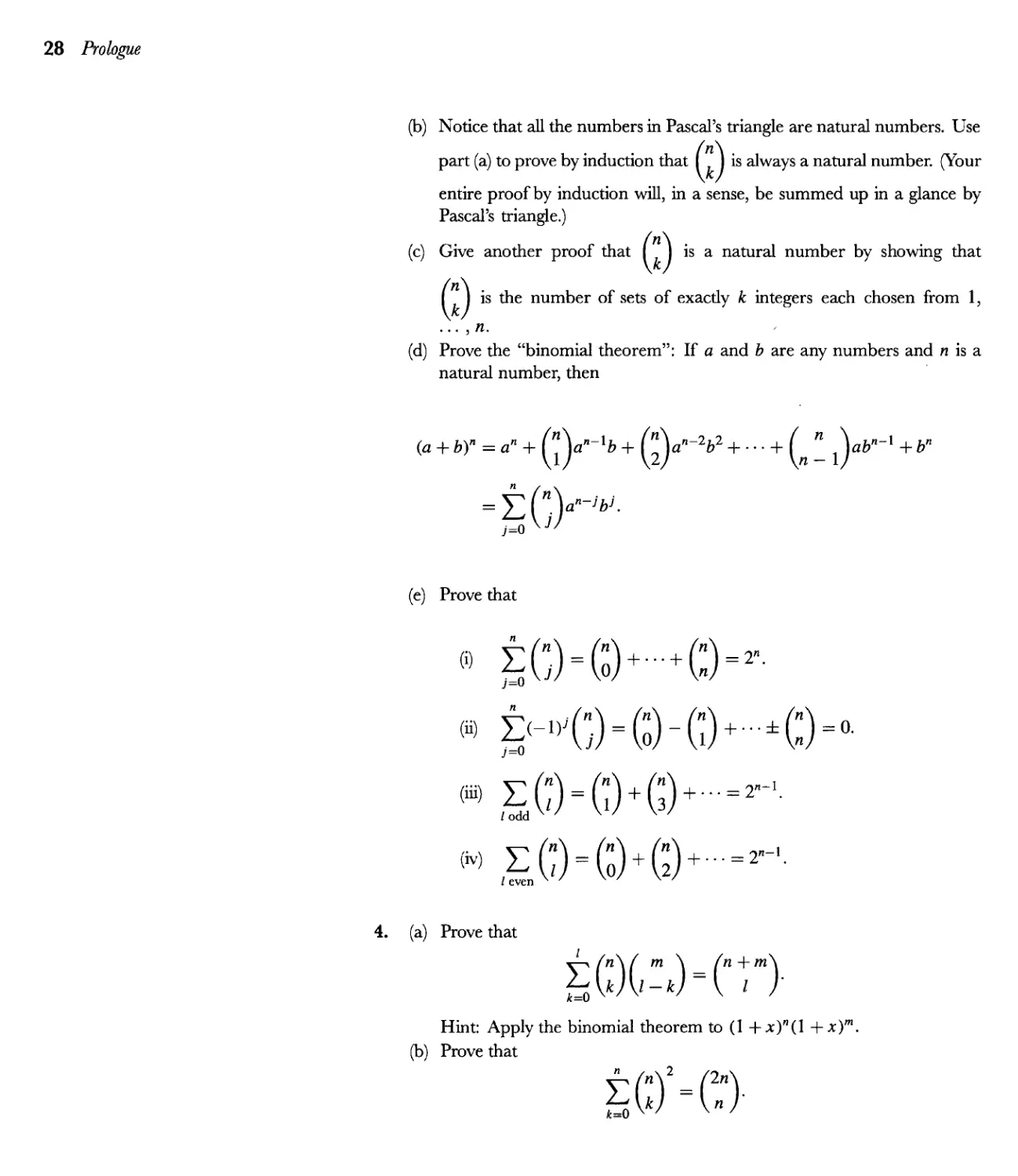
Notice that all the numbers in Pascal’s triangle are natural numbers. Use
part (a) to prove by induction that
is always a natural number. (Your
entire proof by induction will, in a sense, be summed up in a glance by
Pascal’s triangle.)
Give another proof that
is a natural number by showing that
is the number of sets of exacdy к integers each chosen from 1,
n.
(d) Prove the “binomial theorem”: If a and b are any numbers and n is a
natural number, then
(a + b)n — an + 2b2 + + (
(e) Prove that
4. (a) Prove that
(b)
Hint: Apply the binomial theorem to (1 + x)"(l + x)m.
Prove that
k=0
2n
n
2. Numbers of Various Sorts 29
5. (a) Prove by induction on n that
1 — rn+1
1 + r + r2 4-----H r" = —------
1 — r
if r / 1 (if r = 1, evaluating the sum certainly presents no problem).
(b) Derive this result by setting 5 — 1 + r 4-Hr”, multiplying this equation
by r, and solving the two equations for S.
6. The formula for I2 4------h n2 may be derived as follows. We begin with the
formula
(k + I)3 — A;3 = 3k2 + 3k + 1.
Writing this formula for к = 1, ... , n and adding, we obtain
23 - I3 = 3 • I2 + 3 • 1 + 1
З3 - 23 = 3 • 22 + 3 • 2 + 1
(n + I)3 — n3 = 3 • n2 + 3 • n + 1
(n + 1)3- 1 = 3[12 + + n2].+3[1 + • • + и] + n.
n n
Thus we can find к2 if we already know к (which could have been
fc=l . fc=l
found in a similar way). Use this method to find
(i) I3 4-------H n3.
(ii) I4 + • • • + n4.
(Ш) П + 2^3 +‘" + n(n + l)‘
.. . 3 5 2n +1
H i2.22 + 22.32 +'” + n2(n + 1)2-
*7. Use the method of Problem 6 to show that kp can always be written in
f=l
the form
np+^ i о
----? + Anp + Bnp~l + Cnp~2 + • • • .
P + 1
(The first 10 such expressions are
30 Prologue
о
k=i
+'n2+'n
3 z о
A=1
Vi-7 - ‘n4 X 1 „3 X b,2
/ A — д7! + 2^ + дМ
A-1
52^'4 = |/!5 +
k=l
ST' ;,5 _ I „6 , 1 „5
/ . k' ~ 611 + 2n
A=l
n
5>6 = N + b6
A=l
y>7 = 1 »8 + l«7
z J о Z
A=l
f>8 = h’ + b8
Jt=l
n
A=l
J-n Ю . 1„9
10 ' 2 1
+
+
+
+
+
+
J>10 = ±,г" + ^10 +
A=l
2"5 ~b3 +T2n
Г2п6 ~ + V2"2
2 7 7 5,2 3 1
3H “ Т5П + 9/( — 30/J
3„8 _l„6+!„4 _A,;2
4" IO" 2" 20"
|ZZ9 - 1777 + bi5 — 5«3 _|_
A11'
Notice that the coefficients in the second column are always j, and that after
the third column the powers of n with nonzero coefficients decrease by 2 until
n2 or n is reached. The coefficients in all but the first two columns seem to
be rather haphazard, but there actually is some sort of pattern; finding it may
be regarded as a super-perspicacity test. See Problem 27-17 for the complete
story.)
8. Provc that every natural number is either even or odd.
9. Provc that if a set A of natural numbers contains hq and contains к + 1
whenever it contains k, then A contains all natural numbers > hq.
10. Pt•ove the principle of mathematical induction from the well-ordering prin-
ciple.
11. Provc the principle of complete induction from the ordinary principle of
induction. Hint: If Л contains 1 and A contains n + 1 whenever it contains
1, ..., n, consider the set В of all к such that 1,.... к arc all in A.
12. (a) If a is rational and b is irrational, is a + b necessarily irrational? What
if a and b are both irrational?
2. Numbers of Various Sorts 31
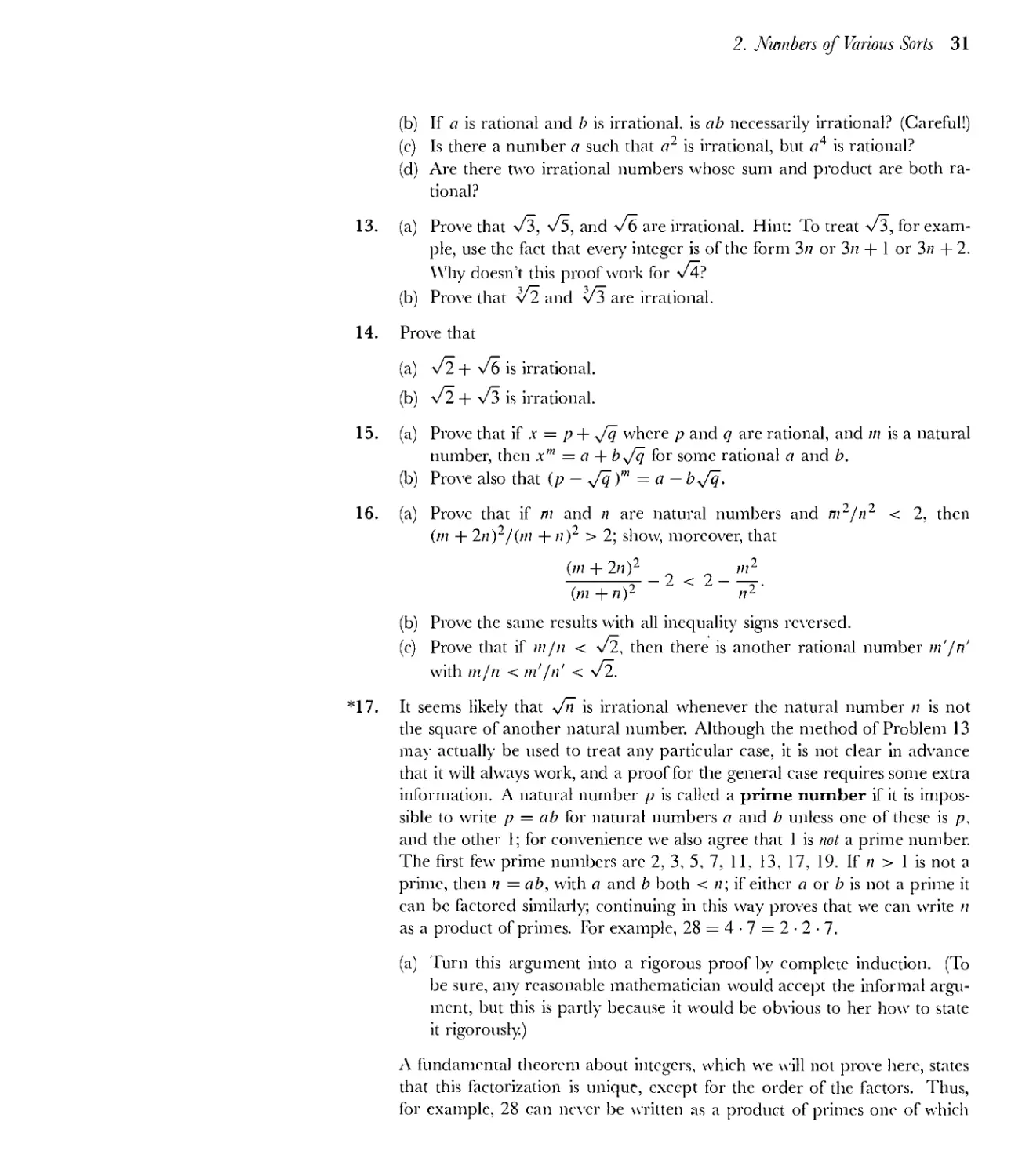
(b) If a is rational and b is irrational, is ab necessarily irrational? (Careful!)
(c) Is there a number a such that л2 is irrational, but о 4 is rational?
(d) Are there two irrational numbers whose sum and product are both ra-
tional?
13. (a) Prove that \/3, s/5, and s/б are irrational. Hint: To treat V3, for exam-
ple, use the fact that every integer is of the form 3n or 3n + 1 or 3n + 2.
Why doesn’t this proof work for \/4?
(b) Prove that and V3 are irrational.
14. Prove that
(a) f2 + ч/б is irrational.
(b) f2 + f3 is irrational.
15. (a) Prove that if x — p + fq where p and q are rational, and m is a natural
number, then xm = a + bfq for some rational a and b.
(b) Prove also that (p — fq)m = a — bfq.
16. (a) Prove that if m and n are natural numbers and m2/n2 < 2, then
(m + 2/z)2/(?n -HO2 > 2; show, moreover, that
(m + 'lnf a 11,2
---------5--2 < 2---------=-.
(m + n)2 u2
(b) Prove the same results with all inequality signs reversed.
(c) Prove that if m/n < s/2, then there is another rational number m'/n!
with m/n < m'/п' < \/2.
*17. It seems likely that fn is irrational whenever the natural number n is not
the square of another natural number. Although the method of Problem 13
may actually be used to treat any particular case, it is not clear in advance
that it will always work, and a proof for the general case requires some extra
information. A natural number p is called a prime number if it is impos-
sible to write p — ab for natural numbers a and b unless one of these is p,
and the other 1; for convenience we also agree that 1 is not a prime number.
The first few prime numbers are 2, 3, 5, 7, 11, 13, 17, 19. If n > 1 is not a
prime, then n = ab, with a and b both < n; if either a or b is not a prime it
can be factored similarly; continuing in this way proves that we can write n
as a product of primes. For example, 28 — 4 • 7 = 2 2 • 7.
(a) Turn this argument into a rigorous proof by complete induction. (To
be sure, any reasonable mathematician would accept the informal argu-
ment, but this is partly because it would be obvious to her how to state
it rigorously.)
A fundamental theorem about integers, which we will not prove here, states
that this factorization is unique, except for the order of the factors. Thus,
for example, 28 can never be written as a product of primes one of which
32 Prologue
is 3, nor can it be written in a way that involves 2 only once (now you should
appreciate why 1 is not allowed as a prime).
(b) Using this fact, prove that yTi is irrational unless n = irp for some natural
number m.
(c) Prove more generally that t/n is irrational unless n — mk.
(d) No discussion of prime numbers should fail to allude to Euclid's beautiful
proof that there are infinitely many of them. Prove that there cannot be
only finitely many prime numbers p\, p2, рз, ... , pn by considering
P\ • P2 • • P„ + 1
*18.
(b)
Prove that if x satisfies
xn + а,г_]л” 1 + • • + <?o = 0,
for some integers a„-i, ... , ao, then x is irrational unless x is an integer.
(Why is this a generalization of Problem 17?)
Prove that v6- v2 — v3 is irrational.
(c) Prove that V2 + \/2 is irrational. Hint: Start by working out the first 6
powers of this number.
19. Prove Bernoulli’s inequality: If h > — 1, then
(1 + h)n > 1 + nh
for any natural number n. Why is this trivial if h > 0?
20. The Fibonacci sequence ai, ci2, аз,... is defined as follows:
«1 = 1,
«2 = 1,
an = a„_] + n„_2 for n > 3.
This sequence, which begins 1, 1,2, 3, 5, 8, ... , was discovered by Fibonacci
(circa 1175-1250), in connection with a problem about rabbits. Fibonacci
assumed that an initial pair of rabbits gave birth to one new pair of rabbits
per month, and that after two months each new pair behaved similarly. The
number a„ of pairs born in the nth month is + n„-2, because a pair of
rabbits is born for each pair born the previous month, and moreover each
pair born two months ago now gives birth to another pair. The number of
interesting results about this sequence is truly amazing—-there is even a Fi-
bonacci Association which publishes a journal, The Fibonacci Quarterly. Prove
that
One way of deriving this astonishing formula is presented in Problem 24-16.
2. Numbers of Various Sorts 33
21. The Schwarz inequality (Problem 1-19) actually has a more general form:
Give three proofs of this, analogous to the three proofs in Problem 1-19.
22. The result in Problem 1-7 has an important generalization: If an > 0,
then the “arithmetic mean”
«1 + • • • +
An = --------------
n
and “geometric mean”
Gn = </бЦ ...a„
satisfy
G„ < A„.
(a) Suppose that «i < An. Then some a, satisfies a, > An', for convenience,
say «2 > An. Let tq = An and let «2 — a\ + a2 ~ • Show that
> «1^2-
Why does repeating this process enough times eventually prove that Gn <
A„? (This is another place where it is a good exercise to provide a formal
proof by induction, as well as an informal reason.) When does equality7
hold in the formula Gn < A„?
The reasoning in this proof is related to another interesting proof.
(b) Using the fact that Gn < An when n — 2, prove, by induction on k, that
G„ < A„ for n —2k.
(c) For a general n, let 2m > n. Apply part (b) to the 2m numbers
я ], .... an, Atl..An
2m-n times
to prove that G„ < An.
23. The following is a recursive definition of a”:
a1 — a,
a”+l = a" -a.
Prove, by induction, that
a"+m = an am,
(a")"‘ = anw.
(Don’t try to be fancy: use either induction on n or induction on tn, not both
at once.)
34 Prologue
24. Suppose we know properties Pl and P4 for the natural numbers, but that
multiplication lias never been mentioned. Then the following can be used
as a recursive definition of multiplication:
1 -b = b,
(a + 1) • b = a b + b.
Prove the following (in the order suggested!):
a (b + c) = a b + a c (use induction on «),
a • 1 = a,
a • b — b a (you just finished proving the case b = 1).
25. In this chapter we began with the natural numbers and gradually built up to
the real numbers. A completely rigorous discussion of this process requires
a little book in itself (see Part V). No one has ever figured out how to get to
the real numbers without going through this process, but if we do accept the
real numbers as given, then the natural numbers can be defined as the real
numbers of the form 1, 1 + 1, 1 + 1 + 1, etc. The whole point of this problem
is to show that there is a rigorous mathematical way of saying “etc.”
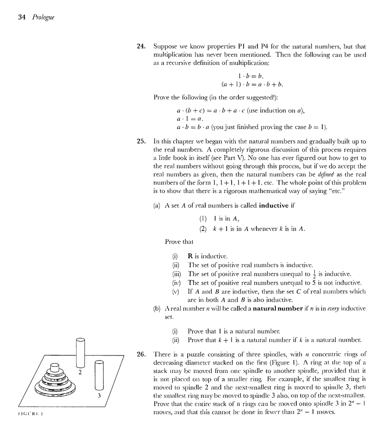
(a) A set A of real numbers is called inductive if
(1) 1 is in A,
(2) к + 1 is in A whenever к is in A.
Provethat
(i) R is inductive.
(ii) The set of positive real numbers is inductive.
(ii i) The set of positive real numbers unequal to is inductive.
(iv) The set of positive real numbers unequal to 5 is not inductive.
(v) If A and В are inductive, then the set C of real numbers which
are in both A and В is also inductive.
(b) A real number n will be called a natural number if n is in every inductive
set.
(i) Prove that 1 is a natural number.
(ii) Prove that к + 1 is a natural number if к is a natural number.
26. There is a puzzle consisting of three spindles, with n concentric rings of
decreasing diameter stacked on the first (Figure 1). A ring at the top of a
stack may be moved from one spindle to another spindle., provided that it
is not placed on top of a smaller ring. For example, if the smallest ring is
moved to spindle 2 and the next-smallest ring is moved to spindle 3, then
the smallest ring maybe moved to spindle 3 also, on top of the next-smallest.
Prove that the entire stack of n rings can be moved onto spindle 3 in 2" — 1
moves, and that this cannot be done in fewer than 2" — 1 moves.
2. Numbers of Various Sorts 35
*27. University B. once boasted 17 tenured professors of mathematics. Tradi-
tion prescribed that at their weekly luncheon meeting, faithfully attended by
all 17, any members who had discovered an error in their published work
should make an announcement of this fact, and promptly resign. Such an an-
nouncement had never actually been made, because no professor was aware
of any errors in her or his work. This is not to say that no errors existed,
however. In fact, over the years, in the work of every member of the de-
partment at least one error had been found, by some other member of the
department. This error had been mentioned to all other members of the
department, but the actual author of the error had been kept ignorant of the
fact, to forestall any resignations.
One fateful year, the department was augmented by a visitor from another
university, one Prof. X, who had come with hopes of being offered a perma-
nent position at the end of the academic year. Naturally, he was apprised, by
various members of the department, of the published errors which had been
discovered. When the hoped-for appointment failed to materialize, Prof X
obtained his revenge at the last luncheon of the year. “I have enjoyed my visit
here very much,” he said, “but I feel that there is one thing that I have to tell
you. At least one of you has published an incorrect result, which has been
discovered by others in the department.” What happened the next year?
**28. After figuring out, or looking up, the answer to Problem 27, consider the fol-
lowing: Each member of the department already knew what Prof. X asserted,
so how could his saying it change anything?
PART
FOUNDATIONS
The statement is so frequently made
that the differential calculus deals with
continuous magnitude, and yet
an explanation of this continuity is
nowhere given;
even the most rigorous expositions
of the differential calculus do not base
their proofs upon continuity but,
with more or less consciousness of the fad,
they either appeal to geometric notions
or those suggested by geometry,
or depend upon theorems which are never
established in a purely arithmetic manner.
Among these, for example,
belongs the above-mentioned theorem,
and a more careful investigation
convinced me that this theorem, or
any one equivalent to it, can be regarded
in some way as a sufficient basis
for infinitesimal analysis.
It then only remained to discover its true
origin in the elements of arithmetic
and thus at the same time
to secure a real definition of
the essence of continuity.
I succeeded .Nov. 24, 1858, and
a few days afterward 1 communicated
the results
of my meditations to my dear friend
Durege with whom I had a long
and lively discussion.
RICHARD DEDEKIND
CHAPTER
FUNCTIONS
PROVISIONAL DEFINITION
Undoubtedly the most important concept in all of mathematics is that of a
function—in almost every branch of modern mathematics functions turn out to
be the central objects of investigation. It will therefore probably not surprise you
to learn that the concept of a function is one of great generality. Perhaps it will
be a relief to learn that, for the present, we will be able to restrict our attention to
functions of a very special kind; even this small class of functions will exhibit suffi-
cient variety to engage our attention for quite some time. We will not even begin
with a proper definition. For the moment a provisional definition will enable us to
discuss functions at length, and will illustrate the intuitive notion of functions, as
understood by mathematicians. Later, we will consider and discuss the advantages
of the modern mathematical definition. Let us therefore begin with the following:
A function is a rule which assigns, to each of certain real numbers, some other real
number.
The following examples of functions are meant to illustrate and amplify this defi-
nition, which, admittedly, requires some such clarification.
Example 1 The rule which assigns to each number the square of that number.
Example 2 The rule which assigns to each number у the number
y3 + 3y + 5
y2 + 1
Example 3 The rule which assigns to each number с ф 1,-1 the number
c3 + 3 c + 5
c2 — 1
Example 4 The rule which assigns to each number x satisfying — 17 < x < тг/З
the number x2.
Example 5 The rule which assigns to each number a the number 0 if a is
irrational, and the number 1 if a is rational.
Example G The rule which assigns
to 2 the number 5,
, 36
to 17 the number —,
7Г
39
40 Foundations
to — the number 28,
36
to — the number 28,
7Г
and to any у /2, 17, тг2/17, or 36/тг, the number 16 if у is of the form a -\-b\Zl
for a, b in Q.
Example 7 The rule which assigns to each number t the number F + x. (This
rule depends, of course, on what the number x is, so we are really describing
infinitely many different functions, one for each number x.)
Example 8 The rule which assigns to each number ; the number of 7’s in the
decimal expansion of z, if this number is finite, and —тг if there are infinitely many
7’s in the decimal expansion of z-
One thing should be abundantly clear from these examples—a function is any
rule that assigns numbers to certain other numbers, not just a rule which can
be expressed by an algebraic formula, or even by one uniform condition which
applies to every number; nor is it necessarily a rule which you, or anybody else,
can actually apply in practice (no one knows, for example, what rule 8 associates
to 7t). Moreover, the rule may neglect some numbers and it may not even be clear
to which numbers the function applies (try to determine, for example, whether the
function in Example 6 applies to 7r). The set of numbers to which a function does
apply is called the domain of the function.
Before saying anything else about functions we badly need some notation. Since
throughout this book we shall frequently be talking about functions (indeed we shall
hardly ever talk about anything else) we need a convenient way of naming func-
tions, and of referring to functions in general. The standard practice is to denote
a function by a letter. For obvious reasons the letter is a favorite, thereby
making “g” and “Л” other obvious candidates, but any letter (or any reasonable
symbol, for that matter) will do, not excluding “x” and “у”, although these letters
arc usually reserved for indicating numbers. If f is a function, then the number
which f associates to a number x is denoted by f(x)—this symbol is read “ f of
x” and is often called the value off atx. Naturally, if we denote a function by x,
some other letter must be chosen to denote the number (a perfectly legitimate,
though perverse, choice would be leading to the symbol x(/)). Note that the
symbol /(x) makes sense only for x in the domain of f; for other x the symbol
/(x) is not defined.
If the functions defined in Examples 1-8 are denoted by /, g, It, r, x, 0, ax,
and y, then we can rewrite their definitions as follows:
(1) j\x) = x2 for all x.
(2) g(y) = Д for all y.
V“ + 1
c3 + 3c + 5
(3) /г(с) = ----5------ for all c f 1,-1.
--- I
3. Functions 41
(4) r(x) — x~ for all x such that —17 < x < л/3.
(5) 5(x) =
x irrational
x rational.
(6) 0(x) =
(7) a.v(t) — F + x for all numbers t.
(8) J.(A)= ("я
exactly n J's appear in the decimal expansion of x
infinitely many 7’s appear in the decimal expansion of x.
These definitions illustrate the common procedure adopted for defining a func-
tion f—indicating what /(x) is for every number x in the domain of /. (Notice
that this is exactly the same as indicating f(a) for every number n, or f(b) for ev-
ery number b, etc.) In practice, certain abbreviations are tolerated. Definition (1)
could be written simple
(1) /(x) = x2
the qualifying phrase “for all x’’ being understood. Of course, for definition (4)
the only possible abbreviation is
(4) r(x) = x2. —17 < x < 7T/3.
It is usually understood that a definition suc-h as
№) = - + —*—. x/0.1
X x — 1
can be shortened to
£(x) = - H-----J—;
x x — 1
in other words, unless the domain is explicitly restricted further, it is understood to consist of
all numbers for which the definition makes any sense at all.
You should have little difficulty checking the following assertions about the func-
tions defined above:
/(x+l) = /(x) + 2x+l;
g(x) = h(x) if x3 + 3x + 5=0;
r(x + 1) = r(x) + 2x + 1 if —17 < x < у - 1;
42 Foundations
six + у) — s(x) if у is rational;
a.t(x) =x [fix) + 1];
yf) = °-
If the expression fisia)) looks unreasonable to you, then you are forgetting that
s(a) is a number like any other number, so that fisia)) makes sense. As a matter
of fact, fisia)) = sia) for all a. Why? Even more complicated expressions than
fisia)) are, after a first exposure, no more difficult to unravel. The expression
f(r(s(0(a3(y(i)))))).
formidable as it appears, may be evaluated quite easily with a little patience;
/(r(s(0(a3(y(l))))))
= /(r(5(0(a3(O)))))
= /(r(^(0(3))))
= /(r(^(16)))
= /(r(l))
= /(l)
= 1.
The first few problems at the end of this chapter give further practice manipulating
this symbolism.
The function defined in (1) is a rather special example of an extremely impor-
tant class of functions, the polynomial functions. A function f is a polynomial
function if there are real numbers ao, ... , an such that
fix) = a„x" + + • • • + azx2 + др’ + oq, for all x
(when fix) is written in this form it is usually tacitly assumed that afl 0). The
highest power of x with a nonzero coefficient is called the degree of f; for
example, the polynomial function f defined by fix) — 5x6 + 137л4 — тг has
degree 6.
The functions defined in (2) and (3) belong to a somewhat larger class of func-
tions, the rational functions; these are the functions of the form p/q where? p
and q are polynomial functions (and q is not the function which is always 0). The
rational functions are themselves quite special examples of an even larger class of
functions, very thoroughly studied in calculus, which are simpler than many of the
functions first mentioned in this chapter. The following arc examples of this kind
of function:
9 . 9
X+X +XS111 X
; 2
A Sill A' +A'Sin Л'
(10) fix) - sin(x2).
(11) f(x) = sin(sin(x2)).
(9) fW =
3. Functions 43
.'>..9 . ? 7 . /х + sin(x sinx)
(121 /(x) — sm-fsmfsm-fx sm x~))) sin I -;--
' \ x + sin X
By what criterion, you may feel impelled to ask, can such functions, especially a
monstrosity like (12), be considered simple? The answer is that they can be built
up from a few simple functions using a few simple means of combining functions.
In order to construct the functions (9)—(12) we need to start with the "‘identity
function” I, for which I(x) — x, and the “sine function” sin, whose value sin(x) at
x is often written simple sinx. The following are some of the important ways in
which functions may be combined to produce new functions.
If f and g are any two functions, we can define a new function f + g, called
the sum of f and g, by the equation
(/ + g)(x) = /(x) + g(x).
Note that according to the conventions we have adopted, the domain of f + g
consists of all x for which “/(x) + g(x)” makes sense, i.e., the set of all x in both
domain f and domain g. If A and В are any two sets, then А П В (read “A
intersect B” or “the intersection of A and B”) denotes the set of x in both A
and 5; this notation allows us to write domain(/ + g) = domain f П domain g.
. f
In a similar vein, we define the product f g and the quotient — (or f/g} of
g
f and g by
(f g)(x) = /(x) • g(x)
and
(f\, , /(X)
~ (x) = ——.
\gj g(x)
Moreover, if g is a function and c is a number, we define a new function c g by
(c-g)(x) = cg(x).
This becomes a special case of the notation f • g if we agree that the symbol c
should also represent the function f defined by /(x) — c; such a function, which
has the same value for all numbers x, is called a constant function.
The domain of f • g is domain f П domain g. and the domain of c • g is simply
the domain of g. On the other hand, the domain of f/g is rather complicated—it
may be written domain f П domain g П (x : g(x) 0), the symbol {д' : g(x) 0}
denoting the set of numbers x such that g{x) 0. In general, {x : ...} denotes
the set of all x such that ...” is true. Thus {x : x3 + 3 < 11} denotes the set of
all numbers x such that x3 < 8, and consequently {x : x3 + 3 < 11} = {x : x < 2}.
Either of these symbols could just as well have been written using у everywhere
instead of x. Variations of this notation are common, but hardly require any
discussion. Any one can guess that {x > 0 : x3 < 8) denotes the set of positive
numbers whose cube is less than 8; it could be expressed more formally as {x :
x > 0 and x3 < 8}. Incidentally, this set is equal to the set (x : 0 < x < 2}. One
44 Foundations
variation is slightly less transparent, but very standard. The set {1,3, 2,4}, for
example, contains just the four numbers 1, 2, 3, and 4; it can also be denoted by
{.г : r = 1 or _r = 3 or л = 2 or x =4}.
Certain facts about the sum, product, and quotient of functions are obvious con-
sequences of facts about sums, products, and quotients of numbers. For example,
it is very easy to prove that
(f + g) + = f + (g + /’)•
The proof is characteristic of almost every proof which demonstrates that two
functions are equal—the two functions must be shown to have the same domain,
and the same value at any number in the domain. For example, to prove that
(/ + g) + h = f + (g + /?), note that unraveling the definition of the two sides gives
[(/ + g)+/t](A-) = (/ + g)(A)+/z(A)
= [/(A) + g(A)] +Л(Х)
and
[/+(g+/0](A) = /(X)+ (g + /t)(A)
= /U) + [g(A) + /t(x)],
and the equality of [/(x) + g(x)] + Л (x) and f (x) + [g(x) + h(x)] is a fact about
numbers. In this proof the equality of the two domains was not explicitly men-
tioned because this is obvious, as soon as we begin to write down these equations;
the domain of (/ + g) + h and of / + (g + /;) is clearly domain f П domain g П
domain Л. We naturally write f + g + Л for (/ + g) + h = f + (g + /;), precisely
as we did for numbers.
It is just as easy to prove that (/ • g) • h = f • (g • Л), and this function is denoted
by f • g • h. The equations f + g — g + f and f • g = g f should also present
no difficulty.
Using the operations +, •, / we can now express the function / defined in (9)
ЬУ
/ + /•/ + /• sin • sin
/ - ------:-------:----:--•
1 • sin +1 • sin • sin
It should be clear, however, that we cannot express function (10) this way. We re-
quire yet another way of combining functions. This combination, the composition
of two functions, is by far the most important.
If / and g are any two functions, we define a new function f og, the compo-
sition of / and g, by
(/°g)(A) = /(g(A-));
the domain of f og is {x : x is in domain g and g(x) is in domain /}. The symbol
“/og” is often read “/ circle g.” Compared to the phrase “the composition of f
and g” this has the advantage of brevity, of course, but there is another advantage
of far greater import: there is much less chance of confusing / о g with g о /, and
3. Functions 45
these must not be confused, since they are not usually equal; in fact, almost any f
and g chosen at random will illustrate this point (try f = I I and g — sin, for
example). Lest you become too apprehensive about the operation of composition,
let us hasten to point out that composition is associative:
(/ 0 g) 0 h = f о (g о Л)
(and the proof is a triviality); this function is denoted by f о g о h. We can now
write the functions (10), (11), (12) as
(10) / = sin о (/•/),
(11) f = sin о sin о (/ • /),
(12) f = (sin sin) о sin о (sin • sin) о (/ • [(sin • sin) о (/•/)]) •
(I + sin о (/ • sin)\
------------;------ I.
I + sin /
One fact has probably already become clear. Although this method of writing
functions reveals their ‘‘structure” very clearly, it is hardly short or convenient. The
shortest name for the function f such that f(x) — sin(.r2) for all x unfortunately
seems to be “the function f such that /(x) = sin(x2) for all x.” The need for
abbreviating this clumsy description has been clear for two hundred years, but no
reasonable abbreviation has received universal acclaim. At present the strongest
contender for this honor is something like
x —> sin (л2)
(read “x goes to sin(x2)” or just “x arrow sin(x2)”), but it is hardly popular among
writers of calculus textbooks. In this book we will tolerate a certain amount of
ellipsis, and speak of “the function /(x) = sin(x2).” Even more popular is the
quite drastic abbreviation: “the function sin(x2).” For the sake of precision we
will never use this description, which, strictly speaking, confuses a number and
a function, but it is so convenient that you will probably end up adopting it for
personal use. As with any convention, utility is the motivating factor, and this
criterion is reasonable so long as the slight logical deficiencies cause no confusion.
On occasion, confusion will arise unless a more precise description is used. For
example, “the function x + f3” is an ambiguous phrase; it could mean either
x -> x +1\ i.e., the function f such that /(x) — x +t3 for all x
or
t —> x + t3, i.e., the function f such that fit) = x + t3 for all t.
As we shall see, however, for many important concepts associated with functions,
calculus has a notation which contains the “x built in.
By now we have made a sufficiently extensive investigation of functions to war-
rant reconsidering our definition. We have defined a function as a “rule,” but it is
hardly clear what this means. If we ask “What happens if you break this rule?” it
is not easy to say whether this question is merely facetious or actually profound.
46 Foundations
A more substantial objection to the use of the word “rule” is that
/U) = x2
and
fix') = x2 + 3x + 3 — 3(x + 1)
arc certainly different rules, if by a rule we mean the actual instructions given for
determining /(л); nevertheless, we want
/(x) = x2
and
/(x) — x2 + 3x + 3 — c(x + 1)
to define the same function. For this reason, a function is sometimes defined as an
“association” between numbers; unfortunately the word “association” escapes the
objections raised against “rule” only because it is even more vague.
There is, of course, a satisfactory way of defining functions, or we should never
have gone to the trouble of criticizing our original definition. But a satisfactory
definition can never be constructed by finding synonyms for English words which
are troublesome. The definition which mathematicians have finally accepted for
“function” is a beautiful example of the means by which intuitive ideas have been
incorporated into rigorous mathematics. The correct question to ask about a
function is not “What is a rule?” or “What is an association?” but “What does
one have to know about a function in order to know all about it?” The answer to
the last question is easy—for each number x one needs to know the number /(x);
we can imagine a table which would display all the information one could desire
about the function /(x) = x2:
7Г
/(A)
1
1
4
4
2
2
Э
7Г"
— 7Г
It is not even necessary to arrange the numbers in a table (which would actually
be impossible if wc wanted to list all of them). Instead of a two column array we
can consider various pairs of numbers
(1,1), (-1,1), (2,4), (-2,4), (тг.тг2), (У2,2),...
3. Functions 47
simply collected together into a set.* To find /(1) we simply take the second
number of the pair whose first member is 1; to find /(я) we take the second
number of the pair whose first member is я. We seem to be saying that a function
might as well be defined as a collection of pairs of numbers. For example, if we
were given the following collection (which contains just 5 pairs):
/ = {(1,7), (3,7), (5,3), (4,8), (8,4)),
then /(1) =7, /(3) = 7, /(5) =3, /(4) = 8, /(8) = 4 and 1, 3, 4, 5, 8 are the
only numbers in the domain of /. If we consider the collection
/ = {(1,7), (3.7), (2,5), (1,8), (8,4)},
then /(3) = 7, /(2) = 5, f (8) = 4; but it is impossible to decide whether /(1) = 7
or /(1) = 8. In other words, a function cannot be defined to be any old collection
of pairs of numbers; we must rule out the possibility which arose in this case. We
are therefore led to the following definition.
DEFINITION A function is a collection of pairs of numbers with the following property: if (u,h) and (u,c) are both in the collection, then b = c; in other words, the collection must not contain two different pairs with the same first element.
This is our first full-fledged definition, and illustrates the format we shall always
use to define significant new concepts. These definitions are so important (at
least as important as theorems) that it is essential to know when one is actually
at hand, and to distinguish them from comments, motivating remarks, and casual
explanations. They will be preceded by the word DEFINITION, contain the term
being defined in boldface letters, and constitute a paragraph unto themselves.
There is one more definition (actually defining two things at once) which can
now be made rigorously:
DEFINITION If / is a function, the domain of / is the set of all a for which there is some b such that (л, b) is in /. If a is in the domain of /, it follows from the definition of a function that there is, in fact, a unique number b such that (u, b) is in f. This unique b is denoted by f(a).
With this definition we have reached our goal: the important thing about a
function / is that a number /(.r) is determined for each number .r in its domain.
You may feel that we have also reached the point where an intuitive definition has
been replaced by an abstraction with which the mind can hardly grapple. Two
consolations may be offered. First, although a function has been defined as a
♦The pairs occurring here are often called “ordered pairs,” to emphasize that, for example, (2. 4) is
not the same pair as (4, 2). It is only fair to warn that we are going to define functions in terms of
ordered pairs, another undefined term. Ordered pairs can be defined, however, and an appendix to
this chapter has beeii provided for skeptics.
48 Foundations
collection of pairs, there is nothing to stop you from thinking of a function as a
rule. Second, neither the intuitive nor the formal definition indicates the best way
of thinking about functions. The best way is to draw pictures; but this requires a
chapter all by itself.
PROBLEMS
1. Let f(x) = 1/(1 + x). What is
(i) /(/(-Y)) (for which x does this make sense?).
(ii) /Q).
(iii) f(cx).
(iv) /(x+y).
(v) /(x) + /(y).
(vi) For which numbers c is there a number x such that f(cx) — f(x).
Hint: There are a lot more than you might think at first glance.
(vii) For which numbers c is it true that f (ex) = f(x) for two different
numbers x?
2. Let g(x) = x2, and let
0, x rational
1 X L x irrational.
(i) For which у is h(y) < y?
(ii) For which у is Л(у) < g(y)?
(iii) What is g(h(z)) — A(z)?
(iv) For which w is g(w) < w?
(v) For which £ is g(g(£)) = g(e)2
3. Find the domain of the functions defined by the following formulas.
(i) /(x) = y/1 - x2.
(ii) /(x) = \/l - /1 -x2.
1 1
(m) /(x) ----------- +-------.
x — 1 x — 2
(iv) f(x) = >/l - x2 + \/x2 - 1.
(v) /(x) = у 1 - x + \/x -2.
4. Let 5(x) = x2, let P(x) = 2 (i) (ii) (iii) (iv) (v) * * * * х, and let s(x) = sinx. Find each of the following.
In each case you answer should be a number.
(i) (SoP)(y).
(ii) (5o.v)(y).
(iii) (5 о P о s)(t) + (5 о P)(t).
(iv) s(l3).
5. Express each of the following functions in terms of 5, P, s, using only
+, , and о (for example, the answer to (i) is P о 5). In each case your
3. Functions 49
answer should be a function.
(i) /(x) = 2si"L
(ii) /(x) = sin2v.
(iii) /(x) = sinx2.
(iv) /(x) = sin2x (remember that sin2 x is an abbreviation for (sinx)2).
(v) /(0 = 2" . (Note: ab' always means this convention is adopted
because lab)c can be written more simply as abci)
(vi) flu) — sin (2" + 2"2).
(vii) fly) = sin(sin(sin(222 '))).
(viii) fla) = 2sir?a + sin(«2) + 2sinCa2+sina>.
Polynomial functions, because they are simple, yet flexible, occupy a favored
role in most investigations of functions. The following two problems illustrate their
flexibility, and guide you through a derivation of their most important elementary
properties.
6. (a) If X], ... , x„ are distinct numbers, find a polynomial function f of
degree и — 1 which is 1 at x( and 0 at x7 for j f i. Hint: the product of
all (x — Xj) for j f i, is 0 at Xj if j f i. (This product is usually denoted
by
n
Псх-х/Ь
the symbol П (capital pi) playing the same role for products that X plays
for sums.)
(b) Now find a polynomial function f of degree n — 1 such that /(x( ) =
where O|, ... , an are given numbers. (You should use the functions
fi from part (a). The formula you will obtain is called the “Lagrange
interpolation formula.”)
7. (a) Prove that for any polynomial function /, and any number a, there is a
polynomial function g, and a number b, such that fix) = (x — a)glx)-\-b
for all x. (The idea is simply to divide (x — a) into fix) by long division,
until a constant remainder is left. For example, the calculation
x2 Tx —2
x — 1 Ух?1 —3x + 1
2 о
X —5x
2
X —x
—2x + 1
—2x + 2
- 1
50 Foundations
shows that x3 — 3x + 1 — (x — l)(x2 + x - 2) - 1. A formal proof is
possible by induction on the degree of /.)
(b) Prove that if f{a) — 0, then /(x) — (x — n)g(x) for some polynomial
function g. (The converse is obvious.)
(c) Prove that if f is a polynomial function of degree n, then f has at most
n roots, i.e., there are at most n numbers a with /(«) = 0.
(d) Show that for each n there is a polynomial function of degree n with
n roots. If n is even find a polynomial function of degree n with no
roots, and if n is odd find one with only one root.
8. For which numbers a, b, c, and d will the function
satisfy f{f(x)) = x for all x (for which this equation makes sense)?
9. (a) If A is any set of real numbers, define a function Сд as follows:
. fl, x in A
Fa (a) — in л
| (J, x not in A.
Find expressions for Сдпв and Сдив and Cr_a. in terms of Сд and Cg-
(The symbol A A В was defined in this chapter, but the other two may
be new to you. They can be defined as follows:
A U В = {x : x is in A or x is in B},
R — A = {x : x is in R but x is not in A}.)
(b) Suppose f is a function such that /(x) — 0 or 1 for each x. Prove that
there is a set A such that f = Сд.
(c) Show that f = if and only if f — Сд for some set A.
10. (a) For which functions f is there a function g such that f — g~? Hint: You
can certainly answer this question if “function” is replaced by “number.”
(b) For which functions f is there a function g such that f — 1 /g?
*(c) For which functions b and c can we find a function x such that
(x(t))2 + b(t)x (r) + c(r) = 0
for all numbers t ?
*(d) What conditions must the functions a and b satisfy if there is to be a
function x such that
a(t)x(t) + b(t) = 0
for all numbers t? How many such functions x will there be?
11. (a) Suppose that H is a function and у is a number such that H(H(y)) — y.
What is
80 limes
3. Functions 51
(b) Same question if 80 is replaced by 81.
(c) Same question if H(H(y)) = H(y).
*(d) Find a function H such that Я(Я(х)) = H(л) for all numbers x, and
such that /7(1) = 36, Я (2) = я/3, Я(13) = 47, Я(36) - 36, Я(я/3) =
я/3, Я(47) — 47. (Don’t try to "solve” for Я(х); there are many func-
tions Я with Я(Я(х)) = Я (x). The extra conditions on Я are supposed
to suggest a way of finding a suitable Я.)
*(e) Find a function Я such that Я(Я(х)) — Я(х) for all x, and such that
Я(1) = 7, Я(17) = 18.
12. A function f is even if f(x) = f(—x) and odd if /(x) — -f(-x'). For
example, f is even if /(x) = x2 or /(x) = |x| or /(x) = cosx, while f is
odd if /(x) = x or /(x) = sinx.
(a) Determine whether f + g is even, odd, or not necessarily either, in the
four cases obtained by choosing f even or odd, and g even or odd. (Your
answers can most conveniently be displayed in a 2 x 2 table.)
(b) Do the same for f • g.
(c) Do the same for fog.
(d) Prove that every even function f can be written /(x) — g(|x|), for in-
finitely many functions g.
*13. (a) Prove that any function f with domain R can be written f — E + O,
where E is even and О is odd.
(b) Prove that this way of writing f is unique. (If you try to do part (b) first,
by “solving” for E and О you will probably find the solution to part (a).)
14. If f is any function, define a new function |/| by |/|(x) = |/(x)|. If f
and g are functions, define two new functions, max(/, g) and min(/, g), by
max(/, g)(x) = max(/(x), g(x)),
min(/, g)(x) = min(/(x), g(x)).
Find an expression for max(/, g) and min(/, g) in terms of | |.
15. (a) Show that f — max(J, 0) + min(/, 0). This particular way of writing
f is fairly useful; the functions max(/, 0) and min(/, 0) are called the
positive and negative parts of f.
(b) A function f is called nonnegative if /(x) > 0 for all x. Prove that any
function f can be written f = g — h, where g and h are nonnegative,
in infinitely many ways. (The “standard way” is g — max(/, 0) and h —
— min(/, 0).) Hint: Any number can certainly be written as the difference
of two nonnegative numbers in infinitely many ways.
*16. Suppose f satisfies f(x + y) — /(x) + f(y) for all x and y.
(a) Prove that f(x} -I----h x„) = /(x,) H----+ /(x„).
(b) Provc that there is some number c such that /(x) = ex for all rational
numbers x (at this point we’re not trying to say anything about /(x) for
irrational x). Hint: First figure out what c must be. Now prove that
52 Foundations
/(x) = ex, first when x is a natural number, then when x is an integer,
then when x is the reciprocal of an integer and, finally, for all rational x.
*17. If /(x) = 0 for all x, then f satisfies /(x + y) = /(x) + f (y) for all x and y,
and also /(x • y) = /(x) • /(у) for all x and y. Now suppose that f satisfies
these two properties, but that /(x) is not always 0. Prove that /(x) = x for
all x, as follows:
(a) Prove that f (1) — 1.
(b) Prove that /(x) = x if x is rational.
(c) Prove that f (x) > 0 if x >0. (This part is tricky, but if you have
been paying attention to the philosophical remarks accompanying the
problems in the last two chapters, you will know what to do.)
(d) Prove that f (x) > /(y) if x > y.
(e) Prove that /(x) — x for all x. Hint: Use the fact that between any two
numbers there is a rational number.
*18. Precisely what conditions must f, g, h, and к satisfy in order that /(x)g(y) =
h(x)k(y) for all x and y?
*19. (a) Prove that there do not exist functions f and g with either of the following
properties:
(i) /(x) + g(y) = xy for all x and y.
(ii) /(x) • g(y) = x + у for all x and y.
Hint: Try to get some information about f or g by choosing particular
values of x and y.
(b) Find functions f and g such that /(x + y) = g(xy) for all x and y.
*20. (a) Find a function f, other than a constant function, such that |/(y) —
fW\ < |y - x|.
(b) Suppose that f(y) — f(x) < (y — x)2 for all x and y. (Why does this
imply that |/(y) — /(x)| < (y — x)2?) Prove that f is a constant function.
Hint: Divide the interval from x to у into n equal pieces.
21. Prove or give a counterexample for each of the following assertions:
f о (g +Л) = f о g + f о h.
(g + h)° f = f + Л о f-
1 1
7----= 7 °&-
f °g f
1 /1\
7— = ^° ( /
f°g \gJ
Suppose g = h о f. Prove that if /(x) = f(y), then g(x) — g(y).
Conversely, suppose that f and g are two functions such that g(x) — g(y)
whenever /(x) = f(y)- Prove that g = А о f for some function A. Hint:
Just try to define h(z) when z is of the form z — /(x) (these arc the only c
that matter) and use the hypotheses to show that your definition will not
run into trouble.
(a)
(b)
(c)
(d)
22. (a)
(b)
3. Functions 53
23. Suppose that f c g = /, where / (л ) = _v. Prove that
(a) if x / y, then g(x) ±
(b) every number b can be written b — f (a) for some number a.
*24. (a) Suppose g is a function with the property that glx) gf.v) if .v У-
Provc that there is a function f such that f о g = I.
(b) Suppose that f is a function such that every number b can be written
b = f (a) for some number a. Provc that there is a function g such that
f °g = F
*25. Find a function f such that g - f = I for some g, but such that there is no
function h with f oh = I.
*26. Suppose f og = / and h о f = I. Prove that g = h. Hint: Use the fact that
composition is associative.
27. (a) Suppose fix) = л+ 1. Are there any functions g such that f °g = g° f?
(b) Suppose f is a constant function. For which functions g does f о g =
g ° /?
(c) Suppose that fog = g :> f for all functions g. Show that f is the identity
function, fix) = x.
28. (a) Let F be the set of all functions whose domain is R. Pi ove that, using +
and • as defined in this chapter, all of properties P1-P9 except P7 hold
for F, provided 0 and I are interpreted as constant functions.
(b) Show that P7 does not hold.
*(c) Show that P10-P12 cannot hold. In other words, show that there is
no collection P of functions in F, such that Pl0-P 12 hold for P. (It is
sufficient, and will simplify things, to consider only functions which are 0
except at two points л'о and _Г|.)
(d) Suppose we define f < g to mean that fix) < g(x) for all л. Which of
P'IO-P'13 (in Problem 1-8) now hold?
(<) f < gF^ h о f < h о g? Is f oh < goh?
54 Foundations
APPENDIX. ORDERED PAIRS
Not only in the definition of a function, but in other parts of the book as well,
it is necessary to use the notion of an ordered pair of objects. A definition has
not yet been given, and we have never even stated explicitly what properties an
ordered pair is supposed to have. The one property which we will require states
formally that the ordered pair (a,b) should be determined by a and b, and the
order in which they are given:
if (a, b) — (c, d). then a — c and b — d.
Ordered pairs may be treated most conveniently by simply introducing (a.b)
as an undefined term and adopting the basic property as an axiom—since this
property is the only significant fact about ordered pairs, there is not much point
worrying about what an ordered pair “really” is. Those who find this treatment
satisfactory need read no further.
The rest of this short appendix is for the benefit of those readers who will feel
uncomfortable unless ordered pairs are somehow defined so that this basic property
becomes a theorem. There is no point in restricting our attention to ordered pairs
of numbers; it is just as reasonable, and just as important, to have available the
notion of an ordered pair of any two mathematical objects. This means that our
definition ought to involve only concepts common to all branches of mathematics.
The one common concept which pervades all areas of mathematics is that of a
set, and ordered pairs (like everything else in mathematics) can be defined in this
context; an ordered pair will turn out to be a set of a rather special sort.
The set {«, Z?}, containing the two elements a and b, is an obvious first choice,
but will not do as a definition for (a, b), because there is no way of determining
from {a, b] which of a or b is meant to be the first element. A more promising
candidate is the rather startling set:
{{«},{«, Ж-
This set has two members, both of which are themselves sets; one member is the set
{«}, containing the single member «, the other is the set {«, Z?}. Shocking as it may
seem, we arc going to define (a, b) to be this set. The justification for this choice is
given by the theorem immediately following the definition the definition works,
and there really isn’t anything else worth saying.
DEFINITION
(a, b) = {{«}, {«. b}}.
If (a, b) — (c, d), then a — c and b — d.
THEOREM 1
proof The hypothesis means that
{{«}, {«,/;}} = {{c}, {C. d}}.
Now ({«}, {«, b}} contains just two members, {«} and {a.b}; and a is the only
common element of these two members of { («}, {«, b}). Similarly, c is the unique
3, Appendix. Ordered Pairs 55
common member of both members of {{c}, [c, dj}. Therefore a = c. \Ne there-
fore have
{{a}, {a, Й}} = {{«}, {a,d}},
and only the proof that b = d remains. It is convenient to distinguish 2 cases.
Case 1. b = a. In this case, {a, b] — {a}, so the set {{a}, {a, b}} really has only one
member, namely, {a}. The same must be true of {{a}, {a,d}}, so {a,d} = {a},
which implies that d — a — b.
Case 2. b / a. In this case, b is in one member of {{a}, {a, b}} but not in the
other. It must therefore be true that b is in one member of {{a}, {a, d}} but not
in the other. This can happen only if b is in {a, d}, but b is not in {a}; thus b = a
or b = d, but b ф a-, so b = d. |
CHAPTER
GRAPHS
Mention the real numbers to a mathematician and the image of a straight line will
probably form in her mind, quite involuntarily. And most likely she will neither
banish nor too eagerly embrace this mental picture of the real numbers. “Geomet-
ric intuition” will allow her to interpret statements about numbers in terms of this
picture, and may even suggest methods of proving them. Although the properties
of the real numbers which were studied in Part I are not greatly illuminated by a
geometric picture, such an interpretation will be a great aid in Part II.
You are probably already familiar with the conventional method of considering
the straight line as a picture of the real numbers, i.e., of associating to each real
number a point on a line. To do this (Figure 1) we pick, arbitrarily, a point which
we label 0, and a point to the right, which we label 1. The point twice as far to
the right is labeled 2, the point the same distance from 0 to I, but to the left of 0,
is labeled —1, etc. With this arrangement, if a < b, then the point corresponding
to a lies to the left of the point corresponding to b. We can also draw rational
numbers, such as j, in the obvious way. It is usually taken for granted that the
irrational numbers also somehow fit into this scheme, so that every real number
can be drawn as a point on the line. We will not make too much fuss about
justifying this assumption, since this method of “drawing” numbers is intended
solely as a method of picturing certain abstract ideas, and our proofs will never
rely on these pictures (although we will frequently use a picture to suggest or help
explain a proof). Because this geometric picture plays such a prominent, albeit
inessential role, geometric terminology is frequently employed when speaking of
numbers—thus a number is sometimes called a point, and R is often called the
real line.
The number |« — b\ has a simple interpretation in terms of this geometric picture:
it is the distance between a and b, the length of the line segment which has a as one
end point and b as the other. This means, to choose an example whose frequent
occurrence justifies special consideration, that the set of numbers x which satisfy
|x — rt | <8 may be pictured as the collection of points whose distance from a is
less than 8. This set of points is the “interval” from a — 8 to a + 8, which may also
be described as the points corresponding to numbers .r with a — 8 < x < a + e
a + £
(Figure 2).
Sets of numbers which correspond to intervals arise so frequently that it is desir-
able to have special names for them. The set {.r : a < x < b} is denoted by (a, b)
and called the open interval from a to b. This notation naturally creates some
ambiguity, since (a. b) is also used to denote a pair of numbers, but in context it is
always clear (or can easily be made clear) whether one is talking about a pair or
an interval. Note that if a > b, then (a,b) = И, the Set with no elements; in prac-
56
4. Graphs 57
a b a b
--------f---------)---------•---------•--------
he open interval (a, b) the closed interval [a, h]
a
the interval (—00, a)
a
the interval (o, 00)
a
------------------------------------------------
the interval (—00, a]
a
--------------------------*
the interval [«. co)
FIGURE 3
FIGURE 4
/(A) = 1
FIGURE 5 /(a) = 4
tice, however, it is almost always assumed (explicitly if one has been careful, and
implicitly otherwise), that whenever an interval (a, b) is mentioned, the number a
is less than b.
The set {x : a < x < b} is denoted by [a, Z?] and is called the closed interval
from a to b. This symbol is usually reserved for the case a < b, but it is sometimes
used for a — b, also. The usual pictures for the intervals (a, b) and [a, b] are shown
in Figure 3; since no reasonably accurate picture could ever indicate the difference
between the two intervals, various conventions have been adopted. Figure 3 also
shows certain “infinite” intervals. The set {.r : x > a} is denoted by (<7. 00),
while the set {a' : x > «} is denoted by [a, 00); the sets (—00, <7) and (—oc. <7] are
defined similarly. At this point a standard warning must be issued: the symbols 00
and — oc. though usually read “infinity” and “minus infinity,” are purely suggestive;
there is no number “00” which satisfies oc > a for all numbers a. While the
symbols oc and —00 will appear in many contexts, it is always necessary to define
these uses in ways that refer only to numbers. The set R of all real numbers is
also considered to be an “interval,” and is sometimes denoted by (—00, 00).
Of even greater interest to us than the method of drawing numbers is a method
of drawing pairs of numbers. This procedure, probably also familiar to you, re-
quires a “coordinate system,” two straight lines intersecting at right angles. To
distinguish these straight lines, we call one the horizontal axis, and one the vertical
axis. (More prosaic terminology, such as the “first” and “second” axes, is probably
preferable from a logical point of view, but most people hold their books, or at
least their blackboards, in the same way, so that “horizontal” and “vertical” are
more descriptive.) Each of the two axes could be labeled with real numbers, but
we can also label points on the horizontal axis with pairs (<7. 0) and points on the
vertical axis with pairs (0, b), so that the intersection of the two axes, the “origin”
of the coordinate system, is labeled (0, 0). Any pair (a, b) can now be drawn as
in Figure 4, lying at the vertex of the rectangle whose other three vertices are la-
beled (0, 0), (<7, 0), and (0, b). The numbers a and b are called the first and second
coordinates, respectively, of the point determined in this way.
Our real concern, let us recall, is a method of drawing functions. Since a func-
tion is just a collection of pairs of numbers, we can draw a function by drawing
each of the pairs in the function. The drawing obtained in this way is called the
graph of the function. In other words, the graph of f contains all the points cor-
responding to pairs (x, /(x)). Since most functions contain infinitely many pairs,
drawing the graph promises to be a laborious undertaking, but, in fact, many
functions have graphs which are quite easy to draw.
Not surprisingly, the simplest functions of all, the constant functions /(x) — c,
have the simplest graphs. It is easy to see that the graph of the function /(x) — c
is a straight line parallel to the horizontal axis, at distance c from it (Figure 5).
The functions f (x) — ex also have particularly simple graphs—straight lines
through (0,0), as in Figure 6. A proof of this fact is indicated in Figure 7:
58 Foundations
FIGURE 8
Let x be some number not equal to 0, and let L be the straight line which passes
through the origin O, corresponding to (0,0), and through the point A, corre-
sponding to (x, ex). A point A', with first coordinate y, will lie on L when the
triangle А'В'О is similar to the triangle ABO, thus when
A'B' _ AB
OB’ ~ ~OB ~c'
this is precisely the condition that A' corresponds to the pair (y, cy), i.e., that A'
lies on the graph of f. The argument has implicitly assumed that c > 0, but the
other cases arc treated easily enough. The number c, which measures the ratio of
the sides of the triangles appearing in the proof, is called the slope of the straight
line, and a line parallel to this line is also said to have slope c.
This demonstration has neither been labeled nor treated as a formal proof.
Indeed, a rigorous demonstration would necessitate a digression which we are
not at all prepared to follow. The rigorous proof of any statement connecting
geometric and algebraic concepts would first require a real proof (or a precisely
stated assumption) that the points on a straight line correspond in an exact way
to the real numbers. Aside from this, it would be necessary7 to develop plane
geometry as precisely as we intend to develop the properties of real numbers.
Now the detailed development of plane geometry is a beautiful subject, but it is by
no means a prerequisite for the study of calculus. We shall use geometric pictures
only as an aid to intuition; for our purposes (and for most of mathematics) it is
perfectly satisfactory to define the plane to be the set of all pairs of real numbers,
and to define straight lines as certain collections of pairs, including, among others,
the collections {(x,cx) : x a real number}. To provide this artificially constructed
geometry with all the structure of geometry studied in high school, one more
definition is required. If (a, b) and (c, d) are two points in the plane, i.e., pairs of
real numbers, we define the distance between (a, b) and (c. d) to be
У(<7 - c)2 + (b - d)2.
If the motivation for this definition is not clear, Figure 8 should serve as adequate
explanation—with this definition the Pythagorean theorem has been built into our
geometry*
Reverting once more to our informal geometric picture, it is not hard to see
(Figure 9) that the graph of the function /(x) = ex + d is a straight line
with slope c, passing through the point (0. d). For this reason, the functions
/(x) = ex + d are called linear functions. Simple as they are, linear func-
tions occur frequently, and you should feel comfortable working with them. The
following is a typical problem whose solution should not cause any trouble. Given
two distinct points (а,Ь) and (c,d), find the linear function f whose graph goes
through (a, b) and (c, d). This amounts to saying that f (a) = b and /(c) = d. If
*Thc fastidious reader might object to this definition on the grounds that nonnegative numbers
arc not yet known to have square roots. This objection is really unanswerable at the moment—the
definition will just have to be accepted with reservations, until this little point is settled.
4. Graphs 59
FIGURE 10
f is to be of the form f(x') = ax + fl, then we must have
aa + fl — b,
ac + fl = d:
therefore a = (d — b)/(c — a) and fl = b — [(</ — fi)/(c — a)]a, so
d— b d — b d — b
f (x) =------x + b---------a =-------(,v — a) + b.
c — a c — a c — a
a formula most easily remembered by using the “point-slope form” (see Problem 6).
Of course, this solution is possible only if a 7^ c; the graphs of linear functions
account only for the straight lines which are not parallel to the vertical axis. The
vertical straight lines are not the graph of any function at all; in fact, the graph of a
function can never contain even two distinct points on the same vertical line. This
conclusion is immediate from the definition of a function—two points on the same
vertical line correspond to pairs of the form (a, b) and (a, c) and., by definition, a
function cannot contain (a, b) and (a, c) if b ф c. Conversely, if a set of points in
the plane has the property that no two points lie on the same vertical line, then
it is surely the graph of a function. Thus, the first two sets in Figure 10 are not
graphs of functions and the last two are; notice that the fourth is the graph of a
function whose domain is not all of R, since some vertical lines have no points on
them at all.
After the linear functions the simplest is perhaps the function f (x) = x2. If we
draw some of the pairs in f, i.e.. some of the pairs of the form (x, x2), we obtain
a picture like Figure 11.
• (2, 4)
rl 2)
4-1
(1, 1)
(0,0)
FIGURE I I
60 Foundations
It is not hard to convince yourself that ail the pairs (л, л2) lie along a curve like
the one shown in Figure 12; this curve is known as a parabola.
Since a graph is just a drawing on paper, made (in this case) with printer’s ink,
the question “Is this what the graph really looks like?” is hard to phrase in any
sensible manner. No drawing is ever really correct since the line has thickness.
Nevertheless, there are some questions which one can ask: for example, how can
you be sure that the graph does not look like one of the drawings in Figure 13?
It is easy to see, and even to prove, that the graph cannot look like (a); for if
0 < x < y, then .r2 < y2, so the graph should be higher at у than at x, which is
not the case in (a) . It is also easy to see, simply by drawing a very accurate graph,
first plotting many pairs (x, л2), that the graph cannot have a large “jump” as in (b)
or a “corner” as in (c). In order to prove these assertions, however, we first need
to say, in a mathematical way, what it means for a function not to have a “jump”
or “corner”; these ideas already involve some of the fundamental concepts of
calculus. Eventually we will be able to define them rigorously, but meanwhile you
may amuse yourself by attempting to define these concepts, and then examining
your definitions critically. Later these definitions may be compared with the ones
mathematicians have agreed upon. If they compare favorably, you are certainly
to be congratulated!
The functions f(x) = x", for various natural numbers n, are sometimes called
power functions. Their graphs are most easily compared as in Figure 14, by
drawing several at once.
The power functions are only special cases of polynomial functions, introduced
in the previous chapter. Two particular polynomial functions are graphed in
I I СИ' l< I, I з
riGURE 14
4. Graphs 61
FIGURE I 5
Figure 15, while Figure 16 is meant to give a general idea of the graph of the
polynomial function
/(x) = altxn +a„_ix"-1 H-----|-a0,
in the case an > 0.
In general, the graph of f will have at most n — 1 “peaks” or “valleys” (a “peak”
is a point like (x, /(x)) in Figure 16, while a “valley” is a point like (y, /(y)). The
number of peaks and valleys may actually be much smaller (the power functions,
for example, have at most one valley). Although these assertions are easy to make,
we will not even contemplate giving proofs until Part III (once the powerful meth-
ods of Part III are available, the proofs will be very easy).
Figure 17 illustrates the graphs of several rational functions. The rational func-
tions exhibit even greater variety than the polynomial functions, but their behavior
will also be easy to analyze once we can use the derivative, the basic tool of Part III.
Many interesting graphs can be constructed by “piecing together” the graphs of
functions already studied. The graph in Figure 18 is made up entirely of straight
lines. The function f with this graph satisfies
\/Z/
/(—) = (-D"+1,
\ n /
/(X)-1, |x|> 1,
and is a linear function on each interval [l/(n + 1), 1/n] and [— 1/n, —l/(n + 1)].
(The number 0 is not in the domain of f.) Of course, one can write out an explicit
formula for f (x), when x is in [l/(n + 1), 1/n]; this is a good exercise in the use
of linear functions, and will also convince you that a picture is worth a thousand
words.
FIGURE 16
62 Foundations
FIGURE 17
FIGURE 18
4. Graphs 63
It is actually possible to define, in a much simpler way, a function which exhibits
this same property of oscillating infinitely often near 0, by using the sine function,
which we will discuss in detail in Chapter 15. As usual, we are using radian
measure, so an angle of 2тг means an angle “all the way around” a circle, an
angle of rt an angle half way around (or 180° in layman’s terms), an angle of тг/2
a right angle, etc.
The graph of the sine function is shown in Figure 19.
Now consider the function /(x) — sin 1/x. The graph of f is shown in Fig-
ure 20. To draw this graph it helps to first observe that
/(x) = 0 for x = .....
7Г 27Г Э7Г
/(x) — — 1 for X — -x—, -4-----------, , . . . .
jjr j7r + 2л + 4тг
Notice that when x is large, so that 1/x is small, /(x) is also small; when x is
FIGURE 20
64 Foundations
FIGURE 21
“large negative,” that is, when |x| is large for negative x, again f(x) is close to 0,
although /(x) < 0.
An interesting modification of this function is /(x) = x sin 1/x. The graph of
this function is sketched in Figure 21. Since sin 1 /x oscillates infinitely often near 0
between 1 and —1, the function /(x) = x sin 1/x oscillates infinitely often between
x and —x. The behavior of the graph for x large or large negative is harder to
FIGURE 22
4. Graphs 65
(a)
(b)
FIGURE 23
analyze. Since sin 1 /x is getting close to 0, while x is getting larger and larger, there
seems to be no telling what the product will do. It is possible to decide, but this is
another question that is best deferred to Part III. The graph of f(x) — x2sin 1 /x
has also been illustrated (Figure 22).
For these infinitely oscillating functions, it is clear that the graph cannot hope to
be really “accurate.” The best we can do is to show part of it, and leave out the
part near 0 (which is the interesting part). Actually, it is easy to find much simpler
functions whose graphs cannot be “accurately” drawn. The graphs of
/(*) =
A'2,
2,
and g(x) =
can only be distinguished by some convention similar to that used for open and
closed intervals (Figure 23).
Out last example is a function whose graph is spectacularly nondrawable:
0,
1,
x irrational
x rational.
The graph of f must contain infinitely many points on the horizontal axis and
also infinitely many points on a line parallel to the horizontal axis, but it must not
contain either of these lines entirely. Figure 24 shows the usual textbook picture
of the graph. To distinguish the two parts of the graph, the dots are placed closer
together on the line corresponding to irrational x. (There is actually a mathemat-
ical reason behind this convention, but it depends on some sophisticated ideas,
introduced in Problems 21-5 and 21-6.)
The peculiarities exhibited by some functions are so engrossing that it is easy
to forget some of the simplest, and most important, subsets of the plane, which
are not the graphs of functions. The most important example of all is the circle.
A circle with center (a, b) and radius r > 0 contains, by definition, all the points
(a, y) whose distance from (л, b) is equal to r. The circle thus consists (Figure 25)
of all points (a, y) with
У(а — t?)2 + (y — b)2 = f
or
(x - a)2 -I- (y - bj2 = r2.
66 Foundations
The circle with center (0,0) and radius 1, often regarded as a sort of standard copy,
is called the unit circle.
A close relative of the circle is the ellipse. This is defined as the set of points,
the sum of whose distances from two “focus” points is a constant. (When the two
foci are the same, we obtain a circle.) If, for convenience, the focus points are
taken to be (—c, 0) and (c, 0), and the sum of the distances is taken to be 2a (the
factor 2 simplifies some algebra), then (x, y) is on the ellipse if and only if
V(x - (~c))2 + y2 + V(x - c)2 + y2 = 2a
or
У(х + c)2 + y2 = 2a — s/ (x — c)2 + y2
or
x2 + 2cx + c2 + y2 — 4a2 — 4a V(x — c)2 + y2 + x2 — 2cx + c2 + y2
or
4(cx — a2) = —4a s/ (x — c)2 + y2
or
c2x2 — 2cxa2 + a4 = a2(x2 — 2cx + c2 + y2)
or
(c2 - a2)x2 — a2y2 = a2(c2 - a2)
or
2 2
X у
-----1-----------
9 i 9 9
— cL
This is usually written simply
x2
a2
b2
where b = a2 — c2 (since we must clearly choose a > c, it follows that
a2 — c2 > 0). A picture of an ellipse is shown in Figure 26. The ellipse inter-
sects the horizontal axis when у = 0, so that
x = ±a,
FIGURE 26
4. Graphs 61
and it intersects the vertical axis when x = 0, so that
v2
The hyperbola is defined analogously, except that we require the difference of
the two distances to be constant. Choosing the points (—c, 0) and (c, 0) once
again, and the constant difference as 2д, we obtain, as the condition that (x,y)
be on the hyperbola,
У (x + с)2 + у2 — У(х — c)2 + y2 = ±2n.
which may be simplified to
In this case, however, we must clearly choose c > a, so that o2 — c2 < 0. If
b = у/c2 — n2, then (x, y) is on the hyperbola if and only if
x2 y2 _
~ fe2
The picture is shown in Figure 27. It contains two pieces, because the difference
between the distances of (x. y) from (—c, 0) and (c, 0) may be taken in two dif-
ferent orders. The hyperbola intersects the horizontal axis when у — 0, so that
x = ±u, but it never intersects the vertical axis.
It is interesting to compare (Figure 28) the hyperbola with a = b = V2 and
the graph of the function /(x) = 1/x. The drawings look quite similar, and
the two sets are actually identical, except for a rotation through an angle of я/4
(Problem 23).
Clearly no rotation of the plane will change circles or ellipses into the graphs of
functions. Nevertheless, the study of these important geometric figures can often
be reduced to the study of functions. Ellipses, for example, are made up of the
IIGL'RE 28
68 Foundations
graphs of two functions,
/(x) - b J1 - (x2/a2),
and
g(x) - —b У1 - (x2/fl2),
—a < x < a
—a < x < a.
Of course, there are many other pairs of functions with this same property. For
example, we can take
fM =
b у/1 — (x2/n2),
—b у/ 1 — (x2/a2).
and
gM =
—b у/ 1 — (x2/a2),
b у/ 1 — (x2/a2.
—a < x < 0.
0 < x < a
—a < x < 0
0 < x < a
We could also choose
and
/U) = b у/1 — (x2/o2), x rational, — a < x < a
-Ьу/\ - (x2/o2), x irrational, — a < x < a
x rational, — a < x < a
—b \/1 — (x2/a2),
b у/ 1 — (x2/a2).
x irrational, — a < x < a.
But all these other pairs necessarily involve unreasonable functions which jump
around. A proof, or even a precise statement of this fact, is too difficult at present.
Although you have probably already begun to make a distinction between those
functions with reasonable graphs, and those with unreasonable graphs, you may
find it very difficult to state a reasonable definition of reasonable functions. A
mathematical definition of this concept is by no means easy, and a great deal of this
book may be viewed as successive attempts to impose more and more conditions
that a “reasonable” function must satisfy. As we define some of these conditions,
we will take time out to ask if we have really succeeded in isolating the functions
which deserve to be called reasonable. The answer, unfortunately, will always be
“no,” or at best, a qualified “yes.”
PROBLEMS
1. Indicate on a straight line the set of all x satisfying the following conditions.
Also name each set, using the notation for intervals (in some cases you will
also need the U sign).
О /
4. Graphs 69
< a (give an answer in terms of a. distinguishing various cases).
(vii) x2 + 1 >2.
(viii) (x + l)(x - l)(x - 2) > 0.
2. There is a very useful way of describing the points of the closed interval [a, b]
(where we assume, as usual, that a < b).
(a) First consider the interval [0, /?], for b > 0. Prove that if x is in [0, b],
then x — tb for some t with 0 < t < 1. What is the significance of the
number /? What is the mid-point of the interval [0, b]?
(b) Now prove that if x is in [«,/?], then x = (1 — t)a + tb for some t with
0 < t < 1. Hint: This expression can also be written as a + t(b — a).
What is the midpoint of the interval [a, b]? What is the point 1/3 of the
way from a to b?
(c) Prove, conversely, that if 0 < t < 1, then (1 — t)a + tb is in [a, b].
(d) The points of the open interval («, b) are those of the form (1 — t)a + tb
for 0 < t < 1.
3. Draw the set of all points (x, y) satisfying the following conditions. (In most
cases your picture will be a sizable portion of a plane, not just a line or curve.)
(i) x > y.
(ii) x + a > у + b.
(iii) у < x2.
(iv) у < x2.
(v) |x- у | < 1.
(vi) |x+y|< 1.
(vii) x + у is an integer.
(viii) ----- is an integer.
x + у
(lx) (x - I)2 + (y - 2)2 < 1.
4. Draw the set of all points (x, y) satisfying the following conditions:
(i) И + |у| = 1.
(ii) ]x| — |y| = 1.
(iii) |x-l| = |y-l|.
(iv) 11 - x| = |y - 11.
(v) X2 + у2 = 0.
(vi) xy = 0.
(vii) x2 - 2x + у2 = 4.
(vin) л = у .
70 Foundations
5. Draw the set of all points (x, y) satisfying the following conditions:
(i) x = y2.
П * = lyl-
(iv) x — sin у.
Hint: You already know the answers when x and у are interchanged.
6. (a) Show that the straight line through (u, b) with slope m is the graph of the
function f (x) — m(x — a) + b. This formula, known as the ‘‘point-slope
form” is far more convenient than the equivalent expression f(x) —
mx + (b — шя); it is immediately clear from the point-slope form that the
slope is m, and that the value of f at a is b.
(b) For а ф c, show that the straight line through (a.b) and (c, d) is the
graph of the function
d — b
f(x) = -------(x -a) + b.
c — a
(c) When are the graphs of /(x) — mx + b and g(x) — m'x + b' parallel
straight lines?
7. (a) For any numbers A, B, and C, with A and В not both 0, show that the
set of all (x. y) satisfying Ax + By + C — 0 is a straight line (possibly a
vertical one). Hint: First decide when a vertical straight line is described.
(b) Show conversely that every straight line, including vertical ones, can be
described as the set of all (x, y) satisfying Ax + By + C = 0.
8. (a) Prove that the graphs of the functions
/(x) = mx + b,
g(x) = nx + c,
are perpendicular if mn = — 1, by computing the squares of the lengths
of the sides of the triangle in Figure 29. (Why is this special case, where
the lines intersect at the origin, as good as the general case?)
(b) Prove that the two straight lines consisting of all (x, y) satisfying the con-
ditions
Ax + By + C = 0,
Ax + B'y + C = 0.
arc perpendicular if and only if Л A' + BB' — 0.
9. (a) Provc, using Problem 1-19, that
У(X| + yi)2 + (л'2 + У2)2 < ^A’l2 + X?2 + x/y 1 2 + У22.
4. Graphs 71
(b) Prove that
^C<3 ~ А1Г + (>'3 _ )’l)2 < (A2 - A'l)2 + (У2 “ >’l)2
+ V70'3 - -V2)2 + (УЗ - У2)2-
Interpret this inequality geometrically (it is called the “triangle inequal-
ity”). When does strict inequality hold?
10. Sketch the graphs of the following functions, plotting enough points to get
a good idea of the general appearance. (Part of the problem is to make
a reasonable decision how many is “enough”; the queries posed below are
meant to show that a little thought will often be more valuable than hundreds
of individual points.)
(i) f (а) = л H—. '(What happens for a near 0, and for large a? Where
A
does the graph lie in relation to the graph of the identify function? Why
does it suffice to consider only positive a at first?)
(ii) /(a) = a -
A
(iii) /(a)=a2 + -^.
7 1
(iv) /(A)=AZ-p-.
11. Describe the general features of the graph of f if
(i) f is even.
(ii) f is odd.
(iii) f is nonnegative.
(iv) /(a) = /(a + a) for all a (a function with this property is called peri-
odic, with period a.
12. Graph the functions /(a) = ^/x for tn = 1, 2, 3, 4. (There is an easy way to
do this, using Figure 14. Be sure to remember, however, that "t/x means the
positive /nth root of a when m is even; you should also note that there will be
an important difference between the graphs when tn is even and when tn is
odd.)
13. (a) Graph /(a) = |a| and /(a) = a2.
(b) Graph /(a) — I sin a I and /(a) = sin2 a. (There is an important differ-
ence between the graphs, which we cannot yet even describe rigorously.
Sec if you can discover what it is; part (a) is meant to be a clue.) 14
14. Describe the graph of g in terms of the graph of f if
72 Foundations
(i)
(ii)
(iii)
(iv)
(v)
(vi)
(vii)
(viii)
(Lx)
g(x) = fix') + c.
g(x) = f(x + c). (It is easy to make a mistake here.)
C^(i) (ii) (iii) * * * * * * X\ (Distinguish the cases c = 0, c > 0, c < 0.
g(x) = /(ex). &
g(x) = /(1/x).
gU) = /(И).
gU) = l/(A-)|.
g(x) = max(/. 0).
g(x) = min(/, 0).
g(x) = max(/. 1).
15. Draw the graph of /(x) — ax2 + bx + c. Hint: Use the methods of Prob-
lem 1-18.
16. Suppose that A and C are not both 0. Show that the set of all (x, y) satisfying
Ax2 + Bx + Cy2 + Dy + E — 0
is either a parabola, an ellipse, or an hyperbola (or a “degenerate case”: two
lines [either intersecting or parallel], one line, a point, or 0). Hint: The
case C = 0 is essentially Problem 15, and the case A = 0 is just a minor
variant. Now consider separately the cases where A and В are both positive
or negative, and where one is positive while the other is negative. When do
we have a circle?
17. The symbol [x] denotes the largest integer which is < x. Thus, [2.1] = [2] =
2 and [—0.9] — [—1] = —1. Draw the graph of the following functions
(they are all quite interesting, and several will reappear frequently in other
problems).
(i) /(-v)=M-
(ii) /(x) = x-[x],
(iii) /(x) = y/x - [x],
(iv) /(x) = [x] + /г - [х].
(v) /(x) = - .
_x _
(vi) /(x) =
_x_
18. Graph the following functions.
(i) /(x) = {x}, where {x) is defined to be the distance from x to the nearest
integer.
(ii) /(x) = {2x).
(iii) /(x) = {x} + j{2x}.
(iv) /(x) = {4x).
(v) /(x) = {x} + j{2x} + j{4x}.
4. Graphs 73
Many functions may be described in terms of the decimal expansion of a num-
ber. Although we will not be in a position to describe infinite decimals rigorously
until Chapter 23, your intuitive notion of infinite decimals should suffice to carry
you through the following problem, and others which occur before Chapter 23.
There is one ambiguity about infinite decimals which must be eliminated: Every
decimal ending in a string of 9’s is equal to another ending in a string of 0’s (e.g.,
1.23999 ... = 1.24000...). We will always use the one ending in 9’s.
*19. Describe as best you can the graphs of the following functions (a complete
picture is usually out of the question).
(i) f{x) = the 1st number in the decimal expansion of x.
(ii) /(x) = the 2nd number in the decimal expansion of x.
(iii) f (x) — the number of 7’s in the decimal expansion of x if this number
is finite, and 0 otherwise.
(iv) /(x) = 0 if the number of 7’s in the decimal expansion of x is finite,
and 1 otherwise.
(v) /(x) = the number obtained by replacing all digits in the decimal
expansion of x which come after the first 7 (if any) by 0.
(vi) /(x) = 0 if 1 never appears in the decimal expansion of x, and n if 1
first appears in the nth place.
*20. Let
0, x irrational
/(x) = 1 p . ...
x — — rational in lowest terms.
9 <7
(A number p/q is in lowest terms if p and q are integers with no common
factor, and q > 0). Draw the graph of f as well as you can (don’t sprinkle
points randomly on the paper; consider first the rational numbers with q = 2,
then those with q — 3, etc.).
21. (a) The points on the graph of f (x) = x2 are the ones of the form (x, x2).
Prove that each such point is equidistant from the point (0, |) and the
graph of g(x) = — £. (See Figure 30.)
(b) Given a horizontal line L, the graph of g(x) = y, and a point P = (a, (5)
not on L, so that у -p /3, show that the set of all points (x, y) equidistant
from P and L is the graph of a function of the form f (x) = ax^ + Zix + c.
What is this set if у = /3?
*22. (a) Show that the square of the distance from (c, d) to (x.nix) is
x2(m2 + 1) +x(—2md — 2c) + d2 + c2.
Using Problem 1-18 to find the minimum of these numbers,, show that
the distance from (c, d) to the graph of /(x) = mx is
| cm — d\/y/m2 + 1.
(b) Find the distance from (c, d) to the graph of /(x) = mx + b. (Reduce?
this case to part (a).)
74 Foundations
FIGURE 31
*23. (a) Using Problem 22, show that the numbers x' and y' indicated in Fig-
ure 31 are given by
, 1 1
x = —= x H---= y,
72 V2
, 1 1
У =~~^x + ~r^y-
V2 V2
(b) Show that the set of all (x, y) with (х'/л/2 )2 — (у'/л/2 )2 = 1 is the same
as the set of all (x, y) with xy — 1.
4, Appendix 1. Vectors 15
APPENDIX 1. VECTORS
Suppose that v is a point in the plane; in other words, v is a pair of numbers
v = (vi, V2).
FIGURE 1
For convenience, we will use this convention that subscripts indicate the first and
second pairs of a point that has been described by a single letter. Thus, if we
mention the points w and z, it will be understood that w is the pair (uq, W2),
while z is the pair (zi, Z2)-
Instead of the actual pair of numbers (vi, иг), we often picture v as an arrow
from the origin О to this point (Figure 1), and we refer to these arrows as vectors
in the plane. Of course, we’ve haven’t really said anything new yet, we’ve simply
introduced an alternate term for a point of the plane, and another mental picture.
The real point of the new terminology7 is to emphasize that we are going to do
some new things with points in the plane.
For example, suppose that we have two vectors (i.e., points) in the plane,
v — (vi, V2), W — (W|,W2).
Then we can define a new vector (a new point of the plane) v + w by the equation
(1) V + W — (V] + Up. V2 + U>2).
Notice that all the letters on the right side of this equation are numbers, and the
-1- sign is just our usual addition of numbers. On the other hand, the + sign on
the left side is new: previously, the sum of two points in the plane wasn’t defined,
and we’ve simply used equation (1) as a definition.
A very7 fussy mathematician might want to use some new symbol for this newly
defined operation, like
v + ил or perhaps v ® w.
but there’s really no need to insist on this; since v + w hasn’t been defined before,
there’s no possibility of confusion, so we might as well keep the notation simple.
Of course, any one can make new notation; for example, since it’s our definition,
we could just as well have defined v + w as (vj + w\ • w^. eg + wp), or by some
other equally weird formula. The real question is, does our new construction have
any particular significance?
Figure 2 shows two vectors v and w, as well as the point
(vi + W| , V2 + W2),
which, for the moment, we have simply indicated in the usual way. without drawing
an arrow. Note that it is easy to compute the slope of the line L between v and
our new point: as indicated in Figure 2, this slope is just
(V2 + W2) — Ь'2 W2
(u, + W|) - U| u>| ’
and this, of course, is the slope of our vector w. from the origin О to (u>i, ug). In
other words, the line L is parallel to w.
FIGURE 2
76 Foundations
Similarly, the slope of the line M between (wj, W2) and our new point is
(иг + W2) — W2 lb
(U1+W1)-U2 fl’
which is the slope of the vector u; so M is parallel to v. In short, the new point
v + w lies on the parallelogram having v and w as sides. When we draw v + w as
an arrow (Figure 3), it points along the diagonal of this parallelogram. In physics,
vectors are used to symbolize forces, and the sum of two vectors represents the
resultant force when two different forces are applied simultaneously to the same
object.
Figure 4 shows another way of visualizing the sum w. If we use “w” to denote
an arrow parallel to w, and having the same length, but starting at v instead of at
the origin, then и + w is the vector from О to the final endpoint; thus we get to
v + w by first following t>, and then following w.
Many of the properties of + for ordinary numbers also hold for this new + for
vectors. For example, the “commutative law”
v + w = w + v,
is obvious from the geometric picture, since the parallelogram spanned by v and
w is the same as the parallelogram spanned by w and v. It is also easily checked
analytically, since it states that
(ui + Wi, l?2 + W2) = (wi 4- iq, W2 + V2),
and thus simply depends on the commutative law for numbers:
iq + W1 = liq 4- W|,
W2 + ™2 — U>2 + V2-
Similarly, unraveling definitions, we find the “associative law”
[v + w] + £ = V + [ill + ’] .
Figure 5 indicates a method of finding v + w + z.
The origin О = (0, 0) is an “additive identity,”
О + v = v + О = v,
and if we define
-V - (-V1, -v2),
then we also have
v + (—v) — — v + r — O.
Naturally we can also define
w — v = w + (— u),
exactly as with numbers; equivalently,
w — v = (U’| — 1'1. tin — 1’2)-
FIGCRE 5
4, Appendix 1. Vectors 77
(a)
(b)
FIGURE 6
Just as with numbers, our definition of w — v simply means that it satisfies
v + (w — v) = w.
Figure 6(a) shows v and an arrow “w — v” that is parallel to w — v but that starts
at the endpoint of v. As we established with Figure 4, the vector from the origin
to the endpoint of this arrow is just v + (w — v) — w (Figure 6(b)). In other words,
we can picture w — v geometrically as the arrow that goes from v to w (except that
it must then be moved back to the origin).
There is also a way of multiplying a number by a vector: For a number a and
a vector v = (t>i, 112), we define
a v — (avi, av2)
(We sometimes simply write av instead of a v; of course, it is then especially
important to remember that v denotes a vector, rather than a number.) The
vector a v points in the same direction as v when a > 0 and in the opposite
direction when a < 0 (Figure 7).
You can easily check the following formulas:
a (b - u) — (ab) v,
1 • v — v,
0- v = O,
— 1 v = — V.
Notice that we have only defined a product of a number and a vector, we have
not defined a way of ‘multiplying’ two vectors, to get another vector.* However,
there are various ways of ‘multiplying’ vectors to get numbers, which are explored
in the following problems.
PROBLEMS
1. Given a point v of the plane, let Rg(v) be the result of rotating v around the
origin through an angle of в (Figure 8). The aim of this problem is to obtain
a formula for Rg, with minimal calculation.
(a) Show that
/?e(l. 0) — (cos#, sin#), [we should really write Rg((V 0)), etc.]
/?е(0. 1) — (—sin#, cos#).
(b) Explain why we have
Rs(v + w) = Rg(v) + Re(w).
R9(a w) = a Re(w).
(c) Now show that for any point (x. y) we have
Rg(x, y) = (x cos # — у sin #. x sin # + у cos #).
*If you jump 10 Chapter 25, you’ll find that there is an important way of defining a product, but
this is something very special for the plane—it doesn’t work for vectors in 3-space, for example, even
though the other constructions do.
FIGURE 8
78 Foundations
(d) Use this result to give another solution to Problem 4-23.
2. Given v and w, we define the number
V • W — V| ?7’। + V2W2',
this is often called the ‘dot product’ or ‘scalar product’ of v and w (‘scalar’
being a rather old-fashioned word for a number, as opposed to a vector).
(a) Given v, find a vector w such that v • w = 0. Now describe the set of all
such vectors w.
(b) Show that
v • w — w • v
и (w + z) = v w + v z
and that
a (v • w) = (a • u) • w = v • (a • tn).
Notice that the last of these equations involves three products: the dot
product • of two vectors; the product • of a number and a vector; and
the ordinary product • of two numbers.
(c) Show that v • 1» > 0, and that v • v = 0 only when v = O. Hence we can
define the norm ||u|| as
HUI =
which will be 0 only for v = O. What is the geometric interpretation of
the norm?
(d) Prove that
)|v + in|| < ||v|| + IIin||,
and that equality holds if and only if v — 0 or w — 0 or w — a • v for
some number a > 0.
(e) Show that
II v + tn||2 - ||v - w||2
v • w = ----------------------.
4
3. (a) Let Re be rotation by an angle of 9 (Problem 1). Show that
Re(v) • Re(w) = v • w.
(b) Let e = (1.0) be the vector of length 1 pointing along the first axis, and
let w = (cos0, sin 0); this is a vector of length 1 that makes an angle of в
with the first axis (compare Problem 1). Calculate that
e • w — cos0.
Conclude that in general
v • w = ||n|| • II in || • cos 6,
where 9 is the angle between t> and in.
4, Appendix 1. Vectors 79
HGLRF. io
4. Given two vectors v and w, we’d expect to have a simple formula, involving
the coordinates vi, V2, >vi, for the area of the parallelogram they span.
Figure 9 indicates a strategy for finding such a formula: since the triangle
with vertices w, A, v + w is congruent to the triangle OBv, we can reduce
the problem to an easier one where one side of the parallelogram lies along
the horizontal axis:
(a) The line L passes through v and is parallel to w, so has slope W2/w\.
Conclude that the point В has coordinate
VtW2 - W]V2
U’2
and that the parallelogram therefore has area
detfv, w) — v\W2 — w\V2-
This formula, which defines the determinant det, certainly seems to be simple
enough, but it can’t really be true that detfv, w) always gives the area. After
all, we clearly have
detfw, v) = — det(v, iv),
so sometimes det will be negative! Indeed, it is easy to see that our “deriva-
tion” made all sorts of assumptions (that n>2 w'as positive, that В had a positive
coordinate, etc.) Nevertheless, it seems likely that detfv, w) is ± the area; the
next problem gives an independent proof.
5. (a) If v points along the positive horizontal axis, show that detfv, w) is the
area of the parallelogram spanned by v and w for w above the horizontal
axis (w-> > 0), and the negative of the area for w below this axis.
(b) If Be is rotation by an angle of 6 (Problem 1), show that
det(/?gv, Rew) — detfv, w).
Conclude that detfv, w) is the area of the parallelogram spanned by
v and w when the rotation from v to w is counterclockwise, and the
negative of the area when it is clockwise.
6. Show that
detfv, w + z) — detfv, w) + detfv, z)
detfv + w, z) — detfv, z) + detfw, z)
and that
a detfv, w) = detfu • v. w) — detfv, a w).
7. Using the method of Problem 3, show that
detfv, w) = ||v|| • ||w|| sin0,
which is also obvious from the geometric interpretation (Figure 10).
80 Foundations
APPENDIX 2. THE CONIC SECTIONS
Although we will be concerned almost exclusively with figures in the plane,
defined formally as the set of all pairs of real numbers, in this Appendix we want
to consider three-dimensional space, which we can describe in terms of triples of
real numbers, using a “three-dimensional coordinate system,” consisting of three
straight lines intersecting at right angles (Figure 1). Our horizontal and vertical axes
now mutate to two axes in a horizontal plane, with the third axis perpendicular to
both.
One of the simplest subsets of this three-dimensional space is the (infinite) cone
illustrated in Figure 2; this cone may be produced by rotating a “generating line,”
of slope C say, around the third axis.
For any given first two coordinates x and y, the point (.v. y, 0) in the horizontal
plane has distance \/.v2 + у 2 from the origin, and thus
(1) (x, y, z) is on the cone if and only if z = ±CVx2 + y2.
We can descend from these three-dimensional vistas to the more familiar two-
dimensional one by asking what happens when we intersect this cone with some
plane P (Figure 3).
If the plane is parallel to the horizontal plane, there';; certainly no mystery--the
intersection is just a circle. Otherwise, the plane P intersects the horizontal plane
4, Appendix 2. The Conic Sections 81
FIGURE 5
in a straight line. We can make things a lot simpler for ourselves if we rotate
everything around the vertical axis so that this intersection line points straight out
from the plane of the paper, while the first axis is in the usual position that we
are familiar with. The plane P is thus viewed “straight on,” so that all we see
(Figure 4) is its intersection L with the plane of the first and third axes; from this
view-point the cone itself simply appears as two straight lines.
If this line L happens to be vertical, consisting of all points (a, z) for some a,
then equation (1) says that the intersection of the cone and the plane consists of
all points (a, y,z) with
Z2 _ C2y2 = C2a2f
which is an hyperbola.
Otherwise, in the plane of the first and third axes, the line L can be described
as the collection of all points of the form
(x, Mx + B),
where M is the slope of L. For an arbitrary point (x, y, z) it follows that
(2) (x, у, z) is in the plane P if and only if z = Mx + B.
Combining (1) and (2), we see that (x, y, z) is in the intersection of the cone and
the plane if and only if
(*) Mx + В = ±С\/?+ у2.
Now we have to choose coordinate axes in the plane P. We can choose L as the
first axis, measuring distances from the intersection Q with the horizontal plane
(Figure 5); for the second axis we just choose the line through Q parallel to our
original second axis. If the first coordinate of a point in P with respect to these
axes is x, then the first coordinate of this point with respect to the original axes
can be written in the form
ax + P
for some a and /3. On the other hand, if the second coordinate of the point with
respect to these axes is y, then у is also the second coordinate with respect to the
original axes.
Consequently, (*) says that the point lies on the intersection of the plane and the
cone if and only if
M(ax + p) + B = ±C\/(ax + /3)2 + y2.
Although this looks fairly complicated, after squaring we can write this as
C2y2 - a2(M2 - C2)x2 + Ex + F = 0
for some E and F that we won’t bother writing out.
Now Problem 4-16 indicates that this is either a parabola, an ellipse, or an
hyperbola. In fact, looking a little more closely at the solution, we see that the
82 Foundations
values of E and F are irrelevant:
(1) If M = ±C we obtain a parabola;
(2) If С2 > M2 we obtain an ellipse;
(3) If C2 < M2 we obtain an hyperbola.
These analytic conditions arc easy to interpret geometrically (Figure 6):
(1) If our plane is parallel to one of the generating lines of the cone we obtain
a parabola;
(2) If our plane slopes less than the generating line of the cone (so that our
intersection omits one half of the cone) we obtain an ellipse;
(3) If our plane slopes more than the generating line of the cone we obtain an
hyperbola.
FIGURE 6
1 1Gl RE 7
In fact, the very names of these “conic sections” are related to this description.
The word parabola comes from a Greek root meaning ‘alongside,’ the same root
that appears in parable, not to mention paradigm, paradox, paragon, paragraph,
paralegal, parallax, parallel, and even parachute. Ellipse comes from a Greek root
meaning ‘defect,’ or omission, as in ellipsis (an omission, ... or the dots that in-
dicate it). And hyperbola comes from a Greek root meaning ‘throwing beyond,’ or
excess. With the currency of words like hyperactive, hypersensitive, and hyperven-
tilate, not to mention hype, one can probably say, without risk of hyperbole, that
this root is familiar to almost everyone.*
PROBLEMS
1. Consider a cylinder with a generator perpendicular to the horizontal plane
(Figure 7); the only requirement for a point (.v, y, z) to lie on this cylinder is
* Although the correspondence between these roots and the geometric picture correspond so beau-
tifully, for the sake of dull accuracy it has to be reported that the Greeks originally applied the words
to describe features of certain equations invoic ing the conic sections.
4, Appendix 2. The Conic Sections 83
FIGURE 8
that (.v, y) lies on a circle:
2,2 z-2
x + y- = C~.
Show that the intersection of a plane with this cylinder can be described by
an equation of the form
(ax + fi)2 + у2 — C2.
What possibilities are there?
2. In Figure 8, the sphere S, has the same diameter as the cylinder, so that its
equator C| lies along the cylinder; it is also tangent to the plane P at Fi.
Similarly, the equator Ci of Si lies along the cylinder, and Si is tangent to P
at Fi.
(a) Let z be any point on the intersection of P and the cylinder. Explain
why the length of the line from z to F\ is equal to the length of the vertical
line L from z to Ci.
(b) By proving a similar fact for the length of the line from z to Fi, show that
the distance from c to Fi plus the distance from z to Fi is a constant, so
that the intersection is an ellipse, with foci F\ and Fi.
3. Similarly, use Figure 9(a) to prove geometrically that the intersection of a
plane and a cone is an ellipse when the plane intersects just one half of the
cone. Similarly, use (b) to prove that the intersection is an hyperbola when
the plane intersects both halves of the cone.
(a) (b)
Fl G I R E 9
84 Foundations
APPENDIX 3. POLAR COORDINATES
In this chapter we’ve been acting all along as if there’s only one way to label
points in the plane with pairs of numbers. Actually, there are many different
ways, each giving rise to a different “coordinate system.” The usual coordinates
of a point are called its cartesian coordinates, after the French mathematician
and philosopher Rene Descartes (1596-1650), who first introduced the idea of
coordinate systems. In many situations it is more convenient to introduce polar
coordinates, which are illustrated in Figure 1. To the point P we assign the polar
coordinates (r, #), where r is the distance from the origin О to P, and 9 is the
measure, in radians, of the angle between the horizontal axis and the line from
О to P. This 9 is not determined unambiguously. For example, points on the
right side of the horizontal axis could have either 9 — 0 or 9 — 2tt; moreover, 9
is completely ambiguous at the origin O. So it is necessary to exclude some ray
through the origin if we want to assign a unique pair (r, 9) to each point under
consideration.
On the other hand, there is no problem associating a unique point to any pair
(r, 9). In fact, it is possible (though not approved of by all) to associate a point
to (r. 9) when r < 0, according to the scheme indicated in Figure 2. Thus, it
always makes sense to talk about “the point with polar coordinates (r, 9),” (with
or without the possibility of r < 0), even though there is some ambiguity when we
talk about “the polar coordinates” of a given point.
P is the point with polar coordinates (r, 0|)
and also the point with polar coordinates
(-rty2)-
FI OU RE 2
It is clear from Figure 1 (and Figure 2) that the point with polar coordinates
(r, 9) has cartesian coordinates (x, y) given by
x = r cos#,
у = r sin 9.
4, Appendix 3. Polar Coordinates 85
Conversely, if a point has cartesian coordinates (x,y), then (any of) its polar co-
ordinates (r, 0) satisfy
Г = ±УA'2 + y2
tan в = — if л: ф 0.
x
Now suppose that f is a function. Then by the graph of f in polar co-
ordinates we mean the collection of all points P with polar coordinates (г, 0)
satisfying r = f (9). In other words, the graph of f in polar coordinates is the
collection of all points with polar coordinates (f(0),0). No special significance
should be attached to the fact that we are considering pairs (/(£),#), with f (0)
first, as opposed to pairs (x, /(%)) in the usual graph of /; it is purely a matter of
convention that r is considered the first polar coordinate and 0 is considered the
second.
The graph of f in polar coordinates is often described as “the graph of the
equation r = f(0).” For example, suppose that f is a constant function, /(0) = a
for all 0. The graph of the equation r — a is simply a circle with center О and
radius a (Figure 3). This example illustrates, in a rather blatant way, that polar
coordinates are likely to make things simpler in situations that involve symmetry
with respect to the origin O.
The graph of the equation r = 0 is shown in Figure 4. The solid line corresponds
to all values of 0 > 0, while the dashed line corresponds to values of 0 < 0.
(a)
FIGURE 4
As another example involving both positive and negative r, consider the graph of
the equation r = cos 0. Figure 5(a) shows the part that corresponds to 0 < 0 < тг/2
Figure 5(lt) shows the part corresponding to я/2 < 0 < тт; here r < 0. You can
check that no new points are added for 0 > п or 0 < 0. It is easy to describe
this same graph in terms of the cartesian coordinates of its points. Since the polar
coordinates of any point on the graph satisfy
r = COS (9,
86 Foundations
and hence
r2 — r cosd,
its cartesian coordinates satisfy the equation
9 ?
X + у = X
which describes a circle (Problem 4-16). [Conversely, it is clear that if the cartesian
coordinates of a point satisfy x2 + у 2 = x, then it lies on the graph of the equation
r — cos#.]
Although we’ve now gotten a circle in two different ways, we might well be
hesitant about trying to find the equation of an ellipse in polar coordinates. But
it turns out that we can get a very nice equation if we choose one of the foci as
the origin. Figure 6 shows an ellipse with one focus at O, with the sum of the
distances of all points from О and the other focus f being 2a. We’ve chosen f to
the left of O, with coordinates written as
(—2sa, 0).
(We have 0 < e < 1, since we must have 2a > distance from f to (?).
FIGURE 6
The distance r from (x, y) to О is given by
(1) r2 = x2 + y2.
By assumption, the distance from (x, y) to f is 2a — r, hence
(2a — r)2 = (x - [—2sa])2 + y2,
or
(2) 4a2 — 4ar + r2 = x2 + 4eax + 4e2a2 4- y2.
Subtracting (1) from (2), and dividing by 4a, we get
a — r = ex + e2a,
4, Appendix 3. Polar Coordinates 87
or
> 2
r = a — ex — ea
= (1 — £2)a — ex,
which we can write as
(3) r — A — ex, for Л = (1 — e2)a.
Substituting r cos# for x, we have
r — A — er cosd,
r(l + £ cost?) = A,
and thus
A
1 + £ COS в '
In Chapter 4 we found that
is the equation in cartesian coordinates for an ellipse with 2a as the sum of the
distances to the foci, but with the foci at (—c, 0) and (c, 0), where
b = yja2 — c2.
Since the distance between the foci is 2c, when this ellipse is moved left by c
units, so that the focus (c, 0) is now at the origin, we get the ellipse (4) when we
take c = ea or e = c/a (with equation (3) determining A). Conversely, given
the ellipse described by (4), for the corresponding equation (5) the value of a is
determined by (3),
A
Я "j J ’
1 — £2
and again using c — ea, we get
b = a2 — c2 — a2 — e2a2 — ay/\ — e2 — -
УГ^Т2
Thus, we can obtain a and b, the lengths of the major and minor axes, immediately
from £ and A.
The number
the eccentricity of the ellipse, determines the “shape” of the ellipse (the ratio of the
major and minor axes), while the number A determines its “size,” as shown by (4).
88 Foundations
G.y) • y=a
0
PROBLEMS
1. If two points have polar coOrdinates (г,, d,) and (/‘2.^2), show that the dis-
tance d between them is given by
d2 = ri2 + Г22 — 2r|/‘2 cos(di — 6*2).
What does this say geometrically?
2. Describe the general features of the graph of f in polar coordinates if
(i) f is even.
(ii) f is odd.
(iii) /(d) = f(e + 7i).
3. Sketch the graphs of the following equations.
(i) r = a sin 9.
(ii) r — a seed. Hint: It is a very simple graph!
(iii) r = cos 2d. Good luck on this one!
(iv) r = cos 3d.
(v) r = |cos2d|.
(vi) r = |cos3d|.
4. Find equations for the cartesian coordinates of points on the graphs (i), (ii)
and (iii) in Problem 3.
5. Consider a hyperbola, where the difference of the distance between the (wo
foci is the constant 2a, and choose one focus at О and the other at (—2sa, 0).
(In this case, we must have s > 1). Show that we obtain the exact same
equation in polar coordinates
A
r — -----------
1 + E COS d
as we obtained for an ellipse.
6. Consider the set of points (л, у) such that the distance (x, v) to О is equal to
the distance from (x, y) to the line у = a (Figure 7). Show that the distance
to the line is a — r cosd, and conclude that the equation can be written
a = /‘(1 + cos d).
Notice that this equation for a parabola is again of the same form as (4).
7. Now, for any A and s, consider the graph in polar coordinates of the equa-
tion (4), which implies (3). Show that the points satisfying this equation satisfy
(1 — s2)x2 + y2 = A2 — 2A₽x.
Using Problem 4-16, show that this is an ellipse for s < I, a parabola for
£ = 1, and a hyperbola for e > I.
FIG I R i: 7
4, Appendix 3. Polar Coordinates 89
8. (a) Sketch the graph of the cardioid r = 1 — sin 6.
(b) Show that it is also the graph of r = — 1 — sin0.
(c) Show that it can be described by the equation
2 , 2 / 2 , 2
x + у = V x + у — у,
and conclude that it can be described by the equation
(x2 + y2 + y)2 = x2 + y2
9. Sketch the graphs of the following equations.
(i) r = 1 — j sin 6.
(ii) r — 1 — 2sin0.
(iii) r = 2 + cos0.
10. (a) Sketch the graph of the lemniscate
r2 = 2a2 cos 20.
(b) Find an equation for its cartesian coordinates.
(c) Show that it is the collection of all points P in Figure 8 satisfying
d\d2 = a2.
(d) Make a guess about the shape of the curves formed by the set of all P
satisfying d\d2 = b, when b > a2.and when b < a2.
CHAPTER
LIMITS
The concept of a limit is surely the most important, and probably the most difficult
one in all of calculus. The goal of this chapter is the definition of limits, but we
are. once more, going to begin with a provisional definition; what we shall define
is not the word “limit” but the notion of a function approaching a limit.
PROVISIONAL DEFLNITION
The function f approaches the limit I near a, if we can make f(x) as close as we
like to I by requiring that x be sufficiently close to, but unequal to, a.
Of the six functions graphed in Figure 1, only the first three approach I at a.
Notice that although g(a) is not defined, and h(a) is defined “the wrong way,” it
is still true that g and It approach I near a. This is because we explicitly ruled
out, in our definition, the necessity of ever considering the value of the function
at a—it is only necessary that f (x) should be close to / for x close to a, but unequal
to a. We are simply not interested in the value of f(a), or even in the question of
whether f(a) is defined.
One convenient way of picturing the assertion that f approaches / near a is
provided by a method of drawing functions that was not mentioned in Chapter 4.
In this method, we draw two straight lines, each representing R, and arrows from
a point x in one, to f(x) in the other. Figure 2 illustrates such a picture for two
different functions.
90
5. Limits 91
с
(a) fix) - c
FIGURE 2
(b) f(x) = X3
Now consider a function f whose drawing looks like Figure 3. Suppose we ask
that f(x) be close to I, say within the open interval В which has been drawn
in Figure 3. This can be guaranteed if we consider only the numbers x in the
interval A of Figure 3. (In this diagram we have chosen the largest interval which
will work; any smaller interval containing a could have been chosen instead.) If we
FIGURE з
FIGURE 4
choose a smaller interval B' (Figure 4) we will, usually, have to choose a smaller A',
but no matter how7 small we choose the open interval B. there is always supposed
to be some open interval A which works.
A similar pictorial interpretation is possible in terms of the graph of f, but in
this case the interval В must be drawn on the vertical axis, and the set A on the
horizontal axis. The fact that fix) is in В when x is in A means that the part of the
graph lying over A is contained in the region which is bounded by the horizontal
lines through the end points of compare Figure 5(a), where a valid interval A
has been chosen, with Figure 5(b), where A is too large.
FIGURE 5
92 Foundations
FIGURE 6
To take a specific simple example, let’s consider the function f(x) = 3x with
a — 5 (Figure 6). Presumably f should approach the limit 15 near 5—we ought
to be able to get f(x) as close to 15 as we like if we require that x be sufficiently
close to 5. To be specific, suppose we want to make sure that 3x is within of
15. This means that we want to have
15 — —
10
which we can also write as
10’
10
To do this we just have to require that
10'
30 <X 5 < 30’
or simply |x — 5| < jq', There is nothing special about the number p-j. It is just as
easy to guarantee that |3x — 151 < p^; simply require that |x — 5| < In fact,
if we take any positive number £ we can make |3x — 151 < £ simply by requiring
that |x — 51 < s/3.
There’s also nothing special about the choice a = 5. It’s just as easy to see that
f approaches the limit 3a at a for any a\ To ensure that
|3x — 3a | < £
we just have to require that
£
|x -o| < -.
Naturally, the same sort of argument works for the function /(x) — 3,000,000x.
We just have to be 1,000,000 times as careful, choosing |x — u| < e/3,000,000 in
order to ensure that |/(x) — д| < e.
The function f (x) = x2 is a little more interesting. Presumably, we should be
able to show that /(x) approaches 9 near 3. This means that we need to show
how to ensure the inequality
|x2 - 9| < E
for any given positive number e by requiring |x — 3| to be small enough. The
obvious first step is to write
|x2 — 9| = |x — 3| • |x + 3|,
which gives us the useful |x — 3| factor. Unlike the situation with the previous
examples, however, the extra factor here is |x+31, which isn’t a convenient constant
like 3 or 3,000,000. But the only crucial thing is to make sure that we can say
something about how big |x + 3| is. So the first thing we’ll do is to require that
|x — 3| < 1. Once we’ve specified that |x — 3| < I, or 2 < x < 4, we have
5 < x + 3 < 7 and we’ve guaranteed that |x + 3| <7. So we now have
|.r2 — 9| = |x — 3| • |x + 3| < 7|x — 3|,
5. Limits 93
which shows that we have |x2 — 9| < £ for |x — 3| < s/7, provided that we’ve
also required that |x — 3| < 1. Or. to make it look more official: we require that
|x — 3| < min(£/7, 1).
The initial specification |x — 3| < 1 was simply made for convenience. We
could just as well have specified that |x — 3| < or |x — 3| < 10 or any other
convenient number. To make sure you understand the reasoning in the previous
paragraph, it is a good exercise to figure out how the argument would read if we
chose |x — 3| < 10.
Our argument to show that f approaches 9 near 3 will basically work to show
that f approaches a2 near a for any a, except that we need to worry a bit more
about getting the proper inequality for |x + u|. We first require that |x — < 1,
again with the expectation that this will ensure that |x + a | is not too large. In
fact, Problem 1-12 shows that
|x| - |u| < |x - u| < 1,
so
|x| < 1 + |«|.
and consequently
|X + u| < |x| + |fl| < 2|«| + 1,
so that we then have
|.Г2 - 6f2| — |X - 61| • |X +o|
< |x — a\ (2|u| + 1),
which shows that we have |x2 —n2| < £ for |x — a\ < e/(2|a| + 1), provided that we
also have |x — a| < 1. Officially: we require that |x — u| < min(s/(2|«| + 1). 1).
In contrast to this example, we’ll now consider the function /(x) = 1/x (for
x / 0), and try to show that f approaches 1 /3 near 3. This means that we need
to show how to guarantee the inequality
for any given positive number e by requiring |x — 3| to be small enough. We begin
by writing
giving us the nice factor |x — 31, and even an extra | for good measure, along with
the problem factor l/|x|. In this case, we first need to make sure that |x | isn’t too
small, so that l/|x| won’t be too large.
We can first require that |x — 3| < 1, because this gives 2 < x < 4, so that
1 1 1
4 <7<2'
94 Foundations
which not only tells us that — «с —, but also that x > 0, which is important in
—. We now have
2
order to conclude that —
3
6
possible values for x
FIGURE 7
which shows that we have
also required that |x — 3| < 1. Op to make it look official again: we require that
|x — 3| < min(6e, 1).
If we instead wanted to show that f approaches —1/3 near —3, we would begin
by stipulating that |x — (—3) | < 1, giving —4 < x < —2, once again implying that
| l/x| < 1 /2, so that everything works as before.
To show in general that f approaches 1 /a near a for any a we proceed in
basically the same way except that, again, we have to be a little more careful
in formulating our initial stipulation. It’s not good enough simply to require that
|x — д| should be less than 1, or any other particular number, because if a is close to
0 this would allow values of x that are negative (not to mention the embarrassing
possibility that x = 0, so that /(x) isn’t even defined!).
The trick in this case is to first require that
1 /31 < £ for |x — 3| < 6s, provided that we’ve
' 1 2 ’
in other words, we require that x be less than half as far from 0 as a (Figure 7).
You should be able to check first that x / 0 and that l/|x| < 2/|д|, and then work
out the rest of the argument.
With all the work required for these simple examples, you may have begun to
quail at the prospect of tackling even more complicated functions. But that won’t
really be necessary, since we will eventually have some basic theorems that we can
rely on. Instead of worrying about the unpleasant algebra that might be involved
in functions like /(x) = x3 or /(x) = 1/x3, we’ll turn our attention to some
examples that might appear to be even more frightening.
Consider first the function /(x) = x sin 1/x (Figure 8). Despite the erratic
behavior of this function near 0 it is clear, at least intuitively, that f approaches
I = 0 near a = 0 (remember that our provisional definition specifically exempts
x = a from consideration, so it doesn’t matter that this function isn’t even defined
at 0). We want to show that we can get /(x) = xsin 1/x as close to 0 as desired
if we require that x be sufficiently close to 0, but / 0. In other words, for any
number £ > 0, we want to show that we can ensure that
l/Cr) - 0| =
X sin —
by requiring that |x| = |x — 0| is sufficiently small (but / 0). But this is easy. Since
. 1
sin —
X
< 1,
for all x ± 0,
5. Limits 95
we have
. 1
x sin —
X
for all x 0,
so we can make |x sin 1 /x | < £ simply by requiring that |x | < £ and 0.
For the function f(x) = x2sin 1/x (Figure 9) it seems even clearer that f ap-
proaches 0 near 0. If, for example, we want
2 • 1
x sin —
1
io’
then we certainly need only require that |x|
that |x2| < and consequendy
2 • 1
x sin —
x
< jq and x 0, since this implies
100 10 ‘
(We could do even better, and allow |x| < 1/ViO and x / 0, but there is no
particular virtue in being as economical as possible.) In general, if £ > 0, to
ensure that
2 • 1
x sin —
x
we need only require that
|x | < £ and x / 0,
provided that £ < 1. If we are given an s which is greater than 1 (it might be, even
though it is “small” fi’s which are of interest), then it does not suffice to require
that |x | < £, but it certainly suffices to require that |x | < 1 and x / 0.
As a third example, consider the function /(x) = yixjsin 1/x (Figure 10). In
order to make |л/|х| sin 1/x | < £ we can require that
|x | < £2 and x / 0
FIGURE 10
(the algebra is left to you).
96 Foundations
Finally, let us consider the function /(x) = sin 1 /x (Figure 11). For this function
it is false that f approaches 0 near 0. This amounts to saying that it is not true
for every number £ > 0 that we can get \f (x) — 0| < £ by choosing x sufficiently
small, and / 0. To show this we simply have to find one £ > 0 for which the
condition |/(x) — 0| < £ cannot be guaranteed, no matter how small we require
|x| to be. In fact, £ — s will do: it is impossible to ensure that |/(x)| < | no
matter how small we require |x| to be; for if A is any interval containing 0, there
is some number x = 1 /(|тг + 2/ztt) which is in this interval, and for this x we have
/(*)= I-
This same argument can be used (Figure 12) to show that f does not approach
any number near 0. To show this we must again find, for any particular number I,
some number £ > 0 so that |/(x) — /| < £ is not true, no matter how small x is
required to be. The choice £ = | works for any number /; that is, no matter how
small we require |x| to be, we cannot ensure that |/(x) — /| < The reason is.
that for any interval A containing 0 we can find both xj and хг in this interval
with
/(xi)=l and /(x2) = -l.
namely
1 , 1
xi - --------— and x2 - ч-------------------
ijji + 2п7г + linn
for large enough n and m. But the interval from I — | to I + 5 cannot contain
both —1 and 1, since its total length is only 1; so we cannot have
11 — 11 < and also | — 1 — 11 < |,
no matter what / is.
Fhe phenomenon exhibited by f (x) = sin 1/x near 0 can occur in many ways.
If we consider the function
0. x irrational
1. x rational,
5. Limits 91
FIGURE 13
x rational
x irrational
then, no matter what a is, f does not approach any number / near a. In fact, we
cannot make |/(x) — l\ < | no matter how close we bring x to a, because in any
interval around a there are numbers x with /(x) = 0, and also numbers x with
f(x) = 1, so that we would need |0 — l\ < j and also 11 —1\ <
An amusing variation on this behavior is presented by the function shown in
Figure 13:
/(x) =
x, x rational
0, x irrational.
The behavior of this function is “opposite” to that of g(x) = sin 1/x; it ap-
proaches 0 at 0, but does not approach any number at a, if a 0. By now you
should have no difficulty convincing yourself that this is true.
We conclude with a very simple example (Figure 14):
/(A ) -
-1,
1,
x < 0
x > 0.
If a > 0, then f approaches 1 near a: indeed, to ensure that |/(x) — 1| < e it
certainly suffices to require that |x — u| < a, since this implies
—a < x - a
or 0 < x
so that /(x) — 1. Similarly, if b < 0, then f approaches -1 near b: to ensure
that I/(x) — (—1)1 < £ it suffices to require that ]x — b\ < — b. Finally, as you may
easily check, f does not approach any number near 0.
The time has now come to point out that of the many demonstrations about
limits which we have given, not one has been a real proof The fault lies not
with our reasoning, but with our definition. If our provisional definition of a
function was open to criticism, our provisional definition of approaching a limit
is even more vulnerable. This definition is simply not sufficiently precise to be
used in proofs. It is hardly clear how one “makes” f (x) close to / (whatever
“close” means) by “requiring” x to be sufficiently close to a (however close “suffi-
ciently” close is supposed to be). Despite the criticisms of our definition you may
feel (I certainly hope you do) that our arguments were nevertheless quite convinc-
ing. In order to present any sort of argument at all, we have been practically forced
to invent the* real definition. It is possible to arrive at this definition in several steps,
each one clarifying some obscure phrase which still remains. Let us begin, once
again, with the provisional definition:
The function f approaches the limit / near a, if we can make f (x) as close
as we like to / by requiring that x be sufficiently close to, but unequal to, a.
The ven' first change which we made in this definition was to note that making
z О o
/(x) close to / meant making |/(x) — i\ small, and similarly for x and a:
98 Foundations
The function f approaches the limit / near a, if we can make |/(x) —/| as
small as we like by requiring that |x — n| be sufficiently small, and x / a.
The second, more crucial, change was to note that making \f (x) — l\ “as small as
we like” means making |/(x) —1\ < £ for any e > 0 that happens to be given us:
The function f approaches the limit / near a, if for every number s > 0 we
can make |/(x) — l\ < £ by requiring that |x — n| be sufficiently small, and
x a.
There is a common pattern to all the demonstrations about limits which we have
given. For each number £ > 0 we found some other positive number, 8 say, with
the property that if x a and |x — «| <8, then |/(x) —1\ < £. For the function
/(x) = x sin 1/x (with a = 0, I = 0), the number 8 was just the number £;
for /(x) = yixjsin 1/x, it was £2; for /(x) = x2 it was the minimum of 1 and
£/(2|n| + 1). In general, it may not be at all clear how to find the number 3.
given £, but it is the condition |x — «| < 8 which expresses how small “sufficiently”
small must be:
The function f approaches the limit I near a, if for every £ > 0 there is some
<5 > 0 such that, for all x, if |x — fl| <8 and x a, then \f (x) — /| < £.
This is practically the definition we will adopt. We will make only one trivial
change, noting that “|x — «| < <5 and x / a” can just as well be expressed ”0 <
|x - < <5.”
DEFINITION
The function f approaches the limit I near a means: for every £ > 0 there
is some 8 > 0 such that, for all x, if 0 < |x — a| < 8, then |/(x) — l\ < £.
This definition is so important {everything we do from now on depends on it) that
proceeding any further without knowing it is hopeless. If necessary memorize it,
like a poem! That, at least, is better than stating it incorrectly; if you do this you
are doomed to give incorrect proofs. A good exercise in giving correct proofs is to
review every fact already demonstrated about functions approaching limits, giving
formal proofs of each. In most cases, this will merely involve a bit of rewording
to make the arguments conform to our formal definition—all the algebraic work
has been done already. When proving that f does not approach I at a, be sure to
negate the definition correctly:
If it is not true that
for every £ > 0 there is sonic 8 > 0 such that, for all x, if 0 < |x — u| <8,
then |/(x) - /| < £,
then
5. Limits 99
there is some s > 0 such that for every 8 > 0 there is some x which satisfies
0 < |x — я | < <3 but not |/(x) — l\ < s.
Thus, to show that the function /(x) = sin 1/x does not approach 0 near 0, we
consider s — and note that for every <5 > 0 there is some x with 0 < |x — 0| < S
but not | sin 1/x — 0 | < J —namely, an x of the form 1 /(я/2 + 2ля), where n is
so large that 1 /(n/2 + 2яя) < <3.
As a final illustration of the use of the definition of a function approaching a
limit, we have reserved the function shown in Figure 15, a standard example, but
one of the most complicated:
/(%) =
0, x irrational, 0 < x < 1
\/q, x = p/q in lowest terms, 0 < x < 1.
(Recall that p/q is in lowest terms if p and q are integers with no common factor
and q > 0.)
For any number a, with 0 < a < 1, the function f approaches 0 at a. To prove
this, consider any number £ > 0. Let n be a natural number so large that 1 /n < £.
Notice that the only numbers x for which |/(x) — 0| < e could be false are:
112131234 1 л-1
2" 3’3’ 4'4’ 5’5’5’5’ " n. n '
(If a is rational, then a might be one of these numbers.) However many of these
numbers there may be, there are, at any rate, only finitely many. Therefore, of all
these numbers, one is closest to a; that is, \p/q — я| is smallest for one p/q among
these numbers. (If a happens to be one of these numbers, then consider only the
values |p/q — я| for p/q ф a.) This closest distance may be chosen as the <5. For
if 0 < |x — я| < <3, then x is not one of
1 n — 1
2 ’ ’ n
100 Foundations
------------------1-----------------------------------r
/ ------v------‘ '-------v-------• m
1 .1. m| 1 m|
length —-— length —-—
rit; URL 16
and therefore |/(x) — 0| < e is true. This completes the proof Note that our
description of the 3 which works for a given e is completely adequate— there is no
reason why we must give a formula for 8 in terms of e.
Armed with our definition, wc are now prepared to prove our first theorem; you
have probably assumed the result all along, which is a very reasonable thing to do.
This theorem is really a test case for our definition: if the theorem could not be
proved, our definition would be useless.
THEOREM 1 A function cannot approach two different limits near a. In other words, if f
approaches I near a, and f approaches in near <?, then I = in.
proof Since this is our first theorem about limits it will certainly be necessary to translate
the hypotheses according to the definition.
Since f approaches I near a, we know that for any e > 0 there is some number
<51 > 0 such that, for all x,
if 0 < |x — a\ < 5|, then \f(x) — l\ < e.
Wc also know, since f approaches m near a. that there is some 83 > 0 such that,
for all x,
if 0 < |x — a\ < 83, then |/(.v) — in\ < s.
We have had to use two numbers, <$i and 83, since there is no guarantee that the 8
which works in one definition will work in the other. But, in fact, it is now easy to
conclude that for any e > 0 there is some 8 > 0 such that, for all x,
if 0 < |x — «I < 8, then |/(x) — l\ < e and |/(x) — ni\ < s;
we simply choose 8 — min(3j, З2).
To complete the proof we just have to pick a particular e > 0 for which the two
conditions
\f(x) - /1 < s and |/(x) - m\ < e
cannot both hold, if / 7^ 111. The proper choice is suggested by Figure 16. If
/ m, so that \l —nzI > 0, wc can choose [/ — 111|/2 as our e. It follows that there
is a 8 > 0 such that, for all x,
if 0 < |x - «I <8, then |/(x) -I\ <
and I/(л) - m\ <
'This implies that for 0 < |x — «| < 8 wc have
|/ - n;| = |/ - /(x) + /(x) - m\ < |/ - f(x)\ + |/(x) - in\
\l - 'H| \l - '» I
< 2 + 2
- |/ -"И.
a contradiction. |
5. Limits 101
The number I which f approaches near a is denoted by lim f ix) (read: the limit
of /(л ) as x approaches a). This definition is possible only because of Theorem 1,
which ensures that lim /(л) never has to stand for two different numbers. The
equation
lim /(x) = I
has exactly the same meaning as the phrase
f approaches / near a.
The possibility still remains that f does not approach I near a, for any I, so that
lim /(x) = I is false for every number I. This is usually expressed by saving that
"lim f (x) does not exist."
A
Notice that our new notation introduces an extra, utterly irrelevant letter x,
which could be replaced by f, y, or any other letter which does not already
appear—the symbols
lim /(x), lim /(t), lim /(y).
x—*a t—>a y—>a
all denote precisely the same number, which depends on f and a, and has nothing
to do with x, t, or у (these letters, in fact, do not denote anything at all). A more
logical symbol would be something like lim f, but this notation, despite its brevity,
a
is so infuriatingly rigid that almost no one has seriously tried to use it. The notation
lim f (x) is much more useful because a function f often has no simple name, even
though it might be possible to express /(x) by a simple formula involving x. Thus,
the short symbol
lim (x~ + sinx)
г—
could be paraphrased only by the awkward expression
lim f where f (x) — x2 + sin x.
<7
Another advantage of the standard symbolism is illustrated by the expressions
lim x + t3,
л—
lim x + t3.
t->a
The first means the number which f approaches near a when
fix) — x + t3, for all x;
the second means the number which f approaches near a when
fit) = x + t3, for all t.
You should have little difficulty (especially if you consult Theorem 2) proving that
lim x + t3 = a + t3,
x—>a
linix +t3 = x + a3.
t^>a
102 Foundations
These examples illustrate the main advantage of our notation, which is its flex-
ibility. In fact, the notation lim f(x) is so flexible that there is some danger of
x^>a
forgetting what it really means. Here is a simple exercise in the use of this no-
tation, which will be important later: first interpret precisely, and then prove the
equality of the expressions
lim /(x) and lim /(а + /г).
x—*a /г—*0
An important part of this chapter is the proof of a theorem which will make
it easy to find many limits, as wc promised long ago. The proof depends upon
certain properties of inequalities and absolute values, hardly surprising when one
considers the definition of limit. Although these facts have already been stated in
Problems 1-20, 1-21, and 1-22, because of their importance they will be presented
once again, in the form of a lemma (a lemma is an auxiliary theorem, a result that
justifies its existence only by virtue of its prominent role in the proof of another
theorem). The lemma says, roughly, that if x is close to xo, and у is close to yo,
then x + y will be close to xo + yo, and xy will be close to xoyo, and 1/y will be
close to 1 /yo- This intuitive statement is much easier to remember than the precise
estimates of the lemma, and it is not unreasonable to read the proof of Theorem 2
first, in order to see just how these estimates are used.
LEMMA (1) If
then
(2) If
|x - x0| < and 1У - Уо1 < 2’
|(x +y) - (xo + yo)l < £
/ E \ £
x — xnl < min I 1, ---------— I and |y — ynl < т----------—,
V 2(|y0| + 1)/ Л 2(|x0| + I)
then
(3) If yo 0 and
then у / 0 and
l-vy - xoyol < £
IУ - yol < min
I yol g|Vol2
2 ’ 2
£.
У У0
I’ROOl
(I)
|(x + y) - (xo + yo) I = I (a- - -V0) + (y - yo) I
E E
< |x — A'ol + I у — yol < 2 + у = £-
(2) Since |x — xqI < I we have
|XI - l-vol < l-v-xol < I,
5. Limits 103
so that
Thus
И < l + |xo|.
|xy - xoyol = |x(y — Уо) + Уо(х - X0)|
< |x| • ly - yol + lyol • |x -x0|
< (1 + |x0|) • s + lyol • ozl f
2(|x0| + 1) 2(|y0| + 1)
£ £
< 2 +2 = £'
(3) We have
lyol - lyl < ly - yol <
so |y| > |yol/2. In particular, у 0, and
1 2
lyl < lyol'
Thus
1 1 lyo - yl 2 1 «lyol2 .
— . - — < —~— = £ 1
У У0 |y 1 •lyol lyol lyol 2 и
THEOREM 2 If lim /(x) — I and lim g(x) = m, then
x—>a x—>a
(1) lim(/ + g)(x) =1 + m;
x^a
(2) lim(/ -g)(x) =1 -m.
x—>a
Moreover, if m ф 0, then
(3) lim । | (x) = —.
\g/ m
PROOF The hypothesis means that for every £ > 0 there are 51,^2 > 0 such that, for
all x,
if 0 < |x — a\ < Si, then |/(x) —1\ < £,
and if 0 < |x — a\ < З2, then |g(x) — m\ < £.
This means (since, after all, s/2 is also a positive number) that there are 3i, З2 > 0
such that, for all x,
£
if 0 < |x - al < 3i, then |/(x) - l\ < -,
£
and if 0 < |x — a\ < З2, then |g(x) — m\ < —.
Now let 3 — min(3i,32). If 0 < |x — a\ <3, then 0 < |x — a\ < 3i and
0 < |x — a I <3г are both true, so both
8 8
and \g(x)-m\<-
104 Foundations
are true. But by part (1) of the lemma this implies that |(/ + g)(x) — (Z + m)| < 8.
This proves (1).
To prove (2) we proceed similarly, after consulting part (2) of the lemma. If
e > 0 there are <$i, <$2 > 0 such that, for all x,
(8 \
1, I , M I,
2(|m| + 1)/
£
and if 0 < lx — a| < 87, then |e(x) — m\ < -.
2(|/| + 1)
Again let 8 — min(5i, 82). If 0 < |x — a\ <8, then
(£ \ 8
1 ’ ixn ) and “mI < . lx•
2(|m| + l)7 2(|Z| + 1)
So, by the lemma, \(f g)(x) — I • m\ <8, and this proves (2).
Finally, if e > 0 there is a 8 > 0 such that, for all x,
(\m\ е|тп12\
“2“, —-— I .
But according to part (3) of the lemma this means, first, that g(x) 0, so (1 /g)(x)
makes sense, and second that
/1
\g
(x)----
m
< 8.
This proves (3). |
Using Theorem 2 we can prove, trivially, such facts as
,. x3 + 7x5 a3 + 7a5
hm —5 — — —5 —,
x->a xz + 1 + 1
without going through the laborious process of finding a 8, given an e. We must
begin with
lim 7 = 7,
x-*a
lim 1 = 1,
x^>a
lim x = a,
but these are easy to prove directly. If we want to find the 8, however, the proof of
Theorem 2 amounts to a prescription for doing this. Suppose, to take a simpler
example, that we want to find a 8 such that, for all x,
if 0 < |x — a I < <5, then |x2 + x — (a2 + a)| < 8.
5. Limits 105
Consulting the proof of Theorem 2(1), we see that we must first find <$i and <5э > 0
such that, for all x,
if 0 < |x — <71 < 5i, then |x2 — u2| < —
£
and if 0 < |x — n| < <?2, then |x — n| < —.
Since we have already given proofs that lim x2
л-* a
to do this:
= a2 and lim x = a, we know how
x-*a
(E
1, -—--
2|n| + 1
£
52 = 2'
Thus we can take
(/ £ \
I 2 I £
min I 1,---/, —
\ 2|«| + 1/ 2
If а ф 0, the same method can be used to find a 5 > 0 such that, for all x,
I i ] :
if 0 < |x — n| < <5, then i --- < £.
x2 a2
The proof of Theorem 2(3) shows that the second condition will follow if we find
a <5 > 0 such that, for all x,
if 0 < |x — a\ < S, then |x2 — u2| < min
Thus we can take
3 = min
. / |«|2 £|«|4
mm ——,
у 2 2
\ 2|« I + 1
Naturally, these complicated expressions for 8 can be simplified considerably, after
they have been derived.
One technical detail in the proof of Theorem 2 deserves some discussion. In
order for lim /(x) to be defined it is, as we know, not necessary for f to be defined
x—*a
at a, nor is it necessary for f to be defined at all points x a. However, there
must be some <5 > 0 such that /(x) is defined for x satisfying 0 < |x — rz| < <5;
otherwise the clause
“if 0 < |x — n| < 5, then |/(x) —1\ < г”
would make no sense at all, since the symbol /(x) would make no sense for
some x’s. If f and g are two functions for which the definition makes sense,
it is easy (o see that the same is true for f + g and f g. But this is not so
clear for 1/g, since \/g is undefined for x with g(x) = 0. However, this fact gets
established in the proof of Theorem 2(3).
106 Foundations
There are times when we would like to speak of the limit which f approaches
at n, even though there is no 8 > 0 such that fix) is defined for x satisfying
0 < |x — a | < 8. For example, we want to distinguish the behavior of the two
functions shown in Figure 17, even though they are not defined for numbers less
than a. For the function of Figure 17(a) we write
lim fix) = I or lim fix) — I.
(The symbols on the left are read: the limit of fix) as .r approaches a from above.)
These “limits from above” are obviously closely related to ordinary limits, and the
definition is very similar: lim fix) = I means that for every £ > 0 there is a 8 > 0
Л—>л +
such that, for all x,
if 0 < л — a < 8, then \f(x) —1\ < £.
(The condition “0 < x — a < 8" is equivalent to “0 < |x — g| < 8 and x > a.")
“Limits from below” (Figure 18) are defined similarly: lim f(x) = I (or
x^a~
lim fix) — I) means that for every £ > 0 there is a 8 >0 such that, for
all x,
if 0 < a — x < 8, then | fix) —1\ < £.
It is quite possible to consider limits from above and below even if f is defined
for numbers both greater and less than a. Thus, for the function f of Figure 14,
we have
lim fix) = 1 and lim /(x) = — 1.
x^0+ x^O-
It is an easy exercise (Problem 29) to show that lim fix) exists if and only if
x—>a
lim fix) and lim fix) both exist and are equal.
x—>a+ x^a
Like the definitions of limits from above and below, which have been smuggled
into the text informally, there are other modifications of the limit concept which
will be found useful. In Chapter 4 it was claimed that if x is large, then sin 1/x is
close to 0. This assertion is usually written
lim sin 1 /x = 0.
The symbol lim fix) is read “the limit of fix) as x approaches 00,” or “as x
Л -* X) *
becomes infinite,” and a limit of the form lim fix) is often called a limit at infinity.
5. Limits 107
Figure 19 illustrates a general situation where lim f{x) — l. Formally, lim f(x) =
X—>OQ X—>OO
I means that for every e > 0 there is a number N such that, for all x,
if x > N, then \f (x) — l\ < e.
The analogy with the definition of ordinary limits should be clear: whereas the
condition “0 < |x — a\ < 8” expresses the fact that x is close to a, the condition
“x > №’ expresses the fact that x is large.
FIGURE 19
We have spent so little time on limits from above and below, and at infinity,
because the general philosophy behind the definitions should be clear if you un-
derstand the definition of ordinary limits (which are by far the most important).
Many exercises on these definitions are provided in the Problems, which also con-
tain several other types of limits which are occasionally useful.
PROBLEMS
1. Find the following limits. (These limits all follow, after some algebraic ma-
nipulations, from the various parts of Theorem 2; be sure you know which
ones are used in each case, but don’t bother listing them.)
x->l X -I- 1
x3 — 8
lim------—.
(iii) lim---------—.
k ' x->3 x — 2
x" - y"
(iv) lim---------------.
X — у
2. Find the following limits.
108 Foundations
1 - >/1 — x2
(и) lim---------------.
х->0 X
r 1 - У1-Х2
(ш) lim---------=-----.
x->0 X2
3. In each of the following cases, determine the limit I for the given a, and
prove that it is the limit by showing how to find a 8 such that |/(x) — l\ < e
for all x satisfying 0 < |x — a\ < 8.
(i) f(x) = x[3 — cos(x2)], a — 0.
(ii) f(x) - x2 + 5x — 2, a = 2.
100
(in /(x) =------, a = 1.
x
(iv) f(x) = x4, arbitrary a.
(v) /(x) = x4 + -, a = 1.
x
(vi) f(x) - -—, a = 0.
2 — sm x
(vii) /(x) = УЙ, a = 0.
(viii) /(x) = fx, a = 1.
4. For each of the functions in Problem 4-17, decide for which numbers a the
limit lim /(x) exists.
x->a
*5. (a) Do the same for each of the functions in Problem 4-19.
(b) Same problem, if we use infinite decimals ending in a string of 0’s
instead of those ending in a string of 9’s.
6. Suppose the functions f and g have the following property: for all £ > 0
and all x,
(£2\
— I + e, then |/(x) — 2| < s,
9 J
if 0 < |x — 2| < e2, then |g(x) — 4| < s.
For each £ > 0 find a 8 > 0 such that, for all x,
(i)
(ii)
(iii)
(iv)
if 0 < |x — 2| <8, then \f(x) + g(x) — 6| < £.
if 0 < |x — 2| < 8, then |/(x)g(x) — 8| < £.
if 0 < |x — 2| < 8, then
if 0 < |x — 2| <8, then
1 1
g(x) 4
fW) 1
g(x) 2
7. Give an example of a function f for which the following assertion is false".
If |/(x) — Z| < £ when 0 < |x — a\ < 8, then |/(x) — l\ < e/2 when
0 < |x — a| < <5/2.
5. Limits 109
8. (a) If lim f(x) and lim g(x) do not exist, can lim[f (л) + g(x)] exist? Can
x—>a x-+a x—*a
lim f(x)g(x) exist?
x—
(b) If lim f(x) exists and lim[/(x) + g(x)] exists, must lim g(x) exist?
л—>a x—*a x^a
(c) If lim /(x) exists and lim g(x) does not exist, can lim [/(x)+g(x)] exist?
л—x—>a x—>a
(d) If lim /(x) exists and lim /(x)g(x) exists, does it follow that lim g(x)
x—*a x—>a
exists?
9. Prove that lim f (x) = lim f (a + It). (This is mainly an exercise in under-
x->a h-+0
standing what the terms mean.)
10. (a) Pi ove that lim f (x) = / if and only if lim [/(x) — /] — 0. (First see why
x—x—>a
the assertion is obvious; then provide a rigorous proof. In this chapter
most problems which ask for proofs should be treated in the same way.)
(b) Prove that lim /(x) — lim f (x — a).
r->0 x-ta
(c) Prove that lim /(x) = lim /(x3).
.t-*0 x-»0
(d) Give an example where lim /(x2) exists, but lim f(x) does not.
л—»0 x->0
11. Suppose there is a 3 > 0 such that /(x) — g(x) when 0 < |x —rz| < <5. Prove
that lim f(x) = limf(x). In other words, lim/(x) depends only on the
x—>a x—>a x—>a
values of /(x) for x near a—this fact is often expressed by saying that limits
are a “local property.” (It will clearly help to use 3', or some other letter,
instead of 3, in the definition of limits.)
12. (a) Suppose that /(x) < g(x) for all x. Prove that lim /(x) < lim g(x),
x—>a x—>a
provided that these limits exist.
(b) How can the hypotheses be weakened?
(c) If /(x) < g(x) for all x, does it necessarily follow that lim/(x) <
lim g(x)?
Л —
13. Suppose that /(x) < g(x) < h(x) and that lim /(x) — lim Л(х). Prove that
x-*a x-*-a
lim g(x) exists, and that lim g(x) = lim /(x) — lim /i(x). (Draw a picture!)
x—>a x—*a x-+a x-+a
*14. (a) Prove that if lim /(x)/x = / and b 0, then lim f(bx)/x — bl. Hint:
Write f(bx)/x = b[f\bx)/bx\.
(b) What happens if b = 0?
(c) Part (a) enables us to find lim(sin2x)/x in terms of lim(sinx)/x. Find
x->0 x->0
this limit in another way.
15. Evaluate the following limits in terms of the number a — lim(sinx)/x.
(i) lim
X
.... .. sin«x
(u) lim -------.
x-o sin bx
110 Foundations
..... sin2 2л
(in) lim----------.
.r->0 X
sin22x
(iv) lim-------5—.
X“
1 - cosx
V limn---------5--•
л—0 X“
tan2x + 2x
(vi) lim----------=—.
v r-*o x-fx2
.... ,. xsinx
(vii) hm ---------.
1 — cosx
. sin(x + A) — sinx
(vTll) lim -------------------.
v ' Zi—>0 h
sin(x2 — 1)
lx) hm----------------.
х-И X — 1
.. .. x2(3 + sinx)
(x) hm ---------;---
x-»0 (x+sinx)2
/ ! \3
(xi) lim(x2 — I)3 sin I ----- I .
\X — 1 /
16. (a) Prove that if lim /(x) = I, then lim |/|(-v) = \l\-
x—>a x-+a
(b) Prove that if lim /(x) — I and lim g(x) = m, then lim max(/, g)(x) —
x^>a x^>a х—>л
max(/, nt) and similarly for min.
17. (a) Prove that lim 1/x does not exist, i.e., show that lim 1/x = / is false for
л^О л-0
every number /.
(b) Prove that lim l/(x — 1) does not exist.
x-* 1
18. Prove that if hm /(x) = /, then there is a number <5 > 0 and a number M
x—>a
such that |/(x)| < M if 0 < |x — «| < 6. (What does this mean pictorially?)
Hint: Why does it suffice to prove that I— 1 < f (x) < /+1 forO < |x—л| < 5?
19. Prove that if /(x) — 0 for irrational x and /(x) — 1 for rational x,
then lim /(x) does not exist for any a.
л* —► a
*20. Prove that if /(x) = x for rational x, and /(x) = —x for irrational x, then
lim /(x) does not exist if a 0.
x—*a
21. (a) Prove that if lim g(x) = 0, then lim g(x) sin 1/x = 0.
x-»0 л—>()
(b) Generalize this fact as follows: If lim g(x) = 0 and \h(x)| < M for all x,
v —»0
then lim g{x)h(x) = 0. (Naturally it is unnecessary to do part (a) if you
л —> 0
succeed in doing part (b); actually the statement of part (b) may make it
easier than (a)—that’s one of the values of generalization.)
5. Limits 111
22. Consider a function f with the following property: if g is any function for
which lim g(x) does not exist, then lim[/(x) + g(x)] also does not exist.
Prove that this happens if and only if lim f (x) does exist. Hint: This is
x-»0
actually very easy: the assumption that lim f (x) does not exist leads to an
x—>0
immediate contradiction if you consider the right g.
**23. This problem is the analogue of Problem 22 when f + g is replaced by f g.
In this case the situation is considerably more complex, and the analysis
requires several steps (those in search of an especially challenging problem
can attempt an independent solution).
(a) Suppose that lim /(x) exists and is 7^ 0. Prove that if lim g(x) does not
exist, then lim f(x)g(x) also does not exist.
X—>0
(b) Prove the same result if lim |/(x)| = 00. (The precise definition of this
x—>0
sort of limit is given in Problem 37.)
(c) Prove that if neither of these two conditions holds, then there is a function
g such that lim g(x) does not exist, but lim /(x)g(x) does exist.
,v-*0 x—>0
Hint: Consider separately the following two cases: (1) for some £ > 0
we have |/(x)| > £ for all sufficiently small x. (2) For every £ > 0, there
are arbitrarily small x with |/(x)| < £. In the second case, begin by
choosing points xn with |x„| < \/n and |/(x„)| < \/n.
*24. Suppose that An is, for each natural number n, some finite set of numbers in
[0, I], and that A„ and A,n have no members in common if m n. Define
f as follows:
_ 1/n, x in A,,
0. x not in An for any n.
Prove that lim f (x) = 0 for all a in [0. 1].
25. Explain why the following definitions of lim f (x) — / are all correct:
x—>a
For every 8 > 0 there is an £ > 0 such that, for all x,
(i) if 0 < |x — <71 < £, then \f (x) — l\ <8.
(ii) if 0 < |x — u| < £, then |/(x) — l\ < 8.
(iii) if 0 < |x — u| < s, then |/(x) — l\ <58.
(iv) if 0 < |x — uI < £/10, then |/(x) — l\ <8.
*26. Give examples to show that the following definitions of lim f (x) = / are not
x^a
correct.
(a) For all 8 >0 there is an £ > 0 such that if 0 < |x — «| < 3, then
|/(X)-/| <£.
(b) For all £ > 0 there is a 8 > 0 such that if |/(x) — l\ < £, then 0 <
|x — «I <3.
112 Foundations
27. For each of the functions in Problem 4-17 indicate for which numbers a the
one-sided limits lim f (x) and lim /(x) exist.
*28. (a) Do the same for each of the functions in Problem 4-19.
(b) Also consider what happens if decimals ending in 0’s are used instead of
decimals ending in 9’s.
29. Prove that lim /(x) exists if lim f(x) = lim f(x).
x^-a л—»a+ x—-a~
30. Prove that
(i) lim+/(x)= lim f(-x).
(ii) lim/(|x|) = lim /(x).
.r-O x—>0+
(iii) lim f (x 2) = lim+ f (x).
(These equations, and others like them, are open to several interpretations.
They might mean only that the two limits are equal if they both exist; or that
if a certain one of the limits exists, the other also exists and is equal to it; or
that if either limit exists, then the other exists and is equal to it. Decide for
yourself which interpretations are suitable.)
31. Suppose that lim f (x) < lim f(x). (Draw a picture to illustrate this as-
a —»a ~ a —> a+
sertion.) Prove that there is some 8 > 0 such that /(x) < f(y) whenever
x < a < у and |x — «| <5 and |y — a| <5. Is the converse true?
32. Prove that lim (altx" + • • • + ao)/(bmx"‘ + • • + bo) (with a„ / 0 and bm / 0)
exists if and only if m > n. What is the limit when in — n? When in > n?
Hint: the one easy limit is lim \/xk — 0; do some algebra so that this is the
A'—>OO
only information you need.
33. Find the following limits.
x + sin3 x
(i) hm
-r sin x
(n) hm
,v-*oc X- + 5
(iii ) lim \/x2 + x — x.
... .. x2(l + sin2x)
iv) hm ----------;---r-.
(x + smx)2
34. Prove that lim f(\/x)— lim f(x).
v_o+
35. Find the following limits in terms of the number a — lim(sinx)/x.
sinx
(i) hm --------.
x —oc x
.1
(n) hm x sm —.
x~oc x
5. Limits 113
36. Define “ lim /(x) = Z.”
x—>—oo
(a) Find lim (anxn -I----\-uq)/(bmxm-\------\-bo).
(b) Prove that lim f(x)= lim /(—x).
Л->ОО X—>— 00
(c) Prove that lim /(1/x) = lim /(x).
x->-oo
37. We define lim /(x) = oo to mean that for all N there is a 8 > 0 such that,
x—*a
for all x, if 0 < |x — a\ < 8, then /(x) > N. (Draw an appropriate picture!)
(Of course, we may still say that lim /(x) “does not exist” in the usual sense.)
x—>a
(a) Show that lim l/(x — 3)2 = oo.
X—>3
(b) Prove that if /(x) > £ > 0 for all x, and lim g(x) = 0, then
x^>a
lim/(x)/|g(x)| = oo.
x—>a
38. (a) Define lim /(x) — oo and lim /(x) = oo. (Or at least convince your-
x—>a‘ x-+a~
self that you could write down the definitions if you had the energy. How
many other such symbols can you define?)
(b) Prove that lim 1/x = oo.
;r->0+
(c) Prove that lim /(x) — oo if and only if lim /(1/x) = oo.
X->0+ ' X-»0O
39. Find the following limits, when they exist.
x3 + 4x — 7
lim —г----------
x->oo 7x2 — X + 1
(ii) lim x(l + sin2x).
,¥-►00
(iii) lim x sin2 x.
x—>oo
2 1
(iv) lim x sin —.
x-*oo X
(v) lim Vx2 + 2x — x.
X—>OQ
(vi) lim xfy/x + 2 — y/x).
л->оо
40. (a) Find the perimeter of a regular л-gon inscribed in a circle of radius r.
[Answer: 2rn sin (я/п).]
(b) What value does this perimeter approach as n becomes very large?
(c) What limit can you guess from this?
114 Foundations
(a) For c > 1, show that c1/” = %/c approaches 1 as n becomes very large.
Hint: Show that for any e > 0 we cannot have c^n > 1 + £ for large n.
(b) More generally, if c > 0, then c1/Z! approaches 1 as n becomes very large.
After sending the manuscript for the first edition of this book off to the printer,
I thought of a much simpler way to prove that lim x2 — a2 and lim x3 =
x->a
a2, without going through all the factoring tricks on page 92. Suppose, for
example, that we want to prove that lim x2 = a2, where a > 0. Given
x—
£ > 0, we simply let 8 be the minimum of у/a2 + e — a and a — у/ a2 — e
(see Figure 19); then |x — a| <6 implies that yj a2 — e < x < y/a2 + e, so
a2 — £ < x2 < a2 + £, or |x2 — a2| < £. It is fortunate that these pages had
already been set, so that I couldn’t make these changes, because this “proof”
is completely fallacious. Wherein lies the fallacy?
6
CHAPTER
CONTINUOUS FUNCTIONS
If f is an arbitrary function, it is not necessarily true that
FIGURE 1
lim fix) = fia).
x—*a
In fact, there are many ways this can fail to be true. For example, f might not
even be defined at a, in which case the equation makes no sense (Figure 1).
Again, lim fix) might not exist (Figure 2). Finally, as illustrated in Figure 3,
even if f is defined at a and lim fix) exists, the limit might not equal fia).
x^»a
FIGURE 2
We would like to regard all behavior of this type as abnormal and honor, with
some complimentary designation, functions which do not exhibit such peculiarities.
The term which has been adopted is “continuous.” Intuitively, a function f is
continuous if the graph contains no breaks, jumps, or wild oscillations. Although
this description will usually enable you to decide whether a function is continuous
simply by looking at its graph (a skill well worth cultivating) it is easy to be fooled,
and the precise definition is very important.
The function f is continuous at a if
lim fix) = fia).
x—>a
We will have no difficulty finding many examples of functions which are, or arc
not, continuous at some number a—every example involving limits provides an
example about continuity, and Chapter 5 certainly provides enough of these.
The function fix) = sin 1 /x is not continuous at 0, because it is not even defined
at 0, and the same is true of the function g(.v) = x sin l/.r. On the other hand, if
we are willing to extend the second of these functions, that is, if we wish to define
115
116 Foundations
a new function G by
{x sin 1 /x, x 7^ 0
n
a, x — (J,
then the choice of a = G(0) can be made in such a way that G will be continuous
at 0—to do this we can (if fact, we must) define G(0) = 0 (Figure 4). This sort of
extension is not possible for f; if we define
( sin 1/x, x/0
F(x) = n
[a, x = U,
then F will not be continuous at 0, no matter what a is, because lim f (x) does
not exist.
The function
{x, x rational
0, x irrational
is not continuous at a, if a 7^ 0, since lim f (x) does not exist. However, lim /(x) —
0 = /(0), so f is continuous at precisely one point, 0.
The functions /(x) — c, g(x) — x, and /?(x) — x2 are continuous at all num-
bers a, since
lim f (x) = lim с = c = f (a),
x-^a x—>a
lim g(x) — lim x — a - g(a),
x—»a a —>a
lim /?(x) = lim x2 = a2 = h(a).
X~*a A—
Finally, consider the function
{0, x irrational
l/q, x = p/q 111 lowest terms.
In Chapter 5 we showed that lim f (x) = 0 for all a (actually, only for 0 < a < 1,
but you can easily see that this is true for all a). Since 0 = f (a) only when a is
irrational, this function is continuous at a if a is irrational, but not if a is rational.
It is even easier to give examples of continuity if we prove two simple theorems.
theorem 1 If f and g are continuous at u, then
(I) f + 8 is continuous at a,
(2) f • g is continuous at a.
Moreover, if g(a) 7^ 0, then
(3) I /g is continuous at a.
6. Continuous Functions 117
proof Since f and g are continuous at a,
lim/(x) =/(«) and lim g(x) = g(a).
X—>d x—
By Theorem 2(1) of Chapter 5 this implies that
lim (/ + g)(x) = f(a) + g(«) = (/ + g)(u),
x^a
which is just the assertion that f + g is continuous at a. The proofs of parts (2)
and (3) are left to you. |
Starting with the functions /(x) = c and fix) — x, which are continuous at a,
for every a. we can use Theorem 1 to conclude that a function
bnx" 4-----
f(X) = ----------------:----------
C,nX”' +c„1_ix"' ’d---hc0
is continuous at every point in its domain. But it is harder to get much further
than that. When we discuss the sine function in detail it will be easy to prove that
sin is continuous at a for all «; let us assume this fact meanwhile. A function like
sin2 x + x2 + x4 sin x
----------л . 2-
sin x + 4x2 sin x
can now be proved continuous at every- point in its domain. But we are still
unable to prove the continuity of a function like /(x) — sin(x2); we obviously
need a theorem about the composition of continuous functions. Before stating this
theorem, the following point about the definition of continuity7 is worth noting. If
we translate the equation lim /(x) = /(<?) according to the definition of limits,
л—*47
we obtain
for every7 c > 0 there is 3 > 0 such that, for all x.
if 0 < |x — «] < <5, then |/(x) — f (u)| < e.
But in this case, where the limit is f(a), the phrase
0 < |x -a| < 8
may be changed to the simpler condition
|x — «| < 5,
since if x — a it is certainly true that |/(x) — f (u)| < s.
theorem 2 If g is continuous at a, and f is continuous at g(u), then fog is continuous at a.
(Notice that f is required to be continuous at g(«), not at a.)
proof Let e > 0. We wish to find a 8 > 0 such that for all x,
if |x -o| < 8. then |(/ о g)(x) - (/ og)(«)| < f,
i.e., |/(g(x)) -/(g(«))| < f.
118 Foundations
We first use continuity of f to estimate how close g(x) must be to g(a) in order
for this inequality to hold. Since f is continuous at g(a), there is a S' > 0 such
that for all y,
(I) if I.V - g(a)| < S', then |/(y) - f(g(a))\ < e.
In particular, this means that
(2) if |g(x) - g(a)| < S', then \f(g(x)) - f(g(a))\ < £.
We now use continuity of g to estimate how close x must be to a in order for the
inequality |g(x) — g(«)| < S' to hold. The number S' is a positive number just like
any other positive number; we can therefore take S' as the e (!) in the definition of
continuity of g at a. We conclude that there is a 8 > 0 such that, for all x,
(3) if |x - a| < S, then |g(x) - g(a)| < S'.
Combining (2) and (3) we see that for all x,
if |x - «I <8, then |/(g(x)) - f(g(a))\ < e. |
We can now reconsider the function
r. . at sin \/x, x 0
/U) = 0. ,r = 0.
Wc have already noted that f is continuous at 0. A few applications of Theorems 1
and 2, together with the continuity of sin, show that f is also continuous at a, for
а ф 0. Functions like /(_v) = sin(x2 + sin(x + sin2(x3))) should be equally easy
for you to analyze.
The few theorems of this chapter have all been related to continuity of functions
at a single point, but the concept of continuity doesn’t begin to be really interesting
until we focus our attention on functions which are continuous at all points of some
interval. If f is continuous at x for all x in (a.b), then f is called continuous
on (a, b); as a “special case”, f is continuous on R = (—oo, oo) [see page 57] if
it is continuous at x for all x in R. Continuity on a closed interval must be defined
a little differently; a function f is called continuous on [u, ft] if
(1) f is continuous at x for all x in (u, ft),
(2) lim /(x) = /(«) and lim /(x) = /(ft).
x—>d+ x-*b
(We also often simply say that a function is continuous if it is continuous at x for
all x in its domain.)
Functions which are continuous on an interval are usually regarded as especially
well behaved; indeed continuity might be specified as the first condition which a
“reasonable” function ought to satisfy. A continuous function is sometimes de-
scribed, intuitively, as one whose graph can be drawn without lifting your pencil
from the paper. Consideration of the function
_ Asin ’А’ л'#°
> ~ 0. x = 0
6. Continuous Functions 119
shows that this description is a little too optimistic, but it is nevertheless true that
there are many important results involving functions which arc continuous on an
interval. There theorems are generally much harder than the ones in this chapter,
but there is a simple theorem which forms a bridge between the two kinds of results.
The hypothesis of this theorem requires continuity at only a single point, but the
conclusion describes the behavior of the function on some interval containing the
point. Although this theorem is really a lemma for later arguments, it is included
here as a preview of things to come.
THEOREM 3 Suppose f is continuous at a, and f(a) > 0. Then f(x) > 0 for all x in some
interval containing more precisely there is a number <5 > 0 such that f(x) > 0
for all x satisfying |x — n| < 8. Similarly, if f (a) < 0, then there is a number 8 > 0
such that f (x) < 0 for all л satisfying |x — <8.
PROOF Consider the case f (a} > 0. Since f is continuous at u. for every £ > 0 there is a
8 > 0 such that, for all x,
f(a)+e = 2/(a) -|-------------
if |x — n| < <5, then |/(x) — f (o)| < £.
i.e., —£ < f(x) - f(a) < 8.
In particular, this must hold for £ = (a), since ^f(a) > 0 (Figure 5). Thus
there is 8 > 0 so that for all x.
if |x -a\ < 8, then < f(x) - f (a) <
and this implies that f(x) > 4 f («) > 0. (We could even have picked £ to be f (a)
itself, leading to a proof that is more elegant, but more confusing to picture.)
A similar proof can be given in the case f(a) < 0: take £ — Or one
can apply the first case to the function — f. |
FIGURE 5
PROBLEMS
1. For which of the following; functions f is there a continuous function F with
О -J
domain R such that F(x) = f (x) for all x in the domain of f?
/(x) — 0, x irrational.
/(x) = \/q, x = p/q rational in lowest terms.
2. At which points are the functions of Problems 4-17 and 4-19 continuous?
120 Foundations
3. (a) Suppose that f is a function satisfying |/(x)| < |x| for all x. Show that
f is continuous at 0. (Notice that /(0) must equal 0.)
(b) Give an example of such a function f which is not continuous at any
а ф 0.
(c) Suppose that g is continuous at 0 and g(0) = 0, and |/(x)l < |g(x)l-
Prove that f is continuous at 0.
4. Give an example of a function f such that f is continuous nowhere, but \f |
is continuous everywhere.
5. For each number a, find a function which is continuous at a, but not at any
other points.
6. (a) Find a function f which is discontinuous at 1, ... but continuous
at all other points.
(b) Find a function f which is discontinuous at 1, , and at 0, but
continuous at all other points.
7. Suppose that f satisfies f (x + y) = /(x) + f(y), and that f is continuous
at 0. Prove that f is continuous at a for all a.
8. Suppose that f is continuous at a and f(a) =0. Prove that if а Ф 0, then
f + a is nonzero in some open interval containing a.
9. (a) Suppose f is defined at a but is not continuous at a. Prove that for
some number e > 0 there arc numbers x arbitrarily close to a with
\f(x) — f (a)\ > £. Illustrate graphically.
(b) Conclude that for some number e > 0 either there are numbers x arbi-
trarily close to a with f (x) < f (a) — £ or there are numbers x arbitrarily
close to a with fix) > f (a) + £.
10. (a) Prove that if f is continuous at a, then so is |/|.
(b) Prove that every function f continuous on R can be written f — E + O,
where E is even and continuous and О is odd and continuous.
(c) Prove that if f and g are continuous, then so are max(f, g) and
min(/, g).
(d) Prove that every continuous f can be written f — g — h, where g and ft
are nonnegative and continuous.
11. Prove Theorem 1(3) by using Theorem 2 and continuity of the function
/G) = \/x.
*12. (a) Prove that if f is continuous at I and lim g(x) = I, then lim f(g(x)) =
x—>a x —>a
f (I). (You can go right back to the definitions, but it is easier to consider
the function G with G(x) = g(x) for x a, and G(«) = I.)
(b) Show that if continuity of f at I is not assumed, then it is not generally
true that lim f(g(x)) = /(lim g(x))- Hint: Try /(x) = 0 for x / I, and
Л—Л—>t7
/(/) = ••
6. Continuous Functions 121
13. (a) Prove that if f is continuous on [a, b], then there is a function g which
is continuous on R, and which satisfies g(x) = /(x) for all л in [a,b].
Hint: Since you obviously have a great deal of choice, try making g
constant on (—oo, «] and [b, oo).
(b) Give an example to show that this assertion is false if [«, b] is replaced
by (n, b).
14. (a) Suppose that g and h are continuous at a, and that g(a) = h(a). Define
f(x) to be g(x) if x > a and h(x) if x < a. Prove that f is continuous
at a.
(b) Suppose g is continuous on [«,£?] and h is continuous on [b, c] and
g(b) = h(b). Let f (x) be g(x) for x in [a,/;] and Л(х) for x in [b, c].
Show that f is continuous on [a, c], (Thus, continuous functions can be
“pasted together”.)
15. Prove that if f is continuous at a, then for any £ > 0 there is a 8 > 0 so that
whenever |x — n| <8 and |y — n| < 8, we have |/(x) — /(y)| < £.
16. (a) Prove the following version of Theorem 3 for “right-hand continuity”:
Suppose that lim f{x) = f(a), and f(a) > 0. Then there is a number
А—>Д+
8 > 0 such that f(x) > 0 for all x satisfying 0 < x — a <8. Similarly,
if f(a) < 0, then there is a number 8 > 0 such that /(x) < 0 for all x
satisfying 0 < x — a <8.
(b) Prove a version of Theorem 3 when lim /(x) = f(b).
x—>b~
17. If lim /(x) exists, but is ф f(a), then f is said to have a removable dis-
x—>a
continuity at a.
(a) If f (x) — sin 1/x for x ф 0 and /(0) — 1, does / have a removable
discontinuity at 0? What if /(x) — x sin 1 /x for x 0, and /(0) = 1?
(b) Suppose f has a removable discontinuity at a. Let g(x) — /(x) for
x ф a, and let g(a) = lim /(x). Prove that g is continuous at a. (Don’t
x^-a
work very hard; this is quite easy.)
(c) Let /(x) = 0 if x is irrational, and let f{p/q) = \/q if p/q is in lowest
terms. What is the function g defined by g(x) = lim f (у)?
*(d) Let f be a function with the property that every point of discontinuity
is a removable discontinuity. This means that lim f(y) exists for all x,
У-*
but f may be discontinuous at some (even infinitely many) numbers x.
Define g(x) — lim /(y). Prove that g is continuous. (This is not quite
y->x
so easy as part (b).)
**(e) Is there a function f which is discontinuous at every point, and which has
only removable discontinuities? (It is worth thinking about this problem
now, but mainly as a test of intuition; even if you suspect the correct
answer, you will almost certainly be unable to prove it at the present
time. Sec Problem 22-33.)
CHAPTER
THREE HARD THEOREMS
This chapter is devoted to three theorems about continuous functions, and some
of their consequences. The proofs of the three theorems themselves will not be
given until the next chapter, for reasons which are explained at the end of this
chapter.
theorem 1 If f is continuous on [mb] and f(a) < 0 < /(b), then there is some л in [mb]
such that /(.r) = 0.
(Geometrically, this means that the graph of a continuous function which starts
below the horizontal axis and ends above it must cross this axis at some point, as
in Figure 1.)
theorem 2 If f is continuous on [mb], then f is bounded above on [mb], that is, there is
some number N such that f (л ) < W for all x in [m b].
(Geometrically, this theorem means that the graph of f lies below some line par-
allel to the horizontal axis, as in Figure 2.)
THEOREM 3
If f is continuous on [mb], then there is some number у in [mb] such that
f (v) > f (л) for all x in [m b] (Figure 3).
These three theorems differ markedly from the theorems of Chapter 6. The
hypotheses of those theorems always involved continuity at a single point, while
1'1 Gt RE 2
122
7. Three Hard Theorems 123
the hypotheses of the present theorems require continuity on a whole interval
[л./?]—if continuity fails to hold at a single point, the conclusions may fail. For
example, let f be the function shown in Figure 4,
/(x) -
-1.
1,
0 < x < V2
V2 < x < 2.
Then f is continuous at every point of [0,2] except V2, and /(0) < 0 < /(2),
but there is no point x in [0, 2] such that /(x) = 0; the discontinuity at the single
point V2 is sufficient to destroy the conclusion of Theorem 1.
Similarly, suppose that f is the function shown in Figure 5,
FIGURE 4
[О, x=0.
Then f is continuous at every point of [0, 1] except 0, but f is not bounded above
on [0, 1]. In fact, for any number N > 0 we have f(\/2N) =-2N > N.
This example also shows that the closed interval [a, b] in Theorem 2 cannot be
replaced by the open interval (a, b), for the function f is continuous on (0, 1), but
is not bounded there.
Finally, consider the function shown in Figure 6,
On the interval [0, 1] the function f is bounded above, so f does satisfy the
conclusion of Theorem 2, even though f is not continuous on [0, 1]. But f
does not satisfy the conclusion of Theorem 3—there is no у in [0, 1] such that
f(y) > /(x) for all x in [0, 1]; in fact, it is certainly not true that /(1) > f(x) for
all x in [0, 1] so we cannot choose у — 1, nor can we choose 0 < у < 1 because
f(y) < /(x) if x is any number with у < x < 1.
This example shows that Theorem 3 is considerably stronger than Theorem 2.
Theorem 3 is often paraphrased by saying that a continuous function on a closed
interval “takes on its maximum value” on that interval.
As a compensation for the stringency of the hypotheses of our three theorems,
the conclusions are of a totally different order than those of previous theorems.
They describe the behavior of a function, not just near a point, but on a whole in-
terval; such “global” properties of a function are always significantly more difficult
to prove than “local” properties, and are correspondingly of much greater power.
To illustrate the usefulness of Theorems 1,2, and 3, we will soon deduce some im-
portant consequences, but it will help to first mention some simple generalizations
of these theorems.
THEOREM 4 If f is continuous on [o, bj and f (a) < c < f(b), then there is some x in [я. b]
such that /(x) = c.
124 Foundations
PROOF Let g = f — c. Then g is continuous, and g(a) < 0 < g(b). By Theorem 1, there
is some x in [й, Z?] such that g(x) — 0. But this means that f (x) = c. |
theorem 5 If f is continuous on [fl./)] and f(a) > c > f(b), then there is some x in [a, b]
such that f(x) = c.
PROOF The function — f is continuous on [n,Z?] and —/(a) < — c < —f(b). By The-
orem 4 there is some x in [a,b] such that — f(x) = —c, which means that
f(x) = c. |
Theorems 4 and 5 together show that f takes on any value between /(a)
and f(b). We can do even better than this: if c and d are in [a, b], then f
takes on any value between /(c) and f(d). The proof is simple: if, for example,
c < d, then just apply Theorems 4 and 5 to the interval [c, d\. Summarizing, if a
continuous function on an interval takes on two values, it takes on every value in
between; this slight generalization of Theorem 1 is often called the Intermediate
Value Theorem.
THEOREM 6 If / is continuous on [a, Z>], then / is bounded below on [a,b], that is, there is
some number N such that f(x) > N for all x in [й, Z>J.
PROOF The function — / is continuous on [a, Z>]_, so by Theorem 2 there is a number M
such that —/(x) < M for all x in [a, b]. But this means that f (x) > — M for all x
in [rt, Z?], so we can let N — —M. |
Theorems 2 and 6 together show that a continuous function / on [й, Z?] is
bounded on [й. Z>], that is, there is a number N such that |/(x)| < N for all x in
[n.Z?]. In fact, since Theorem 2 ensures the existence of a number N\ such that
/(x) < N\ for all x in [a,Z>], and Theorem 6 ensures the existence of a number
N2 such that f(x) > Nt for all x in [a, Z?], we can take N = max(|Ni |, |ZV2|).
THEOREM 7 If / is continuous on [n, b], then there is some у in [a, Z?] such that /(y) < f(x)
for all x in [a, Z?].
(A continuous function on a closed interval takes on its minimum value on that
interval.)
proof The function —/ is continuous on [a, b]; by Theorem 3 there is some у in [n.Z>]
such that —f(y) > —f(x) for all x in [a.Z>], which means that /(y) < /(x) for
all .v in [й . h\. I
Now that we have derived the trivial consequences of Theorems 1, 2, and 3, we
can begin proving a few interesting things.
THEOREM 8 Every positive number has a square root. In other words, il a > 0, then there is
some number x such that x2 — a.
7. Three Hard Theorems 125
Consider the function /(x) = x2, which is certainly continuous. Notice that the
statement of the theorem can be expressed in terms of /: “the number a has a
square root” means that f takes on the value a. The proof of this fact about f
will be an easy consequence of Theorem 4.
There is obviously a number b > 0 such that f(b) > a (as illustrated in Figure 7);
in fact, if a > 1 we can take b = a, while if a < 1 we can take b — 1. Since
/(0) < a < f(b), Theorem 4 applied to [0, b\ implies that for some x (in [0, &]),
we have /(x) — a, i.e., x2 — a. |
Precisely the same argument can be used to prove that a positive number has
an nth root, for any natural number n. If n happens to be odd, one can do
better: every number has an nth root. To prove this we just note that if the positive
number a has the nth root x, i.e., if x" — a, then (—x)" = —a (since n is odd), so
—a has the nth root —x. The assertion, that for odd n any number a has an nth
root, is equivalent to the statement that the equation
x" - a = 0
has a root if n is odd. Expressed in this way the result is susceptible of great
generalization.
О
theorem 9 If n is odd. then any equation
x" + n„_ix" *4-----h«o = O
has a root.
PROOF We obviously want to consider the function
f(x) = X™ + <7„_ix” 1 + • • • + «0!
we would like to prove that f is sometimes positive and sometimes negative. The
intuitive idea is that for large |x|, the function is very7 much like g(x) — xn and,
since n is odd, this function is positive for large positive x and negative for large
negative x. A little algebra is all we need to make this intuitive idea work.
The proper analysis of the function f depends on writing
/(x) = x" + <7„_]x'l-] 4----1- <70 = x" (1 4- — 4-----h —) .
\ x xn /
Note that
«л-1 «л-2 «о I K-11 l«oI
I о I * I . I • ’ • I .
X X2 xn I |x| |x"|
Consequently, if we choose x satisfying
(*) |x| > 1,2n|n„_i|,2/t|«oh
then |xAj > |x | and
\<bi-k I l«n—A'I l«n— 1
|xAj < |x| < 2h|«„_a| 2л’
126 Foundations
so
a„_i «,,_2 «о 1 11
-------1---=- + ••• H-----<--------1-----1--=-.
x x2 xn 2n 2n 2
n terms
In other words,
_ 1 < . _i_ fl° < 1
2~ x '"'x" — 2’
which implies that
1 i an— 1 a0
- < 1 + — + • + —.
2 x xn
Therefore, if we choose an X| > 0 which satisfies (*), then
(xi)" „ /, an~\ an \
< (X1)'' 1 + — + = /(Xi),
2 \ x, (X|)« J
so that /(X|) > 0. On the other hand, if X2 < 0 satisfies (*)., then (Х2)" < 0 and
(хг)" , w (i , 6!"-1 । । a° A rz s
—T- > (X2) ' 1 + ---------- + • + —— = /(x2),
2 \ X2 (X2)"/
so that /(л'2) < 0.
Now applying Theorem 1 to the interval |x2. x,] we conclude that there is an x
in [xt.xj] such that /(x) = 0. |
Theorem 9 disposes of the problem of odd degree equations so happily that it
would be frustrating to leave the problem of even degree equations completely
undiscussed. At first sight, however, the problem seems insuperable. Some equa-
tions, like x2 — 1 — 0, have a solution, and some, like x~ + 1 — 0, do not—what
more is there to say? If we are willing to consider a more general question, how-
ever, something interesting can be said. Instead of trying to solve the equation
x" + n„_]x''_| -I----|-яо — 0,
let us ask about the possibility of solving the equations
x” + a„_\x" ' + •• + ад = c
for all possible numbers c. This amounts to allowing the constant term ciq to vary.
The information which can be given concerning the solution of these equations
depends on a fact which is illustrated in Figure 8.
The graph of the function /(x) — xn +an- ix”-1 + • •+«o, with n even, contains.,
at least the way we have drawn it, a lowest point. In other words, there is a
number у such that /(y) < /(x) for all numbers x—the function f takes on a
minimum value, not just on each closed interval, but on the whole line. (Notice
that this is false if n is odd.) The proof depends on Theorem 7, but a tricky
application will be required. We can apply Theorem 7 to any interval [a. ft], and
obtain a point yo such that f (yo) is the minimum value of f on [«. ft|; but if [a. ft]
happens to be the interval shown in Figure 8, for example, then the point yo will
not be the place where f has its minimum value for the whole line. In the next
7. Three Hard Theorems 127
theorem the entire point of the proof is to choose an interval [n. b] in such a way
that this cannot happen.
theorem to If n is even and f(x) = xn + an_[Xn~l + + «о, then there is a number у such
that /(y) < f(x) for all x.
As in the proof of Theorem 9, if
M = max(l. 2n|u,!-il.........2n|aolh
then for all x with |x | > Л/. we have
Since n is even, x" >0 for all x, so
2
, ii (t i an-l . , fl0 \ j., \
< Хп Ц--------H------h — = /(x),
X X Xя/
provided that |x| > M. Now consider the number /(0). Let b > 0 be a number
such that bn > 2/(0) and also b > M. Then, if x > b, we have (Figure 9)
x" b"
/(*) > у > у > /(0).
Similarly, if x < — b, then
r" (-&)" bn
2 ~ ~2 =^2~ /(0)’
Summarizing:
if x > b or x < — b, then /(x) > /(0).
Now apply Theorem 7 to the function / on the interval [—£>,/?]. We conclude
that there is a number у such that
(1) if — b < x < b, then /(y) < /(x).
In particular, /(y) < /(0). Thus
(2) if x < — b or x > b, then f (x) > /(0) > /(y).
Combining (1) and (2) we see that /(y) < /(x) for all x. |
Theorem 10 now allows us to prove the following result.
THEOREM 11 Consider the equation
Xn + on-IX" *+•••+ «о — c-
128 Foundations
and suppose и is even. Then there is a number m such that (*) has a solution for
c > nt and has no solution for c < m.
PROOF
FIGURE 10
fIGURE II
Let /(x) = x" + 1 + • • • + r?o (Figure 10).
According to Theorem 10 there is a number у such that /(y) < /(x) for all x.
Let nt = /(у). If c < tn, then the equation (*) obviously has no solution, since
the left side always has a value > tn. If c = m, then (*) has у as a solution.
Finally, suppose c > m. Let b be a number such that b > у and f(b) > c. Then
f (у) = m < c < f(b). Consequently, by Theorem 4, there is some number x in
[y, b] such that fix') = c, so x is a solution of (*). |
These consequences of Theorems 1, 2, and 3 are the only ones we will derive
now (these theorems will play a fundamental role in everything we do later, how-
ever). Only one task remains—to prove Theorems 1, 2, and 3. Unfortunately,
we cannot hope to do this—on the basis of our present knowledge about the real
numbers (namely, Pl-Pl 2) a proof is impossible. There are several ways of con-
vincing ourselves that this gloomy conclusion is actually the case. For example,
the proof of Theorem 8 relies only on the proof of Theorem 1; if we could prove
Theorem 1, then the proof of Theorem 8 would be complete, and we would have
a proof that every positive number has a square root. As pointed out in Part I, it
is impossible to prove this on the basis of PI -PI 2. Again, suppose we consider the
function
/U) =
xL — 2
If there were no number x with x2 = 2, then / would be continuous, since the
denominator would never = 0. But / is not bounded on [0, 2]. So Theorem 2
depends essentially on the existence of numbers other than rational numbers, and
therefore on some property of the real numbers other than Pl-Pl 2.
Despite our inability to prove Theorems 1, 2, and 3, they are certainly results
which we want to be true. If the pictures we have been drawing have any con-
nection with the mathematics we are doing, if our notion of continuous function
corresponds to any degree with our intuitive notion, Theorems 1, 2, and 3 have
got to be true. Since a proof of any of these theorems must require some new
property of R which has so far been overlooked, our present difficulties suggest a
way to discover that property: let us try to construct a proof of Theorem 1, for
example, and see what goes wrong.
One idea which seems promising is to locate the first point where f (x) = 0, that
is, the smallest x in [a, b] such that /(x) = 0. To find this point, first consider
the set A which contains all numbers x in [«, Z?] such that f is negative on [mx].
In Figure 11, x is such a point, while x’ is not. The set A itself is indicated by a
heavy line. Since f is negative at a, and positive at b, the set A contains some
points greater than a, while all points sufficiently close to b are not in A. (We are
here using the continuity of f on [a, b], as well as Problem 6-16.)
7. Three Hard Theorems 129
Now suppose a is the smallest number which is greater than all members of A;
clearly a < a < b. We claim that f (a) = 0, and to prove this we only have to
eliminate the possibilities f (a) < 0 and /(a) > 0.
Suppose first that f(ot) < 0. Then, by Theorem 6-3, f(x) would be less than 0
for all x in a small interval containing a, in particular for some numbers bigger
than a (Figure 12); but this contradicts the fact that a is bigger than every member
of A, since the larger numbers would also be in A. Consequently, /(o') < 0 is
false.
On the other hand, suppose /(a) > 0. Again applying Theorem 6-3, we see that
/(x) would be positive for all x in a small interval containing a, in particular for
some numbers smaller than a (Figure 13). This means that these smaller numbers
are all not in A. Consequently, one could have chosen an even smaller a which
would be greater than all members of A. Once again we have a contradiction;
/(ctj > 0 is also false. Hence /(a) = 0 and, we are tempted to say, Q.E.D.
We know, however, that something must be wrong, since no new properties of R
were ever used, and it does not require much scrutiny to find the dubious point.
It is clear that we can choose a number a which is greater than all members of A
О
(for example, we can choose a = b), but it is not so clear that we can choose a
smallest one. In fact, suppose A consists of all numbers x > 0 such that x2 < 2.
If the number Vl did not exist, there would not be a least number greater than
all the members of A; for any у > \/2 we chose, we could always choose a still
smaller one.
Now that we have discovered the fallacy, it is almost obvious what additional
property' of the real numbers we need. All we must do is say it properly and use it.
That is the business of the next chapter.
PROBLEMS
1. For each of the following functions, decide which are bounded above or below
on the indicated interval, and which take on their maximum or minimum
value. (Notice that / might have these properties even if / is not continuous,
and even if the interval is not a closed interval.)
j) /(x) = x2 on (-1, 1).
ii) /(x) = x3 on (—1. 1).
'iii) /(x) = x2 on R.
'iv) /(x) — x2 on [0, oo).
v) /(x) = 2 X X < Cl ’ — on (—a — l,n + 1). (We assume a > — 1, so a + 2, x > a
that —a — 1 < a + 1; it will be necessary’ to consider several possibilities
for a.)
(vi) /(x) = 2 ' " on [—a — 1, a + 1 ]. (Again assume a > — 1.) a + 2, x > a
(vii) /(x) = 0, x irrational „ ,, i / / • i on 0, 1 . l/ry, x = p/q in lowest terms
130 Foundations
, ' ,z 4 fl, x irrational
(viii) /(x) = , . . . . on [0, 11.
[l/ty, x = p/q in lowest terms
z- x ,z , fl, X irrational
(lx) /(x) = . on [0, 11.
[ — l/г/, x — p/q 111 lowest terms
1 x, x rational rn
M /,Л,= 1 0. x irrational
(xi) /(x) — sin2(cos .r + \/(i+(i2)on [0, <73|.
(xii) /(x) = [x] on [0, л].
2. For each of the following polynomial functions f, find an integer n such that
f (x) = 0 for some x between n and n + 1.
(i) /(x) = x3 —x + 3.
(ii) /(x) = x5 + 5x4 + 2x + 1.
(hi) /(x) = x5 + x + l.
(iv) /(x) = 4x2-4x +1.
3. Prove that there is some number x such that
17Q 163
(!) *179+:-------------Г^=И9.
1 + x2 + sin X
(ii) sin x = x — 1.
4. This problem is a continuation of Problem 3-7.
(a) If n — к is even, and > 0, find a polynomial function of degree 11 with
exactly к roots.
(b) A root a of the polynomial function f is said to have multiplicity m
if /(x) = (x — fl)mg(x), where g is a polynomial function that does not
have <7 as a root. Let f be a polynomial function of degree n. Suppose
that f has к roots, counting multiplicities, i.e., suppose that к is the sum
of the multiplicities of all the roots. Show that n — к is even.
5. Suppose that f is continuous on [я, b] and that f (x) is always rational. What
can be said about f?
6. Suppose that f is a continuous function on [—1. 1] such that x2 + (/(x))2 — 1
for all x. (This means that (x, f (x)) always lies on the unit circle.) Show that
either f (x) = У1 — x2 for all x, or else f (x) — —у/1 — x2 for all x.
7. How many continuous functions f are there which satisfy (/(x))2 = x2 for
all x?
8. Suppose that f and g arc continuous, that f2 — g2, and that /(x) 0 for
all x. Prove that cither /(x) — g(x) for all x, or else /(x) = —g(x) for all x.
9. (a) Suppose that / is continuous, that f (x) = 0 only for x = a, and that
/(x) > 0 for some x > <7 as well as for some .r < a. What can be said
about f (x) for all x ф a?
7. Three Hard Theorems 131
(b) Again assume that f is continuous and that fix) — 0 only for x — a,
but suppose, instead, that /(x) > 0 for some x > a and /(x) < 0 for
some x < a. Now what can be said about /(x) for x a?
*(c) Discuss the sign of x3 + x2y + xy2 + y3 when x and у are not both 0.
10. Suppose f and g are continuous on [«. b] and that /(«) < g(a), but f(b) >
g(b). Prove that f(x) = g(x) for some x in [л. b], (If your proof isn’t ven’
short, it’s not the right one.)
(1, 1)
11. Suppose that f is a continuous function on [0, 1] and that /(x) is in [0, 1]
for each x (draw a picture). Prove that /(x) = x for some number x.
12. (a) Problem 11 shows that f intersects the diagonal of the square in Fig-
ure 14 (solid line). Show that f must also intersect the other (dashed)
diagonal.
(b) Prove the following more general fact: If g is continuous on [0, 1] and
g(0) — 0, g( 1) — 1 or g(0) — 1, g(l) — 0, then f (x) = g(x) for some x.
13. (a) Let f (x) = sin 1/x for л 0 and let /(0) =0. Is f continuous on
[—1. 1]? Show that f satisfies the conclusion of the Intermediate Value
Theorem on [— 1, 1]; in other words, if f takes on two values somewhere
on [—1, 1], it also takes on every value in between.
*(b) Suppose that f satisfies the conclusion of the Intermediate Value Theo-
rem, and that f takes on each value only once. Prove that f is continuous.
*(c) Generalize to the case where f takes on each value only finitely many
times.
14. If f is a continuous function on [0. 1], let \\f || be the maximum value of \ f\
on [0. 1].
(a) Prove that for any number c we have ||c/|| = |c| • || f ||.
*(b) Prove that \\f + g|| < ||/|| + ||g||. Give an example where \\f +g|| /
ll/ll + llgl|.
(c) Prove that ||A - f\\ < ||Л - g|| + ||g - f\\.
*15. Suppose that ф is continuous and lim ф(х)/х" = 0 = lim ф(х)/х".
Х—>(УФ ОС
(a) Prove that if n is odd, then there is a number x such that xn + ф(х) = 0.
(b) Prove that if ti is even, then there is a number у such that у" + ф(у) <
x" + ф(х ) for all x.
Hint: Of which proofs does this problem test your understanding?
*16. (a) Suppose that f is continuous on (a, b) and lim f(x) = lim f(x) — co.
x—*a+ x — b~
Prove that f has a minimum on all of (a, b).
(b) Prove the corresponding result when a = —oo and/or b — co.
*17. Let f be any polynomial function. Prove that there is some number v such
that |/(y)| < |/(x)| for all x.
132 Foundations
FIGURE 16
*18. Suppose that f is a continuous function with fix') > 0 for all x, and
lim f(x) — 0 = lim f(x). (Draw a picture.) Provc that there is some
x—>OO X—>~OG
number у such that f(y) > f(x) for all x.
*19. (a) Suppose that f is continuous on [a, b], and let x be any number. Prove
that there is a point on the graph of f which is closest to (x.O); in
other words there is some у in [a,b] such that the distance from (x,0)
t° (>’, /(>’)) is < distance from (x, 0) to (z, f(z)) for all z in [a. Z?]. (See
Figure 15.)
(b) Show that this same assertion is not necessarily true if [a, // is replaced
by (a, b) throughout.
(c) Show that the assertion is true if [я, b] is replaced by R throughout.
(d) In cases (a) and (c), let g(x) be the minimum distance from (x. 0) to a
point on the graph of f. Prove that g(y) < g(x) + |x — y|. and conclude
that g is continuous.
(e) Prove that there are numbers xq and X] in [я.Ь] such that the distance
from (xo.O) to (xi, /(xi)) is < the distance from (xo',0) to (xf,/(x/))
for any xo', X]' in [я, b],
20. (a) Suppose that f is continuous on [0. 1] and /(0) = /(1). Let n be any
natural number. Prove that there is some number x such that f (x) =
f(x+ 1 /л), as shown in Figure 16 for л =4. Hint: Consider the function
g(x) = f(x) — f(x + l/м); what would be true if g(x) / 0 for all x?
*(b) Suppose 0 < a < 1, but that a is not equal to 1 //? for any natural
number n. Find a function f which is continuous on [0, 1] and which
satisfies /(0) = /(1), but which does not satisfy /(x) = f(x + я) for
any x.
*21. (a) Prove that there does not exist a continuous function f defined on R
which takes on every value exactly twice. Hint: If f(a) — f(b) for
a < b, then either /(x) > f(a) for all x in (a,b) or /(x) < f{a) for
all x in (a, b). Why? In the first case all values close to f(a), but slightly
larger than f(a), are taken on somewhere in (a,b); this implies that
/(x) < /(я) for x < a and x > b.
(b) Refine part (a) by proving that there is no continuous function / which
takes on each value either 0 times or 2 times, i.e., which takes on exactly
twice each value that it does take on. Hint: The previous hint implies
that / has either a maximum or a minimum value (which must be taken
on twice). What can be said about values close to the maximum value?
(c) Find a continuous function f which takes on every value exactly 3 times.
More generally, find one which takes on every value exactly n times, if
n is odd.
(d) Provc that if n is even, then there is no continuous / which takes on
every value exactly n times. Hint: To treat the case n = 4, for example,
let /(xi) = /(x2) = /(x3) = /(x4). Then either /(x) > 0 for all x in
two of the three intervals (xj,x2), (x2, x3), (x3,x4), or else /(x) < 0 for
all x in two of these three intervals.
CHAPTER
LEAST UPPER BOUNDS
This chapter reveals the most important property of the real numbers. Never-
theless, it is merely a sequel to Chapter 7; the path which must be followed has
already been indicated, and further discussion would be useless delay.
DEFINITION
A set A of real numbers is bounded above if there is a number x such that
x > a for every a in A.
Such a number x is called an upper bound for A.
Obviously A is bounded above if and only if there is a number x which is an
upper bound for A (and in this case there will be lots of upper bounds for A); we
often say, as a concession to idiomatic English, that “A has an upper bound” when
we mean that there is a number which is an upper bound for A.
Notice that the term “bounded above” has now been used in two ways—first, in
Chapter 7, in reference to functions, and now in reference to sets. This dual usage
should cause no confusion, since it will always be clear whether we are talking
about a set of numbers or a function. Moreover, the two definitions are closely
connected: if A is the set {/(x) : a < x < b}, then the function f is bounded
above on [a, bj if and only if the set A is bounded above.
The entire collection R of real numbers, and the natural numbers N, are both
examples of sets which are not bounded above. An example of a set which is
bounded above is
A = {x : 0 < x < 1}.
To show that A is bounded above we need only name some upper bound for A,
which is easy enough; for example, 138 is an upper bound for A, and so are 2,
11|, and 1. Clearly, 1 is the least upper bound of A; although the phrase
just introduced is self-explanatory, in order to avoid any possible confusion (in
particular, to ensure that we all know what the superlative of “less” means), we
define this explicitly.
DEFINITION
A number x is a least upper bound of A if
(1) x is an upper bound of A,
and (2) if у is an upper bound of A, then x < y.
133
134 Foundations
The use of the indefinite article “a” in this definition was merely a concession
to temporary ignorance. Now that we have made a precise definition, it is easily
seen that if x and у are both least upper bounds of A, then x — y. Indeed, in this
case
x < y, since у is an upper bound, and x is a least upper bound,
and у < x, since x is an upper bound, and у is a least upper bound;
it follows that x = y. For this reason we speak of the least upper bound of A.
The term supremum of A is synonymous and has one advantage. It abbreviates
quite nicely to
sup A (pronounced “soup A")
and saves us from the abbreviation
lub A
(which is nevertheless used by some authors).
There is a series of important definitions, analogous to those just given, which
can now be treated more briefly A set A of real numbers is bounded below if
there is a number x such that
x < a for every7 a in A.
Such a number x is called a lower bound for A. A number x is the greatest
lower bound of A if
(1) x is a lower bound of A,
and (2) if у is a lower bound of A. then x > y.
The greatest lower bound of A is also called the infimum of A, abbreviated
inf A:
some authors use the abbreviation
gib A.
One detail has been omitted from our discussion so far— the question of which
sets have at least one, and hence exactly one, least upper bound or greatest lower
bound. We will consider only least upper bounds, since the question for greatest
lower bounds can then be answered easily (Problem 2).
If A is not bounded above, then A has no upper bound at all, so A certainly
cannot be expected to have a least upper bound. It is tempting to say that A does
have a least upper bound if it has some upper bound, but, like the principle of
mathematical induction, this assertion can fail to be true in a rather special way.
If A — 0, then A is bounded above. Indeed, any number x is an upper bound
for 0:
x > у for every у in 0
simply because there is no у in 0. Since every number is an upper bound for 0,
there is surely no least upper bound for 0. With this trivial exception however.
8. Least Upper Bounds 135
our assertion is true - and very important, definitely important enough to warrant
consideration of details. We are finally ready to state the last property7 of the real
numbers which we need.
(P13) (The least upper bound property) If A is a set of real numbers.
A 0. and A is bounded above, then A has a least upper bound.
Property P13 may strike you as anticlimactic, but that is actually one of its
virtues. To complete our list of basic properties for the real numbers we require no
particularly abstruse proposition, but only a property so simple that wc might feel
foolish for having overlooked it. Of course, the least upper bound property is not
really so innocent as all that; after all, it does not hold for the rational numbers Q,.
For example, if A is the set of all rational numbers x satisfying x2 < 2, then there
is no rational number у which is an upper bound for A and which is less than or
equal to every7 other rational number which is an upper bound for A. It will become
clear only gradually how significant P13 is, but we are already in a position to
demonstrate its power, by supplying the proofs which were omitted in Chapter 7.
theorem 7-1 If f is continuous on [mb] and /(«) < 0 < f(b), then there is some number x
in [«, b] such that /(x) = 0.
Our proof is merely a rigorous version of the outline developed at the end of
Chapter 7—we will locate the smallest number x in [a, b] with /(x) = 0.
Define the set A, shown in Figure 1, as follows:
A = {x : a < x < b. and / is negative on the interval [u,x]|.
Clearly A / 0, since a is in A; in fact, there is some 8 > 0 such that A contains
all points x satisfying a < x < a + 6; this follows from Problem 6-16, since f is
continuous on [«, b] and f(a) < 0. Similarly, b is an upper bound for A and, in
fact, there is a 8 > 0 such that all points x satisfying b — 8 < x < b are upper
bounds for A; this also follows from Problem 6-16, since f(b) > 0.
From these remarks it follows that A has a least upper bound a and that
a < a < b. We now wish to show that f (o') = 0, by eliminating the possibil-
ities < 0 and f(a) > 0.
Suppose first that f U') < 0. By Theorem 6-3, there is a 8 >0 such that
/(x) < 0 for a — 8 < x < a + 8 (Figure 2). Now there is some number xq in A
which satisfies a — 8 < xq < a (because otherwise a would not be the least upper
bound of A). This means that f is negative on the whole interval [я,хо]. But if
xi is a number between a and a +5, then f is also negative on the whole interval
[xq,xi]. Therefore f is negative on the interval [a,xi], so xi is in A. But this
contradicts the fact that a is an upper bound for A; our original assumption that
f(a) <0 must be false.
Suppose, on the other hand, that f(a) > 0. Then there is a number 8 > 0 such
that /(x) > 0 for a — 8 < x < a + 8 (Figure 3). Once again we know that there is
an xq in A satisfying a — 8 < xq < but this means that f is negative on [«, xqJ,
136 Foundations
which is impossible, since /(xo) > 0- Thus the assumption f(a) > 0 also leads to
a contradiction, leaving f(a) — 0 as the only possible alternative. |
The proofs of Theorems 2 and 3 of Chapter 7 require a simple preliminary
result, which will play much the same role as Theorem 6-3 played in the previous
proof.
THEOREM 1 If f is continuous at a, then there is a number 8 > 0 such that f is bounded
above on the interval (a — 8, a + 5) (sec Figure 4).
PROOF Since lim /(x) = /(a), there is, for every e > 0, a 8 > 0 such that, for all x,
x—*a
if |x - < 3, then |/(x) - /(a)| < e.
It is only necessary to apply this statement to some particular s (any one will do),
for example, £ — 1. We conclude that there is a 3 > 0 such that, for all x,
if |x — a| < 3, then |/(x) — f(a)| < 1.
It follows, in particular, that if |x — a| <3, then /(x) — /(a) < 1. This completes
the proof: on the interval (a — 8, a + 3) the function f is bounded above by
/(«) + !•!
It should hardly be necessary' to add that we can now also prove that f is
bounded below on some interval (a — 3, a + 3), and, finally, that f is bounded on
some open interval containing a.
A more significant point is the observation that if lim /(x) = then there
x—>a+
1 KU’RI, 4
8. Least Upper Bounds 137
is a 3 > 0 such that f is bounded on the set {x : a < x < a + 3}. and a similar
observation holds if lim f(x) — f(.b). Having made these observations (and
x-*b~
assuming that you will supply the proofs), we tackle our second major theorem.
theorem 7-2 If f is continuous on [mb], then f is bounded above on [a, b].
THEOREM 7-3
Let
A = [x : a < x < b and f is bounded above on [a,x]}.
Clearly A 0 (since a is in A), and A is bounded above (by b). so A has a least
upper bound a. Notice that we arc here applying the term “bounded above” both
to the set A, which can be visualized as lying on the horizontal axis, and to f, i.e.,
to the sets {f (y) a < у < x}, which can be visualized as lying on the vertical axis
(Figure 5).
Our first step is to prove that we actually have a = b. Suppose, instead, that
a < b. By Theorem 1 there is 3 > 0 such that f is bounded on (a—3, a+3). Since
a is the least upper bound of A there is some xq in A satisfying a—8 < xo < & This
means that f is bounded on [а. л'о]. But if A] is any number with a < xj < a +3,
then f is also bounded on [xq.xj]. Therefore f is bounded on [a,at], so at is
in A, contradicting the fact that a is an upper bound for A. This contradiction
shows that a — b. One detail should be mentioned: this demonstration implicitly
assumed that a < a [so that f would be defined on some interval (a — 3. a + 3)];
the possibility a — a can be ruled out similarly, using the existence of a 3 > 0 such
that f is bounded on {x : a < x < a + 3).
The proof is not quite complete—we only know that f is bounded on [mx] for
every x < b, not necessarily that f is bounded on [mb], However, only one small
argument needs to be added.
There is a 3 > 0 such that f is bounded on {л : b — 3 < x < b}. There is xq
in A such that b — 8 < xq < b. Thus f is bounded on [m xq] and also on [xo, b],
so f is bounded on [mb]. |
To prove the third important theorem we resort to a trick.
If f is continuous on [mb], then there is a number v in [m b] such that f (y) >
f (x) for all x in [mb].
PROOF We already know that f is bounded on [m b], which means that the set
{/(x) : x in [a, b]}
is bounded. This set is obviously not 0, so it has a least upper bound a. Since
a > /(x) for x in [m b] it suffices to show that a = f (y) for some у in [a. bj.
Suppose instead that a f(y) for all у in [m b], d’hen the function g defined
bv
I
g(x) —---------, x in [m bl
«-/(X) L 1
138 Foundations
is continuous on [«,/?], since the denominator of the right side is never 0. On the
other hand, a is the least upper bound of {/(x) : x in [a, b|}; this means that
for every 8 > 0 there is x in [«. b] with a — f (x) < 8.
This, in turn, means that
for every 8 > 0 there is x in [«, b] with g(x) > I /e.
But this means that g is not bounded on [«,/?], contradicting the previous theo-
rem. |
At the beginning of this chapter the set of natural numbers N was given as an
example of an unbounded set. We are now going to prove that N is unbounded.
After the difficult theorems proved in this chapter you may be startled to find
such an ‘‘obvious” theorem winding up our proceedings. If so, you are, perhaps,
allowing the geometrical picture of R to influence you too strongly. “Look,” you
may say, “the real numbers look like
---I----I----1----I-------- -4 d--------------------------—
0 12 3 n x n + 1
so every number x is between two integers /?, n + 1 (unless x is itself an integer).”
Basing the argument on a geometric picture is not a proof, however, and even the
geometric picture contains an assumption: that if you place unit segments end-to-
end you will eventually get a segment larger than any given segment. This axiom,
often omitted from a first introduction to geometry, is usually attributed (not quite
justly) to Archimedes, and the corresponding property for numbers, that N is not
bounded, is called the Archimedean property of the real numbers. This property' is not
a consequence of Pl P12 (see reference [14] of the Suggested Reading), although
it does hold for Q, of course. Once we have P13 however, there are no longer
any problems.
theorem 2 N is not bounded above.
PROOF Suppose N were bounded above. Since N 0, there would be a least upper
bound a for N. Phen
a > n for all n in N.
Consequently,
a > n + 1 for all n in N,
since* n + I is in N if n is in N. But this means that
a — 1 > n for all n in N,
and this means that a — 1 is also an upper bound for N, contradicting the fact that
a is the least upper bound. |
8. Ixast Upper Bounds 139
There is a consequence of Theorem 2 (actually an equivalent formulation) which
we have very often assumed implicitly.
THEOREM 3 For any £ > 0 there is a natural number n with \/n < E.
PROOF Suppose not: then \/n > г for all n in N. Thus n < \/e for all n in N. But this
means that 1 /e is an upper bound for N, contradicting Theorem 2. |
A brief glance through Chapter 6 will show you that the result of Theorem 3
was used in the discussion of many examples. Of course. Theorem 3 was not
available at the time, but the examples were so important that in order to give
them some cheating was tolerated. As partial justification for this dishonesty we
can claim that this result was never used in the proof of a theorem, but if your faith
has been shaken, a review of all the proofs given so far is in order. Fortunately,
such deception will not be necessary again. We have now stated every property of
the real numbers that we will ever need. Henceforth, no more lies.
PROBLEMS
1. Find the least upper bound and the greatest lower bound (if they exist) of
the following sets. Also decide which sets have greatest and least elements
(i.e., decide when the least upper bound and greatest lower bound happens
to belong to the set).
(i) : и in Nt.
— : n in Z and п ф 0
n
{л : л- = 0 or x = 1/n for some n in N}.
{x : 0 < x < v2 and x is rational}.
{x : x2 + x + 1 > 0}.
{x : x2 + x - 1 < 0}.
(vii) {x : x < 0 and x2 3 + x — 1 < 0}.
- + (-!)" : и in N
2. (a) Suppose A 0 is bounded below. Let — A denote the set of all —x
for x in A. Prove that — A / 0, that —A is bounded above, and that
— sup(—A) is the greatest lower bound of A.
(b) If A 0 is bounded below, let В be the set of all lower bounds of A.
Show that В 0, that В is bounded above, and that sup В is the greatest
lower bound of A.
3. Let f be a continuous function on |yz, b| with /(«) < 0 < /(/?).
(a) The proof of Theorem 7-1 showed that there is a smallest x in
with f (x) — 0. If there is more than one x in [tt, b] with /(x) = 0,
is there necessarily a second smallest? Show that there is a largest x in
140 Foundations
[«, b] with f(x) — 0. (Try to give an easy proof by considering a new
function closely related to /.)
(b) The proof of Theorem 7-1 depended upon considering A — {x : a <
x < b and f is negative on [a,x]}. Give another proof of Theorem 7-1,
which depends upon consideration of В = |x : a < x < b and /(x) <
0}. Which point x in [«,/?] with /(x) = 0 will this proof locale? Give
an example where the sets A and В are not the same.
*4. (a) Suppose that f is continuous on /A] and that f(a) — f(b) — 0.
Suppose also that /(xq) > 0 for some xq in [mb]. Prove that there are
numbers c and d with a < c < xq < d < b such that /(c) = /(d) = 0,
but /(x) > 0 for all x in (c, d). Hint: The previous problem can be used
to good advantage.
(b) Suppose that f is continuous on [m b] and that f(a) < f(b). Prove that
there are numbers c and d with a < c < d < b such that /(c) = /(a)
and f(d) = f (b) and /(a) < /(x) < f(d) for all x in (c. d).
5. (a) Suppose that у — x > 1. Prove that there is an integer к such that
x < к < у. Hint: Let I be the largest integer satisfying / < x, and
consider / + 1.
(b) Suppose x < y. Prove that there is a rational number r such that x <
r < y. Him: If 1 /п < у — x, then ny — nx > 1. (Query: Why have parts
(a) and (b) been postponed until this problem set?)
(c) Suppose that r < s are rational numbers. Prove that there is an irrational
number between r and m Hint: As a start, you know that there is an
irrational number between 0 and 1.
(d) Suppose that x < y. Prove that there is an irrational number between x
and y. Hint: Il is unnecessary to do any more work; this follows from
(b) and (c).
*6. A set A of real numbers is said to be dense if every open interval contains a
point of A. For example, Problem 5 shows that the set of rational numbers
and the set of irrational numbers are each dense.
(a) Prove that if / is continuous and /(x) = 0 for all numbers x in a dense
set A, then /(x) = 0 for all x.
(b) Prove that if / and g are continuous and /(x) = g(x) for all x in a dense
set A, then /(x) = g(x) for all x.
(c) If we assume instead that /(x) > g(x) for all x in A, show that /(x) >
g(x) for all x. Can > be replaced by > throughout?
7. Prove that if / is continuous and /(x + y) = /(x) + f(y) for all x and y,
then there is a number c such that /(x) = ex for all x. (This conclusion
can be demonstrated simply by combining the results of two previous prob-
lems.) Point of information: There do exist noncontinuo'us functions / satisfying
/(x + y) = /(x) + /(y) for all x and y, but we cannot prove this now; in
fact, this simple question involves ideas that arc usually never mentioned in
undergraduate courses (sec reference [7] in the Suggested Reading).
8. Least Upper Bounds 141
*8. Suppose that f is a function such that < /(/?) whenever a < b (Fig-
ure 6).
(a) Prove that lim f (x) and lim f(x) both exist. Hint: Why is this prob-
x-+a~ x—*«+
lem in this chapter?
(b) Prove that f never has a removable discontinuity (this terminology'comes
from Problem 6-17).
(c) Prove that if f satisfies the conclusions of the Intermediate Value The-
orem, then f is continuous.
If f is a bounded function on [0. I], let |||/||| = sup{ |/(x)| : x in [0. 1J}.
Prove analogues of the properties of || || in Problem 7-14.
Suppose a > 0. Prove that every number x can be written uniquely in the
form x = ka + x', where к is an integer, and 0 < x' < a.
(a) Suppose that a\, пт, аз,... is a sequence of positive numbers with
Wl < nn/2. Prove that for any £ > 0 there is some n with a,, < £.
(b) Suppose P is a regular polygon inscribed inside a circle. If P' is the
inscribed regular polygon with twice as many sides, show that the differ-
ence between the area of the circle and the area of P' is less than half the
difference between the area of the circle and the area of P (use Figure 7).
(c) Prove that there is a regular polygon P inscribed in a circle with area
as close as desired to the area of the circle. In order to do part (c) you
will need part (a). This was clear to the Greeks, who used part (a) as the
basis for their entire treatment of proportion and area. By calculating
the areas of polygons, this method (“the method of exhaustion”) allows
computations of тг to any desired accuracy; Archimedes used it to show
that < 7Г < ^. But it has far greater theoretical importance:
*(d) Using the fact that the areas of two regular polygons with the same num-
ber of sides have the same ratio as the square of their sides, prove that the
areas of two circles have the same ratios as the square of their radii. Hint:
Deduce a contradiction from the assumption that the ratio of the areas
is greater, or less, than the ratio of the square of the radii by inscribing
appropriate polygons.
12. Suppose that A and В are two nonempty sets of numbers such that x < у
for all x in A and all у in В.
(a) Prove that sup A < у for all у in B.
(b) Prove that sup A < inf B.
13. Let A and В be two nonempty sets of numbers which are bounded above, and
let A + B denote the set of all numbers x+y with x in A and у in B. Prove that
sup(A+B) = sup A+supB. Hint: The inequality sup(A + B) < sup A+supB
is easy. Why? To prove that sup A + sup В < sup(A + B) it suffices to prove
that sup A + sup В < sup(A + /?) + £ for all £ > 0; begin by choosing x in A
142 Foundations
and у in В with sup A - x < e/2 and sup В — у < e/2.
FI (JURE 8 I------------1--------1----------------1----1-----1
«1 «2 «3 b2 b\
14. (a) Consider a sequence of closed intervals l\ — [tq, Z?i], /2 = [aq- ^2]- • • •
Suppose that a„ < a„+\ and b„+[ < bn for all n (Figure 8). Prove that
there is a point x which is in every
(b) Show that this conclusion is false if we consider open intervals instead of
closed intervals.
The simple result of Problem 14(a) is called the “Nested Interval Theorem.” It
may be used to give alternative proofs of Theorems 1 and 2. The appropriate
reasoning, outlined in the next two problems, illustrates a general method, called
a “bisection argument.”
*15. Suppose f is continuous on [<7,Z?] and /(«) < 0 < f(b). Then either
/((« + b)/2) = 0, or f has different signs at the end points of the interval
[«,(«+ Z?)/2], or f has different signs at the end points of [(я + b)j2, b].
Why? If + b)/2) 0, let l\ be the interval on which / changes sign.
Now bisect 1\. Either f is 0 at the midpoint, or f changes sign on one of the
two intervals. Let /2 be that interval. Continue in this way, to define In for
each n (unless f is 0 at some midpoint). Use the Nested Interval Theorem
to find a point x where f(x) = 0.
*16. Suppose f were continuous on [<7, b], but not bounded on [«./?]. Then f
would be unbounded on either [«.(<?+ b)/2] or [(<7+ Z?)/2, Z?]. Why? Let /1
be one of these intervals on which f is unbounded. Proceed as in Problem 15
to obtain a contradiction.
17. (a) Let A — {x : x < a}. Prove the following (they are all easy):
(i) If x is in A and у < x, then у is in A.
(ii) A 0.
(iii) A / R.
(ixr) If x is in A. then there is some number x' in A such that x < x'.
(b) Suppose, conversely, that A satisfies (i)-(iv). Prove that A = {.v : x <
sup A}.
*18. A number x is called an almost upper bound for A il there are only
finitely many numbers у in A with у > л. An almost lower bound is
defined similarly.
(a) Find all almost upper bounds and almost lower bounds of the sets in
Problem 1.
(b) Suppose that A is a bounded infiiiilc set. Prove lhal the set В of all
almost upper bounds of A is nonempty, and bounded below.
8. Least Upper Bounds 143
(c) It follows from part (b) that inf В exists; this number is called the limit
superior of A, and denoted by lim A or lim sup A. Find lim A for each
set A in Problem 1.
(d) Define lim A, and find it for all A in Problem 1.
*19. If A is a bounded infinite set prove
(a) lim A < lim A.
(b) lim A < sup A.
(c) If lim A < sup A, then A contains a largest element.
(d; The analogues of parts (b) and (c) for lim.
shadow points
11 c. L.' R L 9
20. Let f be a continuous function on R. A point x is called a shadow point
of f if there is a number у > x with /(y) > /(.x). The rationale for this
terminology is indicated in Figure 9; the parallel lines are the rays of the sun
rising in the east (you are facing north). Suppose that all points of (a. b) are
shadow points, but that a and b are not shadow points. Clearly, f(a) > f(b).
(a) Suppose that f(a) > f(b). Show that the point where f takes on its
maximum value on [o, b] must be a.
(b) Then show that this leads to a contradiction, so that in fact we must have
f(<D = fU>).
This little result, known as the Rising Sun Lemma, is instrumental in
proving several beautiful theorems that do not appear in this book; see
page 450.
144 Foundations
APPENDIX. UNIFORM CONTINUITY
DEFINITION
Now that we've come to the end of the "foundations,” it might be appropriate
to slip in one further fundamental concept. This notion is not used crucially in
the rest of the book, but it can help clarify many points later on.
We know that the function f(x) = .v2 is continuous at a for all a. In other
words,
if a is any number, then for every s > 0 there is some 8 > 0
such that, for all ,r, if |.r — a\ < 8, then |.r2 — a2| < £.
Of course, 3 depends on s. But 3 also depends on a—the 3 that works at a might
not work at b (Figure 1). Indeed, it’s clear that given e > 0 there is no one 3 > 0
that works for all a, or even for all positive a. In fact, the number a + 3/2 will
certainly satisfy |.v — л| <8, but if a > 0, then
32
a8 + —
4
> «3,
and this won’t be < e once a > £/8. (This is just an admittedly confusing compu-
tational way of saying that f is growing faster and faster!)
On the other hand, for any s > 0 there will be one 3 > 0 that works for all a
in any interval [—N, А]. In fact, the 3 which works at N or —N will also work
everywhere else in the interval.
As a final example, consider the function f(x) — sin l/.r, or the function whose
graph appears in Figure 18 on page 62. It is easy to sec that, so long as £ < 1,
there will not be one 3 > 0 that works for these functions at all points a in the
open interval (0, 1).
These examples illustrate important distinctions between the behavior of various
continuous functions on certain intervals, and there is a special term to signal this
distinction.
The function f is uniformly continuous on an interval A if for every £ > 0
there is some 3 > 0 such that, for all x and у in A,
if |.r - y| < 3, then |/(.r) - f(y)| < £.
We’ve seen that a function can be continuous on the whole line, or on an open
interval, without being uniformly continuous there. On the other hand, the func-
tion f (x) = x2 did turn out to be uniformly continuous on any closed interval.
This shouldn’t be too surprising it’s the same sort of thing that occurs when we
ask whether a function is bounded on an interval and uc would be led to suspect
that any continuous function on a closed interval is also uniformly continuous on
that interval. In order to provc this, we’ll need to deal first with one subtle point.
Suppose that we have two intervals |u, b] and \b. cj with the common end-
point b. and a function f that is continuous on |c/, cj. Let £ > 0 and suppose that
8, Appendix. Uniform Continuity 145
< 3
-------•------I-------I----•
a x b у c
FIGURE 2
the following two statements hold:
(i) if x and у are in [fl. b] and |x — y| < 3j, then \f (x) — /(y)| < £,
(ii) if x and у arc in [b, c] and |x — y| < 82, then |/(x) — /(y)| < £.
We’d like to know if there is some 3 > 0 such that |/(x) — /(y)| < £ whenever
.r and у are points in [a,c] with |x — y| < 8. Our first inclination might be to
choose 8 as the minimum of 3i and 3т. But it is easy to see what goes wrong
(Figure 2): we might have x in [fl, Л] and у in [b, c], and then neither (i) nor (ii)
tells us anything about |/(x) — /(y)|. So we have to be a little more cagey, and
also use continuity of f at b.
LEMMA Let a < b < c and let f be continuous on the interval [л.с]. Let £ > 0, and
suppose that statements (i) and (ii) hold. Then there is a 8 > 0 such that,
if x and у are in [fl, c] and |x — у| < 8. then |/(x) — f (y)| < £.
PROOF Since f is continuous at b, there is а З3 > 0 such that,
£
if |x - b\ < 83, then |/(x) - f(b)\ <
It follows that
(iii) if |x - b\ < 33 and |y - b\ < 33, then |/(x) - /(y)| < s.
Choose 3 to be the minimum of 3i, 82, and 33. Wc claim that this 3 works. In
fact, suppose that x and у arc any two points in [fl, c] with |x — у | <8. If x and у
are both in [n, b], then |/(x) — /(y)| < £ by (i); and if x and у are both in [b. c],
then |/(x) — /(y)| < £ by (ii). The only other possibility is that
x < b < у or у < b < x.
In either case, since |x — y| < 8, we also have |x — < 8 and |y — b\ <8. So
l/(-v) - /(y)l < £ by (iii). I
THEOREM 1 If f is continuous on [п, Z?], then f is uniformly continuous on [л. ft].
proof It’s the usual trick, but we’ve got to be a little bit careful about the mechanism of
the proof. For £ > 0 let’s say that f is £-good on [«, />] if there is some 3 > 0 such
that, for all у and z in [«,£>],
if |y - <| < 3, then |/(y)- fCA\ <£
Then we’re trying to prove that f is E-good on [«, /2] for all £ > 0.
Consider any particular £ > 0. Let
A — {x : a < x < b and f is £-good on [a. x ]}.
Then Л / 0 (since a is in A), and A is bounded above (by Ip, so A has a least
upper bound a. Wc really should write a£, since A and a might depend on £. But
wc won't since wc intend to prove that a — b, no matter what £ is.
146 Foundations
Suppose that we had a < h. Since f is continuous at a, there is some <5q > 0
such that, if |y — cv| < <5q, then |/(v) —/(a)| < £/2. Consequently, if |y —a| <^o
and |c — o?| < <So, then |/(y) — /C)| < £. So f is surely £-good on the interval
[o' — <5o.ff + <So]- On the other hand, since a is the least upper bound of A, it
is also clear that f is s-good on [a, a — <5q]- Then the Lemma implies that f is
£-good on [u,» + <?o], so a + <?o is in A, contradicting the fact that a is an upper
bound.
To complete the proof we just have to show that a = b is actually in A. The
argument for this is practically the same: Since f is continuous at b, there is some
<3q > 0 such that, if b — <Sq < у < b, then |/(y) — f(b}\ < e/2. So f is £-good on
[/? — <5q, b], But f is also £-good on [«. b — <5o], so the Lemma implies that f is
£-good on |«. /?]. |
PROBLEMS
1. (a) For which of the following values of a is the function /(x) = x“ uni-
formly continuous on [0, oo): a — 1/3, 1/2, 2, 3?
(b) Find a function f that is continuous and bounded on (0, 1], but not
uniformly continuous on (0, 1].
(c) Find a function f that is continuous and bounded on [0, oo) but which
is not uniformly continuous on [0, oo).
2. (a) Prove that if f and g are uniformly continuous on A, then so is f + g.
(b) Prove that if f and g are uniformly continuous and bounded on A, then
fg is uniformly continuous on A.
(c) Show that this conclusion does not hold if one of them isn’t bounded.
(d) Suppose that f is uniformly continuous on A, that g is uniformly con-
tinuous on B, and that /(x) is in В for all x in A. Prove that g о f is
uniformly continuous on A.
3. Use a “bisection argument” (page 142) to give another proof of Theorem 1.
4. Derive Theorem 7-2 as a consequence of Theorem 1.
PART ХЗ/
DERIVATIVES
AND
INTEGRALS
In 1604, al the height of
his scientific career, Galileo argued
that for a rectilinear motion
in which speed increases proportionally
to distance covered,
the law of motion should be
just that (x = ct2)
which he had discovered
in the investigation of falling bodies.
Between 1695 and 1700
not a single one of the monthly issues
of Leipzig’s Acta Eruditorum was published
without articles of Leibniz,
the Bernoulli brothers
or the Marquis de I’Hopital treating,
with notation only slightly different from
that which we use today,
the most varied problems of
differential calculus, integral calculus
and the calculus of variations.
Thus in the space of almost precisely
one century
infinitesimal calculus or,
as we now call it in English,
The Calculus,
the calculating tool par excellence,
had been forged;
and nearly three centuries of
constant use have not completely dulled
this incomparable instrument.
NICHOLAS BOURBAKI
CHAPTER
DERIVATIVES
The derivative of a function is the first of the two major concepts of this section.
Together with the integral, it constitutes the source from which calculus derives
its particular flavor. While it is true that the concept of a function is fundamental,
that you cannot do anything without limits or continuity; and that least upper
bounds are essential, everything we have clone until now has been preparation—if
adequate, this section will be easier than the preceding ones—for the really exciting
ideas to come, the powerful concepts that are truly characteristic of calculus.
Perhaps (some would say “certainly”) the interest of the ideas to be introduced
in this section stems from the intimate connection between the mathematical con-
cepts and certain physical ideas. Many definitions, and even some theorems, may
be described in terms of physical problems, often in a revealing way. In fact, the
demands of physics were the original inspiration for these fundamental ideas of
calculus, and we shall frequently mention the physical interpretations. But we
shall always first define the ideas in precise mathematical form, and discuss their
significance in terms of mathematical problems.
The collection of all functions exhibits such diversity that there is almost no
hope of discovering any interesting general properties pertaining to all. Because
continuous functions form such a restricted class, we might expect to find some
nontrivial theorems pertaining to them, and the sudden abundance of theorems
after Chapter 6 shows that this expectation is justified. But the most interesting
and most powerful results about functions will be obtained only when we restrict
our attention even further, to functions which have even greater claim to be called
“reasonable,” which are even better behaved than most continuous functions.
Figure 1 illustrates certain types of misbehavior which continuous functions can
display. The graphs of these functions are “bent” at (0,0), unlike the graph of
Figure 2, where it is possible to draw a “tangent line” at each point. The quotation
marks have been used to avoid the suggestion that we haw defined “bent” or
149
150 Derivatives and Integrals
“tangent line,” although we are suggesting that the graph might be “bent” at a
point where a “tangent line” cannot be drawn. You have probably already noticed
that a tangent line cannot be defined as a line which intersects the graph only
once—such a definition would be both too restrictive and too permissive. With
such a definition, the straight line shown in Figure 3 would not be a tangent line
to the graph in that picture, while the parabola would have two tangent lines at
each point (Figure 4), and the three functions in Figure 5 would have more than
one tangent line at the points where they are “bent.”
FIGURE 5
A more promising approach to the definition of a tangent line might start with
“secant lines,” and use the notion of limits. If h 0, then the two distinct points
(<7, /(«)) and (u + h, f(ct + /?)) determine, as in Figure 6, a straight line whose
slope is
f(a + /?) - f(a)
It
As Figure 7 illustrates, the “tangent line” at (ci, fia}) seems to be the limit, in
some sense, of these “secant lines,” as h approaches 0. We have never before
talked about a “limit” of lines, but we can talk about the limit of their slopes: the
9. Derivatives 151
slope of the tangent line through (a. f («)) should be
f(a +h)-f(a)
lim---------------.
Л-0 h
We are ready for a definition, and some comments.
DEFINITION
FIGURE 7
The function f is differentiable at a if
f(a ~h)-f(a)
hm---------------exists.
h^O h
In this case the limit is denoted byf'(a) and is called the derivative off at
a. (We also say that f is differentiable if f is differentiable at a for every a
in the domain of f.)
The first comment on our definition is really an addendum; we define the
tangent line to the graph of f at («,/(«)) to be the line through (<?,/(«))
with slope f(a). This means that the tangent line at (u, /(a)) is defined only if
f is differentiable at a.
The second comment refers to notation. The symbol f'(a) is certainly rem-
iniscent of functional notation. In fact, for any function f, we denote by /The
function whose domain is the set of all numbers a such that f is differentiable
at a. and whose value at such a number a is
f(a+h) — f(a)
hm------------------.
л-»0 h
(To be very precise: f is the collection of all pairs
( .. f(a-h) - f(a)\
a, lim------------------
\ л-o h J
for which lim [/(«+ /i) — /(«)]//? exists.) The function f' is called the derivative
h—>0
of f.
Our third comment, somewhat longer than the previous two, refers to the phys-
ical interpretation of the derivative. Consider a particle which is moving along a
straight line (Figure 8(a)) on which we have chosen an “origin” point O, and a
direction in which distances from О shall be written as positive numbers, the dis-
tance from О of points in the other direction being written as negative numbers.
Let s(t) denote the distance of the particle from O, at time t. The suggestive nota-
tion s(t) has been chosen purposely; since a distance s(t) is determined for each
i =0 t = 1
motion of the particle ->—•-----> « -
? = 5 ? =4 1=3 / t =
FIGURE 8, a
line along which particle is moving
152 Derivatives and Integrals
number t, the physical situation automatically supplies us with a certain function s.
The graph of 5 indicates the distance of the particle from O, on the vertical axis,
in terms of the time, indicated on the horizontal axis (Figure 8(b)).
The quotient
s(a + If) — s(a)
h
has a natural physical interpretation. It is the “average velocity” of the particle
during the time interval from a to a + h. For any particular a, this average speed
depends on h, of course. On the other hand, the limit
s(a + If) - s(a)
lim ---------------
h^O h
depends only on a (as well as the particular function 5) and there are important
physical reasons for considering this limit. We would like to speak of the “velocity
of the particle at time ubut the usual definition of velocity is really a definition
of average velocity; the only reasonable definition of “velocity at time a” (so-called
“instantaneous velocity”) is the limit
.. s(a + /1) — s(a)
hm-----------------
л->0 /z
Thus we define the (instantaneous) velocity of the particle at a to be s'(a).
Notice that s'(a) could easily be negative; the absolute value |/(«)| is sometimes
called the (instantaneous) speed.
It is important to realize that instantaneous velocity is a theoretical concept,
an abstraction which does not correspond precisely to any observable quantity.
While it would not be fair to say that instantaneous velocity has nothing to do
with average velocity, remember that s’(t) is not
s(t + h) — s(f)
h
for any particular Л, but merely the limit of these average velocities as h ap-
proaches 0. Thus, when velocities are measured in physics, what a physicist really
measures is an average velocity7 over some (very7 small) time interval; such a pro-
cedure cannot be expected to give an exact answer, but this is really no defect,
because physical measurements can never be exact anyway.
The velocity of a particle is often called the “rate of change of its position.” This
notion of the derivative, as a rate of change, applies to any other physical situation
in which some quantity varies with time. For example, the “rate of change of
mass” of a growing object means the derivative of the function m, where in(t) is
the mass at time t.
In order to become familiar with the basic definitions of this chapter, we will
spend quite some time examining the derivatives of particular functions. Before
proving the important theoretical results of Chapter 11, we want to have a good
idea of what the derivative of a function looks like. The next chapter is devoted
exclusively to one aspect of this problem- calculating the derivative of compli-
cated functions. In this chapter we will emphasize the concepts, rather than the
9. Derivatives 153
calculations, by considering a few simple examples. Simplest of all is a constant
function. f(x) = c. In this case
/(fl+/l)-/(fl) c — c
lim----------------= hm--------= 0.
Л-»0 h h->Q h
Thus f is differentiable at a for every number a, and f'(a) = 0. This means that
the tangent line to the graph of f always has slope 0, so the tangent line always
coincides with the graph.
Constant functions are not the only ones whose graphs coincide with their tan-
gent lines—this happens for any linear function f (x) = ex +d. Indeed
,/z , |. /(«+/;) - /(a)
J (a) = hm--------------------
/i-^О h
c(a + /?) + d — [ca + сП
= hm----------------------------
h->() h
.. ch
= lim — = c;
л-0 h
the slope of the tangent line is c, the same as the slope of the graph of f.
A refreshing difference occurs for f (x) = x2. Here
. r /(« + //)-/(«)
f (a) = hm ------------------
л->-0 h
(a + h)2 — a2
= lim -----------:—
й->0 h
a2 + 2ah + h2 — a2
= hm -------------------
й—0 /1
= lim 2a + h
л-0
= 2a.
Some of the tangent lines to the graph of f are shown in Figure 9. In this picture
each tangent line appears to intersect the graph only once, and this fact can be
checked fairly easily: Since the tangent line through (a, a-) has slope 2a, it is the
graph of the function
g(x) = 2a (x -a) + a2
= 2ax — a2.
Now, if the graphs of f and g intersect at a point (x. /(x)) = (x, g(x)), then
x2 = 2ax — a2
or x2 — 2ax + a2 — 0;
so (x — a)2 =0
or x = <7.
In other words, (a, a2) is the only point of intersection.
154 Derivatives and Integrals
The function f (x) = x2 happens to be quite special in this regard; usually a
tangent line will intersect the graph more than once. Consider, for example, the
function /(a) = x3. In this case
f,( , r /(« +/?)-/(«)
f (a) = hm------------------
/i-^О h
(a + /г)3 - a3
— hm----------------
Л—»0 h
a7 + 3a2/? + 3ah2 + /г3 — a3
— hm------------------------------
Л-.0 II
3a2h + 3ah2 + ft3
= hm--------------------
л-»0 h
— lim 3a2 + 3ah + h2
Й-0
— 3a2.
Thus the tangent line to the graph of f at (a. a3) has slope 3a2. This means that
the tangent line is the graph of
g(x) = 3a2(x - a) + a3
= 3a2x — 2a3.
The graphs of f and g intersect at the point (x, /(x)) = (x.g(x)) when
x3 _ 3a2x — 2a3
or x3 — 3a2x + 2a3 — 0.
This equation is easily solved if we remember that one solution of the equation
has trot to be x = a, so that (x — a) is a factor of the left side; the other factor can
O 7 ' z 7
then be found by dividing. We obtain
(x — a)(x2 + ax — 2a2) = 0.
It so happens that x2 + ax — 2a2 also has x — a as a factor; we obtain finally
(x — a)(x — a)(x + 2a) — 0.
Thus, as illustrated in Figure 10, the tangent line through (a, a3) also intersects
the graph at the point (—2a, —8a3). These two points are always distinct, except
when a = 0.
We have already found the derivative of sufficiently many functions to illustrate
the classical, and still very popular, notation for derivatives. For a given function f,
the derivative f' is often denoted by
df{-D
dx
For example, the symbol
dx2
9. Derivatives 155
denotes the derivative of the function /(x) — x2. Needless to say, the separate
parts of the expression
W)
dx
are not supposed to have any sort of independent existence the c/’s are not num-
bers, they cannot be canceled, and the entire expression is not the quotient of two
other numbers “<//(x)” and “cZx.” This notation is due to Leibniz (generally
considered an independent co-discoverer of calculus, along with Newton), and is
affectionately referred to as Leibnizian notation.* Although the notation df(x)/dx
seems very complicated, in concrete cases it may be shorter; after all, the symbol
dx~/dx is actually more concise than the phrase “the derivative of the function
/(x) = x2.”
The following formulas state in standard Leibnizian notation all the information
that we have found so far:
Although the meaning of these formulas is clear enough, attempts at literal
interpretation are hindered by the reasonable stricture that an equation should
not contain a function on one side and a number on the other. For example, if
the third equation is to be true, then either df(x//dx must denote /'(x), rather
than or else 2x must denote, not a number, but the function whose value at x
is 2x. It is really impossible to assert that one or the other of these alternatives is
intended; in practice df(x)/dx sometimes means f and sometimes means /'(x),
while 2x may denote either a number or a function. Because of this ambiguity,
most authors are reluctant to denote /'(«) by
instead /'(«) is usually denoted by the barbaric, but unambiguous, symbol
df(x)
dx
* Leibniz was led to this symbol by his intuitive notion of the derivative, which he considered to be,
not the limit of quotients f/(.r +Л) — / (x)|//t, but the “value” of this quotient when h is an "infinitely
small” number. This “infinitely small” quantity was denoted by dx and the corresponding “infinitelv
small” difference /(r+d.r)-/ (.r) by Although this point of view is impossible to reconcile with
properties (P1)-(P13) of the real numbers, some people find this notion of the derivative congenial.
156 Derivatives and Integrals
In addition to these difficulties, Leibnizian notation is associated with one more
ambiguity. Although the notation dx^/dx is absolutely standard, the notation
df(x)/dx is often replaced by df/dx. This, of course, is in conformity with the
practice of confusing a function with its value at x. So strong is this tendency that
functions arc often indicated by a phrase like the following: “consider the function
у = .r2.” We will sometimes follow classical practice to the extent of using у
as the name of a function, but we will nevertheless carefully distinguish between
the function and its values —thus we will always say something like “consider the
function (defined by) y(x) — x2.”
Despite the many ambiguities of Leibnizian notation, it is used almost exclu-
sively in older mathematical writing, and is still used very frequently today. The
staunchest opponents of Leibnizian notation admit that it will be around for quite
some time, while its most ardent admirers would say that it will be around for-
ever, and a good thing too! In any case, Leibnizian notation cannot be ignored
completely.
rhe policy adopted in this book is to disallow Leibnizian notation within the
text, but to include it in the Problems; several chapters contain a few (immediately
recognizable) problems which arc expressly designed to illustrate the vagaries of
Leibnizian notation. Trusting that these problems will provide ample practice in
this notation, we return to our basic task of examining some simple examples of
derivatives.
The few functions examined so far have all been differentiable. To fully ap-
preciate the significance of the derivative it is equally important to know some
examples of functions which are not differentiable. The obvious candidates are the
three functions first discussed in this chapter, and illustrated in Figure 1; if they
turn out to be differentiable at 0 something has clearly gone wrong.
Consider first f (x) — |x|. In this case
/(0 + /z)-/(0) _ \h\
h h ’
Now \h\/h = 1 for h > 0, and \h\/h = —1 for h < 0. This shows that
.. /(Л) - /(0) , . f
lim-------------- does not exist.
h
In fact,
.. /(Л) - /(0) ,
hm --------------= 1
л-о+ h
. r /(/') -/(0) .
and hm ------------------= — 1.
h->0- h
(These two limits are sometimes called the right-hand derivative and the left-
hand derivative, respectively, of f at 0.)
9. Derivatives 157
If a / 0, then f'(a) does exist. In fact,
f’(x) = 1
rw = -l
ifx > 0,
ifx < 0.
The proof of this fact is left to you (it is easy if you remember the derivative of a
linear function). The graphs of f and of f are shown in Figure 11.
For the function
/CO = I x
I x
x < 0
x >0,
a similar difficulty arises in connection with We have
Therefore,
h
but
h2 h
~h=h'
h <0
h >0.
r /(Л)-/(0) n
lim -----------= 0,
л^о- h
lim ----------= 1.
л^о+ h
Thus /'(0) does not exist; f is not differentiable at 0. Once again, however, f'(x)
exists for x 0—it is easy to see that
{2x
1
The graphs of f and f are shown in Figure 12.
Even worse things happen for /(x) = \/|x|. For this function
/W - /(Q)
h
h>0
_ 1
h ~
h < 0.
this case the right-hand limit
lim
h^0+
/W~/(0)
h
— lim —=
Л->0+
does not exist; instead l/\/7i becomes arbitrarily large as h approaches 0. And,
what’s more, becomes arbitrarily large in absolute value, but negative
(Figure 13).
FIGURE 1 3
158 Derivatives and Integrals
The function f (x) — 1/x, although not differentiable at 0, is at least a little
better behaved than this. The quotient
/(/!) - /(0)
h
^2 _ X
h /72/3
(W
simply becomes arbitrarily large as h goes to 0. Sometimes one says that f has
an “infinite” derivative at 0. Geometrically this means that the graph of f has a
“tangent line” which is parallel to the vertical axis (Figure 14). Of course, fk-x) =
- Vx has the same geometric property; but one would say that f has a derivative
of “negative infinity7” at 0.
Remember that differentiability is supposed to be an improvement over mere
continuity. This idea is supported by7 the many7 examples of functions which are
continuous, but not differentiable; however, one important point remains to be
noted:
THEOREM 1 If f is differentiable at a. then f is continuous at a.
proof г ft \ i \ fi\ i" fka-\-h) fka)
rKUUI hm f(a + h) — f (a) = hm--------------------- h
h^O h
f{a + h)-f{a)
= hm -----------------• hm n
h^0 h h—r0
= f ka) • 0
= 0.
As we pointed out in Chapter 5, the equation lim f ka + h)- fka) = 0 is equivalent
h—>-0
to lim f (л) = fka)', thus f is continuous at a. |
It is very7 important to remember Theorem 1, and just as important to remember
that the converse is not true. A differentiable function is continuous, but a con-
tinuous function need not be differentiable (keep in mind the function fkx) =• jaj,
and you will never forget which statement is true and which false).
The continuous functions examined so far have been differentiable at all points
with at most one exception, but it is easy to give examples of continuous functions
which are not differentiable at several points, even an infinite number (Figure 15).
Actually, one can do much worse than this. There is a function which is continuous
II Gt RL 15
9. Derivatives 159
\ЛЛ vA/-%
(a) (b)
(c)
FIGURE 16
(d)
everywhere and differentiable nowhere! Unfortunately, the definition of this function will
be inaccessible to us until Chapter 24, and I have been unable to persuade the
artist to draw it (consider carefully what the graph should look like and you will
sympathize with her point of view). It is possible to draw some rough approxima-
tions to the graph, however; several successively better approximations are shown
in Figure 16.
Although such spectacular examples of nondifferentiability must be postponed,
we can, with a little ingenuity, find a continuous function which is not differentiable
at infinitely many points, all of which are in [0, 1]. One such function is illustrated in
Figure 17. The reader is given the problem of defining it precisely; it is a straight
line version of the function
/(x) =
. 1
x sin —,
X
0,
x f 0
x = 0.
This particular function f is itself quite sensitive to the question of differentiability.
Indeed, for h f 0 we have
FIGURE 17
160 Derivatives and Integrals
h sin — 0
h
-------T. = i.-= sm 7?
h-----------------------------------------h-h
Long ago we proved that lirn sin 1/ h does not exist, so f is not differentiable at 0.
Geometrically, one can see that a tangent line cannot exist, by noting that the
secant line through (0,0) and (h, f(h)) in Figure 18 can have any slope between
— 1 and 1, no matter how small we require h to be.
FIGURE 18
This finding represents something of a triumph; although continuous, the func-
tion f seems somehow quite unreasonable, and we can now enunciate one math-
ematically undesirable feature of this function—it is not differentiable at 0. Nev-
ertheless, one should not become too enthusiastic about the criterion of differen-
tiability. For example, the function
g(x) =
x2 sin —, x 0
x
0, x = 0
is differentiable at 0; in fact g' (0) = 0:
lim
л—>0
g(/i) - g(0)
h
h2 sin —
- lim------——
л->0 h
= lim h sin —
h—^0 h
= 0.
The tangent line to the graph of g at (0, 0) is therefore the horizontal axis (Fig-
ure 19).
This example suggests that we should seek even more restrictive conditions on a
function than mere differentiability. We can actually use the derivative to formulate
such conditions if we introduce another set of definitions, the last of this chapter.
9. Derivatives 161
FIGURE 19
For any function f, we obtain, by taking the derivative, a new function f (whose
domain may be considerably smaller than that of /). The notion of differentia-
bility can be applied to the function f', of course, yielding another function (f')',
whose domain consists of all points a such that f is differentiable at a. The func-
tion (/')' is usually written simply f" and is called the second derivative of f.
If f"(a) exists, then f is said to be 2-times differentiable at a, and the number
f"(a) is called the second derivative of f at a.
In physics the second derivative is particularly important. If s(t) is the posi-
tion at time t of a particle moving along a straight line, then s"(t) is called the
acceleration at time t. Acceleration plays a special role in physics, because, as
stated in Newton’s laws of motion, the force on a particle is the product of its mass
and its acceleration. Consequently you can feel the second derivative when you
sit in an accelerating car.
There is no reason to stop at the second derivative—we can define f'" = (/")',
f"" = (f"')', etc. This notation rapidly becomes unwieldy, so the following abbre-
viation is usually adopted (it is really a recursive definition):
/(1) = Л
Thus
/(1) = f
= f" = (/')',
/(3) = f" = (/")',
y(4) _ у-гш _
etc.
The various functions /(A), for к > 2, are sometimes called higher-order
derivatives of f.
Usually, we resort to the notation only for к > 4, but it is convenient to
have defined for smaller к also. In fact, a reasonable definition can be made
for /t0), namely,
/(0> = f-
162 Derivatives and Integrals
Leibnizian notation for higher-order derivatives should also be mentioned. The
natural Leibnizian symbol for /"(x), namely,
dx
is abbreviated to
d2f(x)
(dx)2 ’
or more frequently to
d2f(x)
dx2
Similar notation is used for /(t)(x).
The following example illustrates the notation and also shows, in one very
simple case, how various higher-order derivatives are related to the original func-
tion. Let f(x) = x2-. Then, as we have already checked,
f’(x) = 2x,
/"(x) = 2,
f"'(x) = 0,
/w(x) = 0, iffc>3.
Figure 20 shows the function f, together with its various derivatives.
A rather more illuminating example is presented by the following function,
whose graph is shown in Figure 21(a):
/(x) =
x > 0
x < 0.
It is easy to see that
FIGURE 20
fm(x) = 0, к > 3
Moreover,
Now
f'(a) = la
f'(a) = -la
if a > 0,
if a < 0.
r f(h) - /(0)
f (0) = lim------------
h->0 h
.. f(h)
— hm —-—.
г г h2 n
lim ----- — lim — = 0
h—>0+ h h^0+ h
, .. fW -h2
and lim --------= hm --------— 0,
h й-»0- h
so
/'(0) = lim = 0.
h—>0 h
This information can all be summarized as follows:
/'(x) = 2|x|.
9. Derivatives 163
FIGURE 2 1
It follows that /"(0) does not exist! Existence of the second derivative is thus a
rather strong criterion for a function to satisfy. Even a “smooth looking” function
like f reveals some irregularity when examined with the second derivative. This
suggests that the irregular behavior of the function
gi-f =
x2 sin —, л'9 0
X
0, x = 0
might also be revealed by the second derivative. At the moment we know that
g'(0) = 0, but we do not know g'(u) for any a / 0, so it is hopeless to begin
computing g"(0). We will return to this question at the end of the next chapter,
after we have perfected the technique of finding derivatives.
PROBLEMS
1. (a) Prove, working directly from the definition, that if /(x) = 1/x, then
fia} = -1 /a2, for а f 0.
(b) Prove that the tangent line to the graph of f at («, 1 /a) does not intersect
the graph of f, except at (u, 1/n).
2. (a) Prove that if /(x) = 1/x2, then fia} = -2/a2, for a f 0.
(b) Prove that the tangent line to f at (a, 1/fl2) intersects f at one other
point, which lies on the opposite side of the vertical axis.
3. Prove that if fix} — fx, then fia} — 1/ (2 fa). for a > 0. (The expression
you obtain for [/(<? + h) - fia)]/h will require some algebraic face lifting,
but the answer should suggest the right trick.J
4. For each natural number n, let 5„(x) = x". Remembering that Si'(x) = 1,
Sfix} — 2x, and Sfix} = 3x2, conjecture a formula for 5„'(x). Prove your
conjecture. (The expression (x + h)n may be expanded by the binomial
theorem.)
5. Find f if fix} = [x],
6. Prove, starting from the definition (and drawing a picture to illustrate):
(a) if gix) = fix} + c, then g'(x) = fix}:
(b) if gix} = efix}. then g'ix) = efix).
7. Suppose that fix} — x3.
(a) What is /'(9), /'(25), /'(36)?
(b) What is /'(32), /'(52), /'(62)?
(c) What is f(a2}, fix2}?
If you do not find this problem silly, you are missing a very important point:
fix2} means the derivative of / at the number which we happen to be
calling x2; it is not the derivative at x of the function gix) — fix2}. Just to
drive the point home:
(d) For fix} = x3, compare fix2} and g'ix) where gix) — fix2).
164 Derivatives and Integrals
8. (a) Suppose g(x) — f (x+c). Prove (starting from the definition) that g'(x) =
f'fx + c). Draw a picture to illustrate this. To do this problem you must
write out the definitions of g'(x) and f(x + c) correctly. The purpose
of Problem 7 was to convince you that although this problem is easy, it is
not an utter triviality; and there is something to prove: you cannot simply
put prime marks into the equation g(x) — f (x + c). To emphasize this
point:
(b) Prove that if g(x) — f(cx), then g'fx) = c- /'(ex'). Try to see pictorially
why this should be true, also.
(c) Suppose that f is differentiable and periodic, with period a (i.e.,
f(x + a) = f(x) for all x). Prove that f is also periodic.
9. Find fix') and also f(x + 3) in the following cases. Be very methodical,
or you will surely slip up somewhere. Consult the answers (after you do the
problem, naturally).
(i) /(x) = (x + 3)5.
(ii) /(x+3)=x5.
(iii) f(x +3) = (x + 5)7.
10. Find f(x) if /(a) = g(t + x), and if /(/) = g(t + x). The answers will not
be the same.
11. (a) Prove that Galileo was wrong: if a body falls a distance s(t) in t seconds,
and s' is proportional to 5, then 5 cannot be a function of the form
s(t) = ct2.
(b) Prove that the following facts are true about 5 if s(t) = (a/2)t2 (the first
fact will show why we switched from c to a/2):
(i) = a (the acceleration is constant).
(ii) O'(/)]2 = 2as(t).
(c) If s is measured in feet, the value of a is 32. How many seconds do you
have to get out of the way of a chandelier which falls from a 400-foot
ceiling? If you don't make it, how fast will the chandelier be going when
it hits you? Where was the chandelier when it was moving with half that
speed?
12. Imagine a road on which the speed limit is specified at every single point. In
other words, there is a certain function L such that the speed limit x miles
from the beginning of the road is L(x). Two cars, A and B, arc driving along
this road; car A’s position at time t is «(/), and car B’s is b(t).
(a) What equation expresses the fact that car A always travels at the speed
limit? (The answer is not a'(,t) = L(t).)
(b) Suppose that 4 always goes at the speed limit, and that B's position at
time t is Д’s position at time t — I. Show that В is also going at the speed
limit at all times.
(c) Suppose, instead, that В always stays a constant distance behind A. Un-
der what conditions will В still always trawl at the speed limit?
9. Derivatives 165
13. Suppose that f(a) — g(a) and that the left-hand derivative of f at a equals
the right-hand derivative of g at a. Define li(x) = f(x) for x < a, and
h(x) = g(x) for x > a. Prove that h is differentiable at a.
14. Let fix) = x2 if x is rational, and f(x) = 0 if x is irrational. Prove that
f is differentiable at 0. (Don’t be scared by this function. Just write out the
definition of /'(0).)
15. (a) Let f be a function such at |/(x)| < x2 for all x. Prove that f is
differentiable at 0. (If you have done Problem 14 you should be able to
do this.)
(b) This result can be generalized if x2 is replaced by |g(x)|, where g has
what property?
16. Let a > 1. If f satisfies \f (x)| < |x|", prove that f is differentiable at 0.
17. Let 0 < < 1. Prove that if f satisfies |/(x)| > |xp and /(0) = 0, then f
is not differentiable at 0.
*18. Let /(x) = 0 for irrational x, and \/q for x = p/q in lowest terms. Prove
that f is not differentiable at a for any a. Hint: It obviously suffices to prove
this for irrational a. Why? If a — m.axazai,... is the decimal expansion
of a, consider [f (a + h) — f(a)]/h for h rational, and also for
Л = —0.00... 0«„+1a,l+2 ....
19. (a) Suppose that f(a) = g(a) = h(a), that f(x) < g(x) < h(x) for all x,
and that /'(«) = h'(a). Prove that’# is differentiable at a, and that
f'(a) = g'(a) = h'(a). (Begin with the definition of g'(«).)
(b) Show that the conclusion does not follow if we omit the hypothesis
f(a) = g(a) = li(a).
20. Let f be any polynomial function; we will see in the next chapter that f
is differentiable. The tangent line to f at (n, /(«)) is the graph of g(x) =
f'(a)(x — a) + /(«)• Thus f(x) — g(x) is the polynomial function </(x) =
/(x) — f'(a)(x — a) — f(a). We have already seen that if /(x) = x2, then
d(x) = (x — a)2, and if /(x) = x3, then <7(x) = (x — л)2(х + 2a).
(a) Find d(x) when f(x) — x4, and show that it is divisible by (x — a)2.
(b) There certainly seems to be some evidence that d(x) is always divisible by
(x — a)2. Figure 22 provides an intuitive argument: usually, lines parallel
to the tangent line will intersect the graph at two points; the tangent line
intersects the graph only once near the point, so the intersection should
be a “double intersection.” To give a rigorous proof, first note that
d(x) f (x) — f (a)
------ -------------------/ («)•
x — a x — a
Now answer the following questions. Why is f(x) — f (a) divisible
by (x — «)? Why is there a polynomial function h such that /i(x) =
166 Derivatives mid Integrals
d(x}l(x - a) for x- / a? Why is lim /z(x) — 0? Why is h(a') = 0? Why
x—*a
does this solve the problem?
21. (a) Show that f'(d) = lim [/(x) — f(a)]/(x — a). (Nothing deep here.)
(b) Show that derivatives are a “local property”: if fix') = g(x) for all x in
some open interval containing a, then f'(a) — g'(a). (This means that
in computing you can ignore f (x) for any particular x a. Of
course you can’t ignore /(x) for all such x at once!)
22. (a) Suppose that f is differentiable at x. Prove that
/'(x) — lim
/<->0
/(х+Л)-/(х-Л)
2/z
Hint: Remember an old algebraic trick—a number is not changed if the
same quantity is added to and then subtracted from it.
**(b) Prove, more generally that
f (x) = hm --------------——------------
.Although we haven’t encountered something like lim before, its mean-
ing should be clear, and you should be able to make an appropriate e-8
definition. The important thing here is that we actually have lim^ , so
that we are only considering positive h and k.
23. Prove that if f is even, then /'(x) — — /'(—x). (In order to minimize con-
fusion, let g(x) — /(—x); find g'(x) and then remember what other thing g
is.) Draw a picture!
24. Prove that if f is odd, then /'(x) — /'(—x). Once again, draw a picture.
25. Problems 23 and 24 say that f' is even if f is odd. and odd if f is even.
What can therefore be said about f^?
26. Find /"(x) if
(i) f(x) = x3.
(ii) /(x) = x5.
(iii) /'(x)=x4.
(iv) /(x+3) = x5.
27. If S„(x) = x". and 0 < к < л, prove that
28. (a) Find /'(x) if /(x) = |x|3. Find f"(x). Docs f"'(x) exist for all x?
(b) Analyze f similarly if f (x) = x4 for x > 0 and f (x) = —x4 for x < 0.
9. Derivatives 167
29. Let f (jc) = xn for x > 0 and let f(x) = 0 for x < 0. Prove that exists
(and find a formula for it), but that /(n)(0) does not exist.
30. Interpret the following specimens of Leibnizian notation; each is a restate-
ment of some fact occurring in a previous problem.
CHAPTER
10
DIFFERENTIATION
The process of finding the derivative of a function is called differentiation. From the
previous chapter you may have the impression that this process is usually laborious,
requires recourse to the definition of the derivative, and depends upon successfully
recognizing some limit. It is true that such a procedure is often the only possible
approach—if you forget the definition of the derivative you are likely to be lost.
Nevertheless, in this chapter we will learn to differentiate a large number of func-
tions, without the necessity of even recalling the definition. A few theorems will
provide a mechanical process for differentiating a large class of functions, which
are formed from a few simple functions by the process of addition, multiplication,
division, and composition. This description should suggest what theorems will be
proved. We will first find the derivative of a few simple functions, and then prove
theorems about the sum, products, quotients, and compositions of differentiable
functions. The first theorem is merely a formal recognition of a computation
carried out in the previous chapter.
THEOREM I If f is a constant function, /(x) — c, then
f'(a) = 0 for all numbers a.
PROOF f'{a} = linl .+/;) = lim £z£ = o. I
л-о h л-о h
The second theorem is also a special case of a computation in the last chapter.
theorem 2 If f is the identity function, fix’) = x, then
— 1 for all numbers a.
proof f'i \ г +
1 KUU1 f (a) — hm -----------------
h^O h
a + h - a
= hm ----------
л-о h
= lim 7 = 1 • I
л-о h
'rhe derivative of the sum of two functions is just what one would hope— the
sum of the derivatives.
168
10. Differentiation 169
THEOREM 3
PROOF
THEOREM 4
PROOF
THEOREM 5
PROOF
If f and g are differentiable at a, then f + g is also differentiable at a, and
(/ + g)'(«) = /'(a)+ /(«).
,e , . r (f + g)(a + h)~ (f + g)(a)
(/ + g) (<?) = Inn------------------------------------
Л—*0 /1
lim /(n + h) + g(a + h) - [f(a) + g(n)]
л-O h
= lim ’ f {q + /?) - /(») g(fl + h) - g(a)'
h^O h h
f(a + h)-f(a) g(n + /?)-g(n)
lim----------------1- lim-------------
h^O h h^O h
= f'(a)+g'(a). |
(/ • g)'(rz) = lim
h—>0
= lim
= lim
h^O
= lim
л^о
The formula for the derivative of a product is not as simple as one might wish,
but it is nevertheless pleasantly symmetric, and the proof requires only a simple
algebraic trick, which we have found useful before—a number is not changed if
the same quantity is added to and subtracted from it.
If f and g are differentiable at a, then f g is also differentiable at a, and
(/ g)'(a) = f'(a) g(a) + /(«)• g'(a).
( f g)(n + /z) - (/ g)(q)
h
f(a + h)g(a + h)- f(a)g(a).
h
+ /z)[g(n+ /z) -g(rz)] [/(hr + /z) - /(n)]g(a)~
I1 h
f, । n r g(a + h)-g(a) f(a + /z) - f(a)
f(a + h) hm---------:---------f- lim ----------------• hm g(a)
Л-0 h h^O /z h^O
= f{a) g’(a) + /'(rz) • g(«).
(Notice that we have used Theorem 9-1 to conclude that lim f(a + /z) = /(«).) |
*0
In one special case Theorem 4 simplifies considerably:
If g(.r) = cf(x) and f is differentiable at a. then g is differentiable at a, and
g'(n) = c
If /z(x) = c, so that g = h • J\ then by Theorem 4.
g'(a) = (/z • /)'(«)
= /z(rz) • /'(«) + h'(a) f (a)
= c f'(a) + 0- /(«)
= c • f\a). |
170 Derivatives and Integrals
Notice, in particular, that (—/)'(«) — and consequently (/ — g)'(a) =
(/ + [-§])'(«) = /'(«) - g’(<D.
To demonstrate what we have already achieved, we will compute the derivative
of some more special functions.
theorem 6 If f(x) — x" for some natural number /2, then
f'(a) — na"~l for all a.
proof The proof will be by induction on 12. For 11 = 1 this is simply Theorem 2. Now
assume that the theorem is true for 12, so that if /(x) = x", then
f(a) = na"~x for all a.
Let g(x) — x"+1. If 7(x) — x, the equation x"+1 — xn x can be written
g(x) — f (x) I(x) for all x;
thus g = f l. It follows from Theorem 4 that
g'(«) = (/ • /)'(«) - /'(«) /(«) + /(«) • Z'(«)
= /га”-1 • a + a11 • 1
- na" + an
= (72 + 1)«", for all a.
This is precisely the case 12 + 1 which we wished to prove. |
Putting together the theorems proved so far we can now find f for f of the
form
/(x) — anx" +a„_ix"-1 4---------h ci2x2 + <7]X + «о-
We obtain
/'(x) — 12a,,x"~' + (12 — 1 ix"-2 4------1- 2a2x 4-«ь
We can also find f":
f"(x) = n(n - \)a„x"~2 + (72 - l)(n - 2)«„_ix',_3 4------h 2a2.
This process can be continued easily. Each differentiation reduces the highest
power of x by 1, and eliminates one more a,. It is a good idea to work out the
derivatives /(4), and perhaps /(5), until the pattern becomes quite clear. The
last interesting derivative is
fW(x) = 22la„-.
for к > 22 we have
/(A)(x) = 0.
Clearly, the next step in our program is to find the derivative of a quotient f/g.
It is quite a bit simpler, and, because of Theorem 4, obviously sufficient to find
the derivative of 1 /g.
10. Differentiation 171
theorem 7 If g is differentiable at a, and g(a) / 0, then 1/g is differentiable at a, and
1
g
(a) -
-g'(a)
proof Before we even write
/1\ 71\
I - I (a + h) — ( - (я)
\g/____________\gj
h
we must be sure that this expression makes sense—it is necessary to check that
(1 /g)(a + h) is defined for sufficiently small h. This requires only two observations.
Since g is, by hypothesis, differentiable at a, it follows from Theorem 9-1 that g is
continuous at a. Since g(a) / 0, it follows from Theorem 6-3 that there is some
<5 > 0 such that g(a + /z) ф 0 for \h| < 8. Therefore (l/g)(a + /?) does make sense
for small enough h, and we can write
/ix /i\ ii
( — I (a + h) — ( — I (a) --------- — -----
lim W---------------b) = |im S(° + ft)----------jW
h^o h i>^o h
r g(«) - g(a + h)
/z[g(a) • g(a + /z)]
r -[g(a +h) -g(a)] 1
л-O h g(a)g(a + Л)
-[g(a+ /z)-g(a)] 1
= hm---------------------• hm----------------
h—>0 h h->0 g(a) • g(a + h)
7 t 1
= (a)
(Notice that we have used continuity of g at a once again.) |
The general formula for the derivative of a quotient is now easy to derive.
Though not particularly appealing, it is important, and must simply be memo-
rized (I always use the incantation: “bottom times derivative of top, minus top
times derivative of bottom, over bottom squared.”)
THEOREM 8
If f and g are differentiable at a and g(a) ф 0, then f/g is differentiable at a,
and
g(fl) /(fl) - f(a) g'(a)
U'ffi)]2
172 Derivatives and Integrals
proof Since f/g = f • (1 /g) we have
f\ (
-(«)=/•- (a)
g J \ g)
, /Ц /1/
= /(fl) • - (fl) + /(a) • - (fl)
\g) \g)
_ /(a) /(fl)(-g'(fl))
g(fl) [g(a)]2
_ /(fl)-g(g)-/(a)-gz(fl) .
[g(«)]2
We can now differentiate a few more functions. For example,
x2 — 1
if /(*) = 2 , , . then /(x) =
x2 + 1
if f ~ 1 ’ then =
x2 + 1
(x2 + l)(2x) - (x2 - l)(2x) _
(x2 + I)2
(x2 + 1) — x(2x) 1 — x2
(x2 + I)2 (x2 + l)2 ’
4x
(x2 + l)2’
if f(x) = —, then /(x) = - —у = (-l)x 2-
x x2
Notice that the last example can be generalized: if
/(x) =x-" =-^,
x"
for some natural number n,
then
. —nx"-1 i
f = (~П)Х ’
thus Theorem 6 actually holds both for positive and negative integers. If we inter-
pret /(x) = x° to mean /(x) = 1, and /(x) = 0 • x-1 to mean /(x) = 0, then
Theorem 6 is true for n = 0 also. (The word “interpret” is necessary because it is
not clear how 0° should be defined and, in any case, 0 • 0“1 is meaningless.)
Further progress in differentiation requires the knowledge of the derivatives of
certain special functions to be studied later. One of these is the sine function. For
the moment we shall divulge, and use, the following information, without proof:
sin7 (a) — cos a for all fl,
cos'(fl) = — sin a for all a,
This information allows us to differentiate many other functions. For example, if
У(х) = x sinx,
then
/(x) = x cosx + sinx,
/'(x) = —x sinx + cosx + cosx
— —x sin x + 2 cos x;
10. Differentiation 173
if
g(A) = sin" л — sin л • sin л,
then
g' (x) — sin л cosa + cosa sin A
— 2 sin A COS A,
g"(x) — 2 [(sin a)(— sin a) + cos a cos a]
= 2 [cos2 a — sin2 a] ;
if
h (A ) — COS2 A — COS A • COS A,
then
А'(л) = (cos a)(—sin a) + (—sin a) COS A
= —2 sin A COS A ,
h"(x) = —2[cos2a' — sin2 a].
Notice that
g'(A) + //(a) = 0,
hardly surprising, since (g + А) (л) — sin2 a + cos2 a — 1. As we would expect, we
also have g"(x) + А "(л) = 0.
The examples above involved only products of two functions. A function involv-
ing triple products can be handled by Theorem 4 also; in fact it can be handled
in two ways. Remember that f g • h is an abbreviation for
(f g)-h or /•(.?• A).
Choosing the first of these, for example, we have
(/ g А)'(л) = (У g)'(A) /?(л) + (У §)(а)А'(а)
= [/'(x)g(A) + /(A)g'(A)]/?(A) + /(A)g(A)/?'(A)
= /'(-v)^(a)A(a)+ У(а)^'(а)Л(а) + У(а)^(а)/1'(а).
The choice of f • (g • A) would, of course, have given the same result, with a
different intermediate step. The final answer is completely symmetric and easily
remembered:
(/ • g • A)' is the sum of the three terms obtained by differentiating each of f.
g, and A and multiplying by the other two.
For example, if
f(x) = a3 sin A COSA,
then
/'(a) = 3a2 sin a cos a + a3 cosa cosa + л3 (sin л)(— sin a).
Products of more than 3 functions can be handled similarly. For example, you
should have little difficulty deriving the formula
(/ • g h • А)'(л) = /'(а)й(а)Л(а)А(а) + /(а)§'(а)Л(а)А(а)
+ /(а)5(а)//(а)/:(а)+ /(а)^(а)Л(а)А-,(а).
174 Derivatives and Integrals
Yon might even try to prove (by induction) the general formula:
n
Qi • • • • • Л)'(х) = J2/i(.r) •. • • • ... /„(%).
/=1
Differentiating the most interesting functions obviously requires a formula for
(/ э g)'lx) in terms of f and g'. To ensure that f о g be differentiable at a, one
reasonable hypothesis would seem to be that g be differentiable at a. Since the
behavior of f о g near a depends on the behavior of f near gla) (not near a), it
also seems reasonable to assume that f is differentiable at gla). Indeed we shall
prove that if g is differentiable at a and f is differentiable at gla), then f о g is
differentiable at a, and
If = /'(£(«)) g'(a).
This extremely important formula is called the Chain Rule, presumable because
a composition of functions might be called a “chain” of functions. Notice that
(fog)' is practically the product of f and g', but not quite: f must be evaluated
at gla) and g' at a. Before attempting to prove this theorem we will try a few
applications. Suppose
/(x) = sinx2.
Let us, temporarily, use S to denote the (“squaring”) function 5(х) = x2. Then
f — sin о $.
Therefore we have
f'l*) = sin'(S(x)) Y(x)
— COSA'2 • 2x.
Quite a different result is obtained if
fix) = sin2 A.
In this case
f — S о sin,
so
fix) = S'fsina) • sin'(x)
= 2 sin x cos x.
Notice that this agrees (as it should) with the result obtained by writing f = sin • sin
and using the product formula.
Although wc have invented a special symbol, S, to name the “squaring” function.,
it docs not take much practice to do problems like this without bothering to write
down special symbols for functions, and without even bothering to write down the
particular composition which f is—one soon becomes accustomed to taking f
apart in one’s head. The following differentiations may be used as practice for
such mental gymnastics* if you find it necessary to work a few out on paper, by
all means do so, but try to develop the knack of writing f immediately after seeing
10. Differentiation 175
the definition of /; problems of this sort are so simple that, if you just remember
the Chain Rule, there is no thought necessary.
if /(x) = sinx3 then f\x) = cosx3 • 3x2
/(x) = sin3x . 1 /(x) — sin — X /(x) = sin (sinx) /(x) — sin(x3 + 3x2) f'(x) = 3 sin2 x • cosx , 1 /-Ц f (x) - cos - • 1 — I X \ X2 / f'(x) = QOS(sinx) • cosx f’(x) = cos(x3 + 3x2) • (3x2 + 6x)
/(x) = (x3 + 3x2)53 /'(x) = 53(x3 + 3x2)52 • (3x2 + 6x)
A function like /(x) = sin2x2 = [sinx2]2,
which is the composition of three functions,
f = S о sin о 5,
can also be differentiated by the Chain Rule. It is only necessary to remember
that a triple composition f о g о h means (fog)oh or f о (g о /г). Thus if
/(x) — sin2 x2
we can write
f = (5 о sin) о 5.
f — S о (sin о S).
The derivative of either expression can be found by applying the Chain Rule
twice; the only doubtful point is whether the two expressions lead to equally simple
calculations. As a matter of fact, as any experienced differentiator knows, it is much
better to use the second:
f = S о (sin о 5).
We can now write down f'(x) in one fell swoop. To begin with, note that the first
function to be differentiated is 5, so the formula for /'(x) begins
/'(*) = 2( )
Inside the parentheses we must put sinx2, the value at x of the second function,
sin о S. Thus we begin by writing
/'(x) x2
(the parentheses weren't really necessary; after all). We must now multiply this
much of the answer by the derivative of sin о S at x; this part is easy—it involves a
composition of two functions, which we already know how to handle. We obtain,
for the final answer,
f(x) = 2sinx2 • cosx2 2x.
176 Derivatives and Integrals
The following example is handled similarly. Suppose
/(x) = sin (sinx2).
Without even bothering to write down f as a composition g<~hok of three functions,
we can see that the left-most one will be sin, so our expression for f'(x) begins
/Ч.г) )
Inside the parentheses we must put the value of Л %(x); this is simply sinx2 (what
you get from sin(sin x") by deleting the first sin). So our expression for f'(x) begins
/'(x) = cos (sin x2)
We can now forget about the first sin in sin(sinx2); we have to multiply what we
have so far by the derivative of the function whose value at x is sinx2—which is
again a problem we already know how to solve:
/(x) = cos(sinx2) cosx2 2x.
Finally, here are the derivatives of some other functions which are the composition
of sin and S, as well as some other triple compositions. You can probably just
“see” that the answers are correct—if not, try writing out f as a composition:
if /(x) = sin((sinx)2) /(x) = [sin(sin x)]2 f(x) = sin(sin(sinx)) /(x) = sin2(x sin x) then f'(x) = cos((sinx)2) • 2sinx • cosx f'(x) = 2sin(sinx) • cos(sinx) • cosx f'(x) = cos(sin(sinx)) cos(sinx) cosx f'(x) — 2sin(xsinx) -cos(xsinx)
• [sin x + x cos x]
/(x) — sin(sin(x2sinx)) f'tx) = cos(sin(x2sinx)) • cos(x2sinx)
• [2xsinx + x2cosx].
The rule for treating compositions of four (or even more) functions is easy-
always (mentally) put in parentheses starting from the right,
f ° (g ° (Л ok}),
and start reducing the calculation to the derivative of a composition of a smaller
number of functions:
f\g(h(k(x))))
For example, if
f (x) = sin2(sin2(x)) [ f — S о sin 5 sin
= So (sin о (S sin))]
then
f (x) = 2 sin (sin x) • cos(sin x) 2sinx • cosx:
10. Differentiation 177
if
f(x) = sin ((sin x2)2) [f — sin - 5 о sin о 5
— sin о (So (sin о 5))]
then
f'(x) — cos((sinx2)2) • 2sinx2 • cosx2 2x:
if
fix) — sin2(sin(sin .r)) [fill in yourself, if necessary]
then
f'(x) = 2sin(sin(sinx)) • cos(sin(sinx)) • cos(sinx) • cosx.
With these examples as reference, you require only one thing to become a master
differentiator—practice. You can be safely turned loose on the exercises at the end
of the chapter, and it is now high time that we proved the Chain Rule.
The following argument, while not a proof, indicates some of the tricks one
might try, as well as some of the difficulties encountered. We begin, of course,
with the definition—
(/ °g)'(n) = lim
Л-0
(/ ° g)(« + /?) ~ (/ ° g)(«)
h
.. f(g<ci + /?)) - f(g(a))
hm-------------------------
h-+o h
Somewhere in here we would like the expression for g'(a). One approach is to
put it in by fiat:
.. /(g(«+/’))-/(g(«)) .. figia +/?))- f(g(<D) g(a + h)-g(a)
hm----------------------= hm----------------------•----------------.
h^O h л-»0 g(a + h) — g(a) h
This does not look bad, and it looks even better if we write
r (/° g)(« + Л) - (/°g)(«)
hm--------------------------
л-»0 h
.. f(g(a) + [gffi + h) -gffi)]) - fig(a)) g(a + Л) - g(a)
= hm----------------------------------------- hm--------------.
л—>0 g(a + /?) — g(a) h-^o h
The second limit is the factor g'(ei) which we want. If we let g(a + /?) — g(a) — к
(to be precise we should write k(h)'), then the first limit is
f(g(a) + k) - f(g(a))
hm ----------------------.
Л-О к
It looks as if this limit should be /'(g(n)), since continuity' of g al a implies that к
goes to 0 as h does. In fact, one can, and we soon will, make this sort of reasoning
precise. There is already a problem, however, which you хл ill have noticed if you
are the kind of person who does not divide blindly. Even for h ф 0 we might have
gia + h) — g(a) = 0, making the division and multiplication by g(a + h) — g(a)
meaningless. True, we only care about small Л, but g(a + /?) — g(a) could be 0
for arbitrarily small h. The easiest way this can happen is for g to be a constant
178 Derivatives and Integrals
function, g(x) = c. Then g(a + h~) — g(a) — 0 for all h. In this case, f л g is also
a constant function, (/ о = f(c), so the Chain Rule does indeed hold:
(/ ° g)'(o) = 0 = f'(g(a)) g'(a).
However, there are also nonconstant functions g for which g(a + It) — g(a) — 0
for arbitrarily small h. For example, if a — 0, the function g might be
S(-v) =
x2sin —, л ф 0
A'
0, A = 0.
In this case, g'(0) = 0, as we showed in Chapter 9. If the Chain Rule is correct, we
must have (f о g)'(0) = 0 for any differentiable /, and this is not exactly obvious.
A proof of the Chain Rule can be found by considering such recalcitrant functions
separately, but it is easier simply to abandon this approach, and use a trick.
theorem 9 (The chain rule) If g is differentiable at a, and f is differentiable at g(<7), then f og is differentiable
at o, and
(/ = /'(§(«)) • <?'(«)•
PROOF
Define a function ф as follows:
+/;)) - /(,§(«))
0(Л) = g(a + /;) - g(o)
if g(a + //) — g(a) / 0
if g(a + /?) - g(a) = 0.
It should be intuitively clear that ф is continuous at 0: When h is small,
g(a + h) — g(a) is also small, so if g(a + It) — g(a) is not zero, then ф(к) "ill
be close to f'lg(a')); and if it is zero, then ф(И) actually equals f(g(a')). which
is even better. Since the continuity of ф is the crux of the whole proof we will
provide a careful translation of this intuitive argument.
We know that f is differentiable at g(a). This means that
f(g(a) + k) - f(g(a))
hm----------------------
= f'(gW).
Thus, if e > 0 there is some number 8' > 0 such that, for all k.
... Tn ... f(g(<D + k)~ f(g(a)) ,
(1) if 0 < |A| < <5 . then -------------------------f (g(a)) <£
К
Now g is differentiable at a, hence continuous at a, so there is a 8 > 0 such that,
for all h,
(2) if \h\ < 3, then |g(n + It) - g(«)| < 8'.
Consider now any h with |/z| <8. If к — g(a + h) — gla) 0, then
f(g(a + h)) -f(g(a)) f(g(a) + k)~ f(g(a))
ф(к) =----------------------------------=------------------------;
g(a + Й) - g(a) к
it follows from (2) that |£| < 8’, and hence from (I) that
\ф(Ь) ~ < £
10. Differentiation 179
On the other hand, if g(a + h) — g(a) — 0, then ф(1г) — figia)), so it is surely
true that
I0W - f'(g(a))\ <e.
We have therefore proved that
lim 0(/i) = f'(g(a)),
h^-0
so ф is continuous at 0. The rest of the proof is easy. If h 0, then we have
f(g(a +й)) — f(g(a)) g(a + h)-g(a)
----------;-----------= 0(A) ---------
h---------------------h
even if g(a + h) — g(a) — 0 (because in that case both sides are 0). Therefore
z, w ч f(g(a + h)) - f(g(a)) g(a + h) — g(a)
(f ° g) (a) = lim----------------------= lim ф(П) lim-----------------
h—>0 h л~»0 л-»о h
= /'(§(«)) • g'<fl). |
Now that we can differentiate so
look at the function
many functions so easily we can take another
/(x) =
, 1
x sin —, x / 0
X
0, x = 0.
In Chapter 9 we showed that /'(0) = 0, working straight from the definition (the
only possible way). For x ^0 we can use the methods of this chapter. We have
/'(x) = 2x sin —h x2 cos —
X X
1 \
X2/ ’
Thus
2x sin-----cos —, x 0
x x
0, x = 0.
As this formula reveals, the first derivative f' is indeed badly behaved at 0—it is
not even continuous there. If we consider instead
/(x) =
x3 sin —, x ф 0
x
0, x = 0,
then
* I A
3xzsin------xcos—, x/0
X X
0, x = 0.
In this case f is continuous at 0, but /"(0) does not exist (because the expres-
sion 3x2sin 1/x defines a function which is differentiable at 0 but the expression
—x cos 1 /x does not).
180 Derivatives and Integrals
As you may suspect, increasing the power of x yet again produces another
improvement. If
j-, , x4 sin —, x A 0
/U) = j X
0, X = 0,
then
л" ф 0
x =0.
(/')'(O) = 0, and /"(x) is
— sin —, x ф 0
x
0, x = 0.
л 3 *
4x sin —
0,
>-2
1
cos —,
X
It is easy to compute, right from the definition, that
easy to find for x 0:
(x) =
, 1 . 1 o 1
12x~ sin----4x cos-----lx cos —
In this case, the second derivative f" is not continuous at 0. By now you may have
guessed the pattern, which two of the problems ask you to establish: if
/U) =
7.1
x2" sin —, x ^0
X
0, x = 0,
then /'(0), ... , /^(O) exist, but is not continuous at 0; if
fM =
x 2/1+1 sin—,
x
0, x = 0,
then /'(0)..../(п)(0) exist, and /(/l) is continuous at 0, but is not differ-
entiable at 0. These examples may suggest that “reasonable" functions can be
characterized by the possession of higher-order derivatives—no matter how hard
we try to mask the infinite oscillation of /(x) = sin 1 /x, a derivative of sufficiently
high order seems able to reveal the underlying irregularity. Unfortunately, we will
see later that much worse things can happen.
After all these involved calculations, we will bring this chapter to a close with
a minor remark. It is often tempting, and seems more elegant, to write some of
the theorems in this chapter as equations about functions, rather than about their
values. Thus Theorem 3 might be written
(f + g)' = f' + g',
Theorem 4 might be written as
(/•£)' = f -g' + f -g,
and T heorem 9 often appears in the form
(f ° g)' = (f ° gD g
10. Differentiation 181
Strictly speaking, these equations may be false, because the functions on the left-
hand side might have a larger domain than those on the right. Nevertheless, this
is hardly worth worrying about. If f and g are differentiable everywhere in their
domains, then these equations, and others like them, are true, and this is the only
case any one cares about.
PROBLEMS
1. As a warm up exercise, find f'(x) for each of the following f. (Don’t worry
about the domain of f or just get a formula for /'(x) that gives the right
answer when it makes sense.)
(i) /(x) = sin(x+x2).
(ii) /(.r) = sin x + sin x2.
(iii) /(x) = sin(cosx).
(iv) /(x) = sin(sinx).
, . / cos x \
(v) /(x) = sm(------).
/(A) =
sinfeos x)
(vii) /(x) = sin(x + sinx).
(viii) f(x) = sin(cos(sinx)).
2. Find /'(x) for each of the following functions f. (It took the author 20 min-
utes to compute the derivatives for the answer section, and it should not take
you much longer. Although rapid calculation is not the goal of mathematics,
if you hope to treat theoretical applications of the Chain Rule with aplomb,
these concrete applications should be child’s play—mathematicians like to
pretend that they can’t even add, but most of them can when they have to.)
(i) /(x) = sin((x + l)2(x+ 2)).
(ii) /(x) = sin3(x2 + sin x).
(iii) /(x) = sin2((x + sinx)2).
/ x3 \
(iv) /(x) = Sin ------r).
/(x) = sin(x sin x) + sin(sin x2).
/(x) = (cosx)312.
(v) /(x) = sin(x sin x) + sin(sin x‘)
(vi) /(x) = (cosx)31\
(vn) j(x) = sm xsmx sin x .
(viii) /(x) = sin3(sin2(sinx)).
(Lx) /(x) = (x + sii?x)6.
(x) /(x) = sin(sin(sin(sin(sin x)))).
(xi) /(x) = sin((sin7x7 + I)7).
(xii) /(x) = (((x 2 + x)3 + x)4 + x)5.
/ ***\ Г/ • / 9 । • / Э । 'X
(xiii) /(x) = sin(x2 + sin(x2 + sin x2)).
(xiv) /(x) = sin(6cos(6sin(6cos6x))).
182 Derivatives and Integrals
(xvi) /(x) =
x + sinx
(xvii) /(x) = sin . / x3
(xviii)/(x) = sin
sinx
x — sinx
3. Find the derivatives of the functions tan, cotan, sec, cosec. (You don’t have
to memorize these formulas, although they will be needed once in a while; if
you express your answers in the right way, they will be simple and somewhat
symmetrical.)
4. For each of the following functions f, find /Ч/(х)) (not (f о /)z(x)).
©
(iii)
(iv)
f(x) = sinx.
/(x) = x2.
/(X) = 17.
5. For each of the following functions f, find f(f'(x)).
(i) /(x) = p
(ii) /CO = x2.
(iii) /(x) = 17.
(iv) /(x) = 17x.
6. Find f' in terms of g' if
(i) /(x) = g(x + g(a)).
(ii) /(x) = g(x g(a)).
(iii) /(x) = g(x + g(x)).
(iv) /(x) = g(x)(x - a).
(v) /(x) = g(a)(x - a).
(vi) /(x + 3) = g(x2).
7. (a) A circular object is increasing in size in some unspecified manner, but it
is known that when the radius is 6, the rate of change of the radius is 4.
Find the rate of change of the area when the radius is 6. (If r(t) and A(t)
represent the radius and the area at time t, then the functions r and A
satisfy A = 7rr2; a straightforward use of the Chain Rule is called for.)
10. Differentiation 183
(b) Suppose that we are now informed that the circular object we have been
watching is really the cross section of a spherical object. Find the rate
of change of the volume when the radius is 6. (You will clearly need to
know a formula for the volume of a sphere; in case you have forgotten,
the volume is times the cube of the radius.)
(c) Now suppose that the rate of change of the area of the circular cross
section is 5 when the radius is 3. Find the rate of change of the volume
when the radius is 3. You should be able to do this problem in two
ways: first, by using the formulas for the area and volume in terms of
the radius: and then by expressing the volume in terms of the area (to
use this method you will need Problem 9-3).
8. The area between two varying concentric circles is at all times 9я in2. The
rate of change of the area of the larger circle is IO.t in2/sec. How fast is the
circumference of the smaller circle changing when it has area 16тг in-?
9. Particle A moves along the positive horizontal axis, and particle В along the
graph of /(x) = — ffbx. .r < 0. At a certain time, A is at the point (5,0)
and moving with speed 3 units/sec; and В is at a distance of 3 units from
the origin and moving with speed 4 units/sec. At what rate is the distance
between A and В changing?
10. Let /(x) = x2 sin 1 /x for x 0, and let /(0) = 0. Suppose also that h and к
are two functions such that
//(x) = sin2(sin(x + 1)) k'(.x) = /(x + 1)
Л(0) =3 7t(0) = 0.
Find
(i) (/оЛ)'(О).
(ii) (к О /)'(0).
(iii) a'(x2), where a(x) — /?(x2). Exercise great care.
11. Find /'(0) if
/(r)=. g(-v)sin-, X/0
0. x = 0.
and
#(0) = g'(0) = 0.
12. Using the derivative of f (x) = 1/x, as found in Problem 9-1, find (l/g)'(x)
by the Chain Rule.
13. (a) Using Problem 9-3, find /'(x) for — I < x < 1, if f (x) = У1 — x2.
(b) Prove that the tangent line to the graph of f at (а, У1 — u2) intersects
the graph only at that point (and thus show that the elementary geometry
definition of the tangent line coincides with ours).
184 Derivatives and Integrals
14. Pi ove similarly that the tangent lines to an ellipse or hyperbola intersect these
sets only once.
15. If f + g is differentiable at a, are f and g necessarily differentiable at a?
If f • g and f are differentiable at a, what conditions on f imply that g is
differentiable at
16. (a) Prove that if f is differentiable at u, then |/| is also differentiable at a,
provided that f (а) f- 0.
(b) Give a counterexample if /(<?) = 0.
(c) Prove that if / and g are differentiable at a, then the functions
max(/, g) and min(/, g) are differentiable at provided that f(a) £
g(a).
(d) Give a counterexample if f (a) — g(a).
17. Give an example of functions f and g such that g takes on all values, and fog
and g are differentiable, but f isn’t differentiable. (The problem becomes
trivial if we don’t require that g takes on all values; g could just be a constant
function, or a function that only takes on values in some interval («,/?), in
which case the behavior of f outside of («, b) would be irrelevant.)
18. (a) If g = f2 find a formula for g' (involving /').
(b) If g — (f')2, find a formula for g' (involving /").
(c) Suppose that the function f > 0 has the property that
Find a formula for f" in terms of f. (In addition to simple calculations,
a bit of care is needed at one point.)
19. If f is three times differentiable and f'(x) f 0, the Schwarzian derivative of f
at x is defined to be
(a) Show that
W ° g) = [2/ 3 S] • g'2 + &g-
(b) Show that if f(x) = ———, with ad — be / 0. then 2/ — 0. Conse-
e.v + d
quently, 2 (/ о g) = Qg.
20. Suppose that fM(a) and gM(a) exist. Prove Ixibmz’s formula'.
n
(/•£)("M = £
4=0
"\fkfa)-g("-kfa).
К /
10. Differentiation 185
*21. Prove that if /(,!>(g(a)) and g<ffa) both exist, then (/ og)w(fl) exists. A
little experimentation should convince you that it is unwise to seek a formula
for (/ о g)(n)(rz). In order to prove that (f о g)(n)(a) exists you will therefore
have to devise a reasonable assertion about (f ogYffa) which can be proved
by induction. Try' something like: “(/ ° gY”4a) exists and is a sum of terms
each of which is a product of terms of the form ... .”
22. (a) If f(x) = anxn+an_\xl'~1-]------1-«о5 find a function g such that g' = f.
Find another.
(b) if
r, ' b2 by bm
f(x) — ~2 + — H--------к —,
xz xJ x,n
find a function g with g' = f.
(c) Is there a function
rt \ n । । । b] bm
f\x) — anx + • • • + ao H----h • • • H--
X x"’
such that /'(x) = 1/x?
23. Show that there is a polynomial function f of degree n such that
(a) /'(x) = 0 for precisely n — 1 numbers x.
(b) fr(x} = 0 for no x, if и is odd.
(c) /'(x) = 0 for exactly one x, if n is even.
(d) /'(x) = 0 for exactly к numbers x, if n — к is odd.
24. (a) The number a is called a double root of the polynomial function f if
/(x) = (x — a)2g(x) for some polynomial function g. Prove that a is a
double root of f if and only if a is a root of both f and f.
(b) When does /(x) = ax2 + bx + c (a / 0) have a double root? What does
the condition say geometrically?
25. If f is differentiable at a, let d(x) = /(x) — f'(a)(x — a) — f(a). Find d'(a).
In connection with Problem 24, this gives another solution for Problem 9-20.
*26. This problem is a companion to Problem 3-6. Let a\,. ..,an and b\, ... ,b„
be given numbers.
(a) If X], ... , xn are distinct numbers, prove that there is a polynomial func-
tion f of degree 2n — 1, such that f(xj) = f'(xj) = 0 for j / z, and
f(xj) = a-, and f'(xi) — bi. Hint: Remember Problem 24.
(b) Prove that there is a polynomial function f of degree 2/z — 1 with f (x,) —
at and ff(xi) = bi for all z.
*27. Suppose that a and b are two consecutive roots of a polynomial function f,
but that a and b are not double roots, so that we can write /(x) =
(x — a)(x — b')g(x) where g(a) / 0 and g(b) / 0.
(a) Prove that g(a) and g(b) have the same sign. (Remember that a and b
arc consecutive roots.)
186 Derivatives and Integrals
(b) Prove that there is some number x with a < x < b and f'ix) — 0. (Also
draw a picture to illustrate this fact.) Hint: Compare the sign of f'ia)
and fib).
(c) Now prove the same fact, even if a and b are multiple roots. Hint: If
У(д-) = (x — a)"‘(x — b)l!gix) where g(a) Ф 0 and gib) 0, consider the
polynomial function hix) = f(x)/(x — a)"'~]ix — .
This theorem was proved by the French mathematician Rolle, in connection
with the problem of approximating roots of polynomials, but the result was
not originally stated in terms of derivatives. In fact, Rolle was one of the
mathematicians who never accepted the new notions of calculus. This was
not such a pigheaded attitude, in view of the fact that for one hundred years
no one could define limits in terms that did not verge on the mystic, but on
the whole history has been particularly kind to Rolle; his name has become
attached to a much more general result, to appear in the next chapter, which
forms the basis for the most important theoretical results of calculus.
28. Suppose that fix) = xg(x) for some function g which is continuous at 0.
Prove that f is differentiable at 0, and find f'(0) in terms of g.
29. Suppose f is differentiable at 0, and that /(0) = 0. Prove that fix) = xgix)
for some function g which is continuous at 0. Hint: What happens if you try
to write g(x) = f (x)/x?
30. If fix) = x~” for n in N, prove that
(zz — 1)!
= (—l/A lf” for _v / 0.
\ к J
*31. Prove that it is impossible to write _r = f ix)gix) where f and g are differ-
entiable and /(0) = g(0) = 0. Hint: Differentiate.
32. What is /(А)(л) if
(a) fix)= l/ix-a)11?
*(b) f(x) = I/O2- 1)?
*33. Let f ix) = x2'1 sin 1 /x if .r / 0, and let /(0) = 0. Prove that /'(0), ....
У(,,)(0) exist, and that У*"5 is not continuous at 0. (You will encounter the
same basic difficulty as that in Problem 21.)
*34. Let fix) — x2"+l sin 1 /x if .v / 0, and let /(0) = 0. Prove that /'(0)......
У(,,)(0) exist, that У’"1 is continuous at 0, and that У(н) is not differentiable
at 0.
10. Differentiation 187
35. In Leibnizian notation the Chain Rule ought to read:
df(g(x)) _ d/(y) dg(x)
dx dy y=gM dx
Instead, one usually finds the following statement: “Let у — g(x) and
z = /(y). Then dz_dz dy”
dx dy dx
Notice that the z in dz/dx denotes the composite function f eg, while the z
in dz/dy denotes the function f; it is also understood that dz/dy will be “an
expression involving y,” and that in the final answer g(x) must be substituted
for y. In each of the following cases, find dz/dx by using this formula; then
compare with Problem 1.
(i)
(ii)
(iii)
(iv)
Z — sin y,
Z = sin y,
Z = sin и,
Z = sin v,
у = x + x2.
у = COS X.
и = sinx.
v = cos и, и = sinx.
CHAPTER
SIGNIFICANCE OF THE DERIVATIVE
One aim in this chapter is to justify the time we have spent learning to find the
derivative of a function. As we shall see, knowing just a little about f tells us a
lot about f. Extracting information about f from information about f' requires
some difficult work, however, and we shall begin with the one theorem which is
really easy.
This theorem is concerned with the maximum value of a function on an interval.
Although we have used this term informally in Chapter 7, it is worthwhile to be
precise, and also more general.
Let f be a function and A a set of numbers contained in the domain of f.
A point x in A is a maximum point for f on A if
f (x) > /(y) for every- у in A.
The number /(x) itself is called the maximum value of f on A (and we also
say that f “has its maximum value on A at x”).
Notice that the maximum value of f on A could be /(x) for several different x
(Figure 1); in other words, a function f can have several different maximum points
on A, although it can have at most one maximum value. Usually we shall be
interested in the case where A is a closed interval [«, b]; if f is continuous, then
Theorem 7-3 guarantees that f does indeed have a maximum value on [«, b\.
The definition of a minimum of f on A will be left to you. (One possible
definition is the following: f has a minimum on A at x, if — f has a maximum
on A at x.)
We are now ready for a theorem which does not even depend upon the existence
of least upper bounds.
THEOREM 1 Let f be any function defined on (n. b). If x is a maximum (or a minimum) point
for f on («, b), and f is differentiable at x, then f'{x) — 0.
(Notice that we do not assume differentiability, or even continuity, of f at other
points.)
PROOF Consider the case where f has a maximum at x. Figure 2 illustrates the simple idea
behind the whole argument—secants drawn through points to the left of (x. f(.\))
have slopes > 0, and secants drawn through points to the right of (x. /(x)) have
slopes < 0. Analytically, this argument proceeds as follows.
188
11. Significance of the Derivative 189
FIGURE 3
DEFINITION
THEOREM 2
PROOF
If h is any number such that x + h is in (a, b), then
/(х)>/(х+Л),
since f has a maximum on (a, b) at л. This means that
/(х+Л)-/(х)<0.
Thus, if h > 0 we have
f(x + h) - /(x) < o
h ~
and consequently
On the other hand, if h < 0, we have
/(x + /Q-/(x) > Q
h ~ '
so
Дх + Л)-/(х)
hm ------------------ > 0.
h^0~ h
By hypothesis, f is differentiable at x, so these two limits must be equal, in fact
equal to /'(x). This means that
/'(x) < 0 and f‘(x) > 0,
from which it follows that f'(x) = 0.
The case where f has a minimum at x is left to you (give a one-line proof). |
Notice (Figure 3) that we cannot replace (a. b) by [«, b] in the statement of the
theorem (unless we add to the hypothesis the condition that x is in (a, b).)
Since /'(x) depends only on the values of f near x, it is almost obvious how to
get a stronger version of Theorem 1. We begin with a definition which is illustrated
in Figure 4.
Let f be a function, and A a set of numbers contained in the domain of f.
A point x in A is a local maximum [minimum] point for f on A if
there is some 8 > 0 such that x is a maximum [minimum] point for f on
АП(х-5.х + 5).
If x is a local maximum or minimum for f on (a. b) and f is differentiable at x.
then /'(x) = 0.
You should sec why this is an easy application of Theorem 1. |
190 Derivatives and Integrals
The converse of Theorem 2 is definitely not true—it is possible for f'(x) to be 0
even if x is not a local maximum or minimum point for f. The simplest example
is provided by the function /(x) = x3; in this case /'(0) = 0, but f has no local
maximum or minimum anywhere.
Probably the most widespread misconceptions about calculus are concerned
with the behavior of a function f near x when f(x) — 0. The point made in
the previous paragraph is so cpiickly forgotten by those who want the world to be
simpler than it is, that we will repeat it: the converse of Theorem 2 is not true—the
condition f'(x) = 0 docs not imply that x is a local maximum or minimum point
of f. Precisely for this reason, special terminology has been adopted to describe
numbers x which satisfy the condition /'(x) = 0.
DEFINITION
a local
minimum point maximum point
I'lGlRE 4
A critical point of a function f is a number x such that
f\x) = 0.
The number /(x) itself is called a critical value of f.
The critical values of f, together with a few other numbers, turn out to be the
ones which must be considered in order to find the maximum and minimum of a
given function f. To the uninitiated, finding the maximum and minimum value
of a function represents one of the most intriguing aspects of calculus, and there
is no denying that problems of this sort are fun (until you have done your first
hundred or so).
Let us consider first the problem of finding the maximum or minimum of f
on a closed interval [u,/?]. (Then, if f is continuous, we can at least be sure
that a maximum and minimum value exist.) In order to locate the maximum and
minimum of f three kinds of points must be considered:
(1) The critical points of f in [«,/?].
(2) The end points a and b.
(3) Points x in [a, /?] such that f is not differentiable at x.
If x is a maximum point or a minimum point for f on [m b], then x must be in one
of the three classes listed above: for if x is not in the second or third group, then
x is in (a, b) and f is differentiable at x; consequently /'(x) = 0, by Theorem 1,
and this means that x is in the first group.
If there are many points in these three categories, finding the maximum and
minimum of f may still be a hopeless proposition, but when there arc only a few
critical points, and only a few points where f is not differentiable, the procedure is
fairly straightforward: one simply finds /(x) for each x satisfying /'(x) = 0, and
/(x) for each x such that /' is not differentiable at x and, finally, /(t/) and f(b).
The biggest of these will be the maximum value of /, and the smallest will be the
minimum. A simple example follows.
11. Significance of the Derivative 191
Suppose we wish to find the maximum and minimum value of the function
/(.V) = Л'3 - X
on the interval [—1,2]. To begin with, we have
/'(л) = За2 - 1,
so f'(x) — 0 when 3л2 — 1 — 0, that is, when
л = У1/3 or — У 1 /3.
The numbers У1 /3 and —У1/3 both lie in [—1.2], so the first group of candidates
for the location of the maximum and the minimum is
(i) У17з, -УТ/3.
The second group contains the end points of the interval,
(2) -1,2.
The third group is empty, since f is differentiable everywhere. The final step is to
compute
/(УТТз) = (УТ7з У - УТ7з = |УТ7з - уТ7з =
1Л7з,
/(-Х/Т7з) = (-УТ7з )3 - (-УТ7з ) - -1УТ7з + УТТз -1уТ/з.
/(-!) = 0,
/(2)-6.
Clearly the minimum value is — |У 1 /3, occurring at У1 /3, and the maximum
value is 6. occurring at 2.
This sort of procedure, if feasible, will always locate the maximum and minimum
value of a continuous function on a closed interval. If the function we are dealing
with is not continuous, however, or if we are seeking the maximum or minimum
on an open interval or the whole line, then we cannot even be sure beforehand
that the maximum and minimum values exist, so all the information obtained by
this procedure may say nothing. Nevertheless, a little ingenuity will often reveal
the nature of things. In Chapter 7 we solved just such a problem when we showed
that if n is even, then the function
/(a) = A'" + Л„_]Л" l+--- + «o
has a minimum value on the whole line. This proves that the minimum value must
occur at some number x satisfnng
0 = /'(a) = ha"1 + (и — 1)«„_ia"~2 H--------h йь
If we can solve this equation, and compare the values of /(a) for such a, we can
actually find the minimum of f. One more example may be helpful. Suppose we
wish to find the maximum and minimum, if they exist, of the function
192 Derivatives and Integrals
on the open interval (—1, 1). We have
/'(x) =
2л-
(1 — X2)2
so f'(x) — 0 only for x = 0. We can see immediately that for x close to 1 or — 1 the
values of /(x) become arbitrarily large, so f certainly does not have a maximum.
This observation also makes it easy to show that f has a minimum at 0. We just
note (Figure 5) that there will be numbers a and b, with
— 1 < a < 0 and 0 < b < 1,
such that /(л ) > /(0) for
— 1 < x < a and b < x < 1.
I 1 (. ( R 1. 6
This means that the minimum of f on [a, i>] is the minimum of f on all of
(—1, 1). Now on [«,&] the minimum occurs either at 0 (the only place where
f — 0), or at a or b, and a and b have already been ruled out, so the minimum
value is /(0) = 1.
In solving these problems we purposely did not draw the graphs of f(x) = x3 —x
and /(x) =1/(1 —x2), but it is not cheating to draw the graph (Figure 6) as long
as you do not rely solely on your picture to prove anything. As a matter of fact, we
are now going to discuss a method of sketching the graph of a function that really
gives enough information to be used in discussing maxima and minima—in fact
we will be able to locate even local maxima and minima. This method involves
consideration of the sign of /'(x), and relies on some deep theorems.
The theorems about derivatives which have been proved so far, always yield
information about f in terms of information about f. This is true even of Theo-
rem 1, although this theorem can sometimes be used to determine certain informa-
tion about f, namely, the location of maxima and minima. When the derivative
was first introduced, we emphasized that /'(x) is not [f(x + h) — /(х)]//г for any
particular h, but only a limit of these numbers as h approaches 0; this fact becomes
painfully relevant when one tries to extract information about f from information
about The simplest and most frustrating illustration of the difficulties encoun-
tered is afforded by the following question: If f'(x) = 0 for all x, must f be a
constant function? It is impossible to imagine how f could be anything else, and
this conviction is strengthened by considering the physical interpretation—if the
velocity of a particle is always 0, surely the particle must be standing still! Never-
theless it is difficult even to begin a proof that only the constant functions satisfy
/'(x) = 0 for all x. The hypothesis f'(x) — 0 only means that
/(x+h)-/(x)
Inn--------------- — 0.
л-о h
and it is not at all obvious how one can use the information about the limit to
derive information about the function.
11. Significance of the Derivative 193
The fact that f is a constant function if /'(x) — 0 for all x, and many other facts
of the same sort, can all be derived from a fundamental theorem, called the Mean
Value Theorem, which states much stronger results. Figure 7 makes it plausible
that if f is differentiable on [o, b], then there is some x in {a, b) such that
f(b) - f(a)
b — a
Geometrically this means that some tangent line is parallel to the line between
(a, f(a)) and (b, f(by). The Mean Value Theorem asserts that this is true—there
is some x in (m b) such that /'(x), the instantaneous rate of change of f at x, is
exactly equal to the average or “mean” change of f on [«, b], this average change
being [f(b) — f(a)]/[b — «]. (For example, if you travel 60 miles in one hour,
then at some time you must have been traveling exactly 60 miles per hour.) This
theorem is one of the most important theoretical tools of calculus—probably the
deepest result about derivatives. From this statement you might conclude that the
proof is difficult, but there you would be wrong—the hard theorems in this book
have occurred long ago, in Chapter 7. It is true that if you try to prove the Mean
Value Theorem yourself you will probably fail, but this is neither evidence that the
theorem is hard, nor something to be ashamed of. The first proof of the theorem
was an achievement, but today we can supply a proof which is quite simple. It
helps to begin with a very special case.
THEOREM 3 (ROLLE’S THEOREM)
If f is continuous on [n,b] and differentiable on («. b), and /(n) — f(b), then
there is a number x in {a, b) such that f'(x) — 0.
proof If follows from the continuity of f on [a. b] that f has a maximum and a minimum
value on [mb].
Suppose first that the maximum value occurs at a point x in (mb). Then
f'(x) = 0 by Theorem 1, and we are done (Figure 8).
Suppose next that the minimum value of f occurs at some point x in (mb).
Then, again, f'(x) — 0 by Theorem 1 (Figure 9).
Finally, suppose the maximum and minimum values both occur at the end
points. Since f(a) = f(b), the maximum and minimum values of f arc equal,
so f is a constant function (Figure 10), and for a constant function we can choose
any x in (mb). |
Notice that we really needed the hypothesis that f is differentiable everywhere
on (mb) in order to apply Theorem 1. Without this assumption the theorem is
false (Figure 11).
You may wonder why a special name should be attached to a theorem as easily
proved as Rolle’s Theorem. The reason is, that although Rolle’s Theorem is a
special case of the Mean Value Theorem, it also yields a simple proof of the Mean
Value Theorem. In order to prove the Mean Value Theorem we will apply Rolle’s
Theorem to the function which gives the length of the vertical segment shown in
194 Derivatives and Integrals
Figure 12; this is the difference between /(x), and the height at x of the line L
between (a, f(a)) and (b, fib)). Since L is the graph of
we want to look at
#(x) =
/(x)
fib)-fia)
b — a
(x - fl) + /(fl),
------------ (x - a) - /(a).
b — a
As it turns out, the constant /(«) is irrelevant.
THEOREM 4 (THE MEAN VALUE THEOREM) If / is continuous on [a, b] and differentiable on (fl, b), then there is a number x in (a, b) such that /V) _
proof Let
/?(.v) = /(x) -
/(/?)-/(fl)-!
-—---------- (x-fl)
Clearly, h is continuous on [a, b] and differentiable on la. bf and
h(a) = /(я).
h(b) = /(b) -
= f(a).
COROLLARY 1
fib)-fia)
Consequently, we may apply Rolle’s Theorem to h and conclude that there is
some x in la. b) such that
0 = b'(x) = /'(x)-
flb) - fia)
b — a
so that
b — a
Notice that the Mean Value Theorem still fits into the pattern exhibited by
previous theorems—information about / yields information about /'. This infor-
mation is so strong, however, that we can now go in the other direction.
If / is defined on an interval and /'(x) = 0 for all x in the interval, then / is
constant on the interval.
PROOF Let fl and b be any two points in the interval with a /= b. Then there is some .v in
11. Significance of the Derivative 195
FIGURE 13
COROLLARY 2
PROOF
DEFINITION
COROLLARY 3
PROOF
(a, b) such that
rco=
b — a
But f'(x) = 0 for all x in the interval, so
Q _ f(b) - f(a)
b — a ’
and consequently f(a) = f(b). Thus the value of f at any two points in the
interval is the same, i.e., f is constant on the interval. |
Naturally, Corollary 1 does not hold for functions defined on two or more in-
tervals (Figure 13).
If f and g arc defined on the same interval, and f'(x) — g'(x) for all x in the
interval, then there is some number c such that f — g + c.
For all .v in the interval we have (/ — g)'(x) — f'(x) — g'(x) = 0 so, by Corollary 1,
there is a number c such that f — g = c. |
The statement of the next corollary requires some terminology; which is illus-
trated in Figure 14.
A function is increasing on an interval if f(a) < f(b) whenever a and b are
two numbers in the interval with a < b. The function f is decreasing on
an interval if f(a) > f(b) for all a and b in the interval with a < b. (We
often say simply’ that f is increasing or decreasing, in which case the interval is
understood to be the domain of f.)
If /'(-' ) > 0 for all x in an interval, then f is increasing on the interval; if /'(-<) < 0
for all x in the interval, then f is decreasing on the interval.
Consider the case where f'(x) > 0. Let a and b be two points in the interval with
a < b. Then there is some .v in (n,Z>) with
f (-*) =----1--------•
b — a
But f’(x) > 0 for all x in (a, b), so
/(&) ~ /(«) >0
b - a
Since b — a > 0 it follows that f(b) > f(a).
The proof when /'(a) < 0 for all x is left to you. |
196 Derivatives and Integrals
Notice that although the converses of Corollary 1 and Corollary 2 are true (and
obvious), the converse of Corollary 3 is not true. If f is increasing, it is easy to
see that /'(x) > 0 for all x, but the equality sign might hold for some x (consider
/(x) = X3).
Corollary 3 provides enough information to get a good idea of the graph of
a function with a minimal amount of point plotting. Consider, once more, the
function /(x) = x3 —x. Wc have
/'(x) = 3x2 - 1.
(b) a decreasing function
FIGURE 14
We have already noted that /'(x) = 0 for x = У1 /3 and x — — J 1 /3, and it is
also possible to determine the sign of /'(x) for all other x. Note that 3x“ — 1 > 0
precisely when
3x2 > 1
r2 > 1
x > У1 /3 or x < —\/l/3:
thus 3x2 — 1 <0 precisely when
-УТ/з < x < yi/3.
Thus f is increasing for x < —у/1 /3, decreasing between —\/l/3 and у/1 /3,
and once again increasing for x > у/1 /3. Combining this information with the
following facts
(1) /(-УТ73) = 2УГ73,
/(У17з) = -2Л7з,
(2) /(x) =0forx = -1,0, 1,
(3) /(x) gets large as x gets large, and large negative as x gets large negative.
it is possible to sketch a pretty respectable approximation to the graph (Figure 15).
By the way, notice that the intervals on which f increases and decreases could
have been found without even bothering to examine the sign of f'. For example,
since f' is continuous, and vanishes only at —у/1 /3 and у/1 /3, we know that f
always has the same sign on the interval (—у/1 /3, У1 /3 ). Since /(—У1/3 ) >
f(y/\/3), it follows that f deereases on this interval. Similarly, f' always has the
same sign on (^1 /3, co) and f (x) is large for large x, so / must be increasing on
(У1 /3, co). Another point worth noting: If f is continuous, then the sign of f'
on the interval between two adjacent critical points can be determined simply by
finding the sign of f\x) for any one x in this interval.
Our sketch of the graph of /(x) — x3 — x contains sufficient information
to allow us to say with confidence that —у/1 /3 is a local maximum point, and that
у/ I /3 is a local minimum point. In fact, wc can give a general scheme for dccid-
11. Significance of the Derivative 197
FIGURE 15
ing whether a critical point is a local maximum point, a local minimum point, or
neither (Figure 16):
(1) if f' > 0 in some interval to the left of x and f < 0 in some interval to
the right of x, then x is a local maximum point.
(2) if f < 0 in some interval to the left of x and f > 0 in some interval to
the right of x, then x is a local minimum point.
(3) if f has the same sign in some interval to the left of x as it has in some
interval to the right, then x is neither a local maximum nor a local minimum
point.
(There is no point in memorizing these rules—you can always draw the pictures
yourself.)
The polynomial functions can all be analyzed in this way, and it is even possible
to describe the general form of the graph of such functions. To begin, we need a
FIGURE 16
198 Derivatives and Integrals
result already mentioned in Problem 3-7: If
fix) = anx" + «„-ix"-1 ------H «о,
then f has at most n “roots,” i.e., there are at most n numbers x such that
fix) — 0. Although this is really an algebraic theorem, calculus can be used
to give an easy proof. Notice that if xi and x? are roots of f (Figure 17), so that
/(xi) = f(xz) = 0, then by Rolle’s Theorem there is a number x between xi
and X2 such that fix) = 0. This means that if f has к different roots xj < X2 <
• • < Xk, then /' has at least к — 1 different roots: one between xq and X2, one
between хг and X3, etc. It is now easy to prove by induction that a polynomial
function
f(x) = anx" + -|----1- a0
has at most n roots: The statement is surely true for n — 1, and if we assume that
it is true for n, then the polynomial
gix) = bll+lx’l+l + b„xn -|--1- b0
could not have more than n + 1 roots, since if it did, g' would have more than n
roots.
With this information it is not hard to describe the graph of
fix) = anxn + «„-ix"-1 4------1- «о-
The derivative, being a polynomial function of degree n — 1, has at most
n — 1 roots. Therefore f has at most n — 1 critical points. Of course, a criti-
cal point is not necessarily a local maximum or minimum point, but at any rate,
if a and b are adjacent critical points of f, then f will remain either positive or
negative on («, b), since f is continuous; consequently, f will be either increasing
or decreasing on ia, b). Thus f has at most n regions of decrease or increase.
As a specific example, consider the function
fix) = x4 —2x2.
Since
fix) =4x3 — 4x =4x(x - l)(x + 1),
the critical points of f are —1,0, and 1, and
/(-!)=-!.
/(0) = 0.
/(!) = -!•
The behavior of f on the intervals between the critical points can be determined
by one of the methods mentioned before. In particular, we could determine the
sign of f on these intervals simply be examining the formula for fix). On the
other hand, from the three critical values alone wc can sec (Figure 18) that f
increases on (—1,0) and decreases on (0. 1). To determine the sign of f on
I I Gl’RE 18
11. Significance of the Derivative 199
(—oo, —1) and (1, oo) we can compute
f(-2) = 4 • (-2)3 - 4 • (-2) = -24,
/'(2) =4 - 23 - 4 - 2 = 24,
and conclude that f is decreasing on (—oo, —1) and increasing on (1, oo). These
conclusions also follow from the fact that /(x) is large for large x and for large
negative x.
о
We can already produce a good sketch of the graph; two other pieces of infor-
mation provide the finishing touches (Figure 19). First, it is easy to determine that
/(x) — 0 for x = 0, ±%/2; second, it is clear that f is even, /(x) = /(—x), so the
graph is symmetric with respect to the vertical axis. The function /(x) = x3 — x,
already sketched in Figure 15, is odd, /(x) = —/(—x), and is consequently sym-
metric with respect to the origin. Half the work of graph sketching may be saved
by noticing these things in the beginning.
Several problems in this and succeeding chapters ask you to sketch the graphs
of functions. In each case you should determine
(1) the critical points of f,
(2) the value of f at the critical points,
(3) the sign of f in the regions between critical points (if this is not already
clear),
(4) the numbers x such that /(x) = 0 (if possible),
(5) the behavior of /(x) as x becomes large or large negative (if possible).
Finally, bear in mind that a quick check, to see whether the function is odd or
even, may save a lot of work.
This sort of analysis, if performed with care, will usually reveal the basic shape
of the graph, but sometimes there are special features which require a little more
thought. It is impossible to anticipate all of these, but one piece of information is
often very important. If f is not defined at certain points (for example, if f is a
rational function whose denominator vanishes at some points), then the behavior
of f near these points should be determined.
For example, consider the function
x2 — 2x + 2
/(x) =----------;—,
200 Derivatives and Integrals
which is not defined at 1. We have
(x-l)(2x 2) - (x2 — 2x + 2)
f M =---------------------------------
(x - 1/
= x(x - 2)
(x - 1 )2
Thus
(1) the critical points of / are 0, 2.
Moreover,
(2) /(0) = —2,
/(2) = 2.
Because f is not defined on the whole interval (0, 2), the sign of /' must be
determined separately on the intervals (0, 1) and (1,2), as well as on the intervals
(—oo, 0) and (2, oo). We can do this by picking particular points in each of these
intervals, or simply by staring hard at the formula for f. Either way we find that
(3) /'(x) > 0 if x < 0,
f'(x) <0 if 0 < x < 1,
/'(x) <0 if 1 < x < 2,
f'(x) > 0 if 2 < x.
Finally, we must determine the behavior of /(x) as x becomes large or large
negative, as well as when x approaches 1 (this information will also give us another
way to determine the regions on which f increases and decreases). To examine
the behavior as x becomes large we write
clearly /(x) is close to x — 1 (and slightly larger) when x is large, and /(x) is close
to x — 1 (but slightly smaller) when x is large negative. The behavior of f near 1
is also easy to determine; since
lim (x2 — 2x + 2) = 1 / 0,
the fraction
x2 - 2x + 2
x - 1
becomes large as x approaches 1 from above and large negative as x approaches 1
from below.
All this information may seem a bit overwhelming, but there is only one way
that it can be pieced together (Figure 20); he sure that you can account for each
feature of the graph.
When this sketch has been completed, we might note that it looks like the graph
11. Significance of the Derivative 201
FIGURE 20
of an odd function shoved over 1 unit, and the expression
x2 — 2x + 2 (x — I)2 + 1
x — 1 x — 1
shows that this is indeed the case. However, this is one of those special features
which should be investigated only after you have used the other information to get
a good idea of the appearance of the graph.
Although the location of local maxima and minima of a function is always re-
vealed by a detailed sketch of its graph, it is usually unnecessary to do so much
work. There is a popular test for local maxima and minima which depends on the
behavior of the function only at its critical points.
THEOREM 5 Suppose f'(a) — 0. If f"(a) > 0, then f has a local minimum at a; if f"(a) < 0,
then f has a local maximum at a.
PROOF By definition,
/"(a) = lirn
h^0
f'(a + h) — f'(a)
h
Since f'(a) — 0, this can be written
f”{a) = lim
л-+о
f'(a + h)
h
202 Derivatives and Integrals
THEOREM 6
Suppose now that f"(a) > 0. Then f'(a + /;)//? must be positive for sufficiently
small /?. Therefore:
f'(a + h) must be positive for sufficiently small h > 0
and f'(a + /t) must be negative for sufficiently small h < 0.
This means (Corollary 3) that f is increasing in some interval to the right of a
and f is decreasing in some interval to the left of a. Consequently, f has a local
minimum at a.
The proof for the case f"(q) < 0 is similar. |
Theorem 5 may be applied to the function f(x) — x3 — x, which has already
been considered. We have
f(x) = 3x2 - 1
f"(x) - 6x.
At the critical points, — У1 /3 and /1 /3, we have
у"(-/Т7з) = -б/Т7з < о,
Г(Л7з) = б/Т7з>о.
Consequently, — /1/3 is a local maximum point and /1 /3 is a local minimum
point.
Although Theorem 5 will be found quite useful for polynomial functions, for
many functions the second derivative is so complicated that it is easier to consider
the sign of the first derivative. Moreover, if a is a critical point of f it may happen
that f"(a) = 0. In this case, Theorem 5 provides no information: it is possible
that a is a local maximum point, a local minimum point, or neither, as shown
(Figure 21) by the functions
/(x) - -x4. /(x) - x4, /(x) - x5:
in each case f'(0) = /"(0) — 0, but 0 is a local maximum point for the first, a
local minimum point for the second, and neither a local maximum nor minimum
point for the third. This point will be pursued further in Part IV
It is interesting to note that Theorem 5 automatically proves a partial converse
of itself
Suppose /"(«) exists. If f has a local minimum at a, then f"(a) > 0; if f has a
local maximum at a. then f"(a) < 0.
I’KOOE Suppose f has local minimum at a. If f"(a) < 0, then f would also have a
local maximum at a, by Theorem 5. Thus f would be constant in some interval
containing a, so that f'(a) — 0. a contradiction. Thus we must have f"(q) > 0.
The case of a local maximum is handled similarly. |
11. Significance of the Derivative 203
(This partial converse to Theorem 5 is the best we can hope for: the > and <
signs cannot be replaced by > and <, as shown by the functions /(x) = x4 and
/(X) = "A'4.)
The remainder of this chapter deals, not with graph sketching, or maxima and
minima, but with three consequences of the Mean Value Theorem. The first is a
simple, but very beautiful, theorem which plays an important role in Chapter 15,
and which also sheds light on many examples which have occurred in previous
chapters.
THEOREM 7 Suppose that f is continuous at u, and that /'(x) exists for all x in some interval
containing a, except perhaps for x — a. Suppose, moreover, that lim f'(x) exists.
x—
Then f'(a) also exists, and
/'(«) = Hm /'(x).
л—><?
PROOF By definition,
f (a) = hm-------------------------------------------------.
J /,->0 II
For sufficiently small h > 0 the function f will be continuous on [<?,« + /?] and
differentiable on {a. a + /?) (a similar assertion holds for sufficiently small h < 0).
By the Mean Value Theorem there is a number a), in (a, a + /?) such that
—7t— = f to).
Now cth approaches a as h approaches 0. because ai, is in (a. a + h); since
lim /'(a) exists, it follows that
x—>a
A F + /г) - F A F f’( \
f (a) = hm --------------- = hm f (ah) = hm f (x).
h^O 11 h-+0
(It is a good idea to supply a rigorous £-8 argument for this final step, which we
have treated somewhat informally.) |
Ел ен if f is an everywhere differentiable function, it is still possible for f to be
discontinuous. This happens, for example, if
/(x) =
x2 sin -.
X
X fiO
x =0.
According to Theorem 7. however, the graph of f can never exhibit a disconti-
nuity of the type shown in Figure 22. Problem 61 outlines the proof of another
beautiful theorem which gives further information about the function and Prob-
lem 62 uses this result to strengthen Theorem 7.
The next theorem, a generalization of the Mean Value Theorem, is of interest
mainly because of its applications.
204 Derivatives and Integrals
THEOREM 8 (THE CAUCHY MEAN VALUE THEOREM) If f and g are continuous on |«,Z>] and differentiable on (a,b), then there is a number x in (a, b) such that [f(b) ~ = [gib) - g(n)]/'(x). (If gib) / g(a), and g'(x) / 0, this equation can be written f(b) — f(a) = f'(x) g(b)-g(a) g'(x)' Notice that if gix) = x for all л, then g'ix) = 1, and we obtain the Mean Value Theorem. On the other hand, applying the Mean Value Theorem to f and g separately, we find that there are x and у in (a, b) with f(b)-f(a) _ f'(x) g(b) — g(a) gfiy)' but there is no guarantee that the x and у found in this way will be equal. These remarks may suggest that the Cauchy Mean Value Theorem will be quite difficult to prove, but actually the simplest of tricks suffices.)
PROOF Let hix) = f(x)[g(b) - g(a)J - gix)[fib) - f(a)]. Then h is continuous on [n, Z?], differentiable on («.£>), and Л(«) = f(a)gib) - g(a)f(b) = h(b). It follows from Rolle’s Theorem that h'(x) = 0 for some x in (a, b), which means that ° = f'M[g(b) - g(«)] - g’(x)[f(b) - f (a)]. | The Cauchy Mean Value Theorem is the basic tool needed to prove a theorem which facilitates evaluation of limits of the form r /(*) hm , x^a g(x) when Hm fix) — 0 and lim gix) = 0. x—>a x-+a In this case, Theorem 5-2 is of no use. Every derivative is a limit of this form, and computing derivatives frequently requires a great deal of work. If some derivatives are known, however, many limits of this form can now be evaluated easily.
THEOREM 9 (L’HOPITAL’S RULE) Suppose that Hm f(x) = 0 and lim gix) = 0, A—>£/ X—><7 and suppose also that lim ff(x)/g'ix) exists. Then lim fix)/gix) exists, and x—*a x—>a ' /(M .. f(x) hm — hm . x^“ g(x) g'ix)
(Notice that Theorem 7 is a special case.)
11. Significance of the Derivative 205
proof The hypothesis that lim /'(x)/g'(x) exists contains two implicit assumptions:
x—>a
(1) there is an interval (u — <5, a + 3) such that f'(x) and g'(x) exist for all x in
(« — 3, a + 3) except, perhaps, for x — a,
(2) in this interval g'(.r) 0 with, once again, the possible exception
of x — a.
On the other hand, f and g are not even assumed to be defined at a. If we define
f(a) = g(a) = 0 (changing the previous values of f (a) and g(u), if necessary),
then f and g are continuous at a. If a < x < a + 3, then the Mean Value
Theorem and the Cauchy Mean Value Theorem apply to f and g on the interval
[«, x] (and a similar statement holds for a — 3 < x < a). First applying the Mean
Value Theorem to g, we see that g(x) =/ 0, for if g(x) — 0 there would be some xi
in {a, x") with g'(xi) — 0, contradicting (2). Now applying the Cauchy Mean Value
Theorem to f and g, we see that there is a number oix in (<7,x) such that
Ш-r) - OJg'fa.r) = [#(*) - 0]/'(a.J
or
/(%) = №x)
g(.r) g'foh) ‘
Now ax approaches a as x approaches a, because ax is in (<7,x); since we are
assuming that lim f'(y)/g'(y) exists, it follows that
y-+a
fM f\ax) f’(y)
hm------- = hm---------— hm---------.
g(X) *-*a g'(ax) y^a g> (y)
(Once again, the reader is invited to supply the details of this part of the argu-
ment.) |
PROBLEMS
1. For each of the following functions, find the maximum and minimum values
on the indicated intervals, by finding the points in the interval where the
derivative is 0, and comparing the values at these points with the values at
the end points.
(i) /(x) = x3 — x2 — 8x + 1 on [-2,2].
(ii) f(x) = x5 + x + 1 on [—1, 1].
(iii) /(x) = 3x4 — 8x3 + 6x2 on [—|],
(iv) /(X) = X5+Ix+1 HJJ-
tv) = on [-1,1].
X- + 1
(vi) /(x) = 1 on [0, 5].
206 Derivatives and Integrals
2. Now sketch the graph of each of the functions in Problem 1, and find all
local maximum and minimum points.
3. Sketch the graphs of the following functions.
(i) /(x) = x + |.
3
(n) /(x) -- x +
X2
(iii) /(x) = -7—y.
(iv) /(x) = TT72‘
1 A
П
4. (a) If < • • • < an, find the minimum value of /(x) — У^(х — a/)2.
i=l
n
*(b) Now find the minimum value of /(x) = |x — a,|. This is a problem
i=l
where calculus won’t help at all: on the intervals between the a;’s the
function f is linear, so that the minimum clearly occurs at one of the a,,
and these are precisely the points where f is not differentiable. However,
the answer is easy to find if you consider how /(x) changes as you pass
from one such interval to another.
*(c) Let a > 0. Show that the maximum value of
1 + |x| + 1 + |x — a\
is (2 + a)/(l + a). (The derivative can be found on each of the intervals
(—oo, 0), (0, a), and (a, oo) separately.)
5. For each of the following functions, find all local maximum and minimum
points.
(i)
(ii)
(iii)
(iv)
(v)
/(x) =
X,
5,
-3,
9,
7,
~ { 1/q,
x/3,5, 7,9
x = 3
x = 5
x — 7
x = 9.
x irrational
x = p/q in lowest terms.
= {o.’
/(x)=|o:
x rational
x irrational.
x — i/n for some n in N
otherwise.
if the decimal expansion of x contains a 5
otherwise.
11. Significance of the Derivative 207
6. Prove the following (which we often use implicitly): If f is increasing on (a, b)
and continuous at a and b, then f is increasing on [«,&]. In particular, if f
is continuous on [a, b] and f' > 0 on (a, b), then f is increasing on [«. b],
7. A straight line is drawn from the point (0, a) to the horizontal axis, and
then back to (1, b), as in Figure 23. Prove that the total length is shortest
when the angles a and /8 are equal. (Naturally you must bring a function
into the picture: express the length in terms of x, where (.r, 0) is the point
on the horizontal axis. The dashed line in Figure 23 suggests an alternative
geometric proof; in either case the problem can be solved without actually
finding the point (x. 0).)
8. (a) Let (xq, yo) be a point of the plane, and let L be the graph of the function
f (x) = mx + b. Find the point x such that the distance from (xo, yo) to
(x, /(x)) is smallest. [Notice that minimizing this distance is the same as
minimizing its square. This may simplify the computations somewhat.]
(b) Also find x by noting that the line from (xo, yo) to (x, /(x)) is perpen-
dicular to L.
(c) Find the distance from (xo, yo) to L, i.e., the distance from (xq, yo) to
(x, /(x)). [It will make the computations easier if you first assume that
b — 0: then apply the result to the graph of f (x) — mx and the point
(x0, Уо — b).] Compare with Problem 4-22.
(d) Consider a straight line described by the equation Ax + By + C =
0 (Problem 4-7). Show that the distance from (xo, yo) to this line is
(Ax0 + By0 + С)/Уа2 + В2.
9. The previous Problem suggests the following question: What is the relation-
ship between the critical points of f and those of /“?
10. Prove that of all rectangles with given perimeter, the square has the greatest
area.
11. Find, among all right circular cylinders of fixed volume V, the one with
smallest surface area (counting the areas of the faces at top and bottom, as
in Figure 24).
12. A right triangle with hypotenuse of length a is rotated about one of its legs
to generate a right circular cone. Find the greatest possible volume of such
a cone.
13. Show that the sum of a positive number and its reciprocal is at least 2.
14. Find the trapezoid of largest area that can be inscribed in a semicircle of
radius a, with one base lying along the diameter.
15. Two hallways, of widths a and b, meet at right angles (Figure 25). What
is the greatest possible length of a ladder which can be carried horizontally
around the corner?
FIG L’RE 25
208 Derivatives and Integrals
FIGURE 26
16. A garden is to be designed in the shape of a circular sector (Figure 26), with
radius R and central angle 0. The garden is to have a fixed area A. For
what value of R and 0 (in radians) will the length of the fencing around the
perimeter be minimized?
17. A right angle is moved along the diameter of a circle of radius a, as shown
in Figure 27. What is the greatest possible length (Л + B) intercepted on it
by the circle?
18. Ecological Ed must cross a circular lake of radius 1 mile. He can row across
at 2 mph or walk around at 4 mph, or he can row part way and walk the
rest (Figure 28). What route should he take so as to
(i) see as much scenery as possible?
(ii) cross as quickly as possible?
19. (a) Consider points Л and В on a circle with center O, subtending an angle
of a = LAOC (Figure 29). How must В be chosen so that the sum of
the areas of LAO В and LB ОС is a maximum? Hint: Express things
in terms of 0 = IAOB.
(b) Prove that for n > 3, of all л-gons inscribed in a circle, the regular л-gon
has maximum area.
*20. The lower right-hand corner of a page is folded over so that it just touches
the left edge of the paper, as in Figure 30. If the width of the paper is a and
the page is very long, show that the minimum length of the crease is Зх/Зо,/4.
21. Figure 31 shows the graph of the derivative of f. Find all local maximum and
minimum points of f.
22.
FIG U RE 30
23.
24.
Suppose that f is a polynomial function, f(x) = xn + «„-jx"-1 + • • • + «о,
with critical points —1, 1, 2, 3, 4, and corresponding critical values 6, 1,2,
4, 3. Sketch the graph of /, distinguishing the cases n even and n odd.
(a) Suppose that the critical points of the polynomial function /(x) = x" +
a„_ IX"-1 + • • • + no are-1, 1,2,3, and /"(-1) = 0, /"(1) > 0, /"(2) <
0, /"(3) — 0. Sketch the graph of f as accurately as possible on the
basis of this information.
(b) Does there exist a polynomial function with the above properties, except
that 3 is not a critical point?
Describe the graph of a rational function (in very general terms, similar to
the text’s description of the graph of a polynomial function).
11. Significance of the Derivative 209
25. (a) Prove that two polynomial functions of degree m and n, respectively,
intersect in at most max(m, n) points.
(b) For each m and n exhibit two polynomial functions of degree m and n
which intersect max(in,n) times.
26. Suppose f is a polynomial function of degree n with f > 0 (so n must be
even). Prove that f + f + f" + • + > 0.
*27. (a) Suppose that the polynomial function /(x) — x" + u„_ix"-1 + • • • + «о
has exactly к critical points and f"(x) Ф 0 for all critical points x. Show
that ii — к is odd.
(b) For each n, show that if n — к is odd, then there is a polynomial function
f of degree n with к critical points, at each of which f" is non-zero.
(c) Suppose that the polynomial function f(x) — x" + an_ix''-1 + • • • + «о
has к i local maximum points and kz local minimum points. Show that
Ъ = k[ + 1 if n is even, and kz — k\ if n is odd.
(d) Let n, k\, kz be three integers with kz = k\ + 1 if n is even, and kz — k\ if
n is odd, and k\ + kz < n. Show that there is a polynomial function f of
degree n, with k\ local maximum points and kz local minimum points.
Hint: Pick a\ < az < < cikl+k2 and try f(x) — J-J (лг — <7,) - (1 +x2)1
for an appropriate number I. ,=1
28. (a) Prove that if /'(x) > M for all x in [a, Z?], then f(b) > f(a) + M(b — a),
(b) Prove that if /'(x) < M for all x in [a, 6], then f(b) < /(a) + M(b —a).
(c) Formulate a similar theorem when \f'(x) | < M for all x in [a, Z?].
29. Suppose that /'(x) > M > 0 for all x in [0, 1]. Show that there is an interval
of length | on which \f \ > M/A.
30. (a) Suppose that f{x) > g'(x) for all x, and that f(a) — g(a). Show that
/(x) > g(x) for x > a and /(x) < g(x) for x < a.
(b) Show by an example that these conclusions do not follow without the
hypothesis /(«) = g(«).
(c) Suppose that /(a) = g(a), that /'(x) > g'(x) for all x, and that /'(xo) >
g'(*o) for some xq > a. Show that /(x) > g(x) for all x > xq.
31. Find all functions f such that
(a) /'(x) = sinx.
(b) /"(x) = x3.
(с) /'"(x)=x+x2.
32. Although it is true that a weight dropped from rest will fall 5(t) = 16t2
feet after t seconds, this experimental fact does not mention the behavior of
weights which arc thrown upwards or downwards. On the other hand, the
law s"(t) — 32 is always true and has just enough ambiguity to account for
the behavior of a weight released from any height, with any initial velocity.
For simplicity let us agree to measure heights upwards from ground level:
in this case velocities arc positive for rising bodies and negative for falling
bodies, and all bodies fall according to the law s"(t) = —32.
210 Derivatives and Integrals
FIGURE 32
(a) Show that 5 is of the form s(t) = — 16t2 + at + (L
(b) By setting t — 0 in the formula for 5, and then in the formula for s',
show that s (t) — — 16t2 + v^t + .vq, where ,vq is the height from which the
body is released at time 0, and uq is the velocity with which it is released.
(c) A weight is thrown upwards with velocity v feet per second, at ground
level. How high will it go? (“flow high” means “what is the maximum
height for all times”.) What is its velocity at the moment it achieves its
greatest height? What is its acceleration at that moment? When will it
hit the ground again? What will its velocity be when it hits the ground
again?
33. A cannon ball is shot from the ground with velocity v at an angle a (Fig-
ure 32) so that it has a vertical component of velocity v sin a and a hori-
zontal component и cos a. Its distance s(t) above the ground obeys the law
s(t) = — 16r2 + (v sin a)t, while its horizontal velocity remains constantly
v cos a.
(a) Show that the path of the cannon ball is a parabola (find the position at
each time t, and show that these points lie on a parabola).
(b) Find the angle a which will maximize the horizontal distance traveled
by the cannon ball before striking the ground.
34. (a) Give an example of a function f for which lim f(x) exists, but
lim /'(x) does not exist.
x—
(b) Prove that if lim /(x) and lim /'(л) both exist, then lim f'(x) = 0.
Л'—X—>OC .Y—>00
(c) Prove that if lim /(x) exists and lim /"(x) exists, then lim /"(x) = 0.
(See also Problem 20-22.)
35. Suppose that f and g are two differentiable functions which satisfy
fg’ — fg = 0. Prove that if /(«) = 0 and g(a) / 0, then f(x) — 0 for all x
in an interval around a. Hint: On any interval where f/g is defined, show
that it is constant.
36. Suppose that |/(x) — /(y)| < |x — y|” for n > 1. Prove that f is constant by
considering f. Compare with Problem 3-20.
37. A function f is Lipschitz of order a at x if there is a constant C such that
(*) l/(A')-/(y)| < C|x— v|“
for all у in an interval around x. The function f is Lipschitz of order a on an
interval if (*) holds for all x and у in the interval.
(a) If f is Lipschitz of order a > 0 at x, then f is continuous at x.
(b) If f is Lipschitz of order a > 0 on an interval, then f is uniformly
continuous on this interval (see Chapter 8, Appendix).
(c) If f is differentiable at x. then f is Lipschitz of order 1 at x. Is the
converse true?
(dj If f is differentiable on [ст, /?], is f Lipschitz of order 1 on [flA]:’
(c) If f is Lipschitz of order a > 1 on [«.A], then f is constant on |u, ft|.
11. Significance of the Derivative 211
38. Prove that if
^ + ?1 + ... + J!4=o.
1 2 n + 1
then
яо + ярН---------h atlx" = 0
for some x in (0, 1).
39. Prove that the polynomial function /ш(х) = x3 — 3x + in never has two roots
in [0. 1], no matter what in may be. (This is an easy consequence of Rolle’s
Theorem. It is instructive, after giving an analytic proof, to graph /о and fl-
and consider where the graph of fm lies in relation to them.)
40. Suppose that f is continuous and differentiable on [0, 1], that /(x) is in
[0, 1] for each x, and that f'(x) / 1 for all x in [0, 1]. Show that there is
exactly one number x in [0, 1] such that /(x) = x. (Half of this problem
has been done already, in Problem 7-11.)
41. (a) Prove that the function /(x) — x2— cosx satisfies /(x) = 0 for precisely
two numbers x.
(b) Prove the same for the function /(x) = x2 — x sin x — cosx.
*(c) Prove this also for the function /(x) = 2x2 — x sin x — cos2x. (Some
preliminary estimates will be useful to restrict the possible location of the
zeros of /.)
*42. (a) Prove that if f is a twice differentiable function with /(0) = 0 and
/(1) = 1 and /'(0) = /'(1) = 0, then |/"(x)| > 4 for some x in (0, 1).
In more picturesque terms: A particle which travels a unit distance in
a unit time, and starts and ends with velocity 0, has at some time an
acceleration > 4. Hint: Prove that either f"(x) > 4 for some x in (0, ^),
or else /"(x) < —4 for some x in (^, 1).
(b) Show' that in fact we must have |/"(x)| > 4 for some x in (0, 1).
43. Suppose that f is a function such that f\x) — 1/x for all x > 0 and /(1) =
0. Prove that /(xy) — /(x) + /(y) for all x,y > 0. Hint: Find g'(x) when
g(x) = /(xy).
44. Suppose that / satisfies
f"(x) + /'(X)g(x) - /(x) = 0
for some function g. Prove that if / is 0 at two points, then / is 0 on the
interval between them. Hint: Use Theorem 6.
45. Suppose that f is continuous on [a, b\, that it is zz-times differentiable on
(a, b), and that /(x) — 0 for/z + 1 different x in [«. /?]. Prove that /(л)(х) = 0
for some x in (a, b).
212 Derivatives and Integrals
46. Let xj,..., x„+i be arbitrary points in [«,£>], and let
/i+l
2(-v) = ]> - v')-
i=i
Suppose that f is (n + l)-times differentiable and that P is a polynomial
function of degree < n such that P(x,) — /(x,) for i — 1. .... n + 1 (see
Problem 3-6). Show that for each x in [a, b] there is a number c in («, b)
such that
/(л-)-р(л-) = 2(л)-^
(л + 1)!
Hint: Consider the function
F(t) = 2(a-)[/(/) - PR)] - QU)[flx) - C(x)].
Show that F is zero at n + 2 different points in [«.£], and use Problem 45.
47. Prove that
1 < Убб-8 < 1
(without computing Убб to 2 decimal places!).
48.
Prove the following slight generalization of the Mean Value Theorem: If f
is continuous and differentiable on (a, b) and lim fly) and lim f (y) exist,
y—+a+ y—*b~
then there is some л in (a, b) such that
lim fly) - lim fly)
f'D) = —--------------------•
b — a
(Your proof should begin: “This is a trivial consequence of the Mean Value
Theorem because ... ”.)
49. Prove that the conclusion of the Cauchy Mean Value Theorem can be written
in the form
fib) - f{a) _ fix)
glb)-gla) g'ix)'
under the additional assumptions that gib) Ф gla) and that f'lx) and g'ix)
are never simultaneously 0 on la.b).
50. Prove that if f and g are continuous on [a. Л] and differentiable on la. b),
and g'ix) / 0 for x in la. b), then there is some x in la, b) with
f'lx) = fix)-fia)
g'(x) gib)-gix)
Hint: Multiply out first, to see what this really says.
51. What is wrong with the following use of I’Hopital's Rule:
x3+x—2 Зх2 T 1 6x
hm -=---- — Inn —-— — hm — = 3.
wl?-3x + 2 х-и 2x —3 л-1 2
(The limit is actually —4.)
11. Significance of the Derivative 213
52. Find the following limits:
(i) lim X .
x^O tan x
cos2x — 1
(in hm---------z-----.
r->0 X2
53. Find /'(0) if
fD) =
x^O
x = 0,
and g(0) = g'(0) = 0 and g"(0) = 17.
54. Prove the following forms of I’Hopital’s Rule (none requiring any essentially
new reasoning;).
О/
(a) If lim /(x) = lim g(x) = 0, and lim f'(x)/g'(x) = /, then
.V—>a+ x—>a+ л—»a+
lim f(x)/g(x) = I (and similarly for limits from below).
(b) If lim/(x) = limg(x) = 0, and lim f'(x)/g'(x) = oo, then
x—>a x—>a x—>a
lim f(x)/g(x) = oo (and similarly for —oo, or if x —> a is replaced
x^a
by x —> a+ or x —> af.
(c) If lim f(x) — lim g(x) — 0, and lim /'(xj/g'D) = /, then
X—>00 ’ X—>00 X^-00
lim /(x)/g(x) = I (and similarly for —oo). Hint: Consider
x—>oo
Дш+/(1/х)/§(1/х).
(d) If lim /(x) = lim g(x) — 0, and lim f'(x)/g'(x) — oo, then
x—>00 X —>00 x—>oo
lim /(x)/g(x) = oo.
X—>00
55. There is another form of I’Hopital’s Rule which requires more than algebraic
manipulations: If lim /(x) — lim g(x) — oo, and lim f'(x)/g'(x) = /,
X—>00 x—>00 X —>00
then lim f(x)/g(x) = /. Prove this as follows.
X->O0 ‘
(a) For every £ > 0 there is a number a such that
ffD
g'D)
< e for x > a.
Apply the Cauchy Mean Value Theorem to f and g on [n,x] to show
that
/(x) - /(n)
g(x) - g(a)
< £ for x > a.
(Why can we assume g(x) — g(a) / 0?)
214 Derivatives and Integrals
(b) Now write
/(-<) _ /(*) ~ /(«) /(*) g(.v) - g(a)
g(x) g(x)-g(<?) /(x)-/(a) g(x)
(why can we assume that f(x) — f (а) ф 0 for large x?) and conclude
that
£ ( )
---- — I < 2e for sufficiently large x.
gU)
56. To complete the orgy of variations on 1’Hopital’s Rule, use Problem 55 to
prove a few more cases of the following general statement (there are so many
possibilities that you should select just a few, if any, that interest you):
If lim /(x) = lim g(x) = { } and lim f'(x}/g'(x) = ( ), then lim
] л-[] л-4 ] л-^[]
/(x)/g(x) = ( ). Here [ ] can be a or a+ or a~ or oo or —oo, and { }
can be 0 or oo or —oo, and ( ) can be / or oo or —oo.
57. If f and g are differentiable and lim /(x)/g(x) exists, does it follow that
lim /'(x)/g'(x) exists (a converse to FHopital’s Rule)?
X—
58. Prove that if f' is increasing, then every tangent line of f intersects the graph
of f only once. (In particular, this is true for the function f (x) — x" if n is
even.)
59. Redo Problem 10-18(c) when
, Э 1
(ГТ = /- J2-
(Why is this problem is this chapter?)
*60. (a) Suppose that f is differentiable on [a,/?]. Prove that if the minimum
of f on [m h) is at a, then f'(a) > 0, and if it is at h, then f(b) < 0.
(One half of the proof of Theorem 1 will go through.)
(b) Suppose that f'(a) < 0 and f’(b) > 0. Show that fix) — 0 for some x
in (<7, b). Hint: Consider the minimum of f on [a,b]; why must it be
somewhere in (a, b)?
(c) Prove that if f(q)< c < f'(b), then /'(x) — c for somex in (u, b). (This
result is known as Darboux’s Theorem. Note that we arc not assuming
that f' is continuous.) Hint: Cook up an appropriate function to which
part (b) may be applied.
61. Suppose that f is differentiable in some interval containing a, but that f is
discontinuous at a. Prove the following:
(a) The one-sided limits lim f'(x) and lim /'(x) cannot both exist. (This
x —>d+ x—
is just a minor variation on Theorem 7.)
(b) These one-sided limits cannot both exist even if we allow limits with the
value Too or —oo. Hint: Use Darboux’s Theorem (Problem 60).
11. Significance of the Derivative 215
*62. It is easy to find a function f such that \f | is differentiable but f is not.
For example, we can choose /(x) = 1 for x rational and f(x) — —1 for
x irrational. In this example f is not even continuous, nor is this a niere
coincidence: Prove that if \f | is differentiable at a, and f is continuous at a,
then f is also differentiable at a. Hint: It suffices to consider only a with
/(o) — 0. Why? In this case, what must | f |'(«) be?
*63. (a) Let у 0 and let n be even. Prove that xn + у" — (x + у)" only
when д- — 0. Hint: If xo" + у" = Oo + у)", apply Rolle’s Theorem to
/(x) = л" + у'' — О + У)'1 on [0. до].
(b) Prove that if у f 0 and n is odd, then x" + у" = (x + y)'' only if x — 0
or X = — y.
64. Suppose that /(0) = 0 and f is increasing. Prove that the function g(x) =
/(x)/x is increasing on (0. oo). Hint: Obviously you should look at g'(x).
Prove that it is positive by applying the Mean Value Theorem to f on the
right interval (it will help to remember that the hypothesis /(0) = 0 is essen-
tial, as shown by the function /(x) = 1 +x").
65. Use derivatives to prove that if n > 1, then
(1 + x)" > 1 + nx for — 1 < x < 0 and 0 < x
(notice that equality holds for x = 0).
66. Let /(x) =x4sin2 1/x for x 0, and let /(0) — 0 (Figure 33).
(a) Prove that 0 is a local iniiiimuin point for f.
(b) Prove that /'(0) = /"(0) — 0.
This function thus provides another example to show that Theorem 6 cannot
be improved. It also illustrates a subtlety about maxima and minima that
often goes unnoticed: a function may not be increasing in any interval to the
right of a local minimum point, nor decreasing in any interval to the left.
FIGURE 33
*67. (a) Prove that if /'(«) > 0 and /' is continuous at «, then f is increasing in
some interval containing a.
The next two parts of this problem show that continuity of /' is essential.
(b) If g(x) = x2 sin 1 /x, show that there are numbers x arbitrarily close to 0
with g(x) = 1 and also with gfix) = —1.
216 Derivatives and Integrals
(c) Suppose 0 < a < 1. Let f(x) = ax + x2sin \/x for x 0, and let
/(0) = 0 (see Figure 34). Show that f is not increasing in any open
interval containing 0, by showing that in any interval there arc points x
with /'(x) > 0 and also points x with fix') < 0.
FIG UR E 34
**68.
The behavior of f for a > 1, which is much more difficult to analyze, is
discussed in the next problem.
Let /(x) — ax +x2sin 1/x for x 0, and let /(0) — 0. In order to find
the sign of f'(x) when a > 1 it is necessary to decide if 2x sin 1 /x — cos 1 /x
is < — 1 for any numbers x close to 0. It is a little more convenient to
consider the function g(y) = 2(siny)/y - cosy for у / 0; we want to know
if g(y) < -1 for large y. This question is quite delicate; the most significant
part of g(y) is - cosy, which does reach the value —1, but this happens only
when sin у = 0, and it is not at all clear whether g itself can have values
< — 1. The obvious approach to this problem is to find the local minimum
values of g. Unfortunately, it is impossible to solve the equation g'(y) = 0
explicitly, so more ingenuity is required.
(a) Show that if g'(y) = 0, then
/ 2 - v2
cos v = (sm y) I —---
\ 2y
and conclude that
/2 + y2
£(y) = (sm y) I —---
\ 2У
11. Significance of the Derivative 217
(b) Now show that if g'(y) = 0, then
sin2 у =
4y2
4 + v4 ’
and conclude that
|g(v)| -
2 + y2
Vd + y4
(c) Using the fact that (2 + y2)/v 4 + у 4 > 1, show that if a = 1, then f is
not increasing in any interval around 0.
(d) Using the fact that lim (2 + у2)/У4 + v4 — 1, show that if a > 1, then
f is increasing in some interval around 0.
**69. A function f is increasing at a if there is some number 8 > 0 such that
/(-v) > /(«) if a < x <a + 8
and
/(x) < f (a) if a - 8 < x < a.
Notice that this does not mean that f is increasing in the interval (a — 8,
n + 5); for example, the function shown in Figure 34 is increasing at 0, but
is not an increasing function in any open interval containing 0.
(a) Suppose that f is continuous on [0, 1] and that f is increasing at a for
every a in [0, 1]. Prove that f is increasing on [0, 1]. (First convince
yourself that there is something to be proved.) Hint: For 0 < b < 1,
prove that the minimum of f on [b, 1] must be at b.
(b) Prove part (a) without the assumption that f is continuous, by consider-
ing for each b in [0, 1] the set Sb = {x : /(y) > f(b) for all у in [Z>.x]}.
(This part of the problem is not necessary for the other parts.) Hint:
Prove that Sb = {.v : b < x < 1} by considering sup Sb-
(c) If f is increasing at a and f is differentiable at a. prove that f'(a) > 0
(this is easy).
(d) If f'(a) > 0, prove that f is increasing at a (go right back to the definition
of /'(«)).
(e) Use parts (a) and (d) to show, without using the Mean Value Theorem,
that if f is continuous on [0, 1] and f'(a) > 0 for all a in [0, 1], then f
is increasing on [0, 1].
(f) Suppose that f is continuous on [0, 1] and /'(«) = 0 for all a in (0, 1).
Apply part (e) to the function g(x) = /(x) + ex to show that /(1) —
/(0) > —£. Similarly, show that /(1) — f (O') < £ by considering h(x) =
sx — f(x). Conclude that /(0) — /(1).
This particular proof that a function with zero derivative must be constant has
many points in common with a proof of H. A. Schwarz, which may be the
first rigorous proof ever given. Its discoverer, at least, seemed to think it was.
See his exuberant letter in reference [54] of the Suggested Reading.
218 Derivatives and Integrals
**70. (a) If f is a constant function, then every point is a local maximum point
for f. It is quite possible for this to happen even if f is not a constant
function: for example, if f (x) = 0 for x <0 and /(x) = 1 for x >
0. But prove, using Problem 8-4, that if f is continuous on [a,b] and
every point of [a,b] is a local maximum point, then f is a constant
function. The same result holds, of course, if every point of [a,b] is a
local minimum point.
(b) Suppose now that every point is either a local maximum or a local mini-
mum point for the continuous function f (but we don’t preclude the pos-
sibility that some points are local maxima while others are local minima).
Prove that f is constant, as follows. Suppose that /(no) < f(bo)- We
can assume that /(no) < f(x) < /(bo) for < x < bg. (Why?) Using
Theorem 1 of the Appendix to Chapter 8, partition [ao, bo] into intervals
on which sup f — inf f < (/(bo) — /(ao))/2; also choose the lengths of
these intervals to be less than (bo — flo)/2- Then there is one such interval
[«i,bi] with «о < ai < bi < bo and /(ai) < /(bj). (Why?) Continue
inductively and use the Nested Interval Theorem (Problem 8-14) to find
a point x that cannot be a local maximum or minimum.
**71. (a) A point x is called a strict maximum point for / on A if / (x) > f(y)
for all у in A with у x (compare with the definition of an ordinary
maximum point). A local strict maximum point is defined in the
obvious way. Find all local strict maximum points of the function
0, x irrational
/(x) =1 P . .
—, x — — in lowest terms.
<7 q
It seems quite unlikely that a function can have a local strict maximum
at every point (although the above example might give one pause for
thought). Prove this as follows.
(b) Suppose that every point is a local strict maximum point for /. Let
xi be any number and choose a\ < xi < b\ with b\ — a\ < 1 such
that /(xi) > /(x) for all x in [a\, bi]. Let X2 / xi be any point in
(«1, b[) and choose a\ < ai < X2 < br < b\ with /22 — «2 < such that
/(хг) > /(x) for all x in [«2, Ьг]. Continue in this way, and use the
Nested Interval Theorem (Problem 8-14) to obtain a contradiction.
11, Appendix. Convexity and Concavity 219
DEFINITION 1
FIGURE I
or
DEFINITION 2
APPENDIX. CONVEXITY AND CONCAVITY
Although the graph of a function can be sketched quite accurately on the basis
of the information provided by the derivative, some subtle aspects of the graph are
revealed only by examining the second derivative. These details were purposely
omitted previously because graph sketching is complicated enough without wor-
rying about them, and the additional information obtained is often not worth the
effort. Also, correct proofs of the relevant facts are sufficiently difficult to be placed
in an appendix. Despite these discouraging remarks, the information presented
here is well worth assimilating, because the notions of convexity and concavity are
far more important than as mere aids to graph sketching. Moreover, the proofs
have a pleasantly geometric flavor not often found in calculus theorems. Indeed,
the basic definition is geometric in nature (see Figure 1).
A function f is convex on an interval, if for all a and b in the interval, the line
segment joining (a, f (a)) and (Z?, f (b)) lies above the graph of f.
The geometric condition appearing in this definition can be expressed in an
analytic way that is sometimes more useful in proofs. The straight line between
(<7, /(«)) and (b. f(b)) is the graph of the function g defined by
g(x) =
f(b) - f(a)
b — a
(x — a) + f(a).
This line lies above the graph of f at x if g(x) > /(x), that is, if
-----------(x -a) + f(a) > f(x)
b — a
fib) - f(a)
~ ~ - -(-r - «) > - f(a)
b — a
or
f(b) ~ f(a) > /(-r) - f(a)
b — a x — a
We therefore have an equivalent definition of convexity.
A function f is convex on an interval if for a, x, and b in the interval with
a < x < b we have
< f(b) — f(a)
x — a b — a
220 Derivatives and Integrals
If the word “over” in Definition 1 is replaced by “under” or, equivalently, if the
inequality in Definition 2 is replaced by
/(x) - /(fl) > fib) - f la)
x — a b — a
we obtain the definition of a concave function (Figure 2). It is not hard to see that
the concave functions are precisely the ones of the form —/, where / is convex.
For this reason, the next three theorems about convex functions have immediate
corollaries about concave functions, so simple that we will not even bother to
state them.
Figure 3 shows some tangent lines of a convex function. Two things seem to be
true:
(1) The graph of / lies above the tangent line at (o, /(«)) except at the point
(o, f (я)) itself (this point is called the point of contact of the tangent line).
(2) If a < b, then the slope of the tangent line at (я, f (я)) is less than the slope
of the tangent line at lb, fib))', that is, f is increasing.
As a matter of fact these observations are true, and the proofs are not difficult.
theorem 1 Let / be convex. If / is differentiable at a, then the graph of / lies above
the tangent line through (я, /(«)), except at (a, /(a)) itself. If a < b and / is
differentiable at a and b, then /'(fl) < fib).
proof If 0 < Л] < /?2, then as Figure 4 indicates,
... /(fl +h\) - /(fl) /(fl +/o) ~ /(a)
Л| Л2
A nonpictorial proof can be derived immediately from Definition 2 applied to
a < a + h] < fl + ^2- Inequality (1) shows that the values of
/(fl +h) - f la)
h
11, Appendix. Convexity and Concavity 221
FIGURE 4
decrease as h 0+. Consequendy,
f (a + h) — f (a~)
f (a) < --------------- tor h > 0
h
(in fact f'(a ) is the greatest lower bound of all these numbers). But this means that
for h > 0 the secant line through (a, /(a)) and (a + h, f (a + /i)) has larger slope
than the tangent line, which implies that (a + h, f(a + h)) lies above the tangent
line (an analytic translation of this argument is easily supplied).
For negative h there is a similar situation (Figure 5): if /12 < h\ < 0, then
f(a + hC-f(a) > f(a + h2) - f(a)
h\ h2
This shows that the slope of the tangent line is greater than
f(a + h) - f(a) r n
--------------- tor h < 0
h
(in fact fia) is the least upper bound of all these numbers), so that f(a + /i) lies
above the tangent line if h < 0. This proves the first part of the theorem.
FIGURE 5
222 Derivatives and Integrals
Now suppose that a < b. Then, as we have already seen (Figure 6),
i /(a + (fe - a)) -/(a) .
j (a) < -------------------- since b — a > U
b — a
= f(b) - /(a)
b — a
and
f(b + (a -b»-f(b) .
f (b) > ---------------- sine
a — b
= /(«) - f(b) = f(b) - f(a)
a — b b — a
Combining these inequalities, we obtain f'(a) < |
Theorem 1 has two converses. Here the proofs will be a little more difficult.
We begin with a lemma that plays the same role in the next theorem that Rolle’s
Theorem plays in the proof of the Mean Value Theorem. It states that if f
is increasing, then the graph of f lies below any secant line which happens to be
horizontal.
lemma Suppose f is differentiable and f is increasing. If a < b and /(a) = f(b), then
/(x) < f(a) = f(b) for a < x < b.
proof Suppose that /(x) > /(a) = f(b) for some x in (a,b). Then the maximum of
f on [a, b\ occurs at some point xo in (a, b) with /(xo) > f(a) and, of course,
/'(xo) = 0 (Figure 7). On the other hand, applying the Mean Value Theorem to
the interval [a, xq], we find that there is xi with a < xi < xq and
=
- f(a)
XQ-a
>0,
contradicting the fact that f is increasing. |
11, Appendix. Convexity and Concavity 223
THEOREM 2
PROOF
We now attack the general case by the same sort of algebraic machinations that
wc used in the proof of the Mean Value Theorem.
If f is differentiable and f is increasing, then f is convex.
Let a < b. Define g by
FIGURE 8
g(x) = /(-f) -
f(b)-f(a)
---;------(* - «)•
b — a
It is easy to see that g' is also increasing; moreover, g(a) = g(b) — f(a). Applying
the lemma to g we conclude that
g(x) < /(«) if a < x < b.
In other words, if a < x < b, then
f(x) -
f(b) — f(a)
b — a
(.r -a) < f(a)
or
f(x) - /(«)
x — a
f(b) - f(ct)
b — a
Hence f is convex. |
THEOREM 3
PROOF
If f is differentiable and the graph of f lies above each tangent line except at the
point of contact, then f is convex.
Let a < b. It is clear from Figure 8 that if (b, f(b)) lies above the tangent line at
(a. f(a)), and («, /(«)) lies above the tangent line at (b, f(b)), then the slope of
the tangent line at (b, f (b)) must be larger than the slope of the tangent line at
(a, f(a)). The following argument just says this with equations.
Since the tangent line at (a, f (a)) is the graph of the function
g(x) = f(a)(x-a) + f(a).
and since (b, f (b)) lies above the tangent line, we have
(1) f(b) > f'(a)(b -«) + /(«).
Similarly, since the tangent line at (b, f(b)) is the graph of
h(x) = f'(b)(x—b) + f(b),
and (a. f (a)) lies above the tangent line at (b, f (b)), we have
(2) f(a)> f(b)(a-b) + f(b).
It follows from (1) and (2) that f(a) < f'(b).
It now follows from Theorem 2 that f is convex. |
If a function f has a reasonable second derivative, the information given in these
theorems can be used to discover the regions in which f is convex or concave.
224 Derivatives and Integrals
Consider, for example, the function
/(*) = il 2'
1 + xl
For this function,
—2x
f '(x) = ----------------------------------
J (1+x2)2
Thus f'(x) = 0 only for x = 0, and /(0) = 1, while
У'(х) >0 if x < 0,
/'(x) <0 if x > 0.
Moreover,
/(x) > 0 for all x,
/(x) -> 0
as x —> oo or —oo,
f is even.
The graph of f therefore looks something like Figure 9. We now compute
(1 + x2)2(—2) + 2x • [2(1 + x2) • 2x]
(1+x2)4
2(3x2 - 1)
(1 +x2)3
It is not hard to determine the sign of f"(x). Note first that /"(x) = 0 only when
x = У1/3 or —y/1/3. Since f" is clearly continuous, it must keep the same sign
on each of the sets
(_оо,-УТ7з),
(-Л7з,/17з),
(Л7з, oo).
11, Appendix. Convexity and Concavity 225
Since we easily compute, for example, that
/"(-D= |>0’
/"(0) = -2 < 0,
/"(!)= |>0,
we conclude that
f" > 0 on (—oo, —-/1/3 ) and (-/1/3, oo),
f" <0on (-УТ7з,/Т7з).
Since f" > 0 means f' is increasing, it follows from Theorem 2 that f is convex on
(—oo, —/1/3) and (/1/3, oo), while on (-Л7з,Л7з) f is concave (Figure 10).
Notice that at (-/1/3, |) the tangent line lies below the part of the graph to the
right, since f is convex on (/1/3, oo), and above the part of the graph to the left,
since f is concave on (—-/1 /3, -/1/3); thus the tangent line crosses the graph. In
general, a number a is called an inflection point of f if the tangent line to the
graph of f at (a. f (аУ) crosses the graph; thus -/1 /3 and —-/1/3 are inflection
points of f (л ) = 1/(1 T x“). Note that the condition f"(a) = 0 does not ensure
that a is an inflection point of /; for example, if /(x) = x4, then /"(0) = 0, but
f is convex, so the tangent line at (0, 0) certainly doesn’t cross the graph of f. In
order to conclude that a is an inflection point of a function f, we need to know
that f" has different signs to the left and right of a.
This example illustrates the procedure which may be used to analyze any func-
tion f. After the graph has been sketched, using the information provided by f,
the zeros of f" are computed and the sign of f" is determined on the intervals
between consecutive zeros. On intervals where f" > 0 the function is convex;
on intervals where f" < 0 the function is concave. Knowledge of the regions of
convexity and concavity of f can often prevent absurd misinterpretation of other
data about f. Several functions, which can be analyzed in this way, are given in
the problems, which also contain some theoretical questions.
226 Derivatives and Integrals
To round out our discussion of convexity and concavity, we will prove one further
result that you may already have begun to suspect. We have seen that convex and
concave functions have the property that every tangent line intersects the graph
just once; a few drawings will probably convince you that no other functions have
this property, but the only proof I know is rather tricky.
THEOREM 4 If f is differentiable on an interval and intersects each of its tangent lines just
once, then f is either convex or concave on that interval.
There are two parts to the proof.
(1) First we claim that no straight line can intersect the graph of f in three different
points. Suppose, on the contrary, that some straight line did intersect the graph
of f at («, /(«)), (b, f (£>)) and (c, /(c)), with a < b < c (Figure 11). Then we
would have
(]) fib) - f(a) = fjc) - f(a)
b — a c — a
Consider the function
f(x)-f(a)
gix) -----------
x — a
for x in [b, с].
Equation (1) says that g(b) — g(c). So by Rolle’s Theorem, there is some number x
in (b. c) where 0 = g'(x), and thus
0 = (x - a)f'(x) - [fix) - f(a)]
, fix) ~ fia)
f ix ) =------------
x — a
But this says (Figure 12) that the tangent line at (x, fix)) passes through («, fia)),
contradicting the hypotheses.
(2) Suppose that no < bo < cq and r?j < b\ < ci are points in the interval. Let
xt = (1 - t)a0 +
yt — (1 - t)bo + ib] 0 < t < 1.
Zt - (1 - t)cQ + /С]
Then л'о = ao and aq = a] and (Problem 4-2) the points x, all lie between ao
and r?|, with analogous statements for y, and Zt- Moreover,
x, < yf < ~t for 0 < I < 1.
Now consider the function
,, fiyD-fix,) fizD-fix,) „ .
gil) —-------------- — --------------- lor 1) < t < 1.
У, - Xt Zt - X,
By step (1), g(J) 0 for all / in |(), 11. So either g(l) > 0 for all / in [0, I] or
g(j) < 0 for all 1 in [0, 1]. Thus, either / is convex or / is concave. |
11, Appendix. Convexity and Concavity 227
PROBLEMS
1. Sketch, indicating regions of convexity and concavity and points of inflection,
the functions in Problem 11-1 (consider (iv) as double starred).
2. Figure 30 in Chapter 11 shows the graph of f'. Sketch the graph of f.
3. Show that f is convex on an interval if and only if for all x and у in the
interval we have
f(tx + (1 - t)y) < tf(x) + (1 - t)f(y). for 0 < t < 1.
(This is just a restatement of the definition, but a useful one.)
4. (a) Prove that if f and g are convex and f is increasing, then fog is convex.
(It will be easiest to use Problem 3.)
(b) Give an example where g о f is not convex.
(c) Suppose that f and g are twice differentiable. Give another proof of the
result of part (a) by considering second derivatives.
5. (a) Suppose that f is differentiable and convex on an interval. Show that
either f is increasing, or else f is decreasing, or else there is a number c
such that f is decreasing to the left of c and increasing to the right of c.
(b) Use this fact to give another proof of the result in Problem 4(a) when f
and g arc (one-time) differentiable. (You will have to be a little careful
when comparing /'(g(x)) and f'(g(yA f°r x < У-)
(c) Prove the result in part (a) without assuming f differentiable. You will
have to keep track of several different cases, but no particularly clever
ideas are needed. Begin by showing that if a < b and f(a) < f(b), then
f is increasing to the right of b; and if f(a) > f(b), then f is decreasing
to the left of a.
*6. Let f be a twice-differentiable function with the following properties:
/(x) > 0 for x > 0, and f is decreasing, and /'(0) = 0. Prove that
/"(x) — 0 for some x > 0 (so that in reasonable cases f will have an inflec-
tion point at x—an example is given by f(x) = 1/(1 +x2)). Every hypothesis
in this theorem is essential, as shown by f (x) — 1 — x2, which is not positive
for all x; by /(x) = x2, which is not decreasing; and by f(x) — 1/G + 1),
which does not satisfy /'(0) = 0. Hint: Choose xo > 0 with /'(xq) < 0. We
cannot have /'(y) < f'(xo) for all у > xo- Why not? So /'Gl) > /'Go) for
some X[ > xq. Consider /' on [0, xj].
*7. (a) Prove that if f is convex, then /([x + y]/2) < [/(x) + /(y)]/2.
(b) Suppose that / satisfies this condition. Show' that f(kx + (1 — fc)y) <
kf(.x) + (1 — k)f(y) whenever к is a rational number, between 0 and 1,
of the form m]'ln. Hint: Part (a) is the special case n = 1. Use induction,
employing part (a) at each step.
(c) Suppose that / satisfies the condition in part (a) and / is continuous.
Show that / is convex.
228 Derivatives and Integrals
н
*8. For ii > 1, let /?i, be positive numbers with — 1.
/=1
n
(a) For any numbers X|,..., x„ show that p(.r, lies between the smallest
and the largest jq. /=1
H—1 n—1
(b) Show the same for (1 /t) Ptxi-> where t = р/.
/=| i=l
(п ч п
У2 Pix, । < Ptf(xi).
i=i ‘ i=i
Hint: Use Problem 3, noting that pn = 1 — t. (Part (b) is needed to show
«-I
that (1 /t) У2 ptXi is in the domain of f if jti, ..., xn are.)
i=l
*9. (a) For any function f, the right-hand derivative, lim [f(a + h) — f(a)]/h, is
h—>0+
denoted by Д_(а), and the left-hand derivative is denoted by f'_(a). The
proof of Theorem 1 actually shows that f'+(a) and fl_(a) always exist if
f is convex on some open interval containing a. Check this assertion,
and also show that Д. and f'_ are increasing, and that f'_(a) < f'^(a).
(b) Conversely, suppose that f is convex on [a, and g is convex on [b, c],
with f (b) — g(b) and f'_(b) < g'+(b) (Figure 13(a)). If we define h
on [n.c] to be f on and g on [Z?,c], show that h is convex on
[я, с]. Hint: Given P and Q on opposite sides of О = (fi, f (b)), as in
Figure 13(b), compare the slope of OQ with that of PO.
(c) Show that if f is convex, then f'+(a) = fP(a) if and only if f'+ is con-
tinuous at a. (Thus f is differentiable precisely when f'+ is continuous.)
Hint: [f (b) — f(a)]/(b — a) is close to fL(a) for b < a close to a, and
f'+(b) is less than this quotient.
*10. (a) Prove that a convex function on R, or on any open interval, must be
continuous.
(b) Give an example of a convex function on a closed interval that is not
continuous, and explain exactly what kinds of discontinuities are possible.
11. Call a function f weakly convex on an interval if for a < b < c in this interval
we have
/(*) ~ /(a) < /(£) ~ /(a)
x— a ~ b — a
।----------1----1
a be
(b)
1 1 G L R E 1 3
(a) Show that a weakly convex function is convex if and only if its graph
contains no straight line segments. (Sometimes a weakly convex function
is simply called “convex,” while convex functions in our sense are called
“strictly convex”.)
(b) Reformulate (he theorems of this section for weakly convex functions.
11, Appendix. Convexity and Concavity 229
12. Find two convex functions f and g such that fix) — g(x) if and only if x
is an integer. Hint: First find an example where g is merely weakly convex,
and then modify it, using the result of Problem 9 as a guide.
13. A set A of points in the plane is called convex if A contains the line segment
joining any two points in it (Figure 14). For a function f, let Af be the set
of points (x,y) with у > f(x), so that Af is the set of points on or above
the graph of f. Show that Ay is convex if and only if f is weakly convex,
in the terminology of the previous problem. Further information on convex
sets will be found in reference [18] of the Suggested Reading.
(b) a non-convex subset of the plane
(a) a convex subset of the plane
FIGURE 14
CHAPTER
12
INVERSE FUNCTIONS
We now have at our disposal quite powerful methods for investigating functions;
what we lack is an adequate supply of functions to which these methods may
be applied. We have studied various ways of forming new functions from old—
addition, multiplication, division, and composition—but using these alone, wc can
produce only the rational functions (even the sine function, although frequently
used for examples, has never been defined). In the next few chapters we will
begin to construct new functions in quite sophisticated ways, but there is one
important method which will practically double the usefulness of any other method
we discover.
If we recall that a function is a collection of pairs of numbers, we might hit upon
the bright idea of simply reversing all the pairs. Thus from the function
f = {(1,2), (3,4), (5,9), (13,8)},
we obtain
g = {(2, 1),(4.3), (9. 5). (8, 13)}.
While /(1) =2 and /(3) = 4, we have g(2) = 1 and g(4) — 3.
Unfortunately, this bright idea does not always work. If
/ = {(1,2),(3,4),(5.9),(13,4)},
then the collection
{(2, 1), (4,3), (9, 5), (4, 13)}
is not a function at all, since it contains both (4, 3) and (4, 13). It is clear where
the trouble lies: /(3) = /(13), even though 3 13. This is the only sort of thing
that can go wrong, and it is worthwhile giving a name to the functions for which
this does not happen.
DEFINITION
A function / is one-one (read “one-to-one”) if f(a) f (b~) whenever a b.
The identity’ function / is obviously one-one, and so is the following modifica-
tion:
S(-r) =
д', .r 3.5
3, л = 5
5, x = 3.
The function /(x) = л'2 is not one-one, since /(— I) = /(1). but ifwc define
g(x) = Д'2, X > 0
230
12. Inverse Functions 231
DEFINITION
(and leave g undefined for x < 0), then g is one-one, because g is increasing (since
g'tx) = 2x > 0, for x > 0). This observation is easily generalized: If n is a natural
number and
/(x)=x'!,
x > 0,
then f is one-one. If n is odd, one can do better: the function
f(x) = x" for all x
is one-one (since /'(x) — nxn~l > 0, for all x 0 0).
It is particularly easy to decide from the graph of f whether f is one-one: the
condition f (a) У f(b) for a У b means that no horizontal line intersects the graph
of f twice (Figure 1).
a one-one function
FIGURE 1
a function that is not one-one
(a)
(b)
If we reverse all the pairs in (a not necessarily one-one function) f we obtain, in
any case, some collection of pairs. It is popular to abstain from this procedure un-
less f is one-one, but there is no particular reason to do so—instead of a definition
with restrictive conditions we obtain a definition and a theorem.
For any function f, the inverse of f, denoted by У \ is the set of all pairs
(a, b) for which the pair (b, a) is in f.
theorem 1 f 1 is a function if and only if f is one-one.
proof Suppose first that f is one-one. Let (a,b) and (a.c) be two pairs in f~l. Then
(b,a) and (c, n) are in f, so a — f(b) and a — f(c\, since f is one-one this
implies that b = c. Thus /-1 is a function.
Conversely, suppose that f~l is a function. If f (b) = f(c), then f contains
the pairs (b. f (/?)) and (c, /(c)) = (c, /(/?)), so (/(b), b) and (/(b), c) are in f~l.
Since f~[ is a function this implies that b — c. Thus / is one-one. |
232 Derivatives and Integrals
The graphs of f and are so closely related that it is possible to use the
graph of f to visualize the graph of /-1. Since the graph of consists of all
pairs (a, b) with (b, a) in the graph of f, one obtains the graph of from the
graph of f by interchanging the horizontal and vertical axes. If f has the graph
shown in Figure 2(a),
This procedure is awkward with books and impossible with blackboards, so it is
fortunate that there is another way of constructing the graph of f~1. The points
12. Inverse Functions 233
(a.b) and (b,a) are reflections of each other through the graph of I(x) = x,
which is called the diagonal (Figure 4). To obtain the graph of J'1 wc merely
reflect the graph of f through this line (Figure 5).
(o, b)
/
/
✓ 'diagonal
/
(C, d) /
• /
/
/ •(.b.a)
/ *(d. c)
FIGURE 4
Reflecting through the diagonal twice will clearly leave us right back where we
started; this means that (/-1)-1 = f, which is also clear from the definition. In
conjunction with Theorem 1, this equation has a significant consequence: if f
is a one-one function, then the function is also one-one (since is a
function).
There are a few other simple manipulations with inverse functions of which you
should be aware. Since («, b) is in f precisely when (b. a) is in /-1, it follows that
b = f (a) means the same as a = f~l(b).
Thus /-l (/?) is the (unique) number a such that f (a) — b', for example, if f(x) —
x3, then /-1(Z>) is the unique number a such that u3 = b. and this number is. by
definition, Vb.
The fact that /-1(x) is the number у such that /(>’) — x can be restated in a
much more compact form:
f (/-l(x)) = x, for all x in the domain of /-l.
Moreover,
/-1(/(x)) = x, for all x in the domain of /;
this follows from the previous equation upon replacing f by /-1. These two
important equations can be written
Г'о/=/
(except that the right side will have a bigger domain if the domain of f or f~1 is
not all of R).
234 Derivatives and Integrals
PROOF
Since many standard functions will be defined as the inverses of other functions,
it is quite important that we be able to tell which functions are one-one. We have
already hinted which class of functions are most easily dealt with—increasing and
decreasing functions are obviously one-one. Moreover, if f is increasing, then /-1
is also increasing, and if f is decreasing, then f~1 is decreasing (the proof is left
to you). In addition, f is increasing if and only if — f is decreasing, a very useful
fact to remember.
It is certainly not true that every one-one function is either increasing or decreas-
ing. One example has already been mentioned, and is now graphed in Figure 6:
g(-D =
x, x 3,5
3, x =5
5, x = 3.
Figure 7 shows that there are even continuous one-one functions which are neither
increasing nor decreasing. But if you try drawing a few pictures you will soon
suspect that every one-one continuous function defined on an interval is either
increasing or decreasing.
If f is continuous and one-one on an interval, then f is either increasing or
decreasing on that interval.
The proof proceeds in three easy steps:
(1) If a < b < c are three points in the interval, then
either (i) /(fl) < f(b) < f(c)
or (ii) /(n) > f(b) > f(c).
Suppose, for example, that f(a) < f(c). If we had f(b) < f(a) (Figure 8), then
the Intermediate Value Theorem applied to the interval [Zu c] would give an x with
a
FIGURE 8
b < x < c and f(x) = f(a), contradicting the fact that f is one-one on [fl. с].
Similarly, f (b) > f(c) would lead to a contradiction, so /(fl) < /(/>) < f(c).
Naturally, the same sort of argument works for the case f(a) > f(c).
(2) If a < b < c < d are four points in the interval, then
either (i) /(a) < f(b) < f(c) < /(d)
or (ii) /(a) > /(Z?) > /(c) > /(d).
12. Inverse Functions 235
(3) Take any a < b in the interval, and suppose that /(a) < f(b). Then f is
increasing: For if c and d are any two points, we can apply (2) to the collection
{a, b, c, d} (after arranging them in increasing order). |
Henceforth we shall be concerned almost exclusively with continuous increasing
or decreasing functions which are defined on an interval. If f is such a function,
it is possible to say quite precisely what the domain of f~l will be like.
Suppose first that f is a continuous increasing function on the closed interval
[a, £>]. Then, by the Intermediate Value Theorem, f takes on every value between
/(a) and f(b). Therefore, the domain of f~l is the closed interval [/(a), /(Z?)].
Similarly, if f is continuous and decreasing on [a, b], then the domain of f~l is
L/W/(«)]
If f is a continuous increasing function on an open interval (a, Z?) the analysis
becomes a bit more difficult. To begin with, let us choose some point c in (a, b).
We will first decide which values > /(c) are taken on by /. One possibility is that
/ takes on arbitrarily large values (Figure 9). In this case / takes on all values
> f(c), by the Intermediate Value Theorem. If, on the other hand, / does not
take on arbitrarily large values, then A = {/(x) : c < x < Z?) is bounded above,
so A has a least upper bound a (Figure 10). Now suppose у is any number with
/(с) < у < a. Then / takes on some value /(x) > у (because a is the least
upper bound of A). By the Intermediate Value Theorem, / actually takes on
the value y. Notice that / cannot take on the value a itself; for if a — /(x) for
a < x < b and we choose t with x < t < b, then / (/) > a, which is impossible.
Precisely the same arguments work for values less than /(c): either / takes on
all values less than /(c) or there is a number / < /(c) such that / takes on all
values between / and f(c), but not / itself.
This entire argument can be repeated if / is decreasing, and if the domain of /
is R or (u,oo) or (—oo, a). Summarizing: if / is a continuous increasing, or
decreasing, function whose domain is an interval having one of the forms (a,b),
(—oo, b), (a, oo), or R, then the domain of /-l is also an interval which has one
of these four forms, and we can easily fit the remaining types of intervals, (a, b],
[a, Z>], (—oo, Z>], and [a, oo), into this discussion also.
Now that we have completed this preliminary analysis of continuous one-one
functions, it is possible to begin asking which important properties of a one-one
function are inherited by its inverse. For continuity there is no problem.
THEOREM 3 If / is continuous and one-one on an interval, then /-1 is also continuous.
PROOF We know by Theorem 2 that / is either increasing or decreasing. We might as
well assume that / is increasing, since we can then take care of the other case by
applying the usual trick of considering —/. We might as well assume our interval
is open, since it is easy to see that a continuous increasing or decreasing function
on any interval can be extended to one on a larger open interval.
We must show that
lim /-1 (x) = / 1 (Z?)
236 Derivatives and Integrals
for each b in the domain of f 1. Such a number b is of the form f (a) for some a
in the domain of f. For any £ > 0, we want to find a 8 > 0 such that, for all x,
if f (a) — 8 < x < f (a) + <5, then a — £ < (л) < a + £.
Figure 11 suggests the way of finding 8 (remember that by looking sideways you
see the graph of /~1): since
a — £ < a < a + e,
it follows that
f(a - £) < /(<?) < f(a + £)
we let 8 be the smaller of f (a +e) — /(«) and f (a) — f(a — £). Figure 11 contains
the entire proof that this <5 works, and what follows is simply a verbal account of
the information contained in this picture.
Our choice of <5 ensures that
/(<? - e) < f(a) - 8 and f (a) + 8 < f(a + £).
Consequently, if
f(a)-8<x < /(«) + <?,
then
f(a - £) < x < f(a +s).
Since f is increasing, f~1 is also increasing, and we obtain
/-’(/(«-О) < Г\х) < /-'(/(«+£)),
i.e.,
a — £ < /“‘(.r) < a + £,
which is precisely what we want. |
Having successfully investigated continuity of f~l, it is only reasonable to tackle
differentiability7. Again, a picture indicates just what result ought to be true. Fig-
ure 12 shows the graph of a one-one function f with a tangent line L through
(a. f (a)). If this entire picture is reflected through the diagonal, it shows the graph
of and the tangent line L’ through (/(n).a). The slope of L' is the reciprocal
of the slope of L. In other words, it appears that
<r',v,“)) = 7W
This formula can equally well be written in a way which expresses (/-1)'(/?) di-
rectly, for each b in the domain of
(r,)'(b) = 7TFW
Unlike the argument for continuity', this pictorial "'proof” becomes somewhat
involved when formulated analytically. There is another approach which might
12. Inverse Functions 237
be tried. Since we know that
/(/И(х)) = .г,
it is tempting to prove the desired formula by applying the Chain Rule:
/V1(x))-(/-1)'(x)= 1,
SO
(a)
THEOREM 4
PROOF
Unfortunately, this is not a proof that /-1 is differentiable, since the Chain Rule
cannot be applied unless f~[ is already known to be differentiable. But this argu-
ment does show what (/-1)'(х) will have to be if is differentiable, and it can
also be used to obtain some important preliminary information.
If f is a continuous one-one function defined on an interval and = 0,
then f~[ is not differentiable at a.
We have
If /-l were differentiable at a, the Chain Rule would imply that
hence
which is absurd. |
0-(Г1)'(«)= 1,
A simple example to which Theorem 4 applies is the function f(x) — x3. Since
f'(Q) = 0 and 0 = f~1 (0), the function f~l is not differentiable at 0 (Figure 13).
Having decided where an inverse function cannot be differentiable, we are now
ready for the rigorous proof that in all other cases the derivative is given by the
formula which we have already “derived” in two different ways. Notice that the
following argument uses continuity of /-1, which we have already proved.
theorem 5 Let f be a continuous one-one function defined on an interval, and suppose that
f is differentiable at /-1(Z>), with derivative f'(f~l(b)) 0. Then f-1 is differ-
entiable at b, and
i , 1
(f~})(b) =-------=----.
f'(f-4b))
proof Let b = /(«). Then
f-\b + h)- f~l(b)
hm---------------------
.. f~l(b + h)—a
— Inn ---------------
Л->0 h
238 Derivatives and Integrals
Now every number b + h in the domain of can be written in the form
b + h = f(a + k)
for a unique к (we should really write k(/i), but we will stick with к for simplicity).
Then
f~l(b + h) — a
lim----------------
л->0 h
f~\f(a + k))-a
— lim--------------------
й->0 /(a + k) — b
h->0 f(a + k) — f(d)
We are clearly on the right track! It is not hard to get an explicit expression for k",
since
b + h = f(a + к)
we have
f~l(b + h) = a + k
or
k = гЧь + ю-гЧы
Now by Theorem 3, the function is continuous at b. This means that к
approaches 0 as h approaches 0. Since
lim = f (fl) = Г(ГЧЬУ) 0,
k->0 к
this implies that
(f 1} ф) = f'(f-4b)Y 1
The work we have done on inverse functions will be amply repaid later, but here
is an immediate dividend. For n odd, let
fn(x) = xn for all x;
for n even, let
fn(x) = xn, x>0.
Then fn is a continuous one-one function, whose inverse function is
g„(x) = Vx =x1/n.
12. Inverse Functions 239
By Theorem 5 we have, for x 0,
8n (x) = fn'(fn-HxY)
_ 1
1
~ n(x1/n)n~1
_ J_ 1
n x1-d/«)
_ 1 .x(l/«)-l.
n
Thus, if f(x)=xa, and a is an integer or the reciprocal of a natural number, then
/'(x) = axa~\ It is now easy to check that this formula is true if a is any rational
number: Let a = m/n, where m is an integer, and n is a natural number; if
/(x) =xm/" = (x1/")"!,
then, by the Chain Rule,
/z(x) = w(x1/nr-1---x(1/n)-1
n
= ™ . x[(m/n)-(l/n)]+[(l/«)-l]
n
n
Although we now have a formula for /'(x) when /(x) = xa and a is rational,
the treatment of the function /(x) — xa for irrational a will have to be saved
for later—at the moment we do not even know the meaning of a symbol like x^.
Actually, inverse functions will be involved crucially in the definition of xa for
irrational a. Indeed, in the next few chapters several important functions will be
defined in terms of their inverse functions.
PROBLEMS
1. Find f 1 for each of the following f.
(i) /(x)=x3 + l.
(ii) /(x) = (x—I)3.
(iii) /(x) = { X^x ’
I -X2
(iv) fix') = 3
I 1 — X .
rational
irrational.
x > 0
x < 0.
240 Derivatives and Integrals
(vii) f (0.f?[«2^3 • • ) — O.«2tf 1^3 • • • (Decimal representation is being used.)
(viii) fix) = X -1 < x < 1.
1 — xz
2. Describe the graph of f 1 when
(i) f is increasing and always positive.
(ii) f is increasing and always negative.
(iii) f is decreasing and always positive.
(iv) f is decreasing and always negative.
3. Prove that if f is increasing, then so is /“*, and similarly for decreasing
functions.
4. If f and g are increasing, is f + g? Or f g? Or f о g?
5. (a) Prove that if f and g are one-one, then f о g is also one-one. Find
(/ og)-1 in terms of /“* and g-1. Hint: The answer is not f~l о g-1.
(b) Find g-1 in terms of f~l if g(x) = 1 + f (x).
6. Show that /(x) = —±— is one-one if and only if ad — be / 0, and find
ex + d
f~] in this case.
7. On which intervals |u. h] will the following functions be one-one?
(i) /(x) = x3 —3x2.
(ii) /(x)-x5 + x.
(iii) /(x) = (1+x2)-1.
8. Suppose that f is differentiable with derivative fix) = (1 + x3) '/2. Show
that g = satisfies g"(x) = |g(x)2.
9. Suppose that f is a one-one function and that /-l has a derivative which is
nowhere 0. Prove that f is differentiable. Hint: There is a one-step proof.
10. As a follow up to Problem 10-17, what additional condition on g will insure
that f is differentiable?
11. Find a formula for (/-1)"(x).
*12. Prove that if /'(/-l(-v)) A 0 and fff~l(x)) exists, then (/-l)(A)(x) exists.
13. The Schwarzian derivative was defined in Problem 10-19.
(a) Prove that if II fix) exists for all x, then 2>/-l(v) also exists for all x in
the domain of f~[.
(b) Find a formula for 3)/_|(x).
12. Inverse Functions 241
*14. (a) Prove that there is a differentiable function f such that [/(x)]5 + f(x) +
x = 0 for all x. Hint: Show that f ean be expressed as an inverse
function. The easiest way to do this is to find And the easiest way
to do this is to set x = /-1(y).
(b) Find f in terms of f, using an appropriate theorem of this chapter.
(e) Find f in another way, by simply differentiating the equation defining f.
The function in Problem 14 is often said to be defined implicitly by the
equation y5+y+x — 0. The situation for this equation is quite special, however. As
the next problem shows, an equation does not usually define a function implicitly
on the whole line, and in some regions more than one function may be defined
implicitly.
15. (a) What are the two differentiable functions f which are defined implicitly
on (— 1, 1) by the equation x2+y2 = 1, i.e., which satisfy x2+[/(x)]2 = 1
for all x in (—1, 1)? Notice that there are no solutions defined outside
[-13]-
(b) Which functions / satisfy x2 + [/(x)]2 =—1?
*(c) Which differentiable functions f satisfy [/(x)]3 — 3f (x) — x? Hint: It
will help to first draw the graph of the function g(x) = x3 — 3x.
In general, determining on what intervals a differentiable function is defined im-
plicitly by a particular equation may be a delicate affair, and is best discussed in the
context of advanced calculus. If we assume that f is such a differentiable solution,
however, then a formula for f'(x) can be derived, exactly as in Problem 14(c), by
differentiating both sides of the equation defining f (a process known as “implicit
differentiation''):
16. (a) Apply this method to the equation [f (x)]2 + x2 — 1. Notice that your
answer will involve f (x); this is only to be expected, since there is more
than one function defined implicitly by the equation y2 + x2 — 1.
(b) But check that your answer works for both of the functions f found in
Problem 15(a).
(e) Apply this same method to [/(x)]3 — 3/(x) = x.
17. (a) Use implicit differentiation to find f'{x) and f"(x) for the functions f
defined implicitly by the equation x3 + y3 — 7.
(b) One of these functions f satisfies /(—1) = 2. Find /'(—1) and
for this f.
18. The collection of all points (x, y) such that 3x3 + 4x2y — xy2 + 2y3 = 4
forms a certain curve in the plane. Find the equation of the tangent line to
this curve at the point (—1. 1).
19. Leibnizian notation is particularly convenient for implicit differentiation. Be-
cause у is so consistently used as an abbreviation for /(x), the equation in x
and у which defines f implicitly will automatically stand for the equation
242 Derivatives and Integrals
which f is supposed to satisfy. How would the following computation be
written in our notation?
У 4 + V3 + xy = 1,
4уз^+з^+у+4=0.
dx ax dx
dy — у
dx 4y3 + 3y2 + x
20. As long as Leibnizian notation has entered the picture, the Leibnizian no-
tation for derivatives of inverse functions should be mentioned. If dy/dx
denotes the derivative of f, then the derivative of f~x is denoted by dx/dy.
Write out Theorem 5 in this notation. The resulting equation will show you
another reason why Leibnizian notation has such a large following. It will
also explain at which point (У-1)' is to be calculated when using the dx/dy
notation. What is the significance of the following computation?
л’ = y",
У = AJ/",
dxxln dy 1 1
dx dx dx ny"~^
dy
21. Suppose that f is a differentiable one-one function with a nowhere zero
derivative and that f — F'. Let G(x) — xf~l(x) — F(f~l(x)). Prove that
G'(x) — y-1(.r). (Disregarding details, this problem tells us a very interesting
fact: if we know a function whose derivative is /, then we also know one
whose derivative is f~l. But how could anyone ever guess the function G?
Two different ways are outlined in Problems 14-14 and 19-16.)
22. Suppose h is a function such that /i'(x) — sin2(sin(x + 1)) and h(0) = 3.
Find
(i) (/г'УСЗ).
(ii) (^“^'(З), where fi(x) = h(x + 1).
23. (a) Prove that an increasing and a decreasing function intersect at most once.
(b) Find two continuous increasing functions f and g such that f(x) = g(.r)
precisely when x is an integer.
(c) Find a continuous increasing function f and a continuous decreasing
function g, defined on R, which do not intersect at all.
*24. (a) If f is a continuous function on R and f = , prove that there is at
least one x such that f (.r) = .r. (What does the condition f = f~x mean
geometrically?)
(b) (live several examples of continuous f such that f — and f(x) = x
for exactly one .r. Hint: Try decreasing f, and remember the geometric
interpretation. One possibility is f (л) — —.v.
12. Inverse Functions 243
(c) Prove that if f is an increasing function such that f = /-1, then
/(x) = x for all x. Hint: Although the geometric interpretation will
be immediately convincing, the simplest proof (about 2 lines) is to rule
out the possibilities /(x) < x and /(x) > x.
*25. Which functions have the property that the graph is still the graph of a func-
tion when reflected through the graph of — / (the “antidiagonal”)?
26. A function f is nondecreasing if /(x) < /(y) whenever x < y. (To be
more precise we should stipulate that the domain of f be an interval.) A
nonincreasing function is defined similarly Caution: Some writers use
“increasing” instead of “nondecreasing,” and “strictly increasing” for our
“increasing.”
(a) Prove that if f is nondecreasing, but not increasing, then f is constant
on some interval. (Beware of unintentional puns: “not increasing” is not
the same as “nonincreasing.”)
(b) Prove that if f is differentiable and nondecreasing, then /'(x) > 0 for
all x.
(c) Prove that if fix') > 0 for all x, then f is nondecreasing.
*27. (a) Suppose that /(x) > 0 for all x, and that f is decreasing. Prove that
there is a continuous decreasing function g such that 0 < g(x) < /(x) for
all x.
(b) Show that we can even arrange that g will satisfy lim g(x)//(x) = 0.
244 Derivatives and Integrals
APPENDIX. PARAMETRIC REPRESENTATION OF CURVES
The material in this chapter serves to emphasize something that we noticed a
long time ago—a perfectly nice looking curve need not be the graph of a function
(Figure 1). In other words, we may not be able to describe it as the set of all points
(x, f(x)). Of course, we might be able to describe the curve as the set of all points
(/(x),x); for example, the curve in Figure 1 is the set of all points (_v2, a ). But
even this trick doesn’t work in most cases. It won’t allow us to describe the circle,
consisting of all points (x, y) with x2 + y2 = 1, or an ellipse, and it can’t be used
to describe a curve like the one in Figure 2.
The simplest way of describing curves in the plane in general harks back to the
physical conception of a curve as the path of a particle moving in the plane. At
each time t, the particle is at a certain point, which has two coordinates; to indicate
the dependence of these coordinates on the time t, we can call them u(t) and v(t).
Thus, we end up with two functions. Conversely, given two functions и and v, we
can consider the curve consisting of all points n(f)). This curve is said to
be represented parametrically by и and v, and the pair of functions и, n is called a
parametric representation of the curve. The curve represented parametrically by
и and v thus consists of all pairs (x, y) with x — u(t) and у = v(t). It is often
described briefly as “the curve x = u(t), у = v (/).” Notice that the graph of a
function f can always be described parametrically, as the curve x — t, у — f(t).
Instead of considering a curve in the plane as defined by two functions, we
can obtain a conceptually simpler picture if we broaden our original definition of
function somewhat. Instead of considering a rule which associates a number with
another number, we can consider a “function c from real numbers to the plane,”
i.e., a rule c that associates, to each number t, a point in the plane, which we can
denote by c(t). With this notion, a curve is just a function from some interval of
real numbers to the plane.
Of course, these two different descriptions of a curve are essentially the same:
A pair of (ordinary) functions и and v determines a single function c from the real
numbers to the plane by the rule
c(t) = (u(t). v(t)).
and, conversely, given a function c from the real numbers to the plane, each c(t)
is a point in the plane, so it is a pair of numbers, which we can call w(t) and v(t),
so that we have unique functions u and v satisfying this equation.
In Appendix 1 to Chapter 4, we used the term “vector” to describe a point in
the plane. In conformity with this usage, a curve in the plane may also be called
a “vector-valued function.” The conventions of that Appendix would lead us to
write c(t) = (ci(f), r'2(/)), but in this Appendix we’ll continue to use notation like
c(f) = (n(t), u(/)) to minimize the use of subscripts.
A simple example of a vector-valued function that is quite usefid is
e(r) = (cos t, sin /),
which goes round and round the unit circle (Figure 3).
12, Appendix. Parametric Representation of Curves 245
For two (ordinary) functions f and g, we defined new functions f + g and f g
by the rules
(1) (f+g)(x) = f(x)+g(x).
(2) (/ •§)(%) = f(x)-g(x).
Since we have defined a way of adding vectors, wc can imitate the first of these def-
initions for vector-valued functions c and d: we define the vector-valued function
c + d by
(c + d)(O = c(/) + d(/).
where the + on the right-hand side is now the sum of vectors. This simply amounts
to saying that if
c(t) = («(/),
d(t) = z(C),
then
(c + c/)(t) = (»(r). v(r)) + (W)- г(0) = («(/) -r w(t). + <(/)).
Recall that we have also defined a • v for a number a and a vector v. To
extend this to vector-valued functions, we want to consider an ordinary function a
and a vector-valued function c, so that for each t we have a number сх(г) and a
vector c(t). Then we can define a new vector-valued function a • c by
(a • c)(t) = a(r) • c(r),
where the • on the right-hand side is the product of a number and a vector. This
simply amounts to saying that
(a • c)(r) = a(r) • («(/), v(r)) = (a(r) • u(t), a(f) v(0).
Notice that the curve a e,
(a • e) (t) = (a (/) cos t, a (t) sin t),
is already quite general (Figure 4). In the notation of Appendix 3 to Chapter 4,
the point (a e)(t) has polar coordinates a(t) and t, so that (a e)(t) is the “graph
of a in polar coordinates.”
Even more generally given any vector-valued function c, we can define new
functions r and в by
c(0 - r(r) • e(0(r)),
where r(t) is just the distance from the origin to c(t), and 0(f) is some choice of
the angle of c(t) (as usual, the function в isn’t defined unambiguously, so one has
to be careful when using this way of writing an arbitrary curve c).
We aren’t in a position to extend (2) to vector-valued functions in general, since
we haven't defined the product of two vectors. However, Problems 2 and 4 of
Appendix 1 to Chapter 4 define two real-valued products v • w and det(t>. w). It
246 Derivatives and Integrals
should be clear, given vector-valued functions c and d, how we would define two
ordinary (real-valued) functions
c-d and det(c, d).
Beyond imitating simple arithmetic operations on functions, we can consider
more interesting problems, like limits. For c(t) = (h(/), v(Z)), we can define
(*) lim c(t) = lim(»(/), и(/)) to be ( lim «(/), lim v(t)) .
t—>a t^>a \t^a t^a /
Rules like
lim c + d = lim c + lim d,
t-*a t—>a t—>a
lim a • c = lim a(t) lim c
t—*a t^>a t—>a
follow immediately. Problem 10 shows how to give an equivalent definition that
imitates the basic definition of limits directly.
Limits lead us of course to derivatives. For
c(t) = u(0)
we can define c' by the straightforward definition
c(a) — v’la')}.
We could also try to imitate the basic definition:
,/ . .. c(a +/?) — c(a)
c (a) = hm-----------------,
h
where the fraction on the right-hand side is understood to mean
• [c(<7 + 11) - C(tf)].
As a matter of fact, these two definitions are equivalent, because
c(a + h) — c(a) Iu(a + h) — u(a) v(a + h) — v(a)\
hm------------------= hm --------------------, ----------------
h-+0 11 h—>0 \ 11 11 }
(u(a + h)—u(a) и(я + ft) - w(n)\
— hm --------------------, hm-----------------
V—0 11 h^O 11 /
by our definition (*) of limits
= (w'(fl),
Figure 5 shows c(a + h) and c(u), as well as the arrow from c(a) to c(a + ft);
as we showed in Appendix 1 to Chapter 4, this arrow is c(a + h) — c(u), except
moved over so that it starts at c(a). As h —> 0, this arrow would appear to move
closer and closer to the tangent of our curve, so it seems reasonable to define the
tangent line of c at c(a) to be the straight line along c'(«), when c'(a) is moved
over so that it starts at c(n). In other words, we define the tangent line of c at c(a)
as the set of all points
c(a) + .v • c'(a)'.
12, Appendix. Parametric Representation of Curves 247
for 5- = 0 we get the point c(a) itself, for $ = 1 we get c(u) + c'(«), etc. (Note,
however, that this definition does not make sense when c'(«) — (0. 0).) Problem 1
shows that this definition agrees with the old one when our curve c is defined by
c(0 - (b /(0),
so that we simply have the graph of f.
Once again, various old formulas have analogues. For example,
(c + d)'(a) — c (a) + d\a).
(a? • c)'(a) = a (a) • c(a) + a (a) c(a).
or, as equations involving functions,
(c + d)' = c + d'.
(a • c)' = a' • c + a • c.
These formulas can be derived immediately from the definition in terms of the
component functions. They can also be derived from the definition as a limit,
by imitating previous proofs; for the second, we would of course use the standard
trick of writing
a(a + h)c(a + //) — a(a)c(a) =
a(a + /;) • [c(<? + h) — c(«)] + [a(a + /;) — «(«)] • c(«).
We can also consider the function
d(t) = c(p(t)) = (co P)(t),
where p is now an ordinary function, from numbers to numbers. The new curve d
passes through the same points as c, except at different times; thus p corresponds
to a “reparameterization” of c. For
c — (u, v),
d = (и о p, v о p),
we obtain
d'(a) = ((// о p)\a), (и о p)\aP)
= (p (a)u\p(a)P p\a)v'(p(a)P)
= p\a) (u'(p(a)P v'(p(a)))
= p'(a) c'(p(a)),
or simply
d' = p (с о p).
Notice that if p(a) = a, so that d and c actually pass through the same point at
time a, then d'(a) = p'(a) c'(aP so that the tangent vector d'(a) is just a multiple
of c'(a). This means that the tangent line to c at c(u) is the same as the tangent
line to the reparameterized curve d at d(a) — c(a). The one exception occurs
248 Derivatives and Integrals
when p'(a) — 0, since the tangent line for d is then undefined, even though the
tangent line for c may be defined. For example, d(t) = c(ri) won’t have a tangent
line defined at t — 0, even though it’s merely a reparameterization of c.
Finally, since we can define real-valued functions
(c • J)(/) = c(t) • d(t),
det(c, d)(/) — det(c(/), d(t)),
we ought to have formulas for the derivatives of these new functions. As you might
guess, the proper formulas are
(c • d)'(a) — c(a) • d'ta) + c'(a) • d(a),
[det(c, d)]'(<7) = det(c\ d)(a) + det(c, d')(a).
These can be derived by straightforward calculations from the definitions in terms
of the component functions. But it is more elegant to imitate the proof of the or-
dinary product rule, using the simple formulas in Problems 2 and 4 of Appendix 1
to Chapter 4, and, of course, the “standard trick” referred to above.
PROBLEMS
1. (a) For a function f, the “point-slope form” (Problem 4-6) of the tangent
line at (a, f(a)) can be written as у — f (u) = (x — a)f'(ari so that the
tangent line consists of all points of the form
(x, f(a) + (x -a)f'(a)).
Conclude that the tangent line consists of all points of the form
(« +5, /О) + sf'(a)).
(b) If c is the curve <?(/) = (t, conclude that the tangent line of c at
(a, /(«)) [using our new definition] is the same as the tangent line of f
at (a, /(«)).
2. Let c(t) — (/(/), t2), where f is the function shown in Figure 21 of Chap-
ter 9. Show that c lies along the graph of the non-differentiable function
h(x) = |xI, but that c'(0) — (0, 0). In other words, a reparameterization can
“hide” a corner. For this reason, we are usually only interested in curves c
with c' never equal to (0, 0).
3. Suppose that x — n(t), у = v(t) is a parametric representation of a curve,
and that и is one-one on some interval.
(a) Show that on this interval the curve lies along the graph of f = сон-1.
(b) If и is differentiable on this interval and u'(t) ± 0, show that at the point
x = h(/) wc have
12, Appendix. Parametric Representation of Curves 249
In Leibnizian notation this is often written suggestively as
dy
dy _ dt
dx dx
dt
(c) We also have
4. Consider a function f defined implicitly by the equation х2/3 + y2/3 — 1.
Compute f'(x) in two ways:
(i) By implicit differentiation.
(ii) By considering the parametric representation л = cos3 t, v = sin31.
5. Let x — u(t), у — v(t) be the parametric representation of a curve, with
и and v differentiable, and let P — (jp). yo) be a point in the plane. Prove
that if the point Q — (w(F), v(F)) on the curve is closest to (ло. yo), and zz'(F)
and t/(F) are not both 0, then the line from P to Q is perpendicular to the
tangent line of the curve at Q (Figure 6). The same result holds if Q is
furthest from (ло, yo).
We’ve seen that the “graph of f in polar coordinates” is the curve
(f e)(z) = (f(t)cost, /(r)sint);
in other words, the graph of f in polar coordinates is the curve with the para-
metric representation
x = /(#)cos#. y = /(0)sin0.
6. (a) Show that for the graph of f in polar coordinates the slope of the tangent
line at the point with polar coordinates (/(#), #) is
f (в) cos в + f'(6) sin#
—f (0) sin # + f'(0) cos в
(b) Show that if /(#) — 0 and f is differentiable at #, then the line through
the origin making an angle of # with the positive horizontal axis is a
tangent line of the graph of f in polar coordinates. Use this result to
add some details to the graph of the Archimedean spiral in Appendix 3
of Chapter 4, and to the graphs in Problems 3 and 10 of that Appendix
as well.
(c) Suppose that the point with polar coordinates (/(#),#) is further from
the origin О than any other point on the graph of f. What can you
say about the tangent line to the graph at this point? Compare with
Problem 5.
250 Derivatives and Integrals
(d) Suppose that the tangent line to the graph of f at the point with po-
lar coordinates (/(0),0) makes an angle of a with the horizontal axis
(Figure 7), so that a — в is the angle between the tangent line and the
ray from О to the point. Show that
f(0)
tan (o' — 0) =------.
/'(0)
7. (a) In Problem 8 of Appendix 3 to Chapter 4 we found that the cardioid
r — 1 - sin в is also described by the equation (a2 + y2 + y)2 = x2 + y2.
Find the slope of the tangent line at a point on the cardioid in two ways:
(i) By implicit differentiation.
(ii) By using the previous problem.
(b) Check that at the origin the tangent lines are vertical, as they appear to
be in Figure 8.
FIG UR E 8
The next problem uses the material from Chapter 15. in particular, radian
measure, and the inverse trigonometric functions and their properties.
8. A cycloid is defined as the path traced out by a point on the rim of a rolling
wheel of radius a. You can see a beautiful cycloid by pasting a reflector on
the edge of a bicycle wheel and having a friend ride slowly in front of the
headlights of your car at night. Lacking a car, bicycle, or trusting friend, you
can settle instead for Figure 9.
FIGURE 9
12, Appendix. Parametric Representation of Curves 251
(a) Let m(/) and v(t) be the coordinates of the point on the rim after the
wheel has rotated through an angle of t (radians). This means that the
arc of the wheel rim from P to Q in Figure 10 has length at. Since the
wheel is rolling, at is also the distance from О to Q. Show that we have
the parametric representation of the cycloid
u(t) — a(t — sin t)
v(t) — a(l — cost).
Figure 11 shows the curves we obtain if the distance from the point to the
center of the wheel is (a) less than the radius or (b) greater than the radius.
In the latter case, the curve is not the graph of a function; at certain times
the point is moving backwards, even though the wheel is moving forwards!
FIGURE 11
In Figure 9 we drew the cycloid as the graph of a function, but we really
need to check that this is the case:
(b) Compute and conclude that и is increasing. Problem 3 then shows
that the cycloid is the graph of f — и о u~l, and allows us to compute
f'CY
(c) Show that the tangent lines of the cycloid at the “vertices” are vertical.
It isn’t possible to get an explicit formula for f, but we can come close.
(d) Show that
u(t) — a arccos-------— ± f[2a — i'(/)]it(7).
a
Hint: first solve for t in terms of v(r).
252 Derivatives and Integrals
FIGURE 12
(e) The first half of the first arch of the cycloid is the graph of g \ where
g(v) = a arccos------— — -J(2a — y)y.
a
9. Let и and v be continuous on [«,/;] and differentiable on (a.b)-, then и
and v give a parametric representation of a curve from P = (u(a),v(a))
to Q = (u(b), v(b)). Geometrically, it seems clear (Figure 12) that at some
point on the curve the tangent line is parallel to the line segment from P
to Q. Prove this analytically. Hint: This problem will give a geometric
interpretation for one of the theorems in Chapter 11. You will also need to
assume that we don’t have w'(.v) = и'(л) = 0 for any x in («,&) (compare
Problem 2).
10. The following definition of a limit for a vector-valued function is the direct
analogue of the definition for ordinary functions:
limc(t) = I means that for every £ > 0 there is some 8 > 0 such that, for
t—*a
all t, if 0 < |t — a| <5, then ||c(7) — /Ц < s.
Here || || is the norm, defined in Problem 2 of Appendix 1 to Chapter 4. If
I = (I i, 12), then
||c(r) -/II2 = |H(r) - h I2 + |v(r) - /2I2.
(a) Conclude that
|m(G-/1I < k(r)-/|| and |u(r)-/2| < ||c(r)-/||,
and show that if lim c(r) — / according to the above definition, then we
also have
limw(f)=/i and lim v(r) = /2,
/ —t—*a
so that lim c(t) = I according to our definition (*) in terms of component
functions, on page 246.
(b) Conversely, show that if lim c(r) = / according to the definition in terms
of component functions, then also lim c(t) = I according to the above
t—
definition.
CHAPTER
13
INTEGRALS
The derivative does not display its full strength until allied with the “integral,” the
second main concept of Part III. At first this topic may seem to be a complete
digression—in this chapter derivatives do not appear even once! The study of
integrals does require a long preparation, but once this preliminary work has been
completed, integrals will be an invaluable tool for creating new functions, and the
derivative will reappear in Chapter 14, more powerful than ever.
Although ultimately to be defined in a quite complicated way, the integral for-
malizes a simple, intuitive concept that of area. By now it should come as
no surprise to learn that the definition of an intuitive concept can present great
difficulties—“area” is certainly no exception.
In elementary geometry, formulas are derived for the areas of many plane fig-
ures, but a little reflection shows that an acceptable definition of area is seldom
given. The area of a region is sometimes defined as the number of squares, with
sides of length 1, which fit in the region. But this definition is hopelessly inadequate
for any but the simplest regions. For example, a circle of radius 1 supposedly has
as area the irrational number я, but it is not at all clear what “я squares” means.
Even if we consider a circle of radius 1 /\/я, which supposedly has area 1, it is hard
to say in what way a unit square fits in this circle, since it does not seem possible
to divide the unit square into pieces which can be arranged to form a circle.
In this chapter we will only try to define the area of some very special regions
(Figure 1)—those which are bounded by the horizontal axis, the vertical lines
through (a, 0) and (Л,0), and the graph of a function f such that f (x) > 0
for all x in [a, b]. It is convenient to indicate this region by R(f,a,b). Notice that
these regions include rectangles and triangles, as well as many other important
geometric figures.
The number which we will eventually assign as the area of /?(/. a,b} will be
called the integral of f on [«,/>]. Actually, the integral will be defined even for
functions f which do not satisfy the condition /(x) > 0 for all x in [a, /?]. If f is
the function graphed in Figure 2, the integral will represent the difference of the
area of the lightly shaded region and the area of the heavily shaded region (the
“algebraic area” of R{f.a,b)).
The idea behind the prospective definition is indicated in Figure 3. The interval
[<7, b] has been divided into four subintervals
[toNi] Pl-'?] p2- /3] Рз-М]
by means of numbers Го, /], b, ti, /4 with
<7 = to < Г] < ti < /3 < /4 — b
(the numbering of the subscripts begins with 0 so that the largest subscript will
equal the number of subintervals).
FIGURE 3
253
254 Derivatives and Integrals
On the first interval [to, 0] the function f has the minimum value m\ and the
maximum value Л7,; similarly, on the zth interval [t,_|, t,] let the minimum value
of f he iiii and let the maximum value be Л7/. The sum
5 = ПЦ(Г\ - t0) + IH2(t2 - ti) + »Z3(t3 - t2) + »t4(M - ?3)
represents the total area of rectangles lying inside the region R(f,a, b), while the
sum
5 = Mi(t[ - t0) + M2(t2 - ti) + M3(t3 - t2) + M4(t4 - t3)
represents the total area of rectangles containing the region R(f,a,b). The guid-
ing principle of our attempt to define the area A of R( f,a, b) is the observation
that A should satisfy
s < A and A < S,
and that this should be true, no matter how the interval [a, b] is subdivided. It is to be
hoped that these requirements will determine A. The following definitions begin
to formalize, and eliminate some of the implicit assumptions in, this discussion.
DEFINITION Let a < b. A partition of the interval [a,b] is a finite collection of points in [a. b], one of which is a, and one of which is b.
The points in a partition can be numbered to, . .., tn so that a = t0 < ti < • < t„_i < t„ = b; we shall always assume that such a numbering has been assigned.
DEFINITION Suppose f is bounded on [a, ti] and P — {to, • • •, t„} is a partition of [o, ti], Let nii = inf{/(-r) : t,_i < a- < ti}, Mi = sup{/(Af) : 6-i < x < ti]. The lower sum of f for P, denoted by L{f, P), is defined as n L(f,P) = ^/nn(ti-ti_l). Z=1 The upper sum of f for P, denoted by U(f, P), is defined as n U(f,P) = ^Mi(ti-ti_i). i=\
The lower and upper sums correspond to the sums 5 and S' in the previous
example; they are supposed to represent the total areas of rectangles lying below
and above the graph of f. Notice, however, that despite the geometric motivation,
these sums have been defined precisely without any appeal to a concept of “area.”
13. Integrals 255
Two details of the definition deserve comment. The requirement that f be
bounded on [«./?] is essential in order that all the m, and Mi be defined. Note,
also, that it was necessary to define the numbers nij and M, as inf’s and sup’s,
rather than as minima and maxima, since f was not assumed continuous.
One thing is clear about lower and upper sums: If P is any partition, then
Llf, P) < Ulf, P).
because
n
Llf,P) = ^n,lt,-tl_]).
i=]
и if, P) =
r = l
and for each i we have
inft, - tj-0 < Mft, -
On the other hand, something less obvious ought to be true: If P\ and Pi are
any two partitions of [«, Z>], then it should be the case that
Ш Pf)<U(f, Pf).
because Llf, P\) should be < area Rlf.a.b), and Ulf, Pi) should be > area
Rif, a, b). This remark proves nothing (since the “area of Rif, a, b)” has not even
been defined yet), but it does indicate that if there is to be any hope of defining the
area of Rif, a, b), a proof that Llf, P\) < UIf, Pi) should come first. The proof
which we are about to give depends upon a lemma which concerns the behavior of
lower and upper sums when more points are included in a partition. In Figure 4
the partition P contains the points in black, and Q contains both the points in
black and the points in grey. The picture indicates that the rectangles drawn for
the partition Q are a better approximation to the region Rif, a, b) than those for
the original partition P. To be precise:
LEMMA If Q contains P (i.e., if all points of P are also in Q), then
Llf P) < Llf, Q).
Ulf. P) > Ulf, Q).
PROOF Consider first the special case (Figure 5) in which Q contains just one more point
than P:
P = [t0.....tn},
Q = {to......Zjt-1,w, tk. -.Un},
where
a = to < q < • • • < tk-\ < и < tk < • • • < tn = b.
256 Derivatives and Integrals
о
Let
m' = inf{/(x) : ^_| < x < и},
m" = inf{/(x) : и < x < tk}.
Then
Ш P) = -^-1),
/=1
к— 1 n
Llf, 2) = - U) + rn'(u - tk-i) + ni"(tk - W) + ^2 ш'({‘ ~ z'~|)-
<=1 (=t+l
To prove that L(f, P) < L(f, Q) it therefore suffices to show that
'nkltk - tk-i) < ni'ln - tk_\) + in'(tk - u).
Now the set {/(x) : ] < x < tk} contains all the numbers in {/(x) : tk-x <
x < n}, and possibly some smaller ones, so the greatest lower bound of the first set
is less than or equal to the greatest lower bound of the second; thus
nik < ni'.
Similarly,
mk < m".
Therefore,
mkltk - tk_]) = mk(n - tk_f) + nik(tk - ii) < nif(u - tk—\) + m"(tk - uf
This proves, in this special case, that L(f, P) < L(f, Q). The proof that U If, P) >
U If, Q) similar, and is left to you as an easy, but valuable, exercise.
The general case can now be deduced quite easily. The partition Q can be
obtained from P by adding one point at a time; in other words, there is a sequence
of partitions
P = Px,P2,...,Pa = Q
such that Pj+\ contains just one more point than Pj. Then
Ulf, P) = L(f, P() < Llf. P2) < • • < Llf, Pa) = Llf. 2).
and
и if. P) = U(f, Pl) >(/(/. p2) >• > Ulf. P„) = Ulf. 2). I
The theorem wc wish to provc is a simple consequence of this lemma.
THEOREM 1 Let Pi and P2 be partitions of [mb], and let f be a function which is bounded
on [a,bj. Then
Llf. Pi) < Ulf, P2).
13. Integrals 257
PROOF There is a partition P which contains both P\ and P? (let P consist of all points
in both Pj and P2). According to the lemma,
Llf, Pi) < L(/, P) 5 Ulf, P) < U(f Pf). |
f C) = c
a = !q ti ti l„-i t„ = b
FIGURE 6
It follows from Theorem I that any upper sum Ulf, P') is an upper bound for
the set of all lower sums Llf, P). Consequently, any upper sum U If, P') is greater
than or equal to the least upper bound of all lower sums:
sup{P(/, P) : P a partition of [«, h|} < Ulf, P'),
for every P'. This, in turn, means that sup{L(/, P)} is a lower bound for the set
of all upper sums of f. Consequently,
sup{L(/, P)} <inf{C(/,P)}.
It is clear that both of these numbers are between the lower sum and upper sum
of f for all partitions:
Llf P')<sup{L(/, P)} <Ulf, P'),
Llf, P') < inf {{/(/, P)} <Ulf P'),
for all partitions P'.
It may well happen that
sup{L(/,P)} =inf{t/(/,P};
in this case, this is the only number between the lower sum and upper sum of f
for all partitions, and this number is consequently an ideal candidate for the area
of Rif, a. b). On the other hand, if
sup{L(/, P)} < inf{C(/, P)},
then even' number .r between sup{L(/, P)} and inf [Ulf, P)} will satisfy
Llf, P')<x<Ulf, P')
for all partitions P'.
It is not at all clear just when such an embarrassment of riches will occur. The
following two examples, although not as interesting as many which will soon ap-
pear, show that both phenomena are possible.
Suppose first that fix) = c for all .r in [o, b] (Figure 6). If P = (?o, is
any partition of [n, b], then
in, = M, = f.
so
n
LlfP)^^clti-t,-\)=clb-a).
/=1
UlfP) = ^c{ti-t,_})=db-a).
/=1
258 Derivatives and Integrals
a = to fj ti f„-i f„ = b
FIG L' RE 7
DEFINITION
In this case, all lower sums and upper sums are equal, and
sup{L(/, P)} = inf {U(f P)} = c(b - «).
Now consider (Figure 7) the function f defined by
{0, x irrational
1, x rational.
If P = {to,..., b,} is any partition, then
mt = 0, since there is an irrational number in [/,_]. /,],
and
M, = 1, since there is a rational number in
Therefore,
n
1=1
H
i=i
Thus, in this case it is certainly not true that sup{L(/, P)} = inf [U(f, P)}. The
principle upon which the definition of area was to be based provides insufficient
information to determine a specific area for P(/, a, b)—any number between 0
and b — a seems equally good. On the other hand, the region R(f,a,b) is so
weird that we might with justice refuse to assign it any area at all. In fact, we can
maintain, more generally, that whenever
sup{P(/, P)}^inf{t7(/, P)},
the region R(f,a,b) is too unreasonable to deserve having an area. As our ap-
peal to the word “unreasonable” suggests, we are about to cloak our ignorance in
terminology.
A function f which is bounded on [«, b] is integrable on [«, b] if
sup{L(/, P) : P a partition of [n, £?]} = inf{U(/, P) : P a partition of [«, £>]}.
In this case, this common number is called the integral of / on [m b] and is
denoted by
/ f-
J a
(The symbol f is called an integral sign and was originally an elongated 5, for
“sum;” the numbers <7 and b arc called the lower and upper limits of integration.)
The integral f is also called the area of R(f, a, b) when /(x) > 0 for all x
in [«, b |.
13. Integrals 259
If f is integrable, then according to this definition,
/•ft
Z>(/, P) < / f < U(f, P) for all partitions P of [n, b].
J a
Moreover, f is the unique number with this property.
This definition merely pinpoints, and does not solve, the problem discussed
before: we do not know which functions are integrable (nor do we know how to
find the integral of f on [«,&] when f is integrable). At present we know only
two examples:
l'b
(1) if f(x) — c, then f is integrable on [a. b\ and / f = c (b — a).
J a
(Notice that this integral assigns the expected area to a rectangle.)
(2) if/(.r) =
x irrational
x rational,
then f is not integrable on [a. b].
Several more examples will be given before discussing these problems further.
Even for these examples, however, it helps to have the following simple criterion
for integrability stated explicitly.
theorem 2 If f is bounded on [a,b], then f is integrable on if and only if for every
£ > 0 there is a partition P of [a, 6] such that
U(f, P) — L(f, P) <s.
PROOF Suppose first that for every £ > 0 there is a partition P with
U(f. P) - L(f, P) <e.
Since
inf{t/(/, P’)} < U(f,P),
^\Uf, P')} > L(f P),
it follows that
inf {t/(/, P')} - sup{L(/, P')) < £.
Since this is true for all £ > 0, it follows that
sup{L(/, P')} = inf{t/(/,P'));
by definition, then, f is integrable. The proof of the converse assertion is similar:
If f is integrable, then
sup{L(/,P)} = inf{£/(/, P)}.
This means that for each £ > 0 there arc partitions P', P" with
U(f, P'f - L(f. P') < £.
260 Derivatives and Integrals
Let P be a partition which contains both P' and P". Then, according to the
lemma,
U(f, P) < U(Js P'U
L(f, P) > L(/, P'):
consequently,
U(J, P) - L(f, P) < {/(/, P") - Р(/, P') < £. |
fk;ure 8
Although the mechanics of the proof take up a little space, it should be clear
that Theorem 2 amounts to nothing; more than a restatement of the definition
of integrability. Nevertheless, it is a very convenient restatement because there is
no mention of sup’s and inf's, which are often difficult to work with. The next
example illustrates this point, and also serves as a good introduction to the type
of reasoning which the complicated definition of the integral necessitates, even in
very simple situations.
Let f be defined on [0. 2] by
H?:
Suppose P — {/o....../„} is a partition of [0, 2] with
0-1 < 1 < !j
(see Figure 8). Then
mt = Ml = Q if i j,
but
tHj = 0 and Mj — 1.
Since
;-t n
L{f, P) = - /,_]) + - /;_]) + £2 "Uh•- b-1).
i=l i=y+l
j-l >i
U(J\ P) = (/,• - /,-1) + Mj(tj -/;_])+ £2 ~ '/-!)>
(=1 /=j+l
we have
U(f, P) — L(f, P) = /7-/7_i.
This certainly shows that f is integrable: to obtain a partition P with
t/(/, P) - L(f, P) < e,
it is only necessary to choose a partition with
0-1 < 1 < lj and !j — 0-1 < £•
Moreover, it is clear that
L(f, P) < 0 < t/(/, P) for all partitions P.
13. Integrals 261
Since f is integrable, there is only one number between all lower and upper sums,
namely, the integral of f, so
f2
/ / = 0.
Jo
Although the discontinuity of f was responsible for the difficulties in this exam-
ple, even worse problems arise for very simple continuous functions. For example,
let f(x) = x, and for simplicity consider an interval [0,b], where b > 0. If
P — {to, • - -, t„} is a partition of [0, b], then (Figure 9)
m,: = ti-\ and Mi = t.
and therefore
L(/, P) = - t,_i)
i=l
— to(t\ — to) + ti(t2 — ti) + • • + t„_l(t„ — t„_i),
и(/,Р)^^(ь-^)
i=i
= h(Л - to) + - ti) + • • + tn(tn - t„-i).
Neither of these formulas is particularly appealing, but both simplify considerably
for partitions Pn = {to,..., tn] into n equal subintervals. In this case, the length
ti — t,_i of each subinterval is b/n, so
to = 0,
b
ti = ~,
n
2b
ti= —, etc;
n
in general
ib
ti =
П
Then
n
L(f’ Pn) = ' t/'-l (ti ti- 1)
i=l
b
n
262 Derivatives and Integrals
Remembering the formula
! + ••• + £ =
k(k + V)
2
this can be written
L(f, Pn) =
(n - l)(n)
2
n — 1 b2
n 2
bl
n2
Similarly,
i=l
_ V— -
_ ” n
n(n + 1) b2
2 n2
- n + 1 b2
n 2
If n is very large, both L(/, Pn) and U(f, Pn) are close to b2/2, and this remark
makes it easy to show that f is integrable. Notice first that
2 b2
U(f, Pn) — L(f, Pn) = — •
n 2
This shows that there are partitions Pn with U(f, Pn) — L(f, Pn) as small as desired.
By Theorem 2 the function f is integrable. Moreover, /q f may now be found
with only a little work. It is clear, first of all, that
b2
L(f,P„)<-<U(f,Pn) for all n.
This inequality shows only that b2/2 lies between certain special upper and lower
sums, but we have just seen that U(f, Pn) — L(f, Pn) can be made as small as
desired, so there is only one number with this property. Since the integral certainly
has this property, we can conclude that
fb b2
Jo 2
Notice that this equation assigns area b2/2 to a right triangle with base and alti-
tude b (Figure 10). Using more involved calculations, or appealing to Theorem 4,
it can be shown that
[b b2 a2
Л 2 2
13. Integrals 263
The function /(x) = x2 presents even greater difficulties. In this case (Fig-
ure 11), if P = {to> • •, tn} is a partition of [0, b\, then
mt = = (Г/-1)2 and Mi = f(ti) = ti2.
Choosing, once again, a partition Pn — {to, , tn} into n equal parts, so that
i • b
ti =
П
the lower and upper sums become
n
L(f,Pn) = ^ti^2-(ti-ti-i)
i=l
= -
b3
n3
j=0
n
;=i
Recalling the formula
I2 + • • • + k2 = gk(k + l)(2k + 1)
from Problem 2-1, these sums can be written as
b3 1
L(J,P„) = ^- -ffi-l)(n)(2n-l),
о
b3 1
U{f, Pn) = • 7(« + D(«)(2n + 1).
6
It is not too hard to show that
b3
L(J,Pn)<^ <U(J,Pn),
and that U{f, P„) — L(/, Pn) can be made as small as desired, by choosing n
sufficiently large. The same sort of reasoning as before then shows that
[b b3
Jo -3
This calculation already represents a nontrivial result—the area of the region
bounded by a parabola is not usually derived in elementary geometry. Never-
theless, the result was known to Archimedes, who derived it in essentially the same
264 Derivatives and Integrals
way. The only superiority we can claim is that in the next chapter we will discover
a much simpler way to arrive at this result.
Some of our investigations can be summarized as follows:
f _ c • (b -a)
if f(x) = c for all a,
if /(a) = a for all A',
if /(a) = a2 for all a
This list already reveals that the notation f suffers from the lack of a convenient
notation for naming functions defined by formulas. For this reason an alternative
notation,* analogous to the notation lim f (a), is also useful:
fb
I f(x)dx means precisely the same as
a
Thus
cdx — c • (b — a),
Notice that, as in the notation lim /(a), the symbol a can be replaced by any
.x—>a
other letter (except f, a, or b, of course):
rb rb rb rb rb
I f(x)dx= / f(t)dt= / f(a)da= / f(y)dy= / friridc.
a J a J a J a J a
The symbol dx has no meaning in isolation, any more than the symbol a
has any meaning, except in the context lim f (a). In the equation
X—>(1
/,3
2 . °
x dx — —
3
♦The notation fb f(x)dx is actually the older, and was for many years the only, symbol for the
integral. Leibniz used this symbol because he considered the integral to be the sum (denoted by f)
of infinitely many rectangles with height f(x) and “infinitely small” width tlx. Later writers used
xo.....a,। to denote the points of a partition, and abbreviated x,- — x, _| by Дх,. The integral was
n
defined as the limit as Дх,- approaches 0 of the sums /(x,-) Дх, (analogous to lower and upper
i=l
sums). The fact that the limit is obtained by changing to f, f (x,) to f(x), and Дх,- to dx, delights
many people.
13. Integrals 265
the entire symbol x2dx may be regarded as an abbreviation for:
the function f such that fix) = x2 for all x.
This notation for the integral is as flexible as the notation lim /(л). Several ex-
,r—
amples may aid in the interpretation of various types of formulas which frequently
appear; we have made use of Theorems 5 and 6.*
(1)
(2)
(3)
(Z> - u) + (J - c)
The computations of x dx and x2 dx may suggest that evaluating integrals
is generally difficult or impossible. As a matter of fact, the integrals of most func-
tions are impossible to determine exactly {although they may be computed to any degree
of accuracy desired by calculating lower and upper sums}. Nevertheless, as we shall see in
the next chapter, the integral of many functions can be computed very easily.
Even though most integrals cannot be computed exactly, it is important at least
to know when a function f is integrable on [u, b\. Although it is possible to say
precisely which functions are integrable, the criterion for integrability is a little too
difficult to be stated here, and we will have to settle for partial results. The next
Theorem gives the most useful result, but the proof given here uses material from
the Appendix to Chapter 8. If you prefer, you can wait until the end of the next
chapter, when a totally different proof will be given.
*Lest chaos overtake the reader when consulting other books, equation (1) requires an important
qualification. This equation interprets f’ у dx to mean the integral of the function f such that each
value /(л) is the number y. But classical notation often uses у for у(л), so у dx might mean the
integral of some arbitrary function y.
266 Derivatives and Integrals
THEOREM 3 If f is continuous on [o, b], then f is integrable on [a, h].
PROOF
Notice, first, that f is bounded on [a, 6], because it is continuous on [n,Z?]. To
prove that f is integrable on [«, Z?], we want to use Theorem 2, and show that for
every e > 0 there is a partition P of [a, b] such that
Ulf P) - Llf, P) < s.
Now we know, by Theorem 1 of the Appendix to Chapter 8, that f is uniformly
continuous on [«, Z?]. So there is some 3 > 0 such that for all x and у in [a, &],
if |x - y| < 3, then \f (x) - /(y)| < —-—-.
2(Z? — a)
The trick is simply to choose a partition P = {tQ, ... , tn] such that each |t, —1,-_ । | <
3. Then for each i we have
£
\flx) ~ fly)\ < ------- for all x, у in
2lb - a)
and it follows easily that
E E
Mj — nij < ---------- < -------.
2(Z? — a) b — a
Since this is true for all i, we then have
r
Ulf, P) - Llf, P) = ^IMi - /»,)(?, - /,_])
i=l
= -b-a
b — a
— E,
which is what we wanted. |
Although this theorem will provide all the information necessary for the use of
integrals in this book, it is more satisfying to have a somewhat larger supply of
integrable functions. Several problems treat this question in detail. It will help to
know the following three theorems, which show that f is integrable on [a. Z?], if it
is integrable on [a, c] and [c, bf that f + g is integrable if f and g are; and that
c • f is integrable if f is integrable and c is any number.
As a simple application of these theorems, recall that if f is 0 except at one
point, where its value is 1, then f is integrable. Multiplying this function by c, it
follows that the same is true if the value of f at the exceptional point is c. Adding-
such a function to an integrable function, we see that the value of an integrable
function may be changed arbitrarily at one point without destroying integrability.
By breaking up the interval into many snbintervals, we sec that the value can be
changed at finitely many points.
The proofs of these theorems usually use the alternative criterion for integrability
in Theorem 2; as some of our previous demonstrations illustrate, the details of the
13. Integrals 267
argument often conspire to obscure the point of the proof. It is a good idea to
attempt proofs of your own, consulting those given here as a last resort, or as a
check. This will probably clarify the proofs, and will certainly give good practice
in the techniques used in some of the problems.
theorem 4 Let a < c < b. If f is integrable on [«,/?], then f is integrable on [a, c] and on
[c, b]. Conversely, if f is integrable on [д,с] and on [c, b], then f is integrable
on [a, b]. Finally, if f is integrable on [<?, b], then
pb pc pb
I f= f+ f-
a J a J c
proof Suppose f is integrable on [я, b], If £ > 0, there is a partition P — {to, • • •, L} of
[<7, b] such that
U(f, P) — L(f, P) <£.
We might as well assume that c — tj for some j. (Otherwise, let Q be the partition
which contains Zq, ..., tn and c; then Q contains P, so — L(f,Q) <
U(f, P) - L(f, P) < £.)
Now P' — {to....tj} is a partition of [a, c] and P" — {ty,..., t„) is a partition
of [c. b\ (Figure 12). Since
L(f,P) = L(f, P') + L(f.P").
U(f.P) = U(f.P')+U(f.P").
we have
[С(/. Pf) - L(f, P')] + [U(f, P") - L{f, P")] = Ulf, P) - L(f, P) < £.
Since each of the terms in brackets is nonnegative, each is less than £. This shows
that f is integrable on [«, c] and [c, b]. Note also that
L(f, P') <
L{f, P") <
so that
z> c pb
L(f,P)< f+ f < U(f, P).
Since this is true for any P, this proves that
Now suppose that f is integrable on [«, c] and on [c, b]. If e > 0, there is a
partition P' of [a, c] and a partition P" of [c, h] such that
С(/,Р')-Р(/. P') <£/2.
t/(/,P")-L(/,P") <£/2.
268 Derivatives and Integrals
о
If P is the partition of [fl. b] containing all the points of P' and P", then
Uf, P) = L(f, P') + L(/,P"),
U(f, P) =U(f, P') + U(f, P");
consequently,
U(f, P) - L(f, P) = [U(f, P') - L(f, P')] + [U(f, P") - L(f, P")] < e. |
Theorem 4 is the basis for some minor notational conventions. The integral
f was defined only for a < b. We now add the definitions
a pb pa
/ = 0 and / f = — I f if a > b.
Ja Jb
With these definitions, the equation f + f = f holds for all a, c, b even
if a < c < b is not true (the proof of this assertion is a rather tedious case-by-case
check).
/
THEOREM 5 If f and g are integrable on [fl. b], then f + g is integrable on [fl. b] and
b rb pb
(f + g) = f + g-
J a J a
PROOF Let P — {to, • • , 6,} be any partition of [fl. £>]. Let
in, = inf{(/ + g)(x) : f,_] < x < t,}.
ш/ = inf{/(x) ; t,_i < x < f,}.
m" = inf{g(x) : r,_i < x < t,},
and define Mt, M,’, M," similarly. It is not necessarily true that
iiii = nij' + mi".
but it is true (Problem 10) that
in, > nij' + т/'.
Similarly,
Mi < М/ + M".
Therefore,
L(j, P) + L(g, P) < L(f + g, P)
and
U{f + g.P) <U(f,P) + U(g,P).
Thus,
L(f, P) + L(g, P) < L(f + g,P)< U(f + g, P) < U(J. P) + U(g, P).
Since f and g are integrable, there are partitions P', P" with
U(f. P') - L(f. P') < S/2,
Utg, P"} - L(g, P") < e/2.
13. Integrals 269
If P contains both P' and P", then
U(f. P) + U(g, P) - [L(f, P) + L(g, P)] < £,
and consequently
U(f + g. P) — L(f + g, P) <e.
This proves that f + g is integrable on [a, Z?]. Moreover,
(1) L(f,P) + L(g.P)<L(f + g.P)
< U(f + g,P) < U(f.P)+U(g, P);
and also
(2) L(f, P) + L(g, P) < f f+t g <U(f,P) + U(g,P).
J a J a
Since U(f, P) — L(f, P) and U(g, P) — L(g, P) can both be made as small as
desired, it follows that
U(f, P) + U(g, P) - [L(f, P) + L(g, P)]
can also be made as small as desired; it therefore follows from (1) and (2) that
b s*b t*b
(/+§) = f+ g-l
J a J a
THEOREM 6 If f is integrable on [«,/?], then for any number c, the function cf is integrable
on [o, b] and
proof The proof (which is much easier than that of Theorem 5) is left to you. It is a good
idea to treat separately the cases c > 0 and c < 0. Why? |
(Theorem 6 is just a special case of the more general theorem that f • g is
integrable on [«,£?], if f and g are, but this result is quite hard to prove (see
Problem 38).)
In this chapter we have acquired only one complicated definition, a few simple
theorems with intricate proofs, and one theorem which required material from the
Appendix to Chapter 8. This is not because integrals constitute a more difficult
topic than derivatives, but because powerful tools developed in previous chapters
have been allowed to remain dormant. The most significant discovery of calculus
is the fact that the integral and the derivative are intimately related—once we
learn the connection, the integral will become as useful as the derivative, and as
easy to use. The connection between derivatives and integrals deserves a separate
chapter, but the preparations which we will make in this chapter may serve as a
hint. We first state a simple inequality concerning integrals, which plays a role in
many important theorems.
270 Derivatives and Integrals
THEOREM 7
Suppose f is integrable on [л, b] and that
m < f (a ) < M for all x in [a, /?].
Then
m(b — a) < I f < M(b — a).
J a
PROOF
It is clear that
THEOREM 8
m(b - a) < L(f, P) and U(f. P) < M(b - «)
for every partition P. Since f = sup{L(/. P)) — inf{[7(/, P)}, the desired
inequality follows immediately. |
Suppose now that f is integrable on [a, b]. We can define a new function f on
[a. b\ by
F(.r)= I f= f f<Ddt.
J a Ju
(This depends on Theorem 4.) We have seen that f may be integrable even if it
is not continuous, and the Problems give examples of integrable functions which
are quite pathological. The behavior of F is therefore a very pleasant surprise.
If f is integrable on [a, b] and F is defined on [«. //] by
then F is continuous on [«, b].
proof Suppose c is in [«, b\. Since f is integrable on [a, b] it is, by definition, bounded
on [«,/?]; let M be a number such that
|/(x)l < M for all .r in [я. b].
If h > 0, then (Figure 13)
/•c+li pc pc+h
F(c + h) — F(c) = / /-//=/ f.
J a J a J c
Since
— M < /(x) < M for all x,
it follows from Theorem 7 that
— M Ii < I f < Mir,
in other words,
(1) - M • h < F(c + h) - F(c) < M • h.
If h < 0, a similar inequality can be derived: Note that
F(c + h)~ F(c)= [ + f = - [ f.
Jc Jc+h
13. Integrals 271
Applying Theorem 7 to the interval [c + h, c], of length — h, we obtain
Mh <1 f < —Mh\
Jc+h
multiplying by —1, which reverses all the inequalities, we have
(2) Mh < F(c + Л) - F(c) < —Mh.
Inequalities (1) and (2) can be combined:
|F(c + h) - F(c)\ < M |/i|.
Therefore, if £ > 0, we have
|F(c + h) — F(c)| < £,
provided that |/z| < e/M. This proves that
lim F(c + h) = F(c);
h-+0
in other words F is continuous at c. |
FIGURE 14
Figure 14 compares f and F(x) — f* f for various functions /; it appears
that F is always better behaved than f. In the next chapter we will see how true
this is.
272 Derivatives and Integrals
PROBLEMS
1. Prove that x3 dx = b4/A, by considering partitions into n equal subin-
tl
tervals, using the formula for /3 which was found in Problem 2-6. This
/=1
problem requires only a straightforward imitation of calculations in the text,
but you should write it up as a formal proof to make certain that all the fine
points of the argument arc clear.
2. Prove, similarly, that x4 dx = if/5.
I!
*3. (a) Using Problem 2-7, show that the sum kp/np+} can be made as close
t=i
to l/(p + 1) as desired, by choosing n large enough.
(b) Prove that Jq xp dx = bp+x/(p + 1) .
*4. This problem outlines a clever way to find / xp dx for 0 < a < b. (The
J a
result for a = 0 will then follow by continuity.) The trick is to use partitions
P = bo,..., z„} for which all ratios r — t, /r,_ i are equal, instead of using
partitions for which all differences t, — are equal.
(a) Show that for such a partition P we have
tj — a • clf" for c —
a
(b) If fix) = xp, show; using the formula in Problem 2-5, that
Ulf,P) = rzp+1(l
/=1
1 — r^1/»
= (ap+x - z7p+1)c</’+1’/''------------
{ ’ 1-c(p+D/»
= lbp+l -ap+x)cp/"
1
1 +c‘/"4-----\-cPtn
and find a similar formula for Llf, P).
(c) Conclude that
fb „ bp+} -ap+'
I x dx — -----
J a P+ 1
(You might find Problem 5-41 useful.)
5. Evaluate without doing any computations:
13. Integrals 273
6. Prove that
sin t
t + 1
dt > 0
for all x > 0.
7. Decide which of the following functions are integrable on [0, 2], and calculate
the integral when you can.
/(*) =
/(x) = x + [x].
0<x < 1
1 < x < 2.
0 <x < 1
1 < x < 2.
x rational
x irrational.
x of the form a + b Vl for rational a and b
x not of this form.
x = 0 or x > 1.
(vii) f is the function shown in Figure 15.
FIGURE 15
8. Find the areas of the regions bounded by
(i) the graphs of /(x) = x2 and g(x) = — + 2.
(ii) the graphs of /(x) = x2 and g(x) — —x2 and the vertical lines through
(—1,0) and (1,0).
(iii) the graphs of /(x) = x2 and g(x) = 1 — x2.
(iv) the graphs of /(x) = x2 and g(x) = 1 — x2 and /i(x) = 2.
(v) the graphs of /(x) = x2 and g(x) = x2 — 2x + 4 and the vertical axis.
274 Derivatives and Integrals
(vi) the graph of /(at) — y/x, the horizontal axis, and the vertical line
through (2, 0). (Don't try to find / Jxclx; you should see a way of
JO
guessing the answer, using only integrals that you already know how to
evaluate. The questions that this example should suggest are considered
in Problem 21.)
9. Find
fb / fd \
/ (/ f(x)g(y)dy\dx
J a \J c /
in terms of f and J? g. (This problem is an exercise in notation, with a
vengeance; it is crucial that you recognize a constant when it appears.)
10. Prove, using the notation of Theorem 5, that
nij' + ni” = inf{/(A-j) + g(.r2) : 6-1 < X].a-2 < t,) < w,.
11. (a) Which functions have the property that every lower sum equals every
upper sum?
(b) Wliich functions have the property that some upper sum equals some
(other) lower sum?
(c) Which continuous functions have the property that all lower sums are
equal?
*(d) Which integrable functions have the property that all lower sums are
equal? (Bear in mind that one such function is f(x) = 0 for .r irrational,
/(a-) = 1/q for a — p/q in lowest terms.) Hint: You will need the
notion of a dense set, introduced in Problem 8-6, as well as the results of
Problem 30.
12. If ci < b < c < d and f is integrable on [u. d], prove that f is integrable on
[/?, с]. (Don’t work hard.)
13. (a) Prove that if f is integrable on [«. /?] and /(a) > 0 for all x in [a. 6|,
fb
then I f > 0.
J a
(b) Prove that if f and g are integrable on [m /?] and f(x) > g(.r) for all .v
fb fb
in [a, b], then / f > / g. (By now it should be unnecessary to warn
Ju Ja
that if you w ork hard on part (b) you are wasting time.)
14. Pi•ove that
fb fb-rc
/ /(a)c/a = / f(x — c)dx.
Ju Ja+r
(The geometric interpretation should make this very plausible.) Hint: Every
partition P — {to,...,?,,) of |«. b] gives rise to a partition P' — {/q + c.
.... l„ + c} of [n + c. b + c], and conversely.
13. Integrals 275
*15. For a. b > 1 prove that
ra 1 1 rah 1
-dt + -dt = -dt.
t 1 t
ra rab
Hint: This can be written / \/tdt — I \/tdt. Every partition P =
Jt . Jb
{to, ..., 61} of [1, a] gives rise to a partition P' — {btQ.btn} of [ft, ab],
and conversely.
*16. Prove that
rcb rb
/ f(t)dt=c f(ct)dt.
J ca J a
(Notice that Problem 15 is a special case.)
17. Given that the area enclosed by the unit circle, described by the equation
x2 + y2 = 1, is я, use Problem 16 to show that the area enclosed by the
ellipse described by the equation .r2/a2 + y2/ft2 = 1 is nab.
rh-
18. This problem outlines yet another way to compute / xn dx\ it was used by
J a
Cavalieri, one of the mathematicians working just before the invention of
calculus.
/• 1 ra
(a) Let c„ = I x" dx. Use Problem 16 to show that / xn dx = cna"+}.
Jo Jo
(b) Problem 14 shows that
r2a ra
/ xn dx = I (x+a)"dx.
JO J-a
Use this formula to prove that
2"+1c„a"+1 =2fl"+1 У (Th-
(c) Now use Problem 2-3 to prove that cn — l/(n + 1).
19. Suppose that f is bounded on [u. b] and that f is continuous at each point
in [u,ft] with the exception of л'о in (u.ft). Prove that f is integrable on
[«, b]. Hint: Imitate one of the examples in the text.
20. Suppose that f is nondecreasing on [a,b]. Notice that f is automatically
bounded on [a,b], because f(a) < f(x) < f (b) for x in [a, ft].
(a) If P = (to, .... 61} is a partition of [<7. ft], what is L(f, P) and U(f. Р)?
(b) Suppose that ?, — U—1 = & for each i. Prove that U(f. P) — £(/, P) =
8[f(b) — f(a)].
(c) Prove that f is integrable.
(d) Give an example of a nondecreasing function on [0, 1 ] which is discon-
tinuous at infinitely many points.
276 Derivatives and Integrals
It might be of interest to compare this problem with the following extract
from Newton’s Principia*
LEMMA II
If in any figure z\acE, terminated by the right lines Ла, ЛЕ, and the curve acE,
there he inscribed any number of parallelograms ЛЬ, Be, Cd, &c., comprehended
under equal bases AB, BC, CD, &c., and the sides, Bb, Cc, Dd, &c., parallel
to one side Aa of the figure; and the parallelograms aKbl, bLcm, cMdn, &c., are
completed: then if the breadth of those parallelograms be supposed to be diminished,
and their number to be augmented in infinitum, I say, that the ultimate, ratios
which the inscribed figure AKbLcMdD, the circumscribed figure AalbmcndoE,
and curvilinear figure AabcdE, will have to one another, are ratios of equality.
For the difference of the inscribed and circumscribed figures is the
sum of the parallelograms KI, Lm, Mn, Do, that is (from the equality
of all their bases), the rectangle under one of their bases Kb and the
sum of their altitudes Aa, that is, the rectangle ABla. But this rectangle,
because its breadth AB is supposed diminished in infinitum, becomes less
than any given space. And therefore (by Lem. 1) the figures inscribed
and circumscribed become ultimately equal one to the other; and much
more will the intermediate curvilinear figure be ultimately equal to either.
QE.D.
Suppose that f is increasing. Figure 16 suggests that
/ f-'=bf-l(b) -af-\a) - / f.
J a Jf '(a)
(a) If P = [Zq, •(„} is a partition of [fl.bj, let Pr = {f~l (to), • • •,
У 1 }. Prove that, as suggested in Figure 17,
P) + U(f, P') = bf-'(b) - af-fa).
(b) Now prove the formula stated above.
/*h
(c) Find / 'fx dx for 0 < a < b.
J a
22. Suppose that f is a continuous increasing function with /(0) = 0. Prove
that for a, b > 0 we have Young's inequality,
Ad ph
ab < / f(x)dx + / /“’(A)d.r.
JO Jo
and that equality holds if and only if b = f (a). Hint: Draw a picture like
Figure 16!
♦Newton's Pnncigia, X Revision of Mott’s Translation, by Florian Cajori. University of California
Press, Berkeley, California, 1946.
13. Integrals 277
23. (a) Prove that if f is integrable on [a,b] and m < /(x) < M for all x in
[a.b], then
[ f (x)dx = (b — a)p.
J a
for some number /л with m < ц < M.
(b) Prove that if f is continuous on [a, b], then
fb
/ f(x)dx =
J a
for some § in [a.b],
(c) Show by an example that continuity is essential.
(d) More generally, suppose that f is continuous on [a,b] and that g is
integrable and nonnegative on [a.b]. Prove that
rb s*b
/ f(x)g(x)dx = f(£) g(x)dx
J a J a
for some £ in [a, b]. This result is called the Mean Value Theorem for
Integrals.
(e) Deduce the same result if g is integrable and nonpositive on [a, b].
(f) Show that one of these two hypotheses for g is essential.
FIGURE 19
24. In this problem we consider the graph of a function in polar coordinates
(Chapter 4, Appendix 3). Figure 18 show's a sector of a circle, with central
- 0
angle 0. When 0 is measured in radians, the area of this sector is rz • —. Now
consider the region A shown in Figure 19, where the curve is the graph in
polar coordinates of the continuous function f. Show that
1 I6' >
area A — - I f(0Yd0.
-
*25. Let f be a continuous function on [a. b]. If P = {to..tn} is a partition of
[a.b]. define
a/, pi = У A-r,_i)2 +[/см-/(г,-,)]2.
278 Derivatives and Integrals
a -t0 ti
?2 ^4 = b
The number €(/, P) represents the length of a polygonal curve inscribed in
the graph of f (sec Figure 20). We define the length of f on [я, b] to be
the least upper bound of all €(/, P) for all partitions P (provided that the set
of all such f(/, P) is bounded above).
(a) If f is a linear function on [«,&], prove that the length of f is the
distance from (a, f (a)) to (b, f(b)).
(b) If f is not linear, prove that there is a partition P — {a,t,b} of
such that £(/, P) is greater than the distance from (a, f (<?)) to (b,
(You will need Problem 4-9.)
(c) Conclude that of all functions f on [<?, b] with f (ci) = c and f (b) = d,
the length of the linear function is less than the length of any other. (Or,
in conventional but hopelessly muddled terminology: “A straight line is
the shortest distance between two points”.)
(d) Suppose that f is bounded on [a,b]. If P is any partition of [n.h]
show that
С(У1 + (/')2. P) < £(/. P) < £/(У1 +(/')2. P).
Hint: Use the Mean Value Theorem.
(e) Why is sup{L(\/1 + {f')2. P)} < sup{£(/, P)}? (This is easy.)
(f) Now show that sup{£(/, P)} < inf {t/(У1 + (/')", P)}, thereby proving
that the length of f on [a. /?] is / v 1 + (/')2. if v 1 + (/')2 is inte-
grable on [«,/?]. Hint: It suffices to show that if P' and P" are any two
partitions, then f(/, P') < Lt(У1 + (/z)2, P"). If P contains the points
of both P' and P", how does £(/, P') compare to f(/, Р)?
(gj Let T(.r) be the length of the graph of f on [n..v], and let J(.v) be the
length of the straight line segment from (a,f(a)) to (.r, /(.v)). Show
I-------74 . .
that if v 1 + (/ )" is integrable on /2] and /' is continuous at a (i.e.,
if lim f'(s') = /'(«)), then
A'—
Hint: It will help to use a couple of Mean Value Theorems.
(h) In Figure 21, the part of the graph of f between | and is just half the
1
16 8
size of the part between J, and 1, the part between and | is just half
the size of the part between and |, etc. Show that the conclusion of
part (gj does not hold for this f.
26. A function 5 defined on |«, b ] is called a step function if there is a partition
P = {z0. ..., Z„} of [«, b] such (hat s is a constant on each (/,_[, Z() (the values
of .s' at z, may be arbitrary).
(a) Prove that if f is integrable on |«,b], then for any e > 0 there is a step
13. Integrals 279
fb
function s\ < f with /
J a
fb fb
with / S2 — I f < £
J a Ja
(b) Suppose that for all e > 0 there are step functions s\ < f and sz > f
fb fb
such that / sz — / p < e. Prove that f is integrable.
Ja Ja
fb
(c) Find a function f which is not a step function, but which satisfies / f —
Ja
L(f, P) for some partition P of [a, fi].
fb
I si < £, and also a step function sz > f
a
*27. Prove that if f is integrable on [mb], then for any e > 0 there are continuous
fb fb
functions g < f < h with / h — / g < e. Hint: First get step functions
J a J a
with this property; and then continuous ones. A picture will help immensely.
28. (a) Show that if .vi and s'o are step functions on [mb], then si + sz is also.
pb pb pb
(b) Prove, without using Theorem 5, that / (si + si) = / -V1 + / s2-
J a J a J a
(c) Use part (b) (and Problem 26) to give an alternative proof of Theorem 5.
29. Suppose that f is integrable on [mb]. Prove that there is a number x in
f x fb
[a, b] such that / f = / f. Show by example that it is not always possible
J a J x
to choose x to be in (mb).
*30. The purpose of this problem is to show that if f is integrable on [mb], then
f must be continuous at many points in [m b],
(a) Let P = {/0...../„} be a partition of [mb] with U(f. P) — L(f, P) <
b — a. Prove that for some i we have M, — < 1.
(b) Prove that there are numbers a\ and b, with a < a\ < b, < b and
sup{/(x) : ai < x < b\} — inf{/(x) : ai < x < bi} < I. (You can choose
[fli, bi] = [/,-i, /,] from part (a) unless i = 1 or a; and in these two cases
a very simple device solves the problem.)
(c) Prove that there are numbers az and bs with ai < as < bs < b\ and
sup{/(x) : az < x < bs) — inf{/(x) : as < x < bs} < 5.
(d) Continue in this way to find a sequence of intervals /„ = [<7„,b„] such
that sup{/(x) : x in /„) — inf {/(x) : x in /„} < 1/». Apply the Nested
Intervals Theorem (Problem 8-14) to find a point x at which f is con-
tinuous.
(c) Prove that f is continuous at infinitely many points in [a, b],
P b
*31. Let f be integrable on [mb]. Recall, from Problem 13, that / f > 0 if
f (x) > 0 for all x in [m b].
(a) Give an example where f (x) > 0 for all x, and f (x) > 0 for some x in
fb
[m b], and / f = 0.
280 Derivatives and Integrals
(b) Suppose /(x) > 0 for all x in [a. b] and f is continuous at xo in [a, b]
rb
and /(xq) > 0. Prove that / f > 0. Hint: It suffices to find one lower
sum L(f, P) which is positive.
(c) Suppose f is integrable on [a, b] and /(x) > 0 for all x in [a, b~\. Prove
that / f > 0. Hint: You will need Problem 30; indeed that was one
Jл
reason for including Problem 30.
*32. (a) Suppose that f is continuous on [a, b] and / fg = 0 for all continuous
functions g on [a, b]. Prove that f = 0. (This is easy; there is an obvious
g to choose.)
(b) Suppose f is continuous on [a,b] and that / fg — 0 for those con-
tinuous functions g on [a,b] which satisfy the extra conditions g(a) —
g(b) = 0. Prove that f = 0. (This innocent looking fact is an important
lemma in the calculus of variations; see reference [22] of the Suggested
Reading.) Hint: Derive a contradiction from the assumption /(xo) > 0
or /(xq) < 0; the g you pick will depend on the behavior of f near xq.
33. Let /(x) = x for x rational and /(x) = 0 for x irrational.
(a) Compute L(f, P) for all partitions P of [0,1].
(b) Find inf{C(/, P) : P a partition of [0, 1]).
*34. Let /(x) — 0 for irrational x. and \/q if x = p/q in lowest terms. Show
/1
that f is integrable on [0. 1] and that / f — 0. (Every lower sum is clearly
Jo
0; you must figure out how to make upper sums small.)
*35. Find two functions f and g which are integrable, but whose composition
g о f is not. Hint: Problem 34 is relevant.
*36. Let f be a bounded function on [a,b] and let P be a partition of [a.b].
Let М, and ni, have their usual meanings, and let М/ and m/ have the
corresponding meanings for the function \f |.
(a) Prove that Mi' — m/ < M, — нц.
(b) Prove that if f is integrable on [a, b], then so is \f |.
(c) Prove that if f and g are integrable on [a, b], then so are max(/. g) and
min(/. g).
(d) Prove that f is integrable on [a.b] if and only if its “positive part”
niax(/. 0) and its “negative part” min(/, 0) are integrable on [a. b].
37.
Prove that if f is integrable on [a.b]. then
f(t)dt < / |/(r)| ch.
Hint: This follows easily from a certain string of inequalities; Problem 1-14
is relevant.
13. Integrals 281
*38. Suppose f and g are integrable on [«,£>] and f(x),g(x) > 0 for all x in
[«,£>]. Let P be a partition of [a, Z>]. Let Mf and т/ denote the appropriate
sup’s and inf’s for f, define M" and mi" similarly for g, and define M, and m,
similarly for fg.
(a) Prove that Mi < Mt’Mi" and m, > т/т".
(b) Show that
U(fg, P) - L(fg, P) < ^[M/Mi” - - ti_i).
(c) Using the fact that f and g are bounded, so that \f (x)|, |g(x)| < M for
x in [a, b], show that
V(fg, P) - L(fg, P)
< M ^[Mj' - - Г/-1) + - m,"](/,- - t,_i)
(d) Prove that fg is integrable.
(e) Now eliminate the restriction that f (x), g(x) > 0 for x in [o, b].
39. Suppose that f and g are integrable on [a, b], The Cauchy-Schwarz inequality
states that
(a) Show that the Schwarz inequality is a special case of the Cauchy-Schwarz
inequality.
(b) Give three proofs of the Cauchy-Schwarz inequality by imitating the
proofs of the Schwarz inequality in Problem 2-21. (The last one will
take some imagination.)
(c) If equality holds, is it necessarily true that f = Xg for some A,? What if
f and g are continuous?
replaced by a and b?
*40. Suppose that f is integrable on [0, x] for all x > 0 and lim f (x) = a. Prove
that
X—>OQ
lim — / f (r) dt = a.
Hint: The condition lim /(x) = a implies that /(t) is close to a for
„N+M
t > some N. This means that / f(t) dt is close to Ma. If M is large in
comparison to N, then Ma/(N + M) is close to a.
282 Derivatives and Integrals
APPENDIX. RIEMANN SUMS
THEOREM 1
Suppose that P = {Zq, .... Z„) is a partition of [a, b], and that for each i we
choose some point x, in [Z,_i, Z,]. Then we clearly have
n
L(f, P) < ftxMi - b-1) py
n i = l
Any sum f (х,)(Г; — f,_|) is called a Riemann sum of f for P. Figure 1 shows
f=l
the geometric interpretation of a Riemann sum; it is the total area of n rectangles
that lie partly below the graph of f and partly above it. Because of the arbitrary
way in which the heights of the rectangles have been picked, we can’t say for
sure whether a particular Riemann sum is less than or greater than the integral
fb
I flx)dx. But it does seem that the overlaps shouldn’t matter too much; if the
J a
bases of all the rectangles are narrow enough, then the Riemann sum ought to be
close to the integral. The following theorem states this precisely
Suppose that f is integrable on [mb], Then for every £ > 0 there is some 8 > 0
such that, if P = {Zq, ..., Z„) is any partition of [a, b] with all lengths t, — Z,_| < <5,
then
ll
J2/(a-,)(z,- -z,_i)-
/=i
for any Riemann sum formed by choosing x, in [z,_|, Z,].
PROOF Since the Riemann sum and the integral both lie between Llf, P) and Ulf, P),
this amounts to showing that for any given £ we can make UIf, P) — Llf, P) < £
by choosing a 8 such that Ulf, P) — Llf, P) < £ for any partition with all lengths
Z/' ti — I < <5.
The definition of f being integrable on [mb] includes the condition that |/| <
M for some M. First choose some particular partition P* — {//q......11 к} for
which
Ulf, P*)-Llf, P*) <8/2,
and then choose a <5 such that
3 < ——.
4MK
For any partition P with all t, — z,_| <8, we can break the sum
Ulf, P) - Llf, P) = - M/JfZ; - zz_j)
! = 1
into two sums. The first involves those z for which the interval [z,_|, t, ] is coin-
pletely contained within one of the intervals [z/j_j, »j|. This sum is clearly <
Ulf, P*) — Llf, P*) < £/2. For all other z we will have z,_i < Uj < ti for
some j = 1.....К — 1, so there arc at most К — 1 of them. Consequently, the
sum for these terms is < IK — 1) • 2M 8 < 8/2. |
13, Appendix. Riemann Sums 283
The moral of this tale is that anything which looks like a good approximation
to an integral really is, provided that all the lengths /, — /,•_] of the intervals in the
partition are small enough. Some of the following problems should bring home
this message with even greater force.
PROBLEMS
1. Suppose that f and g are continuous functions on [а,Л]. For a partition
P = {?o..........L} of [«, b] choose a set of points x, in [z,_ j, h] and another set
of points и, in [//_], /,]. Consider the sum
n
i = l
Notice that this is not a Riemann sum of fg for P. Nevertheless, show that
all such sums will be within e of / fg provided that the partition P has all
J a
lengths ti —1,_| small enough. Hint: Estimate the difference between such a
sum and a Riemann sum: you will need to use uniform continuity (Chapter
8, Appendix).
2. This problem is similar to, but somewhat harder than, the previous one.
Suppose that f and g are continuous nonuegative functions on [«,£]. For a
partition P, consider sums
H
22 + £('</) (h - h-1 )•
/=1
Show that these sums will be within s of I >/ f + g if all t; — Tt—\ are small
enough. Hint: Use the fact that the square-root function is uniformly con-
tinuous on a closed interval [О, М].
3. Finally, we’re ready to tackle something big! (Compare Problem 13-25.)
Consider a curve c given parametrically by two functions it and v on [<7, Z>],
For a partition P = {?q, of [u, Л] we define
" !----------------------------------------
fU, P) = 22 V - «(Л-1)]2 + [Uh) - w(h-i)]2;
i=i
this represents the length of an inscribed polygonal cunc (Figure 2). We
define the length of c to be the least upper bound of all £(/, P), if it exists.
284 Derivatives and Integrals
Prove that if u' and v' are continuous on [a, b], then the length of c is
+ v'2.
4. Let f' be continuous on the interval [£?o> #1]- Show that the graph of f in
polar coordinates on this interval has the length
I--------
I Vf2 + f'2.
J So
5. Using Theorem 1, show that the Cauchy-Schwarz inequality (Problem 13-39)
is a consequence of the Schwarz inequality.
CHAPTER
I ^4» THE FUNDAMENTAL THEOREM
OF CALCULUS
THEOREM 1 (THE FIRST
FUNDAMENTAL THEOREM
OF CALCULUS)
From the hints given in the previous chapter you may have already guessed the
first theorem of this chapter. We know that if f is integrable, then F (x) = f* f is
continuous; it is only fitting that we ask what happens when the original function f
is continuous. It turns out that F is differentiable (and its derivative is especially
simple).
Let f be integrable on [o.ft], and define F on [o.ft] by
rx
F(x) = / f.
J a
If f is continuous at c in [n, ft], then F is differentiable at c, and
F'(c) = /(c).
(If c — a or ft, then F'(c) is understood to mean the right- or left-hand derivative
of F.)
PROOF
We will assume that c is in (o, ft): the easy modifications for c = a or ft may be
supplied by the reader. By definition,
F' (c) = lim
A-0
F(c + ft) - F(c)
ft
Suppose first that ft > 0. Then
Define nih and Мц as follows (Figure 1):
nth — inf{/(x) : c < x < c + ft),
Mh — sup{/(x) : c < x < с -I- ft).
It follows from Theorem 13-7 that
c+h
lllh
Therefore
F(c -I- ft) — F(c)
If ft < 0, only a few details of the argument have to be changed. Let
mh — inf{/(x) : c + ft < x < c),
Mh = sup{/(x) : c + ft < x < c).
285
286 Derivatives and Integrals
Then
mh (~h) <
Mh (-h).
Since
fc+h pc
F(c + h) — F^c) = I f = - f
J c Jc+h
this yields
mh-h> F(c + h) — F(c) > Mh • h.
Since h < 0, dividing by h reverses the inequality again, yielding the same result
as before: F(c + Л) - F(c) mh < < Mh. h
This inequality is true for any integrable function, continuous or not. Since f is
continuous at c, however,
lim mh = lim Mh - f(c), h^O h^Q
and this proves that
\ Г F(<c + h1 ~ ft x F (c) - lim - /(c). | л-»0 h
Although Theorem 1 deals only with the function obtained by varying the upper
limit of integration, a simple trick shows what happens when the lower limit is
varied. If G is defined by
rb
G(x)= / /,
14. The Fundamental Theorem of Calculus 287
then
/•/) flX
G{x}= / f- f.
J ci J a
Consequently, if f is continuous at c, then
G'(c) = -/(c).
The minus sign appearing here is very fortunate, and allows us to extend Theo-
rem 1 to the situation where the function
F(x) = [ f
J a
is defined even for x < a. In this case we can write
F(x) = -^ /,
so if c < a we have
F'(c) = -(-/(<?)) = /(c).
exactly as before.
Notice that in either case, differentiability of F at c is ensured by continuity of /
at c alone. Nevertheless, Theorem 1 is most interesting when / is continuous at
all points in [fl. b], In this case F is differentiable at all points in [a. b] and
F = f.
In general, it is extremely difficult to decide whether a given function / is the
derivative of some other function; for this reason Theorem 11-7 and
Problems 11-60 and 11-61 arc particularly interesting, since they reveal certain
properties which / must have. If / is continuous, however, there is no problem
at all—according to Theorem I, / is the derivative of some function, namely the
function
F(x) = f f.
J a
Theorem 1 has a simple corollary which frequently reduces computations of
integrals to a triviality.
COROLLARY If / is continuous on [n, b] and / = g' for some function g, then
/ b
f = g(b) - g(a).
J a
PROOF Let
F(x) = f /.
«/ a
Then F' = / = g' on [a, /?]. Consequently; there is a number c such that
T = g + F.
288 Derivatives and Integrals
The number c can be evaluated easily: note that
0 = F(«) = g(a) + c,
so c — —g(ap, thus
F(x) = g(x)—g(a).
This is true, in particular, for x = b. Thus
b
f = F(b) = g(b) - g(a). |
The proof of this corollary tends, at first sight, to make the corollary seem useless:
after all, what good is it to know that
rb
if g is, for example, g(x) = fj f ? The point, of course, is that one might happen
to know a quite different function g with this property. For example, if
x3
g(x) = — and fix) = x2,
then g'ix) = f (a) so we obtain, without ever computing lower and upper sums:
a3
T’
a natural number and gix) =
fb ' , b3
У Л6/Л = т
One can treat other powers similarly; if n
x"+1 /In + 1), then g'ix) = x", so
Cb . b"+i
is
an+l
Ju ,l । 1 ,l ~ 1
For any natural number n, the function fix) = x~n is not bounded on any interval
containing 0, but if a and b are both positive or both negative, then
rb h~n+l n_"+!
/ x~n dx =----------------------.
Ja ~n +1 — П + 1
Naturally this formula is only true for n f — 1. I Ye do not know a simple expression for
The problem of computing this integral is discussed later, but it provides a good
opportunity to warn against a serious error. The conclusion of Corollary 1 is often
confused with the definition of integrals—many students think that fb f is defined
as: “gib) — g(a), where g is a function whose derivative is f." This “definition” is
not only wrong - it is useless. One reason is that a function f may be integrable
without being the derivative of another function. For example, if /(л ) = 0 for
x / 1 and f[ 1) = 1, then f is integrable, but f cannot be a derivative (why not?).
There is also another reason that is much more important: If f is continuous,
14. The Fundamental Theorem of Calculus 289
then we know that f — g' for some function g; but we know this only because of
Theorem 1. The function fix) — l/.r provides an excellent illustration: if x > 0,
then fix) — g'lx), where
fx 1 ,
#(a-) - / -dt,
Ji t
and we know of no simpler function g with this property.
The corollary to Theorem 1 is so useful that it is frequently called the Second
Fundamental Theorem of Calculus. In this book, that name is reserved for a
somewhat stronger result (which in practice, however, is not much more useful).
As we have just mentioned, a function f might be of the form g' even if f is not
continuous. If f is integrable, then it is still true that
fb
/ f = g(b)~ g(.a).
J a
The proof, however, must be entirely different—we cannot use Theorem 1, so we
must return to the definition of integrals.
THEOREM 2 (THESECOND FUNDA- If f is integrable on [я, t] and f = g' for some function g, then
MENTAL THEOREM OF CALCULUS)
/ f = g(b)-gla).
J a
PROOF Let P — {tg........Ll be any partition of [fl, &]. By the Mean Value Theorem there
is a point Xj in [t(_]. /)] such that
gib) ~ Ш-i) = g'U,)(h - t,-i)
= f(Xi)(ti - Z,_|).
If
m, = inf{/(x) : r,_] < x < г,),
Mi = sup{/(x): Л-1 < x < r,-},
then clearly
in,(b - h-i) < f(x,)(ti - ti_i) < MiCt - tj-T
that is,
nii(ti -tj-\) <glh)-g(ti_l) < MjCi -tj-C.
Adding these equations for г = 1. .. ., n we obtain
-ti_\) <g(b)-g(a) <
i=l i=l
so that
Llf. P) <glb)-gla) <Ulf,P)
for every partition P. But this means that
glb)-gla) =
290 Derivatives and Integrals
We have already used the corollary to Theorem 1 (or, equivalently; Theorem 2)
to find the integrals of a few elementary functions:
g"+i
n + Г
n/-l.
FIG и R I, з
(a and b both positive or
both negative if n > 0).
As we pointed out in Chapter 13, this integral does not always represent the area
bounded by the graph of the function, the horizontal axis, and the vertical lines
through (a. 0) and (ft, 0). For example, if a < 0 < ft, then
does not represent the area of the region shown in Figure 2, which is given
instead by
Similar care must be exercised in finding the areas of regions which are bounded
by the graphs of more than one function—a problem which may frequently involve
considerable ingenuity in any case. Suppose, to take a simple example first, that
we wish to find the area of the region, shown in Figure 3, between the graphs of
the functions
/(x) = x2 and g(x)=x3
on the interval [0, 1]. If 0 < x < 1, then 0 < x3 < x~, so that the graph of g lies
below that of /. The area of the region of interest to us is therefore
area R(f, 0, 1)— area R(g.0, 1),
which is
x dx
xVv=l-l=
1
12'
This area could have been expressed as
(/'-£)
If g(x) < f(x) for all x in |cz, ft|, then this integral always gives the area bounded
by f and g, even if f and g are sometimes negative. The easiest way to see this is shown
in Figure 4. If c is a number such that f + c and g +c are nonnegative on |«, ft],
then the region R\, bounded by f and g, has the same area as the region Ri,
14. The Fundamental Theorem of Calculus 291
bounded by f + c and g + c. Consequently,
FIGURE 4
pb pb
area — area Ri — / (/ + c) — / (g + c)
Ja J a
pb
= / [(/ + c) - (g + <•)]
«/ a
pb
= / (f-gY
J a
This obseivation is useful in the following problem: Find the area of the region
bounded by the graphs of
fix) = x3 - x and g(x) = x2.
The first necessity is to determine this region more precisely. The graphs of f
and g intersect when
or
or
or
On the interval ([1 — V5J/2, 0) we have .r3 — x > x2 and on the interval
(0. [1 + ]/2) we have x2 > л3 — x. These assertions are apparent from the
graphs (Figure 5), but they can also be checked easily, as follows. Since fix) — glx)
only if x — 0, [1 + J/2, or [1 — f5 ]/2, the function f — g does not change sign
on the intervals ([1 — x/5]/2. 0) and (0, [1 + x/5 ] /2); it is therefore only necessary
to observe, for example, that
(-1)3-(-!)-(-|)2 = i>0,
I3 - 1 - I2 = -1 < 0,
to conclude that
f-g>0 on([l -T5]/2.0).
f-g<0 on (0, [1 + v/5]/2).
The area of the region in question is thus
r0
I (x3 — x - x2) dx + I [x2 - (x3 - x)] dx.
Jo
As this example reveals, one of the major problems involved in finding the areas
of a region may be the exact determination of the region. There are, however,
more substantial problems of a logical nature we have thus far defined the areas
of some very special regions only, which do not even include some of the regions
whose areas have just been computed! We have simply assumed that area made
292 Derivatives and Integrals
FIGURE 5
sense for these regions, and that certain reasonable properties of “area” do hold.
These remarks are not meant to suggest that you should regard exercising ingenuity
to compute areas as beneath you, but are meant to indicate that a better approach
to the definition of area is available, although its proper place is somewhere in
advanced calculus. The desire to define area was the motivation, both in this
book and historically for the definition of the integral, but the integral does not
really provide the best method of defining areas, although it is frequently the proper
tool for computing them.
It may be discouraging to learn that integrals are not suitable for the very pur-
pose for which they were invented, but we will soon see how essential they are for
other purposes. The most important use of integrals has already been emphasized:
if f is continuous, the integral provides a function у such that
У(л-) = f{x).
This equation is the simplest example of a “differential equation” (an equation
for a function у which involves derivatives of y). The Fundamental Theorem
of Calculus says that this differential equation has a solution, if f is continuous.
In succeeding chapters, and in various problems, we will solve more complicated
equations, but the solution almost always depends somehow on the integral; in
order to solve a differential equation it is necessary to construct a new function,
and the integral is one of the best ways of doing this.
Since the differentiable functions provided by the Fundamental Theorem of
Calculus will play such a prominent role in later work, it is very important to
realize that these functions may be combined, like less esoteric functions, to yield
still more functions, whose derivatives can be found by the Chain Rule.
Suppose, for example, that
r3 1
f(.x)= -----— dt.
J a 1 + Sin" t
14. The Fundamental Theorem of Calculus 293
Although the notation tends to disguise the fact somewhat, f is the composition
of the functions С* J C(x) = x3 and F(x) = / dt. J a 1 4" sin t
In fact, f(x) = F(C(x))', in other words, f = F oC. Therefore, by the Chain
Rule, f'(x) = Fz(C(x)) • C'(x) = F'(x3) 3x2 = 2 3x2. 1 + sin2 x3
If f is defined, instead, as
fa 1 /(*) = / . 2 dt, Jx3 1 + Sin2 t
then f (*) = , . 2 □ ' 3*2' 1 + sin2x3
If f is defined as the reverse composition,
fW =([\ 1 2 dt) ’ \*/ a 1 4- sin t J
then f'(x) = C'(F(x)) F'(x) =3(r^_Ay.^_. \Ja 1 + Sin t / 1 + Sin X
Similarly, if nsinjc | /(*) = - — dt, J a 1 + Sin t ra 1 £(*) = / . 2 dt' J sin x 1 + sin t . / rx 1 \ h(x) = sin I / —r— dt 1 , \J a 1 + sin21 J
then f(x) = -2 COSX’ 1 + sin (sinx) g'(x) — -COSX, 1 + sin (sinx) h'(x) = cos ( f dt ) • . \Ja 1 + sin21 / 1 + sin2 X
294 Derivatives and Integrals
The formidable appearing function
fM = ----
Ja 1 + SIH^ t
is also a composition; in fact, f — F о F. Therefore
/'(A-) = F(F(x)) • F'(x)
I 1
l+sin1 2(f------L_^ l+sin2/
\Ja 1 + Sin" t /
As these examples reveal, the expression occurring above (or below) the integral
sign indicates the function which will appear on the right when f is written as a
composition. As a final example, consider the triple compositions
which can be written
f — F о F о C and g — F о F о F.
Omitting the intermediate steps (which you may supply, if you still feel insecure),
we obtain
1 a 2
—s— A ,
• 2 т
in
1
-------=— dt
1 + sin21
1
I + sin2 x
Like the simpler differentiations of Chapter 10, these manipulations should be-
come much easier after the practice provided by some of the problems, and, like
the problems of Chapter 10, these differentiations are simply a test of your under-
standing of the Chain Rule, in the somewhat unfamiliar context provided by the
Fundamental Theorem of Calculus.
'Fhe powerful uses to which the integral will be put in the following chapters
all depend on the Fundamental Theorem of Calculus, yet the proof of that the-
orem was quite easy- it seems that all the real work went into the definition of
the integral. Actually, this is not quite true. In order to apply Theorem 1 to a
continuous function we need to know that if f is continuous on [«, /?|, then f is
integrable on [«, h]. Although we’ve already offered one proof of this result, there
14. The Fundamental Theorem of Calculus 295
is a more elementary argument that you might prefer. Like most “elementary"
arguments, it’s quite tricky, but it has the virtue that it will force a review of the
proof of Theorem 1.
If f is any bounded function on [л. b], then
sup{L(/, P~)} and inf{£/(/, F)}
will both exist, even if f is not integrable. These numbers are called the lower
integral of f on [«, b] and the upper integral of f on [«. b], respectively, and
will be denoted by
L f and U / f.
J a J a
The lower and upper integrals both have several properties which the integral
possesses. In particular, if a < c < b, then
pb лс pb pb pc pb
L/ / = L/ f + L f and и / /=U/ f + v f,
J a J a J c J a J a J c
and if m < f (л) < M for all a in [ri, />], then
m(b - a) < L f f < U f f < M(b — «).
J a J a
The proofs of these facts are left as an exercise, since they are quite similar to the
corresponding proofs for integrals. The results for integrals are actually a corollary'
of the results for upper and lower integrals, because f is integrable precisely when
pb pb
L/ / = U / f.
Ju Ju
We will prove that a continuous function f is integrable by showing that this
equality always holds for continuous functions. It is actually easier to show that
L Г / = U Г f
Ju J a
for all x in [«,&]; the trick is to note that most of the proof of Theorem 1 didn’t
even depend on the fact that f was integrable!
THEOREM 13-3
PROOF
If f is continuous on [o. &], then f is integrable on [«,/>].
Define functions L and U on [д, Л] by
L(x) = l[ f and {/(%) = U f f.
J a J a
Let x be in (a. b). If h > 0 and
mh = inf{/(/) : x < t < x + h},
Mh = sup{/(7) : x < t < x + h},
296 Derivatives and Integrals
then
px+h rx+h
mh • h < L I f < U / f < Mh • h,
J X J X
SO
mh • h < L(x + h) — L(x) < U(x + h) — U(x) < Mh • h
or
L(x + h) — L(x) U(x + h) — U (x)
mh <------------------<----------:--------< Mh.
h h
If h < 0 and
mh = inf {/(/) : x + h < t < x.},
Mh = sup{/(t) : x + h < t < x},
one obtains the same inequality, precisely as in the proof of Theorem 1 ’
Since f is continuous at x, we have
lim mh = lim Mh = f(x),
h-»0 h-+0
and this proves that
Z/(x) = U'(x) = f(x) for x in (a, b).
This means that there is a number c such that
U(x) = L(x) + c for all x in [a, b].
Since
(7 (a) = L(a) — 0,
the number c must equal 0, so
U(x) = L(x) for all x in [a, b].
In particular,
pb fb
V f = U(b) = L(b) — Llf,
Ja Ja
and this means that f is integrable on [a,b]. |
PROBLEMS
1. Find the derivatives of each of the following functions.
/•X3
(i) F(x) = / sin3 t dt.
.... rr A 1 .
X (Г ---------. 2 dt\dy.
5 V8 1 + t2 + siir t /
b 1
-------;------,-dt.
1 +12 + sin21
F(x) =
14. The Fundamental Theorem of Calculus 297
(v) F(x)= / ------ X _ dt.
J a 1 + t1 + Sin t
(vii) F \ where F(x} = / —dt.
Ji 1
Cx 1
(viii) F-1, where F(x) = / dt.
Jo fl-t2
(Find (F ^'(x) in terms of
F-’(x).)
2. For each of the following f, if F(x) = fj f, at which points x is F'(x) =
/(x)? (Caution: it might happen that F'(x) = /(x), even if f is not contin-
uous at x.)
(i) /(x) = 0 if x < 1, /(x) = 1 if x > 1.
(ii) /(x) = 0 if x < 1, /(x) = 1 if x > 1.
(iii) /(x) = 0 if x f 1, /(x) = 1 if x = 1.
(iv) /(x) = 0 if x is irrational, /(x) = \fq if x = p/q ’m lowest terms.
(v) /(x) = 0 if x < 0, /(x) = x if x > 0.
(vi) /(x) = 0ifx<0orx> 1, /(x) = l/[l/x] if 0 < x < 1.
(vii) f is the function shown in Figure 6.
(viii) /(x) — 1 if x = \/n for some и in N, /(x) = 0 otherwise.
3. Show that the values of the following expressions do not depend on x:
Г 1 f/x 1
(1) / -----у dt + / -----у dt.
Jo 1+Г2 Jo 1+r2
Zsin x ।
dt, x in (0, nil}.
cosx 1 — t2
298 Derivatives and Integrals
4. Find (Z-1)'(0) if
rx
(i) f(x) = / 1 + sin(sint) dt.
Jo
rx
(ii) f(x) = / cos(cost)dt.
Jl
(Don’t try to evaluate f explicitly.)
5. Find a function g such that
(i) / tg(t) dt = x + x2.
Jo
(ii) / tg(t)dt = x + x2.
Jo
(Notice that g is not assumed continuous at 0.)
6. (a) Find all continuous functions f satisfying
cx
I f = (f(x))2 + C for some constant C 0
Jo
assuming that f has at most one 0.
(b) Also find a solution that is 0 on an interval (—oo, b] with 0 < b, but
non-zero for x > b.
(c) Finally, for C = 0 and any interval [a, b] with a < 0 < b, find a solution
that is 0 on [a, b], but non-zero elsewhere.
7. Use Problem 13-23 to prove that
(i)
(И)
1 < f1 x6 1
~ Jo 7777
3 f1/2 /l-х J 73
8 “ Jo у I + x X ~ 4 '
8. Find F'(x) if F(x) — /q xf(t) dt. (The answer is not xf(x)\ you should
perform an obvious manipulation on the integral before trying to find F'.)
9. Prove that if f is continuous, then
/ f(u)(x — u)du— I \ I f(t)dt\du.
Jo Jo \Jo )
Hint: Differentiate both sides, making use of Problem 8.
*10. Use Problem 9 to prove that
f f(u)(x — u)2 du = 2 f (f (f f(t)dt\dui\du2-
Jo Jo \Jo \Jo / /
11.
Find a function f such that f'"(x) — 1 j 7\ +sin2x. (This problem is
supposed to be easy; don’t misinterpret the word “find.”)
14. The Fundamental Theorem of Calculus 299
12. A function f is periodic, with period a, if fix +a) = fix) for all x.
(a) If f is periodic with period a and integrable on [0, a], show that
/•a pb+a
I f — I f for all b.
Jo Jb
(b) Find a function f such that f is not periodic, but f is. Hint: Choose
a periodic g for which it can be guaranteed that fix) = Jq g is not
periodic.
(c) If f is periodic with period a and /(a) — /(0), then f is also periodic
with period a.
*(d ) Conversely, if f is periodic with period a and f is periodic (with some
period not necessarily = a), then /(a) — /(0).
13. Find /q fx dx, by simply guessing a function f with f'lx) = 'fx, and using
the Second Fundamental Theorem of Calculus. Then check with Prob-
lem 13-21.
*14. Use the Fundamental Theorem of Calculus and Problem 13-21 to derive the
result stated in Problem 12-21.
*15. Let Ci, C and Cj be curves passing through the origin, as shown in Figure 7.
Each point on C can be joined to a point of Ci with a vertical line segment
and to a point of C2 with a horizontal line segment. We will say that C bisects
Ci and C2 if the regions A and В have equal areas for every point on C.
(a) If Ci is the graph of fix) — x2, x > 0 and C is the graph of fix) — 2x2,
x > 0, find C2 so that C bisects Ci and C2.
(b) More generally, find C2 if Ci is the graph of fix) — xm, and C is the
graph of fix) — cx"‘ for some c > 1.
16. (a) Find the derivatives of Fix) = 1 /t dt and G(x) = \/t dt.
(b) Now give a new proof for Problem 13-15.
*17. Use the Fundamental Theorem of Calculus and Darboux’s Theorem (Prob-
lem 11-60) to give another proof of the Intermediate Value Theorem.
18. Prove that if h is continuous, f and g are differentiable, and
rgW
Fix) = / hlt)dt,
Jf(.X)
then F'lx) — hlglx)) g'lx) — hlflx)) fix). Hint: Try to reduce this to
the two cases you can already handle, with a constant either as the lower or
the upper limit of integration.
19. Let f be integrable on [a, b], let c be in la, b), and let
Fix) = [ f, a < x < b.
J a
For each of the following statements, give either a proof or a counterexample.
(a) If f is differentiable at c, then F is differentiable at c.
(b) If f is differentiable at c, then F' is continuous at c.
(c) If f is continuous at c, then F’ is continuous at c.
300 Derivatives and Integrals
*20. Let
/(-<) =
1
cos —, X ф 0
X
0. A- = 0.
Is the function F(x) = f differentiable at 0J Hint: Stare at page 179.
21. Suppose that /' is integrable on [0, 1] and /(0) = 0. Prove that for all x in
[0, 1] we have
l/(.r)|<J (' |/'|2.
V Jo
Show also that the hypothesis /(0) = 0 is needed. Hint: Problem 13-39.
*22. Suppose that f is a differentiable function with /(0) = 0 and 0 < f < 1.
Prove that for all x > 0 we have
*23. (a) Suppose G' = g and F' = f. Prove that if the function у satisfies the
differential equation
(*) g(y(x)) yz(x) — /(r) for all x in some interval.
then there is a number c such that
(** ) G(y(x)) — F(x) + c for all x in this interval.
(b) Show, conversely, that if у satisfies (**), then у is a solution of (*).
(c) Find what condition у must satisfy if
(In this case g(r) — 1 +1 and f(t) = 1 +t2.) Then “solve” the resulting
equations to find all possible solutions у (no solution will have R as its
domain).
(d) Find what condition у must satisfy if
У 00 = l + 5[y(x)]4‘
(An appeal to Problem 12-14 will show that there are functions satisfying
the resulting equation.)
(e) Find all functions у satisfying
y(x)y'(x) = -л.
Find the solution у satisfying y(0) = — 1.
14. The Fundamental Theorem of Calculus 301
24.
25.
26.
27.
In Problem 10-19 wc found that the Schwarzian derivative
f"'(-C з //"(x)\2
/'(.V) 2\f'(x)J
was 0 for f(x) = (ax + b)/(cx + d). Now suppose that f is any function
whose Schwarzian derivative is 0.
(а) У"2//'3 is a constant function.
(b) f is the form f(x) = (ax + b}/(cx + d). Hint: Consider it = f and
apply the previous problem.
The limit lim fj1 f, if it exists, is denoted by ff f (or ff f (л) dx}, and
called an “improper integral.”
(a) Determine ff xr dx, if r < —1.
(b) Use Problem 13-15 to show that ff \/xdx does not exist. Hint: What
can you say about f \/xdx?
(c) Suppose that f(x) > 0 for x > 0 and that ff f exists. Prove that if
0 < g(x) < f(x) for all x > 0, and g is integrable on each interval
[0, N], then ff g also exists.
(d) Explain why ff 1/(1 + x2)dx exists. Hint: Split this integral up at 1.
Decide whether or not the following improper integrals exist.
0
L=dx.
-4- y3
f00 X
(ii) / ------^dx.
Jo l+.r3/2
poo 1
(iii) / —-= dx (this is really a type considered in Problem 28).
Jo xf 1 + x
The improper integral f is defined in the obvious way, as lim f.
But another kind of improper integral ff f is defined in a nonobvious way:
it is Jq00 f + fi provided these improper integrals both exist.
(a) Explain why 1/(1 + x2)dx exists.
(Id) Explain why x dx does not exist. (But notice that lim x dx does
exist.)
(c) Prove that if f exists, then lim ffN f exists and equals ff^f-
Show moreover, that lim f and lim (f,-, f both exist and equal
n^ooj~n j 4
f- Can you state a reasonable generalization of these facts? (If you
can’t, you will have a miserable time trying to do these special cases!)
302 Derivatives and Integrals
28. There is another kind of “improper integral” in which the interval is
bounded, but the function is unbounded:
29.
(b)
*(b)
If a > 0, find lim f“ \/fxdx. This limit is denoted by \/fxdx,
even though the function fix') = l/fx is not bounded on [0, a], no
matter how we define f (0).
Find xr dx if — 1 < r < 0.
Use Problem 13-15 to show that /q x-1 dx does not make sense, even as
a limit.
Invent a reasonable definition of f |x |r dx for a < 0 and compute it for
-1 < r < 0.
Invent a reasonable definition of J_lD ~ x2)~}^2 dx, as a sum of two
limits, and show that the limits exist. Hint: Why does J°j(l + x)~1^2 dx
exist? How does (1 + x)-1/2 compare with (1 — x2)_,/2 for —1 < x < 0?
If f is continuous on [0, 1], compute lim x j ------dt.
If f is integrable on [0, 1] and continuous at 0, compute
dt.
30.
lim x
m0+
It is possible, finally, to combine the two possible extensions of the notion of
the integral.
If fix') = l/s/x for 0 < x < 1 and fix') = 1/x2 for x > 1, find
/»OO
/ flx)dx (after deciding what this should mean).
Jo
Show that / xr dx never makes sense. (Distinguish the cases — 1 <
Jo
r < 0 and r < — 1. In one case things go wrong at 0, in the other case
at oo; for r = — 1 things go wrong at both places.)
CHAPTER
15
THE TRIGONOMETRIC FUNCTIONS
The definitions of the functions sin and cos are considerably more subtle than
one might suspect. For this reason, this chapter begins with some informal and
intuitive definitions, which should not be scrutinized too carefully, as they shall
soon be replaced by the formal definitions which we really intend to use.
In elementary geometry an angle is simply the union of two half-lines with a
common initial point (Figure 1).
FIGURE 1
More useful for trigonometry are “directed angles,” which may be regarded as
pairs (/i, /2) of half-lines with the same initial point, visualized as in Figure 2.
figure 2
If for /1 we always choose the positive half of the horizontal axis, a directed angle
is described completely by the second half-line (Figure 3).
Since each half-line intersects the unit circle precisely once, a directed angle is
described, even more simply, by a point on the unit circle (Figure 4), that is, by a
point (x, y) with x2 4- у 2 = 1.
FIGURE 3
303
304 Derivatives and Integrals
The sine and cosine of a directed angle can now be defined as follows (Figure 5):
a directed angle is determined by a point (л, у) with x2 + у2 = 1; the sine of the
angle is defined as y, and the cosine as x.
Despite the aura of precision surrounding the previous paragraph, we are not
yet finished with the definitions of sin and cos. Indeed, we have barely begun.
What we have defined is the sine and cosine of a directed angle; what we want
to define is sinx and cosx for each number x. The usual procedure for doing
this depends on associating an angle to every number. The oldest method is to
“measure angles in degrees.” An angle “all the way around” is associated to 360,
an angle “half-way around” is associated to 180, an angle “a quarter way around”
to 90, etc. (Figure 6). The angle associated, in this manner, to the number x, is
called “the angle of x degrees.” The angle of 0 degrees is the same as the angle
of 360 degrees, and this ambiguity is purposely extended further, so that an angle
of 90 degrees is also an angle of 360 + 90 degrees, etc. One can now define a
function, which we will denote by sin , as follows:
sin (x) = sine of the angle of x degrees.
There are two difficulties with this approach. Although it may be clear what we
mean by an angle of 90 or 45 degrees, it is not quite clear what an angle of \/2
degrees is, for example. Even if this difficulty could be circumvented, it is unlikely
that this system, depending as it does on the arbitrary choice of 360, will lead
to elegant results—it would be sheer luck if the function sinJ had mathematically
pleasing properties.
“Radian measure” appears to offer a remedy for both these defects. Given any
number x, choose a point P on the unit circle such that x is the length of the
arc of the circle beginning at (1,0) and running counterclockwise to P (Figure 7).
The directed angle determined by P is called “the angle of x radians.” Since the
length of the whole circle is 2tt, the angle of x radians and the angle of 2я + x
radians are identical. A function sinr can now be defined as follows:
sinr(x) = sine of the angle of x radians.
This same method can easily be adopted to define sin ; since we want to have
sin' 360 = sinr 2.t, we can define
. Г 2лX . r 7ГХ
Sin -r = s"1 360 =Sin 180’
We shall soon drop the superscript r in sinr. since sinr (and not sin’) is the only
function which will interest us; before we do, a few words of warning are advisable.
The expressions sin x and sinrx are sometimes written
sinx °
sinx radians,
but this notation is quite misleading; a number x is simply a number—it does not
carry a banner indicating that it is “in degrees” or “in radians.” If the meaning
15. The Trigonometric Functions 305
of the notation “sin x” is in doubt one usually asks:
“Is x in degrees or radians?’’
but what one means is:
“Do you mean ‘sin’' or ‘sinr’?”
Even for mathematicians, addicted to precision, these remarks might be dispens-
able, were it not for the fact that failure to take them into account will lead to
incorrect answers to certain problems (an example is given in Problem 19).
Although the function sinr is the function which we wish to denote simply by sin
(and use exclusively henceforth), there is a difficulty involved even in the definition
of sinr. Our proposed definition depends on the concept of the length of a curve.
Although the length of a curve has been defined in several problems, it is also easy
to reformulate the definition in terms of areas. (A treatment in terms of length is
outlined in Problem 28.)
Suppose that x is the length of the arc of the unit circle from (1,0) to P; this arc
thus contains х/2тг of the total length 2я of the circumference of the unit circle.
Let S denote the “sector” shown in Figure 8; S is bounded by the unit circle, the
horizontal axis, and the half-line through (0, 0) and P. The area of 5 should be
xj2n times the area inside the unit circle, which we expect to be тг; thus 5 should
have area
x x
2тг = 2'
We can therefore define cosx and sinx as the coordinates of the point P which
determines a sector of area x/2.
With these remarks as background, the rigorous definition of the functions sin
and cos now begins. The first definition identifies л as the area of the unit circle—
more precisely, as twice the area of a semicircle (Figure 9).
DEFINITION
л = 2
x2 dx.
(This definition is not offered simply as an embellishment; to define the trig-
onometric functions it will be necessary to first define sinx and cosx only for
0 < X < 7T.)
The second definition is meant to describe, for —1 < x < 1, the area A(x) of
the sector bounded by the unit circle, the horizontal axis, and the half-line through
(x, а/ 1 — x2). If 0 < x < 1, this area can be expressed (Figure 10) as the sum of
the area of a triangle and the area of a region under the unit circle:
Fdt.
FIGURE 9
2
306 Derivatives and Integrals
DEFINITION
This same formula happens to work for —1 < x < 0 also. In this case (Figure 11),
the term .-----
r2
2
is negative, and represents the area of the triangle which must be subtracted from
the term ,
— /2 dt.
A(x) = ----
r2 f1 /-------------
----f I \/l — I2 dt.
FIGURE 11
Notice that if — 1 < x < 1, then A is differentiable at x and (using the Funda-
mental Theorem of Calculus),
A'(x) = -
2
-2x
x —..... +
2y/l -x2
—x2 + (1 — x2)
г 2
1 -2л2
2x/l -x2
1 — 2x2 — 2(1 — x2)
2 У1 — x2
2.x/1 — x2
Notice also (Figure 12) that on the interval [—1. 1] the function A decreases
from p 1
A(— 1) = 0 + I \/l — t2 dt — —
J-i 2
to A(l) = 0. This follows directly from the definition of A, and also from the fact
that its derivative is negative on (—1, 1).
For 0 < x < я we wish to define cosx and sinx as the coordinates of a point
P = (cosx, sinx) on the unit circle which determines a sector whose area is x/2
(Figure 13). In other words:
DEFINITION
If 0 < x < я, then cos x is the unique number in [—1, 1] such that
x
A (cosx) =
and
sin x = 1 — (cosx)2.
15. The Trigonometric Functions 307
This definition actually requires a few words of justification. In order to know
that there is a number у satisfying A(y) = x/2, we use the fact that A is continuous,
and that A takes on the values 0 and n/2. This tacit appeal to the Intermediate
Value Theorem is crucial, if we want to make our preliminary definition precise.
Having made, and justified, our definition, we can now proceed quite rapidly.
THEOREM 1
If 0 < x < n, then
cos'(x) = — sinx,
sin'(x) = cosx.
PROOF If В = 2A, then the definition A(cosx) = x/2 can be written
B(cosx) — x;
in other words, cos is just the inverse of B. We have already computed that
A'(x) =----1
2^1 -x2
from which we conclude that
B'(x) =-----1
У1 -x2
Consequendy,
cos'(x) — (B~l)'(x)
1
“ B'(B-4x))
1
~ 1
У1- [5-1(х)]2
= — л/l — (cosx)2
= — sin x.
Since
sinx = у/1 — (cosx)2,
we also obtain
. , 1 —2cosx • cos'(x)
sin (x) - ------- -
2 V1 — (cosx)2
cos x sin x
sinx
— COS X. I
The information contained in Theorem 1 can be used to sketch the graphs of
308 Derivatives and Integrals
sin and cos on the interval [0, nJ. Since
cos'(x) = — sinx < 0,
0 < x < it,
FIGURE 15
the function cos decreases from cos 0 = 1 to cos it = — 1 (Figure 14). Consequendy,
cos у = 0 for a unique у in [0, л]. To find у, we note that the definition of cos,
x
A(cosx) =
means that
A(0) =
so i
у = 2 f 71-t2 dt.
Jo
It is easy to see that
so we can also write
Now we have
sin'(x) = cosx
0 < x < 7Г/2
ТГ/2 < X < 7Г,
so sin increases on [0, тг/2] from sinO = 0 to sin л/2 = 1, and then decreases on
[л/2, tt] to sin л = 0 (Figure 15).
The values of sinx and cosx for x not in [0,л] are most easily defined by a
two-step piecing together process:
(1) If it < x < 2л, then
sinx = — sin(27T — x),
cosx = cos (2л — x).
FIGURE 16
Figure 16 shows the graphs of sin and cos on [0, 2л].
(2) If x = 2л Л 4- x' for some integer £, and some x' in [0, 2л], then
sin x = sin x',
cosx - - cosx7.
Figure 17 shows the graphs of sin and cos, now defined on all of R.
Having extended the functions sin and cos to R, we must now check that the
basic properties of these functions continue to hold. In most cases this is easy. For
example, it is clear that the equation
• 2 2
sm x + cos x = 1
15. The Trigonometric Functions 309
FIGURE 17
holds for all x. It is also not hard to prove that
sin'(x) = cosx,
cosz(x) = - sinx,
if x is not a multiple of л. For example, if л < x < 2тг, then
sinx = — sin(2jr — x),
so
sin'(x) = — sin,(2jr — x) (—1)
= cos(2tt — x)
= COS X.
If x is a multiple of л we resort to a trick; it is only necessary to apply Theo-
rem 11-7 to conclude that the same formulas are true in this case also.
310 Derivatives and Integrals
The other standard trigonometric functions present no difficulty at all. We
define
1
secx =-------
COST
sinx
tan x =-------
cosx
1
CSC x = —----
Sill X
cos X
cotx = —-----
sin X
x / кл + л/2,
The graphs are sketched in Figure 18. It is a good idea to convince yourself that
the general features of these graphs can be predicted from the derivatives of these
functions, which are listed in the next theorem (there is no need to memorize the
statement of the theorem, since the results can be rederived whenever needed.)
THEOREM 2
If x 7^ кл + л/2, then
If x 7^ кл, then
sec'(x) = secx tanx,
tan'(x) — sec2 x.
csc'(x) — — CSCx cotx,
cot (x) — — csc~x.
x / кл.
proof Left to you (a straightforward computation). |
The inverses of the trigonometric functions are also easily differentiated. The
trigonometric functions are not one-one, so it is first necessary to restrict them
to suitable intervals; the largest possible length obtainable is л, and the intervals
usually chosen are (Figure 19)
[—л/2. tt/2] for sin.
[0, л] for cos,
(—л/2, л/2) for tan.
(The inverses of the other trigonometric functions are so rarely used that they will
not even be discussed here.)
The inverse of the function
/(x) = sinx, — л/2 < x < л/2
is denoted by arcsin (Figure 20); the domain of arcsin is [—1, IJ. The notation
sin has been avoided because arcsin is not the inverse of sin (which is not one-
one), but of the restricted function f; sometimes this function f is denoted by Sin,
and arcsin by Sin- .
15. The Trigonometric Functions 311
The inverse of the function
g(x) = cosx, 0 < x < я
is denoted by arccos (Figure 21); the domain of arccos is [—1,1]. Sometimes g
is denoted by Cos, and arccos by Cos-1.
The inverse of the function
/?(x) = tanx, —7r/2 < x < zr/2
is denoted by arctan (Figure 22); arctan is one of the simplest examples of a
differentiable function which is bounded even though it is one-one on all of R.
Sometimes the function h is denoted by Tan, and arctan by Tan-1.
The derivatives of the inverse trigonometric functions are surprisingly simple,
and do not involve trigonometric functions at all. Finding the derivatives is a simple
matter, but to express them in a suitable form we will have to simplify expressions
like
cos(arcsin x), secfarctan x).
FIGURE 23
A little picture is the best way to remember the correct simplifications. For exam-
ple, Figure 23 shows a directed angle whose sine is x—the angle shown is thus an
angle of (arcsin x) radians; consequently cos(arcsin x) is the length of the other
side, namely, У1 — x2. However, in the proof of the next theorem we will not
resort to such pictures.
THEOREM 3 If — 1 < X < 1, then
arcsin'(x) =
v/1 - X2
-1
arccos (x) = .
У1 — x 2
Moreover, for all x we have
arctan'(x) =
312 Derivatives and Integrals
proof arcsin'(x) = (/ ^'(x)
1
~ /Ч/’Чх))
_ 1
sinz(arcsinx)
_ 1
cos(arcsinx)
Now
[sin(arcsinx)]2 + [cos(arcsinx)]2 = 1,
that is,
x2 + [cos(arcsinx)]2 =1;
therefore,
cos(arcsin x) = -\/l — x2.
(The positive square root is to be taken because arcsinx is in (—тг/2, тг/2), so
cos(arcsinx) > 0.) This proves the first formula.
The second formula has already been established (in the proof of Theorem 1).
It is also possible to imitate the proof for the first formula, a valuable exercise if
that proof presented any difficulties. The third formula is proved as follows.
arctan'(x) = (Л-1)' (x)
1
_ 1
tan'(arctan x)
1
sec2 (arctan x)
Dividing both sides of the identity
sin2 a + cos2 a = 1
by cos2 a yields
tan2 a + 1 = sec2 a.
It follows that
[tan(arctan x)]2 + 1 = sec2 (arctan x),
or
x2 + 1 — sec2 (arctan x),
which proves the third formula. |
The traditional proof of the formula sinz(x) = cosx (quite different from the one
given here) is outlined in Problem 27. This proof depends upon first establishing
15. The Trigonometric Functions 313
the limit
sin h
lim------= 1,
a->o h
and the “addition formula”
sin(x + y) = sin x cos у + cosx sin у.
Both of these formulas can be derived easily now that the derivative of sin and cos
are known. The first is just the special case sinz(0) = cosO. The second depends
on a beautiful characterization of the functions sin and cos. In order to derive this
result we need a lemma whose proof involves a clever trick: a more straightforward
proof will be supplied in Part IV
lemma Suppose f has a second derivative everywhere and that
f" + / = o,
/(0) = 0,
/'(0) = 0.
Then f = 0.
proof Multiplying both sides of the first equation by f' yields
Thus
[(_Л)2 + /2]' = 2(/'Г + Я') = о,
so (/z)2 + f2 is a constant function. From /(0) = 0 and f'(0) — 0 it follows that
the constant is 0; thus
[/'(x)]2 + [/(x)]2 — 0 for all x.
This implies that
/(x) = 0 for all x. |
theorem 4 If f has a second derivative everywhere and
Г + / = о,
/(0) = a,
/'(0) = b,
then
f = b • sin + a • cos.
(In particular, if /(0) — 0 and /'(0) = 1, then f = sin: if /(0) = 1 and /'(0) = 0,
then f = cos.)
314 Derivatives and Integrals
proof Let
g(x) = /(*) — b sinx — a cosx.
Then
g'(x) = f'(x) — bcosx + a sinx,
g"(x) = f"(x) + bsinx + a cosx.
Consequently,
g" + g = 0,
g(0)=0,
g'(0)=0,
which shows that
0 = g(x) = /(x) — bsinx — a cosx, forallx.|
theorem 5 If x and у are any two numbers, then
sin(x + y) = sinx cosy + cosx sin y,
cos(x + у) = cos x cos у — sin x sin у.
PROOF For any particular number у we can define a function f by
/(x) =sin(x Ту).
Then
f\x) = cos(x + y)
/"(x) = - sin(x + y).
Consequently,
f" + f = 0,
/(0) = siny,
/'(0) = cosy.
It follows from Theorem 4 that
f = (cos y) • sin + (sin y) • cos;
that is,
sin(x + y) = cos у sin x + sin у cos x, for all x.
Since any number у could have been chosen to begin with, this proves the first
formula for all x and y.
The second formula is proved similarly. |
As a conclusion to this chapter, and as a prelude to Chapter 18, we will mention
an alternative approach to the definition of the function sin. Since
arcsin'(x) = , for — 1 < x < 1,
71^2
15. The Trigonometric Functions 315
it follows from the Second Fundamental Theorem of Calculus that
• о Г 1
arcsin x = arcsin x — arcsin 0 = / —, dt.
О У1 - /2
This equation could have been taken as the definition of arcsin. It would follow
immediately that
arcsin' (x) =
the function sin could then be defined as (arcsin) 1 and the formula for the deriva-
tive of an inverse function would show that
sin(x) = vl - sin2x.
which could be defined as cosx. Eventually, one could show that /I(cosx) = x/2,
recovering at the very end of the development the definition with which we started.
While much of this presentation would proceed more rapidly, the definition would
be utterly unmotivated: the reasonableness of the definitions would be known to
the author, but not to the student, for whom it was intended! Nevertheless, as
we shall see in Chapter 18, an approach of this sort is sometimes very reasonable
indeed.
PROBLEMS
1. Differentiate each of the following functions.
(i) /(x) = arctan (arctan (arctan x)).
(ii) f (x) = arcsin (arctan (arccosx)).
(iii) /(x) = arctan(tanx arctan x).
(iv) /(x) = arcsin ( . 1 . ] .
\/l + x2/
2. Find the following limits by I’Hopital’s Rule.
sinx — x + x3/6
(i) hm------------5---------.
л—O X-3
.... .. sinx - x+ x3/6
(n) hm-----------j------.
x-0 X4
,..., .. cosx — 1 + x2/2
(in) hm-----------z------.
x—>0 X2
... cosx — 1 + x2/2
(iv) hm-----------;------.
x->0 X4
z. arctanx - x + x3/3
(v) hm-----------------------.
x—>0 x-*
(vi) lim |-------;- ).
x--0 уX S111X/
316 Derivatives and Integrals
3. Let fix) =
sinx
x
1,
X # 0
x = 0.
(a) Find /'(0).
(b) Find /"(0).
At this point, yon will almost certainly have to use I’Hopital’s Rule, but in
Chapter 24 we will be able to find /(A)(0) for all k, with almost no work
at all.
4. Graph the following functions.
(a) /(x) = sin2x.
(b) fix) = sin(x2). (A pretty respectable sketch of this graph can be ob-
tained using only a picture of the graph of sin. Indeed, pure thought
is your only hope in this problem, because determining the sign of the
derivative f'lx) = cos(x2)-2x is no easier than determining the behavior
of f directly. The formula for /'(x) does indicate one important fact,
however—/'(0) = 0, which must be true since f is even, and which
should be clear in your graph.)
(c) /(x) = sinx + sin2x. (It will probably be instructive to first draw the
graphs of g(x) = sinx and Л(х) = sin2x carefully on the same set of
axes, from 0 to 2тг, and guess what the sum will look like. You can
easily find out how many critical points f has on [0, 2zr | by considering
the derivative of f. You can then determine the nature of these critical
points by finding out the sign of f at each point; your sketch will probably
suggest the answer.)
(d) fix) — tanx —x. (First determine the behavior of f in (—тг/2, тг/2); in
the intervals (krr — тг/2, ктг + тг/2) the graph of f will look exactly the
same, except moved up a certain amount. Why?)
(e) fix) = sinx — x. (The material in the Appendix to Chapter 11 will be
particularly helpful for this function.)
sin x
(f) fix) = X
xf()
1, x = 0.
(Part (d) should enable you to determine approximately where the zeros
of f' are located. Notice that f is even and continuous at 0; also consider
the size of f for large x.)
(g) /(x) = xsinx.
*5. The hyperbolic spiral is the graph of the function fid) = a/6 in polar coordi-
nates (Chapter 4, Appendix 3). Sketch this curve, paying particular attention
to its behavior for в close to 0.
6. Prove the addition formula for cos.
15. The Trigonometric Functions 317
7. (a) From the addition formula for sin and cos derive formulas for sin2x,
cos 2x, sin 3x, and cos 3x.
(b) Use these formulas to find the following values of the trigonometric func-
tions (usually deduced by geometric arguments in elementary trigonom-
etry):
. 71 7Г V2
sin — = cos — = —
4 4 2
7Г
tan — — 1,
4
. 7t 1
sm = J ’
7Г л/З
cos6 =
8. (a) Show that A sin(x 4- B) can be written as a sinx 4- b cosx for suitable a
and b. (One of the theorems in this chapter provides a one-line proof.
You should also be able to figure out what a and b are.)
(b) Conversely, given a and b, find numbers A and В such that asinx 4-
b cosx = A sin(x + B) for all x.
(c) Use part (b) to graph /(x) — VSsinx 4- cosx.
9. (a) Prove that
tan x + tan у
tan(x + y) = --------------
1 — tan x tan у
provided that x, y, and x + у are not of the form ктт 4- jt/2. (Use the
addition formulas for sin and cos.)
(b) Prove that
, ( x + y\
arctan x 4- arctan у — arctan I ---- I,
\ 1 — xy /
indicating any necessary restrictions on x and y. Hint: Replace x by
arctan x and у by arctan у in part (a).
10. Prove that
arcsin a 4- arcsin (3 = arcsin (cr
indicating any restrictions on a and jS.
11. Prove that if m and n are any numbers, then
sinznx sinnx = [cos(/n — n)x — cos(m 4- n)x],
sin mx cos nx = j [sin(tn 4- n)x 4- sin(m — n)x],
cosmx cosnx — [cos(tn 4- n)x 4- cos(m — n)x].
-£2 +£vZl-a2),
318 Derivatives and Integrals
12. Prove that if m and n are natural numbers, then
1 0, m ф n
sm mx sin nx dx = <
I Tt, m = n
[ o, m n
cos mx cos nx dx = <
I TC, m = n
sin mx cos nx dx = 0.
These relations are particularly important in the theory of Fourier series. Al-
though this topic will receive serious attention only in the Suggested Reading
(see reference [26]), the next problem provides a hint as to their importance.
13. (a) If f is integrable on [—я, я], show that the minimum value of
Z7T
(/CO — fl cosnx)2dx
-7Г
occurs when
1 fn
a = — I f(x)cosnxdx,
tt J—л
and the minimum value of
Z7T
(/(x) — fl sin nx)2 dx
-7Г
when
If . ,
a=— I /(x)sinnxax.
Я J—7T
(In each case, bring a outside the integral sign, obtaining a quadratic
expression in a.)
(b) Define
1 Г
an = — I f(x)cosnxdx,
1 Г
bn = — / /(x)sinnx dx,
л J-л
n = 0, 1,2,...,
n — 1,2,3,....
Show that if c, and di are any numbers, then
2
dx
(N
fM- -£ + У^ cn cos nx + dn sin nx
n=i
/ N
I [f(x)]2dx-27T (^^- + У2апс„+1
~л \ л=1
Г* / Лп2 * >
I [f(x)]2dx - я I — + ^2«п2 +Ь2
\ 2 п=1 /
/ / \2 N \
I I cq ао \ г-к 2 , zj . ч21
+ ТС I ( —=-> (сп — ап) + (dn — bn) I ,
\\V2 72/ j /
\ 4 П=1 /
71
У^сп2 + dn2
Л=1
15. The Trigonometric Functions 319
thus showing that the first integral is smallest when = c(- and b, — d{.
In other words, among all “linear combinations” of the functions sn(x) =
sinих and cn(x) — cosn.x for 1 < n < N, the particular function
N
n=l
has the “closest fit” to f on [—тг, тг].
14. (a) Find a formula for sin x + sin y. (Notice that this also gives a formula for
sin x — sin y.} Hint: First find a formula for sin (a + b) + sin (a — b). What
good does that do?
(b) Also find a formula for cosx + cos у and cosx — cos y.
15. (a) Starting from the formula for cos 2x, derive formulas for sin2 x and cos2 x
in terms of cos2x.
(b) Prove that
x /1 + cos x . x /1 — cos x
cos — = ./--------- and sm — = ./-------------
2 V 2 2 V 2
for 0 < X < 7T/2.
(c) Use part (a) to find sin2x dx and f^cos2xdx.
(d) Graph /(x) —sin2x.
16. Find sin (arctan x) and cos(arctanx) as expressions not involving trigono-
metric functions. Hint: у = arctanx means that x = tan у = sin yj cosy =
sin у j'] 1 — sin2 y.
17. If x = tan a/2, express sin и and cosa in terms of x. (Use Problem 16; the
answers should be very simple expressions.)
18. (a) Prove that sin(x + я/2) = cosx. (All along we have been drawing the
graphs of sin and cos as if this were the case.)
(b) What is arcsin(cosx) and arccos(sin x)?
19.
1 1
-----=• dt. Hint: The answer is not 45.
о
dt.
0
. 1
20. Find lim x sm —.
.r—*co x
21. (a) Define functions sin' and cos0 by sin (x) = sin(7rx/180) and cos°(x) =
cos(7rx/180). Find (sin1)' and (cos0)' in terms of these same functions.
SHI ° X 1
(b) Find lim---------- and lim x sin —.
л-O x лг-'-оо x
22. Prove that every point on the unit circle is of the form (cos0, sind) for at
least one (and hence for infinitely many) numbers 9.
320 Derivatives and Integrals
О В = (1.0)
I IG I KE 24
23. (a) Prove that rr is the maximum possible length of an interval on
which sin is one-one, and that such an interval must be of the form
[2Ъг — 7г/2, 2 k л + 7г/2] or [2Л'тг + тг/2, 2(к + 1)тг — тг/2].
(b) Suppose we let g(x) — sinx for x in (2k л — Л-/2, 2кл + тг/2). What is
or1)'?
24. Let /(x) = secx for 0 < x < л. Find the domain of /-1 and sketch its
graph.
25. Prove that | sinx — sin y| < |x — y| for all numbers x ± y. Hint: The same
statement, with < replaced by < , is a very straightforward consequence of a
well-known theorem; simple supplementary considerations then allow < to
be improved to < .
*26. It is an excellent test of intuition to predict the value of
lim / /(x) sin Ax dx.
Continuous functions should be most accessible to intuition, but once you
get the right idea for a proof the limit can easily be established for any inte-
grable f.
(a) Show that lim sin Ax dx — 0, by computing the integral explicitly.
(b) Show that if 5 is a step function on [a,b] (terminology from Prob-
lem 13-26), then lim fb x(x) sin Ax dx = 0.
(c) Finally, use Problem 13-26 to show that lim f /(x)sinAxdx = 0 for
X->oo a
any function f which is integrable on [«,/>]. This result, like Problem 12.
plays an important role in the theory of Fourier series: it is known as the
Riemann-Lebesgue Lemma.
27. This problem outlines the classical approach to the trigonometric functions.
The shaded sector in Figure 24 has area x/2.
(a) By considering the triangles О AB and ОС В prove that if 0 < x < n/A,
then
sin x x sin x
2 2 2 cos x
(b) Conclude that
sin x
cosx < ---- < 1,
x
and prove that
г sinx i
hm------— 1.
Л- ->0 X
(c) Use this limit to find
I — cosx
hm---------.
.v—>0 X
15. The Trigonometric Functions 321
(d) Using parts (b) and (c), and the addition formula for sin, find sinz(x),
starting from the definition of the derivative.
*28. This problem gives a treatment of the trigonometric functions in terms of
length, and uses Problem 13-25. Let /(x) = \/l — x2 for — 1 < x < 1.
Define T(x) to be the length of f on [x, 1].
(a) Show that
ff(x)= / dt.
T У1 -f2
(This is an improper integral, as defined in Problem 14-28, so you must
first prove the corresponding assertion for the length on [x, 1 — s] and
then prove that T(x) is the limit of these lengths as £ ^ 0+.)
(b) Show that
T(x) —----, for —1 < x < 1.
v/TTu
(c) Define n as f£(—1). For 0 < x < я, define cosx by ff(cosx) — x, and
define sinx — >J 1 — cos2x. Prove that cos'(x) = — sinx and sinz(x) =
cosx for 0 < x < n.
*29. Yet another development of the trigonometric functions was briefly men-
tioned in the text—starting with inverse functions defined by integrals. It
is convenient to begin with arctan, since this function is defined for all x.
To do this problem, pretend that you have never heard of the trigonometric
functions.
(a) Let of(x) = (1 + f2)-1 dt. Prove that a is odd and increasing, and that
lim cv(x) and lim a(x) both exist, and are negatives of each other. If
X^<X) X—>—OQ
we define л — 2 lim a(x), then aC1 is defined on (—я/2, я/2).
(b) Show that (ex 1 )'(x) = 1 + [cx_1(x)]2.
(c) For —я/2 < x < я/2, define tanx — a-1(x), and then define sinx =
tanx/х/1 + tan2 x. Show that
(i) lim sinx — 1
(ii) lim sin x = — 1
л ——.t/2*
(111} sm (XJ = tanx
I. x = 0
(iv) sin"(x) = — sin x for — я/2 < x < я 2.
*30. If we arc willing to assume that certain differential equations have solutions,
another approach to the trigonometric functions is possible. Suppose, in
particular, that there is some function yo which is not always 0 and which
satisfies yo" + yo = 0.
322 Derivatives and Integrals
(a) Prove that yo2 + (yo7)2 is constant, and c-onclude that either j’o(O*) 0
or yo'(O) / 0.
(b) Prove that there is a function 5 satisfying s" + 5 = 0 and 5(0) =0 and
s'(0) = 1. Hint: Try s of the form nyo + byrf.
If we define sin = 5 and cos — s', then almost all facts about trigono-
metric functions become trivial. There is one point which requires work,
however—producing the number rr. This is most easily done using an
exercise from the Appendix to Chapter 11:
(c) Use Problem 6 of the Appendix to Chapter 11 to prove that cos x cannot
be positive for all x > 0. It follows that there is a smallest xq > 0 with
cosxq = 0, and we can define tt = 2xo-
(d) Prove that sin?r/2 = 1. (Since sin2 + cos2 = 1, we have sin?r/2 = ±1;
the problem is to decide why sin 7t/2 is positive.)
(e) Find cos7r, sin л-, cos 2л-, and sin 2л-. (Naturally you may use any addi-
tion formulas, since these can be derived once we know that sin7 — cos
and cos7 = — sin.)
(f) Prove that cos and sin are periodic with period 2л\
31. (a) After all the work involved in the definition of sin, it would be discon-
certing to find that sin is actually a rational function. Prove that it isn’t.
(There is a simple property of sin which a rational function cannot pos-
sibly have.)
(b) Prove that sin isn’t even defined implicitly by an algebraic equation; that
is, there do not exist rational functions fo, .... fn-\ such that
(sinx)" + /„_|(x)(sinx)"-1 -I----1- /bU) — 0 for all x.
Hint: Prove that /о — 0, so that sin x can be factored out. The remaining
factor is 0 except perhaps at multiples of л. But this implies that it is 0
for all x. (Why?) You are now set up for a proof by induction.
*32. Suppose that ф\ and </>? satisfy
Ф\" + gid>] = 0.
Ф1 + 81Ф1 = 0,
and that gi > g\.
(a) Show that
Ф\''Ф1 — Ф1'Ф\ — (g2 — §1)Ф1Ф2 = 0.
(b) Show that if </>i(x) > 0 and (foU) > 0 for ah x >n fo- then
/ [Ф1"02 ~ Ф1Ф\\ > 0-
J a
and conclude that
[01'(/2)020) - Ф\'(а)Ф2(а)] - [ф\(Ь)ф2(Ь) - ф\(а)ф2(а\] > 0.
15. The Trigonometric Functions 323
(c) Show that in this case we cannot have ф\(а) = ф\(Ь) = 0. Hint: Con-
sider the sign of ф['(а) and ф['(Ь).
(d) Show that the equations 0, (a) = ф[ (£>) = 0 are also impossible if ф\ > 0,
02 < 0 or 0i < 0, 02 > 0, or 0| < 0, 02 < 0 on (a, b). (You should be
able to do this with almost no extra work.)
The net result of this problem may be stated as follows: if a and b are
consecutive zeros of 0i, then 02 must have a zero somewhere between
a and b. This result, in a slightly more general form, is known as the
Sturm Comparison Theorem. As a particular example, any solution of
the differential equation
y" + (x + Dy = 0
must have at least one zero in any interval (пгт. (n + 1 )тг).
33. (a) Using the formula for sinx — sin у derived in Problem 14, show that
sin(£ + |)x — sin(T — |)x — 2 sin — cos Dr.
(b) Conclude that
1 sin (л + |)x
- + cosx + cos 2x + • • • + cos nx = ---------------
2 n • x
2 sill —
2
Like two other results in this problem set, this equation is very important
in the study of Fourier series, and we also make use of it in Problems 1943
and 23-22.
(c) Similarly, derive the formula
(n+1 \ . ni \
--------x sin —X
2 / \2 /
SIH X -I- sin zx -t- • -1- sin nx — --------------.
sin -
(A more natural derivation of these formulas will be given in Prob-
lem 27-14.)
pb pb
(d) Use parts (b) and (c) to find / sinx<7x and / cosxdx directly from
JO JO
the definition of the integral.
♦CHAPTER
16
П IS IRRATIONAL
This short chapter, diverging from the main stream of the book, is included to
demonstrate that we are already in a position to do some sophisticated mathemat-
ics. This entire chapter is devoted to an elementary proof that яг is irrational. Like
many “elementary” proofs of deep theorems, the motivation for many steps in our
proof cannot be supplied; nevertheless, it is still quite possible to follow the proof
step-by-step.
Two observations must be made before the proof. The first concerns the func-
tion
which clearly satisfies
0 < /„(s) < — for 0 < x < 1.
nl
An important property of the function fn is revealed by considering the expression
obtained by actually multiplying out s"(l — x)n. The lowest power of x appearing
will be n and the highest power will be 2n. Thus fn can be written in the form
1 2"
A(x) = y^CjX',
nl £'
i=n
where the numbers c, are integers. It is clear from this expression that
fn (0) = 0 if к < n or к > 2n.
Moreover,
fn~n\x) = —[n!c„ + terms involvings]
nl
fn(n+l)(x) = — Г(п + 1)!c„+i + terms involvings]
nl
fn{2"4x) = -А(2п)1с2п].
nl
324
16. л is Irrational 325
This means that
/л(л+1)(0) = (n + l)cn+i
/л(2л)(0) = (2n)(2« - 1) + 1)с2л,
where the numbers on the right are all integers. Thus
/лда(0) is an integer for all k.
The relation
A(x) - /л(1 -x)
implies that
/nw(x) = (-i)7«w(i-^);
therefore,
/„(i)(l) is also an integer for all k.
The proof that л is irrational requires one further observation: if a is any
positive number, and e > 0, then for sufficiently large n we will have
a"
^!<e‘
To prove this, notice that if n >2a, then
a”+1 a an 1 an
(n + 1)! n + 1 n! 2 nl
Now’ let «о be any natural number with no > 2a. Then, whatever value
ап°
(no)!
may have, the succeeding values satisfy
a(«o+l) 1 an°
(«0 + 1)! " 2 (no)!
fl(n0+2) 1 ^(«o+b 11 a”o
(n0 + 2)! " 2 («о + 1)! "22 (n0)!
a(«o+fc) 1 a"o
(no + k)\ ' 2* (no)!'
an° If к is so large that — < (n0)!£ 2k, then
326 Derivatives and Integrals
a(n0+k)
--------- < £,
(no + k)l
which is the desired result. Having made these observations, we are ready for the
one theorem in this chapter.
THEOREM 1 The number я is irrational; in fact, я2 is irrational. (Notice that the irrationality
of я2 implies the irrationality of я, for if я were rational, then я2 certainly would
be.)
PROOF Suppose я2 were rational, so that
я2 = "
b
for some positive integers a and b. Let
(1) G(x) = bn [я2п fn(x) - я2и -2Л"(х) + я2"-4/п(4)(х)
- ••• + (—!)”Л(2я)(х)].
Notice that each of the factors
^я2”"2* = Ьп(л2)п~к = bn (^f ~k = an~kbk
is an integer. Since fn^k\G) and /nw(l) are integers, this shows that
G(0) and G(l) are integers.
Differentiating G twice yields
(2) G"(x) = bn[n2nfn"(x) - 7t2n~2fn^(x) + + (-l)”/„(2n+2)(x)].
The last term, (—!)"/„(2"+2)(x), is zero. Thus, adding (1) and (2) gives
(3) G"(x) + 7t2G(x) = Ьптт2п+2 fn(x) = тг2ап fn(x).
Now let
H(x) = G'(x) 8ШЯХ — яС(х) СО5ЯХ.
Then
H'(x) = nG'(x) созях + G"(x) sinrtx — 7гС'(х) cosnx + я2С(х) втях
= [G"(x) + я2С(х)] sin ях
= я2ал/п(х) sin ях, by (3).
By the Second Fundamental Theorem of Calculus,
я2 [ а"/„(х)зтяхdx = H(l) — H(0)
Jo
= G'(l) sin я -яС(1) cos я — G'(0) sinO + яС(0) cosO
= я[С(1) + G(0)].
Thus
f1
я / а”/и(х)8тях dx is ап integer.
Jo
16. 7t is Irrational 327
On the other hand, 0 < fn(x) < \/n\ for 0 < x < 1, so
ла"
Q < ла" f„(x) sin лх <----- for 0 < x < 1.
nl
Consequently,
f' ла"
0 < л I a" fn(x) sin тгл' dx < ---.
Jo
This reasoning was completely independent of the value of n. Now if n is large
enough, then
f1 . ла"
0 < л I an fn(x) sin лх dx < ----- < 1.
Jo
But this is absurd, because the integral is an integer, and there is no integer between
0 and 1. Thus our original assumption must have been incorrect: л~ is irrational. |
This proof is admittedly mysterious; perhaps most mysterious of all is the way
that л enters the proof—it almost looks as if we have proved л irrational without
ever mentioning a definition of л. A close reexamination of the proof will show
that precisely one property of л is essential—
sin(Tr) — 0.
The proof really depends on the properties of the function sin, and proves the
irrationality of the smallest positive number x with sin x = 0. In fact, very few
properties of sin are required, namely,
sin' = cos,
cos' = — sin,
sin(0) = 0,
cos(O) = 1.
Even this list could be shortened; as far as the proof is concerned, cos might just
as well be defined as sinh The properties of sin required in the proof may then be
written
sin" + sin = 0,
sin(0) = 0,
sinz (0) = 1.
Of course, this is not really very surprising at all, since, as we have seen in the
previous chapter, these properties characterize the function sin completely.
PROBLEMS
1. (a) For the areas of triangles OAB and OAC in Figure 1, with LAO В < л/А.
show that we have
328 Derivatives and Integrals
1 — >/l — 16(area О AB)2
2
area О AC = —
2
Hint: Solve the equations xy = 2(area О AB), x2 + y2 = 1, for y.
(b) Let Pm be the regular polygon of m sides inscribed in the unit circle. If
Am is the area of Pm show that
A2m = ^2-2^Г^2Ат/т)2.
This result allows one to obtain (more and more complicated) expressions
for A2*, starting with A4 = 2, and thus to compute n as accurately
as desired (according to Problem 8-11). Although better methods will
appear in Chapter 20, a slight variant of this approach yields a very
interesting expression for n:
2. (a) Using the fact that
area(OAB) _
area(OAC)
show that if am is the distance from О to one side of Pm, then
(b) Show that
2
--- = CU4 • Qfg • . . . • «2*-' •
A2‘
(c) Using the fact that
7Г
am = cos —,
m
and the formula cosx/2 = J-------- (Problem 15-15), prove that
etc.
16. л is Irrational 329
Together with part (b), this shows that 2/тг can be written as an “infinite
product”
2 _ 1 1 1 /Т 11 Я 1 /Т
л~ 2 ' 2 + 2 V 2 ' 2 + 2 V 2 + 2V 2
to be precise, this equation means that the product of the first n factors
can be made as close to 2/тг as desired, by choosing n sufficiendy large.
This product was discovered by Francois Viete in 1579, and is only one of
many fascinating expressions for я, some of which are mentioned later.
^CHAPTER
17
I f PLANETARY MOTION
Nature and Nature’s Laws lay hid in night
God said “Let Newton be,” and all was light.
Alexander Pope
FIGURE 1
Unlike Chapter 16, a short chapter diverging from the main stream of the book,
this long chapter diverges from the main stream of the book to demonstrate that
we are already in a position to do some real physics.
In 1609 Kepler published his first two laws of planetary motion. The first law
describes the shape of planetary orbits:
The planets move in ellipses, with the sun at one focus.
The second law involves the area swept out by the segment from the sun to the
planet (the ‘radius vector from the sun to the planet’) in various time intervals
(Figure 1):
Equal areas are swept out by the radius vector in equal times. (Equivalently, the area
swept out in time t is proportional to t.)
Kepler’s third law, published in 1619, relates the motions of different planets. If a
is the major axis of a planet’s elliptical orbit and T is its period, the time it takes
the planet to return to a given position, then:
The ratio л3/Т2 is the same for all planets.
Newton’s great accomplishment was to show (using his general law that the
force on a body is its mass times its acceleration) that Kepler’s laws follow from the
assumption that the planets are attracted to the sun by a force (the gravitational
force of the sun) always directed toward the sun, proportional to the mass of the
planet, and satisfying an inverse square law; that is, by a force directed toward
the sun whose magnitude varies inversely with the square of the distance from the
sun to the planet and directly with the mass of the planet. Since force is mass
times acceleration, this is equivalent simply to saying that the magnitude of the
acceleration is a constant divided by the square of the distance from the sun.
Newton’s analysis actually established three results that correlate with Kepler’s
individual laws. The first of Newton’s results concerns Kepler’s second law (which
was actually discovered first, nicely preserving the symmetry of the situation):
330
17. Planetary Лlotion 331
FIGURE 2
Kepler’s second law is true precisely for ‘central forces’, i.e., if and only the force between
the sun and the planet always lies along the line between the sun and the planet.
Although Newton is revered as the discoverer of calculus, and indeed invented
calculus precisely in order to treat such problems, his derivation hardly seems to
use calculus at all. Instead of considering a force that varies continuously as the
planet moves, Newton first considers short equal time intervals and assumes that
a momentary force is exerted at the ends of each of these intervals.
To be specific, let us imagine that during the first time interval the planet moves
along the line /j P2, with uniform velocity (Figure 2a). If, during the next equal
time interval, the planet continued to move along this line, it would end up at
fj, where the length of P\P2 equals the length of P2T3. This would imply that
the triangle SP\ P2 has the same area as the triangle SP2P3 (since they have equal
bases, and the same height)—this just says that Kepler’s law holds in the special
case where the force is 0.
Now suppose (Figure 2b) that at the moment the planet arrives at P2 it experi-
ences a force exerted along the linefrom S to P2, which by itself would cause the planet
to move to the point Q. Combined with the motion that the planet already has,
this causes the planet to move to R, the vertex opposite P2 in the parallelogram
whose sides are P2P3 and P2Q-
Thus, the area swept out in the second time interval is actually the triangle
SP2R- But the area of triangle SP2R is equal to the area of triangle SP3P2, since
they have the same base SP2, and the same heights (since RP3 is parallel to SP2).
Hence, finally, the area of triangle SP2R is the same as the area of the original
triangle S P\ P2 ! Conversely, if the triangle SRP2 has the same area as SP\ P2, and
hence the same area as SP3P2, then RP3 must be parallel to SP2, and this implies
that Q must lie along SP2-
Of course, this isn’t quite the sort of argument one would expect to find in a
modern book, but in its own charming way it shows physically just why the result
should be true.
To analyze planetary motion we will be using the material in the Appendix to
Chapter 12, and the “determinant” det defined in Problem 4 of Appendix 1 to
Chapter 4. We describe the motion of the planet by the parameterized curve
c(t) — r(Z)(cos0(t), sin6>(r)),
so that r always gives the length of the line from the sun to the planet, while 6
gives the angle, which we will assume is increasing (the case where 0 is decreasing
then follows easily). It will be convenient to write this also as
(1) c(t) = r(t) • e(0(t)),
where
e(t) = (cos t, sin t)
is just the parameterized curve that runs along the unit circle. Note that
e'(Z) — (— sin t, cos t)
332 Derivatives and Integrals
is also a vector of unit length, but perpendicular to e(r), and that we also have
(2) det(e(r), e'(r)) = 1.
Differentiating (1), using the formulas on page 247, we obtain
(3) c'(D = r'(r) • e(0(r)) + r(r)0'(r) • e'(0(t)),
and combining with (1), together with the formulas in Problem 6 of Appendix 1
to Chapter 4, we get
det(c(t), c'(0) = r(t)r'(t) det(e(0(r)), e(0(r))) + r(t)20'(t) det(e(d(/)), e'(d(O))
= /4OW)det(e(0(r)),eW))).
since det(u, v) is always 0. Using (2) we then get
(4) det(c, </) = r2d'.
As we will see, r20' turns out to have another important interpretation.
Suppose that A(f) is the area swept out from time 0 to t (Figure 3). We want
to get a formula for and, in the spirit of Newton, we’ll begin by making
an educated guess. Figure 4 shows A(t + h) — A(J), together with a straight line
segment between c(r) and c(t + /?). It is easy to write down a formula for the area
of tire triangle A(/?) with vertices O, c(t), and c(t + /?): according to Problems 4
and 5 of Appendix 1 to Chapter 4, the area is
area(A(/?)) = x det(c(t), c(t + h) — <?(/))•
Since the triangle Д(Л) has practically the same area as the region A(t + h) — A(f),
this shows (or practically shows) that
A'(Z) = lim
A(t + h)-A(t)
h
area A (A)
= hm ----------
h-*0 h
lj J r c(t + h} - c(t)\
— -к det c(t), hm -----------------
2 \ h-+0 h J
= 2det(c(r), U(r)).
A rigorous derivation, establishing more in the process, can be made using Prob-
lem 13-24, which gives a formula for the area of a region determined by the graph
of a function in polar coordinates. According to this Problem, we can write
1 /-0(0
(*) d(7) = - / PWrW
2 7б(0)
if our parameterized curve c(t) = r(t) e(P(f)) is the graph of the function p in
polar coordinates (here we’ve used ф for the angular polar coordinate, to avoid
confusion with the function 0 used to describe the curve c).
17. Planetary Motion 333
Now the function p is just
p — г о
[for any particular angle 0, 6~ '(</>) is the time at which the curve c has angular
polar coordinate ф, so r($-1(/)) is the radius coordinate corresponding to ф].
Although the presence of the inverse function might look a bit forbidding, it’s
actually quite innocent: Applying the First Fundamental Theorem of Calculus
and the Chain Rule to (*) we immediately get
A'(0 = jpW))2-0'(z)
— ^r(t)20'(/), since p = г о $-1.
Briefly,
a' = ^r2e'.
Combining with (4), we thus have
(5) A' = | det(c, c') =
Now we’re ready to consider Kepler’s second law. Notice that Kepler's second law
is equivalent to saying that A' is constant, and thus it is equivalent to A" = 0. But
A" — j[det(c, c')] — | det(c', c) + | det(c, c") (see page 248)
= 2 det(c, c").
So
Kepler’s second law is equivalent to det(c, c") — 0.
Putting this all together we have:
THEOREM 1 Kepler’s second law is true if and only if the force is central, and in this case each
planetary path c(z) = r (z) • e(0(z)) satisfies the equation
(/^2) r20z — det(c, c') — constant.
PROOF Saying that the force is central just means that it always points along c(z). Since
<?"(Z) is in the direction of the force, that is equivalent to saying that c"(z) always
points along c(t). And this is equivalent to saying that we always have
det(c, c") — 0.
We’ve just seen that this is equivalent to Kepler’s second law.
Moreover, this equation implies that [det(c. c')] — 0, which by (5) gives (AS)- |
334 Derivatives and Integrals
Newton next showed that if the gravitational force of the sun is a central force
and also satisfies an inverse square law, then the path of any object in it will be a
conic section having the sun at one focus. Planets, of course, correspond to the
case where the conic section is an ellipse, and this is also true for comets that visit
the sun periodically; parabolas and hyperbolas represent objects that come from
outside the solar system, and eventually continue on their merry way back outside
the system.
theorem 2 If the gravitational force of the sun is a central force that satisfies an inverse square
law, then the path of any body in it will be a conic section having the sun at one
focus (more precisely, either an ellipse, parabola, or one branch of an hyperbola).
PROOF
Notice that our conclusion specifies the shape of the path, not a particular param-
eterization. But this parameterization is essentially determined by Theorem 1: the
hypothesis of a central force implies that the area A(t) (Figure 5) is proportional
to t, so determining c(t) is essentially equivalent to determining A for arbitrary
points on the ellipse. Unfortunately, the areas of such segments cannot be deter-
mined explicitly* This means that we have to determine the shape of the path
c(r) = r(t) • e(0(O) without finding its parameterization! Since it is the function
г о 9~[ which actually describes the shape of the path in polar coordinates, we
shouldn’t be surprised to find 0-1 entering into the proof
By Theorem 1, the hypothesis of a central force implies that
r20' = det(c. с) = M
for some constant M. The hypothesis of an inverse square law can be written
(*) c"(r) - - e(9(t))
r(tY-
for some constant H. Using (Л'э), this can be written
c"(0 H
= - e(0(t)).
0'(O м
Notice that the left-hand side of this equation is
So if we let
D = c'oT1
(this is the main trick—“wc consider c as a function of 0”), then the equation can
be written as
D (0(f)) = - — e(0(/)) = - —(cos0(t), sm0(t)).
M M
♦More precisely, we can’t write down a solution in terms of Familiar "standard functions,” like sin,
arcsin, etc.
17. Planetary Motion 335
and we can write this simply as
, н . ( н H .
D (it) =----(cos и, sm u) =------cosm,------sm и
M \ M M
[for all и of the form 0(t) for some /], completely eliminating 9.
The equation that we have just obtained is simply a pair of equations, for the
components of D, each of which we can easily solve individually; we thus find that
(H sin и H cos и
-------+ A, --------
—M M
for two constants A and B. Letting и = 0(t) again we thus have an explicit formula
for c':
H • sin 9
—M
H • cos 9
[Here sin 9 really stands for sino0, etc., abbreviations that we will use throughout.]
Although we can’t get an explicit formula for c itself, if we substitute this equa-
tion, together with c = r(cos0, sin (9), into the equation
det(c, c') — M (equation (АГ2)),
we get
H , H . ?
— cos2 9 + В cos 9 -I-sm2 9 — A sm 9
M M
which simplifies to
H В A . j
r —r- -|-cos 9---sm 9 = 1
M2 M M
Problem 15-8 shows that this can be written in the form
r(t)
—у + Ccos(0(t) + £))
= M,
M
for some constants C and D. We can let D — 0, since this simply amounts to
rotating our polar coordinate system (choosing which ray corresponds to 9 — 0),
so wc can write, finally,
r [ 1 + £ cos 0] = = A.
But this is the formula for a conic section derived in Appendix 3 of Chapter 4
(together with Problems 5, 6, and 7 of that Appendix). |
In terms of the constant M in the equation
r29' - M
and the constant Л in the equation of the orbit
r [ 1 + £ cos 0] — A
336 Derivatives and Integrals
the last equation in our proof shows that we can rewrite (*) as
M2 1
(** ) c"(0 = - —-—j e(0(O).
A r(f)z
Recall (page 87) that the major axis a of the ellipse is given by
/ ' A
(a) a = 1--------------------Л’
while the minor axis b is given by
A
' x/1 - e2’
b2
— = a.
Consequently,
c)
Remember that equation (5) gives
A'(f) = \r2e' = \M,
and thus
A(t) = ±Mt.
We can therefore interpret M in terms of the period T of the orbit. This period T
is, by definition, the value of t for which we have 0(f) = 2тг, so that we obtain the
complete ellipse. Hence
area of the ellipse = A(T) = ^MT,
or
2(area of the ellipse) 2л ab
by Problem 13-17.
Hence the constant M2 /A in (**) is
M2 _ An2a2b2
~A ~ T2A
4тг2а3
= -y2~> using (c).
This completes the final step of Newton’s analysis:
theorem з Kepler’s third law is true if and only if the accelerations c''(t) of the various planets,
moving on ellipses, satisfy
rz
for a constant G that does not depend on the planet.
17. Planetary Motion 337
It should be mentioned that the converse of Theorem 2 is also true. To prove
this, we first want to establish one further consequence of Kepler’s second law.
Recall that for
e(Z) = (cos t, sin z)
we have
e'(Z) — (— sin z, cos Z).
Consequently,
e"(t) — (— cos t, — sin Z) = —e(z).
Now differentiating (3) gives
c"(z) - r"(Z) - e(0(z)) + r'(z)0'(Z) e'(0(Z))
+ r'(Z)0'(O • e'(0(Z)) + Г(Z)e,z(Z) • e (0(Z)) + r(Z)0'(Z)0'(Z) • e"(6>(Z)).
Using e"(Z) = — e(Z) we get
c"(Z) = [r"(Z) - r(Z)0'(Z)2] e(0(z)) + [2r'(O0'(O + r(Z)6>"(Z)] • e'(0(Z)).
Since Kepler’s second law implies central forces, hence that c"(z) is always a mul-
tiple of c(z), and thus always a multiple of e(0(z)), the coefficient of e'($(Z))
must be 0 [as a matter of fact, we can see this directly by taking the derivative of
formula (АГ2)] Thus Kepler’s second law implies that
(6) c"(Z) = [r"(r) - r(Z)0'(O2] - e(0(z)).
theorem 4 If the path of a planet moving under a central gravitational force lies on a conic
section with the sun as focus, then the force must satisfy an inverse square law.
PROOF As in Theorem 2, notice that the hypothesis on the shape of the path, together
with the hypothesis of a central force, which is equivalent to Kepler’s second law,
essentially determines the parameterization. But we can’t write down an explicit
solution, so we have to obtain information about the acceleration without actually
knowing what it is.
Once again, the hypothesis of a central force implies that
{Ki) r2e’ = m,
for some constant M, and the hypothesis that the path lies on a conic section with
the sun as focus implies that it satisfies the equation
(A) r [ 1 + e cos 0] = A,
for some £ and Л. For our (not especially illuminating) proof, we will keep differ-
entiating and substituting from these two equations.
First we differentiate (A) to obtain
/'[1 + £ cos0] — erO' sin 0=0.
Multiplying by r this becomes
//-'[1 + 8 cos0] — sr20' sin 0=0.
338 Derivatives and Integrals
Using both (A) and (Kd), this becomes
Ar' — eM sin в = 0.
Differentiating again, we get
Ar" — eMO' cos 0 = 0.
Using (K2) we get
„ sM2
Ar--------cos0 = 0,
r2
and then using (A) we get
„ Л/2 Г Л 1 n
Ar - -----1 =0.
r2 L r
Substituting from (Kdj yet again, we get
„ 1/2
A[r"-r(0')2] + — =0,
r2
or
r" - r(0')2 = - -^-.
Ar2
Comparing with (6), we obtain
Л/2
c’\f) = --=e(0(Z)),
Ar2
which is precisely what we wanted to show: the force is inversely proportional to
the square of the distance from the sun to the planet. |
I ^4 THE LOGARITHM AND
CHAPTER I Wr7 EXPONENTIAL FUNCTIONS
In Chapter 15 the integral provided a rigorous formulation for a preliminary def-
inition of the functions sin and cos. In this chapter the integral plays a more
essential role. For certain functions even a preliminary definition presents difficul-
ties. For example, consider the function
/(U= IOC
This function is assumed to be defined for all x and to have an inverse function,
defined for positive x, which is the “logarithm to the base 10,”
f-\x) = log10x.
In algebra, 10v is usually defined only for rational x, while the definition for ir-
rational X is quietly ignored. A brief review of the definition for rational x will
not only explain this omission, but also recall an important principle behind the
definition of 10Y.
The symbol 10" is first defined for natural numbers n. This notation turns out
to be extremely convenient, especially for multiplying very large numbers, because
10" • 10'" = 10"+"'.
The extension of the definition of 10v to rational x is motivated by the desire
to preserve this equation; this requirement actually forces upon us the customary
definition. Since we want the equation
10° • 10" = 100+" = 10"
to be true, we must define 10° = 1; since we want the equation
IO’" • 10" = 10° = 1
to be true, we must define !()“" = 1/10"; since we want the equation
10lz” 10lz" = IQ 1/»++1/» = 1O1 = io
n times n times
to be true, we must define 10lz" = >/10; and since we want the equation
10lz” • . • 10*z" = 10 *z”+ +1/» _ 10"'/"
m times m times
to be true, we must define 10'"z" = (>/10)'".
Unfortunately, at this point the program comes to a dead halt. We have been
guided by the principle that 10Y should be defined so as to ensure that 10<+v =
10T10v; but this principle does not suggest any simple algebraic way of defining
339
340 Derivatives and Integrals
10х for irrational x. For this reason we will try some more sophisticated ways of
finding a function f such that
(*) f(x + y) — fix) fly) for all x and y.
Of course, we are interested in a function which is not always zero, so we might
add the condition /(1) 0. If we add the more specific condition /(1) — 10,
then (*) will imply that fix) — 1 O' for rational x, and 10v could be defined as /(x)
for other x; in general f (x) will equal [f( 1 )]x for rational x.
One way to find such a function is suggested if we try to solve an apparently
more difficult problem: find a differentiable function f such that
/(x + y) — fix) f(y) for all x and y,
/(!)= 10.
Assuming that such a function exists, we can try to find f'—knowing the derivative
of f might provide a clue to the definition of f itself. Now
f'e s r fD + h)~fD)
f (x) - lim -------------
/1^0 h
.. fW • f(h) ~ fD)
— hm -----------------
h-^0 h
- fix) • hm--------.
Л-»0 h
The answer thus depends on
rnn г /(/7) -1
f (0) = hm-----------
h^O h
for the moment assume this limit exists, and denote it by a. Then
f'lx) = a fix) for all x.
Even if a could be computed, this approach seems self-defeating. The derivative
of f has been expressed in terms of f again.
If we examine the inverse function — log10, the whole situation appears in
a new light:
1 1
«/(/“'(a)) ax'
The derivative of f~l is about as simple as one could ask! And, what is even
/•Л
more interesting, of all the integrals / x" dx examined previously, the integral
J a
pb
I x-1 dx is the only one which we cannot evaluate. Since log10 1 — 0 we should
J (I
have
1 D 1
-/ -dt = log10x-logl() 1 = log1()x.
a t
18. The Logarithm and Exponential Functions 341
This suggests that we define log10x as (I/a) / dt. The difficulty is that a is
Ji
unknown. One way of evading this difficulty is to define
log x = У — dt.
and hope that this integral will be the logarithm to some base, which might be
determined later. In any case, the function defined in this way is surely more
reasonable, from a mathematical point of view, than log10. The usefulness of
log10 depends on the important role of the number 10 in arabic notation (and thus
ultimately on the fact that we have ten fingers), while the function log provides a
notation for an extremely simple integral which cannot be evaluated in terms of
any functions already known to us.
DEFINITION If л > 0, then
The graph of log is shown in Figure 1. Notice that if x > 1, then log x > 0,
and if 0 < x < I, then logx < 0, since, by our conventions,
fx 1 f1 1
/ — dt — — I — dt < 0.
J\ t Jx t
For x < 0, a number logx cannot be defined in this way, because /(/) = 1// is
not bounded on [x, 1].
FIGURE 1
The justification for the notation “log” comes from the following theorem.
THEOREM 1
If x, у > 0, then
log(xy) = logx + log y.
342 Derivatives and Integrals
PROOF Notice first that log'(x) = 1/x, by the Fundamental Theorem of Calculus. Now
choose a number у > 0 and let
f(x) = log(xy).
Then
f'(x) = log(xy) • у = — • у =
xy X
Thus f’ = log/ This means that there is a number c such that
/(x) — logx + c for all x > 0,
that is,
log(xy) = logx + c for all x > 0.
The number c can be evaluated by noting that when x = 1 we obtain
log(l • y) = log 1 4- c
= c.
Thus
log(xy) = log x + log у for all x.
Since this is true for all у > 0, the theorem is proved. |
corollary 1 If n is a natural number and x > 0, then
log(x") = nlogx.
PROOF Let to you (use induction). |
COROLLARY 2
If x, у > 0,then
= logx — logy.
PROOF
This follows from the equations
logx = log
+ logy. |
Theorem 1 provides some important information about the graph of log. The
function log is clearly increasing, but since log'(x) — 1/x, the derivative becomes
very small as x becomes large, and log consequendy grows more and more slowly.
It is not immediately clear whether log is bounded or unbounded on R. Observe,
however, that for a natural number n,
log(2") = n log 2 (and log 2 > 0);
it follows that log is, in fact, not bounded above. Similarly,
log(^) =1°gl “log2” = “«log2;
18. The Logarithm and Exponential Functions 343
therefore log is not bounded below on (0, 1). Since log is continuous, it actu- ally takes on all values. Therefore R is the domain of the function log-1. This important function has a special name, whose appropriateness will soon become clear.
DEFINITION The “exponential function,” exp, is defined as log-1. The graph of exp is shown in Figure 2. Since logx is defined only for x > 0, we always have exp(x) > 0. The derivative of the function exp is easy to determine.
THEOREM 2 For all numbers x, exp'(x) = exp(x).
PROOF exp (x) = (log *) (x) = log'(log-1(x))
1
- 1
log-1 (л)
= log-1 (л) = exp(x). I
A second important property of exp is an easy consequence of Theorem 1.
THEOREM 3 If x and у are any two numbers, then
cxp(x + y) = exp(x) exp(y).
PROOF Let x' = exp(x) and y' — exp(y), so that
DEFINITION
x = log x',
у = log у'.
Then
x + у = logx' + logy' = log(x'y').
This means that
exp(x + y) = x'y' = exp(x) • exp(y). |
This theorem, and the discussion at the beginning of this chapter, suggest that
exp(l) is particularly important. There is, in fact, a special symbol for this number.
e — exp(l).
344 Derivatives and Integrals
This definition is equivalent to the equation
fe 1
1 = loge = I — dt.
Jl t
As illustrated in Figure 3,
Г2 1
I - dt < 1, since 1 • (2 — 1) is an upper sum for
71 f /(O = l/?on [1,2],
and
f4 1
I - dt > 1, since £ • (2 — 1) + | • (4 — 2) = 1 is a lower
71 ? sum for /(r) = 1/? on [1,4].
Thus
Jl t Jl t Jl t
which shows that
2 < e < 4.
In Chapter 20 we will find much better approximations for e, and also prove that
e is irrational (the proof is much easier than the proof that n is irrational!).
As we remarked at the beginning of the chapter, the equation
exp(x + y) = exp(x) • exp(y)
implies that
exp(x) = [ехр(1)]л
= ex, for all rational x.
Since exp is defined for all x and exp(x) = e* for rational x, it is consistent with
our earlier use of the exponential notation to define ex as exp(x) for all x.
DEFINITION
For any number x, ex = exp(x).
The terminology “exponential function” should now be clear. We have suc-
ceeded in defining ex for an arbitrary (even irrational) exponent x. We have not
yet defined ax, if a / e, but there is a reasonable principle to guide us in the
attempt. If x is rational, then
ax = (e\o&ay - gXloga
But the last expression is defined for all x, so we can use it to define ax.
18. The Logarithm and Exponential Functions 345
DEFINITION
If a > 0, then, for any real number x,
cT = ^logO_
(If a = e this definition clearly agrees with the previous one.)
The requirement a > 0 is necessary, in order that logn be defined. This is not
unduly restrictive since, for example, we would not even expect
(-D'/г X yzr
to be defined. (Of course, for certain rational x, the symbol ax will make sense,
according to the old definition; for example,
(-l)l/3 = = _L)
Our definition of ax was designed to ensure that
(^x)v — exy for all x and y.
As wc would hope, this equation turns out to be true when e is replaced by any
number a > 0. The proof is a moderately involved unraveling of terminology. At
the same time we will prove the other important properties of ax.
theorem 4 If a > 0, then
(1) (ab)c — abc for all b,c.
(Notice that ab will automatically be positive, so (ab)c will be defined);
(2) a1 — a and ax+y — ax • ay for all x, y.
(Notice that (2) implies that this definition of ax agrees with the old one for all
rational x.)
PROOF (1) (ab)C = eci°Sah — ec[oS(ehl°Sa') — ^(Mogfl) _ ecbloga _ abc
(Each of the steps in this string of equalities depends upon our last definition, or
the fact that exp — log-1.)
(2) а' — ellos<J = г|о§а = «,
а*+У _ g(x+v)loga _ ^loga+ylogfl _ ^xloga . ^vloga _ . ay
Figure 4 shows the graphs of f(x) — ax for several different a. The behavior
of the function depends on whether a < I, a = 1, or « > 1. If a — 1, then
346 Derivatives and Integrals
f (x) = H = 1. Suppose a > 1. In this case log a > 0. Thus,
if x < y,
then x log a < у log a,
so ел1о8п < ey}°^a,
i.e., ax < ay.
In other words,
FIGURE 5
Thus the function f (x) = ax is increasing. On the other hand, if 0 < a < 1,
so that logo < 0, the same sort of reasoning shows that the function f (x) = ax
is decreasing. In either case, if a > 0 and a 1, then f (x") = ax is one-one.
Since exp takes on every positive value it is also easy to see that ax takes on every
positive value. Thus the inverse function is defined for all positive numbers, and
takes on all values. If f (x) = ax, then is the function usually denoted by log(!
(Figure 5).
Just as ax can be expressed in terms of exp, so log0 can be expressed in terms
of log. Indeed,
if
then
so
or
У = ,°gox.
x = ay = ey^a
logx = у logfl.
logx
logn’
log*
logo'
and g(x) — logQx are both easy to find:
,og« * =
The derivatives of f (x) — a
/(x) — cxloga. so /'(x) = log n eAloga = log a ax.
logx , 1
g(x) = ------, so g (x) - —--------.
log fl X log fl
A more complicated function like
/(*) - g(x)h(x>
is also easy to differentiate, if you remember that, by definition,
= eh(x^ lo8£(x>-
it follows from the Chain Rule that
y'(x) = eh(x} lo8s(-v) .
= g(x)hM-
, e'(x)
h (x) logg(x) + A(x)———
g(x) J
, g'(x)"
h (x)logg(x) +/i(x)—— .
g(-D J
There is no point in remembering this formula-—simply apply the principle behind
it in any specific case that arises; it docs help, however, to remember that the first
factor in the derivative will be #(*)Л(л)-
18. The Logarithm and Exponential Functions 347
There is one special case of the above formula which is worth remembering.
The function fix) = xa was previously defined only for rational a. We can now
define and find the derivative of the function fix) — xa for any number a; the
result is just what we would expect:
fix) = xa = e"loRA
so
f'lx)= _.eala^ = --x“ =axa~l.
X X
Algebraic manipulations with the exponential functions will become second na-
ture after a little practice—just remember that all the rules which ought to work
actually do. The basic properties of exp are still those stated in Theorems 2 and 3:
exp'(x) = ;exp(x),
exp(x + y) = exp(x) • exp(y).
In fact, each of these properties comes close to characterizing the function exp.
Naturally, exp is not the only function f satisfying f — f, for if f — cex, then
f'lx) = cex = fix)', these functions 'are the only ones with this property, however.
theorem 5 If f is differentiable and .
f'lx) = fix) for all x,
then there is a number c such that
fix) = cex for all x.
PROOF Let
(This is permissible, since ex ф 0 for all x.) Then
,( . exf'lx)-flx)ex
8 lx) =-------—^2------- = °-
lexF
Therefore there is a number c such that
g(.r) — ----= c for all x. |
ex
The second basic property of exp requires a more involved discussion. The
function exp is clearly not the only function f which satisfies
flx + y) = fix)- fly).
In fact, fix) = 0 or any function of the form fix) = ax also satisfies this equation.
But the true story is much more complex than this—there are infinitely many other
functions which satisfy this property, but it is impossible, without appealing to more
advanced mathematics, to prove that there is even one function other than those
348 Derivatives and Integrals
already mentioned! It is for this reason that the definition of 10r is so difficult:
there are infinitely many functions f which satisfy
/(x + y) = /(x) • /(y),
/(1) = io,
but which are not the function f (x) = 10v! One thing is true however—any
continuous function f satisfying
/(.r + y) = /(x) /(y)
must be of the form /(x) — ax or /(x) — 0. (Problem 38 indicates the way to
prove this, and also has a few words to say about discontinuous functions with this
property.)
In addition to the two basic properties stated in Theorems 2 and 3, the function
exp has one further property which is very important—exp “grows faster than any
polynomial.” In other words,
For any natural number n,
lim — = oo.
x—-oo xn
The proof consists of several steps.
Step 1. ex > x for all x, and consequently lim ex = oo (this may be considered
x—*oo
to be the case n = 0).
To prove this statement (which is clear for x < 0) it suffices to show that
x > log x for all x > 0.
If x < 1 this is clearly true, since logx <0. If x > 1, then (Figure 6) x — 1 is an
upper sum for f(t) — \/t on [1, x], so logx < x — 1 < x.
ex
Step 2. lim — — oo.
x—oo x
To prove this, note that
By Step 1, the expression in parentheses is greater than 1, and lim ex/1 = oo; this
shows that lim ex/x — oo.
A—>OC
Step 3. lim — — oo.
x—-oo xn
Note that
ii
18. The Logarithm and Exponential Functions 349
The expression in parentheses becomes arbitrarily large, by Step 2, so the nth
power certainly becomes arbitrarily large. |
It is now possible to examine carefully the following very interesting function:
/(x) = <?-1/*2, x 0. We have
no=^/<4.
XJ
Therefore,
f'lx) <0 for x < 0,
/'(x) > 0 for x > 0,
so f is decreasing for negative x and increasing for positive x. Moreover, if |x | is
large, then x2 is large, so —1/x2 is close to 0, so e~^x is close to 1 (Figure 7).
FIGURE 7
The behavior of f near 0 is more interesting. If x is small, then 1/x2 is large,
so e17*2 is large, so e~}/x = l/(e17x ) is small. This argument, suitably stated with
f’s and 3’s, shows that
lime-17*2 =0.
Therefore, if we define
_ I e 17*2, x /0
then the function / is continuous (Figure 8). In fact, / is actually differentiable
FIGURE 8
350 Derivatives and Integrals
at 0: Indeed
e~x/hl 1/h
/'(0) = lim —— = lim ,
л->0 h h->0 e(VA)2
and
r 1/A . x 1/h x
lim = lim —7-, while lim „ „ , = — lim —t-.
h^>0+ gd/*)2 x->oo e(x2) h_^Q- e(\/hy л—>oo e(x2)
We already know that
r e
lim — =00;
r->oo X
it is all the more true that
e(-t2)
lim ------= 00,
х-юо X
and this means that
lim — 0.
r—>00 z>(*z)
Thus
e 1/x2 Д-, x / 0
x5
We can now compute that
r(ro=fcM>
й->о h
„ 1
2-е-1/*2 2-^4 2x4
lun-----j---— hm , — lim —5-;
л^о /14 h-,-0 gW x->oo e(x2)
an argument similar to the one above shows that /"(0) = 0. Thus
f"(x) =
«1д2--г+е 1д2‘4’ x^°
уЧ YO
о,
х = 0.
This argument can be continued. In fact, using induction it can be shown (Prob-
lem 40) that /да(0) = 0 for every k. The function f is extremely flat at 0, and
approaches 0 so quickly that it can mask many irregularities of other functions.
For example (Figure 9), suppose that
e 1/x2 • sin —, x / 0
x
0, x = 0.
18. The Logarithm and Exponential Functions 351
It can be shown (Problem 41) that for this function it is also true that /(i) (ii) (iii) (iv) (v) (vi) * (viii) (ix) (x) (xi)(0) = 0
for all k. This example shows, perhaps more strikingly than any other, just how
bad a function can be, and still be infinitely differentiable. In Part IV we will
investigate even more restrictive conditions on a function, which will finally rule
out behavior of this sort.
FIGURE 9
PROBLEMS
1. Differentiate each of the following functions (remember that ab‘ always de-
notes
(i) fix) = ee‘ .
(ii) fix) = log( 1 + logfl + logfl + el+f,l+'))).
(iii) fix) = fsinx)sin(sinx).
(iv) fix) — evo
(v) fix) = fsinv)(sini)',nr.
(vi) fix) = log^jsinA-.
[/ A" \ "I leg! sin ex)
arcsin I —-----)
\ sin x / J
(viii) f(a) = (log(3 + е4))е4л + (arcsin x),og3.
(ix) fix) = (logx)log\
(x) fix) = Xх.
(xi) fix) — 5П1(.Г81П(?Ш)).
2. (a) Check that the derivative of log of is f'/f.
This expression is called the logarithmic derivative of /.It is often easier
to compute than /', since products and powers in the expression for /
become sums and products in the expression for logo/. The deriva-
tive /' can then be recovered simply by multiplying by /; this process is
called logarithmic differentiation.
(b) Use logarithmic differentiation to find fix) for each of the following.
(i) fix) = (1 + a)(1 + ex\
352 Derivatives and Integrals
r-\ t< (3—x)1/3x2
(u) /(x) (1_x)(3+x)2/3-
(iii) f(x) = (sinx)cosx 4- (cosx)sinx.
__ fi X
(iv) f(x) = 2 —x-.
3. Find
f’(t)
f(t~)
dt
(for f > 0 on [a, Z>]).
4. Graph each of the following functions.
(a) f(x) = ex+i.
(b) /(x) = esin\
(c) f(x) — ex + e~x. i (Compare the graph with the graphs of exp and
(d) f(x) = ex - e~x. J 1/exp.)
__ g X (fa ____ J 2
(e) /(x) — gX + e~x ~ e2x + i ~ 1 e2x + 1'
5. Find the following limits by I’Hopital’s Rule.
(i)
(ii)
lim
x->0
lim
x->0
ex — 1 — x — x2/2
x2
ex - 1 - x - x2/2 - x3/6
x3
..... e — 1—x—x2/2
(in) lim--------z------
K ' x->0 x3
log(l+x)-x+x2/2
(iv) lim-------x---------.
' x^O X2
(v)
log(l+x) — x+ x2/2
hm---------5---------
x^O xJ
log(l +x) — x +x2/2 — x3/3
(vi) lim-------------------------------------
' x—>0 X3
6. Find the following limits by I’Hopital’s Rule.
(i) lim(l — x)1/*.
x-»0
(ii) lim (tanx)tan2x.
(iii) lim (cos x)1^2.
x-s-0
18. The Logarithm and Exponential Functions 353
7. The functions
. , ex — e~x
sinh x =----------,
2
ex + e~x
coshx —-----------,
€x — e~x 2
tanhx —-----------— 1------z----.
ex + e x e2x + 1
are called the hyperbolic sine, hyperbolic cosine, and hyperbolic
tangent, respectively (but usually read ‘sinch,’ ‘cosh,’ and ‘tanch’). There
are many analogies between these functions and their ordinary trigonometric
counterparts. One analogy is illustrated in Figure 10; a proof that the region
shown in Figure 10(b) really has area x/2 is best deferred until the next chap-
ter, when we will develop methods of computing integrals. Other analogies
are discussed in the following three problems, but the deepest analogies must
wait until Chapter 27. If you have not already done Problem 4, graph the
functions sinh, cosh, and tanh.
8. Prove that
(a) cosh2 — sinh" — 1.
(b) tanh" +1 / cosh" = 1.
(c) sinh(x + y ) — sinh x cosh у + cosh x sinh у.
(d) cosh(x + y) — cosh x cosh у + sinh x sinh у.
(e) sinh' = cosh.
(f) cosh' — sinh.
(g) tanh' = —
cosh"
9. The functions sinh and tanh are one-one; their inverses sinh-1 and tanh-1,
are defined on R and (— 1, 1), respectively. These inverse functions are some-
times denoted by arg sinh and arg tanh (the “argument” of the hyperbolic
sine and tangent). If cosh is restricted to [0, oo) it has an inverse, denoted
by arg cosh, or simply cosh-1, which is defined on [1, oo). Prove, using the
information in Problem 8, that
(a) sinh(cosh 1 x) = Ух2 — 1.
(b) cosh(sinh-1 x) — У1 + x2.
(c) (sinh-1)'(x) — ----.
ATT2
(d) (cosh-l)'(x) = for x > 1.
Jx^\
(e) (tanh-1)'(x) =-----у for |x| < 1.
1 — X"
354 Derivatives and Integrals
10.
(a) Find an explicit formula for sinh-1, cosh-1, and tanh-1 (by solving the
equation у = sinh-1 x for x in terms of y, etc.).
(b) Find
f” 1 я
Ja 1 + X2
fb 1
/ dx for a, b > 1 or a, b < — 1,
J а -Уд:2 — 1
fb 1
/ -------^dx for |a|, |6| < 1.
Ja 1 — xz
Compare your answer for the third integral with that obtained by writing
11.
Show that
is not bounded on [2, oo).
12. Let f be a nondecreasing function on [1, oo), and define
F(x) = / -----dt, x > 1.
Jl t
Prove that f is bounded on [1, oo) if and only if F/ log is bounded on [1, oo).
13. Find
(a) lim ax for 0 < a < 1. (Remember the definition!)
Л—>oc
(b) lim ---------.
x-»oo (logx)"
z x r (logx)"
(c) lim --------.
x->oo x
( IV
(-1)" (log-j
(d) lim x(logx)". Hint: x(logx)" =-------------------—
x->0+ 1
(e) lim xx. X
x->0+
14. Graph /(x) = Xх for x > 0. (Use Problem 13(e).)
15. (a) Find the minimum value of /(x) = ex/xn for x > 0, and conclude that
/(x) > en/пп for x > n.
(b) Using the expression f'(x) = ex(x — n)/x"+1, prove that f'(x) >
en+l/(n 4- 1)"+1 for x > n + 1, and thus obtain another proof that
lim /(x) — oo.
A!—>00
16. Graph /(x) = ex/xn.
18. The Logarithm and Exponential Functions 355
17. (a) Find lim log(l + y)/y. (You can use I’Hopital’s Rule, but that would be
v->0
silly.) '
(b) Find lim xlog(l + 1/x).
.r-»oo
(c) Prove that e — lim (1 + 1/x) *.
A—‘ОС
(d) Prove that ea = lim (1 + a/x)x. (It is possible to derive this from part (c)
with just a little algebraic fiddling.)
*(e) Prove that log/? = lim xlkFx — 1).
A^OC
18. Graph fix) = (1 + 1 /x)x for x > 0. (Use Problem 17(c).)
19. If a bank gives a percent interest per annum, then an initial investment I
yields /(1 + я/100) after 1 year. If the bank compounds the interest (counts
the accrued interest as part of the capital for computing interest the next
year), then the initial investment grows to / (1 +<7/100)" after n years. Now
suppose that interest is given twice a year. The final amount after n years
is, alas, not /(1 +<7/100)2", but merely /(1 + «/200)2"—although interest is
awarded twice as often, the interest must be halved in each calculation, since
the interest is a/2 per half year. This amount is larger than /(14- <7/100)",
but not that much larger. Suppose that the bank now compounds the interest
continuously, i.e., the bank considers what the investment would yield when
compounding к times a year, and then takes the least upper bound of all
these numbers. How much will an initial investment of 1 dollar yield after
1 year?
20. (a) Let f (x) = log |x| for r ^0. Prove that fix) = 1 /x for r ^0.
(b) If fix) 0 for all x, prove that (log |/|)' = f/f.
21. Suppose that 011 some interval the function f satisfies f — cf for some
number c.
(a) Assuming that f is never 0, use Problem 20(b) to prove that |/(x)| = lecx
for some number I (> 0). It follows that fix) = kecx for some к.
(b) Show that this result holds without the added assumption that f is
never 0. Hint: Show that f can’t be 0 at the endpoint of an open
interval on which it is nowhere 0.
(c) Give a simpler proof that fix) = kecx for some к by considering the
function glx) = flx)/ecx.
(d) Suppose that f = fg' for some g. Show that fix) = keg{x} for some к.
*22. A radioactive substance diminishes at a rate proportional to the amount
present (since all atoms have equal probability' of disintegrating, the total
disintegration is proportional to the number of atoms remaining). If A (/)
is the amount at time /, this means that A'It) = eAlt) for some c (which
represents the probability that an atom will disintegrate).
(a) Find Alt) in terms of the amount Xq = M0) present at time 0.
356 Derivatives and Integrals
(b) Show that there is a number r (the “half-life” of the radioactive element)
with the property that A([ + r) = A(t)/2.
23. Newton’s law of cooling states that an object cools at a rate proportional to
the difference of its temperature and the temperature of the surrounding
medium. Find the temperature T(t) of the object at time t, in terms of its
temperature To at time 0, assuming that the temperature of the surrounding
medium is kept at a constant, M. Hint: To solve the differential equation
expressing Newton’s law, remember that T' = (T — M)'.
24. Prove that if fix) — f fit) dt, then f — 0.
JO
25. Find all continuous functions f satisfying
W Г f = ex.
Jo
(ii) Г f=l-e2f
Jo
26. Find all functions f satisfying /'(/) = /(/) + / f{t)dl.
Jo
27. Find all continuous functions f which satisfy the equation
(/(x))2= ( flt)—^dl.
Jo 1 +
28. (a) Let f and g be continuous functions on with g nonnegative. Sup-
pose that for some C we have
fix) <C + f fg, a <x <b.
Ja
Prove Gronwall’s inequality.
fix) < CeL s.
Hint: Consider the derivative of the function Л(.г) — (C + f* fg}e -L s.
(b) Let f and g be nonnegative functions with g continuous and f differen-
tiable. Suppose that fix) = gix) fix) and f (0) = 0. Prove that f = 0.
(Compare Problem 21.)
29. (a) Prove that
v2 л3 x"
I + -v + — + — +------h — < ex for x > 0.
2! 3! nI
Hint: Use induction on n, and compare derivatives.
(b) Give a new proof that lim ex/x" — oo.
30. Give yet another proof of this fact, using the appropriate form of I’Hopital’s
Rule. (See Problem I 1 -56.)
18. The Logarithm and Exponential Functions 357
31. (a) Evaluate lim e 1(2 I e‘~ dt. (You should be able to make an educated
X—>OO Jq
guess before doing any calculations.)
(b) Evaluate the following limits.
2 /-x+(l/x) 2
(i) lim e x I e' dt.
x->oo Jx
э z-x+(logx)/x
(ii) lim e~x~ I e' dt.
X—>00 J x
/-x+(logx)/2x
(iii) lim I e’ dt.
X—>00 1
32. This problem outlines the classical approach to logarithms and exponentials.
To begin with, we will simply assume that the function f(x) = ax, defined in
an elementary way for rational x, can somehow be extended to a continuous
one-one function, obeying the same algebraic rules, on the whole line. (See
Problem 22-29 for’a direct proof of this.) The inverse of f will then be
k denoted by log„.
(a) Show, directly from the definition, that
, / л А1/л
loga (x) = hm log„ I 1 + -
Л—>U \ X J
= - Tog (lim(l +k)1/k
x a
Thus, the whole problem has been reduced to the determination of
lim(l + /!)1/л. If we can show that this has a limit e, then log/(x) =
h—>0
(b)
1
- • loge e ~
exp(x).
Let an —
show that
—, and consequently exp = loge 1 has derivative exp'(x) =
IV
H— for natural numbers n. Using the binomial theorem,
n /
Conclude that an < an+\.
(c) Using the fact that \/k\ < 1 /2t-1 for к > 2, show that all an < 3. Thus,
the set of numbers {ai, л?- ay,...} is bounded, and therefore has a least
upper bound e. Show that for any £ > 0 we have e — an < e for large
enough n.
(d) If n < x < n + 1, then
1 V / IV / 1 \ "+i
1 H---r ) < I 1 H— ) < (1 H— )
n + 1 / \ X/ \ nJ
358 Derivatives and Integrals
•----« >--•
APB
•-•->-----
Q
FIGURE I 1
Conclude that lim I 1 4— ) = e. Also show that lim I 1 H— ) = e,
r^oo \ X ) у x)
and conclude that lim(l + Л)'7А — e.
h-^0
*33. A point P is moving along a line segment AB of length 107 while another
point Q moves along an infinite ray (Figure 1 1). The velocity of P is always
equal to the distance from P to В (in other words, if P(t) is the position of P
at time t, then P'(t) — 107 — /-*(/)), while Q moves with constant velocity
Q\t) — 107. The distance traveled by Q after time t is defined to be the
Napierian logarithm of the distance from P to В at time t. Thus
107Z = Nap log[ 107 — P(/)].
This was the definition of logarithms given by Napier (1550-1617) in his
publication of 1614. Mirijici logarithmonum canonis description (A Description of
the Wonderful Law of Logarithms); work which was done before the use of
exponents was invented! The number 107 was chosen because Napier’s ta-
bles (intended for astronomical and navigational calculations), listed the loga-
rithms of sines of angles, for which the best possible available tables extended
to seven decimal places, and Napier wanted to avoid fractions. Prove that
7 l0?
Nap log x = 10 log-------.
Hint: Use the same trick as in Problem 23 to solve the equation for P.
*34. (a) Sketch the graph of /(x) = (logx)/x (paying particular attention to the
behavior near 0 and oo).
(b) Which is larger, e~ or ле?
(c) Prove that if 0 < x < 1, or x — e, then the only number у satisfying
x-v = yJ is у = x; but if x > 1, x e, then there is precisely one number
у x satisfying x? — yT: moreover, if x < e, then у > e, and if x > e,
then у < e. (Interpret these statements in terms of the graph in part (a)!)
(d) Prove that if x and у are natural numbers and xv — yx, then x — у or
x — 2. у — 4, or x = 4. у = 2.
(e) Show that the set of all pairs (x, y) with x-v = yx consists of a curve and
a straight line which intersect; find the intersection and draw a rough
sketch.
**(f) For 1 < x < e let g(x) be the unique number > e with xs(x) = g(x)v.
Prove that g is differentiable. (It is a good idea to consider separate
functions,
Mv) = !2S± о <., <<
X
log X
/2(x) = —. e<x
X
18. The Logarithm and Exponential Functions 359
and write g in terms of f\ and fz. You should be able to show that
,, ' = [g(*)]2 1 - logx
8 Л 1 -logg(x) x2
if you do this part properly.)
*35. This problem uses the material from the Appendix to Chapter 11.
(a) Prove that exp is convex and log is concave.
H
(b) Prove that if 22 Pi — 1 and all Pi > 0, then lor all Zi > 0 we have
(=1
. . . Zn?” < PlZj T ' T PnZn-
(Use Problem 8 from the Appendix to Chapter 11.)
(c) Deduce another proof that G„ < A„ (Problem 2-22).
36. (a) Let f be a positive function on [a, b], and let P„ be the partition of [a, b]
into n equal intervals. Use Problem 2-22 to show that
—L(log/, P„) < log f—— Ltf, Pn)].
b — a \b — a )
(b) Use the Appendix to Chapter 13 to conclude that for all integrable f > 0
we have
1 fb / 1 fb \
------ / log f < log ------- / f I .
b — a Ja \b — a Ja J
A more direct approach is illustrated in the next part:
(c) In Problem 35, Problem 2-22 was deduced as a special case of the in-
equality
(n \ n
22 P'x') - 22 P'S^ii
!=i / !=i
n
for pi > 0, 22 pi — 1 and g convex. For g concave we have the reverse
(=1
inequality
n / n \
22 Pig^ii - g (22piXi) •
;=1 \r=] /
Apply this with g = log to prove the result of part (b) directly for any
integrable f.
(d) State a general theorem of which part (b) is just a special case.
37. Suppose f satisfies f = f and /(x + y) = /(x)/(v) Гог all x and y. Prove
that f = exp or f = 0.
360 Derivatives and Integrals
* 38. Prove that if f is continuous and f(x + y) — f(x)f (y) for all x and y, then
either f — 0 or f(x) — [f (1 )]v for all x. Hint: Show that /(x) = [/(I)]*
for rational x, and then use Problem 8-6. This problem is closely related to
Problem 8-7, and the information mentioned at the end of Problem 8-7 can
be used to show that there are discontinuous functions f satisfying /(x+y) —
/(•U/(y).
* 39. Prove that if f is a continuous function defined on the positive real numbers,
and /(xy) = f (x) + /(y) for all positive x and y, then / = 0 or /(x) =
/(e) logx for all x > 0. Hint: Consider g(x) = f(ex).
* 40. Prove that if /(x) = for x / 0, and /(0) = 0, then /(A)(0) = 0 for
all к (you will encounter the same sort of difficulties as in Problem 10-21).
Hint: Consider functions g(x) = e~[/x P(l/x) for a polynomial function P.
* 41. Prove that if /(x) = e~1 sin 1 /x for x 0, and /(0) = 0, then (0) = 0
for all k.
42. (a) Prove that if ex is a root of the equation
(*) anx" + n„_ix"-1 H--------1-<?ix + no — 0,
then the function y(x) = eax satisfies the differential equation
(** ) <7„y(n) + |_V1 ’ -I------1-aiy' + <7oy = 0.
*(b) Prove that if ce is a double root of (*), then y(x) = xeax also satisfies (**).
Hint: Remember that if ex is a double root of a polynomial equation
/(x) = 0, then f’(a) = 0.
*(c) Prove that if ex is a root of (*) of order r, then y(x) = Xkeax js a solution
for 0 < к < r - 1.
If (*) has n real numbers as roots (counting multiplicities), part (c) gives
n solutions yi.....yn of (**).
(d) Prove that in this case the function ciyi + • • • + c„y„ also satisfies (**).
It is a theorem that in this case these are the only solutions of (**). Prob-
lem 21 and the next two problems prove special cases of this theorem,
and the general case is considered in Problem 20-26. In Chapter 27 we
will see what to do when (*) does not have n real numbers as roots.
*43. Suppose that / satisfies f" — f — 0 and /(0) = /'(0) = 0. Prove that / = 0
as follows.
(a) Show' that /2 — (/')2 = 0.
(b) Suppose that /(x) 0 for all x in some interval (<7, fi). Show that either
/(x) = cex or else /(x) = ce~x for all x in («, fi), for some constant c.
**(c) If /(xo) 0 for xq > 0, say then there would be a number a such that
0 < a < xq and /(«) = 0, while /(x) ф 0 for a < x < xq. Why? Use
this fact and part (b) to deduce a contradiction.
18. The Logarithm and Exponential Functions 361
*44. (a) Show that if f satisfies f" — f — 0, then /(x) = aex + be~x for
some a and b. (First figure out what a and b should be in terms of /(0)
and /'(0), and then use Problem 43.)
(b) Show' also that f = a sinh +b cosh for some (other) a and b.
45. Find all functions f satisfying
(a) /(») = /(»-).
(b) =
*46. This problem, a companion to Problem 15-30, outlines a treatment of the ex-
ponential function starting from the assumption that the differential equation
f' — f has a nonzero solution.
(a) Suppose there is a function f 0 with f = f. Prove that f (л) 0 for
each x by considering the function g(x) = /(xq + x)/(xq — x), where
/(x0) / 0.
(b) Show that there is a function f satisfying f — f and /(0) = 1.
(c) For this f show that /(x + y) = /(x) • f(y) by considering the function
g(x) = fix + y)//(x).
(d) Prove that f is one-one and that (/“')'(x) = 1/x.
47. Let f and g be continuous functions such that lim f (x) = lim g(x) — oo.
X—*OO л—>OQ
We say that f grows faster than g (f g) if
ZU)
hm --------= oo,
g(X)
and we say that f and g grow at the same rate (J ~ g) if
lim —exists and is f 0, oo.
Л--.ОО g(x)
For example, for any polynomial function P with lim P(x) = oo (i.e., P
Jf—>00
is non-constant and has positive leading coefficient) we have exp P and
P log” for any positive integer n.
(a) Given f and g, with lim /(x) — lim g(x) = oo, is it necessarily true
A—>00 X—>00
that one of the three conditions / » g or g » f or f ~ g holds?
(b) If f » g, then f + g ~ f.
(c) If
^>c>l
for sufficiently large x, then f g.
(d) If f g and F(x) = f, G(x) = / g, does it necessarily follow
JO Jo
that F » G?
362 Derivatives and Integrals
(e) Arrange each of the following sets of functions in increasing order of
growth (for convenience, we indicate each function simply by giving its
value at x):
(i) x3, ex, x3 + log(x3), log4x, (logx)*, Xх, x + e~5x, x3 logx.
(ii) xlog2x, e5x, log(x*), e*2, xx, xlog*, (logx)*.
(iii) e*, xe, xx, e*2, 2*, ex/2, (logx)2*.
48. Suppose that gi, g2, gi,... are continuous functions. Show that there is a
continuous function f which grows faster than each g,.
49. Prove that log10 2 is irrational.
CHAPTER
19
INTEGRATION IN ELEMENTARY TERMS
Every computation of a derivative yields, according to the Second Fundamental
Theorem of Calculus, a formula about integrals. For example,
if F(x) = x(logx) — x then F'(x) = logx;
consequently,
/ logx dx — F{b) — F(a) — Z?(log£?) — b— [«(loga) — a], 0<a.b.
J a
Formulas of this sort are simplified considerably if we adopt the notation
F(x) = F(b) - F(a).
We may then write
fb ь
I logx dx = x(logx) — x
J a a
This evaluation of logx dx depended on the lucky guess that log is the deriva-
tive of the function F(x) = x(logx)—x. In general, a function F satisfying F' = f
is called a primitive of f. Of course, a continuous function у always has a
primitive, namely,
F(x)= Г f,
J a
but in this chapter we will try to find a primitive which can be written in terms of
familiar functions like sin, log, etc. A function which can be written in this way
is called an elementary function. To be precise,* an elementary function is
one which can be obtained by addition, multiplication, division, and composition
from the rational functions, the trigonometric functions and their inverses, and the
functions log and exp.
It should be stated at the very outset that elementary' primitives usually cannot
be found. For example, there is no elementary function F such that
F'(x) = e~*2 for all x
(this is not merely a report on the present state of mathematical ignorance; it is
a (difficult) theorem that no such function exists). And, what is even worse, you
*The definition which we will give is precise, but not really accurate, or at least not quite standard.
Usually the elementary functions are defined to include “algebraic” functions, that is, functions g
satisfying an equation
U'(x))" + /,,_i(x)(g(x))''-' + • • • + /o(x) = 0.
where the f, are rational functions. But for our purposes these functions can be ignored.
363
364 Derivatives and Integrals
will have no way of knowing whether or not an elementary primitive can be found
(you will just have to hope that the problems for this chapter contain no misprints).
Because the search for elementary primitives is so uncertain, finding one is often
peculiarly satisfying. If wc observe that the function
F(x) — x arctan x —
satisfies
F'(x) — arctan x
(just how we would ever be led to such an observation is quite another matter), so
that
arctan x dx — x arctan x —
log( 1 + x2)
then we may feel that we have “really” evaluated arctan x dx.
This chapter consists of little more than methods for finding elementary prim-
itives of given elementary functions (a process known simply as “integration”),
together with some notation, abbreviations, and conventions designed to facilitate
this procedure. This preoccupation with elementary functions can be justified by
three considerations:
(1) Integration is a standard topic in calculus, and everyone should know
about it.
(2) Every once in a while you might actually need to evaluate an integral, under
conditions which do not allow you to consult any of the standard integral
tables (for example, you might take a (physics) course in which you are
expected to be able to integrate).
(3) The most useful “methods” of integration are actually very important the-
orems (that apply to all functions, not just elementary ones).
Naturally, the last reason is the crucial one. Even if you intend to forget how
to integrate (and you probably will forget some details the first time through), you
must never forget the basic methods.
These basic methods are theorems which allow us to express primitives of one
function in terms of primitives of other functions. To begin integrating we will
therefore need a list of primitives for some functions; such a list can be obtained
simply by differentiating various well-known functions. The list given below makes
use of a standard symbol which requires some explanation. The symbol
means “a primitive of f" or, more precisely, “the collection of all primitives of
The symbol f f will often by used in stating theorems, while / f(x)dx is most
useful in formulas like the following:
19. Integration in Elementary Terms 365
This “equation” means that the function F(x) = x4/4 satisfies F'(x) = x3. It
cannot be interpreted literally because the right side is a number, not a function,
but in this one context we will allow such discrepancies; our aim is to make the
integration process as mechanical as possible, and we will resort to any possible
device. Another feature of the equation deserves mention. Most people write
x3 dx —
4
to emphasize that the primitives of fix) — x3 are precisely the functions of the
form F(x) = x4/4 + C for some number C. Although it is possible (Problem 14)
to obtain contradictions if this point is disregarded, in practice such difficulties do
not arise, and concern for this constant is merely an annoyance.
There is one important convention accompanying this notation: the letter ap-
pearing on the right side of the equation should match with the letter appearing
after the “d” on the left side—thus
7 n
u3 du = —.
4
tx2
tx dx - —,
xt2
T
A function in / f(x)dx, i.e., a primitive of /, is often called an “indefinite
integral” of f, while /J’ f (x) dx is called, by way of contrast, a “definite integral.”
This suggestive notation works out quite well in practice, but it is important not to
be led astray At the risk of boring you, the following fact is emphasized once again:
the integral f(x) dx is not defined as “F(b) — F(a), where F is an indefinite
integral of /” (if you do not find this statement repetitious, it is time to reread
Chapter 13).
We can verify the formulas in the following short table of indefinite integrals
simply by differentiating the functions indicated on the right side.
a dx = ax
/x',+!
x”dx =----, H^-l
n+ 1
fl , f f 1 . P . f dx r
I — <7x = logx I I —dx is often written I — for convenience; similar
abbreviations are used in the last two examples of this
table.)
I ex dx = ex
sinxdx = — cosx
366 Derivatives and Integrals
о
f cos x dx — sin x
У sec2 x dx = tan x
У sec x tan x dx — sec x
Г dx
I -----» — arctan x
J 1 +x2
Two general formulas of the same nature are consequences of theorems about
differentiation:
У [/(•*) +g(*)] dx = У f(x)dx + У g(x)dx,
У c- f(x)dx — c • У f(x)dx.
These equations should be interpreted as meaning that a primitive of f + g can
be obtained by adding a primitive of f to a primitive of g, while a primitive of
c f can be obtained by multiplying a primitive of f by c.
Notice the consequences of these formulas for definite integrals: If f and g are
continuous, then
pb pb pb
/ [/(*) + <?(*)] dx = / f(x)dx + / g(x)dx,
Ju J a Ja
ab pb
I c- f(x)dx = c- I f(x)dx.
Ja Ja
These follow from the previous formulas, since each definite integral may be writ-
ten as the difference of the values at a and b of a corresponding primitive. Con-
tinuity is required in order to know that these primitives exist. (Of course, the
formulas are also true when f and g are merely integrable, but recall how much
more difficult the proofs are in this case.)
The product formula for the derivative yields a more interesting theorem, which
will be written in several different ways.
THEOREM 1 (INTEGRATION BY PARTS) If f' and g! are continuous, then
У /У = fg - У f'g-
f(x)g'(x)dx = f(x)g(x) - ( f'(x)g(x)dx,
x)g'(x)dx = f(x)g(x)
b лЬ
- / f'(x)g(x)dx.
a J a
(Notice that in the second equation f (x)g(x') denotes the function f • g.)
19. Integration in Elementary Terms 367
PROOF The formula
(M = fg + fg'
can be written
fg' = (fgY ~ fg-
Thus
I fg= I (fg)' ~ j fg,
and fg can be chosen as one of the functions denoted by f {fg)' This proves the
first formula.
The second formula is merely a restatement of the first, and the third formula
follows immediately from either of the first two. |
As the following examples illustrate, integration by parts is useful when the func-
tion to be integrated can be considered as a product of a function f. whose deriva-
tive is simpler than f, and another function which is obviously of the form g'.
xex dx
44
fg'
— xex — j 1 • ex dx
4 4 4 4
f g f g
— xex — ex
xsin x dx = x • (— cos x) — j 1 • (— cos x) dx
f g' f g f g
— —x COS X + sin X
There are two special tricks which often work with integration by parts. The
first is to consider the function g' to be the factor 1, which can always be written
in.
logxdx = 1 logx dx = x logx — f x • (1/x) dx
g' f g f g f
— x(logx) — X.
The second trick is to use integration by parts to find f It in terms of f It again,
and then solve for f h. A simple example is the calculation
(1/x) logx dx = logx • logx —
4 4 4 4
g' f g f
(1 /x) • log x dx.
4 4
f g
which implies that
/ 1 2
2 / — logxc/x = (logx)
368 Derivatives and Integrals
or
f 1 J , (logx)2
I — logx dx — —-—
J X л*
A more complicated calculation is often required:
exsinxdx = ex • (—cosx) — / ex • (— cosx)dx
g’
J g J g
= —excosx+ / excosxdx
и v'
= — ex cosx + \ex • (sin
ex (sinx)dx];
и
v
u' v
therefore,
ex sin x dx = ex(sin x — cosx)
or
ex (sin x — cosx)
e sin x dx =
2
Since integration by parts depends upon recognizing that a function is of the
form g', the more functions you can already integrate, the greater your chances for
success. It is frequently reasonable to do a preliminary integration before tackling
the main problem. For example, we can use parts to integrate
f g'
if we recall that J logx dx = x(logx) — x (this formula was itself derived by inte-
gration by parts); we have
У (logx)(logx)dx - (logx)[x(logx) — x] — У (l/x)[x(logx) — x] dx
I*
f g' f g f g
- (log x)[x (logx) — x] — У [logx — 1] dx
= (logx)[x(logx) — x] — У logxdx + У Idx
= (log x)[x (logx) — x] — [x(logx) — x] +x
= x(logx)2 — 2x(logx) + 2x.
The most important method of integration is a consequence of the Chain Rule.
The use of this method requires considerably more ingenuity than integrating by
parts, and even the explanation of the method is more difficult. We will therefore
19. Integration in Elementary Terms 369
develop this method in stages, stating the theorem for definite integrals first, and
saving the treatment of indefinite integrals for later.
THEOREM 2
(THE SUBSTITUTION FORMULA)
PROOF
If f and g' are continuous, then
rg'-b) rb
/ f = (f ° g)-g'
J 8(a) Ja
rg(b) rb
/ /(») du = / f(g(*)) • g'(x) dx.
Jg(a) J a
If F is a primitive of /, then the left side is F(g(/?)) — F(g(«)). On the other
hand,
(F о g)’ - (F' о g) g' = (/ о g) • g',
so F о g is a primitive of (fog), g' and the right side is
(F о g)(b) - (F о g)(a) = F(g(b)) - F(g(a)). |
5 cost dx
The simplest uses of the substitution formula depend upon recognizing that a
given function is of the form (fog) - g'. For example, the integration of
rb / rb \
/ sin5 x cos x dx
Ja
is facilitated by the appearance of the factor cost, which will be the factor g'(x)
for g(x) = sinx; the remaining expression, (sinx)5, can be written as (g(x))5 =
f(g(x)), for f(u) = u5. Thus
rb
I sin5 x cosx dx
Ja
g(x) = sin x
./(») = u5
b
g(b)
f(u) du
Ja J g(a)
Tmb 5 sin6/? sin6 a
— I и du — —------------------—.
«/sin fl u u
The integration of tanx dx can be treated similarly if we write
fb Гь — sin x
I tnnxdx — — I -------------dx.
J a J a COST
In this case the factor —sinx is g'(x), where g(x) = cosx; the remaining factor
l/cosx can then be written /(cost) for f(u) = \/u. Hence
rb
( tan x dx
a
g(x) = cosx
/(«) - -
It
b
X =
cosb |
— du = log(cosu) — log(cosb).
370 Derivatives and Integrals
Finally, to find
notice that 1/x = g'(x) where g(x) = logx, and that 1/logx = /(g(x)) for
/(и) = l/и. Thus
fb i g(x) = logx
/ ----dx 1
Ja xlogx f(u) = -
L и J
fb ng(b)
= / f(g(x))g'(x)dx = I f(u)du
J a Jg(a)
/logb |
= / -du = log (log fe) - log(loga).
J log a «
Fortunately, these uses of the substitution formula can be shortened considerably.
The intermediate steps, which involve writing
fb fg(b}
I f(g(xY)g'(x)dx= I f(u)du,
Ja Jg(a)
can easily be eliminated by noticing the following: To go from the left side to the
right side,
substitute
и for g(x)
du for g'(x) dx
sinh
и for sinx
du for cosxdx
(and change the limits of integration);
the substitutions can be performed directly on the original function (accounting
for the name of this theorem). For example,
/b r
/ sin5 x cos x dx substitute
J a
and similarly
Cb — sinx
J a COS X
fcosb |
j - du.
cos a
Usually we abbreviate this method even more, and say simply:
“Let и — g(x)
du = g'(x) dx.”
. . . и for cosx
dx substitute . _ . =
du for — sinxdx
Thus
f 1 w
a *bgX
let и = log x
du = - dx
x
In this chapter we are usually interested in primitives rather than definite in-
tegrals, but if we can find f(x)dx for all a and b, then we can certainly find
19. Integration in Elementary Terms 371
/ f(x)dx. For example, since
fb
j sin5xcosxdx =
а в
• 6 . -6
sin b sm a
6~~
it follows that
• 6
. 5 sm x
sm x cos x dx — —-—
6
Similarly,
— log cos x,
[ —г—dx = log(logx).
J X log X
It is quite uneconomical to obtain primitives from the substitution formula by first
finding definite integrals. Instead, the two steps can be combined, to yield the
following procedure:
(1) Let
и = g(x),
du = g'(x)dx\
(after this manipulation only the letter и should appear, not the
letter x).
(2) Find a primitive (as an expression involving m).
(3) Substitute g(x) back for u.
Thus, to find
sin5 x cos x dx,
(1) let
w = sinx,
du — cosxdx
so that we obtain
(2) evaluate
u6
~6 ’
(3) remember to substitute sinx back for u, so that
/• 6
• 5 . sm x
sm x cos x dx = —-—.
6
372 Derivatives and Integrals
Similarly, if
и = log*,
du = — dx,
x
then
[ 1 . , fl ,
/ — ---dx becomes / — du = log u,
J x log x Ju
so that
I ^dI=lo^ogx)-
To evaluate
[ T * 7
J 1+x2
let
и = 1 + x2,
du = 2x dx;
the factor 2 which has just popped up causes no problem—the integral becomes
1 I 1 , 1,
2 / «‘/“ = 21Og“’
SO
/i^2^ = |‘0g(l+A
(This result may be combined with integration by parts to yield
//* x
1 • arctan x dx = x arctan x — / ——= dx
J 1+x2
= x arctanx — log(l + x2),
a formula that has already been mentioned.)
These applications of the substitution formula* illustrate the most straight-
forward and least interesting types—once the suitable factor g'(x) is recognized,
the whole problem may even become simple enough to do mentally. The following
three problems require only the information provided by the short table of indefi-
nite integrals at the beginning of the chapter and, of course, the right substitution
* The substitution formula is often written in the form
У f(u}du = у f(g(x)}g'(x)dx, u=g(x}.
This formula cannot be taken literally (after all, f f(u) du should mean a primitive of f and the
symbol f f (g(x))g'(x) dx should mean a primitive of (f ° g) g'; these are certainly not equal).
However, it may be regarded as a symbolic summary of the procedure which we have developed. If
we use Leibniz’s notation, and a little fudging, the formula reads particularly well:
У f(u}du = У f(u)^-dx.
19. Integration in Elementary Terms 373
(the third problem has been disguised a little by some algebraic chicanery).
/*2 5 j
/ sec x tan x dx,
[(cosx)es,n * dx.
Г ex
J у/1 - e2jc
If you have not succeeded in finding the right substitutions, you should be able to
guess them from the answers, which are (tan6x)/6, esinx, and arcsin e\ At first you
may find these problems too hard to do in your head, but at least when g is of the
very simple form g(x) = ax + b you should not have to waste time writing out the
substitution. The following integrations should all be clear. (The only worrisome
detail is the proper positioning of the constant—should the answer to the second be
e3'/3 or Зе3г? I always take care of these problems as follows. Clearly f e2x dx =
e2x- (something). Now if I differentiate F(x) = Tx, I get F'(x) = Зе3', so the
“something” must be to cancel the 3.)
f dx
J ГГз =logU + 3>'
У cos 4x dx —
sin(2x + \)dx —
f dx
sin 4x
4 ’
— cos(2x + 1)
1 + 4x2
arctan 2x
2
More interesting uses of the substitution formula occur when the factor g'(x)
does not appear. There are two main types of substitutions where this happens.
Consider first
Г 1 +ex
J 1 ~ex
The prominent appearance of the expression ex suggests the simplifying substitu-
tion
w = e',
du = ex dx.
Although the expression ex dx does not appear, it can always be put in:
We therefore obtain
/ ---------du.
J 1 - и и
374 Derivatives and Integrals
which can be evaluated by the algebraic trick
/1 | и 1 f 2 1
-------- - du — I -----1—du = —21og(l — u) + logw,
1 — и и J 1 — и и
so that
/1 + ex
dx = —21og(l -ex) + logex = -21og(l - ex) + x.
1 — ex
There is an alternative and preferable way of handling this problem, which does
not require multiplying and dividing by ex. If we write
и = ex, x = logu,
dx = — du,
и
then
f l + ex J . , [ 1+u 1
I i-----dx immediately becomes / у------------du.
Most substitution problems are much easier if one resorts to this trick of express-
ing x in terms of u, and dx in terms of du, instead of vice versa. It is not hard to
see why this trick always works (as long as the function expressing и in terms of x
is one-one for all x under consideration): If we apply the substitution
u = g(x), x=g~l(u)
dx = (g~l)'(u) du
to the integral
У f(g(x))dx,
we obtain
(1) j f(u)(g~l)!(u)du.
On the other hand, if we apply the straightforward substitution
w - g(x)
du — g'(x)dx
to the same integral,
/(g(x))dx = f f(g(x)) g(x)dx,
J g \X)
we obtain
(2)
j /(«) •
------:---du.
g'(g 4«))
The integrals (1) and (2) are identical, since (g x)'(u) = l/g'(g l(u)).
As another concrete example, consider
g2x
Vex + 1
dx.
19. Integration in Elementary Terms 375
In this case we will go the whole hog and replace the entire expression у/ex + 1
by one letter. Thus we choose the substitution
и2 = ex + 1,
и2 - 1 — ex, x — log(M2 - 1),
2м
dx = ------- du.
и2 — 1
The integral then becomes
f (m2-!)2
J и
2м
u2 — 1
/2 2и3
и — 1 du = —-------2u.
Thus
e2x
dx = |(ex + 1)3/2 - 2(ex + 1)1/2.
Another example, which illustrates the second main type of substitution that can
occur, is the integral
x2dx.
In this case, instead of replacing a complicated expression by a simpler one, we
will replace x by sin u, because y/1 — sin2 и = cos и. This really means that we
are using the substitution и = arcsin x. but it is the expression for x in terms of и
which helps us find the expression to be substituted for dx. Thus,
let x = sinu, [и — arcsin x]
dx = cos м t/м;
then the integral becomes
sin2 и cos и
cos и du.
The evaluation of this integral depends on the equation
2 1 + cos 2и
cos и —----------
2
(see the discussion of trigonometric functions below) so that
/2 f 1 + cos 2u и sin 2м
cos и du = I --------du — — H------—
/2 2 4
and
----у , arcsin x sin (2 arcsin x)
— x2 dx =---------- 1
2
arcsin x
= 2
arcsin x
4
+ — sin (arcsin x) • cos(arcsinx)
1
2 + 2
2
376 Derivatives and Integrals
Substitution and integration by parts are the only fundamental methods which
you have to learn; with their aid primitives can be found for a large number of
functions. Nevertheless, as some of our examples reveal, success often depends
upon some additional tricks. The most important are listed below. Using these
you should be able to integrate all the functions in Problems 1 to 10 (a few other
interesting tricks are explained in some of the remaining problems).
1. TRIGONOMETRIC FUNCTIONS
Since
sin2 x + cos2 x = 1
and
n 2 -2
cos 2x = cos x — sin X,
we obtain
cos2x = cos2x — (1 — cos2x) = 2cos2x — 1,
cos 2x = (1 — sin2 x) — sin2 x = 1 — 2 sin2 x,
or
,2 1 — cos 2x
sm x = - ,
2 1 + cos 2x
cos x “------------.
2
These formulas may be used to integrate
У sin"xdx,
if n is even. Substituting
(1 — cos2x) (l + cos2x)
for sin2x or cos2x yields a sum of terms involving lower powers of cos. For
example,
If n is odd, n = 2k + 1, then
/ sin”xdx= / sinx(l — cos2x)*dx;
19. Integration in Elementary Terms 377
the latter expression, multiplied out, involves terms of the form sinx cosz x, all of
which can be integrated easily. The integral for cos” x is treated similarly. An
integral
sin" x cos'" x dx
is handled the same way if n or m is odd. If n and m are both even, use the
formulas for sin2 x and cos2 x.
A final important trigonometric integral is
-----dx = [ sec x dx = logfsec x + tan x).
cosx J
Although there are several ways of “deriving” this result, by means of the meth-
ods already at our disposal (Problem 13), it is simplest to check this formula by
differentiating the right side, and to memorize it.
2. REDUCTION FORMULAS
Integration by parts yields (Problem 21)
sin" x dx =------sin" 1
n
------- [ sin" 2x<7x,
n
J | c
cos" x dx = — cos"-1 x sin x 4--------/ cos"-2 x dx,
n n J
1 1 x 2n — 3 Г 1
(x2 + 1)” 2n — 2 (x2 + I)"-1 + 2n — 2 j (x2 + I)"-1
and many similar formulas. The first two, used repeatedly, give a different method
for evaluating primitives of sin" or cos". The third is very important for integrating
a large general class of functions, which will complete our discussion.
3. RATIONAL FUNCTIONS
Consider a rational function p/q where
p(x) = anxn + a^-jx"-1 4--1- «о-
qlx) - bmxm + bm-\xm~' + • • + b0.
We might as well assume that an = bm = 1. Moreover, wc can assume that n < m,
for otherwise we may express p/q as a polynomial function plus a rational function
which is of this form by dividing (the calculation
is a simple example). The integration of an arbitrary rational function depends
on two facts; the first follows from the “Fundamental Theorem of Algebra” (see
Chapter 26, Theorem 2 and Problem 26-3), but the second will not be proved in
this book.
378 Derivatives and Integrals
theorem Every polynomial function
<у(л) — x'" + bm_\xin + • • • + bo
can be written as a product
4 U) = (x - tf]/1 •.•(x - cyJ'^a-2 + fax + yi/1 • ... • (x2 + fax + yiY'
(where n +------1- rk + 2(.v । H-h s/) = m).
(In this expression, identical factors have been collected together, so that all
x — otj and x2 + fax + y, may be assumed distinct. Moreover, we assume that each
quadratic factor cannot be factored further. This means that
A2 - 4y; < 0,
since otherwise we can factor
into linear factors.)
THEOREM
If n < in and
p(x) = x" + «„-ix"-1 ч---H ao,
q(x) = xm + bm_ixm~l + • • • + b0
= (x - o'!/1 • ... • (x -ak)rt(x2 + Ax + и)51 ... (x2 + Дх + yi)s‘.
then p(x)/<?(x) can be written in the form
PD) _ ai.i at,n
q(x) L(x-ai) (x-tfi)''.
°Ti + ... +
(x - ak) (x - акУк
Ьхлх + с\Л
_(x2 + A* + У1)
+ C1.S,
(x2 + fax + yi)S|
bl,\X + Qj bi,s,x + C/„S.;
(x2 + A-r + yl) + + (x2 + fax + yifa
This expression, known as the “partial fraction decomposition” of p(x)/(?(x), is
so complicated that it is simpler to examine the following example, which illustrates
such an expression and shows how to find it. According to the theorem, it is
possible to write
2x7 + 8x6 + 13x5 + 20x4 + 15x3 + 16x2 + 7x + 10
(x2 +x + 1 )2(x2 + 2x + 2)(x - I)2
a b ex + d ex + f gx + b
x — I (x — I)2 x2 + 2x +2 x2 + x + 1 (X2 + x + 1 )2
19. Integration in Elementary Terms 379
To find the numbers a, b, c, d, e, f, g, and h, write the right side as a polynomial
over the common denominator (x2 + x + l)2(x2 + 2x + 3)(x — I)2; the numerator
becomes
a(x — l)(x2 + 2x + 2)(x2 + x + I)2 + b(x2 + 2x + 2)(x2 + x + I)2
+ (ex + d)(x — l)2(x2 + x + 1 )2 + (ex + f)(x — 1 )2(x2 + 2x + 2)(x2 + x + 1)
+ (gx + /?)(х - 1 )2(x2 + 2x + 2).
Actually multiplying this out (!) we obtain a polynomial of degree 8, whose coef-
ficients are combinations of a,h. Equating these coefficients with the coeffi-
cients of 2x7 + 8x6+ 13x5 + 20x4-|- 15x3 + 16x2+7x+ 10 (the coefficient of x8 is 0)
we obtain 8 equations in the eight unknowns a....h. After heroic calculations
these can be solved to give
<7=1, b — 2, c=l, d = 3,
e = 0, f = 0. g = 0, h = 1.
Thus
2x7 + 5x6 + 13x5 + 20x4 + 17x3 + 16x2 + 7x + 7
(x2 + x + 1 )2(x2 + 2x + 2)(x — I)2
f 1 . f 2 , f 1 л f x + 3 J
J (x-1) J (x-1)2 J (x2TxTl)2 J x2 + 2x + 2
(In simpler cases the requisite calculations may actually be feasible. I obtained this
particular example by starting with the partial fraction decomposition and convert-
ing it into one fraction.)
We are already in a position to find each of the integrals appearing in the above
expression; the calculations will illustrate all the difficulties which arise in integrat-
ing rational functions.
The first two integrals are simple:
2
(x - I)2
The third integration depends on “completing the square”:
x2+x+ I = (x + j)2 + I
(If we had obtained — | instead of | we could not take the square root, but in this
case our original quadratic factor could have been factored into linear factors.) We
380 Derivatives and Integrals
can now write
The substitution
1
changes this integral to
16 f Jl
V J (»2+ 1)2 d“'
which can be computed using the third reduction formula given above.
Finally, to evaluate
f x + 3
/ —s----~----x- dx
J (x2 + 2x + 2)
we write
Г x + 3 1 f 2x + 2 f 2
J x2 + 2x + 2dX=2j х2 + 2х+2±Х + J (x + I)2 + 1
The first integral on the right side has been purposely constructed so that we Gan
evaluate it by using the substitution
и = x2 + 2x + 2,
du = (2x + 2) dx
The second integral on the right, which is just the difference of the other two. is
simply 2 arctan(x + 1). If the original integral were
f x + 3 dx~ - ( 2x + 2 dr ( 2 dГ
J (x2 + 2x + 2)" X~2J (x2+ 2x+ 2y,CX + J [(x + 1 )2 + 1]" ‘ Л'
the first integral on the right would still be evaluated by the same substitution.
The second integral would be evaluated by means of a reduction formula.
This example has probably convinced you that integration of rational functions
is a theoretical curiosity only, especially since it is necessary to find the factorization
of q(x) before you can even begin. This is only partly true. We have already seen
that simple rational functions sometimes arise, as in the integration
/• 1 + ex
/ ------dx\
J 1 - e'
another important example is the integral
19. Integration in Elementary Terms 381
Moreover, if a problem has been reduced to the integration of a rational function,
it is then certain that an elementary primitive exists, even when the difficulty or
impossibility of finding the factors of the denominator may preclude writing this
primitive explicitly.
PROBLEMS
1. This problem contains some integrals which require little more than alge-
braic manipulation, and consequently test your ability to discover algebraic
tricks, rather than your understanding of the integration processes. Never-
theless, any one of these tricks might be an important preliminary step in
an honest integration problem. Moreover, you want to have some feel for
which integrals are easy, so that you can see when the end of an integration
process is in sight. The answer section, if you resort to it, will only reveal
what algebra you should have used.
tan2jc dx. (Trigonometric integrals are always very touchy, because
there are so many trigonometric identities that an easy
problem can easily look hard.)
2. The following integrations involve simple substitutions, most of which you
should be able to do in your head.
ex sine'' dx.
382 Derivatives and Integrals
(ii) / xe dx.
/log X
-----dx. (In the text this was done by parts.)
r \ f
1V J e2x + 2ex + Г
(v) / ee ex dx.
(viii) Уxy/1 — x2dx.
(ix) У log(cosx)tan x dx.
flog(logx)
(x) / ----—2— dx.
J X log X
3. Integration by parts.
в) J x3ex2 dx.
iii) / eax sin bx dx.
'iv) I x2sinxdx.
(v) y* (logx)3afx.
f log(logx)
(vi) / -----------dx.
J x
(vii) / sec3 x dx. (This is a tricky and important integral that often comes
up. If you do not succeed in evaluating it, be sure to
consult the answers.)
(viii) / cos(logx)dx.
(ix) / y/x logx dx.
(x) I x(logx)2t/x.
19. Integration in Elementary Terms 383
4. The following integrations can all be done with substitutions of the form
x — sin u, x — cos w, etc. To do some of these you will need to remember
that
I secx dx — log(secx + tanx)
as well as the following formula, which can also be checked by differentiation:
esc x dx = — log(csc x + cot x).
In addition, at this point the derivatives of all the trigonometric functions
should be kept handy.
(i)
(ii)
(iii)
(iv)
— -....... (You already know this integral, but use the substitution
V । x — sin и anyway, just to see how it works out.)
dx 7 7
. (Since tanz и + 1 — sec2 u, you want to use the substi-
v 1 + л'2 tution x = tan и.)
dx
\/x2 — 1
dx
— . (The answer will be a certain inverse function that was
xxx2 — 1 given short shrift in the text.)
(v)
И
(vii)
(viii)
(ix)
(*)
You will need to remember the methods for
integrating powers of sin and cos.
5. The following integrations involve substitutions of various types. There is
no substitute for cleverness, but there is a general rule to follow: substitute
for an expression which appears frequently or prominently; if two different
troublesome expressions appear, try to express them both in terms of some
new expression. And don’t forget that it usually helps to express x directly
in terms of w, to find out the proper expression to substitute for dx.
384 Derivatives and Integrals
dx
\[x + -Ух
dx
. (The substitution и = leads to an integral requir-
v 1 + gX ing yet another substitution; this is all right, but both
substitutions can be done at once.)
dx
2 + tan x
-. (Another place where one substitution can be made to
v vx + 1 do the work of two.)
4* + l
------ dx.
2х + 1
x.
*1
Vl —X
x — 1
dx. (In this case two successive substitutions work out best;
there are two obvious candidates for the first substitu-
tion, and either will work.)
• -\dx.
xz
6. The previous problem provided gratis a haphazard selection of rational func-
tions to be integrated. Here is a more systematic selection.
2x2 + 7x — 1
-=---Э-----aX.
x3 + xz — x — 1
2x + 1
x3 — Зх2 + 3x — 1
x3 + 7x2 — 5x + 5
-----й----rv dx.
(x — l)2(x + I)3
2x2 + x + 1
---~dx.
(x + 3)(x - I)2
x3+x+2
x* + 2x2 + l
Зх2 + Зх + 1
хз+2х2 + 2х + 1
dx
19. Integration in Elementary Terms 385
*7.
/dx
- , which looks a little different from any of the previous
v x" — x2
problems. Hint: It helps to write (xn —x2)1/2 = x(x"-2 — 1)1/2. Extra Hint 1:
Use a substitution of the form и2 = ... to obtain an answer involving arctan.
Extra Hint 2: Use a substitution of the form у = x“ to obtain an answer
involving arcsin.
*8. Potpourri. (No holds barred.) The following integrations involve all the
methods of the previous problems
arctan x
-------~-dx.
1 T x2
x arctan x
dx.
+ x2 dx.
= dx.
4
2-l
dx.
1 + sin x
3
x cos x — sin x
-------=------dx.
COS2X
nx dx.
(To factor x6 + 1, first factor y3 + 1, using Problem 1-1.)
The following two problems provide still more practice at integration, if you need
it (and can bear it). Problem 9 involves algebraic and trigonometric manipulations
and integration by parts, while Problem 10 involves substitutions. (Of course, in
many cases the resulting integrals will require still further manipulations.)
9. Find the following integrals.
(i) У log(<a2 + x2) dx.
/1 + cos x ,
—T“2----dx-
sin2 x
.... f x + 1
(in) / , dx.
J V'4 — x2
(iv) У x arctan x dx.
386 Derivatives and Integrals
(v) У sin3xdx.
Г sin3x
(vi) / —x— ax.
J COSZ X
(vii) У x2 arctan x dx.
/x dx
-r~-
y/x2 — 2x + 2
(ix) У sec3 x tanx dx.
(x) У x tan2 x dx.
10. Find the following integrals.
There are obvious substitutions to try,
but integration by parts is much easier.
Comparing the answers obtained is,
perhaps, instructive.
f .... f dx
J
(ix) У (arcsin x )2 dx.
(x) У x5 arctan (x 2 )dx.
11. If you have done Problem 18-10, the integrals (ii) and (iii) in Problem 4 will
look very familiar. In general, the substitution x = cosh и often works for
integrals involving Vx2 — 1, while x = sinh и is the thing to try for integrals
involving y/x2 + 1. Try these substitutions on the other integrals in Prob-
lem 4. (The method is not really recommended; it is easier to stick with
trigonometric substitutions.)
*12. The world’s sneakiest substitution is undoubtedly
x 2
t = tan —, x = 2 arctan t, dx = ----------x dt.
2 1 + t2
19. Integration in Elementary Terms 387
As we found in Problem 15-17, this substitution leads to the expressions
2t 1 - t2
Sin X = -----7, COS X — -----------=.
This substitution thus transforms any integral which involves only sin and
cos, combined by addition, multiplication, and division, into the integral of
a rational function. Find
j-—;------. (Compare your answer with Problem l(viii).)
-----—j—. (In this case it is better to let t = tanx. Why?)
1 — sin2 x
dx
. (There is also another wav to do this, using
»smx + />rosx probleml5.8)
(iv) / sin“ x dx. (An exercise to convince you that this substitution
J should be used only as a last resort.)
f dx
(v) / ----— -----. (A last resort.)
v ' J 3 + 5 sin x k J
*13. Derive the formula for f secxdx in the following two ways:
(a) By writing
1 cos x
cos x cos2 X
cosx
= i ~
1 — sm x
1 Г cos x
2 1 + sin
cos x
1 — sin x
an expression obviously inspired by partial fraction decompositions. Be
sure to note that f cosx/(l — sinx)dx = — log(l — sinx); the minus sign
is very important. And remember that у log a = log у/a. From there
on, keep doing algebra, and trust to luck.
(b) By using the substitution t — tanx/2. One again, quite a bit of manip-
ulation is required to put the answer in the desired form; the expression
tanx/2 can be attacked by using Problem 15-9, or both answers can
be expressed in terms of t. There is another expression for f secxdx,
which is less cumbersome than log(secx + tanx); using Problem 15-9,
we obtain
У secx dx = log
. ( (x л
= log (Jan (2 + 4
This last expression was actually the one first discovered, and was due,
not to any mathematician’s cleverness, but to a curious historical acci-
388 Derivatives and Integrals
dent: In 1599 Wright computed nautical tables that amounted to definite
integrals of sec. When the first tables for the logarithms of tangents were
produced, the correspondence between the two tables was immediately
noticed (but remained unexplained until the invention of calculus).
14. The derivation of / ex sin л dx given in the text seems to prove that the only
primitive of f (x) — £*sinx is F(x) — £*(sinx — cosx)/2, whereas Fix) =
ev(sinx — cosx)/2 + C is also a primitive for any number C. Where does C
come from? (What is the meaning of the equation
У ex sin x dx — ex sinx — ex cos x — j ex sin x dx?)
15. Suppose that f" is continuous and that
/ [fix) + /"(x)] sin x dx = 2.
JO
Given that fin) — 1, compute /(0).
16. (a) Find f arcsin xdx, using the same trick that worked for log and arctan.
*(b) Generalize this trick: Find f f~lix)dx in terms of / fix)dx. Compare
with Problems 12-21 and 14-14.
17. (a) Find f sin4 x dx in two different ways: first using the reduction formula,
and then using the formula for sin x.
(b) Combine your answers to obtain an impressive trigonometric identity.
18. Express f log(logx) dx in terms of /(logx) 1 dx. (Neither is expressible in
terms of elementary functions.)
19. Express f x2e х* dx in terms of J e x2dx.
20. Prove that the function f (x) = ex / ie5x + ex + 1) has an elementary' primitive.
(Do not try to find it!)
21. Prove the reduction formulas in the text. For the third one write
/dx Г dx Г x2 dx
ix2 + i)n~J (x2+l)”-1 J (x2+l)"
and work on the last integral. (Another possibility is to use the substitution
x — tan u.)
22. Find a reduction formula for
(a) fx"exdx
(b) У(logx)''dx.
*23. Prove that
fct,sh ' rz------------------------- cosh x sinh x x
/, =-------2--------2’
(See Problem 18-7 for the significance of this computation.)
19. Integration in Elementary Terms 389
24. Prove that
pb pb
I f(x)dx = I f(a + b—x)dx.
J a J a
(A geometric interpretation makes this clear, but it is also a good exercise in
the handling of limits of integration during a substitution.)
25. Prove that the area of a circle of radius r is тгг2. (Naturally you must remem-
ber that я is defined as the area of the unit circle.)
26. Let ф be a nonnegative integrable function such that ф(х) = 0 for |x| > 1
и
and such that / 0=1. For h > 0, let
J-i
Фь(х) = уф(х/Ь).
h
ph
(a) Show that 0/,(x) — 0 for |x| > h and that I ф>г — 1.
(b) Let f be integrable on [—1, 1] and continuous at 0. Show that
f1 Ih
lim / 0/,/= lim / 0л/=/(0).
(c) Show that
.. f1 h
hm / —;----------------------------» dx = 7Г.
л->0+ j_i h2 + x2
The final part of this problem might appear, at first sight, to be an exact
analogue of part (b), but it actually requires more careful argument.
(d) Let f be integrable on [—1, 1] and continuous at 0. Show that
Z"1 h
lim / —=f(x)dx = я/(0).
h^0+ h2 +x2
Hint: If h is small, then h/(h2 + x2) will be small on most of [—1, !]•
The next two problems use the formula
1 f6' 2
? / f^2d0,
2 J90
derived in Problem 13-24, for the area of a region bounded by the graph of f in
polar coordinates.
27. For each of the following functions, find the area bounded by the graphs in
polar coordinates. (Be careful about the proper range for 0, or you will get
nonsensical results!)
(i) /(#)=usin#.
(ii) /(#) = 2 + cos#.
(iii) ftd)1 — 2a2 cos 2#.
(iv) /(#) = fl cos 20.
390 Derivatives and Integrals
28. Figure 1 shows the graph of f in polar coordinates; the region О AB thus
1 2
has area — / fib) dO. Now suppose that this graph also happens to be
the ordinary graph of some function g. Then the region О AB also has area
area ДOxi S + / g — area AOxqA.
Jx!
Prove analytically that these two numbers are indeed the same. Hint: The
function g is determined by the equations
x = /(0)cos0, g(x) = fib) sin в.
The next four problems use the formulas, derived in Problems 3 and 4 of the
Appendix to Chapter 13, for the length of a curve represented parametrically (and,
in particular, as the graph of a function in polar coordinates).
29. Let c be a curve represented parametrically by w and v on [«,/?], and let h
be an increasing function with Л(«) = a and h(b) = b. Then on [d. b] the
functions й — и о h, v — v о h give a parametric representation of another
curve c; intuitively, c is just the same curve c traversed at a different rate.
(a) Show, directly from the definition of length, that the length of c on fn, b\
equals the length of c on [a, b].
(b) Assuming differentiability of any functions required, show that the
lengths are equal by using the integral formula for length, and the ap-
propriate substitution.
30. Find the length of the following curves, all described as the graphs of func-
tions, except for (iii), which is represented parametrically.
(i) f(x)= |(x2 +2)3/2. 0<x<l.
(ii) /(x) = x3 + j|^. l<x<2.
(iii) x = a3 cos3 t, у — a3 sin3 t, 0 < t < 2тг.
(iv) /(x) = log(cosx), 0 < x < лг/6.
(v) fix) = logx, 1 < x < e.
(vi) fix) = arcsin e', -log2<x<0.
31. For the following functions, find the length of the graph in polar coordinates.
(i) fib) = a cost?.
(ii) fid) = u(l - cosb).
(iii) fib) — a sin2(0/2).
(iv) fib) = 0 0 < b < 2л-.
(v) /(0) = 3scc0 0 < b < Л-/3.
19. Integration in Elementary Terms 391
32. In Problem 8 of the Appendix to Chapter 12 we described the cycloid, which
has the parametric representation
x — u(t') = a(t — sin t), у = v(t) = z?(l — cos t).
(a) Find the length of one arch of the cycloid. [Answer: 8m]
(b) Recall that the cycloid is the graph of v о u~l. Find the area under
one arch of the cycloid by using the appropriate substitution in f f and
evaluating the resultant integral. [Answer: Зтгл2.]
33. Use induction and integration by parts to generalize Problem 14-10:
f (n)(v - и)" ,
--------------rhl
n!
f(t) dt
34. If f is continuous on [mb], use integration by parts to prove the Riemann-
Lebesgue Lemma for f:
lim / f(t) sin(Xt) dt = 0.
This result is just a special case of Problem 15-26, but it can be used to prove
the general case (in much the same way that the Riemann-Lebesgue Lemma
was derived in Problem 15-26 from the special case in which f is a step
function).
35. The Mean Value Theorem for Integrals was introduced in Problem 13-23.
The “Second Mean Value Theorem for Integrals” states the following. Sup-
pose that f is integrable on [a,b] and that ф is either nondecreasing or
nonincreasing on [mb]. Then there is a number £ in [o, b] such that
rb r£ rb
I f (х)ф(х) dx = ф(а) / f (x) dx + ф(Ь) I f(x)dx.
a J n T
In this problem, wc will assume that f is continuous and that ф is differen-
tiable, with a continuous derivative ф'.
(a) Prove that if the result is true for nonincreasing ф. then it is also true for
nondecreasing ф.
(b) Prove that if the result is true for nonincreasing ф satisfying ф(Ь) — 0,
then it is true for all nonincreasing ф.
Thus, we can assume that ф is nonincreasing and ф(Ь) = 0. In this case,
we have to prove that
/ f (х)ф(х) dx = ф(а) I f(x)dx.
J a J a
(c) Provc this by using integration by parts.
(d) Show that the hypothesis that ф is either nondecreasing or nonincreasing
is needed.
392 Derivatives and Integrals
From this special case of the Second Mean Value Theorem for Integrals, the
general case could be derived by some approximation arguments, just as in the case
of the Riemann-Lebesgue Lemma. But there is a more instructive way; outlined
in the next problem.
36. (a) Given a\,... ,an and b[.......b„, let sk — a, + • + ak. Show that
(*) сцЬ[ -I----+ a„b„ = (Z?i — /?г) + S2(b2 — bD
T T i (.bn—\ bn) T snblt
This disarmingly simple formula is sometimes called “Abel’s formula for summation
by parts.” It may be regarded as an analogue for sums of the integration by parts formula
[ f\x)g(x)dx = f{b)g(b) - f(a)g(a) - f f(x)g'(x)dx,
Ja Ju
especially if we use Riemann sums (Chapter 13, Appendix). In fact, for a partition
P — {to...6,} of [«. b], the left side is approximately
(!) £2 /('Alld'A-lWA-‘k-ib
k=l
while the right side is approximately
ЖИО - /(n)^(a) - J2 fWgUkKtk ~ >k-1)
A=1
which is approximately
f(h)g(h) - f(a)g(a) - Y fb^-^bk -ik-i)
= f(b)g(b) - f(ci)g(a) + £2 fbk)[g(tk-]) ~ №)]
A=l
= f(b)g(b) - f(a)gbP) + ^[fbk) - /(«)] • [g(/A-i) - gt^)]
A = l
+ f(a)j2g(lk_i) - g(Jk>-
A=1
Since the right-most sum is just g(a) - g(b), this works out to be
(2) [f(b) - f(a)]g(b) + ^[fbk) ~ /(«)] • [#('a- 1) - «Ш
A=1
If we choose
"A = f'Wk - 'A-|)> bk=g(Jk_i)
then
n
(1) is £2«аЛ.
A=1
which is the left side of (*), while
A A
4 — //—i) is approximately ^fbi:)-/(?,•_,) = f(tk) - fbi).
<=i i=l
SO
n
(2) is approximately snbn + У2 sk(bk ~ fy-ib
A=1
which is the right side of (*).
19. Integration in Elementary Terms 393
This discussion is not meant to suggest that Abel’s formula can actually be derived from
the formula for integration by parts, or vice versa. But, as we shall see, Abel’s formula can
often be used as a substitute for integration by parts in situations where the functions in
question aren’t differentiable.
(b) Suppose that {bn} is nonincreasing, with bn > 0 for each n, and that
m <a\ + —I- an < M
for all n. Prove Abel’s Lemma:
b\m < a\b\ + • • • + anbn < b\M.
(And, moreover,
bkm < akbk 4------1- anbn <bkM,
a formula which only looks more general, but really isn’t.)
(c) Let f be integrable on [a, b] and let ф be nonincreasing on [a, b] with
ф(Ь) = 0. Let P = {t0,..., tn} be a partition of [a, b]. Show that the
sum
n
(=1
lies between the smallest and the largest of the sums
k
<=1
Conclude that
fb
/ /(x)0(x)dx
J a
lies between the minimum and the maximum of
and that it therefore equals ф(а) I f(t) dt for some £ in [a, b\.
J a
37. (a) Show that the following improper integrals both converge.
(b) Decide which of the following improper integrals converge.
394 Derivatives and Integrals
Г1
38. (a) Compute the (improper) integral / logxdx.
Jo
Г71
(b) Show that the improper integral / log(sinx)dx converges.
Jo
(c) Use the substitution x = 2u to show that
/>7Г Г”/-
I log(sinx)dx = 2 / log(sinx)dx + 2 / log(cosx)dx 4- л log2.
Jo " Jo Jo
гл/2
(d) Compute / log(cosx)dx.
Jo
f7t
(e) Using the relation cosx = sin(7r/2 — x), compute / log(sinx)dx.
Jo
39. Prove the following version of integration by parts for improper integrals:
/*OQ O© /•oo
/ n'(x)v(x)dx = w(x)v(x) — / u(x)v'(x) dx.
J a a J a
The first symbol on the right side means, of course,
lim tt(x)v(x) — u(a)v(a).
x-»oo
*40. One of the most important functions in analysis is the gamma function,
Г(х)= [ e^'t^dt.
Jo
(a) Prove that the improper integral Г(х) is defined if x > 0.
(b) Use integration by parts (more precisely, the improper integral version
in the previous problem) to prove that
Г(х + 1) = хГ(х).
(c) Show that Г(1) = 1, and conclude that Г(п) — (n — 1)! for all natural
numbers h.
The gamma function thus provides a simple example of a continuous function
which “interpolates” the values of n! for natural numbers n. Of course there
are infinitely many continuous functions f with /(/?) = (n — 1)!; there are
even infinitely many continuous functions f with f(x + 1) = x/(x) for all
x > 0. However, the gamma function has the important additional property
that log о Г is convex, a condition which expresses the extreme smoothness
of this function. A beautiful theorem due to Harold Bohr and Johannes
Mollerup states that Г is the only function f with logo/ convex, /(1) = 1
and f (x + 1) — xf(x). See reference [43] of the Suggested Reading.
*41. (a) Use the reduction formula for f sin" x dx to show that
x dx =
sin" ~xdx.
19. Integration in Elementary Terms 395
(b) Now show that
sin2"+1 x dx =
2 4 6
3’5'7
sin2" x dx =
13 5
2'46
2n
2n + 1
2и — 1
2n
and conclude that
7t_2 24466
2 “ I ’ 3 ’ 3 ' 5 ’ 5 ’ 7
2n
2n — 1
f^2 . 7
_ / sin x dx
Jo_______________
ТГ/2
sin2"+1 x dx
(c) Show that the quotient of the two integrals in this expression is between
1 and 1 + l/2n, starting with the inequalities
0 < sin2n+1 x < sin2" x < sin2"-1 x for 0 < x < tt/2.
This result, which shows that the products
2 2 4 4 6 6 2n 2n
T3 3 5 5 7" 2и — 1 ' 2n + 1
can be made as close to n/2 as desired, is usually written as an infinite
product, known as Wallis’ product:
л 2 2 4 4 6 6
2 ~ I’ 3 ’ 3 ’ 5 ’ 5 ’ 7 ’ " ’
(d) Show also that the products
1 2 • 4 • 6 ... • 2n
~jn 1 • 3 • 5 •... • (2n — 1)
can be made as close to y/я as desired. (This fact is used in the next
problem and in Problem 27-19.)
Wallis’ procedure was quite different! He worked with the integral Jq (1 — л2)” dx
(which appears in Problem 42), hoping to recover, from the values obtained for natural
numbers n, a formula for
£= / (\-x2)'!2dx.
4 Jo
A complete account can be found in reference [49] of the Suggested Reading, but the
following summary gives the basic idea. Wallis first obtained the formula
f1 , 2 n 24 2n
/ (l-x2)n dx=—
JO 3 5 2n + 1
(2-4---2n)2
______________________________2" (nl)2
2 • 3 • 4 • • 2n(2n + 1) 2n + 1 (2zi)l
He then reasoned that tt/4 should be
2
-x2)V2^=±-llJ
396 Derivatives and Integrals
If we interpret j! to mean Г(1 + j), this agrees with Problem 45, but Wallis did not
know of the gamma function (which was invented by Euler, guided principally by Wallis'
(2h\
J, Wallis hoped to find 7! by
finding D + ) for p = q — 1 /2. Now
\ P J
(p + q\ _ (P +qtip + V - 1) - (p + 1)
\ P / <?!
and this makes sense even if p is not a natural number. Wallis therefore decided that
/5 + 9\ (5 +?)• (j)
\ 2 / 4- '
With this interpretation of P ) for p = 1/2, it is still true that
\ P )
Ip + Q + Ц _ P + q + I (P + q\
\ P J <7+1 \ P /
/ 5 + p\
Denoting ( ] I by IV(p) this equation can be written
' 2 '
7 + 9 + I 2q + 3
№(? + !)= ~ , W(q) = -2—VV(9),
<7 + 1 2q + 2
which leads to the table
q 1 2 3
3 3 5 3 5 7'"
W(p) 2 2'4 2'4'6
But, since W(j) should be 4/rr, Wallis also constructs the table
a 1 3 5
9 2 2 2
worn A 4.4 4.4.6
и(q) л л 3 л 3 5
Next Wallis notes that if , <+, rt3> "4 are 4 successive values W(q), W(q + 1), W(q + 2)
W(q + 3), appearing in either of these tables, then
cr> <13 <74 . 2q — 3 2q + 5 2q + 7
— > — > — since -------------- > ----------------
a 1 «2 a3 2q + 2 2q + 4 2q + 6
(this says that logc(l/VV) is convex, compare the remarks before Problem 41), which
implies that
Wallis then argues that this should still be true when a,, ai, «3, ец are four successive
values in a combined table where q is given both integer and half-integer values! Thus,
taking as the four successive values W(„ + j). IV(«), VV(n + j), IV (,; + 1), he obtains
4 4 6 2n + 4 4 4 6 2,i+2 3 5 2n + 3
7Г 3 5 2n+3 л 3 5 2,i + l 2 4 2,i + 2
4 4 6 2„+2 3 5 7 2„ + 1 3 5 7 2,i+ 1
7Г 3 5 2,i + 1 2 4 6 2,i \ 2 4 6 2n
which yields simply
2,t + 4 4 2 • 4 4 • 6 • 6 • • • (2„)(2,i)(2,i + 2) / 2,i + 3
2,t + 3 n _ 3 • 3 5 • 5 • • (2,i + 1 )(2,t + 1) _ у 2,i + 2'
from which Wallis’ product follows immediately.
19. Integration in Elementary Terms 397
**42
POO
It is an astonishing fact that improper integrals / f(x)dx can often be
Jo
Ib
computed in cases where ordinary integrals / fix') d x cannot. There is no
rb rCC
/ _ 2 I _ 2
elementary formula for / e~x dx, but we can find the value of / e x dx
Ja ... ^0
precisely! There are many ways of evaluating this integral, but most require
some advanced techniques; the following method involves a fair amount of
work, but no facts that you do not already know.
(a) Show that
fl > 2 4
| (1 -x2)ndx = - -
о J J
1 _ 77 1
0 (1+x2)" “ 2 2
2n
2n + 1 ’
3 2n - 3
4 ’ ’ ’ ’ ’ 2n — 2'
(This can be done using reduction formulas, or by appropriate substitu-
tions, combined with the previous problem.)
(b) Prove, using the derivative, that
for 0 < x < 1.
for 0 < x.
(c) Integrate the nth powers of these inequalities from 0 to 1 and from 0 to
oo, respectively. Then use the substitution у — Vn x to show that
2 4 2n
3 ' 5 ’ ' 2n + 1
f7" ,2 f00 .2
< I e v dy < I e y dy
Jo Jo
л 1 3 2n — 3
- 2 4...2n—2‘
(cl) Now use Problem 41(d) to show that
e y2 dy =
2
**43.
(a) Use integration by parts to show that
b sin x cos a
-----dx —
x----a
- / -^-dx
Ь J а
and conclude that J^°(sinx)/x</x exists. (Use the left side to investigate
the limit as a 0+ and the right side for the limit as b oo.)
398 Derivatives and Integrals
(b) Use Problem 15-33 to show that
sin(n + |)t
------------dt = л
Jo • z
sin —
2
for any natural number n.
Prove that
lim / sin(A 4-
dt = 0.
Hint: The term in brackets is bounded by Problem 15-2(vi); the
Riemann-Lebesgue Lemma then applies.
(d) Use the substitution и = (Л + ^)t and part (b) to show that
sinx 7t
----dx = —.
x 2
/»OO
44. Given the value of / (sinx)/xdx from Problem 43, compute
Jo
by using integration by parts. (As in Problem 38, the formula for sin 2x will
play an important role.)
*45. (a) Use the substitution и = tx to show that
1 г00
Г(х) — — / e~u',x du.
x Jo
(b) Findr(i).
*46. (a) Suppose that -------- is integrable on every interval [a, b] for 0 < a < b,
and that lim f(x) = A and lim f(x) = B. Prove that for all a, /3 > 0
X->0 X-+0O
we have
f00/(ax) -/(^x) f
I -----------------dx — (A — B) log —.
Jo X a
fN f(ax) — f(flx)
Hint: To estimate / ----------------dx use two different substitutions.
Л x
r°° fW
(b) Now suppose instead that / ----dx converges for all a > 0 and that
J a %
lim /(x) = A. Prove that
x-»0
Г° flax) - f(0x) f
I ----------------dx — A log —.
o x a
19. Integration in Elementary Terms 399
(c) Compute the following integrals:
/•oo -ax _ -fix
(i) / ----------------dx.
Jo -v
f00 cosCaa) — cos(^x)
(n) / ---------------------dx.
Jo x
In Chapter 13 we said, rather blithely, that integrals may be computed to any
degree of accuracy desired by calculating lower and upper sums. But an applied
mathematician, who really has to do the calculation, rather than just talking about
doing it, may not be overjoyed at the prospect of computing lower sums to evaluate
an integral to three decimal places, say (a degree of accuracy that might easily be
needed in certain circumstances). The next three problems show how more refined
methods can make the calculations much more efficient.
We ought to mention at the outset that computing upper and lower sums might
not even be practical, since it might not be possible to compute the quantities m,
and Mj for each interval [z,_|, z(]. It is far more reasonable simply to pick points x,
ll
in [z, _ i, z,] and consider f(xi) • (z, — Z(_[). This represents the sum of the areas
i=l
of certain rectangles which partially overlap the graph of f—see Figure 1 in the
Appendix to Chapter 13. But we will get a much better result if we instead choose
the trapezoids shown in Figure 2.
Suppose, in particular, that we divide [u,b] into n equal intervals, by means of
the points
( b — a\
Z( = <7 + i I ---- ) = a + ih.
\ n J
Then the trapezoid with base [z(_], z,] has area
/(fi-i)+ /('/)
n ’ (Z; Z( _ [)
400 Derivatives and Integrals
and the sum of all these areas is simply
/('.) + /(«) Ж) + /(П) 7(Ь) + Ж-1)
/z 11 1
= /(«) + 2^/(« + ih) + f(b) ,
b — a
h = ------
n
This method of approximating an integral is called the trapezoid rule. Notice that to
obtain from S„ it isn’t necessary to recompute the old f (ti); their contribution
to Езл is just So in practice it is best to compute E2, S4, Sg, ... to get
rb rb
approximations to / f. In the next problem we will estimate / f —
Ja J a
47. (a) Suppose that f" is continuous. Let P, be the linear function which agrees
with f at r,_i and Using Problem 11-46, show that if n, and N, are
the minimum and maximum of f" on and
then
- t,_ 1 )(x - ti) dx
(b) Evaluate / to get
mh3 D _ Nth3
— - , у -p’^ ~
(c) Conclude that there is some c in (a. b) with
Notice that the “error term” (b — u)3f''(e)/l2n2 varies as 1/zz2 (while
the error obtained using ordinary sums varies as 1/n).
We can obtain still more accurate results if we approximate f by quadratic
functions rather than by linear functions. We first consider what happens when
the interval [<?,£>] is divided into two equal intervals (Figure 3).
48. (a) Suppose first that a = 0 and b = 2. Let P be the polynomial function
of degree < 2 which agrees with f at 0. L and 2 (Problem 3-6). Show
that
f2 1
/ P = -[/(0) + 4/(l) + /(2)].
Jo a
(b) Conclude that in the general case
b — a
6
Ж)+4/
a + /А
2 )
+ f(J’)
19. Integration in Elementary Terms 401
/-ft fb
(c) Naturally / P — I f when f is a quadratic polynomial. But, re-
Ja Ja
markably enough, this same relation holds when f is a cubic polynomial!
Prove this, using Problem 11-46; note that f" is a constant.
The previous problem shows that we do not have to do any new calculations
to compute / Q when Q is a cubic polynomial which agrees with f at a, b, and
J a
a + b
—-—: we still have
2
b-a
6
(a -|- b\
f(a)+4fl — \ + f(b)
But there is much more lee-way in choosing Q, which we can use to our advantage:
49. (a) Show that there is a cubic polynomial function Q satisfying
2(«) = /(«), Q(b) = f(b).
Hint: Clearly Q(x) = P(x) + A(x — a)(x — b) I x-----— I for some A.
(b) Prove that if /(4) is defined on [a, b], then for every x in [n, Z?] we have
/ a + b\2 /(4)(?)
/(x) - Q(x) = (x - «) (x - — j (x - b)^^
for some £ in (a.b). Hint: Imitate the proof of Problem 11-46.
(c) Conclude that if /(4) is continuous, then
b — а Г , I a + b\ "I (b — n)5 ,,,
/ f = ~T~ Ж> + 4/ — +/(b)
Ja ° L \ / J ZOOU
for some c in (a, b).
(d) Now divide [«, Zi] into 2n intervals by means of the points
b — a
I, — a + i h, /1 — ——.
2n
Prove Simpson’s rule:
fb b-а/ " \
/ /(«) + 4 E /(/2,-1) + 2E /(Z2i) + f (M
•'» 6" \ + + /
(b — a)5
2880»4
/(4)(c)
for some c in (a, b).
402 Derivatives and Integrals
APPENDIX. THE COSMOPOLITAN INTEGRAL
We originally introduced integrals in order to find the area under the graph of
a function, but the integral is considerably more versatile than that. For example,
Problem 13-24 used the integral to express the area of a region of quite another
sort. Moreover, Problem 13-25 showed that the integral can also be used to ex-
press the lengths of curves—though, as we’ve seen in Appendix to Chapter 13, a
lot of work may be necessary to consider the general case! This result was prob-
ably a little more surprising, since the integral seems, at first blush, to be a very
two-dimensional creature. Actually, the integral makes its appearance in quite a
few geometric formulas, which we will present in this Appendix. To derive these
formulas we will assume some results from elementary geometry (and allow a little
fudging).
Instead of going down to one-dimensional objects, we’ll begin by tackling some
three-dimensional ones. There are some very special solids whose volumes can
be expressed by integrals. The simplest such solid V is a “solid of revolution,”
obtained by revolving the region under the graph of f > 0 on [«.£?] around
the horizontal axis, when we regard the plane as situated in space (Figure 1).
If P — {to. •••An) >s any partition of [fl,b], and ai, and M, have their usual
meanings, then
- f,_|)
is the volume of a disc that lies inside the solid V (Figure 2). Similarly,
лМ21ц — Z(_]) is the volume of a disc that contains the part of V between
and t,. Consequently,
n n
л — t,_i) < volume V < л
i=i (=1
But the sums on the ends of this inequality are just the low er and upper sums for
f2 on [fl, b\-.
л L(f2. P) < volume V < л Ulf2, P).
FIGURE 3
Consequently, the volume of V must be given by
fh
volume V — л I
Ja
This method of finding volumes is affectionately referred to as the “disc method.”
Figure 3 shows a more complicated solid V obtained by revolving the region
under the graph of f around the vertical axis (V is the solid left over when we start
with the big cylinder of radius b and take away both the small cylinder of radius a
and the solid P| sitting right on lop of it). In this case wc assume a > 0 as well
19, Appendix. The Cosmopolitan Integral 403
as f > 0. Figures 4 and 5 indicate some other possible shapes for V.
I I Gt'RE 4
For a partition P = {Zq.......we consider the ‘‘shells” obtained by rotating the
rectangle with base zj and height m, or M, (Figure 6). Adding the volumes
of these shells we obtain
ll fl
тг niiltj2 — ?i-i2) < volume V < тг Mpt2 — z,-|2),
/=1 /=1
which we can write as
/7 П
ti YynAti + Z,_i)(Z, - h-i) < volume V < я M, (z, + Z,-i)(Z,- - Z,_[).
i=l i=l
Now these sums are not lower or upper sums of anything. But Problem 1 of the
Appendix to Chapter 13 shows that each sum
H ll
~ h-1) and »?;?,_! (Z, - Гу_1)
(=1 /=1
fb
can be made as close as desired to / xf(x)dx by choosing the lengths Z, — i
J Cl
small enough. The same is true of the sums on the right, so we find that
/•/?
volume V — 2я / xf(x)dx\
J a
this is the so-called “shell method” of finding volumes.
The surface area of certain curved regions can also be expressed in terms of inte-
grals. Before we tackle complicated regions, a little review of elementary geometric
formulas may be appreciated here.
Figure 7 shows a right pyramid made up of triangles with bases of length I and
altitude 5. The total surface area of the sides of the pyramid is thus
where p is the perimeter of the base. By choosing the base to be a regular polygon
404 Derivatives and Integrals
FIGURE 8
with a large number of sides we sec that the area of a right circular cone (Figure 8)
must be
(b)
FIGURE 9
FIGURE 10
where s is the ‘‘slant height.” Finally, consider the frustum of a cone with slant
height 5 and radii rj and Г2 shown in Figure 9(a). Completing this to a cone, as
in Figure 9(b), we have
51 _ 5] + S
Г] П
SO
Г[5 r^S
51 — -------. 51 + 5 = -------.
r2 - Г] r2 - Г1
Consequently, the surface area is
,.2 ,.2
I 2 — / |
2Г^2(51 +5) —7ГГ|51 = JT S-------- =7TS(r] + Гэ).
Гэ — /'1
Now consider the surface formed by revolving the graph of f around the hori-
zontal axis. For a partition P — {to...tn} we can inscribe a series of frustums of
cones, as in Figure 10. The total surface area of these frustums is
" /-------------------------------------------------
v- /y-i)2 + - /(ь-t)]2
1=1
=я 1 + o, -^i).
(_] V \ I b-i /
By the Mean Value Theorem, this is
n
tr 22[/(h_ 1) + /'(6)]v/l + /'U)2 (t, -
/=1
for some x,- in (G-i, G). Appealing to Problem 1 of the Appendix to Chapter 13,
we conclude that the surface area is
2я [ /(х)У1 +/'(x)2 dx.
J a
PROBLEMS
1. (a) Find the volume of the solid obtained by revolving the region bounded
by the graphs of f(x) = x and /(x) — x2 around the horizontal axis.
(b) Find the volume of the solid obtained by revolving (his same region
around the vertical axis.
2. Find the volume of a sphere of radius r.
19, Appendix. The Cosmopolitan Integral 405
3. When the ellipse consisting of all points (x, y) with x^lal + y^/b^ = 1 is
rotated around the horizontal axis we obtain an “ellipsoid of revolution”
(Figure 11). Find the volume of the enclosed solid.
4. Find the volume of the “torus” (Figure 12), obtained by rotating the circle
(x — a)2 + y2 = b2 (a > b) around the vertical axis.
5. A cylindrical hole of radius a is bored through the center of a sphere of
radius la (Figure 13). Find the volume of the remaining solid.
FIGURE 13
406 Derivatives and Integrals
6. (a) For the solid shown in Figure 14, find the volume by the shell method.
(b) This volume can also be evaluated by the disc method. Write down
the integral which must be evaluated in this case; notice that it is more
complicated. The next problem takes up a question which this might
suggest.
7. Figure 15 shows a cylinder of height b and radius f(b), divided into three
solids, one of which, Vj, is a cylinder of height a and radius f(a). If f
is one-one, then a comparison of the disk method and the shell method of
computing volumes leads us to believe that
fb
7tbf(b)2 — 7taf(a)2 — л I f(x)2dx — volume V2
Ja
ff(b)
= 2л yf~4y)dy.
Jf(a)
Prove this analytically, using the formula for j f~l from Problem 19-16, or
more simply by going through the steps by which this formula was derived.
FIGURE 15
19, Appendix. The Cosmopolitan Integral 407
8. (a) Figure 16 shows a solid with a circular base of radius a. Each plane
perpendicular to the diameter AB intersects the solid in a square. Using
arguments similar to those already used in this Appendix, express the
volume of the solid as an integral, and evaluate it.
(b) Same problem if each plane intersects the solid in an equilateral triangle.
9. Find the volume of a pyramid (Figure 17) in terms of its height h and the
area A of its base.
10. Find the volume of the solid which is the intersection of the two cylinders
in Figure 18. Hint: Find the intersection of this solid with each horizontal
11. (a) Prove that the surface area of a sphere of radius r is 4тгг2.
(b) Prove, more generally, that the area of the portion of the sphere shown
in Figure 19 is 2тгг/г. (Notice that this depends only on ti, not on the
position of the planes.)
FICH’RE 19
408 Derivatives and Integrals
(c) A circular mud puddle can just be covered by a parallel collection of
boards of length at least the radius of the circle, as in Figure 20(a). Prove
that it cannot be covered by the same boards if they are arranged in any
non-parallel configuration, as in (b).
(a) (b)
FIGURE 20
12. (a) Find the surface area of the ellipsoid of revolution in Problem 19-3.
(b) Find the surface area of the torus in Problem 19-4.
13. The graph of /(x) = 1/x, x > 1 is revolved around the horizontal axis
(Figure 21).
(a) Find the volume of the enclosed “infinite trumpet.”
(b) Show that the surface area is infinite.
(c) Suppose that we fill up the trumpet with the finite amount of paint found
in part (a). It would seem that we have thereby coated the infinite inside
surface area with only a finite amount of paint. How is this possible?
FIGURE 2 1
PART
INFINITE
SEQUENCES
AND
INFINITE
SERIES
One of ille most remarkable series of
algebraic analysis is the following:
, m , m(m — 1) ,
1 + — x + —1 2-------x2
1 1 -2
+ m(m ~ ~ хз + . . .
1-2-3
, m(m ~ 1) • • • [m - (n - 1)] xn
1-2.....................n
+ • • •
When m is a positive whole number
the sum of the series,
which is then finite, can be expressed,
as is known, by (J + x)m.
When m is not an integer,
the series goes on to infinity, and it will
converge or diverge according
as the quantities
m and x have this or that value.
In this case, one writes the same equality
x л m
(1 + x)ni = 14—- x
1
1 -2
... It is assumed that
the numerical equality will always occur
whenever the series is convergent, but
this has never yet been proved.
NIELS HENRIK ABEL
эн
J В J APPROXIMATION BY
CHAPTER Bfav POLYNOMIAL FUNCTIONS
There is one sense in which the “elementary functions” are not elementary at all.
If p is a polynomial function,
p(x) = ao + a\x 4------F a„x",
then p(x) can be computed easily for any number x. This is not at all true for
functions like sin, log, or exp. At present, to find logx = \/t dt approximately
we must compute some upper or lower sums, and make certain that the error
involved in accepting such a sum for logx is not too great. Computing ex —
log-1(x) would be even more difficult: we would have to compute log a for many
values of a until we found a number a such that log a is approximately x—then a
would be approximately ex.
In this chapter we will obtain important theoretical results which reduce the
computation of /(x), for many functions f, to the evaluation of polynomial func-
tions. The method depends on finding polynomial functions which are close ap-
proximations to f. In order to guess a polynomial which is appropriate, it is useful
to first examine polynomial functions themselves more thoroughly.
Suppose that
p(x) = ao + d----------к anxn.
It is interesting, and for our purposes very important, to note that the coefficients a,
can be expressed in terms of the value of p and its various derivatives at 0. To
begin with, note that
p(0) = a0.
Differentiating the original expression for p(x) yields
p'(x) = ai + 2a2x -|---+ na„x'!-1.
Therefore,
p'(0)=jP<1)(0)=a1.
Differentiating again we obtain
p"(x) = 2a2 + 3 • 2 • ayx + • • • + n(n — 1) • a„x"“2.
Therefore,
p"(0) = p<2)(0) = 2a2.
In general, we will have
p(A)(0) = k\ak or ak -
k\
If we agree to define 0! = 1, and recall the notation = p, then this formula
holds for к — 0 also.
41)
412 Infinite Sequences and Infinite Series
If we had begun with a function p that was written as a ‘‘polynomial in (.r — a),"
p(x) = a0 + a\(x - a) --------------------------\-a„(.v - a)”,
then a similar argument would show that
plk\a)
°k = ~fifi~-
Suppose now that f is a function (not necessarily a polynomial) such that
all exist. Let
and define
Pn.a(x) = «0 + «1U - «) +-----h a„(x - a)11.
The polynomial P,Ka is called the Taylor polynomial of degree n for f at a.
(Strictly speaking, we should use an even more complicated expression, like Pn,lt.f >
to indicate the dependence on f: at times this more precise notation will be useful.)
The Taylor polynomial has been defined so that
P„fik)(a) = for 0 <k<n;
in fact, it is clearly the only polynomial of degree < n with this property.
Although the coefficients of Pn,a,f seem to depend upon f in a fairly compli-
cated way, the most important elementary functions have extremely simple Taylor
polynomials. Consider first the function sin. We have
sin(0) = 0,
sin'(O) = cosO = 1,
sin"(0) = — sinO — 0,
sin'" (0) — — cos 0 — — 1,
sin(4) (0) — sinO = 0.
From this point on, the derivatives repeat in a cycle of 4. The numbers
sin(A) (0)
ak = ^r~
are
°- ‘-o- 4 « 4-4-°4.......................
Therefore the Taylor polynomial FSi+l.o of degree 2n + 1 for sin at 0 is
y.3 ^.5 д-7
/J2,i+i,o(-v) = л - 3? + 5Г - 7? + ’' ’ + I-1} (2/; + ])! •
(O1 course, /J2n+I.O = ^2п+2.о)-
20. Approximation by Polynomial Functions 413
The Taylor polynomial P2n,0 °f degree 2/z for cos at 0 is (the computations are
left to you)
д.2 ^.4 д.6 д-2л
P2.,ofr)= 1- 2! +4! ” 6! +'" + (-l)"W
The Taylor polynomial for exp is especially easy to compute. Since exp(i)(0) =
exp(O) = 1 for all k, the Taylor polynomial of degree n at 0 is
X a2 x^ x^ xn
=1+р + 2Г + ^ + ^ + -- - + ^-
The Taylor polynomial for log must be computed at some point fl 0, since
log is not even defined at 0. The standard choice is a — 1. Then
log'(л) = —, log'(l) = 1;
x
log"(A-) - - log"(l) = —1;
2
log'" (x) = , log'"( 1) = 2;
in general
logM)(x) = (~1} 1.(A~1)!, log(A)fl) = 1)!.
X*
Therefore the Taylor polynomial of degree n for log at 1 is
T,,1(A-) = (A-- 1)-
(x-1)2 (x-1)3 (-1Г-1(х-1Г
2 + 3 + ”‘ + n
It is often more convenient to consider the function /(x) = log( 1 +x). In this
case we can choose a = 0. We have
/a)(x) = log^’fl +x),
so
/a)(0) = iogfA)d) = c-iy-'a-- Di.
Therefore the Taylor polynomial of degree n for f at 0 is
x2 x3 x4 (- If-Lr"
Ci.oU) = a — — + —------T +' " ------------
2 3 4 n
There is one other elementary function whose Taylor polynomial is important-
arctan. The computations of the derivatives begin
arctan'(x) —
arctan'(O) =
arctan" (x) =
— 2x
arctan"(0) = 0:
arctan (x) =
(l+x2)2-(-2) + 2x-2(l+x2)-2x ,
arctan (0) = — 2.
2x4
414 Infinite Sequences and Infinite Series
It is clear that this brute force computation will never do. However, the Taylor
polynomials of arctan will be easy to find after we have examined the properties
of Taylor polynomials more closely—although the Taylor polynomial Pn,a.f was
simply defined so as to have the same first n derivatives at a as f, the connection
between f and Pn.a.f will actually turn out to be much deeper.
One line of evidence for a closer connection between f and the Taylor polyno-
mials for f may be uncovered by examining the Taylor polynomial of degree 1,
which is
Pl,aM = fW + f\a)(x-a).
Notice that
/(.r)-P,.fl(A') f(x) — f(a)
--------------=------------------f (a).
x — ci x — a
Now, by the definition of fr(a) we have
/(Л-)- P1.„(X)
hm-----------------— 0.
x — ci
In other words, as x approaches a the difference /(a) — not only becomes
small, but actually becomes small even compared to x — a. Figure 1 illustrates the
graph of f (a ) = ex and of
Z’i.o(x) = /(0) + /'(0)x = 1+a-,
which is the Taylor polynomial of degree 1 for f at 0. The diagram also shows
the graph of
f"(0) v2
^2,o(x) = /(0) + /'(0) + J-^-x2 = 1 + A- + —,
which is the Taylor polynomial of degree 2 for f at 0. As л approaches 0, the
difference /(л‘) — /Ь.оСг) seems to be getting small even faster than the difference
20. Approximation by Polynomial Functions 415
fix) — Pi,o(x). As it stands, this assertion is not very precise, but we are now
prepared to give it a definite meaning. We have just noted that in general
fix) - P\a(x)
lim--------------- = 0.
x->a x — a
For fix) = ex and a = 0 this means that
fix) - Pi,o(x) fS-l-x
lim---------------= lim------------= 0.
x^O X x->0 X
On the other hand, an easy double application of I’Hopital’s Rule shows that
ex - 1 -x 1
lun------=---= - 0.
x^O X1 1
Thus, although fix) — P\ qIx) becomes small compared to x, as x approaches 0, it
does not become small compared to x2. For Pz.olx) the situation is quite different;
the extra term x2/2 provides just the right compensation:
x2
ex — 1 — x ——
i™ 2
. ex - 1 -
im
^0
ex — 1
- lim —-— - 0,
-»o 2
This result holds in general—if f'la) and f'la) exist, then
in fact, the analogous assertion for is also true.
THEOREM 1 Suppose that f is a function for which
f'la).....fn\a)
all exist. Let
ffa)
ak = ~kT
0 < к < n,
and define
Pn.alx) = ao + ai(x -a)H---------han(x -a)n.
Then
lim
x—*a
fix) - Pn.alx)
lx — a)n
= 0.
416 Infinite Sequences and Infinite Series
proof Writing out Pn,a(x) explicitly, we obtain
fW - —q—<x - a)
/(.x) - Pn,a(x) _ ,=o 1' _ /(n)(u)
(x — a)n (x — a)n n!
It will help to introduce the new functions
n t f^(a)
Q(x) = —-—(x - a)' and g(x) = (x - a)n;
i!
i=0
now we must prove that
r /(x)-eu) /«>(«)
hm------------------------------------— -------.
g(x) n!
Notice that
e(%) =/a)(a), k<n-l,
g^(x) = n\(x — а)п~к/(п — к)1.
Thus
lim[/(x) - g(x)] = f(a) - Q(a) = 0,
lim[/'(x) - Q'(x)J = f'(a) - Q'(a) = 0,
x—>a
lim [/(n-2)(x) - Q(”-2)(x)] - f<n~2fa) - Q'n~2>(a) = 0.
x—»a
and
lim g(x) — lim g'(x) — • • = lim g(n~2fix) = 0.
x—>a x—>a x-+a
We may therefore apply I’Hopital’s Rule n — 1 times to obtain
r /(x)-e(x) r /("-‘Чх) - е("-])(х)
hm —-----------= hm-----------------------.
x->a (x — a)" x~>a n'.ix—a')
Since Q is a polynomial of degree n — 1, its (n — 1 )st derivative is a constant; in
fact, Q(/!-1)(x) — Thus
r /(x)-G(x) f(n~l4x) - f(n~l4a)
hm------------ - lim---------------------
x~>a (x — a)n x—^a nl(x—a)
and this last limit is /(n)(a)/n! by definition of I
One simple consequence of Theorem 1 allows us to perfect the test for local
maxima and minima which was developed in Chapter 11. If a is a critical point
of f, then, according to Theorem 11-5, the function f has a local minimum
at a if f"(a) > 0, and a local maximum at a if f"(a) < 0. If f"(a) = 0 no
20. Approximation by Polynomial Functions 417
conclusion was possible, but it is conceivable that the sign of f'"(a) might give
further information; and if f"'la) = 0, then the sign of /(4)(fl) = 0 might be
significant. Even more generally, we can ask what happens when
(*) /'(«) = /"(«) = ••• = /"-%) = 0,
The situation in this case can be guessed by examining the functions
fix) = (x - a)n,
g(.r) = -(х-аУ.
which satisfy (*). Notice (Figure 2) that if n is odd, then a is neither a local
maximum nor a local minimum point for f or g. On the other hand, if n is
even, then f, with a positive nth derivative, has a local minimum at a, while
g, with a negative nth derivative, has a local maximum at a. Of all functions
satisfying (*), these are about the simplest available; nevertheless they indicate the
general situation exactly. In fact, the whole point of the next proof is that any
function satisfying (*) looks very much like one of these functions, in a sense that
is made precise by Theorem 1.
theorem 2 Suppose that
/'(«) = = /"-%) = 0.
fWla)^Q.
(1) If n is even and /(,,)(а) > 0, then f has a local minimum at a.
(2) If n is even and f(,v>la) < 0, then f has a local maximum at a.
(3) If n is odd, then f has neither a local maximum nor a local minimum at a.
PROOF There is clearly no loss of generality in assuming that fia) = 0, since neither the
hypotheses nor the conclusion are affected if f is replaced by f — fia). Then,
since the first n — 1 derivatives of f at a are 0, the Taylor polynomial P,ba of f is
f'(a) fMla)
PnAA = fia) + ^(x - a) + • • + ^(x - a)n
1! nl
FIGURE 2
Thus, Theorem 1 states that
0 = lim
x—*a
fix) - P„.a(x)
(x - ay
— lim
x—
fix)
_(x — fl)"
Consequently, if x is sufficiently close to fl, then
fMla)~
nl
fix) . . . fwla)
-------- has the same sign as
lx-a)'1-& a!
Suppose now that n is even. In this case (x — a)” > 0 for all x a. Since
f (x)/(x — a)" has the same sign as /(п)(о)/л! for x sufficiently close to fl, it follows
418 Infinite Sequences and Infinite Series
that /(x) itself has the same sign as fn(a)/n\ for x sufficiently close to a. If
f(n\a) > 0, this means that
f(x) > 0 = f(a)
for x close to a. Consequently, f has a local minimum at a. A similar proof works
for the case fi'fia) < 0.
Now suppose that n is odd. The same argument as before shows that if x is
sufficiently close to a, then
ffx) , i m
-------- always has the same sisfn.
(.v - a)n 7 b
But (x — a)" > 0 for x > a and (x — a)'1 < 0 for x < a. Therefore /(x) has different
signs for x > a and x < a. This proves that f has neither a local maximum nor
a local minimum at a. |
J IG l RE 3
Although Theorem 2 will settle the question of local maxima and minima for
just about any function which arises in practice, it does have some theoretical
limitations, because ffk\a) may be 0 for all k. This happens (Figure 3(a)) for the
function
/(л) = Ь-'"!. ->-*0
0. ,v = 0.
which has a minimum at 0, and also for the negative of this function (Figure 3(b)),
which has a maximum at 0. Moreover (Figure 3(c)), if
/U) =
e-'A2,
0,
— e ~ 'A2.
x > 0
x =0
x < 0,
then fw (0) — 0 for all k, but f has neither a local minimum nor a local maximum
at 0.
The conclusion of Theorem 1 is often expressed in terms of an important con-
cept of “order of equality.'’ Two functions f and g are equal up to order n
at a if
.. /U) - g(x)
hm--------------= 0.
(x — a)"
In the language of this definition, Theorem 1 says that the Taylor polynomial
Pn.a.f equals f up to order n at a. The Taylor polynomial might very well have
been designed to make this fact true, because there is at most one polynomial of
degree < n with this property; This assertion is a consequence of the following
elementary theorem.
THEOREM 3
Let P and Q be two polynomials in (x — a), of degree < n, and suppose that P
and Q are equal up to order n at a. 'Then P = Q.
I’ROOI
Let R — P — Q. Since R is a polynomial of degree < n, it is only necessary to
20. Approximation by Polynomial Functions 419
prove that if Л(х) = &о+-- + ^(х-а)”
satisfies г Ж*) n hm = 0, (x — d)'1
then R = 0. Now the hypothesis on R surely imply that
r R^ Л Г О
lim--------— =0 lor 0 < i < n.
(x — a)1
For i — 0 this condition reads simply lim R(x) = 0; on the other hand,
lim Я(л) = lim [/zq + b\(x — a) + • • + bn(x — «)'']
x—>a x—>a
= bQ.
Thus bQ — 0 and
R(x) = b\(x — a) +------\-bn(x — a)n.
Therefore,
—— = b\ + bilx — «) + •••+ b,.(x — u)"-1
x — a
and
г R^> ,
hm------- = b\.
X — a
Thus b\ = 0 and
R(x) = bz(x - a)2 -I----1- b„(x - a)n.
Continuing in this way, we find that
b0 = • • • = bn = 0. |
corollary Let f be zz-times differentiable at a, and suppose that P is a polynomial in (x — a)
of degree < n, which equals f up to order n at a. Then P = Plt,a,f-
proof Since P and Pn.a.f both equal f up to order n at a, it is easy to see that P equals
Pn.a.f up to order it at a. Consequently, P = Pn.a.f by the Theorem. |
At first sight this corollary appears to have unnecessarily complicated hypotheses;
it might seem that the existence of the polynomial P would automatically imply
that f is sufficiently differentiable for Pn,a.f to exist. But in fact this is not so. For
example (Figure 4), suppose that
rz ч _ | x"+l. x irrational
[ 0, x rational.
If P(x) = 0, then P is certainly a polynomial of degree < n which equals f up to
order n at 0. On the other hand, f'(a) does not exist for any a 0, so /"(0) is
undefined.
420 Infinite Sequences and Infinite Series
When f does have n derivatives at a, however, the corollary may provide a
useful method for finding the Taylor polynomial of f. In particular, remember
that our first attempt to find the Taylor polynomial for arctan ended in failure.
The equation r* }
arctan x — I -------dt
Jo 1+t2
suggests a promising method of finding a polynomial close to arctan—divide 1
by 1 + Г2, to obtain a polynomial plus a remainder:
1 /_ 1 W+1 ^2n+2
‘ =1-,2 + ,4_,» + ... + (_1Л2. + < 1 <
1 + t2 1 + t2
This formula, which can be checked easily by multiplying both sides by 1 + Z2,
shows that
px f2n+2
arctan x = / 1 — t2 + f4 — • • + (— l)"z2” dt + (—1)"+1 / ------~dt
Jo Jo 1 + t2
v3 v5 v2«+l px fln+l
А Л . M_1_1 / *
According to our corollary, the polynomial which appears here will be the Taylor
polynomial of degree 2n + 1 for arctan at 0, provided that
Г ?2n+2 л
v2n+l
Since
^2n+2
----^dt
lim
= 0.
t2n+2dt
|x|2»+3
2n 4- 3 ’
this is clearly true. Thus we have found that the Taylor polynomial of degree
2n + 1 for arctan at 0 is
* 3 yS у2и+1
P2„+l.o(x) = x- - + -- -- - + (-1)"——-.
3 5 2n + 1
20. Approximation by Polynomial Functions 421
By the way, now that we have discovered the Taylor polynomials of arctan, it is
possible to work backwards and find arctan<Z:)(0) for all k: Since
д.З %5 ^.2»+l
Pln+1,0 (*) — -----у + 7?----• • • + (— 1)"-——г,
3 5 2n + 1
and since this polynomial is, by definition,
л m л arctan(2)(0) 7 arctan(2"+1)(0) >
arctan (0)(0) + arctan(1)(0) +------x2 + • • • + —.r2”+1,
we can find arctana)(0) by simply equating the coefficients of xk in these two
polynomials:
arctan (0)
------------= 0 if к is even,
kl
arctan(2/+l)(0) (— l)z
(21 + 1)! “ 21+ 1
or arctant2/+1)(0) = (—l)z • (2/)!.
A much more interesting fact emerges if we go back to the original equation
^3 ^.5 ^2«+l r*x ^2/?+2
arctan л = л - — + —-----------+ (-!)'' ' + (-1 )',+ 1 / 9 dr,
3 5 2n + 1 Jo 1 + t~
and remember the estimate
|x|2n+3
2n + 3
When |.v| < 1, this expression is at most 1/(2» + 3), and we can make this as
small as we like simply by choosing n large enough. In other words, for |.r| < 1
we can use the Taylor polynomials for arctan to confute arctan л as accurately as we like.
The most important theorems about Taylor polynomials extend this isolated result
to other functions, and the Taylor polynomials will soon play quite a new role.
The theorems proved so far have always examined the behavior of the Taylor
polynomial Pna for fixed n, as л approaches a. Henceforth we will compare Taylor
polynomials Pna for fixed x, and different n. In anticipation of the coming theorem
we introduce some new notation.
If f is a function for which Pn,a(x) exists, we define the remainder term
Rn.a(x) by
fix) = P„.alx) + Rn.a(x)
f"\a)
= /(«) + f - a) H--------------h -—•—(_x - a)'1 + R„,a(x).
ill
We would like to have an expression for R„tl(x) whose size is easy to estimate.
There is such an expression, involving an integral, just as in the case for arctan.
One way to guess this expression is to begin with the case n = 0:
f(x) = f(a) + Rofx).
422 Infinite Sequences and Infinite Series
The Fundamental Theorem of Calculus enables us to write
fx
f(x) = f(a) + f'(t)dt,
J a
so that
^0,aU)= [ f'(t)dt.
J a
A similar expression for /?i a(x) can be derived from this formula using integra-
tion by parts in a rather tricky way: Let
u(t) = f'(t) and v(t) = t — x
(notice that x represents some fixed number in the expression for v(t), so v'(t) = 1);
then
I f'(t)dt = I 1 dt
Ja Ja J, ф
«(0 v'(t)
Since v(x) — 0, we obtain
f"(t)(t-x)dt.
i ф
m'(0 v(r)
f(x) = f(a)+[ f'(t)dt
J a
= f(a)-u(a)v(a)+ f f"(t)(x-t)dt
J a
f(a) +f\a)(x-a)+ f f"(t)(x-t)dt.
J a
Thus
(t)(x —t)dt.
It is hard to give any motivation for choosing v(t) — t — x, rather than v(t) — t.
It just happens to be the choice which works out, the sort of thing one might
discover after sufficiently many similar but futile manipulations. However, it is
now easy to guess the formula for Т?2,й(х). If
— (x — ti2
u(f) - f'\t} and v(t) =---------------,
then v'(t) — (x — t), so
This shows that
fx f^(t)
R2,a(x) = I —-—(x - f)2dt.
J a
You should now have little difficulty giving a rigorous proof, by induction, that
20. Approximation by Polynomial Functions 423
if is continuous on [a,x], then
7?n,fl(x) = / --~~(x-tyidt.
Ja nl
This formula is called the integral form of the remainder, and we can easily esti-
mate it in terms of estimates for on [a, x]. If m and M are the minimum
and maximum of /п\ on [й,х], then Л,г,а(х) satisfies
m
(x-t)n dt < Rn,a(x) < M
(x — t) dt,
so we can write
Rn,a(x) - a
(x - д)л+1
n + 1
for some number a between m and M. Since we’ve assumed that is con-
tinuous, this means that for some t in {a, x) we can also write
Л„.а(х) =
nl n + 1
y(n+l)
(и + 1)!
(x-«)"+1.
which is called the Lagrange form of the remainder (these manipulations will look
familiar to those who have done Problem 13-23).
The Lagrange form of the remainder is the one we will need in almost all
cases, and we can even give a proof that doesn’t require to be continuous
(a refinement admittedly of little importance in most applications, where we often
assume that f has derivatives of all orders). This is the form of the remainder that
we will choose in our statement of the next theorem (Taylor’s Theorem).
LEMMA
Suppose that the function R is (n + l)-times differentiable on [mb], and
/?'%) = () for к = 0, 1,2, ...,m
Then for any x in (a, b] we have
R(x) R<n+l4t)
(x — а)л+1 (n + 1)!
for some t in (a, x).
PROOF
For ti = 0, this is just the Mean Value Theorem, and we will prove the theorem
for all n by induction on n. To do this we use the Cauchy Mean Value Theorem
to write
R(x) R'(z) 1 R\z) r • z ч
----------v = -----z----------ГТ — ----т----------ГТ for some z m (mx),
(x — a)',+2 (n + 2)(z — a),l+l n + 2 (z — a)n+1
and then apply the induction hypothesis to R' on the interval [a, z] to get
_ВД_
(x -a)"+2
1 (R'yn+l\t)
n + 2 (n + 1)!
for some t in {a, z)
tf("+2)(7)
(и+ 2)! ' 1
424 Infinite Sequences and Infinite Series
THEOREM 4 (TAYLOR’S THEOREM)
Suppose that are defined on [a,x], and that Rn,a(x) is defined by
f(x) = f(a) + /'(a)(A - a) H--h -—-—(x -a)n + Rn,a(x).
n\
Then
RnAx)=--------— (x — a)”+1 for some t in (a, x)
(n + 1)!
(Lagrange form of the remainder).
PROOF The function Rn,a satisfies the conditions of the Lemma by the very' definition of
the Taylor polynomial, so
RnAx) = /?„.Q(,,+1)(0
(x — o)”+1 (n + 1)!
for some t in (a,x). But
p (я+1) /-(я+1)
— J ?
since Rn a — f is a polynomial of degree n. |
Applying Taylor’s Theorem to the functions sin, cos, and exp, with a — 0, we
obtain the following formulas:
sinx
x3 x5 x2n+I sin(2”+2)(Z)
-----1----------1- (-1)”----------1----------—
3! 5! v (2n +1)! (2n + 2)
cosx
cos(2n+b(r) n+1
(2n + l)!
(n + 1)!X
(of course, we could actually go one power higher in the remainder terms for sin
and cos).
Estimates for the first two are especially easy. Since
|sin(2"+2)(t)| < 1
for all t,
we have
sing"+2l(<) ,„+2 |x|2«-2
(2n + 2)! “ (2n + 2)!’
Similarly, we can show that
cos(2"+1)(Q 2n+1
(2n + 1)!
|x|2n+1
(2n + 1)!
20. Approximation by Polynomial Functions 425
These estimates are particularly interesting, because (as proved in Chapter 16) for
any e > 0 we can make
xn
— < £
nl
by choosing n large enough (how large n must be will depend on x). This enables
us to compute sin x to any degree of accuracy desired simply by evaluating the
proper Taylor polynomial Pn,o(x). For example, suppose we wish to compute
sin 2 with an error of less than 10~4. Since
22«+2
sin2 = P2»+1.o(2) + R, where |Z?| < ———
(2/2 + 2)!
we can use P2,,+1 ,o(2) as our answer, provided that
(2/2 + 2)!
A number n with this property can be found by a straightforward search—it ob-
viously helps to have a table of values for nl and 2" (see page 432). In this case it
happens that /2=5 works, so that
sin 2 = Рц.о(2) + R
23 25 27 29 211
= 2 ~ 3? + 5? ~ 7? + 9? ~ И! +
where |/?| < 10-4.
It is even easier to calculate sin 1 approximately, since
sin 1 = P2«+l,o(l) + where |7?| < - 1
(2/2 + 2)!
To obtain an error less than £ we need only find an n such that
1
(2/z + 2)! <e'
and this requires only a brief glance at a table of factorials. (Moreover, the indi-
vidual terms of T2«+i.o(l) will be easier to handle.)
For very small x the estimates will be even easier. For example,
sin -k = (1) + R. where W <
To obtain |/?| < IO-10 we can clearly take n = 4 (and we could even get away
with n = 3). These methods can actually be used to compute tables of sin and
cos; a high-speed computer can compute F^n+i.oU') for many different x in almost
no time at all. Nowadays, computers, and even cheap calculators, determine the
values of such functions “on-the-fly”, though by specialized methods that are even
faster.
426 Infinite Sequences and Infinite Series
Estimating the remainder for ex is only slightly harder. For simplicity assume
that x > 0 (the estimates for x < 0 are obtained in Problem 15). On the interval
[0, x] the maximum value of e! is ex. since exp is increasing, so
ex x',+ 1
° - (йй)!’
Since we already know that e < 4, we have
^лд./;+1 Дл v/i+l
0+1)! < 0+1)!’
which can be made as small as desired by choosing n sufficiendy large. How large
n must be will depend on x (and the factor 4' will make things more difficult).
Once again, the estimates are easier for small x. If 0 < x < 1, then
x" 4
ex = 1 + л- H--h • • • 4--h /?, where 0 < R < ------.
2! и! 0 + 1)!
In particular, if n = 4, then
o<«<4<4
5! 10
so
£’ = fl = i + i + ^ + ^ + ^ + /?' whcre ° < R < To
“ 2 + 24
which shows that
2 < e < 3.
(This then shows that
0 < R <
3Tx"+1
0+1)!'
allowing us to improve our estimate of R slightly.) By taking n — 7 you can
compute that the first 3 decimals for e are
e = 2.718 ...
(you should check that n = 7 does give this degree of accuracy, but it would be
cruel to insist that you actually do the computations).
The function arctan is also important but, as you may recall, an expression for
arctan<fc)(r) is hopelessly complicated, so that our expressions for the remainder
are pretty useless. On the other hand, our derivation of the Taylor polynomial for
arclan automatically provided a formula for the remainder:
A'3 (- l)"A-2,,+ 1 (-l)"+lZ^+2
arctan x = x - — + ••• + - -+ / -----------j—7------dt.
3 2n + 1 Jo 1 +1-
20. Approximation by Polynomial Functions 427
As we have already estimated,
C-x pn+1^2n+2
JO 1 + t2
I t2n+2dt
0
|x|2',+3
2n + 3
For the moment we will consider only numbers x with |x| < 1. In this case, the
remainder term can clearly be made as small as desired by choosing n sufficiently
large. In particular,
1 1 (-1)" 1
arctan 1 = 1--------------------h -——- + R. where |/?| < -——.
3 5 2п И- 1 2/z -|- 3
With this estimate it is easy to find an n which will make the remainder less than
any preassigned number; on the other hand, n will usually have to be so large as to
make computations hopelessly long. To obtain a remainder < 10-4, for example,
we must take n > (104 — 3)/2. This is really a shame, because arctan 1 = я/4,
so the Taylor polynomial for arctan should allow us to compute л. Fortunately,
there are some clever tricks which enable us to surmount these difficulties. Since
I^2«+1,o(a)| <
|х|2п+3
2н + 3 ’
much smaller u’s will work for only somewhat smaller x’s. The trick for computing
yr is to express arctan 1 in terms of arctan x for smaller x; Problem 6 shows how
this can be done in a convenient way.
From the calculations on page 413, we see that for x > 0 we have
where
Y»+1
~ П + 1
(-Dy+i
n + 1
and there is a slightly more complicated estimate when — 1 < x < 0 (Problem 16).
For this function the remainder term can be made as small as desired by choosing
n sufficiently large, provided that —1 < x < 1.
The behavior of the remainder terms for arctan and f (x) = log(x + 1) is quite
another matter when |x | > 1. In this case, the estimates
| |2n+3
1^2»+1.0U)I < ——у for arctan.
2n + 3
IЛ„.о(х)| < —— (x > 0) for /,
л + 1
are of no use, because when |x| > 1 the bounds x"'/m become large as m be-
comes large. This predicament is unavoidable., and is not just a deficiency of our
estimates. It is easy to get estimates in the other direction which show that the
remainders actually do remain large. To obtain such an estimate for arctan, note
428 Infinite Sequences and Infinite Series
that if t is in [0, x] (or in [x,0] if x < 0), then
1 + /2 < 1+x2 <2x2, if|x| > L,
so
лл f2»+2
Jo T+?
|x|2',+ l
4/? + 6
To get a similar estimate for log(l + x), we can use the formula
i - t + r — + (-d"-1Z"-1+ O2£
+ t i +
to get
ЛЛ | y2 r3 vn
log(l+x)=/ —— dt=X~ — + -------------h(-l)',_| —
Jo 1 +1 2 3 /!
If x > 0, then for t in [0, x] we have
1 + t < 1 + x < 2x, if x > 1,
so
Гл tn 1 fx rn
/ -----dt>— t"dt = ——
Jo t + 1 2x Jo 2/z + 2
These estimates show that if |x| > 1, then the remainder terms become large as
n becomes large. In other words, for |x | > 1, the Taylor polynomials for arctan
and f are ofino use whatsoever in computing arctan x and log(x + 1). This is no tragedy,
because the values of these functions can be found for any x once they are known
for all x with |x| < 1.
This same situation occurs in a spectacular way for the function
Дх)=И
I 0, x — 0.
We have already seen that /(A)(0) = 0 for every natural number k. This means
that the Taylor polynomial P„q for f is
p.,.0(.v) = /(0) + m.t + ^ + ..- + ^°».e
2! n'
= 0.
In other words, the remainder term R„ o(x) always equals /(x), and the Taylor
polynomial is useless for computing /(x), except for x = 0. Eventually wc will be
able to oiler some explanation for the behavior of this function, which is such a
disconcerting illustration of the limitations of Taylor’s Theorem.
The word “compute” has been used so often in connection with our estimates
for the remainder term, that the significance of Taylor’s Theorem might be mis-
construed. It is true that Taylor’s Theorem can be used as a computational aid
20. Approximation by Polynomial Functions 429
(despite its ignominious failure in the previous example), but it has even more im-
portant theoretical consequences. Most of these will be developed in succeeding
chapters, but two proofs will illustrate some ways in which Taylor’s Theorem may
be used. The first illustration will be particularly impressive to those who have
waded through the proof, in Chapter 16, that л is irrational.
theorem 5 e is irrational.
PROOF We know that, for any n,
111 3
e = e1 = 1 + — + -I-H — + /?„, where 0 < Rn < ———.
1! 2! n! (n + 1)!
Suppose that e were rational, say e = a/b, where a and b are positive integers.
Choose n > b and also n > 3. Then
a 1 1
- = 1 + 1 + ^tH-4—г + Я„,
b 2! n!
so
n\a . . n\ n!
— =«! + «! + — ч------h — +n\Rn.
b 2! n\
Every term in this equation other than n\Rn is an integer (the left side is an integer
because n > b). Consequently, n\Rn must be an integer also. But
° <Rn < (ГЛ)! ’
so
3 3
+~T < 4
which is impossible for an integer. |
The second illustration is merely a straightforward demonstration of a fact
proved in Chapter 15: If
f" + f = O,
/(0) = 0,
/'(0) = 0,
then / — 0. To prove this, observe first that exists for every k; in fact
y(3) = = _jy
f(4) = (у®)' = (-/')' = = f,
/(5) = (/W)' =
etc.
430 Infinite Sequences and Infinite Series
This shows, not only that all f(le> exist, but also that there are at most 4 different
ones: /, /', — f, —f'. Since /(0) = /'(0) = 0, all /(i)(0) are 0. Now Taylor’s
Theorem states, for any n, that
fM =
О + 1)!
(x-a)"
for some t in [0, x], Each function /("+l) is continuous (since /("+2) exists), so for
any particular x there is a number M such that
iy(n+D(r)l < д/ for 0 < t < x, and all n
(we can add the phrase “and all n” because there are only four different
Thus
1/0)1 <
M|x|"+I
0 + 1)!
Since this is true for every n, and since |x\"/n! can be made as small as desired by
choosing n sufficiently large, this shows that | f (x) | < £ for any £ > 0; consequently,
/(x) = 0.
The other uses to which Taylor s Theorem will be put in succeeding chapters
are closely related to the computational considerations which have concerned us
for much of this chapter. If the remainder term Rn.a(x) can be made as small as
desired by choosing n sufficiently large, then /(x) can be computed to any degree
of accuracy desired by using the polynomials Рп.а(х). As we require greater and
greater accuracy we must add on more and more terms. If we are willing to add
up infinitely many terms (in theory at least!), then we ought to be able to ignore
the remainder completely. There should be “infinite sums” like
3 5 7
JC X X1
r2 4 6 8
..2 v3 ..4
2! 3! 4!
3 5 7
X X X
arctan x = x —— + —--------------— +
“> 3 4
X X
log( I + X) = X - у + у - — + • • •
We are almost completely prepared for this step. Only one obstacle remains—
we have never even defined an infinite sum. Chapters 22 and 23 contain the
necessary definitions.
20. Approximation by Polynomial Functions 431
PROBLEMS
1. Find the Taylor polynomials (of the indicated degree, and at the indicated
point) for the following functions.
(i) fix) = ee \ degree 3, at 0.
(ii) fix) — esmx degree 3, at 0.
’1 Л It
(in) sin; degree 2n7 at
(iv) cos; degree 2л, at я.
(v) exp; degree n, at 1.
(vi) log; degree n, at 2.
(vii) fix) = x5 + x3 + x; degree 4, at 0.
(viii) fix) = x5 + x3 + x; degree 4, at 1.
fix) = TT-degree 2л + 1, at 0.
I 4-
fix) — -j---; degree n, at 0.
2. Write each of the following polynomials in x as a polynomial in (x — 3). (It
is only necessary to compute the Taylor polynomial at 3, of the same degree
as the original polynomial. Why?)
(i) x2 — 4x — 9.
(ii) x4 — 12x3 + 44x2 + 2x + 1.
(iii) x5.
(iv) ax2 + bx + c.
3. Write down a sum (using } notation) which equals each of the following
numbers to within the specified accuracy. To minimize needless computa-
tion, consult the tables for 2" and nl on the next page.
(i) sin 1; error < 10-17.
(ii) sin 2; error < 10“12.
(iii) sin j; error < IO-20,
(iv) e; error < 10-4.
(v) e2; error < 10-5.
432 Infinite Sequences and Infinite Senes
n 2" nl
1 2 1
2 4 2
3 8 6
4 16 24
5 32 120
6 64 720
7 128 5,040
8 256 40,320
9 512 362,880
10 1,024 3,628,800
11 2,048 39,916,800
12 4,096 479,001,600
13 8,192 6,227,020,800
14 16,384 87,178,291,200
15 32,768 1,307,674,368,000
16 65,536 20,922,789,888,000
17 131,072 355,687,428,096,000
18 262,144 6,402,373,705,728,000
19 524,888 121,645,100,408,832,000
20 1,048,576 2,432,902,008,176,640,000
*4. This problem is similar to the previous one, except that the errors demanded
are so small that the tables cannot be used. You will have to do a little
thinking, and in some cases it may be necessary' to consult the proof, in
Chapter 16, that x"/n\ can be made small by choosing n large—the proof
actually provides a method for finding the appropriate n. In the previous
problem it was possible to find rather short sums; in fact, it was possible
to find the smallest n which makes the estimate of the remainder given by
Taylor’s Theorem less than the desired error. But in this problem, finding any
specific sum is a moral victory (provided you can demonstrate that the sum
works).
(i)
(ii)
(iii)
(iv)
(v)
sin I; error < 10_(1°10).
e; error < IO-1000.
sin 10; error < 1O~20.
e5 * * * * 10; error < IO-30.
arctan error < 10_(|°Ю).
5. (a) In Problem 11-41 you showed that the equation .v2 = cosx has pre-
cisely two solutions. Use the third degree Taylor polynomial of cos to
show that the solutions arc approximately ±>/2/3, and find bounds on
the error. Then use the fifth degree Taylor polynomial to get a better
approximation.
(b) Similarly, estimate the solutions of the equation 2x2 = x sinx ± cos2x.
20. Approximation by Polynomial Functions 433
6.
7.
(a) Prove, using Problem 15-9, that
л I 1
— = arctan - + arctan -,
7T 1 1
— — 4 arctan-----arctan ——-.
4 5 239
(b) Show that 7Г = 3.14159 .... (Every budding mathematician should ver-
ify a few decimals of л. but the purpose of this exercise is not to set you
off on an immense calculation. If the second expression in part (a) is
used, the first 5 decimals for л can be computed with remarkably little
work.)
Suppose that <7,- and b, are the coefficients in the Taylor polynomials at a of f
and g, respectively In other words, a, — f{,\a)/i\ and b, — . Find
the coefficients c, of the Taylor polynomials at a of the following functions,
in terms of the <7,’s and b,'s.
fg-
I f(t)dt.
a
8.
k(x) = I f(t)dt.
JO
Prove that the Taylor polynomial of f(x) — sin(x2) of degree 4n 4-2 at 0
is
(b)
..6 10 ..4 л—2
X2-- + ^------------+ (-!)”—----------•
3! 5! ’ (2n + I)!
Hint: If P is the Taylor polynomial of degree 2n + 1 for sin at 0, then
sinx = P(x) + K(x), where lim /?(x)/x2n+l = 0. What does this imply
v->0
about lim T?(x2)/x4"+2?
Find /<A)(0) for all k.
In general, if /(x) = g(xm), find f(k\0) in terms of the derivatives of g
at 0.
n.a.g-
The ideas in this problem can be extended significantly in ways that are explored
in the next three problems.
9. (a) Problem 7 (i) amounts to the equation
Pn,a,f+g = Pn.a.f +
Give a more direct proof by writing
f (-f ) — Pn.a, f G) + Rn.a.j W >
&(*) = Pn.a.g (-f) +
and using the obvious fact about Rn,a.f + Rn.a.g-
434 Infinite Sequences and Infinite Series
(b) Similarly, Problem 7 (ii) could be used to show that
Pn.a.fg — [Pn,a,/ '
where |P|„ denotes the truncation of P to degree n, the sum of all
terms of P of degree < n [with P written as a polynomial in x — «].
Again, give a more direct proof, using obvious facts about products in-
volving terms of the form R„.
(c) Prove that if p and q are polynomials in x — a and lim R(x)/(x —«)" — 0,
. JC-+O
then
p(q(x) + R(x)) = p(<?(x)) + R(x)
where
lim R(x)/(x — a)n = 0.
л—>0
Also note that if p is a polynomial in x — a having only terms of degree
> n, and q is a polynomial in x — <7 whose constant term is 0, then all
terms of p(q(x — a)) are of degree > n.
(d) If a = 0 and b = g(a) — 0, then
P«,a,/og = 0 Pn,a,g]n-
(Problem 8 is a special case.)
(e) The same result actually holds for all a and any value of g(n). Hint:
Consider F(x) — f (x + g(n)), G(x) = g(x+a) and 77(x) = G(x) — g(a).
(f) If g(a) = 0, then
P„a .J- = [1 4- Pn.a.g + (Pn.a.g) + ' ’ ’ + (Pn.a,g) ]„•
1-Я
10. For the following applications of Problem 9, we assume a = 0 for simplicity,
and just write Pnj instead of Pn,a,f-
(a) For /(x) = ex and g(x) = sinx, find P^j+g{x).
(b) For the same f and g, find Psjg.
(c) Find P5,tan(x). Hint: First use Problem 9 (f) and the value of P5,cos(x) to
find Ps.l/cosU)- (Answer: x + у + qy)
(d) Find P4j for /(x) — e2x cosx. (Answer: 1 + 2x + jx2 + |x3 — -yfX4)
(e) Find Psj- for /(x) = sinx/cos 2x. (Answer: x + yx3 + p^jx5)
(f) Find Pb f for /(x) = x3/[( 1 +х2)ел]. (Answer: x3 —x4 — j.v5 + |x6)
11. Calculations of this sort may be used to evaluate limits that we might other-
wise try to find through laborious use of I’Hopital’s Rule. Find the following:
ex — \ — x — ^x2 A(x)
(a) Inn----------;------= hm --------.
x-»0 x —sinx %->0D(x)
Hint: First fiticl Рз.ол(х) and Рз.о.п(х) for the numerator and denomi-
nator W(x) and D(x).
20. Approximation by Polynomial Functions 435
(b) lim 1 + x-----;—
x->0 x — sin x
Hint: For the term ex/(l+x), first write 1/(1 +x) = 1 —x+x2—x3 + -• •.
lim I —z—
\sin x
,.. 1 - cos(x2)
(d) 1тА——•
x->0 X2Sin X
*->o sin2 x sin(x2) ‘
(sin x) (arctan x) — x2
lim----------------=------
x-»0 1 — cos(x2)
Starting with the Taylor polynomial of degree 2n + 1 for sin x, together with
the estimate for the remainder term derived on page 424, show that
(X2 x4 x2" \
1 " 3! + 5! + ' ' + <-1)” (2» + 1)! ) +
where
|д. |2n+l
and use this to conclude that
dx =
1703
1800
.946
with an error of less than 10 3.
13. Let
x / 0
x = 0.
(a) Find the Taylor polynomial of degree n for f at 0, compute /®(0), and
give an estimate for the remainder term Rn,o,f-
f1
(b) Compute / f with an error of less than 10-4.
JO
fOA
14. Estimate / exp(x2)Jx with an error of less than 10-5.
JO
436 Infinite Sequences and Infinite Senes
15. Provc that if x < 0, then the remainder term Rn о for ex satisfies
l^n.ol <
|лТ+1
16. Prove that if —1 < л < 0, then the remainder term Rn$ for log( 1 + x)
satisfies
|x|"+1
- (1 +л-)(п+ 1)’
*17. (a) Show that if |g'(x)l < M\x ~ a\" for |x — n| < <5, then |g(x) — g(a)| <
M\x -<+1/0; + 1) for |x -«| < <5.
(b) Use part (a) to show that if lim g'(x)/{x — a)n = 0, then
л—* a
.. gU) - g(a)
nm ----------—
(x-«),!+1
= 0.
(c) Show that if g(x) = f(x) - Pn,a,f(x), then g\x) = f'(x) - Рп-\.а,/'(х).
(d) Give an inductive proof of Theorem 1, without using I’Hopital’s Rule.
18. Deduce Theorem 1 as a corollary of Taylor’s Theorem, with any form of
the remainder. (The catch is that it will be necessary to assume one more
derivative than in the hypotheses for Theorem 1.)
19. Lagrange’s method for proving Taylor’s Theorem used the following device.
We consider a fixed number x and write
(*) /(-v) = /(D + f'(0(x -() + + ^(x - ty + S(t)
nl
for S(f) = Rnl(x). The notation is a tip-off that we are going to consider the
right side as giving the value of some function for a given f, and then write
down the fact the derivative of this function is 0, since it equals the constant
function whose value is always f (x). To make sure you understand the roles
of x and t, check that if
g(0 =
/<*>(?) t
then
g'(0 =
Ad
k(x — t)k 1
(-D +
/(A+1)(D
Ad
(к- 1)!
(x-O4-1
G - 0k
20. Approximation by Polynomial Functions 437
(a) Show that
(/7-1)! n\
and notice that everything collapses to
S'O) = - /( + >G)(-v - 0".
и’
Noting that
ад = я„Дх) = o.
S(a) = Rn.aM,
apply the Cauchy Mean Value Theorem to the functions S and /?(t) =
(x — t)"+1 on [n,x] to obtain the Lagrange form of the remainder
(Lagrange actually handled this part of the argument differently).
(b) Similarly, apply the regular Mean Value Theorem to S to obtain the
strange hybrid formula
Rn.aM = -------———(x - t)”(x - a).
n\
This is called the Cauchy form of the remainder.
20. Deduce the Cauchy and Lagrange forms of the remainder from the integral
form on page 423, using Problem 13-23. There will be the same catch as in
Problem 18.
I know of only one situation where the Cauchy form of the remainder is used.
The next problem is preparation for that eventuality.
a(a — 1) •... • (a — л + 1)
21. For every number a, and every natural number /?, we define the “binomial
coefficient”
a
n
/ oi \ . , / Ot \
and we define I = 1, as usual. If ot is not an integer, then is never 0,
\0/ \/7/
and alternates in sign for n > a. Show that the Taylor polynomial of degree n
for f(x) — (1 +x)“ at 0 is P„.o
and that the Cauchy and
Lagrange forms of the remainder are the following:
438 Infinite Sequences and Infinite Series
Cauchy form:
Я„,о(х) =
(a — n) ,
-------X (Л -/)"(]
a (a — 1) ..
n!
, / a \ , , /x — t
= (/?+!) )x(l +/)" ——
\л + 1/ V+'
t in (0, x) or (x, 0).
Lagrange form:
a„,o U) —-------——77;-----x (1+0
a
(1 + ?)Q,_„_]
t in (0, x) or (x, 0).
Estimates for these remainder terms are rather difficult to handle, and arc
postponed to Problem 23-21.
22. (a) Suppose that f is twice differentiable on (0, 00) and that |/(x)| < Mq
for all x > 0, while |/"(x)| < М2 for all x > 0. Use an appropriate
Taylor polynomial to prove that for any x > 0 we have
, 2 h
\f (x)| < —Mq + —M-> for all h > 0.
h 2
(b) Show that for all x > 0 we have
\f'(x-)\<2fiM0M2.
Hint: Consider the smallest value of the expression appearing in (a).
(c) If f is twice differentiable on (0, 00), f" is bounded, and /(x) ap-
proaches 0 as x —> 00, then also /'(x) approaches 0 as x 00.
(d) If lim /(x) exists and lim /"(x) exists, then lim f”{x) = lim f(x) =
0. (Compare Problem 11-34.)
23. (a) Prove that if f"(a) exists, then
. .. f(a+h) +f{a-h)-2f(a)
t (a) = hm-----------------z-------------.
Л-.0 Л2
The limit on the right is called the Schwarz second derivative of f at a. Hint:
Use the Taylor polynomial Рг.яС*) with x = a + h and with x — a — h.
(b) Let /(x) — x~ for x > 0, and —x2 for x < 0. Show that
/(0 + Й) + /(0-Л)- 2/(0)
hm--------------—---------------
л->о /?2
exists, even though /"(0) docs not.
(c) Prove that if / has a local maximum al a, and the Schwarz second
derivative of / at a exists, then it is < 0.
20. Approximation by Polynomial Functions 439
(d) Prove that if exists, then
.. f (ah) — f (a — h) — 2hf'(a)
—-— = hm---------------------?--------------.
3 h-+0 h3
24. Use the Taylor polynomial Pi.a.f, together with the remainder, to prove a
weak form of Theorem 2 of the Appendix to Chapter 11: If f" > 0, then
the graph of f always lies above the tangent line of f, except at the point
of contact.
*25. Problem 18-43 presented a rather complicated proof that f = 0 if f"—f — 0
and /(0) — /'(0) = 0. Give another proof, using Taylor’s Theorem. (This
problem is really a preliminary skirmish before doing battle with the general
case in Problem 26, and is meant to convince you that Taylor’s Theorem is
a good tool for tackling such problems, even though tricks work out more
neatly for special cases.)
**26. Consider a function f which satisfies the differential equation
= Ec/(7)-
7=0
for certain numbers uq, ..., an_i. Several special cases have already received
detailed treatment, either in the text or in other problems; in particular, we
have found all functions satisfying f' — f, or f"+f = 0, or f" — f = 0. The
trick in Problem 18-42 enables us to find many solutions for such equations,
but doesn’t say whether these are the only solutions. This requires a uniqueness
result, which will be supplied by this problem. At the end you will find some
(necessarily sketchy) remarks about the general solution.
(a) Derive the following formula for (let us agree that will be 0):
Л-1
7 = 0
(b) Deduce a formula for y<"+2)
The formula in part (b) is not going to be used; it was inserted only to con-
vince you that a general formula for ;s out of tjle question. On the
other hand, as part (c) shows, it is not very hard to obtain estimates on the
size of f(n+k)(x).
(c) Let N — max(l, |«ol, • • •. 1«я-11)- Then |«7-_i + ап_\ар < 2№; this
means that
fl — 1
/("+D = where |fc/| < 2N2.
7=0
440 Infinite Sequences and definite Series
Show that
n—1
y(«+2) _ where |6j2| < AN3,
j=0
and, more generally,
n—1
f(n+k) = £ bjkf(j), where \bjk | < 2kNk+1.
j=o
(d) Conclude from part (c) that, for any particular number x, there is a
number M such that
\fin+k\x)\ <M -2kNk+l for all k.
(e) Now suppose that /(0) = f'(0) = • • • = /(л-1)(0) = 0. Show that
M-2k+lNk+2\x\n+k+l M-\2Nx\n+k+i
' ~ (n+k+1)'. ~ (n+k+iy ’
and conclude that f = 0.
(f) Show that if fa and /2 are both solutions of the differential equation
n-1
/" =
7=0
and /i(?)(0) = /2(j)(0) for 0 < j < n — 1, then fa = /2-
In other words, the solutions of this differential equation are determined
by the “initial conditions” (the values /^(O) for 0 < j < n — 1). This
means that we can find all solutions once we can find enough solutions
to obtain any given set of initial conditions. If the equation
xn — a„_]Xn~l —---------ao = 0
has n distinct roots oq,..., an, then any function of the form
f(x) — cieaix H-------cnea"x
is a solution, and
/(0) =ci +----------
/'(0) =aiciH------------\-ancn,
fn-l4Q)^aln-fix+---+ann~lcn.
As a matter of fact, every solution is of this form, because we can obtain
any set of numbers on the left side by choosing the c’s properly, but we
will not try to prove this last assertion. (It is a purely algebraic fact, which
you can easily check for n = 2 or 3.) These remarks are also true if some
20. Approximation by Polynomial Functions 441
of the roots are multiple roots, and even in the more general situation
considered in Chapter 27.
**27. (a) Suppose that f is a continuous function on [a, b] with f(a) = f(b)
and that for all x in (a, b) the Schwarz second derivative of f at x is 0
(Problem 23). Show that f is constant on [a,b]. Hint: Suppose that
f (x) > f(a) for some x in (a, b). Consider the function
g(x) = f(x) ~ - a)(b - x)
with g(a) = g(b) = f(a). For sufficiently small s > 0 we will have
g(x) > g(a), so g will have a maximum point у in (a, b). Now use
Problem 23(c) (the Schwarz second derivative of (x — a)(b — x) is simply
its ordinary second derivative).
(b) If f is a continuous function on [a, b] whose Schwarz second derivative
is 0 at all points of (a, b), then f is linear.
*28. (a) Let /(x) = x4 sin 1 /x2 for x Ф 0, and /(0) = 0. Show that / = 0 up to
order 2 at 0, even though /"(0) does not exist.
This example is slightly more complex, but also slightly more impressive,
than the example in the text, because both f'(a) and f"(a) exist for
a ^0. Thus, for each number a there is another number m(a) such that
(*) f(x) = /(a) + f'(a)(x - a) + (x - a)2 + Ra(x),
where lim ^a-X- - 0;
(x — a)2
namely, m(a) = f"(a) for a 0, and m (0) = 0. Notice that the function
m defined in this way is not continuous.
(b) Suppose that f is a differentiable function such that (*) holds for all a,
with m(a) = 0. Use Problem 27 to show that f"(a) = /н(а) = 0 for
all a.
(c) Now suppose that (*) holds for all a, and that m is continuous. Prove
that for all a the second derivative exists and equals m(a).
*CHAPTER
21
Лш I e IS TRANSCENDENTAL
The irrationality of e was so easy to prove that in this optional chapter we will
attempt a more difficult feat, and prove that the number e is not merely irrational,
but actually much worse. Just how a number might be even worse than irrational
is suggested by a slight rewording of definitions. A number x is irrational if it is
not possible to write x = a/b for any integers a and £>, with b / 0. This is the
same as saying that x docs not satisfy any equation
bx — a — 0
for integers a and b, except for a — 0, b — 0. Viewed in this light, the irrationality
of \/2 does not seem to be such a terrible deficiency; rather, it appears that У2 just
barely manages to be irrational—although xT is not the solution of an equation
«|-V + (IQ = 0,
it is the solution of the equation
x2 - 2 = 0,
of one higher degree. Problem 2-18 shows how to produce many irrational num-
bers x which satisfy higher-degree equations
anxn + -I---+ n0 — 0,
where the are integers not all 0. A number which satisfies an “algebraic’" equa-
tion of this sort is called an algebraic number, and practically every number we
have ever encountered is defined in terms of solutions of algebraic equations (я
and e arc the great exceptions in our limited mathematical experience). All roots,
such as
are clearly algebraic numbers, and even complicated combinations, like
arc algebraic (although we will not try to prove this). Numbers which cannot be
obtained by the process of solving algebraic equations are called transcendental;
the main result of this chapter states that e is a number of this anomalous sort.
The proof that e is transcendental is well within our grasp, and was theoretically
possible even before Chapter 20. Nevertheless, with the inclusion of this proof, we
can justifiably classify ourselves as something more than novices in the study of
higher mathematics; while many irrationality proofs depend only on elementary
properties of numbers, the proof that a number is transcendental usually involves
442
21. e is Transcendental 443
some really high-powered mathematics. Even the dates connected with the tran-
scendence of e are impressively recent—the first proof that e is transcendental,
due to Hermite, dates from 1873. The proof that we will give is a simplification,
due to Hilbert.
Before tackling the proof itself, it is a good idea to map out the strategy; which
depends on an idea used even in the proof that e is irrational. Two features of the
expression
1 * 1
? — 1 + — + 4----3—- + Rn
1! 2! nl
were important for the proof that e is irrational: On the one hand, the number
can be written as a fraction p/q with q < n\ (so that n\ {p/q) is an integer); on the
other hand, 0 < R„ < 3/(n + 1)! (so //!/?„ is not an integer). These two facts show
that e can be approximated particularly' well by' rational numbers. Of course, every
number .r can be approximated arbitrarily' closely by' rational numbers—if e > 0
there is a rational number r with |x — r| < e; the catch, however, is that it may be
necessary’ to allow a very large denominator for r, as large as \/e perhaps. For e
we arc assured that this is not the case: there is a fraction p/q within 3/(л + 1)!
of e, whose denominator q is at most n\. If you look carefully at the proof that e
is irrational, you xx ill see that only' this fact about e is ever used. The number e is
by no means unique in this respect: generally speaking, the better a number can be
approximated by rational numbers, the worse it is (some evidence for this assertion
is presented in Problem 3). The proof that e is transcendental depends on a natural
extension of this idea: not only e, but any finite number of powers e, e2, ... , e",
can be simultaneously approximated especially well by rational numbers. In our
proof we wil 1 begin by assuming that e is algebraic, so that
(*) ane" A---+«ie + «o = O, at) / 0
for some integers aq, ... , aH. In order to reach a contradiction we will than find
certain integers M, M\, .. . , Mn and certain ‘"small” numbers Ci, ... , such that
i Mi+ci
e = ---------,
M
2 _ М2 + Q
,1 _ Мц +
e ~ M ’
Just how small the e’s must be will appear when these expressions are substituted
into the assumed equation (*). After multiplying through by M we obtain
[«0 M + a^M 1 + • • + anM„\ + [e 1 + • • + c„an J — 0.
444 Infinite Sequences and Infinite Series
The first term in brackets is an integer, and we will choose the M's so that it will
necessarily be a nonzero integer. We will also manage to find e’s so small that
|€1«1 H-----\-€nan\ <
this will lead to the desired contradiction—the sum of a nonzero integer and a
number of absolute value less than cannot be zero!
As a basic strategy this is all very reasonable and quite straightforward. The
remarkable part of the proof will be the way that the M's and e’s are defined. In
order to read the proof you will need to know about the gamma function! (This
function was introduced in Problem 19-40.)
theorem 1 e is transcendental.
PROOF Suppose there were integers «q, ... , a,,. with ao 0, such that
(*) anen + an_\en * 4- • • • + oo — 0.
Define numbers M, M\, ... , Mn and 6], ... , as follows:
Г°° x^-’[(x - 1) •...• (x - n)]pe~x ,
I ---------------------------dx.
'о (p—1)1
t f00 х^-1Г(х — 1) •... • (x —
(p - 1)!
l)-...-(x-n)]pe“
------:----------- dx.
(Р-1)!
dx,
Jk
fk p-\
к I Л
€k = ek / ------
JO
The unspecified number p represents a prime number* which we will choose later.
Despite the forbidding aspect of these three expressions, with a little work they will
appear much more reasonable. We concentrate on M first. If the expression in
brackets,
[(x — 1 )•...• (x — л)],
is actually multiplied out, we obtain a polynomial
x" + ---±n!
*The term “prime number” was defined in Problem 2-17. An important fact about prime numbers
will be used in the proof, although it is not proved in this book: If p is a prime number which does
not divide the integer a, and which docs not divide the integer b, then p also docs not divide ab.
The Suggested Reading mentions references for this theorem (which is crucial in proving that the
factorization of an integer into primes is unique). We will also use the result of Problem 2-17(d),
that there are infinitely many primes—the reader is asked to determine at precisely which points this
information is required.
21. e is Transcendental 445
with integer coefficients. When raised to the pth power this becomes an even
more complicated polynomial
xnp + • • ± (nX)p.
Thus M. can be written in the form
nP 1 z-00
where the Ca are certain integers, and Co = ±(n!)p. But
/•OO
/ xk e~x dx — kl.
Jo
Thus
(р-1+а)!
Now, for а = 0 we obtain the term
±(n!)p^—^ = ±(n!)p.
(p — 1)!
We will now consider only primes p > n; then this term is an integer which is not
divisible by p. On the other hand, if а > 0, then
(p- 1 +а)!
Ca —-----7VC- = C<*(P + « - 1)(p + a - 2) ... • p,
(p- 1)!
which if divisible by p. Therefore M itself is an integer which is not divisible by p.
Now consider Mk. We have
Мк=ек ----------------7----ГП----------dx
Jk <P ~ 1)!
Г00 х^Их - 1) ... • (x - n)]pe-(x-V t
~k (P77!)!
This can be transformed into an expression looking very much like M by the
substitution
и = x — к
du — dx.
The limits of integration are changed to 0 and oo, and
(и + к)р~{ [(и + к — 1) ... и ... • (и + к — п)]ре~и ,
Мк= —------------------------------------—-------------------------du.
Jo (р - 1)!
There is one very significant difference between this expression and that for M.
The term in brackets contains the factor и in the fcth place. Thus the pth power
contains the factor up. This means that the entire expression
(и + к)р~1 [(и + к — 1) •... • (и + к — и)]р
446 Infinite Sequences and Infinite Series
is a polynomial with integer coefficients, every term of which has degree at least p.
Thus
up
—1^—Ги'^'Ии =fD/'’-|+a)!.
(Р-l)! Jo </>-0!
where the Da are certain integers. Notice that the summation begins with a = 1;
in this case every term in the sum is divisible by p. Thus each Mk is an integer
which is divisible by p.
Now it is clear that
к Mk + Q .
eK — ---------, к — I,. ..,n.
M
Substituting into (*) and multiplying by M we obtain
[aoM + ci\M\ + • • + (inMn] + [б?]С] + • • + = 0.
In addition to requiring that p > n let us also stipulate that p > |r?o I • This means
that both M and no are not divisible by p, so gqM is also not divisible by p. Since
each Mk is divisible by p, it follows that
aoM + a ] M ] + • • + anMn
is not divisible by p. In particular it is a nonzero integer.
In order to obtain a contradiction to the assumed equation (*), and thereby
prove that e is transcendental, it is only necessary to show that
can be made as small as desired, by choosing p large enough; it is clearly sufficient
to show that each |ey I can be made as small as desired. This requires nothing more
than some simple estimates; for the remainder of the argument remember that n
is a certain fixed number (the degree of the assumed polynomial equation (*)). To
begin with, if 1 < к < n, then
lQ|-e / ------------7-----iTi-----------dx
Jo (P - 1)!
„ f l)-...-(x-H)l^-"
< e I -----------------,----------dx.
Jo (P ~ 1)!
Now let A be the maximum of |(x — 1) • ... • (x — n)| for x in [0, »]. Then
e,!nP-'AP fn
Ql < -------- / dx
(p-W Jo
e"np~}Ap ,
< -------- / e dx
~ (P- D! Jo
ennp-'Ap
~ (p-iy.
ennpAp _ efiiAY
- (p - ])! “ (/? _ 1)! ’
21. e is Transcendental 447
But n and A arc fixed; thus (nA)p/(p — 1)! can be made as small as desired by
making p sufficiently large. |
This proof, like the proof that я is irrational, deserves some philosophic af-
terthoughts. At first sight, the argument seems quite ‘‘advanced”—after all, we
use integrals, and integrals from 0 to oo at that. Actually, as many mathemati-
cians have observed, integrals can be eliminated from the argument completely;
the only integrals essential to the proof are of the form
/ xke~xdx
Jo
for integral k, and these integrals can be replaced by kl whenever they occur.
Thus Al, for example, could have been defined initially as
>‘p
M = ^Ca
a=0
(p - 1 + tv)!
(P- 1)!
where Ca are the coefficients of the polynomial
[(л- — 1) •... • (.r — n)]p.
If this idea is developed consistently, one obtains a “completely elementary” proof
that e is transcendental, depending only on the fact that
1 1 1
1+П+Й + 3!+'" '
Unfortunately, this “elementary” proof is harder to understand than the original
one—the whole structure of the proof must be hidden just to eliminate a few
integral signs! This situation is by no means peculiar to this specific theorem—
“elementary7” arguments are frequently more difficult than “advanced” ones. Our
proof that я is irrational is a case in point. You probably remember nothing
about this proof except that it involves quite a few complicated functions. There is
actually a more advanced, but much more conceptual proof, which shows that tr
is transcendental, a fact which is of great historical, as well as intrinsic, interest. One
of the classical problems of Greek mathematics was to construct, with compass
and straightedge alone, a square whose area is that of a circle of radius 1. This
requires the construction of a line segment whose length is у/л, which can be
accomplished if a line segment of length л is constructible. The Greeks were
totally unable to decide whether such a line segment could be constructed, and
even the full resources of modern mathematics were unable to settle this question
until 1882. In that year Lindemann proved that л is transcendental; since the
length of any segment that can be constructed with straightedge and compass can
be written in terms of +, •, —, Ч-, and and is therefore algebraic, this proves
that a line segment of length л cannot be constructed.
The proof that л is transcendental requires a sizable amount of mathematics
which is too advanced to be reached in this book. Nevertheless, the proof is not
much more difficult than the proof that e is transcendental. In fact, the proof
448 Infinite Sequences and Infinite Series
for л is practically the same as the proof for e. This last statement should certainly
surprise yon. The proof that e is transcendental seems to depend so thoroughly
on particular properties of e that it is almost inconceivable how any modifications
could ever be used for tv. after all, what does e have to do with я? Just wait and
see!
PROBLEMS
1. (a) Prove that if a > 0 is algebraic, then fia is algebraic.
(b) Prove that if a is algebraic and r is rational, then a + r and ar are
algebraic.
Part (b) can actually be strengthened considerably: the sum, product,
and quotient of algebraic numbers is algebraic. This fact is too difficult
for us to prove here, but some special cases can be examined:
2. Prove that л/2 + л/З and s/2(l + >/3) are algebraic, by actually finding
algebraic equations which they satisfy. (You will need equations of degree 4.)
*3. (a) Let a be an algebraic number which is not rational. Suppose that a
satisfies the polynomial equation
/(л) = a„x" +an^ixn~l d-----b«o = 0,
and that no polynomial function of lower degree has this property. Show
that f{p/q) fi 0 for any rational number p/q. Hint: Use Prob-
lem 3-7(b).
(b) Now show that \f {p/q)\ > 1 /q" for all rational numbers p/q with q > 0.
Hint: Write f(p/q) as a fraction over the common denominator q”.
(c) Let M — sup{ |/'(x)| : |.r — a| < 1 }. Use the Mean Value Theorem
to prove that if p/q is a rational number with |a — p/q\ < 1, then
I0' — PIq\ > \/Mqn- (It follows that for c = min(l, I/М) we have
|a — p/q\ > c/qn for all rational p/q.)
*4. Let
a = 0.110001000000000000000001000...,
where the 1’s occur in the /?! place, for each n. Use Problem 3 to prove that
a is transcendental. (For each n, show that a is not the root of an equation
of degree n.)
Although Problem 4 mentions only one specific transcendental number, it should
be clear that one can easily construct infinitely many other numbers a which do
not satisfy |а — p/q\ > c/qn for any c and n. Such numbers were first considered
by Lionville (1809 1882), and the inequality in Problem 3 is often called Lionville’s
inequality. None of the transcendental numbers constructed in this way happens to
be particularly interesting, but for a long time Lionville’s transcendental numbers
were the only ones known. This situation was changed quite radically by the work
of Cantor (1845 1918), who showed, without exhibiting a single transcendental
21. e is Transcendental 449
number, that most numbers are transcendental. The next two problems provide an
introduction to the ideas that allow us to make sense of such statements. The basic
definition with which we must work is the following: A set A is called countable
if its elements can be arranged in a sequence
....
The obvious example (in fact, more or less the Platonic ideal of) a countable set
is N, the set of natural numbers; clearly the set of even natural numbers is also
countable:
2,4, 6, 8...
It is a little more surprising to learn that Z, the set of all integers (positive, negative
and 0) is also countable, but seeing is believing:
0, 1,-1,2, -2,3,-3,....
The next two problems, which outline the basic features of countable sets, are
really a series of examples to show that (1) a lot more sets are countable than one
might think and (2) nevertheless, some sets are not countable.
*5. (a) Show that if A and В are countable, then so is A U В = {x : x is in A or
x is in В }. Hint: Use the same trick that worked for Z.
(b) Show that the set of positive rational numbers is countable. (This is really
quite startling, but the figure below indicates the path to enlightenment.)
(c) Show that the set of all pairs (т.п) of integers is countable. (This is
practically the same as part (b).)
(d) If A], A2, A?,. ... are each countable, prove that
Al UA2U A3U...
is also countable. (Again use the same trick as in part (b).)
(e) Prove that the set of all triples (/, m, n) of integers is countable. (A triple
(/, m, n) can be described by a pair (/, m) and a number /!.)
(f) Prove that the set of all zt-tuples («], a?, .., an) is countable. (If you have
done part (e), you can do this, using induction.)
(g) Prove that the set of all roots of polynomial functions of degree n with
integer coefficients is countable. (Part (f) shows that the set of all these
450 Infinite Sequences and Infinite Series
polynomial functions can be arranged in a sequence, and each has at
most n roots.)
(h) Now use parts (cl) and (g) to prove that the set of all algebraic numbers
is countable.
*6. Since so many sets turn out to be countable, it is important to note that the
set of all real numbers between 0 and 1 is not countable. In other words,
there is no way of listing all these real numbers in a sequence
Of 1 — O.<71 1<712«13«14 • •
«2 = 0.«21^22^23^24 • - -
«3 — 0.<73i«32a33«34 •
(decimal notation is being used on the right). To prove that this is so, suppose
such a list were possible and consider the decimal
O.cq [Й22й33й44 ,
where ann = 5 if ann 5 and a„n = 6 if am, = 5. Show that this number
cannot possibly be in the list, thus obtaining a contradiction.
Problems 5 and 6 can be summed up as follows. The set of algebraic numbers
is countable. If the set of transcendental numbers were also countable, then the
set of all real numbers would be countable, by Problem 5(a), and consequently the
set of real numbers between 0 and 1 would be countable. But this is false. Thus,
the set of algebraic numbers is countable and the set of transcendental numbers
is not (“there are more transcendental numbers than algebraic numbers”). The
remaining two problems illustrate further how important it can be to distinguish
between sets which are countable and sets which are not.
*7. Let f be a nondecreasing function on [0, 1]. Recall (Problem 8-8) that
lim fix') and lim f(x) both exist.
,r—<i+ x^a~
(a) For any s > 0 prove that there are only finitely many numbers a in
[0, 1] with lim /(x) — lim /(x) > e. Hint: There are, in fact, at most
[/(!)- /(0)]/s of them.
(b) Prove that the set of points at which f is discontinuous is countable.
Hint: If lim /(x) — lim /(x) > 0, then it is > l/п for some natural
,r—>«+ л—*a~
number n.
This problem shows that a nondecreasing function is automatically con-
tinuous at most points. For differentiability the situation is more difficult
to analyze and also more interesting. A nondecreasing function can fail
to be differentiable at a set of points which is not countable, but it is still
true that nondecreasing functions arc differentiable at most points (in a
different sense of the word “most”). Reference [38] of the Suggested
Reading gives a proof using the Rising Sun Lemma of Problem 8-20.
21. e is Transcendental 451
For those who have done Problem 9 of the Appendix to Chapter 11, it
is possible to provide at least one application to differentiability of the
ideas already developed in this problem set: If f is convex, then f is
differentiable except at those points where its right-hand derivative f+'
is discontinuous; but the function f+' is increasing, so a convex function
is automatically differentiable except at a countable set of points.
*8. (a) Problem 11-70 showed that if every point is a local maximum point for
a continuous function f, then f is a constant function. Suppose now that
the hypothesis of continuity is dropped. Prove that f takes on only a
countable set of values. Hint: For each x choose rational numbers ax
and bx such that ax < x < bx and x is a maximum point for f on
(ax,bx). Then every value /(x) is the maximum value of f on some
interval (ax, bx). How many such intervals are there?
(b) Deduce Problem 11-70(a) as a corollary.
(c) Prove the result of Problem 11-70(b) similarly.
CHAPTER
DEFINITION
22
шяш INFINITE SEQUENCES
The idea of an infinite sequence is so natural a concept that it is tempting to
dispense with a definition altogether. One frequently writes simply “an infinite
sequence
aj, a2, a3, a4, «5, • • •
the three dots indicating that the numbers «, continue to the right “forever.” A
rigorous definition of an infinite sequence is not hard to formulate, however; the
important point about an infinite sequence is that for each natural number, n,
there is a real number This sort of correspondence is precisely what functions
are meant to formalize.
An infinite sequence of real numbers is a function whose domain is N.
From the point of view of this definition, a sequence should be designated by a
single letter like a, and particular values by
t?(l),n(2).o(3)......
but the subscript notation
«1, ci2, . ..
is almost always used instead, and the sequence itself is usually denoted by a symbol
like {«„}. Thus {/;}, {(—1)"}, and {1 /n} denote the sequences a, fl, and у defined
ЬУ
an = n.
A sequence, like any function, can be graphed (Figure 1) but the graph is usually
rather unrevealing, since most of the function cannot be fit on the page.
FIGURE 1
452
22. Infinite Sequences 453
1--------.---------.---------.--------.---------
0 O'] Of2 a3 a4 a5
--------•--h
= р5=Рз=Р1 0
Pl = @4 = Pf> = • •
। У4 * У2.
о У5 УЗ yi
FIGURE 2
A more convenient representation of a sequence is obtained by simply labeling
the points ai, a%, аз, on a line (Figure 2). This sort of picture shows where
the sequence “is going.” The sequence {«„} “goes out to infinity,” the sequence
{Pn} “jumps back and forth between —1 and 1,” and the sequence {/„} “converges
to 0.” Of the three phrases in quotation marks, the last is the crucial concept
associated with sequences, and will be defined precisely (the definition is illustrated
in Figure 3).
I — e
FIGURE 3
l aN+\ / + e a3 a2 <21
DEFINITION
A sequence {«„} converges to I (in symbols lim an = I) if for every г > 0 there
n—>oo
is a natural number N such that, for all natural numbers n,
if n > jV, then \an —1\ < e.
In addition to the terminology introduced in this definition, we sometimes say
that the sequence {o„} approaches I or has the limit I. A sequence {a„} is said
to converge if it converges to / for some /, and to diverge if it does not converge.
To show that the sequence {y„} converges to 0, it suffices to observe the following.
If £ > 0, there is a natural number N such that 1 / Az < £. Then, if n > N we
have
1 1
/„ = -< — <£, SO |y„ - 0| < £.
n N
The limit
lim \//i + 1 — y/ii = 0
n—>00
will probably seem reasonable after a little reflection (it just says that \/n + 1 is
practically the same as y/n for large n), but a mathematical proof might not be so
454 Infinite Sequences and Infinite Series
obvious. To estimate V« + 1 — fin we can use an algebraic trick:
/ Г + 1 ~ )(>/n + 1 + \[n )
Vn+1— x/n — -----------— ----—--------
fin + 1 + fin
n + 1 — n
fin + 1 + y/n
1
It is also possible to estimate fin + 1 — fin by applying the Mean Value Theorem
to the function /(x) = fix on the interval [n,n + 1]. We obtain
. for some x in (n, n + 1)
Ifix
1
Either of these estimates may be used to prove the above limit; the detailed proof
is left to you, as a simple but valuable exercise.
The limit
lim 3"3 + 7”2 + 1 _ 3
n—»oo 4л3 — 8л + 63 4
should also seem reasonable, because the terms involving л3 are the most impor-
tant when n is large. If you remember the proof of Theorem 7-9 you will be able
to guess the trick that translates this idea into a proof—dividing top and bottom
by л3 yields
Зл3 4- 7л2 + 1
4л3 — 8л + 63
n*- nJ
Using this expression, the proof of the above limit is not difficult, especially if one
uses the following facts:
If lim an and lim bn both exist, then
Л—>0C n->00
lim (a„ + bn) = lim an + lim bn,
П->ОО П—>ОО П->ОО
lim (an • bn) = lim an • lim bn',
n—*<x> n—>00 n—>oo
moreover, if lim bn 0, then bn 0 for all n greater than some N, and
л-*оо
lim an/bn = lim an/ lim bn.
n^><X) n->OQ n-^OO
3 -I------h —
n пл
8 63’
4 —r
22. Infinite Sequences 455
(If we wanted to be utterly precise, the third statement would have to be even
more complicated. As it stands, we arc considering the limit of the sequence
{<?„} — {an/blt}, where the numbers cn might not even be defined for certain n < N.
This doesn’t really matter—we could define cn any way we liked for such n—
because the limit of a sequence is not changed if we change the sequence at a
finite number of points.)
Although these facts are very useful, we will not bother stating them as a
theorem—you should have no difficulty proving these results for yourself, because
the definition of lim atI — I is so similar to previous definitions of limits, especially
/!—>OO
lim f(x) = I-
x —>oo
The similarity between the definitions of lim an = I and lim /(л) = I is
я —> 00 X -*• oo
actually closer than mere analogy'; it is possible to define the first in terms of the
second. If f is the function whose graph (Figure 4) consists of line segments joining
the points in the graph of the sequence («„}, so that
У(л-) = («„+) - я„)(л- — п) + a„ n < x < n + 1,
then
lim an — I if and only if lim f(.x) — I.
X—>(X)
Conversely, if f satisfies lim f(x) — I, and we set an = f (n), then lim a„ = I.
This second observation is frequently very' useful. For example, suppose that
0 < a < 1. Then
lim a" = 0.
л—>oo
To prove this we note that
hm ax = lim = 0.
A'^-OC X—>00
since logo < 0, so that a log<7 is a negative and large in absolute value for large x.
Notice that we actually have
lim an = 0 if |д| < I;
for if a < 0 we can write
lim a" = lim (-1 )>|" = 0.
/1—«—>00
456 Infinite Sequences and Infinite Series
The behavior of the logarithm function also shows that if a > 1, then an be-
comes arbitrarily large as n becomes large. This assertion is often written
lim a" = oo, a > 1,
n—>oo
and it is sometimes even said that {a"} approaches oo. We also write equations
like
lim —an = —oo,
Л—>OQ
and say that {—a"} approaches —oo. Notice, however, that if a < — 1, then lim an
n-»oo
does not exist, even in this extended sense.
Despite this connection with a familiar concept, it is more important to visualize
convergence in terms of the picture of a sequence as points on a line (Figure 3).
There is another connection between limits of functions and limits of sequences
which is related to this picture. This connection is somewhat less obvious, but con-
siderably more interesting, than the one previously mentioned—instead of defining
limits of sequences in terms of limits of functions, it is possible to reverse the pro-
cedure.
THEOREM 1 Let f be a function defined in an open interval containing c, except perhaps at c
itself, with
lim/(x) = /.
X—>c
Suppose that {a„} is a sequence such that
(1) each an is in the domain of f,
(2) each an c,
(3) lim an — c.
Л—>0O
Then the sequence satisfies
lim /(«„) = I.
n—>oo
Conversely, if this is true for every sequence {«„} satisfying the above conditions,
then lim f (x) = I.
x->-c
PROOF Suppose first that lim f(x) = I. Then for every s > 0 there is a 5 > 0 such that,
x->c
for all x,
if 0 < |x — c| <8, then |/(x) — l\ < £.
If the sequence {«„} satisfies lim an — c, then (Figure 3) there is a natural num-
n—>oo
ber N such that,
if n > N, then |ez„ — c| < <S.
By our choice of 8, this means that
<8,
22. Infinite Sequences 457
showing that lim /(a„) = I. Suppose, conversely, that lim f (an) — I for every sequence {an} with lim an = n—>0Q c. If lim /(x) = I were not true, there would be some £ > 0 such that for every x—*c <5 > 0 there is an x with 0 < |x — c| < <5 but |/(x) — l\ > £. In particular, for each n there would be a number x„ such that 0 < |x„ - c| < - but |/(x„) - l\ > £. n Now the sequence {x;,} clearly converges to c but, since \f (x„) — l\ > £ for all /?, the sequence {/(xy)} does not converge to I. This contradicts the hypothesis, so lim /(x) = I must be true. | Theorem 1 provides many examples of convergent sequences. For example, the sequences (a,J and {£>„} defined by an = sin (13d—z-] \ bn = cos (sin ( 1 + (— 1H , \ \ 11 / / clearly converge to sin(l 3) and cos (sin (1)), respectively. It is important, however, to have some criteria guaranteeing convergence of sequences which arc not obvi- ously of this sort. There is one important criterion which is very easy to prove, but which is the basis for all other results. This criterion is stated in terms of concepts
. • 1 a I 6!2 fl3 Щ of defined for functions, which therefore apply also to sequences: a sequence {«„} is
FIGURE 5 increasing if <7„+i > an for all n, nondecreasing if <7n+i > an for all л, and bounded above if there is a number M such that an < M for all n; there are sim- ilar definitions for sequences which are decreasing, nonincreasing, and bounded below.
THEOREM 2 If {«,,} is nondecrcasing and bounded above, then {n„} converges (a similar state- ment is true if {с?,,} is nonincreasing and bounded below).
PROOF The set A consisting of all numbers aH is, by assumption, bounded above, so Л has a least upper bound a. We claim that lim an = a (Figure 5). In fact, if 8 > 0, n— there is some a,v satisfying a — a^ < £, since a is the least upper bound of A. Then if n > N we have an > a^, so a — an < a — ay < 8. 'This proves that lim an — a. | «—►ОС
458 Infinite Sequences and Infinite Series
2 and 6 are peak points
---1 I I I I I I I I I I
123456789 10 11
FIGURE 6
LEMMA
PROOF
COROLLARY (THE
BOLZANO-WEIERSTRASS THEOREM)
The hypothesis that {a,,} is bounded above is clearly essential in Theorem 2: if
(an} is not bounded above, then (whether or not {д(1} is nondecrcasing) (a„} clearly
diverges. Upon first consideration, it might appear that there should be little
trouble deciding whether or not a given nondecreasing sequence {an} is bounded
above, and consequently whether or not {a,J converges. In the next chapter such
sequences will arise very naturally and, as we shall see, deciding whether or not
they converge is hardly a trivial matter. For the present, you might try to decide
whether or not the following (obviously increasing) sequence is bounded above:
1, I + 5, 1 + 5 + ^, 1 + 7 + j + д', ....
Although Theorem 2 treats only a very special class of sequences, it is more
useful than might appear at first, because it is always possible to extract from an
arbitrary sequence {a,,} another sequence which is either nonincreasing or else
nondecreasing. To be precise, let us define a subsequence of the sequence {a„}
to be a sequence of the form
cini, atl2, o,l3, . ..,
where the nj arc natural numbers with
n 1 < 112 < ny .
Then every sequence contains a subsequence which is either nondecreasing or
nonincreasing. It is possible to become quite befuddled trying to prove this as-
sertion, although the proof is very short if you think of the right idea; it is worth
recording as a lemma.
Any sequence {a„} contains a subsequence which is either nondecreasing or non-
increasing.
О
Call a natural number n a “peak point” of the sequence {a„} if am < an for all
m > 11 (Figure 6).
Case 1. The sequence has infinitely many peak points. In this case, if Л] < л 2 <
лз < • • are the peak points, then > аП2 > а„3 > • • •, so {a,l(} is the desired
(nonincreasing) subsequence.
Case 2. The sequence has only finitely many peak points. In this case, let П] be greater
than all peak points. Since 11 \ is not a peak point, there is some л 2 > n\ such that
a„2 > С11Ц. Since П2 is not a peak point (it is greater than Л1, and hence greater
than all peak points) there is some /23 > 112 such that апз > аП2. Continuing in this
way we obtain the desired (nondecreasing) subsequence. |
If wc assume that our original sequence {«„} is bounded, we can pick up an
extra corollary along the way.
Every bounded sequence has a convergent subsequence.
22. Infinite Sequences 459
Without some additional assumptions this is as far as we can go: it is easy to
construct sequences having many, evenly infinitely many, subsequences converg-
ing to different numbers (sec Problem 3). There is a reasonable assumption to
add, which yields a necessary and sufficient condition for convergence of any se-
quence. Although this condition will not be crucial for our work, it does simplify
many proofs. Moreover, this condition plays a fundamental role in more advanced
investigations, and for this reason alone it is worth stating now.
If a sequence converges, so that the individual terms are eventually all close to
the same number, then the difference of any two such individual terms should be
very small. To be precise, if lim a„ — I for some I, then for any e > 0 there is
an N such that |«„ — l\ < 8/1 for n > A; now if both n > N and in > N, then
|г?н Clm | < |С1ц 11 T \l am | < — T — — 8.
This final inequality, |a;I — «w| < which eliminates mention of the limit I, can
be used to formulate a condition (the Cauchy condition) which is clearly necessary
for convergence of a sequence.
DEFINITION
A sequence {ct„} is a Cauchy sequence if for every e > 0 there is a natural
number N such that, for all m and n,
if ж, n > N, then |r?„ — r?m| < £
(This condition is usually written lim — an\ — 0.)
m,n^>oo
The beauty of the Cauchy condition is that it is also sufficient to ensure conver-
gence of a sequence. After all our preliminary work, there is very little left to do
in order to prove this.
THEOREM 3 A sequence {«„} converges if and only if it is a Cauchy sequence.
PROOF We have already shown that {a„} is a Cauchy sequence if it converges. The proof of
the converse assertion contains only one tricky feature: showing that every Cauchy
sequence {a„} is bounded. If we take e — 1 in the definition of a Cauchy sequence
we find that there is some N such that
|n»i — n(!| < 1 for т.п > N.
In particular, this means that
|r?w - aN+\ | < 1
for all m > N.
Thus {<?,„ : in > A} is bounded; since there are only finitely many other n,’s the
whole sequence is bounded.
460 Infinite Sequences and Irfinite Series
The corollary to the Lemma thus implies that some subsequence of {an} con-
verges.
Only one point remains, whose proof will be left to you: if a subsequence of a
Cauchy sequence converges, then the Cauchy sequence itself converges. |
PROBLEMS
1. Verify each of the following limits.
(i) lim = 1.
«-►oo n + 1
(ii) lim ” + 3 — 0.
«—>oo n3 + 4
(iii) lim У«2 + 1 — У« + 1 = 0. Hint: You should at least be able to prove
n->00
that lim Уи2 + 1 — y/n2 — 0.
Л—>oo
n!
(iv) lim — = 0.
«-►oo nn
(v) lim = 1, a > 0.
«-►OO
(vi) lim Уп = 1.
«-►oo
(vii) lim y/n2 + n = 1.
n->oo
(viii) lim Уап +bn = max (a, b), a,b > 0.
n—>oo
су(и)
(ix) lim ------ = 0, where a(n) is the number of primes which divide n.
п-юо П
Hint: The fact that each prime is > 2 gives a very simple estimate of
how small a(n) must be.
n
'£tp J
2. Find the following limits.
n n + 1
lim -------------------.
«—►oo П + 1 n
(ii) lim n — *Jn + afin + b.
П-+ОО
(hi)
(iv)
M
(vi)
.. 2" + (—1)”
lim -—j---------—-r.
Zt—>00 2n+1 +(-l)"+1’
.. (—l)"Vnsin(n”)
lim -----------------,
«—>oo n + 1
,. an — bn
hm -------—-.
«-►oo an + bn
lim ncn, |c| < 1.
ft—>00
22. Infinite Sequences 461
- r 2"2
(vn) hm —
/!—*O0 Ц\
3. (a) What can be said about the sequence {a,,} if it converges and each an is
an integer?
(b) Find all convergent subsequences of the sequence 1, —1, 1, —1, 1, —1,
.... (There are infinitely many, although there are only two limits which
such subsequences can have.)
(c) Find all convergent subsequences of the sequence 1,2, 1, 2, 3, 1,2,
3, 4, 1, 2, 3, 4, 5, .. . . (There are infinitely many limits which such
subsequences can have.)
(d) Consider the sequence
1 12 12 3 12 3 4 1
2’ 3' 3’ 4’ 4’ 4’ 5’ 5’ 5’ 5’ 6’ ’ ' ' '
For which numbers a is there a subsequence converging to a?
4. (a) Prove that if a subsequence of a Cauchy sequence converges, then so
does the original Cauchy sequence.
(b) Prove that any subsequence of a convergent sequence converges.
5. (a) Prove that if 0 < a < 2, then a < fi2a < 2.
(b) Prove that the sequence
x/2, У2У1 ...
converges.
О
(c) Find the limit. Hint: Notice that if lim an — I, then lim fi2an = \P21.
H-+OQ П—^СО
by Theorem 1.
6. Let 0 < d] < b[ and define
j--1— . dn + bn
П/i+i — у anb„. O/i+i — 2
(a) Prove that the sequences {«„} and {£>„} each converge.
(b) Prove that they have the same limit.
7. In Problem 2-16 we saw that any rational approximation к/1 to -*/2 can be
replaced by a better approximation (k + 21)/(k + /). In particular, starting
with к — I — 1, we obtain
(a) Prove that this sequence is given recursively by
a 1 = L a n+ j — 1 + -—;---•
1 +dn
462 Infinite Sequences and Infinite Series
(b) Prove that lim an
expansion
2. This gives the so-called continued fraction
8.
2 +
Hint: Consider separately the subsequences |«2»1 and ).
(c) Prove that for any natural numbers a and b,
f a2 + b = a H---------------.
b
2a + ---------
2a + • • •
Identify the function f(x)= lim (lim (cosn! тт.г)2А). (It has been mentioned
л-кх,
many times in this book.)
9. Many impressive looking limits can be evaluated easily (especially by the
person who makes them up), because they are really lower or upper sums in
disguise. With this remark as hint, evaluate each of the following. (Warn-
ing: the list contains one red herring which can be evaluated by elementary
considerations.)
(“)
(iii)
(iv)
(v)
(vi)
10. Although limits like lim Vn and lim a" can be evaluated using facts about
the behavior of the logarithm and exponential functions, this approach is
vaguely dissatisfying, because integral roots and powers can be defined with-
out using the exponential function. Some of the standard “elementary” ar-
guments for such limits are outlined here; the basic tools arc inequalities
derived from the binomial theorem, notably
(I +/;)" > I +nh, for A > 0;
and, for part (e),
(1 + /i) > I +uh + —-—-h2>----h2. for A > 0.
22. Infinite Sequences 463
(a) Provc that lim a'1 = oo if a > 1, by setting a = 1 + /z, where h > 0.
n—
(b) Provc that lim an = 0 if 0 < a < 1.
fl—
(c) Prove that lim 1/a — 1 if a > 1, by setting fici — 1 d-Л and estimating h.
(d) Prove that lim ?/a — 1 if 0 < a < 1.
n—
(e) Provc that lim tfn = 1.
fl —>0O
11. (a) Provc that a convergent sequence is always bounded.
(b) Suppose that lim an — 0, and that some an > 0. Prove that the set of
all numbers an actually has a maximum member.
12. (a) Provc that
—— < log(n + 1) - logn < -.
n + 1 n
(b) if
1 1 1
«Л = 1 + ^ + T- d--------1----logzz,
2 3 n
show that the sequence {an} is decreasing, and that each an > 0. It
follows that there is a number
у = lim I 1 + • • • H-----logzz
у n
This number, known as Euler’s number, has proved to be quite refractory;
it is not even known whether у is rational.
13. (a) Suppose that f is increasing on [1, oo). Show that
/(1)+ •• + /(«- 1) < [ f(x)dx < /(2) + ••• + /(«).
a i
(b) Now choose f = log and show that
n11 (/7 + l)"+l
---г < n! < ;
e>i-i en
it follows that
1
hm -------— —.
n-»oo n e
This result shows that VzzI is approximately n/e, in the sense that the
ratio of these two quantities is close to 1 for large n. But we cannot
conclude that n! is close to (n/e)n in this sense; in fact, this is false. An
estimate for n \ is very desirable, even for concrete computations, because
n! cannot be calculated casilv even with logarithm tables. The standard
(and difficult) theorem which provides the right information will be found
in Problem 27-19.
464 Infinite Sequences and Infinite Series
14. (a) Show that the tangent line to the graph of f at (xj, /(xi)) intersects the
horizontal axis at (хг. 0), where
A2 = Ai
/(Al)
/'(Al)'
This intersection point may be regarded as a rough approximation to
the point where the graph of f intersects the horizontal axis. If we now
start at X2 and repeat the process to get X3, then use X3 to get X4, etc.,
we have a sequence {x„) defined inductively by
ZU,,)
A«+1 — An .
f (a„)
Figure 7 suggests that {x„J will converge to a number c with /(c) = 0;
this is called Newtons method for finding a zero of /. In the remainder
of this problem we will establish some conditions under which Newton’s
method works (Figures 8 and 9 show two cases where it doesn’t). A few
facts about convexity may be found useful; see Chapter 11, Appendix.
(b) Suppose that /.' f" > 0, and that we choose xi with /(xi) > 0. Show
that xi > X2 > хз > • • • > c.
(c) Let 8k = xk — c. Then
8k =
/(aJ
/'(&)
for some in (с, хд). Show that
Conclude that
/(АП
/'fe)/'(AA)
• /"(%)(A4 - Ы
= _ /(-^ )
“ /'&-) f'(*ky
for some ijk in (c, xk), and then that
(d) Let m — f'(c) = inf f on [c, xi] and let M = sup/" on [c, xq]. Show
that Newton’s method works if xj — c < in/M.
(e) What is the formula for x„+] when /(x) — x2 — A?
If we take A — 2 and xi — 1.4 we get
x, = 1.4
x2 = 1.4142857
x3 = 1.4142136
л4 = 1.4142136,
which is already correct to 7 decimals! Notice that the number of correct
decimals at least doubled each time. This is essentially guaranteed by the
inequality (*) when M/m < I.
22. Infinite Sequences 465
FIGURE 10
15. Use Newton’s method to estimate the zeros of the following functions.
(i) /(x) = tanx — cos2x near 0.
(ii) f (x') = cosx — x2 near 0.
(iii) fix') — x3 + x — 1 on [0, 1].
(iv) f (x) = x3 — 3x2 + 1 on [0, 1].
*16. Prove that if lim an = /, then
n—>00
.. aid-------h«„
hm --------------= /.
«-►oo n
Hint: This problem is very similar to (in fact, it is actually a special case of)
Problem 13-40.
17. (a) Prove that if lim — a„ = I, then lim ап/п = I. Hint: See the
n—*00 /z—*oc
previous problem.
(b) Suppose that f is continuous and lim f (x + 1) — /(x) = /. Prove
X —>DO
that lim /(x)/x — I. Hint: Let a„ and bn be the inf and sup of f on
[n, n + 1].
*18. Suppose that an > 0 for each n and that lim an+\/an = I. Prove that
n—>oo
lim — I. Hint: This requires the same sort of argument that works in
n—>Oc-
Problem 16, except using multiplication instead of addition, together with
the fact that lim fia — 1, for a > 0.
Л —OO
19. (a) Suppose that {a,,} is a convergent sequence of points all in [0, 1]. Prove
that lim an is also in [0, 1].
n—> OG
(b) Find a convergent sequence {«„} of points all in (0, 1) such that lim an
is not hi (0, 1).
20. Suppose that f is continuous and that the sequence
•v. f(x). /Шх)). /(/(/(x))), ...
converges to /. Prove that I is a “fixed point” for f, i.e., f (Z) — I. Hint: Two
special cases have occurred already.
21. (a) Suppose that f is continuous on [0, 1] and that 0 < f (x) < 1 for all x in
[0, 1]. Problem 7-1 ] shows that f has a fixed point (in the terminology
of Problem 20). If f is increasing, a much stronger statement can be made:
For any x in [0, 1], the sequence
X. /(X), /(/(x))....
has a limit (which is necessarily a fixed point, by Problem 20). Prove this
assertion, by examining the behavior of the sequence for f (x) > x and
/(x) < x, or by looking at Figure 10. A diagram of this sort is used
in Littlewood’s Mathematician's Miscellany to preach the value of drawing
pictures: “For the professional the only proof needed is [this Figure].”
466 Infinite Sequences and Infinite Series
*(b) Suppose that f and g arc two continuous functions on [0, 1|, with 0 <
f(x) < 1 and 0 < g(x) < 1 for all л in [0, 1], which satisfy f о g —
g о f. Suppose, moreover, that f is increasing. Show that f and g have
a common fixed point; in other words, there is a number / such that
/(/) = I — g(J). Hint: Begin by choosing a fixed point for g.
For a long time mathematicians amused themselves by asking whether the
conclusion of part (b) holds without the assumption that f is increasing, but
two independent announcements in the Notices of the American Mathemati-
cal Society, Volume 14. Number 2 give counterexamples, so it was probably
a pretty silly problem all along.
The trick in Problem 20 is really much more valuable than Problem 20 might
suggest, and some of the most important "‘fixed point theorems” depend upon
looking at sequences of the form x, /(x), /(/(x)), .... A special, but representa-
tive, case of one such theorem is treated in Problem 23 (for which the next problem
is preparation).
22. (a) Use Problem 2-5 to show that if c / 1, then
em _ r"+l
ty'+U - —-----------------------.
1 — c
(b) Suppose that |c| < 1. Provc that
lim c"' + • • • + c" = 0.
(c) Suppose that {x„} is a sequence with |x„ — x„+] | < c", where 0 < c < 1.
Prove that {x„} is a Cauchy sequence.
23. Suppose that f is a function on R such that
(*) |/(x) - /(y)| < c|x - y|, for all X and y,
where c < 1. (Such a function is called a contraction?}
(a) Provc that f is continuous.
(b) Provc that f has at most one fixed point.
(c) By considering the sequence
-V, /(x), /(/(X)).....
for any x, provc that f does have a fixed point. (This result, in a more
general setting, is known as the “contraction lemma.”)
24. (a) Prove that if f is differentiable and |/'| < 1, (hen f has at most one
fixed point.
(b) Prove that if |/'(x)| <c< I for all x, then f has a fixed point.
(c) Give an example to show that the hypothesis |/'(x)| < 1 is not sullicient
to ensure that f has a fixed point.
25. This problem is a sort of converse to the previous problem, het bn be a
sequence defined by b\ — a, b„+\ — f(b„}. Prow that if b = lim b„ exists
22. Infinite Sequences 467
and f is continuous at b, then \f'(b) | < 1 (provided that we don’t already
have bn — b for some n). Hint: If |/'(й)| > 1, then |/'(x)| > 1 for all x in
an interval around b, and b„ will be in this interval for large enough n. Now
consider f on the interval [b,b„],
26. This problem investigates for which a > 0 the symbol
makes sense. In other words, if we define b[ = a, bn+\ = ab", when does
b — lim b„ exist? Note that if b exists., then ab = b by Problem 20.
n —»oo
(a) If b exists, then a can be written in the form yL>’ for some y. Describe
the graph of g(y) — yl/>y and conclude that 0 < a < el?e.
(b) Suppose that 1 < a Show that {bn\ is increasing and also bn < e.
This proves that b exists (and also that b < e).
The analysis for a < 1 is more difficult.
(c) Using Problem 25, show that if b exists, then < b < e. Then show
that e~e <a< .
From now on we will suppose that e~e < a < 1.
(d) Show that the function
/U) = 7^-
log-v
is decreasing on the interval (0, 1).
(e) Let b be the unique number such that ab — b. Show that a < b < 1.
Using part (e), show that if 0 < x < b, then x < aa* < b. Conclude that
/ — lim c?2n+i exists and that a“ = I.
(f) Using part (e) again, show that I = b.
(g) Finally, show that lim «2„+2 = b, so that lim bn = b.
n—*oc
27. Let {x„} be a sequence which is bounded, and let
y„ = sup{x„, X„+i,X„+2, . • .
(a) Prove that the sequence {y,,} converges. The limit lim y„ is denoted by
lim x„ or limsupx,;, and called the limit superior, or upper limit,
»-»oo
of the sequence {x,,}.
(b) Find lim x„ for each of the following:
II—* OC
1
11) Xn — —.
n
(ii) x„ — (- I)'' -.
n
468 Infinite Sequences and Infinite Series
(iii) x„ = (-1)"
n
(iv) x„ = Цп
Define lim x„ (or lim inf xn) and prove that
lim x„ < lim xn.
л-»оо л—oc
(d) Prove that lim x„ exists if and onlv if lim x„ = lim xn and that in this
«-*00____________________ ' л-^оо
case lim x„ = lim xn — lim xn.
л^со
(e) Recall the definition, in Problem 8-18. of lim A for a bounded set A.
Prove that if the numbers x„ are distinct, then lim xn = lim A, where
!1->X
A — {x„ : n in N}.
28. In the Appendix to Chapter 8 we defined uniform continuity of a function
on an interval. If /(x) is defined only for rational x, this concept still makes
sense: we say that f is uniformly continuous on an interval if for every £ > 0
there is some <3 > 0 such that, if x and у are rational numbers in the interval
and |x - y| <8, then \f(x) - f(y)\ < e.
(a) Let x be any (rational or irrational) point in the interval, and let {x„} be
a sequence of rational points in the interval such that lim x„ — x. Show
that the sequence {/(x,,)} converges.
(b) Prove that the limit of the sequence {f(xn)} doesn’t depend on the choice
of the sequence {x„}.
We will denote this limit by /(x), so that f is an extension of f to the
whole interval.
(c) Prove that the extended function f is uniformly continuous on the inter-
val.
29. Let a > 0, and for rational x let f(x) — ax, as defined in the usual elementary
algebraic way. This problem shows directly that f can be extended to a
continuous function f on the whole line. Problem 28 provides the necessary
machinery.
(a) For rational x < y, show that ax < ay for a > 1 and ax > ay for a < 1.
(b) Using Problem 10, show that for any £ > 0 wc have |u ' — 1| < £ for
rational numbers x close enough to 0.
(c) Using the equation ax — ay = ay(ax~y — 1), prove that on any closed
interval f is uniformly continuous, in the sense of Problem 28.
(d) Show that the extended function f of Problem 28 is increasing for a > 1
and decreasing for a < 1 and satisfies f (x + y) = f (x) f (y).
22. Infinite Sequences 469
*30. The Bolzano-Weierstrass Theorem is usually stated, and also proved, quite
differently than in the text—the classical statement uses the notion of limit
points. A point .r is a limit point of the set A if for every £ > 0 there is a
point a in A with |x — а| < £ but x a.
(a) Find all limit points of the following sets.
(i) I — : n in N .
111
(ii) I —I----: ii and m in N
I и in
1 d— : n in N .
n J
(iv) Z.
(v) Q........................
(b) Prove that ,r is a limit point of A if and only if for every £ > 0 there are
infinitely many points a of A satisfying |.r — a| < £.
(c) Prove that lim A is the largest limit point of A, and lim A the smallest.
The usual form of the Bolzano-Weierstrass Theorem states that if A is
an infinite set of numbers contained in a closed interval [a, b], then some
point of [o. b] is a limit point of A. Provc this in two ways:
(d) Using the form already proved in the text. Hint: Since A is infinite, there
are distinct numbers xj, x?, л'з, ... in A.
(e) Using the Nested Intervals Theorem. Hint: If [o. Л] is divided into two
intervals, at least one must contain infinitely many points of A.
31. (a) Use the Bolzano-Weierstrass Theorem to prove that if f is continuous
on [u, b], then f is bounded above on [fl. Z>]. Hint: If f is not bounded
above, then there are points x„ in [fl, b] with /(x„) > ii.
(b) Also use the Bolzano-Weierstrass Theorem to prove that if f is contin-
uous on [a, b], then f is uniformly continuous on [fl, b] (see Chapter 8,
Appendix).
**32. (a) Let {fl,J be the sequence
112123123412
2’ 3’ 3’ 4’ 4’ 4’ 5' 5’ 5’ 5' 6’ 6’ ’ ’ ’ '
Suppose that 0 < a < b < I. Let N(n; a.b) be the number of integers
j < и such that fl7- is in (a, b). (Thus 2V(2; |, — 2, and A (4; |, |) — 3.)
Prove that
N(n; a, b)
hm ----------= b — a.
n->oo n
(b) A sequence {fl,,} of numbers in [0, I] is called uniformly distributed
in [0, 1] if
N(ri;a,b)
lint --------— b — a
n—>cxj /7
470 Infinite Sequences and Infinite Series
for all a and b with 0 < a < b < 1. Prove that if s is a step function
defined on [0, 1], and {an} is uniformly distributed in [0, 1], then
f1 s(ai) 4-----hs(un)
I s — lim ----------------------.
Jq n-»oo n
(c) Prove that if [an} is uniformly distributed in [0,1] and f is integrable
on [0, 1], then
Г' r /(«!) + ••• + f(an)
/ /= lim -------------------------.
JO "~>0° n
**33. (a) Let f be a function defined on [0, 1] such that lim /(y) exists for all a
y^a
in [0, 1]. For any e > 0 prove that there are only finitely many points a
in [0, 1] with | lim /(y) — f (a)| > £. Hint: Show that the set of such
y-+a
points cannot have a limit point x, by showing that lim /(y) could not
у ►x
exist.
(b) Prove that, in the terminology of Problem 21-5, the set of points where
f is discontinuous is countable. This finally answers the question of
Problem 6-17: If f has only removable discontinuities, then f is contin-
uous except at a countable set of points, and in particular, f cannot be
discontinuous everywhere.
CHAPTER
INFINITE SERIES
Infinite sequences were introduced in the previous chapter with the specific inten-
tion of considering their “sums”
«1 + «2 + «3 H----
in this chapter. This is not an entirely straightforward matter, for the sum of
infinitely many numbers is as yet completely undefined. What can be defined are
the “partial sums”
sn = a i + • • • + n, i.
and the infinite sum must presumably be defined in terms of these partial sums.
Fortunately, the mechanism for formulating this definition has already been devel-
oped in the previous chapter. If there is to be any hope of computing the infinite
sum fli + «2 + «з + • • , the partial sums sfl should represent closer and closer ap-
proximations as и is chosen larger and larger. This last assertion amounts to little
more than a sloppy definition of limits: the “infinite sum” fli +«2 + <23 + • • • ought
to be lim s„. This approach will necessarily leave the “sum” of many sequences
n—
undefined, since the sequence {s„} may easily fail to have a limit. For example, the
sequence
1. -1, 1. -1, ...
with fl„ = (—1)''+1 yields the new sequence
5-1 = fli = 1,
= «1 +«2 = 0,
53 = a\ + az + «3 = 1,
5 4 = «1 + «2 + «3 + «4 = 0.
for which lim sn does not exist. Although there happen to be some clever ex-
H—
tensions of the definition suggested here (see Problems 12 and 24-20) it seems
unavoidable that some sequences will have no sum. For this reason, an acceptable
definition of the sum of a sequence should contain, as an essential component,
terminology which distinguishes sequences for which sums can be defined from
less fortunate sequences.
471
472 Infinite Sequences and Infinite Series
DEFINITION
The sequence {«„} is summable if the sequence {.v„} converges, where
sn = «1 H----------------------------------h«„.
In this case, lim s„ is denoted by
n—
У^ a„ (or, less formally, «1 + ui + «3 + • • •)
«=1
and is called the sum of the sequence {«„}.
The terminology introduced in this definition is usually replaced by less precise
expressions; indeed the title of this chapter is derived from such everyday language.
OO
An infinite sum У^ ci„ is usually called an infinite series, the word “series” emphasiz-
H= 1
ing the connection with the infinite sequence {a,,}. The statement that {«„} is, or
OO
is not, summable is conventionally replaced by the statement that the series a„
l!= 1
does, or docs not, converge. This terminology is somewhat peculiar, because at
co
best the symbol У^ an denotes a number (so it can’t “converge”), and it doesn’t de-
n=]
note anything at all unless {an} is summable. Nevertheless, this informal language
is convenient, standard, and unlikely to yield to attacks on logical grounds.
Certain elementary arithmetical operations on infinite series are direct conse-
quences of the definition. It is a simple exercise to show that if {<?,,} and {£>„} are
summable, then
СЮ 00 00
- y^ an + У2b'"
n=I n=l »=1
oc oc
У2 c - a,, с - У2 an •
n=l »=1
As yet these equations are not very interesting, since we have no examples of
summable sequences (except for the trivial examples in which the terms are even-
tually all 0). Before we actually exhibit a summable sequence, some general con-
ditions for summability will be recorded.
There is one necessary and sufficient condition for summability which can be
stated immediately. The sequence {«,,} is summable if and only if the sequence {.v„}
converges, which happens, according to Theorem 22-3, if and only if hm sm —
sn — 0; this condition can be rephrased in terms of the original sequence as follows.
23. Infinite Series 473
THE CAUCHY CRITERION
The sequence {a„} is summable if and only if
lim an+i +------------------------------ha,„ = 0.
Although the Cauchy criterion is of theoretical importance, it is not very useful
for deciding the summability of any particular sequence. However, one simple
consequence of the Cauchy criterion provides a necessary condition for summability
which is too important not to be mentioned explicitly.
THE VANISHING CONDITION
If {fl,7} is summable, then
lim an = 0.
И—>00
This condition follows from the Cauchy criterion by taking m = n + 1; it can also
be proved directly as follows. If lim s„ = I, then
П-+ОО
lim fl,( = lim (.v„ — = lim sn — lim azi]
n—*00 Zl—*00 00 n-+<X)
= 1-1 = 0.
Unfortunately, this condition is far from sufficient. For example, lim 1 /п = 0,
n—>cv
but the sequence {1 /n} is not summable; in fact, the following grouping of the
numbers \/n shows that the sequence {5,,} is not bounded:
>1 >1 >1
-2 -2 -2
(2 terms, (4 terms, (8 terms,
each >4) each>g) each
The method of proof used in this example, a clever trick which one might never
see, reveals the need for some more standard methods for attacking these problems.
These methods shall be developed soon (one of them will give an alternate proof
00
that l/и does not converge) but it will be necessary to first procure a few
n=l
examples of convergent series.
The most important of all infinite series are the “geometric series”
У2 r" = 1 + Г + r2 + r3 + • • • .
,i=0
Only the cases |r| < 1 are interesting, since the individual terms do not approach 0
if |r| > 1. These series can be managed because the partial sums
s„ — 1 + r H----1- rn
can be evaluated in simple terms. The two equations
sn = 1 + r + r2 + • • • + rn
rs„ = r + r2H----------Hr"+r',+ 1
474 Infinite Sequences and Infinite Series
lead to 5„(1 -Г) = 1 -r" + 1 or 1 -r"+' Sn = 1 1 — r (division by 1 — r is valid since we are not considering the case r — 1). Now lim rn = 0, since |r < 1. It follows that /?—>oo 00 1 -n+1 1 У rn = lim = , |r| < 1- n->-rx> 1 — r 1 — f n=0 In particular, CO / | \ H oo / | \ n « L(l =L(?) -1 = ^-! = !. »=1 V‘"/ «=0 V 7 * 2 that is, 2 + | + g + T6H = an infinite sum which can always be remembered from the picture in Figure 1. 0 1 I 7 । U 2 4 8 1 —A ]H 1— i i i 2 4 8 FIGURE 1 Special as they are, geometric series are standard examples from which important tests for summability will be derived. For a while we shall consider only sequences {«„) with each «„ > 0; such sequences are called nonnegative. If {«„) is a nonnegative sequence, then the se- quence {.s„} is clearly nondecreasing. This remark, combined with Theorem 22-2, provides a simple-minded test for summability:
THE BOUNDEDNESS CRITERION A nonnegative sequence {«„} is summable if and only if the set of partial sums sn is bounded. By itself, this criterion is not very helpful deciding whether or not the set of all sn is bounded is just what we are unable to do. On the other hand, if some convergent series are already available for comparison, this criterion can be used to obtain a result whose simplicity belies its importance (it is the basis for almost all other tests).
THEOREM 1 (THE COMPARISON TEST) Suppose that 0 < a„ < b„ for all n.
23. Infinite Series 475
00 00
Then if У bn converges, so does У an.
Л=1 Л=1
PROOF If
Sn = @1 T ’ ’ ‘ T On,
tn = b\ + • • • + bn,
then
0 < sn < tn for all n.
oo
Now {?„} is bounded, since У converges. Therefore {^J is bounded; conse-
Л=1
ОС
quently, by the boundedness criterion У^ an converges. |
Л=1
Quite frequendy the comparison test can be used to analyze very complicated
looking series in which most of the complication is irrelevant. For example,
2 + sin3(n + 1)
2" + n2
Л=1
converges because
2 + sin3(n +1) 3
2" + n2 < 2"’
and
00
00
л= 1
is a convergent (geometric) series.
Similarly, we would expect the series
OO
(XJ Л OU
у — = зу—
2n 2”
Л=1 Л=1
1
. 2" — 1 + sin2 n3
n=l 1
to converge, since the nth term of the series is practically 1/2” for large n, and we
would expect the series
oo .
П + 1
“ n2 + 1
n=l
to diverge, since (n + l)/(n2 + 1) is practically 1/n for large n. These facts can
be derived immediately from the following theorem, another kind of “comparison
test.”
THEOREM 2
(THE LIMIT COMPARISON TEST)
OO 00
If an, bn >0 and lim anlbn = c / 0, then У an converges if and only if У bn
converges. л=1 л=1
476 Infinite Sequences and Infinite Series
00
proof Suppose converges. Since lim anjbn — c, there is some N such that
Л=1
cin < 2cbn for n > N.
00
But the sequence 2c b„ certainly converges. Then Theorem 1 shows that
n=N
00 00
an converges, and this implies convergence of the whole series an, which
n=N n=l
has only finitely many additional terms.
The converse follows immediately, since we also have lim bn/an = 1/c fi 0. |
The comparison test yields other important tests when we use previously an-
oo
alyzed series as catalysts. Choosing the geometric series the convergent
/2=0
series par excellence, we obtain the most important of all tests for summability.
theorem з (the ratio test) Let an > 0 for all n, and suppose that
.. йп+1
lim ----= r.
n-*oo a„
co
Then converges if r < 1. On the other hand, if r > 1, then the terms an
n=}
oo
are unbounded, so an diverges. (Notice that it is therefore essential to compute
n=l
lim an+]/an and not lim a„/c/„+i!)
n—>oo n—>oo
PROOF Suppose first that r < 1. Choose any number 5 with r < s < 1. The hypothesis
lim ^±1 = r < 1
n-»oo an
implies that there is some N such that
' f . jLT
----- < 5 lor n > N.
Cl„
This can be written
an+\ < san for n > N.
Thus
Плч-l S satM.
- 2
<lN+2 < SClN+\ < S Clx,
ClN+k < Sk(lN.
23. Infinite Series 477
00 00
Since ^2aNSk = a\'^^sk converges, the comparison test shows that
£=0 k=0
00 00
^2 a" = У2 aN+k
n=N k—0
oo
converges. This implies the convergence of the whole series У^ап.
Л=1
The case r > 1 is even easier. If 1 < s < r, then there is a number N such that
an
which means that
aN+k > O-NSk к = 0, 1, . . . ,
so that the terms are unbounded. |
00
As a simple application of the ratio test, consider the series У2 l/и!. Letting
n=l
an = 1/n! we obtain
1
an+l = (n + 1)! = nl = 1
an 1 (n + 1)! n + T
Thus
lim ^- = 0,
n->oo an
00
which shows that the series У2 Vя I converges. If we consider instead the series
n=l
00
, where r is some fixed positive number, then
n— 1
j.n+1
.. (и + 1)! г Г
lim --------— — lim --------- = 0,
n-»0C fn n-^-co n + 1
Й!
00
so ^r"/n! converges. It follows that
n=l
rn
lim — — 0,
n—>oo и!
478 Infinite Sequences and Infinite Series
a result already proved in Chapter 16 (the proof given there was based on the same
OO
ideas as those used in the ratio test). Finally, if we consider the series лг" we
»=l
have
(n + l)r',+ l n+1
hm -------------- — hm r -------= r,
H —1-00 llf11 Я—»OO 11
since lim (n + 1)/л = I. This proves that if 0 < r < 1, then nr" converges,
я-*оо <
я=1
and consequently
lim nr" — 0.
n —>oo
(This result clearly holds for — I < г < 0, also.) It is a useful exercise to provide a
direct proof of this limit, without using the ratio test as an intermediary.
Although the ratio test will be of the utmost theoretical importance, as a practical
tool it will frequently be found disappointing. One drawback of the ratio test is
the fact that lim a„+\/an may be quite difficult to determine, and may not even
n—+ OO
exist. A more serious deficiency, which appears with maddening regularity; is the
fact that the limit might equal 1. The case lim an+i/atI — 1 is precisely the one
н—>сю
which is inconclusive: {«„} might not be summable (for example, if an = 1/л),
OO
but then again it might be. In fact, our very next test will show that У\1 /л)2
Л=1
converges, even though
This test provides a quite different method for determining convergence or diver-
gence of infinite series—dike the ratio test, it is an immediate consequence of the
comparison test, but the series chosen for comparison is quite novel.
THEOREM 4 (THE INTEGRAL TEST)
Suppose that f is positive and decreasing on [1, oo), and that f(n) = an for all n.
OO
Then an converges if and only if the limit
Л=1
exists.
PROOF
/•a
The existence of lim / f is equivalent to convergence of the scries
23. Infinite Series 479
Now, since f is decreasing we have (Figure 2)
I f < /(")•
n
The first half of this double inequality shows that the series an+1 may be com-
OO pu-l-l oo 00
pared to the series proving that У2 fl»+i (and hence У converges
. /1=1 n /1=1 /1=1
л A
if lim / exists.
A —>oo J ]
The second half of the inequality shows that the series / / f may be com-
pared to the scries prov:
H=1
A
n=l
Only one example using the integral test will be given here, but it settles the
question of convergence for infinitely many series at once. If p > 0, the conver-
gence of l/np is equivalent, by the integral test, to the existence of
„=1
Now
[p - 1) AP-1 + p - 1 ’
log A. p = 1.
This shows that lim /
J.
A
\/xp dx exists if p > 1, but not if p < 1. Thus У 1 /пр
Я=1
converges precisely for p > 1. In particular, У 1/n diverges.
n= 1
The tests considered so far apply only to nonnegative sequences, but nonpositive
sequences may be handled in precisely the same way. In fact, since
all considerations about nonpositive sequences can be reduced to questions involv-
ing nonnegative sequences. Sequences which contain both positive and negative
terms are quite another story.
OO
If is a sequence with both positive and negative terms, one can con-
»=1
OO
sidcr instead the sequence У |«„|, all of whose terms are nonnegative. Cheerfully
n= 1
480 Infinite Sequences and Infinite Series
ignoring the possibility that we may have thrown away all the interesting informa-
tion about the original sequence, we proceed to eulogize those sequences which
are converted by this procedure into convergent sequences.
DEFINITION
OO oo
The series is absolutely convergent if the series У^ \an | is convergent.
/7=1 /1=1
(In more formal language, the sequence {a„} is absolutely summable if the
sequence {|«,;|} is summable.)
Although we have no right to expect this definition to be of any interest, it turns
out to be exceedingly important. The following theorem shows that the definition
is at least not entirely useless.
theorem 5 Every absolutely convergent series is convergent. Moreover, a series is absolutely
convergent if and only if the series formed from its positive terms and the series
formed from its negative terms both converge.
CO
PROOF If |<Я„ I converges, then, by the Cauchy criterion,
/2=1
lim |a„+iH----------------------------------------------------|-|«ли| =0.
m ,n-+oo
Since
+ • + a,n | < |n„+i ! + ••• + |,
it follows that
lim an+i -I-----+ o„, =0,
m,n-»oo
co
which shows that an converges.
/1=1
To prove the second part of the theorem, let
+ _ 1 ifa„ > 0
a'1 ~ | 0, if a„ < 0.
_ _ 1 a„, if n,; < 0
a" ~ I 0, if a„ > 0.
oo co oo
so that is the series formed from the positive terms of У^ , and У^а„
/1=1 /1=1 /1=1
is the series formed from the negative terms,
oo co
If and У^ both converge, then
«=] //=1
CO CO CO CO
i««i = - (««”)] = ^2a,,+ _
/1=1 /1=1 //=1 /2=1
23. Infinite Series 481
OO
also converges, so an converges absolutely.
n=l
oo oo
On the other hand, if 1а» I converges, then, as we have just shown, an
n=l n=l
also converges. Therefore
and
both converge. |
It follows from Theorem 5 that every convergent series with positive terms can
be used to obtain infinitely many other convergent series, simply by putting in
minus signs at random. Not every convergent series can be obtained in this way,
however—there are series which are convergent but not absolutely convergent
(such series are called conditionally convergent). In order to prove this state-
ment we need a test for convergence which applies specifically to series with positive
and negative terms.
theorem 6 (Leibniz’s theorem) Suppose that
ai > a.2 > аз > • • • > 0,
and that
lim an = 0.
И—>oo
Then the series
OO
J2(-l)"+1a„ = a\ - 02 + a3 - a4 + a5-----------
n=l
converges.
PROOF Figure 3 illustrates relationships between the partial sums which we will establish:
(1) S2 <S4 < Sf, < ,
(2) 51 > S3 > s5 > • • • ,
(3) sk <si if A: is even and I is odd.
S2 54 56 58 510 512 5ц 5957 55 53 51
FIGURE 3
482 Infinite Sequences and Infinite Series
To prove the first two inequalities, observe that
(1) ^2n+2 — $2n 4" ^2n+l Cl2n+2
— since #2n4-l — ^2n4-2
(2) ^2л+3 = $2л+1 - a2n+2 + 02n+3
— ^2n+l, since O2n+2 — <^2n+3-
To prove the third inequality, notice first that
S2n - S2n-1 ~ d2n
< S2n-i since a2n > 0.
This proves only a special case of (3), but in conjunction with (1) and (2) the general
case is easy: if к is even and I is odd, choose n such that
2n > к and 2n — 1 > I;
then
Sk < $2n < S2n-1 < Si,
which proves (3).
Now, the sequence {52n} converges, because it is nondecreasing and is bounded
above (by si for any odd I). Let
a = sup{52n} = lim s2n.
n->oo
Similarly, let
ft = inf{s2n+i} = lim j2n+i-
n->00
It follows from (3) that a < ft; since
У2л+1 - S2n = a2n+i and lim an = 0
n—^oo
it is actually the case that a = ft. This proves that a = ft — lim sn. |
n—>00
The standard example derived from Theorem 6 is the series
i_l+l_l.l_________________
1 2'3 4 + 5
OO
which is convergent, but not absolutely convergent (since 1 /n does not con-
n=l
verge). If the sum of this series is denoted by x, the following manipulations lead
to quite a paradoxical result:
r - 1 _ 1 + 1 _ 1_|_ 1 _ 1+ ...
* ~ 1 2'3 4^5 6
_ i _1_1j.1_1_1j.1_J__________Lxl_ J_____Lx
— 1 2 4^3 6 8'5 10 12 7 14 16
(the pattern here is one positive term followed by two negative ones)
= (1 ~ 5) ~ | ~ g) ~ | + (5 ~ п) ~ П + Й ~ 1Z^ ~ 13 “I
~ ~ j + g~ l + 13-T2 + 13~13^
-1/1 1 1 lx’ lx1 1 x. 1
~ 21~ 2 + 3 ~ 4 ' 5 ~ (P 7 ~ 8 ' " ’'
= jX,
23. Infinite Series 483
so .v = x/2. implying that .r = 0. On the other hand, it is easy to see that x / 0:
the partial sum 5? equals |, and the proof of Leibniz’s Theorem shows that x > S2-
This contradiction depends on a step which takes for granted that operations
valid for finite sums necessarily have analogues for infinite sums. It is true that the
sequence
1 _1 1 _1 _1 1_____________L_____
2’ 4' 3- 6’ 8' 5’ 10’ 12' •’
contains all the numbers in the sequence
1 1 _1 1 _1 1 _1 1 L ± _J_
2’ 3’ 4’ 5’ 6’ 7’ 8’ 9’ 10’ IT 12.....
In fact, {/?„} is a rearrangement of {«„} in the following precise sense: each
b„ = where f is a certain function which “permutes” the natural numbers,
that is, every natural number m is /(n) for precisely one n. In our example
f (2m + 1) = 3m + 1
f (4m) = 3m
f (4m + 2) = 3m + 2
(the terms L g,... go into the 1st, 4th, 7th, ...
places),
(the terms — j, — ... go into the 3rd, 6th, 9th,
... places),
(the terms —g,—go into the 2nd, 5 th, 8 th,
... places).
OO oo
Nevertheless, there is no reason to assume that bn should equal these
ll~ I n=l
sums are, by definition, lim b{ + • • + b„ and lint «[ + •••+«„, so the particular
fl—>oo «—>oo
00
order of the terms can quite conceivably matter. The series У^(— l)"+1/n is not
n = 1
special in this regard; indeed, its behavior is typical of series which are not ab-
solutely convergent—the following result (really more of a grand counterexample
than a theorem) shows how bad conditionally convergent series are.
OO
THEOREM 7 If converges, but does not converge absolutely, then for any number a there
Л=1
is a rearrangement {/?„} of {«„} such that = a.
„=1
OO OG
PROOF Let pn denote the series formed from the positive terms of {a„} and let ^<7,,
M=1 n=l
denote the series of negative terms. It follows from Theorem 5 that at least one of
these series does not converge. As a matter of fact, both must fail to converge, for
if one had bounded partial sums, and the other had unbounded partial sums, then
484 Infinite Sequences and Infinite Series
OO
the original series У2 an would also have unbounded partial sums, contradicting
n=l
the assumption that it converges.
Now let a be any number. Assume, for simplicity, that a > 0 (the proof for
OO
a < 0 will be a simple modification). Since the series Pn is not convergent,
n=l
there is a number N such that
N
^pn> a.
Л=1
We will choose N\ to be the smallest N with this property. This means that
A^-l
(1) ^2 pn < a,
Л = 1
v,
but (2) ^2 Pn > “•
Л=1
Then if
5i = 52pn,
n=l
we have
5] - a < pNl.
Pn,
I I N-------------Г Г ’l---------------------------
0 pi + • • • + PNj-i a Pi + • • • + Pn,-i + Pn,
FIGURE 4
This relation, which is clear from Figure 4, follows immediately from equation (1):
7V1-1
51 - a < Si - J2 Pn = P/v, •
л= 1
To the sum 5i we now add on just enough negative terms to obtain a new sum 7j
which is less than a. In other words, we choose the smallest integer for which
M,
T\- 5i + J2?n <a.
n= 1
As before, we have
o; — 7j < — qMr
We now continue this procedure indefinitely, obtaining sums alternately larger
and smaller than a, each time choosing the smallest Nk or Mk possible. The
23. Infinite Series 485
sequence
p\,..., pN{, q\, ..., qM}, PN\+\...Pn2, • •
is a rearrangement of {«„}. The partial sums of this rearrangement increase to 5],
then decrease to T\, then increase to Sz, then decrease to Tz, etc. To complete the
proof we simply note that |SA—a| and |7*—a| are less than or equal to p^k or —qMk,
respectively, and that these terms, being members of the original sequence {a;j},
ОС
must decrease to 0, since У~^ citl converges. |
n=l
Together with Theorem 7, the next theorem establishes conclusively the distinc-
tion between conditionally convergent and absolutely convergent series.
OO 00
theorem 8 If У~^ r?,, converges absolutely, and {bn} is any rearrangement of {tz,;}, then У^b,t
л=1 n=l
also converges (absolutely), and
OO 00
= ^bn.
11=1 11 = 1
PROOF Let us denote the partial sums of {«„} by sn, and the partial sums of {b„} by tn.
OO
Suppose that £ > 0. Since У^ an converges, there is some N such that
n=i
00
sn < £.
n=l
co
Moreover, since У^ |an | converges, we can also choose N so that
»=1
221я”| - (1й||нн i^d <e'
n=i
i.e., so that
\aN+1 I + l«N+2l + |Ow+3 | + •<£.
Now choose M so large that each of a\,..., ац appear among b\........Ьм. Then
whenever ni > M, the difference tm — sn is the sum of certain tZ;, where a\,... ,cin
are definitely excluded. Consequently,
— s.vl £ l«iV+iI + l«A'+2l + Hn+з! + • • •
486 Infinite Sequences and Infinite Series
Thus, if m > M, then
00
' Un tm
n=l
00
= ' un sn (tm sN)
n=l
oo
n=\
00 00
Since this is true for every £ > 0, the series У bn converges to У an.
n=\ n=l
OO
To show that У converges absolutely, note that {|b„|} is a rearrangement
n= 1
oo oo
of {|<я„ |}; since У \a„ | converges absolutely, У \bn | converges by the first part of
n=l И=1
the theorem. |
Absolute convergence is also important when we want to multiply two infinite
series. Unlike the situation for addition, where we have the simple formula
OO OO 00
У +
n=l 77 = 1 n=l
there isn’t quite so obvious a candidate for the product
(00 \ / OO \
у j = («i +«2 н—) • (bi+Ьг h—).
Л=1 ' 4=1 '
It would seem that we ought to sum all the products atbj. The trouble is that these
form a two-dimensional array, rather than a sequence:
«1^1 aife2 aife3
«2^1 a2b2 a2Z>3
a3bl a3b2 a3b3
Nevertheless, all the elements of this array can be arranged in a sequence. The
picture below shows one way of doing this, and of course, there are (infinitely)
many other ways.
23. Infinite Series 487
Suppose that {c,,} is some sequence of this sort, containing each product cijbj
just once. Then we might naively expect to have
OO 00 oo
?i=i ?i=i n=i
But this isn’t true (see Problem 10), nor is this really so surprising, since we’ve said
nothing about the specific arrangement of the terms. The next theorem shows
that the result does hold when the arrangement of terms is irrelevant.
THEOREM 9
00 00
If and ^2converge absolutely, and {c,,} is any sequence containing the
//=1 л=1
products ajbj for each pair (j, j), then
PROOF Notice first that the sequence
L L
Pl = }2|a' l'Z1^'1
/ = 1 >1
converges, since {<?„} and {bn} are absolutely convergent, and since the limit of a
product is the product of the limits. So {pz.} is a Cauchy sequence, which means
that for any £ > 0, if L and L' are large enough, then
L’ L' L L
y^-ZN-Z^’Z1^1
i=l y=l /=1 j=\
£
2
It follows that
E£
\ai\-\bj\<-<£.
i or j>L
Now suppose that N is any number so large that the terms cn for n < N include
every term а,Ь, for f, j < L. Then the difference
//=1
/=1 7=1
consists of terms ajbj with i > L or j > L. so
(2)
/V L L
Zc» -
//=1 i=l 7=1
< l«/|-|^7l
/ or j>L
< £
by(l).
But since the limit of a product is the product of the limits, we also have
(3)
oo oo L L
/ = 1 7=1 /=1 7=1
< £
488 Infinite Sequences and Infinite Series
for large enough L. Consequently, if we choose L, and then N, large enough, we
will have
oo oo N
i=i j=i i=i
oo oo L L
r = l 7=1 , = 1 J=1
L L N
^Pbj ~^cn
i = l 7=1 n=l
< 2s by (2) and (3),
which proves the theorem. |
Unlike our previous theorems, which were merely concerned with summability,
this result says something about the actual sums. Generally speaking, there is
no reason to presume that a given infinite sum can be “evaluated” in any simpler
terms. However, many simple expressions can be equated to infinite sums by using
Taylor’s Theorem. Chapter 20 provides many examples of functions for which
/U) - V J—У (x - a)' + Rn,a(x),
i=0
where lim Rn,a(x) — 0. This is precisely equivalent to
n—>00
f(x) = lim > —-—(x - a) ,
n-»oo*—' z
i=0
which means, in turn, that
i=0
As particular examples we have
r3 „5 r7
yv ./v «А
sinx = x- — + — - — ,
X2 X4 X6
cosx=l“2! + 4! “6! + "’
л3 д.5 X1
arctan x = x —— + —----— + • • • , |x | < 1,
2 3 4 5
lOg(l+x) = X-y + y-^- + y + • , -1 <X< 1.
23. Infinite Series 489
(Notice that the series for arctan x and log( 1 + x) do not even converge for |x | > 1;
in addition, when x — — 1, the series for log(l + x) becomes
_ 1 _ 1 _ 1 _ 1_______
1 2 3 4
which does not converge.)
Some pretty impressive results are obtained with particular values of x:
, „ , 1 1 1
More significant developments may be anticipated if we compare the series for
sin x and cos x a little more carefully. The series for cos x is just the one we would
have obtained if we had enthusiastically differentiated both sides of the equation
3 5
X X
term-by-term, ignoring the fact that we have never proved anything about the
derivatives of infinite sums. Likewise, if we differentiate both sides of the for-
mula for cosx formally (i.e., without justification) we obtain the formula cos'(x) =
— sinx, and if we differentiate the formula for ex we obtain exp'(x) = exp(x).
In the next chapter we shall see that such term-by-term differentiation of infinite
sums is indeed valid in certain important cases.
PROBLEMS
1. Decide whether each of the following infinite series is convergent or diver-
gent. The tools which you will need are Leibniz’s Theorem and the compar-
ison, ratio, and integral tests. A few examples have been picked with malice
aforethought; two series which look quite similar may require different tests
(and then again, they may not). The hint below indicates which tests may be
used.
490 Infinite Sequences and Infinite Series
0° J
= . (The summation begins with n = 2 simply to avoid
1 the meaningless term obtained for n = 1).
n=l
00 |
n= 1
Л=1
y^log”
n
1
y1 .
^lo8"
00 ]
у -1 _.
“ (logn)*
П=£
oo ,
y— .
“ (log и)"
n=Z
1
Vv _ 1 _________
(logn)"’
n=2
oo
M2
n=l
oo 1
У sin
n
n=l
oo ,
У-1-.
n log n
00 1
у______!___.
n(logn)2
oo ,
У______i.
n2(logn)
n=2
oo .
nl
n=l
У 2”n!
n=l
23. Infinite Series 491
3"/d
Hint: Use the comparison test for (i), (v), (vi), (ix), (x), (xi), (xiii), (xiv), (xvii);
the ratio test for (vii), (xviii), (xix), (xx); the integral test for (viii), (xv), (xvi).
The next two problems examine, with hints, some infinite series that require
more delicate analysis than those in Problem 1.
*2. (a) If you have successfully solved examples (xix) and (xx) from Problem 1,
OO
it should be clear that У дяи!/п” converges for a < e and diverges for
n= 1
00
a > e. For a = e the ratio test fails; show that У е'ЬР/>г” actually
/1—1
diverges, by using Problem 22-13.
00
(b) Decide when У >г"/д'1п! converges, again resorting to Problem 22-13
/1 = 1
when the ratio test fails.
00 oo
*3. Problem 1 presented the two series У (log n)~k and У (logn)-'1, of which
n=2 n=2
the first diverges while the second converges. The series
OO |
у________1____
(logn)lo§”
which lies between these two, is analyzed in parts (a) and (b).
00
(a) Show that ffi ey/yy dy exists, by considering the series У (e//t)”.
n=i
(b) Show that
00 1
у________!____
У (logn)l°g"
n—2.
converges, by using the integral test. Hint: Use an appropriate substitu-
tion and part (a).
(c) Show that
OO ,
diverges, by using the integral test. Hint: Use the same substitution as
in part (b), and show directly that the resulting integral diverges.
492 Infinite Sequences and Infinite Series
1
4. Decide whether or not l + l/)i converges.
n=l 11
OO co
5. (a) Prove that if converges absolutely, then so does
M=1 »=1
*(b) Show that this does not hold for conditional convergence.
6. Let f be a continuous function on an interval around 0, and let an = /(1 /n)
(for large enough /1).
(a) Prove that if converges, then /(0) — 0.
11=1 co
(b) Prove that if /'(0) exists and converges, then /z(0) — 0.
/?= 1 oq
(c) Prove that if /"(0) exists and f (0) — /'(0) — 0, then converges.
OO n=l
(d) Suppose a„ converges. Must /'(0) exist?
(c) Suppose /(0) = /'(0) = 0. Must a,, converge?
,7=1
OO
7. (a) Let {a,,} be a sequence of integers with 0 < an < 9. Prove that У'а,, 10-"
H= 1
exists (and lies between 0 and 1). (This, of course, is the number which
we usually denote by О.а^аэазсц ....)
(b) Suppose that 0 < x < I. Prove that there is a sequence of integers {«„}
co
with 0 < a„ < 9 and У'рз,, 10~" — x. Hint: For example, cq — [lOx]
77=1
(where [y] denotes the greatest integer which is < y).
(c) Show that if {<?„} is repeating, i.e., is of the form aj,a2..........ak,
OO
a।. «2...«a-, ci], ci2,.. •, then 10“” is a rational number (and find
И=1
it). The same result naturally holds if {a„} is eventually repeating, i.e., if
the sequence {«v+a-} is repeating for some N.
(d) Prove that if x = 10~~” is rational, then {«,,} is eventually repeat-
n= 1
ing. (Just look at the process of finding the decimal expansion of p/q—
dividing q into p by long division.)
8. Suppose that {«„} satisfies the hypothesis of Leibniz’s Theorem. Use the
proof of Leibniz’s Theorem to obtain the following estimate:
OO
X/- 1)"+ 'a,, - [a]-ci2~\------±«v]
»=1
< «v+i-
23. Infinite Series 493
00
9. (a) Prove that if an > 0 and lim ficfi = r, then p a„ converges if r < 1,
/1—>00
n— 1
and diverges if r > 1. (The proof is very similar to that of the ratio test.)
OO
This result is known as the “root test.” More generally, converges
«=l
if there is some 5 < 1 such that all but finitely many </«7 are — A and
00
a i, diverges if infinitely many ficfi are > 1. This result is known as the
,i=l
“delicate root test” (there is a similar delicate ratio test). It follows, using
OO
the notation of Problem 22-27, that an converges if lim ficfi < 1
____________________ n=\ ____
and diverges if lim ficfi > 1; no conclusion is possible if lim ficfi = 1.
(b) Prove that if the ratio test works, the root test will also. Hint: Use a
problem from the previous chapter.
It is easy to construct series for which the ratio test fails, while the root
test works. For example, the root test shows that the series
1 + | + ф2 + ф2 + ф3 + ф3 + ---
converges, even though the ratios of successive terms do not approach a
limit. Most examples are of this rather artificial nature, but the root test
is nevertheless quite an important theoretical tool.
II
10. For two sequences {«„} and let с,, — (Then c„ is the sum
t=i
of the terms on the nth diagonal in the picture on page 486.) The series
OO oo ОС
У2 cn is called the Cauchy product of and If an = bn —
л = 1 n=l
(— V)" /fin, show that |c„| > 1, so that the Cauchy product does not con-
verge.
11. (a) Consider the collection A of natural numbers that do not contain a 9 in
their usual (base 10) representation. Show that the sum of the reciprocals
of the numbers in A converges. Hint: How many numbers between 1 and
9 are in A?; how many between 10 and 99?; etc.
(b) If В is the collection of natural numbers that do not have all 10 digits
0, .... 9 in their usual representation, then the sum of the reciprocals of
the numbers in В converges. (So “most” integers must have all ten digits
in their representation.)
12. A sequence {a(J} is called Cesaro summable, with Cesaro sum /, if
(where Sk = a i + • • + «a). Problem 22-16 shows that a summable sequence
494 Infinite Sequences and Infinite Series
is automatically Cesaro summable, with sum equal to its Ccsaro sum. Find
a sequence which is not summable, but which is Cesaro summable.
13. Suppose that an > 0 and {an} is Cesaro summable. Suppose also that the
CO
sequence {««„} is bounded. Prove that the series £«„ converges. Hint: If
«=1
n 1 n Ц
sn = у a, and (?„ = — / Si, prove that sn------------is bounded.
fl i-^1 n + 1
1=1 1=1
14. This problem outlines an alternative proof of Theorem 8 which does not rely
on the Cauchy criterion.
(a) Suppose that a„ > 0 for each n. Let {/?,,} be a rearrangement of {«„},
and let s„ — r?i + • • + an and tn = b\ + • • • + bn. Show that for each n
there is some m with sn < tm.
OO oo co
(b) Show that < £/>„ if exists.
л=1 H=1 n=l
oo oo
(c) Show that
H=1 n=l
00
(d) Now replace the condition an > 0 by the hypothesis that £ a„ converges
n= 1
absolutely, using the second part of Theorem 5.
OO
15. (a) Prove that if £^«n converges absolutely, and {bn} is any subsequence of
n=l
OO
{n„}, then £/?„ converges (absolutely).
n=i
OO
(b) Show that this is false if £ an does not converge absolutely.
n=i
OO
*(c) Prove that if £^«,; converges absolutely, then
n=l
OO
«и = («1 + «3 + «5 + ' ' ' ) + («2 + «4 + «6 + ' ’ ’ )•
n=l
16.
OO 00
Prove that if £ an is absolutely convergent, then £ «,,
/1=1 И=1
oo
< £l«n|.
n=l
*17. Problem 19-43 shows that the improper integral f^(smx)/x dx converges.
Prove that fifi |(sin.r)/.v|r/.r diverges.
*18. Find a continuous function f with f (л ) > 0 for all л such that f(x)dx
exists, but lim /(л) docs not exist.
A —>OO
23. Infinite Series 495
Let /(x) = x sin 1/x for 0 < x < 1, and let /(0) — 0. Recall the definition
of f(/, P) from Problem 13-25. Show that the set of all £(/. P) for P a
partition of [0. 1] is not bounded (thus f has “infinite length”). Hint: Try
partitions of the form
2 2 2 2 2
(2//+1)я’ 7я ’ 5я Зя я’
Let f be the function shown in Figure 5. Find f, and also the area of the
shaded region in Figure 5.
In this problem we will establish the "binomial series”
for any a, by showing that lim /?„,o(x) = 0. The proof is in several steps,
/I—*00
and uses the Cauchy and Lagrange forms as found in Problem 20-21.
(b)
OO / \
Use the ratio test to show that the series I jr4 does indeed converge
*=0
for |r | < 1 (this is not to say that it necessarily converges to (1 + r)“). It
(cA
)r" — 0 for |r| < 1.
/2 J
Suppose first that 0 < x < 1. Show that lim /?„,o(x) = 0, by using
Lagrange’s form of the remainder, noticing that (1 + /J0'-"'1 < 1 for
(c) Now suppose that — 1 < x <0; the number t in Cauchy’s form of the
remainder satisfies — 1 < x < t < 0. Show that
|х(1+г)“ *| < |x|M, where M = max(l, (1 +x)“ !),
and
x - t
1 +t
Using Cauchy’s form of the remainder, and the fact that
(a \ (a — 1\
, . = o'!
n + 1 / \ n /
show that lim /?,,.q(x) — 0.
n—>oo
22. (a) Suppose that the partial sums of the sequence {<?„} are bounded and that
OO
{<M is a sequence with b„ > bn+\ and lim bn = 0. Prove that / anb„
/} = 1
converges. This is known as Dirichlet’s test. Hint: Use Abel’s Lemma
(Problem 19-36) to check the Cauchy criterion.
(b) Derive Leibniz’s Theorem from this result.
496 Infinite Sequences and Infinite Series
(c) Prove, using Problem 15-33, that the series y^(cos/t.r)/zt converges if x
/1=1
is not of the form 2kn for any integer к (in which case it clearly diverges).
OO
(d) Prove Abel's test: If У converges and {b„} is a sequence which is either
»i=l
CO
nondecreasing or nonincreasing and which is bounded, then a „b,,
H = 1
converges. Hint: Consider b„ — b, where b = lim b,,.
я—*oc
oo
*23. Suppose {a„} is decreasing and lim a„ = 0. Prove that if > a„ converges,
ll—>OO t—1
»=1
oo
then У 2”Й2" also converges (the “Cauchy Condensation Theorem”). No-
n= 1
oo oo
tice that the divergence of У 1 /n is a special case, for if у ।/n converged,
//=1 n=l
oo
then У 2"(1/2") would also converge; this remark may serve as a hint.
//=1
OO OO oo
*24. (a) Prove that if У^ a,,2 and У^ Z?„2 converge, then У converges.
>7=1 /7=1 >7=1
OO oo
(b) Prove that if У a,,2 converges, then У a„//t“ converges for any a > ^.
>7=1 /7=1
*2 5. Suppose {a,,} is decreasing and each a„ > 0. Prove that if У aH converges,
w= 1
then lim na„ — 0. Hint: Write down the Cauchy criterion and be sure to
H—*oo
use the fact that {a,J is decreasing.
OO
*2 6. If У a„ converges, then the partial sums s„ are bounded, and lim a„ = 0.
' H—+OO
/7=1
It is tempting to conjecture that boundedness of the partial sums, together
OO
with the condition lim a„ — 0, implies convergence of the series / an.
//=1
Find a counterexample to show that this is not true. Hint: Notice that some
subsequence of the partial sums will have to converge; you must somehow allow
this to happen, without letting the sequence of partial sums itself converge.
27. Prove that ifa„ > 0 and У^ diverges, then У^ -—-— also diverges. Hint:
/7= 1 11= 1
Compare the partial sums. Docs the converse hold?
23. Infinite Series 497
OO
28. For bn > 0 we say that the infinite product bn converges if the sequence
n n=l
pn = Jl bi converges, and also lim pn 0.
r 1 n->oo
1=1
00
(a) Prove that if bn converges, then bn approaches 1.
n=l
oo oo
(b) Prove that | bn converges if and only if log bn converges.
n=l Л=1
00 oo
(c) For an > 0, prove that |(1 + an) converges if and only if con-
n=l Л=1
verges. Hint: Use Problem 27 for one implication, and a simple estimate
for log(l + a) for the reverse implication.
The remaining parts of this Problem show that the hypothesis an > 0 is
needed.
(d) Use the Taylor series for log(l + x) to show that for sufficiently small x
we have
|x2 < x - log(l +x) < |x2.
00
Conclude that if all an > —1 and У an converges, then the series
Л=1
OO 00
У log(l + an) converges if and only if У an2 converges. Similarly,
n=l n=l
00 00
if all an > — 1 and У^ afi converges, then y^log(l + an) converges if
И=1 Л=1
00
and only if У^ап converges. Hint: Use the Cauchy criterion.
n=l
(e) Show that
converges, but
diverges.
(f) Consider the sequence
i _ i 1 _! 1 _1 1 1 1 1 _1
' — 1 ’ 2 ’ 3’ 4’ 3’ 4’3’ 4’ 5’ 6’ 5’ 6’ 5’ 6’ • ~'
1 pair 3 pairs 5 pairs
498 Infinite Sequences and Infinite Series
00
(compare Problem 26). Show that diverges, but
n=l
oo
Па+^) = 1-
л=1
00 z j
29. (a) Compute Г"Г ( 1----y
n \ «
n=2
(b) Compute ]~[(1 + x2") for |x| < 1.
n=l
00
30. The divergence of 1 /n is related to the following remarkable fact: Any
n=l
positive rational number x can be written as a finite sum of distinct numbers
of the form 1 /n. The idea of the proof is shown by the following calculation
for Since
27 _ 1 _ 23
31 2 — 62
23 1 _ 7
62 3 — 186
7 1 1
186 < 4’ ‘ ’ 26
7____1_ _ 1
186 27 — 1674
we have
22- 1 +1 + _L + _L_
31 - 2 + 3 + 27T 1674-
Notice that the numerators 23, 7, 1 of the differences are decreasing.
(a) Prove that if l/(n +1) < x < \/n for some n, then the numerator in this
sort of calculation must always decrease; conclude that x can be written
as a finite sum of distinct numbers 1/k.
OO
(b) Now prove the result for all x by using the divergence of У~* 1/n.
n—l
CHAPTER
ЭД
J “R UNIFORM CONVERGENCE AND
ШЯ I POWER SERIES
The considerations at the encl of the previous chapter suggest an entirely new way
of looking at infinite series. Our attention will shift from particular infinite sums
to equations like
which concern sums of quantities that depend on x. In other words, we are
interested in functions defined by equations of the form
/(.r) = /, (x) + /2(X) + h(x) + • • •
(in the previous example fn(x) — x"~f(n — 1)1). In such a situation {fn} will be
some sequence of functions; for each x we obtain a sequence of numbers {/„ (x)},
and /(x) is the sum of this sequence. In order to analyze such functions it will
certainly be necessary to remember that each sum
+ /2С*) + /з(*) + •
is. by definition, the limit of the sequence
/](x). /i(x) + /2(x). /i(x) + ffx) + /3(x), ....
If we define a new sequence of functions {xn} by
$n — f\ + • • • + fn,
then we can express this fact more succinctly by writing
/(x) = lim sn(x).
n—>00
For some time we shall therefore concentrate on functions defined as limits,
/(x) = lim /n(x).
n—> ОС
rather than on functions defined as infinite sums. The total body of results about
such functions can be summed up very7 easily: nothing one would hope to be
true actually is—instead we have a splendid collection of counterexamples. The
first of these shows that even if each fn is continuous, the function f may not be!
Contrary to what you may expect, the functions /„ will be very simple. Figure 1
shows the graphs of the functions
499
500 Infinite Sequences and Infinite Series
FIGURE 2
These functions are all continuous, but the function f(x) = lim fn(x) is not
continuous; in fact,
lim f„(x) =
n—>CKj
0,
0<x < 1
x > 1.
Another example of this same phenomenon is illustrated in Figure 2; the func-
tions f„ are defined by
fn(x) =
FIGURE 3
-1,
nx,
1.
1
X <-------
n
1 1
----< x < -
n---n
1
— < X.
n
In this case, if x < 0, then fn (x) is eventually (i.e., for large enough «) equal to -1,
and if x > 0, then f,Ax) is eventually 1, while /„(0) = 0 for all n. Thus
lim /„(x) =
n—*oc
-1, x<0
0. x = 0
1. x > 0;
so. once again, the function f (x) = lim fn(x) is not continuous.
By rounding off the corners in the previous examples it is even possible to
produce a sequence of differentiable functions {/„} for which the function /(x) —
lim fffx) is not continuous. One such sequence is easv to define explicitly;
л->оо J '
These functions are differentiable (Figure 3), but wc still have
lim /„(x) -
-1. x<0
0, x = 0
1, x > 0
Continuity and differentiability arc, moreover, not the only properties for which
problems arise. Another difficulty is illustrated by the sequence {/„} shown in
Figure 4; on the interval [0, l/л] the graph of fn forms an isosceles triangle of
altitude n, while /«(x) = 0 for x > l/л. These functions may be defined explicitly
as follows:
24. Uniform Convergence and Power Series 501
2n2x,
“ 2n
2n — 2n2x, — < л < —
2n n
0,
n
Because this sequence varies so erratically near 0. our primitive mathematical
instincts might suggest that lim fn{x) does not always exist. Nevertheless, this
n—>OO
limit does exist for all x, and the function f(x) — hm f„(x) is even continuous.
n-+<x
In fact, if x > 0, then /,(х) is eventually 0, so lim f,(x) = 0; moreover, /„(0) = 0
H—>00
for all n, so that we certainly have lim /„(0) = 0. In other words, /(x) —
n—TOO
lim /„(x) — 0 for all x. On the other hand, the integral quickly reveals the
Л—>00
strange behavior of this sequence; we have
but
о
cl
1
2’
= 0.
0
Thus,
lim / fH(x)dx f I lim fn(x)dx.
Jq Jq n—><x
This particular sequence of functions behaves in a way that we really never
imagined when we first considered functions defined by limits. Although it is true
that
/(x) — lim f„(x) for each x in [0, 1],
the graphs of the functions fn clo not “approach” the graph of f in the sense of
lying close to it—if, as in Figure 5, we draw a strip around f of total width 2s (al-
lowing a width of £ above and below), then the graphs of f, do not lie completely
within this strip, no matter how large an n we choose. Of course, for each x there
is some N such that the point (x. fn(x)) lies in this strip for n > N; this assertion
just amounts to the fact that lim /„(a ) = /(x). But it is necessary to choose larger
and larger TV’s as x is chosen closer and closer to 0, and no one N will work for
all x at once.
The same situation actually occurs, though less blatantly, for each of the other
examples given previously. Figure 6 illustrates this point for the sequence
A strip of total width 2e has been drawn around the graph of f (x) = lim /n(x).
n—*cx
If £ < 5, this strip consists of two pieces, which contain no points with second
502 Infinite Sequences and Infinite Series
FIGURE 7
DEFINITION
coordinate equal to since each function /„ takes on the value the graph of
each fn fails to lie within this strip. Once again, for each point x there is some N
such that (x. /л(х)) lies in the strip for n > N; but it is not possible to pick one N
which works for all x at once.
It is easy to check that precisely the same situation occurs for each of the other
examples. In each case we have a function f, and a sequence of functions {/„},
all defined on some set A, such that
f(x) = lim fn(x) for all x in A.
This means that
for all £ > 0, and for all x in A, there is some N such that if n > N, then
l/(-V) - fn (X)| < £.
But in each case different Л/'s must be chosen for different x’s, and in each case it
is not true that
for all £ > 0 there is some N such that for all x in A, if n > N, then
l/(-r) - /„(x)| < £.
Although this condition differs from the first only by a minor displacement of the
phrase “for all x in A,” it has a totally different significance. If a sequence {/„}
satisfies this second condition, then the graphs of eventually lie close to the
graph of /, as illustrated in Figure 7. This condition turns out to be just the one
which makes the study of limit functions feasible.
Let {ft} be a sequence of functions defined on A, and let f be a function which
is also defined on A. Then f is called the uniform limit of {/„} on A if for
every £ > 0 there is some N such that for all x in A,
if n > N, then |/(x) - /„(x)| < £.
We also say that {f„} converges uniformly to/ опЛ, or that f„ approaches
/ uniformly on Л.
As a contrast to this definition, if we know only that
/(x) = lim /„(x) for each x in A,
п—см
then we say that {/„} converges pointwise to / опЛ. Clearly, uniform conver-
gence implies pointwisc convergence (but not conversely!).
Evidence for the usefulness of uniform convergence is not at all difficult to amass.
Integrals represent a particularly easy topic; Figure 7 makes it almost obvious that
if {ff,} converges uniformly to f, then the integral of fn can be made as close
to the integral of f as desired. Expressed more precisely, we have the following
theorem.
24. Uniform Convergence and Power Series 503
theorem 1 Suppose that {/„} is a sequence of functions which are integrable on [a. Z?], and
that {/„} converges uniformly on [a, Z?] to a function f which is integrable on
[«,/?]. Then
r-b ph
/ f = lim / fn-
J a Ja
PROOF Let £ > 0. There is some N such that for all n > N we have
I/O) - /„(x)| < £ for all x in [a, Z>].
л ) - /„(x)] dx
= s(b — a).
Since this is true for any £ > 0, it follows that
The treatment of continuity is only a little bit more difficult, involving an
‘‘e/3-argument.” a three-step estimate of |/(x) — f (.v + Л)|. If {/,,} is a sequence
of continuous functions which converges uniformly to f, then there is some n such
that
(1) I/O) -/„0)1 < |,
g
(2) |/(х + Л)-Л(х + /;)| <
Moreover, since fn is continuous, for sufficiently small h we have
(3) |/„О)-/„О+Л)1 < |.
It will follow from (1), (2), and (3) that \ f (л) — /(.v +Л)1 < e- In order to obtain (3).
however, we must restrict the size of \h | in a way that cannot be predicted until n
has already been chosen; it is therefore quite essential that there be some fixed n
which makes (2) true, no matter how small \h \ may be—it is precisely at this point
that uniform convergence enters the proof
THEOREM 2 Suppose that {/„} is a sequence of functions which are continuous on [«, b], and
that {fn} converges uniformly on [a, Z;| to f. Then f is also continuous on [a, b],
PROOF For each x in [«, Z?] we must prow that f is continuous at x. We will deal only
with x in («. by, the cases x = a and x = b require the usual simple modifications.
504 Infinite Sequences and Infinite Series
Let e > 0. Since {/„} converges uniformly to f on [a, b], there is some n such
that
\f(y) - Л(у)| < | for all у in [a, 6].
In particular, for all h such that x + h is in [a, Z>], we have
(1) I/O) - A(x)| <
(2) |/(x +Л) - fn(x + /z)| < |.
Now fn is continuous, so there is some 8 > 0 such that for |/z| < 8 we have
(3) IA(x) - fn(x +/z)| < |.
Thus, if |A| < 5, then
\f(x + h)~ f(x)\
= \f(x + h) - fn(x+h) + f„(x +h) - fn(x) + fn(x) - /(x)|
< \f(x + h) - fn(x+h)\ + \fn(x+h) - fn(x)\ + Ifn(x) - У(х)|
£ £ £
< 3 + 3 + 3
= £.
This proves that f is continuous at x. |
After the two noteworthy successes provided by Theorem 1 and Theorem 2,
the situation for differentiability turns out to be very disappointing. If each fn is
differentiable, and if [fn] converges uniformly to f, it is still not necessarily true
that f is differentiable. For example, Figure 8 shows that there is a sequence of
differentiable functions [fn} which converges uniformly to the function f(x) = |x |.
24. Uniform Convergence and Power Series 505
Even if f is differentiable, it may not be true that
/'(*) = lim /„'(x);
this is not at all surprising if we reflect that a smooth function can be approximated
by very rapidly oscillating functions. For example (Figure 9), if
1 • 2
/„(x) = - sin(n x),
n
then {fn} converges uniformly to the function /(x) = 0, but
fn'{x) = n cos(n2x),
and lim n cos(n2x) does not always exist (for example, it does not exist if x = 0).
n—*oc
Despite such examples, the Fundamental Theorem of Calculus practically guar-
antees that some sort of theorem about derivatives will be a consequence of Theo-
rem 1; the crucial hypothesis is that {/„'} converges uniformly (to some continuous
function).
theorem 3 Suppose that {/„} is a sequence of functions which are differentiable on [a,b],
with integrable derivatives /„', and that {fn} converges (pointwise) to f. Suppose,
moreover, that {//} converges uniformly on [a, b] to some continuous function g.
Then f is differentiable and
/'(x) = lim /„'(x).
n—><X)
PROOF Applying Theorem 1 to the interval [a,x], we see that for each x we have
= lim [/„(x) - /„(n)]
= fU) - Да)-
506 Infinite Sequences and Infinite Series
Since g is continuous, it follows that f'(.x) = g(.x) — lim /,/(x) for all x in the
interval [«, b]. |
Now that the basic facts about uniform limits have been established, it is clear
how to treat functions defined as infinite sums,
/(х) = /1(х) + /2(х) + /з(л-) + ... .
This equation means that
/(x) = lim /|(х) H-------1- /„(x):
our previous theorems apply when the new sequence
/1, /i + A /i + fi + /з, - -
converges uniformly to f. Since this is the only case we shall ever be interested
in, we single it out with a definition.
DEFINITION 00 The series У^ fn converges uniformly (more formally: the sequence (/„} is n=l uniformly summable) to f on A, if the sequence /1 » /1 + fl. f\ + fl + fl e • • converges uniformly to f on A.
We can now apply each of Theorems 1,2, and 3 to uniformly convergent series;
the results may be stated in one common corollary.
OO
corollary Let fn converge uniformly to f on [a, Z?].
»=1
(1) If each fn is continuous on [rz, b], then f is continuous on [д,/>].
(2) If f and each fn is integrable on [«, b], then
pb oo pb
I ~ / fn’
Ja /j=1 Ja
OO
Moreover, if /„ converges (pointwise) to f on [a, b], each fn has an integrable
n=l
00
derivative and /,/ converges uniformly on [«. b] to some continuous func-
"=1
tion, then
CO
(3) Лх) = £//(х) for all X in [«,/?].
n=l
24. Uniform Convergence and Power Series 507
proof (I) If each fn is continuous, then so is each f\ 4---h fn, and f is the uniform limit
of the sequence /1, f\ + fi, fi + /2 + /3, • • • , so f is continuous by Theorem 2.
(2) Since fi. fi + /2, /1 + /2 + /3, • converges uniformly to f, it follows from
Theorem 1 that
(3) Each function /[ + ••• + fn is differentiable, with derivative // + •• + fn',
and fi', fi' + fz, fl' + fi+ff, ... converges uniformly to a continuous function,
by hypothesis. It follows from Theorem 3 that
f'(x) = lim [//(л) 4-------h f„\x)]
OO
= E r’ai-1
«=1
At the moment this corollary is not very useful, since it seems quite difficult to
predict when the sequence /1, /1 +/2, /1 + /2+/3,• • • will converge uniformly. The
most important condition which ensures such uniform convergence is provided by
the following theorem; the proof is almost a triviality because of the cleverness
with which the very simple hypotheses have been chosen.
THEOREM 4
(THE WEIERSTRASS M-TEST)
Let {f„} be a sequence of functions defined on A, and suppose that {Л7„} is a
sequence of numbers such that
\f„(x)I < M„ for all л in A.
OO co
Suppose moreover that Mn converges. Then for each x in A the series Л(л )
л=| л=1
converges (in fact, it converges absolutely), and УУ fn converges uniformly on A
n=l
to the function
н=1
508 Infinite Sequences and Infinite Series
OO
PROOF For each x in A the series 22 |/n (x)| converges, by the comparison test; conse-
n=l
OO
quently /nCO converges (absolutely). Moreover, for all x in A we have
n=l
|/(x)-[/i(x) + -.- + ^(x)]| =
22
n=W+l
< 22
л=#+1
00
< Y, м-
n=N+l
00 00
Since 22 Mn converges, the number 22 Mn can be made as small as desired,
n=l n=N+l
by choosing N sufficiently large. |
FIGURE 1 1
The following sequence {fn] illustrates a simple application of the Weierstrass
Af-test. Let {x} denote the distance from x to the nearest integer (the graph of
/(x) = {x} is illustrated in Figure 10). Now define
AW =
The functions and /2 are shown in Figure 11 (but to make the drawings simpler,
10" has been replaced by 2"). This sequence of functions has been defined so that
the Weierstrass Af-test automatically applies: clearly
l/«(x)|<Y^ for all X,
24. Uniform Convergence and Power Series 509
oo oo
and 1/10" converges. Thus У^ converges uniformly; since each fn is con-
n=l Zi=l
tinuous, the corollary implies that the function
OO OO |
/(х) = £Л(х)=£—(IO".r)
H=l И=1
is also continuous. Figure 12 shows the graph of the first few partial sums f\ +
+ /„. As n increases, the graphs become harder and harder to draw, and
OO
the infinite sum У^ fn is quite undrawable, as shown by the following theorem
H=1
(included mainly as an interesting sidelight, to be skipped if you find the going too
rough).
THEOREM 5 The function
oo ,
«=1
is continuous everywhere and differentiable nowhere!
PROOF We have just shown that f is continuous; this is the only part of the proof which
uses uniform convergence. We will prove that f is not differentiable at a, for
any a, by the straightforward method of exhibiting a particular sequence {hm}
approaching 0 for which
f (a + hm) — f (a)
hm ---------------------------------------------------------
hm
does not exist. It obviously suffices to consider only those numbers a satisfying
0 < a < 1.
Suppose that the decimal expansion of a is
a = O.ai«2<T3a4 • • • •
Let hm = 10-"' if a„, 4 or 9, but let hm — —10-"' if am — 4 or 9 (the reason for
these two exceptions will appear soon). Then
/0+/?»,)-/(«) = ул 1 {10"(д±/?„,)}-{10"u}
hm 10" ±10-"'
n= I
OO
= У2±10"'-"[{10"(« +hm)} - {io"«}].
H=1
This infinite series is really a finite sum, because if n > in, then 10"h,„ is an integer,
so
{10"(tz + //„,)} - {10"o} - 0.
On the other hand, for n < m we can write
10"a = integer + O.u„+1(7„+2«;i+3 • • • am ...
10"(a + hm) - integer + O.(7„+pz„+2«„+3 ... (am ± 1)...
510 Infinite Sequences and Infinite Series
I-1G L R E 1 2
(in order for the second equation to be true it is essential that we choose h,„ =
—10-'" when ain = 9). Now suppose that
0.<1д+1 fl,l+2<bi+3 @m ' — 2'
Then we also have
1дл+2ял+3 • • • (@m i I)’” < j
(in the special case in — n + 1 the second equation is true because we chose
h,n = —10-"' when am — 4). This means that
{10"(n +/;„,)} - {10"a} = ±10"-"',
and exactly the same equation can be derived when O.n,l+i n,)+2<7,!+з ... > Thus,
for n < in we have
10"'-''[{10"(fl+ /?,,,)}-{10''а}] =±1.
In other words,
/(a + /im) - /(a)
h„,
is the sum of tn — 1 numbers, each of which is ± 1. Now adding +1 or — 1 to a
number changes it from odd to even, and vice versa. The sum of tn — 1 numbers
each ±1 is therefore an even integer if tn is odd, and an odd integer if m is even.
Consequently the sequence of ratios
/(a+/?,„)-/(a)
hm
cannot possibly converge, since it is a sequence of integers which are alternately
odd and even. |
In addition to its role in the previous theorem, the Weierstrass M-test is an ideal
tool for analyzing functions which are very well behaved. We will give special
attention to functions of the form
/(x) = ]Га„(х - fl)",
n=0
which can also be described by the equation
OG
/(A-) = ]T/„(A-).
n=0
for fn(x) = a„(x — a)n. Such an infinite sum, of functions which depend only
on powers of (x — fl), is called a power series centered at a. For the sake of
simplicity, we will usually concentrate on power series centered at 0,
CXJ
/(a) =
»=0
24. Uniform Convergence and Power Series 511
One especially important group of power series are those of the form
n=0
where f is some function which has derivatives of all orders at a; this series is
called the Taylor series for у at a. Of course, it is not necessarily true that
... ^fW(a)
f(x) = / , —i—- a);
n=0
this equation holds only when the remainder terms satisfy lim Rn,a(x) = 0.
л->оо
OO
We already know that a power series ^2 an%n does not necessarily converge for
all x. For example, the power series
x3
n=0
5 7
XJ X1
—+ ...
converges only for | x | < 1, while the power series
„2 r3 „4 r5
л Л «Л* Л
X-T + T-T + T + '"
converges only for —1 < x < 1. It is even possible to produce a power series which
converges only for x = 0. For example, the power series
OO
n=0
does not converge for x f 0; indeed, the ratios
(n + l)!(x"+1)
------—-------= (n + l)x
n!x"
OO
are unbounded for any x f 0. If a power series flnx” does converge for
n=0
OO
some xq f 0 however, then a great deal can be said about the series ^2 anxn for
n=0
1*01-
Suppose that the series
THEOREM 6
00
/Uo) = ^anxon
n=0
converges, and let a be any number with 0 < a < |xo|. Then on [—a, a] the series
OO
/co = £мл
n=0
512 Infinite Sequences and Infinite Series
converges uniformly (and absolutely). Moreover, the same is true for the series
OO
g(x) = ^nanxn~l.
n=l
Finally, f is differentiable and
OO
f'(x) = ^nanxn~x
Л=1
for all x with |x| < |xq|.
ОС
PROOF Since ^2a„xo” converges, the terms anXQn approach 0. Hence they are surely
n=0
bounded: there is some number M such that
|anx0”| = |a„| • |xo"| < M
for all n.
Now if x is in [—a, a], then |x| < |a|, so
|а„хл| = |a„| • |x"|
= l«nl • Ixol" •
n
a
<M — .
Xo
(this is the clever step)
But |a/xol < 1, so the (geometric) series
OO
EM
n=0
«Е
=0
*0
converges. Choosing M • \a/x$\n as the number Mn in the Weierstrass M-test, it
OO
follows that У^апхп converges uniformly on [—a, a].
n=0
00
To prove the same assertion for g(x) = ^^nanxn~1 notice that
n=l
\nanxn 1
= n\an\ |x" ’|
<n\an\ |a”-1|
M a
< —- n —
|a| xq
Since |a/xol < 1, the series
п 1 Л tX)
CL M CL
— — — > n —
x0 |a| xo
n=l
converges (this fact was proved in Chapter 23 as an application of the ratio test).
24. Uniform Convergence and Power Series 513
CO
Another appeal to the Weierstrass M-test proves that ^fianxn~l converges uni-
ll — 1
formly on [—«, <7].
Finally, our corollary proves, first that g is continuous, and then that
f'(x) = g(x) = na„x"~ 1 for x in [—<7, я].
«=1
Since we could have chosen any number a with 0 < a < |xq|, this result holds for
all x with |x| < |xo|. |
We are now in a position to manipulate power series with ease. Most algebraic
manipulations are fairly straightforward consequences of general theorems about
CO co
infinite series. For example, suppose that /(x) — '^anx" and g(x) — У^Ь„х”,
H=0 n=0
where the two power series both converge for some x<j. Then for |x| < |xo| we
have
CO * co co co
У^<7«х" + b„x" = ^(a„x" + b„x") = У^(а„ + bll')xn.
77=0 77=0 77=0 /7=0
CO
So the series b(x) = У~^(<7„ + b„)x” also converges for |x| < |xq|, and h = f + g
»=o
for these x.
The treatment of products is just a little more involved. If |x| < |xq|, then we
CO co
know that the series У~^<7„х” and У~^ b„x" converge absolutely. So it follows from
77=0 77=0
co 00
Theorem 23-9 that the product ^«„x” • У~^ b„x" is given by
/7=0 77=0
CO co
ЕЕй'а’'^а’;’
1=0 j=0
where the elements ajX'bjX^ are arranged in any order. In particular, we can
choose the arrangement
aobo + (aob] + eq bo)-* + (<70^2 + «ibi + «гЬо)л2 H--
which can be written as
CO 7/
£c„x" for cn = y\akbn_k.
n=0 4=0
This is the “Cauchy product” that was introduced in Problem 23-10. Thus, the
CO
Cauchy product h(x) — У~^ c„x" also converges for |x| < |xo| and h = fg for
«=0
these x.
514 Infinite Sequences and Infinite Series
00
Finally, suppose that /(x) = У^апх”, where a$ / 0, so that /(0) = ao / 0.
n=0
OO
Then we can try to find a power series bnxn which represents 1 /f. This means
n=0
that we want to have
anxn bnxn = l = l+ 0- x+ 0-x2 + -- -.
n=0 n=0
Since the left side of this equation will be given by the Cauchy product, we want
to have
aoi’o = 1
«0^1 +ai&o = 0
aQb2 + a\b\ +a2bo = 0
Since ao / 0, we can solve the first of these equations for bo- Then we can solve
OO
the second for b\, etc. Of course, we still have to prove that the new series У^ bnxn
n=0
does converge for some x / 0. This is left as an exercise (Problem 18).
For derivatives, Theorem 6 gives us all the information we need. In particular,
when we apply Theorem 6 to the infinite series
r3 „5 „7 r9
✓v «Л-
3? + 5? “ 7? + 9? ’
r2 r4 r6 v8
r'V Л,
2? + 4? ~ 6? + 8? ’
X X2 X3 X4
ТУ + 2? + 3?+ 4? + "' ’
we get precisely the results which are expected. Each of these converges for any xo,
hence the conclusions of Theorem 6 apply for any x:
. . 3x2 5x4
sm (x) = 1 - — + —----------
4x3 6x5
___ + ... = _япх,
_ 3x2
exp'(x) = 1 + — + — H---------= exp(x).
J •
sinx
cosx
e
— cosx,
. ,, x 4 3x2
- * 3;
2x
cos'(x) - - — +
,, . , 2x
2,
For the functions arctan and /(x) = log(l +x) the situation is only slightly more
complicated. Since the series
3 5 7
XJ XJ X
arctan x = x —J" "5----f -----
24. Uniform Convergence and Power Series 515
converges for xq = 1, it also converges for |x | < 1, and
arctan'(x) = 1 — x~ + x4 — x6 + • • • = ----у for |x| < 1.
1 + X2
In this case, the series happens to converge for x = —1 also. However, the formula
for the derivative is not correct for x = 1 or x = — 1; indeed the series
1 — x2 + x4 — x6 + • • •
diverges for x = 1 and x — — 1. Notice that this does not contradict Theorem 6.
which proves that the derivative is given by the expected formula only for |x | < |xq|.
Since the series
2 3 4 5
, , X X X X
log(l +.У) = Л - - + — - — + — -
converges for xq = I, it also converges for |x| < 1, and
1 - ,
----- — log (1 + x) = 1 — x + x2 — x3 + - • for |xI < 1.
1 +x
In this case, the original series does not converge for x — —1; moreover, the
differentiated series does not converge for x — 1.
All the considerations which apply to a power series will automatically apply to
its derivative, at the points where the derivative is represented by a power series.
If
OO
/0) =
л=0
converges for all x in some interval (— R, R), then Theorem 6 implies that
00
/'(x) =
n=l
for all x in (—R, R). Applying Theorem 6 once again we find that
f"(x) - - l)a„x"-2,
n=2
and proceeding by induction we find that
fk\x) = - 1) • ... • (n - ^ + l)«„x"-/:.
n=k
Thus, a function defined by a power series which converges in some interval
(—R.R) is automatically infinitely differentiable in that interval. Moreover, the
previous equation implies that
fk\G) = k\ak,
so that
yW(0)
ak ~
516 Infinite Sequences and Infinite Series
In other words, a convergent power series centered at 0 is always the Taylor series at 0 of the
function which it defines.
On this happy note we could easily end our study of power scries and Taylor
series. A careful assessment of our situation will reveal some unexplained facts,
however.
The Taylor series of sin, cos, and exp are as satisfactory as we could desire;
they converge for all x, and can be differentiated term-by-term for all x. The
Taylor series of the function f(x) — log( 1 + x) is slightly less pleasing, because it
converges only for — 1 < x < 1, but this deficiency is a necessary consequence of
the basic nature of power series. If the Taylor series for f converged for any xq
with |xo| > 1, then it would converge on the interval (— |xq|, |xq|), and on this
interval the function which it defines would be differentiable, and thus continuous.
But this is impossible, since it is unbounded on the interval (—1, 1), where it equals
log(l +x).
The Taylor series for arctan is more difficult to comprehend—there seems to
be no possible excuse for the refusal of this series to converge when |x | > 1. This
mysterious behavior is exemplified even more strikingly by the function f (x) =
1/(1 + x2), an infinitely differentiable function which is the next best thing to a
polynomial function. The Taylor series of f is given by
/(x) = —Ц- = 1 - X2 + x4 - x6 + x8---------.
1 + x2
If |x| > 1 the Taylor series does not converge at all. Why? What unseen obstacle
prevents the Taylor series from extending past 1 and — 1 ? Asking this sort of
question is always dangerous, since we may have to settle for an unsympathetic
answer: it happens because it happens—thq^’s the way things are! In this case
there does happen to be an explanation, but this explanation is impossible to give
at the present time; although the question is about real numbers, it can be answered
intelligently only when placed in a broader context. It will therefore be necessary
to devote two chapters to quite new material before completing our discussion of
Taylor series in Chapter 27.
PROBLEMS
1. For each of the following sequences {/„), determine the pointwise limit of
{/„} (if it exists) on the indicated interval, and decide whether {fn} converges
uniformly to this function.
(i) /„(x)=l/x, on [0. 1].
(») ЛС') =
x < Il
X > 72,
on [fl, b\, and on R.
24. Uniform Convergence and Power Series 517
e
(Hi) fn(x) = —, on (l,oo).
(iv) fn(x) = e~nx\ on [-1,1].
(v) fn(x) = on R.
2. This problem asks for the same information as in Problem 1, but the functions
are not so easy to analyze. Some hints are given at the end.
(i) (ii) /„(x) = x" — x2" on [0, 1]. /n(x)- on [0, oo). 1 +n +x
(iii) fn(x) = Jx2 + Д- on [a, oo), a > 0. V
(iv) fn(x) = Jx2 + -4 on R. V
(v) y„(x) = Jx + - — fx on [a, oo), a > 0. V n
(vi) fn(x) = Jx H fx on [0, oo). V n
(vii) fn(x) = n (yjx + — — fx j on [a, oo), a > 0.
(viii)
'x ) on [0, oo) and on (0, oo).
Hints: (i) For each n, find the maximum of \ f — fn \ on [0, 1]. (ii) For each n,
consider \f(x) — Л(х)| for x large, (iii) Mean Value Theorem, (iv) Give a
separate estimate of |/(x) — y„(x)| for small |x|. (vii) Use (v).
3. Find the Taylor series at 0 for each of the following functions.
(i) /(x) = ——, a # 0.
x — a
(ii) /(x) = log(x -a), a < 0.
(iii) У(х) = - . = (1 — x)-1/2. (Use Problem 20-21.)
Vl — x
fK) /(Х)=7ГУ
(v) /(x) = arcsinx.
518 Infinite Sequences and Infinite Series
4. Find each of the following infinite sums.
... . X2 X3 X4
(i) l-x + — - — +
(ii) 1 — x3 + x6 — x9 + • • • for |x | < 1.
Hint: What is 1 — x + x2 — x3 H--------?
2 3 4 5
X X X X
<n,) Т-Г2 + Гз-Г4 + - for|x|<1
Hint: Differentiate.
5. Evaluate the following infinite sums. (In most cases they are f(a) where a
is some obvious number and f(x) is given by some power series. To evalu-
ate the various power series, manipulate them until some well-known power
series emerge.)
ул (—1)"22га7Г2"
«=0
00 i
£?2"+1 w
OO
2л+1
n=0
OO 1
У—-—•
3"(n + 1)
n=U
ул2« + 1
-У 2”n!
n=0
6. If f(x) — (sinx)/x for x / 0 and /(0) = 1, find /да(0). Hint: Find the
power series for f.
7. In this problem we deduce the binomial series (1 +x)“ = У^ ( jx", |x | < 1
n=0
without all the work of Problem 23-21, although we will use a fact established
in part (a) of that problem—the series f(x) = У ( jx" does converge for
n=0 W
|x| < 1.
24. Uniform Convergence and Power Series 519
(a) Prove that (1 + x)f'(x) = af(x) for |x| < 1.
(b) Now show that any function f satisfying part (a) is of the form f(x) =
c(l +x)“ for some constant c, and use this fact to establish the binomial
series. Hint: Consider g(x) = /(x)/(l + x)“.
8. Suppose that fn are nonnegative bounded functions on A and let Mn —
OO 00
sup fn. If У fn converges uniformly on A, does it follow that У Mi con"
n=l n=l
verges (a converse to the Weierstrass M-test)?
9. Prove that the series
00
X
n(l + nx2)
n=l
converges uniformly on R.
10. (a) Prove that the series
o° 1
У 2” sin —
n 3"x
«=0
converges uniformly on [a, oo) for a > 0. Hint: lim(sin h)/h — 1.
(b) By considering the sum from N to oo for x — 2/(tt3n), show that the
series does not converge uniformly on (0, oo).
11. (a) Prove that the series
OO
n=0
converges uniformly on [a, oo) fora > 0. Hint: First find the maximum
of nx/(l + n4x2) on [0, oo).
(b) Show that
d.L)>" у 1
J \N ) ~ 2 ^_n3’
and by using an integral to estimate the sum, show that f (1 /TV2) > 1 /4.
Conclude that the series does not converge uniformly on R.
(c) What about the series
OO
?
1 + n5x2
n=0
520 Infinite Sequences and Infinite Series
12.
13.
14.
(a) Use Problem 15-33 and Abel’s Lemma (Problem 19-36) to obtain a “uni-
form Cauchy condition”, showing that for any e > 0,
En sin kx
к
k=m
can be made arbitrarily small on the whole interval [s, 2тг — e] by choos-
ing m (and n) large enough. Conclude that the series
oo
Esin nx
n
11= 1
converges uniformly on [e, 2тг — s] for s > 0.
(b) For x = 7Г/N, with N large, show that
2N
У sin kx
k=N
N
У sin kx
A=0
2V
7Г
Conclude that
2Л' .
Esin
i.
1
— 2tt ’
and that the series does not converge uniformly on [0, 2тг].
OO
(a) Suppose that /(x) — У апхл converges for all x in some interval
n=0
(—R, R) and that /(x) = 0 for all x in (-R, R). Prove that each an — 0.
(If you remember the formula for an this is easy.)
(b) Suppose we know only that f{xn) — 0 for some sequence {x„) with
lim x„ = 0. Prove again that each an = 0. Hint: First show that
/(0) — oo = 0; then that /'(0) = «i = 0, etc.
This result shows that if /(x) = e-1A2 sin 1/x for x^0, then f cannot
possibly be written as a power series. It also shows that a function defined
by a power series cannot be 0 for x < 0 but nonzero for x > 0—thus a
power series cannot describe the motion of a particle which has remained
at rest until time 0, and then begins to move!
OO 00
(c) Suppose that /(x) = У anxn and g(x) = У bnxn converge for all x
«=0 «=0
in some interval containing 0 and that fit,,,') = g(t>n) for some sequence
{/,„} converging to 0. Show that an = bn for each n.
OO
Prove that if /(x) = / anx" is an even function, then an = 0 for n odd,
n=0
and if f is an odd function, then a„ — 0 for n even.
24. Uniform Convergence and Power Series 521
15. Show that the power series for f(x') — log( 1 — x) converges only for —1 <
x < 1, and that the power series for g(x) — log[( 1 + x)/( 1 — x)] converges
only for x in (—1, 1).
*16. Recall that the Fibonacci sequence {«„} is defined by uj = «2 = 1, an+i =
an + «„-b
(a) Show that an+\/an < 2.
(b) Let
/(x) = £ anxn~} = 1 + x + 2x2 + 3x3 + • • .
«=1
Use the ratio test to prove that f (x) converges if |x| < 1 /2.
(c) Prove that if |x| < 1/2, then
Hint: This equation can be written /(x) — x/(x) — x2/(x) = 1.
(d) Use the partial fraction decomposition for l/(x2 + x— 1), and the power
series for l/(x — a), to obtain another power series for f.
(e) Since the two power series obtained for f must be the same (they are
both the Taylor series of the function), conclude that
OO 00
17. Let /(x) — ^2«„x'’ and g(x) — '^^bnxn. Suppose we merely knew that
/7=0 /7—0
oo
/U)g(x) = cnx" for some cn, but we didn’t know how to multiply series
n=0
in general. Use Leibniz’s formula (Problem 10-20) to show direcdy that this
series for fg must indeed be the Cauchy product of the series for f and g.
CO
18. Suppose that /(x) — '^anxn converges for some xq, and that «о f2 0;
/7=0
for simplicity, we’ll assume that ao = 1. Let {fen} be the sequence defined
recursively by
b0 = 1
„-1
b„ = bkan-k.
k=0
522 Infinite Sequences and Infinite Series
OO
The aim of this problem is to show that У^ also converges for some
/i=0
x 0, so that it represents \/f for small enough |x|.
(a) If all |(7,!a‘o''| < M, show that
/1-1
iw'i <m£iWi-
*=0
(b) Choose M so that |<7„xq" | < Л7, and also so that M/(M2 — 1) < 1. Show
that
IMo” I < m2/’.
(c) Conclude that У~^ converges for |x | sufficiently small.
/i=0
OO 00
*19. Suppose that У^ converges. We know that the series /(x) = У^altxn
л=0 //=0
must converge uniformly on [—mo] for 0 < a < 1, but it may not converge
uniformly on [—1,1]; in fact, it may not even converge at the point — 1
(for example, if f(x) = log(l + x)). However, a beautiful theorem of Abel
shows that the series does converge uniformly on [0, 1]. Consequently, f is
OO oo
continuous on [0, 1] and, in particular, an = lim / anxn. Prove Abel’s
/7=0 /1=0
Theorem by noticing that if \a„, + • • • + «„1 < £, then |a,„x"! + • • +a„x"| < £,
by Abel’s Lemma (Problem 19-36).
OO
20. A sequence {<7,d is called Abel summable if lim У^о„х" exists; Prob-
n=0
lem 19 shows that a summable sequence is necessarily Abel summable. Find
a sequence which is Abel summable, but which is not summable. Hint: Look
over the list of Taylor series until you find one which does not converge at 1,
even though the function it represents is continuous at 1.
21. (a) Using Problem 19, find the following infinite sums.
J_________1_ J___________1_
W 2-1 3•2 + 4•3 5•4 + ‘ ’
(ii) 1 “ I + I “ TO 4-----•
OO oo
(b) Let be the Cauchy product of two convergent power series У^а„
/1=0 /1=0
oo oo
and^'” and suppose merely that У^ c„ converges. Prove that, in fact,
/1=0 /1=0
oo oo
it converges to the product E^E"-
/1=0 /1=0
24. Uniform Convergence and Power Series 523
22. (a) Show that the series
00 v2h+1 vn+l
ЕЛ Л
2n + 1 ” 2л +2
Л7=0
converges uniformly to log(.r + 1) on [—a, a] for 0 < a < 1, but that
at 1 it converges to log 2. (Why doesn’t this contradict Abel’s Theorem
(Problem 19)?)
23. (a) Suppose that {/„} is a sequence of bounded (not necessarily continuous)
functions on [о, /?] which converge uniformly to f on [n, b]. Prove that
f is bounded on \a, b],
(b) Find a sequence of continuous functions on [a, b] which converge point-
wise to an unbounded function on [a, b],
24. Suppose that f is differentiable. Prove that the function f' is the pointwise
limit of a sequence of continuous functions. (Since wc already know exam-
ples of discontinuous derivatives, this provides another example where the
pointwisc limit of continuous functions is not continuous.)
25. Find a sequence of integrable functions {/„} which converges to the (nonin-
tegrable) function f that is 1 on the rationals and 0 on the irrationals. Hint:
Each fn will be 0 except at a few points.
26. (a) Prove that if f is the uniform limit of {/,,} on [a,Z?] and each f„ is
integrable on [a, £>], then so is f. (So one of the hypotheses in Theorem 1
was unnecessary.)
(b) In Theorem 3 we assumed only that {/„} converges pointwise to f. Show
that the remaining hypotheses ensure that {/„} actually converges uni-
formly to f.
(c) Suppose that in Theorem 3 we do not assume {/„} converges to a func-
tion /, but instead assume only that f„(xo) converges for some .tq in
[a, b]. Show that /„ does converge (uniformly) to some f (with f' = g).
(d) Prove that the series
converges uniformly on [0, oo).
27. Suppose that f„ are continuous functions on [0, 1] that converge uniformly
to f. Prove that
p 1 — 1 / n p\
lim / fn= f-
n^°° Jo Jo
Is this true if the convergence isn’t uniform?
524 Infinite Sequences and Infinite Series
28. (a) Suppose that {/„} is a sequence of continuous functions on [a, b] which
approaches 0 pointwise. Suppose moreover that we have /„(x) > /„+i(.r)
> 0 for all n and all x in [«,&]. Prove that {f,} actually approaches 0
uniformly on [m b]. Hint: Suppose not, choose an appropriate sequence
of points x„ in [m b], and apply the Bolzano-Weierstrass theorem.
(b) Prove Dini’s Theorem: If {/„} is a nonincreasing sequence of continuous
functions on [<7,Zi] which approaches the continuous function f point-
wise, then {/„} also approaches f uniformly on [«,/>]. (The same result
holds if {/„} is a nondecreasing sequence.)
(c) Does Dini’s Theorem hold if f isn't continuous? How about if [«, b] is
replaced by the open interval (a, b)?
29. (a) Suppose that {/„} is a sequence of continuous functions on [a,b] that
converges uniformly to f. Prove that if x„ approaches x, then fn(xn)
approaches /(x).
(b) Is this statement true without assuming that the f„ are continuous?
(c) Prove the converse of part (a): If f is continuous on [a,b] and {/„} is
a sequence with the property that fn(xn) approaches /(x) whenever xn
approaches x, then fn converges uniformly to f on Hint: If not,
there is an £ > 0 and a sequence xn with | fn (x„) — f (x„) | > £ for infinitely
many distinct x„. Then use the Bolzano-Weierstrass theorem.
30. This problem outlines a completely different approach to the integral; con-
sequently, it is unfair to use any facts about integrals learned previously.
(b)
(c)
(d)
Let s be a step function on [«, b]. so that 5 is constant on (/,_], b) for
pb «
some partition {/o, • •, bj of [«, b]. Define / .v as a, • (b —Ь-l) where
J" i = l
Si is the (constant) value of a on (b-i, b). Show that this definition does
not depend on the partition {/q....bi}-
A function f is called a regulated function on [o, b] if it is the uniform
limit of a sequence of step functions {5,,} on [ст, b]. Show that in this
case there is. for even’ £ > 0, some N such that for rn. n > N we have
|5„ (x) — s,n (x) I < £ for all x in [«. b].
( pb
Show that the sequence of numbers < / s„
I J a
Suppose that {/„) is another sequence of step functions on [a, b| which
converges uniformly to f. Show that for every £ > 0 there is an N such
that for n > N wc have |sH(x) — tn(x)| < £ for x in [«, b],
pb pb
Conclude that lim / s„ — lim /
Ja Ja
pl>
I f to be lim sn for any sequence of step functions {.sy} converging
J a
uniformly to f. The only remaining question is: Which functions are
regulated?
will be a Cauchy sequence.
means that we can define
24. Uniform Convergence and Power Series 525
*(f) Prove that a continuous function is regulated. Hint: To find a step func-
tion s on [a, b\ with \f(x) — s(x)| < £ for all x in [a, b], consider all у
for which there is such a step function on [a, y].
(g) Every step function 5 has the property that lim s(x) and lim s(x) exist
x—>a+ x—>ar
for all a. Conclude that every regulated function has the same property,
and find an integrable function that is not regulated. (It is also true
that, conversely, every function f with the property that lim /(x) and
lim /(x) exist for all a is regulated.)
x—>a~
*31. Find a sequence {fn} approaching f uniformly on [0, 1] for which we have
lim (length of fn on [0, 1]) length of f on [0, 1]. (Length is defined in
Problem 13-25, but the simplest example will involve functions the length of
whose graphs will be obvious.)
CHAPTER
25
COMPLEX NUMBERS
With the exception of the last few paragraphs of the previous chapter, this book
has presented unremitting propaganda for the real numbers. Nevertheless, the
real numbers do have a great deficiency—not every polynomial function has a
root. The simplest and most notable example is the fact that no number x can
satisfy x2 + 1 =0. This deficiency is so severe that long ago mathematicians
felt the need to “invent” a number i with the property that i2 + I — 0. For a
long time the status of the “number” i was quite mysterious: since there is no
number x satisfying x~ + 1 — 0, it is nonsensical to say “let i be the number
satisfying i2 + 1 — 0.” Nevertheless, admission of the “imaginary” number i to
the family of numbers seemed to simplify greatly many algebraic computations,
especially when “complex numbers” a + bi (for a and b in R) were allowed, and
all the laws of arithmetical computation enumerated in Chapter 1 were assumed
to be valid. For example, every quadratic equation
ax1 + bx + c = 0 (« Ф 0)
can be solved formally to give
—b + y/b2 — 4ac —b — yjb1 — 4ac
If b~ — 4ac > 0, these formulas give correct solutions; when complex numbers are
allowed the formulas seem to make sense in all cases. For example, the equation
x2 Tx + 1 =0
has no real root, since
x2 + x + 1 = (x + ^)2 + > 0, for all x.
But the formula for the roots of a quadratic equation suggest the “solutions”
if we understand \f—3 to mean УЗ • (—1) = УЗ-У—1 — vT j, then these numbers
would be
It is not hard to check that these, as yet purely formal, numbers do indeed satisfy
the equation
x2 + x + 1 = 0.
526
25. Complex Numbers 527
It is even possible to “solve” quadratic equations whose coefficients are themselves
complex numbers. For example, the equation
Л2 + A' + 1 + i = 0
ought to have the solutions
-1 ± У1 -4(1 +() -1 ± У—3 — 4/
“ 2 “ 2 ’
where the symbol У—3 — 4/ means a complex number a + fli whose square is
—3 — 4i. In order to have
(o' + fli)2 — a2 — ft2 + 2afii — —3 — 4/
we need
а2-^2 = -з,
2afl — —4.
These two equations can easily be solved for real a and in fact, there are two
possible solutions:
a — 1 . a — — 1
0 - -2 and 0 = 2.
Thus the two “square roots” of —3 — 4/ are 1 — 2i and —1 + 2i. There is no
reasonable way to decide which one of these should be called >/—3 — 4/, and which
— У—3 — 4i: the conventional usage of \/x makes sense only for real л" > 0, in
which case s/x denotes the (real) nonnegative root. For this reason, the solution
-1 ± У-3 - 4/
X ~ 2
must be understood as an abbreviation for:
— 1 F r
.r = —-—, where r is one of the square roots of —3 —4/.
With this understanding we arrive at the solutions
-1 + 1-2/
as you can easily check, these numbers do provide formal solutions for the equation
x2 + x + 1 + / = 0.
For cubic equations complex numbers are equally useful. Every cubic equation
ax3 + bx2 + c.r + d — 0 (a / 0)
with real coefficients a, b, c, and d, has, as we know, a real root a. and if we divide
ax3 +bx2 + cx +d by л — a we obtain a second-degree polynomial whose roots are
the other roots of пл3+Лх2+сл’+г/ = 0; the roots of this second-degree polynomial
528 Infinite Sequences and Infinite Series
may be complex numbers. Thus a cubic equation will have either three real roots
or one real root and 2 complex roots. The existence of the real root is guaranteed
by our theorem that every odd degree equation has a real root, but it is not really
necessary to appeal to this theorem (which is of no use at all if the coefficients
are complex); in the case of a cubic equation we can, with sufficient cleverness,
actually find a formula for all the roots. The following derivation is presented not
only as an interesting illustration of the ingenuity of early mathematicians, but as
further evidence for the importance of complex numbers (whatever they may be).
To solve the most general cubic equation, it obviously suffices to consider only
equations of the form
.v3 + bx2 + c.v + d — 0.
It is even possible to eliminate the term involving .v2. by a fairly straight-forward
manipulation. If we let
b
then
so
The right-hand side now contains no term with y2. If we can solve the equation
for у we can find ,t; this shows that it suffices to consider in the first place only
equations of the form
.v3 + px +<7=0.
hi the special case p = 0 we obtain the equation .r3 = — q. We shall see later on
that every complex number does have a cube root, in fact it has three, so that this
equation has three solutions. The case p / 0, on the other hand, requires quite
an ingenious step. Let
P
.v = w — -—
3»1
25. Complex Numbers 529
Then
з / P \3 ( P \
0 — x + px + q = ( w — — ) + p(w — -—)+<?
\ 3w/ V 3w/
о Зш3р 3wp3 p3 p3
= W +
з p3 j.
= “' -эт^+’-
This equation can be written
27 (u>3)2 + 21 q (w3) — p3 — 0,
which is a quadratic equation in w3 (!!).
Thus
-27q ± У(27)292 + 4-27р3
Remember that this really means:
2 3
q pJ
where r is a square root of — + —.
We can therefore write
this equation means that w is some cube root of — q/2 + r, where r is some square
root of <?2/4 + p3/27. This allows six possibilities for w, but when these are
substituted into (*), yielding
it turns out that only 3 different values for x will be obtained! An even more
surprising feature of this solution arises when we consider a cubic equation all of
whose roots are real; the formula derived above may still involve complex numbers
in an essential way. For example, the roots of
x3- 15x-4 = 0
530 Infinite Sequences and Infinite Series
are 4, —2 + v3, and —2 — v3. On the other hand, the formula derived above
(with p = —15, q = —4) gives as one solution
,Y = У 2 + V4 - I Ii-----------------15
3 y2 + x/4 — 125
Now,
(2 + /)3 = 23 + 3 • 22/' +3-2-/2 +/3
= 8+ 12/ -6-i
= 2+1 1/.
so one of the cube roots of 2 + 11/ is 2 + / . Thus, for one solution of the equation
we obtain
6 — 3/
15
6 + 3/
15
6 + 3/ 6 — 3/
= 2 + / +
90 - 45/
36 + 9
= 4(1).
The other roots can also be found if the other cube roots of 2 + 11/ are known.
The fact that even one of these real roots is obtained from an expression which
depends on complex numbers is impressive enough to suggest that the use of
complex numbers cannot be entirely nonsense. As a matter of fact, the formulas
for the solutions of the quadratic and cubic equations can be interpreted entirely
in terms of real numbers.
Suppose we agree, for the moment, to write all complex numbers as a + bi,
writing the real number a as a + Qi and the number / as 0 + 1/. The laws of
ordinary arithmetic and the relation /2 = — 1 show that
(<? + bi) + (c + di) — (a + c) + (b + d)i
(a + bi) (c + di) = (ac — bd) + (ad + bc)i.
Thus, an equation like
(1 +2/)-(3+ l/) = 1 +7/
may be regarded simply as an abbreviation for the two equations
1 -3 -2- I = 1.
1 1 + 2 • 3 = 7.
25. Complex Numbers 531
The solution of the quadratic equation ax2 + bx + c = 0 with real coefficients
could be paraphrased as follows:
If
u2 — v2 = b2 — 4«c,
uv — 0.
(i.e., if (u + vi)2 = b2 — 4«c),
. ( —b + и + vi V f-b + u + vi\
i.e., then a ------------- + b \ --------------I + c — 0
\ 2a / \ 2a /
It is not very hard to check this assertion about real numbers without writing
down a single “i,” but the complications of the statement itself should convince
you that equations about complex numbers are worthwhile as abbreviations for
pairs of equations about real numbers. (If you are still not convinced, try para-
phrasing the solution of the cubic equation.) If we really intend to use complex
numbers consistently, however, it is going to be necessary to present some reason-
able definition.
One possibility has been implicit in this whole discussion. All mathematical
properties of a complex number a + bi are determined completely by the real
numbers a and /?; any mathematical object with this same property may reasonably
be used to define a complex number. The obvious candidate is the ordered pair
(a, b) of real numbers; we shall accordingly define a complex number to be a pair
of real numbers, and likewise define what addition and multiplication of complex
numbers is to mean.
DEFINITION
A complex number is an ordered pair of real numbers; if г = (a, b) is a com-
plex number, then a is called the real part of and b is called the imaginary
part of c. The set of all complex numbers is denoted by C. If (a, b) and (c, d)
are two complex numbers we define
(a. b) + (c, d) = (a + c, b + d)
(a, b) (c, d) = (a c — b d,a d + b c).
(The + and appearing on the left side are new symbols being defined, while the
+ and • appearing on the right side are the familiar addition and multiplication
for real numbers.)
When complex numbers were first introduced, it was understood that real num-
bers were, in particular, complex numbers; if our definition is taken seriously this
is not true a real number is not a pair of real numbers, after all. This difficulty
532 Infinite Sequences and Infinite Seri.es
is only a minor annoyance, however. Notice that
(a, 0) + (b, 0) = (n + b, 0 + 0) = (a + b. 0),
(a, 0) • (b, 0) = (t? • b — 0 • 0, a • 0 + 0 • b) — (a • b, 0);
this shows that the complex numbers of the form (a. 0) behave precisely the same
with respect to addition and multiplication of complex numbers as real numbers
do with their own addition and multiplication. For this reason we will adopt the
convention that (a, 0) will be denoted simply by a. The familiar a + bi notation
for complex numbers can now be recovered if one more definition is made.
DEFINITION
i = (0, 1).
Notice that г = (0, 1) • (0, 1) = (—1.0) = —1 (the last equality sign depends
on our convention). Moreover
(«, b) = (a, 0) + (0, b)
= (a, 0) + (£>, 0) • (0, 1)
= a + bi.
You may feel that our definition was merely an elaborate device for defining
complex numbers as "expressions of the form a + bi.” That is essentially correct;
it is a firmly established prejudice of modern mathematics that new objects must
be defined as something specific, not as “expressions." Nevertheless, it is inter-
esting to note that mathematicians were sincerely worried about using complex
numbers until the modern definition was proposed. Moreover, the precise defini-
tion emphasizes one important point. Our aim in introducing complex numbers
was to avoid the necessity of paraphrasing statements about complex numbers in
terms of their real and imaginary parts. This means that we wish to work with
complex numbers in the same way that we worked with rational or real numbers.
For example, the solution of the cubic equation required writing x = w — p/3w,
so we want to know that 1/w makes sense. Moreover, w3 was found by solving a
quadratic equation, which requires numerous other algebraic manipulations. In
short, we are likely to use, at some time or other, an)' manipulations performed on
real numbers. We certainly do not want to stop each time and justify every step.
Fortunately this is not necessary. Since all algebraic manipulations performed on
real numbers can be justified by the properties listed in Chapter 1, it is only nec-
essary to check that these properties are also true for complex numbers. In most
cases this is quite easy, and these facts will not be listed as formal theorems. For
example, the proof of Pl,
[(«, b) + (c, d)] + (<?, f) — (a, b) + f(c, d) + (e. /)]
requires only the application of the definition of addition for complex numbers.
The left side becomes
([« T c] +e, [b + d] + /).
25. Complex Numbers 533
and the right side becomes
(a + [c + e], b + [d + /]);
these two are equal because Pl is true for real numbers. It is a good idea to
check P2-P6 and P8 and P9. Notice that the complex numbers playing the role
of 0 and 1 in P2 and P6 are (0, 0) and (1,0), respectively. It is not hard to figure
out what — (a, b) is, but the multiplicative inverse for (a, b) required in P7 is a little
trickier: if (a, b) / (0, 0), then n2 + b2 / 0 and
(a — b \ , „
УТТ? 2 ; 2 =
a1 + nz + oz/
This fact could have been guessed in two ways. To find (,v, _v) with
(a,b) (x.y) = (1,0)
it is only necessary to solve the equations
ax — by — 1,
bx + ay — 0.
The solutions are x — a/(a2 + b2), у — —b/(a2 + b2). It is also possible to reason
that if l/(« + bi) means anything, then it should be true that
1 1 a — bi a — bi
a + bi a + bi a — bi a2 + b2
Once the existence of inverses has actually been proved (after guessing the inverse
by some method), it follows that this manipulation is really valid; it is the easiest one
to remember when the inverse of a complex number is actually being sought—it
was precisely this trick which we used to evaluate
15 _ 15 6 — 3/
6 + 3/ 6 + 3/ 6 — 3/
90 - 45/
“ 36 + 9 ’
Unlike Pl -P9, the rules P10-P12 do not have analogues: it is easy to prove that
there is no set P of complex numbers such that P10-P12 are satisfied for all complex
numbers. In fact, if there were, then P would have to contain 1 (since 1 = I2) and
also —1 (since —1 = /2), and this would contradict P10. The absence of P10-P12
will not have disastrous consequences, but it does mean that we cannot define
z < w for complex z and w. Also, you may remember that for the real numbers.
P10-P12 were used to prove that 1 + 1^0. Fortunately, the corresponding fact
for complex numbers can be reduced to this one: clearly (1,0) + (1,0) / (0, 0).
Although we will usually write complex numbers in the form a + bi, it is worth
remembering that the set of all complex numbers C is just the collection of all
pairs of real numbers. Long ago this collection was identified with the plane, and
for this reason the plane is often called the “complex plane.''’ The horizontal axis,
which consists of all points (a, 0) for a in R, is often called the real axis, and the
534 Infinite Sequences and Infinite Series
vertical axis is called the imaginary axis. Two important definitions are also related
to this geometric picture.
DEFINITION length \fiy/y*7 = (x, у) = x + iy If z — x + iу is a complex number (with x and у real), then the conjugate z of z is defined as z — x — iy, and the absolute value or modulus z| of z is defined as |z| = Ух2 + у2. (Notice that x2 + y2 > 0, so that \/x2 + у2 is defined unambiguously; it denotes the nonnegative real square root of x2 + y2.)
•z - x - iy Geometrically, z is simply the reflection of z in the real axis, while |z is the
distance from z to (0,0) (Figure 1). Notice that the absolute value notation for
complex numbers is consistent with that for real numbers. The distance between
two complex numbers z and w can be defined quite easily as |z —w|. The following
theorem lists all the important properties of conjugates and absolute values.
theorem i Let z and w be complex numbers. Then
(1) z = z.
(2) z = z if and only if z is real (i.e., is of the form a + Qi, for some real
number a).
(3) z + w = z + w.
(4) ~z = -z.
(5) z w — z • w.
(6) FT=(z)"1,if zfiQ.
(7) |z|2 z • z.
(8) |z w| = |z| |w|.
(9) |z + w| < |z| + |w|.
proof Assertions (1) and (2) are obvious. Equations (3) and (5) may be checked by straight-
forward calculations and (4) and (6) may then be proved by a trick:
0 — 6 = z + (—z) — z -I—z, so -z = —z.
1 = 1 — z • (z_|) — z z J, so z_| — (г)-1.
Equations (7) and (8) may also be proved by a straightforward calculation. The
only difficult part of the theorem is (9). This inequality has, in fact, already oc-
curred (Problem 4-9), but the proof will be repeated here, using slightly different
terminology.
It is clear (hat equality holds in (9) if z — 0 or w = 0. It is also easy to sec that (9)
is true if z — Aw for any real number A (consider separately the cases A > 0 and
A < 0). Suppose, on (he other hand, that z fi for any real number A, and that
25. Complex Numbers 535
w / 0. Then, for all real numbers A,
(*) 0 < |z — Aw|2 = (z - Aw) • (z - ki)
— (z — Aw) • (z — Aw)
= zz + A2ww — A(wz + zw)
= A2|w|2 + |z|2 - A(wz + zw).
Notice that wz + zw is real, since
wz + zw = wz + zw = wz + zw = wz + zw.
Thus the right side of (*) is a quadratic equation in A with real coefficients and no
real solutions; its discriminant must therefore be negative. Thus
(wz + zw)2 - 4|w|2 • |z|2 < 0;
it follows, since wz + zw and |w| • |z| are real numbers, and ]w| • |z| > 0, that
(wz + zw) < 2|w| • |z|.
From this inequality it follows that
|z + w|2 = (z + w) • (z + w)
= |z|2 + I w I2 + (wz + zw)
< |z|2 + Iw|2 + 2|w| • |z|
= (Izl + |W|)2.
which implies that
|z + w| < |z| + |w|. I
The operations of addition and multiplication of complex numbers both have
important geometric interpretations. The picture for addition is very simple (Fig-
ure 2). Two complex numbers z = (a,b) and w = (c, d) determine a paral-
lelogram having for two of its sides the line segment from (0, 0) to z, and the
line segment from (0, 0) to w, the vertex opposite (0, 0) is z + w (a proof of this
geometric fact is left to you [compare Appendix 1 to Chapter 4]).
The interpretation of multiplication is more involved. If z = 0 or w = 0,
then z • w = 0 (a one-line computational proof can be given, but even this is
unnecessary—the assertion has already been shown to follow from P1-P9), so we
may restrict our attention to nonzero complex numbers. We begin by putting every
nonzero complex number into a special form (compare Appendix 3 to Chapter 4).
For any complex number z 0 wc can write
in this expression, |z| is a positive real number, while
536 Infinite Sequences and Infinite Series
so that z/|z| is a complex number of absolute value 1. Now any complex number
a = r + iy with 1 = |o| — x2 + у2 can be written in the form
a = (cos в, sin 9) = cos 9 + i sin 9
for some number 9. Thus every nonzero complex number z can be written
angle of в radians
z — r(cos# + i sin 9)
for some r > 0 and some number 9. The number r is unique (it equals |z|), but 9
is not unique: if 9q is one possibility, then the others arc 9q + 2 k л for к in Z—any
one of these numbers is called an argument of z. Figure 3 shows z in terms of r
and 9. (To find an argument 9 for z = x + iy we may note that the equation
.V + iy = z = jc| (cos 9 + i sin 0)
means that
A' — |z| COS0,
у — |z| sin#.
So, for example, if x > 0 we can take 9 = arctan у/л; if x = 0, we can take
9 = тг/2 when у > 0 and 9 — Зтт/2 when у < 0.)
Now the product of two nonzero complex numbers
z = r(cos9 + i sin#),
w = a(cos0 + i sin ф),
z w = rs (cos # + i sin #) (cos ф + i sin ф)
= r.v[(cos# cos 0 — sin # sin ф) + / (sin # cos0 + cos# sin 0)]
= rs [cos(# + ф) + i sin (# + 0)].
Thus, the absolute value of a product is the product of the absolute values of the
factors, while the sum of any argument for each of the factors will be an argument
for the product. For a nonzero complex number
z — /‘(cos# + i sin #)
it is now an easy matter to prove by induction the following very important formula
(sometimes known as De Moivrc’s Theorem):
zn — |z|" (cos n9 + i sin «#), for any argument # of z.
This formula describes zn so explicitly that it is easy to decide just when z" = w:
theorem 2 Every nonzero complex number has exactly н complex л/th roots.
More precisely, for any complex number w 0, and any natural number ii,
there are precisely n different complex numbers z satisfying z" = u’.
PROOF
Let
w = .v(cos0 + / sill 0)
25. Complex Numbers 537
for s — |w| and some number ф. Then a complex number
Z = r(cos в + i sin 0)
satisfies zn — w if and only if
rn(cos nO + i sin nO) = $(со5ф + i sin ф),
which happens if and only if
rn = s,
cos nO + i sin ив = cos ф + i sin ф.
From the first equation it follows that
r = Vs.
where Vs denotes the positive real nth root of From the second equation it
follows that for some integer k we have
FIGURE 4
Conversely, if we choose r — Vs and в = Ok for some к, then the number z =
r(cosO + i sin0) will satisfy z" = w. To determine the number of nth roots of w,
it is therefore only necessary to determine which such z are distinct. Now any
integer к can be written
к — nq + к'
for some integer q, and some integer к' between 0 and n — 1. Then
O'" о
cos Ok + i sin Ok = cos 0^ + i sin 0?.
This shows that eveiy z satisfying zn = w can be written
z — Vs (cos Ok + i sin Ok) к — 0,..., n — 1.
Moreover, it is easy to see that these numbers are all different, since any two Ok for
к — 0,..., n — 1 differ by less than 2л. |
In the course of proving Theorem 2, we have actually developed a method for
finding the //th roots of a complex number. For example, to find the cube roots
of i (Figure 4) note that |/| = 1 and that л/2 is an argument for /. The cube roots
of i are therefore
, f л . . я-|
I • cos — + i sm — ,
L 6 6 J
Г (л 2л \ /л 2л\~| 5 л 5 л
1 • cos — + — + i sm — + — I = cos — + / sin —.
\ 6 3 / \ 6 3 / 6 6
Г /л 4 л \ . / л 4л \
I • cos — + — + / sm — + —
\ 6 3 / \ 6 3 /
Зл . 3л
= cos ——h i sm —.
2 2
538 Infinite Sequences and Infinite Series
Since
7Г
cos — =
6
SU1 6 ~ 2
3л"
cos —— — 0,
2
5n
cos — —
6
. 5л 1
Sm T “ 2’
37r i
sm -л- — — 1,
2
the cube roots of i are
9
In general, wc cannot expect to obtain such simple results. For example, to find
the cube roots of 2 + 11/, note that |2 + 11/| = \/22 + ll2 — V125 and that
arctan у is an argument for 2+11/. One of the cube roots of 2 + 11/ is therefore
5
(arctan у \ /arctan у
---------I + / sin ---------—
3 / \ 3
Previously we noted that 2 + / is also a cube root of 2 + 11/. Since |2 + /| =
•/22 + 12 = V5, and since arctan is an argument of 2 + /, we can write this
cube root as
2 + / = \/5(cos arctan + / sin arctan |).
These two cube roots are actually the same number, because
arctan у 1
---------= arctan —
3--------2
(you can check this by using the formula in Problem 15-9), but this is hardly the
sort of thing one might notice!
The fact that every complex number has an //th root for all n is just a special
case of a very important theorem. The number / was originally introduced in
order to provide a solution for the equation x2 + 1 =0. The Fundamental Theorem
of Algebra states the remarkable fact that this one addition automatically provides
solutions for all other polynomial equations: every equation
zn + an-]Zn ' + • • + «о = 0 uq, ..., n,;-i in C
has a complex root!
In the next chapter wc shall give an almost complete proof of the Fundamental
Theorem of Algebra; the slight gap left in the text can be filled in as an exercise
(Problem 26-5). The proof of the theorem will rely on several new concepts which
come up quite naturally in a more thorough investigation of complex numbers.
25. Complex Numbers 539
PROBLEMS
1. Find the absolute value and argument(s) of each of the following.
(i) 3 + 4/.
(ii) (3+4/)-1.
(iii) (1 +/)5.
(iv) УЗ+ 4/.
(v) |3 + 4/|.
2. Solve the following equations.
(i) x2 + ix + 1 = 0.
(ii) x4+.r2+l=0.
(iii) x2 + 2ix — 1 =0.
. ix - (1 + i)y = 3.
(2 + i)x + iy = 4 •
(v) л-3 - x2 - .r - 2 = 0.
3. Describe the set of all complex numbers z such that
(iii) |z-«| = L-&|.
(iv) |c - «I + L - b\ = c.
(v) |z| < 1 — real part of z-
4. Prove that |z| = |5|. and that the real part of z is (z+")/2, while the imaginary
part is (z — z)/2i.
5. Prove that |z + w\2 + |z — w|2 = 2(|z|2 + |w|2), and interpret this statement
geometrically.
6. What is the pictorial relation between z and У7 • z\f—i ? (Note that there
may be more than one answer, because л/F and %/—7 both have two different
possible values.) Hint: Wffiich line goes into the real axis under multiplication
7. (a) Prove that if oq, ... , «„_] are real and a + bi (for a and b real; satisfies
the equation zn + + • • • +gq = 0, then a — bi also satisfies this
equation. (Thus the nonreal roots of such an equation always occur in
pairs, and the number of such roots is even.)
(b) Conclude that z" + o„-iz''-1 H------l-«o >s divisible by z2 — 2az + (a2 + b2)
(whose coefficients are real).
*8. (a) Let c be an integer which is not the square of another integer. If a and b
are integers we define the conjugate of a + b^/c, denoted by a + b\/c.
as a — b^/c. Show that the conjugate is well defined by showing that a
number can be written a + b\fc, for integers a and b, in only one wav.
540 Infinite Sequences and Infinite Series
(b) Show that for all a and fi of the form a + bfic, we have a = a; a = ct if
and only if a is an integer; <x + fi — a + —a = —a; a • fi = a • fi\ and
a-1 = (d)-1 if а ф 0.
(c) Prove that if ciq, ... , are integers and z — a + bjc satisfies the
equation z" + + • • + «о — 0, then z = a — bfic also satisfies
this equation.
9. Find all the 4th roots of i; express the one having smallest argument in a
form that does not involve any trigonometric functions.
*10. (a) Prove that if ro is an n th root of 1, then so is afi.
(b) A number a> is called a primitive nth root of 1 if {1, tn, to2, ..., to"-1)
is the set of all /zth roots of 1. How many primitive nth roots of 1 are
there for n — 3, 4, 5, 9?
n-i
(c) Let ш be an nth root of 1, with a> 1. Prove that rfi = 0.
k=0
*11. (a) Prove that if zi, ... , Zk lie on one side of some straight line through 0,
then zi + • + Zk / 0. Hint: This is obvious from the geometric inter-
pretation of addition, but an analytic proof is also easy: the assertion is
clear if the line is the real axis, and a trick will reduce the general case
to this one.
(b) Show further that zi-1, ... , z<-1 all lie on one side of a straight line
through 0, so that zi-1 + • • + za--1 0.
*12. Prove that if |zi | — |Z21 — кз1 and zi + Z2 + ~3 = 0, then zi, Z2, and Z3 are
the vertices of an equilateral triangle. Hint: It will help to assume that zi is
real, and this can be done with no loss of generality. Why?
CHAPTER
26
COMPLEX FUNCTIONS
You will probably not be surprised to learn that a deeper investigation of complex
numbers depends on the notion of functions. Until now a function was (intuitively)
a rule which assigned real numbers to certain other real numbers. But there is no
reason why this concept should not be extended; we might just as well consider a
rule which assigns complex numbers to certain other complex numbers. A rigorous
definition presents no problems (we will not even accord it the full honors of a
formal definition): a function is a collection of pairs of complex numbers which
does not contain two distinct pairs with the same first element. Since we consider
real numbers to be certain complex numbers, the old definition is really a special
case of the new one. Nevertheless, we will sometimes resort to special terminology
in order to clarify the context in which a function is being considered. A function
f is called real-valued if /(z) is a real number for all г in the domain of f, and
complex-valued to emphasize that it is not necessarily real-valued. Similarly,
we will usually state explicitly that a function f is defined on [a subset of] R in
those cases where the domain of f is [a subset of] R; in other cases we sometimes
mention that f is defined on [a subset of] C to emphasize that f (z) is defined for
complex z as well as real z.
Among the multitude of functions defined on C, certain ones are particularly
important. Foremost among these are the functions of the form
f (z) = anZn + an-\Zn 1 + • • • + ao,
where ao, ... , an are complex numbers. These functions are called, as in the
real case, polynomial functions; they include the function /(z) — z (the “identity
function”) and functions of the form f (z) = a for some complex number a (“con-
stant functions”). Another important generalization of a familiar function is the
“absolute value function” /(z) = |z| for all z in C.
Two functions of particular importance for complex numbers are Re (the “real
part function”) and Im (the “imaginary part function”), defined by
Re(x + iy) = x,
Im(x + iy) = y,
for x and у real.
The “conjugate function” is defined by
/(z) = z = Re(z) - i Im(z).
Familiar real-valued functions defined on R may be combined in many ways to
produce new complex-valued functions defined on C—an example is the function
f(x + iv) = ey sin(.r — y) + hr3 cos у.
541
542 Infinite Sequences and Infinite Series
The formula for this particular function illustrates a decomposition which is always
possible. Any complex-valued function f can be written in the form
f = u + iv
for some real-valued functions и and v—simply define u(z') as the real part of f (z),
and i>(z) as the imaginary part. This decomposition is often very useful, but not
always; for example, it would be inconvenient to describe a polynomial function
in this way.
One other function will play an important role in this chapter. Recall that an
argument of a nonzero complex number z is a (real) number 0 such that
Z — I’|(cos 0 + i sin 0).
There are infinitely many arguments for z, but just one which satisfies 0 < 0 <
2л. If we call this unique argument 0(z), then 0 is a (real-valued) function (the
"‘argument function”) on {z in C : z 0}.
“Graphs” of complex-valued functions defined on G, since they lie in 4-dimen-
sional space, are presumably not very useful for visualization. The alternative
picture of a function mentioned in Chapter 4 can be used instead: we draw two
copies of C, and arrows from z in one copy, to f (z) in the other (Figure 1).
The most common pictorial representation of a complex-valued function is pro-
duced by labeling a point in the plane with the value f(z), instead of with z (which
can be estimated from the position of the point in the picture). Figure 2 shows this
sort of picture for several different functions. Certain features of the function are
illustrated very clearly by such a “graph.” For example, the absolute value function
is constant on concentric circles around 0, the functions Re and Im arc constant
on the vertical and horizontal lines, respectively, and the function /(z) — z~ wraps
the circle of radius r twice around the circle of radius r2.
Despite the problems involved in visualizing complex-valued functions in gen-
eral, it is still possible to define analogues of important properties previously defined
for real-valued functions on R, and in some cases these properties may be easier
to visualize in the complex case. For example, the notion of limit can be defined
as follows:
lim /(z) = I means that for every (real) numbers > 0 there is a (real) number
8 > 0 such that, for all z, if 0 < |z — a| < 8, then |/(z) —1\ < £.
26. Complex Functions 543
2 4
(e) /(z)=0(z)
1-1 GV KE 2
544 Infinite Sequences and Infinite Senes
Although the definition reads precisely as before, the interpretation is slightly dif-
ferent. Since |z — w| is the distance between the complex numbers z and w, the
equation lim f(z) = I means that the values of f(z) can be made to lie inside
Z—>a
any given circle around I, provided that z is restricted to lie inside a sufficiently
small circle around a. This assertion is particularly easy to visualize using the “two
copy” picture of a function (Figure 3).
Certain facts about limits can be proved exactly as in the real case. In particular,
lim c — c,
Z—>U
lim z = a,
Z—>a
liin[/(z) + gU)] = lim /(z) + limg(z),
z—z—z—>a
lim f(z) g(z) = lim /(<) • lim g(z),
z—z—z—>Q
lim —= p—J—-, if lim g(z) # 0.
g(z) hmg(c)
z-+a
The essential property of absolute values upon which these results are based is the
inequality |; + w| < |~| + |w|, and this inequality holds for complex numbers as
well as for real numbers. These facts already provide quite a few limits, but many
more can be obtained from the following theorem.
theorem 1 Let f(z) = u(z) + iv(z) for real-valued functions и and v, and let I — a + ifi for
real numbers a and fi. Then lim f(z) — I if and only if
z^-a
lim u(z) - a,
Z^-ti
lim v(z) — fi.
Z—>ti
PROOF Suppose first that lint f(z) = I. If E > 0, there is <5 > 0 such that, for all z,
Z^>(1
if 0 < |c — «| < 8, then \f (c) — /| < £.
The second inequality can be written
|[»C) -or) +ф’(с) -Д]| < £•
26. Complex Functions 545
or
[m(z) - a]2 + [v(z) - d]2 < £2-
Since m(z) — a and u(z) — d are both real numbers, their squares are positive; this
inequality therefore implies that
[u(z) — a]2 < e2 and [u(z) — d]2 < e2,
which implies that
|m(z) — a|<£ and |u(z)—dl<e-
Since this is true for all £ > 0, it follows that
lim u(z) = a and lim v(z) — fl.
z^>a z^>a
Now suppose that these two equations hold. If £ > 0, there is a <5 > 0 such that,
for all z, if 0 < |z — a\ < 8, then
|w(z) - a| < у and |w(z) - a| <
which implies that
|/(z) - Ц = | [«(z) - a] + i [v(z) - d] |
< |w(z) — a| + |i| • |v(z) -
e e
< 2 + 2 = £'
This proves that lim /(z) = I. |
z->a
In order to apply Theorem 1 fruitfully, notice that since we already know the
limit lim z = fl, we can conclude that
z-*a
lim Re (z) = Re(a),
z->a
lim Im(z) = Im(a).
A limit like
lim sin (Re (z)) = sin (Re (a))
z->a
follows easily, using continuity of sin. Many applications of these principles prove
such limits as the following:
lim z = a,
z->a
lim |z| = |a|,
lim ey sin x + ix3 cos у = eb sin a + ia3 cos b.
(x+iy)->a+bi
Now that the notion of limit has been extended to complex functions, the notion
of continuity can also be extended: f is continuous at a if lim f(z) = f(a), and
z—>a
546 Infinite Sequences and Infinite Series
f is continuous if f is continuous at a for all a in the domain of f. The previous
work on limits shows that all the following functions are continuous:
f (2) = a„z" + a„_\z" 1 + • • • + ao>
= c.
/(0 = k-|,
f(x + iy) — <?' sin .v + ix3 cos y.
Examples of discontinuous functions are easy to produce, and certain ones come
up very naturally. One particularly frustrating example is the ‘‘argument func-
tion” 0, which is discontinuous at all nonnegative real numbers (see the “graph”
in Figure 2). By suitably redefining 6 it is possible to change the discontinu-
ities; for example (Figure 4), if 0'(z) denotes the unique argument of z with
тг/2 < 0'(z) < 5tt/2, then 01 is discontinuous at ai for every nonnegative real
number a. But, no matter how 0 is redefined, some discontinuities will always
occur.
2
7Г
2
л
2
Д’
T
7Г
2
д-
2
л
2
д-
2
Зтг
3jt
T
Зтг
У
З.т
T
2^ -2|*
*‘Цл’ *2-jt
-16я
*2|* *21л’
* *2|*
2iT«2T *2jir
•2h-2i/
.21*
2тг 2тт 2тг 2тт 2тг 2тт 2тг 2тт 2тг
Зтг
т
Зя
Зя
Т
Зя
т
= G'(z)
The discontinuity of 0 has an important bearing on the problem of defining a
“square-root function,” that is, a function f such that (/(r))2 = z for all z. For real
numbers the function had as domain only the nonnegative real numbers. If
complex numbers are allowed, then every number has two square roots (except 0,
which has only one). Although this situation may seem better, it is in some ways
worse; since the square roots of z are complex numbers, there is no clear criterion
for selecting one root to be /(<), in preference to the other.
26. Complex Functions 547
FIGURE 5
[я, Z?] x [c, J]
One way to define f is the following. We set f (0) — 0, and for z / 0 we set
/U) = v|z| I cos A z sin
Clearly (/(z))2 = c, but the function f is discontinuous, since в is discontinuous.
As a matter of fact, it is impossible to find a continuous f such that (/(c))2 — z for
all z. In fact, it is even impossible for /(c) to be defined for all c with |c| — 1. To
prove this by contradiction, we can assume that /(1) — 1 (since we could always
replace / by — /). Then we claim that for all 0 with 0 < 0 < 2я we have
/ 0 • в
(*) /(cos 9 + i sm 9) = cos — + z sin —.
The argument for this is left to you (it is a standard type of least upper bound
argument). But (*) implies that
lim f (cos 9 + i sin 9) — cos я + i sin я
= -1
//(D,
even though cos0 + i sin 6* —> 1 as 9 —> 2я. Thus, we have our contradic-
tion. A similar argument shows that it is impossible to define continuous “nth-root
functions” for any n > 2.
For continuous complex functions there are important analogues of certain the-
orems which describe the behavior of real-valued functions on closed intervals. A
natural analogue of the interval [«, b] is the set of all complex numbers z — x + iy
with a < x < b and с < у < d (Figure 5). This set is called a closed rectangle,
and is denoted by [a, b\ x [c, d].
If / is a continuous complex-valued function whose domain is [zz, b] x [c, d],
then it seems reasonable, and is indeed true, that / is bounded on [u, b] x [c, <7].
That is, there is some real number M such that
|/(z)| < M for all z in [a, /?] x [c. c/].
It does not make sense to say that / has a maximum and a minimum value on
[a, b\ x [c, J], since there is no notion of order for complex numbers. If / is a
real-valued function, however, then this assertion does make sense, and is true. In
particular, if / is any complex-valued continuous function on [«,&] x [c. d]. then
|/| is also continuous, so there is some zq in [a, b] x [c. d] such that
|/(co)l < l/WI for all Zin [a,Z>] x [e.J]:
a similar statement is true with the inequality reversed. It is sometimes said that
'“/ attains its maximum and minimum modulus on [u, ft] x [c. d]C
The various facts listed in the previous paragraph will not be proved here, al-
though proofs are outlined in Problem 5. Assuming these facts, however, we can
548 Infinite Sequences and Infinite Series
now give a proof of the Fundamental Theorem of Algebra, which is really quite
surprising, since we have not yet said much to distinguish polynomial functions
from other continuous functions.
THEOREM 2 (THE FUNDAMENTAL
THEOREM OF ALGEBRA)
Let «о- • •
such that
a„_] be any complex numbers. Then there is a complex number z
z" + iz" 1 + <7,1-2’" ^ + • • • + «0 — 0-
PROOF
Let
f(z) — zn + «„-Iz" ’+------boo-
Then f is continuous, and so is the function |/| defined by
|/|(d = l/(z)| = |z" +u„_i:''-1 + ---+«o|.
Our proof is based on the observation that a point co with f (co) = 0 would clearly
be a minimum point for |/|. To prove the theorem we will first show that | f | does
indeed have a smallest value on the whole complex plane. The proof will be almost
identical to the proof, in Chapter 7, that a polynomial function of even degree
(with real coefficients) has a smallest value on all of R; both proofs depend on the
fact that if |z| is large, then |/(z)| is large.
We begin by writing, for z / 0,
so that
Let
M = max(l, 2n|«,|_i|...2/i|«o|).
Then for all z with |z| > M, we have |d'| > Id and
|z| 2h|u„_a-| 2л’
<7„—1 । । «0
z zn
a,,-}
+ ••• +
_ 2’
which implies that
This means that
Id"
l/(dl > for|d>M.
In particular, if |z| > M and also |d > 1/21/(0)|, then
l/(z)| > |/(0)|.
26. Complex Functions 549
Now let [u, b] x [c, d] be a closed rectangle (Figure 6) which contains {z : |z| <
max (Л/, (/2|/(0)|)}, and suppose that the minimum of |/| on [a,b] x [c, d] is
attained at zq, so that
(1) l/(zo)l < l/(z)| for z in [u, b] x [c,d].
It follows, in particular, that \f (zo) I < |/(0)|. Thus
(2) if |z| > max(M, </2|/(0)|), then |/(z)| > |/(0)| > |/(z0)l-
Combining (1) and (2) we see that |/(zo)I < |/(z)| for all z, so that \ f | attains its
minimum value on the whole complex plane at co-
max (M, l/2|/(0)|)
l/OI > l/(0)|
for z here
FIGURE 6
To complete the proof of the theorem we now show that /(zo) = 0. It is
convenient to introduce the function g defined by
S(z) = /(z + z0).
Then g is a polynomial function of degree n, whose minimum absolute value
occurs at 0. We want to show that g (0) = 0.
Suppose instead that g(0) = a 0. If in is the smallest positive power of z
which occurs in the expression for g, we can write
g(z) — a + + c„l + | ~m+l + • • • + c„z"
where P / 0. Now, according to Theorem 25-2 there is a complex number у
such that
550 Infinite Sequences and Infinite Series
Then, setting d^ = cffi, we have
lg(y z) | = |a + ^mzm + dm-izm+1 + • • + dnzn\
This expression, so tortuously arrived at, will enable us to reach a quick contra-
diction. Notice first that if |z| is chosen small enough, we will have
dm +1
a
z -I---------
< 1.
If we choose, from among all z for which this inequality holds, some z which is real
and positive, then
z
Consequently, if 0 < z < 1 we have
1 - zm + zm
Th is is the desired contradiction: for such a number z we have
l<g(yz)| < |orI,
contradicting the fact that tyl is the minimum of |g| on the whole plane. Hence,
the original assumption must be incorrect, and g(0) = 0. This implies, finally, that
/(zo) = о. I
Even taking into account our omission of the proofs for the basic facts about
continuous complex functions, this proof verified a deep fact with surprisingly
little work. It is only natural to hope that other interesting developments will arise
if we pursue further the analogues of properties of real functions. The next obvious
step is to define derivatives: a function f is differentiable at a if
/(« + ,)-/(«) .
lim----------------exists,
.’^0 z
26. Complex Functions 551
in which case the limit is denoted by f'(a). It is easy to prove that
/'(«) = 0 if/(z)=c.
/'(«)=! if/(z) = z,
(/ +#)'(«) = f\a) + g\a),
(f g)\a) = /'(a)g(d-) + f(a)g'(a),
(a) = 8 У if g(a) 0,
\gj [g(«)]2
(/ ° g)'(«) = f'(g(a)) g\ap
the proofs of all these formulas are exactly the same as before. It follows, in
particular, that if f (z) = z", then f'(z) = nz"-1. These formulas only prove the
differentiability of rational functions however. Many other obvious candidates are
not differentiable. Suppose, for example, that
/(x + iy) = x — iy (i.e.,/(z) = c).
If f is to be differentiable at 0, then the limit
/(x + iy)-/(0) x — iy
hm ----------------------= Inn -------------
(x+iy)->-0 x + iy (x+iy)->0 x + iy
must exist. Notice however, that
if у = 0. then -------— = 1,
x + iy
and
•r n , Y “ 'У
if x = 0, then -------= — 1;
x + iy
therefore this limit cannot possibly exist, since the quotient has both the values 1
and — 1 for x + iy arbitrarily close to 0.
In view of this example, it is not at all clear where other differentiable functions
are to come from. If you recall the definitions of sin and exp, you vs ill see that
there is no hope at all of generalizing these definitions to complex numbers. At
the moment the outlook is bleak, but all our problems will soon be solved.
PROBLEMS
1. (a) For any real number y, define a(x) = x + iy (so that a is a complex-
valued function defined on R). Show that a is continuous. (This follows
immediately from a theorem in this chapter.) Show similarly that fl(y) —
x + iy is continuous.
(b) Let f be a continuous function defined on C. For fixed y, let #(x) =
f (x + iy). Show that g is a continuous function (defined on R). Show
similarly that it(y) = f(x + iy) is continuous. Hint: Use part (a).
2. (a) Suppose that f is a continuous real-valued function defined on a closed
rectangle [«, />] x [c, J]. Prove that if f takes on the values /(z) and f (w)
552 Infinite Sequences and Infinite Series
for z and w in [a, Л] x [c, d], then f also takes all values between /(z)
and /(w). Hint: Consider g(t) = f(tz + (1 — t)w) for t in [0, 1].
*(b) If f is a continuous complex-valued function defined on [n,b] x [c, d],
the assertion in part (a) no longer makes any sense, since we cannot talk
of complex numbers between /(z) and f(w). We might conjecture that
f takes on all values on the line segment between /(z) and /(w), but
even this is false. Find an example which shows this.
3. (a) Prove that if oq, ... , a,,_\ are any complex numbers, then there are
complex numbers zi, ... , zH (not necessarily distinct) such that
/1
z"+fl,l-iz" + • • + «0 = J~[(z — Zr).
/=1
(b) Prove that if а$, .. . , «„_] are real, then z" + a„_iz'1-1 + • • • + «o can be
written as a product oflinear factors z+a and quadratic factors z2+az+b
all of whose coefficients are real. (Use Problem 25-7.)
4. In this problem we will consider only polynomials with real coefficients. Such
a polynomial is called a sum of squares if it can be written as h]2 + - • +hn2
for polynomials Л, with real coefficients.
(a) Prove tfiat if f is a sum of squares, then f(x) > 0 for all x.
(b) Prove that if f and g are sums of squares, then so is f g.
(c) Suppose that f (x) > 0 for all x. Show that f is a sum of squares. Hint:
к
First write /(x) — ]~[(x — a/)2g(x), where g(x) > 0 for all x. Then use
/=1
Problem 3(b).
5. (a) Let A be a set of complex numbers. A number z is called, as in the
real case, a limit point of the set A if for every (real) £ > 0, there is
a point a in A with |z — a| < £ but z a. Prove the two-dimensional
version of the Bolzano-Weierstrass Theorem: If A is an infinite subset
of [«, b] x [c, d], then A has a limit point in [a, d] x [c, d]. Hint: First
divide [n, d] x [c, d] in half by a vertical line as in Figure 7(a). Since A
is infinite, at least one half contains infinitely many points of A. Divide
this in half by a horizontal line, as in Figure 7(b). Continue in this way,
alternately dividing by vertical and horizontal lines.
(The two-dimensional bisection argument outlined in this hint is so stan-
dard that the title “Bolzano-Weierstrass” often serves to describe the
method of proof, in addition to the theorem itself. See, for example,
H. Petard, “A Contribution to the Mathematical Theory of Big Game
Hunting,” Amer. Math. Monthly, 45 (1938), 446-447.)
(b) Prove that a continuous (complex-valued) function on x [<?, d] is
bounded on [a, b] x [c, dj. (Imitate Problem 22-31.)
(c) Prove that if f is a real-valued continuous function on [a,d] x [c, d],
then f takes on a maximum and minimum value on [a, b] x [c, d]. (You
can use the same trick that works for Theorem 7-3.)
26. Complex Functions 553
(b) a nonconvex subset of the plane
FIGURE 8
*6. The proof of Theorem 2 cannot be considered to be completely elementary
because the possibility of choosing у with ym — —&]$ depends on Theo-
rem 25-2, and thus on the trigonometric functions. It is therefore of some
interest to provide an elementary proof that there is a solution for the equa-
tion z" — c — 0.
(a) Make an explicit computation to show that solutions of z2 — c — 0 can
be found for any complex number c.
(b) Explain why the solution of zn — c = 0 can be reduced to the case where
n is odd.
(c) Let zo be the point where the function f (z) = zn — c has its minimum
absolute value. If zo 7^ 0, show that the integer m in the proof of Theo-
rem 2 is equal to 1; since we can certainly find у with y1 = —a/ft, the
remainder of the proof works for /. It therefore suffices to show that the
minimum absolute value of / does not occur at 0.
(d) Suppose instead that / has its minimum absolute value at 0. Since n is
odd, the points ±6, ±8i go under f into —c±3”, — c±8ni. Show that for
small 8 at least one of these points has smaller absolute value than — c,
thereby obtaining a contradiction.
7. Let /(z) = (z - Zj)'"1 • ... • (z — Zk)"'" for mi.mk > 0.
к
(a) Show that /'(z) = (z - zj)"'1 • ... • (z - Zk)n,k ^ma(z - zff)-1.
a= 1
к
(b) Let g(z) = - Zc)1. Show that if g(z) = 0, then zi, ..., Zk
«= 1
cannot all lie on the same side of a straight line through z. Hint: Use
Problem 25-11.
(c) A subset К of the plane is convex if К contains the line segment joining
any two points in it (Figure 8). For any set A, there is a smallest convex
set containing it, which is called the convex hull of A (Figure 9); if a
FIGURE 9
554 Irfinite Sequences and Infinite Series
point P is not in the convex hull of A, then all of A is contained on one
side of some straight line through P. Using this information, prove that
the roots of /'(z) = 0 lie within the convex hull of the set {zi,..., z*}-
Further information on convex sets will be found in reference [18] of the
Suggested Reading.
8. Prove that if f is differentiable at z, then f is continuous at z.
*9. Suppose that f = и + iv where и and v are real-valued functions.
(a) For fixed yo let g(x) = u(x + iyo) and h(x) = v(x + iyo). Show that if
f'(x0 + iyo) = a + ifi for real a and ft, then g'(xo) = a and h'(xo) = ft.
(b) On the other hand, suppose that k(y) = u(xo + iy) and l(y) = v(xo + iy).
Show that l'(yo) = a and k'(yo) = —fi.
(c) Suppose that fr(z) — 0 for all z. Show that f is a constant function.
10. (a) Using the expression
1________1
x — i x + i
find f^(x) for all k.
(b) Use this result to find arctan® (0) for all к.
f(x) = TT"2 = (
1 + xL 2i \
CHAPTER
27
COMPLEX POWER SERIES
ад
«1
«6
«2* . *
«3
a*
*ai
,a9
*«to
*. .*ян
«13 я>2
FIGURE 1
FIG URE 2
If you have not already guessed where differentiable complex functions are going
to come from, the title of this chapter should give the secret away: we intend to
define functions by means of infinite series. This will necessitate a discussion of
infinite sequences of complex numbers, and sums of such sequences, but (as was
the case with limits and continuity) the basic definitions are almost exactly the
same as for real sequences and series.
An infinite sequence of complex numbers is, formally, a complex-valued func-
tion whose domain is N; the convenient subscript notation for sequences of real
numbers will also be used for sequences of complex numbers. A sequence {a,,} of
complex numbers is most conveniently pictured by labeling the points a„ in the
plane (Figure 1).
The sequence shown in Figure 1 converges to 0, “convergence” of complex
sequences being defined precisely as for real sequences: the sequence {«„)
converges to I, in symbols
lim an — I,
if for every £ > 0 there is a natural number N such that, for all n,
if n > N, then \an —1\ < e.
This condition means that any circle drawn around I will contain an for all suffi-
ciently large n (Figure 2); expressed more colloquially, the sequence is eventually
inside any circle drawn around /.
Convergence of complex sequences is not only defined precisely as for real
sequences, but can even be reduced to this familiar case.
THEOREM 1 Let
= b„ + i cn for real bn and cn.
and let
I = P + iy
Then lim an — I if and only if
lim bn = fi
П—ЮС
for real /1 and y.
and
lim c„ = y.
n—
PROOF The proof is left as an easy exercise. If there is any doubt as to how to proceed,
consult the similar Theorem 1 of Chapter 26. |
The sum of a sequence {«„} is defined, once again, as lim s„. where
H—>oc
= <7| d-----F an.
555
556 Infinite Sequences and Infinite Series
Sequences for which this limit exists are summable; alternatively, we may say that
CO
the infinite series converges if this limit exists, and diverges otherwise. It
H= 1
is unnecessary to develop any new tests for convergence of infinite series, because
of the following theorem.
THEOREM 2 Let
a„ = bn + ic„ for real bn and c„.
Then У an converges if and only if У bn and У c„ both converge, and in this
n=l n= 1 /1=1
case
PROOF This is an immediate consequence of Theorem 1 applied to the sequence of partial
sums of {«„}. |
There is also a notion of absolute convergence for complex series: the series
OO oo
a„ converges absolutely if the series \an | converges (this is a series of real
/1=1 /1=1
numbers, and consequently one to which our earlier tests may be applied). The
following theorem is not quite so easy as the preceding two.
THEOREM 3 Let
an = bn + icn for real b„ and c„.
Then an converges absolutely if and only if and c„ both converge
«=1 //=1 i/=l
absolutely.
OO oo oo
PROOF Suppose first that У"'/?,, and У~^both converge absolutely, i.e., that l^«l and
//=] Л=1 Л=1
OO Oj
У2 lc« I both converge. It follows that l^«l + Iе" I converges. Now,
//=1 //=1
kbi I “ \b„ + iСи I < \bt, | + |c« I.
oo
It follows from the comparison test that |«„| converges (the numbers \an | and
n=l
•OO
[b„ | + Io, I are real and nonnegative). Thus a„ converges absolutely.
л=1
27. Complex Power Series 557
CO
Now suppose that |a„| converges. Since
/1=1
|й«| = s/bn1 + C„2.
it is clear that
\bn | < |a„| and |c„| < |a„|.
CO 00
Once again, the comparison test shows that |h„| and |c„| converge. |
n=1 «=1
00
Two consequences of Theorem 3 are particularly noteworthy. If an con-
/1=1
00 oo
verges absolutely, then b„ and cn also converge absolutely; consequently
/1=1 n— 1
oo oo oo
andLc" converge, by Theorem 23-5, so converges by Theorem 2.
л=1 /1=1 /1=1
In other words, absolute convergence implies convergence. Similar reasoning
shows that any rearrangement of an absolutely convergent series has the same
sum. These facts can also be proved directly, without using the corresponding the-
orems for real numbers, by first establishing an analogue of the Cauchy criterion
(see Problem 13).
With these preliminaries safely disposed of, we can now consider complex
power series, that is, functions of the form
00
/(z) = ^an(z - a)n = «0 + «l(z - a) + a2(z - a)2 H----.
n=0
Here the numbers a and an are allowed to be complex, and we are naturally
interested in the behavior of f for complex z. As in the real case, we shall usually
consider power series centered at 0,
OO
/(z) = ^Pa„zn;
//=0
in this case, if f (zo) converges, then /(z) will also converge for |z| < |zol- The
proof of this fact will be similar to the proof of Theorem 24-6, but, for reasons
that will soon become clear, we will not use all the paraphernalia of uniform con-
vergence and the Weierstrass M-test, even though they have complex analogues.
Our next theorem consequently generalizes only a small part of Theorem 24-6.
THEOREM 4 Suppose that
OO
^2 anz0>l = ao + alZO + «2<02 + • • •
n=0
558 Infinite Sequences and Infinite Series
converges for some zo / 0- Then if |z| < |zoI, the two series
OO
У7a,,zn = ao + a\z + a^z2 4-------
«=0
ОС'
= fli + lazz + Зазг2 + • • •
11=1
both converge absolutely.
PROOF As in the proof of Theorem 24-6, we will need only the fact that the set of numbers
anzo” is bounded: there is a number M such that
|<7„ zq'1 | < M for all n.
We then have
and, for z fi 0,
OOOO 00
Since the series |z/zoГ and Iz/zol” converge, this shows that both y^u,,zn
«=0 /1=1 /z=0
oo oo
and y^/t^nZ11-1 converge absolutely (the argument for nanzfl1 assumed that
«=1 n=l
z fi 0, but this series certainly converges for z = 0 also). |
Theorem 4 evidently restricts greatly the possibilities for the set
{OO
z : converges .
«=0
OO
For example, the shaded set A in Figure 3 cannot be the set of all z where u„z"
/1=0
converges, since it contains z, but not the number w satisfying |w| < |z|.
It seems quite unlikely that the set of points where a power series converges
could be anything except the set of points inside a circle. If we allow “circles of
radius 0” (when the power series converges only at 0) and “circles of radius oo”
(when the power series converges at all points), then this assertion is true (with one
complication which we will soon mention); the proof requires only Theorem 4 and
a knack for good organization.
27. Complex Power Series 559
THEOREM 5 For any power series
OO
\ anZn = oq + rzjz + (i2Z^ + + • • •
n=0
one of the following three possibilities must be true:
oo
(1) a„z" converges only for z = 0.
n=0
OO
(2) converges absolutely for all z in C.
n=0
oo
(3) There is a number R > 0 such that ^^anz" converges absolutely if |z| < R
»=o
and diverges if |z| > R. (Notice that we do not mention what happens
when |z| = R.)
PROOF Let
{CO x
x in R : converges for some w with |w| = x >.
«=0 '
Suppose first that S is unbounded. Then for any complex number z, there is
oo
a number x in S such that |z| < x. By definition of S, this means that У^ anwn
n=0
OO
converges for some w with |w| = x > |z|. It follows from Theorem 4 that У^ a„zn
n=0
converges absolutely. Thus, in this case possibility (2) is true.
Now suppose that 5 is bounded, and let R be the least upper bound of 5. If
00
R = 0. then y^tLz" converges only for z = 0, so possibility (1) is true. Suppose,
n=0
on the other hand, that R > 0. Then if z is a complex number with |z| < R, there
OO
is a number x in 5 with |z| < x. Once again, this means that '^anw" converges
n=0
OO
for some w with |z| < |w|, so that У^ «„z" converges absolutely. Moreover, if
n=0
OO
|z| > R, then У^ <7„z" does not converge, since |z| is not in S. |
n=0
The number R which occurs in case (3) is called the radius of convergence of
OO
У2«пт'. in cases (1) and (2) it is customary to say that the radius of convergence
л=0
is 0 and oo, respectively. When 0 < R < oo, the circle {z : |z| = R) is called
560 Infinite Sequences and Infinite Series
the terms anzn are not bounded
FIGURE 4
ex.
the circle of convergence of anzn If z is outside the circle, then, of course,
00 n
En —0
anz" does not converge, but actually a much stronger statement can be made:
/1=0
the terms are not even bounded. To prove this, let w be any number with
|z| > |w| > R; if the terms anz" were bounded, then the proof of Theorem 4 would
OO
show that an w" converges, which is false. Thus (Figure 4), inside the circle of
/1 —0 t t .
convergence the series / anz" converges in the best possible way (absolutely) and
»=0
outside the circle the series diverges in the worst possible way (the terms a„zn are
not bounded).
What happens on the circle of convergence is a much more difficult question.
We will not consider that question at all, except to mention that there are power
series which converge everywhere on the circle of convergence, power series which
converge nowhere on the circle of convergence, and power series that do just about
anything in between. (See Problem 5.)
Algebraic manipulations on complex power series can be justified just as in the
oc oo
real case. Thus, if f(z) = J^Unz'' and g(z) — z" both have radius of
//=() n=0
convergence > R. then h(z) = + bn)zn also has radius of convergence
> R and h = f + g inside the cifcft1 of radius R. Similarly, the Cauchy product
oo n
h(z) = '^cnzn, for cn = ^^akbn_k, has radius of convergence > R and h — fg
n=0 k=0
OO
inside the circle of radius R. And if /(z) — ^«„z" has radius of convergence > 0
n=0
OO
and «0 # 0, then wc can find a power series z” with radius of convergence
,1=0
> 0 which represents 1 // inside its circle of convergence.
But our real goal in this chapter is to produce differentiable functions. We
therefore want to generalize the result proved for real power series in Chapter 24.
that a function defined by a power series can be differentiated term-by-term in-
side the circle of convergence. At this point we can no longer imitate the proof of
Chapter 24, even if we were willing to introduce uniform convergence, because no
analogue of Theorem 24-3 seems available. Instead we will use a direct argument
(which could also have been used in Chapter 24). Before beginning the proof,
we notice that at least there is no problem about the convergence of the series
OC
produced by term-by-term differentiation. If the series a„zn has radius of con-
сю
vergence R, then Theorem 4 immediately implies that the series У also
>1 — 1
converges for |z| < R. Moreover, if |z| > R, so that the terms anz" are unbounded,
27. Complex Power Series 561
00
then the terms na„zn~l are surely unbounded, so 52«a„z”_1 does not converge.
/1=1
OO
This shows that the radius of convergence of is also exactly R.
n=l
theorem 6 If the power series
00
/u) =
/1=0
has radius of convergence R > 0, then f is differentiable at z for all z with |z| < R,
and
00
/(z) = ^,na„z!'~X.
n=i
PROOF We will use another “e/3 argument.” The fact that the theorem is clearly true for
polynomial functions suggests writing
00
.... ,л-1
zi=i
OO
52 «/i
/1=0
Cz + hy - zn)
A ((z + А)" — z'!)
n=0
N
2_^“'i
/1=0
((z + A)"—z") Л
CO
У\папУ~Х
/1=1
,n-l
h
h
N
h
/1=0
/1=1
N oo
^^„z”"1-’"-1
/i= 1
/1=1
We will show that for any e > 0, each absolute value on the right side can be made
< s/3 by choosing N sufficiently large and h sufficiently small. This will clearly
prove the theorem.
Only the first term in the right side of (*) will present any difficulties. To begin
with, choose some zo with |z| < |zol < R', henceforth we will consider only h
with |z + h\ < |zol- The expression ((z + h)n — z"')/h can be written in a more
convenient way if we remember that
v" _ y«
------>— = xn~x + xn~2y + x',-3v2 + • + y"-1.
x - y
Applying this to
(z + A)"—z"
h
(z + hy — z"
(z + A) - z
we obtain
U + /\)" = (z + A)"’1 + z(z + A)"-2 + • • • + z'
562 Infinite Sequences and Infinite Series
we have
((г+Л)л-г")
------E------
h
OO
Since
Kz + h)n~' + z(z + h)n~2 + + г”"11 < nlzol"-1,
< n|an| Izol"'1.
But the series 22n|an| • |zol"-1 converges, so if N is sufficiently large, then
n=l
ОС
n=W+l
This means that
oo
n=N+l
((z + h)n—zn)
h
n=N+l
((z + h)n — zn)
< 22 nia"i • i^oi"1 <
n=w+l
In short, if N is sufficiently large, then
for all h with |z + h\ < |zoI-
OO
It is easy to deal with the third term on the right side of (*): Since 22na«z”-1
converges, it follows that if N is sufficiendy large, then "=1
oo W
22«a«zn-1 - 22иа"г”1
n=l n=l
£
3‘
Finally, choosing an N such that (1) and (2) are true, we note that
N
((z + h)n—zn)
h
N
= 22na"z”-1’
Л=1
N
since the polynomial function g(z) — 22 is certainly differentiable. Therefore
n=o
(3)
for sufficiently small h.
As we have already indicated, (1), (2), and (3) prove the theorem. |
27. Complex Power Series 563
FIGURE 5
Theorem 6 has an obvious corollary: a function represented by a power series is
infinitely differentiable inside the circle of convergence, and the power series is its
Taylor series at 0. It follows, in particular, that f is continuous inside the circle of
convergence, since a function differentiable at z is continuous at z (Problem 26-8).
The continuity of a power series inside its circle of convergence helps explain the
behavior of certain Taylor series obtained for real functions, and gives the promised
answers to the questions raised at the end of Chapter 24. We have already seen
that the Taylor series for the function f(z) = 1/(1 + z2), namely,
1 - z2 + z4 - z6 H---,
converges for real z only when |z| < 1, and consequently has radius of conver-
gence 1. It is no accident that the circle of convergence contains the two points
i and —i at which f is undefined. If this power series converged in a circle of
radius greater than 1, then (Figure 5) it would represent a function which was
continuous in that circle, in particular at i and — i. But this is impossible, since it
equals 1/(1 + z2) inside the unit circle, and 1/(1 + z2) does not approach a limit
as z s approaches i or — i from inside the unit circle.
The use of complex numbers also sheds some light on the strange behavior of
the Taylor series for the function
f(x) = I e 1A ’ л 0
lo, X = 0.
Although we have not yet defined ez for complex z, it will presumably be true that
if у is real and unequal to 0, then
/0» = e*1/('^2 = e[/y\
The interesting fact about this expression is that it becomes large as у becomes
small. Thus f will not even be continuous at 0 when defined for complex numbers,
so it is hardly surprising that it is equal to its Taylor series only for z = 0.
The method by which we will actually define ez (as well as sin z and cos z) for
complex z should by now be clear. For real x we know that
x3 x5
smx=x-¥ + --
For complex z we therefore define
Л 74
cos: = 1-2!+4!+ "
z z2
exp(z) =ег = 1 + уу + — + •••
564 Infinite Sequences and Infinite Series
Then sin'(z) — cosz, cos'(z) — — sinz, and exp'(z) — exp(z) by Theorem 6.
Moreover, if we replace z by z'z in the series for ez, and make a rearrangement
of the terms (justified by absolute convergence), something particularly interesting
happens:
so
e'z — cosz + i sinz.
It is clear from the definitions (i.e., the power series) that
sin(—z) = — sin z,
cos(—z) = cosz,
so we also have
e~lz — cos z — i sin z.
From the equations for eiz and e~tz we can derive the formulas
eiz - e~iz
sin z —----------,
2/
e,z + e~,z
cosz =-----------.
The development of complex power series thus places the exponential function at
the very core of the development of the elementary functions—it reveals a con-
nection between the trigonometric and exponential functions which was never
imagined when these functions were first defined, and which could never have
been discovered without the use of complex numbers. As a by-product of this
relationship, we obtain a hitherto unsuspected connection between the numbers e
and я: if in the formula
e,z — cos z + i sin z
we take z = я, we obtain the remarkable result
e'* =-l.
(More generally, is an nth root of 1.)
With these remarks we will bring to a close our investigation of complex func-
tions. And yet there are still several basic facts about power series which have not
been mentioned. Thus far, we have seldom considered power series centered at a,
CO
/(z) = 2>„(z-«)n.
>1=0
27. Complex Power Series 565
FIGURE 6
except for a — 0. This omission was adopted partly to simplify the exposition.
For power series centered at a there are obvious versions of all the theorems in
this chapter (the proofs require only trivial modifications): there is a number R
OO
(possibly 0 or “oo”) such that the series ^fl„(z — fl)" converges absolutely for z
л=0
with |z — я| < R, and has unbounded terms for z with |z — a| > /?; moreover, for
all z with |z — fl | < R the function
OO
/(z) = ^an(z-ay
n=0
has derivative
OO
/'(z) = ^na„(z - fl)"-1.
Я=1
It is less straightforward to investigate the possibility of representing a function
as a power series centered at b, if it is already written as a power series centered
at o. If
OO
/(z) = - fl)"
»=0
has radius of convergence R, and b is a point with \b — n| < R (Figure 6), then it
is true that f(z) can also be written as a power series centered at b,
f(z) = ^bnlz-by
n=0
(the numbers bn are necessarily fM(b)/n\); moreover, this series has radius of
convergence at least R — \b — a| (it may be larger).
We will not prove the facts mentioned in the previous paragraph, and there are
several other important facts we shall not prove. For example, if
OO ОС1
/(z) =£>(;-«)" and g(z) = ^b,,(z - b)n,
71=0 П=0
and g(b) — a, then we would expect that fog can be written as a power series
centered at b. All such facts could be proved now without introducing any basic
new ideas, but the proofs would not be as easy as the proofs about sums, products
and reciprocals of power series. The possibility of changing a power series centered
at a into one centered at b is quite a bit more involved, and the treatment of
fog requires still more skill. Rather than end this section with a tour de force
of computations, we will instead give a preview of “complex analysis,” one of
the most beautiful branches of mathematics, where all these facts are derived as
straightforward consequences of some fundamental results.
Power series were introduced in this chapter in order to provide complex func-
tions which are differentiable. Since these functions are actually infinitely differ-
entiable.. it is natural to suppose that we have therefore selected only a very special
566 Infinite Sequences and Infinite Series
collection of differentiable complex functions. The basic theorems of complex
analysis show that this is not at all true:
If a complex function is defined in some region A of the plane and is differentiable in A,
then it is automatically infinitely differentiable in A. Moreover, for each point a in A the
Taylor series for f at a will converge to f in any circle contained in A (Figure 7).
These facts are among the first to be proved in complex analysis. It is impossible
to give any idea of the proofs themselves—the methods used are quite different
from anything in elementary calculus. If these facts are granted, however, then
the facts mentioned before can be proved very easily.
Suppose, for example, that f and g are functions which can be written as power
series. Then, as we have shown, f and g are differentiable—it then follows from
easy general theorems that f + g, f g, 1/g and fog are also differentiable.
Appealing to the results from complex analysis, it follows that they can be written
as power series.
We already know how to compute the power series for f+g,f-g and \/g from
those for f and g. It is also easy to guess how one would compute an expression
for fog as a power series in (c — b~) when we are given the power series expansions
<Xj
/(Z) =
oo
g(c) = £2 Ыс
4=0
with a — gib) — bo, so that
5(c) - a = ^bifz - b)k.
4=1
First of all, we know how to compute the power series
(g(z)-af = Hrbk(z-bfi\
4=i '
and this power series will begin with (z — b)1. Consequently, the coefficient of zn
in
/(tf(z)) = ^2 «/(,?(:.) — a)1
1=0
can be calculated as a finite sum, involving only coefficients arising from the first n
powers of g(z) — a.
Similarly, if
»=0
has radius of convergence R, then f is differentiable in the region A = {г : |z—«I <
R}. Thus, if b is in A, it is possible to write f as a power series centered at b,
27. Complex Power Series 567
which will converge in the circle of radius R — \b — a|. The coefficient of z"
will be . This series may actually converge in a larger circle, because
у ji,;(z — a)n may be the series for a function differentiable in a larger region
»=o
than A. For example, suppose that f(z) = 1/(1 + z2). Then f is differentiable,
except at i and — i, where it is not defined. Thus /(z) can be written as a power
series with radius of convergence 1 (as a matter of fact, we know that
n=0
a2n = (—1)'' and — 0 if к is odd). It is also possible to write
where bn — . We can easily predict the radius of convergence of this
series: it is У1 + )|)2, the distance from | to i or —i (Figure 8).
As an added incentive to investigate complex analysis further, one more result
will be mentioned, which lies quite near the surface, and which will be found in
any treatment of the subject.
For real z the values of sinz always lie between —1 and 1, but for complex z
this is not at all true. In fact, if z — iy, for у real, then
sin iy =
e’(iy) _ e-‘0'.v) e-y _ ey
If у is large, then sin iy is also large in absolute value. This behavior of sin is typical
of functions which are defined and differentiable on the whole complex plane (such
functions are called entire}. A result which comes quite early in complex analysis is
the following:
Lionville’s Theorem: The only bounded entire functions are the constant functions.
As a simple application of Liouville’s Theorem, consider a polynomial function
/ (z) — z" + «и-1 z” 1 + • • + «о,
where n > 1, so that f is not a constant. We already know that f (z) is large for
large z, so Liouville’s Theorem tells us nothing interesting about f. But consider
the function j
g(z) = 777
f(z)
If f (z) were never 0. then g would be entire: since /(z) becomes large for large z,
the function g would also be bounded, contradicting Liouxille’s Theorem. Thus
f (f) =0 for some z, and we have proved the Fundamental Theorem of Algebra.
PROBLEMS
1. Decide whether each of the following series converges, and whether it con-
verges absolutely.
568 Infinite Sequences and Infinite Series
00
2.
3.
n!
n=l
ул 1 + 2z
2-^ 2n
n=l
00 ;n
л=1
ОС
Л=1
yUogn ! .„logи
n n
n=2
the ratio test to show that the radius of convergence of each of the
;Л
Use
following power series is 1. (In each case the ratios of successive terms will
approach a limit < 1 if |z| < 1, but for |z| > 1 the ratios will tend to oo or
to a limit > 1.)
°° „П
Л=1
00 „л
Л=1
ОС
Л=1
ОС
Л=1
ОС
Л=1
Use the root test (Problem 23-9) to find the radius of convergence of each of
the following power series. (In some cases, you will need limits derived in the
problems to Chapter 22.)
z z2 z3 z4 z5 z6
W 2 + J + 22 + з2 + 23 + 33 + ''' •
00
л=1
00 I n
у n\Z
nn
л=1
00 9
52 2«z •
Л=1
00
Л=1
27. Complex Power Series 569
4. The root test can always be used, in theory at least, to find the radius of
convergence of a power series; in fact, a close analysis of the situation leads
to a formula for the radius of convergence, known as the “Cauchy-Hadamard
formula.” Suppose first that the set of numbers У|л„ | is bounded.
OO
(a) Use Problem 23-9 to show that if lim У|а„| |z| < 1, then a„zn con-
/1—0
verges.
00
(b) Also show that if lim (/|«п| |z| > l,then anzn has unbounded terms.
h-»oo
n=0
OO
(c) Parts (a) and (b) show that the radius of convergence of д,,;" is
__________ n=0
1/ lim \/|«„| (where “1/0” means “oo”). To complete the formula, de-
/?—
fine lim \/|a„| — oo if the set of all У|д„| is unbounded. Prove that in
n—>00
00
this case, дн z” diverges for z # 0, so that the radius of convergence
n=0
is 0 (which may be considered as “1 /oo”).
5. Consider the following three series from Problem 2:
Prove that the first series converges everywhere on the unit circle; that the
third series converges nowhere on the unit circle; and that the second series
converges for at least one point on the unit circle and diverges for at least
one point on the unit circle.
6. (a) Prove that ez ew — ez+w for ah complex numbers z and w by showing
that the infinite series for ez+w is the Cauchy product of the series for ez
and ew.
(b) Show that sin(z + w) = sinz cost/.’ + cosz sin w and cos(z + u’) =
cos z cos w — sin z sin w for all complex z and w.
7. (a) Prove that every complex number of absolute value 1 can be written e,y
for some real number y.
(b) Prove that |U+,>,| = ef for real x and y.
8. (a) Prove that exp takes on every complex value except 0.
(b) Prove that sin takes on every complex value.
9. For each of the following functions, compute the first three nonzero terms of
the Taylor series centered at 0 by manipulating power series.
(i) /(z) = tanz.
(ii) /(z) = z(l -z)-|/2.
570 Infinite Sequences and Infinite Series
(Hi) /(z)
H /(z)
(v) /(z)
(vi) /(z)
(vii) /(z)
esin; j
- log( 1 - Z2).
sin“ z
= z2 ’
_ sin(z2)
z cos2 z
1
“ z4 -2z2 +3'
(viii) f(z) = - ]].
10.
11.
(a) Suppose that we write a differentiable complex function f as f — it +
iv, where и and v arc real-valued. Let й and v denote the restrictions
of и and v to the real numbers. In other words, «(.r) = u(x) for real
numbers x (but й is not defined for other x). Using Problem 26-9, show
that for real x we have
f'(x) = ii'(x) + infix),
w’here f denotes the complex derivative, while ii' and i>r denote the
ordinary derivatives of these real-valued functions on R.
(b) Show, more generally, that
/w(x) = ifikfix) + iv(kfix).
(c) Suppose that f satisfies the equation
(*) /w+fl„_ir1) + -- + W = o,
where the a, are real numbers, and where the denote higher-order
complex derivatives. Show that й and D satisfy the same equation, where
й(А) and DU) now denote higher-order derivatives of real-valued functions
on R.
(d) Show that if a = b + ci is a complex root of the equation z/! + л„_ i z"-1 +
• • + uq = 0, then f (x) = ebx sin ex and f (x) = ebx coscx are both
solutions of (*).
(a) Show that exp is not one-one on C.
(b) Given w fi 0, show that ez = w if and only if z — x + iy with x = log | w|
(here log denotes the real logarithm function), and у an argument of w.
*(c) Show that there docs not exist a continuous function log defined for
nonzero complex numbers, such that cxp(log(z)) — z for all z fi 0.
(Show that log cannot even be defined continuously for |z| = 1.)
Since there is no way to define a continuous logarithm function we can-
not speak of the logarithm of a complex number, but only of “a logarithm
for wfi meaning one of the infinitely many numbers z wit h e: = w. And
27. Complex Power Series 571
for complex numbers a and b we define ab to be a set of complex num-
bers, namely the set of all numbers efeloga or, more precisely, the set of
all numbers ebz where z is a logarithm for a.
(d) If m is an integer, then am consists of only one number, the one given by
the usual elementary definition of am.
(e) If m and n are integers, then the set a"1^" coincides with the set of values
given by the usual elementary definition, namely the set of all bm where b
is an nth root of a.
(f) If a and b are real and b is irrational, then ab contains infinitely many
members, even for a > 0.
(g) Find all logarithms of i, and find all values of i‘.
(h) By (abf we mean the set of all numbers of the form zc for some number z
in the set ab. Show that (I')' has infinitely many values, while I'-' has
only one.
(i) Show that all values of ab c are also values of (ab)c. Is ab c = (аь')сГ\(ас)ь?
12. (a) For real x show that we can choose log(x + z) and log(x — i) to be
log(x + z) — log(V 1 + x2) + i ( — — arctan x^ ,
log(x — z) — log(V 1 + x2) — z — arctan x^ .
(It will help to note that rr/2 — arctan x — arctan 1/x for x > 0.)
(b) The expression
1 1 ( 1 1 A
1 + x2 2z \x — z x + z /
yields, formally,
/* dx 1
J j +~/2 = 2i [log('V " Z ) ~ log('r +
Use part (a) to check that this answer agrees with the usual one.
13. (a) A sequence {«„} of complex numbers is called a Cauchy sequence if
lim |u,„ — n„| — 0. Suppose that a„ — b„ + ic„, where bn and c„ are
т.п—► oo
real. Prove that {«„) is a Cauchy sequence if and only if {/>») and {c„)
are Cauchy sequences.
(b) Prove that every Cauchy sequence of complex numbers converges.
(c) Give direct proofs, without using theorems about real series, that an
absolutely convergent series is convergent and that any rearrangement
has the same sum. (It is permitted, and in fact advisable, to use the proofs
of the corresponding theorems for real series.)
14. (a) Prove that
(n \
n 1 _ Sill ( —X I
= eix ——— = /fi(n+l).r/2
। _
sin -
572 Infinite Sequences and Infinite Series
(b) Deduce the formulas for cos kx and sin kx that arc given in
*=1 4=1
Problem 15-33.
15. Let {an) be the Fibonacci sequence, «i — аг — L an+z — an + <7,l+].
(a) If rn = an+i/atl, show that r„+i = 1 + l/r„.
(b) Show that if r = lim rlt exists, then r = 1 + 1 /r, so that r — (1 + v5 )/2.
(c) Prove that the limit does exist. Hint: If r„ < (1 + V5)/2, then rfi —
rn — 1 < 0 and rn < rn+2-
OO
(d) Show that ^^altzn has radius of convergence 2/(1 + \/5). (Using
«=1
OO
the unproved theorems in this chapter and the fact that ^finz'‘ =
«=1
— l/(z^ + z — 1) from Problem 24-16 we could have predicted that the
radius of convergence is the smallest absolute value of the roots of z2 +
Z—l=0; since the roots are (—1 ± \/5)/2, the radius of convergence
should be (—1 + x/5)/2. Notice that this number is indeed equal to
2/(1+75).)
16. Since (ez — l)/z can be written as the power series 1 + z/2! + z2/3! + • • •
which is nonzero at 0, it follows that there is a power series
„=0
with nonzero radius of convergence. Using the unproved theorems in this
chapter, we can even predict the radius of convergence; it is 2n, since this is
the smallest absolute value of the non-zero numbers z = 2kni for which
ez — 1 =0. The numbers bn appearing here arc called the Bernoulli
numbers.*
(a) Clearly bo = 1. Now show that
_ e: j
2 + 2 ’ e- - 1 ’
ez + 1
ег — 1
and deduce that
b( = — btl = 0 if n is odd and n > 1.
* Sometimes the numbers B,; = (—1)"~'/^/i arc called the Bernoulli numbers, because bn = 0 if n
is odd and > 1 (see part (a)) and because the numbers bin alternate in sign, although we will not
prove this. Other modifications of this nomenclature are also in use.
e~z + I
e~z - 1
27. Complex Power Series 5T5
(b) By finding the coefficient of z" in the right side of the equation
show that
n—1 / Ч
forn>l.
This formula allows us to compute any bk in terms of previous ones, and
shows that each is rational. Calculate two or three of the following:
^2 = 5, = —3h’ ^6 = 43, b% — — jq.
*(c) Part (a) shows that
Y' bln 2n _ z ez + 1 _ Z ez/2 + e~zf2
(2n)! 2 ег — 1 2 e7-!2 — e~7'2
n=Q
Replace z by 2iz and show that
OO ,
zcotz = £-^(-l)"22"z2".
(2nl
*(d) Show that
tan z = cot z — 2 cot 2z.
*(e) Show that
00 h
tanz = £ t^(-1)"-'22”(22" - Dz2-1.
“ (2n)l
n=l
(This series converges for |z| < tt/2.)
17.
The Bernoulli numbers play an important role in a theorem which is best
introduced by some notational nonsense. Let us use D to denote the “differ-
entiation operator,” so that Df denotes f'. Then Dkf will mean and
OO
eDf will mean /п\ (of course this series makes no sense in general,
n=0
but it will make sense if f is a polynomial function, for example). Finally,
let A denote the “difference operator” for which A/(x) = f(x + 1) — f(x).
Now Taylor’s Theorem implies, disregarding questions of convergence, that
00
f(x + 1) = £
n=0
/w(x)
n!
or (*)
(*) /(x + l)-/(x)= ) -----—
nl
n=l
574 Infinite Sequences and Infinite Senes
we may write this symbolically as Д/ = (eD — 1)/, where 1 stands for the
“identity operator.” Even more symbolically this can be written Д = eD — 1,
which suggests that
Thus we obviously ought to have
i.e.,
The beautiful thing about all this nonsense is that it works!
(a) Prove that (**) is literally true if f is a polynomial function (in which case
the infinite sum is really a finite sum). Hint: By applying (*) to fik\ find
a formula for /(А)(л + 1) — f{k\x); then use the formula in Problem 16(b)
to find the coefficient of in the right side of (**).
(b) Deduce from (**) that
/'(0) + • • • + Л») = У + D - /w(0)].
k=0 k'
(c) Show that for any polynomial function g we have
g(O)H----+g(n)= [ g(t)dt + У ^[g(k~'4n + 1)-£(*-1,(0)].
k[
(d) Apply this to g(x) = xp to show that
Using the fact that b\ — — show that
The first ten instances of this formula were written out in Problem 2-7,
which offered as a challenge the discovery of the general pattern. This
may now seem to be a preposterous suggestion, but the Bernoulli num-
bers were actually discovered in precisely this way! After writing out
these 10 formulas, Bernoulli claims (in his posthumously printed work
.lo Conjeclandi, 1713): “Whoever will examine the scries as to their regu-
larity may be able to continue the table.” He then writes down the above
27. Complex Power Series 575
formula, offering no proof at all, merely noting that the coefficients bk
(which he denoted simply by А, В, C, ... ) satisfy the equation in Prob-
lem 16(b). The relation between these numbers and the coefficients in
the power series for z/(ez — 1) was discovered by Euler.
*18. The formula in Problem 17(c) can be generalized to the case where g is not a
polynomial function; the infinite sum must be replaced by a finite sum plus a
remainder term. In order to find an expression for the remainder, it is useful
to introduce some new functions.
(a) The Bernoulli polynomials <pn are defined by
<pn(x) = \l)bn~kxk-
k=0 ' '
The first three are
<pi(x)=x-^,
2 1
< p2(x) = x — X + -,
6
, ч 3 3x2 x
< p3(x) =xJ - — + -.
Show that
< p„(0) = bn,
< pnO =bn if n > 1,
(pnf(x) = n<pn_[(x),
< Pn(x) = (-1)”^„(1 — x).
Hint: Prove the last equation by induction on n.
(b) Let Rkik{x) be the remainder term in Taylor’s Theorem for f(k\ on the
interval [x, x + 1], so that
JV f(k+n)( \
(*) /w(x + l)-/w(x) = 52^------------r^ + V(x).
' n\
n=l
Prove that
N , N ,
k=o k‘ k=0 K'
Hint: Imitate Problem 17(a). Notice the subscript N — к on R.
(c) Use the integral form of the remainder to show that
УЛ/(х+1 О („+1)
TV! J v
576 Infinite Sequences and Infinite Series
(d) Deduce the “Euler-Maclaurin Summation Formula”:
gU) + g(x + 1)4--1- g(x +n)
x+n+1 fi К
g(t)dt + — [ga-l)(x 4-n + 1) -?*-1)(л)] + StfU,n),
k=l k'
where
(e) Let d/n be the periodic function, with period 1, which satisfies =
for 0 < t < 1. (Part (a) implies that if n > 1, then ifi is continuous,
since (1) = </>«(0), and also that is even if n is even and odd if n is
odd.) Show that
SN(x, n) - -
if x is an integer j.
Unlike the remainder in Taylor’s Theorem, the remainder 5/v(x,//) usually
docs not satisfy lim Sn(x, n) — 0, because the Bernoulli numbers and functions
become large very rapidly (although the first few examples do not suggest this).
Nevertheless, important information can often be obtained from the summation
formula. The general situation is best discussed within the context of a specialized
study (“asymptotic series”), but the next problem shows one particularly important
example.
**19. (a) Use the Euler-Maclaurin Formula, with N = 2, to show that
log 1 + • • • + log(/i — 1)
1 , 1
- log n 4-----
2 ® 12
dt.
(b) Show that
( цп+ 1 /2^— n + 1/(12»)
dt.
i//2(t)/2t2 dr exists, and show
that if a = cxp(/3 + 11/12), then
( n!
ann+\/2c,-n + 1/(12, i)
----dr.
2t2
”+"+'«t>gn,)A
f Nl
*
27. Complex Power Series 577
(d)
Problem 19-41(d) shows that
In
7Г = lim
n—>oo
Use part (c) to show that
. a2n2n+ie~2n22n
Jn = lim ------———-—
and conclude that a = 'J'lrt.
Show that
0.
Jo Jo
(You can do the computations explicidy, but the result also follows im-
mediately from Problem 18(a).) Conclude that
fx [ > 0 for 0 < x < 1/2
тД(х) = / faiCdt
JO I < 0 for 1 /2 < x' < 1,
with тД(п) = 0 for all n. Hint: Graph 1Д on [0, 1], paying particular
attention to its values at xq, and xi, where xo and x\ are the roots
of (fa (Figure 9).
(f) Noting that ^(x) = —Vr(l — x), show that
- cx
i/r(x) = / on [0,1],
Jo
(g)
and hence everywhere, with i/r(n) = 0 for all n.
Finally, use this information and integration by parts to show that
(h)
Using the fact that the maximum value of I^CUI for x in [0, 1] is
conclude that
„ f00 ^2(0 . 1
° Jn 2t2 d Yin'
Finally, conclude that
Vbinn+xi2e-n
'2^n"+1/2e-n+1/(12„)
578 Infinite Sequences and Infinite Series
The final result of Problem 19, a strong form of Stirling’s Formula, shows that
n! is approximately л/2тг nn+^2e~n, in the sense that this expression differs from n!
by an amount which is small compared to n when n is large. For example, for
n — 10 we obtain 3598696 instead of 3628800, with an error < 1%.
A more general form of Stirling’s Formula illustrates the “asymptotic” nature of
the summation formula. The same argument which was used in Problem 19 can
now be used to show that for N > 2 we have
/ n! \ = ул bk r00 M)
\V2tt nn+l/2e~n) ^k(k-Y)nk~x J" NtN
Since is bounded, we can obtain estimates of the form
f°° M)
jn Nt"
MN
nN-v
If N is large, the constant Mn will also be large; but for very large n the factor
nl~N will make the product very small. Thus, the expression
^jrn"+1/2e "
bk
k(k — l)n*-1
may be a very bad approximation for n! when n is small, but for large n (how large
depends on N) it will be an extremely good one (how good depends on N).
PART ХУ
EPILOGUE
There was a most ingenious Architect
who had contrived a new Method
for building Houses,
by beginning at the Roof and working
downwards to the Foundation.
JONATHAN SWIFT
CHAPTER
28
FIELDS
Throughout this book a conscientious attempt has been made to define all im-
portant concepts, even terms like “function,” for which an intuitive definition is
often considered sufficient. But Q and R, the two main protagonists of this story,
have only been named, never defined. What has never been defined can never be
analyzed thoroughly, and “properties” P1-P13 must be considered assumptions,
not theorems, about numbers. Nevertheless, the term “axiom” has been purposely
avoided, and in this chapter the logical status of Pl-Pl3 will be scrutinized more
carefully.
Like Q and R, the sets N and Z have also remained undefined. True, some
talk about all four was inserted in Chapter 2, but those rough descriptions are far
from a definition. To say, for example, that N consists of 1, 2, 3, etc., merely
names some elements of N without identifying them (and the “etc.” is useless).
The natural numbers can be defined, but the procedure is involved and not quite
pertinent to the rest of the book. The Suggested Reading list contains references
to this problem, as well as to the other steps that are required if one wishes to
develop calculus from its basic logical starting point. The further development
of this program would proceed with the definition of Z, in terms of N, and the
definition of Q in terms of Z. This program results in a certain well-defined
set Q, certain explicitly defined operations + and -, and properties Pl-Pl 2 as
theorems. The final step in this program is the construction of R, in terms of Q.
It is this last construction which concerns us. Assuming that Q, has been defined,
and that Pl Pl2 have been proved for Q, we shall ultimately define R and prove all
of Pl Pl 3 for R.
Our intention of proving Pl P13 means that we must define not only real num-
bers, but also addition and multiplication of real numbers. Indeed, the real num-
bers are of interest only as a set together with these operations: how the real
numbers behave with respect to addition and multiplication is crucial; what the
real numbers may actually be is quite irrelevant. This assertion can be expressed in
a meaningful mathematical way, by using the concept of a “field,” which includes
as special cases the three important number systems of this book. This extraordi-
narily important abstraction of modern mathematics incorporates the properties
P1-P9 common to Q, R, and C. A field is a set F (of objects of any sort what-
soever), together with two “binary operations” + and • defined on F (that is, Pro
rules which associate to elements a and b in F, other elements a + b and a • b
in F) for which the following conditions are satisfied:
(1) (a + b) + c = a + (b + c) for all a, b, and c in F.
(2) There is some element 0 in F such that
(i) a + 0 = a for all a in F,
(ii) for every a in F, there is some element b in F such that a + b — 0.
581
582 Epilogue
(3) a + b = b + a for all a and b in F.
(4) (a • Z?) • c = a • (Z? • c) for all a, b, and c in F.
(5) There is some element 1 in F such that 1^0 and
(i) a • 1 — a for all a in F,
(ii) For every a in F with a 0, there is some element b in F such that
a • b — 1.
(6) a • b = b • a for all a and b in F.
(7) a • (Z? + c) = a • b + a • c for all a, b, and c in F.
The familiar examples of fields are, as already indicated, Q,, R, and C, with
+ and • being the familiar operations of + and •. It is probably unnecessary to
explain why these are fields, but the explanation is, at any rate, quite brief. When
+ and • are understood to mean the ordinary + and •, the rules (1), (3), (4), (6), (7)
are simply restatements of Pl, P4, P5, P8, P9; the elements which play the role of 0
and 1 are the numbers 0 and 1 (which accounts for the choice of the symbols 0, 1);
and the number b in (2) or (5) is —a or 0Г1, respectively. (For this reason, in an
arbitrary field F we denote by —a the element such that a + (—a) = 0, and by
u-1 the element such that a • a~l — 1, for a ^4 0.)
In addition to Q,R, and C, there are several other fields which can be described
easily. One example is the collection F\ of all numbers a + b^/2 for a, b in Q.
The operations + and • will, once again, be the usual + and • for real numbers.
It is necessary to point out that these operations really do produce new elements
of F\\
(a + b \[2) + (c + d ) — (a + c) + (Z? + d) \/2, which is in F\;
(a + b\fl) • (c + dV2) — (ac + 2bd) + (be + cid)V2, which is in F\.
Conditions (1), (3), (4), (6), (7) for a field are obvious for F\ \ since these hold for
all real numbers, they certainly hold for all real numbers of the form a + b\^2.
Condition (2) holds because the number 0 = 0+0\/2 is in F\ and, for o' = aFb-^2
in F\ the number ft — (—a) + (—b)V2 in F\ satisfies a + ft — 0. Similarly,
1 = 1+ 0a/2 is in F\ , so (5i) is satisfied. The verification of (5ii) is the only slightly
difficult point. If a + Zjx/2 0, then
a + Z?a/2 --------— = 1;
a + Z?V2
it is therefore necessary to show that \/(a + Z>\/2) is in F\. This is true because
1 a — b~-/2 a (~b)
a + by/2 (a-bV2)(a + bV2) a2-2b2 a2-2b2
(The division by a —b\/2 is valid because the relation a —b\/2 = 0 could be true
only if a = b = 0 (since \/2 is irrational) which is ruled out by the hypothesis
и + b-/2 ф 0.)
The next example of a field, /b, is considerably simpler in one respect: it con-
tains only two elements, which we might as well denote by 0 and 1. The operations
28. Fields 583
and • are described by the following tables. 0 1
+ 0 1 •
0 0 1 0 0 0
1 1 0 1 0 1
The verification of conditions (l)-(7) are straightforward, case-by-case checks. For
example, condition (1) may be proved by checking the 8 equations obtained by
setting a, b, c — 0 or 1. Notice that in this field 1 + 1 = 0; this equation may also
be written 1 = — 1.
Our final example of a field is rather silly: F? consists of all pairs (a, a) for a
in R, and + and • are defined by
(a, a) + (b, b) = (o + b,a + b),
(a, a) • (b, b) = (a • b, a • b).
(The + and • appearing on the right side are ordinary addition and multiplication
for R.) The verification that F3 is a field is left to you as a simple exercise.
A detailed investigation of the properties of fields is a study in itself, but for our
purposes, fields provide an ideal framework in which to discuss the properties of
numbers in the most economical way. For example, the consequences of P1-P9
which were derived for ‘‘numbers” in Chapter 1 actually hold for any field; in
particular, they are true for the fields Q, R, and C.
Notice that certain common properties of Q, R, and C do not hold for all fields.
For example, it is possible for the equation 1 + 1 = 0 to hold in some fields, and
consequently a — b — b — a does not necessarily imply that a = b. For the field
C the assertion 1 + 1/0 was derived from the explicit description of C; for the
fields Q and R, however, this assertion was derived from further properties which
do not have analogues in the conditions for a field. There is a related concept
which does use these properties. An ordered field is a field F (with operations +
and •) together with a certain subset P of F (the “positive” elements) with the
following properties:
(8) For all a in F, one and only one of the following is true:
(i) « = 0,
(ii) a is in P,
(iii) —a is in P.
(9) If a and b are in P, then a + b is in P.
(10) If a and b are in P, then a • b is in P.
We have already seen that the field C cannot be made into an ordered field.
The field F2, with only two elements, likewise cannot be made into an ordered
field: in fact, condition (8), applied to 1 = — 1, shows that 1 must be in P; then (9)
implies that 1 + 1 = 0 is in P, contradicting (8). On the other hand, the field F\,
consisting of all numbers a + b'/'l with a.b in Q, certainly can be made into
584 Epilogue
an ordered field: let P be the set of all a + which are positive real numbers
(in the ordinary sense). The field Fy can also be made into an ordered field; the
description of P is left to you.
It is natural to introduce notation for an arbitrary ordered field which corre-
sponds to that used for Q and R: we define
a > b
a < b
a < b
a > b
if
if
if
if
a — b is in P,
b > a,
a < b or a — b.
a > b or a = b.
Using these definitions we can reproduce, for an arbitrary ordered field F, the
definitions of Chapter 7:
A set A of elements of F is bounded above if there is some .r in F such
that x > a for all a in A. Any such x is called an upper bound for A. An
element x of F is a least upper bound for A if x is an upper bound for A
and x < у for every у in F which is an upper bound for A.
Finally, it is possible to state an analogue of property P13 for R; this leads to the
last abstraction of this chapter:
A complete ordered field is an ordered field in which every nonempty set
which is bounded above has a least upper bound.
The consideration of fields may seem to have taken us far from the goal of
constructing the real numbers. However, we are now provided with an intelligible
means of formulating this goal. There are two questions which will be answered
in the remaining two chapters:
1. Is there a complete ordered field?
2. Is there only one complete ordered field?
Our starting point for these considerations will be Q, assumed to be an or-
dered field, containing N and Z as certain subsets. At one crucial point it will be
necessary to assume another fact about Q:
Let x be an element of Q with x > 0. Then for any у in Q there is some n
in N such that nx > y.
This assumption, which asserts that the rational numbers have the Archimedean
property of the real numbers, does not follow from the other properties of an
ordered field (for the example that demonstrates this conclusively see reference [14]
of the Suggested Reading). The important point for ns is that when Q is explicitly
constructed, properties Pl-Pl2 appear as theorems, and so docs this additional
28. Fields 585
assumption; if we really began from the beginning, no assumptions about Q would
be necessary.
PROBLEMS
1. Let F be the set {0, 1.2} and define operations + and • on F by the following
tables. (The rule for constructing these tables is as follows: add or multiply
in the usual way, and then subtract the highest possible multiple of 3; thus
2-2 = 4 —3+1, so 2-2=1.)
+ 012 -012
0 0 1 2 0 0 0 0
1 1 2 0 1 0 1 2
2 2 0 1 2 0 2 1
Show that F is a field, and prove that it cannot be made into an ordered
field.
2. Suppose now that we try to construct a field F having elements 0, 1,
2, 3 with operations + and • defined as in the previous example, by adding
or multiplying in the usual way, and then subtracting the highest possible
multiple of 4. Show that F will not be a field.
3. Let F = {0, La,/?} and define operations + and • on F by the following
tables.
+ 0 1 a • 0 1 а Д
0 0 1 a P 0 0 0 0 0
1 1 0 V a 1 0 1 01 P
a a P 0 1 O' 0 a P 1
P V a 1 0 0 1 a
Show that F is a field.
4. (a) Let F be a field in which 1 + 1 = 0. Show that a + a = 0 for all a (this
can also be written a = —a).
(b) Suppose that a + a = 0 for some а ф 0. Show that 1 + 1=0 (and
consequently b + b = 0 for all b).
586 Epilogue
5. (a) Show that in any field we have
(1 + + 1) • (1 + + 1) = 1 + • + 1
in times и times »tn times
for all natural numbers nt and n.
fb) Suppose that in the field F we have
1 + - + 1= 0
m times
for some natural number m. Show that the smallest in with this property
must be a prime number (this prime number is called the characteristic
of F).
6. Let F be any field with only finitely many elements.
(a) Show that there must be distinct natural numbers in and n with
1 + + 1 = 1 + + 1 .
in times n times
(b) Conclude that there is some natural number к with
1 + • • • + 1 =0.
к times
7. Let a, b, c, and d be elements of a field F with a • d — b • c 0. Show that
for any o' and ft in F the equations
a • л + b • у = ot,
c • x + d • у — p,
can be solved for .v and у in F.
8. Let a be an element of a field F. A “square root” of a is an element b of F
with Л2 — b • b — a.
(a) How many square roots does 0 have?
(b) Suppose а ф 0. Show that if a has a square root, then it has two square
roots, unless 1 + 1 — 0, in which case a has only one.
9. (a) Consider an equation .v2 + b • x + c = 0, where b and c are elements of
a field F. Suppose that b2 — 4 • c has a square root r in F. Show that
(~b + r)/2 is a solution of this equation. (Here 2 = 1 + 1 and 4 = 2 + 2.)
(b) In the field Ft_ of the text, both elements clearly have a square root.
On the other hand, it is easy to check that neither element satisfies the
equation .r2 + .v + 1 =0. Thus some detail in part (a) must be incorrect.
What is it?
10. Let F be a field and a an element of F which does not have a square root.
TTiis problem shows how to construct a bigger field F', containing F, in
which a does have a square root. (This construction has already been carried
28. Fields 587
through in a special case, namely, F = R and a = — 1; this special case should
guide you through this example.)
Let F' consist of all pairs (x, y) with x and у in F. If the operations on F
are + and •, define operations © and 0 on F' as follows:
(x, y) © (z, w) — (x + z, у + w),
(x, У) 0 (z, w) = (x • z + a • у • w, у • z + x • w).
(a) Prove that F', with the operations ® and 0, is a field.
(b) Prove that
(x,0)® (y,0) = (x + y,0),
(x,0) 0 (y, 0) = (x • y, 0),
so that we may agree to abbreviate (x, 0) by x.
(c) Find a square root of a = (a, 0) in F'.
11. Let F be the set of all four-tuples (w,x,y,z) of real numbers. Define +
and • by
(5, t, u, v) + (if, X, y, z) — (s + W, t +x, и + у, v + z),
(s, t, u, v) • (w, x, y, z) = (sw — tx — uy — vz, sx + tw + uz — vy,
sy + uw + vx — tz, sz + vw + ty — их).
(a) Show that F satisfies all conditions for a field, except (6). At times the
algebra will become quite ornate, but the existence of multiplicative in-
verses is the only point requiring any thought.
(b) It is customary to denote
(0, 1,0,0) by i,
(0, 0,1,0) by j,
(0,0,0, 1) byfc.
Find all 9 products of pairs i, j, and k. The results will show in particular
that condition (6) is definitely false. This “skew field” F is known as the
quaternions.
ЭС1
J Ж/ CONSTRUCTION OF THE
CHAPTER ШШ REAL NUMBERS
The mass of drudgery which this chapter necessarily contains is relieved by one
truly first-rate idea. In order to provc that a complete ordered field exists we will
have to explicitly describe one in detail; verifying conditions (1)—(10) for an ordered
field will be a straightforward ordeal, but the description of the field itself, of the
elements in it, is ingenious indeed.
At our disposal is the set of rational numbers, and from this raw material it is
necessary to produce the field which will ultimately be called the real numbers.
To the uninitiated this must seem utterly hopeless—if only the rational numbers
are known, where are the others to come from? By now we have had enough
experience to realize that the situation may not be quite so hopeless as that casual
consideration suggests. The strategy to be adopted in our construction has already
been used effectively for defining functions and complex numbers. Instead of
trying to determine the “real nature” of these concepts, we settled for a definition
that described enough about them to determine their mathematical properties
completely.
A similar proposal for defining real numbers requires a description of real num-
bers in terms of rational numbers. The observation, that a real number ought to
be determined completely by the set of rational numbers less than it, suggests a
strikingly simple and quite attractive possibility: a real number might (and in fact
eventually will) be described as a collection of rational numbers. In order to make
this proposal effective, however, some means must be found for describing “the
set of rational numbers less than a real number” without mentioning real num-
bers, which are still nothing more than heuristic figments of our mathematical
imagination.
If A is to be regarded as the set of rational numbers which are less than the
real number a, then A ought to have the following property: If x is in A and у
is a rational number satisfying у < л, then у is in A. In addition to this property,
the set A should have a few others. Since there should be some rational number
x < a, the set A should not be empty. Likewise, since there should be some
rational number x > a, the set A should not be all of Q. Finally, if x < a, then
there should be another rational number у with x < у < a, so A should not
contain a greatest member.
If we temporarily regard the real numbers as known, then it is not hard to
check (Problem 8-17) that a set A with these properties is indeed the set of rational
numbers less than some real number a. Since the real numbers arc presently
in limbo, your proof, if you supply one, must be regarded only as an unofficial
comment on these proceedings. It will serve to convince you, however, that we
have not failed to notice any crucial property of the set A. 'There appears to be
no reason for hesitating any longer.
588
29. Construction of the Real Numbers 589
DEFINITION
A real number is a set си, of rational numbers, with the following four proper-
ties:
(1) If x is in oi and у is a rational number with у < x, then у is also in a.
(2)
(3) a f Q.
(4) There is no greatest element in ct; in other words, if x is in ct, then there
is some у in a with у > x.
The set of all real numbers is denoted by R.
Just to remind you of the philosophy behind our definition, here is an explicit
example of a real number:
a = {x in Q : x < 0 or x2 < 2}.
It should be clear that a is the real number which will eventually be known as fl,
but it is not an entirely trivial exercise to show that a actually is a real number.
The whole point of such an exercise is to prove this using only facts about Qj
the hard part will be checking condition (4), but this has already appeared as a
problem in a previous chapter (finding out which one is up to you). Notice that
condition (4), although quite bothersome here, is really essential in order to avoid
ambiguity; without it both
{x in Q : x < 1}
and
{x in Q : x < 1}
would be candidates for the “real number 1.”
The shift from A to a in our definition indicates both a conceptual and a no-
tational concern. Henceforth, a real number is, by definition, a set of rational
numbers. This means, in particular, that a rational number (a member of Q)
is not a real number; instead every rational number x has a natural counterpart
which is a real number, namely, {y in Q : у < x}. After completing the construc-
tion of the real numbers, we can mentally throw away the elements of Q and
agree that Q will henceforth denote these special sets. For the moment, however,
it will be necessary to work at the same time with rational numbers, real numbers
(sets of rational numbers) and even sets of real numbers (sets of sets of rational
numbers). Some confusion is perhaps inevitable, but proper notation should keep
this to a minimum. Rational numbers will be denoted by lower case Roman letters
(x, y, z, a, b, c) and real numbers by lower case Greek letters (cr, /3, y); capital
Roman letters (А, В, C) will be used to denote sets of real numbers.
The remainder of this chapter is devoted to the definition of +, •, and P for R,
and a proof that with these structures R is indeed a complete ordered field.
We shall actually begin with the definition of P, and even here we shall work
backwards. We first define a < fi; later, when +, •, and 0 are available, we shall
define P as (he set of all a with 0 < a, and prove the necessary properties for P.
590 Epilogue
The reason for beginning with the definition of < is the simplicity of this concept
in our present setup:
Definition. If a and fl arc real numbers, then ot < fl means that a is contained in
/3 (that is, every element of a is also an element of j8), but a f /3.
A repetition of the definitions of <, >, > would be stultifying, but it is interesting
to note that < can now be expressed more simply than < ; if a and /3 are real
numbers, then a < [3 if and only if a is contained in /1.
If A is a bounded collection of real numbers, it is almost obvious that A should
have a least upper bound. Each a in A is a collection of rational numbers; if these
rational numbers are all put in one collection /3, then (3 is presumably sup A. In
the proof of the following theorem we check all the little details which have not
been mentioned, not least of which is the assertion that f3 is a real number. (We
will not bother numbering theorems in this chapter, since they all add up to one
big Theorem: There is a complete ordered field.)
theorem If A is a set of real numbers and A f- 0 and A is bounded above, then A has a
least upper bound.
PROOF Let /3 — {.r : x is in some a in A}. Then /3 is certainly a collection of rational
numbers; the proof that (3 is a real number requires checking four facts.
(1) Suppose that x is in [3 and у < x. The first condition means that x is in a
for some a in A. Since a is a real number, the assumption у < x implies
that у is in a. Therefore it is certainly true that у is in /3.
(2) Since A 0, there is some a in A. Since a is a real number, there is some
x in a. This means that x is in /3, so /3 7^ 0.
(3) Since A is bounded above, there is some real number у such that a < у
for every a in A. Since у is a real number, there is some rational number
x which is not in у. Now a < у means that a is contained in y, so it is
also true that x is not in a for any a in A. This means that x is not in /3;
so # Q.
(4) Suppose that x is in (3. Then x is in a for some a in A. Since a does not
have a greatest member, there is some rational number у with x < v and у
in a. But this means that у is in /3; thus (3 does not have a greatest member.
These four observations prove that [3 is a real number. The proof that f3 is the
least upper bound of A is easier. If a is in A, then clearly ot is contained in /3; this
means that a < (3, so /3 is an upper bound for A. On the other hand, if у is an
upper bound for A, then a < у for every a in A; this means that a is contained
in y, for every a in A, and this surely implies that [3 is contained in y. This, in
turn, means that /3 < y; thus /J is the least upper bound of A. |
The definition of + is both obvious arid easy, but is must be complemented with
a proof that this “obvious” definition makes any sense at all.
29. Construction of the Real Numbers 591
Definition. If a and fi are real numbers, then
a + /3 = {л : x = у + z for some у in a and some z in /3}.
THEOREM If a and /3 are real numbers, then a + fi is a real number.
proof Once again four facts must be verified.
(1) Suppose w < x for some x in a + fi. Then x — у + z for some у in a and
some z in fi, which means that w < у + z, and consequently, w — у < z.
This shows that w — у is in fi (since z is in fi, and fi is a real number). Since
w = у + (w — y), it follows that w is in ot + fi.
(2) It is clear that a + fi f 0, since a f 0 and fi f 0.
(3) Since a f Q and fi f Q, there are rational numbers a and b with a
not in a and b not in fi. Any x in a satisfies x < a (for if a < x, then
condition (1) for a real number would imply that a is in o'); similarly any у
in fi satisfies у < b. Thus x + у < a + b for any x in a and у in fi. This
shows that a + b is not in a + fi, so a + fi f Q.
(4) If x is in a + fi, then x = у + z for у in a and z in fi. There are y' in a
and z' in fi with у < у' and z < z'', then x < y' + z' and y' + z! is in a + fi.
Thus a + fi has no greatest member. |
By now you can see how tiresome this whole procedure is going to be. Every time
we mention a new real number, wc must prove that it is a real number; this requires
checking four conditions, and even when trivial they require concentration. There
is really no help for this (except that it will be less boring if you check the four
conditions for yourself). Fortunately, however, a few points of interest will arise
now and then, and some of our theorems will be easy. In particular, two properties
of + present no problems.
THEOREM If o', fi, and у are real numbers, then (a + fi) + у = a + (fi + y).
proof Since (x + y) + z — x + (y + z) for all rational numbers x, у, and z, every member
of (a + fi) + у is also a member of a + (fi + y), and vice versa. |
theorem If a and fi are real numbers, then a + fi = fi + a.
PROOF Left to you (even easier). |
To prove the other properties of + we first define 0.
Def nition. 0 = {x in Q : x < 0}.
It is, thank goodness, obvious that 0 is a real number, and the following theorem
is also simple.
592 Epilogue
theorem If a? is a real number, then a + 0 — a.
PROOF If .V is in a and V is in 0, then у < 0, so x + у < x. This implies that x + у is in a.
Thus every member of a + 0 is also a member of a.
On the other hand, if x is in a, then there is a rational number у in a such that
у > x. Since x — у + (x — y), where у is in a, and x — у < 0 (so that x — у is
in 0), this shows that x is in a + 0. Thus every member of a is also a member
of a + 0. |
The reasonable candidate for —a would seem to be the set
{x in Q, : —x is not in a?}
(since —x not in a means, intuitively, that —x > a, so that x < —a). But in certain
cases this set will not even be a real number. Although a real number a does not
have a greatest member, the set
Q — a = {x in Q : x is not in a}
may have a least element xo; when a is a real number of this kind, the set
{x : —x is not in <x} will have a greatest element —xq. It is therefore necessary to
introduce a slight modification into the definition of —a, which comes equipped
with a theorem.
Definition. If « is a real number, then
—a — {x in Q : —x is not in a. but — x is not the least element of Q, — a).
THEOREM
PROOF
If a is a real number, then —a is a real number.
(1) Suppose that x is in —a and у < x. Then —у > —x. Since —x is not in a,
it is also true that — у is not in a. Moreover, it is clear that — у is not the
smallest element of Q —a, since —x is a smaller element. This shows that
у is in —a.
(2) Since a fi Q,, there is some rational number у which is not in a. We can
assume that у is not the smallest rational number in Q — a (since у can
always be replaced by any y' > y). Then —у is in —a. Thus —а fi 0.
(3) Since a fi 0, there is some x in a. Then —x cannot possibly be in —a, so
Ф Q.-
(4) If x is in —a, then —x is not in a, and there is a rational number у < —x
which is also not in a. Let г be a rational number with у < ; < — x. Then
z is also not in a, and z is clearly not the smallest element of Q, — a. So
—z is in —o'. Since — z > x, this shows that — a does not have a greatest
element. |
The proof that a + (—a?) — 0 is not entirely straightforward. The difficulties
are not caused, as you might presume, by the finicky details in the definition
29. Construction of the Real .Numbers 593
of —a. Rather, at this point we require the Archimedean property of Q stated on
page 584, which does not follow from Pl-Pl 2. This property is needed to prove
the following lemma, which plays a crucial role in the next theorem.
lemma Let o' be a real number, and z a positive rational number. Then there are (Figure 1)
rational numbers x in a, and у not in a. such that у — .r — z. Moreover, we may
assume that у is not the smallest element of Q — a.
PROOF
Suppose first that c is in o'. If the numbers
z, 2z. 3:
were all in a, then every rational number would be in a, since every rational num-
ber w satisfies w < nz for some n, by the additional assumption on page 584. This
contradicts the fact that a is a real number, so there is some к such that .r — kz is
in a and у — (к + 1); is not in a. Clearly у — x = г.
Moreover, if у happens to be the smallest element of Q — o', let x' > x be an
element of o', and replace x by x', and у by у + (x' — x).
If z is not in a, there is a similar proof, based on the fact that the numbers (—n)z
cannot all fail to be in or. |
FIGURE 1
THEOREM
If a is a real number, then
a + (—o') = 0.
proof Suppose x is in a and у is in —a. Then — у is not in a, so —у > x. Hence
л + у < 0, so x + у is in 0. Thus every member of a + (—or) is in 0.
It is a little more difficult to go in the other direction. If г is in 0, then —г > 0.
According to the lemma, there is some x in o', and some у not in or, with у not the
smallest element of Q — a, such that у — x = —z. This equation can be written
x + (—у) = E- Since x is in a, and —у is in —a, this proves that z is in or + (—or). |
Before proceeding with multiplication, we define the “positive elements” and
prove a basic property:
Definition. P = (or in R : or > 0}.
Notice that a + /3 is clearly in P if a and are.
594 Epilogue
THEOREM If a is a real number, then one and only one of the following conditions holds:
(i) a = 0,
(ii) ot is in P,
(iii) —a is in P.
PROOF If a contains any positive rational number, then a certainly contains all negative
rational numbers, so a contains 0 and а ф 0, i.e., a is in P. If ot contains no
positive rational numbers, then one of two possibilities must hold:
(1) ot contains all negative rational numbers; then ot = 0.
(2) there is some negative rational number x which is not in ot; it can be as-
sumed that a is not the least element of Q — a (since .r could be replaced
by x/2 > л); then — ot contains the positive rational number —x, so, as we
have just proved, —ot is in P.
This shows that at lea.st one of (i)-(iii) must hold. If a = 0, it is clearly impossible
for condition (ii) or (iii) to hold. Moreover, it is impossible that a > 0 and —a > 0
both hold, since this would imply that 0 = ot + (—cr) > 0. |
Recall that ot > fi was defined to mean that ot contains /3, but is unequal to fi.
This definition was fine for proving completeness, but now we have to show that
it is equivalent to the definition which would be made in terms of P. Thus, we
must show that ot — fi > 0 is equivalent to ot > fi. This is clearly a consequence
of the next theorem.
theorem If ot, fi, and у are real numbers and ot > fi, then ot + у > fi + y.
PROOF The hypothesis a > fi implies that fi is contained in ot; it follows immediately from
the definition of + that fi + у is contained in ct + y. This shows that ct + y > fi + y.
We can easily rule out the possibility of equality, for if
ot + у = fi + y.
then
ot - (ot + y) + (-y) = (fi + y) + (-y) = fi,
which is false. Thus ot + y>fi + y.f
Multiplication presents difficulties of its own. If ot, fi > 0, then a • fi can be
defined as follows.
Definition. If a and fi arc real numbers and ot, fi >0, then
a • fi — |- : z < 0 or z — .r у for some a in ot and у in fi with a\ у >0}.
THEOREM If ot and fi are real numbers with ot. fi > 0, then ot • fi is a real number.
29. Construction of the Real Numbers 595
PROOF
As usual, we must check four conditions.
(I) Suppose w < c, where c is in a • fi. If w < 0, then w is automatically
in a • fi. Suppose that w > 0. Then z > 0, so z — x • у for some positive x
in a and positive v in fi. Now
wz wxv f w \
w = — = —- = I — x I у.
Since 0 < w < z, we have w/z < 1, so (w/z) • x is in a. Thus w is in a • fi.
(2) Clearly a • fi 0.
(3) If x is not in cr, and у is not in /3, then x > x' for all x' in a, and у > у'
for all y' in fi. Hence xy > x'y' for all such positive x' and y'. So xy is not
in a • /3; thus a • fi fi Q.
(4) Suppose w is in a • fi, and w < 0. There is some x in a with x > 0 and
some у in /3 with у > 0. Then z = xy is in a • fi and z > w. Now suppose
w > 0. Then w = xy for some positive x in a and some positive у in f).
Moreover, a contains some x' > x; if ' = x'y, then ; > xy = w, and c is
in a • fi. Thus a • fi docs not have a greatest element. |
Notice that a • fi is clearly in P if a and fi arc. This completes the verification
of all properties of P. To complete the definition of • we first define |ср |.
Definition. If a is a real number, then
I a, if a > 0
| —a. if a < 0.
Definition. If a and fi are real numbers, then
a • fi =
0, if a = 0 or fi = 0
|u| • |/3 |, if a > 0, fi > 0 or a < 0, fi < 0
— (|cx | • |/31X if o' > 0, fi < 0 or a < 0, fi > 0.
As one might suspect, the proofs of the properties of multiplication usually in-
volve reduction to the case of positive numbers.
theorem If a, fi, and у are real numbers, then a • (fi • у) = (u • fi) • у.
proof This is clear if a, fi, у > 0. The proof for the general case requires considering
separate cases (and is simplified slightly if one uses the following theorem). |
THEOREM
If a and f> arc real numbers, then a • fi — fi • a.
596 Epilogue
PROOF This is clear if a, fl > 0, and the other eases are easily checked. |
Definition. l = {jrinQ:.r< 1}.
(It is clear that 1 is a real number.)
THEOREM If o' is a real number, then a • 1 = a.
PROOF Let a > 0. It is easy to see that every member of a • 1 is also a member of a.
On the other hand, suppose x is in a. If x < 0, then x is automatically in a • 1.
If x > 0, then there is some rational number у in a such that x < y. Then
x = у • (x/y), and x/y is in 1, so x is in a • 1. This proves that a • 1 — a if a > 0.
If a < 0, then, applying the result just proved, we have
a . 1 = -(|a|. 111) = —(|a|) = a.
Finally, the theorem is obvious when a — 0. |
Definition. If a is a real number and a > 0, then
u-1 — {x in Q : x < 0, or л- > 0 and 1 /x is not in a, but 1 /x is not the smallest
member of Q — u};
if a < 0, then o'-1 = — (|cy|)—1.
THEOREM If a is a real number unequal to 0, then o' 1 is a real number.
PROOF Clearly it suffices to consider only a > 0. Four conditions must be checked.
(1) Suppose у < x, and x is in o'-1. If у < 0, then у is in o'-1. If у > 0, then
x > 0, so 1 /x is not in a. Since 1/y > 1 /x, it follows that 1 /у is not in u.
and 1/y is clearly not the smallest element of Q — a, so у is in o'-1.
(2) Clearly a 1 0.
(3) Since a > 0, there is some positive rational number x in a. Then 1/x is
not in a-1, so o'-1 Q.
(4) Suppose x is in u-1. If x < 0, there is clearly some у in u-1 with у > x
because u-1 contains some positive nationals. If x > 0, then 1/x is not in a.
Since 1 /x is not the smallest member of Q — a, there is a rational number
у not in a, with у < 1 /х. Choose a rational number z with у < z. < 1 /x.
Then 1Д is in u-1. and 1/z > x. Thus u-1 docs not contain a largest
member. |
In order to prove that u-1 is really the multiplicative inverse of a, it helps to
have another lemma, which is the multiplicative analogue of our first lemma.
lemma Let o' be a real number with a > 0, and z a rational number with c > L Then
there are rational numbers x in o', and у not in a, such that y/x = c. Moreover,
we can assume that у is not the least clement of Q - a.
29. Construction of the Real Numbers 597
proof Suppose first that z is in a. Since г — 1 > 0 and
z" = (1 +(Z_ 1))" > 1 + n(z- 1),
it follows that the numbers
z,z2,z3,...
cannot all be in a. So there is some к such that x = zA is in ot. and v — z*+1 is not
in a. Clearly y/x = z. Moreover, if у happens to be the least element of Q, — ot,
let x' > x be an element of ot, and replace x by x' and у by yx'/x.
If z is not in ot, there is a similar proof, based on the fact that the numbers 1 /zk
cannot all fail to be in a. |
theorem If a is a real number and a 0, then ot • a-1 = 1.
proof It obviously suffices to consider only ot > 0, in which case a-1 >0. Suppose that
x is a positive rational number in ot, and у is a positive rational number in a-1.
Then 1/y is not in a, so 1/y > x: consequently xy < 1, which means that xy is
in 1. Since all rational numbers x < 0 are also in 1, this shows that every member
— ' J
of ot • or-1 is in 1.
To prove the converse assertion, let z be in 1. If z < 0, then clearly z is in
ot • a-1. Suppose 0 < z < 1. According to the lemma, there are positive rational
numbers x in ot, and у not in a, such that y/x = 1/z; and we can assume that у
is not the smallest element of Q, — ot. But this means that z — x • (1/y), where x
is in ot, and 1/y is in a-1. Consequently, z is in a • a-1. |
Wc are almost done! Only the proof of the distributive law remains. Once again
we must consider many cases, but do not despair. The case when all numbers are
positive contains an interesting point, and the other cases can all be taken care of
very' neatly:
THEOREM If a. fl, and у are real numbers, then ot»(fl + y)=ct»fl+ct-y.
PROOF Assume first that a, fl, у > 0. Then both numbers in the equation contain all
rational numbers < 0. A positive rational number in a • (fl + y) is of the form
x (y + z) for positive x in a, у in fl, and z in у. Since x • (y + z) = x • у + x • z,
where x у is a positive element of a • fl, and x • z is a positive element of ot • у,
this number is also in ot • fl + a • y. Thus, every element of ot • (fl + y) is also in
a • fl + a • y.
On the other hand, a positive rational number in a • fl + ot • у is of the form
xj у + X2 • z for positive X|,X2 in a, у in fl, and z in y. If xi < хг. then
(•Vl/хг) • У < у, so (xi/хг) • у is in fl. Thus
X| у + X2 • Z = X2[(X]/X2)y + z]
is in ot • (fl + y). Of course, the same trick works if X2 < X|.
To complete the proof it is necessary' to consider the cases when ct. fl. and у
arc not all > 0. If any' one of the three equals 0, the proof is easy’ and the cases
598 Epilogue
involving a < 0 can be derived immediately onc-e all the possibilities for fi and
у have been accounted for. Thus we assume a > 0 and consider three cases:
fi.y <0, and fi < 0, у > 0, and fi > 0, у < 0. The first follows immediately from
the case already proved, and the third follows from the second by interchanging fi
and y. Therefore we concentrate on the case fi < 0, у > 0. There are then two
possibilities:
(1) fi + у > 0. Then
a • у = a • ([/? + y] + |) = a • (fi + y) + a • |/?|.
so
cr • (fi + y) = -(a • |Д|) + or • у
= a • fi + a • y.
(2) fi + у < 0. Then
o' • |ув| = of • (l/J + у I + y) = a • |/J + у I + at • y,
so
u«(/l + y) = —(a-|/3 + y|) = —(a-|/3|) + o'-y = 0'-^ + a-y. |
This proof completes the work of the chapter. Although long and frequently
tedious, this chapter contains results sufficiently important to be read in detail at
least once (and preferably not more than once!). For the first time we know that we
have not been operating in a vacuum —there is indeed a complete ordered field, the
theorems of this book are not based on assumptions which can never be realized.
One interesting and horrid possibility remains: there may be several complete
ordered fields. If this is true, then the theorems of calculus are unexpectedly rich
in content, but the properties P1-P13 are disappointingly incomplete. The last
chapter disposes of this possibility; properties POP 13 completely characterize the
real numbers—anything that can be proved about real numbers can be proved on
the basis of these properties alone.
PROBLEMS
There are only two problems in this set, but each asks for an entirely different
construction of the real numbers! The detailed examination of another construc-
tion is recommended only for masochists, but the main idea behind these other
constructions is worth knowing. The real numbers constructed in this chapter
might be called “the algebraist’s real numbers,” since they were purposely defined
so as to guarantee the least upper bound property, which involves the ordering <,
an algebraic notion. The real number system constructed in the next problem
might be called “the analyst’s real numbers,” since they are devised so that Cauchy
sequences will always converge.
1. Since every real number ought to be the limit of some Cauchy sequence
of rational numbers, we might try to define a real number to be a Cauchy
29. Construction of the Real Numbers 599
sequence of rational numbers. Since two Cauchy sequences might converge
to the same real number, however, this proposal requires some modifications.
(a) Define two Cauchy sequences of rational numbers {«„) and {bn} to be
equivalent (denoted by {<?„} ~ {/>„}) if lim (n„ — b„) — 0. Prove that
{«„} ~ {«„), that {b„} ~ {«„} if {(/„} ~ {/?„}, and that {«„} ~ {<?„} if
{«»} ~ {/>,,} and {/?„} ~ {c„J.
(b) Suppose that a is the set of all sequences equivalent to {«„}, and fl is the
set of all sequences equivalent to {/?„). Provc that either а И fl — 0 or
a — fl. (If a (~\fl f 0, then there is some {cH} in both a and fl. Show that
in this case a and fl both consist precisely of those sequences equivalent
to {<?„}.)
Part (b) shows that the collection of all Cauchy sequences can be split up
into disjoint sets, each set consisting of all sequences equivalent to some
fixed sequence. We define a real number to be such a collection, and
denote the set of all real numbers by R.
(c) If a and fl are real numbers, let {<?„) be a sequence in a, and {h,,} a
sequence in fl. Define a + fl to be the collection of all sequences equiva-
lent to the sequence {«„ + b„}. Show that {a„ + b„] is a Cauchy sequence
and also show that this definition does not depend on the particular se-
quences {«„} and {/?„} chosen for a and fl. Check also that the analogous
definition of multiplication is veil defined.
(d) Show that R is a field with these operations; existence of a multiplicative
inverse is the only interesting point to check.
(e) Define the positive real numbers P so that R will be an ordered field.
(f) Prove that every Cauchy sequence of real numbers converges. Remem-
ber that if {a,,} is a sequence of real numbers, then each a„ is itself a
collection of Cauchy sequences of rational numbers.
2. This problem outlines a construction of "the high-school student’s real num-
bers.’" We define a real number to be a pair (n. {b„}). where a is an inte-
ger and {b„} is a sequence of natural numbers from 0 to 9, with the pro-
viso that the sequence is not eventually 9; intuitively, this pair represents
a + ^b„\0~". With this definition, a real number is a very concrete ob-
Z7= 1
ject, but the difficulties involved in defining addition and multiplication are
formidable (how do you add infinite decimals without worrying about ear-
ning digits infinitely far out?). A reasonable approach is outlined below; the
trick is to use least upper bounds right from the start.
(a) Define («, {b„)) < (c, {d„)) if a < c, or if a = c and for some n we have
b„ < d„ but bj = dj for 1 < j < n. Using this definition, provc the least
upper bound property.
k
(b) Given a — (a, [b„}), define cn — a + intuitively, аь is the
h=1
600 Epilogue
rational number obtained by changing all decimal places after the £th
к
to 0. Conversely, given a rational number r of the form a + bn 10“",
n=l
let r' denote the real number (a, (bn'}), where bn' = bn for 1 < n < к
and bn' = 0 for n > Л. Now for a = (a, {&„}) and — (c, {d„}) define
a + fl = sup{(cu£ + flk)' : к a natural number}
(the least upper bound exists by part (a)). If multiplication is defined
similarly, then the verification of all conditions for a field is a straight-
forward task, not highly recommended. Once more, however, existence
of multiplicative inverses will be the hardest.
CHAPTER
30
UNIQUENESS OF THE REAL NUMBERS
We shall now revert to the usual notation for real numbers, reserving boldface
symbols for other fields which may turn up. Moreover, we will regard integers and
rational numbers as special kinds of real numbers, and forget about the specific
way in which real numbers were defined. In this chapter we are interested in only
one question: are there any complete ordered fields other than R? The answer
to this question, if taken literally, is "yes.” For example, the field F3 introduced in
Chapter 28 is a complete ordered field, and it is certainly not R. This field is a
“silly” example because the pair (<7, a) can be regarded as just another name for
the real number <7; the operations
(a, <7) + (b, b) = (a + b, a + b),
(a, <7) • (b, b) — (<7 b, a b),
are consistent with this renaming. This sort of example shows that any intelligent
consideration of the question requires some mathematical means ofdiscussing such
renaming procedures.
If the elements of a field F are going to be used to rename elements of R, then
for each a in R there should correspond a “name” f (a) in F. The notation f(a)
suggests that renaming can be formulated in terms of functions. In order to do
this we will need a concept of function much more general than any which has
occurred until now; in fact, we will require the most general notion of “function”
used in mathematics. A function, in this general sense, is simply a rule which
assigns to some things, other things. To be formal, a function is a collection of
ordered pairs (of objects of any sort) which does not contain two distinct pairs with
the same first element. The domain of a function f is the set A of all objects a
such that (a,b) is in f for some Z?; this (unique) b is denoted by f(a). If f(a) is
in the set В for all a in A, then f is called a function from A to B. For example,
if f(x) = sinx for all x in R (and f is defined only for x in R), then f is a
function from R to R; it is also a function from R to [-1-1];
if f (3) = sin z for all z in C, then f is a function from C to C;
if f(z) — ez for all z. in C, then f is a function from C to C; it is also a
function from C to {z in C : z ф 0);
Q is a function from {z in C : z 0} to {x in R : 0 < x < 2тг};
if / is the collection of all pairs (<7, («,«)) for a in R, then f is a function
from R to F3.
601
602 Epilogue
Suppose that F\ and Fz are two fields; we will denote the operations in F\ by
Ф, O, etc., and the operations in Fz by +, •, etc. If Fz is going to be considered
as a collection of new names for elements of F\, then there should be a function
from Fi to Fz with the following properties:
(1) The function f should be one-one, that is, if x ф v, then we should have
/(x) # flyf tints means that no two elements of F\ have the same name.
(2) The function f should be “onto,” that is, for every element z in Fz there
should be some x in Fi such that z — /(x); this means that every element
of Fz is used to name some element of F\.
(3) For all x and у in F\ we should have
/(x®y) = /W + /(y),
/(x©y) = /(x)./(y);
this means that the renaming procedure is consistent with the operations of
the field.
If we are also considering F\ and Fz as ordered fields, we add one more re-
quirement:
(4) If x @y, then fix) < f(y).
A function with these properties is called an isomorphism from F; to Fz. This
definition is so important that we restate it formally.
DEFINITION
If Fi and Fz are two fields, an isomorphism from F\ to Fz is a function f
from Fi to Fz with the following properties:
(1) If x / y, then fix) / fly).
(2) If z is in Fz, then z = fix) for some x in F\.
(3) If x and у are in F\, then
fix ф y) = fix) + fly),
fix о у) = fix) . fly).
If Fi and Fz are ordered fields we also require:
(4) If x@y, then fix) < fly).
The fields Fi and Fz are called isomorphic if there is an isomorphism between
them. Isomorphic fields may be regarded as essentially the same—any important
property of one will automatically hold for the other. Therefore, wc can, and
should, reformulate the question asked at the beginning of the chapter; if F is a
complete ordered field it is silly to expect F to equal R—rather, wc would like to
know if F is isomorphic to R. In the following theorem,. F will be a field., with
operations + and •, and “positive elements” P; we write a < b to mean that b — a
is in P, and so forth.
30. Uniqueness of the Real Numbers 603
THEOREM If F is a complete ordered field, then F is isomorphic to R.
PROOF Since two fields are defined to be isomorphic if there is an isomorphism between
them, we must actually construct a function f from R to F which is an isomor-
phism. We begin by defining f on the integers as follows:
/(0) = 0,
f(n ) = 1 4- .. . + 1 for n > 0,
n times
/(n) = -(l + ... + 1) for n < 0.
|/i| times
It is easy to check that
f(m + п) = f(m) 4- f(n),
f(m • ri) = f(m) • /(n),
for all integers m and n, and it is convenient to denote /(/i) by n. Wc then
define f on the rational numbers by
f(m/n) = mfn = m • n-1
(notice that the n-fold sum 1 4- • • • 4- 1 / 0 if n > 0, since F is an ordered field).
This definition makes sense because if m/n = к/1, then ml = nk, so m-/ = k-n, so
m • и-1 — к • l~l. It is easy to check that
/(ri +r2) = /(n)4-/(r2),
/(ri-r2) = /(r1)-/(r2).
for all rational numbers ri and r2, and that /(ri) < /(r2) if rj < r2.
The definition of /(x) for arbitrary x is based on the now familiar idea that
any real number is determined by the rational numbers less than it. For any x
in R, let Ax be the subset of F consisting of all f(r), for all rational numbers
r < x. The set Ax is certainly not empty, and it is also bounded above, for if r$
is a rational number with rQ > x, then /(rg) > f(r) for all f(r) in Ал. Since F
is a complete ordered field, the set has a least upper bound; we define f (x) as
sup Ax.
We now have f (x) defined in two different ways, first for rational x, and then for
any x. Before proceeding further, it is necessary to show that these two definitions
agree for rational x. In other words, if x is a rational number, we want to show
that
sup Ax = f (x),
where f (x) here denotes m/n, for x = m/n. This is not automatic, but depends
on the completeness of F; a slight digression is thus required.
Since F is complete, the elements
1 4-... 4- 1 for natural numbers n
n times
604 Epilogue
form a set which is not bounded above; the proof is exactly the same as the proof
for R (Theorem 8-2). The consequences of this fact for R have exact analogues
in F: in particular, if a and b are elements of F with a < b, then there is a rational
number r such that
a < fir) < b.
Having made this observation, we return to the proof that the two definitions
of /(x) agree for rational x. If у is a rational number with у < x, then we
have already seen that fly) < fix). Thus every element of Ax is < /(x).
Consequently,
sup Ax < /(x).
On the other hand, suppose that we had
supA.r < /(x).
Then there would be a rational number r such that
sup Ax < fir) < fix).
But the condition /(r) < fix) means that r < x, which means that /(r) is in the
set Ax; this clearly contradicts the condition supAv < fir). This shows that the
original assumption is false, so
supAr = f(x).
We thus have a certain well-defined function f from R to F. In order to show
that f is an isomorphism we must verify conditions (1)—(4) of the definition. We
will begin with (4).
If x and у are real numbers with x < y, then clearly Ax is contained in Ay.
Thus
fix) = sup Ax < supAv = fly).
To rule out the possibility of equality, notice that there are rational numbers r
and s with
x < r < s < y.
We know that fir) < fls). It follows that
fix) < fir) < fls) < fly).
This proves (4).
Condition (1) follows immediately from (4): If x / y, then either x < у or
у < x; in the first case fix) < fly), and in the second case fly) < fix); in
either case fix) / fly).
To prove (2), let a be an element of F, and let В be the set of all rational
numbers r with fir) < a. The set В is not empty, and it is also bounded above,
because there is a rational number s with fls) > a, so that fls) > fir) for r
in B, which implies that x > r. Let x be the least upper bound of B; we claim
that fix) = a. In order to provc this it suffices to eliminate the alternatives
/(x) < a,
a < fix)-
30. Uniqueness of the Real Numbers 605
In the first case there would be a rational number r with
fix) < fir) < a.
But this means that x < r and that r is in B, which contradicts the fact that
x = sup B. In the second case there would be a rational number r with
a < fir) < fix).
This implies that r < x. Since x = sup B, this means that r < 5 for some 5 in B.
Hence
fir) < f Is) < a,
again a contradiction. Thus fix) = a, proving (2).
To check (3), let x and у be real numbers and suppose that flx+y) f
fix) + fly). Then either
fix + y) < fix) + fly) or fix) + fly) < /(x + y).
In the first case there would be a rational number r such that
/(x+y) < fir) < fix) + fly).
But this would mean that
x + у < r.
Therefore r could be written as the sum of two rational numbers
r = Г| + r2, where x < /у and у < r2.
Then, using the facts checked about / for rational numbers, it would follow that
fir) = /(n + r2) = /(Г1) + flr2) > fix) + fly).
a contradiction. The other case is handled similarly.
Finally, if x and у are positive real numbers, the same sort of reasoning shows
that
/(x-y) = /(x)./(y);
the general case is then a simple consequence. |
This theorem brings to an end our investigation of the real numbers, and resolves
any doubts about them: There is a complete ordered field and, up to isomorphism,
only one complete ordered field. It is an important part of a mathematical educa-
tion to follow a construction of the real numbers in detail, but it is not necessary
to refer ever again to this particular construction. It is utterly irrelevant that a real
number happens to be a collection of rational numbers, and such a fact should
never enter the proof of any important theorem about the real numbers. Reason-
able proofs should use only the fact that the real numbers are a complete ordered
field, because this property of the real numbers characterizes them up to isomor-
phism, and any significant mathematical property' of the real numbers will be true
for all isomorphic fields. To be candid I should admit that this last assertion is just
a prejudice of the author, but it is one shared by almost all other mathematicians.
606 Epilogue
PROBLEMS
1. Let f be an isomorphism from F\ to Ft.
(a) Show that /(0) = 0 and /(1) = 1. (Here 0 and 1 on the left denote
elements in Fi, while 0 and 1 on the right denote elements of F2.)
(b) Show that /(—o) = —/(fl) and /(a-1) = /(fl)-1, for fl 0.
2. Here is an opportunity to convince yourself that any significant property of
a field is shared by any field isomorphic to it. The point of this problem is
to write out very formal proofs until you are certain that all statements of
this sort are obvious. F\ and F2 will be two fields which are isomorphic; for
simplicity we will denote the operations in both by + and •. Show that:
(a) If the equation x2 + 1 = 0 has a solution in Fj, then it has a solution
in F2.
(b) If every polynomial equation x" + fl„_j • x"-1 + • •• + aq = 0 with
«0, ...,fl„_i in Fj, has a root in F\, then every polynomial equation
x" + b»-i • x"-1 + •• + /’0 = 0 with />q, , b,, \ in Ft has a root in Ft.
(c) If 1 + • • + 1 (summed m times) = 0 in F\, then the same is true in F2.
(d) If Fi and Ft are ordered fields (and the isomorphism / satisfies /(x) <
/(y) for x < y) and Fj is complete, then Ft is complete.
3. Let / be an isomorphism from F\ to F2 and g an isomorphism from F2
to F3. Define the function gof from F\ to F3 by (g о /)(х) — g(/(x)).
Show that g ° / is an isomorphism.
4. Suppose that F is a complete ordered field, so that there is an isomorphism /
from R to F. Show that there is actually only one isomorphism from R
to F. Hint: In case F = R, this is Problem 3-17. Now if / and g are two
isomorphisms from R to F consider g~] о /.
5. Find an isomorphism from C to C other than the identity function.
SUGGESTED
READING
A man ought to read
just as inclination leads him;
for what he reads as a task
will do him little good.
SAMUEL JOHNSON
One purpose of this bibliography is to guide the reader to other sources, but the
most important function it can serve is to indicate the variety of mathematical
reading available. Consequently, there is an attempt to achieve diversity, but no
pretense of being complete. The present plethora of mathematics books would
make such an undertaking almost hopeless in any case, and since I have tried to
encourage independent reading, the more standard a text, the less likely it is to
appear here. In some cases, this philosophy may seem to have been carried to
extremes, as some entries in the list cannot be read by a student just finishing a
first course of calculus until several years have elapsed. Nevertheless, there are
many selections which can be read now, and I can’t believe that it hurts to have
some idea of what lies ahead.
For most references, only the title and author have been given, since so many of
these books have gone through numerous editions and printings, often having gone
out of print at some point only to be resurrected later on by a different publisher
(often as an inexpensive paperback by the redoubtable Dover Publications or by
the Mathematical Association of America). More exact information really isn’t
necessary, since it is now so easy to search for books on-line at Amazon.com and
other sites.
f is used to indicate books whose availability, either new or used, is problematical.
Author and title searches may turn up other intriguing books by the same author,
or other books with similar titles. In addition, many of these books will still be
found in well-stocked academic libraries, perhaps the best place of all to search;
despite the convenience of the internet, nothing matches the experience of an
actual (as opposed to a virtual) library, with books stacked according to subject,
awaiting serendipitous discovery.
One of the most elementary unproved theorems mentioned in this book is the
“Fundamental Theorem of Arithmetic”, that every natural number can be written
as a product of primes in only one way. This follows from the basic fact alluded
to on page 444, a proof of which will be found near the beginning of almost
any book on elementary number theory. Few books have won so enthusiastic an
audience as
[1] An Introduction to the Theory of Numbers, by G. H. Hardy and E. M. Wright.
Two other recommended books are
j [2] A Selection of Problems in the Theory of Numbers, by W. Sierpinski.
[3] Three Pearls of Number Theory, by A. Khinchin.
The Fundamental Theorem also applies in more general algebraic settings, see
references [33] and [34].
The subject of irrational numbers straddles the fields of number theory and
analysis. An excellent introduction will be found in
[4] Irrational Numbers, by I. M. Niven.
609
610 Suggested Reading
Together with many historical notes, there are references to some fairly elementary
articles in journals. There is also a proof that л is transcendental (see also [59])
and, finally, a proof of the “Gelfond-Schncidcr theorem”: If a and b arc algebraic,
with a/Oorl, and b is irrational, then ab is transcendental.
All the books listed so far begin with natural numbers, but whenever necessary
take for granted the irrational numbers, not to mention the integers and rational
numbers. Several books present a construction of the rational numbers from the
natural numbers, but one of the most lucid treatments is still to be found in
[5] Foundations of Analysis, by E. Landau.
While many mathematicians arc content to accept the natural numbers as a nat-
ural starting point, numbers can be defined in terms of sets, the most basic starting
point of all. A charming exposition of set theory can be found in a sophisticated
little book called
[6] Naive Set Theory, by P. R. Halinos.
Another very good introduction is
[7] Theory of Sets, by E. Kamke.
Perhaps it is necessary to assure some victims of the “new math” that set theory
does have some mathematical content (in fact, some very deep theorems). Using
these deep results, Kamke proves that there is a discontinuous function f such
that f(x + y) = f (л) + /(у) for all x and y.
Inequalities, which were treated as an elementary topic in Chapters 1 and 2,
actually form a specialized field. A good elementary introduction is provided by
[8] Analytic Inequalities, by N. Kazarinoff.
Twelve different proofs that the geometric mean is less than or equal to the arith-
metic mean, each based on a different principle, can be found in the beginning of
the more advanced book
[9] An Introduction to Inequalities, by E. Beckcnbach and R. Bellman.
The classic work on inequalities is
[10] Inequalities, by G. H. Hardy, J. E. Littlewood, and G. Polya.
Each of the authors of this triple collaboration has provided his own contribution
to the sparse literature about the nature of mathematical thinking, written from a
mathematician’s point of view. My favorite is
[11] A Mathematicians Apology, by G. H. Hardy.
Littlewood’s anecdotal selections are entitled
‘[[12] d Mathematicians Miscellany, by J. IL Littlewood.
Suggested Reading 611
Polya’s contribution is pedagogy at the highest level:
[13] Mathematics and Plausible Reasoning (Vol. I: Induction and Analogy in Mathematics;
tVol. II: Patterns of Plausible Inference), by G. Polya.
Geometry is the other main field which can be considered as background for
calculus. Though Euclid’s Elements is still a masterful mathematical work, greater
perspective is supplied by some more modern texts, which examine foundational
questions, non-Eucliclean geometry the role of the ’‘Archimedean axiom” in geom-
etry, and further results from “classical geometry”. Of the following three books,
the first, listed in previous editions of this book, has probably been supplanted by
the later ones, which cover some more advanced material, and perhaps require a
little more sophistication on the part of the reader.
f [14] Elementary Geometry from an Advanced Standpoint, by E. Moise.
[15] Euclidean and Non-Euclidean Geometries, by M. J. Greenberg.
[16] Geometry: Euclid and Beyond, by R. Hartshorne.
In addition, all sorts of fascinating geometric things can be found in
[17] Introduction to Geometry, by H. S. Coxeter.
Almost all treatments of geometry at least mention convexity, which forms an-
other specialized topic. I cannot imagine a better introduction to convexity, or a
better mathematical experience in general, than reading and working through
t [18] Convex Figures, by I. M. Yaglom and W. G. Boltyanskii.
This book contains a carefully arranged sequence of definitions and statements of
theorems, whose proofs are to be supplied by the reader (worked-out proofs are
supplied in the back of the book). Its current unavailability is perhaps a testament
to the lack of interest in working through exercises, which might also apply to
another geometry book modeled on the same principle:
] [19] Combinatorial Geometry in the Plane, by H. Hadwiger and H. Debrunner.
Along with these two out-of-the-ordinary books, I might mention an extremely
valuable little book, also of a specialized sort,
[20] Counterexamples in Analysis, by B. Gelbaum and J. Olmsted.
Many of the example in this book come from more advanced topics in analysis,
but quite a few can be appreciated by someone who knows calculus.
Of the infinitude of calculus books., two arc considered classics:
[21] A Course of Pure Mathematics, by G. H. Hardy.
[22] Differential and Integral Calculus (two volumes), by R. Courant.
612 Suggested Reading
Courant is especially strong on applications to physics. There is also a more mod-
ern update
[23] Introduction to Calculus and Analysis, by R. Courant and F. John.
Speaking of applications to physics, an elegant exposition of the material in
Chapter 17, together with much further discussion, can be found in the article
[24] On the geometry of the Kepler problem, by John Milnor; in The American Mathe-
matical Monthly, Volume 90 (1983), pp. 353-365.
(In this paper the curve c' of Chapter 17 is denoted by v., and the derivative of
the important composition v о (V1 (page 334) is introduced quite off-handedly as
dv/r/0.) A “straight-forward’’ derivation of Kepler’s laws, together with numerous
references, can be found in another article in this same journal,
[25] The mathematical relationship between Kepler’s laws and Newton’s laws, by
Andrew T. Hyman; in The American Mathematical Monthly. Volume 100
(1993), pp. 932- 936.
The later parts of Volume I of Courant contain material usually found in ad-
vanced calculus, including differential equations and Fourier series. An introduc-
tion to Fourier series (requiring a little advanced calculus) will also be found in
[26] An Introduction to Fourier Series and Integrals, by R. Seeley.
The second volume of Courant (advanced calculus in earnest) contains addi-
tional material on differential equations, as well as an introduction to the calculus
of variations. A widely admired book on differential equations is
[27] Lectures on Ordinary Differential Equations, by W. Hurewicz.
A good example of new approaches and new topics is provided by
[28] Differential Equations, Dynamical Systems, and An Introduction to Chaos,
by M. Hirsch, S. Smale, and R. L. Devaney.
I will bypass the more or less standard advanced calculus books (which can easily
be found by the reader) since nowadays the presentation of advanced calculus for
mathematics students is based upon linear algebra. One of the first treatments of
advanced calculus using linear algebra is the very nice book
f [29] Calculus of Vector Functions, by R. H. Crowell and R. E. Williamson.
More recent books to be recommended are
[30] Advanced Calculus of Several Variables, by С. H. Edwards, Jr.
[31] Multivariable Mathematics, by T. Shifrin.
And of course I am still partial to an older text
1321 Calculus on Manifolds, by M. Spivak.
Suggested Reading 613
There are three other topics which are somewhat out of place in this bibli-
ography because they are gradually becoming established as part of a standard
undergraduate curriculum. The purposeful study of fields and related systems is
the domain of‘'algebra.” Two excellent texts are
[33] Algebra, by Michael Artin.
[34] Abstract Algebra, by D. Dummit and R. Foote.
For “complex analysis”, the promised land of Chapter 27, the classical text is
[35] Complex Analysis, by L. Ahlfors.
Rather revolutionary when it was first published, it might now be considered some-
what old-fashioned, and you might prefer the second in a series of books (3 and
counting) that have appeared more recently:
[36] Fourier Analysis: An Introduction, by E. Stein and R. Shakarchi.
[37] Complex Analysis, by E. Stein and R. Shakarchi.
[38] Real Analysis, by E. Stein and R. Shakarchi.
And, since the topic of “real analysis” [high-octane Calculus] has been broached,
two classics should be mentioned. The first, affectionately known as '‘baby Rudin”,
was the source of several problems that appear in this book.
[39] Principles of Mathematical Analysis, by W. Rudin.
[40] Functional Analysis, by W. Rudin.
The subject of “topology'” has not been mentioned before, but it has really been
in the background of many discussions, since it is the natural generalization of the
ideas about limits and continuity' which play such a prominent role in Part II of
this book. The standard text is now
[41] Topology, by J. R. Munkres.
For the related field of “differential topology'”, see
[42] Differential Topology, by V Guillemin and A. Pollack.
The next few topics, ranging from elementary to very' difficult, are included
in this bibliography because they have been alluded to in the text. The gamma
function has an elegant little book devoted entirely' to its properties, most of them
proved by using the theorem of Bohr and Mollerup which was mentioned in Prob-
lem 19-40:
f [43] The Gamma Function, by E. Artin
The gamma function is only' one of several important improper integrals in math-
ematics. In particular, the calculation of /q00 e~x~ dx (see Problem 19-42) is impor-
614 Suggested Reading
tant in probability theory, where the “normal distribution function’"
Ф(л) — f е~ъу‘dy
TTit J-co
plays a fundamental role. A classic book on probability theory' is
[44] An Introduction to Probability Theory and Its Applications, by \V. Feller.
The impossibility of integrating certain functions in elementary terms (among
them f(x) = e~x~) is a fairly esoteric topic. A discussion of the possibilities of
integrating in elementary terms, with an outline of the impossibility proofs, and
references to the original papers of Liouville, will be found in
[45] The Integration of Functions of a Single Variable, by G. H. Hardy.
The basically algebraic ideas behind the arguments were made much clearer over
a hundred years after Liouville’s work, in the paper
[46] On Liousville’s Theorem onfunctions with elementary integrals, by M. Rosenlicht; in
Pacific Journal of Mathematicr, Volume 24, No. 1 (1968), pp. 153-161. (Also
available on-line: go to projecteuclid.org and search for Rosenlicht.)
For a good overview of the subject, and some more recent developments, see
[47] Integration in finite terms: the Liousville theory, by T. Kasper; in Mathematics
Adagazine, Volume 53, No. 4 (1980), pp. 195—201.
Reference [46] makes use of the notions of “differential algebra"’, a field in which
a related but seemingly more difficult problem had been solved earlier: There are
simple differential equations (у" + xy — 0 is a specific example) whose solutions
cannot be expressed even in terms of indefinite integrals of elementary' functions.
This fact is proved on page 43 of the (60-page) book:
f [48] An Introduction to Differential Algebra, by I. Kaplansky
A few words should also be said in defense of the process of integrating in
elementary' terms, which many mathematicians look upon as air art (unlike differ-
entiation, which is merely a skill). You are probably already aware that the process
of integration can be expedited by tables of indefinite integrals. There arc several
books containing extensive tables of integrals (and also tables of series and prod-
ucts), but for most integrations it suffices to consult one of the fairly extensive tables
of indefinite integrals that arc available on-line, for example, at sosmath. com, and
at wikipedia.org, with its ever-expanding source of generally definitive entries for
mathematics and physics.
The remaining references arc of a somewhat different sort. They fall into three
categories, of which the first is historical.
For the history of calculus itself, an excellent comprehensive source, filled with
Suggested Reading 615
detailed explicit examples, rather than generalized descriptions, is
[49] The Historical Development of Calculus, by С. H. Edwards, Jr.
Some historical remarks, and an attempt to incorporate them into the teaching of
calculus, will be found in
[50] The Calculus: A Genetic Approach, by O. Toeplitz.
An admirable textbook on the history of mathematics in general is
[51] An Introduction to the History of Mathematics, by H. Eves.
As might be inferred from the quotation on page 39, the basic idea for constructing
the real numbers is derived from Dedekind, whose contributions can be found in
[52] Essays on the Theory of Numbers, by R. Dedekind.
The most important notions of set theory, especially the proper treatment of infinite
numbers, were first introduced by Cantor, whose work is reproduced in
[53] Contributions to the Founding of the Theory ofTransfinite Numbers, by G. Cantor.
The letter of H. A. Schwarz referred to in Problem 1 1-69 will be found in
J [54] Ways of Thought of Great Mathematicians, by H. Meschkowski.
Finally, a great deal of interesting historical material may also be found on-line at
the site www-groups.dcs.st-and.ac.uk/~history/
The second category in this final group of books might be described as “pop-
ularizations.” There are a surprisingly large number of first-rate ones by real
mathematicians:
[55] 1Т7ш/ is Mathematics?, by R. Courant and H. Robbins.
[56] Geometry and the Imagination, by D. Hilbert and S. Cohn-Vossen.
[57] The Enjoyment of Mathematics, by H. Rademacher and O. Toeplitz.
f [58] Famous Problems of Mathematics, by H. Tietze; Graylock Press, 1965.
One of the most renowned “popularizations” is especially concerned with the
teaching of mathematics:
[59] Elementary Mathematics from an Advanced Standpoint, by F. Klein (vol. 1: Arith-
metic. Algebra, Analysis', vol. 2: Geometry)', Dover, 1948.
«
Volume 1 contains a proof of the transcendence of л which., although not so ele-
mentary as the one in [4], is a direct analogue of the proof that e is transcendental,
replacing integrals with complex line integrals. It can be read as soon as the basic
facts about complex analysis arc known.
The third category is the very opposite extreme—original papers. The diffi-
culties encountered here are formidable, and I have only had the courage to list
616 Suggested Reading
one such paper, the source of the quotation for Part IV. It is not even in English,
although you do have a choice of foreign languages. The article in the original
French is in
[60] Oeuvres Completes d’Abel.
It first appeared in a German translation in the JournalJur die reine und angewandte
Mathematik, Volume 1, 1826. To compound the difficulties, these references will
usually be available only in university libraries. Yet the study of this paper will
probably be as valuable as any other reading mentioned here. The reason is
suggested by a remark of Abel himself, who attributed his profound knowledge of
mathematics to the fact that he read the masters, rather than the pupils.
ANSWERS
TO SELECTED
PROBLEMS
CHAPTER 1
1. (i) 1 — a]a — a~l(ax) — (<э-1л)х = 1 • x = x.
(iii) If x2 = y2, then 0 = x2 — y2 = (x — y)(x + y), so either x — у — 0 or
x + у = 0, that is, either x = — у or x = y.
(vi) Replace у by — у in (iv).
2. One step requires dividing by x — у = 0.
3. (i) a/b — ab~l = (nc)(Z?-lc-1) = (flc)(k)-1 (by (iii)) — ac/bc.
(ii) (ad + bc)/(bd) — (ad + bc)(bd)~^ — (ad + bc)(/j-1d-1) (by (iii)) —
ab~\ + cd-1 — a/b + c/d.
(iii) ab(a~]b~]) — (a a~])(b b-1) — 1, so rz-1 • b~] = (ab)~l.
(v) (a/b)/(c/d) — (a/b)(c/d)~l — (a • b-l)(c • d-1)-1 — (a • £>-1)(с-1 • d) —
ad(b~' c-1) — ad(bc)~x — (ad)/(be).
4. (i) x<-l.
(iii) x > or x < —77.
(v) All x, since x2 — 2x + 2 = (x — 1)2 + 1.
(vii) x > 3 or x < —2, since 3 and —2 are the roots of x2 — x — 6 = 0.
(ix) x > n or —5 < x < 3.
(xi) x < 3.
(xiii) 0 < x < 1.
5. (i) b — a and d — c are in P, so (b — a) + (d — c) = (b + d) — (a + c) is
in P. Thus, b + d > a + c.
(iii) Using (ii), — c < — d: then (i) implies that a + (—c) < b + (—d).
(v) (b — a) and — c are in P, so — c(b — a) = ac — bc is in P. that is, ac > be.
(vii) Using (iv), a > 0 and a < 1, so a2 < a.
(Lx) Substitute a for c and b for d in (viii).
9. (i) 72 + 73 - 75 + 77.
(iii) |д + b| + |c| - |o + b + c|.
(v) 72+73+75-77.
10. (i) a if a > —b and b > 0:
—a if a < —b and b < 0;
a + 2b if a > — b and b < 0;
—a — 2b if a < — b and b > 0.
(iii) x— x2 if x > 0;
-x - x2 if x < 0.
11. (i) x —11,—5.
(iii ) —6 < x < —2.
(v) No x (the distance from x to 1 plus the distance from x to —1 is at
least 2).
(vii) x — 1,-1.
12. (i) (|xy|)2 = (xy)2 = x2y2 = |x|2|y|2 = (|x| |y|)2; since |xy| and |x| • |y|
are both > 0, this proves that |xy| = |x| |y|.
(iii) |x|/|y| = |x| • |y|_| = |x| • |y-’| (by (ii)) = |xy-1| (by (i)) = |x/y|.
(v) It follows from (iv) that |x| = |y — (y — x)| < |y| + |y — x|, so |x| — |y| <
У - yl-
(vii) |x + у + z| < |x + у | + |r| < |x| + |y| + Id. If equality holds, then
|x + y| = |x| + |y|, so x and v have the same sign. Moreover. ’ must
619
620 Answers to Selected Problems
have the same sign as x + y, so x, у, and z must all have the same sign
(unless one is 0).
CHAPTER 2
1. (i) Since I2 — 1 • (2) • (2 • 1 + l)/6, the formula is true for n = 1. Suppose
that the formula is true for k. Then
I2 + • • • + k2 + (k + I)2 =
*(*+!>(?*+i) + (t + 1)2
6
^±-^[fc(2fc + 1) + 6(k + 1)]
о
^±l>[(fc + 2)(2* + 3)]
о
(fc+l)(£ + 2)(2[A:+l] + l)
6
so the formula is true for к + 1.
2. (i)
£(2i - 1) = 1 + 3 + 5 + • • • + (2n - 1)
i=i
= l+ 2 + 3 + -- - + 2n — 2(1 + ••• + /!)
(2n)(2n + 1)
— n(n + 1)
5. (a) Since
the formula is true for n = 1. Suppose that
1 - r"+1
1 + rH-----Hr" = —------.
1 — r
Then
1 — r"+1
1 + r 4---Hr" +r"+1 = —--------Hr"+1
1 — r
I __ j.n+1 | j.n+1
~ 1-r
_ 1 - r"+2
” 1-r ’
(b)
S = 1 + r H----Hr"
rS = r H-------+ r" + r"+1.
Thus
5(1 — r) = S -rS = 1 -r"+1,
Answers to Selected Problems 621
so
1 - r'!+1
1 -r
5 =
6. (i) From
(A + I)4 - A4 = 4A3 + 6A2 + 4k + 1, к = 1,..., n
we obtain
(n + I)4 - 1 = 4 A3 + 6 A2 + 4 У^А + ».
k=l k=l k=l
, , 144 , n(h + l)(2n + 1) /?(/? +1)
« (n + 1) — 1 — 6--------------------------------4-------------n
у к3 =------------------------------6-------------------2---------
, 4
*=1
4 3 2
п п п
=Z+T+Z
(iii) From
А А + 1 AIA+1)
we obtain
п + 1 А (А + 1)
8. 1 is either even or odd, in fact it is odd. Suppose n is either even or odd;
then n can be written either as 2A or 2A + 1. In the first case n + 1 = 2A + 1
is odd; in the second case n + 1 = 2k + 1 + 1 = 2(A + 1) is even. In either
case, n + 1 is either even or odd. (Admittedly, this looks fishy, but it is really
correct.)
9. Let В be the set of all natural numbers / such that hq — 1 +1 is in A. Then
1 is in B, and I + 1 is in В if I is in B. so В contains all natural numbers,
which means that A contains all natural numbers > hq.
12. (a) Yes, for if a + b were rational, then b — (n + b) — a would be rational. If
a and b are irrational, then a + b could be rational, for b could be r — a
for some rational number r.
(b) If a — 0, then ab is rational. But if a / 0, then ab could not be rational,
for then b = (ab) • a-1 would be rational.
(c) Yes; for example, \[2.
(d) Yes; for example, \/2 and — V2.
13. (a) Since
(3n + I)2 = 9n2 + 6n + 1 = 3 (3/72 + 2n) + 1,
(3n + 2)2 = 9n2 + 12n + 4 = 3 (3zz2 + 4n + 1) + 1,
it follows that if A2 is divisible by 3, then A must also be divisible by 3.
Now suppose that were rational, and let \/3 = p/q where p and
622 Answers to Selected Problems
q have no common factor. Then p2- = 3q2, so p2 is divisible by 3, so
p most be. Thus, p = 3p' for some natural number p', and conse-
quently (3//)2 = 3<y2, or 3(p')2 = q2. Thus, q is also divisible by 3, a
contradiction.
The same proofs work for У5 and Уб, because the equations
(5n + 1 )2 = 25n2 + 10л + 1 — 5 (5л 2 + 2n) + 1,
(5л + 2)2 = 25л2 + 20/! + 4 = 5 (5л 2 + 4л) + 4,
(5/i + 3)2 = 25/г2 + 30л + 9 = 5 (5/i2 + 6л + 1) + 4,
(5л + 4)2 = 25л2 + 40л + 16 = 5(5/i2 +8л + 3)+ 1,
and the corresponding equations for numbers of the form 6л +//1, show
that if k2 is divisible by 5 or 6, then к must be. The proof fails for s/4,
because (4/1 + 2)2 is divisible by 4. (For precisely this reason this proof
cannot be used to show that in general is irrational if a is not a
perfect square - we have no guarantee that (a/i + /л)2 might not be a
multiple of a for some /л < a. Actually, this assertion is true, but the
proof requires the information in Problem 17.)
(b) Since
(2/i + I)3 — 8л3 + 12л2 + 6л + 1 — 2(4л3 + 6л2 + 3л) + 1,
it follows that if k2 is even, then к is even. If У2 = p/q where p and
q have no common factors, then p3 — 2q2, so p1 2, is divisible by 2, so p
must be. Thus, p = 2p' for some natural number p', and consequently
(2p')3 = 2q2, or 4(p')3 = q2. Thus, q is also even, a contradiction.
The proof for УЗ is similar, using the equations
(3/i + 1 )3 = 27 л 3 + 27/i2 + 9/i + 1 = 3 (9/i3 + 9л 2 + 3/i) + 1.
(3/i + 2)3 = 27л3 + 54л2 + 36л + 8 = З(9л3 + 18л2 + 12л + 2) + 2.
19. If л — 1, then (1 +/i)'! — 1 +лЛ. Suppose that (1 + h)n > 1 +/1Л. Then
(1 +/i)"+1 - (1 + /i)(l +/1)” > (1 + /i)(l + л/i), since 1 +/i > 0
= 1 + (/1 + 1)7? +л/12 > 1 + (л + 1)/1.
For h > 0, the inequality follows directly from the binomial theorem, since
all the other terms appearing in the expansion of (1 + /1)" are positive.
1. (i) (x + l)/(x + 2); the expression f(f(x)) makes sense only when x — 1
and x —2.
(iii) 1/(1 + ex) (for x / — 1 /с if c 0).
(v) (x + у + 2)/(x + 1) (y + 1) (for x, у Ф — 1).
(vii) Only c — 1, since /(x) = /(ex) implies that x = ex, and this must be
true for at least one x / 0.
2. (i) v > 0 and rational, or у > 1.
(iii) 0.
(v) -1,0,1.
CHAPTER 3
Answers to Selected Problems 623
3. (i) {x : — 1 < x < 1).
(iii) {x : x / 1 and x 2}.
(v) 0.
4. (i) 22L
(iii) 22smt + sin(2r).
5. (i) Pos.
(iii) s о S.
(v) P о P.
(vii) SosoSoPaPoPoS.
11. (a) y.
(b) H(y).
(c) H(y).
12. (a) even odd
even even neither
odd neither odd
(b)
(c)
even odd
even even odd
odd odd even
g even
g odd
f even f odd
even even
even odd
(d) Let g(x) = f(x) for x > 0 and define g arbitrarily for x < 0.
21. (a) Let g(x) = h(x) = 1 and let f be a function for which /(2) / /(1) +
f (1) • Then f°(g + h)^fog + foh.
(b) [(g + Л) ° /](x) = (g + h)(f (x)) = g(/(x)) + h(f (x)) = (g о /)(х) + (Л о
/)(*) = [С? ° f) + (h о /)](х).
(с) 7---= гг < " = 7^^х)) = ( 7 0 S ) (*)•
f°g f(g(xY) f \f /
(d) Let g(x) = 2 and let f be a function for which /(j) 1/7(2). Then
l/(/og)//o(l/g).
624 Answers to Selected Problems
CHAPTER 4
1. (i) (2,4).
(iii) la — £, a + s).
(v) [-2.2].
(vii) (—oo. 1] U [1, oo).
3. (i) All points below the graph of fix) = x.
(iii) All points below the graph of f lx) = x2.
(v) All points between the graphs of fix) = a + 1 and fix) — a — 1.
(vii) A colleetion of straight lines parallel to the graph of /(a) = — x, inter-
secting the horizontal axis at the points (tt,O) for integers n.
(ix) All points inside the circle of radius 1 and around (1,2).
4. (i) A square with vertices (1,0), (0, 1), (—1,0), and (0, — 1).
(iii) The union of the graph of /(a) — x and of fix) = 2 — x.
(v) The point (0, 0).
(vii) The circle of radius У5 around (1.0), since a2 — 2x + y2 = (a — I )2 +
у2— 1.
6. (a) Simply observe that the graph of fix) = mix — a) + b = mx + lb — ma)
is a straight line with slope m, which goes through the point la,b). (The
important point about this exercise is simply to remember the point slope
form.)
(b) The straight line through la, b) and (c. d) has slope (d — b)/(c — a), so
the equation follows from part (a).
(c) When m = m' and b b'. In that case, there is clearly no number a with
fix) = gix), while such a number a always exists if m m', namely,
a = )b' — b)/lm — m’).
7. (a) If В = 0 and A 0, then the set is the vertical straight line formed
by all points (a. y) with a = —C/A. If В / 0. the set is the graph of
fix) = l-A/B)x + l-C/A).
(b) The points (a, y) on the vertical line with a = a are precisely the ones
which satisfy 1 • a + 0 • у + (—a) = 0. The points (a, y) on the graph of
f (x) = mx + b are precisely the ones which satisfy I— m)x+ 1 - y + (—b) =
0.
11. (i) The graph of f is symmetric with respect to the vertical axis.
(ii) The graph of f is symmetric with respect to the origin. Equivalently,
the part of the graph to the left of the vertical axis is obtained by re-
flecting first through the vertical axis, and then through the horizontal
axis.
(iii) The graph of f lies above or on the horizontal axis.
(iv) T he graph of f repeats the part between 0 and a over and over.
21. (a) The square of the distance from (a, a2) to (0, |) is
Answers to Selected Problems 625
which is the square of the distance from (x, x2) to the graph of g.
(b) The point (x, y) satisfies this condition if and only if
(x - a)2 + (у - /3)2 = (y - y)2,
or
x2 — 2ax + a2 + y2 — 2/3y + )82 = y2 — 2yy + y2,
or
У =
1 A 2 , ( a A , /a2 + y32-y2
2/J — 2y / \У — fl ) \ 2/J — 2y
If = y, so that P is on the line L, then the solution is the vertical line
through P.
CHAPTER 5
1-
„3 __ о
lim------— = lim(x2 + 2x + 4) = 12. .
x—>2 X — 2 x->2
(iv)
lim хП~уП = lim + x"-2y + ... + x/-2 + y-1
Х-+У x — у *^У
= + ул-1 + . . . + = nyn-\
(vi)
Vo + й — \fcL (Va + й — y/a )(Va A h + \fa)
Inn----------------= Inn-------------. ----—----------
л->0 h h-,0 h (-ja + h. + -ja)
1
= lim —-==--------—
л->0 A a 4- h + ja
_ 1
2-,/a
3. (i) I — 0. For all x we have | cos(x2)| < 1, so |3 — cos(x2)| < 4, and thus
|/(x) - 0| = |x| • |3 - cos(x2)| < 4 |x|.
So we can take 3 = e/4.
(iii) I = 100. We have
—- 100 = 100- - -1 = 100 —-|x-l|.
X X |x I
The initial stipulation |x — 1| < makes x > j, so l/|x| < 2, so we
then have
|/(x) - 100| < 200 • |x - 1|.
So we can take 8 = min(l/2, e/200).
626 Answers to Selected Problems
(v) I = 2. The same sort of argument that was used in the text and in
number (iii) shows that
< e for 0 < |x — 1| < <$i — min(l/2, s/2).
so that
8
< - for 0 < |x — 11 < <$i = min(l/2, s/4).
Similarly, the solution to number (iv) gives a 82 such that
|x4 — 11 < £ for 0 < |x — 11 < 82,
and we have a corresponding 82. Then we can take 8 — min(5[, 82).
(vii) I — 0. Let 8 — e2.
6. (i) We need |/(x) — 2| < £/2 and |g(x) — 4| < £/2, so we need
/ / 2 \ 2
./.'>/ S \ 8 8
о < 1-Г - 2| < mm sin“ — + —
\ \ 36 / 2 4
(iii) We need
|g(.r) - 4| < min
so we need
0 < |x — 2| < [min(2, 8£)]2 = 8.
9. Let / — lim /(x) and define g(ft) = f(a + ft). Then for every £ > 0 there is
a 8 > 0 such that, for all x, if 0 < |x — a | < 5, then |/(x) — I < £|. Now, if
0 < |ft| <8, then 0 < |(ft + д) — a | < 8, so \f(a + ft) —1\ < £. This inequality
can be written |g(ft) —1\ < e. Thus, lim e(ft) = /, which can also be written
h^-0
lim = /. The same sort of argument shows that if lim f(a+h) = m,
h->0 " h—^0
then lim f(x) = rn. So either limit exists if the other does, and in this case
X—
they are equal.
10. (a) Intuitively, we can get f (x) as close to / as we like if and only if we can
get /(x) — /as close to 0 as we like. The formal proof is so trivial that it
takes a bit of work to make it look like a proof at all. To be very precise,
suppose lim /(x) — I and let g(x) = /(x) — /. Then for all £ > 0 there
x->a
is a 8 > 0 such that, for all x, if 0 < |x — u| <8, then |/(x) —1\ <8.
This last inequality can be written |g(x) — 0| < £, so lim g(x) = 0. The
x—>a
argument in the other direction is similarly uninteresting.
(b) Intuitively, making x close to a is the same as making x — a close to 0.
Formally: Suppose that lim /(x) = /, and let g(x) — f(x — a). Then
x—>a
for all £ > 0 there is a 8 > 0 such that, for all x, if 0 < |x — a| < <5,
then |/(x) — l\ <8. Now, if 0 < I < 8, then 0 < |(y + a) — r/| < 5, so
Answers to Selected Problems 627
\f(y +a) —l\ < £. But this last inequality can be written |g(y) — l\ < e.
So lim gly) — I. The argument in the reverse direction is similar.
(c) Intuitively, x is close to 0 if and only if x3 is. Formally: Let lim fix) =
I. For every s > 0 there is a <5 > 0 such that if 0 < |x| < 8, then
|/(x) — Z| < 8. Then if 0 < |x| < min(l,5), we have 0 < |x3| < 8, so
|/(x3) — l\ < 8. Thus, lim /(x) — I. On the other hand, if we assume
,r->0
that lirn/(x3) exists, say lim/(x3) = m, then for all £ > 0 there is a 8
such that if 0 < |x| < 8, then \f (x3) — w| < s. Then if 0 < |x| < 53,
we have 0 < |%/x| < 8, so |/([Ух]3) — m\ < e, or |/(x) — m\ < 8. Thus
lim /(x) — m.
(d) Let fix) = 1 for x > 0, and fix) — — 1 for x < 0. Then lim fix2) = 1,
x->0
but lim fix) does not exist.
,r-»0
17. (a) The function fix) = 1/x cannot approach a limit at 0, since it becomes
arbitrarily large near 0. In fact, no matter what 8 > 0 may be, there
is some x satisfying 0 < |x| < 5, but 1/x > |/| + 8, namely, any x <
min(5, 1/(|/| + fi)). Any such x does not satisfy |(l/x) —/)| < £.
(b) No matter what 8 > 0 may be, there is some x satisfying 0 < |x — 11 < 8.
but 1 / (x — 1) > |/| + £, namely, any x < min(l +5,1 + 1/(|/| + £)).
Such an x does not satisfy 11 /(x — 1) — 11 < 8. (It is also possible to apply
Problem 10(b): lim 1/x — lim l/(x — 1) if the latter exists, so this limit
does not exist, because of part (a).)
25. (i) This is the usual definition, simply calling the numbers 8 and £, instead
of £ and 8.
(ii) This is a minor modification of (i): if the condition is true for all 5 > 0,
then it applies to 8/2, so there is an £ > 0 such that if 0 < |x — n| < £,
then |/(x) — l\ < 8/2 < 8.
(iii) This is a similar modification: apply it to 8/5 to obtain (i).
(iv) This is also a modification: it says the same thing as (i), since £/10 > 0,
and it is only the existence of some £ > 0 that is in question.
29. If lim fix) — lim fix) = I, then for every' £ > 0 there are 5], 82 > 0 such
_r—x-+a~
that, for all x,
if a < x < a + then |/(x) — l\ <8,
if a — 82 < x < a, then \f (x) — l\ < 8.
Let 5 = min(5i,52). If 0 < |x — a| < 5, then either a — 82 < a — 8 < x < a
or else a < x < a + 5 < a + 51, so |/(x) — /| < 8.
30. (i) If I = lim fix), then for all 8 > 0 there is a 5 > 0 such that |/(x)—1\ <
£ for 0 < x < 5. If —5 < x < 0, then 0 < —x < 5, so \fl~x) —1\ <8.
Thus lim fl—x) — I. Similarly, if Um fix) exists, then lim fix)
exists and has the same value. (Intuitively, x is close to 0 and positive if
and only if —x is close to 0 and negative.)
628 Answers to Selected Problems
(ii) If I — lim f(x'). then for all £ > 0 there is a 5 > 0 such that |/(x) —1\ <
£ for 0 < x < <5. So if 0 < |.v| < 6, then |/(|x|) — l\ < £. Thus
lim /(|x|) — I. The reverse direction is similar. (Intuitively, if x is close
.¥—>0
to 0, then |x | is close to 0 and positive.)
(iii) If / = lim /(x). then for all £ > 0 there is a 5 > 0 such that |/(x) —1\ <
£ for 0 < x < 8. If 0 < |x| < Vs. then 0 < x2 < <5. so |/(x2) —1\ < £.
Thus lim /(x2) — I. The reverse direction is similar. (Intuitively, if x
.V —* 0
is close to 0, then x2 is close to 0 and positive.)
34. If / = lim f(x). then for every £ > 0 there is some IV such that |/(x)—/| < £
for x > IV, and we can clearly assume that N > 0. Now, if 0 < x < 1//V,
then 1/x > N. so |/(l/x) — l\ < £. Thus Hm /(1/x) = I. The reverse
,v-»0+
direction is similar.
CHAPTER 6
CHAPTER 7
1. (i) F(x) = a + 2 for all x.
(iii) F(x) = 0 for all x.
1. (i) Bounded above and below; minimum value 0; no maximum value.
(iii) Bounded below but not above; minimum value 0.
(v) Bounded above and below. If a < —1/2, then a < —a — 1, so f(x) =
a + 2 for all x in (—a — l,«4-l),sou + 2is the maximum and minimum
value. If —1/2 < a < 0, then / has the minimum value u2, and if
a > 0, then / has the minimum value 0. Since a + 2 > (a + I)2 only
for (—1 — x/5 )/2 < a < (— 1 + VS )/2, when a > —1/2 the function /
has a maximum value only for <?<(—!+ V5 (the maximum value
being a + 2).
(vii) Bounded above and below; maximum value 1; minimum value 0.
(Lx) Bounded above and below; maximum value 1; minimum value —1.
(xi) / has a maximum and minimum value, since / is continuous.
2. (i) n = —2, since /(—2) < 0 < /(—1).
(iii) n = — 1, since /(— I) = —1 < 0 < /(0).
3. (i) If /(x) = x179 + 163/( 1 +x2 + sin2x) — 119, then / is continuous on
R and /(2) > 0, while /(—2) < 0, so /(x) = 0 for some x in (—2, 2).
5. f is constant, for if / took on two different values, then / would take on all
values in between, which would include irrational values.
7. (1) /(x) = x;
(2) /(x) = —x;
(3) /(x) - |x|;
(4) /(x) = -|x|.
10. Apply Theorem 1 to/ — g.
Answers to Selected Problems 629
11. If /(0) = 0 or /(1) = 1, choose x — 0 or 1. If /(0) > 0 — /(0) and
/(1) < 1 = / (1), then Problem 10 applied to f and I implies that fix) — x
for some x.
CHAPTER 8
1. (i) 1 is the greatest element, and the greatest lower bound is 0, which is
not in the set.
(iii) 1 is the greatest element, and 0 is the least element.
(v) Since {.v : x2+x + 1 > 0} = R, there is no least upper bound or greatest
lower bound.
(vii) Since {a : a < 0 and x2 + x — 1 < 0} = ([—1 — У5 ]/2. 0), the greatest
lower bound is [— 1 — \/5]/2, and the least upper bound is 0; neither
belongs to the set.
2. (a) Since A 0, there is some x in A. Then —x is in —A, so —A 0.
Since A is bounded below, there is some у such that у < x for all x in
A. Then — у > —x for all x in A, so —у > z for all z in —A, so —A is
bounded above. Let a = sup(—A). Then a is an upper bound for —A,
so. reversing the argument just given, — a is a lower bound for A.
Moreover, if fl is any lower bound for A, then — fl is an upper bound for
—A, so — fl > a, so fl < —a. Thus —a is the greatest lower bound for A.
5. (a) If / is the largest integer with l < x, then I + 1 > x, but I + 1 < x + 1 < y.
So wc can let к = I + 1. (Proof that a largest such integer I exists:
Since N is not bounded above, there is some natural number n with
—n < x < n. There are consequently only a finite number of integers /
with — n < I < x. Pick the largest.)
(b) Since у — x > 0, there is some natural number n with 1/и < у — x.
Since ny — nx > 1, there is, by part (a), an integer к with их < к < ny,
which means that x < k/n < y.
(c) Choose r + \'^2ls — r)/2.
(d) By part (b), there is a rational number r with x < r < y, and therefore
a rational number s with x < r < s < y. Apply part (c) tor <5.
10. Let к be the largest integer < x/a (the solution to Problem 5 shows that such
a к exists), and let x' = x — ka > 0. If x — ka = x' >a, then A' > (k + 1 )a.
so к + I < x/a, contradicting the choice of k. So 0 < x' < a.
12. (a) Since any у in В satisfies у > x for all x in A. any у in В is an upper
bound for A, so у > sup A.
(b) Part (a) shows that sup A is a lower bound for B, so sup A < inf B.
13. Since x < sup A and у < sup В for every x in A, and у in B, it follows that
x + у < sup A + sup B. Thus, sup A + sup В is an upper bound for A + B, so
sup(A + B) < sup A +sup B. If x and у are chosen in A and B, respectively,
so that sup A—x < s/2 and sup B—y < s/2, then sup A+sup B — (x + y) < e.
Hence,
sup(A + B) > x + у > sup A + sup В — e.
630 Answers to Selected Problems
CHAPTER 9
1- (a)
1 1
\ г f(a + h)~ f(a) a + h~a
f (a) — lim----------------= lim —i—--------
h->0 h h->0 h
r -1 1
= hm —------— —-------
h-+oa(a + n) a1
(b) The tangent line through (a, 1/a) is the graph of
St» = - a) + -
a
_ -x 2
a2 a
If /(x) = g(x), then
1 x 2
— =-----~ "i-
x a1 a
or
x2 — lax + a2 = 0,
so x = a.
1. (a)
1 _ J_
f( ч r /(« + ft)-/(a) r (a + Л)2 a2
f (a) = lim----------------= lim ---------------
h^-o h h->0 h
(—2ah — h2) 2
= lim —75-------—--------
h->0 ha2(a + h)2 cP
(b) The tangent line through (a, 1/a2) is the graph of
x 2 ч 1
g(x) =------T(x -a) +
aL
2.
a3 a2
If /(x) = g(x), then
1 _ -2x £
x2 a3 + a2 ’
or
2x3 — 3ax2 + a3 = 0,
or
0 = (x — a)(2x2 — ax — a2) = (x — a)(2x + a)(x — a).
So x — a or x = —a/2; the point (—a/2, 4/a2) lies on the opposite side
of the vertical axis from (a, 1/a2).
Answers to Selected Problems 631
3.
/(а + Л)-/(а)
/ (а) = lim---------------= lim
h->0
— lim
— lim
4.
Conjecture: 5n'(x) = nx” Proof:
c ,, . r S„(x+/i) - 5„(x) (x+/z)”-x”
iSft \X j — lim — lirn
л->о h h^>o h
n
xn-jhj - xn
= lim -
h->-0
= lim V [ H '\xn~ihi~[
xn 1 — nx” 1
since lim 1 = 0 for j > 1.
h->0
5.
6.
f'(x) = 0 for x not an integer, and /'(x) is not defined if x is an integer.
. r g(x + /z)-g(x) [/(х + Л) + с]- [/(x) + c]
g (x) = lim---------------= lim---------------7-----------1
h h^O
/(х+Л)-/(х) el/ 4
— lim-----;-----— / (x).
7.
8.
(b)
(b)
(d)
. r g(x + A)-g(x) c/(x+/z)-c/(x)
g (x) = lim------------= lim------
Л->0 h h^>0
/(х + Л)-/(х) cl/ x
— c • lim------------— cf (x).
f(9) = 3 • 92; /'(25) = 3 • (25)2; /'(36) = 3 • (36)2.
/'(32) = /'(9) = 3 • 92; /'(52) = /'(25) = 3 (25)2; /'(62) = /'(36) =
3 • (36)2.
/'(a2) - 3(a2)2 = 3a4; /'(x2) = 3(x2)2 = 3x4.
/'(x2) = 3x4; but g(x) = x6, so g'(x) = 6x5.
h
h — V a
h
h
1
h
h
h
h
h
h
. r g(x+A)-g(x)
g (x) — lim-----------= lim
h->0
h
h
= lim
л->о
h
632 Answers to Selected Problems
g'(x) = lim
Л—>0
g(x + h) - g(-v)
h
f (ex + ch) - f (ex)
= lim---------------------
h^O h
c[f (ex + ch) - f (ex)] c[f (ex + k) - f(cx)]
= hm-------------------------= hm---------------------------
/1—>0 ch A-*0 к
f (ex + k) - f (ex)
= c hm-----------------
k^O к
= c f'(cx).
9.
10.
11.
21.
26.
30.
(Compare the manipulations in this calculation with Problem 5-14.)
(c) If #(л) — f(x + <r), then g'(x) — f'(x + a), by part (a). But g = /, so
f'(x) = g'(x) = f'(x +a) for all л, which means that f' is periodic, with
period a.
fi) If g(x) — .v5, then g'(x) = 5л4. Now f(x) — g(x + 3), so by Prob-
lem 8(a), f'(x) = g'(x + 3) = 5(л + 3)4. And f(x + 3) = 5(x + 6)4.
(ii) f (x) — (x — 3)5, so f'(x) — 5(л —3)4, as in part (i). And /'(л+3) — 5л4.
(iii) f(x) = (x + 2)7, so f'(x) — 7(x + 2)6, as in part (i). And f'(x + 3) —
7(.v+5)6.
If f(x) = g(t +x), then f'(x) = g'(r+x),by Problem 8(a). If f(t) = g(/+x),
then f’(t) — g'(t + л). by Problem 8(a), so f'(x) = g'(2v).
(a) If s(t) — ct~, then s'(t) — 2ct, and there is no number к such that
s'(t) = ks(t) [that is, 2ct = A'ct2] for all t.
(By the way, at this point we do not know any nonzero function f for
which f' is proportional to f. After Chapter 18 it might be amusing to
determine what the world would be like if Galileo were correct.)
(h) (i) If s(t) = (a/2)t\ then s'(t) = at, so sf,(t) = a.
(ii) [^'(г)]2 — (at)~ = 2a (a/2)t~ = 2as(t).
(c) The chandelier falls s(t) = 16r2 feet in t seconds, so it falls 400 feet in
t seconds, if 400 = 16t2, or t = 5. After 5 seconds the velocity will
he s'(5) — 5a — 5 • 32 = 160 feet per second. The speed was half this
amount when 80 = s’(t) = 32t, or t —
(a) This is another way of writing the definition (see Problem 5-9).
(b) This follows from Problem 5-11, applied to the functions a(h) =
If (a + h) - f(a)]/h and 0(h) = [g(« + h) - g(a)]/h.
(i) f"(x) = 6л.
(iii) f"(x) = 4л3.
fi) means that f'(a) = na"~l if f (x) = x".
(iii) means that g'(a) = f'(a) if g(x) = f(x) + c.
(v) means the same as fiii).
(vii) means that g' (b) = f(b + a) if g(x) = f(x + a).
fix) means that g'(b) — cf(cb) if g(x) — f(cx).
CHAPTER 10
I. (i) (I + 2л) • cos(.v +.v2).
fiii) (— sin л) • cos(cosa).
/ cos л \ —л sin л - cos л
(v) cos (-------- • ---------5-------
' л / Л -
Answers to Selected Problems 633
2.
(vii) (cos(x + sinx)) • (1 4- cosx).
(i) (cos((x + l)2(x + 2))) • [2(x + l)(x + 2) + (x + I)2].
(iii) [2sin((x + sinx)2) cos((x + sinx)2)] • 2(x 4- sinx)(l 4- cosx).
(v) (cos(xsinx)) (sinx +xcosx) + (cos(sinx2)(cosx2)) • 2x.
(vii) (2 sin x cos x sin x2 sin2 x2) + (2x cos x2 sin2 x sin2 x2)
+ (4x sin x2 cosx2 sin2 x sin x2).
(ix) 6(x + sin5x)5(l 4-5sin4xcosx).
(xi) cos(sin7x7 4- I)7 • 7(sin7x7 4- I)6 • (7sin6x7 • cosx7 • 7x6).
(xiii) cos(x2 4- sin(x2 4- sinx2)) • [(2x 4- cos(x2 4- sinx2) • (2x 4- 2x cosx2))].
(1 4-sinx)(2x cosx2 • sin2x 4-sin x2 • 2 sinx cosx) — cosx sinx2sin2x
(1 + sinx)2
4.
5.
(i)
6.
7.
(b)
cos
/ x3 \
sm I ---- )
\ sinx / /
2 • I *3 \ 3 / X3 \ /Зх2 sinx — X3 COSX
3x sin -— ) — x cos -------I • ---------z-------
\sinx/ \sinx/ \ sin^x
/ r3
• 21х
sin ----
\ sinx
2
_ (x + I)2
(x+2)2’
2x2.
-x2.
17.
/'(x) = g'(x 4- g(a)).
f'W = g\x 4- g(x)) • (1 + g'(x)).
f'W = g(a).
A'(t} = 2лг(р)г'(Г). Since r'(t) = 4 for that t with r(Z) = 6, it follows
that A'(t) = 2л • 6 • 4 = 48тг when r(/) = 6.
If V(t) is the volume at time t, then V(Z) = 4лг(г)3/3, so V'(t) =
4тгг(?)2г'(О = 4л 62 • 4 = 576tt when r(z) = 6.
First method: Since A'(t) — 2лг(Г)г'(1), and A'(t) = 5 for r(Z) — 3, it
follows that
3
, A'(r) 5
r = 5—FT = when = 3‘
1лг{1) ОЛ
Thus
V'(/) =4лг({)2г'(1)
= 4л - 9 ~
6л
= 30 when r(Z) = 3.
634 Answers to Selected Problems
To apply the second method, we first note that if
fit) = A(t)3/2 =
then, using Problem 9-3 and the Chain Rule,
f'lt) = J------• 3A(t)2A'(t)
2/40)3
= 2A0)3/2 ' ЗЛ(°2л'(/)
3
= - A(Z)1'/2A'(t) (just as we might have guessed).
Now
v - 47r/,(-^3 - 47rlr(f)2]3/2
_ 4[тгг0)2]3/2
Зтг1/2
_ 4A(t)3/2
" Зл-!/2 '
So
= 2-3-5 = 30.
10. (i) If о A)'(0) = f'lhlO)) Л'(0) = Г (3) • sin2(sin 1) =
[6 sin | — cos |] sin2 (sin 1).
(iii) a'(x2) = h1 lx4) 2x2 = sin2(sin(x4 + 1)) • 2x2.
12. The Chain Rule implies that
(x) = (fo g)'(x) = f'(g(x)) g'(x)
gj
= --Д2 -S'(x).
g(x)2
... dz dz dy
35. 1 — = — — = (cos y)
dx dy dx
..... dz dz du
in) — = — — = (cost/)
dx du dx
(1 + 2x) = (cos(x + x2)) (1 + 2x).
(cosx) = (cos(sinx)) • (cosx).
CHAPTER 11
1. (i) 0 = f'lx) = 3x2 — 2x — 8 for x = 2 and x = — 5, both of which are in
[-2,2];
/(-2) = 5, /(2) =-11, /(-f) = ^;
maximum = minimum = —11.
Answers to Selected Problems 635
(iii) 0 = fix) = 12x3 — 24x2 + 12л = 12х(л2 — 2x + 1) for л = 0 and
x = 1, of which only 0 is in [—5, j];
/<4> = ii. r<°> = 0;
43 • • n
maximum = minimum = (J.
(y) 0 = fix) =
x2 + 1 — (x + 1 )2x 1 — 2x — x2
(x2 + I)2 = (x2+ I)2
for x — — I + V2 and x = —1 — Vl, of which only —1 + Vl is in
[-1-1];
/(-I) = 0. /(J) = f, /(-I + 72) = (I + V2)/2;
maximum = (1 + x/2)/2, minimum = 0.
2. (i) — | is a focal maximum point, and 2 is a focal minimum point.
(iii) 0 is a focal minimum point, and there are no focal maximum points.
(v) —1 + V2 is a focal maximum point, and —1 — V2 is a focal minimum
point.
4. (a) Notice that f actually has a minimum value, since f is a polynomial
function of even degree. The minimum occurs at a point x with
0 = /'(x) = 2^(x-a,),
<=1
so X = (<7| н--h an)/n.
5. (i) 3 and 7 are local maximum points, and 5 and 9 are local minimum
points.
(iii) All irrational x > 0 are local minimum points, and all irrational x < 0
are focal maximum points.
(v) x is a local minimum point if its decimal expansion does not contain a 5.
It is a local maximum point if its decimal expansion contains exactly
one 5 that is followed by an infinite string of 9’s. In all other cases, x is
both a local maximum point and a local minimum point.
7. If /(x) is the total length of the path, then
fix) = Ух2 +«2 + У(1 — x)2 + b2.
The positive function f clearly has a minimum, since lim /(x) = lim f (x)
A—»OO .t—>— OU
= 00, and f is differentiable everywhere, so the minimum occurs at a point
x with fix) = 0. Now, fix) — 0 when
Ух2 + <72 У ( 1 — x)2 + /?2
This equation says that cosa = cos f
It is also possible to notice that f (x) is equal to the sum of the lengths of the
dashed line segment and the line segment from (x, 0) to (1, b). This is short-
est when the two line segments lie along a line (because of Problem 4-9(b). if
636 Answers to Selected Problems
a rigorous reason is required); a litde plane geometry shows that this happens
when a = fi.
10. If jc is the length of one side of a rectangle of perimeter P, then the length
of the other side is (P — 2x)/2, so the area is
AU) =
x(P — 2x)
2
So the rectangle with greatest area occurs when x is the maximum point for f
on (0, P/2). Since A is continuous on [0, P/2], and A(0) = A(P/2) — 0,
and A(x) > 0 for x in (0, P/2), the maximum exists. Since A is differentiable
on (0, P/2), the minimum point jc satisfies
P — 7.x
0 = A'(x) = —---------x
_ P—4jc
2~ ’
SO X = P/4.
11. Let S(r) be the surface area of the right circular cylinder of volume V with
radius r. Since
V — nr2h where h is the height,
we have h = V/тег2, so
S(r) = 2nr2 + 2nrh
2 2V
= 2яг2 H-----.
We want the minimum point of S on (0, oo); this exists, since lim S(r) —
r—>0
lim 5(r) = oo. Since S is differentiable on (0, oo), the minimum point r
r—>oo
satisfies
2V
0 = S'(r) = 4лт -
4лт3 - 2V
~ r2
or
21. 1 is a local maximum point, and 3 is a local minimum point.
28. (a) We have
f(b) - f(a)
---:------= J \.x) tor some x in (a, b)
b — a
. >M,
so f(b) — f(a) >M(b — a).
Answers to Selected Problems 637
(b) We have
flb)-fla)
-----------= j (x) for some x in (a, b)
b — a
< m,
so fib) — f la) < m(b — a).
(c) If |/'(x)| < M for all x in [a,b], then — M < /(x) < M, so
/(a) - M(b — a) < fib) < f la) + M(b - a),
or
<M(b-a).
31. (a) f (x) = — cosx + a for some number a (because /(x) = — cosx is one
such function, and any two such functions differ by a constant function).
(b) fix) = x4/4 + n for some number a, so f (x) =x5/20 + ax + /? for some
numbers a and b.
(c) fix) = x2 + x3/3 + a for some a, so /'(x) = x3/6 + x4/12 + ax + b
for some a and b, so /(x) = x4/24 + x5/60 + ax2/2 + bx + c for some
numbers a, b, and c. Equivalently, and more simply, fix) = x4/24 +
x5/60 + ax2 + bx + c for some numbers a, b, and c.
32. (a) Since s"lt) = —32, we have sft) = — 32t + a for some a, so sit) —
— 16r2 + at + fi for some a and fi.
(b) Clearly, 5(0) — 0 + 0 + fi and 5'(0) — 0 + a. Thus, a — i’o and fi — sq.
(c) In this case, .vq — 0 and vq = v, so sit) = —16/2 + vt. The maximum
value of 5 occurs when 0 = s’It) = —32/ + u, or t = u/32, so the
maximum value is
64 + 32
64'
At that moment the velocity is clearly 0, but the acceleration is —32 (as
at any time). The weight hits the ground at time t > 0 when
0 = sit) = —16/2 + vt.
or t = u/16 (it takes as long to fall back down as it took to reach the top).
The velocity is then
s’(у/16) = -32 + v
\ lo/
— — V
(the same velocity with which it was initially moving upward).
638 Answers to Selected Problems
47. Apply the Mean Value Theorem to /(x) = -/x on [64, 66]:
V66-V64 1 .
————— = / (x) = —— for some x in [64, 66].
66 — 64 2<x
Since 64 < x < 81, we have 8 < yfx < 9, so
1 V66-8 1
2^9 < 2 < 2JL
51. I’Hopital’s Rule does not lead to the equation
CHAPTER 12
3x2 + 1
-> 1 2x — 3
6x
— Inn —
x->l 2
because lim 3x2 +1^0.
Л—>1
52. (i)
r X 1 2 1
hm-------= lim —г— = hm cos x — 1.
x—>0 tan x x->0 sec2 x x->0
(ii)
cos2x —1 —2sinxcosx
lim-----------= lim----------------= — 1.
x—>0 X2 2x
1- (i) f Чх) = (x - 1)1/3. (If у = f ^x), then x = /(y) = y3 + 1, so
у = (x — 1)1/3.)
(iii) f~x = f. (If у = /_1(х), then
x = /(у) =
у, у rational
—у, у irrational;
since ±у is rational or irrational if and only if у is, we have у = x if x
is rational and у = —x if x is irrational, so у = /(x).)
x,
— 1 >
x / ai......an
x — ai, i — 2,..., n
an, x — ai.
(vii) f 1 = f.
2. (i) f~x is increasing and f~l(x) is not defined for x < 0.
(iii) f~x is decreasing and f~x(x) is not defined for x < 0.
3. Suppose f is increasing. Let a < b. Then f~~x(a) ф since f~x is
one-one. So either < f~l(b) or /-1(a) > f~l(b). But if f~x(a) >
f~x(b), then
b = f(f~l(b)) < =
a contradiction. The proof is similar for decreasing f, or one can consider
—f instead.
4. Clearly, f + g is increasing, for if /(a) < f(b) and g(a) < g(b), then
(/ + g)(a) = f(a) + g(a) < /(b) + g(b) = (/ + g)(b).
f • g is not necessarily increasing; for example, if /(x) = g(x) = x. (But / • g
Answers to Selected Problems 639
is increasing if /(x), g(x) > 0 for all x.)
f ° g is increasing, for if a < b, then g(a') < g(b), so f(g(a)) < f(g(b)).
5- (a) If (/ о g)(x) = (/ ° g)(y), so that f(g(x)) = f(g(y)), then g(x) = g(y),
since f is one-one, so x = y, since g is one-one.
(/ ° #)-1 = g~' ° /-1: for if у = (/ о g)-1(x), then x = (/ о g)(y) =
f(g(y)), so g(y) = so у = g-1(/“l(x)).
6. If /(x) = /(y), then
ax + b ay + b
ex + d cy +d'
so
acxy + bey + adx + bd = acxy + ady + box + bd,
or
ad(x — y') = bc(x — y).
If ad Ф be, this implies that x — у = 0. (But if ad = be, then /(x) = /(y)
for all x and у in the domain of /.)
If у — f~\x), then x = f(y), so
ay + b
x =------
cy + d
so
,_b 4 -dx + b
f X(x) = У =------------ for x / a/с.
ex — a
7. (i) Those intervals [a, b] which are contained in (—oo, 0] or [0,2] or
[2, oo), since f is increasing on (—oo,0] and [2, oo), and decreasing
on [0,2].
(iii) Those intervals [a, b] which are contained in (—oo, 0] or [0, oo), since
f is increasing on (—oo, 0] and decreasing on [0, oo).
11. Since
(r'№) = TTw
we have
[/'(/-Чх))]2
[/'(/“1 (•*))]3
20. The formula for the derivative reads:
dx 1
dy ~ dy ‘
dx
(In this formula, it is understood that dx/dy means (/-1)'(y), while dy/dx
is an “expression involving x,” and in the final answer x must be replaced
by y, by means of the equation у = /(x).)
640 Answers to Selected Problems
The computation in Problem 20, when completed, shows that
dxx'n _ 1 _ 1
dx п(х1/")п~1 nx1-(1/«)
= 1л(1/л)-1
П
21.
G'(x) = х(Г})'(х) + Г\х) - ГС/Лх)) • (Г'У(х)
= х(Г 1)’(х) + Г1(х) - У(/-’(х)) • (/-1)'(х)
= х(Г1)/(х) + Г1(х)-х(/-,)/(х)
= Г1(х).
22. ®
h’(h~i(3)) й'(0) sin2 (sin 1)
CHAPTER 13 1. If Рл = {tg,..., is the partition with t, = ib/n, then
n
L(f, Pn) = £>-l)3 • (ti ~ t.-l)
i=l
and similarly
Clearly L(f, Pn) and U(f. Pn) can be made as close to i>4/4 as desired by
choosing n sufficiently large, so U(f, Pn) — L(f, Pn) can be made as small
as desired, by choosing n large enough. This shows that f is integrable.
Moreover, there is only one number a with L(f, Pn) < a < U(f, Pn) for
all n; since /q x3 dx has this property, the proof that Jq x3 dx = b4/4 will
be complete once we show that L(/, Pn) < b4/4 < U(f, Pn) for all n. This
Answers to Selected Problems 641
can be done by a straightforward computation, but it actually follows from
the fact that Л(/, Pn) and U(f, P„) can be made as close to M/4 as desired
by choosing n sufficiently large. In fact, if it were true that b4/4 < J®л3 dx,
then it would not be possible to make U(f, Pn) as close as desired to M/4 by
choosing n large enough, since each Ulf, Pn) > x^ dx, and similarly we
cannot have M/4 > f^x^clx.
2. We have
p _ b5 (n - I)5 (n - I)4 (n - I)3 (n - 1)
5 + 2 + 3 30
Clearly Llf. P„) and Ulf. P„) can be made as close to M/5 as desired by
choosing n large enough. As in Problem 1, this implies that x4dx — b5/5.
7- (i) /о f = °-
(Hi) /o2/ = 3;
(v) f is not integrable.
(vii) JoV = 1-
(Fora rigorous proof that the functions in (i), (iii), and (vii) are integrable,
see Problem 19. The values of the integrals, which are clear from the
geometric picture, can also be deduced rigorously by using the ideas in
the proof of Problem 19, together with known integrals.)
8- (i)
(v)
I [(л2 — 2x 4- 4) — л2] dx — 4.
Jo
9.
b / /</ \ rb / rd \
( / /СОМЗ’Му I dx = f I fix) I gly)dy I dx (here fix) is the constant,
rd rb
= / g(y)dy- / f(x)dx
J c J a
rd
(here / g(y) dy is the constant).
13. (a) Clearly L(/, P) > 0 for every partition P.
642 Answers to Selected Problems
(b) Apply part (a) to f — g, and use the fact that
23.
33.
37.
m(b — a) < L(f, P) < U(f, P) < M(b - a)
for all partitions P of [a, b]. Consequently,
m(b — a) < f f (x)dx < M(b — a).
J a
Thus
[ f(x)dx
V = h-----------
b — a
satisfies m < /z < M.
(b) Let m and M be the minimum and maximum values of f on [a, 6].
Since f is continuous, it takes on the values m and M, and consequently
the number /z of part (a).
(a) 0.
Since
we have
so
r*b pb /»b
I \f\< f< l/l,
a J a J a
fb
(Problem 36 implies that / | f | makes sense.)
J a
CHAPTER 14
1. (i) (sin3 x3) • 3x2.
f(vii) * * x 1
(™) / ;—?—~rdt-
1 + t2 + sin t
rb 1
M / ;-------—dt.
J a 1 “I- t Ч- Sin t
(vii) (F"1)'(x) =---------= F-1(x).
k 7 F'tF-ЧхУ)
2. (i) Allx/l.
(iii) All x ф 1.
(v) Alix.
(vii) All x 0. (F is not differentiable at 0 because F(x) = 0 for x < 0, but
there are x > 0 arbitrarily close to 0 with = j.)
Answers to Selected Problems 643
4. (i)
1 , л 1 1
(f-1Y(O) -----------=-------------------
УХУ"1 (0)) 1 + sin(sin(y-1(O)))
= .*=1.
1 + sm(smO)
8. F(x) = x f so
Jo
F\x) = xf(x)+ f f(t)dt.
Jo
11.
/U) = / I / / - dt I dz I dy.
Jo \Jo \Jo V1 + sin21 / /
We can choose
Then
fb iA\/n)+l
/ tfldx = f(b)-№ = -.-----
- + 1
n
CHAPTER 15
1.
2.
7.
1 + arctan2 (arctan x) 1 + arctan2 x 1+x2
(iii)
1 /2 tan x
------------------z- • I sec x arctan x + --
1 + (tanx arctanx)2 \ 1 + x-
(i) 0.
(iii) 0.
(v) 0.
(a)
sin2x — sin(x +x) — sinxcosx +cosxsinx = 2sinxcosx.
cos 2x — cos2 x — sin2 x = 2 cos2 x — 1 = 1 — 2 sin2 x.
sin 3x — sin(2x + x) = sin 2x cos x + cos 2x sin x
— 2 sin x cos2 x + (cos2 x — sin2 x) sin x
— 3 sm x cos x — sm x.
cos 3x — cos(2x + x) — cos 2x cos x — sin 2x sin x
— (cos2 x — sin2 x) cos x = 2 sin2 x cos x
= cos3 x — sin2 x cos x — 2 sin2 x cos x
= cos3 x — 3 sin2 x cos x
= 4 cos3 x — 3 cos x.
644 Answers to Selected Problems
(b) Since costt/4 > 0 and
_ 7Г 7Г 9 7Г
0 = cos — = cos 2 • — = 2 cos — — 1,
2 4 4
we have costt/4 — V2/2. It follows, since sinn-/4 > 0 and sin2 +
cos2 = 1, that sinjr/4 = 'J'il'l, and consequently tan7r/4 = 1. Sim-
ilarly, since costt/6 > 0 and
0 = cos = cos 3 • ~ = 4 cos3 — 3 cos ,
2 6 6 6
we have costt/6 — sf'il'l. It follows, since sin7r/6 > 0, that sin7r/6 =
71-(7з/2)2 = 1.
9- (a)
tan(x + y) =
sin(x + y)
cos(x + y)
sin x cos у + cos x sin у
cos x cos у — sin x sin у
sin x cos у cos x sin у
COS X cos у COS X cos у
cos x cos у sin x sin у
COS X cos у cos x cos у
tan x + tan у
1 — tan x tan у
(b) From part (a) we have
tan (arctan x) + tan (arctan y)
tan (arctan x + arctan y) = ----------------------------
1 — tan (arctan x) tan (arctan y)
_ X +y
1 — xy’
provided that arctan x, arctan у, and arctan x + arctan у кл + тг/2.
Since —тг/2 < arctan x, arctan у < л/2, this is always the case except
when arctan x + arctan у = ±тг/2, which is equivalent to xy — 1. From
this equation we can conclude that
/ x + у
arctan x + arctan у = arctan I -----
\1 — xy
provided that arctan x4-arctan у lies in (—тг/2, лг/2), which is true when-
ever xy < 1. (If x, у > 0 and xy > 1, so that arctanx + arctan у > л/2,
then we must add л to the right side, and if x, у < 0 and xy > 1, so
that arctanx + arctan у < — тг/2, then we must subtract л.)
Answers to Selected Problems 645
11. The first formula is derived by subtracting the second of the following two
equations from the first:
cos(m — ri)x = cos(mx — nx) — cos mx cos(—nx) — sin mx sin(—nx)
— cos mx cos nx + sin mx sin nx,
cos(m + n)x = cosmx cosnx — sin mx sinnx.
The other formulas are derived similarly.
12. It follows from Problem 11 that if m Ф n, then
1 f*
sinmx sin nx dx = — / [cos(m — n)x — cos(m + »)x] dx
J-7t
1
2
sin(m — п)л
m — n
sin(m + п)л
m+n
sin(m — п)л
m — n
sin(m + п)гг
m + n
(Note that sin(m — n)(—7r) — sin(m — n)n since m — n is an integer.) But if
m = n, then
1 f*
sin mx sin nx dx = — I 1 — cos(m + n)x dx
J —7Г
sin(m + п)л
m + n
sm(m + п)л
—л-----------
m + n
The other formulas are proved similarly.
15. (a) We have
cos 2x = cos x — sm x
= 1 — 2sin2x
= 2cos2x — 1.
So
,2 1 — cos 2x
sin x = - ,
2 1 + cos 2x
cos x =------------.
(b) These formulas follow from part (a), because cos x/2 > 0 and sin x/2 > 0
(since 0 < x < 7Г/2).
(c)
b
sin2 x dx =
b
cos2 x dx =
r 1 — cos2x 1 1 . . .
/ -----------dx = —(b — a) — -(sm2o — sm 2a).
a
fb 1 + cos2x 1 1 . . _
I -----------dx — -(b — a) + -j-(sin 2b — sm 2a).
a **
646 Answers to Selected Problems
CHAPTER 18
19. (a) arctan 1 — arctan 0 = тг/4.
(b) lim arctan x — arctan 0 = я/2.
20. lim x sin — — lim — sin x = 1.
X x->0+ X
21. (a)
Z • ox// X Л / TtX \ 71
<Sln)W=lTOCO4i80) = w“S (I)-
7Г . / TtX \ —7Г
(со5)М=Т80 -81п(180)=180ЯП W'
sin°x sin(7Tx/18O) n
lim-------— Inn---------------= lim ——
x-»0 X л->0 X z-»0 180
lim x sin° — = lim
X x->0+
sin X
7Г
180’
1.
sin(7rx/180)
7ГХ/180
7T
180’
ee
(sinx)sin(smx)[(log(sinx)) cos(sinx) • cosx
+ (cosx/sinx) • sin(sinx)] .
{COSX 1
cos x • log(sin x) + sin x —-1
sinx J
cosx
sinx
,e
ee ex.
(sinx)(sulJt)SinJt
+ (sinx)sinj:
• e
( x
arcsm I -—
\sinx
X
-i log(sin ex)
(cos Ele-
sin ex
, . sm x — x cos x
+ log(sin e ) ------------------------------------
• ( x \ /, ( x \2 2
arcsm ( -— ) J 1 — I ----1 • sm x
\sinx/ V \sinx/
(ix)
, 1 1
log(logx)------1-logx • ----
X log X
(xi) cos(xsin(*sini)) • xsin(*sinr) • cos(xsin*) • xsinx logx
{, cosxl sin(xsinx)
cos x • log x H--------1 4---------------
X J X
5. (i) 0.
Answers to Selected Problems 647
8' cosh2 x — sinh2 x =
2 / x -x\2
/ e — e \
“ \ 2 )
2
e2x 1 e~2x e2x 1 e~2x
~T + 2 + ~T~ ~ ~4~~2 + ^~
(c)
(ех-е-х\/еУ + е-У\ (ех+е-х\/еУ-е-У\
sinh x cosh у + cosh x sinh у = I ----I I---------I + I---------I I--------I
'ex+y e~x~y e~x+y ex~y~\ Гех+у e~x~y e~x+y ex~y~
. 4 4 4 4 J L 4 4 4 4 J
ex+y _ g-(x+y)
=-------2------= sinh(* + 37)-
(e) Since
ex + e~x
sinhx =----------,
2
we have
, ~ e x
sinh (x) =-------= coshx.
(g) Since
sinh x
tanh x — —-— ,
coshx
we have
, (coshx)2 — (sinhx)2
tanh (x) — -----------г-------
cosh2 x
= —к- by part (a),
cosh x
9. (a) If у — cosh-1 x, then у > 0 and
x = cosh у = У1 4- sinh2 у by Problem 7(a).
So
sinh(cosh-1 x) = sinh у — Vx2 — 1 since sinh у > 0 for у > 0.
(c)
(sinh-1)'(x) = -—-—j----------
sinh'(sinh (x))
1
cosh (sinh -1(x))
= Д-— by part (b).
л/1+х2
648 Answers to Selected Problems
(e)
(tanh-1)'(x) =--------———।,
tanh (tanh (x))
= cosh2(tanh-1(x)).
Now,
? 1
tanhz у 4---------------5— = 1 by Problem 8(b),
cosh2 у
so
7 1
tanh (tanh (x)) 4-------=------=-----= 1>
cosh2(tanh (x))
or
2 -1 1
cosh (tanh (x)) = ------=.
1 — x2
10. (a) If у = sinh-1 x, then
ey — e~y
x = sinh у ---------------------------------------
so
ey — e~y = 2x,
•2y - 2xey -1=0
so or Similarly, (b) fb Ja у 1 fb 1 J 1 F dx = Ja Vx2—1 r" 1 , L i-*2 ey — x + y/1 + x2 since ey > 0 у = sinh-1 x = log(x + y/1 + x2). cosh-1 x = log(x + 1/x2 — 1), tanh-1 x = j log(l + x) — 2 log(l — x). dx = sinh-1 b — sinh-1 a by Problem 9(c) + X2 = log(A> + д/l + b2) - log (a + >/1 + a2). log(b + \!b2 — 1) — log(a + у/ a2 — 1) a,b > 1 — log(—b + y/b2 — 1) + log(—a + y/a2 — 1) a, b < — 1 = |[log(l + b) - log(l - b) - log(l + a) + log(l - a)].
Answers to Selected Problems 649
13. (a) lim ax = lim e'loSa. Since logo < 0, we have lim xloga = — oo, so
X->OO X —>OO X —>00
lim Cloga = 0.
X—>00
I x ]. (logx)” yn
(c) hm ----------= hm — =0.
x—>oo x y—*oo
(e) lim Xх = lim ег1°§л. Now, lim xlogx = 0 by part (d), so lim хл = I.
V ' x—>0+ x^0+ x—>0+ & / r \ / д.^0+
17. (a) lim log(l + y)/y — log'(l) = 1.
y->0
(b) lim xlog(l + 1/x) — lim log(l + y)/y = 1.
X—>00 y—>0+
(c)
e = exp(l) — exp(lim xlog(l + 1/x))
X—>OO
(*) — lim exp (x log (1 + 1/x))
x—>oo
= lim (1 + 1/х)л.
X—>00
(The starred equality depends on the continuity of exp at 1, and can
be justified as follows. For every £ > 0 there is some 8 > 0 such that
\e — expy| < £ for |y — 1| < 8. Moreover, there is some N such that
|x log(l + 1 /x) — 1| < 5 for x > N. So \e — exp(x log( 1 + 1 /x))| < £ for
x > N.
(d)
ea — [ lim (1 + 1/х)л]“ — lim (1 + 1 /x)ax
x—>oo x^oc
= lim (1 + l/x)flV
ax—>oo
= lim (1 + а/уУ.
_y—>00
19. After one year the number of dollars yielded by an initial investment of one
dollar will be
lim (1 +u/100x)Y = ea/10°.
X—>oo
20. (a) Clearly f'(x) — 1/x for x >0. If x < 0, then /(x) — log(—x), so
/'(x) = (-!) l/(-x)= 1/x.
(b) We can write log |/| as g о f where g(x) — log |x | is the function of part
(a). So (log 1/1У = (g' о fyf=
21. (c) Let g(x) — /(.x^/e0*. Then
ecxf'(x) -f(x)cecx
S =--------------^7----------- = °-
so there is some number к such that g(x) — k for all x.
22. (a) According to Problem 21, there is some к such that A(Z) — kecl. Then
к — ke°'1 — Aq. So A(z) = Aoect.
(b) If A(t + r) = X(Z)/2, then
A(Z'+tr =
2
650 Answers to Selected Problems
so ectecz = e:t /2 or ecz = j. sor = —(log2)/с. It is easy to check that
this r does work.
23. Newton’s law states that, for a certain (positive) number c,
T'(t)=c(T - M),
which can be written
(T - M)' = c(T - M).
So by Problem 21 there is some number к such that
T(f)-M = kect,
and к = keOt = T(0) -M = T0-M. So T(0 = M + (Го - M)ect.
CHAPTER 19 1. (i) (^3 + ^)Д/7 = х1/10 + х~1/3.
.... 1 л/х — 1 — -s/x + 1
(u) ~r=---------^== =-------------5-------•
yX — 1 -|- у X -|- 1
(iii) {ex + е2л + е3*)/е4* — e~2x + e~2x + e~x.
ax/bx = (a/b)x = exXo^a/b}
(v) tan2 x = sec2 x — 1. , .. 1 l/«2 (vi) _ „ = o. a2 + x2 j /x\2 Vaz , .. 1 l/o (vn) / = 1 yja^ — x'1 'J\ — (x/d)2 1 1 — sinx 1 — sinx (viii) . = - = = 1 + sm x 1 - sin x COS2 x 8x2 + 6x + 4 6 (ix) — = 8x-2 + —-. X + 1 X + 1 (x) 1 _ 1 \/2x— x2 V1 ~ (a — I)2 2. (i) —cose*. (Let и = ex.) (iii) (logx)2/2. (Let и = logx.) (v) ee". (Let и = ee*.) (vii) 2e>//*. (Let и — ^/x.) (ix) -(log(cosx))2/2. (Let и = log(cosx) 3' ® f x2ex dx = x2ex — f 2xex dx — x2e seczx — secx tanx. x — 2 xex — f ex dx
= x2ex — 2xex + 2ex.
Answers to Selected Problems 651
(iii) We have
f ax • , . eflxsin/?X b f ax и x
I e sin bx dx —----------I e cos bx dx
J a a J
eax sin bx b Гeax cos bx b f nY/ . , 4 ,
=--------------------------/ e (— sin bx)dx ,
a a |_ a a J J
so
/a . b
eax sinbx dx — —z-~eax sinbx----z-~eax cosbx.
a2 + b2 a2 + b2
(v) Using the result /(log x)2 dx — x (logx)2 — 2x (log x) + 2x from the text,
we have
У (logx)3 dx — [x(logx)2 — 2x(logx) + 2x] logx
f 1 2
— I — [x(logx) — 2x(logx) + 2x] dx
— x(logx)3 — 2x(logx)2 + 2x logx
— У (logx)2dx + 2[x logx — x] — 2x
— x(logx)3 — 2x(logx)2 + 2x logx
— [x(logx)2 — 2x(logx) + 2x] + 2[x logx — x] — 2x
— x(logx)3 — 3x(logx)2 + 6x logx — 6x.
(vii)
О i A i
sec x dx = I (sec x)(secx)dx = tanxsecx — / (tanx)(secx tanx)dx
— tan x sec x —
— tan x sec x —
У secx(sec2x — 1) dx
I secixdx+ I secxdx,
so
О i
sec x dx — j [tan x sec x + log(sec x + tan x)].
2x3/2 4
logx - -x3/2
4. (i) Let x = sin u, dx = cos и du. The integral becomes
cos и du
s/1 — sin2 и
1 du — и — arcsin x.
652 Answers to Selected Problems
(iii) Let x = sec и, dx = sec и tan и du. The integral becomes
sec и tan и du f
— — - / sec и du = log (sec и + tan u)
(v) Let x = sin и, dx = cos и du. The integral becomes
cos и du
sin uy/1 — sin2 и
У esc и du = — log(csc и + cot u)
(vii) Let x = sin и, dx = cos и du. The integral becomes
о
(sm и cos и) cos и du =
sin3 и cos2 и du = У (sin u)(l — cos2 и) cos2 и du
3 5
2 4 COS U COSJ U
(sin и)(cos u — cos u)du =---------------1-----—
(1—X2)3/2 (1 — x2)5/2
3 + 5
(ix) Let x — tan u, dx — sec2 и du. The integral becomes
secu sec2 и du — j sec^ и du
= j [tan и sec и + log(sec и + tan и)] by Problem 3(vii)
= 2 [х-У1 +x2 + log(x + >/l + X2)].
5. (i) Let и — у/x + 1, x = и2 — 1, dx = 2и du. The integral becomes
= 2и — 21og(l + и) = 2y/x + 1 — 21og(l + -\/x + 1).
(iii) Let и — x1/6, x = и6, dx = би5 du. The integral becomes
6w5 du , f ( о , 1 \ _ a „ 2 x s' ,
—-----r = 6/ I и2 — u + 1------ I du = 2и3 — Зи2 + 6u — 6 log(u + 1)
и5+и2 J \ и + 1 J
= 2y/x — 3-Ух + 6 tyx — 61og(t/x + 1).
Answers to Selected Problems 653
(v) Let и = tanx, x — arctan u, dx = du / (1 + u2). The integral becomes
f 1 ( 1 u — 2 \
J (1+и2)(2 + и) 5 J \2 + и 1 + и2)
1 Г du 1 Г 2u 2 Г du
5 J 2 + и 10 / 1 + и2 5 J 1 + и2
1 1 2 2
= - log(2 + и) - — log(l + и ) + - arctan и
112
— ylog(2 + tanx) — — log(l +tan2x) + —x.
1 — и \ ,
------7“ I
u(u + 1)/
1 2 ъ
---------- I du
и и + 1 7
(vii) Let и — 2х, x — (log u)/(log 2), dx = du/(ulog2). The integral
becomes
1 f u2 + 1 1
---- I ---------du =----
log 2 J (и + 1)и log 2
_ 1
log2
= Ду[« T log и - 21og(« + 1)]
log2
= Ду [2Л + x log 2 - 2log(2x + 1)].
log 2
(ix) Let и = y/x, x = u2, dx = 2u. The integral becomes
y/\ —u22u du
1 — и
Now let и — sin y, du — cosy dy. The integral becomes
(1 — sin2 y) sin у
----i-----:-------dy
1 — smy
2 cos у sin у cos у
1 — sin у
(1 + sin y) sin у dy
sin у dy +
sin 2y
— —2 cos у + у------— = —2 cos У + У ~ sin У cos У
— —2>/l — u2 + arcsin и — и
= —2^/1 — * + arcsin
x.
The substitution и — -/1 — x, x = 1 — u2, dx = — 2u du leads to
—2u2 du
1 — -y/1 — и2
654 Answers to Selected Problems
and the substitution и — sin у then leads to
—2 sin2 у cos у dy
-------------------= —2 sin у — у — sin у cos у
1 — cos у
= —2u — arcsin и — u-J 1 — и2
~ —2-^1 — x — arcsin У1 —~x — y/1 — x4~x
These answers agree, since
arcsin y/x = — — arcsin -y/1 —x
(check this by comparing their derivatives and their values for x = 0).
6. In these problems I will denote the original integral.
(i)
f 2 f 3
1=1 -----г dx + / ----—s- dx
J x-1 J (x + 1)2
= 21og(x —1)----|-г.
(iii)
fl f 4
1=1 -------dx + / -------—r dx
J (x-1)2 J (x + 1)3
1 2
__ (x-1) “ (x +I)2’
(v)
, 1 f 2x J f 4 J
' = - I ---7 dx + I -z---- dx
2 J x2+ 1 J x2 + 1
= j log(x2 + 1) + 4 arctan x.
(vii)
, f 1 . f 2x
J (x + 1) J (x2+x + l)
f 1 f 2x + 1 Г 1
J x + l J X2 + X + 1 J X2 + x + 1
Now
------
U + з)2 + I
4
3
2j3
—-— arctan
Answers to Selected Problems 655
so
so
/ — log(x + 1) + log(x2 + x + 1) -
2x + l
(x2 + x + l)2
2x T1
(x2 +x + l)2
(x2 T x T l)2
Now the substitution
и = (x + 0 , dx = du
changes the second integral to
16 -УЗ Г du
J (m2 + 1)2‘
Using the reduction formula, this can be written
8-УЗ Г и 1 f du
|_2(и2+ 1) + 2 J w2 + l_
1
x2 + X + 1
У3(х + |)
4(x2 + x + 1)
4-Уз
9
(x + 2)) •
14. The equation f ex sin x dx — ex sinx — ex cosx — f ex sinx dx means that any
function F with F'(x) = ex sinx can be written F(x) = ex sinx — ex cosx —
G (x) where G is another function with G' (x) = ex sin x. Of course, G = F+c
for some number c, but it is not necessarily true that F = G.
16. (a)
arcsin x dx
1 • arcsin x dx — x arcsin x
= x arcsin x + У1 — x2.
656 Answers to Selected Problems
17. (a)
sin4x dx —
sin3 x cos x 3 [ . 2
--------------h — I sin x dx
4 4 J
sin3 x cos x
4
3 Г sin x cos x If
1 dx
3 sin x cos x 3
sin3 x cos x
(b) It follows that these two answers are the same, since they have the same
value for x — 0.
21.
sin" x
(sinx)(sin” !x)dx
• n~ 1
= — COS X sin
_2
cosx (sin x)cosxJx
, 1
= — cosx sm
+ (n — 1) / (sin” 1 2 x — sin” x) dx,
so
1 M 1 /*
sin”xdx =----cosx sin"-1 xH------/ sin"-2xt/x.
n nJ
(b)
/cos"x^ = /'(cosx)(eos"-4)^
= sinx cos"-1 x + (n — 1) У sinx(cos"-2x) sinx dx
= sin x cos"-1 x + (n — 1) / (cos"-2 x — cos" x)dx,
so
„ 1 и — 1 [ „_ч
cos x dx = - sin x cos x H----------/ cos x dx.
n
n
Answers to Selected Problems 657
(c)
2(1 -h)(x2 + I)”-1
so
Г dx 1 л 2n — 3 C 1
J (x2 + 1)" 2(n — 1) (x2 + I)"'1 2(n — 1)J (x2 + I)"-1
We can also use the substitution x — tan и, dx — sec2 и du, which
changes the integral to
sec2 и du Г 2 9
-----5----= / cos ~ и du
sec2" и J
1 '>„_3 . 2n — 3 f -> 4
— -----— cos" и sm и + ----------- / cos" и du
2n — 2 2n — 2 J
1 1 x 2n — 3 Г dx
2n — 2 । )2«-3 yr2 _|_ j 2n — 2 j (x2+l)" 1
1 x 2n — 3 Г dx
2{n — 1) (x2 + I)"-1 2n — 2 J (x2 + 1
CHAPTER 20
1- (i) /\o(x) = e + ex + ex2 + (5e/3!)x3.
D . (x - тг/2)2 (x - тг/2)4 (—))"(-v — тг/2)2"
H = I--------2!-----+ —----------------+---------W'.--------•
(v) p„.i(x) = e + e(x - 1) + е(Л 2! H---------h
(vii) P4 q(x) = x + x3.
И J^+l.oC*) = 1 -x2 +x4--------------1-(—l)"x2n.
2. If f is a polynomial function of degree n, then = 0. It follows from
Taylor’s Theorem that Rn a{x) = 0, so /(x) = P„,a(x).
(i) —12 + 2(x — 3) + (x — 3)2.
(iii) 243 + 405(x - 3) + 270(x - 3)2 + 90(x - З)3 + I5(x - 3)4 + (x - 3)5 *.
9
3- ^(F+i)! (since (2ЙТ2)! < 10-17 for 2,1 + 2 - 19' orn - 9)'
i=0
8
(iii) —4-—fsince 5---------------- < IO-20 for 2n + 2 > 18,
k 7 * 2l(2i + 1)! \ 22"+2(2/!+2)!
i=0
or 11 > 8 I.
658 Answers to Selected Problems
*3 2/ / . 2"+' \
— (since -------— < 1СГ5 for n + 1 > 14, or n > 13).
i! \ (n + ) “ /
i=0 \ /
7. (i) Ci=ai+bj.
Q = (/ + !)«,-.
f(t)dt: Cj — «,_]/i for i > 0.
CHAPTER 22
1. (i) 1 — n/(n + 1) — 1 /(.n + 1) < e for n -r 1 > 1 /e.
(iii) lim Ун2 + 1 — У» + 1 = lim (Ун2 + 1 — xfrp ) + lim ( У» — Ун + 1 )
= 0+0 = 0. (Each of these two limits can be proved in the same way
that lim (Ун + 1 — -Jn) — 0 was proved in the text.)
(v) Clearly lim (log a)/n = 0. So lim (/a = lim e*1'’8"’7'' — (by Theo-
Н—>ЪО
rem 1) — 1.
(vii) Ун2 < Ун2 + n < У2п2. so (У77)2 < Уii2 + п < V2((/n)2, and
lim ( Ун )2 = lim x^2( (/n )2 = 1 by parts (v) and (vi).
H—*OC
(ix) Clearly a(n) < log-, n. and lim (log, n)/n = 0.
5. (a) If 0 < <7 < 2, then a~ < 2a < 4, so a < >/2a < 2.
(b) Part (a) shows that
У2 < yiyl < Уг^гу! < • • • < 2.
so the sequence converges by Theorem 2.
(c) If this sequence is denoted by {«,)}, then the sequence [х/2аи } is the
same as {«„+i}. So the hint shows that / = У2/, or / — 2.
8. If -V is rational, then n\nx is a multiple of n for sufficiently large n, so
(cos л! ял)2* — 1 for all such h, so lim (lim (cos н!ял)2*) = 1. If л is
n=oo k^>co
irrational, then п!ял is not a multiple of я for any n, so | cosn\ nx| < 1, so
lim (cosи! ял)2* = 0, so f (л) = 0.
к—>oc
9. (i) / e'dx = e — 1. (Use partitions of [0, 1] into n equal parts.)
Jo
(iii) [ ----dx = log 2.
1 Jo 1+x
Г1 1 1
(v) / —----5- dx = -.
Jo (I + л)- 2
CHAPTER 23
1. (i) (Absolutely) convergent, since |(sin n9)/ii2| < 1/n2.
(iii) Divergent, since the first 2n terms have sum + • • + 1/n. (Leibniz’s
Theorem does not apply since the terms are not decreasing in absolute
value.)
Answers to Selected Problems 659
(v)
Divergent, since
1
1
Convergent, since
.. (n + l)2/(n + 1)! fn +
hm ---------x— --------= hm
n—>oo 77 2/п! n->00 у П
2.^ = o.
(ix) Divergent, since l/(logn) > 1/n.
(xi) Convergent, since l/(logn)" <
(xiii) Divergent, since
n2 1
n3 + 1 2n
for large enough n.
(xv) Divergent, since
/.V j
/ —:-----dx — log(log N) — log(log 2) —> oo as N —> oo.
J2 xlogx
(Notice that f(x) = l/(xlogx) is decreasing on [2, oo), since
,/z ч -[1+logx]
f < 0 for x > 1.
(xlogx)2
(xvii) Convergent, since l/n2(logn) < 1/n2 for n > 2.
(xix) Convergent, since
2”+1(n + l)!/(n + 1)"+1
Inn
n—>00
2nn\/nn
2(n + l)n"
= lim ------------г
m-oo (n + l)n+1
r 2 2
= Inn 7---777г - - -
n^-oo / 1 \ e
1 + -
\ n /
by Problem 18-17.
7. (a) For each N we clearly have
N
oo
Г" = 1,
n=l
n=l
00
so ^2a„10-” converges by the boundedness criterion, and lies between
n=l
0 and 1. (Actually, this number is denoted by О.п^газад ... only when
the sequence {an} is not eventually 0.)
660 Answers to Selected Problems
20. The area of the shaded region is j. The integral is
“ 2! + — + — 3^] "I ) — 2^2 — 4] + [| — yg] H )
-itl _i_l 1 \_ldxl±±x±x A
~ 2'2 ' 8 + 32 128 ' ' > 2'4 16 + 64 + 256 d >
= 5(! + ? + гб + ^-)-|(1 + | + ^ + ^H->
~ 8 V + 4 + 42 + 43 + ‘ ’ J
_ 1 1
_ 1
" 6’
CHAPTER 24
JO, x = 0
11, 0<x < 1.
1- (i)
/U) = lim AU) =
л->оо
{/„} does not converge uniformly to f.
(iii) f(x) = lim fn(x} = 0 (since lim xn = 00 for x > 1). The sequence
Л->00 «->00
{fn} does not converge uniformly to f; in fact, for any n we have fn(x)
large for sufficiently large x.
(v) f{x) = lim fn(x) = 0, and {AJ converges uniformly to f, since
I AU) I < 1/n for all x.
4. (i) e x.
(iii) If
X2 X3 X4
/(x) = "Z ~—Z + —X — , |x I < 1
J 2 3-2 4-3
then
= log(l +x) |x| < 1,
so for |xI < 1 we have /(x) — (1 + A)log(l + x) — (1 + x) + c for
some number c. Since /(0) = 0, we have c = 1, so /(x) = (1 + x) •
log(l + x) — x for |x| c 1.
Answers to Selected Problems 661
CHAPTER 25
6. Since
we have
/(X)
ул (-I)''*2"*1
(2п + 1)!
n=U
ул (-irx2"
(2л + 1)!
n=\)
for x — 0). So
(-1)"
i---~T’ k = 2n
2n + 1
0, к odd.
4
3-
(notice that the right side is 1
/W(0) =
1. (i) |3 + Ai| — 5; 0 — arctan
(iii) |(1 +05| =(|1+/|)5 = (V2)5; since тг!А = arctan 1/1 is an argument
for 1 + i, an argument for (1 + i)5 is 5tf/4.
(v) |(|3 + 4i|)| = |5| = 5; 0 = 0.
2- (i)
—i i 1—4
X = 2
—i ± V5 i
= 2
(—l + x/5)i (—1 —x/5)i
“ 2 °Г 2
(iii) x2 + 2ix — 1 = (x + i)2, so the only solution is x = — i.
(v) x3 4 — x2 — x — 2 — (x — 2)(x2 + x + 1). The solutions are
3. (i) All z = iy with у real.
(iii) All z on the perpendicular bisector of the line segment between a and b.
(v) For z = x + iy, we need vx2 + у2 < 1 — x. This requires that 1 — x >
0, and then our inequality is equivalent to x2 + y2 < (1 — x)2, or
x < (1 — y2)/2 (and conversely this inequality implies that x < |, so
that 1 — x > 0 holds). The set of points x + iy with x = (1 — y2)/2 is the
parabola pointing along the second axis, with the point + Oi closest
to the origin, and which passes through the points 0 + i and 0 — i; the
desired set of complex numbers is the set of points inside this parabola.
4. |x + iy\2 = x2 + y2 = x2 + (—y)2 — |x — iy|2.
(z + z)/2 = [(x + iy) + (x - iy)]/2 = x.
(z - z)/2 = [(x + iy) - (x - iy)]/2i = y.
5. |z + w|2 + |z — w|2 = (z + w)(z + w) + (z — w)(z — w) = 2zz + 2ww =
2(|z|2 + |w|2). Geometrically, this says that the sum of the squares of the
diagonals of a parallelogram equal the sum of the squares of the sides.
662 Answers to Selected Problems
CHAPTER 27
00
1. (i) Converges absolutely, since |(1 + z)n/n\\ = (\/2)"/«!, and У~^(л/2)п/п!
Л=1
converges.
(iii) Converges, but not absolutely since the real terms form the series
_1+1_1+1_________
2^4 6'8
and the imaginary terms form the series
2.
Diverges, since the real terms form the series
log3 „log 4 log 5 log 7 „log 8 log 9
~ + 2~ + ~ + ~ + 2“8 '
The limit
5
9
И"+7(л + 1)2 .. ( П \2| । H
hm 1 2 = Iun —ГТ ) |z| = |z|
n->oc \z\ /П£ n-*oo \n + 1 /
is < 1 for |z| < 1, but > 1 for |z| > 1.
The limit
lzl”+1
hm —— = H
n^-oo |Z|”
is < 1 for |z| < 1 but > 1 for |z| > 1-
The limit
3.
nn+l I I(л+1)!
lim J 1 ,— = lim 2|z|(n+1)!-"!
Zt-»OO 2"|z|”’ n—>oo
is 0 for |z| < 1, but oo for |z| > 1.
The limits
2n /|z|2” |z| J 2лИ / |z|2n+1 И
hm J —— = —= and lim ./ ——— —
n—too у 3" V3 П->ОО У 2n+1 y2
are < 1 for |z| < v 2, so the series converges absolutely for |z| < v2.
But the series does not converge absolutely for |z| > V2, so the radius
of convergence is VZ
Since
г " г lzl «Г lz| u D 1,1 m V >
lim ./ —— = hm — Jn = — by Problem 22-1 vi),
Л >0C V 2” 2 2
the radius of convergence is 2.
The limit
lim i/2"z"! = 2 lim z(" 1)!
is 0 for |z| < 1, but oo for |z| > 1, so the radius of convergence is 1.
GLOSSARY
OF SYMBOLS
Р 9 (-oo, a) 57 e 244,331
1«1 и (-oo,a] 57 c + d 245
77 12 (—oo,oo) 57 a c 245
max (л, у) 16 И ' n c •d 246
min(x, у) 16 {x} ' '2 det(c, d) 246
£ (“epsilon”) 18 V + w 75 c' 246
N 21 V • w 78 R{f,a,b) 253
0 23 llvll 78 lAfP) 254
и! 23 det(u. w) 79 U(f,P) 254
п 8 (“delta”) 98
24 lim f(x) 101 x—>л / / 258 J a
lim/ 101 rh
ЛЭ a / f(x)dx 264
Q 25 lim f (x) 106 Ja
R 25,589 x—>a+ W,P) 277
С)27 lim / (x) 106 XJ,4J W) 278
\к/ f(x) 40,47,601 lim /(x) 106 x—>a~ bf/ 295
I 43 lim f(x) 106 Ja
f + g 43,245 xfo и f 295
А П В 43 lim /(x) 106 Ja
f g 43 x—*oo f<X>
f/g 43 lim /(x) 113 j f 301
с g 43
43 hm / (x) = oo 113 x—»a f f(x)dx 301
{а,..., z} 44 lim /(x) = oo 113 J a
f + g + h 44 x->00 f f 301
f •gh 44 sup A 134 J—oo
f ° g 44 lub A 134 ЛОО
f ° g ° h 45 inf A 134 / / 301
x -+ f(x) 45 gib A 134 J —oo
ahC 49 lim A 143 sin0 304
n 49 lim sup A 143 lim A 143 sinr 304 я 305
1=1 — A(x) 306
CA 50 /'(a) 151 cos 306, 308, 563
A JB 50 /' 151 sin 306, 308. 563
R — A 50 d/(x) 154 sec 310
l/l 51 dx tan 310
max(/,g) 51 df(x) 155 esc 310
min(/,g) 51 dx cot 310
f<g 53 f" 161 arcsin 310
the pair (a, b) 54 /"' 161 arccos 311
the open interval (a, b) fw 161 arctan 311
56 [a, b] 57 d2f(x) 162 e 331 log 341
dx2 exp 343,563
(a, oo) 57
[a, oo) 57 Г1 231 e 343
665
666 Glossary of Symbols
e* 344
a1 345
loga 346
sinh 353
cosh 353
tanh 353
arg cosh 353
arg sinh 353
arg tanh 353
Nap log 358
\b
F(x) 363
ff 364
f f(x')dx 364
Г(х) 394
Pn,a 412
Pn.a.f 412
Rn.a 421.
[P]„ 434
(“)437
M 452
lim an 453
lim an = oo 456 n->oo у 463 lim xn 467 П-+ОО sin 563 cos 563 exp 563 bn 572
lim sup xn 467 Bn 572
n->oo D 573
lim x„ 468 Dk 573
Г2—>OC eD 573
lim inf x„ 468 A 573
n~>OQ <Pn 575
N(rr,a,b) 469 576
00 + 581,591
472 / = 1 • 581,594
0 581,591
i 526,532 1 582,596
C 531 -a 582,592
z 534 a-1 582,596
|z| 534 P 583
Re 541 > 584,590
Im 541 < 584,590
e 542 > 584,590
lim /(z) 542
z->a < 584,590
f'(a) 551 lai 595
INDEX
AalbmcndoE, 276
Abel, Niels Henrik, 410, 522
Abel summable, 522
Abel’s formula for summation by parts,
392
Abel’s Lemma, 393
Abel’s test, 496
Abel’s Theorem, 522
Absolute value, 11
of a complex number, 534
Absolutely convergent, 480, 556
Absolutely summable, 480
Acceleration, 161
Acta Eruditorum, 148
Addition, 3
associative law for, 9
commutative law for, 9
of complex numbers, 531
geometric interpretation of, 535
of vector-valued functions, 245
of vectors, 75
Addition formula
for arcsin, 317
for arctan, 317
for cos, 314
for sin, 313, 314
for tan, 317
Additive identity
existence of, 9
for vectors, 76
Additive inverses
existence of, 9
Algebra, Fundamental Theorem of,
377, 538, 548, 567
Algebraic functions, 363
Algebraic number, 442
Algebraist’s real numbers, 598
Almost lower bound, 142
Almost upper bound, 142
Analyst’s real numbers, 598
Angle, 303
directed, 303
Antidiagonal, 243
Arabic numerals, multiplication of, 8
Arc length, 278, 283
Arccos, 311
derivative of, 311
Archimedes, 138, 141, 263
Archimedian property
for the rational numbers, 584
for the real numbers, 138
Archimedian spiral, 85, 249
Arcsec, 320, 383
Arcsin, 310
addition formula for, 317
derivative of, 311
Taylor series for, 517
Arctan, 311
addition formula for, 317
derivative of, 311
Taylor polynomials for, 413, 420
remainder term for, 426
Area, 253, 258
Arg cosh, 353
Arg sinh, 353
Arg tanh, 353
Argument, 536
Argument function, 542
discontinuities of, 546
Argument of the hyperbolic
functions, 353
Arithmetic mean, 33
Arrow, 75, 76
“x arrow sin(x2)”, 45
Associative law
for addition, 9
of vectors, 76
for multiplication, 9
Average velocity, 152
Axis
horizontal, 57
imaginary, 534
real, 533
vertical, 57
Bacon, Francis, vi
Basic properties of numbers., 3
“Bent graphs”, 149
Bernoulli, Jakob, 148, 574
Bernoulli numbers, 572
Bernoulli polynomials, 575
Bernoulli’s inequality, 32
Big game hunting, mathematical
theory of, 552
Binary’ operation, 581
669
670 Index
Binomial coefficient, 27, 437
Binomial series, 495, 518
Binomial theorem, 28
Bisection argument, 142, 552
Bohr, Harold, 394
Bolzano-Weierstrass Theorem, 458, 469,
552
Bound
almost lower, 142
almost upper, 142
greatest lower. 134
least upper, 133, 584
lower, 134
upper, 133
Boundedness criterion, 474
Bounded above. 122, 133,457,584
Bounded below, 134, 457
Bourbaki, Nicholas, 148
Cantor, Georg, 448
Cardioid, 89, 250
Cartesian coordinates, 84
Cauchy
Condensation Theorem, 496
criterion, 473
form of the remainder, 437
Mean Value Theorem, 204
product, 493. 513
sequence, 459, 571
equivalence of. 599
Cauchy-Hadamard formula. 569
Cauchy-Schwarz inequality. 281
Cavalieri, Bonaventura, 275
Cesaro summable, 493
Chain Rule, 174 ffi
proof of, 178
Change, rate of, 152
Characteristic (of a field), 586
Circle, 65
“f circle g”, 44
unit, 66
Circle of convergence, 560
Classical notation
for derivatives, 154-156, 162, 167,
187,241-242
for integrals, 265
Cleio, 186
Closed interval, 57
Closed rectangle, 547
Closure under addition, 9
Closure under multiplication, 9
Commutative law
for addition, 9
of vectors, 76
for multiplication, 9
Comparison test, 474
limit, 475
Comparison Theorem, Sturm, 323
Complete induction, 23
Complete ordered field, 584, 603
Completing the square, 17, 379
Complex analysis, 565
Complex function
continuous. 545, 546
differentiable, 550
graph of, 542
limit of, 542
nondifferentiable, 551
Taylor series for, 563
Complex nth root, 536
Complex numbers, 526, 531
absolute value of, 534
addition of, 531
geometric interpretation of, 535
geometric interpretation of, 533-534
imaginary part of, 531
infinite sequence of. 555
infinite series of. 555-557
logarithm of, 570
modulus of, 534
multiplication of, 531
geometric interpretation
of, 535-536
real part of, 531
Complex plane, 533
Complex power series, 557
circle of convergence of, 560
radius of convergence of, 559
Complex-valued functions, 541
Composition of functions, 44
Coneaxe function, 220
Conditionally convergent series, 481
Cone, 80
generating line of, 80
surface area of, 404
Conic sections, 80; see also Ellipse,
Hyperbola, Parabola
Conjugate, 534, 539
Index 671
Conjugate function, 541
Constant function, 43
Construction of the real numbers,
588 If.
Continued fraction, 462
Continuous, uniformly, 144
Continuous at a, 115, 545
Continuous function, 115, 118,546
nowhere differentiable, 159, 509
Continuous on (a, b), 118
Continuous on [«, b], 118
Contraction, 466
Contraction lemma, 466
Converge
pointwise, 502
uniformly, 502, 506
Convergent Sequence, 453, 555
Convergent series, 472, 556
absolutely, 480, 556
conditionally, 481
Convex function, 219
strictly, 228
weakly, 228
Convex subset of the plane, 229. 553
Cooling, Newton’s law of, 356
Coordinate
first, 57
second, 57
Coordinate system, 57
cartesian, 84
origin of, 57
Coordinates
polar. 84
“Corner", 60
Cos. 303 304, 306, 321-322, 563
addition formula for, 314
derivative of, 172, 307
inverse of, see Arccos
Taylor polynomials for, 413
remainder term for, 424
Cosh, 353
Cosine, hyperbolic, 353
Cot, 310
derivative of, 310
Countable, 449
Counting numbers, 21
Critical point, 190
Critical value, 190
Csc. 310
derivative of, 310
Cubic equation, general solution,
528-529
Curve
parameterized, tangent line of, 246
parametric representation of, 244
reparameterization of, 247
Cycloid, 250
Darboux’s Theorem, 214
De Moivre’s Theorem, 536
Decimal expansion, 73, 492, 599
Decreasing function, 195
Decreasing sequence, 457
Dedekind, Richard, 38
Defined implicitly, 241
Definite integral, 365
DEFINITION, 47
Definition, recursive. 23
Degree (of a polynomial), 42
Degree measurement, 304-305
Delicate ratio lest, 493
Delicate root test, 493
Dense, 140
Derivative, 149 IE, 151
classical notation for, 154-156, 162,
167, 187,241-242
higher-order, 161
“infinite’’, 158
left-hand. 156
Leibnizian notation for, see Derivative,
classical notation for
logarithmic, 351
"negative infinity". 158
of /, 151
of f at a, 151
of vector-valued function, 246
right-hand, 156
Schwarzian, 184
second, 161
Schwarz, 439
Derivative of quotient, incantation for,
171
Descartes, Rene, 84
Determinant, 79
of vector-valued functions, 248
Diagonal, 233
672 Index
Difference operator, 573
Differentiable, 151,550
Differential equation, 292, 300, 321,
322-323, 356, 361,438-440
initial conditions for, 440
Differentiation, 168 If.
implicit, 241
logarithmic, 35 1
Differentiation operator, 573
Dini’s Theorem, 524
Directed angle, 303
Dirichlet’s test, 495
Disc method, 402
Discontinuities of a nondecreasing
function, 450
Discontinuity, removable, 121
Disraeli, Benjamin, 2
Distance, 58, 534
shortest between two points, 278
Distributive law, 9
Diverge, 453, 556
Division, 6
Division by zero, 6
Domain, 40, 41, 47, 601
Dot product
of vectors, 78
of vector-valued functions, 246
Double intersection, 165
Double root, 185
Durege. 38
О
e, 343
irrationality of, 429
relation with л, 448, 564
transcendentality of, 444
value of, 344, 426
Eccentricity of ellipse, 87
Elementary function, 363
Ellipse, 66. 82
axes of. 87
eccentricity of, 87
equation in polar coordinates, 86- 87
focus point of, 66, 86
major axis ol. 87
minor axis of, 87
Ellipsoid of revolution, 405
Empty collection, 23
Entire function, 567
Epsilon, 18
Equal up to order n, 418
Equality, order of, 418
Equations, differential, see Differential
equations
Equivalent Cauchy sequences, 599
Etymology lesson, 82
Euler, Leonhard, 575
Euler’s number, 463
Euler-Maclaurin Summation Formula,
576
Even function, 51, 199
Even number, 25
Eventually inside, 555
Exhaustion, method of, 141
Exp, 343 ff, 563
classical approach to, 357
elementary definition of, 468
Taylor polynomials for, 413
remainder term for, 426
Expansion, decimal, 73, 492, 599
Extension of a function, 115-116
Factorial, 23
Factorials, table of, 432
Factorization into primes, 31
Fibonacci, 32
Fibonacci Association. 32
Fibonacci Quarterly. The, 32
Fibonacci sequence, 32, 521, 572
Field, 581
characteristic of, 586
complete ordered, 584, 603
ordered, 583
First coordinate, 57
First Fundamental Theorem of Calculus.
285
Fixed point of a function, 465
Focus point, 66, 86
Force, as vector, 76
Four leaf clover, 88
Fourier series, 318,320,323
Fraction, continued, 462
Function, 39, 47
absolute value, 541
Index 673
Function [continued]
argument, 542
discontinuities of, 546
complex valued, 541
composition of, 44
concave, 220
conjugate, 541
constant, 43
continuous, 115 ff.
convex, 219
critical point of, 190
critical value of, 190
decreasing, 195
derivative of, 149 If.
differentiable, 151, 550
elementary, 363
entire, 567
even, 51, 199
exponential, 343-344
extension of, 115-116
fixed point of, 465
from A to B, 601
from real numbers to the plane, 244
graphs of, 57-65, 198, 542
hyperbolic, 353
identity, 43
imaginary’ part, 541
implicitly defined, 241
increasing, 195
integrable, 258
integral of, 258
inverse, 231 ff.
linear, 58
local maximum point of, 189
local minimum point of, 189
local strict maximum point of, 218
logarithm, 341, 346
maximum point of, 188
maximum value of, 188
minimum value of, 188
most general definition of, 601
negative part of, 51
nondecreasing, 243
nonincreasing, 243
nonnegative, 51
notation for, 40, 45
odd, 51, 199
one-one, 230
periodic, 71, 164, 298
polynomial, 42
positive part of, 51
power, 60
product of, 43
quotient of, 43
rational, 42
real part, 541
real-valued, 541
‘reasonable". 68, 118, 149, 180
regulated, 524
square root, 546-547
step, 278
strict maximum point of, 218
sum of, 43
trigonometric, 303 ff.
value at %, 40
vector-valued, 244
Fundamental Theorem of Algebra, 377,
538, 549, 567
Fundamental Theorem of Calculus
First, 285
Second, 289
Gabriel, 408
Galileo Galilei, 148, 164
Gamma function, 394, 444
Generating line, of a cone, 80
Geometric mean, 33
Geometric series, 473
Global property', 123
Goes to, “л goes to sin(.r2)”, 45
Graph of polynomial function, 197-198
Graph sketching, 196-201
Graphs, 57-65, 85 ff., 90-91, 197-198,
542
Gravitation, 330
Greatest lower bound, 134
Grin and bear it, 385 -386
Gronwall’s inequality, 356
Grow
at the same rate as, 361
faster than, 361
674 Index
Hadamard, see Cauehy-Hadamard
formula
Half-life (of radioactive substance), 356
Hermite, Charles, 443
High-school student’s real numbers, 599
Higher-order derivatives, 161
Hilbert, David, 443
Horizontal axis, 57
Hyperbola, 67, 82
equation in polar coordinates, 88
Hyperbolic cosine, 353
Hyperbolic functions, 353
Hyperbolic sine, 353
Hyperbolic spiral, 316
Hyperbolic tangent, 353
Identity
additive, 9
multiplicative, 9
Identity function, 43
Identity operator, 574
Imaginary axis. 534
Imaginary part function. 541
Imaginary part of a complex number,
531
Implicit differentiation, 241
Implicitly defined, 241
Improper integral, 301-302, 397-399
Incantation for derivative of quotient,
171
Increasing at «, 217
Increasing function, 195
Increasing sequence, 457
Indefinite integral, 365
Indefinite integrals, short table of,
365-366
Induction, mathematical, 21
complete, 23
Inductive set of real numbers. 34
Inequalities, 9
in an ordered field, 584
Inequality
Bernoulli’s, 32
Cauchy-Schwarz, 281
geometric-arithmetic mean, 33
Gronwall’s, 356
Jensen’s, 228
Lionville’s, 448
Schwarz, 17,33,281
triangle, 71
Young’s, 276
Infimum, 134
“Infinite” derivative, 158
Infinite intervals, 57
Infinite product, 329, 395, 497
Infinite sequence, 452, 555
Infinite series, 471
multiplication of, 486
Infinite sum, 430, 471
Infinite trumpet, 408
Infinitely many primes, 32
“Infinitely small”, 155, 264
Infinity-', 57
minus, 57
Inflection point, 225
Initial conditions for differential equa-
tions, 440
Instantaneous speed. 152
Instantaneous velocity. 152
Integer, 25
Integrable, 258
Integral, 258
classical notation for, 264—265
definite, 365
improper, 301-302, 397-399
indefinite, 365
short tabic of. 365- 366
Leibnizian notation for, see Integral,
classical notation for
lower, 295
Mean Value Theorem for, 277
Second Mean Value Theorem for,
391
upper, 295
Integral form of the remainder, 423
Integral sign. 258
Integral test, 478
Integration
by parts, 366 ff.
by substitution, 369 If.
limits of, 258
of rational functions, 377 11.
Interest (finance), 355
Index 675
Intermediate Value Theorem, 124, 131,
135,299
Interpolation, Lagrange, 49
Intersection of sets, 43
Interval, 56
closed, 57
infinite, 57
open, 56; see also Nested Intervals
Theorem
Inverse
additive, 9
multiplicative, 9
Inverse of a function, 231 ff.
Inverse square law, 330
Inverses of trigonometric functions,
see Trigonometric functions
Irrational numbers, 25
Isomorphic fields, 602
Isomorphism, 602
Jensen’s inequality, 228
Johnson, Samuel. 607
Jump, 60
Kepler, Johannes, 330
Kepler’s laws of planetary motion, 330
Lagrange form of the remainder, 423,
436
Lagrange interpolation formula, 49
Large negative, 64
Least upper bound, 133 If, 584
Least upper bound property, 135
Lebesgue, see Riemann-Lebesgue
Lemma
Left-hand derivative, 156
Leibniz. Gottfried Wilhelm, 155, 264
Leibniz's formula, 184
Leibniz's Theorem, 481
Leibnizian notation for derivatives, 154-
156, 167, 187, 241
for higher order derivatives, 162
Lemma, 102
Lemniscate, 89
Length, 278, 283
L’Hopital, Marquis de, 148
L’Hopital’s Rule, 204, 213-214
Limit, 90 fl., 98, 542
at infinity, 106
“does not exist”, 101
from above, 106
from below, 106
of a sequence, 453
of vector-valued function, 246, 252
uniqueness of, 100
Limit comparison test, 475
Limit of integration. 258
Limit point, 469, 552
Limit superior, 143, 467
Lindemann, Ferdinand von, 447
Line, real, 56
Line, tangent, see Tangent line
Linear functions. 58
Lionville, Joseph, 448
Lionville's inequality, 448
Lionville’s Theorem, 567
Lipschitz of order a, 210
Local maximum point of function, 189
higher-order derivative test for, 417
second derivative test for, 201
Local minimum point of function, 189;
see also Local maximum point
Local property, 109, 123, 166
Local strict maximum point, 218
Log, 341, 346
Taylor polynomials for, 413
remainder term for, 427
Logarithm
classical approach to, 357
Napierian, 358
of a complex number, 570
to the base 10, 339
Logarithmic derivative, 35 1
Lower bound, 134
almost, 142
greatest, 134
Lower integral, 295
676 Index
Lower limit of integration, 258
Lower sum, 254
Lowest terms, 73
Multiplicative inverses, existence of, 9
Multiplicity (of a root), 130, 185-186
Maclaurin, see Euler-Maclaurin summa-
tion formula
Major axis of ellipse, 87
Mass, rate of change of, 152
Mathematical induction, 21
Maximum of two numbers, 16
Maximum point of a function, 188
local, 189; see also Local maximum
point
local strict, 218
strict, 218
Maximum value of function, 188
Mean
arithmetic, 33
geometric, 33
Mean Value Theorem, 193, 194
Cauchy, 204
for integrals, 277
Second, 391
Method of exhaustion, 141
Minimum of function, 188
Minimum of two numbers, 16
Minimum point of a function, local,
189; see also Local minimum point
Minor axis of ellipse, 87
Minus infinity, 57
Mirifici logarithnionum canonis description,
358
Modulus of a complex number, 534
Mollerup, Johannes, 394
Multiplication, 5
associative law for, 9
closure under, 9
commutative law for, 9
of arabic numerals , 8
of complex numbers, 531
geometric interpretation, 535 -536
of function and vector-valued func-
tion, 245
of infinite scries, 486
of number and vector, 77
of vectors , 77
Multiplicative identity, existence of, 9
Napier, John, 358
Napierian logarithm, 358
Natural numbers, 21, 34
Negative, large, 64
“Negative infinity”, derivative, 158
Negative number, 9
Negative numbers, product of two, 7
Negative part of a function, 51
Nested Interval Theorem, 142
Newton, Isaac, 155, 276, 330
Newton’s law of cooling, 356
Newton’s laws of motion, 161
Newton’s method, 464
Nondecreasing function, 243
Nondecreasing sequence, 457
Nondifferentiable complex functions,
551
Nonincreasing function, 243
Nonincreasing sequence, 457
Nonnegative function, 51
Nonnegative sequence, 474
Norm, 78, 252
Notational nonsense, 573
Nowhere differentiable continuous
function, 509
nth root, 71, 536
existence of, 125, 536, 553
primitive, 540
Null set, 23
Number
algebraic, 442
complex, 526, 531
counting, 21
even, 25
imaginary', 526
irrational, 25
natural, 21, 34
odd, 25
prime, 31
rational, 25
real, 25, 534, 589
transcendental, 442
Numbers, basic properties of, 3
Index 677
Odd function, 51, 199
Odd number, 25
One-one function, 230
Open interval, 56
“Or”, 6
Order of equality, 418
Ordered field, 583
complete, 584
Ordered pair, 47 (footnote), 54
Origin (of a coordinate system), 57
Pair, 46
ordered, 47 (footnote), 54
Parabola, 60, 82
area under, 263
equation in polar coordinates, 88
Parallelogram, 76
Parameterized curve, tangent line of,
246
Parametric representation of a curve,
244
Partial fraction decomposition, 378
Partial sums, 471
Partition, 254
Parts
Abel’s formula for summation by, 392
integration by, 366 ff.
Pascal’s triangle, 27
“Peak”, 61
Peak point, 458
Period of a function, 71, 164, 298
Periodic function, 71, 164, 298
Perpendicularity of lines, 70
Petard, H., 552
Pig, yellow, v, 375
Pigheaded, 186
Plane, 58
complex, 533
Planetary motion, Kepler’s laws of, 330
Point, 56
Point of contact, 220
Point-slope form of equation of a line,
59, 70
Polar coordinates, 84 ff.
Polynomial function, 42
graph of, 61, 197 ff.
multiplicity of roots, 130,185-186
Polynomials, Bernoulli, 575
Pope, Alexander, 330
Position, rate of change of, 152
Positive element of R, 593
Positive elements of an ordered
field, 583
Positive number, 9
Positive part of a function, 51
Power functions, 60
Power series, 510
complex, 557
centered at a, 510, 564
Powers of 2, table of, 432
Prime number, 31
characteristic of a field, 586
infinitely many of, 32
unique factorization into, 31
Primitive, 363
Primitive nth root, 540
Principia, 276
Product, 5
Cauchy, 493, 513
infinite, 329, 395, 497
of function and vector-valued func-
tion, 245
of functions, 43
of number and vector, 77
of two negative numbers, 7
of vectors, 77
Pyramid
surface area of, 403
volume of, 407
Pythagorean theorem, 25, 58
л-, 305
Archimedes’ approximation of, 141
irrationality of, 326
relation to e, 448, 564
transcendentality of, 447
value of, 433
Victe’s product for 2/tr, 329
Wallis’ product for тг/2, 395
Quaternions, 587
Quotient of functions, 43
678 Index
Rabbits
growth of population, 32
Radian measure, 63, 304-305
Radioactive decay, 355 356
Radius of convergence of complex
power series, 559
Rate of change of mass, 152
Rate of change of position, 152
Ratio test, 476
delicate, 493
Rational functions, 42
integration of, 377 ff
Rational numbers, 25
Real axis, 533
Real line, 56
Real number (formal definition), 589
Real numbers, 25
algebraist’s. 598
analyst's, 598
Archimedian property of, 138
construction of, 588 If.
high-school student’s, 599
inductive set of, 34
Real part function, 541
Real part of a complex number, 531
Real-valued function, 541
Rearrangement of a sequence, 483
“Reasonable” function, 68, 118. 149.
180
Rectangle, closed. 547
Recursive definition, 23
Reduction formulas, 377
Regulated function, 524
Remainder term for Taylor poly-
nomials, 421,423,437
Removable discontinuity, 121
Reparameterization, 247
Revolution
ellipsoid of, 405
solid of, 402
Riemann sum, 282
Riemann-Lebesgue Lemma, 320, 391
Right-hand derivative, 156
Rising Sun Lemma, 143
Rolle, Michel, 186
Rolle’s Theorem, 193
Root
multiplicity of, 130, 185*186
Root of a polynomial function, 50
double, 185; see also nth roots
Root test, 493
delicate, 493
Same sign, 12
Scalar, 78
Scalar product of vectors, 78
Schwarz, H. A., 217
Schwarz inequality, 17, 33, 281
Schwarz second derivative, 438
Schwarzian derivative, 184
Sec, 310
derivative of, 310
inverse of, see Arcsec
Secant line, 150
Second coordinate, 57
Second derivative, 161
Schwarz, 438
Second derivative test for maxima and
minima, 201
Second Fundamental Theorem of
Calculus, 289
Second Mean Value Theorem for
Integrals, 391
Sequence
absolutely summable, 480
Cauchy, 459
complex, 571
equivalence of. 599
complex numbers, 555
convergent, 453
pointwise, 502
uniformly, 502
decreasing, 457
divergent, 453, 556
Fibonacci, 32,521,572
increasing, 457
infinite, 452, 555
limit of, 453
nondecreasing, 457
nonincreasing, 457
nonnegative, 474
rearrangement of, 483
summable, 472
Series
absolutely convergent, 480
conditionally convergent, 481
Index 679
Series {continued}
convergent, 472, 556
Fourier, 318, 320, 323
geometric, 473
power, 510, 557
Taylor, 511
Set, 22
empty, 23
Sets
intersection of, 43
notation for, 43—44
Shadow point, 143
Shell method, 403
Sigma, 24
Sign, 12
Simpson’s rule, 401
Sin, 43, 303-304, 306, 321-322, 563
addition formula for, 313, 314
derivative of, 172, 307
inverse of, see Arcsin
Taylor polynomials for, 412
remainder term for, 424
Sine, hyperbolic, 353
Sine function, 43
Sinh, 353
Sketching graphs, 196-201
Skew field, 587
Slope of a straight line, 58
Solid of revolution, 402
Speed, instantaneous. 152
Spiral
Archimedian, 85, 249
hyperbolic, 316
Square root, 12, 527
existence of, 124
Square root function. 546-547
Square root in a field, 586
Squaring the circle, 447
Step function, 278
Stirling’s Formula, 578
Straight line
analytic definition, 58
shortest distance between two points,
278
slope of, 58
Strict maximum point, 218
Strictly convex, 228
Sturm Comparison Theorem, 323
Subsequence, 458
Substitution
integration by, 369 ff.
world’s sneakiest, 386
Substitution formula, 369
Subtraction, 5
Sum
finite, 3-4
infinite, 430,471
lower, 254
of an infinite sequence, 472
of an infinite sequence of complex
numbers, 555
of functions, 43
of vector-valued functions, 245
of vectors. 75
partial, 471
sigma notation for. 24
upper. 254
Sum of squares, 552
Summable, 472, 556
Abel, 522
absolutely, 480
Cesaro, 493
uniformly, 506
Summation by parts, Abel’s formula for,
392
Supremum, 134
Surface area
of cone, 404
of pyramid, 403
of solid of revolution, 404
Swift, Jonathan, 580
Symmetry in graphs, 199
Tan, 310
derivative of, 310
inverse of, see Arctan
Taylor series for, 573
Tangent, hyperbolic, 353
Tangent line, 149, 151
of parameterized curve, 246
point of contact of, 220
“Tangent line”, vertical, 158
Tanh, 353
Taylor polynomial, 412 ff.
remainder term of, 421, 423, 427;
see also specific functions
680 Index
Taylor series, 511 Taylor’s Theorem, 424 Torus, 405 Transcendental number, 442 Trapezoid rule, 400 Triangle inequality, 71 Trichotomy law, 9 Trigonometric functions, 303 ff., see also cos, cot, esc, sec, sin, tan integration of, 376-377 inverses of, 310 ff., see also arccos, arcsec, arcsin, arctan Trumpet infinite, 408 Truncation of a polynomial, 434 Two-time differentiable, 161 Uniform limit, 502 Uniformly continuous function, 144 Uniformly convergent sequence, 502 Uniformly convergent series, 506 Uniformly distributed sequence, 469 Uniformly summable, 506 Uniqueness of factorization into primes, 31 of limits, 100 Unit circle, 66 Upper bound, 133, 584 almost, 142 least, 133 Upper integral, 295 Upper limit of integration, 258 Upper sum, 254 “Valley”, 61 Value absolute, see Absolute value Value of f at x, 40 Vanishing condition, 473 Vector-valued functions, 244 Vector-valued functions determinant of, 246 derivative of, 246 dot product of, 246 limit of, 246, 252 multiplication of function by, 245 sum of, 245 Vectors, 75 addition of, 75 as forces, 76 dot product of, 78 multiplication by numbers, 77 multiplication of, 77 scalar product of, 78 Velocity' average, 152 instantaneous, 152 Vertical axis, 57 Victe, Franqois, 329 Volume, 402-403 of solid of revolution, 402 Wallis’ product, 395 Weakly convex, 228 Weierstrass, see Bolzano-Weierstrass Theorem Weierstrass M-test, 507 Well-ordering principle, 23 Wright, Edward, 388 Young’s inequality, 276 Zahl, 25 Zero, division by, 6