CONTEMPORARY
MATHEIMTICS
Titles in this Series
VOLUME 1
VOLUME 2
VOLUME 3
VOLUME 4
VOLUME 5
VOLUME 6
Markov random f ielde and their applicatione
Ross Kindermann and J. Laurie Snell
Proceedings of the conference on integrati
topotogy, and geometry in linear spaces
William H.Graves, Editor
The cloeed greph and P-cloeed graph
properties in generel topology
T. R. Hamlettand L L Herrington
Probleme of eleetic stability and vibratione
Vadim Komkov, Editor
Rational constructions of modules
for simple Lie elgebras
George B. Seligman
Umbral calculus and Hopf algebrae
Robert Morris, Editor

MATICS
Volume 6
Umbral Calculus
and Hopf Algebras
AIYIERICAN mATHEmATICAL SOCIETY
Providence • Rhode island

PROCEEDINGS OF THE CONFERENCE ON
UMBRAL CALCULUS AND HOPF ALGEBRAS
HELD AT THE UNIVERSITY OF OKLAHOMA
NORMAN, OKLAHOMA
MAY 15-20, 1978
EDITED BY
ROBERT MORRIS
Library of Congress Cataloging in Publication Data
Main entry under title:
Umbral calculus and Hopf algebras.
(Contemporary mathematics; v. 6)
Bibliography: p.
Contents: Coal gab rat and b I algebras in combinatorics/S. A. Jonf and G.-C. Rota-Hopf
algebras and combinatorics/Warren Nichols and Moss Sweedier.
1. Combinatorial analysis—Addresses, essays, lectures. 2. Hopf algebras—Addresses, essays,
lectures. 3. Calculus—Addresses, essays, lectures. I. Series: Contemporary mathematics
(American Mathematical Society); v. 6.
QA164.U43 511'.6 81-22756
ISBN 0-6218-5003-2 AACR2
ISSN 0271-4132
1980 Mathematics Subject Classification. Primary 05B30, 16A24, 05B20, 05-02, 16A20.
Copyright © 1982 by the American Mathematical Society
Printed in the United States of America
All rights reserved except those granted to the United States Government
This book may not be reproduced In any form without the permission of the publishers

CONTENTS
Preface
Coalgebras and bialgebras in combinatorics
S. A. JONI AND G.C ROTA
Hopf algebras and combinatorics
WARREN NICHOLS AND MOSS SWEEDLER
v

PREFACE
The present volume represents a unique blending of two fields only recently
recognized as related. On one hand lies the field of Combinatorics with roots (at least
immediately traceable via generating functions to Umbral Calculus, the specialty at
hand) in the 19th century writings of Boole on operator calculus. Both the
foundations and much of the history of the Umbral Calculus are explored in great clarity
in [R-K-0 and R-R] which have extensive bibliographies. On the other hand is the
field of Hopf Algebras, which is usually traced to the paper of Milnor and Moore
[M-M] but whose first general exposition is little more than a decade old [S].
For some years, Gian-Carla Rota wrote that this theory should be directly
applicable to Combinatorics, especially the Umbral Calculus, but the first distinct
attention given by specialists is probably the lecture Moss Sweedler save at the 13-th
Dennison Algebra Conference, Dennison College, 1978. This did not really appear in
print, nor did Sweedler's Hopf Algebra colleagues sieze the subject and carry it fur
ther forward.
Both Rota and Sweedler, therefore, were pleased when the University of
Oklahoma was able to support their joint appearance at a conference funded by the
J. C. Karcher Foundation in May, 1978. The conference centered on lectures they
gave, with S. A. Joni assisting Rota. Sweedler lectured first on elementary coalgebra
theory aimed at combinatorists. Rota on elementary combinatorics aimed at the
algebraists. Both lectures converged toward those who were or would work at the
intersection. Sweedler and Warren Nichols prepared notes of Sweedler's talks and
Joni and Rota of Rota's and a mimeographed version was circulated by the
Oklahoma Mathematics Department. The present volume represents an attempt to make
these more accessible.
The Sweedler notes here are essentially unchanged from those distributed by
Oklahoma. They aim, in a direct and elementary way, to give the reader sufficient
knowledge of coalgebra theory to understand the coalgebra formulation of special
sequences of polynomials.
The Rota notes are reproduced with permission from [J-R], and represent a
reworking of the original, with corrections and a few additions. They contain
detailed applications not only to Umbral Calculus, but to partition studies, incidence
algebras, lattice theory, and other traditional spheres of combinatoric interest. The
notes form a broad survey for anyone who would like detailed and concrete examples
of the areas already known to be amenable to a coalgebraic approach.
VII

viii PREFACE
References
[J-R] S. A. Joni and G.-C. Rota, Coalgebras and Bialgebras in Combinatorics,
Studies in Applied Math. 61 (1979), pp. 93-139.
[M-M] J. Milnor, and J. C. Moore, On the Structure of Hopf Algebras, Annals of
Math. 81 (1965), pp. 211-264.
[R-K-0] G. C. Rota, D. Kahaner, and A. Odiyszko, Finite Operator Calculus, J.
Math. Appl., 42 (1978), pp. 685-760.
[R-R] S. Roman and G.-C. Rota, The Umbral Calculus, Advances in Mathematics,
27 (1978), pp. 95-188.
[S] M. E. Sweedler, Hopf Algebras, W. A. Benjamin, New York, 1969.
Robert Morris
University of Massachusetts
at Boston
September 1981

Contemporary Mathematics
Volume 6, 1982
Coalgebras and Bialgebras in Combinatorics
By S.A. Joni* and G.-C Rota^
The following material is discussed in this paper: Incidence Coalgebras for PO
sets; Reduced Boolean Coalgebras; Divided Powers Coalgebra; Dirichlet Coal-
gebra; Eulerian Coalgebra; Faa di Bruno Bialgebra; Incidence Coalgebras for
Categories; The Umbral Calculus; Infinitesimal Coalgebras; Creation and
Annihilation Operators; Point Lattice Coalgebras; Restricted Placements;
Cleavages; and Hereditary Bialgebras.
Dedicated to William T. Tutte on his 60th birthday.
Forse altri camera con miglior plettro
—Ariosto
I. Introduction
A great many problems in combinatorics are concerned with assembling, or
disassembling, large objects out of pieces of prescribed shape, as in the familiar
board puzzles. Even in the seemingly simple case of finite sets, very little is
known on, say, the structure of families of sets subject to restrictions. The oldest
result in this direction is Sperner's theorem, which gives the structure of all
maximum size families of subsets of a finite set, subject to the restriction that no
set in the family may be contained in another. On the blueprint of Spemer's
theorem, a host of similar results have been developed, largely in the last fifteen
years, but the proofs rely more on ingenuity than on general techniques.
In more complicated cases, our understanding is even more limited; rarely,
except perhaps in number theory, has a branch of mathematics been so rich in
relevant problems and so poor in general ideas as to how such problems may be
attacked.
This paper grew out of an attempt to make some of the combinatorial
problems of assemblage available to a public of algebraists. It originated from
Address for correspondence: Professor G.-C. Rota, Room 2-351, M.I.T., Cambridge, MA 02139.
•Research partially supported by NSF Contract No. MCS 7820264.
Research partially supported by NSF Contract No. MCS 7701947
1980 Mathematics Subject Classification. Primary 05B30, 16A24.
Reprinted, by permission, from Studies in Applied Mathematics 61 (1979), 93-139,
© Massachusetts Institute of Technology, 1979, published by Elsevier North Holland, Inc.
1

2
S. A. Joni and G.-C. Rota
the realization that the notions of coalgebra, bialgebra, and Hopf algebra,
recently introduced into mathematics, may give in a variety of cases a valuable
formal framework for the study of combinatorial problems. Armed with this
realization, we have assembled in this paper a variety of coalgebras and
bialgebras which arise in combinatorics, in the hope of interesting both the
combinatorist in search of a theoretical horizon, and the algebraist in search of
examples which may point to new and general theorems.
The modesty of our undertaking cannot be overemphasized. We have simply
given a list of coalgebras and bialgebras as possible objects of investigation, and
proved only a few elementary results whenever the proofs were indispensable to
the understanding of the examples.
Several of the coalgebras described below are presented here for the first
time, notably puzzles, closure coalgebras, infinitesimal coalgebras, hereditary
bialgebras, rook coalgebras, and cleavages. Others are drawn from previous
work on the subject by P. Doubilet, M. Henle, R. W. Lawvere, S. Roman, R.
Stanley, and ourselves.
It must be stressed that the coalgebras of combinatorics come endowed with
a distinguished basis, and many an interesting combinatorial problem can be
formulated algebraically as that of transforming this basis into another basis
with more desirable properties. Thus, a mere structure theory of coalgebras—or
Hopf algebras—will hardly be sufficient for combinatorial purposes.
Most of the content of this paper was developed from the Hopf Algebras and
Combinatorics lectures presented by G.-C. Rota during the Umbral Calculus
Conference at the University of Oklahoma on May 15-19, 1978. The authors
take this opportunity to thank Professor M. Marx and Professor Robert Morris
of the Mathematics Department of the University of Oklahoma for giving them
an opportunity to present these ideas to a responsive audience of coalgebraists,
as well as for their gracious hospitality.
II. Notation and terminology
Very little knowledge is required to read this work. Most of the concepts basic
enough to be left undefined in the succeeding sections will be introduced here.
A partial ordering relation (denoted by <) on a set P is one which is reflexive,
transitive, and antisymmetric (that is, a<b and b<a imply a = b). A set P
together with a partial ordering relation is a partially ordered set, or PO set for
short. For x<y in P, the segment (or interval) [xyy] is the collection of all
elements z in P such that x <z <y. A PO set is said to be locally finite if every
segment is finite. All the PO sets we shall consider will be locally finite.
A PO set P is said to have a 0 or a 1 if it has a unique minimal or maximal
element. An element y is said to cover x if the segment [x,y] has two elements.
An atom of P is an element which covers a minimal element.
An ordered ideal in a PO set P is a subset J which has the property that if
yGJ and x<y, then x6/.
The product P X Q of two PO sets P and Q is the set of all ordered pairs (p,q)
where peP and q^Qy with (p>q)>(rys) if and only if p>r and ?>j. The
product of any number of PO sets is defined similarly.
A lattice is a PO set where the max and min of two elements (we call them
join and meet, and write them V and /\) are defined. A sublattice U of a lattice

Coalgebras and Bialgebras in Combinatorics 3
L is a subset of L which is a lattice under the induced partial ordering such that
the join and meet of any two elements in L are the same as those in L. A
distributive lattice is one in which for all/>,?,/* in L, pA(?Vr) = (PAr)V(PA?)
and/>V(*A')-(/>V')A(/>V*)-
A partition it of a set 5 is a collection of pairwise disjoint nonempty subsets of
S> called the blocks of tt, whose union is 5. The lattice of partitions 11(5) is the
set of all partitions of S ordered by refinement: a partition tt is less than or equal
to a partition a (or tt is a refinement of o) if each block of tt is contained in a
block of a. The 0 of 11(5) is the partition having all blocks of size one, and the 1
is the partition with one block. For further study of lattices, the reader is
referred to Birkhoff.
We come now to the definition of the incidence algebra $(P) of a locally
finite PO set P over a field K. We shall assume throughout that K has
characteristic zero. The members of 5(P) are functions of two variables/: P X P
-*/C such that f(x,y) = Q unless x<y. The sum of two functions, as well as
multiplication by scalars, is defined as usual. The product (or convolution)
f*g = h is defined by
h(x,y) = 2 A^z)g{ziy).
Since P is locally finite, the variable z in the above sum ranges over the finite
segment [x,y]. It is immediate that this product is associative, and the unit
element S is
1 if x=y,
. 0 otherwise
No further knowledge of the incidence algebra is required in the present paper;
the reader is referred to [4] and [12] for studies of this algebra.
A coalgebra is a triple (C.Xe) with C a /^-vector space, A:C-*C®C a map
called diagonalization or comultiplication, and e:C-*K a map called the counit or
augmentation, where A and e satisfy the following commutative diagrams:
c >c®c
a J, J, a®/ (coassociativity), (2.1)
/®A
c®c > C&C&C
8(x,y) =
/c®c
iS
\
a C®K
(counitary property). (2.2)
/ /®e
C®C
Thus, coassociativity says (/®A)<> A = (A®/)° A, or in words, after diagona-
lizing once, we can next diagonalize in either factor and obtain the same result.
When we write "a coalgebra C," we mean "a coalgebra (C,A,e)."
A subcoalgebra of a coalgebra C is a subspace W such that h{W)QW®W* A
coideal of C is a subspace J such that A(/)C/® C+C®J and ¢(/) = 0. If — is
an equivalence relation on a basis of C such that the subspace J spanned by

4
S. A. Joni and G.-C. Rota
{f—g>f~g\ is a coideal, then the quotient space C/~ can be endowed with the
coalgebra structure of the quotient coalgebra of C modulo /.
A space B which is simultaneously an algebra and a coalgebra is said to be a
bialgebra if the diagonalization A and counit e are algebra maps.
Let C be a coalgebra, A an algebra, and set for c G C
Ac = 2 CW®C2/-
1
We give Hom(C,A) an algebra structure by defining the product or convolution
f*g = h as follows:
A(c) = /»g(c) = 2/(c1;)g(c2,).
i
The unit of this algebra is we, where u is the unit of A.
Let // be a bialgebra, and let us define / in Hom(//,//) to be map 1(h) = h
for all A in //. If it exists, the unique element S in H which is inverse under * to
I (i.e., S*I=I*S=ue) is the antipode of //. A bialgebra with an antipode is a
Hopf algebra. For a further study of bi-, co-, and Hopf algebras, the reader is
referred to [27].
III. Section coefficients
We begin with the abstract concept of section coefficients. This concept arises as
a natural generalization of the binomial coefficients. We shall see many
examples in the later sections, particularly in Sec. IV-IX. Using section coefficients,
one can give an alternative definition of coalgebras (with a specified basis) that
does not involve commutative diagrams. Let fj denote a set. Section coefficients
(i\j9k) of 5 arise by specifying and counting the number of ways an element /' in
i can be "cut up" into the ordered pair of pieces y, A: (with j9 k in 5). The
multisection coefficients (i\j>p*q) count the number of ways we can "cut" i into
the ordered triple of pieces j\p,q. To get (i\j,p,q) we could cut /' into piecesj\k
and then cut k into pieces/?,<7 in all possible ways, and we want to get the same
number if we cut /' into pieces s,q and then cut s into pieces y',/? in all possible
ways. More precisely, section coefficients are a mapping
(ij\k)*-*(i\j\k)GZ
satisfying
Given /,
the number of ordered pairsy,£ (3.1)
such that (i\jyk)^=0 is finite
and
2(i\M)(k\p,q) = ^(i\s,q)(s\jyp). (3.2)
k s
The common value of the two sides of (3.2) is denoted (i\j,p,q). Iterating (3.2)
allows us to define more general multisection coefficients (i\j\k,...tp,q).

Coalgebras and Bialgebras in Combinatorics
Often, there exists a function t:i—*K such that
2('U*)«0")-4.*.
J
2(i\j,k)e(k) = 8u. (3.3)
k
If i is a commutative semigroup (written additively), the section coefficients
are called bisection coefficients if they satisfy
('+-/!/>.*) - 2 (<l/>i>?i)0'l/>2>?2)- (3.4)
qy + qi-q
In words, cutting up /+y is the same as cutting i and./ individually and piecing
back together.
Example 3.1 (Binomial coefficients): The binomial coefficients are defined by
. 0 otherwise.
They count the number of ways a set with n element can be "cut up" into two
disjoint sets of size./ and k(**n —J). Usually, we write I . J for these coefficients.
The condition (3.2) is easily seen to be satisfied, since
(n\J*P*4)
n\
j\p\q\
if y'+/> + ?«/i,
0 otherwise,
and for j+p + q*n9
/n|/n-TW n\ (p + q)\ n\ (y+p)!
1 XhP'q) j\{p + q)\ p\q\ (j+p)\q\ j\p\
The well-known Vandermonde convolution identity
('"hI.,U)U)
shows that the binomial coefficients are bisection coefficients.
Each collection of section coefficients satisfying (3.1), (3.2), and (3.3) gives
rise to a coalgebra C in the following way: we associate to each i in i the
variable xt- and let C be the free vector space spanned by the x/s. The counit e is

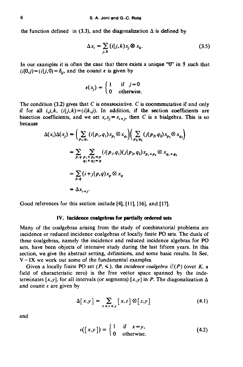
6
S. A. Joni and G.-C. Rota
the function defined in (3,3), and the diagonalization A is defined by
Ax,-2('U*)*>®**. (3.5)
M
In our examples it is often the case that there exists a unique "0" in 9 such that
(i\0j) = (i\j\0) = Sij9 and the counit e is given by
ix) = (1 if J = 0
J I 0 otherwise.
The condition (3.2) gives that C is coassociative. C is cocommutative if and only
if for all ij,ky (i\j\k) = (i\kj). In addition, if the section coefficients are
bisection coefficients, and we set *,-.X/"*,■+,-, then C is a bialgebra. This is so
because
A(*,)A(*,) » ( 2 (i|/».^.K®*„)( 2 U\p»qi)xp®x\
~ 2 2 {^Px^diAPi^x^^®x
P>4 Pl+P2~P
q\ + q2-q
= HlO+j\p><?)xp®xq
p*q
- *Xi+r
Good references for this section include [4], [11], [16], and [17].
IV. Incidence coalgebras for partially ordered sets
Many of the coalgebras arising from the study of combinatorial problems are
incidence or reduced incidence coalgebras of locally finite PO sets. The duals of
these coalgebras, namely the incidence and reduced incidence algebras for PO
sets, have been objects of intensive study during the last fifteen years. In this
section, we give the abstract setting, definitions, and some basic results. In Sec.
V-IX we work out some of the fundamental examples.
Given a locally finite PO set (Py <), the incidence coalgebra Q(P) (over K, a
field of characteristic zero) is the free vector space spanned by the inde-
terminates [x,y], for all intervals (or segments) [xty] in P. The diagonalization A
and counit e are given by
A[*>>>] = 2 [x,z]®[z,y] (4.1)
x <z <y
and
10 otherwise.

Coalgebras and Bialgebras in Combinatorics
Here, the section coefficients are
([x\>x2]\[y\>y2]>[*i>*2])= (0
if ^1=^1, x2= z2 andy2 = zv
otherwise.
It is immediate that Q(P) is coassociative. Moreover, it is cocommutative if and
only if the order relation is trivial, i.e., no two elements of P are comparable.
Note that e*(P) = Hom(G(P),K) is isomorphic to <*(/>), the incidence
algebra of />, since if/,g eg *(/>), then
f°g[x,y] = 2 f[x>*]g[z>y]
x <z <y
which is precisely the definition of f*g in §(P).
It is frequently the case in enumeration problems that the full incidence
coalgebra is not required; rather, we want to work with a smaller quotient
coalgebra of Q(P). These quotient coalgebras, called reduced incidence
coalgebras, are obtained by taking suitable equivalence relations on P.
Definition 4.1. An equivalence relation — on the segments of P is said to be
order compatible if the subspace spanned by the collection {[jc,.y] — [w»u]|[x,v]~
[u,v]} is a coideal.
Whenever ~~ is order compatible, the quotient space B(P)/~~ is isomorphic
to a quotient coalgebra of 6-(P) (see [27, p.22]). In general, there is no simple
criteria expressible in terms of the partial ordering to decide when an
equivalence relation on P is order-compatible. A useful sufficient condition due to
D.A. Smith [4, p. 276] is the following.
Proposition 4.1. An equivalence relation ~~ on the segments of P is order
compatible if whenever [x,y]~~[u,v\ there exists a bijection ¢, depending in general
on [x,y], of[x,y] onto [u,v] such that [xx,yx]~to(xx),4(yx)]for all x <xx <yx <y.
Note that the linear dual (Q(P)/~)* is isomorphic to the reduced incidence
algebra i(P)/~.
If ~~ is an order compatible equivalence relation on Pt we call the nonempty
equivalence classes of G(P)/~ types, and we think of Q(P)/~~ as the vector
space spanned by the variables jca associated to each type a. Each such reduced
incidence coalgebra gives rise to a collection of section coefficients (a|/?,v)>
where (a\P,y) counts the number of distinct z in any interval [x,y] of type a
such that [jc,z] is of type P and [z,y] is of type y, and the diagonalization in
Q(P)/~ is given by
**« - 2(«lfty)*jB®*r.
where the sum ranges over all ordered pairs of types /?, y.
The standard reduced incidence coalgebra is obtained from the equivalence
relation
[*,.y]~[m,u] if and only if [x,y] is isomorphic to [w,u].

8 S. A. Jonr and G.-C. Rota
One way of obtaining bialgebras of combinatorial interest is to form reduced
incidence coalgebras. We shall return several times to the question of when a
reduced incidence coalgebra is a bialgebra.
The following definition is motivated by the fact that the lattice of closed
ideals of an incidence algebra is distributive [4].
Definition 4.2. A combinatorial coalgebra is a coalgebra whose lattice of
subcoalgebras is distributive.
The characterization of all combinatorial coalgebras is an opening problem.
At present, we can prove
Theorem 4.1. Every (full) incidence coalgebra is a combinatorial coalgebra.
Proof: Let W be a subcoalgebra of G(P). If [xty] is in Wj then for all
x<w<z <y, [w,z] is in W. This is seen as follows: If x<z<y, then the term
[jc,z]<8[z,.y] occurs in A[jc,.y]. The occurrence of the segment [x,z] (and [zfy]) is
unique, and all segments are linearly independent. Thus, we must have [x,z] and
[z,y] in W. Since [jc,z]E W, the same argument applies and gives that for all
x<w<z <y, we must have [w,z] in W. Thus the collection of segments of W
forms an order ideal in the PO set of all segments of P, Seg(/>), ordered by
inclusion. Conversely, if J is an order ideal in Seg(/>)„ then AJ C/<8/, so that
the linear span of J forms a subcoalgebra of Q(P). Therefore, the lattice of
subcoalgebras of Q(P) is isomorphic to the lattice of order ideals of Seg(-P). A
well-known theorem of Birkhoff states that the lattice of order ideals of any PO
set is distributive, and our proof is complete.
V. Reduced Boolean coalgebras
The Boolean PO set (lattice) © consists of all finite sets of positive integers
ordered by inclusion. The minimum element of this lattice is the empty set. The
Boolean incidence coalgebra 6(¾) is spanned by all segments [A,B] with
A[A,B] = 2 [A9C]®[C,B].
AQCQB
1. Boolean coalgebras
The Boolean coalgebra © is the coalgebra spanned by all sets of (positive)
integers, with (for A Ec&)
AA = 2 AX®A2 (5.1)
AlnA2^0
Ax LMj — A
and
L 0 otherwise.

Coalgebras and Bialgebras in Combinatorics 9
Note that in (5.1)» AVA2 is an ordered pair. This coalgebra is isomorphic to the
reduced Boolean incidence coalgebra obtained by setting [A,B]~[C,D] if and
only if B — A = D — C. Thus, each set A represents the equivalence class of all
segments [B,C] such that C— B = A.
2. Binomial coalgebras
For each integer s>0, we define the binomial coalgebra Bs to be vector space
K[xvx2,...9xs] with
("I «,)<<»i «,) V
(5.2)
and
/ n, n\ f 1 if /t|= • • • =/i ,=0,
L 0 otherwise.
Each binomial coalgebra is seen to be the Boolean incidence coalgebra
modulo the coideal generated by a compatible — as follows: For s=l9 the
(univariate) binomial coalgebra Bx= K[x] is obtained by setting [A,B]~[C,D]
if and only if \B — A\ = \D — C\. This is the standard reduced incidence
coalgebra. Here the section coefficients are the binomial coefficients (,).
For j«2, we set [A,B]~[C,D] if and only if the numbers of even and odd
integers in B — A and D-C are equal. For general s, we set [A,B]~[C,D] if
and only if for all k = 1,2,..., sy
\{ieB-A\i~k mods}\ = \{jeD-C\j^k mods}\.
It is easy to verify that the binomial coalgebras are cocommutative bialgebras,
and in fact, Hopf. algebras with the antipode S given by S(xt) = - jc,. In addition,
the dual B* is isomorphic to the algebra of formal exponential power series in s
variables. A final heuristic remark: "2?^»©.
9»
3. Polynomial sequences of Boolean and binomial type
A polynomial sequence p„(x) is said to be of binomial type if
deg/?„(jc) = n for all /i, (5.3)
and
Pn{x+y)=*2(nk)pk{x)pn_k{y). (5.4)
*-0

10
S. A. Joni and G.-C. Rota
Let us rephrase (5.4) in the landuage of bialgebras. The polynomial ring
Ajjc,_y] is seen to be isomorphic to /C[jc]<8/£[jc] under the mapping jc^x<8 1 and
y\-+\<8jc. By linearity, for any polynomials q(x) and r(y), q(x)t-*q(x)®\ and
r(y)*-+\®r(x). Thus, (5.4) can be restated
n
A map /7 mapping the binomial coalgebra K[x] to itself is a coalgebra map if
A 0/7 = (/7(8/7)0 A. Thus, a polynomial sequence is of binomial type if and only if
it is the image of {jc"} under an invertible coalgebra map /7. This is seen as
follows. Let/7n(jc) denote the image of x" under/?. Since K[x] is a bialgebra, we
have
(Ac,)*" = Apm(x) = p„(Ax) = Pn(x® 1 + 10 x), (5.6)
and clearly
■
n
((/?<8/?)oA)*" = 2 (nk)Pk(x)®Pm-k(x). (5.7)
Therefore, if p is an invertible coalgebra map, deg p„(x) = n and (5.5) holds, and
conversely.
Multivariate polynomial sequences of binomial type, {/>„,...^0^-.. >■*,)}, are
similarly seen to correspond to invertible coalgebra maps of Bs to itself.
Examples of sequences of polynomials of binomial type include jc", (*)„ =
x(x- \)- • • (jc-/i+ 1), x(x — na)"~l, and the Laguerre, Gould, and exponential
polynomial sequences. The reader is referred to [3] and [5] for further examples,
and to [18] for their multivariate analogs.
A polynomial sequence indexed by the finite subsets of a set {pA(x)) is said
to be of Boolean type if
PA(*+y)= 2 PAt{x)pAl{y). (5.8)
Ax + Ai- A
or equivalently, if pA(x) is the image of A under a coalgebra map from <$> to
K[x]. [Usually, we require that deg /^00 = 1-^1.] Chromatic polynomials of
graphs provide combinatorially interesting examples of polynomials of Boolean
type. Given a graph G, the chromatic polynomial of G, 9Cc(jc), counts the
number of proper colorings (i.e. assignments of colors to the vertices of G so that
no edge connects two vertices of the same color) of G with x colors. Given a
subset H of the vertex set of G, we think of H as the full subgraph of G obtained
by restricting the vertex set of G to H, Similarly, we denote by G\H the graph
obtained by restricting the vertex set of G to G — H. Tutte, in [28], states
bXG(x +y) = 2 %H(x)%G,H(y). (5.9)
H

Coalgebras and Bialgebras in Combinatorics 11
This is not difficult to verify, since every proper coloring of G in x+y different
colors decomposes uniquely into the proper colorings of the subgraph H colored
with the jc colors and G\H colored with the>> colors, and conversely.
Polynomials of Boolean type were first studied by J. P. S. Kung and T. Zaslavsky.
4. Puzzles
Everyone is familiar with solitaire games where several flat pieces of wood or
cardboard are to be assembled into a required shape, for example, a square, as
in the following figure:
Little is known at present of the underlying mathematical theory that might
lead, for example, to an algorithm for verifying that an assigned shape can be
assembled out of a given set of pieces. We shall develop here the very first step
in such a program, namely, the precise definition of a puzzle as a very special
type of coalgebra. The definition of comultiplication is in fact a natural
rendering of the combinatorial operation of cutting up an object into a set of
pieces.
Before introducing the general definition, we shall describe the coalgebra
associated with the puzzles in the above picture. We shall develop the
construction in two steps. In the first step we define the placement coalgebra; in the
second step we decribe a quotient coalgebra of the placement coalgebra, modulo
a certain coideal. The quotient coalgebra will be called the puzzle or the piece
coalgebra, and we shall see that the difficulty of the puzzle is carried in the
structure of this coideal.
The pieces of the puzzle are
a hP 2 pieces
b EHD 3 pieces (5.10)
c Q 1 piece.
The board is the four-by-four square

12
S. A. Joni and G.-C Rota
on which pieces are to be placed. The squares are labeled by Cartesian
coordinates.
A placement of some of the pieces on the board is a subset of the board
obtained by placing some of the pieces on the board without overlapping. For
example the placement
(5.11)
is obtained by placing two pieces of shape ay a piece of shape 6, and a piece of
shape cy as indicated. In a placement, no more than the alloted number of pieces
is allowed.
Two placements covering the same squares by distinct sets of pieces, or by
pieces placed in different positions are considered to be different, for example,
•—•—*
•—•— —«
and
r~
J,-
•
—i
are distinct, as are
i—•
and
J
•>—
rf-
The pieces in a placement need not be adjacent. To every placement />,
specified by the occupied squares and the position of the pieces, we associate a
variable x(p% and we denote by V the free module over the integers spanned by
the variables x{p) and the variable 1, which denotes the trivial placement of no
pieces.
We now define a comultiplication on the module Vy as follows. Up and q are
placements, it is clear what is meant by saying that q is a subplacement of p. The
pieces used in q are a submultiset of the pieces in p, and they are placed in the

Coalgebras and Bialgebras in Combinatorics
13
same positions. For example,
r-
is a subplacement of the placement given in (5.11), whereas
Ft
.L
is not a subplacement. Thus, there is a partial ordering of placements, and we
denote this PO set by P. P has a unique minimal element, the empty placement,
but in general it has no maximal element. Furthermore, for any placement /?,
the segment {q\q<p} is a Boolean algebra; therefore, the PO set P is a simplicial
complex. We are now ready to define the placement coalgebra. For any
placement/?, list all ordered pairs (q.r) such that
q and r are subplacements of/?,
q and r do not overlap,
the union of q and r is the placement/?.
Now set
(5.12a)
(5,12b)
(5,12c)
M/0-2*(*)®*00
(5.13)
where the sum ranges over all such pairs. For example, if/? is the placement
hT--±
(5.14)
and jcj,jc2,...,jc6 are the placements shown in Fig, 1, then
Ajc(/?) = 1 <8 x(p) + xx <8> jc6 + x2 <8 jc4 + jc3 <8 jc5 + jc4 <8 jc2 + jc5 <8 jc3
+ X6®X! + x(/0® 1.

14
S. A. Joni and G.-C. Rota
*
mm
x,
x*
X -1 +
2* ^ It*
: :_±_
4- *-"
T-,
t:
= *
•■-«--•
Figure 1.
It is intuitively clear that the comultiplication just defined is coassociative, in
fact, it follows from the coassociativity of the Boolean coalgebra. The counit e is
defined by
£(1) = 1 and e(x(p)) = 0 for all x(p) * 1.
(5.15)
We now come to the definition of a puzzle, at least in the special case we are
considering. To this end, we begin by defining an equivalence relation on
placements. We shall say that/?—q when:
p and q are obtained by placing,
possibly in different positions, the same pieces
with the same multiplicity,
(5.16a)
and
the placement q can be obtained from the placement/?
by rigidly sliding and rotating (and possibly turning over,
depending on the rules of the game) placement/?.
(5.16b)
For example, any two placements of single pieces of the same shape are
equivalent. As another example,
•— —♦—(—•
^^H ^^H MM
t
• 4
■■ I 1 I ii
and
+
•
' ■
i
are equivalent.

Coalgebras and Bialgebras in Combinatorics 15
It is immediate that the relation ~~ is an equivalence. An equivalence class
will be called a shape. The equivalence classes corresponding to placements of a
single piece will be called, appropriately enough, pieces.
The most important remark is that the submodule C of V generated by all
elements
x(p)-*(<?)>
where p—q, is a coideal. Again, this is intuitively clear, but we shall verify it in
detail. We have
**(/>) = 2 *(/>!,) ®*(/>2,)
and
and it follows from the definition of equivalence that the families {(pu*p2i)} and
{(awa2i)} °f ordered pairs can be put into one-to-one correspondence in such a
way that the entries are respectively equivalent. We can therefore write
x(pu) ® x(p2i) - x(qu) ® x(q2l)
= [x(pu)-x(qu)]®x(p2i) + x(qu)®[x(p2i)-x(q2i)].
Thus, if /?—<7, then
Mx(p)-x(q)) = 2[x(pu)-x(qu)]®x(p2i)
i
+ x(qu)9[x(p2i)-x(g2i)].
In other words, this shows that AC C C<8 V+ V<&C, and thus proves that C is a
coideal (see [27, p. 18]). We can therefore take the quotient coalgebra V/C. This
coalgebra generated by shapes is called a puzzle. If p is the placement given in
(5.14), then in the puzzle (or quotient coalgebra) we have jc,—jc2 and x4~x6.
Thus (if we represent each equivalence class by its placement of smallest index)
in the puzzle
Ax(p) = 1<8jc(/?) + 2(jc,<8jc4) + jc3<8jc5 + jc5® jc3 + 2(jc4<8jc,) + jc(/?)<8 1,
From the preceding example it is now easy to extract the general definition of
a puzzle. One begins with a finite simplicial complex /\ and one associates to P
a placement coalgebra in the same way as we have done above: to every/? in P,
one associates the set of ordered pairs (q,r) such that q\Jr=p and q/\r = 0.

16
S. A. Joni and G.-C. Rota
From this, one obtains the definition of the placement coalgebra in exactly the
same way. A puzzle is now generally defined as the quotient of the placement
coalgebra by a coideal defined by an equivalence relation among the elements of
The basic problem about puzzles is to determine how many distinct shapes
cover the entire board. At present, too little is known about the structures of
puzzles to even hazard a conjecture on how one might approach the problem.
VI. Divided powers coalgebra
Let N denote the lattice of nonnegative integers under natural ordering. The
incidence coalgebra Q(N) is spanned by all segments [ij] with
H*J]= 2 [i.k]®[kj].
i<k<j
The divided powers coalgebra *D is the vector space K[x] with
n
Ajc" = 2 xk®xn~k
k*Q
and
It is the standard reduced incidence coalgebra of G(N), and its dual 6D* is
isomorphic to the algebra of formal power series k[[x]] (with the usual
multiplication). Multivariate divided powers coalgebras are similarly defined to be the
standard reduced incidence coalgebra of
G(NS) = G(Nx--- xN).
v ->
s times
VII. Dirichlet coalgebra
Let Z + denote the lattice of positive integers ordered by divisibility, i.e., m <n if
and only if m divides /i. The 0 of this lattice is 1. The equivalence relation on the
segments of Q(Z +) which gives the Dirichlet coalgebra is [ij]~[k,l] if and only
if j/i = l/k. Alternatively, the Dirichlet coalgebra D is the vector space spanned
by the variables {/ix:/i = 0,1,2,...}, with
A(/ix)= 2 Px®qx
and

Coalgebras and Bialgebras in Combinatorics 17
D has a natural algebra structure given by nxmx = {nm)x. While D is not a
bialgebra, the comultiplication is an algebra map when n and m are coprime,
that is,
A(nxmx) = A(nx)A(mx)
whenever the gcd of n and m equals 1.
The linear dual D* is isomorphic to the algebra of formal Dirichlet series, the
isomorphism being given by
w) = 2^-
Multivariate Dirichlet coalgebras are obtained from the same equivalence
relation on the incidence coalgebra (?(Z + X • • ■ X Z +).
The standard reduced incidence coalgebra is a subcoalgebra of the Dirichlet
coalgebra. Let [ij] and [kj] be two segments, and let
j/i «/?;*'.•• />/' and l/k = qf»• • * qf-
be their respective prime factorizations. The segments [ij] and [kj] are
isomorphic if and only if j=r, and as multisets, the collections {a,} and {/?■} are the
same. In other words, given /i, let shape(/i) = (A,,A2,...) where Xk is the number
of distinct primes in the factorization of n which occur precisely k times. Then
[ij]~~[kj] if and only if shape(y//) = shape(//&),
VIII. Eulerian coalgebra
Let V denote the lattice of all finite-dimensional subspaces of a vector space of
countable dimension over GF {q\ ordered by inclusion. The minimal element of
V is the trivial subspace. The standard reduced incidence coalgebra of 6(V) is
obtained by setting
[X*Y]~~[S*T] ifandonlyif dimY_dimx = dimT■dims-
The section coefficients count the number of subspaces of dimension k
contained in a subspace of dimension /i, which is given by the Gaussian coefficient
n
k
(\-q)(\-q2)--(\-qn)
If we set [n]q\ =(1 - q)(\ - q2)- --(1- q"), then

18
S. A. Joni and G.-C. Rota
The Eulerian coalgebra E is the vector space K[x\ with
A-0L J<?
n
n-k
xk ® JC
and
e(xn) = 80tm.
It is cocommutative, and E* is isomorphic to the algebra of formal Eulerian
power series, the isomorphism being given by
/~*.>-2&V
IX. The Faa di Bruno bialgebra
The Faa di Bruno coalgebra V? is the standard reduced incidence coalgebra for
the full lattice of partitions, II. As such, it bears the same relationship to the
lattice of partitions as does the binomial coalgebra to the lattice of subsets and
the Eulerian coalgebra to the lattice of subspaces of a vector space over a finite
field. In this section we shall show that this coalgebra is a bialgebra. (The proof
is due to Doubilet [11].) Moreover, this bialgebra serves as a blueprint for the
formulation and understanding of the general class of hereditary bialgebras
presented in Sec. XV11.
The full lattice of partitions, II, is the lattice of all set partitions of Z*
(positive integers) having exactly one infinite block and finitely many finite
blocks, ordered by refinement (see Sec. 11).
Every segment [o,t] of n is isomorphic to I1A' x 11A>X • • • X n£* ■ •, where IIn
is the lattice of partitions of an /i-set, and \k equals the number of blocks of r
which consist of k blocks of o. (This isomorphism can be seen by thinking of the
/th block of a as the "element" B^ and [o,t] as a partition on the collection of
2?/s, with a as the finest partition.) To each segment [o,t] of n, we associate the
sequence A = (l, 1,..., 1,2,...,2—) of A, ones, A2 twos,...,sometimes written
A = (lAl2Al- ■ ■) or equivalently, jca'jcAj... =x\ A, or x\ is the type of [o,t], and
clearly [aj.rj is isomorphic to [o2>T2l tf an^ on'y tf they have the same type. The
type A = (l°2°- •• n] ...)= xn is often written as n. We shall use the symbols
a,/?,A,p,/x to denote types.
q count the number of partitions ir contained in
[0,(1,2,...,/i)] = nn such that [0,tt] is of type a and [tt,(1,2,...,/i)] is of type (3.
Note that if a — xflx£2- - * jc„rt\ we must have a, +2a2+ ... +/ia„ = n and (3 =
xa +a +...+a ■ These section coefficients, known as the Faa di Bruno coefficients,
are given explicitly by
The section coefficients
n
n\
a1!a2!...an!(l!)("(2!r...(/i!r
(9.1)

Coalgebras and Bialgebras in Combinatorics
19
The explicit coalgebra structure of 5" is as follows. As a vector space, 5" is
isomorphic to K[xl9x2,...] = K[x], The diagonalization A and counit e are given
by
Ax* = 2
«,/? L
X
«,/8
[a<8x/»
(9.2)
and
<«*) = {
_ / 1 if A = (0,0,0,...) or (1,0,0,...)
0 otherwise.
(9.3)
If o<ir and 5 is a block of tt, then by on 5 we mean the partition of B
consisting of the blocks of o contained in B, Let [o,t] be of type xmx„> i.e., r has
two blocks B and B\ where B contains m blocks of o, and B' contains /i.
Suppose 7T is such that o<tt<t, [or\B9irr\B] is of type jc,a,jc"2,,.., and [on
/ /
5',7rn B'] is of type jcf'xf2- • •. Then clearly [o,ir] is of type jcj*, + a'jc£2+a2- • * =
xaxfl'. Similarly, if [irnB^nB] is of type x^ and [TTC\B\mBf] is of type xfi\
then [7t,t] is of type x^x^'. Thus, for all /n,/i,p,/x,
XmXn
U,/I
s
'm
«,/8
«',/5'
(9.4)
where addition of sequences is defined by (la,2a2 •
(l«.+*i2"« + fc...), i.e. xV = xa + ^. It follows that
x"®xM in A(xjA(xm). This is equivalent to
*mXn
• • ) + (1^...) =
is the coefficient of
s
v.fx L
x^x^-fSf^W^lfS
a.0 L
a,0
a.,3 L
a,)5
xa®x'|. (9.5)
More generally,
But this is just
X^X22'"
is the coefficient of x"®x" in A(x,)AlA(x2)A2- • •.
4(^--) = ^,)^(^
(9,6)
In addition, it is clear from (9.3) that
e(x^...) = e(X])\(x2P
Hence, we have shown
Theorem 9.1. ^ is a bialgebra under ordinary multiplication and the coalgebra
structure obtained from the standard reduced incidence coalgebra of £(ri).

20 S. A, Joni and G.-C. Rota
Note that F is non-cocommutative. By Theorem 9.1, the space of all /f-liner
maps from 5" to itself, Hom^.f), is an algebra with multiplication (or
convolution) ♦ defined by
X
/<x")g(x'). (9.7)
A function/ in Hom((?F, *?) is said to be multiplicative if and only if for all A,
f(x^*-x^...)=f(xl)x\..f(xn)x».... Any such function is determined by the
values it takes on the segments n„. Let 911 (V7) denote the class of multiplicative
functions. The following elementary result is fundamental [4],
Proposition 9,1, The convolution of two multiplicative functions is
multiplicative.
Thus, 911(^) is a subsemigroup of the multiplicative semigroup Hom(Sr,Sr).
If/e9H(S), let /(/i) denote/(TTJ, that is,/([o,r]) for all [o,t] of type n. For
/,ge9H(5), we get from (9,1) and (9.7) that
,.&)- y ■!«■>•'■■•/<■■>■*«■+-+«■>, (,.8)
Theorem 9,2 (Doubilet, Rota, Stanley). The semigroup 911(^) is anti-isomor-
phic to the algebra of all formal power series with zero constant term over K[\] in
the variable u under the operation of functional composition. The anti- isomorphism
is given by f\-*f{u), where
CO
rt-1
/(-)-2^--- (9.9)
Proof: Clearly the map defined by (9.9) is a bijection, so we need only check
that multiplication is preserved. Now
The coefficient of u" in the expansion of
c-l
v\
IS
y /(»,)■ ■/("k) _ y k\ /(l)"1.../(/I)""
I
Vt>\

Coaigebras and Bialgebras In Combinatorics 21
where the summation is taken over a,+2a2+ ... +nan = n and ax+ ... +an=*k9
since there are k\/ax\...an\ ways of ordering the partition ax+2a2+ ... + nan =
n. When we multiply (9,11) by g{k)/k\ and sum over all k> we obtain (9.8), and
the proof follows.
?F is not a Hopf algebra, since ti{xx)^xx®xv It can be realized as a Hopf
algebra in A"[x] localized at jc,, with
te)-
— ® —
x, X]
A proof of the existence of the antipode is given by demonstrating that a certain
recursion can be carried out. An explicit formula can be obtained using the
Lagrange inversion theorem [19].
In K[\] localized at ^,,911(5) is anti-isomorphic to the group of all invertible
(under functional composition) formal power series. The inverse of any function
can be obtained by composition of this function with the antipode S. For a
more detailed discussion of the Hopf-algebra aspects of ?F, we refer the reader to
[11], [19].
X. Incidence coaigebras for categories
Certain enumeration problems (see [4, p, 283]) lead to counting over structures
more complicated than a single PO set. The concept of a Mobius category [21],
gives one such structure. To extend the notion of incidence and reduced
incidence coaigebras for PO sets to these situations, we are led to define
incidence coaigebras for categories,
A locally finite category is a category in which for each morphism /, the
collection of pairs of morphisms ((/1,/2):/^/2==/} is finite,
Given a locally finite category A/, the incidence coalgebra Q(M) is the free
vector space over K spanned by the indeterminates /, where / is a morphism of
M with coalgebra structure given by
4/-2 /,®/2. (10.1)
and
£(f\ = I l if /= idP for some object p in A/,
10 otherwise.
Let — denote an equivalence relation on the morphisms of A/, The subspace
generated by ~ is the subspace of Q(M) spanned by the collection {/— g: f~~g\.
We say — is compatible if the subspace generated by — is a coideaL A reduced
incidence coalgebra Q(M)/— is the quotient coalgebra of Q{M) modulo the
coideal generated by a compatible ~ relation.

22
S. A. Joni and G.-C. Rota
Given two morphisms /,g in A/, we say that g divides f if there exists
morphisms hfk in A/ such that f=h°g°k. Let [/] denote the subcategory
generated by {g\g divides /}. The standard reduced incidence coalgebra is
obtained via the following equivalence on the morphisms: We set /~g if and
only if [/] is isomorphic (as a subcategory) to [g]. Clearly the subspace
generated by this equivalence relation is a coideal.
The range of meaningful reduced incidence coalgebras for categories is much
larger than those of PO sets. For example, the inner reduced incidence coalgebra
arises by setting f~~g if and only if there exists an invertible morphism h in M
such that [/]— h°[g)°h~\ and the strongly reduced incidence coalgebra arises
by setting f~g if and only if there exists a category isomorphism <p: [/]-*[g]
such that <p(f) = g-
Example 10.1: Every locally finite PO set P can be viewed as a locally finite
category as follows: the objects of M are the elements (or vertices) of /\ and
there is a unique morphism fXiyx-*y if and only if x<y. Clearly, if jc <z <y>
then fXiZ°fZty=fXty and [fxy] corresponds to the interval [xyy\. There are no
invertible morphisms (other than the trivial ones, i.e. /x x), so that in this case,
the inner reduced incidence coalgebra is the full incidence coalgebra. Moreover,
in this case the standard reduced and strongly reduced incidence coalgebra are
isomorphic.
Example 10,2: Every finite group G can be viewed as a locally finite category.
The category has only one object, and each morphism fg corresponds to an
element of G. Composition of morphisms is given by/. °L =L v , and if e is the
identity element of GJe is the identity morphism. In contrast to the case of PO
sets, the standard reduced incidence coalgebra for this category is isomorphic to
the trivial category (consisting of one object and one morphism), whereas the
inner reduced incidence coalgebra is isomorphic to the category of conjugacy
classes of G. Indeed, in the inner reduced coalgebra, we have/~g if and only if
there exists an h such that /= hgh " \ that is, / is conjugate to g. Let J denote the
subspace generated by ~, If /—g, then to each pair (/,,/2) such that /, /2 =/
there correspond a unique pair (g]yg2) such that g}g2 = g and /^g,. The
correspondence is given explicitly by g,- = A-l/-A. Therefore
a(/- g) = 2/,, ®/2l. - 2 h ~ %h ® h - %h
= 2 [Uu-h-%h)®h, + h-%h®{f2i-h-%ih)}
i
Hence J is a coideal and 6(M)/~ is isomorphic to the category of conjugacy
classes of G, as asserted. In the strongly reduced incidence category we have
/~~g if and only if there exists a group automorphism <p such that <f(f) = g.
As we have seen in Sec. IV (Theorem 4.1), the lattice of subcoalgebras of the
incidence coalgebra for PO sets is distributive. This is also trivially true for the
lattice of subcoalgebras of the incidence coalgebra for a group G, because there

Coalgebras and Bialgebras in Combinatorics 23
are no proper subcoalgebras. It is, however, in general false. For example, let M
be the category
when? ia of. =j} and f. ° ib =fjj =1,2. The lattice of subcoalgebras of this category
is noi a distributive lattice. This is easily seen as follows: Let L(A) denote the
linea. span of A, and set M} = L(iaJb); M2= L(fuia,ib); M3 = L(f2ja,ib); M4 =
L(, ] +f2>iaJb)' Then each A/,, is a subcoalgebra of G(M)> and
M2A(M3VM4) = A/2>
whereas
(M2AM,)V(M2/\M4) = M}
In fact, the segment [MVQ(M)) is isomorphic to the lattice of subspaces of a
two-dimensional vector space over Ky and it is well known that this lattice is not
distributive.
XL The umbral calculus
The binomial bialgebra has been studied in great detail, in particular with regard
to applications to combinatorics, in a series of papers beginning with Mullin and
Rota [2], followed by Kahaner, Odlyzko, and Rota [3] and finally Roman and
Rota [5]. Elegant expositions of the results of Mullin and Rota were given by
Aigner [6], Garsia [14], Liu [22], and several others. We shall summarize the
main lines of this theory, keeping in mind that these results should act as
blueprints for yet to be carried out generalizations to the more complex
bialgebras and coalgebras arising in combinatorics, some of which are described
in the rest of the present paper.
The comultiplication
Ax"-2(2)**®x-\ (lllI>-
k
on the algebra of polynomials p(x) of one variable, defines a bialgebra structure.
The dual algebra on linear functions L—where we denote by <L|/?(jc)> the
action of the linear functional L on the polynomial p(x)—is seen to be
<Z.,Z.2|*"> = 2(£)<^l*A><^|*"-*>- (11.2)

** S- A. Joni and G.-C. Rota
The dual algebra, with the augmentation e acting as the identity, has been called
the umbral algebra by Roman and Rota. The umbral algebra is isomorphic to
the algebra of formal power series under the map
even in a topological sense. The formal power series thus associated to a linear
functional is said to be its indicator.
The algebra of shift-invariant operators on polynomials is the algebra of all
linear operators T mapping polynomials into polynomials, such that TEa = EaTy
where Ea is the shift operator mappingp(x)-*p(x + a)> for all a. It turns out that
the umbral algebra is also isomorphic to the algebra of shift invariant operators
under the map sending the linear functional L to the operator Q given by
e*"= 2(*)ai**>*"-A-
A coalgebra isomorphism t/, that is, a one-to-one onto linear operator on
polynomials such that
At/jc" = 2(2)^*® Ux"~k 01-4)
k
has been called an umbral operator by Mullin and Rota. The adjoint of an
umbral operator is an isomorphism of the umbral algebra, and conversely, with
due respect to topology. The sequence p„(x)= t/jc", where V is an umbral
operator, is said to be of binomial type, and is characterized by the identity
k
Sequences of binomial type are of frequent occurrence in combinatorics, and
have motivated much of the work on the umbral calculus. For example the
sequences (jc)„ = jc(jc- 1)- * • (jc-/i + 1), x(x-na)"~\ and the Laguerre
polynomials are of binomial type.
A delta functional L is a linear functional such that <L|1 > =0 and <L|jc> ^0.
To every delta functional one can associate two polynomial sequences of
binomial type: the associated sequence p„(x) uniquely defined by the biortho-
gonality requirements
<Lk\p„(x)> - n\8k.m, (11.6)
and the conjugate sequence q„(x), defined by

Coalgebras and Bialgebras in Combinatorics
Conversely, every sequence of binomial type, pn(x)y is the associated sequence
and the conjugate sequence of unique delta functional, say L and L, which are
said to be reciprocal.
A shift-invariant operator Q associated to a delta functional L is said to be a
delta operator. If p„(x) is the associated sequence of the linear functional Ly then
the identity Qp„(x)=np„_l(x) shows that the sequence p„(x) is related to the
delta operator Q in a manner analogous to D and jc". This leads to the
generalization to delta operators of several classical formulas of the calculus; as
the simplest example, Taylor's formula generalizes to
For example, for the sequence pn(x) = (x)nt the delta operator Q is the difference
operator A defined by A/?(jc)=/?(jc+ I)—/?(jc). Every delta operator Q equals the
product DP, where Dp(x)=p'(x) is the ordinary derivative, and the inverse
operator P ~] exists. The operator P is called the transfer operator of the
sequence pn(x). We come now to the first basic fact of the umbral calculus,
which is the transfer formula:
Pm(x)~xP-"x*-\ (11.9)
where P is the transfer operator of the sequence of binomial type p„(x). This
formula is closely related to the Lagrange inversion formula for formal power
series (15).
To introduce the next basic fact, we consider the operator x mapping p(x) to
xp(x). The operator Q'^Qx — xQ is called the Pincherle derivative of the
operator Q, and is also shift-invariant if Q is. Now, if Q is the delta operator of
the sequence p„(x)t then the recurrence formula
pn(x) = x(QT1p„-i(x) (11.10)
gives another way of explicitly computing a sequence of binomial type.
We now come to the fundamental fact of the umbral calculus. If p„(x) is a
sequence of binomial type, then its generating function is of the form
2^/"-exp[*(a,/+5p+ )j-e*«> (11.11)
for some formal power series/(/) such that a0 = 0 and ax^0y (a delta series, for
short) and conversely. If p„(x) is the associated sequence for the delta functional
L with indicator g(/), then the series /(/) and g(t) are inverse in the sense of
functional composition, that is, /(g(/))a»g(/(/))= /. Furthermore, if pn(x) is the
conjugate sequence of the delta functional L, then/(/) is the indicator of L.
Functional composition is also related to umbral operators. It turns out that
every umbral operator U is uniquely related to a delta series «(/), and if L has

26
S A. Joni and G.-C. Rota
indicator /(/), then the linear functional U*(L) has the indicator /(«(/)); the
converse is also true.
The coalgebraic statement of this fact leads to the interpretation and rigoriza-
tion of the classical technique of treating indices as exponents, from which the
umbral calculus derives its name. If p„(x) = 1tkan kxk and qk(x) are sequences of
polynomials of binomial type, then the polynomial sequence
r„(x) = 2 «„,*<?*(*) =/>„(q(*)) (11.12)
k
is called the umbral composition of the sequences p„(x) and q„(x). It turns out
that the sequence rn(x) is also of binomial type; furthermore, if the indicators of
the delta functionals L and M with respect to which p„(x) and g„(x) are the
associated sequences are, respectively, /(/) and g(/), then the corresponding
indicator of the sequence r„(x) is the functional composition/(g(/)).
Among many other facts of the umbral calculus which cannot be mentioned
here—but some of which will be found in the memoir of Roman and Rota—we
mention the extension of the preceding results to other module actions of the
umbral algebra; in fact, it would be of the utmost interest to classify all such
module actions. For example, a natural action is defined on the ring of inverse
formal power series
/(» = 2^
by sending /~" to (/ +a)"", thus defining the operator £a, and then taking a
suitable closure. In this way, one can define "inverse" analogs of all sequences
of binomial type; for example,
v '"" (x+l)(x + 2)-.-(x + n)'
leading to a generalization of the classical theory of factorial series.
XII. Infinitesimal coalgebras; the Newtonian coalgebra
Recall that a bialgebra A is a vector space which is simultaneously an algebra
and a coalgebra such that the comultiplication A is an "endomorphism" of A (as
an algebra). The analogy between endomorphisms and derivations leads us to
define an infinitesimal coalgebra A to be a vector space which is simultaneously
an algebra and a coalgebra (possibly without a counit) such that the
comultiplication A is a derivation of A in the sense that forp7q in A,
A(pq) = (Ap)(q®\) + (\®p)(Aq). (12.1)

Coalgebras and Bialgebras in Combinatorics 27
In this section we shall present only one infinitesimal coalgebra, the Newtonian
coalgebra. The study of this coalgebra should provide a prototype for the
general study of infinitesimal coalgebras.
Let us recall the definition of the Newton divided differences. The Oth
divided difference is
[/:¾] =/(*o).
The first divided difference is
r/.r x I _/(*o)-/(*i)
x0 xx
the second
r, -, _ [/:*q,*i]-[/;*i,*2]
[J-xo>x\>x2] — v - v *
x0 x2
and the *th divided difference [/; jc0,...,jca] is obtained by iteration.
A polynomial sequence {p„(x)} [with p0(x)= 1] is said to be of Newtonian
type if
—— 2- aW^-a-iOO- (12.2)
* y k-o
Two examples of such sequences are {jc"}, and {(x-ra)"} for any a. There are
two coalgebras within which we can study these polynomial sequences. As
vector spaces and as algebras, both are isomorphic to K[x]. The first coalgebra
we shall consider is the Newtonian coalgebra, denoted N* The comultiplication in
TV is
w-;W:^ (12.3)
x y
and is easily checked to be coassociative. There is no counit in N* Moreover, it is
immediate to verify that
A(/7<7) = A/? (<7<81) + (1 ®p)Aqt
so that N is an infinitesimal coalgebra. The kth divided difference [p-x0t...txk]
-A^(x). This coalgebra setting gives an elegant proof of Newton's formula,
namely
oo
/(*)•■ 2 (x-x0)---(x-xk)[f:x09...9xk].
k-0

28 S A. Joni and G.-C. Rota
In the dual algebra, the following striking relationship between divided
differences and ordinary differentiation is seen. Let us set, for all /?,
<e,l/(*)> =/(/>)
Then
<WAX)> p-q ■
and
<&/(*)>=rip).
An extensive study of the theory within this setting has been pursued by S.
Roman [25].
A different approach was taken by Garsia and Joni. Using the umbral
machinery with the "differentiation" operator A defined by
Axn = x»-\
and the "multiplication" operator B defined by
„n+i
Bxn*
/i+l '
they define a polynomial sequence {q„(x)} (<70(jc)^ 1] to be of Newjonian type if
xqn{x)-ygn(y) A
—— = 2- *(*)«.-*(j0- (12.4)
x y *-o
Note that <?n(0)m0 for all n> 1. Examples of such sequences are {jc"}, {jc(jc +
Here, the underlying coalgebra structure is given by
Ap{x) = Mx)-yp(y)
x—y
and
e(x")= M> n7°> .
{0 otherwise
(that is, e is evaluation at zero).

Coalgebras and Bialgebras in Combinatorics 29
In this setting, all of the results within the umbral calculus, appropriately
modified (see [13]) for the "differentiation" A and "multiplication" B, apply. For
example it is not difficult to show that {q„(x)} is of Newjonian type if and only
if
where/(w) is an, invertible (under functional composition) formal power series.
It turns out that polynomial sequences of Newtonian and Newjonian type are
essentially the same class of polynomial sequences. Indeed, we have
Theorem 12.1. A polynomial sequence {p„(x)} is of Newtonian type if and only
if the polynomial sequence {q„(x)} defined by
, v / 1, /1 = 0,
g"{X)~[xpm-i(x)9 n>\
is of Newjonian type.
The Newjonian coalgebra setting provided the machinery for the explicit
computation of the "Newtonian analogs" of many of the classical polynomial
sequences (e.g. Laguerre, Abel, exponential, Gould, etc.).
XIII. Creation and annihilation operators
The creation and annihilation operators we present here generalize those of
quantum field theory.
Let {(i\j\k)} be a collection of section coefficients satisfying the extra
condition that for each ordered pair (/»*)» the set {i'(i\j,k)^=0} is finite, and let
C be the coalgebra defined by these section coefficients and a given counit e (see
Sec. III). Creation and annihilation operators are linear maps from C to itself
defined as follows:
for each y G 5, the creation operator Kj is
V*-2('U*)*, (13.1)
and the annihilation operator Aj is
AjXk = ^{k\j,i)x, (13.2)
If the section coefficients are all equal to zero or one, and if, in addition, for
each/,* there is at most one / such that (i\j\k)= 1, then the creation operator Kj
acting on jc* gives the "piece" i obtained by piecing k and/ together if it exists,

30
S. A. Joni and G.-C. Rota
and zero otherwise. Similarly, the annihilation operator Aj acting on xk gives the
piece i which when added to the piece7 is the piece k, if such a piece exists, and
zero otherwise.
For example, let us look at the situation when C is an incidence coalgebra for
a PO set. An easy computation gives
A[*AU>V]
[y,v] if jc*= u and x<y <v7
10, otherwise.
Similarly
Ki*Au*v] =
' [x9v] if y=uy
. 0 otherwise.
In a puzzle, KjXk gives a list (with multiplicities) of all possible jc, obtainable by
piecing together Xj and jc*. Similarly, AjXk gives a list (with multiplicities) of all
possible pieces jc, such that jc, and Xj can be pieced together to form jc*.
Straightforward computations give
KPAjxk = Z(*Lm)(?I/m'K,
and
AjKpxk = 2 0\p>k)(i\j9q)xr
If the section coefficients are bisection coefficients, then C is a bialgebra, and in
addition,
Akxi+J ~ 2j (^p^iK^Pt^)*
Proposition 13.1. If § is a commutative semigroup {written additively), then
KjK/ = K/Kj ™ ^-+/ ana* AjAt = AfAj = Aj+t
if and only if for allj,kj,q
^(k\j,p)(p\l,q) = '2(k\l,p)(p\j,q)
P P
= {k\j+l,q\ (13.3)

Coalgebras and Bialgebras in Combinatorics 31
Proof:
K&x,- Kjfap\hq)x^
^(P\l,q)(k\hp)xk
and
k
Therefore, KjK{= KJ+/ if and only if
{k\j+l,q) = ^(p\hq)(k\jyp).
p
The same argument using K,Kj completes the proof for creation operators, and
the analogous argument holds for annihilation operators.
The coalgebra C, considered as a vector space, has a natural inner product:
Theorem 13.1. The bilinear form
<*/l*y>c = 2('U<7)*K)
on C is symmetric and nondegenerate.
Proof; Since e is the counit of C, we have
xt = 2 OU ?)«(*,)*;• (13.4)
M
Equating coefficients of the jc's on both sides gives
<*i\xj>c " SOIMW**) = V
Theorem 13.2. Relative to the symmetric form < , >c, Aj and Kj are adjoint
operators.
Proof: We show that
<Ai*j\xk>c = <Xj\Ki*k>c
for all ij\k. Expanding the left side gives
<AiXj\xk}c = 2 U\hp)<xp>Xk>c " (-/!'.*)
7»'

32 S. A. Joni and G.-C. Rota
since (x ,xk}c=8 k. Similarly, the right-hand side gives
<Xj\K*k>c - 20>l'>*)<*^> = 01'.*).
as desired.
In the following examples we see how creation and annihilation operators cut
up and piece together sets and partitions.
Example 13.1: For the binomial coalgebra, the creation and annihilation
operators are easily seen to be
**-m
Xk+J
and
[ 0 otherwise.
Example 13.2: Let X and Y be subsets. The creation and annihilation
operators for the Boolean coalgebra are
K Y= iXuY if *n Y = 0>
x 10 otherwise
and
A Y= ( Y~X if X(^Y>
x I 0 otherwise.
Example 13.3: The creation and annihilation operators for the Faa di Bruno
coalgebra are a bit more complicated than those of the previous two examples.
Let a, /?, and X denote types of partitions. The creation operators Ka are, by
definition,
x
Since (X|o,£)^0 only if )8,+2)82+...+/1)8,, = 0, + 02+...+0,,, A,+2A2
+ ...+/i\,«a, + 2a2+...+/10,,, and X, + X2+ ...+\, = 0i+ & + ... + /*„, the
types xx occurring in Kaxfi [with multiplicites (X\a,j3)] are seen to be the types
obtainable by merging, in all possible ways, the blocks of a partition of type a so
that the resulting partition has the same number of blocks as /?. The
multiplicities count the number of ways in which a given type can occur.

Coalgebras and Bialgebras in Combinatorics 33
The annihilation operators AQ are
A
so here we must have ax + 2a2 +...+ na„ = fix + 2/?2 +...+ nfin, \x + 2A2
+ ... +/1^,^0,+ ... +a„, and X, + X2 + ... +\, = j3| + j32+ ••• + A, for the "type
xx to occur in Aaxfi. Thus we obtain a list of all the types of partitions (with
appropriate multiplicities) of a set of size a{ + ... +an with the same number of
blocks as ft.
XIV. Point-lattice coalgebras
Let £ be a finite point lattice, that is, a lattice in which every element is the
supremum of a set of atoms. It is well known and easily proved that £ is
isomorphic to the lattice of closed sets relative to the closure operation defined
on subsets of the set & of atoms by
J« {pE&\p<supA} for A C &.
The closure operation enjoys the properties
A QAy (14.1a)
J=/f, (14.1b)
if A C 5, then ACB (14.1c)
(but not, in general A U 5 = AuB). The complements of closed sets, called open
sets, can be characterized even more simply by
(1) the union of any family of open sets is an open set,
(2) every open set is the union of the minimal nonempty open sets it
contains.
Thus, every point lattice can be represented as the family of all open sets in a
closure relation where the join in the lattice is set-theoretic union. In the
following we shall assume that £ is so represented by a fixed set &. We shall
further assume that £ has a unique minimal element, which is represented by
the empty set. This representation of £ allows us to define a very interesting
coalgebra structure on ¢. As a vector space, this coalgebra Q (£) is isomorphic
to the free vector space over K with basis consisting of all open sets of ¢. For
each open set A cff, the diagonalization is
LA - 2 AX®A2, (14.3)
A i, A2 open
AtnA2-0
AtUA2-A

34
S. A. Joni and G.-C. Rota
and the counit is
e(A)=H *UA=0 (14.4)
v ' 10 otherwise. v '
Since the union of open sets is again an open set, it follows immediately that-the
above diagonalization (14.3) is coassociative. Since point lattices occur in many
combinatorial investigations, the study of this class of coalgebras should prove
very interesting. We give three examples of point-lattice coalgebras.
Example 14.1 (The Boolean coalgebra): Finite-dimensional Boolean
coalgebras arise from the point lattice of subsets of {1,2,...,n). This lattice can
be represented as follows: the minimal nonempty open sets are the sets
consisting of one element, i.e., the sets {_/}, for 1 <j<n. Thus, every subset is an open
set. Hence, for each A>
LA= 2 AV®A2,
AlnA2 = 0
A tuA2~A
so that these coalgebras are isomorphic to subcoalgebras of the Boolean
coalgebra defined in Sect. V.
Example 14.2 (The nXn board): Let & denote the collection of the n2 squares
{aij)nij-\ on an /iX/i square board. Our point lattice £ is represented by the
following family of open subsets of &: the minimal nonempty open sets are the
lines of the board, where a line, by definition, is either a row or column. The
open sets consist of all possible unions of lines, so each open set A is uniquely
determined by the two subsets of {1,2,...,n)
R(A) = {/|row i is in A } and C(A) = {_/|columny is in A }.
Two open sets Ax and A2 can have AxnA2 = 0 if and only if either )/^(^,)) =
1^(^2)1 m0 or 1^(^)1 = 1^(^2)1 = 0- Thus, our comultiplication A breaks up open
sets which are unions of rows or unions of columns, and leaves intact any open
set which is a combination of both rows and columns.
Example 14.3 (Graphs): Let § =(V,E) be an undirected graph with vertex set
V, \V\< 00, and edge set E. Here, our point lattice is the family of open subsets
of V defined as follows: the minimal nonempty open sets are (unordered) pairs
of vertices/? and q such that there is an edge in E connecting/? and q. We shall
sometimes write (p,q) to denote such an edge. An open set A is a subset of V
such that for each/?G^, there exists a qEA such that (p,q) is an edge in E.
(Note that q need not be unique.) Our comultiplication gives all ways of dividing
an open vertex set A into two disjoint sets Ax and A2 such that each vertex in Ai%
/■ 1,2, remains connected to some other vertex in Ar For example, let § be the

Coalgebras and Bialgebras in Combinatorics 35
graph given by the following figure:
/ A 3 V
w/
V = {1,2,...,7}.
Then {1,5,2}® {3,6,4,7} occurs in A V> whereas {1,2,3,5}® {4,6,7} does not.
An element p in any lattice £ is said to be a join-irreducible element if it
cannot be expressed as the join of two incomparable elements of £. Every
element in £ is the supremum of a set of join irreducibles, and £ is isomorphic
to the lattice of closed sets relative to the closure operation defined on subsets of
the set of join irreducibles J by
A = {pGJ\p <supA} for A QJ.
Thus, the construction given for the point-lattice coalgebras extends in the
obvious way to a construction for general lattices.
XV. Restricted placements
A fundamental concept in the study of permutations with restricted positions is
that of a non-taking subset of a board. A non-taking subset of a board is a
collection of squares {ay} such that no two squares have the same row or
column index. They are best visualized as follows: if we place a rook on each
square in a given set A> then A is non-taking if and only if no rook can "take"
any other rook, that is, no two rooks are in the same row or column.
In this section we shall give a very general setting for the construction of
non-taking sets; non-taking sets of boards arise as one special case. Another
special case gives totally unconnected collections of vertices in graphs, which are
closely related to the problem of colorings of graphs. Within this context we are
lead to a very natural interpretation of Mobius inversion for a large class of
lattices, and a coalgebra closely associated with enumerations of non-taking sets.
In order that this paper may be reasonably self-contained, we give a brief
sketch of Mobius inversion for an arbitrary locally finite PO set P. The reader is
referred to [1] for a more complete discussion. In enumeration, we often wish to
calculate f(y), a function on P, and it turns out to be much easier to calculate
*(*) = 2 f(y)-
y>x
As an example, if P is the lattice of subsets of {1,2,...,/i}, and f(A) is the

36
S A. Joni and G.-C. Rota
number of permutations of {1,2,...,n) whose set of fixed points is precisely Ay
then it is easy to see that
g(A) *= 2 /(^) = the number of permutations whose set of
B^A fixed points contains A
~{n-\A\)\.
We obtain the values of/ (in terms of the values of g) via Mobius inversion.
The zeta function is the function in the incidence algebra § (P) defined by
S(x,y) = {
_ / 1 if x<y,
0 otherwise.
The inverse of f (under *), /x, is the Mobius function. That is, /i satisfies, for all
x<y>
2 ii(x,z)£(z9y) = 2 S(x9z)n(z9y)
x<2<y x <z <v
Sx.y ~
1 if X=y> (15.1)
. 0 otherwise.
Theorem 15.1 (Mobius inversion). Let f and g be functions on a given PO set
P such that
g(x) = 2 /00. (15.2)
y>x
Then
Proof: Equation (15.2) states that
g(y)- 2/(^ = 2^0^)/(^).
z>y z
Thus, multiplying both sides by /x(jc,_y) and summing over_y gives
2 tix,y)g(y) = 2 2 fi{x,y)${y,z)f{z)
y 2 y
= 2 8xJ(z) = f(x).

Coalgebras and Bialgebras in Combinatorics 37
As in Sec, XIV, we shall assume that we are given a point lattice t:\
represented as a family of open subsets of a set &. We shall call nonempty
minimal open sets forbidden sets. Given £, we construct a new lattice St(£), the
lattice of stars of £, as follows: for each/? Efi, the star ofp, st(/?), is the union of
all forbidden (minimal nonempty open) sets containing/?. If A is any subset of
fi, we set
st(A) = U st(/>).
p<EA
We say that an element S in £ is a star if and only if S = st(^) for some A ccf.
(Note that A is, in general, not unique.) If A CZ?, then s\(A)Cst(B). We say that
A generates S if st(A)= S and for all A' c A, st(^y) c st(^). The lattice St(£)
consists of all stars of £, ordered by inclusion, where the join is set-theoretic
union. St(£) is, in general, not a sublattice of £. Indeed, the meets in the two
lattices are not necessarily the same, since if S and T are stars, then in St(£).
their meet will be the maximal star contained in S n T, whereas in £, their meet
is the maximal open set contained in S n T, Moreover, St(£) need not be a point
lattice. We shall give an example of this later in this section.
A subset A of & will be said to be non-taking when for all p ¥=q in A, p £ st(<7)
and q$s\(p). We define two functions/and g on St(£) as follows: given a star
S, let g(S) be the number of non-taking sets whose star contains S, and let/(5)
be the number of non-taking sets whose star equals S. Clearly,
g(s)= 2 f(n (15.4)
where T ranges over all stars. Hence, by Mobius inversion,
f(S)= 2 n(S,T)g(T), (15.5)
and we have exhibited a combinatorial interpretation of Mobius inversion over
any lattice of stars.
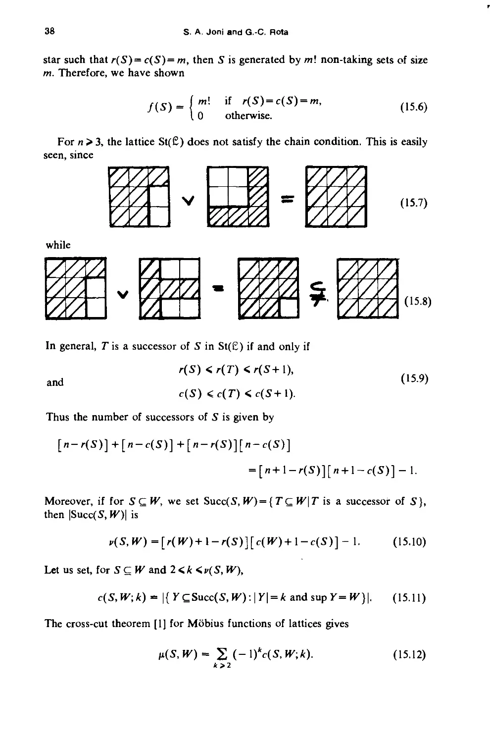
For our first example, let us return to the problem of rooks on an n x n board.
As in Example 14.2, our point lattice £ is represented by the family of open
subsets of & (where ff is the collection of squares {a^} of the board) whose
forbidden sets are lines. The minimal nonempty stars of £ are the unions of the
two lines through each square a0. Thus, the number of atoms of St(£) is /i2, and
since every star is a union of these minimal stars, St(£) is a point lattice. A
non-taking set A Cff is, by definition, a set such that for each aiJ¥=ape/ in A,
apq$-sl{aij) an(* aij^s^iapq)' Clearly there is a bijection between these sets and all
possible placements on die nXn board of non-taking rooks.Recall that for an
open set A, R(A)={i\row i is in A) and C(A)= {_/|column j is in A}. Let
r(A) = \R(A)\ and c(A) = \C(A)\. If A generates the star S, then |^| =
max(r(S),c(S)). The number of sets generating S equals the number of maps
from a set with max(r(S),c(S)) elements onto a set with min(r(S),c(5))
elements. Moreover, A is non-taking if and only if r(st(A))— c(st(A)). Thus, if S is a

r
38
S A. Joni and G.-C. Rota
star such that r(S)=c(S)=mf then S is generated by ml non-taking sets of size
m. Therefore, we have shown
fts\ _ f ™x* if r(S)=c(S) = my
\ 0 otherwise.
(15.6)
For n >3, the lattice St(£) does not satisfy the chain condition, This is easily
seen, since
z
^M
while
A
'/,
fj
YA
/A
yA
*
(15.7)
//
//
'/,
t /
/;
'j
//
y
(15.8)
In general, T is a successor of S in St(£) if and only if
and
r(S)<r(T)<r(S+\),
c{S) <c(T) <c(S+l).
(15.9)
Thus the number of successors of S is given by
[«-r(S)] +[»-c(S)] + [n- r(S)][/i-c(S)]
-[n+l-r(S)][n + l-c(S)]- 1.
Moreover, if for SQW, we set Succ(S, W)={ TQ W\T is a successor of S),
then |Succ(S, W)\ is
i>(S,W)=[r(W)+\-r(S)][c{W)+\-c{S)}- 1. (15.10)
Let us set, for S C W and 2 < k < v(S, W),
c(S,W;k)~ \{YQSucc(S,W):\Y\ = k&n&supY=W}\. (15.11)
The cross-cut theorem [1] for Mobius functions of lattices gives
/x(S,W)= 2 (-\)kc(S,W;k).
k>2
(15.12)

Coalgebras and Bialgebras in Combinatorics 39
While the constants in (15.11) are not tremendously difficult to calculate in any
given interval, no closed formula is known at this time.
Finally, let us calculate the values of g(S). If T is a star generated by a
non-taking set and TDS, then r(T) = c(T) = m >max(r(S),c(S)), and there are
precisely
n-r(S)\(n-c(S)\
m-r(S)j\m-c(S)j
such T. Hence, there are
n-r{S)\(n-c{S)\
m-r(S))\m-c(S))
non-taking sets of size m whose star contains S. Therefore, we have
Z(S)- t ("-'<S>)("-C(rS>W. (15 13)
TTcx /cxx \m~r\S)l \ m — c(S)]
m-max(r(S),c(S)) \ \ // \ \ //
Let us now turn to the case of graphs. As in Example 14.3, given a finite
graph § =( V, E% our lattice £ is represented by the family of open subsets of V
whose forbidden sets consist of two-point subsets {p,q} such that (p,q) is an
(undirected) edge in E. The minimal nonempty stars will be a collection of
st(/?)*s, but not every st(p) is necessarily minimal. A two-subset {/?,<?} is
nontaking if and only if p&st(q) and q&st(p), that is (p,q) is not an edge of @.
Thus, nontaking subsets correspond to collections of vertices where no two are
connected by an edge of §.
A proper coloring of a graph is a placement of colors, one on each vertex
of §, such that no edge connects two vertices of the same color. Clearly,
the maximum number of vertices we can color with one color is equal to
max^ {\A\ :A in non-taking}. The minimum number of colors needed to
properly color a graph is equal to the smallest k such that there exists a collection of
pairwise disjoint non-taking subsets Ax,A2,...,Ak whose union is V.
Since the class of all finite graphs is extremely general, one would not expect
to be able to obtain general formulas for the functions / and g. However, in
many specific cases, they are very simple. As an example, let § be the graph
■©■
3

40
S. A. Joni and G-C. Rota
There are six stars in Vy and St(£) is
5H0
*ti¥)
The non-taking subsets are 0, {!}, {2}, {3}, {4}, {5}, {1,3}, and {2,4}. Thus,
mu)) =
1, 0<7<4,
3, 7 = 5,
(15.14)
and
g(st(y» =
8, 7 = 0,
4, 1<7<4,
3, 7 = 5.
(15.15)
Now consider the graph
I
Here the lattice St(£) is not a point lattice. Indeed the minimal nonempty stars
are {1,2,3}, {1,2,4}, {1,3,4}, {4,5}, and {4,6}. Thus, st(4)= {2,3,4,5,6} is not a
minimal star, and is not the join of the minimal nonempty stars contained in it.
Let us recall that our point lattice £ is represented by a family of open
subsets of the set &. For some sets AC&9 the enumeration of the non-taking
subsets contained in A can be reduced to counting the number of non-taking
subsets contained in certain subsets of A. The precise determination of when this
occurs leads us to the following definition. We say that two subsets A and B split
(or form a splitting of) a subset W if A u B= Wy Anst(B) = 0, and st(A)n B =
0. Let A and B split W, and suppose S is a non-taking subset of W. Clearly,
S nA and So B are non-taking subsets of A and Z?, respectively. Conversely, if
S is a non-taking subset of A, and T is a non-taking subset of B, then S u T is a
non-taking subset of W, To see this let sGS, /eT, and jGst(/). Then sElAc\
st(Z?), but Anst(B) is empty. Let r(W\k) denote the number of non-taking

Coalgebras and Bialgebras in Combinatorics
41
subsets of W of size k. Then for any splitting A,B of W, we have shown
n
(^n)= *2(nk)r(A,k)r(Byn-k).
(15.16)
*-o
This identity is a generalization of those given by Henle for morphs relative to
certain dissects [17]. If & itself admits a nontrivial splitting AyB* then £ is the
direct product of the lattices of open subsets of A and B.
The Henle coalgebra % (£), associated to a point lattice £, studies the splits
of &. More precisely, % (£) is the vector space over K with basis consisting of
all subsets of &. The diagonalization A and counit e are given by
&A =
(Al,A2) ordered
splits of A
AX®A2
(15.17)
and
e(A)
1 if A=0,
0 otherwise
(15.18)
That the comultiplication A is coassociative is easily verified. The full nXn rook
board admits no nontrivial splittings. However, if W is the subset shown in Fig.
2, then
MV = 0®W+ Wx® W2+ W2<8> Wx+ W®0.
A graph § with admit a splitting if and only if it has more than one connected
component.
A^Z,
2
Figure 2.

42
S. A. Joni and G.-C. Rota
XVI. Cleavages
We shall next discuss a class of coalgebras that generalizes the classical notion
of the shuffle algebra to partially ordered sets. A family 2 of PO sets is called an
SBC family (suitable for building cleavages) when it satisfies the following
condition:
if P is a partially ordered set in 2,
and if Q is a partially ordered subset of P in 2,
then the partially ordered subset P-Q also belongs to 2. (16.1)
Under this condition we define a cleavage of a PO set P in 2 as an ordered
pair (Q,R) of subsets of P—with the inherited partial order—such that Q(~\R =
0, (? U * = />, and £> and R belong to 2.
The cleavage coalgebra of the family 2, C (2), is now defined as follows.
Associate a variable xP to each P in 2, including 1 for the empty PO set, and let
C (2) be the vector space having the Ays as a basis. Set
&*p = 2 xq®xr> (16.2)
(Q.R)
where the sum ranges over all cleavages ((?,/?) of P. The counit e(xF) is zero
unless xP= 1, and e(l)= 1; the verification of coassociativity is immediate.
We shall call a family 2 of types (i.e. isomorphism classes) of partially ordered
sets a reduced SBC family when it satisfies the following condition:
if a is a type in 2,
if P is a partially ordered set of type a,
if Q is a partially ordered subset of P,
and if the type 8 of Q belongs to 2, then the type y
of the partially ordered subset P—Q belongs to 2. (16.3)
Clearly, if 2 is an SBC family, and if 2 is the family of types (or isomorphism
classes) of 2, then 2 is a reduced SBC family. The reduced cleavage coalgebra of
the family 2 is the vector space C(2) freely spanned by the variables xa
associated to each type a, including 1 for the empty PO set, with
where the sum ranges over all ordered pairs (/?,y) of types in 2 such that a
partially ordered set P of type a contains a cleavage of type (/?,?).
The section coefficients (a|/?,y) are integers counting the number of
cleavages of type ()3, y) in a partially ordered set of type a. The counit is the obvious
one, and again the verification of coassociativity is immediate.
If 2 is an SBC family and 2 is the family of types of 2, then the reduced
cleavage coalgebra C(2) is isomorphic to the quotient of the cleavage coalgebra

Coalgebras and Bialgebras in Combinatorics 43
C(2) modulo the coideal generated by xF — xQ for all isomorphic PO sets P, Q in
2.
Examples of SBC and reduced SBC families are not abundant, and we shall
only give three.
Example 16.1. Let 2 be the family of all finite linearly ordered subsets; 2 is
the family of all types of finite linearly ordered subsets. The cleavage coalgebra
C(2) is isomorphic to the Boolean coalgebra. The reduced cleavage coalgebra
C(2) turns out to be isomorphic to the shuffle coalgebra. It is well known that
this coalgebra is a bialgebra, where the noncommutative multiplication is simply
juxtaposition.
Example 16.2. Let 2 be the family of all finite forests, and 2 the reduced
family consisting of all types of finite forests, considered as PO sets. Clearly 2 is
an SBC family. 2 defines an interesting reduced cleavage coalgebra, the tree
coalgebra, which does not seem to have been studied. We do not know whether
the tree coalgebra can be significantly turned into a bialgebra.
Example 16.3: Let 2 be the family of all finite PO sets; 2, the reduced family
of all types of PO sets. The associated reduced cleavage coalgebra, we
conjecture, should have some notable universal mapping characterization, generalizing
the universal properties of the shuffle coalgebra.
Several SBC subfamilies (reduced SBC subfamilies) of PO sets defined by
restricting the length or width of the PO sets (types) allowed give subcoalgebras
of the cleavage (reduced cleavage) coalgebra. For example, one can take all PO
sets (types of PO sets) with the property that in each P, no chain exceed in
length an integer n prescribed in advance.
The cleavage and reduced cleavage coalgebras can be viewed as
generalizations of the incidence and reduced incidence coalgebras. Very probably, other
coalgebras "in between" these two extremal cases can be defined.
XVII. Hereditary bialgebras
We come now to the description of a class of bialgebras—indeed, of Hopf
algebras—which are probably the richest in structure and combinatorial
applications. They are obtained from hereditary classes of matroids, a notion
which we proceed to discuss briefly.
Recall that a matroid M(S) on a (finite) set S is a closure relation defined on
the subsets of S which enjoys the MacLane-Steinitz exchange property: if A is
any_subset of S, A its closure, and pyq elements of S such that q^A up but
q&A, thenpEA u <?. We shall need only a few elementary concepts from the
theory of matroids; further details can be found in the books by Crapo and
Rota [9] and by Welsh. The direct sum of two matroids M(S,) and M(S2) on
disjoint sets S, and S2 is defined as M(Sl + S2) by setting Axu A2 = Al\jA2,
where Ax QSr A matroid is said to be connected when it is not isomorphic to a
nontrivial direct sum of two matroids. Every matroid M(S) is uniquely the
direct sum of connected matroids M(St) obtained from the blocks S, of a
suitable partition of the set S, A segment of a matroid is defined as follows. Let

44
S. A. Joni and G.-C. Rota
A and B be closed sets of M(S), and let ACB. The segment M(A,B;S) is the
matroid defined as the set B-A with, for CCB-A, the closure C of C to be
C=C vA-A.
In the following we denote by Greek letters isomorphism classes, or types, of
matroids. The lattice of closed sets of a matroid is called a geometric lattice. Two
non-isomorphic matroids may have isomorphic geometric lattices. In fact,
among all non-isomorphic types of matroids having isomorphic geometric
lattices, there is one which is canonically associated with the geometric lattice L as
follows: the set S is the set of atoms of the lattice L_(that is, elements covering
the minimum element), and for ACS, one sets A = {pGS:p <supA}. This
matroid is called the combinatorial geometry associated to the geometric lattice
L.
The geometric lattice of the segment matroid M{A,B\S) is isomorphic to the
segment [A,B] in the geometric lattice L of the matroid M(S).
We come now to our main notion. A hereditary class H of matroids is a
family of types of combinatorial geometries with the following properties:
(1) If a and (3 belong to //, then the direct sum a + ft is a combinatorial
geometry, and it belongs to //. The geometric lattice of a + ft is the product, in
the sense of partially ordered sets, of the geometric lattices of a and /?.
(2) If M(A,B; S) is a segment of a matroid M(S) and the type of M(S) is in
//, then the combinatorial geometry of the type of the matroid M(A,B\S) also
belongs to //.
(3) If a belongs to H and a is isomorphic to the nontrivial direct sum
a = oti + a2 of combinatorial geometries, then a, E //.
Let // be a hereditary class, with types a,/?,y in H. The section coefficient
(a| >3,y) of H is defined to be the number of closed sets A in a matroid M{S) of
type a such that the segment M{0,A\S) is of type (3 and the segment
M(A,S;S) is of type y. It is easy to see that this number depends only on the
types a,/?,y.
We have the important
Proposition 17.1. The section coefficients of a hereditary class of matroids are
section coefficients.
Proof: We have to prove the identity
2(«l/*,Y)(Yk,o) = (a|j3,w,o)
Y
-2(«l*.°)(*l&ff).
8
Let (a| fi,7r,o) be the number of pairs of closed sets A C B of a matroid M(S) of
type a such that M(0,A\ S) is of type/3, M(A,B\ S) is of type 77, and M(B,S,S)
is of type a. The first sum is obtained by fixing^ and letting B vary, whereas the
second sum is obtained by fixing B and letting A vary.
More important is the

Coalgebras and Btalgebras in Combinatorics 45
THEOREM 17.1. The section coefficients associated with a hereditary class of
matroids H are bisection coefficients.
Proof: We define a semigroup structure on the hereditary class H by taking
direct sums as addition. For clarity, we shall prove the bilinear identity for the
special case (a|/?,y) where a = al + a2 and the a, are connected (nontrivial)
types; the general case is similar. Thus, we need to show that
(«i + a2lfry) = 2 (ail0i,Yi)(a2|02.Y2)-
Yi + Y2"Y
To this end, let A Q S be a closed set of \f(S\ and let M(S) be the direct sum of
A/(S,) and A/(S2). Then the matroid M(0,A;S) is isomorphic to the direct sum
of the matroid M(0,Ax\Sx) and M(0,A2;S2) where A^AnS^ Similarly, the
matroid M(A,S;S) is isomorphic to the direct sum of M(A{,5,:5,) and
A/(i42,S2;S^. Counting, we obtain the desired identity.
Thus, associating the variable xa to each type of the hereditary class //, we
obtain a bialgebra where the underlying algebra is the polynomial algebra in the
variables xa for which a is a connected type, and the comultiplication is defined
by
&xa «2(a|i8,Y)x^®xY.
The augmentation is defined in the obvious way.
The bialgebras obtained by this construction will be called hereditary bialge-
bras. We list some of the examples previously discussed.
(1) The Boolean algebra of subsets of finite sets turns out to be a hereditary
bialgebra, which is in fact the binomial bialgebra.
(2) The Faa di Bruno bialgebra is the hereditary bialgebra obtained by taking
the bond closure (see [1]) on graphs which are direct sums of complete graphs.
(3) The Eulerian coalgebra is also associated—although rather trivially—
with a hereditary bialgebra. One takes all direct sums of matroids whose
geometric lattices are the lattices of all subspaces of a vector space over a finite
field. If a is connected, then A(jca) agrees with the definition already given.
Other notable hereditary classes of matroids are (4) all finite sets of points in
projective space over a fixed field; (5) all series-parallel networks, (6) all graphs,
(7) all planar graphs; (8) all unimodular matroids.
Each hereditary bialgebra leads to a generalization of the umbral calculus, for
which the umbral calculus in one variable, outlined in Sec. XI, is the blueprint.
We believe the development of such "hereditary" calculi to be one of the most
promising prospects of present-day combinatorics.
In the preceding theorem (Theorem 17.1), an essential role is played by the
very special factorization properties of matroids. Thus, the notion of hereditary

46
S. A. Joni and G.-C. Rota
bialgebras can be extended to any family of PO sets where one can prove the
factorization properties required to make the above proof work. One such class
is the class of semimodular lattices. The discovery of the most general such class,
if any, may well lead to a class of bialgebras sharing a simple axiomatic
definition.
In closing, we remark that the detailed study of hereditary bialgebras should
have as some of its goals the extension to hereditary bialgebras of the
exponential formula of the binomial bialgebra, as well as generalizations of the Lagrange
inversion formula.
References
Items listed in the bibliographies of the principal references, unless specifically
cited in this work, will not be repeated.
Principal references
1. G.-C. Rota, On the foundations of combinatorial theory I: Theory of Mobius functions, Z.
Wahrscheinlichkeistheorie 2: 340-368 (1964).
2. R. Mullin and G.-C. Rota, On the foundations of combinatorial theory III: Theory of
binomial enumeration, Graph Theory Appl. 168 (1970).
3. G.-C. Rota, D. Kahaner, and A. Odlyzko, Finite operator calculus, J. Math. Anal. Appl. 42:
685-760(1973).
4. P. Doubilet, G.-C. Rota, and R. Stanley, On the foundations of combinatorial theory VI: The
idea of a generating function, in Sixth Berkeley Symposium on Mathematical Statistics and
Probability, 2, Berkeley U. P., 1972, pp. 267-318.
5. S. Roman and G.-C. Rota, The umbral calculus, Advances in Math. 27(2): 95-188 (1978).
Additional references
6. M. Aigner, Kombinatorik, Vol. I and II, Springer-Verlag, 1975-76.
7. J. D. Bjorken and S. D. Drell, Relativistic Quantum Mechanics, McGraw-Hill, New York,
1964.
8. N. Bourbaki, Algebray Hermann, Paris, 1970, Chapter III.
9. H. Crapo and G.-C. Rota, Combinatorial Geometries, M.I.T. Press, Cambridge, Mass., 1971.
10. J. A. Dieudonne, Introduction to the Theory of Formal Groups, M. Dekker, New York, 1973.
11. P. Doubilet, Studies in partitions and permutations, Ph.D. thesis, M.I.T., 1974.
12. R. Feinberg, Characterization of incidence algebras, Ph.D. thesis, Univ. of Wisconsin, 1974.
13. J. Fillmore and S. G. Williamson, A linear algebra setting for the Mullin-Rota theory of
polynomials of binomial type, Linear and Multilinear Algebra 1: 67 (1973).
14. A. M. Garsia, An expose of the Mullin-Rota theory of polynomials of binomial type, Linear and
Multilinear Algebra, 1: 43 (1973).
15. A. M. Garsia and S. A. Joni, A new expression for umbral operators and power series inversion,
Proc. Amer. Math. Soc. 64: 179-185 (1977).
16. J. R. Goldman and G.-C. Rota, On the foundations of combinatorial theory IV: Finite vector
spaces and Eulerian generating functions, Studies in Appl. Math. XLIX (3): 239-258 (1970).
17. M. Henle, Binomial enumeration on dissects, Trans. Amer. Math. Soc. 202: 1-38 (1975).
18. S. A. Joni, Polynomials of binomial type and the Lagrange inversion formula, Ph.D. thesis,
Univ. of California, 1977.
19. S. A. Joni, Antipodes and inversion of formal series, J. Algebra (1979), to appear.

Coalgebras and Bialgebras in Combinatorics 47
20. R. W, Lawvere, The convolution ring of a small category, to appear.
21. P. Lbroux, Les categories de Mobius, Cahiers Topologie Gom, DifferentieUe XVI (3): 280-283
(1975).
22. C L. Liu, Topics in Combinatorial Mathematics, M.A.A., Washington, D.C, 1972.
23. G. Polya, Picture writing, Amer. Math. Monthly 63: 689 (1956).
24. S. Roman, The algebra of divided differences, in preparation.
25. G.-C. Rota and D. A. Smith, Enumeration under group action, Annali Scuola Norm. Sup. Ser.
/KIV:637-646(1977).
26. H. Schubert, Categories, Springer, Berlin, 1972.
27. M. E. Sweedler, Hopf Algebras, Benjamin, New York, 1969.
28. W. T. Tutte, On dichromatic polynomials, J. Combinatorial Theory 2: 301 (1967).
Carnegie-Mellon University
Massachusetts Institute of Technology
(Received September 15, 1978)

Contemporary Mathematics
Volume 6, 1982
Hopf Algebras and Combinatorics
by Warren Nichols and Moss Sweedler
The following material is discussed in this paper: Coalgebras
from Formulas; Grouplikes; Primitives; Coalgebra Definitions and
Examples; Coalgebra Maps; Convolution Algebras; Coproduct of
Subspaces; Comodules; Sheffer Sequences; Coalgebra Maps to 10 °°;
Coradical Filtration; Conjugate Sequences; Associated Sequences;
Algebra-Coalgebra Interactions; Bialgebras; Measuring;
Comeasuring; Hopf Algebras; Antipodes; Pincherle Derivative;
Recurrence Formula; Transfer Formula; Dual Coalgebras.
I. Introduction
These are a revision by the second author of notes taken by the
first author at lectures by the second author.
I shall try to give a seductive overview of coalgebra and
Hopf algebra theory and some of its relations to combinatorics,
especially to the umbral calculus- Skimming through many
definitions, terms, examples, results but few proofs- I hope that by
the end of these lectures you will have a sense of familiarity
with coalgebras and Hopf algebras and you will be motivated to
really learn about them.
Thanks to Warren Nichols for taking these notes and for
cleaning up where I was too terse, incomplete, slip-shod or
wrong. Warren has made helpful additions and deletions,
including an interesting example of a non-subcoalgebra.
References in the form [p.**] are to Hopf Algebras by
Moss E- Sweedler, W.A. Benjamin, New York, 1969.
I9H0 Subject Classification. 05-02, 16-A24
Address for correspondence: Professor Moss E. Sweedler,
Mathematics Department, Cornell University, Ithaca,NY, 14853
C I9U Amricaa MalbMMtkaJ Society
49

50 W. Nichols and M. Sweedler
II. Coalgebras from formulas
We first encounter coalgebras as their diagonalization A arises
from generic addition formulas. Some examples are: (i) the
trigometric identities sin(x+y) = sin(x)cos(y) + cos(x)sin(y),
cos(x+y) = cos(x)cos(y) - sin(x)sin(y); (ii) the exponential
law . ex+y = exey; (iii) sequences {p (x)} of polynomials in
one variable, with degree p = n, satisfying the relations
pn(a+b) = tf_Q ( i)Pi(a)Pn«i('b)' these are known as sequences of
binomial type; and (iv) the divided power sequences of
polynomials (dn(x)} , satisfying dR(a+b) = e£=q dj_( a)dn_±(b),
which can be obtained in characteristic zero by replacing p (x)
with p (x)/nl .
Let k be any field. There is an algebra map
A:k[x] •* k[x]®k[x] defined by sending x to x&l + l®x; we
then have A( l) = 1®1, and A(xn) = (Ax)n = (x®l + l®x)n . For
any polynomial f(x), we have A(f(x)) = f(A(x)). Note that
f(x<8>l) = f(x)<8>l, and f ( 1<8>x) = l®f (x) .
Give k[x] the ideal topology determined by <x> , (i.e. an
element of k[x] is "small" if it is divisible by a large power
of x). Give k[x] ® k[x] the ideal topology determined by
^x®l, l®x^ . Then A is continuous, and passing to the completion
yields a map
A:k[[x]] -* k[x] ® k[x] = k[[x ® 1, 1 ® x] ]
which extends A. Write A for £. Note that
k[ [ x] ] ®k[ [ x] ] c k[ [ x®l, lax] ].
If k has characteristic zero, using the power series
expansion of sin(x) and cos(x) we have
A(sin(x)) = sin(A(x)) = sin(x®l + l®x)
= sin( x®l) cos( l®x) + cos( x®l) sin( l®x)
= (sin(x)<8>l)( l®cos(x)) + (cos(x)<8>l)( l®sin(x))
= sin(x)®cos( x) + cos(x)®sin(x) .
Similarly, A(cos(x)) = cos( x)«cos( x) - sin(x)®sin(x) . For
,. . . « x A/ x\ A(x) x®1-H®x
the power series expansion ofe: A(e)=ev'=e =
ex«lel®x = (exg)1)( lg)ex) = ex®ex . (More generally,

Hopf Algebras and Combinatorics 51
A(e*x) = e*x®e*x for any A e k.)
With sequences of binomial type, we need not pass to the
completion: A(pn(x)) = pn(x®l+l®x) = e£=q (n)p±(x®l)pn-i(lax) =
^±=0 (i)Pi(x)®Pn.i(x) - The calculation for sequences of divided
powers is similar. The upshot is that each addition formula
naturally gives a formula for the action of A.
Next we view coalgebra diagonalization A arising from
operator formulas. The first of these is the formula for an
algebra map o from algebras A to B: o(aa) = o(a)o(a) for
all a,a e A. Another formula arises from the derivations of an
algebra A-- the maps d:A •* A which satisfy
d(aa) = d(a)a + ad(a) for all a,a e A. More generally,
consider the higher derivations {d } which satisfy the
Leibnitz formula d^(act) = l£=Q (T ^ ( a)(T ^1^ (a). If
d:A -* A is a derivation and the characteristic is zero, setting
d^ = dn/nl gives fcrn'l, a higher derivation.
Let ff be a vector space, and A,B algebras. Suppose we
are given a map "-"rlT •*■ Hom(A,B), sending E e TT to h:A -* B.
Define two evaluation maps: H®A -* B by E$a •*■ h(a), and
TM&A8A -* B by E1 ® E2®a«a to h1(a)h2(a).
A map A:IT -* ff ® ff which makes the diagram commute:
H ® A ® A A ® T ® X > H ® H ® A 5¾ A
I ® mult
evaluation
7T -* A evaluation v _
H & A > B
gives an operator formula as follows: if A(E) = eE. ,® E. 2 >
then
OPERATOR h(aa) = - (a). (a) fQr all a>a e A .
FORMULA 1'x x>d
In this situation, we say that H measures A to B.
An example, suppose that a:A •*■ B is an algebra map. Let
ff be a one dimensional space with basis "o • Define
A:IT -* H" # IT by A(*o) = "a <8 "a . Then the formula
c(act) = o(a)o(a) shows that H measures A to B if

52
W. Nichols and M. Sweedler
H + Hom(A,B), o -» c
When A = B, and d:A -* A is a derivation, let H have
basis T,cT and define A(T) = I ® I , and
A(d) =T®d*+d®T. Then H measures A to itself if
TT -* Hom(A,A), T -* I, cT -* d . Here I is the identity map in
Hom(A,A).
Given a higher derivation {d
(n)
TnT^
} of A, let [dvli/ 1 be a
Then H
basis for H, and set A(d^n)) = r£=Q d(i) ® d( n i] .
measures A to itself if IT + Hom(A,A), d^nJ -* d'n' . Higher
derivations are especially useful in characteristic p ) C ,
where derivations vanish on p powers.
As you can see from the examples measuring unifies homo-
morphisms, derivations and higher derivations. A technique
afforded by measuring is to turn operator statements into
coalgebra statements and then to deduce facts about the operators
from coalgebra results.
Of particular importance in the study of coalgebras are
elements g satisfying the conditions A(g) = g®g and ( e to be
explained shortly) c( g) = 1- The elements are called grouplike.
Their existence may depend in part upon the field k; for
instance, if i = J^l e k, then cos(x) ±i sin(x) = e± x are
grouplike. Also, primitive elements are important. An element
d is g-primitive if A(d) = g®d + d®g where g is grouplike.
III. Coalgebra definitions and examples
A coalgebra is a vector space C over a field K, together with
linear maps A : C •* C®C (the coproduct) and e:C -> k (the
counit), making the diagrams commute:
A
A
I«A
-> C®C
A®I
\/
-> C&05&C
k#C
C&k
and
e®I
1(55 6
The first diagram says that A is coassociative; the second,
that e is a left and right counit for A .

Hopf Algebras and Combinatorics 53
An important tool for coalgebra manipulations is the
E notation* When working with elements x-,,Xp, ...,x of an
associative algebra, it is convenient to write xix2**,xn in
place of xi(xp('--xn i(xrJ'-')) and to think °^ x,x ...x as
denoting the result of multiplication performed in any
association whatsoever. E notation is the appropriate dual procedure
for coalgebras.
n
Write ® C for the n-fold tensor product of C with itself.
n+1
Define A : C •* ® C by: A, = A, and An = (A®I®. - . ®l) <>A ,.
Thus, A (c) is obtained from A .,(c) by applying A to the
first factor. Write A (c) = E/ rt\ c,®. ..®c -, - We emphasize
n ^ c) x n+ x
that the E is a dummy summation sign serving merely to remind
us that A (c) is a sum of elements of the form x.,®Xp®. ..®x ,-.
where each x. e C- The symbols c,,...,c 1 do not denote
X X I 1 I -id
particular elements, but are merely place-holders.
E notation is often used in connection with multilinear
functions. Suppose that V is a vector space, and
n n
f : x C = Cx.-.xC -* V a multilinear map- Let F : ® C -* V be
the induced map. Write E/ \ f(c,, ...,c ) for F(A t(c)).
Again, the E is dummy and the c.Ts are place-holders. If we
express A^ n(c) = E. c, .®c0 .®..®c ,, where c. . e C for
n-x j x, j d9 j n, j 1, j
all i,j, then F(An-1(c)) = E. f ( c^ y ..., c^ ^) .
For example, let C be a coalgebra, A an algebra, and
g,h: C •* A linear maps. The notation E/ \ g(c-,)h(Cp) is
interpreted as follows: CxC •*■ A sending (d,e) to g(d)h(e)
is a bilinear map. This induces a linear map F : 0®C -* A,
given by F - mult *(g®h). Then E(cj g(c1)h(c2) = F(a(c)) .
More explicitly, if we write A(c) = E7=1 c1 ^®c2 . where
c-, ., cQ j e C for all i , then
_L, 1 £Zf X
E(c) g(C;L)h(c2) = rj=1 g(C;L>±)h(c2ji)
E notation can be used to convey concisely the information
in commutative diagrams. For example, A: C -* C®C is

5^ W. Nichols and M. Sweedler
coassociative iff Z/^ A(c-L)®c2 = Z/Q\ c^Qb( c2) for all c e C.
Also, e:C + k is a counit for A iff
r(c) c(cl>c2 = C = =( c) clc(c2) '
We will say that C is cocommutative if A=T©A, where
T : C®C •* 0®C is the "twist" map sending d®e to e<$d. In I
notation this condition is I/\ c-^c^ = L/ \ c2®cn • Many of
the coalgebras important in combinatories are cocommutative.
Here are a number of examples of coalgebras.
1. The trigonometric coalgebra ^ • This coalgebra has basis
s,c with A(s) = s®c + c®s, A(c) = c®c - s®s, e(s) = 0, e(c) = 1.
(Think of s, c as the functions sin(x), cos(x), then e
corresponds to evaluation at zero-)
2. The divided power coalgebras £N, J0 °° . Here $ °° has
basis {di}i > Q , with A(dn) = rJ-0 d1®dn-1, e(dn) = 60^n .
To get £> take only dQ,d^,.. .,cL-. Notice that dQ is
group like and d-. is d^-primitive.
3. The coalgebras ft , ft°° of binomial type. These are
similar to the divided power coalgebras. ft00 has basis
?°±h > 0' wlth A(bn} = =i-0 OWi ' ^V = 60,n' ASaln'
bQ is grouplike and b.^ is bQ-primitive. In characteristic
zero, ft00 is isomorphic to 0" °° > with d corresponding to
N
bn/nJ . To get ft take only bQ,.. .bN .
k. For any set S form a coalgebra with the elements s of S
as a basis by setting A( s) = s®s, e(s) = 1.
5. For each positive integer n, the comatric coalgebra Mc(n,k)
has basis {xj_-j}i -t=i> with A(x.j,) = ^_=1 xj_k®xjt-| » and
c(xj ,) = 6. ,. In contrast to the examples above, M (n,k) is
not cocommutative if n >_ 2 .
6. We can form a coalgebra C with basis g,h,t by declaring
g,h to be grouplike, and setting A(^) = g#£ + £®h, e( t) = 0,
This coalgebra lives inside M (2,k), with g = x,,, h = x22,

Hopf Algebras and Combinatorics
55
t = x-jo- It is not cocoTimutative.
7. The incidence coalgebra. Let J& be a partially ordered set.
Let C have basis {(x,y) e J x J : x( y , x near y} ,
Mx near y" means that {z e J : x ^ z ^ y} is finite.
Define A((x,y)) = I (x, z)®(z,y), and e((x,y)) = 6Y „ .
x < z < y x'y
Note that example 6 is an incidence coalgebra, with
i = {x,y}, x < y, g = (x,x), h = (y,y), t = (x,y) .
8. Let V be any vector space. Let C = k©V. Declare
g = (1,0) to be grouplike. Identifying v e V with (0, v) e C,
set A( v) = gg>v + v®g, and e( v) = 0 . Thus the elements of V
are g-primitive.
IV. Coalgebra Maps
Let C,D be coalgebras. A coalgebra map f : C •*■ D is a linear
transformation which makes the diagrams below commute:
-> D
c®c-
f®f
-4/
->D®D
-> D
This can be written A(f(c)) = I/ x f ( c1)®f( c ), and
e(f(c)) = e(c). Subcoalgebras correspond to injective coalgebra
maps; a subspace V of C defines a subcoalgebra of C if
A(V) c V®V, for in this case the A and e for C can be used
to define a coalgebra structure on V. A coalgebra quotient of
C is given by a surjective coalgebra map; the kernel of such a
map is called a coideal. A subspace K of C is a coideal if
and only if A(K) c K®C + C®K and c( K) = 0; in this case,
C/K has a unique coalgebra structure so that the canonical
projection C •*■ C/K is a coalgebra map. In general, any
coalgebra map f : C •* D has a unique factorization:
- 1 > D
<*
C/Ker f = Coker ( f )-
-> lm(f)

56 W. Nichols and M. Sweedler
Now a digression for budding coalgebraists to point out
difficulties when k is not a field but merely a commutative
ring- Others please skip this digression by proceeding to the
beginning of section V, page 57.
Since the tensor product of injections may fail to be
injective, >je cannot identify the tensor product of submodules of
C with a submodule of G8>C .
First an example where V is a submodule of a coalgebra C,
and there may be more than one coalgebra structure on V with
the natural inclusion V *-* C a coalgebra map- Take
k = Z, C = Z © Z/4Z, with g = (1, 0) grouplike, and x = ( 0, l)
g-primitive. Let V be the submodule spanned by g and 2x.
Then V = ZSZ/2Z as a Z-module. V can be made into a coalgebra
by letting g be grouplike, and 2x g-primitive. Alternatively
define a coproduct A1 on V, with g still grouplike, but
now with Ar(2x) = g®( 2x) + ( 2x)<8>( 2x) + (2x)®g in V®V, and
e( 2x) = 0. This second coalgebra structure has an additional
grouplike element g+(2x), and thus is not isomorphic to the
first structure. However, for each coalgebra structure on V
the inclusion V **> C is a coalgebra map, since in Ct&C the
term 2x®2x = 4x®x = 0®x = 0.
Second, an example where V is a submodule of C with
A(V) c Im(V®V •* C®C), yet V has no coalgebra structure with
V ** C a coalgebra map. This example was supplied by
Warren Nichols. The example is without a counit. (A counit could
easily be adjoined.) Let k = Z, C = Z/8z©^2Z, x = (1,0),
z = (0,1). Define A : C -* C®C by: A( x) = 0, A( z) = kx®x .
(Since ^x®x has order 2 in 08>C, A is well-defined.) Let
y = 2x, V = Zy + £z c C. Since A( z) = y<gfy, we have
A(V) c Im(V®V -* C®C). However, the map A:V -* Og>C has no lifting
to V®V, since every preimage of A( z) in V®V has order 4.
Turning to quotients, let K be a submodule of C. The
kernel of the natural map G8C -* CA®CA is
Im(K®C -* 08>C) + Im( C®K -* C®C). Thus, a submodule K of C is
the kernel of a surjective coalgebra map iff
A(K) c Im(K®C -* G8C) + Im( C®K ■* 0®C), and e(K) = 0, so the
characterization of coideals is still correct. However, the
kernel of a non-surjective coalgebra map may not be a coideal.
Again with k = Z, let D = Z © Z/2Z © Z, with
dn = (1,0,0), d-, = (0,1,0), dQ = (0,0,1) being a sequence of

Hopf Algebras and Combinatorics 57
divided powers. Take E = / © ZA-Z, with eQ = (1,0), 6,=(0,1)
also a sequence of divided powers. Define f: D -* E by:
f(dQ) = eQ, f(d1) ^ 26-^ f(d2) = 0. Then f is a coalgebra
map; we check only (f®f)A(d2) = (f®f) (d0®d2 + d1®d1 + d2®dQ) =
0 + 2e1®2e1 + 0 = ^e1®e1 = 0 = A( f ( d2)) - Ker f = £d2 is not a
coideal of C, since A(d2) d d2®C + 08»d2 .
V. The convolution algebra
Returning to the setting k a field, let C be a coalgebra, A
an algebra. ( "An algebra is defined by taking the defining
diagrams for a coalgebra and reversing arrows. If — old
coalgebraists joke.) Algebras are assumed to be associative and
have unit.
Hom(C,A) has an algebra structure, with the product (called
"convolution") defined by (f*g)(c) = I, x f(c1)g(c2) for
f, g e Hom(C,A) and c e C. In terms of maps,
f*g = (mult) »(f®g) °A. The unit e of Hom(C,A) is given by
e(c) = c(c)l. The algebra structure is functorial: if o: A •* B
is an algebra map, and Y : C •* T is a coalgebra map, then
Hom( Y, a) is an algebra map where Hom( Y, <j) : Hom(D,A) •* Hom(C,B),
is defined by Hom( Y, a) ( f) = oof*Y, for f e Hom(D,A). When
A is the ground field k, we get the dual algebra C* = Hom(C,k).
There is a natural algebra injection C*®A -* Hom(C,A), defined
by (f®a)(c) = f(c)a for feC*, aeA, ceC. This map is an
algebra isomorphism when C or A is finite dimensional.
Let A be an algebra, f: C -> D a coalgebra map. (The case
A = k is the most important.) We have an algebra map
Hom(f,A) : Hom(D,A) + Hom(C,A), sending h e Hom(D,A) to
h°feHom( C,A). Identify the kernel of this map as (Im(f)) ,
the maps from D to A which vanish of f(C). The image of
Hom(f,A) is (Ker f; , the maps from C to A vanishing on
Ker f . Thus if C is a subcoalgebra of D, C^ is an ideal
of Hom(D,A); and if K is a coideal of C, KL is a
subalgebra of Hom( C,A).
We take J. --perp-- of both subspaces of C and subspaces
of Hom(C,A). For a subspace X of C :
X = [g € Hom(C,A) : X c Ker g} c Hom(C,A) . For a subspace
Y of Hom(C,A) : Y = 0 „ Ker V • In general some subspaces

58 W. Nichols and M. Sweedler
of Hom(c,A) will not be the X of any subspace of C. Taking
the -LTs of finite dimensional subspaces of C as a basis of
open neighborhoods of zero in Hom(c,A) induces a topology of a
topological group on Hom( C,A). In this topology X Ts of
subspaces of C are closed and if A = k, the ground field,
then the closed subspaces of Hom(C,A) are precisely the X Ts
of subspaces of C.
For general algebras A if J c Hom(C,A) is an ideal,
then J"1- is a subcoalgebra of C. If U c Hom(C,A) is a
subalgebra, then UX is a coideal in C if A = k but UX
need not be a coideal in C when A ^ k. In fact for C = 0
and A = k[x]/ ( x > , the subspace U of Hom(C,A) spanned
by _e and the linear map f: C -* A determined by
dQ -* 0, d1 -* x, d« •*■ 0 is a subalgebra where U = kdp c C
and U is not a coideal in C.
When A = k X-ing gives a bijective correspondence between
the set of subcoalgebras of C and the set of closed ideals in
Hom(C,k). X -ing also gives a bijective correspondence between
the set of coideals of C and the set of closed subalgebras of
Hom(C,k).
Checking our examples:
First D°° . Define elements {tn} of Hom( O °°,A) by:
tn(dj = 6„ 1 . Then Hom( /9 °°,A) = A[ [ t] ] as vector spaces.
in n, ni
We have (tr*ts)(<g = L^0 tr( d±) t8^) = 6^^1 . Thus
tr*ts = t14"8 , and Hom( £T°°,A) »A[[t]] as algebras. Note
that Hom(/JN,A) ^A[t]/(tN+1) .
Similarly, Hom(ft ,A) = A{{t}} as algebras. Here we write
the formal symbol -p- for the element in Hom(a°°,A) with
IT <V = V we have TT * IT = (T> Wi ■ When
characteristic k = 0,
A{{t}} «A[[t]], Jr < > T^ t1
Let J~ be the trigonometric coalgebra. Write
Hom( y ,A) = ksQAs*, where _c is the unit and s* is defined
by: s*(c) = 0, s*( s) = 1. We have
(s**s*)(s) = s*(s)s*(c) + s*(c)s*(s) = 0, and

Hopf Algebras and Combinatorics 59
(s**s*)(c) = s*(c)s*(c) - s*(s)s*(s) = -1- Thus, S**S* = -£.
This shows that Hom( X ,A) = AQkj^T
If i = J^l e k, ^T = k(c+is)€)k(c-is) is the sum of
one-dimensional subcoalgebras. ( MThe dual of a coalgebra tends
to contain what is needed to split it."--old coalgebraists
proverb.)
If C is a coalgebra with a basis of grouplike elements
indexed by the elements of a set S, then Hom(c,A) = II A
seS
as algebras.
We now take C = Mc(n,k), the comatric coalgebra. C has
basis (xi-»}]_ < i i < n" Hom(C,A) has dual A-basis {eji}-
We have Hom(c,A)2? M(n,A) = M(n,k)s$iA, where M(n,-) is the
nxn matrix algebra over ,T-'T . Note that duality allows us to
identify certain important subspaces of C . For example, the
subspace J = E. \ ., kx. , is the -L of the upper-triangular
matrices, and thus a coideal. The upper-triangular matrices
are isomorphic to Hom(C/J,A) as an algebra.
When C has basis g,h, £ with g, h grouplike and
A( £)=g®£+4,®h, we can realize Hom(c,A) as upper-triangular
matrices over A, with g,h,t dual to the matrix elements
ell'e22'e12 -
VI. The coproduct of subspaces
Let C be a coalgebra, U,V c C subspaces. Define
UAV = Ker( C ——> CfcC -* C/U ® CA) = A-1( C®V+U®C). (UAV
is often written UAV in the literature, and called the wedge.)
The coideal condition A(u) c U ® C + C ® U can be written
U c U A U. The significance of the operation is clear from its
dual: in Hom(C,A), we have (UAV)"1" = U1 * VX (sums of
products). The wedge will be useful later in describing the
coradical filtration.
VII. Comodules
Let C be a coalgebra. A right C-comodule is a pair (M,¢),
where M is a vector space, and i|r:M -* M ® C is a linear map
such that the diagrams commute:

6o
W- Nichols and M. Sweedler
M
*
-> M ® C
M
M®C-
-4 > M ® c
♦®I
->M ® C ® C
^
I®€
M ® k
Write Tt<( m) = E/ \ m..®m2 . (This is the I notation for
comodules.) The lowest number in i|r (m) = L/ \ nu®. . .®m , holds
an M-place.) Note that (C,A) is a right C-comodule.
For U c M, V c C write
U*V = Ker(M
*
-> M®C -> M/U ® C/V) •
Let M,N be right C-comodules. Then f:M -> N is a
comodule map if the diagram commutes:
M
-> N
*M
M®C
f®I
*N
-> N®C .
We look at some examples of comodules.
Let C be the comatric coalgebra M (n,k). Let M have
basis {vi]i=i • Set ♦( vi^ = *m=i vi®xii" Note that, for each
t we have a comodule injection f.:M-*C defined by f.(v.) = x. ,.
Let C be the incidence coalgebra on the partially
ordered set -A - For each t e jo , let M, be a vector space
with basis {(u): u e Ji , u ^ t, u near t}. Define
*. :M. + M.®C by: ♦.((u)) = E (v)®(v,u). Then (M.,*J
z z z z t<v<u t t
is a right C-comodule. We have a comodule injection f.:M -> C,
defined by ft((v)) = (t,v).
Here is an example related to factor sequences,
coalgebra is B°° . The comodule Q00 has basis ^_n^n=0
Set
-i
The
.00
*(q ) = I? ~ ( <)q ,<8b ,
T\H_n/ "i=o ^n-i'^-i n-i
where as usual ( "£) = (-l)k (n+£_1) and (£) = 6Q fc. The

Hopf Algebras and Combinatorics 6l
tie-in with factor sequences will be described at the end of this
section and at the end of (XI, 3)-
VIII- Sheffer sequences and comodule maps
Consider fi°° with the usual basis 0^ 3 o and let ^ei^o c ft°°
be a sequence satisfying:
Aen = ^1=0 (i)ei ®Vi"
This is the notion of fe. } being Sheffer with respect to {b. }.
Defining f: B -* B , f(*>n) = en > (*) insures that f is
00 ., , . . . 00
a comodule map where 8 is considered as a right 8 -comodule.
Conversely if g: B •*■ B°° is a right ft -comodule map and
e. = g(tO then (*) is satisfied. Hence Sheffer sequences may
be identified with comodule maps from B°° to itself. In fact if
{b! } is any basis for B°° which is a sequence of binomial type
and g:B°° •*■ B°° a comodule map then {g(bj)} is the Sheffer
sequence for {b!} equivalent to g.
All this carries over to & °° . Call {f±} c 13 °° Sheffer
for {d±} if
A<fn> = «S-OfiWn-r I
In characteristic zero (*) and (j) relate by the
correspondence e./ii K ^ f*> b-t/J»r K ^ d-|- As with B°° the
Sheffer sequences correspond to the comodule maps from 6 °° to
itself, with © °° considered as a right /S°°-comodule.
Turning to duality considerations* Let M be a right
C-comodule. Recall that C* = HohlJ C,k) is an algebra. For
f e C* , m e M, define f-m = 1/^ m-jf(m2) = (l®f)*(m) eM®k = M.
This makes M into a left C*-module.
Note that M is a locally finite C*-module i.e. M is the
union of its finite-dimensional submodules. Indeed, if
♦(m) = r?=1 m.®^ , then f*m = r?=1 mif(ci) eC*-m c S?=1 km. .
It is true for C = © °° — but not for coalgebras in general
— that every locally finite C*-module arises in the above

62 W. Nichols and M. Sweedler
manner from a C-comodule.
Let M,N be right C-comodules. A map f:M •*■ N is a
comodule map iff it is a C*-module map. A subspace K of M
is a C*-submodule iff it is a C-subcomodule i.e. i|»(K) c K&C.
(There are problems when not working over a field.) If K is a
subcomodule, then M/K has a natural comodule structure, and
the isomorphism theorems hold.
If U is a left C*-module, then U has a largest C*-sub-
module U which arises from a C-comodule structure.
Recall that C is a right C-comodule, and thus a left
C*-module. For c*eC*, ccC write this action as
c*->c = Z/Q\ c1c*(c2) = E/ x c-^c*)^. (The fl-»" notation avoids
confusion with other actions which will be introduced; the star
on an element of C* is purely decorative, and should not be
confused with the notation for a dual basis.) Note that
<c*|c> = <e|c*-*c>. More generally, the following "contragra-
dienceTI formula holds: for c*,d* e C*, c e C we have
<c *d |c> = <c |d ->c>. Indeed, <c |d -*c> = <c |l/c) c-^d^c^
= E(c) <c*|c1><d*|c2> =<c**d*|c> .
Left C-comodules are analogous to right C-comodules. C is
*
a left C-comodule, and thus a right C -module; write the action
as c-*c = E/ Xc Ic^Cp. This gives the "contragradience"
formula <c d |c) = E/ cXd |c*c /. The coassociativity of A
gives that C is a C*-bimodule: we have
c ->(c<-d ) = I(c)<d Ic^c^c \c^> = (c ->c)<-d'
Suppose that V is a sub-bimodule of C. Since V is a
left C*-module, we have A(V) C V<8C. Similarly A(v) c 08V, so
A(V) c (V®C) 0 (C®V) = V<8V. Thus, V is a subcoalgebra.
Conversely, subcoalgebras are sub-bimodules.
Local finiteness shows that if W is a finite-dimensional
subspace of C, then the submodules C *W and W*C are
finite-dimensional. For c e C, we have that c e C -* c *- C
a finite-dimensional sub-bimodule. Thus £ is_ the union of its
finite-dimensional subcoalgebras; this is often called the
Fundamental Theorem of Coalgebras. C -»c*C is the subcoalgebra
generated by c; we see that it can be recovered from Ap(c) .
*

Hopf Algebras and Combinatorics 63
If A is an algebra, N a left A-module, then N* is a
right A-module via <n*a|n> a <n*|an> for n* e N*, a e A,
n e N. This is called the contragradient action of A on N*.
In particular, if M is a right C-comodule, then M* is a
right C*-module. This action can be obtained more directly as
follows: given our structure map t:M •* M«d C, form
♦ *: (M 8 C)* -> M. In general, for any vector spacec V, W we
have an injection cp:V* » W* -* (V ®W)*, induced by
cp(v* to w*)(v to w) = <v*|v><w*|w> . ( cp is an isomorphism if
either V or W is finite-dimensional.) Then
I *cp:M ®C •*■ (M8C) -> M is the contragradient action. When
M = C (as a right C-comodule) the contragradient action of C
* *
on M = C is simply right multiplication.
*
When M is a right C-comodule so that M is a right
C -module then M is a left C -module. For M c M the
left action of C is the original c -¾ m = L mXc | m3 .
(m) *
If M -* N is a right C-comodule map, then N -* M* is a
right C -module map. In particular, if V is a right sub-
comodule of C, then Vx = Ker( C -* V ) is a right ideal of
C . Conversely, the ± of a right ideal of C is a right
subcomodule of C. The analogous results hold on the left.
*
The left and right C -module structure on C interplay to
give umbral theorems on shift-invariant operators. Here is an
example.
If M is an A-bimodule, there is a map R from A to
the set End*M of endmorphisms of M as a left A-module, given
hy R(a)(m) = ma for a e A, m e M.
Let C be a coalgebra, and consider End-^C . (Recall
that f:C -> C lies in EndQ*C iff f is a map of right
C-comodules iff A(f(c)) = T/Q\ f(c^ ® c2 for all c e C.)
*
We assert: R: C •* End«*C is an isomorphism. The inverse map
E:Endc*C -* C* is given by E( f) = e»f.
If c* e C*, then <ER(c*)|c> = <c|r(c*)c> = <c|c--c*> =
<c*|c>. Thus ER(C*) = c* .
If f e Endc*C , c e C, then RE(f)(c) = c*E(f) =
L(c) c(f(c1))c2 = (c»id)A(f(c)) = f(c). Thus RE( f) = f

64 W- Nichols and M. Sweedler
and R:C ——>Endp#C. We can describe R by R( c ) = <-c for
c e C .
Apply the above to the specific case C = 6°° , C = k[[t]]
*
Since C is cocommutative, the left and right C -module
structures on C coincide; i.e. t-* = *-t*
We have t->dR = e£=0 di<t|dn-i> = dn_r (t-*dQ = 0). If
we formally write d = ^-p then 10 °° = k{x] and t-> is the
n n.
operator -*-- . An operator T:k[x] •*■ k[ x] is called shift-
invariant if it commutes with -*— .
dx
If an operator f : j$°° -* A9°° commutes with tA , then it
commutes with tn-> for all n . Since tn->dm = 0 if n > m,
m
it follows that f commutes with the action of every element
of k[[t]]. Thus Endvrrtl1 ^ °° consis"ts precisely of the
shift-invariant operators. Our results thus tell that every
shift-invariant operator f: A9 °° ** (5°° can be realized as
f = ( Cf) j = «.( €f) .
Let f: O00 -* iQ °° be a comodule map i.e. shift-invariant
operator. Since f = cf■> we have that f must satisfy
f(d ) = E^=0 d.e(f(d .))♦ Conversely, this relation
characterizes the comodule maps.
Restating our results, every L e k[[t]] = /9 °° defines
a shift-invariant operator L-> on 0 - Each shift-invariant
operator f arises in this manner from a unique L, given by
L = e«f = ^=0 c(f(di))ti .
Recall that Sheffer sequences correspond to comodule maps.
Thus, each sequence {e } which is Sheffer relative to {d }
is defined by a unique L e k[ [t]], given by the condition
I>d = e .
n n
.00
Let us now look at the factor sequence example where Q is
a right comodule for B°°, with fa-n^n^O' ^i^O the resPec"t"
ive bases and *( q_n) = e£=0 (nIi)<l_i ® bn-i -

Hopf Algebras and Combinatorics 65
Dualize. Let {A } be the (topological) basis dual to
i
te-n^' and ^TT^ dual to ^bi^* Q°° is a riSht fi°° -module,
with the action given by
= ^ < A-nK-n> = (\"n)6-m,,-n = (>-m-,,-n
= ("?<A-m-J^-n>-
Thus .
A -1,-= Cm)A
-m TT K V -m-l .
A typical element of Q°° can be written X?_0 A.A . . If we
think of A_n as U"n then t acts as ^ . Note that Q00*
is not a locally finite ft°° -module. In fact kA 0 is the only
non-zero finite dimensional submodule. This shows that when M
is a C-comodule, M is a locally finite C*-module but M* may
not be.
IX. Coalgebra maps to ld°° and the coradical filtration
Let C be a coalgebra, a: C •* 19°° a coalgebra map. Write
a(c) = 2M_oai(c)di' where c^ e C . Since e(a(c)) = c(c),
we have a0 = e. Since a is a coalgebra map, we must have
(a <8 a) A(c) = A(a(c)) for all c e C. Thus,
^=0 s(c) ai<cl)ctJ<c2)di » dj = i;=0 Ii+J=n an(c)di ® dy
Comparing coefficients of d^®d4 > shows that a. , = ct.*a
for all i, j. Thus an = ai ♦
Note that since for each c e C, a( c) is an actual element
of 0 °° — not an infinite sum —we must have an(c) = 0 for
large n. Thus (c^) (c) = 0 for some n — n depending on c.
Call such a, locally nilpotent. The above calculation shows
*
that any locally nilpotent a., e C determines a coalgebra map
a:C -> 000 via the formula a(c) = t"=0 (ct1) (c)d±, and conversely.
Here is another interpretation. We shall characterize the

66 W. Nichols and M. Sweedler
coalgebra maps C -* /5 as certain exponentials. For an
algebra A let A{x] be the divided polynomial ring over A
which has free A-module basis consisting of the formal symbols
[t-t) which commute with elements of A and multiply
1# i=0
(|r-)(fj-) = (*jJ) fl+JT^ * A^XH denotes the divided power
series ring over A which is similar to A{x] except {^}
is a topological basis, i.e. infinite sums r?_0 a. tt e A[fx}}
are permitted* A{x} c A{{x}} as a subalgebra* For a e A
i x1
define exp ax ■ I a -tj- e A{{x}}. If a,a e A commute then
(exp ax)(exp ax) = exp(a+a)x. If a e A is nilpotent then
exp ax € A {x} -
Let us identify Q °° with k{x] by d± < >*y . There
are "bialgebra" reasons for this which will appear in (XI.l).
For a coalgebra C there is a natural algebra map
E:Hom(C,k{x}) <—> C*{{x}}
f _> lUJji
where for f e Hom(C,k{x}), {f.} c C is defined by
f(c) = I fx(c)TT c c C .
f e Hom(C,k{x}) is a coalgebra map if and only if f. = f
and f, is locally nilpotent. In this case E(f) = exp f..x
and exp f,x "almost" lies in C {x} in that the local
nilpotence of fn implies that I fZ"(c) *-,- is only a finite
sum for each c e C. In particular if C is finite dimensional
*
then exp f,x does lie in C {x}. So the coalgebra maps
C->k{x} = )900 are precisely the exponentials exp f,x with
f- locally nilpotent.
When we write a coalgebra map a: C •* J©°° = k{x] as
_po i x
a = exp hx = e7=0 h -tt for h locally nilpotent then h
can be recovered from a by h( c) = -r- a( c) | Q . Also the dual
algebra map a : $°° =* k[[t]] •* C sends t to

Hopf Algebras and Combinatorics 67
* * *
h e C and this determines a or recovers h from a •
Still another view of coalgebra maps C •*■ (d is given in
section XIII-
What are the locally nilpotent elements of C ? The
answer depends (in large part) upon the coradical of C.
A coalgebra is called "simple" if it has no proper
subalgebras. By the fundamental theorem of coalgebras, every
simple coalgebra is finite-dimensional. The coradical CQ of
a coalgebra C is the sum of the simple subcoalgebras of C.
Cq is the sum of the simple left subcomodules of C, and also
the sum of the simple right subcomodules* CQ is the Jacobson
radical of C - The coradical of 0 °° is kdQ. The coradical
of 8°° is kbQ.
-1,
Define inductively CR = cn_]_A CQ = A" ( C .8 C + C ® C J .
Then each C is a subcoalgebra. C , => C , and C = U C
A(Cn) c r^=Q C± <8 Cn_± - {Cn} is called the coradical
filtration of C.
If g e C is grouplike then kg is a simple subcoalgebra
being one dimensional—so that g e kg c C0 . If d e C is
g-primitive then d e C-,, in fact d e kg A kg.
If M is a right C-module the coradical filtration on M
is given by
MQ = fO}+C0
Mi = Mi-l*C0 •
The filtration satisfies MQ c M1 c M2 c ... each M. is a
subcomodule, M = U M. and ♦(*!) c E?_ n M. ® C ..
j l n I--v/ l n—i
Incidentally the coNakayama lemma for comodules goes: if M
is a right C-comodule with subcomodule N and Ni)rC0 = N then
N = M.
For the coalgebra 0°° the coradical filtration is given
by A?°° = ©n , the subspace of 13 °° with basis fdo'*""dn^*
In characteristic zero the picture is the same for B°° ;
i.e. ft°° = Bn. This follows from the characteristic zero

68 W. Nichols and M. Sweedler
coalgebra isomorphism of t9 °° and B°° . In positive character
istic p the element b has diagonalization
n n ^
Ab n = lP=0 (P ) b 8 b = bQ <8 b n«) b since the
p p -i p
"intermediate" binomial coefficients are zero mod p. Hence b
is b0-primitive and lies in ft0? . We go no further with the
coradical filtration of B°° in positive characteristic.
Back to a general coalgebra C and locally nilpotent
elements* The coradical filtration satisfies
An Ac ) c r C 3...3C
n"! n e+..,+e n el em
l m
e±>0
If m ^ n then CQ must appear in each term of the sum.
Thus if h e Hom(C,A) for some algebra A and h( O = fO}
0
m,
it follows h (C ) = {0} for m > n. Thus the condition
C0 c Ker h is sufficient to insure that h is locally nilpotent
However, the condition is not necessary: Mc(2,k) is a simple
coalgebra so M ( 2,k) = M ( 2, k)0 gives the coradical filtration.
The matrix element e.. 2 (dual to x-, 2) does not vanish on
c 2
M (2, k)0 yet e-i o = 0. When C is cocommutative an element
of C is locally nilpotent if and only if it vanishes on CQ.
The reason is that if h e C "lives" on CQ it must "live"
on some simple subcoalgebra D c CQ. Thus the inclusion D -* C
inducing an algebra map C -* D maps h to a non-zero element
of D • Since D is a finite dimensional simple commutative
algebra it is a field and contains no non-zero nilpotents. If
*
h e C were locally nilpotent it would map to a nilpotent in
*
D since D is finite dimensional*
In general an element h e Hom(C,A) is locally nilpotent
if and only if for each finite dimensional coalgebra D c C
there is n -- depending on D — with D c Ker fn .
When g is a grouplike in C we have h (g) = h( g) .

Hopf Algebras and Combinatorics 69
Thus the condition h( g) = 0 for g grouplike in C is clearly
needed for h to be locally nilpotent- Remember grouplikes
in C lie in CQ .
X- Conjugate sequences and associated sequences
Let us now consider the special case C = y3°°. We have a
coalgebra map a: l9 °° •*■ 0 °° , given by a( d ) = e . Then
A(en) = A(a(dn)) = (a®a)A(dn) = E^=Q ^±^n_± . a may not be
injective. In general if C is a coalgebra with Cn = kg where
g is grouplike then a coalgebra map a: C -* D is injective iff
it is injective on the g-primitives. Thus our a: Q °° -> j©00
is injective iff e1 ^ 0.
00 i
By previous considerations a is given by d •* r.» n L (d)d.
where L e 19 °°* = k[ [ t] ] and L( dQ) = 0 i.e. L e <t> the
00 i
maximal ideal- We have e = a( d ) = ^±-q L ^dn^di* This is the
formula for a conjugate sequence although it is usually assumed
that L is a delta, which means that L e <t>, L $ <t7. Thus
a conjugate sequence of {d.} is the image of fd. } under a
coalgebra map* I.e. {ct( d .) } is the conjugate sequence to {d. }
arising from a*
Conversely if (c.} c /900 is a not necessarily linearly
independent sequence of divided powers, i.e.
Acn = *£=0 Ci ® Cn-i' t{c±] = 61,0 ' then * *> " * ®" ' di * ci
is a coalgebra map and ic±} ^s the conjugate sequence to {d. }
arising from 0. We have established the bijective
correspondences
6onjugate sequences.! (Coalgebra maps] The
equences of divided) < > /from 0°° to X > set
I powers in /9°°. J [itself. J <t>.
{a(d.)} < > a < > a (t)
Thus each L e <t> defines a sequence of divided powers* This
sequence of divided powers is linearly independent iff en ^ °
iff L * <t^> .

70 W. Nichols and M. Sweedler
For a coalgebra map a: A300 -* h/ °° set L = a (t) e^tX
Here L may not be a delta; i.e. perhaps L e <t7 * For
F e k[[t]] and L e <t> the functional evaluation F( L)
converges and gives a well defined element of k[[t]]. So it
makes ser^se to describe a : k[ [ t] ] -* k[ [ t] ] by a (F) = F(L ) .
Let 0: /0°° ** k/°° be another coalgebra map- Then
(j5*a)*(t) = a*(j5*(t)) = a*^) = 1^( Lj . Thus L^ = L^ Lj .
In general if Y: C -* D is a coalgebra map it may happen
that y( C ) ^ D . For example let Y be the dual of the
inclusion of the 3x3 upper-triangular matrices into M(3>k)»
Mc(3>k) = C is simple implies C = CQ. Being dual to an
inclusion implies Y is onto. But D = D^ ^ DQ. However
Y( C ) c D when C is cocommutative. The first step
Y( cQ) c Dq follows from the fact that a subalgebra of a finite-
dimensional simple commutative algebra is simple; the other
inclusions follow from this. In particular any coalgebra map
a: 0 °° -* /9°° will preserve the coradical filtration. Thus if
{e } is a sequence of divided powers we must have degree e <C n
from all n.
Let a: A»" + 0™ be a coalgebra map. Then a is of the
form a(d) = f^=Q Li(d)di where L e £°°* = k[ [ t] ] and
L(dQ) = 0. If L ^ 0 we can write L = antn + an+1tn+1+. • •
where n >_ 1 and a ^ 0* It is easy to see that L (d ) = 0
if ni > m and Li(dni) = (a^1 . Thus a(dnj_) = (a^1^
+ lower terms and a is surjective unless L = 0. In this case
a(d) = e(d)d0 for all d. Recall that a*:k[[t]] + k[ [ t] ] sends
t to L c <t> . The dual fact is that a is injective unless
L = 0.
Now turning to associated sequences.
Let a: & °° -> B °° be a coalgebra map. Write
a(d) = l£=0 Li(d)d±. Then a is injective iff a is bijective
iff L is a delta. In this case we have an inverse coalgebra

Hopf Algebras and Combinatorics
71
map a"1. Define fR = a"1(dn). Then {fn} is a linearly
independent sequence of divided powers to the delta L. We
have <Li|fJ> = <a*(ti)|fJ> = <ti|a(fJ> = <ti|dJ> = 6 . Thus
{f.} is the basis of $ °° which is dual to {LJ}.
The picture for associated sequences is given by the bijective
correspondences
''Associated sequences*
Sequences of divided
powers in A300 which are
linearly independent*
{a"1(di)}
•*,
><■
Coalgebra
isomorphisms
"> ^ from fd
00
<■
<—>
to itself.
a
s
The
■^ set
<t>-<t^.
< > a (t)
XI. Algebra-coalgebra interactions
Let A be an algebra. Then As&A is an algebra with unit 1»1
and multiplication determined by (a#b)(c«d) = ac®bd. If A is
equipped with algebra maps A:A •*■ A&A and c:A -» k so that
(A,A, c) is a coalgebra, then A is called a bialgebra. Dually,
a bialgebra is a coalgebra equipped with multiplication and unit
maps which are coalgebra maps.
For example 19 °° is a bialgebra with did-j = mult(d.&d.)
= (^)(1,^. • The unit is dA .
i i+j 0
The identification
d. = tt provides an algebra isomorphism & °° * k{x}. The
corresponding coalgebra structure on k{x] is given by
*& = 6i,0' A<KT> = ^=0 IT • t&T • Thus kW is a
bialgebra with this coalgebra structure. This identification
of Id with k{x] appeared in section IX in the exponential
interpretation of coalgebra maps C -* /5°°. B°° is a bialgebra
with h.b = mult(b.®b .) = b. .
The unit is b
0*
In
characteristic zero the coalgebra isomorphism /9 °° 5f g00, d.< > h^/iJ
is a bialgebra isomorphism.
The algebra k[x] can be given a bialgebra structure by
declaring A(x) = x®l + lftx and c(x) = 0. Since A and e

72 W. Nichols and M. Sweedler
are to be algebra maps they extend uniquely to all of k[x] . In
any characteristic k[ x] = fl°° , x < > b and we take this for
an identification.
2. Measuring
Let A,B be algebras, C a coalgebra. Let p: C®A-»B be a map.
There is a vector space isomorphism Hom(0»A,B) = Hom( A, Hom( C,B)
in which p corresponds to the map p„ defined by
p2(a) = p(-®a) e Hom(C,B) where p2(a):C -> B, c «• p( c<8>a) .
Say that (C, p) measures A to B if po:A "* Hom(C,A) is an
algebra map.
We can give this condition in terms of the map p itself.
Let us write p( c&a) = c(a) e B. The unit condition for an
algebra map gives us c( 1.) = e(c)l~. The multiplicative
condition shows that for all a,a e A the operator formula
c(aa) = £/ x c1(a)c2(a) holds.
Note that if c is grouplike, then c acts as a homomor-
phism from A to B. If c is g-primitive (with g grouplike)
then c is a derivation from A to B with respect to the
homomorphism given by g.
For an example let A be an algebra in characteristic zero
and 9:A •* A a derivation. Define p: id °°®A •* A by
p(d.®a) = d (a)/iJ . $ °° measures A to A.
For another example let H be a bialgebra. H acts on
itself by right and left translation. This gives us contragrad-
* *
ient actions on H : for g, h e H, f e H , we have
<f *g|h> » <f |gh> h <h-tf |&> .
This action f *-g of H on H must not be confused with
M. M. M.
the action f -»g = I g.<f | g^> of H on H which is the
contragradient action of H on H c H
*
Let us verify that H measures H to itself. Let
*
g,h e H. Recall that the unit lr»* of H is c. We have
<h->e|g> = <e|gh> by definition of ^
= ^e|g^e|h^ since e is an algebra map
= <c(h)c|^>
Thus h->lR* = efh)!^ .

Hopf Algebras and Combinatorics
73
Now let f ,1* e H
<h->(fV)|&> = <fV|gh>
by definition of ■*
by definition of mult-
plication in H*
since A is an algebra
map
Thus
= <f ®l |A(gh)>
= <fV*|r(gMh) g^aggh^
= *(g),(h) <*#l6ihiX4#|g2h^
= L(g),(h) < Vf * I Si>< V^* I S2>
= <r(h) (Vf*)(h2V)!&>
h-*( f l ) = E/.xCh^f ){h2*l ) and we are done
by definition of -*
by definition of
multiplication in H*
3» Comeasuring
This is useful for factor sequences. Let C, D be coalgebras,
A an algebra and Y: C -* D®A. Define Y-^ D -* Hom(C,A) by
Y^d )(c) = (d ®l)Y(c) e k®A = A. Say that (A, Y) comeasures
C to D if Y-, is an algebra map. This is equivalent to
requiring the following diagrams to commute:
-> D8A
e»I
C
A
C<8C
1-
->D®A
I
Y$Y
D®A®D®A
J I»twist®I
A»id
D®D«tA<8iA
I$I®mult
->D®D®A
This can be interpreted in the following way* For any
vector space M let us consider M®A to be an A-bimodule via
a*(mga) s m®( act) a (m®a)-a for meM, a,aeA
If N is another vector space, identify (M&A)8fl(NgA) with
M<8N<8iA via
yA
(maa)®A(n«a) <-
For any coalgebra E define
-> m®n®act

n
W. Nichols and M« Sweedler
AA = A<8l : E®A
eA = e®I : E<SA
-> E<8E®A = (B»A)«)a(E*A)
A
-> kSA = A
When A is commutative this is the base extension of
coalgebra structure from k to A.
For the comeasuring Y: C •*■ D8A define
Yr : 0&A
Yr : OSA
-> B&A by Yr(c<8a) = Y(c)a
-> D«A Yn(c®a) = aY(c)
Yr is a right A-module map, Y1' is a left A-module map and so
Y1S)Yn:(0aA)(8)A(C®A) -* (D«A) <8A( D®A) is well defined. Note Y'=Yn
if A is commutative.
Commutativity of the first comeasuring diagram is equivalent
to commutativity of the diagram
C®A
Yr or Y"
-> D®A
A
By the "or" in the diagram we mean that commutativity of the
above diagram with the top arrow Yr is equivalent to
commutativity of the first comeasuring diagram and comrautativity of the
above diagram with the top arrow Y" is equivalent to
commutativity of the first comeasuring diagram. We shall use f,orn in
the same fashion in the next diagram. Commutativity of the
second comeasuring diagram is equivalent to commutativity of:
c (c * <*i?—> cm Y' or Y" > DSA
08A
(C®A)<8A(0&A)
y'$y"
-> (D<&A)<8A(D®A)
In case A is commutative the second comeasuring diagram
being commutative is equivalent to commutativity of the diagram:

Hopf Algebras and Combinatorics
75
CfiA
A
(0»)«)A(C®A)
t *, it
Yf=Y
txxvt
Y'<8Y
-> D®A
A
-> (D®A)®A(D«iA)
A
Thus when A is commutative Y; C •*■ D®A being a comeasuring
is equivalent to Yr:C<8iA -* D®A being a coalgebra map of
coalgebras defined over A, i.e. an A-coalgebra map.
In the factor sequence example A is commutative.
Recall Q°° has basis (¢^1^0 and is a comodule for
Bro = k[x] where *( q_n) = ^=0 (n-i^-i^"1' Give Q°° a
coalgebra structure by declaring fa-n^o to be a se<luence of
divided powers, i.e. e( q_n) = 6Q n A( q_n) = e£=0 q.^Qi^ •
If [A } is a (topological) dual basis to (<l_n}> then
A-n'A-m = A~(n+mV Thus we may identify Q°° with k[tu~ H
with (U^lnSo a toPolo6ical dual basis to ta.nl^o*
Hom(Q°°,k[x]) = ktxltfU"1]] as an algebra. The map
*x : Q*
00:
-> Hom( q", k[ x])
kttU"1]]
k[x][[U-1]]
is given by
VO = =%o (~>~n~*x3
which is the same as the usual factor sequence definition
(U+x)"n = r°Ln ("^U"11"^ . As observed earlier -- for
k[x]* = k{{t}} where t e k[ x] satisfies
acts on kCCU"1]] as JjL .
<*!*"> = •„,!--
-1-
It is sometimes useful to think of k[[U ]] as being a
"complete" k[x]-comodule, with structure map
*x : k[[U_:L]] ■* k[[U_1]]^k[x] = k[x][[U-1]] defined by
-nwi-n-J^J

e
76 W. Nichols and M. Sweedler
XII. Hopf algebras and formulas
A Hopf algebra is a bialgebra H which is equipped with a map
S:H + H such that 1/^ 1^(hg) = e(h) = r, h* S(h1)h2 for all
h e H. S is an algebra and a coalgebra anti-homomorphism
[p. 7^"] • It plays the role for a Hopf algebra that the inverse
map plays for a group; indeed, if H is a Hopf algebra and
g e H is grouplike, then S(g) = g~ . S is called the antipod
of H.
Let c e H, g , h e H . If c is grouplike then since
*
the contragradient action of H on H is a measuring, c*
is an algebra map and
c"M(cV)^) = [c"^(cV)]1c"V] =
* / -1 *\
= g *(c x-»h )
Using E notation here gives a generalization of this
result when c is not necessarily grouplike. The technique
more-or-less consists of writing in the appropriate fl£/ \ M and
subscripts and changing the "(c"1)" to "s(c)" in (*). This
is a powerful method of generalizing to Hopf algebras, formulas
and constructions for groups. It is one of the useful aspects
of L notation.
The first and last terms of (*) become
XII.I i(c) S(c1)^((c2V)*h*) = g**(S(c)^h*)
Here is the verification following the line of reasoning at
(*). Using that ^ is a measuring and that S is a coalgebra
antihoraorphism, the left side becomes
I( c) [S( c2) ->( c3 V) 1 *[S( cx) Ah*]
= r/ \[«(Cp)l-*g ]*[s(c,)-*h ] by the antipode condition
= I(c)[lV]lS(Cl)e(c2)^] = g**(s(c)->h*).
A second genreal formula is
XII. II (h*->a)b = I/bx (S(b2) *h*) ^(ab^ for a,beH, h*eH*

ves
Hopf Algebras and Combinatorics 77
It has been used to develop a theory of the integral for Hopf
algebras. The proof is similar to that of (xll.l).
Let us now consider ft00 = k[ x] where k is a field of
characteristic zero so B°° = JD°°. The antipode is given by
S(x) = -x thus S(xn) = (-l)nxn . Note that
<x*tn|xm/mi> = <tn|(m-i-l)xnH"1/(nH-l)J> = (m+lU _. Thus
x-*tn = nt11"1 and for any H e k[[t]] = k[x]* x-»H =^- H.
Write iP for xn->H the nth derivative of H with respect to t
With xn=c, L=g,M=h, (XII.l) becomes
¢=0 (-D1(J)x14(xn'1-»L)M) = L((-l)nxn-M) = (-l)n(xn-M)L .
Thus %=Q ( -1) H J) ( £^)° = ( -1) °»ft. . This gi'
M®L = ^=0 (-1)^^)(37^=¾)^ and hence by switching index
XII.Ill
For (XII.II), let b = xn, h* = L. Then
(L^a)xn = rj=0 (-D^tJJt^-^L) * (ax1)
Switching index and using x-* =<rr
(L>a)xn = ^=0(-DJ(^)L0Maxn-J) XII. IV
Recall that L> is a shift-invariant operator — it
commutes with D = jrrr • Recall that every shift invariant
operator U is uniquely of the form L> where L = e©U. Write
x for the operator on k[x] which multiplies each element
by x. It is easily checked that Dx^ - x D = I and using
this it is easily checked that Ux^ - x U is shift-invariant
for any shift invariant operator U- Define *-*U as
Ux - x U. This is the Pincherle Derivative of U. By what
we have already observed *~*U is shift-invariant if U is.
For U = L>
c(DU(xn)) =€(u(xn+1)) =<L|xn^1>=<x-L|xn>=<^L|xn>
This shows that if U = L> then ^U = (^. L) ^ m Let us write
®U for the nth Pincherle derivative of U. Thus if U = L>

78 W. Nichols and M. Sweedler
then ®U = L®-* . Formula XII. IV now becomes
XII.V U(a)xn = rj=0 (-DJ(5)0U(axn-J)
for any a e k[x] and any shift invariant operator U.
Now some standard combinatorial proofs in the new language.
Let {e.} be the associated sequence of divided powers
to a delta L. Let a be the coalgebra map corresponding to
L; thus, a(d) = l£ 0 L (d)x /11 and fe.} is the unique
sequence of divided powers with ct( e.) = x /11 . Recall that
<L |e,> = 6. , i.e. {L } is the topological dual basis to
{ei} . Since <Li| en> =<Li*1|L^en> , this characterization
of {e } is equivalent to:
'^n* = 60,n and Lien = en-l
XII.VI Recurrence Formula: e = — x(Lr" J*e .,)
where L1 = -rrL. To verify this we apply L to ix(L'" -*e^ n)
Qw n n—x
<Li|x(L.-1,en.1)i>=<X,Li|L.-1,en.1>i
= <iLi-lL,|L,-l,en_i>= <i lI-Il.!,.-!^^
-4Li_1len-l>-*ifn-
This completes the verification that {L } is a topological
dual basis to the sequence defined inductively by the recurrence
formula XII.VI with initial term eQ = 1. Hence the sequence
defined by XII.VI is the original {e.} sequence.
Since L is a delta it lies in <t> - <t^ and L = tP
for invertible P e k[[t]].
1 n n"x
XII.VII Transfer Formula: e„ = ±x(P~ -> f„ «i t)
n n ^ n~xy•
For verification using (XII.IV) With P"n for L, x11"1
for a and x for x gives
xCP-^x11-1) = ij=0 (-l)J(J)p-n©-xn-J
= P"n-Xn - P^'-x11-1

Hopf Algebras and Combinatorics 79
Divide by nJ and apply L which equals t P :
n A a n-n. n-1
nT? ^ P ^T—I (n-1)!
= <tiPiF-n|^> - <tiPi *1 I ?&r>
= <pi-n|tiJ^> +<pi-n-lp,,ti^|g)j>
When i) n this yields zero and when i=n this yields <e|l>-K)
which equals 1. Assume i < n and use
i**±xl/U = x^'VtM)' for i < l. The last term set off above
becomes
^P lu^rjV + <P P| (n-i-1) /
. n-i-1 . t n-i-1
- / x pi-nix \ , ^pi-n-lpf ix \
a 4 t n-i-1 . t n-i-1
_ i-n /pi-n-lpt ix v /pi-n-lpt ix x
" 7T=T <P P '(n-i-1) r + <P P '( n-i-1) l?
This is zero showing that the transfer formula XII.VII gives
a dual basis to {L } .
XIII. The dual coalgebra
*
If C is a coalgebra then C is an algebra. Beginning with
an algebra A to what extent is the dual a coalgebra? If A
*
is finite dimensional then A is a coalgebra. If A is
infinite dimensional there is a canonical largest subcoalgebra
* o
of A which is denoted A and is called the coalgebra dual
of A.
The concept of the coalgebra dual is necessary for an
understanding of why t-* acts as a derivation on JD°° = k{x] or
ft°°=k[x], where £)°°*= k[ [ t] ] and ft00* = k{ft}}. In the factor
sequence example at the end of (XI.3) t acts on k[[U" ]] as
the derivation -m . The coalgebra dual provides the reason.
If B is a finite dimensional algebra the full dual B has
a natural coalgebra structure in this manner: dualize the multi-
plication map B®B ■> B to get a map B -> (B®B) . Since the natural
# # #
map B ®B •*■ (B<*B) is an isomorphism when B is finite
dimensional we have the composite B -* (B«B) > B &B which
is our coproduct A. The counit is the dual of the algebra

80 W. Nichols and M. Sweedler
unit map k •*■ B.
Now assume that A is possibly infinite dimensional. If
B is a finite dimensional algebra and f:A -*B is an algebra
* *
surjection then the dual map B ** A is injective and allows
us to define a coalgebra structure on the subspace
Im(B )-= (Ker f) of A , By taking other choices for B
and f we obtain other coalgebra structures on subspaces of
*
A . We would like to show that this process is consistent i.e.
that any two such coalgebras agree on their intersection.
Let f:A -*► B and g:A -* D be surjections to finite
dimensional algebras. BxD is a finite dimensional algebra and
a ►* (f(a),g(a)) defines an algebra map from A to BxD. Let
E be the image of this map and h:A -* E the algebra surjection
defined by the above rule. We now have a commutative diagram
of surjective algebra maps where the maps out of E c BxD are
induced by the projections: B^ BxD > D .
Dualizing we obtain the compatibility diagram
Both B *■* E and D *-> E are coalgebra maps; hence the
*
coalgebra structures on subspaces of A are consistent.
We can define a coalgebra structure on A = U^ I"*" c A
where ^5 = {I c A: I is a two sided ideal and A/l is finite
dimensional} by giving each I the coalgebra structure dual
to A/l. A° is called the coalgebra dual to A. The duality
is not perfect. For example if A is a field which is infinite
dimensional as a vector space over k then A = {0} since

Hopf Algebras and Combinatorics 8l
{0} is the only finite dimensional quotient algebra of A.
If A and B are algebras and f:A -* B is an algebra map
then f :B ** A satisfies f (B°) c A . Let f° denote f
restricted from B° to A . The map f is a coalgebra map.
*
Begin with a coalgebra C to obtain an algebra C and
form C °. The natural map C -* C has image in C °. The
*o
map C -* C is a coalgebra map.
The natural pairing A ®A induces a map
A°ig>A ^i y k and A measures A to k. If A is a bialgebra
then A is an algebra from the coalgebra structure on A and
o *
A is not only a coalgebra but a subalgebra of A . With its
algebra and coalgebra structures A is a bialgebra. If A
is a Hopf algebra with antipode S then the transpose S :A -» A
carries A° to itself. S |A° makes A° into a Hopf algebra.
When A is a bialgebra A is a left A -module via -» from
the coalgebra structure on A. Since A is a subalgebra of
A -> gives A a left A°-module structure. A° measures A
to A.
Suppose C ^D®A, where (A, Y) comeasures C to D,
*
as in (XI. 3). Dualizing gives (D«A) >C . Form the
composite h:
h:D <8>A -* D ®A -> (D®A) —*->C
C and D are algebras since C and D are coalgebras. By
h:D ®A° -* C , A° measures D to C .
First example take A = & = k[ [ t] ]. Every non-zero
ideal I of A is of the form <t / for some n. There is the
natural vector space embedding J)00-*- JD°° = A . Within
A <t^ = span{dQ, ..., d .}. The coalgebra structure on
^t1^ induced by the map (A/l) *-* A is the usual divided
power structure. Thus JO = A = JD .
The fact that D°° ° = JD°° enables us to say still more
about coalgebra maps C -* £>°°. If a is such a coalgebra map
then a ; JO °° -* C is an algebra map. The composite
C - c"u -i-i-> £T"" = JD
*0 Ct v —.00*0 r^oo

82 W. Nichols and M- Sweedler
* _ *
is a. Beginning with an algebra map f:£) - k[[t]] -* C
yields a coalgebra map ]3: C •*■ JB°° as the composite
c*° -£l-> £ "*° = £>"
and ]3 = f. Hence there is a bijective correspondence
coalgebra | f algebra maps
maps from C > < > /from JD°°*=k[ [ t] ]
to »°° 1 to C*
*
a ^ a
(c + c*° -^->£T) < f
This ties in with the "exponential" characterization of
coalgebra maps C to $D°° in section IX. A coalgebra map
a: C -» JD°° was shown to be of the form exp hx with h e C , h
locally nilpotent. The corresponding algebra map S°° =k[ [ t] ] -> C
is determined by t -» h.
The second example of the dual coalgebra is the case
A = k[x] = ft°°. Identify A* with k{{t}} as before.
ke = kl = <x> c A° and A( l) = 1®1. A = k[x] -* k[x]/<xnfl> = B
* * * o
dualizes to B *-* A and actually B *> A since B is a finite
— —n *
dimensional algebra. If B has basis 1, x, ...x and B has
dual basis e=aTo'Tl'-'-,Tn then ATm ~ **i=0 Ti8Tm-i* Under
B -> A , T^ maps to —r which shows —p e A and
m mi m.1
^.m ti .m-i .1
A 5T = ¢=0 TT ®(hrri • The span of W in A is the
divided polynomial algebra k{t}.
As already mentioned A° measures A to A under the -*
action of A° on A. Since t = rf e A and At = Ifct + t®l
it follows that t-* acts as a derivation. It is easily checked
that t-»x = 1 from which it follows that t-* must be the
derivation -*— .
Turn to the comeasuring example at the end of (XI, 3)*
ilitQ00 -> Q°°i8)k[x] yields the measuring Q00 ®k[ x] ° -* Q°° i.e.
kttU"1]]®}^]0 + ^[[U"1]]. Since t e k[x]° with At = l&t + t®l
it follows that t acts as a derivation. It is easily checked

Hopf Algebras and Combinatorics 83
-1 -2
that t carries U to -U and t acts continuously
from which it follows that t acts as <*** .
The group like elements of A act as algebra maps from
A = k[x] to k. There is one such element for each A e k; it
is the unique algebra map which sends x to A, and is repre-
sented by the power series e = lT=0 A (n-j- ). Grouplike
elements are always linearly independent. The k-span T of
{e :A e ir] is the group algebra of k the underlying additive
group of k.
If k is algebraically closed A° is generated by k{t]
and T; in fact A° ^ k{t}®r as Hopf algebras. This follows
from the Kostant structure theorem for cocommutative pointed
Hopf algebras [pp. 176-7]. However A° is larger in the non-
algebraically closed case. For example in characteristic zero
if i = JT£ d k then <x2+2> = k cos t + k sin t is not in
k{t)T. Of course if i g k we have sin t = |> ( e"1*- e1^ and
1 / it -it> r
cos t = ■£ ( e + e )g".
00 0±* _00
In characteristic zero Sd = ft = k[x] and the previous
analysis applies. In positive characteristic £ each d^ is
p-power nilpotent for i ) 0. Hence £)00 is local with unique
maximal ideal spanned by {di}T=i • This implies that the
coradical of £)°°° is kc = kl c 30°° = k[ [ t] ] . In a fashion
similar to the demonstration for ft00 it follows that t lies
in J9°°0 with At = l®t + t®l and t act as -*— on JD°°=k{x} .
Since £)°°° is a subalgebra of k[ [ t] ] = JD°°* it follows that
k[t] c X)000. However k[ t] is not all of Q°°° for example
2 3
v = t + tp + tp + tp + .. . lies in S°°0 and Av = l®v + v®l.
XIV. Epilogue
In my opinion the umbral calculus Hopf algebra interplay has the
— as yet unrealized — potential to prove its worth in a major
way. The coalgebra point of view helps to explain what is
happening in many umbral calculus situations. Yet the
verifications of the recurrence formula XII.VI and transfer formula
XII.VII were merely the old proofs in the new language- The

84 W. Nichols and M. SWeedler
formulas XII.I, XII.II and resulting XII.Ill, XII.IV and
XII.V do take advantage of the Hopf algebra setting for their
proofs but I don't know what they help count.
This is not meant to be discouragement but rather
encouragement for Work demonstrating the value of the combinatorics
coalgebra interplay. An important application of the umbral
calculus in which coalgebra or Hopf algebra techniques are
essential would do the trick just fine.
ABCDEFGHU-AMS-S9S765432