CALCULUS
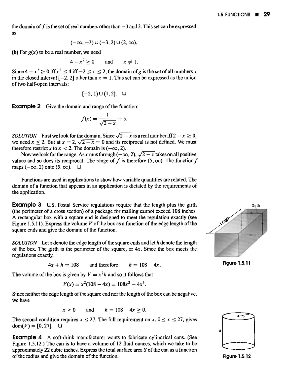
ONE VARIABLE
1807C
®wiley|
2 0 0 7?
JOHN WILEY & SONS, INC.

This text is devoted to the study of single variable calculus. While applications from
the sciences, engineering, and economics are often used to motivate or illustrate
mathematical ideas, the emphasis is on the three basic concepts of calculus: limit, derivative,
and integral.
This edition is the result of a collaborative effort with S.L. Salas, who scrutinized
every single sentence in the text for possible improvement in precision and readability.
His gift for writing and his uncompromising standards of mathematical accuracy and
clarity illuminate the beauty of the subject while increasing its accessibility to students.
It has been a pleasure for me to work with him.
FEATURES OF THE TENTH EDITION
Precision and Clarity
The emphasis is on mathematical exposition; the topics are treated in a clear and
understandable manner. Mathematical statements are careful and precise; the basic
concepts and important points are not obscured by excess verbiage.
Balance of Theory and Applications
Problems drawn from the physical sciences are often used to introduce basic concepts
in calculus. In turn, the concepts and methods of calculus are applied to a variety of
problems in the sciences, engineering, business, and the social sciences through text
examples and exercises. Because the presentation is flexible, instructors can vary the
balance of theory and applications according to the needs of their students.
Accessibility
This text is designed to be completely accessible to the beginning calculus student
without sacrificing appropriate mathematical rigor. The important theorems are explained

and proved, and the mathematical techniques are justified. These may be covered or
omitted according to the theoretical level desired in the course.
Visualization
The importance of visualization cannot be over-emphasized in developing students'
understanding of mathematical concepts. For that reason, over 1200 illustrations
accompany the text examples and exercise sets.
Technology
The technology component of the text has been strengthened by revising existing
exercises and by developing new exercises. Well over half of the exercise sets have problems
requiring either a graphing utility or a computer algebra system (CAS). Technology
exercises (designated by ^) are designed to illustrate or expand material developed
within the sections.
Projects
Projects with an emphasis on problem solving offer students the opportunity to
investigate a variety of special topics that supplement the text material. The projects typically
require an approach that involves both theory and applications, including the use of
technology. Many of the projects are suitable for group-learning activities.
Early Coverage of Differential Equations
Differential equations are formally introduced in Chapter 7 in connection with
applications to exponential growth and decay. First-order linear equations, separable equations,
and second linear equations with constant coefficients, plus a variety of applications,
arc treated in a separate chapter immediately following the techniques of integration
material in Chapter 8.
CHANGES IN CONTENT AND ORGANIZATION
In our effort to produce an even more effective text, we consulted with the users of the
Ninth Edition and with other calculus instructors. Our primary goals in preparing the
Tenth Edition were the following:
1. Improve the exposition. As noted above, every topic has been examined for possible
improvement in the clarity and accuracy of its presentation. Essentially every section
in the text underwent some revision; a number of sections and subsections were
completely rewritten.
2. Improve the illustrative examples. Many of the existing examples have been
modified to enhance students* understanding of the material. New examples have been
added to sections that were rewritten or substantially revised
3. Revise the exercise sets. Every exercise set was examined for balance between drill
problems, midlevel problems, and more challenging applications and conceptual
problems. In many instances, the number of routine problems was reduced and new
midlevel to challenging problems were added.
Specific changes made to achieve these goals and meet the needs of today's students
and instructors include:

Comprehensive Chapter-End Review Exercise Sets
The Skill Mastery Review Exercise Sets introduced in the Ninth Edition have been
expanded into chapter-end exercise sets. Each chapter concludes with a comprehensive
set of problems designed to test and to re-enforce students' understanding of basic
concepts and methods developed within the chapter. These review exercise sets average
over 50 problems per set.
Precalculus Review (Chapter 1)
The subject matter of this chapter—inequalities, basic analytic geometry, the function
concept and the elementary functions—is unchanged. However, much of the material
has been rewritten and simplified.
Limits (Chapter 2)
The approach to limits is unchanged, but many of the explanations have been revised.
The illustrative examples throughout the chapter have been modified, and new examples
have been added.
Differentiation and Applications (Chapters 3 and 4)
There are some significant changes in the organization of this material. Realizing that
our treatments of linear motion, rates of change per unit time, and the Ncwton-Raphson
method depended on an understanding of increasing/decreasing functions and the
concavity of graphs, we moved these topics from Chapter 3 (the derivative) to Chapter 4
(applications of the derivative). Thus. Chapter 3 is now a shorter chapter which focuses
solely on the derivative and the processes of differentiation, and Chapter 4 is expanded
to encompass all of the standard applications of the derivative—curve-sketching,
optimization, linear motion, rates of change, and approximation. As in all previous editions,
Chapter 4 begins with the mean-value theorem as the theoretical basis for all the
applications.
Integration and Applications (Chapters 5 and 6)
In a brief introductory section, area and distance are used to motivate the definite
integral in Chapter 5. While the definition of the definite integral is based on upper and
lower sums, the connection with Riemann sums is also given. Explanations, examples,
and exercises throughout Chapters 5 and 6 have been modified, but the topics and
organization remain as in the Ninth Edition.
The Transcendental Functions, Techniques of Integration
(Chapters 7 and 8)
The coverage of the inverse trigonometric functions (Chapter 7) has been reduced
slightly. The treatment of powers of the trigonometric functions (Chapter 8) has been
completely rewritten. The optional sections on first-order linear differential equations
and separable differential equations have been moved to Chapter 9, the new chapter on
differential equations.
Some Differential Equations (Chapter 9)
This new chapter is a brief introduction to differential equations and their applications.
In addition to the coverage of first-order linear equations and separable equations noted

above, we have moved the section on second-order linear homogeneous equations with
constant coefficients from the Ninth Edition's Chapter 18 to this chapter.
Sequences and Series (Chapters 11 and 12)
Efforts were made to reduce the overall length of these chapters through rewriting
and eliminating peripheral material. Eliminating extraneous problems reduced several
exercise sets. Some notations and terminology have been modified to be consistent with
common usage.
SUPPLEMENTS
An Instructor's Solutions Manual, ISBN 0470127309, includes solutions for all
problems in the text
A Student Solutions Manual, ISBN 0470105534, includes solutions for selected
problems in the text.
A Companion Web site, www.wiley.com/college/salas, provides a wealth of resources
for students and instructors, including:
• PowerPoint Slides for important ideas and graphics for study and note taking.
• Online Review Quizzes to enable students to test their knowledge of key concepts.
For further review diagnostic feedback is provided that refers to pertinent sections of
the text.
• Animations comprise a series of interactive Java applets that allow students to explore
the geometric significance of many major concepts of Calculus.
• Algebra and Trigonometry Refreshers is a self-paced, guided review of key algebra
and trigonometry topics that are essential for mastering calculus.
• Personal Response System Questions provide a convenient source of questions to
use with a variety of personal response systems.
• Printed Test Bank contains static tests which can be printed for quick tests.
• Computerized Test Bank includes questions from the printed test bank with
algorithmically generated problems.
WILEYPLUS
Expect More from Your Classroom Technology
This text is supported by WileyPLUS—a powerful and highly integrated suite of
teaching and learning resources designed to bridge the gap between what happens in the
classroom and what happens at home. WileyPLUS includes a complete online version
of the text, algorithmically generated exercises, all of the text supplements, plus course
and homework management tools, in one easy-to-use website.
Organized Around the Everyday Activities You Perform in Class,
WileyPLUS Helps You:
Prepare and present: WileyPLUS lets you create class presentations quickly and
easily using a wealth of Wiley-provided resources, including an online version of the
textbook, PowerPoint slides, and more. You can adapt this content to meet the needs
of your course.

Create assignments: WileyPLUS enables you to automate the process of assigning
and grading homework or quizzes. You can use algorithmically generated problems
from the text's accompanying test bank, or write your own.
Track student progress: An instructor's grade book allows you to analyze individual
and overall class results to determine students' progress and level of understanding.
Promote strong problem-solving skills: WileyPLUS can link homework problems to
the relevant section of the online text, providing students with context-sensitive help.
WileyPLUS also features mastery problems that promote conceptual understanding
of key topics and video walkthroughs of example problems.
Provide numerous practice opportunities: Algorithmically generated problems
provide unlimited self-practice opportunities for students, as well as problems for
homework and testing.
Support varied learning styles: WileyPLUS includes the entire text in digital format,
enhanced with varied problem types to support the array of different student learning
styles in today's classroom.
Administer your course: You can easily integrate WileyPLUS with another course
management system, grade books, or other resources you are using in your class,
enabling you to build your course your way.
WileyPLUS Includes A Wealth of Instructor and Student Resources:
Student Solutions Manual: Includes worked-out solutions for all odd-numbered
problems and study tips.
Instructor's Solutions Manual: Presents worked out solutions to all problems.
PowerPoint Lecture Notes: In each section of the book a corresponding set of lecture
notes and worked out examples are presented as PowerPoint slides that are tied to
the examples in the text.
View an online demo at www.wiley.com/college/wileyplus or contact your local
Wiley representative for more details.
The Wiley Faculty Network—Where Faculty Connect
The Wiley Faculty Network is a faculty-to-faculty network promoting the effective use
of technology to enrich the teaching experience. The Wiley Faculty Network facilitates
the exchange of best practices, connects teachers with technology and helps to enhance
instructional efficiency and effectiveness. The network provides technology training
and tutorials, including WileyPLUS training, online seminars, peer-to-peer exchanges
of experiences and ideas, personalized consulting, and sharing of resources.
Connect with a Colleague
Wiley Faculty Network mentors are faculty like you, from educational institutions
around the country, who are passionate about enhancing instructional efficiency and
eflFectiveness through best practices. You can engage a faculty mentor in an online
conversation at www.whcrefacultyconnect.com.
Connect with the Wiley Faculty Network
Web: www.wherefacultyconnect.com
Phone: 1-866-FACULTY

CHAPTER 1 PRECALCULUS REVIEW 1
1.1 What is Calculus? 1
1.2 Review of Elementary Mathematics 3
1.3 Review of Inequalities 11
1.4 Coordinate Plane; Analytic Geometry 17
1.5 Functions 24
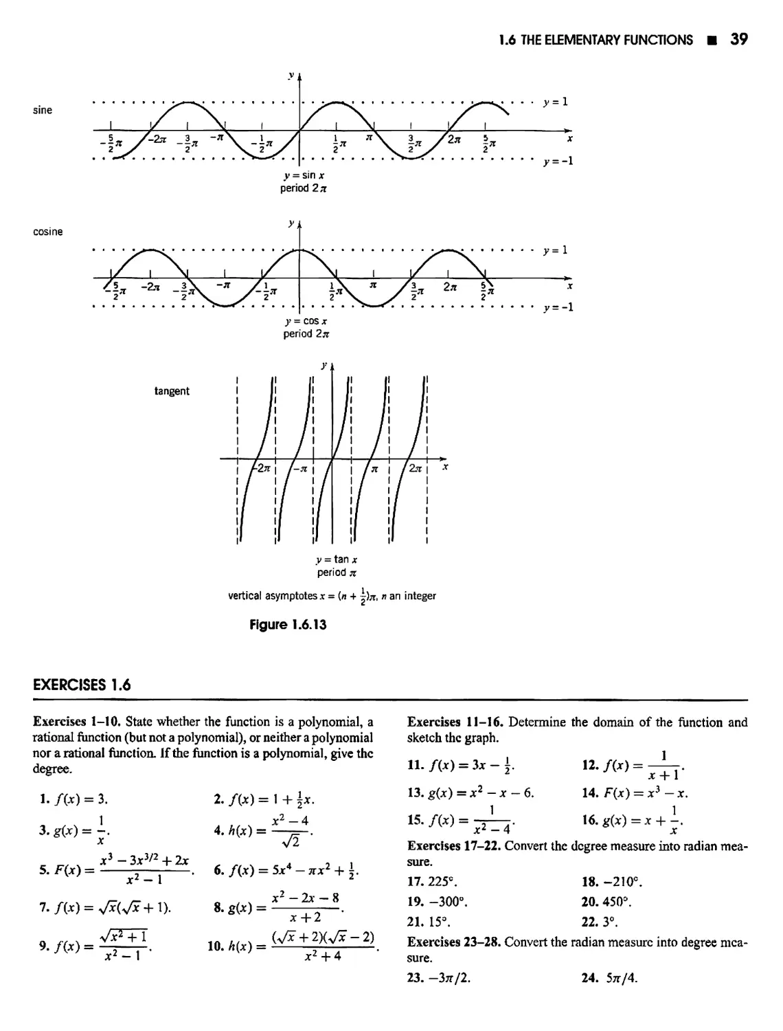
1.6 The Elementary Functions 32
1.7 Combinations of Functions 41
1.8 A Note on Mathematical Proof; Mathematical Induction 47
CHAPTER 2 LIMITS AND CONTINUITY 53
2.1 The Limit Process (An Intuitive Introduction) 53
2.2 Definition of Limit 64
2.3 Some Limit Theorems 73
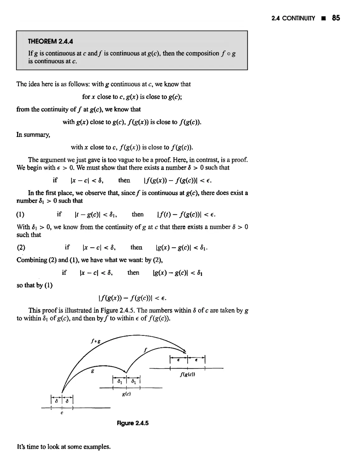
24 Continuity 82
2.5 The Pinching Theorem; Trigonometric Limits 91
2.6 Two Basic Theorems 97
Project 2.6 The Bisection Method for Finding the Roots of /(jc) = 0 102

XVI
CONTENTS
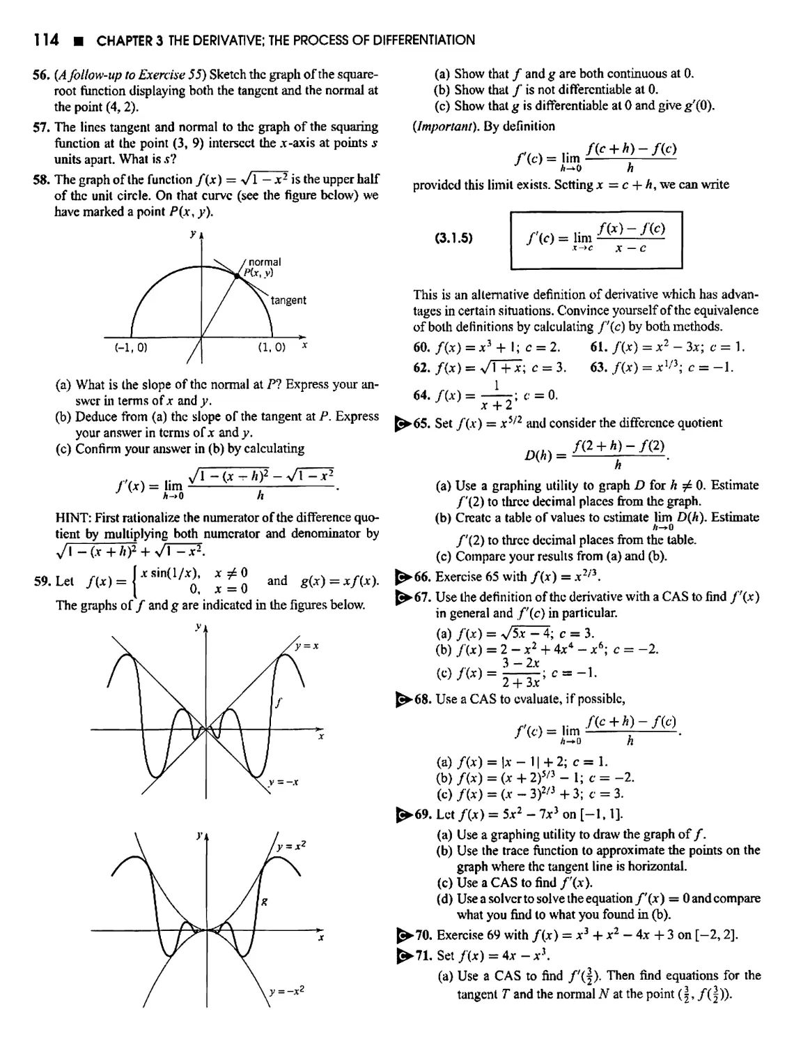
CHAPTER 3 THE DERIVATIVE; THE PROCESS OF DIFFERENTIATION 105
3.1 The Derivative 105
3.2 Some Differentiation Formulas 115
3.3 The d/dx Notation; Derivatives of Higher Order 124
3.4 The Derivative As A Rate of Change 130
3.5 The Chain Rule 133
3.6 Differentiating The Trigonometric Functions 142
3.7 Implicit Differentiation; Rational Powers 147
1
a
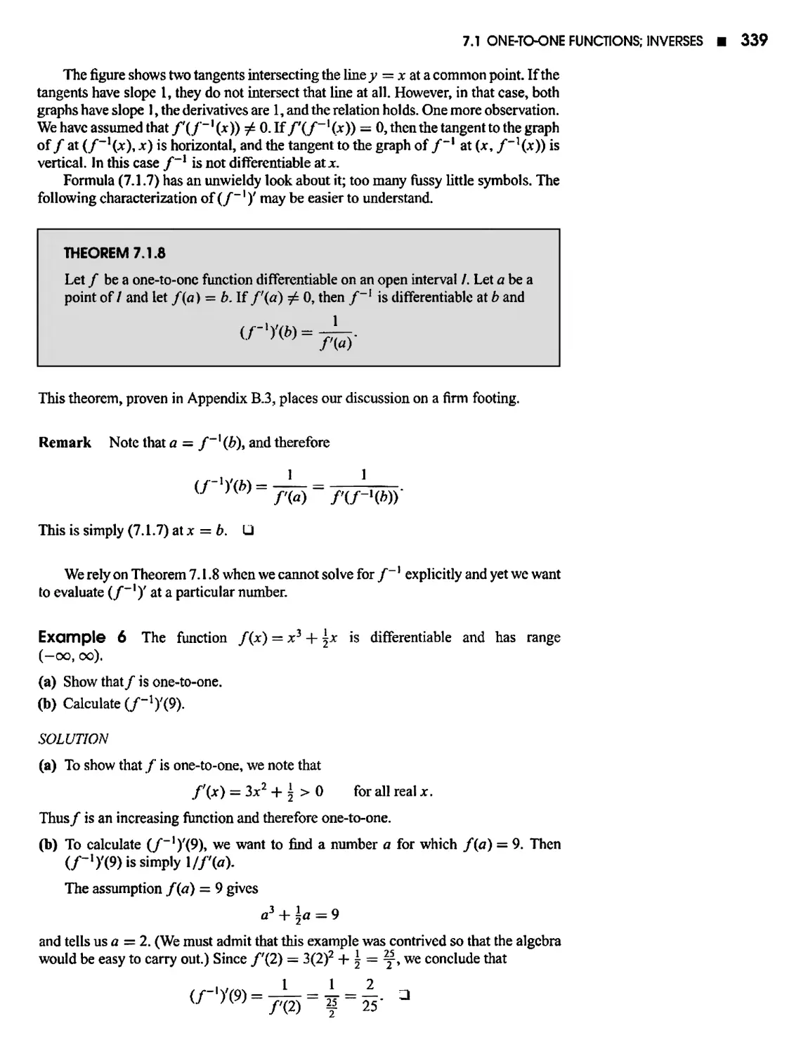
tl», fib))
b
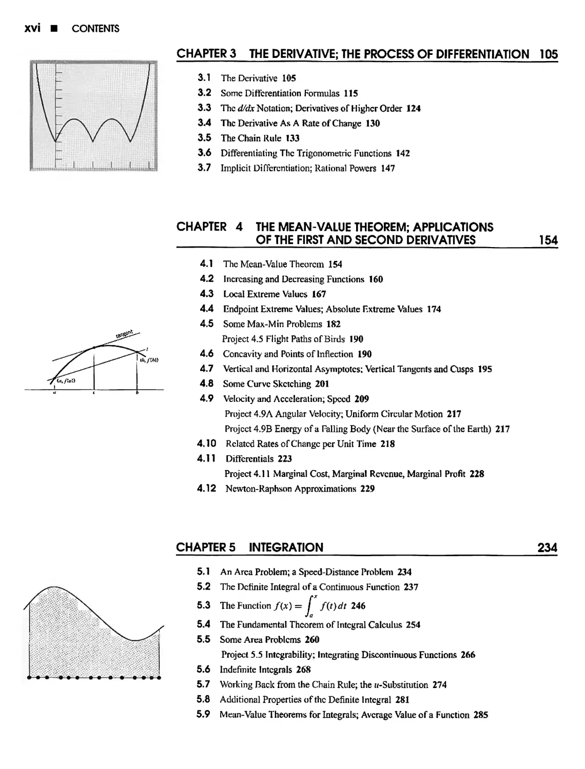
CHAPTER 4 THE MEAN-VALUE THEOREM; APPLICATIONS
OF THE FIRST AND SECOND DERIVATIVES 154
4.1 The Mean-Value Theorem 154
4.2 Increasing and Decreasing Functions 160
4.3 Local Extreme Values 167
4.4 Endpoint Extreme Values; Absolute Extreme Values 174
4.5 Some Max-Min Problems 182
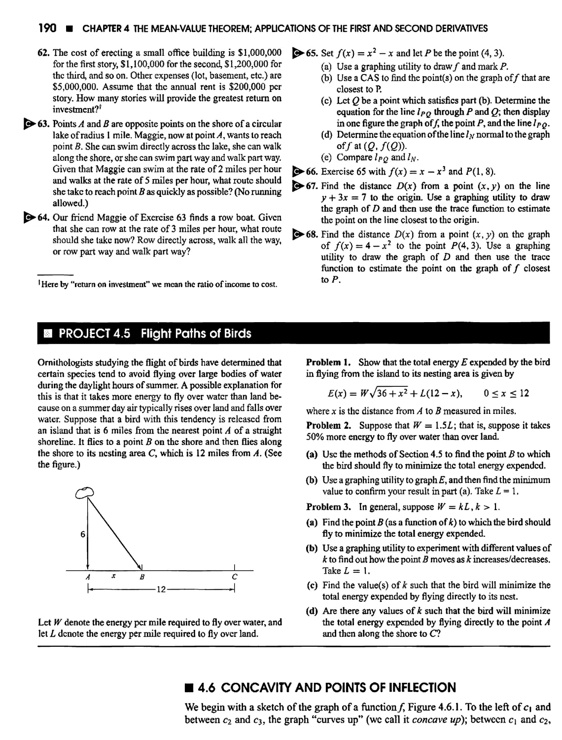
Project 4.5 Flight Paths of Birds 190
4.6 Concavity and Points of Inflection 190
4.7 Vertical and Horizontal Asymptotes; Vertical Tangents and Cusps 195
4.8 Some Curve Sketching 201
4.9 Velocity and Acceleration; Speed 209
Project 4.9A Angular Velocity; Uniform Circular Motion 217
Project 4.9B Energy of a Falling Body (Near the Surface of the Earth) 217
4.10 Related Rates of Change per Unit Time 218
4.11 Differentials 223
Project 4.11 Marginal Cost. Marginal Revenue, Marginal Profit 228
4.12 Newton-Raphson Approximations 229
CHAPTER 5 INTEGRATION
234
5.1
5.2
5.3
5.4
5.5
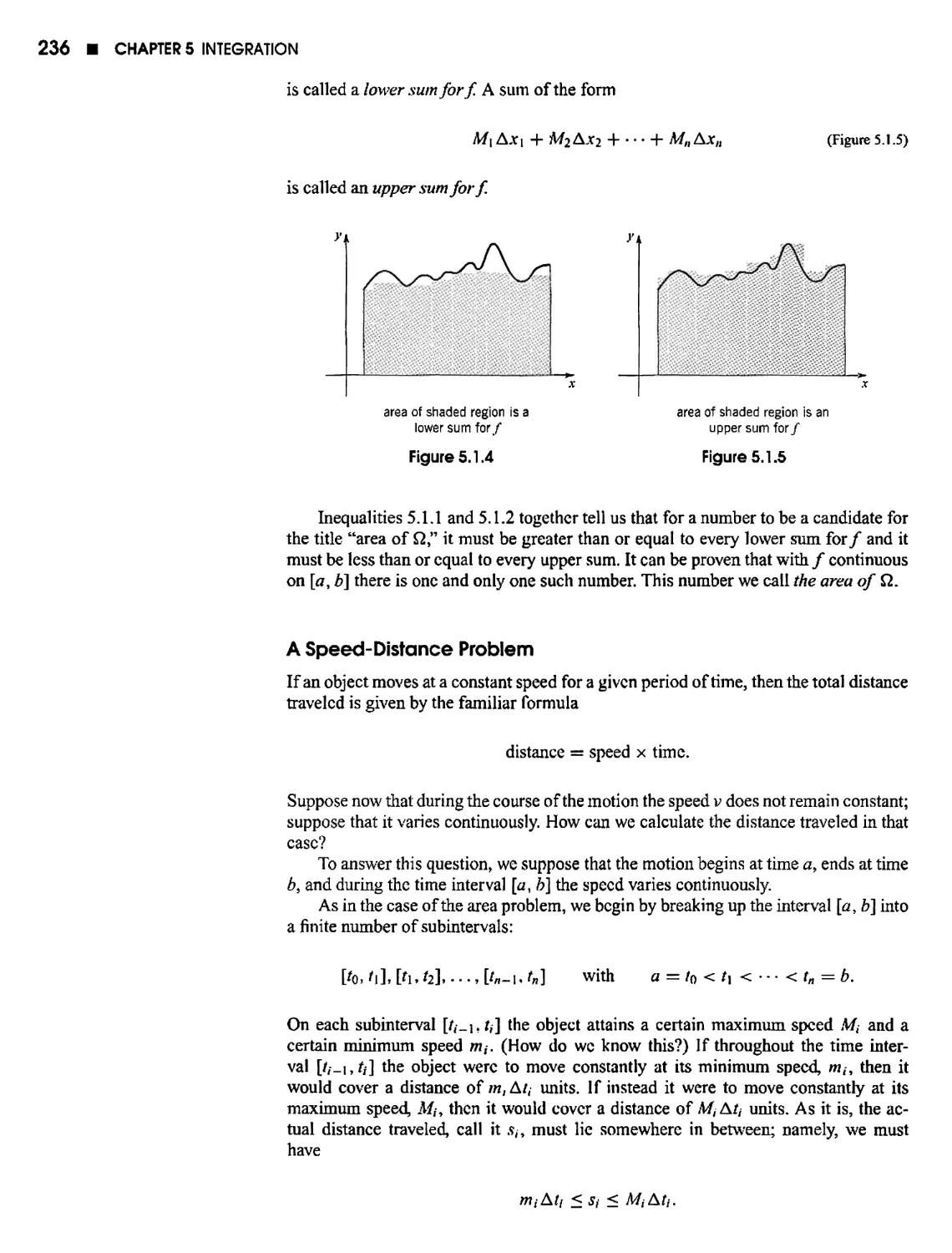
An Area Problem; a Speed-Distance Problem 234
The Definite Integral of a Continuous Function 237
The Function /(*) = / f(f)dt 246
The Fundamental Theorem of Integral Calculus 254
Some Area Problems 260
Project 5.5 Integrability; Integrating Discontinuous Functions 266
5.6 Indefinite Integrals 268
5.7 Working Back from the Chain Rule; the ^-Substitution 274
5.8 Additional Properties of the Definite Integral 281
5.9 Mean-Value Theorems for Integrals; Average Value of a Function 285

CHAPTER 6 SOME APPLICATIONS OF THE INTEGRAL 292
6.1 More on Area 292
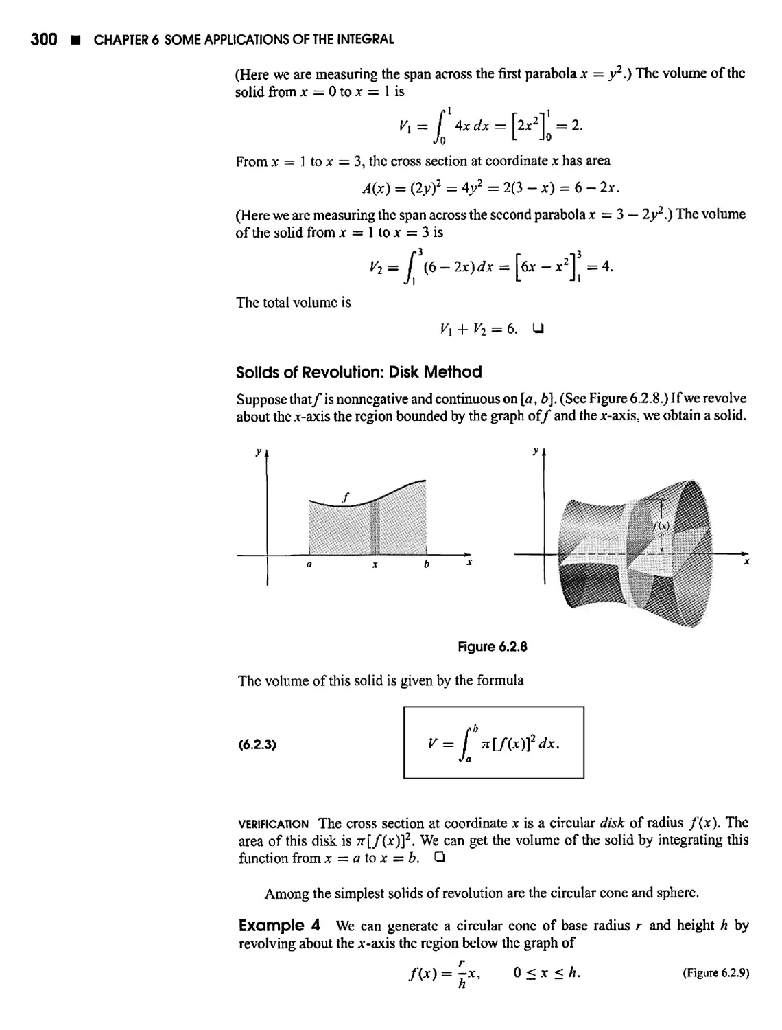
6.2 Volume by Parallel Cross Sections; Disks and Washers 296
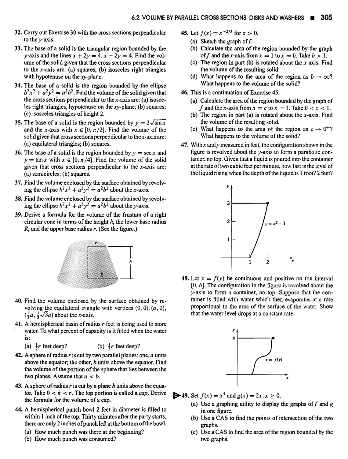
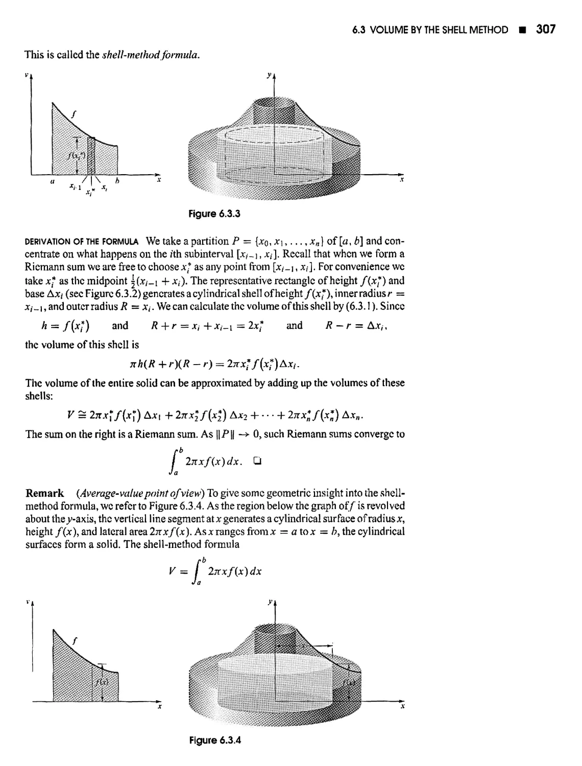
6.3 Volume by the Shell Method 306
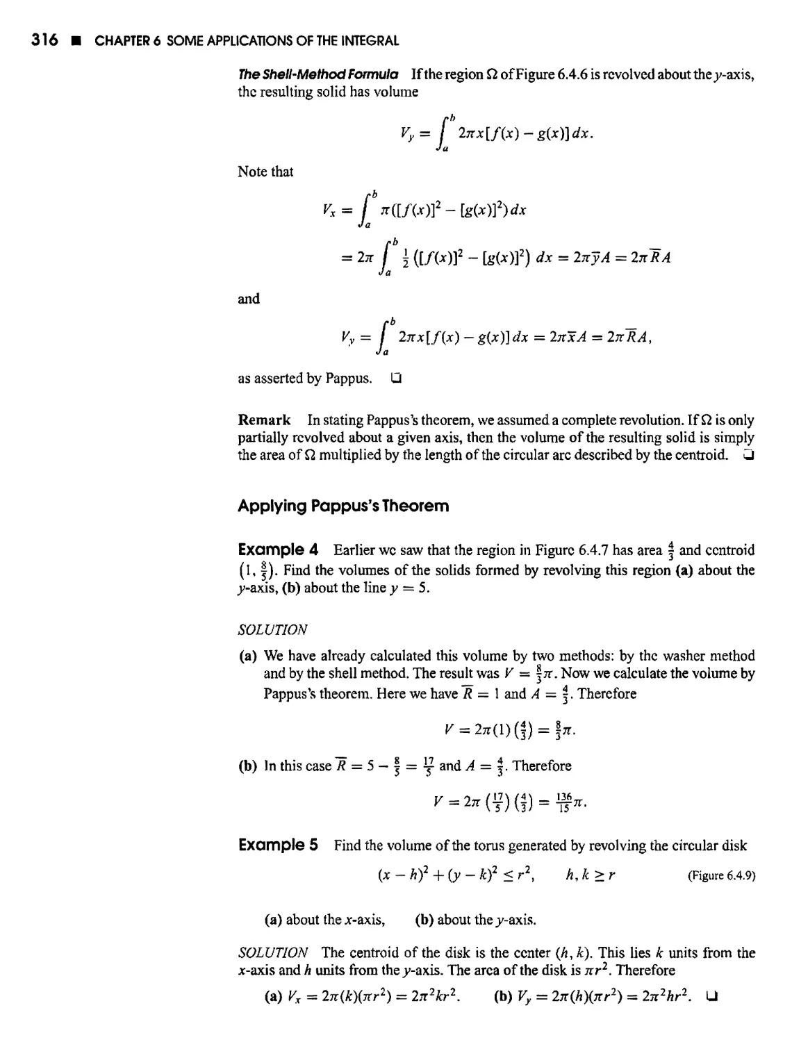
6.4 The Centroid of a Region; Pappus's Theorem on Volumes 312
Project 6.4 Centroid of a Solid of Revolution 319
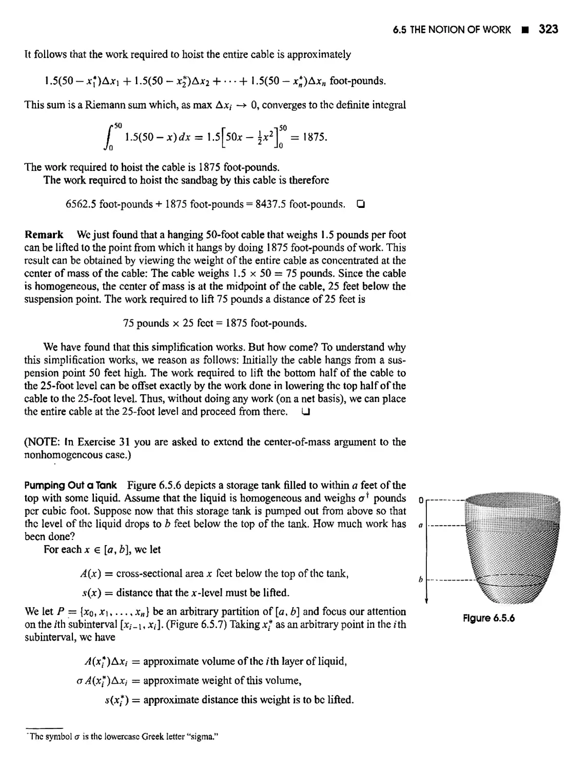
6.5 The Notion of Work 319
#6.6 Fluid Force 327
CHAPTER 7 THE TRANSCENDENTAL FUNCTIONS 333
7.1 One-to-One Functions; Inverses 333
7.2 The Logarithm Function, Part I 342
7.3 The Logarithm Function, Part II 347
7.4 The Exponential Function 356
Project 7.4 Some Rational Bounds for the Number e 364
7.5 Arbitrary Powers; Other Bases 364
7.6 Exponential Growth and Decay 370
7.7 The Inverse Trigonometric Functions 378
Project 7.7 Refraction 387
7.8 The Hyperbolic Sine and Cosine 388
#7.9 The Other Hyperbolic Functions 392
CHAPTER 8 TECHNIQUES OF INTEGRATION 398
8.1 Integral Tables and Review 398
8.2 Integration by Parts 402
Project 8.2 Sine Waves y = smnx and Cosine Wavesy — cosnx 410
8.3 Powers and Products of Trigonometric Functions 411
8.4 Integrals Featuring Vo2 - x2< */a2 -\-x2, V*2 - a2 417
8.5 Rational Functions; Partial Fractions 422
*8.6 Some Rationalizing Substitutions 430
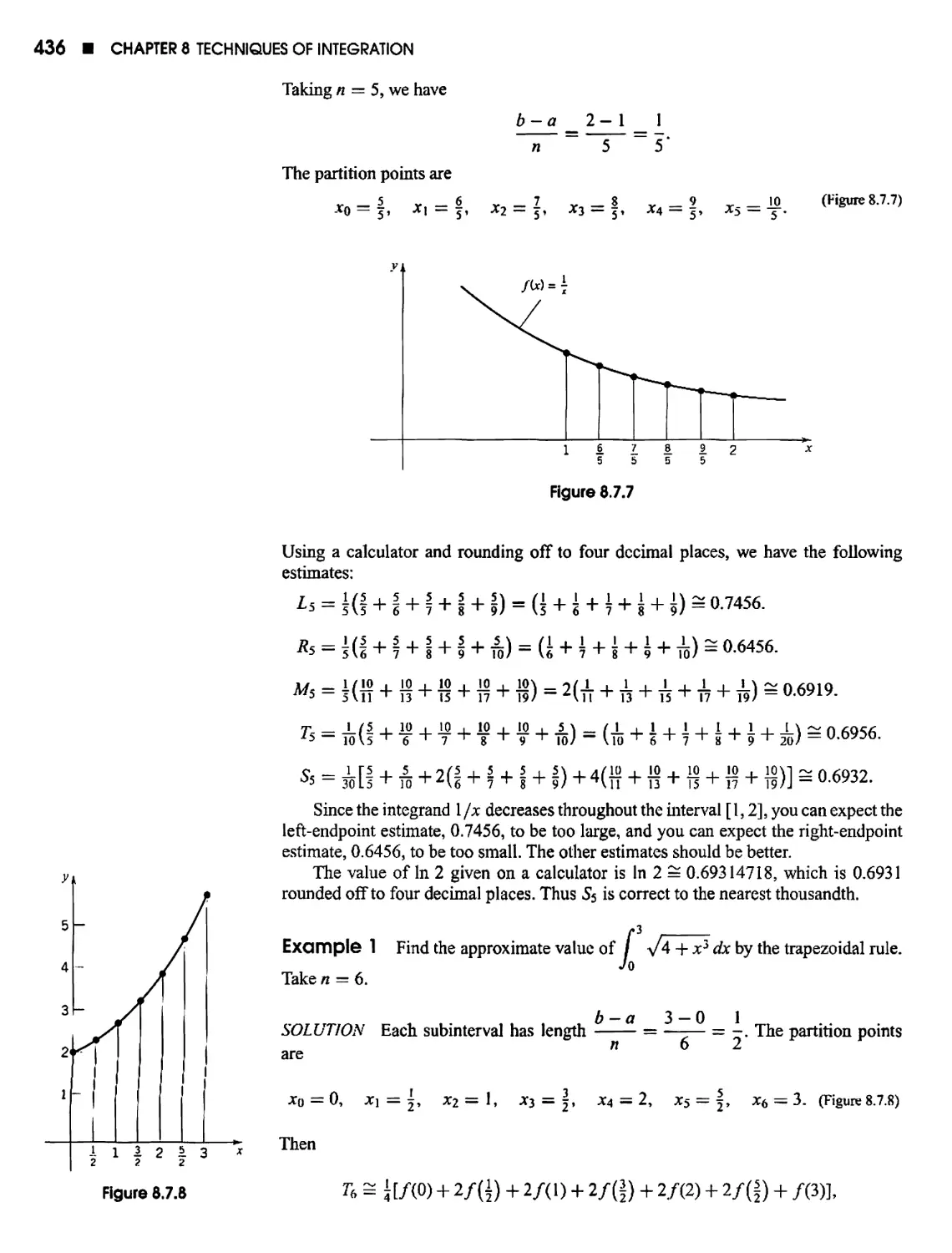
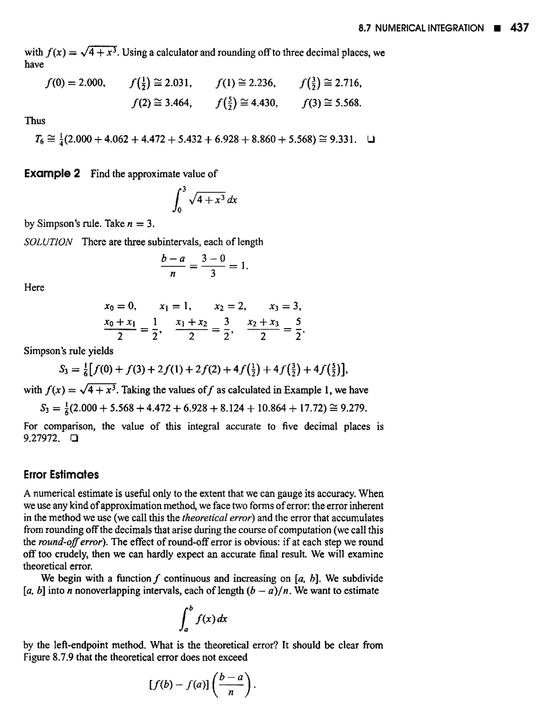
8.7 Numerical Integration 433
CHAPTER 9 SOME DIFFERENTIAL EQUATIONS 443
9.1 First-Order Linear Equations 444
9.2 Integral Curves; Separable Equations 451
Project 9.2 Orthogonal Trajectories 458
9.3 The Equation y" -t- ay + by = 0 459
"Denotes optional section.

XViii ¦ CONTENTS
CHAPTER 10 THE CONIC SECTIONS; POLAR COORDINATES;
PARAMETRIC EQUATIONS
469
10.1 Geometry of Parabola, Ellipse, Hyperbola 469
10.2 Polar Coordinates 478
10.3 Sketching Curves in Polar Coordinates 484
Project 103 Parabola, Ellipse, Hyperbola in Polar Coordinates 491
10.4 Area in Polar Coordinates 492
10.5 Curves Given Parametrically 496
Project 10.5 Parabolic Trajectories 503
10.6 Tangents to Curves Given Parametrically 503
10.7 Arc Length and Speed 509
10.8 The Area of A Surface of Revolution; The Centroid of a Curve; Pappus's Theorem
on Surface Area 517
Project 10.8 The Cycloid 525
CHAPTER 11 SEQUENCES; INDETERMINATE FORMS;
IMPROPER INTEGRALS
528
11.1 The Least Upper Bound Axiom 528
11.2 Sequences of Real Numbers 532
11.3 Limit of a Sequence 538
Project 11.3 Sequences and the Newton-Raphson Method 547
11.4 Some Important Limits 550
11.5 The Indeterminate Form (0/0) 554
11.6 The Indeterminate Form (oo/oo); Other Indeterminate Forms 560
11.7 Improper Integrals 565
I Mx)
CHAPTER 12 INFINITE SERIES
575
-W
12.1 Sigma Notation 575
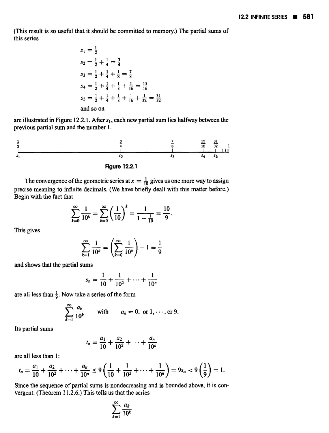
12.2 Infinite Series 577
12.3 The Integral Test; Basic Comparison, Limit Comparison 585
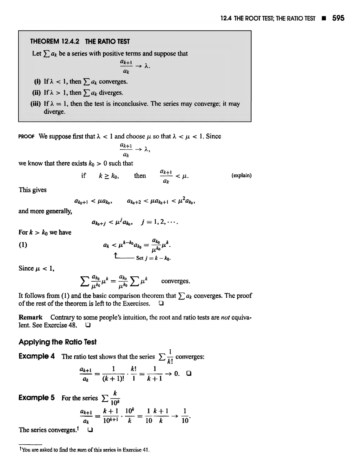
12.4 The Root Test; the Ratio Test 593
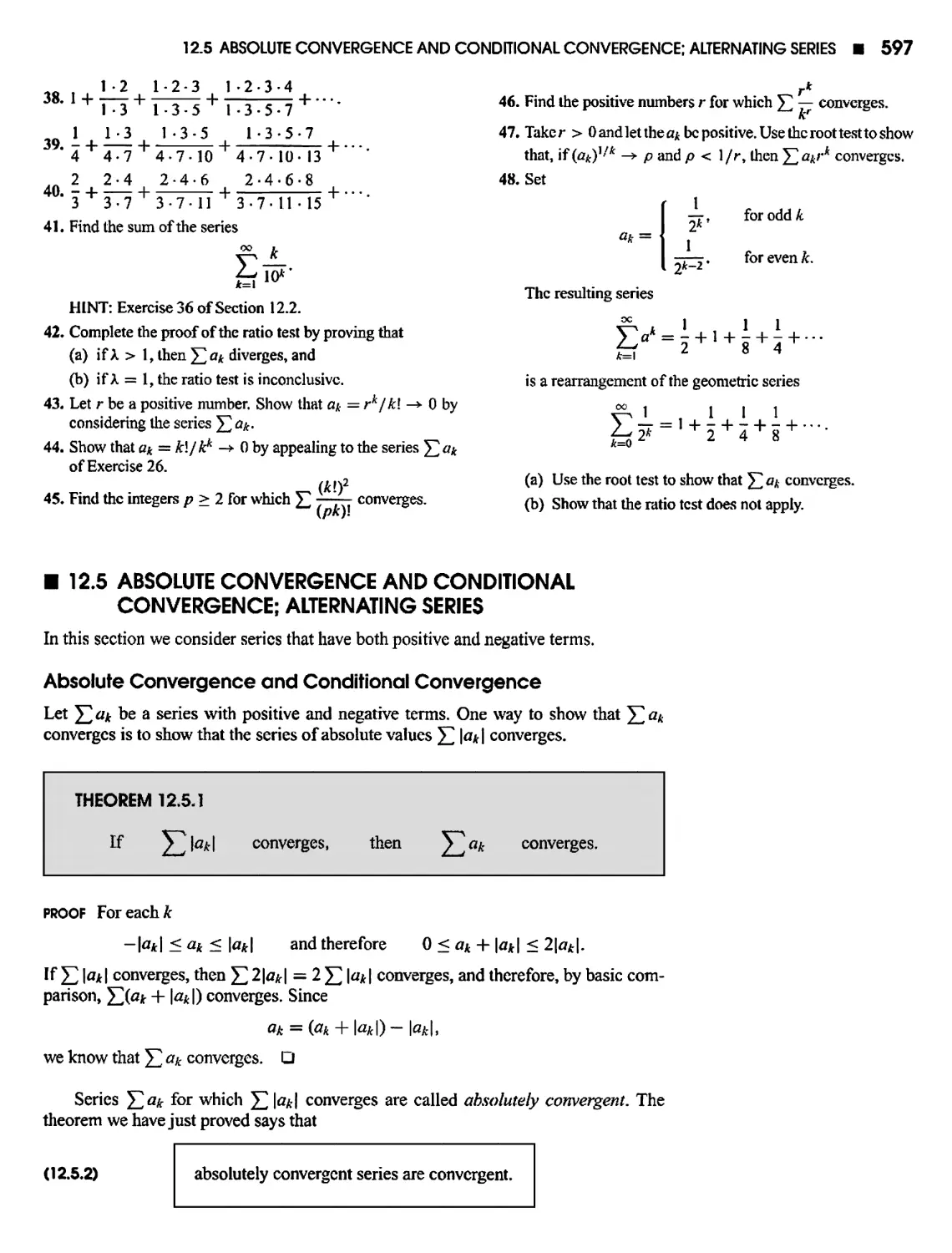
12.5 Absolute Convergence and Conditional Convergence; Alternating Series 597
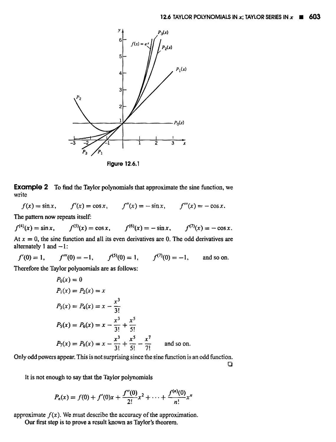
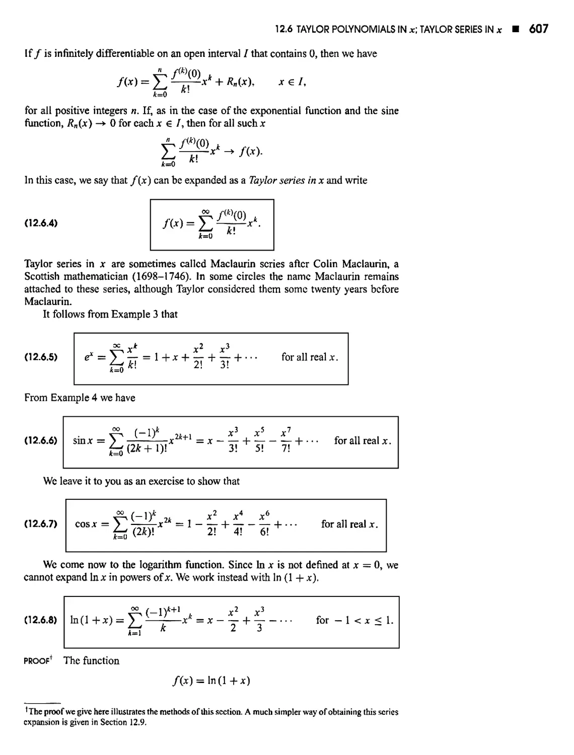
12.6 Taylor Polynomials in x; Taylor Series in x 602
12.7 Taylor Polynomials and Taylor Series in x — a 613
12.8 Power Series 616
12.9 Differentiation and Integration of Power Series 623
Project 12.9AThe Binomial Series 633
Project 12.9B Estimating n 634

APPENDIX A SOME ADDITIONAL TOPICS
A-1
A.l Rotation of Axes; Eliminating the Av-Term A-1
A.2 Determinants A-3
APPENDIX B SOME ADDITIONAL PROOFS A^
B.I The Intermediate-Value Theorem A-8
B.2 Boundcdness; Extreme-Value Theorem A-9
B.3 Inverses A-10
B.4 The Imcgrability of Continuous Functions A-ll
B.5 The Integral as the Limit of Riemann Sums A-14
ANSWERS TO ODD-NUMBERED EXERCISES A-15
Index 1-1
Table of Integrals Inside Covers

TABLES OF INTEGRALS
POWERS
/un*1 f du
u*du = - + C/2#-l 2. /— = ln|w| + C
n-fl J u
EXPONENTIALS AND LOGARITHMS
3. [e*du = eu+C 4. fpudu=^- + C
5. f ueudu = ueu-eu + C 6. f u2eudu = wV -2ueu +2eu + C
7. f u*eudu = uneu -n f un~leudu 8. f Inudu = ulnu-u+ C
9. j(lnu)2du = u(\nu)2-2ulnu + 2u + C 10. / u\r\udu= ±w2lnw- \u2 + C
11. /"tf-lniiA = i/-+,rJ5fL-—I-. 1+e 12. f4^ = ln|lnW| + C
y [w +1 (« + l)2J 7 wlnw
SINES AND COSINES
13. I sinudu =—cosu + C 14. / cosudu = sint/ + C
15. / sin21/ cfo = |w — | sin2w + C 16. I cos2 udu = ju + | sin 2w + C
17. / sin3wt/z/= icos3w — cost/-hC 18. I cos^udu = sinw — jsin3i/ + C
** f n , sin"""1 wcosw n-l f . n_2 ,
19. / sin"w </w = + / wf 2udu
J n n J
~~ f cosw~,wsinw n — \f ~
20. / cos" udu = 1 / cos" l u du
J n n J
21. / usinudu = —wcosw + sinw + C 22. J wcoswdw = wsinw+ cosw+ C
23. I un sinudu =-un cosu + n I un~l cosudu 24. I un cosudu = un sinu - n J un~l sinu
+- f . . .sin [(/w - /t)w] sin [(m + #i)i/] 2/2
25. / s\nmusmnudu= —-?-—-^-± ^VL , .^ + C> m r n
du
2{m - n) 2(m + n)
n [(m — n)u] sin [(m + n)
2{m — n) 2{m + ri)
>s [(w — w)«] cos [(m + j
2(/w — n) 2(m + «)
~ f , sin[(ro-n)w] sin [(m + n)u] 2 2
26. cos mu cos nudu = —?-—-f-^ + ^_ t x + C, m2 ^ n2
*~ f • , cos[(w-w)«] cos [(/w + w )a] ^ 5/5
27. / sin mu cos nu du = ^—-^ ^ t / J + C, m2 ? n2
28. / eausin6w</w = *t L,(asinbu — bcosbu) + C
eflM cos 6w tfw = -=—-r (a cos bu + 6 sin 6w) + C
a2 + o2

TANGENTS AND SECANTS
30
i. / tanudu = ln|secw| + C 31. / SQeudu = In|secw + tanw| + C
32, / tan2 u du = tan u — u + C 33. / sec2 u du = tan u + C
34. / secwtanwrfw = secw + C 35. / tan3w*/a = |tan2w-}-ln|cosw|+ C
36. / sec3 udu= | sect/tanw + | ln|secw + tanw| + C
-*„ f * , tan""1 ii f „_7 , „ f n , sec*"2iitan« n-2 f „2 ,
37. I tan'1 m^/h = / tan" 2udu 38. / sec" udu = + / secn~2udu
J n —\ J J n-\ n — \J
CONTANGENTS AND COSECANTS
39, / cot it du = In | sin u \ + C 40. / esc u du — In |csc u - cotu\ + C
41. / co1?udu = -cotw — u + C 42. / esc2udu = — cotw + C
43. / escweotwdu = — cscw + C 44. / cot3 udu = — ^cot2u — ln|sinw| + C
45. / ess? udu = -icscw cotw + |ln|csct/— cotw| + C
/cot""1 u f o
cof a </w = 1 / cof1"2 w rfu
(rfj/
Awm f „ , cscn~2i/cotw n-2 f n ,
47. / esc"udu = 1- I cscn"2ui
J n— I n — 1 J
HYPERBOLIC FUNCTIONS
48. / sinhwtfw = coshu + C 49. / coshw^/w = sinha + C
50. / tanh u du = In (cosh w) + C 51. / coth u du = In | sinh u\ + C
52. / sech u du = arctan (sinh w) + C 53. / csch u du = In | tanh ?u| + C
54. I scch2wrfw = tanha + C 55. / csch2udu = -cothm + C
56. I sech m tanh w Ju = —sech u + C 57. / csch u coth w rfw = —csch u + C
58. / sinh2 udu = ? sinh2w - |w + C 59. / cosh2 udu = | sinh2m 4- ?w 4- C
60. / tanh2udu = u -tanhw + C 61. I coih2udu = u-cothu + C
62. / w sinh udu — u cosh w — sinh w + C 63. / u cosh udu = u sinh w — cosh u + C
{fable continued at the back)

{continued fivm the front)
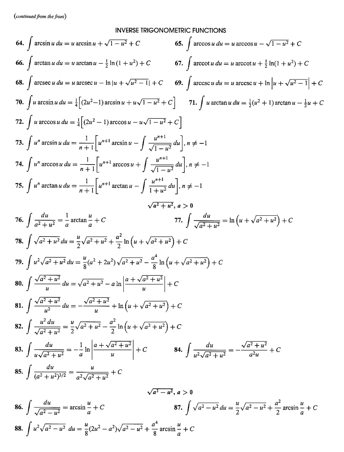
INVERSE TRIGONOMETRIC FUNCTIONS
64. / arcsinudu = u arcsinu + Vl — w2 + C 65. / arccosudu = u arccos& — Vl — w2 + C
66. / arctan w du = w arctan w — ^ In (I + u2) + C 67. / arccot udu = u arccot a + ^ ln(l +u2) + C
68. / arcsecudu = u arcsec*< — In |u + +Ju2 - 11 + C 69. / arccscu da = a arccscw + In \u + «Ju2 — 1 + C
70. / u arcsinwdu = ? (2a2—1)arcsinu + u^\ —u2 + C 71. / u axotmudu = \{u2 + 1)arctanu — \u + C
72. / uarccoswA* = | (2*/2 — 1)arccosu — u^j\ -u2 + C\
73. / u" arcsmudu = k,,+1 arcsinu — / //»! »=?—1
74. / mw arccos udu = w"+1 arccos w + / //» L«^-l
75. / un arctan u <ia = mw+i arctanw — / =¦ duLn±—\
\Za2 + «2,* > 0
„^ [ dll \ U „ f du / r-z r\ „
76. / — - = -arctan- + C 77. / = Iil(u+ y/a2+u2)+C
J a2 + u2 a a J Ja2 + u2 \ '
/2
Ja2 + u2du = *tja2 + u2 + %- In (it + Va2 + u2\ + C
/4
u2s/a2+u2du = |(a2 + 2a2) VV + w2 - y In (« + Ja2 + a2) + C
fja2 + u2 rrr-2 i |a + Va2 + «2| , ^
J u \ u \
80
81
82
Va2 + u2 , yfaTTu1
J u
du = —
+
]n(u + y/a2 + u2)+C
83. /_^= = -Iln
J uWa2 + u2 a
: + Vtf2 + u2
+ C
84./-
du
Va2 +
:2\/tf2 + a2
+ C
85.
86
88
'" / {a2 + u
:2)3/2 ^2V^T^
+ c
. = arcsin — + C
-Ja2 -u2 a
i. f u2y/a2 -u2 du = ^(2u2 - a2)y/a2 -u2 + -
Jo c
y/a1 -u2, a > 0
//—z r U /—z r a2 U
s/a2 — u2du = -si a2 —n2-\ arcsin — + C
2 2 a
n arcsin - + C
8 a

™ f va2 - U2 , 1 r-z r . U „ ^ t U2 du U r-z r a2 . 1/ „
90. / - du = —y/a2 - u2 - arcsin- + C 91. / , = --Vfl2 - w2 + — arcsin- + C
J u2 u a J J a1 - w2 2 2 a
a + Va2 — w2
+c 93. / , A" =—Ly^r^+c
7 tfVa2-»2 «2«
92. / —7=== = — In
J wva2 — w2 <*
94. /(a2 - u2)3/2 </u = -|(2«2 - 5a2)V^^2 + ~ arcsin - + C
5- / (a2 - w2)3/2 " a2^2—2 + C 96' / ^^2 - Ya
Ju2-a2, a>0
In
a + w
a — w
+ C
97. / —7===z = - arcsec — + C 98. / — — du = \Ju2 -a2-a arcsec - + C
J w Vw2 - a2 a a J u a
I y/u2-a2du = ^\/w2-a2 - y In L + Vw2-a2| + C
/ iiV«2 - a2 du = ?(2e/2 - a Vi/2 - a2 - ^- In In + v/i/2 - a2| + C
J o o ' I
99.
00.
01.
02.
03.
05.
06.
07.
08.
10.
r V"2 - a2 , -Ju2 -a2 ,i r-z ri „
/ z du = + In m + Vw2 - a2\ + C
J «- « I I
/"2 ^M M r^ ^ °2. I rz rl ~
, , = tVm2 - a2 + — to u + V«2 -a2\ + C
Vw2 — a2 ¦*¦ 2 1 l
/" a*w Vm2 - a2 „ ,n. f d
xr du
a2)3/2 ^V?^2"
+ c
/wdu -u , , /-; „
a + bu, V* + *«
. / " l[ ^Tr(a + bu-ala\a + bu\) + C
J a + bu b2
—r- = ^rr[(a + 6w)2 - 4*(fl + 6") + 2fl2 ln l« + *"l] + c
a + bu 2bi
C 109. f -
du 1 ,
-— = -ln
-±bu) a
a + bu
1 b ,
= + ^ln
2(a 4- bu) au a2
du 1
a + bu
-^rln
a + bu
f—
/u Ju a 1 f di
(a+bu? = b2(a + bu) + b~2^a + M + C Ul-)ul^+bu)2~a(a + bu) a2
C vr du 1 / a2 \
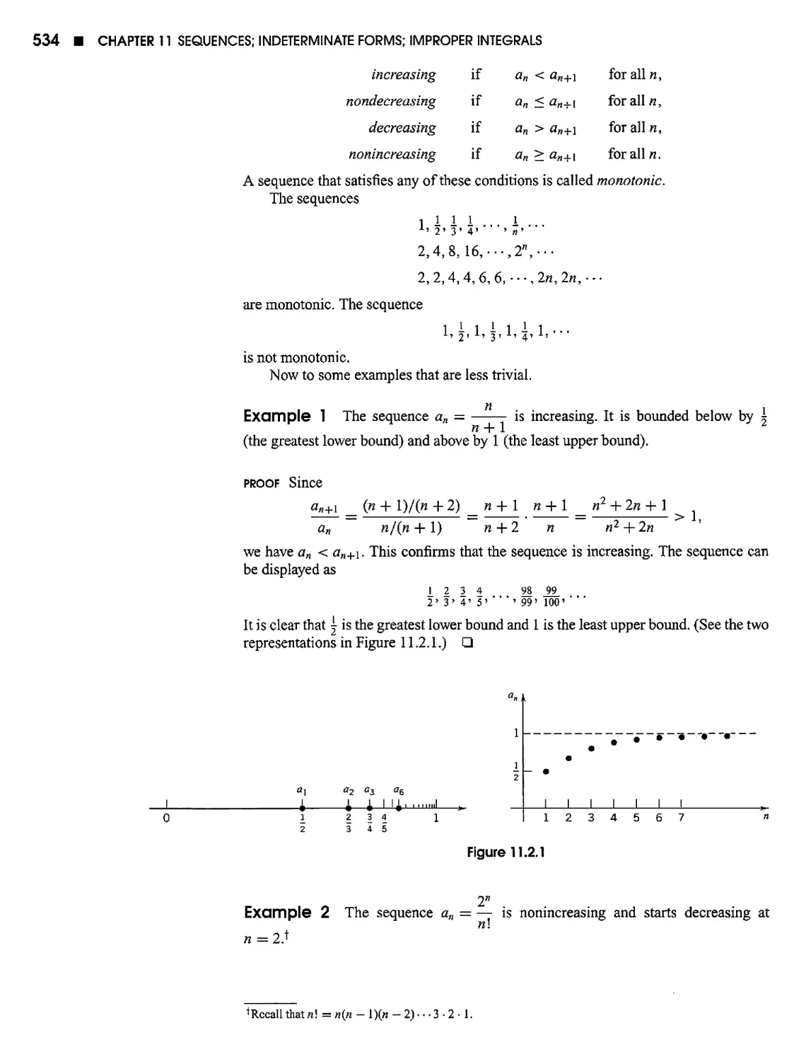
13. / " = -z-h(bu - 2aUa + bu + C 114. / uVaTbu du = —-(3bu -2a)(a + buf<2 + C
J -Ja + bu 3o- J 15r

In this chapter we gather together for reference and review those parts of elementary
mathematics that are necessary for the study of calculus. We assume that you are
familiar with most of this material and that you don't require detailed explanations. But
first a few words about the nature of calculus and a brief outline of the history of the
subject.
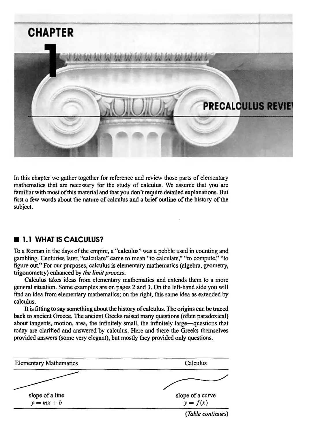
¦ 1.1 WHAT IS CALCULUS?
To a Roman in the days of the empire, a "calculus" was a pebble used in counting and
gambling. Centuries later, "calculare" came to mean "to calculate," "to compute," "to
figure out." For our purposes, calculus is elementary mathematics (algebra, geometry,
trigonometry) enhanced by the limit process.
Calculus takes ideas from elementary mathematics and extends them to a more
general situation. Some examples are on pages 2 and 3. On the left-hand side you will
find an idea from elementary mathematics; on the right, this same idea as extended by
calculus.
It is fitting to say something about the history of calculus. The origins can be traced
back to ancient Greece. The ancient Greeks raised many questions (often paradoxical)
about tangents, motion, area, the infinitely small, the infinitely large—questions that
today are clarified and answered by calculus. Here and there the Greeks themselves
provided answers (some very elegant), but mostly they provided only questions.
Elementary Mathematics Calculus
slope of a line slope of a curve
y = mx + b y = f(x)
(Table continues)

1.2 REVIEW OF ELEMENTARY MATHEMATI
mass of an object mass of an object
of constant density of varying density
center of a sphere center of gravity of
a more general solid
After the Greeks, progress was slow. Communication was limited, and each scholar
was obliged to start almost from scratch. Over the centuries, some ingenious solutions
to calculus-type problems were devised, but no general techniques were put forth.
Progress was impeded by the lack of a convenient notation. Algebra, founded in the
ninth century by Arab scholars, was not fully systematized until the sixteenth century.
Then, in the seventeenth century, Descartes established analytic geometry, and the stage
was set.
The actual invention of calculus is credited to Sir Isaac Newton (1642-1727),
an Englishman, and to Gottfried Wilhelm Leibniz (1646-1716), a German. Newton's
invention is one of the few good turns that the great plague did mankind. The plague
forced the closing of Cambridge University in 1665, and young Isaac Newton of Trinity
College returned to his home in Lincolnshire for eighteen months of meditation, out
of which grew his methodojfluxions', his theory of gravitation, and his theoiy of light.
The method of fluxions is what concerns us here. A treatise with this title was written
by Newton in 1672, but it remained unpublished until 1736, nine years after his death.
The new method (calculus to us) was first announced in 1687, but in vague general
terms without symbolism, formulas, or applications. Newton himself seemed reluctant
to publish anything tangible about his new method, and it is not surprising that its
development on the Continent, in spite of a late start, soon overtook Newton and went
beyond him.
Leibniz started his work in 1673, eight years after Newton. In 1675 he initiated the
basic modern notation: dx and /. His first publications appeared in 1684 and 1686. These
made little stir in Germany, but the two brothers Bernoulli of Basel (Switzerland) took
up the ideas and added profusely to them. From 1690 onward, calculus grew rapidly and
reached roughly its present state in about a hundred years. Certain theoretical subtleties
were not fully resolved until the twentieth century.
¦ 1.2 REVIEW OF ELEMENTARY MATHEMATICS
In this section we review the terminology, notation, and formulas of elementary
mathematics.
Sets
A set is a collection of distinct objects. The objects in a set are called the elements or
members of the set. We will denote sets by capital letters A> B,C,... and use lowercase
letters a, /?, c.... to denote the elements.

CHAPTER 1 PRECALCULUS REVIEW
For a collection of objects to be a set it must be well-defined; that is, given any
object x, it must be possible to determine with certainty whether or not x is an clement
of the set. Thus the collection of all even numbers, the collection of all lines parallel
to a given line /, the solutions of the equation x2 = 9 are all sets. The collection of all
intelligent adults is not a set. It's not clear who should be included.
Notions and Notation
the object x is in the set A x € A
the object x is not in the set A x ? A
the set of all x which satisfy property P {x : P]
({x:*2 = 9} = {-3,3})
A is a subset ofB, A is contained inB A C B
B contains A BOA
the union of A andB A U B
(AUB = {x :x eAorx e B))
the intersection of A and B AD B
(ADB = {x :x e A and x € B})
the empty set 0
These are the only notions from set theory that you will need at this point.
Real Numbers
Classification
positive integers* 1,2,3,...
integers 0,1, —1,2, —2,3, —3,...
rational numbers p/q, with p, q integers, q ^ 0;
for example, 5/2,-19/7, -4/1 = -4
irrational numbers real numbers which are not rational;
for example \/2, \fl, n
Decimal Representation
Each real number can be expressed as a decimal. To express a rational number p/q as
a decimal, we divide the denominator q into the numerator/?. The resulting decimal
either terminates or repeats'.
3 27 43
- = 0.6, ^ = 1.35, — = 5.375
5 20 8
are terminating decimals;
^ = 0.6666 -=0.6, ^ = 1.363636.-= 1.36, and
— = 3.135135... = 3.135
37
are repeating decimals. (The bar over the sequence of digits indicates that the sequence
repeats indefinitely.) The converse is also true; namely, every terminating or repeating
decimal represents a rational number.
*Also called natural numbers.

1.2 REVIEW OF ELEMENTARY MATHEMATK
The decimal expansion of an irrational number can neither terminate nor repeat.
The expansions
y/l = 1.414213562 • • • and n = 3.141592653 • • •
do not terminate and do not develop any repeating pattern.
If we stop the decimal expansion of a given number at a certain decimal place,
then the result is a rational number that approximates the given number For instance,
1.414 = 1414/1000 is a rational number approximation to \fl and 3.14 = 314/100 is
a rational number approximation to jr. More accurate approximations can be obtained
by using more decimal places from the expansions.
The Number Line (Coordinate Line, Real Line)
On a horizontal line we choose a point O. We call this point the origin and assign to it
coordinate 0. Now we choose a point V to the right of O and assign to it coordinate 1.
See Figure 1.2.1. The distance between O and U determines a scale (a unit length). We
go on as follows: the point a units to the right of O is assigned coordinate a\ the point
a units to the left of O is assigned coordinate —a.
In this manner we establish a one-to-one correspondence between the points of a
line and the numbers of the real number system. Figure 1.2.2 shows some real numbers
represented as points on the number line. Positive numbers appear to the right of 0,
negative numbers to the left of 0.
-J 1 1 I i ! 1 I I I L
-2 zZ -1 dl 0 1 1 1 2 V5 3
4 2 4 2
Figure 1.2.2
Order Properties
(i) Either a < b, h < a, or a = b.
(ii) If a < b and b < cs then a < c.
(iii) If a <b, then a + c < b + c for all real numbers c.
(iv) If a < b and c > 0, then ac < be,
(v) If a < b and c < 0, then ac > bc\
(Techniques for solving inequalities are reviewed in Section 1.3.)
Density
Between any two real numbers there are infinitely many rational numbers and infinitely
many irrational numbers. In particular, there is no smallest positive real number.
Absolute Value
f a, if a > 0
la{ = \-a, ifa<0.
other characterizations \a\ = max{a? —a); \a\ = Va*.
geometric interpretation \a\ = distance between a and 0;
\a — c\ = distance between a and c.
o l
_l L_
0 U
Figure 1.2.1
(trichotomy)
(transitivity)

¦ CHAPTER 1 PRECALCULUS REVIEW
properties (i) |a| = 0 iff a = 0.f
(H) |-a| = |a|.
(Hi) \ab\ = \a\\b\.
{?Vnib\SiM?~lbi (.tattiwgktaqurihy)"
(\) \\a\- \t?\\ <\a- b\. (a variani of the triangle inequality)
(vi) \a\2 = \a2\=a2.
Techniques for solving inequalities that feature absolute value are reviewed in
Section 1.3.
Intervals
Suppose that a < ft. The open interval (a, b) is the set of all numbers between a and b:
(a% b) = [x : a < x < ft}. -« o o *-
ci b
The closed interval [a, b] is the open interval (a, b) together with the endpoints a
and/?:
[a, b] = [x : a <x <ft).
There are seven other types of intervals:
(a, b] = {x : a < x < ft},
[a, b) = {x : a < x < ft},
(a, oo) = [x : a < x],
[a, oc) = {.v : a < x),
(-oo,b) = [x :x < b],
(-ootb] = {x:x <ft},
(—00, 00) = the set of real numbers.
Interval notation is easy to remember: we use a square bracket to include an end-
point and a parenthesis to exclude it. On a number line, inclusion is indicated by a solid
dot, exclusion by an open dot. The symbols 00 and —00, read "infinity" and "negative
infinity" (or "minus infinity"), do not represent real numbers. In the intervals listed
above, the symbol 00 is used to indicate that the interval extends indefinitely in the
positive direction; the symbol —00 is used to indicate that the interval extends indefinitely
in the negative direction.
Open and Closed
Any interval that contains no endpoints is called open: (a, 6), {a, 00), (-oo, ft),
(—oc, 00) are open. Any interval that contains each of its endpoints (there may be
one or two) is called closed: [a, ft], [a, oc), (—oc, ft] are closed. The intervals (a, ft]
and [a, ft) are called half-open (half-closed): (a, ft] is open on the left and closed on the
right; [a, ft) is closed on the left and open on the right. Points of an interval which are
not endpoints are called interior points of the interval.
^
•—
a
<+
a
a
a
a
—«
6
*»
b
b
b
b
*
^By IflP wc mean "if and only if." This expression is used so often in mathematics thai it's convenient to
have an abbreviation for it
• The absolute value of the sum of two numbers cannot exceed the sum of their absolute values. This is
analogous to the fact that in a triangle the length of one side cannot exceed the sum of the lengths of the
other two sides.

1.2 REVIEW OF ELEMENTARY MATHEMATICS
Boundedness
A set S of real numbers is said to be:
(i) Bounded above if there exists a real number M such that
x < M for all x € S;
such a number M is called an upper bound for S.
(ii) Bounded below if there exists a real number m such that
m < x for all x € 5;
such a number m is called a lower bound for S.
(iii) Bounded if it is bounded above and belowj
Note that if M is an upper bound for S, then any number greater than M is also an
upper bound for S, and if m is a lower bound for 5, than any number less than m is also
a lower bound for S.
Examples The intervals (—oo, 2] and (-oo, 2) are both bounded above by 2 (and
by every number greater than 2), but these sets are not bounded below. The set of
positive integers {112,3,...} is bounded below by 1 (and by every number less than 1),
but the set is not bounded above; there being no number M greater than or equal to all
positive integers, the set has no upper bound. All finite sets of numbers are bounded—
(bounded below by the least element and bounded above by the greatest). Finally, the
set of all integers, {• • •, -3, —2, — 1,0, 1,2,3, • • •}, is unbounded in both directions; it
is unbounded above and unbounded below. ?
Factorials
Let n be a positive integer. By n factorial, denoted n\, we mean the product of the
integers from n down to 1:
if!=n(n-l)(w-2)---3-2-l.
In particular
1!= 1, 2! = 2-1=2, 31=3-2.1=6, 4! =4-3-2- 1 =24, and soon.
For convenience we define 0! = 1.
Algebra
Powers and Roots
p factors
a real, p a positive integer a] = a, ap = a a a
a^O: a°=l, <r'= 1/a'
laws of exponents al>Jr<i = apaq, ap-« = apa'q, (a<ty = apq
a real q odd axlq, called the ?th root of a, is the number b such
that bq = a
a nonnegative, q even al/q is the nonnegative number b such that bH =a
notation #1/<? can be written tfa (aI/2 is written <Ja)
rational exponents ap!q = (a^q)p
*In defining bounded above, founded belo\v\ and bounded we used the conditional "if,M not "iff." We could
have used "iff," but that would have been unnecessary. Definitions arc by their very nature "iff" statements.

CHAPTER 1 PRECALCULUS REVIEW
Examples
2° = 1, 21 = 1. 22 = 2 • 2 = 4, 23 = 2 • 2 • 2 = 8, and so on
25+3 = 25 • 23 = 32 • 8 = 256, 23~5 = 2"2 = 1/22 = 1/4
(22)3 = 23'2 = 26 = 64, (2lf = 2" = 26 = 64
8'/3 =2, (-8)1'3 = -2, 16'/2 = ^16 = 4, 16"+= 2
85/3 _ (gi/3)S = 25 = 32, 8~s/3 = (81''3)"5 = 2"5 = 1/25 = 1/32 Q
Basic Formulas
(o + bf
{a-bf
(a + bf
(a-b?
a2-b2
a3-*3
aA-bA
More generally:
a" - b" = (a - b){a"-] + a"-2b + ¦¦¦ + ab"~2 + b"~l)
Quadratic Equations
The roots of a quadratic equation
ax2 + bx + c = 0 with a ^ 0
are given by the general quadratic formula
-b±Jb2-4ac
r = 2a *
If b2 — 4ac > 0, the equation has two real roots; if A2 — 4ac = 0, the equation has one
real root; if b1 — 4ac < 0, the equation has no real roots, (It has two complex roots.)
Geometry
Elementary Figures
Triangle Equilateral Triangle
s
area = | V3 s2
= a2 + 2ab + b2
= a2-2ab + bz
= a3 + 3a2b + 3ab2 + b>
= a3-la2b + 3ab2-b'i
= (a-b)(a + b)
= (a- b)(a2 + ab + b2)
= (a- b)(a3 + a2b + ab2 + b3)
b
area = jbh

1.2 REVIEW OF ELEMENTARY MATHEMATICS ¦
Rectangle
Rectangular Solid
area = Iw
perimeter = 2/ 4- 2vv
diagonal = V72 + w2
volume = Iwh
surface area = 2/w + 2lh + 2wh
Square
Cube
area = jc2
perimeter = Ax
diagonal -xy/2
volume = x3
surface area = 6x2
Circle
Sphere
area = nr*
circumference = 2nr
volume = |7rr3
surface area = Anr2
Sector of a Circle: radius r, central angle 9 measured in radians (see Section 1.6).
arc length
arc length = r9
area = \r26
{Table continues)

10 ¦ CHAPTER! PRECALCULUSREVIEW
EXERCISES 1.2
Right Circular Cylinder
Right Circular Cone
volume = nr2h
lateral area = 2nrh
total surface area = 2nr2 + 2nrh
volume = \nr2h
slant height = s/r2 + h2
lateral area = nr+Jr2 + h2
total surface area = itr2 + nr%fr2 + h2
Exercises 1-10. Is tlie number rational or irrational?
3.2.131313... = 2.13.
5.0.
7.^8.
9.-V9.
2.-6.
4.V2-3.
6. 7i — 2.
8. 0.125.
10.(^-^3X72 + 73)
Exercises 11-16. Replace the symbol * by <, >, or = to make
the statement true.
12. 0.33 *f
14. 4 * >/l6.
16. 7T*f.
18.|-4|.
20.|-5|-|8|.
22. |2-tt|.
11. § * 0.75.
13.72*1.414.
15. -f * -0.285714.
Exercises 17-23. Evaluate
17. |6|.
19. |-3-7|.
21.|-5| + |-8|.
23. |5 - 75|.
Exercises 24-33. Indicate on a number line the numbers x that
satisfy the condition.
24. jc > 3
26. -2 < x < 3.
28.jc2> 16.
30. x2 > 0.
32. |.v + l|>3.
25. x <-\.
27. jc2 < 16.
29. |*| <0.
31. |x-4| <2.
33. \x + 3| < 0.
Exercises 34-40. Sketch the set on a number line.
34. [3, oo). 35. (-oo, 2).
36. (-4,3]. 37. [-2,3] U [1,5].
38. [-3, §) H (§, §]. 39. (-oo, -1) U (-2, oo).
40. (-oo, 2) O [3t oo).
Exercises 41-47, State whether the set is bounded above,
bounded below, bounded. If a set is bounded above, give an
upper bound; if it is bounded below, give a lower bound; if it is
bounded, give an upper bound and a lower bound.
42. {0,-1,-2,-3....}.
45. {x : x2 > 3}.
41.(0,1,2,3,4].
43. The set of even integers.
44. {x :x < 4}.
46.{^:« = 1,2,3...}.
47. The set of rational numbers less than \/2.
Exercises 48-50.
^48. Order the following numbers and place them on a. number
line: ^,2^, 72,3* ,n\
17 + 2*;*
^49. Let *o = 2 and define x„ =
3-r-
for n =
1,2,3,4,... Find at least five values for xn. Is the set
S = {xo, x\fx2 x„,...) bounded above, bounded
below, bounded? If so, give a lower bound and/or an upper
bound for S. If n is a large positive integer, what is the
approximate value of x„?
. 231 + 4*;_i
»$Q. Rework Exercise 49 with jco = 3 and xn = r
Exercises 51-56. Write the expression in factored form.
51. jc2- 10.x+ 25. 52. 9.v2-4.
53. 8x6 + 64. 54. 27x3 - 8.
55. 4jc2 + 12* + 9. 56. 4x4 + 4*2 + 1.
Exercises 57-64. Find the real roots of the equation.
57. x2 - x - 2 = 0.
59. x2 - 6x + 9 = 0.
61. x2 - 2a- + 2 = 0.
63.x2+4* + 13 = 0.
Exercises 65-69. Evaluate.
65. 5!.
58. a2 -9 = 0.
60. 2*2 - Sx - 3 = 0.
62.x2 + 8a + 16 = 0.
64. x2 - 2x + 5 = 0.
5!
67.
69.
8!
3(5!'
71
0(7!'
68.
91
3!6!

1.3 REVIEW OF INEQUALITIES ¦ 11
70. Show that the sum of two rational numbers is a rational
number.
71. Show that the sum of a rational number and an irrational
number is irrational.
72. Show that the product of two rational numbers is a rational
number.
73. Is the product of a rational number and an irrational number
necessarily rational? necessarily irrational?
74. Show by example that the sum of two irrational numbers (a)
can be rational; (b) can be irrational. Do the same for the
product of two irrational numbers.
75. Prove that V2 is irrational. HINT: Assume that \fl = p/q
with the fraction written in lowest terms. Square both sides
of this equation and argue that both/? and q must be divisible
by 2.
76. Prove that V5 is irrational
77. Let S be the set of all rectangles with perimeter P. Show that
the square is the element of S with largest area.
78. Show that if a circle and a square have the same
perimeter, then the circle has the larger area. Given that a circle and a
rectangle have the same perimeter, which has the larger area?
The following mathematical tidbit was first seen by one of the
authors many years ago in Granville, Longley. and Smith,
Elements of Calculus, now a Wiley book.
79. Theorem (a phony one): 1 = 2.
PROOF (a phony one): Let a and b be real numbers, both
different from 0. Suppose now that a = b. Then
ab = b2
ab-a2=b2-a2
a{b-a) = (b + a)(b-a)
a = b + a.
Since a = 6, we have
a = 2a.
Division by a, which by assumption is not 0, gives
1=2. Q
What is wrong with this argument?
¦ 1.3 REVIEW OF INEQUALITIES
All our work with inequalities is based on the order properties of the real numbers given
in Section 1.2. In this section we work with the type of inequalities that arise frequently
in calculus, inequalities that involve a variable.
To solve an inequality in x is to find the numbers x that satisfy the inequality. These
numbers constitute a set, called the solution set of the inequality.
We solve inequalities much as we solve an equation, but there is one important
difference. We can maintain an inequality by adding the same number to both sides,
or by subtracting the same number from both sides, or by multiplying or dividing both
sides by the same positive number. But if we multiply or divide by a negative number,
then the inequality is reversed:
x — 2 < 4 gives x < 6, x + 2 < 4
-rx < 4 gives x < 8,
gives
x < 2,
but
— -x < 4 gives x > —8.
1—note, the inequality is reversed
Example 1 Solve the inequality
-3(4-jc)< 12.
SOLUTION Multiplying both sides of the inequality by — j, we have
4 — x > —4. (the inequality has been reversed)
Subtracting 4, we get
-jc > -8.

CHAPTER 1 PRECALCULUS REVIEW
To isolate jc, we multiply by —1. This gives
x < 8. (the inequality has been reversed again)
The solution set is the interval (—oc, 8]. ? « • >-
8
There are generally several ways to solve a given inequality. For example, the last
inequality could have been solved as follows:
-3(4-jc) < 12,
-12 + 3jc < 12,
3x < 24, (we added 12)
x < 8. (we divided by 3)
To solve a quadratic inequality, we try to factor the quadratic. Failing that, we can
complete the square and go on from there. This second method always works.
Example 2 Solve the inequality
x2 - 4x + 3 > 0.
SOLUTION Factoring the quadratic, we obtain
(*- l)(x-3)>0.
The product (jc — l)(r — 3) is zero at 1 and 3. Mark these points on a number line
(Figure 1.3.1). The points 1 and 3 separate three intervals:
(-00,1), (1,3), (3foo>.
+ + + + + + + + + + + + 0 0 + + + + 4- + + + + + + +
< m • >
1 3
Figure 1.3.1
On each of these intervals the product (x — \)(x — 3) keeps a constant sign:
on (-oo, 1) [to the left of 1] sign of (jc - IX* - 3) = (-)(—) = +;
on (1, 3) [between 1 and 3] sign of (x - l)(x - 3) = (+)(-) = —;
on (3, oo) [to the right of 3] sign of (x - \)(x — 3) = (+)(+) = +.
The product (x — 1)(jt — 3) is positive on the open intervals (-oo, 1) and (3, oo). The
solution set is the union (-oc, I) U (3, oo). Q « -o o >
Example 3 Solve the inequality
jc2 - 2x + 5 < 0.
SOLUTION Not seeing immediately how to factor the quadratic, we use the method
that always works: completing the square. Note that
x2 - 2x + 5 = (x2 - 2x + 1) + 4 = (x - l)2 + 4.
This tells us that
x2 — 2x + 5 > 4 for all real x,
and thus there are no numbers that satisfy the inequality we arc trying to solve. To put
it in terms of sets, the solution set is the empty set 0. ?

1.3 REVIEW OF INEQUALITIES
In practice we frequently come to expressions of the form
k\, fe, • • •, k„ positive integers, a\ < a-i < • • • < an. Such an expression is zero at
#i, #2,..., #»• It is positive on those intervals where the number of negative factors is
even and negative on those intervals where the number of negative factors is odd.
Take, for instance,
(x + 2){x-l)(x-3).
This product is zero at -2, 1,3. It is
negative on (-00, —2),
positive on (—2t 1),
negative on (1,3),
positive on (3,00).
(3 negative terms)
(2 negative terms)
(1 negative term)
(0 negative terms)
See Figure 1.3.2
-0 + + + + + -I-+ + + + + + + + + + + + + + 0-
-0++++
Figure 1.3.2
Example 4 Solve the inequality
(x + 3)5(x- I)(*-4)2 <0.
SOLUTION We view (a* + 3)5(jc - 1)(jc - 4)2 as the product of three factors: (x + 3)5,
(x - 1), (x - 4)2. The product is zero at -3,1,4. These points separate the intervals
(-00,-3), (-3,1), (1,4), (4,00).
On each of these intervals the product keeps a constant sign:
positive on (—00, —3),
negative on (-3,1),
positive on (1,4),
positive on (4, 00).
(2 negative factors)
(1 negative factor)
(0 negative factors)
(0 negative factors)
See Figure 1.3.3.
++++++++0 0+++++++++0++++++++
-3
Figure 1.3.3
The solution set is the open interval (-3,1). ? " I§ J"
This approach to solving inequalities will be justified in Section 2.6
Inequalities and Absolute Value
Now we take up inequalities that involve absolute values. With an eye toward developing
the concept of limits (Chapter 2), we introduce two Greek letters: 8 (delta) and €
(epsilon).

iHAPTER 1 PRECALCULUS REVIEW
As you know, for each real number a
(1.3.1)
\a =
a if a > 0.
-a, if a < 0,
\a\ = max{tf, —a}, |a| = Va*.
We begin with the inequality
|*| < 5
where 8 is some positive number, To say that |jc| < 8 is to say that x lies within <5 units
of 0 or, equivalently, that x lies between —8 and 8. Thus
(1.3.2)
|*| < 8 iff - S < x < 5.
The solution set is the open interval (—8,8).
To say that |jc - c\ < 8 is to say that x lies within 8 units of c or, equivalently, that
x lies between c — S and c + 5. Thus
(1.3.3)
|* — c| < <5 iff c — 8 < x < c + 8.
i
-o-
c-d c c+d
\x-c{<6
The solution set is the open interval (c — 5, c + 8).
Somewhat more delicate is the inequality
0 < \x-c\ <&.
Here we have }x — c\ < 8 with the additional requirement that a* ^ c. Consequently,
(1.3.4)
0 < }x — c\ < 8 iff c - 8 < x < c or c <x <c + 8.
The solution set is the union of two open intervals: (c — <5, c) U (c, c + 5).
The following results are an immediate consequence of what we just showed.
x <
iff — i < .x < 5;
|jr - 5| < 1 iff 4 < x < 6;
0 < |jc — 5| < ! iff 4 < jc < 5 or 5 < x < 6;
[solution set: (-5.5)]
[solution set: (4, 6)]
[solution set: (4, 5) U (5, 6)1
Example 5 Solve the inequality
|x+2|<3.
SOLUTION Once we recognize that ]x + 2| = |* - (—2)|, we are in familiar territory.
|x-(-2)|<3 iff -2-3<x<-2 + 3 iff - 5 < jc < 1.

1.3 REVIEW OF INEQUALITIES
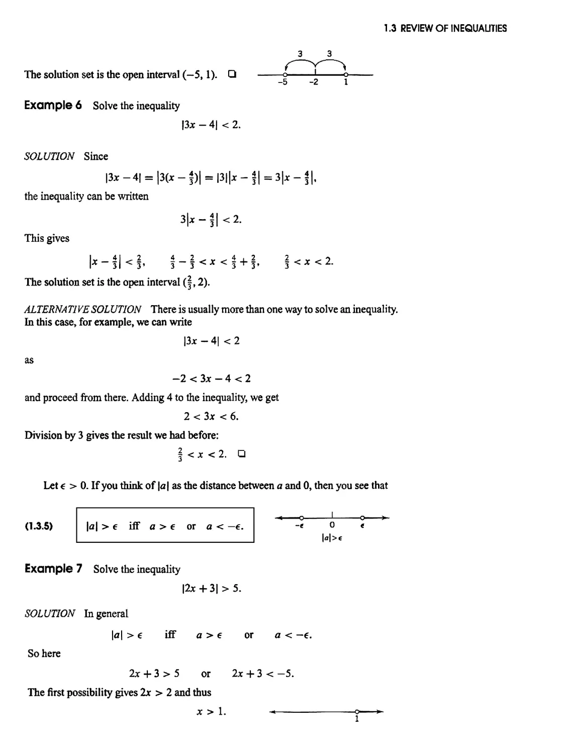
The solution set is the open interval (-5,1). Q
Example 6 Solve the inequality
|3x - 4| < 2.
SOLUTION Since
|3x -4| = |3(x - |)| = |3||x - \| = 3|x - *|,
the inequality can be written
3|x-f|<2.
This gives
4,2 2
X * I < T, ^ X "^ X "^ -n "T" T9 "Z "^ A ^ ^.
The solution set is the open interval (|, 2).
ALTERNATIVE SOLUTION There is usually more than one way to solve an inequality.
In this case, for example, we can write
|3jc - 4| < 2
as
-2 < 3x - 4 < 2
and proceed from there. Adding 4 to the inequality, we get
2 < 3jc < 6.
Division by 3 gives the result we had before:
\ < x < 2. ?
Let € > 0. If you think of \a\ as the distance between a and 0, then you see that
(1.3.5)
Example
\a\ > e iff a > € or a < —€.
7 Solve the inequality
|2x + 3|>5.
SOLUTION In general
\a\ > e iff a > e or a < —e.
So here
2x + 3 > 5 or 2x + 3 < -5.
The first possibility gives 2jc > 2 and thus
x > 1. -*
1
0
—0 >'

16 ¦ CHAPTER 1 PRECALCULUS REVIEW
The second possibility gives 2x < -8 and thus
x < — 4 < o ^
-4
The total solution is therefore the union
(-00,-4)11(1,00). ? ^_o o ^
-4 1
We come now to one of the fundamental inequalities of calculus: for all real numbers
a and by
EXERCISES 1.3
(1.3.6)
\a + b\<\a\ + \b\.
This is called the triangle inequality in analogy with the geometric observation that "in
any triangle the length of each side is less than or equal to the sum of the lengths of the
other two sides."
PROOF OF THE TRIANGLE INEQUALITY The key here is to think of |x| as </?.
Note first that
(a + bf = a2 + lab + b2 < \a\2 + 2|a||6| + \b\2 = (|*| + \b\f.
Comparing the extremes of the inequality and taking square roots, we have
y/(a+b? < |fl| + |6|- (Exercise51)
The result follows from observing that
y/(a + b)2=\a + b\. ?
Here is a variant of the triangle inequality that also comes up in calculus: for all
real numbers a and b,
(1.3.7)
\la\-\b\\<\a-b\.
The proof is left to you as an exercise.
Exercises 1-20. Solve the inequality and mark the solution set
on a number line.
Exercises 21-36. Solve the inequality and express the solution
set as an interval or as the union of intervals.
1. 2 + 3* < 5.
3. 16* +64 < 16.
5. ±(l+*)<f(l-*).
7. x2 - 1 < 0.
9.x2 - x - 6 > 0.
11.2*2+*- 1 <0.
13. jc(jc - lX*-2)>0.
15,*3-2x2 + *>0.
17. *3(* - 2)(* + 3)2 < 0.
19. x2(x - 2)(* + 6) > 0.
2. |(2*+3) < 6.
4.3*+5>±(*-2).
6. 3* - 2 < 1 + 6x.
8. x2 + 9* + 20 < 0.
10. Jt2 -4* -5 >0.
12. 3*2+4*-4>0.
14.x(2*- l)(3x-5)<0.
16. x2 - 4x + 4 < 0.
18.*2(x-3)(*+4)2>0.
20. 7x(* - 4)2 < 0.
21. |*| <2.
23. |x| > 3.
25. |x - 2| < |.
27. 0 < |*| < 1.
29. 0<|*-2| <{.
31. 0< |*-3| <8.
33. |2x + l| <|.
35. |2*+5| > 3.
22. |*| > 1.
24. |*-1| <1.
26. \x-\\ <2.
28. 0< \x\<\.
30. 0<|x-||<2.
32. |3* - 5| < 3.
34. |5* - 3| < \.
36. |3* + i| > 5.
Exercises 37-42. Each of the following sets is the solution of an
inequality of the form \x — c\< 8. Find c and $.

1.4 COORDINATE PLANE; ANALYTIC GEOMETRY ¦ 17
37. (-3t 3). 38. (-2, 2).
39. (-3, 7). 40.(0,4).
41. (-7, 3). 42. (a, b).
Exercises 43-46. Determine all numbers A > 0 for which the
statement is true.
43. If \x - 2| < I, then \Zx - 4| < A.
44. If |jc -2\<A, then \2x - 4| < 3.
45. lf|jt + l| < /Mhcn|3jt + 3| <4.
46. If |* + 1| < 2, then |3x + 3| < A,
47. Arrange the following in order: I, x, *Jx, 1/x, l/^/x, given
that:(tf)jc > \;(b)0<x < 1.
48. Given that x > 0, compare
x-fl
—7 ^d if
x + l Vx + 2
49. Suppose that ab > 0. Show that if a < bs then \/b < \/a.
50. Given that a > 0 and b > 0, show that if a2 <b2, then
a < Z>.
51. Show that if 0 < a < b, then *fa < «/b.
52. Show that \a — b\ < \a\ 4-1&| for all real numbers a and &.
53. Show that \\a\ — \b\\ < |a — 6| for all real numbers a and &.
HINT: Calculate ||<z|-|Z>||2.
54. Show that \a + b\ = |«| + |6| iff <z& > 0.
55. Show that
a b
if 0 < a < b.
then
1+a ~ 1+b
56. Let a, &, c be nonnegative numbers. Show that
a
if a < b + c,
then
6 c
+ ¦
1 4-a ~~ 1 + 6 1+6-
57. Show that if a and b are real numbers and a < b, then
a < (a 4- 6)/2 < 6. The number (a + &)/2 is called the
arithmetic mean of a and Z>.
58. Given that 0 < a < by show that
rr "+ ^
a < Vab < —— < 6.
" 2 ~
The number \fab is called the geometric mean of a and b.
¦ 1.4 COORDINATE PLANE; ANALYTIC GEOMETRY
Rectangular Coordinates
The one-to-one correspondence between real numbers and points on a line can be used
to construct a coordinate system for the plane. In the plane, we draw two number lines
that are mutually perpendicular and intersect at their origins. Let O be the point of
intersection. We set one of the lines horizontally with the positive numbers to the right
of O and the other vertically with the positive numbers above O. The point O is called
the origin, and the number lines are called the coordinate axes. The horizontal axis
is usually labeled the x-axis and the vertical axis is usually labeled the y-axis. The
coordinate axes separate four regions, which are called quadrants. The quadrants are
numbered I //, III IV in the counterclockwise direction starting with the upper right
quadrant. See Figure 1.4.1.
Rectangular coordinates are assigned to points of the plane as follows (see Figure
1.4.2.). The point on the *-axis with line coordinate a is assigned rectangular coordinates
(a, 0). The point on the^-axis with line coordinate b is assigned rectangular coordinates
(0, b). Thus the origin is assigned coordinates (0,0). A point P not on one of the
coordinate axes is assigned coordinates (a, b) provided that the line l\ that passes
through P and is parallel to the>>-axis intersects the x-axis at the point with coordinates
(a, 0), and the line h that passes through P and is parallel to the jc-axis intersects the
>>-axis at the point with coordinates (0, b).
This procedure assigns an ordered pair of real numbers to each point of the plane.
Moreover, the procedure is reversible. Given any ordered pair (a, b) of real numbers,
there is a unique point P in the plane with coordinates (a, b).
To indicate P with coordinates (a, b) we write P(a, b). The number a is called the
x-coordinate (the abscissa); the number b is called the y-coordinate (the ordinate). The
coordinate system that we have defined is called a rectangular coordinate system. It
is often referred to as a Cartesian coordinate system after the French mathematician
Rene Descartes (1596-1650).
11
III
>'j
1 (
0
I
, 1
/
1 1
IV
X
Figure 1.4.1
y.
b
o
d
i
c
\
\
1
1
d)
\
1/'
1
1
[
i a
T
i
\
1
l'l
X
Figure 1.4.2

18
CHAPTER 1 PRECALCULUS REVIEW
Distance and Midpoint Formulas
Let Po(xo,yo) and P\(xi,y\) be points in the plane. The formula for the distance
d(Po, P\) between Pq and P\ follows from ^Pythagorean theorem:
d(P0,Pi) = Vl^i -^ol2 + lyi -yd2 = A*\ -*o)2 + (yi -yo)2.
-H2 = a2
(Figure 1.4.3)
Distance : d(PQ, P{) = ^(jcj - x0)2 + (yx - j0)2
Figure 1.4.3
*V*i^i>
Midpoint: M =(^,^)
Figure 1.4.4
Let A/(jc, 7) be the midpoint of the line segment PqP\- That
*o + *i . yo+y\
x = —-— and y = —-—
2 '2
follows from the congruence of the triangles shown in Figure 1.4.4
Lines
(i) Slope Let / be the line determined by Po(xo, yo) and P\ {x\, y\). If/ is not vertical,
then x\ 7^ xq and the slope of / is given by the formula
X\—Xq (Figure 1.4.5)
With 0 (as indicated in the figure) measured counterclockwise from the jc-axis,
m =tan0.f
The angle 9 is called the inclination of/. If/ is vertical, then 0 = jt/2 and the slope of
/ is not defined.
(ii) Intercepts If a line intersects the x-axis, it does so at some point (a, 0). We call a
the x-intercept. If a line intersects they-axis, it does so at some point (0, b). We call b
the j-intercept. Intercepts are shown in Figure 1.4.6.
*The trigonometric functions are reviewed in Section 1,6.

1.4 COORDINATE PLANE; ANALYTIC GEOMETRY
19
y*
Po^o.voi pi<*i.yil
0<<?<f
m = -—-r = 0
0 = 0
Figure 1.4.5
•VI ">0 -
m- -—r- <0
x\ - xo
f <*<*
(ill) Equations
** J
vertical line
horizontal line
point-slope form
slope-intercept form
two-intercept form
general form
x = a,
y = b.
y -yo = m(x -A*o).
y = mx + b.
(y = 6 at a: = 0)
(^-intercept a; v-intcrcept b)
{A and tf not both 0)
Ax + By + C = 0.
(iv) Parallel and Perpendicular Nonvertical lines
parallel m\ = mi.
perpendicular m \ mi = — 1.
(v) The Angle Between Two Lines The angle between two lines that meet at right
angles is n/2. Figure 1.4.7 shows two lines (/|, k with inclinations 9\, fc) that intersect
but not at right angles. These lines form two angles, marked a and n - a in the figure.
The smaller of these angles, the one between 0 and 7r/2, is called the angle between l\
and I2. This angle, marked a in the figure, is readily obtained from 0\ and 62*
If neither l\ nor l2 is vertical, the angle a between l\ and l2 can also be obtained
from the slopes of the lines:
tana =
m\ — /«2
I +m\m2
The derivation of this formula is outlined in Exercise 75 of Section 1.6.
Example 1 Find the slope and the ^-intercept of each of the following lines:
/, : 20* - 24y - 30 = 0, t2 : 2x - 3 = 0, /3 : Ay + 5 = 0.
x-inlercept a \ ^-intercept b
Figure 1.4.6
Figure 1.4.7
SOLUTION The equation of Z| can be written
y = \*-\-

¦ CHAPTER 1 PRECALCULUS REVIEW
This is in the form y = mx + b. The slope is |, and thejMntercept is — f.
The equation of l2 can be written
x — 2*
The line is vertical and the slope is not defined. Since the line does not cross the j>-axis,
the line has no ^-intercept.
The third equation can be written
The line is horizontal. The slope is 0 and the ^intercept is — f. The three lines are
drawn in Figure 1.4.8. ?
y\
3
2
1
1 1 1
-3 -2 -1
-1
j4.
/ -3
i
l>
i / \ ,
y * 3 *
'=f*-7
yi
3
2
1
1 1 1
-3 -2 -1
-1
-2
-3
i
-
L
1
-
h
i i ,
2 3 Jf
*-! '
Figure
> 1.4.8
y>
3
2
1
1 1 1
-3 -2 -1
-2
-3
i
-
iii,
1 2 3 x
Z h
-
,:.i
Example 2 Write an equation for the line l2 that is parallel to
/, : 3x - 5y + 8 = 0
and passes through the point P{—3,2).
SOL tVr/O/V The equation for lx can be written
The slope of l\ is 5. The slope of li must also be |. (For nonvcrtical parallel lines, m, = m2.)
Since h passes through (—3,2) with slope I, we can use the point-slope formula
and write the equation as
,-2 = f(* + 3). U
Example 3 Write an equation for the line that is perpendicular to
l\ : x - Ay + 8 = 0
and passes through the point P(2, —4).
SOLUTION The equation for /1 can be written
y = ±x + 2.

1.4 COORDINATE PLANE; ANALYTIC GEOMETRY
The slope of l\ is \. The slope of h is therefore —4. (For nonvertical perpendicular
lines, mim2 = -1.)
Since h passes through (2, —4) with slope —4, we can use the point-slope formula
and write the equation as
j + 4 = -4(jc-2). ?
Example 4 Show that the lines
/, :3x-4j/ + 8 = 0 and 72 : \2x-5y- 12 = 0
intersect and find their point of intersection.
SOLUTION The slope of l\ is | and the slope of h is y. Since /i and li have different
slopes, they intersect at a point.
To find the point of intersection, we solve the two equations simultaneously:
3x - Ay + 8 = 0
12jc-5y- 12 = 0.
Multiplying the first equation by -4 and adding it to the second equation, we obtain
11^44 = 0
y = 4.
Substituting y = 4 into either of the two given equations, we find that x = |. The lines
intersect at the point (|, 4). ?
Circle, Ellipse, Parabola, Hyperbola
These curves and their remarkable properties are thoroughly discussed in Section 10.1.
The information we give here suffices for our present purposes.
Circle
Figure 1.4.9

I CHAPTER 1 PRECALCULUS REVIEW
Ellipse
Parabola
X2 \2
Figure 1.4.10
y k
a2 fr*
?4
v = a a: , a > 0
V = tf*2,tf<0
Hyperbola
y = a.x'' + for + ?, a > 0 y = ax2 +bx + c.a<Q
Figure 1.4.11
y.
\ \
s X
\ X
N X
^ x
\ X.
N X^
\ ^"S^,
\
s
\
X
/*
/
/
s
/ X^
/ X
/ x
s X
/ X
/ X
s X
X /
X /
X y
X y
X y
x y
X /
*X /
p-***^ s
y
y
/
/
s
^
\
X. \
X \
X ^
X s.
X ^
X ^
X N
.r
Figure 1.4.12

Remark The circle, the ellipse, the parabola, and the hyperbola are known as the
conic sections because each of these configurations can be obtained by slicing a "double
right circular cone" by a suitably inclined plane. (See Figure 1.4.13.) ?
circle ellipse parabola hyperbola
Figure 1.4.13
EXERCISES 1.4
Exercises 1-4. Find the distance between the points.
1. P0(0,5), /M6, -3). 2. P0(2,2), />,(5t 5).
3. P0(5, -2), P,(-3,2). 4. />0(2, 7), A(-4, 7).
Exercises 5-8. Find the midpoint of the line segment P0Pi.
5. P0(2, 4), Fj(6, 8). 6. P0(3, -1), P.(-l, 5).
7. P0(2, -3), P,(7, -3). 8. fi,(a, 3), P,(3, a).
Exercises 9-14. Find the slope of the line through the points.
9. P0(-2, 5), P)(4, 1). 10. ft(4, -3), Pi(-2, -7).
11. P(at fc). g(4f a). 12. P(4, -1), g(-3, -1).
13. P(jc0, 0), 0(0, ;>o). 14. O(0,0), P(x0, Jo).
Exercises 15-20. Find the slope and v-intercept.
15. y = 2x- 4. 16. 6-5x = 0.
17. 3y = x + 6. 18. 6v - 3* + 8 = 0.
19. 7,x-3y-f4 = 0. 20. v = 3.
Exercises 21-24. Write an equation for the line with
21. slope 5 and ^-intercept 2.
22. slope 5 and ^-intercept —2.
23. slope —5 and ^'-intercept 2.
24. slope —5 and ^-intercept —2.
Exercises 25-26. Write an equation for the horizontal line
3 units
25. above the *-axis.
1.4 COORDINATE PLANE; ANALYTIC GEOMETRY ¦ 23
26. below the jc-axis.
Exercises 27-28. Write an equation for the vertical line 3 units
27. to the left of the >>-axis.
28. to the right of they-axis.
Exercises 29-34. Find an equation for the line that passes
through the point P(2, 7) and is
29. parallel to the *-axis.
30. parallel to they-axis.
31. parallel to the line 3y - 2x + 6 = 0.
32. perpendicular to the line y - 2x + 5 = 0.
33. perpendicular to the line 3y — 2x H- 6 = 0.
34. parallel to the line y - 2x + 5 = 0.
Exercises 35-38. Determine the point(s) where the line
intersects the circle.
35..v = jc, x2+y2 = l.
36. y = wx, x2 + y2 = 4.
37. 4jc + iy = 24, x2 + y1 = 25.
38. y = mx + />, *2 4- y2 = b1.
Exercises 39-42. Find the point where the lines intersect.
39. h : 4* - y - 3 = 0, l2 : 3jc - 4y + 1 = 0.
40. li:3x+y-5 = 0, l2:lx- \0y + 27 = 0.
41.!{ :4jc->> + 2 = 0. /2 : \9x+y = 0.

24 ¦ CHAPTER 1 PRECALCULUS REVIEW
42. /, : 5x - 6y + 1 = 0, l2 : 8x 4- Sy + 2 = 0.
43. Find the area of the triangle with vertices (1, -2), (—1,3),
(2,4).
44. Find the area of the triangle with vertices (-1,1), (3, V5),
(V5.-1).
45. Determine the slope of the line that intersects the circle
x2 + y2 = 169 only at the point (5, 12).
46. Find an equation for the line which is tangent to the circle
x2 + y2 - 2x + 6y - 15 = 0 at the point^, 1). HINT: A
line is tangent to a circle at a point P iff it is perpendicular
to the radius at P.
47. The point P(l, — 1) is on a circle centered at C(— 1,3). Find
an equation for the line tangent to the circle at P.
Exercises 48-51. Estimate the point(s) of intersection.
4S.I: :3x-4y = 79 h : -5* + 2j>=11.
49. /, : 2.41 jc + 3.29y = 5. l2 : 5.13* - 4.27v = 13.
50. lx : 2x - 3y = 5, circle : x2 + >>2 = 4.
51. circle : a*2 + y2 = 9, parabola : y = x2 — 4x + 5.
Exercises 52-53. The perpendicular bisector of the line
segment PQ is the line which is perpendicular to PQ and passes
through the midpoint of PQ. Find an equation for the
perpendicular bisector of the line segment that joins the two points.
52. P(-l,3), 2(3,-4).
53. P( 1,-4), 2(4,9).
Exercises 54-56. The points are the vertices of a triangle. State
whether the triangle is isosceles (two sides of equal length), a
right triangle, both of these, or neither of these.
54. P0(-4,3). Pi(-4.-l), ft(2,l).
55. fb(-2,5), P,(l,3), ft(-l.O).
56.Po(-l,2), fl(lf3), P2(4,l).
57. Show that the distance from the origin to the line Ax + By +
C = 0 is given by the formula
</(0,/) =
\c\
JA2 + B2
58. An equilateral triangle is a triangle the three sides of which
have the same length. Given that two of the vertices of an
equilateral triangle are (0,0) and (4,3), find all possible
locations for a third vertex. How many such triangles are there?
59. Show that the midpoint M of the hypotenuse of a right
triangle is equidistant from the three vertices of the triangle.
HINT: Introduce a coordinate system in which the sides of
the triangle are on the coordinate axes; see the figure.
60. A median of a triangle is a line segment from a vertex to the
midpoint of the opposite side. Find the lengths of the
medians of the triangle with vertices (-1, —2), (2, I), (4t -3).
61. The vertices of a triangle are (1,0), (3,4). (-1, 6). Find the
point(s) where the medians of this triangle intersect.
62. Show that the medians of a triangle intersect in a single point
(called the centroid of the triangle). HINT: Introduce a
coordinate system such that one vertex is at the origin and one
side is on the positives-axis; see the figure.
)'k
(a,b)
(c,0)
63. Prove that each diagonal of a parallelogram bisects the other.
HINT: Introduce a coordinate system with one vertex at the
origin and one side on the positive *-axis.
64. Pi(x}.yi), P2(x2,y2% Pifayi), Pa(x4, \>a) are the vertices
of a quadrilateral. Show that the quadrilateral formed by
joining the midpoints of adjacent sides is a parallelogram.
65. Except in scientific work, temperature is usually measured
in degrees Fahrenheit (F) or in degrees Celsius (C). The
relation between F and C is linear. (In the equation that relates
F to C, both F and C appear to the first degree.) The freezing
point of water in the Fahrenheit scale is 32°F; in the Celsius
scale it is 0C,C. The boiling point of water in the Fahrenheit
scale is 212°F; in the Celsius scale it is 1Q0UC. Find an
equation that gives the Fahrenheit temperature F in terms of the
Celsius temperature C. Is there a temperature at which the
Fahrenheit and Celsius readings are equal? If so. find it.
66. In scientific work, temperature is measured on an absolute
scale, called the Kelvin scale (after Lord Kelvin, who
initiated this mode of temperature measurement). The relation
between Fahrenheit temperature F and absolute temperature
K is linear. Given that K= 273° whenF= 32c,andK= 373°
when F = 212°, express K in terms of F. Then use your result
in Exercise 65 to determine the connection between Celsius
temperature and absolute temperature.
¦ 1.5 FUNCTIONS
The fundamental processes of calculus (called differentiation and integration) are
processes applied to functions. To understand these processes and to be able to carry them
out, you have to be comfortable working with functions. Here we review some of the
basic ideas and the nomenclature. We assume that you are familiar with all of this.

Functions can be applied in a very general setting. At this stage, and throughout the
first thirteen chapters of this text, we will be working with what are called real-valued
Junctions of a real variable, functions that assign real numbers to real numbers.
Domain and Range
Let's suppose that D is some set of real numbers and that/ is a function defined on D.
Then/ assigns a unique number f(x) to each number* inD. The number f{x) is called
the value off at jc, or the image ofx under/ The set Z), the set on which the function is
defined, is called the domain of/ and the set of values taken on by/ is called the range
off In set notation
dom (/) = Z), range (/) = {/(jc): x e D}.
We can specify the function/ by indicating exactly what /(jc) is for each jc in D.
Some examples. We begin with the squaring ftinction
f(x) = a*2, for all real numbers x.
The domain of/ is explicitly given as the set of real numbers. Particular values taken
on by/ can be found by assigning particular values to jc. In this case, for example,
/(4) = 42 = 16, /(-3) = (-3)2 = 9, /(0) = 02 = 0.
As x runs through the real numbers, x2 runs through all the nonnegative numbers. Thus
the range off is [0, oo). In abbreviated form, we can write
dom (/) = (-oo, oo), range (/) = [0, oo)
and wc can say that/ maps (—oo, oc) onto [0, oo).
Nowlet's look at the function g defined by
g(x) = V2x + 4, x e [0, 6].
The domain of g is given as the closed interval [0, 6]. At jc = 0, ? takes on the value 2:
?(0) = V2.0 + 4 = V4 = 2;
at x = 6, g has the value 4:
g(6) = V2-6 + 4 = >/l6 = 4.
As jc runs through the numbers in [0, 6], g(jc) runs through the numbers from 2 to 4.
Therefore, the range of g is the closed interval [2,4]. The function g maps [0, 6] onto
[2,4].
Some functions are defined piecewise. As an example, take the function h> defined
by setting
,, x [2x + 1, ifjc <0
h{x) = { x\ if jc > 0.
As explicitly stated, the domain of h is the set of real numbers. As you can verify, the
range of h is also the set of real numbers. Thus the function h maps (—oo, oo) onto
(—oo, oo). A more familiar example is the absolute value junction f(x) = |jc|. Here
f( \-\ x* if ^ > 0
nx,~ [ —jc, ifx<0.
The domain of this function is (—oo, oo) and the range is [0, oo).
Remark Functions are often given by equations of the form y = /(jc) with x restricted
to some set D, the domain of/ In this setup x is called the independent variable (or
the argument of the function) and>>, except in special cases, clearly dependent onx, is
called the dependent variable. ?

CHAPTER 1 PRECALCULUS REVIEW
The Graph of a Function
Iff is a flmction with domain D, then the graph off is the set of all points P(x, f(x))
with x in D. Thus the graph of/ is the graph of the equation y = f(x) with x restricted
to D\ namely
the graph of / = {(*, y) :x e D%y = f(x)}.
The most elementary way to sketch the graph of a function is to plot points. We plot
enough points so that we can "see" what the graph may look like and then connect the
points with a "curve." Of course, if we can identify the curve in advance (for example,
if we know that the graph is a straight line, a parabola, or some other familiar curve),
then it is much easier to draw the graph.
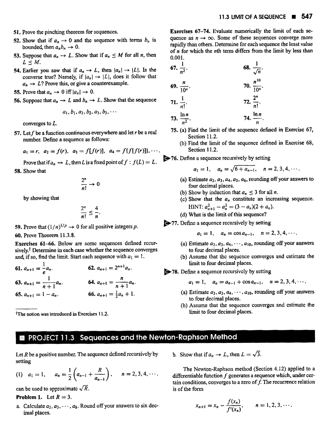
The graph of the squaring function
f(x) = x2, x ? (-00, oo)
is the parabola shown in Figure 1.5.1. The points that we plotted are indicated in the
table and marked on the graph. The graph of the function
g(x) = V2*+4, x € [0,6]
is the arc shown in Figure 1.5.2
X
0
±1
±1
±2
*2
0
A
1
4
(-2,4) n
M2,4)
JPU, Jf2)
Ml, 1)
-2 -1 I 1 2 x
Figure 1.5.1
X
0
2
4
6
VZt74
2
\^s2.8
Vl2s3.5
4
1
6
4
2<
>
-
P{x, V2r + 4)
<^2Tv8)
1
2
(6,4)
(4, \T2)
i 1 >
4 6 x
Figure 1.5.2
The graph of the function
h(x) =
2x + U
if* <0
if x > 0
and the graph of the absolute value function are shown in Figures 1.5.3 and 1.5.4.
Although the graph of a function is a "curve" in the plane, not every curve in the
plane is the graph of a function. This raises a question: How can we tell whether a curve
is the graph of a function?
A curve C which intersects each vertical line at most once is the graph of a function:
for each P(x} y) € C, define f(x) = y. A curve C which intersects some vertical line
more than once is not the graph of a function: If P(x, y^) and P(x, ^2) are both on C,
then how can we decide what f(x) is? Is it y\; or is it y-p.
These observations lead to what is called the vertical line test: a curve C in the
plane is the graph of a function iff no vertical line intersects C at more than one point.
Thus circles, ellipses, hyperbolas are not the graphs of functions. The curve shown in
Figure 1.5.5 is the graph of a function, but the curve shown in Figure 1.5.6 is not the
graph of a function.

1.5FUNCTIC*
(2,4)
[-X, x<0
Figure 1.5.4
n
Figure 1.5.5
Figure 1.5.6
Graphing calculators and computer algebra systems (CAS) are valuable aids to
graphing, but, used mindlessly, they can detract from the understanding necessary for
more advanced work. We will not attempt to teach the use of graphing calculators or
the ins and outs of computer software, but technology-oriented exercises will appear
throughout the text.
Even Functions, Odd Functions; Symmetry
For even integers n, {—x)n = x"; for odd integers n, (—x)n = — x". These simple
observations prompt the following definitions:
A function/ is said to be even if
/(-*) = /(*) for a11 x € dom (/);
a function/is said to be odd if
f(-x) = —f(x) for all x e dom (/).
The graph of an even function is symmetric about they~axis7 and the graph of an
odd function is symmetric about the origin. (Figures 1.5.7 and 1.5.8.)
The absolute value function is even:
f(-x) = \-x\ = \x\=f(x).

28 ¦ CHAPTER 1 PRECALCULUS REVIEW
(-x,f{-x))
U./W)
Figure 1.5.7
Figure 1.5.8
-2\
yt
3
2
1
l
-1 /
^¦3
i
J-
-
\
1
l y^Ax-x3
2\ **
Figure 1.5.9
Its graph is symmetric about they-axis. (See Figure 1.5.4.)The function f(x) = Ax — x*
is odd:
/(_x) = 4(-*) - (-*3) = -4x + jc3 = -(4* - x3) = -f(x).
The graph, shown in Figure 1.5.9, is symmetric about the origin.
Convention on Domains
If the domain of a function/ is not explicitly given, then by convention we take as
domain the maximal set of real numbers x for which f(x) is a real number. For the
function f(x) = x3 + 1, we take as domain the set of real numbers. For g(jc) = <Jxy
we take as domain the set of nonnegative numbers. For
*(*> = -!-
x — 2
we take as domain the set of all real numbers x: ^ 2. In interval notation.
dom(/) = (-oo, oo), dom(g) = [0, oo), and dom(A) = (-oo, 2) U (2, oo).
The graphs of the three functions are shown in Figure 1.5.10.
P{X, Jt3 4- 1)
/U)=Jt3+l)
y*
P{X, YX)
Figure 1.5.10
h(x) = -
Example 1 Give the domain of each function:
(a) f(x) =
x2 + x-6'
x- 1
SOLUTION (a) You can see that f(x) is a real number iff*2 + x - 6 ^ 0. Since
Jc2+Jc-6 = (jt + 3)(,r-2),

1.5 FUNCTIONS ¦ 29
the domain of/is the set of real numbers other than —3 and 2. This set can be expressed
as
(-oo, -3) U (-3, 2) U (2, oo).
(b) For g(x) to be a real number, we need
4-*2>0 and x^\.
Since 4 - x2 > 0 iff jc2 < 4 iff — 2 < x < 2, the domain of g is the set of all numbers jc
in the closed interval [-2,2] other than x = 1. This set can be expressed as the union
of two half-open intervals:
[-2,1)U(1,2]. U
Example 2 Give the domain and range of the function:
/(*)=-7=L= + 5.
V2 — x
SOLUTION First we look for the domain. Since *j2 — x is a real number iff 2 — x > 0,
we need * < 2. But at x = 2, V2 — x = 0 and its reciprocal is not defined. We must
therefore restrict x to x < 2. The domain is (—oo, 2).
Now we look for the range. Asjc runs through (-oc, 2), y/2 — x takes on all positive
values and so does its reciprocal. The range of/ is therefore (5, oo). The function/
maps (-oo, 2) onto (5, oo). Q
Functions arc used in applications to show how variable quantities are related. The
domain of a function that appears in an application is dictated by the requirements of
the application.
Example 3 U.S. Postal Service regulations require that the length plus the girth
(the perimeter of a cross section) of a package for mailing cannot exceed 108 inches.
A rectangular box with a square end is designed to meet the regulation exactly (see
Figure 1.5.11). Express the volume V of the box as a function of the edge length of the
square ends and give the domain of the function.
SOLUTION Let x denote the edge length of the square ends and let h denote the length
of the box. The girth is the perimeter of the square, or Ax. Since the box meets the
regulations exactly,
4x + h = 108 and therefore h = 108 - Ax. Fj9ure }SU
The volume of the box is given by V = x2h and so it follows that
V(x) = x2(108 - Ax) = \0Sx2 - Ax\
Since neither the edge length of the square end nor the length of the box can be negative,
we have
x>0 and /? = 108-4* >0.
The second condition requires x < 27. The full requirement on jc, 0 < x < 27, gives
dom(K) = [0,27]. ?
Example 4 A soft-drink manufacturer wants to fabricate cylindrical cans. (See
Figure 1.5.12.) The can is to have a volume of 12 fluid ounces, which we take to be
approximately 22 cubic inches. Express the total surface area 5" of the can as a function
of the radius and give the domain of the function.
Girth
v*
J?
Figure 1.5.12

30 ¦ CHAPTER 1 PRECALCULUS REVIEW
SOLUTION Let r be the radius of the can and h the height. The total surface area (top,
bottom, and lateral area) of a right circular cylinder is given by the formula
S = 2nr2 + 2nrh.
Since the volume V = 7tr2h is to be 22 cubic inches, we have
22
7tr2h = 22
and
h =
TXT*
and therefore
Sir) = 2;rr2 + 2nr
Since r can take on any positive value, dom (S) = (0, oo). ?
(3)-
. 2 44
27rr2 + —.
r
(square inches)
EXERCISES 1.5
Exercises 1-6. Calculate (a) /(0), (b)/(l), (c)/(-2), (d)/(3/2).
1. /(*) = 2at2 - 3x + 2. 2. /(x) = ^=1
4./(jc)=|x+3|-5x.
1
3. /(a) = Vx2 + 2x.
5./(x) = ^
6./(x)=l-
|x + 2|+x2' "JV"' ' (x + l)2'
Exercises 7-10. Calculate (a) f(-x), (b)/(l/x), (c)/(a + b).
x
7./(x) = x2-2x.
9. f(x) = vT+I2".
8./(x) =
10./(x) =
1
|x2-l|'
Exercises 11 and 12. Calculate f{a + h) and [f(a + h)~
/(a)]/ A for MO.
11. /(a) = 2x2 - 3*. 12. /(x) = -1^.
Exercises 13-18. Find the number(s) a-, if any, where/takes on
the value 1.
13. f(x) = |2 - a-|. 14. /(at) = ^Thx".
15. /(a-) = x2 + 4jc + 5. 16. /(a-) = 4 + 10a- - a-2.
17./(x) =
18. /(*)=-.
Exercises 19-30. Give the domain and range of the function.
19./(x)=|x|. 20.g(A-)=*2-l.
21. f(x) = 2x - 3. 22. gix) = V? + 5.
23. fix) =1.
at'
24. gix) = -.
x
26. g(x) = 7x^3.
2J8.g(A) = 7x^1-1.
30.g(x) =
25. /(x) = JT=x.
27./(x) = ^/7=7-l.
29./(x)=-7=i=. — &v-/-
V2 - x V4 - x"
Exercises 31-40. Give the domain of the function and sketch
the graph.
31./(x) = l. 32./(x) = -l.
33. fix) = 2x.
35./(x)=±x + 2.
37. fix) = J4=~P.
39./(x) = x2-x-6.
34./(*) = 2x+l.
36./(x) = -|x-3.
38. fix) = V^x2.
40./(x)=|x-l|.
Exercises 41-44. Sketch the graph and give the domain and
range of the function.
At t< \ I -1. x <0
4L/(*>=( l. *>0.
42. fix) =
43. fix) =
44. fix) =
x2. x<0
1-x. x > 0.
I +x, 0 <x < 1
x, 1 < x < 2
jx + l, 2<x.
x2, x < 0
-1, 0 <x <2
x, 2<x.
Exercises 45-48. State whether the curve is the graph of a
function. If it is, give the domain and the range.
45.
y
3
2
/l
1 l /i
-3 -2/-1
/ _1
• -2
-3
i
-
1
1
—
-
-
2
I
3
X

1.5 FUNCTIONS ¦ 31
46.
1 1
-3 -2
y
3
2
V l
J-l
/ -I
-2
-3
i
i
1 1 1
1 1
2 3
X
47.
yt
3
2
l
i i i
-3 -2 -1
-1
-2
-3
-
-,
-
-
1
1
I I
2 3
JC
48.
Exercises 49-56. State whether the function is odd, even, or
neither.
5Q.f(x) = x2 + l.
52.g(x) = x(x2 + l).
54. F(x) = x + -.
49.
51.
53.
«
/(*) =
?(*) =
/(*)»
f{r\ ^
.V3.
x(x -
X2
1-1
X
1)
*l'
x2-9
56. f(x) = Vx^x*.
^>57. The graph of f(x) = j*3 + ^x2 - 12a: - 6 looks
something like this:
(b) Find the zero(s) of/(the values of x for which fix) = 0)
accurate to three decimal places.
(c) Find the coordinates of the points marked A and B,
accurate to three decimal places.
?>58. The graph of fix) = —xA •+- 8x2 -f x — 1 looks something
like this:
(a) Use a graphing utility to sketch an accurate graph off.
(b) Find the zero(s) of/, if any. Use three decimal place
accuracy.
(c) Find the coordinates of the points marked A and B,
accurate to three decimal places.
^>Exercises 59 and 60. Use a graphing utility to draw several views
of the graph of the function. Select the one that most accurately
shows the important features of the graph. Give the domain and
range of the iunction.
59. f(x) = |*3 - 3x2 - 24jc + 4|.
60. fix) = Vx^^S.
61. Determine the range of y = x2 — 4a* — 5:
(a) by writing y in the form (x - a)2 + b.
(b) by first solving the equation for jc.
2x
62. Determine the range of v = :
4 — x
(a) Use a graphing utility to sketch an accurate graph off.
(a) by writing y in the form a + .
(b) by first solving the equation for x.
63. Express the area of a circle as a function of the
circumference.
64. Express the volume of a sphere as a function of the surface
area.
65. Express the volume of a cube as a function of the area of one
of the faces.
66. Express the volume of a cube as a function of the total surface
area.
67. Express the surface area of a cube as a function of the length
of the diagonal of a face.
68. Express the volume of a cube as a function of one of the
diagonals.
69. Express the area of an equilateral triangle as a function of
the length of a side.
70. A right triangle with hypotenuse c is revolved about one of
its legs to form a cone. (See the figure.) Given that x is the
length of the other leg, express the volume of the cone as a
function of jc.

32 ¦ CHAPTER 1 PRECALCULUS REVIEW
71. A Norman window is a window in the shape of a rectangle
surmounted by a semicircle. (See the figure.) Given that the
perimeter of the window is 15 feet, express the area as a
function of the width x.
75. A string 28 inches long is to be cut into two pieces, one piece
to form a square and the other to form a circle. Express the
total area enclosed by the square and circle as a function of
the perimeter of the square.
76. A tank in the shape of an inverted cone is being filled with
water. (See the figure.) Express the volume of water in the
tank as a function of the depth h.
72. A window has the shape of a rectangle surmounted by an
equilateral triangle. Given that the perimeter of the window
is 15 feet, express the area as a function of the length of one
side of the equilateral triangle.
73. Express the area of the rectangle shown in the accompanying
figure as a function of the x-coordinate of the point P.
74. A right triangle is formed by the coordinate axes and a line
through the point (2.5). (See the figure.) Express the area of
the triangle as a function of the ^-intercept
77. Suppose that a cylindrical mailing container exactly meets
the U.S. Postal Service regulations given in Example 3. (See
the figure.) Express the volume of the container as a function
of the radius of an end.
¦ 1.6 THE ELEMENTARY FUNCTIONS
The functions that figure most prominently in single-variable calculus are the
polynomials, the rational functions, the trigonometric functions, the exponential functions,
and the logarithm functions. These functions are generally known as the elementary
functions. Here we review polynomials, rational functions, and trigonometric functions.
Exponential and logarithm functions are introduced in Chapter 7.
Polynomials
We begin with a nonnegative integer w. A function of the form
P(x) = anxn + a*-!*"""1 H \- a\x + a{) for all real x,

1.6 THE ELEMENTARY FUNCTIONS ¦ 33
where the coefficients a„, an-\,..., a\, ao are real numbers and an ^ 0 is called a (real)
polynomial of degree n.
If n = 0, the polynomial is simply a constant function:
P(x) = ao for all real x.
Nonzero constant functions are polynomials of degree 0. The ftinction P(x) = 0 for all
real x is also a polynomial, but we assign no degree to it
Polynomials satisfy a condition known as the factor theorem: if P is a polynomial
and r is a real number, then
P(r) = 0 iff (jc - r) is a factor of P(x).
The real numbers r at which P(x) = 0 are called the zeros of the polynomial.
The linear functions
P(x) = ax + b, a^O
are the polynomials of degree 1. Such a polynomial has only one zero: r = —b/a. The
graph is the straight line y — ax 4- b.
The quadratic functions
P(x) = ax2 + bx+ct a^O
are the polynomials of degree 2. The graph of such a polynomial is the parabola y =
ax1 + bx + c. If a > 0, the vertex is the lowest point on the curve; the curve opens up.
If a < 0, the vertex is the highest point on the curve. (See Figure 1.6.1.)
vertex
a<0
Figure 1.6.1
The zeros of the quadratic function P(x) — ax1 + bx + c are the roots of the quadratic
equation
ax1 + bx + c = 0.
The three possibilities are depicted in Figure 1.6.2. Here we are taking a > 0.
It-Aac 0
two real roots
fr2-4ac = 0
one real root
Figure 1.6.2
h*-4ac 0
no real roots
Polynomials of degree 3 have the form P(x) = ax3 + bx1 + ex + d> a ^ 0. These
functions are called cubics. In general, the graph of a cubic has one of the two following
shapes, again determined by the sign of a (Figure 1.6.3). Note that we have not tried to

34 ¦ CHAPTER 1 PRECALCULUS REVIEW
locate these graphs with respect to the coordinate axes. Our purpose here is simply to
indicate the two typical shapes. You can see, however, that for a cubic there are three
possibilities: three real roots, two real roots, one real root. (Each cubic has at least one
real root.)
a 0 Cubics a
Figure 1.6.3
Polynomials become more complicated as the degree increases. In Chapter 4 we
use calculus to analyze polynomials of higher degree.
Rational Functions
A rational JUnction is a function of the form
R(x) =
Q(x)
where P and Q are polynomials. Note that every polynomial P is a rational function:
P(x) = P(x)/l is the quotient of two polynomials. Since division by 0 is meaningless,
a rational function R = P/Q is not defined at those points* (if any) where Q(x) = 0; J?
is defined at all other points. Thus, dom (R) = [x : Q(x) ^ 0}.
Rational functions J? = P/Q are more difficult to analyze than polynomials and
more difficult to graph. In particular, we have to examine the behavior of R near the
zeros of the denominator and the behavior of J? for large values of x, both positive and
negative. If, for example, the denominator Q is zero at x = a but the numerator P is
not zero at x = a, then the graph of R tends to the vertical as x tends to a and the
line x = a is called a vertical asymptote. If as x becomes very large positive or very
large negative the values of R tend to some number b> then the line y = b is called a
horizontal asymptote. Vertical and horizontal asymptotes are mentioned here only in
passing. They will be studied in detail in Chapter 4. Below are two simple examples.
(i) The graph of
1 I
*(*) =
X2 _ 4x + 4 (x - 2)2
is shown in Figure 1.6.4. The line x = 2 is a vertical asymptote; the ltne>- = 0 (the
jc-axis) is a horizontal asymptote.
(ii) The graph of
.2 v2
R(x) X
x2-l (x- l)(x + 1)
is shown in Figure 1.6.5. The lines x = 1 and x = — 1 are vertical asymptotes; the
line y = 1 is a horizontal asymptote.

1.6 THE ELEMENTARY FUNCTIONS ¦ 35
^\ 1 N^
.T = -lj
r
Jx = 1
y=l
Figure 1.6.5
The Trigonometric Functions
Radian Measure Degree measure, traditionally used to measure angles, has a serious
drawback. It is artificial; there is no intrinsic connection between a degree and the
geometry of a rotation. Why choose 360° for one complete revolution? Why not 100c?
or 400°?
There is another way of measuring angles that is more natural and lends itself better
to the methods of calculus: measuring angles in radians.
Angles arise from rotations. We will measure angles by measuring rotations.
Suppose that the points of the plane are rotated about some point 0. The point 0 remains
fixed, but all other points P trace out circular arcs on circles centered at 0. The farther P
is from 0, the longer the circular arc (Figure 1.6.6). The magnitude of a rotation about
0 is by definition the length of the arc generated by the rotation as measured on a circle
at a unit distance from 0.
Now let 9 be any real number. The rotation of radian measure 9 (we shall simply call
it the rotation 9) is by definition the rotation of magnitude |0| in the counterclockwise
direction if 9 > 0, in the clockwise direction if 9 < 0. If 6 = 0, there is no movement;
every point remains in place.
In degree measure a full turn is effected over the course of 360°. In radian measure,
a full turn is effected during the course of In radians. (The circumference of a circle
of radius I is 2n.) Thus
2n radians = 360 degrees
one radian = 360/2tt degrees = 57.30°
one degree = 2;r/360 radians = 0.0175 radians.
The following table gives some common angles (rotations) measured both in
degrees and in radians.
degrees
radians
0°
0
30°
b
45°
\*
60°
i*
90°
I*
120°
?
135°
4*
150°
1*
180°
n
270°
3^
2n
360°
In
Cosine and Sine In Figure 1.6.7 you can see a circle of radius 1 centered at the origin
of a coordinate plane. We call this the unit circle. On the circle we have marked the
points (1,0).
Now let 9 be any i;eal number. The rotation 9 takes A (1,0) to some point P, also on
the unit circle. The coordinates of P are completely determined by 9 and have names
Figure 1.6.6
Ai\% 0)
Figure 1.6.7

36 ¦ CHAPTER 1 PRECALCULUS REVIEW
P{cos ft sin 9)
Figure 1.6.8
related to 0. The second coordinate of P is called the sine of 9 (we write sin 9) and the
first coordinate of P is called the cosine of 9 (we write cos 6). Figure 1.6.8 illustrates
the idea. To simplify the diagram, we have taken 9 from 0 to lit.
For each real 9, the rotation 9 and the rotation 6 -h 2n take the point A to exactly
Ail 0) *he same P0^ P* '* f°U°ws that f°r each 0,
sin(0 + 2;r) = sin 9, cos(0 + 2;r) = cos#.
In Figure 1.6.9 we consider two rotations: a positive rotation 9 and its negative
counterpart —9. From the figure, you can see that
sm(-0) = — sin0, cos(-0) = cos0.
The sine function is an odd function and the cosine function is an even function.
In Figure 1.6.10 we have marked the effect of consecutive rotations of \n radians:
(a, b) -> (-6, a) -> (-a, -?) -* (6, -a).
In each case, (x, y) -> (—yy x). Thus,
sin(# + \n) = cos#, cos(0 + ^jt) = -sin0.
A rotation of n radians takes each point to the point antipodal to it: (x, y) -> (—jc, —j>)-
Thus
sin(0 + n) = - sin9, cos(0 + n) = - cos0.
/'(cos ft sin 0)
0<cos(-0), sin(-tf))
(-*,-«
Figure 1.6.9
Figure 1.6.10
Tangent, Cotangent, Secant, Cosecant There are four other trigonometric functions:
the tangent, the cotangent, the secant, the cosecant. These are obtained as follows:
tan0 =
sinfl
cos 6'
cote =
cos0
sin0'
sec0 =
1
cos©'
CSC0 =
1
sin0
The most important of these functions is the tangent. Note that the tangent function is
an odd function
, ^ sin(-0) -sin0
tan(-0) = —V-rr = r- = - tan0
cos(-0) cos0
and repeats itself every n radians:
sin(0+jr) -sm0
tan(0 + 7T) = —7- i = = tan 9.
cos(0+jt) -cos0

1.6 THE ELEMENTARY FUNCTIONS ¦ 37
Particular Values The values of the sine, cosine, and tangent at angles (rotations)
frequently encountered are given in the following table.
sin#
cos0
tan0
0
0
1
0
b
]
2
173
iV3
\*
&
fr
1
?*
M
i
2
V)
\*
1
0
—
\n
M
i
2
Si
\*
ivi
-|V2
-1
t*
1
2
-^
-^
^
0
-l
0
§*
-1
0
—
2*
0
1
0
The (approximate) values of the trigonometric functions for any angle 0 can be obtained
with a hand calculator or from a table of values.
Identifies Below we list the basic trigonometric identities. Some are obvious; some
have just been verified; the rest are derived in the exercises.
(i) unit circle
sin2 0 + cos2 0 = 1, tan2 0 + 1 = sec2 0, 1 + cot2 0 = esc2 0.
(the first identity is obvious; the other two follow from the first)
(ii) periodicity*
sin(0 + 2n) = sin 9, cos(0 + 2iz) = cos 0, tan(0 + n) = tan 0
(Hi) odd and even
sin(-0) = — sin 0, cos(-0) = cos 0, tan(-0) = — tan 0.
(the sine and tangent are odd functions; the cosine is even)
(iv) sines and cosines
sin(0+jr) =-sin0, cos(0 + n) = - cos0,
sin(0 + ^7t) = cos0, cos(0 + \n) = — sin0,
sin(i7r - 0) = cos0, cos(^;r — 0) = sin0.
(only the third pair of identities still has to be verified)
(v) addition formulas
sin(a + (3) = sin a cos (5 + cos a sin /?,
sin(or — /*) = sin or cos fi — cos a sin 0,
cos(a + ?) = cosacos/J -sin a sin/J,
cos(cr — j8) = cos a cos ? + sin a sin ?.
(taken up in the exercises)
(vi) double-angle formulas
sin20 = 2sin0cos0, cos20 = cos20 - sin2 0 = 2cos20 -1 = 1 -2sin20.
(follow from the addition formulas)
*A function/ with an unbounded domain is said to be periodic if there exists a number p > 0 such that,
if $ is in the domain off, then $ + p is in the domain and f($ -f p) = /(#). The least number/; with this
property (if tliere is a least one) is called the period of the function. The sine and cosine have period 2ix.
Their reciprocals, the cosecant and secant, also have period 2tz. The tangent and cotangent have period it.

38 ¦ CHAPTER 1 PRECALCULUS REVIEW
(vii) half-angle formulas
sin2(9= i(l -cos20), cos20 = \(l + cos 20)
(follow from the double-angle formulas)
adjacent side
Figure 1.6.11
In Terms of a Right Triangle For angles 9 between 0 and n/2, the trigonometric
functions can also be defined as ratios of the sides of a right triangle. (See Figure 1.6.11.)
sin0 =
COS0 =
tan# =
opposite side
hypotenuse
adjacent side
hypotenuse
opposite side
adjacent side'
csc0 =
sec 9 =
cot 6 =
hypotenuse
opposite side'
hypotenuse
adjacent side'
adjacent side
opposite side*
(Exercise 81)
Arbitrary Triangles Let a, b, c be the sides of a triangle and let A, B, C be the opposite
angles. (See Figure 1.6.12.)
area \ab sinC = ^ac sin 2? = ^bc sin A.
law of sines
sin A sin B sin C
Figure 1.6.12
a b c
law of cosines a2 = b2 + c2 — 2bc cos A,
b2 = a2 -f-c2 -laccosB,
c2 = a2 + b2 -2abcosC.
(taken up in the exercises)
Graphs Usually we work with functions y = f(x) and graph them in the xy-plane. To
bring the graphs of the trigonometric flinctions into harmony with this convention, we
replace 9 by x and write y = sin x, y = cos x, y = tanx. (These are the only functions
that we are going to graph here.) The functions have not changed, only the symbols:
x is a rotation that takes A(\, 0) to the point P(cosx, sinx). The graphs of the sine,
cosine, and tangent appear in Figure 1.6.13.
The graphs of sine and cosine are waves that repeat themselves on every interval
of length 27r. These waves appear to chase each other. They do chase each other. In the
chase the cosine wave remains ^tc units behind the sine wave:
cosjc = sin(jc + \n).
Changing perspective, we see that the sine wave remains \n units behind the cosine
wave:
sin* =cos(x + |;r).
All these waves crest at y — 1, drop down to y = -1, and then head up again.
The graph of the tangent function consists of identical pieces separated every n
units by asymptotes that mark the points x where cosjc = 0.

1.6 THE ELEMENTARY FUNCTIONS ¦ 39
1
-iv
\/
/-231
1
-!-
\i
~n\
l
s:b
>'A
/ 1
**
;r\
I
xfV
/2*
l
i»
*
' * y--l
v = sin jc
period 2,t
>* = cos x
period 2jy
tangent
v = tan x
period n
vertical asymptotes .v = (« + -)*, /? an integer
Figure 1.6.13
EXERCISES 1.6
Exercises 1-10, State whether the function is a polynomial, a
rational function (but not a polynomial), or neither a polynomial
nor a rational function. If the function is a polynomial, give the
degree.
1. f{x) = 3.
5. F(x) =
t3 - 3jc3'2 + 2x
x2-l
7./(*) = v?(>/T+l).
9. /(*) =
x2-\
2. f{x) = 1 + \x.
x2 -4
6. f(x) = 5x4 - 7tx2 + *.
*2-2x-8
10. h(x) =
x + 2 *
(yr + 2)(y^-2)
x2 + 4
Exercises 11-16. Determine the domain of the function and
sketch the graph.
11. f(x) = 3* - ±
2*
12.
14.
16.
/(*) =
f<*) =
«<*) =
:.«+1'
: X3 — X
1
-* + -.
13. g(x) = *2 - * - 6.
15./W = _L_.
Exercises 17-22. Convert the degree measure into radian
measure.
17.225°. 18.-210°.
19. -300°. 20. 450°.
21. 15°. 22. 3°.
Exercises 23-28. Convert the radian measure into degree
measure.
23. -3tt/2. 24. 5tt/4.

40 ¦ CHAPTER 1 PRECALCULUS REVIEW
25. 5tt/3. 26. -lljr/6.
27. 2. 28. ->/3.
29. Show that in a circle of radius k a central angle of 0 radians
subtends an arc of length r$.
30. Show that in a circular disk of radius r, a sector with a central
angle of 9 radians has area \r20. Take 0 between 0 and 2jt.
HINT: The area of the circle is xr2.
Exercises 31-38. Find the numbers) x in the interval [0. 2tt]
which satisfy the equation,
31. sin* = 1/2. 32. cos* = -1/2.
33. tan x/2 = 1. 34. \/$m2* = 1.
35. cos* = V2/2. 36. sin 2* = — V5/2.
37. cos 2x = 0. 38. tan* = -V5.
?> Exercises 39-44. Evaluate to four decimal place accuracy.
39. sin51°. 40. cos 17°.
41. sin(2.352). 42. cos(-13.461).
43. tan 72.4°. 44. cot(7.31l).
?> Exercises 45-52, Find the solutions x that are in the interval
[0, 2tt]. Express your answers in radians and use four decimal
place accuracy.
45. sin* = 0.5231. 46. cos* = -0.8243.
47. tan* = 6.7192. 48. cot* = -3.0649.
49. sec* = -4.4073. 50. esc* = 10.260.
?> Exercises 51-52. Solve the equation /(*) = yo for* in [0,2n]
by using a graphing utility. Display me graph of/ and the line
v = yo in one figure; then use the trace function to find the
point(s) of intersection.
51. /(*) = sin 3*: y0 = -l/\/2.
52. /(*) = cos +*; yo=\
Exercises 53-58. Give the domain and range of the
function.
53. /(*) = I sin*| 54. g{x) = sin2* -f cos2 *.
55. /(*) = 2 cos3*. 56. F(x) = 1 -f sin*.
57. /(*) = 1 + tan2 *. 58. /?(*) = Vcos2*.
Exercises 59-62. Determine the period. (The least positive
number/? for which f{x + p) = /(*) for all *.)
59. /(*) = sin ttx . 60. /(*) = cos 2*.
61. /(*) = cos i*. 62. /(*) = sin jx.
Exercises 63-68. Sketch the graph of the function.
63. /(*) = 3 sin 2*. 64. /(*) = 1 + sin *.
65. g(x) == I - cos*. 66. F(*) = tan \x.
67. /(*) = vW*. 68. g(*) = -2cos*.
Exercises 69-74. State whether the function is odd, even, or
neither.
73. /(*) = *3 + sin*.
74. h(x) =
cos*
69./(*) = sin3*.
71./(*) = 1+cos2jc.
70. ?(*) = tan*.
72. g(*) = sec*.
75. Suppose that l\ and h are two nonvcrtical lines, \ini\mi =
-1, then l\ and I2 intersect at right angles. Show that if l\ and
h do not intersect at right angles, then the angle a between
l\ and li (see Section 1.4) is given by the formula
tan or =
HINT: Derive the identity
W] — m%
1 +m\rri2
tan(0, - 02) =
tantfj —tan #2
1 +tan0itan02
by expressing the right side in terms of sines and cosines.
Exercises 76-79. Find the point where the lines intersect and
determine the angle between the lines.
76. /,: 4* -y - 3 = 0, /2: 3* -Ay + 1 = 0.
/2:7*-10y + 27 = 0.
I2: l9*+;' = 0.
!2: 8* + 5 v + 2 = 0.
1, * rational
0, * irrational
but has no period.
81. Verify that, for angles 0 between 0 and jt/2, the definition
of the trigonometric functions in terms of the unit circle and
the definitions in terms of a right triangle are in agreement.
HINT: Set the triangle as in the figure.
77. /,:3*+>'-5=0.
78./l:4*-v + 2 = 0,
79. /,: 5* - 6y +1=0,
80. Show that the function f(x)
¦{.
is periodic
The setting for Exercises 82, 83. 84 is a triangle with sides
a, b, c and opposite angles A, B, C.
82. Show that the area of the triangle is given by the formula
A = \ab sin C.
83. Confirm the law of sines:
sin/* _ sin2? __ sinC
a b c
HINT: Drop a perpendicular from one vertex to the opposite
side and use the two right triangles formed.
84. Confirm the law of cosines:
a2 = b2 -f c2 — 2bc cos A.
HINT: Drop a perpendicular from angle B to side b and use
the two right triangles formed.

1.7 COMBINATIONS OF FUNCTIONS ¦ 41
85. Verify the identity
cos(ar — p) = cose* cos 0 + sin a sin/2.
HINT: With P<md Q as in the accompanying figure, calculate
the length of PQ by applying the law of cosines.
P(cos «, sin a)
86. Use Exercise 85 to show that
cos(a -f P) = cos a cos P — sin a sin /?.
87. Verify the following identities:
sin(j7T -0) = cos (9, cos(jjr — 0) = sinfl.
88. Verify that
sin(a -f P) = sin or cos ? + cos a sin ?.
HINT: sin(<* + /?) = cos[(|,t - a) - p].
89. Use Exercise 88 to show that
sin(a - P) = sin or cos ^ — cos a sin p.
90. It has been said that "all of trigonometry lies in the
undulations of the sine wave." Explain.
^>91. (a) Use a graphing utility to graph the polynomials
f(x) = x4 + 2x3 - 5x2 - 3x + 1,
g(.r) = -a*4 + *3 + 4jc2 - ox -h 2.
(b) Based on your graphs in part (a), make a conjecture
about the general shape of the graphs of polynomials of
degree 4.
(c) Test your conjecture by graphing
/(jc) = x4-4*2+4;t + 2 and g(x) = -x*.
Conjecture a property shared by the graphs of all
polynomials of the form
P(x) = x4 -|- ax3, + bx2 + ex + d.
Make an analogous conjecture for polynomials of the
form.
Q(x) = -x4 + ax3 + bx2 + ex + d.
^•92. (a) Use a graphing utility to graph the polynomials.
f(x)=x5-7x3+6x + 2%
g(x) = -x5 + 5jc3 - 3x - 3.
(b) Based on your graphs in part (a), make a conjecture
about the general shape of the graph of a polynomial of
degree 5.
(c) Now graph
P(x) = x5 + ax4 + bx3 + ex2 + dx + e
for several choices of a, b, c, d, e. (For example, try
a = b = c = d = e = 0.) How do these graphs
compare with your graph of/ from part (a)?
?>93, (a) Use a graphing utility to graph fA (x) = A cos x for
several values of A', use both positive and negative values.
Compare your graphs with the graph of fix) = cos*.
(b) Now graph fg(x) = cos Bx for several values of B.
Since the cosine function is even, it is sufficient to use
only positive values for B. Use some values between 0
and 1 and some values greater than 1. Again, compare
your graphs with the graph of f(x) = cos*.
(c) Describe the effects that the coefficients A and B have
on the graph of the cosine function.
^94. Let fa(x) = x'\ n = 1,2,3....
(a) Using a graphing utility, draw the graphs of fa for
n — 2,4, 6 in one figure, and in another figure draw the
graphs of f„ for n = 1,3, 5.
(b) Based on your results in part (a), make a general sketch
of the graph of/,, for even n and for odd n.
(c) Given a positive integer k9 compare the graphs of fa and
fa+\ on [0,1] and on (1, oo).
¦ 1.7 COMBINATIONS OF FUNCTIONS
In this section we review the elementary ways of combining functions.
Algebraic Combinations of Functions
Here we discuss with some precision ideas that were used earlier without comment.
On the intersection of their domains, functions can be added and subtracted:
(/ + g)(x) = f{x) + g(x), if - g)(x) = f(x) - gix);
they can be multiplied:
ifg)(x) = fix)gix);

42 ¦ CHAPTER 1 PRECAICULUS REVIEW
and, at the points where g(x) ^ 0, we can form the quotient:
a special case of which is the reciprocal:
Example 1 Let
fix) = Vx +3 and g(x) = y/5-x - 2.
(a) Give the domain of/ and of #.
(b) Determine the domain off + g and specify (/ + #)(*)•
(c) Determine the domain of f/g and specify (f/g)(x)-
SOLUTION
(a) We can form V* + 3 iffx + 3 > 0, wliich holds iff x > -3. Thus dom(/) =
[-3, oo). We can form y/5 — x — 2 iff 5 — x > 0, which holds iff x < 5, Thus
dom(g) = (-oo. 5].
(b) dom(/ + g) = dom(/) n dom(g) = [-3, oo) H (-oo, 5] = [-3,5],
{f + g)(x) = f(x)+g(x) = VT+3 + y/5^-2.
(c) To obtain the domain of the quotient, we must exclude from [ —3, 5] the numbers
x at which g(x) = 0. There is only one such number: x = 1. Therefore
dom (t J = {x e [-3, 5]: x ^ 1} = [-3,1)U(1. 5],
W g(x) V5^I-2
We can multiply functions/ by real numbers or and form what are called scalar
multiples off:
(Q-/X*) = <*/(*).
With functions/ and g and real numbers a and ft, we can form linear combinations:
W + Pg)(x) = af(x) + pg{x).
These are just specific instances of the products and sums that we defined at the
beginning of the section.
You have seen all these algebraic operations many times before:
(i) The polynomials are simply finite linear combinations of powers xn, each of which
is a finite product of identity functions f(x) = x. (Here we are taking the point of
view that x° = 1.)
(ii) The rational functions are quotients of polynomials.
(Hi) The secant and cosecant are reciprocals of the cosine and the sine.
(iv) The tangent and cotangent are quotients of sine and cosine.
Vertical Translations (Vertical Shifts) Adding a positive constant c to a function raises
the graph by c units. Subtracting a positive constant c from a function lowers the graph
by c units. (Figure 1.7.1.)

1.7 COMBINATIONS OF FUNCTIONS ¦ 43
y = COS x -f 2
y = COS x - 2
Figure 1.7.1
Composition of Functions
You have seen how to combine functions algebraically. There is another (probably less
familiar) way to combine functions, called composition. To describe it, we begin with
two functions,/ and g, and a number x in the domain of g. By applying g to x, we get
the number g(x). If g(x) is in the domain of/ then we can apply/ to g(x) and thereby
obtain the number f(g(x)).
What is f(g(x))7 It is the result of first applying g to x and then applying / to g(x).
The idea is illustrated in Figure 1.7.2. This new function—it takes x in the domain of g
to g(x) in the domain of/ and assigns to it the value f(g(x))—is called the composition
off with g and is denoted by / o g. (See Figure 1.7.3.) The symbol fog is read "f
circle g."
Figure 1.7.2
In set notation,
dom(/ o g) = {x € dom(g): g{x) e dom(/)}
Example 2 Suppose that
g{x) = x2
(the squaring function)

44 ¦ CHAPTER 1 PRECALCULUS REVIEW
and
f{x) = * + 3. (the function thai adds 3)
Then
(f o g)(x) = f(g(x)) = g(x) + 3 = *2 + 3.
Thus, / o g is the function that//^/ squares and then adds 3.
On the other hand, the composition of g with/ gives
(gof)(x) = g(f(x)) = (x + 3)2.
Thus, g o / is the function that first adds 3 and then squares.
Since/ and g are everywhere defined, both fog and g o f are also everywhere
defined. Note that g o / is /jo/ the same as fog. ?
Example 3 Let /(*) = jc2 - 1 and g(;c) = J3-x.
The domain of g is (—oo, 3]. Since/ is everywhere defined, the domain of / o g
is also (-00, 3]. On that interval
(/og)W = /feW) = (>/3^)2-l=(3-.v)-l=2-x.
Since g(f(x)) = -^3 - f(x)9 we can form g(f(x)) only for those * in the domain
of/ for which f(x) < 3. As you can verify, this is the set [-2,2]. On [-2,2]
(g o /)« = g(/(x)) = ^/3 - (x2 - 1) = J*-x\ Q
Horizontal Translations (Horizontal Shifts)
Adding a positive constant c to the argument of a function shifts the graph c units left:
the function g(x) = f{x + c) takes on at jc the value that/ takes on at x + c. Subtracting
a positive constant c from the argument of a function shifts the graph c units to the
right: the function h(x) = f(x - c) takes on at* the value that/takes on at x - c. (See
Figure 1.7.4.)
\i
-2
\U.
2 x
g(x)=/U+2) *<*)=/(*-2)
Figure 1.7.4
We can form the composition of more than two functions. For example, the triple
composition / o g o h consists of first h9 then g, and then/:
(f°goh)(x) = f[8(h(x))].

1.7 COMBINATIONS OF FUNCTIONS ¦ 45
We can go on in this manner with as many fimctions as we like.
Example 4 If /(*) = -, g(x) = x2 + l, h(x) = cos*,
x
then (/ogoA)(x) = /[g(/iW)]= l l
. Q
cos2 x + 1
Example 5 Find functions/ and g such that f og=z F given that
F(jc) = (jc + 1)5.
-4 SOLUTION The function consists of first adding 1 and then taking the fifth power.
We can therefore set
g(x) = X + 1 (adding i)
and
/(*) — x • (taking the fifth power)
As you can see,
if o g)(*) = f(g(x)) = [g(x)]s = (x + I)5. U
Example 6 Find three functions /, g, h such that f ogoh = F given that
1
F(x) =
1*1 + 3'
A SOLUTION F takes the absolute value, adds 3, and then inverts. Let h take the
absolute value:
set h(x) = \x\.
Letgadd3:
set g(x) = x + 3.
Let/ do the inverting:
set f(x) = -.
x
With this choice of f, g, h, we have
1 1 1
(fogoh){x) = f\g(h(x))] =
g(h(x)) h(x) + 3 |x|+3
EXERCISES 1.7
Exercises 1-8. Set f(x) = 2x2 - 3x + 1 andg(x) = x2 + l/x. 7. (/ og)(l). 8. (g o fy.1).
Calculate the indicated value. Exercises 9-12. Determine f + g,f-g,f-g, f/g, and give
1. (/ + *X2). 2. (f - g){-1). ^ domain of each
/A 9./(x)o2x-3. «(x) = 2-x.
3. (/ • ?)(-2). 4. (-J (1). 10< f(x) = x2 _ { g(x) = x + yx_
5. (2/ - 3g)(i). 6. (^-_I J (-1). n m = sjn2x g{x) = cQS 2x

46 ¦ CHAPTER 1 PRECALCULUS REVIEW
13. Given that /(x) = x + l/y/x and g(x) = ^/x — 2s/x, find
(a)6/ + 3g,(b)/-g,(c)//g.
14. Given that
rt , f 1 — jc, x < 1 . , . f 0, a: <
find / 4- g, / — g, / • g. HTNT: Break up the domains of
the two functions in the same manner.
Exercises 15-22. Sketch the graph with/ and g as shown in the
figure.
15.2g. 16.1/.
17.-/. 18. Og.
19. -2g. 20. / + g.
21. /-*. 22./ + 2g.
Exercises 23-30. Form the composition fog and give the
domain.
23. f(x) = 2x + 5, g(x) = x2.
24./(x)=x2, g(x) = 2x+5.
25./(x) = V^ g(*) = *2 + 5.
26./(x)=x2+x, g(A-) = ^
27./(x)=t/x, g(x) = (*-2)/x.
28./(x) = l/(x-1), g(x)=x2.
29. /(x) = vT^, g(x) = cos 2x.
30. f(x) =s </l -x, g(x) = 2 cos jc for x 6 [0, 2jr].
Exercises 31-34. Form the composition fog oh and give the
domain.
31./'(x) = 4x, g(x) = x-l, h(x) = x2.
32./(x)=x-l, g(x) = 4x, *(x) = x2.
1 I
33./W = ? «W=2r + l
, h{x) = x2
1
h(x) = x*
x ' 2x + 1
Exercises 35-38. Find/ such that / o g = F given that
1 -I- jc2 I + T4
1+X4 1+X*
36.g(x) = x2? F(x) = *x2+?.
37. g(x) = 3x, /7(jc) = 2sin3jc.
38. g(x) = -x2. F(x) = V«2+*2.
Exercises 39-42. Find g such that / o g = F given that
39./(x)=x3, F(x) = (l-1/x4)2.
40. f{x) = x + -, F(x) = tf2x2 + ^-r.
41. /(x) = x2 + 1, F{x) = (2x3 - l)2 + 1.
42. f(x) = sinx, F(x) = sin 1/x.
Exercises 43-^46. Find fog and go/.
43./(x) = V*\g(*) = *2.
44./(x) = 3x + l, g(x) = x2.
45. /(x) = 1 — x2, g(x) = sinx.
46./(x) = x3 + L g(x) = #T^T.
47. Findg given that (/ + g)(x) = fix) + c.
48. Find/ given that (/ o g)(x) = g(x) 4- c.
49. Find g given that (/g)(x) = c/(x).
50. Find/ given that (/ o g)(x) = cg(x).
51. Take/ as a function on [0, a] with range [0, b] and take g as
defined below. Compare the graph of g with the graph of/;
give the domain of g and the range of g.
(a) &) = fix - 3). (b) g(x) = 3/(x + 4).
(c)gW = /(2x). (d)g(x) = /(ix).
52. Suppose that/ and g are odd functions. What can you
conclude about / • g?
53. Suppose that/ and g arc even functions. What can you
conclude about / • g?
54. Suppose that/ is an even function and g is an odd function.
What can you conclude about / • g?
55. Forx > 0, / is defined as follows:
fix)
|x, 0<x < 1
-}1, x>l.
How is/ defined forx < 0 if (a)/ is even? (b)/ is odd?
56. For x > 0, /(x) = x2 — x. How is/ defined for x < 0 if
(a)/ is even? (b)/ is odd?
57. Given that / is defined for all real numbers, show that the
function g(x) = /(x) + /(—x) is an even function.
58. Given that / is defined for all real numbers, show that the
function /?(x) = /(x) — /(—x) is an odd function.
59. Show that every function defined for all real numbers can be
written as the sum of an even function and an odd function.
60. Forx ^ 0, 1, define
/,(X) = X, /2(jc) = i, /3(X)=1-X?
This family of functions is closed under composition; that
is, the composition of any two of these functions is again one
of these functions. Tabulate the results of composing these
functions one with the other by filling in the table shown in
the figure. To indicate that / o /} = fk, write "/*" in the
ith rowjth column. We have already made two entries in the
table. Check out these two entries and then fill in the rest of
the table.

1.8 A NOTE ON MATHEMATICAL PROOF; MATHEMATICAL INDUCTION ¦ 47
/. h h U h k
h
h
h
U
h
A
^Exercises 61-62. Set f(x) = jc2 -4,g(*)= —--,h(x) =
2x
Vx-f 4, and k(x) = . Use a CAS to find the indicated
3+x
composition,
61. (a) fog; (b)gok; (c)fokog.
62.(a)gcf; (b)kog; (c)gofok.
^Exercises 63 and 64. Set f(x) = x2 and F(x) = (x - a)2 + b.
63. (a) Choose a value for a and, using a graphing utility, graph
F for several different values of b. Be sure to choose
¦ 1.8 A NOTE ON MATHEMATICAL PROOF;
MATHEMATICAL INDUCTION
Mathematical Proof
The notion of proof goes back to Euclid's Elements, and the rules of proof have changed
little since they were formulated by Aristotle. We work in a deductive system where
truth is argued on the basis of assumptions, definitions, and previously proved results.
We cannot claim that such and such is true without clearly stating the basis on which
we make that claim.
A theorem is an implication; it consists of a hypothesis and a conclusion:
if (hypothesis)..., then (conclusion)
Here is an example:
If a and b are positive numbers, then ab is positive.
A common mistake is to ignore the hypothesis and persist with the conclusion: to insist,
for example, that ab > 0 just because a and b arc numbers.
Another common mistake is to confuse a theorem
ify4, then 5
with its converse
if 5, then ,4.
The fact that a theorem is true does not mean that its converse is true: While it is true
that
both positive and negative values. Compare your graphs
with the graph of/; and describe the effect that varying
b has on the graph of F.
(b) Now fix a value of b and graph F for several values of a;
again, use both positive and negative values. Compare
your graphs with the graph of/, and describe the effect
that varying a has on the graph of F.
(c) Choose values for a and /?, and graph -F. What effect
does changing the sign of F have on the graph?
64. For all values of a and b> the graph of F is a parabola which
opens upward. Find values for a and b such that the parabola
will have ^-intercepts at — | and 2. Verify your result
algebraically.
^>Exercises 65-66. Set f(x) = sin*.
65. (a) Using a graphing utility, graph cf for c = — 3, —2,
— 1,2,3. Compare your graphs with the graph of/.'
(b) Nowgraphstx) = f(cx) fore = -3, -2, -I, i, 1,2, 3.
Compare your graphs with the graph of/
66. (a) Using a graphing utility, graph g(x) = f(x —c) for
c = — |;r, — \n, \n, ^jt, 7T, 27r. Compare your graphs
with the graph of/
(b) Now graph g(x) = af(bx — c) for several values of
a,b,c. Describe the effect of a, the effect of b, the effect
ofc.
if a and b are positive numbers, then ab is positive,

48 ¦ CHAPTER 1 PRECALCULUS REVIEW
it is not true that
if ab is positive, then a and b are positive numbers;
[(-2)(-3) is positive but -2 and —3 are not positive].
A third, more subtle mistake is to assume that the hypothesis of a theorem
represents the only condition under which the conclusion is true. There may well be other
conditions under which the conclusion is true. Thus, for example, not only is it true that
if a and b are positive numbers, then ab is positive
but it is also true that
if a and b are negative numbers, then ab is positive.
In the event that a theorem
if A, then B
and its converse
if 5, then A
are both true, then we can write
A if and only if B or more briefly A iff B.
We know, for example, that
if x > 0, then \x\ = x;
we also know that
if |x|=x, then;c>0.
We can summarize this by writing
x>0 iff |*|=;c.
Remark We'll use "iff" frequently in this text but not in definitions. As stated earlier
in a footnote, definitions are by their very nature iff statements. For example, we can
say that "a number r is called a zero of P if P(r) = 0;" we don't have to say "a number
r is called a zero ofP iff P(r) = 0." In this situation, the "only if" part is taken for
granted. *J
A final point. One way of proving
if A, then B
is to assume that
(I) A holds and B does not hold
and then arrive at a contradiction. The contradiction is taken to indicate that (1) is a
false statement and therefore
if A holds, then B must hold.
Some of the theorems of calculus are proved by this method.
Calculus provides procedures for solving a wide range of problems in the physical
and social sciences. The fact that these procedures give us answers that seem to make
sense is comforting, but it is only because we can prove our theorems that we can have
confidence in the mathematics that is being applied. Accordingly, the study of calculus
should include the study of some proofs.

1.8 A NOTE ON MATHEMATICAL PROOF; MATHEMATICAL INDUCTION ¦ 49
Mathematical Induction
Mathematical induction is a method of proof which can be used to show that certain
propositions are true for all positive integers n. The method is based on the following
axiom:
You can think of the axiom of induction as a kind of "domino theory." If the first
domino falls (Figure 1.8.1), and if each domino that falls causes the next one to fall,
then, according to the axiom of induction, each domino will fall.
r<\
domino theory
Figure 1.8.1
While we cannot prove that this axiom is valid (axioms are by their very nature
assumptionjs and therefore not subject to proof), we can argue that it is plausible.
Let's assume that we have a set S that satisfies conditions (A) and (B). Now let's
choose a positive integer m and "argue" that m € S.
From (A) we know that 1 € S. Since 1 € S, we know that 1 + 1 e S, and thus that
(1 -f 1) 4-1 € S, and so on. Since m can be obtained from 1 by adding 1 successively
(m — 1) times, it seems clear that m e S.
To prove that a given proposition is true for all positive integers n9 we let S be
Ae set of positive integers for which the proposition is true. We prove first that 1 € 5;
that is, that the proposition is true for n = 1. Next we assume that the proposition is
true for some positive integer k, and show that it is true for k -f 1; that is, we show
mat k e S implies that k + 1 e S. Then by the axiom of induction, we conclude that S
contains the set of positive integers and therefore the proposition is true for all positive
integers.
Example 1 Well show that
1+2 + 34 (-/* = r for all positive integers n.

50 ¦ CHAPTER 1 PRECALCULUS REVIEW
SOLUTION Let S be the set of positive integers n for which
1+2+3H \-n = - .
Then 1 e S since
x = 1(1 + 0
2
Next, we assume that k s S; that is, we assume that
,+2+,...+«_S+J).
Adding up the first fc + 1 integers, we have
1+2+ 3+ >-. + * + (i+l) = [1+2+3+ ••• + *]+ (*+!)
k(k+\)
+ {k + I) (by the induction hypothesis)
^*(Ar+l) + 2(*+l)
2
_(* + lX* + 2)
2
and so A + 1 6 5. Thus, by the axiom of induction, we can conclude that all positive
integers are in S\ that is, we can conclude that
1+2 + 3-1 h * = —— for all positive integers «. ?
Example 2 We'll show that, if x > -1, then
(1 + x)n > 1 + nx for all positive integers n,
SOLUTION We take x > — 1 and let S be the set of positive integers n for which
(1+x)" > \+nx.
Since
(l+xj^l+l-*,
we have 1 e 5.
We now assume that k e S. By the definition of 5,
(1+x)* > 1+Ajc.
Since
(1 + x)*+1 = (1 + *)*(] + x) > (1 + fctXl + x) (explain)
and
(1 +fct)(l +*) = 1 +(* + l)x +fcc2 > 1 +(* + 1)*,
we can conclude that
(l+x)M >l+(k+l)x
and thus that k + 1 e S.
We have shown that
1 € S and that * € S implies * + 1 € S.

1.8 A NOTE ON MATHEMATICAL PROOF; MATHEMATICAL INDUCTION ¦ 51
By the axiom of induction, all positive integers are in S. >J
Remark An induction does not have to begin with the integer 1. If, for example,
you want to show that some proposition is true for all integers n > 3, all you have to
do is show that it is true for n = 3, and that, if it is true for n = k, then it is true for
n = k + 1. (Now you are starting the chain reaction by pushing on the third domino.)
EXERCISES 1.8
Exercises 1-10. Show that the statement holds for all positive
integers n.
\.2n<2*. 2. 1 H-2/i < 3".
3.2° + 2! + 22+23-f—• + 2M~] =2"- 1.
4. 1+34-54-. ..+(2w-l) = *2.
5. 12 + 22 + 32 + — + «2 = |«0i + 1X2h + 1).
6. I3+23+33 + --- + «3=(l+2 + 3 + --.-M)2.
HINT: Use Example 1.
7. l3+23 + ... + (w- I)3 < \n4 < l3+23 + .-- + *3.
8. !2 + 22 + -.. + (k-1)2< i/i3 < l2-h22 + ."+«2.
^1 1 1
7l V5 V3
1 n
1
1 1 1
* 1.2 + 2 .3 + 3 • 4 + ' *' + n(n 4-1) /1 + I"
11. For what integers /1 is 32"+' 4- 2"+2 divisible by 7? Prove that
your answer is correct.
12. For what integers n is 9" - 8w — 1 divisible by 64? Prove
that your answer is correct.
13. Find a simplifying expression for the product
0-J)(-O-(-J)
and verify its validity for all integers n > 2.
14. Find a simplifying expression for the product
K)H)-K)
and verify its validity for all integers n > 2.
15. Prove that an #-sided convex polygon has \N(N - 3)
diagonals. Take N > 3.
16. Prove that the sum of the interior angles in an iv"-sided convex
polygon is (N - 2)180°. Take N > 2,
17. Prove that all sets with n elements have 2" subsets. Count
the empty set 0 and the whole set as subsets.
18. Show that, given a unit length* for each positive integer w,
a line segment of length <Jn can be constructed by straight
edge and compass.
19. Find the first integer n for which rr — n + 41 is not a prime
number.
CHAPTER 1. REVIEW EXERCISES
Exercises 1-4. Is the number rational or irrational?
1.1.25. 2. JT5J5.
3. V5+i. 4.1.001001001....
Exercises 5-8. State whether the set is bounded above, bounded
below, bounded. If the set is bounded above, give an upper bound;
if it is bounded below, give a lower bound; if it is bounded, give
an upper bound and a lower bound.
5.S={l,3,5t7,...}.
6.S={x:x<l}.
7. S = {jc : I* + 2| <3}.
8. S=[(-l/ny :/i = 1,2,3,...}.
Exercises 9-12. Find the real roots of the equation.
9. 2jc2 +x - 1 = 0. 10. x2 +2a- + 5 = 0.
11. Jt2 - 10* + 25 = 0. 12. 9x3 - jc = 0.
Exercises 13-22. Solve the inequality. Express the solution as
an interval or as the uniou of intervals. Mark the solution on a
number line.
13. 5x - 2 < 0.
15. x2 - x - 6 > 0.
„ x + l
¦(x+2X*-2)
19. (*-2|< 1.
2
14. 3x + 5< 5(4-jc).
16.;t(jc2-3jt+2)<0.
>0.
ia
x2 - Ax + 4
21
x + 4
>2
x2 - 2x - 3 -
20. |3jc - 2| > 4.
5
<0.
22
jc + 1
< 1.
Exercises 23-24. (a) Find the distance between the points P, Q.
(b) Find the midpoint of the line segment PQ.
23. P(2, -3), 0(1,4). 24. />(-3, -4), fi(-l, 6).

52 ¦ CHAPTER 1 PRECALCULUS REVIEW
Exercises 25-28. Find an equation for the line that passes
through the point (2, -3) and is
25. parallel to the^-axis.
26. parallel to the line y = 1.
27. perpendicular to the line 2x - 3y = 6.
28. parallel to the line 3a + Ay = 12.
Exercises 29-30. Find the point where the lines intersect.
29. h : x - 2v = -4, l2:3x+4y = 3.
30. lr.4x-y = -2, h : 3* +2v = 0.
31. Find the point(s) where the line v = 8jc — 6 intersects the
parabola^ = 2x2.
32. Find an equation for the line tangent to the circle
jc2+j>2 + 2x-6v-3 = 0
at the point (2,1).
Exercises 33-38. Give the domain and range of the function.
33. f(x) = 4 - x2. 34. f{x) = 3a* - 2.
35. f(x) = V7=4. 36. /(a) = i71^41?
37. f(x) = V1+4jc2. 38. fix) = |2x + 11.
Exercises 39-40. Sketch the graph and give the domain and
range of the function.
»-/<H4*-t ill
ah ft \ (*2 + 2, x<0
40. fix) = { ~ 7 A .
J v (2 — a~, a* > 0
Exercises 41-44. Find the number(s) x in the interval [0, 2jt]
which satisfy the equation.
41. sin.r = — 5. 42. cos2.x = —\.
43. tan(*/2) = -1. 44. sin 3a = 0.
Exercises 45-48. Sketch the graph of the function.
45. fix) = cos 2a-. 46. fix) = - cos 2a\
47. fix) = 3 cos 2x. 48. fix) = ? cos 2x.
Exercises 49-51. Form the combinations f+g,f — g,f-
g, fig and specify the domain of combination.
49. fix) = 3a: + 2, g(x) = a2 - 1.
50. fix) = x2-4, gix) = x + l/x.
51. fix) = cos2x, g(x) = sin2a, for x € [0t 2*].
Exercises 52-54. Form the compositions fog and go f, and
specify the domain of each of these combinations.
52. fix) = x2 - 2a, g(jc) = x + 1.
53. fjx) = VTTT g(jt) = x2-5.
54. /(a) = Vl -a2, gix) = sin2x.
55. (a) Write an equation in x and y for an arbitrary line / that
passes through the origin.
(b) Verify that if Pia, b) lies on / and a is a real number,
then the point Qiaa, ab) also lies on /.
(c) What additional conclusion can you draw if or > 0? if
or<0?
56. The roots of a quadratic equation. You can find the roots of
a quadratic equation by resorting to the quadratic formula.
The approach outlined below is more illuminating. Since
division by the leading coefficient does not alter the roots of
the equation, we can make the coefficient 1 and work with
the equation
a2 + ax + b = 0.
(a) Show that the equation a2 + ax -f b = 0 can be written
as
(a - a)2 - p2 = 0, or
(x - a)2 = 0, or
(x-c*)2 + /32 = 0.
HINT: Set a = —a/2, complete the square, and go on
from there.
(b) What are the roots of the equation (a - a)2 — $2 = 0?
(c) What are the roots of the equation (a - a)2 = 0?
(d) Show that the equation (jc - a)2 + fi2 = 0 has no real
roots.
57. Knowing that
\a + b\ < \a\ + \b\ for allied a, 6
show that
\a\-\b\< \a-b\ for all real a,b.
58. (a) Express the perimeter of a semicircle as a function of
the diameter,
(b) Express the area of a semicircle as a function of the
diameter.

¦ 2.1 THE LIMIT PROCESS (AN INTUITIVE INTRODUCTION)
We could begin by saying that limits are important in calculus, but that would be a
major understatement. Without limits, calculus would not exist. Evety single notion of
calculus is a limit in one sense or another. For example,
What is the slope of a curve? It is the limit of slopes of secant lines. (Figure 2.1.1.)
What is the length of a curve? It is the limit of the lengths of polygonal paths inscribed
in the curve. (Figure 2.1.2)
What is the area of a region bounded by a curve? It is the limit of the sum of areas of
approximating rectangles. (Figure 2.1.3)
yt
i
R
'x\
region R
y.
i
^^
1 approximating x
rectangle
y\
3 approximating *
rectangles
Vi
8 approximating x
rectangles
y,
i
14 approximating x
rectangles
Figure 2.1.3

54 ¦ CHAPTER 2 LIMITS AND CONTINUITY
The Idea of Limit
Technically there are several limit processes, but they are all very similar. Once you
master one of them, the others will pose few difficulties. The limit process that we start
with is the one that leads to the notion of continuity and the notion of differentiability.
At this stage our approach is completely informal. All we are trying to do here is lay
an intuitive foundation for the mathematics that begins in Section 2.2
We start with a number c and a function/ defined at all numbers x near c but not
necessarily at c itself. In any case, whether or not/ is defined at c and, if so, how is
totally irrelevant.
Now let L be some real number. We say that the limit of fix) as x tends to c is L
and write
lim fix) = L
X-+C
provided that (roughly speaking)
as x approaches c,f(x) approaches L
or (somewhat more precisely) provided that
f(x) is close to Lfor all x ^ c which are close to c.
Let's look at a few functions and try to apply this limit idea. Remember, our work
at this stage is entirely intuitive.
Example 1 Set f(x) = 4* + 5 and take c = 2. As x approaches 2,4x approaches
8 and 4x + 5 approaches 8 + 5 = 13. We conclude that
lim/(a) =13. ?
Example 2 Set f(x) = VI — * and take c = -8. As x approaches -8,1 -x
approaches 9 and ^/l —x approaches 3. We conclude that
lim /¦(*) = 3.
,v~>-8
If for that same function we try to calculate
lim/(x)t
we run into a problem. The function f(x) = «/l —x is defined only for x < 1. It is
therefore not defined for x near 2, and the idea of taking the limit as x approaches 2
makes no sense at all:
lim fix) does not exist. ?
Example 3
,. jc3-2jc+4 5
lim r = -.
*->3 X2 + 1 2
First we work with the numerator: as x approaches 3, x3 approaches 27t -2x approaches
-6, and x2 - 2x + 4 approaches 27 - 6 + 4 = 25. Now for the denominator as z
approaches 3, x2 + 1 approaches 10. The quotient (it would seem) approaches 25/10 =
5/2. ?

2.1 THE LIMIT PROCESS (AN INTUITIVE INTRODUCTION) ¦ 55
The curve in Figure 2.1.4 represents the graph of a function/ The number c is on
the jt-axis and the limit L is on the j>-axis. As x approaches c along the jt-axis, f(x)
approaches L along the^-axis.
y>
fix)
1
t
k
fix)
i
/f
A
y( !
/i ! !
/ X-^C-*r-X >X
Figure 2.1.4
As we have tried to emphasize, in taking the limit of a function/ as x tends to c,
it does not matter whether/ is defined at c and, if so, how it is defined there. The only
thing that matters is the values taken on by/ at numbers x near c. Take a look at the
three cases depicted in Figure 2.1.5. In the first case, /(c) = L. In the second case,/
is not defined at c. In the third case,/ is defined at c, but f(c) ^ L. However, in each
case
lim f(x) = L
X-+C
because, as suggested in the figures,
as x approaches c, f(x) approaches L.
yi
fix)
t
fix)
,
/ X'
»^
/f
1 1
1 1
1 1
1 »
C-«—X X
(a)
ib)
<c)
Figure 2.1.5
Example 4 Set/(x) =
x2-9
and let c = 3. Note that the function / is not defined
x — 3
at 3: at 3, both numerator and denominator are 0. But that doesn't matter. For x ^ 3,
and thereforejfcr allx near 3,
s2-9
x-3'
(x - 3)(x + 3)
= jc + 3.

AND CONTINUITY
x2-9
Therefore, if x is dose to 3, then = x + 3 is close to 3 + 3 = 6. We conclude
x — 3
/ that
x2-9
lim — = lim (x + 3) = 6.
x-»l x — 3 jc—>3
The graph off is shown in Figure 2.1.6. ?
Example 5
lim — = 12.
jr->2 X -2
jt3 — 8
The function fix) = — is undefined at* = 2. But, as we said before, that doesn't
' x-2
matter. For all x ^2,
x3-S (x-2)(x2 + 2x+4) _ 2
x-2 x-2
Therefore,
= xl + 2x + 4.
*3-;
lim = lim {x1 + 2x + 4) = 12. ?
x-»2 a: — 2 *-»2
Example 6 If f(x) =l3x .1' * ^ J then lim f(x) = -4.
It does not matter that /(O) = 10* For x / 0, and thus for all x near 0,
/(*) = 3>x - 4 and therefore lim /(*) = lim Qx - 4) = -4. ?
One-Sided Limits
Numbers x near c fall into two natural categories: those that lie to the left of c and those
that lie to the right of c. We write
to indicate that
lim f(x) = L [The left-hand limit off(x) as x tends to c is L.]
as x approaches cfrom the left,f(x) approaches L>
We write
lim f{x) = L [The right-hand limit off(x) as x tends to c is L.]
to indicate that
as x approaches cfrom the right, f(x) approaches L.'
tThe left-hand limit is sometimes written lim fix) and the right-hand limit, lim f(x).

2.1 THE LIMIT PROCESS (AN INTUITIVE INTRODUCTION) ¦ 57
As an example, take the function indicated in Figure 2.1.7. As x approaches 5 from
the left, f(x) approaches 2; therefore
lim f{x) = 2.
jc->5~
As x approaches 5 from the right, f(x) approaches 4; therefore
lim f{x) = 4.
The full limit, lim f(x), does not exist: consideration ofx < 5 would force the limit to
jr-*5'
be 2, but consideration of x > 5 would force the limit to be 4.
For a full limit to exist, both one-sided limits have to exist and they have to be equal.
Example 7 For the function/ indicated in Figure 2.1.8,
In this case
lim fix) = 5 and lim f(x) = 5.
lim fix) = 5.
It does not matter that /(—2) = 3.
Examining the graph off near jr = 4, we find that
lim f(x) = 7 whereas lim f(x) = 2.
x->4~ jr-*4+
Since these one-sided limits are different,
lim f(x) does not exist. 3
A'-*4
Figure 2.1.8
Example 8 Set f(x) = x/\x\. Note that f(x) = 1 for x > 0, and f(x) = -1 for
x <0:
/(*) =
1, if* > 0
-1, ifx < 0.
(Figure 2.1.9)
Let's try to apply the limit process at different numbers c.
If c < 0, then for all x sufficiently close to c, x < 0 and f(x) = -1. It follows that
for c < 0
lim/(;c)= lim (-!) = -!.
>!i
i-v-
i I I I
1 I I
9-1
/W = f
Figure 2.1.9
If c > 0, then for all x sufficiently close to c, x > 0 and f(x) = 1. It follows that for
c <0
lim f{x) = lim (1) = l.
However, the function has no limit as x tends to 0:
lim /(*) = -! but lim/(jc)=l. ?
jt-+0~ x->0+

58 ¦ CHAPTER 2 LIMITS AND CONTINUITY
y^
Figure 2.1.10
Example 9 We refer to the function indicated in Figure 2.1J0 and examine the
behavior of f(x) for x close to 3 and x close to 7.
As x approaches 3 from the left or from the right, f(x) becomes arbitrarily large
and cannot stay close to any number L. Therefore
lim fix) does not exist.
As x approaches 7 from the left, f{x) becomes arbitrarily large negative and cannot
stay close to any number L. Therefore
lim f(x) does not exist.
jc-»7
The same conclusion can be reached by noting that as x approaches 7 from the right,
f(x) becomes arbitrarily large. ?
Remark To indicate that f(x) becomes arbitrarily large, we can write f(x) -> oo.
To indicate that f(x) becomes arbitrarily large negative, we can write f(x) -> — oo.
Go back to Figure 2.1.10, and note that for the function depicted there the following
statements hold:
as* —> 3"
Consequently,
f(x) -> oo and as x -+ 3+, fix) -> oo.
Also,
as x -» 3, fix) -+ oo.
asx
/(*)¦
-oo
and
as*
f(x) -* oo.
We can therefore write
as x —> 7,
l/WI
oo. U
Figure 2.1.11
Example 10 We set
/(*) =
1
x-2
and examine the behavior of f(x) (a) as x tends to 4 and then (b) as x tends to 2.
(a) As x tends to 4, x — 2 tends to 2 and the quotient tends to 1/2. Thus
lim/(*) = -.
(b) As x tends to 2 from the left, f(x) ->- -oo. (See Figure 2.1.11.) As x tends to 2
from the right, f(x) -^ oo. The function can have no numerical limit as x tends to
2. Thus
lim f(x) does not exist.
However, it is true that
as jc
l/(*)l
oo. Q

2.1 THE UMIT PROCESS (AN INTUITIVE INTRODUCTION) ¦ 59
t- i 11 ~ ~, . f 1 — X2, X < 1
Example 11 &*/(*)= '
I l/(x - 1), x > 1.
For x < 1, /(x) = 1 - x2. Thus
lim/(x) = 0.
*-*i-
Forx > l,/(x) = l/(x — l).Tlierefore,asx -> l+,/(x)-> oo. The function has no
numerical limit as x -> 1:
We now assert that
lim f(x) does not exist.
lim fix) = 2.
jc—¦• 1.5
To see this, note that forx close to 1.5, x > land therefore/(x) = l/(x - 1). It follows
that
lim fix) = lim =* —: = 2.
x-»\.5J V Jr^l.5x - 1 0.5
See Figure 2.1.12. ?
Figure 2.1.12
Example 12 Here we set f{x) = sin (jt/x) and show that the function can have no
limit as x -» 0.
y =iM^jf)
The function is not defined at x = 0, but, as you know, that's irrelevant. What keeps
/ from having a limit as x -* 0 is indicated in Figure 2.1.13. As x -» 0, /(x) keeps
oscillating between y = 1 and y = — 1 and therefore cannot remain close to any one
number L.t Q
In our final example we rely on a calculator and deduce a limit from numerical
calculation.
t We can approach x — 0
by numbers a„ =
4« + 1
and by numbers fc„ = —
4« + r
* = 0,1,2,3,.... As you can check, f(an) = 1 and f(bn) = -1. This confirms the oscillatory behavior
of/near j: =0.

60 ¦ CHAPTER 2 LIMITS AND CONTINUITY
Example 13 Let j\x) = (sin *)/.*. If we try to evaluate/ at 0, we get the
meaningless ratio 0/0;/ is not defined at x = 0. However,/ is defined for all x ^ 0, and so
we can consider
,. sinjc
lim .
x-+o x
We select numbers that approach 0 closely from the left and numbers that approach 0
closely from the right. Using a calculator, we evaluate/ at these numbers. The results
are tabulated in Table 2.1.1.
¦ Table 2.1.1
(Left side)
x (radians)
-1
-0.5
-0.1
-0.01
-0.001
sin.t
X
0.84147
0.95885
0.99833
0.99998
0.99999
(Right side)
x (radians)
1
0.5
0.1
0.01
0.001
sin.v
X
0.84147
0.95885
0.99833
0.99998
0.99999
These calculations suggest that
i- sinx i a v sinx i
lim = 1 and nm = 1
x->0~ X x-»0+ X
and therefore that
.. sinx
lim = 1.
*-*o x
The graph of/ shown in Figure 2.1.14, supports this conclusion. A proof that this limit
is indeed 1 is given in Section 2.5. ?
Figure 2.1.14
If you have found all this to be imprecise, you are absolutely right. Our work so
far has been imprecise. In Section 2.2 we will work with limits in a more coherent
manner.

2.1 THE LIMIT PROCESS (AN INTUITIVE INTRODUCTION) ¦ 61
EXERCISES 2.1
Exercises 1-10. You are given a number c and the graph of a
function/ Use the graph to find
(a)lim/<*) <b) lim /(*) (c) lim f(x) (d) f(c)
1. c = 2.
>=/Cx)
4. c = 4.
y=fU)
5- c = -2.
2. c = 3.
r=/W
3. c = 3.
6. c= 1.
j=/W

62 ¦ CHAPTER 2 LIMITS AND CONTINUITY
7.c=l.
8.c = -l.
9, c = 2.
10.c = 3.
^*
;-/<*)
1_J l_L
;'=/(*)
y=fix)
Exercises 11-12. Give the values of c for which lim f(x) does
X-+C
not exist.
11.
12.
.v =/(*>
Exercises 13-49. Decide on intuitive grounds whether or not the
indicated limit exists; evaluate the limit if it does exist.
13. lim(2x -1).
15. lim(x2-2x+4).
JT-+-2
17. lim (1*1-2).
14. 1im(2-5x).
16. lim V*2 + 2x + l.
X-+4
18. lim -V
x-+0 \x\
19. lim
21 lim
x-*\ X -f 1
-2
2x-6
20, lim
*-+-i x -f 1
22. lim
23. lim
x-*3 X-3
25. lim
x-3
27. lim
*->3x2-6x + 9*
x-2
24. lim
x-3
26. lim
x->23x — 6
x2-6x + 9
2x2-3x-f-2*
x-3
x2-3x+2
x-2
28. lim *7 r-
*-ix2-3x + 2
29. lim (* + -\ 30. lim (x + - J.
x-o\ x/ x-*i \ x)
2x - 5x2
x-3
31. lim .
x-»0 X
X2-l
33. lim —.
X->1 X — 1
x3-i
35. lim r.
x-+l Jf + l
32. lim -——
*->3 6 - 2x
x3- I
34. lim -
x->\ X - 1
x2 + l
36. lim -i—-
X-»l X2 — 1

37.1im/(*); /(*) = { J; *x± °
38.1im/(,); /M-f3?; * J J.
».u-/(x); /w=jjco: Jil
40.1im/<*); /(,) = { "? ^ °
4..lim/W; Ax)=[l+Xl< ~°
(2x x < 1
43.1im/(*); /«={,?; * ^ }.
44.1im/(,); /W-f,^ * * |.
2.1 THE LIMIT PROCESS (AN INTUITIVE INTRODUCTION) ¦ 63
^54. Estimate
,. Icosx -2 + x2 , ,.
Iim (radian measure)
x-*Q X4
by evaluating the quotient aU = ±1, ±0.1. ±0.01, ±0.0001,
±0.0001.
fe-55. (a) Use a graphing utility to estimate lim f(x):
2x2 — I Ijc -h 12
(0 /(*) =
Hi) fix) =
jr-4
2jc2 — IIjc + 12
jc2 - Hx + 16 '
(b) Use a CAS to find each of the limits in part (a).
?>56. (a) Use a graphing utility to estimate lim f(x):
3x2 - 10* - 8
*—o
ac v /'m /v x J 2, x rational
45. lim/(*); /<*)={ _2, x irrational.
2jc, x rational
2, x irrational.
(i) fix) =
(ii)/(*) =
5x2+16\x-16'
5*2 - 26.v + 24
4a*2- 11*-20'
46.
47.
48.
49.
lim/(jc)
,._ v?*
lim
x-*\
K_ n/x2
lim
x-+S
lim —=
; m=\
+ 1-V2
JC- 1
+ 5-V30
*-5
2 + l
(b) Use a CAS to find each of the limits in part (a).
x):
x2-4x-\-4
?>57. (a) Use a graphing utility to estimate lim f(x):
«/W=^-Ar^; <«)/<*) = :
x-2 ' ^~'jy>"' x _ y 5 _ x
(b) Use a CAS to find each of the limits in part (a).
?>58. (a) Use a graphing utility to estimate lim f(x)
^ x—>2
*-i V2x + 2-2
Exercises 50-54. After estimating the limit using the prescribed
values ofx, validate or improve your estimate by using a graphing
utility.
^50. Estimate
(i)/W =
2x - 718^1
(")/(*) =
2-v^
4_v2 • — ^_4'
(b) Use a CAS to find each of the limits in part (a).
^>Exercises 59-62. Use a graphing utility to find at least one
number c at which lim f(x) does not exist.
lim
1 — cos x
* + l
A—0 X
by evaluating the quotient at x = ±1, ±0.1, ±0.01, ±0.001. 60. f(x) =
(radian measure) Ijc3 + 1T
\6x2 -x- 35|
^51. Estimate
2x-5
lim
tan2x
(radian measure)
*-+0 x
by evaluating the quotient at x = ±1, ±0.1, ±0.01, ±0.001.
61. f(x) =
62. f(x) =
M
x5 + 2xA + 13x3 + 26x2 + 36* + 72"
5jc3-22x2 + 15x+18
^52. Estimate
lim
x -sinjc
(radian measure)
x3 - 9jc2 + 27* - 27 *
^63. Use a graphing utility to draw the graphs of
f(x) = - sinjc and g(x) = x sin
G)
.*-0 X3
after evaluating the quotient at x = ±1, ±0.1, ±0.01, Tor x # 0 between -x/2 and n/2. Describe the behavior of
±0.001, ±0.0001. fix) and g(x) for* close to 0.
^•53. Estimate ^64. Use a graphing utility to draw the graphs of
lim
c3/2 _ 1
i x-\
by evaluating the quotient at:x = 0.9,0.99,0.99, 0.9999 and
atx = 1.1,1.01, 1.001, 1.0001.
f(x) = - tan x and g(x) = x tan
x
G)
for jc ^ 0 between -n/2 and 7r/2. Describe the behavior of
f(x) and g(x) for x close to 0.

¦ CHAPTER 2 UMITS AND CONTINUITY
n
M 2.2 DEFINITION OF LIMIT
In Section 2.1 we tried to give you an intuitive feeling for the limit process. However,
our description was too vague to be called "mathematics." We relied on statements such
as
and
"as x approaches c, f(x) approaches V
*f(x) is close to L for all x ^ c which are close to c.
But what exactly do these statements mean? What are we saying by stating that "/(*)
approaches i"? How close is close?
In this section we formulate the limit process in a coherent manner and, by so doing,
establish a foundation for more advanced work.
As before, in taking the limit of f{x) as x approaches c, we don't require that
/ be defined at c, but we do require that/ be defined at least on an open interval
(c — pyc + p) except possibly at c itself
—o—
c-p
-o
c
c + p
To say that
lim f(x) = L
is to say that \f(x) — L | can be made as small as we choose, less than any € > 0 we
choose, by restricting x to a sufficiently small set of the form (c — ?, c) U (c, c -I- 8), by
restricting x by an inequality of the form 0 < |-V — c| < S with 5 > 0 sufficiently small.
Phrasing this idea precisely, we have the following definition.
Figures 2.2.1 and 2.2.2 illustrate this definition.
Figure 2.2.1
A 1—-
c *
il
6 , 6
I I I
A
c x
-f-o-H
U-
ft.
For each e>0 there exists <5 > 0 such that, if 0<\x-c\<6,
k^>
+-o—)-
ft
thenl/U)-ll<e.
Figure 2.2.2

2.2 DEFINITION OF LIMIT ¦ 65
Except in the case of a constant function, the choice of 5 depends on the previous
choice of 6. We do not require that there exists a number 8 which "works" for all €, but
rather, that for each € there exists a 8 which "works" for that particular €.
In Figure 2.2.3, we give two choices of e and for each we display a suitable 5. For
a & to be suitable, all points within 8 of c (with the possible exception of c itself) must
be taken by the function / to within € of L. In part (b) of the figure, we began with a
smaller e and had to use a smaller S.
6 c c+d *
{a)
c-6 c c+<5 x
(«
Figure 2.2.3
The 8 of Figure 2.2.4 is too large for the given e. In particular, the points marked
jci and xi in the figure are not taken by / to within e of L.
y.
fix*)
J \-*2'
A*i>
,
If
!
i
c-<5J
he*
"1
i
_.1
i
i
i
2 C + 6 X
Figure 2.2.4
As these illustrations suggest, the limit process can be described entirely in terms
of open intervals. (See Figure 2.2.5.)
(2.2.2)
Let/ be defined at least on an open interval (c - /?, c + p) except
possibly at c itself. We say that
lim/(*) = !
x-*c
if for each open interval (L — e, L + e) there is an open interval
(c — 5, c + 8) such that all the numbers in (c - 8, c + 8), with the
possible exception of c itself, are mapped by/ into (I — e, L + e).
Next we apply the e, 5 definition of limit to a variety of functions. At first you may
find the e, 8 arguments confusing. It usually takes a little while for the 6,8 idea to take
hold.

66 ¦ CHAPTER 2 LIMITS AND CONTINUITY
Example 1 Show that
lim (2*-1) = 3
x-2
Figure 2.2.6
lim(2jc- 1) = 3.
x-*2
(Figure 2.2.6)
Finding a 8. Let e > 0. We seek a number 8 > 0 such that
if 0<|x-2|<<$, then |(2x-1)-3| < *.
What we have to do first is establish a connection between
|(2x-l)-3| and |x-2|.
The connection is evident:
(*) \(2x - 1) - 3| = |2x - 4| = 2|x - 2|.
To make \(2x — 1) — 3| less than e, w? need to make 2\x — 2\<€9 which we can
accomplish by making |jc — 2| < e/2. This suggests that we choose 8 = \e.
Showing that the 8 "works." If 0 < \x - 2| < \z, then 2\x - 2\ < € and, by
(*),|(2x-l)-3|<*. ?
lim (2 - 3a:) = 5
Figure 2.2.7
Remark In Example 1 we chose 8 = 56, but we could have chosen any positive
number 8 less than \e. In general, if a certain 8* ** works" for a given e, then any 5 less
than 5* will also work. Q
Example 2 show that
lim (2 - 3x) = 5.
JC-*-l
{Figure 2.2.7)
Finding a 8. Let € > 0. We seek a number 5 > 0 such that
if 0< |jc — (—1)1 <S, then |(2-3x)- 5| < e.
To find a connection between
I*-(-1)| and |(2-3x)-5|,
we simplify both expressions:
I*-<-l)| = |*+ 1|
and
|(2 — 3jc) — 5| = I — 3jc — 3| = I — 3||jc + 1| = 3\x + 1|.
We can conclude that
(**) |(2-3x)-5| = 3|jc-(-1)|.
We can make the expression on the left less than € by making |jc — (—1)1 less than c/3.
This suggests that we set 8 = |e.
Showing that the 8 "works." If 0 < |x - (-1)1 < j€, then 3\x - (-1)| < e and, by
(**), |(2 - 3x) - 5| < €. ?
Three Basic Limits
Here we apply the €, <5 method to confirm three basic limits that are intuitively obvious.
(If the e, 8 method did not confirm these limits, then the method would have been
thrown out a long time ago.)

2.2 DEFINITION OF LIMIT ¦ 67
Example 3 For each number c,
(2.2.3)
lim x = c.
x-*c
(Figure 2.2.8)
PROOF Let c be a real number and let € > 0. We must find a 8 > 0 such that
if 0 < \x — c\ < 8, then \x — c\ < €.
Obviously we can choose 8 = e. ?
/M = *
Figure 2.2.8
Example 4 For each real number c
(2.2.4)
proof Let c be a real number and let € > 0. We seek a 5 > 0 such that
if 0<|jc-c|<<$, then ||jc| - |c|| < *.
Since
|W-|c||<|x-c|f
we can choose S = e, for
if 0<|x-c|<6, then ||*|-|c||<€. ?
(Figure 2.2.9)
[(1.3.7)]
Example 5 For each constant k
(2.2.5)
lim k = k.
x-*c
(Figure 2.2.10)
PROOF Here we are dealing with the constant function
m=k.
Let € > 0. We must find a 5 > 0 such that
if 0 < |jc — c\ < Sy then \k - k\ < €.
Since \k - k\ = 0, we always have
|*-*| <*
no matter how S is chosen; in short, any positive number will do for 8. ?
Usually €, 8 arguments are carried out in two stages. First we do a little scratch
work, labeled "finding a 5" in Examples 1 and 2. This scratch work involves working
backward from \f(x) — L| < 6 to find a 8 > 0 sufficiently small so that we can begin
with the inequality 0 < \x — c\ < 8 and arrive at \f{x) — L\ < 6, This first stage is
c-8 c c+8
\c\+e
id
ld_€//(*)=Ui
Iimin=id
Figure 2.2.9
y*
k + e
k
k-c
-fix) = k
c-8 c c + 1
lim k = k
Jt-»C
Figure 2.2.10

68
CHAPTER 2 LIMITS AND CONTINUITY
/0c)=^
Figure 2.Z 11
just preliminary, but it shows us how to proceed in the second stage. The second stage
consists of showing that the S "works" by verifying that, for our choice of 5, it is true
that
if 0<|jc-c|<5, then \f(x)-L\<€.
The next two examples will give you a better feeling for this idea of working backward
to find a 8.
Example 6
lim*2 = 9
(Figure 2.2.11)
Finding a 8. Let e > 0. We seek a 5 > 0 such that
if 0<|jc-3|<S, then |;c2-9|<6.
The connection between |jc — 3| and |jc2 — 9| can be found by factoring:
jc2-9 = (x + 3)(jc-3),
and thus,
(¦) |x2-9| = |x+3||x-3|.
At this point, we need to get an estimate for the size of |jc + 3| for x close to 3. For
convenience, well take x within one unit of 3.
If |jc — 3| < 1, then 2 < x < 4 and
|* + 3|<|*| + |3|=x + 3<7.
Therefore, by (*),
(**) if |*-3|<1, then \x2 -9| < 7\x -3|.
If, in addition, |jc — 3| < 6/7, then it will follow that
\x2 - 9| < 7(6/7) = 6.
This means that we can let 8 = the minimum of 1 and 6/7.
Showing that the 8 "works" Let 6 > 0. Choose 5 = min{l, 6/7} and assume that
Then
0 < |jc - 3| < 8.
\x - 3| < 1 and \x - 3| < 6/7.
2 + €N
2
2-e
¦—i
/W = ^
x _ \: • 1 1 >
4-5 4 4-fS x
lim>?"=2
Figure 2.2.12
By (**),
|*2-9|<7|*-3|,
and since |jc — 3| < 6/7, we have
\x2 -9\< 7(6/7) = 6.
Example 7
lim sfx = 2.
JC-+4
Finding a 8. Let 6 > 0. We seek a 8 > 0 such tha
if 0 < \x - 4| < 5, then
(Figure 2.2.12)
IV*-2| <€.

2.2 DEFINITION OF LIMIT
69
To be able to form y/x, we need to have x > 0. To ensure this, we must have 8 < 4.
(Explain.)
Remembering that we must have 8 < 4, let's move on to find a connection between
\x — 4| and \Jx — 2|. With x > 0, we can form *Jx and write
x -4 = (VI)2 - 22 = (V^ + 2)(v^- 2).
Taking absolute values, we have
|jc-4| = |v^ + 2||^-2|.
Since \y/x + 2| > 2 > 1, it follows that
|V*-2| <|x-4|.
This last inequality suggests that we can simply set 8 < e. But remember the requirement
S < 4. We can meet both requirements on 8 by setting S = the minimum of 4 and e.
Showing that the 8 "works" Let e > 0. Choose 8 = min{4, e] and assume that
0< |x-4| <S.
Since 8 < 4, we have jc > 0, and so «/x is defined. Now, as shown above,
|;t-4| = |V^ + 2||V?-2|.
Since |<Jx + 2| > 2 > 1, we can conclude that
K/x-2|<|*-4|.
Since \x - 4| < S and 5 < <?, it does follow that |x - 2| < 6. ?
There are several different ways of formulatingthe same limit statement. Sometimes
one formulation is more convenient, sometimes another. In particular, it is useful to
recognize that the following four statements are equivalent:
(i) lim/(jc) = Z,
X-+C
(iii) lim(/(x) - L) = 0
x-*e
(ii) lim f(c + h)=L
A-.-0
(iv)lim|/(x)-L|=0.
X-±C
(2.2.6)
The equivalence of (i) and (ii) is illustrated in Figure 2.2.13: simply think of h as
being the signed distance from c to x. Then x = c¦ + A, and x approaches c iff h
approaches 0. It is a good exercise in e, 8 technique to prove that (i) is equivalent
to (ii).
,A<0, h>0 .
r* **t* H
Figure 2.2.13
Example 8 For f(x) = x2, we have
limjc2 = 9
x->3
lim (x2 - 9) = 0
.r-+3
Um(3 + hf = 9
A->0
lim |i-2- 9| = 0
Jr-»3
We come now to the €, 8 definitions of one-sided limits. These are just the usual
6, S statements, except that for a left-hand limit, the 8 has to "work" only for x to
the left of c, and for a right-hand limit, the 8 has to "work" only for x to the right
ofc.

70 ¦ CHAPTER 2 LIMITS AND CONTINUITY
As our intuitive approach in Section 2.1 suggested,
Figure 2.2.14
Figure 2.2.15
(2.2.9)
lim/(*)=L iff Km f(x) = L
and
Km f(x)=L.
The result follows from the fact that any <S that "works" for the limit will work for
both one-sided limits, and any 5 that "works" for both one-sided limits will work for
the limit.
Example 9 For the function defined by setting
2x + l, x<0
I x~ — x, x > 0,
(Figure 2.2.14)
lim f(x) does not exist.
proof The left- and right-hand limits at 0 are as follows:
lim /(*)= Km (2x + l)=l, lim f(x)= lim (x2 - x) = 0.
Since these one-sided limits are different, lim f{x) does not exist. ?
Example 10 For the function defined by setting
\+X2, X < 1
3, AT = 1
4-2x, x > 1,
(Figure 2.2.15)
lim g(x) = 2.

2.2 DEFINITION OF LIMIT
71
proof The left- and right-hand limits at 1 are as follows:
.2
lim g(x) = lim(l+;r) = 2,
x-*\- Jf —> 1 -
lim g(x) = lim (4 - 2x) = 2.
x->-l+ .r->l +
Thus, lim g(x) = 2. NOTE: It does not matter that g(\) ^ 2. ?
At an endpoint of the domain of a function we can't take a (full) limit and we can't
take a one-sided limit from the side on which the function is not defined, but wc can
try to take a limit from the side on which the function is defined. For example, it makes
no sense to write
lim y/x
or
lim +Jx.
x-+ o-
But it does make sense to try to find
As you probably suspect, this one-sided limit exists and is 0.
lim Jx.
.T->0+
(Figure 2.2.16)
/«=<&
Figure 2.2.16
EXERCISES 2.2
Exercises 1-20. Decide in the manner of Section 2.1 whether or
not the indicated limit exists. Evaluate the limits that do exist.
*2(1+jc)
1. lim
3. lim
x(l-fjc)
5, lim
-o 2x2
x4-l
Jc-l X - 1
7.
9.
11.
13.
lim -
*->0 |
lim
x->-2
lim
lim
x\'
X
X
X2-
+Jx -
X
+ 3
7*+12
-1
2. lim
4. lim
x->4
6. lim
jr-»-
8. lim
—o 2x
x
x->4 ji+r
1-JC
Jr^>"-1 X -f 1*
2-l
x^\x2-2x + \'
10. lim
x-3
x-*9 ^/x — 3 '
12. lim ?-.
x-+Q- \x\
14. lim V^I1.
X-+3"
15. lim f(x) if f(x) = j 22 l' X~l
16. lim /(*) if/(*) =1 , !' * ~ "I
x-»-i- l*+2, jc > —1
¦li
17. lim/(x) if/(a)
JC-»2
18. Iim/(x)if/(.x) =
x-+3
jc an integer
otherwise.
jc2, jc < 3
7, jc = 3
Ir + 3, -r > 3.
19. lim f(x) if f(x)
x-+2'
-It
x an integer
otherwise.
20.1im/(*)if/W={? ^{
21. Which of the S's displayed in the figure "works" for the
given 6?
22. For which of the e's given in the figure does the specified I
work?
Exercises 23-26. Find the largest 8 that "works" for the given e>
23. lim 2x =2; €=0.1.
x-*\
25. lim ±x = 1; e =0.01.
x—+2 z
24. lim 5x = 20; € = 0.5.
x-*4
26. lim \x = |; € = 0.1.
.t->2 3 3

72 ¦ CHAPTER 2 LIMITS AND CONTINUITY
?>27. The graphs of j\x) = <Jx and the horizontal lines y = 1.5
and y = 2.5 are shown in the figure. Use a graphing utility
to find a 5 > 0 which is such that
if 0 < \x - 4| < 5,
y
2.5
2
1.5
then
lv^-2|<0.5.
^28. The graphs of f(x) = 2x2 and the horizontal lines y = 1
and y — 3 are shown in the figure. Use a graphing utility to
find a 8 > 0 which is such that
if
0 < |x + II <.
then
|2x2-2| <1.
>\
\
1
1
-1
1
3
2
/
•V
^Exercises 29-34. For each of the limits stated and the €*s
given, use a graphing utility to find a 8 > 0 which is such that
if 0 < \x - c\ < <5, then \f(x) — L\ < €. Draw the graph off
together with the vertical lines x = c — 8,x =c + 8 and the
horizontal lines y = L - e}y = L +€.
29. lim {{x2 +x + 1) = 4; € = 0.5, € = 0.25.
30. lim (x3 + 4x + 2) = 2; e = 0.5, € = 0.25.
31. lim *~ \ = 2; 6 = 0.5, 4 = 0.25.
32. lim
*-l y/x-\
1 -3jc
*->-! 2a:+4
2; € = 0.5, 6 = 0.1.
33. lim ^^ = 3; 6 = 0.25, € = 0.1.
v->0 X
34. lim tan(;r*/4) = 1;€ = 0.5, € = 0.1.
Give an e,8 proof for the following statements.
35. lim(2x - 5) = 3.
37. lim(6:c-7)= 11.
39. lim |1 -3x| = 5.
x-+2
36. lim(3x - 1) = 5.
*->2
38. lim(2 - 5x) = 2.
x-*0
40. lim |x - 2| = 0.
.t-*2
41. Let/ be some function for which you know only that
if 0<|x-3|<lt then \f(x) - 5| < 0.1.
Which of the following statements arc necessarily true?
(a) If |jc - 3| < 1, then \f(x) - 5| < 0.1.
(b) If |jr - 2.5| < 0.3, then |/(x) - 5| < 0.1.
(c) 1im/(;c) = 5.
(d) If0 < \x - 3| < 2, then \f(x) - 5| < 0.1.
(e) If 0 < \x - 3| < 0.5, then |/(jr) - 5| < 0.1.
(0 If 0 < |* - 3| < J, then \f(x) - 5| < ±(0.1).
(g) If 0 < |at - 3| < 1, then \f(x) - 5| < 0.2.
(h) Tf 0 < |jc - 3| < 1, then \f(x) - 4.95| < 0.05.
(i) Iflim/(*) = I,then4.9<Z <5.1.
.Y-*3
42. Suppose that | A - B\ < e for each e > 0. Prove that A = B,
HINT: Suppose that A ^ B and set e = \\A - B\.
Exercises 43-44. Give the four limit statements displayed in
(2.2.6), taking
43. fix) = -L., c = 3 44. f(x) = -^, c = 1.
45. Prove that
(2.2.10)
Hm/(x) = Ot iff lim \f(x)\ = 0.
46. (a) Prove that
if lim/(*) = /-, then lim |/(x)| = \L\.
X-+C X-+C
(b) Show that the converse is false. Give an example where
lim | f(x)\ = |I| and lim /(*) = M ^ L.
and then give an example where
lim | fix) | exists but lim fix) does not exist.
X-*C Af->C
47. Give an €, 8 proof that statement (i) in (2.2.6) is equivalent
to(ii),
48. Give an *, 8 proof of (2.2.9).
49. (a) Show that lim y/x = y/c for each c > 0.
HINT: If x and c are positive, then
(b) Show that lim y/x = 0.
Give an €, 8 proof for the following statements.
50. lim a2 = 4.
jr->2
51. Iim.r3 = l.
52. lim V7TT = 2.
54. Prove that, for the function
53. lim 73^1 = 0.
g(*)
¦|?
a- rational
A' irrational.
limg(A-) = 0.
x-+0

2.3 SOME LIMIT THEOREMS ¦ 73
55. The function
/(*)
¦li
x rational
x irrational
is called the Dirichlel junction. Prove that for no number c
does lim f(x) exist.
Prove the limit statement.
56. Urn f{x) = L iff lim /(c - |A|) =s t.
57. lim /*(*) = ? iff lim/(c + |A|) = L.
58. lim f(x) = L iff lim[/(x) -1] = 0.
59. Suppose that lim f(x) = I.
(a) Prove that if /, > 0, then f(x) > 0 for all x ^ c in an
interval of the form (c — y> c + y).
HINT: Use an e, 5 argument, setting ^ = L.
(b) Prove that if L < 0, then /(a) < 0 for all x ^ c in an
interval of the form (c — y, c + p).
60. Prove or give a counterexample: if f(c) > 0 and lim fix)
exists, then f(x) > 0 for all Jt in an interval of the form
(c - y, c + y).
61. Suppose that /(*) < g(.v) for all x e (c — />. c + p), except
possibly at c itself.
(a) Prove that lim f(x) < lim gtx), provided each of these
x-*c x
-delimits exist.
(b) Suppose that/(.r) < g(*)foralljt € (e - p, c -+• p),
except possibly at c itself. Does it follow that lim f(x) <
X-H-
limg(x)?
62. Prove that if lim f(x) = L, then there are positive numbers
8 and B such that if 0 < \x - c] < <5, then \f(x)\ < B.
¦ 2.3 SOME LIMIT THEOREMS
As you probably gathered by working through the previous section, it can become
rather tedious to apply the €, 8 definition of limit time and time again. By proving some
general theorems, we can avoid some of this repetitive work. Of course, the theorems
themselves (at least the first ones) will have to be proved by e, 8 methods.
We begin by showing that if a limit exists, it is unique.
proof We show L = M by proving that the assumption L ^ M leads to the false
conclusion that
il-A/l < |I-Af|.
Assume that L ^ M. Then \L - M\{2 > 0. Since lim f\x) = I, we know that
there exists a S\ > 0 such that
(1) if 0<|jc-c|<«i, then \f(x) - L\ < \L - M|/2.
(Here we are using \L - M\/2 as €.)
Since lim fix) = M, we know that there exists a S2 > 0 such that
(2) if 0<|*-c|<«2, then |/(*)- L\ < \L - A/|/2.
(Again, wc arc using \L — /V/l/2 as €.)
Now let .Y| be a number that satisfies the inequality
0 < \x\ — c\ < minimum of S\ and 52.
Then, by (1) and (2),
l/(x,)-L|<^ and ,/(*,)- M| <^fl.

74 ¦ CHAPTER 2 LIMITS AND CONTINUITY
It follows that
< |L-/(jc,)| + |/(*i)-^I
by the triangle .
inequality —'
\a\ = \-a\
proof Let € > 0. To prove (i), we must show that there exists a 8 > 0 such that
if 0 < |jc - c\ < 5, then \[f(x) + g(x)] ~[L+M]\<€.
Note that
(*) \lf(x) + g(x)] - [L + M]\ = |[/<*) -1] + [g(x) - Af]|
<|/(jc)-I| + |^)-M|.
We can make \[f(x) + g(x)] — [L + M]\ less than € by making \f(x) — L\ and
|g(jt) - A/| each less than ^e. Since € > 0, we know that |e > 0. Since
lim fix) = I and lim g(x) = A/,
we know that there exist positive numbers S\ and &i such that
if 0 < );c-c| <<$i, then \f(x)-L\<\c
and
if 0 < |x - c| < 52, then |g(x) - M| < ±6.
Now we set 8 = the minimum of S\ and 82 and note that, if 0 < |jc — c| < 5, then
|/(jt)-Z|<±e and |g(x)-M|<^.
Thus, by (*),
\[f(x) + g{x)]-[L + M]\<€.
In summary, by setting 8 = min{<5|, 82}, we find that
if 0<|x-c|<5 then |[/0O + g(*)] - [L + M}\ < *.
This completes the proof of (i). For proofs of (ii) and (iii), see the supplement to this
section. ?

2.3 SOME LIMIT THEOREMS ¦ 75
If you are wondering about lim[/(*) — #(*)]>note that
and so the result
(2.3.3)
\im[f(x)-g(x)] = L-M
follows from (i) and (ii).
Theorem 2.3.2 can be extended (by mathematical induction) to any finite collection
of functions; in particular, if
lim f\(x) = L [, lim f2(x) = L2,
X-+C X-+C
and a\, cti,..., an are real numbers, then
lim/„(*) = L„,
(2.3.4)
Also,
(2.3.5)
lim[a\f\(x) + ot2fi{x) + • • • + anfn(x)]
X-+C
= ct\L\ +a2L2-\ VctnLn.
lim[f{(x)f2(x)"-fn(x)] = L]L2.--Ln.
For each polynomial P(x) = a„x" H h a\x + a0 and each real number c
(2.3.6)
proof Wc already know that
lim P(x) = P(c).
limx = c.
X-+C
From (2.3.5) we know that
lim xk = ck for each positive integer k.
X-+C
We also know that lim ao = a$. It follows from (2.3.4) that
x-*c
lim [a„xn H +a\x+ao] = ancn -h haxc + a0,
X-+C
which says that
lim P(x) = P(c).
X-+C
A function / for which lim f{x) = f{c) is said to be continuous at c. What we just
x-*-e
showed is that polynomials are continuous at each number c. Continuous functions,
our focus in Section 2.4, have a regularity and a predictability not shared by other
functions.

76 ¦ CHAPTER 2 UMITS AND CONTINUITY
Examples
lim (5*2 - 12* + 2) = 5(1)2 - 12(1)+ 2 = -5,
lim (14;c5 - lx2 + 2x + 8) = 14(0)5 - 7(0)2 + 2(0) + 8 = 8,
x-*-0
lim (2x3 + Jt2-2x-3) = 2(-l)3 + (-l)2-2(-l)-3 = -2. Q
JC-> — 1
We come now to reciprocals and quotients.
proof Given in the supplement to this section. Q
Examples
f. i l 1 1 ,.1 11^
lim -^ = —, lim -r—- = -, lim — = -—— = -. ?
x-+4x2 16 .t—2 jc3 - 1 7 x->-3 |jc| | — 3| 3
Once you know that reciprocals present no trouble, quotients become easy to handle.
proof The key here is to observe that the quotient can be written as a product:
With lim fix) = L and lim —— = —,
the product rule [part (iii) of Theorem 2.3.2] gives
x-»c g{x) M M
This theorem on quotients applied to the quotient of two polynomials gives us the
limit of a rational function. If R = P/Q where P and Q are polynomials and c is a real
number, then
(2.3.9)
P(x} Pic)
lim *(*) = lim -^ = T^H = *(c), Prided g(c) ^ 0.
x^c x-+c Q(X) Q(C)

2.3 SOME LIMIT THEOREMS ¦ 77
This says that a rational function is continuous at all numbers c where the denominator
is different from zero.
Examples
„ 3*-5 6-5 1 t. Jt3-3;c2 27-27 A ^
lim —t = = —, lim — = = 0. LJ
*->2x2+l 4 + 1 5' *->3 l-x2 1-9
There is no point looking for a limit that does not exist. The next theorem gives a
condition under which a quotient does not have a limit.
proof Suppose, on the contrary, that there exists a real number K such that
x^c g(X)
Then
fix)
= 0 • K = 0.
L = lim fix) = lim \g(x). ^1 = \rmg(x) • lim -
This contradicts our assumption that L ^ 0. G
Examples From Theorem 2.3.10 you can see that
x2 3jc — 7 5
lim-i-, lim ^4, and lim-
all fail to exist. ?
Now we come to quotients where both the numerator and denominator tend to zero.
Such quotients will be particularly important to us as we go on.
Example 1 Evaluate the limits that exist:
;c2-x-6 (*2~3x-4)2 x + 1
(a) hm —, (b) lun , (c) lim -—;— —r.
w *-3 x-3 x-*4 x-4 *— i(2*2+7x + 5)2
SOLUTION
(a) First we factor the numerator
jc2-*-6 _ Q: + 2)(jc-3)
x — 3 x — 3
For* 7* 3,
x2 — x - 6
jc-3
= x + 2.

78 ¦ CHAPTER 2 LIMITS AND CONTINUITY
Therefore
t. x2-x-6 f. , ^ ,
hm — = lim (x + 2) = 5.
Jt-O X - 3 *-3
(b) Note that
(x2 - 3x -4)2 [(x + l)(x -4)]2 _ (x + l)2(x -Af
x — 4 jc — 4 jc —4
Thus for x t^4,
(x2-3x-4)2 , , 2
jc —4
It follows that
= (jc+ !)'(*-4).
lim ? 3x 4) = iim (* + i)2(^ - 4) = o.
,v->4 X - 4 x-*4
(c) Since
x + 1 x+ 1 x+1
(2x2 + Ix + 5)2 [(2x + 5)(x + l)]2 (2x + 5)2(jc + l)2'
forx t^—1,
x + 1 1
(2x2 + 7x + 5)2 " (2x + 5)2(x + 1)"
As x -> — 1, the denominator tends to 0 but the numerator tends to 1. It follows from
Theorem 2.3.10 that
1™ ~ r^r; rr does not exist
^-i(2x + 5)2(x+l)
Therefore
lim tzs—= ^ does not exist ?
*->-i (2x2 + 7x + 5)2
Example 2 Justify the following assertions.
. l/x - 1/2 1 x-9 .
(a) lim — = -- (b) lim -=—- = 6.
x->2 X-2 4 ^9^-3
SOLUTION
(a) Forx ^2,
2-x
l/*-l/2 = "2r = -(x-2) _-l
x-2 x-2 2x(x-2) 2x'
Thus
x-»2 X-2 *-2[2xJ 4
(b) Before working with the fraction, we remind you that for each positive number c
lim \/x = </c. (Exercise 49, Section 2.2)

2.3 SOME LIMIT THEOREMS ¦ 79
Now to the fraction. First we "rationalize" the denominator:
x-9 x-9 y/x+3 (x- 9)(V* + 3)
*/x—3 a/x — 3 *Jx + 3
It follows that
x-9
x-9
= V* + 3 (x^9).
lim - ,
x-+9 *Jx — 3 *-*9
= lim[V* + 3] = 6. Q
Remark In this section we phrased everything in terms of two-sided limits. Although
we won't stop to prove it, analogous results carry over to one-sided limits. ?
EXERCISES 2.3
1. Given that
lim /(a*) = 2, limg(x) = -1, lim h(x) = 0,
X-+C X-+C X-*C
evaluate the limits that exist. If the limit does not exist, state
how you know that.
(a) \\m[f(x)-g(x)].
x-*c
(Olim^.
x-+c g(X)
(e)lim^.
2. Given that
(b) 1im[/(*)]2.
X-+C
(d) lim
(f) lim
1
*-*'f(x)-g(x)
lim f(x) = 3. lim g(x) = 0. lim h(x) = -2,
X-+C X-+C X^C
evaluate the limits that exist. If the limit does not exist, state
how you know that.
(a) Iim[3/(x)-2A(x)].
jr-»-c
(c) lim
x-*c X — C
(e) lim
3. When asked to evaluate
(b) llm[h(x)f.
x->c h(x)
(1) lim[3 + g(x))2
J$(;?-i)(rh)-
Moe replies that the limit is zero since lim =0
*->4[;c 4 J
and cites Theorem 2.3.2 as justification. Verify that the limit
is actually — ^ and identify Moe's error.
4. When asked to evaluate
f. *2 + x-12
lim -—,
*->3 X — 3
Moe says that the limit does not exist since lim(jc — 3) = 0
and cites Theorem 2.3.10 (limit of a quotient) as
justification. Verify that the limit is actually 7 and identify Moe's
error.
Exercises 5-38. Evaluate the limits that exist
5. lim 3.
x->2
6. lim(5-4x)2.
7. lim (x2 + 3x - 7).
9. lim |x2-8|.
11. limfx--|.
.v-o \ x)
13. lim
x2 + \
15. lim
X
T-2JC2-4*
17. Mm hi I + 7Y
A-*o V h}
19. lim :
21. lim
x2-4
V^-2
23. lim
4 x -4
x2 — x — 6
25. lim
*-i (jc + 2)2
\-\/h2
27. lim
A-0 1 - 1//?
1-1//1
29. lim
*->o 1 + 1/A
/2 + 6* + 5
31. lim
*->- i/2 + 3f + 2'
t + a/t
33. lim
x$-\
.v^ix4-!'
35. lim h
(¦¦*)¦
37. hm - + .
38. ,ta(-*L_-?-\
¦*->-4\*+4 *+V
8.
10.
12.
14.
16.
18.
20.
22.
24.
26.
28.
30.
32.
34.
36.
lim 3|jc-1|.
jr-*— 2
lim ^—z .
2-*2
lim —-—.
x-+s 4x
X2
lim ——-.
*->ojc2 + i
lim*Cl-|Y
h-+Q \ h)
y x-2
hm^—-.
.t-*2 X2 - 4
(jr2_x_6)2
lim #
x-+-2 X+2
lim —= .
x-i V7-1
x2-x-6
^2-(7T2J5-
.. 1-1/A2
Ion i±i>*
/r-Ol-hl/^2
.. V*2-4
hm .
x-2* X-2
X2- 1
lim ——-.
*-»-i *3 - 1
W2(l+l}
lim (-*l+-U
x^-a\x-\-4 x+4J

80 ¦ CHAPTER 2 LIMITS AND CONTINUITY
39. Evaluate the limits that exist,
(a) Kmfi-jY
«s[(H)te)}
«ft[e-i)(^)T-
40. Evaluate the limits that exist.
/ . r x2+x + 12 x2+*-12
(a) lim —. (b) lim
(c) lim
.v->-3
*->3 x — 3
(x2+X-12)2
x-3
(d) lim
-3 X-3
x2+x-12
3 (x-3)2
41. Given that /(x) = x2 — 4x, evaluate the limits that exist.
(a) lim
(c) lim
A->3
/(*)-/(4)
x-4
x-3 '
(b) lim
x-»i
(d) lim
.t->3
/(*)-/0)
x-l
/(*)-,A2)
x-3
42. Given that fix) = x\ evaluate the limits that exist.
(a) lim
r-»-3
(c) lim
A*)-fQ)
x-3
/(*) ~ /(3)
*-2 '
(b) lim
(d) lim
f(x)-f(2)
x-3 *
/(¦O-/0)
*->! X-l
43. Show by example that lim[/(x) + g(x)] can exist even if
.r—yc
lim j\x) and lim g(x) do not exist.
x~>c x-*c
44. Show by example that lim[/(x)g(x)] can exist even if
lim f(x) and lim gix) do not exist.
X-*C X-+C
Exercises 45-51. True or false? Justify your answers.
45. If lim [fix) + gix)] exists but lim /(x) does not exist, then
x-*c x->v
lim gix) does not exist.
x-*c
46. If lim[/(x) -f g(x)] and lim fix) exist, then it can happen
x^-c x^-c
that lim gix) does not exist
47. If lim yffix) exists, then lim fix) exists.
.t-»e
48. If lim j\x) exists, then lim J fix) exists.
49. Tf lim /(x) exists, then lim —— exists.
x^c x^c fix)
50. If f(x) < g(x) for all x # c, then lim /(x) < lim #(x).
jr->c .r—»-e
51. If /(x) < gix) for all x ^ c, then lim /(x) < lim gix).
52. (a) Verify that
max(/(x), g(x)} = ± {[/(*) + gix)] + |/(x) - g{x)\}.
(b) Find a similar expression for min [fix), gix)}.
53. Let h(x) = min{/(x), g(x)} and //(x) = max{/(x), g(x)}.
Show that
if lim fix) = L and lim g(x) = L,
then lim A(x) = Z. and lim /f(x) = L.
HINT: Use Exercise 52.
54. iStability of limit) Let/ be a function defined on some
interval (c - />, c + p). Now change the value of/ at a finite
number of points Xi, X2,..., xn and call the resulting
function^
(a) Show that if lim /(x) = I, then lim gix) = L.
X->C X-*C
(b) Show that if lim does not exist, then lim gix) does not
x-*c x—*-c
exist.
55. (a) Suppose that lim/(x) = 0 and lim[f(x)g(x)] = 1.
x-*c x->c *
Prove that lim gix) does not exist.
X-+C
(b) Suppose that lim fix) = L # 0 and liin[/(x)g(x)] =
1. Does lim gix) exist, and if so, what is it?
x->c
56. Let / be a function defined at least on an interval
(c - p, c + p). Suppose that for each function g
lim [fix) + gix)] does not exist if lim gix)
X-+C X^-C
does not exist.
Show that lim fix) does exist.
X-+C
(Difference quotients) Let / be a function and let c and c + h
be numbers in an interval on which/ is defined. The expression
f{c + h)-f(c)
h
is called a difference quotient for/ (Limits of difference
quotients as h -> 0 arc at the core of Chapter 3.) In Exercises 57-60,
calculate
lim^:
for the function/ and the number c.
57.
58.
59.
60.
61.
/(*) =
/(*) =
/"<*) =
/(*) =
--2x2-
- 3x; c = 2.
= x3 + l; c = -l.
= y/x;
= !/(*
Calculate
c = 4.
+ 1); c=L
lim^t^
A->-0 A
-Ac)
-/(*)
for each of the following functions:
(a) /(*) = *.
(b) f(x) = x2.
(c) /(x) = x3.
(d)/(x)=*4.
(e) fix) = x'\ n an arbitrary positive integer.
Make a guess and confirm your guess by induction.

•SUPPLEMENT TO SECTION 2.3
PROOF OF THEOREM 2.3.2 (ll)
Wc consider two cases: a # 0 and a = 0. If a ^ 0, then e/\a\ > 0 and, since
lim /(*) = L,
wc know that there exists 8 > 0 such that,
if 0<\x-c\<&, then \f(x)-L\<^~.
I** i
From the last inequality, we obtain
Ml/M -L\<€ and thus \af(x) — ctL\<€.
The case a = 0 was treated before. (2.2.5) Q
PROOF OF THEOREM 2.3.2 (ill)
Wc begin with a little algebra:
\f(x)g(x) - L A/| = \[f(x)g(x) - f(x)M] + [f(x)M - LM]\
< \f(x)g(x) - f(x)M\ + \f(x)M - LM\
= \f(x)\\g(x)-M\ + \M\\f(x)-L\
< l/Wllg(x)-^|+(l + |A/|)|/(x)-L|.
Now let € > 0. Since lim f(x) = L and lim g(x) = M, we know the following:
x-+c x-t-c
1. There exists 8\ > 0 such that, if 0 < |x - c\ < 8U then
|/(*)-?| < 1 and thus |/(jc)| < 1 + |Z,|.
2. There exists 52 > 0 such that
if 0 < |jc - c\ < 82t then \g(x) - M\ <
3. There exists 8} > 0 such that
if Q<\x-c\< 83y then \f(x) - L\ <
We now set 8 = min{<$i, ^2, 53} and observe that, if 0 < \x — c\ < <5, then
\f(x)-IM\ < \f(x)\\g(x)-M\ + (l + \M\)\f(x)-L\
- (l+|i|>(rfin)+(,+l"l)(T^)=s-
by(l)—f t_by(2) t_by (3)
PROOF OF THEOREM 2.3.7
Forg(x) # 0,
lg(x)-A/|
lg(x)||M| •
Choose ?1 > 0 such that
if 0 < |x - c\ < &u then \g(x) ~ M\ < ^—-.
\l + \M\)
J 1_
g(x) M

82 ¦ CHAPTER 2 LIMITS AND CONTINUITY
For such x,
and thus
^ 1
1
\M\ 1 2
„(,)(>_ sothat __<_
i
" M
\g(x) ~M\ 2 2
Now let e > 0 and choose 82 > 0 such that
M2
if 0 < |jc - c\ < 62, then \g(x) - A/| < — €.
Setting 8 = min{?i, 82 )> wc find that
if 0 < |jc - c| < «,
then
J l_
<€. 3
¦ 2.4 CONTINUITY
In ordinary language, to say that a certain process is "continuous" is to say that it
goes on without interruption and without abrupt changes. In mathematics the word
"continuous" has much the same meaning.
The concept of continuity is so important in calculus and its applications that we
discuss it with some care. First we treat continuity at a point c (a number c), and then
we discuss continuity on an interval.
Continuity at a Point
The basic idea is as follows: We are given a function/ and a number c. We calculate
(if we can) both lim f(x) and /(c). If these two numbers are equal, we say that/ is
continuous at c. Here is the definition formally stated.
Figure 2.4.1
If the domain of/ contains an interval (c - p,c + /?), then / can fail to be
continuous at c for only one of two reasons: cither
(i) fhas a limit as x tends to c, but lim f(x) ^ /(c), or
(ii) fhas no limit as x tends to c.
In case (i) the number c is called a removable discontinuity. The discontinuity can be
removed by redefining/ at c. If the limit is L, redefine/ at c to be L.
In case (ii) the number c is called an essential discontinuity. You can change the value of
/ at a billion points in any way you like. The discontinuity will remain. (Exercise 51.)
The function depicted in Figure 2.4.1 has a removable discontinuity at c. The
discontinuity can be removed by lowering the dot into place (i.e., by redefining/ at c to bei).

The functions depicted in Figures 2.4.2, 2.4.3, and 2.4.4 have essential
discontinuities at c. The discontinuity in Figure 2.4.2 is, for obvious reasons, called a, jump
discontinuity. The functions of Figure 2.4.3 have infinite discontinuities.
Figure 2.4.3
In Figure 2.4.4, we have tried to portray the Dirichlet function
/(*)= _,;
i,
x rational
x irrational.
Q(c) #0, [(2.3.9)]
[(2.2.4)]
At no point c does/ have a limit. Each point is an essential discontinuity. The function
is everywhere discontinuous.
Most of the functions that you have encountered so far are continuous at each point
of their domains. In particular, this is true for polynomials P,
lim P{x) = P{c), [(2.3.6)]
X-*C
for rational functions (quotients of polynomials) R = P/Q,
P(x) P(c)
lim R(x) = lim -H = *7^T = R(c) provided
x^c x-+c Q(x) Q(c)
and for the absolute value function,
lim |*| = |c|.
x->c
As you were asked to show earlier (Exercise 49, Section 2.2),
lim *Jx = yfc for each c > 0.
x-*c
This makes the square-root function continuous at each positive number. What happens
at c = 0, we discuss later.
With/ and g continuous at c> we have
lim/(*) = /(*) \im g(x) = g(c)
.Y-+C ,T—>C
and thus, by the limit theorems,
Hm[/W + Six)] = f(c) + g(c), lim[/(x) - g{x)] = f{c) - g(c)
lim[<xf(x)] = ctj\c) for each real a lim[f(x)g(x)] = f(c)g(c)
X-+C X-*C
and, if g(c) ± 0, lim[/(x)/g(.r)] = f(c)/g(c).

84 ¦ CHAPTER 2 LIMITS AND CONTINUITY
We summarize all this in a theorem.
These results can be combined and extended to any finite number of functions.
x3 - x
Example 1 The function F(x) = 3|x| + -=— + 4 is continuous at all real
xl — 5x + 6
numbers other than 2 and 3. You can see this by noting that
F = 3f + g/k+k
where
/to = 1*17 g(x) = x3-xi h(x) = x2-5x + 6, k(x) = 4.
Since / g,h,k are everywhere continuous, F is continuous except at 2 and 3, the
numbers at which h takes on the value 0. (At those numbers F is not defined.) Q
Our next topic is the continuity of composite functions. Before getting into this,
however, let's take a look at continuity in terms of e? 8. A direct translation of
Inn/(x) =/(c)
into e, 5 terms reads like this: for each e > 0, there exists a 8 > 0 such that
if 0 < \x - c\ < S, then \f(x) - f(c)\ < <=.
Here the restriction 0 < \x — c\ is unnecessary. We can allow |x — c\ = 0 because then
x = c, f(x) = /(c), and thus \f(x) - f{c)\ = 0. Being 0, |/(x) - /(c)| is certainly
less than e.
Thus, an €, 8 characterization of continuity at c reads as follows:
(2.4.3)
r , . * t\ for each € > 0 there exists a 5 > 0 such that
/ is continuous at c if { ^ , , * ^ , r, , „ ..
J J if \x - c < 5, then \f(x) - f(c)\ < €.
In intuitive terms
/ is continuous at c if for x close to c, f(x) is close to /(c).
We are now ready to take up the continuity of composite functions. Remember the
defining formula: (/ o g)(x) = f(g(x)). (You may wish to review Section 1.7.)

The idea here is as follows: with g continuous at c, we know that
for jc close to c, g(x) is close to g(c);
from the continuity off at g(c), we know that
with g(x) close to g(c), f(g(x)) is dose to f(g(c)).
In summary,
with x close to c, f(g(x)) is close to f(g(c)).
The argument we just gave is too vague to be a proof. Here, in contrast, is a proof.
We begin with € > 0. We must show that there exists a number 8 > 0 such that
if \x - c\ < 6, then \f(g(x)) - f(g(c))\ < t.
In the first place, we observe that, since/ is continuous at g(c)> there does exist a
number S\ > 0 such that
(1) if |/ - g(c)\ < Su then |/(/) - f(g(c))\ < t.
With S\ > 0, we know from the continuity of g at c that there exists a number 5 > 0
such that
(2) if \x-c\< 5, then \g(x) - g(c)\ < Sx.
Combining (2) and (1), we have what we want: by (2),
if \x - c\ < S, then \g(x) - g(c)\ < S,
so that by (1)
\Mx))-f(g(c))\<c-
This proof is illustrated in Figure 2.4.5. The numbers within S of c are taken by g
to within &\ of g(c), and then by/ to within € of f(g(c))>
Figure 2.4.5
It's time to look at some examples.

86 ¦ CHAPTER 2 LIMITS AND CONTINUITY
Example 2 The function F(x) =
jx2+l
x-3
is continuous at all numbers greater
than 3. To see this, note that F = fog, where
f(x) = V* and g{x) =
x2+l
x-3
Now, take any c > 3. Since g is a rational function and g is defined at c, g is continuous
at c. Also, since g(c) is positive and / is continuous at each positive number, / is
continuous at g(c). By Theorem 2.4.4, F is continuous at c. ?
The continuity of composites holds for any finite number of functions. The only
requirement is that each function be continuous where it is applied.
Example 3 The function F(x) =
1
is continuous everywhere except
5-V*2+16
at x = ±3, where it is not defined. To see this, note that F = f ogokoh, where
x
g(x) = 5 - xt k(x) = </x% h(x) = x2 + 16,
and observe that each of these functions is being evaluated only where it is continuous.
In particular, g and h are continuous everywhere, / is being evaluated only at nonzero
numbers, and k is being evaluated only at positive numbers. ?
Just as we considered one-sided limits, we can consider one-sided continuity.
The function of Figure 2.4.6 is continuous from the right at 0; the function of Figure
2.4.7 is continuous from the left at 1.
fti) = vat
Figure 2.4.6
Figure 2.4.7
It follows from (2.2.9) that a function is continuous at c iff it is continuous from both
sides at c. Thus

(2.4.6)
/is continuous ate iff/(c), lim /(jc), Hm f(x)
all exist and are equal.
Example 4 Determine the discontinuities, if any, of the following function:
f(x) = { 1, 0 < X < 1 (Figure 2.4.8)
2x + \.
1,
x2 + \,
x <0
0 < x < 1
x> 1.
SOLUTION Clearly / is continuous at each point in the open intervals
(-oo, 0), (0,1), (1, oo). (On each of these intervals / is a polynomial.) Thus, we have
to check the behavior of/ at x = 0 and x = 1. The figure suggests that / is continuous
at 0 and discontinuous at 1. Indeed, that is the case:
lim /(*)= lim(2x + l) = I,
x-*0~ jc-»0-
/(0)=1.
This makes / continuous at 0. The situation is different at x = 1:
lim f(x)= Iim(l)= 1.
lim /(*)= lim (1)= 1
and
lim /(jc)= lim (jc2+1) = 2.
Thus / has an essential discontinuity at 1, a jump discontinuity. ?
Example 5 Determine the discontinuities, if any, of the following function:
/« =
SOLUTION It should be clear that / is continuous at each point of the open intervals
(-00, -]), (—1, 1), (1,4), (4, 7), (7,00). All we have to check is the behavior of/ at
x = -1, 1,4,7. To do so, we apply (2.4.6).
The function is continuous at x = — 1 since /(— 1) = (-1)3 = — 1,
[ x\
x2-2.
6 — x,
6
7-jc'
. 5jc + 2,
x <-l
-1 <v < 1
1 <x <4
4 < x < 7
x>7.
lim /(*) = lim (x3)=-l,
:-*•—!" x->—1~
and
lim /(*)= lim (jc2 — 2) = — i.
Our findings at the other three points are displayed in the following chart. Try to verify
each entry.
c
I
1 4
1 7
/(c)
5
not defined
37
lim fix)
x-*c"
-1
2
does not exist
lira fix)
X-+C+
5
2
37
Conclusion
discontinuous ,
discontinuous
discontinuous
The discontinuity at x = 4 is removable: if we redefine / at 4 to be 2, then / becomes
continuous at 4. The numbers 1 and 7 are essential discontinuities. The discontinuity at
1 is a jump discontinuity; the discontinuity at 7 is an infinite discontinuity: f(x) -» 00
asx —> 7~\ ?

88 ¦ CHAPTER 2 UMITS AND CONTINUITY
Figure 2.4.9
Continuity on Intervals
A function/ is said to be continuous on an interval if it is continuous at each interior
point of the interval and one-sidedly continuous at whatever endpoints the interval may
contain.
For example:
(i) The function
f(x) = Vl-x*
is continuous on [-1, I] because it is continuous at each point of (—1,1),
continuous from the right at — 1, and continuous from the left at I. The graph of the
function is the semicircle shown in Figure 2.4.9.
(ii) The function
/<*) =
is continuous on (— 1, 1) because it is continuous at each point of (— 1,1). It is not
continuous on [—1,1) because it is not continuous from the right at —1. It is not
continuous on (— 1,1] because it is not continuous from the left at 1.
(iii) The function graphed in Figure 2.4.8 is continuous on (—oo, 1] and continuous on
(1, oo). It is not continuous on [1, oo) because it is not continuous from the right
atl.
(iv) Polynomials, being everywhere continuous, are continuous on (-oo, oo).
Continuous functions have special properties not shared by other functions. Two
of these properties are featured in Section 2.6. Before we get to these properties, we
prove a very useful theorem and revisit the trigonometric functions.
EXERCISES 2.4
1. The graph off is given in the figure.
(a) At which points is / discontinuous?
(b) For each point of discontinuity found in (a), determine
whether / is continuous from the right, from the left, or
neither.
(c) Which, if any, of the points of discontinuity found in (a)
is removable? Which, if any; is a jump discontinuity?
2. The graph of g is given in the figure. Determine the intervals
on which g is continuous.
Exercises 3-16. Determine whether or not the function is
continuous at the indicated point. If not, determine whether the
discontinuity is a removable discontinuity or an essential discontinuity.
If the latter, state whether it is a jump discontinuity, an infinite
discontinuity, or neither.

2.4 CONTINUITY ¦ 89
3./(x) = x3-5x+l; x=2.
4- gix) = v;(* " I)2 + 5; x = l.
5. /(x) = vV + 9; x = 3.
6./(x) = |4-x2|; x=2.
7-/(x)={ x\ x>2;
x = 2,
x = 2.
x = 2.
x = 2.
x = 1.
1-X, X<1
1, Jf = l; x = l.
x2-l, x> 1;
13. h(x) =
jc + 1
-2, x
1
I4.g(*) = jx~+T' JC#~1
I 0, x = -l;
x + 2 ,.
xl — 4
4, x = 2;
-x2, x < 0
0, x = 0
1/x2, x > 0;
x=-l.
x = -1.
15./(x) =
16. f(x) =
x=2
x = 0
Exercises 17-28. Sketch the graph and classify the
discontinuities (if any) as being removable or essential. If the latter, is it a
jump discontinuity, an infinite discontinuity, or neither.
II.
17. f(x) = i.
19. /(*) = •
20. /(*) =
r-l|.
\ x2-4
x-2'
I 4'
' jc-3
x^9'
I
6*
18. h(x) =
x#2
x = 2.
x # 3, -3
x = 3, -3
\x
21. /(x) =
22.g(x) =
x+2
x2-x-6'
x # -2,3
-i. x=-2,3.
2x - 1, x < 1
0, x = l
1/x2, x > 1.
»./(*) =
24.g(x) =
25. A(x) =
26.g(x) =
27. fix) =
-1. x
x\ -
1, 1
I, x
±x -
>/*¦ 4
1, x
x2? 0
18 1 .
-r, 2
-x2t
3,
2-x,
1/x2.
2x-h9,
x2+l,
3x-l,
x + 6.
<-1
-1 <x< 1
< X.
<-2
-2 < x < 4
<x.
<0
<x < 1
<x < 2
<x.
X<-1
x = -l
-1 <x < 1
1 <x.
x <-2
-2<x< 1,
1 < x < 3
3<x.
».*(*)=
x + 7, x < —3
|x-2|. -3<x<-l
x2 — 2x, — 1 < x < 3
2x-3, 3<x.
29. Sketch a graph of a function/ that satisfies the following
conditions:
1. dom(/)=[-3,3].
2. /(-3) = /(--l)=i;/(2) = /(3) = 2.
3. / has an infinite discontinuity at -1 and a jump
discontinuity at 2.
4. / is right continuous at -1 and left continuous at 2.
30. Sketch a graph of a function / that satisfies the following
conditions:
1. dom(/) = [-2,2].
2. /(-2) = /(-l) = /(l) = /(2) = 0.
3. / has an infinite discontinuity at —2, a jump
discontinuity at —I, a jump discontinuity at 1, and an infinite
discontinuity at 2.
4. / is continuous from the right at — I and continuous from
the left at 1.
Exercises 31-34. If possible, define the function at 1 so that it
becomes continuous at 1.
—. 32. fix) =
31. fix) =
33. fix) =
|x-l|
34./(x) =
x-1
(*-»)2
i*-ir
is con-
35. Let /(*)={ Ax *2^ Xxt.\ Find A given that /
tinuous at 1.
{^2^2 x < 2
,. A ' ~ For what values of A is/
(1 - A)x, x > 2. J
continuous at 2?

90 ¦ CHAPTER 2 LIMITS AND CONTINUITY
37. Give necessary and sufficient conditions on A and B for the
function
/<*) =
Ax - B< x < 1
3x, 1 < jc < 2
Bx1 - A< 2<x
to be continuous at x = I but discontinuous at x = 2.
38. Give necessary and sufficient conditions on A and 5 for the
function in Exercise 37 to be continuous at jc = 2 but
discontinuous at x = 1.
fe-39. Set f(x) = I l + CX* X * I Find a value of c that makes
*^ J y ' [c — x, x >2.
f continuous on (—oo, oo). Use a graphing utility to verify
your result.
[]-cx+dx2< x<-\
x2 +x, -1 < x < 2 Find values of
cx2 + dx + 4, x>2.
c and d that make/ continuous on (—oo, oo). Use a graphing
utility to verify your result.
Exercises 41-44. Define the function at 5 so that it becomes
continuous at 5.
41. f(x) = —. 42. f(x) :
^40.Set/(jc) =
x-5
Vx~=l
43./(r) =
44. f(x) =
y/2x~=\-3
x-5 '
six2 - Ix + 16 - V6
(x - 5)y/x + 1
Exercises 45-47. At what points (if any) is the function
continuous?
AC f( \ -_ P » X rat»°na^
• J I- ) — J q^ x irrational.
46. g(x)
47. h(x):
fZxr,
rational
irrational.
x an integer
otherwise.
48. The following functions are important in science and
engineering:
1. The Heaviside junction Hc(x) = I .'
2. The unit pulse function
P€Ax)=-[Hc(x)-Hc+i(x)].
(a) Graph Hc and Z^fC.
(b) Determine where each of the functions is continuous.
(c) Find \im_Hc(x) and lim Ha(x). What can you say-
about lim //(jc)?
49. (Important) Prove that
/ is continuous at c iff lim /(c -f h) = /(c).
50. (Important) Let/ and g be continuous at c. Prove that if:
(a) /(c) > 0, then there exists 8 > 0 such that
/(jc) > 0 for all jc 6 (c - <5, c 4- 5).
(b) /(c) < 0, then there exists <S > 0 such that
f(x) < 0 for all x € (c - <$> c + 5).
(c) /(c) < g(c), then there exists 5 > 0 such that
/(jc) < g(x) for all jc € (c - <3, c + <5).
51. Suppose that/ has an essential discontinuity at c. Change
the value of / as you choose at any finite number of points
X] ? x2 x„ and call the resulting function g. Show that g
also has an essential discontinuity at c.
52. (a) Prove that if/ is continuous everywhere, then |/| is
continuous everywhere.
(b) Give an example to show that the continuity of |/| does
not imply the continuity of/
(c) Give an example of a function / such that / is
continuous nowhere, but |/| is continuous everywhere.
53. Suppose the function / has the property that there exists a
number B such that
\m-f(c)\<3\x-c\
for all jc in the interval (c — p. c + p). Prove that / is
continuous at c.
54. Suppose the function / has the property that
l/(*)-/(OI<l*-*l
for each pair of points x, I in the interval (a, b). Prove that /
is continuous on (a, b).
55. Prove that if
/r->0 h
exists, then / is continuous at c.
56. Suppose that the function / is continuous on (—oo, oo).
Show that / can be written
where fe is an even function which is continuous on
(-oo, oo) and /<> is an odd function which is continuous
on (-oo, oo).
(•>Exercises 57-60. The function/ is not defined at x = 0. Use a
graphing utility to graph/ Zoom in to determine whether there
is a number k such that the function
k< x = 0
is continuous at jc = 0. Tf so, what is ?? Support your conclusion
by calculating the limit using a CAS.
-.- *, » sinSjc
57./(*) =
F(jc):
sin 2*
58./(jc) =
S9.f(x) =
»./(*) =
1 — cosZv
sinx
M
x sin2jc
sinjc2

2.5 THE PINCHING THEOREM; TRIGONOMETRIC LIMITS ¦ 91
¦ 2.5 THE PINCHING THEOREM; TRIGONOMETRIC LIMITS
Figure 2.5.1 shows the graphs of three functions/ g, h. Suppose that, as suggested by
the figure, for* close to c,f is trapped between g and h, (The values of these functions
at c itself are irrelevant.) If, as x tends to c, both g(x) and h(x) tend to the same limit
Z,, then f{x) also tends to L. This idea is made precise in what we call the pinching
theorem.
Figure 2.5.1
PROOF Let e > 0. Let p > 0 be such that
if 0 < |jc - c\ < p, then h(x) < f(x) < g(x).
Choose S) > 0 such that
if 0<|jc-c|<$i, then I - € < h(x) < L + 6.
Choose 82 > 0 such that
if 0 < \x - c\ < 82, then L — € < g(x) < L + €.
Let 8 = min{/7,5j, <52}. Forx satisfying 0 < \x - c\ < 8, we have
!-*<*(*)< /(*) < g(x) <L+€%
and thus
\f(x)-L\<e. ?

92 ¦ CHAPTER 2 LIMITS AND CONTINUITY
Remark With straightforward modifications, the pinching theorem holds for
onesided limits. We do not spell out the details here because throughout this section we
will be working with two-sided limits. Q
We come now to some trigonometric limits. All calculations are based on radian
measure.
As our first application of the pinching theorem, we prove that
(2.5.2)
lim sin x = 0.
PROOF To follow the argument, see Figure 2.5.2.*
For small x ^ 0
0 < | sin*| = length of TF < length of TF < length of AP = |*|.
Thus, for such x
0 < |sinx| < \x\.
x>0
x<0
Figure 2.5.2
Since
lim0 = 0 and lim |jc| = 0,
we know from the pinching theorem that
lim I sin jc| = 0 and therefore lim sinx = 0. Zl
From this it follows readily that
(2.5.3)
proof In general, cos2 x + sin2 x = 1. For x close to 0, the cosine is positive and we
have
cos* = Vl — sin2jc.
As x tends to 0, sin a* tends to 0, sin2 x tends to 0, and therefore cos x tends to 1. 3
Recall that in a circle of radius 1, a central angle of x radians subtends an arc of length )jc|.

2.5 THE PINCHING THEOREM; TRIGONOMETRIC LIMITS ¦ 93
Next we show that the sine and cosine functions are everywhere continuous; which
is to say, for all real numbers c>
(2.5.4)
lim sinx = sine
X-+C
and
limcosx =cosc.
x—*c
proof Take any real number c. By (2.2.6) we can write
lim sin x as
X-+C
lim sm(c + h).
This form of the limit suggests that we use the addition formula
sin (c + h) = sin c cos h + cos c sin A.
Since sin c and cos c are constants, we have
lim sin (c + h) = (sin c)(lim cos h) + (cos c)(lim sin h)
h~>0 h-+0 A->0
= (sinc)(l) + (cosc)(0) = sine.
The proof that lim cos x = cos c is left to you. U
The remaining trigonometric functions
tanjc =
sinjc
coXx —
COS X
secjc =
1
1
cscx =
sinx
cos.x sm.r cosjc
are all continuous where defined. Justification? They are all quotients of continuous
functions.
We turn now to two limits, the importance of which will become clear in
Chapter 3:
(2.5.5)
Remark These limits were investigated by numerical methods in Section 2.1, the
first in the text, the second in the exercises. ?
proof We show that
,. sin*
lim = 1
*-*o x
by using some simple geometry and the pinching theorem. For any x satisfying
0 < x < n/2 (see Figure 2.5.3), length of~PB = sinx, length of 05 = cos x, and
length ft? = 1. Since triangle OAQ is a right triangle, tan x = QA/1 = QA.
Now
area of triangle OAP = -(1) sin jc = - sin x
area
of sector OAP = -(l)2x = -x
1 t sin x
area of triangle OAQ = -(l)tan x = .
2 2 cos jc
Figure 2.5.3

94 ¦ CHAPTER 2 LIMITS AND CONTINUITY
Since triangle OAP c sector OAP c triangle OAQ (and these are all proper
containments), we have
1 . 1 1 sin*
rsm* < -x < -
2 2 2 cos*
i x l
1 < - <
sin* cos*
sinjc
cos* < < 1.
x
This inequality was derived for x > 0, but since
sin(—*) — sin* sin*
cos (—*) = cos x and
—* -*
this inequality also holds for a: < 0.
We can now apply the pinching theorem. Since
lim cos jc = 1 and lim 1 = 1,
we can conclude that
Now let's show that
-. sm*
lim = 1.
t. 1— COSJC
lim = 0.
x->0 X
For small x ^ 0, cos x is close to 1 and so cos x ^ — 1. Therefore, we can write
1 — cos*
_ /lj-COS*\ /l+COS*\f
~~ \ JC / Vl+COSJC/
1 — COS2 X
*(1 +COSJC)
sin2*
jc(1 +cosjc)
sin*\ / sin*
sin*\ /
kl+cos*
Since
,. sin* , , .. sin* 0
lun = 1 and lim = - = 0,
*->o x x-*o 1 + cos* 2
it follows that
t. 1-cos* _ „
lim = 0. ?
x-+0 *
tTh is "triclc" is a fairly common procedure with trigonometric expressions. It is much like using "conjugates"
to revise algebraic expressions:
3 3 4-V5 3(4-V2)
4-fvf 44-V^ 4-V2 14

2.5 THE PINCHING THEOREM; TRIGONOMETRIC LIMITS ¦ 95
Remark The limit statements in (2.5.5) can be generalized as follows:
<2.5.6>
For each number a ^ 0
,. sinax
hm = 1
.*-><> ax
lim
*—o
1 — cos ax
= 0.
ax
Exercise 38. Q
We are now in a position to evaluate a variety of trigonometric limits.
Example 1 Find lim
sin4x
->o 3x
and
lim
1 — cos 2x
5x "
SOLUTION To calculate the first limit, we "pair off5 sin Ax with Ax and use (2.5.6):
sin Ax A smAx A sin Ax
3x "" 4 * 3x " 3 " Ax
Therefore,
,. smAx ,. [4 sin Ax 1 41.
lim —— = lim - —-— = - lim
x-+o 3x *-o[3 Ax J 3*-o
sin4x _ A 4
o Ax =3( )= 3'
The second limit can be obtained the same way:
,. l-cos2x ,. 2 l-cos2x 2 ,. l-cos2x 2,„x _ ,,
lim = lim = - hm = -(0) = 0. U
jr-o 5x ^o5 2x 5^0 2x 5
Example 2 Find lim x cot 3x.
SOLUTION We begin by writing
x cot 3x = x
cos 3x
sin3x
"5 (-4")
3 \sm3x/
(cos 3x),
Since
,. sin 3x
lim —— = 1
*-*o 3.x
gives
lim . ^ = 1,
-v^-o sm3x
and lim cos 3x = cos 0 = 1, we see that
lim x cot3x = - lim ( . „ 1 lim (cos3x) = -(1)(1) = -. Q
t—>o 3 *-*o \sm3x/ jc-^o 3 3
sin (x - \ix)
Example 3 Find lim
»/4 (*-W
SOLUTION
We know that
sin (x - |tt)
sin (x - \n)
X-j7t
sin (x — j7r)
lim —V i=l*
x-*jr/4 x — ^7T

96 ¦ CHAPTER 2 LIMITS AND CONTINUITY
Since lim (x - \n) = 0, you can see by Theorem 2.3.10 that
X-+7ZJ4 *
sin (x-jn)
lim
^2
Example 4 Find lim
x-+o secx — 1
does not exist. ?
EXERCISES 2.5
SOLUTION The evaluation of this limit requires a little imagination. Since both the
numerator and denominator tend to zero as x tends to zero, it is not clear what happens
to the fraction. However, we can rewrite the fraction in a more amenable form by
multiplying both numerator and denominator by sec x + 1.
2 /secx + 1\
- 1 \secx + 1/
secx — 1 sec*
x2(secx + I) x2(secx + 1)
sec2 x — 1
tan2 jc
x2cos2x(sccx 4-1)
sin2x
= (-—) (cos2x)(secx + 1).
Since each of these factors has a limit as x tends to 0, the fraction we began with has a
limit:
lim —- = lim (-?—) • lim cos2* • lim(secx + 1) = (1)(1)(2) = 2. ?
*—osecx — 1 x-*o\sinjc/ *-»o x-»o
Exercises 1-32. Evaluate the limits that exist.
2x
„ ,. sin 3*
1. lim .
x->i) X
3. lim
3*
*-*o sin 5x
„ ,. sin4x
5. lim -r-r—.
x-+Q sin 2x
sinx2
7. lim .
x-*0 X
« ,. sinx
9. lim -^-.
x->0 X2
11. lim
sin2 3x
t-6 5x2
2x
13. lim
x->o tan 3x
15. lim x esc x.
x->0
17. lim-
x_>o 1 — cos 2x
2. lim
x-+o smx
A «. sin3x
4. lim .
x-*o 2x
sin 3x
6. lim
-o 5jc
8. lim
sinx*
x~>0 X1
10. lim
sin2 x2
12. lim
x->0 .X2
tan23x
14. lim
c-^o 4.x2
4x
16. lim
J—0
jc—o cot 3x
cosx — 1
18. lim
2x
x2 - 2x
*->o sin3x
19. lim
*->o
21. lim
1 - sec2 2x
2x2+x
23. lim
x-*o sinx
tan3x
*-»o 2x2 + 5x'
secx - 1
25. lim
*->o xsecx
<si I SmX
27. lim .
29.
11
**>
lim
x->n/2
lim
x-*njA
lim
cosx
X — j7T
sin (x +
x —
sin (x +
H-
**
**>-
1
1
x-+x/6
X-fr
20. lim .
*-*o zxesex
^ ,. 1 — cos4x
22. lim .
x-*Q 9x2
24. limx2(l+cot23x).
x->0
26. lim
X->7T/A
28. lim
1 — cosx
sin2jc
x—o x(l — cosx)
SU1X
30. lim
x-*x X —7Z
HINT: x + \n =x-\jt + \n.
33. Show that lim cos a* = cos c for all real numbers c.

2.6 TWO BASIC THEOREMS ¦ 97
Exercises 34-37. Evaluate the limit, taking a and b as nonzero
constants.
34. lim
sinajt
o bx
sin a*
35. lim
1 — cos ax
37. lim
o bx
cos ax
x-+o cos bx
36. lim . , .
x-»o sin bx
38. Show that
if lim f(x) = L, then lim f(ax) = L for each a ^ 0.
HINT: Let € > 0. If <5| > 0 "works" for the first limit, then
$ = 8[/\a\ "works" for the second limit.
Exercises 39-42. Evaluate lim[ f(c + h)- f(c)]/h.
//~>0 '
39. f(x) = sinx, c = jt/4. HINT: Use the addition formula for
the sine function.
40. f(x) = cos A", c = tt/3.
41. j\x) = cos 2*, c = 7T/6.
42./(x) = sin3jc,c = 7r/2.
43. Show that lim x sin(l/x) = 0. HINT: Use the pinching
x-*Q
theorem.
44. Show that lim(jc - ;r)cos2[l/(x - n)] = 0.
X-*7T
45. Show that lim |* — 11 sin jc = 0.
46. Let/ be tlie Dirichlet function
/w-{J:
Show that lim xf(x) = 0.
x—0
x rational
x irrational.
47. Prove that if there is a number B such that \f(x)\ < B for
all x 5* 0, then lim xf(x) = 0. NOTE: Exercises 43-46 are
special cases of this general result.
48. Prove that if there is a number B such that \f(x)/x\ < B for
all x # 0, then lim /(x) = 0.
*-¦<)
49. Prove that if there is a number B such that
\f(x) - L\/\x -c\<B for all jc ^ c, then lim /(*) = I.
x->c
50. Given that lim f(x) = 0 and \g(x)\ < B for all jc in an in-
x-*c
terval (c — />, c + /?), prove that
lim/(*)?(*) = ().
X-*C
^Exercises 51-52. Use the limit utility in a CAS to evaluate the
limit.
2(k- 15a:2
51. lim
*-*o sin 2x
tan*
52. lim
x-+0 X1
1^53. Use a graphing utility to plot f(x) = —^— on [-0.2,0.2].
tan 3a*
Estimate lim /(jc); use the zoom function if necessary.
Verily your result analytically.
t&>54. Use a graphing utility to plot fix) = on
^ tanx+x
[-0.2, 0.21. Estimate lim fix); use the zoom function if
necessary. Verify your result analytically.
¦ 2.6 TWO BASIC THEOREMS
A function which is continuous on an interval does not "skip" any values, and thus its
graph is an "unbroken curve." There are no "holes" in it and no "jumps " This idea is
expressed coherently by the intermediate-value theorem.
y\
fib)
K
fia)
,
-r^
a
1
i
c
/I
1
1
1
1
1
b
X
Figure 2.6.1
We illustrate the theorem in Figure 2.6.1. What can happen in the discontinuous
case is illustrated in Figure 2.6.2. There the number K has been "skipped "
It's a small step from the intermediate-value theorem to the following observation:
''continuous Junctions map intervals onto intervals/'
A proof of the intermediate-value theorem is given in Appendix B. We will assume
the result and illustrate its usefulness.
fib)
K
m\-
Figure 2.6.2

98 ¦ CHAPTER 2 LIMITS AND CONTINUITY
Here we apply the theorem to the problem of locating the zeros of a function. In
particular, suppose that the function/ is continuous on [a, b] and that either
f(a) < 0 < f{b) or f(b) < 0 < f{a) (Figure 2.6.3)
Then, by the intermediate-value theorem, we know that the equation f(x) = 0 has at
least one root between a and b.
Figure 2.6.3
Example 1 We set f(x) = x2-2. Since /(l) = -1 < 0 and /(2) = 2 > 0, there
exists a number c between 1 and 2 such that /(c) = 0. Since/ increases on [1,2], there
is only one such number. This is the number we call *Jl.
So far we have shown only that y/l lies between 1 and 2. We can locate \/2 more
precisely by evaluating/ at 1.5, the midpoint of the interval [1,2]. Since /(l.5) =
0.25 > 0 and /(l) < 0, we know that \[l lies between 1 and 1.5. We now evaluate/ at
1.25, the midpoint of [1, 1.5]. Since/(1.25) = -0.438 < 0 and/(L5) > 0, we know
that \fl lies between 1.25 and 1.5. Our next step is to evaluate/ at 1.375, the midpoint
of [1.25,1.5]. Since /(1.375) = -0.109 < 0 and /(1.5) > 0, we know that a/2 lies
between 1.375 and 1.5. We now evaluate/ at 1.4375, the midpoint of [1.375, 1.5].
Since/(l.4375) = 0.066 > 0and/(1.375) < 0, we know that V2 lies between 1.375
and 1.4375. The average of these two numbers, rounded off to two decimal places, is
1.41. A calculator gives sfl = 1.4142. So we are not far off. ?
The method used in Example 1 is called the bisection method. It can be used to
locate the roots of a wide variety of equations. The more bisections we carry out, the
more accuracy we obtain.
As you will see in the exercise section, the intermediate-value theorem gives us
results that are otherwise elusive, but, as our next example makes clear, the theorem
has to be applied with some care.
y Example 2 The function f(x) = 2/x takes on the value — 2 at jc = — 1 and it takes
1 /1 on the value 2 at x = 1. Certainly 0 lies between —2 and 2. Does it follow that/ takes
/ ] on the value 0 somewhere between —1 and 1? No: the function is not continuous on
/ I [-1, 1 ], and therefore it can and does skip the number 0. ?
1/ I Boundedness; Extreme Values
/[ i x
/ i A function/ is said to be bounded or unbounded on a set / in the sense in which the
/ [ set of values taken on by/ on the set / is bounded or unbounded.
/ i For example, the sine and cosine functions are bounded on (—oo, oo):
j -l<sinx<l and - 1 < cosjc < 1 for all x e (-oo, oo).
y a tan x Both functions map (-oo, oo) onto [— 1, 1 ].
The situation is markedly different in the case of the tangent. (See Figure 2.6.4.)
Figure 2.6.4 The tangent ftmction is bounded on [0,7r/4]; on [0, n/2) it is bounded below but

2.6 TWO BASIC THEOREMS ¦ 99
not bounded above; on (-tt/2, 0] it is bounded above but not bounded below; on
{—n/2> n/2) it is unbounded both below and above.
Example 3 Let
*<*) =
. 11A2.
0,
jc> 0
x = Q.
(Figure 2.6.5)
It is clear that g is unbounded on [0, oo). (It is unbounded above.) However, it is bounded
on [ I, oo). The function maps [0, oo) onto [0, oo), and it maps [ 1, oo) onto (0,1]. Q
A function may take on a maximum value; it may take on a minimum value; it may
take on both a maximum value and a minimum value; it may take on neither.
Here are some simple examples:
/(*) =
1,
0,
x rational
x irrational
takes on both a maximum value (the number 1) and a minimum value (the number 0)
on every interval of the real line.
The function
f(x)=x2 x6(0,5]
takes on a maximum value (the number 25), but it has no minimum value.
The function
x
x € (0, oc)
has no maximum value and no minimum value.
For a function continuous on a bounded closed interval, the existence of both a
maximum value and a minimum value is guaranteed The following theorem is
fundamental.
For obvious reasons, M and m are called the extreme values of the function.
The result is illustrated in Figure 2.6.6. The maximum value M is taken on at the
point marked d, and the minimum value m is taken on at the point marked c.
Figure 2.6.6
>'l
2
1
,
-
1
1
1
2
f
3
JC
Figure 2.6.5
In Theorem 2.6.2, the full hypothesis is needed. If the interval is not bounded, the
result need not hold: the cubing function f(x) = jc3 has no maximum on the interval
[0, oo). If the interval is not closed, the result need not hold: the identity function

100
CHAPTER 2 LIMITS AND CONTINUITY
>'i
5
3
1
0
,
'
- 9
1
1
f/
m
1
5
X
Figure 2.6.7
f(x) = x has no maximum and no minimum on (0,2). If the function is not continuous,
the result need not hold. As an example, take the function
f(*)'
3,
3,'
x = 1
1 < x < 5
x = 5.
The graph is shown in Figure 2,6.7. The function is defined on [1, 5], but it takes on
neither a maximum value nor a mmimum value. The function maps the closed interval
[1,5] onto the open interval (1, 5).
One final observation. From the intermediate-value theorem we know that
"continuous functions map intervals onto intervals"
Now that we have the extreme-value theorem, we know that
"continuous functions map bounded closed intervals [a, b] onto bounded closed
intervals [m, M\." (See Figure 2.6,8.)
Of course, if/' is constant, then M = m and the interval [m, M] collapses to a point.
A proof of the extreme-value theorem is given in Appendix B, Techniques for
determining the maximum and minimum values of functions are developed in Chapter
4. These techniques require an understanding of "differentiation " the subject to which
we devote Chapter 3,
EXERCISES 2.6
Exercises 1-8. Use the intermediate-value theorem to show that
there is a solution of the given equation in the indicated interval.
1. 2x> - 4x2 + 5x - 4 = 0; [1,2].
2.x4-x~l=0; [-1,1].
3. sin a- +2cosjc - x2 = 0; [0?tt/2].
4. 2tan*-Jt = 1; [0,*/4].
5'*2-2 + i = 0; IM-
6.x5l2+x[f2 = l; [-1,1].
7.*3=V7T2; [1,2],
8. V*2-3x-2 = 0; [3,5].
9. Let f(x) = x5 - 2x2 + 5x. Show that there is a number c
such that /(c) = 1 >
10. Let.f(x) = —l— + l
Show that there is a number
c € (1,4) such that f[c) = 0.
11. Show that the equation x* — Ax + 2 = 0 has three distinct
roots in [—3, 3] and locate the roots between consecutive
integers.
12. Use the intermediate-value theorem to prove that there exists
a positive number c such that c3 = 2.
Exercises 13-24, Sketch the graph of a function/ that is defined
on [0,1] and meets the given conditions (if possible).
13./ is continuous on [0, 1], minimum value 0» maximum
value j.
14*/ is continuous on [0, 1), minimum value 0, no maximum
value.
15./ is continuous on (0, 1), takes on the values 0 and 1, but
does not take on the value ^.
16,/ is continuous on [0,1], takes on the values —1 and 1, but
does not take on the value 0.
17./ is continuous on [0, 1], maximum value 1, minimum
value 1.
18. / is continuous on [0,1 ] and nonconstant, takes on no integer
values.
19./ is continuous on [0, 1], takes on no rational values.
20* / is not continuous on [0,1 ], takes on both a maximum value
and a minimum value and every value in between.
21./ is continuous on (0,1), takes on only two distinct values.
22./ is continuous on (0,1), takes on only three distinct values.
23, / is continuous on (0,1), and the range off is an unbounded
interval.

2.6 TWO BASIC THEOREMS ¦ 101
24./ is continuous on [0,1], and the range of/ is an unbounded
interval.
25. (Fixed-point property) Show that if / is continuous on
[0, 1] and 0 < fix) < 1 for all x e [0,1], then there
exists at least one point c in [0, 1] at which f(c) = c.
HINT: Apply the intermediate-value theorem to the function
gix) = x-f(x).
26. Given that/ and g are continuous on [a,b], that f(a) <
g(a), and g(b) < f(b\ show that there exists at least one
number c in (a, b) such that /(c) = g(c). HINT: Consider
/(*)-?(*)•
27. From Exercise 25 wc know that if / is continuous on
[0, 1] and 0 < j\x) < 1 for all x e [0,1], then the graph
of/intersects the diagonal of the unit square that joins the
vertices (0, 0) and (1, 1). (See the figure.) Show that under
these conditions
(a) the graph of/ also intersects the other diagonal of the
unit square
(b) and, more generally, if g is continuous on [0, 1] with
g(0) = 0andg(1)= l,or withg(O) = 1 andg(l) = 0,
then the graph of/ intersects the graph of g.
28. Use the intermediate-value theorem to prove that every real
number has a cube root. That is, prove that for any real
number a there exists a number c such that c3 = a.
29. The intermediate-value theorem can be used to prove that
each polynomial equation of odd degree
xn + ati-\Xn~l H \-a\x + ao = 0 with n odd
has at least one real root. Show that the cubic equation
x3 + ax2 + bx + c = 0
has at least one real root.
30. Let n be a positive integer.
(a) Prove that if 0 < a < b9 then an < b".
HINT: Use mathematical induction.
(b) Prove that every nonnegative real number* has a unique
nonnegativc nth root x,/w.
HINT: The existence of jc ] /n can be seen by applying the
intermediate-value theorem to the function /(f) = t" for
/ > 0. The uniqueness follows from part (a).
31. The temperature T (in °C) at which water boils depends on
the elevation above sea level. The formula
gives the approximate value of T as a function of the
elevation h measured in meters. Use the intermediate-value
theorem to show that water boils at about 98°C at an
elevation of between 4000 and 4500 meters.
32. Assume that at any given instant, the temperature on the
earth's surface varies continuously with position. Prove that
there is at least one pair of points diametrically opposite
each other on the equator where the temperature is the same.
HINT: Form a function that relates the temperature at
diametrically opposite points of the equator.
33. Let C denote the set of all circles with radius less than or
equal to 10 inches. Prove that there is at least one member
of C with an area of exactly 250 square inches.
34. Fix a positive number P. Let 11 denote the set of all
rectangles with perimeter P. Prove that there is a member of
1Z that has maximum area. What are the dimensions of the
rectangle of maximum area? HINT: Express the area of an
arbitrary clement of 1Z as a function of the length of one of
the sides.
35. Given a circle C of radius R. Let T denote the set of all
rectangles that can be inscribed in C. Prove that there is a
member of T that has maximum area.
^>Exercises 36-39. Use the intermediate-value theorem to
estimate the location of the zeros of the function. Then use a
graphing utility to approximate these zeros to within 0.001.
36. f(x) = 2x*+4x-4.
37. f(x) = .v3 - 5.v + 3.
38. /(jc)=jr5-3jt + l.
39./(*)=.v3-2sin*+ ±.
^Exercises 40-43. Determine whether the function/ satisfies the
hypothesis of the intermediate-value theorem on the interval
[a, b]. If it docs, use a graphing utility or a CAS to find a number
c in (a, b) such that f{c) = {[/(a) + /(&)].
Jt+1
40./(*) =
41./(*) =
*2 + r
4.Y + 3
[-2,3].
[-3,2].
(jt-ir
42. f(x) = sec*; [-*, 2*].
43. /(*) = sin* - 3 cos2*; [jt/2, 2x]
^Exercises 44-47. Use a graphing utility to graph/on the given
interval. Is/ bounded? Does it have extreme values? If so, what
are these extreme values?
a-3 - 8x + 6
44. f(x) =
4* + l
2x
-; [0,5].
Tih) = 100.862 - 0.0415VA+ 431.03
45'/tv)=TT^; [~2'21-
46./(.v)=^; [-7T/2.7T/2].
1 — cos x
47./(x) = —; [-2,2].

102 ¦ CHAPTER 2 LIMITS AND CONTINUITY
PROJECT 2.6 The Bisection Method for Finding the Roots of f (>0 = 0
If the function/ is continuous on [a, Z>], and if f(a) and f(b)
have opposite signs, then, by the intermediate-value theorem, the
equation f(x) = 0 has at least one root in {a, b). For simplicity,
let's assume that there is only one such root and call it c. How can
we estimate the location of c? The intermediate-value theorem
itself gives us no clue. The simplest method for approximating c
is called the bisection method. It is an iterative process—a basic
step is iterated (carried out repeatedly) until c is approximated
with as much accuracy as we wish.
It is standard practice to label the elements of successive
approximations by using subscripts n = lf 2t 3, and so forth. We
begin by setting u\ — a and \>\ = b. Now bisect [ii]. vi]. If c is
the midpoint of [«i, vj], then we are done. If not, then c lies in
one of the halves of [u\, vj. Call it [it2, U2]. If c is the midpoint
of [ui, 1*2], then we are done. If not, then c lies in one of the
halves of [uo, v{\. Call that half [uy, v$] and continue. The first
three iterations for a particular function are shown in the figure.
After n bisections, we are examining the midpoint mn of
the interval [u„, vn]. Therefore, we can be certain that
1 .1/ , 1 fv„-i-un^\ b-a
|c-»J<5(*-n.)=^ J j =... = —.
Thus, m„ approximates c to within (b — a)/2n. If we want m„ to
approximate c to within a given number e, then we must carry
out the iteration to the point where
2"
< €.
Problem 1. In Example 1 we used the function f(x) = x2 - 2
and the bisection method to obtain an estimate of \/2 accurate
to within two decimal places.
(a) Suppose we want a numerical estimate accurate to within
0.001. How many iterations would be required to achieve
this accuracy?
(b) How many iterations would be required to obtain a
numerical estimate accurate to within 0.0001? 0.00001 ?
Problem 2. The function f(x) = .v3 + x — 9 has one zero c.
Locate c between two consecutive integers.
(a) How many iterations of the bisection method would be
required to approximate c to within 0.01? Use the bisection
method to approximate c to within 0.01.
(b) How many iterations would be required to approximate c to
within 0.001? 0.0001?
Problem 3. The function f(x) = sin* + x + 3 has one zero
c. Locate c between two consecutive integers.
(a) How many iterations of the bisection method would be
required to approximate c to within 0.01? Use the bisection
method to approximate c to within 0.01.
(b) How many iterations would be required to approximate c to
within 0.00001? 0.000001?
The following modification of the bisection method is
sometimes used. Suppose that the function/; continuous on [atb],
has exactly one zero c in the interval {a, b). The line connecting
(a, f(a)) and (b, f(b)) is drawn and the x- intercept is used as the
first approximation for c instead of the midpoint of the interval.
The process of bisection is then applied and continued until the
desired degree of accuracy is obtained.
Problem 4. Carry out three iterations of the modified bisection
method for the functions given in Problems 1,2, and 3. How does
this method compare with the bisection method in terms of the
rate at which the approximations converge to the zero cl

2.6 TWO BASIC THEOREMS
103
CHAPTER 2. REVIEW EXERCISES
Exercises 1-30. State whether the limit exists; evaluate the limit
if it does exist.
x2-3
1.
1
5.
lim
x-*y
lim
lim
x-2»
Jc + 3'
(*-3)2
x 4-3
x-2
\x-2\
x->0 \X X /
9. lim
11. lim
1a: — 11
x
Jx-l
x2 + 4
-2 x2 + 2x + 1"
x2-9
3x2-5x + 6*
x"^3+ |JC-3| '
x3-l
2. lim
jc-*2
4. lim
x-3
6. lim
jc-* —
8. lim
x->3
10. lim
c-l |x3
13. lim
x-+r
i x-1
V*2 - 2x - 3
15. lim
x3-8
17. lim
*-*2x4 -3x2 -4*
tan22x
12. lim
.t-^3"4
14. lim
16. lim
II
-2x
• N/x^I
V* + 5 - 3
x-4 '
5x
19. lim
jc-o 3x2
x2 - 3x
x-»o sin2x
18. lim x esc 4x.
x->0
21. lim
x-*o tanx
sin3x
20. lim
*-»o 5x2 — 4x"
23. lim —: .
x->-jr smx
25. hm
22. lim
cosx
x-«r/2 2x — JT
5x2
jc^o 1 — cos2x
24. lim
x-2" |X2 - 4|'
x2 - 3x + 2
26. lim
-2x3-8"
1-2/x
27. lim
28. lim
-2 1-4/x2"
1 - 9/x2
Jf->3 1 + 3x
29.limAx) if/w={3/_+x;; ;;;
3 +x, x < —2
5, x = -2
x2 — 3, x > —2.
31. Let/ be some function for which you know only that
30. lim f{x) if fix) =
x-»-2
if 0<|x-2|<l, then |/(x)-4|<0.L
Which of the following statements are necessarily true?
(a) If 0 < |x - 2| < I, then |/(x) -4| < 0.1.
(b) If 0 < |x - 2| < i, then |/(x) - 4| < 0.05.
(c) If 0 < |x - 2.5| < 0.2, then |/(x) - 4| < 0.1.
(d) If 0 < |x - 1.5! < 1, then |/(x) - 4| < 0.1.
(e) If lim/(x) = Z,, then 3.9<L<4.1.
x-*2
2x2 - 3ax + x - a - 1
32. Find a numbers for which lim
.Y-*-3
ists and then evaluate the limit.
x2-2x-3
33. (a) Sketch the graph of
/(*) =
3x+4,
-2x-2,
2x,
x\
x<-l
-1 <x <2
x>2
x = -l,2.
(b) Evaluate the limits that exist,
(i) Hm f(x).
.r-»-l-
(ii) lim /(*).
(iii)lim /(x).
(iv) lim /(x).
.V-+2"
(v) lim /(*).
x->2+
(vi)lim/(jt).
x->2
(c) (i) Is/ continuous from the left at —1? Is/ continuous
from the right at-1?
(ii) Is/ continuous from the left at 2? Is/ continuous
from the right at 2?
34. (a) Docs
lim cos (
.T->0 \
1 -cosx\ . „T^ , ^
— 1 exist? If so, what is the limit?
2x /
(b) Does lim cos f ^ ) exist? If so, what is the limit?
jc-*o \ 2x /
35. Set/(x) =
2x2-l, x<2
A % x = 2 For what values of A and
x3 - 25x, x > 2.
B is f continuous at 2?
36. Give necessary and sufficient conditions on A and B for the
function
/(*)
Ax + B, x < -1
2x, -1 <x <2
2Bx-A, 2<x
to be continuous at x = -I but discontinuous atx = 2.
Exercises 37-40. The fttnetion / is continuous everywhere
except at a. If possible, define / at a so that it becomes continuous
at a.
x3 -2x - 15
37./(x) =
x+3
38. f(x) =
39. f{x) =
40. fix) =
x/x+T-2
x-3
sin^x
a = -3.
a =3.
x
1 —cosx
0 = 0.
a=0.
41. A function / is defined on the interval [a, b\. Which of the
following statements are necessarily true?
(a) If fia) > 0 and fib) < 0, then there must exist at least
one number c in (a, b) for which /(c) = 0,

104 ¦ CHAPTER 2 LIMITS AND CONTINUITY
(b) If/is continuous on [a, b] with/(a) < 0 and f(b) > 0,
then there must exist at least one number c in (a, b) for
which /(c) = 0.
(c) Iff is continuous on {a, b) with f(a) > 0 and f(b) < 0,
then there must exist at least one number c in (a, b)9 for
which f(c) = 0.
(d) If / is continuous on [a%b] with /(c) = 0 for some
number c in (a, 6), then f(a) and /(6) have opposite
signs.
Exercises 42-43. Use the intermediate-value theorem to show
that the equation has a solution in the interval specified
42. x3 - 3* - 4 = 0, [2, 3J.
43. 2 cos*-* + 1f [1,2].
Exercises 44-46, Give an e, 8 proof for each statement.
44. 1im(5* - 4) = 6.
45. lim |2x+5| = 3.
46. lim yjx -5 = 2.
47. Prove that if lim [/(*)/*] exists, then lim f(x) = 0.
48. Prove that if lim g(x) = / and iff is continuous at /, then
lim f(g(x)) ="/(/). HINT: See Theorem 2.4.4.
49. A function/ is continuous at all x > 0. Can/ take on the
value zero at and only
(a) at the positive integers?
(b) at the reciprocals of the positive integers?
If the answer i s yes, sketch a figure that supports your answer;
if the answer is no, prove it.
50. Two functions / and g arc everywhere defined. Can they
both be everywhere continuous
(a) if they differ only at a finite number of points?
(b) if they differ only on a bounded closed interval [a, /;]?
(c) if they differ only on a bounded open interval (a, b)l
Justify your answers.

¦ 3.1 THE DERIVATIVE
Introduction
We begin with a function /. On the graph of/ we choose a point (x, f(x)) and a nearby
point (jc + A, f(x + A)). (See Figure 3.1.1.) Through these two points we draw a line.
We call this line a secant line because it cuts through the graph of /.* The figure shows
this secant line first with h > 0 and then with h < 0.
secant line X *
h>0
(xjix))
h>0
Figure 3.1.1
Whether h is positive or negative, the slope of the secant line is the difference quotient
f(x + h)-f(x)
: . (Check this out.)
' The word "secant" comes from the Latin "sccare," to cut.

106 ¦ CHAPTER 3 THE DERIVATIVE; THE PROCESS OF DIFFERENTIATION
If we let h tend to zero (from one side or the other), then ideally die point
(x + /?, f{x + h)) slides along the curve toward (jc, fix)), x + h tends to jc, fix + h)
tends to f(x), and the slope of the secant
(*)
h
tends to a limit that we denote by /'(*)*. While (*) represents the slope of the
approaching secant, the number f\x) represents the slope of the graph at the point (x, fix)).
What we call "differential calculus" is the implementation of this idea.
Derivatives and Differentiation
As indicated in the introduction, the derivative
J V ' A-fO h
represents slope of the graph of f at the point ix% fix)). The line that passes through
the point (*, fix)) with slope fix) is called the tangent line at the point (jc, fix)).
(This line is marked by dashes in Figure 3.1.1.)
Example 1 We begin with a linear ftmction
fix) = mx + b .
The graph of this function is the line y = mx + b> a line with constant slope m. We
therefore expect f\x) to be constantly w. Indeed it is: for h ^ 0,
fix +h)- fix) [mix +h) + b]- [mx + b] mh
* = * = T=m
and therefore
,,, , r f(x + h)-f(x)
f ix) = hm = lim m = m. U
/i-O h h->0
Example 2 Now we look at the squaring function
fix) = x2.
To find fix), we form the difference quotient
fix+h)-fix) ix + h)2-x2
(Figure 3.1.2)
Figure 3.1.2
* This prime notation goes back to the French mathematician Joseph-Louis Lagrange (1736-1813). Other
notations are introduced later.

3.1 THE DERIVATIVE ¦ 107
and take the limit as h -*¦ 0. Since
(x + hf - x2 (x2 + 2xh + h2) - x2
2xh + h2
= 2x + h,
we have
Therefore
f(x + h)-f(x)
= 2x + k.
fix) = lim /(jr + ")-/Cv) = lim (2x + h) = 2x.
h-+Q h k-*Q
The slope of the graph changes with x. For * < 0, the slope is negative and the
curve tends down; at x = 0, the slope is 0 and the tangent line is horizontal; for x > 0,
the slope is positive and the curve tends up. ?
Example 3 Here we look for f\x) for the square-root function
f{x) = y/x% x > 0. (Figure 3.1.3)
Since f'(x) is a two-sided limit, we can expect a derivative at most for x > 0.
We take x > 0 and form the difference quotient
f(x + h)-f(x) y/xTh-Jx-
We simplify this expression by multiplying both numerator and denominator by
y/x + /j -f- y/x. This gives us
Ax + h)-f(x)
(x + A)-*
It follows that
/*(,/* + h + V?) >/*+/* + y/jC
1
2V3F*
At each point of the graph to the right of the origin the slope is positive. As x increases,
the slope diminishes and the graph flattens out. ?
The derivative f is a function, its value at x being fl{x). However, this function
/' is defined only at those numbers x where / is difFerentiable. As you just saw in
Example 3, while the square-root function is defined on [0, oo), its derivative f is
defined only on (0, oc):
f(x) = y/x for all *>0; f(x) = —- onlyforx>0.
2y/X
To differentiate a function / is to find its derivative /'.
Example 4 Let's differentiate the reciprocal function
X (Figure 3.1.4)
We begin by forming the difference quotient
f(x + h)-f{x)
x+h
x
square-root function
Figure 3.1.3
tangent
Figure 3.1.4

108 ¦ CHAPTER 3 THE DERIVATIVE; THE PROCESS OF DIFFERENTIATION
Now we simplify:
11 x x + h -h
x + h x __ x(x + h) x(x + h) _ x(x + h) _ -1
h h h ~~ x(x-\-h)'
It follows that
A,), h, *»+*>-¦"»>. a.-d''.
ft-+o h h->o x(x 4- h) x2
The graph of the function consists of two curves. On each curve the slope, —l/x2,
is negative: large negative for x close to 0 (each curve steepens as x approaches 0 and
tends toward the vertical) and small negative for x far from 0 (each curve flattens out
as x moves away from 0 and tends toward the horizontal). 3
Evaluating Derivatives
Example 5 We take f(x) = 1 - x2 and calculate /'(-2).
We can first find ff(x):
A-*o h
,. [1 — (jc -h A)2] — [1 — jc2] ,. -2xh-h2
= lim - - Y— ' = lim ; = lim(-2r - h) = -2x
and then substitute —2 forx:
/'(-2) = -2(-2) = 4.
We can also evaluate /'(—2) directly:
A-^-0 h
,. [I-(-2 + A)2]-[l-(-2)2] ,. Ah-h2 ,.
= hm- '-4— -—— = Iim-—; = lim(4-A) = 4. U
A-*0 h fi-fO h A->-0V
Example 6 Let's find f'(-3) and /'(1) given that
x2, x < 1
¦f(-x)~ \2x-\, x>l.
By definition,
A-0 h
For all x sufficiently close to —3, f(x) = x2. Thus
a xk v (~3-f/?)2-(-3)2 (9-6A-f-/i2)-9 , ^ .. ,
/ (-3) = lim - = lim = hm (-6 + K) = -6.
Now let's find
Since / is not defined by the same formula on both sides of 1, we will evaluate this
limit by taking one-sided limits. Note that /(l) = l2 = 1.

To the left of 1, f(x) = x2. Thus
,im /(l +/.)-/(!) = Um (l+tf-1
To the right of 1, /(jc) = 2x - 1. Thus
,ta Ai+«)-AD. a.wn-*)-!)-!. lim 2 = 2.
The limit of the difference quotient exists and is 2:
AD-«mA1+*»-/[l)-2. O
Tangent Lines
If / is diflfcrcntiable at c, the line that passes through the point (c, f(c)) with slope
/'(c) is the tangent line at that point. As an equation for this line we can write
(31.2)
y-f(c) = f(c)(x-c).
(point-slope form)
This is the line through (c, /(c)) that best approximates the graph of / near the point
(c,/(c)).
Example 7 We go back to the square-root function
and write an equation for the tangent line at the point (4,2).
As we showed in Example 3, for x > 0
r w = J=.
Thus f'(A) = |. The equation for the tangent line at the point (4,2) can be written
y-2 = \(x-4). ?
Example 8 We differentiate the function
f(x) = xi-\2x
and seek the points of the graph where the tangent line is horizontal. Then we write an
equation for the tangent line at the point of the graph where x — 3.
First we calculate the difference quotient:
f(x +h)- f(x) _ [(x + hf - 12Qc + h)) - [x3 - 12a-]
h h
x3 + 3x2h + 3xh2 + h3 - 12x - IZh -x3 + 12*
h
3x2h + 3xh2 + /i3 - I2h
= 3x2 + 3xh + h2-12.

110 ¦ CHAPTER 3 THE DERIVATIVE; THE PROCESS OF DIFFERENTIATION
Now we take the limit as h —> 0:
(-2,16)
(2,-16)
Figure 3.1.5
fix) = Urn
/jj-J-0
/(x+ *)-/(*)
= lim(3x2 + 3xh + h2- 12) = 3x2 - 12.
The function has a horizontal tangent at the points (x, f(x)) where /'(*) = 0. In
this case
f(x) = 0 iff 3.r2-l2 = 0 iff x = ±2.
The graph has a horizontal tangent at the points
(-2, /(-2)) = (-2,16) and (2, /(2)) = (2, -16).
The graph of / and the horizontal tangents are shown in Figure 3.1.5.
The point on the graph where x = 3 is the point (3, f(3)) = (3? -9). The slope at
this point is f(3) = 15, and the equation of the tangent line at this point can be written
y + 9=15(x-3). ?
A Note on Vertical Tangents
The cube-root function
is everywhere continuous, but as we show below, it is not differentiable at x = 0. The
difference quotient at x = 0,
f(0 + h)-f(0) _ /t1/3-0_ 1
h h ~ h2'*'
increases without bound as h -> 0. In the notation established in Section 2.1,
/(0 + h) -/(<))
as h -> 0,
oc.
Thus / is not differentiable at x = 0.
The behavior of / at x = 0 is depicted in Figure 3.1.6. For reasons geometrically
evident, we say that the graph of/ has a vertical tangent at the origin.1
no derivative at 0
Figure 3.1.7
Differentiability and Continuity
A function can be continuous at a number* without being differentiable there. Viewed
geometrically, this can happen for only one of two reasons: either the tangent line at
(x, /(*)) is vertical (you just saw an example of this), or there is no tangent line at
(x, f(x)). The lack of a tangent line at a point of continuity is illustrated below.
The graph of the absolute value function
m = \x\
is shown in Figure 3.1.7. The function is continuous at 0 (it is continuous everywhere),
but it is not differentiable at 0:
/(0 + *)-/(0)_|0 + A|-|0|-jA|_j-l, A<0
1, h >0
so that
and thus
Um/(0 + .)-/(0) = _1
A->0" h
lim
A^0
/(0 + A)-/(0)
lim/(0 + .)-/(0) = 1
*-o+ h
does not exist.
* Vertical tangents will be considered in detail in Section 4.7.

3.1 THE DERIVATIVE ¦ 111
The lack of differentiability at 0 is evident geometrically. At x = 0 the graph
changes direction abruptly and there is no tangent line.
Another example of this sort of behavior is offered by the function
/C
Hi,
+ i-
x < 1
x> 1.
(Figurc 3.1.8)
As you can check, the function is everywhere continuous, but at the point (I, 1) the
graph has an abrupt change of direction. The calculation below confirms that / is not
differentiate at .r = I:
lim
um
/O+*)-/(!)
/(1+A)-/(0
r (l+/z)2-l h2 + 2h v n , _x „
hm p = hm - = hm (h + 2) = 2,
i(l+A) + I-l
= hm -—
Since these one-sided limits are different,
u,Ai + «)-AO
= «- (?) - i
a-o- \2/ 2
does not exist.
For our last example,
/(jr) = |x3-6r2 + 8x|+3,
(Figurc 3.1.9)
we used a graphing utility.1 So doing, it appeared that / is differentiable except, possibly,
at x — 0, at a- = 2, and at x = 4. There abrupt changes in direction seem to occur. By
zooming in near the point (2, f(2)), we confirmed that the left-hand limits and right-
hand limits of the difference quotient both exist at x = 2 but are not equal. See Figure
3.1.10. A similar situation was seen at x = 0 and x = 4. From the look of it, / fails to
be differentiable at x = 0, at x = 2, and at x = 4.
Although not every continuous function is differentiable, every differentiable
function is continuous.
proof For h t?Q and x +h in the domain of/,
/(,+*)-/M=/('+*,)-/w>.
With / differentiable at x,
lim/(,+t)-/W
A-0 A
Since lim h = 0, we have
)im[/(x + A)-/(jc)] = [lim
f(x+ h)-f(x
A-0
i>].[a*]=/W.o = o.
no derivative at 1
Figure 3.1.8
-l<.r<5, 0<>'<10
a-s*Avi„';xr?r?as;Wi?ifeJ*i*ri
Figure 3.1.9
1.997 <Lt<2.003, 2.996 <>•?3.
006
H't«,*'Hx«SJ^^JX<3'SS.1t;t'S'J«,*!:?,**S*'«#^^&
Figure 3.1.10
* It wasn't necessary to use a graphing utility here, but wc figured that the use of it might make for a pleasant
change of pace

112 ¦ CHAPTER 3 THE DERIVATIVE; THE PROCESS OF DIFFERENTIATION
It follows that
lim/(x +A) = /(*),
/j->0
(2.2.6)
and thus / is continuous at x. Q
EXERCISES 3.1
Exercises 1-10. Differentiate the function by forming the
difference quotient
/(* + /,)-/(*)
and taking the limit as h tends to 0.
1. f(x) = 2 - 3a-. 2. f(x) = k, k constant.
3. /(*) = 5x - x2. 4. f{x) = 2x3 4-1.
S.f(x) = x\ 6./(x) = l/(*+3).
7. fix) = VT^T. 8. fix) = a3 - 4jc.
9. f{x) = l/x2. 10.f(x)=l/Jx.
Exercises 11-16. Find f'{c) by forming the difference quotient
/<e + A>-/(c)
22. Exercise 21 for the function / graphed below.
and taking the limit as h -+ 0.
ll.f(x) = x2-4x; c = 3.
13. f(x) = 2x3 + 1; c = l.
l5./(*) =
x + 4
; c = -2.
12. /(*) = Ix - x2: c = 2
U.f(x) = 5-x4',c = -\.
16. fix) = x/o^Tx; c = 2.
Exercises 17-20. Write an equation for the tangent line at
(c,fic)).
17. f(x) = 5* - x2; c = 4. 18. fix) = ^x; c = 4.
19. /(*) = 1 /x2; c = -2. 20. fix) = 5 - x>; c = 2.
21. The graph of/ is shown below.
(a) At which numbers c is / discontinuous? Which of the
discontinuities is removable?
(b) At which numbers c is / continuous but not
differentiate?
Exercises 23-28. Draw the graph of/; indicate where / is not
differentiable.
23./(*) = |* + 11-
25. f(x) = VFl
24.f(x)=\2x-5\.
26./(x)=|jc2-4|.
Exercises 29-32. Find /'(c) if it exists.
29./(.x) = j^^2; J<;; c=i.
{3a:2 x < 1
2;r + 1, x > 1;
31. /(at) = { , , ..2 i c = -1.
[(a-I- l)z, a- > —1;
32./(*)={-j?
x < 3
*>3;
c = 3.
Exercises 33-38. Sketch the graph of the derivative of the ftinc-
tion indicated.
33.

3.1 THE DERIVATIVE ¦ 113
^>-U+xi:
40. Set
J{x)-\(x-\)2, x>0.
(a) Determine /'(.*) for* ^ 0.
(b) Show that / is not differentiable at x = 0.
41. Find A and B given that the function
x < 1
X > 1.
is differentiable at x = 1.
42. Find ,4 and 5 given that the function
f( \ - I *2 ~ 2' * - 2
'w"~ \Bx2 + Axt x>2
is differentiable at x = 2.
Exercises 43-48, Give an example of a function / that is defined
for all real numbers and satisfies the given conditions.
43./'(*) = 0 for all real*.
44. f'(x) - 0 for all x # 0; /'(0) does not exist.
45. f'{x) exists for all x ^ — I; /'(— 1) docs not exist.
46. f(x) exists for all x ^ ± 1; neither /'(1) nor f'(—\) exists.
47./'(l) = 2and/(l) = 7.
48. /'(*) = i for* < 0 and f'(x) = -1 for* > 0.
49. Set/-(x) = (^~^ X?J
J ' \ 2x — 2, jc > 2.
(a) Show that / is continuous at 2.
(b) Is / differentiable at 2?
50. Let /(.y) = Xy/x, x > 0. Calculate /'(*) for each x > 0.
51.Set/(*)=j x2( v>Q
(a) Is / differentiable at 0?
(b) Sketch the graph off.
52. Set
r/ \—\x< * rational ( . (*2, x rational
-f{X) "~ [ 0, jc irrational, ^*v' ~~ { 0, x irrational.
(a) Show that / is not differentiable at 0.
(b) Show that g is differentiable at 0 and give g'(0).
(Normal lines) If the graph of/ has a tangent line at (c, /(c)),
then
(3.1.4)
the line through (c, /(c)) that is perpendicular
to the tangent line is called the normal line.
53. Write an equation for the normal line at (c, /(c)) given that
the tangent line at this point
(a) is horizontal;
(b) has slope f(c) # 0:
(c) is vertical.
54. All the normals through a ci rcular arc pass through one point.
What is this point?
55. As you saw in Example 7, the line y — 2 = \ (x — 4) is tangent
to the graph of the square-root function at the point (4,2).
Write an equation for the normal line through this point.

114 ¦ CHAPTER 3 THE DERIVATIVE; THE PROCESS OF DIFFERENTIATION
56. (A follow-up to Exercise 55) Sketch the graph of the square-
root function displaying both the tangent and the normal at
the point (4,2).
57. The lines tangent and normal to the graph of the squaring
function at the point (3, 9) intersect the a*-axis at points s
units apart. What is.??
58. The graph of the function f{x) = vT
(a) Show that / and g are both continuous at 0.
(b) Show that / is not diftercntiable at 0.
(c) Show that g is differentiable at 0 and give g'(0).
{Important). By definition
w, , .. /fr + *)-/(c)
/ (c) = lim
of the unit circle. On that curve (see the figure below) we
have marked a point P(x, y).
normal
Kv, v)
x- n the upper half provided this limit exists. Setting x = c + h, we can write
tangent
(a) What is the slope of the normal at PI Express your
answer in terms of x and y.
(b) Deduce from (a) the slope of the tangent at P. Express
your answer in terms of x and y.
(c) Confirm your answer in (b) by calculating
J\x) = lim
n->0
v/1 - {X -r fl)2 - yfT^P-
HFNT: First rationalize the numerator of the difference
quotient by multiplying both numerator and denominator by
yi-(.v+/o2 + >/rr?.
en t * n \ f .tsin(l/.v), jt^O - , . rt x
59. Let f(x)=\ qxLz0 and g(x)=xf(x).
The graphs of / and g are indicated in the figures below.
(3.1.5)
f\c) = lim
m-jxc)
This is an alternative definition of derivative which has
advantages in certain situations. Convince yourself of the equivalence
of both definitions by calculating /'(c) by both methods.
60. fix) = X* + I; c = 2. 61. f(x) = x2 - 3x; c = 1.
62. f(x) = y/TTx; c = 3. 63. f(x) = x1^; c = -1.
64. f(x) =
x+2
c = 0.
?>65. Set f(x) = x5/2 and consider the difference quotient
(a) Use a graphing utility to graph D for h ^ 0. Estimate
/'(2) to three decimal places from the graph.
(b) Create a table of values to estimate lim D(/t). Estimate
/r-»0
f'il) to three decimal places from the table.
(c) Compare your results from (a) and (b).
^66. Exercise 65 with fix) = *2/3.
^>67. Use the definition of the derivative with a CAS to find fix)
in general and /'(c) in particular.
(a) fix) = V5x~=4; c = 3.
(b) fix) = 2 - x2 + 4*4 - jc6; c = -2.
^68. Use a CAS to evaluate, if possible,
(a)/(*) = |A--1|+2;c=l.
(b)/(x) = (x + 2)5/3-i;c = -2.
(c)/(*) = (*-3)2'3+3; c = 3.
^69. Let fix) = 5x2 - 7a:3 on [-1,1].
(a) Use a graphing utility to draw the graph of/.
(b) Use the trace function to approximate the points on the
graph where the tangent line is horizontal.
(c) Use a CAS to find fix).
(d) Use a solver to solve the equation/' (x) = 0 and compare
what you find to what you found in (b).
^70. Exercise 69 with fix) = a-3 + x2 - Ax + 3 on [-2,2].
^71. Set/(jc) = 4*-AJ.
(a) Use a CAS to find /'(§)- Then find equations for the
tangent T and the normal N at the point (|, /(|)).

3.2 SOME DIFFERENTIATION FORMULAS
115
(b) Use a graphing utility to display N, 7\ and the graph of
/ in one figure.
(c) Note that T is a good approximation to the graph of/
for x close to |. Determine the interval on which the
vertical separation between T and the graph of / is of
absolute value less than 0.0 L
72, If f{x) = jc, then f'(x) = 1 • x° = 1.
If f{x) = x1, then fix) = 2xl = 2x.
(a) Show that
if f(x) = x\ then f(x) = 3x2.
(b) Prove by induction that for each positive integer /i,
/(*) = x" has derivative fix) = «X*"].
HINT:
(x +A/+l -**+1 =xix + A)* -jc • a* +/i(* + A)*.
¦ 3.2 SOME DIFFERENTIATION FORMULAS
Calculating the derivative of
f{x) = ix3 + 2x - 3)(4v2 + I) or /(*) = ^J^
by forming the appropriate difference quotient
A
and then taking the limit as h tends to 0 is somewhat laborious. Here we derive some
general formulas that enable us to calculate such derivatives quite quickly and easily.
We begin by pointing out that constant functions have derivative identically 0:
(3.2.1)
if fix) = a, a any constant, then fix) = 0 for all x,
and the identity function f(x) = x has constant derivative I:
(3.2.2)
if f(x) = x, then f(x) = 1 for all x.
proof For/(jt) = a,
f(x) = lim /(* + *)-/(*> = lim ^ = lim 0 = 0.
/i->0 h A-M> h h-*0
For fix) = x,
,v , r Ax + h)-f(x) r (* + *)-* A
f (jc) = lim - = lim = lim T = hm 1 = 1. Q
h->0 h A—0 h A->0 h h-*0
Remark These results can be verified geometrically. The graph of a constant function
f(x) = a is a horizontal line, and the slope of a horizontal line is 0. The graph of the
identity function fix) = x is the graph of the line y = x. The line has slope 1. ?

116 ¦ CHAPTER 3 THE DERIVATIVE; THE PROCESS OF DIFFERENTIATION
proof To verify the first formula, note that
(f + 8)(x + h)-(f + g)(x) [f(x + h) + g(x + h)] - [f{x) + g(x)]
fix + h) - f(x) g(x + h)- g(x)
h h
By definition,
f(x + h)-f(x)
lim
= f\x)
and
limg(.v + /.)-g(*) ,
A-o h
Tims
lim(/ + ^ + *)-(/ + S)W= , ,
/i->o h
which means that
(/ + g)'(*) = /'(*) + ??'(*)¦
To verify the second formula, we must show that
lim («/>(,+/,)-(,»/)(,)
A-5-0 h
This follows directly from the fact that
(a/Xx + h) - (afXx) <xf(x + h) - af(x)
v/Qc+ky-mi Q
Remark In this section and in the next few sections we will derive formulas for
calculating derivatives. It will be to your advantage to commit these formulas to memory.
You may find it useful to put these formulas into words. According to Theorem 3.2.3,
"the derivative of a sum is the sum of the derivatives " and
"the derivative of a scalar multiple is the scalar multiple of the derivative." J
Since / — g = / + (—g), it follows that if / and g are difFerentiable at x9 then
f — gis differentiable atx, and
(3.2.4)
(/-S^v) = /'(*)-?(*).
"The derivative of a difference is the difference of the derivatives"
These results can be extended by induction to any finite collection of functions: if
fufi fn are difFerentiable at x9 and a{, <*2> • • •, ot„ are numbers, then the linear
combination a\f\ + a2h + ... + ccnfn is differentiable at x and
(3.2.5)
(ai/i+«2/2 + --- + a,./*)to
"The derivative of a linear combination is the linear combination of the
derivatives"

3.2 SOME DIFFERENTIATION FORMULAS ¦ 117
"The derivative of a product is the first function times the derivative of the
second plus the second Junction times the derivative of the first."
proof We form the difference quotient
if ¦ gXx + &)-(/• g)(x) = f{x + h)g(x + ft) - f(x)g(x)
h h
f(x + h)g(x + A) - f(x + h)g(x) + f(x + h)gix) - fix)gix)
and rewrite it as
/fr^ + *>-*M]+^/('-'>-/M],
[Here we have added and subtracted f(x + h)g(x) in the numerator and then regrouped
the terms so as to display the difference quotients for / and g.] Since / is differentiable
at x, we know that / is continuous at x (Theorem 3.1.5) and thus
lim/(* + *) = /(*).
«->o
(Exercise 49, Section 2.4)
Since
„,* + «)-!»>.,(,) „„„ „m/(* + *)-/(*)
//->o h h-+o n
we obtain
(f-g)(x + h)-(f-g)(x)
lim
/»-*o k
,. s, . ,,r [g(x + h)-g(x)l /%l. [f(x+h)-f(x)l
lim f(x + h) hm — / + g(x) lim — j-—J-^-
= f{x)gf(x) + g{x)f{xy Q
Using the product rule, it is not hard to show that
(3.2.7)
In particular,
for each positive integer n
p(x) = x" has derivative p'(x) = nxn~l.
p(x) = x
pix) = x2
p(x) = x>
p(x) = x4
has derivative
has derivative
has derivative
has derivative
//(*) = 1 = 1.*°,*
p'{x) = 2x,
p'{x) = 3*2,
p'(x) = 4x\
and so on.
* In this setti ng we are following the convention that jc° is identically 1 even though in itself 0° is meaningless.

118 ¦ CHAPTER 3 THE DERIVATIVE; THE PROCESS OF DIFFERENTIATION
proof OF (3.2.7) We proceed by induction on n. If n = 1, then we have the identity
function
p(x) = x,
which we know has derivative
p'(x) = 1 = 1 • x°.
This means that the formula holds for n = 1.
We assume now that the result holds for n = k; that is, we assume that if p(x) = x*,
then p'(x) = Ax*""1, and go on to show that it holds for n = k + 1. We let
p(x) = xM
and note that
p(x) = x <xk.
Applying the product rule (Theorem 3.2.6) and our induction hypothesis, we obtain
/>'(*) = x • Ax*"1 + x* ¦ 1 = (k+ l)x*.
This shows that the formula holds for n = k + 1.
By the axiom of induction, the formula holds for all positive integers n. Q
Remark Formula (3.2.7) can be obtained without induction. From the difference
quotient
p(x + h)-p(x) __ (* + /*)*-x"
h ~ h
apply the formula
a" - bn =(a- b)(a"-1 + an~2b + • •. + abn~2 + A""1), (Section 1.2)
and you'll see that the difference quotient becomes the sum of n terms, each of which
tends to xn~x as h tends to zero. U
The formula for differentiating polynomials follows from (3.2.5) and (3.2.7):
(3.2.8)
For example,
P(x) = 12x3 - 6x - 2 has derivative P'(x) = 36x2 - 6
and
Q(x) = |x4 - 2x2 + x + 5 has derivative Q\x) = x3 - 4x + 1.
Example 1 Differentiate F(x) = (x3 - 2x + 3X4x2 + 1) and find F'(-1).
SOLUTION We have a product F(x) = /(x)g(x) with
f(x) = x3 - 2x + 3 and g(x) = 4x2 + 1.
If
then
P(x) = a„x" + a„-ix"~l + ¦•• + a2x2 + atx + aQ,
P'(x) = naax"-1 + (n - \)an-\x"-2 + ¦¦• + 2a2x + ax.

3.2 SOME DIFFERENTIATION FORMULAS ¦ 119
The product rule gives
F'(x) = f(x)g'(x) + g(x)f(x)
= (x3 - 2x + 3)(8jc) + (4jc2 + l)(3x2 - 2)
= 8x4 - 16*2 + 24* + 12x4 - 5*2 - 2
= 20jc4-2U2 + 24jc-2.
Setting jc = -1, we have
F'(-1) = 20(-l)4 - 21(-1)2 + 24(-l) - 2 = 20 - 21 - 24 - 2 = -27. Q
Example 2 Differentiate f^x) = (ax + b)(cx + d), where a, 6, c, rf are constants.
SOLUTION We have a product F(x) = f(x)g(x) with
f(x) = ax + b and g(x) = ex + d.
Again we use the product rule
F,(x) = f(x)^(x) + g(x)f(x).
In this case
Ff(x) = (ax + b)c + (ex + d)a = 2acx + be + ad.
We can also do this problem without using the product rule by first carrying out the
multiplication
F(x) = acx2 + bcx + adx + bd
and then differentiating
F'(x) — 2acx + bc + ad. 3
Example 3 Suppose that g is diiBFerentiable at each x and that
F(x) = (jc3 - 5jc)g(jc). Find F'(2) given that g(2) = 3 and g'(2) = -1.
SOLUTION Applying the product rule, we have
F'(x) = [(*3 - Sx)g(x)]' = (x3 - 5x)g'(x) + g(x)(3x2 - 5).
Therefore,
F'(2) = (-2)g'(2) + (7)g(2) = (-2)(-l) + (7)(3) = 23. U
We come now to reciprocals.
proof Since g is differentiable at x,g is continuous at jc. (Theorem 3.1.5) Since
g(x) ^ 0, we know that 1 /g is continuous at x and thus that
1 1
A->0 g(* + A) g(x)

120 ¦ CHAPTER 3 THE DERIVATIVE; THE PROCESS OF DIFFERENTIATION
For h different from 0 and sufficiently small, g(x + h)^0. The continuity of g at x and
the fact that g(x) ^ 0 guarantee this. (Exercise 50, Section 2.4) The difference quotient
for l/g can be written
hlg(x + h)
1
Lg{x + h) g(x)\ U g(x + h)g(x) J
[gjx + h)-g(x)l
g(x + h)g(x)
As h tends to zero, the right-hand side (and thus the left) tends to
g'(x)
\S(X)]2
Q
Using the reciprocal rule, we can show that Formula (3.2.7) also holds for negative
integers:
(3.2.10)
for each negative integer ny
p(x) = x11 has derivative p'(x) = nxn~l.
This formula holds at all x except, of course, at x = 0, where no negative power is even
defined. In particular, for x ^ 0,
p(x) = x~l has derivative p'(x) = (- \)x"2 = -jc"2,
p(x) = x~2 has derivative p\x) = —2x"~3,
p(x) = x~3 has derivative p\x) = — 3x~4,
and so on.
proof of (3.2. i o) Note that
p(x) = ——- where g(x) = x~~n and - n is a positive integer.
g(x)
The rule for reciprocals gives
Example 4 Differentiate f{x) = — -- and find f\\).
_5__ 6
x2 x
SOLUTION To apply (3.2.10), we write
f(x) = 5x-2-(>x-i.
Differentiation gives
f(x) = -\0x-3+6x-2.
Back in fractional notation,
Ax) = -— + -•
xi x2
Setting* = 5, we have
/(!) = __!!>+_* _80 + 24 = -56. U
J\2) (,)3 (,)2

3.2 SOME DIFFERENTIATION FORMULAS ¦ 121
Example 5 Differentiate f(x) = —r , where a, b, c arc constants.
ax1 + ox -h c
SOLUTION Here we have a reciprocal f(x) = l/g(x) with
g(x) = ax2 + bx + c.
The reciprocal rule (Theorem 3.2.9) gives
\g(x)]2 [ax2 + bx + c]2'
Finally we come to quotients in general.
"The derivative of a quotient is the denominator times the derivative of the
numerator minus the numerator times the derivative of the denominator, all
divided by the square of the denominator"
Since f/g = f(\/g\ the quotient rule can be obtained from the product and
reciprocal rules. The proof of the quotient rule is left to you as an exercise. Finally, note
that the reciprocal rule is just a special case of the quotient rule. [Take f(x) = 1.]
From the quotient rule you can see that all rational functions (quotients of
polynomials) are differentiable wherever they are defined.
6x2 - 1
Example 6 Differentiate F(x) = —A .
x* + 5x + \
SOLUTION Here we are dealing with a quotient F(x) — f(x)/g(x). The quotient rule,
-,. . g{x)f(x)-f(x)gXx)
lg(x)]2
(x4 + 5x + l)(12x) - (6x2 - 1)(4jc3 + 5)
(x4 + 5x + \)2
_ -12jc5+4r3 + 3(k2 4- 12x4-5
" (x4 + 5a- + 1)2 ' 3
Example 7 Find equations for the tancent and normal lines to the graph of
at the point (2, /(2)) = (2, -2).
gives
F'(x) =

122
CHAPTER 3 THE DERIVATIVE; THE PROCESS OF DIFFERENTIATION
EXERCISES 3.2
SOLUTION We need to find f'(2). Using the quotient rule, we get
(1 - 2*X3) - 3x(-2) 3
/(*) =
This gives
/'(2) =
(1-2-x)2
3
-7xV
(~3)2
(1-2*)
3'
[1 - 2(2)]2
As an equation for the tangent, we can write
y - (-2) = \{x - 2), which simplifies to y + 2 = \(x - 2).
The equation for the normal line can be written y + 2 = — 3(x — 2). Q
Example 8 Find the points on the graph of
4x
«">"x»+4
where the tangent line is horizontal.
SOLUTION The quotient rule gives
/(*) =
(jc2+4)(4)-4x(2;c) 16-4a:2
(.x2+4)2 (x2+4)2'
The tangent line is horizontal only at the points (x, /(*)) where f'{x) = 0. Therefore,
we set f'(x) = 0 and solve for x:
16 -Ax2
0
iff
16-4*2 = 0
iff
x = ±2.
(x2 + 4)2
The tangent line is horizontal at the points where x = — 2 or x = 2. These are the points
(-2, /(-2)) = (-2, -1) and (2, /(2)) = (2,1). See Figure 3.2.1. Q
Remark Some expressions are easier to differentiate if we rewrite them in more
convenient form. For example, we can differentiate
,, x x5-2x x*-2
/(*) = ..¦> = —
by the quotient rule, or we can write
f(x) = (x*-2)x-]
and use the product rule; even better, we can write
f(x) = x*-2x-x
and proceed from there:
/(jc) = 3jc2 + 2*-2. ?
Exercises 1-20. Differentiate.
1. F(x) = 1 —jc. 2. F(x) = 2(1+ x).
3. F(x) = 1 lx5 - 6x3 + 8. 4. F(x) = 4r.
xl
5. F(x) = ax2 + bx + c; a, />, c constant.
4 3'
r t*, x * * X~ X
6.F(,)=___ + ___
I
x2
9. G(jc) = 02- 1)(jc-3).

3.2 SOME DIFFERENTIATION FORMULAS ¦ 123
10.JF(x) = x--.
x
11. G(x) =
1 — jc
.,._,. ax — b ,
12. r (x) = -; a,b%cyd constant.
ex — a
13. G(x) =
x2-1
14. G(x) =
2x -I- 3
15. G(x)=(x3 - 2x)(2x 4- 5). 16. G(x) =
7.y4 + U
x + 1 "
x3 4- 3x
x2-l "
1 4-x4
17.C(x) = —^. 18.C(x) = 2 -.
jc - 2 x2
19. G(x) = (9x
M.^)-(.+i)(.+^).
Exercises 21-26. Find /'(0) and f'(l).
21. /(jc) = -^. 22. f(x) = x2(x + 1).
23. f{x) =
x-2
1-x2
I 4-x2'
24./(x) =
2x2 + jc + 1
x2+2x + r
25. /(x) = 7; a,b,c,d constant.
JK ; ex + d
+* s, x ax2 + 6x -f c
26. /(x) = —;—- ; a.b,c constant.
J ex' + bx + a
Exercises 27-30. Find /'(0) given that /?(()) = 3 and h'(Q) = 2.
27. /(x) = x/>(x). 28. /(x) = 3x2/*(x) - 5x.
29. /(x) = A(jc) - J-. 30. /(x) = /z(x) + -i-.
/*(x) /*(*)
Exercises 31-34. Find an equation for the tangent line at the
point (c, /(c)).
32. /(jc) = (x3 - 2x + 1 )(4x - 5); c = 2.
33. /(x) = (x2 - 3)(5x - x3); c = 1.
34. /-(x) = x2- —; c = -2.
x
Exercises 35-38. Find the point(s) where the tangent line is
horizontal.
35./(x) = (x-2)(x2-x-ll).
36. f(x) = x2 - -. 37. f(x) = -?-.
X X2 -f 1
38./(x) = (x + 2)(x2-2x-8).
Exercises 39-42. Find all x at which (a) f\x) = 0;
(b)/'(x)>0;(c)/'(x)<0.
39. fix) = x4 - 8x2 4- 3. 40. fix) = 3x4 - 4x3 - 2.
4 t2 — 2x -4- 4
41. /(*) = .x + 4. 42. /(*) = * *J\
xz xl 4- 4
Exercises 43-44. Find the points where the tangent to the
graph of
43. fix) = -x2 - 6 is parallel to the line y = 4x — 1.
44. fix) = x3 - 3x is perpendicular to the line 5y — 3x = 8.
Exercises 45-48. Find a function / with the given derivative.
45. fix) = 3x2 4- 2x + 1. 46. fix) = 4x3 - 2x + 4.
47. fix) = 2x2 - 3x - \. 48. fix) = x4 4- 2x3 + -1=.
X2 ly/X
49. Find A and B given that the derivative of
{Axy + Bx + 2, x < 2
is everywhere continuous. HINT: First of all, / must be
continuous.
50. Find A and B given that the derivative of
/(*) =
Ax2 4-5, x<-l
?x5+,4x + 4, x >-1
is everywhere continuous.
51. Find the area of the triangle formed by the x-axis, the tangent
to the graph of fix) = 6x — x2 at the point (5, 5), and the
normal through this point (the line through this point that is
perpendicular to the tangent).
52. Find the area of the triangle formed by the x-axis and the
lines tangent and normal to the graph of /(x) = 9 — x2 at
the point (2, 5).
53. Find A, B, C such that the graph of fix) = Ax2 4- Bx 4- C
passes through the point (1,3) and is tangent to the line
4x 4- v = 8 at the point (2, 0).
54. Find/I, B, C Dsuch that the graph of/(x) = Ax3 4- flx2 +
Cx 4- D is tangent to the line v = 3x — 3 at the point (1,0)
and is tangent to the line y = 18x — 27 at the point (2,9).
55. Find the point where the line tangent to the graph of
the quadratic function /(x) = ax2 + bx+c is horizontal.
NOTE: This gives a way to find the vertex of the parabola
y = ax2 + bx 4- c.
56. Find conditions on at b, c, d which guarantee that the graph
of the cubic /;(x) = ax* 4- bx2 4- cx 4- d has:
(a) exactly two horizontal tangents.
(b) exactly one horizontal tangent.
(c) no horizontal tangents.
57. Find the points (c, /(c)) where the line tangent to the graph
of fix) = x3 - x is parallel to the secant line that passes
through the points (-1. /(-I)) and (2? /(2)).
58. Find the points (c, /(c)) where the line tangent to the graph
of fix) = x/(x 4- 1) is parallel to the secant line that passes
through the points (1, /(l)) and (3? /(3)).
59. Let/(x) = 1/x.x > 0. Show that the triangle that is formed
by each line tangent to the graph of/ and the coordinate axes
has an area of 2 square units.
60. Find two lines through the point (2,8) that are tangent to the
graph of fix) =x3.
61. Find equations for all the lines tangent to the graph of
fix) = x3 - x that pass through the point (-2,2).

124 ¦ CHAPTER 3 THE DERIVATIVE; THE PROCESS OF DIFFERENTIATION
62. Seif(x) = x\
(a) Find an equation for the line tangent to the graph of/ at
(c/(c)),c#0.
(b) Determine whether the tangent line found in (a)
intersects the graph of / at a point other than (c, c3).
If it docs, find the x -coordinate of the second point of
intersection.
63. Given two functions / and g, show that iff and / + g are
differentiable, then g is differentiable. Give an example to
show that the differentiability of / + g does not imply that
/ and g are each differentiable.
64. We are given two functions / andg, with / and / • g
differentiable. Does it follow that g is differentiable? If not, find
a condition that guarantees that g is differentiable if both /
and / ¦ g are differentiable,
65. Prove the validity of the quotient rule.
66. Verify that, if /, g, h are differentiable, then
{fgh)'(x) = f\x)g(x)h{x) + f(x)g'(x)h(x) + f(x)g(x)h'(x).
HINT: Apply the product rule to [f(x)g(x)]k(x).
67. Use the result in Exercise 66 to find the derivative of
F(x) = (.x2 + 1)[1 + (1/jc)](2x3 - x + 1).
68. Use the result in Exercise 66 to find the derivative of
GCv) = v^[l/(l+2.v)](x2-r-.T-l).
69. Use the product rule to show that if/ is differentiable, then
g(x) = [f(x)]2 has derivative g\x) = 2f{x)f{x).
70. Use the result in Exercise 69 to find the derivative of
g(A-) = (jr3-2.x2+x + 2)2.
^Exercises 71-74. Use a CAS to find where f\x) = 0,
f(x) > 0. f\x) < 0. Verify your results with a graphing utility.
7L/(.t) =
jc + I
72. f(x) = 8a5 - 60x4 + 150a3 - 125jc2
73./(.v) =
xA - 16
74. f(x) =
XJ + 1
^>75. Set/(x) = sin.r.
(a) Estimate f\x) at a* = 0,a- = 7r/6, a: = jt/4, x = jt/3,
and x = jt/2 using the difference quotient
f(x + h)-f(x)
h
taking A = ±0.001.
(b) Compare the estimated values of f{x) found in (a) with
the values of cos x at each of these points.
(c) Use your results in (b) to guess the derivative of the sine
function.
^76. Let f(x) = x4 +xy - 5*2 + 2.
(a) Use a graphing utility to graph / on the interval [-4,4]
and estimate the x -coordinates of the points where the
tangent line to the graph of / is horizontal.
(b) Use a graphing utility to graph |/|. Are there any points
where / is not differentiable? If so, estimate the numbers
where / fails to be differentiable.
¦ 3.3 THE d/dx NOTATION; DERIVATIVES OF HIGHER ORDER
The d/dx Notation
So far we have indicated the derivative by a prime. There are, however, other notations
that are widely used, particularly in science and in engineering. The most popular of
these is the "double-tf" notation of Leibniz.* In the Leibniz notation, the derivative of
a function y is indicated by writing
dy
dx
dy
dt
dy
dz
if
if
if
is a function of x,
is a function off,
is a function of z.
and so on. Thus,
dy
dv
1
¦4- 3 M-»' ¦> 2 f \ dy 2 r uy
* Gottfried Wi Ihelm Leibniz (1646-1716), the German mathematician whose role in the creation of calculus
was outlined on page 3.

3.3 THE d/dx NOTATION; DERIVATIVES OF HIGHER ORDER ¦ 125
The symbols
d d d
—, —, —, and so forth
dx dt dz
are also used as prefixes before expressions to be differentiated. For example,
-^-(x3 - 4x) = 3x2 - 4, ^-(t2 + 3t + 1) = It + 3, ^-(z5 - 1) = 5z4.
dx dt dz
In the Leibniz notation the differentiation formulas read:
ax ax ax ax ax
^[/(*)g(*)] = /(*)^b(*)]+g(*)^[/(*)].
d r i i _ i </
^LiwJ""feWP^[g('x)]'
</ r/wi =
dx [g(x)\
[g(x)]2
Often functions / and g are replaced by u and v and the x is left out altogether. Then
the formulas look like this:
d du dv
dx dx dx'
d v du
—(uv) = u—
dx dx
/1\ 1 dv d
t\v) v2 dx' dx
d du
—(au) = a—,
dx dx
du
dx
du dv
The only way to develop a feeling for this notation is to use it. Below we work out some
examples.
Example 1 Find -f for y = ^Inl.
dx * 5jc + 2
SOLUTION We use the quotient rule:
dy (5* + 2)^(3*-1)-(3*-1)^(5*+ 2)
dx = (5* + 2)2
(5* + 2)(3)-(3x-l)(5) 11
(5a-+2)2 (5-r + 2)2'
Example 2 Find ^ for ^ = (.v3 + l)(3x5 + 2x - 1).
dx
SOLUTION Here we use the product rule:
If = (x3 + 1)-^-(3a-5 4- 2x - 1) + Qx$ + 2x- l)4-(xi + 1)
dx dx dx
= (x3 + l)(15x4 + 2) + (3jc5 + 2x - l)(3x2)
= (15a-7 + 15jr4 + 2.v3 + 2) + (9a-7 + 6x3 - 3a-2)
= 24a-7 + 15jc4 + 8jc3 - 3jc2 + 2. Q

126 ¦ CHAPTER 3 THE DERIVATIVE; THE PROCESS OF DIFFERENTIATION
Example 3 Fmd-^fa--r|—Y
SOLUTION
-fa-—U-e3)--(—"I
dt\ t*-\) dr} dt\t*-\)
,f2 \^-m)-t(2t)]_ 2 t2+
~ L «2-D2 J~ V-
i)2"
Example 4 Find-^ for « = x(x + l)(x + 2).
dx
SOLUTION You can think of was
[x(x + l)](x + 2) or as x[(x + l)(x + 2)].
From the first point of view,
g = [^ + l)](l) + (,+2)^ + l)]
= x(x + 1) + (x + 2)[x(l) + (* + 1X1)]
(*) = *(Ar+l) + (jt + 2)(2x + l).
From the second point of view,
^ = X^X + l*x + 2)1 + (* + 'X* + 2)(1)
= x[(x + 1X1) + (x + 2X1)] + (* + l)(* + 2)
(**) = x(2x + 3) + (x + 1)(jc + 2).
Both (*) and (**) can be multiplied out to give
— = 3x2 + 6x + 2.
dx
Alternatively, this same result can be obtained by first carrying out the multiplication
and then differentiating
u = x(x+ 1)0 + 2) = x(x2 + 3x + 2) = x3 + 3x2 + 2x
so that
^ = 3*2 + 6x + 2. ?
dx
Example 5 Evaluate dy/dx at jc = 0 and x = 1 given that y =
x2
x
2-4*
SOLUTION
Atx=0, ^- =
dx
dy (x2 — 4)2* — x
lx = (x2 - 4)2
\2x) 8*
~ (x2-4)2'
80 dy 8-1
-(02.4)2-°' atAT-l, dx- (l2_4)2-
Remark The notation
dy
dx
jc=s*j
8
9
= -r. ^

3.3 THE d/dx NOTATION; DERIVATIVES OF HIGHER ORDER ¦ 127
is sometimes used to emphasize the fact that we are evaluating the derivative dy/dx at
x = a. Thus, in Example 5, we have
dy\ „ , dy
-4- = 0 and -f-
dx |x=0 dx
x=l
~S°
Derivatives of Higher Order
As we noted in Section 3.1, when we differentiate a function / we get a new function /',
the derivative off. Now suppose that /' can be differentiated. If we calculate (f')\ wc
get the second derivative off This is denoted f". So long as we have differentiability,
wc can continue in this manner, forming the third derivative off written /'", and so on.
The prime notation is not used beyond the third derivative. For the fourth derivative of
f we write f{4) and more generally, for the nth derivative we write /(w). The functions
/', f, /¦'", f® f{n) are called the derivatives of / of orders 1,2,3,4 /i,
respectively. For example, if /(*) = x5, then
f'(x) = 5*4, f(x) = 20x3, /'"(*) = 60jc2, f{4)(x) = 120c, f{5)(x) = 120.
In this case, all derivatives of orders higher than five are identically zero. As a variant
of this notation, you can write y = x5 and then
y = 5^4, y" = 2Qx\ /" = 6ftc2t and so on.
Since each polynomial P has a derivative P' that is in turn a polynomial, and each
rational function Q has a derivative Q that is in turn a rational fimction, polynomials
and rational functions have derivatives of all orders. In the case of a polynomial of
degree w, derivatives of order greater than n are all identically zero. (Explain.)
In the Leibniz notation the derivatives of higher order are written
dx1 ~~ dx \dx)'
d3v d (d2y\
or
Below we work out some examples.
Example 6 iff(x) = x4 - 3x~l + 5, then
f(x) = 4x3 + 3x~2 and f(x) = \2x2 - 6x"3. Q
soon.
Example 7
—(x5 - Ax1 + 7x) = 5x4 - 12x2 + 7,
dx
—t(jc5 - 4x3 + 7x) = — (5jc4 - 12x2 + 7) = 20.r3 - 24*,
dx2 dx
4t(*5 - 4*3 + 7*) = -r-(20^3 ~ 24*) = 60x2 - 24. ?
dx* dx
Example 8 Finally, we consider j> = x *. In the Leibniz notation
dx ' dx2 dx3 dx4

128 ¦ CHAPTER 3 THE DERIVATIVE; THE PROCESS OF DIFFERENTIATION
On the basis of these calculations, we are led to the general result
^l = (-l)"n\x-"-1. [Recall that n! = n(n - l)(/i - 2) • • • 3 - 2 • 1.]
In Exercise 61 you are asked to prove this result. In the prime notation we have
"2 /' = 2x~\ y"' = -6x~\ y4> = 24*-5,
EXERCISES 3.3
y =-* .
In general
yw = i-iynix-*-1. ?
Exercises 1-10. Find dy/dx.
l.y = 3xA -x2 + i.
- 1
3. y = x .
x
v
S.y =
1+x2'
6. y = x(x - 2)(x + 1).
x3 + l
9.v =
:3-T
2. y = x2 + 2x~A.
2x
4.y =
l-x
7. v =
1 -x
10.j> =
d+Jf)
Exercises 11-22. Find the indicated derivative.
II. -?-(2x - 5). 12. ^-(5x+2).
«X OX
13.-^-[(3x2-x-')(2x + 5)].
ax
14. 4-Kfcr2 +3*-,X2x _ 3,-2)].
ax
d /2r3 + 1\
*l '4 /
18.4-
C/W \M3 + 1/
rf« Vi-2«7
19- f (-!!-- -f-Y 20. f [«M - «2)<1 - „3)].
a« \« - 1 u + 1 / </«
_d_ /x3+x2+x+l\ _rf_ /x3+x2+x-l\
" dx \x3-x2+x-\)' ' dx \xi-x2+x+])'
Exercises 23-26. Evaluate dy/dx atx = 2.
23..y = (x + l)(x+2)(x + 3).
24.v = (x + l)(x2 + 2)(x3+3).
25. v =
(x - 1)(jc - 2)
(x+2) ¦
26. y =
(x2 + l)(x2-2)
x2 + 2
Exercises 27-32. Find the second derivative.
27. f{x) = 7x3 - 6x5.
28. /(x) = 2x5 - 6x4 + 2x - 1.
29. f(x) =
xz-3
30./(x) = x2--.
31./"(*) = (*2-2)(jT2+2).
Exercises 33-38. Find d*y/dx3.
33. y = |jc3 + ^2-f-JC-f-K
34. y = (1 + 5xf. 35. >> = (It - 5)2.
36. y = ?x3 - ^2 + x - 3.
37. y = xJ -
1
38.>> =
x4 + 2
xJ x
Exercises 39-44. Find the indicated derivative.
40. 4s \(x2 - 3x)^(x +x_l)
rfx2
'dx'
'}
4L^[3x-A
rf5
42. —j [ax4 + fcx3 + ex2 + rfx + e].
ax5
Exercises 45-48. Find a functiony = /(a) for which:
2
45. / = 4.x3 -x2 + 4x. 46. / = x - -^ + 3.
47.^=5x4+l.
48.^=4x5-1-2.
dx x4

3.3 THE d/dx NOTATION; DERIVATIVES OF HIGHER ORDER
129
53. Set f{x) =
49. Find a quadratic polynomial p with p{\) = 3, pf{\) = -2,
and//'(l) = 4.
50. Find a cubic polynomial p with p{—1) = 0. p'(— 1) = 3,
/7,,(-1) = -2,and/?/,'(-l) = 6.
51. Set fix) = xn,napositive integer
(a) Fmd/<*>(*) for * = /z.
(b) Find f*\x) for * > w.
(c) Find/<*>(*) for ?<w.
52. Let /? be an arbitrary polynomial
p(x) = anxn -f-aM_|.xrt"1 -I htfiA: +ao,an 7*0-
&) Find id"/dx»)[pix)].
(b) What is (dk/dxk)[p(x)] for * > «?
'*2, a>0
Q, x < 0 '
(a) Show that / is differentiate at 0 and give /'(O).
(b) Determine f{x) for all jc,
(c) Show that /"(0) does not exist.
(d) Sketch the graph of/ and /'.
f*3, x>0
(a)Findg'(0)andg"(0).
(b) Determine g'(.x) and g"(x) for all other x.
(c) Show that g'"(0) does not exist.
(d) Sketch the graphs of g, g\ g".
55. Show that in general
(/' *)"(*> * Ax)g"(x) + fix)gix).
56. Verify the identity
/(*)*"(*) - f"(x)g(x) = ?.[f(x)g\x) - f(x)g(x)].
Exercises 57-60. Find the numbers x for which (a) f"(x) = 0,
(b)rw>o,(c)f(x)<o,
57. f(x) = x\ 5S.f(x)=x\
59. f(x) = xA + 2a-3 - 12a-2. 60. f(x) = x4 + 3a3 - 6*2 - a:.
61. Prove by induction that
j«+i
(b) Give the general formula for (a-")-
if ^ = a- \
then -^- = (-l)n/2ix-w-1.
62. Calculate/. y'\y" fory = 1/jt2. Use these results to guess
a formula for/*0 for each positive integer /j, and then prove
the validity of your conjecture by induction.
63. Let u% v. w be differentiablc functions of a*. Express the
derivative of the product uvw in terms of the functions
w, v, w, and their derivatives.
d"
64. (a) Find J7^n) for w = 1, 2t 3,4, 5. Give the general
formula.
dx"
1 </"
. Find a formula for ——[fix)].
1 —a* ax"
1 -.t
1+oc
Use a CAS to find a formula for
^68.
65. Set f(x) =
^66. Set fix) =
dn
^67. Set fix) = a-3 -a:.
(a) Use a graphing utility to display in one figure the graph
off and the line /: x - 2y + 12 = 0.
(b) Find the points on the graph of / where the tangent is
parallel to /.
(c) Verify the results you obtained in (b) by adding these
tangents to your previous drawing.
Set/(jc) = jc4-jt2.
(a) Use a graphing utility to display in one figure the graph
of/ and the line / : x - 2y — 4 = 0,
(b) Find the points on the graph of / where the normal is
perpendicular to /.
(c) Verify the results you obtained in (b) by adding these
normals to your previous drawing.
^69. Set fix) = a-3 + a*2 - 4a: + 1.
(a) Calculate fix).
(b) Use a graphing utility to display in one figure the graphs
of / and /'. If possible, graph / and /' in different
colors.
(c) What can you say about the graph of/ where f\x) < 0?
What can you say about the graph of/ where fix) > 0?
Set f(x) = a-4 - a-3 - 5a2 - x - 2.
(a) Calculate /'(*).
(b) Use a graphing utility to display in one figure the graphs
of / and /'. If possible, graph / and /' in different
colors.
(c) What can you say about the graph of/where/'(.v) < 0?
What can you say about the graph off where f'(x) > 0?
^71. Set fix) = {x> - 3a2 + 3jc + 3.
(a) Calculate fix).
(b) Use a graphing utility to display in one figure the graphs
of / and /'. If possible, graph / and /' in different
colors.
(c) What can you say about the graph off where fix) = 0?
(d) Find the a-coordinate of each point where the tangent to
the graph of/ is horizontal by finding the zeros off to
three decimal places.
^72. Set fix) = |.t3 - 3a2 + 4a* + I.
(a) Calculate fix).
(b) Use a graphing utility to display in one figure the graphs
of / and /'. If possible, graph / and /' in different
colors.
(c) What can you say about the graph off where fix) = 0?
(d) Find the a*-coordinate of each point where the tangent to
the graph of/ is horizontal by finding the zeros off to
three decimal places.
J^70.

130 ¦ CHAPTER 3 THE DERIVATIVE; THE PROCESS OF DIFFERENTIATION
y.
ri
>'o
,
/l
/ !
/ >i -)'o
/ 1
/*i" xo
1
Xq Xj
y\-yo-»*txi-XQ)
X
Figure 3.4.1
¦ 3.4 THE DERIVATIVE AS A RATE OF CHANGE
In the case of a linear function y = rnx + b, the graph is a straight line and the slope
m measures the steepness of the line by giving the rate of climb of the line, the rate of
change ofy with respect to x.
As x changes from xo to x\, y changes m times as much:
y\ ->o = m(*\ -*o)
Thus the slope m gives the change in y per unit change in x,
In the more general case of a differentiable function
(Figure 3.4.1)
the graph is a curve. The slope
y = /(*)
d>f ft \
Tx=f{x)
still gives the rate of change ofy with respect to x9 but this rate of change can vary
from point to point. At x = x\ (see Figure 3.4.2) the rate of change of y with respect
to x is f'(x\); the steepness of the graph is that of a line of slope f'(x\). At x = xo, the
rate of change of y with respect to x is /'(a^); the steepness of the graph is that of a
line of slope /'fe). At x — x-$, the rate of change ofy with respect to x is /'fo); the
steepness of die graph is that of a line of slope f'(x^).
mS =/'<*3)
XX X2 X3
Figure 3.4.2
The derivative as a rate of change is one of the fundamental ideas of calculus.
Keep it in mind whenever you see a derivative. This section is only introductory. We'll
develop the idea further as we go on.
Example 1 The area of a square is given by the formula A = x2 where x is the
length of a side. As x changes, A changes. The rate of change of A with respect to x is
the derivative
When x — \, this rate of change is ^: the area is changing at half the rate of*. When
x = ^, the rate of change of A with respect to x is 1: the area is changing at the same rate
as x. When x = 1, the rate of change of A with respect to x is 2 : the area is changing
at twice the rate of jc.
In Figure 3.4.3 we have plotted A against x. The rate of change of A with respect
to x at each of the indicated points appears as the slope of the tangent line. ?
Example 2 An equilateral triangle of side x has area
A = \V3x2.
(Check this out.)

3.4 THE DERIVATIVE AS A RATE OF CHANGE ¦ 131
m = 2
A=xz, x>0
Figure 3.4.3
The rate of change of A with respect to x is the derivative
dA - IJlx
When x = 2v^3, the rate of change of A with respect to x is 3. In other words, when
the side has length 2\/3, the area is changing three times as fast as the length of the
side, l)
Example 3 Set>> =
x-2
(a) Find the rate of change of y with respect to x at x = 2.
(b) Find the value(s) of x at which the rate of change of y with respect to x is 0.
SOL UTION The rate of change of y with respect to x is given by the derivative, dyjdx:
dy jc2(l)-(jt-2)(2jt) -x2+4x 4-x
dx
v4
(a) At* =2,
dy __ 4 - 2 _ 1
!x~ 23 ~4"
dfy 4 — jc
(b) Setting — = 0, we have —r^ = 0, and therefore x = 4. The rate of change of y
dx x3
with respect to x at x = 4 is 0. ?
Example 4 Suppose that we have a right circular cylinder of changing
dimensions. (Figure 3.4.4.) Wrhen the base radius is r and the height is h9 the cylinder has
volume
V = iir2h.
Figure 3.4.4

132
CHAPTER 3 THE DERIVATIVE; THE PROCESS OF DIFFERENTIATION
If> remains constant while h changes, then V can be viewed as a function of A.
The rate of change of V with respect to h is the derivative
dV 2
If h remains constant while r changes, then V can be viewed as a function of r. The
rate of change of V with respect to r is the derivative
dV o u
7h=2nrh-
Suppose now that r changes but V is kept constant. How does h change with respect
to /•? To answer this, we express h in terms of r and V:
h = —- = — ~2
nr2 7i
Since V is held constant, h is now a function of r. The rate of change of h with respect
to r is the derivative
dh_ ___2V
dr jc
r.3 = _2(^_3 = _„j u
JT
2h_
r
EXERCISES 3.4
1. Find the rate of change of the area of a circle with respect to
the radius r. What is the rate when r = 2?
2. Find the rate of change of the volume of a cube with respect
to the length s of a side. What is the rate when 5=4?
3- Find the rale of change of the area of a square with respect
to the length z of a diagonal. What is the rate when z = 4?
4« Find the rate of change of y = l/x with respect to jc at
jc = —1.
5. Find the rate of change of y = [x(x -f 1)]"' with respect to
x at x = 2.
6. Find the values of jc at which the rate of change of y —
jc3 — 12x2 H- 45x — 1 with respect to jc is zero.
7. Find the rate of change of the volume of a sphere with respect
to the radius r.
8. Find the rate of change of the surface area of a sphere with
respect to the radius r. Wrhat is this rate of change when
r = r0? How must/o be chosen so that the rate of change is
1?
9. Find jc0 given that the rate of change of y = 2jc2 + x — I
with respect to .r at x = Xq is 4.
10. Find the rate of change of the area A of a circle with respect
to (a) the diameter d; (b) the circumference C.
11. Find the rate of change of the volume V of a cube withrespect
to
(a) the length w of a diagonal on one of the faces.
(b) the length z of one of the diagonals of the cube.
12. The dimensions of a rectangle arc changing in such a way
that the area of the rectangle remains constant. Find the rate
of change of the height h with respect to the base b.
13. The area of a sector in a circle is given by the formula
A = \r26 where r is the radius and 0 is the central angle
measured in radians.
(a) Find the rate of change of A with respect to 0 if r remains
constant.
(b) Find the rate of change of A with respect to r \f0 remains
constant
(c) Find the rate of change of 0 with respect to r \iA remains
constant
14. The total surface area of a right circular cylinder is given by
the formula A = 2jrr(r + //) where ;* is the radius and h is
the height.
(a) Find the rate of change of A with respect to h if r remains
constant
(b) Find the rate of change of A with respect to r ifh remains
constant.
(c) Find the rate of change of h with respect to r if A remains
constant.
15. For what value of* is the rate of change of
y = ax2 + bx + c with respect to x
the same as the rate of change of
z — bx1 + ax -f- c with respect to xl
Assume that a, b, c are constant with a ^ b.
16. Find the rate of change of the product f(x)g(x)h(x) with
respect to a- at x = 1 given that
/(1) = 0, ?(1) = 2, A(l) = ~2,
/'(!)= 1, ?'0) = -l. *'(!) = 0

¦ 3.5 THE CHAIN RULE
In this section we take up the differentiation of composite functions. Until we get to
Theorem 3.5.6, our approach is completely intuitive—no real definitions, no proofs,
just informal discussion. Our purpose is to give you some experience with the standard
computational procedures and some insight into why these procedures work. Theorem
3.5.6 puts this all on a sound footing.
Suppose that y is a differentiable function of u and u in turn is a differentiate
function of x. Then y is a composite function of x. Does y have a derivative with
respect to x? Yes it does, and dy/dx is given by a formula that is easy to remember:
(3.5.1)
dy dy du
dx du dx'
This formula, known as the chain rule, says that
"the rate of change ofy with respect to x is the rate of change ofy with respect
to u times the rate of change ofu with respect to x."
Plausible as all this sounds, remember that we have proved nothing. All we have done
is assert that the composition of differentiable functions is differentiable and given you
a formula—a formula that needs justification and is justified at the end of this section.
Before using the chain rule in elaborate computations, let's confirm its validity in
some simple instances.
If y = 2w and u — 3x, then y = 6x. Clearly
dy^ =6 = 2.3 = ^—
dx du dx'
and so, in this case, the chain rule is confirmed:
dy dy du
dx du dx'
If y = w3 and u = x2, then y = (x2)3 = x6. This time
dx du dx
and once again
dx du dx
Example 1 Find dy/dx by the chain rule given that
U-] A
y = and
M+1
SOLUTION
dy _{u+\){\)-{u -D(l)_
du (w+l)2 (u
so that
u =x2.
2 * du n
—— and —- = 2x
+ l)2 dx

134 ¦ CHAPTER 3 THE DERIVATIVE; THE PROCESS OF DIFFERENTIATION
Remark We would have obtained the same result without the chain rule by first
writing^ as a function of x and then differentiating:
with
u-\
y =
and
and
M+l
dy {x2 + \)2x-(x2-\)2x
u = x , we have y =
x2-\
a-2 + 1
4*
dx
(*2+1)2
(x2 + l)2'
'J
Suppose now that you were asked to calculate
-f[(*2-l>,0°].
dx
You could expand (x2 - l)100 into a polynomial by using the binomial theorem (that's
assuming that you are familiar with the theorem and are adept at applying it) or you
could try repeated multiplication, but in either case you would have a terrible mess on
your hands: (x2 — 1),0() has 101 terms. Using the chain rule, we can derive a formula
that will render such calculations almost trivial.
By the chain rule, we can show that, if u is a differentiate function of x and n is a
positive or negative integer, then
(3.5.2)
d , hv » i du
—(un) = nu"-1—.
ax ax
If n is a positive integer, the formula holds without restriction. If n is negative, the
formula is valid except at those numbers where u(x) = 0.
proof Set v = u11. In this case,
dy _ dy du
dx du dx
gives
To calculate
d , „, d . ndu ti-.\du n
dx du dx dx
f t(*2 - in.
dx
we set u = x2 — 1. Then by our formula
-^-[(jt2 - l)100] = 100(x2 - \f}-^(x2 - 1) = lOOtr2 - l)*2x = 200*(*2 - 1)".
dx
dx
Remark While it is clear that (3.5.2) is the only practical way to calculate the
derivative of y = (x2 — l)100, you do have a choice when differentiating a similar, but
simpler, function such as y = {x2 — l)4. By (3.5.2)
4-K*2 - J)4] = 4(*2 - l)3"7-(*2 - 1) = 4(jc2 - 1)32jc = 8jc(jc2 - I)3.
dx dx
On the other hand, if we were to first expand the expression (x1 — I)4, we would get
y = x% - 4x6 + 6x4 - Ax1 + 1

3.5 THE CHAIN RULE
135
and then
^ = 8x7 - 24jc5 + 24x3 - 8*.
dx
As a final answer, this is correct but somewhat unwieldy. To reconcile the two results,
note that 8jc is a factor ofdy/dx:
4^ = 8*(x6 - 3jc4 + 3x2 - I),
ax
and the expression in parentheses is (x2 — I)3 multiplied out. Thus,
^ = 8jt(*2-l)3,
ax
as we saw above. However, (3.5.2) gave us this neat, compact result much more
efficiently. LI
Here are additional examples of a similar sort.
Example 2
d_
dx
•(,+rf ^(,+i)--(,+i)^(,+i)-(,^). 0
Example 3
-?-[1 + (2 + 3x)5]3 = 3[1 + (2 + 3x)5]2-^-[l + (2 + 3x)5].
ax dx
Since
-?-[1 + (2 + 3a:)5] = 5(2 + 3*)4-?-(2 + 3.x) = 5(2 + 3x)4(3) = 15(2 + 3x)\
dx dx
we have
—[1 + (2 + 3jt)5]3 = 3[1 + (2 + 3x)5]2[15(2 + 3x)4]
dx
= 45(2 + 3*f[l + (2 + 3xyy. 3
Example 4 Calculate the derivative of /(*) = 2x3(x2 - 3)4.
SOLUTION Here we need to use the product rule and the chain rule:
-^-[2* V - 3)4] = 2x^[(x2 - 3)4] + (x2 - 3)4-^(2x3)
dx dx dx
= 2x3[4(*2 - 3)3(2x)] + (x2 - 3)\6x2)
= 16x4(*2 - 3)3 + 6x2(x2 - 3)4 = 2jc2(x2 - 3)3(1 1a:2 - 9). G
The formula
dy dy du
dx du dx
can be extended to more variables. For example, if a: itself depends on s, then we have
(3.5.3)
dy dy du dx
ds du dx ds

136 ¦ CHAPTER 3 THE DERIVATIVE; THE PROCESS OF DIFFERENTIATION
If, in addition, s depends on /, then
<3.5.4>
dy dy du dx ds
dt ~ du dx ds dt'
and so on. Each new dependence adds a new link to the chain.
Example 5 Find dy/ds given that y = 3m + 1, u = x 2, x = 1 — s.
SOLUTION
du dx ds
Therefore
?_?** (3X-2,-')(-l> = <*-' = 6<1-,)- O
ds du dx ds
Example 6 Find dy/dt at / = 9 given that
W+2
v =
k-1'
t/ = (3.v - 7)2, * = Vr.
SOLUTION As you can check,
rfy 3 du
du (u-l)2% ds
At t — 9, we have 5 = 3 and w = 4, so that
dy 3 1 rfw
= 6(3,-7), d4= l
dt 2s/t'
du (4-1)2 3'
Thus, at / = 9,
6(9_7) = 12, ?= ' =i.
</s dt 2>/9 6
dt dudsdt \ 3JK J\6J 3
Example 7 Gravel is being poured by a conveyor onto a conical pile at the constant
rate of 60tt cubic feet per minute. Frictional forces within the pile are such that the
height is always two-thirds of the radius. How fast is the radius of the pile changing at
the instant the radius is 5 feet?
SOLUTION The formula for the volume V of a right circular cone of radius r and
height h is
V = \nr2h.
However, in this case we are told that h = ir, and so we have
(*)
V=\nr\
Since gravel is being poured onto the pile, the volume, and hence the radius, are
functions of time /. We are given that d V/dt = 60* and we want to find dr/dt at the

instant r = 5. Differentiating (*) with respect to t by the chain rule, we get
dt ~~dF~di~~^7tr'7t'
Solving for dr/dt and using the fact that dVJdt = 60jt, we find that
dr _ 180tt _ 90
Tt " 2tt/-2 ~~ 71*
When r = 5,
c/r _ 90 _ 90
dt ~~ (5)2 " 25 ~
Thus, the radius is increasing at the rate of 3.6 feet per minute at the instant the radius
is 5 feet. ?
So far we have worked entirely in Leibniz's notation. What does the chain rule
look like in prime notation? Let's go back to the beginning. Once again, let y be a
differentiate function of w: say
y = /(«).
Let u be a differentiable function of x: say
w = ?(*)•
Then
y = f(u) = f{g(x)) = (fog)(x)
and, according to the chain rule (as yet unproved).
dy dy du
dx du dx
Since
the chain rule can be written
(3.5.5)
(fog)'(x) = fXg(x))g'{x).
The chain rule in prime notation says that
"the derivative of a composition f ogatxis the derivative of fat g{x) times the
derivative ofg at x."
In Leibniz's notation the chain rule appears seductively simple, to some even
obvious. "After all, to prove it, all you have to do is cancel the rfw's":
dy dy dd
dx dti dx
Of course, this is just nonsense. What would one cancel from
{fog)\x) = f{g{x))g\x)1
Although Leibniz's notation is useful for routine calculations, mathematicians generally
turn to prime notation where precision is required.

138 ¦ CHAPTER 3 THE DERIVATIVE; THE PROCESS OF DIFERENTIATION
It is time for us to be precise. How do we know that the composition of differentiable
functions is differentiable? What assumptions do we need? Under what circumstances
is it true that
(fog)'ix) = f'ig(x))g'(X)7
The following theorem provides the definitive answer.
A proof of this theorem appears in the supplement to this section. The argument is
not as easy as "canceling" the du's.
One final point. The statement
is often written
(f0gUx) = f(g(x))g'(x)
d
dx
[f(g(x))] = f'(g(x))g'(x).
EXERCISES 3.5
Exercises 1-6. Differentiate the function: (a) by expanding
before differentiation, (b) by using the chain rule. Then reconcile
your results.
1. ^ =(x2+ I)2. 2. y = (x3 - I)2.
3.y = (2x + \)\ 4. y = (x2 + I)3.
S.y = (x+x~1)2. 6.y = Qx2-2x)2.
Exercises 7-20. Differentiate the function.
S.fix) = (\+2x)*.
l.fix) = i\-2x)-\
9.f(x) = ix$-xw)20.
11./(,)=(,-I)4.
13.f(x) = ix-xi + xs)*.
15. fit) = ir' + r2)4.
18./(x)=[(2* + l)2 + (;c + l)2]3
20. fix)=[i6x+x5)-x+x]2.
10./(*)=(*2 + i).
^-(ttt)4-
14./<f) = (/-f2)3.
16. f(x)
_(4x + iY
~\5x-2j ¦
Exercises 21-24. Find dy/dx at x = 0.
21. y =
1
-, k=2x + 1.
1+w2'
22.^ = 1/ + -. w = (3x+l)4.
u
23.y = -^—% w = (5x2 + l)4.
l-4a'
1 -x
24. v = u3 — u -f1, u =
1 +x
Exercises 25-26. F'm&dy/dt.
25. y = 1 ~" " w = 1 + jc2, x = 2t-5.
1 + u2
1 — 7r
26. y = l + u2, u = :T, * = 5f + 2.
1 +*2
Exercises 27-28. Find dy/dx at jc = 2.
27. y = (s + 3)2,.? = Vr^l, t = x2.
2*.y = j±±,s = t-j% / = V*.
Exercises 29-38. Evaluate the following, given that
/(0) = 1, /'(<)) = 2, /(1) = 0, /'(0=1,
/(2) =1, /(2)=1,
*(0) = 2, gX0)=1tg(l)=1, ^(1) = 0.
g(2)=K ^(2)= 1,
A(0) = 1, A'(0) = 2, A(l) = 2, A'(l) = 1,
A(2) = 0, /i'(2) = 2.

3,5 THE CHAIN RULE ¦ 139
32.(gof)'(Q).
34.(go/)'(2).
36.(/qAo^)'(1).
38. Qro A o/)'(<)).
29.(/og)'(0).
31.(/og)'(2).
33. (go/)'(!).
35.(/o/i)'(0).
37.{go/oA)'(2).
Exercises 39-42. Find f"(x).
39.f(x) = (x3+xf.
40. f(x) = (.r2 - 5a: + 2)10.
4L/(jr)=(T4l)3-
42. /(a) = Vx2 + 1 (recall that^-[v^] = -LY
\ a* 2v*/
Exercises 43-46. Express the derivative in prime notation.
43.^[/(*2 + l)].
45.?[[/W]2 + ,]. -,JcL/W + 1
Exercises 47-50. Determine the values of x for which
(a) /'(*) = 0; (b)f(x) > 0; (c)f(x) < 0.
47. /(a:) = (1 +x2)-2. 48. /(*) = (1 -x2}2.
49. f(x) = jc(1 + jc2)"1. 50. f(x) = x(l - x2)3.
Exercises 51-53. Find a formula for the nth derivative.
46 L f/W"1]
5L.y =
1
52. >¦ =
I-.v 1+jc
53. jk = (a + bx)n; w a positive integer, a, 6 constants.
54. y =
/>x + c
, tf, 6, c constants.
Exercises 55-58. Find a function y = fix) with the given
derivative. Check your answer by differentiation.
55. yr = 3(x2 + l)2(2x). 56. y' = lx(x2 - 1).
57. ^ = 2(xy - 2)(3x2). 58. ^ = 3* V + 2)2.
dx ax
59. A function L has the property that L\x) = 1/* for x # 0.
Determine the derivative with respect to x ofL(x2 + 1).
60. Let / and g be differentiate functions such that f(x) =
g(x) and g'(.r) = /(*), and let
//(*) = [/M]2-[g(*)]2.
Find #'(*)•
61. Let / and g be differentiate functions such that f(x) =
g(;c) and g'(.v) = -/(*), and let
T(x) = [f(x)]2 + [g(x)]2.
Find r(x).
62. Let / be a differentiate function. Use the chain rule to show
that:
(a) if / is even, then /' is odd.
(b) if / is odd, tlien /' is even.
63. The number a is called a double zero (or a zero of multiplicity
2) of the polynomial P if
P(x) = (x-a)2q(x) and q(a)?Q.
Prove that if a is a double zero of P, then a is a zero of both
PandP',andP»^0.
64. The number a is called a triple zero (or a zero of multiplicity
3) of the polynomial P if
P(x) = (x - afq(x) and q(a) ^ 0.
Prove that if a is a triple zero of P, then a is a zero of P, P\
andP",andP"'(a)^0.
65. The number a is called a zero of multiplicity k of the
polynomial P if
P(x) = (x - a)kq{x) and $ (a) ^ 0.
Use the results in Exercises 63 and 64 to state a theorem
about a zero of multiplicity k.
66. An equilateral triangle of side length x and altitude h has
area A given by
A = -—x where x =
ft.
Find the rate of change of A with respect to h and determine
this rate of change when h = !>/%.
67. As air is pumped into a spherical balloon, the radius increases
at the constant rate of 2 centimeters per second. What is the
rate of change of the balloon's volume when the radius is
10 centimeters? (The volume V of a sphere of radius r is
\nr\)
68. Air is pumped into a spherical balloon at the constant rate
of 200 cubic centimeters per second. How fast is the surface
area of the balloon changing when the radius is 5
centimeters? (The surface area S of a sphere of radius r is 47rr2.)
69. Newton's law of gravitational attraction states that if two
bodies are at a distance r apart, then the force F exerted by
one body on the other is given by
fo-) = -A
where k is a positive constant. Suppose that, as a function of
time, the distance between the two bodies is given by
r(/) = 49r-4.9/2, 0<r < 10*
(a) Find the rate of change of F with respect to /.
(b) Show that (F o r)'(3) = -(F o r)'(7).
^70. Set f(x) = ^T=T.
(a) Use a CAS to find /'(9). Then find an equation for the
line / tangent to the graph of / at the point (9, /(9)).
(b) Use a graphing utility to display / and the graph of / in
one figure.
(c) Note that / is a good approximation to the graph off for
jc close to 9. Determine the interval on which the vertical
separation between / and the graph of / is of absolute
value less than 0.01.

140 ¦ CHAPTER 3 THE DERIVATIVE; THE PROCESS OF DIFFERENTIATION
(^7L Set f(x) =
1
1+jt2'
(a) Use a CAS to find /'(l). Then find an equation for the
line / tangent to the graph off at the point (!,/(!)).
(b) Use a graphing utility to display / and the graph of f in
one figure.
(c) Note that / is a good approximation to the graph off for
x close to 1. Determine the interval on which the vertical
separation between / and the graph of / is of absolute
value less than 0.01.
fe>72. Use a CAS to find ^- [*2-?t(*2 + 1)41
^ ax |_ ax* J
^-73. Use a CAS to express the following derivatives in /'
notation.
<¦>*
^
['&)]
'
/
X2 - I
x2-{- 1
{^¦74. Use a CAS to find the following derivatives:
(a) — [ux{u2(x))l
ax
{b) [U](u2(u3(x)))],
ax
(C) ^["1("2("3(W4(JC))))].
</2
^75* Use a CAS to find a formula for —[/(g(x))].
'SUPPLEMENT TO SECTION 3.5
To prove Theorem 3.5.6, it is convenient to use a slightly different formulation of derivative.
PROOF Fix x. For each t ^ x in the domain of /, define
/('WW
Note that
and therefore
G(0 =
G{x + h) =
t -x
f(x + h)-f{x)
f is differentiable at x iff lim G(x + h) exists.
The result follows from observing that
lim G(x +h) = L
iff
limG(/) = L.
For the equivalence of these two limits wc refer you to (2.2.6). U
PROOF OF THEOREM 3.5.6 By Theorem 3.5.7 it is enough to show that
/(g<0)-/fe(*))
lim :
t-x
= f(g(x)te(x).
We begin by defining an auxiliary function F on the domain of / by setting
f(y)-f{g{*))
F(y) =
y - g(x)
f&x)), y = g(*)

3.6 THE CHAIN RULE ¦ 141
F is continuous at g(x) since
lim m = lim /w-y.
v—K(i) .v->8(jt) y - g(x)
and the right-hand side is (by Theorem 3.5.7) f'(g(x)), which is the value of F at g(:c). For
(1)
/C«(/))-/(8(x))
/ -x
= /'(gCO)
rgo-gcoi
To see this we note that, if g(t) = g(x), then both sides are 0. If g(t) ^ g(x), then
/(g(O)-Z(g(-v))
F(g(0) =
g(')-g(x)
so that again wc have equality.
Since g, being difTerentiable at x, is continuous at x and since F is continuous at g(x), we
know that the composition F o g is continuous at jr. Thus
lim F(g(t)) = F(g(x)) = f'(g{x)).
1 by our definition of F
This, together with (1), gives
lim:
'->* / — x
= f(g(x))g'(*)- Q
PROJECT 3.5 ON THE DERIVATIVE OF u"
If n is a positive or negative integer and the function // is
difTerentiable at jc, then by the chain rule
^[u(x)]" =n[u(x))"-l^-[u(x)],
except that, if n is negative, the formula fails at those numbers
x where n(x) = 0.
We can obtain this result without appealing to the chain rule
by using the product rule and carrying out an induction on n.
Let it be a difTerentiable function of jc. Then
d-[u(x).u(x)]
±M*)?
dxL
= u(x)^[u(x)] + u(x)?.[u(x)]
= 2u(x)—[tt(x));
= u(x)±[u(x))2 + [u(x)]^[u(x)]
= 2[u(x)]2^-[u(x)] + [u(x))2-f[u(x)]
ax ax
= 3[u(x)]2-f[u(x)].
ax
Problem 1. Show that
^[u(x)]4=4[u(x)Y-^[u(x)].
ax ax
Problem 2. Show by induction that
—~[u(x)]n = n[u(x)]n~l— [u(pc)] for ail positive integers^.
ax ax
Problem 3. Show that if n is a negative integer, then
^[u(x)]"=n[u(x)Y-l^[u{x)]
except at those numbers x where u(x) = 0. HINT: Problem 2
and the reciprocal rule.

142 ¦ CHAPTER 3 THE DERIVATIVE; THE PROCESS OF DIFFERENTIATION
¦ 3.6 DIFFERENTIATING THE TRIGONOMETRIC FUNCTIONS
An outline review of trigonometry—definitions, identities, and graphs—appears in
Chapter 1. As indicated there, the calculus of the trigonometric functions is simplified
by the use of radian measure. We will use radian measure throughout our work and
refer to degree measure only in passing.
The derivative of the sine function is the cosine function:
(3.6.1)
—(sin*) = cos*.
dx
PROOF Fix any number *. For ft ^ 0,
sin(* -f A) — sin* [sinx cosft + cosx sinA] — [sin*]
cos A - 1 sinA
= sin* h cos*——.
Now, as shown in Section 2.5
f. cosA — 1 f ,. smA
Urn - = 0 and lim —— = 1.
a->o h a-+o h
Since x is fixed, sin* and cos* remain constant as h approaches zero. It follows that
cos h - I
t, sin(jc + h) — sm
hm -
/»^o h
in* ,. / . cosh — I sin ft \
— = lun I sin* : hcosx—-— I
*->o\ ft ft /
(,. cosft — 1\ A. sinft\
hm : I + cos* ( lun —— I.
/j-o A ) \/i->o h )
Thus
,. sin(*+ A) —sin* . . w/vv . wilv n
hm — j- = (sm*)(0) + (cos*)(l) = cos*. ?
h^o h
The derivative of the cosine function is the negative of the sine function:
(3.6.2)
—-(cos*) = -sin*.
ax
proof Fix any number *. For ft ^ 0,
cos(* + ft) = cos* cos ft - sin* sin ft.
Therefore
cos(* + A) — cos* [cos* cosft — sin* sin ft] — [cos*]
hm = lim
h^O ft /r->0 ft
= cos*
= -sin*. ?
/,. cosft — 1\ / smft\
( hm - I — sm* { lim I
Example 1 To differentiate /(*) = cos * sin *, we use the product rule:
d d
f (*) = cos*—-(sin*) + sin*-—(cos*)
dx ax
= cos*(cos*) + sin*(—sin*) = cos2* — sin2*. G

3.6 DIFFERENTIATING THE TRIGONOMETRIC FUNCTIONS ¦ 143
We come now to the tangent function. Since tanx — sin*/cosx, we have
—(tanx) =
dx
cosx —-(sinx) — sin x —-(cos x)
dx
dx
cos^x
cos2 x + sin2 x
cos2x
= sec2x.
cos^x
The derivative of the tangent function is the secant squared:
(3.6.3)
—(tanx) = sec x.
dx
The derivatives of the other trigonometric functions are as follows:
(3.6.4)
—(cotx) = —esc x,
—-(secx) = sec x tanx,
ax
d
—(cscx) = — cscxcotx.
dx
The verification of these formulas is left as an exercise.
It is time for some sample problems.
Example 2 Find /'(tf/4) for f(x) = x cotx.
SOLUTION We first find /'(*). By the product rule,
f'{x) = x—(cotx) + cotx-—(x) = -x csc2x + cotx.
dx dx
Now we evaluate /' at jr/4:
f'(x/4) = ~{V2)2 + l = \-^. Q
Example 3 Find —
dx
1 - secx
tanx
SOLUTION By the quotient rule,
]¦
d d
l -secx! tanx—(1 -secx)-(l -secx)—(tanx)
d fl -secx"1 _
dx i tanx J
tan2x
tanx(— secx tanx) — (1 - secx)(sec2x)
tan2x
sec x(sec2 x — tan2 x) — sec2 x
tan2x
sec x — sec2 x sec x( 1 — sec x)
(sec2x — tan2x = 1)
1
tan2x
tan2x
Example 4 Find an equation for the line tangent to the curve y = cos x at the point
where x = 7r/3.

144 ¦ CHAPTER 3 THE DERIVATIVE; THE PROCESS OF DIFFERENTIATION
SOLUTION Since costt/3 = 1/2, the point of tangency is (ar/3, 1/2). To find the
slope of the tangent line, we evaluate the derivative
dy
dx
= — sin*
at x = jt/3. This gives m = — V3/2. The equation for the tangent line can be written
v/3
1 V3 / n\
2 = -t(x-t)-
Example 5 Set f(x) = x + 2 sin x. Find the numbers x in the open interval (0,2n)
at which (a) /'(*) = 0, (b) f(x) > 0, (c) f(x) < 0.
SOL UTION The derivative of / is the function
/'(*) = l+2cos;c.
The only numbers in (0, 27r) at which f(x) = 0 are the numbers at which cos x = - \ :
x = 2^/3 and x = 47r/3. These numbers separate the interval (0, 2jt) into three open
subintervals (0, 2tt/3), (2tt/3, 47r/3), (4;r/3, 27r). On each of these subintervals f
keeps a constant sign. The sign of /' is recorded below:
sign of/' + + + + + + + + 0
o t
• Q—
2ir/3
4n/3
2ic
Answers:
(a) f{x) = 0 at x = 2^/3 and x = 4jr/3.
(b) fix) > 0 on (0, 2,t/3) U (4jt/3, 2tt).
(c) /'(*) < 0 on (2jt/3, 4^/3). 3
The Chain Rule Applied to the Trigonometric Functions
Iff is a differentiable function of u and u is a differentiable function of x, then, as you
saw in Section 3.5,
d r „ . d r „, ,,*/« w, dw
Written in this form, the derivatives of the six trigonometric functions appear as follows:
(3.6.5)
d , . du
—-(sinw) = cosu—,
dx dx
\ d 2 du
—(tanw) = sec u—,
dx dx
\ d , du
-—(sec u) = sec u tan u —,
—(cos a) =
d
—(cotw) =
-—(esc t/) =
dx
du
— smu —,
dx
9 rfw
-csczw—,
dx
du
— CSC H COt K—-.
Example 6
Example 7
d d
—(cos 2a:) = -sin2jc—(2jc) = -2sin2x. ?
ax dx
-^-[sec(x2 + 1)] = sec(x2 + l)tan(*2 + l)^-(*2 + 1)
dx dx
= 2x sec(x2 + 1) tan(x2 + 1). ?

3.6 DIFFERENTIATING THE TRIGONOMETRIC FUNCTIONS ¦ 145
Example 8
d -\ d ¦>
—(siir 7tx) = —(sin;r*)
dx dx
o d
= 3(sin^-JcV-—(suittjc)
dx
2 d
= 3(sin7T;c) COSTTJC—(7TJC)
dx
= 3(sinjtjc)2 cos;r*(7r) = 3tt sin2tzx costcx. J
Our treatment of the trigonometric functions has been based entirely on radian
measure. When degrees are used, the derivatives of the trigonometric functions contain
the extra factor -^n ? 0.0175.
Example 9 Find —(sin *°).
dx
SOLUTION Since x° = ±ttx radians,
—(sin*0) = —(sin ±.jvx) = ^7t cos ±xx = ±n cos**. U
The extra factor j^n is a disadvantage, particularly in problems where it occurs
repeatedly. This tends to discourage the use of degree measure in theoretical work.
EXERCISES 3.6
Exercises 1-12. Differentiate the function.
2. y = *2sec*.
4. y = sin2*.
6.y = 3r2tanr.
L y = 3cosx -4sec*.
3. y = *3csc*.
5. >* = cos2/.
7. y = sin4 <Ju.
9. y = tan*2.
11.^ =:[jc + cotjrx]4.
8. y = ttoscu2.
10. y = cos *Jx.
12..y = [*2-sec2*]3.
Exercises 13-24, Find the second derivative.
14. y = cos*.
16. y = tan327T*.
13. y = sin*.
cos*
15, y =
1 + sin*
17. ^ = cos3 2w.
19.7 = tan It.
21. jy =*2sin3*.
23. y = sin2 * + cos2 *.
18. >' = sin5 3t.
20. j> = cot4w.
sin*
22. v
1 —cos*
24. y = sec2 * — tan2 *.
Exercises 25-30. Find the indicated derivative.
d*
d4
25. —(sin*).
26. —r(COS*).
dx4
27^[^(/c-34 *?[&"*]
29.—[/(sin 3*)].
30. — [sin(/(3*))].
Exercises 31-36. Find an equation for the line tangent to the
curve at the point with * coordinate a.
31. 7 = sin*; a = 0. 32. y = tan*; a = ;r/6.
33. y = cot*; a = tt/6. 34. y = cos*; a = 0.
35. >> = sec*; a = n/4. 36. y = cscx; a=7r/3.
Exercises 37-46. Determine the numbers * between 0 and 2jt
where Ihe line tangent to the curve is horizontal.
37. y = cos*. 38. y — sin*.
39. y = sin* -f v^3 cos*. 40. y = cos* — V3sin*.
41. ;> = sin2*.
43. y = tan* -2*.
45. v = 2sec* + tan*.
42. y = cos2*.
44. v = 3 cot* +4*.
46. y = cot* — 2esc*.
Exercises 47-50. Find all * in (0, 2tt) at which (a) f(x) = 0;
(b)/Xr)>0;(c)/'(*)<0.
47. /(*) = * 4- 2 cos*. 48. /(*) = * - >/2sin*.
49. /*(*) = sin* + cos*. 50. /(*) = sin* — cos*.
Exercises 51-54. Find dy/dt (a) by the chain rule and (b) by
writing y as a function of/ and then differentiating.
51. v = it1 — 1, u = sec*, * = nt.
52. y = [|(1 + w)]\ u = cos*, * = It.
53. y = [\(\ - i/)]4, u = cos*, * = It.
54. y = 1 - k2, m = esc*, * = 3/.

146 ¦ CHAPTER 3 THE DERIVATIVE; THE PROCESS OF DIFFERENTIATION
55, It can be shown by induction that the nth derivative of the
sine function is given by the formula
69. Setg(x) =
S?(smx) =
[(_l)("-D/2COSJC; „0(|d
(— l)w'/2sinx. n even.
Persuade yourself that this formula is correct and obtain a
similar formula for the nth derivative of the cosine function.
56. Verify the following differentiation formulas:
d 2
(a) — (cotx) = —esc x.
ax
(b) —(secx) = see* tan a:,
ax
d
(c) — (cscx) = — esc x cot x.
dx
57. Use the identities
cosx = sin (— - x) and sinx = cos ( — - x J
to give an alternative proof of (3.6.2).
58. The double-angle formula for the sine function takes the
form: sin Ix = 2 sin x cos x. Differentiate this formula to
obtain a double-angle formula for the cosine function.
59. Set/(>:) = sinx. Show that finding/'(0) from the definition
of derivative amounts to finding
lim
sin x
(see Section 2.5)
60. Set f(x) = cos a*. Show that finding /'(0) from the
definition of derivative amounts to finding
lim
COS A* —
Exercises 61-66. Find a function / with the given derivative.
Check your answer by differentiation.
61. /'(x) = 2cosx — 3sinx.
62. /'(x) = sec2 x - esc2 x.
63. f'(x) = 2 cos 2x + sec x tan x.
64. f(x) = sin3x - csc2x cot2x,
65. f(x) = 2x cos(x2) - 2 sin2x.
66. f'(x) = x2 sec2(x3) + 2 sec 2x tan 2x.
In Exercise 62, Section 3.1, you were asked to show that /'
is continuous at 0 but not differentiate there, and that g is
differentiate at 0. Both /' and g are differentiable at each
x # a
(a) Find /'(*) and g'(x) for x ^ 0.
(b) Show that gf is not continuous at 0.
67. Set /(*) =
z:o c * /•/ \ f COSX, X > 0
68. Set /(x) = \ . ' -
J ; \ax + b, x < 0.
(a) For what values of a and b is / differentiable at 0?
(b) Using the values of a and b you found in part (a), sketch
the graph of /.
70
sinx, 0 <x < 2tt/3
ax -I- b, 27T/3 <x <2n,
(a) For what values of a and b is g differentiable at 2jt/3?
(b) Using the values of a and b you found in part (a), sketch
the graph of g.
J v ' \b-\- sm(x/2), x > jt/3.
(a) For what values of a and b is f differentiable at jt/3?
(b) Using the values of a and b you found in part (a), sketch
the graph of/.
71. Let y = A sin cot + B cos cot where A, B.co are constants.
Show that y satisfies the equation
72. A simple pendulum consists of a mass m swinging al the
end of a rod or wire of negligible mass. The figure shows a
simple pendulum of length L. The angular displacement 6
at time t is given by a trigonometric expression:
0(t) = A $m(cot + <p)
where A, co, <f> are constants.
--__l --
(a) Show that the function 9 satisfies the equation
_+0,20 = 0.
dt2
(Except for notation, this is the equation of Exercise 71.)
(b) Show that 0 can be written in the form
0(t) = A sin cot 4- B cos cot
where A% B, co are constants.
73. An isosceles triangle has two sides of length c. The angle
between them is x radians- Express the area A of the
triangle as a function of x and find the rate of change of A with
respect to x.
74. A triangle has sides of length a and b, and the angle between
them is x radians. Given that a and b are kept constant, find
the rate of change of the third side c with respect to x. HINT:
Use the law of cosines.
?>75. Let /(x) = cos&x, k a positive integer. Use a CAS to find
(a) |^[/(*)],
(b) all positive integers m for which y = f{x) is a solution
of the equation y,f + my = 0.
?>76. Use a CAS to show that y = A cos V2x 4- B sin V2x is a
solution of the equation y" + 2y = 0. Find A and B given that
y(0) = 2 and /(0) = -3. Verify your results analytically.

3.7 IMPLICIT DIFFERENTIATION; RATIONAL POWERS ¦ 147
^>77. Let f(x) = sinx - cos 2x for 0 < x < lit,
(a) Use a graphing utility to estimate the points on the graph
where the tangent is horizontal.
(b) UseaCAStoestimatcthcnumbersjcatwhich/'(*) = 0.
(c) Reconcile your results in (a) and (b).
^78. Exercise 77 with f(x) = sin* - sin2x for 0 < x < 2ir.
^ Exercises 79-80. Find an equation for the line / tangent to the
graph of / at the point with jc-coordinate c. Use a graphing
utility to display / and the graph of / in one figure. Note that / is a
good approximation to the graph off forx close toe. Determine
the interval on which the vertical separation between / and the
graph of/ is of absolute value less than 0.01.
79. f(x) = sin a*; c = 0. 80. /(jc) = tan jc; c = tt/4.
¦ 3.7 IMPLICIT DIFFERENTIATION; RATIONAL POWERS
Up to this point we have been differentiating functions defined explicitly in terms of an
independent variable. We can also differentiate functions not explicitly given in terms
of an independent variable.
Suppose we know that y is a differentiate function of x and satisfies a particular
equation in x andy. If we find it difficult to obtain the derivative of y, either because the
calculations are burdensome or because we arc unable to express y explicitly in terms
of x, we may still be able to obtain dy/dx by a process called implicit differentiation.
This process is based on differentiating both sides of the equation satisfied by x and y.
¦x2 (Figure 3,7.1) satisfies the
Example 1 We know that the function y = «JT
equation
x2 + y2 = 1. (Figure 3.7.2)
We can obtain dy/dx by carrying out the differentiation in the usual manner, or we can
do it more simply by working with the equation x2 + v2 = 1.
Differentiating both sides of the equation with respect to jc (remembering that y is
a differentiate function of x), we have
d -> d -> d
dx dx dx
dy
2x + 2v-f = 0
" dx
1 (by the chain rule)
dy x
dx /
We have obtained dy/dx in terms of x and y. Usually this is as far as we can go. Here
we can go further since we have y explicitly in terms of x. The relation y = VI —x2
gives
dy x
dx ~ Vl -x2'
Verify this result by differentiating y = Vl — x2. in the usual manner. U
Example 2 Assume that y is a differentiate function of jc which satisfies the given
equation. Use implicit differentiation to express dy/dx in terms of jc and y.
(a) 2x2y - y* + 1 = jc + 2y. (b)cos(x - y) = (2x + l)3y.
SOLUTION
(a) Differentiating both sides of the equation with respect to jc, we have
2x
[dy
~di
dv
Jy
+ 4xy - oy--i- = 1 + 2-f1
dx
(by the product rule)
J
dy
dx
-(by the chain rule)
(2jc2 - 3y2 - 2)-^ = 1 - Axy
dx

148 ¦ CHAPTER 3 THE DERIVATIVE; THE PROCESS OF DIFFERENTIATION
Therefore
dy
1 — Axy
dx 2x2-3y2-2"
(b) We differentiate both sides of the equation with respect to x:
sin(x - y) \\ - ?1 = (2x + 1)3? + 3(2* + l)2(2)y
(by the chain rule)
JT
[sin(;c - y) - (2x + l)3]-^ = 6(2* + l)2y + sin(;c - y).
Thus
-3 -2 -1
-2
dL
dy_ _ 6(2jc+ l)2,y + sin(x-y)
rfjc ~~ sin(x -y)- (2jc + l)3
Example 3 Figure 3.73 shows the curve 2jc3 + 2y3 = 9xy and the tangent line at
the point (1,2). What is the slope of the tangent line at that point?
J L_^
12 3* SOLUTION We want dy/dx where x = 1 and y = 2. We proceed by implicit
differentiation:
6x2 + 6y2^ = 9x^+9y
2T3 + 2r* = 9iy
Figure 3.7.3
dx dx
l^ = 3x—
dx dx
2x2 + 2y^ = 3x^ + 3y.
Setting x = 1 and y = 2, we have
dx dx dx dx 5
The slope of the tangent line at the point (1,2) is 4/5. ?
We can also find higher derivatives by implicit differentiation.
Example 4 The function y = (4 + x2)l/3 satisfies the equation
y* - x2 = 4.
Use implicit differentiation to express d2y/dx2 in terms of* and y.
SOLUTION Differentiation with respect to x gives
(*)
Differentiating again, we have
(by the product rule) -
3/
2A
dx2
o!—
Since (*) gives
dy 2x
dx ~ 3y2'

3.7 IMPLICIT DIFFERENTIATION; RATIONAL POWERS ¦ 149
we have
*?+*(?)'-»-i
As you can check, this gives
d2y _ 6v3 - 8*2
Remark If we differentiate x2 + v2 = — 1 implicitly, we find that
dy
ax
i . dy x
and therefore — = —.
ax y
However, the result is meaningless. It is meaningless because there is no real-valued
function^ of* that satisfies the equation*2 +>'2 = — 1. Implicit differentiation can be
applied meaningfully to an equation in x and y only if there is a differentiable function
y of* that satisfies the equation. ?
Rational Powers
You have seen that the formula
-f-(x") = nxn~[
ax
holds for all real * if/? is a positive integer and for all * ^ 0 if n is a negative integer.
For * i=. 0, we can stretch the formula to n = 0 (and it is a bit of a stretch) by writing
ax ax
The formula can then be extended to all rational exponents p/q:
(3.7.1) | -^-(*^) = ^t(^)-1.
ax q
The formula applies to all * ^ 0 where xplq is defined.
derivation OF (3.7.1) We operate under the assumption that the flmction y = x^q is
differentiable at all * where x[fq is defined. (This assumption is readily verified from
considerations explained in Section 7.1.)
From.y = x^q we get
yq = x.
Implicit differentiation with respect to * gives
and therefore
qy Tx = x
^ = iy1-? = I^u-?)/-? = ixc/«)-i.
dx q q q
So far wc have shown that
dx q
The function y = xplq is a composite function:

150 ¦ CHAPTER 3 THE DERIVATIVE; THE PROCESS OF DIFFERENTIATION
Applying the chain rule, we have
*: = P(xi/*)p-i*-(xvi) = pxip-wLx<l'*>-* = ?xw*y-i
dx dx q q
as asserted. 3
Here are some simple examples:
dx 3 dx l dx
If u is a differentiable function of x, then, by the chain rule
(x5/2) = f XV\ ?(*~7/9) = -l*-1619-
(3.7.2)
dx q dx
The verification of this is left to you. The result holds on every open jc-interval where
«(/>/<?)-¦ is defined.
Example 5
(a)i(l + *2)l/5] = |(1 +x1Y*l\2x) = |x(l +jc2)"4/5.
dx 3 J
(b)-^-[(l -x2)2/i] = |(1 - x2rxl\-2x) = -ix{l -x2)-1'3.
dx '
(c)?[(l -jc2)"4] = 1(1 -.r2)-3/4(-2.x) = -ix(l-x2)-3'\
The first statement holds for all real x, the second for all x ^ ± 1, and the third only for
JC€(-1,1). ?
Example 6
d_
Ix
\\+x2) J 2\1+jcV dx\\+x2)
_ I ( x V1/2 (1 +x2)(l)-x(2x)
"2\\+x2J
2\ 1/2
i /i+x*y i-x2
~ 2\ x ) (1+jc2>
0+x2)2
1 -JC2
2JCV2(1 +^2)3/2 •
The result holds for all jc > 0. ?
EXERCISES 3.7
Preliminary note. In many of the exercises below you are asked
to use implicit differentiation. We assure you that in each case
there is a function y = y(x) that satisfies the indicated equation
and has the requisite derivative.
Exercises 1-10. Use implicit differentiation to express dy/dx
in terms of* andy.
L*2-hy2=4.
3. 4x2 + 9y2 = 36.
5.x4 + 4*\v + y4 = 1.
l.(x-y)2-y = 0.
9. sin(.v -f y) =xy>
2. a*3 + >-3 - 3xv = 0.
4. ^ + 7^ = 4.
6. x2 - x2y + xy2 + y2 = 1.
8. 0-' + 3jc)2-4x=0.
10. tsaaxy = xy.

3.7 IMPLICIT DIFFERENTIATION; RATIONAL POWERS ¦ 151
Exercises 11-16. Express d2y/dx2 in terms of x and v.
11. y2 4- 2xy = 16. 12. x2 - 2xy + 4y2 = 3.
14.
-3Ay = 18.
13. y2 + xy - x2 = 9.
15. 4tany = a\ 16. sin2 a + cos2y = 1.
Exercises 17-20. Evaluate dy/dx and cPy/dx2 at the point
indicated.
17.A2-4y2=9; (5,2).
18. x2 + Axy + y3 + 5 = 0; (2,-1).
19. cos(a + 2y) = 0; (;r/6, tt/6).
20. a = sin2 y; (?,jt/4).
Exercises 21-26. Find equations for the tangent and normal lines
at the point indicated.
21. 2x + 3y = 5; (-2, 3).
22. 9a2 + 4y2 = 72; (2,3).
23.*2 + Ay + 2y2=28; (-2,-3).
24. a*3 — axy + 3c/y2 = 3a3;
25. a-= cosy; (i.f).
26. tanAy =a; (1, f).
Exercises 27-32. Find dy/dx.
27. y = (a-3 + 1)1/2.
29. y = #2x2 + 1.
. y = V2^x^VT^72
(a, a).
28. y =
30. y:
32. V :
:(*+l)1/3.
:(jf + l)1/3(jt+2)2/3.
3L v = ./>- v2.A- r2
Exercises 33-36. Carry out the differentiation.
d ( r- 1 \ _ </
33
</a
35,
34.
rfx
lation.
(Tin)-
37. {Important) Show the general form of the graph.
n a positive even integer.
n a positive odd integer.
n an odd integer greater than 1.
Exercises 38-42. Find the second derivative.
39. y
41. y
(a)/(*) = *»/«,
(b)/(jc) = A^,
(C)/(A) = A2^,
• y/a + bx.
¦ y/xtmy/x.
38. .v = vV+ x2.
40.y = xVa2-x2.
42. v = <Jx sin yfx.
43. Show that all normals to the circle a2 +y2 = r2 pass through
the center of the circle.
44. Determine the a*-intercept of the tangent to the parabola
y2 = x at the point where x = a.
The angle between two curves is the angle between their tangent
lines at the point of intersection. If the slopes are m\ and ni2,
then the angle of intersection a can be obtained from the formula
tana =
nil — wi
1 -f m\tn2
45. At what angles do the parabolas y1 = 2px -f p2 and
y2 = p2 - 2px intersect?
46. At what angles does the line y = 2a intersect the curve
a2 - xy + 2y2 = 28?
47. The curves y = a2 and a = y3 intersect at the points (1,1)
and (0,0). Find the angle between the curves at each of these
points.
48. Find the angles at which the circles (a — l)2 -h y2 = 10 and
a2 4- (y — 2)2 = 5 intersect
Two curves arc said to be orthogonal iff, at each point of
intersection, the angle between them is a right angle. Show that the
curves given in Exercises 49 and 50 are orthogonal.
49. The hyperbola a2 - y2 = 5 and the ellipse 4a2 + 9y2 = 72.
50. The ellipse 3a2 + 2y2 = 5 and y3 = a2.
HINT: The curves intersect at (1,1) and (-1,1)
Two families of curves are said to be orthogonal trajectories (of
each other) if each member of one family is orthogonal to each
member of the other family. Show that the families of curves
given in Exercises 51 and 52 are orthogonal trajectories.
51. The family of circles a2 + y2 = r2 and the family of lines
y = /77 A,
52. The family of parabolas a = av2 and the family of ellipses
53. Find equations for the lines tangent to the ellipse
4x2+y2 = 72 that are perpendicular to the line
x + 2y + 3 = 0.
54. Find equations for the lines normal to the hyperbola
4a2 - y2 = 36 that are parallel to the line 2a + 5y - 4 = 0.
55. The curve (a2 + y2)2 = a2 — y2 is called a lenmiscate. The
curve is shown in the figure. Find the four points of the curve
at which the tangent line is horizontal.
56. The curve a2/3 -f y2^ = c*2/3 is called an astroid. The curve
is shown in the figure.
(0,-fl)

152 ¦ CHAPTER 3 THE DERIVATIVE; THE PROCESS OF DIFFERENTIATION
(a) Find the slope of the graph at an arbitrary point (*i, y\ \
which is not a vertex.
(b) At what points of the curve is the slope of the tangent
lineO, 1,-1?
57. Show that the sum of the jc- and ^-intercepts of any line
tangent to the graph of
xl/2+ 1/2 _cl/2
is constant and equal to c.
58. A circle of radius 1 with center on the j>-axis is inscribed
in the parabola y = 2x2. Sec the figure. Find the points of
contact.
^>60. Exercise 59 with J\x) = 3#c2.
^>Exercises 61 and 62. Use a graphing utility to determine where
(a)/'(.v) = 0; (b)/(.v)>0; (c)/'(r)<0,
x2 + l
61./(.x)=jcv^rTT.
62. f(x) =
^
^59. Set fix) = llfx. Use a CAS to
(a)Find^)=/(V(°>.
(b) Find lim d(lx) and lim d(h).
/»->0 h~*0l
(c) Is there a tangent line at (0,0)? Explain.
(d) Use a graphing utility to draw the graph off on [—2,2].
?>63. A graphing utility in parametric mode can be used to graph
some equations in x and y. Draw the graph of the equation
x2 + y2 = 4 first by setting x = /,>' = V4 — t2 and then by
setting jc = t,y = -\/4 - t1,
^ Exercises 64-67. Use a CAS to find the slope of the line tangent
to the curve at the given point. Use a graphing utility to draw the
curve and the tangent line together in one figure.
64. 3x2+4,r = 16; P(2,l).
65. Ax2 - y2 = 20; />(3,4).
66. 2 sin v - cos* = 0; P(0, n/6).
67.^ + ^ = 4; P(1,3V3)-
?>68. (a) Use a graphing utility to draw the graph of the equation
jc3 -f v3 = 6xy.
(b) Use a CAS to find equations for the lines tangent to the
curve at the points where x = 3.
(c) Draw the graph of the equation and the tangent lines in
one figure.
?>69. (a) Use a graphing utility to draw the figure-eight curve
4 2 2
.v =.y — y .
(b) Find the a*-coordinates of the points of the graph where
the tangent line is horizontal.
^>70. Use a graphing utility to draw the curve (2 —x)y2 = x2.
Such a curve is called a cissoid.
CHAPTER 3. REVIEW EXERCISES
Exercises 1-4. Differentiate by taking the limit of the
appropriate difference quotient.
1. f(x) = jc3 - 4a- -f 3. 2. /(jc) = VI + 2x.
1
3.g(x) =
jc-2'
4. F(x) = Asin.v.
Exercises 5-22. Find the derivative.
5. y = x2>* - 72'3. 6. y = 2x3'4 - 4a-1''4.
7.>-=!*32*y2. 8./(/) = (2-3/2)3.
xs — I
ll.y = hi + 4) • l2.y=x<j2T3x.
13. y = tan yjlx 4- 1. 14. g(x) = x2 cos(2jc - 1).
15. F(x) = (a- 4- 2)2VATr+~2. 16. y =
a2 +x2
17./?(0 = rscc/2 + 2r3. 18. y =
sin 2a:
19. s =
3/2-3/
2 + 3/
21. f(9) = cot(30 + *). 22. v =
Exercises 23-26. Find f(c).
23. f{x) = tfc + y/x; c = 64.
24. /(jc) = xVt^x1; c = 2.
t + COS JC '
20. r = 02V3 - 4(9.
a* sin 2*
1+A'2 "
25. f(x) = a2 sinz 7TA-; c = -.
6
26. /(a) = cot 3.x; c = -?r.
Exercises 27-30. Find equations for the lines tangent and normal
to the graph of/ at the point indicated.
27. f(x) = lx3 - a-2 + 3; (1,4).
28-/(A*) = !ri; ("1'"5)-

3.7 IMPUCIT DIFFERENTIATION; RATIONAL POWERS
153
29./(x) = (x+l)sin2x; (0,0).
M.f(x) = xy/TTxI; (l,v5).
Exercises 31-34. Find the second derivative.
31. f(x) = cos (2 - x). 32. f{x) = (x2 + 4)*''2.
33. y =s x sin x. 34. g(w) = tan2 w.
Exercises 35-36. Find a formula for the n1* derivative.
35.y = (a-bx)n.
36. v =
hx+c
Exercises 37-40. Use implicit differentiation to express dy/dx
in terms of x -andy.
37. x*y + *y3 = 2. 38. tan (jc + 2y) = x2y.
39. 2x3 + 3x cosy = 2x>>. 40. x2 + 3x^/7 = 1 + x/y.
Exercises 41-42. Find equations for the lines tangent and normal
to the curve at the point indicated.
41. x2 + 2xy - ly2 = 9; (3,2).
42. y sin 2x — x$\t\y = ^n\ (\tc, \iz).
Exercises 43-44. Find all x at which (a) /'(jc) = 0;
(b)/'(x)>0; (c)/'(x)<0.
43. /(x) = .v3-9x2 + 24x + 3.
Exercises 45-46. Find all x in (0, 2n) at which (a) /'(*) = 0;
(b)/'(x)>0; (c)/'(x)<0.
45. /(jc) = x + sin 2x 46. f(x) = a/3x - 2 cosx.
47. Find the points on the curve y = |x3/2 where the inclination
of the tangent line is (a) 7r/4, (b)~60°, (c) 7r/6.
48. Find equations for all tangents to the curve y = x3 that pass
through the point (0,2).
49. Find equations for all tangents to the curve y = x3 — x that
pass through the point (-2,2).
50. Find A, B, C given that the curve y = Ax2 + Bx + C
passes through the point (1,3) and is tangent to the line
x - y + 1 = 0 at the point (2, 3).
51. Find A, B, C, D given that the curve y = Ax* -f Bx2 +
Cx + D is tangent to the line y = 5x — 4 at the point (1,1)
and is tangent to the line y = 9x at the point (—1, —9).
52. Show that d/dx(x~n) = -«/xrt+1 for all positive integers n
by showing that
limir_L--±i
h-+oh lix + h)" x"J
r/H-l '
Exercises 53-57. Evaluate the following limits. HTNT: Apply
either Definition 3.1.1 or (3.1.5).
(1+/02 -2(1 +A)+ 1
53. lim
h->0
54. hm
56. lim
h-+Q h
x5 - 32
sin (±jt + h) - \
55. lim —V6 ,—2-.
-2 x-2
57. lim
smx
x-*x X — 7t
58. The figure is intended to depict a function / which is
continuous on [xq, oo) and differentiable on (xq, oo).
For each x € (xo, oo) define
M(x) = maximum value of/ on [x0, x].
m(x) = minimum value of / on [xq, jc].
a, Sketch the graph of M and specify the number(s) at which
M fails to be differentiate.
b. Sketch the graph of w and specify the number(s) at which
m fails to be differentiate.

¦ 4.1 THE MEAN-VALUE THEOREM
We come now to the mean-value theorem. From this theorem flow most of the results
that give power to the process of differentiation j
Note that for this number
f(b)-f(a) = f'(c)(b-a).
The quotient
fib)-f{d)
b-a
is the slope of the line / that passes through the points (a, f{a)) and (ft, f{b)). To say
that there is at least one number c for which
b-a
is to say that the graph off has at least one point (c> f(c)) at which the tangent line is
parallel to the line /. See Figure 4.1. i.
*TV\^l\ieoiem^^sfeKXs\axtdaaApio\^\>v tt»?Te«icYima\Yitt^ ^\136-\&Y$y

4.1 THE MEAN-VALUE THEOREM ¦ 155
Figure 4.1.1
We will prove the mean-value theorem in steps. First we will show that if a function
/ has a nonzero derivative at some point x<>, then, for jc close to xq, f(x) is greater than
f(xo) on one side of jcq and less than /(xo) cm the other side of xq.
proof We take the case /'(*o) > 0 and leave the other case to you. By the definition
of the derivative,
/¦<*> +*>-/(*o)
lim
= /'(*o).
With f'(xo) > 0 we can use /'(*<)) itself as e and conclude that there exists 8 > 0 such
that
7(*o + A)-/(jc0)
if 0 < |*| < 5, then
For such k we have
¦/(*o)
</(*>)¦
and thus
In particular,
(*)
-/ (*o) < ; / (xq) < / C*o)
C</Mfcfw<2/W
(Why?)
/(*o + *)-/(*o)
>0.
We have shown that (*) holds for all numbers k which satisfy the condition
0 < |*| < 5. If 0 < h < 5, then 0 < \h\ < S and 0 < | - h\ < S. Consequently,
/(sq + A)-/(xq) > q m& /(xo-h)-f(xo) > Q
h -ft

156 ¦ CHAPTER 4 THE MEAN-VALUE THEOREM; APPLICATIONS OF THE FIRST AND SECOND DERIVATIVES
tangent
Figure 4.1.2
The first inequality shows that
f{x0 + h) - /(*o) > 0 and therefore f(x0) < f(x0 + h).
The second inequality shows that
f(xo - h) - f(xo) < 0 and therefore J\xq - h) < /(*o). ^
Next we prove a special case of the mean-value theorem, known as Rolle's theorem
[after the French mathematician Michel Rolle (1652-1719), who first announced the
result in 1691]. In Rolle's theorem we make the additional assumption that f(a) and
f(b) are both 0. (See Figure 4.1.2.) In this case the line through (a, f(a)) and (b, f(b))
is horizontal. (It is the x-axis.) The conclusion is that there is a point (c, f(c)) at which
the tangent line is horizontal.
proof If/ is constantly 0 on [a, h]> then /'(c) = 0 for all c in (a, b). Iff is not
constantly 0 on [a, b], then/ takes on either some positive values or some negative values.
We assume the former and leave the other case to you.
Since/ is continuous on [a, b]> f must take on a maximum value at some point
cof[fl, b] (Theorem 2.6). This maximum value, /(c), must be positive. Since f(a)
and f(b) are both 0, c cannot be a and it cannot be b. This means that c must lie in
the open interval (a, b) and therefore f\c) exists. Now f\c) cannot be greater than
0 and it cannot be less than 0 because in either case/ would have to take on values
greater than /(c). (This follows from Theorem 4.1.2.) We can conclude therefore that
/(c) = 0. ?
Remark Rolle's theorem is sometimes formulated as follows:
That these two formulations are equivalent is readily seen by setting f(x) = g(x) — g(a)
(Exercise 44). ?
Rolle's theorem is not just a stepping stone toward the mean-value theorem. It is in
itself a useful tool.
Example 1 We use Rolle's theorem to show that p{x) = 2jc3 + 5x - 1 has exactly
one real zero.

4.1 THE MEAN-VALUE THEOREM ¦ 157
SOLUTION Sincep is a cubic, we know that/? has at least one real zero (Exercise 29,
Section 2.6). Suppose that/? has more than one real zero. In particular, suppose that
p(a) = p(b) = 0 where a and b arc real numbers and a ^ /?. Without loss of generality,
we can assume that a < h. Since every polynomial is everywhere differentiable, p is
differentiable on (a, b) and continuous on [a, b]. Thus, by Rolle's theorem, there is a
number c in (a, b) for which p'(c) — 0. But
p\x) = 6x2 + 5 > 5 for all xy
and p'(c) cannot be 0. The assumption that/? has more than one real zero has led to a
contradiction. We can conclude therefore that/7 has only one real zero. 3
We are now ready to give a proof of the mean-value theorem.
proof OF the mean-value theorem We create a function g that satisfies the conditions
of Rolle's theorem and is so related to/ that the conclusion g(c) = 0 leads to the
conclusion
f\c) =
f(b)-f(fl)
The function
is exactly such a function. A geometric view of g(x) is given in Figure 4.1.3. The line
that passes through (a, fid)) and (b, fib)) has equation
v = (x -a) + f(a).
b — a
[This is not hard to verify. The slope is right, and, at jc = a, y = f(a).] The difference
\f\b)-f{a)i
g(x) = fix) - U
'-(x-a) + n
»]
is simply the vertical separation between the graph of/ and the line featured in the
figure.
If/ is differentiable on (a, b) and continuous on [a, /?], then so is g. As you can
check, g(a) and g(b) are both 0. Therefore, by Rolle's theorem, there is at least one
number c in («, b) for which g'(c) = 0. Since
we have
Since ^(c) = 0,
g'W = /'(*)-
fib)-
b-
fib) -
-/(«)
-a
- fie)
b-a
f'(c) =
fjb)-fja)
b-a '
Q
(b./ib))
(a,f{a,
Figure 4.1.3
Example 2 The function
fix) = yr=7.
1 <x < 1

158
CHAPTER 4 THE MEAN-VALUE THEOREM: APPUCATIONS OF THE FIRST AND SECOND DERIVATIVES
Figure 4.1.4
satisfies the conditions of the mean-value theorem: it is differentiable on (—1,1) and
continuous on [—1, 1], Thus, we know that there exists a number c between — 1 and 1
at which
-/(i) = o,/(-D = 72
f'(c) =
i-(-i) t_;
What is c in this case? To answer this, we differentiate/ By the chain rule,
1
/'(*) = -
2jT^-x
The condition /'(c) = -\yfl gives
2«jr=i 2
Solve this equation for c and you'll find that c = |.
The tangent line at (i, f(\)) = (5, \ V2) is parallel to the secant line that passes
through the endpoints of the graph. (Figure 4.1.4) ?
Example 3 Suppose that / is differentiable on (1,4), continuous on [1,4], and
/(l) = 2. Given that 2 < f'{x) < 3 for all x in (1,4), what is the least value that/can
take on at 4? What is the greatest value that/ can take on at 4?
SOLUTION By the mean-value theorem, there is at least one number c between 1 and
4 at which
/(4)-/(l) = /(c)(4-l) = 3/(c).
Solving this equation for /(4), we have
/(4) = /(D + 3/'(c).
Since f'(x) > 2 for every x in (1,4), we know that f(c) > 2. It follows that
7(4) > 2 + 3(2) = 8.
Similarly, since f\x) < 3 for everyx in (1,4), we know that f'(c) < 3, and therefore
/(4)<2 + 3(3) = ll.
We have shown that /(4) is at least 8 and no more than 11. ?
Functions which do not satisfy the hypotheses of the mean-value theorem
(differentiability on (a, b\ continuity on [a, b]) may fail to satisfy the conclusion of the
theorem. This is demonstrated in the Exercises.
EXERCISES 4.1
Exercises 1-4. Show that/' satisfies the conditions of Rolled
theorem on the indicated interval and find all numbers c on the
interval for which f'{c) = 0.
l./(*) = *3-jr; [0,1].
2. f{x) = x4 - 2x2 - 8; [-2, 2].
3./(jc) = sin2x; [0,2;r].
4.f(x)=xW-2xW; [0,8].
Exercises 5-10. Verify that f satisfies the conditions of the
mean-value theorem on the indicated interval and find all
numbers c that satisfy the conclusion of the theorem.
S.f(x)=x2; [1,2].
6./(x) = 3V?-4x; [1,4].
7./(x)=x3; [K3].
S.f(x) = x2»; [1.8].

4.1 THE MEAN-VALUE THEOREM ¦ 159
9. f{x) = VT^; [0,1].
10. /(jO = jc3-3.*; [-1.1].
11. Determine whether the function f(x) = Vl —x2/(3 + x2)
satisfies the conditions of Rolle's theorem on the interval
[— 1,1]. If so. find the numbers c for which f\c) = 0.
12. The function f(x) = x2/2 — 1 has zeros at x = — 1 and at
x = l.
(a) Show that /' has no zeros in (— 1,1).
(b) Show that this does not contradict Rolle's theorem.
13. Docs there exist a differentiable function/ with /(0) =
2, /(2) = 5, and fix) < 1 for all x in (0, 2)? If not, why
not?
14. Docs there exist a differentiable function/ with fix) = 1
only at* = 0,2, 3,and/'(x) = 0 only at x = -1.3/4, 3/2?
Ifnot,whynot?
15. Suppose that/ is differentiable on (2, 6) and continuous on
[2,6]. Given that 1 < f(x) < 3 for all x in (2S 6), show that
4</(6)-/(2)<12.
16. Find a point on the graph of f(x) = x2 -h x 4- 3, x between
— I and 2, where the tangent line is parallel to the line through
(-1,3) and (2, 9).
17. Sketch the graph of
f2*+2, x<-\
I jc^ — jc, x > -1
and find the derivative. Determine whether/ satisfies the
conditions of the mean-value theorem on the interval [—3,2]
and, if so, find the numbers c that satisfy the conclusion of
the theorem.
18. Sketch the graph of
rt , l2 + .x3, x < 1
and find the derivative. Determine whether/ satisfies the
conditions of the mean-value theorem on the interval [—1,2]
and, if so, find die numbers c that satisfy the conclusion of
the theorem.
19. Set /(jc) = Ax2 + Bx + C. Show that, for any interval
[a, b]9 the number c that satisfies the conclusion of the mean-
value theorem is (a + b)/2y the midpoint of the interval.
20. Set fix) = x"~' t a = -1,6 = 1. Verify that there is no
number c for which
b — a
Explain how this does not violate the mean-value theorem.
21. Exercise 20 with f(x) = \x\.
22. Graph the function f(x) = |2jc - 1| - 3. Verify that
/(-l) = 0 = /(2) and yet fix) is never 0. Explain how
this does not violate Rolle's theorem.
23. Show that the equation 6a*4 — Ix -f- 1 =0 does not have
more than two distinct real roots.
24. Show that the equation 6x$ + 13.x* -f1 = 0 has exactly one
real root.
25. Show that the equation x3 + 9x2 -f 33.v - 8 = 0 has exactly
one real root.
26. (a) Let/ be differentiable on (a, *). Prove that if /'(jc) ^ 0
for each x € (a, b), then /' has at most one zero in
(a. b).
(b) Let/ be twice differentiable on (a,b). Prove that if
f"(x) ^ 0 for each x e(a. b), then/ has at most two
zeros in (a,b).
27. Let P(x) = a„x" -\ h a\x + a0 be a nonconslant
polynomial. Show that between any two consecutive roots of the
equation P'(x) = 0 there is at most one root of the equation
P(xY= 0.
28. Let/ be twice differentiablc. Show that, if the equation
/(a-) = 0 has n distinct real roots, then the equation f\x) =
0 has at least n — 1 distinct real roots and the equation
fix) = 0 has at least n — 2 distinct real roots.
29. A number c is called afixedpoint off if/(c) = c. Prove that
if/ is differentiable on an interval / and fix) < 1 for all
x € /, then/ has at most one fixed point in /. HINT: Form
Six) = fix)-x.
30. Show that the equation*3 +ax +b = 0 has exactly one real
root if a > 0 and at most one real root between -^>/3\a\
and f\/3|tf| ifa < 0.
31. Set f{x) = .y3 - 3a- + b.
(a) Show that fix) = 0 for at most one number jc in
(b) Determine the values of b which guarantee that / (x) = 0
for some number jc in [—1, 1].
32. Set f(x) = a:3 - 3a2x + b, a > 0. Show that fix) = 0 for
at most one number x in [—a, a],
33. Show that the equation x" H- ax 4- b = 0,« an even positive
integer, has at most two distinct real roots.
34. Show that the equation xn 4- ax -f- b = 0, n an odd positive
integer, has at most three distinct real roots.
35. Given that |/'(x)| < 1 for all real numbers jc, show that
|/(jci ) - /(a'2)I < |xi — X2\ for all real numbers x\ and .y?.
36. Let/ be dilTcrentiable on an open interval /. Prove that, if
fix) = 0 for all x in /, then/ is constant on /.
37. Let/ be ditTercntiabie on (at b) with fia) = fib) = 0 and
fie) = 0 for some c in ia, b). Show by example that / need
not be continuous on [ay b].
38. Prove that for all real x tmdy
(a) | cos.r - cos v| < I* - >!|.
(b) | sin* - sin;<'| < |jc — v|>
39. Let/ be differentiablc on ia, b) and continuous on [a, b].
(a) Prove that if there is a constant M such that f(x) < M
for all jc e ia,b). then
/(6)</(fl)+W(6-a).

160 ¦ CHAPTER 4 THE MEAN-VALUE THEOREM; APPLICATIONS OF THE FIRST AND SECOND DERIVATIVES
(b) Prove that if there is a constant m such that fix) > m
for all x € (a,b)t then
f(b)>Aa) + m(b-a).
(c) Parts (a) and (b) together imply that if there exists a
constant K such that |/'(a*)| < K on (a, b)% then
f(a) - K(b -a)< f{b) < f(a) + K& - a).
Show that this is the case.
40. Suppose that / and g are difTerentiable functions and
J (x)g'(x) ~~ s(x)f(x)nas no zeros on some interval /.
Assume that there are numbers a, b in / with a < b for which
f(a) = fib) = 0» and that/ has no zeros in (a, b). Prove
that if g(a) ^ 0 and gib) =^ 0, then g has exactly one zero
in (a, b). HINT: Suppose that g has no zeros in (a, b) and
consider h = //#. Then consider k = g/j\
41. Suppose that/ and g are nonconstant, everywhere
difTerentiable functions and that /' = g and g/ = —f. Show that
between any two consecutive zeros of/ there is exactly one
zero ol*g and between any two consecutive zeros of g there
is exactly one zero of/.
42. (Important) Use the mean-value theorem to show that if /
is continuous at * and at x + h and is difTerentiable between
these two numbers, then
fix +h)~ f{x) = f(x + 0hyh
for some number 6 between 0 and 1. (In some texts this is
how the mean-value theorem is stated.)
43. Let h > 0. Suppose/ is continuous on [xo — h,xo + h] and
difTerentiable on (a*o — /i, xo -f h). Show that if
lim /'(*) = I,
then/ is difTerentiable at *o and f'(xo) ¦
cise 42.
; L. HINT: Excr-
44. Suppose that g is difTerentiable on (a% b) and continuous on
[a, b]. Without appealing to the mean-value theorem, show
that if g(a) = gib), then there is at least one number c in
(a, b) for which g'ic) = 0. HINT: Figure out a way to use
Rollers theorem.
45. iGeneralization of the mean-value theorem) Suppose that
/ and g both satisfy the hypotheses of the mean-value
theorem. Prove that if g' has no zeros in (a, b), then there is at
least one number c in ia, b) for which
fib)- f(a) = f(c)
gib) - gia) g'ic)'
This result is known as the Cauchy mean-value theorem. It
reduces to the mean-value theorem if g{.t) = jc. HTNT: To
prove the result, set
Fix) = [/(*) - fia)]gix) - [gib) - g(a)]fix).
^ Exercises 46-47. Show that the given function satisfies the
hypotheses of Rolle's theorem on the indicated interval. Use
a graphing utility to graph /' and estimate the numbers) c
where /'(c) = 0. Round off your estimates to three decimal
places.
46. fix) = 2a*3 + 3x2 - 3x - 2; [-2, 1].
47. f(x) = 1 - a-3 - cos (jtjc/2); [0,1].
^48. Set f(x) = xA - x* +x2 —x. Find a number by if possible,
such that Rolle's theorem is satisfied on [0, b\ If such anum-
ber b exists, find a number c that confirms Rolle's theorem
on [0, b] and use a graphing utility to draw the graph of/
together with the line y = fie).
^49. Exercise 49 with f(x) = xA + x3 + x2 - x.
^Exercises 50-52. Use a CAS. Find the jc-intercepts of the graph.
Between each pair of intercepts, find, if possible, a number c that
confirms Rolle's theorem.
50./(jc) =
:2+2a- + 2*
-16
52. fix) = 125a-7 - 300a-6 - 160x5 + 2336x4 -h 80a3 -
4288a-2 + 3840a* -1024.
Suppose that the function / satisfies the hypotheses of the mean-
value theorem on an interval [a, b]. We can find the numbers c
that satisfy the conclusion of the mean-value theorem by finding
the zeros of the function
#(*) = /'(*)-
f(b)~f(a)
b-a '
^Exercises 53-54. Use a graphing utility to graph the function g
that corresponds to the given/ on the indicated interval.
Estimate the zeros of g to three decimal places. For each zero c in
the interval, graph the line tangent to the graph of/ at (c, /(c)),
and graph the line through (a, /(«)) and (6, fib)). Verify that
these lines are parallel.
53. fix) = x4 -7a-2 +2; [1,3].
54. /(a) = a- cosx + 4sinx; [-n/2, n/2].
(•>Exercises 55-56. The function/ satisfies the hypotheses of the
mean-value theorem on the given interval [a, b]. Use a CAS to
find the number(s) c that satisfy the conclusion of the theorem.
Then graph the function, the line through the endpoints (a, fid))
and (6, J\b)), and the tangent line(s) at (c, /(c)).
55. f{x) = a-3 - jc2 -I- a- - 1; [1,4].
56. fix) = x4 - 2.x3 - a-2 - x + 1; [-2,3].
¦ 4.2 INCREASING AND DECREASING FUNCTIONS
We are going to talk about functions "increasing" or "decreasing" on an interval,
place our discussion on a solid footing, we will define these terms.
To

4.2 INCREASING AND DECREASING FUNCTIONS ¦ 161
Figure 4.2.1
Preliminary Examples
(a) The squaring function
f(x) = x2
decreases on (-oo, 0] and increases on [0, oo).
(b) The function
fix)
fl, x<
[x, x >
(Figure 4.2.1)
(Figure 4.2.2)
is constant on (—oo, 0); there it neither increases nor decreases. On [0, oo) the
function increases.
(c) The cubing function
/(x) = X3 (Figure 4.2.3)
is everywhere increasing.
(d) In the case of the Dirichlet function,
*(*) =
1, x rational
0, x irrational,
(Figure 4.2.4)
there is no interval on which the function increases and no interval on which the
function decreases. On every interval the function jumps back and forth between 0
and 1 an infinite number of times. U
Iff is a differentiate function, then we can determine the intervals on which /
increases and the intervals on which / decreases by examining the sign of the first
derivative.
proof Choose any two numbers x\ and X2 in / with x\ < xi. Since/ is diffcrentiable
on /, it is continuous on /. Therefore we know that/ is difFerentiable on (x\, X2) and
Figure 4.2.2
yk
Figure 4.2.3
>'A
Dirichlet function
Figure 4.2.4

CHAPTER 4 THE MEAN-VALUE THEOREM; APPUCATIONS OF THE FIRST AND SECOND DERIVATIVES
continuous on [xi, x2]. By the mean-value theorem there is a number c in (x\, x2) for
which
x2-xx
In (i), f'(x) > 0 for all x> Therefore, f(c) > 0 and we have
/te)-/(*i) > 0^ which implies that j.^ < ^.(t2)
In (ii), f'(x) < 0 for all x. Therefore, f'{c) < 0 and we have
f(x2)-f(x{) ^ Q whjch ^ that > ^
x2-x\
In (iii), /'(x) = 0 for all x. Tlierefore, f'(c) = 0 and we have
f(x2)-AxO
X2 - X\
= 0, which implies that f{x\) = f(x2).
Remark In Section 3.2 we showed that if/ is constant on an open interval 7, then
f'(x) = 0 for all x € /. Part (iii) of Theorem 4.2.2 gives the converse: if f{x) = 0 for
all x in an open interval /, then / is constant on /. Combining these two statements, we
can assert that
?
Theorem 4.2.2 is useful but doesn't tell the complete story. L00L for example, at
the function f(x) = x2. The derivative f\x) = 2jc is negative for jc in (—00,0), zero
at jc = 0, and positive for jc in (0, oc). Theorem 4.2.2 assures us that
/ decreases on (-00,0) and increases on (0, oc),
but actually
/ decreases on (-00,0] and increases on [0, 00).
To get these stronger results, we need a theorem that applies to closed intervals.
To extend Theorem 4.2.2 so that it works for an arbitrary interval 7, the only
additional condition we need is continuity at the endpoint(s).
The proof of this theorem is a simple modification of the proof of Theorem 4.2.2.
It is time for examples.

4.2 INCREASING AND DECREASING FUNCTIONS ¦ 163
Example 1 The function f(x) = Vl-x1 has derivative f'(x) = -x/Vl -x2.
Since f'(x) > 0 for all x in (-1,0) and/ is continuous on [—1,0],/ increases on
[-1,0]. Since f'(x) < 0 for all x in (0, 1) and/ is continuous on [0, 1], / decreases
on [0,1]. The graph of/ is the semicircle shown in Figure 4.2.5. U
Example 2 The function f(x) = 1/x is defined for all x ^ 0. The derivative
ff(x) = -1/jc2 is negative for all x ^ 0. Thus the function/ decreases on (—oo, 0)
and on (0, oo). (See Figure 4.2.6.) Note that we did not say that / decreases on
(-oo, 0) U (0, oo); it does not. If jc, < 0 < x2, then f(x{) < f(x2). 3
Example 3 The function g(x) = \x$ - 3x4 - 4x3 + 22a:2 - 24* + 6 is a
polynomial. It is therefore everywhere continuous and everywhere differentiable.
Differentiation gives
g'(x) = AxA - 12jc3 -\2x2+ 44jt - 24
= 4(jc4 - 3x3 - 3x2 + 11* - 6)
= 4(x+2)(jc-1)2(;c-3).
The derivative gf takes on the value 0 at —2, at 1, and at 3. These numbers determine
four intervals on which gf keeps a constant sign:
(-oo,-2), (-2,1), (1,3), (3,oo).
The sign of gr on these intervals and the consequences forg are as follows:
Figure 4.2.5
y\\f
Figure 4.2.6
sign of g':
+ + + + + + + + + + + + 0 0 0+ + + + + + +
behavior of g:
increases
decreases
1 decreases 3 increases
Since g is everywhere continuous, g increases on (—00, —2], decreases on [—2,3], and
increases on [3,00). (See Figure 4.2.7.) 3
Example 4 Let f(x) = x — 2 sin x, 0 < x < 2jt. Find the intervals on which/
increases and the intervals on which/ decreases.
SOLUTION In this case f'(x) = 1 - 2 cos*. Setting f'(x) = 0, we have
1 — 2cosx = 0
and therefore
cos* = j.
The only numbers in [0,27r] at which the cosine takes on the value 1/2 are jc = it/3
and x = 5tt/3. It follows that on the intervals (0, jt/3), (;r/3, 5tt/3), (5jt/3, 2ar), the
derivative /' keeps a constant sign. The sign of/' and the behavior off are recorded
below.
(3, -24.6)
Figure 4.2.7
sign off-.
- 0 + +++++ + + + + + ++++++++ + •+•+ + ++++0-
behavior of/:
decreases
x
increases
2k
decreases
Since / is continuous throughout, / decreases on [0,7r/3], increases on
[jt/3, 5;t/3], and decreases on [57T/3,27r]. (See Figure 4.2.8.) Q

164 ¦ CHAPTER 4 THE MEAN-VALUE THEOREM; APPLICATIONS OF THE FIRST AND SECOND DERIVATIVES
v,
x /
3 /
. 1 /
<H-^>
if
i 1
5? 2K
3
X
Figure 4.2.8
^*
1 2
Figure 4.2.9
While the theorems we have proven have wide applicability, they do not tell the
whole story.
Example 5 The function
/(*) =
x3, x < 1
5*+ 2, x > 1
is graphed in Figure 4.2.9. Obviously there is a discontinuity at jc = 1. The derivative
fix) is
3x2 on (—oo, 1), nonexistent at x = 1, ^ on (1, oo).
Since /'(jc) > 0 on (—oo, 0) and/ is continuous on (-oo, 0], / increases on (—oo, 0]
(Theorem 4.2.3). Since f\x) > 0 on (0, 1) and is continuous on [0,1), / increases
on [0, 1) (Theorem 4.2.3). Since/ increases on (-oo, 0] and on [0,1), / increases
on (—oo, 1). (We don't need a theorem to tell us that.) Since f'{x) > 0 on (1, oc)
and/ is continuous on [1, oo), / increases on [1, oo). (Theorem 4.2.3) That/
increases on (—oo, oo) is not derivable from the theorems we've stated but is obvious by
inspection. Q
Example 6 The function
«<*) =
3* + 2, x < 1
x3, x > 1
is graphed in Figure 4.2.10. Again, there is a discontinuity at x = L Note that g'(x) is
^ on (-oo, 1), nonexistent at x = 1, 3x2 on (1, oo).
The functiong increases on (—oo, 1) and on [1, oc) but does not increase on (—oc, oo).
The figure makes this clear. U
Equality of Derivatives
If two differentiable functions differ by a constant,
/(*) = *(*)+C.
then their derivatives are equal:
f(x) = gXx).

4.2 INCREASING AND DECREASING FUNCTIONS ¦ 165
The converse is also true. In fact, we have the following theorem.
proof Set H = f — g. For the first assertion apply (iii) of Theorem 4.2.2 to H. For
the second assertion apply (iii) of Theorem 4.2.3 to //. We leave the details as an
exercise. LI
We illustrate the theorem in Figure 4.2.11. At points with the same x-coordinate the
slopes are equal, and thus the curves have the same steepness. The separation between
the curves remains constant; the curves are "parallel."
Example 7 Find / given that f'(x) = 6x2 - Ix - 5 for all real x and f(2) = 1.
SOLUTION It is not hard to find a function with the required derivative:
d_
dx
(ix* - l-x1 - 5x\ = 6x2 -lx-5.
By Theorem 4.2.4 we know that f(x) differs from g(x) = 2x3 - $x2 - 5x only by
some constant C. Thus we can write
f(x) = 2.t3 - \x2 -5x + C.
To evaluate C we use the fact that f(2) = 1. Since f(2) = 1 and
/(2) = 2(2)3 - |(2)2 - 5(2) + C = 16 - 14 - 10 + C = -8 + C,
we have — 8 + C = 1. Therefore, C = 9. The function
fix) = 2jc3 - \x2 - Sx + 9
is the function with the specified properties. Q
EXERCISES 4.2
Figure 4.2.11
Exercises 1-24. Find the intervals on which / increases and the
intervals on which / decreases.
1. f(x) = xi-3x+2.
3. f(x) = x + -.
x
S./(.t) = x3(l+x).
7. /(*) = (* + I)4.
1
9. f(x) =
11. /(*) =
|x-2|'
x2 + \
x2-r
2.fix) = x3-3x2 + 6.
4./(*) = (x-3)3.
6.fix) = xix + l)ix + 2).
8. f(x) = 2x-\.
10. fix) =
12. fix) =
1+*2'
x2
x2 + V
l3.fix) = \x2-5\.
1+x2
"./(*)=„ 2+x2
19. f(x) = X - COS*. 0 < X < 27T.
20.'/(x)=jc + sinx, 0 < jc <2n.
21. /(x) = cos2x-h2cos.v, 0 <x < it.
22. fix) = cos2jc, 0 < x < it.
23. f(x) = \/3* - cos2x, 0 < jc < 7r.
24. f(x) = sin2* - V3sin.r. 0 < x < n.
14. f(x) = x2(l+x)2.
H.f(x) = x2+1-^.
18./(j) = |x + 1||x-2|.

166 ¦ CHAPTER 4 THE MEAN-VALUE THEOREM; APPLICATIONS OF THE FIRST AND SECOND DERIVATIVES
Exercises 25-32. Define/ on the domain indicated given the
following information.
25. (-oo, oo); f'(x) = x2-li /(l) = 2.
26. (-co, oo); /'(*) = 2.x-5; f{2) = 4.
27. (-oo, oo); f(x) = 5xA + 4a-3 + 3x2 + 2x + 1;
/(0) = 5.
28.(0,oo); /'(*) = 4a-3; /(1) = 0.
29.(0,oo); f(x)=xl'*-xi*2; /(O) = 1.
30.(0,oo); /'(*)= a-5-5*-'/5; /(1) = 0.
31. (-oo. oc); f\x) = 2 + sin*; /(O) = 3.
32. (-oc. oc); f(x) = 4x + cos*; /(O) = 1.
Exercises 41-42. The graph of a function/ is given. Sketch
the graph of/'. Give the intervals on which /'(a) > 0 and the
intervals on which f'(x) < 0.
41.
Exercises 33-36. Find the intervals on which/ increases and
the intervals on which/ decreases.
I* + 7, x < -3
|*+1|, -3<x<l
5-2.*, ]<x.
34. f(x):
42.
35. fix) =
36. fix) =
(x-\)2
5-a\
7-2.v,
4-.v2,
7-2a-,
3.v - 10,
.v + 2.
(*-I)2.
8-jc.
2jc-9,
6,
x < 1
1 < x < 3
3 <jc.
x < 1
1 < A < 3
3 < A .
A* <0
0< a* < 3
3 <jc <7
7 <x
x = 0,3,7
Exercises 37-40. The graph of/' is given. Draw a rough sketch
of the graph of/ given that /(O) = 1.
Exercises 43-46. Sketch the graph of a diflerentiable function/
that satisfies the given conditions, if possible. If it's not possible,
explain how you know it's not possible.
43. fix) > 0 for all x, /(O) = 1, and f'(x) < 0 for all x.
44. /(I) = -1, f\x) < 0 for all x ^ 1, and /'(l) = 0.
45. /(-1) = 4, /(2) = 2, and f'(x) > 0 for all x.
46. f(x) = 0 only at a = 1 and at x = 2. /(3) = 4, /(5) = -I.
Exercises 47-50. Either prove the assertion or show that the
assertion is not valid by giving a counterexample. A pictorial
counterexample suffices.
47. (a) If/ increases on [a, b] and increases on [b, c], men/
increases on [a, c].
(b) If/ increases on [a, b] and increases on (b, c], then/
increases on [a, c],
48. (a) If/ decreases on [a, b] and decreases on [b, c], then/
decreases on [ayc].
(b) If/ decreases on [a, b) and decreases on [b, c]9 then/
decreases on [a, c].
49. (a) If/ increases on (a, b), then there is no number x in
(a, 6) at which/'(.*) <0.
(b) If/ increases on (a, b), then there is no number x in
(a,/>) at which/'(a-) = 0.
50. If /'(a) = 0 at x = 1, A' = 2. x = 3, then/ cannot possibly
increase on [Ot 4],
51. Set f(x) = x — sin A".
(a) Show that/ increases on (—oc, oo).
(b) Use the result in part (a) to show that sin x < x on (0, oo)
and sin a' > x on (—oo, 0).
52. Prove Theorem 4.2.4.

4.3 LOCAL EXTREME VALUES ¦ 167
53. Set /(*) = sec2* and g(*) = tan2* on the interval
(-f, f). Show that /'(*) = g\x) for all x in (-§, §).
54. Having carried out Exercise 53, you know from Theorem
4.2.4 that there exists a constant C such that f(x) — g(x) =
C for all x in (-jt/2, tt/2). What is C?
55. Suppose that for all real x
/'(*) =-g(x) and g'(*) = /(*).
(a) Show that f2(x) + g2{x) = C for some constant C.
(b) Suppose that /(0) = 0 and ?(0) = 1. What is C?
(c) Give an example of a pair of functions that satisfy parts
(a) and (b).
56. Assume that/* andg are differentiablc on the interval (—c. c)
and/(0) = ?(0).
(a) Show that if /'(*) > g'{x) for all * € (0, c), then
f(x) > g(x) far all * 6 (0, c).
(b) Show that if /(*) > g'(x) for all * € (-c, 0), then
fix) < g(x) for all x € (-c, 0).
57. Show that tan x > x for all x e (0, tt/2).
58. Show that 1 - x2/2 < cos* for all * € (0, oo).
59. Let n be an integer greater than 1. Show that (1 +x)n >
1 + nx for all x < 0.
60. Show that at - *3/6 < sinx for all x > 0.
61. It follows from Exercises 51 and 60 that
foralljc>0.
Use this result to estimate sin4°. (The* above is in radians).
62. (a) Show that cos* < I - {x2 + ±x4 for all x > 0.
(b) It follows from part (a) and Exercise 58 that
1 - \x2 < cosjc < 1 - \x2 + ±x4 for all* > 0.
Use this result to estimate cos 6°. (The * above is in radians.)
^Exercises 63-66. Use a graphing utility to graph/and its
derivative /' on the indicated interval. Estimate the zeros of /' to three
decimal places. Estimate the subintervals on which / increases
and the subintervals on which / decreases.
63. f(x) = 3*4 - I 0*3 - 4x2 + 10* -f 9; [-2,5].
64. /(*) = 2*3 - x2 - 13* - 6; [-3,4].
65. /(*) = * cos* - 3 sin2*; [0, 6].
66. /(*) = *4 + 3*3 - 2*2 + 4* + 4; [-5, 3].
^Exercises 67-70. Use a CAS to find the numbers * at which
(a)/'(*) = 0, (b)/'(*)>0, (c)/'(*)< 0.
67. f(x) = cos3 *, 0 < * < 2k.
68. f{x) = -t4=t- 69. f(x): *2_1
70. f(x) = &xs - 36*4 + 6*3 + 73*2 + 48* + 9.
J^-71. Use a graphing utility to draw the graph of
/(*) = sin * sin (* + 2) - sin2(* + 1).
From the graph, what do you conclude about/and /"'?
Confirm your conclusions by calculating /'.
¦ 4.3 LOCAL EXTREME VALUES
In many problems in economics, engineering, and physics it is important to determine
how large or how small a certain quantity can be. If the problem admits a mathematical
formulation, it is often reducible to the problem of finding the maximum or minimum
value of some function.
Suppose that/ is a function defined at some number c. We call c an interior point
of the domain of/ provided / is defined not only at c but at all numbers within an open
interval (c - <$, c + 8). This being the case, / is defined at all numbers x within 5 of c.
We illustrate these notions in Figure 4.3.1. A careful look at the figure suggests that
local maxima and minima occur only at points where the tangent is horizontal [fie) =
0] or where there is no tangent line [fie) does not exist]. This is indeed the case.

168
CHAPTER 4 THE MEAN-VALUE THEOREM; APPLICATIONS OF THE FIRST AND SECOND DERIVATIVES
Figure 4.3.1
proof Let's suppose that / has a local extreme value at c, and let's suppose that /'(c)
exists. If f{c) > 0 or f'(c) < 0, then, by Theorem 4.1.2, there must be points X] and
X2 arbitrarily close to c for which
/(*,)</(c) </(jt2).
This makes it impossible for a local maximum or a local minimum to occur at c.
Therefore, if /'(c) exists, it must have the value 0. The only other possibility is that
/'(c) does not exist. ?
On the basis of this result, we make the following definition (an important one):
/U) = 3-.t2
Figure 4.3.2
As a consequence of Theorem 4.3.2, in searching for local maxima and local
minima, the only points we need to consider arc the critical points.
We illustrate the technique for finding local maxima and minima by some examples.
In each case the first step is to find the critical points.
Example 1 For
/(*) = 3-jc2,
(Figure 4.3.2)
T Also called the critical numbers for / We prefer the term "critical point" because it is more in consonance
with the term used in the study of functions of several variables.

4.3 LOCAL EXTREME VALUES ¦
the derivative
/'(*) =-2*
exists everywhere. Since f'{x) — 0 only at x = 0, the number 0 is the only critical
point. The number /(0) = 3 is a local maximum. ?
Example 2 In the case of
/(*)=!* +11 + 2= {
-X-rl, X < — 1
x + 3, x>-L
(Figure 4.3.3)
differentiation gives
/'« =
-1,
does not exist,
1,
x <-l
x = -\
x>-\
This derivative is never 0. It fails to exist only at — 1. The number -1 is the only critical
point. The value /(— 1) = 2 is a local minimum. G
Example 3 Figure 4.3.4 shows the graph of the function f(x) =
The domain is (-oo, 1) U (1, oc). The derivative
x- 1
/(*) = -:
1
(*-l)2
exists throughout the domain of/ and is never 0. Thus there are no critical points. In
particular, 1 is not a critical point for / because 1 is not in the domain of/ Since/ has
no critical points, there are no local extreme values. 3
caution The fact that c is a critical point for/ does not gurantee that f(c) is a local
extreme value. This is made clear by the next two examples. 3
Example 4 In the case of the function
f(x) = x\ (Figure 4.3.5)
the derivative f{x) = 3x2 is 0 at 0, but /(0) = 0 is not a local extreme value. The
function is everywhere increasing. 3
Example 5 The function
Ax)
-\-
-2x+5,
i*+2,
x <2
x>2
(Figure 4.3.6)
is everywhere decreasing. Although 2 is a critical point [/'(2) does not exist], /(2) = 1
is not a local extreme value. ?
There are two widely used tests for determining the behavior of a function at a
critical point. The first test (given in Theorem 4.3.4) requires that we examine the
sign of the first derivative on both sides of the critical point. The second test (given in
Theorem 4.3.5) requires that we examine the sign of the second derivative at the critical
point itself.
T
local minimum = 2
J
-1
/(x)=|x+l|+2
Figure 4.3.3
-VA
Figure 4.3.5
Figure 4.3.6

170 ¦ CHAPTER 4 THE MEAN-VALUE THEOREM; APPLICATIONS OF THE FIRST AND SECOND DERIVATIVES
/'(c) = 0
Figure 4.3.7
f'{c) does not exist
Figure 4.3.8
/to a*4-2X3
Figure 4.3.11
f{c) = 0
Figure 4.3.9
f'ic) does not exist
Figure 4.3.10
proof The result is a direct consequence of Theorem 4.2.3. ?
Example 6 The function /(*) = x4 - 2x2 has derivative
f(x) = 4jc3 - 6x2 = 2*2(2;c - 3).
The only critical points are 0 and 1. The sign of/' is recorded below.
sign of/*:
-0 + + 4- + + + + + + + + + + -I-
behavior of/:
decreases 0 decreases I increases
2
Since f keeps the same sign on both sides of 0t /(0) = 0 is not a local extreme
value. However, /(|) = -1| is a local minimum. The graph of/ appears in Figure
4.3.11. ?
Example 7 The function f(x) = 2*5/3 + 5*2/3 is defined for all real x. The
derivative of / is given by
f(x) = ^a-2'3 + f jc"1'3 = %x-V\x + 1), x ^ 0.

4.3 LOCAL EXTREME VALUES ¦ 171
Since f'(—V) = 0 and f'(0) does not exist, the critical points are -1 and 0. The sign
of /' is recorded below. (To save space in the diagram, we write "dne" for "does not
exist")
sign of J\ + +++ + + + -H-+ +++++0-
- dne + + + + + + + + + + + + +
behavior of/:
increases
-1
decreases
increases
In this case /(— 1) = 3 is a local maximum and /(0) = 0 is a local minimum. The
graph appears in Figure 4.3.12. Q
Remark Note that the first-derivative test can be used at c only if/ is continuous
at c. The function
/(*)
_ f 1 +2jc,
"" J 5-x,
x < 1
X > 1
(Figure 4.3.13)
has no derivative at x = 1. Therefore 1 is a critical point. While it is true that /'(jc) > 0
for jc < 1 and f(x) < 0 for x > 1, it does not follow that /(l) is a local
maximum. The function is discontinuous at x = 1 and the first-derivative test does not
apply. Q
There are cases where it is difficult to determine the sign of/' on both sides of a
critical point. If/ is twice differentiable, then the following test may be easier to apply.
fix) = 2x5-'3 + Sx2*
Figure 4.3.12
/w.f;*2*-*"
L_5 — jrr x > 1
Figure 4.3.13
(Note that no conclusion is drawn if f"(c) = 0.)
proof We handle the case f"(c) > 0. The other is left as an exercise. (Exercise 32)
Since /" is the derivative of /', we see from Theorem 4.1.2 that there exists a S > 0
such that, if
then
c — 8 < x\ < c <X2 < c + 8,
f\xx)<f\c)<f\x2y
Since f{c) = 0, we have
f'(x) < 0 for x in (c - 8, c) and f(x) > 0 for x in (c, c + 5).
By the first-derivative test, /(c) is a local minimum. U
Example 8 For f(x) = 2x3 - 3x2 - 12jc + 5 we have
/'(jc) = 6x2 - 6x - 12 = 6(*2 - x - 2) = 6(x - 2)(x + 1)
and
/"(*) = 12x - 6.

172 ¦ CHAPTER 4 THE MEAN-VALUE THEOREM; APPLICATIONS OF THE FIRST AND SECOND DERIVATIVES
The critical points are 2 and — 1; the first derivative is 0 at each of these points. Since
/"(2) = 18 > 0 and /"(-l) = -18 < 0, we can conclude from the second-derivative
test that f(2) = —15 is a local minimum and /(—I) = 12 is a local maximum. Q
Comparing the First- and Second-Derivative Tests
The first-derivative test is more general than the second-derivative test. The first-
derivative test can be applied at a critical point c even iff is not differentiable at c
(provided of course that / is continuous at c). In contrast, the second-derivative test
can be applied at c only if/ is twice differentiable at c, and, even then, the test gives us
information only if /"(c) ^ 0.
Example 9 Set f(x) = x4>'3. Here /'(*) = |x1/3 so that
/'(0) = 0, f(x) < 0 for x < 0, f{x) > 0 for x> 0.
By the first-derivative test, /(0) = 0 is a local minimum. We cannot get this infonnation
from the second-derivative test because fix) = f x~2/3 is not defined at x = 0. Q
Example 10 To show what can happen if the second derivative is zero at a critical
point c, we examine the functions
f{x) = x3, g(x) = X4, hix) = -X4. (Figure 4.3.14)
y.
f
1/:
X
\]
J":
X
Figure 4.3.14
y,
f
.
\ Mx)=-.
In each case x = 0 is a critical point:
fix) = 3x\ g'ix) = 4a-\ h\x) = -4.x3,
/'(0) = 0, g'(0) = 0, A'(0) = 0.
hi each case the second derivative is zero at x = 0:
fix) = 6x, g"ix) = 12*2, A"(0) = —12jc2,
/"(0) = 0, g"(0) = 0t /z"(0) = 0.
The first function, fix) = x3, has neither a local maximum nor a local minimum at
x = 0. The second function, g(xr) = x4, has derivative g'ix) = 4x3. Since
g'ix) < 0 for x < 0, g'(*) > 0 for jc> 0,
g(0) is a local minimum. (The first-derivative test.) The last function, being the negative
of g, has a local maximum at x = 0. Q

EXERCISES 4.3
4.3 LOCAL EXTREME VALUES ¦ 173
Exercises 1-28. Find the critical points and the local extreme
values.
1. f(x) = x3 + 3x-2.
3.f(x) = x + -.
x
S.f(x) = x2(l-x).
l+x
1-x'
2
2.f(x) = 2x*-4x2 + 6.
A.f{x) = x2--
xl
6.f(x) = (]-x)2(l+x).
10. f(x) = \xz - 16|.
13. f{x) = (1 - 2x)(x - \)\ 14. f(x) = (1 -*)(1 + xf.
r2
7./(x) =
U.f(x) = x\l-x)\
15./(*)=_.
17. /(x) = x2v^H,
16. f(x) = xy\-x.
1 1
!*./(*) =
X+l JC-2
19. /(*) = |jc-3| + |2x +1|. 20. /(x) = a:7/3 - 7x1/3.
21. /(x) = x2''3 + 2x-W. 22. f(x) =
x + l
23. /(x) = sinx + cosx, 0 < jc < 2n.
24. /(a:) = x + cos2x, 0 < x < n.
25. fix) = sin2x — V3sinx, 0 < x <n.
26. f{x) = sin2 jc, 0 < x < 2tc.
27. /(x) = sinx cosx - 3 sinx + 2x, 0 < x < 2n.
28. /(x) = 2sin3x - 3sinx, 0 < x < 7r.
Exercises 29-30. The graph of/' is given, (a) Find the intervals
on which / increases and the intervals on which / decreases,
(b) Find the local maximum(s) and the local minimum(s) off
Sketch the graph off given that /(0) = 1.
29.
30.
31. Let / and g be the differentiable functions, with graphs,
shown below. The point c is the point in the interval [a, h]
where the vertical separation between the two curves is
greatest. Show that the line tangent to the graph off at x = c is
parallel to the line tangent to the graph of g at x = c.
32. Prove the validity of the second-derivative test in the case
that f"{c) < 0.
33. Let f(x) = ax2 + bx 4- c, a ^ 0. Show that/ has a local
maximum at x = -b/(2a) if a < 0 and a local minimum
there if a > 0.
34. Let f(x) = ax3 4- Z>x2 4- ex -f- d, a ^ 0. Under what
conditions on a, b, c will/ have: (1) two local extreme values,
(2) only one local extreme value, (3) no local extreme values?
35. Find the critical points and the local extreme values of the
polynomial
P(x) = x4 - 8x3 + 22x2 - 24x + 4.
Show that the equation P(x) = 0 has exactly two real roots,
both positive.
36. A function/ has derivative
/'(x)=*3(x-l)2(x+i)(x-2).
At what numbers x, if any, does / have a local maximum?
A local minimum?
37. Suppose that p(x) = anx" +an-\xn~[ H htfi*+tfo
has critical points — 1,1,2,3, and corresponding values
p(-l) = 6, p(l) = \,p(2) = 3, pQ) = 1. Sketch a
possible graph forp if: (a) n is odd, (b) n is even.
38. Suppose that f(x) = Ax2 4- Bx 4- C has a local minimum
at x =f 2 and the graph passes through the points (—1,3) and
(3, -1). Find A, B, C.
39. Find a and b given that /(x) = ax/(x2 4- b2) has a local
minimum at x = —2 and /'(0) = L
40. Let f{x) = xpi\ — x)qt p and q integers greater than or
equal to 2.
(a) Show that the critical points of/ arc 0, p/ip + q), 1.
(b) Show that ifp is even, then/ has a local minimum
atO.

174 ¦ CHAPTER 4 THE MEAN-VALUE THEOREM; APPLICATIONS OF THE FIRST AND SECOND DERIVATIVES
(c) Show that if q is even, then/ has a local minimum at 1.
(d) Show that/ has a local maximum at p/(p 4- q) for all
p and q under consideration.
41, Prove that a polynomial of degree n has at most n — 1 local
extreme values.
42. Let v = /(x) be differentiable and suppose that the graph
of/ docs not pass through the origin. The distance D from
the origin to a point P(xt f(x)) of the graph is given by
B = Jx2 + lf{x)]2.
Show that if D has a local extreme value at c, then the line
through (0,0) and (c, /(c)) is perpendicular to the line
tangent to the graph of/ at (ct /(c)),
43* Show that f(x) = xA - 7x2 — Sx - 3 has exactly one
critical point c in the interval (2t 3).
44. Show that f(x) = sin* + jx2 - 2x has exactly one critical
point c in the interval (2,3).
-2 + h
45. Set /(*) =
dur
ex2 +<
-, rf # 0. Use a CAS to show that/ has
a local minimum at x = 0 if ad — be > 0 and a local
maximum at x = 0 if ad — be < 0, Confirm this by calculating
ad — be for each of the functions given below and using a
graphing utility to draw the graph.
(a) /(*)=- r- (b)/(x) =
4-x2
x2 + 2
46. Set
/CO
¦I
x2sm(\/x)y
0,
*#0.
jc = 0.
Earlier wc stated that / is differentiable at 0 and that
/'(0) = 0. Show that/ has neither a local maximum nor
a local minimum at x = 0.
^•Exercises 47-49. Use a graphing utility to graph the function
on the indicated interval, (a) Use the graph to estimate the
critical points and local extreme values, (b) Estimate the intervals
on which the function increases and the intervals on which the
function decreases. Round off your estimates to three decimal
places.
47. f(pc) = 3x3 - lx2 - 14x + 24; [-3,4].
48. f(x) = |3x3 + x2 - lOx + 2| + 3x: [-4,4].
^ ,, . 8sin2x r ^ ^
49./(*)=—T—;[-3,3].
1 + i*
^Exercises 50-52, Find the local extreme values of/ by using a
graphing utility to draw the graph of/ and noting the numbers
x at which /'(x) = 0.
50. /(*) = -*5 + 13x4 - 67x3 + 17U-2 - 216* + 108.
5L/(jc)=x2V3JP32.
52./(*) = cos22*.
^>Exercises 53-54. The derivative /' of a function/ is given. Use
a graphing utility to graph /' on the indicated interval. Estimate
the critical points of/ and determine at each such point whether
/ has a local maximum, a local minimum, or neither. Round off
your estimates to three decimal places.
53. fix) = sin2 x + 2 sin2x; [-2,2].
54. /'(*) = 2x* + x2 - Ax + 3; [-4,4].
¦ 4.4 ENDPOINT EXTREME VALUES; ABSOLUTE EXTREME VALUES
We will work with functions defined on an interval or on an interval with a finite number
of points removed.
A number c is called the left endpoint of the domain of/ if/ is defined at c but
undefined to the left of c. We call c the right endpoint of the domain of/ if/ is defined
at c but undefined to the right of c.
The assumptions made on the structure of the domain guarantee that if c is the left
endpoint of the domain, then/ is defined at least on an interval [c, c + S\ and if c is
the right endpoint, then/ is defined at least on an interval (c — S, c\.
Endpoints of the domain can give rise to what are called endpoint extreme values.
Endpoint extreme values (illustrated in Figures 4.4.1^4.4.4) are defined below.
endpoint
maximum
endpoint
Figure 4.4.1
Figure 4.4.2

4.4 ENDPOINT EXTREME VALUES; ABSOLUTE EXTREME VALUES ¦ 175
endpoint
maximum
endpoint
minimum
Figure 4.4.3
Figure 4.4.4
Endpoints in the domain of a continuous function which is differentiable at all
points of the domain near that endpoint can be tested by examining the sign of the
first derivative at nearby points and then reasoning as we did in Section 4.3. Suppose,
for example, that c is a left endpoint and that / is continuous from the right at c. If
/'(*) < 0 at all nearby x > c, then/ decreases on an interval [c, c + S) and f(c) is an
endpoint maximum. (Figure 4.4.1) If, on the other hand, f\x) > 0 at all nearby x > c,
then/ increases on an interval [c\ c + S) and /(c) is an endpoint minimum. (Figure
4.4.2) Similar reasoning can be applied to right endpoints.
Absolute Maxima and Absolute Minima
Whether or not a function / has a local extreme value or an endpoint extreme value at
some point c depends entirely on the behavior of/ at c and at points close to c. Absolute
extreme values, which we define below, depend on the behavior of the function on its
entire domain.
Wc begin with a number d in the domain of/ Here d can be an interior point or
an endpoint.
A function can be continuous on an interval (or even differentiable there) without taking
on an absolute maximum or an absolute minimum. All we can say in general is that if/
takes on an absolute extreme value, then it does so at a critical point or at an endpoint.

176 ¦ CHAPTER 4 THE MEAN-VALUE THEOREM; APPLICATIONS OF THE FIRST AND SECOND DERIVATIVES
There are, however, special conditions that guarantee the existence of absolute
extreme values. From Section 2.6 we know that continuous functions map bounded
closed intervals [a, b] onto bounded closed intervals [m, M\\ M is the maximum value
taken on by / on [a, b] and m is the minimum value. If [a, b] constitutes the entire
domain off, then, clearly, M is the absolute maximum and m is the absolute minimum.
For a fiinction continuous on a bounded closed interval [a, b], the absolute extreme
values can be found as indicated below.
Step 1. Find the critical points c\, ci, (These are the numbers in the open interval
(a, b) at which the derivative is zero or does not exist.)
Step 2. Calculate /(*), /fa), f(c2) f(b).
Step 3. The greatest of these numbers is the absolute maximum value off and the least
of these numbers is the absolute minimum.
Example 1 Find the critical points of the function
/(*) = l+4jt2-i*4, * 6[-l,3].
Then find and classify all the extreme values.
SOLUTION Since / is continuous and the entire domain is the bounded closed interval
[— 1,3], we know that / has an absolute maximum and an absolute minimum. To find
the critical points of/ we differentiate:
f'(x) = 8jc - Zr3 = 2jc(4 - x2) = lx(2 - x)(2 + x).
The numbers x in (— 1,3) at which f'(x) = 0 are x = 0 and x = 2. Thus, 0 and 2 are
the critical points.
The sign of/' and the behavior off are as follows:
sign off
behavior off
0 + + + + + + + + 0-
O-
2 decreases 3
/(_l)=l+4(-l)2-i(-l)4 = f
Figure 4.4.5
-1 decreases 0 increases
Taking the endpoints into consideration, we have:
is an endpoint maximum;
f(Q) =1 is a local minimum;
/(2) = 1 + 4(2)2 - i(24) = 9 is a local maximum;
/(3) = 1 + 4(3)2 - j(3)4 = -\ is an endpoint minimum.
The least of these extremes, /(3) = — \y is the absolute minimum; the greatest of these
extremes, f(2) = 9, is the absolute maximum. The graph of the function is shown in
Figure 4.4.5. ?
Example 2 Find the critical points of the function
* x2 + 2x + 2.
/(*) =
x2- 2*+2,
-j <* <0
0 < x < 2.
Then find and classify all the extreme values.
SOLUTION Since/ is continuous on its entire domain, which is the bounded closed
interval [— \, 2], we know that/ has an absolute maximum and an absolute minimum.
Differentiating / we see that /'(x) is
2x + 2 on (-^,0),
nonexistent at x = 0, 2x - 2 on (0,2).

4.4 ENDPOINT EXTREME VALUES; ABSOLUTE EXTREME VALUES
177
This makes x = 0 a critical point. Since /'(*) = 0 at x = 1,1 is a critical point.
The sign off and the behavior of/ are as follows:
sign of/':
behavior of/:
+ + + + 4-+dne 0 + + + + + + +
_I increases 0
2
decreases
1 increases |
2
Therefore
/H)=i-l+2=f
/(0) = 2
/(l)=l-2 + 2=l
/(2) = 2
is an endpoint minimum;
is a local maximum;
is a local minimum;
is an endpoint maximum.
The least of these extremes, f(l) = 1, is the absolute minimum; the greatest of these
extremes, f(0) = /(2) = 2, is the absolute maximum. The graph of the function is
shown in Figure 4.4.6. ?
Behavior of f(x) as x —> oo and as x —> -oo.
We now state four definitions. Once you grasp the first one, the others become
transparent.
To say that
as x -> oo, f(x) -» oo
is to say that, as x increases without bound, f(x) becomes arbitrarily large. More
precisely, given any positive number M, there exists a positive number K such that
if x>K, then f(x)>M.
For example, as jc -> oo,
oo,
V\
+x'
oo,
tan
(i4)
OO
To say that
as x -> oo, /(*) -> -oo
is to say that, as x increases without bound, f(x) becomes arbitrarily large negative:
given any negative number A/, there exists a positive number K such that
if x > K% then f(x) < M.
For example, as x —> oc,
.4
To say that
—oo,
1 — *Jx -> —oo,
tan
(H)—
as
oo
a: -> — oo, f(x)
is to say that, as x decreases mthout bound, f(x) becomes arbitrarily targe: given any
positive number M, there exists a negative number K such that
if x <K, then /(*) > M.
For example, as x -> —oo,
x -» oo,
Finally, to say that
vTT
00,
tan I
as
-oo,
(14)
/(x) -* -oo
oo.
(-H)
(0.2)
(2,2)
(1.1)
Figure 4.4.6

178
CHAPTER 4 THE MEAN-VALUE THEOREM; APPLICATIONS OF THE FIRST AND SECOND DERIVATIVES
is to say that, as x decreases without bound, f(x) becomes arbitrarily large negative:
given any negative number M, there exists a negative number K such that,
if x < K,
For example, as x -> -oo,
then f(x) < M.
X -> — 00,
— a/1 — X —> — OC,
tan
U 2 J
-00.
Remark As you can readily see, /(x) -^ -oo iff —f(x) -> oo. ?
Suppose now that P is a nonconstant polynomial:
P(x) = anxn + a*-!**"1 + • • • + a\x + a0 (a„ ^ 0, n > 1).
For large \x\ — that is, for large positive x and for large negative x — the leading term
anxn dominates. Thus, what happens to P{x) as x -> ±oo depends entirely on what
happens to anxn. (You are asked to confirm this in Exercise 43.)
Example 3
(a) As x -> oo, 3x4 - lOOx3 + 2x - 5 -+ oo since 3x4 -> oo.
(b) As jc -» -oo, 5x3 + 12x2 + 80 -> -oo since 5x3 -> -oo. ?
(2, 4\5)
Finally, we point out that if/(jc) -> oo, then/ cannot have an absolute maximum
value, and if/(jc) —^ —oo, then/ cannot have an absolute minimum value.
Example 4 Find the critical points of the function
f(x) = 6^/x — xV*-
Then find and classify all the extreme values.
SOLUTION The domain is [0, 00). To simplify the differentiation, we use fractional
exponents:
/(x) = 6x1/2-x3/2.
On (0, 00)
fXx) = 3x-^-2-x^ = 3J^l.
2 2^/x
Since f{x) = 0 at x = 2, we see that 2 is a critical point.
The sign of/' and the behavior of/ are as follows:
sign of/': + + + + + + + 0
(Verify this.)
Therefore,
Figure 4.4.7
behavior of/: 0 increases 1 decreases x
/(O) = 0 is an endpoint minimum;
/(2) = 6V2 - 2\/2 = 4V2 is a local maximum.
Since f(x) = v^(6 — x) ->¦ —00 as x ->¦ oo, the function has no absolute minimum
value. Since/ increases on [0, 2] and decreases on [2, oo), the local maximum is the
absolute maximum. The graph of/ appears in Figure 4.4.7. ?

4.4 ENDPOINT EXTREME VALUES; ABSOLUTE EXTREME VALUES
179
A Summary for Finding All the Extreme Values (Local, Endpoint,
and Absolute) of a Continuous Function /
Step 1. Find the critical points—the interior points c at which /'(c) = 0 or f{c) does
not exist.
Step 2. Test each endpoint of the domain by examining the sign of the first derivative
at nearby points.
Step 3* Test each critical point c by examining the sign of the first derivative on both
sides of c (the first-derivative test) or by checking the sign of the second
derivative at c itself (second-derivative test).
Step 4. If the domain is unbounded on the right, determine the behavior of f(x) as
x -+ oc; if unbounded on the left, check the behavior of f(x) as x -> — oo.
Step 5. Determine whether any of the endpoint extremes and local extremes are
absolute extremes.
Example 5 Find the critical points of the function
f(x) = ±(x3 - \x2 - fix + 2), x e [-2, oo).
The find and classify all the extreme values.
SOLUTION To find the critical points, we differentiate:
f(x) = \{3x2 - 3* - 6) = \{x + IX* - 2).
Since f'{x) = 0 at x = — 1 and x = 2, the numbers —1 and 2 are critical points.
The sign of/' and the behavior of/ are as follows:
sign of/':
behavior of/:
+++++++0-
• 0 + + + + + + +
-2 increases -1
decreases
2 increases *
We can see from the sign of /' that
/(-2) = i(-8-6 + 12 + 2) = 0
/(-l) = l(-l^| + 6 + 2)=sn
/(2) = 4(8-6-12 + 2) =-2
is an endpoint minimum;
is a local maximum;
is a local minimum.
The function takes on no absolute maximum value since f(x) ->¦ oc as x -* oo;
/(2) = —2 is the absolute minimum value. The graph of f is shown in Figure
4.4.8. Q
(2, -2)
Figure 4.4.8

180
CHAPTER 4 THE MEAN-VALUE THEOREM; APPLICATIONS OF THE FIRST AND SECOND DERIVATIVES
Example 6 Find the critical points of the function
fix) = sin x - sin2 jt, x e [0,2n].
Then find and classify all the extreme values.
SOLUTION On the interval (0, 2n)
fix) = cos* - 2sinjccosjc = cosx(l — 2sin:c).
Setting fix) = 0, we have
cosjc(1 — 2 sin*) = 0.
This equation is satisfied by the numbers x at which cos* = 0 and the numbers x at
which sin* = j. On (0,27r), the cosine is 0 only at * = 7r/2 and * = 3^/2, and the
sine is \ only at * = n/6 and * = 5tt/6. The critical points, listed in order, are
tt/6, jt/2, 5tt/6, 37T/2.
The sign of/7 and the behavior off are as follows:
sign of/': + + + 0 0 + + + + + + 0 0 + + + + + + + + +
• • • » » • *-
6 2 6 2
behavior of/: increases decreases increases decreases increases
Therefore
f(0) = 0 is an endpoint minimum; /(tt/6) = | is a local maximum;
f(7r/2) = 0 is a local minimum; /(57r/6) = | is a local maximum;
f(3n/2) = —2 is a local minimum; f(2n) = 0 is an endpoint maximum.
Note that fin/6) = f(5n/6) = ? is the absolute maximum and f(37t/2) = —2 is the
absolute minimum. The graph of the function is shown in Figure 4.4.9. 3
EXERCISES 4.4
Figure 4.4.9
Exercises 1-30. Find the critical points. Then find and classify
all the extreme values.
1. /(*) = V7T2.
2. /(*) = (*-!)(*- 2).
3./(x) = *2-4jc + 1, *e[0,3].
4. f(x) = 2x2 + 5* - I, jc € [-2,0].
1
5./(*)=jc2 + -
x
6.fix) = x + -

4.4 ENDPOINT EXTREME VALUES; ABSOLUTE EXTREME VALUES ¦ 181
7./(x) = x2 + -. xe[i,2].
S.f(x) = x + \, x[l,>/2].
x*
9.f(x) = (x-l)(x-2), x€[0,2].
10. f{x) = (x- l)\x - 2)2, x 6 [0,4].
x
«./(*) =
4 + x2'
-v e [-3,1].
*<=[-!, 2].
13. /(x) = (x - v^)2. 14. /(x) = x«/4=x*.
16./(x) = ^-4=-
15. /(x) = xV3^"x.
n. /(jc) = 1 - #rn~.
18./(x) = (4x-1)l''3(2x-l)2/3.
19. /(x) = sin2 x - y/3 cos x, 0 < jc < 7T.
20. /(x) = COt JC -f X, 0 < X < j7T.
21. /(x) = 2cos3x + 3 cos x, 0 < x < n.
22. /(jc) = sin 2x - x, 0 < jc < n.
23. /(x) = tanx — x, — 5Jr<x<^7r.
24. /(x) = sin4x - sin2x, 0 < x < \n.
-2x, 0<x < 1
25. /(x) = { x - 3, 1 < x < 4
5-x, 4<x<7.
26. f(x) =
27. f(x) =
28,/(x) =
29./(*)={
30. /(x) =
jc -4-9, -8<x<-3
x24-x, -3<x<2
5x — 4, 2 < x < 5.
x2 + l, -2<x<-1
5 + 2x-x2, -l<x<3
x — 1, 3 <x < 6.
(2-2x~x2, -2<x<0
|x-2|, 0<x<3
±(x-2)\ 3<x<4.
|jc + 1|, -3<x<0
*2 - 4x + 2, 0 < x < 3
2x - 7, 3 < x < 4.
-x2, 0 < x < 1
2x, 1 < x < 2
2<x <3.
-±x2
Exercises 31-34. Sketch the graph of an everywhere diffcren-
tiable function that satisfies the given conditions. If you find that
the conditions are contradictory and therefore no such function
exists, explain your reasoning.
31. Local maximum at —1, local minimum at 1, /(3) = 6 the
absolute maximum, no absolute minimum.
32. /(0) = 1 the absolute minimum, local maximum at 4, local
minimum at 7, no absolute maximum.
33. /(I) = /(3) = 0, f(x) > 0 for all x.
34. fix) = 0 at each integer x; / has no extreme values.
35. Show that the cubic p(x) = x3 4- ax2 + bx + c has extreme
values UTa2 > 36.
36. Let r be a rational number, r > 1, and set
/(x) = (l-hx)r-(l+rx)
for
x> -1.
Show that 0 is a critical point for/ and show that /(0) = 0
is the absolute minimum value.
37. Suppose that c is a critical point for/ and fix) > 0 for
x # c. Show that if /(c) is a local maximum, then/ is not
continuous at c.
38. What can you conclude about a function/ continuous on
[a, b], if for some c in (a, b), fie) is both a local maximum
and a local minimum?
39. Suppose that/ is continuous on [a,b] and fid) = f(b).
Show that/ has at least one critical point in (a, b).
40. Suppose that c\ < ci and that/ takes on local maxima at c\
and C2- Prove that if/ is continuous on [c] ,0*2], then there
is at least one point c in (ci, q) at which/ takes on a local
minimum.
41. Give an example of a nonconstant function that takes on
both its absolute maximum and absolute minimum on every
interval.
42. Give an example of a nonconstant function that has an
infinite number of distinct local maxima and an infinite number
of distinct local minima.
43. Let P be a polynomial with positive leading coefficient:
P(x) = a„xn 4- an-\xn~x 4- • • • 4- a\x 4- tfo, n > 1.
Clearly, as x -» 00, anxn -> 00. Show that, as x -> 00,
P(x) -> 00 by showing that, given any positive number Mf
there exists a positive number K such that, if x > K, then
Pix) > M.
44. Show that of all rectangles with diagonal of length c, the
square has the largest area.
45. Let p and q be positive rational numbers and set /(x) =
xp{\ — x)*, 0 < x < 1. Find the absolute maximum value
of/
46. The sum of two numbers is 16. Find the numbers given that
the sum of their cubes is an absolute minimum.
47. If the angle of elevation of a cannon is 0 and a projectile
is fired with muzzle velocity v ft/sec, then the range of the
projectile is given by the formula
v2 sin 20 „
R = ——— feet.
32
What angle of elevation maximizes the range?
48. A piece of wire of length L is to be cut into two pieces,
one piece to form a square and the other piece to form an
equilateral triangle. How should the wire be cut so as to
(a) maximize the sum of the areas of the square and the
triangle?

182
CHAPTER 4 THE MEAN-VALUE THEOREM; APPLICATIONS OF THE FIRST AND SECOND DERIVATIVES
(b) minimize the sum of the areas of the square and the
triangle?
Jj*> Exercises 49-52, Use a graphing utility to graph the function on
the indicated interval. Estimate the critical points of the
function and classify the extreme values. Round off your estimates
to three decimal places.
49. f{x) = x3 - Ax + 2x shut; [-2.5,3].
50. f(x) = x4 - Ix1 + lOx + 3; [-3, 3].
51. f(x) = x cos 2x - cos2 x; [—jr, n].
52. fix) = 5x2V + 3x5'3 + 1; [-3, 1].
^>Exercises 53-55. Use a graphing utility to determine whether
the function satisfies the hypothesis of the extreme-value
theorem on [a, b] (Theorem 2.6.2). If the hypothesis is satisfied, find
the absolute maximum value M and the absolute minimum value
m. If the hypothesis is not satisfied, find M and m if they exist.
53. fix) ^
54. fix) =
55. fix) =
1-VT=7, ifl<Jt<2
1 - i/jT-I, if2 < x < 3;
?*-¦?. if0<Jc<3
V* - 3 + 2t if3<^<4;
ir + 1,
ifl <x <4
V*-:3 4-2, if4<*<6;
[*.*] = [1.3].
[«,*] = [0,4].
[^,6] = [1,6].
Figure 4.
¦ 4.5 SOME MAX-M1N PROBLEMS
The techniques of the preceding tvvo sections can be brought to bear on a wide variety of
max-min problems. The key idea is to express the quantity to be maximized or minimized
as a function of one variable. If the function is differentiable, we can differentiate and
analyze the results. We begin with a geometric example.
Example 1 An isosceles triangle has a base of 6 units and a height of 12 units. Find
the maximum possible area for a rectangle that is inscribed in the triangle and has one
side resting on the base of the triangle. What are the dimensions of the rectangle(s) of
maximum area?
SOLUTION Figure 4.5.1 shows the isosceles triangle and a rectangle inscribed in the
specified manner. In Figure 4.5.2 we have introduced a rectangular coordinate system.
With x and y as in the figure, the area of the rectangle is given by the product
A = 2xy.
This is the quantity we want to maximize. To do this we have to express A as a function
of only one variable.
Since the point (jc, y) lies on the line that passes through (0,12) and (3,0),
y = 12-4*. (Verify this.)
The area of the rectangle can now be expressed entirely in terms of jc:
A(x) = 2x(l2 - 4jc) = 24* - 8x2.
Since x and y represent lengths, x and y cannot be negative. As you can check, this
restricts x to the closed interval [0,3].
Our problem can now be formulated as follows: find the absolute maximum of the
function
Aix) = 24x -8a-2, x G [0,3].
The derivative
i*'(x) = 24-16x
is defined for all x e (0,3). Setting A\x) = 0, we have
24 — 16* = 0 which implies x = |.

4.5 SOME MAX-MIN PROBLEMS ¦ 183
The only critical point is x = |. Evaluating A at the endpoints of the interval and at the
critical point, we have:
A(0) = 24(0) - 8(0)2 = 0,
^(l)=24(f)-8(|)2=18,
A(3) = 24(3) - 8(3)2 = 0.
The function has an absolute maximum of 18, and this value is taken on at x = |. At
x = |, the base 2x = 3 and the height y = 12 - Ax = 6.
The maximum possible area is 18 square units. The rectangle that produces this
area has a base of 3 units and a height of 6 units. ?
The example we just considered suggests a basic strategy for solving max-min
problems.
Strategy
Step 1. Draw a representative figure and assign labels to the relevant quantities.
Step 2. Identify the quantity to maximized or minimized and find a formula for it.
Step 3. Express the quantity to be maximized or minimized in terms of a single variable;
use the conditions given in the problem to eliminate the other variable(s).
Step 4. Determine the domain of the function generated by Step 3.
Step 5. Apply the techniques of the preceding sections to find the extreme value(s).
Example 2 A paint manufacturer wants cylindrical cans for its specialty enamels.
The can is to have a volume of 12 fluid ounces, which is approximately 22 cubic inches. h
Find the dimensions of the can that will require the least amount of material. See
Figure 4.5.3.
SOLUTION Let r be the radius of the can and h the height. The total surface area Fl9ure 4'5 3
(top, bottom, lateral area) of a circular cylinder of radius r and height h is given by the
formula
5 = 27r/-2 + 27rr/2.
This is the quantity that we want to minimize.
Since the volume V = nr2h is to be 22 cubic inches, we require that
22
nr2h = 22 and thus h = —-.
izr2
It follows JBrom these equations that r and h must both be positive. Thus, we want to
minimize the function
/ 22 \ 44
S(r) = lizr2 + 2nr[ —- = 2irr2 + —, re (0, oo).
\nr2J r
Differentiation gives
dS M 44 4irr3-44 4(*r3-ll)
= 4nr r- =
dr r2 r
2

184 ¦ CHAPTER 4 THE MEAN-VALUE THEOREM; APPLICATIONS OF THE FIRST AND SECOND DERIVATIVES
The derivative is 0 where nr3 — 11=0, which is the point tq = (1 1/jt)1/3. Since
dS .
Tr 1S
negative for r < ro
0 at r = r0
positive for r > r0,
S decreases on (0, r<)] and increases on [>o, oo). Therefore, the function S is minimized
by setting r = r0 = (11/jt)1/3.
The dimensions of the can that will require the least amount of material are as
follows:
radius r = (1 \/n)l/3 = 1.5 inches, height h =
22
7T(11/7T)2/3
= 3 inches.
= 2(11/tt)i/3
The can should be as wide as it is tall. Q
Figure 4.5.4
Example 3 A window in the shape of rectangle capped by a semicircle is to have
perimeter/?. Choose the radius of the semicircular part so that the window admits the
most light.
SOLUTION We take the point of view that the window which admits the most light is
the one with maximum area. As in Figure 4.5.4, we let jc be the radius of the semicircular
part and y be the height of the rectangular part. We want to express the area
A = \tzx2 + 2xy
as a function of x alone. To do this, we must express y in terms of jc.
Since the perimeter is p, we have
and thus
p = 2x + 2y + 7t x
y=lilp-(2 + x)x].
Since x and y represent lengths, these variables must be nonnegative. For both x andj
to be nonnegative, we must have 0 < x < p/(2 + n).
The area can now be expressed in terms of jc alone:
A(x) = \-jix1 + 2xy
= \nx2 + 2x{\[p-(2 + 7t)x])
= ±7rx2 + px - (2 + n)x2 = px - (2 + \n) x1.
We want to maximize the function
^(jc) = px - (2 + \n)x2.. 0 < jc < p/(2 + n).
The derivative
^(x) = p-(4 + 7r)jc
is 0 only at x = p/(4 + n). Since ,4(0) = A[p/(2 + jt)] = 0, and since A'(x) > 0 for
0 < x < p/(4 + n) and A'(x) < 0 for p/(4 + n) < x < p/(2 + n)y the function A
is maximized by setting x = p/(4 + n). For the window to have maximum area, the
radius of the semicircular part must be p/{4 + n). G
Example 4 The highway department is asked to construct a road between point
A and point B. Point A lies on an abandoned road that runs east-west. Point B is 3
miles north of the point of the old road that is 5 miles east of A. The engineering

4.5 SOME MAX-MIN PROBLEMS ¦ 185
division proposes that the road be constructed by restoring a section of the old road
from A to some point P and constructing a new road from P to B. Given that the cost of
restoring the old road is $2,000,000 per mile and the cost of a new road is $4,000,000
per mile, how much of the old road should be restored so as to minimize the cost of the
project.
SOLUTION Figure 4.5.5 shows the geometry of the problem. Notice that we have
chosen a straight line joining P and B rather than some curved path. (The shortest
connection between two points is provided by the straight-line path.) We let x be the
amount of old road that will be restored. Then
y/9 + (5 - a)2 = ^34 - IOjc + a2
is the length of the new part. The total cost of constructing the two sections of
road is
C(x) = 2 • 106jc +4 • 106[34 - 10a + a2]i/2, 0 < x < 5.
We want to find the value of x that minimizes this function.
Differentiation gives
C\x) = 2 • 106 + 4 • 106 (i) [34 - 10a +x2]",/2(2x - 10)
. , 4.106(*-5)
= 2-10° +
Setting C'(x) = 0, we find that
1 +
[34-IOjc+jc2]1/*'
2(x-5)
0 < a < 5.
= 0
[34 - 10a + a2]1/2
2(x - 5) = -[34 - 10a- + a2],/2
4(a2 - 10a + 25) = 34 - 10* + x2
3a2 - 30a + 66 = 0
a2- I0a+22 = 0.
By the general quadratic formula, we have
V9 + (5-*>2
P 5-
Figure 4.5.5
x_io±yioo-4(22)_5±^
The value a = 5 + V3 is not in the domain of our function; the value we want is
x = 5 - V3. Wc analyze the sign of C:
sign of C\
-0 + + + ++
behavior of C: 0 5-%'3 5
decreases increases
Since the function is continuous on [0, 5], it decreases on [0,5 — V3] and increases
on [5 — \/3, 5]. The number x = 5 — VJ = 3.27 gives the minimum value of C.
The highway department will minimize its costs by restoring 3.27 miles of the old
road. ?
Example 5 {The angle of incidence equals the angle of reflection.) Figure 4.5.6
depicts light from point A reflected by a mirror to point B. Two angles have been
marked: the angle of incidence, ft, and the angle of reflection, 9r. Experiment shows
Figure 4.5.6

186 ¦ CHAPTER 4 THE MEAN-VALUE THEOREM; APPLICATIONS OF THE FIRST AND SECOND DERIVATIVES
A [alt a2)
that 0/ = 6r. Derive this result by postulating that the light travels from A to the mirror
8 (blt b2) and then on to B by the shortest possible path.*
i
«1 X bx
Figure 4.5.7
SOLUTION We write the length of the path as a function of jc. In the setup of Figure
4.5.7,
L(x) = y/(x -ax)2 + a\ + J(x - bx)2 -I- bj, x e [au h].
Differentiation gives
jc — a\ x — b\
L'(x) =
yfix-atf+al Jix-btf + %
Therefore
!'(*) = 0 iff
x — a\
b,-x
iff sin (9; = sin Br
That L{x) is minimal when 0, = 9r can be seen by noting that L"{x) is always positive,
(see the figure)
//'(*) =
+ ¦
h\
[(x - ax )2 + afF2 [(jc - b}? + 62F2
and applying the second-derivative test, 3
>0,
(We must admit that there is a much simpler way to do Example 5, a way that
requires no calculus at all. Can you find it?)
Now we will work out a simple problem in which the function to be maximized is
defined not on an interval or on a union of intervals, but on a discrete set of points, in
this case a finite collection of integers.
Example 6 A small manufacturer of fine rugs has the capacity to produce 25 rugs
per week. Assume (for the sake of this example) that the production of the rugs per
week leads to an annual profit which, measured in thousands of dollars, is given by the
function P = lOOn — 600 — 3«2. Find the level of weekly production that maximizes P.
SOLUTION Since n is an integer, it makes no sense to differentiate
P= 100k-600-3/r
with respect to n.
Table 4.5.1, compiled by direct calculation, shows the profit P that corresponds to
each production level n from 8 to 25. (For n < 8. P is negative; 25 is full capacity.) The
table shows that the largest profit comes from setting production at 17 units per week.
We can avoid the arithmetic required to construct the table by considering the
function
f{x) = 100* - 600 - 3x2, 8 < x < 25.
'This is a special case ofFermat's principle of least lime, which says that, of all (neighboring) paths, light
chooses the one that requires the least time. If light passes from one medium to another, the geometrically
shortest path is not necessarily the path of least time.

4.5 SOME MAX-MIN PROBLEMS ¦ 187
¦ Table 4.5.1
' n
8
9
10
11
12
13
P
8
57
100
137
168
193
n
14
15
16
17
18
19
P
212
225
232
233
228
217
n
20
21
22
23
24
25
^~1
200
177
148
113
72
25
For integral values of x, the function agrees with P. It is continuous on [8, 25] and
differentiable on (8, 25) with derivative
/'(*)= 100-fix.
Obviously,/'(*) = Oatx = ±f = 16f. Since f(x) > 0on(8,16§)and is continuous
at the endpoints, /increases on [8, 16|]. Since /'(*) < 0 on (16|, 25) and is continuous
at the endpoints, / decreases on [16|, 25]. The largest value off corresponding to an
integer value of x will therefore occur at x = 16 or at x = 17. Direct calculation of
/(16) and /(17) shows that the choice x = 17 is correct. ?
EXERCISES 4.5
1. Find the greatest possible value of xy given that x and y are
both positive and x + y = 40.
2. Find the dimensions of the rectangle of perimeter 24 that has
the largest area.
3. A rectangular garden 200 square feet in area is to be fenced
off against rabbits. Find the dimensions that will require the
least amount of fencing given that one side of the garden is
already protected by a barn.
4. Find the largest possible area for a rectangle with base on
the jc-axis and upper vertices on the curve y = 4 - x2.
5. Find the largest possible area for a rectangle inscribed in a
circle of radius 4.
6. Find the dimensions of the rectangle of area A that has the
smallest perimeter.
7. How much fencing is needed to define two adjacent
rectangular playgrounds of the same width and total area 15,000
square feet?
8. A rectangular warehouse will have 5000 square feet of floor
space and will be separated into two rectangular rooms by an
interior wall. The cost of the exterior walls is SI 50 per linear
foot and the cost of the interior wall is $ 100 per linear foot.
Find the dimensions that will minimize the cost of building
the warehouse.
9. Rework Example 3; this time assume that the semicircular
portion of the window admits only one-third as much light
per square foot as docs the rectangular portion.
10. A rectangular plot of land is to be defined on one side by
a straight river and on three sides by post-and-rail fencing.
Eight hundred feet of fencing are available. How should the
fencing be deployed so as to maximize the area of the plot?
11. Find the coordinates of P that maximize the area of the
rectangle shown in the figure.
(0,3)
12. A triangle is to be formed as follows: the base of the triangle
is to lie on the x-axis, one side is to lie on the line y = 3*,
and the third side is to pass through the point (1,1). Assign a
slope to the third side that maximizes the area of the triangle.
13. A triangle is to be formed as follows: two sides are to lie on
the coordinate axes and the third side is to pass through the
point (2, 5). Assign a slope to the third side that minimizes
the area of the triangle.
14. Show that, for the triangle of Exercise 13, it is impossible
to assign a slope to the third side that maximizes the area of
the triangle.
15. What are the dimensions of the base of the rectangular box
of greatest volume that can be constructed firom 100 square
inches of cardboard if the base is to be twice as long as it is
wide? Assume that the box has a top.
16. Exercise 15 under the assumption that the box has no top.
17. Find the dimensions of the isosceles triangle of largest area
with perimeter 12.
18. Find the point(s) on the parabola^ = g*2closestto the point

188 ¦ CHAPTER 4 THE MEAN-VALUE THEOREM; APPUCATIONS OF THE FIRST AND SECOND DERIVATIVES
19. Find the point(s) on the parabola a* = v2 closest to the point
(0,3).
20. Find A and B given that the function y = Ax'1'2 + Bxh'2
has a minimum of 6 at x = 9.
21. Find the maximal possible area for a rectangle inscribed in
the ellipse 16x2 + 9y2 = 144.
22. Find the maximal possible area for a rectangle inscribed in
the ellipse b2x2 + a2y2 = a2h2.
23. A pentagon with a perimeter of 30 inches is to be constructed
by adjoining an equilateral triangle to a rectangle. Find the
dimensions of the rectangle and triangle that will maximize
the area of the pentagon.
24. A 10-foot section of gutter is made from a 12-inch-wide strip
of sheet metal by folding up 4-inch strips on each side so
that they make the same angle with the bottom of the gutter.
Determine the depth of the gutter that has the greatest
carrying capacity. Caution: There are two ways to sketch the
trapezoidal cross section. (Sec the figure.)
25. From a 15 x 8 rectangular piece of cardboard four
congruent squares are to be cut out, one at each corner. (See the
figure.) The remaining crosslike piece is then to be folded
into an open box. What size squares should be cut out so as
to maximize the volume of the resulting box?
~'W: ;: "';"" ..¦ -
i-J'"'i
' 1
— I ; ;
—~—* ." * r * *
t ¦
L--
I
_ , J
i
8
i
-15-
26. A page is to contain 81 square centimeters of print. The
margins at the top and bottom are to be 3 centimeters each and,
at the sides, 2 centimeters each. Find the most economical
dimensions given that the cost of a page varies directly with
the perimeter of the page.
27. Let ABC be a triangle with vertices A = (-3,0),
B = (0,6), C = (3, 0). Let P be a point on the line segment
that joins B to the origin. Find the position of P that
minimizes the sum of the distances between P and the vertices,
28. Solve Exercise 27 with A = (-6, 0), B = (0. 3),
C = (6,0).
29. An 8-foot-high fence is located 1 foot from a building.
Determine the length of the shortest ladder that can be leaned
against the building and touch the top of the fence.
30. Two hallways, one 8 feet wide and the other 6 feet wide, meet
at right angles. Determine the length of the longest ladder
that can be carried horizontally from one hallway into the
other.
31. A rectangular banner is to have a red border and a
rectangular white center. The width of the border at top and bottom
is to be 8 inches, and along the sides 6 inches. The total area
is to be 27 square feet. Find the dimensions of the banner
that maximize the area of the white center.
32. Conical paper cups arc usually made so that the depth is *Jl
times the radius of the rim. Show that tins design requires
the least amount of paper per unit volume.
33. A string 28 inches long is to be cut into two pieces, one piece
to form a square and the other to form a circle. How should
the string be cut so as to (a) maximize the sum of the two
areas? (b) minimize the sum of the two areas?
34. What is the maximum volume for a rectangular box (square
base, no top) made from 12 square feet of cardboard?
35. The figure shows a cylinder inscribed in a right circular cone
of height 8 and base radius 5. Find the dimensions of the
cylinder that maximize its volume.
36. As a variant of Exercise 35, find the dimensions of the
cylinder that maximize the area of its curved surface.
37. A rectangular box with square base and top is to be made to
contain 1250 cubic feet. The material for the base costs 35
cents per square foot, for the top 15 cents per square foot, and
for the sides 20 cents per square foot. Find the dimensions
that will minimize the cost of the box.
38. What is the largest possible area for a parallelogram
inscribed in a triangle ABC in the manner of the figure?
c
39. Find the dimensions of the isosceles triangle of least area
that circumscribes a circle of radius r.
40. What is the maximum possible area for a triangle inscribed
in a circle of radius r?
41. The figure shows a right circular cylinder inscribed in a
sphere of radius r. Find the dimensions of the cylinder that
maximize the volume of the cylinder.

4.5 SOME MAX-MIN PROBLEMS ¦ 189
42. As a variant of Exercise 41, find the dimensions of the
right circular cylinder that maximize the lateral area of the
cylinder.
43. A right circular cone is inscribed in a sphere of radius r as
in the figure. Find the dimensions of the cone that maximize
the volume of the cone.
44. What is the largest possible volume for a right circular cone
of slant height a?
45. A power line is needed to connect a power station on the
shore of a river to an island 4 kilometers downstream and 1
kilometer offshore. Find the minimum cost for such a line
given that it costs $50,000 per kilometer to lay wire under
water and $30,000 per kilometer to lay wire under ground.
46. A tapestry 7 feet high hangs on a wall. The lower edge is 9 feet
above an observer's eye. How far from the wall should the
observer stand to obtain the most favorable view? Namely,
what distance from the wall maximizes the visual angle of
the observer? HINT: Use the formula for tan {A — B).
47. An object of weight W is dragged along a horizontal plane by
means of a force P whose line of action makes an angle 0 with
the plane. The magnitude of the force is given by the formula
fi sin 0 + cos 0
where fi denotes the coefficient of friction. Find the value of
6 that minimizes P.
48. The range of a projectile fired with elevation angle 6 at an
inclined plane is given by the formula
2t>2cos0sin(0-a)
° = 7
g cos2 a
where a is the inclination of the target plane, and v and g
are constants. Calculate 9 for maximum range.
49. Two sources of heat are placed s meters apart—a source of
intensity a at A and a source of intensity b at B. The intensity
of heal at a point P on the line segment between A and B is
given by the formula
*2 + (s-x)2'
where x is the distance between P and A measured in
meters. At what point between A and B will the temperature be
lowest?
50. The distance from a point to a line is the distance from mat
point to the closest point of the line. What point of the line
Ax -h By + C = 0 is closest to the point (x\, y\)? What is
the distance from (*i, y\) to the line?
51. Let/ be a differentiate function defined on an open interval
/. Let P(af b) be a point not on the graph of/ Show that if
P Q is the longest or shortest line segment that joins P to the
graph of/ then PQ is perpendicular to the graph of/
52. Draw the parabola v = x2. On the parabola mark a point/* ^
O. Through P draw the normal line. The normal line
intersects the parabola at another point Q. Show that the distance
between P and Q is minimized by setting P = (±^, t )•
53. For each integer w, set f(n) = 6n4 — I6n3 + 9n2. Find the
integer n that minimizes /(«).
54. A local bus company offers charter trips to Blue Mountain
Museum at a fare of S37 per person if 16 to 35 passengers
sign up for the trip. The company does not charter trips for
fewer than 16 passengers. The bus has 48 seats. If more than
35 passengers sign up, then the fare for every passenger is
reduced by 50 cents for each passenger in excess of 35 that
signs up. Determine the number of passengers that generates
the greatest revenue for the bus company,
55. The Hotwheels Rent-A-Car Company derives an average
net profit of S12 per customer if it services 50 customers or
fewer. If it services more than 50 customers, then the average
net profit is decreased by 6 cents for each customer over 50.
What number of customers produces the greatest total net
profit for the company?
56. A steel plant has the capacity to produce x tons per day of
low-grade steel andy tons per day of high-grade steel where
?_ 40-5x
y " 10 —jt *
Given that the market price of low-grade steel is half that of
high-grade steel, show that about 5^ tons of low-grade steel
should be produced per day for maximum revenue.
57. The path of a ball is the curve v = mx — ^(m2 + 1)jc2.
Here the origin is taken as the point from which the ball
is thrown and m is the initial slope of the trajectory. At a
distance which depends on w, the ball returns to the height
from which it was thrown. What value of m maximizes this
distance?
58. Given the trajectory of Exercise 57, what value of m
maximizes the height at which the ball strikes a vertical wall 300
feet away?
59. A truck is to be driven 300 miles on a freeway at a
constant speed of v miles per hour. Speed laws require that
35 < v < 70. Assume that the fuel costs $2.60 per gallon and
is consumed at the rate of 1 + (^) v2 gallons per hour. Given
that the driver's wages are $20 per hour, at what speed should
the truck be driven to minimize the truck owner's expenses?
60. A tour boat heads out on a 100-kilometer sight-seeing trip.
Given that the fixed costs of operating the boat total S2500
per hour, that the cost of fuel varies directly with the square
of the speed of the boat, and at 10 kilometers per hour the
cost of the fuel is S400 per hour, find the speed that
minimizes the boat owner's expenses. Is the speed that minimizes
the owner's expenses dependent on the length of the trip?
61. An oil drum is to be made in the form of a right circular
cylinder to contain 16n cubic feet. The upright drum is to be taller
than it is wide, but not more than 6 feet tall. Determine the
dimensions of the drum that minimize surface area.

190 ¦ CHAPTER 4 THE MEAN-VALUE THEOREM; APPUCATIONS OF THE FIRST AND SECOND DERIVATIVES
62, The cost of erecting a small office building is $1,000,000
for the first story, $1,100,000 for the second, $1,200,000 for
the third, and so on. Other expenses (lot, basement, etc.) are
$5,000,000. Assume that the annual rent is $200,000 per
story. How many stories will provide the greatest return on
investment?7
^ 63, Points^ and B are opposite points on the shore of a circular
lake of radius 1 mile. Maggie, now at point A, wants to reach
point B. She can swim directly across the lake, she can walk
along the shore, or she can swim part way and walk part way.
Given that Maggie can swim at the rate of 2 miles per hour
and walks at the rate of 5 miles per hour, what route should
she take to reach point B as quickly as possible? (No running
allowed.)
^ 64. Our friend Maggie of Exercise 63 finds a row boat. Given
that she can row at the rate of 3 miles per hour, what route
should she take now? Row directly across, walk all the way,
or row part way and walk part way?
'Here by "return on investment" we mean the ratio of income to cost.
^>65. Set f(x) = x2 - x and let P be the point (4, 3).
(a) Use a graphing utility to draw/' and mark P.
(b) Use a CAS to find the point(s) on the graph of/ that are
closest to P.
(c) Let Q be a point which satisfies part (b). Determine the
equation for the line Ipq through P and Q; then display
in one figure the graph of/ the point P, and the line Ipq.
(d) Determine the equation of the line /.y normal to the graph
of/at (0,/"(g)).
(e) Compare Ipq and /#.
^66. Exercise 65 with f(x) = x-x2 and P(l, 8).
^67- Find the distance D(x) from a point (x,y) on the line
y + 3x = 7 to the origin. Use a graphing utility to draw
the graph of D and then use the trace function to estimate
the point on the line closest to the origin.
^68. Find the distance D(x) from a point (x.y) on the graph
of f(x) = 4 — x2 to the point P(4,3). Use a graphing
utility to draw the graph of D and then use the trace
function to estimate the point on the graph of/ closest
to P.
PROJECT 4.5 Flight Paths of Birds
Ornithologists studying the flight of birds have determined that
certain species tend to avoid flying over large bodies of water
during the daylight hours of summer. A possible explanation for
this is that it takes more energy to fly over water than land
because on a summer day air typically rises over land and falls over
water. Suppose that a bird with this tendency is released from
an island that is 6 miles from the nearest point A of a straight
shoreline. It flics to a point B on the shore and then flies along
the shore to its nesting area C, which is 12 miles from A. (See
the figure.)
-12-
Let W denote the energy per mile required to fly over water, and
let L denote the energy per mile required to fly over land.
Problem 1. Show that the total energy E expended by the bird
in flying from the island to its nesting area is given by
?(*) = 0V36 + x2 + I(12-Jt), 0<x<12
where x is the distance from A to B measured in miles.
Problem 2. Suppose that W = 1.51; that is, suppose it takes
50% more energy to fly over water than over land.
(a) Use the methods of Section 4.5 to find the point B to which
the bird should fly to minimize the total energy expended.
(b) Use a graphing utility to graph ?, and then find the minimum
value to confirm your result in part (a). Take ? = 1.
Problem 3. In general, suppose W = kL, k > 1.
(a) Find the point B (as a function of k) to which the bird should
fly to minimize the total energy expended.
(b) Use a graphing utility to experiment with different values of
k to find out how the point B moves as k increases/decreases.
TakeL = 1.
(c) Find the value(s) of k such that the bird will minimize the
total energy expended by flying directly to its nest.
(d) Are there any values of k such that the bird will minimize
the total energy expended by flying directly to the point A
and then along the shore to C?
¦ 4.6 CONCAVITY AND POINTS OF INFLECTION
We begin with a sketch of the graph of a function/ Figure 4.6.1. To the left of c\ and
between C2 and c$, the graph "curves up" (we call it concave up); between c\ and C2,

4.6 CONCAVITY AND POINTS OF INFLECTION ¦
191
and to the right of C3, the graph "curves down" (we call it concave down). These terms
deserve a precise definition.
c*vh up T *N&>
Figure 4.6.1
Stated more geometrically, the graph is concave up on an open interval where the slope
increases and concave down on an open interval where the slope decreases.
One more observation: where concave up, the tangent line lies below the graph;
where concave down, the tangent line lies above the graph. (Convince yourself of this
by adding some tangent lines to the curve shown in Figure 4.6.1.)
Points that join arcs of opposite concavity are called points of inflection. The graph
in Figure 4.6.1 has three of them: (ci, f(c\)), (ci> /fe)), (?3, f{c^)). Here is the formal
definition:
Example 1 The graph of the quadratic function f(x) = x2 - Ax + 3 is concave up
everywhere since the derivative f\x) = 2x — 4 is everywhere increasing. (Sec Figure
4.6.2.) The graph has no point of inflection. Q
Example 2 For the cubing function f(x) = *3, the derivative
f\x) = 3jc2 decreases on (—00,0] and increases on [0, oc).
Thus, the graph of/ is concave down on (-00,0) and concave up on (0,00), The
origin, (0,0) = (0, /(0))t is a point of inflection, the only point of inflection. (See Figure
4.6.3.) U
/<*) =
Iff is twice differentiable, we can determine the concavity of the graph from the
sign of the second derivative.
Figure 4.6.3

192 ¦ CHAPTER 4 THE MEAN-VALUE THEOREM; APPLICATIONS OF THE FIRST AND SECOND DERIVATIVES
PROOF Apply Theorem 4.2.2 to the function /'. U
The following result gives us a way of identifying possible points of inflection.
proof Suppose that (c, /(c)) is a point of inflection. Let's assume that the graph of/
is concave up to the left of c and concave down to the right of c. The other case can be
handled in a similar manner.
In this situation /' increases on an interval (c - 8, c) and decreases on an interval
(c,c + &).
Suppose now that f"{c) exists. Then /' is continuous at c. It follows that /
increases on the half-open interval (c - 5, c] and decreases on the half-open interval
[c, c + S). This says that /' has a local maximum at c. Since by assumption /"(c) exists,
/"(c) = 0. (Theorem 4.3.2 applied to /'.)
We have shown that if /"(c) exists, then /"(c) = 0. The only other possibility is
that /"(c) does not exist. (Such is the case for the function examined in Example 4
below.) Q
Example 3 For the function
f(x) = JC3 - 6x2 + 9x + 1 (Figure 4.6.4)
we have
f(x) = 3x2 - \2x + 9 = 3(jc2 - 4x + 3)
and
/'(*) = 6x - 12 = 6(jc - 2).
Note that /"(jc) = 0 only at x = 2, and /" keeps a constant sign on (-oo, 2) and on
(2, oo). The sign of/" on these intervals and the consequences for the graph of/ are
as follows:
sign of/": 0++ + + + + + + + + + + + + + + + + +
* +.
graph of/: concave down 2 concave up *
point of
inflection
The point (2, /(2)) = (2,3) is a point of inflection. Ul
y
5
l
I
A I'
\ \<2'3) /
/ point of \ /
1 inflection \ /
111
12 3 x
Jlx) = jc3 - 6*2 + 9.v + 1
Figure 4.6.4

4.6 CONCAVITY AND POINTS OF INFLECTION ¦ 193
Example 4 For
f(x) = 3jc5/3 - 5x
(Figure 4.6.5)
we have
/V) = 5x2/3-5 and fXx)=®x-W.
The second derivative does not exist at x = 0. Since
f"(x) is I neSative< for* <0
J K } [positive, forx>0,
the graph is concave down on (—00,0) and concave up on (0,00). Since/ is continuous
at 0, the point (0, /(0)) = (0,0) is a point of inflection. J
caution The fact that /"(c) = 0 or /"(c) does not exist does not guarantee that
(c, /(c)) is a point of inflection. (The statement that constitutes Theorem 4.6.4 is not
an iff statement.) As you can verily, the function /(jc) = x4 satisfies the condition
/"(0) = 0, but the graph is always concave up and there are no points of inflection.
If/ is discontinuous at c, then /"(c) does not exist, but (c, f{c)) cannot be a point of
inflection. A point of inflection occurs at c iff/ is continuous at c and the point (c, /(c))
joins arcs of opposite concavity. CI
Example 5 Determine the concavity and find the points of inflection (if any) of the
graph of
/(jc) = jc + cos jc, jc € [0,2;r].
SOLUTION For jc € [0, 2tt], we have
f{x) = 1 - sinjc and f"(x) = -cosx.
On the interval under consideration /"(jc) = 0 only at x = tt/2 and jc = 37r/2, and /"
keeps constant sign on (0, tt/2), on (7r/2,3;r/2), and on (in/2, 2iz). The sign of/" on
these intervals and the consequences for the graph of/ are as follows:
sign Of/":
-0 + + + + + + + + + + + + + -t + + + + + 0-
graph of/: 0
3?
2
2k
concave
down
concave
up
concave
down
The points (tt/2, /(tt/2)) = (n/2, jt/2), and (3jt/2, /(3jt/2)) = (3ar/2, 3jt/2)
are points of inflection. The graph of/ is shown in Figure 4.6.6. U
(-l,2)"Vt
(1,-2)
/U) = 3x&/3-5x
Figure 4.6.5
y\
3/r
2
2
,
~" points of ^
inflection
- Ty
1 1
0
s*f
/ 12" 2}
1 1 >
3* 2tf x
2
/(*)=* +COS*
Figure 4.6.6
EXERCISES 4.6
1. The graph of a function/ is given in the figure, (a)
Determine the intervals on which/ increases and the intervals on
which/ decreases; (b) determine the intervals on which the
graph of/ is concave up, the intervals on which the graph
is concave down, and give the ^-coordinate of each point of
inflection.

194
CHAPTER 4 THE MEAN-VALUE THEOREM; APPLICATIONS OF THE FIRST AND SECOND DERIVATIVES
2. Exercise 1 applied to the function/ graphed below.
1
a j
/ j\
/ /> \
y
i
c
/ d
1
e
m
/>
I
n
X
3. The figure below gives the graph of a function/ the graph of
its first derivative /', and the graph of its second derivative
/", but not in the correct order. Which curve is the graph of
which function?
(«)
(b)
4. A function/ is continuous on [—4,4] and twice
differentiate on (-4,4). Some information on /, /', and f" is
tabulated below:
9. fix) = \x4 - |x2.
I3.f(x) = {l-x)2(l+x)2.
15./W-'-^
10./(jc) = x3(1-x).
x + 2
U.f(x):
x-2
6x
*2 + l*
16./W = (x-3)1/5.
18. fix) = x^4-x2.
1+Vx*
17./(x) = (x + 2)5/\
19. fix) = sin2 x% x €[0,jt].
20. f(x) = 2 cos2 x - x2, x e [0, jt].
21. /(x) = x2 + sin2x, x 6 [0, jt].
22./(x) = sin4x, x e[0,7r].
^-Exercises 23-26. Find the points of inflection of the graph of/
by using a graphing utility.
23./(*)«
*4-81
24. f(x) = sin2 x - cos x, -2n <x < In.
25. f{x) = xi + 9x4 + 26.x3 + 18.*2 - 27jc - 27.
Exercises 27-34. Find: (a) the intervals on which/ increases
and the intervals on which/decreases; (b) the local maxima and
the local minima; (c) the intervals on which the graph is concave
up and the intervals on which the graph is concave down; (d)
the points of inflection. Use this information to sketch the graph
off.
27. f(x) = x3-9x. 28. fix) = 3x* + 4x3 + 1.
29. f{x) = -?-. 30. /(*) = x^ix - 6f'\
31. /(a*) = x + siiu, x € [—n, tt].
32. fix) = sin* + cosx, x e [0,2^].
33-^={3,-2; *>!.
^a /•/ x [2x +4, x <
"•/M={3-x*, x^
* <-1
x > —1.
X
fix)
(-4, -2)
positive
negative
-2
0
negative
(-2,0)
negative
negative
0
negative
0
(0,2) 2
negative 0
positive 0
(2,4)
negative
negative
(a) Give the x-coordinates of the local maxima and minima
of/.
(b) Give the ^-coordinates of the points of inflection of the
graph of/.
(c) Given that /(0) = 0, sketch a possible graph for /.
Exercises 5-22. Describe the concavity of the graph and find
the points of inflection (if any).
5. fix) = -.
x
7. fix) = x3 - 3x + 2.
6./(x)=x +
1
8. f{x) = 2x2 - 5x + 2.
Exercises 35-38. Sketch the graph of a continuous function/
that satisfies the given conditions.
35. /(0) = 1. /(2) = -1; /'(0) = /'(2) = 0, f'(x) > 0 for
|x - 1| > 1, fix) < 0 for \x - 1| < 1 ;/"(*) < 0 for
x < l./"(x)>0forx > 1.
36. f"ix)>0 if \x\ > 2t f"{x) < 0 if \x\ < 2;/'(0) = 0,
fix) > Oifx < 0, fix) < Oifx > 0;/(0) = 1, /(-2) =
/(2) = j, /(x) > 0 for all x, / is an even function.
37. fix) < Oifx < 0,/"(x) > Oifx > 0;/'(-l) = f(l) =
0, /'(0) does not exist, fix) > 0 if |x| > 1/'(x) < 0

4.7 VERTICAL AND HORIZONTAL ASYMPTOTES; VERTICAL TANGENTS AND CUSPS ¦ 195
if Lr| < 1 (x #0);/(-l) = 2,/(l) = -2;/ is an odd
function.
38. /(-2) = 6, /(I) = 2, /(3) = 4; /'(I) = /'(3) = 0, f(x) <
0 if |x - 2| > 1, f'{x) > 0 if |jc - 2| < l;f"(x) < 0 if
\x + 1| < 1 or* > 2, /"(x) > 0 if \x - 1| < 1 or* < -2.
39. Find d given that (d. f(d)) is a point of inflection of the
graph of
f(x) = (x-a)(x-b)(x-c).
40. Find c given that the graph of fix) = ex2 -f- x~2 has a point
of inflection at (1,/(!)).
41. Find a and b given that the graph of fix) = ax3 + bx2
passes through die point (—1,1) and has a point of inflection
where x = \.
42. Determine A and B so that the curve
y = Ax]/2 + Bx'[/2
has a point of inflection at (1,4).
43. Determine A and B so that the curve
y = Acos2x + B sin 3x
has a point of inflection at in/6,5).
44. Find necessary and sufficient conditions on A and B for
fix) = yJx2 + Sjc + C
(a) to decrease between^ and Z? with graph concave up.
(b) to increase between A and B with graph concave down.
45. Find a function/ with f'(x) = 3jc2 - 6x + 3 for all real jc
and (1, —2) a point of inflection. How many such functions
are there?
46. Set f(x) = sin*. Show that the graph of/ is concave down
above the x-axis and concave up below the jc-axis. Does
g(x) = cos* have the same property?
47. Set p{x) = *3 + ax2 + bx + c\
(a) Show that the graph of/7 has exactly one point of
inflection. What is x at that point?
(b) Show that/? has two local extreme values iff a2 > 3b.
(c) Show that/7 cannot have only one local extreme value.
48. Show that if a cubic polynomial p(x) = jc3 4- ax2 + bx +c
has a local maximum and a local minimum, then the
midpoint of the line segment that connects the local high point
to the local low point is a point of inflection.
49. (a) Sketch the graph of a function that satisfies the
following conditions: for all real x, fix) > 0, /'(jc) > 0.
/"(*)>0;/(0) = 1.
(b) Does there exist a function which satisfies the
conditions: f(x) > 0, /'(jc) < 0, f"{x) < 0 for all real jc?
Explain.
50. Prove that a polynomial of degree n can have at most n — 2
points of inflection.
(•>Exercises 51-54. Use a graphing utility to graph the function on
the indicated interval, (a) Estimate the intervals where the graph
is concave up and the intervals where it is concave down, (b)
Estimate the jc-coordinale of each point of inflection. Round off
your estimates to three decimal places.
51. fix) = jc4 - 5x2 + 3; [-4,4].
52. fix) = x sinjc; [-2;r, 2tt].
53. fix) = I + jc2 - 2x cosx; [-jt, it].
54./(.v) = .r2/V-4); [-5,5].
^Exercises 55-58. Use a CAS to determine where:
(a) fix) = 0, (b) f(x) > 0,
(c) /"(jc) < 0.
55. fix) = 2 cos2 x - cos.x. 0 < jc < 27r.
v2
57. f(x) = x'' - 4x9 + 6xy - 4x5 + x3.
58. f(x) = W16-*2.
4.7 VERTICAL AND HORIZONTAL ASYMPTOTES;
VERTICAL TANGENTS AND CUSPS
Vertical and Horizontal Asymptotes
In Figure 4.7.1 you can see the graph of
1
yi
/(*) =
\x-c\
for jc close to c.
As jc -^ c, fix) -* oo; that is, given any positive number My there exists a positive
number S such that
if 0 < |* - c\ < S, then fix) > M.
The line jc = c is called a vertical asymptote. Figure 4.7.2 shows the graph of
1
*(*) = "
\x-c\
for x close to c.
vertical
asymptote
Figure 4.7.1

196 ¦ CHAPTER 4 THE MEAN-VALUE THEOREM; APPLICATIONS OF THE FIRST AND SECOND DERIVATIVES
vertical
asymptote
Figure 4.7.2
Figure 4.7.3
Figure 4.7.4
Figure 4.7.5
In this case, as jc ->¦ c,g(x) -* —oo. Again, the line* = c is called a vertical asymptote.
Vertical asymptotes can arise from one-sided behavior. With/ and g as in Figure
4.7.3, we write
and
g(x) -> -oo.
as jc —> c~, f{x) -> oo
With/ and g as in Figure 4.7.4, we write
as x -> c+, /(jc) -» oo and g(jc) -> —oo.
In each case the line jc = c is a vertical asymptote for both functions.
Example 1 The graph of
f(x) = lv + 6 = 3<* + 2>
JK ' jc2-2jc-8 (jc+2)(jc-4)
has a vertical asymptote at x = 4: as jc -» 4+, /(jc) —> oo and as x -* 4~, /(jc)
oo. The vertical line a* = —2 is not a vertical asymptote since as x ->¦ —2, /(x) tends
{. (Figure 4.7.5) 3
to a finite limit: lim f(x) = lim 3/(jc - 4) = —
jc->-2 x-*-2
From your knowledge of trigonometry you know that as x -» 7r/2~, tanjc —> oo
and as * -> 7T/24", tan jc -> —oo. Therefore the line jc = 7r/2 is a vertical asymptote.
In fact, the lines jc = {In + \)n/2, n = 0, ±1, ±2,..., are all vertical asymptotes for
the tangent function. (Figure 4.7.6)
2k *
Figure 4.7.6

4.7 VERTICAL AND HORIZONTAL ASYMPTOTES; VERTICAL TANGENTS AND CUSPS ¦ 197
The graph of a function can have a horizontal asymptote. Such is the case
(see Figures 4.7.7 and 4.7.8) if, as x -> oo or as x -* — oo, fix) tends to a finite
limit.
v = i-
horizontal asymptote
as*-*«,/(*) ->?
Figure 4.7.7
y = L
as .t —»-oo, fix) -»I
Figure 4.7.8
Example 2 Figure 4.7.9 shows the graph of the function
/go=-±-.
x — 2
As „t -> 2", /(a:) -* -oo; as x -*¦ 2"1", f(x) -+ oo. The line x = 2 is a vertical
asymptote.
As jc -» oo,
/<*) =
i
i.
jc - 2 I - 2/x
The same holds true as jc -*• —oo. The line y = 1 is a horizontal asymptote. ?
Example 3 Figure 4.7.10 shows the graph of the function
cos*
As x -*¦ 0+, cos* -*¦ 1, l/x —> oo, and
cosx
/(*) =
= (cos*)(i)
oo.
The line x = 0 (they-axis) is a vertical asymptote.
As x -^ oo,
\x\ ~ \x\
and therefore
/(*) =
cosx
0.
The line y = 0 (the x-axis) is a horizontal asymptote. In this case the graph does not
stay to one side of the asymptote. Instead, it wiggles about it with oscillations of ever
decreasing amplitude. G
Example 4 Here we examine the behavior of
x + 1 — y/x x + \—y/x
g(x)
x2-2x + \ (x- I)
yl
horizontal
asymptote y = 1
vertical
asymptote
x=2
Figure 4.7.9
Figure 4.7.10

198 ¦ CHAPTER 4 THE MEAN-VALUE THEOREM; APPLICATIONS OF THE FIRST AND SECOND DERIVATIVES
First, two observations: (a) Because of the presence of y/x, g is not defined for
negative numbers. The domain of g is [0, 1) U (1, oo). (b) On its domain, g remains
positive.
As* -> 1,
x + 1 - y/x -> 1, (x — l)2 -> 0, and g(x) -» oo.
Thus, the line x = 1 is a vertical asymptote.
As x -» oc,
X + 1-^X_ ]+l/X- Ify/X
g{X)~ x2-2x + \~ x-2+l/x ~* ¦
(The numerator tends to 1 and the denominator tends to oo.) The line y = 0 (the x-axis)
is a horizontal asymptote. J
The behavior of a rational function
a„xn + -.- + a\x+cio
R(x) = T^TT Ti—TT <fl* ^ °' bk ^ °)
bkx*-\ \-b\X + b0
as x -» oo and asJC-> —oo is readily understood after division of numerator and
denominator by the highest power of x that appears in the configuration.
Examples
(a) For x ± 0, set
x* - 4x3 - 1 l/x - 4/x2 - l/x5
/<*) =
2x5-x 2-l/x4
Both as x -> oo and as x -» —oo,
l/x - 4/x2 - l/x5 -» 0, 2 - l/x4 -* 2, and f(x) -> 0.
(b) Forx ^0, set
- *2 - 3* + 1 _ 1-3/x-f l/x2
y(*}" 4x2-l " 4-l/x2 '
Both as x —> oo and as x -> —oo,
1 - 3/x + l/x2 -» 1, 4 - l/x2 -* 4, and /(x) -+ 1/4.
(c) For x ^ 0, set
_ 3x3 - 7x2 + 1 _ 3-7/x + l/x3
f{X)~ x2-9 ~ l/x-9/x3 '
Note that for large positive x, f(x) is positive, but for large negative x, /(x)
is negative. As x -» oo, the numerator tends to 3, the denominator tends to 0, and
the quotient, being positive, tends to oc; as x -> —oo, the numerator still tends to
3, the denominator still tends to 0, and the quotient, being negative this time, tends
to -oo. ?
Vertical Tangents; Vertical Cusps
Suppose that/ is a function continuous at x = c. We say that the graph of/ has a
vertical tangent at the point (c, /(c)) if
as x -» c, f'(x) -> oo or /'(x) -» —oo.

4.7 VERTICAL AND HORIZONTAL ASYMPTOTES; VERTICAL TANGENTS AND CUSPS ¦ 199
Examples (Figure 4.7.11)
(a) The graph of the cube-root function f(x) = xi/3 has a vertical tangent at the point
(0,0):
as jc->0, /'(*) = J*"2'3 -> oc.
The vertical tangent is the line jc = 0 (the v-axis).
(b) The graph of the function f(x) = (2 — jc)1/5 has a vertical tangent at the point
(2,0):
as x -+ 2, f{x) = -i(2 - *r4/5 -+ -oo.
The vertical tangent is the line x = 2. 3
I vertical tangent
(a) (b)
Figure 4.7.11
Occasionally you will see a graph tend to the vertical from one side, come to a
sharp point, and then virtually double back on itself on the other side. Such a pattern
signals the presence of a "vertical cusp."
Suppose that/ is continuous at x = c. We say that the graph off has a vertical
cusp at the point (c, f{c)) if
as x tends to c from one side, f(x) -> oo
and
as x tends to c from the other side, f(x) -> -oo.
Examples (Figure 4.7.12)
(a) The function f(x) = jc2/3 is continuous at x = 0 and has derivative f\x) = |x"1/3.
As jc -> 0+, /'(x) -> oo; as x -> 0~, /'(*) -> -oo. This tells us that the graph
off has a vertical cusp at the point (0,0).
(b) The function f(x) = 2 - (x — 1)2/5 is continuous at x = 1 and has derivative
/'(*) = — |(jc — I)-3/5. Asx -> 1", /'(*) -+ °o:asx -> 1+, /'(*) -> -00. The
graph has a vertical cusp at the point (1,2).
/(*)=.t2'3 /(x) = 2-(x-l)2/5
Figure 4.7.12

200 ¦ CHAPTER 4 THE MEAN-VALUE THEOREM; APPUCATIONS OF THE FIRST AND SECOND DERIVATIVES
EXERCISES 4.7
I. The graph of a function/ is given in the figure.
3x
(a) Asx
(b) As.*
—>
—>
(c) As x ->
(d) As*
—>
-i,
r,
i+,
CO,
>?
/(*)
f(x) -
/(*)-
(e) Asx-> -oo, /(*)-*?
(f) What are the vertical asymptotes?
(g) What are the horizontal asymptotes?
. The graph of a function/ is given in the figure.
(a) As x -* oo, f(x) -v?
(b) Asx->Z>+,/(x)-V?
(c) What are the vertical asymptotes?
(d) What are the horizontal asymptotes?
(e) Give the numbers c, if any, at which the graph of/ has
a vertical tangent,
(0 Give the numbers c, if any, at which the graph of/ has
a vertical cusp.
Exercises 3-20. Find the vertical and horizontal asymptotes
3. /(x) =
5. f{x) =
7./<» =
3x-l
x2
x-2'
2a-
x2-9*
9. /C
11./(.*) =
nm'-
4. f(x) =
6. /(*) =
8. /(*) =
M./(x) =
x+2
4x
x2 + l"
-Jx
Ajx-x'
4x2
3x
(2*-5)2
(3x-1)2'
>/4x2 + 1
13./(x) =
15./(x) =
2y/x -x - 1
17./(*)=V^T4-v^.
sinx
U./(x) =
16. /(x) =
rl/3
x2'3-4*
19. f(x) =
sinx - 1
18- /GO = v^- v^-2.
20./(x) = —-.
secx - 1
Exercises 21-34. Determine whether or not the graph off has
a vertical tangent or a vertical cusp at c.
21./(x) = (x+3)4'3; c = -3.
22./(x) = 3+x2/5; c = 0.
23./(x) = (2-x)4'5; c = 2.
24./(x) = (x+l)-,/3; c = -l.
25. f{x) = 2x3*'5 - x6>'5; c = 0.
26./(x) = (x-5)7/5; c = 5.
27./(x) = (x + 2)-2''3; c = -2.
28. /(x) = 4 - (2 - x)3/7; c = 2.
29. /(x) = x/Ix^Tf; c=l.
30./(x)=x(x-l),/3; c = l.
31./(x)=|(x + 8)l/3l; c = -8.
32. /(x) = V^x2"; c = 2.
fxI/3+2, x<0
33. f{x) = I. .,« . c = 0.
34./(x) =
l-xl/5, x>0;
1 + v^x, x < 0
(4x-x2),/3, x>0;
c = 0.
Exercises 35-38. Sketch the graph of the function, showing all
asymptotes.
35./(x)=^l 36./(x)= ]
37./(x) =
x-2
x
38./(x) =
(* + 1)2"
x-2
1+X2' — -/v~, x2_5jf+fi"
^Exercises 39-42. Find (a) the intervals on which/ increases
and the intervals on which/ decreases, and (h) the intervals on
which the graph of/ is concave up and the intervals on which
it is concave down. Also, determine whether the graph of/ has
any vertical tangents or vertical cusps. Confirm your results with
a graphing utility.
39. fix) = x - 3x,/3. 40. f{x) = x2'3 -x1/3.
41. fix) = f x5'3 - 3x2/3. 42. fix) = VIST.
Exercises 43-46. Sketch the graph of a function / that
satisfies the given conditions. Indicate whether the graph of/ has
any horizontal or vertical asymptotes, and whether the graph
has any vertical tangents or vertical cusps. If you find that no
function can satisfy all the conditions, explain your reasoning.
43./(x)>l for all x, /(0)= i;/"(x)<0 for all x#0;
fix) -+ oo as x -> 0+, fix) -* -oo as x -+ 0".

4.8 SOME CURVE SKETCHING ¦ 201
44. /(0) = 0, /(3) = /(-3) = 0; /(a) -* -oo as * -> 1,
/(jc) ->• -oo as a* -> -1, /(a*) -* 1 as* -> oc, /(a-) -» 1
as x -» -oc; /''(a) < 0 for all a ^ ±1.
45. /(O) = 0; /(a) -> —1 as x -» oo, /(a) -> 1 as x -» -oo;
/'(x) -> -oo as x -+ 0: /"(*) < 0 for a < 0, /"(x) > 0
for x > 0; / is an odd function.
46. /(0) = l;/(x) -> 4asx->-co,/(x)->- —ocasx-* — oc;
/'(x) -+ oc as x -> 0; /"(*) > 0 for * < 0, /"(x) < 0 for
x > 0.
47. Let /; and # be positive integers, q odd, jy < q. Let /(x) =
x^. Specify conditions on^ and q so that
(a) the graph of/ has a vertical tangent at (0,0).
(b) the graph of/ has a vertical cusp at (0,0).
48. [Oblique asymptotes) Let r(x) = p(x)/q(x) be a rational
function. If (degree of p) = (degree of q) + 1, then /* can be
written in the form
r(x) = ax + b-\——- with (degree Q) < (degree q).
H v. /
Show that [r(x) - (ax + b)] -> 0 both as x -> oo and as
x —> —oo. Thus the graph of/ "approaches the line y =
¦ 4.8 SOME CURVE SKETCHING
During the course of the last few sections you have seen how to find the extreme values
of a function, the intervals on which a function increases, and the intervals on which
it decreases; how to determine the concavity of a graph and how to find the points of
inflection; and, finally, how to determine the asymptotic properties of a graph. This
information enables us to sketch a pretty accurate graph without having to plot point
after point after point.
Before attempting to sketch the graph of a function, we try to gather together the
information available to us and record it in an organized form. Here is an outline of the
procedure we will follow to sketch the graph of a function/
(1) Domain Determine the domain of/; identify endpoints; find the vertical
asymptotes; determine the behavior of/ as x —> oo and as x -> —oo.
(2) Intercepts Determine the x- and y-intcrcepts of the graph. [The;Hntcrcept is the
value /(0); the x-intercepts are the solutions of the equation f(x) = 0.]
(3) Symmetry/periodicity If/ is an even function [f(—x) = f(x)], then the graph
of/ is symmetric about they-axis; if / is an odd function [/(—*) = -/(*)], then
the graph of/ is symmetric about the origin. If / is periodic with period />, then
the graph of/ replicates itself on intervals of length p.
(4) First derivative Calculate /'. Determine the critical points; examine the sign of
/'' to determine the intervals on which/ increases and the intervals on which/
decreases; determine the vertical tangents and cusps.
(5) Second derivative Calculate /". Examine the sign of /" to determine the intervals
on which the graph is concave up and the intervals on which the graph is concave
down; determine the points of inflection.
(6) Points of interest and preliminary sketch Plot the points of interest in a preliminary
sketch: intercept points, extreme points (local extreme points, absolute extreme
points, endpoint extreme points), and points of inflection.
(7) The graph Sketch the graph of/ by connecting the points in a preliminary sketch,
making sure that the curve "rises," "falls," and "bends" in the proper way. You may
wish to verify your sketch by using a graphing utility.
ax -f b" both as x -> oo and as x -> —oo. The line y =
ax -f b is called an oblique asymptote.
Exercises 49-52. Sketch the graph of the function showing all
vertical and oblique asymptotes.
«.m-±±. 5«./(.v)=^+^-2
x + l
(x - I)2
51./(*)= —-j. S2.f(x)
^•Exercises 53-54. Use a CAS to find the oblique asymptotes.
Then use a graphing utility to draw the graph of/ and its
asymptotes, and thereby confirm your findings.
„ ., x 3.r4-4x3-2r2 + 2*+2
53. f(x) =
54. f(x) =
x- — x
5x3 - 3x2 + Ax - 4
x2 + l
^•Exercises 55-56. Use a graphing utility to determine whether
or not the graph of/ has a horizontal asymptote. Confirm your
findings analytically.
55. f(x) = v/.r2 + Ix -x. 56. f(x) = Vx4 -a2 - x2.

202 ¦ CHAPTER 4 THE MEAN-VALUE THEOREM; APPUCATIONS OF THE FIRST AND SECOND DERIVATIVES
Figure 4.8.1 gives some examples of elements to be included in a preliminary
sketch
*h
(2,4)
7V
local maximum: (2, 4)
n
(3,2)
point of inflection: (3, 2)
Figure 4.6.1
J 4
(4, 1)
endpoint minimum: (4, 1)
Example 1 Sketch the graph of f(x) = \x4 - 2x2 + |.
SOLUTION
(1) Domain This is a polynomial function; so its domain is the set of all real numbers.
Since the leading term is \xA, f(x) -» oo both as x -+ oo and as x -> — oo. There
are no asymptotes.
(2) Intercepts The y-intercept is f(Q) = \. To find the ^-intercepts, we solve the
equation f(x) = 0:
\x4 - 2x2 + | = 0.
a-4 - 8jc2 + 7 = 0,
(x2 - l)(x2 - 7) = 0,
(x + 1)(jc - 1)(jc + y/l)(x - n/7) = 0,
The x-intercepts are x = ±1 and x = ±y/l.
(3) Symmetry/periodicity Since
/(-*) = *("*)4 - 2(-*2) + \ = |*4 - 2x2 + | = /(a),
/ is an even function, and its graph is symmetric about thcj'-axis; / is not a periodic
function.
(4) First derivative
f'(x) = x3 - 4x = x(x2 - 4) = *(* + 2)(x - 2).
The critical points are x = 0. x = ±2. The sign of/' and behavior of/:
sign of/':
-0 + + + 4 + + + + + + 0 0 + 4- + + + + + + + +
behavior off: decreases
-2 increases 0 decreases 2
local local local
minimum maximum minimum
increases
(5) Second derivative
/•«-*>-4-3(,-^)(, + ?).

4.8 SOME CURVE SKETCHING
203
The sign of f" and the concavity of the graph off:
Sign of/":+ + + + + + + + + + + + + + -»-0-
-0 + + + + -f4--H- + + + + +
concavity:
concave
up
^2
V3
point of
inflection
concave
down
2_
\'3
point of
inflection
concave
up
(6) Points of interest and preliminary sketch (Figure 4.8.2)
(0* |) : ^-intercept point
(-1,0),(1,0),(-V7,0),(V7,0):
(0.|):
(-2, -f), (2, -f):
(-2/V3, -17/36), (2/V3, -17/36):
x-mtercept points.
local maximum point.
local and absolute minimum points.
points of inflection.
(7) The graph Since the graph is symmetric about the>'-axis. we can sketch the graph
for x > 0? and then obtain the graph for x < 0 by a reflection in the v-axis. See
Figure 4.8.3. ?
>'A
2
kM
-3\ -2 /(-l,
(-V7,0) /
(-2/^-1)
0)
-11-
-2h
(1, 0)\
+
2 ' 3
(>/7, 0)
Figure 4.8.2
4 4
Figure 4.8.3
<2,-f)
Example 2 Sketch the graph of f(x) = x4 - 4x3 + 1, -1 < x < 5.
SOL?/770/V
(1) Domain The domain is [—1, 5); —1 is the left endpoint, and 5 is a "missing"
right endpoint. There are no asymptotes. We do not consider the behavior off as
x —> ±00 since/ is defined only on [— 1, 5).
(2) Intercepts The ^-intercept is /(0) = 1. To find the x-intcrcepts, we must solve
the equation
x4 - Ax1 + I = 0.
We cannot do this exactly, but we can verify that /(0) > 0 and /(I) < 0, and that
/(3) < 0 and /(4) > 0. Thus there are Jt-interccpts in the interval (0,1) and in the
interval (3,4). We could find approximate values for these intercepts, but we won't
stop to do this since our aim here is.a sketch of the graph, not a detailed drawing.
<3) Symmetry/periodicity The graph is not symmetric about the y-axis: f(—x) ^
f(x). It is not symmetric about the origin: /(—*) ^ —/(*). The function is not
periodic.

204
CHAPTER 4 THE MEAN-VALUE THEOREM; APPLICATIONS OF THE FIRST AND SECOND DERIVATIVES
(4) First derivative For* € (—1,5)
f\x) = 4jc3 - 12jc2 = 4x2(x - 3).
The critical points are x = 0 and jc = 3.
Sign of/': 0 0 + + + + + + + + + + + + +
behavior of/: -1 decreases 0
endpoint no
maximum extreme
decreases
3
local
minimum
increases
5
missing
endpoint
n
(-1,6)
V
(5, 126>
y
m
(0,1)
^
(2.-15)
(3, -26)
Figure 4.8.4
(3, -26)
Figure 4.8.5
(5) Second derivative.
f'{x) = 12jc2 — 24* = \2x(x - 2).
The sign of/" and the concavity of the graph of/:
sign of/"
+ + + + + + 0 0 + + + ++++++++++++ + + + +
concavity: -1 concave 0
UP point
of
inflection
concave
down
2
point
of
inflection
concave
up
(6) Points of interest and preliminary sketch (Figure 4.8.4)
(0,1)
(-1.6)
(2,-15)
(3, -26)
^-intercept point; point of inflection with horizontal tangent.
endpoint maximum point.
point of inflection.
local and absolute minimum point
Asx approaches the missing endpoint 5 from the left, f(x) increases toward a value
of 126.
(7) The graph Since the range of/ makes a scale drawing impractical, we must be
content with a rough sketch as in Figure 4.8.5. In cases like this, it is particularly
important to give the coordinates of the points of interest. ?
A'2 -3
Example 3 Sketch the graph of /(jc) = ——.
SOLUTION
(1) Domain The domain of/ consists of all x ^ 0, the set (-00, 0) U (0, 00). The
v-axis (the line x = 0) is a vertical asymptote: /(jc) -> 00 as x -> 0~ and f(x) ->
—00 as jc -» 0+. The x-axis (the line y = 0) is a horizontal asymptote: fix) -* 0
both as jc —> 00 and as x -> —00.
(2) Intercepts. There is noy-interccpt since/ is not defined at* = 0. Thex-interccpts
are jc = ±VJ.
(3) Symmetry Since
/(-*)=
(-*Y - 3
*2-3
= -fix),
(-*)3 i
the graph is symmetric about the origin;/ is not periodic.
(4) First derivative. It is easier to calculate f if we first rewrite f(x) using negative
exponents:

4.8 SOME CURVE SKETCHING ¦ 205
gives
//(jc) = -jr~2 + 9x"4 =
9-x2
The critical points of/ are x = ±3. NOTE: x = 0 is not a critical point since 0 is
not in the domain of/
The sign of/' and the behavior of/:
Sign of/':
- 0 + + + + + + + + +++ + dne++++ + + + + + + + + 0-
behavior of/: decreases -3
local
minimum
increases
3
local
maximum
decreases
(5) Second derivative
/"(*) = 2*-3-36;T5 =
2(x2 - 18) 2(x - 3V2)(* + 3V2)
The sign of /" and the concavity of the graph of/:
concavity: concave -3\2
down point of
Inflection
fff-r-ri-Ti
concave
up
0
concave
down
3V2
point of
inflection
•T T T f f
concave
up
,r
(6) Points of interest and preliminary sketch (Figure 4.8.6)
(-73,0), (73,0)
(-3,-2/9)
(3,2/9)
(-372, -572/36), (372,572/36)
(7) The graph See Figure 4.8.7. Q
x-intercept points,
local minimum point,
local maximum point,
points of inflection.
•45
_l I LJJ_
-4 -3 -2r-l
X
(¦** -§)>.-!)
•0.2 ^
[*&.
¦0.1
+
J I L
11 2 3 4
V3
Figure 4.8.6
h^-^TjS:-!)
Hgure 4.8.7
Example 4 Sketch the graph of f(x) = |x5/3 - 3x2'3.
1. Domain The domain of/ is the set of real numbers. Since we can express f(x) as
|x2/3(* — 5), we see that, as x -» oo, /(r) -* oo, and as jr -> -oo, /(r) -» -oo.
There are no asymptotes.

206
CHAPTER 4 THE MEAN-VALUE THEOREM; APPLICATIONS OF THE FIRST AND SECOND DERIVATIVES
2. Intercepts Since /(0) = 0, the graph passes through the origin. Thus jc = 0 is an
^-intercept and y = 0 is the >'-intercept; x = 5 is also an „Y-intercepL
3. Symmetry/periodicity There is no symmetry:/ is not periodic.
4. First derivative
jc -2
/(r) = x2/3-2x-1/3 =
r>/3 *
The critical points are x = 0 and x = 2. The sign of/' and the behavior of/:
sign of/': + + 4 + + dne 0 + + + + + + + +
behavior of/: increases 0
local
maximum
decreases
2 increases A"
local
minimum
Note that, as x -* 0", /'(jc) -> oo, and as x ->• 0', /'(jc) -* —oo. Since/ is
continuous at jc = 0, and /(0) = 0, the graph of/ has a vertical cusp at (0, 0).
5. Second derivative
fix) = f jc-1/3 + f jc"*/3 = h-*<\x + 1).
The sign of/" and the concavity of the graph of/:
sign of /":
• 0+++++++++++++++++++++++++dne +++++ + +
concavity: concave -1
down point
of
inflection
concave
up
concave
up
6. Points of interest and preliminary sketch (Figure 4.8.8)
(0,0)
(0,0), (5,0)
(2, -9^4/5)
(-1,-18/5)
v-intercept point, local maximum point; vertical cusp.
jc-intercepts points.
local minimum point, /(2) = —2.9.
point of inflection.
7. The graph See Figure 4.8.9. 3
J I I L
-i A
(-1, -3.6)
r5 x
<2, -2.9)
(-1,-3.6)
Figure 4.8.8
Figure 4.8.9
Example 5 Sketch the graph of f(x) = sin2;c - 2 sin*.
SOLUTION
(1) Domain The domain of/ is the set of all real numbers. There are no asymptotes
and, as you can verify, the graph of/ oscillates between \*/3 and —§\/3 both as
x —> oo and as .x —> —oo.

4.8 SOME CURVE SKETCHING
207
(2) Intercepts The ^-intercept is /(0) = 0. To find the x-intercepts, we set f(x) = 0:
sin2jc — 2 sin* = 2 sin* cos jc — 2sinjc
= 2sinjc(cosjc — I) = 0.
Since sin x = 0 at all integral multiples of it and cos x = 1 at all integral multiples
of 27T, the jc-intercepts are the integral multiples of tt: all x = ±nn.
(3) Symmetry/periodicity Since the sine is an odd function,
f(-x) = sin(—2x) — 2sin(-x) = — sin 2* + 2 sin* = -/(*).
Thus,/ is an odd function and the graph is symmetric about the origin. Also,/ is
periodic with period 2tt. On the basis of these two properties, it would be sufficient
to sketch the graph of/ on the interval [0. jt]. The result could then be extended to
the interval [-7T, 0] using the symmetry, and then to (-oo, oo) using the
periodicity. However, for purposes of illustration here, we will consider/ on the interval
(4) First derivative
f{x) = 2 cos 2x — 2 cos x
= 2(2 cos2 x - 1) — 2 cos x
= 4 cos2 x — 2 cos x — 2
= 2(2cosx + 1)(cosjc - 1).
The critical points in [-;r, n] are jc = — 2tt/3; jc = 0, x = 2^/3.
sign of/':
+ + + + + + + + + 0 0 0 + + + + + + + + + 0
behavior of/: -x increases z2? decreases
3
local
maximum
decreases
2*
3
local
minimum
increases
(5) Second derivative
/"(*) = -4 sin 2* +2 sin*
= — 8 sin x cos x +2 sin*
= 2sinx(-4cosx + 1).
/"(x) = 0 at x = -7r, 0,7r, and at the numbers x in [—x, n] where cos* = J,
which are approximately ±1.3. The sign off" and the concavity of the graph on
sign of/": 0 -
-0+++++0 0+++++++++++++0
concavity:-* -1.3 0 1.3
concave I concave I concave
down I up | down
point of point of point of
inflection inflection inflection
concave
up
(6) Points of interest and preliminary sketch (Figure 4.8.10)
(0,0): ^-intercept point.
(-7rt 0), (0,0), (;rt 0): jc-intercept points; (0, 0) is also a point of inflection.
(-|tt, |\/3): local and absolute maximum point; |>/3 = 2.6.
(|7r, -f \/3): local and absolute minimum point; -|\/3 = —2.6.
(-1.3,1.4), (1.3, —1.4): points of inflection (approximately).
(-1.3, 1.4)^
3
^k
1.3 2* K *
3
1- (1.3,-1.4)
Figure 4.8.10

208 ¦ CHAPTER 4 THE MEAN-VALUE THEOREM; APPUCATIONS OF THE FIRST AND SECOND DERIVATIVES
(1.3,-1.4)
6*.-!*)
Figure 4.8.11
Figure 4.8.12
EXERCISES 4.8
(7) The graph The graph off on the interval [—n, n] is shown in Figure 4.8.11. An
indication of the complete graph is given in Figure 4.8.12. ?
Exercises 1-54. Sketch the graph of the Function using the
approach presented in this section.
l./(*) = (*-2)2. 2./(.v)=l-(*-2)2.
3./(x) = a-3-2x2+jc + L
4. fix) = xl - 9x2 + 24* - 7.
5. f(x) = x3 4- 6a-2, x € [-4,4].
6. f(x) = x4 - 8x2, x € (0, oo).
7./(x) = f.r3-i.v2- 10*-1.
8. /(*) = x(x2 + 4)2.
9./(*)=*2 + -.
x
11./(Jt)=:
.x-4
10./(x) = x--.
x+2
12. /(-v) =
x e [0.4].
13./(*) = 2</F-*,
14. f(x) = {x-y/x, x e [0,9]
15./(x) = 2 + (x-M)6''5
17. 7(x) = 3x5 + 5xJ.
19. /(x) = 1 + (x - 2)5'3
21. /(*) =
A"2
(A"
x2
+ 4'
A"
+ 3)2'
0
*-
-4'
23. /(*) =
25. f{x) =
27. f{x) = xVT^x.
28./(*) = (*-I)4-2(*-l)2.
29. /(*) = a: + sin 2x, x € [0, *].
30. /(*) = cos3 .v 4- 6cosx, x € [0, n],
31./(*) = C0S4*. .T€[0,7T].
16.
18.
20.
22.
ii
?A
/(*) =
/(Jt) =
/(x) =
/<*> =
fix) =
2 + (x
3x4 +
l+(x
2x2
x + r
X
x2 + l
1
+ 1)7'5
4x3.
-2)A»
x- —x
32.
33.
34.
35.
36.
38.
40.
42.
fix) ¦¦
fix) ¦
fix)
fix)
fix) ¦¦
f(x) ¦
fix)
— cos 2*, x € [0, tt]*
2 sin3 .v + 3 sin*, x e [0, n].
¦ sin4*. * e [0.7r],
:(x + 1)3-3(x + 1)2 + 3(* + 1).
44. fix) =
37. /(*) = x2(5-x)3.
39.fix) = 3-\x2-\\.
41./(*) = *(*-I)1/5.
43./(*)=*2-6*,/3.
45. fix) = ^~
46.
48.
49.
50.
51.
52.
53.
x\x + 5)2.
4-|2x-*2|.
X -*1/3.
x2(* - 7)1'3.
2x
V.v + 4
3 cos Ax, x € [0.;r].
2 sin 3*, * 6 [0,;r].
3-f2cotx+csc2*t * e(0, +tt).
47. /(x) =
/(*)
/(*)
/(*)
/(*) = 2 tan.v — see2*, * € (0, \n).
fix)
fM
i x-2*
y/x2-2
54. fix) =
55,
2cos* -t-sin *.
sin*
1 -sin*'
1
JC € (—7Z\ 7r).
X 6 (-7T, tf).
1 — COS JC. '
, Given:/ is everywhere continuous,/ is differentiable at all
x ^ 0, /(()) = 0, and the graph off is as indicated below.
"*l
-5
-3
y\
-r\
\
^
/
A
X

4.9 VELOCITY AND ACCELERATION; SPEED
209
(a) Determine the intervals on which/ increases and the
intervals on which it decreases; find the critical points
of/
(b) Sketch the graph of /"; determine the intervals on which
the graph of/ is concave up and those on which it is
concave down.
(c) Sketch the graph of/
56. Set
c3 _ -1/3
rt*\- I *sin(l/x), x ?> 0
°\x> -\ 0, x = 0,
¦I
//(*)
x2sin(l/.x), x^O
0, jc =0.
(a) Sketch a figure that shows the general nature of the graph
off.
(b) Sketch a figure that shows the general nature of the graph
ofG.
(c) Sketch a figure that shows the general nature of the graph
oftt
(d) Which of these functions is continuous at 0?
(e) Which of these functions is differentiate at 0?
-. Show that f(x)-x2 -> 0
57. Set f(x) = . snow mat J{x)-x* -» U as
x -> iboo. This says that the graph of/ is asymptotic to
the parabola y = x2. Sketch the graph off and feature this
asymptotic behavior.
5& The lines y = (b/a)x and y = —(b/a)x are called
asymptotes of the hyperbola
a2 b2
(a) Draw a figure that illustrates this asymptotic behavior.
(b) Show that the first-quadrant arc of the hyperbola, the
curve
b
a
y=°-^
is indeed asymptotic to the line y = (b/a)x by showing
that
b r- b
-y/x2 — a2 jc
a a
0 as x
oc.
(c) Proceeding as in part (b), show that the second-quadrant
arc of the hyperbola is asymptotic to the line y =
—{b/a)x by taking a suitable limit as x —> —oo. (The
asymptotic behavior in the other quadrants can be
verified in an analogous manner, or by appealing to
symmetry.)
¦ 4.9 VELOCITY AND ACCELERATION; SPEED
Suppose that an object (some solid object) moves along a straight line. On the line of
motion we choose a point of reference, a positive direction, a negative direction, and a
unit distance. This gives us a coordinate system by which we can indicate the position
of the object at any given time. Using this coordinate system: we denote by x(t) the
position of the object at time /.* There is no loss in generality in taking the line of
motion as the x-axis. We can arrange this by choosing a suitable frame of reference.
You have seen that the derivative of a function gives the rate of change of that
function at the point of evaluation. Thus, if x(t) gives the position of the object at time
t and the position function is differentiable, then the derivative x'(t) gives the rate of
change of the position function at time L We call this the velocity at time t and denote
it by v(t). In symbols,
(4.9.1)
K0 = *'(')•
Velocity at a particular time / (some call it "instantaneous velocity" at time t) can
be obtained as the limit of average velocities. At time t the object is at x{t) and at time
/ -h A it is at x(t + h). If// > 0, then [/, t + h] is a time interval and the quotient
x(t + h)- x(t) __ x(t + h) - x(t)
(t + h)-t h
Mf the object is larger than a point mass, we can choose a spot on the object and view the location of that
spot as the position of the object. In a course in physics an object is usually located by the position of its
center of mass. (Section 17.6.)

210
CHAPTER 4 THE MEAN-VALUE THEOREM; APPLICATIONS OF THE FIRST AND SECOND DERIVATIVES
gives the average velocity during this time interval. If h < 0, then [/ + k, t] is a time
interval and the quotient
x(t) - x(t + h) x(t) - x(t + h)
t-(t + h)
-A
which also can be written
x(t + h) - x(t)
gives the average velocity during this time interval. Thus, whether h is positive or
negative, the difference quotient
x{t + h) - x(t)
h
gives the average velocity of the object during the time interval of length \h | that begins
or ends at t The statement
<;(/) = xf(t) = Jim
/;—>0
x{t + h) - x(0
expresses the velocity at time / as the limit as h -> 0 of these average velocities.
If the velocity function is itself cliffercntiable, then its rate of change with respect
to time is called the acceleration; in symbols,
(4.9.2)
In the Leibniz notation.
a(0 = f'(0 = *"(<).
(4.9.3)
V
dx
~ dt
and
a
dv
dt
d2x
= y
The magnitude of the velocity, by which we mean the absolute value of the velocity, is
called the speed of the object:
(4.9.4)
speed at time / = v(t) = \v(t)\.
The four notions that we have just introduced — position, velocity, acceleration,
speed — provide the framework for the description of all straight-line motion.* The
following observations exploit the connections that exist between these fundamental
notions:
(1) Positive velocity indicates motion in the positive direction (jc is increasing). Negative
velocity indicates motion in the negative direction (x is decreasing).
(2) Positive acceleration indicates increasing velocity (increasing speed in the positive
direction, decreasing speed in the negative direction). Negative acceleration
indicates decreasing velocity (decreasing speed in the positive direction, increasing
speed in the negative direction).
^Extended by vector methods (Chapter 14), these four notions provide the framework for the description
of all motion.

4.9 VELOCITY AND ACCELERATION; SPEED ¦ 211
(3) If the velocity and acceleration have the same sign, the object is speeding up, but
if the velocity and acceleration have opposite signs, the object is slowing down.
PROOF of (i) Note that i? = xf. If v > 0, then x* > 0 and x increases. If v < 0, then
x' < 0 and x decreases. Q
proof OF (2) Note that
__ f v, in the positive direction
—v, in the negative direction.
Suppose that a > 0. Then v increases. In the positive direction, v = v and therefore v
increases; in the negative direction, v = — v and therefore v decreases.
Suppose that a < 0. Then v decreases. In the positive directions = v and therefore
v decreases; in the negative direction, v = — u and therefore v increases. U
proof of (3) Note that
v2 = v2 and -r(y2) = 2vv' = 2va.
dt
Ifv and a have the same sign, then va > 0 and v2 = v2 increases. Therefore v increases,
which means the object is speeding up. If v and a have opposite sign, then va < 0
and v2 = v2 decreases. Therefore v decreases, which means the object is slowing
down. Q
Example 1 An object moves along the #-axis; its position at each time / given by
the function
x(0 = /3-12f2 + 36f-27.
Let's study the motion from time / = 0 to time / = 9.
The object starts out at 27 units to the left of the origin:
jc(0) = 03 - 12(0)2 + 36(0) - 27 = -27
and ends up 54 units to the right of the origin:
jc(9) = 93 - I2(9)2 + 36(9) - 27 = 54.
We find the velocity function by differentiating the position function:
v(t) = x'(t) = 3r2 - 24/ + 36 = 3(f - 2){t - 6).
We leave it to you to verify that
v(t) is
positive for 0 < t < 2
0, at t = 2
negative, for 2 < t < 6
0, at t = 6
positive, for 6 < t < 9.
We can interpret all this as follows: the object begins by moving to the right [v(t) is
positive for 0 < t < 2]; it comes to a stop at time / = 2[v(2) = 0]; it then moves left
[v(t) is negative for 2 < t < 6]; it stops at time t = 6[v(6) = 0]; it then moves right
and keeps going right [v(t) > 0 for 6 < t < 9J.

212 ¦ CHAPTER 4 THE MEAN-VALUE THEOREM; APPLICATIONS OF THE FIRST AND SECOND DERIVATIVES
We find the acceleration by differentiating the velocity:
a(t) = i/(/) = 6/ - 24 = 6(/ - 4),
We note that
f negative, for 0 < / < 4
a{t) is | 0, at / = 4
I positive, for 4 < / < 9.
At the beginning the velocity decreases, reaching a minimum at time / = 4. Then the
velocity starts to increase and continues to increase.
Figure 4.9.1 shows a diagram for the sign of the velocity and a corresponding
diagram for the sign of the acceleration. Combining the two diagrams, we have a brief
description of the motion in convenient form. The direction of the motion at each time
t g [0,9] is represented schematically in Figure 4.9.2.
sign of v{t)\ + + + + + 0
0 2
object
moving
right
sign of a(t):
0
velocity
decreasing
object
moving
left
- - 0 + + + +-f+ + -H + +
6 9
object
moving
right
- — 0 + + + + + + + + + + + + + + +
4
9
velocity
increasing
t
t
sign of At)-.1,
sign of M:
motion of to the
object right,
slowing
down
to the
left,
speeding
up
to the
left,
slowing
down
to the
right,
speeding
up
Figure 4.9.1
x(t)\
54
5
-2
-27<
i '
"/ 2
>•-
1
V
l
6
/ 9*/
Figure 4.9.3
«-6< . '
f = 0* > '
-«/ = 9
I I
-27
0 5
Figure 4.9.2
54
*<*)
Another way to represent the motion is to graph x as a function of t9 as we do in
Figure 4.9.3. The velocity v(t) = x'(t) then appears as the slope of the curve. From
the figure, we see that we have positive velocity from t = 0 up to t — 2, zero velocity
at time / = 2, then negative velocity up to f = 6, zero velocity at t — 6, then positive
velocity to / = 9. The acceleration a(t) = v'(t) can be read from the concavity of the
curve. Where the graph is concave down (from t = 0 to t = 4), the velocity decreases;
where the graph is concave up (from / = 4 to t = 9), the velocity increases. The speed
is reflected by the steepness of the curve. The speed decreases from t = 0 to t = 2,
increases from t = 2 to t = 4, decreases from / = 4 to t = 6, increases from / = 6 to
/ = 9. ?

4.9 VELOCITY AND ACCELERATION; SPEED
213
A few words about units. The units of velocity, speed, and acceleration depend on
the units used to measure distance and the units used to measure time. The units of
velocity arc units of distance per unit time:
feet per second, meters per second, miles per hour, and so forth.
The units of acceleration are units of distance per unit time per unit time:
feet per second per second, meters per second per second,
miles per hour per hour, and so forth.
Free Fall Near the Surface of the Earth
(In what follows, the line of motion is clearly vertical. So, instead of writing x(t) to
indicate position, we'll follow custom and write y(t). Velocity is then y'(t)9 acceleration
is yf\t)y and speed is 1/(010
Imagine an object (for example, a rock or an apple) falling to the ground. (Figure
4.9.4.) We will assume that the object is in free fall; namely, that the gravitational pull
on the object is constant throughout the fall and that there is no air resistance J
Galileo's formula for the free fall gives the height of the object at each time / of
the fall:
(4.9.5)
y(0 = -]2gt2 + vQt+yo
Figure 4.9.4
where g is a positive constant the value of which depends on the units used to measure
time and the units used to measure distance.^
Let's examine this formula. First, the point of reference is at ground level and the
positive^ direction is up. Next, since v(0) = yo, the constant yo represents the height
of the object at time t = 0. This is called the initial position. Differentiation gives
/(0 = -g* + uo.
Since /(0) = v<>, the constant vo gives the velocity of the object at time / = 0. This is
called the initial velocity. A second differentiation gives
/(') = -*¦
This indicates that the object falls with constant negative acceleration —g.
The constant g is a gravitational constant. If time is measured in seconds and
distance in feet, then g is approximately 32 feet per second per second1*; if time is
measured in seconds and distance in meters, then g is approximately 9.8 meters per
TIn practice, neither of these conditions is ever fully met. Gravitational attraction near the surface of the
earth does vary somewhat with altitude, and there is always some air resistance. Nevertheless, in the setting
in which we will be working, the results that we obtain are good approximations of the actual motion.
^Galileo Galilei (1564-1642), a great Italian astronomer and mathematician, is popularly known today for
his early experiments with falling objects. His astronomical observations led him to support the Copcrnican
view of the solar system. For this he was brought before the Inquisition.
§Thc value of this constant varies slightly with latitude and elevation. It is approximately 32 feet per second
per second at the equator, elevation zero. In Greenland it is about 32.23.

214 ¦ CHAPTER 4 THE MEAN-VALUE THEOREM; APPUCATIONS OF THE FIRST AND SECOND DERIVATIVES
second per second. In making numerical calculations, we will take g as 32 feet per
second per second or as 9.8 meters per second per second. Equation 4.9.5 then reads
y(t) = -16/2 + vot + yo (distance in feet)
or
y(t) = 4.9*2 + vot + yo. (distance in meters)
Example 2 A stone is dropped from a height of 98 meters. In how many seconds
does it hit the ground? What is the speed at impact?
SOLUTION Here yo = 98 and vq = 0. Consequently, we have
y(t) = -4.9/2 + 98.
To find the time / at impact, we set y(t) = 0. This gives
-4.9/2 + 98 = 0, t2 = 20, / = ±V20 = ±2^5.
We disregard the negative value and conclude that it takes 2%/5 = 4.47 seconds for the
stone to hit the ground.
The velocity at impact is the velocity at time / = 2\/5. Since
v(t) = /(/) = -9.8/,
we have
v(2>/S) = -(l9.6h/5 = -43.83.
The speed at impact is about 43.83 meters per second. Q
Example 3 An explosion causes some debris to rise vertically with an initial velocity
of 72 feet per second.
(a) In how many seconds does this debris attain maximum height?
(b) What is this maximum height?
(c) What is the speed of the debris as it reaches a height of 32 feet (i) going up?
(ii) coming back down?
SOLUTION Since we are measuring distances in feet, the basic equation reads
y(O = -16/2 + u0f+>&.
Here yo = 0 (it starts at ground level) and vq = 72 (the initial velocity is 72 feet per
second). The equation of motion is therefore
y(0 = -16/2 + 72/.
Differentiation gives
u(0=/(0 = -32/ + 72.
The maximum height is attained when the velocity is 0. This occurs at time / = || = |.
Since y(%) = 81, the maximum height attained is 81 feet.
To answer part (c), we must find those times / for which y(t) = 32. Since
>-(0 = -16/2 + 72f,

4.9 VELOCITY AND ACCELERATION; SPEED ¦ 215
the condition y{t) = 32 yields -16/2 + 72/ = 32, which simplifies to
16/2- 72/ +32 = 0.
This quadratic has two solutions, / = \ and / = 4. Since v{\) = 56 and i>(4) = —56,
the velocity going up is 56 feet per second and the velocity coming down is —56 feet
per second. In each case the speed is 56 feet per second. Q
EXERCISES 4.9
Exercises 1-6. An object moves along a coordinate line, its
position at each time t > 0 given by x(t). Find the position, velocity,
and acceleration ai time /(>. What is the speed at time /<>?
l.*(/) = 4-f-3/-/2; t0 =5
2. x(/) = 5/-/3; t0 = 3.
18
3. .*(/) =
*o= I-
4. x(t) =
It
t + v
/0 = 3.
t + 2
5.*(/) = (/2 + 5/)(/2 + /-2); /0 = 1.
«.jr(f) = (f2-3/Xf2+3/); t0 = 2.
Exercises 7-10. An object moves along the jr-axis, its position
at each time t > 0 given by x(t). Determine the times, if any at
which (a) the velocity is zero, (b) the acceleration is zero.
7. *(/) = 5/ + 1. 8. x(t) = At2 - l + 3.
9. x(t) = if3 - 6/2 + 9/ - 1. 10. x(t) = t4 - 4/3 + 4/2 + 2.
Exercises 11-20. Objects A% B,C move along the;t-axis. Their
positions x(t) from time / = 0 to time / = t$ have been graphed
in the figure as functions of/.
x{t),
>
'*'" >.
^o>
, object C
</ / s object a
t
11. Which object begins farthest to the right?
12. Which object finishes farthest to the right?
13. Which object has the greatest speed at time t\l
14. Which object maintains the same direction during the time
interval [t\, h]l
15. Which object begins moving left?
16. Which object finishes moving left?
17. Which object changes direction at time til
18. Which object speeds up throughout the time interval [0, /j]?
19. Which objects slow down during the time interval [t\,t2Y?
20. Which object changes direction during the time interval
Exercises 21-28. An object moves along the x-axis. its
position at each time / > 0 given by jc(/). Determine the time
interval(s), if any, during which the object satisfies the given
condition.
21. x(t) = i* - 12/3 + 28/2; moves right.
22. x(t) = /3 - 12/2 + 21/; moves left,
23. jc(/) = 5/4 - /5; speeds up.
24. x(t) = 6t2 -14; slows down.
25. x(t) = /3 - 6t2 - 15/; moves left slowing down.
26. jc(/) = /3 — 6t2 - 15/; moves right slowing down.
27. jc(0 = tA - 8/3 + 16/2; moves right speeding up,
28. x(t) = tA - 8/3 + 16/2; moves left speeding up.
Exercises 29-32. An object moves along a coordinate line, its
position at each lime / > 0 being given by *(/). Find the times t
at which the object changes direction.
29. x(t) = (f + \)2(t - 9)3. 30. x(t) = t(t - 8)\
31. x(t) = (/3 - 12/)4. 32. x(t) = (t2 - 8/ -r 15)3.
Exercises 33-38. An object moves along the jc-axis, its position
at each time / given by x(t). Determine those times from t = 0 to
/ = 2jt at which the object is moving to the right with increasing
speed.
33. jc(/) = sin 3/. 34. x(t) = cos2/.
35. .v(/) = sin/ —cost. 36. x(t) = sin/ + cos/.
37. x(t) = / -f 2 cos/. 38. x(t) = / - V2sin/.
In Exercises 39-52. neglect air resistance. For the numerical
calculations, takeg as 32 feet per second per second or as 9.8 meters
per second per second.
39. An object is dropped and hits the ground 6 seconds later.
From what height, in feet, was it dropped?
40. Supplies are dropped from a stationary helicopter and
seconds later hit the ground at 98 meters per second. How high
was the helicopter?
41. An object is projected vertically upward from ground level
with velocity v. Find the height in meters attained by the
object.
42. An object projected vertically upward from ground level
returns to earth in 8 seconds. Give the initial velocity in feet
per second.
43. An object projected vertically upward passes every height
less than the maximum twice, once on the way up and once
on the way down. Show that the speed is the same in each
direction. Measure height in feet.

216 ¦ CHAPTER 4 THE MEAN-VALUE THEOREM; APPLICATIONS OF THE FIRST AND SECOND DERIVATIVES
44. An object is projected vertically upward from the ground.
Show that it takes the object the same amount of time to
reach its maximum height as it takes for it to drop from that
height back to the ground. Measure height in meters.
45. A rubber ball is thrown straight down from a height of 224
feet at a speed of 80 feet per second. If the ball always
rebounds with one-fourth of its impact speed, what will be the
speed of the ball the third time it hits the ground?
46. A ball is thrown straight up from ground level. How high
will the ball go if it reaches a height of 64 feet in 2 seconds?
47. A stone is thrown upward from ground level. The initial
speed is 32 feet per second, (a) In how many seconds will
the stone hit the ground? (b) How high will it go? (c) With
what minimum speed should the stone be thrown so as to
reach a height of at least 36 feet?
48. To estimate the height of a bridge, a man drops a stone into
the water below. How high is the bridge (a) if the stone hits
the water 3 seconds later? (b) if the man hears the splash
3 seconds later? (Use 1080 feet per second as the speed of
sound.)
49. A falling stone is at a certain instant 100 feet above the
ground. Two seconds later it is only 16 feet above the ground.
(a) From what height was it dropped? (b) If it was thrown
down with an initial speed of 5 feet per second, from what
height was it thrown? (c) If it was thrown upward with an
initial speed of 10 feel per second from what height was it
thrown?
50. A rubber ball is thrown straight down from a height of 4 feet.
If the ball rebounds with one-half of its impact speed and
returns exactly to its original height before falling again, how
fast was it thrown originally?
51. Ballast dropped from a balloon that was rising at the rate of
5 feet per second reached the ground in 8 seconds. How high
was the balloon when the ballast was dropped?
52. Had the balloon of Exercise 51 been falling at the rate of
5 feet per second, how long would it have taken for the
ballast to reach the ground?
53. Two race horses start a race at the same time and finish in a
tie. Prove that there must have been at least one time t
during the race at which the two horses had exactly the same
speed.
54. Suppose that the two horses of Exercise 53 cross the finish
line together at the same speed. Show that they had the same
acceleration at some instant during the race.
55. A certain tollroad is 120 miles long and the speed limit is
65 miles per hour. If a driver's entry ticket at one end of the
tollroad is stamped 12 noon and she exits at the other end at
1:40 p.m., should she be given a speeding ticket? Explain.
56. At 1:00 p.m. a car's speedometer reads 30 miles per hour and
at 1:15 p.m. it reads 60 miles per hour. Prove that the car's
acceleration was exactly 120 miles per hour per hour at least
once between 1:00 and 1:15.
57. A car is stationary at a toll booth. Twenty minutes later, at a
point 20 miles down the road, the car is clocked at 60 mph.
Explain how you know that the car must have exceeded the
60-mph speed limit some time before being clocked at 60
mph.
58. The results of an investigation of a car accident showed that
the driver applied his brakes and skidded 280 feet in 6
seconds. If the speed limit on the street where the accident
occurred was 30 miles per hour, was the driver exceeding
the speed limit at the instant he applied his brakes? Explain.
HINT: 30 miles per hour = 44 feet per second.
59. {Simple harmonic motion) A bob suspended from a spring
oscillates up and down about an equilibrium point, its
vertical position at time t given by
y(t) = A sin (aH + <p0)
where A, a), cpo are positive constants. (This is an
idealization in which we are disregarding friction.)
i *v
i -^
I *%>
I %
-4
(a) Show that at all times t the acceleration of the bob /'(/)
is related to the position of the bob by the equation
y"(0 + a>2v(0 = 0.
(a) Determine the velocity function v. Use a graphing utility
to graph v as a function of t.
(b) Use the graph to estimate the times when the object is
moving right and the times when it is moving left.
(c) Use the graphing utility to graph the speed v of the
object as a function of t. Estimate the time(s) when the
object stops. Estimate the maximum speed from / = 1
to t = 4.
(d) Determine the acceleration function a and use the
graphing utility to graph it as a function of/. Estimate the times
when the object is speeding up and the times when it is
slowing down.
(e) Graph the velocity and acceleration functions on the
same set of axes and use the graphs to estimate the times
when the object is speeding up and the times when it is
slowing down.
(b) It is clear that the bob oscillates from —A to A, and the
speed of the bob is zero at these points. At what
position does the bob attain maximum speed? What is this
maximum speed?
(c) What are the extreme values of the acceleration
function? Where does the bob attain these extreme values?
^60. An object moves along the jc-axis, its position from t = 0 to
t = 5 given by

4.9B VELOCITY AND ACCELERATION; SPEED ¦ 217
PROJECT 4.9A Angular Velocity; Uniform Circular Motion
As a particle moves along a circle of radius r, it effects a change
in the central angle, marked 9 in Figure A. We measure 6 in
radians. The angular velocity, cof of the particle is the time
rate of change of 9; that is, a> = dO/S. Circular motion with
constant, positive angular velocity is called uniform circular
motion.
Problem 1. A particle in uniform circular motion traces out a
circular arc. The time rate of change of the length of that arc is
called the speed of the particle. What is the speed of a particle
that moves around a circle of radius r with constant, positive
angular velocity art
Problem 2. The kinetic energy, KE. of a particle of mass m is
given by the formula
KE=±mv2
where u is the speed of the particle. Suppose the particle in
Problem 1 has nass m. What is the kinetic energy of the particle?
Figure A
Problem 3. A point P moves uniformly along the circle
x2 + y2 = r2 with constant angular velocity a>. Find the x- and
^-coordinates of P at time / given that the motion starts at time
t = 0 with 0 = #o- Then find the velocity and acceleration of the
projection of P onto the x-axis and onto they-axis. [The
projection ofP onto the *-axis is the point (x, 0); the projection of P
onto they-axis is the point (0, y).]
Problem 4. Figure B shows a sector in a circle of radius r. The
sector is the union of the triangle T and the segment S. Suppose
that Hie radius vector rotates counterclockwise with a constant
angular velocity of <o radians per second. Show that the area of
the sector changes at a constant rate but that the area of T and
the area of S do not change at a constant rate.
*The symbol <o is the lowercase Greek letter "omega."
Figure B
Problem 5. Take 5 and T as in Problem 4. While the area of S
and the area of T change at different rates, there is one value of
9 between 0 and tt at which both areas change at the same rate.
Find this value of 9.
PROJECT 4.9B Energy of a Falling Body (Near the Surface of the Earth)
If we lift an object, we counteract the force of gravity. In so
doing, we increase what physicists call the gravitational potential
energy of the object. The gravitational potential energy of an
object is defined by the formula
GPE = weight x height.
Since the weight of an object of mass m is mg where g is the
gravitational constant (we take this from physics), we can write
GPE = mg)}
where y is the height of the object.
If we lift an object and release it, the object drops. As it
drops, it loses height and therefore loses gravitational potential
energy, but its speed increases. The speed with which the object
falls gives the object a form of energy called kinetic energy> the
energy of motion. The kinetic energy of an object in motion is
given by the formula
KE = \mv2
where v is the speed of the object. For straight-line motion with
velocity v we have v2 = v2 and therefore
KE = ±mv2.
Problem 1. Prove the law of conservation of energy:
GPE + KE = C, constant
HINT: Differentiate the expression GPE + KE and use the fact
that dv/dt = -g.

218 ¦ CHAPTER 4 THE MEAN-VALUE THEOREM; APPLICATIONS OF THE FIRST AND SECOND DERIVATIVES
Problem 2. An object initially at rest falls freely from height
yo. Show that the speed of the object at height >> is given by
v = j2g(yo - y).
Problem 3. According to the results in Section 4.9, the
position of an object that falls from rest from a height y0 is
given by
y{t) = -\gt2+y0.
Calculate the speed of the object from this equation and show
that the result obtained is equivalent to the result obtained in
Problem 2.
¦ 4.10 RELATED RATES OF CHANGE PER UNIT TIME
In Section 4.9 we studied straight-line motion and defined velocity as the rate of change
of position with respect to time and acceleration as the rate of change of velocity with
respect to time. In this section we work with other quantities that vary with time. The
fundamental point is this: ifQ is any quantity that varies with time, then the derivative
dQ/dt gives the rate of change of that quantity with respect to time.
Example 1 A spherical balloon is expanding. Given that the radius is increasing at
the rate of 2 inches per minute, at what rate is the volume increasing when the radius
is 5 inches?
SOLUTION Find dVjdt when r = 5 inches, given that drjdt — 2 in./min and
V = jJTT . (volume of a sphere of radius r)
Both r and V are functions oft. Differentiating V = far3 with respect to t, we have
dV A 2dr
dt dt
Setting r = 5 and drjdt = 2, we find that
dV 9
— = An{52)2 = 200tt.
dt
When the radius is 5 inches, the volume is increasing at the rate of 200^ cubic inches
per minute. ?
Example 2 A particle moves clockwise along the unit circle x2 + y2 = t. As it
passes through the point (1/2, V3/2), its ^-coordinate decreases at the rate of 3 units
per second. At what rate does the ^-coordinate change at this point?
SOLUTION Find dx/dt when x = 1/2 and y = V5/2, given that dyjdt = -3
units/sec and
x2+y2 = l.
(equation of circle)
Differentiating x2 + v2 = 1 with respect to t9 we have
^ dx „ dv
2xi;+2yt=0
, t dx dy
and thus jc— + y— = 0.
dt dt
Setting x = 1/2, y = \/3/2, and dy/dt = —3, we find that
and therefore
&¦?-*-
dt
As the object passes through the point (1/2, V3/2), the x-coordinate increases at the
rate 3 V3 units per second. ?

4.10 RELATED RATES OF CHANGE PER UNIT TIME ¦ 219
Example 3 A13-foot ladder leans against the side of a building, forming an angle 0
with the ground. Given that the foot of the ladder is being pulled away from the building
at the rate of 0.1 feet per second, what is the rate of change of 0 when the top of the
ladder is 12 feet above the ground?
SOLUTION Find dO/dt when y = 12 feet, given that dx/dt = 0.1 ft/sec and
x
cos 6 =
13
Differentiation with respect to t gives
dd 1 dx
— smO—- = —-r-
dt 13 dt
When y = 12, sin 6 = {§. Setting sin0 = {§ and dx/dt = 0.1, we have
(\2\d9 1 /A1X , ,_ </0 1
" TT -r = T^(°-1) and thus — = -—-.
\13/ * 13 rf/ 120
When the top of the ladder is 12 feet above the ground, 9 decreases at the rate of ^
radians per second (about half a degree per second). ?
Example 4 Two ships, one heading west and the other east, approach each other on
parallel courses 8 nautical miles apart.* Given that each ship is cruising at 20 nautical
miles per hour (knots), at what rate is the distance between them diminishing when the
ships are 10 nautical miles apart?
SOLUTION Let>> be the distance between the ships measured in nautical miles. Since
the ships are moving in opposite directions at the rate of 20 knots each, their horizontal
separation (see the figure) is decreasing at the rate of 40 knots. Thus, we want to find
dy/dt when y = 10, given that dx/dt = —40 knots. (We take dx/dt as negative since
x is decreasing.) The variables x and y are related by the equation
x2 + 82 = y2.
Differentiating x2 + 82 = y2 with respect to ty we find that
(Pythagorean theorem)
2,4 + 0 = 24:
dt dt
dx dy
and consequently x — = y—.
dt dt
When y = 10, x = 6. (Explain.) Setting x = 6, y = 10, and dx/dt = —40, we have
6(-4Q) = 10^
dt
so that -p = -24.
dt
(Note that dy/dt is negative since y is decreasing.) When the two ships are 10 miles
apart, the distance between them is diminishing at the rate of 24 knots. ?
The preceding examples were solved by the same general method, a method that
we recommend to you for solving problems of this type.
Step 1. Draw a suitable diagram, and indicate the quantities that vary.
Step 2. Specify in mathematical form the rate of change you are looking for, and record
all relevant information.
Step 3. Find an equation that relates the relevant variables.
Step 4. Differentiate with respect to time / the equation found in Step 3.
Step 5. State the final answer in coherent form, specifying the units that you are using.
13 ft,
8 miles
:The international nautical mile measures 6080 feel.

220 ¦ CHAPTER 4 THE MEAN-VALUE THEOREM; APPUCATIONS OF THE FIRST AND SECOND DERIVATIVES
Figure 4.10.1
L i
/i * 6
Figure 4.10.2
balloon j
observer
500 ft
Example 5 A conical paper cup 8 inches across the top and 6 inches deep is full of
water. The cup springs a leak at the bottom and loses water at the rate of 2 cubic inches
per minute. How fast is the water level dropping when the water is exactly 3 inches
deep?
SOLUTION We begin with a diagram that represents the situation after the cup has
been leaking for a while. (Figure 4.10.1.) Wc label the radius and height of the remaining
"cone of water" r and A. We can relate r and h by similar triangles. (Figure 4.10.2.)
We measure r and h in inches. Now we seek dh/dt when h = 3, given that dV/dt =
-2in3/min,
1
V = -7ir2h
3
(volume of cone)
and
r _4_ 2
h "6" 3
Using the second equation to eliminate r from the first equation, we have
2
(similar triangles)
1 (2h\\ 4 -
Differentiation with respect to t gives
dV 4 t2dh
dt 9 dt
dh l
and thus — = -—.
dt In
Setting h = 3 and dV/dt = -2, we have
When the water is exactly 3 inches deep, the water level is dropping at the rate of 1 /2n
inches per minute (about 0.16 inches per minute). ?
Example 6 A balloon leaves the ground 500 feet away from an observer and rises
vertically at the rate of 140 feet per minute. At what rate is the inclination of the
observer's line of sight increasing when the balloon is exactly 500 feet above the ground?
SOLUTION Let x be the altitude of the balloon and 6 the inclination of the observer's
line of sight. Find d9/dt when x = 500, given that dx/dt = 140 ft/min and
x
tantf =
500*
Differentiation with respect to t gives
JO
1 dx
secz0— = .
dt 500 dt
When x = 500, the triangle is isosceles. This implies that 9 = n/4 and sec 0 — V2.
Setting sec 9 — y/2 and dx/dt = 140, we have
dB 1 d6
{y/lf — = —(140) and therefore — = 0.14.
dt 500 dt
When the balloon is exactly 500 feet above the ground, the inclination of the observer's
line of sight is increasing at the rate of 0.14 radians per minute (about 8 degrees per
minute). ?
Example 7 A water trough with vertical cross section in the form of an equilateral
triangle is being filled at a rate of 4 cubic feet per minute. Given that the trough is
12 feet long, how fast is the level of the water rising when the water reaches a depth of
4 feet?

4.10 RELATED RATES OF CHANGE PER UNIT TIME
221
SOLUTION Let x be the depth of the water measured in feet and V the volume of
water measured in cubic feet. Find dx/dt when x = 3/2, given that d V/dt = 4 ft3/min.
area of cross section
volume of water =
12^jcA=4>/3*2.
Differentiation of V = 4V3x2 with respect to / gives
dt dt
Setting x = 3/2 and d V/dt = 4, we have
and thus —— = _
dt 3V3
'-5*
water
level
cross section of trough
When the water reaches a depth of 1 ^ feet, the water level is rising at the rate of
|>/3 feet per minute (about 0.19 feet per minute). ?
EXERCISES 4.10
1. A point moves along the line jc + 2y = 2. Find (a) the rate
of change of the y-coordinate, given that the x-coordinate
is increasing at the rate of 4 units per second; (b) the rate
of change of the ^-coordinate, given that the y-coordinate is
decreasing at the rate of 2 units per second.
2. A particle is moving in the circular orbit x2 -h y2 = 25. As
it passes through the point (3,4), its y-coordinate is
decreasing at the rate of 2 units per second. At what rate is the
jc-coordinate changing?
3. A particle is moving along the parabola y2 = 4(x + 2). As it
passes through the point (7,6), itsy-coordinate is increasing
at the rate of 3 units per second. How fast is the jc-coordinate
changing at this instant?
4. A particle is moving along the parabola 4y = (a* -f- 2)2 in
such a way that its .Y-coordinate is increasing at the constant
rate of 2 units per second. How fast is the particle's distance
fromthepoint(—2,0) changing as it passes through the point
(2,4)?
5. A particle is moving along the ellipse .v2/16 -f y2/4 = 1.
At each lime / its x- and y-coordinates are given by x =
4cos?,y = 2sinf. At what rate is the particle's distance
from the origin changing at time /? At what rate is this
distance from the origin changing when / = 7r/4?
6. A particle is moving along the curve y = x</x, x > 0. Find
the points on the curve, if any, at which both coordinates are
changing at the same rate.
7. A heap of rubbish in the shape of a cube is being compacted
into a smaller cube. Given that the volume decreases at the
rate of 2 cubic meters per minute, find the rate of change
of an edge of the cube when the volume is exactly 27 cubic
meters. What is the rate of change of the surface area of the
cube at that instant?
8. The volume of a spherical balloon is increasing at the
constant rate of 8 cubic feet per minute. How fast is the radius
increasing when the radius is exactly 10 feet? How fast is
the surface area increasing at that time?
9. At a certain instant the side of an equilateral triangle is a
centimeters long and increasing at the rate of k centimeters
per minute. How fast is the area increasing?
10. The dimensions of a rectangle are changing in such a way
that the perimeter remains 24 inches. Show that when the
area is 32 square inches, the area is either increasing or
decreasing 4 times as fast as the length is increasing.
11. A rectangle is inscribed in a circle of radius 5 inches. Tf the
length of the rectangle is decreasing at the rate of 2 inches
per second, how fast is the area changing when the length is
6 inches?
12. A boat is held by a bow line that is wound about a bollard
6 feet higher than the bow of the boat. If the boat is drifting
away at the rate of 8 feet per minute, how fast is the line
unwinding when the bow is 30 feet from the bollard?
13. Two boats are racing with constant speed toward a finish
marker, boat A sailing from the south at 13 mph and boat
B approaching from the east. When equidistant from the
marker, the boats are 16 miles apart and the distance
between them is decreasing at the rate of 17 mph. Which boat
will win the race?
14. A spherical snowball is melting in such a manner that its
radius is changing at a constant rate, decreasing from 16 cm to
10 cm in 30 minutes. How fast is the volume of the snowball
changing when the radius is 12 cm?
15. A 13-foot ladder is leaning against a vertical wall. If the
bottom of the ladder is being pulled away from the wall
at the rate of 2 feet per second, how fast is the area of the

222 ¦ CHAPTER 4 THE MEAN-VALUE THEOREM; APPLICATIONS OF THE FIRST AND SECOND DERIVATIVES
triangle formed by the wall, the ground, and the ladder
changing when the bottom of the ladder is 12 feet from the wall?
16. A ladder 13 feet long is leaning against a wall. If the foot of
the ladder is pulled away from the wall at the rate of 0.5 feet
per second, how fast will the top of the ladder be dropping
when the base is 5 feet from the wall?
17. A tank contains 1000 cubic feet of natural gas at a
pressure of 5 pounds per square inch. Find the rate of change
of the volume if the pressure decreases at a rate of 0.05
pounds per square inch per hour. (Assume Boyle's law:
pressure x volume = constant.)
18. The adiabatic law for the expansion of air is PV1A = C. At
a given instant the volume is 10 cubic feet and the pressure
is 50 pounds per square inch. At what rate is the pressure
changing if the volume is decreasing at a rate of 1 cubic foot
per second?
19. A man standing 3 feet from the base of a lamppost casts a
shadow 4 feet long. If the man is 6 feet tall and walks away
from the lamppost at a speed of 400 feet per minute, at what
rate will his shadow lengthen? How fast is the tip of his
shadow moving?
20. A light is attached to the wall of a building 64 feet above
the ground. A ball is dropped from that height, but 20 feet
away from the side of the building. The height y of the ball at
time / is given by v(/) = 64 - 16r2. Here we are measuring
y in feet and / in seconds. How fast is the shadow of the ball
moving along the ground I second after the ball is dropped?
21. An object that weighs 150 pounds on the surface of the earth
will weigh 150(1 + -^r)"1 pounds when it is r miles above
the earth. Given that the altitude of the object is increasing
at the rate of 10 miles per minute, how fast is the weight
decreasing when the object is 400 miles above the surface?
22. In the special theory of relativity the mass of a particle
moving at speed v is given by the expression
m
where m is the mass at rest and c is the speed of light. At
what rate is the mass of the particle changing when the speed
of the particle is \c and is increasing at the rate of 0.01c per
second?
23. Water is dripping through the bottom of a conical cup 4
inches across and 6 inches deep. Given that the cup loses
half a cubic inch of water per minute, how fast is the water
level dropping when the water is 3 inches deep?
24. Water is poured into a conical container, vertex down, at the
rate of 2 cubic feet per minute. The container is 6 feet deep
and the open end is 8 feet across. How fast is the level of the
water rising when the container is half full?
25. At what rate is the volume of a sphere changing at the instant
when the surface area is increasing at the rate of 4 square
centimeters per minute and the radius is increasing at the
rate of 0.1 centimeter per minute?
26. Water (lows from a faucet into a hemispherical basin 14
inches in diameter at the rate of 2 cubic inches per second.
How fast does the water rise (a) when the water is exactly
halfway to the top? (b) just as it runs over? (The volume of
a spherical segment is given by izrh1 — jizh3 where r is the
radius of the sphere and h is the depth of the segment.)
27. The base of an isosceles triangle is 6 feet. Given that the
altitude is 4 feet and increasing at the rate of 2 inches per
minute, at what rate is the vertex angle changing?
28. As a boy winds up the cord, his kite is moving horizontally
at a height of 60 feet with a speed of 10 feet per minute. How
fast is the inclination of the cord changing when the cord is
100 feet long?
29. A revolving searchlight \ mile from a straight shoreline
makes 1 revolution per minute. Howr fast is the light moving
along the shore as it passes over a shore point 1 mile from
the shore point nearest to the searchlight?
30. A revolving searchlight 1 mile from a straight shoreline turns
at the rate of 2 revolutions per minute in the
counterclockwise direction.
(a) How fast is the light moving along the shore when it
makes an angle of 45° with the shore?
(b) How fast is the light moving when the angle is 90c?
31. A man starts at a point A and walks 40 feet north. He then
turns and walks due cast at 4 feet per second. A searchlight
placed at A follows him. At what rate is the light turning 15
seconds after the man started walking east?
32. The diameter and height ofa right circular cylinder arc found
at a certain instant to be 10 centimeters and 20 centimeters,
respectively. If the diameter is increasing at the rate of 1
centimeter per second, what change in height will keep the
volume constant?
33. A horizontal trough 12 feet long has a vertical cross section
in the form of a trapezoid. The bottom is 3 feet wide, and
the sides are inclined to the vertical at an angle with sine |.
Given that water is poured into the trough at the rate of 10
cubic feet per minute, how fast is the water level rising when
the water is exactly 2 feet deep?
34. Two cars, car A traveling east at 30 mph and car B traveling
north at 22.5 mph, are heading toward an intersection /. At
what rate is the angle FAB changing when cars A and B arc
300 feet and 400 feet, respectively from the intersection?
35. A rope 32 feet long is attached to a weight and passed over a
pulley 16 feet above the ground. The other end of the rope is
pulled away along the ground at the rate of 3 feet per second.
At what rate is the angle between the rope and the ground
changing when the weight is exactly 4 feet off the ground?
36. A slingshot is made by fastening the two ends ofa 10-inch
rubber strip 6 inches apart. If the midpoint of the strip is
drawn back at the rate of 1 inch per second, at what rate is
the angle between the segments of the strip changing 8
seconds later?
37. A balloon is released 500 feet away from an observer. If the
balloon rises vertically at the rate of 100 feet per minute and
at the same time the wind is carrying it away horizontally at
the rate of 75 feet per minute, at what rate is the inclination
of the observer's line of sight changing 6 minutes after the
balloon has been released?

4.11 DIFFERENTIALS ¦ 223
38. A searchlight is continually trained on a plane that flies
directly above it at an altitude of 2 miles at a speed of 400
miles per hour. How fast does the light turn 2 seconds after
the plane passes directly overhead?
39. A baseball diamond is a square 90 feet on a side. A player
is running from second base to third base at the rate of 15
feet per second. Find the rate of change of the distance from
the player to home plate at the instant the player is 10 feet
from third base. (If you are not familiar with baseball, skip
this problem.)
40. An airplane is flying at constant speed and altitude on a line
that will take it directly over a radar station on the ground.
At the instant the plane is 12 miles from the station, it is noted
that the plane's angle of elevation is 30° and is increasing at
the rate of 0.5D per second. Give the speed of the plane in
miles per hour.
41. An athlete is running around a circular track of radius 50
meters at the rate of 5 meters per second. A spectator is
200 meters from the center of the track. How fast is the
distance between the two changing when the runner is
approaching the spectator and the distance between them is
200 meters?
Exercises 42-44. Here x and y are functions of f and are related
as indicated. Obtain the desired derivative from the information
given.
dy
42. 2xy2 - y = 22. Given that -j- = -2 when x = 3 and y =
2, find
dx_
dt'
dt
dy
43. x — yfxy = 4. Given that — = 3 when x = 8 and y = 2,
dx
find^.
dt
dx
44. sinx = 4cosy - 1. Given that —- = -1 when* = it and
y=-find-.
¦ 4.11 DIFFERENTIALS
In Figure 4.11.1 we have sketched the graph of a differentiable function/ and below it
the tangent line at the point (jc, f(x)).
fix + h) -fix)
fix)h i
y
x + h
Figure 4.11.1
As the figure suggests, for small h ^ 0, f(x + h) — f(x\ the change in/ from x to
x + h can be approximated by the product f{x)h\
(4.11.1)
How good is this approximation? It is good in the sense that, for small h the difference
between the two quantities,
LA*+ *)-/(*)]-A*)*.
is small compared to h. How small compared to hi Small enough compared to h that
its ratio to h, the quotient
[/(*+/*)-/(*)]-/'(*)/>

224 ¦ CHAPTER 4 THE MEAN-VALUE THEOREM; APPLICATIONS OF THE FIRST AND SECOND DERIVATIVES
tends to 0 as h tends to 0:
lim [f(x+h)-/(x)]-f(x)h = lim f(X+h)-f(x) _ lim nm
h-*Q h h->0 h h-+Q h
= f(x)-f'(x) = 0.
The quantities f{x + h) — f(x) and f'(x)h have names:
Display 4.11.1 says that, for small h, Af and df are approximately equal:
&f = df.
How close is the approximation? Close enough (as we just showed) that the quotient
Af-df
xh
\ ^
h~
if!
x h
Rgure4.11.2
tends to 0 as A tends to 0.
Let's see what all this amounts to in a very simple case. The area of a square of
side x is given by the function
f{x) = jc2, x > 0.
If the length of each side increases from x to x + h, the area increases from f{x) to
f(x + h). The change in area is the increment A/:
A/ = /(* + /z)-/0c)
= (jc+A)2-jc2
= (x2+Zxh+h2)-x2
= 2xh + h2.
As an estimate for this change, we can use the differential
df = f'(x)h = 2xh. (Figure 4.11.2)
The error of this estimate, the difference between the actual change A/ and the estimated
change df is the difference
A/-rf/ = A2.
As promised, the error is small compared to h in the sense that
A/ - df h2 ,
h h
tends to 0 as h tends to 0.
t A is a Greek letter, the capital of h. Af is read "delta /"

Example 1 Use a differential to estimate the change in f(x) = x2/s
(a) as x increases from 32 to 34, (b) as x decreases from 1 to -j|.
SOLUTION Since f'(x) = jx~1/s = 2/{5x3/s), we have
df = f(x)h = JLh.
(a) We set x = 32 and h = 2. The differential then becomes
A change in jc from 32 to 34 increases the value of/ by approximately 0.1. For
comparison, our hand calculator gives
A/ = /(34) - /(32) = 4.0982 - 4 = 0.0982.
(b) We set x = 1 and h = --^. In this case, the differential is
"/=5<|pH) = -| = -004'
A change in x from 1 to ^ decreases the value of/ by approximately 0.04. For
comparison, our hand calculator gives
A/ = /(0.9) -/(!) = (0.9)2/5 - (1)2/5 = 0.9587 - 1 = -0.0413. ?
Example 2 Use a differential to estimate: (a) >/l04, (b) cos 40°.
SOLUTION
(a) We know that VTOO = 10. We need an estimate for the increase of
fix) = Jx~
as* increases from 100 to 104. Here
/(*)=r^= and df = f'(x)h h
2^/x " 2*Jx"
With jc = 100 and h = 4,df becomes
4 =1=0.2.
2V100 5
A change in x from 100 to 104 increases the value of the square root by approximately
0.2. It follows that
n/104 ^ vT00 + 0.2 = 10 + 0.2 = 10.2.
As you can check, (10.2)2 = 104.04. Our estimate is not far off.
(b) Let f(x) = cos at, where as usual x is given in radians. We know that cos 45° =
cos(jt/4) = \/2/2. Converting 40° to radians, we have
40* = 45c - 5° = « - (—) 5 = ^ - -^ radians.
= 45c-5« = *-(^)5=*-^K
4 VI80/ 4 36
We use a differential to estimate the change in cos* as jc decreases from n/4 to
(;r/4)-(7r/36):
f'(x) = — sin* and df = f\x)h = -h sin x.

226 ¦ CHAPTER 4 THE MEAN-VALUE THEOREM; APPLICATIONS OF THE FIRST AND SECOND DERIVATIVES
0617.
With* = jt/4 and h = —tt/36, df is given by
., ( n\ ¦ (n\ n V2 n-s/2 ^
<// = -(-WS'nU) = 36T = ^72-=0
A decrease in x from jt/4 to (tt/4) — (7r/36) increases the value of the cosine by
approximately 0.0617. Therefore,
cos40c = cos45° + 0.0617 = 0.7071 + 0.0616 = 0.7688.
Our hand calculator gives cos 40° = 0.7660. ?
Example 3 A metal sphere with a radius of 10 cm is to be covered by a 0.02 cm
coating of silver. Approximately how much silver will be required?
SOLUTION We will use a differential to estimate the increase in the volume of a sphere
if the radius is increased from 10 cm to 10.02 cm. The volume of a sphere of radius r
is given by the formula V = jtt/*3. Therefore
dV = 4nr2h.
Taking r = 10 and h = 0.02, we have
dV = 4tt(10)2(0.02) = 8tt = 25.133.
It will take approximately 25.133 cubic cm of silver to coat the sphere. ?
Example 4 A metal cube is heated and the length of each edge is thereby increased
by 0.1%. Use a differential to show that the surface area of the cube is then increased
by about 0.2%.
SOLUTION Let x be the initial length of an edge. The initial surface area is then
S(x) = 6x2. As the length increases from x to x + h, the surface area increases from
S(x) to S(x + h). We will estimate the ratio
AS S(x + h)-S(x)
S " S(x)
by
— taking h = 0.00 Ix.
Here
S(x) = 6x\ dS = \2xh = 12*(0.001x),
and therefore
dS 12*(0.00iJt) AAM
v 1 = 0.002.
S 6x2
If the length of each edge is increased by 0.1%, the surface area is increased by about
0.2%. Q
EXERCISES4.il
1. Use a differential to estimate the change in the volume of ^Exercises 3-8. Use a differential to estimate the value of the in-
a cube caused by an increase h in the length of each side. dicated expression. Then compare your estimate with the result
I nterpret geometrically the error of your estimate A V — d V. given by a calculator.
2. Use a di flerential to estimate the area of a ring of inner radius
r and width h. What is the exact area? 3. ^1002. 4. 1/V243.

4.11 DIFFERENTIALS ¦ 227
5. ^153. 6. (26)2'3.
7. (33)3'5 8. (33)-1/5.
^Exercises 9-12. Use a differential to estimate the value of the
expression. (Remember to convert to radian measure.) Then
compare your estimate with the result given by a calculator.
9. sin 46°. 10. cos 62°.
11. tan 28° 12. sin43°.
13. Estimate /(2.8) given that /(3) = 2 and f'(x) = (x3 + 5)l/5.
14. Estimate /(5.4) given that /(5) = 1 and f'(x) = ^+1.
15. Find the approximate volume of a thin cylindrical shell with
open ends given that the inner radius is r, the height is h, and
the thickness is /.
16. The diameter of a steel ball is measured to be 16
centimeters, with a maximum error of 0.3 centimeters. Estimate by
differentials the maximum error (a) in the surface area as
calculated from the formula 5 = 4:tr2; (b) in the volume as
calculated from the formula V = \nr3.
17. A box is to be constructed in the form of a cube to hold 1000
cubic feet. Use a differential to estimate how accurately the
inner edge must be made so that the volume will be correct
to within 3 cubic feet.
18. Use differentials to estimate the values of x for which
(a) VT+T-v^ <0.01.
(b) vyxTT-^< 0.002.
19. A hemispherical dome with a 50-foot radius will be given
a coat of paint 0.01 inch thick. The contractor for the job
wants to estimate the number of gallons of paint that will be
needed. Use a differential to obtain an estimate. (There are
231 cubic inches in a gallon.)
, View the earth as a sphere of radius 4000 miles. The volume
of ice that covers the north and south poles is estimated to
be 8 million cubic miles. Suppose that this ice melts and the
water produced distributes itself uniformly over the surface
of the earth. Estimate the depth of this water.
. The period P of the small oscillations of a simple pendulum
is related to the length L of the pendulum by the equation
where g is the (constant) acceleration of gravity. Show that
a small change dL in the length of a pendulum produces a
change dP in the period that satisfies the equation
20
21
dP
P
2 L'
22. Suppose that the pendulum of a clock is 90 centimeters long.
Use the result in Exercise 21 to determine how the length
of the pendulum should be adjusted if the clock is losing 15
seconds per hour.
23. A pendulum of length 3.26 feet goes through one complete
oscillation in 2 seconds. Use Exercise 21 to find the
approximate change in P if the pendulum is lengthened by 0.01
feet.
24. A metal cube is heated and the length of each edge is thereby
increased by 0.1%. Use a differential to show that the volume
of the cube is then increased by about 0.3%.
25. We want to determine the area of a circle by measuring
the diameter x and then applying the formula A = \nx2.
Use a differential to estimate how accurately we must
measure the diameter for our area formula to yield a result that
is accurate within 1 %.
26. Estimate by differentials how precisely x must be determined
(a) for our calculation of xn to be accurate within 1%; (b)
for our estimate of xi/n to be accurate within 1 %. (Here n is
a positive integer.)
Litrie-o(h) Let g be a function defined at least on some open
interval that contains the number 0. We say that g(h) is little-o(Ii)
and write g(h) = o{h) to indicate that, for small h, g(h) is so
small compared to h that
/»-o h
27. Determine whether the statement is true.
(a) h3 = o(h)
h2
(c) h1'3 =o(h).
28. Show that if g(k) = o(h\ then Y\mg(h) = 0.
29. Show that if g\(h) = o{h) and g2(h) = o{h)y then
*i(A) +&(h) = o(h) and g{(h)g2(h) = o(h).
30. The figure shows the graph of a differcntiable function/ and
a line with slope m that passes through the point (x, /(x)).
The vertical separation at x + h between the line with slope
m and the graph of/ has been labeled g(h).
slope m
(a) Calculate g(h).
(b) Show that, of all lines that pass through (xt /(x)), the
tangent line is the line that best approximates the graph
off near the point (x, f(x)) by showing that
g(h) = o(h) iff m = f(x).

228 ¦ CHAPTER 4 THE MEAN-VALUE THEOREM; APPLICATIONS OF THE FIRST AND SECOND DERIVATIVES
Show that
Here we dispense with g(h) and call o(h) any expression in h
which, for small h, is so small compared to h that
lim —— = 0.
h-+0 h
31. {A differentiable function is locally almost linear.) Iff is a
linear function.
then
f(x) = mx + b,
f(x+h)-f(x) = mh.
(4.11.3)
What is m here?
a function f is differentiable at x
exists a number m such that
f(x+h)-
- f{x) = mh 4
iff there
¦o(A).
PROJECT 4J 1 Marginal Cost, Marginal Revenue, Marginal Profit
In business and economics we recognize that costs, revenues,
and profits depend on many factors. Of special interest to us
here is the study of how costs, revenues, and profits are affected
by changes in production and sales. In this brief section we make
the simplifying assumption that all production is sold and
therefore units sold = units produced.
Suppose that C(x) represents the cost of producing jc units.
Although x is usually a nonnegative integer, in theory and
practice il is convenient to assume that C(x) is defined for x in some
interval and that the function C is differentiable. In this context,
the derivative C'(x) is called the marginal cost at x.
This terminology deserves some explanation. The
difference C(x + 1) — C(jc) represents the cost of increasing
production from x units to jc -f 1 units and, as such, gives the cost of
producing the (x + I)-st unit. The derivative C'(x) is called the
marginal cost at x because it provides an estimate for the cost
of the (x + \)-st unit: in general,
C(x + A)-C(x)?C'(x)A.
At h = 1 this estimate reads
(difiFerential estimate)
C(jr + l)-C(*)?C;(*).
Thus, as asserted,
C'{x) = cost of (x + l)-st unit. Q
By studying the marginal cost function C, we can obtain an
overall view of the changing cost patterns.
Similarly, if R(x) represents the revenue obtained from the
sale of x units, then the derivative /?'(*)» called the marginal
revenue atx, provides an estimate for the revenue obtained from
the sale of the (jc + l)-st unit.
If C = C(jc) and R = R(x) arc the cost and revenue
functions associated with the production and sale of jc units, then the
function
P(x)=R(x)-C(x)
is called the profit function. The points x (if any) at which C(x) =
R(x) — that is, the values at winch "cost" = "revenue"—
are called break-even points. The derivative P'{x) is called the
marginal profit atx. By Theorem 4.3.2, maximum profit occurs
at a point where P'(x) = 0, a point where the marginal profit is
zero, which, since
/>'(*) = *'(x)-C'(x),
is a point where the marginal revenue R'(x) equals the marginal
cost C'(jc).
A word about revenue functions. The revenue obtained from
the sale of x units at an average price p(x) is the product of x
and p(x):
R(x) = xp(x).
In classical supply-demand theory, if too many units are sold,
the price at which they can be sold comes down. It may come
down so much that the product xp(x) starts to decrease. If the
market is flooded with units, p(x) tends to zero and revenues are
severely impaired. Thus it is that the revenue R(x) increases with
x up to a point and then decreases. The figure gives a graphical
representation of a pair of cost and revenue functions, shows
the break-even points, and indicates the regions of profit and
loss.

4.12 NEWTON-RAPHSON APPROXIMATIONS ¦ 229
Problem I. A manufacturer determines that the total cost of
producing x units per hour is given by the function
C(x) = 2000 + 50*-—.
(dollars)
What is the marginal cost at production level 20 units per hour?
What is the exact cost of producing the 21st component?
Problem 2. A manufacturer determines that the costs and
revenues that result from the production and sale of jc units per day
are given by the functions
C(*) = 12,000 + 30x and R(x) = 650* -5x2.
Find the profit function and determine the break-even points.
Find the marginal profit function and determine the
production/sales level for maximum profit.
Problem 3. The cost and revenue functions for the production
and sale of x units are
C(*)=4x + 1400 and R(x) ¦¦
x*
:20.X-—.
50
(a) Find the profit function and determine the break-even
points.
(b) Find the marginal profit function and determine the
production level at which the marginal profit is zero.
(c) Sketch the cost and revenue functions in the same coordinate
system and indicate the regions of profit and loss. Estimate
the production level that produces maximum profit.
Problem 4. The cost and revenue functions are
C(x) = 3000 + 5x and R(x) = 60* - 2x >/x,
with x measured in thousands of units.
(a) Use a graphing utility to graph the cost function together
with the revenue function. Estimate the break-even points.
(b) Graph the profit function and estimate the production level
that yields the maximum profit.
Problem 5. The cost and revenue functions are
lOx
CC) = 4 + 0.75r and R^-^-—.
with jc measured in hundreds of units.
(a) Use a graphing utility to graph the cost function together
with the revenue function. Estimate the break-even points.
(b) Graph the profit function and estimate the production level
that yields the maximum profit. Exactly how many units
should be produced to maximize profit?
Problem 6. Let C(x) be the cost of producing jc units. The
average cost per unit is A(x) = C(x)/x. Show that if C"(x) > 0,
then the average cost per unit is a minimum at the production
levels jc where the marginal cost equals the average cost per unit.
Problem 7. Let R(x) be the revenue that results from the sale of
x units. The average revenue per unit is B(x) = R(x)/x. Show
that if R"{x) < 0, then the average revenue per unit is a
maximum at the values x where the marginal revenue equals the
average revenue per unit.
¦ 4.12 NEWTON-RAPHSON APPROXIMATIONS
Figure 4.12.1 shows the graph of a function/ Since the graph of/ crosses the x-axis
at jc = c, the number c is a solution (root) of the equation f(x) = 0. In the setup of
Figure 4.12.1, we can approximate c as follows: Start at x\ (see the figure). The tangent
line at (*i, f(x\)) intersects the x-axis at a point X2 which is closer to c than a*i. The
tangent line at (X2, f{xi)) intersects the x-axis at a point x^ which in turn is closer to
c than Jt2. la this manner, we obtain numbers *i, Jt2, *3,..., xn, xn+\, which more and
more closely approximate c.
Figure 4.12.1

230
CHAPTER 4 THE MEAN-VALUE THEOREM; APPLICATIONS OF THE FIRST AND SECOND DERIVATIVES
There is an algebraic connection between x„ and x„+\ that we now develop. The
tangent line at (x„, f(x„)) has the equation
y - /(*») = /'(*«)(•* - *«)•
The jt-intercept of this line, x„+\, can be found by setting y = 0:
0-f(x„) = f'(x„)(xn+l-xn).
Solving this equation for Jt„+i , we have
Figure 4.12.2
(4.12.1)
xn+\ — xn ~
f(x„)
This method of locating a root of an equation f(x) = 0 is called the Newton-
Raphson method. The method does not work in all cases. First, there are some conditions
that must be placed on the function / Clearly, / must be diffcrentiable at points near the
root c. Also, if f'{xn) — 0 for some n, then the tangent line at (xn> f(xn)) is horizontal
and the next approximation xn+\ cannot be calculated. See Figure 4.12.2. Thus, we will
assume that f(x) ^ 0 at points near c.
The method can also fail for other reasons. For example, it can happen that the
first approximation x\ produces a second approximation *2, which in turn takes us back
to jci. In this case the approximations simply alternate between jci and*2. See Figure
4.12.3. Another type of difficulty can arise if f\x\) is close to zero. In this case the
second approximation x2 can be worse than X\, the third approximation x-$ can be worse
than x2, and so forth. See Figure 4.12.4.
./M
Figure 4.12.3
Figure 4.12.4
Figure 4.12.6
There is a condition that guarantees that the Newton-Raphson method will work.
Suppose that/ is twice differentiable and that f(x)f"{x) > 0 for all x between c and
jci. If fix) > 0 for such jc, then f'(x) > 0 for such jc and (as shown in Section 4.6)
the graph bends up, and we have the situation pictured in Figure 4.12.5. On the other
hand, if f(x) < 0 for such jc, then f"(x) < 0 for such x and (as shown in Section 4.6)
the graph bends down, and we have the situation pictured in Figure 4.12.6. In each of
these cases the approximations x\, xi, x$,... tend to the root c.
Example 1 The number \/J is a root of the equation x2 — 3 = 0. We will estimate
a/3 by applying the Newton-Raphson method to the function f(x) = x2 — 3 starting

4.12 NEWTON-RAPHSON APPROXIMATIONS
231
at x\ = 2. [As you can check, f(x)f"(x) > 0 on (>/3,2) and therefore we can be sure
that the method applies.] Since f\x) = 2x, the Newton-Raphson formula gives
Xn
\ ?xn / zxn
Successive calculations with this formula (using a calculator) are given in the following
table:
n
Xn
¦t*+3
1 2
2 1.75000
3 1.73214
1.75000
1.73214
1.73205
Since (1.73205)2 = 2.999997, the method has generated a very accurate estimate of
>/3 in only three steps. ?
EXERCISES 4.12
?> Exercises IS. Use the Newton-Raphson method to estimate a
root of the equation f(x) = 0 starting at the indicated value of
x: (a) Express xn+\ in terms of x„. (b) Give x4 rounded off to
five decimal places and evaluate/ at that approximation.
1. f(x) = x2 - 24; a-, =5.
2. /•(*)= jc3-4jc + 1; x{ =2.
3. f(x) = x3-25; xx =3. 4. f(x)=x5 -30; *i=2.
5. /(jc) = cos jc — x; x\ = 1.
6. /(*) = sin a* — a2; jci = 1.
7,/(.0 = v/^ + 3-x; x, = 1.
8. /(a) = a* H- tan.v; xj = 2.
9. The function /(*) = jr,/3 «s 0 at .v = 0. Verify that the
condition f(x)f,f(x) > 0 fails everywhere. Show that the
Newton-Raphson method starting at any number* i # 0 fails
to generate numbers that approach the solution x = 0.
Describe the numbers x\, xt, x^,... that the method generates,
10. What results from the application of the Newton-Raphson
method to a function/ if the starting approximation x\ is
precisely the desired zero of/?
,Set/tr) = 2r3-3A2-l.
(a) Show that the equation f(x) = 0 has a root between 1
and 2.
(b) Show that the Newton-Raphson method process started
at x\ = 1 fails to generate numbers that approach the
root that lies between 1 and 2.
(c) Estimate this root by starting at x\ =2. Determine *4
rounded off to four decimal places and evaluate /(JC4).
f^l2. The function f\x) = a*4 - 2x2 — j^ has two zeros, one at a
point a between 0 and 2, and the other at —a, (/ is an even
function.)
(a) Show that the Newton-Raphson method fails in the
search for a if we start at .v = \, What are the outputs
x\, x2% X3,... in this case?
?>11.
(b) Estimate a by starting at x\ = 2. Determine X4 rounded
off to five decimal places and evaluate f(x4).
13. Set f(x) = x2 — a, a > 0. The roots of the equation /(a*) =
0 are ±+Ja.
(a) Show that if jci is any initial estimate for +Ja, then the
Newton-Raphson method gives the iteration formula
*"+,=H-v"+?i
n > 1.
(b) Take a = 5. Starting at x\ = 2, use the formula in part
(a) to calculate xa to five decimal places and evaluate
f(x4).
14. Set /(a) = xk — a, k a positive integer, a > 0. The number
al/k is a root of the equation /(a) = 0.
(a) Show that if a*j is any initial estimate for al'k, then the
Newton-Raphson method gives the iteration formula
1 l\, .s a
Note that for k = 2 this formula reduces to the formula
given in Exercise 13.
(b) Use the formula in part (a) to approximate v^23. Begin
at xi = 3 and calculate *4 rounded off to five decimal
places. Evaluate fix*).
15. Set f(x)=--a,a ^ 0.
x
(a) Apply the Newton-Raphson method to derive the
iteration formula
x„+i =2xn -ax;n w > 1.
Note that this formula provides a method for calculating
reciprocals without recourse to division.
(b) Use the formula in part (a) to calculate 1 /2.7153 rounded
off to five decimal places.

232 ¦ CHAPTER 4 THE MEAN-VALUE THEOREM; APPLICATIONS OF THE FIRST AND SECOND DERIVATIVES
16. Set /(x) = a4 - 7x2 - 8x - 3.
(a) Show that/ has exactly one critical point c in the interval
(2,3).
(b) Use the Newton-Raphson method to estimate c by
calculating *3. Round off your answer to four decimal places.
Docs/ have a local maximum at c, a local minimum, or
neither?
17. Set fix) = sin* + \x2 - 2x.
(a) Show that f has exactly one critical point c in the interval
(2.3).
(b) Use the Newton-Raphson method to estimate c by
calculating X3. Round ofl'your answer to four decimal places.
¦ CHAPTER 4. REVIEW EXERCISES
Exercises 1-2. Show that/ satisfies the conditions of RohVs
theorem on the indicated interval and find all the numbers c on
the interval for which /'(c) = 0.
l./(x) = x3-x; [-1,1].
2. fix) = sin a- + cos x - I; [0, 2jt].
Exercises 3-6. Verify that/ satisfies the conditions of the mean-
value theorem on the indicated interval and find all the numbers
c that satisfy the conclusion of the theorem.
3./(x) = x3-2x + l; [-2,3].
4. fix) = VT^T; [2.5].
7. Set f(x) = x2/y - 1. Note that /(-I) = /(I) = 0.
Verify that there does not exist a number c in (—1,1) for
which /'(c) = 0. Explain how this does not violate Rolle's
theorem.
8. Set f(x) = (x + l)/(.v - 2). Show that there does not exist
a number c in (1,4) for which /(4) -/(!) = /'(c)(4 - 1).
Explain how this does not violate the mean-value theorem.
9. Does there exist a differemiable function/ with /(1) =
5, /(4) = 1, and /'(a) > -1 for all x in (1,4)? If not, how
do you know?
10. Let /(a) = x3 - 3x + k,k constant.
a. Show that fix) = 0 for at most one x in [—1,1 ].
b. For what values oik does f(x) = 0 for some x in [— 1, 1 ] ?
Exercises 11-16. Find the intervals on which/ increases and
the intervals on which/ decreases; find the critical points and
the local extreme values.
11. fix) = 2*3 + 3x2 -hi. 12. f(x) = x4 - 4jc + 3.
13. f{x) = (jc + 2)2(x - 1 )\ 14. f(x) = x + -i
x1
15./(.x)=T^.
16. /(a) = sin a - co$a\ 0 < x < In.
Exercises 17-22. Find the critical points. Then find and classify
all the extreme values.
17. f{x) = x3 + 2x2 + x + 1; x s [-2,1].
Docs/ have a local maximum at c, a local minimum, or
neither?
18. Approximations to tt can be obtained by applying
the Newton-Raphson method to /(a) = sinx starting at
xi = 3.
(a) Find X4 rounded off to four decimal places.
(b) What are the approximations if we start at x\ = 6?
19. The equation x + tan a =0 has an infinite number of
positive rools r1.r2.r3 r„ slightly larger than (n — ^)rr.
Use the Newton-Raphson method to find r{ and r2 to three
decimal place accuracy.
18. f{x) = a4 - 8a2 -I- 2; jc e [-1, 3].
19./(x)=x2 + ~; *€[1,4].
20. fix) = cos2 x + sin a; a <e [0, 2tt].
21. fix) = Av/T^; x e (-oo, 1].
A2
22. fix) =—-; jt€(2,oc).
A — 2
Exercises 23-25. Find all vertical, horizontal, and oblique (see
Exercises 4.7) asymptotes.
3x2 - 9a x2 - 4
23. fix) = — -. 24. f(x) = '
x2 — a - 12 x2 — 5a + 6
25. m = j?-v
Exercises 26-28. Determine whether or not the graph of/ has
a vertical tangent or a vertical cusp at c.
26./(x) = (x-l)3/5; c = l,
27./(x)=fx7'5-5jc2'5; c = 0.
28. /(a) = 3aj/3(2 + a); c = 0.
Exercises 29-36, Sketch the graph of the function using the
approach outlined in Section 4.8.
29, fix) = 6 + 4a3 - 3a4. 30. fix) = 3x5 - 5a3 + 1.
3K f(x) = vT^? 32- /W = x2/3(jc " 10)*
33. fix) = asfA^x. 34. fix) = a4 -2x2 + 3.
35. fix) = sin a 4- \/3 cos a, x € [0, 2.t].
36. fix) = sin2 a — cos a, x e [0, 2tt].
37. Sketch the graph of a function/ that satisfies the following
conditions:
/(-I) = 3. /(0) = 0, /(2) = -4;
/'(-1) = /'(2) = 0;
fix) > 0 for a < -1 and forx > 2yf'(x) < 0
if — 1 < x < 2;
/"(x) < 0 for a < i f\x) > 0 forx > I.

4.12 NEWTON-RAPHSON APPROXIMATIONS ¦ 233
38. Given that the surface area of a sphere plus the surface area
of a cube is constant, show that the sum of the volumes is
minimized by letting the diameter of the sphere equal the
length of a side of the cube. What dimensions maximize the
sum of the volumes?
39. A closed rectangular box with a square base is to be built
subject to the following conditions: the volume is to be 27
cubic feet, the area of the base may not exceed 18 square
feet, the height of the box may not exceed 4 feet. Determine
the dimensions of the box (a) for minimal surface area: (b)
for maximal surface area.
40. The line through P(l>2) intersects the positive x-axis at
A(a, 0) and the positive v-axis at 5(0, b). Determine the
values of a and b that minimize the area of the triangle GAB.
41. A right circular cylinder is generated by revolving a
rectangle of given perimeter P about one of its sides. What
dimensions of the rectangle will generate the cylinder of maximum
volume?
42. A printed page is to have a total area of 80 square inches. The
margins at the top and on the sides are to be 1 inch each; the
bottom margin is to be 1.5 inches. Determine the dimensions
of the page that maximize the area available for print.
43. An object moves along a coordinate line, its position at
time / given by the function x(t) = r -f 2 cos f. Find those
times from / = 0 to / = 2tt when the object is slowing
down.
44. An object moves along a coordinate line, its position at
time t given by the function x(i) = (4t - l)(f - l)2, t > 0.
(a) When is the object moving to the right? When to the left?
When does it change direction? (b) What is the maximum
speed of the object when moving left?
45. An object moves along a coordinate line, its position at time
t given by the function x(t) = \/7TT t > 0. (a) Show that
the acceleration is negative and proportional to the cube of
the velocity, (b) Use differentials to obtain numerical
estimates for the position, velocity, and acceleration at time
/ = 17. Base your estimate on / = 15.
46. A rocket is fired from the ground straight up with an initial
velocity of 128 feet per second, (a) When does the rocket
reach maximum height? What is maximum height? (b) When
docs the rocket hit the ground and at what speed?
47. Ballast dropped from a balloon that was rising at the rate of
8 feet per second reached the ground in 10 seconds. How
high was the balloon when the ballast was released?
48. A ball thrown straight up from the ground reaches a height
of 24 feet in 1 second. How high will the ball go?
49. A boy walks on a straight, horizontal path away from a light
that hangs 12 feet above the path. How fast does his shadow
lengthen if he is 5 feet tall and walks at the rate of 168 feet
per minute?
50. The radius of a cone increases at the rate of 0.3 inches per
minute, but the volume remains constant. At what rate does
the height of the cone change when the radius is 4 inches
and the height is 15 inches?
51. A railroad track crosses a highway at an angle of 60°. A
locomotive is 500 feet from the intersection and moving away
from it at the rate of 60 miles per hour. A car is 500 feet from
the intersection and moving toward it at the rate of 30 miles
per hour. What is the rate of change of the distance between
them?
52. A square is inscribed in a circle. Given that the radius of the
circle is increasing at the rate of 5 centimeters per minute, at
what rate is the area of the square changing when the radius
is 10 centimeters?
53. A horizontal water trough 12 feet long has a vertical cross
section in the form of an isosceles triangle (vertex down).
The base and height of the triangle are each 2 feet. Given
that water is being drained out of the trough at the rate of
3 cubic feet per minute, how fast is the water level falling
when the water is 1.5 feet deep?
54. Use a differential to estimate /(3.8) given that /(4) = 2 and
f(x)= l/3x~=4.
55. Use a differential to estimate /(4.2) given that /(*) =
Jx + \/y/x.
Exercises 56-57. Use a differential to estimate the value of the
expression.
56. v^83. 57. tan43'.
58. A spherical tank with a diameter of 20 feet will be given a
coat of paint 0.05 inches thick. Estimate by a differential the
amount of paint needed. (Assume that there are 231 cubic
inches in a gallon.)
^Exercises 59-60. Use the Newton-Raphson method to estimate
a root of f(x) = 0 starting at the indicated value: (a) Express
jc,h.i in terms of x„. (b) Give ?4 rounded off to five decimal
places and evaluate/ at that approximation.
59. f(x) = x3 - 10; .v, = 2.
60. f{x) = x sin* — cos.v; x\ = L

¦ 5.1 AN AREA PROBLEM; A SPEED-DISTANCE PROBLEM
An Area Problem
In Figure 5.LI you can see a region ?2 bounded above by the graph of a continuous
function /, bounded below by the x-axis, bounded on the left by the line x = a, and
bounded on the right by the line x = b. The question before us is this: What number,
if any, should be called the area of ?2?
Figure 5.1.1
To begin to answer this question, we split up the interval [a, b] into a finite number
of subintervals
[>o, *i], [*[, *2], •. • ¦[x„-\, x„] with
This breaks up the region ft into n subregions:
a = xq < x\ <
<xn = b.
(Figure 5.1.2)
We can estimate the total area of ?2 by estimating the area of each subregion Qt and
adding up the results. Let's denote by M the maximum value off on [r,-_i, jc,] and by

5.1 AN AREA PROBLEM; A SPEED-DISTANCE PROBLEM ¦ 235
tt*T Oo Q.
a=x0 Xi x2 x3
xn = b x
Rgure 5.1.2
mi the minimum value. (We know that there are such numbers because/ is continuous.)
Consider now the rectangles rt and Rt of Figure 5.1.3. Since
ri?CiiQRif
we must have
area of r, < area of Q/ < area of J?/.
Since the area of a rectangle is the length times the width,
mi(xi — jc/_i) < area of ft, < M,(x; — */_i).
Setting Ajc/ = xt — */_i, we have
ntjAxf < area of ft, < MtAxi.
This inequality holds for / = 1, i = 2,..., i = n. Adding up these inequalities, we get
on the one hand
(5.1.1)
and on the othei
(5.1.2)
m\Ax\ +TO2Ajc2H \-mnAxit < areaofft,
rhand
area of ft < M[Ax\ + M2Ax2 H h MnAx„.
A sum of the form
m\Ax\ + m2Ax2 H h mnAxn
(Figure 5.1.4)

236 ¦ CHAPTERS INTEGRATION
is called a lower sum for f A sum of the form
M\ AX\ + M2&X2 H h M„Ax„ (Figure 5.1.5)
is called an upper sum for f
area of shaded region is a area of shaded region is an
lower sum for/ upper sum for/
Figure 5.1.4 Figure 5.1.5
Inequalities 5.1.1 and 5.1.2 together tell us that for a number to be a candidate for
the title "area of ?2," it must be greater than or equal to every lower sum for/ and it
must be less than or equal to every upper sum. It can be proven that with / continuous
on [a, b] there is one and only one such number. This number we call the area of ft.
A Speed-Distance Problem
If an object moves at a constant speed for a given period of time, then the total distance
traveled is given by the familiar formula
distance = speed x time.
Suppose now that during the course of the motion the speed v does not remain constant;
suppose that it varies continuously. How can we calculate the distance traveled in that
case?
To answer this question, we suppose that the motion begins at time a, ends at time
b, and during the time interval [a, b] the speed varies continuously.
As in the case of the area problem, we begin by breaking up the interval [at b] into
a finite number of subintervals:
[h, t\l [t\,ti]> • • •»[//i-1, t„] with a = t0 < t} < • - • < tn = b.
On each subinterval [f/-i, f,-] the object attains a certain maximum speed A/< and a
certain minimum speed m,. (How do we know this?) If throughout the time
interval [/,-_i,fj] the object were to move constantly at its minimum speed, miy then it
would cover a distance of m, A/, units. If instead it were to move constantly at its
maximum speed, A//, then it would cover a distance of M, Ati units. As it is, the
actual distance traveled, call it $h must lie somewhere in between; namely, we must
have
th/A// < S( < MiAtj.

5.2 THE DEFINITE INTEGRAL OF A CONTINUOUS FUNCTION ¦ 237
The total distance traveled during full the time interval [a, b\ call it s, must be the sum
of the distances traveled during the subintervals [/;_i, //]; thus we must have
S = S\ +S2-\ \~Sn.
Since
m\ A/j < s\ < M\At\
m2 At2 <s2< M2At2j
mnAtn <s„ <MnAt„,
it follows by the addition of these inequalities that
m\At\ + m2At2-i VmnAtn <$ < MxAt{ + M2At2-\ + MnAt„.
A sum of the form
m\ At\ + m2At2 H \-m„At„
is called a lower sum for the speed function. A sum of the form
M) At) + M2At2 + • • • + M„Atn
is called an upper sum for the speed function. The inequality we just obtained for s tells
us that s must be greater than or equal to every lower sum for the speed function, and
it must be less than or equal to every upper sum. As in the case of the area problem,
it turns out that there is one and only one such number, and this is the total distance
traveled.
¦ 5.2 THE DEFINITE INTEGRAL OF A CONTINUOUS FUNCTION
The process we used to solve the two problems in Section 5.1 is called integration,
and the end results of this process are called definite integrals. Our purpose here is to
establish these notions in a more general way. First, some auxiliary notions.
(5.2.1)
By 2l partition of the closed interval [a, b], we mean a finite
subset of [a, h] which contains the points a and b.
We index the elements of a partition according to their natural order. Thus, if we say
that
P = {*0i*ii*2i ...9x„-\9x„) is a partition of [a, b]y
you can conclude that
a = xq < x\ < • • • < x„ — b.
Example 1 The sets
{ai}, {0,i,l}, {0tJ,ifl}, {0ti, }.?.§, 1|
are all partitions of the interval [0, I]. J
If P = {jco,*i, Jt2,...,*w-i, xn) is a partition of [a, b], then P breaks up [a, b]
into n subintervals
[*o, *iL [*it x2],.. •, [xn-ux„] of lengths Axx, Ax2i..., Axn.

238 ¦ CHAPTER 5 INTEGRATION
Suppose now that / is continuous on [a, b]. Then on each subinterval [jc/_i , x{\
the function / takes on a maximum value, Mi9 and a minimum value, m,.
The number
Uf(P) = MxAxx
+ M2Ax2 + •
- + MnAx„
is called the P upper sum for f and the number
L/{P) = m\Ax\
+ m2 Ax2 + *
is called the P lower sum for f
• + mttAxn
Example 2 The function f(x) = 1 +x2 is continuous on [0,1]. The partition
p = {0, i, |, 1} breaks up [0,1] into three subintervals
[*o,*i] = [0, l2] , [xux2] = [i, |] , [*2,*3] = [i I]
of lengths
ixi = \ - 0 = f, Ax2 = | - 1 = i, Ajc3 = 1 - I = i.
Since/ increases on [0,1], it takes on its maximum value at the right endpoint of each
subinterval:
Ml = f({) = l M2 = /(|) = f|, M3 = /(l) = 2.
The minimum values are taken on at the left endpoints:
„1=/(0)=1, m2 = f(l) = l, mi = f(l) = f6.
Thus
Uf(P) = Mi Ax, + M2Ax2 + M2Ax3 = f (±) + f§ (|) + 2 (i) = g = 1.52
and
Lf(P) = mjAx! +m2Ax2 + W3AX3 = 1 (I) + I (I) + § (I) = g S 1.20.
For a geometric interpretation of these sums, see Figure 5.2.1. ?
upper sum lower sum
(a) (b)
Figure 5.2.1

5.2 THE DEFINITE INTEGRAL OF A CONTINUOUS FUNCTION ¦ 239
Example 3 The function f{x) = costtx is continuous on [0, |]. The partition y
P = {0,^,^^,^,|} breaks up [0, |] into five subintervals l
[x0,xi] = [0, A]. [xi.x2] = [l\l [*2,*3] = [M1
[X3,X4] = &H [X4,X5] = [H]
of lengths
Ax{ = i, A*2 = 15, A.r3 = ±, Ax4 = ?, Ax5 = ^. —
See Figure 5.2.2.
The maximum values off on these subintervals are as follows:
M\ = /(0) = cos 0 = I, M2 = f(\) = cos ±jt = ? VJ,
Ws = /(}) = cos ijr = i V2? M4 = /(|) = cos \n = 0,
M5 = f(l) = cos \n = -f Figure 5.2.2
and the minimum values are as follows:
w> =/(s) = cos+7r = iV5, w2 = /(^) =cos^ = ±\/2,
m* = /(l) = cos ln = °» m4 = /{|) = cos §;r = -|,
*»5 = /(|) = cos \n = -±V2.
Therefore
and
M/')=^(i) + lV2(1L) + 0(I) + H)(I) + (-IV2)(IL)^0.06. ?
Both in Example 2 and in Example 3 the separation between U/(P) and Lf(P)
was quite large. Had we added more points to the partitions we chose, the upper sums
would have been smaller, the lower sums would have been greater, and the separation
between them would have been lessened.
By an argument that we omit here (it appears in Appendix B.4), it can be proved
that, with/ continuous on [a, b]> there is one and only one number / that satisfies the
inequality
Lf(P) <I< Vf(P) for all partitions P of [a, b].
This is the number we want.

240 ¦ CHAPTER 5 INTEGRATION
The symbol / dates back to Leibniz and is called an integral sign. It is really an
elongated S—as in Sum. The numbers a and b are called the limits of integration (a is
the lower limit and b is the upper limit) J and we will speak of integrating a function
/ from a to b. The function / being integrated is called the integrand. This is not the
only notation. Some mathematicians omit the dx and simply write fa f. We will keep
the dx. As we go on, you will see that it does serve a useful purpose.
In the expression
Ja
f(x)dx
the letter x is a "dummy variable"; in other words, it can be replaced by any letter not
already in use. Thus, for example,
f f(x)d(x)9 f Rt)dL I f(z)dz
Ja Ja Ja
all denote exactly the same quantity, the definite integral off from a to b.
From the introduction to this chapter, you know that if / is nonnegative and
continuous on [a>b], then the integral of f from x = a to x = b gives the area below the
graph of / from x = a to x = b:
A= I f(x)dx.
-F
J a
You also know that if an object moves with continuous speed v(t) = \v(t)\ from time
/ = a to time t = b, then the integral of the speed function v gives the distance traveled
by the object during that time period:
fv{t)dt= f\v{t)\dt.
Ja Ja
We'll come back to these applications and introduce others as we go on. Right now we
carry out some computations.
Example 4 (The integral of a constant Junction)
(5.2.4)
In this case the integrand is the constant function f(x) = k. To verify the formula, wc
take P = {xq,X),...9 x„} as an arbitrary partition of [a, b]. Since / is constantly k on
[a, 6], / is constantly k on each subinterval [jc,-_i , xj. Thus both w/ and Mt are ?, and
both Lf(P) and Uf(P) are
AA-q + kAx2 -\ h fcAjc* = k(Ax\ + Ax2 H h Ajt„) = k(b — a).
explain —J
Therefore it is certainly true that
I/OP) < Kb - a) < Uf(P).
^There is no connection between the term "limit" as used here and the limits introduced in Chapter 2.

5.2 THE DEFINITE INTEGRAL OF A CONTINUOUS FUNCTION
241
Since this inequality holds for all partitions P of [a, b], we can conclude that
f(x)dx = k(b-a). Q
I
For example,
3<?c = 3[l -(-!)] = 3(2) = 6
and
-i
10
-2 dx = -2(10 - 4) = -2(6) = -12.
y\
If k > 0, the region between the graph and the x-axis is a rectangle of height k
erected on the interval [a, b]. (Figure 5.2.3.) The integral gives the area of this rectangle.
Example 5 (The integral of (he identity function)
flx) = k
b x
Figure 5.2.3
(5.2.5)
xdx=Ub2-a2).
Here the integrand is the identity function f(x) = x. (Figure 5.2.4.) To verily the
formula we take P = {xo, x\,..., x„} as an arbitrary partition of [a, b]. On each subin-
terval [jct-__i, x,], the function f(x) = x has a maximum value Af, and a minimum value
in/. Since f is an increasing function, the maximum value occurs at the right endpoint
of the subintcrval and the minimum value occurs at the left endpoint. Thus M, = x/
and mt = x,_i. It follows that
and
U/(P) = xi A*i 4- x2Ax2 -1 h xn Axn
Lf(P) = x0Ax{ + x\Ax2 -\ h xn-\ AxM.
Xl-\ < kxf+Xi-i) <Xt.
For each index i
Multiplication by Ax/ = x,- — x,_i gives
Xi-l Ax, < \{Xi +X[-\)(Xi -X;-i) < XjAx,,
which we write as
x,_iAx, < ±(x,2 -x,2^) <x,Ax,-.
Summing from i = 1 to i = w, we find that
<**) Lf(P) <\{x\- xl) + \{x\ - x}) + • • • + \{x2„ - x2n_t) < Uf(P)
The sum in the middle collapses to
\{xt-xl) = \tf-a\
Consequently
Lf(P)<\(b2-a2)<Uf{P).
(explain)
Figure 5.2.4

242 ¦ CHAPTER 5 INTEGRATION
-VA
f(x) = x
~A
area of shaded region: fZxdx
Figure 5.2.5
-v,
9
1
L
/W = x* 1 \
J\\
1 2 3
X
area of shaded region: f*x2 dx = y
Figure 5.2.6
Since P was chosen arbitrarily, we can conclude that this inequality holds for all
partitions P of [a, b]. It follows that
xdx=±(b2-a2). ?
For example,
f x dx = i[32 - (-1)2] = i(8) = 4 and / jc dx = ±[22 - (-2)2] = 0.
If the interval [a, b] lies to the right of the origin, then the region below the graph of
f(x) = x, xe[a,b]
is the trapezoid shown in Figure 5.2.5. The integral
f xdx
gives the area of this trapezoid: A = (6 — a)[j(a + b)] = |(62 — a2).
Example 6
/
x2dx=24.
(Figure 5.2.6)
" 1
Let P = {jco,*i, ..., x„} be an arbitrary partition of [1, 3]. On each subinterval
[xf_i, x/] the function f(x) = jc2 has a maximum A// = a? and a minimum ntj = x2_,.
It follows that
tyC/^^A^ + .-.+^Ax
and
(Verify Ihis)
?/(P) = xgA*i 4- • -• H-x^A*,.
For each index /, 1 < i < «,
3jcJLj < x2.! + *<_i*/ +xf < 3xf.
Division by 3 gives
*f_i < + (*?., + *f-i*,- +x?) <*2.
We now multiply this inequality by A*/ = *; — x,_i. The middle term then becomes
jCxJU + *,-i*/ + xi2)fo -*/-i) = j(x,3 —-x/_,)»
and shows that
xf^Axt < Kxf-xf^SxfAXi.
The sum of the terms on the left is i/(P). The sum of all the middle terms collapse
tof:
The sum of the terms on the right is Uf(P). Clearly, then,
L/(P) < f < Uf{P).

5.2 THE DEFINITE INTEGRAL OF A CONTINUOUS FUNCTION ¦ 243
Since P was chosen arbitrarily, we can conclude that this inequality holds for all
partitions P of [1,3]. It follows that
f;
x2dx=^. Q
The Integral as the Limit of Riemann Sums
For a function / continuous on [a, b], we have defined the definite integral
Ja
f(x)dx
as the unique number that satisfies the inequality
Lj(P) < J f{x)dx < Uj{P) for all partitions P of [a, b].
Ja
This method of obtaining the definite integral {squeezing toward it with upper and lower
sums) is called the Darboux method.**
There is another way to obtain the integral that, in some respects, has distinct
advantages. Take a partition P = {x0, Jti ,...,*„} of [a, b], P breaks up [a, b] into n
subintervals
of lengths
[*o»*iL [*i, *2], • • -, [*n-i.*»]
A*i, Ax2,.-., Ax„.
Now pick a point** from [*o, *|] and form the product f(x*)Ax\; pick a point jc? from
[*i, x2] and form the product /(jc|)A*2; go on in this manner until you have formed
the products
/<*?)A*,, /(*2*)Ax2;..., JK)Axn.
The sum of these products
is called a Riemann sum.^ Since m/ < f(x*) < Mf for each index /, it's clear that
(5.2.6)
Lf(P) < S*(P) < Uf(P).
This inequality holds for all partitions P of [a, b].
Example 7 Let J\x) = jc2, x € [1,3]. Take P = {1, \, 2, 3} and set
X\ - 4'
X2 - 4'
i3 -j.
(Figure 5.2.7)
Here A,vi = j, A*2 = j, A.v3 = 1. Therefore
f After the French mathematician J. G. Darboux (1842-1917).
r* After the German mathematician G. F. B. Riemann (1826-1866).
Figure 5.2.7

244
CHAPTER 5 INTEGRATION
In Example 6 we showed that
(•3
/
*2&=[}*3]| = f-l = f =8.667.
Our Riemann approximation is pretty good. 3
For each partition P of [a> 6], we define ||P||, the norm of P, by setting
||P|| = max Ax,-, / = 1,2, ...,/i.
The definite integral of / is the limit of Riemann sums in the following sense: given
any e > 0, there exists a S > 0 such that
if \\P\\<8>
then
\S*(P)-
Ja
f(x)dx\ <€
no matter how the x* are chosen within the [x,-\ , */],
We can express this by writing
(5.2.7)
Ja
f(x)dx = lim S*(P),
|/>|->0
which in expanded form reads
f
Ja
f{x)dx = ([ limo [/"(x?) Ax, + /(x2*)Ax2 + • • • + /«) Ax.].
A proof that the definite integral of a continuous function is the limit of Riemann
sums in the sense just explained is given in Appendix B.5. Figure 5.2.8 illustrates the
idea. Here the base interval is broken up into eight subintervals. The point x* is chosen
from [x0, X|], x| from [x\. X2], and so on.
yi
I xf I .t2* I *3* I jc4* I *5* I x6* I x7* I x8* I
x0 *] X2 x3 XA ^5 x6 x7 x8
Figure 5.2.8
While the integral represents the area under the curve, the Riemann sum represents the
sum of the areas of the shaded rectangles. The difference between the two can be made
as small as we wish (less than e) simply by making the maximum length of the base
subintervals sufficiently small—that is, by making ||P|| sufficiently small.
This approach to the definite integral was invented by Riemann some years before
Darboux began his work. For this reason the integral we have been studying is called
the Riemann integral.

5.2 THE DEFINITE INTEGRAL OF A CONTINUOUS FUNCTION ¦ 245
Remark The process of integration can be extended to discontinuous functions so
long as they are not "too" discontinuous.* Basically there are two ways to do this: One
way is to extend the meaning of upper and lower sums. Another way, more accessible
to us with die tools at hand, is to continue with Riemann sums. This is the course we'll
follow when we return to this subject. (Project 5.5.) ?
*Whal we mean by this will be touched upon in Project 5.5.
EXERCISES 5.2
Exercises 1-10. Calculate Lf(P) and Uf{P).
l.f(x) = 2x, *€[<U]; P={0,i,|,l}.
2./(*)=l-*f xe[0,2]; P = {0, ±, f, 1,2}.
i.f(x) = x2, *e[-l,0]; P = {-1,-1,-1,0}.
4/(x)=l-x2, xe[0,\]; P = {(), 1,1,1}.
5. f(x) = 1 +x\ x € [0, I]; P = {0, 1, 1}.
6./(x) = V7. *€[0,1]; P^-S'S^M-1)-
l.f(x)=x2, jt € [—1.1]; ^ = {-1,-1,1,1,1}.
8./(*)«*', x €[-1,1]; p = j-l,-|,-1,1,1.1}.
9. f(x) = sin x, x e [0, n]; P = {0,1*. Ijt,x\.
10. f(x) = cos x, x € [0,*]; P = {0, Ijt, 1,t, jr} .
11. Let / be a function continuous on [—1,1] and take P as a
partition of [—1, I]. Show that each of the following three
statements is false.
(a) L/(P) == 3 and tf/(P) = 2.
(b)L/(P) = 3, U/(P) = 6, and /" f(x)dx = 2.
(c)I/(P) = 3, Uj(P) = 6, and /* /(*)&= 10.
12. (a) Given that P = {xo, *i,..., x„} is an arbitrary partition
of [>, 6], find Lf(P) and ?//(P) for /(*) = x + 3.
(b) Use your answers to part (a) to evaluate
Ja
f(x)dx.
13. Exercise 12 taking f(x) = -3x.
14. Exercise 12 taking f(x) = 1 + 2x.
Exercises 15-18. Express the limit as a definite integral over the
indicated interval.
15. lim [(x2 + 2x\ -3) Ax\ + (*2 + 2*2-3) Ax2 + -• -
+ (^- + 2*,,-3) A*,,]; [-1,2].
16. lim r(jr2-3jt0)Ajt| + (x?-3*0 Ajt2+ ••-
|/»|i->0LV ' v
+ (x^i — 3xw-i) Ajc„]; [0,3].
17. lim [(/f)2sin(2/; + 1)A/i-h(^)2sin(2r| + l)Ar2 + ---
+(/;)2sin(2/;+l)Af„] where /'efo-i.ft-],
/ = l,2,...,/i; [0,2*].
18. lim
v^f
¦^+w^A*+-+whA'-
HH->0 [(/f)2 + 1
where r* € [/,-,, /,], * = 1, 2,..., n\ [1,4].
19. Let Q be the region below the graph of f(x) = x2. x €
[0, 1]. Draw a figure showing the Riemann sum S*(P) as
an estimate for this area. Take P = {0,1,1, |, 1} and set
* — i
A", =
.*, =
20. Let Q be the region below the graph of f(x) = \x + 1, x e
[0, 2]. Draw a figure showing the Riemann sum S*(P) as
an estimate for this area. Take P = {0, 1, f, 1, §. 2} and let
the jc* be the midpoints of the subiniervals.
21. Let f(x) = 2jc, x € [0,1]. lake P = {0,1,1,1,^.1} and
set
*1 =
_ X
~~ 16' A3 — 8'
Calculate the following:
(a)I/(P). (b)S*(P). (€)?//( P).
22. Taking / as in Exercise 21, determine
f(x)dx.
23. Evaluate
Jo
f
Jo
x3 dx
using upper and lower sums. HINT;
b* - a* = (bs + b2a + 6a2 + a*)(b - a).
24. Evaluate
/
JO
X4<sfr
using upper and lower sums.
Exercises 25-30. Assume that / and g are continuous, that
a < b, and that fa'f(x)dx > f„g[x)dx. Which of the statements
necessarily holds for all partitions P of [a, b]'? Justify your
answer.
25. Lg(P) < Uf(P). 26. LR(P) < L/(P).
27. LS(P) < f f(x)dx. 28. Ug(P) < U/(P).
Ja
29. Uj(P) > f g(x)dx. 30. Ug(P) < f f(x)dx.
Ja Ja
31. A partition P = {xq, x\,x2 x„-\, x,,} of [<i, A] is said
to be regular if the subintcrvals [jc/_i , Xj] all have the same
length Ax = (b- a)jn. Let P = {at0, jci, , ^_i, x,,} be

246 ¦ CHAPTER 5 INTEGRATION
a regular partition of [a, b]. Show that if / is continuous and (b) Show that
increasing on [a, b], then
Uf(P)-Lf(P) = [f(b)-f(a)]Ax.
32. Let P = {.to, a*i, JC2,. •., xn-\»*>i} be a regular partition of
the interval [a, b]. (Sec Exercise 31.) Show that if/ is
continuous and decreasing on [a.b]y then
Uj(P) - Lf(P) = [f (a) - f(b)] Ax.
^33. Set f(x) = ^/^+I2.
(a) Verify that / increases on [0,2].
(b) Let P = {jco. X[,..., jc„_i, x„} be a regular partition of
[0,2]. Determine a value of n such that
0< / f(x)dx-Lr(P)<0.L
Jo
(c) Use a programmable calculator or computer to calculate
ii) f(x)dx with an error of less than 0,1.
^34. Set /(*)= 1/(1+ a-2).
(a) Verify that / decreases on [0,1].
(b) Let P = {jco ? x i,..., xn _ \, x„} be a regular partition of
[0,2]. Determine a value of n such that
0< / f{x)dx-Lf{P)< 0.1.
Jo
(c) Use a programmable calculator or computer to calculate
/o f(x)dx with an error of less than 0.05. NOTE: You
will see in Chapter 7 that the exact value of this integral
IS 7T/4.
35. Show by induction that for each positive integer k,
I +2 + 3 + --. + *=|Jt(A:+l).
36. Show by induction that for each positive integer A%
l2 + 22 + 32 + • • • + k2 = \k{k + 1)(2* + 1).
37. Lei P
— {¦*¦<)> -*i i #2i • • ¦ i */?—i j •*«} be a regular partition of
the interval [0, /?], and set f(x) = jc.
(a) Show that 40,
Lf(P) = 4[0+ 1 +2 + 3 + . - ¦ + (« - 1)]. 42i
!,(/>) = -[02 + l2 + 22 + .-. + (« - I)2].
Z>2
y/(P)=_[]+2 + 3 + ... + «].
(c) Use Exercise 35 to show that
Lf(P)=±b2(\-\\P\\) and uf(P)={b2(l + \\P\\).
(d) Show that for all choices of x*-points
lim S%P)=i62 and therefore / xrfr=i*2.
Il^l-l) 2 Jo
38. Let Z3 = {jco, A|, X2,..., a*„_i, *„} be a regular partition of
[0,/;],andlet/(.v) = .v2.
(a) Show that
(b) Show that
Uf{P) = ^j[l2-h224-32H + n2].
(c) Use Exercise 36 to show that
M^)=^3(2-3||P|| + ||P||2) and
U/tP) = zt?{2 + 3\\P\l + \\P\\2).
(d) show that for all choices of x* -points
fb
lim S(P) = {b* and therefore / x2dx=\b\
39. Let / be a function continuous on [a, b]. Show that
if P is a partition of [a, b]9 then Lf(P\ Uf(P), and
\[Lf(P) + Uj(P)] are all Ricmann sums.
Exercises 40-43. Using a regular partition P with 10 subinter-
vals, estimate the integral
(a) byLf(P)*ndbyVf(P)9 (b) by ±[Lf(P) + Uf(P)]t
(c) by S~(P) using the midpoints of the subintervals. How
docs this result compare with your result in part (b)?
Jo
[x3+2)dx.
4L
/ \fxdx.
Jo
. / :A. 43. / sin itxdx.
h 1+*2 h
¦ 5.3 THE FUNCTION F(x) = f*f{t)dt
The evaluation of the definite integral
[
f(x)dx
directly from upper and lower sums or from Riemann suras is usually a laborious and
difficult process. Try, for example, to evaluate
?(*+*-&> - Crh
¦dx

5.3 THE FUNCTION F(x) = f*f(t)dt ¦ 247
from such sums. Theorem 5.4.2, called the fundamental theorem of integral calculus,
gives us another way to evaluate such integrals. This other way depends on a connection
between integration and differentiation described in Theorem 5.3.5. Along the way we
will pick up some information that is of interest in itself.
This result can be justified as follows: By adding points to a partition, we make the
subintervals [x^uxt] smaller. This tends to make the minima, w,, larger and the
maxima, Miy smaller. Thus the lower sums are made bigger, and the upper sums are
made smaller. The idea is illustrated (for a positive function) in Figures 5.3.1 and 5.3.2,
as points are added to a partition, the lower sums tend to get bigger
Figure 5.3.1
#-#--•-—»-¦-#—-* • #-¦»—»¦
as points are added to a partition, the upper sums tend to get smaller
Figure 5.3.2
The next theorem says that the integral is additive on intervals.
For nonnegative functions /, this theorem is easily understood in terms of area. The
area of part I in Figure 5.3.3 is given by
l
f(0dt,
Figure 5.3.3

246 ¦ CHAPTER 5 INTEGRATION
the area of part 11 by
and the area of the entire region by
The theorem says that
J fit)dn
f f(t)dt.
Ja
the area of part 1 + the area of part II = the area of the entire region.
U
The fact that the additivity theorem is so easy to understand does not relieve us of
the necessity to prove it. Here is a proof.
proof OF theorem 5.3.2 To prove the theorem, we need only show that for each partition
Pof[a,b]
L/(P) < f fit) dt+ f fit) dt < Vf(P). (Why?)
Ja Jc
We begin with an arbitrary partition of [a, b]:
P = {*o>*i* ••• ¦ *«}•
Since the partition Q = P U [c] contains P9 we know from Theorem 5.3.1 that
(1) Lf(P) < Lf{Q) and Uf{Q) < Uj{P).
The sets
fii = fin[a,c] and Q2 = Qr\[c,b]
are partitions of [a, c] and [c, b]9 respectively. Moreover
(2) Lf{Qx) + Lf(Q2) = Lf{Q) and Uf(Q0 + Uf(Q2) = U/(Q).
Since
LjiQi) < ff(t)dt < UfiQO and Lf(Q2) < f f{t)dt < Vf{Q2\
J a Jc
we have
LjiQx) + Lf{Q2)< [Cf(t)dt+ [ f(t)dt<Uf(Q1) + Uf(Q2X
Ja Jc
and thus by (2),
LfiQ) < jT/(0 dt + J j\t) dt < Uf(Q).
Therefore, by (1),
LjiP) < jjit)dt + J fit) dt < UfiP). Q

5.3 THE FUNCTION F(x) = f*f(t)dt ¦ 249
Until now we have integrated only from left to right: from a number a to a number
b greater than a. We integrate in the other direction by defining
(5.3.3)
faf(t)d( = - I f(t)dt.
Jb Ja
The integral from any number to itself is defined to be zero:
(5.3.4)
With these additional conventions, the additivity condition
fj\t)dt+l f(t)dt= f j\t)dt
J a Jc Ja
holds for all choices of a, b, c from an interval on which / is continuous, no matter
what the order of a, bt c happens to be. We have left the proof of this to you as an
exercise. (Exercise 16)
We are now ready to state the all-important connection that exists between
integration and differentiation. Our first step is to point out that if/' is continuous on [a, b]
and c is any number in [a, b], then for each x in [a, b], the integral
f
is a number, and consequently we can define a function F on[a% b] by setting
F(x) = fX f(t)Jt.
proof We will prove the theorem for the special case where the integration that defines
F is begun at the left endpoint a; namely, we will prove the theorem for the following
function:
F{x)
-A
Ja
mdt.
(The more general case is
left to you as Exercise 34.)
We begin with jc in the half-open interval [a, b) and show that
r F(x + h)-F(x)
hm = fix).
/i->o» h

250 ¦ CHAPTERS INTEGRATION
A pictorial argument that applies to the case where / > 0 is roughed out in Figure
5.3.4.
Fix) = area from a to x and Fix + A) = area from a to or 4 h. Therefore
Fix + h) - Fix) = area from x to x + h. For small h this is approximately fix) h. Thus
Fix + h)-Fix) . . , . /U)/r ,, ,
: is approximately J—i— = fix).
n ft
Figure 5.3.4
Now to a proof. For a<x<x + h<b<
px px+h px+h
/ /(/>*+ / mdt= I mdt.
Ja Jx Ja
Therefore
px±h px px+h
\ f(t)dt- f(t)dt= / /(/)*,
Ja Ja Jx
which, by the definition of F, gives
(1)
F(x + h)-F(x)
rx+h
= Jx
mdt.
On the interval [jc, x + k], an interval of length /?, / takes on a maximum value Mh
and a minimum value m^. On [x, x + A], the product M^h is an upper sum for / and
mjjh is a lower sum for /. (Use the partition {jc, x + h}.) Therefore
px+h
fntt-h < / f(t)dt< Mh -h.
It follows from (1) and the fact that h is positive that
F(x + h) - F(x)
Since / is continuous on [x, x + h],
<Mh.
and thus
(2)
lim mh = fix) = lim Mh
lim = f(x).
/r-*0~ h
This last statement follows from the "pinching theorem," Theorem 2.5.1, which,
as we remarked in Section 2.5, applies also to one-sided limits. In a similar manner we
can prove that, for jc in the half-open interval (a, b]>
F(x + h)-F(x)
(3)
lim
= /(*)•
Forx in the open interval (a, &), both (2) and (3) hold, and we have

5.3 THE FUNCTION F(x) = faxf{t)dt ¦ 251
This proves that F is differentiate on (a, b) and has derivative F'(x) = f(x).
All that remains to be shown is that F is continuous from the right at a and
continuous from the left at b. Limit (2) at jc = a gives
Now, for h > 0,
F(tf + A) - F(a) = ¦ • A,
and so
lim [F(a + A) - F(a)] = lim (F{a + h) F{a) . h] = f(a). lim A = 0.
A-*0-*" /?->0" \ h J h-*0+
Therefore
lim F(a + h) = F(a).
This shows that F is continuous from the right at x = a. The continuity of F from the
left at x = 6 can be shown in a similar manner by applying limit (3) at x = b. ?
Example 1 The function F(x) = / (2/ +11) dt for all x e [-1, 5] has derivative
F'(x) = 2x + x2 for all jc € (-1,5). ?
Example 2 For ail real jc, define
F(x)= I sinntdt.
Jo
Find F'(f) and /="(-?).
SOLUTION By Theorem 53.5,
ft*) = sin ttx for all real *.
Thus, F'(l) = sin (f jt) = \<Jl and F'( - I) = sin (- \iz) = -1. ?
Example 3 Set
r* l
F(jc) = / -dt for all real numbers x.
Jo l + <2
(a) Find the critical points of F and determine the intervals on which F increases and
the intervals on which F decreases.
(b) Determine the concavity of the graph of F and find the points of inflection (if any).
(c) Sketch the graph of/7.
SOLUTION
(a) To find the intervals on which F increases and the intervals on which F decreases,
we examine the first derivative of F. By Theorem 5.3.5,
F'(x) = for all real jc.
1+jc2

252 ¦ CHAPTER 5 INTEGRATION
Figure 5.3.5
Since F'(x) > Oforallrealx, F increases on (-oo, oo); there are no critical points,
(b) To determine the concavity of the graph and to find the points of inflection, we use
the second derivative
F"W=(TW
The sign of F" and the behavior of the graph of F are as follows:
sign of F":
behavior of graph:
4- + + + + + 0 ¦
concave
up
0
t
point
of
inflection
concave
down
(c) Since F(0) = 0 and F'(0) = 1, the graph passes through the origin with slope 1. A
sketch of the graph is shown in Figure 5.3.5. As you'll see in Chapter 7, the graph
has two horizontal asymptotes: y =\n and y = — \n. Q
EXERCISES 5.3
1. Given that
/ f(x) & = 6, [ f(pc)dx = 49 f f(x)dx = 1,
J0 JO J2
find the following:
(a) [ f(x)dx. (b) [ f(x)dx. (c) f f(x)dx.
Jo J\ J\
(d) / f(x)dx. (e) f J\x)dK. (f) / f(x)dx.
JO Jl «/5
2. Given that
j f(x)dx = 5, j f(x)dx = 7, j f(x)dx=U,
find the following:
(a) f Xx)dx. (b) ff(x)dx. (c) j*f(x)dx.
j f(x)dx. (e) f f(x)dx. (f) [ f(x)dx.
J3 JS t/4
to show
r2dx_
J[ X
4, Use upper and lower sums to show that
f] dx
0.6 < / < 1.
(d)
3. Use upper and lower sums to show that
0.5 < / — < 1.
k 1
+ x2
5. For* > -1, set F(x) = f*tjt + \dt
(a) FindF(O). (b) FindP'(*)- (c) FindF'(2).
(d) Express F(2) as an integral of ts/t + 1.
(e) Express —F(x) as an integral of /y/t + 1.
6. Let F(x) = f*t sin tdt.
(a) Find^Tr), (b) Find F'{x). (c) FindF'(±jr).
(d) Express F(2jr) as an integral of t sin t.
(e) Express — F{x) as an integral of t sin t.
Exercises 7-12. Calculate the following for eachi7 given below:
(a) F'(-l). (b) F'(0). (c) F'(±). (d) F"(x).
7.FWaBr *
Jo '2 + 9
9. F(x) = f tyfx
/•0
8. F{x)= / y/fi + ldt.
t2 + 1 dt 10. F(x) = f
sin ntdL
11. F(x)
¦r
COS TTtdt.
12. /*(*)
-f
(r + ir*.
13. Show that statements (a) and (b) are false.
(a) U/(P\) = 4 for the partition P{ = {0, 1, §, 2}, and
C//(/>2) = 5 for the partition P2 = {0; \, 1, |, 2}.
(b) I / ( Pl ) = 5 for the partition Pi = {0,1,11 2}, and
L/(P2) = 4 for the partition P2 = {0, |, L f, 2}.
14. (a) Which continuous functions / defined on [a, 6], have
the property that ?f{P) = Uf(P) for some partition PI
(b) Which continuous functions / defined on [a, b] have
the property that ?/ (P) = Uf(Q) for some partitions P
and Q?
15. Which continuous functions / defined on [a, b] have the
property that all lower sums C/(P) are equal?
16. Show that if / is continuous on an interval /, then
[Cf(t)dt+ f f(i)dl= f j\t)dt
J a Jc J a
for every choice of«, ft, c from L HINT: Assume a < b and
consider the four cases; c =a,c = h,c < a,b < c. Then
consider what happens if a > b or a = b.

5.3 THE FUNCTION F(x) = j*f(t)dt ¦ 253
Exercises 17 and 18. Find the critical points for F and, at each
critical point, determine whether F has a local maximum, a local
minimum, or neither.
fx t - 1 fx / - 4
19. For x >0,set F(x)
-f
(1/0*.
(a) Find the critical points for F, if any, and determine the
intervals on which F increases and the intervals on which
F decreases.
(b) Determine the concavity of the graph of F and find the
points of inflection, if any.
(c) Sketch the graph of F.
20. Let F(x)
•F
Jo
t(t - 3)2rf/.
(a) Find the critical points for F and determine the
intervals on which F increases and the intervals on which F
decreases.
(b) Determine the concavity of the graph of F and find the
points of inflection, if any.
(c) Sketch the graph of/*'.
21. Suppose that /ischfrercntiablewith/'(x) > Oforalljc,and
suppose that /(1) = 0. Set
F(x)
-r
Jo
/</)*•
Justify each statement.
(a) F is continuous.
(b) F is twice diffcrcntiable.
(c) x = 1 is a critical point for F.
(d) F takes on a local minimum at x = 1.
(e)F(l)<0.
Make a rough sketch of the graph of F,
22. Suppose that g is differentiate with g'(x) < 0 for all
x < 1, #'(1) = 0, and g'(A) > 0 for all x > 1, and suppose
that g(l) = 0. Set
G(*)= [Xg(t)cit.
JO
Justify each statement.
(a) G is continuous.
(b) G is twice differentiate.
(c) a* = 1 is a critical point for G.
(d) The graph of G is concave down for x < 1 and concave
up for a > 1.
(e) G is an increasing function.
Make a rough sketch of the graph of G.
23. (a) Sketch the graph of the function
(b) Calculate F(x)
K) {2+x, 0<jc<3.
/(/)<//, -1 < x < 3, and sketch
the graph of F.
(c) What can you conclude about / and F at x = 0?
24. (a) Sketch the graph of the function
x2+a-, 0<*<1
/(*) =
2x, 1 <x <3.
(b) Calculate F(x) = / f(t)dtt 0 < x < 3, and sketch the
Jo
graph of F.
(c) What can you conclude about / and F at x = 1?
Exercises 25-28. Calculate F'(jc).
25.F(x) I t cos tdt. HINT: Set w = x3 and use the
^° chain rule.
pcos.r
/cos.r
y/\ - t2dt.
27. F(x) = / (r-sin2/)<//.
f sin:
29. Set F(x)
It
dt. Determine
Jo ' -r t2
(a) F<0). (b) F'(0). (c) F"(0).
/•*2 sin2f
30. Set F(x) = 2x + / =¦ A. Determine
Jo 1+'2
(a) F(0). (b) F'(x).
31. Assume that / is continuous and
X
Zt
0 4+X2
(a) Determine /(0).
(b) Find the zeros of/, if any.
32. Assume that / is continuous and
f(l)dt = sinx — x cos a:.
r
Jo
(a) Determine f{{n). (b) Find/'(a).
33. 04 mean-value theorem for integrals) Show that if/ is
continuous on [a, b], then there is a least one number c in (a, b)
for which
f(x)dx = f(c)(b-a).
F
34. We proved Theorem 5.3.5 only in the case that the
integration which defines F is begun at the left endpoint a. Show
that the result still holds if the integration is begun at an
arbitrary point c € {a, b).
35. Let / be continuous on [a,b]. For each x e [a,b] set
F(x) = J* f(t) dt, and G(x) = f /(/) dt
taking c and d from [a, 6].
(a) Show that F and G differ by a constant.
(b) Show that F(x) - G(x) = // f(t)dt

254 ¦ CHAPTER 5 INTEGRATION
36. Let / be everywhere continuous and set
f(*) = /*['/,/(tt)H*"
Find (a)/*(*). (b)F'(i). (c)F"(jc). (d)F'(l).
?> Exercises 37-40. Use a CAS to carry out the following steps:
(a) Solve the equation F'(x) = 0. Determine the intervals on
which F increases and the intervals on which F decreases.
Produce a figure that displays both the graph of F and the
graph of F'.
(b) Solve the equation F"(x) = 0. Determine the intervals on
which the graph of F is concave up and the intervals
on which the graph of F is concave down. Produce a
figure that displays both the graph of F and the graph
ofF".
37. F(x
38. F(x
39. F(x
40. F(x
= f (/2-3/-4)Jr.
= / (2 - 3 cost)dt, x e [0, 2tt]
Jo
= / sin It dt% x 6 [0,2tt]
= j (2-t?dt.
¦ 5.4 THE FUNDAMENTAL THEOREM OF INTEGRAL CALCULUS
The natural setting for differentiation is an open interval. For functions / defined on
an open interval, the antiderivatives of / are simply the functions with derivative /.
For continuous functions defined on a closed interval [a,b], the term "antiderivative"
takes into account the endpoints a and b.
Theorem 5.3.5 tells us that iff is continuous on [a, b], then
F(x)
Ja
f(t)dt
is an antiderivative for / on [a, b]. This gives us a prescription for constructing anti-
derivatives. It tells us that we can construct an antiderivative for / by integrating /.
The theorem below, called the "fundamental theorem/' goes the other way. It gives
us a prescription, not for finding antiderivatives, but for evaluating integrals. It tells us
that we can evaluate the integral
Ja
f(t)dt
from any antiderivative of/ by evaluating the antiderivative at b and at a.

5.4 THE FUNDAMENTAL THEOREM OF INTEGRAL CALCULUS ¦ 255
proof From Theorem 5.3.5 we know that the function
*"(*)= f fit)dt
Ja
is an antiderivative for / on [af b]. If G is also an antidcrivative for f on [a, b\y then
both F and G are continuous on [a, b] and satisfy F\x) = G'(x) for all x in (a, b).
From Theorem 4.2.4 we know that there exists a constant C such that
F{x) = G(x) + C for all x in [a, 6],
Since F(a) = 0,
G(a) + C = 0 and thus C = -G(a).
It follows that
F(x) = G(x) - G(a) for all x in [a, A].
In particular,
rh
f{t) dt = F(b) = Gib) - G(a). a
/
We now evaluate some integrals by applying the fundamental theorem. In each case
we use the simplest antiderivative we can think of.
r-
Example 1 Evaluate / x2dx.
SOLUTION As an antiderivative for f(x) = x2, we can use the function
G{x) = \x3. (Verify this.)
By the fundamental theorem,
x2dx = G(4) - G(l) = }(4)3 - |(1)3 = f - i = 21.
MOTE: Any other antiderivative of f(x) = x2 has the form H(x) = ^x2 + C for
some constant C. Had we chosen such an H instead of G, then we would have had
x2dx = H(4) - //(i) = [|(4)3 + C] - [|(1)3 + C] = f + C - i - C = 21;
the C's would have canceled out. 3
r
r
/.tf/2
Example 2 Evaluate/ sin xclx.
Jo
SOLUTION Here we use the antiderivative G(x) = — cos x:
¦*/2
sinx<fr=G(7r/2)-G(0)
= -cos(7r/2)-[-cos(0)] = 0-(-l) = l. ?
jo
Notation Expressions of the form G(b) — G(a) are conveniently written
In this notation
^W=|V]* = i(4)3-|(l)3 = 21
and
•*/2 r -iff/2
sin* dx — — cos x = — cos(7r/2) — [— cos(0)] = 1. ?
/"
Jo

256
CHAPTER 5 INTEGRATION
To calculate
f(x)dx
by the fiindamental theorem, we need to find an antiderivative for /. We do this by
working back from the results of differentiation.
For rational ry
dx
(jcr+l) = (r + l)xr.
Thus, if r ^ — 1,
d /jr,,+1 \ _
dx \r + \) ""
This tells us that
G(x) =
rr+l
r+l
is an antiderivative for /(jc) = ;er.
Some common trigonometric antiderivatives are listed in Table 5.4.1. Note that in
each case the function on the left is the derivative of the function on the right.
¦ Table 5.4.1
Function
sin a'
sec2 x
|_ sec x tan x
Antiderivative
— cosx
tan.x
sec*
Function
cos*
esc2 x
esc x cot x
Antiderivative
sin*
— cot.r
— cscx J
We continue with computations,
p2 j^ r2
,-2l2
/ sec2/<# = [tan/j =tan^ -tan—^ = \/3 -(-1) =V3 + I.
J-x/4 L J-W4 3 4
f^2 r -p/2 ^ r 7ti
f esc jc cot* dx = — escx = - csc — csc — = — 1 - (—2) = 1.
Jx/6 L J*/6 2 L 6J
Example 3 Evaluate / (2x - 6jc4 + 5)dx.
Jo
SOLUTION As an antiderivative we use G(x) = *2 - f *5 + 5x:
/ (lt-6x4 + 5)^ = p~fx54-5jcll = l-f+5 = f. ?
Example 4 Evaluate / (jc - l)(x + 2) ^jc.
SOLUTION First we carry out the indicated multiplication:
(jc-1)(jc + 2) = x2 + jc-2.

5.4 THE FUNDAMENTAL THEOREM OF INTEGRAL CALCULUS ¦ 257
As an antiderivative we use G(x) = j*3 -f \x2 — 2x:
f (x - 1)(jc + 2)dx = [\x3 + \x2 - 2x]' = -^. Q
We now give some slightly more complicated examples. The essential step in each
case is the determination of an antiderivative. Check each computation in detail.
f5 Vx~^l dx = f\x - I)'/2 dx = [|(x - l)3^ = f.
[ (4-Vxfdx= f (\6-%y/x' + x)dx = [l6x-?xV2 + {x2]1 = f.
f-<77W!-(<^r2<*=[<<+2>-']r-A-
The Linearity of the Integral
The preceding examples suggest some simple properties of the integral that are used
regularly in computations. Throughout, take / and g as continuous functions and a and
ft as constants.
L Constants may be factored through the integral sign:
(5.4.3)
For example,
[ af(x)dx = a [ f(x)dx.
? ljxdx-lj f\*dx = I [^ = f [(4)^ _ (1)3/2] = 2[g _ ,j = .
/ 2co$xdx = 2 I cosxdx = 2[sin*]* =2 sin—— sin0
II. The integral of a sum is the sum of the integrals:
(5.4.4)
For example,
r
= / f(x)dx+ /
J a J a
[f(x) + g(x)]dx= / f(x)dx+ / g(x)dx,
run fx/Z rjijl
I (sin.v + cosx)dx= / $mxdx+ I cosxdx
Jo Jo Jo
= [~cos*L +[sin;c]o/2
= (— cos tt/2) — (— cos 0) + sin 7r/2 — sin 0
= 1 + 1=2.

258 ¦ CHAPTER 5 INTEGRATION
HI. The integral of a linear combination is the linear combination of the integrals:
EXERCISES 5.4
(5.4.5)
/ [«/(*) + feW]dx = a f f(x)dx + p f g(x)dx.
J a J a J a
This applies to the linear combination of more than two functions. For example,
/ (2x-6x4 + 5)dx = 2 f xdx-6 [ x4dx + / 5dx
JO JO JO JO
This is the result obtained in Example 3.
Properties I and II are particular instances of Property III. To prove III, let F be an
antiderivative for / and let G be an antiderivative for g. Then, since
[aF(x) + 0G(x)Y = <xF'(x) + pG'{x) = af(x) + fe(x),
it follows that aF + pG is an antiderivative for af + fig. Therefore,
[«/(*) + Pg(x)] dx = [aF(x) + pG(x)]ba
= [aF(b) + pG(b)] - [aF(a) + pG(a)]
= a[F(b) - F(a)] + p[G(b) - G(a)]
= a [ f(x)dx + p f g(x)dx.
Ja Ja
f
Ja
r*/4
Example 5 Evaluate / sec*[2tan* — 5 sec *]</*.
Jo
SOLUTION
I sec*[2tan* - 5 secx]dx = / [2secx tan* - 5 sec2x] dx
JO JO
r*/4
= 2 / sec* tan* dx — 5 / sec2x dx
Jo Jo
p -ijt/4 r -p/4
= 2 sec* - 5 tan*
= 2 I sec — - secO 1 - 5 |tan — - tan01
= 2[V2-1]-5[I-0] = 2v/2-7. ?
Exercises 1-34. Evaluate the integral.
I. f (2x-3)«fr.
Jo
S. / SxAdx.
i:
(3* + 2) dx.
(2x + x2)dx.
f 2^dx.
f 2y/x^ldx.
6. f %xdx.
JO

5.4 THE FUNDAMENTAL THEOREM OF INTEGRAL CALCULUS
259
9. j (x + \\x-2)dx.
n. ?(*+$)*.
13. [\xy*-xl/2)dx.
Jo
15. f (x + \)]7dx.
Jo
17. f {yfi-Jx'fdx.
Jo
21. / 2x{x2 + \)dx.
¦i
L
/•.T/4
27. / esc u cot u
29. / simrdLx.
Jo
31. I l—x -2sec2* jdx.
r*/2
23. / cos at/a.
cJT/4
25. / 2sec2xdx.
f.T/4
/0
(r3 -f i2) du
12. f 7a6<*a\
14. f (x3/A~2xl/2)dx.
Jo
f (a2x-x3)dx.
Jo
f (x - ifdx.
22. f 3x2(x2 + l)dx.
Jo
24. / 3smxdx.
Jo
i-w/3
26. / sec a tan a dr.
28. / —csc2 udu.
Jn/4
»/4
30. / icosxdc.
r*/2
32. / cscx(cotx - 3 csc a) dx.
Jtt/A
*f[?(v^>]*- 34-f[?(sin3x\
Exercises 35-38. Calculate the derivative with respect to x
(a) without integrating; that is, using the results of Section 5.3;
(b) by integrating and then differentiating the result
dx.
,s.f\,
+ 2fdt.
f
Jo
36. / (cosf-sinf)*.
/1k+\ rl
\sccu\zwudu, 38./ i(t-X)dt.
39. Define a function F on [1, 8] such that F'(x) = 1/x and
(a)F(2) = 0; (b) F(2) =-3.
40. Define a function F on [0,4] such that F'(x) = Vl -hx2and
(a)F(3) = 0; (b)F(3)=1.
Exercises 41-44. Verify that the function is nonncgative on the
given interval, and then calculate the area below the graph on
that interval.
41./(a) = 4.x-.v2; [0.4].
42./(x) = av^+1; [1.9].
43. f(x) = 2 cos a; [-jt/2, tt/4].
44. f{x) = sec a tan a; [0, jt/3].
Exercises 45-48. Evaluate.
45. (a) f (a-3)c/x.
46. (a) / (2x + 3)dx.
47. (a) f'(x2-l)d:
48. (a) /"
(b) j" |Zt + 3|
(b> /; -
3\dx.
dx.
cosxdx.
x. (b) I \x*-l\dx.
2 J-2
(b) / | cos a | 4a.
J-.T/2
Exercises 49-52. Determine whether the calculation is valid. If
it is not valid, explain why it is not valid.
f27T r t2*
49. / x cos a dx = x sin a -f- cos a = 1 — 1. = 0.
50. / sec2A^x= [tanxT' =0-0 = 0.
52. j' \x\dx = F1a|a|1 = 2 - (-2) = 0.
53. An object starts at the origin and moves along the a-axis
with velocity
t>(r)= 10/ -rt 0</< 10.
(a) What is the position of the object at any time /t
0 < t < 10?
(b) When is the object's velocity a maximum, and what is
its position at that time?
54. The velocity of a bob suspended on a spring is given:
i>(0 = 3sinr+4cosf, t > 0.
At time t = 0, the bob is one unit below the equilibrium
position. (See the figure.)
(a) Determine the position of the bob at each lime t > 0.
(b) What is the bob's maximum displacement from the
equilibrium position?
i
0+ equilibrium
*^5> J position
! i-
Exercises 55-58. Evaluate the integral.
« f4 rt w „ , I 2a + I, 0<a<1
55-/0 A***' ^) = | 4-x, 1<a<4.
r* f4 r< w r, * I 2 +A2, -2<a <C
S6.]jix)dx; /W=j,x+2 Q?^4

260 ¦ CHAPTER 5 INTEGRATION
«« [*** r, \j rt \ Usinjc, 0<x<jry
58. / f(x)dx; /(*) = {0 , - J
y0 y * [ 2 + cosx, jt/2 < x <
72
3*/2.
59. Let /Or) =
and set g(x)
x + 2, -2 < a- < 0
2, 0 < x < 1
4 - 2x, 1 < x < 2,
=/;
/(')*.
(a) Carry out the integration.
(b) Sketch the graphs off and g.
(c) Where is / continuous? Where is / differentiable?
Where is g differentiable?
60. Let/(jc) =
2-x2, -1 <*< 1
1, 1 < x < 3
2x - 5, 3 < a- < 5
andletg(*) = / /(0*.
(a) Carry out the integration.
(b) Sketch the graphs off and g.
(c) Where is / continuous? Where is / differentiable?
Where is g differentiable?
61. (Important) If / is a function and its derivative /' is
continuous on [a, b], then
' f\t)dt = f{b)-f(ay
f
Jo
Explain the reasoning here.
62. Let / be a function such that /' is continuous on [a, b].
Show that
/
Ja
f(t)f\t)dt=\[f\b)- f\a)l
63. Given that / has a continuous derivative, compare
Tx\\ /«*
to
f
dt
[f(t)]dL
64. Given that / is a continuous function, set F(x) =
f(* xj\l)dL Find F\x), HrNT: The answer is not xj\x).
Figure 5.5.1
Figure 5.5.2
¦ 5.5 SOME AREA PROBLEMS
The calculations of area that we carry out in this section are all based on what you
already know: if/ is continuous and nonnegative on [a, b], then the area under the
graph of / from x=<2tojc = 6is given by the integral of / from x = a to jc = b;
namely, with Q as in Figure 5.5.1
(5.5.1)
area of ft
-i:
f(x)dx.
Example 1 Find the area below the graph of the square-root function from x = 0
to* = 1.
SOLUTION The graph is pictured in Figure 5.5.2. The area below the graph is |:
fjZdx = j\l*dx = [lxW]lo = l ?
Example 2 Find the area of the region bounded above by the curve y = 4 — jc2 and
below by the x-axis.
SOLUTION The curve intersects the x-axis at x = -2 and x = 2. See Figure 5.5.3.
The area of the region is y:
Figure 5.5.3
f (4 - xz)dx = [4* - ±jc3]2 = f.

5.5 SOME AREA PROBLEMS
261
NOTE: The region is symmetric with respect to the y-sxis. Therefore, the area of the
region can be stated as 2 /0"(4 — x2)dx:
2[Z(4 - x2)dx = 2[4x - I*3]* = 2(8 - |) = 2(f) = f.
We'll have more to say about the symmetry considerations in Section 5.8 U
Now we calculate the areas of somewhat more complicated regions. To avoid
excessive repetitions, let's agree at the outset that throughout this section the symbols
/, g, h represent continuous functions.
.v=/U)
>"*
>•=/<*)
->'*
area of ii = area of Q3 - area of Q2
Figure 5.5.4
Look at the region Q shown in Figure 5.5.4. The upper boundary of ?2 is the graph
of a nonnegative function / and the lower boundary is the graph of a nonnegative
fiinction g. We can obtain the area of J2 by calculating the area of Q\ and subtracting
off the area of &2- Since
area of S2\
we have
area of Q
We can combine the two integrals and write
rb fib
= / f(x)dx and area of Q2= I g(x)dx,
Ja Ja
oh pb
= / f(x)dx — j g(x)dx.
Ja Ja
(5.5.2)
-L
area ofQ=f [f(x) — g(x)] dx.
Example 3 Find the area of the region bounded above by the line y — x + 2 and
bounded below by the parabola y = x2.
SOLUTION The region is shown in Figure 5.5.5. The limits of integration were found
by solving the two equations simultaneously:
x + 2 = x2 iff j2-*-2 = 0
iff (jc+1)(;c-2) = 0
iff jc = —1 or x = 2.
Figure 5.5.5

262 ¦ CHAPTER 5 INTEGRATION
The area of the region is given by the integral
f [(x + 2) - jc2] dx = [f*2 + 2x - \x^
= (2 + 4-f)-(!-2 + iH 3
We derived Formula 5.5.2 under the assumption that / andg were both nonnegative,
but that assumption is unnecessary. The formula holds for any region ?2 that has
l\
l\
i V
i V
a ^
y,
.;. ; , "'/ \
y = g(x)
) X
Figure 5.5.6
y =/<*) + C
Figure 5.5.7
and
an upper boundary of the form y = /(*). x e ia> b]
a lower boundary of the form y = g(jt)f x e [a. b].
To see this, take Q as in Figure 5.5.6. Obviously, Q is congruent to the region
marked Qr in Figure 5.5.7; Qf is ?2 raised C units. Since ?2' lies entirely above the
x-axis, the area of ?2' is given by the integral
/ {[fix) + C] - [g(x) + C])dx= f [/(*) - g(*)] A.
Since area of 12 = area of ?2',
area of ?2= / [/(*)-?(*)]<&
Ja
as asserted.
Example 4 Find the area of the region shown in Figure 5.5.8.
Ja
y>
/
Y y\
Y i
Y i
r i
4
y = cos x^?&:\':?: :M>
5.7
4
1
, 1
K i
X
Figure 5.5.8
SOLUTION From jc = x/4 to jc = 57r/4 the upper boundary is the curve y = sin*
and the lower boundary is the curve y = cos jc. Therefore
area of ?2 = / [sin jc - cosx] rfx
Jn/A
r -|5*/4
= — cosjc — sin* = 2v2. ?
L J*/4
JT/4
Example 5 Find the area between
y = Ax and y = jc3
from jc = —2 to jc = 2.

SOLUTION A rough sketch of the region appears in Figure 5.5.9. The drawing is not
to scale. What matters to us is that y = x3 is the upper boundary from a- = -2to.r = 0,
but it is the lower boundary from x = 0 to x = 2. Therefore
area = / [x3 — Ax] dx+ I [Ax — *3] dx
J-l JO
= [0-(-4)] + [4-0] = 8. u
Example 6 Use integrals to represent the area of the region ?2 = Q\ U Q2 shaded
in Figure 5.5.10.
SOLUTION From x = a to x = b, the curve y = f{x) is above the .x-axis. Therefore
fb
area of ^i = / f(x)dx.
Ja
From x = b to x = c, the curve y — /(jc) is below the *-axis. The upper boundary for
&2 is the curve y = 0 (the je-axis) and the lower boundary is the curve y = f(x). Thus
area of fi2= / [0-f(x)]dx=- f f(x)dx.
Jb Jb
The area of ?2 is the sum of these two areas:
area of ft = [ f(x)dx- f f(x)dx. Q
Ja Jb
Figure 5.5.11 shows the graph of a function that crosses the x-axis repeatedly. The
area between the graph off and the jc-axis from x = a to x = e is the sum
area of Q\ + area of Qi + area of Q3 -h area of Q*.
5.5 SOME AREA PROBLEMS
263
Figure 5.5.11
By the reasoning applied in Example 6, this area is
/ /(x)dx- fCf(x)dx+ f f(x)dx- f f{x)dx.
J a Jb Jc Jd
What is the geometric significance of
r
Ja
f{x)dxl
Answer: Since
f f{x)dx = f f(x)dx+ f f(x)dx+ f f(x)dx+ f f(x)dx,
Ja Ja Jb Jc Jd
y - 4.x
Figure 5.5.9
y=fb)
Figure 5.5.10

264 ¦ CHAPTER 5 INTEGRATION
we have
i\
i'\
i \
i \
i \
* \
', Q
-1
3
2
11
i \
,
y:
I
¦.]..;
= *2
-2* /
/ i
/ !
/ i
/ '
/u4
V .•'•.¦'I
f2 3
*
Figure 5.5.12
f
f(x) dx = area of Q \ - area of &2 + area of &3 — area of Q*
= area of (J2| U Q3) - area of (Q2 U ^4)-
For a function that changes sign, the region between the graph and the jc-axis has
two parts: the part above the x-axis and the part below the Jt-axis. The integral gives the
area of the part above the x-axis minus the area of the part below the x-axis.
Example 7 Evaluate
/>-
2x)dx and interpret the result in terms of areas.
Then find the area between the graph of f(x) = x2 — 2x and the x-axis from x = — 1
to x = 3.
SOLUTION The graph of f(x) = x2 -2x is shown in Figure 5.5.12. Routine
calculation gives
/y-2.)*-[ix>-x»]'4
This integral represents the area of (Q\ U Q>i) minus the area of ?22 •
The area between the graph of/ and the jc-axis from x = -1 to x = 3 is the sum
A = area of ?2X -f- area of Q2 + area of ^3
= f (x2-2x)dx+\- f (x2-2x)dx\ + J (xz-2x)dx
(x2-2x)dx + / (2x-;c2)<& + / (x2-lx)dx
-1 Jo J2
=[V*!I,+P-H/[V*2]
4 4 4 . Ifc
r + T + T = 4- u
3 3 3
We come now to Figure 5.5.13. We leave it to you to convince yourself that the
area A of the shaded part is as follows:
V(x) ~Six)]dx + JC[g{x) - f(x)]dx
d
+ j [/(*) - g(x)] dx + j' [h(x) - g(x)] dx. ?
>•=/«
y = g(x)
Figure 5.5.13

EXERCISES 5.5
5.5 SOME AREA PROBLEMS ¦ 265
Exercises 1-10. Find the area between the graph of/ and the
x-axis.
l./(x) = 2 + x\ x€[0J].
2. fix) = (.v -I- 2)-2. a €[0.2].
3. f{x) = v/FTT, a- € [3.8].
4./(x)=x2(3+a). x €[0,8].
5. f{x) = (2x2 + I)2, x €[0,1].
6./(x)=±(x + l)-,/2, a €[0,8].
7./(x) = a2 - 4, jc€[1,2].
8. f[x) = cosx, a € [{n, \n\
9. fix) = sin a, a- € [ijr, Ijt].
10./(x) = X3-H, A €[-2,-1].
Exercises 11-26. Sketch the region bounded by the curves and
find its area.
ll.y = V*. y=*2.
12. v = 6a — a2, y = 2a.
13. y = 5 - a-2, y = 3 - x.
14. y = 8, y = a2 + 2a.
15.y = 8-x2, y = A2.
16. j = Jx, y = \x.
17. x3- 10y2 = 0, a:- v = 0.
18. v2 - 27x = 0, a + y = 0.
19. x - y2 + 3 = 0, a - ly = 0.
20. y2 = 2x,x-y = 4.
21.y = x, y = 2a, y=4.
22. y=x2, y = -v/x\ x=4.
23. y = cosx, y = 4a2 - n1.
24. y = sinx, y = 7rx - a2.
25. y = x, y = sinx, x = 7r/2.
26. y = x-fl, y = cosa, x=7r.
27. The graph of /(a) = x2—x-6is shown in the
accompanying figure.
(a) Evaluate /_3 fix) dx and interpret the result in terms of
areas.
(b) Find the area between the graph of/ and the x-axis from
x = —3 to a = 4.
(c) Find the area between the graph of/ and the x-axis from
x = -2tox = 3.
28. The graph of fix) = 2 sinx, x € [—7r/2,3;r/4] is shown in
the accompanying figure.
n 1
1
•vt
/
/
3/r
4
JC
(a) Evaluate fjjn fix) dx and interpret the result in terns of
areas.
(b) Find the area between the graph of/ and the x-axis from
x = -tt/2 to a = 3.T/4.
(c) Find the area between the graph of/ and the x-axis from
x = -7i/I to x = 0.
29. Set fix) = a3- x.
(a) Evaluate fl2fix)dx.
(b) Sketch the graph of/ and find the area between the graph
and the x-axis from x = —2 to x = 2.
30. Set fix) = cosx 4- sinx.
(a) Evaluate &fix)dx.
(b) Sketch the graph of/ and find the area between the graph
and the x-axis from x = —;r to x = n.
^>31. Set fix) = x3 - 4x + 2,
(a) Evaluate f'_2 J\x)dx.
(b) Use a graphing utility to graph / and estimate the
area between the graph and the x-axis from x = —2 to
x = 3. Use two decimal place accuracy in your
approximations.
(c) Are your answers to parts (a) and (b) different? If so,
explain why.
^32. Set f{x) = 3x2 - 2cosx.
(a) Evaluate f^/2f(x)dx.
(b) Use a graphing utility to graph / and estimate the area
between the graph and the x-axis from x = -tt/2 to
x = n/2. Use two decimal place accuracy in your
approximations.
Are your answers to parts (a) and (b) different? If so,
explain why.
2+ I, 0<x< I
(c)
33. Set fix) =
3 -x, 1 <x < 3.

266 ¦ CHAPTER 5 INTEGRATION
Sketch the graph of / and find the area between the graph
and the x-axis.
34. Set f(x) =\ /" 92 ~ -
J v I 4 — r% 1 < x < 2.
Sketch the graph of/ and find the area between the graph
and the x-axis.
35. Sketch the region bounded by the x-axis and the curves
y = sinx and y = cos* with x e [0, tt/2], and find its
area,
36. Sketch the region bounded by y = 1 and v = 1 + cos x with
x € [0, jt], and find its area.
^37. Use a graphing utility to sketch the region bounded by the
curves y = x3 + 2x and y = 3x 4-1 with x € [0.2], and
estimate its area. Use two decimal place accuracy in your
approximations.
^38. Use a graphing utility to sketch the region bounded by the
curves y = x4 — 2x2 and>* = 4 — x2 with x e [—2, 2], and
estimate its area. Use two decimal place accuracy in your
approximations.
39. A sketcii of the curves y = xA—x2— 12 and y = h is
shown in the figure.
(a) Use a graphing utility to get an accurate drawing of
>' = x4-x2- 12.
(b) Find the area of region II.
(c) Estimate h so that region I and region II have equal
areas.
40. A sketch of the curves y = x3 - x4 and y = his shown in
the figure. Estimate h so that region I and region II have
equal areas.
P ROJ E CT 5.5 I nteg rabi I ity; I ntegrati ng Disconti nuous Functions
Integrability
We begin with a function / defined on a closed interval [a, b].
Whether or not / is continuous on [a, Z?], we can form arbitrary
Riemann sums
S\P) = /(*r)Ax, + f{x\)Ax, +... + /(x;)Ax„.
If these Riemann sums tend to a finite limit / in the sense already
explained (5.2.7), then we say that / is (Riemann) integrable on
\ayb] and set
/'
f(x)dx=l.
A complete explanation of which functions are integrable
and which functions are not integrable is beyond the scope
of this text. Roughly speaking, a function is integrable iff it
is not "too" discontinuous. Thus, for example, the Dirichlet
function
/«=
1, x rational
0, x irrational
(which, as you know, is everywhere discontinuous) is not
integrable on [a, b]: choosing the x* to be rational, we have
f(xj) = 1 for all z, and therefore
?*(/>) = (l)Axi+(l)Ax2 +-
+ (l)Ax„ =b — a;
choosing the x? to be irrational, we have /(x*) = 0 for all i, and
therefore
S*(P) = (0)Ax, + (0)Ax2 + . • • + (0)Ax„ = 0.
Clearly the S*( P) do not tend to a limit as \\P\\ = max Ax,- tends
to 0. On the other hand, it can be shown that iff is bounded and
has at most an enumerable set of discontinuities
X],X2, . . .,X„, ... ,
then / is integrable on [a, b]. In particular, bounded functions
with only a finite number of discontinuities are integrable. These
are the only functions we will be working with.
Remark Were this a treatise in advanced mathematics, we
would have to elaborate on the notion of integrability. But this
is not a treatise in advanced mathematics; it is a text in calculus,
and for calculus the integration of discontinuous functions is not
very important. What is important to us in calculus is the link
between integration and differentiation described in Theorem
5.3.5 and Theorem 5.4.2. This link is broken at the points where
the integrand is discontinuous. Q

5.5 SOME AREA PROBLEMS ¦ 267
Integrating Discontinuous functions
Figure A shows three rectangles: the closed rectangle R\, the
rectangle R2 obtained from R\ by removing the rightmost side,
and the rectangle R$ obtained from R[ by removing both sides.
;.: ,¦:/"!.,
b x
y>
»
a
•:• &2 ¦' ".
.. 1
I
h
X
I !
t . *3 I
T ¦.¦¦;.-¦ ¦ ¦ ¦ I
_J L_ _ J *_
a b x
Figure A
The area of R[ is (b - a)h. What is the area of R2'2 Wc
obtain #2 by removing a line segment, which is a set of area 0.
It follows that the area of #2 is also (b — a)h. Thus R3 also has
area (b — a)h.
It is only a small step from these considerations to the
following observation: If a region Q has area A, then every region
which differs from Q by only a finite number of line segments
also has area A.
In what follows wc will begin by integrating over a closed
interval [a, b] fimctions g that differ from a continuous function
/ at only a finite number of points. By restricting ourselves to
nonnegative functions, we can interpret the integral as the area
under the graph and conclude that
f g(x)dx = f
Ja Jq
f{x)dx.
Figure B shows the graph of
?(*) =
x=G
1
2*
x, 0 < x < 1
4. * = i.
Otv\tt, Y\g differs fron\\he\&en\ity function f(x) = x onty
at x = 0 and x = 1. Therefore
Figure C shows the graph of
gM =
0, jc = -1
x2, -1 <x < 0
1, jc=0
x2, 0 < x < 1
0, x = l.
Figure C
On [— 1,1] g differs from the squaring function f(x) = x2
only at x = — 1, x = 0, x = 1. Therefore
I^x)dx=?x2dx=M-r
We come now to a slightly different situation. Figure D
shows the graph of
g(x) =
X, X € [0, 1)
JC — lt JC€[1,2)
x-2, at € [2, 3)
x-3, x€[3.4)
0, x=4.
Figure B
This functions has jump discontinuities at x = 1, a- =2,jc =
3, x = 4. Wc can integrate g on [0,4] by integrating from
integer to integer and adding up the results:
/ g(x)dx= [ xdx+ f (x-l)&+ f (x-2)dx
Jo Jo Ji Ji
+ f (x-2)dx.
Since the area under each line segment is ?, the integral of g
addsupto4(|) = 2. L)

268 ¦ CHAPTER 5 INTEGRATION
Figure D
Problem 1. {The greatest integer functions) The expression [*)
is used to denote the greatest integer less than .v.
a. Sketch the graph of the function g{x) = [*) and integrate g
from* = Oto* = 5.
The expression [x] is used to denote the greatest integer less than
or equal to x.
b. Sketch the graph of g(x) = [x] and integrate g from x = 0
to.* = 5.
c. Sketch the graph of h(x) = [x] — [x) and integrate h from
x = 0 to x =5.
Problem 2. Graph the function g and evaluate the integral of
g over the interval on which it is defined
a.
/ x_ j2-x, 0 <* < 1
8{x}~ [2+x, 1<*<2.
g(x) =
x2, 0<* <2
2 <* < 5,
g(x) =
cos*, 0 < x < |jt
sin*, \n < x < n
l 5. x <x < lit.
Problem 3. For each of the functions g in Problem 2, form the
integral
g(x) = r
g(t)dt.
a. Show that for the first function, G is not differentiate at
* = 1.
b. Show that for the second function, G is not differentiate at
* = 2.
c. Show that for the third function, C is not diflerentiable at
x = ^7t and not differentiablc at * = n.
HTNT: In each case show that at the selected value of*
lim G(X + /,)-G(x) * lun <*»+*>-<**>.
a-*o h /?-<>•>- h
¦ 5.6 INDEFINITE INTEGRALS
We begin with a continuous function /. Iff is an antiderivative for / on [a, b], then
<1> f'f(x)dx=[F(x)]ba.
If C is a constant, then
[F(x) + c]* = [F(b) + C] - [F(a) + C] = F(b) - F(a) = [>(*)]*.
Thus we can replace (1) by writing
r /"(*)«& =j>(jr) + c]*.
f
Ja
If we have no particular interest in the interval [a, b] but wish instead to emphasize that
F is an antiderivative for /, which on open intervals simply means that F' = /, then
we omit the a and the b and simply write
/
f(x)dx=F(x) + C.
Antiderivatives expressed in this manner are called indefinite integrals. The constant
C is called the constant of integration; it is an arbitrary constant and we can assign
to it any value we choose. Each value of C gives a particular antiderivative, and each
antiderivative is obtained from a particular value of C.
For rational r different from — 1 we have
/
xrdx =
r + 1
+ C.

5.6 INDEFINITE INTEGRALS
269
In particular,
fx2dx = \x3 + C and f\ftdx = \x^2 + C.
Table 5.6.1 gives the antiderivatives of Table 5.4.1 expressed as indefinite integrals.
¦ Table 5.6.1
i sinx<fr = —
I sec2 x dx =
/
cosjc + C
lanx + C
secx tanx dx = secx + C
/¦
/ esc2 x <& =
cos adx = sinx + C
¦ cot* •+- C
cscx cot* dx= — esc* -f C
The calculation of indefinite integrals is a linear process. Unless ot and /? are both
zero,
(5.6.1)
Jlaf(x) + 0g(x)]dx = a J f(x)dx + fi f g{x)dx)
The equation holds in the following sense: if F and G are antiderivatives for / and gy
then
/k
/(*) + Pg(x)] dx = aF(x) + 0G(x) + C
and
a ( f(x) dx + pj g(x) dx = a[F(x) + C,] + j8[G(*) + C2]
= aF(x) + $G(x) + aC\ + $C2.
With or and 0 not both zero, aC\ + fiCz is an arbitrary constant that we can denote by
C thereby confirming (5.6.1). ?
Example 1 Calculate f[5xi/2 - 2 esc2 x] dx.
SOLUTION
f[5x3/2 - 2esc2x]dx = 5 f x3/2dx - 2 !csc2*dx
= 5 (|) x5/2 + C, - 2(- cotx) + C2
= 2x5/2+2cotJC+C.
writing C for C| + C2 —^
Example 2 Find / given that f'(x) = jc3 + 2 and /(0) = 1.
SOLUTION Since /' is the derivative off, f is an antiderivative for /'. Thus
f(x) = A*3 + 2) </* = i.r4 + 2* + C
* Explain how (5.6.1) fails if a and ft are both zero.

270 ¦ CHAPTER 5 INTEGRATION
for some value of the constant C. To evaluate C, we use the fact that /(0) = 1. Since
/(0)=1 and /(0) = i(0)4 +2(0) +C = C,
we see that C = 1. Therefore
f(x) = \x* + 2x + l. Q
Example 3 Find / given that
f\x) = 6x - 2, /'(l) = -5, and /(l) = 3.
SOLUTION First we get /' by integrating /":
/'(*) = /(fix - 2)dx = 3x2 - 2x + C.
Since
/(l) = -5 and //(1) = 3(1)2-2(1) + C=1+C,
we have
-5 = 1 + C and thus C = -6.
Therefore
f{x) = 3x2 - 2jc - 6.
Now we get /" by integrating /':
) = f(3x2 -2x-6)dx = x2-x2-6x + K.
fix
(We are writing the constant of integration as K because we used C before and it would
be confusing to assign to C two different values in the same problem.) Since
/(I) = 3 and /(I) = (l)3 - (l)2 - 6(1) + AT = -6 + ?,
we have
3 = -6 + K and thus JC = 9.
Therefore
/(*) = x3 - x2 - 6x + 9. ?
Application to Motion
Example 4 An object moves along a coordinate line with velocity
v(t) = 2 — 3t + t2 units per second.
Its initial position (position at time / = 0) is 2 units to the right of the origin. Find the
position of the object 4 seconds later.
SOLUTION Let x(t) be the position (coordinate) of the object at time /. We are given
that x(0) = 2. Since x'(t) = v{t),
x{t) = / v(t)dt = f(2 - 3r + t2)dt = 2t- ^2 + If3 + C.

5.6 INDEFINITE INTEGRALS ¦ 271
Since jc(0) = 2 and x(0) = 2(0) - |(0)2 + |(0)3 + C = C, we have C = 2 and
x(/) = 2/-|/2 + if3 + 2.
The position of the object at time t = 4 is the value of this function at f = 4:
x(4) = 2(4)-f(4)2 + I(4)3 + 2 = 7l.
At the end of 4 seconds the object is 7^ units to the right of the origin.
The motion of the object is represented schematically in Figure 5.6.1. Q
5
J L
J L
Figure 5.6.1
Recall that the speed v is the absolute value of velocity (Section 4.9):
speed at time t = v{t) — \v(t%
and the integral of the speed function gives the distance traveled (Section 5.1):
(5.6.2)
f Iw
Ja
(/)| dt = distance traveled from time t = a to time t = b.
Example 5 An object moves along the *-axis with acceleration a(t) = 2t — 2 units
per second per second. Its initial position (position at time t = 0) is 5 units to the right
of the origin. One second later the object is moving left at the rate of 4 units per second.
(a) Find the position of the object at time t = 4 seconds.
(b) How far does the object travel during these 4 seconds?
SOLUTION (a) Let x(t) and v(t) denote the position and velocity of the object at time
r. We are given that x(0) = 5 and v(\) = -4. Since v'(t) = a{t\
v{t) = f a(t)dt = ((It -2)dt=t2-2t + C.
Since
v(l) = -4 and v(l) = (l)2-2(l) + C =-1+C,
we have C = — 3 and therefore
v(/) = /2-2f-3.
Since *'(0 = v(0,
x(t)
= ( v(t)dt = ((t2 -2t- 3)dt = ^/3 - t2 - 3/ + K.
^>mce
x(0) — 5 and
*(0) = KO)3-(0)2-3(0) + K = ?,

272 ¦ CHAPTER 5 INTEGRATION
we have K = 5. Therefore
C(0 = i/3 -11 - 3r + 5.
3. At time t = 4 the objeu .<, 3
As you can check, x(4) = — |. At time f = 4 the object is f units to the left of the
ongm.
(b) The distance traveled from time / = 0 to t = 4 is given by the integral
s= f |v(f)l</'= / |/2-2r-3|rf/.
Jo Jo
To evaluate this integral, we first remove the absolute value sign. As you can verify,
.,2 9, *,_J-('2-2f-3), 0</<3
Thus
5 = / (3 + It - t2)dt+ f (t2 -It- 3)dt
= [3' + '2-H/[5'J-'2-3'I = T
During the 4 seconds the object travels a distance of y units.
The motion of the object is represented schematically in Figure 5.6.2. 3
c^
1 1
-4
w
1 1
5
3
1 1 1 1 1
0
Figure 5.6.2
1 ' x
5 *
QUESTION The object in Example 5 leaves x = 5 at time / = 0 and arrives at x = — |
at time/ = 4. The separation between x = 5 and* = — f is only |5 - (—1)| = y.How
is it possible that the object travels a distance of y units?
ANSWER The object does not maintain a fixed direction. It changes direction at time
t = 3, You can see this by noting that the velocity function
v(0 = /2-2/-3 = (f-3)(* + l)
changes signs at / = 3.
Example 6 Find the equation of motion for an object that moves along a straight
line with constant acceleration a from an initial position *<> with initial velocity u0-
SOLUTION Call the line of the motion the Jt-axis. Here a(t) = a at all times t. To find
the velocity we integrate the acceleration:
v(0= / adt = <
The constant C is the initial velocity vo:
v0 = i;(0) = ^0-fC = C.
We see therefore that
v(t) = 0/ +vo.
at + C.

5.6 INDEFINITE INTEGRALS ¦ 273
To find the position function, we integrate the velocity:
x(t) = I v(t)dt = j(at + v0)dt = \af- + v0t + K.
The constant K is the initial position jc0:
jc0 = jc(0) = {a • 02 + vQ • 0 + K = K.
The equation of motion can be written
(5.6.3)
*(/)= Uf+VQt+XoJ
•in the case of a free-falling body, a = — g and we have Galileo's equation for free fall. Sec (4.9.5). There
we denoted the initial position by y$ (instead of by xq) because there the motion was viewed as taking place
along the y-axis.
EXERCISES 5.6
Exercises 1-18. Calculate.
1.
f dx
J x*'
3. f(ax+b)dx.
dx
vT+7
9. f(t-a)(!-b)dt.
13. j g(x)g'(x)dx.
15. / \mxsec2xdx.
J (4x + l)2
dt.
2. j{x-\fdx.
4. f(ax2 + b)dx.
10. f(t2-a)(t2-b)dt.
12. /"(2-V*X2+ >/*)<**
i«; /¦ ^
sin-tcosxrfx.
,-3 + 1)2 ~ •
Exercises 19-32. Find / from the infomiation given.
19./'(jc) = 2x-1, /(3) = 4.
20./'(*) = 3-4*. /(1) = 6.
21. f'(x) = ax+b. /(2) = 0.
22. f'{x) = ax2 +bx+c, f(0) = 0.
23. f(x) = sinx, /(0) = 2.
24. /'(*) = cosx, /(tt) = 3.
25. /"(x) = 6x - 2, /'(0)=1,
26./"(*) = -12*2, /(0)=1,
27./"(x) = x2-x, /'(D = 0.
28./"(x)=l-x,
29. f"(x) = cosx,
/(2)=1,
/'(0)=1.
/(0) = 2.
/(0) = 2.
/(I) = 2.
/(2) = 0.
/(0) = 2.
30. f"(x) = sinx, /'(0) = -2, /(0) = 1.
31. f"(x) = Ix - 3, /(2) = -l, /(0) = 3.
32./"(*) = 5-4*. /(1)=1, /(0) = -2.
33. Compare ?. \f f{x)dx\ to f ^-[f(x)]dx.
34. Calculate
/
[fwg'to-gix^wdx.
35,
An object moves along a coordinate line with velocity
v(t) = 6/2 — 6 units per second. Its initial position
(position at time / = 0) is 2 units to the left of the origin (a) Find
the position of the object 3 seconds later, (b) Find the total
distance traveled by the object during those 3 seconds.
36. An object moves along a coordinate line with acceleration
a(t) = (f + 2)3 units per second per second, (a) Find the
velocity function given that the initial velocity is 3 units per
second, (b) Find the position function given that the initial
velocity is 3 units per second and the initial position is the
origin,
37. An object moves along a coordinate line with acceleration
a(t) = (/ + 1)~1/2 units per second per second, (a) Find the
velocity function given that the initial velocity is 1 unit per
second, (b) Find the position function given that the initial
velocity is 1 unit per second and the initial position is the
origin.
38. An object moves along a coordinate line with velocity
v(t) = r(l - /) units per second. Its initial position is 2 units
to the left of the origin, (a) Find the position of the object
10 seconds later, (b) Find the total distance traveled by the
object during those 10 seconds.
39. A car traveling at 60 mph decelerates at 20 feet per second
per second, (a) How long does it take for the car to come to
a complete stop? (b) What distance is required to bring the
car to a complete stop?
40. An object moves along thex-axis with constant acceleration.
Express the position x(t) in terms of the initial position xq,

274 ¦ CHAPTER 5 INTEGRATION
the initial velocity v(), the velocity v(t)9 and the elapsed
time /.
41. An object moves along the x-axis with constant acceleration
a. Verify that
[v(t)]2 = v2 + 2a[x(t)-x0l
42. A bobsled moving at 60 mph decelerates at a constant rate
to 40 mph over a distance of 264 feet and continues to
decelerate at that same rate until it comes to a full stop, (a) What
is the acceleration of the sled in feet per second per second?
(b) How long does it take to reduce the speed to 40 mph? (c)
How long does it take to bring the sled to a complete stop
from 60 mph? (d) Over what distance does the sled come to
a complete stop from 60 mph?
43. In the AB-run, minicars start from a standstill at points, race
along a straight track, and come to a full stop at point B one-
half mile away. Given that the cars can accelerate uniformly
to a maximum speed of 60 mph in 20 seconds and can brake
at a maximum rate of 22 feet per second per second, what is
the best possible time for the completion of the AB-run?
Exercises 44-46. Find the general law of motion of an object
that moves in a straight line with acceleration a(/). Write xq for
the initial position and vq for the initial velocity.
44. a{t) = sin/. 45. a(t) = 2A + 65/.
46. a(t) = cos/.
47. As a particle moves about the plane, its ^'-coordinate changes
at the rate of t2 — 5 units per second and its v-coordinate
changes at the rate of 3/ units per second. If the particle is
at the point (4,2) when / = 2 seconds, where is the particle
4 seconds later?
48. As a particle moves about the plane, its x-coordinatc changes
at the rate of t — 2 units per second and its j-coordinate
changes at the rate of <Ji units per second. If the particle is
at the point (3. 1) when t = 4 seconds, where is the particle
5 second later?
49. A particle moves along the x-axis with velocity v(t) =
At + B. Determine A and B given that the initial velocity
of the particle is 2 units per second and the position of the
particle after 2 seconds of motion is 1 unit to the left of the
initial position.
50. A particle moves along the .t-axis with velocity v(t) =
At2 + 1. Determine A given that x(i) = x(0). Compute the
total distance traveled by the particle during the first second.
51. An object moves along a coordinate line with velocity
v(t) = sin t units per second. The object passes through the
origin at time / = n/d seconds. When is the next time: (a)
that the object passes through the origin? (b) that the object
passes through the origin moving from left to right?
52. Exercise 51 with v(t) = cosr.
53. An automobile with varying velocity v(t) moves in a fixed
direction for 5 minutes and covers a distance of 4 miles.
What theorem would you invoke to argue that for at least
one instant the speedometer must have read 48 miles per
hour?
54. A speeding motorcyclist sees his way blocked by a haywagon
some distance s ahead and slams on his brakes. Given that
the brakes impart to the motorcycle a constant negative
acceleration a and that the haywagon is moving with speed v\
in the same direction as the motorcycle, show that the
motorcyclist can avoid collision only if he is traveling at a speed
less than v\ 4- *J2\a\s.
55. Find the velocity v(t) given that a{t) = 2[v(t)]2 and t»0 # 0.
Exercises 56 and 57. Find and compare
d
dx
(J f(x)d^ and f^[f(x)]dx.
56. f{x) =
x2 —x- + x4
57. f(x) = cos* — 2 sinx.
^>Exercises 58-61. Use a CAS to find / from the information
given.
58. f(x) =
^
/(4) = 2.
59. /'(*) = cosx - 2 sinx; /(jt/2) = 2.
60. fix) = 3 sin* + 2 cos*; /(0) = 0, /'(0) = 0.
61. /"(*) = 5 - 3x + x2; /(0) = -3, /'(0) = 4.
¦ 5.7 WORKING BACK FROM THE CHAIN RULE;
THE u-SUBSTITUTION
To differentiate a composite function, we apply the chain rule. To integrate the outputs
of the chain rule, we have to apply the chain rule in reverse. This process requires some
ingenuity.
Example 1 Calculate
/
(x2-lfxdx.
SOLUTION From the chain rule we know that
—[(.v2 - I)5] = 5(jc2 - \)A2x = 10(.x2 - ])Ax.
ax

5.7 WORKING BACK FROM THE CHAIN RUL?; THE i>SUBSTITUTION ¦ 275
Working back from this, we have
f(x2 - \)Ax dx = i / 10(x2 - l)Ax dx = ^(x2 - l)5 + C.
You can check the result by differentiation. ?
Example 2 Calculate
/ sin2xcosxrfx.
SOLUTION Since
—[smx] = cosx,
dx
we know from the chain rule that
d \ n
—-[sin jcI = 3 sin x cos*.
dx
Working back from this, we have
/ sin2 x cos x tfx = 5 /
You can check the result by differentiation. ?
sin2xcosxdx = k f 3sin2xcosxdx = | sin3x + C.
Example 3 Calculate
/ 2x2sin(x* + \)dx.
SOLUTION Since
we know that
df
—[cosjcJ = — sin*,
—[cos (x3 + 1)] = - sin (x3 + 1) 3x2.
Therefore
/2x2sin(x3 + t)dx:=-§ I -sin(x3 + \)3x2dx = -§cos(x3 + I) + C.
You can check the result by differentiation. Q
We carried out these integrations by making informed guesses based on our
experience with the chain rule. The underlying principle can be stated as follows:

276 ¦ CHAPTER 5 INTEGRATION
proof The key here is the chain rule. If / is continuous and F' = f, then
J f(u(x))u'{x)dx = j F'{u(x))u'(x)dx = f ^("(*))]<k = W*)) + C.
by the chain rule —J
The u-substitution, described below, offers a somewhat mechanical way of carrying
out such calculations. Set
u = u(x), du = ur{x)dx.
Then write
/ f{u{x))u\x) clx = / /(i/) rfw = F(u) + C = F(«(*)) + C. ?
'—where F' = /
Below we carry out some integrations by w-substitution. In each case the first step is
to discern a function u = u(x) which, up to a multiplicative constant, puts our integral
in the form
j f(u(x))u'(x)dx.
Example 4 Calculate
J (3"+5x)2
1 «,
SOLUTION Set u = 3 + 5x, du = 5dx. Then
and
7^—TT? <k = T ( 7^w 1 = 7" 2^w
(3 + 5x)2 w2 \5 / 5
/ dx=- f u"2du = --t/~l + C = + C. 3
J (3 + 5*)2 SJ 5 ^ 5(3 + 5x) +
Example 5 Calculate / x2y/4 + x3dx.
SOLUTION Set u = 4 + x3, du = 3x2 dx. Then
x2>/4 + x3dx = (4 + *3)l/2 x2dx = k1'2rfu
and
,1/2 i efti
/ ^V^+I3 & = i f w1/2<fo = |u^2 + C = |(4 + x3)3'2 + C. 3
Example 6 Calculate I 2x3 sec2(x4 +l)&.
SOLUTION Set w = jc4 + 1, du = 4jc3 dx. Then
2x3 sec2(x4 + \)dx = 2sec2(s4+l)s3<fr = | sec2 k rfw
sec2« idu
and
f 2x3 sec2(x4 + 1) dx = \ j sec2 tf dt/ = ± tan w + C = ± tan (*4 + 1) + C. U

5.7 WORKING BACK FROM THE CHAIN RULE; THE ^SUBSTITUTION ¦ 277
Example 7 Calculate / sec3*tan*dx.
SOLUTION We can write sec3* tanx dx as sec2a* sec * tanx dx. Setting
u = sec*, du = sec* tan* d*,
we have
sec3* tan* dx = sec2 x (sec* tan*)dx = u2du.
u' du
Therefore
/ sec3*tanxdc = I u2du = ±w3 + C = ±sec3* + C. Q
Remark Every integral that we have calculated by a w-substitution can be
calculated without it. All that's required is a firm grasp of the chain rule and some
capacity for pattern recognition. Suggestion: redo these calculations without using a
w-substitution. ?
Example 8 Evaluate / (x2 - 1)(*3 - 3* + if dx.
Jo
SOLUTION We need to find an antiderivative for the integrand. The indefinite
integral
/«2-
l)(x3-3* + 2)3<?c
gives the set of all antiderivatives, and so we will calculate this first. Set
u = *3 - 3* +2, du = (3*2 - 2>)dx = 3(*2 - \)dx.
Then
(*2 - 1)(*3 - 3.x + ifdx = (*3 - 3* + 2)3 (*2 - \)dx = \u*du.
\du
It follows that
f (x2 - 1)(*3 - 3* + 2fdx = \ f uldu = ±u4 + C = ^(*3 - 3* + 2)4 + C.
To evaluate the definite integral, we need only one antiderivative. We choose the
one with C = 0. This gives
f (*2 - 1)(*3 - 3* + 2fdx = [i(*3 - 3* + 2)4]2 = 20. ?
The Definite Integral / f(u{x))uf(x)dx
Ja
We can evaluate a definite integral of the form
f f{u{x))uXx)ch
Ja

278 ¦ CHAPTERS INTEGRATION
by first calculating the corresponding indefinite integral as we did in Example 8 or by
employing the following formula:
(5.7.2)
f{u(x))u\x)dx= / f(u)du.
Juia)
This formula is called the change-of variables formula. The formula can be used to
evaluate fa f(u(x)) u'(x) dx provided that u' is continuous on \ay b] and / is
continuous on the set of values taken on by u on [a, b]. Since u is continuous, this set is an
interval that contains a and b.
PROOF Let F be an antiderivative for /. Then F' = f and
f f{u(x))u'(x)dx = [ F\u{x))u(x)dx
Ja Ja
= \F(u(x)) = F{u(b)) - F(u(a)) = / f(u)du.
L Ja Ju(a)
We redo Example 8, this time using the change-of-variables formula.
Example 9 Evaluate / (x2 - l)(x3 - 3* + 2)3 dx.
Jo
SOLUTION As before, set u = x3 - 3x + 2, du = 3(x2 - l)dx. Then
(x2 - I )(jc3 - 3* + 2)3 = ±w3 du.
At x = 0, u = 2. At jc = 2, u = 4. Therefore,
f (*2 - 1)(jc3 - 3jc + 2fdx = \ f u*du
Example 10 Evaluate / cos nx sin nx dx.
Jo
SOLUTION Set u = cos nx, du = -n sin 7Tjc d*. Then
cos3 nx smnx */* = cos3 nx sin re* rfjc = —^u3du.
JT
At x = 0,« = 1. At x = 1/2, u = 0. Therefore
/"/2 3 • ^ l/°3, 1 /" 3, 1 T1 411 1 -,
/ cos nxsmnxdx= / u du = — / trrfw = — -u = —. J
Jo n J\ n Jo n [4 J0 An
The ^-substitution can be applied to every integral with a continuous integrand:
ff(x)dx = ff(u(x))u'(x)dx.
t—set u(x) = x
Of course there is no point to this. A w-substitution should be made only if it facilitates
the integration. In the next two examples we have to use a little imagination to find a
useful substitution.

5.7 WORKING BACK FROM THE CHAIN RULE; THE ^SUBSTITUTION
279
Example 11 Calculate / x(x - 3)5 dx.
SOLUTION Set u = x - 3. Then du = dx and x = u + 3.
Now
x(x - 3)sdx = (i# + 3)w5<& = (a6 + 3w5) </u
and
f x(x - 3)5</jc = f(u6 + 3m5) tfa
= Lu1 + lu6 + C=\(x-3)7+l1(x-3y + C. Q
/¦vT
Example 12 Evaluate / jc5V^2 + I <&.
jo
SOLUTION Set w = jc2 + 1. Then du = 2jc dr and x1 = u - 1.
Now
*V*2 + 1 dx = jc4 ^*2 + 1 xi = j(« - l)2Vw rfw.
(w-l)2 V« i^
At jc = 0, u = 1. At x = y/3, u = 4. Thus
/•VS ,
/ jcVjc2 + 1<?c = j/fa - l)2V^^w
= I/fa5/2_2W3/2 + i/1/2)rfi/
= l[2w7/2_|w5/2+2w3/2J4
EXERCISES 5.7
Exercises 1-20. Calculate.
i. / dx .
; (2-3*)*-
3. I j2x~T\dx.
5. f(ax + b)VAdx.
9. f x2(\ + x3)*'4 dx.
"¦lahf*
15. f 5x(x2 + \)'*dx.
4. / Jax + bdx.
6. I 2ax(ax2 + b)4 dx.
10. I xn~Wa + bxn dx.
n.f-j^ds.
16. /*2x3(l-x4rV4<fc
17. jx-ll\x^ + \)-2dx. IS. f
4x+6
19.
/
fc3*3
VI-a4*4
:<&.
Exercises 21-26. Evaluate.
21. f x(jc2 + 1)3«/x
Jo
20,
22
24
Vjc2 + 3jc + 1
ij-i
dx.
:dx.
r x*-1
J si a + to"
. / 3jc2(4 + 2x3)2<?c.
h «Jr2 + 16
25. jT yja*-y* dy. 26. f y2 (l - ^ d>.
Exercises 27-30. Find the area below the graph of /.
27. /(jc) = jcvOc2 + 1, * € [0,2].
a/w=p?TlF' *6[0,2]*
29. /(jc) = jc"3(1 +jc-2)-3, jc € [1,2].

280
CHAPTERS INTEGRATION
Exercises 31-37. Calculate.
31. / xy/x + I dx. [set u = x + 1]
32. J2xs/x~^\dx. 33. f x^2x -
Idx.
t(2t+3fdL
35,
/¦_L_
37. /¦'4±L<fc.
Jo v* +
:d*.
1
K/
36. J x\x2 + \)bdx.
fs x2
38. / dx.
Jl V* - 1
39. Find an equation y = /(a*) for the curve that passes through
the point (0,1) and has slope
dy
dx
40. Find an equation y = f(x) for the curve that passes through
the point (4, |) and has slope
<V 1
dx ~ 2V*(1+V*)2'
Exercises 41-64. Calculate.
41. I cos(3x + \)dx. 42. I smlnxdx.
43. / csc27txdx.
45. /sin(3-2x)dx.
47. / cos4xsinxdx.
f sin V? ^
44. / sec2xtan2xdr.
46. / sin2 x cos x dr.
48. / xsec2x2dx.
49,
50
^
sinx
. / esc (1 - 2x) cot (1 - 2x) dx.
51. / Vl -hsin j cos a* dx. 52. /
J J vl + cosx
53, / sin ;rx cos ttx dr. 54. / sin2 nx cos ;rx dr.
55. / sin nx cos2 7rx dx. 56. / (1 + tan2 x) sec2 * dx.
57. / x sin3x2 cos*2dr.
I x sin4(x2 - 7r)cos (x2 - 7r)d\\
/sec2x , ,„ f csc22x
dx. 60. /
vT+tanx J
58,
59
cos(l/x)
dx.
6../
63. / x2 tan(x3 4- n)sec2 (x3 + jt) dx.
y/2 -f- cot 2x
«./*s®*
64. l(xsin2x+x2 sin x cos x) dr.
Exercises 65-70. Evaluate.
sin4 x cosx dr. 66. / secxtanxdr.
¦IT J-71/3
y 1/3 /•! ^ n
67. / sec2 ttx dr. 68. / cos2 —x sin —x dx.
Jl/4 Jo ^ 2
/•/T/2 r*
/ sinxcos3xdx. 70. / xcosx2dx.
Jo Jo
69. / sinxcos3xdx. 70
Jo
71. Derive the formula
/ sin2 x dx = \x — \ sin2x -f- C.
HINT: Recall the half-angle formula
sin20 = +(1 -cos 20).
72. Derive the formula
/ cos2 x dx = \x + | sin 2x -f C.
Calculate.
73. / cos25xdx.
75. / cos22xdx.
l
74.
76.
/ sin23xdr.
I shrxdr.
Jo
Exercises 77-81, Find the area between the curves.
77. y = cosx, y = — sinx, x = 0, x = |.
78. v = cos7rx, ,y = sin;rx, x = 0, x = \.
79. >> = cos27rx, >y = sin27rxt x = 0, x = |.
80. ;> = cos2 ttx, y = — sin2nx, x =. 0, x = ?.
81. .y = csc2ttx, <v = sec2^x, *=?, * = ?.
82. Calculate
/
sin x cos xdx.
(a) Settings =sinx.
(b) Setting it = cosx.
(c) Reconcile your answers to parts (a) and (b).
83. Calculate
/
sec2xtanxdr
(a) Settingw = secx.
(b) Settings = tanx.
(c) Reconcile your answers to parts (a) and (b).
84. Let f be a continuous function, c a real number. Show that
pb+c fb
(a) / f(x-c)dx= f(x)dx,
and, if c / 0,
(b) - fCf(x/c)dx= f f{x)dx.

5.8 ADDITIONAL PROPERTIES OF THE DEFINITE INTEGRAL ¦ 281
For Exercises 85 and 86 reverse the roles of x and u in (5.7.2)
and write
/ Ax)clx= f{x{u))x\u)du.
Jx(a) Ja
85. (The area of a circular region) The circle x2 + y2 = r2
encloses a circular disc of radius r. Justify the familiar formula
A = izr1 by integration. HINT: The quarter-disk in the first
quadrant is the region below the curve y = vV2 -*2, x €
[0, r]. Therefore
A =4 f y/r2-x2dx.
Set X = r sin w, </.x = r cos m </m.
86. Find the area enclosed by the ellipse Z>2*2 + a2y2 = a2b2.
M 5.8 ADDITIONAL PROPERTIES OF THE DEFINITE INTEGRAL
We come now to some properties of the definite integral that we'll make use of time and
time again. Some of the properties are pretty obvious; some are not. All are important.
I. The integral of a nonnegative continuous function is nonnegative:
.1)
if f(x) > 0 for all x e [a, b], then
The integral of a positive continuous function is positive:
1.2)
if f{x) > 0 for all x e [a, b], then
f f(x)dx > 0.
[ f(x)dx>0.
Ja
Reasoning: (5.8.1) holds because in this case all of the lower sums L/(P) are
nonnegative; (5.8.2) holds because in this case all the lower sums are positive. U
II. The integral is order-preserving: for continuous functions / and g,
(5.8.3)
and
if /(*)
if Ax) <
< g(x) for all x 6
:*<*)
for all x
[a,b].
e[a,6],
then
then
f f(x)dx
Ja
I f{x)dx
< f g(x)dx
Ja
<J g(x)dx.
(5.8.4)
proof OF (5.8.3) If f(x) < g(x) on [a, b], then f(x) - f(x) > 0 on [a, b].
Thus by (5.8.1)
fig(x)-f(xy]dx>0.
Ja
This gives
[ g(x)dx- [ f(x)dx>0
Ja Ja
and shows that
f f{x)dx< fyg(x)dx.
Ja Ja
The proof of (5.8.4) is similarly simple. 3

282 ¦ CHAPTER 5 INTEGRATION
HI. Just as the absolute value of a sum of numbers is less than or equal to the sum of
the absolute values of those numbers,
|*| + *2 + ' • ' + *„| < |*i | + |*21 + • • ' + |*«l,
the absolute value of an integral of a continuous function is less than or equal to
the integral of the absolute value of that function:
(5.8.5)
proof of (5.8.5) Since -|/(*)l < /(*) < l/(*)l> it follows from (5.83) that
- [\f(x)\dx< f f(x)dx< f \f(x)\dx.
Ja Ja Ja
This pair of inequalities is equivalent to (5.8.5). ?
IV. If/ is continuous on [a, b], then
(5.8.6)
m(b
Ja
f{x)dx<M(b-a)
where m is the minimum value of/ on [a, b] and M is the maximum.
Reasoning: m(b — a) is a lower sum for / and M(b — a) is an upper sum. Q
You know from Theorem 5.3.5 that, if/ is continuous on [a, ?], then for all
x e (a,b)
hif.™*)-™-
Below we give an extension of this result that plays a lai^e role in Chapter 7.
V, If / is continuous on [a, h] and u is a dififerentiable function of* with values in
[a, b]9 then for all w(*) € (a, b)
(5.8.7)
proof of (5.8.7) Since / is continuous on [a, b], the function
F(u)= f7(0*
Ja
is dififerentiable on (a, b) and
F'(u) = f(u).
This we know from Theorem 5.3.5. The result that we are trying to prove follows from
noting that
pu(x)
/ f{t)dt=F(u(x))
Ja
and applying the chain rule:
Tx {[* J{t)dt) = ?[F(U(X))] = f'(w(a))w'('y) = /("W)^)- D

5.8 ADDITIONAL PROPERTIES OF THE DEFINITE INTEGRAL
283
dx \h \+t )
Example 1 Find
SOLUTION At this stage you probably cannot carry out the integration: it requires the
natural logarithm function. (Not introduced in this text until Chapter 7.) But for our
purposes, that doesn't matter. By (5.8.7),
d If 1 \ 1 2 3x2
dx\JC l+t )~ 1+X3 ~ 1+Jf3
Example 2 Find A (^_L_,/).
SOLUTION The idea is to express the integral in terms of integrals that have constant
lower limits of integration. Once we have done that, we can apply (5.8.7). In this case,
we choose 0 as a convenient lower limit. Then, by the additivity of the integral,
f2x 1 /»2at
Thus
Jo 1+/2 Jx \+t2 Jo l + t2
f2* ! j f2x l j F l ;
Jx l+t2 Jo l+t2 Jo 1+/2
Differentiation gives
?2x
i (f TT? *) " i (f TT75 <*) " E (ITT? ")
1 r(2)-^(.)= 2
1
1+(2jc)2W 1+jc2W 1+4jc2 I -Ha-2
. ?
by (5.8.7)
VI. Now a few words about the role of symmetry in integration. Suppose that / is
continuous on an interval of the form [—a, a], a closed interval symmetric about
the origin.
(5.8.8)
(a) if / is odd on [-a, a], then / f(x) dx = 0.
J—a
/a ra
f(x) dx = 2 / f(x) dx.
•a* JO
These assertions can be verified by a simple change of variables. (Exercise 34.)
Here we look at these assertions from the standpoint of area. For convenience we
refer to Figures 5.8.1 and 5.8.2.
For the odd function,
/a /»0 ra
f(x)dx = / f(x)dx+l
a J-a JO
f(x) dx= f(x)dx+ I f(x) dx = area of ft, - area of Q2 = 0.
For the even function,
/a pa
f(x) dx = area of Q[ + area of ^2 = 2(area of ?22) = 2 1 f{x)dx. (J
¦a JO
n
I.' '¦*%:¦¦
/odd
Figure 5.8.1
/even
Figure 5.6.2

284 ¦ CHAPTER 5 INTEGRATION
Suppose wc were asked to evaluate
(sin x — x cosx)3dx.
f
J-7,
A laborious calculation would show that this integral is zero. We don't have to carry
out that calculation. The integrand is an odd function, and the interval of integration is
symmetric about the origin. Thus we can tell immediately that the integral is zero:
f
J -7
(sin* — a* cosxfdx = 0.
EXERCISES 5.8
Assume that f and g are continuous on [a, b] and
f f(x)dx> f g(x)dx.
Ja Ja
Answer questions 1-6, giving supporting reasons.
1. Docs it necessarily follow that jQ [f{x) — g{x)] dx > 0?
2. Docs it necessarily follow that f(x) > g(x) for all x g
[a.b]7
3. Docs it necessarily follow that f(x) > g(x) for at least some
xs[a,b]7
4. Docs it necessarily follow that
\f'f(x)dx\>\[ g(x)dJ
\Ja I \Ja
5. Does it necessarily follow that f*\f(x)\ dx > f*\g{x)\ dx*>
6. Docs it necessarily follow that fjf\f(x)\ dx > f* g(x)dx'?
Assume that / is continuous on [a, b] and
f(x)dx = 0.
L
Answer questions 7-15, giving supporting reasons.
7. Does it necessarily follow that f(x) = 0 for all x e [a, b]l
8. Does it necessarily follow that f(x) = 0 for at least some
x € [fl, *]?
9. Does it necessarily follow that fQ \f(x)\ dx = 0?
10. Does it necessarily follow that | f*f(x) dx\ = 0?
11. Must all upper sums U/(P) be nonnegative?
12. Must all upper sums U/(P) be positive?
13. Can a lower sum L/(P) be positive?
14. Docs it necessarily follow that f*[f(x)]2 dx = 0?
15. Docs it necessarily follow that f^[f(x) + X\dx = b-al
16. Derive a formula for
dx \Ju{x)' )
given that u is diffcrcntiable and / is continuous.
*?(ff)-
dx\h vTTTy
22. 4" (f sint2dl\.
dx \JaDX )
Exercises 17-23. Calculate.
dx \Jo V2M-5
24. Show that
i Of */(/)*)=JXvix))v'{x) " wwyw
given that w and v are diiferentiable and / is continuous.
Exercises 25-28. Calculate, HTNT: Exercise 24.
27. 4- ( [^ tV\+t2dt\ 28. 4- ( I X cos2/<A
dx VJtant / dx \J3x )
29. Prove (5.8.4).
30. (Important) Prove that, if/ is continuous on [a, b] and
rb
f |/(*)l«k = 0,
Ja
then f(x) = 0 for all x in [a, b]. HINT: Exercise 50, Section
2.4.
31. Find H' (2) given that
Ac 1 + 41
32. Find H' (3) given that
/-/(*) = - f [2t-3H'(t)]dt.
x J3

5.9 MEAN-VALUE THEOREMS FOR INTEGRALS; AVERAGE VALUE OF A FUNCTION
285
33. (a) Let / be continuous on [—a, 0]. Use a change of variable
to show that
/ f(x)dx = f f(-x)dx.
J-a JO
(b) Let / be continuous on [-a, a]. Show that
f(x)dx = /
a JO
[/(*) +A-*)]dx.
34. Let / be a function continuous on [—a, a]. Prove the
statement basing your argument on Exercise 33.
(a)
f f(x)dx =
J-a
0 if/is odd.
(b)
/ f(x)dx = 2 r f(x)dx if/i
J-a Jo
is even.
Exercises 35-38. Evaluate using symmetry considerations.
rx/4 /.3 ,3
/T/4
<
¦jr/4
f*/3
/ °
35. / (x + s\n2x)dx.
4
r*/3
f '3
36- / 1 5
7-3 1+'2
dt.
37. / (l-f-Az-cosA:)rfr.
T/3
^2
/JT/4
(
¦n/4
(jr -2x + sin.x + cos2r)rfr.
¦ 5.9 MEAN-VALUE THEOREMS FOR INTEGRALS;
AVERAGE VALUE OF A FUNCTION
We begin with a result that we asked you to prove earlier. (Exercise 33, Section 5.3.)
We now have the following identity:
(5.9.2)
Ja
x)dx = (the average value off on [a, b]) • (b — a).
This identity provides a powerful, intuitive way of viewing the definite integral.
Think for a moment about area. If / is constant and positive on [a, b], then Q, the areaM= (the const2nt va,ue <*/>(/>-*)
region below the graph, is a rectangle. Its area is given by the formula
Figure 5.9.1
area of Q = (the constant value off on [a, b]) • (b — a). (Figure 5.9.1)
Iff is now allowed to vary continuously on [a, fc], then we have
area
offt= f
Ja
f(x)dx,
and the area formula reads
area of Q = (the average value off on [a, b]) • (b — a).
(Figure 5.9.2)

286 ¦ CHAPTER 5 INTEGRATION
v
>
f(c)l
(
t c
f
^t—¦;
Figure 5.9.2
Think now about motion. If an object moves along a line with constant speed v
during the time interval [a, b], then
distance traveled = (the constant value of v on [a, b]) • (b — a).
If the speed v varies, then we have
fh
distance traveled = / v(t)dtt
Ja
and the formula reads
distance traveled = (the average speed on [a, b]) • (b — a).
Let's calculate some simple averages. Writing /avg for the average value of/ on
[ay b], we have
1 fb
/avg= T / f(x)dx.
b-a Ja
The average value of a constant function f(x) = k is, of course, k\
1 [b i r -i/> k
/avg = 7 / kdx=- \x\ =7 (b-a) = k.
b — aja b — al Ja b — a
The average value of a constant multiple of the identity function f(x) = ax is the
arithmetical average of the values taken on by the function at the endpoints of the
interval:
1 r<*/L2 2x1 ab + aa fjb) + f{a)
= b^l2(b "0)J = ^^ = 2 •
What is the average value of the squaring function f(x) = x2l
f~' = rb f/ix - ih [rl - rb (^)
The average value of the squaring function on [a,b] is not ^(b2 + a2); it is
l/t.2
(b- + ab + a2). On [1, 3] the values of the squaring function range from 1 to 9.
While the arithmetic average of these two values is 5, the average value of the squaring
function on the entire interval [1, 3] is not 5; it is y.

5.9 MEAN-VALUE THEOREMS FOR INTEGRALS; AVERAGE VALUE OF A FUNCTION
There is an extension of Theorem 5.9.1 which, as you'll see, is useful in applications.
287
We will prove this theorem (and thereby obtain a proof of Theorem 5.9.1) at the end of
this section. First, some physical considerations.
The Mass of a Rod Imagine a thin rod (a straight material wire of negligible thickness)
lying on the x-axis from x = a to x — b. If the mass density of the rod (the mass per
unit length) is constant, then the total mass M of the rod is simply the density X times
the length of the rod: M = X(b — a)) If the density X varies continuously from point
to point, say X = X(x), then the mass of the rod is the average density of the rod times
the length of the rod:
M = (average density) • (length).
This is an integral:
(5.9.4)
The Center of Mass of a Rod Continue with that same rod. If the rod is homogeneous
(constant density), then the center of mass of the rod (we denote this point by x.v/) is
simply the midpoint of the rod:
XM = ^(^ + ^)* (the average of* from a to b)
If the rod is not homogeneous, the center of mass is still an average, but now a weighted
average, the density-weighted average of x from a to b; namely, xm is the point for
which
pb rb
X\f I X(x)dx= I xX(x)dx.
Ja Ja
Since the integral on the left is M, we have
(5.9.5)
Example 1 A rod of length L is placed on the x-axis from jc = 0 to x = L. Find the
mass of the rod and the center of mass given that the density of the rod varies directly
as the distance from the jc = 0 endpoint of the rod.
^The symbol X. is the Greek letter "lambda."

288 ¦ CHAPTER 5 INTEGRATION
SOLUTION Here \{x) = kx where k is some positive constant. Therefore
M= J kx dx = \\kx2X = \kl?
and
cmM= f x(kx)dx = f kx2dx=hkx*]L = \kl?.
Division by M gives Xm = |L.
0 vfi L
In this instance the center of mass is to the right of the midpoint This makes sense.
After all, the density increases from left to right. Thus mass accumulates near the right
tip of the rod. U
We know from physics that, close to the surface of the earth, where the force of
gravity is given by the familiar formula W = mg, the center of mass is the center of
gravity. This is the balance point. For the rod of Example 1, the balance point is at
x = |L. Supported at that point, the rod will be in balance.
Later (in Project 10.6) you will see that a projectile fired at an angle follows a
parabolic path. (Here we are disregarding air resistance.) Suppose that a rod is hurled
into the air end over end. Certainly not every point of the rod can follow a parabolic
path. What moves in a parabolic path is the center of mass of the rod.
We go back now to Theorem 5.9.3 and prove it. [There is no reason to construct a
separate proof for Theorem 5.9.1. It is Theorem 5.9.3 withg(x) identically 1.]
PROOF of theorem 5.9.3 Since / is continuous on [a, b], f takes on a minimum value
m on [a, b] and a maximum value M. Since g is nonnegative on [a, b],
»»g{x) < f(x)g(x) < Mg(x) for all x in [a, b].
Therefore
pb pb pb
/ mg{x)dx< / f(x)g(x)dx< / Mg(x)clx
Ja Ja Ja
and
pb pb pb
ml g(x)dx< f(x)g(x)dx<M I g(x)clx.
Ja Ja Ja
We know that fa g(x)dx > 0. If fa g(x)dx = 0, then, by the inequality we just
derived, fa f(x)g{x)dx = 0 and the theorem holds for all choices of c in (a, b). If
f*g(x)dx> 0,then
1
b
f(x)g(x)dx
m < ^—[i < M
f
g(x)clx

5.9 MEAN-VALUE THEOREMS FOR INTEGRALS; AVERAGE VALUE OF A FUNCTION
289
and by the intermediate-value theorem (Theorem 2.6.1) there exists a number c in (a, b)
for which
Obviously, then,
f f(x)g(x)dx
[
g(x)dx
Ac)! g(x)dx= [ f{x)g{x)dx. ?
Ja Ja
EXERCISES 5.9
Exercises 1-12. Determine the average value of the function on
the indicated interval and find an interior point of this interval at
which the function takes on its average value.
1. f(x) = mx + />, x € [0, c].
2.f(x) = x\
3.f(x) = x\
4./(x) = x-2.
5./(*)=|*|,
6. /(x) = x,/3.
*€[-l,l].
*e[-l,l].
*€[M1.
xe[-2.2].
x G [-8, 8].
7.f(x) = 2x-x2, x €[0,2].
8. f(x) = 3 - 2x, jc € [0, 3J.
9./<*)=,/?. *€[0,9].
10. /(jc) = 4-jc2, x €[-2,2].
11./(x) = sinjc, x €[0,2*].
12. /(*) = cosx, x € [0,7r].
13. Let f(x) = x"t w a positive integer. Determine the average
value off on the interval [a,b].
14. Given that / is continuous on [a, fc], compare
f(b)(b-a) and /* /(****.
(a) if / is constant on [a, b]\ (b) if / increases on [atb];
(c) if / decreases on [a, b].
15. Suppose that / has a continuous derivative on [a, b\ What
is the average value of /' on [a, b]l
16. Determine whether the assertion is true or false on an
arbitrary interval [a, b] on which / and g are continuous.
(a) if + g)avg = /avg + ?avg.
(b) (<*/)avg = a/avg.
(C) (/g)avg = (/avg)(gavg).
(d) (/g)avg = (/avg)/?avg).
17. Let P(xyy) be an arbitrary point on the curve y = x2.
Express as a function of x the distance from P to the origin
and calculate the average of this distance as x ranges from 0
toVX
18. Let P(x, y) be an arbitrary point on the line y = mx.
Express as a function of x the distance from P to the origin
and calculate the average of this distance as jc ranges from
Otol.
19. A stone falls from rest in a vacuum for / seconds. (Section
4.9). (a) Compare its terminal velocity to its average
velocity; (b) compare its average velocity during the first +/
seconds to its average velocity during the next \t seconds.
20. Let / be continuous. Show that, iff is an odd function, then
its average value on every interval of the form [—a. a] is
zero.
21. Suppose that / is continuous on [a, b] and fa f(x)dx = 0.
Prove that there is at least one number c in (a, b) for which
f(c) = 0.
22. Show that the average value of the functions f(x) = sin^x
and g(x) = costtx is zero on every interval of length 2/i, n
a positive integer.
23. An object starts from rest at the point xo and moves along
the x-axis with constant acceleration a.
(a) Derive formulas for the velocity and position of the
object at each time / > 0.
(b) Show that the average velocity over any time interval
[fi, t{\ is the arithmetic average of the initial and final
velocities on that interval.
24. Find the point on the rod of Example 1 that breaks up that
rod into two pieces of equal mass. (Observe that this point
is not the center of mass.)
25. A rod 6 meters long is placed on the x-axis from x = 0 to
x = 6. The mass density is 12/v^T+T kilograms per meter.
(a) Find the mass of the rod and the center of mass.
(b) What is the average mass density of the rod?
26. For a rod that extends from x = a to jc = b and has mass
density A = a(x), the integral
Ja
(x-c)X(x)dx
gives what is called the mass moment of the rod about the
point x = c. Show that the mass moment about the center of
mass is zero. (The center of mass can be defined as the point
about which the mass moment is zero.)

290 ¦ CHAPTER 5 INTEGRATION
27. A rod of length L is placed on the jc-axis from x = 0 to
x = L. Find the mass of the rod and the center of mass if the
mass density of the rod varies directly: (a) as the square root
of the distance from x = 0; (b) as the square of the distance
from* = L.
28. A rod of varying mass density, mass M. and center of
mass xm, extends from x = a to x = b. A partition P =
{xq. x |,..., x„} of[a%b] decomposes the rod into n pieces
in the obvious way. Show that, if the n pieces have masses
M\, Mi M„ and centers of mass **/,,xm2, . • • **,w„»
then
XmM = xmx M\ +xm2M2 H \-XM„Mn.
29. A rod that has mass M and extends from x = 0 to x = L
consists of two pieces with masses M\, Aft. Given that the
center of mass of the entire rod is at x = \L and the center
of mass of the first piece is at x = |l, determine the center
of mass of the second piece,
30. A rod that has mass M and extends from jc = 0 to x = L
consists of two pieces. Find the mass of each piece given
that the center of mass of the entire rod is at x = |?, the
center of mass of the first piece is at x = \L, and the center
of mass of the second piece is at x = \L.
31. A rod of mass M and length L is to be cut from a long piece
that extends to the right from x = 0. Where should the cuts
be made if the density of the long piece varies directly as the
distance from jc = 0? (Assume that M > \kL2 where k is
the constant of proportionality in the density function.)
32. Is the conclusion of Theorem 5.9.3 valid if g is negative
throughout [a. /;]? If so, prove it.
33. Prove Theorem 5.9.1 without invoking Theorem 5.9.3.
34. Let / be continuous on [a, b]. Let a < c < b. Prove that
f{c) = lim (average value of/ on [c — h,c + h]).
35. Prove that two distinct continuous functions cannot have the
same average on every interval.
36. The arithmetic average of n numbers is the sum of the
numbers divided by n. Let / be a function continuous on [a,b].
Show that the average value of / on [a, b] is the limit of
arithmetic averages of values taken on by / on [a, b] in the
following sense: Partition [a, b] into n subintervals of equal
length (b - a)/n and let S*{P) be a corresponding Riemann
sum. Show that S*(P)/(b — a) is an arithmetic average of
n values taken on by / and the limit of these arithmetic
averages as \\P\\ —> 0 is the average value off on [a, b].
37. A partition P = [jco, *i, *2« • • • , x„) of [a, b] breaks up
[a, b] into n subintervals
[*o,*i], [x\tx2\,.... [*„-],*,,].
Show that if / is continuous on [a, b]„ then there are n
numbers jc* e [xt-], Xf] such that
f{x)dx = /(xf)Ax, + /(*J)Ax2 + • • • + f(x;)Axn.
f
Ja
^38.
^39.
^41.
(Thus each partition P of [a, b] gives rise to a Riemann sum
which is exactly equal to the definite integral.)
Let /(*) = x3 -X +1 for* e [-1,2].
(a) Find the average value off on this interval.
(b) Estimate with three decimal place accuracy a number c
in the interval at which / takes on its average value.
(c) Use a graphing utility to illustrate your results with a
figure similar to Figure 5.9.2.
Exercise 38 taking f(x) = sinx with x e [0, tt].
Exercise 38 taking f(x) = 2cos2x with jc e [-tt/4, 7t/6].
Set/(jc)=-jc4 + 10;c2+25.
(a) Estimate the numbers a and b with a < b for which
f(a) = f(b) = 0.
(b) Use a graphing utility to draw the graph off on [a, b].
(c) Estimate the numbers cm (a, b) for which
f(x)dx = f(c)(b-a).
f
Ja
^>42. Exercise 41 taking f{x) = 8 + x2 - xA.
CHAPTER 5. REVIEW EXERCISES
Exercises 1-22. Calculate.
x3 - 2x + 1
'7 -T*
3. I t2(l + ty)10dt.
dx.
(/2/} - I)2
dt.
xdx.
J y/X
2. A*3/5 - 3jc5/Vx
j{\+2y/x~fdx.
2dx.
8. fx2(2 + 2x3)*dx.
10. fs^dx.
J vl-f-sinjt
13. I(\an3e-co\3e)2d0.
¦dx.
' J 1 +cos2jc
17. / $ec*7ixtzii7ixdx.
19. f ax>/TTbxdx.
21. [M
J yrr
gjx)gf(x)
y/l +g2(x)
dx.
12. /(sec0-tan0)2</0.
14. / xsm3 x2cosx2dx.
J I — sin2x
18. f axjl+bx2dx.
20. I ax2y/}+bxdx.
J g3(>
gKx)

5.9 MEAN-VALUE THEOREMS FOR INTEGRALS; AVERAGE VALUE OF A FUNCTION
291
dx.
Exercises 23-28. Evaluate.
/•7T/4 i.JT/8
25. / sin32xcos2x</r. 26. / (tan22x + sec22x)</x.
Jo Jo
27. / (x2 + l)(x3 + 3x - 6),/3 dx.
Jo
-j:
» /•fl±^*:
x2/3
29. Assume that / is a continuous function and that
f f(x)dx=l, f f(x)dx=l, f f(x)<lx = %.
JO JQ J2
(a) Find ?/<*)&.
(b) Find ?/<*)*.
(c) Explain how we know that f(x) > 4 for at least one x in
[3,5].
(d) Explain how we know that f(x) < 0 for at least one x in
P,3].
30. Let / be a function continuous on [-2,8] and let g(x) =
/R />8
f(x)dx = 4, what is / g(x)dx?
Exercises 31-36. Sketch the region bounded by the curves and
find its area.
31. y = 4 — x2t y = x H- 2,
32.;p:=4-x2tx+;p + 2 = 0.
33.;/2=x. x = 3>>.
34. y = V?, the x-axis, y = 6 - x.
35. .y = x3, the x-axis, x -t->> = 2.
36.4y = x2-x4,x+^-|-l =0.
Exercises 37-41. Carry out the differentiation.
«-i(TA>
42. At each point (x, y) of a curve y the slope is xVx2 -f-1. Find
an equation y = f(x) for y given that y passes through the
point (0, 1).
43. Let F(x) = / 2 , i , „ <//,
x real
j0 /2 + 2f+2
(a) Does F take on the value 0? If so, where?
(b) Show that F increases (—oo, oo).
(c) Determine the concavity of the graph of F.
(d) Sketch the graph of F.
44. Assume that / is a continuous function and that
F
Jo
tf{i) dt = x sin x 4- cosx — I.
(a) Find f(jr). (b) Calculate f\x).
Exercises 45-47. Find the average value of f on the indicated
interval.
45./(x) =
VxM^
[0,4].
46. f{x) = x + 2 sinjc; [0, it].
47. Find the average value of f(x) = cosx on every closed
interval of length 27T.
Exercises 48-53. Let / be a function continuous on [a, p] and
let Q be the region between the graph of / and the x-axis from
x = a to x = p. Draw a figure. Do not assume that / keeps
constant sign.
48. Write an integral over [a, p] that gives the area of the portion
of ft that lies above the x-axis minus the area of the portion
of Q that lies below the x-axis.
49. Write an integral over [a, p] that gives the area of Q.
50. Write an integral over [a, p] that gives the area of the portion
of Q that lies above the x-axis.
51. Write an integral over [a, p] that gives the area of the portion
of Q that lies below the x-axis.
52. A rod extends from x = 0 to x = a, a > 0. Find the center
of mass if the density of the rod varies directly as the distance
fromx = 2a.
53. A rod extends from x = 0tox=a,a >0. Find the center
of mass if the density of the rod varies directly as the distance
from x = | a.

¦ 6.1 MORE ON AREA
Representative Rectangles
You have seen that the definite integral can be viewed as the limit of Riemann sums:
(1) f f(x)dx = Iim [/(*?) Ax, + f{x*) Ax2 + ¦ • • + f(x*„) Ax,,].
With x* chosen arbitrarily from [*/_i, *,•], you can think of f(xf) as a representative
value of/ for that interval. If/ is positive, then the product
/(*;) A*,-
gives the area of the representative rectangle shown in Figure 6.1.1. Formula (1) tells
us that we can approximate the area under the curve as closely as we wish by adding
up the areas of representative rectangles. (Figure 6.1.2)
Figure 6.1.1
Figure 6.1.2
Figure 6.1.3 shows a region Si bounded above by the graph of a function/ and
bounded below by the graph of a function g. As you know, we can obtain the area of Q

6.1 MORE ON AREA
293
by integrating the vertical separation f(x) — g(x) from x = a to x = b:
-f
Ja
{/(*)-g&)]dx>
In this case the approximating Riemann sums are of the form
[A*') "*(*f )]A*, + [/(x$ -g(*2*)]Ax2 + ¦•¦ + [/(*;) -g{x;)]Ax..
Figure 6.1.3
Here a representative rectangle has
height /(*;) - g(xT), width Ax(,
and area
[/(**)-g(x*)]AXi.
Example 1 Find the area A of the set shaded in Figure 6.1.4.
SOLUTION From x = — 1 to x = 2 the vertical separation is the difference
2x2 - (x4 - 2x2). Therefore
A = I [2x2 - (*4 - 2x2)]dx = f (4x2-x*)dx
Areas Obtained by Integration with Respect to y
We can interchange the roles played by x and y. In Figure 6.1.5 you see a region Q,
the boundaries of which are given not in terms of x but in terms of j>. Here we set the
representative rectangles horizontally and calculate the area of the region as the limit
ofsumsoftheform
[F(yl) - G(y;)]Ayi + [F(yl) - G(y|)]A* + - • • + [Ftf) - G(y;)]Ayn.
These are Riemann sums for the integral ofF — G. The area formula now reads
A= [ [F(y)-G(y)]dy.
Jo
In this case we are integrating with respect to y the horizontal separation F{y) - G( v)
from y = c to y = d.
Figure 6.1.4

294 ¦ CHAPTER 6 SOME APPLICATIONS OF THE INTEGRAL
y>
1
-l
i
(1,1)
, i,
\
(i,-i)
t ] %
Jz '*
<?= 3 - 2y2
Figure 6.1.6
x = F{y)
Figure 6.1.5
Example 2 Find the area of the region bounded on the left by the curve x = y2 and
bounded on the right by the curve x = 3 — 2y2.
SOLUTION The region is sketched in Figure 6.1.6. The points of intersection can be
found by solving the two equations simultaneously:
x=y*
and
jc = 3 - 2/
together imply that
y = ±\.
The points of intersection are (1, 1) and (1% -1). The easiest way to calculate the area
is to set our representative rectangles horizontally and integrate with respect to y. We
then find the area of the region by integrating the horizontal separation
(3-2j/2)-/ = 3-3;>2
from>- = — 1 to y = 1:
NOTE: Our solution did not take advantage of the symmetry of the region. The region
is symmetric about the jc-axis (the integrand is an even function of y\ and so
A = lf (3-3y2)dy = 2[3y-y3]lo = 4.
Example 3 Calculate the area of the region bounded by the curves x.= y2 and
x — v = 2 first (a) by integrating with respect to jc and then (b) by integrating with
respect toy.
SOLUTION Simple algebra shows that the two curves intersect at the points (1,-1)
and (4, 2).
(a) To obtain the area of the region by integration with respect to jc, we set the
representative rectangles vertically and express the bounding curves as functions of jc.
Solving x = v2 for y we get y = ±^fx\y = <Jx is the upper half of the parabola
and y — —y/x is the lower half. The equation of the line can be written y = x — 2.
(See Figure 6.1.7.)

6.1 MORE ON AREA ¦ 295
Figure 6.1.7
Figure 6.1.8
The upper boundary of the region is the curve y = y/x. However, the lower
boundary consists of two parts: y = —y/x from x = 0 to x = 1, and y = x — 2
from x = 1 to x = 4. Thus, we use two integrals:
A = f [Vx-(-jx)]dx+ I [y/x-(x-2)]dx
(b) To obtain the area by btegration with respect to y, we set the representative
rectangles horizontally. (See Figure 6.1.8.) The right boundary is the line x = y + 2 and
the left boundary is the curve x = y2. Since y ranges from -1 to 2,
A = j [(y + 2)-y2]dy=[±y2 + 2>>-^?| = §.
In this instance integration with respect to y was the more efficient route to take. Zl
EXERCISES 6.1
Exercises 1-14. Sketch the region bounded by the curves.
Represent the area of the region by one or more integrals (a) in terms
of at; (b) in terms of y. Evaluation not required.
2. y = x2, y = —4x.
4, y = y/x, y = x3,
y = 0.
7.y = \x\, 3y-x = Z.
l.y = x2, y=x + 2.
3.y=x3> y = 2x2.
5. y = — y/x, y = x — 6,
6. jc = >>3. jc = 3>*-f2.
8. >=*, y = 2x, y = l.
9.x +4 = /, x = 5. 10.x = |.y|, jc=2.
M.yzzlx, jc+y = 9, y =z x — I.
\2.y
= v3
j> = jt + ;c — 1.
13. ^ = jc1/3, y=x2+x- 1.
14. ;>=jc + 1, y + 3jc = 13, 3#y-f-x + l=0.
Exercises 15-26. Sketch the region bounded by the curves and
calculate the area of the region.
15. 4jc = Ay — y2, 4x — y = 0.
16. x+y2- 4 = 0. x+y = 2.
17.x=y2, x = l2-2y1.
18. x+ 7 = 2y2, ;> =jc3.
19. a: + ^ - y3 = 0, x - v + y2 = 0.
20. 8* = j3, 8jc = 2y3 + y2 - 2y.
21. y = cos jc, y = sec2 a*, jc g [-jt/4, jt/4].
22. y = sin2 jc, y = tan2 x> x € [-tt/4, 7r/4].
HINT: sin2x = \{\ -cos2x).
23. j = 2cos;c, v = sin2jc, x € [-jr, jt].
24. y = sinjc, j> = sin2x, x € [0, jr/2].
25. v = sin4 jc cos jc, jc € [0, n/2].
26. ,v = sin2x, y = cos2jc, x € [0, tt/4].
Exercises 27-28, Use integration to find the area of the triangle
with the given vertices.
27. (0,0), (1,3), (3,1).
28. (0,1), (2,0), (3,4).
29. Use integration to find the area of the trapezoid with vertices
(-2.-2)f (1,1), (5,1), (7,-2).
30. Sketch the region bounded by y = .v3, y = —x, and v = I.
Find the area of the region.

296 ¦ CHAPTER 6 SOME APPLICATIONS OF THE INTEGRAL
31. Sketch the region bounded by y = 6 — .t2, y = x(x < 0),
and y = — x(x > 0). Find the area of the region.
32. Find the area of the region bounded by the parabolas x2 =
Apy and y2 = 4px, p a positive constant.
33. Sketch the region bounded by y = x2 and;/ = 4. This region
is divided into two subregions of equal area by a line y = c.
Find c.
34. The region between y = cos x and the x-axis for x €
[0, n/2] is divided into two subregions of equal area by a
line x = c. Find c.
Exercises 35-38. Represent the area of the given region by one
or more integrals.
35. The region in the first quadrant bounded by the x-axis, the
line y = V3Jt> and the circle jc2 + v2 = 4.
36. The region in the first quadrant bounded by the^-axis, the
line y = -fix, and the circle x2 + y2 = 4.
37. The region determined by the intersection of the circles
x2 + y* = 4 and(.v - 2)2 4- 0 - 2)2 = 4.
38. The region in the first quadrant bounded by the x-axis, the
parabola y = .v2/3, and the circle x2 -f y2 = 4.
39. Take a > 0, b > 0, n a positive integer A rectangle with
sides parallel to the coordinate axes has one vertex at the
origin and opposite vertex on the curve y = bx" at a point
where x = a. Calculate the area of the part of the rectangle
that lies below the curve. Show that the ratio of this area to
the area of the entire rectangle is independent of a and b, and
depends solely on n.
40. (a) Calculate the area of the region in the first quadrant
bounded by the coordinate axes and the parabola y =
1 +a — ax2, a > 0.
(b) Determine the value of a that minimizes tins area.
JjMl. Use a graphing utility to draw the region bounded by the
curves v = x4 - 2x2 and y = x+ 2. Then find
(approximately) the area of the region.
?>42. Use a graphing utility to sketch the region bounded by the
curves y = sin x and y = \x - 1|. Then find (approximately)
the area of the region.
43. A section of rain gutter is 8 feet long. Vertical cross
sections of the gutter are in the shape of the parabolic region
bounded by y = |*2 and y = 4, with x and_y measured in
inches. What is the volume of the rain gutter?
HINT: V = (cross-sectional area) x length.
44. (a) Calculate the arca^ of the region bounded by the graph
°ff(x) — 1 A2 ^ thejc-axis with* € [1, />].
(b) What happens to A as b -> oo?
45. (a) Calculate the area A of the region bounded by the graph
of f(x) = 1 /y/x and the A-axis with x € [1, b].
(b) WTiat happens to A as b -» oc?
46. (a) Let r > 1, r rational. Calculate the area^i of the region
bounded by the graph of f(x) = \/xr and the *-axis
with x € [1, b]. What happens to A as b -> oo?
(b) Let 0 < r < 1, r rational. Calculate the area A of the
region bounded by the graph of f(x) = l/xr and the
x-axis with x e [hb]. What happens to A as b -* oo?
¦ 6.2 VOLUME BY PARALLEL CROSS SECTIONS;
DISKS AND WASHERS
Figure 6.2.1 shows a plane region Q and a solid formed by translating Q along a line
perpendicular to the plane of Q. Such a solid is called a right cylinder with cross
section Q.
HIM
Figure 6.2.1
If ?2 has area A and the solid has height /i, then the volume of the solid is a simple
product:
V = A - h. (cross-sectional area • height)

6.2 VOLUME BY PARALLEL CROSS SECTIONS; DISKS AND WASHERS
Two elementary examples are given in Figure 6.2.2.
297
v = (nr2)h = (cross-sectional area) • height V = (/- w) • h = (cross-sectional area) • height
Figure 6.2.2
To calculate the volume of a more general solid, we introduce a coordinate axis and
then examine the cross sections of the solid that are perpendicular to that axis. In Figure
6.2.3 we depict a solid and a coordinate axis that we label the x-axis. As in the figure,
we suppose that the solid lies entirely between x = a and x = b. The figure shows an
arbitrary cross section perpendicular to the x-axis. By A(x) we mean the area of the
cross section at coordinate x.
If the cross-sectional area A(x) varies continuously with x, then we can find the
volume V of the solid by integrating A(x) from jc = a to x = b:
(6.2.1)
DERIVATION OF THE FORMULA Let P = {jc0, xu x2,..., x„] be a partition of [a, b].
On each subinterval [jcj_i, xt] choose a point x*. The solid from */_i to jc,- can be
approximated by a slab of cross-sectional area A(x*) and thickness Ajc,-, The volume
of this slab is the product
A(xf)Axt. (Figure 6.2.4)
The sum of these products,
A(xf)Ax} + A{xX)Ax2 + - • • + A(x*n)Axn,
is a Riemann sum which approximates the volume of the entire solid. As ||P|| -> 0,
such Riemann sums converge to
f
Ja
, area A (x)
1p3ffl-;--^?U---'-¦'¦¦¦¦¦/¦—*-
¦*,?i*ra ' fn¦'¦¦:¦¦¦ ¦ ¦/x
,^fe,/<;.'^:::-,y
.t b
Figure 6.2.3
Figure 6.2.4
A(x)dx.
Remark (Avemge-value point of view) Formula (6.2.1) can be written
(6.2.2)
V = (average cross-sectional area) • (b — a).

298 ¦ CHAPTER 6 SOME APPUCATIONS OF THE INTEGRAL
Example 1 Find the volume of the pyramid of height h given that the base of the
pyramid is a square with sides of length r and the apex of the pyramid lies directly
above the center of the base
SOLUTION Set the x-axis as in Figure 6.2.5. The cross section at coordinate x is a
square. Let s denote the length of the side of that square. By similar triangles
is ^r
2s vL
h-x
and therefore s = T(h — x).
h
*4
.M-V,
v-i
Figure 6.2.5
The area A(x) of the square at coordinate x is s2 = (r2/h2){h - x)2. Thus
Example 2 The base of a solid is the region enclosed by the ellipse
jc2 v2
— + — = 1.
a2* &
Find the volume of the solid given that each cross section perpendicular to the x-axis
is an isosceles triangle with base in the region and altitude equal to one-half the base.
SOLUTION Set the x-axis as in Figure 6.2.6. The cross section at coordinate jc is an
isosceles triangle with base PQ and altitude \PQ. The equation of the ellipse can be
written
b2
Since
y2 = -(a2-x2)
length of TQ = 2y = —y/a2-x2,
a

6.2 VOLUME BY PARALLEL CROSS SECTIONS; DISKS AND WASHERS ¦ 299
40
''111
Figure 6.2.6
the isosceles triangle has area
We can find the volume of the solid by integrating A(x) from x = — a to x = a:
V = [ A(x)dx = 2 ^ A{x)dx
J-a a JO
' by symmetry
Example 3 The base of a solid is the region between the parabolas
x = y2 and x = 3 - 2y2.
Find the volume of the solid given that the cross sections perpendicular to the x-axis
are squares.
SOLUTION The solid is pictured in Figure 6.2.7. The too parabolas intersect at (1,1)
and (I, — 1). From x = 0 to x = 1 the cross section at coordinatex has area
A(x) = (2y)2=4yl = 4x.
x = 3 - 2v2
x=0 *=1
Figure 6.2.7

300
CHAPTER 6 SOME APPLICATIONS OF THE INTEGRAL
(Here we are measuring the span across the first parabola x = v2.) The volume of the
solid from x = 0 to x = 1 is
Vx = f 4xctx = hx2] =2.
From x = 1 to x = 3, the cross section at coordinate x has area
A(x) = (2>02 = Ay2 = 2(3 - x) = 6 - 2x.
(Here we are measuring the span across the second parabola x = 3 — ly1.) The volume
of the solid from x = 1 to x = 3 is
The total volume is
= f (6 - 2x)dx = hx - jc21 = 4.
V{ + V2 = 6. U
Solids of Revolution: Disk Method
Suppose that/ is nonncgative and continuous on [a, b], (See Figure 6.2.8.) If we revolve
about the x-axis the region bounded by the graph off and the jc-axis, we obtain a solid.
ill! '
1H
^f ¦¦¦¦¦ $&$&&
'¦•.¦¦¦.¦ &g#&
Figure 6.2.8
The volume of this solid is given by the formula
(6.2.3)
Ja
7t[f(x)]2dx.
verification The cross section at coordinate x is a circular disk of radius f(x). The
area of this disk is n [f(x)]2. We can get the volume of the solid by integrating this
function from x = ato x = b. Q
Among the simplest solids of revolution are the circular cone and sphere.
Example 4 We can generate a circular cone of base radius r and height h by
revolving about the x-axis the region below the graph of
f(x) = ?*.
0<x < h.
(Figure 6.2.9)

6.2 VOLUME BY PARALLEL CROSS SECTIONS: DISKS AND WASHERS ¦ 301
****m§ ®^?
*m:
Figure 6.2.9
By (6.2.3),
volume of cone = / it \-x \ dx = —z- I x2dx = —r- — = \nr2h. ?
h \.h J h2 JQ h* L 3 Jo
2 r 3 V'
I** I "V»J I
Example 5 A sphere of radius r can be obtained by revolving about the *-axis the
region below the graph of
f(x) = v/r2-A'2, -r <x <r.
(Draw a figure.)
Therefore
volume of sphere = / nir1 - jc2) dx = 7r r2x — j*3 = |;rr3.
NOTE: Archimedes derived this formula (by somewhat different methods) in the third
century B.C. L)
We can interchange the roles played by x and j>. By revolving about they-axis the
region of Figure 6.2.10, we obtain a solid of cross-sectional area A(y) = 7z{g(y)]2 and
volume
(6.2,4)
-I
Ag(y)fdy.
J'i
jkS&
ss&j
«*&
Figure 6.2.10

302 ¦ CHAPTER 6 SOME APPLICATIONS OF THE INTEGRAL
Example 6 Let Q be the region bounded below by the curve y = x2''3 + 1, bounded
to the left by the j/-axis, and bounded above by the line y = 5. Find the volume of the
solid generated by revolving Q about the >>-axis. {See Figure 6.2.1 L)
y\
5
1
i
(8,5)
_^-—~*^
^^"^ 7 = *2/3+l
1 ,
8 x
Figure 6.2.11
SOLUTION To apply (6.2.4) we need to express the right boundary of ?2 as a
function of y\
y = *2/3 + 1 gives x2p =y-\ and thus x = (y - 1)3/2.
The volume of the solid obtained by revolving Q about the^-axis is given by the integral
V = J|" 7z[g(y)]2dy = Jrf[(y- \)^2fdy
-jr*-**--^!-
(An 3
Solids of Revolution: Washer Method
The washer method is a slight generalization of the disk method. Suppose that/ and g
are nonnegative continuous functions with g(x) < f(x) for all x in [a, b]. (See Figure
6.2.12.) If we revolve the region Q about the x-axis, we obtain a solid. The volume of
Figure 6.2.12

6.2 VOLUME BY PARALLEL CROSS SECTIONS; DISKS AND WASHERS ¦ 303
this solid is given by the formula
(6.2.5)
V = I n([f(x)f - [g(x)]2)dx.
Ja
(washer method about the x-axis)
verification The cross section at coordinate x is a circular ring (in this setting we call
it a washer) of outer radius f(x), inner radius g(x), and area
A(x) = n[f(x)f - n[g(x)f = n{[f(x)}2 - [g(x)]2).
We can get the volume of this solid by integrating A(x) from x = a to x = /;. ?
As before, wc can interchange the roles played by x and y. By revolving the region
depicted in Figure 6.2.13 about they-axis, we obtain a solid of volume
(6.2.6)
¦r-
<\F(y)?-[G{y)i)dy.
(washer method about the 7-axis)
>>
x=G(y)
-U
1
x = F{y)
Figure 6.2.13
*¦¦¦ )r:pss^: *N.
Example 7 Find the volume of the solid generated by revolving the region between
y = x2 and v = lx
(a) about the .r-axis. (b) about the j>-axis.
SOLUTION The curves intersect at the points (0,0) and (2,4).
(a) We refer to Figure 6.2.14. For each jc from 0 to 2, the x cross section is a washer of
outer radius 2x and inner radius jc2. By (6.2.5),
V= f n[(2x)2-(x2)2]dx = 7r f {Ax2 - x4)dx = tt[|jc3 - ±Jt5]2 =

304 ¦ CHAPTER 6 SOME APPLICATIONS OF THE INTEGRAL
Figure 6.2.14
Figure 6.2.15
(b) The solid is depicted in Figure 6.2.15. For each j> from 0 to 4, they cross section is
a washer of outer radius y/y and inner radius \y. By (6.2.6),
v=r * M2 ~ (^)2idy=* rCv ¦ *f) dy
EXERCISES 6.2
Exercises 1-16. Sketch the region Q bounded by the curves and
find the volume of the solid generated by revolving this region
about the x-axis.
1. y = x. y — 0, x = I.
2. x +,y = 3, y = Q, x = 0
y = 8, X = 0.
1/3
y = X
y = 2 — x
x = 0, x = i.T
4
12.^ = 1-1x1, j>=0.
[-~ y = 0.
3. y=x2, ;> = 9 4. y=x3,
5. y = y/x, ;>=x3. 6. jy=x2,
7. y = x\ xH-y= 10. y = h
8. y = y/x. x + y = 6, y = 1.
9. y=x2, y = x + 2. 10. y = x2,
ll.y = V4^j?, v = 0.
13. y = secx,
14. y = cscx.
15. y = cosx, y = x + I,
16. y — sinx, x = j7T, x = \n> y — 0.
Exercises 17-26. Sketch the region ?2 bounded by the curves and
find the volume of the solid generated by revolving this region
about the y-axis.
17. y = 2x, y = 4, x = 0.
18.x + 3y = 6, x=(), y = 0.
i.
x = 4?r,
X = 2^'
y = 0.
y=x]<\
20.x=y2T x=4.
22.y = x2,
24. x+y = 3, 2x+j> = 6.
25.x =y\ x=2-y2.
21.y = v^ y=x*.
23. y=x, y = 2x, x=4.
x = 0.
' x =0.
r = v3
19. x = y
x = i
v = 0.
26. x = y/9^~y
27. The base of a solid is the disk bounded by the circle
x2 + y2 = r2. Find the volume of the solid given that the
cross sections perpendicular to the x-axis are: (a) squares;
(b) equilateral triangles.
28. The base of a solid is the region bounded by the ellipse
4x2 + 9y2 = 36. Find the volume of the solid given mat
cross sections perpendicular to thex-axis are: (a) equilateral
triangles; (b) squares.
29. The base of a solid is the region bounded by y = x2 and
y = 4. Find the volume of the solid given that the cross
sections perpendicular to the x-axis are: (a) squares; (b)
semicircles; (c) equilateral triangles.
30. The base of a solid is the region between the parabolas
x = y2 and x = 3 — 2y2. Find the volume of the solid given
that the cross sections perpendicular to the x-axis are:
(a) rectangles of height h; (b) equilateral triangles;
(c) isosceles right triangles, hypotenuse on the xy-plane.
31. Carry out Exercise 29 with the cross sections perpendicular
to the y-axis.

6.2 VOLUME BY PARALLEL CROSS SECTIONS; DISKS AND WASHERS ¦ 305
32. Carry out Exercise 30 with the cross sections perpendicular
tothey-axis.
33. The base of a solid is the triangular region bounded by the
j>-axis and the lines x + 2y = 4, x — 2y = 4. Find the
volume of the solid given that the cross sections perpendicular
to the x-axis arc: (a) squares; (b) isosceles right triangles
with hypotenuse on the xy-plane.
34. The base of a solid is the region bounded by the ellipse
b2x2 + a2y2 = a2b2. Find the volume of the solid given that
the cross sections perpendicular to the x-axis are: (a)
isosceles right triangles, hypotenuse on the xy-plane; (b) squares;
(c) isosceles triangles of height 2.
35. The base of a solid is the region bounded by y = ly/sinx
and the x-axis with x € [0,7r/2]. Find the volume of the
solid given that cross sections perpendicular to the x-axis are:
(a) equilateral triangles; (b) squares.
36. The base of a solid is the region bounded by y = secx and
y = tanx with x € [0, x/4]. Find the volume of the solid
given that cross sections perpendicular to the x-axis are:
(a) semicircles; (b) squares.
37. Find the volume enclosed by the surface obtained by
revolving the ellipse b2x2 -f a2y2 = a2b2 about the x-axis.
38. Find the volume enclosed by the surface obtained by
revolving the ellipse b2x2 4- a2y2 = a2b2 about the^-axis.
39. Derive a formula for the volume of the frustum of a right
circular cone in terms of the height /i, the lower base radius
R, and the upper base radius r. (See the figure.)
r
i ¦•:¦¦• W •
»¦ .¦•.¦.'¦>;¦..•
felt.
40. Find the volume enclosed by the surface obtained by
revolving the equilateral triangle with vertices (0, 0), (a, 0),
(~a, |>/3a) about the x-axis.
41. A hemispherical basin of radius r feet is being used to store
water. To what percent of capacity is it filled when the water
is:
(a) \r feet deep? (b) \r feet deep?
42. A sphere of radius r is cut by two parallel planes: one, a units
above the equator; the other, b units above the equator. Find
the volume of the portion of the sphere that lies between the
two planes. Assume that a < b.
43. A sphere of radius r is cut by a plane h units above the
equator. Take 0 < h < r. The top portion is called a cap. Derive
the formula for the volume of a cap.
44. A hemispherical punch bowl 2 feet in diameter is filled to
within 1 inch of the top. Thirty minutes after the party starts,
there are only 2 inches of punch left at the bottom of the bowl.
(a) How much punch was there at the beginning?
(b) How much punch was consumed?
45. Let /(x) = x ~2/3 for x > 0.
(a) Sketch the graph of f.
(b) Calculate the area of the region bounded by the graph
of/and the x-axis from x = 1 tox =&.Take/> > 1.
(c) The region in part (b) is rotated about the x-axis. Find
the volume of the resulting solid.
(d) What happens to the area of the region as b -» oc?
What happens to the volume of the solid?
46. This is a continuation of Exercise 45.
(a) Calculate the area of the region bounded by the graph of
/ and the x-axis from x = c to x = 1. Take 0 < c < I.
(b) The region in part (a) is rotated about the x-axis. Find
the volume of the resulting solid.
(c) What happens to the area of the region as c -> 0+?
What happens to the volume of the solid?
47. With x and^ measured in feet, the configuration shown in the
figure is revolved about the y-axis to form a parabolic
container, no top. Given that a liquid is poured into the container
at the rate of two cubic feet per minute, how fast is the level of
the liquid rising when the depth of the liquid is 1 foot? 2 feet?
12 *
48. Let x = f(y) be continuous and positive on the interval
[0, b]. The configuration in the figure is revolved about the
.y-axis to form a container, no top. Suppose that the
container is filled with water which then evaporates at a rate
proportional to the area of the surface of the water. Show
that the water level drops at a constant rate.
.v,
i
r\
X
^49. Set /(x) = x5 and g(x) = 2x, x > 0.
(a) Use a graphing utility to display the graphs off and g
in one figure.
(b) Use a CAS to find the points of intersection of the two
graphs.
(c) Use a CAS to find the area of the region bounded by the
two graphs.

306 ¦ CHAPTER 6 SOME APPLICATIONS OF THE INTEGRAL
(d) The region in part (c) is revolved about the .v-axis. Use
a CAS to find the volume of the resulting solid.
50. Carry out Exercise 49 taking f(x) = y/2x — 1 and g(x) =
x2 - 4x + 4.
51. The region between the graph of /(a*) = +Jx and the A*-axis,
0 < x < 4, is revolved about the line y = 2. Find the volume
of the resulting solid.
52. The region bounded by the curves y = (x — l)2 and
v = x 4- 1 is revolved about the line y = — 1. Find the
volume of the resulting solid.
53. The region between the graph of y = sin* and the .v-axis,
0 < a* < jrt is revolved about the line y = 1. Find the volume
of the resulting solid.
54. The region bounded by y = sin.v and >* = cosa% with
;r/4 < x < it, is revolved about the line y = 1. Find the
volume of the resulting solid.
55. The region bounded by the curves y = ,v2 — 2x andy = 3.v
is revolved about the line v = — 1. Find the volume of the
resulting solid.
56. Find the volume of the solid generated by revolving the
region bounded by y = x2 and x = y2: (a) about the line
x = —2: (b) about the line x = 3.
57. Find the volume of the solid generated by revolving the
region bounded by y2 = 4* and y = a*: (a) about the x-axis;
(b) about the line a- = 4.
58. Find the volume of the solid generated by revolving the
region bounded by y = a*2 and v = 4x: (a) about the line
a* = 5; (b) about the line x = — I.
59. Find the volume of the solid generated by revolving the
region OAB in the figure about: (a) the A--axis; (b) the line
AB; (c) the line CA; (d) thejy-axis.
C(0.8) *
A{4,8)
/?(4, 0)
60. Find the volume of the solid generated by revolving the
region OAC in the figure accompanying Exercise 59 about:
(a) thc>'-axis; (b) the line CA\ (c) the line AB; (d) the x-axis.
Figure 6.3.1
Figure 6.3.2
¦ 6.3 VOLUME BY THE SHELL METHOD
Figure 6.3.1 shows the region ?2 below the curve y = 5.x — a-5 from x = 0 to x = 1.
By revolving SI about thcy-axis we obtain a solid of revolution. This solid has a certain
volume. Call it V. To calculate V by the washer method we would have to express
the curved boundary of Q in the form x = (j>{y\ and this we can't do: given that
y = 5a- — jc5, we have no way of expressing x in terms of y. Thus, in this instance,
the washer method fails. Below we introduce another method of calculating volume, a
method by which we can avoid the difficulty just cited. It is called the shell method
To describe the shell method of calculating volumes, we begin with a solid cylinder
of radius R and height h, and from it we cut out a cylindrical core of radius r. (Figure
6.3.2)
Since the original cylinder has volume 7tR2h and the piece removed has volume
7ir2h, the cylindrical shell that remains has volume
(6.3.1)
nR2h - nr2h = 7Th(R + r)(R-r).
We will use this shortly.
Now let [a. b] be an interval with a > 0 and let/' be a nonnegative function
continuous on [ay b]. If the region bounded by the graph of/ and the .x-axis is revolved
about thejy-axis, then a solid is generated. (Figure 6.3.3) The volume of this solid can
be obtained from the formula
(6.3.2)
Ja
2nxf{x)dx.

6.3 VOLUME BY THE SHELL METHOD
307
This is called the shell-method formula.
— - jjfjfjsfr-.^;"-.
Figure 6.3.3
derivation OF the formula We take a partition P = {x0, *i,..., x„) of [a, b] and
concentrate on what happens on the ith subinterval [x,-_], x,-]. Recall that when we form a
Riemann sum we are free to choose x* as any point from [xi-\, */]. For convenience we
take x* as the midpoint jfo-i + a*,). The representative rectangle of height f(x*) and
base Axt (sec Figure 6.3.2) generates a cylindrical shell of height/(**), inner radius r =
Xj~\, and outer radius R = Xi. We can calculate the volume of this shell by (6.3.1). Since
h = f(x*) and R+r=xf+ x,--i = 2x* and R -r = A*,,
the volume of this shell is
7ih(R + r)(V? - r) = 2jrx?f(x;)Axh
The volume of the entire solid can be approximated by adding up the volumes of these
shells:
V ^ 2nx;f(x*}) Ax, + 2jcx*f(x$) Ax2 + - • ¦ + 27rx*nf(x*) A.v„.
The sum on the right is a Riemann sum. As ||P|| -> 0, such Riemann sums converge to
2nxf(x)dx. ?
/
Remark (Average-value point of view) To give some geometric insight into the shell-
method formula, we refer to Figure 6.3.4. As the region below the graph off is revolved
about the.y-axis, the vertical line segment at x generates a cylindrical surface of radius x,
height f(x\ and lateral area 2nxf(x). As*ranges from* = a tax = /?, the cylindrical
surfaces form a solid. The shell-method formula
-/
Ja
2itxf{x)dx
y,
i
!
j
N. *l
^>s^V
¦ Jsiti::
c&ivv;^-. :< ¦
$&&***t
Figure 6.3.4

308 ¦ CHAPTER 6 SOME APPLICATIONS OF THE INTEGRAL
states that the volume of this solid can be expressed by writing
Figure 6.3.5
(6.3.3)
(the average lateral area
the component cylindrical surfaces
of \ (, _ .
nrfacesy ^ ^
y
4
3
{
/*X
1 ;
f 4
X
This is the point of view we'll take. Q
Example 1 The region bounded by the graph of f(x) = 4x — x2 and the jc-axis
from x = 1 to x = 4 is revolved about the y-axis. Find the volume of the resulting
solid.
SOLUTION See Figure 6.3.5. The line segment x units from the j;-axis, 1 < jc < 4,
generates a cylinder of radius x, height f(x), and lateral area 2nxf(x). Thus
V = [ 2nx{Ax - x2)dx = 2n f {Ax1 - x3)dx = 2n\\x3 - \x*X = f *. ?
The shell-method formula can be generalized. With Q the region from x = a to
a- = & shown in Figure 6.3.6, the volume generated by revolving Q about the>>-axis is
given by the formula
(6.3.4)
K = | 2jcx[f(x)-g(x)]dx.
(shell method about the ;>-axis)
The integrand 2jtx[f(x) — g(x)] is the lateral area of the cylindrical surface, which is
at a distance x from the axis of rotation.
As usual, we can interchange the roles played by x and v. With ?2 the region from
y = c to v = d shown in Figure 6.3.7, the volume generated by revolving ?2 about the
x-axis is given by the formula
(6.3.5)
-f
2xy[F(y)-G(y)]dy.
(shell method about the a:-axis)
x=C(y) x = F(y)
Figure 6.3.6
Figure 6.3.7

6.3 VOLUME BY THE SHELL METHOD
309
The integrand 2-jiy [F(y) - G(y)] is the lateral area of the cylindrical surface, which
is at a distance y from the axis of rotation.
Example 2 Find the volume of the solid generated by revolving the region between
-2 and v = 2x
(a)aboutthej>-axis,
y = x
(b) about the x-axis.
SOLUTION The curves intersect at the points (0, 0) and (2,4).
(a) We refer to Figure 6.3.8. For each x from 0 to 2 the line segment at a distance x
from the j/-axis generates a cylindrical surface of radius jc, height (2x - x2\ and
lateral area 2;rjt(2* - x2). By (6.3.4),
V = [ 27tx(2x-x2)dx = 2tt f (2x2-x3)dx = 27tUx3 - \x4f = §tt.
(b) We begin by expressing the bounding curves as functions of y. We write x = y/y
for the right boundary and x = ^y for the left boundary. (See Figure 6.3.9.) For
each y from 0 to 4 the line segment at a distance y from the x-axis generates a
cylindrical surface of radius;', height (^/y — ^y\ and lateral area 2ny(Jy - \ v).
By (6.3.5),
V = / 2ny(Jy- \y)dy = it f (2y3/2-y2)dy
Jo Jo
Zx-x*
Figure 6.3.8
Figure 6.3.9
Example 3 A round hole of radius r is drilled through the center of a half-ball of
radius a (r < a). Find the volume of the remaining solid.
SOLUTION A half-ball of radius a can be formed by revolving about the y-axis the
first quadrant region bounded by x2 + y2 = a2. What remains after the hole is drilled
is the solid formed by revolving about the y-axis only that part of the region which is
shaded in Figure 6.3.10.
2 + v?=,i2
Figure 6.3.10

310 ¦ CHAPTER 6 SOME APPLICATIONS OF THE INTEGRAL
(r. \a2 - r2)
X=N'fl2->^
Figure 6.3.11
(r, \&~^r$)
y = Va2 - x2
r x a
Figure 6.3.12
rV^1
(a) By the washer method. We refer to Figure 6.3.11.
i. Ja2-r2 / 2 \ ?*Jql-tz
V= x[W<t2-y2\ -r2\dy = n {a2-r2-y2)dy
= iz[(a2 - r2)y - l/]"'^ = \n(a2 - r2)3'2 .
(b) By the shell method. We refer to Figure 6.3.12.
V = f 27TXy/a2-x2dx.
Set u = a2 — x2, du = — 2x dx. At x = r, w = a2 — r2; at x = a, i/ = 0.
Therefore,
V = f 2nxy/a2-x2 dx =-n [ ul/2du = 7t f ul/2du
Jr Ja*-r2 JO
If r = 0, no hole is drilled and F = 17ra3, the volume of the entire half-ball. Q
In our last example we revolve a region about a line parallel to they-axis.
Example 4 The region & between y = y/x and y =x2,0 <x <1, is revolved
about the line x = —2. (See Figure 6.3.13.) Find the volume of the solid which is
generated.
CD
* = -2
Figure 6.3.13
SOLUTION We use the shell method. For each x in [0,1] the line segment at x
generates a cylindrical surface of radius x + 2, height y/x — x29 and lateral area
27r(jr + 2){y/x — x2). Therefore
V= f 27t(x + 2)(yfi-x2)dx
Jo
= 2n f (x3/2 + 2xl/2 - jc3 - Zx2)dx
Jo

6.3 VOLUME BY THE SHELL METHOD ¦ 311
Remark We began this section by explaining that the washer method does not provide
a way for us to calculate the volume generated by revolving about the y-axis the region
shown in Figure 6.3.1. By the shell method we can easily calculate this volume:
V = f 2nx(5x-xs)dx = 2n ( (5x2-x6)dx = 2nhx3 - ^x7]1 = ffw. ?
EXERCISES 6.3
Exercises 1-12. Sketch the region Q bounded by the curves and
use the shell method to find the volume of the solid generated
by revolving & about the y-axis.
1. y = x, y — 0, x = L
2. x + y = 3, y = 0, x = 0.
3. v = </x, x = 4, y = 0,
4.y=x3, x = 2, y = 0,
5, y = y/x, y = x3. 6, y = x2, y = x1''3.
7. j = x, v = 2x, y = 4.
8. >» = x, y = JL x 4- y = 6.
9. x = >f2\ x = y + 2. 10. x = y2. x = 2 — y.
ll.x = y/9^yit x = 0.
i2.x = M, x=2-y2.
Exercises 13-24* Sketch the region Q bounded by the curves and
use the shell method to find the volume of the solid generated
by revolving Q about the x-axis,
13. x + 3y = 6, y = 0, x= 0.
14. y = x, y = 5, x = 0,
15. y = x2', y = 9. 16. y = x3,
17. y = •>/** 7 = *3
y =8, X = 0.
y = x]'\
v = 2 — x.
18.y = x2,
19. y = x2, y = x + 2. 20. y = x2,
21. y = x, j = 2x, x = 4.
22. y = x, x + y = 8, x = 1.
23. y = Vl -*2, x+y=l.
24. y = x2, y = 2-|x|.
Exercises 25-30. The figure shows three regions within the unit
square. Express the volume obtained by revolving the indicated
region about the indicated line: (a) by an integral with respect to
x; (b) by an integral with respect toy. Calculate each volume by
evaluating one of these integrals
25. Q\, they-axis. 26. Q\, the line y = 2.
27. ?b, the x-axis. 28. Q2, the line x = —3.
29. Q3, the y-axis. 30. Q3, the liney = — I.
3 J ¦ Use the shell method to find the volume enclosed by the
surface obtained by revolving the ellipse h2x2 + a2y2 = a2b2
about the y-axis.
32. Carry out Exercise 31 with the ellipse revolved about the
x-axis.
33. Find the volume enclosed by the surface generated by
revolving the equilateral triangle with vertices (0,0), (a, 0),
{\a, ^\/3a) about they-axis.
34. A ball of radius r is cut into two pieces by a horizontal plane
a units above the center of the ball Determine the volume
of the upper piece by using the shell method.
35. Carry out Exercise 59 of Section 6.2, this time using the shell
method,
36. Carry out Exercise 60 of Section 6.2, this time using the shell
method,
37. (a) Verify that F(x) = x sin x -+- cos x is an antiderivative
of /(x) = xcosx.
(b) Find the volume generated by revolving about the y-
axis the region between y = cosx and the x-axis, 0 <
x < jt/2.
38. (a) Sketch the region in the right half-plane that is outside
the parabola y = x2 and is between the lines y = x + 2
and y = 2x — 2.
(b) The region in part (a) is revolved about the y-axis. Use
the method that you find most practical to calculate the
volume of the solid generated.
For Exercises 39-42, set
a/3x, 0<x < 1
1 <x < 2,
f(x) =
and let ?2 be the region between the graph of/ and the x-axis.
(See the figure.)
J1.V3)
= V4-

312 ¦ CHAPTER 6 SOME APPLICATIONS OF THE INTEGRAL
39. Revolve Q about they-axis.
(a) Express the volume of the resulting solid as an integral
in*.
(b) Express the volume of the resulting solid as an integral
in v.
(c) Calculate the volume of the solid by evaluating one of
these integrals.
40. Carry out Exercise 39 for Q revolved about the .\-axis.
41. Carry out parts (a) and (b) of Exercise 39 for Q revolved
about the line x = 2.
42. Carry out parts (a) and (b) of Exercise 39 for Q revolved
about the line y = — 1.
43. Let Q be the circular disk (x - bf + y2 < a2,0 < a < b.
The doughnut-shaped region generated by revolving Q about
thejiMixis is called a torus. Express the volume of the torus as:
(a) a definite integral in x.
(b) a definite integral in y.
44. The circular disk*2 -I- y2 < a2, a > 0, is revolved about the
line x —a. Find the volume of the resulting solid.
45. Let rand h be positive numbers. The region in the first
quadrant bounded by the line x/r -f- yj h = 1 and the coordinate
axes is rotated about the v-axis. Use the shell method to
derive the formula for the volume of a cone of radius r and
height h.
46. A hole is drilled through the center of a ball of radius r,
leaving a solid with a hollow cylindrical core of height h. Show
that the volume of this solid is independent of the radius of
the ball.
47. The region Q in the first quadrant bounded by the parabola
y = r2 — x2 and the coordinate axes is revolved about the
>>-axis. The resulting solid is called a paraboloid. A vertical
hole of radius a, a < r, centered along the^-axis, is drilled
through the paraboloid. Find the volume of the solid that
remains: (a) by integrating with respect to*; (b) by integrating
with respect to v.
^48. (a) Draw the graph of f{x) = sin jtjc2, _t e [-3,3].
(b) Let Q be the region bounded by the graph off and the
.X-axis with x € [0,1]. If Q is revolved about the x-axis
and the disk method is used to calculate the volume, then
the resulting integral cannot be readily evaluated by the
fundamental theorem of calculus. Use aCAS to estimate
this volume.
(c) If Q is revolved about the jv-axis and the shell method
is used to calculate the volume, then the resulting
integral can be evaluated by the fundamental theorem of
calculus. Calculate this volume.
|^49. Set f{x) = sin.v and?(x) = \x.
(a) Use a graphing utility to display the graphs of/ and g
in one figure.
(b) Use a CAS to find the points of intersection of the two
graphs.
(c) Use a CAS to find the area of the region bounded by the
two graphs.
(d) The region in part (c) is revolved about the .y-axis. Use
a CAS to find the volume of the resulting solid.
^>50. Set f{x) = —^—2 andg(.r) = § - \x.
(x + \y
(a) Use a graphing utility to display the graphs of/ and g
in one figure.
(b) Use a CAS to find the points of intersection of the two
graphs.
(c) Use a CAS to find the area of the region in the first
quadrant bounded by the graphs.
(d) The region in part (c) is revolved about the v-axis. Use
a CAS to find the volume of the resulting solid.
6.4 THE CENTROID OF A REGION; PAPPUS'S THEOREM
ON VOLUMES
•>'*
Figure 6.4.1
The Centroid of a Region
In Section 5.9 you saw how to locate the center of mass of a thin rod. Suppose now
that we have a thin distribution of matter, a plate, laid out in the .ry-plane in the shape
of some region ?2. (Figure 6.4.1) If the mass density of the plate varies from point to
point, then the determination of the center of mass of the plate requires the evaluation
of a double integral. (Chapter 17) If, however, the mass density of the plate is constant
throughout ?2, then the center of mass depends only on the shape of Q and falls on a
point (J: y) that we call the cenlmid. Unless Q has a very complicated shape, we can
locate the centroid by ordinary one-variable integration.
We will use two guiding principles to locate the centroid of a plane region. The first
is obvious. The second we take from physics; the result conforms to physical intuition
and is easily justified by double integration
Principle 1: Symmetry If the region has an axis of symmetry, then the centroid (3c, J)
lies somewhere along that axis. In particular, if the region has a center, then the center
is the centroid.

6.4 THE CENTROID OF A REGION; PAPPUS'S THEOREM ON VOLUMES ¦ 313
Principle 2: Additivity If the region, having area A, consists of a finite number of
pieces with areas A \ , A„ and centroids (x\, j^),..., (xn, Jn\ then
(6.4.1)
xA =X\A[ H VxnAn and yA =yxA\ -\ VynAn.
We are now ready to bring the techniques of calculus into play. Figure 6.4.2 shows
the region Q, under the graph of a continuous function/ Denote the area of ?2 by A.
The centroid (J, y) of ?2 can be obtained from the following formulas:
(6.4.2)
xA
Ja
xf(x)dx, yA
-f
[f(x)fdx.
Figure 6.4.2
derivation To derive these formulas we choose a partition P = {xq, x\% ...» x„] of
[a, b]. This breaks up [a, b] into n subintervals [xj-\, */]. Choosing x* as the midpoint
of [jcx-_i , Xj], we form the midpoint rectangles Rj shown in Figure 6.4.3. The area of fl,
is f(x*) A.vy, and the centroid of i?,- is its center (**, 5/^*)). By (6.4.1), the centroid
Qcp>Jp) of the union of all these rectangles satisfies the following equations:
JpAp = x\f(x\) Ax} + • - • + </(*;) AxHt
yPAP = ?[/(*f)]2A*. + - + \[f(x;)]2Axn.
(Here A p represents the area of the union of the n rectangles.) As || P\\ -> 0, the union
of rectangles tends to the shape of ?2 and the equations we just derived tend to the
formulas given in (6.4.2). ?
Before we start looking for centroids, we should explain what we are looking for.
We learn from physics that, in our world of W — mg, the centroid of a plane region ?2
is the balance point of the plate ?2, at least in the following sense: If Q has centroid
(*, JO, then the plate ft can be balanced on the line x = J and it can be balanced on the
line y = y. If (JF, y) is actually in Q, which is not necessarily the case, then the plate
can be balanced at this point.
b x
Figure 6.4.3
Example 1 Locate the centroid of the quarter-disk shown in Figure 6.4.4.
SOLUTION The quarter-disk is symmetric about the line y = x. Therefore we know
that ~x = y. Here
yA = [ 5[/(*)]2rf* = [ ^r2 -x^dx = \[r2x - i*3! = F-
b(x) = n/P^I* *
Since A = |nr2,
_ ir3 _ Ar
y~ \nr2~ In"
The centroid of the quarter-disk is the point
Figure 6.4.4

314
(0, h)
x2dx
CHAPTER 6 SOME APPUCATIONS OF THE INTEGRAL
NOTE: It is almost as easy to calculate ~xA\
JA = f xf(x)dx = / xy/r2 —x
Jo Jo
= -i / nl/2rftt [« = (r2-x2),du = -2xdx]
Jr2
and proceed from there. Q
Example 2 Locate the ccntroid of the triangular region shown in Figure 6.4.5.
J>-S* + A
SOLUTION The hypotenuse lies on the line
y—lx+h
b (b, 0) x Hence
Figure 6.4.5
and
xA = I xf(x)dx = I \-tx2 + hx)dx = -b2h
yA = jf i[/(x)]2 dx = \fob (?*2 - ^x + A2) dx = ±b*.
Since ,4 = \bh, we have
The centroid is the point (j6, 5/2). U
Figure 6.4.6 shows the region ?2 between the graphs of two continuous functions/
and g. In this case, if ?2 has area A and centroid (3c ¦ y), then
(6.4.3)
M = f x[f(x)-g(x)]dx, yA= f {([f(x)]2 - \g(x)]2)dx.
Ja Ja
Figure 6.4.6
verification Let A/ be the area below the graph off and let Ag be the area below the
graph of g. Then, in obvious notation,
xA + xgAg = xjA/ and J><4 + j^g = J/A/
Therefore
/•ft r& ph
JA = x/^y - xgAg = I xf(x)dx - / xg(x)dx = / *[/(*) - g(x)]dx
Ja Ja Ja
yA=JfAf-JgAg= I \[f(x)fdx-t \\g(x)fdx
Ja Ja
= f i2(U\x)}2-[g(x)f)dx. ?
Ja
and

6.4 THE CENTROID OF A REGION; PAPPUS'S THEOREM ON VOLUMES
315
Example 3 Locate the centroid of the region shown in Figure 6.4.7.
SOLUTION Here there is no symmetry we can appeal to. We must carry out the
calculations.
A = j [/<*) - g(x))dx = j (2x - x2)dx = [x2 - I*3]* = I
x= / x[f(x)-g(x)]<
Jo
yA= I ±([Ax)f-[g(x)
Jo
Therefore x = \/\ = I andy = ff/f = |. The centroid is the point (l, §).
Pappus's Theorem on Volumes
All the formulas that we have derived for volumes of solids of revolution are simple
corollaries to an observation made by a brilliant ancient Greek, Pappus of Alexandria
(circa 300 a.d.).
\dx = j (2x2-x3)dx = [§*3 - I*4]'o = \,
<)]2)dx = [j\^-x*)dx = I|V - ^l = B.
Figure 6.4.7
axis
, axis
centroid
Figure 6.4.8
Basically we have derived only two formulas for the volumes of solids of revolution:
The Washer-Method Formula If the region ?1 of Figure 6.4.6 is revolved about the
T-axis, the resulting solid has volume
V.<= [}*([f(x)}2-[g(x)]2)dx-
Ja
~IKs iheorem is found in Book VII of Pappus's Mathematical Collection, largely a survey of ancient
sherry to which Pappus made many original contributions (among them this theorem). Much of what
*s know today of Greek geometry we owe to Pappus.

316 ¦ CHAPTER 6 SOME APPLICATIONS OF THE INTEGRAL
The Shell-Method Formula If the region ?2 of Figure 6.4.6 is revolved about they-axis,
the resulting solid has volume
Vy= f'2nx[f(x)-g(x)]dx.
Ja
Note that
V*=f *([f(x)]2-[g(x)]2)dx
Ja
rb -
= 2x \ {[f{x)]2 - [g(x)]2) dx = InyA = 2nRA
Ja
and
Ja
b __
2rcx[f{x) — g{x)]dx = 2nJA = IjzRA,
as asserted by Pappus. U
Remark In stating Pappus's theorem, we assumed a complete revolution. If Q is only
partially revolved about a given axis, then the volume of the resulting solid is simply
the area of Q multiplied by the length of the circular arc described by the centroid Q
Applying Pappus's Theorem
Example 4 Earlier we saw that the region in Figure 6.4.7 has area | and centroid
(l»f). Find the volumes of the solids formed by revolving this region (a) about the
^-axis, (b) about the line y = 5.
SOLUTION
(a) We have already calculated this volume by two methods: by the washer method
and by the shell method. The result was V = |jt. Now we calculate the volume by
Pappus's theorem. Here we have R = 1 and A = %. Therefore
K = 27T(l)(f) = |7T.
(b) In this case J? = 5 - § = ^ and A = \. Therefore
r»2*(?)(*) = W*-
Example 5 Find the volume of the torus generated by revolving the circular disk
(x - hf + (y - kf < r2} h,k>r (Figure 6.4.9)
(a) about the *-axis, (b) about the y-axis.
SOLUTION The centroid of the disk is the center (/i, k). This lies k units from the
jt-axis and h units from they-axis. The area of the disk is nr2. Therefore
(a) Vx = 2n(k){nr2) = 2n2kr2. (b) Vy = 2n(h){nr2) = 2n2hr2. U

6.4 THE CENTROID OF A REGION; PAPPUS'S THEOREM ON VOLUMES ¦ 317
0
WW I
Figure 6.4.9
Example 6 Locate the centroid of the half-disk
x2+y2<r2, y>0
by appealing to Pappus's theorem.
SOLUTION Since the half-disk is symmetric about the >-axis, we know that x = 0.
All we need is y.
If we revolve the half-disk about the x-axis, we obtain a solid ball of volume *irr3.
The area of the half-disk is \tzv2. By Pappus's theorem
\7tr* = 2ny{\nr2).
Simple division gives ~y = Ar/3n. ?
Remark Centroids of solids of revolution are introduced in Project 6.4. ?
EXERCISES 6.4
Exercises 1-14. Sketch the region bounded by the curves.
Locate the centroid of the region and find the volume generated by
revolving the region about each of the coordinate axes.
y=Qt x = 2.
v = 6, jc = 1.
\.y = *Jx, y = 0> x=4. 2. v = x\
3. y=x2, y=x1/3. 4. .V=.r3,
5. y = 2x. y = 2, x = 3. 6. y = 3.\\
7. y = at2 + 2, j = 6, x = 0.
8.y = jc2 +1, >' = L x = 3.
9.<Jx + y/y=h x+y = \.
l^.y = ^/^^^x2, x+y=l.
lhy=x2, v = 0, x = l, x=2.
12. ^jc"3, >>=!, x = 8.
13. y=x, x+y = 6, j> = 1.
14. >>=x, _y = 2x, x=3.
Exercises 15-24 Locate the centroid of the bounded region
determined by the curves.
15. y = 6x — x2, y =x. 16. >> = 4x — a*2, v = 2x — 3.
17.x2=4>\ x-2.y+4 = 0.
18.>> = x2t 2x->> + 3 = 0.
19. y* = jc2t 2y = x. 20. v2 = 2x, y=x-x2.
21. y = x2 — 2x, >>-f6x — x2.
22. y = 6x — x2, x + y = 6.
23.x + 1=0, x+x2 = 0.
24. V? H- Jy = y/a% x = 0, ;> = 0.
25. Let Q be the annular region (ring) formed by the circles
x2+y2 = \
+ ;>2 = 4.
(a) Locate the centroid of Q. (b) Locate the centroid of the
first-quadrant part of Q. (c) Locate the centroid of the upper
half of SI.
26. The ellipse bzx2 + cry2 = a2b2 encloses a region of area
nab. Locate the centroid of the upper half of the region.

318 ¦ CHAPTER 6 SOME APPUCATIONS OF THE INTEGRAL
27. The rectangle in the accompanying figure is revolved about
the line marked /. Find the volume of the resulting solid.
i
28. In Example 2 of this section you saw that the centroid of the
triangle in Figure 6.4.5 is at the point (^b, ^h).
(a) Verify that the line segments that join the centroid to the
vertices divide the triangle into three triangles of equal
area.
Find the distance d from the centroid of the triangle to
the hypotenuse.
Find the volume generated by revolving the triangle
about the hypotenuse.
29. The triangular region in the figure is the union of two right
triangles ?l\, Qi* Locate the centroid: (a) of Q\, (b) of &2,
(c) of the entire region.
(b)
(c)
30. Find the volume of the solid generated by revolving the
entire triangular region of Exercise 29. (a) about the X-axis;
(b) about the j-axis.
(a) Find the volume of the ice-cream cone of Figure A.
(A right circular cone topped by a solid hemisphere.)
(b) Find x for the region & in Figure B.
31
32. The region Q in the accompanying figure consists of a square
S of side 2r and four scmidisks of radius r. Locate the
centroid of each of the following.
(a) Q. (b) Qi. (c) SUfti. (d) SUQ3.
(e) SUQ[UQj. (t) SUftiU!^.
(g) Sua, UQ2U?23,
__J-o,,_
33. Give an example of a region that does not contain its
centroid
34. The centroid of a triangular region can be located without
integration. Find the centroid of the region shown in the
accompanying figure by applying Principles 1 and 2, Then
verify that this point x, y lies on each median of the triangle,
two-thirds of the distance from the vertex to the opposite
side.
{b, h)
(0,0)
(«, 0)
Figure B
?>35. Use a graphing utility to draw the graphs of y = 1/x and
y = a'3 for x > 0. Let Q be the region bounded by the two
curves. Use a CAS to find:
(a) the area of Q.
(b) the centroid of Q; plot the centroid.
(c) the volume of the solid generated by revolving Q about
the x-axis.
(d) the volume of the solid generated by revolving Q about
thev-axis.
?>36. Exercise 35 with y = x2 - 2x + 4 andy = 2x + 1.
J^-37. Use a graphing utility to draw the graphs of y = 16 - 8*
and y = x4 — 5x2 + 4. Let ?1 be the region bounded by the
two curves. Use a CAS to find:
(a) the area of Q. (b) the centroid of Q.
^38. Exercise 37 with v = 2 -r V* + 2 and y = \{5x2 +
3x - 2).

6.5 THE NOTION OF WORK ¦ 319
PROJECT 6.4 Centroid of a Solid of Revolution
If a solid is homogeneous (constant mass density), then the
center of mass depends only on the shape of the solid and is called
the centroid. In general, determination of the centroid of a solid
requires triple integration. (Chapter 17.) However, if the solid
is a solid of revolution, then the centroid can be found by one-
variable integration.
Let SI be the region shown in the figure and let T be the
solid generated by revolving ft around the x-axis. By
symmetry; the centroid of T is on the x-axis. Thus the centroid of T is
determined solely by its x-coordinatc x.
Problem 1. Show that xV = Jtf xx [f(x)]2 dx where V is the
volume of T,
HINT: Use the following principle: if a solid of volume V
consists of a finite number of pieces with volumes V\% V2,..., Vn
and the pieces have ccntroids .?i > x2,..., x„> then x V = ~x\ V\ +
x2V2 + •-• + Jc,JFw.
Now revolve ?2 around thcy-axis and let 5 be the resulting
solid. By symmetry, the centroid of S lies on the >?-axis and is
determined solely by its ^-coordinate y.
Problem 2. Show that y V = f* nx[f{x]\2dx where V is the
volume of S.
Problem 3. Use the results in Problems 1 and 2 to locate the
centroid of each of the following solids:
(a) A solid cone of base radius r and height h.
(b) A ball of radius r.
(c) The solid generated by revolving about the x-axis the first-
quadrant region bounded by the ellipse b2x2 + a2y2 = a2b2
and the coordinate axes.
(d) The solid generated by revolving the region below the graph
of f(x) = V*. x € [0,1], (i) about the ,r-axis; (ii) about the
>>-axis.
(e) The solid generated by revolving the region below the graph
of f{x) = 4 - x2, x € [0, 2], (i) about the x-axis; (ii) about
the^-axis.
¦ 6.5 THE NOTION OF WORK
We begin with a constant force F directed along some line that we call the .r-axis. By
convention we view F as positive if it acts in the direction of increasing x and negative
if it acts in the direction of decreasing x. (Figure 6.5.1)
F>0
F<0
Figure 6.5.1
Suppose now that an object moves along the x-axis from x = a to x = b subject
to this constant force F. The work done by F during the displacement is by definition
the force times the displacement:
(6.5.1)
W = F-{b- a).
It is not hard to see that, if/7 acts in the direction of the motion, then W > 0, but
if F acts against the motion, then W < 0. Thus, for example, if an object slides off a
table and falls to the floor, then the work done by gravity is positive (earth's gravity
points down). But if an object is lifted from the floor and raised to tabletop level, then
the work done by gravity is negative. However, the work done by the hand that li fts the
object is positive.

320 ¦ CHAPTER 6 SOME APPLICATIONS OF THE INTEGRAL
To repeat, if an object moves from jc = a to x = b subject to a constant force F%
then the work done by F is the constant value of F times b — a. What is the work done
by F if F does not remain constant but instead varies continuously as a function of jc?
As you would expect, we then define the work done by F as the average value ofF
times b—a:
(6.5.2)
(Figure 6.5.2)
^WWWvV^fll
constant force
lY=F>(b-a)
variable force
W=\bF{x)dx
Figure 6.5.2
Hooke's Law
You can sense a variable force in the action of a steel spring. Stretch a spring within
its elastic limit and you feel a pull in the opposite direction. The greater the stretching,
the harder the pull of the spring. Compress a spring within its elastic limit and you
feel a push against you. The greater the compression, the harder the push. According to
Hooke's law (Robert Hooke, 1635-1703), the force exerted by the spring can be written
F(x) = -kx
where A: is a positive number, called the spring constant and jc is the displacement from
the equilibrium position. The minus sign indicates that the spring force always acts in
the direction opposite to the direction in which the spring has been deformed (the force
always acts so as to restore the spring to its equilibrium state).
Remark Hooke's law is only an approximation, but it is a good approximation for
small displacements. In the problems that follow, we assume that the restoring force of
the spring is given by Hooke's law. ?
Example 1 A spring of natural length /,, compressed to length \l, exerts a
force F0.
(a) Find the work done by the spring in restoring itself to natural length.
(b) What work must be done to stretch the spring to length j^L?
SOLUTION Place the spring on the jc-axis so that the equilibrium point falls at the
origin. View compression as a move to the left. (See Figure 6.5.3.)
Our first step is to determine the spring constant. Compressed \L units to the left,
the spring exerts a force F0. Thus, by Hooke's law
Fo = F(-lL) = -*(-iL) = |*L.
Therefore k — ZFo/L. The force law for this spring reads
F(x)
-m

6.5 THE NOTION OF WORK ¦ 321
ffrfffflffM . iMfflflffiM .
Figure 6.5.3
th
1?
OV x
Figure 6.5.4
(a) To find the work done by this spring in restoring itself to equilibrium, we integrate
F(x) from x = — + L tox = 0:
W
y-i/8 J J-l/x \ L ) L L 2 J_i/8 16
(b) We refer to Figure 6.5.4. To stretch the spring, we must counteract the force of the
spring. The force exerted by the spring when stretched jc units is
To counter this force, we must apply the opposite force
The work we must do to stretch the spring to length j? L can be found by integrating
-F(x) from x = 0 to x = ±L:
2-.Z./10
W
=r—rm—-m: =t-°
Units The unit of work is the work done by a unit force which displaces an object a
unit distance in the direction of the force. If force is measured in pounds and distance
is measured in feet, then the work is given in foot-pounds. In the SI system force is
measured in newtons, distance is measured in meters, and work is given in newton-
meters. These are calledjou/ej. There are other units used to quantify work, but for our
purposes foot-pounds and joules are sufficient.*
Example 2 Stretched | meter beyond its natural length, a certain spring exerts a
restoring force with a magnitude of 10 newtons. What work must be done to stretch the
spring an additional \ meter?
SOLUTION Place the spring on the x-axis so that the equilibrium point falls at the
origin. View stretching as a move to the right and assume Hooke's law: F(x) = -kx.
When the spring is stretched 5 meter, it exerts a force of —10 newtons (10 newtons
to the left). Therefore, -10 = -k(\) and k = 30.
'The terra "newton" deserves definition. In general, force is measured by the acceleration that it imparts.
The definition of a newton of force is made on that basis; namely, a force is said to measure 1 newton if it
acts in the positive direction and imparts an acceleration of 1 meter per second per second to a mass of 1
kilogram.

322 ¦ CHAPTER 6 SOME APPLICATIONS OF THE INTEGRAL
To find the work necessary to stretch the spring an additional j meter, we integrate
the opposite force —F(x) = 3Gjc from x = 5 to x = §:
W
= / :
30* dx = 30
-12/3
x* I =5 joules. Q
Iv2
9
J1/3
Counteracting the Force of Gravity
To lift an object we must counteract the force of gravity. Therefore, the work required
to lift an object is given by the equation
(6.5.3)
work = (weight of the object) x (distance lifted).
,-50
If an object is lifted from level x = a to level x = b and the weight of the object
varies continuously with x—say the weight is w(x)—then the work done by the lifting
force is given by the integral
(6.5.4)
This is just a special case of (6.5,2).
Example 3 A 150-pound bag of sand is hoisted from the ground to the top of a
50-foot building by a cable of negligible weight. Given that sand leaks out of the bag
at the rate of 0.75 pounds for each foot that the bag is raised, find the work required to
hoist the bag to the top of the building.
SOLUTION Once the bag has been raised* feet, the weight of the bag has been reduced
to 150 — 0.75* pounds. Therefore
r-50
W
= / {\5Q-0JSx)dx = \\5Qx -\{QJ5)x2
= 150(50) - |(0.75)(50)2 = 6562.5 foot-pounds Q
Figure 6.5.5
Example 4 What is the work required to hoist the sandbag of Example 3 given that
the cable weighs 1.5 pounds per foot?
SOLUTION To the work required to hoist the sandbag of Example 3, which we found
to be 6562.5 foot-pounds, we must add the work required to hoist the cable.
Instead of trying to apply (6.5.4), we go back to fundamentals. We partition the
interval [0,50] as in Figure 6.5.5 and note that the /th piece of cable weighs 1.5 Ax,-
pounds and is approximately 50 — x* feet from the top of the building. Thus the work
required to lift this piece to the top is approximately
(1.5) Ax,- (50 - x*) = 1.5(50 - *;)Ajc,- foot-pounds.
*The weight of at) object of mass m is the product mg where g is (he magnitude of the acceleration due to
gravity. The value of g is approximately 32 feet per second per second; in the metric system, approximately
9.8 meters per second per second.

6.5 THE NOTION OF WORK ¦ 323
It follows that the work required to hoist the entire cable is approximately
1.5(50 - *f )A*i + 1.5(50 - Jt|)Ajc2 + •••+! -5(50 - x*)Axn foot-pounds.
This sum is a Riemann sum which, as max Ax,- -> 0, converges to the definite integral
f50 r -po
/ 1.5(50 -x)dx = 1.5|50jc — i.v2J = 1875.
The work required to hoist the cable is 1875 foot-pounds.
The work required to hoist the sandbag by this cable is therefore
6562.5 foot-pounds + 1875 foot-pounds = 8437.5 foot-pounds. ?
Remark We just found that a hanging 50-foot cable that weighs 1.5 pounds per foot
can be lifted to the point from which it hangs by doing 1875 foot-pounds of work. This
result can be obtained by viewing the weight of the entire cable as concentrated at the
center of mass of the cable: The cable weighs 1.5 x 50 = 75 pounds. Since the cable
is homogeneous, the center of mass is at the midpoint of the cable, 25 feet below the
suspension point. The work required to lift 75 pounds a distance of 25 feet is
75 pounds x 25 feet = 1875 foot-pounds.
We have found that this simplification works. But how come? To understand why
this simplification works, we reason as follows: Initially the cable hangs from a
suspension point 50 feet high. The work required to lift the bottom half of the cable to
the 25-foot level can be offset exactly by the work done in lowering the top half of the
cable to the 25-foot level. Thus, without doing any work (on a net basis), we can place
the entire cable at the 25-foot level and proceed from there. Ul
(NOTE: In Exercise 31 you are asked to extend the center-of-mass argument to the
nonhomogeneous case.)
Pumping Out a Tank Figure 6.5.6 depicts a storage tank filled to within a feet of the
top with some liquid. Assume that the liquid is homogeneous and weighs a* pounds
per cubic foot. Suppose now that this storage tank is pumped out from above so that
the level of the liquid drops to b feet below the top of the tank. How much work has
been done?
For each x e [ay b], wc let
A{x) = cross-sectional area x feet below the top of the tank,
s(x) = distance that the x-level must be lifted.
We let P = {xo, x\,..., xn} be an arbitrary partition of [a, b] and focus our attention
on the ith subinterval [x/_i, xi]. (Figure 6.5.7) Taking xf as an arbitrary point in the ith
subinterval, we have
A(xf)Axi = approximate volume of the ith layer of liquid,
aA(xf)AXf = approximate weight of this volume,
s(xf) = approximate distance this weight is to be lifted.
bh—
m?
Figure 6.5.6
7The symbol a is the lowercase Greek letter "sigma."

324 ¦ CHAPTER 6 SOME APPLICATIONS OF THE INTEGRAL
Figure 6.5.7
Therefore
as(x*)A(xf)Axi = approximate work (weight x distance) required to pump out
this layer of liquid.
The work required to pump out all the liquid can be approximated by adding up all
these terms:
W = asix^Aix^Ax^ + as{x^)A{xl)Ax1 + - - • + Gs(x*)A(x*)Axn.
The sum on the right is a Riemann sum. As \\P\\ -> 0, such Riemann sums converge
to give
(6.5.5)
W
-f
Ja
<js(x) A(x) dx.
We use this result in Example 5.
Figure 6.5.8
Example 5 A hemispherical water tank of radius 10 feet is being pumped out,
(See Figure 6.5*8.) Find the work done in lowering the water level from 2 feet below
the top of the tank to 4 feet below the top of the tank given that the pump is placed (a)
at the top of the tank, (b) 3 feet above the top of the tank.
SOLUTION Take 62.5 pounds per cubic foot as the weight of water. From the figure
you can see that the cross section x feet below the top of the tank is a disk of radius
VlOO-x2. The area of this disk is
A(x) = 7t(10Q-x2).
In case (a) we have s(x) = x. Therefore
W
¦jf
62.57rx(100 - xl) dx = 33,750 n = 106,029 foot-pounds.

6.5 THE NOTION OF WORK ¦ 325
In case (b) wc have s(x) = x + 3. Therefore
W = / 62.5;r(x + 3)(100 - x2)dx = 67,750 it = 212, 843 foot-pounds. ?
Suggestion: Work out Example 5 without invoking Formula (6.5.5). Simply construct
the pertinent Riemann sums.
EXERCISES 6.5
Exercises 1-2. An object moves along the x-axis coordinatized
in feet under the action of a force of F(x) pounds. Find the work
done by F in moving the object from x = a to x = b.
1. F{x) = xix2 + \f\ a = 1,6 = 4.
2. F{x) = 2*^/7+7; 0 = 3,Z> = 8.
Exercises 3-6. An object moves along the x-axis
coordinatized in meters under the action of a force of F(x) newtons.
Find the work done bv F in moving the object from x = a to
x = b.
3. F(x) = jcv/PTT; a = 0. b = 3.
4. .F(jc) = jc2 4- cos2*; a = 0, b = |,t.
5. ^(x) = a- 4 sin 2*; a = ?;r, /> = n.
^ cos2jc 1
ft, /(r) = ; fl = 0, ? = -7T.
V2 4- sin 2.t 2
7. A 600-pound force compresses a 10-inch automobile coil
exactly 1 inch. How much work must be done to compress
that coil to 5 inches?
8. Five foot-pounds of work are needed to stretch a certain
spring from 1 foot beyond natural length to 3 feet beyond
natural length. How much stretching beyond natural length
is achieved by a 6-pound force?
9. Stretched 4 feet beyond natural length, a certain spring
exerts a restoring force of 200 pounds. How much work is
required to stretch the spring: (a) 1 foot beyond natural length?
(b) 15 feet beyond natural length?
10. A certain spring has natural length L. Given that W is the
work required to stretch the spring from L feet to L + a
feet, find the work required to stretch the spring: (a) from L
feet to L 4- 2a feet; (b) from L feet to L 4- na feet; (c) from
L 4- a feet to L 4- 2a feet; (d) from L 4- a feet to L 4- na
feet.
11. Find the natural length of a spring given that the work
required to stretch it from 2 feet to 2.1 feet is one-half of the
work required to stretch it from 2.1 feet to 2.2 feet.
12. A cylindrical tank of height 6 feet standing on a base of
radius 2 feet is full of water. Find the work required to pump
the water: (a) to an outlet at the top of the tank; (b) to a level
of 5 feet above the top of the tank. (Take the weight of water
as 62.5 pounds per cubic foot.)
13. A cylindrical tank of radius 3 feet and length 8 feet is laid
out horizontally. The tank is half full of oil that weighs
60 pounds per cubic foot.
(a) Verify that the work done in pumping out the oil to the
top of the tank is given by the integral
960 / (x 4- 3)^ - jc2 dx.
Jo
Evaluate this integral by evaluating the integrals
/ xy/9-x2dx and f ^9-x2dx
Jo Jo
18. What is the work done by gravity if the tank of Exercise 17
is completely drained through an opening at the bottom?
19. A container of the form obtained by revolving the parabola
y = lx2,0 < x < 4, about the^-axis is frill of water. Here
x and y are given in meters. Find the work done in pumping
the water: (a) to an outlet at the top of the tank; (b) to an
outlet 1 meter above the top of the tank. Take a = 9800.
20. The force of gravity exerted by the earth on a mass m at a
distance r from the center of the earth is given by Newton's
formula,
where M is the mass of the earth and G is the universal
gravitational constant. Find the work done by gravity in pulling
a mass m from r = r\ to r = r2.
21. A chain that weighs 15 pounds per foot hangs to the ground
from the top of an 80-foot building. How much work is
required to pull the chain to the top of the building?
22. A box that weighs w pounds is dropped to the floor from
a height of d feet, (a) What is the work done by gravity?
separately,
(b) What is the work required to pump out the oil to a level
4 feet above the top of the tank?
^14. Exercise 12 with the same tank laid out horizontally Use a
CAS for the integration.
15. Calculate the work required to hoist the cable of Example 4
by applying (6.5.4).
16. In the coordinate system used to derive (6.5.5) the
liquid moves in the negative direction. How come W is
positive?
17. A conical container (vertex down) of radius r feet and height
h feet is full of liquid that weighs a pounds per cubic foot.
Find the work required to pump out the top ^h feet of liquid:
(a) to the top of the tank; (b) to a level k feet above the top
of the tank.

326 ¦ CHAPTER 6 SOME APPLICATIONS OF THE INTEGRAL
(b) Show that the work is the same if the box slides to the
floor along a smooth inclined plane. (By saying "smooth "
we are saying disregard friction.)
23. A 200-pound bag of sand is hoisted at a constant rate by a
chain from ground level to the top of a building 100 feet
high.
(a) How much work is required to hoist the bag if the weight
of the chain is negligible?
(b) How much work is required to hoist the bag if the chain
weighs 2 pounds per foot?
24. Suppose that the bag in Exercise 23 has a tear in the bottom
and sand leaks out at a constant rate so that only 150 pounds
of sand are left when the bag reaches the top.
(a) How much work is required to hoist the bag if the weight
of the chain is negligible?
(b) How much work is required to hoist the bag if the chain
weighs 2 pounds per foot?
25. A 100-pound bag of sand is lifted for 2 seconds at the rate
of 4 feet per second. Find the work done in lifting the bag if
the sand leaks out at the rate of half a pound per second.
26. A rope is used to pull up a bucket of water from the bottom
of a 40-foot well. When the bucket is ftill of water, it weighs
40 pounds; however, there is a hole in the bottom, and the
water leaks out at the constant rate of 5 gallon for each
10 feet that the bucket is raised. Given that the weight of
the rope is negligible, how much work is done in lifting the
bucket to the top of the well? (Assume that water weighs
8.3 pounds per gallon.)
27. A rope of length / feet that weighs a pounds per fool is lying
on the ground. What is the work done in lifting the rope so
that it hangs from a beam: (a) / feet high; (b) 2/ feet high?
28. A load of weight w is lifted from the bottom of a shaft h feet
deep. Find the work done given that the rope used to hoist
the load weighs a pounds per foot.
29. An 800-pound steel beam hangs from a 50-foot cable which
weighs 6 pounds per foot. Find the work done in winding
20 feet of the cable about a steel drum.
3U. A water container initially weighing w pounds is hoisted by
a crane at the rate of n feet per second. What is the work
done if the container is raised m feet and the water leaks out
constantly at the rate of/? gallons per second? (Assume that
the water weighs 8.3 pounds per gallon.)
31. A chain of variable mass density hangs to the ground from
the top of a building of height h. Show that the work required
to pull the chain to the top of the building can be obtained by
assuming that the weight of the entire chain is concentrated
at the center of mass of the chain.
32. An object moves along the *-axis. At x = a it has velocity
va9 and at x = b it has velocity vt>. Use Newton's second law
of motion, F = ma = m{dv/dt)% to show that
/h 1 1
F(x)dx = jmv2h - -wid".
The term |wt'2 is called the kinetic energy of the object.
What you have been asked to show is that the work done on
an object equals the change in kinetic energy of that object.
This is an important result.
33. An object of mass m is dropped from a height h. Express the
impact velocity in terms of the gravitational constant g and
the height h.
In Exercises 34-37 use the relation between work and kinetic
energy given in Exercise 32.
34. The same amount of work on two objects results in the speed
of one being three times that of the other. How are the masses
of the two objects related?
35. A major league baseball weighs 5 oz. How much work is
required to throw a baseball at a speed of 95 mph? (The
ball's mass is its weight in pounds divided by 32 ft /sec2, the
acceleration due to gravity.)
36. How much work is required to increase the speed of a 2000-
pound vehicle from 30 mph to 55 mph?
37. The speed of an earth satellite at an altitude of 100 miles is
approximately 17,000 mpk How much work is required to
launch a 1000-lb satellite into a 100-mile orbit?
(Power) Power is work per unit time. Suppose an object moves
along the *-axis under the action of a force F. The work done by
F in moving the object from jc = a to arbitrary x is given by the
integral
W = I F(u)dit.
Ju
Viewing position as a function of time, setting x = x(t\ wc have
dW dx
F = -aT = F(JC(0)^7 = F[x(t)] t,(/)*
This is called the power expended by the force F. Tf force is
measured in pounds, distance in feet, and time in seconds, then
power is given in foot-pounds per second. If force is measured
in newtons, distance in meters, and time in seconds, then power
is given in joules per second. These are called watts. Commonly
used in engineering is the term horsepower:
1 horsepower = 550 foot-pounds per second
= 746 watts.
38. (a) Assume constant acceleration. What horsepower must
an engine produce to accelerate a 3000-pound truck
from 0 to 60 miles per hour (88 feet per second) in
15 seconds along a level road?
(b) What horsepower must the engine produce if the road
rises 4 feet for every 100 feet of road?
HTNT: Integration is not required to answer these questions.
39. A cylindrical tank set vertically with height 10 feet and
radius 5 feet is half-filled with water. Given that a I -horsepower
pump can do 550 foot-pounds of work per second, how long
will it take a ^-horsepower pump:
(a) to pump the water to an outlet at the top of the tank?

•6.6 FLUID FORCE ¦ 327
(b) to pump the water to a point 5 feet above the top of the
tank?
40. A storage lank in the form of a hemisphere topped by a
cylinder is filled with oil that weighs 60 pounds per cubic
foot The hemisphere has a 4-foot radius; the height of the
cylinder is 8 feet.
(a) How much work is required to pump the oil to the top
of the tank?
(b) How long would it take a \ -horsepower motor to empty
out the tank?
41. Show that the mte of change of the kinetic energy of an object
is the power of the force expended on it.
¦ '6.6 FLUID FORCE
If you pour oil into a container of water, you'll see that the oil soon rises to the top. Oil
weighs less than water.
For any fluid, the weight per unit volume is called the weight density of the fluid.
We'll denote this by the Greek letter <r.
An object submerged in a fluid experiences a compressive force that acts at right
angles to the surface of the body exposed to the fluid. (It is to counter these compressive
forces that submarines have to be built so structurally strong.)
Fluid in a container exerts a downward force on the base of the container. What is
the magnitude of this force? It is the weight of the column of fluid directly above it.
(Figure 6.6.1.) If a container with base area A is filled to a depth h by a fluid of weight
density a, the downward force on the base of the container is given by the product
(6.6.1)
F = ahA.
Fluid force acts not only on the base of the container but also on the walls of the
container. In Figure 6.6.2, we have depicted a vertical wall standing against a body of
liquid. (Think of it as the wall of a container or as a dam at the end of a lake.) We want
to calculate the force exerted by the liquid on this wall.
level of
the liquid --^J1
^0
Figure 6.6.2
As in the figure, we assume that the liquid extends from depth a to depth b, and
we let \v(x) denote the width of the wall at depth x. A partition P = {.to, jci ,... ,xn}
of [a, b] of small norm subdivides the wall into n narrow horizontal strips. (See Figure
6.6.3.)
We can estimate the force on the ith strip by taking x* as the midpoint of [.v/_i, jc,].
Then
and
w(x*) = the approximate width of the ith strip
w(x*)Axi = the approximate area of the ith strip.
\?j:$;$^ —r
Figure 6.6.1

328 ¦ CHAPTER 6 SOME APPLICATIONS OF THE INTEGRAL
Figure 6.6.3
Since this strip is narrow, all the points of the strip are approximately at depth**. Thus,
using (6.6.I), we can estimate the force on the /th strip by the product
Adding up all these estimates, we have an estimate for the force on the entire wall:
F = ax*w(x*)Axi + (j.r|w(4)Aa'2 + h crx*w(x*)Axn.
The sum on the right is a Riemann sum for the integral
<jxw(x) dx.
f
As || P || -> 0, such Riemann sums converge to that integral. Thus we have
(6.6.2)
fluid force against the wall
-f
Ja
axw(x) dx.
The Weight Density of Water The weight density a of water is approximately
62.5 pounds per cubic foot; equivalently, about 9800 newtons per cubic meter. Well
use these values in carrying out computations.
Example 1 A cylindrical water main 6 feet in diameter is laid out horizontally.
(Figure 6.6.4) Given that the main is capped half-full, calculate the fluid force on
the cap.
Figure 6.6.4

*6.6 FLUID FORCE ¦ 329
SOLUTION Here a = 62.5 pounds per cubic foot. From the figure we see that
w(x) = 2\/9 — x2. The fluid force on the cap can be calculated as follows:
F = f (62.5)^(2n/9-jc2) dx = 62.5 / 2xy/9~x2dx = 1125 pounds. ?
Jo Jo
Example 2 A metal plate in the form of a trapezoid is affixed to a vertical
dam as in Figure 6.6.5. The dimensions shown are in meters. Calculate the fluid
force on the plate taking the weight density of water as 9800 newtons per cubic
meter.
water level
Figure 6.6.5
SOLUTION First we find the width of the plate x meters below the water level. By
similar triangles (see Figure 6.6.6),
/ = i(8-jc) so that w(x) = S + 2t = 16-x.
water level
Figure 6.6.6
The fluid force against the plate is
/ 9800x(16 - jc) dx = 9800 f (16x - x2)dx
= 9800[8jr2 - |jc31 =2,300,000 newtons. ?

330 ¦ CHAPTER 6 SOME APPLICATIONS OF THE INTEGRAL
EXERCISES *6.6
1. A rectangular plate 8 feet by 6 feet is submerged vertically
in a tank of water, an 8-foot edge at the surface of the water.
Find the force of the water on each side of the plate.
2. A square plate 6 feet by 6 feet is submerged vertically in a
tank of water, one edge parallel to the surface of the water.
Calculate the fluid force on each side of the plate given that
the center of the plate is 4 feet below the surface of the water.
3. A vertical dam at the end of a reservoir is in the form of an
isosceles trapezoid: 100 meters across at the surface of the
water. 60 feet across at the bottom, Given that the reservoir is
20 meters deep, calculate the force of the water on the dam.
4. A square metal plate 5 meters by 5 meters is affixed to the
lowermost portion of the dam of Exercise 3. What is the
force of the water on the plate?
5. A plate in the form of an isosceles trapezoid 4 meters at the
top, 6 meters at the bottom, and 3 meters high has its upper
edge 10 meters below the top of the dam of Exercise 3.
Calculate the force of the water on this plate.
6. A vertical dam in the shape of a rectangle is 1000 feet wide
and 100 feet high. Calculate the force on the dam given that
(a) the water at the dam is 75 feet deep;
(b) the water at the dam is 50 feet deep.
7. Each end of a horizontal oil tank is elliptical, with
horizontal axis 12 feet long, vertical axis 6 feet long. Calculate the
force on an end when the tank is half full of oil that weighs
60 pounds per cubic foot
8* Each vertical end of a vat is a segment of a parabola (vertex
down) 8 feet across the top and 16 feet deep. Calculate the
force on an end when the vat is full of liquid that weighs 70
pounds per cubic foot.
9. The vertical ends of a water trough are isosceles right
triangles with the 90° angle at the bottom. Calculate the force on
an end of the trough when the trough is full of water given
that the legs of the triangle are 8 feet long.
10. The vertical ends of a water trough are isosceles triangles 5
feet across the top and 5 feet deep. Calculate the force on an
end when the trough is fiill of water.
11. The ends of a water trough are semicircular disks with radius
2 feet. Calculate the force of the water on an end given that
the trough is full of water.
12. The ends of a water trough have the shape of the parabolic
segment bounded by y = x2 — 4 and y = 0; the measure-
¦ CHAPTER 6. REVIEW EXERCISES
Exercises 1^4. Sketch the region bounded by the curves.
Represent the area of the region by one or more definite integrals (a)
in terms of x; (b) in terms of>\ Find the area of the region using
the more convenient representation,
1. y = 2 — x2, v = —x
ments are in feet. Assume that the trough is full of water and
set up an integral that gives the force of the water on an end.
13. A horizontal cylindrical tank of diameter 8 feet is half full
of oil that weighs 60 pounds per cubic foot Calculate the
force on an end.
14. Calculate the force on an end of the tank of Exercise 13
when the tank is full of oil.
15. A rectangular metal plate 10 feet by 6 feet is affixed to a
vertical dam, the center of the plate 11 feet below water level.
Calculate the force on the plate given that (a) the 10-foot
sides are horizontal, (b) the 6-foot sides are horizontal.
16. A vertical cylindrical tank of diameter 30 feet and height
50 feet is full of oil that weighs 60 pounds per cubic foot.
Calculate the force on the curved surface.
17. A swimming pool is 8 meters wide and 14 meters long. The
pool is 1 meter deep at the shallow end and 3 meters deep at
the deep end; the depth increases linearly from the shallow
end to the deep end. Given that the pool is full of water,
calculate
(a) the force of the water on each of the sides,
(b) the force of the water on each of the ends.
18. Relate the force on a vertical dam to the centroid of the
submerged surface of the dam.
19. Two identical metal plates are affixed to a vertical dam. The
centroid of the first plate is at depth h \, and the centroid of
the second plate is at depth h 2. Compare the forces on the two
plates given that the two plates are completely submerged.
20. Show that if a plate submerged in a liquid makes an angle 0
with the vertical, then the force on the plate is given by the
formula
rh
F= / ax w(x)sec0 dx
Ja
where a is the weight density of the liquid and w(x) is the
width of the plate at depth x, a <x <b.
21. Find the force of the water on the bottom of the swimming
pool of Exercise 17.
22. The face of a rectangular dam at the end of a reservoir is 1000
feet wide, 100 feet tall, and makes an angle of 30c with the
vertical. Find the force of the water on the dam given that
(a) the water level is at the top of the dam;
(b) the water at the dam is 75 feet deep.
2. y = x3, y = —x, y = 1
3.y2=2(x-\),x-y = 5
A.y* =x2> x-3y + 4 = Q
5. Find the area of the region bounded by y = sinx and y =
cos x between consecutive intersections of the two graphs.

*6.6 FLUID FORCE ¦ 331
6. Find the area of the region bounded by y = tan2 x and the
x-axis from x = 0 to jc = n/4.
7. The curve y2 = x(l — x)2 is shown in the figure. Find the
area of the loop.
8. The curve x1/2 H-yl/2 = a1'2 is shown in the figure. Find the
area of the region bounded by the curve and the coordinate
axes.
14. x2 = 4y, y = ^x; y-axis.
15. j^ = jc3, y=l, x = 0; a--axis.
16. y = x3, y = 1, x = 0; y-axis.
17. y = secx, y = 0, 0<x<7r/4; x-axis.
18. y = cosx, — ;r/2 < x < tc/2; x-axis.
19. y = sin a-2, 0 < x < V^; y-axis.
20.y = cosx2, 0 < a* < Vtt/2; y-axis.
21. y = 3x — x2, y = a'2 — 3x, y-axis.
y=x2 —3x, x=4.
y=x + \; A"-axis.
y = 3x; y-axis.
Exercises 25-30. The figure shows three regions within the
rectangle bounded by the coordinate axes and the lines x = 4 and
y = 2. Express the volume obtained by revolving the indicated
region about the indicated line: (a) by an integral with respect to
x; (b) by an integral with respect toy. Calculate each volume by
evaluating one of these integrals
22.y = 3x-x2,
23.y = (x-l)2t
24. y = a2 - 2x,
9. The base of a solid is the disk bounded by the circle
a-2 -J- y2 = r2. Find the volume of the solid given that the
cross sections perpendicular to the x-axis are: (a)
semicircles; (b) isosceles right triangles with hypotenuse on the
xj'-plane.
10. The base of a solid is the region bounded by the equilateral
triangle of side length a with one vertex at the origin and
altitude along the positive x-axis. Find the volume of the
solid given that cross-sections perpendicular to the x-axis
are squares with one side on the base of the solid.
11. The base of a solid is the region in the first quadrant bounded
by the coordinate axes and the line 2x + 3y = 6. Find the
volume of the solid given that the cross sections
perpendicular to the x-axis are semicircles.
12. A solid in the shape of a right circular cylinder of radius 3
has its base on thexy-plane. A wedge is cut from the cylinder
by a plane that passes through a diameter of the base and is
inclined to the xy-plane at an angle of 30°. Find the volume
of the wedge.
Exercises 13-24. Sketch the region Q bounded by the curves
and find the volume of the solid generated by revolving & about
the axis indicated.
13. x2 = 4y, y = ^x; x-axis.
25. &i; the x-axis. 26. Q\: the line y = 2.
27. Q2'> tne line x = —1. 28. Q2; the y-axis.
29. Q$; the y-axis. 30. Qy, the line y = -2.
Exercises 31-34. Find the centroid of the bounded region
determined by the curves.
31.y = 4-x2, y = 0. 32. y=x\ y = 4x.
33. y = x2 - 4, y = 2x - x2.
34. y = cosx, y = 0 from x = -tt/2 tox = 7r/2.
Exercises 35-36. Sketch the region bounded by the curves.
Determine the centroid of the region and the volume of the solid
generated by revolving the region about each of the coordinate
axes.
35. y = x, y = 2-x2, 0<x<l
36. y=x3, x=y3, 0<x<i.
37. An object moves along the x-axis from x = 0 to x = 3
subject to a force F(x) = x>/7 + x2. Given that x is measured
in feet and F in pounds, determine the work done by F,
38. One of the springs that supports a truck has a natural length
of 12 inches. Given that a force of 8000 pounds compresses
this spring \ inch, find the work required to compress the
spring from 12 inches to 9 inches.

332 ¦ CHAPTER 6 SOME APPLICATIONS OF THE INTEGRAL
39. The work required to stretch a spring from 9 inches to
10 inches is 1.5 times the work needed to stretch the spring
from 8 inches to 9 inches. What is the natural length of the
spring?
40. A conical tank 10 feet deep and 8 feet across the top is filled
with water to a depth of 5 feet. Find the work done in
pumping the water (a) to an outlet at the top of the tank; (b) to
an outlet 1 foot below the lop of the tank. Take a = 62.5
pounds per cubic foot as the weight density of water.
41. A 25-foot chain that weighs 4 pounds per foot hangs from
the top of a tall building. How much work is required to pull
the chain to the top of the building?
42. A bucket that weighs 5 pounds when empty rests on the
ground filled with 60 pounds of sand. The bucket is lifted
to the top of a 20 foot building at a constant rate. The sand
leaks out of the bucket at a constant rate and only two-thirds
of the sand remains when the bucket reaches the top. Find
the work done in lifting the bucket of sand to the top of the
building.
43. A spherical oil tank of radius 10 feet is half full of oil that
weighs 60 pounds per cubic foot. Find the work required to
pump the oil to an outlet at the top of the tank.
44. A rectangular fish tank has length 1 meter, width \ meter,
depth j meter. Given that the tank is full of water, find
(a) the force of the water on each of the sides of the tank;
(b) the force of the water on the bottom of the tank.
Take the weight density of water as 9800 newtons per cubic
meter.
45. A vertical dam is in the form of an isosceles trapezoid 300
meters across the top, 200 meters across the bottom, 50
meters high.
(a) What is the force of the water on the face of the dam
when the water level is even with the top of the dam?
(b) What is the force of the water on the dam when the water
level is 10 meters below the the top of the dam?
Take the weight density of water as 9800 newtons per cubic
meter.

Some real numbers satisfy polynomial equations with integer coefficients:
| satisfies the equation 5x — 3 = 0;
\fl satisfies the equation x2 — 2 = 0.
Such numbers are called algebraic. There are, however, numbers that are not algebraic,
among them n. Such numbers are called transcendental.
Some functions satisfy polynomial equations with polynomial coefficients:
f(x) = -=. satisfies the equation (nx -f \fl)f(x) — x = 0;
nx + v 2
f(x) = 2*/x - 3x2 satisfies the equation [f(x)f + 6x2f(x) + (9x4 - 4x) = 0.
Such functions are called algebraic. There are, however, functions that are not
algebraic. Such functions are called transcendental You are already familiar with some
transcendental functions—the trigonometric functions. In this chapter we introduce
other transcendental functions: the logarithm function, the exponential function, and
the trigonometric inverses. But first, a little more on functions in general.
¦ 7.1 ONE-TO-ONE FUNCTIONS; INVERSES
One-to-One Functions
A function can take on the same value at different points of its domain. Constant
functions, for example, take on the same value at all points of their domains. The
quadratic function f(x) = x2 takes on the same value at — c as it does at c; so does the
absolute-value function g(x) = |jc|. The function
/(*)=l+(*-3)(*-5)
2l<es on the same value at x = 5 as it does at x = 3:
/(3)=1, /(5) = 1.

334
CHAPTER 7 THE TRANSCENDENTAL FUNCTIONS
Functions for which this kind of repetition does not occur are called one-to-one
functions.
y,
/ i
/ i
/ *l
*
i
*2 x
f is not one-to-one: /ix}) =fU2) Thus, iff is one-to-one and X], xi are different points of the domain, then
Figure 7.1.1 /(*i) #/(*2).
/ is one-to-one
Figure 7.1.2
The functions
/(*) = *3
and
f{x) = V*
are both one-to-one. The cubing function is one-to-one because no two distinct numbers
have the same cube. The square-root function is one-to-one because no two distinct
nonnegative numbers have the same square root.
There is a simple geometric test, called the horizontal line test, which can be used to
determine whether a function is one-to-one. Look at the graph of the fiinction. If some
horizontal line intersects the graph more than once, then the function is not one-to-one.
(Figure 7.1.1) If, on the other hand, no horizontal line intersects the graph more than
once, then the function is one-to-one (Figure 7.1.2).
Inverses
We begin with a theorem about one-to-one functions.
proof The proof is straightforward. If x is in the range off then/ must take on the
value x at some number. Since f is one-to-one, there can be only one such number. We
have called that number g(x). ?
The function that we have named g in the theorem is called the inverse off and is
usually denoted by the symbol f~l.
Figure 7.1.3

7.1 ONE-TO-ONE FUNCTIONS; INVERSES ¦ 335
Remark The notation /~! for the inverse function is standard, at least in the United
States. Unfortunately, there is the danger of confusing f~] with the reciprocal of/,
that is, with l/f(x). The "-1" in the notation for the inverse of/ is not an exponent]
/-1(x) does not mean l//(x). On those occasions when we want to express l//(x)
using the exponent — 1, we will write [f(x)]~l. ?
Example 1 You have seen that the cubing function
f(x) = x3
is one-to-one. Find the inverse.
SOLUTION We set y = f\x) and apply/ to both sides:
f(y) = *
y2 = x
(/ is the cubing function)
Recalling that y = /"*(*), we have
The inverse of the cubing function is the cube-root function. The graphs of f(x) = x3
and /"" l (x) = x,/3 are shown in Figure 7.1.4. ?
Figure 7.1.4
Remark We set y = / l(x) to avoid clutter. It is easier to work with a single letter
y than with the expression /"*l (x). 3
Example 2 Show that the linear function
y = 3x — 5
is one-to-one. Then find the inverse.
SOLUTION To show that / is one-to-one, let's suppose that
/(*¦) =/(*2).
Then
3#i — 5 = 3^2 — 5
3xi = 3x2
X] = X2.
The function is one-to-one since
/(*i) = ffa) implies x{ = x2.
(Viewed geometrically, the result is obvious. The graph is a line with slope 3 and as
such cannot be intersected by any horizontal line more than once.)
Now let's find the inverse. To do this, we set^ = /_1(x) and apply / to both sides:
/G0 = *
3 y - 5 = x
3y = x + 5
* = !* + !¦

336 ¦ CHAPTER 7 THE TRANSCENDENTAL FUNCTIONS
Figure 7.1.5
Recalling that y = f l(x), we have
The graphs off and f~] are shown in Figure 7.1.5. ?
Example 3 Find the inverse of the function
/(.t) = (l-jt3)1/5 + 2.
SOLUTION We set y = f~\x) and apply/ to both sides:
f(y) = *
(l->'3),/5+2 = x
(1 -^3)1/5 =x -2
1 - y* = (jc - 2)5
y3 = 1 - (X - 2)5
y = [l-(*-2)]5]I/3.
Recalling that y = f~x(x), we have
.Tl(*) = [l-(*-2)5]l/3. U
Example 4 Show that the function
F(x) = jc5 + 2x3 + 3* - 4
is one-to-one.
SOLUTION Setting F(*! ) = F(jc2), we have
jcf + 2x? + 3*i - 4 = *| + 2x\ + 3x2 - 4
xf + 2xj* + 3xi = x{ + 2x| + 3x2-
How to go on from here is far from clear. The algebra becomes complicated.
Here is another approach. Differentiating F, we get
Ff(x) = 5x* + 6x2 + 3.
Note that F'(x) > 0 for all x and therefore F is an increasing function. Increasing
functions are clearly one-to-one: x\ < xi implies F(x\) < Ffa), and so F(x\) cannot
possibly equal Ffo). ?
Remark In Example 4 we used the sign of the derivative to test for one-to-oneness.
For functions defined on an interval, the sign of the derivative and one-to-oneness can
be summarized as follows: ftinctions with positive derivative are increasing functions
and therefore one-to-one; functions with negative derivative are decreasing ftinctions
and therefore one-to-one. Zi
Suppose that the function/ has an inverse. Then, by definition, f~[ satisfies the
equation
(7.1.4)
f(f (*)) = * for all x in the range of /.

7.1 ONE-TO-ONE FUNCTIONS; INVERSES ¦ 337
It is also true that
(7.1.5)
/ l (/(*)) = x for all x in the domain of /.
proof Take x in the domain of/ and set y = /(jc). Since y is the range of/
f(rl(y)) = y-
This means that
/(/-'(/(*))) = /(*)
and tells us that / takes on the same value at f~l(f(x)) as it does atx. With/ one-to-one,
this can only happen if
rl(/(*)) = *- a
Equation (7.1.5) tells us that f~] undoes what is done by/:
/ takes x to f(x); f~] takes fix) back to x. (Figure 7.i.6)
Equation (7.1.4) tells us that/ undoes what is done by /"':
f~l takes x to f~\x)\ /takes /_1(jc) back to x. (Figure 7.1,7)
It is evident from this that
domain of/ != range of/ and range of/ l= domain of/
The Graphs of f and fl
The graph of/ consists of points (jc, /(jc)). Since f~] takes on the value x at f{x\
the graph of/"1 consists of points (/(#), jc). If, as usual, we use the same scale on the
j-axis as we do on the jc-axis, then the points (jc, /(jc)) and (/(jc), x) are symmetric
with respect to the line y = x. (Figure 7.1.8.) Thus we see that
the graph of/ l is the graph of/ reflected in the line y = jc.
This idea pervades all that follows.
Example 5 Sketch the graph of /~l for the function / graphed in Figure 7.1.9.
SOLUTION First we draw the line y =x. Then we reflect the graph of/ in that line.
The result is shown in Figure 7.1.10. 'J
Continuity and Differentiability of Inverses
Let/ be a one-to-one function. Then / has an inverse, f~l. Suppose, in addition, that
/is continuous. Since the graph of/ has no "holes" or "gaps" and since the graph of
/~l is simply the reflection of the graph of / in the line y = jc, we can conclude that
The graph of /"l also has no holes or gaps; namely, we can conclude that f~l is also
continuous. We state this result formally; a proof is given in Appendix B.3.
Figure 7.1.6
f-Kx)
Figure 7.1.8
Figure 7.1.9
Figure 7.1.10

338 ¦ CHAPTER 7 THE TRANSCENDENTAL FUNCTIONS
Now suppose that / is differentiable. Is Z"1 necessarily differentiable? Let's
assume so for the moment.
From the definition of inverse, we know that
fW l (*)) = x for a^ * in tlie range of /.
Differentiation gives
However, by the chain rule,
^[/cr'(*))] = i.
^L/ir'(*))!=at'mktVw.
Therefore
/cr1(*)xr1)'w=i,
and,if/'(rl(-v))#0,
(7.1.7)
(/")'« = 7;
1
f'U-Kx))
For a geometric understanding of this relation, we refer you to Figure 7.1.11.
Figure 7.1.11
The graphs of/ and / ' are reflections of each other in the line y = x. The tangent
lines /) and h are also reflections of each other. From the figure,
IT'/M = slope of/, = f }X)~h, f\r\x)) = slope of h = ~A~b
x-b
/-'(*)-*'
so that (f )'(x) and f'(f l(x)) are indeed reciprocals.

7.1 ONE-TO-ONE FUNCTIONS; INVERSES ¦ 339
The figure shows two tangents intersecting the line y — x at a common point. If the
tangents have slope 1, they do not intersect that line at all. However, in that case, both
graphs have slope 1, the derivatives are 1, and the relation holds. One more observation.
We have assumed that /"(/"' (jc)) ?" 0.If f'(f~l (*)) = °> ^cn the tangent to the graph
of/ at (f~~l(x), x) is horizontal, and the tangent to the graph of/"1 at (jc, f~\x)) is
vertical. In this case f"x is not differentiable at jc.
Formula (7.1.7) has an unwieldy look about it; too many fussy little symbols. The
following characterization of (Z-1)' may be easier to understand.
This theorem, proven in Appendix B.3, places our discussion on a firm footing.
Remark Note that a = f~\b), and therefore
U m = 7(a) = f(f-l(b)Y
This is simply (7.1.7) at jc = b. U
We rely on Theorem 7.1.8 when we cannot solve for /"] explicitly and yet we want
to evaluate (Z-1)' at a particular number.
Example 6 The function f(x) = x3 + \x is differentiable and has range
(-oo, oo).
(a) Show that/ is one-to-one.
(b) Calculate (Z"1)'^).
SOLUTION
(a) To show that / is one-to-one, we note that
f(x) = 3x2 + i > 0 for all real jc .
ThusZ is an increasing function and therefore one-to-one.
(b) To calculate (Z"1)'(9), we want to find a number a for which f(q) = 9. Then
(f-l)'(9) is simply \/f'(a).
The assumption f(a) = 9 gives
a3 + \a = 9
and tells us a = 2. (We must admit that this example was contrived so that the algebra
would be easy to carry out.) Since f'(2) = 3(2)2 + | = y, we conclude that

340
CHAPTER 7 THE TRANSCENDENTAL FUNCTIONS
Finally, a few words about differentiating inverses in the Leibniz notation. Suppose
that>^ is a one-to-one Junction of jc:
y = y(x)-
Then x is a one-to-one function ofy:
x = x(y).
Moreover,
y(x(y)) = y for all y in the domain of jr.
Assuming that y is a differentiable function of jc and jc is a differentiable function ofy,
we have
y'(*(y))x'(y) = h
which, if yf(x(y)) ^ 0, gives
In the Leibniz notation, we have
(7.1.9)
*'(y) =
dx
Ty~
1
' >>'(x(y)Y
l
' dy/dx'
The rate of change of x with respect to v is the reciprocal of the rate of change ofy with
respect to x.
Where are these rates of change to be evaluated? Given that y(a) = b, the right
side is to be evaluated at x = a and the left side at y = b.
EXERCISES 7.1
Exercises 1-26. Determine whether or not the function is one-
to-one and, if so, find the inverse. If the function has an inverse,
give the domain of the inverse.
1. /(x) = 5x + 3.
3. f(x)=l-x2.
5. /(x) = x5+l.
7. /<x)=l+3x3.
9. f(x) = (l-x)\
11. /(*) = (* +I)3+2.
13. f(x) = xi>'5.
15. f(x) = (2-3xf.
17. f{x) = smx,xe\-~, -J
18. f(x) = cosx.x e [-y, j]
2. /(x) = 3*+ 5.
4. /(x) = x5.
6. /(x)=x2-3x + 2.
8. /(x) = x3-l.
10. /(x) = (l-x)4.
12. f(x) = (4x - l)3.
14. /(x)=1 -(x-2)1/3.
16. /(x) = (2-3x2)3.
19. f(x)=-.
X
21. /(*)=* +
20. f(x) =
1 —jc
1
22. f(x) = —.
J \x\
23. f(x) =
25. /(*) =
1
jc3 + r
jc + 2
24. /(*) =
26. /<*) =
1
1 -x
1
jc + r ""' yv"/ (x + i)2/3'
27. What is the relation between a one-to-one function / and the
function C/"1)"1?
Exercises 28-31. Sketch the graph of the inverse of the function
graphed below.
28. 29.

7.1 ONE-TO-ONE FUNCTIONS; INVERSES
341
30.
31.
>\
i
i
r I
1
X
32. (a) Show that the composition of two one-to-one functions,
/ and g, is one-to-one.
(b) Express (/ o g)~l in terms of/"1 and g~].
33. (a) Let fix) = |x3 + x2 + kx, k a constant. For what
values of A- is/ one-to-one?
(b) Let g(x) = jc3 -h kx2 +x,ka constant For what values
of k is g one-to-one?
34. (a) Suppose that f has an inverse, /(2) = 5, and /'(2) =
-f. what is cr1)^)?
(b) Suppose that/ has an inverse, /(2) = —3, and /'(2) =
§. If g =!//-», what is ^(-3)?
Exercises 35-44. Verify that/ has an inverse and find (f~{)'(c).
35./(x) = x3 + l; c = 9.
36./(x) = I -2.x -x2; c = 4.
37. f{x) = x + 2^/x, * > 0; c = 8.
38. f(x) = sin*, -j7T < x < \n\ c = -5.
39. /(x) = 2x + cosx; c = ;r.
40./(x)=^±|, x>l; c = 3.
41. /(x) = tanx, -\tt < x < j7t; c = \/3.
42. /(x) = jc5 + 2x3 + 2x; c = -5.
43. f(x) = 3x —^, x > 0; c = 2.
44./(x) = x — ;r-hcosx, 0 < x < 27r; c = —1.
Exercises 45-47. Find a formula for (/~l)'(x) given that/ is
one-to-one and its derivative satisfies the equation given.
45. f(x) = f(x). 46. f\x) = 1 + [/(x)]2.
48. Set
For Exercises 49 and 50, let fix) = ;.
J cx + d
49. (a) Show that / is one-to-one iff ad -bc^O.
(b) Suppose that ad-bc^ 0. Find f~l.
50. Determine the constants a,b,cyd for which f = f~[.
51. Set
„ . fx3- 1, x <0
(a) Sketch the graph of/ and verify that/ is one-to-one.
(b)Find/"1.
/(*)
= f Jl+t2dt.
(a) Show that / has an inverse.
(b) Find (/-')'(()).
52. Set
f(x) = f Jl6 + t*dt.
(a) Show that f has an inverse.
(b) Find (/->)'«)).
53. Let /" be a twice differenliable one-to-one function and set
*=¦/-'.
(a) Show that
*"<*) = -
(b) Suppose that the graph of/ is concave up (down). What
can you say then about the graph of/_l?
54. Let P be a polynomial of degree n.
(a) Can P have an inverse if n is even? Support your answer.
(b) Can P have an inverse if n is odd? If so, give an example.
Then give an example of a polynomial of odd degree that
docs not have an inverse.
55. The function fix) = sinx, —7r/2 < x < tt/2, is one-to-
one, differentiablc, and its derivative does not take on the
value 0. Thus / has a differentiate inverse y = /_I(x).
Find dyjdx by setting f(y) = x and differentiating
implicitly Express the result as a function of x.
56. Exercise 55 for /(x) = tanx, -7r/2 < x < jr/2.
-1
Exercises 57-60. Find /
57. /(x) = 4 + 3v/x~=T, x > 1.
58. /(x) =
3x
2x + 5
59. /(x)= #fT7+2
x ? -5/2.
60. f(x) =
1 -x
1+x
?> Exercises 61-64. Use a graphing utility to draw the graph of/
Show that / is one-to-one by consideration of/'. Draw a figure
that displays both the graph of/ and the graph of/-1.
61. /(x) = x3 + 3x + 2. 62. /(x) = x3'5 - 1.
63. /(x) = 4sin2x, -jr/4 < x < tt/4.
64. /(x) = 2 - cos 3x, 0 < x < jt/3.

342 ¦ CHAPTER 7 THE TRANSCENDENTAL FUNCTIONS
area of shaded region = L{x) =J^y
Figure 7.2.1
¦ 7.2 THE LOGARITHM FUNCTION, PART I
You have seen that if n is an integer different from — 1, then the fimction f(x) = xn is
a derivative:
71+1
" dx v*i + iy"
This formula breaks down if /i = —1, for then n + 1 = 0 and the right side of the
formula is meaningless.
No function that we have studied so far has derivative x~l = l/x. However, we
can easily construct one: set
L(x)
-/>
From Theorem 5.3.5 we know that L is differentiable and
L'(x) = -
X
for all x > 0.
This function has a remarkable property that we'll get to in a moment. First some
preliminary observations: Make sure you understand them.
(1) L is defined for all jc > 0.
(2) Since
L\x) = I
for all jc > 0,
L increases on (0, oo).
(3) L{x) is negative if 0 < x < 1, 1(1) = 0, L[x) is positive for* > 1.
(4) For jc > 1, L{x) gives the area of the region shaded in Figure 7.2.1.
Now to the remarkable property,
proof Set b > 0. For all x > 0, L(xh) and L(x) have the same derivative:
^[L(xb)] = \-b=± = ^-[L(x)l
dx jl xb x dx
chain rule -
Therefore the two functions differ by some constant C:
L(xb) = L(x) + C.
We can evaluate C by setting x = 1:
L(b) = L(\ • b) = 1(1) + C = C.
L(l) = o
(Theorem 4.2.4)

7.2 THE LOGARITHM FUNCTION. PART I
343
It follows that, for all x > 0,
L(xb) = L(x) + L(b).
We get the statement made in the theorem by setting x = a. Q
From Theorem 7.2.1 and the fact that L(\) — 0, it readily follows that
(7.2.2)
(1) for all positive numbers b, L(\/b) = — L(b)
and
(2) for all positive numbers a and b, L(a/b) = L(a) - L(b).
PROOF
(1)0 = 1(1) = L(b • 1/6) = Lib) + L{\/b) and therefore
(2) L(a/b) = L{a • l/b) = L{a) + L(l/b) = L(a) - L(b). D
L(\/b) = -!(*);
We now prove that
(7.2.3)
for all positive numbers a and all rational numbers p/q,
Liar!*) = -L(a).
proof You have seen that d[L(x)]/dx — l/x. By the chain rule,
d , 1 d
dxl xP^dx '
(3.7.1) 1
=;Mf)"""-'=fGK[?H
Since L(xp!q) and — L(x) have the same derivative, they differ by a constant:
H
L(Xp/(<) = -I(x) + C.
Since both functions are zero at x = 1, C = 0. Therefore L(xp/q) — — L(x) for all
jc > 0. We get the theorem as stated by setting x = a. ?
The domain of L is (0, oc). What is the range of L?
(7.2.4)
The range of L is (—oo. oc).
proof Since L is continuous on (0, oo), we know from the intermediate-value theorem
that it "skips" no values. Thus, the range of L is an interval. To show that the interval
is (—oo, oo), we need only show that the interval is unbounded above and unbounded
below. We can do this by taking M as an arbitrary positive number and showing that L
takes on values greater than Ml and values less than — M.

344 ¦ CHAPTER 7 THE TRANSCENDENTAL FUNCTIONS
Let M be an arbitrary positive number. Since
L(2)= / -dt
-lr
is positive (explain), we know that some positive multiple of 1(2) must be greater than
M; namely, we know that there exists a positive integer n such that
nL(2) > M.
Multiplying this equation by -1, we have
-nL{2) < -M.
Since
nL{2) = L(2n) and - nL(2) = L(2~n\ (7.2.3)
we have
L(2n) > M and L(2~n) < -M.
This proves that the range of L is unbounded in both directions. Since the range of L is
an interval, it must be (-co, oo), the set of all real numbers. Q
The Number e
Since the range of L is (—oo, oo) and L is an increasing function (and therefore one-to-
one), we know that L takes on as a value every real number and it does so only once. In
particular, there is one and only one real number at which L takes on the value 1. This
unique number is denoted throughout the world by the letter e^.
Figure 7.2.2 locates e on the number line: the area under the curve v = I// from
t = 1 to t = e is exactly 1.
The Logarithm Function
Since
we see from (7.2.3) that
Lie)
-/>-•
(7.2.5)
for all rational numbers p/q
L(e*"*) = -.
The function that we have labeled L is known as the natural logarithm function, or
more simply as the logarithm function, and from now on L(x) will be written In jc. Here
are the arithmetic properties of the logarithm function that we have already established*
Both a and b represent arbitrary positive real numbers.
(7.2.6)
ln(l) = 0,
]n(ab) = In a + In b,
ln(a/b) = In a - In/?,
ln(e)=l,
ln(i/Z>) = -ln&,
7 After the celebrated Swiss mathematician Lconhard Euler (1707-1783), considered by many the greatest
mathematician of the eighteenth century.

7.2 THE LOGARITHM FUNCTION, PART I
345
The Graph of the Logarithm Function
You know that the logarithm function
-=n
dt
has domain (0, oo), range (—oc, oc), and derivative
ax x
For small x the derivative is large (near 0, the curve is steep); for large x the derivative
is small (far out, the curve flattens out). At x = 1 the logarithm is 0 and its derivative
1/x is 1. [The graph crosses the x-axis at the point (1,0), and the tangent line at that
point is parallel to the line y — x.] The second derivative,
d1
1
is negative on (0, oc). (The graph is concave down throughout.) We have sketched the
graph in Figure 7.2.3. The;>-axis is a vertical asymptote:
asjc -> 0"\ \nx -> —oo.
Example 1 We use upper and lower sums to estimate
1 ^ f2dt
In 2= / —
(Figure 7.2.4)
from the partition
p_M— J0H]2J3J4J5J6J7j8J920_oi
r "" t1 ~~ 10' 10' 10' 10- 10' 10' 10' 10' 10' 10' 10 ~~ z'*
Using a calculator, we find that
J (P\— ± /JS i ]0 i H) i 10 . J0 t 10 , 20 , JO , JO , ]0\
LAr^ ~~ 10 Vll "T" 12 "*" 13 "^ 14 "•¦ 15 "¦" 16 "•" 17 "*" 18 "^ 19 "^ 20/
= -L + -L + -L + -L-I--L.
11 x 12 T 13 ^ 14 ^ 15
T6 + ii + T, + Tr) + i>0.66S
and
77 (P\ — ±^a-iSa-lila-I^-ui^-uI^-i-iil4-15-i-12-LlO\
^.A^; — io \\0 "T" 11 f" 12 "T" 13 "•" 14 "I" 15 "•" 16 "r" 17 "*" 18 "*" 19^
= ^4-^ + ^4-^ + ^ + ^ + -L + -^-i--^4-J-<0719
10 ^ 11 ^ 12 ^ 13 ^ 14 ^ 15 ^ 16 ^ 17 ^ 18 ^ 19 ^ u'' l7.
We know then that
0.668 < Lf{P) < In 2 < f//(P) < 0.719.
The average of these two estimates,
±(0.668 +0.719) = 0.6935,
is not far off. Rounded off to four decimal places, our calculator gives In 2 = 0.6931.
y\
2
1
/
/
Z1
-2
-3
/ y=\t)x
'' \r\ III,
/l 2 3 4 5 *
7
4
|
Figure 7.2.3
Figure 7.2.4
Table 7.2.1 gives the natural logarithms of the integers 1 through 10 rounded off to
the nearest hundredth.
Example 2 Use the properties of logarithms and Table 7.2.1 to estimate the
following:
(a) In 0.2. (b) In 0.25. (c) In 2.4. (d) In 90.
¦ Table 7.2.1
// ln/2
1 0.00
2 0.69
3 L10
4 1.39
5 1.61
n
6
7
8
9
10
ln/i
1.79
1.95
2.08
2.20
2.30

346 ¦ CHAPTER 7 THE TRANSCENDENTAL FUNCTIONS
SOLUTION
(a) ln0.2 = ln? = -ln5S-1.61. (b) ln0.25 = ln± = -ln4S -1.39.
(c) ln2.4 = lnf =ln2Kl) = In3 + ln4-ln5^0.88.
(d) In 90 = In [(9)(l0)] = In 9 + In 10 = 4.50. l_l
Example 3 Estimate e on the basis of Table 7.2.1.
SOLUTION We know that Ine = 1. From the table you can see that
31n3-lnl0Sl.
The expression on the left can be written
ln33 - In 10 = In27 - In 10 = In % = ln2.7.
This tells us that In2.7 = 1 and therefore e = 2.7. ?
Remark It can be shown that e is an irrational number, in fact a transcendental
number. The decimal expansion of e to twelve decimal places reads
e = 2.718281828459.+ 3
'Exercise 66 in Section 12.6 guides you through a proof of the irrationality of e. A proof that e is
transcendental is beyond the reach of this text.
EXERCISES 7.2
Exercises 1-10. Estimate the logarithm on the basis of Table
7.2.1; check your results on a calculator.
1. In 20. 2. In 16.
3. In 1.6. 4. In34.
5. In 0,1. 6. In 2.5.
7. In7.2. 8. ln«/<S36.
9. In VI 10. In 0.4.
11. Verify that the area under the curve y = l/x from x = 1
to x = 2 equals the area from x = 2 to x = 4, the area
from jc = 3 to x = 6, the area from x = 4 to x = 8, and,
more generally, the area from x = k to x = 2k. Draw some
figures.
12. Verify that the area under the curve y = \/x from x = 1 to
x = m equals the area from x = 2 to x = 2m, the area from
x = 3 to jc = 3w, and, more generally, the area from x =k
to* = km.
13. Estimate
by using the approximation ^[I/(P) + Uf(P)] with
P = (1 = S 2 10 it 12-151
14. Estimate
ln2.S = /"?
by using the approximation j[L/(P) + Uf(P)] with
p_M_4 5 6 7 8 9 10 _ 9 o
r — ll — 4' 4' 4' 4' 4' 4* 4 ~~ ^'J''
15. Taking In 5 = 1.61, use differentials to estimate
(a) In 5.2, (b) In4.8, (c) In5.5,
16. Taking In 10 = 2.30, use differentials to estimate
(a) In 10.3, (b) In 9.6, (c)mll.
Exercises 17-22. Solve the equation for x.
17. In* = 2. 18. ln* = -l.
19. (2 - Inx) \nx = 0. 20. {\nx = In (2* - 1).
21. ln[(2x + IX* +2)] = 2ln(.v + 2).
22.21n(x+2)-±lnx4 = l.
23. Show that
x-*\ X — 1
rmtm v, , lnx \nx — lnl ,. « .. .
HINT: Note that = — and interpret the limit
x — 1 x - 1
as a derivative.

7.3 THE LOGARITHM FUNCTION, PART II ¦ 347
Exercises 24-25. Let n be a positive integer greater than 2. Draw
relevant figures.
24. Find the greatest integer A- for which
1 1
. + I<h».
25. Find the least integer k for which
, 1 1 1
In/* < 1 +- + - + ••• + -.
2 3 k
^>Exercises 26-28. A function g is given. (i)Use the intermediate-
value theorem to conclude that there is a number r in the indicated
interval at which g(r) = In r. (ii) Use a graphing utility to draw a
figure that displays both the graph of the logarithm and the graph
of g on the indicated interval. Find r accurate to four decimal
places.
26.g(x) = 2x-3; [1,2].
27.g(x) = sinx; [2,3].
28. ?(*)=-; [1.2].
A*
^>Exercises 29-30. Estimate the limit numerically by evaluating
the function at the indicated values of x. Then use a graphing
utility to zoom in on the graph and justify your estimate.
29. lim-^-; x = 1 ±0.5, I ±0.1,1± 0.01,1 ±0.00h
x-+1 JC — 1
1 ±0.0001.
30. lim y/x\nx\ x =0.5, 0.1, 0.01, 0.001, 0.0001.
JC-4-0+
7.3 THE LOGARITHM FUNCTION, PART II
Differentiating and Graphing
We know that for x > 0
—(lnx)=-.
ax x
As usual, we differentiate composite functions by the chain rule. Thus
iln(l + x2)] = -i—^l +X2) = -if- forall realx
ax 1 + x2 dx 1 + jc2
and
?Un(1+3,)] = _L_|_(,+3l),_L- f„ral„>-..
Example 1 Determine the domain and find f'(x) for
/(x) = 1n(xx/4 + x2).
SOLUTION For x to be in the domain of f9 we must have xV4 + x2 > 0, and thus we
must have x > 0. The domain of/ is the set of positive numbers.
Before differentiating f we make use of the special properties of the logarithm:
f(x) = In (xy/4+x2) = In x + In [(4 + x2){/2] = In x + { In (4 + x2).
From this we see that
m-W '
* ' 2 4 + x2
Example 2 Sketch the graph of
-I x - 4 + 2x2
~x 4 + x2 ~ x(4 + x2)'
/(x) = ln|x|.
SOLUTION The function, defined at all x ^ 0, is an even function: /(— x) = f(x) for
all x 7^ 0. The graph has two branches:
j> = ln(—x), x<0 and y = Inx, x > 0.
Each branch is the mirror image of the other. (Figure 7.3.1.) 3
j.lnUI
Figure 7.3.1

348 ¦ CHAPTER 7 THE TRANSCENDENTAL FUNCTIONS
Example 3 {Important) Show that
>'A
1\-
'\
f{x) = x\r\x
Figure 7.3.2
2 x
(7.3.1)
-f(ln|*|)=-
dx x
for all x^O.
SOLUTION For* > 0,
</ rf 1
—(In|x|) = — (lnx) = -.
dx dx x
For x < 0, we have |jc| = -a* > 0, and therefore
fa
(lnW) = ^n*-,)] = ^<-*> = (^) (-.) - I. Q
Applying the chain rule, we have
d , 1
—(ln|l-x3|) = - j-
dx 1 — *¦> dx
'(!-,>)- -S*1
1
x3 -1
and
^(h,H|)4o.t-ii)4w,-2i)=-L-L
ax \ \x — 2\J dx dx x — lx — <
Example 4 Set f(x) = x Injc.
(a) Give the domain of / and indicate where f takes on the value 0. (b) On what
intervals does / increase? decrease? (c) Find the extreme values off. (d) Determine
the concavity of the graph and give the points of inflection, (e) Sketch the graph off.
SOLUTION Since the logarithm function is defined only for positive numbers, the
domain off is (0r oo). The function takes on the value 0 at x = 1 : /(l) = 1 In 1 = 0.
Differentiating f we have
f'(x) = x hlnx = 1 +lnx.
x
To find the critical points of/, we set f\x) = 0;
1 + \r\x = 0t In* = -1, X = -. (verify this)
e
Since the logarithm is an increasing function, the sign chart for /' looks like this:
368
sign of/': 0+++++++++++++++++++++
o •
behavior of/: decreases -jr increases
f decreases on (0,1 /e] and increases on [ 1 /ey oo). Therefore
f(l/e) = - In (i) = -(In 1 - lne) = -- = ~^= = -0..'
e \e/ e e 2.72
is a local minimum for / and the absolute minimum.
Since f"(x) = l/x > 0 for jc > 0, the graph off is concave up throughout. There
are no points of inflection.
Yon can verify numerically that lim x \nx = 0. Finally note that as x -» oc,
xlnx^oa x^
A sketch of the graph off is shown in Figure 7.3.2. G

7.3 THE LOGARITHM FUNCTION, PART II
349
Example 5 Set f(x) = In (-^— J.
(a) Specify the domain of/ (b) On what intervals does / increase? decrease? (c) Find
the extreme values of/ (d) Determine the concavity of the graph and find the points
of inflection, (e) Sketch the graph, specifying the asymptotes if any.
SOLUTION Since the logarithm function is defined only for positive numbers, the
domain of/ is the open interval (1, oo).
Making use of the special properties of the logarithm, we write
f(x) = In*4 - ln(x - 1) = 41nx - \n(x - 1).
Differentiation gives
3*-4
•^X) x x-l x(x-\)
/"(*) = -- +
1
{x - 2)(3x - 2)
x2 (x-l)2 x2(x-l)2 '
Since / is defined only for x > 1, we disregard all x < 1, Note that /'(*) = 0 at
x = 4/3 (critical point) and we have:
sign of/':
-Q + + 4--f + + -f + + ++ + + + +
behavior of f: 1 ±
3
decreases increases
Thus / decreases on (1, |] and increases on [|, oo). The number
/(*)=41n4-31n3 = 2.25
is a local minimum and the absolute minimum. There are no other extreme values.
Testing for concavity: observe that f"(x) = 0 at x = 2. (We ignore x = 2/3 since
2/3 is not part of the domain of/) The sign chart for /" looks like this:
Sign 01/": + + + + + + + + -H-H-+-H- + + + + + +0-
concavity: 1
concave up
concave down
The graph is concave up on (1, 2) and concave down on (2, oo). The point
(2,/(2)) = (2,41n2)?(2,2.77)
is a point of inflection, the only point of inflection.
Before sketching the graph, we note that the derivative
X X — 1
is very large negative for x close to 1 and very close to 0 for x large. This tells us that
the graph is very steep for x close to 1 and very flat for x large. See Figure 7.3.3. The
line x — 1 is a vertical asymptote: as jc -> 1+, f(x) -> oo. u
Figure 7-3.3
Integration
The integral counterpart of (7.3.1) takes the form
(7.3.2)
The relation is valid on every interval that does not include 0.

350 ¦ CHAPTER 7 THE TRANSCENDENTAL FUNCTIONS
Integrals of the form
——<*x wtih u(x) ^ 0 can be written I -du
u(x) J u
by setting
Example 6 Calculate
u = u(x), du = u'(x)dx.
U
4x3
dx.
SOLUTION Up to a constant factor, x2 is the derivative of 1 — 4x3. Therefore, we set
u = 1 - 4*3, du = —I2x2dx.
Example 7 Evaluate
f2 6x2
f2 6x2 + 2
¦Jf + 1
dx.
SOLUTION Set « = x2 + x + 1, </» = (3x2 + l)dx.
At* = 1, u = 3;atx = 2, u = 11.
/ -5 -dx=2 — = 2 ln«
J, *3+;t + l /, k L 'Ja
= 2(lnll-ln3) = 21n(^). ^
Here is an example of a different sort.
Example 8 Calculate
/?*¦
SOLUTION Since 1/* is the derivative of lnx, we set
This gives
H = ln*, du = -dx.
x
fl^dx= [udu = \u2 + C=]i(lnx)2 + C. ?
Integration of the Trigonometric Functions
We repeat Table 5.6.1:
/ shut dx — - cos* + C
J sec2x dx = tanx + C
f sec* tanjc dx = sec* + C
1 cos* dx = sin* + C
/ esc2 x dx — — cot jc + C
/ escx cot* dx = — cscx + C

7.3 THE LOGARITHM FUNCTION, PART II ¦ 351
Now that you are familiar with the logarithm function, we can add four more basic
formulas to the table:
(7.3.3)
I tanxdx = -ln|cos*| + C = ln|sec*| + C
I cot* dx = In | sin*| 4- C
I sec* dx = ln|sec*+tan*| + C
/ esc* dx = In | esc* - cot*| + C
The derivation of these formulas runs as follows:
f , f Sin* r
/ tan* dx = / dx
J J cos*
(set u = cosx> du = - sin* dx)
= -J^- = -]n\u\ + C
= -ln|cos*| + C = ln
= ln|sec*| + C.
cos*
1
cos*
+ C
/[ cos* .
cot* dx — I ——</*
J sin*
(set u = sin*, du = cos* 4/*)
/
du
= / — = ln|w| + C = ln|sin*f + C.
u
/ sec* dx ±: I
•j
I
sec* +tan* T
sec * dx
sec* + tan*
sec * tan * +sec2* T
dx
sec* + tan*
[set u = sec x -f tan x, </w = (sec x tan * + sec2 x) dx]
du
= / —=ln|w| + C = ln|sec* + tan*| + C.
' u
The derivation of the formula for / esc* dx is left to you.
Example 9 Calculate f cot** dx.
SOLUTION Setw = **, du = ndx.
t i r i l
I cotxx dx = — I cotu du = — ln|sinw| + C = —In I suurxl + C. ?
J it J n n
^Only experience prompts us to multiply numerator and denominator by secx -f tan x.

352 ¦ CHAPTER 7 THE TRANSCENDENTAL FUNCTIONS
Remark The w-substitution simplifies many calculations, but you will find with
experience that you can carry out many of these integrations without it ?
*/8
Example 10 Evaluate/ scc2x dx
Jo
SOLUTION As you can check, \ In | sec 2x + tan 2a* | is an antiderivative for sec2x.
Therefore
L
"/Z . r -i*/8
sec2* dx — ^ In | sec2x + tan2*|
o L Jo
= \[\n{j2 + 1) - In l] = iln(V2+ 1)^0.44 ?
/sec l>x
-* z-dx-
I + tan 3x
SOLUTION Set u = 1 + tan 3*, du = 3 sec2 3* dx.
/sec2 3jc , C du i i
—dx = \ / — = iln|w| + C = ±ln|l+tan3x|+C. U
1 + tan 3x J J u J ¦*
Logarithmic Differentiation
We can differentiate a lengthy product
g(x) = g\(x)g2(x)---gn(x)
by first writing
In\g(x)\ = \n(\gi(x)\\g2(x)\ ¦ • • \ga(x)\)
= In |g,(x)| + In |gj(*)| + • • • + In |g,(*)|
and then differentiating:
g'oo = gj(*> t g;wl , g;w
g(*) glOO g2to g«(*)'
Multiplication by g(x) then gives
(7.3.4)
\g\{x) gl(x) gn(x)J
The process by which g'(x) was obtained is called logarithmic differentiation.
Logarithmic differentiation is valid at all points * where g(x) ^ 0. At points x where
g(x) = 0, the process fails.
A product of n factors,
g(x) = g\(x)g2(x)--gn{x)
can, of course, also be differentiated by repeated applications of the product rule,
Theorem 3.2.6. The great advantage of logarithmic differentiation is that it Tcadily
gives us an explicit formula for the derivative, a formula that's easy to remember and
easy to work with.
Example 12 Calculate the derivative of
g(x) = x(x-\)(x-2)(x-3)
by logarithmic differentiation.

7.3 THE LOGARITHM FUNCTION, PART II ¦ 353
SOI. UTION We can write down g'(x) directly from Formula (7.3.4):
g'(x) = x(x - ix* -2X* -3)(- + _!- + _!- + -L-) ;
\x x — I x — 2 x — 3/
or we can go through the process by which we derived Formula (7.3.4):
In \g(x)\ = In |*| + ln|* - 1| + In |* - 2| + ln|* - 3|,
*w_i+ JL + ' + '
g(x) x x -I x-2 x-3
g'(x) = x(x-l)(x-2){x-3)(- + -^— + ^— + -L-). Q
\x x — I x — 2 x — 3 /
The result is valid at all numbers * other than 0,1,2,3. These are the numbers where
g(*) = 0. Q
Logarithmic differentiation can be applied to quotients.
Example 13 Calculate the derivative of
^_(x2 + l)\2x-5f
8{X)~ (*2 + 5)2
by logarithmic differentiation.
SOLUTION Our first step is to write
g(jc) = (x2 + 1)3(2* - 5?(x2 + 5)"2.
Then, according to (7.3.4),
(*2 + l)3(2*-5)2r3(*2+l)2(2*) 2(2*-5)(2) (-2)(*2 + 5)-3
gW (*2 + 5)2 [ (*2 + l)3 (2*-5)2 (*2 + 5)~2
_ (x2 + 1)3(2* - 5)2 (_6x_ 4 _ Ax \
(*2 + 5)2 U2 + l+2^-5 x2 + 5j'
We don't have to rely on (7.3.4). We can simply write
In |g(*)| = In \(x2 + 3)3| + In |(2* - 5)2| - In |(*2 + 5)2|
= 3 In |*2 + 11 + 2 In \2x - 5| - 2In |*2 4- 5|
and go on from there:
gf{x) 3(2*) 2(2) 2(2*)
g(*) *2 + l 2*-5 *2 + 5
, J Sx 4 4* \
8iX) = 8ix){xTTT + 2x^5-x^5)'
The result is valid at all numbers x other than §. At this number g(*) = 0. J

354
CHAPTER 7 THE TRANSCENDENTAL FUNCTIONS
EXERCISES 7.3
That logarithmic differentiation fails at the points where a product g(x) is 0 is not
a serious deficiency because at these points we can easily apply the product rule. For
example, suppose that g(a) = 0. Then one of the factors ofg(x) is 0 at x = a. We write
that factor in front and call it gi(x). We then have
g(x) = g\(x)[g2(x)- • -gn(x)] with g\(a) = 0.
By the product rule,
g'(x) = 8iix)—\gi(x) • - • g„(x)] +g[(x) [g2(x). ••*„(*)].
Since g\{a) = 0,
g(a) = g\(a)[g2(a)^^gn(a)].
We go back to the function of Example 12 and calculate the derivative of
g(x) = x(x-l)(x-2)(x-3)
at x = 3 by the method just described. Since it is the factor x - 3 that is 0 at x = 3, we
write
g(x) = (x-3)[x(x-l)(x-2)].
By the product rule,
Therefore
g'(x) = (x - 3)^t*(* " JX* - 2)] + l[x(x - l)(x - 2)].
s'(3) = 3(3-l)(3 -2) = 6.
Exercises 1-14. Determine the domain and find the derivative.
1. /(*) = In4*.
3. /Qt) = ln(x3-H).
5. /(jc) = lnvnT3?.
7. /¦(*) = In |*4-1|.
9./(x) = (2;c + l)2ln(2jt + l)
x+2
10. /(x) = ln. 3 ,
I*3 — 11
12. f{x) = In v/xTTT.
14./(x) = cos(lnx).
Exercises 15-36. Calculate.
/ tan3x rfx.
/ xsccjc2^.
17<
19.
21,
2. /(jt) = ln(2* + l).
4. /(A) = ln[(x-hl)3].
6. /(*) = (m*)3.
8. f(x) = ln(lnjc).
1
11. /(*)= .
lnjc
13. /(jc) = sin(lnx).
/
/• csi
y 2-f-cotjr
24 |ln(,+a)
18,
20
22
tfx.
sec^jr^iix.
esc2 x
x + a
dx.
dx.
25.
27.
29.
/sinx
2 +cos
cosx
dx,
dx
dx.
[J-
J x\nx
f dx
J WlnrV
jc(lnx)
_ f sinx - cosjc ,
31. / - dx.
J sinx +cosjc
32./
26,
28,
30,
sec2 2x
tan 2*
2
/se<
/S&
sec 2* tan 2x
+ sec2x
dx.
I
y/x
/(l + secjt)2rfx.
Exercises 37-46. Evaluate
33. f-«L-dXm
J l+x
35.
</x. HINT: Set w = 1+ Vx.
tan (In x)
34,
36,
f—
f?1 —
X x '
37,
39
j(3-cscx)2dx.
42. /
38,
40,
tan7rx dx.

7.3 THE LOGARITHM FUNCTION. PART II ¦ 355
f7*'2 COSX /*'T'Z
43. / :—dx. 44. / (l+cscx)2Jx.
XT/6 1+sinx Jn/A
f^2 fe lnx
45. / cotxafx. 46. / dx.
Jn/4 J] X
47. Pinpoint the error in the following:
/5rV* = K-2|]|=to3-
48. Show that lim = 1 from the definition of deriva-
x-*0 X
tive.
Exercises 49-52. Calculate the derivative by logarithmic
differentiation and then evaluate g' at the indicated value of x.
49. g(x) = (x2 + l)2(x - l)5x3; x = 1.
50. g(x) = a:(a: + a)(x + b)(x + c); x =-b.
x\x - 1)
51.g(x) =
x=0.
(x + 2)(x2 + l)'
Exercises 53-56. Sketch the region bounded by the curves and
find its area.
53. ;> = sec*, y = 2s x=0, x = n/6.
54. y= csc^nx, 7 = x, x = \.
55. j/ = tanx, v=l, x = 0.
56. j/ = secxt y = cosx, a: = 0, x = j.
Exercises 57-58. Find the area of the part of the first quadrant
that lies between the curves.
57. x-{-Ay-5 = 0 and xy = 1.
58. x + y - 3 = 0 and xy = 2.
59. The region bounded by the graph of f(x) = 1 /y/l +x and
the x-axis for 0 < x < 8 is revolved about the x-axis. Find
the volume of the resulting solid.
60. The region bounded by the graph of /(x) = 3/( 1 + a:2) and
the x-axis for 0 < x < 3 is revolved about the >>-axis. Find
the volume of the resulting solid.
61. The region bounded by the graph of f(x) = y/secx and the
x-axis for — tz/3 < x < jt/3 is revolved about the x-axis.
Find the volume of the resulting solid
62. The region bounded by the graph of fix) = tan a- and the
x-axis for 0 < a: < 7r/4 is revolved about the x-axis. Find the
volume of the resulting solid.
63. A particle moves along a coordinate line with acceleration
a(t) = —(t + l)"2 feet per second per second. Find the
distance traveled by the particle during the time interval [0,4]
given that the initial velocity v(0) is 1 foot per second.
64. Exercise 63 taking v{0) as 2 feet per second.
Exercises 65-66. Find a formula for the wth derivative.
65. ?>*). «.?[]„(!_,)].
67. Show that fesex dx = \n\ cscx - cotx| + C using the
methods of this section.
68. (a) Show that for n = 2, (7.3.4) reduces to the product rule
(3.2.6) except at those points where g(x) = 0.
(b) Show that (7.3.4) applied to
«(*) =
&(*)
reduces to the quotient rule (3.2.10) except at those points
where g(x) = 0.
Exercises 69-74. (i) Find the domain of/ (ii) find the intervals
on which the function increases and the intervals on which it
decreases, (iii) find the extreme values, (iv) determine the
concavity of the graph and find the points of inflection, and, finally,
(v) sketch the graph, indicating asymptotes.
69. /(x) = ln(4-x). 70. /(x) = x-lnx.
71. /(x) = x2lnx. 72. /(x) = hi(4-x2).
tt/M-Inf^]. 74./W = ln[^T].
75. Show that the average slope of the logarithm curve from
x=atox = bis
>-a \a)'
76. (a) Show that f(x) = In 2x and g(x) = In 3x have the same
derivative.
(b) Calculate the derivative of F(x) = In kx, where k is any
positive number.
(c) Explain these results in terms of the properties of
logarithms.
^•Exercises 77-80. Use a graphing utility to graph / on the
indicated interval. Estimate the x-intcrcepts of the graph of/ and
the values of x where / has either a local or absolute extreme
value. Use four decimal place accuracy in your answers.
77./(x) = v^mx; (0,10].
78./(x)=x3lnx; (0,2].
79./(x) = sin(lnx); (1,100].
80. /(x) = x2ln(sinx); (0,2].
?>81. A particle moves along a coordinate line with acceleration
a(t) = 4 - 2(r + 1) + 3/(/ + 1) feet per second per second
from/ = 0to/ = 3.
(a) Find the velocity v of the particle at each time t during
the motion given that v(0) = 2.
(b) Use a graphing utility to graph v and a together.
(c) Estimate the time t at which the particle has maximum
velocity and the time at which it has minimum velocity.
Use four decimal place accuracy.
^>82. Exercise 81 with a(t) = 2 cos2(/ + 1) + 2/{t + 1) feet per
second per second from / = 0 to / = 7.
^83. Set /(x) = 1 /x and g(x) = -x2 + Ax - 2.
(a) Use a graphing utility to graph/ and g together.

356 ¦ CHAPTER 7 THE TRANSCENDENTAL FUNCTIONS
(b) Use a CAS to find the points where the two graphs inter- ^Exercises 85-86. Use a CAS to find (i) f'(x) and /"(*); (ii) the
sect. points where /, /' and /" are zero; (iii) the intervals on which
(c) Use a CAS to find the area of the region bounded by the /, /' and /" are positive, negative; (iv) the extreme values off
two graphs. \nx «* „ ^ l+21nx
, 85. /(*)=—. 86. /(*)-
^ 84. Exercise 83 taking f(x) = —— and g(x) = \x - 2|. x
2VlnT
¦ 7.4 THE EXPONENTIAL FUNCTION
Rational powers of e already have an established meaning: by ep/q we mean the qth
root of e raised to thepth power But what is meant by e^ or e*?
Earlier we proved that each rational power ep/q has logarithm p/q:
(7.4.1)
The definition of ez for z irrational is patterned after this relation.
What is e^? It is the unique number that has logarithm y/2. What is e* ? It is the unique
number that has logarithm n. Note that ex now has meaning for every real value of*:
it is the unique number that has logarithm x.
Figure 7.4.1
Some properties of the exponential function are listed below.
(1) In the first place,
(7.4.4)
lneT = x for all real*
Writing L(x) = hue and E(x) = e*, we have
L(E(x)) = x for all real jc.
This says that the exponential JUnction is the inverse of the logarithm function.
(2) The graph of the exponential function appears in Figure 7.4.1. It can be obtained
from the graph of the logarithm by reflection in the line y = x.

7.4 THE EXPONENTIAL FUNCTION ¦ 357
(3) Since the graph of the logarithm lies to the right of the ;>-axis, the graph of the
exponential function lies above the x-axis:
(7.4.5)
e* > 0 for all real x.
(4) Since the graph of the logarithm crosses the x-axis at (1, 0), the graph of the
exponential function crosses they-axis at (0,1):
In 1 = 0 gives e° = 1.
(5) Since they-axis is a vertical asymptote for the graph of the logarithm function, the
x-axis is a horizontal asymptote for the graph of the exponential function:
as* -» — oo, e* -> 0.
(6) Since the exponential function is the inverse of the logarithm function, the logarithm
function is the inverse of the exponential function; thus
(7.4.6)
exnx =x forallx>0.
You can verify this equation directly by observing that both sides have the same
logarithm:
ln(e?,n*) = ln.r
since, for all real t> lne' = /.
You know that for rational exponents
e(pf<I+r/s) _ eplq # gfs ^
This property holds for all exponents, including irrational exponents
PROOF
lne"+* = a + b = \nea + In** = ln(e* • eb).
The one-to-oneness of the logarithm function gives
ea+b = ea.eh. Q
We leave it to you to verify that
(7.4.8)
e~h = 1 and e*~b = ^.
We come now to one of the most important results in calculus. It is marvelously
simple.

358 ¦ CHAPTER 7 THE TRANSCENDENTAL FUNCTIONS
proof The logaritlim function is differentiate, and its derivative is never 0. It follows
(Section 7.1) that its inverse, the exponential function, is also difFerentiable. Knowing
this, we can show that
by differentiating both sides of the identity
lnex = x.
On the left-hand side, the chain rule gives
d 1 d
—(lne*)=-—(e*).
dx e* dx
On the right-hand side, the derivative is 1:
?,)-!.
Equating these derivatives, we have
liL(e*) = l and thus -?-(e*) = e*. ?
e* dx dx
Compositions are differentiated by the chain rule.
Example 1
(a) -^-(ekx) = e^^-ikx) = ekxk = kekx.
dx dx
(c) ^r{e~x2) = e~x2^(-x2) = e~x\-2x) = -2x e'x\ Q
dx dx
The relation
—-(ex) = ex and its corollary -r~{ekx) = k ekx
dx dx
have important applications to engineering, physics, chemistry, biology, and economics.
We take up some of these applications in Section 7.6.
Example 2 Let f{x) = xe~x for all real jc.
(a) On what intervals does / increase? decrease?
(b) Find the extreme values off.
(c) Determine the concavity of the graph and find the points of inflection.
(d) Sketch the graph indicating the asymptotes if any.

SOLUTION
7.4 THE EXPONENTIAL FUNCTION
359
f(x)=xe'xt
f(x) = xe-x(-l) + e-x = (1 -x)e~\
f"(x) = (1 - x) e~x(-1) - e" = (x - 2) <TA.
Since e~x > 0 for all x, we have /'(*) = 0 only at jc = 1. (critical point) The sign of
/' and the behavior of/ are as follows:
sign of/': +-H- + + + + + + + + + + +++++ + + 0-
behavior of/:
Increases
1
decreases
The function / increases on (—oc, 1] and decreases on [1, oo). The number
^ 0.368
/(I) = 1 ^ J_
JK } e 2.72
is a local maximum and the absolute maximum. The function has no other extreme
values.
The sign of /" and the concavity of the graph of/ are as follows:
sign of/": ¦
-0+++++++
concavity:
concave down
2 concave up
The graph is concave down on (-oo, 2) and concave up on (2, oo). The point
(2, /(2)) = (2,2e~2) = ^2, ^—) = (2,0.27)
is a point of inflection, the only point of inflection. In Section 11.6 we show that as
jc -> 00, f(x) = x/e* -> 0. Accepting this result for now, we conclude that the x-axis
is a horizontal asymptote. The graph is given in Figure 7.4.2. Zl
2 horizontal asymptote x
, = 0
Example 3 Let f(x) = e~xlfl for all real x.
(a) Determine the symmetry of the graph and find the asymptotes.
(b) On what intervals does/ increase? decrease?
(c) Find the extreme values.
(d) Determine the concavity of the graph and find the points of inflection.
(e) Sketch the graph.

360
CHAPTER 7 THE TRANSCENDENTAL FUNCTIONS
(-1. <?1/2)
l,e-^)
Figure 7.4.3
SOLUTION Since /(-*) = e"("r)2/2 = e"*2/2 = /(*), / is an even function. Thus
the graph is symmetric about the >>-axis. As x —> ±oc, e~x /2 —> 0. Therefore, the
x-axis is a horizontal asymptote. There are no vertical asymptotes.
Differentiating/ we have
/'(*) = <T*2/2(-*) = -
xe
-x2/2
= _Y/_v*-*2/2\ _ /.-j2/2 = {Y2 _
f(x) = -x{-xe'x /2)
= (* - iy
-^2/2
Since e *2/2 > 0 for all x, we have /'(*) = 0 only at x = 0 (critical point). The sign of
f and the behavior of/ are as follows:
sign of/': + + + + + + + + + + + + + + + + + + + + 0-
behavior of/:
decreases
The function increases on (—oo, 0] and decreases [0, oo). The number
/(0) = e° = 1
is a local maximum and the absolute maximum. The function has no other extreme
values.
Now consider f\x) = (x2 - l)e~r2/2. The sign of /" and the concavity of the
graph off are as follows:
sign of f: + + + + + + + 0 0+ + + + -»- + +
• • • »-
concavity: -10 1
concave point concave point concave
up of down of up
inflection inflection
The graph off is concave up on (-oo, — 1) and on (1, oo); the graph is concave down
on (—1,1). The points (—1, e~{/2) and (1, e~l/2) are points of inflection.
The graph off is the bell-shaped curve sketched in Figure 7.4.3.* Q
The integral counterpart of Theorem 7.4.9 takes the form
(7.4.10)
In practice
/ eti(x)u'(x) dx is reduced to / eu du
by setting
u = u(x), du = u(x)dx.
Example 4 Find / 9 elxdx.
SOLUTION Seti/ = 3;c, du = 3dx.
f 9 e3x dx = 3 f e" du = 3eu + C = 3 e*x + C.
rBell-shaped curves play a big role in probability and statistics.

7.4 THE EXPONENTIAL FUNCTION ¦ 361
If you recognize at the very beginning that
d ,
3e3x = — (e3*),
dx
then you can dispense with the w-substitution and simply write
{9eXtdx = 3f3e3xdx=3e3x + C. ?
/eJx
— dx.
y/X
SOLUTION Set u = y/x, du = —— dx.
2y/x
f *-=dx = 2 f eudu = 2eu + C = 2e^ + C.
If you recognize from the start that
then you can dispense with the w-substitution and integrate directly:
/e3x
— -dx.
SOLUTION We can put this integral in the form
/ — du
by setting
u =e3x + 1, du = 3e3xdx.
Then
/^^^ = 5/irfw = ibfw| + c = 3ln(e3v + 1) + c Q
Example 7 Evaluate
Jo
/o
SOLUTION Setw = -±jc2, du = -xdx.
At * = 0, w = 0; at* = >/21n3, a = -ln3.Thus
/2h3 /.-ln3
/ xe~x/2dx = - / eudu = -|>J = 1 - eT,n3 = 1 - \ = |.
Q

362
CHAPTER 7 THE TRANSCENDENTAL FUNCTIONS
EXERCISES 7.4
Example 8 Evaluate/ e\ex + \){/5dx.
Jo
SOLUTION SetK = e-T + lt du = e*dx.
At x = 0, u = 2; at jc = 1, w = e + 1. Thus
/ ex(e* + l)1/5dx = / ul/idu = [|m6^5J = \[(e + l)6'5 - 26'5]. Q
Exercises 1-24. Differentiate.
l.y = e~2x.
3.y = e*1~l.
5. y = eMnx.
7.y=x-le-x.
9. y = ±(e* + e~x).
U.y=e^lti^/x.
13. > = (^3 + I)2.
15.>• = (;r2-2x+2)<¦r^
17.,-^.
19.^ = e4,nT.
21./(.t) = sin(e2*).
23./(^) = ^"1tcosjc.
Exercises 25-42. Calculate.
25. f e^dx.
27. / <?**</*.
/
37.f^=
39. / 7-i
J 2eZx +
41. / cos
29,
33
35
dx.
e*dx.
dx.
dx.
dx.
3
™xdx.
Exercises 43-52. Evaluate.
43.
Jo
2.y = le2x+{.
4.y = 2e~4x.
6. y = x2ex.
10. y = \{ex - e~x).
l2.>' = (3-2e-v)3.
r* In rr
45. / e-6xdx.
14. y = (e2x -
16. y = jc V
*)2.
**-l
J e^ + 1
20. v = ln^x.
22./(x) = esin2x.
24./(*) = ln(cos€'2jr).
26. / e"Zxdx.
28. / eax+hdx.
IT?'
I'
4QJsinp
42. f <TX[1 + cos(01 </*.
30. / xe~x dx.
32. / ~—=-dx
34. / eVlxdx
36,
38. / :;; , dx
sin(e~Zr)
<*A\
44,
/¦
Jo
JO
/" ex + 1
51. / xCe*1
47.
49.
rfx.
•rfx.
46.
48.
50.
+ 2)dx.
I xe x dx.
Jo
I dx.
Jo <?
Jo 4-e*
f
Jo
f In rrj'4
52. / efsece^dx.
e~kxdx.
53. Let a be a positive constant.
(a) Find a formula for the wth derivative of f(x) = e?x.
(b) Find a formula for the >rth derivative of/(jc) = e'™.
54. A particle moves along a coordinate line, its position at time
t given by the function
x(t) = Aekr + Be'*. (A > 0, B > 0, k > 0)
(a) Find the times t at which the particle is closest to the
origin.
(b) Show that the acceleration of the particle is proportional
to the position coordinate. What is the constant of
proportionality?
55. A rectangle has one side on the x-axis and the upper two
vertices on the graph of y = e~x'. Where should the vertices be
placed so as to maximize the area of the rectangle?
56. A rectangle has two sides on the positive jc- and v-axes and
one vertex at a point P that moves along the curve y = ex in
such a way that y increases at the rate of \ unit per minute.
How is the area of the rectangle changing when y = 3?
57. Set/(x) = «TY\
(a) What is the symmetry of the graph?
(b) On what intervals does the function increase? decrease?
(c) What are the extreme values of the function?
(d) Determine the concavity of the graph and find the points
of inflection.
(e) The graph has a horizontal asymptote. What is it?
(f) Sketch the graph.
58. Let ft be the region below the graph of y = e* from x = 0
to x = 1.
(a) Find the volume of the solid generated by revolving Q
about the ,v-axis.

7.4 THE EXPONENTIAL FUNCTION
363
(b) Set up the definite integral that gives the volume of the
solid generated by revolving Q about the>'-axis using the
shell method. (You will sec how to evaluate this integral
in Section 8.2.)
59. Let Q be the region below the graph of y = e~x* from x = 0
to x = 1.
(a) Find the volume of the solid generated by revolving Q
about the y-axis.
(b) Form the definite integral that gives the volume of the
solid generated by revolving & about the jc-axis using
the disk method. (At this point we cannot carry out the
integration.)
Exercises 60-63. Sketch the region bounded by the curves and
find its area.
60. x = e2v, x = e~\ x = 4.
61.y = ex, y = e2x, y = e4,
62. y = <?\ y = e, y = jc, x = 0.
63. x = ey, y = 1. y = 2, a = 2.
Exercises 64-68. Determine the following: (i) the domain; (ii)
the intervals on which / increases, decreases; (iii) the extreme
values; (iv) the concavity of the graph and the points of inflection.
Then sketch the graph, indicating ail asymptotes.
64. f(x) = (1 - x)e*. 65. fix) = <*V*lK
66. f(x) = x2e~x. 67. fix) = x2 In*.
68./(x) = (*-xV*
69. For each positive integer n find the number xn for which
f** e*dx = n.
70. Find the critical points and the extreme values. Take k as a
positive integer.
(a) /(*) = ** In*, x > 0.
(b) /(jc) = x*e-xf a-real.
71. Take a > 0 and refer to the figure.
72. Prove that for all x > 0 and all positive integers n
? 3 H
X" X Xn
ex > l+x+ —+ — +-.. + —.
2! 3! n\
Recall that w! = n(n - l)(/i - 2) • • • 3 • 2 • 1.
HINT: ex = 1 + f e1*// > 1 + / di = l+x
Jo Jo
ex = 1+ I* e(dt> 1+ f (l+/)rf/
Jo Jo
JC2
= 14-* + —, and so on.
73. Prove that, if w is a positive integer, then
e* > xn for all * sufficiently large.
HINT: Exercise 72.
^74. Set fix) = ?T*2 andg(*) = x2.
(a) Use a graphing utility to draw a figure that displays the
graphs of/ and g.
(b) Estimate the A-coordinates a and b(a < b) of the two
points where the curves intersect. Use four decimal place
accuracy.
(c) Estimate the area between the two curves from a* = a to
* = />.
^>75. Exercise 74 with f(x) = e* and g(x) = 4 — x2.
^>Exercises 76-78. Use a graphing utility to draw a figure that
displays the graphs of/ and g. The figure should suggest that / and g
are inverses. Show that this is true by verifying that f(g(x)) = jc
for each x in the domain of g.
76. f(x) = e2x, gix) = In V*; a- > 0.
77. f{x) = e*2, g(x) = vUTI; a > 1.
78. /(jc) = ev"2, ?(a) = 2 -fin a; jc > 0.
^>79. Set fix) = sin e*. (a) Find the zeros of/ (b) Use a graphing
utility to graph/
^80. Exercise 79 with fix) = e"nx - 1.
^81. Set fix) = e"x andg(x) = In a-.
(a) Use a graphing utility to draw a figure that displays the
graphs of/ and g.
(b) Estimate the A-coordinate of the point where the two
graphs intersect.
(c) Estimate the slopes at the point of intersection.
(d) Are the curves perpendicular to each other?
J^82. (a) Use a graphing utility to draw a figure that displays the
graphs of fix) = \0e~x and gix) = 7 - e*.
(b) Find the A-coordinates a and b (a < b) of the two points
where the curves intersect.
(c) Use a CAS to find the area between the two curves from
x = a to .t = b.
^-83. Use a CAS to calculate the integral.
(a) Find the points of tangency, marked A and B.
(b) Find the area of region 1.
(c) Find the area of region II.
<c>/
\ux\x
-dx.
(b)
h-i^h-
-dx.
COS* X

364 ¦ CHAPTER 7 THE TRANSCENDENTAL FUNCTIONS
B PROJECT 7.4 Some Rational Bounds for the Number e
/
(l +
V
p
n,
<"
1
<e
<
/
1 +
V
p
rij
\n~
!
-i
The purpose of this project is to lead you through a proof that,
for each positive integer n
(7.4.11)
It will follow that
(l + |)2<e<(l + D3>
(l+4)3<e<(l+|)4,
(l + ^)4<e<(l+i)5, and so on.
The proof outlined below is based directly on the definition of
the logarithm function
r i
lnx = / -dtf x > 0
Ji t
and on the characterization of e as the unique number for which
1
r
¦dt = \.
The proof has two steps.
Step 1. Show that for each positive integer «,
_¦ <h(l + I)<I.
n + 1 V n) n
HINT: For all numbers f in [l, 1 + ?]»
1 1
< - < 1.
Step 2. Show that
1+i"'-
IV
1+- <*<!+-
»+!
by applying the exponential function to each entry in the
inequality derived in Step 1.
The bounds that we have derived for e are simple, elegant,
and easy to remember, but they do not provide a very efficient
method for calculating e. For example, rounded off to seven
decimal places,
i yuu
1 + —J ^2.7048138 and
1 +
1
Too
= 2.7318620.
Apparently a lot of accuracy here, but it doesn't help us much in
finding a decimal expansion for e. It tells us only that, rounded
off to one decimal place, e = 2.7. For a more accurate decimal
expansion of e, we need to resort to very large values of n. A
much more efficient way of calculating e is given in Section 12.6.
¦ 7.5 ARBITRARY POWERS; OTHER BASES
Arbitrary Powers: The Function f(x) = *'
The elementary notion of exponent applies only to rational numbers. Expressions such
as
105, 21'3,
-4/5
TC
-1/2
make sense, but so far we have attached no meaning to expressions such as
10^, 2*, 7'A 7t<.
The extension of our sense of exponent to allow for irrational exponents is conveniently
done by making use of the logarithm function and the exponential function. The heart
of the matter is to observe that for x > 0 and p/q rational,
(To verify this, take the logarithm of both sides.) We define xz for irrational z by setting
r,z\nx
x = e
We can now state that
(7.5.1)
if
x > 0,
x = e
,r Injf
then
for all real numbers r.

7.5 ARBITRARY POWERS; OTHER BASES ¦ 365
In particular,
With this extended sense of exponent, the usual laws of exponents still hold:
(7.5.2)
PROOF
xr*m* = rrxs
= ¦-, (Xy = x>
xr+s Jr-\-s)\nx = pr\nx # sin* _ r a
xr-s (r-s)lnx _ ^rlnjr ^ -sin* _
(xrY = «*1njr' = er*{nx = *". ?
grlnx xr
gslnx
The differentiation of arbitrary powers follows the pattern established for rational
powers; namely, for each real number r and each x > 0
(7.5.3)
PROOF
—(xr) = rxr~\
—(Jtr) = -He'1"*) = erIn^-y-(rlnx) = xr - - =/•*'-'.
rfjc ax ax x
Another way to see this is to write f(x) = xr and use logarithmic differentiation:
ln/(x) = rlnjc
fix) _ r
f{x) x
w, v rf{x) rxr r_x
/u) = = =rx . ?
x x
Thus
^-(x^)=V2x^2-1 and -?-(**) = ***-'.
ax \ / ax
vl-i
As usual, we differentiate compositions by the chain rule. Thus
^ [(jc2 + 5)^] = V3(x2 + 5)^~l ?(x2 + 5) = 2V3 jc(jc2 + 5)
Example 1 Find — Ux2 + 1)3*1.
ax L J
SOLUTION One way to find this derivative is to observe that (x2 + l)3jf = e3'lna'2+,)
and then differentiate:
J- [{x1 + \fX] = L |> b(^+D] = ^ln^+1) l3x . _*_ + 3 h(x2 + 0j
= (^2 + l)*V[^T+31n(x2-fl)].

366
CHAPTER 7 THE TRANSCENDENTAL FUNCTIONS
Another way to find this derivative is to set f(x) = (x2 4- l)ix, take the logarithm of
both sides, and proceed from there
\nf(x) = 3x-\n(x2 + l)
f{x) = 3x • -^ + [In (x2 + 1)](3) = -^-T + 3 ln(x2 + I)
/(*)
x2 + l
x2 + \
/'Cr) = /(x)[-|^T + 31n(x2 + l)]
= (x2 + l)3* T^-y + 3ln(x2 + 1)1. ?
Each derivative formula gives rise to a companion integral formula. The integral
version of (7.5.3) takes the form
(7.5.4)
/
rr+l
xrdx =
r+1
+ C, for r^-1.
Note the exclusion of r = — 1. What is the integral if r = -1?
,3
Example 2 Find / —-^—— </*.
K j (2jc4 + ir
SOLUTION Set w = 2x4 + 1, du = 8x3Jjc.
f x3 , If Tl 1 / m1-3' \ ^ (2x4+l)l"3r
Base p: The Function /(*) = />*
To form the function f(x) = xrt we take a positive variable x and raise it to a constant
power r. To form the function f(x) = pxf we take a positive constant p and raise it to
a variable power*. Since lr = 1 for all x, the function is of interest only if/? ^ L
Functions of the form f(x) = px are called exponential functions with base p. The
high status enjoyed by Euler's number e comes from the fact that
For other bases the derivative has an extra factor:
(7.5.5)
PROOF
For example,
j^Wh*
^-(px)=^-(exlnp) = exlnp\np = px\np. Q
ax ax
4-(2x) = 2* In2 and 4"(10*) = 10* In 10.
ax ax

7.5 ARBITRARY POWERS: OTHER BASES ¦ 367
The next differentiation requires the chain rule:
4- (2ixl) = 2^(ln2)^-(3x2) = 6*2^ In2.
ax V / dx
The integral version of (7.5.5) reads
(7.5.6)
/
pxdx = px + C.
mp
The formula holds for all positive numbers/? different from 1. For example,
!lxdx = ^-2x + C,
J ln2
Example 3 Find / xS'^dx.
SOLUTION Setw = -jt2, du = -2xdx.
/XT'*,--i/«.—I(Jj)? + C
1 5~x2 + c. a
21n5
Example 4 Evaluate f TP^dx.
SOLUTION Set u = 2x - 1, du = 2 rfx.
At jc = 1, « = 1; at* =2, w = 3. Thus
f»2 i r3 i r i n3
/ 3lr-' dx = i / 3udu = i [-i- -3tfl = ii S 10.923. ?
3\ 2Jx 2 [>3 J, ln3
Base p: The Function fix) = log, *
If p > 0, then
lnp' = /ln/? for all/.
Ifp is also different from 1, then In p ^ 0, and we have
In/)
= /.
This indicates that the function
/(*) = ;—
mp
satisfies the relation
In view of this, we call
f(p') = t for all real t.
hue
Inp

368 ¦ CHAPTER 7 THE TRANSCENDENTAL FUNCTIONS
the logarithm ofx to the basep and write
(7.5.7)
\nx
log px = -—.
p In/?
The relation holds for all x > 0 and assumes that p is a positive number different
from 1. For example,
f „„ ln32 ln25 51n2 e
log2 32 = -^r = ^-r- = -T-T- == 5
In 2 ln2
ln2
and
log
100
fM = ln(TC)=1nlO-1 = -lnlO^ 1
In 100 InlO2 21nl0 2'
We can obtain these same results more directly from the relation
(7.5.8)
log„ p' = t.
Accordingly
log2 32 = log2 25 = 5 and log100 Q = log^ClOO"1/2) = -i.
Since log^ x and In x differ only by a constant factor, there is no reason to introduce
new differentiation and integration formulas. For the record, we simply point out that
d d /uiaA 1
-(1^*) = -^—j = —.
If/? is ?, the factor ln/7 is 1 and we have
d /, x l
—(l0g^)= -.
ax x
The logarithm to the base e, In = logc„ is called the natural logarithm (or simply the
logarithm) because it is the logarithm with the simplest derivative.
Example 5 Calculate
(a) ?(log5 M), (b) ^Dog2(3*2 + 1)]. (c)
SOLUTION
/
1
xlnlO
-d*.
(b)
1
by the chain rule
(3x2 + l)ln2^
(3x2 + 1) =
6x
(3x2 + l)hi2'
w/^io*-51o/i*-m5 + c-l*'1" + c- Q

7.5 ARBITRARY POWERS; OTHER BASES ¦ 369
EXERCISES 7.5
Exercises 1-8. Evaluate.
1.log264. 2. log2^.
3-log^. 4.1ogl00.01.
5. log5l. 6. log50.2.
7.1og5125. 8. log243.
Exercises 9-12. Show that the identity holds.
9. log^x^log^x + log^y.
10. log, - = - log, x. 11. log, x* = y log, x.
12. log, -= log, x- log, y.
Exercises 13-16. Find the numbers x which satisfy the equation.
13. 10*=**. 14. log5x = 0.04.
15. log, 10 = log4100. 16. log, 2 = 1og3 x.
17. Estimate In a given that eh < a < eh->
18. Estimate eb given that lnxi < b < 1nx2.
Exercises 19-28. Differentiate.
20.g(x)=43<\
22. F(x) = S-^+s.
U.h(x) = T*nx\
26.g(x) =
log
10^
28. h(x) = a x coshx.
30
32
2"xdx.
19. /(x) = 32t.
21./(x) = 25r3,n\
23. g(x) = yiofol.
25./(x) = tan(log5x).
27. F(x) = cos(2* + 2-*).
Exercises 29-35. Calculate.
29. fydx.
31. [(x2 + 3-x)dx.
*' J xIn5*
J x
36. Show that, if a, b, c are positive, then
logfl c = log^ b logA c
provided that a and h are both different from 1.
Exercises 37-40. Find /'(<?).
37. f(x) = log3 x. 38. f{x) = x log3 x.
39. /(*) = In(lnx). 40. /(x) = log3(log2x).
Exercises 41-42. Calculate ff(x) by first taking the logarithm
of both sides.
f xl<T*2dx.
34. f ^fdx.
41. /(x) = p\
Exercises 43-52. Calculate.
43. i-[(x + 1)'].
«JC
45. ^-[(Inx)1"-1].
42. /(jc) = /*».
44. —[(In*)*].
46.
=[an
47. — [x**].
49. 4-[(sinJfr"].
ax
51. f [.v(2'>].
tfX
53. Show that
48. — [(cosjc)(x2+1)].
ax
50. -^-[x{xl)].
ax
52. — [(tan*)"**].
ax
asx -> co,
• K)"
—> e.
HINT: Since the logarithm function has derivative I at
* = 1,
. . ln(1+A)-lnl ln(l+A) ,
as h -* 0, = > 1.
ft «
Exercises 54-58. Draw a figure that displays the graphs of both
functions.
54./(*) = ** and ?(x) = 3\
55. fix) = e< and #(x) = 2*.
56. /(x) = lnx and g(x) = log3 x.
57./(x) = 2* and #(x) = log2x.
58. fix) = In x and g(x) = log2 x.
Exercises 59-65. Evaluate.
59. / 2-*dx.
i
60. / 4xdx.
61. / -?-_
i xln2
2
62. / if'dx
63.
64.
65.
/ PX/2
Jo
f x\Q{+xldx.
Jo v/T+T
Jo
ix , v2
+ xV*.
Exercises 66-68. Give the exact value.
66. 7,/,n7. 67. 5(,n,7)/(ln5>.
68.(16),/,n2.
?> 69. (a) Use a graphing utility to draw a figure that displays the
graphs of both fix) = 2X andg(x) = x2 — 1.
(b) Use a CAS to find the x-coordinates of the three points
where the curves intersect.
(c) Use a CAS to find the area of the bounded region that
lies between the two curves.
^70. Exercise 69 for/(x) = 2~* and#(x) = 1/x2.

370 ¦ CHAPTER 7 THE TRANSCENDENTAL FUNCTIONS
¦ 7.6 EXPONENTIAL GROWTH AND DECAY
We begin by comparing exponential change to linear change. Let y = y(t) be a function
of time t.
If j is a linear function, a function of the form
y(t) = kt + C, (A, C constants)
then y changes by the same additive amount during all periods of the same duration:
y(l + At) = k(t + At) + C = (kt + C) + IcAt = y(t) + kAt.
During every period of length At, y changes by the same amount kAt.
\fy is a function of the form
y(t) = Cekt, (A, cconstants)
thenj> changes by the same multiplicative factor during all periods of thesameduration:
y(t + At) = Cek^At) = CeklekAt = ek*'y(t).
During every period of length At, y changes by the factor ekAt.
Functions of the form
f(t) = Cekt
have the property that the derivative f(t) is proportional to f(t):
f(t) = Ckekl = kCekt = */(/).
Moreover, they are the only such functions:
proof We assume that
and write
Multiplying this equation by e~k\ we have
(*) e-V(0-*^/(0 = 0.
Observe now that the left side of this equation is the derivative
-r[*~*7(0]. (Verify this.)
Equation (*) can therefore be written
jt[e-klAt)] = 0.
It follows that
e~kl f(t) = C for some constant C

7.6 EXPONENTIAL GROWTH AND DECAY ¦ 371
Multiplication by ekt gives
f(t) = Cekt. Q
Remark In the study of exponential growth or decay, time is usually measured from
time / = 0. The constant C is the value off at time / = 0:
/(0) = Ce° = C.
This is called the initial value off Thus the exponential f(t) = Cekf can be written
f(0 = f(0)ek<. ?
Example 1 Find /(/) given that /'(/) = 2/(/) for all / and /(0) = 5.
SOLUTION The fact that /'(/) = 2/(0 tells us that f(t) = Ce2t where C is some
constant. Since /(0) = C = 5, we have f(t) = 5e2t. ?
Population Growth
Under ideal conditions (unlimited space, adequate food supply, immunity to disease,
and so on), the rate of increase of a population P at time t is proportional to the size of
the population at time /. That is,
P\t) = kP(t)
where k > 0 is a constant, called the growth constant. Thus, by our theorem, the size
of the population at any time / is given by
P(t) = P(0)ekt,
and the population is said to grow exponentially. This is a model of uninhibited growth.
In reality, the rate of increase of a population does not continue to be proportional to the
size of the population. After some time has passed, factors such as limitations on space
or food supply, diseases, and so forth set in and affect the growth rate of the population.
Example 2 In 1980 the world population was approximately 4.5 billion and in the
year 2000 it was approximately 6 billion. Assume that the world population at each
time t increases at a rate proportional to the world population at time t. Measure t in
years after 1980.
(a) Determine the growth constant and derive a formula for the population at time /.
(b) Estimate how long it will take for the world population to reach 9 billion (double
the 1980 population).
(c) The world population for 2002 was reported to be about 6.2 billion. What population
did the formula in part (a) predict for the year 2002?
SOLUTION Let P(t) be the world population in billions / years after 1980. Since
P(0) = 4.5 = §, the basic equation P'(t) = kP{t) gives
(a) Since P(20) = 6, we have
f e20k = 6, 20* = In f = In f, k = ^ In f ^ 0.0143.
The growth constant k is approximately 0.0143. The population t years after 1980
is
P(0 = fe0'0143'.

372 ¦ CHAPTER 7 THE TRANSCENDENTAL FUNCTIONS
(b) To find the value of * for which P(t) = 9, we set leMWt = 9:
In ?
go.oi43, = 2> 0 0 [43t = ,n 2 and t= ^^ ~ 48 47
Based on the data given, the world population should reach 9 billion approximately
48 j years after 1980—around midyear 2028. (As of January 1,2002, demographers
were predicting that the world population would peak at 9 billion in the year 2070
and then start to decline.)
(c) The population predicted for the year 2002 is
P(22) ^ |en-0143(22) = 9^0.3146 ~ 6m
billion, not far off the reported figure of 6.2 billion. ?
Bacterial Colonies
Example 3 The size of a bacterial colony increases at a rate proportional to the size
of the colony. Suppose that when the first measurement is taken, time t = 0, the colony
occupies an area of 0.25 square centimeters and 8 hours later the colony occupies 0.35
square centimeters.
(a) Estimate the size of the colony / hours after the initial measurement is taken* What
is the expected size of the colony at the end of 12 hours?
(b) Find the doubling time, the time it takes for the colony to double in size.
SOLUTION Let S(t) be the size of the colony at time 2, size measured in square
centimeters, / measured in hours. The basic equation Sf(t) = IcS(t) gives
S(t) = S(0)ekt.
Since 5(0) = 0.25, we have
5(0 = (0.25)/'.
We can evaluate the growth constant k from the fact that 5(8) = 0.35:
0.35 = (0.25) A e** = 1.4, 8* = In (1.4)
and therefore
* = ? In (1.4) = 0.042.
(a) The size of the colony at time t is
S{t) = (0.25) e°M2t square centimeters.
The expected size of the colony at the end of 12 hours is
5(12) = (0.25)e°'042(12) = (0.25) e0'504 = 0.41 square centimeters.
(b) To find the doubling time, we seek the value oft for which S(t) = 2(0.25) = 0.50.
Thus we set
(0.25) eu-WZf = 0.50
and solve for /:
e0M2t = 2 0 M2, = ]n 2 t = Jl^L = i6.50.
0.042
The doubling time is approximately 16^ hours. ?

7.6 EXPONENTIAL GROWTH AND DECAY ¦ 373
Remark There is a way of expressing S(t) that uses the exact value of k. We have
seen that k = | In (1.4). Therefore
S(t) = (0.25)e('/8),n(M) = (0.25) e^lA^ = (0.25)(1.4)f/8.
We leave it to you as an exercise to verify that the population function derived in
Example 2 can be written P(t) - \ (|)f/2°. ?
Radioactive Decay
Although different radioactive substances decay at different rates, each radioactive
substance decays at a rate proportional to the amount of the substance present: if A{t)
is the amount present at time t, then
A'{t) = kA(t) for some constant k.
Since A decreases, the constant k, called the decay constant, is a negative number. From
general considerations already explained, we know that
A(t) = A(0)ekt
where A(0) is the amount present at time / = 0.
The half-life of a radioactive substance is the time T it takes for half of the substance
to decay. The decay constant k and the half-life T are related by the equation
(7.6.2)
Ar = -ln2.
proof The relation A{T) = jA(0) gives
A(0) = A(0)ekT, ekT = ± Jfcr = -ln2. Q
Example 4 Today we have Aq grams of a radioactive substance with a half-life of
8 years.
(a) How much of this substance will remain in 16 years?
(b) How much of the substance will remain in 4 years?
(c) What is the decay constant?
(d) How much of the substance will remain in t years?
SOLUTION We know that exponentials change by the same factor during all time
periods of the same length.
(a) During the first 8 years Aq will decrease to \Aq, and during the following 8 years
it will decrease to ±(±>40).= \Aq. Answer: \Aq grams.
(b) In 4 years Aq will decrease to some fractional multiple a Aq and in the following 4
years to ol2Aq. Since «2 = \, a = V2/2. Answer: (>/2/2)Aq grams.
(c) In general, kT = - In 2. Here T = 8 years. Answer: k = -5 In 2.
(d) In general, A(t) = A(0)ekt. Here ,4(0) = A0 and k = -? In2. Answer: A(t) =
Aoe-kln2)t Q
Example 5 Cobalt-60 is a radioactive substance used extensively in radiology. It
has a half-life of 5.3 years. Today we have a sample of 100 grams.

374 ¦ CHAPTER 7 THE TRANSCENDENTAL FUNCTIONS
(a) Determine the decay constant of cobalt-60.
(b) How much of the 100 grams will remain in / years?
(c) How long will it take for 90% of the sample to decay?
SOLUTION
(a) Equation (7.6.2) gives
, -in2 -In2_
? = —- = —— = -0.131.
T 5.3
(b) Given that A(0) = 100, the amount that will remain in t years is
A(t)= lOOe"0131'.
(c) If 90% of the sample decays, then 10%, which is 10 grams, remains. We seek the
time t at which
100e-0131' = 10.
We solve this equation for t:
e-o.i3if = o.i, -0.131/ = ln(0.1), / = ^| = 17.6.
It will take approximately 17.6 years for 90% of the sample to decay. ?
Compound Interest
Consider money invested at annual interest rate r. If the accumulated interest is credited
once a year, then the interest is said to be compounded annually; if twice a year, then
semiannually; if four times a year, then quarterly. The idea can be pursued further.
Interest can be credited every day, every hour, every second, every half-second, and
so on. In the limiting case, interest is credited instantaneously. Economists call this
continuous compounding.
The economists' formula for continuous compounding is a simple exponential:
(7.6.3)
A(t) = AoeT*.
Here / is measured in years,
Aq = A(0) = the initial investment,
r = the annual interest rate expressed as a decimal,
A(t) = the principal at time /.
a derivation of the compound interest formula Fix t and take h as a small time
increment. Then
A(t + h) - A(t) = interest earned from time / to time t + h.
Had the principal remained A{i) from time t to time / + A, the interest earned during
this time period would have been
rhA(t).
Had the principal been A(t + h) throughout the time interval, the interest earned would
have been
rhA(t+h).

7.6 EXPONENTIAL GROWTH AND DECAY ¦ 375
The actual interest earned must be somewhere in between:
rhA{t) < A(t + h) - A(t) < rhA(t + h).
Dividing by h, we get
h
If A varies continuously, then, as h tends to zero, rA(t + h) tends to rA(t) and (by the
pinching theorem) the difference quotient in the middle must also tend to rA{t)\
h-*Q h
This says that
A'(t) = rA(i).
Thus, with continuous compounding, the principal increases at a rate proportional to
the amount present and the growth constant is the interest rate r. Now, it follows that
A(t) = Cert.
If Aq is the initial investment, we have C = Ao and therefore A(t) = A^'1. ?
Remark Frequency of compounding affects the return on principal, but (on modest
sums) not very much. Listed below are the year-end values of SI000 invested at 6%
under various forms of compounding:
(a) Annual compounding: 1000(1 + 0.06) = S1060.
(b) Quarterly compounding: 1000[1-h(.06/4)]4 = S1061.36.
(c) Monthly compounding: 1000[1 +(.06/12)]12 = $1061.67.
(d) Continuous compounding: 1000e006 = $ 1061.84. Q
Example 6 $1000 is deposited in a bank account that yields 5% compounded
continuously. Estimate the value of the account 6 years later. How much interest will
have been earned during that 6-year period?
SOLUTION Here A0 = 1000 and r = 0.05. The value of the account t years after the
deposit is made is given by the function
A(t)= lOOOe0-05'.
At the end of the sixth year, the value of the account will be
A(6) = 1000e()05(6) = 1000 c03 = 1349.86.
Interest earned: $349.86. Q
Example 7 How long does it take to double your money at interest rate r
compounded continuously?
SOLUTION During t years an initial investment Ao grows in value to
A(t) = AoeTt.
You double your money once you have reached the time period t for which
Solving this equation for /, we have
^-2. ,/ = in2, ,= *2S^. Q
r r

376 ¦ CHAPTER 7 THE TRANSCENDENTAL FUNCTIONS
For example, at 8% an investment doubles in value in |~| = 8.625 years.
Remark A popular estimate for the doubling time at an interest rate ct% is the rule
qf72:
72
doubling time = —.
a
According to this rule, the doubling time at 8% is approximately ~ = 9 years. Here is
how the rule originated:
0.69 _ 69 ^ 72
of/100 a a
For rough calculations 72 is preferred to 69 because 72 has more divisors.' ?
'This way of calculating doubling time is too inaccurate for our purposes. Wc will not use it.
EXERCISES 7.6
Jj^NOTE: Some of these exercises require a calculator or graphing
utility.
1. Find the amount of interest earned by S500 compounded
continuously for 10 years:
(a) at 6%, (b) at 8%, (c) at 10%.
2. How long does it take for a sum of money to double if
compounded continuously:
(a) at6%? (b) at8%? (c) at 10%?
3. At what rate r of continuous compounding does a sum of
money triple in 20 years?
4. At what rate r of continuous compounding does a sum of
money double in 10 years?
5. Show that the population function derived in Example 2 can
be written P(f) = § (f)'/2°.
6. A biologist observes that a certain bacterial colony triples
every 4 hours and after 12 hours occupies 1 square
centimeter.
(a) How much area was occupied by the colony when first
observed?
(b) What is the doubling time for the colony?
7. A population P of insects increases at a rate proportional to
the current population. Suppose there are 10,000 insects at
time / = 0 and 20,000 insects a week later.
(a) Find an expression for the number P(t) of insects at each
time t > 0.
(b) How many insects will there be in \ year? hi 1 year?
8. Determine the time period in which y = Cekl changes by a
factor of q.
9. The population of a certain country increases at the rate
of 3.5% per year. By what factor docs it increase every 10
years? What percentage increase per year will double the
population every 15 years?
10. According to the Bureau of the Census, the population of
the United States in 1990 was approximately 249 million
and in 2000, 281 million. Use this information to estimate
the population in 1980. (The actual figure was about 227
million.)
11. Use the data of Exercise 10 to predict the population for
2010. Compare the prediction for 2001 with the actual
reported figure of 284.8 million.
12. Use the data of Exercise 10 to estimate how long it will take
for the U.S population to double.
13. It is estimated that the arable land on earth can support a
maximum of 30 billion people. Extrapolate from the data given
in Example 2 to estimate the year when the food supply will
become insufficient to support the world population. (Rest
assured that there are strong reasons to believe that such
extrapolations arc invalid. Conditions change.)
14. Water is pumped into a tank to dilute a saline solution. The
volume of the solution, call it Vy is kept constant by
continuous outflow. The amount of salt in the tank, call it s> depends
on the amount of water that has been pumped in; call this x.
Given that
ds s
dx~ = ~~V'
find the amount of water that must be pumped into the tank
to eliminate 50% of the salt. Take V as 10,000 gallons.
15. A 200-liter tank initially full of water develops a leak at the
bottom. Given that 20% of the water leaks out in the first
5 minutes, find the amount of water left in the tank t
minutes after the leak develops if the water drains off at a rate
proportional to the amount of water present.
16. What is the half-life of a radioactive substance if it takes 5
years for one-third of the substance to decay?
17. Two years ago there were 5 grams of a radioactive substance.
Now there are 4 grams. How much will remain 3 years from
now?

7.6 EXPONENTIAL GROWTH AND DECAY ¦ 377
18. A year ago there were 4 grains of a radioactive substance.
Now there are 3 grams. How much was there 10 years
ago?
19. Suppose the half-life of a radioactive substance is n years.
What percentage of the substance present at the start of a
year will decay during the ensuing year?
20. A radioactive substance weighed n grams at time / = 0.
Today, 5 years later, the substance weighs m grams. How much
will it weigh 5 years from now?
21. The half-life of radium-226 is 1620 years. What percentage
of a given amount of the radium will remain after 500 years?
How long will it take for the original amount to be reduced
by 75%?
22. Cobalt-60 has a half-life of 5,3 years. What percentage of
a given amount of cobalt will remain after 8 years? If you
have 100 grams of cobalt now, how much was there 3 years
ago?
23. (The power of exponential growth) Imagine two racers
competing on the jc-axis (which has been calibrated in
meters), a linear racer LIN [position function of the form
x\(t) = ki + C] and an exponential racer EXP [position
function of the form x2(t) = ekt + C]. Suppose that both
racers start out simultaneously from the origin, LIN at
1 million meters per second EX? at only 1 meter per second.
In the early stages of the race, fast-starting LIN will move
far ahead of EXP, but in time EXP will catch up to LIN, pass
her, and leave her hopelessly behind. Show that this is true
as follows:
(a) Express the position of each racer as a function of time.
measuring t in seconds.
(b) Show that LIN's lead over EXP starts to decline about
13.8 seconds into the race.
(c) Show that LTN is still ahead of EXP some 15 seconds
into the race but far behind 3 seconds later.
(d) Show that, once EXP passes LIN, LIN can never catch
up.
24. (The weakness of logarithmic growth) Having been soundly
beaten in the race of Exercise 23, LIN finds an opponent
she can beat, LOG, the logarithmic racer [position function
x$(t) = k In (t + 1) + C]. Once again the racetrack is the x-
axis calibrated in meters. Both racers start out at the origin,
LOG at 1 million meters per second, LIN at only 1 meter
per second. (LIN is tired from the previous race.) In this
race LOG will shoot ahead and remain ahead for a long
time, but eventually LIN will catch up to LOG, pass her,
and leave her permanently behind. Show that this is true as
follows:
(a) Express the position of each racer as a function of time
f, measuring / in seconds.
(b) Show that LOG'S lead over LIN starts to decline 106 - 1
seconds into the race.
(c) Show that LOG is still ahead of LIN 107 — I seconds
into the race but behind LIN 108 — I seconds into the
race.
(d) Show that, once LIN passes LOG, LOG can never catch
up.
25. Atmospheric pressure p varies with altitude h according to
the equation
dp
— = kp where k is a constant.
ah
Given that p is 15 pounds per square inch at sea level and
10 pounds per square inch at 10,000 feet find/? at: (a) 5000
feet; (b) 15,000 feet.
26. The compound interest formula
Q = Pert
can be written
P = Qe~rt.
In this formulation we have P as the investment required
today to obtain Q in / years. In this sense P dollars is present
value of Q dollars to be received / years from now. Find the
present value of $20,000 to be received 4 years from now.
Assume continuous compounding at 4%.
27. Find the interest rate r needed for $6000 to be the present
value of SI 0,000 8 years from now.
28. You are 45 years old and are looking forward to an annual
pension of $50,000 per year at age 65. What is the present-
day purchasing power (present value) of your pension if
money can be invested over this period at a continuously
compounded interest rate of: (a) 4%? (b) 6%? (c) 8%?
29. The cost of the tuition, fees, room, and board at XYZ
College is currently 525,000 per year. What would you expect
to pay 3 years from now if the costs at XYZ are rising at
the continuously compounded rate of: (a) 5%? (b) 8%? (c)
12%?
30. A boat moving in still water is subject to a retardation
proportional to its velocity. Show that the velocity / seconds
after the power is shut off is given by the formula v = ae~kt
where a is the velocity at the instant the power is shut off.
31. A boat is drifting in still water at 4 miles per hour; 1 minute
later, at 2 miles per hour. How far has the boat drifted in that
1 minute? (See Exercise 30,)
32. During the process of inversion, the amounts of raw sugar
present decreases at a rate proportional to A. During the first
10 hours, 1000 pounds of raw sugar have been reduced to
800 pounds. How many pounds will remain after 10 more
hours of inversion?
33. The method of carbon dating makes use of the fact that all
living organisms contain two isotopes of carbon, carbon-
12, denoted l2C (a stable isotope), and carbon-14, denoted
,4C (a radioactive isotope). The ratio of the amount of 14C
to the amount of l2C is essentially constant (approximately
1/10,000). When an organism dies, the amount of I2C present
remains unchanged, but the 14C decays at a rate proportional
to the amount present with a half-life of approximately 5700
years. This change in the amount of 14C relative to the amount
of l2C makes it possible to estimate the time at which the
organism lived. A fossil found in an archaeological dig was
found to contain 25% of the original amount of ,4C. WTiat
is the approximate age of the fossil?

378 ¦ CHAPTER 7 THE TRANSCENDENTAL FUNCTIONS
34. The Dead Sea Scrolls are approximately 2000 years old. How
much of die original l4C remains in them?
Exercises 35-37. Find all the functions / that satisfy the
equation for all real L
35. /'(/) = tf{l). HINT: Write /(/) - tf(t) = 0 and multiply
the equation by e~r/2.
36. f'(t) = sin //(/). 37. /'(/) = cos tf(t).
38. Let g be a function everywhere continuous and not
identically zero. Show that if /'(/) = g(t)f(t) for all real /, then
either/ is identically zero or/ does not take on the value
zero.
¦ 7.7 THE INVERSE TRIGONOMETRIC FUNCTIONS
Arc Sine
-.... .f=i
,.=-i
y = sin x
Figure 7.7.1
Figure 7.7.1 shows the sine wave. Clearly the sine function is not one-to-one: it takes
on every value from — 1 to I an infinite number of times. However, on the interval
[-\n, \n~\ it takes on every value from -1 to 1, but only once. (See the solid part of
the wave.) Thus the function
y = sinx? x e [—j*\ ^]
maps the interval [-\tt, |?t] onto [—1, 1] in a one-to-one manner and has an inverse
that maps [—1,1] back to [~^f jtc]> also in a one-to-one manner. The inverse is called
the arc sine function:
y = arcsinjc, x e [-1,1]
is the inverse of the function
y = sin*, x e [-j*, j**] .
These functions are graphed in Figure 7.7.2. Each graph is the reflection of the other
in the line y = x.
y = sin .r, x e
[-i*H
y = arc$\nx, xe[-l, 1]
Figure 7.7.2

Since these functions are inverses,
7.7 THE INVERSE TRIGONOMETRIC FUNCTIONS ¦ 379
¦ Table 7.7.1
(7.7.1)
and
(7.7.2)
for all x € [— 1,1], sin (arcsin x) — x
for all x € [-^>5*]> arcsin (sin x) = x.
Table 7.7.1 gives some representative values of the sine function from x = —\n
to x = xjr. Reversing the order of the columns, we have a table for the arc sine. (Table
7.7.2.)
On the basis of Table 7.7.2 one could guess that for all x e [— 1, 1 ]
arcsin (—x) = — arcsin (x).
This is indeed the case. Being the inverse of an odd function (sin(-x) = - sin jc for
all x e [—\n% \tt]\ the arc sine is itself an odd function. (We leave it to you to verify
this.)
Example 1 Calculate if defined:
(a) arcsin (sin ^n) (b) arcsin (sin j?r)
(c) sin (arcsin j )
(e) sin (arcsin 2).
SOLUTION
(d) arcsin (sin ^7r)
(a) Since j^tc is in the interval [—jjt, j;t], we know from (7.7.2) that
arcsin (sin —tt) = ^n.
(b) Since \n is not in the interval [— \n, \n], we cannot apply (7.7.2) directly. However,
\k = \n + 2n and sin(jtt + 2tt) = sin(^). Therefore
arcsin (sin |tt) = arcsin (sin Itt) = j7r.
from (7.7.2)
(c) From (7.7.1),
sin (arcsin i) = |.
(d) Since \n is not within the interval [—\n> \tz\ we cannot apply (7.7.2) directly.
However, \n = 2n — \n. Therefore
arcsin (sin |jt) = arcsin [sin (-i^r)] = — \iz.
from (7.7.2) f
(e) The expression sin (arcsin 2) makes no sense since 2 is not in the domain of the arc
sine. (There is no angle with sine 2.) The arc sine is defined only on [-1,1]. Q
X
-in
-i»
~\*
-I*
0
**
\*
\*
11*
sinjc
-1
-W
-\J2
I
2
0
I
2
iV2
^
1
Table 7.7.2
X
-1
-\4i
-\Si
1
2
0
1
2
! |V5
iV3
i
arcsin
"i*
"i»
-?*
-**
0
**
^
\*
{it

380 ¦ CHAPTER 7 THE TRANSCENDENTAL FUNCTIONS
Since the derivative of the sine function,
—(sinx) = cosx,
dx
is nonzero on (—^tt, \n), the arc sine function is differentiate on the open interval
(—1,1)*. We can find the derivative as follows; reading from the accompanying figure
\x (0<x<l)
\x (-1 <.r<0)
y
sin y
dy
cosjy—
dx
dy
dx
= arcsm*
= X
= 1
1
cosy
1
vr=
,T2
Thus
(7.7.3)
—(arcsinA*) =
dx
VT^2'
Example 2
—(arcsm 3x ) = ,
dxK y/l-Ox2)2 dx
' the chain rule
^(3*2)= 6X
VI -9xA'
NOTE: We continue with the convention that if the domain of a function/ is not
specified explicitly, then it is understood to be the maximal set of real numbers x for
which f{x) is a real number. In this case, the domain is the set of real numbers x for
which -1 < 3x2 < 1. This is the interval [-1/V3, 1/a/3]. ?
The integral counterpart of (7.7.3) reads
(7.7.4)
/
dx
7T^
= arcsinx + C.
Example 3 Show that for a > 0
(7.7.5)
/
dx . x
, = arcsm - + C.
Vtf2 - x2 a
SOLUTION We change variables so that a2 is replaced by 1 and we can use (7.7.4).
To this end we set
ait = x, adit = dx.
Section 7.1.

7.7 THE INVERSE TRIGONOMETRIC FUNCTIONS ¦ 381
Then
/dx _ t adu _ adu
Ja2-x2=J Va2-a2u2 = aW^u2
-!
t
since a > 0 '
du x
. = arcsinw + C = arcsin — + C. 3
Example 4 Evaluate /
Jo
SOLUTION By (7.7.5),
V3
dx
f dx
J V4^?~;
/ , , a* = arcsin — = arcsin — arcsinO = — - 0 = «r. U
Jo V4^j? L 2Jo 2 3 3
arcsin— + C.
It follows that
Arc Tangent
Although not one-to-one on its full domain, the tangent function is one-to-one on the
open interval (— \n, \tc) and on that interval the function takes on as a value every real
number. (See Figure 7.7.3.) Thus the function
y = tanx, x e (—|tt, ^it)
maps the interval (—| jt, \ti) onto (—oo, oo) in a one-to-one manner and has an inverse
that maps (-oo, oo) back to (-jtt, \n\ also ir
called the arc tangent: the arc tangent function
that maps (-oo, oo) back to (-5^, \tz\ also in a one-to-one manner. This inverse is
y = arctanx, x € (-00,00)
2K
i T —
2'T
1
X
iy = tarr1Jtrxreal
^ = tan^.re(-|^t|^)
Figure 7.7.3

382 ¦ CHAPTER 7 THE TRANSCENDENTAL FUNCTIONS
is the inverse of the function
y = tanx, jc G (—j7r, |tt) .
These functions are graphed in Figure 7.7.3.
Each graph is the reflection of the other in the line y = x. While the tangent has
vertical asymptotes, the inverse tangent has horizontal asymptotes. Both functions are
odd functions.
Since these functions are inverses,
(7.7.6)
for all real numbers x tan (arctan x) = x
and
(7.7.7)
for all x € {-{n, 5>r)> arctan (tanx) = x.
It is hard to make a mistake with (7.7.6) since that relation holds for all real numbers,
but the application of (7.7.7) requires some care since it applies only to x in (— jjt, ^n).
Thus, while arctan (tan ^n) = \n, arctan (tan \tc)^ In.To calculate arctan (tan \n),
we use the fact that the tangent function has period it. Therefore
arctan (tan \n) — arctan (tan |jt) = |jr.
The final equality holds since \n e (—\tc, \n\
Since the derivative of the tangent ftmction,
—(tanjt) = sec jc =
ax
cos2 x'
is never 0 on (—\n% \tt\ the arc tangent function is everywhere differentiable. (Section
7.1) We can find the derivative as we did for the arc sine: reading from the figure
We have found that
(77.8)
t
sec2 y
y = arctan x
anj> = x
dy _ 1 2.. _
1
1 — n "" — ^oj> y — ~
ax sec2 y 1 +x2
d (aictan*) '
^(arctanA)-i + v2.
Example 5
d , 1
—[arctan {ax1 + bx + c)] = —:— ., ,
</* 1+ (a*2 + &c + c)2 dx
by the chain rule
lax + b
—(ax2 + bx + c)
1 + (ax1 + bx + c)2'

The integral counterpart of (7.7.8) reads
7.7 THE INVERSE TRIGONOMETRIC FUNCTIONS ¦ 383
(7.7.9)
(7.7.10)
It,
f dx
I - = arctan* + C.
J 1+x2
fora^O,
f dx 1 x „
I -= r = - arctan - + C.
J a1 + xz a a
SOLUTION We change variables so that a2 is replaced by 1 and we can use (7.7.9).
We set
au — x, adu = dx.
Then
f dx _ f adu _ 1 f du
J a2+x2 "J a2+a2u2 ~a] 1 + u2
1 ^,1 X ^ r-L
= - arctan u + C = — arctan - + C. ?
. a a a
(7.7.9)
Example 7 Evaluate / A * 0.
y0 4+x2
SOLUTION By (7.7.10),
</* 1 * ^
= - arctan — + C,
22 +
and therefore
p2
r rf* P *r 1 t i A * ,
/ r = - arctan - = - arctan 1 - - arctan 0 = —. U
JQ 4 + x2 L2 2j0 2 2 8
Arc Cosine, Arc Cotangent, Arc Secant, Arc Cosecant
These functions are not as important to us as the arc sine and arc tangent, but they do
deserve some attention.
Arc Cosine While the cosine function is not one-to-one, it is one-to-one on [0, n] and
maps that interval onto [—1,1]. (Figure 1.6.13) The arc cosine function
y = arccos*, x e [—1,1]
is the inverse of the function
y = cosx, jt € [0. jt].
Arc Cotangent The cotangent ftmction is one-to-one on (0, jt) and maps that interval
onto (—oo, oo). The arc cotangent function
y = arccotx, x € (-co, oo)
is the inverse of the function
y = cot a:, x € (O.tt).

384
CHAPTER 7 THE TRANSCENDENTAL FUNCTIONS
Arc Secant, Arc Cosecant These functions can be defined explicitly in terms of the
arc cosine and the arc sine. For |*| > 1, we set
arcsecjc = arccos(l/jc), arccsc* = arcsin(l/x).
In the Exercises you are asked to show that for all |jc | > 1
sec (arcsec x) = x and esc (arccsc x) = x.
Relations to \tt
Where defined
(7.7.11)
arcsinx + arccosx = jtt,
arctanx + arccotx = \n,
arcsec x + arccsc jc = jtt.
(Section 1.6)
We derive the first relation; the other two we leave to you. (Exercises 73,74.)
Our derivation is based on the identity
cos0 = sin(j7T -6),
Suppose that y — arccosje. Then
cosj> = x with y e [0, jt]
and therefore
sin Qtt - j>) = x with {\n - y) € [~^r, ±jt].
It follows that
arcsinx = \n — y, arcsinx +y= \x< arcsin jc + arccosx = \n
as asserted. Q
Derivatives
(7.7.12)
—^arcsin x^ —
dxK } yr—?•
^(orctanx)- {+x2,
\ d, l
1 dxx ~~' |x|V3?^T'
—carccosjc j —
dx{3ICC0"x) ,/rr^i
d, x 1
larccoixj _
ax 1 + xl
— (^rcctc t\ — - -
dx \X\y/P^l
verification The derivatives of the arc sine and the arc tangent were calculated
earlier. That the derivatives of the arc cosine and the arc cotangent are as stated follows
immediately from (7.7.11). Once we show that
d t , 1
-—(arcsec x) = ,
dxK } \x\^=\

7.7 THE INVERSE TRIGONOMETRIC FUNCTIONS
385
the last formula will follow from (7.7.11). Hence we focus on the arc secant. Since
arcsecx = arccos (l/x),
the chain rule gives
—(arcsec*) = —, • —
dx yi - {\/xf dx
VF
G)
This tells us that
—(arcsecx) =
ax
1
I -x^P~^T'
forx > 1
forx < —1.
The statement
-—-(arcsecx) = .
is just a summary of this result. ?
Remark on Notation The expressions arcsin x, arctan jc , arccos x, and so on are
sometimes written sin"1 x, tan"1 x, cos"1 x, and so on. Q
EXERCISES 7.7
Exercises 1-9. Determine the exact value.
1. (a) arctan 0; (b) arcsin (-V3/2).
2. (a) arcsec 2; (b) arctan (V5).
3. (a) arccos (-\); (b) arcsec (-\/2).
4. (a) sec (arcsec [-2/V3]);
5. (a) cos (arcsec 2);
6. (a) arcsin (sin [11^/6]);
7. (a) arccos (sec [7;r]/6);
8. (a) cos (arcsin [5]);
(b) sec (arccos [—|]).
9. (a) sin (2 arccos [5]);
(b) arctan (sec 0).
(b) arctan (tan [11tt/4]).
(b) arcsec (sin [13jt/6]).
(b) sec (arctan [|]).
(b) cos (2 arcsin [f]).
10. (a) What are the domain and range of the arc cosine?
(b) What are the domain and range of the arc cotangent?
Exercises 11-32. Differentiate.
11. y = arctan (x + 1).
13. /(jc) = arcsec (2jc2).
15. f(x) = jc arcsin Ix.
17. m = (arcsin .t)2.
arctan x
19. v = .
12. y = arctan yfx.
14. f(x) = e* arcsin x.
16. f(x) = earctanx.
18. v = arctan ex.
21. /(jc) = Varctanlr.
23. y = arctan (In x).
20. y = arcsec Vx2 + 2.
22. /(x) = In (arctan x).
24. g(jc) = arcsec (cosx -f 2).
25. 0 = arcsin(Vi -a*2). 26. $ = arcsin ( |.
Vr-f V
27. g(*) = x2 arcsec"1 ( - J. 28. 0 = arctan ( T V
29. y = sin [arcsec (In x)]. 30. /(jc) = e"0"1'.
31. /(jc) = sjc2 - x1 + c arcsin (-Y Take c> 0.
X / X \
32. ^ = ' - arcsin (-). Take c > 0.
sjc1 -X2 > C /
33. If 0 < x < 1, then arcsin * is the radian measure of the acute
angle that has sine jc. We can construct an angle of radian
measure arcsin x by drawing a right triangle with a side of
length x and hypotenuse of length 1. Use the accompanying
figure to determine the following:
(a) sin (arcsin x).
(b) cos (arcsin*).
(c) tan (arcsin jc).
(d) cot (arcsin x).
(c) sec (arcsin x).
(f) esc (arcsin x).
34. If 0 < x < 1, then arctan x is the radian measure of the acute
angle with tangent x. We can construct an angle of radian

386 ¦ CHAPTER 7 THE TRANSCENDENTAL FUNCTIONS
measure arctan jc by drawing a right triangle with legs of
length x and 1. Use the accompanying figure to determine
the following:
(a) tan (arctan x)
(c) sin (arctan x)
(e) sec (arctan jc)
35. Calculate
J M
l
y/a1 - (x + b)2
HINT: Set <w=*+&.
(b) cot (arctan jc)
(d) cos (arctan jc)
(f) esc (arctan x).
dx taking a > 0.
36. Calculate
37. Show that
/ L_
J a2 + (x +
I
b)2
dx taking a > 0.
:dx =
arcsec - + C,
\xWx2-a2
taking a > 0.
38. (a) Verify, without reference to right triangles, that for all
\x\>\
sec (arcsec jc) = .x and esc (arcsec x) = x.
(b) What is the range of the arc secant? (The arc secant is
the inverse of the secant restricted to this set)
(c) What is the range of the arc cosecant? (The arc cosecant
is the inverse of the cosecant restricted to this set.)
Exercises 39-52. Evaluate.
39.
Jo
41,
r dx
I/V5 dx
vT^c*
i
43 /"-*!_
Jo 25+*2'
h 9+4*2-
C dx
¦ i_i 1+x2'
•1
•jf;
V4^'
8 dx
xjx2 -16
49./_
3/2 W16*2 - 9
-2 rfx
J4 (X-
2)^
dx
(x-3)V-t2-6jc + 8
-3 ^-(x + 3)2
fin 2
51. / . " , dx.
J0 i+e2*
?rcl
J y[Y=x~i
Jin
r
Jo V3-4jc2
/ln2 Vl ~ e-2*
1
rfjt.
<fr.
Exercise 53-62. Calculate,
53, ' X
54. f-^=dx.
J V9-tan2x
55- I TL-ld
J l+*4
J 9 +tan2.
/arcsinx
59
61
dx.
dx.
J xj\-(\nx?
56./
J 3 +
._ f arctanx f
60. / Tdx.
J 1+x2
62 f *r
¦J x[l + (lnx)2]"
</4x~^
cosx
sin2x
63. Find the area below the curve _y = l/\/4—x2fromx = — 1
to* = 1.
64. Find the area below the curve y = 3/(9 -h x2) from jc = -3
to x = 3.
65. Sketch the region bounded above by y = 8/(jc2 + 4) and
bounded below by Ay = x2. What is the area of this region?
66. The region below the curve y = 1/V4 4- x2 from x = 0 to
x = 2 is revolved about the x-axis. Find the volume of the
resulting solid.
67. The region in Exercise 66 is revolved about they-axis. Find
the volume of the resulting solid,
68. The region below the curve y = l/x2Vx2 — 9 from x =
2\/3 to x = 6 is revolved about they-axis. Find the volume
of the resulting solid.
69. A billboard k feet wide is perpendicular to a straight road
and is s feet from the road From what point on the road
would a motorist have the best view of the billboard; that
is, at what point on the road (see the figure) is the angle 0
subtended by the billboard a maximum?
70. A person walking along a straight path at the rate of 6 feet
per second is followed by a spotlight that is located 30 feet
from the path. How fast is the spotlight turning at the instant
the person is 50 feet past the point on the path that is closest
to the spotlight?
71. (a) Show that
F(x) = -y/a2 — x2 + — arcsin (—), a > 0
2 2 \a/
is an antiderivative for f(x) = y/a2 — x2.
(b) Use the result in part (a) to calculate / y/a2 — x2 dx
J —a
and interpret your result as an area.

72. Set
f(x) = arctan
m-
x * l/a.
(a) Show that /'(*) =
1
;tx^ l/a.
1+x2'
(b) Show that there is no constant C such that f(x) =
arctan* + C for all x # l/a.
(c) Find constants C\ and C2 such that
f(x) = arctanx + C\ for* < l/a
/(*) = arctanx -f- C2 forx > l/a.
73. Show, without reference to right triangles, that
arctanx -f arccotx = \n for all real x.
HINT: Use the identity cot0 = tan (\n - 0).
74. Show, without reference to right triangles, that
arcsecx 4- arccscx = ^n for |x| > 1.
75. The statement
. dx = arcsin 3 — arcsin 0 = arcsin 3
is nonsensical since the sine function does not take on the
value 3. Where did we go wrong here?
f
Jo
7.7 THE INVERSE TRIGONOMETRIC FUNCTIONS ¦ 387
^76. Evaluate
lim
arcsin x
x^O X
numerically. Justify your answer by other means.
^>77. Estimate the integral
r03 ,
/
Jo
dx
by using the partition {0, 0.1, 0.2,0.3, 0.4,0.5} and the
intermediate points
xf = 0.05, jc| = 0.15, *3* = 0.25,
x\ = 0.35, xl = 0.45.
Note that the sine of your estimate is close to 0.5. Explain
the reason for this.
^•78. Use a graphing utility to draw the graph of f(x) = ^
on [0,10].
(a) Calculate/a" f(x)dx for* = 1000,2500,5000,10,000.
(b) What number are these integrals approaching?
(c) Determine the value of
lim
f —
Jo 1+-
¦dx.
PROJECT 7.7 Refraction
Dip a straight stick in a pool of water and it appears to bend.
Only in a vacuum docs light travel at speed c (the famous c
of E = mc2). Light does not travel as fast through a material
medium. The index of refraction n of a medium relates the speed
of light in that medium to c:
n =
speed of light in the medium
index of refraction «,
When light travels from one medium to another, it changes
direction; we say that light is refracted. Experiment shows that the
angle of refraction Br is related to the angle of incidence #,• by
Snell*s law:
ntsinOj = nrsin0r.
Like the law of reflection (see Example 5, Section 4.5), Snell's
law of refraction can be derived from Fermat's principle of least
time.
Problem 1. A light beam passes from a medium with index of
refraction n\ through a plane sheet of material with top and
bottom faces parallel and then out into some other medium
with index of refraction /?2- Show that Sneli's law implies the
n\ sin 0i = ni sin #2 regardless of the thickness of the sheet or
its index of refraction.
A star is not where it is supposed to be. The index of
refraction of the atmosphere varies with height above the earth's
surface, n = n(y), and light that passes through the atmosphere
follows some curved path, y = y(x). Think of the atmosphere
as a succession of thin parallel slabs. When a light ray strikes a
slab at height y9 it is traveling at some angle 0 to the vertical;
when it emerges at height y -f- Ay9 it is traveling at a slightly
different angle, 0 + &6.

388
CHAPTER 7 THE TRANSCENDENTAL FUNCTIONS
Problem 2.
(a) Use the result in Problem 1 to show that
1 dn J9 d2y/dx2
= -cot0— = — r.
n dy dy 14- (dy/dx)2
(b) Verify that the slope of the light path must vary in such a
way that
1 + (dy/dx)2 = (constant) [n(y)]2.
(c) How must n vary with height y for light to travel along a
circular arc?
¦ 7.8 THE HYPERBOLIC SINE AND COSINE
Certain combinations of the exponentials e* and e~* occur so frequently inmathematical
applications that they are given special names. The hyperbolic sine (sinh) and hyperbolic
cosine (cosh) are the functions defined as follows:
(7.8.1)
sinh* = Uex - e~x), coshjc = \(ex + e~x).
The Teason for these names will become apparent as we go on.
Since
and
we have
(7.8.2)
?(sinh*) = ? [I(e* - e-*j\ = ±(e* + e")
-^-(coshx) = L [l(e* + e-*j\ = \(e* - *"*).
dx
dx
d d
—(sinhx) = coshjc, —(coshjc) = sinh jr.
dx dx
In short, each of these functions is the derivative of the other.
The Graphs
We begin with the hyperbolic sine. Since
sinh(-x) = \(e~x - e*) = -i(e* - e~x) = -sinhx,
the hyperbolic sine is an odd function. The graph is therefore symmetric about the
origin. Since
— (sinh x) = cosh x = Uex + e~x) > 0 for all real x,
dx L
the hyperbolic sine increases everywhere. Since
d2 d
you can see that
3^j (sinhx) = -^-(cosh*) = sinh* = {(e* ~ e~x)>
d2
-7-r-(sinhjc) is
dx1
negative, for x < 0
0, at x = 0
positive, for x > 0.

7.8 THE HYPERBOLIC SINE AND COSINE ¦ 389
The graph is therefore concave down on (-00.0) and concave up on (0, oc). The point
(0, sinh 0) = (0,0) is a point of inflection, the only point of inflection. The slope at the
origin is cosh 0 = 1. A sketch of the graph appears in Figure 7.8.1.
We turn now to the hyperbolic cosine. Since
cosh(-jc) = \{e"x +ex) = \{e? +e~x) = coshx,
the hyperbolic cosine is an even function. The graph is therefore symmetric about the
y-axis. Since
-—(cosh x) = sinh x,
ax
you can sec that
-—(cosh x) is
ax
negative, for x < 0
0, at x = 0
positive, for x > 0.
The function therefore decreases on (—00,0] and increases on [0,00). The number
cosh 0 = ±(e° + e"°) = ?(1 + 1) = 1
is a local and absolute minimum. There are no other extreme values. Since
d2 d
—- (cosh jc) = — (sinh x) = cosh jc > 0 for all real x.
dx2 dx
the graph is everywhere concave up. (See Figure 7.8.2.)
Figure 7.8.3 shows the graphs of three functions:
y = sinh* = ±(e* - e~x), y = \e?, y = cosh* = Ue*+e~ )
Since e x > 0, it follows that, for all real jc,
sinh* <\ex < coshx. for al, rcalXm
Although markedly di fferent for negative x, these functions are almost indistinguishable
for large positive x. This follows from the fact that, as x -> 00, e~x —> 0.
The Catenary
A preliminary point: in what follows we use the fact that for all real numbers /
cosh2/ = 1 +sinh2/.
The verification of this identity is left to you as an exercise.
Figure 7.8.4 depicts a flexible cable of uniform density supported from two points
of equal height. The cable sags under its own weight and so forms a curve. Such a curve
is called a catenary. (After the Latin word for chain.)
To obtain a mathematical characterization of the catenary, we introduce an x,y-
coordinate system so that the lowest point of the chain falls on the positive ^-axis
(Figure 7.8.5). An engineering analysis of the forces that act on the cable shows that
the shape of the catenary, call it y = f(x), is such that
(*)
where a is a positive constant that depends on the length of the cable and on its mass
density. As we show below, curves of the form
v = cosh x
Figure 7.8.2
Figure 7.8.3
WS^TW^WW^W-
fffffffllf^
(**)
y = a cosh - + C
a
(C constant)
Figure 7.8.4

390
CHAPTER 7 THE TRANSCENDENTAL FUNCTIONS
Figure 7.8.5
Figure 7.8.6
meet this condition exactly:
dy
— = a (sinh - j - = sinh -
dx \ a/ a a
—— = (cosh - ) - = - cosh -
dxz \ a/ a a a
d2y 1 * 1 r ~TT 1 I (dy
-4 = - cosh- = -/l + sinh2 - = -J 1 + ( -f-
dxz a a a\ a a\ \dx
t_
follows from cosh t = 1 4- sinh t
The cable of Figure 7.8.5 is of the form
x
y = a cosh - + (h — a).
a
[This assertion is based on the fact that only curves of the form (**) satisfy (*) and the
conditions imposed by Figure 7.8.5. This can be proven.]
The Gateway Arch in St. Louis, Missouri, is in the shape of an inverted catenary
(see Figure 7.8.6). This arch is 630 feet high at its center, and it measures 630 feet
across the base. The value of the constant a for this arch is approximately 127.7, and
its equation takes the form
>; = -127.7cosh(x/I27.7) +757.7.
Identities
The hyperbolic sine and cosine functions satisfy identities similar to those satisfied by
the "circular" sine and cosine*
(7.8.3)
cosh2r — sinh2r = 1,
sinh (t + 6') = sinh t cosh $
cosh (t 4- s) = cosh t coshj
sinh 2t = 2 sinh l cosh t,
cosh It = cosh2 / + sinh21.
+ cosh t
sinh s,
1 -hsinh/ sinhs,
The verification of these identities is left to you as a collection of exercises.
(cos *, sin t)
area of circular sector =jt
Figure 7.8.7
Relation to the Hyperbola x2 — y1 = l
The hyperbolic sine and cosine are related to the hyperbola x2 — y2 = 1 much as the
"circular" sine and cosine are related to the circle x2 + y2 = 1:
1. For each real t
cos21 + sin2*. = 1,
and thus the point (cos t, sin/) lies on the circle x2 + y2 — 1. For each real t,
cosh2/ - sinh2* = 1,
and thus the point (cosh t9 sinh i) lies on the hyperbola x2 — y2 = 1.
2. For each t in [0, 2n] (see Figure 7.8.7), the number ^t gives the area of the circular
sector generated by the circular arc that begins at (1, 0) and ends at (cos t, sin t). As

7.8 THE HYPERBOLIC SINE AND COSINE ¦ 391
we prove below, for each / > 0 (see Figure 7.8.8), the number \t gives the area of y
the hyperbolic sector generated by the hyperbolic arc that begins at (1, 0) and ends
at (cosh/, sinh/).
proof Let A(l) be the area of the hyperbolic sector. Then,
/cosht
y/x2 - 1 d.X.
The first term, \ cosh / sinh /, gives the area of the triangle OPQ, and the integral
/cosh/
y/x2 - 1 dx
gives the area of the unshaded portion of the triangle. We wish to show that
A(t) = {t forall/>0.
We will do so by showing that
A\t) = i for all t > 0 and ,4(0) = 0.
Differentiating A(t), we have
r rf d Id/ fco$ht \
A'{t) = i cosh t—(sinh t) + sinh /—(cosh /) - — I / y/x1 - ldx\%
and therefore
j / ncosht \
(1) A'(t) = ±(cosh2 / + sinh2 r) - — f / Vx2^l dx J,
Now we differentiate the integral:
— I I y/x2 - 1 dx ] = >/cosh2/- 1—(coshr) = sinh/ • sinh/ = sinh2/.
* (5.8.7)
Substituting this last expression into (1), we have
A\t) = ^(cosh2 / + sinh2 /) - sinh2 / = ^(cosh2 / - sinh2/) = |.
It is not hard to see that A(0) = 0:
/coshO /»l
V*2 - \dx = ±(1)(0) - / Vx2 - 1 dx = 0. Q
EXERCISES 7.8
area of hyperbolic sector = h
Figure 7.8.8
Exercises 1-18. Differentiate.
1. y = sinh*2.
3. y = Vcosharx.
sinhx
5.y =
2. y = cosh (*+#)•
4. y — (sinh^x)(coshflJc).
sinh.t
6o'=—.
cosh* - 1
7. y = a sinh bx - b cosh a.r.
8. y = e*(coshjc + sinh jc).
9. y — In | sinhtf*!. 10.7 = In |1 — coshaxl
11. y = sinh(e2*). 12. j^ = cosh (In jc3).
13. y = e~x cosh 2*. 14. >* = arctan (sinh jc).
15. y = In (cosh x). 16. v = In (sinhx).
17. y = (sinh *)*. 18. y = jc4*5*1 x .
Exercises 19-25. Verify the identity.
19. cosh2/ -sinh2/ = 1.
20. sinh (/ + s) = sinh / coshs + cosh / sinh5.
21. cosh(/ + s) = cosh/ cosh* -I-sinh/ sinhs.
22. sinh2/ = 2sinh/ cosh/.
23. cosh2/= cosh2/+ sinh2/= 2cosh2/ - 1 =2sinh2f+ 1.

392 ¦ CHAPTER 7 THE TRANSCENDENTAL FUNCTIONS
24. cosh (—r) = cosh t; the hyperbolic cosine function is even.
25. sinh (—/) = — sinh r; the hyperbolic sine function is odd.
Exercises 26-28. Find the absolute extreme values.
26. y = 5 cosh* -f 4 sinhx.
27. y = -5 cosh* + 4 sinhx.
28. y = 4 cosh x -f 5 sinh .v.
29. Show that for each positive integer n
(cosh x + sinh x)n = cosh nx + sinh rcx.
30. Verify that y = A cosh ox + # sinh ex satisfies the equation
31. Determine i4, 5, and c so that j/ = A cosh ex + B sinhcx
satisfies the conditions /' - 9y = 0,y(Q) = 2,y'(Q) = 1.
Take c > 0.
32. Determine /4, ?, and c so that j> = A cosh ex + B sinh ex
satisfies the conditions Ay" - y = 0, y(0) = 1, /(0) = 2.
Take c > 0.
Exercises 33-44. Calculate.
33. / cosh ax dx.
35. / sinh2 ax cosh ax dx.
36. I sinh ax cosh2 axdx.
37. r
39. / -,-
J coslrax
41. / cosh2x^x
43. | Sinh ^ '
7"
34. / sinhaxa'x.
sinh ax
cosh ax
sinh ax
dx.
dx.
40,
42
cosh ax
sinh ax
xdx
V*
/
I. / sinh2*
/sinh2^eC05h2jrrfx.
It
sinhx
-h coshx
45.
46.
47.
48.
49.
50.
51.
52.
f(x) = coshx, x € [-1,1].
/(x) = sinh2x, xe[0,4].
Find the area below the curve y = sinhx from x = 0 to
x = In 10.
Find the area below the curve y = cosh 2x from x = — In 5
tox = ln5.
Find the volume of the solid generated by revolving about the
x-axis the region between y = coshx and y = sinhx from
x =0tox = 1.
The region below the curve v = sinh x from x = 0 to x =
In 5 is revolved about the x-axis. Find the volume of the
resulting solid.
The region below the curve y = cosh 2x from x = - In 5 to
x = In 5 is revolved about the x-axis. Find the volume of the
resulting solid.
(a) Evaluate
(b) Evaluate
sinhx
hm .
coshx
hm
^53-
^54,
Exercises 45 and 46. Find the average value of the function on
the interval indicated.
if 0 < a < 1 and if a > 1.
Use a graphing utility to sketch in one figure the graphs of
f(x) = 2 — sinh x and g(x) = coshx.
(a) Use a CAS to find the point in the first quadrant where
the two graphs intersect.
(b) Use a CAS to find the area of the region in the first
quadrant bounded by the graphs of/ and g and the >>-axis.
Use a graphing utility to sketch in one figure the graphs of
j\x) = coshx - 1 andg(x) = 1/coshx.
(a) Use a CAS to find the points where the two graphs
intersect.
(b) Use a CAS to find the area of the region bounded by the
graphs off and g.
¦ *7.9 THE OTHER HYPERBOLIC FUNCTIONS
The hyperbolic tangent is defined by setting
sinhx
tanhx =
cosh x ex + e~x
There is also a hyperbolic cotangent, a hyperbolic secant, and a hyperbolic cosecant:
coshx .1 ,1
cothx = . , ,
sinhx
The derivatives are as follows:
sechx =
cosh x'
cschx =
sinhx'
(7.9.1)
U 9
-—(tanhx) = sech x,
dx
-—(cothx) = —csch jc,
dx
d d
-—(sechx) = —sechx tanhx, -—(cschx) = —cschx cothx.
dx dx

*7.9 THE OTHER HYPERBOLIC FUNCTIONS
393
These formulas arc easy to verify. For instance,
—(tanhx) = — I
sinhx\ coshx—(sinhx) —sinhjc—(coshjc)
D-
= dx dx^
dx \ cosh x ) costrx
cosh2x — sinh2jc
cosh2x
cosh2 x
= sech2Jt.
We leave it to you to verify the other formulas.
Let's examine the hyperbolic tangent a little further. Since
, , v sinh(—x) — sinhx
tanh(-x) = ———- = — = -tanhx,
cosh(—x) coshx
the hyperbolic tangent is an odd function and thus the graph is symmetric about the
origin. Since
d ,
—(tanhx) = sech x > 0 for all real x,
dx
the function is everywhere increasing. From the relation
**-*-* ex e**-l ** + 1 - 2
tanhx =
e2x + T
ex + e~x ex + e~x & eZx + 1 e2* + 1
you can see that tanhx always remains between —1 and 1. Moreover,
asx —> oct tanhx —> 1 and asx —> —oo, tanhx -> — 1.
The lines y = 1 and 7 = — 1 are horizontal asymptotes. To check on the concavity of
the graph, we take the second derivative:
d2 d 7 d
—-r(tanhx) = — (sech x) = 2 sechx— (sech x)
dx2"
dx
Since
tanhx =
ex + e~
1S
you can see that
dx2
(tanhx) is
dx
= 2 sechx (—sechx tanhx)
= —2 sech2x tanhx*
negative, for x < 0
0, at x = 0
positive, for x > 0,
positive, for x < 0
0, at x = 0
negative, for x > 0.
The graph is therefore concave up on (—00,0) and concave down on (0,00). The point
(0, tanh 0) = (0,0) is a point of inflection. At the origin the slope is
scch20 =
1
cosh2 0
= 1.
The graph is shown in Figure 7.9.1.

394 ¦ CHAPTER 7 THE TRANSCENDENTAL FUNCTIONS
n
horizontal asymptote
horizontal asymptote
>> = tanh*
Figure 7.9.1
The Hyperbolic Inverses
Of the six hyperbolic functions, only the hyperbolic cosine and its reciprocal,
hyperbolic secant, fail to be one-to-one (refer to the graphs of y = sinh;*, y = cosh*, and
y = tanhx). Thus, the hyperbolic sine, hyperbolic tangent, hyperbolic cosecant, and
hyperbolic cotangent functions all have inverses. If we restrict the domains of the
hyperbolic cosine and hyperbolic secant functions to x > 0, then these functions will also
have inverses. The hyperbolic inverses that are important to us are the inverse hyperbolic
sine, the inverse hyperbolic cosine> and the inverse hyperbolic tangent.
These functions,
y = sinh {x,
y = cosh x, y = tanh x,
are the inverses of
y = sinh jc, y = cosh x (x > 0), y = tanhx
respectively.'
PROOF To prove (i), we set y — sinh"1 x and note that
sinhj> =x.
This gives in sequence:
\{ey - e~y) = jc, ey - e~y = 2x e>' -2x- e"> = 0, e2y - 2x ey - 1 = 0.
This last equation is a quadratic equation in ey. From the general quadratic formula,
we find that
e>' = \(2x ± V4jc2 + 4) = x± Vx^+T.
Since ey > 0, the minus sign on the right is impossible. Consequently, we have
ey = jc + y/x2+\t
jThe expressions sinh"' jc, cosh"1 jc, tan~J x can be written arcsinhjv, arccoshx, arctanhjr. However the
"—1" notation is more common.

*7.9 THE OTHER HYPERBOLIC FUNCTIONS
395
and, taking the natural log of both sides,
y = ]r\(x + y/x2 + ly
To prove (ii), we set
y = cosh-1 xt x > 1
and note that
cosh;y=jt and y > 0.
This gives in sequence:
\{f» + e~y) = x, ev + e~-v = 2x, ?>' - 2xey +1=0.
Again we have a quadratic in ey. Here the general quadratic formula gives
& = \{2x ± y/Ax1 - 4) = x± V^^T.
Since y is nonnegative,
e> = x ± yjx2 - 1
cannot be less than 1. This renders the negative sign impossible (check this out) and
leaves
ey = x + y/x2-l
as the only possibility. Taking the natural log of both sides, we get
y = ]n(x + y/x2-l).
The proof of (iii) is left as an exercise. G
EXERCISES 7.9
Exercises 1-10. Differentiate.
I. y = tanh2x,
3,y = ln(tanhx).
5. y = sinh(arctan e2*).
7.j/ = coth(v/*T+T).
sech*
9. y = .
1 + cosh*
2. y = tanh2 3*.
4. >' = tanh (In*).
6. y = sech(3*2-f 1).
8. y = In (scch x).
cosh x
10. j> =
1 -f sech x
Exercises 11-13. Verify the formula.
d ,
11. —(coth*) = -csclrx.
ax
d
12. —-(sech x) = —scch x tanhx.
ax
d
13. —(eschje) = -csehxeothx.
dx
14. Show that
tanh (/ + s) =
tanhr 4-tanh.s
1 +tanhf tanhs"
15. Given that tanhxo = f» find (a) scch x0.
HINT: 1 -tanh2* = sech2*. Then find (b) cosh*0, (c)
sinh *o, (d) coth *0» (e) csch xQ.
16. Given that tanh /0 = —-j|, evaluate the remaining hyperbolic
functions at/o-
17. Show that, if*2 > 1, then * - V*2 -1 < 1.
18. Show that
tanh ] x
19. Show that
-K^)-
—1 < x < 1.
(7.9.3)
—(sinh y) = —¦
20. Show that
(7.9.4)
—(cosh x) = ,
21. Show that
(7.9.5)
_(ttnh'x)-T_?,
* real.
*> 1.
-1 <*< 1.

396 ¦ CHAPTER 7 THE TRANSCENDENTAL FUNCTIONS
22. Show that
dx
23. Show that
—(secrT1*) =
cvT^:
—(csch jjc) = .
dx |.v|7TTF
24. Show that
—(coth 1a)=- j,
</a* 1 — *2
0<x < 1.
jc#0.
|A'|>1.
25. Sketch the graph of y = sech x, giving: (a) the extreme
values; (b) the points of inflection; and (c) the concavity.
26. Sketch the graphs of (a) y = coth*, (b) y = csch a-.
27. Graph y = sinh a' and y = sinh"' x in the same coordinate
system. Find all points of inflection,
28. Sketch the graphs of (a) j* = cosh-1 a, (b) y = tanh-1 x.
29. Given that tan 0 = sinh a-, show that
(a) — = seen a*.
dx
(b) a* = In (sec <t> + tan <p).
30. The region bounded by the graph of y — sech x between
x = — 1 and a* = 1 is revolved about the A-axis. Find the
volume of the solid generated.
Exercises 31—40. Calculate.
31. / tanh.v dx. 32. / coihxdx.
33. / scclix*/*. 34. / csohxdx.
35. / sech3* tanh a* dx. 36. / x sech2*2 dx.
37. / tanh x In (cosh x) dx.
/sech2*
38. (1^
J cosh'
tanhA*
dx.
39,
¦ tanh a*
</*.
/
40. / tanh5jc sech\x dx.
Exercises 41-43. Verify the formula. In each case, take a > 0.
41. / ' dx = sinh-' (-) + C.
42. I . ' . dx = cosh-1 (-) + C.
7 V.v2 - a2 W
"7;^?*-
1 ,.
-tanh
1
+ C
+ C
if|x| <a.
if |a| > a.
- coth"
44. If an object of mass m falling from rest under the action of
gravity encounters air resistance that is proportional to the
square of its velocity, then the velocity v(t) of the object at
time / satisfies the equation
dv j
m— =mg — kv
at
where k > 0 is the constant of proportionality and g is the
gravitational constant.
(a) Show that
V k \Y m J
is a solution of the equation which satisfies t«(0) = 0.
(b) Find
lim v(t).
t-rOO
This limit is called the terminal velocity of the body.
CHAPTER 7. REVIEW EXERCISES
Exercises 1-8. Determine whether the function/ is one-to-one
and, if so, find the inverse.
l./(x) = xl/3+2.
5. f(x) = e]/x.
7. f(x) = .v In*.
2. f(x) = x2-x-6.
4./(*) = (2.t + l)3.
6. f(x) = sin2a- + cos.r
2a- + 1
8. f{x) =
3-2x"
Exercises 9-12. Show thai / has an inverse and find
trlY(c)-
9. /(*)= ——; c=±
J w 1 + e*' 2
10. f{x) = 3a* - -r, x > 0; c = 2.
A*3
11./(a) = / >/4 + t2dt; c = 0.
12. /(a) = a* - n -f-cosA-; c = —I.
Exercises 13-22. Calculate the derivative.
13. /(a) = (Ina2)3. 14. y = 2 sin (<?*).
15.g(A) =
tJlx i \sinhjr
16./(x) = (x2+l)!
1 4- e2x*
17. y = In (a3 + 3X). 18. ?(x) = arctan(cosh a).
19. f(x) = (coshA)l/T. 20. fix) = 2A-3arcsin(A2).

"7.9 THE OTHER HYPERBOLIC FUNCTIONS ¦ 397
21. f(x) = log3 {jz^)- 22- fix) = arcsecV2F + 4.
Exercises 23-38. Calculate.
23. / d\ 24. /
J VI -<?* J\ *
25. /"-^L_
J 4+sin2x
27.|SeCV^-
24.
26
V3F
clnj:
f 5,n*
31. / -^r -dx.
33. flx<mh2xdx.
f5 1
35. / ————-dx.
J2 x2-4x + 13
37. f sech2 (^) rfx.
</x.
x
/ tanxln(cosx)rfx.
28. f —-7L=dx.
J xVP^9
30. / x2ex'dx.
Jo
^ f sec* tanx ,
32. / — r-rfx.
J 1 + sec2 x
C ex
J ex + e~x
J vT5-f-2x-x2
/ tanh22xdx.
34,
36.
38.
dx.
:dx.
Exercises 39-42. Find the area below the graph.
39. y =
xe[0,1]. 40..y =
1
x2 + r
x € [0,1].
x2 + l
42.y=7f^. ,€[0.J].
43. (a) Apply the mean-value theorem to the function /(x) =
In (1 4- x) to show that for all x > -1
X
1+x
< ln(l 4-x) < x.
(b) Use the result in part (a) to show that lim — = 1.
x-*Q X
44. Show that for all positive integers m and n with \ < m <n
1
In < - + t t
m m m +1
+ ¦
1 i n
« W7 — 1
HINT:
nW*
*+' dx 1
7*?
45. Find the area of the region between the curve xy = a2, the
x-axis, and the vertical lines x = a, x = 2a.
46. Find the area of the region between the curve y = sec \nx
and the x-axis from jc = —^ and x = I.
47. Let Q be the region between the graph of v = (1 + a-2)"1''2
and the x-axis, from x = 0 to x = v^. Find the volume
of the solid generated by revolving Q (a) about the x-axis;
(b) about the >>-axis.
48. Let Q be the region between the graph of y = (1 + x2)-1'4
and the x-axis, from x = 0 to x = ?. Find the volume of
the solid generated by revolving ?2 (a) about the x-axis;
(b) about the ^-axis.
In y
49. Let f(x) = —- on (0, oo). (a) Find the intervals where/
increases and the intervals where it decreases; (b) find the
extreme values; (c) determine the concavity of the graph and
find the points of inflection; (d) sketch the graph, including
all asymptotes.
50. Exercise 49 for the function /(x) = x2e~x .
51. Given that \a\ < I, find the value of b for which
/¦
Jo
Vl-fc2x2
,dx
__ r i_
"Jo >/r^
:dx.
52. Show that
fl a fa \
I r-r dx = / r dx for all real numbers a.
h l+a2*2 h 1+*2
53. A certain bacterial culture, growing exponentially, increases
from 20 grams to 40 grams in the period from 6 a.m. to
8 a.m.
(a) How many grams will be present at noon?
(b) How long will it take for the culture to reach 200 grams?
54. A certain radioactive substance loses 20% of its mass per
year. What is the half-life of the substance?
55. Polonium-210 decays exponentially with a half-life of 140
days.
(a) At time / = 0 a sample of polonium-210 has a mass of
100 grams. Find an expression that gives the mass at an
arbitrary time t.
(b) How long will it take for the 100-gram mass to decay to
75 grams?
56. From 1980 to 1990 the population of the United States grew
from 227 million to 249 million. During that same period the
population of Mexico grew from 62 million to 79 million. If
the populations of the United States and Mexico continue to
grow at these rates, when will the two populations be equal?
57. The population of a suburb of a large city is increasing at a
rate proportional to the number of people currently living in
the suburb. If, after two years, the population has doubled
and after four years the population is 25,000, find:
(a) the number of people living in the suburb initially;
(b) the length of time for die population to quadruple.
58. Let p and q be numbers greater than 1 which satisfy the
condition 1 jp + \jq = 1. Show that for all positive a and b
, aP W
ab< — + —.
P R
HINT: Let C be the curve y = x'-1, x > 0. Let Qi be the
region between C and the x-axis from x = 0 to x = a. Let
Q2 be the region between C and the jp-axis from y = 0 to
y = b. Argue that
ab < area of Q | -f area of &2-

¦ 8.1 INTEGRAL TABLES AND REVIEW
We begin by listing the more important integrals with which you are familiar.
L / kdu = ku + C, k constant.
2. I urdu = + C, r constant, ri-1.
J r + \
3. f -du = ln\u\ + C. 4. [eudu = eu + C.
f Pu
5. / pudu = h C, /? > 0 constant, /? ^ 1.
J in/?
6. / sin a du = - cos w + C. 7, / cos u du = sin w + C.
8. / tenudu = ln|secw| + C. 9. / cotudu = ln|sinw| + C.
10. / secwdu = In| secw -I- tanu\ + C.
11. I esc u du = In |csc w - cot w| + C.
12. / seewtanwe/w = secw + C. 13. / escucotudu = -cscw + C.
14. / sec2m <fo = tan a + C. 15. / csc2w tfw = — cot u + C.
-, / ^w . " ^
16. / , at/ = arcsm — 4- C, a > 0 constant.
du , . u
. # t/ = arcsm —
17. / -= ^ = - arctan — + C, a > 0 constant.
J a1 + ul a a

8.1 INTEGRAL TABLES AND REVIEW ¦ 399
18. / . du = - arcsec — + C. o > 0 constant.
1 1/
, _ v.*. — - arcsec -
\uWu2-a2 a a
19. / sinhw</w = coshw + C. 20. / coshudu = sinhw + C.
For review we work out a few integrals by ^-substitution.
Example 1 Calculate I x tan x2dx.
SOLUTION Set u=x2ydu = 2x dx. Then
/ xtanjt2^* = i / tenudu = iln|secw| + C= ?ln|secjc2| + C.
^ Formula 8
Example 2 Calculate / dx.
Jo
e*+2
SOLUTION Set
w =?* +2, rfw = ex*?c. Atx = 0,m = 3; a/x = l,u =g + 2.
Thus
1e+2
3
Formula 3 '
= to(e + 2)-ln3 = ln[}(e + 2)] = 0.45. Q
j0 ^+2 y3 i/ L M3
Example 3 Calculate / „ C0S „ xl/_ <fc.
^ J (2 + sin2jc)]/3
SOLUTION Set w = 2 + sin 2jc , du = 2cos2x <fcc. Then
J (2 + sin2jc)!/3 2 J wi/3 2 j i\i)
Formula 2 '
= |(2 + sin2^)2/3 + C. U
The final example requires a little algebra.
dx
Example 4 Calculate / -=—^
^ J jc2 + 2jc + 5
SOLUTION First we complete the square in the denominator:
/dx f dx _ f dx
Jt2 + 2x + 5 ~ J (jc2 + 2x + 1) + 4 ~~ J (jc + l)2 + 4'
f du
J w2+4"
We know that
du I u „
- arctan — + C.
2 2
Setting
« = x + 1, du = dx,

400 ¦ CHAPTER 8 TECHNIQUES OF INTEGRATION
we have
f * =[-
J x2 + 2x + 5 J u
du 1 w „ I
.—rr = - arctan - + C = - arctan
2 + 22 2 2 2
ffl+*
Using a Table of Integrals A table of over 100 intergrals, including those listed at the
beginning of this section, appears on the inside covers of this text. This is a relatively
short list. Mathematical handbooks such as Burington's Handbook of Mathematical
Tables and Formulas and CRC Standard Mathematical Tables contain extensive tables;
the table in the CRC reference lists 600 integrals.
The entries in a table of integrals are grouped by the form of the integrand: "forms
containing a 4- bu" "forms containing -Ja2 — u2" "trigonometric forms," and so forth.
The table on the inside covers is grouped in this manner. This is the only table of integrals
we'll refer to in this text.
Example 5 We use the table to calculate
dx
/
VaT^'
SOLUTION Of the integrals containing Va2 4- u29 the one that j&ts our needs is
Formula 77:
/, = In \u 4- \fa2 4- u:
Va2 + u2 I
+ c.
In our case, a — 2 and u = x. Therefore
dx
I
V4+^
= ln
+ V4+"
+ C. 3
Example 6 We use the table to calculate
dx
I
lx2(2x - 1)
SOLUTION The presence of the linear expression 2x — 1 prompts us to look in the
a + bu grouping. The formula that applies is Formula 109:
/
du
u2(a + bu) au
1 b , \a + bu
= h^rln
+ C.
In our case a = —1,6 = 2, u—x. Therefore
f dx _ 1 f dx _ 1 fl
7 3x2(2x - 1) ~ 3 J x2(2x - 1) ~ 3 [x + *
2x-\
+ C. Q
Example 7 We use the table to calculate
/
V9-4jc2
dx.
SOLUTION Closest to what we need is Formula 90:
/
Va2 — u2
du = —y/a2 — u2 —
arcsin - 4- C.
a

8.1 INTEGRAL TABLES AND REVIEW
401
We can write our integral to fit the formula by setting
u = 2x, du = 2dx.
Doing this, we have
/ -2 dx = 2 -2— du = 21 —V9 - w2 - arcsm - + C
= 2 \-T-J9 ~ 4*2 - arcsin — j + C. Q
Check this out. -
EXERCISES 8.1
Exercises 1-38. Calculate,
1. f e2~xdx.
3. / sin7r;tdk.
Jo
5. fsec2(l -x)dx.
7. / cotxdx.
Jjt/t
H. r -^
J_„/4COS2Af
"•j, IT*-
Jo *2 + *2
/sec20
= rfg.
V3 tan (9 + 1
19. / e% dx.
J ae*-b
Vl-T'
J Jc2-t-6xH-
27. / jcsinx2dc.
29. / tan2;>
[c In*3
31. /
Ji x
/* arcsir
10
dx.
arcsin jc
4. / secTrxtanjrxdk.
/o
/ cos§jc?&.
I
r dx
J F"
Jo 1+*4
10. / —j-.
12. / — <fc.
J \A*
/—7=dx.
vr^x^
16. fdV
/sin0
3-2co
14
J VI
<&.
f s
18.
20.
22. / — <&.
*/<?.
/ x2-4x + 13*
r injc
26. / ftonfdx.
28. I -r^—rdx.
J 9 + jc4
30. / cosh 2x sinh3 2* etc.
_ [*IA arctanjc ?
32. / =-</*,
Jo 1+*2
34. jVcosh^-e*)/**.
35. [ -±-dx.
J xlnx
**/4 1+sinx
37./
Jo
<&.
36
38.
7-i *2 +1
•1/2
Jo Vl — x:
:<fr.
o cos^ x
Exercises 39-^48. Calculate using our table of integrals.
~Adx.
39,
41
. j cos*2tdt
43. f-^-.
J x(2x + 3)
. f s/PT9 .
Jo
45.
47.
40.
42
44
46
48,
.t2dv.
tdt.
. / sec4
•(-
J 2 +
J x2^~^~2
:. / Jt3sinx<&.
xdx
¦3x'
49. Evaluate
+ co$xdfr.
HrNT: cos* = 2 cos2 |.x - 1.
50. Calculate / sec2 x tana rf^ in two ways.
(a) Set u = tan* and verify that
/ sec2xtan*dx = ~tan2* -f C\.
(b) Set w = sec x and verify that
/ sec2*tanx J* = |sec2.x -f C2.
(c) Reconcile the results in parts (a) and (b).
51. Verify that, for each positive integer n:
(a) / sin2 nxdx = \n.
Jo
HlNT:sin'0 = |(l-cos20)
(b) / sin nx cos nx dx = 0.
Jo
(c) I sin nx cos nx dx — 0.
Jo

402 ¦ CHAPTER 8 TECHNIQUES OF INTEGRATION
52. (a) Calculate /sin3 x dx. HINT: sin2x = 1 - cos2jc. ^56. (a) Use a graphing utility to sketch the graph of f(x) =
(b) Calculate /sin5x dx. e~*2'.
(c) Explain how to calculate / sin2*"1 x dx for an arbitrary 0>) Let a > 0. The region between the graph off and the
positive integer k. v-axis from x = 0 to x = a is revolved about they-axis.
M ,x ^, , r i , t,.v,^ 2 -> , Find the volume ofthe resulting solid.
53.(a) Cacuatc /tan ***. HINT: tan2* = seer x-l. () Fjnd ft ^ f for which the solid in part (b)hasa
0> Cacuate/tanxrf.v. volume of 2 cubic units.
(c) Calculate/tan'xdx. .
(d) Explain how to calculate / tan2*-1 x dx for an arbitrary ^57- W Use a graphing utility to draw the curves
positive integer k. a*2 + 1
54. (a) Sketch the region between the curves y = cscjc and y = T^Tf for x > "L and x + 2y = 16
v = sin a: over the interval [i;r, ^]. . ,, ,. 4
,. v >, , , * *u r>u > *- in the same coordinate system.
(b) Calculate the area of that region. ,.. _,. . . -\ . . , , , .
; ; _, . i j u f*t • T7- j *u i (b) These curves intersect at two points and determine a
(c) The region is revolved about the A:-axis. Find the volume v 7 , . , . _ „ . x xl_ .. , ^- ,
*^ ii- i-j bounded region Q. Estimate the x-coordinates ofthe two
ofthe resulting solid. • * *• * ,- * * * ^ - i i
° points of intersection accurate to two decimal places.
^>55. (a) Use a graphing utility to sketch the graph of (c) Determine the approximate area ofthe region ?2.
1 7r ^58. (a) Use a graphing utility to draw the curve
f(x) = - for 0 < x < -. ,
SHU + COSJC ~ ~ 2 j;2 = *2(1 - A').
(b) Find A and B such that sin x 4- cos jc = A sin (x + B). (b) Your drawing in part (a) should show that the curve forms
(c) Find the area ofthe region between the graph of/ and a loop for 0 < x < I. Calculate the area ofthe loop,
the jr-axis. HINT: Use the symmetry ofthe curve.
¦ 8.2 INTEGRATION BY PARTS
We begin with the formula for the derivative of a product:
u(x)v'(x) + v(x)u'(x) = (u . v)'(x).
Integrating both sides, we get
[ u(x)v'(x)dx+ I v(x)u'(x)dx= [(u*vy{x)dx.
Since
/ (it - v)'(x)dx = u(x)v(x) + C,
we have
/ n(x)v(x)dx+ I v(x)u'(x)dx = u(x)v(x) + C
and therefore
/ u(x)v'(x)dx=* u(x)v(x)— I v(x)u'(x)dx + C.
Since the calculation of
\x)dx
fv(x)u'(
will yield its own arbitrary constant, there is no reason to keep the constant C. We
therefore drop it and write
(8.2.1)
/ u(x)v'(x)dx = u(x)v(x) — j v(x)u'(x)dx.

8.2 INTEGRATION BY PARTS ¦ 403
The process of finding
by calculating
fu(x)v'(x)dx
f v(x)u'\
(x)dx
and then using (8.2.1) is called integration by parts.
Usually we write
u = u(x), dv = vf{x)dx
du = u'(x)dx, v = v(x).
Then the formula for integration by parts reads
(8.2.2)
/ udv ~uv — / vdu.
Integration by parts is a very versatile tool. According to (8.2.2) we can calculate
/ u dv by calculating I vdu instead. The payoff is immediate in those cases where
we can choose u and v so that
/•
du is easier to calculate than
J udv.
Example 1 Calculate
/*••
dx.
xex - ex + C.
SOLUTION We want to separate x from e?. Setting
u — x, dv —exdx
we have
du = dx, v = e*.
Accordingly,
/ xexdx = / udv = uv — / vdu = xex — f exdx =
Our choice of u and dv worked out well. Does the choice of u and dv make a
difference? Suppose we had set
H = e*, dv=xdx.
Then we would have had
du = ex dx,
In this case integration by parts would have led to
l x e*dx = J udv = uv— f vdu— \x1e? ~\\ x2ex dx,
giving us an integral which at this stage is difficult for us to deal with. This choice of u
and dv would not have been helpful. ?
v = \x\

404 ¦ CHAPTER 8 TECHNIQUES OF INTEGRATION
Example 2 Calculate / jc sin 2x dx.
SOLUTION Setting
w = x, dv = sin2xdx,
we have
du = dx% v = — \cos2x.
Therefore,
J xsm2xdx = —^xco$2x - f -^coslxdx = — ^xcoslx + ^sin2x + C.
As you can verify, had we set
w = sin2a, dv = xdxt
then we would have run into an integral more difficult to evaluate than the integral with
which we started. ?
In Examples 1 and 2 there was only one effective way of choosing u and dv. With
some integrals we have more latitude.
Example 3 Calculate I xlnxdx.
SOLUTION Setting
w = lnx, dv = xdx,
we have
1 x2
du= -dx, v = —.
x 2
The substitution gives
I xlnxdx = I udv = uv — / vdu
- / -^rdx= \x2\nx- i xdx= ^x2lnx- \x2 + C.
= —In*
2
ANOTHER APPROACH This time we set
u=x\r\xy dv=dx
so that
du = (I + \nx)dx, v = x.
In this case the relation
gives
i udv = wu — I uJi/
I jclnxdk = x2ln* - J jc(1 + lnx)afc.
The new integral is more complicated than the one with which we started. It may
therefore look like we are worse off than when we began, but that is not the case. Going

8.2 INTEGRATION BY PARTS ¦ 405
on, we have
I x\nxdx = x2]nx — I xdx— I xlnxdx
2 I x In xdx = x2 hue — f xdx
= x2\nx-±x2 + C
I x In x dx = \x2 tax - \x2 + C.
This is the result we obtained before. In the last step we wrote C/2 as C. We can do
this because C represents an arbitrary constant. ?
Remark As you just saw, integration by parts can be useful even if / v du is not
easier to calculate than / udv. What matters to us is the interplay between the two
integrals. ?
To calculate some integrals, we have to integrate by parts more than once.
Example 4 Calculate I x2e~xdx.
SOLUTION Setting
u = jc2, dv = e~x dxf
we have
du = 2xdx v — —e~x.
This gives
/ x2e~xdx = / udv = uv — f vdu = —x2e'~x — f —2xe~xdx
= -x2e~* + I 2xe"x dx.
We now calculate the integral on the right, again by parts. This time we set
u = 2x, dv = e~x dx.
This gives
du = 2dxy v = -e~x
and thus
I 2xe~xdx = I udv = uv — I vdu = —2xe~x — I —2e~xdx
= -2xe"x + f 2e~x dx = -2xe~x - 2e~x + C.
Combining this with our earlier calculations, we have
f *V*dx = -jcV* -2jc<T* -2e~x +C = -(x2+2x + 2)e~x + C. Q

406 ¦ CHAPTER 8 TECHNIQUES OF INTEGRATION
Example 5 Calculate / ex cos* dx.
SOLUTION Once again we'll need to integrate by parts twice. First we write
u=ex, dv = cosjc dx
du = ex dx, v = sinjc.
This gives
(1) / excosxdx— I udv = uv— f vdu = ex sinx — j exsmxdx.
Now we work with the integral on the right. Setting
u = e*, dv = sin* dx
du =ex dx, v = — cos*,
we have
(2) / e?sinxdx= I udv = uv — / vdu = — e*cos* -f / e*cosxdx.
Substituting (2) into (1), we get
/ ex cos* dx = e? sin jc + ex cos* — / e* cos* c/x
1 \ e* cos* dx = e*(sin* + cos*)
/
ex cos* dx = \e?(sin* + cos*).
2C
Since this is an indefinite integral, we add an arbitrary constant C:
ex cos* dx = ie*(sinx + cos*) + C.
/¦
(We began this example by setting u = ex,dv = cos* dx. As you can check, the
substitution u = cos *, dv = e* <& would have worked out just as well.) u
Integration by parts is often used to calculate integrals where the integrand is a
mixture of function types; for example, polynomials mixed with exponentials,
polynomials mixed with trigonometric functions, and so forth. Some integrands, however, are
better left as mixtures; for example,
/ Ixtf'dx = exl + C and / 3*2cosx^dx = sin*3 + C.
Any attempt to separate these integrands for integration by parts is counterproductive.
The mixtures in these integrands arise from the chain rule, and we need these mixtures
to calculate the integrals.
Example 6 Calculate / *5 cos*3 dx.
SOLUTION To integrate cos x3, we need an *2 factor. So we'll keep *2 together with
cos*3 and set
u = *3,
dv = *2 cos*3 dx.

8.2 INTEGRATION BY PARTS
407
Then
du = 3x dx,
v = isin*3
and
/ x5 cosx3 dx = j*3sin*3— / x2sinx3dx
= i*3 sin*3 + I cos*3 + C. ?
The counterpart to (8.2.1) for definite integrals reads
(8.2.3)
f u(x)v'(x)dx=\u(x)v(x)]h - f v(x)u'(x)dx.
This follows directly from writing the product rule as
u(x)v'(x) = (ii • v)'(x) - v(x)u'(x).
Just integrate from x = a to x = ft.
We can circumvent this formula by working with indefinite integrals and bringing
in the limits of integration only at the end. This is the course we will follow in the next
example.
Example 7 Evaluate I x3\nx dx.
SOLUTION First we calculate the indefinite integral, proceeding by parts. We set
u = lnx, dv=x3dx
du = — dx%
x
1 4
V = -X .
4
This gives
/jc3lnx dx = \xAlnx - I f x3dx = ±xA\nx - ±x4 + C.
To evaluate the definite integral, we need only one antiderivative. We choose the one
with C = 0. This gives
/ x3k*rfx = [ijc4lttx-?x4]2 = 41n2- jf. Q
Through integration by parts, we construct an antiderivative for the logarithm, for
the arc sine, and for the arc tangent.
i:
(8.2.4)
/
lnx dx = * lnx —x + C.
(8.2.5)
/ arcsin x dx = x arcsinjc + y/l — x2 + C.

408 ¦ CHAPTER 8 TECHNIQUES OF INTEGRATION
(8.2.6)
/
arctanx dx = x arctanx - i ln(l + x2) + C.
We will work with the arc sine. The logarithm and the arc tangent formulas are left to
the Exercises.
To find the integral of the arc sine, we set
u — arcsin x,
1
du =
vT
:dx,
dv = dx
V = X.
This gives
/ arcsin x dx = x arcsin x - / . dx = x arcsinx + y 1 — x2 + C, Q
J VT^x^
EXERCISES 8.2
Exercises 1-40. Calculate.
I.
dx.
fxe-'dx.
3. fx2e-xi
5. f x2e~xdx.
Jo
7. f * dx,
9. / x\n«/xdx. 10. / xy/y
J l J()
8
[ x2x
Jo
/
/
dx.
x2dx.
Jl7
Jo
f
Jo
arcsin 2x dx.
^ . arcsin 2x ,
32. / , dx.
¦I
Vl-4*2
33. jc arctan x* dx.
cosV*
6. I x*e-*2dx.
dx
Jx
x(ln x)3'
11
1)
J V^H
13. fonxfdx.
15. f x33xdx.
17. /x{x + 5)XAdx.
19. / xcosxx dx.
Jo
21, f x2(x + l)9dx.
23. / ^sinxtfx.
25. / ln(l+x2)rfx.
27. f x"\nxdx, n ^ -1.
29. / x3sinx2</x.
10. / *Vx + l</x.
Jo
12. (jfV-l)&.
14. f x(x + 5)~lA dx.
16. / y/xlaxdx.
18. f(2* +x2)2dx.
r12 , .
20. / x~sinx </x.
./o
22. f x2(2x-\)-y
24. /V + 2x)24*.
26. J x\n(x+[)dx,
28. I e**ws2xdx.
30. / x3sinx </x.
34. f cosVx dx. HINT: Set u = Jx*dv =
35. I x2cosh2xdx. 36. / xsinh2x2</x.
37. / -arcsin(Inx)t&.
38. / cos (In jc)<&. HINT: Integrate by parts twice.
39. fsia(]nx)dx. 40. f x2(ln x)2 dx.
41. Derive(8.2.4): I inxdx = x\nx-x+C.
42. Derive (8.2.6):
arctanx dx = x arctanx - 5 In(1 + x2) -f- C.
dx.
I'
Derive the following three formulas.
dx.
xk\nxdx
44. feax cos bxdx =
45. /V'si
rk+]
Inx
*+l (*+i)2
<?tfX(a cos 6x + b sin frc)
; sin bx dx =
<*2 + 62
<?"* {a sin &x - /; cos bx)
+ C,*^-1.
+ C.
+ c.
tf2 + fc2
46. What happens if you try integration by parts to calculate
fe*x cosh ax dx? Calculate this integral by some other
method.
47. Set f(x) = x sin x, Find the area between the graph off and
the x-axis from x = 0 to x = x.

8.2 INTEGRATION BY PARTS ¦ 409
48. Set g(x) = x cos \x. Find the area between the graph ofg
and the A--axis from x = 0 to x = jr.
Exercises 49-50. Find the area between the graph off and the
x-axis.
49. f(x) = arcsinx, x e [0, ±].
50. f{x) = xe'2*, xe[0,2].
51. Let Q be the region between the graph of the logarithm
function and the x-axis from x = I to x = e. (a) Find the area
of Q. (b) Find the centroid of Q. (c) Find the volume of the
solids generated by revolving SI about each of the coordinate
axes.
52. Let/(*)= — ,xe[h2e].
(a) Find the area of the region Q bounded by the graph off
and the x-axis.
(b) Find the volume of the solid generated by revolving &
about the x-axis.
Exercises 53-56. Find the centroid of the region under the graph.
53./(*) = **, *€[0,1].
54./(*) = <rxf xe[0, 1].
55. /(jc) = sin jc, x € [0, x].
56. /(jc) = cosx, x 6 [0, \n\
57. The mass density of a rod that extends from x = 0 to x = 1
is given by the function ).(x) = ekx where k is a constant,
(a) Calculate the mass of the rod. (b) Find the center of mass
of the rod.
58. The mass density of a rod that extends from x = 2 to x = 3
is given by the logarithm function /(x) = In jc. (a) Calculate
the mass of the rod. (b) Find the center of mass of the rod.
Exercises 59-62. Find the volume generated by revolving the
region under the graph about the v-axis.
59. /(x) = cos \nx. x e [0,1].
60. f(x) = x sinx, x e [0, n],
61./(x) = x <?\ jc€[0, 1].
62. /(x) = x cosx, x 6 [0, \x\
63. Let ft be the region under the curve y = e*ixe[0A]. Find
the centroid of the solid generated by revolving Q about the
x-axis. (For the appropriate formula, sec Project 6.4.)
64. Let Q be the region under the graph of y = sinx,x 6
[0, ^7T ]. Find the centroid of the solid generated by revolving
Q about the x-axis. (For the appropriate formula, see Project
6.4.)
65. Let Q be the region between the curve y = coshx and thex-
axis from x = 0 to x = I. Find the area of Q and determine
the centroid.
66. Let Q be the region given in Exercise 65. Find the centroid
of the solid generated by revolving Q:
(a) about the x-axis; (b) about the y-axis
67. Let n be a positive integer. Use integration by parts to show
that
XV* dx = —— - - / x"" Wx. a # 0.
a a J
68. Let n be a positive integer. Show that
Aln x)ndx = x(ln x)" - n f(\n x)n~l dx.
The formula given in Exercise 67 reduces the calculation of
/xV dx to the calculation of fxn-le°x dx. The formula
given in Exercise 68 reduces the calculation of/(lnx),J dx to
the calculation of /(Inx)""1 dx. Formulas (suchas these) which
reduce the calculation of an expression in n to the calculation
of the corresponding expression in n — 1 are called reduction
formulas.
Exercises 69-72. Calculate the following integrals by using the
appropriate reduction formulas.
«,./,V„, m/xV*.
71. Aln x)3 dx. 72. /(In xf dx.
73, (a) As you can probably see, were you to integrate / x:V dx
by parts, the result would be of the form
/
xV dx = AxV + ?xV + Cxe* + Dex + E.
Differentiate both sides of this equation and solve for the
coefficients .4, /?, C, D.Tn this manneryou can calculate
the integral without actually carrying out the integration,
(b) Calculate / x3e* dx by using the appropriate reduction
formula.
74. If P is a polynomial of degree k, then
f P(x)exdx = [P(x) - P\x) + • • - ± P{k\x)]e* + C.
Verify this statement. For simplicity, take A- = 4.
75. Use the statement in Exercise 74 to calculate:
(a) f(x2 -3x + l)<?< dx. (b) f(x3-2x)ex dx.
76. Use integration by parts to show that iff has an inverse with
continuous first derivative, then
J /-'(x) dx = x/"1 (x) - f x(f~[y(x)dx.
77. Show that if/ and g have continuous second derivatives and
f(a) = g(a) = f(b) = gib) = 0, then
/ f(x)g"ix)dx= f gix)f\x)dx.
Ja Ju
78. You are familiar with the identity
/(*)-/(")= f f{x)dx.
Ja
(a) Assume that/ has a continuous second derivative. Use
integration by parts to derive the identity
/(*)
- f(a) = f\a)ib - a) - f /"(x) (* - A) dx.
Ja

410 ¦ CHAPTER 8 TECHNIQUES OF INTEGRATION
(b) Assume that / has a continuous third derivative. Use the
result in part (a) and integration by parts to derive the
identity
f(b)-f(a) = f(a)(b-a) +
f'(a)
(b-af
fix)
(x - bfdx.
Going on in this manner, we are led to what are called
Taylor series (Chapter 12).
^79, Use a graphing utility to draw the curve y = x sinx for
x > 0. Then use a CAS to calculate the area between the
curve and the x-axis
(a) from x = 0 to x = it.
(b) from x = n to x = 2it .
(c) from x = 2n to x = 3 jt.
(d) What is the area between the curve and the x-axis from
x = nit to x = (n + l)7r? Take n an arbitrary nonnega-
tive integer.
^80, Use a graphing utility to draw the curve y = x cos* for
x > 0. Then use a CAS to calculate the area between the
curve and the x-axis
(a) from x = \it to x = \n.
(b) from* = |tt tox = |;nr.
(c) from x = \it to x = \n.
(d) What is the area between the curve and the x-axis from
x = ^(2« — 1)7T to x = j(2n -f l)7r? Take n an
arbitrary positive integer.
?>81. Use a graphing utility to draw the curve y = 1 — sinx from
x = 0 to x = n. Then use a CAS
(a) to find the area of the region Q between the curve and
the x-axis.
(b) to find the volume of the solid generated by revolving Q
about the >'-axis.
(c) to find the centroid of Q.
^82, Use a graphing utility to draw the curve y = xex from x = 0
tox = 10. Then use a CAS
(a) to find the centroid of the region Q between the curve
and the x-axis.
(b) to find the volume of the solid generated by revolving Q
about the x-axis.
(c) to find the volume of the solid generated by revolving Q
about the y-axis.
PROJECT 8.2 Sine Waves /= sin nxand Cosine Waves y = cos nx
Problem 1. Show that for each positive integer «,
f sin nx dx = it and l cos nx dx = n.
Jo Jo
HINT: Use the identities
sin2 9 = \ - \ cos29, cos2 0 = 5+5 cos29,
Problem 2. Show that for m^n9
r2n
and
r
sin mx sinnxdx = 0
cos mx cos nx dx = 0.
to show that
I
Jo
2jt
cos mx cos nx dx = / sin mx sin nx dx.
-I
Evaluate the cosine integral by parts.
Problem 3* Show that for m ^ n,
fix
I
Jo
smmx cosnx dx = 0.
r2x
HINT: Verify that
fz
I sin [Qn + n)x] dx = 0.
Jo
Then use the addition formula
HINT: Verify that
f2*
f cos [(m + n)x] dx = 0.
Jo
Then use the addition formula
cos (a + p) = cos a cos ft — sin a sin f$
sin (a + fi) = sin a cos f$ + cos a sin ft
to show that
Jf sin mx cos nx dx + /
0 Jo
Evaluate the second integral by parts.
sin mx cos nx dx + / cos mx sin nx dx = 0.
0 Jo

.3 POWERS AND PRODUCTS OF TRIGONOMETRIC FUNCTIONS ¦ 411
(8.2.6)
Summary
For each positive integer n
f2*
f sin2 nx dx = n
Jo
j cos^ nx dx = 7r,
Jo
and for positive integers m
,2*
/ sinmx smnx dx =
Jo
fin
j cos mx cos nx dx =
Jo
f2"
f sin mx cos h* dx =
and
^*
0,
= 0,
= 0.
These relations lie at the heart of wave theory.
Problem 4. (The superposition of waves) A function of the
form
f(x) = a\ sin* + a2 sin2x H \-an sinwjc + 61 cosx
+ bi cos 2jc H f- 6„ cos nx
is called a trigonometric polynomial, and the coefficients a*, &*
are called the Fourier coefficients.* Determine the a* and Z>* from
it = 1 to k = w.
HINT: Evaluate
/ /(*) sin kx dx and / /(*) cos kx dx
Jo Jo
using the relations just summarized.
t After the French mathematician J. B. J. Fourier (1768-1830), who was
the first to use such polynomials to closely approximate functions of
great generality,
¦ 8.3 POWERS AND PRODUCTS OF TRIGONOMETRIC
FUNCTIONS
Integrals of trigonometric powers and products can usually be reduced to elementary
integrals by the imaginative use of the basic trigonometric identities and, here and there,
some integration by parts.
These are the identities that we'll rely on:
Unit circle relations
sin2 9 + cos2 0 = 1,
Addition formulas
tan20 + l = sec20,
cot2 9 + 1 = esc2 9
sin (a + /3) = sin a cos ft + cos a sin ft
sin(a — ft) = sinof cos/J — cosasin^
cos (a + ft) = cosa cos ft — sin a sin ft
cos (a — ft) = cos a cos ft + sin a sin ft
Double-angle formulas
sin 29 = 2 sin0 cos 0, cos 29 = 1 - 2 sin2 0
Half-angle formulas
sin2 6 = 5-5 cos20, cos20 = 5 + 5 cos20.
Sines and Cosines
Example 1 Calculate
/sir
sin2 * cos5 jc dx.

412 ¦ CHAPTER 8 TECHNIQUES OF INTEGRATION
SOLUTION The relation cos2 x = 1 — sin2 x enables us to express cos4 x in terms of
sin*. The integrand then becomes
(a polynomial in sin*) cos*,
an expression that we can integrate by the chain rule.
/ sin2 x cos5 x dx = J sin2 x cos4 x cos x dx
= / sin2x(l — sin2*)2 cos* rf*
= / (sin2* — 2sin4JC + sin6*)cosx dx
= \ sin3* — | sin5* + ^ sin7* 4- C. J
Example 2 Calculate
i sin5*<&
SOLUTION The relation sin2 jc = 1 — cos2 * enables us to express sin4 * in terms of
cos*. The integrand then becomes
(a polynomial in cosx) sin*,
an expression that we can integrate by the chain rule:
/ sin3 x dx= I sin4 * sin* dx
= 1(1— cos2*)2 sin* dx
= / (1 — 2cos2* + cos4*)sin*t?x
= / sin* dx - 2 / cos2* sin* dx + f cos4* sin* dx
= -cos* + f cos3* — jcos5* + C. ?
Example 3 Calculate
/ sin2xdx and fcos2xdx.
SOLUTION Since sin2 * = j - \ cos2* and cos2 * = \ + \ cos 2*,
i sin2* rfx = / (~ - \ cos2*) dx = 5* — 5 sin2* + C
and
fcos2xdx= I (\ + ±cos2x) dx= i* + + sin2* + C. Q

8.3 POWERS AND PRODUCTS OF TRIGONOMETRIC FUNCTIONS ¦ 413
Example 4 Calculate
/ sin2xcos2*<it.
SOLUTION The relation 2sin* cosjc = sin2x gives sin2or cos2* = ?sin22* and
that we can integrate:
/ sin2* cos2* dx = \ l sin22* dx
= \J{±~]2COs4x)dx
= I / dx - | / cos4x dx = |* - ~ sin4* + C. ?
Example 5 Calculate
/ sin4**/*.
SOLUTION
Therefore
sin4* = (sin2*)2 = (? — \ cos2x) = \ — \ cos2* + \ cos2 2*
= i-icos2* + | + |cos4*
= | — 5 cos 2* + \ cos4x.
/ sin4* dx = / (| — \ cosZr 4-1 cos4*)dx
= §* - ? sin2* + ^ sin4* + C. ?
Example 6 Calculate
sin 5* sin 3* dx.
l>
SOLUTION The only identities that feature the product of sines with different
arguments are the addition formulas for the cosine:
cos (a — ft) = cosa cos /} + since sin/?, cos (or + ?) = cose* cos /J — sina sin 0.
We can express sin a sin /J in terms of something we can integrate by subtracting the
second equation from the first one.
In our case we have
cos 2* = cos (5* — 3*) = cos 5* cos 3* + sin 5* sin 3*
cos 8* = cos(5* + 3*) = cos 5* cos3* — sin5* sin3*
and therefore
sin 5* sin 3* = |(cos2* — cos 8*).

414 ¦ CHAPTER 8 TECHNIQUES OF INTEGRATION
Using this relation, we have
l sin 5* sin 3* dx = 5 / coslr dx - \ / cos 8* dx
= |sin2x~^sin8jc + C. 3
Tangents and Secants
Example 7 Calculate
h'
x dx.
SOLUTION The relation tan2 x = sec2 x - 1 gives
tan4* = tan2*see2* -tan2* = tan2*sec2* — sec2*+ 1.
Therefore
/ tan4* dx = / (tan2*sec2* - sec2* + \)dx
= |tan3*-tan*+* + C. 3
Example 8 Calculate
/ sec3 * dx.
SOL UTfON The relation sec2 * = tan2 * + 1 gives
1 sQc3xdx= f sec*(tan2* + l)dx= f sec*tan2*d*+ / sec*<?t.
We know the second integral, but the first integral gives us problems. (Here the relation
tan2 * = sec2 * — 1 doesn't help, for, as you can check, that takes us right back to where
we started,)
Not seeing any other way to proceed, we try integration by parts on the original
integral. Setting
u = sec*, dv = sec2* dx
du = sec* tan* dx, v = tan*,
we have
/ sec3* dx = sec* tan* — / sec* tan2* dx
= sec* tan* — / sec3* dx + / sec* dx
tan2jc = se^x — 1
2 / sec3*dx = sec*tan* + / sec*dx
I sec3* dx = \ sec* tan* + \ In | sec* + tan*| + C. ?

8.3 POWERS AND PRODUCTS OF TRIGONOMETRIC FUNCTIONS ¦ 415
Example 9 Calculate
SOLUTION Applying the relation sec2jc = tan2* + 1 to sec4*, we can express the
integrand as
(a polynomial in tan*) sec2 *.
We can integrate this by the chain rule:
sec6 * = sec4 * sec2 * = (tan2 * + I )2 sec2 x = (tan4 * + 2 tan2 * + 1) sec2 *.
Therefore
/ sec6* dx — I (tan4* sec2* + 2tan2* sec2* + sec2 x)dx
= | tan5* + \ tan3 * + tan* + C. ?
Example 10 Calculate
/
tan5 * sec3 * dx.
SOLUTION Applying the relation tan2* = sec2* — 1 to tan4*, we can express the
integrand as
(apolynomial in sec*) sec* tan*.
We can integrate this by the chain rule:
= / (sec2 * — l)2 sec2 * sec * tan * dx
= / (sec6 * — 2 sec4 * + sec2 *) sec * tan * dx
= y sec7* - | sec5* + jsec3* + C. ?
Cotangents and Cosecants
The integrals in Examples 7-10 featured tangents and secants. In carrying out the
integrations, we relied on the identity tan2 * 4-1 = sec2 * and in one instance resorted
to integration by parts. To calculate integrals that feature cotangents and cosecants, use
the identity cot2 * + 1 = esc2 * and, if necessary, integration by parts.
EXERCISES 8.3
Exercises 1-44. Calculate. (If you run out of ideas, use the
examples as models.)
sin x dx. 2. I cos2 4*
3. / sin2 3* dx. 4. / cos3 * dx.
5. / cos4 * sin3 * dx.
7. / sinJ*cos3**Zr.
9. / sec2 jr* dx.
6. / sin"1 * cos2 * dx.
8. f sin2 x cos4 x dx.
10. / esc2 Zx dx.

416 ¦ CHAPTER 8 TECHNIQUES OF INTEGRATION
f 3 f * 49. The region bounded by the y-axis, the line y = 1, and the
11. J tan x dx. 12. J cor x dx. curve ^ = tanx<x € [0t tt/4], is revolved about the x-axis.
rn r Find the volume of the resulting solid
l3' j, Sm*X &# 14' j cos3xcos2x ^ 50. Theregionbctwccnthecurvey = tan2 x and the x-axis from
/fx/2 x = 0 to x = 7r/4 is revolved about the x-axis. Find the vol-
sin 2x cos 3.x dx. 16./ cos 2x sin 3x etc. umc of the resulting solid.
/°r 51. The region between the curve y = tan x and the x-axis from
tan2xscc2xdx. 18. / cot2 x esc2 x dx. x = 0 to x = tt/4 is revolved about the line y = -1. Find
J the volume of the resulting solid.
19. / sin2 x sin 2x dx. 20. / cos4 x dx. 52. The region between the curves = sec2 x and thex-axis from
J Jo x = 0 to x = 7r/4 is revolved about the x axis. Find the
volume of the resulting solid.
53. (a) Use integration by parts to show that for n > 2
f :r/2 p
23. / cot2x dx. 24. / tan6x dx. [ sin» x dx = _! sin*-i x cos^ + !Lzl f sin""2xdx.
. / sin6 x dx. 22. / cos5 x sin5 x dx.
fii/2 p
/ cot2 x dx. 24. / tan6 x dx. f sin» xdx = A sirfr-i x cos* + !zl [ sin«
•^ff/6 J J n n J
25. f cot3 x esc3 x dx. 26, / tan3 x sec3 x dx. (b) Then show that
pn/2 n _ j i-Tr/2
H.jsmSxMlxdx. 28.Jsec43xdx. j0 sin''*^=—j0 sin"~2*^
//• • 3 (c) Verify the Wallis sine formulas:
sin5/2 x cos3 x dr. 30. / ^^ dx. for even n > 2,
J cosx
r f /"/2 . „ , _ (ji-1)--»5-3-1 it
31. / tan53x dx. 32. / cot52x dx. J0 sm xctx~ „...6 4-2 " ~2'
/1/3 for odd n > 3,
sin4 37TX cos3 3^rx dx.
1/6
"l/6 / sin"xdx =
l
*/2 («-!)••. 42
#•1/2 Jo W---5-3
34. / cos ;rx cos ^7rx dx.
Jo
54. Use Exercise 53 to show that
K/2 p7T/2
35.
/ cos 4x sin 2x dx. / c°s* xdx= sm x dx.
Jo */° Jo
/j 55. Evaluate by the Wallis formulas:
(sin3x - sinxf dx. f7r/2 f7,/i
(a) / sin7xdx. (b) / cos6xdx.
37, / tan4 x sec4 x dx. 38. / cot4 x esc4 x dx.
J J ^56. Use a graphing utility to draw the graph of the tunc-
/f2x tion f(x) = x + sin 2x, x € [0, it]. The region between the
sin \x cos 2x dx. 40. / sin2 ax dx, a ^ 0. graph off and the x-axis is revolved about the x-axis.
(a) Use a CAS to find the volume of the resulting solid.
41. /* tan3 x sec2x dx. 42. [* esc3 x cotx dx. (b) Calculate the volume exactly by carrying out the inte-
' Jo ' * Jn/4 ' ' ' gration.
rar/6 pn/2 ^57. Use a graphing utility to draw the graph of the function
43. / tan2 2x dx. 44. / tanx sec3/2x dx. g(x) - sin2 a:2, x 6 [0, Jx]. The region between the graph
0 ° of g and the x-axis is revolved about the >>-axis.
45. Find thejirea between the curve y = sin x and the x-axis (a) u$e a CAS {Q find ^ yolume rf^ ^^ ^^
from x - 0 to x - n. ^ ^j^^g ^ volume exactly by carrying out the inte-
46. The region between the curve y = cos x and the x-axis from gration.
x = -x/2tox = n/2 is revolved about the.t-axis. Find the ^ u^agnphingutnitywd^jnonefigurethegnphsofbofl,
volume of the resulting solid. /(jr) =l+cosx ^^ = sjlllx bomx = 0tox=2yr.
47. The region of Exercise 45 is revolved about the x-axis. Find (a) Use a CAS to ^j the ^^ where ^ tWQ curves in.
the volume of the resulting solid. tcrsect. ±CQ Md ±c ^ez. between the two curves.
48. The region bounded by the .y-axis and the curves y = sinx (b) The region between the two curves is revolved about the
and y = cosx, 0 < x < n/4, is revolved about the jc-axis. x-axis. Use a CAS to find the volume of the resulting
Find the volume of the resulting solid solid.

8.4 INTEGRALS FEATURING Va2 - *2, V<t2+x2i Vx2 - a2
417
¦ 8.4 INTEGRALS FEATURING x/a2-*2, vV+*2, V*2-*2
Preliminary Remark By reversing the roles played by jc and u in the statement of
Theorem 5.7.1, we can conclude that
(8.4.1)
if F' = /, then f f{x(u))x\u) du = F(x(u)) + C
and
Jx{a) J a
These are the substitution rules that we will follow in this section. Q
Integrals that feature -J a2 — x2> vV + x2, or y/x2 — a2 can often be calculated
by a trigonometric substitution. Taking a > 0, we proceed as follows:
for yja2 — x2 we set x = a sin u\
for yja2 + x2 we set jc = a tan w;
for y/x2 — a2 we set x = a sec a.
In making such substitutions, we must make clear exactly what values of u we are using.
Failure to do this can lead to nonsensical results.
We begin with a familiar integral.
Example 1 You know that
f
J-c
yja2-x2dx
represents the area of the half-disk of radius a and is therefore \na2. (Figure 8.4.1) We
confirm this by a trigonometric substitution.
For x from -a to a, we set
x = a sinw, cix = a cosu du,
taking u from — \n to ^n. For such u, cos u > 0 and
\Ja2 — x2 = va2 — a2 sin2 u = a cos w.
At m = — ^7r, jc = —a; at w = ^jr, x = a. Therefore
/a pjtfl px/2
yja2 -x2dx = / a1 cos2udu = a2 f {\ + { oos2u) du = jna2. ?
¦a J-x/2 J-tt/2
To a limited extent we can give a geometric view of a trigonometric substitution
by drawing a suitable right triangle. Since the right triangle interpretation applies only
to u between 0 and \n, we will not use it as the basis of our calculations.

418 ¦ CHAPTER 8 TECHNIQUES OF INTEGRATION
Example 2 To calculate
<^?
f dx
J (aZ-x2?/2***
we note that the integral can be written
/fob)*
This integral features y/a2 — jc2. For each x between —a and a, we set
jc=asin«, dx — acosudu,
taking u between — \tx and \n. For such w, cos u > 0 and
%/a2 — x2 = a cos w.
Therefore
/dx _ r acosu
(a2-x2?l2 "" J (acosw)3
= ±(_L_
a2 J cos2 m
du
du
taiiK + C =
a2V^~
+ C.
tanw =
cosw
Check the result by differentiation. ?
Before giving the next example, we point out that, at those numbers u where
cos u ^ 0, sec u and cos u have the same sign (sec u = 1/ cos u).
Example 3 We calculate
js
2+x2dx.
For each real number*, we set
,x = atan«? dx = a sec2 udu,
taking u between — jir and \n. For such w, sec w > 0 and
yja2 + x2 = asecw.
' Check this out.
Therefore
/ \Ja2 + x2dx = I (asQcu)a$ec2udu
= a2 J sec3udu

8.4 INTEGRALS FEATURING V^-x2, vV+*2, Vx2-a* ¦ 419
= —(secwtanw + ln|secw + tanw|)+ C
Example 7, Section 8.3
2 1 a Va/ fl a I
= \xja2+x2 + \a2In |x + Va2+x2| - \a2Ina + C.
Noting that x + Va2 + x2 > 0 and, absorbing the constant —\a2 In o in C, we can
write
(8.4.2)
f y/a2+x2dx = ±Wa2 + ;c2 + \a2 In (x + V«2+x2) + C.
This is a standard integration formula. (Formula 78) Q
Example 4 We calculate
f dx
J Vx^^l'
The domain of the integrand consists of two separated sets: all jc > 1 and all jc < — 1.
Both for x > 1 and x < -1, we set
jt = secw, dx = secutznudu.
For x > 1 we take u between 0 and \n\ for jc < —1 we take u between it and \n. For
such u% tan u > Oand
Therefore,
y/x2 — 1 =tanw.
/dx f seewtanw , f
, = / du — f sec w du
\/x2-1 J tanw J
= ln|secw + tanw| + C
= ln|jc + v/jc2-l| + C.
Check the result by differentiation. ?
Example 5 We calculate
/:
dx
jc2V^3T
For x > 2 and jc < -2, we set
x =2secwt <?x = 2seci/tantf<iw.
For jc > 2 we take u between 0 and | jr; for jc < — 2 we take u between n and |7r. For
suchwTtanw > Oand
Vjc2 — 4 = 2tan«.

420 ¦ CHAPTER 8 TECHNIQUES OF INTEGRATION
With this substitution
V.r2-4
( dx =[
J x*Vx^4 J
j + 1
2 sec u tan u
4 sec2 u • 2 tan «
du
du
4 J sec u
= i/cosM
i . ^ N/^~r4
= - sint/ + C = — h C.
4 4*
Check the result by differentiation. U
Remark Before rushing into a trigonometric substitution, look at the integral
carefully to see whether there is a simpler way to proceed. For instance, you can calculate
/
v^^
dx
by setting x = a sin it, and so on, but you can also carry out the integration by setting
u = a2 — x2. Try both substitutions and decide which is the more effective. Q
Example 6 Calculate
/
dx
>/x2 + 2x + 5
By completing the square under the radical, we can write the integral as
C dx
For each real number*, we set
# + 1=2 tan w, dx = 2 sec2 u du,
taking u between — \ix and \n. For such w, secw > 0 and
v/(jc + l)2 + 4 = ^4 tan2 u + 4 = 2\/tan2 w + 1 = 2 secw.
Therefore
r <fr f 2 sec2 k
i Vx2 + 2jc+1 J 2secw
/¦
</»
= I stcudu = ln|sec« + tanw|+ C
= In |iV*2+2x + 5 + ?(* + 1)1 + C
= lni+ln|V*2 + 2x + 5+x+l| + C.
Absorbing the constant In 5 in C and noting that the expression within the absolute
value signs is positive, we have
, , = In(y/x2 + 2x + 5+x + i)+C.
Vjc2 + 2x + 5 v '
Check the result by differentiation. Q
/

8.4 INTEGRALS FEATURING Vfl5"^1, VV + x2, Vx1^^ ¦ 421
Trigonometric substitutions can be effective in cases where the quadratic is not
under a radical sign. In particular, the reduction formula
(8.4.3)
J (x2+a2f a2"-1 J
du
(a very useful little formula) can be obtained by setting x = a tan u, taking u between
-jit and 5 jr. The derivation of this formula is left to you as an exercise.
EXERCISES 8.4
Exercises 1-34. Calculate.
1.
f dx
J 7^T2'
x2-\dx.
2
J y/T^
/
(1-JC2)3'2
1/2 v2
r" x2
/ x-J4 — x2dx.
3. f x2y/25-x2dx.
Jo
5'J (x* + s?ndK'
7 [ **
Jo >/9T3^
/ * .
J x2V^T^
Cx dx
Jo (5-x*)W
f dx
J x2Vx^^'
C dx
J eto/e2* -9*
f dx
J (X2-4JC+4)3/2'
;/2 V*' - 4
V4=P
Js/2 VA*2 - -
••/
dx.
Vx^^A
10.
V4 + x:
/*T**
2 x2
Vl6^
16. / y/a2-x2dx.
Jo
20. / ,
22. f *
24. r *
i
~7f
3T
26. f . e dx.
¦i
¦I
dx
s/x2-2x-l
V6:
:dx.
x+2
vV+4jcT13
x
31. J xVbx-x2-$dx. 32. A
35. Use inlegration by parts lo derive the formula
/
dx.
dx.
arcsec x dx = x arcsec x — In x -f \/x2 — 1 -f C
36. Calculate f -y/a2-x2dx
(a) by setting it = Va2 — x2.
(b) by a trigonometric substitution.
(c) Then reconcile the results.
37. Verify (8.4.3).
Exercises 38-39. Use (8.4.3) to calculate the integral.
38,
/ (*2 +
¦dx.
39,
J (*2 +
dx.
I)2 ' J (*2 + l)3
Exercises 40-41. Calculate the integral: (a) by integrating by
parts, (b) by applying a trigonometric substitution.
40.
/
x arctan x dx.
«•/
x arcsin x dx.
42. Find the area under the curve y = (Vx2 — 9)/x from x = 3
tox = 5.
43. The region under the curve y = 1/(1 -f x2) from x = 0 to
x = 1 is revolved about the x-axis. Find the volume of the
resulting solid.
44. The shaded part in the figure is called a circular segment.
Calculate the area of the segment:
ix — x*
45. Show that in a disk of radius r a sector with central angle of
radian measure 6 has area A = ^r29. HINT: Assume first

422 ¦ CHAPTER 8 TECHNIQUES OF INTEGRATION
thai 0 < 9 < \n and subdivide the region as indicated in the
figure. Then verify that the formula holds for any sector.
(r,0)
46, Find the area of the region bounded on the left and right by
the two branches of the hyperbola (x2/a2) — (j>2/b2) = 1,
and above and below by the lines y — ±b.
47* Find the area between the right branch of the hyperbola
(x2/9) - (y2/l6) = 1 and the line x = 5,
48. If the circle (x - b)2 +y2 =a2,b > a > 0, is revolved
about the ,y-axis, the resulting "doughnut-shaped" solid is
called a torus. Use the shell method to find the formula for
the volume of the torus.
49. Calculate the mass and the center of mass of a rod that
extends from x = 0tox — a>Q and has mass density
X(x) = (x2+a2)-1'2.
50. Calculate the mass and center of mass of the rod of Exercise
49 given that the rod has mass density X(x) = (x2 + a2)~3/2.
For Exercises 51-53, let Q be the region under the curve
y = *Jx2 - a2 from x = a tox = 4la.
51. Sketch Q, find the area of Q, and locate the centroid.
52. Find the volume of the solid generated by revolving Q about
the jc-axis and determine the centroid of that solid.
53. Find the volume of the solid generated by revolving Q about
the y-axis and determine the centroid of that solid.
54. Use a trigonometric substitution to derive the formula
/
1
Va^Tx1
:Clx
= In (x + y/a2+xA + C.
55. Use a trigonometric substitution to derive the formula
1
/
V^2^
:dx = ln\x + y/x2 -a2\ + C.
^56. Set f{x).
VT-"
=. Use a CAS
(a) to draw the graph of /;
(b) to find the area between the graph of/ and the *-axis
from x = 0 to x = |;
(c) to find the volume of the solid generated by revolving
about the >>-axis the region described in part (b).
^57.Set/(jc):
Jx2^
,x > 3. Use a CAS
(a) to draw the graph off;
(b) to find the area between the graph off and the x-axis
from x = 3 to x = 6;
(c) to locate the centroid of the region described in part (b).
¦ 8.5 RATIONAL FUNCTIONS; PARTIAL FRACTIONS
In this section we present a method for integrating rational functions. Recall that a
rational function is, by definition, the quotient of two polynomials. For example,
/(*) =
1
-4'
g(x) =
2x2 + 3
x(x- I)2'
h(x) =
3x4 - 20jc2 + 17
x3 + 2x2 - 7
are rational functions, but
1
g(x) =
c2 + l
In*
k(x) =
sin*
are not rational functions.
A rational function R(x) = P(x)/Q(x) is said to be proper if the degree of the
numerator is less than the degree of the denominator. If the degree of the numerator
is greater than or equal to the degree of the denominator, then the rational function
is called improper J We will focus our attention on proper rational Junctions because
any improper rational function can be written as a sum of a polynomial and a proper
rational function:
r(x) n
= p(x) +
Q(x)
iThesc terms are taken from the familiar terms used to describe rational numbers pjq.
"This is analogous to writing an improper fraction as a so-called mixed number.

8.5 RATIONAL FUNCTIONS; PARTIAL FRACTIONS ¦ 423
This is accomplished simply by dividing the denominator into the numerator.
As is shown in algebra, every proper rational function can be written as the sum of
partial fractions, fractions of the form
(8.5.1)
Bx + C
and
(*-<*)* (jc2 + 0x + }/)*
with x2 + fix + y irreducible.* Such a sum is called a partial fraction decomposition.
We begin by calculating some partial fraction decompositions. Later we will use
these decompostions to calculate integrals.
Example 1 {The denominator splits into distinct linear factors.) For
jc2-jc-2 ~(jc-2)(jc + 1)
we write
2x A B
+
x2-x-2 x-2 x + V
with the constants A and B to be determined.
Multiplication by (jc — 2)(x +1) yields the equation
(1) 2x = A(x+l) + B(x-2)
We illustrate two methods for finding A and B.
METHOD I We substitute numbers for x in (1):
Setting x = 2, we get 4 = 3A, which gives -4 = f,
Setting x = — 1, we get - 2 = —35, which gives B = |.
The desired decomposition reads
2x 4 2
+
x2-x-2 3(x-2) 3(x+l)'
You can verify this by carrying out the addition on the right.
METHOD 2 (This method is based on the observation that two polynomials are equal
iff their coefficients are equal.)
We rewrite (1) as
2x = (A + B)x + (A- 2B).
Equating coefficients, we have
A + B = 2
A - 2B = 0.
We can find A and B by solving these equations simultaneously. The solutions are again:
T Not factorable into linear expressions with real coefficients. This is the case if fi2 — 4y < 0.

424 ¦ CHAPTER 8 TECHNIQUES OF INTEGRATION
Example 2 (The denominator has a repeated linear factor.) For
2x2 + 3
we write
This leads to
x(x- l)2'
2x2+3 A B
= - + r +
x(x — l)2 x x — 1 (x — l)2"
2x2 + 3 = A(x - l)2 + Bx(x - 1) + Cx.
To determine y?, 5, C, we substitute three values for x. (Method 1.) We select 0 and 1
because for these values of x several terms on the right will drop out As a third value
of x, any other number will do; we select 2 just to keep the arithmetic simple.
Setting x = 0, we get 3 = A.
Setting x = 1, we get 5 = C
Settingx = 2, we get 11 = A + IB + 2C,
which, with A = 3 and C = 5, gives B = -1.
This gives us
2x2+3 3 1 5
x(x — l)2 x x — 1 (x — l)2
Example 3 (The denominator has an irreducible quadratic factor) For
x2 + 5x + 2
(x + l)(x2-f 1)'
we write
x2 + 5x + 2 A Bx + C
(x + l)(x2 + l) x + 1 x2+l
and obtain
x2 + 5x + 2 = ^(x2 + 1) + (Bx + C)(x + 1) = (A + B)x2 + (B + C)x + A + C.

8.5 RATIONAL FUNCTIONS; PARTIAL FRACTIONS ¦ 425
Equating coefficients (Method 2), we have
A + B = l
5 + C = 5
A + C = 2.
This system of equations is satisfied by A =—1,5 = 2, C = 3. (Check this out.) The
decomposition reads
x2 + 5x + 2 -1 2x-f3
(jc + 1)(x2 + 1) x + 1 x2 + l'
(We could have obtained this result by using Method 1; for example, by setting x =
-1,x = 0,jc = 1.) Q
In the examples that follow, we'll use Method 1.
Example 4 (The denominator has an irreducible quadratic factor.) For
1
we write
x(x2+x + lY
_A_ Bx + C
and obtain
x(x2+x + \) x x2+jc-H
1 = A(x2 + x + 1) + (Bx + C)x.
Again, we select values of x that produce simple arithmetic.
I = A (x = 0)
1 = 3 A + B + C (x = 1)
I =A + B-C (* = -!).
From this we find that
A = l, 5 = -l, C = -l,
and therefore
1 1 x + 1
^(x2+x + i) jc #2+* + r
?
Example 5 (27k? denominator has a repeated irreducible quadratic factor.) For
3jc4 + jc3 + 20*2 + 3jc + 31
(jc + 1)(jc2+4)2

426 ¦ CHAPTER 8 TECHNIQUES OF INTEGRATION
we wnte
3x4+x3 + 20x2 + 3x + 3\ A Bx + C Dx + E
+ 0 . A +
(x + l)(;t2+4)2 jc + 1 x2+4 (jc2+4)2'
This gives
3jc4 + jc3 + 20x2 + 3jc + 31 = A(x2 + 4)2 + (Bx + C)(x + \)(x2 + 4)
+ (Dx + E)(x + \).
This time we use x = -1,0,1,2, -2:
50 = 25,4 (jc = —1)
31 = 16A + 4C + ? (* = 0)
58 = 25/f+105 + 10C + 2Z) + 2? (x = 1)
173 = 64,4 + 485 + 24C + 6D + 3E (x = 2)
145 = 64/4 + 165- 8C + 2D- ? (jc = -2).
With a little patience, you can determine that
A = 2, 5=1, C = 0, Z> = 0, tf = -l.
This gives the decomposition
3x4 + x2+20x2 + 3x + 3l 2 x 1
(jc + 1)(jc2 + 4)2 x + l jc2+4 (x2 + 4f
As indicated at the beginning of this section, if the rational function is improper,
then a polynomial will appear in the decomposition.
Example 6 (An improper rational function.) The quotient
x5+2
x2-l
is improper. Dividing the denominator into the numerator, we find that
x5+2 , x + 2
——- = x* + x + -= . (Verify this.)
x* — 1 x2 — 1
The decomposition of the remaining fraction reads
x + 2 A B
x2 - 1 x + 1 x - f
As you can verify, A = — j, 5 = |. Therefore
*5 + 2 3 . 1
= xJ + jc -
2-l 2(x H-1) 2(jc-1)'

8.5 RATIONAL FUNCTIONS: PARTIAL FRACTIONS ¦ 427
We have been decomposing quotients into partial fractions in order to integrate
them. Here we carry out the integrations, leaving some of the details to you.
Example V
J x2-X-2dx j [3(x-2) + 3(x + l)\
dx
2) 3(x •
= |ln|x-2| + fln|jf + l| + C
= }ln[(*-2)4(x+l)2] + C. Q
Example 2'
f 2*2 + 3 A= /p 1 i 5 1
J x{x-l)2 J [x x-i + (x-iy\
dx
= 31n|x|-ln|x-l|-
x-l
+ C
= ln
x-l
x-l
+ C ?
Example 3'
f x2 + Sx + 2 J ff-l , 2x + 3\ J
f I J f 2x + 3 .
= - / -dx + I -t—-dx.
J x + l J x2+l
Since
/
x+l
€fe = — 1h|jc + 1| + Ci
and
/2x + 3 f 2x f 1
——-dx- / ——-dx + 3 / —„—-A: = ]n(x2 + l) + 3arctan^ + C2,
X2 + 1 J X2 + 1 J X2 + 1
*2 + 5jc + 2
we have
/
(x+l)(x2 + 1)
dx = -ln|x + 1| + ln(^ + 1) + 3arctanx + C
= ln
x2+l
x-l
+ 3arctanx + C. Q
Example 4'
To calculate the remaining integral, note that (d/dx)(x2 + ^+l) = 2jc+l.We can
manipulate the integrand to get a term of the form du/u with u — x2 + x + 1:
* + l \[2x + \]+lj 1
__ 2
X2+X + l Jt2+JC+l
= I f 2x + l + ' ^
2 Vjc2 + x + 1 jc2 + x + 1/

428 ¦ CHAPTER 8 TECHNIQUES OF INTEGRATION
This gives us
/-T- rdx = - / -= -dx + - I -= rdx.
The first integral is a logarithm:
- / — -rfjc = -ln(x2+X+ 1) + Q. (x2+jr + l>0 foralLr)
2 J xz + x + 1 2
The second integral is an arc tangent:
1/ 2 1 *,!/.
2/ x2+;r + l 2/ i
fito
-x + r- 2J (^ + I^ + (V3/2)2
Combining the results, we have the integral we want:
-7f,,a-[^(j,+j)]+ti-
/ = ln|;c|--ln(x2+* + l)--^arctan —hc + -J +C. ?
Example 5'
3x* + x3 + 20x2 + 3x + 3l
C3x" + x
J (x
+ l)(x2 + 4)2
dx
~j [x + l+;c2 + 4 (Xi + Ay\dx-
The first two fractions are easy to integrate:
[-?—dX = 2\n\x + l\ + Cu
J x + l
/^'=;/^=5^+-.)+c2
The integral of the last fraction is of the form
f dx
J (x2+a2yr
As you saw in the preceding section, such integrals can be calculated by setting x
a tan w, u e {-\tt, \n). [(8.4.3).] In this case
*- x = 2 tan u
= — /(I +cos2u)du
half-angle formula •
1 I . . ^
16 32
1 ' •
= 77W + 77Sinwcosw + C3
t 6
sin 2« = 2 sin w cos u '
= _arctan_ + _^__j + C3.

8.5 RATIONAL FUNCTIONS; PARTIAL FRACTIONS
429
The integral we want is equal to
21n|x + l[ + ^ln(;t2 + 4)
-l-(—V
— arctan - + C. ?
16 2
Example 6'
dx
2{x + I) 2(x
= K + ^v2-^ln|.v + l| + §ln|x-l|4-C. Cl
EXERCISES 8.5
Exercises 1-8, Decompose into partial fractions.
I
*2 + 7x + 6'
x
(jc-1)(jc2+4a- + 5)'
v4
X* - 1 '
x2 — 3jt — 1
jc3 + x2 - 2.v'
2jc2 + 1
x3-6;c2 + I1a--6'
Exercises 9-30. Calculate.
*7(»-2X* + S)*-
10'/ (r + lX*+2Xx + 3)*-
„ /,2x4-4*3+4ac2+3 .
1Ly—^^—*•
X3 + X2 + X + 2
x4 + 3x2 + 2 '
1
JC^+l)2'
"¦J x'-3x + 2'
,9-i(.v-lH.r +
y .v-16-
jx4 +
16.
18,
a-2 4-3
J jc2-3jc
/
+ 2
¦ dk.
a-2 + 2x + 2'
•<fc.
1)
3 + 4x2 - 4x - 1
T)2
1
A. 24,
„ f 3*5-3JC2^-A-
22•i x»-l A
/• * ¦
; (x2 + 16J»
267^H6-'
'HINT: With a > 0, *4 + a2 = (x2 + J2ax + tt)(x2 - V2ax + a).
x-3
x*+x2
dx.
J A"3 + A2 - 6a'
Exercises 31-34. Evaluate.
31. f -1—4 ydx. 32. /"'
J (x - l)(r
(a- - l)(x2 + l)2
C x2 +x2 + x + 3
J (x2-f l)(x2
+ 3)
dx.
dx.
L
X2+X
2 ^3
dx.
„ f *2-4* + 3 . ^ r2 x3 ,
33. / ——--r ov. 34. I ——rrrdx.
Jx x3 + 2x2+* Jo (j:2 + 2)2
Exercises 35-38. Calculate.
—, de. 36. / -r- -dt.
$in20-2sin0-8 J <?2'+5<?' + 6
37. f I dt. 38. f
J /([In/]2-4) J
sec2*?
tan3 0 - tan2 0
38.
Exercises 39-45. Derive the formula.
f u 1
39. / ;-tfu = 7r(fl+6tf-<2ln|a + &K|) + C.
J a + bu b2
A« f dU ], I
40. / — —- = - In
a 4-iw
+ C.
a +bu
t du 1 _6_
" 7 «2(« + 6w) au a2
r du i j_
'J h(* + 6w)2 ""~a(tf + /;«) + «2 "
43. / — 7 = — In + C.
J al — u- la \a — u\
44. /"j^=-iln|a2-„2| + C.
J a2 - u2
Mm f u2du a , 10 +w
45. / — j = -11 + - in
J a2 - tr 2 \a — w
+ C.
a + bu
+ C.
Exercises 46-47. Calculate
/
rfii
(a + *u)(c + </w)
with the coefficients as stipulated.
46. a,b,c<d all different from 0, ad = be.
47. a, b< cy d all different from 0, a<af ^ 6c.

430 ¦ CHAPTER 8 TECHNIQUES OF INTEGRATION
48. Show that for >> =
*2-r
d"y _ (-\)nn\ [" 1 1 1
dx" ~~ 2 |>-,)/,'H (x + l)w+lJ"
49. Find the volume of the solid generated by revolving the
region between the curve v = \/>/4 — x2 and the jr-axis from
x — 0 to x = 3/2: (a) about the Jt-axis; (b) about the j-axis.
50. Calculate
/
xJarctan;cdc.
51. Find the centroid of the region under the curve y =
(x2 + l)"1 from;c = 0to;c = 1.
52, Find the centroid of the solid generated by revolving the
region of Exercise 51 about: (a) thcr-axis; (b) thejy-axis.
?>53. Use a CAS to decompose into partial fractions.
, , 6*4 + lLv3-2;c2-5;t-2
(a) —
(b) -
x\x +1)3
s3 + 20a:2+4a: + 93
(.v2-f-4)(.x2-9) *
(c)
x2 + Ix + 12
x(x2 -f2x + 4)'
{•>Exercises 54-55. Use a CAS to decompose the integrand into
partial fractions. Use the decomposition to evaluate the integral.
f 2x* - 13a:5 + 23.Y4 - I5x3 4-40x2 -24a: 4- 9
J .x5-6.v4 + 9.t2
54.
-dx.
55,
i
.x6 + 1c5 + 5*4 - I6*3 + 8a:2 +32* -48
^56. Use a CAS to calculate the integrals
1
-dx.
f
x2 + 2x + n
Verify your results by differentiation.
^57. Set
fix) =
dx,n = 0, 1,2.
x24-5jc+6"
(a) Use a graphing utility to draw the graph of/
(b) Calculate the area of the region that lies between the
graph of/ and the x-axis from x = 0 to x = 4.
58. (a) The region of Exercise 57 is revolved about they-axis.
Find the volume of the solid generated,
(b) Find the centroid of the solid described in part (a).
^59. Set
9-x
(a) Use a graphing utility to draw the graph of/
(b) Find the area of the region that lies between the graph
of/ and the x-axis from x = — 2 to x = 9.
60. (a) The region of Exercise 59 is revolved about the A>axis.
Find the volume of the solid generated,
(b) Find the centroid of the solid described in part (a).
¦ *8.6 SOME RATIONALIZING SUBSTITUTIONS
There are integrands which are not rational functions but can be transformed into
rational functions by a suitable substitution. Such substitutions are known as rationalizing
substitutions.
First we consider integrals in which the integrand contains an expression of the form
$ f(x). In such cases, setting u = $f(x\ which is equivalent to setting un = f{x\ is
sometimes effective. The idea is to replace fractional exponents by integer exponents;
integer exponents are usually easier to work with.
Example 1 Find
/
dx
\+</x*
SOLUTION To rationalize the integrand, we set
u1 = x, 2udu = dx,
taking u > 0. Then u = y/x and
J 1 + yft J 1+w J \ l+.uj
divide ¦
1 + u > 0
= 2w-21n(l+«) + C
= 2v? - 2 ln(l+ </*) + ?. Q

#8.6 SOME RATIONALIZING SUBSTITUTIONS
431
Example 2 Find / * _..
* J jfx + y/x
SOLUTION Here the integrand contains two distinct roots, J/x and <s/x. We can
eliminate both radicals by setting
a6 = xy 6u5du — dx,
taking u > 0. This substitution gives y/x = u2 and y/x = «3. Therefore
J &C + y/x~ J W2 + W3 "~ / 1 +W
divide ¦
1 + u > 0 ¦
^6/(„2_„+1_Ti_)
du
= 6[?m3 - |a2 + u - In (1 + u) + C]
= 2^-3^ + 6^-61n(l + ^) + C. Q
Example 3 Find / %/l - e* <&.
SOLUTION To rationalize the integrand, we set
ii = i/l-e*.
Then 0 < u < I. To express dx in terms of u and rfw, we solve the equation for x:
ii2 = 1 - e\ I -u2 = e\ ln(l -w2) = x,
The rest is straightforward:
lu
l-«2
du= dx.
divide; then use '
partial fractions
= 2u + In \u - 11 - 1n \u + 11 + C
I M — 1 I
du
= 2w + In
w + 1
+ C
= 2Vl — e* +ln
vT=F-i
vt-f+i
+ C. Q
Now we consider rational expressions in smx and cos jr. Suppose, for example,
that we want to calculate
/
1
¦dx.
3 sin* — 4cosx
We can convert the integrand into a rational function of u by setting
u tan jjc taking x between — jr and jr.

432 ¦ CHAPTER 8 TECHNIQUES OF INTEGRATION
This gives
cos ^x =
sec2^ yi+tan2^ ^l + «2
and
sin \x = cos \x tan ^x =
2 yrr^*
The right triangle illustrates these relations for x € (0, n).
Note that
and
sin jc = 2 sin ±x cos xjc = r
2 2 1 -h w2
2 1 • 2 I 1 — W
cosx = cos'* kx — sin"1« = ~. ?•
2 2 1 + w2
Since a = tan \x with |jc € (—^;r, 571), ^jc = arctan u and x = 2arctan u.
Therefore
<?c =
• tfw.
l + u2
In summary, if the integrand is a rational expression in sin* and cos jc, then the substi-
tution m = tan hx, x € (—n, n), gives
sin* =
2m
I+w2'
cosx =
l-«2
1+K2'
<fc =
1+W2
¦ <fif
and converts the integrand into a rational function of u. The resulting integral can then
be calculated by the methods of Section 8.5.
Example 4 Find /
l
3 sin* —4 cos at
dx.
SOLUTION Set u = tan \x with x € (-7T, n). Then
1 1
l + u2
3sinx-4cosx [6m/(1 +«2)] - [4(1 -w2)/(l + a2)] 4m2 + 6k-4
and
/
1
3 sin x — 4 cos*
. f l+u2 2 f 1
J 4«2 + 6w-4'1+w2 J 2w2 + 3w-2 "'
Since
-1/5 + 2/5
2k2 + 3m-2 (M + 2X2M-1) w + 2 2u - 1'
(partial fractions)
we have
/ t-^—^ -du = -- I r#w+- / -du
J 2u2 + 3u-2 5 / w + 2 SJ2u-\
= -^In|« + 2| + iln|2ii-l| + C
= -±ln|tani;c+2| + ±1n|2tan±;c-l| + C. ?

EXERCISES "8.6
8.7 NUMERICAL INTEGRATION ¦ 433
Exercises 1-30. Calculate.
dx
dx.
dx.
5. / *Vl + * dx.
7. ({x + 2)>fx~^\dx.
J (H-*2)3
/• Vic
J VTTF'
J V^+4
9. f 2x2(4x + \)-$/2 dx
2h J iax + hfn
I
J 1+*
J *(*l'3-l)
6, / *Vl+*<&.
8. Ax - i)V^
x+2dx.
23
25
¦A.
cos* — sin*
1
10. f *(l+*),/3rf*.
12. f —L= dx.
J vTTl
14./" 1^1 A.
/ i+«?-¦*
f x + 1
/ * v* — <
18
20,
22,
dx.
2Vx^\dx.
dx.
2 + sin x
«Jax + b
24. / -—- dx.
J 2 + cc
r
A.
tan*
J*.
J sin* +
^ / 1 —cos* ,
29. / :—dx.
J 1-I-sin*
Exercises 31-36. Evaluate.
31. / dx.
Jo * + l
Jo 2 +cos*
26
28,
30,
32
34
cos*
sin*
sin2*
/sin.
l+si
f . l
J l+sm*-f
r i
' / 5 + 3sin*
cos*
dx.
. / ~ dx.
Jo 1 + ^
r^—dx.
Jo 14-sin*
35.
W'3
Jo
1
-dx. 36.
;o sin* — cos* - 1 "Jo \ + </x
37. Use the method of this section to show diat
I
dx.
1 -I- tan \x
1 — tan jx
+ C.
/sec*J* = / d* = ln
J cos*
38. (a) Another way to calculate / sec* dx is to write
f , [ cos* / cos*
/ sec*d* = / —r—a*= / =— dx.
J J cos2* J 1 -sin2*
Use the method of this section to show that
/ sec*<& = In J
. /1 + sin * , _
sec*<& = In J- : hC.
1 —sin *
(b) Show that the result in part (a) is equivalent to the
familiar formula
/¦
sec* dx = In | sec * -f tan *| + C.
39. (a) Use the approach given in Exercise 38 (a) to show that
f J t /1-cos * ^
/ esc* dx = In./ 1- C.
J V 1 + cos *
(b) Show that the result in part (a) is equivalent to the
formula
/
esc* dx = In |esc * — cot *| + C.
40. The integral of a rational function of sinh* and cosh* can
be transformed into a rational function of u by means of the
substitution u = tanli \x, Show that this substitution gives
sinh * =
2w
1+*/2 , 2
cosh * = r, dx = du.
l-«2' 1-H2' "~ 1-W2
Exercises 41-44. Integrate by setting u = tanh \x.
41. / sech * dx.
J sinh* 4-
cosh*
dx.
42,
44.
cosh*
; i+c<
l\^Ldx.
dx.
¦ 8.7 NUMERICAL INTEGRATION
To evaluate a definite integral of a continuous function by the formula
Ja
f(x)dx=F(b)-F(a),
we must be able to find an antidenvative F and we must to able to evaluate this an-
tiderivative both at a and at b. When this is not feasible, the method fails.

434
CHAPTER 8 TECHNIQUES OF INTEGRATION
*/~i
Figure 8.7.3
Figure 8.7.4
The method fails even for such simple-looking integrals as
Jo
sin x dx or
[ e~x2dx.
Jo
There are no elementary Junctions with derivative v^sinx or e~x .
Here we take up some simple numerical methods for estimating definite integrals—
methods that you can use whether or not you can find an antiderivative. All the methods
we describe involve only simple arithmetic and are ideally suited to the computer.
We focus now on
f(x)dx.
I
Ju
We suppose that / is continuous on [a> b] and, for pictorial convenience, assume that
/ is positive. Take a regular partition P = {*o, *i > *2* • • •»xn-\, ¦*«} of [a, b],
subdividing the interval into n subintervals each of length (b — a)jn\
with
[a, b] = [x0j *i] U ¦ • • U [xt-\fXj] U • - • U [*„_!, x„]
b-a
AXi = .
The region ?2, pictured in Figure 8.7.1, can be approximated in many ways.
##$
. b-a
*/-l
Figure 8.7.1
Figure 8.7.2
*i X
(1) By the left-endpoint rectangle (Figure 8.7.2):
area = /(.x,-i)Ax, = /(a*,_i) ( —— J .
(2) By the right-endpoint rectangle (Figure 8.7.3):
area ? /(jc,)Ax, = /(*,) P^J •
(3) By the midpoint rectangle (Figure 8.7.4):
(4) By a trapezoid (Figure 8.7.5):
area = l[/(*_i) + f{x,)]Ax, = ^[/(*,_,) + /(*,)] (^)

8.7 NUMERICAL INTEGRATION ¦ 435
(5) By a parabolic region (Figure 8.7.6): take the parabola y — Ax1 + Bx + C that
passes through the three points indicated.
area
= [M_l)+4/(^)+/to)](-?).
You can verify this formula for the area under the parabola by doing Exercises 11
and 12. (If the three points arc collinear, the parabola degenerates to a straight line
and the parabolic region becomes a trapezoid. The formula then gives the area of that
trapezoid.)
The approximations to n,- just considered yield the following estimates for
f(x) dx.
(1) The left-endpoint estimate:
n
(2) The right-endpoint estimate:
Ln = —[/(*0) + /(*l) + • • ' + /(*»-!)].
[/(*.)+ /(*2) +••• + /•(>*)].
(3) The midpoint estimate:
(4) The trapezoidal estimate {trapezoidal rule):
T —
b-a |7(*o) + /(*i) /(*¦) +/fa) /(*,
n I 2 2
„-i)+ /(*„)]
6-0
2n
[/(*«) + 2/fa ) + ••• + 2/fa_,) + /(xB)].
(5) The parabolic estimate (Simpson s rule):
+ 4
>(^) + ... + /(f!bL^)]j.
The first three estimates, L„9Rn,Mn, are Riemann sums (Section 5.2); Tn and 5W,
although not explicitly written as Riemann sums, can be written as Riemann sums.
(Exercise 26.) It follows from (5.2.6) that any one of these estimates can be used
to approximate the integral as closely as we may wish. All we have to do is take n
sufficiently large.
As an example, we will find the approximate value of
by applying each of the five estimates. Here
x
[a,6] = [l,2].
Figure 8.7.5
Figure 8.7.6

436 ¦ CHAPTER 8 TECHNIQUES OF INTEGRATION
Taking n = 5, we have
The partition points are
-*0 = J» *l = 51
b-a 2-1
*2 = <¦ *3 =
Y — 9
x3- 5.
(Figure 8.7.7)
/t*) = i
Figure 8.7.7
i 1 l 2 ? 3
222
Figure 8.7.8
Using a calculator and rounding off to four decimal places, we have the following
estimates:
*5 = Ki + i + ! + § + i) = G + i + * + * + *) = °-74S6.
*s = 5(i + f + l + i + lWas(i + * + i + ! + TO) = <>.6456.
^ = ^(f + f + f + f + f + ^) = (^ + ^ + Hi + i + ^) = 0-6956.
* = M! + A+2(i + * + l + i)+4(if + i§ + S + ^ + fi)] = 0.6932.
Since the integrand 1 jx decreases throughout the interval [1,2], you can expect the
left-endpoint estimate, 0.7456, to be too large, and you can expect the right-endpoint
estimate, 0.6456, to be too small. The other estimates should be better.
The value of In 2 given on a calculator is In 2 = 0.69314718, which is 0.6931
rounded off to four decimal places. Thus 5s is correct to the nearest thousandth.
Example 1 Find the approximate value of / V4 + *3 dx by the trapezoidal rule.
Jo
Take n = 6.
b-a 3-0 1
SOLUTION Each subinterval has length = —-— = -. The partition points
n 6 2
are
*0 = 0, *i = 5, *2 = 1, *3 = f» X4 = 2, X5 = f, *6 = 3. (Figure 8.7.8)
Then
To = i[/(0) + 2/(1) + 2/(1) + 2/(|) + 2/(2) + 2/(|) + /(3)],

8.7 NUMERICAL INTEGRATION ¦ 437
with f(x) = V4 + jc3. Using a calculator and rounding oflFto three decimal places, we
have
/(0) = 2.000, f(\) = 2.031, /(l) ^ 2.236, /(§) = 2.716,
/(2) ^ 3.464, /(§) = 4.430, /(3) = 5.563.
Thus
T6 ^ ±(2.000 + 4.062 + 4.472 + 5.432 + 6.928 + 8.860 + 5.568) = 9.331. (J
Example 2 Find the approximate value of
/ y/4 + x3dx
Jo
by Simpson's rule. Take n = 3,
SOLUTION There are three subintervals, each of length
b-a_3-0_
71 " 3 ~ '
Here
*o = 0, jci = 1, ^2=2, *3 = 3,
Xq + Xi _ ^ Xi + *2 _ 3 *2 + X» _ ?
2 "2' 2 ~2' 2 ~2'
Simpson's rule yields
Si = I [/(0) + /(3) + 2/(1) + 2/(2) + 4/(i) + 4/(|) + 4/(f)],
with /(*) = V4 + jc3. Taking the values of/ as calculated in Example 1, we have
S3 = ±(2.000 + 5.568 + 4.472 + 6.928 + 8.124 + 10.864 + 17.72) ? 9.279.
For comparison, the value of this integral accurate to five decimal places is
9.27972. ?
Error Estimates
A numerical estimate is useful only to the extent that we can gauge its accuracy. When
we use any kind of approximation method, we face two forms of error: the error inherent
in the method we use (we call this the theoretical error) and the error that accumulates
from rounding off the decimals that arise during the course of computation (we call this
the round-off error). The effect of round-off error is obvious: if at each step we round
off too crudely, then we can hardly expect an accurate final result We will examine
theoretical error.
We begin with a function/ continuous and increasing on [a, b]. We subdivide
[a, b] into n nonoverlapping intervals, each of length (b — a)In. We want to estimate
f(x)dx
by the left-endpoint method. What is the theoretical error? It should be clear from
Figure 8.7.9 that the theoretical error does not exceed
[/(*)-/(*)] (^).
L

438 ¦ CHAPTER 8 TECHNIQUES OF INTEGRATION
m\-
/(«)
each width is •?-2-; here n = 6
n
Figure 8.7-9
\f(b)-fia)
_*..
The error is represented by the sum of the areas of the shaded regions. These regions,
when shifted to the right, all fit together within a rectangle of height f(b) — f{a) and
base (b- a)/ n.
Similar reasoning shows that, under the same circumstances, the theoretical error
associated with the trapezoidal method does not exceed
(*)
\mb)
-»»m
In this setting, at least, the trapezoidal estimate does a better job than the left-cndpoint
estimate.
The trapezoidal rule is more accurate than (*) suggests. As is shown in texts on
numerical analysis, if/ is continuous on [a, b] and twice differentiable on (a, /?), then
the theoretical error of the trapezoidal rule,
?j= / f(x)dx-T„
Ja
can be written
(8.7.1)
b" 12 »> 3 (Ch
where c is some number between a and b. Usually we cannot pinpoint c any further.
However, if/" is bounded on [a, b], say \f"(x)\ < M for a < x < b, then
<8.7.2)
M'^"-
Recall the trapezoidal-rule estimate of In 2 derived at the beginning of this section:
?2
ln2= / -dx^0.696.
J\ x

8.7 NUMERICAL INTEGRATION ¦ 439
To find the theoretical error, we apply (8.72). Here
/<*)=i, f^=-^ fXx)=h-
Since f" is a decreasing function, it takes on its maximum value at the left endpoint
of the interval. Thus \f'\x)\ < /"(l) = 2 on [1,2]. Therefore, with a = 1, b = 2, and
n = 5, we have
^ISl2^-2 = no<0'007-
The estimate 0.696 is in theoretical error by less than 0.007.
To get an estimate for
r2i
In 2 = / — dx
J\ x
that is accurate to four decimal places, we need
(b -a?
(1)
Since
12«2
M < 0.00005.
1
12*2 - I2n2 6n2
we can satisfy (1) by having
which is to say, by having
— < 0.00005.
n1 > 3333.
As you can check, n = 58 is the smallest integer that satisfies this inequality. In this
case, the trapezoidal rule requires a regular partition with at least 58 subintervals to
guarantee four decimal place accuracy.
Simpson's rule is more effective than the trapezoidal rule. If/ is continuous on
[at b] and /(4) exists on (a, b), then the theoretical error for Simpson's rule,
?,? = / f(x)dx-Sn,
Ja
can be written
(8.7.3)
where, as before, c is some number between a and b. Whereas (8.7.1) varies as l//r,
this quantity varies as l/«4. Thus, for comparable «, we can expect greater accuracy
from Simpson's rule. In addition, if we assume that f^\x) is bounded on [a, b], say
|/(4>(jc)| < M for a < x < b, then
(8.7.4)

440
CHAPTER 8 TECHNIQUES OF INTEGRATION
To estimate
ln2
-f-
dx
by the trapezoidal rule with theoretical error less than 0*00005, we needed to subdivide
the interval [1,2] into at least fifty-eight subintervals of equal length. To achieve the
same degree of accuracy with Simpson's rule, we need only four subintervals:
for/(*)=l/x, f(4\x) = 24/x\
Therefore |/(4)(x)| < 24 for all x e [1, 2] and
1**1
(2-1)5
24 =
I
2880 nA " 120 nA
This quantity is less than 0.00005 provided only that n4 > 167. This condition is met
by n = 4.
Remark If your calculus course is computer related, you will no doubt see these and
other numerical methods more thoroughly applied. G
EXERCISES 8.7
^•In Exercises 1-10 round off your calculations to four decimal
places.
1. Estimate
Jo
x2 dx
by: (a) the left-cndpoint estimate, n = 12; (b) the right-
endpoint estimate, n = 12; (c) the midpoint estimate,/? = 6;
(d) the trapezoidal rule, n = 12; (e) Simpson's rule, n = 6.
Check your results by performing Hie integration,
2. Estimate
/'
Jo
sin itx dx
by: (a) the midpoint estimate, n = 3; (b) the trapezoidal rule,
n = 6; (c) Simpson's rule, n = 3, Check your results by
performing the integration.
3. Estimate
f
Jo
dx
1+x3
by: (a) the left-endpoint estimate, n = 6; (b) the right-
endpoint estimate, n = 6; (c) the midpoint estimate, n = 3;
(d) the trapezoidal rule, n = 6; (e) Simpson's rule, n = 3.
4. Estimate
L
¦ dx
0 71 +X
by: (a) the trapezoidal rule, n = 6; (b) Simpson's rule, n = 3,
(Note the superiority of Simpson's rule.)
5. Estimate the value of it by estimating the integral
f{ dx
Jo 1+*2
= arctanl = —
4
by (a) the trapezoidal rule, n = 6; (b) Simpson's rule, n = 3.
6* Estimate
f2 dx
Jo V4+A-3
by: (a) the trapezoidal rule, n=4; (b) Simpson's rule, n = 2.
7. Estimate
/ cos y
x2 dx
by: (a) the midpoint estimate, n = 4; (b) the trapezoidal rule,
n = 8; (c) Simpson's rule, n = 4.
8. Estimate
<fr
by: (a) the midpoint estimate, n = 4; (b) the trapezoidal rule,
n = 8; (c) Simpson's rule, w = 4.
9. Estimate
Jo
e x dx
by: (a) the trapezoidal rule, n = 10; (b) Simpson's rule,

8.7 NUMERICAL INTEGRATION ¦ 441
10. Estimate
L
4 J_
lnx
dx
by: (a) the midpoint estimate, n = 4; (b) the trapezoidal rule,
n = 8; (c) Simpson's rule, n = 4.
11. Show that there-is a unique parabola of the form y —
Ax2 + Bx + C through three distinct noncollincar points
with different x-coordinates.
12. Show that the function g{x) = Ax2 •+• Bx + C satisfies the
condition
jf *(x)& = ^ [g(<0 + % (^) + *(*)]
for every interval [a, b].
^Exercises 13-22. Determine the values ofn which guarantee a
theoretical error less than 6 i f the integral is estimated by: (a) the
trapezoidal rule; (b) Simpson's rule.
13. f Jxdx; 6 = 0.01. 14. f x5 dx; 6=0.01.
15. f jxdx; 6=0.00001. 16. / x5 dx; 6 = 0.
17. / smxdx; 6 = 0.001. 18. / cosxdx; 6 = 0J
jo Jo
00001.
001.
is replaced by equality if M is taken as the maximum
value of/" on [a, b],
(b) Set f{x) = xA. Let [a, ft] = [0.1 ] and take n = 1. Show
that in this case the theoretical error inequality
is replaced by equality if M is taken as the maximum
value of fA) on [a, b].
26. Show that, if/ is continuous, then T„ and Sn can both be
written as Riemann sums.
27. Let/ be a function positive on [a, b]. Compare
Mn% T„, f f(x)dx
given that the graph of/ is: (a) concave up; (b) concave
down.
28. Show that \Tn + \Mn = S„.
^29. Use a CAS and the trapezoidal rule to estimate:
(a) / (a- + cos x) dx, n = 50.
Jo
(b) / (x5 - 5x4 + jc3 - 3x2 - x + 4)dx\ n = 30.
<?dx; 6 = 0.01.
/ \x\xdx; 6=0.01. J-4f+ 4
^>30. Use a CAS and Simpson's rule to estimate:
00001.
21. f e^'dx; 6 = 0.0001. 22. f e* dx; 6=0.
Jo Jo
23. Show that Simpson's rule is exact (theoretical error zero) for
every polynomial of degree 3 or less,
24. Show that the trapezoidal rule i s exact (theoretical error zero)
if/is linear.
25. (a) Set /(jc) = x2. Let [a, b] = [0,1] and taken = 2. Show
that in this case the theoretical error inequality
-dx, n = 50.
4 X" + 4
(b) / (x + tmx)dx, n = 25.
Jo
31. Estimate the theoretical error if Simpson's rule with n = 20
is used to approximate
h *2
x2-4
2 + 9
dx.
32. Estimate the theoretical error if the trapezoidal rule with
n = 30 is used to approximate
i
7 x2
dx.
CHAPTER 8. REVIEW EXERCISES
Exercises 1-40. Calculate.
1. / "'* dx.
sin x
/cos;
4 -|- sir
/=
/ sin2rcos.r<fr.
3. / 2jcsinhjc dx.
x-3
fX/4 x2
Jo 1+*2
4. /(tanx-f cotx)2dx.
6. / xarctan*dx\
8. / 3x <T3v dx.
x + 1 dx.
9. f lnvG
Jo
J cos;
13. / «T*
jo
J e* - 4e~x
dx.
coshjedx
10. / dx
J x(\+x>)
12. [™L
J sin A"
J Vx^T
¦dx.
x
^2x3
16.
f^+

442
CHAPTER 8 TECHNIQUES OF INTEGRATION
»¦/
x2xdx.
2
*ex dx.
4^5 .
18.
20.
21./,
j cos'x
J \ x V4 + x^J
I \n(x</x)dx.
f x2ex* dx.
Jo
f
22. sin 2x sin 3x dx.
Jjr/c sm2x
J SI
™ i COS"* f
29. / —3—^c.
sin x
31. I(sm2x + coslx)2dx.
5x + l
26.
28,
30,
32.
J y/x
x+3
V*2+2x-
tan 2x dx.
-.dx.
f3
/ x In v x
Jo
/
2 4- 1 dx.
cos x sin0 x dx.
33,
34,
35,
i (x
x 4- 2)(x2 - 2x + 1)
./*n*W,*.
1
*&.
•/
37. / x2 cos 2x dx.
dx.
p)/2
36. / cos ttx cos 4 ttx<&.
38, / e2*sin4xJx.
39,
1 — sin 2x
I 4- sin 2x
dx.
•/
/ 5x 4- 3
J (x - l)(x2 + 2x + 5)
41. Show that, for a ^ 0,
, . f „ , x" sin ax n f „_, .
(a) / x cos ax dx = fx sin ax dx,
J a a J
(b) / x" sinax <& = + - / xn~]
cos ax dx.
42. Use the formulas in Exercise 41 to calculate
(a) / x2cos3xrfx. (b) / x3sin4xdx.
43. (a) Show that
/
xm(\nx)ndx =
n
xw+1(lnxy
m 4- 1 m 4- 1
x j xm{\nxf-x dx.
(b) Calculate
/V(Ihji
x)3rfx.
44. Calculate the area of the region between the curve y =
x2 arctanx and the x-axis from x = 0 to x = 1.
45. Find the centroid of the region bounded by the graph of
y = ([- x2)-1''2 and the x-axis, x e [0, 5].
46. Let f(x) = x 4- sinx and g(x) = x both for x € [0, jr].
(a) Sketch the graphs off and g in the same coordinate
system.
(b) Calculate the area of the region Q between the graphs
of/ and g.
(c) Calculate the centroid of Q.
47» (a) Find the volume of the solid generated by revolving
about the x-axis the region Q of Exercise 45.
(b) Find the volume of the solid generated by revolving
about the y-axis the region Q of Exercise 45,
48. The region between the curves = In 2x and the x-axis from
x = 1 to x = e is revolved about the y-axis. Find the volume
of the solid generated.
49. Estimate
JO
+ xdx by: (a) the midpoint estimate,
n = 4; (b) the trapezoidal rule, n = 8: (c) Simpson's rule,
n = 4. Round off your calculations to four decimal places.
50. Estimate / Vl 4- 3x dx by: (a) the trapezoidal rule, n = 8;
Jo
(b) Simpson's rule, n = 4. Round off your calculations to
four decimal places, (c) Find the exact value of the integral
and compare it to your results in (a) and (b).
51. For the integral of Exercise 50, determine the values of n
which guarantee a theoretical error of less than 0.00001 if
the integral is estimated by: (a) the trapezoidal rule; (b)
Simpson's rule,
f2 e'x
52. Estimate / — dx by: (a) the trapezoidal rule, n = 8;
J] x
(c) Simpson's rule, n = 4. Round off your calculations to
four decimal places.

Introduction
An equation that relates an unknown function to one or more of its derivatives is called
a differential equation. We have already introduced some differential equations. In
Chapter 7 we used the differential equation
dy
(1) — = ky [there written f •'(/) = */(/)]
to model exponential growth and decay. In various exercises (Section 3.6 and 4.9) we
used the differential equation
(2) §+<^ = 0'
the equation of simple harmonic motion, to model the motion of a simple pendulum
and the oscillation of a weight suspended at the end of a spring.
The order of a differential equation is the order of the highest derivative that appears
in the equation. Thus (1) is a first-order equation and (2) is a second-order equation.
A function that satisfies a differential equation is called a solution of the equation.
Finding the solutions of a differential equation is called solving the equation.
All functions y = Cek/ where C is a constant are solutions of equation (1):
% = kCe* = ky.
dt J
All functions of the form y = C\ cos cot + Ci smcot, where C\ and Ci constants are
solutions of equation (2):
y = C\ coscot + Ci sin&tf
dy
— = — coC] sin cot +C0C2 cos cot
dt
d2y 7^ -> ^ . 9
—r = —o) C\ coscot — a) C2 sino)/ = -ory
dt1

444 ¦ CHAPTER 9 SOME DIFFERENTIAL EQUATIONS
and therefore
d2y
~d?
+ a>2y = 0.
Remark Differential equations reach far beyond the boundaries of pure mathematics.
Countless processes in the physical sciences, in the life sciences, in engineering, and
in the social sciences are modeled-by differential equations.
The study of differential equations is a huge subject, certainly beyond the scope
of this text or any text on calculus. In this little chapter we examine some simple,
but useful, differential equations. We continue the study of differential equations in
Chapter 19.
One more point. In (1) and (2) we used the letter t to indicate the independent
variable because we're looking at changes with respect to time. In much of what follows,
we'll use the letter x. Whetlier we use x or t doesn't matter. What matters is the structure
of the equation ?
¦ 9.1 FIRST-ORDER LINEAR EQUATIONS
A differential equation of the form
(9.1.1)
y' + p{x)y = q(x)
is called & first-order linear differential equation. Here/? and q are given functions
defined and continuous on some interval I.
[In the simplest case, p(x) = 0 for all x, the equation reduces to
/ = *<*).
The solutions of this equation are the antiderivatives of q]
Solving Equations y* + p(x)y = q(x) First we calculate
H(x) = f p(x)dx,
omitting the constant of integration. (We want one antiderivative for p, not a whole
collection of them.) We form eH^x\ multiply the equation by eH^x\ and obtain
e"M/ + eH{x)p(x)y = eH(x)q(x).
The left side of this equation is the derivative of eH^y\ (Verify this.) Thus, we have
d
dx
[eH^y]=eH^q(x).
Integration gives
and yields
e«, = /^WA+c
(9.1.2)
y(x) = e~H<-x)
!¦
eH(x)q{x)dx + C

9.1 FIRSKDRDER UNEAR EQUATIONS ¦ 445
Remark There is no reason to commit this formula to memory. What is important
here is the method of solution. The key step is multiplication by eH^x\ where H(x) =
fp(x) dx. It is multiplication by this factor, called an integrating factor, that enables us
to write the left side in a form that we can integrate directly. ?
Note that (9.1.2) contains an arbitrary constant C A close look at the steps taken
to obtain this solution makes it clear that that this solution includes all the functions
that satisfy the differential equation. For this reason we call it the general solution. By
assigning a particular value to the constant C, we obtain what is called a particular
solution.
Example 1 Find the general solution of the equation
y' + ay = b, atb constants, a^O.
SOLUTION First we calculate an integrating factor:
H(x) = / a dx = ax and therefore eH^
Multiplying the differential equation by eflV, we get
eaxy' + aeaxy = beax.
The left-hand side is the derivative ofeaxy. (Verify this.) Thus, we have
^-[e"xy] = beax.
ax
We integrate this equation and find that
e"K"} = e
eaxy = -eax + C.
a
It follows that
b
y = - + Ce
a
-ax
This is the general solution.
Example 2 Find the general solution of the equation
y' + 2xy = x
and then find the particular solution y for which v(0) = 2.
SOLUTION This equation has the form (9.1.1). To solve the equation, we calculate
the integrating factor eH**\
Multiplication by e** gives
ex y + Ixe^y = xex*
±[Sy]=xS.
Integrating this equation, we get
ex2y = y + C,

446 ¦ CHAPTER 9 SOME DIFFERENTIAL EQUATIONS
which we write as
y = i + Ce-x\
This is the general solution. To find the solution y for which y(0) = 2, we set x =
0, y = 2 and solve for C:
2 = 1 + Ce° = ± + C and so C = §.
The function
is the particular solution that satisfies the given condition. ?
Remark When a differential equation is used as a mathematical model in some
application, there is usually an initial condition y(xu) = yo that makes it possible to
evaluate the arbitrary constant that appears in the general solution. The problem of
finding a particular solution that satisfies a given condition is called an initial-value
problem. ?
Example 3 Solve the initial-value problem:
xy'-2y = 3x\ >>(-!) = 2.
SOLUTION This differential equation does not have the form of (9.1.1), but we can
put it in that form by dividing the equation by x:
X
Now we set
H(x) = / — dx = -2 Inx = Inx'2
and get the integrating factor
eH(x) _ e\nx~2 _ x-2^
Multiplication by x~2 gives
x~2y — 2x~3y = 3x
d o
-[,->,) = 3,.
Integrating this equation, we get
x~2y = \x2 + C,
which we write as
y=\x4 + Cx2.
This is the general solution. Applying the initial condition, we have
X-l) = 2=|(-l)4 + C(-l)2 = | + C.
This gives C = j. The function y = |x4 + \x2 is the solution of the initial-value
problem. (Check this out.) Q

9.1 FIRST-ORDER LINEAR EQUATIONS ¦ 447
Applications
Newton's Law of Cooling Newton's law of cooling states that the rate of change of the
temperature T of an object is proportional to the difference between T and the (assumed
constant) temperature r of the surrounding medium, called the ambient temperature.
The mathematical formulation of Newton's law takes the form
dT
where m is a constant.
Remark The constant m in this model must be negative; for if the object is
warmer than the ambient temperature (T - r > 0), then its temperature will decrease
{dT/dt < 0), which implies m < 0; if the object is colder than the ambient
temperature (r — r < 0), its temperature will increase (dT/dt > 0), which again implies
m <0. Q
To emphasize that the constant of proportionality is negative, we write Newton's
law of cooling as
(9.1.3)
dT
k > 0 constant.
This equation can be rewritten as
dT
— +kT = kT,
dt
a first-order linear equation with p(t) = k and q(t) = kx constant. From the result in
Example 1, we see that
T = ^ + Ce-kf = T + Ce-kt.
k
The constant C is determined by the initial temperature 7X0):
7X0) = r + Ce° = r + C so that C = J(0) - r.
The temperature of the object at any time t is given by the function
(9.1.4)
.-*/
r(/) = T + [r(0)-r](T*'.
Example 4 A cup of coffee is served to you at 185°F in a room where the temperature
is 65°F. Two minutes later, the temperature of the coffee has dropped to 155°E How
many more minutes would you expect to wait for the coffee to cool to lOS^F?
SOLUTION In this case r = 65 and 7(0) = 185. Therefore
7X0 = 65 + [185 - 651c"*' = 65 + 120eT*'.
To determine the constant of proportionality A% we use the fact that T(2) = 155:
7X2) = 65+120<T2A'= 155,
e~2k = %L = f, * = -I ln(3/4) = 0.144.
Taking k as 0.144, we write T(t) = 65 + 120<T0J44/ for the temperature of the coffee
at time /.

448 ¦ CHAPTER 9 SOME DIFFERENTIAL EQUATIONS
Now we want to find the value oft for which T{t) = 105°F. To do this, we solve
the equation
65+l20<T0J44' = 105
for/:
120e"0 ,44' = 40, -0.144/ = In(1/3), t = 7.63min.
Therefore you would expect to wait another 5.63 minutes. Q
Remark In arriving at the function T(t) = 65 + 120e~"0144', we used 0.144 for k.
But this is only an approximation to L We can avoid this slight inaccuracy by stopping
at e~2k = \ and writing
e~* = (f)'/2, ,"* = (|)'/2, r(/) = 65 + 120 (l)r/2.
This version of T is exact and therefore preferable on a theoretical basis. However, it
has a disadvantage: it's harder to use in computations. For our purposes, both versions
of T are acceptable. Q
A Mixing Problem
Example 5 A chemical manufacturing company has a 1000-gallon holding tank
which it uses to control the release of pollutants into a sewage system. Initially the tank
has 360 gallons of fluid containing 2 pounds of pollutant per gallon. Fluid containing
3 pounds of pollutant per gallon enters the tank at the rate of 80 gallons per hour and
is uniformly mixed with the fluid already in the tank. Simultaneously, fluid is released
from the tank at the rate of 40 gallons per hour. Determine the rate (lbs/gal) at which
the pollutant is being released after 10 hours of this process.
SOLUTION Let P(() be the amount of pollutant (in pounds) in the tank at time t. The
rate of change of pollutant in the tank, dP/dty satisfies the condition
dP
— = (rate in) - (rate out).
The pollutant is entering the tank at the rate of 3 x 80 = 240 pounds per hour
(rate in).
Fluid is entering the tank at the rate of 80 gallons per hour and is leaving at the rate
of 40 gallons per hour. The amount of fluid in the tank is increasing at the rate of 40
gallons per hour, and so there are 360 + 40/ gallons of fluid in the tank at time /. We
can now conclude that the amount of pollutant per gallon in the tank at time / is given
by the function
PQ)
360 + 40/'
and the rate at which pollutant is leaving the tank is
360 + 40/ 9 + /
Therefore, our differential equation reads
dP P
— = (rate in) - (rate out) = 240 -
dt v ' v ' 9 + /'

9.1 FIRSKDRDER LINEAR EQUATIONS ¦ 449
which we can write as
dP 1
_ + -J_/> = 240.
dt 9 +1
This is a first-order linear differential equation. Here we have
p^ = ^77 and H& = f9T~tdt = ln|9 + '' = ln{9+t)m (9+t>0)
As an integrating factor, we use
eH{0 _ ^ln(9+/) - 9 + /#
Multiplying the differential equation by 9 +1, we have
(9 + t)— + P = 240{9 + t)
^[(9 + 0^ = 240(9 + /)
(9 + 0P= 120(9+ 02 + C
P(0= 120(9 + 0+ C
:e the amount of pollutant in t
that
9 + t
Since the amount of pollutant in the tank is initially 2 x 360 = 720 (pounds), we see
P(0) = 120(9) + ^ = 720, which implies that C = -3240.
Thus, the function
3240
P(0= 120(9 + 0-— (pounds)
gives the amount of pollutant in the tank at any time /. After 10 hours there are
360 + 40(10) = 760 gallons of fluid in the tank, and there are
P(10)= 120(19)- ^ =2109
pounds of pollutant. Therefore, the rate at which pollutant is being released into the
sewage system after 10 hours is ^ = 2.78 pounds per gallon. Q
EXERCISES 9.1
Exercises 1-6. Determine whether the functions satisfy the dif- 11 v' — 2 v = 1 — 2x 12 xv' -f 2v = C0SX
ferential equation. x
1.2/-, = 0; y^x) = e"2, y2(x)=x* + 2e*V. 13.xy'-4y =-2nx. 14.y' +y = 2 + 2*.
l.y'+xy=x; y,(x) = e^l\ *(x) = 1 + Ce-*. lS.y>-Sy = 0. I6.y>-y = e*.
, l 17.(1 +e*)?+y=l. lS.xy' + y = 0+x)ex.
3./ + y = y2; M*) =-q-j-, y2^ = Ce* + 1' 19./+ 2xy = xe-x*. 29. xy' -y = 2xlnx.
4.y" + 4y = Q; yi(x) = 2 sin 2*. j,2(x) = 2cosx. 2l.y + —y = 0 22. / + —y = (jt + I )5/2
5. /'- 4y = 0; yt(x) = e2x, y2(x) = C$inh2x. * + l x + l
6. /' - 2/ -3y = le3*; y{(x) = e~x + 2e3\
Exercises 23-28. Find the particular solution determined by the
initial condition.
y2(x) - jxe31. n y+ym x y(0) = j
24./-y = e2x, y(l)=l.
Exercises 7-22. Find the general solution.
7. y' -2y= 1. 8. jc/ - 2y = -jc " " 1
9.2/ + 5y = 2. 10.y'-y = -2e->. 25. y'+y = j-^, y(0) = e.

450 ¦ CHAPTER 9 SOME DIFFERENTIAL EQUATIONS
21.xy'-2y=x*e\ y(l) = 0.
28- xyf + 2y = xe~\ y(\) = -l.
29, Find all functions that satisfy the differential equation
/ - y = f - y HINT: Set z = y'-y.
30t Find the general solution of y' + ry — 0, r constant.
(a) Show that if >> is a solution and j>(#) = 0 at some
number a > 0, then >•(*) = 0 for all x (Thus a solution y is
either identically zero or never zero.)
(b) Show that if r < 0, then all nonzero solutions are
unbounded.
(c) Show that if r > 0, then all solutions tend to 0 as
X -> 00.
(d) What are the solutions if r = 0?
Exercises 31 and 32 are given in reference to the diiferential
equation
y? + p(x)y = 0
with/? continuous on an interval /.
31. (a) Show that if y\ and y2 are solutions, then u = y\ +yi
is also a solution,
(b) Show that if y is a solution and C is a constant, then
u = Cy is also a solution.
32. (a) Let a e I. Show that the general solution can be written
y(x) = Ce-E*')dt
(b) Show that ify is a solution and y (b) = 0 for some b e I,
then y(x) = 0 for all x e I.
(c) Show that if ^i and y2 are solutions and y\ (b) = yi{b)
for some b e /, then y\(x) = y2(x) for all a- e T.
Exercises 33 and 34 are given in reference to the differential
equation (9 J. 1)
y + p(x)y = q(x),
with/? and q continuous on some interval /.
33* Let a € / and let H(x) = f* p(t)dt. Show that
y(x) = e-»M ^ q(t)eH^dt
Ja
is the solution of the differential equation that satisfies the
initial condition y(a) = 0.
34, Show that if y\ and y2 are solutions of (9.1.1), then
y = y\ — y2 is a solution of yf + p(x)y = 0.
35, A thennometer is taken from a room where the temperature
is 72°F to the outside, where the temperature is 32°K
Outside tor i minute, the thermometer reads 50CR What will
the thermometer read after it has been outside for I minute?
How many minutes does the thermometer have to be outside
forittoread35°F?
36* A small metal ball at room temperature 20°C is dropped
into a large container of boiling water (100CC). Given that
the temperature of the ball increases 2° in 2 seconds, what
will be the temperature of the ball 6 seconds after
immersion? How long does the ball have to remain in the boiling
water for the temperature of the ball to reach 90°C?
37. An object falling from rest in air is subject not only to
gravitational force but also to air resistance. Assume that the air
resistance is proportional to the velocity and acts in a
direction opposite to the motion. Then the velocity of the object
at time / satisfies an equation of the form
v = 32 — kv>
where k is a positive constant and v(0) = 0. Here we are
measuring distance in feet and the positive direction is down,
(a) Findv(0«
(b) Show that v(t) cannot exceed 32/ k and that v(t) ->
32/& as t —^ oo.
(c) Sketch the graph of v.
38. Suppose that a certain population P has a birth rate dBjdt
and a death rate dD/dL Then the rate of change of P is the
difference
— - — -!*?.
dt ~~ dt dt
(a) Assume that dBjdt = aP and dDjdt = bP, where a and
h are constants. Find P{t) if P(0) = P0 > 0.
(b) What happens to P(t) as / -> oo if
(\)a>b, (ii)a = ?, (iii)a</>?
39. The current / in an electrical circuit consisting of a resistance
i?, inductance L, and voltage E varies with time according to
the formula
Take R, L, E as positive constants.
(a) Find*(0if*(0) = 0.
(b) What limit does the current approach as / -> oo?
(c) In how many seconds does the current reach 90% of this
limit?
40. The current i in an electrical circuit consisting of a
resistance R, inductance L9 and a voltage Esinoyt varies with
time according to the formula
dl
L— + Ri = E sin wt.
dt
Take R, L, E as positive constants.
(a) Find/(0if/(0) = /0.
(b) What happens to the current in this case as t -> oc?
(c) Sketch the graph of L
41. A 200-liter tank, initially full of water, develops a leak at the
bottom. Given that 20% of the water teaks out in the first 5
minutes, find the amount of water left in the tank t minutes
after the leak develops:
(a) if the water drains off at a rate proportional to the amount
of water present.
(b) if the water drains oflat a rate proportional to the product
of the time elapsed and the amount of water present.
42. At a certain moment a 100-gallon mixing tank is full of brine
containing 0.25 pound of salt per gallon. Find the amount of

9.2 INTEGRAL CURVES; SEPARABLE EQUATIONS ¦ 451
salt present t minutes later if the brine is being continuously
drawn off at the rate of 3 gallons per minute and replaced by
brine containing 0.2 pound of salt per gallon.
43. An advertising company introduces a new product to a
metropolitan area of population A/. Let P = P(t) denote
the number of people who become aware of the product by
time /. Suppose that P increases at a rate which is
proportional to the number of people still unaware of the product
The company determines that no one was aware of the
product at the beginning of the campaign [P(0) = 0] and that
30% of the people were aware of the product after 10 days
of advertising.
(a) Give the differential equation that describes the number
of people who become aware of the product by time t.
(b) Determine the solution of the differential equation from
part (a) that satisfies the initial condition P(0) = 0.
(c) How long does it take for 90% of the population to
become aware of the product?
44. A drug is fed intravenously into a patient's bloodstream at
a constant rate r. Simultaneously, the drug diffuses into the
patient's body at a rate proportional to the amount of drug
present,
(a) Determine the differential equation that describes the
amount Q(t) of the drug in the patient's bloodstream at
time /.
(b) Determine the solution Q = Q(t) of the differential
equation found in part (a) that satisfies the initial
condition 0(0) = 0.
(c) What happens to Q(t) as / -* oo?
{^45. (a) The differential equation
dP
— =(2cos27rr)JP
¦ 9.2 INTEGRAL CURVES; SEPARABLE EQUATIONS
Introduction
We begin with a pair of functions P and Q which have continuous derivatives
P' = p,Q; = q and form the equation
(1) P(x) + Q{y) = C, C constant.
Note that in this equation the jt's and j/s are not intermingled; they are separated.
Equation (1) represents a one-parameter family of curves. Different values of the
parameter C give different curves.
If y = y(x) is a diffcrentiable function which on its domain satisfies (1), then by
implicit differentiation we find that
no+ew = o.
Since P' = p and Q' = q,wc have
«2) P(x) + q(y)yf = 0.
In this sense, curves (1) satisfy differential equation (2).
models a population that undergoes periodic
fluctuations. Assume that P(0) = 1000 and find P(t). Use a
graphing utility to draw the graph of P.
(b) The differential equation
dP
— = (2co$2nt)P + 2000 cos 27rf
models a population that undergoes periodic fluctuations
as well as periodic migration. Continue to assume that
P(0) = 1000 and find P(t) in this case. Use a graphing
utility to draw the graph of P and estimate the maximum
value of P.
^•>46. The Gompertz equation
dP
— = />(*-/> In/>),
at
where a and b arc positive constants, is another model of
population growth.
(a) Find the solution of this differential equation that
satisfies .the initial condition P(0) = P0. HINT: Define a
new dependent variable Q by setting Q = In P.
(b) What happens to P{t) as i -* oo?
(c) Determine the concavity of the graph of P.
(d) Use a graphing utility to draw the graph of P in the case
where a = 4, b = 2, and Pq = ^e2. Does the graph
confirm your result in part (c)?

452
CHAPTER 9 SOME DIFFERENTIAL EQUATIONS
What does this mean? It means that if y = y(x) is a differentiate function and its
graph lies on one of the curves
then along the graph of the function the numbers x,y(x), y\x) are related by the
equation
P(x) + q(y(x))y'(x) = 0.
Separable Equations
In our introduction we started with a family of curves in the Ay-plane and obtained
the differential equation satisfied by these curves in the sense explained. Now we
reverse the process. We start with a differential equation and obtain the family of
curves which satisfy it. These curves are called the integral curves (or solution curves)
of the differential equation
Our starting point is a differential equation of the form
(9.2.1)
/>(*) +«(y)/ = o,
with p and q continuous. A differential equation which can be written in this form is
called separable.
To find the integral curves of (9.2.1), we expand the equation to read
P(x) + q(y(x))y,(x) = 0.
Integrating this equation with respect to x> we find that
f p(x) dx + J q(y{x))y\x) dx = C,
where C is an arbitrary constant. From y = y(x\ we have dy = y\x)dx. Therefore
j p(x)clx+Jq(y)dy = C.
The variables have been separated. Now, if P is an antiderivative of p and Q is an
antiderivative of q, then this last equation can be written
(9.2.2)
P(x) + Q(y) = C.
This equation represents a one-parameter family of curves, and these curves are the
integral curves (solution curves) of the differential equation.
Example 1 The differential equation
x+yyf = 0
is separable. (The variables are already separated.) We can find the integral curves by
writing
/"fc+/
y dy = C.

9.2 INTEGRAL CURVES; SEPARABLE EQUATIONS ¦ 453
Carrying out the integration, we have
which, since C is arbitrary, we can write as
For this equation to give us a curve, we must take C > 0, (If C < 0, there are no real
numbers x, y which satisfy the equation. If C = 0, there is no curve—just a point, the
origin.) For C > 0, the equation gives the circle of radius Vc centered at the origin.
The family of integral curves consists of all circles centered at the origin. ?
Example 2 Show that the differential equation
y + yy' = *y-y'
is separable and find an integral curve which satisfies the initial condition y(2) = 1.
SOLUTION First we show that the equation is separable. To do this, we write
(y+|)y = y(x-l)
y(l-x) + (y+l)y' = 0.
Next we divide the equation by y. As you can verify, the horizontal line y — 0 is an
integral curve. However, we can ignore it because it doesn't satisfy the initial condition
y{2) = 1- With y ^ 0, we can write
y + l
1-* +
-y = o,
l-x +
The equation is separable. Writing
H)<-
f(l-x)dx + f(\+-\ dy = C,
we find that the integral curves take the form
x-l-x2+y + \n\y\ = C.
The condition y(2) = 1 forces
2 - {{If + 1+ In (1) = C, which implies
The integral curve that satisfies the initial condition is the curve
x-\x2+y + \n\y\ = 1.
Figure 9.2.1 shows the curve for x > 0. Q
C=l.
y
2
1
i
-
1
1
-^2,1)
1 1
2 3
X
Figure 9.2.1
Functions as Solutions
If the equations of the integral curves can be solved for>> in terms of x, then the integral
curves are graphs of functions y = f(x). Functions so obtained satisfy the differential
equation and are therefore solutions of the differential equation in the ordinary sense.
Example 3 Show that the differential equation
y' = xey-

454 ¦ CHAPTER? SOME DIFFERENTIAL EQUATIONS
is separable and find the integral curves. Show that these curves axe the graphs of
functions. Verify by differentiation that these functions are solutions of the differential
equation
SOLUTION The equation is separable since it can be written as
xe-x-e-»y' = 0. (Verify this.)
Setting
/ xe x dx — I e y dy = C,
we have — xe~x — e x + e y = C and therefore
e"y = xe~x + e'x 4- C.
These equations give the integral curves.
To show that these curves are the graphs of functions, we take the logarithm of
both sides:
ln(e~y) = ]r\(xe-x +e~x +C)
-y = ln(xe-J'+e-x+C)
y = - \n(xe~x + e'x + C).
The integral curves are the graphs of the functions
y = -ln(j«rx + *-x + C).
Since
xe
xe~x + e~x + C xe~x + e~x -r C e~y '
we have
y' = xev'x.
This shows that the functions satisfy the differential equation. 3
Applications
In the mid-nineteenth century the Belgian mathematician P. E Verhulst used the
differential equation
(9.2.3)
jt=ky(M-y\
where k and M are positive constants, to model population growth. This equation
is now known as the logistic equation, and its solutions are functions called logistic
functions. Life scientists have used this equation to model the spread of disease, and
social scientists have used it to study the dissemination of information. In the case of
disease, if M denotes the total number of people in the population under consideration
and y(t) is the number of infected people at time t, then the differential equation states
that the rate of growth of the disease is proportional to the product of the number of
people who are infected and the number who are not infected.

9.2 INTEGRAL CURVES; SEPARABLE EQUATIONS
455
The differential equation is separable, since it can be written in the form
k-
1
y(M-y)
y = o.
Integrating this equation, we have
dy = C
y{M-y)
f (\jM \/M \ ^
kt — / ( h — I ay = C (partial fraction decomposition)
J \ y M-yJ
and therefore
ltoW_lln|Af-j,| = */ + c.
These are the integral curves.
it is a good exercise in manipulating logarithms, exponentials, and arbitrary
constants to show that such equations can be solved for y in terms of /, and thus the
solutions can be expressed as functions of t. The result can be written as
y =
CM
C + e
-mi *
(not the same C as above)
If R is the number of people initially infected, then the solution function y = y(t)
satisfies the initial condition ^(0) = /?. From this we see that
R =
CM
C + l
As you can check, this value of C gives
and therefore
C =
R
M-R
(9.2.4)
y(t) =
MR
R + (M-R)e-m'
This particular solution is shown graphically in Figure 9.2.2. Note thaty is an increasing
function. In the Exercises you are asked to show that the graph is concave up on [0, /|]
and concave down on [flf oo). In the case of a disease, this means that the disease
spreads at an increasing rate up to time / = t\; and after t\ the disease is still spreading,
but at a decreasing rate. As t -> oo, e~m( -> 0, and therefore y^ -^ A/. Over time,
according to this model, the disease will tend to infect the entire population.
v = M
Figure 9.2.2

456 ¦ CHAPTER 9 SOME DIFFERENTIAL EQUATIONS
Example 4 Assume that a rumor spreads through a population of 5000 people at
a rate proportional to the product of the number of people who have heard it and the
number who have not heard it. Suppose that by a certain day, call it time t = 0, 100
people have heard the rumor and 2 days later the rumor is known to 500 people. How
long will it take for the rumor to spread to half of the population?
SOL UTION Let y(t) denote the number of people aware of the rumor by time /. Then y
satisfies the logistic equation with M = 5000 and the initial condition R = v(0) = 100.
Thus, by (9.2.4),
100(5000) 5000
yW~ 100 + 4900e-5000/f/ " 1+49^-5000*/-
The constant of proportionality k can be determined from the condition y(2) = 500:
500 = — 1 + 49e-]0000k = 10 e-iom* = !_
Therefore
-10, 000* = In (9/49) and k = 0.00017.
Taking k as 0.00017, we have
5000
y{t)" l+49<r°-*5<"
To determine how long it will take for the rumor to spread to half of the population, we
seek the value oft for which
5000
2500=TT49^-
Solving this equation for t, we get
1 + 49e-°*5t = 2 e-°'*5t = — / = ln(l/49) ^4 58
+ ' 49' -0.85
It will take slightly more than 4^ days for the rumor to spread to half of the
population. Q
Differential Notation
The equation
(1) />(*) +*00/ = Q
can obviously be written
(2) P(x) + q(y)^ = 0.
In differential notation the equation reads
(3) p(x)dx + q(y)dy = Q.
These equations are equivalent and can all be solved by setting
jp{x)dx + jq{y)dy=C.
Of these formulations we prefer (1) and (2) because they are easy to understand
in terms of the notions we have emphasized; some authors prefer (3) because it leads
more directly to the method of solution:
jp(x)dx + j
p(x)dx+ / q(y)dy=C.

EXERCISES 9.2
9.2 INTEGRAL CURVES; SEPARABLE EQUATIONS ¦ 457
Exercises 1-12. Find the integral curves. If the curves are the
graphs of functions y = f(x\ determine all the functions that
satisfy the equation.
l./s= j/sin(2x+3).
3./ = (xy)\
dy _ sin l/x
' dx *2vcos.v
2.y' = (x2 + l)(y2+y).
4.y' = 3x2(l+y2).
dy y2 + l
o. — = .
ax y 4- xy
7. y = xe*+y.
9.(y\nx)y'
8. y = xy2 — x — y2 -\- 1.
(y + i)2
10. ey sin 2x dx 4- cosx (<?2>1 - y) dy = 0.
ll.(yln^)y=-
y2-M
12. y =
i+2y
x ysmx
Exercises 13-20. Solve the initial-value problem.
"¦I-'Vt^' xo)=0-
14^ = ^-
# dx \+e*>
15 <fr = x2y - y
' dx y + I '
;<1) = 0.
M3)=l.
16. *2y' = y -*y, y(-l) = -1.
17. (xy2 + y2 + * + l)<fr + (y - l)c/v = 0, y(2) = 0.
18. cosy dx 4- (1 + e-*)s\ny dy = 0, y(0) = it/4.
19.y = 6^-v, y(0) = 0.
20.Jcy-y = 2A2>\ y(l) = I.
21. Suppose that a chemical A combines with a chemical B to
form a compound C. In addition, suppose that the rate at
which Cis produced at time / varies directly with the amounts
of A and B present at time t. With this model, if Aq grams of
A arc mixed with Bq grams of By then
~=k(A0-C)(B{)-C).
(a) Find the amount of compound C present at time t if
A0 = B{).
(b) Find the amount of compound C present at time / if
Aq # B{).
|^22. Assume that the growth of a certain biological culture is
modeled by the differential equation
dS
— = 0.00205(800-^),
where S = S(t) denotes the size of the culture, measured in
square millimeters, at time f. When first observed, at time
t = 0, the culture occupied an area of 100 square
millimeters,
(a) Determine the size of the culture at each later time t.
(b) Use a graphing utility to draw the graphs of S and dS/dt.
(c) At what time / does the culture grow most rapidly? Use
three decimal place accuracy.
23. When an object of mass m moves through air or a viscous
medium, it is acted on by a frictional force that acts in the
direction opposite to its motion. This frictional force depends
on the velocity of the object and (within close
approximation) is given by
F(v) = -ew - fiv29
where of and p are positive constants.
(a) From Newton's second law, F = ma, we have
dv o y
m— = — av — pir.
dt
Solve this differential equation to find v = v(t).
(b) Find v if the object has initial velocity v(0) = vo-
(c) What happens to v(t) as t -» oo?
24. A descending parachutist is acted on by two forces: a
constant downward force mg and the upward force of air
resistance, which (within close approximation) is of the form
-fiv2 where 0 is a positive constant. (In this problem we are
taking the downward direction as positive.)
(a) Express t in terms of the velocity v, the initial velocity
Uo, and the constant vc = <>/mg/p.
(b) Express v as a function of/.
(c) Express the acceleration a as a function of/. Verify that
the acceleration never changes sign and in time tends to
zero.
(d) Show that in time v tends to uc.. (This number vc is called
the terminal velocity.)
?>25. A flu virus is spreading rapidly through a small town with a
population of 25,000. The virus is spreading at a rate
proportional to the product of the number of people who have been
infected and the number who haven't been infected. When
first reported, at time / = 0,100 people had been infected
and 10 days later, 400 people.
(a) How many people will have been infected by time f?
(Measure / in days.)
(b) How long will it take for the infection to reach half of
the population?
(c) Use a graphing utility to graph the function you found
in part (a),
26. Let y be the logistic function (9.2.4). Show that dyfdt
increases fory < A//2 and decreases fory > M/2. What can
you conclude about dy/dt when y = A//2? Explain.
27. A rescue package of mass 100 kilograms is dropped from a
height of 4000 meters. As the object falls, the air resistance
is equal to twice its velocity. After 10 seconds, the package's
parachute opens and the air resistance is now four times the
square of its velocity.
(a) What is the velocity of the package the instant the
parachute opens?
(b) What is the velocity of the package t seconds after the
parachute opens?
(c) What is the terminal velocity of the package?

458 ¦ CHAPTER 9 SOME DIFFERENTIAL EQUATIONS
HINT: There are two differential equations that govern the
package's velocity and position: one for the free-fall period
and one for the period after the parachute opens.
28. It is known that m parts of chemical A combine with n parts
of chemical B to produce a compound C Suppose that the
rate at which C is produced varies directly with the product
of the amounts of A and B present at that instant. Find the
amount of C produced in / minutes from an initial mixing of
Ao pounds of A with 50 pounds of B, given that:
(a) n = m,Ao = #o> and ^o pounds of C are produced in
the first minute.
(b) n = m, Aq = \ Bo, and A$ pounds of C are produced in
the first minute.
(c) n ^m. A0 = Bo, and A0 pounds of C arc produced in
the first minute.
HINT: Denote by A(t\ B(t), C{t) the amounts of A, B,C
present at time t. Observe that C(t) = kA(t)B{t). Then note
that
A0 - A(t) = -^—C(t) and BQ - B(t) = —— C[t)
m +n
m -f n
and thus
C'(t) = k
Ao - -J-C(f)l [*o - -3-C(/)l.
m +n JL m+n J
PROJECT 9.2 ORTHOGONAL TRAJECTORIES
If two curves intersect at right angles, one with slope m \ and the
other with slope mi, then m\m2 = — 1. A curve that intersects
every member of a family of curves at right angles is called an
orthogonal trajectory for that family of curves.
A differential equation of the form
where fix, y) is an expression in* and;y, generates a family of
curves: all the integral curves of that particular equation. The
orthogonal trajectories of this family are the integral curves of
the differential equation
y f(x,y)
The figure indicates a family of parabolas y = C.v2. The
orthogonal trajectories of this family of parabolas constitute a
family of ellipses.
Since y = Cx2, we have C = y/x2, and thus
2v
'-»(?)»?•
The orthogonal trajectories are the integral curves of the
differential equation
y =-
2/
As you can check, the solutions of this equation can be written
in the form
x2 + 2y2 = K2.
Problem 1. Find the orthogonal trajectories of the following
families of curves. In each case draw several of the curves and
several of the orthogonal trajectories.
a. 2x + 3y = C
c. xy = C.
e. y = Ce\
b. y = Cx.
cL y = Cx3.
f. x = C/.
Problem 2. Find the orthogonal trajectories of the following
families of curves. In each case use a CAS to draw several of
the curves and several of the orthogonal trajectories. If you can,
graph the curves in one color and the orthogonal trajectories in
another.
a. v2-jc2 = C.
Ce*
c. y = .
b. y2 = Cx\
d. e* sin v = C.
We can establish this by starting with the equation
y = Cx2
and differentiating. Differentiation gives
y'=2Cx.
Problem 3. Show that the given family of curves is self-
orthogonal. Use a graphing utility to graph at least four members
of the family.
a. y2 = 4C(x + C).
b. t+ ^
C2 C2-4

9.3 THE EQUATION/' + ay' + by = 0 ¦ 459
¦ 9.3 THE EQUATION y" + ay' + by = 0
A differential equation of the form
(9.3.1)
y" + ay' + hy = 0,
where a and b are real numbers, is called a homogeneous second-order linear differential
equation with constant coefficients.
By a solution of this equation, we mean a function y = y(x) that satisfies the
equation for all real x.
The Characteristic Equation
As you can readily verify, the function y = e~ax satisfies the differential equation
)/ + ay = 0. (Verify this.)
This suggests that the differential equation
y" + ay' + by = Q
may have a solution of the form y = &*.
If y = e™, then
y' = rerx and /' = rV*.
Substitution into the differential equation gives
r2erx + areT* + 6 erx = er *(r2 + ar + 6) = 0,
and since erx ^ 0,
r2 + ar + b = 0.
This shows that the function y = erx satisfies the differential equation iff
r2 + ar + b = 0.
This quadratic equation in r is called the characteristic equation.
The nature of the solutions of the differential equation
y"+ay' + by = Q
depends on the nature of the characteristic equation. There are three cases to be
considered: the characteristic equation has two distinct real roots; it has only one real root;
it has no real roots. We'll consider these cases one at a time.
Case 1: The characteristic equation has two distinct real roots r\ and ri. In this case
both
y\ = enx and y2 = enx
are solutions of the differential equation.
Case 2: The characteristic equation has only one real root r = of. In this case the
characteristic equation takes the form
This can be written
(r - af = 0.
r2 - 2ar + a2 = 0.

460 ¦ CHAPTER 9 SOME DIFFERENTIAL EQUATIONS
The differential equation then reads
y" — 2<xy' + a2y = 0.
As you are asked to show in Exercise 33, the substitution y = ne** gives
u" = 0.
This equation is satisfied by
the constant function u \ = 1 and the identity function u2 = x.
Thus the original differential equation is satisfied by the products
y\ = eax and y2 = xef*. (Verify this.)
Case 3: The characteristic equation has two complex roots
r}=a + ifi% r2 = ct-i$ with fi ? 0.
In this case the characteristic equation takes the form
(r - a - //})(/• - a + ip) = 0,
which, multiplied out, becomes
r2 - 2ar + (a2 + fi2) = 0.
The differential equation thus reads
y"-2ay' + (a2 + p2)y = 0.
As you are asked to show in Exercise 33, the substitution y = ueax eliminates a and
gives
u" + p2u = 0.
This equation, the equation of simple harmonic motion, is satisfied by the functions
u\ = cos fix and u2 — sin fix J
Thus, the original differential equation is satisfied by the products
yx = eax cos 0jc and y2 = eax sin fix.
Linear Combinations of Solutions; Existence and Uniqueness
of Solutions; Wronskians
Observe that ify\ and y2 are both solutions of the homogeneous equation, then every
linear combination
u(x) = C{y}(x) + C2y2(x)
is also a solution.
proof Set
u = C\y\ + C2y2
and observe that
u' = dvj + C2y'2 and w" = dy" + C2y'l
tYou have seen this before. In any case, you can easily verify it by differentiation.

9.3 THE EQUATION >•" +a/+ ity = 0 ¦ 461
Since yj and y2 are solutions of (9.3.1),
y" + (*y\+by\=b and y{ + ay'2 + by2 = 0.
Therefore,
u" + au' + bu = (Citf + C2y'{) + a{Cxy\ + C2y'2) + b(C}yx + C2y2)
= C,(// + ay[ + by{) + C2(yl + ay'2 + by{)
= d(0) + C2(0) = 0. Q
You have seen how to obtain solutions of the differential equation
/' + ay' + by = Q
from the characteristic equation
r2 + ar + b = 0.
We can form more solutions by taking linear combinations of these solutions. Question:
Are there still other solutions or do all solutions arise in this manner? Answer: All
solutions of the homogeneous equation are linear combinations of the solutions that we
have already found.
To show this, we have to go a little deeper into the theory. Our point of departure
is a result that we prove in a supplement to this section.
Geometrically, the theorem says that there is one and only one solution the graph of
which passes through a prescribed point (.vq, ao) with prescribed slope ct\. We assume
the result and go on from there.
Earned after Count Hocne Wronski, a Polish mathematician (1776-1853),

462 ¦ CHAPTER 9 SOME DIFFERENTIAL EQUATIONS
Note that the Wronskian can be written as the 2 x 2 determinant
Wronslcians have a very special property.
yi(x) yz(x)
y\(x) y'2(x)
(Appendix A.2)
proof Assume that both y\ and yi are solutions of the equation and set
w = y\y'i -wi-
Differentiation gives
W = yxy'{ + y[y'2 - y\/2 - yffi = yiy'{ - yfa.
Since y\ and>'2 are solutions, we know that
y'{ + a/x+byi=0
and
y'l + ay'2 + by2 = 0.
Multiplying the first equation by —yi and the second equation by yx , we have
-y"yi - ay\yi - hy\yi = °
y%y\ + ay'iyi + *wi = °-
We now add these two equations and obtain
Wi-m") + a(y\yf2 -w'i) = °-
In terms of the Wronskian, we have
W' + aW = 0.
This is a first-order linear differential equation with general solution
W(x) = Ce'ax.
If C = 0, then W is identically 0; if C # 0, then W is never zero. ?

9.3THEEQUATlON/' + a/ + *y = 0 ¦ 463
proof Let u be any solution of the equation and let y\, y2 be any two solutions with
nonzero Wronskian. Choose a number jco and form the equations
C\y\(x0) + C2y2(x0) = u(x0)
Ciy[(x{)) + C2y'2(x{)) = u'(xo).
The Wronskian of y\ and yi at jc0>
W(x0) = y\(xQ)y'2(xQ) - y'2(xo)y[(x0)9
is different from zero. This guarantees that the system of equations (1) has a unique
solution given by
c _ u(x0)y'2(xo) - y2(xu)u'(xo) c _ y\(xo)u'(xo) - u(xo)y\(x0)
y\(xo)yi(xo) - y2(xo)y\(x0y 2 y\(xo)y2(x0) - y2(xo)yfi(xoY
Our work is finished. The function C\y\ + C2y2 is a solution of the equation which
by (1) has the same value as u at *o and the same derivative. Thus, by Theorem 9.3.2,
C\y\ + C2y2 and u cannot be different functions; that is,
u = Cxyx + C2>'2-
This proves the theorem. Q
The General Solution
The arbitrary linear combination y = C\y\ + C2y2 of any two solutions with nonzero
Wronskian is called the general solution. By the theorem we just proved, we can obtain
any particular solution by adjusting C\ and C2.
We now return to the solutions obtained earlier and prove the final result, for
practical purposes the summarizing result.

464 ¦ CHAPTER 9 SOME DIFFERENTIAL EQUATIONS
proof To prove this theorem, it is enough to show that the three solution pairs
^xer2x eaxx eax fx ^faf* sin^
all have nonzero Wronskians. The Wronskian of the first pair is the function
ax ax
= eriXr2er2X -r, eTlXeT*x = (r2 -n)e(ri+r2)x.
W(x) is different from zero since, by assumption, r2±r\.
We leave it to you to verify that the other pairs also have nonzero Wronskians. ?
It is time to use what we have learned.
Example 1 Find the general solution of the equation y" + 2yf — I5y = 0. Then
find the particular solution that satisfies the initial conditions
y(0) = 0, /(0) = -l.
SOLUTION The characteristic equation is the quadratic r2 + 2r — 15 = 0. Factoring
the left side, we have
(r + 5)(r-3) = 0.
There are two real roots: -5 and 3. The general solution takes the form
y = Cle-5x + C2e3x.
Differentiating the general solution, we have
y' = -5C}e-5x+3C2e3x.
The conditions
y<0) = 0. /(0) = -l
are satisfied iff
C, + C2 = 0 and - 5C\ + 3C2 = -1.
Solving these two equations simultaneously, we find that
C\ = g, C2 = -f
The solution that satisfies the prescribed initial conditions is the function
Example 2 Find the general solution of the equation y" + 4y' + Ay = 0.
SOLUTION The characteristic equation takes the form r2 + 4r + 4 = 0, which can
be written
(r + 2)2 = 0.
The number —2 is the only root and
y = C\e"2x + Cixe-2*
is the general solution. LI

9.3 THE EQUATION y" + ay' + by = Q ¦ 465
Example 3 Find the general solution of the equation y" + y 4- 3y = 0.
SOLUTION The cliaractenstic equation is r2 4- r 4- 3 = 0. The quadratic formula
shows that there are two complex roots:
The general solution takes the form
y = e~x/2[C\ cos^VUx) 4- C2 sin(±VILr)]. 3
In our final example we revisit the equation of simple harmonic motion.
Example 4 Find the general solution of the equation
y" + co2y = 0. (co ^ 0).
SOLUTION The characteristic equation is r2 + co2 = 0 and the roots are
r\ = o>/, ?'2 = —o)i.
Thus the general solution is
y = C\ cos6;jc + C2 sin cox. ?
Remark As you probably recall, the equation in Example 4 describes the oscillatory
motion of an object suspended by a spring under the assumption that there are no forces
acting on the spring-mass system other than the restoring force of the spring. This
spring-mass problem and some generalizations of it are studied in Section 19.5. In the
Exercises you are asked to show that the general solution that we gave above can be
written
y = A sin (cox + <&),
where A and 0o are constants with A > 0 and $0 e [0,2n). ?
EXERCISES 9.3
Exercises 1-18. Find the general solution.
1. y" + 2/ - 8y = 0. 2. /' -13/4- 42^ = 0.
3- /' 4- 8/ 4- I6y = 0. 4. y" 4- 7/ 4- 3y = 0.
5. / 4- 2/ + 5/ = 0, 6. /' - 3/ 4- %y = 0.
7. 2/' -h 5/ - 3y = 0. 8. /' - \2y = 0.
9. /' + 12y = 0. 10. /' - 3/ 4- |y = 0.
11. 5/ 4- ^/ - |j> = 0. 12. 2/' 4- 3/ = 0.
13. /' -J-9^ = 0. 14. /' - / - 30y = 0.
15. 2/' 4- 2/ + / = 0. 16. /' - 4/ 4- 4v = 0.
17. 8/' 4- 2/ - y = 0. 18. 5/' - 2/ + v = 0.
Exercises 19-24. Solve the initial-value problem.
19. /' - 5/ + 6y = 0, v(0) = 1, /(0) = 1.
20. /' + 2/ 4 7 = 0, y(2) = 1, /(2) = 2.
21./' + ±v = 0, >>(*)= 1, /(*) = -!.
22. / - 2/ 4- 2y = 0, y(Q) = -1, /(0) = -1.
23. /' 4- 4/ 4- 4y = 0, ;>(-!) = 2, /(-l) = 1.
24. /' - 2/ + 5y = 0, j(jt/2) = 0, /(*/2) = 2.
25. Find all solutions of the equation /' - / — 2y = 0 that
satisfy the given conditions:
(a)y(0)=l. (b)/(0) = l.
(c)j>(0)=l. /(0)=l.
26. Show that the general solution of the differential equation
/' - ory = 0 (w > 0)
can be written
y = C\ cosh car 4- C2 sinh wx.
27. Suppose that the roots r\ and r2 of the characteristic equation
are real and distinct. Then they can be written as r\ = a 4- fi
and t'2 — a — fi, where a and 0 are real. Show that the
general solution of the homogeneous equation can be expressed
in the form
y = eax{C\ cosh fix 4- C2 sinh fix).
28. Show that the general solution of the differential equation
y" + <D2y = 0

466 ¦ CHAPTER 9 SOME DIFFERENTIAL EQUATIONS
can be written
y = A sin (cox + 0<j)
where A and <fo are constants with ,4 > 0 and <?o e [0,2n).
29. Complete the proof of Theorem 9.3.6 by showing that the
following solutions have nonzero Wronskians.
(a) yi = eax, yi = x e**. (one root case)
(b) y\ = eax COS^x, v*2 = eax sin ?x. (complex root case)
30. Tn the absence of any external electromotive force, the
current / in a simple electrical circuit varies with time t according
to the formula
tf/2 eft C
(L, R,C constants)*
Find the general solution of this equation given that L =
l,tf=103,and
(a) C = 5 x 10~6.
(b)C = 4x 1(T6.
(c) C = 2x 1()-6.
31. Find a differential equation /' 4- ay' -{-by = 0 that is
satisfied by both functions.
(a) y\=e2xi y2 =e~Ax.
(b) y, =3<?-\ .y2 = 4<?5\
(c) y,=2^» j*=xeK
32. Find a differential equation y 4- ay' -\-by = 0 that is
satisfied by both functions.
(a) y\ = 2cos2x, 72 = — sin2x.
(b) yi = e~2x cos 3.x, y2 = 2e_2x sin 3jc,
33. (a) Showr that the substitution y = eaxu transforms
/' - 2a/ + or2y = 0
into
m" = 0.
(b) Show that the substitution y = eax u transforms
y - 2a/+ (a2 +/52)j; = 0 into m" + 02i/ = O.
Exercises 34 and 35 relate to the differential equation
y + a/ + by = 0, where a and b are nonnegative constants.
•l is inductance, # is resistance, and C is capacitance. If L is given
in henrys, R in ohms. C in farads, and / in seconds, then the current
is given in amperes.
34. Prove that if a and b are both positive, then y(x) -» 0 as
x —»¦ 00 for all solutions y of the equation.
35. (a) Prove that if a = 0 and b > 0. then all solutions of the
equation are bounded,
(b) Suppose that a > 0,b = 0, and y = y(x) is a solution
of the equation. Prove that
lim y(x) = k
tor some constant k. Determine k for the solution that
satisfies the initial conditions: v(0) = yo, y'(0) = y\.
36. (Important) Let V|, 72 be solutions of the homogeneous
equation. Show that the Wronskian of yi, yi is zero iff one
of these functions is a scalar multiple of the oilier.
37. Let y\, y2 be solutions of the homogeneous equation. Show
that if y}(xo) = j^C^o) = 0 for some number *o, then one of
these functions is a scalar multiple of the other,
(Euler equation) An equation of the form
(*) x2y" + vcxy' + py = 0,
where a and ? are real numbers, is called an Euler equation.
38. Show that the Euler equation (*) can be transformed into an
equation of the form
d2y
0
where a and b are real numbers, by means of the change of
variable z = In x. HINT: If z = In jc , then by the chain
rule,
dy dydz dy 1
dx dz dx dz x
Now calculate d2y/dx2 and substitute the result into the
differential equation.
Exercises 39-42. Use the change of variable indicated in
Exercise 38 to transform the given equation into an equation with
constant coefficients. Find the general solution of that equation,
and then express it in terms of x.
39. *2/' - */ - Sy = 0. 40. x2yn - 2xy' + 2y = 0.
41. x2yf/ - 3xy' + Ay = 0. 42. x2ylf - xyf + 5y = 0.
'SUPPLEMENT TO SECTION 9.3
PROOF OF THEOREM 9.3.2
Existence: Take two solutions y\, y2 with nonzero Wronskian
nx)=y](x)y,2(x)-y2(x)y[(x).
For any numbers jcq, oro> aitnc equations
Cd>\(xq) + C2y2(xo) = <*()
Ci/(a-0) H-C2;40o) = «i
can be solved for C\ and C2. For those values of C\ and C?, the fxuiction
y = C} vi + C2y2
is a solution of the homogeneous equation that satisfies the prescribed initial conditions.

9.3 THE EQUATION /' + ay' + by = 0
467
Uniqueness: Let us assume that there are two distinct solutions y\, y2 that satisfy the same
prescribed initial conditions
yiOo) = <*o = ;'2(*o) and y[(x0) = ot\ = y'2(xo).
Then the solution y = y\ — y2 satisfies the initial conditions
y(x0) = Q,y'(x0) = 0.
Since y\ and y2 are, by assumption, distinct functions, there is at least one number x\ at whichy
is not zero. Therefore, by the continuity of y there exists an interval / on which y does not take
on the value zero.
Now let u be any solution of the homogeneous equation. The Wronskian of v and u is zero
atjc0:
W(xQ) = y(x0)u\x0) - u(x0)y'(x0) = (0)u'(xo) - u{xo)(0) = 0.
Therefore the Wronskian ofy and u is everywhere zero. Since y(x) j=- 0 for all x e /, the quotient
u/y is defined on /, and on that interval
T\-) = Z H1 = ^==0' - = C« and M = C^
dx\yj y2 y2 y
We have shown that on the interval / every solution is some scalar multiple of y,
Now let u\ and u2 be any two solutions with a nonzero Wronskian W. From what we have
just shown, there are constants C\ and C2 such that on /
u\ = C\y
and
"2 = C2y.
Then on /
W = Uiu'2 - u2u\ = (C{y)(C2?) - (C2>0(C,v') = QC2(yy' - yyf) = 0,
This contradicts the statement that W ^ 0.
The assumption that there are two distinct solutions that satisfy the same prescribed initial
conditions has led to a contradiction. This proves uniqueness.
CHAPTER 9. REVIEW EXERCISES
Exercises 1-10. Find the general solution
l./+<y = 2<?-2x.
<ly _ ty w*2x
25? - 2/ + 1 *
3. y2 -h 1 = yy sec2*.
5. x2)/ + 3xy =¦ sin 2*.
7. ^ = 1+jc2+/+xV.
dx
8./
x y-y
y + ^ '
.x In y
6. */ + 2y = 2e*2
rt c/v x3 - 2v
9' T = "¦
ax x
10. ^=x>'Vi+^2.
ax
Exercises 11-14. Solve the initial-value problem.
11. x2y' +xy = 2 -hx2; y(\) = 2.
13. c>"xy = ex - 2e^; j(0) = i + -.
2 <?
14. -- = sec.y tan x; y(0) = -.
dx 2
Exercises 15-22. Find the general solution.
15. y" - 2/ + 2y = 0. 16. /' + / + \y = 0.
17. y" - / - 2v = 0. 18. y - 4v' = 0.
19. y - 6y+9v = o. 20. y + 4y = o.
21. y + 4y + 13 v = 0. 22. 3/ - 5y' -2y = 0.
Exercises 23-26. Solve the initial-value problem.
23.y-y = 0; y(0)=l, y(0) = 0.
24. y + 7y + 12>- = 0; y(0) = 2, /(0) = 8.
25. y" - 6/ + 13>> = 0; y(0) = 2, y(0) = 2.
26. y + 4/ + 4y = 0: v(-l) = 2, y(-l)=l.
Exercises 27-28. Find the orthogonal trajectories of the family
of curves.
27. y = Ce2*. 28. y = C
1+x
2'

468 ¦ CHAPTER 9 SOME DIFFERENTIAL EQUATIONS
Exercises 29-30. Find the values of r, if any. for which y = xr
is a solution of the equation.
29. x2y" + Axy + 2>> = 0. 30. x2y" - x/ - iy = 0.
31. An investor has found a business that is increasing in value
at a rate proportional to the square of its present value. If
the business was worth 1 million dollars one year ago and is
worth 1.5 million dollars today, how much will it be worth
1 year from now? One and one-half years from now? Two
years from now?
32. An investor has found a business that is increasing in value
at a rate proportional to the square root of its present value.
If the business was worth 1 miDion dollars two years ago
and is worth 1.44 million dollars today, how much will it be
worth 5 years from now? When will the business be worth
4 million dollars?
33. The rate at which a certain drug is absorbed into the
bloodstream is described by the differential equation
where a and /; are positive constants and y = y(t) is the
amount of the drug in the bloodstream at time t (hours).
(a) Find the solution of the differential equation that satisfies
the initial condition v(0) = 0.
(b) Show that lim y(t) exists and give the value of this limit.
(c) How long will it take for the concentration of the drug
to reach 90% of its limiting value?
34. A metal bar at a temperature of 100CC is placed in a freezer
kept at a constant temperature of 0°C. After 20 minutes the
temperature of the bar is 50CC.
(a) What is the temperature of the bar after 30 minutes?
(b) How long will it take for the temperature of the bar to
reach 25°C?
35. An object at an unknown temperature is placed in a room
which is held at a constant temperature of 70°F. After
10 minutes the temperature of the object is 20°F and after
20 minutes its temperature is 35CF.
(a) Find an expression for the temperature of the object at
time /.
(b) What was the temperature of the object when it was
placed in the room?
36. A 1200-gaIlon tank initially contains 40 pounds of salt
dissolved in 600 gallons of water. Water containing 1/2 pound
of salt per gallon is poured into the tank at the rate of
6 gallons per minute. The mixture is continually stirred and
is drained from the tank at the rate of 4 gallon per minute.
(a) Find 7\ the length of time needed to fill the tank.
(b) Find the amount of salt in the tank at any time f,
0 < / < T.
(c) Find the amount of salt in the tank at the instant it
overflows.
models the population of a certain community. Assume that
P(0) = 2000 and that time t is measured in months.
(a) Find P(t) and show that lim P(t) exists.
(b) Use a graphing utility to draw the graph of P and
estimate how long it will take for the population to reach
90% of its limiting value.
39. A rumor is spreading through a town with a population of
20,000. The rumor is spreading at a rate proportional to the
product of the number of people who have heard it and the
number of people who have not heard it. Ten days ago 500
people had heard the rumor; today 1200 have heard it
(a) How many people will have heard the rumor 10 days
from now?
(b) At what time will the rumor be spreading the fastest?
40. If a flexible cable of uniform density is suspended between
two fixed points at equal height, then the shape y = y(x) of
the cable must satisfy the initial-value problem
(,) §^\Rir **>-*• y(o)=°-
Setting u = dy/dx, we have the equation
(2) » „ iyrr^.
dx a
(a) Solve equation (2).
(b) integrate to find the shape of the cable.
37. A tank initially holds 80 gallons of a brine solution
containing 1/8 pounds of salt per gallon. Another brine solution
containing 1 pound of salt per gallon is poured into the tank
at the rate of 4 gallons per minute. The mixture is
continuously stirred and is drained from the tank at the rate of
8 gallons per minute.
(a) Find T, the length of time needed to empty the tank.
(b) Find the amount of salt in the tank at any time t%
0 < t < T.
(c) Find the amount of salt in the tank at the instant it
contains exactly 40 gallons of the solution.
?>38. The differential equation
^ = P(10-l-10"5/>)
dx

¦ 10.1 GEOMETRY OF PARABOLA, ELLIPSE, HYPERBOLA
You are familiar with parabola, ellipse, hyperbola in the sense that you recognize the
equations of these curves and the general shape. Here we define these curves
geometrically (Figure 10.LI), derive the equations from the geometric definition, and explain
the role played by these curves in the reflection of light and sound (See Figure 10.1.1,)
Geometric Definition
<*i = d2 d\ + d2~* constant \di - d2\ - a constant
parabola ellipse hyperbola
Figure 10.1.1
Parabola
Standard Position F on the positive .y-axis, / horizontal. Then F has coordinates of
the form (c, 0) with c > 0 and / has equation x = —c.
Equation
x2 = 4cyy c > 0.

470 ¦ CHAPTER 10 THE CONIC SECTIONS; POLAR COORDINATES; PARAMETRIC EQUATIONS
axis
Derivation of the Equation A point P(x, y) lies on the parabola iff d\ = di, which
here means
This equation simplifies to
y/x2 + (y-c)2=y + c.
x2 = 4cy
(verify this)
directrix
Figure 10.1.2
Terminology A parabola has a focus, a directrix, a vertex, and an axis. These are
indicated in Figure 10.1.2.
Ellipse
Standard Position F\ and Fj on the *-axis at equal distances c from the origin. Then
F\ isat(-c, 0)andF2at(c, 0). With^i and di as in the defining figure, set d\ +di = 2a.
Equation
jc2 v2
a2 a2 — c2
= 1.
Setting b = y/a2 — c2, we have
(the familiar equation)
Derivation of the Equation A point P{x, y) lies on the ellipse iff d\ -f di = 2a, which
here means iff
y,
fF\(-c,0)
(-fl,0)\ "/
major axis
i
(0.M
^—-^^ minor axis
F2 (c, 0)\ (a, 0)
J x
(0, -b)
y/(x + cf + y2 + J(x - c)2 + y2 = 2a.
This equation simplifies to
x2 >>2
cr a4 — c
2_r2
= 1,
(verify this)
Figure 10.1.3
which, with b = y/a2 - c2, is
a2 + A2
Terminology An ellipse has two foci, F\ and F2, a mq/or ojc/s, a wmor axis, and four
vertices. These are indicated in Figure 10.1.3 for an ellipse in standard position. The
point at which the axes of the ellipse intersect is called the center of the ellipse.
Hyperbola
Standard Position F\ and F2 on the x-axis at equal distances c from the origin.
Then F\ is at (-c, 0) and F2 at (c, 0). With d\ and d2 as in the defining figure, set
\dx-d2\=2a.
Equation

10.1 GEOMETRY OF PARABOLA, ELLIPSE, HYPERBOLA
471
Setting b = \lc2 — a2, we have
a2 b2 ~
(the familiar equation)
Derivation of the Equation A point P(x, y) lies on the hyperbola iff \d\ — tfel = 2a,
which here means iff
y/(x + c)2 +y2- y/(x - c)1 + y1 = ±2a.
This equation simplifies to
a2 c2—a2
= 1,
(verify this)
which, with b = y/c2 — a2, is
^->L = 1
a2 &2
Terminology A hyperbola has two foci, F\ and F2, two vertices, a transverse axis that
joins the two vertices, and two asymptotes. These are indicated in Figure 10.1.4 for a
hyperbola in standard position. The midpoint of the transverse axis is called the center
of the hyperbola.
asymptotes
Figure 10.1.4
Translations
Suppose that .vo and >'o are real numbers and S is a set in the Jty-plane. By replacing each
point (x, y) of 5 by (x+xo,y + yo)9 we obtain a set S' which is congruent to S and
obtained from 5" without any rotation. (Figure 10.1.5.) Such a displacement is called a
translation.
The translation
(x, y) —> (x + xo> y + yo)
applied to a curve C with equation E(x,y) = 01 results in a curve C with equation
E(x -x0,y- yo) = 0.
Figure 10.1.5
I Every equation in x and y can be written in this manner: simply transfer the right side of the equation to
the left side.

472 ¦ CHAPTER 10 THE CONIC SECTIONS; POLAR COORDINATES; PARAMETRIC EQUATIONS
PROOF The coordinates of (x, y) satisfy the equation E(x, y) = 0
iff
the coordinates of (x + xq, y + y0) satisfy the equation E(x — *<>, y - yo) = 0. Q
Examples
(1) The translation (a*, y) -> (x — 1, y + 3) moves points one unit left and three units
up. Applying this translation to the parabola with equation y = \x27 we obtain the
parabola with equation y — 3 = \(x + l)2.
(2) The translation (x, y) -> (x + 5, y - 4) moves points five units right and four units
down. Applying this translation to the ellipse with equation
9^4 '
we obtain the ellipse with equation
(x-5)2 , (y + 4)2
= 1. ?
Earlier (Exercise 57, Section 1.4) you were asked to show that the distance between
the origin and any line /: Ax + By + C = 0 is given by the formula
(*) //(O /) = —J^J
y/A2 + B2
By means of a translation we can show that the distance between any point P(xq, yo)
and the line /: Ax + By + C = 0 is given by the formula
(10.1.1)
d(PJ)=\±o^y^c\
Va^TF
proof The translation (x, y) -> (x — xq , y - yu) takes the point P(xq , y0) to the origin
O and the line /: Ax + By + C = 0 to the line
/': A(x + x0) + B(y + v0) + C = 0.
We can write this equation as
(a constant)
Ax + By + K = 0 with K = Ax0 + By0 + C.
Applying (*) to /', we have
nn r\ '*' \AxQ + Byo + C\
y/A2 + S2 JA2 + B2
Since P and / have been moved the same distance in the same direction, P to O and / to
/\ we can conclude that J(P, /) = d(0, /'). This confirms (10.1.1). 3
We will rely on this result later in the section.
Parabolic Mirrors
The discussion below is based on the geometric principle of reflected light (introduced
in Example 5, Section 4.5): the angle of incidence equals the angle of reflection.

10.1 GEOMETRY OF PARABOLA, ELLIPSE, HYPERBOLA ¦ 473
Take a parabola and revolve it about its axis. This gives you a parabolic surface.
A curved mirror of this form is called a parabolic mirror. Such mirrors are used in
searchlights (automotive headlights, flashlights, etc.) and in reflecting telescopes. Our
purpose here is to explain the reason for this.
We begin with a parabola and choose the coordinate system so that the equation
takes the form x2 = 4cy with c > 0. We can express y in terms of jc by writing
y =
4c
Since
dy 2x x
rf^ = 4^ = 2?
the tangent line at the point P(xo, yo) has slope m = xq/2c and has equation
(1)
(y - )*) = 7?{* ~ Xq).
For the rest, we refer to Figure 10.1.6.
Figure 10.1.6
In the figure we have drawn a ray (a half-line) / parallel to the axis of the parabola,
which in this setup is they-axis. We want to show that the angles marked ft and y are
equal.
Since the tangent line at P(xq, yo) is not vertical, it intersects the >>-axis at some
point T. To find the coordinates of T> we set x = 0 in (1) and solve for>\ This gives
y
cyclic
Since the point (*o, yo) lies on the parabola, we know that x% = 4cyo and therefore
Xq 4cyo
-yo.
The ^-coordinate of T is -yo. Since the focus F is at (c, 0),
cl(F,T) = yo + c.
The distance between F and P is also yo + c :
d(F, P) = yjxt + (y0-c)2 = y/4cyo + (yo-cf = y/(yo -he)2 =yo + c.
(jfg = 4c>'<>) ¦
-(yo + c > 0)

474 ¦ CHAPTER 10 THE CONIC SECTIONS; POLAR COORDINATES; PARAMETRIC EQUATIONS
Since d(F, T) = d(F, P), the triangle TFP is isosceles and the angles marked a and /J
are equal. Since / is parallel to the.y-axis, a = y and thus (and this is what we wanted
to show) /? = y.
The fact that /? = y has important optical consequences. It means (Figure 10.1.7)
that light emitted from a source at the focus of a parabolic mirror is reflected in a beam
parallel to the axis of that mirror; this is the principle of the searchlight. It also means
that light coming to a parabolic mirror in a beam parallel to the axis of the mirror is
reflected entirely to the focus; this is the principle of the reflecting telescope.
parabolic mirrors
principle of the searchlight:
a light source at the focus
sends out a beam of
parallel rays
principle of the reflecting
telescope: parallel rays
converge at the focus
Figure 10.1.7
Elliptical Reflectors
Like the parabola, the ellipse has an interesting reflecting property. To derive it we
work with the ellipse
? + ?-!.
Differentiating implicitly with respect to jc, we get
2* 2ydy „ , , dy b2x
— + -?/ = 0 and thus -f. = -—.
a1 bL ax ax aLy
The slope of the ellipse at a point P(xo, yo) not on the x-axis is therefore
b2xo
<*2yo'
and the tangent line at that point has equation
b2x0{ .
<*2yo
We can rewrite this last equation as
(b2xQ)x + (a2y0)y - a2b2 = 0.
We can now show the following:
(10.1.2)
At each point P of the ellipse, the focal radii F\P
and FiP make equal angles with the tangent.

10.1 GEOMETRY OF PARABOLA, ELLIPSE, HYPERBOLA ¦ 475
proof If P lies on the x-axis, the focal radii both lie on the x-axis and the result is
clear. To visualize the argument for a point P = P(xQ, j0) not on the x-axis, see Figure
10.1.8.
/
/ f ^
1 //"^
I f!k0)
v,
I
^^^^
\ /\
F2(c, 0) J Xx
Figure 10.1.8
To show that F\P and FiP make equal angles with the tangent, we need only show
that the triangles PT\ F\ and PT2F2 are similar. Wc can do this by showing that
djTuFx) _d{T1,F1)
d(FuP) d(F2.P)
which, in view of (10.1.1), can be done by showing that
I - b2x0c - a2b2\ \b2x0c - a2b2\
y/ixo + cf+y*
This equation simplifies to
(x{)c + a2)2
7(*o -cf
(x0c - a-J
+ >b2
2\2
(verify this)
(xo + cf+y2 (xo-cf+y2
(a2 - c2)x2 + u2y2 = a\a2 - c2)
— +
1 I
b2
1.
(b = v'ZfT^c?)
This last equation holds since the point P(x0, vo) is on the ellipse. ?
The result we just proved has the following physical consequence:
(10.1.3)
An elliptical reflector takes light or sound originating
at one focus and reflects it to the other focus.
In elliptical rooms called "whispering chambers," a whisper at one focus, inaudible
nearby, is easily heard at the other focus. You will experience this phenomenon if you
visit the Statuary Room in the Capitol in Washington, D.C. In many hospitals there are
elliptical water tubs designed to break up kidney stones. The patient is positioned so
that the stone is at one focus. Small vibrations set ofFat the other focus are so efficiently
concentrated that the stone is shattered.

476 ¦ CHAPTER 10 THE CONIC SECTIONS; POLAR COORDINATES; PARAMETRIC EQUATIONS
hyperbolic
reflector
Figure 10.1.9
Hyperbolic Reflectors
A straightforward calculation that you are asked to carry out in the Exercises shows
that:
(10.1.4)
At each point P of a hyperbola, the tangent line bisects
the angle between the focal radii F\ P and FiP*
For some consequences of this, we refer you to Figure 10.1.9. There you see the right
branch of a hyperbola with foci F\, Fj. Light or sound aimed at F2 from any point to
the left of the reflector is beamed to F\.
EXERCISES 10.1
Exercises 1-8. Find the vertex, focus, axis, and directrix of the
given parabola. Then sketch the parabola.
\.y=[x2.
3.>-=i(*-l)2.
5.> + 2 = i(x-2)2.
7. y =x2 -4x.
2.y = -\x\
4.y = -\{x-\f.
6.y-2=±(x + 2)2
8.y= x2 +.*¦ + !.
Exercises 9-16. An ellipse is given. Find the center, the foci, the
length of the major axis, and the length of the minor axis. Then
sketch the ellipse.
10.a2/4 +;>2/9=l.
12.3a2+4j>2-12 = 0.
14. 4.1c2 + v2 -6^ + 5=0,
9.Ar2/9 + v2/4=L
11.3*2-h2y2 = 12.
13. 4a2 + 9v2- 18^ = 27.
15. 4(;t-l)2+/ = 64.
16. 16(x - 2)2 + 250 - 3)2 = 400,
Exercises 17-26. A hyperbola is given. Find the center, the
vertices, the foci, the asymptotes, and the length of the transverse
axis. Then sketch the hyperbola.
17.jc2-^2 = L 18..v2-a2 = 1.
19. x2/9 - .y2/l6 = 1. 20. jc2/16 - y2/9 = 1.
21. y2/16 - a2/9 = 1. 22. y2/9 - a2/16 = 1.
23.(a--1)2/9-(v-3)2/16= 1.
24. (x - 1)2/16 - O - 3)2/9 = K
25. 4a-2 - &c -y2 + 6y - 1 = 0,
26.-3*2-hy2-6x=0,
27. A parabola intersects a rectangle of area A at two opposite
vertices. Show that, if one side of the rectangle falls on the
axis of the parabola, then the parabola subdivides the
rectangle into two pieces, one of area I A, the other of area \A.
28. A line through the focus of a parabola intersects the parabola
at two points P and Q. Show that the tangent line through P
is perpendicular to the tangent line through Q.
29. Show that the graph of every quadratic function
y = ax2 + bx + c is a parabola. Find the vertex, the focus,
the axis, and the directrix.
30. Find the centroid of the first-quadrant portion of the elliptical
region b2x2 + a2y2 < a2b2.
31. Find the center, the vertices, the foci, the asymptotes, and
the length of the transverse axis of the hyperbola with
equation xy = 1. HINT: Define new XX-coordinates by setting
x = X+Yandy = X-Y.
32. As t ranges from 0 to 27r, the points (a cos t, b sin t) generate
a curve in the xy-plane. Identify the curve.
33. An ellipse has area A and major axis of length 2«. What is
the distance between the foci?
34. A searchlight reflector is in the shape of a parabolic mirror.
If it is 5 feet in diameter and 2 feet deep at the center, how
far is the focus from the vertex of the mirror?
The line that passes through the focus of a parabola and is
parallel to the directrix intersects the parabola at two points A and B.
The line segment AB is called the latus rectum of the parabola.
In Exercises 35-38 we work with the parabola a2 = 4cv, c > 0.
By ?1 we mean the region bounded below by the parabola and
above by the latus rectum.
35. Find the length of the latus rectum.
36. What is the slope of the parabola at the endpoints of the latus
rectum?
37. Determine the area of Q and locate the centroid.
38. Find the volume of the solid generated by revolving Q about
the v-axis and locate the centroid of the solid. (For the
centroid formulas, see Project 6.4.)
39. Suppose that a flexible inelastic cable (see the figure) fixed at
the ends supports a horizontal load. (Imagine a suspension

10.1 GEOMETRY OF PARABOLA, ELLIPSE, HYPERBOLA ¦ 477
bridge and think of the load on the cable as the roadway.)
Show that, if the load has constant weight per unit length,
then the cable hangs in the form of a parabola.
HINT: The part of the cable that supports the load from 0 to
x is subject to the following forces:
(1) the weight of the load, which in this case is proportional
tox.
(2) the horizontal pull at 0 : p(0).
(3) the tangential pull at x : p(x).
Balancing the vertical forces, we have
kx = p(x) sin 0. (weight = vertical pull at x)
Balancing the horizontal forces, we have
/7(0) = p(x)CQ$0. (pull at 0 = horizontal pull atx)
40. A lighting panel is perpendicular to the axis of a parabolic
mirror. Show that all light rays beamed parallel to this axis
are reflected to the focus of the mirror in paths of the same
length.
41. All equilateral triangles are similar; they differ only in scale.
Show that the same is true of all parabolas.
For Exercises 42-44 we refer to a hyperbola in standard position.
42. Find functions x = #(/). y = y(t) such that, as t ranges over
the set of real numbers, the points (x(t)t y(t)) traverse
(a) the right branch of the hyperbola.
(b) the left branch of the hyperbola.
43. Find the area of the region between the right branch of the
hyperbola and the vertical line x = 2a.
44. Show that at each point P of the hyperbola the tangent line
bisects the angle between the focal radii F\ P and F2P.
Although all parabolas have exactly the same shape (Exercise
41), ellipses come in different shapes. The shape of an ellipse
depends on its eccentricity e. This is half the distance between
the foci divided by half the length of the major axis:
(10.1.5)
e = c/a.
Exercises 45-48. Determine the eccentricity of the ellipse.
45. x2/25 + y2/16 = 1. 46. jc2/16 + v2/25 = 1.
47. (*-l)2/25+ (y + 2)2/9=l.
48. (jc 4-1)2/169 + (y - 1)2/144 = 1.
49. Suppose that E\ and ?2 are both ellipses with the same major
axis. Compare the shape of E{ to the shape of ?2 if ^1 < ^
50. What happens to an ellipse with major axis 2a if e tends
toO?
51- What happens to an ellipse with major axis 2a if e tends
tol?
Exercises 52-53. Write an equation for the ellipse.
52. Major axis from (-3, 0) to (3, 0), eccentricity j.
53. Major axis from (—3,0) to (3, 0), eccentricity |V2.
54. Let / be a line and let J7 be a point not on /. You have seen
that the set of points P for which
rf(F, P) = d(l P)
is a parabola. Show that, if 0 < e < 1, then the set of all
points P for which
d(F< P) = e d(L P)
is an ellipse of eccentricity e. HINT: Begin by choosing a
coordinate system whereby F falls on the origin and / is a
vertical line jc = k.
The shape of a hyperbola is determined by its eccentricity e. This
is half the distance between the foci divided by half the length
of the transverse axis:
(10.1.6)
e = c/a.
For every ellipse, 0 < e < 1.
For all hyperbolas, e > 1.
Exercises 55-58. Determine the eccentricity of the hyperbola.
55.;t2/9-v2/16 = 1. 56.x2/\6-y2/9= 1.
57. jc2 -.v2 = 1. 58. jc2/25 - ^2/l44 = 1.
59. Suppose H\ and #2 are both hyperbolas with the same
transverse axis. Compare the shape of H\ to the shape of B2 if
e\ < e2.
60. What happens to a hyperbola if e tends to 1 ?
61. What happens to a hyperbola if e increases without bound?
62. (Compare to Exercise 54.) Let / be a line and let F be apoint
not on /. Show that, if e > 1, then the set of all points P for
which
d{F%P) = ed(LP)
is a hyperbola of eccentricity, e. HINT: Begin by choosing
a coordinate system whereby F falls on the origin and / is a
vertical line x = k.
63. Show that every parabola has an equation of the form
{ax + pyf = yx + 8y+ e with a2 + P2 # 0.
HINT: Take /: Ax + By + C = 0 as the directrix, F(a, b)
as the focus.

478 ¦ CHAPTER 10 THE CONIC SECTIONS; POLAR COORDINATES; PARAMETRIC EQUATIONS
10.2 POLAR COORDINATES
Figure 10.2.1
We use coordinates to indicate position with respect to a frame of reference. When we
use rectangular coordinates, our frame of reference is a pair of lines that intersect at
right angles. In this section we introduce an alternative to the rectangular coordinate
system called the polar coordinate system. This system lends itself particularly well to
the representation of curves that spiral about a point and closed curves that have a high
polar axis degree of symmetry. In the polar coordinate system, the frame of reference is a point O
that we call the pole and a ray that emanates from it that we call the polar axis. (Figure
10.2.1)
In Figure 10.2.2 we have drawn two more rays from the pole One lies at an angle
of 9 radians from the polar axis; we call it ray 0. The opposite ray lies at an angle of
0 4- Jt radians; we call it ray 9 + it.
ray B + ji
ray 6
polar axis
Figure 10.2.2
Figure 10.2.3 shows some points along these rays, labeled with polar coordinates.
(10.2.1)
In general, a point is assigned polar coordinates [r, 0] if it lies at a
distance |r| from the pole
on the ray 6, if r > 0 and on the ray 6 + n ifr < 0.
ray0
polar axis
polar axis
ray 0 + x
Figure 10.2.3
Figure 10.2.4

10.2 POLAR COORDINATES
479
Figure 10.2.4 shows the point [2, |tt]. The point lies two units from the pole on
the ray \n. The point [-2, \n] also lies two units from the pole, not on the ray |jt, but
on the opposite ray, the ray |;r.
Polar coordinates are not unique. Many pairs [r, 0] can represent the same point.
(1) If r = 0, it does not matter how we choose 9. The resulting point is still the pole:
(10.2.2)
O = [Ot0] for all 0.
(2) Geometrically there is no distinction between angles that differ by an integer
multiple of 2n. Consequently, as suggested in Figure 10.2.5,
(10.2.3)
[r, $] — [r, 9 + Inn], for all integers n.
[rr 0] = [r, 0 + 2ar] = [r, 6 + 4,t] and so on.
polar axis
Figure 10.2.5
(3) Adding jt to the second coordinate is equivalent to changing the sign of the first
coordinate:
(10.2.4)
[/\0 + 7r] = [-r,0].
(Figure 10.2.6)
ray0
'[-2,0 + *] = [2, 0)
'q "\ polar axis
12, 0+*] = [-2, 0]
ray 0 + n
Figure 10.2.6

480 ¦ CHAPTER 10 THE CONIC SECTIONS; POLAR COORDINATES; PARAMETRIC EQUATIONS
Figure 10.2.7
Remark Some authors do not allow r to take on negative values. There are some
advantages to this approach. For example, the polar coordinates of a point are unique
if 9 is restricted to the interval [0,2n) or to (—tt, k]. On the other hand, there are
advantages in graphing and finding points of intersection that follow from letting r
take on any real value, and this is the approach that we have adopted. Since there is no
convention on this issue, you should be aware of the two approaches. U
Relation to Rectangular Coordinates
In Figure 10.2.7 we have superimposed a polar coordinate system on a rectangular
coordinate system. We have placed the pole at the origin and directed the polar axis
along the positive x-axis.
The relation between polar coordinates [r, 9] and rectangular coordinates (x, y) is
given by the following equations:
P°,araX'S ,i*^f.v
— •; (10.2.5)
x=rcos0; y = rs\r\9.
proof We'll consider three cases separately: r = 0, r > 0, r < 0.
Case I: r = 0. In this case the formula holds since [r, 9] is the origin and both x andy
areO:
O = Ocos0, 0 = 0sin#.
Case 2: r > 0. Suppose that [rt 6] = (x, y). Then (x, y) lies on ray 9, and (x/r, y/r)
also lies on ray 9. (Draw a figure.) Since (x, y) lies at distance r from the origin,
x2+y2 = r2.
It follows that
This places (x/r, y/r) on the unit circle. Thus (x/r, y/r) is the point on the unit circle
which lies on ray 6. It follows from the very definition of sine and cosine (Section 1.7)
that
x y
- = cos0, - = sin 9
r r
and thus
x =rcos0, y = rsin0.
Case 3: r < 0. Since [r, 9] = [—r, 9 + n] and — r > 0, we know from the previous
case that
x = -r cos (9 + 7r), y = -r sin (9 + jt).
Since
cos(0 +n) = -cos0 and sin(0 +n) = — sin0,
once again we have
x=rcos0, y = rsin9. U

10.2 POLAR COORDINATES ¦ 481
From the relations we just proved, it should be clear that, unless x = 0,
(10.2.6)
and, under all circumstances,
(10.2.7)
tan0 = ~,
x2 + y2 =r2.
Figure 10.2.8 illustrates all this for points in the first quadrant.
Figure 10.2.8
Example 1 Find the rectangular coordinates of the point P with polar coordinates
[-2, I*].
SOLUTION The relations x = r cos0, y = rsin0 give
x = -2 cos \n = -2(^) = -1, y = -2sin \n = -2(|V3) = -VI
The point P has rectangular coordinates (— 1, — \/3). ?
Example 2 Find all possible polar coordinates for the point P that has rectangular
coordinates (—2,2>/3).
SOLUTION We know that r cos 9 = -2, r sin0 = 2V3. It follows that
r2 = r2 cos2 0 + r2 sin2 0 = (-2)2 + (2a/3)2 = 16,
so that r = ±4.
Taking r = 4, wc have
4cos0 = -2 4sin0 = 2V3
cos0 = -^ sin0 = :[V3,
These equations are satisfied by setting 0 = |jt, or more generally by setting
0 = \n + 2nn.
The polar coordinates of P with first coordinate r = 4 are all pairs of the form
[4, \n 4- 2*7t],
where /? ranges over the set of integers.
We could go through the same process again, this time taking r = -4, but there is
no need to do so. Since [r, 9] = [—r, 6 + n], we know that
[4, \n + Inn] = [-4, (§jr +n) + 2nn\
The polar coordinates of P with first coordinate r — — 4 are thus all pairs of the form
[-4, f n + 2nn]
where again n ranges over the set of integers. ?

482
CHAPTER 10 THE CONIC SECTIONS; POLAR COORDINATES; PARAMETRIC EQUATIONS
r = 2a COS 0
Figure 10.2.9
Here are some simple sets specified in polar coordinates. We leave it to you to draw
appropriate figures.
(1) The circle of radius a centered at the origin is given by the equation
r = a.
The interior of the circle is given by r < a and the exterior by r > a.
(2) The line that passes through the origin with an inclination of a radians has polar
equation
(3) For a ^ 0, the vertical line x =a has polar equation
r cos 9 = a or, equivalently, r = a sec 9.
(What's the equation if a = 0?)
(4) For b t^ 0, the horizontal line y = b has polar equation
r sin0 = b or, equivalently, r = b csc 6.
(What's the equation if b = 0?)
Example 3 Find an equation in polar coordinates for the hyperbola x2 — y2 = a2.
SOLUTION Settingx = r cos6 and y = r sin0, we have
r2cos26>-r2sin20 = a2
r2(cos20-sin2<9) = a2
r2cos20=a2. ?
Example 4 Show that the equation r = 2a cos 6 represents a circle. (Take a > 0
and see Figure 10.2.9.)
SOL UTION Multiplication by r gives
r1 = 2arcos0
x2 + y2 = 2ax
x2 -2ax+ y = 0
*2 - 2ajc + a2 + y2 = a2
(*-*)2+>-2=a2.
This is the circle of radius a centered at the point with rectangular coordinates
(a,0). ?
Symmetry
Symmetry about the jc- and j>-axes and symmetry about the origin are illustrated in
Figure 10.2.10. The coordinates marked are, of course, not the only ones possible. (The
difficulties that can arise from this are explored in Section 10.3.)
Example 5 Test the curve r2 = cos 28 for symmetry.
SOLUTION Since cos [2(-0)] = cos (-26) = cos 2(9, you can see that if [r, 6] is on
the curve, then so is [r, —9], This tells us that the curve is symmetric about the x-axis.
Since
cos [2(jt - 9)] = cos (2tt - 26) = cos (-29) = cos 29,

10.2 POLAR COORDINATES ¦ 483
\r,$]
X
'V\
f [r. 01
1
i
i
i
±[r,-0]
symmetry about the jc-axis symmetry about the >*-axis symmetry about the origin
Figure 10.2.10
you can see that if [r, 9] is on the curve, then so is [r, n — 9], The curve is therefore
symmetric about the j>-axis.
Being symmetric about both axes, the curve must be symmetric about the origin.
You can verify this directly by noting that
cos [2(jt + 9)] = cos (2tt + 29) = cos 20,
so that if [r, 9] lies on the curve, then so does [r, it + 9]. A sketch of the curve appears
in Figure 10.2.11. Such a curve is called a lemniscate. Q
(-1, to[
[l.dt
yt
~N
^
.
/"^^V(1.0))
N. 7n.o] *
r2 = cos 29
lemniscate
Figure 10.2.11
EXERCISES 10.2
Exercises 1-8. Plot the point with these polar coordinates.
1. [1. ?*]. 2- [»• H-
3. [-1,i7T]. 4. [-1.-1*].
5. [4. |jt]. 6. [-2,0].
7. [-?.*]. «.[|,|*].
Exercises 9-16. Give the rectangular coordinates of the point
9. [3, \n\. 10. [4, Itt].
ll.[-l,-jr]. 12. [-1, |ff].
13. [-3t -^tt] 14. [2,0].
Mr%0\
15. [3,-^]. 16. [2,3jt].
Exercises 17-24. Below some points are specified in rectangular
coordinates. Give all possible polar coordinates for each point
17.(0,1). 18.(1,0).
19. (-3,0). 20.(4,4).
21. (2, -2). 22. (3, -3>/3).
23.(4>/3,4). 24.(v^,-l).
25. Find a formula for the distance between [rx, 9\] and [r2,9i\.
26. Show that for r\ > 0, ri > 0, |0i — fel < * the distance
formula you found in Exercise 25 reduces to the law of cosines.

484
CHAPTER 10 THE CONIC SECTIONS; POLAR COORDINATES; PARAMETRIC EQUATIONS
Exercises 27-30. Find the point [r, 0] symmetric to the given
point (a) about the Jt-axis; (b) about the jp-axis; (c) about the
origin. Express your answer with r > 0 and $ € [0,2n).
27.[1.±,t]. 28.[3,-f7r].
29. [-2. \n). 30. [-3,-^].
Exercises 31-36. Test the curve for symmetry about the
coordinate axes and for symmetry about the origin.
31. r = 2 + cosfl. 32. r = cos20.
33. r(sin0 + cos0) = 1. 34. rsinO = l.
35. r2sin20 = 1. 36.?-2cos20 = 1.
Exercises 37-48. Write the equation in polar coordinates.
37. x = 2.
39.2xy = 1.
41. x2 + (y - If = 4.
43. j> =x.
38. v = 3.
40. x2 + v2 = 9.
42. (x-a)2+y2 =a2.
44. x2
¦y
2 =4.
45. x2 +y2 + x = y/x2+y2.
46. v = mx.
48.(x2+y2)2=x2-y2.
Exercises 49-58. Identify the curve and write the equation in
rectangular coordinates.
49. r sin 0 = 4.
51. 0 = J7T.
53. r = 2(1 -costfr1.
55. r = 6cos0.
57. tan 0 =2.
47. (.x2+72)2 = 2x^.
50. r cos 0 = 4.
52. Q1 =
1^2
54. r =2sin0.
56. 6 = -^jr.
58. r = 4sin(0 + ?r).
Exercises 59-62. Write the equation in rectangular coordinates
and identify the curve.
59. r =
2-cos0
4
60. r-.
62. r
l+2sin0
2
61. r =
l-cos0 3 + 2sin0
63. Show that if a and b are not both zero, then the curve
/* =2tf sin0 +26cos0
is a circle. Find the center and the radius.
64. Find a polar equation for the set of points P[r, 0] such that
the distance from P to the pole equals the distance from P
to the line x = —d. Take d > 0. See the figure.
Pb\ 0]
x=-<i
65. Find a polar equation for the set of points P\r, 0] such that
the distance from P to the pole is half the distance from P to
the line x = — d. Take d > 0.
66. Find a polar equation for the set of points P[r, 0] such that
the distance from P to the pole is twice the distance from P
to the line x = — d. Take d > 0.
¦ 10.3 SKETCHING CURVES IN POLAR COORDINATES
Here we sketch some curves that are (relatively) simple in polar coordinates [r, 0] but
devilishly difficult to work with in rectangular coordinates (x> y).
Example 1 Sketch the curve r = 9,9 > 0 in polar coordinates.
SOLUTION At6> = 0,r = O;at0 = \n,r = +7r;at0 = \n,r = \n\ and so on. The
curve is shown in detail from 9 = 0 to 9 = 2n in Figure 10.3.1. It is an unending spiral,
the spiral of Archimedes. More of the spiral is shown on a smaller scale in the right part
of the figure. ?
Now to some closed curves.
Example 2 Sketch the curve r = 1 — 2 cos 9 in polar coordinates.
SOLUTION Since the cosine function is periodic with period 2jt, the curve r =
1 — 2cos# is a closed curve which repeats itself on every 0-interval of length 27r.
We will draw the curve from 9 = 0 to 9 = 27T. That will account for r in every
direction.
We begin by representing the function r = 1 — 2 cos 0 in rectangular coordinates
(9, r). This puts us in familiar territory and enables us to see at a glance how r varies
with<9.

10.3 SKETCHING CURVES IN POLAR COORDINATES ¦ 485
H-.W
ft* 2*]
I^D*H
l
* Polar axis
/[2*. 2*]r
[!*•**]
B* W
r = 0. 0*0*2*
spiral of Archimedes
Figure 10.3.1
In Figure 103.2 we have marked the values of 0 where r is zero and the values of
9 where r takes on an extreme value.
Figure 10.3.2
Reading from the figure we have the following: as 6 increases from 0 to j7r,r
increases from —1 to 0; as 6 increases from \iz to n,r increases from 0 to 3; as 6
increases from x to |w, r decreases from 3 to 0; finally, as 9 increases from \n to 2tt, r
decreases from 0 to -1.
By applying this information step by step, we develop a sketch of the curve
r = 1 — 2 cos 6 in polar coordinates. (Figure 1033.)
[-1. 0]
polar axis
[3.*]
polar axis
Osfl^ff
o*0<*
polar axis
0*0*^*
0*0*2*
Figure 10.3.3

486 ¦ CHAPTER 10 THE CONIC SECTIONS; POLAR COORDINATES; PARAMETRIC EQUATIONS
NOTE: Here we did more work then we had to. Since the function r = 1 - 2 cos 6 is
an even function [r (-0) = r (0)], the polar curve is symmetric about thex-axis. Then,
having drawn the curve from 9 = 0 to 6 = n, we could have obtained the lower half of
the curve simply by flipping over the upper half. ?
Example 3 Sketch the curve r = cos 20 in polar coordinates.
SOLUTION Since the cosine function has period 2;r, the function r = cos20 has
period n. Thus it may seem that we can restrict ourselves to sketching the curve from
8 = 0 to 9 — 7t. But this is not the case. To obtain the complete curve, we must account
for r in every direction; that is, from 9 = 0 to 0 = 2n.
Figure 10.3.4 shows r = cos 29 represented in rectangular coordinates (0, r) from
9 = 0 to 0 = 2jt. In the figure we have marked the values of 0 where r is zero and the
values where r has an extreme value.
Figure 10.3.4
Translating Figure 10.3.4 into polar coordinates [r, 0], we obtain a sketch of the
curve r = cos 20 in polar coordinates. (Figure 10.3.5.) The sketch is developed in eight
stages. These stages are determined by the values of 0 marked in Figure 10.3.4.* ?
« = 4*
O<0<-*
O?0?^;r
O?0<;r
L
OS0?fjr
O?0?2*
Figure 10.3.5
*Once again we did more work than we had to. Since the function r = cos 2d is an even function, the polar
curve r = cos 29 is symmetric about the A-axis. Thus, having drawn the curve from 0 = 0 to 6 = jt, we
could have obtained the rest of the curve by reflection in the horizontal axis.

10.3 SKETCHING CURVES IN POLAR COORDINATES ¦ 487
Example 4 Figure 10.3.6 shows four cardioids, heart-shaped curves. Rotation of
r = 1 + cose by \n radians (measured in the counterclockwise direction) gives
r = 1 + cos (9 - }jt) = 1 + sind.
r= 1 + COS0
r= 1 +sin 0
r= 1-COS0
Figure 10.3.6
r= 1 -sin 0
Rotation by another \n radians gives
r = 1 + cos {6 — n) — 1 — cose.
Rotation by yet another \n radians gives
r = 1 + cos {9 - \tt) = 1 - sine.
Note how easy it is to rotate axes in polar coordinates: each change
cos0 -» sin^ -» —cose -> —sine
represents a counterclockwise rotation by \n radians. Q
At this point we will try to give you a brief survey of some of the basic polar curves.
(The numbers a and b that appear below are to be interpreted as nonzero constants.)
Lines : 6 = a, r = a sec e, r = a cscO.
(Figure 10.3.7)
* = -2
ry = x
•-**
r = -2sec0
Figure 10.3.7
y\ y = 2
r=2csctf
Circles : r = a, r = a sine, r = a cose.
(Figure 10.3.8)
r=2
r = -2 r = 4sin0
Figure 10.3.8
r=-4cos $

488 ¦ CHAPTER 10 THE CONIC SECTIONS; POLAR COORDINATES; PARAMETRIC EQUATIONS
Limagons^ : r = a + ?sin0, r = a + b cosO.
(Figure 10.3.9)
r = 3 + cos 9
convex
limagon
r = | + cos 0
limacon
with a dimple
limagon with
an inner loop
Figure 10.3.9
The general shape of the curve depends on the relative magnitudes of a and b.
Lemniscates^: r2 =a sin 20, r2 = a cos 2$ (Figure 10.3.10)
r2 = 4 sin 20
r2 = 4 cos 20
Figure 10.3.10
Petal Curves: r = a sin/20, r = a cos n0, integer n.
(Figure 10.3.11)
r = sin 30
r = COS 40
Figure 10.3.11
If n is odd, there are n petals. If n is even, there are 2n petals.
Iprom the French term for "snail". The word is pronounced wilh a soft c.
^From the Latin lemniscatus, meaning "adorned with pendant ribbons."

10.3 SKETCHING CURVES IN POLAR COORDINATES ¦ 489
The Intersection of Polar Curves
The fact that a single point has many pairs of polar coordinates can cause
complications. In particular, it means that a point [r\% 9\] can lie on a curve given by a polar
equation although the coordinates n and 9\ do not satisfy the equation. For example,
the coordinates of [2, it] do not satisfy the equation r2 = 4 cos 9:
r2 = 22 = 4 but 4 cos# = 4 cos n = -4.
Nevertheless the point [2,x] does lie on the curve r2 = 4 cos 9, We know this because
[2, tv] = [-2,0] and the coordinates of [—2,0] do satisfy the equation:
r2 = (-2)2 = 4, 4cos0 = 4cos0 = 4
In general, a point P [r\, 9\ ] lies on a curve given by a polar equation i fit has at least
one polar coordinate representation [r, 9] with coordinates that satisfy the equation. The
difficulties are compounded when we deal with two or more curves. Here is an example.
Example 5 Find the points where the cardioids
r=a(l — cos0) and r = a{\ H-cos0) (a>0)
intersect.
SOLUTION We begin by solving the two equations simultaneously. Adding these,
equations, we get 2r = 2a and thus r — a, Given that r — a, we can conclude that
cos 9 = 0 and therefore 9 = \n + rnc. The points [a. \n + nn] all lie on both curves.
Not all of these points are distinct:
for n even, [at \n + rur] = [a, jtt] : for n odd, [ar \n + nn] = [a, \n\
In short, by solving the two equations simultaneously we have arrived at two common
points:
[a, \n] = (0, a) and [ay \n] = (0, -a).
However, by sketching the two curves (see Figure 10.3.12), we see that there is a
third point at which the curves intersect; the two curves intersect at the origin, which
clearly lies on both curves:
for r — a{\ - cos 9) take 9 = 0, 2tt,
for r =a(l-f-cos0) take 9 =jt,3tt, ...,
0= ^n
I lu.k
0
»(i-cos^r
[a, ±*] = (0, a)
/ \ polar axis
Li:
0 = f;r\a, §tf] = (0,-a)
Figure 10.3.12
The reason that the origin does not appear when we solve the two equations
simultaneously is that the curves do not pass through the origin "simultaneously"; that is, they

490 ¦ CHAPTER 10 THE CONIC SECTIONS; POLAR COORDINATES; PARAMETRIC EQUATIONS
do not pass through the origin for the same values of 6. Think of each of the equations
r = a(l — cos0) and r = a(l+cos0)
as giving the position of an object at time 0. At the points we found by solving the
two equations simultaneously, the objects collide. (They both arrive there at the same
time.) At the origin the situation is different. Both objects pass through the origin,
but no collision takes place because the objects pass through the origin at different
times. ?
Remark Problems of incidence [does the point P lie on the curve r = p(0)?] and
problems of intersection [where do the polar curves r = p\{0) and r = pi(9)
intersect?] can usually be analyzed by sketching the curves. However, there are situations
where such problems can be handled more readily by first changing to rectangular
coordinates (x, y). ?
EXERCISES 10.3
Exercises 1-32. Sketch the polar curve.
1.0 =-Jar.
3. r = 4.
5. r = —2 sin 6.
7. rcsc0 =3.
9.r = 0, -\n<6<n.
11. r = sin 3(9.
13. r1 = sin20.
15.r2=4, O<0<f;r.
17. r3 = 9r.
18.0 = -i, l<r<2.
19. r = -1 + sin0.
21. r = sin 26.
22. r = cos30, 0 < 0 < \n.
23. r = cos 50, 0 <0 < ±jr.
24. r = e°. -n < 6 < jr.
25. r = 2 + sin0.
27.r = tan0.
29. r = 2 + sec0.
31. ^ = -1 4-2cos0.
2. r = -3.
4. r = 3cos0.
6.6 = \it.
8. r = l-cos0.
10. r sec 0 = -2.
12. r2 = cos 20.
14. r = cos 20.
16. r = sin0.
20.r2=4r.
26. r = cot0.
28. r =2-cos0.
30. r = 3-csc0.
32. r = l+2sin0.
39,
40.
41.
42.
43.
44.
45.
46.
^47<
^48,
^49,
Exercises 33-36. Detennine whether the point lies on the curve.
33.r2cos0 = l; [1,tt]. 34. r2 = cos20; [1, |tt].
35. r = sinj0; [{.{tv] 36. r2 = sin30; [1,-fjr].
37. Show that the point [2? 7r] lies both on r2 = 4 cos0 and on
r = 3 H-cos0.
38. Show that the point [2, ^jt] lies both on r2 sin 0 = 4 and on
r =2 cos 20.
Exercises 39-46. Sketch the curves and find the points at which
they intersect. Express your answers in rectangular coordinates.
^50.
^51.
^52.
r = sin0, r = — cos0.
r2 = sin0, r = 2 —sin0.
r = cos20, r = —1.
r = 2sin0, r=2cos0.
r = 1 — cos0, r = cos0.
r = 1 — cos0, r = sin0.
r = sin20, r = sin0.
r = 1 -cos0, r = 1 -f sin0.
(a) Use a graphing utility to draw the curves
r= l+cos(0- \n) and r = 1+ cos (0 4-1 jt).
Compare these curves to the curve r = 1 -f cos 0.
(b) More generally, compare the curve r = f{6 — a) to the
curve r = /(0). (Take a > 0.)
(a) Use a graphing utility to draw the curves
r=l+sin0 and r2 = 4sin20
using the same polar axis.
(b) Use a CAS to find the points where the two curves
intersect.
Exercise 48 for the curves
r = l+cos0 and r = l+cos^0.
Exercise 48 for the curves
>- = 2 and r = 2sin30.
Exercise 48 for the curves
r = 1-3cos0 and r=2 — 5sin0.
(a) The electrostatic charge distribution consisting of a
charge q {q > 0) at the point [r, 0] and a charge —q at
[/*, jt] is called a dipole. The lines of force for the dipole
are given by the equations
r = ?sin20.

10.3 SKETCHING CURVES IN POLAR COORDINATES
491
Use a graphing utility to draw the lines of force for
*= K2,3.
(b) The equipotential lines (the set of points with equal
electric potential) for the dipole arc given by the equations
r2 = mcosO
Use a graphing utilityto draw the equipotential lines for
ro = 1,2,3.
(c) Draw the curves r = 2sin20 and r2 = 2cos0 using
the same polar axis. Estimate the jqy-coordinates of the
points where the two curves intersect
?>53. Use a graphing utility to draw the curves
r = l+sin*0-fcos22?0
for k = 1,2,3,4,5. Suggest a name for such curves.
?>54. Useagraphingutilitytodrawthecurver = eco*e — 2cos40.
Suggest a name for this curve.
^55. The curves r = A coskO and r = A sin k6 are known as
petal curves. (See Figure 10.3.11.) Use a graphing utility
to draw the curves
r = 2cos*0
and
r = 2 sin k$
for k = | and k = §. Form a conjecture about the shape of
these curves for numbers k of the form (2m -f l)/2.
?>56. Use a graphing utility to draw the curves
r = 2cos/c# and r=2sin?#
for k = | and k = I. Make a conjecture about the shape of
these curves for k = m/3 (a) m even, not a multiple of 3;
(b) m odd, not a multiple of 3.
PROJECT 10.3 Parabola, Ellipse, Hyperbola in Polar Coordinates
In Section 10.1 we defined a parabola in terms of a focus and a
directrix, but our definitions of the ellipse and hyperbola were
given in terms of two foci; there was no mention of a directrix.
In this project we give a unified approach to the conic sections
that involves a focus and a directrix in all three cases.
Let F be a point of the plane and / a line which does not
pass through F. Wc call F thsfoctts and / the directrix. Let e be a
positive number (the eccentricity) and consider the set of points
P that satisfy the condition
(1)
distance from P to F
distance from P to /
= e.
In the figure, we have superimposed a rectangular coordinate
system on a polar coordinate system. We have placed F at the
origin and taken / as the vertical line x = d% d > 0.
Problem 1. Show that the set of points P that satisfy condition
(1) is given by the polar equation
(2)
ed
1 + e cos 0
Problem 2. Verify the following statements.
a. If 0 < e < 1, equation (2) gives an ellipse of eccentricity e
with right focus at the origin, major axis horizontal:
(x+c)2
= 1 with a =
ed
c = ea.
a2 a2 —c2 I — e2'
b. If e = 1, equation (2) gives a parabola with focus at the
origin and directrix jc = d:
>>=-4H)-
c. If e > 1, equation (2) gives a hyperbola of eccentricity e
with left focus at the origin, transverse axis horizontal:
(x-c)2
r2-n*
= 1 with a =
ed
c = ea.
Problem 3. Identify the curve and write the equation in
rectangular coordinates.
8
a. r =
b. /' =
c. r =
4-h3cos0'
6
1 +2cos0'
6
2 + 2cos0'
Problem 4. Taking a and fi as positive constants, relate the
curves
a
a
a
r =
1 +?sin0
to the curve
HINT: Example 4.
l-?cos#'
r =
l-0sin<9
1 +?cos0

492 ¦ CHAPTER 10 THE CONIC SECTIONS; POLAR COORDINATES; PARAMETRIC EQUATIONS
polar axis
Figure 10.4.1
P = on
polar axis
Figure 10.4.2
Figure 10.4.3
¦ 10.4 AREA IN POLAR COORDINATES
Here we develop a way of calculating the area of a region with boundary given in polar
coordinates.
As a start, we suppose that a and /? are two real numbers with a < fi < a + In.
We take pi as a function that is continuous on [a, ft] and keeps constant sign on that
interval. We want the area of the polar region T generated by the curve
r = p(6), <x<9 <p.
Such a region is portrayed in Figure 10.4.1.
In the figure p{9) remains nonnegative. If p(9) were negative, the region T would
appear on the opposite side of the pole. In either case, the area of T is given by the
formula
(10.4.1)
proof We consider the case where p(0) > 0. We take P = (0i, 02»•.. * 9„] as a partition
of [a, f}] and direct our attention to the region from 0,_i to 0/. We set
r, = min value of p on [0/_i, 0/] and Rt = max value ofp on [0,-_i, 0,].
The part of r that lies from 0,_i to 0, contains a circular sector of radius r, and central
angle A0, — 0<-_ i and is contained in a circular sector of radius Rt with the same central
angle A0,-. (See Figure 10.4.2.) Its area A\ must therefore satisfy the inequality
\r\hSi <A< ±RfA9hK
By adding up these inequalities from i = 1 to 1 = «, we can see that the total area A
of T must satisfy the inequality
(I) Lf{P)<A<Uf{P)
where f(9) = {[p(9)]2. Since/ is continuous and (1) holds for every partition P of
[a, /}], we can conclude that
A= [ f(9)d0= f \[p{6)]2d9. \J
Jot Ja
Example 1 Calculate the area enclosed by the cardioid
r = 1 — cos0t
(Figure 10.4.3)
SOLUTION The entire curve is traced out as 0 increases from 0 to In. Note that
1 — cos0 > 0 for all 0 in [0,2n]. Since 1 — cos 0 keeps constant sign on [0,2n],
A= [ {(\-cos9)2d9 = \ [ (1 -2cos0 + cos20)c/0
Jo Jo
r2*
= \ (!-
JO
2cos0 + ±cos20)<i0.
half-angle formula: cos2 9 = | + \ cos 20
'The symbol p is the lower case Greek letter ~rho."
N The area of a circular sector of radius r and central angle a is jr2<y.

10.4 AREA IN POLAR COORDINATES ¦ 493
Since
Jo
we have
I2*
cosOdO = sin# = 0 and
lo
I
2,T
lit
cos20</0 = ±sin20
2x
= 0,
~ Jo Jo
A slightly more complicated type of region is pictured in Figure 10.4.4. We approach
the problem of calculating the area of the region fi in the same way that we calculated
the area between two curves in Section 5.5; that is, we calculate the area out to r = Pi{9)
and subtract from it the area out to r = p](9). This gives
area
which can be written
ofn= f \[pim2w- f {[pmfdd,
Ja Ja
.o = fi
polar axis
Figure 10.4.4
(10.4.2)
ft*
area of Q = / \{[f>i{9)f - [p\{9)f)d9.
J(X
To find the area between two polar curves, we first determine the curves that serve
as outer and inner boundaries of the region and the intervals of 9 values over which
these boundaries are traced out. Since the polar coordinates of a point are not unique,
extra care must be used to determine these intervals of 9 values.
Example 2 Find the area of the region that lies within the circle r — 2 cos 6 but is
outside the circle r = 1.
SOLUTION The region is shown in Figure 10.4.5. Our first step is to find the values
of 6 for the two points where the circles intersect:
2cos0 = l, cos0 = j, 9 = \n, §tt.
Since the region is symmetric about the polar axis, the area below the polar axis equals
the area above the polar axis. Thus
A = 2 I A([2cos0]2-[1]2)rf0.
Jo
Carry out the integration and you will see that A = j;r + ? V3 = 1.91. Q
Example 3 Find the area A of the region between the inner and outer loops of the
limagon
r = 1 — 2cos0
(Figure 10.4.6)
SOLUTION We find that r = 0 at 9 = n/3 and at $ = 57T/3. The outer loop is traced
out as 9 increases from n/3 to 9 = 57T/3. Thus
area within outer loop
= ^.= / ?[1-2
Jtt/3
eo$9]2d9.
Figure 10.4.5
Figure 10.4.6

494 ¦ CHAPTER 10 THE CONIC SECTIONS; POLAR COORDINATES; PARAMETRIC EQUATIONS
The lower half of the inner loop is traced out as 0 increases from 0 to tz/3 and the upper
half as 9 increases from 5;r/3 to lit, (Verify this.) Therefore
area within inner loop = A2 = / \[l - 2cos6]2d6 + l |[1 - 2 cos0]2 dd.
JO *" Jsn/3
Note that
[ \[l-2cos9]2d9 = A[l-4cos0 + 4cos20]</0
= j / [1 - 4cos0 + 2(1 + cos20)] d0
= \ /[3-4cos0 + 2cos20]</0
Therefore
= + [30-4sin0 + sin20] + C.
and
Ax = {30 - 4 sin 9 + sin 20 = 2tt + §V%
A2 = 2 30 - 4sin0 + sin20 +j 39 - 4sin0 + sin20
= Itt - |V3 + [n - |V3 = n - |V3,
y4 = A\ - A2 = 2tt + \s/3 - (tt - \V3\ = n + 3^3 = 8.34. ?
l2,T
5,t/3
r=2 sin0
Remark We could have done Example 3 more eflBciently by exploiting the symmetry
of the region. The region is symmetric about the *-axis. Therefore
A =2 I |[l-2cos0]2</0-2 I \[\-2cos9fd9. Q
Jtt/3 Jo
Example 4 The region f2 common to the circle r = 2 sin0 and the limagon r =
| — sin 0 is indicated in Figure 10.4.7. The 0-coordinates from 0 to 2n of the points of
intersection can be found by solving the two equations simultaneously:
2sin0 = | - sin0,
sin0 = \,
* = ?*.|*.
Therefore the area of Q can be represented as follows:
C5T/6 r57T/6
area
/• = | -sin0
of Si = / \[2sm9]2d9 + / ±[§ - sin0]2</0 + / |[2sin0]2</0;
J0 Jn/6 Jsn/6
or, by the symmetry of the region,
r*/6
r*/2
area<
Figure 10.4.7
of ft = 2 /" |[2sin0]2J0 + 2 f ±[§ - sin0]2^0.
JO Jn/6
As you can verify, the area of Q is | - y\/3 = 0.68. ?

EXERCISES 10.4
10.4 AREA IN POLAR COORDINATES ¦ 495
Exercises 1-6. Calculate the area enclosed by the curve. Take
a >0.
1. r = acos0 from0 = —^n to0 = ^t.
2. r = a cos30 from 0 = — j[;r to 0 = ?jt.
from0 = — Jff to0 = |;r.
3. r = a</co$
4. r = <i(1 + cos30) from0 = -±7rto0 = \n.
5. r2 = a2 sin2 0. 6. r2 = a1 sin2 20.
Exercises 7-16. Find the area between the curves.
7. ;• = tan 20 and the rays 0 = 0, 0 = * jr.
8. r=cos0. r=$in0, and the rays 0 = 0, 0 = ^n.
9. r = 2 cos0, r = cos0, and the rays 0 = 0, 0 = ^zr.
10. r = 1 4- cos0, r = cos0, and the rays 0 = 0,
0= i*.
11. r = j(4cos0 - scc0) and the rays 0 = 0, 0 = |,t.
12. r = j sec2 ^0 and the vertical line through the origin.
13. r = <?", O<0<7r; r = 0, O<0<;r; the rays
0 = 0, 0=71.
14.r=e°, 27z<0<3n; r = 0, 0 < 0 < 7r; therays
0 = 0, 0 = tt.
15. r = e°y O<0<7r; r = e°/2% O<0<tt; therays
0 = 27T, 0 = 3*.
16. r = e<\ O<0<7r; /• = e<\ 2;r < 0 < 3*; therays
0=0. 0 = jt.
Exercises 17-28. Represent the area by one or more integrals.
17. Outside r = 2, but inside r = 4 sin0.
18. Outside r = 1 — cos0, but inside r = 1 + cos0.
19. Inside r = 4? but to the right of r = 2 sec 0.
20. Inside r = 2, but outside /* = 4 cos 0.
21. Inside r = 4. but between the lines 0 = \it and >* = 2 sec 0.
22. Inside the inner loop of/- = 1 — 2 sin 0.
23. Inside one petal of r = 2 sin 30.
24. Outside r = 1 + cos0, but inside r = 2 - cos0.
25. Interior to both r = 1 — sin0 and r = sin0.
26. Tnsidc one petal of r = 5 cos 60.
27. Outside r = cos20, but inside r = 1.
28. Interior to both r = 2a cos0 and r = 2a sin0, a > 0.
29. Find the area within the three circles: r = 1, r = 2cos0,
r = 2sin0.
30. Find the area outside the circle r = a but inside the lemnis-
cater2 = 2a1 cos 20.
31. Fix a > 0 and let w range over the set of positive integers.
Show that the petal curves r = a cos 2«0 and r = a sin 2k0
all enclose exactly the same area. What is this area?
32. Fix a > 0 and let n range over the set of positive
integers. Show that the petal curves r = a cos([2« -f 1]0) and
r = a sin([2tf + 1]0) all enclose exactly the same area. What
is this area?
Centroids in Polar Coordinates
The accompanying figure shows a region Q bounded by a
polar curve r = p(0) from 0 = a to 0 = fi with a < fi < a 4-
2,t. We take p(0) as nonnegative. A partition of [a, fi], {a =
0o» 0i»02. • • •. ft* = /?}* breaks up ft into n subregions with
areas At and centroids (xj, yj). As explained in Section 6-4, if Q
has centroid (Jt y) and area /I, then
xA = xJVi] +?2^2 H -x^A„,
J A =J[AX + yiA2-\ + %^«-
Approximate (xj.'yi) by the centroid (**,>'*) of the triangle
shown in the figure and approximate A,• by the area of the
circular sector of radius p(x?) from 0 = 0/_i to 0 = 0,-. (Recall
that the centroid of a triangle lies on each median, two-thirds of
the distance from the vertex to the opposite side. Exercise 34,
Section 6.4.)
S=fi
y
y
\^
X
33. Go on to show that the rectangular coordinates xty of the
centroid of ?2 are given by the equations
(10.4.3)
xA
yA
Ju
(0) cos 0d0,
p\0)s\t\0d0
where A is the area of Q.
34. In Section 6.4 we showed that the quarter-disk of Figure
6.4.4 has centroid (4r/37T. 4r/3;r). Obtain this result from
(10.4.3).
35. Find the rectangular coordinates of the centroid of the region
enclosed by the cardioid r = 1 -f cos0.

496
CHAPTER 10 THE CONIC SECTIONS; POLAR COORDINATES; PARAMETRIC EQUATIONS
36. Find the rectangular coordinates of the centroid of the region
enclosed by the cardioid r = 2 4- sin 0.
^Exercises 37-38. Use a graphing utility to draw the polar curve.
Then use a CAS to find the area of the region it encloses.
37. r = 2 + cosfl. 38. r = 2cos30.
?>Exercises 39-40. Use a graphing utility to draw the polar curve.
Then use a CAS to find the area inside the first curve but outside
the second curve.
= 2.
r = 1 — cosfl.
39. r = 4 cos 30,
40. r = 2 cos 0,
?>41. The curve
X 1*+*/
a > 0
is called a strophoid.
(a) Show that in polar coordinates the equation can be written
r = a cos 20 sec 0.
(b) Draw the curve for a = 1,2,4. Use a graphing utility.
(c) Setting a = 2, find the area inside the loop.
^42. The curve
(x2+y2)2=ax2>\ a>Q
is called a bifolium.
(a) Show that in polar coordinates the equation can be written
r = tfsin0cos20.
(b) Draw the curve for a = 1, 2,4. Use a graphing utility.
(c) Setting a = 2, find the area inside one of the loops.
Figure 10.5.1
¦ 10.5 CURVES GIVEN PARAMETRICALLY
So far we have specified curves by equations in rectangular coordinates or by equations
in polar coordinates. Here we introduce a more general method. We begin with a pair
of functions x = x(t)> y = y(0 differentiable on the interior of an interval /. At the
endpoints of I (if any) we require only one-sided continuity.
For each number tin I we can interpret (jc(r), y(t)) as the point with x-coordinate
x(t) and y-coordinate y(t). Then, as t ranges over /, the point (x(t), y(t)) traces out a
path in theory-plane. (Figure 10.5.1.) We call such a path a parametrized curve and refer
to / as the parameter.
Example 1 Identify the curve parametrized by the functions
x(t) = t + l, y(t) = 2t-5 f€(-oc,oo).
SOLUTION We can express y(t) in terms of x(t):
rt0 = 2[x(/)-l]-5 = 2r(/)-7.
The functions parametrize the line y = 2x - 7: as t ranges over the set of real numbers,
the point (x(t), y{t)) traces out the line y = 2x - 7. ?
Example 2 Identify the curve parametrized by the functions
jc(/) = It, y(t) = t2 t e [0, oo).
SOLUTION For each t e [0, oo), both x(t) and y(t) are nonnegative. Therefore the
curve lies in the first quadrant.
From the first equation we have t = ^x(t) and therefore
y(0 = \[*(t)]2.
The fiinctions parametrize the right half of the parabola y = \x2: as f ranges over
the interval [0, oo), the point (x(t), y(/)) traces out the parabolic arc y = \x2, x > 0.
(Figure 10.5.2.) U
Example 3 Identify the curve parametrized by the functions
x(t) = sin2f, y(t) — cost t € [0,7r].

10.5 CURVES GIVEN PARAMETRICALLY ¦ 497
SOLUTION Since x(t) > 0, the curve lies in the right half-plane. Since
x(t) = sin21 = 1 - cos21 = 1 - [y(0]2»
the points (x(t), y(t)) all lie on the parabola
*= l ->'2- (Figure 10.5.3)
(0,1); / = 0
(0,-1)}* = *
x = 1 ->*2 4r) = sin2 /, y(t) = cos / / e [0, ;r]
Figure 10.5.3
At/ = 0,* = Oandy = l;atf = jt,x = Oand j> = — 1. Asf ranges fromOto jt,
the point (x(t), y(t)) traverses the parabolic arc
x = l->>2, -1 <y< 1
from the point (0, 1) to the point (0, -1). Q
Remark Changing the domain in Example 3 to all real t does not give us any more
of the parabola. For any given t we still have
0 < x(t) < 1 and
1<J>(0<1.
As t ranges over the set of real numbers, the point (x(t), y{t)) traces out that same
parabolic arc back and forth an infinite number of times. Q
Straight Lines Given that (xq, yo) ^(x\, y\), the functions
(10.5.1)
x(t) = x0 + t(xt -jt0), y(t) = y0 + t{y\ -yo) / € (-so,oo)
parametrize the line that passes through the points (xq, yo) and (x\, y\).
PROOF If x\ = X[u then we have
x(0 = xq, y(t) = yo + t(y\ - y0).
As t ranges over the set of real numbers, x(t) remains constantly xo and y(t) ranges
over the set of real numbers. The functions parametrize the vertical line x = xq.
If x\ ^ xq, then we can solve the first equation for /:
xQ) - *o
*1 —Xq

498 ¦ CHAPTER 10 THE CONIC SECTIONS; POLAR COORDINATES; PARAMETRIC EQUATIONS
Substituting this into the second equation, we find that
y\ -yo
y(t) -yo-
X\ -Xo
The functions parametrize the line with equation
y\ -yo
[*(0-*o]-
y - yo =
(x-x0).
X\ -XQ
This is the line that passes through the points (*o, yo) and (x\, >*i). Q
Ellipses and Circles Take a, b > 0. The ftinctions x(t) = a cos t, y(t) = b sin / satisfy
the identity
[*(Q]2 , [y(Q]2 _
a2 + h2 "
As / ranges over any interval of length 2n, the point (x(t\ y(t)) traces out the ellipse
x2 v2
a2 + 62
Usually we let t range from 0 to 2tc and parametrize the ellipse by setting
(10.5.2)
jc(/) = acosf, y(t) = bsmt te[0, 2tv].
If b = a, we have a circle. We can parametrize the circle
x2 + y2 = a2
by setting
(10.5.3)
jt(/) = acosi\ y(t) = asint re[0,2jr].
Hyperbolas Take a, b > 0. The functions x(t) = a coshr, v(0 = 6sinh/ satisfy the
identity
MO]2 MO)2 _ .
a2 ft2 "
Since *(*) = a cosh/ > 0 for all /, as / ranges over the set of real numbers, the point
(x{t), y(t)) traces out the right branch of the hyperbola
(Figure 10.5.4)
Figure 10.5.4

10.5 CURVES GIVEN PARAMETRICALLY ¦ 499
Two observations.
(1) Usually we think of/ as representing time. Then (x(t),y(t)) gives position at
time t. As time progresses, (*(/)» y(t)) traces out a path in the xy-planc.
Different parametrizations of the same path give different ways of traversing that path.
(Examples 4 and 5.)
(2) On occasion we'll find it useful to parametrize the graph of a function y = f(x)
defined on an interval /. We can do this by setting
*(/) = u v(0 = fit) t e /,
As / ranges over /, the point (t, f{t)) traces out the graph of/
Example 4 The line that passes through the points (I, 2) and (3, 6) has equation
y = 2x. The line segment that joins these points is the graph of the function
y = 2x> \<x<3.
We will parametrize this line segment in different ways using the parameter t to indicate
time measured in seconds.
We begin by setting
*(0 = '. Xt) = 2t
/e[l,3].
At time t = I, the particle is at the point (1,2). It traverses the line segment and arrives
at the point (3, 6) at time / = 3.
Now we set
*(/) = /+!, ><(/) = 2/ +2
t € [0,2].
At time / = 0, the particle is at the point (1,2). It traverses the line segment and arrives
at the point (3,6) at time t — 2.
The equations
x(/) = 3-/, ></) = 6-2?
te [0,2]
represent a traversal of that same line segment but in the opposite direction. At time
t = 0, the particle is at the point (3, 6). It arrives at (1, 2) at time t = 2.
Set
x(t) = 3-4/, y{t) = 6-8/
/€[0fi].
Now the particle traverses the same line segment in only half a second. At time / = 0,
the particle is at the point (3, 6). It arrives at (1,2) at time t = \.
Finally we set
.v(/) = 2 - cos /, y{t) = 4 - 2cos /
/€[0,4;r].
In this instance the particle begins and ends its motion at the point (1, 2), having
traced and retraced the line segment twice during a span of 4jt seconds. (See Figure
10.5.5.) 3
t = it, 3x
Figure 10.5.5
Remark If the path of an object is given in terms of a time parameter / and we
eliminate the parameter to obtain an equation in x and y, it may be that we obtain a
clearer view of the path, but we do so at considerable expense. The equation in x andy
does not tell us where the particle is at any time /. The parametric equations do. U

500
CHAPTER 10 THE CONIC SECTIONS; POLAR COORDINATES; PARAMETRIC EQUATIONS
x y
Example 5 We return to the ellipse — + — = 1 and again use the parameter t to
a1 bl
measure time measured in seconds.
A particle with position given by the equations
x(t) = a cost, y(t) = bsin t
t € [0, lit]
traverses the ellipse in a counterclockwise manner. It begins at the point (a, 0) and
makes a fiill circuit in 2tt seconds. If the equations of motion are
x(t) = a cos litt, y(t) = -6 sin litt
t € [0, 1],
the particle still travels the same ellipse, but in a different manner. Once again it starts
at (a, 0), but this time it moves clockwise and makes a full circuit in only 1 second. If
the equations of motion are
x(t) = a sin4jr/, y(t) = — b cos4^r
t e [0, oo],
the motion begins at (0, b) and goes on in perpetuity. The motion is clockwise, a
complete circuit taking place every half second. Q
Intersections and Collisions
Example 6 Two particles start at the same instant, the first along the linear path
and the second along the elliptical path
jc2(0 = 2sin}jr/, yiit) = -3 cos \nt t > 0.
"^t"
y>
f 2
1
l
-1
-1
V "2
-3
(0,3)
-\ \
, \\(2,0)
12K **
(a) At what points, if any, do the paths intersect?
(b) At what points, if any, do the particles collide?
SOLUTION To see where the paths intersect, we find equations for them in x and y.
The linear path can be written
3x + ly - 6 = 0, x < f
and the elliptical path
4 9
Solving the two equations simultaneously, we get
x = 2, y = 0 and x = 0, y = 3.
This means that the paths intersect at the points (2,0) and (0,3). This answers part (a).
Now for part (b). The first particle passes through the point (2,0) only when
,N 16 8 ^
xl(/)=T-5/ = 2
and yl(t) = 4t-5 = 0.
As you can check, this happens only when / = |. When / = |, the second particle is
elsewhere. Hence no collision takes place at (2,0) There is, however, a collision at (0,3)
because both particles get there at exactly the same time, / = 2:
Figure 10.5.6
x1(2) = 0 = x2(2), 7l(2) = 3 = y2(2X
(See Figure 10.5.6,) ?

EXERCISES 10.5
10.5 CURVES GIVEN PARAMETRICALLY ¦ 501
Exercises 1-12. Express the curve by an equation in x and y.
1.jc(0 = /2, j/(0 = 2f+ 1.
2.x(/) = 3/-l, y(f) = 5-2f.
3.jc(/) = /2, 7(/) = 4/4 + l.
4..-c(0 = 2/-l, j</) = 8/3 — 5.
5. x(t) = 2cos/, y{t) = 3 sin/.
6. jc(/) = sec2 /, 7(f) = 2 + tan /.
7. *(r) = tan /, y{t) = sec /.
8. *(/) = 2 - sin/, y(t) = cos /.
9. jc(/) = sin/, y(t) = 1 + cos2 /.
10. *(/) = <?', y(t) = 4-e2t.
11. *(/) = 4sin/, >>(/) = 3+ 2sin/.
12. x(t) = csc/s y(t) = cot/.
Exercises 13-21. Express the curve by an equation in x and 7;
then sketch the curve.
13.x(/) = e2/, j(/) = ^-l /<Q.
14. x(/) = 3cos/, 7(/) = 2-cos/ 0</<jt.
15. x(t) = sin/, 7(/) = csc/ 0 < / < \n.
16.jc(/)=1//? >(/)= I//2 0</<3.
17.x(/) = 3+2/? 7(/) = 5-4/ -l</<2.
18.jc(/) = sec/, >;(0 = tan/ 0 < / < ^7r.
19..x(0 = sinjr/, 7(0 = 2* 0</<4.
20. x(t) = 2 sin /, 7(/) = cos / 0 < / < \n.
21. Jt(/) = cot/, 7(/) = esc/ |tt < / < jjt.
22. {Important) Parametrize the polar curve r = p{0),
23. A particle with position given by the equations
jc(0 = sin 2*/, y(t) = cos2*7 / <= [0,1].
starts at the point (0, 1) and traverses the unit circle
x2 + y2 = 1 once in a clockwise manner. Write equations
in the form
*(0 = /(0, K0 = g(0 *€[0,1].
so that the particle
(a) begins at (0,1) and traverses the circle once in a
counterclockwise manner;
(b) begins at (0,1) and traverses the circle twice in a
clockwise manner;
(c) traverses the quarter circle from (1,0) to (0,1);
(d) traverses the three-quarter circle from (1,0) to (0,1).
24. A particle with position given by the equations
starts at the point (3,0) and traverses the ellipse
16a:2 -f 9y2 = 144 once in a counterclockwise manner.
Write equations of the form
*(0 = /(0: ;K0 = g(0 /€[<U],
so that the particle
(a) begins at (3,0) and traverses the ellipse once in a
clockwise manner,
(b) begins at (0,4) and traverses the ellipse once in a
clockwise manner;
(c) begins at (-3, 0) and traverses the ellipse twice in a
counterclockwise manner,
(d) traverses the upper half of the ellipse from (3, 0) to
(0,3).
25. Find a parametrization
*=*(/), 7 = 7(0 '€(-1,1),
for the horizontal line 7 = 2.
26. Find a parametrization
jc(i) = sin/to, 7(0 = cos/(/) t e (0,1),
which traces out the unit circle infinitely often.
Exercises 27-32. Find a parametrization
x = x(t), y = y(t) /€[0,1]
for the given curve.
27. The line segment from (3, 7) to (8,5).
28. The line segment from (2, 6) to (6,3).
29. The parabolic arc x = 1 - 72 from (0, -1) to (0,1).
30. The parabolic arc x = y2 from (4,2) to (0,0).
31. The curve y2 = x3 from (4, 8) to (1, 1).
32. The curve 73 = x2 from (1,1) to (8,4).
(Important) For Exercises 33-36 assume that the curve
C : x = x(/), 7 = 7(0 t 6 [c, d],
is the graph of a nonnegative function 7 = f(x) over an
interval [a, b]. Assume that x'(t) and y(t) are continuous,
x(c) — a andx(rf) = b.
33. (The area under a parametrized curve) Show that
(10.5.4)
the area below C = / y(t)x(t)dt.
x(t) = 3cos27r/, 7(0 = 4sin27r/ / e [0,1].
HINT: Since C is the graph of/, y(t) = /(*(/)).

502
CHAPTER 10 THE CONIC SECTIONS; POLAR COORDINATES: PARAMETRIC EQUATIONS
34. (The centroidofa region under a parametrizedcurve). Show
that, if the region under C has area A and centroid (3c, y),
then
(10.5.5)
xA = x(t) y(t)x(t)dt,
JA=?X2\y(t)?x'(t)dt.
35. (The volume of the solid generated by revolving about a
coordinate axis the region under a parametrized curve) Show
that
(10.5.6)
y(l)fx'(t)dL
Vx = J' *[vi
Vy= I 27zx(t)y(t)x'(t)dL
-provided x(c) > 0
36. (The centroid of the solid generated by revolving about a
coordinate axis the region under a parametrized curve) Show
that
(10.5.7)
xVx
J'Vy
-i
-1
7Tx(t)lv(t)]2x
7Tx(t)[y(t)fX
provided x(c) I
J(i)dL
'(t) dt
>o
37* Sketch the curve
x(t) = at, y(t) = a(l - cost) t e [0, 2?r]
and find the area below it. Take a > 0.
38. Determine the centroid of the region under the curve of
Exercise 37.
39. Find the volume generated by revolving the region of
Exercise 38 about: (a) the x-axis; (b) thcy-axis.
40. Find the centroid of the solid generated by revolving the
region of Exercise 38 about: (a) the x-axis; (b) the^-axis.
41. Give a parametrization for the upper half of the ellipse
b2x2 + a2y2 = a2b2 that satisfies the assumptions made for
Exercises 33-36.
42. Use the parametrization you chose for Exercise 41 to find (a)
the area of the region enclosed by the ellipse; (b) the centroid
of the upper half of that region.
43. Two particles start at the same instant, the first along the ray
x(t) = It 4- 6, y(t) = 5-4/ t > 0
and the second along the circular path
*(r) = 3-5cosjU1 y(t) = 1 + 5sinjrr t > 0.
(a) At what points, if any, do these paths intersect?
(b) At what points, if any, do the particles collide?
44. Two particles start at the same instant, the first along the
elliptical path
xx(t) = 2-3cosTrf, yx(t) = 3 + 7sin7i/ t > 0.
and the second along the parabolic path
x2(0 = 3r + 2, j2(,) = -?(3; + l)2 + if t>0.
(a) At what points, if any, do these paths intersect?
(b) At what points, if any, do the particles collide?
We can determine the points where a parametrized curve
C : x = x(0, y = y(t) t e /
intersects itself by finding the numbers r and s in I(r ^ s) for
which
x(r) = x(s) and y(r) = y(s).
Use this method to find the point(s) of self-intersection of each
of the following curves.
45. x(t) = t2-2L y(t) = f3 - 3/2 + It t real
46. x(t) = cos f(1 - 2 sin /), y(t) = sin t (1 - 2 sin /)
t € [0, 7T].
47. *(/) = sinlnt, y(t) = 2t-t2 t e [0,4].
48. x(l) = t* - 4t, y(t) = t* - 3/2 4- 2t t real.
Exercises 49-52. A particle moves along the curve described
by the parametric equations x = /(/), y = g(t). Use a graphing
utility to draw the path of the particle and describe the motion
of the particle as it moves along the curve.
49. x = It, y = 4t -t2 0 < t < 6.
50. x = 3(t2 - 3), y = t* - It - 3 < / < 3.
51. x = co$(t2 + 0, y = sin (t2 + t) 0 < t < 2.1.
52. x = cos(ln/), y = sin (In t) 1 < t < e2*.
53. Use a graphing utility to draw the curve
x(0) = cos9(a - 6sin0), y(0) = smd (a -bsinO)
from 0 = 0 to 0 = In given that
(a) a= 1,6 = 2.
(b) a = l.b = 2.
(e) a = 2,6=1.
(d) In general, what can you say about the curve if a < bl
a>bl
(e) Express the curve in the form r = p(9).

10.6 TANGENTS TO CURVES GIVEN PARAMETRICALLY ¦ 503
PROJECT 10.5 Parabolic Trajectories
In the early part of the seventeenth century Galileo Galilei
observed the motion of slones projected from the tower of Pisa and
concluded that their trajectory was parabolic. Using calculus,
together with some simplifying assumptions, we obtain results
that agree with Galileo's observations.
Consideraprojcctile fired at an angle 0,0 < 0 < jr/2,from
a point (*(>, y0) with initial velocity vo. (Figure A.) The
horizontal component of vo is t>ocos#, and the vertical component is
i'o sin#. (Figure B.) Let x = x(t)+ y = y(t) be parametric
equations for the path of the projectile.
Figure A
sin#
We neglect air resistance and the curvature of the earth.
Under these circumstances there is no horizontal acceleration
and
*"(/) = 0.
The only vertical acceleration is due to gravity; therefore
;•"(/) = -g-
Problem 1. Show that the path of the projectile (the trajectory)
is given parameirically by the functions
*(/) = (vqco$0)t + *0, y{l) = -{gt1 H~ (vqsin0)t + vy.
Problem 2. Show that in rectangular coordinates the equation
of the trajectory can be written
y = - —=¦ sccz 0 (x - a0) + tan 9(x - x0) + yQ.
2vl
Problem 3. Measure distances in feet, time in seconds, and
set g = 32ft/ sec2. Take (jcq. >o) as the origin and the *-axis as
ground level. Consider a projectile fired at an angle 6 with initial
velocity vq.
a. Give parametric equations for the trajectory; give an
equation in x and y for the trajectory.
b. Find the range of the projectile, which in this case is the
z-coordinatc of the point of impact.
e. How many seconds after firing does the impact take place?
& Choose 0 so as to maximize the range.
e. Choose 0 so that the projectile lands at x = b.
Problem 4.
a. Use a graphing utility to draw the path of the projectile fired
at an angle of 30° with initial velocity vq = 1500 ft/sec.
Determine the range of the projectile and the height reached.
b. Keeping vq = 1500 ft/sec, experiment with several values
of 9. Confirm that 0 = jt/4 maximizes the range. What
angle maximizes the height reached?
¦ 10.6 TANGENTS TO CURVES GIVEN PARAMETRICALLY
Let C be a curve parametrized by the functions
x=x(t), y=y(t)
defined on some interval /. We will assume that / is an open interval and the
parametrizing functions are differentiable.
Since a parametrized curve can intersect itself, at a point of C there can be
(i) one tangent, (ii) two or more tangents, or (iii) no tangent at all. (Figure 10.6.1)
To make sure that there is at least one tangent line at each point of C, we will make the
additional assumption that
(10.6.1)
['W + iywf^o.

504 ¦ CHAPTER 10 THE CONIC SECTIONS; POLAR COORDINATES; PARAMETRIC EQUATIONS
one tangent
two tangents
Figure 10.6.1
no tangent
This is equivalent to assuming thatx'(0 and /(/) are never simultaneously zero. Without
this assumption almost anything can happen. See Exercises 31-35*
Now choose a point (*o, yo) on the curve C and a time to at which
x(t0) = x0 and y(t0) = yo-
We want the slope m of the curve as it passes through the point (x^yo) at time f0*-
To find this slope, we assume that x'('o) ^ 0. With x'(to) ^ 0, we can be sure that, for
h sufficiently small but different from zero,
x(/o + A)-Jt(lb)#0.
For such h we can form the quotient
y(b + h)-y(to)
(explain)
secant line
tangent line
Figure 10.6.2
This quotient is the slope of the secant line pictured in Figure 10.6.2. The limit of this
quotient as h tends to zero is the slope of the tangent line and thus the slope of the
curve. Since
y(t0 + h) -yjtp) = (l/h)[y(h + h) - yjtp)] ^ y'(t0)
x(t0 + h) - x(/0) (1/h)[x(t0 + h) - x{to)] ~* x'fa)
as h ->- 0,
' It could pass through the point (*o, ya) at other times also.

10.6 TANGENTS TO CURVES GIVEN PARAMETRICALLY ¦ 505
you can see that
(10.6.2)
As an equation of the tangent line, we can write
x(*o)
Multiplication by Jt'(/o) gives
/('o)[* - *(*))] ~ A*o)\y - y(to)] = 0
and thus
(point-slope form)
(10.6.3)
y'(f0)[x - x{)] - *'(/o)[y - yo] = 0.
We derived this equation under the assumption thatJt'('o) ^ O.Ifjc'(to) = 0,(10.6.3)
still makes sense. It is simply y'(to)[x — xq] = 0, which, since y\h) # 0^ can be
simplified to read
(10.6.4)
x =x0.
In this case the tangent line is vertical.
Example 1 Find an equation for each tangent to the curve
x(t) = /\ y(t) = 1 - / t € (-oo, oo)
at the point (8,-1).
SOLUTION Since the curve passes through the point (8, — 1) only when t = 2, there
can be only one tangent line at that point. Differentiating x(t) and y(t), we have
x'(t) = 3t\ /(0 = -l
and therefore
*'(2) = 12, /(2) = -l.
The tangent line has equation
(-1)[jc - 8] - 12[y - (-1)] = 0. fey (10.6.3)]
This reduces to
jr+12y + 4 = 0. ?
Example 2 Find the points on the curve
jc(0 = 3-4sinr, y(t) = 4-I-3 cos* t € (-00,00)
at which there is (i) a horizontal tangent, (ii) a vertical tangent.
t We are assuming that x'(t) and /(/) arc not simultaneously zero.

506
CHAPTER 10 THE CONIC SECTIONS; POLAR COORDINATES; PARAMETRIC EQUATIONS
(-1,4),
Figure 10.6.3
SOL UTION Since the derivatives
x'(t) = -4 cos / and /(/) = -3 sin /
are never simultaneously zero, the curve does have at least one tangent line at each of
its points.
To find the points at which there is a horizontal tangent, we set y'(t) = 0. This
gives / = nn, n = 0, ± 1, ±2,... Horizontal tangents occur at all points of the form
(x(n7i), y(rm)). Since
x(nn) = 3 — 4sinA2jr = 3 and y(nn) = 4 + 3cos/77r = j / ,«
horizontal tangents occur only at (3,7) and (3,1).
To find the points at which there is a vertical tangent, we sotx'(t) = 0. This gives
/ = \n + »jt, n = 0, ±1, ±2, • • •. Vertical tangents occur at all points of the form
(x(^7z + nn), y{\n + tin)). Since
x (\n +nn) = 3 -4sin(j7T +nn) =
— 1, n even
7, n odd
and
y {\n + nn) = 4 + 3 cos (\n + nn) = 4,
vertical tangents occur only at (— 1,4) and (7,4). 3
Remark The results obtained in Example 2 become obvious once you recognize the
(7,4) parametrized curve as the ellipse
(*-3)2 , C-4)2
16 9
The ellipse is sketched in Figure 10.6.3 Q
= 1.
Example 3 The curve parametrized by the functions
x(t) =
1
)it) =
td-t2)
t G (-00, OO)
1 + r2' 'w 1+r2
is called a strophoid. The curve is shown in Figure 10.6.4. Find equations for the lines
tangent to the curve at the origin. Then find the points at which there is a horizontal
tangent.
SOL UTION The curve passes through the origin when t = — 1 and when / = I. (Verify
this.) Differentiating x(t) and y(t), we have
*'(') =
At) =
-At
(l+/2)(-20-(l-r2)(2Q =
(1 + f2)2 (1+'2)2
(1 + /2)(1 - 3/2) - r(l - r2)(20 1 - 4r2 -14
Figure 10.6.4
(1+/2)2 0+*2)2 "
At time / = — 1, the curve passes through the origin with slope
y(-p = -i = ,
Therefore, the tangent line has equation y = -x.

10.6 TANGENTS TO CURVES GIVEN PARAMETRICALLY ¦ 507
At time t = 1, the curve passes through the origin with slope
*'0) -i '
Therefore, the tangent line has equation y = x.
To find the points at which there is a horizontal tangent, we set /(t) = 0. this gives
l-4f2-f4 = 0.
This equation is a quadratic in t2. By the quadratic formula,
2
Since t2 > 0, we exclude the possibility that t2 = -2 - \/J. We are left with t2 =
<J5 - 2. This gives f = ±V\/5-2. Note that
(^R^
\-v ; _ v s Q 62
(V5-2)
^-1
= ±0.30.
and
y (±yJV5-2\ = (±VV5 - 2 ) x = (±^^5- 2^
There is a horizontal tangent line at the points (0.62, ±0.30). (The coordinates are
approximations.) 3
We can apply these ideas to a curve given in polar coordinates by an equation of
the form r = p(6). The coordinate transformations
„r=rcos0, y = rsin0
enable us to parametrize such a curve by setting
x{9) = p(<9) cos 0, y{6) = p(0)sin0.
Example 4 Take a > 0. Find the slope of the spiral r = a0 at 6 = {tt. (The curve
is shown for 0 > 0 in Figure 10.6.5.)
SOLUTION We write
x(0) = r cos0 = a6 cos0, j>(0) = r sin 0 = # 0 sin 0.
Now we differentiate:
x'(6) = -a0sin0 + acos0, /(0) = aOcos0 -hasin0.
Since
^'(j*)= —\7Ca and y(jjr) = a,
the slope of the curve at 9 — \n is
,? ; = = -0.64, ?
xf {^JT) n
Figure 10.6.5
Example 5 Find the points of the cardioid r = 1 - cos 9 at which the tangent line
is vertical.

508 ¦ CHAPTER 10 THE CONIC SECTIONS; POLAR COORDINATES; PARAMETRIC EQUATIONS
Figure 10.6.6
SOLUTION Since the cosine function has period In, we need only concern ourselves
with 9 in [0, 2tt). The curve can be parametrized by setting
x(0) = (I - cos60cos6>, y(0) = (1 - cos<9)sin6>.
Differentiating and simplifying, we find that
x'(9) = (2cos# - l)sin0, /(«) = (1 - cos0)(l +2cos0).
The only numbers in the interval [0, 2n) at which xf is zero and y is not zero are
Itf, 7T, |jr. The tangent line is vertical at
[^,ijr], [2,JT], [^ §Jr] . (Figure 10.6.6)
These points have rectangular coordinates (|, |V3), (—2. 0), (1. — 1a/3). ?
EXERCISES 10.6
Exercises 1-8. Find an equation in x and y for the line tangent
to the curve.
!.*(/) = /, >>(0 = <3-I
2.^(0 = /2, y(t) = t + 5
3. x(r) = 2r, v(0 = cos * *
4.jc(0 = 2r-L y(t) = t4
5.x(t) = t2, y(() = (2-02
6.x(i)=Vt> y(t) = t2 + l
7. x(0 = cos31, y(t) = sinJ t
at / = 1.
at * = 2.
at / = 0.
at t = 1.
at / = i.
at / = L
at t = \jt.
3e~
at t = 0.
8. x(0 = e?, y(0:
Exercises 9-14. Find an equation in x and y for the line tangent
to the polar curve at the indicated value of 9.
9. r=4-2sin0 0 = 0.
.10. r = 4cos20 $
4
11. r =
12. r =
- cos0
5
T7T.
0 = 1*.
0
13. r =
14. r =
4 - cos 0
sin 9 — cos 0
sin 9 + cos 0
sin 0 -h cos 0
sin0 - cos0
0 = 0.
0 = 1*.
Exercises 15-18. Parametrize the curve by a pair of
differentiate functions
x = x(t% y = y{t) with [*W + [y'(0]2#0-
Sketch the curve and determine the tangent line at the origin
from the parametrization that you selected.
15* y = *3. 16. x = y*.
17.y5=x\ 18. y = x5.
Exercises 19-26. Find the points (x, y) at which the curve has:
(a) a horizontal tangent; (b) a vertical tangent. Then sketch the
curve.
19. x(t) = 3( - /3, y{t) = / + '!.
20. x{t) = t2- It, y{l) = t3 + 12f.
21. x(t) = 3 - 4 sint, y(() = 4 + 3 cos l.
22. x{t) = sin2f, y(t) = sin*.
23. x(t) = t2- 2t% y(t) = ?3 - It2 + 2i.
24. jc(r) = 2 - 5 cos f, ;/(*) = 3 -h sin*.
25. x(f) = cos r, >•(/) = sin It.
26. jc(r) = 3 + 2sinr? y(t) = 2 + 5 sinr.
27. Find the tangent(s) to the curve
x(t) = -t + 2cos ijrfs ></) = t4 - 4r2
at the point (2, 0),
28. Find the tangent(s) to the curve
x(t) = /3 - *, ><r) = r sin Ijrr
at the point (0, 1).
29. Let P[>i, 0|] be a point on a polar curve r = /(0) as in
the figure. Show that if f(9x) = 0 but f(9{) ^ 0; thenthe
tangent line at P is perpendicular to the line segment OP.
polar axis

10.7 ARC LENGTH AND SPEED ¦ 509
30. If 0 < a < 1, the polar curve r = a — cosO is a limagon
with an inner loop. Choose a so that the curve will intersect
itself at the pole in a right angle.
Exercises 31-35. Verify that x'(0) = /(0) = 0 and that the
given description holds at the point where t = 0. Sketch the
curve.
31..v(/) = /3, y(t) = t2\ cusp.
32. x(t) = /\ y(t) = /5; horizontal tangent.
33. x(t) = r\ y(t) = /3; vertical tangent.
34. x(1) = ty - 1, y(t) = 2/3; tangent with slope 2.
35. x(t) = /2, y{t) = t2 +1; no tangent line.
36. Suppose that x = x(t), y = y(i) are twice differentiable
functions that parametrize a curve. Take a point on the curve
at which x'{t) ^ 0 and d2y/dx2 exists. Show that
(10.6.5)
d2y ^xXt)y"{t)-y\t)x"{t)
dx2 [x'(t)y
Exercises 37-40. Calculate d2y/dx2 at the indicated point
without eliminating the parameter /.
37. x(/) = cos/, y(t) = s'mt at t = '
38.x(/) = /3, y(t) = t-2 at r = 1
at t = j-x.
39. *(/) = e\ y(t) = e~
at / = 0.
40. x{t) = sin2 /, y(t) = cos/ at / = ±jr.
^>41. Let jc = 2 + seer, y = 2 - tan/. Use a CAS to find
d2y/dx2.
?>42. Use a CAS to find an equation in x and j> for the line tangent
to the curve
jc = sin2 / y = cos2 /
at / = \n.
Then use a graphing utility to sketch a figure that shows the
curve and the tangent line.
|^43. Exercise 42 for x = e"3/, y = e{ at t = ln2.
?>44. Use a CAS to find an equation in x andj> for the line tangent
to the polar curve
2 + sin0
ex 9
Then use a graphing utility to sketch a figure that shows the
curve and the tangent line.
¦ 10.7 ARC LENGTH AND SPEED
Figure 10.7.1 represents a curve C parametrized by a pair of functions
x = x(t), y = yif)
te[a9b].
We will assume that the functions arc continuously differentiable on [a, b] (have first
derivatives which are continuous on [a, b]). We want to determine the length of C.
Here our experience in Chapter 5 can be used as a model. To decide what should
be meant by the area of a region ft, we approximated Q by the union of a finite number
of rectangles. To decide what should be meant by the length of C, we approximate C
by the union of a finite number of line segments.
Each number tin [a, b] gives rise to a point P = P(x(t), y(t)) that lies on C. By
choosing a finite number of points in [a, b]9
a = /o < t\ < • < • < h-i <tt < < tn-i <tn=b,
we obtain a finite number of points on C,
Po» /V ..., Pi-i, Pi,... Pn-}, Pn-
We join these points consecutively by line segments and call the resulting path,
Y = PqPi U • • • U P,_lt Pi U • • • U P„^Pn,
a polygonal path inscribed in C. (See Figure 10.7.2.)
The length of such a polygonal path is the sum of the distances between consecutive
vertices:
What is the length of this curve?
Figure 10.7.1
length of y = L(Y) = d(PQ, P{) + .-< + d(Pi-U ft) + ... + dip^, Pn).

510
CHAPTER 10 THE CONIC SECTIONS; POLAR COORDINATES; PARAMETRIC EQUATIONS
a polygonal path inscribed in the curve C
Figure 10.7.2
The ith line segment P,_i P( has length
d(P,-u Pi) = vfafo) -*(/«-i)]2 + L>('/) - y(ti-\)]2
/rxfo)-xfe-Q-|2 , [yit,)-y(tf-<rftt
)•
By the mean-value theorem, there exist points t* and t**t both in the interval (f,-_i, r,),
for which
xft)-*fc-.> =jf,o;) ^ ^)-^-.)=y(r)<
Letting Af, = tt — ?<_,, we have
/,- - /,_i
Adding up these terms, we obtain
L(y)=y/[*w]2+[yvn? Aft+• • •+Vm/;)]2+[/(op A<*-
As written, i(y) is not a Riemann sum: in general, /* ^ /**. It is nevertheless true (and
at the moment we ask you to take on faith) that, as max Att -> 0, L(y) approaches the
integral
J'AxW + [y{tj?dt.
Arc Length Formulas
By the argument just given, admittedly incomplete, we have obtained a way to calculate
arc length. The length of the path C traced out by a pair of continuously difFerentiable
functions
*=*(*). y = y(?) te[a,b]
is given by the formula
(10.7.1)
L(C)= f y/[*V)]2 + b'V)]2dt.
Ja
More insight into this formula is provided in Chapter 14.

10.7 ARC LENGTH AND SPEED
511
Let's use (10.7.1) to obtain the circumference of the unit circle. Parametrizing the
unit circle by setting
we have
and thus
*(/) = cosf, v(/) = sin/ /g[0, 2tt],
*'(/) = - sin t% /(/) = cos t
circumference
Jo
sin2 / + cos2 / dt
= f \dt =
Jo
2tt.
Nothing surprising here. But suppose we parametrize the unit circle by setting
x(t) = cos 2/, >>(/) = sin It t € [0,2*].
Then we have
x'(t) = -2 sin It, y'(t) = 2 cos It
and the arc length formula gives
L(C) = / V 4 sin2 It + 4 cos2 2t dt = :
Jo Jo
2dt = 47t.
This is not the circumference of the unit circle. What's wrong here? There is nothing
wrong here. Formula (10.7.1) gives the length of the path traced out by the parametrizing
functions. The functions x(t) = cos2f, y{t) = sin 2/ with t € [0,27r] trace out the unit
circle not once, but twice. Hence the discrepancy.
When applying (10.7.1) to calculate the arc length of a curve given to us
geometrically, we must make sure that the functions that we use to parametrize the curve trace
out each arc of the curve only once.
Suppose now that C is the graph of a continuously differentiable function
v = /(*),
We can parametrize C by setting
*(/) = ;, y(t) = f(t)
Since
(10.7.1) gives
x € [a. b].
te[a,b].
x'(t) = I and /(f) = /'(/),
L(Q= f Jl + ifWdt.
Ja
Replacing / by x, we can write:
(10.7.2)
The length of the graph of / = / y/\ + [f'(x)]2 dx.
Ja
A direct derivation of this formula is outlined in Exercise 52.
Example 1 The function f(x) = |jc3 + ^x~{ has derivative

512 ¦ CHAPTER 10 THE CONIC SECTIONS; POLAR COORDINATES; PARAMETRIC EQUATIONS
In this case
i+t/w=i+a*4 - \+k4)=\x*+\+\x-*=(±*2+i*-2)2.
The length of the graph from x = 1 to x = 3 is
J y/l+lf'(x)?dx=J J{\x> + \x-*)2dx
Example 2 The graph of the function f(x) = x2 from x = 0 to x = 1 is a parabolic
arc. The length of this arc is given by
f Jl+[f'(x)]2dx = J Jl+4x2dx = 2 [ J(\)2+x2dx
= [VG)2 + ^ + G)2i"(- + v/(i)2 + ^)]]
by (8.4.1) ¦
= iV5 + lln(2 + V5) = L48. U
Suppose now that C is the graph of a continuously differentiable polar function
r = p(0), a < 0 < p.
We can parametrize C by setting
x{9) = p(<9) cos 0, j>(0) = p(0)sinfl 0 e [a, /}].
A straightforward calculation that we leave to you shows that
[x\9)f + [y'(9)]2 = [p(0)]2 + [pW-
The arc length formula then reads
(10.7.3)
L(C)
+ [p\e)fd6.
Example 3 For fixed a > 0, the equation r = a represents a circle of radius a. Here
p(0) = a and p'(#) = 0.
The circle is traced out once as 6 ranges from 0 to 2n. Therefore the length of the curve
(the circumference of the circle) is given by
f Ap(0)]2 + lp'{0?] d0= f Ja2 + 02<i9 = [ ad9 = 2na. ?
Jo Jo Jo
Example 4 We calculate the arc length of the cardioid r = a{\ — cos0). We take
a > 0. To make sure that no arc of the curve is traced out more than once, we restrict

10.7 ARC LENGTH AND SPEED
513
6 to the interval [0, 2n\ Here
p{0) = a{\ -cos0) and p'(8) = asin0,
so that
[Ptf)]2 + [p'(0)]2 =a2(\-2cos6 + cos29) + a2 sin29 = 2a2(l - cos6>).
The identity |(1 - cos 9) = sin2 j0 gives
[p(9)]2 + [p'(6)]2 = 4a2sm2}i8.
The length of the cardioid is 8a:
I V[P(9)]2 + [P'(0)]2 dd= f 2a sin \6 dd = 4a\ - cos ^f* = 8a. Q
^ sin ±0 > 0 for0 € [0, 2tt]
The Geometric Significance of dx/ds and rfj>/rfs
Figure 10.7.3 shows the graph of a function y = f(x) which we assume to be
continuously differentiable. At the point (jc, y) the tangent line has an inclination marked ocx.
Note that ctx e (-^tt, \n).
The length of the arc from a to jc can be written
s(x) = jXJl + [f'(t)]*dt.
Differentiation with respect to jc gives s'(x) = y/\ + [f(x)]2. (Theorem 5.3.5.) Using
the Leibniz notation, we have
tangent
Figure 10.7.3
ds
57 = V1 +
®-*
+ tanzorT = sec ax.
secof.r > 0 fore** € (—\tt, ^tt)
Note that s is a one-to-one function of jc with nonzero derivative (the derivative is at
least 1) and therefore has a differentiable inverse. By (7.1.9)
dx
1
ds sec a.
= cos ax.
To find dy/ds, we note that
dy dv ds dv
tanor, = — = -j-— = -y-secat.
dx as dx ds
chain rule
Multiplication by cosor^ gives
For the record,
— = sin a x
ds
(10.7.4)
dx dy
— = cosccr and — = sin a* where ax is the inclination of the
™ ds tangent line at the point (jc , y).

514 ¦ CHAPTER 10 THE CONIC SECTIONS; POLAR COORDINATES; PARAMETRIC EQUATIONS
Figure 10.7.4
Speed Along a Plane Curve
So far we have talked about speed only in connection with straight-line motion. How
can we calculate the speed of an object that moves along a curve? Imagine an object
moving along some curved path. Suppose that (x(t),y(t)) gives the position of the
object at time t. The distance traveled by the object from time zero to any later time t
is simply the length of the path up to time /:
s(t)
Jo
+ [y'(u)]2du.
The time rate of change of this distance is what we call the speed of the object. Denoting
the speed of the object at time t by v(t)9 we have
v(0 =
=*'(/) =
= V\x
V))2
+ O'(0]2.
(10.7.5)
Example 5 The position of a particle at time / is given by the parametric equations
jc(0 = 3cos2/, >(/) = 4sin2/ /€[0,27r].
Find the speed of the particle at time t and determine the times when the speed is a
maximum and when it is a minimum.
SOL UTION The path of the particle is the ellipse
= 1.
2 *>
9 16
(Figure 10.7.4)
The particle moves around the curve in the counterclockwise direction, the direction
indicated by the arrows. The speed of the particle at time / is
KO = \/[^(0]2 + D',(0]2=\/(-6sin 2/)2 + (8 cos 2/)2=>/36sin22/ + 64cos22f
= \/36 + 28cos22r. (sin2 2t = 1 - cos2 2t)
The maximum speed is 8, and this occurs when cos22f = 1; that is, when t =
0,7r/2, it, 37r/2,27r. At these times, sin2 2f = 0 and the particle is at an end of the
minor axis. The minimum speed is 6, which occurs when cos2 2/ = 0 (and sin2 It = 1);
that is, when t = 7r/4,37r/4, 57t/4, 77r/4. At these times, the particle is at an end of
the major axis. ?
In the Leibniz notation the formula for speed reads
(10.7.6)
If we know the speed of an object and we know its mass, then we can calculate its
kinetic energy.
Example 6 A particle of mass m slides down a frictionless curve (see Figure 10.7.5)
from a point (xq , yo) to a point (x \, y\) under the force of gravity. As discussed in Project
4.9B, the particle has two forms of energy during the motion: gravitational potential
energy mgy and kinetic energy \ m v2. Show that the sum of these two quantities remains
constant:
GPE+KE=C.

10.7 ARC LENGTH AND SPEED ¦ 515
In terms of the variables of motion this reads
mgy + -mv = C.
SOLUTION The particle is subjected to a vertical force — mg (a downward force of
magnitude mg). Since the particle is constrained to remain on the curve, the effective
force on the particle is tangential. The tangential component of the vertical force is
-mg sin a (see Figure 10.7.5.) The speed of the particle is ds/dt and the tangential
acceleration is d2s/dP. (It is as if the particle were moving along the tangent line.)
C*o. yo)
tangent
-mg sin a
Figure 10.7.5
Therefore, by Newton's law F = ma, we have
d2s . dy
m—~ = -mgsin a = -mg—.
dr ds
Thus we can write
by (10.7.4)
dy d2s
dy ds ds d2s
mg—— +m-~—T = 0
* ds dt dt d?
dy dv
mg—+mv— = 0.
a dt dt
Integrating with respect to U we have
mgy + ^mv2 = C,
as asserted. ?
EXERCISES 10.7
-mg
ground level
(we multiplied by ^)
(chain rule)
Exercises 1-18. Find the length of the graph and compare it to
the straight-line distance between the endpoints of the graph.
1./(jc) = 2x + 3, *€[0tl].
2. f(x) = 3x + 2, *€[0,1].
3.f(x) = (x-l)V\ x€[l,4].
4. f(x) = x3'2, jr€[0,44].
5. /(*) =i^(*-3), xe[0,3].
6./(*) = f(.v-l)3/2, Jt€[1.2].
7./(jO=|(.y2+2)3/2, xe[0,l].
«./(*) =J(*2-2)3'2f *€[2,4].

516
CHAPTER 10 THE CONIC SECTIONS; POLAR COORDINATES; PARAMETRIC EQUATIONS
9./(x)=±x2-±Inx, x€[l,5].
10. /(x)=±x2-lnx, jc e [1,4].
H. Ax)
- 3r4/3 _ 3„2/3
XG[1,8].
12. /(x) = ijx5 + xzx-\ xe[1,2].
13./(x) = ln(secx), x e [0, \tt).
14. Ax) = U2, x € [0, 1].
15. Ax) = jxVP^T - | In (x + v?23T), x € [1, 2].
16. /(x) = cosh x, x e [0, In2].
17. Ax) = ^v^TxT+ farcsin (|V3x), x e [0,1].
18. Ax) = In (sin x), x e [?*, |;r].
Exercises 19-24. The equations give the position of a particle
at each time t during the time interval specified. Find the
initial speed of the particle, the terminal speed, and the distance
traveled.
19. a-(0 = /2, y{t) = It from * = 0 to t = V3.
20. x(/) = / - 1, y(t) = \t2 from / = 0 to t = 1.
21.jc(0«r2, >>(/) =/3 from/=0to/ = 1.
22. x(/) = a cos3 /, ^(r) = a sin3 / from / = 0 to / = |tt.
23. x(/) = e' sin /, ;>(/) = e' cos / from t = 0 to r = ?r.
24. x(/) = cos/ + / sin/, ;>(/) = sin/ — / cos r from/ =
0 to / = jr.
25. Let a > 0. Find the length of the path traced out by
x(0) = a(0 - sin0), jK#) = a(l - cos 0)
as 0 ranges from 0 to 2n.
26. Let a > 0. Find the length of the path traced out by
x(0) = 2acos0 —a cos 20,
y(9) = 2asin0 -asin20
as 0 ranges from 0 to 2jt.
27. (a) Let tf > 0. Find the length of the path traced out by
x(0) = 3a cos 0 -f a cos 30,
y{9) = 3a sin 0 - a sin 30
as 0 ranges from 0 to 27r.
(b) Show that this path can also be parametrized by
x(0) = 4a cos3 0, y(9) = 4a sin3 0 0 < 0 < 2tt.
28. The curve defined parametrically by
x(0) = 0 cos0, y(0) = 0 sin 0.
is called an Archimedean spiral. Find the length of the arc
traced out as 0 ranges from 0 to 2n.
Exercises 29-36. Find the length of the polar curve.
29. r = 1 from0 = 0 to 0 = 2n.
30. r = 3 from 9 = 0 to 0 = jr.
31. r = e*9 from 0 = 0 to 0 = 4;r. (logarithmic spiral)
32. r =5 a ee % a > 0, from 0 = -2jt to 0 = 27r.
33. r = e2() from 0 = 0 to 0 = 2tt.
34.
35.
36.
37.
r = 1-T-COS0
r = 1 — cos 0
r = 2a sec0,a
from 0 = 0 to 0
from 0 = 0 to 0
> 0, from 0 =
At time / a particle has position
= 2jr.
= 1*.
Oto0 =
**¦
^42.
x(t) = 1 -I- arctan /, y(t) = 1 - In v7!*'2.
Find the total distance traveled from time/ = 0 to time/ = 1.
Give the initial speed and the terminal speed.
38. At time / a particle has position
x(/) = 1 + cos /, >'(/) = t - sin t.
Find the total distance traveled from time t = 0 to time
/ = 2/. Give the initial speed and the terminal speed.
39. Find c given that the length of the curve >' = Inx fromx = 1
to x = e equals the length of the curve y = ex from x = 0
to x = t\
40. Find the length of the curve y = x2/\ x e [1,8]. HINT:
Work with the mirror image y = x3'2, x € [1,4].
41.Set/(x) = 3x-5on[-3,4].
(a) Draw the graph of/ and the coordinates of the midpoint
of the line segment.
(b) Find the coordinates of the midpoint by finding the
number c for which
f'Vl+lf'{x)?dx = f Jl+[f'(x)]2dx.
Set f(x) = x3/2 on [1,5]. Use a graphing utility to draw the
graph off and a CAS to find the coordinates of the midpoint.
HINT: Find the number c for which
f>/i+lf'(xypdx=±f VT+VWpdx.
43. Show that the curve y = coshx has the property that for
every interval [a, b] the length of the curve from x = a to
x = b equals the area under the curve from x = a to x = b.
?>44. Let /(x) = 2 lnx on [1, e\. Draw the graph of/ and use a
CAS to estimate the length of the graph,
^45. Let /(x) = sin x — x cosx on [0, jt]. Use a graphing utility
to draw the graph of/ and use a CAS to estimate the length
of the graph.
?>46. (a) Use a graphing utility to draw the curve
x(/) = e2r cos 2/, y(t) = e2i sin2/ 0 < / < ?r/3.
(b) Use a CAS to estimate the length of the curve. Round
oil your answer to four decimal places.
^•47. (a) Use a graphing utility to draw the curve
x(/) = /2, y(t) = r-t rreal.
(b) Your drawing should show that the curve has a loop. Use
a CAS to estimate the length of the loop. Round offyour
answer to four decimal places.
^48. The curve
*(0 =
3/
/3 + r
>'(0 =
3/2
r3 + l
/#-l.

10.8 THE AREA OF A SURFACE OF REVOLUTION; THE CENTROID OF A CURVE
517
is called the folium of Descartes.
(a) Use a graphing utility to'draw this curve.
(b) Your drawing in part (a) should show that the curve has
a loop in the first quadrant. Use a CAS to estimate the
length of the loop. Round off your answer to four
decimal places. HINT: Use symmetry.
49. Sketch the polar curve
r = 1 -cos0,
O<0 <n
and calculate the length of the curve.
?>50. Use a graphing utility to draw the polar curve
53. Suppose that/ is continuously difTerentiable from x = a to
x = b. Show that the
r = sin 50,
0 < 0 < 2n
and use a CAS to calculate the length of the curve to four
decimal place accuracy.
^51. (a) Let a > b > 0. Show that the arc length of the ellipse
jt(/) = tfCos/, y(t) = b$mt 0<*<2jr
is given by the formula
r*/2
L =4a I y/l - e2 cos2 tdt.
where e = Vtf2 - b2/a is the eccentricity. The
integrand does not have an elementary antiderivative.
(b) Set a = 5 and 6 = 4. Approximate the arc length of the
ellipse using a CAS. Round oil your answer to two
decimal places.
52. The figure shows the graph of a function/ continuously
differentiable from x = a to x = b together with a polynomial
approximation. Show that the length of this polygonal
approximation can be written as the following Riemann sum:
^l + [/'(*i")]2A*i + • • • + Vl+[/'W)]2AJc„.
As || P || = max Axj tends to 0, such Riemann sums tend to
/ Vl + [f'(x)?dx.
(10.7.7)
length of the graph of / = / I sec[a(x)] | dx
Ja
where a(x) is the inclination of the tangent
line at (x, f(x))>
54. Show that a homogeneous, flexible, inelastic rope hanging
from two fixed points assumes the shape of & catenary:
f(x) = a cosh ( -) = Ufl* + e-'/o). (fl > 0)
HINT: Refer to the figure. The part of the rope that
corresponds to the interval [0, x] is subject to the following
forces:
(1) its weight, which is proportional to its length;
(2) a horizontal pull at 0, p(0);
(3) a tangential pull at x, p(x).
¦ 10.8 THE AREA OF A SURFACE OF REVOLUTION; THE CENTROID
OF A CURVE; PAPPUS'S THEOREM ON SURFACE AREA
The Area of a Surface of Revolution
In Figure 10.8.1 you can see the frustum of a cone; one radius marked r, the other /?.
The slant height is marked s. An interesting elementary calculation that we leave to you

518 ¦ CHAPTER 10 THE CONIC SECTIONS; POLAR COORDINATES; PARAMETRIC EQUATIONS
ill \
J,
Figure 10.8.1
shows that the area of this slanted surface is given by the formula
(10.8.1)
A = n(r + R)s.
(Exercise 21)
This formula forms the basis for all that follows.
Let C be a curve in the upper half-plane (Figure 10.8.2). The curve can meet the
.r-axis, but only at a finite number of points. We will assume that C is parametrized by
a pair of continuously differentiable functions
x = *(0, y = y(t) t e [c, d\.
Furthermore, we will assume that C is simple: no two values of t between c and d give
rise to the same point of C; that is, the curve does not intersect itself.
Figure 10.8.3
Figure 10.8.2
If we revolve C about thex-axis, we obtain a surface of revolution. The area of that
surface is given by the formula
(10.8.2)
A = j 2Ky{t)j[x'{t)Y + \y>(t)YdL
We will try to outline how this formula comes about. The argument is similar to the
one given in Section 10.7 for the length of a curve.
Each partition P = {c = to < t\ < • • • < t„ = d] of [c, d] generates a polygonal
approximation to C (Figure 10.8.3) Call this polygonal approximation Cp. By revolving
Cp about the .Y-axis, we get a surface made up of n conical frustums.
The /th frustum (Figure 10.8.4) has slant height
Si = J[x(ti) - Jcfo-0]2 + \yifi) - y(fi-itf
T 4m
I mm
y(/;)
mmk
Figure 10.8.4
*ft)-;
The lateral area 7t[y(ti-\) + y(ti)]si [see 10.8.1] can be written
7r[y(ti-\) + y(ti)]A
U - ti-\ J L *i — ti-\ J
There exist points t*, ***, ****, all in [/,_i, *,•], such that
XM+rt-ti-iAt). ^.'-^-'-^O. ^"^-'-/(O
tj - %_1
intermediate-value theorem
-mean-value theorem —

10.8 THE AREA OF A SURFACE OF REVOLUTION; THE CENTROID OF A CURVE ¦ 519
Let Atj = /,- — tt-\. We can now write the lateral area of the ith frustum as
The area generated by revolving all of Cp is the sum of these terms:
27ty(ri)y/[xVn]2 + bVr)]2 Aft + • - - + 2ny(t:)yJ[xV?)]2 + \yVr)]2 Afc.
This is not a Riemann sum: we don't know that t* = /** = /***. But it is "close" to a
Riemann sum. Close enough that, as ||P|| -> 0, this "almost" Riemann sum tends to
the integral:
f 2ny(tW[x'(t)]2 + \y(f)]2dt.
That tliis is so follows from a theorem of advanced calculus known as Duhamcl's
principle. We will not attempt to fill in the details. ?
Example 1 Derive a formula for the surface area of a sphere from (10.8.2.)
SOLUTION We can generate a sphere of radius r by revolving the arc
x(t) = rcost, y(t) = r sint / € [0, n]
about the x-axis. Differentiation gives
x'(t) = —r sin ty y(t) = r cos /.
By (10.8.2),
A = In I r sin tyjr2(sin21 + cos21) dt
= 2nr2 I smtdt = 27rr2| -cosM =47rr2. Q
Example 2 Find the area of the surface generated by revolving about the x-axis the
curve y2 — 2 Iny = 4x from y = 1 to y = 2.
SOLUTION We can represent the curve parametrically by setting
x(t) = ?(>2 - 21nf), y(*) = * / € [1,2].
Here
and
[xW + \y'(t)f = [l(r + H)]2. (check this)
It follows that
r2
A= f 2w/[±(/ + r,)]rf/ = f iz(t2 + l)dt = n\\t3 + /]* = fn. Q
Suppose now that C is the graph of a continuously diflferentiable nonnegative
function y = /(*), x € [a,b]. The area of the surface generated by revolving C about
the x-axis is given by the formula

520 ¦ CHAPTER 10 THE CONIC SECTIONS; POLAR COORDINATES; PARAMETRIC EQUATIONS
(10.8.3)
A= f 27tf(xWl + [f'(x)fdx.
Ja
This follows readily from (10.8.2). Set
* = '. >'(') =/(') /€[<*, 6].
Apply (10.3.2) and then replace the dummy variable t by x.
Example 3 Find the area of the surface generated by revolving about the x-axis the
graph of the sine function from x = 0 to x = ^n.
SOLUTION Setting f(x) = sinx, we have /'(*) = cosx and therefore
r/2 j
A= f 2n sinxyl -f-cos2-v dx.
Jo
To calculate this integral, we set
u = cos a*, du = — shut dx.
At x = 0, u = 1; at x = \n, u = 0. Therefore
/o f\
J\+u2du = 2jr / Vl+"2</"
= 2* [i«yr+l^ + ± In (a + VTT^)] *
by(8Al)-
= n[V2 + In (1 + x/2)] = 2.3jt = 7.23. ?
Centroid of a Curve
The centroid of a plane region ?2 is the center of mass of a homogeneous plate in the
shape of ft. Likewise, the centroid of a solid of revolution T is the center of mass of a
homogeneous solid in the shape of T. All this was covered in Section 6.4.
What do we mean by the centroid of a plane curve C? Exactly what you would
expect. By the centroid of a plane curve C, we mean the center of mass of a homogeneous
wire in the shape of C. (There is no suggestion here that the centroid of a curve lies on
the curve itself. In general, it does not,)
We can locate the centroid of a curve from the following principles, which wc take
from physics.
Principle 1: Symmetry. If a curve has an axis of symmetry, then the centroid (x, y)
lies somewhere along that axis.
Principle 2: Additivity. If a curve with length L is broken up into a finite number of
pieces with arc lengths Aji ,..., As„ and centroids (xi, y{), • - •, (xnJn), then
TZ, =x\As\ +---+x„Asn andyL = y}As\ H \-JnAsn.
Figure 10.8.5 shows a curve C that begins at A and ends at B. Let's suppose that the
curve is continuously diffcrentiable (can be parametrized by continuously differentiable
functions) and that the length of the curve is L. We want a formula for the centroid
fry)-
Let (X(s), Y(s)) be the point on C that is at an arc distance s from the initial point
A. (What we are doing here is called parametrizing C by arc length.) A partition

10.8 THE AREA OF A SURFACE OF REVOLUTION; THE CENTROID OF A CURVE ¦ 521
Figure 10.8.5
P = {0 = so < s\ < - • • < sn = L\ of [0, L] breaks up C into n little pieces of lengths
Asi,..., As„ and centroids (xi, J{),..., (T„, Jn). From Principle 2 we know that
xL = x\Asi H hx„As„ and yL = 7,Ast + • • • + y„Asn.
Now for each / let s* = i(st~\ + Si). Then x, = X(sf) and 7/ = Y(sf). [We are
approximating (*/, 7,-) by the center of the ith little piece.] We can therefore write
xL = T,(4)As, + • • • + X,«)A5rt, 71 = Yl(sl)Asl + • • • + 7„(s;)A.y„.
The sums on the right are Riemann sums tending to easily recognizable limits: letting
||P || -> 0, we have
(10.8.4)
xL f X(s)ds and yL
Jo
Jo
Y(s) ds.
These formulas give the centroid of a curve in terms of the arc length parameter. It is
but a short step from here to formulas stated in terms of a more general parameter.
Suppose that the curve C is given parametrically by the functions
x =*(/). y = y(t) te[c,d]
where / is now an arbitrary parameter. Then
*(0 = / vV(")]2 + \y'(u)]2 du, ds = s'(t) dt = y/[x'(t)]2 + [yV)]2 dt.
At s = 0, t = c; at s = L,t = d. Changing variables in (10.8.4) from s to f, we
have
xL = J X(s(t)) s'(t) dt = j X(s(t)W[x'(t)]2 + [yV)]2 dt
yL = j' Y(s(t)) s'(t) dt = j T(s(0)y/[x'(t)? + \y(t)]2 dt.
A moment's reflection shows that
X{s(t)) = x(t) and Y(s(t)) = y(t).

522 ¦ CHAPTER 10 THE CONIC SECTIONS; POLAR COORDINATES; PARAMETRIC EQUATIONS
We can then write
(10.8.5)
xL = J* x{t)y/[x\t)Y + W(t)?dU
rd
yL = j y{tW[*'«)]2 + [y'(0]2dt.
Figure 10.8.6
These are the centroid formulas stated in terms of an arbitrary parameter t.
Example 4 Locate the centroid of the quarter-circle shown in Figure 10.8.6,
SOLUTION We can parametrize that quarter-circle by setting
x(t) = r cos*, y(t) = r sin/ t e [0, tt/2].
Since the curve is symmetric about the line x = y9 we know that x — ~y. Here x'(t) =
—r sin t and y'{i) = r cos /. Therefore
V[*'(0]2 + [/(OP = \/r2sin2/ + r2cos2/ = r.
By (10.8.5)
yL= I (r swt)rdt = r2 I sin/rf/ = r2 -cosn = r2.
Note that L = 7rr/2. Therefore y = r2/L = 2r/7r. The centroid of the quarter-circle
is at the point (2r/jr, 2r/7r). ?
Remark In Section 6.4 we found that the centroid of the quarter-disk is at the point
(4r/37r? 4r/37t). This point is closer to the origin than the centroid of the quarter-circle.
To be expected, since on average the points of the quarter-disk are closer to the origin
than the points of the quarter-circle. ?
Example 5 Take a > 0. Locate the centroid of the cardioid r = a{\ — cos #)¦
SOLUTION The curve (see Figure 10.3.6) is symmetric about thex-axis. Thus 7 = 0.
To find x we parametrize the curve as follows: taking 8 e [0,2jt], we set
x(0) = rcos0 = a(l - cos 6) cos 0,
y{$) = rsinfl = a{\ — cos0)sin0.
A straightforward calculation shows that
[x'{0)f + [>'(0)]2 = 4a2 sin2 \9.
Applying (10.8.5), we have
f7n
xL = / 0(1 - cos 5) cose] [2a sin {o]dO = -fa2.
(check this out) *
By Example 4 of Section 10.7, L = Sa. Thus x = (-f a2) /8a = -\a. The centroid
of the curve is at the point {—\a, 0). ?

10.8 THE AREA OF A SURFACE OF REVOLUTION; THE CENTROID OF A CURVE
523
If C is a continuously differentiable curve of the form
y = f(x), x € [a, b],
then (10.8.5) reduces to
(10.8.6)
:L= I Xy/\ + [f'(x)]2dx, yL= f f(x)y/\ +[/'(*)]2 dx.
Jq Ja
You can easily verify this.
Pappus's Theorem on Surface Area
That same Pappus who gave us that wonderful theorem on volumes of solids of
revolution (Theorem 6.4.4) gave us the following equally marvelous result on surface
area:
Pappus did not have calculus to help him when he made his inspired guesses; he did
his work thirteen centuries before Newton or Leibniz was bom. With the formulas that
we have developed through calculus (through Newton and Leibniz, that is), Pappus's
theorem is easily verified^Call the plane of the curve the .ry-plane and call the axis of
rotation the x-axis. Then R = J and
A = j 2jry(tW[xV)]2 + b>V)]2dt
y(tW[x'(0)2 + [/(OP dt = 2xyL = 2ttRL. ?
EXERCISES 10.8
Exercises 1-10. Find the length of the curve, locate the centroid,
and determine the area of the surface generated by revolving the
curve about the *-axis.
1./(JC)=:4. Jt€[0, l].
2. fix) = 2jc, x e [0, 1].
3.y=f.r, x e[0.3].
4. y = -¦?* +12, * €[0,5].
5.x(/) = 3/. MO = 4/ /G[0,2].
6. r = 5, 0 € [0, \n\
7. jt(/) = 2cos/, >>(0 = 2sinf / € [0, \x\
8. x(t) = cos3 /, y(t) = sin3 / / € [0, \n].
9. x2 +y2 = a2 with a: € [-|a, \a\ andy > 0.
10. r= l+costf, 0 € [0,tt].

524 ¦ CHAPTER 10 THE CONIC SECTIONS; POLAR COORDINATES; PARAMETRIC EQUATIONS
Exercises I1-18. Find the area of the surface generated by
revolving the curve about the Jt-axis.
11./(jc) = i*\ x €[0,2].
12./(*) = V?. *€[1,2].
13.4;y=*\ x €[0,1].
14./-= 9*. x €[0,4].
15. y = cosjc. jc € [0, ?*].
16. f(x) = 271^7, x € [-1, 0].
17. r = <?*, 0e[O. ijr].
18. .y = cosh*, j € [0, In2].
19. Take « > 0. The curve
x(0) = a(0 - sin0), y(0) = a(l - cosfl) 0 real
is called a cycloid.
(a) Find the area under the curve from 0 = 0 to 0 = 27T.
(b) Find the area of the surface generated by revolving this
part of the curve about the x-axis.
20. Take a > 0. The curve
x(0) = 3tf cos 0 + a cos 30,
>>(#) = 3a sin 0 — <zsin30
is called a hypocycloid.
(a) Use a graphing utility to draw the curves with a = 1,
(b) Take a = 1. Find the area enclosed by the curve.
(c) Take a = 1. Set up a definite integral that gives the area
of the surface generated by revolving the curve about
the x-axis.
21. By cutting a cone of slant height s and base radius r along a
lateral edge and laying the surface flat, we can form a sector
of a circle of radius s. (See the figure.) Use this idea to verify
(10.8.1).
^Os2, 0 in radians
22. The figure shows a ring formed by two quarter-circles. Call
the corresponding quarter-discs Qa and Qr. From Section
6.4 we know that Q„ has centroid at (4<z/3jt, 4a/3ju) and Qr
has centroid at (4r/3;rt 4r/37r).
(a) Locate the centroid of the ring without integration.
(b) Locate the centroid of the outer arc from your answer to
part (a) by letting a tend to r.
23. (a) Locate the centroid of each side of the triangle in the
figure.
(b) Use your answers in part (a) to calculate the centroid of
the triangle.
(c) Where is the centroid of the triangular region?
(d) Where is the centroid of the curve consisting of sides
4 and 5?
(e) Use Pappus's theorem to find the lateral surface area of
a cone of base radius 4 and height 3.
24. Find the area of the surface generated by revolving the curve
about the *-axis.
(a) 2jc=tv^^rT + in|>,_.v/p-ZT|,ve[2,5].
(b) 6a2xy = / + 3a4, y e [a, 3a].
25. Use Pappus's theorem to find the surface area of the
torus generated by revolving about the jc-axis the circle
x2+(y-b2) = a2.(Q<a<b)
26. (a) Wc calculated the surface area of a sphere from (10.8.2),
not from (10.8.3). Could we just as well have used
(10.8.3)? Explain,
(b) Verify that (10.8.2) applied to
C: x(t) = cos /, v(r) = r / € [0, 2jt]
gives A = 8jrr. However, the surface obtained by
revolving C about the .v-axis is a cylinder of base radius
r and height 2, and therefore A should be 4jrr. What's
wrong here?
27. (An interesting property of the sphere) Slice a sphere along
two parallel planes a fixed distance apart. Show that the

10.8 THE AREA OF A SURFACE OF REVOLUTION; THE CENTROID OF A CURVE ¦ 525
surface area of the band so obtained depends only on the
distance between the planes, not on their location.
28. Locate the centroid of a first-quadrant circular arc
C:x(t) = roost, y(t) = rs'ml, t e [0i,ft].
29. Find the surface area of the ellipsoid obtained by revolving
the ellipse
fl + ^-1
(0 < b < a)
(a) about its major axis; (b) about its minor axis.
The Centroid of a Surface of Revolution
If a material surface is homogeneous (constant mass density),
then the center of mass of that material surface is called the
centroid. In general, the determination of the centroid of a surface
requires the use of surface integrals. (Chapter 18) However, if
the surface is a surface of revolution, then the centroid can be
found by ordinary one-variable integration.
30. Let Cbe a simple curve in the upper half-plane parametrized
by a pair of continuously differentiate functions.
*=*(/), >' = v(0 tG[cyd].
By revolving C about the x-axis, we obtain a surface of
revolution, the area of which we denote by A. By symmetry, the
centroid of the surface lies on the x-axis. Thus the centroid
is completely determined by its x-coordinate x. Show lhat
(10.8.8)
27rx(t)y(t)Ax'(0? + lyV)]2 dt
by assuming the following additivity principle: if the
surface is broken up into n surfaces of revolution with
areas A |,..., An and the centroids of the surfaces have
^-coordinates x\,..., x,„ then
xA =X]A\ H \-x„A„.
3 I. Locate the centroid of a hemisphere of radius r.
32. Locate the centroid of a conical surface of base radius r and
height h.
33. Locate the centroid of the lateral surface of the frustum of a
cone of height /?, base radius R, upper radius r.
PROJECT 10.8 The Cycloid
Take a wheel (a roll of tape will do) and mark a point on the
rim. Call that point P. Now roll the wheel slowly, keeping your
eyes on P. The jumping-kangaroo path described by P is called a
cycloid. To obtain a mathematical characterization of the cycloid,
let the radius of the wheel be R and set the wheel on the x-axis
so mat the point P starts out at the origin. The figure shows P
after a turn of B radians.
cycloid
Problem I. Show that the cycloid can be parametrized by the
functions
x(9) = R(0 - sin0), y(0) = R(\ - cosO).
HINT: Length of OB = length of PB = RO.
Problem 2.
a. At the end of each arch, the cycloid comes to a cusp. Show
that xr and y are both 0 at the end of each arch.
b. Show that the area under an arch of the cycloid is three times
the area of the rolling circle.
c. Find the length of an arch of the cycloid
Problem 3.
a. Locate the centroid of the region under the first arch of the
cycloid.
b. Find the volume of the solid generated by revolving the
region under an arch of the cycloid about the jc-axis.
c. Find the volume of the solid generated by revolving the
region under an arch of the cycloid about the j-axis.
The curve given parametrically by
x(<t>) = R(<f> + sin0), y(<f>) = R(\ - cos0), 0 6 [-tt, n]
is called the inverted cycloid. It is obtained by reflecting one
arch of the cycloid in the x-axis and then translating the
resulting curve so that the low point is at the origin.
Problem 4. Use a graphing utility to draw the inverted cycloid.
Problem 5.
a. Find the inclination a. of the line tangent to the inverted
cycloid at the point (.*<?, y(<p)).
b. Let s be the arc distance from the low point of the inverted
cycloid to the point (x(0), y(<p)). Show that s =4R sin \4> =
AR sin or, where a is the inclination of the tangent line at
(*(0)..K0)>-
Visualize two particles sliding without friction down an arch
of the inverted cycloid. If the two particles are released at the
same time from di fierent positions, which one will reach the
bottom first? Neither—they will both get there at exactly the same
time. Being the only curve that has this property, the inverted

526 ¦ CHAPTER 10 THE CONIC SECTIONS; POLAR COORDINATES; PARAMETRIC EQUATIONS
arch of a cycloid is known as the tautochrone. the same-lime
curve.
Problem 6. Verify that the inverted arch of a cycloid has the
tautochrone property by showing that:
a. The effective gravitational force on a particle of mass m is
—mgsina, where a is line inclination of the tangent line at
the position of the particle. From this, conclude that
(*)
dh
b. Combine (*) with Problem 5(b) to show that each descending
particle is the downward phase of simple harmonic motion
with period
Thus, while the amplitude of the motion depends on the point of
release, the frequency does not. Two particles released
simultaneously from di fferent poi nts of the curve will reach the 1 ow point
of the curve in exactly the same amount of time: 7*/4 = n s/R/g.
Suppose now that a particle descends without friction along
a curve from point A to a point B not directly below it. What
should be the shape of the curve so that the particle descends
from A to B in the least possible time? This question was first
formulated by Johann Bernoulli and posed by him as a
challenge to the scientific community in 1696. The challenge was
readily accepted and within months the answer was found—by
Johann Bernoulli himself, by his brother Jacob, by Newton, by
Leibniz, and by L'Hopital. The answer? Part of an inverted
cycloid. Because of this, the inverted cycloid is heralded as the
brachystochrone, the least-lime curve.
A proof thai the inverted cycloid is the least-time curve,
the curve of quickest descent, is beyond our reach. The
argument requires a sophisticated variant of calculus known as the
calculus of variations. We can, however, compare the time of
descent along a cycloid to the time of descent along a straight-line
path.
Problem 7. You have seen that a particle descends along the
inverted arch of a cycloid from {rcR%2R) to (0, 0) in time
/ = T/4 = n <s/R/g. What is the time of descent along a slraight-
line path?
CHAPTER 10. REVIEW EXERCISES
Exercises 1-8. Identify the conic section. If the curve is a
parabola, find the vertex, focus, axis, and directrix; if the curve
is an ellipse, find the center, the foci, and the lengths of the major
and minor axes; if the curve is a hyperbola, find the center,
vertices, the foci, the asymptotes, and the length of the transverse
axis. Then sketch the curve.
l.A2-4y-4 = 0.
2.x2-4y2-Kb;+41 =0.
3. x2 + Ay2 + 6x + 8 = 0.
4. 9x2+4y2- l8*-8>> = 23.
5. 4x2 - 9y2 - 8a- - 18v + 31=0.
6. x2 - IO.y - 8>' + 41 = 0.
7. 9.x:2 4- 25/ - 18.v + 100.y -116 = 0.
8. 2a*2 - 3y2 + 4V3x - $<&y = 9.
Exercises 9-10. Give the rectangular coordinates of the point.
9.[-4,|tt]. 10, yi,-\x\.
Exercises 11-14. Points are specified in rectangular coordinates.
Give all possible polar coordinates for each point.
11.(0,-4). 12. (-1,-1).
13.(2^3,-2). 14. (-1,V3).
Exercises 15-18. Write the equation in polar coordinates.
15. y = x2, 16. jc2 + v2 - 2x = 0.
17. a:2 + y2 - 4a + 2y = 0. 18. v2 =* ——-.
1 — A*2
Exercises 19-22. Write the equation in rectangular coordinates.
19. r = 5sec0. 20. r = -4cos0.
21. r = 3co$0 + 4sin0. 22. r2 = sec20.
Exercises 23-26. Sketch the polar curve.
23. r = 2(1 - sin0). 24. r = 2 + cos 29.
25. r = sin2(0/2). 26. r = 1 - 2 sin0.
Exercises 27-28. Sketch the curves and find the points at which
they intersect.
27. r = \/2sin0, r2 = cos 20.
28. r = 2cos0, r = 2\/3 sinfl.
Exercises 29-30. Sketch the curve and find the area it encloses.
29. r = 2( 1 - cos 6). 30. r2 = 4 sin 2(9.
31. Find the area inside one petal of r = 2 cos 46.
32. Find the area inside the circle r = sin 9 but outside the car-
dioidr = 1 -cos#.
33. Find the area which is common to the two circles: r =
2sin0, r = sin0-f-cos0.
Exercises 34-38. Express the curve by an equation in x and y\
then sketch the curve.
34. x = 1//, y = t2+U r#0.
35. x = sin/, .y = cos2r, 0 < t < it,
36. A = cosh/t y = sinhf, — oo < t < oo.
37.A = ef, y = e»-2<? + \% t > 0.
38. A- = r-h2, >> = f2+4/-t-8, / < 0.
39. Find a parametrization x = x(t)t y = y(t), t € [0, I], for
the line segment from (1,4) to (5,6).
40. Find a parametrization x = x{t), y = y(t)t t € [0,1], for
the line segment from (2, — 1) to (-2, 3).

10.8 THE AREA OF A SURFACE OF REVOLUTION; THE CENTROID OF A CURVE ¦ 527
41. A particle traverses the ellipse 4x2 + 9y2 = 36 in a
clockwise manner beginning at thepoint (0,2). Find a parametriza-
tionx =x(i), y = y(t)> t e [0,2;r], for the path of the
particle.
Exercises 42-43. Find an equation in x andy for the line tangent
to the curve.
42. x(t) = 3/ - I, y(t) = 9f2 - 3/, t = 1.
43. *(/) = 3e*, y(t) = 5<r\ t = 0.
44. Find an equation in x andy for the line tangent to the polar
curve C : r = 2 sin20, at 0 = 7r/4.
Exercises 45-46. Find the points (x, y) at which the given curve
has (a) a horizontal tangent, (b) a vertical tangent.
45. x(t) = t2+ 2/, y(t) = /3 4- |f2 - 6/.
46. jc(/) = 2cos/ -cos2f, ;>(/) = 2sin/ - sin2/.
47. Find dty/rfx and d2y/dx2 for the curve C : x = 3/2,
jF = 4/3.
48. An object moves in a plane so that dx/dt and d2y/dt2 are
nonzero constants. Identify the path of the object.
Exercises 49-54. Find the length of the curve.
49. y = jc3/2 + 2 fromx = 0tojt = |.
50. >> = In (1 - *2) from x = 0 to x = ?.
51. jc(0 == cos /, >(0 = sin2 / from /= 0 to / = |tt.
52. x(t) = |r2, y(f) = f(6/ + 9)3'2 from * = 0 to / = 4.
53. r = 1 - sin0 from 0 = 0 to0 = 27r.
54.r =02 from0 = Oto0 =V5.
Exercises 55-58. Find the area of the surface generated by
revolving the curve about the x-axis.
55. y2 = Ax from* = Oto* = 24.
56. x(t) = |/3'2, y(i) = / from / = 3 to / = 8.
57. 6xy — xA + 3 from x = 1 to x = 3.
58. 3jt2+4y2 = 3a2, y > 0.
59. Show that, if/ is continuously diffcrentiabie on [a, b] and
/' is never zero, then the length of the graph of/"*1 = the
length of the graph of/
60. A particle starting at time / = 0 at the point (4, 2) moves
until time t = 1 with x'(t) = x(t) and /(/) = 2y(t). Find
the initial speed vo, the terminal speed Vi, and the distance
traveled s.
Exercises 61-63 concern the astroid: the curve
x2'3+j>2/3=a2/3.
61. Sketch the astroid and show that die curve can be
parametrized by setting
x(0) = acosy9, y(0) = as'm29 6 € [0, 2tt].
62. Find the length of the astroid.
63. Find the centroid of the hrst-quadrant part of the astroid.
64. A particle moves from time / = 0 to / = 1 so that x(t) =
4/ — sin7rf,>>(0 = 4/ -fcos;r/.
(a) When does the particle have minimum speed? When
does it have maximum speed?
(b) What is the slope of the tangent line at the point where
i = i?

¦ 11.1 THE LEAST UPPER BOUND AXIOM
So far our approach to the real number system has been somewhat primitive. We have
simply taken the point of view that there is a one-to-one correspondence between the
set of points on a line and the set of real numbers, and that this enables us to measure
all distances, take all roots of nonnegative numbers, and, in short, fill in all the gaps left
by the set of rational numbers. This point of view is basically correct and has served
us well, but it is not sufficiently sharp to put our theorems on a sound basis, nor is it
sufficiently sharp for the work that lies ahead.
We begin with a nonempty set S of real numbers. As indicated in Section 1.2, a
number M is an upper bound for S if
x < M for all x G S.
It follows that if M is an upper bound for S, then every number in [M, oo) is also an
upper bound for S. Of course, not all sets of real numbers have upper bounds. Those
that do are said to be bounded above.
It is clear that every set that has a largest element has an upper bound: if b is the
largest element of S, then x < b for all x € S. This makes b an upper bound for & The
converse is false: the sets
Sx = (-00, 0) and S2 = {1/2,2/3, 3/4, • • •, n/(n +1), • • •}
both have upper bounds (for instance, 2 is an upper bound for each set), but neither has
a largest element.
Let's return to the first set, Si. While (-oo, 0) does not have a largest element, the
set of its upper bounds, namely [0, oo), does have a smallest element, namely 0. We
call 0 the least upper bound of (—oo, 0).
Now let's reexamine S^. While the set of quotients
n + 1 n + I
does not have a greatest element, the set of its upper bounds, [1,00), does have a least
element, 1. The number 1 is the least upper bound of that set of quotients.

11.1 THE LEAST UPPER BOUND AXIOM ¦ 529
In general, if S is a nonempty set of numbers which is bounded above, then the
least upper bound of 5 is the least number which is an upper bound for S.
We now state explicitly one of the key assumptions that we make about the real
number system. This assumption, called the least upper bound axiom, provides the
sharpness and clarity that we require.
Some find this axiom obvious; some find it unintelligible. For those of you who find it
obvious, note that the axiom is not satisfied by the rational number system; namely, it
is not true that every nonempty set of rational numbers that has a rational upper bound
has a least rational upper bound. (For a detailed illustration of this, we refer you to
Exercise 33.) Those who find the axiom unintelligible will come to understand it by
working with it.
We indicate the least upper bound of a set S by writing lub S. As you will see from
the examples below, the least upper bound idea has wide applicability.
(1) lub (-oo, 0) = 0, lub(-oo, 0] = 0.
(2) lub (-4, -1) = -1, lub(-4, -1] = -1.
(3) lub (1/2,2/3,3/4,...,«/(«+ 1), ¦••} = !.
(4) lub (-1/2, -1/8, -1/27, - • • f -l//r\ ...} = 0.
(5) lub [x : x2 < 3} = lub{x : -x/3 < x < V3} = 73.
(6) For each decimal fraction
b = 0.6(62^3, • • •,
we have
h = lub {0.6,, O.6162,0.bib2b3, • • •}.
(7) If S consists of the lengths of all polygonal paths inscribed in a semicircle of radius
1, then lub S = 7r(half the circumference of the unit circle).
The least upper bound of a set has a special property that deserves particular
attention. The idea is this: the fact that M is the least upper bound of set S does not
guarantee that M is in S (indeed, it need not be, as illustrated in the preceding examples),
but it guarantees that we can approximate M as closely as we wish by elements of S.
PROOF Let € > 0. Since M is an upper bound for S, the condition s < M is satisfied by
all numbers s in S. All we have to show therefore is that there is some number s in 5
such that
A/ — € <s.

530 ¦ CHAPTER 11 SEQUENCES; INDETERMINATE FORMS; IMPROPER INTEGRALS
Suppose on the contrary that there is no such number in S. We then have
x <M - 6 for all jr € S.
This makes M — € an upper bound for S. But this cannot be, for then M — e is an upper
bound for S that is less than M, which contradicts the assumption that M is the least
upper bound. ?
M_€ M The theorem we just proved is illustrated in Figure 11.1.1. Take S as the set of
points marked in the figure. If M = lub S, then S has at least one element in every
Figure 11.1.1 half-open interval of the form (M - ey M].
Example 1
(a) Let S = {1/2,2/3,3/4,• ¦ •, n/(n + 1), • • •} and take e = 0.0001. Since 1 is the
least upper bound of S, there must be a number s € S such that
1-0.0001 <s < 1.
^ . , * i 99*999
There is: take, for example, 5 = ,„„ „,.
1 100,000
(b) Let S = {0,1,2,3} and take s = 0.00001. It is clear that 3 is the least upper bound
of S. Therefore, there must be a number s € S such that
3 - 0.00001 < s < 3.
There is: s = 3. ?
We come now to lower bounds. Recall that a number m is a /owe/* bound for a
nonempty set S if
w < jc for all x € 5.
Sets that have lower bounds are said to be bounded below. Not all sets have lower
bounds, but those that do have greatest lower bounds. We don't have to assume this.
We can prove it by using the least upper bound axiom.
proof Suppose that S is nonempty and that it has a lower bound k. Then
k < s for all s e. S.
It follows that —s < —k for all ,v € S; that is,
{—s : s e S] has an upper bound — k.
From the least upper bound axiom we conclude that {—y : s € S] has a least upper
bound; call it m. Since — s < m for all s e 5, we can see that
—m < s for all s € S,
and thus — m is a lower bound for S. We now assert that -m is the greatest lower bound
of the set S. To see this, note that, if there existed a number m \ satisfying
—m < ni) <s for all s € 5",

11.1 THE LEAST UPPER BOUND AXIOM
531
then we would have
—s < —m [ < m for all s e 5,
and thus m would not be the least upper bound of {— s : s € S] J' 3
The greatest lower bound, although not necessarily in the set, can be approximated
as closely as we wish by members of the set In short, we have the following theorem,
the proof of which is left as an exercise.
The theorem is illustrated in Figure 11.1.2. If m = gib S (that is, if m is the greatest
lower bound of the set 5), then S has at least one element in every half-open interval of
the form [m,m +€).
Figure 11.1.2
Remark Given that a function/ is defined and continuous on [a, &], what do we
know about fl Certainly the following:
(1) We know that if / takes on two values, then it takes on every value in between (the
intermediate-value theorem). Thus / maps intervals onto intervals.
(2) We know that / takes on both a maximum value and minimum value (the extreme-
value theorem).
We "know" this, but actually we have proven none of it. With the least upper bound
axiom in hand, we can prove both theorems. (Appendix B.) Zl
'We proved Theorem 11.1.3 by assuming the least upper bound axiom. We could have proceeded the other
way. We could have set Tlieorem 11.1.3 as an axiom and then proved the least upper bound axiom as a
theorem.
EXERCISES 11.1
Exercises 1-20. Find the least upper bound (if it exists) and the
greatest lower bound (if it exists).
2. [0,2].
4. (-oo, 1).
6.{*:|jc-1|<2}.
8. fjt:x4< 16).
1.(0,2).
3, (0, oo).
5. [x : x2 < 4}.
7. {x : x3 > 8).
9.{2l.2l.2i,...}.
10. {-1,-1,-1,-1....}.
11. {0.9,0.99,0.999,-..}
12. (-2,2,-2.1,2.1,-2.11,2.11,...}.
13. [x:\nx < 1}. 14. {x : ln.x > 0}.
15. {.v : x2 +x - 1 < 0}. 16. {x : x2 +x +2 > 0}.
17. [x : x2 > 4). 18. {x: |x-l|>2}.
19. {.trsinx > -1). 20. \x \ e* < 1}.
Exercises 21-24. Find a number s that satisfies the assertion
made in Theorem 11.1.4 for S and e as given below.
22.5=11.2,3,4). €=0.0001.
"J-
: 0.001.
2n-l
}-
?\ e _ J JL _L_ ' ... (±\
u. o _ 110, ]0()(r )00000, , ^10;
€ = (?)*(* > 1).
24.S-li.i.*.-.(*)V"}. ««(*)*(*?!)•
25. Prove Theorem 11.1.4 by imitating the proof of
Theorem 11.1.2.

532 ¦ CHAPTER 11 SEQUENCES; INDETERMINATE FORMS; IMPROPER INTEGRALS
26. Let S = {a\, a%, a^ • • », a»} be a finite nonempty set of real
numbers.
(a) Show that S is bounded.
(b) Show that lub S and gib S are elements of S.
27* Suppose that b is an upper bound for a set S of real numbers.
Prove that if b € S, then b = lub S.
28. Let 5' be a bounded set of real numbers and suppose that
lub S = gib S. What can you conclude about 5"?
29. Suppose that S is a nonempty bounded set of real numbers
and T is a nonempty subset of S.
(a) Show that T is bounded.
(b) Show that gib S < gib T < lub T < lub S.
30. Show by example
(a) that the least upper bound of a set of rational numbers
need not be rational.
(b) that the least upper bound of a set of irrational numbers
need not be irrational.
31. Let c be a positive number. Prove that the set S =
{c, 2c, 3c, - - ¦, hc\ • • •} is not bounded above.
32. (a) Show that the least upper bound of a set of negative
numbers cannot be positive,
(b) Show that the greatest lower bound of a set of positive
numbers cannot be negative.
33. The set S of rational numbers x with x2 < 2 has rational
upper bounds but no least rational upper bound. The
argument goes like this. Suppose that S has a least rational upper
bound and call itjto. Then either
xo — 2,
or
or
-2<2.
,\,Q Z., Ul Xq > 2, Ul „Vq
(a) Show that x% = 2 is impossible by showing that if x$ =
2, then *o is not rational.
(b) Show that xf} > 2 is impossible by showing that if
xl > 2, then there is a positive integer n for which
(xq — ^)2 > 2, which makes xq — ? a rational upper
bound for S that is less than the least rational upper bound
x0.
(c) Show that Xq < 2 is impossible by showing that if
xl < 2, then there is a positive integer n for which
(*o + ^)2 < 2. This places x0 + ? in S and shows that
xo cannot be an upper bound for S.
34. Recall that a prime number is an integer p > 1 that has
no positive integer divisors other than 1 and p. A famous
theorem of Euclid states that there are an infinite number of
primes (and therefore the set of primes is unbounded above).
Prove that there are an infinite number of primes. HINT;
Following the way of Euclid, assume that there are only a finite
number of primes p\, />2> * • •, Pn and examine the number
x = (PiP2-'Pn)+ 1-
fc-35. Let S = {2, (|)2, (i)\ (f)\ ..., (o±i)V ..}.
(a) Use a graphing utility or CAS to calculate (~^-)* for
n = 5,10, 100, 1000,10,000.
(b) Does S have a least upper bound? If so, what is it? Does
S have a greatest lower bound? Tf so, what is it?
?>36. LetS = {tfi,<72,fl3. ¦ **,?«, • ¦} with a i = 4 and for further
subscripts an+i = 3 — 3/a„.
(a) Calculate the numbers a2, a^,a^, • * •, ajQ.
(b) Use a graphing utility or CAS to calculate ^o,
^30> • • • , #50-
(c) Does S have a least upper bound? If so, what is it? Does
S have a greatest lower bound? If so, what is it?
^37. Let 5 = {v^,V5^,V2vy2V5»"-'}- Thus S =
{a\, a2, a$,4 • -, 0«* • • } with a[ = V5 and for further
subscripts an^.\ = *J2an«
(a) Use a graphing utility or CAS to calculate the numbers
(b) Show by induction that afi < 2 for all n.
(c) What is the least upper bound of SI
(d) In the definition of S, replace 2 by an arbitrary positive
number c\ What is the least upper bound in this case?
1^38. Let S = (VI </2 + V5, y2^hV^W2, - - -}. Thus
a | = a/2 and for further subscripts <2„+i = V2 + tf «.
(a) Use a graphing utility or CAS to calculate the numbers
ai,02,fl3, • - -, «io-
(b) Show by induction that an < 2 for all n.
(c) What is the least upper bound of 5?
(d) Tn the definition of 5, replace 2 by an arbitrary positive
number c. What is the least upper bound in this case?
¦ 11.2 SEQUENCES OF REAL NUMBERS
To this point we have considered sequences only in a peripheral manner. Here we focus
on them.
What is a sequence of real numbers?

11.2 SEQUENCES OF REAL NUMBERS ¦ 533
You may find this definition somewhat surprising, but in a moment you will sec that it
makes sense.
Suppose we have a sequence of real numbers
a\,a2,a3. --,an, •••
What is a\? It is the image of 1. What is a2l It is the image of 2. What is a$l It is the
image of 3. In general, a„ is the image of n, the value that the function takes on at the
integer n.
By convention, a\ is called the first term of the sequence. a2 the second term, and
so on. More generally, an, the term with index n. is called the nth term.
Sequences can be defined by giving the law of formation. For example:
an = - is the sequence 1, j,|,|, •••;
n
bn = is the sequence
12 3 4
2- 3' 4' 5»
n + ]
cn = n1 is the sequence 1,4, 9, 16, ¦ • •.
It's like defining f by giving f{x).
Sequences can be multiplied by constants; they can be added, subtracted, and
multiplied. From
<*i. tf2»03* • •• iff*?* • •• and b\, b2,bz, * • * *&„, •• •
we can form
the scalar product sequence : cta\, aa2, ocas, • • •. aa„,
the sum sequence : a\ + 6lf a2 + b2, a3 + b3, - • •, an + b„,
the difference sequence : a\ — b\, a2 — b2, a3 — 63, - • •, a„ — b„,
the product sequence : a\b\, a2b2, a3b3, • - •, a„bn,
If the 6, 's are all different from zero, we can form
111 l
the reciprocal sequence : —, —, —. • • •, —, • • •,
b\ b2 b3 bn
a\ a2 a3 an
the quotient sequence : —, —, —, • • •. —. • • •.
b\ b2 b3 bn
The range of a sequence is the set of values taken on by the sequence. While there can
be repetition in a sequence, there can be no repetition in the statement of its range. The
range is a set, and in a set there is no repetition. A number is either in a particular set
or it's not. It can't be there more than once. The sequences
0,1, 0f 1, 0, lf 0, 1, • • • and 0, 0,1,1, 0, 0, 1, 1, • • •
both have the same range: the set {0, 1). The range of the sequence
0, 1, -1. 2,2f -2,3,3,3, -3,4,4,4f 4, -4, • • -
is the set of integers.
Boundedness and unboundedness for sequences are what they are for other real-
valued functions. Thus the sequence a„ = 2" is bounded below (with greatest lower
bound 2) but unbounded above. The sequence b„ = 2~n is bounded. It is bounded below
with greatest lower bound 0, and it is bounded above with least upper bound j.
Many of the sequences we work with have some regularity. They either have an
upward tendency or they have a downward tendency. The following terminology is
standard. The sequence with terms an is said to be

534
CHAPTER 11 SEQUENCES; INDETERMINATE FORMS; IMPROPER INTEGRALS
increasing
nondecreasing
decreasing
nonincreasing
if
if
if
if
an < an+i
<*n <an+\
<2n > «»+l
<Zn > fljt+I
for all n,
for all n,
for all n,
for all n.
A sequence that satisfies any of these conditions is called monotonia.
The sequences
-till 1
1? 2' 3' 4'*''» «• ' * '
2,4,8,16,. -.,2",...
2,2,4,4,6,6, ••-,2«,2»,---
are monotonic. The sequence
1 I 1 I 1 1 1 ...
' 2' 3' ' 4'
is not monotonic.
Now to some examples that are less trivial.
Example 1 The sequence an = is increasing. It is bounded below by I
n + 1
(the greatest lower bound) and above by 1 (the least upper bound).
proof Since
an+\ (n + \)/{n +2) n + l n + 1 n2 + 2n + \
n + 2
n2+2n
>1,
an n/(n + 1)
we have an < an+\. This confirms that the sequence is increasing. The sequence can
be displayed as
12 3 4
2> 3> 4' 5'
98 _99,
99' 100'
It is clear that ? is the greatest lower bound and 1 is the least upper bound. (See the two
representations in Figure 11.2.1.) ?
a2 <?3 as
A 1 "I
3 4
4 5
tfIU
1
1
2
^
— •
1
1
•
|
2
I
3
•
I
4
•
I
5
•
I
6
*
1
7
#
•
n
Figure 11.2.1
2n
Example 2 The sequence an = — is nonincreasing and starts decreasing at
n\
» = 2.t
^Recall that n! = »(« — !)(« — 2) - - - 3 - 2 - 1.

11.2 SEQUENCES OF REAL NUMBERS
535
proof The first two terms are equal:
22
= 21 = ^ =
U] 1! * 2!
: a-y.
For n > 2 the sequence decreases:
™+!
/Z!
g/i-H __ _
an "" (/i + 1)1 * 2" ~~ 77 + 1
< 1. (see Figure 11.2.2) 3
Example 3 For c > I, the sequence a„ = c" increases without bound.
proof Choose a number c > 1. Then
tf«-n
„n-M
= C> 1.
This shows that the sequence increases. To show the unboundedness, we take an arbitrary
positive number M and show that there exists a positive integer k for which
c* > M.
A suitable k is one for which
In A*
k>
lncr '
for then
ftlnolnW, lnc*>lnM, ck>A4. 3
Since sequences are defined on the set of positive integers and not on an interval,
they arc not directly susceptible to the methods of calculus. Fortunately, we can
sometimes circumvent this difficulty by dealing initially, not with the sequence itself, but
with a differentiablc function of a real variable jc that agrees with the given sequence at
the positive integers n.
Example 4 The sequence an = — is decreasing. It is bounded above by 1/c? and
below by 0.
proof We will work with the function
ex
Note that /(I) = 1/e = au f(2) = 2/e2 = a2, /(3) = 3/e3 = a3> and so on.
Differentiating j\ we get
ex — xex 1 — x
f(x) =
„2x
ex
Since f'(x) < 0 for x > 1, / decreases on [1, oc). Thus f(\) > f(2) > /(3) > • • •.
Thus a | > ai > a^ > • • •. The sequence is decreasing.
The first term a \ = 1 je is the least upper bound of the sequence. Since all the terms
of the sequence arc positive, 0 is a lower bound for the sequence.
In Figure 11.2.3 we have sketched the graph of f(x) = x/ex and marked some of
the points (/?, an). As the figure suggests, the an decrease toward 0. The number 0 is the
greatest lower bound of the sequence.* J
«„!
2
1
— •
1
1
•
•
ft
i i I
2 3 i
•
I
1- 5
T
6
*
+
n
Figure 11.2.2
TProof of this is readily obtained by a method outlined in Section 11.6.

536 ¦ CHAPTER 11 SEQUENCES; INDETERMINATE FORMS; IMPROPER INTEGRALS
Figure 11.2.3
Example 5 The sequence an = «l/" decreases for n > 3.
proof We could compare an with an+\ directly, but it is easier to consider the function
/(*) = *"*
instead. Since f(x) = e{^x)[nx, we have
For x > e, f'(x) < 0. This shows that / decreases on [<?, oo). Since 3 > e, the function
/ decreases on [3, oo), and the sequence decreases for n > 3. ?
EXERCISES 11.2
Exercises 1-8. The first several terms of a sequence a}. a2 • • •
are given. Assume that the pattern continues as indicated and
find an explicit formula for the an.
2. 2,0, 2,0, 2, • -..
A I 3 7 \5 31
*' 2' 4' 8' 161 32- "*
6.
1.2,5,8,11,14,-...
3 1 _i i _i i ...
¦>¦ *' 3' 5' 7' 9'
* 9 5 JO 12 26
3# Z' 2' 3 ¦ 4 » 5 ¦ ' "*
Exercises 9-40. Determine the boundedness and monotonicity
of the sequence with a„t as indicated.
(-1)"
I 2 _i. ± __L
4' 9' 16' 25' 36'
I vi I * I
9.*.
11.
« + (-!)"
/I
13. (0.9)".
.2
10.
n
12. (1.001)",
-. w-1
15.
17.
19.
«+7'
4/;
>/4w2 + 1'
4"
2" + 100*
"•-(?)¦
16.
18.
20
7?
n
V*2 + i.
2"
4"-hi"
n~
^^TT'
«+2
23.
(» + I)2
27. (-l)2^1^.
2"- 1
29.
2"
31. sin ¦
33.(1.2)-".
35.1- >
37.
39.
n n+ I
ln(w + 2)
»+2 '
3"
(« + l)2'
24. (-1)"V«.
26.
28.
-m
Vw + l
30.-1- 1
2« 2« -h 3
32. (-|)".
34 " + 3
" ln(«+3)'
36. COSH7T.
(-2T
38,
40.
,io •
l-(j)*
3^'
41. Show that the sequence a„ = 5n/n\ decreases for n > 5. Is
the sequence nonincreasing?
42. Let M be a positive integer. Show that a„ = M"/n)
decreases for n > M.

11.2 SEQUENCES OF REAL NUMBERS ¦ 537
43. Show that, if 0 < c < d% then the sequence
an = (cn+d")V"
is bounded and monotonia
44. Show that linear combinations and products of bounded
sequences are bounded.
Sequences can be defined recursively: one or more terms are
given explicitly; the remaining ones are then defined in terms of
their predecessors.
Exercises 45-56. Give the first six terms of the sequence and
then give the wth term.
45. a\ = I; a„+\ —
62. Set a,, =
1
h(/j + I)
, n = 1, 2,3, • • •, and form the sequence
46. a
47. a
48. a
49. a
50. a
51. a
52. a
53. a
54. a
55. a
56. a
= l; a«+
= l; atH.
= l; 0»+
= 1; tf/i+
= 1; «».|.
= 3; a„+
=
—-anti + 1
= #„ + 3/i(/i
= ?(a, + 1).
= ^„ + l.
= a„+2.
+ i)+i
= *n4-2/i4-l.
= 2*,, + !.
= <?„ + ••• 4-<*i.
= 4-tfw.
= 1, ^2 = 3; C7w-n = 2flw -tf„-i, w>2.
= 1, ^2 = 3; d„+i = 3a„ — 2/7 — 1, « > 2.
Exercises 57-60. Use mathematical induction to prove the
following assertions.
57. If a, = 1 and an+i = 2an + 1, then an = 2n - 1.
58. If a\ = 3 and a;/+i =an + 5, then an=5n — 2.
MTP f w + 1 , «
59. If ai = 1 and <*„+! = ——a„t then an = —y.
60. If a i = 1 and a„+i = c/„ —
I . 1
,theng„ = -.
«(« + 1) n
61. Let r be a real number, r ^ 0. Define
S} = 1
S3 = 1 + r + r1
/i-i
5n = l+r+rz+ ...+rJ
(a) Suppose that *• = 1. What is S„ for n = 1,2,3, • ¦ •?
(b) Suppose that r ^ 1. Find a formula for S„ that does
not involve adding up the powers of r. HINT: Calculate
S*-rSH.
$2 = ^1 +<*2
$3 = ** 1 4- #2 4- «3
5„ = tf i 4- ^2 4- #3 H h a„
Find a formula for 5",, that does not involve adding up the
terms a\> 02. «3. * • •• F11NT: Use partial fractions to write
!/[*"(* + 0] as the sum of two fractions.
63. A ball is dropped from a height of 100 feet. Each time it hits
the ground, it rebounds to 75% of its previous height
(a) Let S„ be the distance that the ball travels between the
wth and the (n 4- l)st bounce. Find a formula for S„.
(b) Let Tn be the time that the ball is in the air between the
wth and the (n 4- l)st bounce. Find a formula for T„.
64. Suppose that a bacterial culture is growing exponentially
(Section 7.6) and that the culture doubles every 12 hours.
Obtain a formula for the number P„ of square millimeters of
culture expected in n hours given that the culture measured
5 square millimeters when first observed.
?>65. Define a sequence by setting a„ = \fn2 4- n — n, n = 1,2T
3t • • •. Use a graphing utility or CAS to plot the first 15
terms of the sequence. Determine whether the sequence is
monotonic. If so, in what sense?
^>66. Exercise 65 for the sequence defined recursively by setting
ax = 100, an+\ = j2 + an. it = 1,2, 3, ¦••.
^67. Define a sequence recursively by setting
«i = 1; 0m+i = 1 + «AT, w = l,2,3,-.-.
(a) Show by induction that this is an increasing sequence.
(b) Show by induction that the sequence is bounded above.
(c) Use a graphing utility or CAS to calculate ffa*^
(d) Use a graphing utility or CAS to plot the first 15 terms
of the sequence.
(e) Estimate the least upper bound of the sequence.
(•>68. Define a sequence recursively by setting
a\ = 1; <*ll+i = yficTn. /f = K2,3,---.
(a) Show by induction that this is an increasing sequence.
(b) Show by induction that the sequence is bounded above.
(c) Use a graphing utility or CAS to calculate 02, ay,
(d) Use a graphing utility or CAS to plot the first 15 terms
of the sequence.
(c) Estimate the least upper bound of the sequence.

538 ¦ CHAPTER 11 SEQUENCES; INDETERMINATE FORMS; IMPROPER INTEGRALS
¦ 11.3 LIMIT OF A SEQUENCE
You have seen the limit process applied in various settings. The limit process applied
to sequences is particularly simple and exactly what you might expect.
Example 1 Since
it is intuitively clear that
4n - 1 1
n n'
hm =4.
To verify that this statement conforms to the definition of limit of a sequence, we must
show that for each e > 0 there exists a positive integer K such that
if n>K,
To do this, we fix € > 0 and note that
14/1- I
then
An- 1
-4
H)
-4
1
n
< 6.
We now choose j? sufficiently large that ]/K < e. If n > K, then \/n <\/K<e and
consequently
An- 1
-4
«
1
= - < 6. U
J7
Example 2 Since
it is intuitively clear that
2yfn 2
v^+1 " 1 + 1/V"'
lim —= = 2.
«-*co y/n + 1
To verify that this statement conforms to the definition of limit of a sequence, we must
show that for each e > 0 there exists a positive integer K such that
if n > K,
then
k/n + 1
-2
< €.

11.3 LIMIT OF A SEQUENCE ¦ 539
To do this, we fix € > 0 and note that
2JH
V^+l
-2
2v^-2(V« + l)
-2
Vn + l
2 2
<
y/n + 1 yfri
We now choose^ sufficiently large that 2/ VK < e.lfn > K, then 2/ Vrc < 2/vT < e
and consequently
2^
Jn + \
-2
< — < €. ?
In Section 11.1 we gave meaning to decimal expansion
6 = 0.6|6263- •
through the least upper bound axiom. We stated that
6 = lub{0.6|, O.6162, 0-616263, • ¦ •}.
We can view 6 as the limit of a sequence: set an = O.6162 • • • 6w and we have
lim an = 6.
Example 3 You are familiar with the assertion
I = 0.333
3
Here we justify this assertion by showing that the sequence with terms a„ = 0.333 — 3
satisfies the limit condition
lim a„ = -.
To this end, we fix € > 0 and observe that
n
l
a„-~
0.333 •••3-^
3
0.999 •••9-1
I j_ _1_
3 " Tb7 < 10"'
We now choose*" sufficiently large that 1/10* < e.Un > K, then 1/10" < 1/10^ < e
and therefore
1
an--
1
10"
Limit Theorems
The limit process for sequences is so similar to the limit processes you have already
studied that you may find you can prove many of the limit theorems yourself. In any
case, try to come up with your own proofs and refer to these only if necessary.

540 ¦ CHAPTER 11 SEQUENCES; INDETERMINATE FORMS; IMPROPER INTEGRALS
A proof along the lines of our proof of Theorem 2.3.1 is given in the supplement at the
end of this section. Try to construct your own proof.
Instead of writing
we will often write
or more fully,
Km an = L,
an^ L
an —> L as n —> oo.
(read "aw converges to ?")
proof Assume that an -> L and choose any positive number: 1? for instance. Using 1
as €, you can see that there must be a positive integer K such that
|«„-L|<1 for all n>K.
Since \a„\ — |L| < ||a„| - |?|| < \a„ — L\9 we have
|fl„|<l + |L| for all n>K.
It follows that
\an\ <maz{\a\\, |a2|, •--, Wk-\\> l + 1^11 for all i?.
This proves that the sequence is bounded. ?
Since every convergent sequence is bounded, a sequence that is not bounded cannot
be convergent; namely:
(11.3.5)
The sequences
Every unbounded sequence is divergent.
an = \n7 b„ =
n + V
cn = n In n
are all unbounded. Each of these sequences is therefore divergent.
Boundedness does not imply convergence. As a counterexample, consider the
"oscillating" sequence
{1,0,1,0,1,0,-..}.

11.3 LIMIT OF A SEQUENCE ¦ 541
This sequence is certainly bounded (above by I and below by 0), but it does not converge:
the limit would have to be arbitrarily close both to 0 and to 1.
Boundedness together with monotonicity does imply convergence.
PROOF Suppose the sequence with terms an is bounded above and nondecreasing. If I
is the least upper bound of this sequence, then
an < L for all«.
Now let e be an arbitrary positive number. By Theorem 11.1.2 there exists cik such that
L - e < aK.
Since the sequence is nondecreasing,
Qk < <*n for all n> K.
It follows that
L — e <an < L for all n > K.
This shows that
\an — L | < € for all n > K
and proves that
an -» L.
The nonincreasing case can be handled in a similar manner. ?
Since b — Q.b\b2bz • • • is the least upper bound of the sequence with terms an =
0.6) &2 • • • b„, and this sequence is bounded and nondecreasing, the theorem confirms
that
lim a„ = b.
w-*oc
Example 4 We shall show that the sequence an = (3* + 4n)]/n is convergent. Since
3 = (3")l/" < (3" + 4")l/n < (4" + 4")1'" = (2 • 4*)1/w = 2]/n • 4 < 8,
the sequence is bounded. Note that
(3" + 4n)(tl^lVn = (3" + 4w)1/"(3/I + 4")
= (3* + 4n)l/ny -f (3* + 4n)]/n4\
Since
(3" + 4*)1'" > (3")1"1 = 3 and (3n + 4"),/" > {4")l/n = 4,

542 ¦ CHAPTER 11 SEQUENCES; INDETERMINATE FORMS; IMPROPER INTEGRALS
we have
0" + 4W)("^1)/" > 3 • (3*) -I- 4 • (4") = 3"+1 + 4"+1.
Taking the (n 4- l)st root of the left and right sides of this inequality, we obtain
(3W -|_ 4")1/" > (3W+1 ^_4'-+I)1/(n-rl)
The sequence is decreasing. Being also bounded, it must be convergent. (For the limit
see Exercise 43.) ?
The theorem which follows will help us work with limits of sequences without
having to resort so frequently to the e, K details set forth in Definition 11.3.1.
Proofs of parts (i) and (ii) are left as exercises. For proofs of parts (iii)-(v) see the
supplement at the end of this section.
We are now in a position to handle any rational sequence
a„ —
aknk + ak-\nk ] +•
+ cto
PjnJ + Pj-\nJ-i +••• + #>
To determine the behavior of such a sequence, we need only divide both numerator and
denominator by the highest power of n that occurs.
Example 5
ln4-2n2 + \ 3/n-2/n2 + l/n5
«5 — 3w3
1-3/k2
divide by n5
T-*
Example 6
l — 4w7 l/«7-4
n1 4-12« I + 12/«6
' divide bv «7
l
Q
Example 7
3/r + n + 2 _ 1 - 3/w2 + I//?3 + 2/nA
n3+7/i
\/n + l/n3
divide by n4
Since the numerator tends to 1 and the denominator tends to 0, the sequence is
unbounded. Therefore, it cannot converge. LI

11.3 LIMIT OF A SEQUENCE ¦ 543
We leave the proof to you.
Once again the proof is left to you.
The following is an obvious corollary to the pinching theorem.
(11.3.10)
Suppose that for all n sufficiently large
Ifc'a -> 0,theni„ -> 0.
Example 8
COSH
0 since
COSrt
1
< —
n
and > 0. Q
n
Example 9
y/4 + {l/n)2^2
since
2<v/4 + (l/w)2< y/A + 4{\/n) + (\/nY = 2+\/n and 2+!/*-> 2. Q
Example 10 {A limit to remember)
(11.3.11)
proof In Project 7.4 you were asked to show that
«+i
I l + - 1 < e < I 1 + - I for all positive integers n.

544 ¦ CHAPTER 11 SEQUENCES; INDETERMINATE FORMS; IMPROPER INTEGRALS
Dividing the right inequality by 1 + l/n, we have
r<(i + !Y
In \ n)
1 -h I/a
Combining this with the left inequality, we can write
Since
the pinching
theorem
1 + l/n ~ '
e
l + l/n
guarantees that
i -
-
«)
e
I -
&
ey
<e.
(i + i)"-* o
Continuous Functions Applied to Convergent Sequences
The continuous image of a convergent sequence is a convergent sequence. More
precisely, we have the following theorem:
proof We assume that / is continuous at c and take 6 > 0. From the continuity off
at c we know that there exists a number 8 > 0 such that
if |jc - c| < af then \f(x)-f(c)\ <€.
Since cn -> c, we know that there exists a positive integer K such that
if n> K, then \cn - c\ < 8.
It follows that
if n>K9 then \f(cn) - f(c)\ < €. ?
Example 11 It is clear that
n
Since the functions
/(x) = sinx, f(x) = e*> /(*) = arctanx
are defined at all the n/n and are continuous at 0, we can conclude that
sinn/n -> sin0 = 0, en/n -> e° = 1, arctan7r/n -> arctan0 = 0. ?

11.3 LIMIT OF A SEQUENCE ¦ 545
Example 12
2n~] -> l .
=2 » 2.
n n
Since the functions
are defined at all the terms of the sequence and are continuous at 2, we know that
^ZL.* ta(^ta2.
-> -. ?
2n - 1 2
Example 13
y V - 8 _ n2 - %ln2 if_
16k2 ~ 16 "*" 16"
Since f(x) = tan ^/x is defined at all the terms of the sequence and is continuous at
;r2/16,
lV-[d
... .i2 - 8 /jr2 n , _
tan,/-[^-^tany-=tan- = l. a
Example 14 Since the absolute-value function is everywhere defined and
everywhere continuous,
a,t -> L implies \a„\ -> |?|. U
Stability of Limit
Start with a sequence
Now change a finite number of terms of this sequence, say the first million terms.
We now have a sequence
b\,h2, ••• ,?«, •¦-.
We know nothing about the iM from n = \ton = l, 000,000. But we know that
bn=an for n> 1,000,000.
This is enough to guarantee that
if lim an = Ly then lim b„ = L.
proof If the positive integer K is such that
\an-L\<€ forall n>Kt
then the positive integer K\ = max{AT, 1,000,000} is such that
\bH-L\<€ fora\ln>K}. Q
Similar reasoning shows that
if lim bn = I, then lim a„ = L.

546 ¦ CHAPTER 11 SEQUENCES; INDETERMINATE FORMS; IMPROPER INTEGRALS
EXERCISES 11.3
The following should now be clear:
We cannot deflect a convergent sequence from its limit by changing a finite number
of terms; nor can we force a divergent sequence to converge by changing a finite
number of terms. (For if we could, the convergence of the second sequence would
force the convergence of the first sequence.)
Remark For some time now we have asked you to take on faith two fundamentals of
integration: that continuous functions do have definite integrals and that these integrals
can be expressed as limits of Riemann sums. We could not give you proofs of these
assertions because we did not have the necessary tools. Now we do. Proofs are given
in Appendix B. ?
Exercises 1-40. State whether the sequence converges and, if it
does, find the limit.
1. 2\
n
n
n + 1
2"
4» + l
11, (-1)* Jn.
13. (-|)".
15.
17.
19.
tan
(2«
(3«
nn
An + 1
: + 1)2
-I)2'
n2
V2«4 4-1
21, coshjt.
23. e1^.
25. ln«-ln(« + l).
VnTT
27.
29.
31.
33.
K)
sinn
2.
4.
6.
8.
10.
12
14.
16.
2
n
*/n.
«+(-!)"
n
TV
sin-—.
In
n2
n + V
4*
V^TT*
An
2« + 106'
io10V^
71+1
-Gfr)
20.
22.
n4-\
n4 + n-6'
17«4 +12
24. V4-V«.
2"-l
26.
2"
28.1- 1
n n + 1
L«/2
30. ( 1 + '
n) '
32. 2ln3«-ln(«2+l).
34. arctan I
m
35. V#2 + n — n.
36.
V4«2+«
37. arctan «.
39. arcsin
m
38. 3.444...4.
40 (n + l)(n + 4)
(« + 2)(«+3)
(^Exercises 41-42. Use a graphing utility or CAS to plot the first
15 terms of the sequence. Determine whether the sequence
converges, and if it does, give the limit.
41. (a) Jn.
42. (a) n
3W
(b) -r.
(b) «2sin(jr/«).
43. Show that if 0 < a < b9 then (an + b")1*'" -> b.
44. (a) Determine the values of r for which rn converges,
(b) Determine the values of r for which nrn converges.
45. Prove that
if an -> L and bn -» M, then an + b„ -> L + M.
46. Let or be a real number. Prove that
if an -> L, then aan —>¦ aL.
47. Given that
e show that [ 1 + - I -> e.
H)"
K)"
48. Determine the convergence or divergence of a rational
sequence
• + o?o
aknk -\-ak.ink ] + «
given that: (a) k = j; (b) A" < j; (c) k > j. Justify your
answers. Assume that a* ^ 0 and fij ^ 0.
49. Prove that a bounded nonincreasing sequence converges to
its greatest lower bound.
50, From a sequence with terms an> collect the even-numbered
terms en = ct2„ and the odd-numbered terms on = tf2«-i*
Show that
an -> L iff ett -> L and o» —> L.

11.3 UMIT OF A SEQUENCE ¦ 547
51. Prove the pinching theorem for sequences.
52. Show that if an -* 0 and the sequence with terms bn is
bounded, then anbn -> 0.
53. Suppose that a„ -+ L. Show that if an < M for all w, then
L<M.
54. Earlier you saw that if an -> L, then \an\ -* \L\. Is the
converse true? Namely, if \a„\ —> |L|, does it follow that
an -+ L! Prove this, or give a counterexample.
55. Prove that an -+ 0 iff \an\ -> 0.
56. Suppose that a„ -» L and b„ -* L. Show that the sequence
converges to Z,.
57. Let/ be a function continuous everywhere and let r be a real
number. Define a sequence as follows:
fll=rf a2=/(r), *3 =/[/(')]. *4 = /(/[/(r)]J, • • •
Prove that if a„ -» I, then Lis a fixed point of/ : /(I) = I.
58. Show that
2W
by showing that
2" 4
— < —.
n\ n
59. Prove that (\/n)[/p -* 0 for all positive integers/?.
60. Prove Theorem 11.3.8.
Exercises 61-66. Below are some sequences defined
recursively.^ Determine in each case whether the sequence converges
and, if so, find the limit Start each sequence with a\ = 1.
61. an+] = -an. 62. an+x = 2n+lan.
63. an+\ = ——an-
n + 1
65. an+i = I -a„.
64. an+\ = ——<*„.
n + 1
66. an+\ = {an + 1.
Exercises 67-74. Evaluate numerically the limit of each
sequence as n -> 00. Some of these sequences converge more
rapidly than others. Determine for each sequence the least value
of n for which the nth term differs from the limit by less than
0.001.
67.1.
68.
69.
10"
73. *?
10*
2"
74.1^.
«* n
75. (a) Find the limit of the sequence defined m Exercise 67,
Section 11.2.
(b) Find the limit of the sequence defined in Exercise 68,
Section 11.2.
^•76. Define a sequence recursively by setting
*The notion was introduced in Exercises 11.2.
ai = 1, an = y/6 + a„-\, n = 2, 3,4, •••.
(a) Estimate a2, ayy a4, a$> a$, rounding off your answers to
four decimal places.
(b) Show by induction that an < 3 for all n.
(c) Show that the a„ constitute an increasing sequence.
HINT: a2+1-a2= (3-^X2 + ^).
(d) What is the limit of this sequence?
^-77. Define a sequence recursively by setting
ax = 1, 0w=costfn_i, h = 2, 3,4, •••.
(a) Estimate a2> ay, a*, • • •, a 10, rounding off your answers
to four decimal places.
(b) Assume that the sequence converges and estimate the
limit to four decimal places.
^78. Define a sequence recursively by setting
a\ = 1, a„ =^-.1+costfrt-i, n =2,3,4,--.
(a) Estimate a2, ay, a4t • • •, a 10, rounding off your answers
to four decimal places.
(b) Assume that the sequence converges and estimate the
limit to four decimal places.
PROJECT 11.3 Sequences and the Newton-Raphson Method
Let R be a positive number. The sequence defined recursively by
setting
(1)
01 = 1, an = -(an-i + J* " =2,3,4,
2 V <*fl-i /
can be used to approximate a/7? .
Problem 1. Let R = 3.
a, Calculate a2, ay, • • •, a%. Round off your answers to six
decimal places.
b. Show that if a„ -> L, then L = </3.
The Newton-Raphson method (Section 4.12) applied to a
diffcrentiable function / generates a sequence which, under
certain conditions, converges to a zero of/ The recurrence relation
is of the form
xn+\ =xn - , n = 1,2,3,
/'(*»)

548 ¦ CHAPTER 11 SEQUENCES; INDETERMINATE FORMS; IMPROPER INTEGRALS
Problem 2. Show that recurrence relation (1) is the recurrence
relation generated by the Newton-Raphson method applied to
the function f(x) = x2 — R.
Problem 3. Each of the following recurrence relations is based
on the Newton-Raphson method. Determine whether the
sequence converges and, if so, give the limit.
a. x\ — 1, xn+\ — xn -
3*2
b. x\ = 0, xn+i = xn -
C. *i = 1, Xn+] =Xn —
sin x„ — 0.5
cos*„
lnxn - 1
1/*, '
Problem 4. For each sequence in Problem 3 find a function /
that generates the sequence. Then check each of your answers
by evaluating /.'
"SUPPLEMENT TO SECTION 11.3
PROOF OF THEOREM 11.3.2
IfZ,#M,then
\\L-M\ >0.
The assumption that lim an = L and lim an = M gives the existence of K\ such that
if n>Ku then \an - L\ < \\L - M\
and the existence of Ki such that
if n>K2, then \an - M\ < \\L - M\l
For n > max{K\, AT2), we have
\an-L\ + \an-M\<\L-M\.
By the triangle inequality we have
\L-M\ = \(L-a„) + (aH - M)\ < \L - an\ + \an -M\ = \an - L\ + \an - Ml
Combining the last two statements, we have
\L-M\ < \L-M\.
The hypothesis L ^ M has led to an absurdity. We conclude that L = M. ?
PROOF OF THEOREM 11.3.7 (lll)-(v)
To prove (iii), we set € > 0. For each n,
\anbn - LM\ = \(anhn - anM) + (anM - LM)\
<\an\\bn-M\ + \M\\an-Ll
Since convergent sequences are bounded, there exists Q > 0 such that
\an\ < Q for all n.
Since \M\ < \M\ + 1, we have
(1) \Onbn - LM\ < Q\bn - M\ + (\M\ + 1)1*, - L|.tt
^We can reach these conclusions from Definition 11.3.1 by taking \ \L — M\ as €.
^Soon we will want to divide by the coefficient of \a„ — L\. We have replaced \M\ by \M\ + 1 because
\M\ can be zero.

Since b„ -»• M, wc know that there exists K\ such that
if n>Ku then \b„-M\<j-.
Since a„ -* L, we know that there exists ^"2 such that
if n > K2, then \a„ — L\ <
For n > maxf/fi, fo). both conditions hold, and consequently
2(|M| + D
0|6B - M\+(\M\ + l)|a„ -1| < 1 + 1 = €.
In view of (1), we can conclude that
if n > max{AT|, ^2}, then |a„AM — ?M| < e.
This proves that
a„b„-+LM. ?
11.3 LI M if OF A SEQUENCE ¦ 549
To prove (iv), once again we set e > 0. In the first place
1_!
b„ M
M-bn
b„M
\bn-M\
\K\\M\ '
Since b„ -> M and |A/|/2 > 0, there exists K\ such that
if n>Kx, then |&„-A/| < —-.
This tells us that for n > ?1 we have
|>„|> — and thus ^y<M.
Thus for w > AT 1 we have
(2)
Since b„ -»• A/, there exists A2 such that
J 1_
bn M
^wlbn~Ml
if n>K2> then |^-Af|<
<=|M|2
Thus for n > Ki we have
In view of (2), we can
This proves that
if
be sure that
n > max {A
2
uKil
1
>
-M\<€.
then
1. ?
M
_1 1_
6« JW
< €.
The proof of (v) is now easy:
a„ 1 1 L

550 ¦ CHAPTER 11 SEQUENCES; INDETERMINATE FORMS; IMPROPER INTEGRALS
¦ 11.4 SOME IMPORTANT LIMITS
Our purpose here is to direct your attention to some limits that are particularly important
in calculus and to give you more experience with limit arguments. Before looking at
the proofs given, try to construct you own proofs.
(11.4.1)
Each limit is taken
(1) jc'/" -> 1
(2) x" ->• 0
(3) -^0
xn
<4» ;?-•
<5, !^Uo.
(6) nV"^-\.
(7) (1 + |)".
as n —> oo.
ex
forallx>0.
if \x\ < 1.
for all a > 0.
for all real x.
for all real jc.
(1)
If jc > 0, men
jr"" -> 1 as
proof Fix any x > 0. Since
we see that
CO.
ln(x1/n) = -ln.?,
hi(x1/n)-»0.
We reduce In (x1/B) to xl/" by applying the exponential function. Since the exponential
function is defined at the terms In (xll") and is continuous at 0, it follows from Theorem
11.3.12 that
x\l>< = ffln<*'"> _> e0 = u Q
If |jc| < 1, then
x" -> 0 as
n -> oo.
(2)
proof The result clearly holds for jc = 0. Now fix any x ^ 0 with |jc| < 1 and observe
that the sequence a„ = \x\" is a decreasing sequence:
kl"+l = U'IUT <M".
Let e > 0. By (11A1), e] /n -> 1. Thus there exists an integer K > 0 for which
X <€
«/*
(explain)

11.4 SOME IMPORTANT LIMITS ¦ 551
This implies that |x|* < €. Since the \x\" form a decreasing sequence, we have
\x" \ = \x\" <e
forall n>K. Q
For each a
1^0
>0
as
n
-
oo.
<3)
proof Take a > 0. There exists an odd positive integer/? for which \fp < a. Then
Mp
•<?-G)"*G)
Since \/n -* 0 and the function f(x) = xl/p is defined at the terms 1/n and is
continuous at 0, we have
G)
0, and thus by the pinching theorem, > 0. Q
(4>
For each real x
> 0 as n -> oo.
proof Fix any real number x and choose an integer k > \x\. For n > k +1,
*! " \k\) [k+lk + 2 " n-\\\n) < \ k\ ) \n) '
The middle term is less than 1.
Since k > |jc|, we have
A \x\n kn A*+1\/l\
Since /: is fixed and 1/n -* 0, it follows from the pinching theorem that
•^- -> 0 and thus — -» 0. ?
(5)
lnw
0 as n -> oo.
proof A routine proof can be based on L'HopitaFs rule (Theorem 11.6.1), but that is
not available to us yet. We will appeal to the pinching theorem and base our argument
on the integral representation of the logarithm:
A in* i r i _, i r i _, 2, - . / i i\ A ^
fl n J\ t n Ji y/t nx \y/n n)
(6)
«"" - 1
as n —> oo.

552
CHAPTER 11 SEQUENCES; INDETERMINATE FORMS; IMPROPER INTEGRALS
proof We know that
lani/n = > 0.
«
Applying the exponential function, we have
/,'/"-). e°= 1. ?
(7)
For each real x
as
n -> oo.
proof For x = 0, the result is obvious. For x ^ 0,
rin(l+*/«)-In 1
ln(, + i)"=„ln(l + f)=,
jc/«
]¦
The crux here is to recognize that the bracketed expression is a difference quotient for
the logarithm function. Once we see this, we let h = x/n and write
It follows that
JC\"
* For each/ > 0
At* = 1,1// = 1
limrll.(1+I/,)-inn r
»->oc |_ x/n J a—o L
n,weha
. rin(/ + /i)-ln/1
im ;
ln(l+A)-ln
'-}-
Applying the exponential function, we have
= --(1110=-.
dt t
EXERCISES 11.4
Exercises 1-38. State whether the sequence converges as
n -> oo; if it does, find the limit.
4 logio*
n
1.
3.
5.
7.
9.
11.
13.
2Vnt
/2\n
(:)•
1n(«-f-1)
n
x\mn
n\ '
na/nr a >
4«-i *
01+2)"".
0.
8. n1^^.
12. / e^rfx.
15
17
19
21
23
. f e'xdx.
r dx
.(w + 2),'<"+2>
In n2
n
. /r sin —.
16
23/>-
7«+2 '
18. / e~nxdx.
./o
20./22sin/27r.
• i+i/ji
22.
rl+l-fn dx
j-i+i/zi Vi —
l+l//, VI — Jcz
24. f
2/i
25.
42/1-1 *
»(&)¦•
26.
28.
Jl/n V*

11.4 SOME IMPORTANT LIMITS ¦ 553
¦fe-*>dx. 30.(1 + 1)".
32. / cose1 dx.
33
35. / sin*2 t/x.
37,
-l/a
sin(6/«)
36. (l<l + ~) ,/ > 0, x > 0.
38,
arctan n
sin (3//?) n
39. Show that lim [{n + 1 )1/2 - «1/2] = 0.
40. Show that lim [(«2 4- n)l/2 - n] = +
n-*oo z
41. (a) Show that a regular polygon of n sides inscribed in
circle of radius r has perimeter /?„ = 2m sin (7r//2).
(b) Find
lim pn
/l->00
and give a geometric interpretation to your result.
42. Show that
if 0<c<dt then (<*+d")l/n -+d.
Exercises 43-45. Find the indicated limit.
n(n + 1)
.. r 1+2 + ---+W
43. lim = .
n->oc n*
HINT: 1+ 2 + • • • + n =
z
^ r l2 + 22 + ...-f«2
»-«) (1 + n)(2 + n)
rmTT - * 2 w(« + l)(2« + l)
HINT: l2 + 22 + • • • + n2 = — 7 -.
6
Ac v l3+23 + ... + «3
45. lim
n->oo 2nA + n — 1
HINT: l3 + 23 + • ¦. + n3 = ——A—-.
»2fn + n2
T
46. A sequence a\, #2* • • • is called a Cauchy sequence^ if
(11.4.2)
Show that
(11.4.3)
for each € >
? such that
0 there exists
\a„ —am\ < € for all m,
an index
n >k.
every convergent sequence
is a Cauchy sequence.
t After the French baron Auguslin Louis Cauchy (1789-1857), one of
the most prolific mathematicians of all time.
It is also true that every Cauchy sequence is convergent, but
that is more difficult to prove.
47. (Arithmetic means) For a sequence a\, a^ ¦ • -, set
mn = -(fli+02+ "•+«»)-
n
(a) Prove that if the an form an increasing sequence, then
the mn form an increasing sequence.
(b) Prove that if a,, -> 0, then m„ -> 0.
48. (a) Let aj, 02, • •¦ be a convergent sequence. Prove that
lim(tf„-0„_,) = O.
(b) What can you say about the converse? That is, suppose
that a\, tf2. * • • is a sequence for which
lim(<7„-a„_i) = 0.
n-*oo
Does a\, «2) • • • necessarily converge? If so, prove it; if
not, give a counterexample.
49. Starting with 0 < a < b, form the arithmetic mean
aj = i(a + b) and the geometric mean b\ =Vab. For
n =2, 3,4. .-set
an = \(an-\ + Vi) and ?„ = V^-i^-i-
(a) Show by induction on w that
0M_j > a„ > bn > bn-{ forn = 2,3,4, • • •.
(b) Show that the two sequences converge and lim a„ =
lim />„. The common value of this limit is called the
w-*oo
arithmetic-geometric mean of a and b.
^50. You have seen that for all real x
lim (l + -V = e*.
However, the rate of convergence is different at different
x. Verify that with n = 100, (I + l/nf is within 1% of its
limit, while (1 + 5/n)n is still about 12% from its limit.
Give comparable accuracy estimates at x = I and at x = 5
for/i = 1000.
^51. Evaluate
lim (sin 7-)
«->oc "
numerically and by graphing. Justify your answer by other
means.
^52. We have stated that
lim [(/i2 + n)l/2 - n] = |. (Exercise 40)
Evaluate
lim[(w3+#r)l/3-«]
n->oc
numerically. Then fonnulate a conjecture about
lim [(/?* + nk'l)]/k - n] for k = 1,2.3, • ¦ •
and prove that your conjecture is valid.

554 ¦ CHAPTER 11 SEQUENCES; INDETERMINATE FORMS; IMPROPER INTEGRALS
S3. The sequence defined recursively by setting
tf„_s_2 = <Wi + &n starting with a\ — ai = 1
is called the Fibonacci sequence.
(a) Calculate #3, «4, • • •, aio-
(c) Assume that /*„—>/,, and find L. HINT: Relate rn to
'a-1.
54. Set
(b) Define
Calculater]tr2t •»¦,/•$.
1 2 3
?r ir «z
<2/r+l
Show that an is a Riemann sum for f0 x dx. Does the
sequence #], #2, • ¦ • converge? If so, to what?
¦ 11.5 THE INDETERMINATE FORM (0/0)
For each jc-limit process that we have considered,
as x —> c, as x —> c+, as # —> c~,
if f(x) -> L andg(x) -» M ^ 0, then
as*
oo,
as* -* -oo,
g(*)
M
Oandg(*)-> 0
The attempt to extend this algebra of limits to the case where f(x)
leads to the nonsensical result
f(x) y 0
g(x) ~* 0'
Knowing only that /(*) -> 0 and g(x) -* 0, we can conclude nothing about the
limit behavior of the quotient f(x)/g(x). The quotient can tend to a finite limit:
as
0,
it can tend to ±oo:
as x
it can tend to no limit at all:
as x -» 0,
sin x
sin x
l;
sin*
= oo;
- = l !' X>1 tends
x [ —1, x < 0
to no limit.
For whatever limit process is being used, if f(x) -> 0 and g(x) -> 0, die quotient
f(x)/g(x) is called an indeterminate of the form 0/0.
Such indeterminates can usually be handled by elementary methods. (We have
done this right along.) Where elementary methods are difficult to apply, UHopital's
rule* (explained below) can be decisive. The rule applies equally well to all forms of
x-approach:
as a*
c,
as x
<ISX
asx
00,
asx ->- — oc.
As used in the statement of the rule, the symbol y (the Greek letter gamma) can represent
a real number, it can represent oo, it can represent — oo. By allowing this flexibility to
y, we avoid tiresome repetitions.
t Attributed to the Frenchman G. F. A. UHopital (1661-1704). The result was actually discovered by his
teacher John Bernoulli (1667-1748).

11.5 THE INDETERMINATE FORM (0/0)
555
(11.5.1)
UHdPlTAL'S RULE (0/0)
Suppose that
f{x) ^ 0 and g{x) -* 0
and in the approach g(x) and g'(x) are never 0.
/'(*) ^ f(x)
If
*(*)
y.
then
g(x)
Y<
We defer consideration of the proof of this rule to the end of the section. First we
demonstrate the usefulness of the rule.
cos x
Example 1 Find lim .
*->?r/2 7t — 2x
SOLUTION As x ->¦ n/2, both numerator and denominator tend to zero and it is not
at all obvious what happens to the quotient
f{x) cos x
g(x) n-2xm
Therefore we test the quotient of derivatives:
7i f(x) — sin jc
05 X > 2' g>ix)- -2 ~
It follows from L'Hopital's rule that
n cos x
2 n — 2x
sin jc 1
2 2
1
* 2'
We can express all this on just one line using * to indicate the differentiation of
numerator and denominator:
cos x * ,. — sin jc ,. sin jc 1 _
lim — = lim — = lim ——- = -. ?
x^rr/2 TC - 2x x->x/2 —2 x-+n/2 2 2
Example 2 Find lim -—¦=.
*->o4 smv-x
SOLUTION As x -* 0"*\ both numerator and denominator tend to 0 and
fix) = I 2^ ^ 0 =
g'(x) (cosJx)(l/2[JxJ) cosV^^l
It follows from UHopital's rule that
lim __
x-+q+ sinv^
0.
For short, we can write
lim -—-=z = lim ¦= = 0. 3
*-* o+ sin y/x x-»o- cos y x
Remark There is a tendency to abuse this limit-finding technique. L'Hopital's rule
does not apply to cases where numerator or denominator has a finite nonzero limit. For

556 ¦ CHAPTER 11 SEQUENCES; INDETERMINATE FORMS; IMPROPER INTEGRALS
example,
x ° .
lim = 7 = 0.
*-*o x + cos x 1
A blind application of L'HopitaFs rule leads to
x I
hm
= lim- : = ].
*—o x + cos x x-»o I - sin x
This is nonsense. Q
Sometimes it is necessary to differentiate numerator and denominator more than
once. For two differentiations wc require that g(x)} g'(x)i g"(x) never be zero in the
approach. For three differentiations we require that g(x), g'(x), g"(x), g'"(x) never be
zero in the approach. And so on.
Example 3 Find lim —~*~ .
SOLUTION As x -> 0, both numerator and denominator tend to 0. Here
f'(x) __ e* - 1
g\x) 2x
Since both numerator and denominator still tend to 0, wc differentiate again:
f\x) = ?
rW 2 "
Since this last quotient tends to |, we can conclude that
**-l 1 J , r e*-x-l 1
> - and therefore - > -.
2jc 2 x2 2
We abbreviate this argument by writing
lim z = lim —-— = lim —- = -. U
.v->o x2 x-+o 2x x-+o 2 2
L'HopitaTs rule can be used to find the limit of a sequence.
e2/n - 1
Example 4 Find lim — .
n-+oc \jn
SOLUTION The quotient is an indeterminate of the form 0/0. To apply the methods
of this section, we replace the integer variable n by the real variable x and examine the
behavior of
e2/.v _ ,
——— as x -> oo.
\/x
Applying L'Hopital's rule, we have
limf--iil.m^(-^=2l.me2ft=2
x->oc l/x *-+co (— 1 /JC-) *-»oo
It follows that
e2/» _ !
as n —> oo, —— > 2. J
\/n
To derive L'Hopital's rule, we need a generalization of the mean-value theorem.

11.5 THE INDETERMINATE FORM (0/0) ¦ 557
proof We can prove this by applying Rolle's theorem (4.1.3) to the function
G(x) = bOO - g(a)][f(x) - f(a)] - [g(x) - g(a)}if(b) - /(«)].
Since
G(a) = 0 and G(b) = 0,
there exists (by Rolle's theorem) a number r in (a, b) for which G'(r) = 0.
Differentiation gives
<?'(*) = [2(b) - &)] f(x) - g'(x)[f(b) - f(a)].
Setting jc = r, we have
fe(6) ~ gOOl/V) - gV)[/(*) - /(«)] = 0,
and thus
[g(6) - g(«)]/V) = g'Wt/W " /(«)]•
Since #' is never 0 in (a, b),
g'(r)^0 and g(b)-g(a)?0.
' explain
We can therefore divide by these numbers and obtain
f(r) = Ab)-Aa) Q
g'(r) g(*)-g(«)'
Now we prove L'Hopital's rule for the case x -> c+. This requires that in the
approach g(x) ^ 0 and g'(x) ¦? 0. We assume that, asx -*¦ c+,
/(*)-> 0, g(x)-»0, and ^->y.
We want to show that
proof By defining /(c) = 0 and g(c) = 0, we make / and g continuous on an interval
[c, c + A]. For each x s (c, c + h)
fix) = f(x)-f(c) _f'(r)
g(x) g(x)-g(c) g'(r)
^The same Cauchy who gave us Cauchy sequences.

558
CHAPTER 11 SEQUENCES; INDETERMINATE FORMS; IMPROPER INTEGRALS
with r between c and*. (The Cauchy mean-value theorem applied on the interval [c, *].)
If, as x -* c+,
then
/(*) = fir)
g(x) g'(r)
y. ?
The case x -^ c~ can be handled in a similar manner. The two cases together prove
the rule for the case x —> c.
Here is an outline of the proof of EHopitaPs rule for the case x -> oo.
PROOF The key here is to set x = \/t\
„,„ m. ,im mm. „m z?irm
.woo g'(x) /->0+ [g(l/t)]' r^0+ -t-2g>(l/t)
/-»o+ g'(i/0 ^°'- g(i/0 *->*> gW
' by L'Hopital's rule for the case t -> 0+
EXERCISES 11.5
Exercises 1-32* Calculate.
sin x
1. lim
3. lim
ex - 1
-xr->0 ln(l +X)'
cos a:
5. lim
.t^jr/2 sin2x
2*-l
7. lim
x-»-0 X
9. lim
c^-x1
> 1 X- I
<?* - <?--<
11, lim —:
*->0 SU1X
13, lim
15. lim
x + sin xx
x-+o x — shittx
e* + e~x - 2
o 1 —cos 2x
17. lim
taii7rx
19. lim
*_><) <?* - 1
1 + x-eY
*->o x(eY - 1)
x — tan x
21. lim '
a->o x — sinx
23. lim
25. lim
ln(siiix)
.v->,t/2 (7T — 2x)'
2.
4.
6.
8.
10.
12.
14.
16.
18.
20.
22.
24.
16
lim
lim
lim
x-m
lim
JC-M)
In x
1-x'
*Jx — 2
x-4 '
x — a
xn - an'
arctanx
X
r ^ ~ l
jp-^O JC(1 + x)
lim
lim
lim
lim
lim
x^O
1 — cos*
3x '
ax - (a + 0*
X
x-bi(x + l)
1 — cos 2x
eosx — 1 -\-x2/2
X4
In (sec x)
x2 '
,. x^-x
lim .
*^»o 1 — cos nx
lim
lim
2x — shurx
4x2 - 1 *
<s/x
*o+ ^/x -\-sin^/x'
27. lim
COS X — COS JX
i'-^b sin(x2)
sec2 x — 2tanx
28. lim ^+7-^37.
x^-0 X
29. lim
31. lim
x->it/4 1 -f COS4X
arctanx
3D. lim
x->0
x — arcsinx
sin3x
^ ,. arcsinx
32. lim .
-t-»-0 X
*-><> arctan2x
Exercises 33-36. Find the limit of the sequence,
33. lim
(n/2 — arctan/s)
ln(l-l/n)
34. lim . .
»->oo sm(l/w)
^ ,. 1 „, «. smh ;r//2 — smx/n
35. lim —— — -. 36. lim = .
n^oo n[\r\(n -\-1) — In n] «->•*> sin tt/«
^Exercises 37-42. Use technology (graphing utility or CAS) to
calculate the limit.
37. lim -
39. lim
-1
4x
38. lim —5—.
*->Q sin x
V2x-2
40. lim
tanh x
41. Inn .
*->o x
43, Find the fallacy:
42. lim
2+ *Jx~=2 '
1 + cos 2x
jc-*| 1 — sinx
2+jt + sin x ,
lim —= = lim
1 + cos x
x^Ox3, +X —COS
j;^0 3x2 + 1 + sin x
— sinx
= lim ¦
jc->o 6x + cos x 1
44. Show that, if a > 0, then
lim ate1'"-1) = In a.
= 2 = 0.

11.5 THE INDETERMINATE FORM (0/0)
559
45. Find values of a and b for which
%. cosax — b
lim z—z = -4.
*->o 2x2
46. Find values of a and b for which
,. sin 2x + ax + foe3
lim - = 0.
47. Calculate lim ^-^ .
JC-*0 X
48. Let / be a twice differentiable function and fix a value of x.
(a) Show that
lim/(,+A)-/(,-/,)
(b) Show that
to/fr + *)-2/M + /fr-*).r(K).
/)-»>o h2
49. Given that / is continuous, use UHopital *s rule to determine
50. The integral ?/(x) = / dt plays a role in applied
Jo *
mathematics. Calculate the following limits:
(a) lim *«
(b)hm —^—.
51. The Fresnel function C(x) = I cos2 tdt arises in the study
of the diffraction of light Calculate the following limits:
a—0 X
x-+0 X3
52. (a) Given that the function / is differentiable, f(a) = 0 and
f'(a) ^ 0, detennine
x^a f(X)
(b) Suppose / is A>times differentiable, f(a) = f{a) =
¦.. = /"'(a) = 0, and /*(a) # 0. Calculate.
*-« /(x)
53. Let A(b) be the area of the region bounded by the parabola
y = x2 and the horizontal line y = b (b > 0), and let
T(6) be the area of triangle AOB. (See the figure.) Find
]\mT(b)/A(b).
«b, b)
54. The figure shows an angle $ between 0 and n/2. Let T(9) be
the area of triangle ABC, and let S(0) be the area of the
segment ofthe circle cut by the chord AB. Find lim T(G)/SW).
^55. Set
/(*)
x2 - 16
N/xTT9-5'
(a) Use a graphing utility to graph / What is the behavior
of f(x) asx -> oc? asx -*• -oo?
(b) What is the behavior of / as x -> 4? Confirm your
answer by applying UHopilal's rule.
^ x — sinx
^56. Set /(x)= 3—.
(a) Use a graphing utility to graph / What is the behavior
of f{x) as x -» oo? as x -> -oc?
(b) What is the behavior of/ as x -> 0? Confirm your
answer by applying UHopital *s rule.
^57. Set fix) = .
(a) Use a graphing utility to graph / Estimate
lim f(x).
x-+()
(b) Use UHopitaTs rule to confirm your estimate,
^58. Setg(x) =
(a) Use a graphing utility to graph g. Estimate
limg(x).
x—Q
(b) Use UHopitaTs rule to confirm your estimate.

560 ¦ CHAPTER 11 SEQUENCES; INDETERMINATE FORMS; IMPROPER INTEGRALS
¦ 11.6 THE INDETERMINATE FORM (oo/oc); OTHER
INDETERMINATE FORMS
We come now to limits of quotients where numerator and denominator both tend to oo.
Such quotients are called indeterminates of the form oo/oo for the limit process used
As in the case of L'Hopital's rule (0/0), the result we state applies equally well to
all forms of x-approach:
as x ->- c,
as jc -> c
as x —> c ,
as x -> oo,
as jc —> —oo.
As before, the symbol y can represent a real number, it can represent oo, it can represent
—oo.
(11.6.1)
L'HOPITAL'S RULE (oo/oo)
Suppose that
f(x) -+ ±oo and g(x) -> ±oo
and in the approach g'(x) ^ 0.
m . lhe„ m
g\x) g(x)
If
While the proof of L'Hopital's rule in this setting is a little more complicated than
it was in the (0/0) case,* the application of the rule is much the same.
Example 1 L^t a be any positive number. Show that
(11.6.2)
as x -» oo,
\nx
SOL UTION As x -» oo, both numerator and denominator tend to oo. L'Hopital's rule
gives
r lnx * \/x 1
lim — = hm —-—r = hm = 0. ?
*->oo xa *-*oo (XX<X~] x->oo (%Xa
For example, as x —> oo,
Inx lnx
lnx
Injc
vO.001
all tend to zero.
Example 2 Let a be any positive number. Show that
(11.6.3)
as x -> oo, > oc.
xa
t\Ve omit the proof.

11.6 THE INDETERMINATE FORM (oo/oo); OTHER INDETERMINATE FORMS ¦ 561
SOLUTION Choose a positive integer k > a. For large x > 0
ex ex
xk < x« '
We will prove (11.6.3) by proving that
as x —y oc, —- -» oc.
x*
We do this by L'Hopital's rule. We differentiate numerator and denominator />times:
to 4^ |im *± to «* ±...± Km ? = 00. Q
For example, as x -> oo,
^tt1 JC100> x 10,000
all tend to oo.
Remark Limit (11.6.2) tells us that In x tends to infinity more slowly than any positive
power of x. Limit (11.6.3) tells us that e* tends to infinity more quickly than any positive
power of a'. ?
2"
Example 3 Determine the behavior of a„ = — as n -* oc.
nr
2X
SOLUTION To use the methods of calculus, we investigate lim —. Since both
.r-»oc x
numerator and denominator tend to oo with xy we try L'Hopital's rule:
.. 2* t .. 2*ln2 * 2*(ln2)2
hm — = lim —— = lim = oc.
x-><x> x x-*oo 2x x->oo 2
Therefore the sequence must also diverge to oc. Q
The Indeterminates 0 • oo, oo - oo
The usual way to deal with such indeterminates is to try to write them as quotients to
which we can apply one of UHopitaPs rules.
Example 4 (0 • oo) Find lim V* In*.
SOLUTION As x -> 0+, <Jx -> 0 and In jc -> — oo. Thus we are dealing with an
indeterminate which (up to sign) is of the form 0 • oc.
Writing */x\nx as
In*
1/vT
we can apply L'Hopital's rule oo/oo:
lim <Jx lnx = lim ¦= = lim —:—— = lim —2V^c = 0.
x->0* x->0+ l/*/x Jc-M)+ — Lx-*/2 *-»0+
We could have chosen to write */x\nx as
Jx_
1/lnx'
but, as you can check, the calculations would not have worked out very well. L)

562 ¦ CHAPTER 11 SEQUENCES; INDETERMINATE FORMS; IMPROPER INTEGRALS
Example 5 (oc - oo) Find lim (tan * — sec *).
*-»(7T/2)-
SOLUTION As -v -» (7r/2)", tan* -> oo and sec* -> oo. Thus we are dealing with
an indeterminate of the form oo — oo.
We proceed to write tan x - sec x as a quotient:
sin* 1 sin* — 1
tan* — sec* = = .
cos* cos* cos*
Since the function on the right is an indeterminate of the form 0/0, we can write
sin* - 1 , f. cos* 0
lim = urn —:— = — = 0.
jr-»(jr/2)- COS* x-»(*/2)- — Sin* —1
This shows that lim (tan* - sec*) = 0. D
*-<*r/2)-
The Indeterminates 0°, l°°, oo°
These indeterminates all arise in an obvious manner from consideration of expressions
of the form [f(x)]s(x). Here we require that /(*) remain positive. (Arbitrary powers
are defined only for positive numbers.) Such indeterminates are usually handled by first
applying the logarithm function:
.V = [f(x)]g(x) gives In y = g(x) In /(*)¦
Example 6 (0°) Show that
(11.6.4)
lim xx = 1.
SOLUTION Here wc are dealing with an indeterminate of the form 0°. Our first step
is to take the logarithm of xx. Then we apply L'Hopital's rule:
In* * ,. 1/*
_„_„. y „ , = lim _
x^0+ x->0~ *-><)+ 1/* jc—0+ — l/*2 jc-M)+
lim ln(*v) = lim (* In*) = lim yy- = lim ——- = lim (—*) = 0.
Thus, as * -+ 0, In (**) -* 0 and xx = eln(*x> -* e° = 1. ?
Example 7 (I00) Find lim (1 +*)l/\
SOLUTION Here we are dealing with an indeterminate of the form l00: as * ->
0+, 1 +x -> 1 and 1/* -» oo. Taking the logarithm and then applying L'Hopital's
rule, we have
lim ln(l + *)l/* = lim ln(l+x) ± iim _L = L
jr—0+ x-*0* X x-»0+ 1 -f *
As * -> 0+, ln(l +*),/r -> 1 and (1 +x){/x = eNi+*>"* -* el = e. Set * = \/n
and we have the familiar result: as n -» oo, [1 + (l/»)]n -* e. D
Example 8 (oo°) Show that
if 1 < a < b then lim (a* + hx)x/x = b.

11.6 THE INDETERMINATE FORM (oo/oo); OTHER INDETERMINATE FORMS ¦ 563
SOLUTION Here we are dealing with an indeterminate of the form oo°: as * -> oo,
ax + bx -> oo and l/x -» 0. Taking the logarithm and then applying L'HopitaTs rule,
we find that
}n(ax + bx)
*-*•<» X
lim \n(ax + bx)]/x = lim
* ,. flr*lna + 6*lnfe ,. (aby\na + ln6 , T
= lim - = lim ——— = \nb.
x-^oc a< + bx *->oo (a /by + 1
This gives lim (ax + bx){/x = b. G
The Misuse of L'Hopital's Rules
The calculation of limits by differentiation of numerator and denominator is so com-
pellingly easy that there is a tendency to abuse the method. But note: not all quotients
are amenable to L'Hopital's rules — only those which are indeterminates 0/0 or oo/oc.
Take, for example, the following (mindless) attempt to find
lim *!/\
Taking the logarithm of *1/jr and (mis)applyingL'Hopital's rules, we have
lim In*1'* = lim = lim - = oo.
x->0+ x-+0+ X a—»0+ X
This seems to indicate that as x -> 0+,lnjc,/T -> oo and therefore *1/x = e]nx/x -> oo.
Tliis may look fine, but it's wrong:
\2) 4* \l) 27* W; 256'
The limit of xl/x as x -> 0* is clearly 0, not oo.
Where did we go wrong? We went wrong in applying L' Hopital 's method to calculate
In*
lim .
jc-><f- *
As x —> 0+, In* -» —oo and* -> 0. L'Hopital's rules do not apply.
EXERCISES 11.6
Exercises 1-34. Calculate.
1. lim .
x^-00 1 —X
*3
3. lim j.
x->oo 1 — *3
5. lim (x2 sin — I.
*->00 \ */
7. lim
tan 5*
x->*/2~ tan*
9. lim x2*.
x->0^
ll.lim[*(ln|*|)2].
.Y->0
20*
4.
6.
8.
x-*oo
lim
X-*0G
lim
x->oc
*2 + r
*^-_i
2-*
In**
*
lim(*ln|sin.*
x->0
1).
10. lim (* sin — }.
jr-*oo \ x '
12, lim
In*
*-*o+ cot*
13. lim (- CVrffY 14. lim ^r^.
jc-mx> \x J0 / .t-oo *2
15. lim —= r . 16. lim | sin*|*.
*-^Lsinz* x* \ *^°
17. lim *1/(-T-,}.
18. lim x*mx.
20. lim |sec*|cos\
X—*/2
/ IV
19. lim I cos - I .
21. lim [— - -1 22. lim (*2 +a2f/x)\
x-o[_ln(l +x) *J *-«>
23. lim ( cot*). 24. lim In | , ~ ) .
x-0 \* ) *-oo V*2 + 1 )
a\bx
x>
25. lim (V*2 + 2* - *). 26. lim (l + -)
x-+oo x-*-oo \ jc/
27. lim(jc3 + l)l/h,x. 28. lim (** + l)1/:

564 ¦ CHAPTER 11 SEQUENCES; INDETERMINATE FORMS; IMPROPER INTEGRALS
}^{i+lT-
32. Hm(er + 3x),/*.
29. Iim (coshjc)1'*. 30,
JC-*-O0
31.iimfJ__IY
x-*o\sin;c x)
33. iim (A lJ\ 34# nm (L^\
Exercises 35-42. Find the limit of the sequence.
/I 1\ -*
35. Iim I -In- J.
n-*oo\n 71 J
]/x
37. lim(ln/j)1/w.
39. lim(«2+/2)
n-*oo
41. Iim
2 , „y/«
n2\nn
36. Iim —.
38. Iim — (p > 0).
40. Iim „*»<*/">.
42. Iim (Vh~ - l)1^.
^Exercises 43-46. Use technology (graphing utility or CAS) to
calculate the limit.
43. Iim (sin*)*.
x-»0
44. Iim (tan*)
45. Iim ( |. 46. Iim (sinhjc) x.
.t-^o\sm.t tanx/ jc-*o+
Exercises 47-52. Sketch the curve, specifying all vertical and
horizontal asymptotes.
= **-!
47. y = x
49.y=xex.
Si.y = x2e-
r*'
50. y=xe~x.
52. v = .
The graphs of two functions y = f(x) and y = g(x) are said to
be asymptotic as x -* oo if
Iim [/(*)-#(*)] = ();
X-»CC
they are said to be asymptotic as x to -oo if
Iim [f(x)-g(x)] = Q.
Jf->-OC
These ideas are implemented in Exercises 53-56.
53. Show that the hyperbolic arc y = (b/a)y/x2 — a2 is
asymptotic to the line y = {b/a)x as x -» oo.
54. Show that the graphs of y = cosh* and >> = sinhx are
asymptotic as x —> oc.
55. Give an example of a function the graph of which is
asymptotic to the parabola >> = x2 as x -* oo and crosses the graph
of the parabola exactly twice.
56. Give an example of a function the graph of which is
asymptotic to the line y = x as x -» oo and crosses the graph of
the line infinitely often.
57. Find the fallacy:
r x2 . 2x . 2
Iim —— = hm = Iim —:— = -co.
i-*o+ sinx jc-»o+ cosx x-»o* — sinx
58. (a) Show by induction that, for each positive integer k,
.. On*)* „
hm - = 0.
x-*x X
(b) Show that, for each positive number a,
hm -—— = 0.
59. The geometric mean of two positive numbers a and b is \/a&.
Show that
y/a~b= Iim rV^+^r-
60. The differential equation satisfied by the velocity of an object
of mass m dropped from rest under the influence of gravity
with air resistance directly proportional to the velocity can
be written
(*)
dv
m— +kv = mg,
where k > 0 is the constant of proportionality, g is the
gravitational constant and v(0) = 0. The velocity of the object at
time t is given by
v(t) = (mg/k)(\-e-(k/m)iy
(a) Fix / and find Iim v(t).
(b) Set k = 0 in (*) and solve the initial-value problem
dv
mTrmg,
v(0) = 0.
Does this result fit in with what you found in part (a)?
?> Exercises 61-62. Set f(x) = xe"x. Use a graphing utility to
draw the graph off on [0, 20]. For what follows, take / on the
interval [0, b].
61. (a) Find the area Ah of the region Gfo that lies between the
graph of/ and the x-axis.
(b) Find the centroid (x?, J?) of SV
(c) Find the limit of Ah, xj,. Ji as b -> oo. Interpret your
results geometrically.
62. (a) Find the volume of the solid generated by revolving fit,
about the x-axis.
(b) Find the volume of the solid generated by revolving Q&
about the >>-axis.
(c) Find the limit of each of these volumes as b -> oc.
Interpret your results geometrically.
^63. Let f{x) = (t + x)l/x and g(x) = (1 + jc2)1'* on (0, oo).
(a) Use a graphing utility to graph / and g in the same
coordinate system. Estimate
Iim g(x).
(b) Use L'Hopital 's rule to obtain the exact value of this I imit.
^64. Set f(x) = y/x1 + 3x + 1 - x.
(a) Use a graphing utility to graph/ Then use your graph to
estimate
Iim /(x).
x-*oo

11.7 IMPROPER INTEGRALS ¦ 565
(b) Use L'HdpitaTs rule to obtain the exact value of this limit.
65. Set g{x) = ^/x3 - 5x2 + 2x +1 - x.
(a) Use a graphing utility to graph g. Then use your graph
to estimate
lim g(x).
(b) Use L'HopitaFs rule to obtain the exact value of this limit.
66. The results obtained in Exercises 64 and 65 can be
generalized: Let n be a positive integer and let P be the polynomial
P(pc) = xn+ bixn'[ + b2xn~2 + • • • + bH-ix + bn.
Show that lim ([P(x)]]/n - x) = —.
¦ 11.7 IMPROPER INTEGRALS
In the definition of the definite integral
Ja
f(x)dx
it is assumed that [a,b] is a bounded interval and / is a bounded function. In this section
we use the limit process to investigate integrals in which either the interval is unbounded
or the integrand is an unbounded function. Such integrals are called improper integrals.
Integrals over Unbounded Intervals
We begin with a function / which is continuous on an unbounded interval [a, oo). For
each number b > owe can form the definite integral
f f(x)dx.
If, as b tends to oo, this integral tends to a finite limit I,
lim f f(x)dx = L.
then we write
/ f(x)dx=L
Ja
and say that
/•OO
the improper integral / f(x) dx converges to L ¦
Ja
Otherwise, we say that
roc
the improper integral I f(x)dx diverges.
Ja
In a similar manner,
/.
improper integrals / f(x) dx arise as limits of the form lim / f(x) dx.
f
Ja
Example 1
(a)
(c)
/«00
Jo
J\ *2~
dx = ^.
(b)
r^di
J[ X
diverges.
»i
(d) / cosnxdx diverges.
J—00

566 ¦ CHAPTER 11 SEQUENCES; INDETERMINATE FORMS; IMPROPER INTEGRALS
VERIFICATION
Figure 11.7.1
9-2x-]h
(a) rV*</x= lim [ e-lxdx= lim f-^-1 = lim (\ - -^ = i
r°° dx rb dx
(b) / — = lim / — = lim In 6 = oo.
J1 X b-+ooJx X />-*oo
(«)f*_lta/,*.itar-ir.taf,-i).i.
JI XL b-tooJi X1 /?->ooL JCJ, b-+oc \ 0/
(d) Note first that
/ cos 7i x dx = — sm 7tx \ = si
Ja L* J* *
sin7ra.
As a tends to -oo, sin na oscillates between -1 and 1. Therefore the integral oscillates
between \/n and — 1/jt and does not converge. ?
The usual formulas for area and volume are extended to the unbounded case by the
use of improper integrals.
Example 2 Fix p > 0 and let ?2 be the region below the graph of
1
/¦<*)=
= —, *>1.
XP
As we show below,
area of ?2 = <
f ! :*
\p-i' " /"
-1
oo, if p < 1.
This comes about from setting
area of ?2= nm / —= / —.
b-tooJi X? J\ XP
For/?^ 1,
f°°dx 1# fbdx
I — = lim / — = lim
Jl X? b-*ooJl XP b->oc
T-b«-'-'-'>='
1
oo,
(Figure 1
if p> 1
if p < 1.
Forp = 1,
as you have seen already. Q
For future reference we record the following:
(11.7.1)
/
xdx
— converges if p > I and diverges if 0 < p < 1.
Exam pie 3 A configuration of finite volume with infinite surface area. You have seen
that the region below the graph of f(x) = l/xmxhx > 1 has infinite area. Suppose that

11.7 IMPROPER INTEGRALS ¦ 567
this region of infinite area is revolved about the jc-axis. See Figure 11.7.2. What is the v |
volume of the resulting configuration? It may surprise you somewhat, but the volume
is not infinite. It is in fact n\ using the disk method to calculate volume (Section 6.2),
we have
C00 C00 dx Cb dx
V = / n[f(x)fdx =x -j = it lim / —
r-n*
= n lim — = 7t • 1 = jr.
A-ocL X J,
However, the surface that bounds this configuration does have infinite area (Exercise
41). This surface is known as Gabriel s horn. Q
When it proves difficult to determine the convergence or divergence of an improper
integral, we try comparison with improper integrals of known behavior.
(11.7.2)
(A comparison test) Suppose that / and g are continuous and
0 < f(x) < g(x) for all X e [a, oo). (Figure 11.7.3)
©if r
Ja
(ii)If f
Ja
g(x) dx converges, then
f(x) dx diverges, then
Ja
f
x)dx converges.
g(x)dx diverges.
f** 14-:'H^ ^ T^t-> -tew'
Figure 11.7.2
Figure 11.7.3
A similar result holds for integrals from —oo to b. The proof of (11.7.2) is left to
you as an exercise.
Example 4 The improper integral
f00 dx
Jx VT+x^
converges since
11 f°° dx
<— for* € [l,oo) and j -^
To evaluate
converges.
lim f *
*>-**> J\ Vl +
directly, we would first have to evaluate
rb dx
l
VY+.
for each b > 1,
and this we can't do because we have no way of calculating
/
dx
^/^+7^'
U
r°° dx
Example 5 The improper integral / —=== diverges since
J\ V1+*2
1 1 f°° dx
< —===== forx € [I, oo) and / diverges.
J\ 1 +*
l+X " yfT+X1

568 ¦ CHAPTER 11 SEQUENCES; INDETERMINATE FORMS; IMPROPER INTEGRALS
We can obtain this result by evaluating
Figure 11.7.4
/
dx
i VT+^
and letting b tend to oo. Try to carry out the calculation in this manner. ?
Suppose now that / is continuous on (—oo. oo). The improper integral
/DO
f(x)dx
-00
is said to converge if
/() /«O0
f{x)dx and / f(x)dx
-oo Jo
both converge. In this case we set
'/(*) = L + M
-OO
where
/ fix
J—OO
)dx = L and
r
Jo
f(x)dx = M.
Example 6 Let r > 0. Determine whether the improper integral
F
J— c
r2 + x2
dx
(Figure U.7.4)
converges or diverges. If it converges, give the value of the integral.
SOLUTION According to the dejfinition, we need to determine the convergence or
divergence of both
/ — -dx and / -r z
.«> r2+x2 Jo r2+x2
dx.
For the first integral:
"0
/ — dx = lim / — dx = lim arctan (-)
= — lim arctan f - ) = — (—— ) = —.
For the second integral:
/ — dx = lim / — dx = lim arctan (—)
J0 r2+x2 b^ooj0 r2 + x2 6->ooL Vr/J
Since both of these integrals converge, the improper integral
= lim arctan I
/;->oo
C°° r
J^r2 + x2
dx
converges. The value of the integral is \n + ^n = n. Q

11.7 IMPROPER INTEGRALS ¦ 569
Remark Note that we did not define
(1)
as
(2)
«J-0
f(x)dx
lim / f(x)dx.
It is easy to show that if (1) exists, then (2) exists and (1) = (2). However, the existence
of (2) does not imply the existence of (I). For example, (2) exists and is 0 for every odd
function / but this is certainly not the case for (1). See Exercises 57 and 58. ?
Integrals of Unbounded Functions
Improper integrals can arise on bounded intervals. Suppose that / is continuous on the
half-open interval [a, b) but is unbounded there. See Figure 11,7.5- For each number
c < ft, we can form the definite integral
fCf(x)dx.
Ja
If, as c -> fe", the integral tends to a finite limit L, namely, if
lim / f(x)dx = L,
c^b- Ja
then we write
and say that
Ja
f(x)dx = L
fb
the improper integral I f(x) dx converges to L.
Otherwise, we say that the improper integral diverges.
Similarly, functions which are continuous but unbounded on half-open intervals of
the form (a,b] lead to consideration of
lim / f\
c->a+ Jc
f(x)dx.
If this limit exists and is Lt then we write
rb
f f(x)dx = L
Ja
and say that
fb
the improper integral f f(x) dx converges to L.
Ja
Otherwise, we say that the improper integral diverges.
Example 7
(a) f (1 -x)-2/3dx = 3. (b) / — diverges.
Jo Jo *
yt
I
41iillilill
a c
|
• ii
i *
! x
Figure 11.7.5

570 ¦ CHAPTER 11 SEQUENCES; INDETERMINATE FORMS; IMPROPER INTEGRALS
yk
x = 2
I
A
VERIFICATION
>I
(a) f (l-x)~2/3dx = lim / (1 - jc)"2/3rfx
Jo *-*i"Jo
= lim [ - 3(1 - jc)1/3T = lim [-3(1 - c)1/3 + 3] = 3.
c-*i-L Jo c-*i-
f2 dx f2 dx r I2
I — = lim / — = lim lnx = lim [ln2 — lnc] = so. Q
Jo * c-*o+ Jc x c->o+ L ic c-o+
(b)
Finally, suppose that / is continuous at each point of [a, b] except at some interior
point c where / has an infinite discontinuity. We say that the improper integral
f f{x)dx
converges if both
f(x)dx and
t
f(x)dx
converge. If
we set
f f(x)clx = L and f f(x)dx = M,
I f(x)dx = L+M.
Example 8 Test
(*)
fA dx
Ji (x-2)2
for convergence.
SOLUTION The integrand has an infinite discontinuity at jc = 2. See Figure 11.7.6.
For integral (*) to converge both
* dx
1 2 3 4 x
Figure 11.7.6
/" dx , r dx
I V=W and k V=W
must converge. Neither does. For instance, as c -*• 2",
rc rfjc _ r i_r i
I (*-2)2~L Jf-2j," c-2
1 —> oo.
This tells us that
f2 dx
l\ (x-2)2
diverges and shows that (*) diverges.
If we overlook the infinite discontinuity at x = 2, we can be led to the incorrect
conclusion that

11.7 IMPROPER INTEGRALS ¦ 571
Example 9 Evaluate / -^.
SOLUTION Since the integrand has an infinite discontinuity at x = 0, the integral is
improper. Thus we need to evaluate both
and
r dx _, r dx
L*a md k ?*•
? %=«& ? %=ss. H/5L-* &m - *-2^=5 ^
Note that
r>0
and
[l ?- = lim Z"1 ?- = lim [Sx1/5!1 = lim [5 - 5c1/5] = 5.
J0 A*4/5 c-»0+ Jc AT4/5 <->0+ L Jc c-*0+ L J
It follows that the integral from x = — 2 to x = 1 converges and we have
/_^ = 5 + 5(2'/^ 10.74 Q
EXERCISES 11.7
Exercises 1-34. Below we list some improper integrals.
Determine whether the integral converges and, if so, evaluate the
integral.
f°° dx
Jo 4 + x2"
rOO
. / e^Vx, p > 0.
Jo
7./"*L
Jo vT^P
Jo -s/^x1
i3. r^.,.
15. / xhixdx.
Jo
./_«, 1 H-JC2
21-y *(*+!)•
Jo
«/*
/o 1+*2
4. / e'pxdx, p>0.
Jo
• 1
8,
10.
g </x
r dx_
JO y/x'
fldx
Vo ?•
'i
J, x lnx
f00 _dx_
' Jc x(lnx)
r dx
J./: *
/*
16.
18.
20.
/i/j #3x^1
22. / *<?*«/*.
-DC
31
33,
J3 VF^9
f3 _dx__
J-3x(x + iy
i:
. / e~*sinxtfx. 32. / cos2xdx.
Jo Jo
25.
27.
29. / coshx*/x.
1 #Jx
Jo V*
dx.
[°° X
J i (l+x2)2
28. / dx.
,« f4 dx
30-y, ?nrP6-
34. /
Jo
cosx
rfjr.
/smx
^>Exercise 35-36. Use a graphing utility to draw the graph of the
integrand. Then use a CAS to determine whether the integral
converges or diverges.
35. (a)
fx x
k (16 +
X2)2
dx
dx.
(b)
F
Jo
(16 + x2)2
dx.
C00 x
® / i^hr
Jo 16+ x4
r2 x3
36. (a) / -j==dx.
Jo v2-x
j"00 x
¦dx.
dx.
(c)
Jo
37. Evaluate
dx.
Jo \/2a —.
/ arcsinx</x
Jo
:</*,

572 ¦ CHAPTER 11 SEQUENCES; INDETERMINATE FORMS; IMPROPER INTEGRALS
using integration by parts even though the technique leads
to an improper integral.
38. (a) For what values of r is
e xdx
convergent?
(b) Show by induction that
/ x"e-xdx = nl n = 1,2,3, ¦•
Jo
39. The integral
/
1
o </r(l+jc)
dx
is improper in two distinct ways: the interval of integration
is unbounded and the integrand is unbounded. If we rewrite
the integral as
Jo
1
Jx{i+x)
dx +
l
1
i Jx(l+x)
dx,
then we have two improper integrals, the first having an
unbounded integrand and the second defined on an unbounded
interval¦ Tf each of these integrals converges with values L\
and L2, then the original integral converges and has value
L] + L2* Evaluate the original integral,
40. Evaluate
i:
1
Ca/x
-dx
1
by the method outlined in Exercise 39.
41. The graph of fix) = 1/x with x > I is revolved about the
x-axis. Show that the resulting surface has infinite area. (We
stated this in Example 3.)
42. Sketch the curves y = sccx andy = tanx forO < jc < jt/2.
Calculate the area between the two curves.
43. Let ft be the region bounded by the coordinate axes, the curve
y = 1 l^fx^ and the line x= 1. (a) Sketch ft. (b) Show that
ft has finite area and find it. (c) Show that if ft is revolved
about the x-axis, the configuration obtained does not have
finite volume.
44. Let ft be the region between the curve y = 1/(1 + x2) and
the x-axis; x > 0. (a) Sketch ft. (b) Find the area of ft.
(c) Find the volume obtained by revolving ft about the
x-axis. (d) Find the volume obtained by revolving ft about the
>'-axis.
45. Let ft be the region bounded by the curve y = e~x and
the x-axis, x > 0. (a) Sketch ft. (b) Find the area of ft. (c)
Find the volume obtained by revolving ft about the x-axis.
(d) Find the volume obtained by revolving ft about the
>'-axis. (e) Find the surface area of the configuration in part
<c).
46. What point would you call the centroid of the region in
Exercise 45? Does Pappus's theorem work in this instance?
47. Let ft be the region bounded by the curve y = e~x2 and
the x-axis, x > 0. (a) Show that ft has finite area. (The area
is \^/n, as you will see in Chapter 17.) (b) Calculate the
volume generated by revolving ft about the >-axis.
48. Let ft be the region bounded below by v(x2 + 1) = x, above
byxy= 1, and to the left by x = 1. (a) Find the area of ft.
(b) Show that the configuration obtained by revolving ft
about the x-axis has finite volume, (c) Calculate the volume
generated by revolving ft about the >>-axis.
49. Let ft be the region bounded by the curve y = x"1/4 and
the x-axis, 0 < x < 1. (a) Sketch ft. (b) Find the area of
ft. (c) Find the volume obtained by revolving ft about the
x-axis, (d) Find the volume obtained by revolving ft about
the y-dxis.
50. Prove the validity of comparison test (11.7.2).
Exercises 51-56. Use comparison test (11.7.2) to determine
whether the integral converges.
VTk
[
i:
f00 lnx ,
57. (a) Show that
51,
53.
55.
-.dx.
(1+xT-Vx
2~x"dx.
00 sin2 2x
dx.
dx
2x
/-oo 1+*2
diverges by showing that
2x
1+x2
f
J-c.
gthi
r
Jo
Vx+Tlnx
dx
dx
diverges.
/* 2x
'—rdx = G.
.>1+X2
58. Show that
/CO
sinx dx diverges
-oc
although
fh
(b) lim / sinx dx = 0.
59. Calculate the arc distance from the origin to the point
(x(#i), j>(#0) along the exponential spiral r = aec&'. (Take
a > 0, c> 0.)
60. The function
/oo
= —f
V2tt J- OO
e~il/2dt
is important in statistics. Prove that the integral on the right
converges for all real x.
Exercises 61-64: Laplace transforms. Let / be continuous on
[0, oo). The Laplace transform off is the function F defined by
setting
n
,,-r
Jo
Kj\x)dx.

11.7 IMPROPER INTEGRALS ¦ 573
The domain off is the set of numbers s for which the improper
integral converges. Find the Laplace transform F of each of the
following functions specifying the domain of F.
61./(jr)=l. 62. f(x) = x.
63. /(jc) = cos 2x. 64. f(x) = <?*.
Exercises 65-68: Probability density functions. A nonnegative
function / defined on (—oc, oc) is called a probability density
function if
f
J-t
f(x)dx = 1.
/(*)
65. Show that the function / defined by
6x/(\+3x2)2,
0,
is a probability density function.
66. Let k > 0. Show that the function
ke-*x
¦r
x > 0
x <0
/(*> =
x > 0
* <0
is a probability density function. It is called the exponential
density function.
67. The mean of a probability density function / is denned as
the number
„-?
xf(x)dx.
Calculate the mean for the exponential density function,
68. The standard deviation of a probability density function /
is defined as the number
-.1/2
= [/I(X"M)2/(x)rfX]
where \x, is the mean. Calculate the standard deviation for
the exponential density function.
69. (Useful later) Let/ be a continuous, positive, decreasing
function defined on [1, oc). Show that
f
f(x)dx
converges iff the sequence
an = fn f(x)dx
converges.
CHAPTER 11. REVIEW EXERCISES
Exercises 1-6. Find the least upper bound (if it exists) and the
greatest lower bound (if it exists).
1. {jc : |jc — 2| <3). 2. [x :*2>3}.
3. {x : x2 - x - 2 < 0}. 4. [x : cos* < 1}.
5. {x : e~x'2 < 2}. 6. {jc : in* < e).
Exercises 7-12. Determine the boundedness and monotonicity
of the sequence with an as indicated.
7.
In
9. 1 +
2n
It. -;.
nl
3« + l
(-D"
8.
10.
12.
n2-\
n
4"
l+4»*
sin (njt/2)
Exercises 13-26. State whether the sequence converges and if
it does, find the limit.
(n + IX" + 2)
13. n 2]/n.
n3 + \
17. cos(7r/*)sin(jr/w). 18. (2 + - J .
19. J In (l + - j\ . 20. 3 In2« - \n(n3 + 1).
14.
16.
18.
(/i + 3)(«+4)"
4n2 + 5n + 1
21.
3*2-l
V4n4 + 2/?2 + 3'
22.
#PT4
2/i +1 '
23. (7r/«) cos (n/n).
25. / e~xdx.
Jn
24. (n/;r)sin(/?7r).
fn 1
26. / -=dx.
J] y/X
27. Show that, if an -+ Z, thenar -> L.
28. Suppose that the sequence a„ converges to L. Define the
sequence m„ by
a\ +a2 H ha„
w„ =
n
Prove that rnn -> ?.
29. Choose any real number a and form the sequence
cos a, cos(cos<2), cos(cos(cos«)),
Convince yourself numerically that this sequence converges
to some number L. Determine L and verify that cos L = L.
(This is an effective numerical method for solving the
equation cos x = x.)
30. Find a numerical solution to the equation sin (cos*) = jc.
HINT: Use the method of Exercise 31.
Exercises 31-40. Calculate.
31. lim
5*-t-21nx
33. lim
x-xx) x -\r3\nx
ln(cosjc)
32. lim
x->0 X1
g*-l
x'-^h tan 2a* '
34. limjf1^-^
35. lim
X
*.nr
36. lim
?* _ e-l*
.v->o sin*

574 ¦ CHAPTER 11 SEQUENCES; INDETERMINATE FORMS; IMPROPER INTEGRALS
37. lim x2\nx
x^>0+
38. lim
e* + e~x — x2 — 2
39. lim r "— . 40. lim csc(^x)lnjc.
*-*o sin x— x2 *-»-i
41. Calculate lim xe x / e* dx.
¦'}'
o-Vx2
42. Let n be a positive integer. Calculate lim
*-»¦(> xn
Exercises 43-50. Determine whether the integral converges and,
if so, evaluate the integral.
1*00 p-4* ?\
43,
45,
. / —=dx. 44. / .
J\ V* Jo Vl -*2
r] l r
15. / -2dx. 46. /
Jo 1 - x2 J()
dx.
n/2
46. / secxdx.
„ r sin(;r¦ x) J AO r i
47. / V dx. 48. / 7vn dx.
f00 1 f00 1
49. / dx. 50. / ——-dx.
/>«
51. Evaluate / ln(l/;c)<i* for« > 0.
Jo
52. Find the length of the curves = (a2/3 - _x:2/3)3/2 from* = 0
to* = a,a > 0.
53. Let S and T be nonempty sets of real numbers which are
bounded above. Let S + T be the set defined by
S + T = {x+y:x eSandye T}.
Prove that lub (S + T) = lub 5 -h lub 2\
54. Let S be a nonempty set which is bounded below. Let
B = [b : b is a lower bound of S}. Show that (a) B is
nonempty; (b) 5 is bounded above; (c) lub B = gib S.
55. Let / be a function continuous on (-co, oo) and L a real
number.
(a) Show that
J-o
f(x) dx = L then lim
^°°J-c
[x)dx = L.
(b) Find an example which shows that the converse of (a) is
false.
56. Show that
r
J-c
f(x)dx = L iff
lim
?
f(x) dx = L
in the event that / is (a) nonnegative or (b) even.
57. In general the least upper bound of a set of numbers need
not be in the set. Show that the least upper bound of a set of
integers must be in the set.
58. Let / be a function continuous on [a,b\. As usual, denote
by Lf (P) and U/(P) the upper and lower sums that
correspond to the partition P. What is the least upper bound of
all Lf(Py> What is the greatest lower bound of all Uf{P)l

Mathematics was not invented overnight. Some of the most fruitful mathematical ideas
have their origin in ancient times.
Some 500 years before the birth of Christ, a self-taught country boy, Zeno of Elea,
invented four paradoxes that rocked the intellectual establishment of his day. Here is
one of Zeno's paradoxes clothed in modern terminology.
Suppose that a particle moves along a coordinate line at constant speed. Suppose
that it starts at x = 1 and heads toward the point x = 0. If the particle reaches the
halfway mark x — ^ in / seconds, then it will reach the point x = ¦[ in t + |f seconds,
the point * = jin* + j* + j/ seconds, and so on. More generally, it will reach the
point x = ^rrr in
1 + 2r + i/ + h ?* seconds.
This line of reasoning suggests that the particle cannot reach x = 0 until it has traveled
through the sum of an infinite number of little time segments:
1 + \x + \* + *- * + ?( + •' * seconds.
But what sense does this make? Even if we were very swift of mind and could add at
the rate of one term per nanosecond, we would still never finish. An infinite number of
nanoseconds is still an infinity of time, and that is more time than we have.
Mathematicians sidestep paradoxes of this sort by using infinite series. Before we
begin the study of infinite series, we introduce some notation.
¦ 12.1 SIGMA NOTATION
We can indicate the sequence
1 i I i JL
l' 2» 4' 8» 16' '"
by setting an = (^)n" and writing
We can indicate that same sequence beginning with index 0: set hn = (j)'1 and write
bQ,b\%b2,b'$%b4, • ••.

576 ¦ CHAPTER 12 INFINITE SERIES
More generally, we can set cn = (^)n p and write
Cp> C^+i, Cp+2? Cp+3> Cp+4>
We have the same sequence but have begun with index/?. We will often begin with an
index other than L
The symbol ? is the capital Greek letter "sigma." We write
(1) ?>
ft=0
("the sum of the a* from k equals 0 to k equals «") to indicate the sum
ao + a\-\ \-an.
More generally, for n > mt we write
(2) J>
k=m
to indicate the sum
<*m +<Wi H Hfl«.
In (1) and (2) the letter "k" is being used as a "dummy" variable; namely, it can be
replaced by any other letter not already engaged. For instance,
7 7 7
(=3 y=3 *=3
all mean the same thing:
?3 + #4 + #5 + #6 + ^7*
You know that
(ao + • • • + an) + (b0 + • • • + bn) = («o + 60) + • • - + ((h + bn),
<x(cto H Van) = acto H h aa«,
(fl0 H + **) + (a«+i H \-an) = a0-\ + an.
We can make these statements in ? notation by writing
n n n
k=0 k=0 *=()
n n
a^^k = Ylaak'
m n n
k=Q k=m+\ k=Q
At times well find it convenient to change indices. Observe that
n n-j
Ylak = ]Ca,'+^ (Seti =*-/.)

12.2 INFINITE SERIES
577
You can learn to master this notation by doing the Exercises at the end of the section.
First, one more remark. If all the a* are equal to some fixed number r, then
Obviously,
In particular,
}j ak can be written Y^;
A=0
*=0
^r=/'+rH h r = (n + \)r
A=0
E1 = «+I-
*=o
EXERCISES 12.1
Exercises 1-10. Evaluate.
l.?(3*+l).
3. E2*.
5. ?(-l)*2*.
4 1
7-E^-
*E
s(0"
2. ?(3*-l).
4 1
6. ?(-l)*2*+l.
*=0
8 f <-'>*
io. E(
i=0
->'(0"
Exercises 11-16. Express in sigma notation.
11.1+3 + 5 + 7 + --+21.
12.1-3 + 5-7 + 19.
13.1 .2 + 2 • 3 + 3 • 4 + ... + 35 • 36.
14. The lower sum m\ Ax\ + mi A*2 H Y mnAxn.
15. The upper sum M\ A*j + Mi&x% H h M„Ax„.
16. TheRiemannsum/(jc*)Axi+/(x|)A.X2H h/(.x:*)A#„.
10 7
Exercises 17-20. Write the given sums as ]JT a* and as ? aj+i.
*=3 i=0
17^ + F + '" + 2^-
«* 33 44
18-3i + 4i+'
10
10
10!
,* 3 4 10
19.__.+...__.
^^ 1 1 1 1
20. - + - + - H 1 .
3 T5 7 17
Exercises 21-24. Transform the first expression into the second
by a change of indices.
10
21. E
*
7
E
n + 3
a=2*2 + 1' „~,n2 + 6n + 10
12 (_|y>
22. ? {-±i
»=2 " - '
25 1 28 1
23. T ——• T —-—
15 32* 13 ytn
*=0 *J n=-2(/J -1-2)!
25. Express the decimal fraction 0. a\ai •
• • a,, in sigma notation
using powers of 1/10.
n 1
26. Show that ? -= > V^.
^Exercises 27-30. Use a graphing utility or CAS to evaluate the
sum.
50 1
50 1
50 1
29. T -.
30.
?©'•
¦ 12.2 INFINITE SERIES
While it is possible to add two numbers, three numbers, a hundred numbers, or even a
million numbers, it is impossible to add an infinite number of numbers. The theory of
infinite series arose from attempts to circumvent this impossibility.

578 ¦ CHAPTER 12 INFINITE SERIES
Introduction; Definition
To form an infinite series, we begin with an infinite sequence of real numbers:
tfo, 01, <*2 * * *• We can't form the sum of all the at (there are an infinite number of
them), but we can form the partial sums:
so = ao= /,<*k>
1
s{ =a0 + ai =]TtfA,
2
Si = * o + *i + <*i = ? <*k,
3
$3 = &0 + a\ +02 + 03 = ^ aki
3
*=0
*» = &q + # l + ai + *3 H h a* = X] a*»
and so on.
Remark NOTE: The sum of a series is not a sum in the ordinary sense. It is a
limit ?
Here are some examples.
Example 1 We begin with the series
00 j
t=ov. , ix*+2)
To determine whether this series converges, we examine the partial sums.

Since
1 1 1_
(*+l)(* + 2)~ k+\ k + r
you can see that
II 1 1
1-2 23 w(« + l) («+l)(« + 2)
-(t-j) + G-5)+ • + G-^Tt) + (^T-^i)
, 111 11 1 1
223 k «+l w+1 w+2
Since all but the first and last terms occur in pairs with opposite signs, the sum
"telescopes" to give
sn = 1 - ' r-
n+2
As n -> oo, j„ -» 1. This indicates that the series converges to 1:
oo
1X* + 2) = 1* °
Example 2 The series
?(-1/ and ?2'
illustrate two forms of divergence: bounded divergence, unbounded divergence.
For the first series,
^ = 1-1 + 1-1+... + (-l)\
Here
II, ifniseven
0, if n is odd.
The sequence of partial sums reduces to 1,0,1,0, • • •. Since the sequence diverges, the
series diverges. This is an example of bounded divergence.
For the second series,
= ?2* = l + 2 + 22 + ... + 2w
sn
Since s„ > 2", the sum tends to oo, and the series diverges. This is an example of
unbounded divergence. ?
The Geometric Series
The geometric progression
1 j A , A y X ,'
gives rise to the numbers
1, 1+*, \+x+x2, \+x + x2+x\ •••.

580 ¦ CHAPTER 12 INFINITE SERIES
These numbers are the partial sums of what is called the geometric series:
OO
This series is so important that we will give it special attention.
The following result is fundamental:
(12.2.2)
(i) If |*| <1, then TV = - .
to l~x
00
(ii) If \x\ > 1, then y^x* diverges.
A=0
proof The nth partial sum of the geometric series
takes the form
(1) sn = l+x+x2 + -..+xn.
Multiplication by x gives
XSn =X+X2+X3 + ">+Xn+K
Subtracting the second equation from the first, we have
(1 -xytn^l-x"*1.
For* 7^ 1, this gives
(2)
Sn =
1-JC
If \x I < 1, then xn+1 -> 0 as n -+ oo and thus [by (2)]
1
sn -> ¦:
1 —x
This proves (i).
Now we prove (ii). If jc = 1, then [by (1)] s„ = n + 1 -> oo and the series diverges,
lfx = — 1, then [by (\)]s„ alternates between 1 and 0 and the series diverges. If |jc| > 1,
then xn+l diverges and [by (2)] the sequence of partial sums also diverges. Thus the
series diverges. 3
Setting x = \ in (12.2.2), we have
y- =—=2
By beginning the summation at k = 1 instead of at k = 0, we drop the term 1/2° = 1
and obtain
(12.2.3)

(This result is so useful that it should be committed to memory.) The partial sums of
this series
•*4 2 ^ 4 ^ 8 ^ 16 16
*5 *~~ 2 ^ 4 ^ 8 x 16 ^ 32 "~ 32
and so on
are illustrated in Figure 12.2.1. After S{, each new partial sum lies halfway between die
previous partial sum and the number 1.
1 3 I 15_ 31
2 A 8 16 32 1
I I I ' ' ' "II
Figure 1Z2.1
The convergence of the geometric series at x = ~ gives us one more way to assign
precise meaning to infinite decimals. (We have briefly dealt with this matter before.)
Begin with the fact that
k
^ J_ _ ^ /V\K _ _1 ]0
*=o 1Kr *=o \IU' l io
This gives
Sioft"(S^j l
and shows that the partial sums
5fl~10+102+*"+10«
are all less than 5. Now take a series of the form
Its partial sums
are all less than I:
00
E
|-....
ak
—r with a* = 0, orl,-
" ~ 10 + 102 + + 10„
f t^-<9 —+ —T + --+-
Since the sequence of partial sums is nondecreasing and is bounded above, it is
convergent. (Theorem 11.2.6.) This tells us that the series
00 ^
ak

582
CHAPTER 12 INFINITE SERIES
h
oh
ah
ah
" 1
-
i
i
f*^
r
i
fa
i
l '
t
>
As
' • • •
Figure 12.2.2
is convergent. The sum of this series is what we mean by the infinite decimal
0.ai<?2a3 "-4i---.
Example 3 A ball dropped from height h hits the floor and rebounds to a height
proportional to h, that is, to a height ah with a < 1. It then falls from height ahy hits
the floor and rebounds to the height a(ah) = a2h, and so on. Find the length of the
path of the ball.
SOLUTION The motion of the ball is illustrated in Figure 12.2.2. The length of the
path, call it s, is the sum of the series
s = h + 2ah + 2a2h + 2alh H
00
= h + 2ah[l+ a + a2 + • • •] = h + 2a h ? ak.
The series in a is a geometric series which, since \a\ < 1, converges to 1/(1 - a).
Therefore
s = h + 2ah
I
1-a
If h is 6 feet and a = I, then
5 = 6 + 2(f)6 j=6 + 24 = 30feet.t ^
1 ~~ 3
We will return to the geometric series later. Right now we turn our attention to
series in general.
Some Basic Results
PROOF Let
k=0
*=0
*=0
Note that
un=sn + tn and vn=asn.
TOf course, this is an idealization of what happens in practice. In the world we live in, balls do not keep
bouncing forever. Friction dampens the action.

If sH —> L and tn -> A/, then
un -> L + M and vn -> a?. 3
proof Suppose that the series converges. Then the partial sums tend to some number
L:
*« = ]?**"* L-
*=o
Only one step behind, the sn-\ also tend to L: s„-\ -* L. Since a„ = sn — s^-i, we have
a„ -* I — L = 0. A change in notation gives a* -» 0. Q
(12.2.6)
This is_a very useful observation.
Example 4
k . k
(a) As k -> oo, -—- -> 1. Since -—- -A 0, the series
if
fli^O
then
00
diverges.
2 3 4
2'3+4+5
?fm=0 + ^ + ^ +
diverges.
(b) Since sin* -f> 0 as k -* oo, the series
PC
y^sini = sinO + sin l + sin2 + sin3 H diverges. ?
OO
caution Theorem 12.2.5 does not say that, if a* -* 0, then ? a* converges. There
are divergent series for which a* -* 0. (One such series appears in Example 5.) ?
Example 5 The Ath term of the series
A I 1111
?fV* Vi V2 V3 yft
tends to zero:
au = —¦= -> 0 as A: -> oo.

584 ¦ CHAPTER 12 INFINITE SERIES
However, the series diverges:
1 11 1 n r-
sn = -=l h—>— + ¦•• + — = — = V«^oo. U
vl wn \/n wn sn
/* terms
Back for a moment to Zeno's paradox. Since the particle moves at constant speed
and reaches the halfway point in t seconds, it is expected to reach its destination in It
seconds. The series with partial sums
*» = ' + {* + \* + ¦ • • + ?* = 0 + \ + \ + • • • + ?)(
does converge to It.
EXERCISES 12.2
Exercises 1-10, Find the sum of the series.
OC 1 00 I
mh2k(k+iy "is*2-*"
OC | OO ]
oo 3 oo (—1)*
00 l __ 2k °° 1
co 0^+3 oo i*-l
9. F -— 10. F -—
11. Use series to show that every repeating decimal fraction
represents a rational number (the quotient of two integers).
12. (a) Let j be a positive integer. Show that
CO OC
y^ converges iff J^a* converges.
*=(> k=j
co co j—]
(b) Show that if ? <z* = ?, then ? a* = L — ? ak.
a=o A-=y Jt=o
oo co 7 — I
(c) Show that if ? ak = M, then ? #* = M + ? a*.
Exercises 13-14. Derive the indicated result by appealing to the
geometric series.
•CO 1
13. ?(-l)V" = ——, \x\<\.
*=o 1+x
co 1
14. ?(-l)**2* = —T> |x|<l.
Ar=0 ! -T *z
Exercises 15-18. Find a series expansion for the expression.
15. —^— for |x| < 1. 16. —— for |jc| < 1.
1 — JC 1 + X
17. —^ for |;c| < 1. 18. , * . for |x| < I.
jt+x2 I + 4x2 2
Exercises 19-22. Show tliat the series diverges.
,« , 3 9 27 81
19. 1 + - 4- - + — 4- — 4- • • >.
-#& «•?(?)'•
co lrk-2
23. Assume that a ball dropped to the floor rebounds to a height
proportional to the height from which it was dropped. Find
the total length of the path of a ball dropped from a height
of 6 feet, given it rebounds initially to a height of 3 feet.
24. In the setting of Exercise 23, to what height docs the ball
rebound initially if the total length of the path of the ball is
21 feet?
25. How much money must you deposit at r% interest
compounded annually to enable your descendants to withdraw
n\ dollars at the end of the first year, «2 dollars at the end of
the second year, n$ dollars at the end of the third year, and
so on in perpetuity? Assume that the set of nk is bounded
above, nk < N for all k, and express your answer as an
infinite series.
26. Sum the series you obtained in Exercise 25, setting
(a)r = 5,wfr = 5000(+)*~\
(b)r=6,^ = 1000(0,8)*+1.
(c) r =5,nk = N.
27. Suppose that only 90% of the outstanding currency is
recirculated into the economy: then 90% of that is spent, and so
on. Under this hypothesis, what is the long-term economic
value of a dollar?
28. Consider the following sequence of steps. First, take the unit
interval [0,1] and delete the open interval (|, |). Next, delete
the two open intervals (?, |) and (|, §) from the two
intervals that remain after the first step. For the third step, delete
the middle thirds from the four intervals that remain after the
second step. Continue on in this manner. What is the sum of
the lengths of the intervals that have been deleted? The set

12.3 THE INTEGRAL TEST; BASIC COMPARISON, UMIT COMPARISON
585
that remains after all of the "middle thirds" have been deleted
is called the Cantor middle third set. Give some points that
arc in the Cantor set.
29. Start with a square that has sides four units long. Join the
midpoints of the sides of the square to form a second square
inside the first Then join the midpoints of the sides of the
second square to form a third square, and so on. See the
figure. Find the sum of the areas of the squares.
30. (a) Show that if the series ? a* converges and the series
? bk diverges, then the series ?(tf* + ^*) diverges.
(b) Give examples to show that if ? ak and ? bk both
diverge, then each of the series
?(** + bk) and ]T<>* - bk)
may converge or may diverge.
31. Let ? ak be a convergent series and let Rn = ? ak. Prove
that Rn -* 0 as n -» oc. Note that if s„ is the nth partial sum
OO
of the scries, then ? ak = s„ + Rn;R„ is called the remain-
der,
oc
32. (a) Prove that if ? ak is a convergent series with all terms
*=o
OO
nonzero, then ?(1/«a) diverges,
(b) Suppose that ak > 0 for all k and ? ak diverges. Show
DC
by example that ?(l/fl,0 may converge and it may di-
verge.
33. Show that
although
34. Show that
diverges
diverges.
35. (a) Assume that dk -> 0 and show that
oc
?(«/*-rf*+i) = rfi.
*=!
(b) Sum the following series:
yfk+l-*fk
®E
*-i
y*(*+i>
(")E
2A + 1
^2F(/c+l)2"
36. Show that
tfa--(nb? for w<1-
HINT: Verify that sny the nth partial sum of the series,
satisfies the identity
(1 - x)2sn = 1 - (n + \)xn + nxa+t.
?> (Exercises 37-40. Speed of convergence) Find the least integer
N for which the wth partial sum of the series differs from the
sum of the scries by less than 0.0001.
39. ?
I
*-,*(* +2)
38. E(0.9)*.
41. Start with the geometric series ? x* with \x\ < 1 and a
positive number €. Determine the least positive integer N
for which \L - sn I < e given that the sum of the series is L
and s,\> is the Nth partial sum.
OO
42. Prove that the series ?(a*i-i - ak) converges iff the a„ tend
to a finite limit.
¦ 12.3 THE INTEGRAL TEST; BASIC COMPARISON,
UMIT COMPARISON
Here wc begin our study of series with nonnegative terms: a* > 0 for all k. For such
series the sequence of partial sums is nondecreasing:
sn+i = ^tfjt = a„+\ +22*k > 2Zak = Sn*
*=0
Jfc=0
JM)

586 ¦ CHAPTER 12 INFINITE SERIES
The following simple theorem is fundamental.
proof Assume that the series converges. Then the sequence of partial sums is
convergent and therefore bounded. (Theorem 11,3.4,)
Suppose now that the sequence of partial sums is bounded. Since the terms are
nonnegative, the sequence is nondecreasing. By being bounded and nondecreasing,
the sequence of partial sums converges. (Theorem 11.3,6.) This means that the series
converges. ?
The convergence or divergence of some series can be deduced from the convergence
or divergence of a closely related improper integral.
proof In Exercise 69, Section 11.7, you were asked to show that if/ is continuous,
positive, and decreasing on [1, oo), then
r
f(x)dx converges iff the sequence
W
f(x) cix converges.
We assume this result and base our proof on the behavior of the sequence of integrals.
To visualize our argument, see Figure 12.3.1.
/(2)+•-+/(«>
/(I)+...+/(»-!)
1 2 3 & • • • n-l n 1
1 2 3 4 • • • n-1 n
Figure 12.3,1
Let's suppose that/ is continuous, positive, and decreasing on [l,oo). Since/
decreases on the interval [1,»],
and
/(2) H 1- f(n) is a lower sum for / on [L n]f
/(l) H h f(n - 1) is an upper sum for / on [1, ri\.
Consequently,
7(2) + • • • + /(«) < j" f{x)dx < /(l) + ... + /(«- 1).

12.3 THE INTEGRAL TEST; BASIC COMPARISON. LIMIT COMPARISON
567
If the sequence of integrals converges, it is bounded. Then, by the left inequality,
the sequence of partial sums is bounded and the series converges.
Suppose now that the sequence of integrals diverges. Since/ is positive, the
sequence of integrals increases:
f(x)dx< J f(x)dx
Since this sequence diverges, it must be unbounded. Then, by the right inequality, the
sequence of partial sums is unbounded and the series diverges. J
Applying the Integral Test
Example 1 (The harmonic series)
(12.3.3)
proof The function f(x) = 1/jc is continuous, positive, and decreasing on [1 s oo). We
know that
By the integral test,
rdx a-
I — diverges.
J\ x
y^ - diverges. ?
(11.7.1)
The next example generalizes on this.
Example 2 (The p-series)
(12.3.4)
00 1 111
E — = 1 + — + — H- — H converges iff p > 1.
k=[ kP IP 3P 4P s r
proof If p < 0, then the terms of the series are all greater than or equal to I. Therefore,
the terms do not tend to zero and the series cannot converge. We assume therefore
that p > 0. The function f(x) = l/xp is then continuous, positive, and decreasing on
[1, oo). Thus, by the integral test,
*=i
kP
Earlier you saw that
/
converges iff
00 dx
— converges
Cxdx^
converges.
xP
iff
p>\.
(11.7.1)

588 ¦ CHAPTER 12 INFINITE SERIES
It follows that
OC i
V-
kkP
converges
iff
p>\. ?
Example 3 Show that the series
T—¦— = - .
f^kln(k+l) In 2 21n3 3!n4
1 1
SOLUTION We begin by setting f(x) =
1
diverges.
Since/ is continuous, positive,
x ln(* +1)
and decreasing on [ 1, oo), we can use the integral test. Note first that for all x € [ 1, oo)
1
I
*InOt+l) (x + l)ln(jc + l)
Therefore
rh
[ —r~^ dx> [ r -rfjc = rin[ln(x + 1)]l
/, xhi(x + l) y, (x + l)In(jt + l) L l v ,JJ
= ln[ln(6+l)]-ln[to2].
As b -*¦ oo, 1n[ln(6 + 1)] ->¦ oo. This shows that
»00 ,
f
¦dx
h jc ln(x + 1)
diverges. Therefore the series diverges. Q
Remark on Notation You have seen that for each j > 0
OC 00
y^^k converges iff ^lak converges.
(Exercise 12, Section 12.2.) This tells us that in deciding whether a series converges, it
does not matter where we begin the summation. Where detailed indexing would
contribute nothing, we will omit it and write ? a* without specifying where the summation
begins.
For instance, it makes sense to say that
]P— converges and ]P- diverges
without specifying where the summation begins. Li
In the absence of detailed indexing, we cannot know definite limits, but we can be
sure of the following:
(12.3.5)
0)if E ak and Y.b* converge,
(2) for each a # 0
? aafc converges
and, equivalently,
? Qtak diverges
then
iff
iff
2> + *j
T,ak
?a*
\ converges;
converges
diverges.

12.3 THE INTEGRAL TEST; BASIC COMPARISON, LIMIT COMPARISON ¦ 589
The convergence or divergence of a series with nonnegative terms can often be
determined by comparison with a series of known behavior.
proof The proof is just a matter of noting that, in the first case, the partial sums of ? ctfc
form a bounded increasing sequence and, in the second case, they form an unbounded
increasing sequence. ?
Applying the Basic Comparison Theorem
Example 4
(a) ^ ——- converges by comparison with ^ —:
<b) XI fcS + 5^4 + 7 conver8cs by comparison with ]T —:
WTJFT7<k? = ? and ^h converges< Q
Example 5 Show that Y] — r diverges.
SOLUTION Since
1 1 1
Ak 3k + k 3/f+T
all we have to do is show that
E— diverges.
Ak
This follows by (12.3.5) from the divergence of
Example 6 Show that Y^ —— -- diverges.
*-^ In (k + 6)
SOLUTION Since the graph of .v = Inx stays below the line7 = x> we know that, for
all real jc, \nx < x. It follows that, for all k sufficiently large,
ln(Jfc + 6)<ln(2*)<2*

590 ¦ CHAPTER 12 INFINITE SERIES
and
1 1
<
2k ln(* + 6)
Since J^l/k diverges, Y I/2k diverges. This tells us that the original series
diverges. ?
When direct comparison is difficult to apply, the following test can be useful.
proof Choose e between 0 and L. Since ak/bk -> L, we know that for all k sufficiently
large (for all k greater than some ?0)
<*k T
h
< e.
For such k we have
L — € < — < L +€,
Ok
and thus
(L -e)bk <ak <(L+t)bk.
This last inequality is what we need:
if Y ak converges, then Y(L - €)bk converges, and thus Y bk converges;
if Y bk converges, then Y(L + e)hk converges, and thus Y ak converges. ?
Applying the Limit Comparison Theorem
To apply the limit comparison theorem to a series Y ak> we must find a series Y &k of
known behavior for which ak/bk converges to a positive number.
Example 7 Determine whether the series
converges or diverges.
SOLUTION For large k
1
5*^
As k ->• oo,
1
3
1
V '
-^ 5* - 3
differs little from
5* 1
1
5*
—- .—^
5* -3 '5* 5*-3 1 -3/5* ' *'

12.3 THE INTEGRAL TEST; BASIC COMPARISON, LIMIT COMPARISON ¦ 591
Since
y^ ~j converges,
(it is a convergent geometric series), the original series converges. Q
Example 8 Determine whether the series
^3k2+2k+i
^ A3 + 1
converges or diverges.
SOLUTION For large ? the terms with the highest powers of k dominate. Here 3k2
dominates the numerator and k2 dominates the denominator. Thus, for large k,
3k2 + 2k+l 3k2 3
—— differs little from —r- = --.
k? +1 A3 k
As k -> oo,
3k2 + 2k + 1 9 3 _ 3k3 + 2k2 + k _ 1 + 2/(3*) + l/(3fr2)
k3 + \ * A "" 3A3+3 "" l + l/*3 ~* "
Since
y^7 diverges, ^- diverges.
It follows that the original series diverges. U
Example 9 Determine whether the series
v^ 2A + 5
*-* VF + 3F
converges or diverges.
SOLUTION For large ?, 2k dominates the numerator and VF = k3 dominates the
denominator. Thus, for such k9
2*+ 5 ..„ r , r 2k 2k 2
differs little from
VFT3F sf& & ft2-
As? -* oo,
2*+ 5 # 2 2*3 + 5*2 2*3+5*2 1+5/2*
VFT3F ' A2 2VF+3F 2*yi+3/*3 yi~+W
Since
^— converges, ^7J converges.
It follows that the original series converges. ?
1.
Remark The question of what we can and cannot conclude by limit comparison if
<*kfbk -* 0 or if ak/bk -> oo is taken up in Exercises 47 and 48. Q

592 ¦ CHAPTER 12 INFINITE SERIES
EXERCISES 12.3
Exercises 1-36. Determine whether the series converges or
diverges.
,r± 2T-L-
3-E
s-E
7-E
9-E
1
(2* + l)2'
1
i
¦Jlk^-k
arctan A
1+A-2 "
15. E
17.
19.
21.
*>i
xJ.
25.
27.
E
E
E
E
E
V
2 + 3"*'
2A + 5
5A3 + 3F
1
AlrTfc"
1+2*
1 + 5*"
2A-+1
n/F+T
2A-+1
VF+T
29. E **-**.
31. E
2 + sin k
~k2 "
3f E —
^T
«-?
l
*2 + r
ii. E^- 12-E 1
'4. E
16. E
18. E
A-(A-+l)(A + 2)
1
l+2InA
2
A(lnA-)2'
7/c + 2
2AJ + 7'
A-4-l
20^3F+T
^•E^n.
J..3/2
24. E
26'EVFT
A-V2 + 2/r - 1'
2A- + 1
28. ?
v/W+T)-
30.?A-22-'\
2 + cosA
32-L^TT
1 A-
33- ^ 1+2 + ...+A-- 34 E l+22 + --- + A2'
36. E
2*1
(2k)>:
» 1
37. Find the values ofp for which Y) t-:—;— converges.
oc In A
38. Find the values of/? for which ? -— converges.
00
39. (a) Show that ]T <?""* converges for each a > 0.
(b) Show that ? /re""** converges for each a > 0.
co
(c) Show that, more generally, ]T kne~ak converges for each
nonnegativc integer n and each a > 0.
40. Let /; > 1. Use the integral test to show that
i <y>J__y^_L< l
Cp-i)(» + ly-1 ~** — *" (/7-i)^-1'
This result gives bounds on the error (the remainder) /?„ that
results from using s„ to approximate the sum of the p-series.
?> Exercises 41-42. (a) Use a CAS or graphing utility. Calculate
the sum of the first 100 terms of the series, (b) Use the
inequalities given in Exercise 40 to obtain upper and lower bounds
for R\w (c) Use parts (a) and (b) to estimate the sum of the
series.
«•?=•
k=\ K k=\
For Exercises 43-46. use the error bounds given in Exercise 40.
OC J
^43. (a) lfyouweretouse.>]ootoapproximate]T -j,whatwould
be the bounds on your error?
(b) How large would you have to choose n to ensure that R„
is less than 0.0001?
oc I
^ 44. (a) If you were to use s ioo to approximate ]H —-, what would
be the bounds on your error?
(b) How large would you have to choose n to ensure that R„
is less than 0.0001?
(c) Use the result of part (b) to estimate ? -r.
*=,/cr
~ 1
i use to
?>45. (a) How many terms of the series ? 74 mu^ vou ]
k»\ *
ensure that Rn is less than 0.0001?
(b) How large do you have to choose n to ensure that R„ is
less than 0.001?
oc J
(c) Use the result of part (b) to estimate ? -r.
k=\ *
00 J
?>46. Exercise 45 for the series Y —.
^ *=i A*
Exercises 47 and 48 complete the limit comparison test.
47. Let J2 ak and J2 bk be scries with positive terms. Suppose
that ak/bk -> 0.
(a) Show that if ? bk converges, then ? ak converges.
(b) Show that if J2ak diverges, then ? bk diverges.
(c) Show by example that if J] &k converges, then ? bk may
converge or diverge.
(d) Show by example that if ? bk diverges, then ? ak may
converge or diverge.
[Parts (c) and (d) explain why we stipulated L > 0 in
Theorem 12.3.7.]

12.4 THE ROOT TEST; THE RATIO TEST ¦ 593
48. Let ? ak and ? bk be scries with positive terms. Suppose
that ciklbk -* oo.
(a) Show that if ? bk diverges, then ? a* diverges.
(b) Show that if J2 a* converges, then ? bk converges.
(c) Show by example that if ? a* diverges, then ? bk may
converge or diverge.
(d) Show by example that if ? bk converges, then ? a* may
converge or may diverge.
49. Let Yl Qk be a series with nonnegative terms.
(a) Show that if ? a* converges, then ? af converges.
(b) Give an example where ? a ? converges and ? a*
converges; give an example where ? <zf converges but 52 a*
diverges.
50. Let ? a* be a series with nonnegative terms. Show that if
YLal converges, then XXtf*/A') converges.
51. Let / be a continuous, positive, decreasing function on
[ I, oo) for which J,00 f(x) dx converges. Then we know that
oo
the scries ? f(k) also converges. Show that
^Exercises 52-53. Use a CAS and the result obtained in Exercise
51 to find the least integer n for which the difference between
the sum of the series and the nth partial sum is less than 0.001.
Finds,,.
A=l
Q<L-s„< f(x)dx
Jn
where L is the sum of the series and sn is the nth partial sum.
OO J
53. ?A<r*.
54. Let sn be the nth partial sum of the harmonic series, a series
which you know diverges.
(a) Show that
1n(H+ 1) <sn < 1 + lnw.
(b) Find the least integer n for which s„ > 100.
55. Show that
J~) —j=. converges by comparison with ^ -j-^
' kVk
*V4"
56. Let p and q be polynomials with nonnegative coefficients.
Give necessary and sufficient conditions on p and q for the
convergence of
¦ 12.4 THE ROOT TEST; THE RATIO TEST
We continue our study of series with nonnegative terms. Comparison with the geometric
series
?**
leads to two important tests for convergence: the root test and the ratio test.
proof We suppose first that p < 1 and choose fi9 so that
p < li < I.
Since (a*)1'* -» P,
(ak)[/k < ii for all k sufficiently large.
Thus
cik < fik for all k sufficiently large.

594 ¦ CHAPTER 12 INFINITE SERIES
Since 52 t*>k converges (a geometric series with 0 < fi < 1), we know by the basic
comparison theorem that ? a* converges.
We suppose now that p > 1 and choose /x so that
p > \i > 1.
Since (a*)1'* -> P,
(tf*)17* > /^ for all * sufficiently large.
Thus
at > fik for all k sufficiently large.
Since J2 ^k diverges (a geometric series with \i > 1), we know by the basic comparison
theorem that ? a^ diverges.
To see the inconclusiveness of the root test when p — 1, consider the series 510/*)
and X)0/?2)- The first series diverges while the second series converges, but in each
case (ak)l/k -» 1:
12 = 1.
«•>¦"-(?)"'-(**)'¦
[Earlier we showed that, as A: -* oo, A'lk -* I. (11.4.1)] ?
Applying the Root Test
1
Example 1 For the series ?
(In*)*
<->'" = si-0-
The series converges. ?
2*
Example 2 For the series ?77
k*
^-*Gr-'[G)1-M
-* 2 - I3 = 2.
The series diverges. ?
Example 3 In the case
-1=0-0'
(<ft)«/*.l_I_l.
k
Here the root test is inconclusive. It is also unnecessary: since at = (1 — \/k)k tends
to l/e and not to 0, the series diverges. ?

12.4 THE ROOT TEST; THE RATIO TEST ¦ 595
proof We suppose first that k < 1 and choose \i so that k < \i < 1. Since
we know that there exists Ao > 0 such that
X.
if k > ?o, then —— < jU. (explain)
<*ko+\ < W^ 0*0+2 < pqtfc+i < ^2a*fl,
This gives
and more generally,
tfAo+y <My^0> 7 = 1,2, ..-.
For t>iowe have
(1) a,<M*-V0 = %A
L Set j = k - Ao.
Since pt < 1,
^=^2> converges.
It follows from (1) and the basic comparison theorem that ? a* converges. The proof
of the rest of the theorem is left to the Exercises, ?
Remark Contrary to some people's intuition, the root and ratio tests are not
equivalent. See Exercise 48. U
Applying the Ratio Test
atio test
aM 1 k\ 1
Example 4 The ratio test shows that the series ? tv converges:
0. Q
ak (Jfc+1)! 1 k+l
k
Example 5 For the series ? —f
aM k+l 10* _ lk+l J_
ak ~ 10*+l ' IT ~~ 10 A "^ 10'
The series converges.* (J
tYou arc asked to find the aura of this series in Exercise 41.

596 ¦ CHAPTER 12 INFINITE SERIES
kk
Example 6 For the series ?—•
«*+i
(k+iy. 'kk \ k ) \ k)
Since e > 1, the series diverges. ?
Example 7 For the series Y] , the ratio test is inconclusive:
^2k+l
aM _ 1 2k+\ _ 2k+\ _ 2+1/*
"^T""2(*+l)+r 1 ~2/r + 3 ~2 + 3/*~* '
Therefore, we have to look further. Comparison with the harmonic series shows that
the series diverges:
1 1 V^ 1 lr^l
2*7T>3* and EaJTsE* *"*«¦ Q
Summary on Convergence Tests
In general, the root test is used only if powers arc involved. The ratio test is particularly
effective with factorials and with combinations of powers and factorials. If the terms
are rational functions of A:, the ratio test is inconclusive and the root test is difficult to
apply. Series with rational terms are most easily handled by limit comparison with a
p-series, a series of the form ? 1 /kp. If the terms have the configuration of a derivative,
you may be able to apply the integral test. Finally, keep in mind that, if ak -/> 0, then
there is no reason to try any convergence test; the series diverges. [(12.2.6).]
EXERCISES 12.4
Exercises 1-40. Determine whether the series converges or ^ | / 1 \l/2
diverges.
v *' 6-r(ln*)a
'*3+6*' '^(ln?)*'
1 ^ A*
9,
E*Q). 10. E
1
(In*)1
10*
13-E^- 14. E?- 33. EV "E^?
19.
21.
23.
25.
27.
29.
31.
33.
35.
^k \\n k)
e(-M
^\k+lQ0J
Efc"(U,/*).
vln k
2-4. -2k
^ (2*)! •
Tk\(2k)<
** (3*)' '
it*
E--r.
20.
22.
24.
26.
28.
30.
32.
^(2*)!'
E_il_.
^ 1 +ioo-*
E--
T
^ 1-3--.(2*- 1)
(2*+l>2*
^ln*

12.5 ABSOLUTE CONVERGENCE AND CONDITIONAL CONVERGENCE; ALTERNATING SERIES ¦ 597
„„ , 1-2 1-2-3 I
4^4.7^4.7.10
2 2-4 2-4-6
40. - -f 1
3^3-7 3-7-11
41. Find the sum of the series
2.3.4
1-3•5 - 7 + "
1.357
h4-7- 10- 13
2-4.6.8
3-7-11-15
k=\
10*
HINT: Exercise 36 of Section 12.2.
42. Complete the proof of the ratio test by proving that
(a) if A. > 1, then J2a* diverges, and
(b) if X = 1, the ratio test is inconclusive.
43. Let r be a positive number, Show that ak = rk jk\ -+ 0 by
considering the series ]T ak.
44. Show that ak = k\jkk -> 0 by appealing to the series Ylak
of Exercise 26.
(A!)2
45. Find the integers p > 2 for which ? converges.
(pk)\
46. Find the positive numbers r for which Yl — converges.
K
47. Take r > 0 and let the a* be positive. Use the root test to show
that, if (ak)]/k -> p and p < 1/r, then J^akrk converges.
48. Set
j_
2*'
1
2*~2'
ak =
for odd k
for even /c.
The resulting series
oc
1 1
^a *=-+!+-+-+.
8
is a rearrangement of the geometric series
^1111
(a) Use the root test to show that ? at converges.
(b) Show that the ratio test does not apply.
¦ 12.5 ABSOLUTE CONVERGENCE AND CONDITIONAL
CONVERGENCE; ALTERNATING SERIES
In this section we consider series that have both positive and negative terms.
Absolute Convergence and Conditional Convergence
Let Ylak be a series with positive and negative terms. One way to show that ]Ta*
converges is to show that the series of absolute values ? Wk\ converges.
PROOF For each k
-\ak\ <ak< \ak\
and therefore 0 < ak + \ak\ < 2|tf*l-
If ? \ak\ converges, then ? 2\ak\ = 2 ? \ak\ converges, and therefore, by basic
comparison, ^2(aic + |a*|) converges. Since
ak = (ak + \ak\) - \ak\,
we know that ? a* converges. ?
Series J2ak f°r which ? |tf*| converges are called absolutely convergent. The
theorem we have just proved says that
(12.5.2)
absolutely convergent series are convergent.

598 ¦ CHAPTER 12 INFINITE SERIES
As we will show presently, the converse is false. There are convergent series that are
not absolutely convergent. Such series are called conditionally convergent.
Example 1 Consider the series
y(-i)w ii 1,1
?- *2 22 32 42 + 52 '"•
If we replace each term by its absolute value, we obtain the series
Vl-1 111
i-j 12 ~ ' tl """ XI "¦" ±2 ~*~ '
1
+ ¦
4=l*2 22 32 42 52
This is ap-series with p = 2. It is therefore convergent. This means that the initial
series is absolutely convergent. U
Example 2 Consider the series
i_I_l 1_1 1 1_1_1
2 22 + 23 F + 25 + 26 27 28 + "''
If we replace each terra by its absolute value, we obtain the series
, 11111111
2 22 23 24 25 26 27 28
This is a convergent geometric series. The initial series is therefore absolutely
convergent. Q
Example 3 The series
, 11111
2 3 4 5 6
is only conditionally convergent.
It is convergent (see the next theorem), but it is not absolutely convergent: if we
replace each term by its absolute value, we get the harmonic series
¦ 11111
,+2+3+4+5+6+-- °
Alternating Series
A series such as
, 11111
1-2+3-4+5-6+--
in which consecutive terms have opposite signs is a called an alternating series. As in
our example, we shall follow custom and begin all alternating series with a positive
term. In general, then, an alternating series will look like this:
oo
a0 - a\ + a2 - a3 H = ]P(-l)*a*
with all the ak positive. In this setup the partial sums of even index end with a positive
term and the partial sums of odd index end with a negative terra.

12.5 ABSOLUTE CONVERGENCE AND CONDITIONAL CONVERGENCE; ALTERNATING SERIES ¦ 599
PROOF Iftheseriesconvergcs,thenitstermsmusttendtozero.Thisimpliesthata^ -* 0.
Now we assume that ak -* 0 and show that the series converges. First wc look at
the partial sums of even index, 52m. Since
S2m =(P0-<*\) + («2 - *$) + * * * + («2w-2 - <*2m-]) + <*2m
is a sum of positive numbers, S2m > 0- Since
S2m+2 = $2m " (#2m-H — *2#m+2) and «2w + l ~ ^2w+2 > 0>
it's clear that
^2w-r2 < $2*1-
Tliis shows that the sequence of partial sums of even index is a decreasing sequence
of positive numbers. Being bounded below by (X the sequence converges. (Theorem
11.3.6.) We call the limit L and write
Sim ~* L.
Now we look at the partial sums of odd index, s2m+\, and note that
*2m-M =-S2#w — tf2«+|.
Since S2m -> i and 02™+i -* 0,
Since the partial sums of even index and the partial sums of odd index both tend to i,
the sequence of all partial sums tends to L. (Exercise 50, Section 1 ] .3.) ?
It is clear from the theorem that the following series all converge:
, 11111 ,11111
2 + 3 4 + 5 6+ ' V2 >/3 74^5 V6 ?
2! + 3! 4! + 5[ 6!+'"'
The first two series converge only conditionally; the third converges absolutely.
Estimating the Sum of an Alternating Series You have seen that if a$, «i, a2,»- • is a
decreasing sequence of positive numbers that tends to 0, then
oc
y^(~ 1 fak converges to some sum L.
The number L lies between all consecutive partial sums, sn. sn+\.
From this it follows that .y„ approximates L to within a„+\ :
\s„ -L\ <a„+i.
PROOF We have shown that the partial sums of even index decrease toward L. As you
can show, the partial sums of odd index increase toward L. It follows that L lies between
all consecutive partial sums s„ and s/l+i: one of these is greater than L; the other is less
than L. Therefore, for each index n,
\s„ - L | < \sn - sn+\ I = a„+i. ?

600 ¦ CHAPTER 12 INFINITE SERIES
Example 4 Both
, 11111 lllll
are convergent alternating series. The nth partial sum of the first series approximates the
sum of that series within I /(» + 1); the /7th partial sum of the second series approximates
the sum of that series within 1 /(n + 1 )2. The second series converges more rapidly than
the first series. ?
Example 5 Give a numerical estimate for the sum of the series
fJ=!2__,_! + JL_± + ...
^ (2k+1)1 3! 5! 7!
correct to three decimal places.
SOLUTION By Theorem 12.5.3, the series converges to a sumi. Forsn to approximate
L to thi'ee decimal places, we must have \stl — L\ < 0.0005. Writing out the first few
terms of the series, we have
3!+5! 7!"1"""" 6+120 5040 +'**'
Since a3 = — = —— < —— = 0.0002 < 0.0005,
7! 5040 5000
-1-1 1 - l _I l - 101
S2 ~~ 3! + 5! " 6 + 120 ~ 120
approximates L to within 0.0005.
We can obtain a decimal estimate for L by noting that 0.8416 < j|j < 0.8417. To
three decimal places, L is 0.842. ?
Rearrangements
A rearrangement of a scries Ylak *s a series that has exactly the same terms but in a
different order. Thus, for example,
1.1 1_1 1_1
+ 33 22 + 5* 44 + 77 6*+'"
and
1 1_1_1 1 1_
33 + 55 22 44 + V + 99
are both rearrangements of
In 1867 Ricmann published a theorem on rearrangements of series that underscores
the importance of distinguishing between absolute convergence and conditional
convergence. According to this theorem, all rearrangements of an absolutely convergent
series converge absolutely to the same sum. In sharp contrast, a series that is only
conditionally convergent can be rearranged to converge to any number we please. It can
be arranged to diverge to +oo, to diverge to -oo, even to oscillate between any two
bounds we choose.

12.5 ABSOLUTE CONVERGENCE AND CONDITIONAL CONVERGENCE; ALTERNATING SERIES
601
EXERCISES 12.5
Exercises 1-31- Test these series for (a) absolute convergence,
(b) conditional convergence.
l.l+(-l)+l + ...+ (-!/ + ....
,1111 (-1)*
^ l 2 3 4 , fxA+l k
3.___ + ___ + ...+(_ir__ + ....
1
1 1
21n2 31n3 41n4 51n5
1 +...+(-i)*-L+
A In*
9. EM)'
^ ' In*
1
2^+1
io. E(-iy
,.(*!)2
ii. E
*!
(-2)*"
(2A-)!
,2.Esin(f).
i3.E(-i)*(VF+T-VJ). m. ?<-!)*jJLf-
(-1)*
i7-E(-i)^
19. E
k_
2*"
(-0*
1*. E /^=
k+2
' k - 2VT
Ak-2
2i.E(-D*—
23. E(-D^-sm(l/^).
25. E(-l)*?e_*•
27.E(-l)*:
29. E1
20.EC-D*
k2 + k'
22.E(-U*?.
24.E(-Di+'^.
s, COS 7T&
sin(7r?/4)
26. ?
28. E
costtA:
sin (jt A/2)
Ax/A
A2
1
1
I
30. 1 h
2 3 4 3* + 2 3* + 3 3* + 4
4-5 7-8 V ; P* + 4)(3t + 5) '
Exercises 32-35. The partial sum indicated is used to estimate
the sum of the series. Estimate the error.
32. ?(-l)^li; 520. 33. ?(-l)*_L^ 580.
34-?(-,}i(W: *
35. E(-n*+1A; *>¦
36. Let 5„ be the nth partial sum of the series
*=0
Find the least value of n for which sn approximates the sum
of the series within (a) 0.001, (b) 0.0001.
37. Find the sum of the series of Exercise 36.
?> Exercises 38-39. Use a CAS to find the least integer n for which
sn approximates the sum of the series to the indicated accuracy.
Finds,,.
oc CO 9Y*
38. ?(-i)Ji-li-; 0.001.
39. ?(-1)*
A=0
1
0.005.
VFFT
40. Verify that the series
""2_f2"3"f2 3 4*3 4 + 3 4*'"
diverges and explain how this does not violate the basic
theorem on alternating scries.
41. Let L be the sum of the series
1
fc_n A •
and let sn be the nth partial sum. Find the least value of n for
which sn approximates L to within (a) 0.01, (b) 0.001.
42. Let flo* ai, tf2» • • • be a nonincreasing sequence of positive
numbers that converges to 0. Does the alternating series
?(— l)*tf* necessarily converge?
43. Can the hypothesis of Theorem 12.5.3 be relaxed to require
only that the a^ and the #2*+i form decreasing sequences
of positive numbers with limit 0?
44. Show that if ]Tff* is absolutely convergent and \b^\ < |a*|
for all k, then ? i* is absolutely convergent,
45. (a) Show that if J^ak is absolutely convergent, then Ylal
is convergent,
(b) Show by means of an example that the converse of the
result in part (a) is false.
46. Let ?(— t)*a* be an alternating series with the a* form-
ing a decreasing sequence of positive numbers. Show that
the sequence of partial sums of odd index increases and is
bounded above.
47. In Section 12.8 we prove that, if ?<*ac* converges, then
?ffft** converges absolutely for all x such that \x\ < \c\.
Try to prove this now.
48. Form the series
a-\b+\a-{h+\a-\b + -~.
(a) Express this series in ? notation.
(b) For what positive values of a and b is this series
absolutely convergent? conditionally convergent?

602 ¦ CHAPTER 12 INFINITE SERIES
¦ 12.6 TAYLOR POLYNOMIALS IN x; TAYLOR SERIES IN x
We begin with a fimction / continuous at 0 and form the constant polynomial Pq(x) =
/(0). If/ is differentiable at 0, the linear function that best approximates / at points
close to 0 is the linear polynomial
W = /(0)+ /'«>)*;
Pi has the same value as / at 0 and also has the same first derivative (the same rate of
change):
^i(0) = /(0), />'(0) = /(0).
If/ is twice differentiate at 0, then we can get a better approximation to / by using
the quadratic polynomial
f"(Q}
P2(x) = f(Q) + fX0)x + tA2x2;
P-i has the same value as / at 0 and the same first two derivatives:
ft(0) = /(0), Pi(0) = /«», /?«>) = /'(0).
If/ has three derivatives at 0, we can form the cubic polynomial
W = /(0) + f'(0)X + ^X2 + ^x3;
P3 has the same value as / at 0 and the same first three derivatives:
ft(0) = /(0), P&0) = /'(0), Pi'(0) = /"(0), />3'"(0) = /"'(0).
In general, if/ has w derivatives at 0, we can form the polynomial
f"(0) , f{n)(0)
PM(x) = /(0) + f'(0)x + ^-42 + •.. + ^—^*";
2! «!
P„ has the same value as / at 0 and the same first n derivatives:
A(0) = /(0), p;co) = /'(0), />;(0) = /"(0),..., pW(0) = /(rt)(0).
These approximating polynomials Z^OO, ^i(^), ^2(*). • ¦ • • Pn(x) are called Toy/or
polynomials after the English mathematician Brook Taylor (1685-1731). Taylor
introduced these polynomials in 1712.
Example 1 The exponential function f(x) = ex has derivatives
f{x) = e\ f{x) = e\ /'"(*) = er*, and so on.
Thus
/(0) = 1, /(0) = 1, /"(0) = 1, f'"(Q) = I, • • -, /<">((» = 1.
The nth Taylor polynomial takes the form
x2 x* v"
2! 3! hi
Figure 12.6.1 shows the graph of the exponential function and the graphs of the first
four approximating polynomials. ?

12.6 TAYLOR POLYNOMIALS IN x, TAYLOR SERIES IN x
P2<x)
PAx)
603
Rgure 12.6.1
Example 2 To find the Taylor polynomials that approximate the sine function, we
write
f(x) = sin*, fix) = cos*, f\x) = ^ sin*, fix) = - cos*.
The pattern now repeats itself:
/(4)(*) = sin*, /(5)(*) = cos*, f\x) = - sin*, f\x) = - cos*.
At * = 0, the sine function and all its even derivatives are 0. The odd derivatives are
alternately 1 and — 1:
/'(0)=1, /'"(0)=-l, /(5)(0)=11 ,/™(0) = -l, and so on.
Therefore the Taylor polynomials are as follows:
Poix) = 0
P\(x) = Pi(x) = x
*3
/>3(*) = P4(*) = *- —
X3 X5
Ps(x) = P6(x) = x-'- + -
x x x
P7(x) = P8(*) = * - — + — - — and so on.
Only odd powers appear, This is not surprising since the sine function is an odd function.
Q
It is not enough to say that the Taylor polynomials
f"(0) „ fltyQ)
-x* + • •• +
approximate /(*). We must describe the accuracy of the approximation.
Our first step is to prove a result known as Taylor's theorem.

604 ¦ CHAPTER 12 INFINITE SERIES
proof Fix x in the interval /. Since
[Xf{t)dt = f(x)-A0),
Jo
we have
Jo
We now integrate by parts. We set
u = /(/) and dv = dt.
This forces
du = f"(t)dt.
For v we may choose any function of / with derivative identically 1. To suit our purpose,
we choose
v = — Cx — t).
We carry out the integration by parts and get
f fit) = [ - f'(t)(x - r)]* + jH /"(/)(* - t)di
= /'(0)* + ff"{t){x-t)dt<
Jo
which with (1) gives
fix) = /(0) + f(0)x + f f"(t)(x - l)dt.
Jo
This completes the first step toward the proof of the theorem.
Integrating by parts again [set u = f"(t),dv = (x — t)dt, leading to du —
f"Xt)dt,v = -\(x-tflvKg*
fix) = f(0) + f'(0)x + ^p-x2 + 1 J' /"(/)(* - tf dt.
Continuing to integrate by parts (see Exercise 61), we get after n steps
/(*) = /(0) + f'(0)x + ^x2 + ¦¦¦ + ?^x» + -[' f+]\t)(x - t)n dt,
L\ ft\ n\ Jo
which is what we have been trying to prove. ?

12.6 TAYLOR POLYNOMIALS IN x\ TAYLOR SERIES IN x U 605
To see how closely
Pn(x) = /(0) + /'(0)X + Q^-X1 + ¦¦¦+ i-^-Xn
2! n\
approximates f(x\ we need an estimate for the remainder term R„(x). The following
corollary to Taylor's theorem gives a more convenient form of the remainder. It was
established by Joseph Lagrange in 1797, and it is known as the Lagrange formula for
the remainder. The proof is left to you as an exercise.
Remark If we write Taylor's theorem using the Lagrange formula for the remainder,
we have
with c some number between 0 and jc. This result is an extension of the mean-value
theorem (Theorem 4.1.1), for if we let n = 0 and take jc > 0, we get
f(x) = f(Q) + f'(c)x, which can be written fix) - f(0) = f'(c)(x - 0)
with c € (0, x). This is the mean-value theorem for / on the interval [0, x]. ?
The following estimate for /?„(*) is an immediate consequence of Corollary 12.6.2:
(12.6.3)
|/W,)l<(max|/««>«)l)J^
where J is the closed interval that joins 0 to x.
Example 3 The Taylor polynomials for the exponential function f(x) = ex take
the form
yZ ytt
Pn{x) = 1 +x + — + ... + —, (Example 1)
2! n\
Wc will show with our remainder estimate that for each real x
R„{x) -> 0 as n -> oo,
and therefore we can approximate e* as closely as we wish by Taylor polynomials.
We begin by fixing x and letting M be the maximum value of the exponential
function on the closed interval J that joins 0 to x. (If jc > 0, then M = ex; if* < 0,
A/ = e°=l.) Since
f(n+l)(t) = ei for all n,

606 ¦ CHAPTER 12 INFINITE SERIES
we have
max|/<',+,)(OI = M for all n.
teJ
Thus, by (12.6.3)
lxln+I
From (11.4.4), we know that, as n -* co,
\x\n+l
("+!)!
It follows then that R„(x) -* 0 as asserted. ?
0.
Example 4 We return to the sine function f(x) = sin x and its Taylor polynomials
Pi(x) = P2(x) = Xi
x3
Pi(x)=Pt(x) = x-—t
x3 x5
Ps(x) = P6(x) = x - — + —, and so on.
The pattern of derivatives was established in Example 2; namely, for all k,
/W(x) = sin x, /4*+l)(x) = cos x,
fW+\x) = - sin*, f*k-\x) = - cos x.
Thus, for all n
It follows from
Since
and all real t9
I/W+,)(0I<1.
[ our remainder estimate (12.6.3) that
\x\n+l
———> 0 for all real jc,
(« + !)«
we see that Rn(x) ->> 0 for all real x. Thus the sequence of Taylor polynomials converges
to the sine function and therefore can be used to approximate sin jc for any real number
jc with as much accuracy as we wish. ?
Taylor Series in x
By definition 0! = 1. Adopting the convention that /<0) = /, we can write Taylor
polynomials
f"(0) <> ^(O)
Pn(x) = f(Q) + fXQ)x + ^x2 + --- + l—^x"
L\ ill
in 53 notation:

12.6 TAYLOR POLYNOMIALS IN x; TAYLOR SERIES IN x
607
If/ is infinitely differentiable on an open interval / that contains 0, then we have
/<*> = E Sr^v*+ R«{x)> x€l*
for alt positive integers n. If, as in the case of the exponential function and the sine
function, Rn(x) -» 0 for each x € /. then for all such x
In this case, we say that f(x) can be expanded as a Taylor series in x and write
(12.6.4)
Taylor series in x are sometimes called Maclaurin series after Colin Maclaurin, a
Scottish mathematician (1698-1746). In some circles the name Maclaurin remains
attached to these series, although Taylor considered them some twenty years before
Maclaurin.
It follows from Example 3 that
(12.6.5)
¦x,xk
2 3
X* X*
A=0
3!
for all real*.
From Example 4 we have
(12.6.6)
sin* = "^2
00 (-1)*
So*2**1)!
3! 5! 7!
-X ' = X
for all real x.
We leave it to you as an exercise to show that
(12.6.7)
X2 X4 Xb
cosx=^ y^*2*=i - ~+'- -
=1 (»)«
*=U
2! 4! 6!
+
for all real x.
We come now to the logarithm function. Since In x is not defined at x = 0, we
cannot expand In x in powers of x. We work instead with In (1 + x),
(12.6.8)
j~ f— n*+i
in(i+*)=x;( 1? -*
A=l
*2 ^ *3
for - 1 < x < 1.
proof' The function
/(x) = ln(l+*)
*The proof we give here illustrates the methods of this section. A much simpler way of obtaining this scries
expansion is given in Section 12.9.

608 ¦ CHAPTER 12 INFINITE SERIES
is defined on (—1, oo) and on that interval has derivatives of all orders:
|3'
\+x' J w (\+x)2' J (\+x)
The pattern is now clear: for k > 1
Evaluation at x = 0 gives /^(O) = (-l)*+,(* - 1)! and
/•(A)(0) _ (_!)*+!
ft! ~ ft '
Since /(0) = 0, the «th Taylor polynomial takes the form
Therefore, all we have to show is that
?„(*)-> 0 for -1<*<1.
Instead of trying to apply our usual remainder estimate [in this case, that estimate is
not delicate enough to show that R„(x) -> 0 for x under consideration], we keep the
remainder in its integral form. From Taylor's theorem,
n\Jo
Therefore in this case
1 Cx ^ w1 fx (x — tY
Rn(x) = — / (-l)B+27- '—r(x - *)"<// = (-1)" / 77 tit dt-
n\Jo (l+0n+1 Jo (H-0"+1
For 0 < x < 1 we have
/•* (x — /Y1 r* jc"+1
*c"|-Jl(I+lFr*sj[<-'»,*-rFT-ft
' explain
For —1 < jc < 0 we have
!/?„(*>! =
r (x-ty j r°(t-xY i
By the first mean-value theorem for integrals (Theorem 5.9.1), there exists a number
xn between x and 0 such that
Since — x = \x\ and 0 < 1 + x < I + jc„, we can conclude that
V
™<am'm
Since |jc| < 1 and xn < 0, we have
Xn < \x\x„y xn + \x\ < \x\xH + \x\ = |x|(l +*„).

12.6 TAYLOR POLYNOMIALS IN .v; TAYLOR SERIES IN x ¦ 609
and thus
It follows that
Xn + \X\
<\x\.
*(&)¦
\Rn(x)\ < \x
Since |jc| < 1,/?„(*)-> 0. ?
Remark The series expansion for In (I + x) that we have just verified for — 1 < jc < 1
cannot be extended to other values of x. For x < — 1 neither side makes sense: In (1 + x)
is not defined, and the series on the right diverges. For jc > ljn (1 + x) is defined, but
the series on the right diverges and hence does not represent the function. At x = 1,
the series gives the intriguing result
ln2=l-i + i-? + ".. ?
We want to emphasize again the role played by the remainder term R„(x). We can
form a Taylor series
*=o
for any function / with derivatives of all orders at x = 0, but such a series need not
converge at any number x ^ 0. Even if it does converge, the sum need not be f(x). (See
Exercise 63.) The Taylor series converges tof(x) iff the remainder term Rn(x) tends
toO.
Some Numerical Calculations
If the Taylor series converges to /(jc), we can use the partial sums (the Taylor
polynomials) to calculate /(jc) as accurately as we wish. In what follows we show some
sample calculations. For ready reference we list some values of k\ in Table 12.6.1.
Example 5 Determine the maximum possible error we incur by using P$(x) to
estimate f(x) = e? for jc in the interval [0, 1].
SOLUTION For all x,
x2 x3 xn
e* = l+x + — + — + ••• + — +
2! 3!
n\
Now fix any jc in the interval [0, 1 ]. From Example 3 we have
jc2 jc3 jc4 x5 jc6
*(,)=!+* + - + - + - + - + -
and
|K«(x)| < max |/(7)(/)|^|- = max «d <e*I < 1 < 1 = -1- <0.0006.
0</<.r 7! o<t<x 7! 7! 7! 7! 1680
t_
e? < e
*<3
The maximum possible error we incur by using Pt(x) to estimate ex on [0, 1] is less
than 0.0006. In particular, we can be sure that
.w-x , , l 1 1 ! J 1957
i>6(l)=l + 1 + ^ + ^ + ^ + - + - = —
Table 12.6.1
2!
3!
4!
5!
61
7!
8!
=
=
=
=
=
=
=
k! |
2
6
24
120
720
5,040
40,320 |

610 ¦ CHAPTER 12 INFINITE SERIES
differs from e by less than 0.0006. Our calculator gives j§ = 2.7180556 and e =
2.7182818. This difference is actually less than 0.0003. U
Example 6 Give an estimate for e°2 correct to three decimal places (that is,
remainder less than 0.0005).
SOLUTION From Example 3 we know that the wth Taylor polynomial for e* evaluated
atx = 0.2 = |,
(0.2)2 (0.2)3 (0.2)"
/>n(0.2)=l+0.2 + ^ + 4^ + ... + ^-^,
2! 3! n\
approximates e02 to within
^ e<3
We require
e MW3 1X, < 0.0005,
5"+*(n + 1)!
which is equivalent to requiring
5w+1(w + l)!>6000.
The least integer that satisfies this inequality is n = 3. [54(4!) = 15,000.] Thus
(0.2)2 (0.2)3 7.328
P3(0.2) = 1 + 0.2 + ^- + ^f- = ^— = L22133
2! 3! 6
differs from e° 2 by less than 0.0005. Our calculator gives e02 = 1.2214028, so in fact
our estimate differs by less than 0.00008. ?
Example 7 Use the sine series to estimate sin 0.5 within 0.001.
SOLUTION At x = 0.5 = ±, the sine series gives
sino.5 = 0.5- —+ — 7$- + --
From Example 4, we know that P„(0.5) approximates sin 0.5 to within
(0.5)"+1 1
Note that
—77^—— < 0.001 iff 2{n+x\n + 1)! > 1000.
2W+I(* + 1)!
The least integer that satisfies this inequality is n = 4. [25(5!) = 3840.] Thus
j the coefficient of x4 is 0
(0.5)3 23
P4(0.5) = />3(0.5) = 0.5 - ±jf- = -
approximates sin 0.5 within 0.001.

12.6 TAYLOR POLYNOMIALS IN *; TAYLOR SERIES IN x ¦ 611
Our calculator gives
23
— = 0.4791667 and sin 0.5 = 0.4794255. ?
48
Remark We could have solved the last problem without reference to the remainder
estimate derived in Example 4. The series for sin 0.5 is a convergent alternating series
of the form stipulated in Theorem 12.5.3. By (12.5.4) we can conclude immediately
that sin 0.5 lies between every two consecutive partial sums. In particular
(0.5)3 (0.5)3 (0.5)5
0.4791667 ? 0.5 - ^—}- < sin0.5 < 0.5 - ^—- + ^—L = 0.4794271. Q
Example 8 Use the series for ln(l + x) to estimate In 1.4 within 0.01.
SOLUTION By (12.6.8),
In 1.4 = ln(l + 0.4) = 0.4 - ±(0.4)2 + ±(0.4)3 - \(0Af + • • •.
This is a convergent alternating series of the form stipulated in Theorem 12.5.3.
Therefore In 1.4 lies between every two consecutive partial sums.
The first term less than 0.01 is
I(0.4)4 = ?(0.0256) = 0.0064.
The relation
0.4 - i(0.4)2 + |(0.4)3 - ±(0.4)4 < In 1.4 < 0.4 - i(0.4)2 + ±(0.4)3
gives
0.335 < In 1.4 < 0.341.
Within the prescribed limits of accuracy, we can take In 1.4 = 0.34.* Q
TA much more effective way of estimating logarithms is given in the Exercises.
EXERCISES 12.6
Exercises 1-4. Find the Taylor polynomial P4 for the function /
1. fix) = x - cos*. 2. fix) = VI +*-
3. f(x) = In cos*. 4. f(x) = sec jr.
Exercises 5-8. Find the Taylor polynomial P5 for the given
function f
5. f(x) = (1 + jc)"1. 6. fix) = e* sin*.
7. fix) = tan x. 8. f(x) = x cos x2.
9. Determine Po(x), P((x), P2ix)t Pyix) for
/(jc) = l-* + 3jt2 + 5jr3.
10. Determine P0(x), P\ix), P2(x)9 P^x) ion fix) = (x + l)3.
Exercises 11-16. Determine the nth Taylor polynomial Pn for
the function /
11. f{x) = e'x. 12. f(x) = sinhx.
13. fix) = cosh jc. 14. fix) = In (l - x).
15. fix) = erxt r a real number.
16. f{x) = cos foe, 6 a real number.
Exercises 17-20. Assume that / is a function with |/(n)(x)| < 1
for all n and all real x. {The sine and cosine functions have this
property.)
17. Estimate the maximum possible error if P$il/2) is used to
estimate /(1/2).
18. Estimate the maximum possible error if Pii—2) is used to
estimate /(-2).
19. Find the least integer n for which you can be sure that Pfl(2)
approximates /(2) within 0.001.
20. Find the least integer n for which you can be sure that P„(—4)
approximates /(-4) within 0.001.
Exercises 21-24. Assume that / is a function with |/(n)(*)l < 3
for all n and all real jr.
21. Find the least integer n for which you can be sure that
Pnil/2) approximates /(1/2) with four decimal place
accuracy.
22. Find the least integer n for which you can be sure that P„i2)
approximates f(2) with three decimal place accuracy.

612 ¦ CHAPTER 12 INFINITE SERIES
23. Find the values of x for which you can be sure that P$(x)
approximates fix) within 0.05.
24. Find the values of* for which you can be sure that P^x)
approximates f(x) within 0.05.
Exercises 25-32, Use Taylor polynomials to estimate the
following within 0.01.
25. Je. 26. sin 0.3.
27. sin 1. 28. In 1.2.
29. cos 1. 30. e(l-l
31. sin 10°. 32. cos 6°.
Exercises 33-40. Find the Lagrange form of the remainder
Rn(x).
33.f(x) = elx; n=4.
34. /(;c) = hi(l+;t); n = 5.
35. f(x) = cos2x; n = 4. 36. f(x) = \/x + 1; n = 3.
37. f(x) = tanx; n = 2. 38. /(*) = sin*; # = 5.
39. f(x) = arctan *; « = 2. 40. /(a*) =
1
n = 4.
1+JC
Exercises 41^44. Write the remainder Rn{x) in Lagrange form.
41. j\x) = e~x. 42. f{x) = sin 2.v.
1
43./(x) =
l-x
44./(jc) = ln(l+x).
45. Let Pn be the ??th Taylor polynomial for the function
/(x) = ln(l+x).
Find the least integer n for which: (a) P„i0,5) approximates
lnL5 within 0.01; (b) Pn(0.3) approximates in 1.3 within
0.01; (c) P„(l) approximates In 2 within 0.001.
46. Let Pn be the nth Taylor polynomial for the function
f(x) = sinx.
Find the least integer n for which: (a) P„(l) approximates
sin 1 within 0.001; (b) P«(2) approximates sin 2 within
0.001. (c) P„(3) approximate sin3 within 0.001.
^47. Set/(*) = €?*.
(a) Find the Taylor polynomial Pn for/ of least degree that
approximates e* at x = \ with four decimal place
accuracy. Then use that polynomial to obtain an estimate of
(b) Find the Taylor polynomial P„ for / of least degree that
approximates e* at x = — 1 with four decimal place
accuracy. Then use that polynomial to obtain an estimate
ofl/e.
^48. Set/(x) = cos*.
(a) Find the Taylor polynomial Pn for / of least degree that
approximates cos x at x = jr/30 with three decimal place
accuracy. Then use that polynomial to obtain an estimate
ofcos0r/30).
(b) Find the Taylor polynomial Pn for / of least degree that
approximates cos x° at* = 9 with four decimal place
accuracy. Then use that polynomial to obtain an estimate
of cos 9°.
49. Show that a polynomial Pix) = ao + a\x H h anxn is
its own Taylor series.
50. Show that
^ (-1)*
cos x = ]P -^Tzrxlk for all real x.
A=0
(2*)!
51. Show that
sinh* = y^ — — x2k+] for all real a\
52. Show that
coshx = Y^ ——xlk for all real x.
Exercises 53-57. Derive a series expansion in x for the
function and specify the numbers x for which the expansion is valid.
Take a > 0.
53. f(x) = ea\ 54. fix) = smax.
55. fix) = cos ax, 56. fix) = In (1 — ax).
57./(x) = In (*+*).
58, The series we derived tor In (1 + x) converges too slowly to
be of much practical use. The following series expansion is
much more effective:
(12.6.9)
Derive this series expansion.
59. Set x = ^ and use the first three nonzero terms of (12.6.9)
to estimate In 2.
60. Use the first two nonzero terms of (12.6.9) to estimate In 1.4.
61. Verify the identity
-^ff{M\t)ix-tfdl
by using integration by parts on the second integral
62. Prove Corollary 12.6.2 and then derive remainder estimate
(12.6.3).
?>63. (a) Use a graphing utility to draw the graph of the function
/(*):
f«-|/x2, x^Q.
1 0f x = 0.
(b) Use L; Hopital's rule to show that for every positive
integer n.
-I 'x2
lim = 0.
*->(> xn
(c) Prove by induction that /(rt)(0) = 0 for all n > 1.
(d) What is the Taylor series of/?

12.7 TAYLOR POLYNOMIALS AND TAYLOR SERIES IN x- a ¦ 613
(e) For what values of jc does the Taylor series off actually
converge to /(jc)?
?>64. Set f(x) = cos x. Using a graphing utility or a CAS, draw a
figure that gives the graph of/ and the graphs of the Taylor
polynomials P2t P4l P^, P$.
^65. Set f(x) = ln(l + jc). Using a graphing utility or a CAS,
draw a figure that gives the graph of/ and the graphs of the
Taylor polynomials ?2, ^3, ft, ^5.
66. Show that e is irrational by taking the following steps.
(1) Begin with the expansion
1
and show that the qih partial sum
oc 2
k=t)
satisfies the inequality
0 <q)(e-sQ)< -.
<i
(2) Show that q\sq is an integer and argue that, if e were of
the form pjqy then q\(e — sq) would be a positive integer
less than 1.
¦ 127 TAYLOR POLYNOMIALS AND TAYLOR SERIES IN x - a
So far we have carried out series expansions only in powers of jc. Here we generalize
to series expansions in powers of jc — a where a is an arbitrary real number. We begin
with a more general version of Taylor's theorem.
The polynomial
g"(a) , ?{n)(a)
Pn(x) = g(a) + g'(a)(x - a) + ?±l{x - a)2 + • • • + 2-±+(x - af
is called the nth Taylor polynomial for g in powers ofx — a. In this more general setting,
the Lagrange formula for the remainder, R„(x), takes the form
(12.7.2)
where c is some number between a and jc.
Now let x € /, x ^ a, and let J be the closed interval that joins a to x. Then
(12.7.3)
\R„{x)\<{mzx\g^\t)\\
|x - a\n+x
(« + !)!

614
CHAPTER 12 INFINITE SERIES
If R„(x) -*¦ 0, then we have the series representation
g(x) = g(a) + g'(a)(x -a)+ ^(x -a? + -
which, in sigma notation, takes the form
g{H)(a)
ni
(12.7.4)
k=0
This is known as the Taylor expansion of g(x) in powers of x — a. The series on the
right is called a Taylor series in x — a.
All this differs from what you saw before only by a translation. Define
Then
f(x) = g(x + a).
fk\x) = gM(x + a) and /<*>(0) = gw(«).
The results of this section as stated for g can all be derived by applying the results of
Section 12.6 to the function /
Example 1 Expand g(x) = 4x3 - 3x2 + 5jc - 1 in powers of x - 2.
SOLUTION We need to evaluate g and its derivatives at jc = 2:
g(x) = 4jc3 - 3*2 + 5x - 1
g(x) = 12jc2 - 6.v + 5
#"(*) = 24*-6
?"'(*) = 24.
All higher derivatives are identically 0.
Substitution gives g(2) = 29, g'(2) = 41, g"(2) = 42, g"'(2) = 24, andg«(2) =
0 for all k > 4. Thus, from (12.7.4),
g(x) = 29 + 41(* - 2) + ~(x - 2)2 + ^(x - 2)3
= 29 + 41(*-2) + 21(x-2)2 + 4(;c-2)3. Q
Example 2 Expand g(x) = .t2 In x in powers of jc — 1.
SOLUTION We need to evaluate g and its derivatives at x = 1:
g(x) = jc2lnjc
g'(x) — x +2xlnx
g"(jt) = 3 + 2ln;c
g (x) = 2x
g<4\x) = -2x~2
gV(x) = (2)(2>"3
g<6>(x) = -(2)(2)(3)*-4 = -2(3!)x"4
gV\x) = (2)(2)(3)(4)jc-5 = (2)(4!)x-5
and so on

12.7 TAYLOR POLYNOMIALS AND TAYLOR SERIES IN x - a
615
The pattern is now clear: for k > 3
g«\x) = (-1)*+,2(* - 3)! x~M.
Evaluation at* = 1 givesg(l) = 0, g'(l) = 1, g"(l) = 3 and, for ? > 3,
g«\l) = (-l)M 2(*-3)!.
The expansion in powers of x — 1 can be written
3 °° (— \\k+x
= (,-l)+.„.,)!+2g_(_i_(,_l).. o
Another way to expand g(x) in powers of x — a is to expand g{t + a) in powers of
t and then set t = x — a. This is the approach we take when the expansion in t is either
known to us or is readily available.
Example 3 We can expand g(x) = e*/2 in powers of jc - 3 by expanding
g(f + 3) = e<'+3>/2
in powers off and then setting t = x — 3.
Note that
exponential series
Setting x = x — 3, we have
/c=0 *' *=0 A K]
Since the expansion of g(t + 3) is valid for all real f, the expansion of g(x) is valid for
all real x. ?
Now we prove that
(127.5)
the series expansion
In* = In a + -(x - a) - —(x - a)2 + —^(x - a?
a 2a1 3fl3
is valid for 0 < jc < 2a.
proof We expand In (a + /) in powers of t and then set / = x — a. Note first that
ln(tf + 0 = ln L(l + -) =lna + lnn + - V
From (12.6.8) we know that the expansion
-('¦3-HG),+K:)'--

616
CHAPTER 12 INFINITE SERIES
EXERCISES 12.7
holds for — 1 < t/a < 1; that is, for -a < t < a. Adding In a to both sides, we have
2 , /.%3
hfr+0.i..+i-i(i)+i(i)-
for — a < t < a.
Setting / = x — a, we find that
lnx = lna -f -(x - a) - —^(x - a)2 + —r(x -af
a 2a~ 3a3
for -a < x — a < a and thus for 0 < x < 2a. ?
Exercises 1-6. Find the Taylor polynomial of the function / for
the given values of a and n and give the Lagrange form of the
remainder.
l.f(x) = Jx; a =4, n = 3.
2. f(x) = cos*; a = 7r/3, n = 4.
3. /(jc) = sinx; a = 7r/4, n = 4.
4. /(x) = In x; a = 1, h = 5.
5. f(x) = arctanx; ?2 = 1, n = 3.
6. f(x) = cos7rx; a = ^t /i = 4.
Exercises 7-22. Expand g(x) as indicated and specify the values
of x for which the expansion is valid.
7. g(x) = 3.x3 - 2x2 + 4jc + 1 in powers of x — 1.
8. g(x) = jr4-x3 + x2-x+l in powers of jc — 2.
9. g(x) = 2x5 + x2 - 3a: — 5 in powers of x + 1.
10. g(x) = x-1 in powers of x — 1.
11. g(x) = (1 +X)"1 in powers of x - 1.
12. g(x) = (b + x)_1 in powers of x — a, a ^ -b.
13. g(x) = (1 — 2x)-1 in powers of x + 2.
14. g(x) = e~4* in powers of x + 1.
in powers of x - n.
15. g(x) = sinx
16. g(x) = sinx
17. g(x) = cosx
18. g(x) = cosx
in powers of x- \n.
in powers ofx — jr.
in powers of x — \n.
19. g(x) = sin \itx in powers ofx — 1.
20. g(x) = sinjrx in powers ofx — 1.
21. g(x) = ln(l + 2x) in powers ofx — 1.
22. g(x) = In (2 + 3x) in powers ofx - 4.
Exercises 23-32. Expand g(x) as indicated.
23. g(x) = x lnx in powers ofx — 2.
24. g(x) = x2 + e*x in powers ofx — 2.
25. g(x) = x sinx in powers ofx.
26. g(x) = ln(x2) in powers ofx - 1.
27. g(x) = (1 - 2x)"3 in powers ofx -f 2.
28. g(x) = sin2 x in powers ofx — \n.
29. g(x) = cos2 x in powers ofx — jr.
30. g(x) = (1+ 2x)~4 in powers ofx - 2.
31. g(jc) = xn in powers ofx — 1.
32. g(x) = (x - \)n in powers ofx.
33. (a) Expand ex in powers ofx — a.
(b) Use the expansion to show that eXl+X2 = e*le*2.
(c) Expand e~x in powers of x — a.
34. (a) Expand sin x and cosx in powers of x — a.
(b) Show that both series are absolutely convergent for all
real x,
(c) As noted earlier (Section 12,5), Riemann proved that the
order of the terms of an absolutely convergent series may
be changed without altering the sum of the series. Use
Riemann's discovery and the Taylor expansions of part
(a) to derive the addition formulas
sin(xi +x2) = sinxi cosx2 + cosxt sinx2,
cos(xi +X2) = cosxi cosx2 — sinxi sinx2-
?>35. Use a CAS to determine the Taylor polynomial P(> in powers
of (x - 1) for /(x) = arctanx.
^36. Use a CAS to determine the Taylor polynomial P» in powers
of (x - 2) for f(x) = cosh2*.
¦ 12.8 POWER SERIES
You have become familiar with Taylor series
k\
and
A=0
Jfc!

Here we study series of the form
00 OO
? ak xk and ? ak(x -a)k
*=o
*=0
without regard to how the coefficients ak have been generated. Such series are called
power series: the first is & power series in *; the second is a power series inx —a.
Since a simple translation converts
PC OO
]T a*(x - o)k into ?) a* **'
we can focus our attention on power series of the form
When detailed indexing is unnecessary, we will omit it and write
The following result is fundamental.
proof Suppose that ? akck converges. Then akck -> 0, and, for k sufficiently large,
\akck\ < 1.
This gives
For |jc| < |c|, we have
\akxk\ = \akck\
JM*
< 1.
The convergence of J] \akxk\ follows by comparison with the geometric series. This
proves the first statement.
Suppose now that ^akdk diverges. There cannot exist x with |x| > d at which
? akxk converges, for the existence of such an x would imply the absolute convergence
of ? akdk. This proves the second statement. G

618 ¦ CHAPTER 12 INFINITE SERIES
It follows from the theorem we just proved that there are exactly three possibilities
for a power series:
Case 1. The series converges only atx = 0. This is what happens with
For x ^ 0, kkxk /» 0, and so the series cannot converge.
Case 2. The series converges absolutely at all real numbers x. This is what happens
with the exponential series
Ex*
IT
Case 3. There exists a positive number r such that the series converges absolutely for
| a-| < r and diverges for \x\ > r. This is what happens with the geometric
series
Here there is absolute convergence for \x\ < 1 and divergence for |jt | > 1.
Associated with each case is a radius of convergence:
In Case 1, we say that the radius of convergence is 0.
In Case 2, we say that the radius of convergence is oo.
In Case 3, we say that the radius of convergence is r.
The three cases are pictured in Figure 12.8.1.
convergence only at 0
convergence everywhere
&^$$j:^
'|^^^^|^^^n^^{^^^^^^
divergence
convergence
divergence
-^r
Figure 12.8.1
In general, the behavior of a power series at — r and at r is not predictable. For example,
the series
E*'. E
(-1)*
lu lrX ' 2-^2
kV
all have radius of convergence 1, but the first series converges only on (—1, I), the
second series converges on (— 1, 1 ], the third on [-1, I), and the fourth on [— 1,1 ].
The maximal interval on which a power series converges is called the interval of
convergence. For a series with infinite radius of convergence, the interval of convergence
is (—oo, oo). For a series with radius of convergence r, the interval of convergence can
be [—r, r], (—r, r], [—r, r), or (—r, r). For a series with radius of convergence 0, the
interval of convergence collapses to {0}.

E^'
Example 1 Verify that the series
(1)
has interval of convergence (-1, 1].
SOLUTION First we show that the radius of convergence is 1 (namely, that the series
converges absolutely for |jc| < 1 and diverges for \x\ > 1). We do this by forming the
series
(2)
and applying the ratio test.
We set
=EV
bk = ?\x\k
k
and note that
fti±1=|x|*-1/(A+D
k \x
\k+\
k+\
1*1 -> 1*1.
pc|*/* * + l 1*1*
By flie ratio test, series (2) converges for |*| < 1 and diverges for \x\ > l.t It follows
that series (1) converges absolutely for |*| < 1 and diverges for |x| > 1. The radius of
convergence is therefore 1.
Now we test the endpoints x = —1 and* = 1. At* = —1,
becomes V<zl?(_i)* = ?i.
E^-'
k ^ k - ' ^k
This is the harmonic series, which, as you know, diverges. At x = 1,
<-'>*.,»
becomes
(-1)*
^ k ^ k
This is a convergent alternating series.
We have shown that series (1) converges absolutely for |x| < 1, diverges at — 1,
and converges at 1. The interval of convergence is (-1,1 ]. Q
Example 2 Verify that the series
has interval of convergence [—1,1].
SOLUTION First we examine the series
1 ,
(2)
#*
= Eil
1*1*
Again we use the ratio test. (The root test also works.) We set
*We could also have used the root test:
(*,),/t =
m
M = ^W-W-

620 ¦ CHAPTER 12 INFINITE SERIES
and note that
bk+1 A2 |x|*+» ' ' -2
bk (* + 1)2 |x|*
"(&)
x -> \x
By the ratio test, (2) converges for \x \ < 1 and diverges for |jc | > 1. This shows that (1)
converges absolutely for |jc| < 1 and diverges for |x| > 1. The radius of convergence
is therefore 1.
Now for the endpoints. At jc = — 1,
y^ — xk takes the form ^
(-0'
This is a convergent alternating series. At x = 1,
E*2** becomes E*r
This is a convergent/7-scries. The interval of convergence is therefore the closed interval
[-1,1]. ?
Example 3 Find the interval of convergence of the series
(I)
SOLUTIO.
(2)
We set
E^'-
N We begin by examining the series
E
* *
—X
6*
=E|w-
**-
&f
and apply the root test, (The ratio test also works.) Since
(bk)l/k = \k^k\x\ -> ?|*|, (Recallthat*1'* -> 1.)
you can see that (2) converges
for g|x| < 1, that is, for |jc| < 6,
and diverges
for i|x| > 1, that is, for |jc| > 6.
Testing the endpoints:
at jc = 6, ^2 -j6k = ^ k% which is divergent;
at x = -6 ^ —^(—6)* = ]JP(-l)*fc, which is also divergent.
The interval of convergence is the open interval (—6,6). CJ

Example 4 Find the interval of convergence of the series
(1)
*!
(3*)!
SOLUTION Proceeding as before, we begin by examining the series
(2)
We set
?
*!
(3*)!
= E
k\
(3*)!
\x\".
b>=my{xt
Since factorials are involved, we use the ratio test. Note that
bk+\ (k+\)\ (3*)! M*+l * + l
bk [3(A+1)]I A!
(3/r + 3)(3* + 2)(3*+l)'
1
3(3* + 2X3*+1)
1*1.
Since
1
0,
3(3* + 2)(3*+l)
the ratio b*+i /&* tends to 0 no matter what x is. By the ratio test (2) converges at all x
and therefore (1) converges absolutely at all x. The radius of convergence is oo and the
interval of convergence is (—oo, oo). ?
**
Example 5 Find the interval of convergence of the series ^ ^u**-
**.
SOLUTION Weset bk = -r\x\k and apply the roottest. Since (bt)1/k = lk\x\ -+ oo
for every x ^ 0, the series diverges for all x ^ 0; the series converges only at
x = 0. ?
Example 6 Find the interval of convergence of the series
SOLUTION We consider the series
Ewfr+tfUEiSffr+tf
*23*'
Weset
6* = ^Flx + 21*
and apply the ratio test (the root test will work equally well):
bM _ ^3* |x + 2|*+'_ k2 1
fc ~(* + l)23*+>' |* + 2|* ~ 3(* + l)*|Jf + ' ~* S1*"1" '*
The series is absolutely convergent for -5 < x < 1:
i|.t + 2|<l iff |x + 2|<3 iff -5<x<l.

622
CHAPTER 12 INFINITE SERIES
We now check the endpoints. At x = —5,
This is a convergent p-series. At x = 1,
This is a convergent alternating series. The interval of convergence is the closed interval
[-5,1]. ?
EXERCISES 12.8
1. Suppose that the series E anxk converges at x = 3, What
can you conclude about the convergence or divergence of
the following series?
(a)?fl*2*.
(c)f>*(-3)*.
(b) ?**(-2)*.
(d) EM*.
Ar=0
2. Suppose that the series E a*** converges at jc = —3 and
diverges at x = 5. What can you conclude about the
convergence or divergence of the following series?
(a)5>*2*-
00
(b) E **<-«>*.
1=0
oo
(c)EM*. «D E(-D*«»3*-
*=(> 4=0
Exercises 3-40. Find the interval of convergence.
3. ?*x*.
7. ?(-*)2**2*-
9. T —**.
"•e(is)'**-
,5.5: if,..
"¦4''
4.
6.
8.
10.
12.
14.
16.
18.
20.
E
E
E
E
E
E
E
E
E
-xk
1?
(-1)* *
1+*2
1 *
In* "
kakxk.
3*2 k
k\
a.D-D*^r**.
24. E
2*
(2t)!
25.E(-D*§(*-D*. 26. E^**-
29. E(" I )* TTT-TTI^ + 3>*- 30- E TT(* - 4)*.
(*+D!
22. E^4-
3i.z:(i+i)^.
33.E^(^"2)*.
35.E(-1>*(!)*<*+1)*-
2'/*7T*
_ , x 2x2 3x2 4x4
37-,-2+--T + l6—-
38-^ + ^-1)2 + l(x-1)3 + ^-1)4 + --
„A 3x2 9x4 27x6 81*$
39'T + ^ + -iT + ^ + --
40. ?(* + 1) - ?(* + l)2 + ?(* + l)3 - ?(* + I)4 + • •..
oo
41. Suppose that the scries E ak(x — 0* converges at x = 3.
What can you conclude about the convergence or divergence
of the following series?
(a)f>. (b) E(-OV
*=o i=o
(c) E(-1)*a*2*.
42. Suppose that the series E ak(x + 2)* converges at x = 4.
At what other values of jc must the series converge ? Does
the series necessarily converge at x = — 8?
43. Let E ak*k be a series with radius of convergence r > 0.

12.9 DIFFERENTIATION AND INTEGRATION OF POWER SERIES ¦ 623
(a) Show that if the series is absolutely convergent at one
endpoint of its interval of convergence, then it is
absolutely convergent at the other endpoint.
(b) Show that if the interval of convergence is (—r, r] then
the series is only conditionally convergent at r.
44. Let /• > 0 be arbitrary. Give an example of a power series
? <*k*k wilh radius of convergence r.
oo
45. The power series ? a*** has the property that ak+i = <z*
for all k > 0.
(a) What is the radius of convergence of the series?
(b) What is the sum of the series?
46. Find the interval of convergence of the series ?$*** where
Sk is the kth partial sum of the series
CO ,
n=\
47. Let 5Z &kX be a power series with radius of convergence
r, r possibly infinite.
(a) Given that \ak\l/fc -> pshowthat,ifp ^ 0,thcnr = l/p
and, if p = 0, then r = oo.
(b) Given that \at+\/ak\ -* A. show that, if a # 0, then
r = 1/X and, if a = 0, then r = oo.
48. Let X^*** ^e a Pow^r series with finite radius of
convergence r. Show that the power series ? a**2* has radius of
convergence y/r.
¦ 12.9 DIFFERENTIATION AND INTEGRATION OF POWER SERIES
Differentiation of Power Series
We begin with a simple but important result.
proof Assume that
y^ QkXk converges on (-c, c).
/c=0
Then it converges absolutely on this interval. (You can reason this out from Theorem
12.8.2.)
Now let x be some number in (—c, c) and choose e > 0 such that
\X\ < \X\ +€ < C.
Since |x| + € lies within the interval of convergence,
^2 lfl*(l-* I + €)*l converges.
A=0
As you are asked to show in Exercise 48, for all k sufficiently large,
I***"1! <(|jc| + e)*.

624 ¦ CHAPTER 12 INFINITE SERIES
It follows that for all such k,
\kakxk-[\<\ak(\x\ + *)kl
Since
PC
E Ml* I + 6)* I converges,
we can conclude that
A=0
and thus that
El^^^HE1***** 1| converges
soon
OO jr 00
y^ —{akxk) = ^2 kuk*k~l converges. ?
Repeated application of the theorem shows that
00 d2 °° d3 °° dA
E 5^<****>' E ^t («***)¦ E s?^*)' and
all converge on (—c, c).
Example 1 Since the geometric series
oc
^xk = 14-x+^2+x3+x4+jc5+jc6 + ---.
converges on (—1.1), the series
OO j 00
? — (**) = ? toe*"1 = l+2x + 3x2+4;t3 + 5jt4 + 6A-5 + "-
oo t2 oo
J] -r^(^) = ?*(* - l)xk-2 = 2 + 6jc + 12^2 +20jc3 + 30jc4 + . • .
k=() ^X ?=2
oo j3 oo
? -73 (**) = E*<* " W* ~ 2)JcA~3 = 6 + 24^ + 60x2 + 120a;3 + .. .
and so on
all converge on (— 1, 1). ?
Remark That ? «*** and ? &a*x* have the same radius of convergence does not
indicate that they converge at exactly the same points. If the series have a finite radius
of convergence r, it can happen that the first series converges at r and/or —r and the
second series does not. For example
* = 1 K
converges on [—1,1], but the derived series
k
OO 1

12.9 DIFFERENTIATION AND INTEGRATION OF POWER SERIES ¦ 625
converges only on [— 1,1). At x = 1 this series diverges. Q
Suppose now that
y^ akxk converges on (—c, c).
Then, as we have seen,
y^ —(atxk) also converges on (—c, c).
k=QdX
Using the first series, we can define a function / on (-c, c) by setting
/(*) = ?>***.
Using the second series, we can define a function g on (-c, c) by setting
fc=0 ax
The crucial point is that
fXx) = g(x).
By applying this theorem to /', you can see that /' is itself differentiable. This in
turn implies that f" is differentiable, and so on. In short, / has derivatives of all orders.
The discussion up to this point can be summarized as follows:
For a detailed proof of the diflFerentiability theorem, see the supplement at the end
of this section. We go on to examples.

626 ¦ CHAPTER 12 INFINITE SERIES
Example 2 You know that -j-ie*) = e*< You can see this directly by differentiating
the exponential series:
d_
~dx
set n = k - 1
- <M&*7 S*V*«/ fcfC*-1)' S"!
Example 3 You have seen that
x3 x5 x1 x9 t x2 x4 x6 xB
The relations
</ d
— (sin#) = cosx, — (cosx) = - sinx
ax ax
can be confirmed by differentiating these series term by term:
d , . x f 3x2 5x4 7x6 9x8
_(slnx)=l- — + — -_ + _ -...
X2 X4 JC6 JC8
= I-2!+4!-6! + 8!-- = C°S*
</ , 2x 4x3 6jcs 8x7
-(cosx) = -- + —- — + — -...
X3 X5 X1
= -X+3*-Tl + T!--
oo xk
Example 4 We can sum the series Y^ — for all x in (— 1,1) by setting
k=\
-^Xk
g(x) = ^ — for all x in(—1,1)
and noting that
oc j^_Xr—1 og oo i
' the geometric series
Since
1
we know that
?W = j^ and g(0) = 0,
gW = .in(1_JC) = ln^_L.^
It follows that
00 jfc
oo k / 1 \
J2 T = In ( —— ) for allx in(—1.1). ?

12.9 DIFFERENTIATION AND INTEGRATION OF POWER SERIES ¦ 627
Integration of Power Series
Power series can be integrated term by term.
proof Suppose that ? akXk converges on (—ct c). Then ? 1****1 ^so converges on
(-c, c), (Theorem 12.8.2) Since
—x
we know by basic comparison that
k=0
It follows that
Since
< WkXk\ for all/:,
converges on (—cy c).
a* ^k+i
E"* k V^ a* k+1 / \
YZ\X = Z^ ?77 converges on (-c, c).
m = J2wk and F(*) = ?-^-**+1,
we know from the differentiability theorem that
F'(x) = f(x) and thus f f(x) = F(x) + C. ?
Term-by-term integration can be expressed by writing
(12.9.4)
/6H*-&vH
Example 5 You are familiar with the series expansion
TTi-rrb-S'-'*

628 ¦ CHAPTER 12 INFINITE SERIES
It is valid for all x in (— 1,1) and for no other x. Integrating term by term, we have
for all x in (— 1,1). At jc = 0 both In (1 + x) and the series on the right are 0. It follows
that C = 0 and thus
(-1)"
X2 JC3 X4
ln(l+x) = ?i-JJL;c*+i =x-^_+ ___ + .
A=1
*+l
for all x in (-1,1). ?
In Section 12.6 we asserted that this expansion for In (1 + x) was valid on the half-
closed interval (—1,1]. This gave us an expansion for In 2. Term-by-term integration
gives us only the open interval (—1,1). Well, you may say, it's easy to see that the
logarithm series also converges at x = l.t True enough, but how do we know that it
converges to In 2? The answer lies in a theorem proved by the Norwegian mathematician
Niels Henrik Abel (1802-1829).
From Abel's theorem, it is evident that the series for In (1 +x) does represent the
function at x = 1 and therefore
t l l l
1-2 + 3-4+'
= ln2.
We come now to the arc tangent:
(12.9.6)
X* X5 X1
arctanx =x — — + — T +
for -1 <x< L
t An alternating series with a^ -> 0.

12.9 DIFFERENTIATION AND INTEGRATION OF POWER SERIES
629
proof For all* in (-1, 1)
1
1+*2
l-(-*2)
»-d
,1^2*
k=0
Integration gives
arctan*
-/(&-i*")*-(g?H
+ C.
The constant C is 0, as we can see by noting that both the series on the right and the
arc tangent are 0 at x = 0. Thus, for all x in (— 1,1), we have
arctan x
-E
A=0
(-0* 2*4-1 X X X
2*+l 3^5 7
That the series also represents the function at x = — 1, and jc = 1 follows directly from
Abel9s theorem: at both points the arc tangent is continuous in the sense required; at
both points the series converges. ?
Since arctan 1 = \n, we have
1 ,1111
This series, known to the Scottish mathematician James Gregory by 1671, is an elegant
formula for 7r, but it converges too slowly for computational purposes. A much more
effective way of calculating n is outlined in Project 12.9.B.
Since term-by-term integration can be used to obtain an antiderivative, it can be
used to obtain a definite integral.
Example 6 For all real „v
ex = 1 + x +
It follows that for all real x
X2
—
2!
+
X3
—
3!
+
X4
4!
+
X5
5!
+
xb
6!
X
10
,12
_v2 o ^ % X
e * =l-x2 H H H
2! 3! 4! 5! 6!
and
vH
.13
+
+ •
5(2!) 7(3!) 7(4!) 11(5!) 13(6!)
JO
3 + 5(2!)
1 1
7(3!) + 9(4!)
1
+ •
1
11(5!) 13(6!)
The integral on the left is the sum of the series on the right.
To obtain a decimal estimate for the integral, we work with the series on the
right. The series is an alternating series with terms that tend to 0 and have decreasing
magnitude. Therefore the integral lies between consecutive partial sums. In particular
it lies between
1 1 1
1- ! —
3 + 5(2!)
7(3!) 9(4!) 11(5!)
and
I" 1 _1 1__ _1 I_1 1
L 3 + 5(2!) 7(3!) + 9(4!) 11(5!) J + 13(6!)"

630 ¦ CHAPTER 12 INFINITE SERIES
Simple arithmetic shows that the first sum is greater than 0.74672 and the second sum
is less than 0.74684. It follows that
0.74672 < [ e~*'dx < 0.74684.
JO
Within 0.0001 the integral is 0.7468. ?
The integral of Example 6 was easy to estimate numerically because it could
be expressed as an alternating series to which we could apply the basic theorem on
alternating series. The next example requires more subtlety and illustrates a method
more general than that used in Example 6.
Example 7 We want a numerical estimate for / ex dx. Proceeding as we did in
Jo
Example 6, we find that
1
A
11111 1
ex dx = 1 A ! 1 1 1 1 1- ¦
3 5(2!) 7(3!) 9(4!) 11(5!) 13(6!)
We now have a series expansion for the integral, but that expansion does not take
us directly to a numerical estimate for the integral. We know that $n, the «th partial
sum of the series, approximates the integral, but we don't know the accuracy of the
approximation. We have no handle on the remainder left by sn.
We start again, this time keeping track of the remainder. For x e [0,1],
j (12.6.3)
/ x2 x"\ r xn+l 1 3
„<^1+I+_+...+_j=&w<^___j<__.
If x € [0,1], then x2 € [0, 1] and therefore
Integrating this inequality from x = 0 to x = 1, we have
Carrying out the integration where possible, we see that
0sj[,^-[,+^^+"-+prn)Si)]<OT
We can use this inequality to estimate the integral as closely as we wish. Since
3 1
7! 1680
we see that
< 0.0006, (we took n= 6)
, 11111 1
a = 1+ - + —— + —— + —— + ——+
3 5(2!) 7(3!) 9(4!) 11(5!) 13(6!)
approximates the integral within 0.0006. Arithmetical computation shows that
1.4626 <a< 1.4627.

12.9 DIFFERENTIATION AND INTEGRATION OF POWER SERIES ¦ 631
It follows that
1.4626 < / e*2 dx < 1.4627 + 0.0006 = 1.4633.
Jo
The estimate 1.463 approximates the integral within 0.0004. ?
Power Series; Taylor Series
It is time to relate Taylor series
k=0
to power series in general. The relationship is very simple.
On its interval of convergence, a power series is the Taylor series of its sum.
To see this, all you have to do is differentiate
f(x) -a0+ a\x + a2x2 + • • • + akxk + • • •
term by term. Do this and you will find that /^(O) = k\a^ and therefore
/»(0)
The ak are the Taylor coefficients of/
We end this section by carrying out a few simple expansions.
Example 8 Expand cosh x and sinh* in powers of*.
SOLUTION There is no need to go through the labor of computing the Taylor
coefficients
f(k)(0)
k\ '
By definition,
coshjc = 5(2* +e~x) and sinhjc = \{f - e~x). [(7.8.1)]
Since
we have
Thus
X2 X3 X4 X5
^ = 1+*+2! + 3! + 4! + 5!
2 3 4 5
X* X* X* XJ
e =l-JC+2!-3!+4!-5! +
«L x7k
(2k)\

632 ¦ CHAPTER 12 INFINITE SERIES
and
sinhA'
1 L ,x ,x \ *3 x v^
oc ^.2*+!
(2*+1)1
Both expansions are valid for all real x, since the exponential expansions are valid for
all real x. ?
Example 9 Expand x2 cos x3 in powers of x.
SOLUTION
x2 x4 x6
COS*=,-2!+4!-6! +
Thus
x6 x12 *,s
3 , (*3)2 (X1)4 (X3)6 ,
and
v8 y14 v20
j "» •» A -V At
xcosx =^__ + ___ + ....
This expansion is valid for all real x, since the expansion for cos jc is valid for all real x.
ALTERNATIVE SOLUTION Since
*? -* d /\ . -i\
x'cosx = -7- (isinx-),
ax x^ '
we can obtain the expansion for x2 cos x3 by expanding | sin x3 and then differentiating
term by term. ?
EXERCISES 12.9
Exercises 1-6. Expand f(x) in powers of a% basing your
calculations 011 the geometric series
!¦/¦(*) =
1
1 -x
1
= l+A-+x2 + — +x',-t-"
(I-*)2*
1
2. /(x) =
1
(l-.r)3*
3- '<*> = 71-^- 4' /<*> = I" 0 "')•
(I —a/
5. f(x) = In (1 - jc2). 6. /(jc) = In (2 - 3jc).
Exercises 7-8. Expand j\x) in powers of x, basing your
calculations on the tangent series
tanjc = x + \xl + ^jc5 + ^x7 + • • •.
7. /(x) = sec2 jc. 8. f(x) = In cos*.
Exercises 9-10. Find /(9)(0).
9. f{x) = jc2 sinx. 10. /(jc) = x cosx2.
Exercises 11-22. Expand J (x) in powers of jc.
11, f(x) = sinjc2. 12. f{x) = jc2 arctan jc.
13. /(jc) = e3t .
2x
15./(jf) =
14./(x) = i^.
16. /(a) = xsinhx2.
1-x
19./(x) = xln(l+x3).
21./(x) = xV*\
Exercises 23-26. Evaluate the limit (i) by using L'HopitaTs rule,
(ii) by using power series.
1 — cosx
18. /(x) = coshx sinhx.
20./(x) = (x2+x)ln(1+x).
22. /(x) = x5(sinx + cos2x).
23. lim
x->0 Xz
24. lim
smx —x
x-+o xz
25. lim
cosx — I
26. lim
ex — 1 — x
*-*o xsmx *->(> x arctanx
Exercises 27-30. Find a power series representation for the
improper integral.
+ 0^
27. r^L
Jo i
^ fs arctan r ,
29. / dt
28.
30.
fx \ -cost
Jo ~ir~
fx sin]
dt.
sinhr

12.9 DIFFERENTIATION AND INTEGRATION OF POWER SERIES
633
Exercises 31-36- Estimate to within 0.01 by using series.
31
33
[ e^ dx,
. f sin>/xdx.
Jo
35. /
Jo
arct'<mx2dx.
32. / sinx2dx.
Jo
34. / x4e~*2dx.
Jo
36. [
1 -COS*
Exercises 37-40. Use a power series to estimate the integral
within 0.0001.
„ i{ sin* J ^ r05 1-cosx a
37. / dx. 38. / ; dx.
Jo x Jq x-
/•0.2
40. / xsmxdx.
Jo x Jo
Exercises 41-43. Sum the series.
42. Ei*3**'-
*=o *•'
Jo x
Jo
4\5r"
A-=0 *•'
44.Set/(*) =
ex- I
(a) Expand f(x) in a power series.
(b) Differentiate the scries and show that
45. Set f(x) = x**.
(a) Expand /(*) in a power scries.
(b) Integrate the series and show that
T—-— =
??"*("+2)
46. Deduce the differentiation formulas
d d
—(sinhjc) = coshx, —(coshx) = sinhx
dx dx
from the expansions of sinh* and cosh a* in powers of x.
47. Show that, if ? a*x* and ? &*.** both converge to the same
sum on some interval, then ff* = b* for each k.
48. Show that, if 6 > 0,then
|A'x*_l1 < (|jc| + O* for all k sufficiently large.
49. Suppose that the function / has the power scries
representation f(x) = SXo akxk.
(a) Show that if f is an even function, then a2k+i = 0 for
all k.
(b) Show that if/ is an odd function, then a2k = 0 for
all At.
50. Suppose that the function / is infinitely differentiate on
an open interval that contains 0, and suppose that f(x) =
—2f(x) and /(0) = 1. Express f(x) as a power series in jc.
What is the sum of this series?
51. Suppose that the function / is infinitely differentiate on
an open interval that contains 0. and suppose that f"(x) =
-2f(x) for all x and /(0) = 0, /'((>) = 1. Express f(x) as
a power series in x. What is the sum of this series?
52. Expand f(x% f\x\ and / j\x)dx in power series
(a)/(*) = *2-*\
(b) f(x) = jc arctanx.
Exercises 53-55. Estimate within 0.001 by scries expansion and
check your result by carrying out the integration directly.
I jcln(l +x)dx.
o
u I xe~x dx.
Jo
54. f
Jo
xslnxdx.
55,
56. Show that
n f2 *' i L 23 25 22»+I ]
PROJECT 12.9A The Binomial Series
Starting with the binomial 1 + a* and raising it to the power or,
wc obtain the function
/(jr) = (l+x)".
Here a is an arbitrary real number different from 0. It can be
positive or negative. It can be rational or irrational.
Problem 1. Show that the Taylor series of this function can be
written
, or(«-l) , t tt(a-1)(«-2) 3 ,
l+ax + — jc- + x* + ....
This series is called the binomial series.
Problem 2. Show that the binomial series converges absolutely
on (-1,1). HINT: Use the ratio test
Denote the sum of the binomial series by <p(x).
Problem 3. Use tcrm-by-term differentiation to show that
(1 +jcV(jc) = <*?(*) for all x € (-1,1).
HINT: Compare coefficients.
Problem 4. Form the function
sM =
(l+x)«

634 ¦ CHAPTER 12 INFINITE SERIES
and show that g'ix) = 0 for all x€ (-1,1). HINT: Differentiate
by the quotient rule and apply the identity derived in Problem 3.
From Problem 4 you know that g is constant on (—1,1).
Since g{0) = 1, g(x) = 1 for all x € (-1,1). This tells us
<p{x) = {l+xf
and therefore
for all x e(-l, 1)
(12.9.7)
g(or-lX«-2) 3
3! X +-
This is one of the most important series expansions in
mathematics. Replacing x by —x and setting a = -1, we obtain the
geometric series. The binomial series associated with positive
integer values of or have only a finite number of nonzero terms
(check this out), and these give the binomial expansions of
elementary algebra:
(1-h.x)^ 1+Jt
(l+x)2= l+2* + ;c2
(l+x)3 = 1 + 3x + 3x2+x3
(1+jc)4= l+4;t + 6jr2+4x3+jc4
and so on.
Problem 5. Use the binomial series to obtain a power series in
x for the function given.
a. f(x) = ^/^T7.
c. /(jc) = vTTI2.
e. fix)--
b. f(x) = vT^7.
d. fix) = >/t^f.
vTT~
t/W=T
1
yr+x
Problem 6.
a. Use the binomial series to obtain a power series in x for the
function fix) = l/vTTx*
b. Use the series you found for f to construct a power series for
the function Fix) = arcsin* and give the radius of
convergence.
Problem 7.
a. Use the binomial series to obtain a power series in x for the
function f(x) = 1/Vl +x2.
b. Use the series you found for f to construct a power series for
the function Fix) = sinrT1 jc and give the radius of
convergence. [Use (7.9.3).]
PROJECT 12.9B Estimating tt
The value of it to twenty decimal places is
n « 3.14159 26535 89793 23846.
In Exercises 8.7 you were asked to estimate it by estimating the
integral
L
'. l+"^=4
using the trapezoidal rule and Simpson's rule.
In this project we estimate n (much more effectively) by
using the arc tangent series
X3 X5 X1
arctan x =x —— + —— -z- + •
3 5 7
for - 1 < x < 1
and the relation
(1)
it
— = 4 arctan j — arctan ^.
(This relation was discovered in 1706 by John Machin, a
Scotsman.)
Problem 1. Verify (1). HINT: Using the addition
formula for the tangent function, calculate tan (2 arctan^), then
tan (4 arctan A), and finally tan (4 arctan \ - arctan ^).
The arc tangent series gives
arctani = i-iG)3 + H!)5-Mi)7 + -
and
arctan 239 — 239 3(239) +5(239) 7(239) ^ *
These are convergent alternating series. (The terms alternate in
sign, have decreasing magnitude, and tend to 0.) Thus we know,
for example, that
i\5
and
i-}(i)'<«cu«*<!-*(ir + K!)
239 ~ 3 (239) - arCtan 239-239'
Problem 2. Show that 3.1459262 < it < 3.14159267 by
using six terms of the series for arctan j and two terms of the
series for arctan 255.
Greater accuracy can be obtained by using more terms. For
example, fifteen terms of the series for arctan j and just four
terms of the series for arctan ^ determine it accurately to
twenty decimal places.

12.9 DIFFERENTIATION AND INTEGRATION OF POWER SERIES ¦ 635
Problem 3.
a. Use a CAS to obtain the sum of the first fifteen terms of the
series for arctan + and the first four terms of the series for
arctan ^5.
b. Use the result in part (a) to estimate n. Compare your
estimate to the twenty-place estimate given at the beginning of
this project
¦SUPPLEMENT TO SECTION 12.9
PROOF OF THEOREM 12.9.2
00 oc j 00
Set f(x) = ?>** and g(x) = ? T(akxk) = ?ta*x*
-1
Select x from (—c, c). We want to show that
*=i
,v , r /(*+*)-/(*)
/(x)-lim - =g(x).
For x + h in (—c, c), h ^ 0, wc have
«<*)-
/(* + *)-/(*)
A
E^'-E
ak(x + h)* - akX*
*=i
A=<>
E*^ -E*—a—r
By the mean-value theorem,
»* %»*
(x+Af-x
=*o*y
A-1
for some number f* between x and x + A. Thus we can write
srW-
/(* + *)-/(*)
?kahxk-]-J^katih)*-1
k=\ k=0
*=2
By the mean-value theorem.
X -Ik
-1
= (*-l)ta-]>
*-2
for some number p*-i between x and f*. It follows that
I**"1 - (ft)*"11 = I* - '*I1(* - 1)(p^i)*"2I-
Since |jc — tk\ < \h\ and |p*_i| < \a\ where \a\ = max{|x|, |x + A|),
\xk-x-itk)k-~x\<\h\\ik-\)ctk-2\.
Thus
/<* + AW(x)|
*<*)-
<|A|X)l*(*-»)«*«*'2l-
A=2

636 ¦ CHAPTER 12 INFINITE SERIES
Since this series converges,
lim ||ft| ?|*(* - l)akak-2\\ = 0.
This gives
lim
A->0
g(x)-
f(x + h)-Jlx)
0 and thus f'(x) = lim J (* + *,* J (x) = g(x). Q
*-o h
CHAPTER 12. REVIEW EXERCISES
Exercises 1-4. Find the sum of the series.
™AG)-
4-E
1
'•?(0'
. * (In2)*
Exercises 5-20. Determine convergence or divergence if the
series has only nonnegative terms; determine whether the series is
absolutely convergent, conditionally convergent, or divergent if
it contains both positive and negative terms.
m *(* + 1)
5. ?
1
7-E
*=02A-+r
(-1)*
?j(*+IX* + 2)
(-I)*(100)*
9-E
*=0
ft!
6.
S.
10.
1?.
?
A=0
DO
E
*=0
00
E
*=0
DC
1
(2ft+l)(2ft + 3)
(-1)*
(2ft + IV
ft+1
3*
ft + cos ft
13. ?
(-1)*
fio >/(*+!)(*+ 2)
16.E(-l)*-'^.
*=l a/a:
18. V -4===.
o° 2* 4- ?4
2»- E ~-
*=0 "
DC ?tf
15- E Jr.
A=0**
17 ?2*>!
1 & 2**1 •
* (arctanftV
*to 1+F •
Exercises 21-28. Find the Taylor scries expansion in powers
of a*.
21. f{x) = xe2x\
23. /(*) = ^arctanv^.
25./(x)=.ln(i^).
22./(Jt) = tn(l+:c2).
24. f(x) = a\ a > 0.
26.f(x) = (x+x2)smx2.
27. /(*) = (1 - *)l/3 up to*3. 28. f(x) = arcsinjc up to jc4.
Exercises 29-36. Find the interval of convergence.
29. ? j**.
2k
31. T (x-\)2k.
Exercises 37^40. Find the Taylor series expansion off and give
the radius of convergence.
37. f(x) = e-2* in powers of (x -f 1).
38. f(x) = sin2x in powers of (x - tt/A),
39. /(*) = In* in powers of (x - 1).
30.
32.
34.
36.
E
E
E
E
3* •
?(*-*
* 2*-H
2ft+l"
f(* + D*.
40. /(*) = y/x + 1 in powers of*.
Exercises 41-46. Estimate within the accuracy indicated from a
series expansion.
Jo
"2 «fc
1 -l-jc4'
43. ^§8, 0.01.
0.01.
42. e2f\ 0.01.
44. I .vsinjc4«fo,
JO
46. / x2e~x'dx,
0.01.
0.001.
45. sin48c, 0.0001.
47. Use the Lagrange form of the remainder to show that the
approximation
sin * = * — |*J -f -j^r
is accurate to four decimal places for 0 < * < tt/4.
48. Use the Lagrange form of the remainder to show that the
approximation
cosjfsn-^ + jfc**-^
is accurate to five decimal places for 0 < jc < n/4.

12.9 DIFFERENTIATION AND INTEGRATION OF POWER SERIES
637
49. Find the sum of the series
]Pa* given that ak = /
A--M
xe xdx.
k=\
50. Show thai every sequence of real numbers can be covered by
a sequence of open intervals of arbitrarily small total length;
namelyt show that if ,V|, *2* Xy,... is a sequence of real
numbers and f is positive, then there exists a sequence of open
intervals (an. bn) with a„ < xn < b„ such that
x
51. Prove that the scries ?(rt*+i — ak) converges iff the se-
quencc ak converges.
52* Determine whether or not the scries ? ak converges or di-
verges. If it converges, find the sum.
(a)tf* = ?(-) . (b)
(c),
-SG)"-
-?(i)"
•-?©¦

¦ A.l ROTATION OF AXES; ELIMINATING THE ^-TERM
Rotation of Axes
We begin with a rectangular coordinate system O-xy. By rotating this system about
the origin counterclockwise through an angle of a radians, we obtain a new coordinate
system O-XY, See Figure A. 1.1.
A point P now has two pairs of rectangular coordinates:
(x,y) in the O-xy system and (X7 Y) in the O-XY system.
Here we investigate the relation between (jc, y) and (X, 7). With P as in Figure A. 1.2,
x = r cos (or + /3), y = rsin(a + /8) and X = rcosfi, Y=rsir\ff.
(This follows from 10.2.5.) The addition formulas
cos(a + /3) = cosofcos/* — sine* sin/?, sin(a + ?) = sin or cos/5 + cosasin/J
give
x = r cos (a + P) = (cos a) r cos /3 — (sin a) r sin ^,
j> = r sin (a + /?) = (sin a) a* cos/} + (cosa)r sinyS,
and therefore
(A.1.1)
x = (cos a) X - (sin or) F, y = (sin a) A" + (cos a) Y.
These formulas give the algebraic consequences of a counterclockwise rotation of or
radians.
Equations of Second Degree
As you know, the graph of an equation of the form
ax2 + cy2 + dx + ey + / = 0 with a, c not both 0

APPENDIX A SOME ADDITIONAL TOPICS
is a conic section: except in degenerate cases, a circle, an ellipse, a parabola, or a
hyperbola.
The general equation of second degree in x andy is an equation of the form
(A. 1.2)
ax2 + bxy + cy2 + dx + ey + f = 0 with a, b, c not all 0.
The graph is still a conic section, but, in the presence of an *y-term, more difficult to
visualize.
Eliminating the xy-Term
A rotation of the coordinate system enables us to eliminate the Jty-term. As we'll show,
if in an O-xy coordinate system a curve y has an equation of the form
(1) ax2 + bxy + cy2 + dx+ey + f = 0 withi^O,
then there exists a coordinate system O-XY obtainable from the O-xy system by a
counterclockwise rotation a of less than n/2 radians such that in the O-XY system y
has an equation of the form
(2) AX2 + CY2 + DX + EY + F = 0 with A% C not both 0.
To see this, substitute
x = (cos a) X —(sin a) y, y = (sin a) X + (cos a)Y
into equation (1). This will give you a second-degree equation inZ and Y in which the
coefficient of XY is
—2a cos a sin a + b(cos2 a - sin2 a) + 2c cos a sin a.
This can be simplified to read
(c — a)sin2a +6cos2a.
To eliminate the AT-term, we must have this coefficient equal to zero; that is, we must
have
b cos 2a = (a — c) sin 2a.
Since we are assuming that b ^ 0, we can divide by b and obtain
cos 2a = sin 2a.
-m
We know that sin 2a ^ 0 because, if it were 0, then cos 2a would be 0 and we know
that can't be because sine and cosine are never simultaneously 0. Thus we can divide
by sin 2a and obtain
a — c
cot2a = ——.
b
We can find a rotation a that eliminates the xy-term by applying the arc cotangent
function:
2a = arccot I —— J which gives a = -arccot [ —— J.

A.2 DETERMINANTS ¦ A-3
In summary, we have shown that every equation of form (1) can be transformed into
an equation of form (2) by rotating axes through the angle
(A.1.3)
Note that, as promised, a € (0, n/2). We leave it to you to show that A and C in (2) are
not both zero.
Example 1 In the case of xy -2 = 0,a = c = G,6=l. Setting a = \ arccot 0 =
\ (ln) = 47r> we have
x = (cos\n)X- (sin\n)Y = \Jl{X- 7),
y = (sin \n)X + (cos iff) 7 = \s/l{X + Y).
Equation xy — 2 = 0 becomes
which can be written
\{X2 - Y2) - 2 = 0,
22 22 "
This is the equation of a hyperbola in standard position in the O-XY system. The
hyperbola is sketched in Figure A. 1.3. ?
Example 2 In the case of 1 Lt2 + 4>/3xy + ly1 - 1 = 0, we have a = 11, 6 =
4%/3, c = 7. Thus we set
1 (n~*\ i ( *\ \
a = i arccot ( -=- I = = arccot —= = ±n.
2 V 4V3 / 2 VV3/ 6
As you can verify, equations
x = (cos In) X ~ (sin \n) Y = \ {sflX - K),
y = (sin \n)X + (cos iff) Y = \ (X + V3 Y)
transform the initial equation into 13X2 + 5Y2 - 1 = 0. This we write as
(1/^I3)2 (1/V5)!
This is the equation of an ellipse in standard position in the O-XY system. The ellipse
is sketched in Figure A. 1.4. LI
¦ A.2 DETERMINANTS
By a matrix we mean a rectangular arrangement of numbers enclosed in parentheses.
For example,
e o o j o (! i i
are all matrices. The numbers that appear in a matrix are called the entries.
Figure A. 1.3
Figure AJ .4

A-4 ¦ APPENDIX A SOME ADDITIONAL TOPICS
Each matrix has a certain number of rows and a certain number of columns. A
matrix with m rows and n columns is called anwxw matrix. Thus the first matrix
above is a 2 x 2 matrix, the second a 2 x 3 matrix, the third a 3 x 3 matrix. The first
and third matrices are called square; they have the same number of rows as columns.
Here we will be working with square matrices as these are the only ones that have
determinants.
We could give a definition of determinant that is applicable to all square matrices,
but the definition is complicated and would serve little purpose at this point. Our interest
here is in the 2 x 2 case and in the 3 x 3 case. We begin with the 2 x 2 case.
(A.2.1)
The determinant of the matrix
(ct\ a2\
\b\ bi)
is the number a\b2 — a2b\.
We have a special notation for the determinant. We change the parentheses of the
matrix to vertical bars:
bi
= a\bi — a2b\.
determinant of ( ,l ,2 ) = ,l
\b\ b2J \b\
Thus, for example,
\54 11 = (5 -2) - (8 • 4) = 10 - 32 = -22
»| = (4.I)-(0.0,= ,
4 0
0
We remark on three properties of 2 x 2 determinants:
1. If the rows or columns of a 2 x 2 determinant are interchanged, the determinant
changes sign:
b\ bi
a\ a2
a\ a2
bx b2
'
a2 a\
b2 b\
a\ a2
b\ b2
PROOF Just note that
b\a2 — bjcix — — (a\b2 — a2b\) and a2b\ — tfi?>2 = -(a\bi — 02^1)- 3
2. A common factor can be removed from any row or column and placed as a factor
in front of the determinant:
\Ct\
61
A«2
b2
= X
a\ a2
bi b2
»
Xax a2
kb{ b2
= A
a\ a2
b\ b2

PROOF Just note that
and
(\a\)b2 - QM2)hx = A^^ - a2b\)
(Xa\)b2 - ci2(Xb}) = X(^i*2 - ci2b\). Q
3. If the rows or columns of a 2 x 2 determinant are the same, the determinant is 0.
PROOF
a\ a2
a\ a2
= a\a2 — 0201 = 0,
01 0i
= tfifci — a\b\ =0. U
The determinant of a 3 x 3 matrix is harder to define* One definition is this:
= a\b2C$ — a\biC2 + a2b^c\ — a2b\Ci + a-$b\C2 — a-fiiCx.
a\ a2 03
b\ b2 b$
C\ C2 Cz
The problem with this definition is that it is hard to remember. What saves us is that
the expansion on the right can be conveniently written in terms of 2 x 2 determinants;
namely, the expression on the right can be written
ai(b2C3 - b3c2) - a1{b\c7t - b$c\) + a^{b\c2 - b2C))y
which turns into
Thus we have
01
b2 Z>3
c2 c3
-a2
by h
c\ c3
+ 03
b\ 62
C\ C2\
(A.2.2)
a \ U2 03
b\ 62 63
C\ C2 C'3
= 01
b2 b3
C2 C3
-02
b\ 63
c\ c3
+ 03
b\ b2
c\ c2 \
We will take this as our definition. It is called the expansion of the determinant by
elements of the first row. Note that the coefficients are the entries 01,02*03 of the
first row, that they occur alternately with + and — signs, and that each is multiplied
by a determinant. You can remember which determinant goes with which entry a,- as
follows: in the original matrix, mentally cross out the row and column in which the
entry at is found, and take the determinant of the remaining 2x2 matrix. For example,
the determinant that goes with 03 is
bi b2
c\ c2
4i 02
f b2
4i c2
-*3
b,
C3

A-6
APPENDIX A SOME ADDITIONAL TOPICS
When first starting to work with specific 3x3 determinants, it is a good idea to set up
the formula with blank 2x2 determinants:
a.\ a2 03
b\ b2 h
C\ C2 C3
and then fill in the 2 x 2 determinants by using the "crossing ouf * rule explained above.
Example 1
= fll
-02
+ a3
1 2 1
0 3 4
6 2 5
= 1
3 4
2 5
-2
0 4
6 5
+ 1
0 3
6 2
= 1(15-8)-2(0-24)+1(0-18)
= 7 + 48-18 = 37. ?
EXERCISES A.2
A straightforward (but somewhat laborious) calculation shows that 3x3
determinants have the three properties we proved earlier for 2 x 2 determinants.
1. If two rows or columns are interchanged, the determinant changes sign.
2. A common factor can be removed from any row or column and placed as a factor
in front of the determinant.
3. If two rows or columns are the same, the determinant is 0.
Exercises 1-8. Evaluate the following determinants.
1.
3.
1
3
1
a
7 I
4
1
a
1 -
-1
\a b
b d
-1
1
•
s.
7.
1
2
0
0
0
3
0
4
1
0
2
0
3
1
0
1
0
0
I
1
0
0
a
b
d
0
2
0
0
c
e
ol
0
3I
0
0
/
9. If A is a matrix, its transpose A T is obtained by interchanging
the rows and columns. Thus
(a\ a2\ _(ax b\\
\b\ b2) -\a2 In)
and
(a\ a2 a A la\ bx c\\
b\ b2 by\ =\a2 b2 <^ J .
^i c2 Cs) \as by ci)
Show that the determinant of a matrix equals the
determinant of its transpose: (a) for the 2 x 2 case; (b) for the
3x3 case.
Exercises 10-14. Justify the assertions by invoking the relevant
properties of determinants.
= 0.
.
1 2 3
4 5 6
7 8 9
+
4 5 6
1 2 3
7 8 9
1 2 3
4 5 6
7 8 9
=
4 5 6
7 8 9
1 2 3
12.
14.
1 2 3
4 5 6
7 8 9
+
1 2 3
1 2 3
7 8 9
=
1 2 3
4 5 6
7 8 9
13. \
1 0 7
3 4 5
2 4 6
=
1 0 7
3 4 5
1 2 3
1 2 3
x 2x 3x
4 5 6
= 0.
15. (a) Verify that the equations
3jc + 4y = 6
2x-3y = l

A.2 DETERMINANTS ¦ A-7
can be solved by the prescription
x =
(b) More generally, verify that the equations
a\x + a2y = d
b\x + bzy = e
can be solved by the prescription
x =
6 41 13 6
7 -31 _ \2 7|
3 4? y = Vl 4
2-3 2 -3
\d a2\
\e b2
\a\ a2
\b\ bi
r» y — "
\a\ d\
\b\ e\
a\ a2\
b\ b2 J
provided that the determinant in the denominator is
different from 0.
(c) Devise an analogous rule for solving three linear
equations in three unknowns.
16. Show that a 3 x 3 determinant can be "expanded by the
elements of the bottom row" as follows:
a\ Q2 a$
b\ b2 fa
C\ C2 C3
HINT: You can check this directly by writing out the values of the
determinants on the right, or you can interchange rows twice to
bring the bottom row to the top and then expand by the elements
ofthetoprow.
= Cj
<*2 <*3
b2 b3
-c2
a\ <*3
b, h
+ <*
ai a2
b\ 4*

In this appendix we give some proofs that many would consider too advanced for the
main body of the text. Some details are omitted. These arc left to you.
The arguments presented in Sections B.l, B.2, and B.4 require some familiarity
with the least upper bound axiom. This is discussed in Section 11.1. In addition, Section
B.4 requires some understanding of sequences, for which we refer you to Sections 11.2
and 11.3.
¦ B.l THE INTERMEDIATE-VALUE THEOREM
proof Suppose that f(a) < 0 < f(b). (The other case can be treated in a similar
manner.) Since f{a) < 0, we know from the continuity of / that there exists a number
? such that/ is negative on [a, ?). Let
c = lub {? : / is negative on [a., ?)}.
Clearly, c < b. We cannot have f(c) > 0, for then/ would be positive on some interval
extending to the left of c, and we know that, to the left of c,f is negative. Incidentally,
this argument excludes the possibility that c = b and means that c <b. We cannot have
f(c) < 0, for then there would be an interval [a, 0> with / > c, on which / is negative,
and this would contradict the definition of c. It follows that /(c) = 0. 3

B.2 BOUNDEDNESS; EXTREME-VALUE THEOREM ¦ A-9
PROOF Suppose, for example, that
f(a) <K< f{b).
(The other possibility can be handled in a similar manner.) The function
g{x) = f(x)-K
is continuous on [a, b]. Since
g(a) = f(a) - K < 0 and g(b) = f(b) - K > 0,
we know from the lemma that there is a number c between a and b for which g(c) = 0.
Obviously, then, f(c) = K. ~3
¦ B.2 BOUNDEDNESS; EXTREME-VALUE THEOREM
proof Consider
{x : x € [a, b] and / is bounded on [a, x]}.
It is easy to see that this set is nonempty and bounded above by b. Thus we can set
c = lub {x : f is bounded on [a, x]}.
Now we argue that c = b. To do so, we suppose that c < b. From the continuity of/ at
c, it is easy to see that / is bounded on [c — e, c + 6] for some € > 0. Being bounded on
[a, c — €] and on [c — e, c + e], it is obviously bounded on [a, c + e]. This contradicts
our choice of c. We can therefore conclude that c = b. This tells us that / is bounded on
[a*x] for all x < b. We are now almost through. From the continuity of / we know that
/ is bounded on some interval of the form [b — ?, b]. Since b - € < ft, we know from
what we have just proved that/ is bounded on [a, b - 6]. Being bounded on [a, b — e]
and bounded on [Z> — €, b]9 it is bounded on [a, b]. ?
PROOF By the lemma, / is bounded on [a, b]. Set
M=lub[f(x):x€[a,b]).
We must show that there exists c in [a, b] such that /(c) = A*/, To do this, we set
M - f{x)
If/ does not take on the value M, then g is continuous on [a, b] and thus, by the lemma,
bounded on [a, b\. A look at the definition of g makes it clear that g cannot be bounded
on [a, b]. The assumption that/ does not take on the value M has led to a contradiction.
(That / takes a minimum value m can be proved in a similar manner.) ?

A-10 ¦ APPENDIX B SOME ADDITIONAL PROOFS
¦ B.3 INVERSES
proof If/ is continuous, then, being one-to-one,/ either increases throughout (a, b)
or it decreases throughout (a, b). The proof of this assertion we leave to you.
Suppose now that/ increases throughout (a, b). Let's take c in the domain of/"1
and show that f~l is continuous at c.
We first observe that f~\c) lies in (a, b) and choose € > 0 sufficiently small so
that f~l(c) — € and f~l(c) + e also lie in {a, h). We seek a S > 0 such that
if c - 8 < x < c + <5, then f\c) - * < /"l (*) < /_1(c) + 6.
This condition can be met by choosing <5 to satisfy
Kf~\c) - 6) < c - 8 and c + 8< f(r\c) + €),
for then, if c — ? < jc < c + <S,
/crl(c)-€)<*</crl(c)+o.
and, since f~l also increases,
rl(c)-€<f-Hx)<rl(c)+€.
The case where/ decreases throughout (a, b) can be handled in a similar manner. Li
proof (Here we use the characterization of derivative spelled out in Theorem 3.5.7.)
We take € > 0 and show that there exists a 8 > 0 such that
if 0 < |t — 6| < 5, then '
Since/ is difFerentiable at a, there exists a 8\ > 0 such that
if 0 < \x — or| < 8\, then
/'(*)
< 6.
1
/(*)-
X -
-f(a)
-a
1
< 6,
and therefore
x — a
1
/(*)-/(*) f'{a)
< e.

B.4 THE INTEGRABILITY OF CONTINUOUS FUNCTIONS ¦ A-11
By the previous theorem, f~l is continuous at b. Hence there exists a 5 > 0 such that
if o<|*-*| <<$, then 0 < \f~\t)- f'\b)\ < Su
and therefore
t-b f>(a)
<€. ?
¦ B.4 THE INTEGRABILITY OF CONTINUOUS FUNCTIONS
The aim here is to prove that, if/ is continuous on [a, b]9 then there is one and only
one number / that satisfies the inequality
Lf(P) < / < Uj{P) for all partitions P of [a, b].
For convenience, let's agree to say that the interval [a, b] has the property P^ if
there exist sequences x\% X2, *3, * • • and y\, yo, y$> ¦ • * with
*«, 7/i e [a, 6], |jt„ - j>„| < l//i, |/(x„) - f(y„)\ > €
for all indices n.
proof If/ is not uniformly continuous on [a, 6], then there is at least one € > 0 for
which there is no 8 > 0 such that
if Jrfj>€[a,6] and |x-j;|<S, then \f(x)-f(y)\ <€.
The interval [a, 6] has the property P6 for that choice of 6. The details of the argument
are left to you. ?

A-12 ¦ APPENDIX B SOME ADDITIONAL PROOFS
proof Let's suppose that the lemma is false. For convenience, we let c = \{a + ft), so
that the halves become [a, c] and [c, ft]. Since [a, c] fails to have the property P€, there
exists an integer/? such that
if xyye [a, c] and |* - y\ < 1 //?, then \f(x) - f{y)\ < e.
Since [c, b] fails to have the property P€y there exists an integer q such that
if x,ye [c, ft] and |x - ^| < 1 fq% then |/(x) - f(y)\ < €.
Since/ is continuous at c> there exists an integer r such that, if \x —c\ < \/r, then
\f(x) — f(c)\ < ie. Set $ = max [/?, <7, r] and suppose that
*,j> e [tf,ft], \x-y\ < 1/5.
If jc, y are both in [a, c] or both in [c, ft], then
l/(*)-/(y)l<«.
The only other possibility is that x € [a, c] and y e [c, ft]. In this case we have
|* ~c| < l/r, l^-c| < 1/r,
and thus
l/Cv)-/(c)|<ie. l/C)-/(c)|<^.
By the triangle inequality, we again have
l/(*)-/O0l<€.
In summary, we have obtained the existence of an integer s with the property that
*, y € [a, ft], \x-y\<\ /.v implies |/(*) - f(y)\ < 6.
Hence [a, ft] does not have property P€. This is a contradiction and proves the
lemma. ?
proof We suppose that/ is not uniformly continuous on [a, ft] and base our argument
on a mathematical version of the classical maxim "Divide and conquer".
By the first lemma of this section, we know that [a, ft] has property P€ for some
6 > 0. We bisect [a, ft] and note by the second lemma that one of the halves, say [a\, ft i],
has property P€. We then bisect [a\9 b\] and note that one of the halves, say fa, bi\,
has property P€. Continuing in this manner, we obtain a sequence of intervals [any ftw],
each with property P€. Then for each n we can choose xn> yn e [an, b„] such that
\xn -yn\<l/n and \f(x„) - f(y„)\ > €.
Since
a < an < an+\ < ft„+, < ft,, < ft,
we see that sequences a\, 02»• * • and b\, 62,- • • are both bounded and monotonic. Thus
they are convergent. Since b„ — an -> 0, we see that both sequences converge to the

B.4 THE INTEGRABIUTY OF CONTINUOUS FUNCTIONS ¦ A-13
same limit, say L. From the inequality
an <xit <yn <bny
we conclude that
xn -> L and yn -^ L.
This tells us that
\f(xn)-f(yn)\^\f(L)-f(L)\ = Q.
and contradicts the statement that \f(xn) — f(yn)\ > € for all n. ?
proof P U Q is a partition of [a, b] that contains both P and 0. It is obvious then that
Lf(P)<Lf(PUQ)<Uf(PUQ)<Uf(Qy Q
From this lemma it follows that the set of all lower sums is bounded above and has
a least upper bound L. The number L satisfies the inequality
Lf(P) <L< U/(P) for all partitions P
and is clearly the least of such numbers. Similarly, we find that the set of all upper
sums is bounded below and has a greatest lower bound U. The number U satisfies the
inequality
L/(P) < U < UjiP) for all partitions P
and is clearly the largest of such numbers.
We are now ready to prove the basic theorem.
proof We know that
Lf(P) <L<U < Uf(P) for all P,
so that existence is no problem. We will have uniqueness if we can prove that
/, = (/.
To do this, we take € > 0 and note that/ being continuous on [at b]9 is uniformly
continuous on [a, b]. Thus there exists a 5 > 0 such that, if
x,ye[a,b] and \x-y\< 5, then \f(x) - f(y)\ <
b-a

A-14 ¦ APPENDIX B SOME ADDITIONAL PROOFS
We now choose a partition P = [xq, x\ ,..., x„} for which max Ajc,- < 8. For this
partition P, we have
Uf(P) - Lf{P) = J^ M.Axt - J2 in, Ax,
i=l i=l
n
/=1
< Y] 7 Ax, = V Ax, = (b - a) = e.
j^yb — a b — a~ b — a
Since
C//(P) - i/(P) <€ and 0 < ?/ - L < !/,(/>) - Lf(P)t
you can see that
0< U-L <€.
Since e was chosen arbitrarily, we must have U — L == 0 and L — U. ?
¦ B.5 THE INTEGRAL AS THE LIMIT OF RIEMANN SUMS
For the notation we refer to Section 5.2.
proof Let € > 0. We must show that there exists a 8 > 0 such that
|W)- / Xx)dx
< €¦
if \\P\\< S, then
From the proof of Theorem B.4.6 we know that there exists a 8 > 0 such that
if ||P || < 8, then Uf(P) - L/(P) < 6.
For such P we have
Uf(P) - e < Lf(P) < S*(P) < Uf(P) < Lf(P) + c.
This gives
/ f(x)dx - e < S*(P) < f f{x)dx + €,
Ja Ja
and therefore
I fb I
S%P)- / f(x)dx\ <€. ?

¦ ANSWERS TO ODD-NUMBERED EXERCISES
CHAPTER 1
SECTION 12
1. rational 3. rational 5. rational 7. rational 9. rational II. =
13. > 15. < 17. 6 19. 10 21. 13 23. 5 - </5
25. __l . 27. o i—o ; 29.
•4 0 4 •'
31. 1—• • 33. • s -. 35.
JL 0 x
¦ > • ¦
0 2 & '
m I -
-3 0 •' 0 2
37. « ' 39.
41. bounded; lower bound 0, upper bound 4 43. not bounded 45. not bounded 47. bounded above; %/2 is an upper bound
49. *o =2..rj = 2.75t*2 = 2.58264,*3 = 2.57l33,.x4 = 2.57128,x$ = 2.57128; bounded; lower bound 2, upper bound 3 (the smallest upper
bound = 2.57128...); x„ =2.5712815907(10decimal places).
51. (x - 5)2 53. 8(*2 + 2)(xA - Zx2 + 4) 55. (2x + 3)2
57. 2t-l 59. 3 61. no real roots 63. no real zeros 65. 120 67. 56 69. 1
71. If r and r + s are rational, then .v = (r -f s) — r is rational.
73. The product could be either rational or irrational; 0 • -Jl = 0 is rational, 1 • >/2 = \/2 is irrational. 79. A - a = 0; division by 0
SECTION 1.3
1. (-oo, 1) 3. (-oo,-3) 5. (-oc,-|) 7. (-1,1) 9. (-oc, -2] U[3. oo) 11. [-1, \\
13. (0,l)U(2,oo) 15. [0,oo) 17. (0,2) 19. (-oo, -6)U(2, oc) 21. (-2,2) 23. (-oo,-3)U(3.oo)
25. (§,§) 27. <-lf0)U(0,l> 29. (|,2)u(2,§) 31. (-5.3)U(3,11) 33. (-f,-f)
35. (-cc,-4)U(-l,oo) 37. |x| < 3 39. |.r-2|<5 41. |x+2|<5
43. A > 2 45. A < 4 47. (a) - < 4= < 1 < </x < x (b)x < JZ < I < 4= < -
9 ' X y/X y/X X
SECTION 1.4
1. 10 3. 4>/S 5. (4t6) 7. (§,-3) 9. -f 11. -1 13. ->0/A(i
15. slope 2,#v-interccpt-4 17. slope 5, ^-intercept2 19. slope |,y-intercept | 21. y = 5*-i-2 23. y = -5x + 2 25. ;' = 3
27. * = -3 29. ,y = 7 31. 3>'-2x-17 = 0 33. 2y + 3,v-20 = 0 35. (\*Jl, \s/l) , (-^ -5V2) 37. (3,4). (^.g)
39. (1,1) 41. (-^.§) 43. ^ 45. -? 47. .v-2y-3 = 0 49. (2.36,-0.21) 51. (0.61.2.94),(2.64,1.42)
53. 3.x + 13y - 40 = 0 55. isosceles right triangle 61. (I, l-f) 65. F = \C + 32; -40:
A-15

A-16 ¦ ANSWERS TO ODD-NUMBERED EXERCISES
SECTION 1.5
1. /(0) = 2, /(l) = I, /(-2) = 16, /(§) = 2 3. /(0) = 0, /(!) = x/3, /(-2) = 0. /($) *~
5. /(0) = 0,/(l)=?,/(-2)==-l,/(|)==l§ 7. /(-jc)-x2+2A:,/Q^i^l/(a + 6)==a2+2aA + ^--2a-2^
9. /(-x) = vT+j?,/fij = ^^. /(a+?)==>/<22+2tf2> + 62+l 11. 2«2 +4ah + 2h2 - 3a ~3A;4a - 3 + 2*
13. 1,3 15. -2 17. 3, -3 19. dom (/) = (-oo, oo); range (/) = (0, oo) 21. dom (/) = (-oo, oo); range (f) = (-oo, oo)
23. dom (/) = (-oo, 0) U (0. oo); range (/) = (0, oo) 25. dom (/) = (-ooT 1 ]; range (f) = [0. oo)
27. dom {f) = (-oo, 7J; range (/) = [-1, oo) 29. dom (/) = (-oot 2); range (f) = (0, oo)
31. horizontal line one unit above *-axis 33. line through the origin with slope 2 35. line through (0,2) with slope \
37. upper semicircle of radius 2 centered at the origin 39.
41. dom (/) = (-oo, 0) u (0, oo); range (/) = [-1,1]
43. dom (/) = [0, oo); range (/) = [1, oo)
i i
45. ycs,dom(/) = [-2,2];range(/) = [-2,2] 47.no 49. odd 51. neither 53. even 55. odd
57. (a) 59.
(b) x\ = -6.566, x2 = -0.493,.x3 = 5.559
(c) /<(-4,28.667), 5(3. -28.500)
C2
-5*xS8,0S.ySl00
61. range: [-9, oo) 63. A = —-, where C is the circumference; dom (^4) = [0, oo)
47T
65. V = s3^2, where s is the area of a face; dom V = [0. oo) 67. S = 3</2, where d is the diagonal of a face; dom (S) = [0, oo)
V3
15JC X2 7TX*
69. A = —* 2, where x is the length of a side; dom (A) = [0, oo) 71. A = -- —, 0 < x <
8
30
*+ 2
P2 (28 - P)2
73. y4 = to - -*z, 0 < * < a 75. >4 = — + ¦ A
a 16 4*
,0<P<28 77. V = 7rr2(108 - 2jrr)

ANSWERS TO ODD-NUMBERED EXERCISES
A-17
SECTION 1.6
1. polynomial, degree 0
11. dom {/) = (—oo, oo)
3. rational taction 5. neither 7. neither
13. dom (/) = (—oo, oo)
9. neither
15. dom (J) = (-oo, -2) U (-2,2) U (2. oo)
j
m
17. ^ .9. -f 2.. i 23. -270>
25. 300" 27. 114.59°
31.*.^
6 6
»!
jt 7jt
35. —. —
4" 4
7r 37T 5tt 7*
37# 4' 4 f 4 ' 4
39.0.7771 41.0.7101 43.3.1524 45. 0.5505, n - 0.5505
47. 1.4231,*+ 1.4231 49. 1.7997,2* - 1.7997 51. * = 1.31,1.83,3.40,3.93,5.50, 6.02
53. dom (/) = (-oo, oo); range (/) = [0,1] 55. dom (/) = (-oo, oo); range (/) = [-2,2]
57. dom(/) = (*»-j,far + |) ,i!r = Oi l,±2,...;range(/) = [l.oo) 59. 2 61. 6;r
63. 65. 67.
r
69. odd 71. even 73. odd
91.
,ATA.
-2* -k 0
2x *
-2* -g 0
rvyv\
77. (g,^);approx73» 79. (-^. ^|);approx 82°
93. (c) A changes the amplitude; B stretches or compresses the graph horizontally
SECTION 1.7
15
-27
7. 3
T 3.*
9* (/ + g)(x) = x - 1; domain (-oo, oo)
(/ - #)(*) = 3x - 5; domain (-oo, oo)
(/ • g)M = ~2x2 + 7jc - 6; domain (-oo, oo)
r — j (*) = — ; domain: all real numbers except x = 2
11. (/ + g)(x) = x + V* - 1 - v^TT; domain [1, oo)
(/ — #)(*) = V* - 1 + n/F+T - a;; domain [1, oo)
(/¦g)(x) = v'F^Oc - vT+7) =^V^n"- Vx^Hf;
domain (l,oo]
13. (a)(6/+3g)(x) = 6x + 3Vx\x>0 (b)(/--*)M = x + -^-</?.* >0 (c)(//gX^) = ^|y^.x > 0,x # 2
15. /
17. '
19.

A-18 ¦ ANSWERS TO ODD-NUMBERED EXERCISES
21.
23- (/ o g)(x) = 2x2 + 5; domain (-co, oo) 25. (/ c g)(x) = y/x2 + 5; domain (-co, oo)
27. (/ o g)(x) = ; domain: all real numbers except x = 0f x = 2 29. (/ og)(x) = | sin2x |; domain (—oo, oo)
31. (/ogo/;)(*) = 4(*2- I); domain (-00,00) 33. (Jogoh)(x) = 2.x2 4- 1;domain (-oo, cx>) 35. f(x) = - 37. /(x) = 2sinx
39. g(x)=l |-7?) 41- g(*) = 2x:'-l 43. (fog)(x) = \x\;(gof)(x) = x 45. (/og)(x) = cos2 *;(gc/)(x) = sin(l -x2)
47. g(x) = c 49. g(x) = c
51. (a) dom g = [3, a + 3]; range g = [0,6j
(b) dom g = [-4, a - 4J; range g = [G> 3?]
(c) dom g = [0. ?«]; range g = [0, /?]
(d) dom g = [0.2«J; range g = [0, h]
53. /g is an even function since (/?)(-*) = f(-x)g(-x) = /(x)g(x) = (/g)(x)
55. (a) f{x) = { *; ^ * *_* ° (b) f(x) = j
x. -1 <x < 0
-1, x<-l
59. /(,= /W^H) + iMN a(a„/cfHl)=5l2 + te-16
Qt>)(g°k)(x) = x (c)(fokcg)(x) = x2-4
(2-xf
63. (a) For fixed a, varying b varies the y-coordinate of the vertex of the parabola.
(b) For fixed by varying a varies the x-coordinate of the vertex of the parabola.
(c) The graph of -F is the reflection of the graph of F in the .x-axis.
65. (a) For c > 0. the graph of cf is the graph off scaled vertically by the factor c.
For c < 0, the graph of cf is the graph off scaled vertically by the factor \c\ and then reflected in the x-axis.
(b) For c > I, the graph of g is the graph of/ compressed horizontally;
For 0 < c < 1, the graph of g is the graph off stretched horizontally;
For -1 < c < 0, the graph of g is the graph of/ stretched horizontally and reflected in the .v-axis;
For c < -1, the graph of g is the graph of/ compressed horizontally and reflected in the ;>-axis
SECTION 1.8
11. all positive integers n 13. (l - i) (l - A) ... (l - I) = I 19.* = 41
Chapter 1 Review Exercises
1. rational 3. irrational 5. bounded below; 1 is a lower bound 7. bounded; I is an upper bound,-5 is a lower bound
9. -l,i 11.5 13. (-oc.2/5) 15. (-oc.-2JUl3.oo) 17. (-2.-1)11 (2.oc) 19.(1,3)
21. (-5.-4) U (-4.-3) 23. (a)5V2 (b)(§,?) 25. x = 2 27. y =-Ix 29. (-1.3/2) 31. (1,2), (3,18)
33. dom (/) = (-oc, oo); range (/) = (-oc, 4] 35. dom (/) = [4, oo); range (/) = [0, oc)
37. dom (/) = (-oc, oo); range (/) = [1, oo) 39. dom (/) = (-oo, oc); range (/) = [0. oo) 41. ?*, %n
43. \n
45.
47.

ANSWERS TO ODD-NUMBERED EXERCISES ¦ A-19
49. (/ + ?)(*) = x2+3*-H;domain(-oo.oo) 51. (f + g)(x) - cos2.r + sin2x;domain[0,2tt]
(/ - g)(x) = 3 + 3jt - x2; domain (-oo. oc) (/ - g)(x) = cos2x - sin2x; domain [0,2*]
(fg)(x) = 3x3 + 2x2 - 3* — 2; domain (-oo, oo) (fg)(x) - sin 2xcos2jc; domain (-co, oc)
(f/g)(x) = ~—r; domain x ^ -1, 1 (//gX*) = ^~; domain x e (0,2*), x ^ jt/2, x, 3;r/2
* ! sinzx
53. (/" o gX*) = V-x2 - 4; domain (-oo, -2] U [2, oc)
(g°/)(*) — x -4; domain[-1,oo)
55. (a) y = kx (c) if a > 0, (a, b) and (aa% ab) are on the same side of the origin; if a < 0, (a, b) and (eta, ab) are on opposite sides of the origin.
CHAPTER 2
SECTION 2.1
1. (a) 2 (b)-l (c) does not exist (d)-3 3. (a) does not exist (b)-3 (c) does not exist (d)—3
5. (a) does not exist (b) does not exist (c) does not exist (d) 1 7. (a) 2 (b) 2 (c) 2 (d)-l 9. (a) 0 (b) 0 (c) 0 (d)0
11. c = 0,6 13. -I 15. 12 17. 1 19. 5 21. docs not exist 23. 2 25. does not exist 27. 1
29. does not exist 31. 2 33. 2 35. 0 37. 1 39. 16 41. does not exist 43. 4 45. does not exist
47. l/>/2 49.4 51.2 53. § 55. (a) (i) 5 (ii) does not exist 57. (a) (i)-5/4 (ii) 0 59. c = -l 61. c =-2
63. /(*)-> \,g(x)-*0asx-+0
SECTION 2.2
1. | 3. does not exist 5. 4 7. does not exist 9. -I 11. does not exist 13. 0 15. 2 17. 1 19. 1
21. Si 23. 0.05 25. 0.02 27. 5 = 1.75 29. for € = 0.5, take 8 = 0.24; for € = 0.25, take 5 = 0.1
31. for* = 0.5, take8 = 0.75; fore = 0.25, take8 = 0.43 33. fore = 0.25, take8 = 0.23; fore = 0.1, take 8 = 0.14
35. Take*= ?<-.If0< |jc-4| < ±e,then \(2x -5)- 3| = 2\x -4| < *.
37. Take6 = ?e.IfO<|*-3|< ^,then \(6x - 7) - 11| = 6\x -3| <€.
39. Take 8 = }e. If 0 < [x - 2| < ±c, then ||1 - 3x| - 5| < 3\x - 2| < e. 41. Statements (b), (c), (g), and (i) are necessarily true.
43. (i) lim = - (ii) lim -—-—- = - (iii) lim ( - - J = 0 (iv) lim
.t-O.Y-l 2 A^0(3 + /l)-l 2 ' x-**\x-\ 2) V x^3
45. (i) and (iv) of (2.2.6) with L = 0
61. (b) No. Consider f(x)= 1 -x2 andg(jc) = 1 +x2 on(-lf l)and let c = 0
SECTION 2.3
1. (a) 3 (b) 4 (c) -2 (d) 0 (e) docs not exist (0 j
_J 1
*-l 2
= 0
3. lim ( j ( I = lim ( -—— ) ( ) = lim — = -—; Theorem 2.3.2 does not apply since lim does not
j^4[\je 4j\x-4jj *->4L\ 4x /V*-4/J x-A 4jc 16 *v * x-+*x-4
exist.
5. 3 7. -3 9. 5 11. docs not exist 13. -1 15. docs not exist 17. 1 19. 4 21. \ 23. -f
25. does not exist 27. -1 29. 4 31. a/b 33. 5/4 35. does not exist 37. 2
39. (a) 0 (b) -^ (c)0 (d) does not exist 41. (a) 4 (b)-2 (c) 2 (d) docs not exist 43. f(x) = \/x,g(x) = -l/x,c = 0
45. True. 47. True. 49. False. 51. False. 55. (b) lim g(x) = - 57. 5 59. \
61. (a) I (b) 2x (c) 3*2 (d) 4*3 (e) nxn~[

A-20 ¦ ANSWERS TO ODD-NUMBERED EXERCISES
SECTION 2.4
I. (a) x = —3, x = 0, x = 2, x = 6 (b) At —3, neither, at 0, continuous from the right; at 2, neither, at 6, neither
(c) removable discontinuity at x = 2; jump discontinuity at * = 0
3. continuous 5. continuous 7. continuous 9. removable discontinuity II. jump discontinuity
13. continuous 15. infinite discontinuity 17. no discontinuities 19. no discontinuities
21. infinite discontinuity at x = 3 23. no discontinuities 25. jump discontinuities at 0 and 2
27. removable discontinuity at -2; jump discontinuity at 3 29.
•*f
I 1 ,,l
2 3 a
31. /(I) = 2 33. impossible 35. 4 37. ^ - 5 = 3 with B ? 3 39. c = -3 41. /(5) = ? 43. /(5) = ±
45. nowhere 47. x = 0, jc = 2, and all nonintegral values of x
57. A: = 5/2 59. lim /(*) = - lt lim f(x) = 1; / is discontinuous at 0 for all k.
x-»o- x-»-o+
SECTION 2.5
1. 3 3. I 5. 2 7. 0 9. does not exist 11. f 13. § 15. 1 17. ? 19. -4 21. 1
V2
I 25. 0 27. ->/2 29. -1 31. 0 35. 0 37. 1 39. —
- tt 2
41. ->/3; 51. 10 53. 1/3
SECTION 2.6
1. /(l) = -l<0,/(2) = 6>0 3. /(0) = 2>0./(tt/2)=1-^2/4<0 5. /(}) = ? > 0,/(l) = -± < 0
7. Let/(jr)=x3-v/7T2;/(l)= 1-V3 <0,/(2) = 6>0
9. Let /="(*) = x5 - 2x2 + 5jc - 1; ^(0) = -1 < 0, F(l) = 3 > 0. Therefore there is a number c € (0,1) such that F(c) = 0 which implies
/(c) =1.
11. /(-3) = -13 < 0,/(-2) = 2 > 0;/(0) = 2 > 0, /(l) = -1 < 0, /(2) = 2 > 0; / has a root in (-3, -2), (0,1), and (1,2)
13. t 15. i 17. * 19.
• li ¦
21. impossible by the intermediate-value theorem 23. r
37. / has a zero on (-3, -2), (0.1). (1.2); the zeros of/ are n = -2.4909, rj = 0.6566, r3 = 1.8343
39. /hasazeroon(-2,-l),(0, 1),(1,2); the zeros of/ are n = -1.3482, r2 =0.2620, r3 = 1.0816
41. /is not continuous at x = 1. Therefore / does not satisfy the hypothesis of the intermediate-value theorem.

ANSWERS TO ODD-NUMBERED EXERCISES
A-21
43. / satisfies the hypothesis of the intermediate-value theorem.
/W2)2+/(2,)=.=/(c)forc52384|6S25
45. / is bounded; the maximum value of / is 1, the minimum value is -1
47. / is bounded; no maximum value, the minimum value is approximately 0.3540
Chapter 2 Review Exercises
I. 1 3. 0 5. 1 7. I 9. 0 11. 1/2 13. does not exist
21. -3/4 23. -1 25. -1/4 27. 0 29. 2 31. (c), (c)
33.
:t /
7^
k
15. 3/5 17. 4/3 19. -3
(b) (i) 1 (ii) 0 (iii) does not exist (iv) -6 (v) 4 (vi) does not exist
(c) (i) yes; no (ii) no; yes
35. A = 7, B = 1/4 37. /(-3) = -8 39. /(0) = jt 41. (b)
43. f(x) = 2cosjr - x +1; /(l) = 2cos 1 > 0, f(2) = 2cos2 - 1 < 0 49. (a)yes; f(x) =
jc>0
(b)no
ar, *=0
CHAPTER 3
SECTION 3.1
1.-3 3. 5-2* 5. 4jc3
9. -2x~3 11. 2 13. 6 15. -2
2y/x=\
17. ;k + 3x-16 = 0 19. *-4)> + 3 = 0
21. (a) Removable discontinuity at c = -1; jump discontinuity at c = 1 (b) / is continuous but not differcntiable at c — 0 and c = 3
23. * = -l 25. * = 0 27. jc = 1 29. 4 31. does not exist
33.
35.
37.
o—
—<t—
-2
y
-
¦o
O '»
2 x
39. / is not continuous at 1 41. A = 3, B = -2
In 43-48, there arc many possible answers. Here are some.
43. f{x) = c, c any constant 45. f(x) = Jjc + 11; /(*) = | °j * * " J
47. /(*) = 2x-f5

A-22 ¦ ANSWERS TO ODD-NUMBERED EXERCISES
49. (b) / is not differentiable at 2 51. (a) no (b)
53. (a) x = c; (b) .y - /(c) = —}-<x - c); (c) >• = f{c) 55. y - 2 = -4(x - 4) 57. ^
/W
59. (c)g(Q) = 0 61. /'(I) = -I 63. /'(-I) = \ 65. /'(2) 5= 7.071
67. (a) /(*) = .J-—; /'(3) = -4? 69' (c) ''^ = 10* " 21*2
2v5x-4 2V11
(b) /(x) = -2x + lfc» - 6,'; n-1) = 68 (d) ''W = °"X = °«I0/2'
71. (a) tangent: y - ^ = -^(x - |); normal: 7 - f = f (x - §)
(c) (1.453,1.547)
SECTION 3.2 , ,2^3 *, 1 o
1. -1 3. 55*« - 18^ 5. 2ax +* 7. 4 9. 3x2 - 6x - 1 11. ^*? 13. *X' + 3* + 1)
x3 (I-*)2 (2x + 3)2
15. 8x3 + 15x2-8x-10 17. --i-r- -^ 19. -80x9 + 81x8 -64x7 + 63x6 21. /'(0) = -|;/'(1) = -I
x-^x — zy *
23. /'(0) = 0;/'(l)=-l 25. /'(0)= ^;/(D=^ 27. /(0) = 3 29. /'(0) = $ 31. 2>>-x-8=0
33. y-4x + 12 = 0 35. (-1,27), (3,-5) 37. (-1, -§), (1, f) 39. (a)-2,0,2 41. (a) 2
(b) (-2,0) U (2,00) (b) (-oo, 0) U (2,00)
(c) (-co,-2) U (0,2) (c)(fc2)
43. (-2,-10) 45. f(x) = x3 + x2 + x + C, Cany constant 47. /(x) = fx3 - \x2 + 1/x + C, Cany constant 49. ^ =-2, 5 =-8
51. 4jp 53. /4 = -l,5 = 0,C=4 55. x = ~ 57. c = -l,l 61. .y = -x,,y + 24 = 26(x +3)
63. /(x) = |x| and #(x) = -|x| arc not differentiable at 0; their sum h(x) = 0 is differentiable everywhere.
67. F'(x) = 2x (\ + i) (2x3 -x + 1) + (x2 + 1) (~\ (2x3 -x + I) + (x2 + 1) (l + j) (6x2 - I)
71. (a) 0, -2 73. (a) f\x) ± 0 for all x # 0
(b) (-00, -2) U (0, oc) (b) (0,00)
(c)(-2,-l)U(-l,0) (c)(-oo,0)
— ,,. r»w sin(x+/i)-sinx
75. (a) Let D(h) = —- -^ .
h
At x = 0. D(0.001) ? 0.99999, D(-0.001) ^ 0.99999; atx = tt/6, D(O.OOI) ^ 0.86578, D(-0.001) S 0.86628; atx = ar/4, D(0.001) =
0.70675, D(-0.00l) 3 0.70746; atx = tt/3. D(-0.001) = 0.49957, D(-0.001) ^ 0.50043; atx = ;r/2. 0(0.001)^-0.0005,
D(-0.001)^ 0.0005
(b) cos(0) = 1, cos(*/6) = 0.866025, cos(tt/4) ^ 0.707107, cos(xr/3) = 0.5, cos(n/2) = 0 (c) f'(x) = cosx.

ANSWERS TO ODD-NUMBERED EXERCISES ¦ A-23
SECTION 3 J
1 *
* dx
^=!2x3-2x 3. ?«l + -l 5. ^ = -^4
rfx x2 tfx (1+x2)2
dy_ _ 2x-x2 </y _ -6x2
</x (1-jtf
-r>2
</x (x3-))2
II. 2
13. 18*2 + 30x + 5jc-2 15. ^ ,2} 17. 2
(2<3- I)2 " (I -2m)2
I9> L("-1)2*("+1)2J~ 2U2-02J
21
-2
23. 47 25. i 27. 42x-120x3 29. -6.x"3 31. 4-12*"4 33. 2 35. 0 37. 6 + 60x"6
(d)
(x-l)2
39. 1-4* 41. -24 43. -24 45. y = .v4 - ^x3 +2x2+C,C any constant 47. v = a5 - x~4 -f C, C any constant
49. /?(x) = 2a2 - 6x + 7 51. (a) n! (b) 0 (c) /<*>(x) = n{n - 1) • • • (n - k + 1 )xn~k
53. (a)/'(0) = 0.
»>™-r.: ;<o
57. (a)x = 0 (b)x>0 (c) x < 0 59. (a) x = -2,x = 1 (b) x < -2, a > l (c)-2<x<l
</xv ' </x </x </x </x"LywJ (1-xf-i WV J2 2j2j\>/2 2^2/
69. (a) /'(x) = 3x2 + 2x - 4 (c) The graph is "falling" when f(x) < 0; the graph is rising when f\x) > 0.
71. (a) f\x) = §x2 - 6x + 3 (c) the tangent line is horizontal. (d) xi = 0.586. x2 = 3.414
SECTION 3.4
1. -— =2?rr, 4,t
dr
3. -=,,4
¦55
7 "-4^
3V2
V3
9. x0 = I U. (a) ——H'2 (b) ^-z2
13. (a) ^r1 (b) r0 (c) -4,4r~3 = -20/r 15. x =
SECTION 3.5
1. >>=x4-f2x2 + l;/ = 4x3+4x=4x(x2 + l)
v = (x2 + l)2; / = 2(x2 + l)(2x) = 4x(x2 + 1)
3. y = 8x3 + 12x2 + 6x +1;/ = 24x2 -I-24x + 6 = 6(2x -I- l)2
y = (2x + l)3;/ = 3(2x + 1)2(2) = 6(Zx + I)2
5. /(*) = x2 + 2 +x~2:f(x) = 2x - 2x~3 = 2x(l - x"4)
/(x) = (x +*"l)2;/,(jc) = 2(x + x-'Xl -*-2) = 2x(l +x"2Xl -*-2) = 2x(1 -x~4)
7. 2(l-2x)~2 9. 20(x5-x[0)]9(5x4-\0x9) 11. 4fx--Y (1+-7) l3' 4(x-x3-f x5)3(l - 3x2 + 5x4)
,5. -40-1 + ,-2)3(,-2 + 2,-3} 17. 324x3 [J^] 19. - (^ + ^ + i)
(x*+x + l)
2..-. 23.0 25. ? = g* g = ff -y + *f+f -JWU-SA 27.16 29.. 31.. 33.. 35.2
dt du dx dt [(2/ - 5)4 + 2(2/ - S)2 + 2J21 v J
37. 0 39. 12(x3 + x)2[(3x2 + I)2 + 2x(x3 + x)] 41. **(^*^ *>• 2xf(x2 + 1) 45. 2/(x)/'(x)
47. (a)x=0 (b)x<0 (c)x > 0 49. (a) x =-l.x = 1 (b)-l<x<l (c)x<-I,x>l

A-24 ¦ ANSWERS TO ODD-NUMBERED EXERCISES
51- y(n) = /t "' ., 53. y*> = n\bn 55. y = (x2 + I)3 + C. C any constant 57. y = (x3 - 2)2 + C, C any constant
(1 — xj""*"'
59. I'(x2 + 1) = -^-- 61. T'(x) = 0
x^ + 1
65. Let P{x) be a polynomial function of degree n. The number a is a zero of multiplicity k for P,k < n, iff P(a) = p'{a) = • • • = /^"^(a) = 0
and P(*>(a) ?? 0.
67. 800 7i cm3/sec 69. (a) ^ = ^=(49 - 9.8/)
dt r3
71. (a)/'(l) = -?; x + 2^-2 = 0 73. (a)-^^ 75. [^MlWH + ZlgWlg"^)
(0(0.797,1.202) ^fxrH^-D/^ + l)]
(c)
(1+x2)2
[i + /X*)]2
SECTION 3.6
I. -T- = -3sinx -4secxtanx 3. -f- = 3x2 cscx — x3cscxcotx 5. ~ = -2cosf sinf 7. -^- = 2«~1/2sin3 yfuzosyfu
ax ax dt du
9. 4- = 2x sec2 x2 11. ^ = 4(1 - 7X esc2 ttxX* + cotjrx)3 13. ^ = - sinx 15. ^ = «**0 + sinx)-2
dx dx dxL dx1
17. ^=12cos2M(2sin22x/-cos22tf) 19. ^ =8sec22rtan2/ 21. ^ =(2-9x2)sin3x + 12xcos3x
23. ^4=0 25. sinx 27. (27/3 - 12r)sin3/ -45r2cos3/ 29. 3cos3x/'(sin3x) 31. y = x 33. y - </3 = -4(x - Jjr)
35. >> - >/2 = V2(x - Jjt) 37. at tt 39. at ^n, \jt 41. at ±tt, tt, ?,* 43. at \n% }*, §tt, J* 45. at |tt, ^-ar
47. (a) fix) = 0 at x = Jjr, fir; (b) /'(x) > 0 on (0< Jjt) U (f jr, 2;r) (c) /'(x) < 0 on (Jtt, fir)
49. (a) f(x) = 0 at * = Jjt, J*; (b) /'(x) > 0 on (0, J*) U (far, 2*) (c) /'(x) < 0 on (J*, f w)
f/y ^/y */m rfx 7 -5 </y 5
51. (a) -j- = j- — -j- = (2w)(secxtanx)(7r) = 2* secz xt tan** (b)y = sec2*/ - I; «—¦ = 2sec7tt($CQ7ittanTrf)* = 2;r secz xt tannt
53. (a)^ = ^^^=4[?(I-w)]3(-|) • (-sinx) - 2 = 4[±(1 -cos20]3 sin2/ = (4sin60(2sinrcosr) = 8sin7rcosf
(b)y = [i(l - cos2/)]4 = sin8 /; -/ = 8sin7 rcos/
</" f (-l)^l,/2sinx, /iodd
55. -—(cosx) = { 61. f(x) = 2sinx -f- 3 cosx 4- C, C any constant
rfjc I (-1)"72 cosx, it even
63. f(x) = sin 2x 4- secx + CtC any constant 65. f(x) = sin (x2) + cos 2x + C, C any constant
67. (a) f{x) = sin cos -;g'(x) = 2x sin cos - (b) lim gV) = lim (2x sin cos - ) = Urn cos - does not exist
XXX XX *-*0 x-*Q\ X X) *-*0 X

ANSWERS TO ODO-NUMBERED EXERCISES ¦ A-25
69. (a)a = -4,Z>=^ + f
(b)
73. /*(*)= %c2&inx;A'(x)= ?c*cosx
75. (a) f^AP\x) = *4*coskxt f<4P+l\x) = -Ar4^1 sin kx, (b)m=k2
fl*P+V(x) = -k*r+2 coskx, J^^Hx) = A4'*3 sinfo
77. / has a horizontal tangent at x = * tt, x = ^jr, x = 3.39, x = 6.03 79. y = x;
: - x| < 0.01 on (-0.3924,0.3924)
SECTION 3.7
i.-*
3 _4x 5 x2(x + 3^) ? 2(x-y) ^ y-cos(x+y) n 16
9y * x* + y3 ' 2(x-y)+i ' cos(x+^)-x * (x+.
13.
90
/** " R' dr* " 128 ' dx ~ 1" dx* ~~
yf " (2y + x>3
15. -—r = xXCOSz v- Jx*sin_ycos3 v 17. -—=-, —r = -T-rr ... . „, /7
dx2 2 B ' dx % dx2 128 */x 2 tfx2
21. tangent2x+37-5 = 0;normaI3x-2>' + 12 = 0 23. tangent x 4- 2^ + 8 = 0; normal 2x - y + 1 = 0
25. tangent:
,(2*2-5) if-L-J-^ 35 ^—
37. (a)
(b)
(c)
39- -=7T
262
9(^TH)S
V* sec2 ,/c — tan ^ + 2x sec2 V* tan Jx
4K 4x^
53. y - 2x + 12 = O.y - 2x - 12 = 0 55.
45. at right angles 47. at(lt 1),<* = ar/4; at (0,0), a = n/2
( V6 , V5\ /v/6 , V5\
59. (b)tf(A) -> ooasA -+ 0~ andasft -+ 0+
(c) The graph of / has a vertical tangent at (0,0).
63.
61. /'(x)>0on(-oo,co)
tnt,Y-^A— /J
65. /|(3.4) = 3 67. g
(1.V3)
--VI
* = >,_>•=-,/4._/2

A-26 ¦ ANSWERS TO ODD-NUMBERED EXERCISES
V2
69. (a) Vk (b)x=±^-
m-
Chapter 3 Rev lew Exercises
• rn x * •» a , *, . _1 * / 2 * j a-4+4x3 + 3x2+2.v+2 « ^ * *
'• >«-&-« 3-^> = -(T3^ *'-?«* 7->" = o^T? '•/'W = ^3^5
„. / = _%+4)2 l3. /,",^T 15. rw-^ + ^iy+i ,7. *«-•e^ + tf-elW+tf
* \ *V V2* + l V*2+2
19' r(2 + 3i)ji-3iy/3 21. /'(6>) = -3csc2(30 + tt) 23.1/12 25. 6+^ 27. tangent:^ = 4x; normal: *+4j = 17
29. tangent: ;> = 2a:; normal:^ = -?* 31. /"(x) =-cos(2-jc) 33. /' = 2 cos a* -jcsin* 35. ;>(/T) = (-1 )"»!?"
_ dv 3*2y-|-v3 _ dv 6x2 +3cosj> - 2y . ^
37. -7- = —rr-T^T 39. -7- = —= 5-^ 41. langent: 5* - 3>> = 9; normal: 3a: + 5j> = 19
dx x*+2xy2 dx 2*+ 3* sin y & * *
43. (a) x = 2,4; (b) (-oc, 2) U (4.00); (c) (2, 4)
45. (a) x = J*, Jjr, $*. §,t; (b) (0, jjr)U(§jr, $;r)U(§;r,2ff); (c) (A*. §jr)U(J?r. §;r)
47. (a) .r = 1; (b) x = 3; (c) * = 1/3 49. v = -x.y = 26* + 54 51. A = 1. B = -I, C = 4, ? = -3
53. 0 55. Jx/3 57. -1
CHAPTER 4
SECTION 4.1
I.e. ^30.577 3. c-i^.^I? 5. c=§ 7. c = 1^39 9. c = l>/i 11, c = 0
3 4444 z * *
13. No. 13y mean-value theorem there exists at least one number c e (0,2) such tliat f'{c) = ^-^—-—- = -.
17. fix) = 2 ' 'V ~ 11. - 3 < 0 < -1 and c = 1 21. ,.:"" / ~ = 0 and /'(a-) is never zero; / is not differentiable at 0.
y ix 1, .v > i, (l) — (— 1 j
31. (a) /'(*) = 3*2 - 3 = 3(a-2 - I) # 0 on (-1,1) 37. Set, for instance, /(*) = | *' * * * ^ *
(b)-2<6<2
47. 6-= 0.676 49. c = 0.3045 51. c = 0 53. c = 2.205 55. c = s/j
SECTION 4.2
1. increases on (-00, -I] and [I. oc], decreases on [—1,1] 3. increases on (-00. -1] and [i. oo), decreases on [—1.0) and(0,1]
5. increases on [-1,00), decreases on (-oc, — |] 7. increases on [-1,00), decreases on (-oc, -1 ]
9. increases on (-oo, 2), decreases on (2,00) 11. increases on (-00, -1) and (-1.0], decreases on [0.1) and (1,00)
13. increases on [- \/5.0J and f n/5. oc), decreases on (-00, — «/5\ and [0, y/5] 15. increases on (-oc. -1) and (-1,00)
17. increases on [0,00), decreases on (-dc, 0] 19. increases on [0,2n]
21. increases on [^n, ?r], decreases on [0, §jt] 23. increases on [0, |?r] and [|;r, x]t decreases on [\tt, g?r]
25. f(x)= \x3-x+l 27. f(x) = x5+x4+x*+x2 + x + 5 29. f(x)= |a-4'3 - jfar-V2 + hx > 0 31. f(x) = 2x -cos* + 4

ANSWERS TO ODD-NUMBERED EXERCISES ¦ A-27
33. increases on (-00, —3) and [-1, l]f decreases on [-3, -1] and [I, oo) 35. increases on (-co, 0] and [3, oc), decreases on [0,1) and [lf 3]
37.
39.
(0,L)T
45. Not possible; / is increasing, so /(2) must be greater than /(—I).
47. (a) true (b) false; see Figure 4.2.10
49. (a) true (b) false; f(x) = x3 on (-1J)
55. (b) C = 1 (c) /(*) = sinx, g(x) = cos* 61. 0.06975 < sin4° < 0.06981
63. /'(*) = Oat * =-0.633, 0.5,2.633 65. f(x) = Oatx = 0.770,2.155, 3.798, 5.812
/ is decreasing on [-2, -0.633] and [0,5.2.633] / is decreasing on [0,0,770], [2.155, 3.798], and [5.812, 6]
/ is increasing on [-0.633,0.5] and [2.633, 5] / is increasing on [0.770,2.155] and [3.798, 5.812]
-2<iS5.-40S.i<20
67. (a)0, f,*, ^,2*
<b)(7r,^)U(3f,2,T)
(c)(0,|)U(f,JT)
SECTION 43
1. no critical pts; no local extreme values
69. (a)0
(b)(0,oc)
(c)(-oc,0)
71. / = C constant; f'(x) = 0
3. critical pts. ±1; local max /(-1) = -2, local min /(l) = 2
5. critical pts. 0, j; f(0) = 0 local min, f{\) = 4j local max 7. no critical pts; no local extreme values
9. critical pt -?; local max f{-\) = -8 11. critical pts. 0, \, I; local max /(f) = 2233/55, local min /(l) = 0
13. critical pts. f, I; local max /(§) = ^ 15. critical pts. -2,0; local max /(-2) = -4, local min /(0) = 0
17. critical pts. -2, —E, 0; local max f(-*f) = $ (f)l/3, local min /(0) = 0 19. critical pis. -|, 3; local min f{-\) = \
21. critical pt. 1; local min /(l) = 3 23. critical pts. \n> |7r; local max /(J/r) = V2, local min f(\n) = -V2
25. critical pts. \tt. ^jt, |tt; local max f(jn) = 1 - >/3, local min f{\n) = /(j^) = -\
27. critical pts. j*, |jt; local max /(ftf) = f-v/3 + ^tt, local min/(ijr) = -f\/3-l- |?r
29. (a) / increases on [-2.0] U [3, oc); / decreases on (-oc, -2] U [0,3]
(b) /(0) is a local max; /(-2) and /(3) are local minima.
35. critical points 1,2, 3; local max P{2) = -4, local min />(!) = P(?) = -5

A-28 ¦ ANSWERS TO ODD-NUMBERED EXERCISES
37.
X
-1 0
1 1 1
12 3 *
«even
39. a = 4, b = ±2.
43. (a) /'(*) = 4x3 - 14jc - 8; /'(2) = -4, /'(3) = 58. Therefore f has a zero in (2,3). Since f"(x) = 12*2 - 14 > 0 on [2,3], f has exactly
one zero in (2,3).
47. (a) critical pts. -0.692,2.248; local max /(-0.692) ^ 29.342, local min 7(2.248) ^ -8.766
(b) / is increasing on [-3, -0.692] and on [2.248,4]; / is decreasing on [-0.692,2.248]
49. (a) critical pts. -2.201,-0.654,0.654,2.201;/(-2.201) = 2.226 and /(0.654) = 6.634 are local maxima, /(-0.654) = -6.634 and
/(2.201) = -2.226 are local minima
(b) /is increasing on [-3, -2.201], [-0.654, 0.654], and [2.201, 3];/ is decreasing on [-2.201, -0.654] and [0.654,2.201]
51. fix) > 0on(|,cc);nolocalextrema. 53. critical pts.-1.326, 0, 1.816; local maxima at-1.326 and 1.816, local minimum at 0.
SECTION 4.4
1. f{—2) = 0 endpt min and absolute min
3. critical pt. 2; /(0) = 1 endpt max and absolute max, f(2) = -3 local min and absolute min, /(3) = —2 endpt max.
5. critical pt. 2'1^; /(2"2/3) = 3 • 2~2'2 local min
7. critical pt. 2~*l/3; /{jq) = 10-^q endpt max and absolute max; /(2"1/r}) = 3 ¦ 2~2'3 local min and absolute min, f{2) = 4^ endpt max
9. critical pt |; f{0) = 2 endpt max and absolute max, f{\) = - \ local min and absolute min, /(2) = 0 endpt max
11. critical pt. -2; /(-3) = — -^ endpt max, /(-2) = — \ local min and absolute min, f{\) = \ endpt max and absolute max
13. critical pts. |, I; /(0) = 0 endpt min and absolute min, f{\) = j§ local max, /(l) = 0 local min and absolute min
15. critical pt. 2; f(2) = 2 local max and absolute max, /(3) = 0 endpt min 17. critical pt 1; no extreme values
19. critical pt. f jt; /(0) = — >/3 endpt min and absolute min, y(|?r) = J local max and absolute max, f(x) = VI endpt min
21. /(0) = 5 endpt max and absolute max, /(tt) = -5 endpt min and absolute min
23, critical pt. 0; /(- \x) = %x — >fi> endpt min and absolute min, no absolute max
25. critical pts. 1,4; f(Q) = 0 endpt max, f{\) — -2 local min and absolute min, /(4) = 1 local max and absolute max, /(7) = -2 endpt min
and absolute min
27. critical pts. —1,1,3; /(-2) = 5 endpt max, /(-1) = 2 local min and absolute min, /(I) = 6 local max and absolute max, /(3) = 2 local min
and absolute min
29. critical pts. -1, 0,2; /(-3) = 2 endpt max and absolute max, /(-l) = 0 local min, f(0) = 2 local max and absolute max, /(2) = -2 local
min and absolute min
31. 33. Not possible: f(\) = 0, / increasing implies /(3) > 0.

ANSWERS TO ODD-NUMBERED EXERCISES ¦ A-29
1 if x is a rational number / D \p / a \<i
41. /(*)={ 45. (-?—) I-2-)
|0 if x is an irrational number. \P + 4/ \P + 4/
47. x = n/A 49. critical pts.: —1.452, local max; 0.727, local min; /(-2.5) absolute min; /(3) absolute max
51. critical pts.: -1.683, local max; -0.284, local mm; 0.645, local max; 1.760, local min; f(—n) absolute min; f(x) absolute max.
53. Yes; M = /(2) = l;m = /(L) = /(3) = 0 55. Yes; M = f{6) = 2 + yfl\m = f{\) = \
SECTION 4.5
I. 400 3. 20 by 10 ft 5. 32 7. 600 ft 9. radius of semi-circle P 11. x = 2,>-=| 13, -|
12 + 5jT
15. ^>/3byfV3in. 17. equilateral triangle with side 4 19. (1, i) 21. 24 sq. units
23. height of rectangle jf (5 - «/3) = 4.46 in; side of triangle {2 (6 + \/3) = 7.03 in.
25. f xj 27. (0, \/3) 29. 5>/5 ft 31. 54 by 72 in, 33. (a) use it all for the circle
(b) use 28tt/(4 + n) = 12,32 in. for the circle
35. base radius 4? and height § 37. 10 by 10 by 12.5 ft 39. equilateral triangle with side 2r\/3
41. base radius j7ev/6 and height |i?v/3 43. base radius f R Jl and height \R 45. $160,000 47. tan0 = m
49. x = —m—tttt 53. «=l 55. 125 customers 57. /w = 1 59. 59mph 61. no minimum exists
63. walk along the shore
65. <b)(l+V2.2 + V5) 67. (fjf?)
<c)v - (2 + V2) = j^sjfr - [1 + JZD
SECTION 4.6
I. (a) increasing on [a, b], [d, n]t decreasing on [b, d], [n, p]
(b) concave up on (c, &), (/, m), concave down on (a, c), (k> I), (/??, p); points of inflection at x = c, A, /, and m.
3. (i) /', (ii) /, (iii) /" 5. concave down on (-oo, 0), concave up on (0, oo)
7. concave down on (-oo, 0), concave up on (0, oc); pt of inflection (0,2)
9. concave up on (-oo, - \ \/3), concave down on (- ^ </$, ~ V3), concave up on (? >/3, oo); pts of inflection (— A V3, — ^), (| V3, - ^)
11, concave down on (-oo, —1) and on (0, 1), concave up on (-1, 0) and on (1, oo); pt of inflection (0,0)
13. concave up on (-oc,-i\/J), concave down on (-JV3, ^>/3), concave upon (ja/3, oo); pts of inflection (—1>/3, ?),(jV3, |)
15. concave up on (0, oo) 17. concave down on (—oo, —2), concave up on (-2, oo); pt of inflection (-2,0)
19. concave up on (0, |tt), concave down on (|,t? §;r), concave up on (|?r, ?r); pts of inflection (^tt, *) and (|?rf k)
21. concave up on (0, -^x), concave down on (-rjar, ?*), concave up on (j^tt, *); pts of inflection (tj*. j + t^7*2) ^ (n** I "*" m*3*2)
23. (±3.94822.10.39228) 25. (-3,0), (-2.11652,2.39953). (-0.28349. -18.43523)

A-30 ¦ ANSWERS TO ODD-NUMBERED EXERCISES
27. (a) / increases on (-00, -n/3] and [V3, oc)> decreases on [->/3, V3]
(b) /(-v/3) ? 10.39 local max; f(V3) ^ -10.39 local min.
(c) concave down on (—00.0), concave up on (0,00)
(d) (0,0) is a point of inflection
29. (a) / decreases on (-00, -1] and [ 1,00), increases on [-1,1 ]
(b) /(-I) = -1 local min;/(I) = 1 local max
(c) concave down on (—00, —V5) and (0, >/3), concave up on
(->/3.0)and(>/3,oo)
(d) points of inflection ( - A - ^ ) • (0.0), (A ^ J
31. (a) increasing on [-tt, 7r]
(b) no local max or min
(c) concave up on (-tt, 0), concave down on (0? n)
(d) point of inflection (0,0)
33. (a) increasing on (-00, 00)
(b) no local max or min
(c) concave down on (-oo, 0), concave up on (0,1), no concavity on
(l.oo)
(d) point of inflection (0,0)
3*-2
35.
37.
39. d = \{a + b + c) 41. a = -^ b = | 43. 4 = 18, ? = -4 45. /(*) = *3 - 3x2 + Ix - 3; one
47. (a) p"(x) = 6x -r 2a has exactly one zero; x = -^a.
49. (a)
(b) No. IF/"(.t) < 0 and /'(jc) < 0 for all x, then /(r) < f{0)x + /(0) on (0,00) which implies /(*) -> -00 as x -> oo.
51. (a) concave up on (-4, -0.913) and (0.913,4): concave down on (-0.913,0.913)
(b) points of inflection at x = -0.913.0.913
53. (a) concave up on {-n, -1.996) and (-0.345,2.550); concave down on (-1.996, -0.345) and (2.550, tt)
(b) points of inflection at* = -1.996, -0.345,2.550
55. (a) 0.68824. 2.27492,4.00827,5.59494
(b) (0.68824,2.27492) U (4.00827.5.59494)
(c) (0, 0.68824) U (2.27492,4.00827) U (5.59494, x)

ANSWERS TO ODD-NUMBERED EXERCISES ¦ A-31
57. (a)±l, ±0.71523, ±0.32654
(b) (-0.71523. -0.32654) U (0, 0.32654) U (0.71523, 1), (1, oo)
(c)(-oc, -1) U(-l, -0.71523)U (-0.32654, 0)U(0.32654,0.71523)
SECTION 4.7
1. (a) oc (b) -oo (c) oo (d) 1 (e) 0 (f) x = -1, x = 1 (g) v = 0, ,v = 1 3. vertical; x = j; horizontal; y = I
5. vertical: x = 2; horizontal: none 7. vertical: x = ±3; horizontal: y = 0 9. vertical: x = -j; horizontal: >• = f}
11, vertical: x = |; horizontal; .y = 0 13. vertical: none: horizontal: >> = ±| 15. vertical: x = I; horizontal: y = 0
17. vertical: none; horizontal: ;> = 0 19. vertical: .r = (2/i + j),t; horizontal: none 21. neither 23. cusp
25. tangent 27. neither 29. cusp 31. cusp 33. neither; / not continuous at x = 0
35. 37.
39. (a) increasing on (-oo, -1], [1, oo);
decreasing on [-1,1]
(b) concave down on (-co, 0); concave up
on (0. oo)
vertical tangent at x = 0
41. (a) decreasing on [0, 2]; increasing on (-oc, 0], [2, oo)
(b) concave up on (-1, 0), (0, oo); concave down on (-co, —1) vertical cusp at x = 0
43. vertical cusp at x = 0
45. vertical tangent line at x = 0
v = 1 and v = -1 horizontal asymptotes
47. (a) /; odd
(b) p even

A-32 ¦ ANSWERS TO ODD-NUMBERED EXERCISES
SECTION 4,8
1. v
3. y
(4.160)
9.
(1.3)
11.
13. y
15.
(-1,2)
19.
21.
23.
.V = ~3J
25.
.-2
i "~y ¦ i
27.
k^~
29. y
31.
V
1
\
\
i*
^a/
i-
/
1 l
K
X
33.
35.
37.
39.

ANSWERS TO ODD-NUMBERED EXERCISES ¦ A-33
41.
II 1 x
<1. -5)
51.
l.»±*
55. (a) increasing on (-oo, -1], (0, I], [3, oo); decreasing on [-1,0), [i, 3] critical pts. x = -1,0,1,3
(b) concave up on (-oo, -3), (2, oo) concave down on (-3,0), (0,2) (c)
SECTION 4.9
1. *(5) = -6,v(5) = -7,fl(5) = -2,speed«7 3. *(1) = 6, i>(l) = -2^(1) = f, speed = 2
5. x(i) = 0, v(\) = 18, a(\) = 54, speed = 18 7. (a) none (b) a(t) = 0 for all / > 0 9. (a) / = 1,3 (b) t = 2
11. ^ 13. A 15. ,4 and* 17. A 19. ^andC 21. (0,2), (7, oo) 23. (0,3), (4, oo) 25.(2,5)
27. (0,2- fV3),(4,oo) 29. / = 3 31. f =2,2^3 33. \n </< far, \n </<?», #tt < r < 2*
35. 0</< Jjt. Jjr<r<2ir 37. ?*<*<§* 39.576 ft 41. vg/2g 45. 9ft/scc
47. (a) 2 sec (b) 16 ft (c) 48 ft/sec 49. (a) ^ ft (b) *$ ft (c) 100 ft 51. 984 ft
55. Yes. by the mean-value theorem there is at least one time / = c such that
57. If the speed of the car is less than 60 mi/hr = 1 mi/min, then the distance traveled in 20 minutes is less than 20 miles. Therefore, the car must
have gone at least I mi/min at some time t < 20. Let t\ be the first instant the car's speed is I nii/min. Then the car traveled r <t\ miles during
the time interval [0, f|). Now apply the mean-value theorem on the interval [t\7 20].
59. The bob attains maximum speed of A0l at the equilibrium point.
SECTION 4.10
1. (a) -2 units/sec (b) 4 units/sec
3. 9 units/sec
-I2smf cosf
=; -1 vTO 7. - ^ m/min, - f m2/min
%/l6cos2/ + 4sin2r
9. \akyficm2Vmin II. decreasing7 in.2/$ec 13. boat A 15. -i|*fi?/sec 17. 10ft3/hr
19. 1^0 ft/min, ^ ft/min 21. 0.5634 lb/sec 23. dropping 1/2* in7mm 25. 10/;r cm3/min 27. decreasing 0.04 rad/min

A-34
ANSWERS TO ODD-NUMBERED EXERCISES
29. 57rmi/min 31. ^ =0.031 rad/sec 33. O.lft/min 35. decreasing0.12rad/sec 37. increasing -fa rad/min
39. —^= ft/sec 41. 4.961 m/sec 43. 4
V82
SECTION4.il
1. dV = 3x2h
AK - dV = 2xh2 + /r3 (see figure)
I 111 /*
I UK
3. 10+ -j^j takings = 1000; 10.0067 5. 2- ^taking* = 16:1.9844 7. 8.15 taking* = 32; 8.1491 9. 0.719; 0.7193
11. 0.531; 0.5317 13. 1.6 15. Inrht 17. error<0.01ft 19. 98gallons
27. (a) and (b) arc true 31. m = /'(*)
23. 0.00307 sec 25. within \%
SECTION 4.12
I. (a)xn+\ = ^ + — (b) *4 = 4.89898 3. (a) x„^ = ^- + ^ (—) (b) x4 = 2.92402
2 JC« 3 3 \Xn /
5 (il) Xn+X = ^y.T*" (b) *4 a= 0.73909 7. (a) *.„., = ^ /6 + *ff (b) *4 = 2.30278 9. x„ = (-l)»-l2"x}
sin** + 1
2V*/, 4-3-1
II. (c)jc4 = 1.6777, /(x4) = 0.00020 13. (b)x4 = 2.23607, /(x4) ^ 0.00001 15. (b)
17. (b) jc3 = 2.98827; local min 19. r, = 2.029, r2 ^ 4.913
1
2.7153
10.36828
Chapter 4. Review Exercises
1. c = ±j\/3 3. c = ±y/7]5 5. c=l + «v/3 7. /"isnotdifferentiableon(-i, 1). 9. violates the mean-value theorem
11. increasing on (-co, -1] U [0, co); decreasing on [-1,0]
critical pts. -1,0; /(-1) = 2 local max, /(0) = 1 local min
13. increasing on (-co, -2] U [-3, oc); decreasing on [-2, — |]
critical pis. -2, -jj, 1; /(-2) = 0 local max, /(-|) = -8.381 local min
15. increasing on [— 1,1 ]; decreasing on (-00, — 1 ] U [ 1,00)
critical pts. -1,1; /(—1) = — j local min, /(I) = 5 local max
17. critical pts. -1, - 5; /(-1) = 1 local max, /(- j) = §7 local min;
/(-2) = -1 endpoint and absolute min, /(l) = 5 endpoint and absolute max
19. critical pt. n/2; /(V5) = 4 absolute min, f{A) = 16.25 endpoint and absolute max
21. critical pt. j; /(j) = \ V5 absolute max, /(l) = 0 endpoint min; no local or absolute min
23. vertical: x = 4, x = — 3; horizontal: y — 3 25. vertical: x = 1; oblique: v = x 27. vertical cusp
31.
33.

ANSWERS TO ODD-NUMBERED EXERCISES ¦ A-35
35.
39. (a) 3 x 3 x 3 (b) 3>/2 x 3v/2 x 3/2 41. P/3 x P/6 43. [0, fa]U [\x, |jt] U [|w, 2tt]
45. (b)x(l7)? 4.25. v(17)^0.U72,a(17)^ 0.0032 47. 1520ft. 49. 120 ft/min 51. I5mi/'hr 53. ± ft/min
2*3 4- 10
55. /(4.2) ^ 2.5375 57. tan43° = 0.9302 59. (a) xn+{ = " (b) x4 = 2.15443, /(2.I5443) = 0.00007
3Xn
CHAPTER 5
SECTION 5.2
1. Lf{P) = lUf{P) = ]i 3. Lf{P) = ?, D>(/>) = g 5. ?,(/>) = ft, (/,</>) = 2| 7. /,,(/>) = A, 6;/(P) = g
9. Lf{P) = ?*. <//(/>) = 4i?r 11. (a) L,(P) < Uf(P) but 3*2
(b) Lf(P) < /" /(*)</* < tyCP) but 3 ? 2 < 6
(c) Z,/(P) < f f(x)dx < Ur(P) but 3 < 10 ? 6
13. (a)I/(P) = -3*,(x, -Jco)-3x2fc-xi) 3x„(*„-*«-i) (b) -^(Z>2-«2)
^/(P) = -3*o(jci - *o) - 3xi(x2 - Jfi) 3xn_i(x#, -.r„_i)
/•2.T
»r.
(x2+2x-3)dx
Jo
^sin(2f + 1)rf/ 19.
21. (a) Lf(P)= g
(b) i-(/») = ||
(c) Uf{P) = g
23. J
/•ft fb pb pb
25. necessarily holds: Lg(P) < f g{x)dx < / f(x)dx <U/(P) 27. necessarily holds: Z-^P) < J g(x)dx < I f(x)dx
Ja Ja Ja Ja
29. necessarily holds: ?//(/>)> f f{x)dx > f g(x)dx 33. (b)/i = 25 (c)3.0
41. (a) Lf(P) ? 0.6105, {//(/>) ^ 0.7105 (b) \/2[L/(P) + ty(P)] = 0.6605 (c) S*(P) = 0.6684
43. (a) L/(P) ^ 0.53138, ty(/>) = 0.73138 (b) ^/(P) + ty(/>)] = 0.63138 (c) S*(P) S 0.63926
SECTION 5 J
1. (a)5 (b)-2 (c)-l (d)0 (e)-4 (O I
pi f0
5. (a)F(0) = 0 (b)F,(x) = JCv/7TT (c)F'(2) = 2V3 (d)F(2) = rv7+"U/ (c)-F(x)=/ tJT+ldt

A-36 ¦ ANSWERS TO ODD-NUMBERED EXERCISES
7. (a)^ (b)} <c)? (d) (x~*9)1 9. (a)72 (b)0 (c)-±75 (d)-(T^TT + * VTx^TT)
11. (a)-l (b)l (c)0 (d)-;rsin jtjc 13. (a)Since Pv c P2,Uf(P2) < U/(P\). Q>) Since P\ 9 ft. L/(Pi) < Lf(P2).
15. constant functions 17. x = 1 is a critical number: F has a local minimum atx = 1.
19. (a) F is increasing on (0, co). (b) The graph of F is concave down on (0,cc). (c)
21. (a) / is continuous; Theorem 5.3.5
(b) F'(x) = /(*) and / is differentiable; F"(x) = /'(*)
(c)ni) = /0) = 0
(d)F"(l) = /(l)>0
(e) F(0) = 0, F'(x) < 0 on (0,1), F"(x) > 0 on (0, oo)
23. (a)
(b)F(x) =
2*-j*2 + f. -1<*<0
2x + ?x2+§> 0<x<3
1 2 3
(c) / is continuous at x = 0, but not differentiable; F is continuous and difTerentiable at x =0.
25. F'(.x) = 3x5cos(jt3). 27. F'(x) = 2x[sm2(x2)-x2l 29. (a) 0 (b)2 (c)2 31. (a) /(0) = \ (b)2,-2
37. (a)F'(x) = 0at;c = -l,4;
F increasing on (-co, -1 ]»[4, oo);
F decreasing on [-1,4]
(b)F"(x) = 0at;c = §;
the graph of F is concave up on (\, oo); concave down on (- oo, \)
39. (a) F'(*) = 0atx = 0, f,*, ^,2*;
F increasing on [|,*], 0f,2n]\
F decreasing on [0, §], [7rt 3f ]
(b)F"(*) = Oat* = $,2f,2j^;
the graph of F is concave up on (f, ^-), (^, ^-);
the graph of F is concave down on (0, f), Of, *f\ Of, 2n)
SECTION 5.4
1. -2 3. 1
5.f
7.?
»•?
*3.-T? 15. ^(2I8-1) 17. ?<
19.
21. ^ 23. 1 25. 2 27. 2-72 29. 0 31. f-273 33. 7H-2 35. F'(x) = (jc + if
37. F,(x) = ^c(2x + l)tan(2jc-fl) 39. (a) F — (b)-3+ /*— 41. ^ 43. 2-I-72 45. (a) 3/2 (b)5/2
72 t ^2 ' 2
J2 f ^2
47. (a) 4/3 (b)4 49. valid 51. not valid; l/x3 is not defined at x = 0.

ANSWERS TO ODD-NUMBERED EXERCISES ¦ A-37
53. (a)*(/) = 5/2-V,0</<10 (b)At/ = 5;*(5)=^ 55. y 57. 2 + v/3+I?
59. (a)
g(x) =
[ \x2 + 2x + 2, -2 < x < 0
2x + 2, 0<jc<1
-jc2 + 4jc + I. 1 <x <2
(b)
1 2 x
) i
2
1
1
1
2 T
(c) / is continuous on [-2,2]; / is differentiable on (-2,0), (0,1). (1.2);g is diffcrentiable on (-2,2).
63. f(x) and f(x) - f(a)t respectively
SECTION 5.5
I. J 3. ?
B
area= j
13. area= |
15. area = f
17. area =10
19. area- ^
21. area = 4
{6.3)^,*- 2.v
/2nar <f3
(-2.-1)
25. area=|7r2-l
""""sii"
l^v "Jr
j >=»co»*
/r-4.v2-**
27. (a) - 2r, the area of the region bounded by / and the x-axis for x e [-3, -2] U [3,4] minus the area of the region bounded by / and the jc-axis
for* €[-2.3].
/K\ 53 f„s 125

A-38 ¦ ANSWERS TO ODD-NUMBERED EXERCISES
29. (a)0 (b)5
65 10
31. (a)— (b) 17.87 33. -
35. arca«2->/2
37. 2.86
39. (b)^f (c) It ?9.4489
Area « 2 - V2
SECTION 5.6
1
1,1
1. -r-r+C 3. lux2 + bx + C 5. 2VT+7 + C 7. -x2 + - + C 9. U* - Ua + b)tl + abt + C
II. f^9/2-|(^H-^5/2H-2^^2+C 13. 5[g(x)]2 + C 15. Jsec2x +Cor \tan2x + C 17. ~7-^T+C ^. x2-jc-2
21. ?ax2 + bx-2a-2b 23. 3 - cos* 25. x3 - x2 + x + 2 27. ^(x4 - 2x3 + 2* + 23) 29. x - cosx + 3
31. i*3-!*2-}* + 3 33. ^^ff(x)dxSj=f(xyif^-[f(x)]dx = f(x)-hC
35. (a) 34 units to the right ofthe origin (b) 44 units 37. (a) v(t) = 2(/ + I )1/2 - ! (b) x(t) = ?(/ + l?*2 -1 - \
39. (a)4.4sec (b) 193.6ft 43. 42sec 45. x(/) = x0 + v0t + At2 + Bt* 47. at(^,50) 49. /* = -§,? = 2
51. (a) at/ = ^jt sec (b)at t = -yjr sec 53. mean-value theorem 55. v(t) = v$(\ - 2fvo)~"1
57. — / (cosx - 2$mx)dx = cosx — 2sinx; I — [f(x)]dx = cosx - 2sinx + C 59. /(x) = sinx -I-2cosx + 1
61. /(x)= ^x4-f?3 + fx2+4x-3
SECTION 5.7
I. 3^j + C 3. i(2* + l)V+c 5. ±(^+6)V4 + c 7. __*_+C 9, ^(1+^/4+ c
A3
II.-— ^2+C 13. x^TT + C 15. -f(x2+l)-2 + C 17. -4(x!/4+ |)-i +C 19. -^l-flV + C
21. f 23.0 25. ^W3 27.^ 29. $ 31. § (x + I)5'2 - § (x + I)3/2 + C 33. ^(2x - l)5'2 + \(2x - l)3''2 + C
35. 4^1+^7+0 37. ^>/2-y 39. v = ^(x2 + l)3'2 + § 41. j sin(3x + 1) + C 43. -(cot;rx)/7r+C
45. ?cos(3-2x) + C 47. -^co^x + C 49. -2cosxJ/2 + C 51. ^(l+sinx)3'2 4-C 53. ?*sin2;rx + C
55. - ^ cos3 ttx + C 57. jsin4x2 +C 59. 2(1-l-tanx)1''2 + C 61. -sin(]/x) + C 63. 5 tan2(x3 + *) + C
65. 0 67. (>/3-1)/tt 69. \ 73. jx+^sinlOx+C 75. J 77. 2 79. 1/2* 81. (4v5-6)/3*
83. (a)?sec2x + C (b)?tan2x + C (c) \sec1x + C= j(l+tan2x) + C= \ tan2x + C

ANSWERS TO ODD-NUMBERED EXERCISES ¦ A-39
SECTION 5.8
I- yes; / [/(*) - Six)]dx = f f(x)dx - f g{x)dx > 0 3. yes; if f(x) < g(x) for all jc € [a, b] then
Ja Ja Ja fh ^
j m<ix<j g(x)dx
5. no; take f(x) = 0, g(x) = —1 on [0,1] 7. no; take any odd function on an interval of the form [-c. c]
9. no; / x <fr = 0, but / \x\dx=l 11. yes\Uf(P)> f f(x)dx=0 13. no; L/(P) < I f(x)dx=Q 15. yes
17.
2x
1
, . 19. -/(*) 21. -2$m( } 23. ^ x 25. i 27. 4.ryiT4F-tanjt sec2;c|sec^| 31. *#
x/2^ + 7 x 2(1+*) x 3
35. 0 37. fjr + ^*3 - V5
SECTION 5.9
1. ,4.K.= ?mc + &, jc = ±c 3. /LJ^ = 0, * = 0 5. >4.r=lt * = ±1 7. A.V. = §. .r = L±±V3
9. A.V.**2% x=4 \L A.V. = 0, * = tt 13. ^K = f-—f 15. n /w
(« + !)(*-«) &-«
17. D = >A2 +.x4; ^. P. = |\/3 19. (a) The terminal velocity is twice the average velocity.
(b) The average velocity during the first \t seconds is one-third of the average velocity during the next
5/ seconds.
in)
ti —1\ Jt] 2 2
4n/7 + 2
3V7-3
25. (a) M = 24(v7- l) ;*,« = * 2 (b)^.K. ==4(v/7 - l) 27. (a) A/« J*!3/2,** = $? (b) M= |*L3,*V = ?l
^ W^ I t-jr 2
29. J*,, = (2A/ - M\)L/ZM2 31. x = -i—— 39. (a) .4.P, = 2/tt (b) c ? 0.691
41. (a) 0 =-3.4743.6 = 3.4743
(c) /(c) = ,4. K. = 36.0948 c =* ±2.9545 or c =" ± 1.1274,
Chapter 5. Review Exercises
1. ^7/2 -Jx3/2 + 2x»/2+C 3. ^(i + r3)»+C 5. Jy3/2„1)3+C 7. _^(2-.^/2(4 + 3x) + c
9. J(1 + VS)6 + C 11. 2Vl+sinx + C 13. ^tan30- ± cot3<9 -49 + C 15. ?tan.x + C 17. 3^ sec3 tt* + C
2a
19,
1562
(l + &r)3/2(3to-2) 21. /TTpto + C 23. 9 25. ? 27. 4-J(6)4'3
29. (a) -2 (b) 6 (c) /avg =4 (d) jT / = -2. 31. | 33. | 35. \ 37. ^ 39. ^ - ^
41. -cscjc 43. (a) jc = 0 (b) F(.x) =
(d)
1
jc2+2x + 2
> 0 (c) concave up on (-co, -1), concave down on (-1,00)
45. I 47. 0 49.
jf \f(x)\dx 51. I |jf \f(x)\dx-f^ f{x)dx] 53. *„ = $

A-40 ¦ ANSWERS TO ODD-NUMBERED EXERCISES
CHAPTER 6
SECTION 6.1
1.
-A'Xw^
.V4 4*V?
753)
xu5
X
(5.-3)
13.
(a) f [(x + 2)-x2]dx
(b) jf {Jy-i-y/y)]dy + f Uy-(y-2))dy
(a) / [2x2-x}]dx
r
JO
(a)
/ [0-(-V^)]^+ f [0-(x-6)]dx
Jo Ja
i:
(b) / [(y + 6)-y']dy
(b) f [y-(-y)]dy + J Lk-(3><-8)]</>>
(a) / [j4Tx-(-V4Tx))dx
7-4
(b) ? [5-(^-4)]^
(a) jTPx -(x- 1)]rf* + J[(9-x)-{x-l)]dx
(a) / [xl/3-(x2+x-l)]dx
i:
»>C[(-5+i^n)-(-i-5^]*

ANSWERS TO ODD-NUMBERED EXERCISES ¦ A-41
15. area =
23. area = 8
19. area=f|
21. area = 2~V2
T
v^ 3
N. 2
x=y-r^>t
K?
n 1111A\ * ¦ * * <.3
«6 -4 -4 v^
^*^j§iz
(-«.«2) _2
-
^
(0.1)
, . . _
V *
^ X 5» V4- V
25. arca =
27. 4
29.
31. area-27
-Z^_
33. c = 42/J
r
4
V
\
-2
/
/ .
2 *
35. A = J r^-jK2-^!^ 37. ^ = /" [v/4 - x2 - (2 - v/4x -x2)]dx
39. The ratio is —^—-. 41. area = 7.93
43. 1536cuin. = 0.89cuft 45. (a) A(b) = 2>/? - 2
(b) 4(6) -> oo as x -*¦ oc
SECTION 6.2
17. f * 19. 3®* 21. fir 23. ^* 25. ?*" 27. (a) ^r3 (b) |V3r3 29. (a) ^ (b) g* (c) ^V3
31. (a) 32 (b) 4* (c) 8V5 33. (a) f (b) ^ 35. (a) VI (b) 4 37. \irab2 39. ^(«2 -fr/? +r2)
41. (a)3l|% (b) 14$% 43. P = ±7r(2r3 - 3r2* + h3)

A-42
45. (a)
ANSWERS TO ODD-NUMBERED EXERCISES
jr2/Vx = 3(*l/3-1)
/b
7r(x~2/illr dx = 3*(l - /T1'1)
(d) As b -> oo, A(b) -* oc and V{b) -> 3*
47. - IVmin when the depth is 1 foot; -=- ft/min when the depth is 2 feet 49. (h) x = 0. x = 2,/4 = 1.1892; (c) 0.9428; (d) 5.1234
51. f * 53. 4jt - \tt1 55. 25(hr 57. (a) f tt (b) f * 59. (a) 64* (b) ^n (c) Ifjt (d) l^w
SECTION 6.3
1, *n 3i 128^ 5> 2^ ?i 16jf 9 ^ 11# 36jr |3| g;r ,5> JM4,,. n ?*
19. 5* 21. 64jt 23. ijr 25. (a) F = / 2ttx(1-v^)^ (b) K = f tt/<*v; P = 7*
Jo Jo 5
27. (a) V= f jz(x-x4)dx (b) V = /" 2jry(Jy-y2)dy\ P = ^;r
Jo Jo
}V3
29. (a) V = / 2*jc3</* (b) K= / jt(1 -y)rfy; P = ? 31. ^W 33. |tt
Jo Jo 2
35. (a) 64* (b) ig*tt (c) ^;r (d) ^tt 37. (a) F'(.r) = xcosx (b) V = jz2 -2*
39. (a) T = / 2>/3 jrx2J.x + /" 2stxy/A-x2dx tf>) F = J \t (4 - V) dy (c) r = ^y-^
41. (a) K = / 2>/3jtjc(2 -*)</* + J 2^(2 - xh/4- a:2 </x (b) F = /* .t U2 - -?=) - (2 - yj^-yrf dy
43. (a) K = 2 f * 2xxy/a2-(x-b)2dx (b) K = / *[(& + y'^-.v2)" - (/; - v4/2 -y^rfy
45. K = I" 2** (-(*)* + *) dx = J*'2* 47' ^ " ™V + ^T = I(r2 " "^
49. (b) x = 0,* = 1,8955 (c) 0.4208 (d) 2.6226
SECTION 6.4
* (J. I). Ki = ?*. ^ = A* 11. (|f, g), K, = ^r, K, = ^ 13. (3, j). Vx = f ,, r, = 24* 15. (f. 5) 17. (1, §)
19. (i?,$) 21. (2,4) 23. (-§.0) 25. (a) (0,0) (b) (^.^) <<0 (°< J^) 27' *'= ™*(2c + >/^2T7r)
29. (a) (ffl.jA) (b) (ftf + ^jfc) (c) (3*+56.5*) 31. (a) ^* *3 sin2 0(2 sin 0 + cos6>) (b)
33. An annular region; sec Exercise 25(a). 35. (a) A = { (b) (jf, jf) (c) V = if ;r (d) K = jfyr
37. (a) A=*f (b) (-|. ^p) = (—1.125, 13.8095)
2/esinfl(2sinfl + cos0)
3(7rsin0+2cos0)

ANSWERS TO ODD-NUMBERED EXERCISES ¦ A-43
SECTION 6.5
35;r2 1
I. 817.5 ft-lb 3. ^(64 - 73<*) ft-lb 5. -— - -newton-meters 7. 625 ft-lb 9. (a) 25-ft-lb (b) ^ ft-lb
11. 1.95 ft 13. (a) (6480* + 8640) ft-lb (b) (15. 120* + 8640) ft-lb 15. 8437.5 ft-lb
17- (a> mnr2hla ft"lb W (m7rr2^2(T + ^r2hka) ft-lb 19. (a) 384,7a newton-mctcrs (b) 480tt<j newton-meters
21. 48,000 ft-lb 23. (a) 20,000ft-lb (b) 30,000 ft-lb 25. 796 ft-lb 27. (a) \al2 ft-lb (b) |/2cr ft-lb 29. 20,800 ft-lb
33. v = -V2?& 35. 94.8 ft-lb 37. 9.714 x 109 ft-lb 39. (a) 670sec or 11 min, lOsec (b) 1116sec or 18min, 36sec
SECTION 6.6
1. 90001b 3. 1.437 x 108 newtons 5. 1.7052 x 106newtons 7. 21601b 9. ^Pv^lb 11. 333,331b 13. 25601b
15. (a) 41,250 lb (b) 41,250 lb 17. (a) 297,267 ncwtons (b) 39,200 ncwtons at the shallow end; 352,800 newtons at the deep end
19. F2 = -rFi 21. 2.217 x 106 newtons
ft]
Chapter 6. Review Exercises
l. (*)j(2-x2+x)dx <b)jf iV^y + yW; \
18
3. (a)/ 2y/2x^2dx + j (n/2^2-x+5) dx (b) j (r " 3>'2 + 4K^
5. 2>/2 7. $ 9. (a)fjrr3 (b) f r3 11. \jt 13. ^n 15. fjr 17. it 19. 2* 21. 27*
23. %jr 25. 8* 27. ^tt 29. &n 31. (0, §) 33. (5.-3) 35. (?, g); aroundx-axis: ff;r, aroundj-axis: fjr
37. ^(64-7v^7) 39. 6.5 inches 41. 1250ft-lbs 43. 550,000* ft-lbs
45. (a) ^ x 10* newtons (b) iSp x 105 newtons
CHAPTER 7
SECTION 7.1
1, f-\x) = j(jc -3) 3. notone-to-one 5. f~](x) = (jc - l)1'5 7. /"'(.v) = [fa - 1)]l/3 9. /^(x) = 1 -*,/3
U. /H(*) = (*-2),/3-l 13- /"1(>r) = ^5/3 15. /-I(x)=i(2-.«1^3) 17. f~](x) = arcsiiu (tobe studied in Section 7.7)
/I -x\l/i
19. f~l(x)=\/x 21. not one-to-one 23. f~\x)=l ] 25. fl(x) = (2 - x)/(x - 1) 27. they are equal
29.
31.
y
„ __^
^
*
33. (a) A- > I
(b) -v/3<*<>/3

A-44 ¦ ANSWERS TO ODD-NUMBERED EXERCISES
35. f\x) = 3jc2 > 0 on (-00,00), /'(*) = 0 only at x = 0; (/"' )'(9) = ^ 37. f'(x) = 1 + -p > 0 on (0,00); (fl )'(8) = f
39. /'(*) = 2 - sin* > Oon(-oo.co); (/-»)'(*) = 1 41. /'(*) = sec2 * > 0 on (-n/2, n/2); (/-l)'(73) = 5
43. f(x) = 3 + 1 > 0 on (0,00); (r')'(2) = J 45. (/-')'(*) = - 47. (/-')'(*) =
49. (a)/(*)=^-^^0 iff ad-bc*0 <b) /-'<*) =
rfx-6
^^^?
1
51. (a) /'(*) = vT+P" > 0 (b) (f~lY(0) = -7=
a - ex y/s
53. (b) If/ is increasing, then the graphs of/ and 5 have opposite concavity; if / is decreasing, then the graphs of/ and g have the same concavity.
1
55. (/-»)'(*)=-=L== 57. /-'(jc)-* 8'Y'f25,jc>4 59. f-*(x)=\6-\2x+6x2-x3
SECTION 7.2
1. In2 + ln10^2.99 3. 21n4-In 10 ^ 0.48 5. -In 10 = -2.30 7. In8 + ln9- In 10 ^ 1.98 9. ± In 2 ^0.35
J/-2A 1
f -</x = ln2 13.0.406 15. (a) 1.65 (b) 1.57 (c) 1.71 17. jc=?^ 19. x = l.e2 21. x = l
it *
23. lim -^- = ?2|lil| =i 25. k = n - 1 27. (a) ln3 - sin3 = 0.96 > 0; in2 - sin2 = -0.22 < 0 29. 1
(b) r= 2.2191
SECTION 7.3
1 3jc2 x
1. domain (0, oc), /'(a:) = - 3. domain (-1, 00), f(x) = -^—- 5. domain (-cc, 00), f(x) — j
7. domainall-r^iL/Cx):
4.Y3
jc4-1
9. domain (-?, oc). /'(.v) = 2(2* + 1)[1 4- 21n(2.r + 1)]
11. domain(0,l)U(l,oc),/'(x) = — j 13' domain(0, 00);/(*)=-cos(tax) 15. Jn|x + l| + C 17. -|ln|3-x2| + C
*vl ill i\ I A
19. iln|sec3x| + C 21. ± ln|secx2+tanx2|+ C 23. * _ +C 25. — In 12 + cosx| + C 27. ln|lnx| + C
J - 2(3 — xJ)
29. -^- + C 31. -ln|sinx+cosx| + C 33. i Inf I +xjx\ + C 35. x + 2m|sccx + tan.x| + tanx + C 37. 1
Inx J u J
39. 1 41. 5 In I 43. In | 45. ±ln2 47. The integrand is not defined at x = 2.
49.
53. ^-iln3 55. ^n- — ^ In 2 57. f -ln4 59. 7rln9 61. 2jrln(2 + Vl) 63. InStt 65. (-))"
-l(^l)l

ANSWERS TO ODD-NUMBERED EXERCISES ¦ A-45
69. (i) domain (—oc, 4)
(ii) decreases throughout
(iii) no extreme values
(iv) concave down throughout; no pts of inflection
71. (i) domain (0, oo)
(ii) decreases on (0, e~l>!2)% increases on [e~]'/2, oc]
(iii) f{e~l/2) = - \e~l local and absolute min.
(iv) concave down on (0, <?~3/r2); concave up on
(e3/2t oc) pt of inflection at (e~3/2, - \e~3)
(v)
(v)
ir". -l?c>
73. (i) domain (0, oo) (v)
(ii) increases on (0,1 ]; decreases on [ 1, oo)
(iii) /(1) = In \ local and absolute max
(iv) concave down on (0,2.0582); concave up on (2.0582, oc);
point of inflection (2,0582, -0.9338) (appxox.)
1/1 1
75. average slope = / -dx = \n(b/a) 77. ^-intercept: 1; absolute min at x = e~2; absolute max at x = 10
b-aJa x b-a
79. x-intercepts: 1,23.1407; absolute max at x =4.8105, absolute min at x = 100
81. (a) v(0 = 2 + 2f-/2 + 31n(/- 1) (c) max velocity at/ = 1.5811; min velocity at/ = 0
83. (b) jc-coordinates of points of intersection: x = 1.3.30278
(c) A = 2.34042
(b) /(l) = 0; /V/2) = 0; /V/6) = »
(c) f(x) > 0 on (1, oo); f{x) > 0 on (0, e1/'2); fix) > 0 on (e5/6§ oc);
fix) < 0 on (0,1): fix) < 0 on (e,/2; oc); f'(x) < 0 on (0. e5*'6) (d) /(c,/2) local and absolute maximum
SECTION 7.4
</* </* </* V* / <** ^ 2
11. -r = «^(- + —¦f- I 13. -^ =4*^ (e* +1) 15. -r-=Jt2^r 17. -f- = - ^
</x 2 \.t yx / <'* </* dx (** + I)2
dx
21. 2e2*cosO?lY) 23. /'(*) = -?r2jf(2cosx + sinx) 25. p* + C 27. -ekx + C 29. ?**2+C 31. -e1/Y+C
33. ^r2 + C 35. -8e"^2 + C 37. 27^+7 + C 39. \ In(2c2* + 3) + C 41. <?sinjc + C 43. e - 1 45. |(1 - .t"6)
47. 2 - -^ 49. In \ 51. |<? + J 53. (a) f"\x) = «-«« (b) f<*\x) = (-lyVe^ 55. at (±-^, -*=)
57. (a) / is an even function; symmetric with respect to the .y-axis.
(b) / increases on (-oc. 0]; f decreases on [0, oo).
(c) /(0) = 1 is a local and absolute maximum.

A-46 ¦ ANSWERS TO ODD-NUMBERED EXERCISES
(d) the graph is concave up on (-co,-l/\Z2)U(l/V2,oc); the graph is concave down on (-1/V2,1/V2); points of inflection at
(- 1/V2, e-1'2) and (1A/2, e~1^)
(e) the x-axis (0
59. (a) x(\-e-1) (b) / ne'^dx 61. 4(3/ + 1) 63. e2-e -2
65. (a) domain (-oc.O)U(0,00)
(b) increases on (-co, 0), decreases on (0t 00)
(c) no extreme values
(d) concave up on (-00, 0) and on (0, 00)
(c)
horizontal
asymptote
>•»!
vertical asymptote s «¦ 0
67. (a) domain (0, 00)
(b) f increases on (e"l/2,00); / decreases on (0, e~1/2).
(c) f(e~xf2) = — )/2e is a local and absolute minimum.
(d) the graph is concave down on (0, e~3/2); the graph is concave up
on (<T3/2,00); point of inflection at (e""3/2, -3/2e?)
(e)
0.5 h
69. x„ = ln(* + 1) 71. (a) (±-r e) (b) -{e - 2) (c) ±±±
\ a J a a\
I + 2a2e
e
75. (a)
77.
(b) x =-1.9646;* = 1.0580
(c) 6.4240
79. (a) x = ln(|ii;r|).ii = ±l.±2t...
81. (b) x = 1.3098
(c) /'(1.3098) = -0.26987;^(l.3098) ? 0.76348
(d) no
83. (a) x-lnk*-l|. + C
(b) - |<r5x + iT4t - 2<T3r + 2tT2x - *-* + C
(c) e^'+C
SECTION 7.5
1.6 3. -J 5.0 7.3 9. log,x> =
lnjcy lnx + lnv In* Inv
+ T-^ = l0g„X + l0g/^
op \np Inp lnp Inp

ANSWERS TO ODD-NUMBERED EXERCISES ¦ A-47
11. log„xv = ^ = y^- =y\ogpx 13. 0 15. 2 17. /i <lna < t2 19. f(x) = 2(ln3)32x
r lnp In/? ^
II. /<.<)=(5.n2 + HW* 23. ^,» » . _» 25. /<*) = 2^Sfei>
\ ac / 2In3 xv/log3Jc *ln5
27. F/(.v) = ln2(2-jr-2Jf)sin(2jr-f2-T) 29. ^-+C 31. ix4-^4+C 33. log5|x|-fC 35. -^(In^-J-C 37.
In3 In 3 In 4
<?ln3
39. i 41. f(x) = px\np 43. (x + 1>T \^y + ln(x + 1)1 45. (ln*),nx P+I°<ln*>1 47. r<inx A^jr In* + 2E?^
49. (sinx)cos* J 2Li. _ sinx ln(sinx) 1 51. x2* | — + 2Jf(lnx)(ln 2)1
55.
57.
59" 41nl 61* 2 63% mTo 65' 1 + 1^2 67< appmX* 16""":5(ln7)/(ln5) = (<?,n5)<ln 17)/(ln5) = t>17 = 17
69. (a) the x-coordinates of the points of intersection are: x ~ — 1.198, x = 3 and x = 3.408.
(b) for the interval [-1.198,3], A S 5.5376; for the interval [3,3.408], A = 0.1373
SECTION 7.6
1. (a) $411.06 (b) $612.77 (c)S859.14
3. about 5|% : (In 3)/20 = 0.0549
7. (a) P(t) = 10,000e',n 2 = 10,000(2/ (b) P(26) = 10.000(2)26, />(52) = 10,000(2)52 9. (a) e035 (b) * =
ta2
15
II. P(20) S 317.1 million; P(l 1)^284.4million 13. in theyear2112 15. 200 (jf)'''5 liters 17. 5 (j)5/2 S2.86gms
19. 100[l - (?)l/"]% 21. 80.7%,3240yrs
23. (a) xi(0= 106/,x2(O = *'-l
(b) jtixi(t)-*2(0] = ~[106r - (el - 1)] = 106 -«'.
This derivative is zero at t = 6 In 10 = 13,8. After that the derivative is negative
(c) x2(15)<e,5=(e3)5^205 = 25(105) = 3.2(106)< 15(106) = x,(15)
x2(18) = *»* - 1 = (e3)6 — I = 206 — I = 64(106) - I > 18(106) = xi(18)
.v2(18) - *i(18) = 64(I06) - 1 - 18(106) ^ 46(106)
(d) If by time l\ EXP has passed LIN, then t\ > 6 In 10. For all / > t\ the speed of EXP is greater than the speed of LIN: for
/ > /i > 6 In 10, v2(t) = e1 > 106 = v[(ty
25. (a) 15(§),/2 = 12.25lb/in.2 (b) 15(§fn = 8.161b/in.2 27. 6.4% 29. (a)$29,045.86 (b)$31,781.23 (c)S35,833.24
31. 176/ln2=254ft 33. 11,400years 35. /(/) = (V2''2 37. f{t) = Ceiint
SECTION 7.7
V3
1. (a)0 (b)-J7r 3. (a)|.T (b> J?r 5. (a) | (b) \tt 7. (a) docs not exist (b) docs not exist 9. (a) -y- (b)--

A-48 ¦ ANSWERS TO ODD-NUMBERED EXERCISES
11. -,
1
x2+2x + 2 %' xV4x4 - 1
2x . „ t„ 2arcsinx -A x -(1 -f x2)arctanx
15. . H- arcsm 2x 17. , 19.
V1-4jc2
1
23.
1
25. —
(l+4x2)Varctan2x * x[l+(inx)2] ^ \r\VT=7*
29. cos[arcsec(lnx)]-
vT~=~x^
27. 2xarcsec
X2(l+X2)
G)-^
._ ' „ IEE
x\\nx\J(\nx)2 - I V<? + *
35. arcsin ( j + C
33. (a) x (b) n/T^ (c) ^= (d) ^—^ (e) -7=L= (f) 1
VI - x2 x vl -x2 x
39. ?* 41. \x 43. ^tt 45. ^-t 47. -arcsec4-~ 49. |* 51. arctan2 - ^ ^ 0.322
53. I arcsinjr2 + C 55. j arctanx2 + C 57. j arctan^ tanx) + C 59. \(arcsinxJ2 + C 61. arcsin(lnx) + C
63. ^jt 65. 2n - f 67. 4jt(V2 - 1)
69. v7*2 + sk feet from the point where the line of the sign intersects the road,
71. (b) \na2\ area of semicircle of radius a 75. —:^= is not defined for* > 1.
2 VI -x2
77. estimate = 0.523, sin 0.523 = 0.499 explanation: the integral = arcsin 0.5; therefore sin (integral) = 0.5
SECTION 7.3
1. 2xcoshx2 3.
a sinh ax
5.
1
1. ab(co$hbx-sirihax) 9.
a cosh ox
11. 2*2jccosh(<?2*)
2 \/cosh ax * 1—coshx " ~ x ~~ " ~' " sinh ox
13. -<TX cosh2x + 2 e~* sinh2x 15. tanhx 17. (sinhx)* [In (sinhx) + x cothx] 27. absolute max -3
31. A =2,B = i,c = 3 33. -sinhax+ C 35. — sinh3 ax + C 37. - In (cosh ax) + C 39. ; + C
3 a la a a cosh ax
41. ±($inhx coshx+x) + C 43. 2coshV* + C 45. sinh 1 = 1.175 47. §? 49. jr
51. 7r[ln5 + { sinh(41n5)] ^ 250.492 53. (a) (0.69315, 1.25)
(b) A ^ 0.38629
SECTION 7.9
. _4 .2 . . _ 2e2rcosh(arctan?f2jr) -xcschVx2 + l
1. 2tanhxsechzx 3. sechx cschx 5. 3 7. ,
1+*4* Vx^TT
15. (a) \ (b) \ (c) I (d) I (e) \
25. (a) absolute max f(Q) = 1
(b) points of inflection at x = ln(l + VI) = 0.881,x = -ln(l -f- \/2) =
-0.881
(c) concave up on (-00, — In (14- Vl)) U (In (I 4- V2), 00); concave down
on(-ln(l+>/2),ln(l + x/2))
(d)
9.
-sech x(tanhx + 2 sinhx)
(I + coshx)2

27. (0,0) is a point of inflection for both graphs
t sinh -v
ANSWERS TO ODD-NUMBERED EXERCISES
31. ln(coshx) + C 33. 2arctan (<rT) + C 35. -|sech3.T + C
A-49
37. |[ln(cosh;0)2 + C 39. ln|l+tanh:c|+C
Chapter 7. Review Exercises
I. /"I(.x) = (x-2)3 3. f-\x)=^~ 5. f-l(x) = -L 7. not one-to-one 9. -4 11. { 13. 24<ln*>
^-e3* 3x2 + 3x!nx ^ / ,_ xUx ftanhx mcoshjc"] ^ 2 . x ^
15. /t , »,, 17. , , ,y 19. (coshx)IA =— 21. -— j- 23. arcsm** +C
(i+e2*)2 x3 + 3V [ * x i ln3(l — x2)
25. iarctan(^L)+C 27. 2 in | sec Vx + tan v/*l + C 29. ^-+C 31. | In 5 33.
2 \ 2 / ln5 * i
37. 2tanhl 39. jln2 41. \p 45. a2ln2 47. (a) \x2 (b)2;r
49. (a) increasing on (0, e], decreasing on [<?, oo)
(b) absolute max f{e) = |
(c) concave down on (0r e3'2), concave up on {^{1% oo), point of inflection {e^2, /(e3/2))
(d) the x-axis is a horizontal asymptote
cosh 2* „ _ ,
TJ5- + C 35. ^
2 4 6 8 10
51. 6 = * 53. (a) 160 grams (b) approx. 6.64 hours 55. (a) A(t) = lOOe'ife k2 ^ lOO<rOQ<M95' (b)approx. 58.12 days
57. (a) 6250 (b) approx. 5.36 years
CHAPTER 8
SECTION 8.1
1. -i^-' + C 3. 2/tt 5. -tan(l-*) + C 7. ^ ln3 9. -y/\-x2 + C 11. 0 13. *->/? 15. it/Ac
17. |>/5tanTTT-f-C 19. (l/a)In|a^ -*| +C 21. J ln[(r+ l)2 +4] - ? arctan(?[* + 1]) + C 23. jarcsinjc2+C
25. arctan(x + 3) + C 27. -|cosjc2+C 29. tan*-x + C 31. 3/2 33. |(arcsin.r)2-hC 35. ln|lnjr|+C 37. >/l
39. (Formula 99) |-/t2 - 4 - 2 In |* + >A2 - 4| + C 41. (Formula 18) ? [sin2r - J sin3 2/] + C 43. (Formula 108) $ In
2x+3
+ C

A-50 ¦ ANSWERS TO ODD-NUMBERED EXERCISES
45. (Formula 81)- ~*"9 + In \x + >/x2-f9| + C 47. (Formula 11) x4 [ ^f _ J-l + c 49. 2<Jl
x L 4 16J
53. (aj^tai^j-lnlsccxl-f C (b) 5 tan4x - ?tan2x-}-ln|secx| + C (c) ?tanfix - ± tan4* 4- ?tan2x -ln|sccx|+C
(d) f tan2*-"l x dx = ^ tan2*x - f tan2*-1 * rf*
55. (b) A = >/2, ? = ^ (c) ^y In f ^±1J 57. $) _0.80, 5.80 (c) 27.60
SECTION 8.2
1. -xe'x - e~x + C 3. -}rp-fC 5. 2-5(Tl 7. -2x2(l -x)1'2 - |jc(1 -x)3/2 - |f(l -x)5'*2 + C
9. fe4+3 11. 2VjFTTln(jc + l)-4V7TT-C 13. x(lnx)2 -2xlnx +2* + C
21. -^jx2(jc + I)10 — ^x<* + l)u -h gfeOt + l)12 + C 23. Ie*($jnx-cosx) + C 25. In2 4-j-2
«.«•+! Yn+I jr a/5 — 2 7T 1
27. - rlnx--^—-=• + C 29. -±x2cosx2 + ± sinx2 + C 31. — + —A— 33. -r-Tln2
n +1 (n +1)2 l z 24 4 8 4
35. ?x2sinh2x-jxcosh2x +?sinh2x + C 37. lnx arcsin(lnx) + y/1 - (lnx)2 + C 39. -[sin(lnx)-cos(lnx)] + C
47. * 49. ?- + ^Zi 51. (a) 1 (b)x = — + i >" = ^ - 1 (c) x-axis; ;r(<> - 2), v-axis; ^(e2 + 1)
12 2 4 4 2 "2
53. * = l/(e - My = (e+ l)/4 55. x = \11.y = ±tt 57. (a) A/ = (** - 1)/* (d)xa, = [(* - l)e* + 1 ]/[*(«* - 1)]
59. P = 4 - 8/tt 61. r = 2*(e - 2) 63. x = (e2 4- l)/[2(^ - 1)] 65. area = sinh 1 = —-^;x = —?—,;" = **t_~*
69. (Jx3-J*2+J*- \)<?X+C 71. jrKlnx)3-3(^x^+6 ln.r-6] +C 73. e*[xl - 3*2 + 6x -6] + C
75. (a) (a2 - 5a- + 6)ex + C (b) (x3 - 3x2 + 4x - 4)e* + C
79. (a)?r 81. (a),T-2 = 1.1416
(b)3?r (b),T3-2?r2^ 11.2671
(05* (cXJtt, 0.31202)
(d)(2» +1)^/1 = 0,1,2,...
SECTION 8.3
1. jco<>3x-cosx + C 3. ^- 5. -+cos5x + ±co$7x-C 7. J sin4* - 3 sin6x + C 9. (l/7r)taiurx + C
11. 5 tail2 at-}- In I cos x | -I- C 13. \n 15. | cos* - -^ cos 5* + C 17. $tan3x+C
19. ±sm4x + C 21. ^x- ?sin2x + ^$in4x + ^sm32x-f-C 23. 75-^- 25. -\ esc5 x 4- 5 esc3x + C
27. Isin3.x-1irsin7.t + C 29. fsin7/2x - ?sin11/2x + C 31. ^tan43x - \ tan23x + $ m|sec3x| + C 33. -?—
35. -1/6 37. jtan7x + ?tan5x + C 39. ^cos(fx) - iCos(fx) + C 41. 1/4
43- ^-| «L»/2 47. H! 49.^-, 51.»[l-;+M]
55. (a) || (b)?;r 57. \nl S 4.9348

ANSWERS TO ODD-NUMBERED EXERCISES ¦ A-51
SECTION 8.4
1. arcsin (-) + C 3. {xJx^^X - { Inlx + >/x^7| + C 5. 2arcsin (^) - -*v4-.r2 + C
vT^x2
:+C
17. -In
a
,-Jtf^x1
,. h^fl |i. -«(4-x2yj/2 + c 13. ^JL 15. ^(VgT^ + x)-^—
6 * 16 \/8 + x2
+ C 19. l8-9>/2 21. —J-Va2+x2 + C 23. A 25. -\-y/x*-a2+C
a2x lu a2x
+ C
I
• + C * > 2
2(* 7 2)2 31. -}(6x - x2 - 8)^ + \ arcsin(x - 3) + \{x - 3)V6x-x2-8 + C
+ C, x < 2
I 2(2 -x)2
jt2 + x l / x -I-1 \ 3 3x x
33. r^5—z — ~ 77 arctan I —r— 1 + C 39. - arctanx -I- -r-^—— + -~-—rrr + C
%{x2 + 2* + 5) 16 \ 2 / 8 8(x2 +1) 4(x2 + if
41. i(2x2 - l)arcsinx -I- %J\ -x2 + C 43. ^- + t 45. ^ = ^r2sin?cos0 + /" vV2 -x2 tfx = -r20
4 8 4 2 yrcoS0 2
47. f [10— § In3] 49. M = In(1 + V5), xjVf =
ln(l + V5)
51. ^aV2-ln(>/2 + l)]; i = __* >j?= g - V&i
2 3[V2-ln(V2 + l)] ' 3[v^_in(V2+l)]
53. P, = fTTfl3, j? = \a
57. (b)ta(2+ V5)- ^ (c)x = 2<3^;^>
2 21n(2 + V3)-<v/3 72[2 In (2 + V5) - V5]
>• =
SECTION 8.5
* x + 1 x + 6 * x - 1 x + 1 x2-fl
s.lH + 2tl---L- jW>+m 9.,„
x x -f 2 x - 1 x-1 x - 2 x-3
-1
x + 5
+ C
11. JC2-2x+-+5!n|x~l|-31n|x| + C 13. Tx4 + ^x3 + 6x2 + 32x - -^- + 801n|x - 2|+C 15. 51n|x-2| - 41nlx - 1|+C
x 4 3 x-2
17- 2(^TF+C ,9" J^-H-^ + Jbiix + in-c 21. JLh|?!
1 * ^.
arctan -- + C7
16 2
23. - ln(x2 4-1)H- ^ arctanx + ^2 ^ + C 25. ^ In T2 *2y ^ 1 + ^arctan(x-h l) + ^ arctan(x - 1) + C
j^l+C 29. -i|n|x| + ^ln|x-2|-1|ln|x+3| + C 31. ln({g) 33. ln(§)-2
27. -+41n
X
35. iln
0
X
7+1
$in0-4
sin 4
? + 2!
+ C 37. -In
4
lnr-2
lnr+2
~ - I . \c + du I „
+ c 47- -7—rln ^rr +c
ad — be \a + bu\
49. (a) ±tt In 7 (b) w(4 - v^) 51. x = (2 ln2)/*, j> = (*• + 2)/2tt
53'(a)^? + i^^^W 55. lx3+2x-^ + larctang)+21n^l| + ln|x + 3,
0):^+ 3
(c)
x2 + 4 x + 3 x-3
2x-l 3
x2 + 2x + 4 x
57. (b) 3 ln7 - 5 ln3 59. (b) 11 - In 12

A-52 ¦ ANSWERS TO ODD-NUMBERED EXERCISES
SECTION 8.6
1. -2(v?+ln|l-</c|) + C 3. 21n(VTTF-l)-x + 2vT^r+ C 5. f(l +x)5'2 - jd +*)3/2 +C
7. §(.t-l)5'2 + 2(.x-l)3/2 + C 9. - J*2*" -i-C 11. .t-h2v^ + 2ln|v^-H + C 13. x + 4v/x^T + A\n\Jx~=T- 1| + C
4(1 4- x*Y
15. 2ln(v'TT?*-l)-;r + C 17. f(jr - 8)vTT4 +C 19. ^(4* + 1),/2 + 1(4* + I)"1/2 - ^(4* + l)"3''2 + C
In 11 — tanyI -h C 25. — arctan -^=(2tan| + 1) + C 27. - Inllan^l - - tan2 ^ + C
2J. i^^+C 23.-
29. In
a2y/ax -f 6
1
4-C 31. ^-|-2arctan2 33.
2 + 41n§ 3S.ln(^i)
-2
tanh(x/2)
+ C
| I -h sin x | 1 + tan(ar/2)
41. 2arctan (tanh^)+C 43. -—
SECTION 8.7
1. (a) 506 (b)650 (c)572 (d)578 (e)576 3. (a) 1.394 (b) 0.9122 (c) 1.1776 (d) 1.1533 (e) 1.1614
5. (a)?r = 3.1312 (b)?r =t 3.1416 7. (a) 1.8440 (b) 1.7915 (c) 1.8090 9. (a) 0.8818 (b) 0.8821
13. (a)w>8 (b)/?>2 15. (a)«>238 (b)n > 10 17. (a)«>51 (b)n>A 19. (a) * > 37 (b)«>3
21. (a) n > 78 (b) n > 7 27. (a) Mn< T f{x)dx < T„ (b) r„ < / /(*)</.* < A/„
•/a ./a
29. (a) 49.4578 (b) 1280.56 31. error < 4.01 x 10"7
Chapter 6. Review Exercises
I. ^arctanf^-) +C 3. 2xcosh.v -2sinhx + C 5. - +4ln|x| -41n|.t + II + C
7. -icos.r - ?cos3.v+C = -2cos3jc + C 9. -§-}-lnl6 11. ln|secr| - { sin2* + C 13. \~-\e
15. -In
4
ex-2
<?*+2
+ C 17. ??I--r^+C 19. -Vg\ x2-arcsin-+C 21. l*V2-ie*2+C
In 2 (ln2)2 x2 * 2 2
23. \ tan6.v + C 25. { In(2 + v^) - { In 3 27. | (arcsinx - (jc + 2)Vl - x2\ + C 29. -§* - cot* - J sin2x + C
31. x + ±$\n22x+C 33. In
jc- I
x + 2
— + C 35. | [x3/2 + (x + 1)VF+T] + C 37. ±x2 sin 2* + \x cos2x - \ sin2x + C
39. tan2x-scc2x-x + C 45. |6 3V3 31n_3\ ^ (aj|ffln3 (b);r(2->/3)
49. M4 = 3.0270, T4 = 2.7993,54 = 2.9975 51. (a) 123 (b) 10
CHAPTER 9
SECTION 9.1
1. >i is; V2 is not 3. V| and>*2 arc solutions 5. y\ and yi are solutions 7. ^ = - j + Ce2* 9. v = \ + Ce~5*''2
11. >> = a- + Ce2x 13. >' = fnx + Cx4 15. v = Ce^ 17. ^ = 1 + C{e~* + 1) 19. ^ = e"*2^*2 + C)
21. >> = C(.x + l)"2 23. >• = 2e~x -f-jc — 1 25. y = <Tx[ln(l + <?*) + e - In 2] 27. y = x2Ox - *) 29. >• = C\f? + C2xex

ANSWERS TO ODD-NUMBERED EXERCISES ¦ A-53
35. 7X1) == 40.10°; 1.62min 37. (a) v(t) = ~(1 - e~kl) 39. (a) /(/) = |[1 - e~<RlL)t]
(b) I-«-*<!;*-*-+O-r-oc (b)/(0 ^(amps)as,-* oc
R
L
(c)/ = ¦- In 10 seconds
A
41. (a) 200(^y/s 43. (a) ^ = k{M- P) 45. (a) P«) = lOOOe*"-2"/**
(b) 200(f)''/* liters (b) P(t) = Af(I - *"»¦«») <b> P<'> = 2000^**"V» _ 1000
(c) 65 days
SECTION 9.2
I. y = Ctf-a/2>«*<2jf-^> 3. ^4 + _ = c 5 ^ si|1 ^ + QOsy _ cos / _ j + c 1% e-y =ex _xex +(
9. ki|y+l| + - = ln|]n*|+C 11. y2 = C(lnx)2 - 1 13. arcsiny = I - vT^T2" 15. y + In |v| = — ~x - 5
y ~r i ^
17. j + * + j ln(,J + I)- arctan, = 4 19. y = ln[3^ - 2] 21. (a) C(/) = j—^ (b)C« = ^ - ***>
a CXVn
23. (a) v(t) = , where C is an arbitrary constant. (b) v(0 =
(c) lim \>(t) = 0
25' (a)>>(0 = t + 2^9^°L98, >>(*» = 1^44 (b)40days 27. (a) 88.82 m/sec (b)v(/) = ^'^q^ix '* (<0 15.65 m/sec
SECTION 93
I. y = Ck"4* -f- de* 3. v = C^"4* + C2 Are"4* 5. y = e~x(d cos2jt + C2 sinlt) 7. y = C{ J1*2* + C2 e~3x
9. y = Ci cos2x/3x 4- C2 sin2%/3x 11. y = Ci <?(,/5>r + C2*-<3/4* 13. y = Ci cos3* + C2 sin3x
15. y = <T<,/2>x(CiCOS^+C2sin^:) 17. y = Cie^A)x'-r C2*-(,'2)x 19. y = 2t>2*-elt 21. y = 2cos ^ + sm|
23. y = 7*-**+1> + 5x e-2^~]) 25. (a) y = C^r + (1 - C)e~x (b)y = C e2jf + (2C - l)<rx (c)y = | e2v + ± e"x
31. (a)y" + 2y'-8y = 0 (b)y"-4y-5y = 0 (c) y" - 6/ + 9y = 0
39. y = C\x* + Cix-2 41. y = C{x2+ C2x2\nx
Chapter 9. Review Exercises
1. y + Ce~x - le*1* 3. ln(y2 + 1) = * + 4sin2x + C 5. y = -^^P - —^ + ^ 7- arctan y = x + ^x3 + C
x3 C 2 x 3 ^
9. y = -— + -j 11. y = - In* + - -j- — 13. y = i + e"*"* 15. y = ^r[C| cos.x + C2sin.r] 17. y = Cit?2* + C2e"x
19. y = Cie*x +C2xe*x 21. y = e-lT[C, cos3.x + C2sin3jcJ 23. y=l 25. y = e^PoosZx -2sin2xJ 27. /=C-ji
29, r = -2, —1 31. one year from now: S3 million; one and one-half years from now: $6 million; two years from now: oc
33. <a)>-fll-*-*'] (b)f (c) Jin 10 35. (a) T(i) = 70- ^ (js)'m (b)r(0) = -ia
37. (a) 20 minutes (b) P(t) = 4(20 - f) - ^(20 - 02 (c) 22.5 pounds 39. (a) S 2742 (b)S40days

A-54
ANSWERS TO ODD-NUMBERED EXERCISES
CHAPTER 10
SECTION 10.1
1. vertex (0,0)
focus (0, ±)
axis* = 0
directrix y = - ?
3. vertex (1,0)
focus (1. ?)
axis x = 1
directrix >> = — j
5. vertex (2, -2)
focus(2, -I)
axis* =2
directrix y — -3
7. vertex (2,-4)
focus (2, -x-f)
axis x = 2
directrix >> = — -^
9. center (0,0)
foci(±V5,0)
length of major axis 6
length of minor axis 4
O
11. center (0,0)
foci (0, ±V2)
length of major axis
2>/6
length of minor axis 4
0
13. center (0, 1)
foci(±V5,l)
length of major axis 6
length of minor axis 4
-Gik
15. center (1,0)
foci(I, ±4V3)
length of major axis 16
length of minor axis 8
17. center (0,0)
transverse axis 2
vertices (±1,0)
foci (± VI0)
asymptotes y = ±x
19. center (0,0)
transverse axis 6
vertices (±3,0)
foci (±5.0)
asymptotes v = ± j*
^ '
v
\\
\\
1 '
//
//
/
//
//
//
'[
n-
\\
\\
\
X
21. center (0,0)
transverse axis 8
vertices (0, ±4)
foci (0, ±5)
asymptotes y — ±\x
23. center (1,3)
transverse axis 6
vertices (4,3) and (-2.3)
foci (6,3) and (-4,3)
asymptotes y = ± ?(x — I) + 3
25. center (I, 3)
transverse axis 4
vertices (1,5) and (1,1)
foci(l,3±V5)
asymptotes y = 2x + 1, y = -2* 4- 5
V
TV
31. center (0,0), vertices (1,1) and (—1,-1), foci (<s/2, -s/2) and (\/2, -\/2), asymptotes x = 0 and y — 0, transverse axis 2V2
33. 2Vn2a* - A2/na 35. 4c 37. A = f ?3;x = 0,7 = \c 43. [2>/3 - m(2 + Jl)\ab 45. § 47. J.
49. E[ is fatter than ?2, more like a circle 51. The ellipse tends to a line segment of length 2a.
53. x2/9 + v2 = l 55. f 57. V2
59. The branches of H\ open up less quickly than the branches of Hi.
61. The hyperbola tends to a pair of parallel lines separated by the transverse axis.

ANSWERS TO ODO-NUMBERED EXERCISES
A-55
13. (-§,§V5)
15. (0,-3)
SECTION 10.2
1-7. See figure to the right. 9. (0,3) 11. (1,0)
17. [l,%it+2nn].[-U \n+2nir] 19. [3.n + 2iwr], [-3, 2/ur]
21. [2v^, ^+2/2jr],[-2>/2, |jt + 2^t] 23. [8, ±,t + 2imt], [-8, ?jt + 2mt]
25. v/^+r|-2r,r2cos^,-^) 27. (a) [|, #*] (b) [?, far] (c) [?. J*]
29. (a) [2, §tt] (b) [2. f tt] (c) [2, j,t] 31. symmetry about the at-axis
33. no symmetry about the coordinate axes; no symmetry about the origin
35. symmetry about the origin 37. rcos0 = 2 39. r2 sin20 = I 41. r=4sin0
43. 6 = jt/4 45. r = 1 - cos0 47. r2 = sin 2$ 49. the horizontal line y = 4
51. the line >> = >/Ix 53. the parabola .v2 = 4(x + 1) 55. the circle x2 + v2 = 6.v
57. the line y-2x 59. 3*2 -f 4y2 - 8* = 16, ellipse 61. y2 = %x + 16, parabola
63. (x - b)2 + (y - af = a2 + fc2, centen (6, a), radius: y/a2+b2 65. r =
2 — cos 0
polar axis
SECTION 10.3
I.
/C&±_ "%^
m
15.
23.
31.
33. yes; [1»* ] = [-1, 0] and the pair r = -1,8 = 0 satisfies the equation 35. yes: the pair r = ^ f 0 = \ n satisfies the equation
37. [2, jt] = [-2.0]. The coordinates of [-2,0] satisfy the equation r2 = 4 cos 0, and the coordinates of [2, .t] satisfy the equation r = 3 + cos 9.
39. (0,0), (-$,?) 41. (-1.0), (1.0) 43. (0,0),(I,±}v/3) 45. (0.0), (±*?, J)
47. r = f{9 — or) is the curve r = f(0) rotated counterclockwise a radians.

A-56 ¦ ANSWERS TO ODD-NUMBERED EXERCISES
49.
The rectangular coordinates of the points of intersection are: (0,0), (2,0), (-1,0), (-0.25, ±0.4330)
51. (b) The curves intersect at the pole and at: 53. butterfly 55. a petal curve with 2m petals
r=l-3cos0 r = 2-5sin0
[-2,0] [2.ir]
[3.800,3.510] [3.800,3.510]
[2.412,4.223] [-2.412,1.081]
[-1.267,0,713] [-1.267,0.713]
SECTION 10.4
1. \na2 3. \a2 5. \na2 7. \ - ^jt 9. ^tt 4-1 II. \a2 13. ^(3e2n - 3 -2tt3)
f i([4sin0]2-[2]2)</0 19. / A([4]2 - [2sec*]2)if*
r r»/3 r-T/2 T /•*/} r y ;r/6 /*w/2 -|
21. 2 1 l2(2sec6)2de + \{A?de\ 23./ ?(2 sin 30^0 25. 2 I ?(sin0)2</0 + / ^(\-sm0)2dd\
27. K-%T \{cos20)2dV 29. ?* - ?V5 31. ^- 35. (5/6,0) 37. ^
JO 2 2
39. y+273 41. (c)8-2?r
SECTION 10.5
1. 4x=Ck-!)2 3. ^ = 4jc2 + I,x>0 5. 9*2+4>>2 = 36 7. l+x2=.>'2 9. v = 2 -jc2, -1 <x < I
11. 2j>-6 = *t-4<jr<4
13. y = x-\
15. xy = I
21. >>2=*2 + l
<o.n
[7
r-^#U.>'2)
23. (a) x(t) = - sin 27rf, y(t) = cos2nr/ (b) *(/) = sin4jr/, y{t) = cos 4*/ (c) x(t) = cos ?*/, y{t) = sin ?*7
(d) x(t) =¦ cos $7rr, >>(f) = - sin \nt

ANSWERS TO ODD-NUMBERED EXERCISES
A-57
25. *(r) = tan$;r/t y(t) = 2 27. x(t) = 3 + 5ti y{t) = l-2i 29. x(t) = sinzTrf, ;>(0=-cos7rf
31. A(r) = (2 - r)2, y(t) = (2 - /)3 33. J y{t]x\t)dt = J f{x(t))x'(t)dt = / /"(*)</* = area below C
35. jT 7tlv{t))2x'{t)dt = j 7t[f(x(t))fx'(t)dt=j nlf(x)]2dx = Kx;
/* 2nx{t)y{t)x'{t)dt= f 2nx(t)f(x(t))x,(t)dt = / 2nxf(x)dx = *>
37. /f « 2:rrt2 39. (a) Px = 3tt V (b) Ky = 4* V
41. *(/) = -a cos f, >>(/) = 6 sin f; / € [0, tt] 43. (a) paths intersect at (6, 5) and (8,1) (b) particles collide at (8, 1)
45. curve intersects itself at (0, 0) 47. curve intersects itself at (0, 0) and (0, J)
x2
49. The particle moves along the parabola y = 2x — — from (0, 0) to (12,-12).
51. The particle moves around the unit circle in the counterclockwise direction starting from the point (1,0).
53. (d) The curve has a loop if a < b: no loop if a > b (e) r = a — b sin B
SECTION 10.6
1.3x->^-3 = 0 3.^=1 5. 3* + >'-3 = 0 7. 2x + 2y - V^2 = 0 9. 2x+^-8 = 0 11. x -Sy + 4 = 0
13. x + 2y + 1 = 0
21. (a) at (3,7) and (3,1);
(b) at (-1,4) and (7,4)
I (3,7)
rS
(-1.4)4 1(7.4)
15. *(/) = ftv(/) = i3;
tangent line y = 0
17. x(0 = r5/3..KO = ';
tangent line x = 0
19. (a) none;
(b) at (2,2) and (-2.0)
27. ,v = 0,(^-2)/ + 32.r-64 = 0
31. 33.
J\
Z_
23. (a)at(-f,±§v3);
(b) at (-1,0)
35.
(O.l)
25. (a) at (±|«/2, ±1);
(b) at (±1,0)
37. -8 39. 2 41. cot3 t 43. y-2 = -f(x-±)

A-58 ¦ ANSWERS TO ODD-NUMBERED EXERCISES
SECTION 10.7
1. V$ 3.7 5. 2Vl 7.* 9. 6+|ln5 II. f 13. In (I 4-v^) 15. | 17. ±tt4-?a/3
19. initial speed 2, terminal speed 4; s = 2 V5 4- In (2 4- V5) 21. initial speed 0, terminal speed %/TI; x = ^ (13-/H - 8)
23. initial speed VZ terminal speed >/2e*\s = V2(trT - I) 25. 8a
27. (a) 24a (b) use the identities cos 30 = 4 cos3 0 - 3 cos 0, sin 3(9 = 3 sin 0 - 4 sin3 0 29. 2* 31. Vl(e** - 1)
J3. ?x/5(e4*-1) 35. 4 - 2x/2 37. ln(l + V2) 39. c=l 41. (a)(|.-J)
45. 1^ 4.6984 47. (a) (b) 2.7156
49. 4 51. (b)28.3617 53. ^1 + [f'(x)]2 = VI + tan2[«(x)] = |sec[a(*)]|
SECTION 10.8
1. I = l.(x.y) = (?.4).i4, = &r 3. ?=5,(f!v) = (i2M*=207T 5. ? = 10, (Jc.y) = (3,4), ^T = 80?r
7. I = j;r. .f = 6/tt. y = 6(2 - v^3)/tt, ^T = 4*(2 - VJ) 9. 1 = ^t<i; x = 0. y = 3cx/tt, Ax = 2na2
11. i?r(17>/T7-l) 13. ^,t 15. jr[>/2 + ln(l-rx/2)] 17. §x/lT(2<rr + 1) 19. (a)3;ra2 (b) ^^-
23. (a) the 3.4.5 sides have centroids
(|f0)f(4f2)((J.2)
(b)i = 2,y=j|
(c)* = 2,y=$
(d)*=?,y = 2
(e) A = 20tt
25. 4*2a/>
29. (a)2?r?2 +
2xab
(b) 2™2 + — In
e
l+e
1-e
, where e is the eccentricity c/a = Va2 - b2/a
(2/2 4- r \ /;
——- I - units from the base of radius r
Chapter 10. Review Exercises
I. parabola; vertex (0, -1), focus (0,0), axis x = 0, directrixy — —2
3. ellipse; center (-3,0), focii (-3 ± \ >/l. 0), major axis 2, minor axis 1
5. hyperbola; center (t, -I), vertices (I, -3), (1,1), focii (1. — 1 ± </l3), asymptotes y 4-1 = ±\(x - I), transverse axis4
7. ellipse; center (I, -2). focii (5, -2), (-3, -2), major axis 10, minor axis 6 9. (-2, -2>/3)
11. 14, |^4-2/?,t], /» = 0,±l,±2,-..; [-4, \tt 4-2njr]t n =0,±1,±2, •• •
13. [4,-|?r4-2ji;r]( n = 0, ±1. ±2, ••; [-4, \x + 2nit]% n = 0,±t,±2. •-• 15. r = sec0tan0 17. r =4cos0-2sin0
19. x = 5 21. *2+y2-3x-4y = 0

ANSWERS TO ODD-NUMBERED EXERCISES ¦ A-59
23.
25.
27« [jN^s^Uv^.f*], the pole 29. 6n 31. \jr 33. ?* - :
35. y= \-2x210<x < 1 37. >'=(*- \)2,x> 1
39. x =5 1 + 4/,^ = 4 + 2/ 41. x = 3sin/,v = 2cos/ 43. 5x + 3;' = 30
45. horizontal tangents at (0, 10). (3, -^); vertical tangent at (-1, ^) 47. dy/dx = 2/, d2y/dx2 = 1/3/
51. iA/5 + ;|hi(2+>/5) 53. 8 55. ?fn
57. ^;r 61. 63. (\a.\a)
49. ?
CHAPTER 11
SECTION 11.1
I. Iub = 2;glb = 0 3. nolub;glb = 0 5. Iub = 2;gIb = -2 7. nolub;glb = 2 9. lub = 2±;glb = 2
11. lub =1; gib = 0.9 13. lub = e;glb = 0 15. lub= ?(-l + >/5);glb= J(-l - V5) 17. nolub;noglb
19. no lub; no gib 21. gib S = 0, 0 < (±j> < 0 + 0.001 23. gib S = 0, 0 < (^)2""1 < 0 + (1^)t, n > \{k + 1)
35. (a) 2.48832, 2.59374,2.70481,2.71692,2.71815
(b) lub = e, gib = 2
37. (a)
(<0
a\
1.4142
02
1.6818
^3
1.8340
2
(d) c
SECTION 11.2
1. *n
= 2 + 3(«-
1). n = 1
,2,35...
04
1.9152
05
1.9571
3. «„ =
(-I)*"1
«6
1.9785
»=1,2,.
07
1.9892
08
1.9946
09
1.9973
010
1.9986 |
5,...
i.-i
+ 1
—'i t =
1,2,3,...
2ii-1
7. 0« = I . . .c „, ' where * = 1,2,3,... 9. decreasing; bounded below by 0 and above by 2
J \jn ifn = 2k,

A-
11.
15.
19.
23.
27.
31.
35.
39.
45.
47.
49.
51.
53.
55.
60 ¦ ANSWERS TO ODD-NUMBERED EXERCISES
not monotonic; bounded below by 0 and above by | 13. decreasing; bounded below by 0 and above by 0.9
increasing; bounded below by \ but not bounded above 17. increasing; bounded below by \ V3 and above by 2
increasing; bounded below by ~ but not bounded above 21. increasing; bounded below by 0 and above by In 2
decreasing; bounded below by 1 and above by 4 25. increasing; bounded below by >/3 and above by 2
decreasing; bounded above by -1 but not bounded below 29. increasing; bounded below by ^ and above by I
decreasing; bounded below by 0 and above by 1 33. decreasing; bounded below by 0 and above by |
decreasing; bounded below by 0 and above by j 37. decreasing; bounded below by 0 and above by j In 3
increasing; bounded below by | but not bounded above
fll= t,tf2= 5,03 = 5**4 = 34."5 = lio'^= 750; a" = ,/,l!
01 = #2 = 03 = aA = CIS = 06 = 11 "n — 1
a\ = I,ai = 3,as = 5.04 = 7,05 = 9. a*, = 11; a„ = 2/i - 1
«i = 1, <*2 = 4, A3 = 9, «4 = 16, a$ = 25, a& = 36; a„ = n2
ax = \,az = Uaj, =2,04 =4.a5 = 8?tf6 = 16; a„=2n~2 for« > 3
tfj = l,a2 =3.^3 = 5tt/4 = 7,^5 = 9,<26 = 11; ^« =2n - 1
61. (a)« (b)
1-r"
1-r
63. (a) 150(f)
3\"-x
(b)
?(!)
<"-I>/2
65. increasing; limit ?
67. (c) 2, 2.4142,2.5538,2.6118,.... 2.6180; lub = J(3 + >/5) = 2.6180
SECTION 11.3
1. diverges 3. converges to 0 5. converges to 1 7. converges to 0 9. converges
13. converges to 0 15. converges to 1 17. converges to J
toO 11. diverges
? 19. converges to j <J2 21. diverges 23. converges to 1
25. converges to 0 27. converges to? 29. converges to e1 31. diverges 33. 0 35. j
37. jt/2 39. -tt/2 41. (a) 1 (b) 0 61. converges to 0 63. converges to 0 65. diverges
67.
L = 0.n = 32 69. I = 0, n = 4 71. /. = 0, n = 7 73. I = 0,« = 65 75. (a) +
(b)3
77. (a)
02
0.5403
0.3
0.8576
#4
0.6543
05
0.7935
06
0.7014
07
0.7640
08
0.7221
09
0.7504
010
0.7314
(b) 0.7391; it is the fixed point of f(x) = cos*.
SECTION 11.4
1. converges to 1 3. converges to 0 5. converges to 0 7. converges to 0 9. converges to 1 11. converges to 0
13. converges to 1 15. converges to I 17. converges to n 19. converges to 1 21. converges to 0 23. diverges
25. converges to 0 27. converges to e~l 29. converges to 0 31. converges to 0 33. converges to e* 35. converges to 0
37. 2 41. (b)2?rr. As n -+ cc. the perimeter of the polygon tends to the circumference of the circle. 43. 5 45. \ 51. L = I

ANSWERS TO ODD-NUMBERED EXERCISES ¦ A-61
53. (a)
"3
2
a4
3
*5
5
*6
8
ai
13
an
21
^9
34
010
55
(b)
'•1
1
n
2
n
1.5
^4
1.6667
r5
1.6000
'6
1.625
SECTION 11.5
1.0 3. 1
23. }V§ 25.
-?1.618033989
5. { 7. In2 9. i 11. 2
-| 27. 4 29. J 31. ? 33.
43. lim(2 +.t + sinx) ^ 0, lim(*3 + jc -cos*) ^ 0 45. a =
13.i±i
1 — ;r
1 35. 1
= ±4./> = i
»1
37. 0
4,-i
49. /(0) 51. (a) 1 (b)-$
53.|
17. 7T 19. -I 21. -2
39. 1 41. 1
55. (a) f(x) -+ oc as x -+ ±oo (b) 10 57. (b) In 2 ? 0.6931
SECTION 11.6
1. oo 3. -1
25. I 27. e3
47. >>-axis vertical asymptote
5. oo
29. e 31. 0
M
9. 1
l
11. 0 13. oo
15.
17. e 19. I 21. 4
23. 0
33. -? 35. 0 37. 1 39. 1
49. jc-axis horizontal asymptote
41. 0 43. 1 45. 0
51. *-axis horizontal asymptote
55. example: f(x) = *2 + -—^ 2) 57. lim cosjc / 0
61. (aM* = l-(l+*)*"*
. _ 2-(2+26 + frV* . _ + -|(l+2fr-f262)<T2»
(b)**- 1-(!+*)*-* * **~ 2[1-(1+A>r*]
(c) lim At, = 1; lim */, = 2, lim >'& = A
i»-+00 6-»OC *->«>
63. lim (1 + jc2),/t = 1. 65. lim g(x) = -5/3.
SECTION 11.7
1. 1
3. Jw
23. 4
5. diverges 7. 6 9. ^n
25. diverges 27. diverges 29. diverges
11. 2
31. 1
13. diverges
33. 2e-2
15. -J 17. » 19. diverges 21. In2
35. (a) converges: ^ 37. \x - 1 39. 7r
(b) converges: -^
(c) convenes: -^
(d) diverges
43. (a)
(b)
2 (c) P = / X f —= J dx = ;r / - dx, diverges 45. (a)
(b)l
(d)2n
(e)jr[>/2 + ln(l + v^)J

A-62 ¦ ANSWERS TO ODD-NUMBERED EXERCISES
47. (b) Vy = f Inxe-^dx = n
Jo
f°° dx
49. (a) yi (b) j 51. converges by comparison with / —^
\ (c)2n ° *
(c)2tt
(d)f*
l
1 f°° I f00 dx
53. diverges since for x large the integrand is greater than - and / - dx diverges 55. converges by comparison with j —^
I
1
59. I = (* Vm^/cK"1 61. -; dom (/') = (0, oo) 63. -~^-;\ dom (F) = (0,oo) 67. -
Chapter 11. Review Exercises
1. lub = 5, gib = -1 3. lub = 2, gib = — 1 5. no lub, no gib 7. increasing; bounded below by j, bounded above by |
9. not monotonic; bounded below by 0, bounded above by \ 11. increasing from a$ on; bounded below by 5, not bounded above
13. diverges 15. converges to I 17. converges to 0 19. converges to 0 21. converges to \ 23. converges to 0
25. converges to 0 29. Z. ^ 0.7391 31.5 33. -i 35- «* 37« ° 39- -? 41- 2 43. 2e~l
xdx
-00
CHAPTER 12
SECTION 12.1
II 35 n 10 , 7 J
1. 11 3. 15 5. -5 7. if 9. |f 11. EC*-I) *3. ?*(*+!) ". ?MA*, ". J]i. E x—r:
19. E(-l)k-]T^-r. TV*)'^ 21. set* = »+3 23. set* = «-3 25. ? ^- 27. 1.33333-.. 29. 2.71828-••
SECTION 12*2
1. \ 3. |J 5. f 7. -| 9. 24 15. ZxM 17. ^(—I^jc2**1
/-0 *=0
** /3\* 3 /k+\\k °° / r \-*
l?- L (-) ; geometric series withr = -> 1 21. lim (-4-) =e?Q 23. 18ft 25. X>*(1 + —) 27- S9 29. 32
*=o\2/ 2 *-oo\ A: / *=o v 100/
39. iV = 9999 41. N = ~ , where [[ ]] denotes the greatest integer function.
SECTION 123
1. converges: comparison ? l/k1 3. converges; comparison ? \/k2 5. diverges; comparison Jl/(H 1)
7. diverges; limit comparison ? 1 /A 9. converges; integral test 11. diverges; p-scries with p = \ < I 13. diverges; a* A 0
15. diverges; comparison ? I/* 17- diverges; a* 7^ 0 19. converges; limit comparison ? I/k2 21. diverges; integral test

ANSWERS TO ODD-NUMBERED EXERCISES ¦ A-63
2*
23. converges; limit comparison with ?^ -r 25. diverges; limit comparison 52 l/k 27. converges; limit comparison 52 1/Ar*/2
29. converges; integral test 31. converges; comparison 22 3//c2 33. converges; comparison J] 2/A2
35. converges; comparison 22 l/k1 37. p > 1
41. (a) 1.1777 (b)0.02 < rt4 < 0.0313 (c) 1.1977 < 52 77 < 1.209 43. (a) 1/101 < *i00 < 1/100 (b) 10,001
45. (a) 15 (b) 7 (c) 1.082 49. (b) 22 ak may cither converge or diverge.
22 I/fr4 converges and 21 V*'2 converges; 52 l/#2 converges and 22 V* diverges.
53. /V = 3
SECTION 12.4
1. converges; ratio test 3. converges; root test 5. diverges; ratio test 7. diverges; limit comparison 22 l/k
9. converges; root test 11. diverges; limit comparison 52 l/*/k 13. diverges; ratio test 15. converges; comparison 221/Ar3yf2
17. converges; comparison 22 V*2 19- diverges; integral test 21. diverges;*?* -> <?~100 ^ 0 23. diverges; limit comparison 221/*
25. converges; ratio test 27. converges; comparison 22 V&3/2 29. converges; ratio test 31. converges; ratio test: qt+i/"A -> ^
33. converges; ratio test 35. converges; root test 37. converges; root test 39. converges; ratio test 41. |y
45. p > 2
SECTION 12.5
1. diverges;*?* /> 0 3. diverges; a* y» 0
5. (a) does not converge absolutely; integral test (b) converges conditionally; Theorem 12.5.3 7. diverges; limit comparison 52 1/*
9. (a) does not converge absolutely; limit comparison 22 IA (b) converges conditionally; Theorem 12.5.3 11. diverges; at ¦/+ 0
13. (a) does not converge absolutely; comparison 521/VF+T (b) converges conditionally; Theorem 12.5.3
15. converges absolutely (terms already positive); 22 sm (tt?) ^ 52 tt? = t 22 77 (I sin jc| < |*|) 17. converges absolutely; ratio test
\Akz / 4«~ 4 *-
19. (a) does not converge absolutely; limit comparison 22 1/* (&) converges conditionally; Theorem 12.5.3 21. diverges; a* •/> 0
23. diverges; a* /> 0 25. converges absolutely; ratio test 27. diverges; «jt = ~ for all/: 29. converges absolutely; comparison 22 I/*2
31. diverges; a* y> 0 33. 0.1104 35. 0.001 37. j? 39. # = 39,998
41. (a) 4 (b)6 43. No. For instance, set aik = 2/k and tf2*+i = 1/*.
45. (b) 521/*2 is convergent, 22 —7— '$ not absolutely convergent.
SECTION 12.6
1. ~l+* + ?*2-^.x4 3. -j*2-^*4 5. \-x+x2-x*+x4-x5 7. * -f- j*3 + fc5
9. Pq(x)=\, Pi(a-)=I-x, ft(*)= 1 -Jt + 3*2, P3(*) = l-.* + 3;t2 + 5x3 11. 52(-l)*~
A-0 *(

A-64 ¦ ANSWERS TO ODD-NUMBERED EXERCISES
J» x2k n n }.k
13. ? —- where m = - and n is even 15. V rr** 17- 0.00002 19. n = 9 21. w = 6 23. |x| < L513
M l2k" 2 h=ok'
4*2c -
25.79/48 (79/48 =¦: 1.646) 27.5/6 (5/6^0.833) 29.13/24 (13/24^0.542) 31.0.1745 33. —x\ |c| < [x|
35. Zl^^ w<w 37, 3^c--2^V 39.-MZLA W<W 41. ^?l,»+., |cj < ,,,
15 3 3(1 + c*>> (/i +1)!
43.
——jjr**1, |c|<|x| 45. (a) 4 (b)2 (c)999 47. (a) 1.649 (b) 0.368
A«0 "' *=0 ^^ A-1
59. In 2
-(^H[HG)^G)1^ (S»«-)
63. (d)0 (e)x = 0
65. /^(x) = x - 1a-2, Fj(x) = .r - jx2 + |x3, i>4(x) = x - i*2 + ±*3 - i*4, ft(x) = x - \x2 + }x3 - \xA + ±*5
SECTION 12.7
fa-to- X{x-4\2±JL(x-4$ . *,..* >/2 t y/2 f n\ V2 / 7T \2 72/ tt\ . V2/ ?r\4
-5
*3(x)= i->» 7/i (* - 4?> |c-4|<|jr-4| cose/ ;r\« i n i i jt i
5. /Mx) = j + llx - 1) - i(* - l)J + l(x - l)3 Ri(x) = ^jjj(* " I)", k - II < I* - II
7. 6 + 9(jr - I) + 7(jc - I)3 + 3(jc - 1 )3. (-00,00) 9. -3 + 5(x + I) - I9(.t + l)1 + 20(x + l)3 - 10(jt + l)4 + 2(x + l)s, (-00, 00)
"• S^"-"'<-¦•> "• Swd)"'-"1' <—> »• "¦?fcHi),»-'* Hi]
tt2b,2 + a+l.2*r-2) + gSEtgI:r(,-a' 2S. gj^,*" 2,.g» + 2X* + .)^(« + 2^
35. ftW-J + icx-O-I^-^ + lu-l^-^x-l^ + lcx-l)^
SECTION 12.8
1. (a) absolutely convergent (b) absolutely convergent (c)? (d)? 3. (-1. I) 5. (-00,00) 7. {0}
9. [-2.2) 11. (0) 13. [-1.1) 15. (-1,1) 17. (-10.10) 19. (-00,00) 21. (-00,00) 23. (-3/2,3/2)
25. converges only at a* = 1 27. (-4,0) 29. (-00,00) 31. (-1, 1) 33.(0.4) 35. (-§. 5) 37. (-2.2)

ANSWERS TO ODD-NUMBERED EXERCISES ¦ A-65
39. ——, — 41. (a) absolutely convergent (b) absolutely convergent (c)?
43. (a)2>*r*| = ?|<i*(-r)*|
45. (a) I
(b) If ? \<*k(-rf I converges, then ?ak(-rf converges. (b) ?akxk = ——°{^ 3°2X
SECTION 12.9
1. 1 + 2jc + 3.x2 + • • • + nx"~l + • • • 3. 1 + jbr + n, x2 + • • • +
2! * "*" />!(*-!)!
x" +•
5. ln(l - x2) = -.y2 - ix4 — ijc* 1—>
2 3 «+l
2.4, 17
(-1)*
7.1+,> + i,<+^ + ... 9.-72. n.g(&
(«+l) *
"•Ef** I5-2E*2t+1 "-EhF** ,9-E
L_A "• A_« /—A ** t_1
JEE. ^_n*-n
(-If
v3*+l
2,-E^"+3 2M 2S--5
. 0.804 < / < 0.808 33. 0.600 < / < 0.603
17. §<=!?,*.-,<,<. ^gJg^.-l^s. 3.
35. 0.294 </< 0.304 37.0.9461 39.0.4485 41. e*1 43. 3* V' 45. (a) ? —*
2,4, 8
3 3,
51. /(*) = x - -x3 + -jts - -.y7 + • - = ^ V^ ' n!x2H"l; T aintxV^ 53, 0.0352 < I <0.0359;/ = — --In 1.5 = 0.0354505
55. 0.2640 < / < 0.2643; / = 1 - 2/e = 0.2642411
Chapter 12. Review Exercbes
1. 4 3. 2 5. diverges; limit comparison with ?1 fk 7. absolutely convergent
9. absolutely convergent 11. diverges 13. conditionally convergent
15. converges 17. diverges 19. converges
2 n.+x _ v^ (-1) ^+1 ^ 2y> 1 ^.x1 — . I 1 ¦> 5
=o
21- E 77*M+I »• E ?K*M 25-2 E ^-t^**3 «. i - \* - k*2 -
81*
29.
"5T5,
(-')<2< „a m _ M ^(-u*+l
31. (-oo, oo) 33. (-9, 9) 35. (-4, -2] 37. e2 ? ,, (x + I)*, r = oo 39. ]T i-^—(x - I)*, r = 1
41. 0,494 43. 4.0816 45. 0.74316 49. 2/e
*=0
Appendix A.2. Answers
1. -2 3. 0 5. 5 7. -6
9. Calculate the detenninant of AT and compare it with the determinant of A.
11 2 3
4 5 6
7 8 9
= -
4 5 6
1 2 3
7 8 9
=
4 5 6
7 8 9
1 2 3
II.
15. (c)Lcti) =
13. I
1 0 7
3 4 5
2 4 6
= {(2)
I 0 7
3 4 5
1 2 3
=
1 0 7|
3 4 5
1 2 3
a\ 02 ay
h\ fa fa
t'l c2 o
Thcnjc =
jar
r
|y
«2
&2
C2
*3
^
c3
? =
1".
1*'
Ui
Of
/*
y
a*\
fa\
o
. z = •
fli a2 a
fa fa P
c\ C2 y

¦ INDEX
A
Abel, Niels Henrik, 628
Abel's theorem, 628
Abscissa, 17
Absolute convergence, 597-598
Absolute extreme values, 175-178
Absolute maximum, 175-176
Absolute minimum, 175-176
Absolute value, 5-6,13-16
Absolute value function, 25
Acceleration, 209-213
Addition formulas, 411
Algebra, 7-8
Algebraic combinations of functions,
41-42
Algebraic functions, 333
Alternating series, 598
basic theorem on, 598-599
estimating the sum of, 599-600
Ambient temperature, 447
Anglc(s), 35
of incidence, 387
of refraction, 387
Angular velocity, 217
Antiderivativcs, 254-257
Arbitrary powers, 364-366
Arc cosecant, 384-385
Arc cosine, 383
Arc cotangent, 383
Archimedean spiral, 516
Archimedes, 301
Archimedes, spiral of, 474
Arc length, 509-513
Arc secant, 384-385
Arc sine, 378-381
Arc speed, 514-515
Arc tangcnt(s), 381-383,628-629
Area(s), 234-236
calculating, by integration, 260-264
of circular region, 281
by integration with respect to>», 292-295
in polar coordinates, 492-494
of representative rectangles, 292-293
of surface of revolution, 517-520
Argument (of a function), 25
Aristotle, 47
Arithmetic average, 286,290
Arithmetic-geometric mean, 553
Arithmetic mean, 17
Astroid, 151
Asymptotes, 34-35,471
horizontal 197-198
of hyperbola, 471
oblique, 201
vertical, 195-198
Asymptotic graphs, 564
Average, arithmetic, 286,290
Average revenue per unit, 229
Average value of a function, 285
Average-value point of view, 307
Average velocity, 210
Axis (axes):
of ellipse, 470
of parabola, 470
rotation of. A: 1
B
Bacterial growth, 372-373
Base/>, 366-368
Basic comparison theorem, 589-590
Bernoulli brothers, 526, 554n
Bifolium, 496
Binomial scries, 633-634
Birds, flight paths of, 190-191
Bisection method, 98,102
Bounded divergence, 579
Bounded functions, 98-99
Boundedncss, 7,98-100
Bounded sequences, 533-534,
540-541
Boyle's law, 222
Brachystochronc, 526
Break-even points, 228
C
Calculus of variations, 526
Cantor middle third set, 585
Carbon dating, 377
Cardioids, 487
Cartesian coordinate system, see Rectangular
coordinates
Catenary, 389-390,517
Cauchy, Augustin Louis, 553/j
Cauchy mean-value theorem, 160,
557-558
Cauchy sequence, 553
Center
of ellipse, 470
of hyperbola, 471
Centroid(s):
of curve, 520-523
in polar coordinates, 495
of region, 312-315
of solid of revolution, 317
of surface of revolution, 525
of triangle, 24
Chain rule(s), 133-137
and trigonometric functions,
144-145
Change-of-variablcs formula, 278
Characteristic equation, 459-460
Circle, 9,21
parametrized, 498
unit, 35, 37
Cissoid, 152
Closed interval, 6
Collapsing sums, 241
Collisions, 500
Complex roots, 8
Composition (of functions), 43-45
Compound interest, 374-376
Concavity, 190-193
Conditional convergence, 598
Cone(s):
right circular, 10
Constant:
decay, 373-374
gravitational, 213-214
growth, 371
of integration, 268
spring, 320
Continuity, 82-88
and differentiability, 110-112
on intervals, 88
of inverse functions, 337-340, A: 10
one-sided, 86
at a point, 82-87
Continuous compounding, 374
Continuous functions, 75, 77
integrability of, A:11-14
Convergence:
absolute, 597-598
conditional, 598
interval of, 618-622
of power scries, 617-622
radius of, 618
speed of, 585
Convergent sequences, 540,544
Convergent series, 580-584
alternating series, basic theorem on,
598-599
basic comparison theorem for,
589-590
integral test for, 585-588
k\\\ term of, 583
limit comparison theorem for, 590-591
properties of, 582-584
ratio test for, 595-596
root test for, 593-594
Coordinates, 5,17. See also Polar coordinates;
Rectangular coordinates
Coordinate axes, 17
Coordinate line, 5
Cosecant(s), 36
arc, 384- 385
1-1

1-2 ¦ INDEX
Cosecant(s) (continued)
calculating integrals involving powers and
products of, 415
derivative of, 143
hyperbolic, 392
Cosine(s), 36
arc, 383
calculating integrals involving powers and
products of, 411 414
derivative of, 142
hyperbolic, 388-391
Coiangeni(s), 36
arc, 383
calculating integrals involving powers and
products of, 415
derivative of, 143
hyperbolic, 392
Critical points, 168-169
Cross sections, volume by parallel,
296-304
Cube, 9
Cubic*, 33-34
Cubing function, 161
Curvc(s):
centroid of. 520-523
figure-eight, 152
integral (solution), 451
least-time, 526
orthogonal, 151
parallel, 165
parametrized, 496-500
petal, 488
same-time, 526
sketching, 201-208
speed along plane, 514-515
tangent to, 105-106
Cusps, vertical, 199
Cycloid, 525-526
inverted, 525
Cylinder(s):
right, 296 297
right circular, 10
D
Darboux method, 243
(//denotation, 124-127
Decay constant, 373-374
Decimal representation, 4-5
Decreasing functions, 160-165
Decreasing sequences, 533-536
Definite integral, see under Integral(s)
Degree (of polynomials), 32-34
Degree measure (of angles), 35
Density:
ofreal numbers, 5
weight, 328
Dependent variable, 25
Derivative(s). See also Differentiation
d/dx notation for, 124-127
definition of, 106
of di (Terences, 116
and differentiation, 106-108
equality of, 164— 165
of exponential functions, 358
of higher order, 127-128
of linear combination, 116
of product of two functions, 117-119
of quotients, 121-122
as rate of change, 130-132,217,218-219
acceleration, 209-213
in economics, 228-229
free fall, 213-215
speed, 210
velocity, 209-213
of rational powers, 149-150
and reciprocal rule, 119-121
of scalar multiples, 115-116
of sums, 115-116
and tangent to curve, 105-106
of trigonometric functions, 142-145
and chain rule, 144-145
cosecant, 143
cosine, 142
cotangent, 143
secant, 143
sine, 142
tangent, 143
Descartes, Rene, 3
Determinants, A:3-6
Difference quotient, 106
Differentiability, 106
and continuity, 110-112
of inverse functions, 339, A: 10
Differentiability theorem, 625
Differentials, 223-226
Differential calculus, 106
Differential equations, 443-449
applications of, 447-449
definition, 443
first-order, 443-446
homogeneous equations:
f + a/ + fcy = 0, 459-465
order of, 443
separable, 452-456
applications of, 454-456
definition, 452
solutions of, 443
Differentiation, \Q6-\0K. See also
Derivativc(s)
chain rale for, 133-137
formulas for, 115-122
differences, 116
product rule, 117-119
quotient rule, 121-122
reciprocal rule, 119-121
scalar multiples, 115-116
sums, 115-116
trigonometric functions, 142-145
implicit, 147-150
of logarithm functions, 347-349
logarithmic, 352-354
of power series, 623-626
Dipole, 490
Directrix (of parabola), 470,491
Dirichlet function, 73,83, 161
Discontinuities, 82-83? 87
Discontinuous functions:
intcgrability of, 267-268
integration of, 245
Disk(s), 300
Disk method, 300-302
Distance:
between point and line, 472
in rectangular coordinates, 18
and speed, 236-237
Divergence, 579
Divergence, test for, 583
Divergent sequences, 540-541
Divergent series, 580-584
basic comparison theorem for, 589-590
limit comparison theorem for, 590-591
ratio lest for, 595-596
root test for, 593-594
test for divergence, 583
Domain, 25,28-29
Double-angle formulas, 411
Double zero, 139
Doubling time, 372,376
DuhamcFs principle, 519
Dummy variable, 240
E
e, rational bounds for, 356-362,364
Eccentricity, 491
of ellipse, 477
of hyperbola, 477
Economic applications, 228-229
Elements (of set), 3
Ellipse, 22
geometry of, 469,470
parametrized, 498
in polar coordinates, 491
Elliptical reflectors, 474—475
Endpoint extreme values, 175
Endpoint maximum, 174-175
Endpoint minimum, 174-175
Energy, kinetic, 217
Engineering applications, see Scientific and
engineering applications
Entries (of matrix), A:3
Equations of second degree, A: 1-2
Equilateral triangle, 8,24
Equipotential lines, 491
Error estimates, 437-440
Essential discontinuities, 82
Euclid, 47
Eulcr equation, 466
Even functions, 27-28,201
Existence and uniqueness theorem, 461
Exponents, laws of, 7
Exponential density functions, 573
Exponential function(s), 356-362
with base p, 366-367

INDEX ¦ I
definition, 356
derivatives of, 358
integral of, 360-362
as inverse of logarithm function, 356
Exponential growth/decay, 370-376
bacterial growth, 372-373
compound interest, 374-376
population growth, 371-373
radioactive decay, 373-374
Extreme values, 174-180
absolute, 175-178
endpoint, 175
finding, 179-180
local, 167-172
critical points, 168-169
derivative, 168
and first-derivative test, 170-172
and second-derivative test, 171-172
in max-min problems, 182-187,190-191
Extreme-value theorem, 99-100
proof, A:9
Factorials, 7
Factoring formulas, 8
Fibonacci sequence, 554
Figure-eight curve, 152
First-derivative test, 170-172
First mean-value theorem for integrals,
285-286
First-order equations, 443-449
Fixed-point property, 101
Fluid force, 327-329
Focus (foci), 491
of ellipse, 470
of hyperbola, 471
of parabola, 470
Folium of Descartes, 517
Foot-pounds, 321
Force(s):
fluid, 327-329
of gravity, 322-325
lines of, 490-491
Free fall, 213-215
Fresncl function, 559
Functions), 24-30. See also Continuity;
Transcendental functions
absolute value, 25
algebraic, 333
algebraic combinations of, 41-42
applications of, 29-30
behavior of, as x - ± oo, 177-178
bounded, 98-99
composition of, 43-45
continuous, 75,77
critical points of, 168-169
decreasing, 160-165
domain of, 25,28-29
even, 27-28,201
graphs of, 26-27
image of, 25
increasing, 160-165
integrability of continuous, A:ll-14
integrability of discontinuous, 267-268
linear combinations of, 41-42
logistic. 454
lower sum of, 236,238
odd, 27-28,201
periodic, 37/i, 201
period of a, 31 n
pieccwisc defined, 25
polynomial, 32-34
range of, 25
rational, 34-35
scalar multiples of, 41 -42
sketching graphs of, 201-208
symmetric, 27-28
trigonometric, 35-39
upper sum of, 236,238
vertical line test for, 26
Fundamental Theorem of Integral Calculus,
254-258
derivation of, 246-252
proof, 255
Future value, 377
G
Gabriel's horn, 567
Galileo Galilei, 213
General solution, 445
Geometric mean, 564
Geometric progression, 579
Geometric series, 579-584
Geometry, 8-10
Gompertz equation, 451
Graphs:
of functions, 26-27
of hyperbolic sine/cosine, 388-389
of inverse functions, 337
of logarithm functions, 345-349
m polar coordinates, 484-490
sketching, 201-208
of trigonometric functions, 38-39
Graphing utilities, 27
Gravitational constant, 213-214
Gravity, counteracting force of, 322-325
Greatest lower bound, 530-531,533-534
Gregory, James, 629
Growth constant, 371
H
Half-angle formulas, 411
Halt-life, 373
Half-open (half-closed) interval, 6
Harmonic motion, simple, 216
Harmonic series, 587
Heaviside function, 90
Higher order derivatives, 127-128
Hooke, Robert, 320
Hookc's law, 320-321
Horizontal asymptotes, 34-35,197-198
Horizontal line test, 334
Horizontal translations, 44
Horsepower, 326
Hyperbola, 22
geometry of, 469-471
parametrized, 498-499
in polar coordinates, 491
Hyperbolic functions, 388-395
cosecant, hyperbolic, 392
cosine, hyperbolic, 388-391
cotangent, hyperbolic, 392
inverses of, 394-395
secant, hyperbolic, 392
sine, hyperbolic, 388-391
tangent, hyperbolic, 392-394
Hyperbolic reflectors, 476
Hypocycloid, 524
I
Identities, trigonometric, 37-38
iff statements, 48
Image (of function), 25
Implicit differentiation, 147-150
Improper integrals, 565-571
over unbounded intervals, 565-569
of unbounded functions, 569-571
Improper rational functions, 422
Inclination, 18
Increasing functions, 160-165
Increasing sequences, 533-536
Indefinite integrals, 268-273
^-substitution with, 274-277
Independent variable, 25
Indeterminate form(s), 560-563
oftype0°,562
of type 0/0, 554
of type 0*oo, 561
of type 1^,562
of type oo°, 562-563
of type oo-oo, 561-562
oftypeoc/oo, 560-561
Index of refraction, 387
Induction, mathematical, 49-51
Inequalities, 5, 11-16
and absolute value, 13-16
triangle inequality, 16
Infinite discontinuities, 83
Infinite limits, 58
Infinite series, 575-600,606-634
absolute convergence of, 597-598
alternating series, basic theorem on,
598-599
basic comparison theorem for,
589-590
binomial series, 633-634
conditional convergence of, 598
convergence of, 579-580
convergent::
absolute convergence, 597-598
alternating scries, basic theorem on,
598-599
basic comparison theorem, 589-590

1-4 ¦ INDEX
Infinite series {continued)
conditional convergence, 598
integral test, 585-588
Ath term of, 583
limit comparison theorem for. 590-591
power scries, 617-622
properties, 582-584
ratio test, 595-596
root test for, 593-594
definition, 578
divergence of, 580 584
test for, 583
divergence test for, 583
divergent::
basic comparison theorem for, 589-590
limit comparison theorem for,
590-591
ratio test for, 595-596
root test for, 593-594
geometric series, 580-584
integral test for, 585-588
limit comparison theorem lor, 590-591
partial sums of, 578-579
power series, 616-622
convergence/divergence of, 617-622
definition, 617
differentiation of, 623-626
integration of, 627-631
Taylor scries vs., 631-632
ratio test for, 595-596
rearrangements of, 600
root test for, 593-594
sigma notation for, 575-577
sum of, as limit, 578 579
Taylor series::
power series vs., 631-632
in x. 606-611
in x-a, 613-616
Initial position, 213
Initial-value problems, 446
Initial velocity, 213
Integers, 4
Integrability, 266
of continuous functions, A: 11-14
of discontinuous functions, 267-268
Integra l(s):
and antiderivative, 254-257
definite, 237-245
definition, 237
distance, calculation of, 236-237
formulas for, 239,242
general properties of, 281-284
nutation, 239
Riemann sums, 243-245
u-substirution with. 277-279
of exponential function, 360-362
fundamental theorem of integral calculus for
evaluation of, 254-258
255,285-286
derivation, 246-252
improper, 565-571
over unbounded intervals, 565-569
of unbounded functions, 569-571
indefinite, 268-273
u-substitution with, 274-277
as limit of Riemann sums, A: 14
linearity of, 257-258
mean-value theorems for, 253
first, 285-286
second, 287-289
Riemann, 244
Integral curves, 451
Integral sign, 240
Integral tables, 400
Integral test, 585-588
Integrand, 240
Integrating factors, 445
Integration, 237
area problems using, 260-264
calculating areas by, with respect toy,
292-295
constant of, 268
of discontinuous functions, 245
formulas for, 398-399
of logarithm functions, 349-352
numerical, 433-440
with partial fractions, 423-429
by parts, 402^08
of power series, 627-631
with rationalizing substitutions,
430-432
symmetry in, 283-284
term-by-term, 627-631
of trigonometric functions, 350-352
by trigonometric substitution, 417-421
Intercepts (of line), 18,19
Interest, compound. 374-376
Interior points (on an interval), 6
Intermediate-value thcorem(s), 97-99, A:8
proof, A:9
Intersections, 500
Interval(s), 6
continuity on, 88
of convergence, 618-622
Inverse functions, 334-340
continuity of, 337-340, A: 10
definition, 334
differentiability of, 339, A:10
graphs of, 337
hyperbolic functions, 394-395
notation for, 335,394
one-to-one functions, 334-337
trigonometric functions, 378-385
arc cosecant, 384-385
arc cosine, 383
arc cotangent, 383
arc secant, 384-385
arc sine, 378-381
arc tangent, 381-383,628-629
Inverted cycloid, 525
Irrational numbers, 4-5
Tsosceles triangles, 24
J
Joules, 321
Jump discontinuities, 83
K
Kinetic energy, 217
L
Lagrange, Joseph-Louis, 106/1.197,605
Lagrange formula for the remainder,
605
Laplace transforms, 572-573
Latus rectum (of parabola), 476
Least-time curve, 526
Least upper bound, 528-530
of sequence, 533-534
Least upper bound axiom, 529-530
Left-hand limit(s), 70-71
Leibniz, Gottfried Wiihelm, 3
Leibniz notation, 124-125,340
Lemniscate, 151,482,488
UHtlpital, G. F. A., 554n
L'Hopital's rule, 555-558,563
Limacon, 488
Limit(s), 54-82
definition of, 64-71
existence of, 77-78
idea of, 54-56
infinite, 58
of integration, 240
left-hand, 70-71
lower, 240
nonexistent, 60
one-sided, 56-57, 70-71,79
right-hand, 70-71
of sequences, 536-538
definition, 538
theorems, 536-539
stability of, 545
theorems involving, 73-79, 81-82
trigonometric, 92-96
uniqueness of, 73
upper, 240
Limit comparison theorem, 590-591
Line(s), 18-21
distance between point and, 472
equations for, 19
equipotential,49l
of force, 490-491
intercepts of, 18,19
normal, 113
parallel, 19
parametrized, 497-498
perpendicular, 19
perpendicular bisector of, 24
slope of, 18
straight, 497-498
tangent, 106,109-110
Linear combination, 116
Linearity of integral, 257-258
Linear polynomials, 32-34

INDEX ¦ 1-5
Local extreme values, 167-172
critical points, 168-169
derivative, 168
and first-derivative test, 170-172
and second-derivative test, 171-172
Local maximum, 167-168
Local minimum, 167-168
Logarithm function, 342-354
definition, 344
differentiation of, 347-349, 354
graphing, 345-349
integration of, 349-352
as inverse of exponential function, 356
natural, 344
range of, 343
and trigonometric functions, 350-352
Logarithmic differentiation, 352-354
Logarithm of.x to the base/?. 367-368
Logistic equation, 454
Logistic functions, 454
Lower bound, 7,530-531
greatest, 530-531,533-534
Lower limit, 240
Lower sum, 236-238
M
m x n matrix, A:4
Maclaurin, Colin, 607
Maclaurin series, 607
Major axis (of ellipse), 470
Mapping, 25
Marginal cost, 228
Marginal profit, 228
Marginal revenue, 228
Mass moment, 289
Mathematical induction, 49-51
Mathematical proof, 47-48
Matrices, A:3-6
Maximum:
absolute, 175-176
endpoint, 174-175
local, 167-168
Max-min problems, 182-187,190-191
Mean:
arithmetic, 17
of probability density function, 573
Mean-value theorem(s), 154-158
Cauchy, 557-558
for integrals, 253
first mean-value theorem, 285-286
second mean-value theorem, 287-289
Median (of triangle), 24
Members (of set), 3
Method of fluxions, 3
Midpoint formula, 18
Minimum:
absolute, 175-176
endpoint, 174-175
local, 167-168
Minor axis (of ellipse), 470
Mirrors, parabolic, 472-474
Mixing problems, 448-449
Monotonic sequences, 534
N
Natural logarithm, 368
Natural logarithm functions, 344
Natural numbers, 4w
Newton, Sir Isaac, 3
Newtons (unit), 321
Newton-meters, 321
Newton-Raphson method, 229-231
and sequences, 547-548
Newton's Law of Cooling, 447-448
Newton's Law of Gravitational Attraction,
139
NondecTcasmg sequences, 534
Nonexistent limits, 60
Nonincreasing sequences, 534
Normal lines, 113
Norman window, 32
Notation:
for inverse functions, 335
Leibniz, 124-125,340
sigma, 575-577
Number line, 5
Numerical integration, 433-440
O
Oblique asymptotes, 201
Odd functions, 27-28,201
Onc-sidcd continuity, 86
One-sided limits, 56-57,69-71,79
One-to-one functions, 333-337
continuity of, 337-340
definition, 334
graphs of, 337
horizontal line test for, 334
inverses of, 334-337
One-to-oneness, test for, 336
Open interval, 6
Order (of a differential equation), 443
Ordered pair, 17
Ordinate, 17
Origin, 5,17
Orthogonal curves, 151
Orthogonal trajectories, 151,458
P
n, estimating, 634
Pappus's theorem on surface area, 523
Pappus's theorem on volumes, 315-317
Parabola, 22,469-470
in polar coordinates, 491
Parabolic mirrors, 472-474
Parabolic trajectories, 503
Parallel curves, 165
Parallel lines, 19
Parametrized curves, 496-500
definition, 496
intersections/collisions, 500
tangents to, 503-508
Partial fractions, 423-429
Partial sums, 578-579
Particular solution, 445
Partitions, 237
regular partition, 245
Period, 37*
Periodic functions, 37«, 201
Periodicity of trigonometric functions, 37
Perpendicular bisector, 24
Perpendicular lines, 19
Petal curves, 488
Piecewisc functions, 25
Pinching theorem, 91-93
for sequences, 543-544
Poinds):
continuity at, 82-87
distance between line and, 472
ofinflcction, 191-193
interior, 6
Polar coordinates, 478^183
area in, 492-494
centroids in, 495
ellipse in, 491
graphing in, 484-490
hyperbola in, 491
intersection of polar curves, 489-490
parabola m^ 491
rectangular coordinates, relation to,
480-482
symmetry in, 482-483
Polygonal path, 509-510
Polynomial functions (polynomials),
32-34
derivative of, 118-119
Population growth, 371-373
Positive integers, 4
Power series, 616-622
convergence/divergence of, 617-622
definition, 617
differentiation of, 623-626
integration of, 627-631
Taylor series vs., 631-632
Present value, 377
Pressure, fluid, 327-329
Prime number, 532
Principle of Least Time, 186n
Probability density functions, 573
Product rule, 117-119
Profit function, 228
Proofs, 47-48
Proper rational functions, 422-423
/?-series, 587
Pumping problems, 323-325
Pyramid, volume of, 298
Pythagorean theorem, 18
Q
Quadrants, 17
Quadratic formula, 8
Quadratic functions, 33
Quotient rule, 121-122

1-4 ¦ INDEX
infinite scries {continued)
conditional convergence, 598
integral test, 585-588
ton term of, 583
limit comparison theorem for, 590-591
power scries, 617—622
properties, 582-584
ratio test, 595-596
root test for, 593-594
definition, 578
divergence of, 580-584
test for, 583
divergence test for, 583
divergent::
basic comparison theorem for, 589-590
limit comparison theorem for,
590 591
ratio test for, 595-596
root test for, 593-594
geometric series, 580-584
integral test for, 585-588
limit comparison theorem for, 590-591
partial sums of, 578-579
power scries, 616-622
convergence/divergence of, 617-622
definition, 617
differentiation of, 623-626
integration of, 627-631
Taylor scries vs., 631-632
ratio test for, 595-596
rearrangements of, 600
root test for, 593-594
sigma notation for, 575-577
sum of. as limit, 578-579
Taylor scries::
power series vs., 631-632
in:x, 606-611
in x-a. 613-616
Initial position, 213
Initial-value problems, 446
Initial velocity, 213
Integers, 4
Integrabilily, 266
of continuous functions, A:l 1-14
of discontinuous functions, 267-268
Integral(s):
and antiderivative, 254-257
definite, 237-245
definition, 237
distance, calculation of, 236-237
formulas for, 239,242
general properties of, 281-284
notation, 239
Riemann sums, 243-245
w-substitulion with, 277-279
of exponential function, 360-362
fundamental tlicorcm of integral calculus for
evaluation of, 254-258
255,285-286
derivation, 246-252
improper, 565-571
over unbounded intervals, 565-569
of unbounded functions, 569-571
indefinite, 268-273
w-surjstftution with, 274-277
as limit of Riemann sums, A: 14
linearity of, 257-258
mean-value theorems for, 253
first, 285-286
second, 287-289
Riemann, 244
Integral curves, 451
Integral sign, 240
Integral tables, 400
Integral test, 585-588
Integrand, 240
Integrating factors, 445
Integration, 237
area problems using, 260-264
calculating areas by, with respect toy,
292-295
constant of, 268
of discontinuous functions, 245
formulas for, 398-399
of logarithm functions, 349-352
numerical, 433-440
with partial fractions, 423-429
by parts, 402-408
of power series, 627-631
with rationalizing substitutions,
430-432
symmetry in, 283-284
term-by-term, 627-631
of trigonometric functions, 350-352
by trigonometric substitution, 417-421
Intercepts (of line), 18,19
Interest, compound, 374-376
Interior points {on an interval), 6
Intermediate-value theorem(s), 97-99, A:8
proof, A:9
Intersections, 500
Interval(s), 6
continuity on, 88
of convergence, 618-622
Inverse functions, 334-340
continuity of, 337-340, A: 10
definition, 334
differentiability of, 339, A: 10
graphs of, 337
hyperbolic functions, 394-395
notation for, 335,394
one-to-one functions, 334-337
trigonometric functions, 378-385
arc cosecant, 384-385
arc cosine, 383
arc cotangent, 383
arc secant 384-385
arc sine, 378-381
arc tangent, 381-383, 628-629
Inverted cycloid, 525
Irrational numbers, 4-5
Isosceles triangles, 24
J
Joules, 321
Jump discontinuities, 83
K
Kinetic energy, 217
L
Lagrange, Joseph-Louis, 106* 197,605
Lagrange formula for the remainder,
605
Laplace transforms, 572-573
Latus rectum (of parabola), 476
Least-time curve, 526
Least upper bound, 528-530
of sequence, 533-534
Least upper bound axiom, 529-530
Left-hand limit(s), 70-71
Leibniz, Gottfried Wiihelm, 3
Leibniz notation, 124-125,340
Lemniscate, 151,482,488
L>HDpitai,G.RA.,554«
UHopital's rule, 555-558, 563
Limagon, 488
Limit(s), 54-82
definition of, 64-71
existence of, 77-78
idea of, 54-56
infinite, 58
of integration, 240
left-hand, 70-71
lower, 240
nonexistent, 60
one-sided, 56-57,70-71,79
right-hand, 70-71
of sequences, 536-538
definition, 538
theorems, 536-539
stability of, 545
theorems involving, 73-79,81-82
trigonometric, 92-96
uniqueness of, 73
upper, 240
Limit comparison theorem, 590-591
Line(s), 18-21
distance between point and, 472
equations for, 19
equipotential, 491
of force, 490-491
intercepts of, 18,19
normal, 113
parallel, 19
parametrized, 497-498
perpendicular, 19
perpendicular bisector of, 24
slope of, 18
straight, 497-498
tangent, 106,109-110
Linear combination, 116
Linearity of integral, 257-258
Linear polynomials, 32-34

INDEX ¦ I
Local extreme values, 167-172
critical points, 168-169
derivative, 168
and first-derivative test, 170-172
and second-derivative test, 171-172
Local maximum, 167-168
Local minimum, 167-168
Logarithm function, 342-354
definition, 344
differentiation o? 347-349,354
graphing, 345-349
integration o? 349-352
as inverse of exponential function, 356
natural 344
range of, 343
and trigonometric functions, 350-352
Logarithmic differentiation, 352-354
Logarithm of x to the base/?, 367-368
Logistic equation, 454
Logistic functions, 454
Lower bound, 7, 530-531
greatest, 530-531, 533-534
Lower limit, 240
Lower sum, 236-238
M
m x n matrix, A:4
Maclaurin, Colin, 607
Maclaurin series, 607
Major axis (of ellipse), 470
Mapping, 25
Marginal cost, 228
Marginal profit, 228
Marginal revenue, 228
Mass moment, 289
Mathematical induction, 49-51
Mathematical proof, 47-48
Matrices, A:3-6
Maximum:
absolute, 175-176
endpoint, 174-175
local, 167-168
Max-min problems, 182-187,190-191
Mean:
arithmetic, 17
of probability density function, 573
Mean-value thcorem(s), 154-158
Cauchy, 557-558
for integrals, 253
first mean-value theorem, 285-286
second mean-value theorem, 287-289
Median (of triangle), 24
Members (of set), 3
Method of fluxions, 3
Midpoint formula, 18
Minimum:
absolute, 175-176
endpoint, 174-175
local, 167-168
Minor axis (of ellipse), 470
Mirrors, parabolic, 472-474
Mixing problems, 448-449
Monotonic sequences, 534
N
Natural logarithm, 368
Natural logarithm functions, 344
Natural numbers, 4«
Newton, Sir Isaac, 3
Newtons (unit), 321
Newton-meters, 321
Newton-Raphson method, 229-231
and sequences, 547-548
Newton's Law of Cooling, 447-448
Newton's Law of Gravitational Attraction,
139
Nondecreasing sequences, 534
Nonexistent limits, 60
Nonincreasing sequences, 534
Normal lines, 113
Norman window, 32
Notation:
for inverse functions, 335
Leibniz, 124-125,340
sigma, 575-577
Number line, 5
Numerical integration, 433-440
O
Oblique asymptotes, 201
Odd functions, 27-28,201
One-sided continuity, 86
One-sided limits, 56-57, 69-71, 79
One-to-one functions, 333-337
continuity of, 337-340
definition, 334
graphs of, 337
horizontal line test for, 334
inverses of, 334-337
One-to-onencss, test for, 336
Open interval, 6
Order (of a differential equation), 443
Ordered pair, 17
Ordinate, 17
Origin, 5,17
Orthogonal curves, 151
Orthogonal trajectories, 151,458
P
?r, estimating, 634
Pappus's theorem on surface area, 523
Pappus's theorem on volumes, 315-317
Parabola, 22,469^*70
in polar coordinates, 491
Parabolic mirrors, 472-474
Parabolic trajectories, 503
Parallel curves, 165
Parallel lines, 19
Parametrized curves, 496-500
definition, 496
intersections/collisions, 500
tangents to, 503-508
Partial fractions, 423-429
Partial sums, 578-579
Particular solution, 445
Partitioas, 237
regular partition, 245
Period, 37n
Periodic functions, 37«, 201
Periodicity of trigonometric functions, 37
Perpendicular bisector, 24
Perpendicular lines, 19
Petal curves, 488
Piecewise functions, 25
Pinching theorem, 91 -93
for sequences, 543-544
Poinds):
continuity at, 82-87
distance between line and, 472
ofinflection, 191-193
interior, 6
Polar coordinates, 478-483
area in, 492-494
centroids in, 495
ellipse in, 491
graphing in, 484-490
hyperbola in, 491
intersection of polar curves, 489-490
parabola in, 491
rectangular coordinates, relation to,
480-482
symmetry in, 482-483
Polygonal path, 509-510
Polynomial functions (polynomials),
32-34
derivative of, 118-119
Population growth, 371-373
Positive integers, 4
Power scries, 616-622
convergence/divergence of, 617-622
definition, 617
differentiation of, 623-626
integration of, 627-631
Taylor series vs., 631-632
Present value, 377
Pressure, fluid, 327-329
Prime number, 532
Principle of Least Time, 186w
Probability density functions, 573
Product rule, 117-119
Profit function, 228
Proofs, 47-48
Proper rational functions, 422-423
p-series, 587
Pumping problems, 323-325
Pyramid, volume of, 298
Pythagorean theorem, 18
Q
Quadrants, 17
Quadratic formula, 8
Quadratic functions, 33
Quotient rule, 121-122

1-6 ¦ INDEX
R
Radians, 35-36
Radian measure, 35
Radioactive decay, 373-374
Radius of convergence, 618
Range, 25
of logarithm functions. 343
unbounded 344
Rates of change per unit time, 217,
218-219
Rational bounds for e, 364
Rational functions, 34-35
Rationalizing substitutions, 430-432
Rational numbers, 4
Rational powers, derivatives of, 149-150
Ratio test, 595-596, 619-620
Real line, 5
Real numbers, 4-7
absolute value of, 5-6
boundedness of, 7
classification of, 4
decimal representation of, 4—5
density of, 5
intervals of, 6
on number line, 5
sequences of, 532-536
Rearrangements, 600
Reciprocal rule, 119-121
Rectangle, 9
Rectangular coordinates, 17-23
distance/midpoint formulas, 18
lines, 18-21
polar coordinates, relation to, 480-482
Rectangular solid 9
Recursively defined sequences, 537
Reflectors:
elliptical, 474-475
hyperbolic, 476
Refraction, 387
Removable discontinuities, 82
Repealing decimals, 4
Representative rectangles, 292-293
Revenue per unit, average, 229
Riemann, Bcrnhard 243, 244,600
Riemann integral, 244
Riemann sums, 243-245
integral as limit of. A: 14
Right circular cone, 10
Right circular cylinder, 10
Right cylinder, 296-297
Right cylinder with cross section, 296
Right-hand limits, 70-71
Right triangle, trigonometric functions in terms
of, 38
Rod-
center of mass of, 287-288
mass of, 287
Rolle, Michel, 156
Rolle's theorem, 156-157
Root test, 593-594,619
Rotation of axes, A: 1
Round-oiT error, 437
Rule of 72,376
S
Same-time curve, 526
Scalar multiples, derivatives of,
115-116
Scientific and engineering applications:
energy:
kinetic, 217
half-life, 373
Hooke's law, 320-321
temperature, 24,447-448
work, 319-323
Secant(s), 36
arc, 384-385
calculating integrals involving powers and
products of, 414-415
derivative of, 143
hyperbolic, 392
Second degree, equations of, A: 1-2
Second-derivative test, 171-172
Second mean-value theorem for integrals,
287-289
Second-order equations, 443
Sectors, 9
Segments, circular, 421
Separable equations, 452-456
applications of, 454-456
definition, 452
Sequence(s), 532-536
bounded 533-534,540-541
convergent/divergent, 540-541
increasing/decreasing, 533-536
limits of, 538-536
definition. 538
theorems. 539-536
monotonic. 534
and Newton-Raphson method 547-548
of partial sums, 578-579
pinching theorem for, 543-544
recursively defined 537
unbounded 540-541
Series:
alternating, 598-600
with nonnegative terms, 585-591
Set(s), 3-4
Shell method 306-311,316
Sigma notation, 575-577
Simple harmonic motion, 216
Sine(s), 36
arc, 378-381
calculating integrals involving powers and
products of, 411-414
derivative of, 142
hyperbolic, 388-391
limit of, 92
Slope, 18, 106
Snell's Law of Refraction, 387
Solids of revolution:
centroidof, 317
disk method 300-302
washer method, 302-303
Solution(s):
of differential equations, 443
existence and uniqueness of, 461
Solution curves, 451
Speed 210, 217
along plane curve, 514-515
of convergence, 585
and distance, 236-237
Sphere, 9
volume of, 301
Spiral, Archimedean, 516
Spiral of Archimedes, 474
Spring constant, 320
Square, 9
Square matrices, A:4
Squaring function, 161
Standard deviation, 573
Standard position, 34
of ellipse, 470
of hyperbola, 470
of parabola, 469
Strophoid 496,506
Substitution(s):
rationalizing, 430-432
trigonometric, 417—421
w-substimtion, 274-279
Sums:
collapsing, 241
derivatives of, 115-116
Riemann, 243-245
upper/lower, 236-238
Surface(s):
of revolution:
area of, 517-520
centroid of, 525
Surface area, Pappus's theorem on, 523
Symmetric functions, 27-28
Symmetry:
in integration, 283-284
in polar coordinates, 482-483
T
Tangent(s), 36
arc, 381-383,628-629
calculating integrals involving powers and
products of, 414-415
to curve, 105-106
derivative of, 143
hyperbolic, 392-394
lines, tangent, 106, 109-110
to parametrized curves, 503-508
vertical, 110,198-199,505
Tangent lines, 106
Tautochronc, 526
Taylor polynomials in x, 602-606
Taylor series:
power series vs., 631-633
in.x, 606-611
mx-a, 613-616

INDEX ¦ 1-7
Taylor's theorem, 604-605
Temperature, 24
ambient, 447
Term-by-term integration, 627-631
Terminal velocity, 457
Terminating decimals, 4
Theoretical error, 437-440
Torus, 312,422
Trajectories:
orthogonal, 458
parabolic, 503
Transcendental functions. 333,342-354
exponential functions. 356-362
with base/>, 366-367
definition, 356
derivative of, 358
integral of, 360-362
as inverse of logarithm function,
356
hyperbolic functions, 388-395
cosecant, hyperbolic, 392
cosine, hyperbolic, 388-391
cotangent, hyperbolic, 392
inverses of, 394-395
secant, hyperbolic, 392
sine, hyperbolic, 388-391
tangent, hyperbolic, 392-394
inverse trigonometric functions,
378-385
arc secant, 384-385
arc sine, 378-381
arc tangent, 381-383
logarithm Function, 342-354
definition, 344
differentiation of, 347-349
graphing, 345-349
integration of, 349-352
natural logarithm function, 344
range of, 343
and trigonometric functions,
350-352
trigonometric functions, 350-352
Translations, 471-472
horizontal, 44
vertical, 42-43
Transverse axis (of hyperbola), 471
Trianglc(s), 8
cenrroid of, 24
equilateral, 24
isosceles, 24
median of, 24
trigonometric functions in terms of, 38
Triangle inequality, 16
Trigonometric functions, 35-39
angles, 35
arc tangent, 381-383
calculating integrals involving powers a
products of:
cotangent/cosecant, 415
sines/cosines, 41 (-414
tangent/secant, 414-415
derivatives of, 142-145
and chain rule, 144-145
cosecant, 143
cosine, 142
cotangent, 143
secant, 143
sine, 142
tangent 143
graphs of. 38-39
identities, trigonometric, 37-38
integration of, 350-352
inverse functions, 378-385
arc cosecant, 384-385
arc cosine, 383
arc cotangent, 383
arc secant, 384-385
arc sine, 378-381
arc tangent, 381-383, 628-629
periodicity of, 37
in terms of arbitrary triangle, 38
in terms of right triangle, 38
values of, 37
Trigonometric limits, 92-96
Trigonometric substitutions, 417-421
Triple zero, 139
U
Unbounded divergence, 579
Unbounded functions, 98
integrals of, 569-571
Unbounded range, 344
Uniform circular motion, 217
Uniformly continuous functions,
A:ll
Unit circle, 35, 37
Unit circle relations, 411
Unit pulse function, 90
Upper bound, 7, 528
least, 528-530, 533-534
Upper limit, 240
Upper sum, 236-238
w-substitution, 274-279
with definite integrals, 277-279
V
Value(s):
of / at x 25
of trigonometric functions, 37
Variables, 25
Velocity, 209-213
angular, 217
average, 210
initial, 213
terminal, 457
Verhulst,P.F.,454
Vertex (vertices):
of ellipse, 470
of hyperbola, 471
of parabola, 470
Vertical asymptotes, 34-35,195-198
Vertical cusps, 199
Vertical line test, 26
Vertical tangents, 110,198-199, 505
Vertical translation, 42-43
Volume(s):
Pappus's theorem on, 315-317
by parallel cross sections, 296-304
by shell method, 306-311
w
Wallis sine formulas, 416
Washer method, 302-303,315
Water, weight density of, 328
Watts, 326
Weight density, 328
Weighted average, 287
Well-defined sets, 4
Whispering chambers. 475
Work, 319-323
and Hooke's law, 320-321
per unit of time, 326
tank, pumping out, 323-325
Wronskians, 461-462
X
.Y-axis, 17
jc-coordinate, 17
xy-term, elimination of, A:2-3
Y
>--axis, 17
>'-coordinate, 17
Z
Zeno's paradox. 575,584
Zeroes, 48