/


Автор: Gouriéroux Christian Monfort Alain
Теги: econometrics course of lectures
ISBN: 0-19-877475-3
Год: 2002


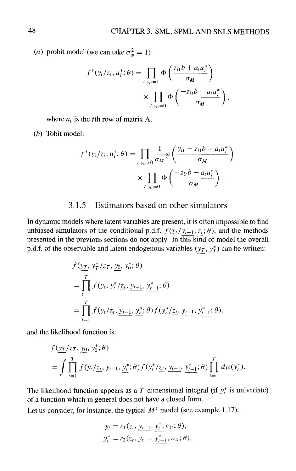
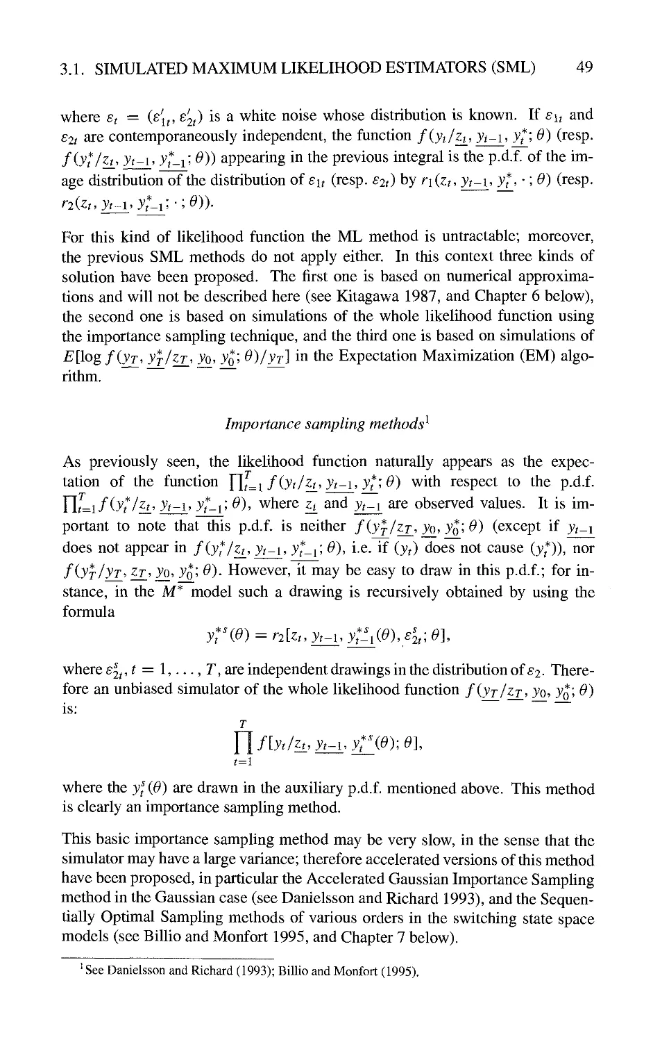
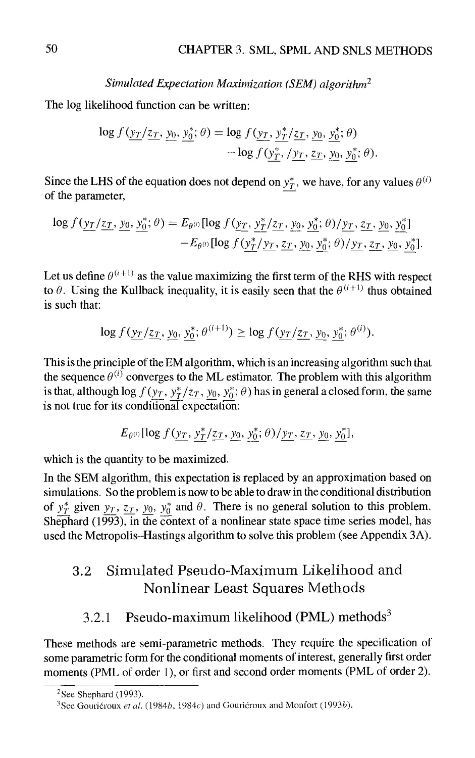
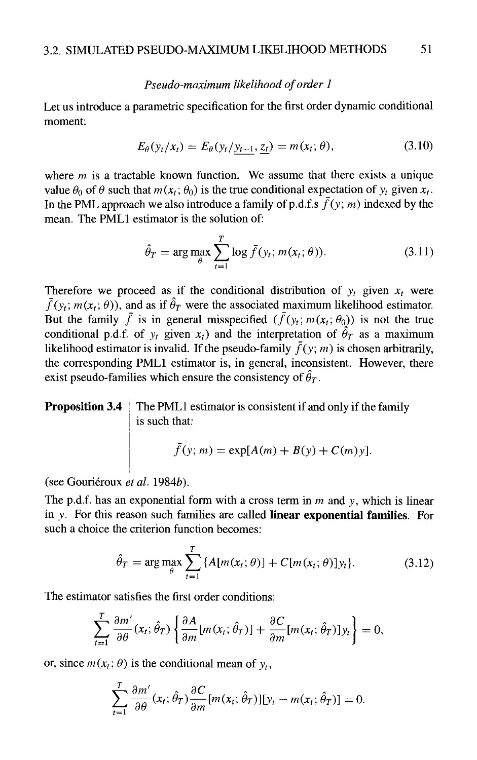
Текст
CORE Lectures
Simulation-Based Econometric Methods
The "CORE Foundation" was set up in 1987 with
the goal of stimulating new initiatives and research
activities at CORE.
One of these initiatives is the creation of
CORE LECTURES,
a series of books based on the lectures delivered each
year by an internationally renowned scientist invited
to give a series of lectures in one of the research areas
of CORE.
CORE Lectures
SIMULATION-BASED
ECONOMETRIC METHODS
CHRISTIAN GOURIEROUX
and
ALAIN MONFORT
OXFORD UNIVERSITY PRESS
Tills hook has been printed digitally and produced in a standard specification
in order to ensure its continuing availability
OXFORD
UNIVERSITY PRESS
Great Clarendon Street, Oxford OX2 6DP
Oxford University Press is a department of the University of Oxford.
It fintliers tlie University's objective of excellence in research, scholarship,
and education by publishing worldwide in
Oxford New York
Auckland Bangkok Buenos Aires Cape Town Chennai
Dar es Salaam Delhi Hong Kong Istanbul Karachi Kolkata
Kuala Lumpur Madrid Melbourne Mexico City Mumbai Nairobi
Sao Paulo Shanghai Singapore Taipei Tolcyo Toronto
with an associated company in Berhn
Oxford is a registered trade mark of Oxford University Press
in the UK and in certain other countries
Pubhshed in the United States
by Oxford University Press Inc., New York
© Christian Gourieroux and Alain Monfort, 1996
The moral rights of the author have been asserted
Database right Oxford University Press (maker)
Reprinted 2002
All rights reserved. No part of this pubhcation maybe reproduced,
stored in a retrieval system, or transmitted, in any form or by any means,
without the prior permission in writing of Oxford University Press,
or as expressly permitted by law, or under terms agreed with the appropriate
reprographics rights organization. Enquiries concerning reproduction
outside the scope of the above should be sent to the Rights Department,
Oxford University Press, at the address above
You must not cirailate this book in any other binding or cover
and you must impose this same condition on any acquirer
ISBN 0-19-877475-3
We are especially grateful to L. Broze and B. Salanie for checking
the presentation and the proofs. They are not responsible
for remaining errors.
We also thank E. Garcia and F. Traore who carefully typed this text
and F. Henry who helped with the layout.
This page intentionally left blank
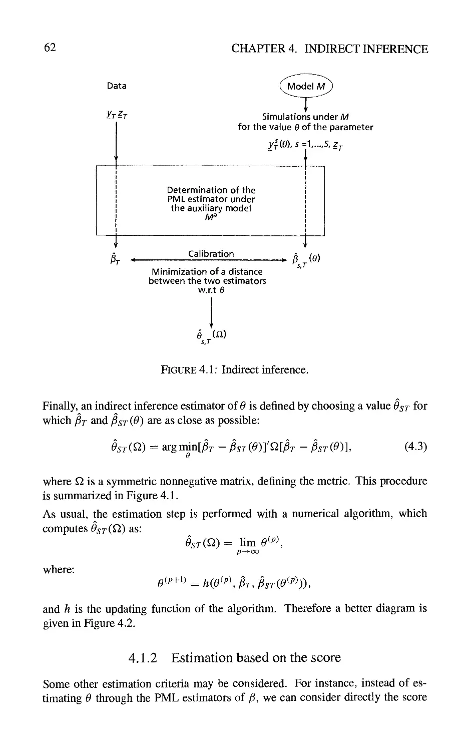
Contents
1 Introduction and Motivations 1
1.1 Introduction 1
1.2 A Review of Nonlinear Estimation Methods 2
1.2.1 Parametric conditional models 2
1.2.2 Estimators defined by the optimization of a criterion function 3
1.2.3 Properties of optimization estimators 6
1.3 Potential Applications of Simulated Methods 7
1.3.1 Limited dependent variable models 8
1.3.2 Aggregation effect 10
1.3.3 Unobserved heterogeneity 11
1-3.4 Nonlinear dynamic models with unobservable factors 12
1.3.5 Specification resulting from the optimization of some
expected criterion 14
1.4 Simulation 15
1.4.1 Two kinds of simulation 15
1.4.2 How to simulate? 15
1.4.3 Partial path simulations 18
2 The Method of Simulated Moments (MSM) 19
2.1 Path Calibration or Moments Calibration 19
2.1.1 Path calibration 20
2.1.2 Moment calibration 20
2.2 The Generalized Method of Moments (GMM) 21
2.2.1 The static case 21
2.2.2 The dynamic case 22
2.3 The Metiiod of Simulated Moments (MSM) 24
VUl
CONTENTS
2.3.1 Simulators 24
2.3.2 Definition of the MSM estimators 27
2.3.3 Asymptotic properties of the MSM 29
2.3.4 Optimal MSM 31
2.3.5 An extension of the MSM 34
Appendix 2A: Proofs of the Asymptotic Properties of the MSM Estimator 37
2A.1 Consistency 37
2A.2 Asymptotic normality 38
3 Simulated Maximum Likelihood, Pseudo-Maximum Likelihood,
and Nonlinear Least Squares Methods 41
3.1 Simulated Maximum Likehhood Estimators (SML) 41
3.1.1 Estimator based on simulators of the conditional density
functions 42
3.1.2 Asymptotic properties 42
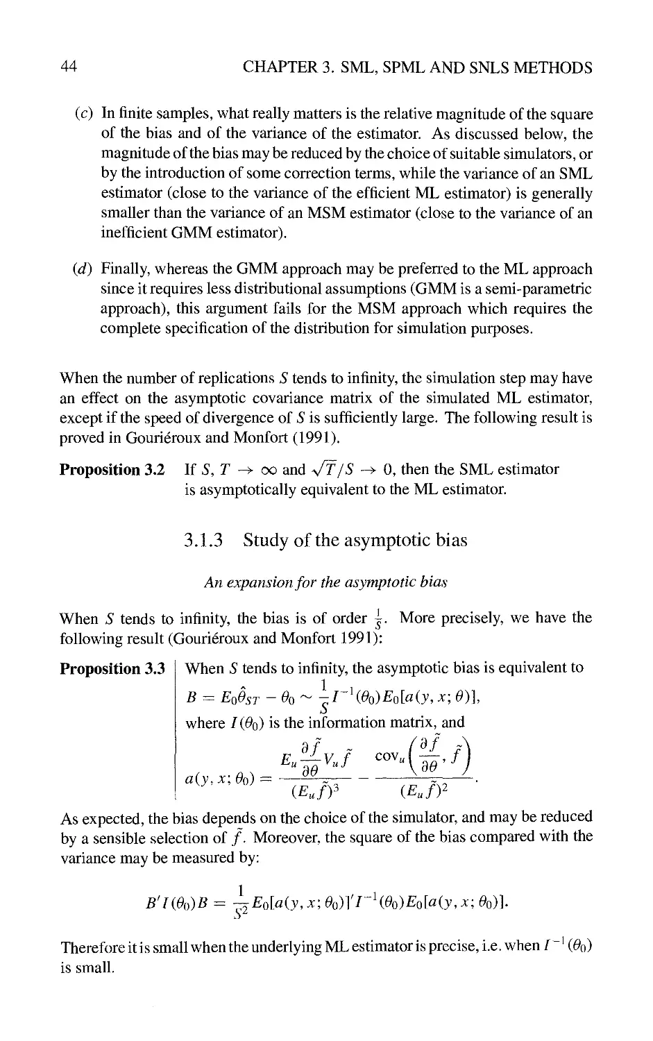
3.1.3 Study of the asymptotic bias 44
3.1.4 Conditioning 45
3.1.5 Estimators based on other simulators 48
3.2 Simulated Pseudo-Maximum Likehhood and Nonhnear Least
Squares Methods 50
3.2.1 Pseudo-maximum likelihood (PML) methods 50
3.2.2 Simulated PML approaches 55
3.3 Bias Corrections for Simulated Nonlinear Least Squares 56
3.3.1 Corrections based on the first order conditions 56
3.3.2 Corrections based on the objective function 57
Appendix 3A: The Metropohs-Hastings (MH) Algorithm 58
3A.1 Definition of the algorithm 58
3A.2 Properties of the algorithm 59
4 Indirect Inference 61
4.1 The Principle 61
4.1.1 Instrumental model 61
4.1.2 Estimation based on the score 62
4.1.3 Extensions to other estimation methods 64
4.2 Properties of the Indirect Inference Estimators 66
4.2.1 The dimension of the auxiliary parameter 66
CONTENTS
IX
4.2.2 Which moments to match? 67
4.2.3 Asymptotic properties 69
4.2.4 Some consistent, but less efficient, procedures 71
4.3 Examples 71
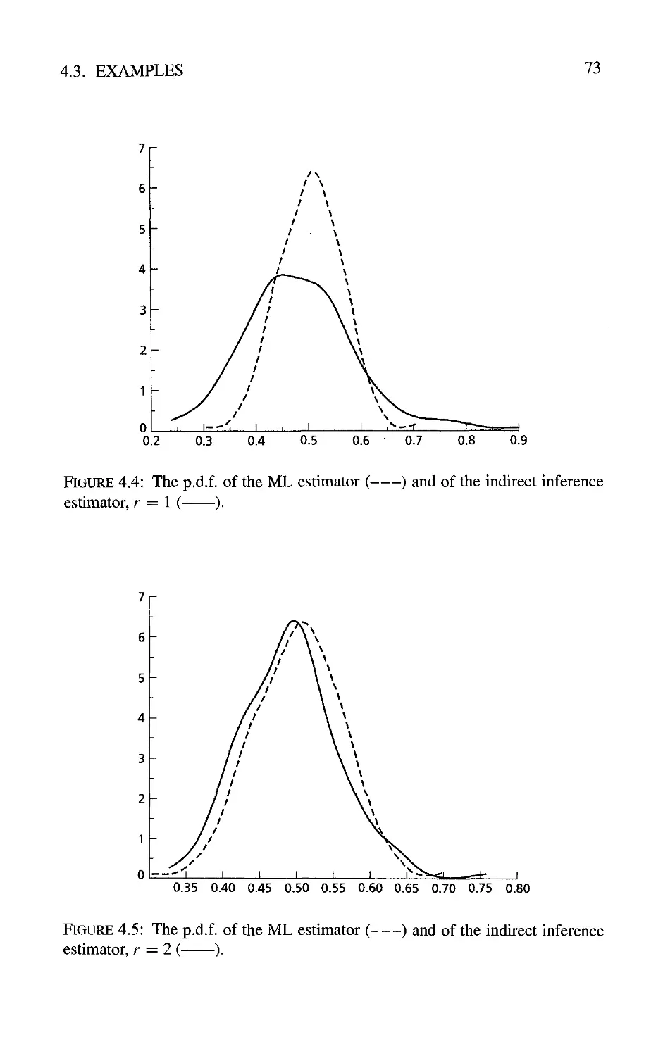
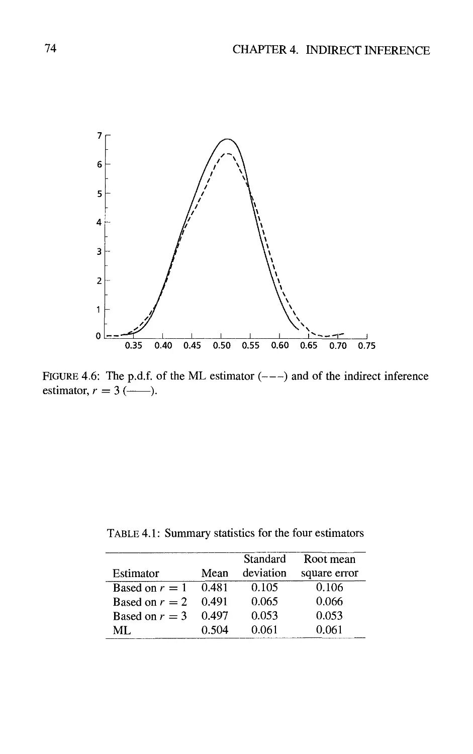
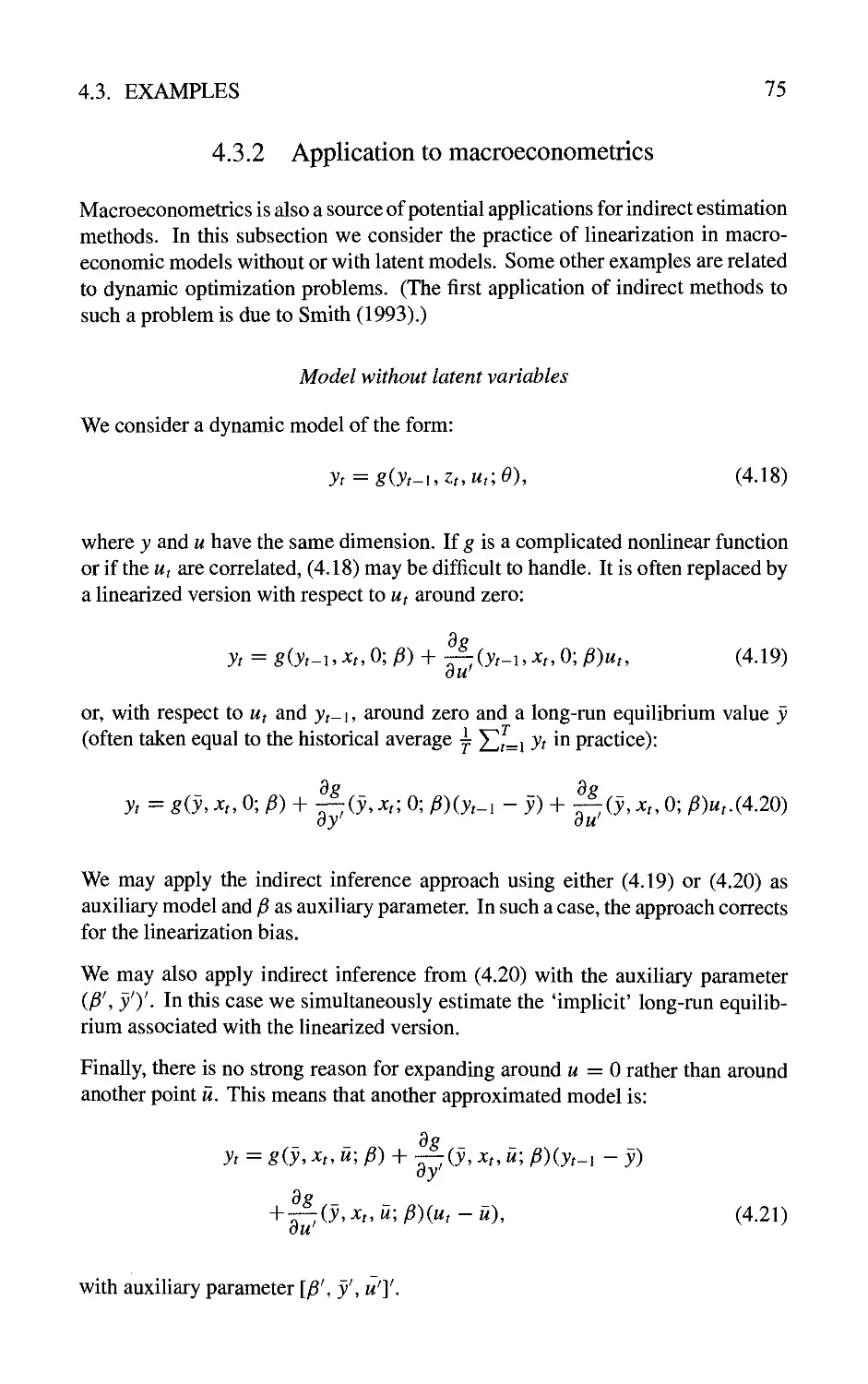
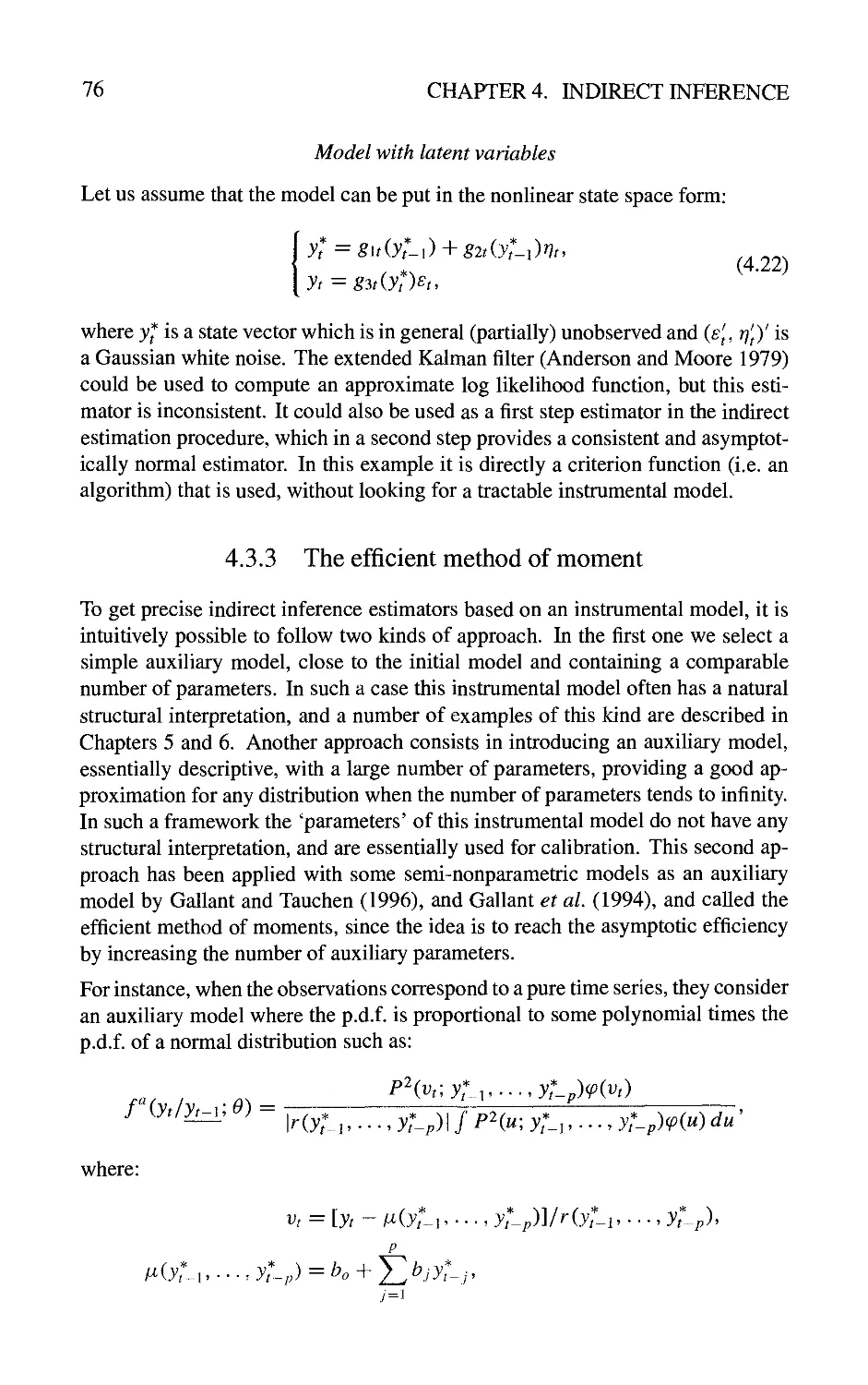
4.3.1 Estimation of a moving average parameter 71
4.3.2 Apphcation to macroeconometrics 75
4.3.3 The efficient method of moment 76
4.4 Some Additional Properties of Indirect Inference Estimators 77
4.4.1 Second order expansion 77
4.4.2 Indirect information and indirect identification 82
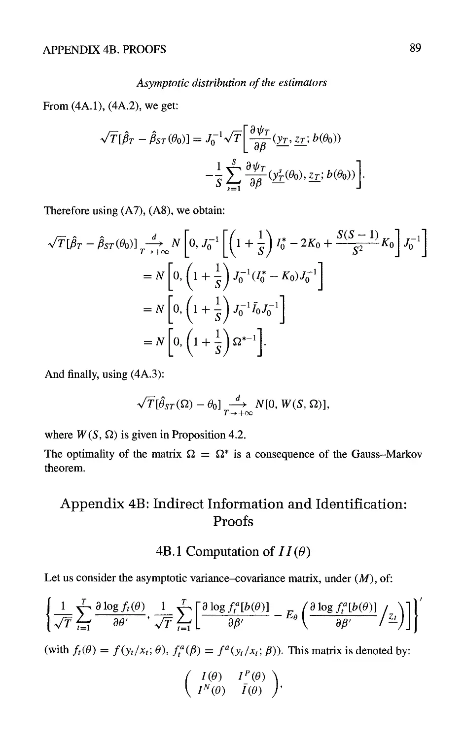
Appendix 4A: Derivation of the Asymptotic Results 84
4A. 1 Consistency of the estimators 85
4A.2 Asymptotic expansions 86
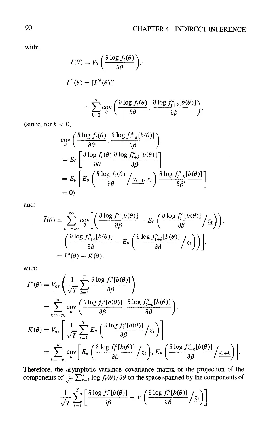
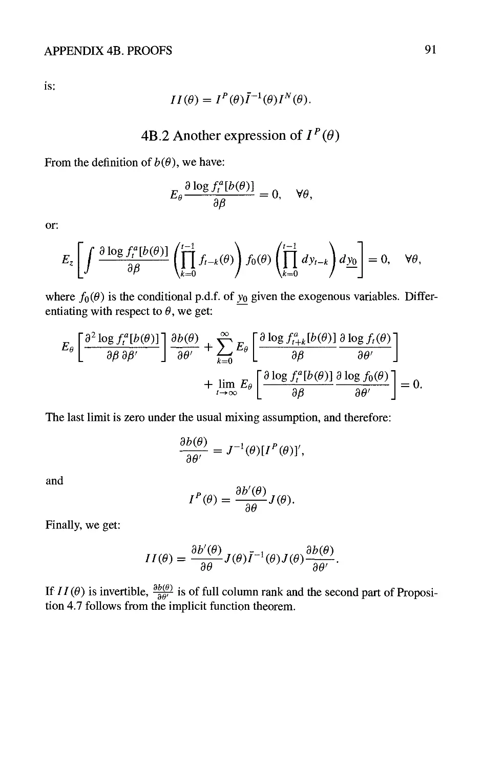
Appendix 4B: Indirect Information and Identification: Proofs 89
4B.1 Computation of II{0) 89
4B.2 Another expression of I^ {9) 91
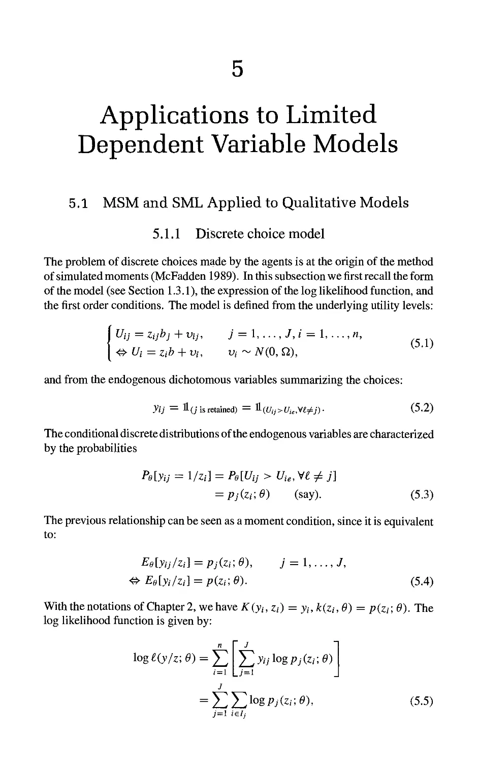
5 Applications to Limited Dependent Variable Models 93
5.1 MSM and SML Apphed to Qualitative Models 93
5.1.1 Discrete choice model 93
5.1.2 Simulated methods 94
5.1.3 Different simulators 96
5.2 Quahtative Models and Indirect Inference based on Multivariate
Logistic Models 100
5.2.1 Approximations of a multivariate normal distribution in a
neighbourhood of the no correlation hypothesis 100
5.2.2 The use of the approximations when correlation is present 102
5.3 Simulators for Limited Dependent Variable Models based on
Gaussian Latent Variables 103
5.3.1 Constrained and conditional moments of a multivariate
Gaussian distribution 103
5.3.2 Simulators for constrained moments 104
5.3.3 Simulators for conditional moments 107
5.4 Empirical Studies 112
5.4.1 Labour supply and wage equation 112
X
CONTENTS
5.4.2 Test of the rational expectation hypothesis from business
survey data 113
Appendix 5A: Some Monte Carlo Studies 115
6 Applications to Financial Series 119
6.1 Estimation of Stochastic Differential Equations from Discrete
Observations by Indirect Inference 119
6.1.1 The principle 119
6.1.2 Comparison between indirect inference and full maximum
likelihood methods 121
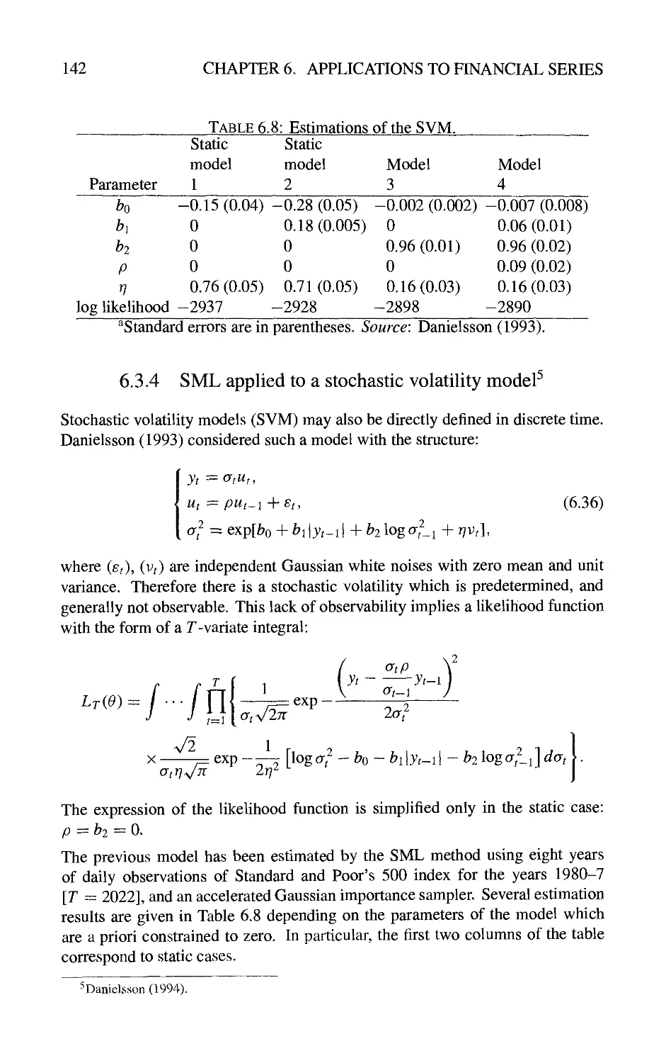
6.1.3 Specification of the volatility 125
6.2 Estimation of Stochastic Differential Equations from Moment
Conditions 133
6.2.1 Moment conditions deduced from the infinitesimal
operator 133
6.2.2 Method of simulated moments 137
6.3 Factor Models 138
6.3.1 Discrete time factor models 138
6.3.2 State space form and Kitagawa's filtering algorithm 139
6.3.3 An auxiliary model for applying indirect inference on
factor ARCH models 141
6.3.4 SML applied to a stochastic volatility model 142
Appendix 6A: Form of the Infinitesimal Operator 143
7 Applications to Sw^itching Regime Models 145
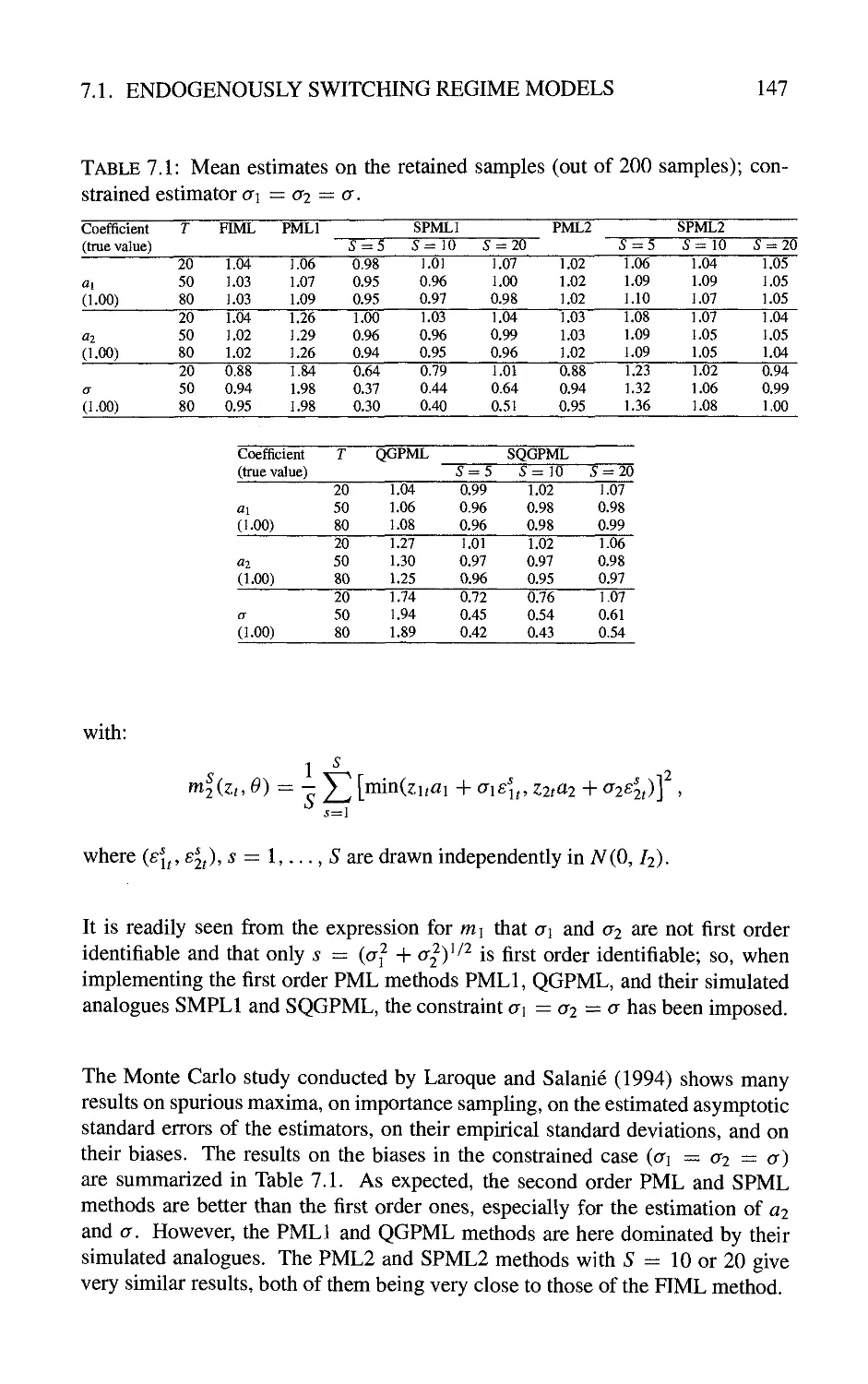
7.1 Endogenously Switching Regime Models 145
7.1.1 Static disequilibrium models 145
7.1.2 Dynamic disequilibrium models 148
7.2 Exogenously Switching Regime Models 151
7.2.1 Markovian vs. non-Markovian models 151
7.2.2 A switching state space model and the partial Kalman
filter 152
7.2.3 Computation of the likelihood function 153
References
Index
159
173
1
Introduction and Motivations
1.1 Introduction
The development of theoretical and applied econometrics has been widely
influenced by the availability of powerful and cheap computers. Numerical calculations
have become progressively less burdensome with the increasing speed of
computers while, at the same time, it has been possible to use larger data sets. We may
distinguish three main periods in the history of statistical econometrics.
Before the 1960s, models and estimation methods were assumed to lead to
analytical expressions of the estimators. This is the period of the linear model, with the
associated least squares approach, of the multivariate linear simultaneous
equations, with the associated instrumental variable approaches, and of the exponential
families for which the maximum likelihood techniques are suitable.
The introduction of numerical optimization algorithms characterized the second
period (1970s and 1980s). It then became possible to derive the estimations and
their estimated precisions without knowing the analytical form of the estimators.
This was the period of nonhnear models for micro data (limited dependent variable
models, duration models, etc.), for macro data (e.g. disequilibrium models,
models with cycles), for time series (ARCH models, etc.), and of nonhnear statistical
inference. This inference was based on the optimization of some nonquadratic
criterion functions: a log likelihood function for the maximum likelihood
approaches, a pseudo-log likelihood function for the pseudo-maximum likelihood
approaches, or some functions of conditional moments for GMM (Generalized
Method of Moments). However, these different approaches require a tractable
form of the criterion function.
This book is concerned with the third generation of problems in which the
econometric models and the associated inference approaches lead to criterion functions
without simple analytical expression. In such problems the difficulty often comes
from the presence of integrals of large dimensions in the probability density
function or in the moments. The idea is to circumvent this numerical difficulty by an
approach based on simulations. Therefore, even if the model is rather complicated,
it will be assumed to be sufficiently simple to allow for simulations of the data,
for given values of the parameters, and of the exogenous variables.
In Section 1.2 we briefly review the classical parametric and semi-parametric
nonhnear estimation methods, such as maximum likeHhood methods, pseudo-
maximum likelihood methods, and GMM, since we wiU discuss their simulated
counterparts in the next chapters.
CHAPTER 1. INTRODUCTION AND MOTIVATIONS
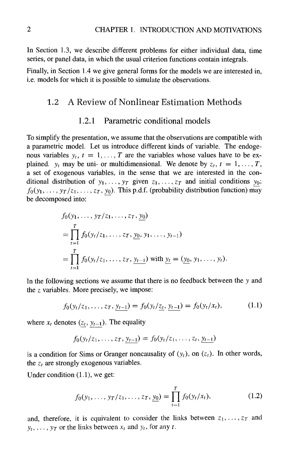
In Section 1.3, we describe different problems for either individual data, time
series, or panel data, in which the usual criterion functions contain integrals.
Finally, in Section 1.4 we give general forms for the models we are interested in,
i.e. models for which it is possible to simulate the observations.
1.2 A Review of Nonlinear Estimation Methods
1.2.1 Parametric conditional models
To simplify the presentation, we assume that the observations are compatible with
a parametric model. Let us introduce different kinds of variable. The
endogenous variables 3^^, ^ — 1,..., T are the variables whose values have to be
explained, jt may be uni- or multidimensional. We denote hy zt, t = 1,..., T,
a set of exogenous variables, in the sense that we are interested in the
conditional distribution of yi,... ,yT given zi,..., zr and initial conditions 3^0-
foiyi^ • • •. yr/zi,... ,zt^ yo)- This p.d.f. (probability distribution function) may
be decomposed into:
Myi, ..^,yT/zi. ■^■,ZT,yo)
T
foiyi/zi,^...ZT.yo,yi^ ■-■^yt-})
T
fo(yt/z}, ..•^zr.yr-i) wither = (yo, yu ■■-.yt)-
In the following sections we assume that there is no feedback between the y and
the z variables. More precisely, we impose:
Myt/zu.,.,ZT,yt-i) = fo(yt/zt,yr-i) = foiyt/xt), (i.i)
where Xt denotes (z^, yt^i)- The equality
fo(yt/zu....zT,yt~i) ^ Myt/zi. ...,zt.yt^)
is a condition for Sims or Granger noncausality of (yt), on (zr). In other words,
the Zt are strongly exogenous variables.
Under condition (1.1), we get:
T
Myu---,yT/z\.^..,ZT.yo) = f|/o(}^fAr). (1-2)
and, therefore, it is equivalent to consider the links between zi,...,Z2 and
yt, '•• ^yr or the links between Xt and v?, for any t.
1.2. A REVIEW OF NONLINEAR ESTIMATION METHODS
Note that we have assumed that the conditional p.d.f. fo(yt/xt) does not depend
on t; more precisely, we assume that the process (yt, Zt) is stationary. Also note
that, in cross sections or panel data models, the index t will be replaced by i and
the >';s will be independent conditionally to the z,s.
To summarize, we are essentially interested in a part (1.2) of the true
unknown distribution of all the observations, since the whole distribution consists
of foiyi^ • • • ^ yr/zi,... .zt^ yo) and of the true unknown marginal distributions
/o(Zl, •• -^ZT^yo) of Zl, " '^ZT^yO;
In order to make an inference about the conditional distribution, i.e. foiyt/^t)^ we
introduce a conditional parametric model. This model M is a set of conditional
distributions indexed by a parameter 0, whose dimension is p:
M = {f(yt/xt;0),0€e}, (1.3)
where 9 C ^^ is the parameter set. This model is assumed to be well-specified;
i.e.
foiyt/xt) belongs to M, (1.4)
and identifiable; i.e., there exists a unique (unknown) value ^o such that:
Myt/xt) = fiyt/xt;Ooy (1.5)
^0 is called the true value of the parameter.
In such a framework, the determination of the unknown conditional distribution is
equivalent to the determination of the true value of the parameter.
1.2.2 Estimators defined by the optimization of a criterion
function
The usual estimation approaches consist in optimizing with respect to the parameter
a criterion depending on the observations >'^, z^, r = 1,..., T. The estimator is
defined by:
Ot = argmax ^r(>'i,... ,yT,Zu ..., zt; 0)
u
= argmax ^7'(6') (say). (1.6)
In practice, the function ^7 is generally differentiable and the estimator is deduced
from the p-dimensional system of first order conditions:
-^(Ot) = 0 ^=^ -^^^^^ =0' j = h...,p. (1.7)
With few exceptions, this system does not admit an analytical solution and the
estimation is obtained via a numerical algorithm. The most usual ones are based
4 CHAPTER 1. INTRODUCTION AND MOTIVATIONS
on the Gauss-Newton approach. The initial system is replaced by an
approximated one deduced from (1.7) by considering a first order expansion around some
value Og:
where j~^ is the Hessian matrix. The condition ^(^) = 0 is approximately
the same as the condition
0^0,-
d^^T(Oq)l ' a^r
dOdO
(0,). (1.8)
dO
The Newton-Raphson algorithm is based on the corresponding recursive formula:
OgJ^l ~ Og —
a^^r '^ ^
dOdO
^0,)
^iO,). (1.9)
As soon as the sequence Oq converges, the limit is a solution Ot of the first order
conditions.
The criterion function may be chosen in various ways depending on the properties
that are wanted for the estimator in terms of efficiency, robustness to some mis-
specifications and computability. We describe below some of the usual estimation
methods included in this framework.
Example 1.1 (Conditional) maximum likelihood
The criterion function is the (conditional) log likeHhood function:
T
t=i
Example 1.2 (Conditional) pseudo-maximum likelihood (PML) (Gourieroux,
Monfort, and Trognon 1984/?, c)
In some appHcations it may be interesting for robustness properties to introduce
a family of distributions which does not necessarily contain the true distribution.
Let us introduce such a family /*(}^r/^r; 0). The PML estimator of ^ based on the
family /* is defined by:
T
0T=sirgmaxJ2^ogriyt/xt;0). (1.10)
t=i
Such pseudo-models are often based on the normal family of distributions. Let us
consider a well-specified form of the first and second order conditional moments:
Eiyt/xt) ^m(xr\0)
Viyt/xt)=:cy^{xt,0) (say).
1.2. A REVIEW OF NONLINEAR ESTIMATION METHODS 5
We may introduce the pseudo-family of distributions N[mixt;0),a^ixt;0)],0 €
0, even if the true distribution is nonnormal. In such a case the criterion function
is:
'^TiO) = J2
^ ^ K ^ 1, 2. .. liyt-mixt-0))^^
t=i I-
-log2;r--logafe^) ^ ^,^^^, ^^
.(1.11)
Example 1.3 Nonlinear least squares (Jennrich 1969, Malinvaud 1970)
The estimator of 0 is obtained by minimizing the prediction errors. With the same
notation as before, it is given by:
6'r = argmin2^[>'^ -m(x^;6')r. (1.12)
It is easily checked that this procedure may be considered as a PML approach
based on the family {N [m(xt; 0), 1], 0 e 0}.
Example 1.4 Generalized method of moments (Hansen 1982, Hansen and
Singleton 1982)
Let us introduce some ^-dimensional function K {yt, Xf) of the observable variables
and let us assume that we have a well-specified expression for the conditional
moment;
Ee[K{yt.Xt)lxt]=k{xt\0). (1.13)
This equality defines some estimating constraints. Indeed, it yields:
Ee[K{yt\Xt)-k{xuO)lxt]=0,
which implies:
Eea'ixt) [K{yu Xt) - k{xu 0)] = 0, (1.14)
for any function a. The idea of the GMM is to look for a value Oj, such that the
empirical counterparts of the constraints (1.14) are approximately satisfied. More
precisely, let us introduce r ^-dimensional functions cty, 7 = 1,..., r, and denote
A = (fli,..., fl;-). Let us also introduce a nonnegative symmetric matrix Q of size
(r X r). Then the estimator is:
Ot = argmmj;^ A'ixt) [K(yt, Xt) - k{xu e)]\
The elements of matrix A{xt) are instrumental variables (with respect to the
constraints).
CHAPTER 1. INTRODUCTION AND MOTIVATIONS
Example L5 Extended methods
It is possible to extend all the previous examples in the following way. Even if
we are interested in the parameters 0, we may introduce in the criterion function
some additional (nuisance) parameters a. Then we can consider the solutions Ot.
ar of a program of the form:
r%y
(OT^ar) == argmax^^(^,a).
0,a
Equivalently, we have:
r%y
Ot = argmax^rC^),
6
where ^7'(^) — max^ ^^(0, a) is the concentrated criterion. Such an approach is
for instance the basis for the adjusted PML method (Broze and Gourieroux 1993).
1.2.3 Properties of optimization estimators
As usual, two kinds of asymptotic properties have to be considered: the consistency
of the estimator, and the form of its asymptotic distribution.
Consistency. If the well normalized criterion function uniformly converges to
some limit function:
lim ^^TiO)^^ooiO),
and if this limit function has a unique maximum 0^, then the estimator Oj ^
argmaxg ^^t(0) converges to this value. Therefore in practice three conditions
have to be fulfilled:
(i) the uniform convergence of the normahzed criterion function;
(ii) the uniqueness of Oq° (identifiability condition of 0 with respect to the
criterion function);
(iii) the equality between this solution 0^ (often called pseudo-true value) and
the true value ^0-
Asymptotic normality. Whenever the estimator is consistent, we may expand the
first order conditions around the true-value ^o- We get:
BO 30 30
<=^ Or - Oq c:^
a^^T " ^ *
30 30'
30
m.
1.3. POTENTIAL APPLICATIONS OF SIMULATED METHODS
7
The criterion function is often such that there exist normalizing factors hj, h\,
with:
hm (^o)
= JiOo), where J(^o)is invertible; (1-16)
^ (^o) -^ A^ [0, / (^o)], where /(^o)is invertible.
/i* dO
(1.17)
Therefore we get:
h
h^j
(Ot-Oo) ^
1 d'^^T
-,-1
7(^0)
^ i(^0)
hr dOdO
_i 1 9*r
1 d^T
h^j do
(Oo)
/i* dO
(Oo)-
We deduce that:
h
^(Ot-Oo)'^N [0, /(^o)"V(^o)i(^o)"'].
h
(1.18)
Under stationarity conditions, we generally have: hj = T, hj = \ff, hj/hj =
Vf.
Optimal choice of the criterion function. Some estimation approaches naturally
lead to a class of estimators. For instance, in the GMM approach we can choose in
different ways the instrumental variables A and the distance matrix Q. Therefore
the estimators Ot(A, Q) and their asymptotic variance-covariance matrices.
K
as
T(A,Q)-Oo))] = i:iA,Q\
are naturally indexed by A and Q. So, one may look for the existence of an optimal
choice for this couple. A, Q, i.e. for a couple A*, Q* such that:
S(A*,^*)<S(A,^), \/A,Q,
where <^ is the usual ordering on symmetric matrices. For the usual estimation
methods, such optimal estimators generally exist.
1.3 Potential Applications of Simulated Methods
In this section we present some parametric problems for which the likelihood
function fiyt/xti 0), and the conditional moments mixti 0), a^{xt\ 0), k{xt\ 0),...,
do not admit a tractable form. In such a framework the optimization algorithms.
8 CHAPTER 1. INTRODUCTION AND MOTIVATIONS
such as the Newton-Raphson algorithms, cannot be used directly since they
require a closed form of the criterion function ^. Generally this difficulty arises
because of the partial observability of some endogenous variables; this lack of
observability will introduce some multidimensional integrals in the expression of
the different functions and these integrals could be replaced by approximations
based on simulations. In such models it is usual to distinguish the underlying
endogenous variables (called the latent variables), which are not totally observable,
and the observable variables. The latent variables will be denoted with an asterisk.
As can be clearly seen from the examples below, this computational problem
appears for a large variety of applications concerning either individual data, time
series, or panel data models, in microeconomics, macroeconomics, insurance,
finance, etc.
1.3.1 Limited dependent variable models
Example 1.6 Multinomial probit model (McFadden 1976)
This is one of the first applications that has been proposed for the simulated
estimation methods we are interested in (McFadden 1989, Pakes and Pollard 1989).
It concerns qualitative choices of an individual among a set of M alternatives. If
the individual i is a utiHty maximizer, and if Uij is the utility level of alternative
j, the selection is defined by:
j is the retained alternative if and only if Uij > Uu ^l y^ j.
The selection model is obtained in two steps. We first describe the latent
variables (i.e. the utiHty levels) as functions of explanatory variables z, using a hnear
Gaussian specification:
Uij = Zijbj + Vij, 7 — 1, ..., M, / = 1, ..., n,
Ui —Zih -^Vi, i — I,. ..,n,
where Uf = ([/a, ..., UimY. Vf = (vn, ..., vimY, and Vi - A^(0, Q).
Then in a second step we express the observable choices in term of the utiHty
levels:
ytj = % is retained by i = '\uij>Uuyi^j).
In such a framework the endogenous observable variable is a set of dichotomous
quaHtative variables. It admits a discrete distribution, whose probabiHties are:
Pij = P[j is retained by i/zi]
= P{Uij>Ua.Wl^j/zi)
= P{zijhj + Vij > zuh + Vii, "il ^ j/zi)
1.3. POTENTIAL APPLICATIONS OF SIMULATED METHODS
where g is the p.d.f. of the M - 1 dimensional normal distribution associated with
the variables vij — vu, I ^ j-
Therefore the distribution of the endogenous observable variables has an
expression containing integrals whose dimension is equal to the number of alternatives
minus one. These integrals may be analytically approximated when / is not too
large (/ < 3 or 4), but for a number of applications, such as transportation choice,
this number may be larger.
Example 1.7 Sequential choices and discrete duration models
In structural duration models, the value of the duration may often be considered as
the result of a sequence of choices. For instance, in job search models (Lancaster
1990, Chesher and Lancaster 1983, Lippman and McCall 1976, Nickell 1979,
Kiefer and Neumann 1979), under some stationarity assumptions each choice is
based on a comparison between the potential supplied wage and a reservation
wage, i.e. a minimal wage above which the job is accepted. Let us denote by y*-^,
y2jj the potential and reservation wages for individual / at time t.
If we consider a sample of individuals becoming unemployed at date zero, the
length of the unemployment spell for individual /" is:
Di^inf{t:yli^>y^,,},
If the latent bivariate model associated with the two underlying wages is a dynamic
linear model, for instance with values of the wages:
yut = ^lyh-i + ^^ykt-i + ^^tci + u^t,
yiit = ^2yu,t-i + hy2i,t-i + zitC2 + U24t,
where (uut, i^2,it) are i.i.d. normal N(0, Q), it is directly seen that the distribution
of the duration has probabilities defined by the multidimensional integrals:
P[A =d] = P{yl,, < yl,„ ..., yl,,_, < >.*,,_„ >.*,, > y^J.
The maximal dimension of these integrals may be very large; since the probabilities
appearing in the likelihood function correspond to the observed values of the
durations, this dimension is equal to max/=^i „.„4*> where n is the number of
individuals.
The same remark appHes for the other examples of sequential choices, in particular
for prepayment analysis (see Frachot and Gourieroux 1994). In this framework
the latent variables are an observed interest rate and a reservation interest rate.
10 CHAPTER 1. INTRODUCTION AND MOTIVATIONS
L3.2 Aggregation effect
The introduction of integrals in the expression of the distribution of the observable
variables may also be the consequence of some aggregation phenomenon with
respect to either individuals or time.
Example L 8 Disequilibrium models with micro markets (Laroque and Salanie
1989, 1993)
Let us consider some micro markets n ~ 1,..., A^, characterized by the micro
demand and supply:
D,{t)^-D{zt.std,s'^,e),
where Zt are some exogenous factors, Std, Sts some macroeconomic error terms,
which are the same for the different markets, and s^, s" some error terms specific
to each market.We assume that (s'^, £") are ii.d., independent of Zt, Std^ ^ts-
We now consider some observations of the exchanged quantity at a macro level
If A^ is large, we get:
N
1
Q'= 1™ -y]mm(DM,Sn{t))
N—^oo A^
^ £e,,^,. [min(D(zr, Std. Bd\ 0), S{zt, Sts. £,; 0))].
Therefore the expression of the observable variable Qf in terms of the exogenous
variable Zt and of the macroeconomic error terms appears as an expectation with
respect to the specific error terms.
Example L9 Estimation of continuous time models from discrete time
observations (Duffie and Singleton 1993, Gourieroux et aL 1993)
In financial applications the evolution of prices is generally described by a diffusion
equation, such as:
dyr=ii(yt.O)dt-^a(yr.O)dWr. (1.19)
where Wt is a Brownian motion. At(jn 0) is the drift term, and a(j;, 0) is the
volatility term. However, the available observations correspond to discrete dates;
they are denoted by ji, j2, • • •, Jr, Jr+i, • • •• The distribution of these observable
variables generally does not admit an explicit analytical form (see Chapter 6),
but appears as the solution of some integral equation. This difficulty may be
seen in another way. Let us approximate the continuous time model (1.19) by
its discrete time counterpart with a small time unit 1/n. We introduce the Euler
approximation y^"^ of the process y.
1.3. POTENTIAL APPLICATIONS OF SIMULATED METHODS
11
This process is defined for dates t = k/n and satisfies the recursive equation;
y{k+\)in -yk/n^ ^1^
^^/-^-^;^K^^/-')^^'
(1.20)
where (sk) is a standard Gaussian white noise. The distribution of yi, y2, ■ - ■, yt,
yt+i,... may be approximated by the distribution of y" , 3^2" ' • •' 3^?" ' 3^?+!
* « ««
We note that the process j*^"^ is Markovian of order one and we deduce that it
is sufficient to determine the distribution of y^"^^ conditional on j}"^ to deduce
the distribution we are looking for. Let us introduce the conditional distribution
of y^l.y, given yi%: f (yl'll.y Jyi%) say. From (1.20), this distribution is
normal with mean yj^/^ + j;f^[yi%; O], and variance licr^{yi%\ O). The conditional
distribution of y^"^^ given j/"^ is given by:
fiyl%/yn-f--[Y\fiyr.
•^ '^ k=0
)
t+k/n
k=l
and requires the computation of an (n - 1)-dimensional integral since we have to
integrate out all the missing values j^"i/„,. • •, j^+(„„i)/„.
1.3.3 Unobserved heterogeneity
1
The introduction of unobserved heterogeneity in nonlinear models also creates
multiple integrals.
Example LIO Random parameter model
A nonlinear regression model such as:
yt = miz'fi) + aWi, / = 1,..., n
Wi -IIN(0,1),
may be extended by allowing parameter 6 to depend on the individuals. To avoid
identification problems, the usual practice consists in writing
yi = mizfii) + awi, / = 1,..., n,
where Oi,i = 1,..., n, are i.i.d. variables, for instance distributed as N(0, Q), and
independent of the error terms Wi, Then the conditional probability distribution
function (p.d.f.) of the endogenous variable yi, given the exogenous variables zt,
is:
fiyi/zi) =
4/4^
a
Y\(p(i^k)duk,
k=l
where K is the number of explanatory variables and (p the p.d.f. of the standard
normal distribution.
^See Gourieroux and Monfort (1991, 1993a).
12 CHAPTER 1. INTRODUCTION AND MOTIVATIONS
Example Lll Heterogeneity factor
The modelling of qualitative variables, count data, duration data, etc., is generally
based on conditional specifications of the form
Kyi/zi) = f{yi;zie),
where / is a well-chosen distribution, such as logistic, Poisson, or exponential,
depending on the kind of endogenous variable. Therefore the whole influence of
the explanatory variables is driven by the scoring function ztO, It is important to
take into account the possibility of omitted explanatory variables independent of
the retained ones. It is known that in a Hnear Gaussian model the OLS estimators
of the 0 parameter remain unbiased in the case of such an omission, but this
property is no longer valid for nonlinear specifications. This heterogeneity will be
introduced by adding an error term to the scoring function:
Kyi/zh Ui) = fiyn ZiO-j-auf),
where for instance the w- are i.i.d. variables, with given p.d.f. g. Then the condi
tional distribution of yi given zt is;
/
Except for some very special and unrealistic choices of the couple of
distributions (/, g) (for instance Poisson-gamma for count data, exponential-gamma for
duration data), the integral cannot be computed analytically.
Two remarks are in order. First, the dimension of the integral is equal to the
number of underlying scoring functions and is not very large in practice. The
numerical problems arise from the large number of such integrals that have to be
evaluated, since this number, which is equal to the number of individuals, may
attain 100000-1 000000 in insurance problems, for instance.
Second, a model with unobserved heterogeneity may be considered a random
parameter model, in which only the constant term coefficient has been considered
random.
1.3.4 Nonlinear dynamic models with unobservable factors
The typical form of such models is:
yt = ri{zt,yt~uytj^uiO),
y^ ^ riizi, yt-i. yt-1»^2^; o),
where (su), (^2?) are independent i.i.d. enor terms the distributions of which are
known (see 1.4.2), and (zt) depicts an observable process of exogenous variables.
1.3. POTENTIAL APPLICATIONS OF SIMULATED METHODS 13
The process (zt) is assumed to be independent of the process (su, szt). yt-i
denotes the set of past values yt-i, yt~2,, -• - of the process y. (yt) is the observable
endogenous process and (yf) is the endogenous unobservable latent factor.
If the functions rifc, yt-]_, yf, -; 0) and r2(z£, yt~u J?Li, -l^) ^e one to one,
the previous equations define the conditional p.d.f. f{yt/zuyt~\,y'^\0) and
fiyf/zi, yt~i, yf^il ^)- Therefore the p.d.f. of jr, yr given zt_ (and some
initial values) is nLi f{yt/zt_, yt~u jf; 0)f(yf/zi, yt-i. yt^. 0), and the likelihood
function, i.e. the p.d.f. of yr, appears as the multivariate integral
T T
n fiy</h' yizi' yl^ (^)f{y:/^A, iizi' yU} ^) 11 '^^^y*^
t=\ t=\
where At(jf) denotes the dominating measure.
Example 1,12 Factor ARCH model (Diebold and Nerlove 1989, Engle et aL
1990)
The relationship between the factors and the observable variables corresponds to
a linear specification:
yt = ^yf + Csu, (su) - IIN(0, id^),
where yt, X are m-dimensional vectors and C is a lower triangular (m x m)
matrix. We introduce here a single factor y*, which is assumed to satisfy an ARCH
evolution:
y* = (ofi +a2y*Ii) S2t, (sit) '^ IIN(0,1), independent of (^u).
Example 1,13 Stochastic volatility model (Harvey et al 1994, Danielsson and
Richard 1993, Danielsson 1994)
The simplest model of this kind is
J, =z:exp(-3;; j£u
J* =a + /73;*_j +as2t,
where {£\t,S2t) is a standard bivariate Gaussian white noise. In this kind of model
the conditional distribution of yt given jf is A'(0, exp yf) and the latent factor y^
is an AR(1) process.
Example LI4 Switching state space models (Shephard 1994, Kim 1994, Billio
and Monfort 1995)
These models are:
yr = ^(3^, yt^) + A(3^, 3Vj_)Ju + ^(^i' Ztzi)^^
3^1* = ^(3^, yt-i) + C(yl, yt^)yl-i + Diy^^, yt^)rjt
y2t ='^0)(y2t~i)Ayro(yt-i)A](^t) +fl{i}(ji-i)%,^i(:y;-i)](w?)
14 CHAPTER 1. INTRODUCTION AND MOTIVATIONS
where {st}^ {n?} are independent standard Gaussian white noises and [ut] is a
white noise, independent of {£?}{«?} and whose marginal distribution is ^o,i]» the
uniform distribution on [0, 1].
In this model the first factor jj* is a quantitative state variable whereas 3^2? is a
binary regime indicator. (The case of more than two regimes is a
straightforward generalization.) This general framework contains many particular cases:
switching ARMA models, switching factor models, dynamic switching
regressions, deformed time models, models with endogenously missing data, etc.
Example LI5 Dynamic disequilibrium models (Laroque and Salanie 1993,
Lee 1995)
In this kind of model the latent factors are demand and supply, whereas the observed
variable >v is the minimum of the demand and the supply. Such a model is:
A = r2o{zt. Dt^u St-u £Dt\ 0)
St = r2s(Zt, A-i, St.^u sst'^ ^)
Qt=rmn{Dt.St) (=r,(Dr,St))
Note that no random error appears in ri; this implies that the model is, in some way,
degenerated and that the general formula given above for the likelihood function is
not valid. However, it is easily shown (see Chapter 7) that the likeHhood function
appears as a sum of 2^ T-dimensional integrals.
1.3.5 Specification resulting from the optimization of some
expected criterion
An example of this kind appears in a paper by Laffont et aL (1991). The authors
derive from economic theory a first price auction model. For an auction with J
bidders, the winning bid has the form
y = £'[max(i;(y--i); Po)/v(j)].
where i;^,; — 1, ..., J are the underlying private values, po is a reservation price,
independent of the VjS, and V(j) is the order statistic associated with the VjS.
In this example the function linking the latent variables fy, ; ^ 1,...,/, po. and
the observed bid y has a directly integral form. Note that, by taking the expectation,
we ehminate the conditioning effect and arrive at:
Ey = E(meLx(v^j-i)^po)),
but some integrals remain because of the max and the ordering of the bids.
1.4. SIMULATION
15
1.4 Simulation
1.4.1 Two kinds of simulation
For a given parametric model, it is possible to define the distribution of ji,..., jr
conditional on zi,..., zr, 3^, f{'/z\,.. •, Zr, 3^; 0), say, and the distribution of
yt conditional on Xf = {zt, yt~\), f(-/xt',0), say. It is particularly important in
the sequel to distinguish two kinds of simulation.
Path simulations correspond to a set of artificial values (yf(0), t = I,. ,,,T) such
that the distribution of yj(6'),..., y^j-iO) conditional on zi,..., zr, 3^ is equal to
/(•/zi, ...,Zr,3^;6').
Conditional simulations correspond to a set of artificial values (jf(6'), t =
1,..., r) such that the distribution of yf(0) conditional on Xt — (zi, yt-i) is
equal to f{'/xt\ 0), and this for any t.
It is important to note that these simulations may be performed for different values
of the parameter, and that the conditional distributions of the simulations will
depend on these values.
Moreover, it is possible to perform several independent replications of such a set of
simulations. More precisely, forpath simulations wecan build several sets y^(0) =
(yf(0),t = I, ,..,T),s = 1,..., 5, such that the variables y^ (0) are independent
conditionally on zi,..., Zr. Jo ^nd ji,..., jr- This possibility is the basis of
simulated techniques using path simulations, since the empirical distribution of
the 3?^(^), ^ = 1,..., 5 will provide for large S a good approximation of the
untractable conditional distribution f(-/z.i, • -..Zt, yo\ 0),
Similarly, for conditional simulations we can build several sets y^(0) = (y^f(0),
t — i, ...,T), s = 1,..., 5, such that the variables yf(0), t = 1,..., T, ^ —
1,..., 5, are independent conditionally on zi,..., Zr, Jo- This possibility is the
basis of simulated techniques using conditional simulations, since the empirical
distribution of y^iO), s = I,,.,, S will provide for large S a good approximation
of the untractable conditional distribution f{-/zt,yt~i\0), and this for any ?.
1.4.2 How to simulate?
A preliminary transformation of the error terms
The usual software packages provide either independent random numbers
uniformly distributed on [0,1], or independent drawings from the standard normal
distribution. The use of these packages requires a prehminary transformation of
the error terms, in order to separate the effect of the parameters and to obtain, after
transformation, the basic distribution.
16
CHAPTER 1. INTRODUCTION AND MOTIVATIONS
Example LI6 Gaussian error terms
If the initial model contains Gaussian error terms £* independently following
A^(0, ^), where Q. depends on the unknown parameter 0, it is possible to use the
transformation £* — Ast, where A A' = Q, and where St has the fixed
distribution A^(0,W).
We may simulate £*^ (0) for a given value of the matricial parameter A(^) by first
drawing independently the components of Sf from the standard normal (^^ is the
corresponding simulated vector) and then computing 6*^(0) = A(0)6^^. When 0
changes it is possible to keep the same drawing s^ of St in order to get the different
drawings of sf. In fact, we shall see later that it is necessary to keep these basic
drawings fixed when 0 changes, in order to have good numerical and statistical
properties of the estimators based on these simulations.
Example 1.17 Inversion technique
If s* is an error term with a unidimensional distribution whose cumulative
distribution function (c.d.f.) F^i-), parameterized by 0, is continuous and strictly
increasing, we know that the variable
follows a uniform distribution on [0,1]. We may draw a simulated value s^ in
this known distribution, and 6^(0) — F^^is^^), obtained by applying the quantile
function, is a simulated value in Fq,
Particular cases are:
Exponential distribution:
Fe(x) = 1 ~ exp(~6'jc), jc > 0, 6* > 0,
1
sj = ~- log(l ~ St), where St - f/[o,i],
U
^t ^-^log^?'
where £^ ^ ^[0,i].
Weibull distribution:
Fe{x) -. 1
s
*
t
t
^\
exp(-jc^), jc >0,6' > 0,
logd ~
where £^ ^ ^[0,i]-
Cauchy distribution:
1 1
F6)(jc) = - H arctan
2 IT
*
61 tan
X
0
where £r ~ ^I0,i]-
1.4. SIMULATION
17
Path simulations
The models of the previous subsections are often defined in several steps from
some latent variables with structural interpretations. We may jointly simulate the
latent and the observable endogenous variables—for instance demand, supply,
and exchanged quantity—in the dynamic disequilibrium model (example 1.15),
the underlying factor and the observed vector in the ARCH model (example 1.12),
the utility levels and the observed alternatives in the multivariate probit model
(example 1.6).
After the preliminary transformation of the error terms, the models have the
following structure:
(M*) \ - — (1.21)
yt = nizi, yt~u y^„i. ^?; 0), r = 1,..., r,
where (Sf) is a white noise whose distribution is known.
The simulated paths of both latent and observable processes are obtained in a
recursive way, from some given value 0 of the parameter, some initial values
Jo, Jo' ^^ observed exogenous path (zt), and simulations of the normalized error
terms (£?). The recursive formulas are:
{yl(0) = yl.y^(0) = yo.
/AO) = n[z^, yl^iO), 3f (^), 6',; O],
Conditional simulations
For a general dynamic model with unobservable latent variables such as (1.21),
it is not in general possible to draw in the conditional distribution of yt given
Zi, •,, ,Zt, yt~\' However, this possibility exists if the model admits a reduced
form of the kind:
(M) yt = r(z^,yt^, 6t',0) r = 1, ..., T, (1.22)
where (e^) is a white noise with a known distribution. The conditional simulations
are defined by:
ft(0)^r(z^,yt^,s',;0), (1.23)
where the s^ are independent drawings in the distribution of Sf
These conditional simulations are different from the path simulations given by:
3^;W = Kzi,j^(^),<;^),
which are computed conditionally to the simulated values and not to the observed
ones.
18 CHAPTER 1. INTRODUCTION AND MOTIVATIONS
1.4.3 Partial path simulations
Finally, we may note that the untractability of the likelihood function is often due
to the introduction of some additional error terms. More precisely, if some error
terms were known, the form of the likelihood function would be easily derived.
Let us partition the vector of errors
Wt
into two subvectors such that the p.d.f. conditional to a path (zt, Ut) has a closed
form. This means that the integration with respect to the remaining errors Wt is
simple. We have:
for any fixed path (j^). Therefore we can approximate the unknown conditional
p.d.f. by:
1 ^
/((jrVfc); 0) - ~Y,l{{yt)/{zt). K); 0),
s=\
i.e. by using simulations only of the u error terms.
Example LI8 Factor ARCH models
Let us consider example (1.12). When the process {S2t) is known, the factors are
also known. The conditional distribution l{{yt)/{B2t)) is equal to the conditional
distribution of {yt) given (jf); i.e., it corresponds to an independent Gaussian
process, with mean Ajf and variance-covariance matrix CC.
Example L19 Random parameter models
In the model:
3;,. = miz'iiO + Q}^^Ui)) + awi. wi -- IIN(0,1), u-, -- IIN(0, Id),
introduced in example 1.10, we may easily integrate out wt conditionally to Wj.
2
The Method of Simulated
Moments (MSM)
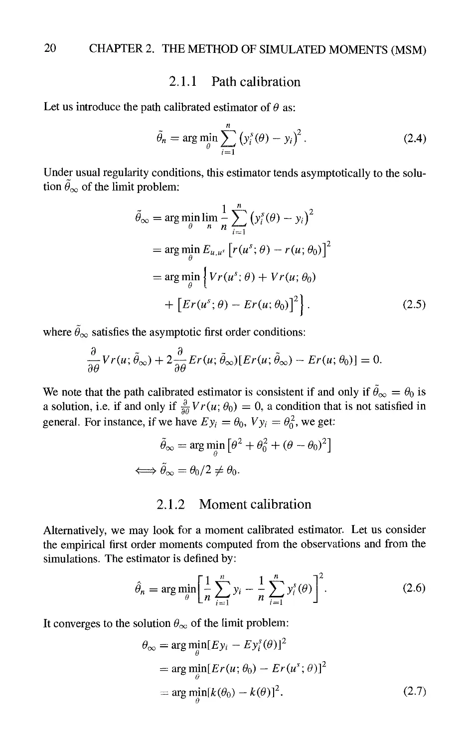
2,1 Path Calibration or Moments Calibration
The basic idea of simulated estimation methods is to adjust the parameter of
interest 0 in order to get similar properties for the observed endogenous variables {yt)
and for their simulated counterparts {y^f{0)). However, the choice of an adequate
calibration criterion is important to provide consistency of the associated
estimators. In particular, two criteria may seem natural: the first one measures the
difference between the two paths {yt, t varying) and {y^^ (0),t varying); the second
one measures the difference between some empirical moments computed on (yt)
and (yf(0)) respectively. It will be seen in this subsection that the first criterion
does not necessarily provide consistent estimators. To illustrate this point, we
consider a static model without exogenous variables. The observable variables
satisfy:
yt =r(w,-;6'o), / = l,...,n, (2.1)
where ^o is the unknown true value of a scalar parameter, (w/) are i.i.d. variables
with known p.d.f. g(u), and r is a given function.
We introduce the first order moment of the endogenous variable:
Eyi = / r(u; Oo)g(u)du = k(Oo) (say), (2.2)
and assume that the function k does not have a closed form.
Now we can replace the unobservable errors by simulations drawn independently
from the distribution g. If wj, / = 1,..., n, are such simulations, we deduce
simulated values of the endogenous variables associated with a value 0 of the
parameter by computing
yUO) = r(u';0), (2.3)
20 CHAPTER 2. THE METHOD OF SIMULATED MOMENTS (MSM)
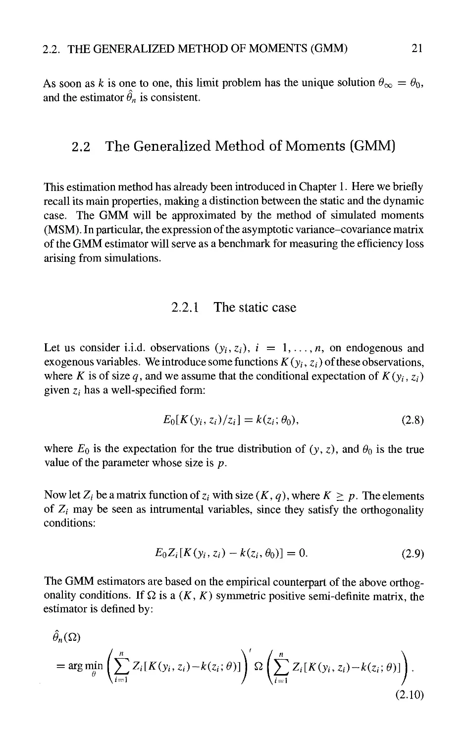
2.1.1 Path calibration
Let us introduce the path calibrated estimator of 6 as:
n
On = arg min ^ [yliO) - y,f . (2.4)
Under usual regularity conditions, this estimator tends asymptotically to the
solution 6^ of the limit problem:
1 "
^oo = argminlim - Y] (y'^iO) - yif
= argmin£^,„. [r(w''; 0) ~ r(u; Oq)]
0
arg min
Vr(u';0)-j-Vr(u;Oo)
+ [Er(w^ 0) - £r(w; 610)]^ . (2.5)
where ^00 satisfies the asymptotic first order conditions:
yr(w; 6*00) + 2—~Er(u; Ooo)[Er(u; Boo) - Er{u\ 0^)] = 0.
dO dO
We note that the path calibrated estimator is consistent if and only if ^00 = ^0 is
a solution, i.e. if and only if ^ Vr(w; ^0) = 0, a condition that is not satisfied in
general. For instance, if we have Eyi = Oq, Vy, = 0^, we get:
6*00 - arg min [O^ + 0^ + (0 ~ Oof]
<=^0^ = O0/2 ^ Go-
2.1.2 Moment calibration
Alternatively, we may look for a moment calibrated estimator. Let us consider
the empirical first order moments computed from the observations and from the
simulations. The estimator is defined by:
n 1 n t2
0^ = arg min
0
n ^—f n *—I'
I—1 (=1
(2.6)
It converges to the solution 6*00 of the limit problem:
0
=: argmin[£'r(w; ^o) — Er{u^\ 6)]
0
.argmin[^(6'o)-^(6')]^ (2.7)
9
2.2. THE GENERALIZED METHOD OF MOMENTS (GMM) 21
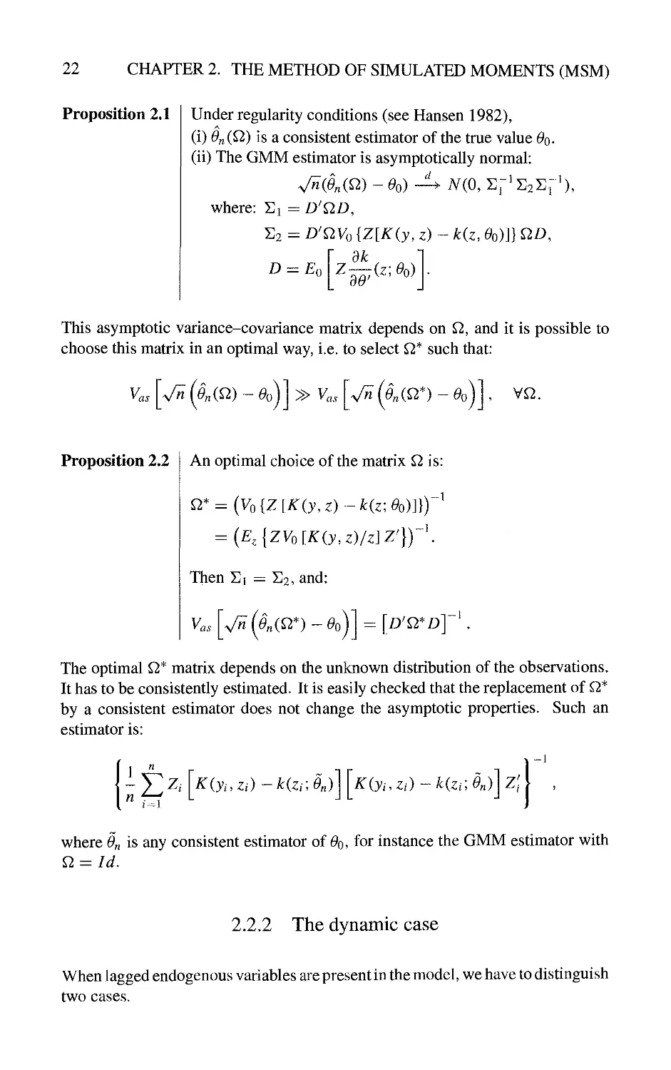
As soon as k is one to one, this limit problem has the unique solution ^00=^0.
and the estimator 0^ is consistent.
2.2 The Generalized Method of Moments (GMM)
This estimation method has already been introduced in Chapter 1. Here we briefly
recall its main properties, making a distinction between the static and the dynamic
case. The GMM will be approximated by the method of simulated moments
(MSM). In particular, the expression of the asymptotic variance-covariance matrix
of the GMM estimator will serve as a benchmark for measuring the efficiency loss
arising from simulations.
2.2.1 The static case
Let us consider i.i.d. observations (yi,Zi), i = 1,..., n, on endogenous and
exogenous variables. We introduce some functions K (yt, zt) of these observations,
where K is of size q, and we assume that the conditional expectation of K (yi, zt)
given Zi has a well-specified form:
E^[K{yiai)/Zi\ = k{zi',e^), (2.8)
where Eq is the expectation for the true distribution of (j, z), and ^0 is the true
value of the parameter whose size is p.
Now let Zi be a matrix function of Zi with size (K,q), where K > p. The elements
of Zi may be seen as intrumental variables, since they satisfy the orthogonafity
conditions:
EoZi[K(yi,Zi) - k(zi, Oo)] = 0. (2.9)
The GMM estimators are based on the empirical counterpart of the above
orthogonality conditions. If ^ is a (K, K) symmetric positive semi-definite matrix, the
estimator is defined by:
= argmin(^Z,[/^(3;,-,z,)-/:(z,;^)]) ^ (^ Z,[/^(j,-, z,)-^(zi; ^)]) .
i^\ / \i^\
(2.10)
22
CHAPTER 2. THE METHOD OF SIMULATED MOMENTS (MSM)
Proposition 2.1
Under regularity conditions (see Hansen 1982),
(i) On(Q>) is a consistent estimator of the true value ^o-
(ii) The GMM estimator is asymptotically normal:
d
-1
7V(o,i]pi]2i]r X
where: Sj = D'QD,
S2 = D'QVo {Z[K(y, z) ~ k(z, Oo)]} QD^
dk
~(z',Oo)
-1
Dz:z£
0
dO
This asymptotic variance-covariance matrix depends on Q, and it is possible to
choose this matrix in an optimal way, i.e. to select Q* such that:
Vas
V^(§nm~Oo) »y„. v^(on(^^)~o,
'0
L
V^.
Proposition 2.2
An optimal choice of the matrix Q, is:
^* = (yo{Z[/^(j,z) -/:(z;^o)]})"'
= {E,{ZVo[K(y,z)/z]r})~\
Then Si = 112, and:
y.
ai-
V^ (^„(^*) ~ 610) = [D'^*D]
The optimal ^* matrix depends on the unknown distribution of the observations.
It has to be consistently estimated. It is easily checked that the replacement of Q*
by a consistent estimator does not change the asymptotic properties. Such an
estimator is:
K{yi,Zi)-k{zi\en)
Kiyt.Zi)
/c(z,;^„)]z;
where On is any consistent estimator of 6*0, for instance the GMM estimator with
^ = Id.
2.2.2 The dynamic case
When lagged endogenous variables are present in the model, we have to distinguish
two cases.
2.2. THE GENERALIZED METHOD OF MOMENTS (GMM) 23
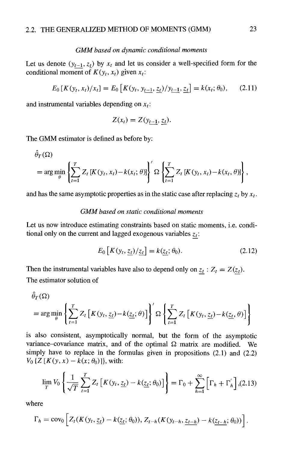
GMM based on dynamic conditional moments
Let us denote (yt~i, Zt) by Xt and let us consider a well-specified form for the
conditional moment of K{yt, Xf) given xf-
E^[K{y,,Xt)/xt\ = Eo[K(y,,y,_^,Zt)/yt^,Zi]=k(x,;Oo), (2.11)
and instrumental variables depending on Xt:
The GMM estimator is defined as before by:
= argmm K] Z, [K(y,, x,)-k(x,; 0)]\ Q K] Z, [K(y,, x,)~k(x,, 0)]\ ,
and has the same asymptotic properties as in the static case after replacing Zt by Xf.
GMM based on static conditional moments
Let us now introduce estimating constraints based on static moments, i.e.
conditional only on the current and lagged exogenous variables zt '-
Eo[K(y,,Zt)/zt]=k(zr,Oo)^ (2.12)
Then the instrumental variables have also to depend only on zt '- Zf — Z(zt)^
The estimator solution of
^r(^)
IT 1 f ^
J2 Zt [K(yu zd-Kzt;. 0)]\ ^ ^ Z, [K{y,, Zt)-k{zt_, 0)]
is also consistent, asymptotically normal, but the form of the asymptotic
variance-covariance matrix, and of the optimal Q. matrix are modified. We
simply have to replace in the formulas given in propositions (2.1) and (2.2)
yo{Z[^(j,x)~/:(jc;^o)]hwith:
II ^ 1 oo
— ^ Z, [K{y,, zj) - k{z£. ^o)] = To + ^ [r, + T,] ,(2.13)
where
Th = covo [z,(K(yt. z,) - /:(z,; ^o)), Zt^H(K(yt^h. Zt^) - k(zt_^; ^o))] •
24 CHAPTER 2. THE METHOD OF SIMULATED MOMENTS (MSM)
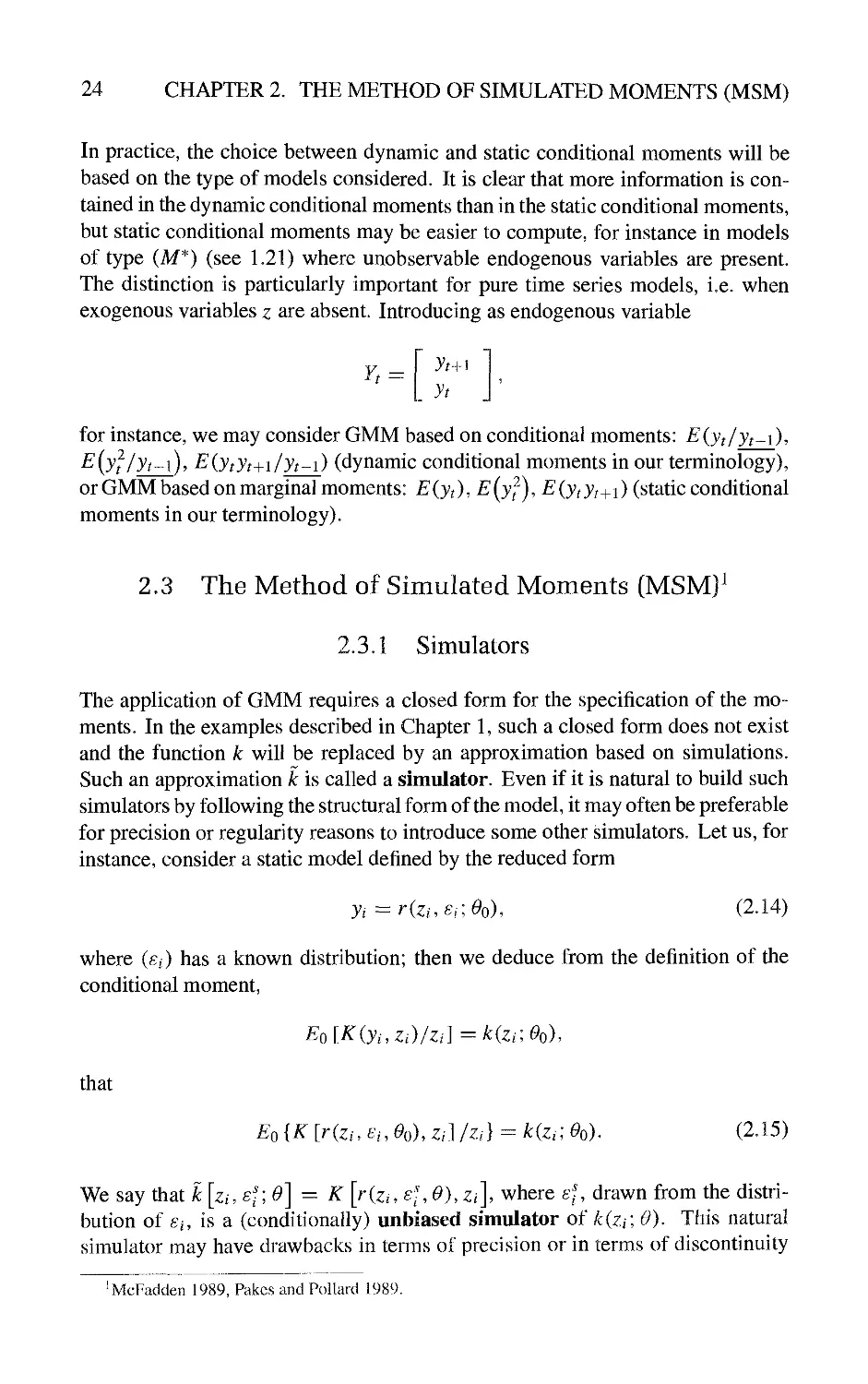
In practice, the choice between dynamic and static conditional moments will be
based on the type of models considered. It is clear that more information is
contained in the dynamic conditional moments than in the static conditional moments,
but static conditional moments may be easier to compute, for iUvStance in models
of type (M*) (see 1.21) where unobservable endogenous variables are present.
The distinction is particularly important for pure time series models, i.e. when
exogenous variables z are absent. Introducing as endogenous variable
Yt =
yt~v\
yt
for instance, we may consider GMM based on conditional moments: E{yt/yt^\),
E{yf/yt^i), E(ytyt+i/yt~i) (dynamic conditional moments in our terminology),
or GMM based on marginal moments: E{yt),E (jf), E {yt yt+\) (static conditional
moments in our terminology).
2.3 The Method of Simulated Moments (MSM]^
2.3.1 Simulators
The application of GMM requires a closed form for the specification of the
moments. In the examples described in Chapter 1, such a closed form does not exist
and the function k will be replaced by an approximation based on simulations.
Such an approximation k is called a simulator. Even if it is natural to build such
simulators by following the structural form of the model, it may often be preferable
for precision or regularity reasons to introduce some other simulators. Let us, for
instance, consider a static model defined by the reduced form
y,=r{zi.Er,e^). (2.14)
where (e/) has a known distribution; then we deduce from the definition of the
conditional moment.
E^\K{yi,zd/Zi]=k{zue^)
that
£o{K [r{zi.Ei^%), z,]/Zi) = kizt; 0^). (2.15)
We say that k [z/, e'-', O'] =^ K [r(z,, e/, 6*), Zi\ where £% drawn from the
distribution of Ei, is a (conditionally) unbiased simulator of k{zi\ 0), This natural
simulator may have drawbacks in tenns of precision or in terms of discontinuity
^McFadden 1989, Pakcs and Pollard 1989.
2.3. THE METHOD OF SIMULATED MOMENTS (MSM) 25
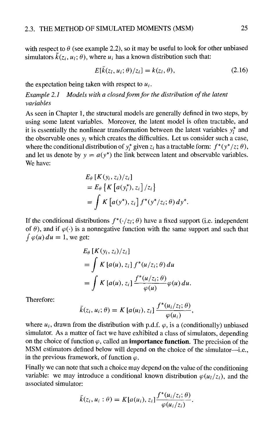
with respect to 0 (see example 2.2), so it may be useful to look for other unbiased
simulators k{zi, ui; 0), where ui has a known distribution such that:
E[k{zi.Ui;e)/zi^=KzuO), (2.16)
the expectation being taken with respect to w,.
Example 2.1 Models with a closed form for the distribution of the latent
variables
As seen in Chapter 1, the structural models are generally defined in two steps, by
using some latent variables. Moreover, the latent model is often tractable, and
it is essentially the nonlinear transformation between the latent variables j* and
the observable ones jt which creates the difficulties. Let us consider such a case,
where the conditional distribution of J* given Zi has a tractable form: f*(y*/z; 9),
and let us denote by j = a(j*) the link between latent and observable variables.
We have:
E9{K{yi,Zi)/Zi]
= Ee{K[a{yt),Zr]/Zi]
= j K [a{y% Zi] f\yVZi\ 0)dy\
If the conditional distributions f*('/zi; 0) have a fixed support (i.e. independent
of 0), and if (p{') is a nonnegative function with the same support and such that
J (p{u)du = 1, we get:
Ee[K(yi,Zi)/zi]
= f K{a{u),zi]f\u/zi\e)du
= I K[a{u),Zi] 7— (p{u)du.
(p{u)
Therefore:
k(zi,Ui;0) = K[a(ui),Zi]~
(p(Ui)
where Wi, drawn from the distribution with p.d.f. ^, is a (conditionally) unbiased
simulator. As a matter of fact we have exhibited a class of simulators, depending
on the choice of function cp, called an importance function. The precision of the
MSM estimators defined below will depend on the choice of the simulator—i.e.,
in the previous framework, of function cp.
Finally we can note that such a choice may depend on the value of the conditioning
variable: we may introduce a conditional known distribution (p(ui/zi), and the
associated simulator:
k(zi,Ui : 0) = K[a(Ui), Zi] ~—-—~.
(p{i^i/Zi)
26 CHAPTER 2. THE METHOD OF SIMULATED MOMENTS (MSM)
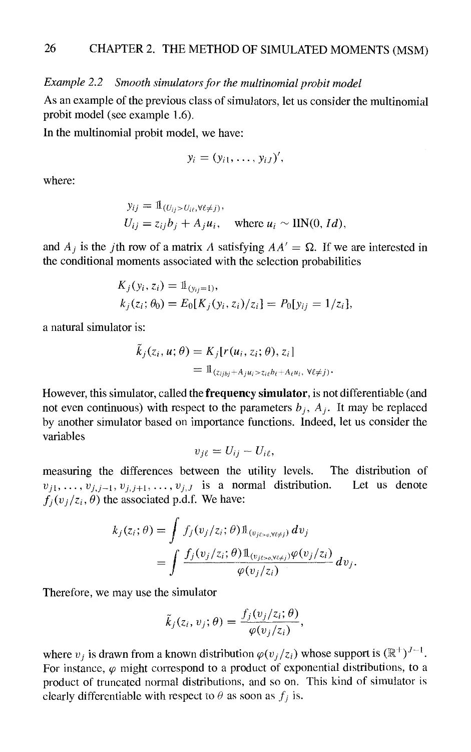
Example 2.2 Smooth simulators for the multinomial probit model
As an example of the previous class of simulators, let us consider the multinomial
probit model (see example 1.6).
In the multinomial probit model, we have:
yi = (ytu • • •. yij)\
where:
Ufj = Zijbj H- AjUi, where ui ^ IIN(0, Id),
and A J is the jth row of a matrix A satisfying AA^ = Q. If we are interested in
the conditional moments associated with the selection probabilities
kjizi; Oo) = EolKjiyi, Zi)/zi] ^ Po[yij = l/zt],
a natural simulator is:
kjizi, u; 0) =^ Kj[r(ui, Zi\ 0), zi]
However, this simulator, called the frequency simulator, is not differentiable (and
not even continuous) with respect to the parameters bj, Aj. It may be replaced
by another simulator based on importance functions. Indeed, let us consider the
variables
measuring the differences between the utility levels. The distribution of
Vjx,... ,Vjj^y,Vjj^i,... ,Vjj is a normal distribution. Let us denote
fj(vj/zi, 0) the associated p.d.f. We have:
kj{Zi\ 0)=: J fj(Vj/Zi; On(v,,.,ye^j) dVj
fj(Vj/Zr, 0)t(y.,^^,,^j)(p(Vj/Zi)
(p(vj/zi)
Therefore, we may use the simulator
<p(Vj/Zi)
where Vj is drawn from a known distribution (p(vj/zi) whose support is (IR"^)-^^^
For instance, (p might correspond to a product of exponential distributions, to a
product of truncated normal distributions, and so on. This kind of simulator is
clearly differentiable with respect to 6 as soon as fj is.
2.3. THE METHOD OF SIMULATED MOMENTS (MSM)
27
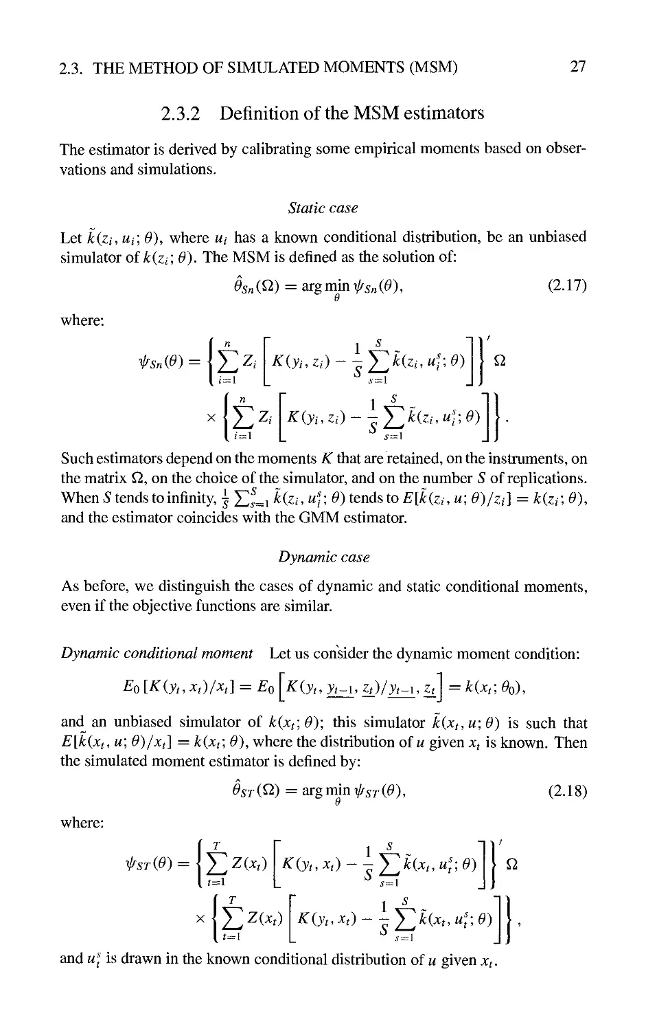
2.3.2 Definition of the MSM estimators
The estimator is derived by calibrating some empirical moments based on
observations and simulations.
Static case
Let k(Zi, Ui\ 0), where w/ has a known conditional distribution, be an unbiased
simulator of k(zi; 0). The MSM is defined as the solution of:
Osni^) = argmim/^5«(^),
9
(2.17)
where:
n
irs„{e) = \J2z.
i^\
1 ^
s^\
Q
n
X
E^.
i:^\
1 ^
K{yi,Zi)--Y,kzi,ul-0)
s^\
Such estimators depend on the moments K that are retained, on the instruments, on
the matrix Q, on the choice of the simulator, and on the number S of replications.
When 5 tends to infinity, ^ X!^^i ^fe^ w^ ^)tendsto£'[A:fe, w; 0)/zi] = k{zi\ 0),
and the estimator coincides with the GMM estimator.
Dynamic case
As before, we distinguish the cases of dynamic and static conditional moments,
even if the objective functions are similar.
Dynamic conditional moment Let us consider the dynamic moment condition:
EolK(yt,Xt)/xt] = Eo K(yt,yt~\, Zt)/yt~\, Zt\ =k(xt;Oo),
and an unbiased simulator of k{xt\9)\ this simulator k(xt,u;0) is such that
E[k(xt, u\ 0)/xt\ = k{xt\ 0), where the distribution of w given Xt is known. Then
the simulated moment estimator is defined by:
Ost{^) = argmin i/sT(0),
u
(2.18)
where:
fsT{0)=H^Z{xt) K(yt,Xt)-^J2^(xt,u',;0) \q
I ^ ~ 11
K(yt,xt)- -J2kxt.u',;0) L
.v-l J J
J2 ^(^')
and w^ is drawn in the known conditional distribution of u given Xt.
28 CHAPTER 2. THE METHOD OF SIMULATED MOMENTS (MSM)
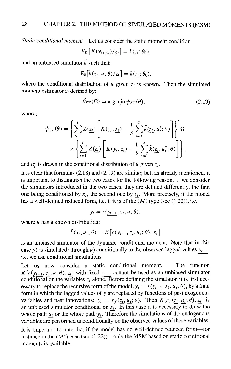
Static conditional moment Let us consider the static moment condition:
and an unbiased simulator k such that:
Eo[kzt_.u;0)/zt_]=k(zt_;Oo).
where the conditional distribution of u given zi is known. Then the simulated
moment estimator is defined by:
Ost(^) - argmmi/r^vrC^), (2.19)
where:
T
irsT(e)^\J2z{zt)
1 ^
K{yt.zt)--Y,kzj_,uY,e)
Q
E^fe)
1 ^
K(y,,z,)--J2k(zuul;e)
and w^ is drawn in the conditional distribution of u given zt-
It is clear that formulas (2.18) and (2.19) are similar, but, as already mentioned, it
is important to distinguish the two cases for the following reason. If we consider
the simulators introduced in the two cases, they are defined differently, the first
one being conditioned by X(, the second one by zt. More precisely, if the model
has a well-defined reduced form, i.e. if it is of the (M) type (see (1.22)), i.e.
where u has a known distribution:
k{xt.Ut\0) — K\r{yt^uZf,Ut\0).Xi'\
is an unbiased simulator of the dynamic conditional moment. Note that in this
case yI is simulated (through u) conditionally to the observed lagged values jt^y,
i.e. we use conditional simulations.
Let us now consider a static conditional moment. The function
K{r{yt^\, Zu u; 0), ^] with fixed yt^i cannot be used as an unbiased simulator
conditional on the variables Zi alone. Before defining the simulator, it is first
necessary to replace the recursive form of the model, yt = r(j(„i, Zt, Ut\ ^),by afinal
form in which the lagged values of y are replaced by functions of past exogenous
variables and past innovations: yt — ffiz^, Ut\ 0). Then ^[r/(^^, ut\ 0), zA is
an unbiased simulator conditional on Zf In this case it is necessary to draw the
whole path Ut or the whole path 7^. Therefore the simulations of the endogenous
variables are performed unconditionally on the observed values of these variables.
It is important to note that if the model has no well-defined reduced form—for
instance in the (A/*) case (sec (1.22))^only the MSM based on static conditional
moments is available.
2.3. THE METHOD OF SIMULATED MOMENTS (MSM)
29
Drawings and Gauss-Newton algorithms
As noted before, the optimization of the criterion function i/r is generally solved by
a numerical algorithm, which requires the computation of the objective function
for different values ^i,..., ^^ of ^. It is important to insist on the fact that the
drawings u^ are made at the beginning of the procedure and kept fixed during the
execution of the algorithm. If some new drawings were made at each iteration
of the algorithm, this would then introduce some new randomness at each step; it
would then not be possible to obtain the numerical convergence of the algorithm,
and the asymptotic statistical properties would no longer be valid.
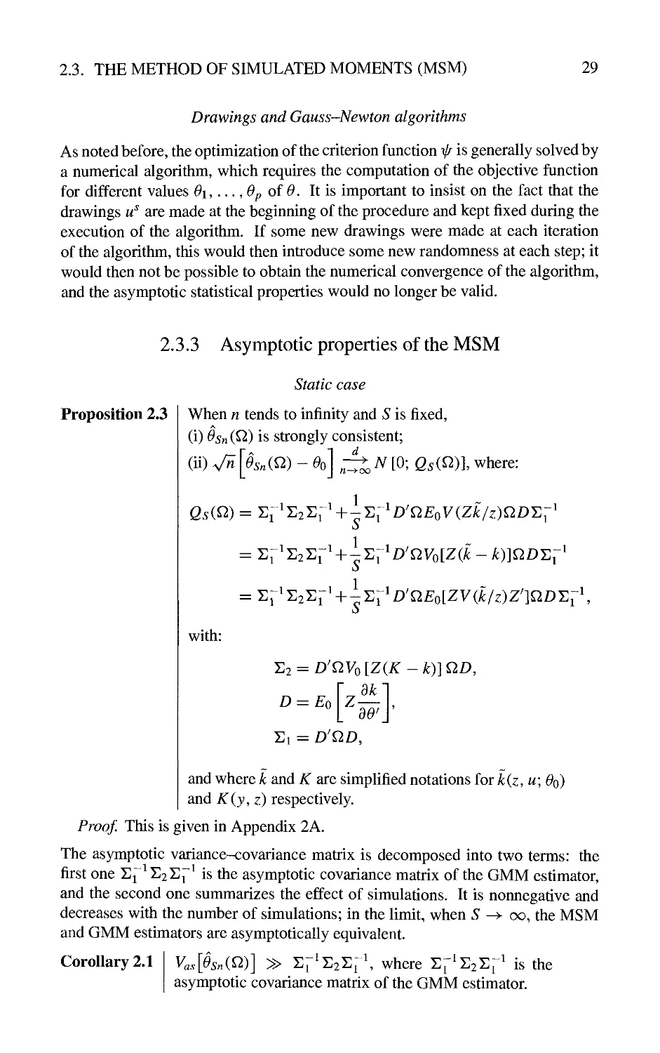
2.3.3 Asymptotic properties of the MSM
Proposition 2.3
Static case
When n tends to infinity and S is fixed,
(i) Osni^) is strongly consistent;
(ii) V^ \Osnm - Oo] ;^ N [0; Qs(Q)l where:
Qs{Q) = 'Ei'T,2T,^'+-'E;^D'QEoV{Zk/z)QD'E;'
1
with:
T>2 = D'QVolZ(K - k)]QD,
dk
D = Eo
30
El = D'QD,
and where k and K are simplified notations for k(z,u] Oq)
and K(y,z) respectively.
Proof. This is given in Appendix 2A.
The asymptotic variance-covariance matrix is decomposed into two terms: the
first one Ejf Ei^r^ is the asymptotic covariance matrix of the GMM estimator,
and the second one summarizes the effect of simulations. It is nonnegative and
decreases with the number of simulations; in the limit, when 5' -> oo, the MSM
and GMM estimators are asymptotically equivalent.
Corollary 2.1
Vas[Osn(^)] » i:^^E2i:i^\ where ^;^'E2^;' is the
asymptotic covariance matrix of the GMM estimator.
30
CHAPTER 2. THE METHOD OF SIMULATED MOMENTS (MSM)
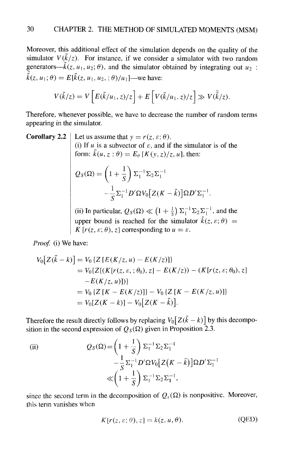
Moreover, this additional effect of the simulation depends on the quality of the
simulator V{k/z). For instance, if we consider a simulator with two random
generators—k{z, U[, U2\ 0), and the simulator obtained by integrating out U2 :
k(z, U[;0) = E[k(z, U], ^2,; 0)/ui]—we have:
Vik/z) = V
Eik/uuz)/z
+ £
V(k/uuz)/z
» V(k/z).
Therefore, whenever possible, we have to decrease the number of random terms
appearing in the simulator.
Corollary 2.2
Let us assume that y — r(z, s; 0).
(i) If u is a subvector of e, and if the simulator is of the
form: k{u, z : 0) ^ Ee [K{y, z)/z. u], then:
1
~;i:;^D'QVo[Z(K -k)]QD'Y.l
S
(ii) In particular, Qs(^) < (l + |) Sf ^S2Sj"\ and the
upper bound is reached for the simulator k(z,£;0) =
K [r(z, £\ 0), z] corresponding tou ^ s.
Proof, (i) We have:
Vo[Z(k - k)] = Vo [Z [E(K/z. u) ~ EiK/z)]}
= Vo{Z[(K[r(z, 8, ; ^o), z] - EiK/z)) - (K[r(z, s- Oo). z]
-EiK/z, u)])}
=. Vo IZ [K ~ EiK/z)]} - Vo {Z [K - EiK/z, u)\}
^V,^[ZiK-k)]^Vo{ZiK-k)].
Therefore the result directly follows by replacing Vo[Z(^ - k)\ by this decompo
sition in the second expression of Qsi^) given in Proposition 2.3.
(ii)
Q5(^)-
i + i)Er^E2sr^
1
s
-Y.-^^D'Q,Vo[Z[K ~ k)]Q.D'Y.\
«
1
i + -iEr^s2Si
since the second term in the decomposition of Qv(^) is nonpositivc. Moreover,
this term vanishes when
K{riz.£U))rA-=^kiz,u,0).
(QED)
2.3. THE METHOD OF SIMULATED MOMENTS (MSM) 31
Table 2.1: Efficiency
Number 5 of replications 1
Lower bound of the asymptotic 50 % 66.6 % 75 % 90 %
relative efficiency
Maximal relative increase of 141 % 122 % 115 % 102 %
confidence intervals
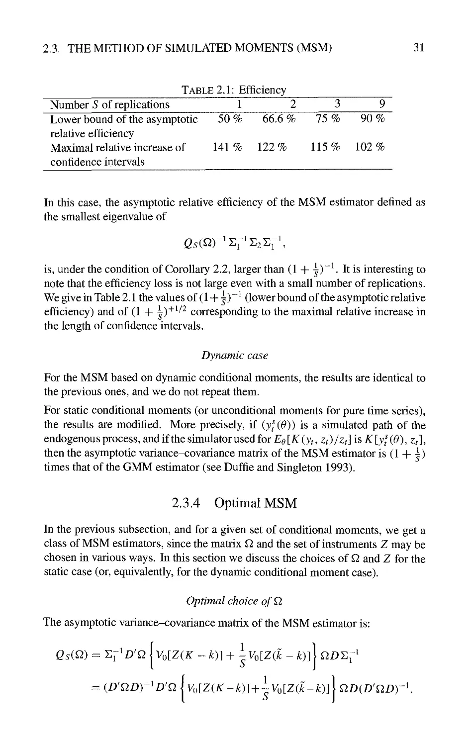
In this case, the asymptotic relative efficiency of the MSM estimator defined as
the smallest eigenvalue of
is, under the condition of Corollary 2.2, larger than (1 + ^y\ It is interesting to
note that the efficiency loss is not large even with a small number of replications.
We give in Table 2.1 the values of (1 +1)" ^ (lower bound of the asymptotic relative
efficiency) and of (1 + ^)^^^^ corresponding to the maximal relative increase in
the length of confidence intervals.
Dynamic case
For the MSM based on dynamic conditional moments, the results are identical to
the previous ones, and we do not repeat them.
For static conditional moments (or unconditional moments for pure time series),
the results are modified. More precisely, if (y'^(0)) is a simulated path of the
endogenousprocess, and if the simulator used for £:^[7r(jf,Zf)/Zf] is 7^[JJ^(^),^J,
then the asymptotic variance-covariance matrix of the MSM estimator is (1 + |)
times that of the GMM estimator (see Duffie and Singleton 1993).
2.3.4 Optimal MSM
In the previous subsection, and for a given set of conditional moments, we get a
class of MSM estimators, since the matrix Q and the set of instruments Z may be
chosen in various ways. In this section we discuss the choices of Q and Z for the
static case (or, equivalently, for the dynamic conditional moment case).
Optimal choice ofQ
The asymptotic variance-covariance matrix of the MSM estimator is:
QsiQ) = ^i'D'nlvdZiK - k)] + ^Vo[Z(k - k)]\ QD^^'
= (D'nDr'D'Qlvo[Z(K~k)]-{-~Vo[Z(k-k)]\ QDiD^QDyK
32
CHAPTER 2. THE METHOD OF SIMULATED MOMENTS (MSM)
From the Gauss-Markov theorem, we know that the nonnegative symmetric matrix
(D'QDy^D'Qi:oQDiD'QDy^ is minimized for Q = Y^^K We deduce the
following result.
Proposition 2.4
We have: Qs(^) > Q^C^*), where the optimal choice
of the matrix is:
1
1
Q^ = \ Vo[Z(K - k)] + ~Vo[Zik - k)]
The asymptotic variance-covariance matrix corresponding to this choice is:
Q,(^*) = (D^n^D) ' ,
(2.20)
where
D = Eo{Z
dk
dO
r
As usual, the optimal matrix depends on the unknown distribution and has to be
consistently estimated. Let us consider the first term, for instance. We have:
Vo VZ{K - k)\ = Eo {[Z(K - k)] [Z(K - k)]'}
1 "
(=1
K{yi,Zi)-k{ziJn)
Kiyi,Zi)-kizi,9„)
if
Z,,
where On is a consistent estimator of ^o-
This approximation is consistent; since k does not have a closed form, it has to
be approximated using the simulator k. To get a good approximation of k, it is
necessary to have a large number of replications 52. Let us denote by u^-2, s =
1,... 52, some other simulated values of the random term with known distribution,
the matrix
/v
^
Aht-.
n ^ ,
1 ^2 .
Kiyi.Zi) - TT X^^fc. <2; ^n)
X
52
K{yi,Zi) - — X^RzM<2;^n)
2 s~i
z
1 1^
S n ^.
i^i
1 ^'
k{Zi. U?-Jn) - — X^^Um <2; On)
Si
s^\
X
52
■^'1.
1 ^ ~
k{Zi. U\'-Jn) - TT y]^fc' ^'2'^ ^n)
-1/ V--1
z.
(2.21)
where u-^ is a simulated value of a, is a consistent estimator of the optimal matrix
^*, when n and 52 tend to infinity. So, whereas the derivation of the estimation of
2.3. THE METHOD OF SIMULATED MOMENTS (MSM)
33
0 by MSM requires only a small number of simulated values, the determination
of the optimal matrix and of the associated precision require a much larger set of
other simulated values; however, these simulations are used only once.
Finally, we may compare the optimal asymptotic variance-covariance matrix of
the MSM with the optimal asymptotic variance-covariance matrix of the GMM.
The latter corresponds to another choice of the matrix ^** := (Vq [Z{K - k)]y^
is given by:
We directly note that Q** ^ Q*, which implies:
Qs(^*) » G*.
It is also clear that:
e* = lim e^C^*).
5->oo
Selection of the instruments
When the optimal matrix is retained, the asymptotic variance-covariance matrix
is:
e^C^*) - {£:ol ^z'\ lvo[Z(K - k)] + -VolZik - k)]\ Eo(z^^
^lE
0
EolZ
VoiK/z)-{-~Vik/z)\Z
EolZ
dk
Jo
-\
Then we can use a classical result on optimal instruments. If A and C are random
matrices of suitable dimensions, are functions of z, and are such that C is square
and positive definite, then the matrix
E^{A'Z')[E^{ZCZ')r'Eo{ZA)
is maximized for Z = A'C ^ and the maximum is E^^i^A'C ^ A)
Proposition 2.5:
The optimal instruments are:
Zl = —{V^{K/z)-\-~V{k/z)r\
where the different functions k, k are evaluated at the
true value ^o- With this choice the asymptotic variance-
covariance matrix is:
Q%=\E
0
dk' / 1 ~
^[y^{K/z)-{-~V{k/z)
ad \ S
dk
'W'
34
CHAPTER 2. THE METHOD OF SIMULATED MOMENTS (MSM)
When S goes to infinity, we find the well-known optimal instruments for the GMM
and the associated asymptotic variance-covariance matrix:
^
Q - £0
dt dk
Vo(K/z)
-11-1
do
do
Also note that when k ^ K, i.e. when the frequency simulator is used, we have:
Z? - 1 +
1
s
and, therefore, the optimal instruments are identical in the MSM and the GMM.
2.3.5 An extension of the MSM
In the usual presentation of the GMM (see Hansen 1982), the true value of the
parameter is defined by a set of estimating constraints of the form:
E^[g{yi.Zr\Oo)/zi\^0
(2.22)
where ^ is a given function of size q\ we consider the static case for notational
convenience. It is important to note that in the previous sections we have considered
a specific form of these estimating constraints, i.e.
giji, Zi\ Go) = Kiyi. zi) - k(zi; Oo) (see (2.8)).
What happens if we now consider the general form (2.22)? As before, we may
introduce an unbiased simulator of giyi, Zi\ 0). This simulator g{yi, zt, ut; 0),
which depends on an auxiliary random term ui with a known and fixed distribution
conditional on yi^zt, is based on a function g with a tractable form and satisfies
the unbiasedness condition:
Elgiyi. Zi. Ui; 0)/yi,zi] = g(yi,Zi; 0).
(2.23)
Then we can define an MSM estimator as a solution of the optimization problem:
/v
Osn(^)
argmm
n 1 S
v
x^
s
;^1 s~\
(2.24)
2.3. THE METHOD OF SIMULATED MOMENTS (MSM)
35
where M^ / = 1,..., n, 5- = 1,..., 5, are independent drawings in the distribution
V
of M, and Zi are instrumental variable functions of zj.
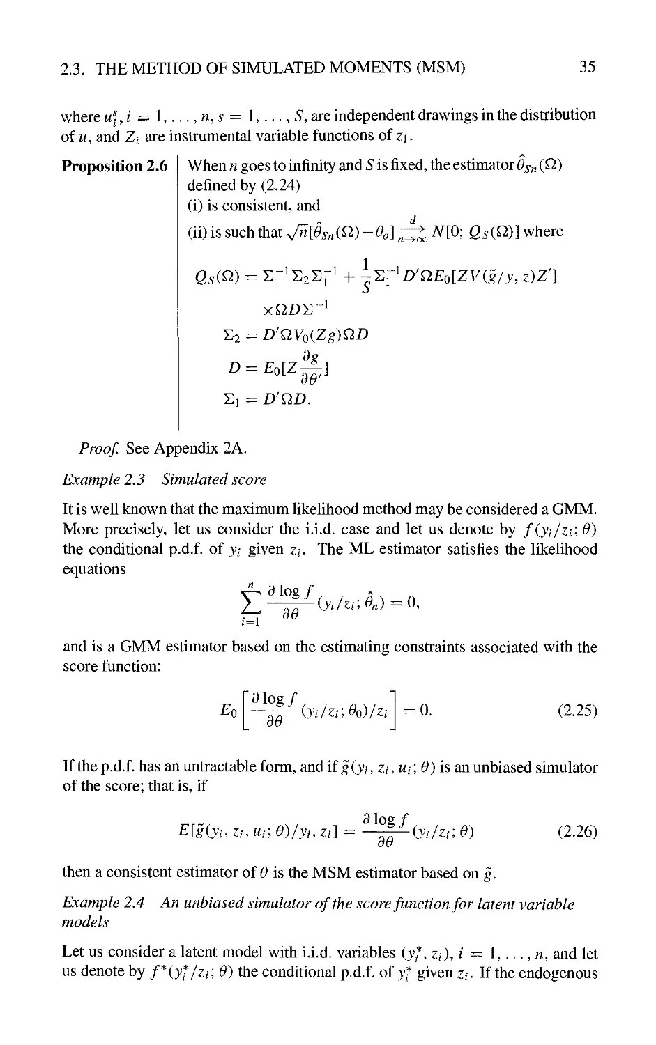
Proposition 2.6
When n goes to infinity and S is fixed, the estimator Osn (^)
defined by (2.24)
(i) is consistent, and
d
(ii) is such that ^[Osn{^)~0o\ rit A^[0; Qs{^)] where
1
11^'
x^DE
1
S2-
9^
Proo/ See Appendix 2A.
Example 2.3 Simulated score
It is well known that the maximum likelihood method may be considered a GMM.
More precisely, let us consider the i.i.d. case and let us denote by f(yi/zi; 0)
the conditional p.d.f. of yi given z/. The ML estimator satisfies the likelihood
equations
^91og/
E
i=\
do
(j./z.-;^„)-0,
and is a GMM estimator based on the estimating constraints associated with the
score function:
Eo
9 log/
(yi/zi;Oo)/zi
= 0.
(2.25)
If the p.d.f. has an untractable form, and if ^(j/, z/, w/; 0) is an unbiased simulator
of the score; that is, if
E[giyi,zu Ui-, e)/yi, Zi] = -^iyi/zr, 9)
ou
then a consistent estimator of 0 is the MSM estimator based on g.
(2.26)
Example 2.4 An unbiased simulator of the score function for latent variable
models
Let us consider a latent model with i.i.d. variables (j*, z/), / = 1,..., n, and let
us denote by f*(yf/zi; 0) the conditional p.d.f. of j* given z/. If the endogenous
36
CHAPTER 2. THE METHOD OF SIMULATED MOMENTS (MSM)
observable variable is a known function of yf : yi ^ a(yf), we know that the
score function is such that:
E
e
^jog/
iy!/zi;0)/y^.Zi
a log/
30
iyi/zi;0)
Therefore it is natural to consider the previous equality as an unbiasedness
condition and to propose the unbiased simulator (9 log f^/dO)(y^-yzi; 0), where yf-^
is drawn in the conditional distribution of yf given j,, z,. If this drawing can be
summarized by a relation (in distribution), i.e.
where Ui has a fixed known distribution, the unbiased simulator is:
a log r
giyt^Zi, Ui\ 0) = —--—[biyi.Zh ua 0)/zi\ 0].
(2.27)
In practice such a simulator will be used only if the function b has a simple form.
This is the case for some limited dependent variable models (see Chapter 5).
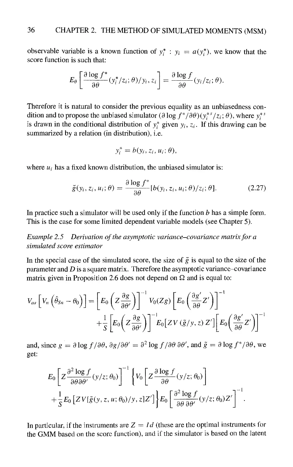
Example 2.5 Derivation of the asymptotic variance-covariance matrix for a
simulated score estimator
In the special case of the simulated score, the size of g is equal to the size of the
parameter and D is a square matrix. Therefore the asymptotic variance-covariance
matrix given in Proposition 2.6 does not depend on Q and is equal to:
V.
a
■' [^" (
/v
^Sn — Oq
EaiZ
30'
Vo(Zg)
E
0
30
-1-1
Z'
+
1
EoiZ
30'
E^[ZV{g/y.z)Z']
E
0
30
-,_]
and, since ^ = 9 log f/30, 3g/30' = 3^ log f/30 30\ md g = 3 log fy30, we
get:
E
0
Z
3^ log /
^-1
3030
(y/z; Oo)
Vo
3 log /■
Z~-^^(y/z;Oo)
30
+ Ieo [ZVlgiy, z, u; Oo)/y, zW]\eo
9' log /
30 30
'-(y/z;Oo)Z
In particular, if the instruments are Z ^ Id (these are the optimal instruments for
the GMM based on the score function), and if the simulator is based on the latent
APPENDIX 2A. PROOFS
37
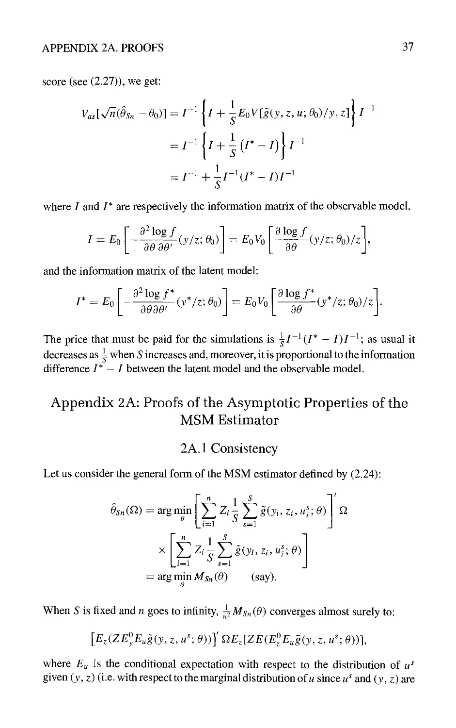
score (see (2.27)), we get:
VaslV^iOsn - Oo)] = r'\l-h -EoV[giy, z, u; Oo)/y, z]
)l'-
where / and /* are respectively the information matrix of the observable model,
I = E
0
92 log /
dOdo
riy/z'.e^)
= EoVo
9 log/
(y/z; Oo)/z
and the information matrix of the latent model:
r = E
0
a' log /
dOdo
-(j*A;^o)
= EoVo
a log /
(j*A;^o)/^
The price that must be paid for the simulations is |/ ^ (/* - /)/ ^; as usual it
decreases as | when S increases and, moreover, it is proportional to the information
difference I* — I between the latent model and the observable model.
Appendix 2 A; Proofs of the Asymptotic Properties of the
MSM Estimator
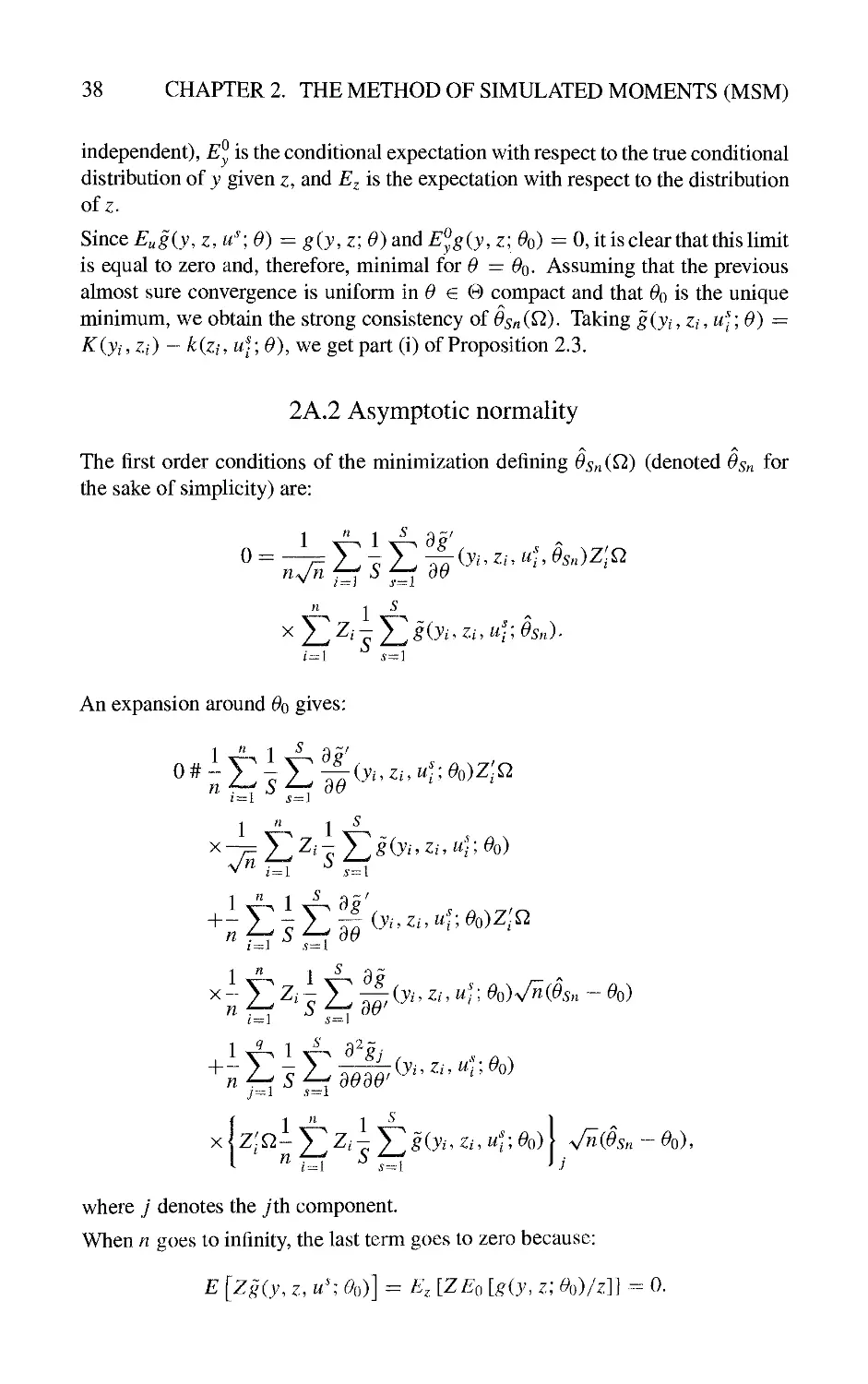
2A.1 Consistency
Let us consider the general form of the MSM estimator defined by (2.24):
-1/
/v
esn(^) =
arg
X
arg
min
e
n 1 5
X]2:,--X]|(j,-,z,-,a
~ n ^ S
I—1 t—1
min J
8
MsniO) (say).
]\0)
Q.
When S is fixed and n goes to infinity, ^MsniO) converges almost surely to:
{E,{ZE%g{y^ z, u'- 0))] QE,lZEiE^^E,g(y, z, u'; 0))l
where £« is the conditional expectation with respect to the distribution of u^
given (y, z) (i.e. with respect to tiie marginal distribution of a since a-" and (y, z) are
38 CHAPTER 2. THE METHOD OF SIMULATED MOMENTS (MSM)
independent), E^ is the conditional expectation with respect to the true conditional
distribution of y given z, and E^ is the expectation with respect to the distribution
of z.
Since E^giy, z, u'; 0) = g{y, z; 0) and E^^gij, z; ^o) = 0, it is clear that this limit
is equal to zero and, therefore, minimal for 0 — 0^. Assuming that the previous
almost sure convergence is uniform in ^ 6 B compact and that ^o is the unique
minimum, we obtain the strong consistency of Osn{^)- Taking g{yi,Zi, u\\ 0) =
f^iyt^Zi) — k{zi, u]\ 0), we get part (i) of Proposition 2.3.
2A.2 Asymptotic normality
/v ^
The first order conditions of the minimization defining Osn{^) (denoted Osn for
the sake of simplicity) are:
n 1 ^
. , 5 ^
An expansion around ^o gives:
1==} s^l
1 ^
X-
E ^^ ^ E S; (y^' ^'-' "/'; Oo)V^0Sn ~~ Oo)
? 1 -S' n2
1 ^ 1 V^ d'gj ^ , ^ ^
n^ S ^ dOdO
x{z;^i^Z,^^^(j,,z,,a'J;^o)) V^0sn-Oo),
where / denotes the jth component.
When n goes to infinity, the last term goes to zero because:
E [Zg(y^ z, u'; Oo)] = E, [ZE^ [g(y. z; ^o)/z]] - 0.
APPENDIX 2A. PROOFS
39
It follows that:
0 # i)'^4= I] ^41]^^^'-^^■'"?'^0^+^'^^^^^^«
Vn fr
^o)
i=l 5=1
with D = EolZ^iy, z; Oq)], where Eq is the expectation with respect to the true
distribution of (y, z).
When n goes to infinity:
1 " 1 "^
-nA "^ ^ S
s=l
converges in distribution to A^(0, S^), with:
S. ^y
s
1 ^
5=:i
= VoE,
1 ^
5 = 1
-hEoVu
1 '^
2:-X^^(j,z,m';^o)
j=i
1
= Vo [Zgiy, z, ^o)] + -^o [ZV,g(y, z, u^; Oo)Z']
This implies that ^{Osn ~ 0) converges in distribution to:
with
i T^r
1
5
i
^ Y.7'Y.oY.7' + -Y.^^D'QEo(ZVu8Z')QDY.~^
i ^2Sj
T.2 = D'QVoiZg)QD.
Particular case
In the particular case where
giy, z.u'; 0)=K(y, z) ~ kiz.u'; 0)
and giy,z;0)=K(y,z)-k(z;0),
we get the results of Proposition 2.3. Since the general form of Qs(^) directly
reduces to the third form given in this proposition with D ^ Eq [Z~~(z, Oq)], the
two other forms are obtained immediately.
This page intentionally left blank
3
Simulated Maximum Likelihood,
Pseudo-Maximum Likelihood,
and Nonlinear Least Squares
Methods
In the previous chapter we discussed the simulated analogues of the method of
moments. We are now considering simulated versions of other estimation
methods such as maximum likelihood, pseudo-maximum likeHhood or nonlinear least
squares. The main characteristic of the associated estimators is their non
consistency when the number 5 of replications is fixed. Therefore theoretical consistency
may only be obtained either by performing a large number S (S —^ +00) of repHca-
tions, or by introducing some correction to eliminate the asymptotic bias; however,
this theoretical problem may not be so important in practice.
3.1 Simulated Maximum Likelihood Estimators (SML)
The maximum likelihood estimator of a parameter 0 is defined as:
/v
Ot = argmajilog fiyr/zr^O), (3.1)
0
where fiyr/zT'-, 0) is the conditional p.d.f. of yr — (ji,..., jr), given zt ~
(zi,..., Zt) and some initial conditions.
We are interested in problems where this p.d.f. has an untractable form, and it is
important to distinguish two cases. In the first case it is possible to find unbiased
simulators of each conditional p.d.f. f(yt/yt-i, Zt} 0), also denoted f{yt/xt\ 0),
appearing in the decomposition:
log fin/zT} 0) = Y11^^ f(yt/^t; 0).
t=i
This first case often occurs if the model has a well-defined reduced form
(see (1.22)):
(M)yt = rizt,yt^u£t;0).
42
CHAPTER 3. SML, SPML AND SNLS METHODS
However, such simulators do not generally exist in dynamic models with unob
servable factors (see Section 1.3.4), defined as
yt ^ ^2(zr, yt~±, y^-A2_^2ti 0).
In this second case other approaches must be found (see Section 3.1.5).
3.1.1 Estimator based on simulators of the conditional density
functions
Let us denote by /(j^r, Xj, u; 0) an unbiased simulator of f{yt/xt\ 0), i.e. such
that
Eifiyt, xt, u; 0)/xt. yt) = fiyt/xt; 0)
(3,2)
and where the conditional distribution of u given Xj, >v is known. In practice this
distribution is often independent of Xj, y^.
Then we may draw independently, for each index t, S simulated values aj, s —-
1,..., 5, of the auxiliary random term u.
Definition 3.1
A simulated maximum likelihood estimator of ^ is:
T
OsT = argmax^log
1 ^
--^/(jr.-^M<;^)
s=\
It is obtained after replacement of the untractable conditional p.d.f. with an unbi
ased approximation based on the simulator.
3.1.2 Asymptotic properties
Let us first study the consistency properties of such estimators. We distinguish
two cases: 5 fixed and 5 tending to infinity with T.
S fixed
If 5 — 1, the objective function,
r
1
;^X^log/(jr'-^r.<;^)
tends asymptotically to the Hmit function:
i/oo(0) = Ei) / [ogf(y,x,u;0)giu)du,
(3.3)
3.1. SIMULATED MAXIMUM LIKELIHOOD ESTIMATORS (SML)
43
where g is the p.d.f. of u. We know that the true value of the parameter ^o is
the solution of maxeEo log f(y/x;0), but it is not in general a solution of the
maximization of (3.3), since the log and the integral do not commute, and Ost is
not consistent. This inconsistency comes from the choice of the simulator / as
an unbiased simulator of /. If log fiyt,Xt,u;0) were an unbiased simulator of
log fiyt/xt', 0), the limit function t/t^ would have been
irooiO) = Eo I log f(y,x,u;e)g(u)du
= Eolog f(y/x;0),
and would have a maximum at ^o- However, in practice it is often possible to
exhibit unbiased simulators of /, but it is difficult to exhibit unbiased simulators
of log/.
S tending to infinity
If 5 tends to infinity, the limit objective function is:
I T fl ^ .
T,S-^oo T
t=l
s=l
= lim -T^log / f(yt,xt,u;e)g(u)du
= Eo log
/ f(yt,xt,u;
0)g{u)du
= Eq log fiyt, Xf; 0), since / is an unbiased simulator of /.
It is the same limit problem as for usual maximum likelihood estimation, and the
estimator is consistent.
Proposition 3.1
(i) The SML estimator is consistent, if T and 5 tend to infinity.
(ii) It is inconsistent if 5 is fixed and T tends to infinity.
When we compare Proposition 3.1 with the property of consistency of MSM valid
even for fixed S, the SML approaches may appear uninteresting. However:
(a) In practice it is sufficient to retain a number 5 of replications such that
OsT ^ lim^^oo Ost, and such a number often is of moderate size.
(b) The MSM also requires a large number of simulations in order to compute
the standard errors of the evStimator.
44 CHAPTER 3. SML, SPML AND SNLS METHODS
(c) In finite samples, what really matters is the relative magnitude of the square
of the bias and of the variance of the estimator. As discussed below, the
magnitude of the bias may be reduced by the choice of suitable simulators, or
by the introduction of some correction terms, while the variance of an SML
estimator (close to the variance of the efficient ML estimator) is generally
smaller than the variance of an MSM estimator (close to the variance of an
inefficient GMM estimator).
(d) Finally, whereas the GMM approach may be preferred to the ML approach
since it requires less distributional assumptions (GMM is a semi-parametric
approach), this aigument fails for the MSM approach which requires the
complete specification of the distribution for simulation purposes.
When the number of replications 5 tends to infinity, the simulation step may have
an effect on the asymptotic covariance matrix of the simulated ML estimator,
except if the speed of divergence of 5 is sufficiently large. The following result is
proved in Gourieroux and Monfort (1991).
Proposition 3.2 If 5, T -^ oo and vT/5 -^ 0, then the SML estimator
is asymptotically equivalent to the ML estimator.
3.1.3 Study of the asymptotic bias
An expansion for the asymptotic bias
When 5 tends to infinity, the bias is of order ~. More precisely, we have the
following result (Gourieroux and Monfort 1991):
Proposition 3.3
When 5 tends to infinity, the asymptotic bias is equivalent to
B - EoOsT-Oo - -r\Oo)Eo[a(y,x;0)l
where /(^o) is the information matrix, and
a(y,x;Oo)=- ''^ ^
(E„/)3 (E„/)2
As expected, the bias depends on the choice of the simulator, and may be reduced
by a sensible selection of /. Moreover, the square of the bias compared with the
variance may be measured by:
B'l(Oo)B = ^Eo[aiy,x;Oo)]'r\eo)Eo[a(y,x;Oo)l
Therefore it is small when the underlying ML estimator is precise, i.e. when / ~ ^ (Go)
is small.
3.1. SIMULATED MAXIMUM LIKELIHOOD ESTIMATORS (SML)
45
A first order correction for the asymptotic bias
As noted before, the inconsistency comes from the choice of a simulator log /
which is a biased simulator of log /. How can we partially correct this effect if
the bias is not too large? We have:
and:
log / = log(/ + / - /)
/-/ l{f-ff
2 p
:^ log / +
/
Eulog f 'i^logf -^
Euf~f I if-f)
f
- -E
U
f
= log/- -Eu
1 (/ - /)
/
Therefore log/ + ^[(/ — f)^/f^] is a simulator of log/ with a smaller bias
than log / in general. A first order correction of the SML estimator consists in
computing the corrected estimator:
OsT =
argmm
e
Ei«g
t=i
1 ^
s=l
E
s=l
1 ^
-i2
s^l
t=l
-i2
^f(yt,Xt,u'j;0)
s=l
3.1.4 Conditioning
(3-4)
In a number of examples described in Chapter 1, the conditional p.d.f. has an
integral form:
fiyt/xt;0)
f'^iyt/xt;u;8)g(u)du,
(3-5)
where w is a subvector of the error term s appearing in the reduced form of the
model. In such a case it is possible to introduce the simulator:
f{y, X, u; 0) =: /*(y/x; w; 0), where u has a distribution with p.d.f. g. (3-6)
46 CHAPTER 3. SML, SPML AND SNLS METHODS
It is also possible to introduce an importance function cp with the same support
as g, such that (p{u) > 0, / (p{u) du — 1, and to introduce the simulator:
f{y, X, u- 0) - r (y/x; u; 0)^. (3.7)
where u has a distribution with p.d.f. cp.
We give below some examples where some conditioning naturally appears.
Example 3.1 Panel probit (or Tobit) model with individual effect
In this model the latent variables are indexed by individual and time and follow a
linear model with individual random effect:
where w,, wa are independent variables with standard normal distributions. The
observable endogenous variables are either
y^^ =:]]^^.-^o) probit model {a^j may be constrained to 1),
or Jit = ya%>0) Tobit model.
The simulators may be based on the conditional distribution of y given z and
the individual effect w, since it is easy to integrate out the other random terms w
because the Wit,t — U ... ,T are independent. We get:
(a) probit model:
t:yi, = l t:yi!=0
(b) Tobit model:
t:yi,>0
^w \ ^w
X I I cDI -
z-^b + auUi
O'y;
Example 3,2 Panel probit (or Tobit) model with individual effect and serially
correlated disturbances (HajivassiHou and McFadden 1990, Keane 1990a, b.
Stern 1992, Gourieroux and Monfort 1993a)
The latent variables satisfy:
ytt = ZiTb-\-a^Ui -\-eit,
^^it = P^^ij-i + (^wWit, t > 2,
'^^^ (1_ ^2)1/2^1-
3.1. SIMULATED MAXIMUM LIKELIHOOD ESTIMATORS (SML) 47
where w/, wu are independent variables with standard normal distribution. The
error term (sit) satisfies an autoregressive formulation and the initial value sn is
assumed to follow the marginal distribution associated with this autoregressive
scheme. For a probit (or Tobit) model based on this latent variable, the p.d.f. of
y conditional on z and u is no longer tractable (since the £/,, f = 1,..., T are
correlated), but another conditioning is available. Let us consider the global error
term for individual /. It is a T-dimensional vector;
^i = OuUfeT +£/, (3.8)
where ej is the vector whose components are equal to one. The variance-
covariance matrix of this error term is:
V^.=alJT + ^, (3.9)
where the entries of Jt are one, and the generic entry of Q. is cotj = [(7^^/
(l-p')]pl''-"^''-
Lemma 3.1 su may be decomposed into:
where (^/^^), {^u) are independent, and {si^ ) is a Gaussian white
noise with variance: o-^/(l + \p\)^ = o-^.
Proof. The spectral density function of (en, t e Z) is equal to:
2 2
27t\l — pexp/6;p 27r(l — 2pcos6; + p^)
2^•
It has a monotonic form with a minimum value for a^(l -\- \p\) ^ and the result
follows.
QED
Now we may consider another decomposition of the global error term:
where £?^ and Vi are independent, vt ^ N[0, (T^Jt + ^ — (ylildj]- Therefore we
can write:
where AA' = a^Jj + ^ - aj^IdT and w* - N{Q, Idj).
If we condition with respect to w*, i.e. if we integrate out sf'\ we obtain the
following conditional p.d.f.:
48 CHAPTER 3. SML, SPML AND SNLS METHODS
(a) probit model (we can take a^. = 1):
f (yi/Zi,uJ;0)^ 1 1 "^
r.y,=0 V ^^
where a^ is the nh row of matrix A.
(b) Tobit model:
^*/ / =^ ^^ FT ^ I y-it - Zitb - atu]
f (yJzi,u-;0)=^ —(p
*
/
r.yu>0 "^^ ^ ^«
^
3.1.5 Estimators based on other simulators
In dynamic models where latent variables are present, it is often impossible to find
unbiased simulators of the conditional p.d.f. f(yt/yt-i, Zt\ 0), and the methods
presented in the previous sections do not apply. In this kind of model the overall
p.d.f. of the observable and latent endogenous variables (yj, y^) can be written:
f {yT_. y^l ZT^. yoi. yl} 0)
T
' f{yr,y:/zuyt-uyU}e)
t = \
T
' f{ytlzt_. yj-u y;; 0)f{y^/zt_. y_t-x_. y^ 0\
and the likelihood function is:
T T
= / n f(yt/z^, yt^. yl; o)f(y:/z^. 3^, y^. o) f] ^/x(y;).
The likelihood function appears as a 7^-dimensional integral (if yf is univariate)
of a function which in general does not have a closed form.
Let us consider, for instance, the typical M^ model (see example 1.17):
y/ ^nizt,yt^,yl_,su',0),
y* ^ r2{zt, yt--\, y^-i■, ^^lu O),
3.1. SIMULATED MAXIMUM LIKELIHOOD ESTIMATORS (SML) 49
where St = (e^, £2^) is a white noise whose distribution is known. If e^ and
S2t are contemporaneously independent, the function f(yt/zt,yt-i,yt, 0) (resp.
f(y^/zt^ yt-uyt-i', O)) appearing in the previous integral is the p.d.f. of the
image distribution of the distribution of Su (resp. S2t) by ri(zt,yt-i^ Zl' *' ^-^ ^^^^P-
r2(zt,yt^i,y^-i:-;0))-
For this kind of likelihood function the ML method is untractable; moreover,
the previous SML methods do not apply either. In this context three kinds of
solution have been proposed. The first one is based on numerical
approximations and will not be described here (see Kitagawa 1987, and Chapter 6 below),
the second one is based on simulations of the whole likelihood function using
the importance sampling technique, and the third one is based on simulations of
^[log f(yT^ yjl^-' yo, 3^0' ^)/3'r] in the Expectation Maximization (EM)
algorithm.
Importance sampling methods
1
As previously seen, the likelihood function naturally appears as the expec-
IT"
tation of the function Y[t=i f^yt/^t^yt-^^ yt"'^^) ^ith respect to the p.d.f.
nr=i/(3'*/£L' ^'-i' ^*-i' ^^' where z^ and yt-i are observed values. It is
important to note that this p.d.f. is neither fiyj/zr^, yo, ^o' ^) (except if yt-i
does not appear in f{y^/zt_, yt-\, y*_i; 0), i.e. if (y^) does not cause (yf)), nor
fiyr/yT^ zji^ yo, yo'-. O). However, it may be easy to draw in this p.d.f.; for
instance, in the M* model such a drawing is recursively obtained by using the
formula
yrm = r2[zt,yt-uy:i,{0),e'2,\0],
where S2^J = I,... ,T ,2C[c independent drawings in the distribution of £2-
Therefore an unbiased simulator of the whole likelihood function fiyj/zT, yo, ^o' ^)
is;
T
Y\f[ytlzuyt-uy_r_{e)\e],
t=l
where the y^^{0) are drawn in the auxihary p.d.f. mentioned above. This method
is clearly an importance sampling method.
This basic importance sampling method may be very slow, in the sense that the
simulator may have a large variance; therefore accelerated versions of this method
have been proposed, in particular the Accelerated Gaussian Importance SampHng
method in the Gaussian case (see Danielsson and Richard 1993), and the
Sequentially Optimal Sampling methods of various orders in the switching state space
models (see Billio and Monfort 1995, and Chapter 7 below).
^ See Danielsson and Richard (1993); Billio and Monfort (1995).
50 CHAPTER 3. SML, SPML AND SNLS METHODS
Simulated Expectation Maximization (SEM) algorithm^
The log likelihood function can be written:
log f{yT^/zT_. JO, 3^; B) = log fiyjj y^lzT_. jo, yl} 0)
- log /(34, /yn zt_. JO' Zo' ^)-
Since the LHS of the equation does not depend on jj, we have, for any values 0^^^
of the parameter,
log fiyi^/zT. yo, Jo; 0) = Eein [log /(jr, J?/^' ZO' Z^' ^)/Zz:' ^' ZO' Zi^
-E'^o) [log fiy^/yr^, zt_. Jo, Jq; ^)/jr, z?:, Jo, Jq]-
Let us define ^^'+^^ as the value maximizing the first term of the RHS with respect
to 0. Using the Kullback inequality, it is easily seen that the ^^'+^^ thus obtained
is such that:
log /(Jr/^r, JO, Jo; 0^'^'^) > log f{yT_/zT_. jo, j^; 0^"^).
This is the principle of the EM algorithm, which is an increasing algorithm such that
the sequence 6^^^ converges to the ML estimator. The problem with this algorithm
is that, although log/(jt-, j^/zr, Jo, Jq^ ^) has in general a closed form, the same
is not true for its conditional expectation:
^0O)[log/(j7-, yj/iT. Jo, Jo; 0)/yT.ZTj jo, Jol,
which is the quantity to be maximized.
In the SEM algorithm, this expectation is replaced by an approximation based on
simulations. So the problem is now to be able to draw in the conditional distribution
of Jr given jt-, zt_, jo, Jq and 0. There is no general solution to this problem.
Shepiard (1993), in the context of a nonlinear state space time series model, has
used the Metropolis-Hastings algorithm to solve this problem (see Appendix 3A).
3.2 Simulated Pseudo-Maximum Likelihood and
Nonlinear Least Squares Methods
3.2.1 Pseudo-maximum likelihood (PML) methods^
These methods are semi-parametric methods. They require the specification of
some parametric form for the conditional moments of interest, generally first order
moments (PML of order 1), or first and second order moments (PML of order 2).
2SeeShephard(1993).
^See Gourieroux et al. (1984/?, 1984r) and Gouricroux and Monfort (1993/?).
3.2. SIMULATED PSEUDO-MAXIMUM LIKELIHOOD METHODS 51
Pseudo-maximum likelihood of order 1
Let us introduce a parametric specification for the first order dynamic conditional
moment:
Ee{yt/xt) = Ee{yt/yt~\. Zt) = mfe; 0), (3.10)
where m is a tractable known function. We assume that there exists a unique
value ^0 of 0 such that m (xt; ^o) is the true conditional expectation of yt given Xt.
In the PML approach we also introduce a family of p.d.f.s f(y; m) indexed by the
mean. The PMLl estimator is the solution of:
T
Ot =argmax^log/(j^;mfc;^)). (3.11)
Therefore we proceed as if the conditional distribution of yt given Xt were
fiyf-, m{xt\ 0)), and as if Ot were the associated maximum Hkelihood estimator.
But the family / is in general misspecified (f(yt', rn(xt', ^o)) is not the true
conditional p.d.f. of yt given Xt) and the interpretation of Ot as a maximum
likelihood estimator is invalid. If the pseudo-family /(j; m) is chosen arbitrarily,
the corresponding PMLl estimator is, in general, inconsistent. However, there
exist pseudo-families which ensure the consistency of Ot •
Proposition 3.4
The PMLl estimator is consistent if and only if the family
is such that:
f(y; m) = exp[A(m) + B{y) + C{m)y\
(see Gourieroux et al. 1984^?).
The p.d.f. has an exponential form with a cross term in m and y, which is Hnear
in y. For this reason such famihes are called linear exponential families. For
such a choice the criterion function becomes:
T
Ot = argmax^ {A[m(x,; 0)] + C[m{xt\ 0)]yt}. (3.12)
The estimator satisfies the first order conditions:
^dm\ ^ \dA . dC . 1
■^ 60 {dm dm J
or, since m{xt\ 0) is the conditional mean of yt,
Edm', - 9C
—-(x,; OT)^[m{xt\ OT^yt ~ m{xt\ Ot)] = 0.
52
CHAPTER 3. SML, SPML AND SNLS METHODS
It is an orthogonality condition corresponding to the first order conditional
moment, with instruments ^fe; ^o)|™Nfe; ^o)]- Several classical families of
distributions belong to the class of linear exponential families. Some examples
are given below along with the associated criteria.
Example 3.3 Univariate normal family (with unit variance)
We have:
f(y; m) =
1
V2jt
1
exp
1
(y ~m)
m
V27t
The associated criterion is such that:
exp
y
+ ym
r
Ot = argminy][j; -mfc; 0)f,
and the PMLl method based on this normal family is the nonlinear least squares
method.
Example 3.4 Multivariate normal family
This kind of family is suitable for multivariate endogenous variables. The p.d.f.
associated with the normal distribution N[m, S], S fixed, is:
/(j; ^) =
exp
r i
{y ~~myi:~'\y~m)
(27r)"/2Vd^tS
The PMLl estimator is a weighted nonhnear least squares estimator:
Ot ^ argmin[j^ - mfe; ^)]'S~^[j^ - mfc; 0)].
0
Example 3.5 Poisson family
We have:
f(y\ m) = exp(—m)
m
y
j!
= exp("-m — log J!+ J log m)
The estimator Is defined by:
T
Or = eirgmsiX^{ytlogm(xt; 0) - m{xt\ 0)},
3.2. SIMULATED PSEUDO-MAXIMUM LIKELIHOOD METHODS 53
and can be computed only if the conditional mean m(xt', 0) is always strictly
positive.
Some other linear exponential families include the binomial, negative binomial,
multinomial, and gamma families.
Pseudo-maximum likelihood of order 2
A similar approach may be followed if we specify both first and second order
dynamic conditional moments:
Eoiyt/xt) = m(xt;0),
Vo(yt/xt) = i:(xt;0).
We now introduce a pseudo-family indexed by its mean and its variance-covariance
matrix. This pseudo-family is denoted by /(j; m, E), and the PML2 estimator is
defined by:
Ot = argmax y]log/(j,; mfe; 0), Efc; 0)). (3.14)
0
The following proposition is the analogue of Proposition 3.4.
Proposition 3,5
The PML2 estimator is consistent if and only if the family
is quadratic exponential, i.e. has the form:
f{y\ m, E) = exp{A(m, E) + B{y) + C{m, T.)y
+y'D{m, £)j}.
Example 3.6 Multivariate normal family
This is the simplest example of a quadratic exponential family. The estimator is
defined by:
^r = argmax> ]--logdeti:(x/; ^)
-\[yt - rn{xt; ^)]'i:fe; Oy^yt - mfe; 0)]\. (3.15)
In the Hterature it is often called a quasi-maximum likelihood estimator, and
is widely used for nonlinear simultaneous equation models and pure time series
models.
54
CHAPTER 3. SML, SPML AND SNLS METHODS
Asymptotic properties of the PML method
Proposition 3.6
As soon as the PML estimator is consistent, it is also
asymptotically normal:
Vf(0T~0o)AN[O,Q],
where:
^a^iog/
J = ~E
0
I = E
Q
aiog/aiog/
Proof, see Gourieroux et ai (1984^?).
PML based on static conditional moments
Until now we have specified the form of some dynamic conditional moments, but
in some problems it is the form of static conditional moments that is given (see
Laroque and Salanie 1993):
Eeiyt/zt) = m(zt;.0),
Vo(yt/zt)^^(zt;0).
(3.16)
The PMLl and PML2 approaches may be appUed as before; the condition for
consistency, i.e. the choice of pseudo-family, remains the same, but the form of
the asymptotic covariance matrix of the PML estimator has to take into account
the serial correlation of the pseudo-score vector d log f/dO. We have:
VaAVf(OT-Oo)) = J~'lJ~\
(3.17)
where:
ro2
J = -Eo
4-00
/= E^o
Pi^^oo
a log /, 9 log ft^h
de
de
f, = f(.y,;m{zf,9o))foiFML\,
or / [y,; m{z£, Oq), Efc; Oq)] for PML2
3.2. SIMULATED PSEUDO-MAXIMUM LIKELIHOOD METHODS
55
3.2.2 Simulated PML approaches
Description of the methods
We are now interested in a parametric model whose likelihood function is un-
tractable. When the likelihood function has no closed form, the same is likely to
be true for dynamic or static conditional moments, and the exact PML methods
cannot be used. In such a case we may extend the PML approaches by introducing
approximations of first (and second) order conditional moments in the expression
of the pseudo-log likelihood function. These approximations are based on
simulations. The simulations will be conditional on >'^ _ i, z^ in the case of dynamic
conditional moments, and will be path simulations (conditional onzi, •. ■ ,ZT,yo)
in the case of static conditional moments.
Example 3.7 Simulated nonlinear least squares based on the dynamic
conditional mean
We consider an unbiased simulator of the first order dynamic conditional moment
m(Xi, u; 0), where u has a known distribution (conditionally on x?), and such that:
E[m(xt, u; 0)/xt] = m(xt; 0) = Eo(yt/xt).
The simulated nonlinear least squares estimator of ^ is:
0
ST
= are min Y^
1 ^
yt - -^^>n(xt,u'f,0)
-i2
s=^l
(3.18)
where the wj are independent drawings of u.
Example 3.8 Simulated PMLl estimator based on the dynamic conditional
mean
More generally, we may use any Hnear exponential family and define the SPMLl
estimator:
0
ST
= arg max Y^ < A
1 ^
-^m(xt\u',;0)
s^l
+ C
1 ^
-^m(xt;u'f;0)
5=1
yt
Example 3.9 Simulated PMLl estimator based on the static conditional
moments
Let us introduce simulated paths (>'/(^)), for given values of zi,..., zt. 0 and
initial values ^ of y. Then | Yfs^i y'i^) is an unbiased simulator of:
Eeiyt/zt) ^m{zt\0).
and:
1 ^
ftiO)-\T.yl(0)
s=^\
S ~\'
ym~\Y.ym
s=^\
56
CHAPTER 3. SML, SPML AND SNLS METHODS
is an unbiased simulator of Ve{yt/zt) = Ti{zt\0).
The SPML2 estimator is obtained by solving the program (3.15) after replacement
ofm{zt\ 0), T^izt'y 0) by the previous approximations.
Asymptotic properties
These are similar to the properties of the SML method (Gourieroux and Mon
fort 1991, Laroque and Salanie 1989, 1993, 1994).
Proposition 3.7
(i) The SPML estimators are consistent if T and S tend
to infinity. They are inconsistent if S is fixed and T tends
to infinity,
(ii) They have the same asymptotic distribution as the
associated PML estimators if Vt/S -> 0.
3.3 Bias Corrections for Simulated Nonlinear Least
Squares
We consider a static model yt = r (zt, W/; 0), and simulated nonhnear least squares
based on the complete simulator m(zt, u\ 0) = r{zt, w; 0). It would be easy to
extend the approaches below to other kinds of simulator and PML approaches.
The SNLS estimator is:
1 s
yt-^Y.'^izt.u'.-e)
T
0
= are min >
s=-l
(3.19)
It satisfies the first order conditions:
T ( ^ s
/=:rl
S^l
dr
(zt,u';OsT)
yt
1 ^
-J2r(Zt,u-l;0sT)
s^l
= 0. (3.20)
-J y
3.3.1 Corrections based on the first order conditions
Asymptotically, i.e. when T tends to infinity, S fixed, the first order conditions are
f . 5
dr
(Zr, W^;^5oo)
1 ^
yt - ~Y^r(ztyu';esoo)
s^l
= 0,
where ^500 = limr Ost- Let us introduce the conditional mean m{zt\0)
Eo(yt/zt).Wc get
I I ^ dr
^0 1 "F Xl ^*^^^' "?' ^5oo) [yt - m(zt\ Osoo)]
S ^ dO
1 ^ rlr 1 _
s ^ do
s
S^A
= 0,
3.3. BIAS CORRECTIONS FOR SNLS
57
or:
£
dm
(zt : ^5oo) [m(zt; Oo) -m(zt; Osoo)]
1
Eq COV
dr_
(zt. u; Osoo). r(zty u\ Osoo)/zt
= 0
We note that the solution ^500 is different from the true value ^0; therefore the
SNLS estimator is inconsistent for fixed S. Moreover, we see that the asymptotic
bias is of order |. This bias comes from the correlation introduced between the
'instruments' %{zt. uf; Osoo) and the residuals yt - r(zt, wj; ^500)-
This correlation vanishes if different simulations are used for the instruments and
for the moments, i.e. if the estimator is defined as a solution of:
EJ-E-
(zt,u;;0)
1 ^
s^l
= 0,
(3.21)
where iij and wj are independent drawings in the distribution of w. Note that this
modified estimator is an MSM estimator, since we have the moment condition:
r.i
-s-
E(yt/zt. Uf,...,Uf ) = m(zt; 0),
and we may choose as conditioning variables Zt = (z/, wj,..., w^*). Therefore
the results of Chapter 2 apply.
This corrected estimator is consistent for S fixed and T tending to infinity, and its
asymptotic variance-covariance matrix is (for 5* = S) given by:
Eo\—(zt;Oo)
30
+
'M
do
Voiyt/zt)
7 (Zt; ^o) J [
-1
dm dm
Eo I —(Zt; eo)—(z,; eo)Voiy,/zt)
do
do
'"-s
Oo)/z,
dm , „ , 9w
+—fo;0o)—fo;0o)
dO
dO
dm dm
xiEo\—(zt;9o)ir:rXzt;eo)
dO
dO
/
1
3.3.2 Corrections based on the objective function
This method is analogous to the one presented in Section 3.1.3 for the SML
approach, but since the criterion function is quadratic it will provide an exact bias
correction. Let us consider the limit of the criterion function:
limiy
yt
-i2
s=l
58
CHAPTER 3. SML, SPML AND SNLS METHODS
= ^0
yt
s ~|2
s^l
1
^0 ^ >'. - /nfo; 0)~~J2 ['•fe, <; 0) ~ m(zt; 0)]
= Eo [y, ~ miz,; e)f + -EoVo[r{z,; u,; e)/Zt]
= EoVoiyt/zt) + Eo[m(zt; Bo) - m{zt\ e)f + --£oVo[rfe, m,; 0)M].
There are three terms in the previous decomposition. It is clear that 0 = Oq gives
the minimum of the sum of the two first terms and that the asymptotic bias is created
by the third term. An idea proposed by Bierings and Sneek (1989) and Laffont
et al. (1991) consists in modifying the criterion function in order to eHminate this
term. Let us consider the following estimator:
0
ST
= argmm^
yt
s ~|2
s^l
1 ^
—y
SVS - 1]
j=i
1
-i2
(3.22)
with S > 2. The limit objective function is now EoVo(yt/zt) + Eo[m(zt\ Oq)
m(zt', 0)]^, and Ost is consistent for S fixed, T tending to infinity.
Appendix 3A: The Metropolis-Hastings (MH) Algorithm
3A.1 Definition of the algorithm
The aim of the Metropolis-Hastings algorithm is to simulate in a distribution
P for which no direct simulation method is available and the p.d.f. of which,
denoted by /, may only be known up to a multiplicative constant.
The MH algorithm is defined as follows (see Metropolis et al. 1953; Hastings
1970):
(i) Choose any starting value x^^K
(ii) At iteration r + 1, draw j^^^ in a candidate (or instrumental) distribution
defined by the p.d.f. giy/x^'^^) and take
APPENDIX 3A. THE METROPOLIS-HASTINGS ALGORITHM 59
^(T+i) _ ^(T) ^^^ probability p(y^^\ x^''^) = min
^(t+1) _ ^(r) otherwise.
(iii) Change t in t + 1, go to (ii).
It is important to note that, since / only appears in p through a ratio, the normalizing
constant may be unknown. Also note that if g(y/x) = g(x/y), the function g no
longer appears in p. Finally, if the starting value x''^^ is such that f(x^^^) > 0, it
is seen that /(jc*^^^^^) > 0 for any t, since a >''^^^ satisfying /(>''^^^) = 0 implies
p(y^'^\x^'^^) = 0 and is not chosen.
3 A.2 Properties of the algorithm
A useful preliminary lemma is the following.
Lemma 3A.1
Let us consider a Markov chain defined by the transition
probabilities^ 2 (>'/x) = q(y/x)dy~\-7t(x)dSx(y),'i^here
£x is the unit mass at x and 7t(x) = 1 — J q(y/x)dy; if
f(x)q(y/x) — f(y)q(x/y)y the distribution P defined
by the p.d.f. / is an invariant distribution of the chain.
Proof. For any mesurable set A we have;
/■/
dQ(y/x)]dP(x)
A
= j[j qiy/x)dy + 7T{x)eAA)]f(x)dx
= J[f q{x / y) f {y)dy]dx + j n (x)Mx) f ix)dx
q(x/y)dx]f(y)dy+ / nix)f{x)dx
= j[l - 7tiy)]fiy)dy + j 7t{x)f{x)dx
= I f{y)dy
JA
= P(A).
QED
60 CHAPTER 3. SML, SPML AND SNLS METHODS
Using this lemma we can show the basic property of the MH algorithm.
Proposition 3A,1 Consider a MH algorithm (in which the p.df.s ^(-/x) have
the same support as /). The MH algorithm defines a
Markov chain admitting P as an invariant distribution.
Proof. The Markov chain defined by the MH algorithm is such that
q{y/x) = p(y,x)g(y/x).
Therefore, we have:
f(^)q(y/^) = f(x)g(y/x)min
f{y)8{x/y)
f(x)g(y/x}
= mm[f(y)g(x/y), f(x)g(y/x)]
= f(y)q(x/y)
,1
and the previous lemma applies.
QED
Under additional assumptions, ergodicity results such as ~ X1t=:1 h(x^-^^)-—^ Eph
a.s. (for any P-integrable function h) can also be shown (see Tiemey 1994; Robert
1996); in particular this result holds if / and g are strictly positive and continuous.
The MH algorithm is often used to draw in a conditional p.d.f. f(x/z) when only
the joint p.d.f. f(x, z) is known, since f(x/z) is proportional to f(x, z)-
The MH algorithm can also be used within the Gibbs algorithm in order to simulate
in some conditional distributions. In this case it is important to note that the Markov
chain obtained by using only one draw of the MH algorithms for each step of the
Gibbs algorithm still has the correct invariant distribution, i.e. the one of the
genuine Gibbs algorithm (see Robert 1996).
4
Indirect Inference
4.1 The Principle^
4.1.1 Instrumental model
When a model leads to a complicated structural or reduced form and to untractable
likelihood functions, a usual practice consists in replacing the initial model (M)
with an approximated one (M^) which is easier to handle, and to replace the
infeasible ML estimator of the initial model,
Ot =argmax^log/(>'^/x^;^),
by the ML estimator computed on the instrumental model:
T
0^ =argmax^log/^(>'^/x^;^).
Since (M^) and /^ are misspecified, the approximated ML estimator is generally
inconsistent. The indirect inference will use simulations performed under the
initial model to correct for the asymptotic bias of 0^. To describe the approach, it
is first important to distinguish the parameters of the two models (M) and (M^).
We denote by p the parameters of (M^). The idea is as follows.
We first compute the PML estimator of p using model (M^):
pr = argmax^logr(j,A,; ^). (4.1)
In parallel, we simulate values of the endogenous variables jf (0) using model (M)
and a value 0 of the parameter. As in previous chapters, we replicate S times such
simulations. Then we estimate the parameter p of the instrumental model from
these simulations. We get:
5 T
Pst(0) = eirgmaxJ2J2^ogr(/,(0)/yyiO), zf, p). (4.2)
Note that for dynamic models we use path simulations.
See Gourieroux et al. (1993), Smith (1993), and Gallant and Tauchen (1996)
62
CHAPTER 4. INDIRECT INFERENCE
Data
It ^7
t
/3
r
Simulations under /W
for the value 0 of the parameter
Determination of the
PML estimator under
the auxiliary model
Calibration
™*.
Minimization of a distance
between the two estimators
w.r.t 0
Kr (^)
b (a)
s.T
Figure 4.1: Indirect inference
Finally, an indirect inference estimator of B is defined by choosing a value Bst for
which ^7- and ^57- (^) are as close as possible:
QsA^) = argmin[^r - Pst(0)]'^[Pt - Pst(0)],
e
(4.3)
where ^ is a symmetric nonnegative matrix, defining the metric. This procedure
is summarized in Figure 4.1.
As usual, the estimation step is performed with a numerical algorithm, which
computes Ost{^) as:
Ost{^)= lim 0^'^\
p-^00
where:
0(P^')=h(0^-^\prJsT(0^-'^)),
and h is the updating function of the algorithm. Therefore a better diagram is
given in Figure 4.2.
4.1.2 Estimation based on the score
Some other estimation criteria may be considered. For instance, instead of
estimating 0 through the PML estimators of ^, we can consider directly the score
4.1. THE PRINCIPLE
63
Model M
simulations of u
Data
Simulations under {M)
for the value Qp of
the parameter
Determination of the
PML estimator under
the auxiliary model
KrK)
Recursive
formula for
implementing
the calibration
criterion
Figure 4.2: Numerical implementation of indirect inference
64 CHAPTER 4. INDIRECT INFERENCE
function of the auxiliary, or instrumental, model. It is given by:
^ a log /«
2]-^|^(j//j/~i.^/;^), (4.4)
and is equal to zero for the PML estimator of ^. An approach proposed by Gallant
and Tauchen (1996) selects a value of 0 such that:
rrffrf <yp — ~
is as close as possible to zero:
Ost(^) = argmin
0
^^ aiog P , , . ~"
t^if^i ^p — -
xE
i^iti ^p — -
(4.5)
where E is a nonnegative symmetric matrix.
4.1.3 Extensions to other estimation methods
In Section 4.1.1 the estimation of 0 is based on the comparison of PML
estimators of p. However, it is possible to generalize this approach. In such
extensions we consider the initial model (M) whose log likelihood function is
Zl/=i log fiyi/yi-i, Zt\0)\ we introduce an auxiliary parameter p and an
estimation method of p based on the maximization of a criterion function (satisfying
some technical conditions given in Appendix 4A):
pT = argmaxT/^T-Cj-/-, Z7-; ^), (4.6)
p —
where:
Zt^ = {Z\, .. .,^7-}.
Estimation based on auxiliary estimators
From simulated values of the endogenous variables yf{0), t = 1,..., T, 5 =
1,..., 5, we can compute:
^5r(^) =argmaxy;V^Hj^(^),Zr;^], (4.7)
and the indirect inference estimator is defined by:
OsTm = argmm[^r - PsTm^^lfiT - PsTiO)], (4.8)
4.1. THE PRINCIPLE
65
where Q is a symmetric nonnegative matrix.
Note that we obtain asymptotically equivalent indirect inference estimators of 0
(see Appendix 4A) if, in the previous minimization, Pst(0) is replaced by
either | ZLi Pt(^)^ with p'^(0) = argmax^ irAy^O). zr, PI
or ^st{0) with ^st{0) = argmax^ i^ST[ysr(^)y ^st\ P\ where the
sequence of values for the exogenous variables is periodically repeated:
ZkT^h = Zhj /: = 0,..., 5 — 1, /i = 1,..., r.
However, the last equivalence requires an additive decomposition for the derivative
of the criterion function
Hi
dp
(y
1 vf^ diri
T 7^1 ^P
which is the case if
1 ^
/=!
(M-estimator type criterion), or if i{/t is a moment criterion of the type
-If
/=!
1 1
(see example 4.1).
Estimation based on the score
In this approach the estimator is defined by:
§st(^) = argmm ( 2 -^[34(^), z^; Pr]
s^l
dir
dp
^^ E-^[^^(^)'^'^^^] '
s^l
dp
(4.9)
where E is a symmetric nonnegative matrix.
66 CHAPTER 4. INDIRECT INFERENCE
4.2 Properties of the Indirect Inference Estimators
4.2.1 The dimension of the auxiliary parameter
Even if we do not want to start a precise discussion of the identification issues at
this stage (see Section 4.4.2), it is useful to make some remarks on the dimension
of the auxiliary parameter p.
A
^ A
First, in order to get a unique solution ^ (or ^) to the previous optimization problem,
the dimension of the auxiliary parameter p must be larger than or equal to the
dimension of the initial parameter ^. It is a kind of order identifiability condition.
Second, if the problem is just identified, i.e. if dim p = dim 0, the different methods
become simpler.
Proposition 4.1
If dim ^ — dim^, we have, for T sufficiently large:
(i) Osri^) = OsT independent of Q;
A A
A A
(ii) Ost(^) =Ost independent of E;
(iii) ^ST ^OsT
Proof.
./v
(i) In the just identified case, Osri^) is the solution of the system
./v
pT = Pst(0)
(since for such a choice the criterion function takes the minimal possible
value 0 for T sufficiently large) and therefore it is independent of Q.
(ii) Similarly, in the just identified case, Osri^) is the solution of the system:
and is independent of E.
(iii) Finally, if
T-^[rT(OsT),ZT:M = o
has a unique solution in Bt, we deduce that this solution is PsriOsr)^ ^nd
from (ii) that it is equal to $t- From (i) we know that pT = PsriOsr). and
therefore ^57 — Ost-
QED
4.2. PROPERTIES OF THE INDIRECT INFERENCE ESTIMATORS 67
4.2.2 Which moments to match?
The title of this subsection refers to the paper by Gallant and Tauchen (1996). The
question is: What is the underlying parameter on which the estimation process is
based?
This value may be specified only if we consider the asymptotic optimization
problem. Let us consider for instance the PML methods used in Section 4.1.1. The
criterion is asymptotically:
1 ^
lim ~T log r{y^ I x^; p) = Eologriyt/xu P).
The solution of this asymptotic problem is the function
b(0) = argmaxEo log fHyt/xt\ P). (4.10)
called the binding function.
The estimation of 0 is based on the pseudo-true value of p, i.e. the value of the
binding function evaluated at the true value of ^o^ ^(^o)-
The indirect inference based on auxiliary PML estimators consists in:
(i) determining pj^ a direct consistent estimator of b(Oo),
(ii) determining psri-), a direct consistent estimator of function b(-) (when
r -> 00, 5 fixed),
(iii) and then solving approximately b(Oo) = b(0) to get an estimator of ^o-
Note that the maximization of the criterion Eq log f^(yt/xt\ p) with respect to p
is equivalent to the minimization of the KuUback-Leibler information criterion:
KLIC = £,log^^^^/"^'^^
fHyt/xt-.py
which gives the proximity between the two conditional distributions fiyt/xt\ 0)
and f^iyt/xt; p); f^iyt/xt; b(0)) corresponds to the distribution of (M^) that is
the closest to fiyt/xti 0).
In some specific cases the parameter b(0) may admit an interpretation in terms of
moments, but in general it has a much more complicated interpretation.
Moreover, as shown in the following example, MSM methods on static conditional
moments are particular cases of indirect inference methods.
68
CHAPTER 4. INDIRECT INFERENCE
(M)
(M^)
Figure 4.3: The binding function.
Example 4.1
If the criterion -{j/j is of the form:
i^riyr^ZT: P) =
1 ^ Tfi ^
~J2^(yt.zt)-p ~J2^(yt,zt)~P
^ t=i ^ t=i
the pseudo-true value of ^ is the marginal moment of k(yt,Xr):
b(Oo) ^ Ee^k(yt,Zt)-
In this case, the indirect inference approach is asymptotically equivalent to an
MSM approach. Indeed, we have:
1 ^
^ -f^k(yt.zt)
45r(^) = argminy]
. T S
and:
/1-
T r=l ^ t=l
ST
)_^l^k[y,(0\Zr]
t = l S=l
Ost(^) = argmin
0
./v
pT
$st(0)]q[$
Pst(0)
= are min
0
t = l s=\
Q
1
T
X
T Z^
T
r-^i
1
s
k(yt.Zt)-~J^ki/AO)^Zt)
S
s=\
4.2. PROPERTIES OF THE INDIRECT INFERENCE ESTIMATORS
69
is an MSM estimator based on the static conditional moment E[k(yt, Zt)/ZT\ and
on the identity instrument matrix. In the pure time series case, i.e. when no
exogenous variables are present, we find the MSM method proposed by Duffie
and Singleton (1993).
4.2.3 Asymptotic properties
The asymptotic properties of the indirect inference estimators are given below for
a general criterion function such that
i^Tiyrjzr.P)
converges to a deterministic limit denoted by t/^ooC^, P), and such that the binding
function b{0) = argmin^ V^oo(^» ^) is injective. We introduce the two matrices:
/o =
-[jt , zr, bida)].
(4.11)
/o =
\imvA sfT^4^{yT,zr,b{e^))
dp
E
0
■^r^(yT,ZT',HOo))/ZT
dp —
(4-12)
Proposition 4.2
The indirect inference estimator Ost(^) is consistent,
asymptotically normal, when S is fixed and T goes to
oo: Vf(OsT(^) ~ Oo) -i N[0, W(5, Q)l where:
W(S, ^) = 1 +
1
db' ^^ db
(^o)^—(^o)
-i-i
dO
dO
Jo
(Oo)
x^^*-^^ —(^o)
dO
db' db
-,_i
dO
dO
1
Q, = JqIq Jq.
Proof. See Appendix 4A.
As for the MSM, the effect of simulations is summarized by the multiplicative
factor 1 + ^.
In the just identified case (dim p = dim 0) we have seen (Proposition 4.1) that the
estimator and, therefore, its asymptotic precision are independent of Q, Indeed
since ^ (^o) is invertible, the variance-covariance matrix reduces to:
W(S, ^) = ( 1 + i
''\oo)^^^m
-1-1
dO
dO
70
CHAPTER 4. INDIRECT INFERENCE
Similar results may be derived for estimators based on the score. They are direct
consequences of the following result (see Appendix 4A).
Proposition 4.3
^
^
The estimators Ost(^) and Ost(Jo^Jo) are asymptoti
cally equivalent:
Vf[§ST(^)~OsT(Jo^Jo)]=Op(l).
^
The indirect inference estimators ^57 (Q) form a class of estimators indexed by the
matrix Q. The optimal choice of this matrix is ^ = ^*.
Proposition 4,4
For the optimal matrix Q* = JqIq^Jq, the asymptotic
variance-covariance matrix of the indirect inference
estimator is simplified in:
W(S, ^*) = 1 +
1
-1
db
(Oo)JoIoJo — (Oo)
dO
-1
Of course, the optimal choice of I) for estimators based on the score is S* = /^ ^
The expression of the asymptotic variance-covariance matrix contains the
derivative of the binding function at the true value. It is possible to estimate this quantity
consistently without determining the binding function and its derivative. b(0) is
the solution of:
b(0) = argmax/?limTA7(3^7('^)'ii; P)
^ —
= argmaxV^oo(<9>/^)-
Equivalently, it satisfies the first order conditions:
dif
00
dp
[0,b(0)] = 0, W
A derivation of this relation with respect to 0 gives:
it implies:
aV
dp 30
^io,bm-^
aV
db
dp dp
~i^^KO)]^[0]=o-^
dO
db_
(^0) =
aV
= /
0
dp dp
dpdO'
^^o^.KOo)]
a Voo
dpdO'
[0,^.b{6^)l
4.3. EXAMPLES
71
We deduce an expression of the asymptotic variance-covariance matrix of the
optimal indirect inference estimator which may be directly computed from the
criterion function:
A consistent estimator of this matrix can be obtained by replacing t/^oo by 1/^7, b(0o)
by Pt, and Iq by a consistent estimator based on simulations (see Gourieroux et
al. 1993: Appendix 2). Significance and specification tests can also be based on
the indirect inference method (see Gourieroux et al. 1993).
4.2.4 Some consistent, but less efficient, procedures
Some symmetrical calibration procedures might also have been introduced. For
instance, we might have considered:
OsT = Bxgmaxi/TiyT, zr, Pst(0)), (4.14)
0
or an estimator based on the score function (see Smith 1993):
OstC^) = argmin
_ dp —
'^9t//"7
_ 9^
(yT,ZT;PsT(0))
(4.15)
However, it can be checked that these methods, while consistent, are generally less
efficient than the optimal ones we have described in the previous subsection.
4.3 Examples
The main step in the indirect inference approach is the determination of a good
instrumental model (M^) or a good auxiliary criterion 1/^7 (which may be an
approximation of the log likelihood function). We now give some examples of the
determination of instrumental models in which the major part of the initial
modelling has been kept. Some other examples, specific to limited dependent variable
models and to financial problems, are given in Chapters 5 and 6 respectively.
4.3.1 Estimation of a moving average parameter^
The initial model
Let us consider a moving average process of order 1:
y,=£,-0£,-i, r = l,...,r, (4.16)
where (£1) is a Gaussian white noise with variance 1.
^See Gourieroux et al. (1993) and Ghysels et al. (19946).
72
CHAPTER 4. INDIRECT INFERENCE
The instrumental model
It is known that pure autoregressive formulations are easier to estimate than
pure moving average formulations, since the pseudo-maximum likelihood method
based on Gaussian errors coincides with ordinary least squares. So, the auxiliary
model that is introduced is:
yt = Piyt-i + • • ■ + Pryr-r + ut,
(4.17)
where Ut is a Gaussian white noise. To get simple estimation procedures, we do
not constrain the autoregressive parameters to be compatible with the truncated
autoregressiveversionoftheMA(l)formulation, i.e. such that ^,- = p\ Therefore
we consider an unconstrained estimation of the autoregression coefficients. The
associated pseudo-true values depend on the choice of the autoregressive order r;
for instance, for r = 1,
b(Oo) = limPiT
T
cov^q(3^/.3^/-i)
i9,
0
(l+^o')
and for r = 2:
b(0o) - lim I ^^^
Veoy^-i
cov0^(yt^i,yt-2)
-^0 1 + 0^
covooiyt-u yt-i)
y0oyt-2
-Oo
0
coyeo(yt.yt-i)
cov0^(yt,yt-2)
Monte Carlo studies
We will compare different estimation methods of parameter 0: the direct maximum
likelihood procedure applied to the MA(1) process, which gives an asymptotically
efficient estimator (we used the Kalman filter), and three indirect inference methods
using an AR(1), an AR(2), or an AR(3) model as the instrumental model.
The comparison is performed through a Monte Carlo study with ^o = 0.5 and 200
replications. The number of observations is T = 250, and we use only one
simulated path: 5=1. Moreover, we do not use the optimal indirect inference
estimator, but only an estimator with Q — Id. In Figures 4.4, 4.5, and 4.6, we
show the estimated finite sample p.d.f. of the ML estimator and of the three indirect
inference estmators. Table 4.1 gives the empirical mean, the standard deviation,
and the square root of the mean square error for each of these estimators. For all
methods the finite sample bias is small. For one lag the efficiency loss is rather
important, but the efficiency is almost reached for r = 2 and completely reached
for r = 3. Furthermore, it is worth noting that in this experiment the computation
of the indirect estimator based on r — 3 is about eighteen times faster than the
computation of the ML estimator.
4.3. EXAMPLES
73
Figure 4.4: The p.d.f. of the ML estimator ( ) and of the indirect inference
estimator, r = 1 ( ).
7r-
6 -
5 -
4 -
3 -
2 -
1 -
01^^
0.35 0.40 0.45 0.50 0.55 0.60 0.65 0.70 0.75 0.80
Figure 4.5: The p.d.f. of the ML estimator ( ) and of the indirect inference
estimator, r = 2 ( ).
74
CHAPTER 4. INDIRECT INFERENCE
1 r
0.35 0.40 0.45 0.50 0.55 0.60 0.65 0.70 0.75
Figure 4.6: The p.d.f. of the ML estimator ( ) and of the indirect inference
estimator, r = 3 ( ).
Table 4.1: Summary statistics for the four estimators
Estimator
Based on r = 1
Based on r = 2
Based on r = 3
ML
Mean
0.481
0.491
0.497
0.504
Standard
deviation
0.105
0.065
0.053
0.061
Root mean
square error
0.106
0.066
0.053
0.061
4.3. EXAMPLES
75
4.3.2 Application to macroeconometries
Macroeconometrics is also a source of potential applications for indirect estimation
methods. In this subsection we consider the practice of linearization in macro-
economic models without or with latent models. Some other examples are related
to dynamic optimization problems. (The first application of indirect methods to
such a problem is due to Smith (1993).)
Model without latent variables
We consider a dynamic model of the form:
yt = g(yt-i,zt,ut;0), (4.18)
where y and u have the same dimension. If g is a complicated nonlinear function
or if the Ut are correlated, (4.18) may be difficult to handle. It is often replaced by
a linearized version with respect to Ut around zero:
yt = g(yt-uxt,0; P) -\- ^(yt-uxt,0; P)ut, (4.19)
or, with respect to u^ and y^-i, around zero and a long-run equilibrium value y
(often taken equal to the historical average j X!f=i yt ^^ practice):
^g 9j?
yt = giy.xt, 0; P) + ---(y^xt; 0; P)(y,_i - y) + ^(y^^r^O; ^)m,.(4.20)
ay' du'
We may apply the indirect inference approach using either (4.19) or (4.20) as
auxiliary model and p as auxiliary parameter. In such a case, the approach corrects
for the linearization bias.
We may also apply indirect inference from (4.20) with the auxiHary parameter
(P', y')'. In this case we simultaneously estimate the 'implicit' long-run
equilibrium associated with the linearized version.
Finally, there is no strong reason for expanding around u =0 rather than around
another point u. This means that another approximated model is:
dg
yt = g(y, xt. u; P) + —(3^, xt, u; P){yt-\ - y)
^g
+ '^,{y.Xt,U\P){ut-u), (4.21)
with auxiliary parameter [^', y', u']'.
76 CHAPTER 4. INDIRECT INFERENCE
Model with latent variables
Let us assume that the model can be put in the nonlinear state space form
yt = 8u(y!-i) + 82t(yr-i)vt,
yt = g3t(yt)£t.
(4.22)
where y* is a state vector which is in general (partially) unobserved and (e^, r}'^)' is
a Gaussian white noise. The extended Kalman filter (Anderson and Moore 1979)
could be used to compute an approximate log likelihood function, but this
estimator is inconsistent. It could also be used as a first step estimator in the indirect
estimation procedure, which in a second step provides a consistent and
asymptotically normal estimator. In this example it is directly a criterion function (i.e. an
algorithm) that is used, without looking for a tractable instrumental model.
4.3.3 The efficient method of moment
To get precise indirect inference estimators based on an instrumental model, it is
intuitively possible to follow two kinds of approach. In the first one we select a
simple auxiliary model, close to the initial model and containing a comparable
number of parameters. In such a case this instrumental model often has a natural
structural interpretation, and a number of examples of this kind are described in
Chapters 5 and 6. Another approach consists in introducing an auxiliary model,
essentially descriptive, with a large number of parameters, providing a good
approximation for any distribution when the number of parameters tends to infinity.
In such a framework the 'parameters' of this instrumental model do not have any
structural interpretation, and are essentially used for calibration. This second
approach has been applied with some semi-nonparametric models as an auxiliary
model by Gallant and Tauchen (1996), and Gallant et al. (1994), and called the
efficient method of moments, since the idea is to reach the asymptotic efficiency
by increasing the number of auxiliary parameters.
For instance, when the observations correspond to a pure time series, they consider
an auxiliary model where the p.d.f. is proportional to some polynomial times the
p.d.f. of a normal distribution such as:
r(y,/y,_,;0) =
P^(yt;y!^v'-^yf-p)^(^t)
r{y't-v • • •' yt-p)\ I p'^(m'^ y!--i > ■ • - y*-p)<p(^) ^w'
where:
vt = [yt - ^(yt-i^-. ■, y*-p)]/r(y'!-i, • ■ •,y^-p),
p
/x(>;;_,,..., 3;;_p = bo + ^^jyt-i^
4.4 SOME ADDITIONAL PROPERTIES 77
7 = 1
where yr is the sample mean, gt the sample standard error, I a logistic map, and
P is a polynomial in u, whose coefficients are polynomial in 3^*_,,..., 3^*„p.
4.4 Some Additional Properties of Indirect Inference
Estimators
In this section we have gathered some additional theoretical results concerning the
indirect inference approach. They concern the second order expansion of indirect
inference estimators and particularly their abihty to reduce the finite sample bias,
and a definition of the indirect information on the parameter of interest contained
in the auxiliary model.
4.4.1 Second order expansion
The form of the expansion
For notational convenience we consider an auxiliary parameter p with the same
size as the parameter of interest 6. We assume that the first step estimator ^j
admits the second order expansion:
where A(v; Oq), B(v; Oq) are random vectors, depending on some asymptotic
random term u, and where the equality is in a distribution sense. We have previously
seen that the first order term A(v; Oq) follows a zero-mean normal distribution.
Considering, for the sake of simplicity, the pure time series framework, i.e. without
explanatory variables, similar expansions are also valid for the first step estimators
based on simulated data. We consider S repHcations and, for each index s, T
simulated values {y^iO), t = I, ...,T}. The first step estimator associated with
this set of simulated values /6f (^) (say) is such that:
^.(«=.(.) + ^ + ^+.(i), <4.24)
where the asymptotic random terms u, Vs, s = 1,..., 5, may be considered as
i.i.d. by definition of the drawings.
78
CHAPTER 4. INDIRECT INFERENCE
Let us now consider an indirect inference estimator Ost defined as the solution of
the system:
1 ^
5 = 1
We shall discuss the second order expansion of ^57,
(4.25)
a"" b"" ( \
in terms of functions A and B. From (4.25), we deduce:
urn ^ , ^("; ^o) ^ B(v; 0o)
b(0o) + p= h
Vf
T
+ o
T )'
(4.26)
and, taking into account the expansion (4.26) of ^57:
b(0o) + ~ h
db
T
fl* db Z?* 1
= ^(^0) + 77777(^0)^ + ^(^o)~ +
dO
yf ai9' r 2r
a
..'d%m ,
9(9 9(9
fl
j~\,...,p
sVf
s_
L
.9=1
+ —^> A(v,;0o)-\-—-2^--(Vs;0o)a
ST ^ dO
+
The identification of the first and second order terms of the two members of the
equality provides the following terms in the expansion for ^57.
Proposition 4.5
a =
-I
b*^
86
db
T-l
dO
7(^0)
db _ 1
86
7(^0)
1 ■^
A(u;0o)--rX]^["-^o)]
•^ .=1
1 ^
fi(v;^o)--^2J^["-^'')]
.?—1
— V^ (Vs', ^o)«*
+
1
2
a
dOdO
- j^l,...,/?
4.4 SOME ADDITIONAL PROPERTIES
79
From these expressions, we can deduce the second order bias of the indirect
inference estimator defined by (4.25). We have:
£«* =
db
-1
dO
-m
1 ^
EA(v;0o)''-J^EA(v,;0o)
5=1
= 0;
Eb* = -
1 x^ dA
— > —(Vsi 9f\)a
5 = 1
1
+ 2^
, 1
J *- 7=1 s = l
1
+ 2
* ^*
9(9 9(9
7(^o)a'a
l.....i? f
j = i,...,p
Since fl* is zero mean, and A(u; Oo),A(Vs; Oo),s = 1,..., 5, arei.i.d.,wededuce
Eb* = -
db
n-i f p
9(9
7(^0)
J^cov
7=1
1 ^
(u.; ^0), «t
5=1 ■/
1
+ 2
Tr
c
92^.,-
7
\dOdO
db
-1-1
9(9
7W
^mva
1 ^
j=\,...,p
cov
9A
9^
(i^; ^o)>
9Z?
9(9
7(^0)
A(u; ^0)
7
1 / 1
+ 2^ + ^
X
Tr
d^b^
J
dOdO
7(^0)
db
-1-1
dO
-m
V(A(v;Oo))
dy_
dO
-1-1
(^0)
J 7=1,...,/?
It may be noted that, whereas the initial second order bias of the first step estimator
is:
(4.27)
the second order bias of the indirect inference estimator no longer depends on the
second order terms B(';0o).
The case of a consistent first step estimator
Even if indirect inference is useful mainly when the initial model is untractable, it
might also be used when a consistent estimator of ^ is easily available, i.e. when
80
CHAPTER 4. INDIRECT INFERENCE
there exists a consistent first step estimator Pt(Oo) such that biOo) = Oq. In such
a framework we will see (as noted by Gourieroux et al. (1994); McKinnon and
Smith (1995)) that indirect inference is a possible approach for correcting for finite
sample bias. In some sense the correction is similar to the one based on the median
proposed by Andrews (1993), or to a kind of bootstrap approach.
By applying the previous proposition to this particular case, we obtain some
simplifications on the second order expansion of the indirect inference estimator.
Proposition 4.6
IfZ?((9)=:6',then
a =
1 ^
5=^.1
s s
5=1
s — l
In particular, we deduce that, when S tends to infinity, we have
hm 6sT =^Pt + ^ hF
(4.28)
The indirect inference estimator is simply equivalent to the initial estimator
corrected for the second order bias. When the number of replications S is finite, the
second order bias of the indirect inference estimator is smaller in absolute value
than the one associated with the first step estimator as soon as:
1 ^
^5
cov
Wj
(v;0olAf(v;0o)
<\EB(v;Oo)l
(4-29)
which gives the limit number of replications providing this improvement.
Example 4.2
To illustrate the previous effect, let us consider the simple case of i.i.d. observations
3^1,. • •, 3^7' with a normal distribution N(m, a^). The true values mo, ctq are
unknown. If the first step estimator is the maximum likelihood estimator, we
have:
1 ^ 1 ^
rriT
T
f-i
t^i
and we know that a| is second order biased . Now we have:
/-I
4.4 SOME ADDITIONAL PROPERTIES
81
where y'^(6) =m-\- au% u] ^ IIN(0,1). Therefore we have:
al\d)
1 ^
Finally, the indirect inference estimator olj of a^ is given by
or:
;;-2
1 ^
1 ^
s=l
1 ^ fl ^
•5 1 ^. 1
U'jf
Y^{Ut -Ut)
(JCT = di
f=l
57
0
5 T
4)2
(4.30)
The finite sample distribution of a^ is such that:
T
^2
r^
a
x\T-\),
0
whereas the finite sample distribution of a^j is such that
a^
ST
z"*^
a
F[r-i,5(r-1)]
0
In Figure 4.7 we give the p.d.f. of Gj/gq and of g^j/gq for T = 20 and 5 - 10.
In the limit case, 5 = +oo, we get {T - 1)0-^7/0^0 '^ X^(^ ~
unbiased.
1), and 0-^7 is
Of course, when 5 is small the gain in the bias is balanced by a loss in the variance.
In the example, the exact first and second order moments are:
Eg^ = G,
0
E[GsT] = (r,
T - 1
2 S(T-l)
0
2 ,2(T-l)
Vg^ = G,
0
j2
5(r-i)~2'
V[gIj] = g,
25^(7-l)[(5+l)(r- l)-2]
^ [S{T -\)-2V-[S{T - \)-A]
82
CHAPTER 4. INDIRECT INFERENCE
1 .t
1.2
1.0
0.8
0.6
0.4
0.2
00
—
—
—
—
1
0.0 0.2 0.4 0.6 0.8 1.0 1.2 1.4 1.6 1.8 2.0
Figure 4.7: The p.d.f. of the estimator with and without correction by indirect
inference T = 20, 5 = 10, ( ): x^(T - 1), ( ): F[T - 1, S(T - 1)].
The mean square errors are:
2x2
MSEr = (Ea^ - a^Y + Va^
= a
0
1 ^2(r-i)
7^2
T2
= a
0
2T - 1
-2 _2x2 , T/-2
MSE,T = (Ea^T - <) + y^,
ST
= a,
2^^(r-i)[(^ + i)(r-i)-2]l
0 l[S(T - l)-2]2 "^ IS(T - l)-2]2[5(r- l)-4]
+
For large T, we have:
2^0
MSEr
T
MSB
57
z"*^
2a^ S + 1
4.4.2 Indirect information and indirect identification
Let us go back to the context of Sections 4.1.1 and 4.1.2, i.e. to the case where the
criterion -if/r is equal to:
^ i2 i°g f ^y' /^'' P^
4.4 SOME ADDITIONAL PROPERTIES
83
where fiytlx,; P) = f"(yt/yt^, zf, /6) is the conditional p.d.f. of some
instrumental model (M"); in other words, i/^r is equal to jL^{P), where L^(;3) is the
log likelihood function of (M"). We still assume that the true conditional p.d.f.
belongs to the family fiytlxf, 6) associated with model (M).
Let us introduce the usual Fisher information matrices of (M) and (M"):
1(0) = Ve
fW) = Vp
dlogf(y,/x,;e)
36
dlogr(y,/xr,P)
9/6
= Ve
= V
P
1 ^d\ogf{y,lx,;6)
J_ ^ dlogj^iyjx^
Note that in the expression of I^{P) the variance-covariance matrix is taken with
respect to the distribution defined by the f^{ytlxt\ P),t = I,. ..,T.
We assume that both of them are invertible, which implies the local identifiability
of both models.
It is natural to say that (M) is locally indirectly identifiable from (M^) if the binding
function b(0) is locally injective, and to introduce the indirect information matrix
of (M) based on (M^) as the asymptotic variance-covariance matrix (under M)
of the vector obtained by the orthogonal projection of the components of:
1 x^^log f(yt/xt;0)
on the space spanned by the components of:
1 ^\dlogr(y,/x,;b(e))
Note that the unconditional expectation
dlogf''(y,/x,;b(e))
9/6
/
Zt
e
^^og riyt I xt\b{6))
dp
is equal to zero because of the definition ofb(0), but that, in general, the conditional
expectation
'dlogfiy./x.^m)/
dp
is different from zero.
It is clear that, under (M), the indirect information matrix, denoted by 11(0),
is smaller, in the usual sense, than 1(0). Moreover, 11(0) has the following
properties.
84
CHAPTER 4. INDIRECT INFERENCE
Proposition 4.7
(i) The indirect information matrix II{6) is equal to
db' - , db
{6)J{6)r\6)J{6)
dO
dO
j(0).
where:
J(0) =
1 ^SHogr(y,/xr;b(0))
T
f=i
dp dp'
= -E
e
I{e)=\imV0
T
3/6 3/6'
^ ^dlogriy,/x,;b(e))
I^^S
3/6
-E
0
3/6
A)]l-
(ii) If the matrix II{0) is invertible, {M) is locally indi
rectly identifiable from (M^).
Proof. See Appendix 4B.
The first part of this property shows that, when the criterion of the indirect
inference method is the log likelihood of an auxiliary model, the asymptotic variance-
covariance matrix of the optimal indirect inference estimators is (see
Proposition 4.4):
i + iV/-'w.
When S tends to infinity we obtain a kind of indirect Cramer-Rao bound, which
is, as in the direct case, the inverse of the Indirect Information matrix.
The second part of Proposition 4.7 shows that the links between information and
local identifiability are identical in the indirect and the direct cases.
Appendix 4A: Derivation of the Asymptotic Results
In this appendix we just sketch the proofs of the asymptotic properties of indirect
inference estimators. The aim is to understand why these estimators are consistent,
to get the form of their asymptotic variance-covariance matrices, and to give
their asymptotic expansions in order to study their asymptotic equivalence. More
precise proofs are given in Gourieroux et aL (1993) and Smith (1993).
APPENDIX 4A. DERIVATION OF THE RESULT 85
4A. 1 Consistency of the estinnators
To prove the consistency, we need several regularity conditions. The most
important ones are:
(Al) The normalized function irriyri^)^ ll} P) tends almost surely to a
deterministic Hmit function tAoo(^» P') uniformly in {0, P) when T goes to oo.
(A2) This limit function has a unique maximum with respect to ^: b(0) =
(A3) -if/T and t/^oo are differentiable with respect to p, and ^j^(0,P) =
(A4) The only solution of the asymptotic first order conditions is b(0):
(A5) The equation ^ = b(0) admits a unique solution in 0.
The proof of consistency is based on the study of the asymptotic optimization
problem. Let us first consider the two intermediate estimators, Pt and Pst(0).
We have:
pT = argmax lArC}^, zr. P) -^ argmax lAooCf^o, P) == biOo),
p ^
s
PsT(0) = Bxgmax y]^lfT(yT(0),ZT;P)^^gmax Sif^(0,p)=:b(0).
^ 7^1 — ^
Therefore fir converges to biOo), and Pst(-) converges to the binding function
b('). Then:
OsTm = argmax [^7 - Pst(0)J ^ [Pt - Pst(0)'J
-^ argmm[b(Oo)-b(0)YQ[b(Oo) -b(0)]
0
= {0 : b(0) = b(0o)] (as soon as Q is positive definite)
= ^0 (from (A5)).
A similar argument based on the derivative ^ gives the consistency of Ost(^)
a^
86
CHAPTER 4. INDIRECT INFERENCE
4A.2 Asymptotic expansions
We need some additional regularity conditions, which essentially concern the
second order differentiability of the functions ij/x, ij/^ with respect to both parameters
0, p and the continuity of the derivatives. Applying the implicit function theorem
will imply the first order differentiability of the binding function b{-). Moreover,
we assume that;
(A6) pWmr^oo-
dp dp
-{yT,ZT:,b(0)) = -
^Voo
dp dp
-(Oo,b(Oo)) = Jo
d
(A7) ^^{yT,ZT\b{0^))_-^ A^(0,/o*).
dp
(A8) limr^oocovo
7^+oo
^—iyriO^)^ ZT\ b{6^)l Vf^[/r'(Oo), Zt\ b{6^)]
= Kq, for 5i ^ 52.
dp
dp
This implies;
Ko =
1q
-Ko =
lim Vq
lim Vo
dif
Eo{Vf-^iyT,ZT;b(e))/zT
9/6
d^j/T
dp
(yT.ZT;b(Oo))
(I—9t//"7
= /o (say).
Asymptotic expansions of Pt and Pst(Oo)
These are directly deduced from the first order conditions. For instance, we have:
d^j/T
VfJ2 -^ W^o), zr, PsriOo)) = 0,
S^
i dp
or
dir
d^ifT
VfJ2 -j^(y^(Oo), zr, b(0o)) + J2 i^[>i(^o)' ^' ^(^«)]
5^1
9/6
.V-1
dp dp
xVf[PsT{Oo)-b(Oo)]^Op(l),
^^ aVr
-)-]
VflPsTiOo) - biOo)] = -J2 ^^(Zl^^o), ZT} biOo))
APPENDIX 4A. DERIVATION OF THE RESULT
87
X
9t//"7
VfJ2-{~{y^(^o),ZT:.b(Oo)) + o,(i)
r 9^
1
5
aVoc
-1-1
dp dp
s
;(0o.b(0o))
X
Vf[PsT(0o)-H0o)]
S
t 3/6
(4A. 1)
Note that, from (4A.1), it is clear that Pst(^) is asymptotically equivalent to
i ELi /^f (^o) (with p^Oo) = argmax^ TA7[3i(^o), zr; P]), and to ^57(^0) =
argmaxg JTsAysri^)^ zstI P] (withz^r+fe = Zh,k = 0,..., 5-1;/? = l,...,r),
provided that we have an additive decomposition:
dp
1 ■^—> dij/i
— — Tjrt^p--
with a fixed number of variables in yt and Zf.
Similarly, we have:
Vf[PT-b(Oo)] = Jo^Vf^{yT,ZT;h(Oo))-\-Op(l)
dp
(4A.2)
Asymptotic expansion ofOsri^)
The first order condition for Ost(^) is:
^WsTim^iPT - /^57(^57(^))] = 0
An expansion around the limit value ^0 gives:
T — Pst(Oo)]
I
%e
m^
86
Vf[esT (n) - Oo] =
db'(eo)db(eo)
de
SI
de
-1
'de
(eo)Q
xVf[$T-0ST(0o)] + Op(l).
(4A.3)
88 CHAPTER 4. INDIRECT INFERENCE
Asymptotic expansion ofOsri^)
The first order condition is:
5 — 1 ^ J [5=1 "
An expansion around the values 6q, biOo) of the parameters provides:
E i^fZl^^o), zr, ^(^o)] S P^E -^[^^H^o), zr, ^(^o)]
+S l~[0o,b(eo)]Vf[§sT(^) ~9o]\= opil),
or, using (4A. 1)
dOd^
'-[eo,bieo)]i:\joVf0sT(0o
)-M
+ y^,(^o, b(eo))Vf(§sT(^) -9o)\= Op(l)
Finally, we get:
ou op
(4A.4)
We know that:
Asymptotic equivalence of the estimators
db , aVoo
A
A
Therefore the asymptotic expansion of 0 sr (S) given in (4A.4) may also be written
Vf0sTi^)-eo)
db' . , db n-' db'
(0o)joi:jo—(eo)
80^ "' 86
86
(6o)Jo^JoVf[^T - 0st(0o)] + Op(l).
A comparison with expansion (4A.3) directly gives Proposition 4.3
T[6sr(^) - 6sr(Jo^Ja)] = Op({).
APPENDIX 4B. PROOFS
89
Asymptotic distribution of the estimators
From (4A.1), (4A.2), we get:
1 ^
4e
L ^P
{yT,ZT;b(eo))
{fj{0o),ZT;HOo))
Therefore using (A7), (A8), we obtain:
Vf0T-fisT(eo)]_-^ N
T^+OO
= N
-1
0,
= N
0,
= N
O.Jo
1
1
1
i + i)/.--2*r, + ^
1)
^o] /q-']
-1/r*
Jq (^ " ^o)*/(
/q ^^oJq ^
0, 1 + - K^
*—
And finally, using (4A.3):
Vf[OsT(^)-eo] -^ N[0,W(S,Q)l
T^+oo
where W(S, Q) is given in Proposition 4.2.
The optimality of the matrix ^ = ^* is a consequence of the Gauss-Markov
theorem.
Appendix 4B: Indirect Information and Identification:
Proofs
4B.1 Computation of 11(0)
Let us consider the asymptotic variance-covariance matrix, under (Af), of:
T r
1 ^31og/,(^) J_ '
3logfnHO)] ^ fdiogfimo)]
— j^^ — — / ^^
dp'
dp'
/
(with ftiO) = f{y,/x,; 0), ff{P) = /"(yt/xt; fi)). This matrix is denoted by:
1(6) I^ie)
I^{6) 1(6)
90
CHAPTER 4. INDIRECT INFERENCE
with:
I {6) = Ve
961
N
r{e) = [i"{e)]
oo
= E
^=^0
cov
9
91og/rW d\ogf^^,[b{6)]\
30
3p
y
(since, for k <0,
and:
cov
9
= E
9
= E
^ log MO) 3 log f;^^,[b(0)]\
30 ' 3p )
3\ogMO) 3 log f^^,[b{0)]
30 3p'
^ log MO)
9
9
30
fyt-uzt)
3logf,\,[biO)]
3p'
-0)
oo
m = E
cov
9
3logfnb(0)] f 3 log f^^biO)]
^9 I :r:: / Zt
^=1—oo
8 log f,\,[bie)]
dp
= i*ie)-Kie),
dp
dp
/
e
d log f,\,[b (6)]
dp
I
Zt
with:
OO
= E
k—-~oo
COV
9
3logff\b{0)\ 3logff^^\b(0)\
3^
3p
K(0) = V,
as
oo
TfV,''
Biog f^[b{e)]
dp
I
Zt
= E
k=--oo
COV
9
9
^log f^[b{0)]
3p
/4
9
diogf,\,ibie)]
dp
I
Zt+k
Therefore, the asymptotic variance-covariance matrix of the projection of the
components of -L l^j^i log M0)/30 on the space spanned by the components of
1 ^'
r=l L.
3log f^[b{0)] ^ (3log f^[b{0)]
t I ^ / Zt
dp
dp
/
APPENDIX 4B. PROOFS
91
is:
-1
N
ii{6) = r{e)r\o)r{6).
4B.2 Another expression of I^{0)
From the definition of Z?(^), we have:
op
or:
3 log f^bjO)]
dp
r-l
t~l
Y\ft-k(0)]MO){Y\dy,Adyo
k:=0
k=0
= 0, V^,
where /o(^) is the conditional p.d.f. of yo given the exogenous variables.
Differentiating with respect to ^, we get:
ro2
0
3'log mno)]
30
9
k=Q
3 log f^_^^[b{0)] b log ft{6)
dp
be
+ lim Eq
d\ogf^[b{6)]d\ogM6)
dp
ae
= 0.
The last limit is zero under the usual mixing assumption, and therefore:
30
and
p 3b'{6)
Finally, we get
11(0) = -T^JiO)rHo)j(0) ^ ^
30
30
If 11(0) is invertible, ^|^ is of full column rank and the second part of Proposi
tion 4.7 follows from the implicit function theorem.
This page intentionally left blank
5
Applications to Limited
Dependent Variable Models
5.1 MSM and SML Applied to Qualitative Models
5.1.1 Discrete choice model
The problem of discrete choices made by the agents is at the origin of the method
of simulated moments (McFadden 1989). In this subsection we first recall the form
of the model (see Section 1.3.1), the expression of the log likelihood function, and
the first order conditions. The model is defined from the underlying utility levels:
^ij = Zijbj + Vij, y = 1,..., 7, / = 1,..., rt,
^Ui=Zib-\-Vi, Vi^N(0,Q).
and from the endogenous dichotomous variables summarizing the choices:
yij — ^O'isretmned) = ^(Uij>Uieye^j)- (5.2)
The conditional discrete distributions of the endogenous variables are characterized
by the probabilities
Poiyu - l/Zi] = PoiUij > Uie, V£ ^ j]
= Pj{zi\6) (say). (5.3)
The previous relationship can be seen as a moment condition, since it is equivalent
to:
EeVyij/Zi] = Pj{Zi\ 0), 7 = 1,..., 7,
^Ee[yi/zi] = p{Zi\e). (5.4)
With the notations of Chapter 2, we have K{yi, zi) = yi, k(Zi,0) = p{zi\6). The
log likelihood function is given by:
n
\ogl{y/z;e) = Y,
J
J
Y^ytj^ogpjizr.o)
Y^log p J (zi;0),
(5.5)
94 CHAPTER 5. APPLICATIONS TO LDV MODELS
where Z^-, y = 1,..., 7, is the subset of individuals for which yij = 1
Finally, the likelihood equations are of the form:
n J
EE^t'-")-'
or, since:
J
3
= —(l)=0,
dO
i:E^^fe;^)b.-^.fc;^)] = o. (5.6)
It is an empirical orthogonality condition, where the instruments are asymptotically
1 ^
Pjizr.Oo) so
Zij(z)= . ..^(Zi\Oo).
This choice of instruments in the GMM allows us to reach efficiency. However,
it has to be noted that such instruments depend on the unknown true value Oo\
therefore they have to be approximated by
I dpi ~
Pj{Zi\6) d6
where ^ is a consistent estimator of 6q, and this replacement has no effect on the
asymptotic distribution of the estimator.
5.1.2 Simulated methods
Let us introduce an unbiased simulator pj(zi,u;0) of pj(Zi; ^), and let us denote
by p^j(Zi,ufj;0) = ~ XiLi PjiZi. u\.\ 6) the average simulator, where uf. is a
notation for (u]j, s = \,... ,S).
MSM
As seen in Chapter 2, we first have to select a set of instruments Zij(zi)\ then the
MSM estimator is the solution of an optimization problem:
in J
'—. 1 " 1
In J
5.1. MSM AND SML APPLIED TO QUALITATIVE MODELS 95
SML
The SML estimator is the solution of:
n J
§sn = arg max ^ ^ ytj log p^jizi ,ufj;0)
n
= arg max ^ ^ log p;? (z/, wf^-; i9),
and satisfies the first order conditions:
n J
1 a
E T.—, J-T~-,WP'^^'^^ "0-^ ^Sn) [yij - fjiZi, Ufj- Osn)] = 0. (5.7)
This orthogonality condition is not an empirical moment orthogonality condition.
Indeed, even asymptotically,
1 3p^(zi.ufj;Oo)
Pjizi,u^j;Oo)
30
is not an instrument, since it depends on the simulated values uf-, which introduce
a correlation between Zij(Oo) and yij — p^(zi, ufj] Oq).
Simulated instruments
It has been proposed to apply the MSM with instruments close to the Z appearing in
the likelihood equations. To destroy the correlation previously discussed between
Z and J — p*^, the idea is to consider:
^ p){Zi.vf.\6) 30 ^
where:
^ffc'4;^) = iE^.fe'^,7:^)-
5 = 1
The v\^ are drawn independently of ±e u\^ and in ±e same distribution. Then we
can look for the estimator ^5„ solution of:
n J
Y,E ^ij^^^n) [yij - p'jizi, ufj; Osn)] = 0,
i=l J~l
fmt
where Osn is a consistent estimator of ^, when /i ^ oo, and 5 is fixed. With such
a choice, and with 5* and S sufficiently large, we may be close to the asymptotic
efficiency.
96 CHAPTER 5. APPLICATIONS TO LDV MODELS
5.1.3 Different simulators
We now have to discuss different possible unbiased simulators of the probabilities
Pjizt; 6). A good simulator has to be smooth, and has to imply a good precision
of the estimator, and short computer time. Some of these simulators have already
been presented in previous chapters. Some others are specific to this qualitative
framework.
The frequency simulator
The latent equations can be written:
Ui = Zib + Aui, where AA' = Q, ui ^ A^[0, Id].
The frequency simulator initially proposed by McFadden (1989) and Pakes and
Pollard (1989) consists in drawing the errors u], and then considering
PjiZiyU';0) = 'i^(zijb-\-Aju-]>Ziib+AiulWl^j), (5.8)
where Aj is the y th row of A.
These simulators have several drawbacks.
(i) If we use a moderate number of replications, the average simulator has a
significant probability of taking the value zero. It is a problem for the SML
method, where we have to compute the logarithm of this quantity.
(ii) Moreover, the frequency simulator is nondifferentiable (and even
discontinuous) with respect to 0. This lack of smoothness does not allow the
use of first order conditions, and introduces both numerical and theoretical
difficulties (see Pakes and Pollard 1989).
(iii) Finally, this simulator is not very efficient for approximating the probability
Pjizi; 0), especially when the number J is large. In such cases some
probabilities pj are small, and a rather large number of replications are needed
to approximate them reasonably.
The importance sampling simulator based on latent variables
This simulator has already been introduced in examples 2.1 and 2.2. We introduce
the vector i;^- whose components are vji = Uij ~ Ua, I = 1,..., y — 1, y +
!,...,/, and whose distribution is known, up to the parameters. If fj(vj/Zi\ 0)
denotes the conditional p.d.f., we have:
Pj(zi;0)= / fj(vj/zi;0)li(vj,M),i^j)dvj
fj{vj/zi\0)
(Pivj/Zi)
t(^y^^:^(ll:^j)(p(Vj/Zi)dVj
5.1. MSM AND SML APPLIED TO QUALITATIVE MODELS 97
where ^ is a known distribution with support (M"^)''"^. The simulator is:
Pj{Zi.v\6) = ■ ■ . , where i; ^(p(v/zi)-
If fj is smooth with respect to ^, the same is true for pj.
Note that, contrary to the frequency simulator, different simulations are used for
the different alternatives j proposed to a same individual. Such a computation of
approximated probabilities, alternative by alternative, will also appear in the other
simulators and increases the precision of these simulators when the importance
sampling functions are well chosen. Note, however, that, when different
simulations are used for the different alternatives, the sum of these simulators over j is
not equal to 1.
The Stem simulator
In qualitative models, including discrete choice models but also sequential choices,
the main problem is to approximate the individual selection probabilities for given
values of the parameter. These selection probabilities are of the form:
P[aj <Vj <bj, y = l,...,m], (5.9)
where v = (ui,..., Vfn)' ^ N(0, S). The values aj, bj and the variance-
covariance matrix S are known as soon as we know the values of the explanatory
variables and the values of the parameters. Therefore they depend on / and 0.
To build an unbiased simulator of the probability of the rectangle D =
n7-i[^i'^j]^^^^^^^'^^'^^^^^^^^^^^(^' S), Stem (1992) proposed to
decompose the variance-covariance matrix S. Let us introduce the smallest eigenvalue A,
of the matrix S; we have S — kidfn ^ 0, and therefore we can write:
S =kIdm-\-CC\ (5.10)
where C is an (m x m) matrix whose rank is m — 1 (or less if the multiplicity
order of k is strictiy larger than 1). We deduce that the initial normal distribution
A^(0, S) is also the distribution of:
f* = Cu-\-kw, (5.11)
where u and w are independent, u ^ A^[0, Id^n], w ^ A^[0, /^mi-
Let us now consider the selection probability:
P[D] = P[aj<v]<bj. y = l,...,m]
= P\aj < CjU -h kwj < bj, y = 1,..., m],
where Cj is the yth row of C,
98
CHAPTER 5. APPLICATIONS TO LDV MODELS
= EP
aj — Cj u
k
<^j<
bj — Cj u
y = 1,..., m/u
aj — CiU bj — CjU
— ^— < Wj < — ^-~
k
k
bj ~CjU
k
^
^j - Cju
k
Therefore:
m r
p{u) = Yl
bj — CjU
^
a
CjU
k
(5.12)
where u ^ N(0, Idm) is an unbiased simulator of PiD). This simulator is based
on the general idea of conditioning introduced in previous chapters.
The GHK simulator
This simulator was first introduced by Geweke (1989) and has been used in
various papers (Borsch-Supan and Hajivassiliou 1993, Hajivassiliou et al. 1996,
Keanel993,Hajivassiliou 1993a, b,c). It is sometimes called the GHK (Geweke-
Hajivassiliou-Keane) simulator. The idea is to directly approximate the
probability of a rectangle.
To simplify the presentation, we first consider the bidimensional case. We have to
estimate the probability of a rectangular domain P[v e D] = P(v e [ai,bi] x
[a2, b2]), where i; ^ N(0, E).
We first transform the random term v to get a random vector with a standard normal
distribution. The transformation may be chosen as a lower triangular matrix:
i; — Au, where A =
an 0
^21 ^22
u
/"*^
N(QJd2), an > 0,^22 > 0.
(5.13)
In terms of wi, W2 the selection probability is:
P[v e D] = P[ai < vi < bu a2 < V2 < ^2]
= P[ai < anui < bu ^2 < ^2i"i +^22^2 < ^2]
= P
a\
< U\ <
bi
a2 «2i . ^2
< Wi + W2 <
_^11 ^11 ^22 ^22 ^22.
= P[ai < ui < Pu Qf2 < W2 + yui < P2] (say)
= P[u e D%
In the w-space the domain Z)* has the form shown in Figure 5.1.
Now let us consider a drawing u^ in the standard normal distribution restricted
(or conditional) to [ofi, /Ji], and a drawing u^ in the standard normal restricted
5.1. MSM AND SML APPLIED TO QUALITATIVE MODELS
99
u
«i
u
p^
u
Figure 5.1: Domain Z)*.
to [Qf2 — ywj, P2 — yw^]- It ^^ easily seen that the distribution of (w*, wj) is not
the bivariate standard normal distribution restricted to Z)*. However, an unbiased
simulator of P[v e D] is:
p(i/T) = [cD(A) - cD(aO][cI>(^2 - K"t) - ^(«2 - K"t)].
1
1
(5.14)
Indeed, we have:
Ep(u1) =
P(«D
^(w!)
[«i,j8i]
^(A) - ^(«l)
^w*
[cD(^2 - yul) - ci)(a2 - yu':)](p(u;)du^
1
= P[(i/l,i/2)GZ)*].
Note that ^2 has not been used, but it has been introduced in order to prepare the
general case.
Finally, it is easy to check that a drawing w* in the standard normal distribution
restricted to [ai, Pi] is deduced from a drawing wi in the uniform distribution
U(o,i) on (0, 1) by the formula:
u\ = cD~^ {[cD(^0 _ cD(aj)]wi + ^(«i)},
(5.15)
since
= P [[^(A) " ^{ciiWx < ^(x) - ^(ofi)]
= [cD(x) - cD(aO][cI>(A) - ^(«i)]~^
100 CHAPTER 5. APPLICATIONS TO LDV MODELS
General case. Let us now consider the extension to a general dimension m. After
the lower triangular transformation, the domain Z)* has the following form:
Olm Si^m -^- Km,m-lWm-l H 1" Km,i"l < Pm
Let us introduce the following drawings:
w! in A^(0, 1) conditional to [ai, Pi]
1
^2 in A^(0,1) conditional to [0^2 ~ K2iWi» P2 — K2iwt]
w^„j in A^(0, 1) conditional to [a,n-i - Km~i,m-2<_2 Km-i,i«t,
Pm~l — Km-l,m-2W^_2 — • • • — )/m-l,l"i]-
An unbiased simulator of P[u e Z)*] = P{v e D) is:
m
p(w*, ..., <__j) = [^(j6i) - ^(ofi)] fI{^[A - KM~i«;_i K/,i«t]
/=2
^[^i ~ KM~i«r-i Ku"i]}- (5-16)
5.2 Qualitative Models and Indirect Inference based on
Multivariate Logistic Models
The indirect inference approach may be based on an approximation of the initial
multivariate probit model for which the selection probabilities (or, equivalently,
the log likelihood function) have a simple analytical expression. In this section
we discuss an approximation based on multivariate logistic models (Gourieroux
et al. 1993, Gourieroux and Jouneau 1994).
5.2.1 Approximations of a multivariate normal distribution in a
neighbourhood of the no correlation hypothesis
Let us consider a random vector Y — (Fi,..., Yp)' with a Gaussian distribution
N{m, E). We introduce the correlation matrix /?, whose entries are the correlation
coefficients pij. The cumulative distribution function of Y is:
G{yi,...,yp)^ P[Yi < yi,...,Yp < yp}
5.2. QUALITATIVE MODELS AND INDIRECT INFERENCE
101
Fi -mi ji -mi
P I <
Yp -rup
* •
<
yp
m
o-i
CTl
a
a
"1
OO
OO
1
1
(2;r)/'/2 VdS^
exp
1 . 1
2
du.
Let us consider a neighbourhood of the no correlation hypothesis. Since R is close
to the identity matrix, we have the expansion:
1
1
(2;r)/'/2 VditR
exp
2
1
/"^s-*
/"^s-*
1
(2:nr)/'/2
1
exp
-u'(Id-\-R
2
idy^u
exp
1
[u'u - w'(i? - W)w]
/"*^
1
,^ 1 + -u'iR - W)w
(2:nr)/'/2 [2
1
X exp
w'w
Therefore a first order expansion of the c.d.f. is:
(^)K^)
(yk--mk\ ^ (yi~mi\
= G(yu...,yp) (say).
(5.17)
In the neighbourhood of the no correlation hypothesis, this function is also
equivalent to:
G(ji,...,jp)-f]cD
yt -mi
a
J<1
"(?)•
*(^).
1^^
G(yu...,yp) (say).
(5.18)
This is a local correction for the correlation effects by the introduction of Mill's
ratios.
Finally, if we consider that the unidimensional normal distribution is well
approximated by a logistic distribution.
^(y) :^ F
7ty_
71 (7ty
1-F
7X2_
^/3
102 CHAPTER 5. APPLICATIONS TO LDV MODELS
1
where F(y) = [1 + exp(-j)] % we get two other approximations:
7t yt - nii
a/3 (Ti
X
Ia-\^^I1EEs( — ^!LZf^\s^ ^ J/-^/
^<^ 3 Va/3 (Tk ) Va/3 ct;
= F(yu....yp) (say), (5.19)
and
i=i
:7r J/ — nii ^^-\ n'^ c ( -^ yj " ^j
G(yu...,y^c.YlF ^^^^^J:^p,s
La/3 ^i 7^ 3 ' Va/3 (Tj
j<i
= F(y,,...,yp) (say), (5.20)
where S(y) = 1 — F(y) is the survival function associated with the logistic
distribution.
5.2.2 The use of the approximations when correlation is present
Let us consider the log likelihood function associated with a discrete choice model.
It is given by:
n J
n J
==EE>'0log/^.(i'0. <0,V£^y),
where {viji = L^;^ - L^/^-, / — 1,..., j ~ 1, y +1,..., 7} has a multivariate normal
distribution whose c.d.f. is G(-; rriijiO), E//(^)), andm/^(^) and T^ij(O) denote the
mean and the covariance matrix.
Therefore L„ = ELi E;d Ju log<^(0; ^o(6'), So(<9))- This log likelihood
function is untractable because of the multiple integrals appearing in G. However,
it may be replaced by approximations such as:
n J
or
n J
Ln ^l^l^yij logG(0; mtjip), Eo(^)),
5.3. SIMULATORS FOR GAUSSIAN LDV MODELS 103
or
(5.21)
n J
Ln = 2^ l^yij logF(0; nnjiP), ^ijip)),
or
which all lead to simple analytical forms of L„.
These approximations can be used as the basis of the indirect inference approach.
An indirect inference estimator of 0 is derived by minimizing a quantity of the
kind:
where
j6„ =argmaxL„(j;j6),
s
^Sn(0) = BirgmaxTL,(/(0),p),
and y^(0) is a set of n simulated vectors yi(0) drawn from the discrete choice
models.
Such an approach is consistent and has a good precision when the correlations are
small (since L„ is a good approximation of L), but also for much larger correlations.
(See Appendix 5A for some Monte Carlo studies.)
5.3 Simulators for Limited Dependent Variable Models
based on Gaussian Latent Variables
5.3.1 Constrained and conditional moments of a multivariate
Gaussian distribution
Section 5.1 has described several simulators for probabilities of the form:
P{aj < vj < bj, y = 1,..., m} = P[v e D],
where D = Yl%Mj^ ^j] and i; = (ui,..., v^Y - A^(0, S).
It is also useful to introduce simulators of some more general moments constrained
by i; G D. These moments may be of the form:
E[h(v)^Di'^)] (constrained moment),
104 CHAPTER 5. APPLICATIONS TO LDV MODELS
or:
E[h{v)/v e D]=^ —^^^ ^ ^^— (conditional moment),
E[^Div)]
where /i is a given integrable function. For instance, conditional computations
naturally appear in limited dependent variable models with truncation effects,
when the variable is observed only if a given constraint v e D is satisfied. But
conditional moments are also important if we perform a direct analysis of first
order conditions in more classical frameworks such as discrete choice models, in
particular if we apply simulated scores (see example 2.3). To illustrate this point,
let us consider a Gaussian variable v ^ N[/x,Jl], and the probability:
P[aj < Vj < bj, y = 1,..., m] = P[aj < Vj < bj, j = l,...,m],
where /x and S are unknown, whereas the dj, bj are known, and where v = v — /x,
a=zd — fi,b = b — fi.
The previous probability is a function of the parameters /x, S:
p[/x,S]= / ll£,(5)——-—;==: exp
(2:nr)"'/2VdetS
^(v-fMy^-'(v~fi)
dv,
where D = HT^i t^j' ^j ] • When we consider the first order conditions associated
with a maximum likelihood approach, we have to compute the derivatives:
3 log p d log p
__l£(^,S) and -^(yx,E).
Some direct computations give:
9 log P . ^. ^ 1 ^P . ^.
9/x ' p(/x, S) 9/x
= Y;'^E[v/v e Dl
and similarly:
^^(/x, S) = l^-'[Eivv^/v G Z)) ™ S]S-^
5.3.2 Simulators for constrained moments
A particular case of constrained moment E\h{v)^D{v)\ is the probability
P\v ^ D\ which corresponds to /i = 1. It explains why the simulators described
in this subsection are direct extensions of the ones presented in Section 5.1.3, and
we will keep the same notations.
5.3. SIMULATORS FOR GAUSSIAN LDV MODELS 105
The Stem simulator
The Gaussian vector i; may be decomposed in:
V = Cu -\- kWj
where w and w are independent, w ^ NiO,Idm),iv ^ A/'CO, Wm)»andA,isascalar,
in practice the smallest eigenvalue of S. We have:
E[h(v)^D{v)] = EE[h{v)^D(v)/u].
Therefore E[h(v) Uo (y)/u'], where u' is drawn in the standard normal distribution
A''(0, Idtn), is an unbiased simulator of the constrained moment. Now we have
to check if the conditional expectation E[h(v)^D(^)/^] has a simple analytical
form. This expectation is equal to:
E[h(v)^D(v)/u] = E[h[Cu + kw]^D(Cu + kw)/u]
/m
h[Cu + kw]^D(Cu + kw) PJ(^(^i) ^^;)
m m m
h[Cu + kw] Y\ ilr"j-Cj» fcj-cyH-|(uj;) ||9?(uJ^0 || dwj.
Such an integral may be easily computed for some specific functions /i, in particular
when h {v) = Y17= i ^ / • This class of h functions is interesting since we have seen
that it naturally appears with Vj = 0,1,2, when we look at the score vectors. For
such products of power functions, the previous multiple integral is a product of
one-dimensional integrals, which are easily derived as soon as we know how to
compute an expression of the form:
J — OO
^(f, fM,r)= (w- fiycpiu)) dw, for r e N. (5.22)
J—oo
It is a simple exercise to establish the following recursion formula:
^(f,/x,0) = cD(f),
^(f, /x, r) = (r~ l)^(f, /x, r - 2) - /x^(f, /x, r - 1)
-it - /x)'*~V(0. for r > 1 (5.23)
(with the convention 0-^(f,/x,—1)=0).
The GHK simulator
Let us recall that we first apply a triangular transformation A such that:
V = Au, where u ~ A^[0, Idm]-
106
CHAPTER 5. APPLICATIONS TO LDV MODELS
Then we make explicit the constraints on u implied by v e D:
oil <ui < Pi
dm ^ Urn -\- Km,m-l"m-l H 1" Km,l"l £ Pm
This set of constraints will be denoted:
u e D\
Next, we introduce the following drawings:
w*inA^(0, 1) conditionally to [Qfi,j6i],
^2 in A^(0, 1) conditionally to [0^2 ~ K2W1. p2 — K2W1J
u^ in A^(0, 1) conditionally to [a
*
ym,m--\-> ^m — l
-Km.l«t]
The distribution of w* = (w*,..., wj^)' is the recursive truncated normal distri
bution withp.d.f.:
g(u) = ^ir(u)
X
m
n
(p(Uj)
jJi'^Wj-YjJ-i^J-i
yj,iui]-^[aj -Yjj^iUj^i
* •
= 11d*(w)
Yjiui]
(5.24)
where p has already been defined in (5.16) and where by convention the denomi
nator is <J>(j6i) — <J>(Qfi) for j = I.
Propositions,!
An unbiased simulator of E[h(v)^D(v)] is
/i[Aw*]p(w*,..., u^__^), where w* follows the recursive
truncated normal distribution defined in (5.24).
Proof. We have:
E[hiAu^)piul..,,ul__,)]
= / /,(AOpK,...,<-i)11d*("*)^7^^
/in in
/i(Aw*)11d*(w*) P|^(w*) PI ^w*
= £(/i(Aw)ll/)*(w)), where w ^ N(0, Id^)
QED
5.3. SIMULATORS FOR GAUSSIAN LDV MODELS
107
The result is similar to the one derived in Section 5.1.2. Just note that it is now
necessary to draw the last component w^ as soon as it appears in the function
/i(Aw*).
5.3.3 Simulators for conditional moments
The question clearly is: How can the conditional distribution of i^ be drawn in
given V e Dl We propose several answers to this question.
Acceptance-rejection methods
A crude acceptance-rejection method consists in drawing simulated values v\
s = 1,..., in the distribution of v until one of these values satisfies the constraint
v^ e D. This first value compatible with the domain is the first simulated value
in the distribution conditional on {u e D}. A drawback of such a practice is the
large number of underlying drawings that may be necessary in order to get one
effective simulated value in the conditional distribution, when P(v e D) is small.
The accelerated acceptance-rejection method will avoid this problem. It is
based on the following lemma:
Lemma 5.1
Let / and g be two p.d.f.s on M^ such that:
(i) the support of g is the domain D;
f(v)
(ii) sup^^^——• <a < +00.
giv)
Let us consider some independent drawings (v\x^), s =
1,..., of uMn the distribution g and of x^ in the uniform
distribution on [0, 1],
Let us define the first drawing si such that f(v^) >
x^ag(v^).
Then the distribution of i;^ = v^^ is:
fivnoiv)
n-l
f(v)dv
i.e. the distribution / conditional onv e D
108 CHAPTER 5. APPLICATIONS TO LDV MODELS
Proof. We have:
P[v < v^ < V -\- dv] = P[v < v^ < V -\- dv/v^ is accepted ]
= P[v <v^ <v^ dv/fiv^) > x^agiv^)]
_ P[v < v^ < V -\-dv, f{v^) > x^ag(v^)]
" P[f(v')>x'ag(v')] *
g(v)dvf(v)[ag(v)]-^
iDiv)f(v)
^Div)
QED
In this accelerated procedure the proportion of efficient drawings, i.e. the ones that
satisfy the constraint, is on average:
< < , fr, f(v)dv
a
Therefore from this point of view the accelerated approach is preferable to the
crude one as soon as of < 1. To get a good performance, we have to choose the
auxiliary p.d.f. g such that a = sup^ ^ is as small as possible. Anyway we
have:
f(v) <ag(v), ifveD,
and by integration:
<aj
Jd
f(v)dv<a I g(v)dv = a.
This gives /^ f(v) dv as the lower bound for a.
Example 5.1 Application to conditioning of the normal distribution
The previous lemma can be applied to the case of multivariate normal distributions,
i.e. to simulations in the distribution of i; conditional on v e D, where i; ^
A^[0, S]. After some change of variable i; = Au,u ^ N[0, /£?;„], it is equivalent to
simulate in the distribution of w given w g Z)*, where Z)* is defined in Section 5.3.2.
In such a case we have:
m
and we may choose as auxiliary p.d.f. with support W the recursive truncated
normal distribution (see (5.24)):
g{u) = tD^U)— --.
p(U{, . . . , Ufn~l)
5.3. SIMULATORS FOR GAUSSIAN LDV MODELS
109
We get:
f{u)
= p{ui,..., Wm-i)
m
"*(«j-Kyj-i"j-i-
m
" Ky,i"i)
Ky,i«i)]
X)]
m
The corresponding accelerated acceptance-rejection method consists in drawing
some underlying simulated values—w^ in the recursive truncated normal
distribution, x^ in the uniform distribution on [0,1]—until the first index s\ for which:
H
s\
X'' <
m
Then we compute v^^ = Au^^, which follows the normal distribution A''(0, S)
conditioned by v e D.
The Gihhs sampling simulator
The basis of the Gibbs sampling is the characterization of a multivariate distribu
tion by the set of all univariate conditional distributions.
Lemma 5.2 Let x = (xy x^)^ be a random vector with a strictly
positive density function f(x) with respect to a product
of measures ®%i d/xj (x,). Then the multivariate distri-
bution is completely characterized by the knowledge of
the conditional distributions fj(xj/x-.j), j = 1,..., m,
where x_; stands for (xi,... ,x;_i,x^+i,... ,Xm),i.e.the
set of all the variables except the one with index j.
Proof. We give it for the bidimensional case. Let us introduce the marginal
distributions /i (xi), /2(x2) of xi and X2. From the Bayes formula, we have:
/l(Xl) = /2(X2)
/l(^l/X2)
/2(X2/Xi)
110
CHAPTER 5. APPLICATIONS TO LDV MODELS
Integrating with respect to J/^i (xi), we get:
/2fe) -
f\{xx/X2)
-1-1
diJi\{xx)
Therefore the marginal distributions (and also the joint distribution) are known as
soon as we know the two conditional distributions.
QED
Remark 5.1
The condition of strict positivity of the multivariate p.d.f. is necessary for the
characterization, as shown by the following counterexample. The distributions
®2
^Zi^ + (1 - oi)Uf'., where a e [0, 1], have the same conditional
distributions. These conditional distributions are either t//Q i\ or t/(i^i) and are
independent of the scalar a.
Proposition 5.2
Let fj(xj/x^j) be the conditional p.d.f. associated with a
multivariate p.d.f. f(x). We recursively define a Markov
process of order 1, x^ = (xf,..., x^), in the following
way:
(i) x^ is given;
(ii) the distribution of xf given x
r-l
is:
r-l
r-1
x^-1) ^ /i(x[/xl/); the distribution
f\ix{/x'2
ofx2 given xf,x^^^ is: fiixl/xl^x^"^,... ,x^~^);
the distribution of x^ given x[,... ,x^„p x^ ^ is:
Then the stationary distribution of the Markov process
is/.
Proof. We will check the property for the bidimensional case. Let us assume
that the distribution of x ^ ~ Ms / (x [ ~', X2 " ^); we have to prove that the distribution
of x^ is also /. The marginal distribution of x[ is:
r-l
r-1 „r-l
Mxl/xl~')f(xl~\xl~')dxl
'dxl~'
r-l
r-l
r-l
= / fM/xl-')f2{xl'')dxl
(where /i(xi) and fiixi) are the marginal p.d.f.s of /(xi, X2)).
Since the conditional distribution of xj given xf is fiixl/x]), the result follows.
QED
5.3. SIMULATORS FOR GAUSSIAN LDV MODELS 111
From the previous property we can approximately simulate a drawing in / in the
following way (called the Gibbs sampler):
(i) First we choose some initial value x^.
(ii) Then we successively draw in the conditional distributions following the
procedure of Proposition (5.2), to derive a simulated path of the Markov
process x'^'\ x =0,... ,T.
It is possible to prove that there exists a number p, 0 < p < 1, such that, for any
function /x,
Eh(x'^^')~ I h(x)f(x)dx <Khp'^, (5.25)
where Kh is a constant depending on h.
Therefore, for T sufficiently large, x^'^ may be considered a good approximation
of a drawing in /. Note that the x^s, r > T, can also be considered as drawn
from /, but that they are not independent.
Example 5.2 Application to the conditioning of a normal distribution
Let us apply the previous approach to a drawing of a value v from the normal
distribution A^[0, E] conditioned by v e D = YlJ^\[^j^ ^j]- The multivariate
distribution is:
^^ ' P[v e D] (27tr/^Vd^ \ ^ J
where v ^ N[0, E].
The p.d.f. is difficult to use directly since P[v e D] has an intractable form. What
about the different univariate conditional distributions? The conditional p.d.f.s are
such that:
fj{Wj/v-.j)dWj c^ Plvoj < Vj < Wj A-dvOj/v^j]
= P[wj < Vj < Wj + dwj/v^j = v~^j, V e D]
= P[Wj < Vj < Wj + dwj/v-j = v^j, aj < Vj < bj],
since the components Vk,k ^ j, already satisfy the constraints. Therefore we see
that the density function fj (Wj/v^j) is the p.d.f. of the conditional distribution of
Vj given v-j = v-j, reconditioned by Vj e [aj,bj]. The conditional distribution
of Vj given v^j = V-j is the normal distribution:
A^[0,<.],
where
Hjj = V(vj), Ey,.y = cov(i;^, v^j), E.^,.y = V(v^j).
112 CHAPTER 5. APPLICATIONS TO LDV MODELS
The conditional p.d.f. fj(vj/v^j) is directly deduced, and has an analytical form:
1 1
fj(Vj/v^j)^lL^aj.bj)(Vj)-
Therefore the successive conditional drawings of the Gibbs sampling will be easily
performed.
5.4 Empirical Studies
In this section we briefly describe empirical studies that have appeared in the
literature. Essentially, we consider models that could not have been estimated without
simulation techniques, because of the presence of high dimensional integrals.
5.4.1 Labour supply and wage equation
Following the seminal approach by Heckman (1981), the labour force participation
is based on the comparison of the maximum wage offered and the reservation wage.
More precisely, let us consider a panel data set on n individuals, i = 1,..., n,
each observed at periods r = 1,..., T. We write the latent model as:
log Wit = mit^'Uit.
* 1 . * (j.2o)
y.^ = log Wit - log W-^ ^ jlit + Vit,
where wh, w*^ are the offered and reservation wages respectively, m/^, /j^a are
the conditional means, and w/r, vu some error terms. These latent variables are
used to define the sequence of individual decisions: the worker i is unemployed
at t 4==^ J,* < 0.
Let an indicator dummy variable be defined as dft — 0 iff y*^ < 0, and du ~
1 otherwise. Then the employment-unemployment history of the individual is
characterized by the vector of indicators da,..., dij.
For studying some questions such as the persistence of aggregate unemployment
or its evolution over the business cycle, it is necessary to specify carefully all the
dynamic aspects of the latent model. It is known that for duration models several
dependences have to be considered:
• the state dependence, i.e. the effect of the current state occupied by an
individual;
• the duration dependence, i.e. the effect of the length of the current spell of
unemployment; a spurious duration dependence may also be due to
unobserved individual heterogeneity;
5.4. EMPIRICAL STUDffiS 113
• the history dependence, e.g. the effect of the cumulated length of
unemployment spells before the current spell (lagged duration dependence), or
the effect of the number of past spells (occurrence dependence);
• the habit persistence, i.e. effect of lagged values of Wu, w*^,....
In summary, the dynamic aspects may be captured either by introducing some
lagged endogenous variables among the explanatory variables, or by
considering some particular structures of the error terms, such as a decomposition in an
unobserved individual effect (the omitted heterogeneity), or an additional time
individual term with an autoregressive structure—for instance,
uit = at + M/f, I Vit = A- + ht^ ^
where a,, ^t, sij, y]ij are independent Gaussian variables, with zero mean and
variances cr^.cr'^, cr^, o^, respectively.
The estimation of the parameters may be based on different kinds of observation. In
practice, these observations may correspond either to the states dn^i = 1,..., A^,
r = 1,..., r (if it is a pure discrete time duration model—see Muhleisen 1993), or
to observations of the states dit and of the wage Wtt when the worker is employed,
dif = 1 (see e.g. Bloemen and Kapteyn 1990, Keane 1993, Magnac, Robin and
Visser 1995). In such a nonlinear framework, even the estimations of the
coefficients of the static explanatory variables may be very sensitive to misspecifications
of the dynamics.
To examine this point, we reproduce in Table 5.1 some results obtained in
Muhleisen (1993). The parameters are estimated by optimizing a simulated log
likelihood function. Since this Ukelihood is a function of some probabilities
associated with the multivariate normal distribution, the GHK simulator has been used.
Because the performance of the GHK estimator depends on the accuracy of the
computations, owing to its recursive structure, a pseudo-random number generator
with 20-digit precision has been used (Kennedy and Gentle 1980).
5.4.2 Test of the rational expectation hypothesis from business
survey data^
The main assumption for rational expectations (RE) is that prediction errors are
uncorrected with any variable in the information available at the previous date.
If yf is the variable to be predicted, and y* ^ is the expectation of this variable held
at date t — 1, the RE assumption implies for instance that the Unear regression of
y*ony*',y;__^,y*^^,
y* = ao + aiy^' + a2y*^x + a3y*Ii + w,, (5.28)
'See Nerlove and Schuermann (1992).
114 CHAPTER 5. APPLICATIONS TO LDV MODELS
Table 5.1: The participation equation^.
Variable
Constant
Age (130)
AgeVlOOO
Nationality (1 = foreign)
Disability (1 ^ yes)
No. of children (age 0-6)
(age 7-10)
(age 11-15)
Partnership (1 = yes)
State (1 = north/west)
Region (1 = rural)
Years of schooling/10
Job status (1 = blue collar)
Union membership
di,t~\
di,t-2
di,t-3
di,t-4
U%i di,t^j
Lagged unemployment
Male unemployment rate
<rl
P
AR(1) error
2.74 (4.5)
1.23(1.3)
-0.55 (1.4)
-0.013(0.14)
-0.22(2.12)
0.04(0.51)
-0.12(1.6)
-0.14(1.8)
0.06 (0.6)
-0.24 (2.7)
-0.06 (0.6)
0.15(0.8)
-0.23 (2.4)
0.09(1.2)
-2.35 (15.2)
-0.015(0.13)
-0.25 (2.5)
-0.49 (4.0)
-0.05 (0.3)
-0.07 (6.0)
-0.98 (3.4)
0.14(1.9)
AR(1) error
+ random effect
2.72 (4.4)
1.93 (1.3)
-0.55 (1.4)
-0.023 (0.24)
-0.22(2.13)
0.04 (0.5)
-0.11(1.6)
-0.13(1.8)
0.07 (0.6)
-0.24 (2.6)
-0.06 (0.7)
0.16(0.8)
-0.23 (2.3)
0.09(1.1)
-2.44(13.5)
0.05 (0.38)
-0.23 (2.30)
-0.47 (3.8)
-0.05 (0.3)
-0.07 (5.8)
-0.98 (3.4)
0.015 (0.40)
0.090 (0.99)
^ The data are taken from six waves of the Socio-Economic Panel for West Germany for the years
1984-1989, and concern 12000 individuals. The estimations are performed using only the history of
the states, and two schemes are considered for the error term vn: a pure autoregressive scheme ^i — 0,
and the complete scheme also including the random effect ^,-. The different explanatory variables,
including some lagged endogenous ones, are included in a linear way in fj.it.
APPENDIX 5A. MONTE CARLO STUDIES
115
is such that ao = CI2 = CI3 = 0, ai = I.
In practice, it is possible to have some time-individual data on expectations and
realizations from business surveys. Unfortunately, these data are qualitative, with
alternatives such as:
/ -^ \.
In a first approach we may consider that such data are deduced from the underlying
quantitative variable by truncation. For instance, the qualitative variable associated
with y*^ is:
ytt =
ifyfr <Zitb-a,
ifZitb -a < yff < zub + a,
ifZitb + OL < y*.
(5.29)
where / is the individual index and t the date. Let us consider the simple case of
two dates, T — 1 and T. We may specify the distribution of the latent variables
y*j, yfj, yfr-i^ 3^z*f-i ^^ multivariate normal:
yt,T
yi,T
V*
yi,T-'i
yij~i _
- A^
( ZijC \
Zijd
ZiJ~\C
\ Zij~\d )
?
( 0^11
I
G\2 0^13
0^22 0^23
0^14 \
0^24
0^12
0^22 /
where zij are observable exogenous variables and where there is independence
between individuals. The associated distribution of the quaUtative observed variables
{yi,Ty y^T^ yij~\ > y^j-O^' ~ 1,..., A^, will contain four-dimensional integrals
and will depend on the parameter 0 = (c',d',b\ a, oij)'.
Nerlove and Schuermann (1992) have estimated such a multinomial probit model
(without explanatory variables), and considered the test of the RE hypothesis. It
requires a preliminary transformation of the constraints (ao = a2 = a^ =0,ai =
1) into constraints on the components of ^. Such constraints include:
C = d, Gx2 = 0^22,
The sample consisted of 1007 manufacturing firms for the fourth quarter of 1986
(T - 1) and the first quarter of 1987 (T), and the estimation has been performed
using the smooth recursive conditioning simulator (GHK). The number of repU-
cations was 20. The RE hypothesis has been rejected from the set of data.
Appendix 5A: Some Monte Carlo Studies
As seen in Chapter 4, the asymptotic and finite sample properties of indirect
inference estimators are improved if the auxiliary model or criterion is well chosen,
especially if the binding function is close to the identity function in the just
identified case. Therefore it may be useful to evaluate the approximations of the bivariate
116
CHAPTER 5. APPLICATIONS TO LDV MODELS
Gaussian c.d.f. proposed in Section 4.2. Let us denote by^2(x,y; p) the c.d.f. of
the normal distribution:
A^
0
0
1 P
P 1
and let us consider the approximated c.d.f. of the form
<^x<^y
4)
y^ ^x^ ^y
X
1 i X — m^ \ i y — My
4)
a
a
y
xM + r
1-4)
X — m
X
a
X
1-4)
y-My
ay
Then we may look at the solution of the minimization problem
min K(mx, ruy, a^, ay, r, p),
where:
K(mx.my,aj,,ay,r, p)
y
(p{x,y\ p)K(x, y,m^,my,a^,ay,r,p)dxdy.
y
n^
Kix, y, mx,my, a^, ay, r, p)
y
= ^2(x,y\p)log
^2(x,y;p)
+[l-4)2(x,3;,p)]log
G(x,y,r,mjc,my,ajc,ay)
1 - ^lix^y^p)
1 - G(x, y, r, m^, m., a^, a.)
y
The criterion ^ is a KuUback-Leibler information criterion measuring a
discrepancy between the two distributions 4)2 and G, where 4)2 corresponds to the initial
model, and the observations are qualitative and dichotomous. The solution of the
minimization problem gives the values of the binding function for the values of the
parameters 0, 0 (for the means), 1, 1 (for the variances), and p for the correlation.
It is easily checked that the two components of the binding function associated with
the means are equal, nix (p) = ^y ip)^ and that the same is true for the components
associated with the variances a^ip) ~ ay(p). Figures 5A.1-5A.3 describe the
three functions ruxip), ajdp), and r(p). It is directly seen that the approximation
has nice properties in the domain P ^ [O, 5] since for these values of p we have:
mAp) -0, aAp) ^ 1
r(p) c:^ p.
APPENDIX 5A. MONTE CARLO STUDIES
117
-0.05 -
-0.10-
0.15 -
0.20
-0.25 -
-0.30
0.35^
Figure 5 A. 1: The component of the binding function nix (•)
1.10
1.08
1.06 H
1.04
1.02
1.00
0.98
0.96
0.94
J L
i
J
0 0.1 0.2 0.3 0.4 0.5 0.6 0.7 0.8 0.9
Figure 5 A.2: The component of the binding function Ox (•)
i
i
0.1 0.2 0.3 0.4 0.5 0.6 0.7 0.8 0.9
Figure 5A.3: The component of the binding function r (•)
This page intentionally left blank
6
Applications to Financial Series
6.1 Estimation of Stochastic Differential Equations from
Discrete Observations by Indirect Inference
6.1.1 The principle
Models without factors
Let us consider a continuous time process satisfying a stochastic differential
equation:
dyt = 8(0, yt)dt + h{e, yt)dWt. (6.1)
where {Wt) is a standard Brownian motion. If the only available observations
correspond to integer dates 1, 2,..., T, it is not possible in general to determine
the analytical form of the density of the observations i{y\,... ,yT\0)- However,
the path of the continuous time process {yt) may be simulated with a good accuracy.
The idea is to introduce the discrete time analogue (or Euler approximation) of (6.1)
corresponding to a small time unit 3 (such that 1/(5 is an integer). More precisely,
we define the process (y/^*) such that:
yf^=yf^ if k3<t<{k + \)3. (6.2)
where
and (ef , k varying) is a Gaussian white noise with unit variance.
Then, for each parameter value 0, we can simulate yf^\0), k = 1,..., [T/8],
s = 1,..., 5*, using (6.2), and deduce simulated values for the observation dates
by just selecting the values corresponding to integer indexes:
y'm = yl'^'iO) (i-e. with k = t/8). (6.3)
It is known that (yi^^) tends in distribution to (yt) when 8 tends to zero at a sufficient
rate (see e.g. Guard 1988). Therefore (6.3) will provide an accurate simulation
of y as soon as 8 is sufficiently small.
120 CHAPTER 6. APPLICATIONS TO HNANCIAL SERIES
Instrumental models
Different instrumental models may be introduced to estimate the parameter 0 of
the diffusion equation. The most natural one is the discrete time version of (6.1)
with the time unit 5 :=:: 1:
yt ^ yt-x + g{p. yt^x) + h{^, y.^O^, (M"). (6.4)
This is a nonlinear autoregressive model, with an explicit form of the log likeUhood
function:
(6.5)
The pseudo-maximum likeUhood estimator ^j = arg^ maxL^(y6) is frequently
used in financial applications to estimate Oq, but it is inconsistent. The indirect
inference approach based on Lj will correct the bias arising from the time
discretization.
It is also possible to introduce some other kinds of auxiliary models, such as
GARCH models, as suggested in Engle and Lee (1994).
Models with factors
A similar approach may be followed for more general models based on the
evolution of underlying factors, yf say. These models may be written:
dy: = giO, y:)dt + hiO, y:)dWr,
yt ^a(y,),
where a is given. The different processes may be multivariate with corresponding
sizes for the matricial functions.
Well-known examples of such models include stochastic volatility models. Such
models contain a subsystem describing the evolution of asset prices 5*^ (say), and
a second subsystem giving the evolution of some state variables with an effect on
the price volatility:
' dSt = MSt, oeiZMdt + aeiZt) dWf,
dZ,^go{Zt)dt + ye{Zt)dW^,
where (Z^^) is a Brownian motion, with possible instantaneous correlation (see
e.g. Scott'1987, Wiggins 1987, Hull and White 1987, for pricing problems in this
framework). In practice, the only available observations are price values at discrete
dates, and the factors driving the volatility are unobserved.
6.1. ESTIMATION OF STOCHASTIC DIFFERENTIAL EQUATIONS 121
As above, it is possible to simulate (yi,..., yr) = (5i,..., 5r) by using a time
discretization of system (6.7) with a small time unit 8. In this simulation step it is
necessary jointly to simulate the observable and latent processes [S^ ,z\ ].
The discretized version of (6.7) with time unit 5 = 1 may be chosen as auxiliary
model {M^). It is given by:
f St = St-i +M^[5,_.i,a^(Z,_.i)] + a^(Zr-i)£f,
Zt = Zt-i + geiZt^i) + K^(Z,_i)£f,
where I ^ ) is a Gaussian white noise with variance-covariance matrix Q.,
(6.8)
The auxiliary parameter is ^6 = \B\ vech^']'. System (6.8) defines a nonlinear
state space modelHng for which the likeHhood function has an untractable form.
However the parameters ^ may be estimated by some Kalman filter type methods
(see Section 6.3.2). These methods would give inconsistent estimators of ^ even
if (6.8) were vaUd; however, first, (6.8) is an approximated model; second, we are
interested in consistent estimators of d not of ^\ and third, indirect inference will
correct for the inconsistency.
Some other examples of factor models are time deformed processes (see e.g.
Clark 1973, and Ghysels et al. 1994a). In such models we introduce two
underlying processes: (i) a price process, expressed in intrinsic time (market time) and
following a stochastic differential equation:
dsi = m(s;) dt + a(5;) dw;,
and (ii) the changing time process Z, which gives the relation between calendar
time and market time. This increasing process may also be assumed to follow a
stochastic differential equation:
dZt = a(Zt) dt + b(Zt) dQ,
where the two processes (W*) and (Ct) are independent Brownian and gamma
processes, respectively.
The observations are the prices at some discrete dates in calendar time, St, t =
1,..., r, where St = S^ .
In the following subsections we describe several applications of this kind which
have recently appeared in the literature.
6.1.2 Comparison between indirect inference and full maximum
likelihood methods
Such comparisons are possibl e only for specific models for which the distribution of
discretized observations is tractable. Two Monte Carlo studies are presented below
122
CHAPTER 6. APPLICATIONS TO HNANCIAL SERIES
and correspond to the geometric Brownian motion and the Omstein-Uhlenbeck
models (see Gourieroux etal 1993, and Broze etal 1995a).
Geometric Brownian motion with drift
This well-known model has been widely used in finance and is the basis of the
derivation of the Black-Scholes formula for option pricing. The price y^ of the
underlying asset is assumed to satisfy the stochastic differential equation:
djt
= Ixdt + adWt
(6.9)
where Wt is a standard Brownian motion and /i and a are the drift and volatility
parameters respectively. By applying Ito's formula, we get the equivalent form:
d{\ogyt) ==: M-
a
2
dt ^-G dWf
(6.10)
We deduce from (6.10) the exact discretized version of (6.9), which corresponds
to a random walk with drift in the log price:
logy, =\ogyt-.i + M-
a
+ a£„ (£,)-IIN(0, 1),
(6.11)
and to a lognormal distribution for the price. Therefore the parameters fx, o may
be estimated by the full maximum likelihood method, i.e. by:
i\f
(MI^OTj)
argmax
T T
-login - -loga^
1 ^ /
2-,
M +
a
We may also introduce the direct Euler approximation of (6.9):
yt = yt^i +M yt^i +or y^^i^^
^(1 +M*)yr-l +cr*3;,„i£;.
«)'-IIN(0, 1),
(6.12)
which gives an autoregressive form for (yt) with some conditional heteroscedas-
ticity. A naive estimator is derived by taking the (pseudo-)maximum Ukelihood
estimator corresponding to (6.12):
(A2,^|)'
T
log27r
argmax
(l+M)yr-l)
21
t=\
t=\
o^yU
6.1. ESTIMATION OF STOCHASTIC DIFFERENTIAL EQUATIONS 123
This estimator is equal to the empirical moments:
M2
^2
yt
It is inconsistent, since the discretization (6.12) is not the right one. The asymptotic
bias is easily derived. For JI2, we have:
E[i2 = E[ -^\ -1 = £expflog^^ |-1
yt~\j \ yt~\
= E
a^
exp I /i - — + a St
- 1
= exp ( M - — j £(expa£f) - 1
= exp/i - 1. (from 6.11)
The bias, i.e. EJI2 — iJi = (exp/^) — (1 + ji), is always positive. Finally, we can
correct for this bias by applying indirect inference on the basis of the auxiliary
model (6.12). We get a third estimator, (As, o^)^
To compare the properties of these three methods—maximum likelihood, naive,
and indirect inference—we reproduce in figures 6.1 and 6.2 the results of a Monte
Carlo study (with 200 replications). The true values of the parameters are/^ = 0.2,
a = 0.5, and the number of observations is T = 150. Indirect inference is applied
with 5* = 1 simulation and with 8 = 1/10.
The positive bias of the naive estimator, and the complete correction by indirect
inference, are clearly seen in the two figures. The indirect inference estimator is
even less biased in finite samples than the ML estimator for the volatility parameter
(see Section 4.4). Of course, the distribution of the indirect inference estimator
is less concentrated than the distribution of the ML estimator, a consequence of
the asymptotic efficiency of the latter. But we have to remind ourselves that the
indirect inference method has been performed with only one replication and that
the concentration might have been improved by increasing the number S. Table 6.1
summarizes the statistical properties of the three estimators.
Estimation of an Omstein-Uhlenbeck process
An Omstein-Uhlenbeck process is a solution of the differential equation:
dyr = k(a - yr) dt + G dWt. (6.13)
It is a three parameter model, with a mean reverting effect: if yt is at some date
far from a, it tends to go back to this value in the following periods (if k is
positive). A: is a return to the mean parameter, o the volatility, and a a 'long-run
124
CHAPTER 6. APPLICATIONS TO HNANCIAL SERIES
12
Figure 6.1: Geometric Brownian motion, estimation of/^r
tor, ---ML estimator, naive estimator.
indirect estima-
14
12
10
8
0
-0.6
-0.4
-0.2
-0.0
0.2
0.4
0.6
0.8
1.0
Figure 6.2: Geometric Brownian motion, estimation of a;
tor, ML estimator, naive estimator.
indirect estima-
6.1. ESTIMATION OF STOCHASTIC DIFFERENTIAL EQUATIONS 125
Table 6.1: First and second order moments.
Estimator
ML
Indirect
Naive
M
(J
M
a
M
a
Mean
0.201
0.503
0.201
0.499
0.220
0.624
Bias
0.001
0.003
0.001
-0.001
0.020
0.124
Standard
deviation
0.040
0.030
0.057
0.087
0.049
0.061
Root mean
square error
0.040
0.030
0.057
0.087
0.053
0.138
equilibrium' around which the path (yt) is varying. Such a model also admits an
exact discretization, which is:
yr = ail - exp(-^)) + (exp(-^))3;,„i + a ( i; 1 £,, (6.14)
l-exp(-2Jt)\^/^
2k
where (st) ^ IIN(0, 1). It corresponds to a Hnear autoregressive formulation of
order 1. It provides some other interpretations of parameters: for instance, the
value of ^ is directly linked with the serial autocorrelation, while a is the mean of
the process.
As in the previous subsection, we are going to compare three estimation methods:
the ML estimator based on (6.14), the PML (or naive) estimator based on the crude
discretization
y, = y,.i + k*(a* - Jr-i) + a*^;, (s^) ^ IIN(0, 1),
and the indirect inference estimator, also based on (6.15). In this simple example
it is easy to look for asymptotic properties of the naive estimator since (6.14)
and (6.15) have the same structure. The limits for the naive estimators are:
a* = a,
1/2
r = 1 - exp(-^) < ^, a-a(i^^fZ^) < a.
Therefore the bias correction by indirect inference is essentially useful for the two
parameters A:, a; in fact, it turns out that the ML and the naive estmators of a and
a* are identical. Figures 6.3 and 6.4 give the distributions of the three estimators,
where the Monte Carlo study has been performed with A: = 0.8,a = 0.1,a = 0.06,
T == 250, 5 = 1, and a simulation time unit of 1/10.
6.1.3 Specification of the volatility
The previous two examples are very specific since the associated continuous time
models have exact discretizations, which is not the case in more general
frameworks. However, we have seen that indirect inference is a good way to correct the
126
CHAPTER 6. APPLICATIONS TO FINANCIAL SERIES
Figure 6,3: The Omstein-Uhlenbeck process, estimation of k:
estimator, ------ ML estimator, naive estimator.
indirect
^uu
180
160
140
120
100
80
60
40
20
0
•
; ■ / \
■ : / \
h- : : / \
; - / \
• J- ^ ^
: •; / / \ V
; / / \ \
1 1 ' 1 1 1 ( 1 ^"--—1-
— 1
0.040 0.045 0.050 0.055 0.060 0.065 0.070 0.075 0.080
Figure 6,4: The Ornsteln-Uhlenbeck process, estimation of o\
estimator, ML estimator, naive estimator.
indirect
6.1. ESTIMATION OF STOCHASTIC DIFFERENTIAL EQUATIONS 127
Table 6.2: First and second order moments of the estimators
Estimat
ML
Indirect
Naive
or
k
a
G
k
a
G
k
a
G
Mean
0.859
0.100
0.063
0.811
0.100
0.060
0.574
0.100
0.043
Bias
0.059
0.000
0.003
0.011
0.000
0.000
-0.226
0.000
-0.017
Standard
deviation
0.122
0.005
0.004
0.170
0.007
0.005
0.051
0.005
0.002
Root mean
square error
0.135
0.005
0.005
0.170
0.007
0.005
0.232
0.005
0.017
asymptotic biases on volatility parameters. In this section we consider other
models with stochastic volatilities and with infeasible maximum likelihood estimators.
(See also Monfardini 1996 for applications of indirect inference on discrete time
stochastic volatility models.)
The Brennan-Schwartz model for the short-term interest rate^
Among the models proposed in Chan et aL (1992), where the short-term interest
rate is assumed to satisfy:
drt = (a-\- firt) dt -h aorf dWt,
the Brennan-Schwartz model (1979) corresponds to the constraint y = 1.
Broze et aL (1993) have estimated such models from rates of return on US Treasury
bills with one month to maturity. The short-term interest rate is identified with
the one-month rate. The data cover the period January 1972-November 1991,
and contain 239 observations. The evolution of this rate in first difference clearly
shows the presence of conditional heteroscedasticity.
A generalized version of (6.16) in which the volatility term has been replaced by
o^r =ao(r,^-hai), (6.15)
has first been estimated from the (misspecified) discretized version, taking into
account the stationarity condition 0 < y < 1. The results are given in Table 6.3.
If these estimators were consistent for the parameters of the underlying
continuous time model (which is not the case, since they have been derived from the
^See Broze et al. (1993); see also DeVi^inne (1994).
128
CHAPTER 6. APPLICATIONS TO FINANCIAL SERIES
2.00
0.00
1972(1) 1974(1) 1976(1) 1978(1) 1980(1) 1982(1) 1984(1) 1986(1) 1988(1) 1990(1)
4.00
Figure 6.5: The US Treasury bill interest rate.
1972(1) 1974(1) 1976(1) 1978(1) 1980(1) 1982(1) 1984(1) 1986(1) 1988(1) 1990(1)
Figure 6.6: The US Treasury bill in difference.
Table 6.3: Estimations from the discretized version.
Parameter
Estimation
a
0.23
iS + 1
0.97
o^o
0.094
0^1
-1.73
y
]
6.1. ESTIMATION OF STOCHASTIC DIFFERENTIAL EQUATIONS 129
Table 6.4: Estimation by indirect inference.
Parameter
Estimation
a
0.03
iS + 1
0.98
c^o
0.102
oi
-0.08
y
1
discretized version), we would have concluded that the Chan et al, model is mis-
specified. Indeed, the estimation of y reaches the limit point between stationarity
and nonstationarity, and the constant term ai in the variance is significantly
different from zero.
However, such a conclusion may be valid only after a bias correction of the previous
estimators. This correction has been performed by indirect inference based on a
discretized version with a time unit of 1/10 (see Table 6.4).
The y estimator still reaches the limit point, which confirms the misspecification.
In fact, it means that the unconstrained estimator of y, i.e. without imposing the
inequality constraint y < 1, would have taken a value strictly larger than one.
The estimators of parameters ^, ao are not strongly modified. On the contrary, the
estimations of a and ai are much more sensitive to the discretization of the model.
Given the previous Monte Carlo results, this is not surprising for the volatility
parameter a^. Concerning the a parameter, the effect is probably a consequence
of the constraint on y. The unconstrained estimator of y (a volatility parameter) is
strongly modified by discretization of the model. Imposing the constraint y = 1
transfers this modification to another parameter measuring the nonstationarity
phenomenon; a is such a parameter.
The informational content of option prices
Pastorello et al. (1994) were interested in comparing the informational content of
option prices and stock prices for the parameters associated with the dynamics of
the volatility. For this purpose, they first introduced a stochastic volatility model
of the form:
^t (6.16)
d\ogat = k{a - logat) dt-\-a dWf,
where St, Ut denote the stock price and the volatility respectively, and where (W/),
{Wf) are two independent standard Brownian motions. Therefore the log volatility
satisfies an Orstein-Uhlenbeck model, and, conditional on the volatility process,
the stock prices have a lognormal formulation with a time varying volatility.
The option prices are deduced from the arbitrage free conditions. Let us consider
a European call option on the asset 5, maturing at time T, with strike K. It delivers
at date T the terminal value max(0, St - K). By arbitrage free arguments, its
130
CHAPTER 6. APPLICATIONS TO HNANCIAL SERIES
price at date / is a discounted expected value of this terminal cash flow, where
the expectation is taken with respect to a pricing (risk-neutral) probabiHty g, and
conditionaUy to the information available at /:
Pt{T, K) = exp[-r(r - t)]E? max(0, St ~ K)].
(6.17)
In the previous expression the instantaneous interest rate r is assumed to be fixed
and deterministic. Even if we assume that the option price only depends on the two
underlying factors (St, at), we are in a framework of incomplete markets, and the
valuation probability Q is not defined in a unique way. However, for the particular
dynamics (6.16), it is possible to exhibit aU the admissible probabiHties Q (see Hull
and White 1987); moreover, if we assume that there is no risk premium associated
with the risk on volatility (the volatility of the volatility), we get a unique pricing
formula:
Pt(T,K)==S,
Et^
^t ^tj
UtJ
exp(-Xf)£'f^
X
Ut,T
Ut,T
, (6.18)
where the expectations are taken with respect to the historical probability (the one
associated with (6.16)), where;
Xt ^ log
St
r rT
/s:exp[-r(r-0]'
Ut,T =
aldu
1
2
(6.19)
and <l> is the c.d.f. of the standard normal distribution.
The formula (6.18) is an extension of the Black-Scholes formula (see Black and
Scholes 1973), which corresponds to the limit case of a constant deterministic
volatility a. In such a case the formula reduces to:
BS
pr(T.K,a)=^s,
^
Xt
G^T -t
+
G^T ~t
exp(-xO^ ~
Xt
G
y/T~l
G
y/T-l
In Pastorello et al. (1993), the observations are stock prices St,t ~l,..., T, and
prices of at-the-money options, i.e. options such that Xt = 0, corresponding to a
sequence of maturities r ~T ~t. The observations are denoted by:
y! - (St, Pt),
t = \ T
where:
P, = P,[f+ r, 5',expr(r-0]
■^St
2.,*(^)^l]-
(6.20)
6.1. ESTIMATION OF STOCHASTIC DIEFERENTIAL EQUATIONS 131
Only one maturity r is introduced date by date in order to avoid deterministic
relationships between observations. Indeed, such relationships will exist as soon
as we introduce two options or more date by date, since the dynamic model (6.16)
only depends on just two underlying factors.
In practice, option prices are often normalized by the Black-Scholes formula in
order to correct partially for the maturity and strike effects. This normalized price,
called impHcit volatility and denoted by a/, is defined as the solution of:
and for at-the-money options it is given by:
X l/2-|.
alduj \
(6.21)
It is of course equivalent to considering the observations y*, t = I,... ,T,ot the
observations yt = (St,crl), t = I,.. .,T.
Three estimation methods of the parameters a, k, a have been considered by
Pastorello et al.
(i) In the first one, they use the observations St,t = \,... ,T, only on the stock
prices. Then the parameters /x, a, k, a are estimated by indirect inference
using as auxiliary model the discretized version of system (6.18) with a time
unit of 1/10.
(ii) In the second one, they use the data only on option prices, i.e. the observed
values of the impHcit volatility, and they apply the Omstein-Uhlenbeck
model directly to these volatiHties. Since this dynamic admits an exact
discretized version, it is equivalent to estimating the AR(1) formulation:
Sf
(I — cxv(—2k)\^^^
2k J
(6.22)
This idea of directly replacing the unobserved volatility by the implicit
volatility derived from the option price is not correct. Since the
underlying volatility is stochastic, we know from (6.21) that a/ does not coincide
with at, and does not follow the Omstein-Uhlenbeck dynamics.
(iii) The third estimation method is also based only on the data on option prices.
It uses the auxihary model (6.22), and then is corrected by indirect inference.
These three methods have been applied to a set of artificially generated data on
(St, Pt), / — 1,..., r. The values of the parameters retained for the data
generating process have been fixed to reasonable levels:
132 CHAPTER 6. APPLICATIONS TO HNANCIAL SERIES
Table 6.5; Summary statistics of estimators of A:.
Indirect inference Indirect inference Uncorrected method
based on (S[) based on (a/) based on (a/)
Mean 0.173 0.117 0.142
Standard error 0.131 0.030 0.026
Table 6.6: Summary statistics of estimators of a.
Indirect inference Indirect inference Uncorrected method
based on (St) based on (a/) based on (a/)
Mean =^^6^46 ^^^^6A2 -6.70
Standard error 0.11 0.04 0.02
fj, — 4.6% per year, which is the average nominal return on Treasury bills for the
period 1948-83.
k = 0.116, a — —6.422, a = 0.192, which correspond to the estimates reported
in Melino and Turnbull (1990).
The Monte Carlo experiments have been performed with a sample size T = 720,
corresponding to daily returns. Some summary statistics are given in Tables 6.5-
6.7.
Since the parameter a measuring the magnitude of the random character of the
volatility is rather high, the implicit volatilities a/ are bad proxies of the
underlying volatilities, and the application of the uncorrected method based on the
observations (a/) leads to strongly biased estimators.
The other important remark concerns the relative precision of the estimators based
on the stock prices (St) and the option prices (a/). It clearly appears that the option
prices are much more informative, especially for the parameters k and a, which
measure the time correlation and the random character of the volatility. Of course.
Table 6.7: Summary statistics of estimators of a.
Indirect inference Indirect inference Uncorrected method
based on (St) based on (a/) based on (a/)
Mean 0.245 0.195 0.065
Standard error 0.134 0.039 0.003
6.2. ESTIMATION OF STOCHASTIC DIFFERENTIAL EQUATIONS 133
better results may have been obtained by a joint use of the two kinds of observation,
but the improvement of the precision would not be very important compared with
the one based uniquely on the information summarized in the impHcit volatility;
moreover, all the methods using stock price data are sensitive to misspecification
errors concerning the dynamics of (Si). Indeed, we have to recall that the pricing
formulas that are derived from the arbitrage free conditions do not depend on the
form of the instantaneous expected return /x(/, St, at) such that:
dSt , „ , . , .„,5
St
= fJi{t,St,at)dt+atdW^.
6.2 Estimation of Stochastic Differential Equations from
Moment Conditions
The parameters of stochastic differential equations may also be estimated by
methods of moments. In this section we present both exact and simulated methods of
moments.
6.2.1 Moment conditions deduced from the infinitesimal
operator^
Infinitesimal operators
Let us consider a strictly stationary continuous time vector Markov process {yt).
We may introduce the family of operators (GO, defined on square integrable
functions by:
Gtip{y) = E[ip{yt)/y^ = y]. (6.23)
Definition 6.1
The infinitesimal operator of the Markov process is the
derivative at / = 0 of the operator G^; it is denoted by A
and given by A = lim;_^o 7 {Gt — Id).
Since the limit lim^-^o j(Gt(p — (p) does not necessarily exist for all square
integrable functions, the infinitesimal operator is in fact defined on a subset of the set
of square integrable functions. This subset is called the domain of the infinitesimal
operator and is denoted by D.
See Hansen and Scheinkman (1995), and Conley et al. (1994).
134
CHAPTER 6. APPLICATIONS TO HNANCIAL SERIES
Proposition 6.1
If the Markov process (yt) satisfies the stochastic
differential equation
dyt =^ iu,(yt)dt -\-a(yr)dWt,
where (Wt) is a. multivariate standard Brownian motion,
the infinitesimal operator is given by:
d(p(y) 1
cr(y)cr'(y)
dMy)
dy dy' _
Proof. See Appendix 6A.
A similar approach for defining another infinitesimal operator may also be followed
for the reverse time process. More precisely, we may introduce the sequence of
operators (G*) defined by:
G^ipiy) - E[ip{y,,)/y, =. 3;],
(6.24)
and their derivative at zero:
A
*
lim~(G!-M)
(6.25)
We denote by D* the domain of A*.
Proposition 6.2
Gf (resp. A*) is the adjoint operator of Gt (resp. A) for the
scalar product associated with the marginal distribution
of 3^,.
Proof. Indeed, we have
E[(p{yt)(p{y(y)] = E[E((p(yt)/yo)(p(yo)]
-^ E[Gt(p(yo)(p(yo)]
rz: {Gt(p.(p).
Similarly, we have:
E[(p(yt)^(yo)] = El(p(yt)E[(p(yo)/yr]]
^ El<p(y,)G:<p(yr)]
We deduce the result from the definition of an adjoint operator
{Gtip.f) ^ {(p.G'lip).
QED
6.2. ESTIMATION OF STOCHASTIC DIFFERENTIAL EQUATIONS 135
Note that the scalar product is the one associated with the marginal probability
distribution of yt, which is time independent because of the stationarity assumption.
The determination of the operator A* sometimes requires the computation of the
stationary distribution of the process. However, for most stationary univariate
diffusions the two operators are equal: A* = A (see Hansen and Scheinkman
1995).
Moment conditions
Proposition 6.3
(i) We have:
EA(p(yt) = 0, ^(p eD
(ii) We have:
ElA(p(yt+i)^(yt) - (p(yt+i)A*^(yt)] = 0,
Proof: (i) We have:
E[Gt(p(yo)] = EEl(p(yt)/yo]
= E(p(yt)
= E(p(yo).
Therefore E [j(Gt - Id)(p(yo)] = 0, and by taking the limit, EA(p(yo) = 0,
(ii) Since A and Gi commute, we have:
E[A(p(yt+i)^(yt)] = E[E(A(p(yi^i)/yt)(p(yt)]
= E[GiA(p(yt)(p(yt)]
= {GiA(p,(p)
= {AGi(p,<p)
= {<p, GtA*<^)
= El<p(y,^i)GlA^^(y,^,)]
= El<p(y,^OE(A'<p(yt)/yt+i]
^ E[<p(y,^,)A'<p(y,)].
QED
136
CHAPTER 6. APPLICATIONS TO FINANCIAL SERIES
We must add that the second set of moment conditions can be extended to functions
without multiplicative forms. lf(p(yt,yt+i)i^ such a function of the two arguments,
we get, for univariate diffusion equations,
E
f^(yt+i)
dip
^yni
1 .
iyt^yt+y^^-o'-iyt+i)
d^ip
{yt.yn-i)
E
dip 1 ^ d^ip
f^(yt)-z-~(yt. yt+i) + ■~cr^(yt+i)--^(yt, yt-^-i)
oyt 2 dyf
f+i
These moment conditions may be used directly as the basis of exact moment
methods in some simple cases. For instance let us consider the Chan et al. (1992)
model introduced in Section 6.1. It corresponds to the stochastic differential
equation:
drt = (a -\- ^Vt) dt + a^yrj dWf
We have, for a function ip possibly depending on the parameter,
dip
e
Aipeir,) - (« + pr,) ^^(r,) + -alr^ ~7^(r,),
dr
1 - 2y d^(Pe
2 " ' dr^
(6.26)
and the moment condition EAipoir^) = 0 is:
E
(a^Pn)
dip
0
1
(r.)
0
(6.27)
In practice, we may introduce several functions ip and the associated moment
conditions. For instance, we may introduce exponential functions ipj(r) = exp(~~ajr),
j — 1,..., p, and the moment conditions will be:
E exp(-ajr^) (a -\- ^r^
a
J -2 2y
<^on
= 0
(6.28)
Properties of the method
Up to now, practical implementations of the previous ideas have been performed
only for some specific modellings (see Conley et al. 1994). Therefore, we will
essentially discuss some general properties of the associated method of moments.
As usual, there is the problem of a suitable choice of the moment conditions, i.e of
the functions ip, since the precisions of the estimators will depend on this choice.
In particular, it would be interesting to know the loss of information resulting from
the use of the conditions EAip(yt) ~ 0, which are essentially marginal conditions
and only take the local dynamic into account through the infinitesimal operator A.
We see from the Chan et al. (1992) example (see (6.27)), that the moment
conditions derived from the infinitesimal operators may be not sufficient to identify the
parameters of interest. If y is clearly identifiable, the other parameters a, ^, cr^
will be determined up to a multiplicative factor.
6.2. ESTIMATION OF STOCHASTIC DIFFERENTIAL EQUATIONS 137
In fact, the main drawback of the Hansen-Scheinkman (1994) approach seems
to be its difficulty of implementation for unobservable factor models. We shall
illustrate this point using the stochastic volatility model considered in Pastorello
et al. (1994). (Another illustration for a time deformed process is given in Ghysels
et al. (1994a).) The model is defined by:
dSt = fJiStdt-^-GtStdW^,
d log Gt = k(a — log Gt) dt -i-G dW^,
or by introducing the bivariate process yt = d'^)'
dyt =
k(a - y2t)
rf/ +
yit exp y2t 0
0 G
dWt
Therefore, considering (p functions independent of the parameter, we have
d(p(yt) dip
Aipiyt) = liyit—^ Vkia - yid-^-iyt)
1
+ 2
ylt ^^vO-yit)
d^ip
Jy{
by:
dyi
{yt)
Let us now assume that the only available data are the stock prices St = yu- In
such a case, the only moment conditions that can be used as a basis for GMM are
the ones for which A(p(yt) depends only on the first coordinate 3^1;, and this for all
the admissible values of the parameters. This constraint is equivalent to:
yi-r-iy)^
dyi
dip
dyi
(y).
yi—iy). y\^M2y2)^ "^^^^
dy:
dyt
dMy)
dy
2
2
simultaneously independent of 3^2, and it is satisfied only by the affine functions
of yI : (p(y) = a -i- by\. Therefore the approach provides uninteresting moment
conditions in the case of parameter independent (p functions.
6.2.2 Method of simulated moments
We have seen that exact methods of moments were difficult to implement,
especially in the case of unobservable factors. An alternative method is the method
of simulated moments. Since the analytical forms of the conditional distribution
of yt given y^ are in general not simulable, the MSM has to be appHed to static
cross moments (see Chapter 2). Such an approach has been followed by Duffie and
Singleton (1993). As before, the use of static moments only is likely to introduce a
loss of precision, especially for the parameters summarizing the nonlinear features
of the dynamics. It seems at least useful to take into account the third and fourth
order moments Eyf, Ey^ in the case of stochastic volatility models, since we know
138 CHAPTER 6. APPLICATIONS TO HNANCIAL SERffiS
that the existence of a stochastic volatility increases the tails of the marginal dis-
tribution, and in particular the kurtosis (see e.g. Engle 1982), together with cross
order moments such as E{yjyf_^) to capture the conditional heteroscedasticity
and E{\y't\yt^k) to capture the leverage effect (see Andersen and Sorensen 1993).
6.3 Factor Models
6.3.1 Discrete time factor models
The modelling of financial time series may also be performed through discrete
time processes. In such a case the absence of analytical forms for the conditional
p.d.f. is not due to problems of time aggregation, but generally comes from the
unobservability of some latent processes (the factors) that drive the dynamics.
After some preliminary transformations, this kind of model may be written as
an (M*) model (see (1.21)) of the form:
3^^ =r\{yt-^\,y^.su\0).
Jt ^r2{yt~\.yt-A^^2t\0).
where the functions r\{yt^\, y*, •; 0) and r2(yt~i, 3^^-]' *' ^) define a one to one
relationship between (su, £2t) and (yt, y*), and where (eu). (sit) are
independent white noises with known distributions. The yt, t — 1,..., 7, variables are
observable, but the factors y*,t~\,...,T, are unobservable.
As mentioned in Section 1.3.4, conditional p.d.f.s are easily derived from
system (6.3). These are the conditional p.d.f. of yt given yt-i, y% denoted by
f(yt/yt~uy*]0), and the conditional p.d.f. of y* given yt-u y^-j. denoted
by f*(yt/yt~u y*-.il ^)- We then deduce the p.d.f. of 3^ = (yu ■ ^ ■, yr),
y^ == (3;*,..., 3;*) given the information 3^0, 3^0-
T
Mm 3i' ^) = n f^y^/yizi^ yl^ o)r{y:/y_t^. yU} oy (6.30)
If the process (yt, 3'f) is strongly stationary and T is large, the effect of the initial
conditions yo, y^ becomes negligible when studying the asymptotic properties of
the estimators .Therefore we will not discuss this problem of initial values. The
likeHhood function (conditional to 3^, y^) has the form of a multivariate integral:
/(3^,/3^, 3;;; ^)/*(3^;/3^, 3^1; ^) dfi(y:)], (6.31)
where fi(y^') denotes the dominating measure.
6.3. FACTOR MODELS 139
Example 6.1 Factor ARCH models
Multivariate ARCH models naturally contain a large number of parameters, and
it is necessary to introduce constraints in order to make this number smaller. A
natural approach, compatible with the needs of financial theory and with some
features of financial series which often have common evolutions in the volatilities,
leads to the introduction of unobserved factors (Diebold and Nerlove 1989, Engle
et aL 1990, King et aL 1990, and Gourieroux et aL 1991).
Let us consider for instance the model with one exogenous factor of the Diebold-
Nerlove type:
y,=Xy;^St, (6.32)
where (yt) is the observable n-dimensional process, (st) is a Gaussian white noise
with an unknown variance-covariance matrix Q, (y*) is the unidimensional factor
independent of (st), and A. is the n-dimensional sensitivity vector of the components
of yt to the common factor y*. We assume that the factor follows an ARCH(l)
formulation (Engle 1982):
3^;-yV(0,«o + «i3^;-i), (6.33)
conditional on yt-i, y*__i (with, for instance, the identification constraints ao > 0,
In this example, we have:
/(.,/z<^,3i^^) = (^7f5^-p
~(yt - Xy:yQ~\yt - ^y!)
r(y:/yt~i, yU ■ &) = —^^=J= exp
1 y't
*2
2 Qfo + ciiy'^fi
6.3.2 State space form and Kitagawa's filtering algorithm^
The dynamic model (6.29) appears as a nonlinear state space system, where the first
subsystem is the measurement equation and the second is the transition equation.
In a Hnear state space system it is well known that the Kalman filter is an algorithm
allowing for the exact computation of the conditional p.d.f. of yt given yt-i (and
the initial conditions). In this subsection we will discuss the possibility of such
an exact algorithm for nonhnear models, and show that, except for some specific
cases, the exact computation of the likelihood function is not possible. Then it
will be necessary to use either numerical or simulated methods.
3
See Kitagawa (1987).
140 CHAPTER 6. APPLICATIONS TO HNANCIAL SERIES
Kitagawa's algorithm explains how to compute recursively the conditional p.d.f,
t~p
f{yp-.j}/yt~\), in the particular case of model (6.29):
^t
yt=ri(yt-.uy;i^,su;0) (6.34)
p
yt = ''^(yL± yt~~p^^ ^^f. o), (6.35)
with the notation y*lj^ = (yf, y^!_-^,..., 3;;^^)^
It requires several steps.
Step I: Time updating
Let us assume that the p.d.f. fiy^lTp^/yt-i) is given. Then we deduce the
conditional p.d.f.
f(y:L,/yt~i) - /(3^;/3^, y:L~')f(y:L~;/yt~i),
where the first term of the RHS in directly deduced from (6.35).
Step 2: One step prediction
We deduce
f(yt, yl[Jyt~i) == f(yt/yt~].y!lJf(y!lJyt~i)
where the first term of the RHS is known from (6.34) and the second is given by
Step 1.
Then, integrating out y^l.^, we get:
p
f(y,/y^) - / f(y„ y:i,/y^)dn^^+' (y;!^).
which is the general term of the likelihood function.
Step 3: Measure updating
From Step 2, we get
/Y *^ / ^ f(yt^yt~p/yi^)
f(yt-p/yt) =^ —7r~7—^—
And, integrating out yt-p, we obtain f{y^ip^i/yt), which is the input of the next
iteration.
In summary, Kitagawa's algorithm provides a recursive computation of the multiple
integral defining the likelihood function.
Such an algorithm is not so simple to implement, since it requires the
computation of integrals. These computations can be done explicitly in the case of
6.3. FACTOR MODELS 141
linear Gaussian state space models, where Kitagawa's algorithm coincides with
the Kalman filter, and when the factor j* is discrete with a finite number of
possible values—b\, ^^.,bj, say. In such a case the integrals reduce to finite sums
(see Hamilton 1989). In the general case, and if p is small, these integrals could
be approximated by numerical methods (see Kitagawa 1987) or by simulation
methods.
6.3.3 An auxiliary model for applying indirect inference on factor
ARCH models^
Since exact computation of the likelihood function can be performed when the
factor takes only a finite number of values, a natural idea is to apply indirect
inference to an approximated version of the ARCH model in which the factor
has been state discretized. Let us consider the factor ARCH model introduced in
(6.32) and (6.33) and a partition of the range of y* in / given classes (aj,aj^i),
J = 0,...,/ — 1, where ao = —oo, aj = -\-oo. The state discretized factor is
defined by:
yt =bj, ify* e (a^,ay+i),
where bj are given real numbers, such as the centres of the classes, except for the
two extreme ones.
The dynamics of the discretized factor may be defined in accordance with the
dynamics of the initial one by:
P[yt = bj/yt-i = bi] = P[y; e {aj,aj+i)/y;_^ e {au a/+i)]
::tP[y^ e{aj,aj+i)/y^,^=bi]
= ^
«j+i
L(«o + «i^?)i/2j
= Pjiiao.ai) (say).
-^
«j
liao + arb^yi^ \
Then the initial factor ARCH model is replaced by the proxy model:
where (e^), {yt) are independent, {st) ~ IIN(0, Q), and {yt) is a qualitative Markov
process with transition probabilities P^/(ao,Qfi). This auxiliary model can be
estimated by the maximum likeHhood method, using Kitagawa's algorithm. Then
the correction for the state discretization of the factors is performed by indirect
inference.
See Gourieroux et al (1993) and Gourieroux (1992).
142 CHAPTER 6. APPLICATIONS TO FINANCIAL SERIES
Table 6.8: Estimations of the SVM.
Parameter
^0
bi
b2
P
^
log likelihood
Static
model
1
-0.15(0.04)
0
0
0
0 J6 (0.05)
-2937
Static
model
2
-0.28 (0.05)
0.18(0.005)
0
0
OJl (0.05)
-2928
Model
3
-0.002 (0.002)
0
0.96 (0.01)
0
0.16(0.03)
-2898
Model
4
-0.007 (0.008)
0.06 (0.01)
0.96 (0.02)
0.09 (0.02)
0.16(0.03)
-2890
a
Standard errors are in parentheses. Source: Danielsson (1993).
63.4 SML applied to a stochastic volatility model^
Stochastic volatility models (SVM) may also be directly defined in discrete time.
Danielsson (1993) considered such a model with the structure:
yt =^ OtUt,
ut = put^i +£;, (6.36)
of = exp[^7o + hi\yt^i\ + h2 \oga}^^ + /^Vr],
where {st), {vt) are independent Gaussian white noises with zero mean and unit
variance. Therefore there is a stochastic volatility which is predetermined, and
generally not observable. This lack of observability implies a likelihood function
with the form of a T-variate integral;
LAO)-- I W =exp-
yt yt-i
2a}
2
V^ 1
X — exp --— [loga^^ -h^- hi\yt-,i\ - b2loga^Ada^
The expression of the likelihood function is simplified only in the static case:
^ == ^72 - 0.
The previous model has been estimated by the SML method using eight years
of daily observations of Standard and Poor's 500 index for the years 1980-7
\T ~ 2022], and an accelerated Gaussian importance sampler. Several estimation
results are given in Table 6.8 depending on the parameters of the model which
are a priori constrained to zero. In particular, the first two columns of the table
correspond to static cases.
5
Danielsson (1994).
APPENDIX 6A. THE INFINITESIMAL OPERATOR
143
As expected, the coefficient Z>2 giving the specific dynamic of the volatiHty is
highly significant. Moreover, the coefficient bi is also significant, which means
that the volatility does not admit an autonomous evolution.
Appendix 6A: Form of the Infinitesimal Operator
Proof. We shall just sketch the proof. We have:
A(p(y) = lim E
1
dt
[(p(yt+dt) - (p(yt)]/yt = y
by using the stationarity assumption. A second order expansion around the value
yt = y provides:
A(p(y) = lim E
dt-^O
1 d(p
+ Hm E
dt-^O
dt dy
1
-(y)dyt/yt = y
d^w
dy't-T—r-.iy)dyt/yt = y
= lim E
dt-^O
_2dt ' dydy
dw ^ dw dWf
^(y)f^(y)^^,(y)<r(y)
Idy
+ lim E
dt-^O
1
2dt
dy
(fi(y)dt^a(y)dWt)
A-
dt
dMy)
dydy'
y
(fi(y)dt
^(r(y)dWt)/yt=y
dw 1
(3^)^(3^)+ lim —E
dy
dt-^o 2dt
[<r(y)dW,]
dMy)
dydy'
<r(y)dW,/y,=y
since E[dWt/yt = 3^] = 0, and the other terms are negligible. Finally, we get
^<P(y) = ^(y)fi(y) + jim :^E \ty ([a(y)dWtr^,^a(y)dWt
dy
dt-^o 2dt
dydy
dw 1
= ^7(3^)^(3^)+ lim-—CTr
dy' dt-^o2dt
r j2
d'<p(y)
_ dy dy'
a(y)dWtdWy(y)
-^2
dMy)
dw 1
= -r-(y)fi(y) + lim Tr
^3^' -^^ dt-^o2dt Idydy
ya(y)E(dWtdW;)a'(y)
-^2
d<P, ^ . . 1 [d'^wiy)
dy' 2 idy dy'
a(y)a^(y)
since E[dWtdW;]=dt Id.
QED
This page intentionally left blank
7
Applications to Switching
Regime Models
7.1 Endogenously Switching Regime Models
7.1.1 Static disequilibrium models
The canonical static disequilibrium model is defined as:
y2t = ZltCll + 02S2t (7.1)
yt = min(3^*^, y^) / = 1,..., 7,
where Z]t^ zit are (row) vectors of observable exogenous variables, y^^ and 3?|^
are latent endogenous variables, yt is observed, and (s]t, S2t) are independently
A^(0,12) distributed. The parameter vector is ^ = (a\, 03, ct] , a2)^
In this simple canonical case the likelihood function is easily computed and is
equal to:
7=1 L <^1 \ ^^ J \ ^2 J Cr2 \ <72 / V aj
(7.2)
where (p and <t> are the p.d.f. and the c.d.f. of A^(0,1) respectively.
However, in multimarket disequilibrium models with nonlinear demand or supply
functions, or in models with micro markets (see Laroque and Salanie 1989), the
likelihood function becomes very complicated, and in some cases untractable. In
order to solve this problem, Laroque and Salanie (1989) introduced various
versions of the simulated pseudo-maximum Hkelihood (SPML) method. Moreover, in
Laroque and Salanie (1994) an evaluation of these methods based on experiments
is given. In these experiments the model retained is the previous canonical model
in which (zj^, Z2f) is a bivariate vector following
A^
5 W 0 0
5 /' I 0 0.5
independently for any / and where a] = a2 — ai = a2 = 1.
The estimation methods considered are the full information maximum likeHhood
method, three versions of the pseudo-maximum likehhood methods, called PML1,
146 CHAPTER 7. APPLICATIONS TO SWITCHING REGIME MODELS
PML2, and QGPML, and their simulated analogues, called SMPLl, SMPL2,
and SPMLG. The three PML methods are obtained by maximizing the following
pseudo-likelihood functions:
T
PMLl: ]\ip[yt-m,{zt.O)]
T
PML2: n—^Jj^"^^^-;'l
T
QGPML: Y\^
r-J
yt -m(z,0)
L lv(Zt,02T)]' J
where O2T is a preliminary estimate of 0 based on the PML2 method and where
^] (zt, 0) and v{zt, 0) are, respectively, the mean and the variance of y^ derived
from the model and given by:
m^iz^O) =Z]a]^ I j-\-Z2a2^ I ]-S(p
with s^ = a? + a| and:
I ' ^2
viz,0)^m2{z,0)--mt{z,0)
with:
/ /IN / 2 2 ■ 2x^ / ^2^2 - Z]a\ \ ,, 2 2 , 2x^ / ^1^1 ~ -^2^2
In other words, these PML methods are based on normal pseudo-likelihood
functions, although yr is clearly not normal; note that in this case, the PMLl and the
QGPML reduce, respectively, to the nonlinear and the quasi-generalized nonlinear
least squares methods.
The simulated analogues of these methods are obtained by replacing mj (z^, 0) and
v{zt, 0) by approximations /nf (z^, 6) and v^{zt, 0) based on simulations, namely:
1 ^
fn^^izt,0) =: " Y]min(z]^6[] +a]ej^,Z2^«2 + 0^2^^)
and:
v'izt, 0) -^ ^-~y [mlizt, 0) -" (m^fo, 0)fl
7.1. ENDOGENOUSLY SWITCHING REGIME MODELS
147
Table 7.1: Mean estimates on the retained samples (out of 200 samples); con
strained estimator o\ ^or^o.
Coefficient
(true value)
a\
(1.00)
ai
(1.00)
a
(1.00)
r
20
50
80
20
50
80
20
50
80
FIML
1.04
1.03
L03
1.04
1.02
1.02
0.88
0.94
0.95
PMLl
1.06
1.07
1.09
1.26
1.29
1.26
1.84
1.98
1.98
5 = 5
0.98
0.95
0.95
1.00
0.96
0.94
0.64
0.37
0.30
SPMLI
5 = 10
I.OI
0.96
0.97
1.03
0.96
0.95
0.79
0.44
0.40
5 = 20
1.07
1.00
0.98
1.04
0.99
0.96
1.01
0.64
0.51
PML2
1.02
1.02
1.02
1.03
1.03
1.02
0.88
0.94
0.95
5 = 5
1.06
1.09
1.10
1.08
1.09
1.09
1.23
1.32
1.36
SPML2
5 = 10
1.04
1.09
1.07
1.07
1.05
1.05
1.02
1.06
1.08
5 = 20
1.05
1.05
1.05
1.04
1.05
1.04
0.94
0.99
1.00
Coefficient
(true value)
a\
(LOO)
ai
(1.00)
a
(LOO)
r
20
50
80
20
50
80
20
50
80
QGPML
1.04
1.06
L08
1.27
1.30
1.25
1.74
L94
1.89
5 = 5
0.99
0.96
0.96
LOl
0.97
0.96
0.72
0.45
0.42
SQGPML
5 = 10
1.02
0.98
0.98
1.02
0.97
0.95
0.76
0.54
0.43
5 = 20
L07
0.98
0.99
1.06
0.98
0.97
L07
0.61
0.54
with:
1 ^
^\{zt. ^^^-{Y^ [min(zu6[i + oxe\^, zitUi + 0^2^^)] >
5=1
where {s\^, 4;)' -^ — 1,..., 5 are drawn independently in A^(0,12).
It is readily seen from the expression for mj that aj and a2 are not first order
identifiable and that only s = {af + a^Y^^ is first order identifiable; so, when
implementing the first order PML methods PMLl, QGPML, and their simulated
analogues SMPLl and SQGPML, the constraint aj - a2 = a has been imposed.
The Monte Carlo study conducted by Laroque and Salanie (1994) shows many
results on spurious maxima, on importance sampling, on the estimated asymptotic
standard errors of the estimators, on their empirical standard deviations, and on
their biases. The results on the biases in the constrained case (aj ~ a2 — a)
are summarized in Table 7.1. As expected, the second order PML and SPML
methods are better than the first order ones, especially for the estimation of «2
and a. However, the PMLl and QGPML methods are here dominated by their
simulated analogues. The PML2 and SPML2 methods with 5 = 10 or 20 give
very similar results, both of them being very close to those of the FIML method.
148 CHAPTER 7. APPLICATIONS TO SWITCHING REGIME MODELS
7.1H Dynamic disequilibrium models
SFML methods
Let us now consider the following dynamic disequilibrium model:
yt =min(>;*,,>;*,)
/ = 1 T
(7.3)
where zu, Zit are (row) vectors of observable exogenous variables, jf^ and j^^
are latent endogenous variables, yt is observed, and {s\t,£2t) are independently
A^(0, h) distributed. (The cases of more than one lag or of autocorrelated
disturbances are straightforward extensions.)
The likelihood function of such a model is intractable. In order to evaluate the
complexity of this function, let us first introduce the notations:
where rt is the regime indicator.
There is a one to one relationship between (j*^ y^t) and {yt, y*, rt), and the
conditional p.d.f. of {yt, yf, rt) given It-i ^ {y\^f~v yji-v £l) ^ (X^ii' ■>'Ld.' ^^=:i' ^l)
is
0\02
,(^L::fp),(2lz_^)u,,,(,,
+,l«z^),(>£z^l^,(„,
, (7.4)
where m\^{9) and m|, {0) are the conditional expectations of y^^ and jI^ given It- \,
i.e.
m\,{0) =^ zuai -Vylt-xh +^2,^-1^1'
mi,{e) = Z2ta2 + ylt-\^2 + ylt-i^i.
and ^ is a notation for the parameter set {a[, 6(2, ^i, ^2, ^i, ^2, ai, 02)'. Note that
the p.d.f. ft{yt, yf, rt/It-i; 0) given in (7.4) is taken with respect to the measure
A.2 ^ {So + ^i), where X2 is the Lebesgue measure on M^ and 80, S] are the unit
masses onO and 1.
We can deduce the p.d.f. of jr, yj, r^ (given some initial values):
l\Myt^y:'^^r/^r~uO). (7.5)
7.1. ENDOGENOUSLY SWITCHING REGIME MODELS 149
Therefore the likeHhood function, or the p.d.f., of yT_ is:
T T
This likelihood function appears as a sum of 2^ T-dimensional integrals, and is,
therefore, a priori intractable.
In this context, it is possible to use the simulated PML method based on static (or
unconditional) moments. More precisely, let us define
Yt = {yt, yt-\^ • • •, yt-k)\ for some k,
Mt{0)^Ee{YJzt).
V,{e)^Ve{Yt/zt)-
The PMLl and PML2 methods, based on normal pseudo-likelihood functions and
on static (or unconditional) moments, consist in minimizing, respectively,
T
Y,\\Y,~M,{e)t
and
T
Y, [logdet V,{0) + (F, - Mt{0))'V-\0){Yt - M,{e))\
Since Mt{0) and Vt{0) do not have closed forms, we consider their simulated
analogues in which Mt{0) and Vt{0) are replaced by approximations based on
path simulations of the model, F/(^) 5 — 1,..., 5:
1 ^
5=1
1 ^
5 = 1
Laroque and Salanie (1993) proposed a Monte Carlo study based on
yit =" Zitai + oisit (7.7)
yt^mm{y\^,yl),
where the z\t are independently distributed in A^(2.5, 2.5^), zit = 5, {su^sit)
follow independently A^(0, h), a^ ^ ai ^ ox ^ oj =^ \, b =^ 0.5, T = 50,
S — 10, 20, 50, fc = 0, and 200 replications have been performed.
The results obtained for the SPML2 estimates are reproduced in Table 7.2. As can
be seen, the estimation biases are rather small in spite of the fact that k has been
taken equal to 0, i.e. Yt is simply yt.
150 CHAPTER 7. APPLICATIONS TO SWITCHING REGIME MODELS
Table 7.2: Monte Carlo experiment in the dynamic disequilibrium model.
U]
b
cii
^1
^2
True value
1.00
0.50
1.00
LOO
LOO
5 = 10
1.02
0.50
1.01
1.03
1.04
Mean
estimate
5 = 20
1.04
0.50
1.00
0.99
1.00
S = 50
1.07
0.49
0.99
0.98
0.96
SML methods
Dispersion of
5= 10
0.22
0.06
0.08
0.28
0.25
estimate
5 = 20
0.24
0.06
0.06
0.26
0.23
5 = 50
0.31
0.05
0.05
0.32
0.20
Lee (1995) has proposed two SML methods based on the following decompositions
oift{yt,yr,rji,^,-e):
My,, y;, r,A_i; 6) = f,{ytlyt, r„I,^y; e)ft{y,/r„I,^u e)f,{r,/I,^,- 6)
(7.8)
and
ftiy,:, yl r,/J,^v, &) = ftiy^/y,, r,,l,_^; e)ft(r,ly„X,_v, e)f,{yjlt-ue).
(7.9)
Using decomposition (7.8), the likelihood function (7.6) appears as the expectation
of the function Hr^^i ft{yt/^t^'^t-\\ 0) with respect to the variables y^,... ,yj,
r\, ... ,rT, and using the probability distribution whose p.d.f. is:
T
Y[ft{y:/yt,n,lt^^i;0)Mn/lr-uO).
Drawing independently S paths {y^^{0), r'{6), t = 1,..., T), .? = 1,..., 5, in
this distribution, we get an unbiased simulator of £r(^)
ft -T-
where 2?:j(^) = {yt:-uyjl^{0).rj^{e).zt}.
Similarly, using decomposition (7.9) we get another unbiased simulator:
.V T
\ilt\f^^y^'^'-y^^y^^^^
^ s--'=\ f-1
7.2. EXOGENOUSLY SWITCHING REGIME MODELS 151
where the S paths iyf'iO), r'^(0), t = I,... ,T), s = I,..., S, have been drawn
independently in the distribution whose p.d.f. is:
T
The latter method gives better results than the former, and in this case the three
required p.d.f.s are:
1 /yt-m1J0)\ {mUe)-yt
ftii/yt.it-uO) = —cp ( ^—1 <D I-^^-^ I /Myt/^t-i;0).
ftiyVyt^ n^^t^u 0) =%f>y,}
\^,.„,Jyl^j!!m)u/''i(o>-y
-,Uo,iL ('-^^^] h'-'"">'-'■
CTi \ CTi / / \ CTi
The last two p.d.f.s show how to draw r^ and yf at each date t: first r^ is drawn
in the distribution on {0,1} defined by ftil/yt, '^t-\\ 0), then yf is drawn in the
truncated normal distribution defined by ftiyf/yt, ^t^ '^t-\\ 0). (We have seen in
Section 5.1.3 how to realize such a drawing efficiently.)
The results of a Monte Carlo study using this method are reported in Lee (1995)
and seem encouraging; however, it seems difficult to extend this approach to more
complicated models where the likelihood function is intractable even in the static
case (for instance, multimarket models).
7.2 Exogenously Switching Regime Models
7.2.1 Markovian vs. non-Markovian models
We consider the case of a model with two regimes, denoted by r^ = 1 and r^ = 0.
The generalization to the case of k regimes is straightforward. These regimes are
driven by a Markov chain, defined by:
n =]l{0}(rr-i)H:ro,l](Wr) +11{l}(rr-i)%,^,](w,), (7.11)
where the Ut follow independently ^o,ih the uniform distribution on [0, 1]; tcq
and TV I are, respectively, the probabilities of staying in state 0 and state 1.
152 CHAPTER 7. APPLICATIONS TO SWITCHING REGIME MODELS
Let us now assume that the observed endogenous variable y^ is given by:
yt =g{y\zl.rl^p,vt\0). (7.12)
where {vt] is a white noise independent of {w^}, with a known distribution, where
ylZp = {yt-\,..., yt~~p). rl__^ ==■ (r^,..., n-p), and ^ is a known function.
The conditional distribution of (y^, r^) given {yt^i, n-i) depends only on {yl'^^
f-i
p
r^Zp), and the process (}'f, r^) isjoindyMarkovian of order/?. (Note that this would
remain true if o were Markovian of order p and if the transition probabilities were
functions of )'^^r^.)
In this case Kitagawa's algorithm, described in Section 6.3.2, can be used to
compute the likelihood function (by taking y^ = n). The integrals appearing in
this algorithm are sums over the 2^"^^ possible values of r/__ and the algorithm
may be tractable if p is not too large. The algorithm thus obtained has been used by
Hamilton in various contexts, in particular in a switching AR(p) model (Hamilton
1989) in which (7.12) is specified as:
<l>(L)(>v -n) =(rv
tj
where <^{L) is a polynomial of degree p in the lag operator L, with <l>(0) = 1.
However, when (yi, r,) is not Markovian such an algorithm cannot be used, since
the number of terms in the sums at date t would be 2^ which makes these sums
rapidly uncomputable.
So, we will extend the model defined by (7.11), (7.12), and in this more general
framework we will define inference methods based on simulations.
7.2.2 A switching state space model and the partial Kalman filter^
Let us consider a switching state space model defined by:
y-f = Krl.p, ylZ^) + Air; ^, ylzl)yt + 5(r;_^, }^;4)£,, (7.13)
y: = Kr;_,, ylZ]^ + Cirl^^. v;i^)>t, + £)«_^, ylzl)m, (7.14)
^t =H)](rr-i)\^^^^yl:_^^^)jjM (7.15)
where {£?}, {rj^} are independent standard Gaussian white noises, {ut} is a white
noise, independent of {£;}{???}, whose marginal distribution is Z//[o,ii. the uniform
distribution on [0, 1] and yo, Zo, tq are nonrandom.
The dimensions of y^ and y^' are denoted by n and k respectively. The regime
indicator variable r^ is assumed to take two values 0 and 1, but an extension to any
finite number of regimes is straightforward, yi is observable, r^ is unobservable,
and y^' is (at least partially) unobservable.
This subsection refers to Biilio and Monfort (1995).
7.2. EXOGENOUSLY SWITCHING REGIME MODELS 153
Note that, from (7.15), yf does not cause r^ in the Granger sense, but yt may cause
rt and, therefore, r^ may be not strongly exogenous but only predetermined.
The framework defined by (7.13)-(7.15) contains many interesting models as
particular cases: switching ARMA models (which may have a nontrivial moving
average part), switching factor models, dynamic switching regressions, deformed
time models, models with endogenously missing data, and so on (see Billio and
Monfort 1995).
The partial Kalman filter, denoted by KF(/y), is defined as the Kalman filter
mechanically applied to the linear state space model obtained from (7.13), (7.14)
for any given sequence rr ■
It can be shown that, if the assumption of noncausality from y* to r^
(implied by (7.15)) holds, the conditional distributions jC{yf/yt-i,rt),X{yf/yt^, r/),
and jC(yt/yt-\,rt) are normal distributions whose expectations and variance-
covariance matrices are the outputs of the partial Kalman filter:
ytit-\{rt), Mt/t-\irt).
These outputs are very useful tools for the computation of the likelihood function
of the model, or of the filters of yf and r^ (Similarly a partial Kalman smoother
can be defined and used for the computation of the smoothers of y* and r^.) In
particular, the p.d.f. f{yt/yt-]_. n) of N{yt/t-i{rt), Mt/t-iirj)) will be useful for
the computation of the likelihood function.
7.2.3 Computation of the likelihood function
The basic sequential sampling method
Let us define, for any rj, the partial likelihood function as:
irirr) = Y\.f(yt/yt^^ n), (7.16)
t=i
and let us denote by P the probability distribution on {0, 1}^ defined by:
T
Y[p(n/ytA.rt-i),
where p{i/yt-u n-i),; = 0, 1, are the probabilities of the Bernoulli distributions
B [(1 - 7ro(ylzlm{o}in^i) + ^i(}'?Z;)ll{i}(r,_,)].
154 CHAPTER 7. APPLICATIONS TO SWITCHING REGIME MODELS
The likelihood function It can be written as:
T
= I],^_| [f{yt/yt^,rj)p{rt/y,_^,r^)
^E^iTirr). (7.17)
In theory, this formula provides an unbiased simulator of £/■ and a way of
approximating It from S independent simulated paths {r/}, 5 = 1, ..., 5", drawn in P;
this approximation is:
S T
.HWf^y^/y^^^^'t)- (V.18)
However this method provides very poor results and must be improved.
Sequentially optimal sampling (SOS) methods
Using arguments based on the sequential optimality of importance sampling
methods, several improvements of the basic sequential sampling method have been
proposed (in Billio and Monfort 1995).
(i) The first order sequentially optimal sampling (SOS(l)) method is based on
the following unbiased simulator of It'-
S T
where:
1
r{ytlyt_^Jj^]) = ^fiyt/yt^. r,rt-i)pir/yt^,rt-)),
riyi)-^riyi/yo.ro). (7.20)
and where the S paths (r/, r = \,... ,T — I), s ~ I,..., S, have been
independently drawn in the distribution on {0, 1}^^^ defined by:
Y[ P* (^t / yi. n^)
t=i
with
p\rt yt. n-x) —-T^T^T""—^"^ =^- ^^'^^^
~ — f''{yi/yt-\.r-t.-y)
7.2. EXOGENOUSLY SWITCHING REGIME MODELS 155
(ii) The second order sequentially optimal sampling (S0S(2)) method uses the
unbiased simulator (assuming T even):
. S T/l
riyi, yi)- J2 n ^*(>'2^' y2k^i/y2k^^ ^), (7.22)
where
f*(yt+\,yt/yt-i,rt~i)
1
r,+i—0,r;—0
and where each of the S paths (r^^ r — 1,.,., T — 2), 5 = 1,..., 5, has
been drawn by pairs using sequentially the probabilities
j?*(0+i,0/}^^+i,0_i) = [/(}^f/}^f-i, r^, 0-i)/(}^f+i/}^f, 0+1, o, O-i)
x/7(o/}V-i_, r^-]_)/7(o+i/}^, o, ^f-i)1/[/*(}^m. }'^/}V-i_, ^f-i)1- (V.24)
(iii) A strong second order sequentially optimal sampling (SOS* (2)) has also
been proposed and is based on the unbiased simulator:
f\yx)r\y2/yx)\i^Y\r\yt/yt^rrU),
where
1
^fjyt/yt-i, rtJt_i)p{rt/yt_urt-\)]\/lyi[f(yt/yt-\, 0,r,-i)
x/7(r,/}^,0_i_)] , (7.25)
and where the S paths {r'^,t — I,... ,T —2) have been sequentially drawn
from:
/?**(r,/}VM,0^)
=^ fjyt/yt-urt, r,_i)/?(r,/}^,_i, r,_i)| ^ [/(}';-M/};r^
1 / f ^
x/^Co-fiM. 0.0-0]
J2 Uiyt^i/yi. 0+1,0,0-!)
x/?(0-M/}'n''r,0-l)/(}'rM-l,0,0-l)/?(0M-l,0-l)]i. (7.26)
156 CHAPTER 7. APPLICATIONS TO SWITCHING REGIME MODELS
Table 7.3: (T =^ 100).
Simulator Simulated Log simulated Variance
likelihood mean likelihood mean x 10^
BASiC r52x 10-2"" ^43^4 ' 12 ^TW^
SOS(l) 0.9902 1.0001 288
SOS(2) 1.0096 0.9999 199
SOS*(2) 1.0078 0.9999 12
This procedure could be generalized to an SOS (/?) method; but, clearly, the
computational burden increases with p—in the limit case /? — T we would get
the exact likelihood function.
Monte Carlo study
In order to evaluate the performances of the previous methods, we consider a simple
case in which the likelihood function is computable by Hamilton's algorithm,
namely the switching AR(1) model:
}'; := /xo + (/xj - /xo)o + (P[zt-i - Mo - (Ml " Mo)0-i] + ^^t, {121)
with:
/xo -= -0.72, Ml ^ 0.94, (p ^ 0.32, a = 0.5,
where r^ is a two state Markov chain defined by no ^ 0.89 (probability of staying
at 0) and Jti ^ 0.84 (probability of staying at 1), and {ej is a standard Gaussian
white noise independent of {r^}.
We considered samples of various lengths T drawn from this process.
For each of the four previous methods (BASIC, SOS(l), SOS(2), SOS*(2)) we
computed S ^ 10 000 simulations of the value of the likelihood function at the true
parameter. Each simulation was divided by the true value of the likelihood function,
and Table 7.3 gives, for T := 100, the mean of these normalized simulations, the
log of this mean divided by the log of the likelihood function, and the estimated
variance of the mean of the normalized simulations.
From Table 7.3 it is clear that the basic method does not work at all, whereas
the SOS(l), SOS(2), S0S*(2) give satisfactory results and the ordering of their
respective performances is as expected.
Figure 7.1 shows the variability of the various simulators. Note that we have
plotted the log simulators in order to be able to show them on the same graph (with
the same scale).
Figure 7.2 shows the convergence rate of the log simulated mean for the various
methods (except the basic method, which does not converge). From this figure it
appears that the SOS*(2) method is the best: for this method, the mean is close
to 1 as soon as S is larger than 50.
7.2. EXOGENOUSLY SWITCHING REGIME MODELS
157
5.0 r
0.0
0.1
0.2
0.3
0.4 0.5 0.6
Simulations (x 10^)
0.7
0.8
0.9
1.0
Figure 7.1: Log simulated likelihood/log likelihood, AR model, T = 100; S =
10000.
1.05
T3
O
O
1.04
^ 1.03
T3
O
O
1.02
V-v —- —
>_
TP
i
i
S0S*(2)
S0S(2)
— S0S(1)
'■■ ^,4*'
tJtifc
0
50
100
150 200 250 300 350 400 450 500
Simulations
Figure 7.2: Convergence of the log simulated likelihood/log likelihood, AR
model, r == 100; 5 = 500.
This page intentionally left blank
REFERENCES
Ait-Sahalia, Y. (1996), 'Non Parametric Pricing of Interest Rate Derivative
Securities', Econometrica, 64: 527-64.
Amaro de Matos, J. (1994), 'MSM Estimators of American Option Pricing
Models', INSEAD Discussion Paper, presented at AFFI Meeting, Tunis.
Andersen, T., and B. Sorensen (1993), 'GMM Estimation of a Stochastic
Volatility Model: A Monte-Carlo Study', Discussion Paper, Northwestern
University.
Anderson, B., and J. B. Moore (1979), 'Optimal Filtering', Prentice-Hall,
Englewood Cliffs, NJ.
Andrews, D. (1993), 'Exactly Median Unbiased Estimation of First Order Au-
toregressive/Unit Root Models', Econometrica, 61: 139-65.
Berry, S., and A. Pakes (1990), 'The Performance of Alternative Simulation
Estimators', Discussion Paper, Yale University.
BiANCHi, C, R. Cesari, and L. Panattoni (1993), 'Alternative Estimators of
a Diffusion Model of the Term Structure of Interest Rate: A Monte Carlo
Comparison', Discussion Paper presented at ESEM, Uppsala.
BiERiNGS, H., and K. Sneek (1989), 'Pseudo-Maximum Likelihood Techniques
in a Simple Rationing Model for the Dutch Labour Market', mimeo.
University of Limburg and Free University of Amsterdam.
BiLLio,M., andA.MONFORT(1995), 'Switching State Space Models: Likelihood
Function, Filtering and Smoothing', Discussion Paper no. 9557, CREST.
Black, F, and M. Scholes (1973), The Pricing of Options and Corporate
Liabilities', Journal of Political Economy, 81: 637-59.
160
REFERENCES
Bloemen, H., and A. Kapteyn (1990), The Joint Estimation of a Non-Linear
Labour Supply Function and a Wage Equation Using Simulated Response
Probabilities', Discussion Paper, Tilburg University.
BoLDUC,D.(1992), 'Generalized Autoregressive Errors in the Multivariate Probit
Model', Transportation Research B—Methodological, 26: 155-70.
- (1994), 'Estimation of Multinomial Probit Models Using Maximum
Simulated Likelihood with Analytical Derivatives and GHK Choice Probability
Simulator', Discussion Paper, Laval University.
—— and M. Kaci (1991), 'Estimation des modeles probit polytomiques: un
survol des techniques'. Discussion Paper 9127, Laval University.
BORCH-SUPAN, A., and V. Hajivassiliou (1993), 'Smooth Unbiased
Multivariate Probability Simulators for Maximum Likelihood Estimation of Limited
Dependent Variable Models', Journal of Econometrics, 58: 347-68.
L. KOTLIKOFF, and J. Morris (1991), 'Health, Children, and Elderly
Living Arrangements: a Multiperiod, Multinational Probit Model with
Unobserved Heterogeneity and Autocorrelated Errors', in Topics in the
Economics of Aging, D. Wise (ed.). University of Chicago Press.
BOSSAERTS, p. (1989), The Asymptotic Normality of Method of Simulated
Moments Estimators of Option Pricing Models', Discussion Paper, Carnegie
Mellon University.
and P. Hillion (1988), 'Method of Moment Tests of Contingent Claims
Asset Pricing Models', Discussion Paper, Carnegie Mellon University.
Brennan, M., and E. Schwartz (1979), 'A Continuous Time Approach to the
Pricing of Bonds', Journal of Banking and Finance, 3: 135-53.
Brown, B. (1990), 'Simulation Based Semi-Parametric Estimation and
Prediction in Nonlinear Systems', Discussion Paper, Rice University.
and R. S. Mariano (1984), 'Residual-Based Procedure for Prediction and
Estimation in Nonlinear Simultaneous Systems', Econometrica, 52: 321-
43.
Broze, L., and C. Gourieroux (1993), 'Covariance Estimators and Adjusted
Pseudo-Maximum Likelihood Method', CORE Discussion Paper 9313.
O. SCAILLET, and J. M. Zakoian (1995), Testing for Continuous-Time
Models of the Short Term Interest Rate', Journal of Empirical Finance, 2,
199-223.
—— and J M Zakoian (1995a), 'Quasi Indirect Inference for Diffusion
Processes', CORE Discussion Paper 9505.
REFERENCES
161
(1995Z?), *Tests de Specification fondes sur des simulations: le
cas des diffusions', Discussion Paper, CORE,
Butler, J. S., and R. Moffitt (1982), *A Computationally Efficient Quadrature
Procedure for One-Factor Multinomial Probit Model', Econometrica, 50:
761-4.
Canova, F (1992), 'Statistical Inference by Calibration', Discussion Paper,
Brown University.
Chan, K., G. Karolyi, F. Longstaff, and A. Sanders (1992), 'An Empirical
Comparison of Alternative Models of the Short Term Interest Rate', Journal
of Finance, 47: 1209-27.
Chesher, a., and T. Lancaster (1983), 'The Estimation of Models of Labour
Market Behaviour', Review of Economic Studies, 50: 609-24.
Clark, P. (1973), 'A Subordinated Stochastic Process Model with Finite Variance
for Speculative Prices', Econometrica, 41: 135-55.
Clement, E. (1994), *Inference statistique des processus de diffusion',
Discussion Paper 9404, CREST.
Coleman, J. (1990), ^Solving the Stochastic Growth Model by PoHcy-Function
Iteration', Journal of Business and Economic Statistics, 8: 27-30,
CoNLEY, T, L. Hansen, E. Luitmer, and J. Scheinkman (1994), ^Estimating
Subordinated Diffusions from Discrete Data', Discussion Paper, University
of Chicago.
Cox, D. R. (1961), Test of Separate Families of Hypotheses', in Proceedings of
the Fourth Berkeley Symposium on Mathematical Statistics and Probability,
i. University of California Press, Berkeley, 105-23.
Dacunha-Castelle, D., and D. Florens (1986), 'Estimation of the Coefficient
of a Diffusion from Discrete Observation', Stochastics, 19: 263-84.
Danielsson, J. (1993), ^Multivariate Stochastic Volatility', Discussion Paper,
University of Iceland.
(1994), ^Stochastic Volatility in Asset Prices: Estimation with Simulated
Maximum Likelihood', Journal of Econometrics, 64: 375-400.
and J.-F Richard (1993), 'Accelerated Gaussian Importance Sampler with
AppHcation to Dynamic Latent Variable Models', Journal of AppHed
Econometrics, 8: 153-73.
Dellaportas, R, and A. Smith (1993), 'Bayesian Inference for GeneraHzed
Linear and Proportional Hazards Models via Gibbs SampHng', Applied
Statistics, 42: 443-59.
162
REFERENCES
Den Haan, W., and A. Marcet (1994), 'Accuracy in Simulations', Review of
Economic Studies, 61: 3-17.
De Winne, R. (1994), 'Processus de diffusion de taux d'inter^t et correction du
biais de discretisation', mimeo, FUCAM.
DiEBOLD, F., and M. Nerlove (1989), The Dynamic of Exchange Rate
Volatility: a Multivariate Latent Factor ARCH Model', Journal of Applied
Econometrics, 4: 1-22.
DUFFIE, D., and K. Singleton (1993), 'Simulated Moments Estimation of
Markov Models of Asset Prices', Econometrica, 61: 929-52.
Engle,R. (1982), 'Autoregressive Conditional Heteroscedasticity with Estimates
of the Variance of United Kingdom Inflations', Econometrica, 50; 987-
1007.
and G. Lee (1994), 'Estimating Diffusion Models of Stochastic Volatility',
Discussion Paper, University of California at San Diego.
V No, and M. ROTHSCHILD (1990), 'Asset Pricing with a Factor ARCH
Covariance Structure: Empirical Estimates for Treasury Bills', Journal of
Econometrics, 45: 213-37.
Erden, T, and M. Keane (1992), 'A Dynamic Structural Model for Estimating
Market Structure in Panel Data', Discussion Paper, University of Alberta.
Frachot, a., and C. Gourieroux (1994), Titrisation et remboursements an-
ticipes, Economica, Paris.
J. P. Lesne, and E. Renault (1995), 'Indirect Inference Estimation of
Factor Models of the Yield Curve', Discussion Papers, Universite d'Evry.
Gallant, A. R. (1987), Nonlinear Statistical Models, John Wiley, New York.
and G. Tauchen (1996), 'Which Moments to Match?', Econometric Theory
(forthcoming).
~— and H. White (1988), A Unified Theory of Estimation and Inference for
Nonhnear Dynamic Models, Basil Blackwell, Oxford.
' D. HsiEH, and G. Tauchen (1994), 'Estimation of Stochastic Volatility
Models with Diagnostics', Discussion Paper, Duke University.
Gelfand, a., and A. SMITH (1990), 'Sampling Based Approaches to Calculating
Marginal Densities', .lournal of the American Statistical Association, 85:
398-409.
REFERENCES
163
S. Hills, A. Racine Poon, and A. Smith (1990), 'Illustration of Bayesian
Inference in Normal Data Models using Gibbs Sampling', Journal of the
American Statistical Association, 85: 972-85.
A. Smith, and T. Lee (1992), 'Bayesian Analysis of Constrained Parameter
and Truncated Data Problems', Journal of the American Statistical
Association, 87: 523-32.
Genon-Catalot, V. (1990), 'Maximum Contrast Estimation for Diffusion
Processes from Discrete Observations', Statistics, 21: 99-116.
Geweke, J. (1989a), 'Efficient Simulation from the Multivariate Normal
Distribution Subject to Linear Inequality Constraints and the Evolution of
Constraint Probabilities', Discussion Paper, Duke University.
(1989Z?), 'Statistical Inference in Dynamic Behavioral Models using the
Simulated Multinomial Likelihood Function', Discussion Paper, North
CaroHna University.
(1991), 'Efficient Simulation From the Multivariate Normal and Student t-
Distributions Subject to Linear Constraints', Computing Science and
Statistics, Proceedings of the Twenty Third Symposium on the Interface.
Computing Science and Statistics, America Statistical Association, Alexandria,
VA, 571-78.
M. Keane, andP. Runkle (1992a), 'Alternative Computational Approaches
to Statistical Inference in the Multinomial Probit Model', Discussion Paper,
Federal Reserve Bank of Minneapolis.
and P RUUD (1992Z?), 'Alternative Computational Approaches
to Statistical Inference in the Multinomial Probit Model', Discussion Paper,
University of Minnesota,
J. R. Slonim, and G. Zarkin (1992c), 'Econometric Solution Methods
for Dynamic Discrete Choice Problems', Discussion Paper, University of
Minnesota.
Ghysels, E., C. Gourieroux, and J. Jasiak (1994a), 'Market Time and Asset
Price Movements: Theory and Estimation', Discussion Paper, CREST and
CIRANO.
Ghysels, K, L. Khalaf, and C. Vodounou (1994Z?), 'Simulation Based
Inference in Moving Average Models', Discussion Paper, University of Montreal,
Gourieroux, C. (1992), Modeles ARCH et applications financi^res, Economica,
Paris; English translation, Springer Verlag, forthcoming.
and F. Jouneau (1994), 'Multivariate Distributions for Limited Dependent
Variable Models', Discussion Paper, CEPREMAR
164
REFERENCES
and A. Monfort (1989), Statistique et modeles econom^triques, Ecoaom-
ica, Paris; English translation, Cambridge University Press, 1995,
(1991), 'Simulation Based Econometrics in Models with
Heterogeneity', Annales d'Economie et de Statistique, 20/1: 69-107.
- ~—— (1993a), 'Simulation Based Inference: a Survey with Special Refer-
eace to Paael Data Models', Journal of Econometrics, 59: 5-33,
(1993Z?), Tseudo Likelihood Methods', in Handbook of Statistics, G.
S. Maddala, C. R. Rao, and H. Vinod (eds.), North-Holland, Amsterdam.
(1995), 'Testing, Encompassing, and Simulating Dynamic Econometric
Models', Econometric Theory, 11: 195-~228.
and A. Trognon (1984a), 'Estimation and Test in Probit Models with
Serial Correlation', in Alternative Approaches to Time Series Analysis, J,
P. Florens, et al. (eds.), University St Louis, Brussels.
(1984Z?), 'Pseudo-Maximum Likelihood Methods: Theoiy',
Econometrica, 52: 681-700,
(1984c), 'Pseudo-Maximum Likelihood Methods: Applications
to Poisson Models', Econometrica, 52: 701-20.
A. E. Renault, and A. Trognon (1987), 'Simulated Residuals',
Journal of Econometrics, 34: 201-52.
(1991), 'Dynamic Factor Models', Discussion Paper, CREST.
(1993), 'Indirect Inference', Journal of Applied Econometrics,
8: 85-118.
E C. Renault, and N. Touzi (1994), 'Calibration by Simulation for Small
Sample Bias Correction', Discussion Paper, CREST.
Gregory, A. W., and G. W. Smith (1991), 'Calibration as Testing Inference
in Simulated Macroeconomic Models', Journal of Business and Economic
Statistics, 9: 297-303.
Guard, T. C. (1988), Introduction to Stochastic Differential Equations, Marcel
Dekker, New York.
Hajivassiliou, V. A. (1993a), 'A Simulation Estimation Analysis of the
External Debt Crises of Developing Countries', Discussion Paper 1057, Cowles
Foundation, Yale University.
(1993Z?), 'Simulation Estimation Methods for Limited Dependent Variable
Models', in Handbook of Statistics, ii, G. S. Maddala, C. R. Rao, and H.
Vinod (eds.), North-Holland, Amsterdam, 519-43.
REFERENCES
165
(1993c), 'Simulation for Multivariate Normal Rectangle Probabilities and
their Derivatives: The Effects of Vectorization', in International Journal of
Supercomputer Applications, 231-53.
- and D. McFadden (1989), 'Country Heterogeneity and External Debt
Crises: Estimation by the Method of Simulated Moments', mimeo,
(1990), The Method for Simulated Scores for the Estimation of LDV
Models with an AppHcation to External Debt Crises', Discussion Paper 697,
Cowles Foundation, Yale University.
and P RUUD (1994), 'Estimation by Simulation', forthcoming in Handbook
of Econometrics , iv, C. Engle, and D. McFadden (eds.), North-Holland,
Amsterdam,
D. McFadden, and P. Ruud (1996), 'Simulation of Multivariate Normal
Rectangle Probabilities', Journal of Econometrics, 72: 85-134,
Hamilton, J. (1989), 'A New Approach to the Economic Analysis of Nonsta-
tionary Time Series and the Business Cycle', Econometrica, 57: 357-84,
Hansen, L, (1982), 'Large Sample Properties of GeneraHzed Method of
Moments Estimators', Econometrica, 50: 1029-54,
and J, SCHEINKMAN (1995), 'Back to the Future: Generating Moment
Implications for Continuous Time Markov Processes', Econometrica, 63(4):
767-804,
and K, Singleton (1982), 'GeneraHzed Instrumental Variables Estimation
of Nonlinear Rational Expectations Models', Econometrica, 50: 1269-86,
Harvey, A,, E, Ruiz, and N, Shephard (1994), 'Multivariate Stochastic
Variance Models', Review of Economic Studies, 61: 247-64,
Hastings, W, K, (1970),'Monte Carlo Sampling Methods Using Markov Chains
and their Applications', Biometrika, 57: 97-109,
Hausman, J., and D, Wise (1978), 'A Conditional Probit Model for QuaHtative
Choice: Discrete Decisions, Recognizing Interdependence and
Heterogenous Preferences', Econometrica, 46: 403-26,
Heaton, J, (1995),'An Empirical Investigation of Asset Pricing with Temporally
Dependment Reference Specifications', Econometrica, 63: 681-717,
Heckman, J. (1981), 'Statistical Models for Discrete Panel Data', in Structural
Analysis of Discrete Data with Economic AppHcations, C, Manski and D.
McFadden (eds,), MIT Press, Cambridge, Mass.
166
REFERENCES
HOTZ, J., and R. Miller (1993), 'Conditional Choice Probabilities and the
Estimation of Dynamic Programming Models', Review of Economic Studies,
60: 497-530.
and S. Sanders (1990), The Estimation of Dynamic Discrete Choice
Models by the Method of Simulated Moments', Discussion Paper, University of
Chicago,
R. Miller, S. Sanders, and J. Smith (1992), 'A Simulation Estimator
for Dynamic Models of Discrete Choice', Discussion Paper, University of
Chicago,
Hull, J., and A. White (1987), The Pricing of Options on Assets with Stochastic
Volatility', Journal of Finance, 3: 281-300.
ICHIMURA, H., and T. ScottThompson (1993), 'Maximum LikeHhood
Estimation of a Binary Choice Model with Random Coefficients of Unknown
Distribution', Discussion Paper 268, University of Minnesota.
Ingram, B. R, and B. S. Lee (1991), 'Estimation by Simulation of Time Series
Models', Journal of Econometrics, 47: 197-207.
Jennrich, R., (1969), 'Asymptotic Properties of Nonlinear Least Squares
Estimators', Annals of Mathematical Statistics, 40: 633-43.
Keane, M., and K. Wolpin (1992), 'Solution and Estimation of Discrete
Dynamic Programming Models by Simulation: Monte Carlo Evidence',
Discussion Paper, University of Minnesota.
Keane, M. P. (1990), Tour Essays in Empirical Macro and Labor Economies',
Ph.D. dissertation, Brown University.
(1993), 'Simulation Estimation for Panel Data Models with Limited
Dependent Variable Models', in Handbook of Statistics, ii, G. S. Maddala,
C. R. Rao, and H. Vinod (eds.), North-Holland, Amsterdam, 545-70.
(1994), 'A Computationally Practical Simulation Estimator for Panel Data
with Applications to Estimating Temporal Dependence in Employment and
Wages', Econometrica, 62: 95-116.
Kennedy, J., and J. Gentle (1980), Statistical Computing, Marcel Dekker, New
York.
KiEFER, N., and G. Neumann (1979), 'An Empirical Job Search Model with
a Test of the Constant Reservation Wage Hypothesis', Journal of Political
Economy, 87: 89-107.
Kim C. J. (1994), 'Dynamic Linear Models with Markov Switching', Journal of
Econometrics, 60: 1-22.
REFERENCES
167
Kim, S., and N. Shephard (1994), 'Stochastic Volatility: Likelihood Inference
and Comparison with ARCH Models', Discussion Paper, Nuffield College,
Oxford.
King, M., M. Sentana, and S. Wadhwani (1990), 'A Heteroscedastic Model of
Assets Returns and Risk Premia with Time Varying Volatility: an
Application to Sixteen World Stock Markets', mimeo, London School of Economics.
KiTAGAWA, G. (1987), 'Non Gaussian State Space Modeling of Nonstationary
Time Series', Journal of the American Statistical Association, 85: 1032-41.
KOOREMAN, P., and G. Ridder (1983), 'The Effects of Age and
Unemployment Percentage on the Duration of Unemployment', European Economic
Review, 20: 41-57.
Laffont, J. J., H. OSSARD, and Q. Vuong (1995), 'Econometrics of First-Price
Auction', Econometrica, 63: 953-80.
Lancaster, T. (1990), The Econometric Analysis of Transition Data, Cambridge
University Press.
Laroque, G., and B. Salanie (1989), 'Estimation of Multi-Market Fix-Price
Models: an Application of Pseudo Maximum Likelihood Methods',
Econometrica, 57: 831-60.
(1993), *Simulation Based Estimation of Models with Lagged Latent
Variables', Journal of Applied Econometrics, 8: 119-33.
(1994), 'Estimating the Canonical Disequilibrium Model: Asymptotic
Theory and Finite Sample Properties', Journal of Econometrics, 62: 165-
210.
Lee, L. F. (1990), 'On the Efficiency of Methods of Simulated Moments and
Maximum Simulated Likelihood Estimation of Discrete Response Models',
Discussion Paper 260, University of Minnesota.
(1995a), 'Simulation Estimation of Dynamic Switching Regression and
Dynamic Disequilibrium Models: Some Monte Carlo Results', Working
Paper 9512, Hong Kong University.
(1995Z?), *Asymptotic Bias in Simulated Maximum Likelihood of Discrete
Choice Models', Econometric Theory, 11: 937-83.
Lerman, S., and C. Manski (1981), *0n the Use of Simulated Frequencies to
Approximate Choice ProbabiHties', in Structural Analysis of Discrete Data
with Econometric Applications, C. Manski and D. McFadden (eds.), MIT
Press, Cambridge, Mass, 305-19.
168
REFERENCES
LiPPMAN, S., and J. McCall (1976), 'The Economics of Job Search: a Survey',
Economic Inquiry, 14: 155-367.
LiPSTER, R. S., and A. N. Shiryayev (1977), Statistics of Random Processes, I
General Theory, Springer-Verlag, Berlin.
~ (1978), Statistics of Random Processes, 11, Applications, Springer-
Verlag, Berlin,
Lo, A, (1988), 'Maximum Likelihood Estimation of Generalized Ito Processes
with Discretely Sampled Data', Econometric Theory, 4: 231-47.
McCULLAGH, P, and J. A.Nelder(1989), Generalized Linear Models, Chapman
& Hall, London.
McFadden, D. (1976), 'Quantal Choice Analysis: a Survey', Annals of
Economics and Social Measurement, 5: 363-90,
(1989), 'A Method of Simulated Moments for Estimation of Discrete
Response Models without Numerical Integration', Econometrica, 57: 995-
1026.
and P RUUD (1987), 'Estimation of Limited Dependent Variable Models
from the Regular Exponential Family by the Method of Simulated Moment',
Discussion Paper, University of California at Berkeley,
(1990), 'Estimation by Simulation', Discussion Paper, MIT.
McGrattan, E. (1990), 'Solving the Stochastic Growth Model by Linear-
Quadratic Approximation', Journal of Business and Economic Statistics,
8: 41-4.
McKiNNON, J. G., and A. A. Smith (1995), 'Approximate Bias Correction in
Econometrics', Discussion Paper, Queen's University.
Magnac, T., J. M. Robin, and M. Visser (1995), 'Analysing Incomplete
Individual Employment Histories Using Indirect Inference', Journal of AppHed
Econometrics, 10: 153-70.
Malinvaud, E. (1970), 'The Consistency of Nonlinear Regressions', Annals of
Mathematical Statistics, 41: 956-69.
Marcet, a, (1993), 'Simulation Analysis of Dynamic Stochastic Models:
Applications to Theory and Estimation', Discussion Paper 6, University of
Barcelona.
Mariano, R. S., and B. W. Brown (1985), 'Stochastic Prediction in Dynamic
Nonlinear Econometric Systems', Annales deTJNSEE, 59-60: 267-78.
REFERENCES
169
Melino, a., and S. M. TurnbuLL (1990), 'Pricing Foreign Currency Options
with Stochastic Volatility', Journal of Econometrics, 45: 239-65,
Metropolis, N., A. W. Rosenbluth, M. N. Rosenbluth, A. H. Teller, and
E. Teller (1953), 'Equations of State Calculations by Fast Computing
Machines', Journal of Chemical Physics, 21: 1087-92,
MizON, G, E,, and J.-F Richard (1986), The Encompassing Principle and its
AppHcation to Testing non Nested Hypotheses', Econometrica, 54: 657-78,
MONFARDINI, C, (1996), 'Estimating Stochastic Volatility Models Through
Indirect Inference', Discussion Paper, European Institute, Florence.
MoRAN, P. (1984), 'The Monte-Carlo Evaluation of Orthant Probabilities for
Multivariate Normal Distributions', AustraHan Journal of Statistics, 26: 39-
44.
MuHLEiSEN, M, (1993), 'Simulation Estimation of State Dependence Effects in
Unemployment', Discussion Paper, University of Munich.
Nelson, D, (1990), 'ARCH Models as Diffusion Approximations', Journal of
Econometrics, 45: 7-38.
NeRLOVE, M., and T. Schuermann (1992), 'Testing a Simple Joint Hypothesis of
Rational and Adaptive Expectations with Business Surveys: an Exercise in
Simulation Based Inference', Discussion Paper, University of Pennsylvania.
and M. Weeks (1992), 'The Construction of Multivariate Probability
Simulators with an Application to the Multivariate Probit Model', Discussion
Paper, University of Pennsylvania.
Newey, H. (1982), 'Maximum LikeHhood Estimation of Misspecified Models',
Econometrica, 50: 1-28.
Newey, W. K. (1989a), 'Locally Efficient, Residual Based Estimation of
Nonlinear Models', Discussion Paper, Princeton University.
(1989Z?), 'Distribution-Free Simulated Moment Estimation of NonHnear
Errors in Variables Models', Discussion Paper, MIT.
(1993), 'Flexible Simulated Moment Estimation of Nonlinear Errors in
Variables Models', Discussion Paper 9318, MIT,
Newey, W. K„ and K, D. West (1987), 'A Simple, Positive Definite Het-
eroscedasticity and Autocorrelation Consistent Covariance Matrix',
Econometrica, 55: 703-8.
Nickell, S. (1979), 'Estimating the Probability of Leaving Unemployment',
Econometrica, 47: 1249-66,
170
REFERENCES
Fakes, A., and D. Pollard (1989), 'Simulation and the Asymptotics of
Optimization Estimators', Econometrica, 57: 1027-57.
Pardoux, E., and D. Talay (1985), 'Discretization and Simulation of Stochastic
Equations', Acta Applicandae Mathematica, 3: 23-47.
Pastorello, S., E. Renault, and N. Touzi (1994), 'Statistical Inference for
Random Variance Option Pricing', Discussion Paper, CREST.
Pesaran, H., and B. Pesaran (1993), 'A Simulation Approach to the Problem
of Computing Cox's Statistic for Testing Non-Nested Models', Journal of
Econometrics, 57: 377-92.
Rao, p. (1988), 'Statistical Inference from Sampled Data for Stochastic
Processes', Contemporary Mathematics, 20, American Mathematical Society.
Richard, J.-F. (1973), Posterior and Predictive Densities for Simultaneous
Equation Models, Springer-Verlag, Berhn.
(1991), 'Applications of Monte Carlo Simulation Techniques in
Econometrics and Game Theory', Discussion Paper, Duke University.
Robert, C. P (1996), Methodes de Monte Cario par Chaines de Markov, CREST.
Robinson, P. (1982), 'On the Asymptotic Properties of Models Containing
Limited Dependent Variables', Econometrica, 50: 27-41.
RUDEBUSCH, G. D. (1993), 'Uncertain Unit Root in Real GNP', The American
Economic Review, 83: 264-72.
RUUD, P. (1991), 'Extensions of Estimations Methods Using the EM Algorithm',
Journal of Econometrics, 49: 305-41.
Scott, L. (1987), 'Option Pricing when the Variance Changes Randomly:
Theory, Estimation and Application', Journal of Financial and Quantitative
Analysis, 22: 419-^38.
Shephard, N. (1993), 'Fitting Nonlinear Time Series with Apphcations to
Stochastic Variance Models', Journal of Applied Econometrics, 8: 563-
84.
. (1994), 'Partial non-Gaussian State Space', Biometrika, 81(1): 115--31.
Smith, A. (1990), 'Three Essays on the Solution and Estimation of Dynamic
Macroeconometric Models', Ph.D. dissertation, Duke University.
-^^ (1993), 'Estimating Nonlinear Time Series Models Using Simulated Vector
Autoregressions', Journal of Applied Econometrics, 8: 63-84.
REFERENCES
171
Stein, E. M., and J. C. Stein (1991), 'Stock Price Distribution with Stochastic
Volatihty: an Analytic Approach', Review of Financial Studies, 4; 727-52.
Stern, S. (1992), 'A Method of Smoothing Simulated Moments of Probabilities
in the Multinomial Probit Models', Econometrica, 60: 943-52.
Thelot, C. (1993), 'Note surlaloi logistiqueetI'imitation', AnnalesdeI'lNSEE,
42: 111-25.
TiERNEY, L. (1994), 'Markov Chains for Exploring Posterior Distributions (with
discussion)', Annals of Statistics, 22: 1701-62.
Touzi, N. (1994), 'A Note on Hansen-Scheinkman's Back to the Future:
Generating Moment Implications for Continuous Time Markov Processes',
Discussion Paper, CREST.
Van Dijk, H. K. (1987), 'Some Advances in Bayesian Estimation Methods using
Monte Carlo Integration', in Advances in Econometrics, vi, T. B. FOMBY
and G. F. RHODES (eds.), JAI Press, Greenwich, CT.
Van Praag, B. M.S., and J. P. Hop (1987), 'Estimation of Continuous Models on
the Basis of Set-Valued Observations', Paper presented at the Econometric
Society European Meeting, Copenhagen.
White, H. (1982), 'Maximum Likelihood Estimation of Misspecified Models',
Econometrica, 50: 1-28.
Wiggins, J. (1987), 'Option Values under Stochastic Volatihty', Journal of
Financial Economics, 19: 351-72.
Zeger, S., and R. Karim (1991), 'Generahzed Linear Models with Random
Effects: a Gibbs Sampling Approach', Journal of the American Statistical
Association, 86: 79-86.
Zellner, a., L. Bauwens, and H. Van Dijk (1988), 'Bayesian Specification
Analysis and Estimation of Simultaneous Equation Models using Monte
Carlo Methods', Journal of Econometrics, 38: 39-72.
This page intentionally left blank
INDEX
accelerated acceptance-rejection method 109
accelerated Gaussian importance sampling 49
acceptance-rejection method 109
adjusted PML method 6
aggregation effect 10
ARCH model 13, 18, 141, 143
auction model 14
bias correction 44, 56
binding function 67, 85
Black-Scholes formula 122,130
Brennan-Schwartz model 127
changing time process 121
conditional simulation 15, 17
conditioning 45
continuous time model 10
diffusion equation 10, 120
discrete choice model 93
disequilibrium model 10, 14, 17, 145, 148
duration model 9, 113
dynamic condition moment 23, 54
efficient method of moment 76
Euler approximation 10, 119, 122
expectation maximization (EM) 50
factor ARCH model 13, 18, 141, 143
factor model 120, 138
frequency simulator 26, 96
finite sample bias 80
Gauss-Newton algorithm 29
generahzed method of moments 5,21
geometric Brownian motion 122
GHK simulator 98, 105
Gibbs sampling 60,109
heterogeneity 11, 12, 113
imphcit long run equihbrium 75
implicit volatihty 131
importance sampling simulator 25, 49, 96
indirect identification 82, 87
indirect inference 61,66,77, 100, 119, 121
indirect information 82, 84, 87
individual effect 46
infinitesimal operator 133,142
instrumental model 61, 72, 83, 120
instrumental variable 21,22,33
inversion technique 16
job search model 9
Kitagawa's filtering algorithm 139
KuUback-Leibler information criterion 67
latent variable 8, 25, 35, 75, 96, 103, 138
leverage effect 137
limited dependent variable 8,91, 103
linear exponential family 51
linearization bias 75
macroeconometrics 75
maximum likelihood 4,35,41,43
method of simulated moments 24, 27,29, 31,37,
67,94
Metropolis-Hastings algorithm 50, 58
Mill's ratios 101
moment calibration 19, 20
moving average parameter 71
multinomial probit model 8, 26
multivariate logistic model 100
Newton-Raphson algorithm 4, 8
nonlinear estimation method 2
nonlinear least squares 5,41,56
order identifiability condition 66
option price 129
optimal instruments 33
optimal MSM 31
optimization estimators 6
Omstein-Uhlenbeck model 123,129
173
174
INDEX
panel probit model 46
partial Kalman filter 152
path calibration ! 9, 20
path simulation 15, 17,18
probit model 17
pseudo-maximum likelihood 4,50,51, 145
pseudo-true value 6, 67
quadratic exponential family 53
quasi-maximum likelihood 53, 145
random parameter 11,18
recursive truncated normal 104
second order expansion 77
selection of the instruments 33
semi-parametric approach 44
sequential choice 9
sequentially optimal sampUng 49, 154
simulated expectation maximization
algorithm 50
simulated maximum likelihood 42, 142, 150
simulated nonlinear least squares 55, 56
simulated PML 54, 148
simulated score 35,36
simulator 24
smooth simulator 26
static conditional moment 23, 54, 55
Stern simulator 97, 105
stochastic differential equation 119, 133
stochastic volatility 13, 120, 129, 137, 142
switching regime model 145,151
switching state space model 13, 49, 152
true value of the parameter 3
unbiased simulator 24, 28, 34, 41
weighted nonlinear least squares 52