Про Laine
Nevanlinna Theory and
Complex Differential Equations
w
DE
G
Walter de Gruyter
Berlin • New York 1993

de Gruyter Studies in Mathematics
1 Riemannian Geometry, Wilhelm Klingenberg
2 Semimartingales, Michel Metivier
3 Holomorphic Functions of Several Variables, Ludger Каир
and Bur chard Каир
4 Spaces of Measures, Corneliu Constantinescu
5 Knots, Gerhard Burde and Heiner Zieschang
6 Ergodic Theorems, Ulrich Krengel
7 Mathematical Theory of Statistics, Helmut Strasser
8 Transformation Groups, Tammo torn Dieck
9 Gibbs Measures and Phase Transitions, Hans-Otto Georgii
10 Analyticity in Infinite Dimensional Spaces, Michel Herve
11 Elementary Geometry in Hyperbolic Space, Werner Fenchel
12 Transcendental Numbers, Andrei B. Shidlovskii
13 Ordinary Differential Equations, Herbert Amann
14 Dirichlet Forms and Analysis on Wiener Space,
Nicolas Bouleau and Francis Hirsch

Author
Ilpo Laine
Department of Mathematics
University of Joensuu
P.O. Box 111
SF-80101 Joensuu
Finland
Series Editors
Heinz Bauer
Mathematisches Institut
der Universitat
Bismarckstrasse 1 lA
D-8520 Erlangen, FRG
Jerry L. Kazdan
Department of Mathematics
University of Pennsylvania
209 South 33rd Street
Philadelphia, PA 19104-6395, USA
Eduard Zehnder
ETH-Zentrum/Mathematik
Ramistrasse 101
CH-8092 Zurich
Switzerland
1991 Mathematics Subject Classification: 30-02; 34-02; 30D35, 34A20
) Printed on acid-free paper which falls within the guidelines of the ANSI to ensure permanence and durability.
Library of Congress Cataloging-in-Publication Data
Laine, Ilpo.
Nevanlinna theory and complex differential equations / Ilpo
Laine.
p. cm. — (De Gruyter studies in mathematics ; 15)
Includes bibliographical references and index.
ISBN 3-11-013422-5 (alk. paper)
1. Nevanlinna theory. 2. Differential equations. 3. Functions
of complex variables. I. Title. II. Series.
QA331.L24 1993
515/.35-dc20 92-35852
CIP
Die Deutsche Bibliothek — Cataloging-in-Publication Data
Laine, Ilpo:
Nevanlinna theory and complex differential equations / Ilpo
Laine. - Berlin ; New York : de Gruyter, 1993
(De Gruyter studies in mathematics ; 15)
ISBN 3-11-013422-5
NE: GT
© Copyright 1992 by Walter de Gruyter & Co., D-1000 Berlin 30. -
All rights reserved, including those of translation into foreign languages. No part of this book may
be reproduced or transmitted in any form or by any means, electronic or mechanical, including
photocopy, recording, or any information storage and retrieval system, without permission in writing
from the publisher. Printed in Germany.
Disk conversion: Danny Lee Lewis, Berlin. Printing: Gerike GmbH, Berlin. Binding: Dieter Mikolai,
Berlin. Cover design: Rudolf Hubler, Berlin.

Preface
This book arose from a relatively long process. The idea first appeared many years
ago, due to my longstanding research collaboration with Professor Steven Bank
(Urbana). While visiting Urbana in 1987,1 prepared the first draft, which appeared
later on as a survey article in Finnish. The second draft was used for my lectures
at the University of Erlangen in 1989. Several parts of the manuscript also served
as a basis for a large number of graduate seminars at the University of Joensuu.
Finally, the finishing touch was made during the Spring School in Potential Theory,
organized by the University of Prague, in the inspiring scenery of the Krkonose
Mountains in April 1992.
From the many colleagues who owe my gratitude, Professor Steven Bank
(Urbana) had the most essential influence on the subjectmatter of this book, due to
our numerous discussions during almost twenty years. He also commented several
parts of the manuscript. Nevertheless, the responsibility for any errors or defects
in the book is mine. Professor Heinz Bauer (Erlangen) encouraged me to complete
the writing process. He also proposed that the book could be accepted in the Walter
de Gruyter series Studies in Mathematics.
Concerning the staff at the Department of Mathematics, University of Joensuu, I
am pleased to mention in public Kari Katajamaki and Liisa Kinnunen who helped
me by checking a multitude of details and by commenting several versions of
various chapters. Their efforts can be found in many passages throughout my
exposition. My research secretary, Riitta Heiskanen, converted my drafts into a
readable form with an admirable skill.
Academy of Finland, University of Joensuu and University of Erlangen have
been the institutions which provided me with financial support. With a probability
which is very close to one, this book would have never appeared without this
support.
Last, but definitely not least, my warm thanks are due to my family. Their
patience with the seemingly endless process of writing has been simply astonishing.
I hope they have not been persistent in vain.
Joensuu, April 1992 Про Laine

Contents
Introduction 1
Chapter 1
Results from function theory 5
Chapter 2
Nevanlinna theory of meromorphic functions 18
Chapter 3
Wiman-Valiron theory 50
Chapter 4
Linear differential equations: basic results 53
Chapter 5
Linear differential equations: zero distribution in the second order case . 74
Chapter 6
Complex differential equations and the Schwarzian derivative 110
Chapter 7
Higher order linear differential equations 127
Chapter 8
Non-homogeneous linear differential equations 144
Chapter 9
Basic non-linear differential equations 165
Chapter 10
The Malmquist-Yosida-Steinmetz type theorems 192
Chapter 11
First order algebraic differential equations 221
Chapter 12
Second order algebraic differential equations 248

viii Contents
Chapter 13
Algebraic differential equations of arbitrary order 257
Chapter 14
Algebraic differential equations and differential fields 285
Bibliography 311
Index 339

Introduction
Differential equations in the complex domain is an area of mathematics admitting
several ways of approach. The local theory is perhaps the most investigated of
these approaches. Its basic results, say the local existence and uniqueness theorem
of solutions, singularity theory etc., can be found in a large number of text-books
of differential equations. Our focus of interest is different. The basic existence and
uniqueness theorem and the basic linear structure of solutions of linear differen-
differential equations are the only results from the local theory we assume the reader is
familiar with in advance. The global theory, where our interest lies, can also be
studied in many different ways. For instance, one may consider it from the al-
algebraic point of view, see e.g. Matsuda [1], from the differential equations point
of view, see e.g. Jurkat [1], or one may consider complex differential equations
from the direction of function theory, which is the approach of this exposition.
Precisely, our aim has been to show how the Nevanlinna theory may be applied to
get insight into the properties of solutions of complex differential equations. The
first such applications were made, to the best of our knowledge, by F. Nevanlinna
[1] in 1929, who considered the differential equation/" +A(z)f = 0 in the case of
a polynomial A(z) in connection of a study of meromorphic functions with max-
maximal deficiency sum, by R. Nevanlinna [1], who considered the same equation in
connection of covering surfaces with finitely many branch points and by K. Yosida
[l]-[5] who proved the celebrated Malmquist theorem via the Nevanlinna theory
in [1]. The first one who made systematic studies in the applications of Nevanlinna
theory into complex differential equations was H. Wittich beginning from 1942.
From the early contributions in this area we still add the article by A. Gol'dberg
[1] which is perhaps the most important paper treating general algebraic differen-
differential equations before seventies. Now, apart from a few other earlier contributions,
one had to wait up to the end of sixties before the global theory of complex dif-
differential equations, in connection with Nevanlinna theory, became more popular.
During the last two decades several active groups of mathematicians in different
countries have played a remarkable role. However, up to now, only a few survey
articles (see Nikolaus [6], Eremenko [3], Mues [7]) and a relatively small number
of books (see e.g. Bieberbach [1], Wittich [9], Herold [1], Hille [3], Petrenko [1],
Jank and Volkmann [3], He and Xiao [5]) exist where at least a substantial part has
been devoted to complex differential equations. Despite of the many advantages of
these surveys and books, some of their limitations perhaps justify to offer a new
reference. Especially, concerning most of the above books, their main emphasis is
something else than the title of this book. The best source hitherto is perhaps the
book by Jank and Volkmann [3], p. 163-241; nevertheless, the major part of [3] is

2 Introduction
devoted to the Nevanlinna theory itself. To avoid unnecessary repetition, we have
omitted here some material and some technically complicated proofs which can be
found in the book of Jank and Volkmann.
The aim of this book is twofold. First of all, we have tried to give a concise
treatment of Nevanlinna theory applications into the global theory of complex dif-
differential equations, beginning from the classical results and ending, at least for
the major part, up to current research trends. Reading of this book certainly be-
becomes easier, if some familiarity with the Nevanlinna theory is preassumed. As
mentioned above, the prerequisites from the theory of differential equations are
practically nonexisting, restricting themselves to the usual undergraduate material.
Our second aim lies in the hope that an interested graduate student could find here
an easy access to this special area of differential equations. The most important
mathematical background a graduate student needs is a reasonable working knowl-
knowledge of function theory, say e.g. on the level of Veech [1]. We also hope that
the material of this book could be useful for graduate level lecture courses and
seminars.
The material in this book has been organized as follows. The first three chap-
chapters contain some background material, mostly from function theory. Specially,
Chapter 2 collects the relevant parts of the Nevanlinna theory, from the point of
view of applications into differential equations. If a proof has been omitted here,
an exact reference has been pointed out. One of the key results in Chapter 2 is
the famous Clunie lemma, see Section 2.4, presented here in all details, including
several variants and related results. Chapter 3 contains the central results from
the Wiman-Valiron theory, sometimes more powerful than the Nevanlinna theory
itself, to estimate the order of growth of an entire function. With one exception
only, proofs have been omitted in this short chapter. This is due to the fact that
Jank and Volkmann [3], Chapters 4 and 21, gives an excellent exposition the reader
will be advised to consult.
The next five chapters are devoted to linear differential equations. Chapters 4
through 6 form the elementary part, consisting of basic applications of the Nevan-
Nevanlinna theory, mostly into the second order homogeneous linear differential equa-
equations in the complex plane. Despite of their elementary nature, most of what can
be found in Chapter 5 and Chapter 6 originates from the last decade. Concerning
higher order linear differential equations and non-homogeneous differential equa-
equations, it may be somewhat surprising that Nevanlinna theory applications are still
fairly few. However, some recent investigations, see Frank and Hellerstein [1],
Bank and Langley [3] and Langley [7] show that surprisingly much similarity with
the second order, resp. homogeneous, case appears. The problem is that the meth-
methods of proof tend to be rather complicated. Therefore, Chapter 7 and Chapter 8
don't try to be complete. On the contrary, we have tried to extract from the existing
very few original sources those parts where the proofs remain reasonably simple.
The last six chapters consider non-linear algebraic differential equations, mak-
making some occasional returns back to the linear theory. Chapter 9 gives a short

Introduction 3
excursion into the simple non-linear equations, consisting of the Riccati equation,
some of the Painleve equations, and the Schwarzian differential equation, while
Chapter 10 gives a justification to their special status via the nowadays classi-
classical Malmquist argument. For the Riccati type differential equations, this argument
gives a complete classification today, while the situation remains incomplete for
the Painleve type. Chapters 11 through 13 then present Nevanlinna theory applica-
applications into the global theory of algebraic differential equations in general. The final
Chapter 14 is of a bit different nature, written to show how Nevanlinna theory
and abstract algebraic reasoning together may produce interesting results in the
area of complex differential equations. We feel that Chapter 14 is introductory. In
fact, the author is convinced that the topics of this chapter should be investigated
in more details to obtain some really deep results. For more references related to
Chapter 14, we mention here Bank [28] and Rubel [1].
Essentially all results given in this book can be found in the original literature,
at least in a closely related form. However, a number of proofs have been modified
to make them more easily accessible to a non-expert reader. Straightforward com-
computations have been mostly omitted. In fact, in easy situations, this should bring
no difficulties to the reader, while modern symbolic software may always be used
to check the more complicated cases.
Concerning our extensive reference list, we have given a minimum number
of references only from function theory and other areas of mathematics. In fact,
we give nothing more than those references which have been strictly needed in
our argumentation. On the other hand, we have tried to include as many articles
from the global theory complex differential equations and closely related areas
as possible. For the convenience of the reader, we have included the necessary
review information to almost all items, mostly based on Mathematical Reviews
and, occasionally, on Jahrbuch der Mathematik or on Zentralblatt fur Mathematik.
Since we have tried to compile an exposition which gives a reasonably easy
access to the value distribution theory of solutions of complex differential equa-
equations, some aspects of recent research have been omitted intentionally. Such ar-
areas are, for instance, the following ones: A) Most of the recent results based on
Phragmen-Lindelof type advanced arguments, see e.g. Bank and Langley [2]-[4].
B) Factorization theory of meromorphic solutions of complex differential equa-
equations. In this area a good reference book recently appeared, see Chuang and Yang
[1]. The reader should observe that factorization theory in itself presents an excel-
excellent example of the applications of the Nevanlinna theory. C) Algebroid solutions
of complex differential equations, see He and Xiao [5] which creates, however, lan-
language problems to many of the eventual readers. D) Tsuji value distribution theory
applications into complex differential equations, see e.g. Rossi [3]. E) The recent
research related to the asymptotic integration of complex differential equations, due
to several mathematicians by the end of eighties, including the important papers by
Bruggemann [1], [2] and Steinmetz [20]. F) The applications of the Strodt theory
into the value distribution of solutions of complex differential equations, see e.g.

4 Introduction
several papers by Bank. Many of these omitted areas are still, at least partially,
under strong development. One should perhaps wait some years before it can be
seen how an exposition about these topics should be compiled.

Chapter 1
Results from function theory
This chapter contains some background material which seems to be of frequent
use in the theory of complex differential equations. However, the Nevanlinna the-
theory and the Wiman-Valiron theory will be considered separately in the next two
chapters.
1.1 Two lemmas from real analysis
These two elementary lemmas find their use when exceptional sets typical in the
Nevanlinna theory have to be avoided from the conclusions.
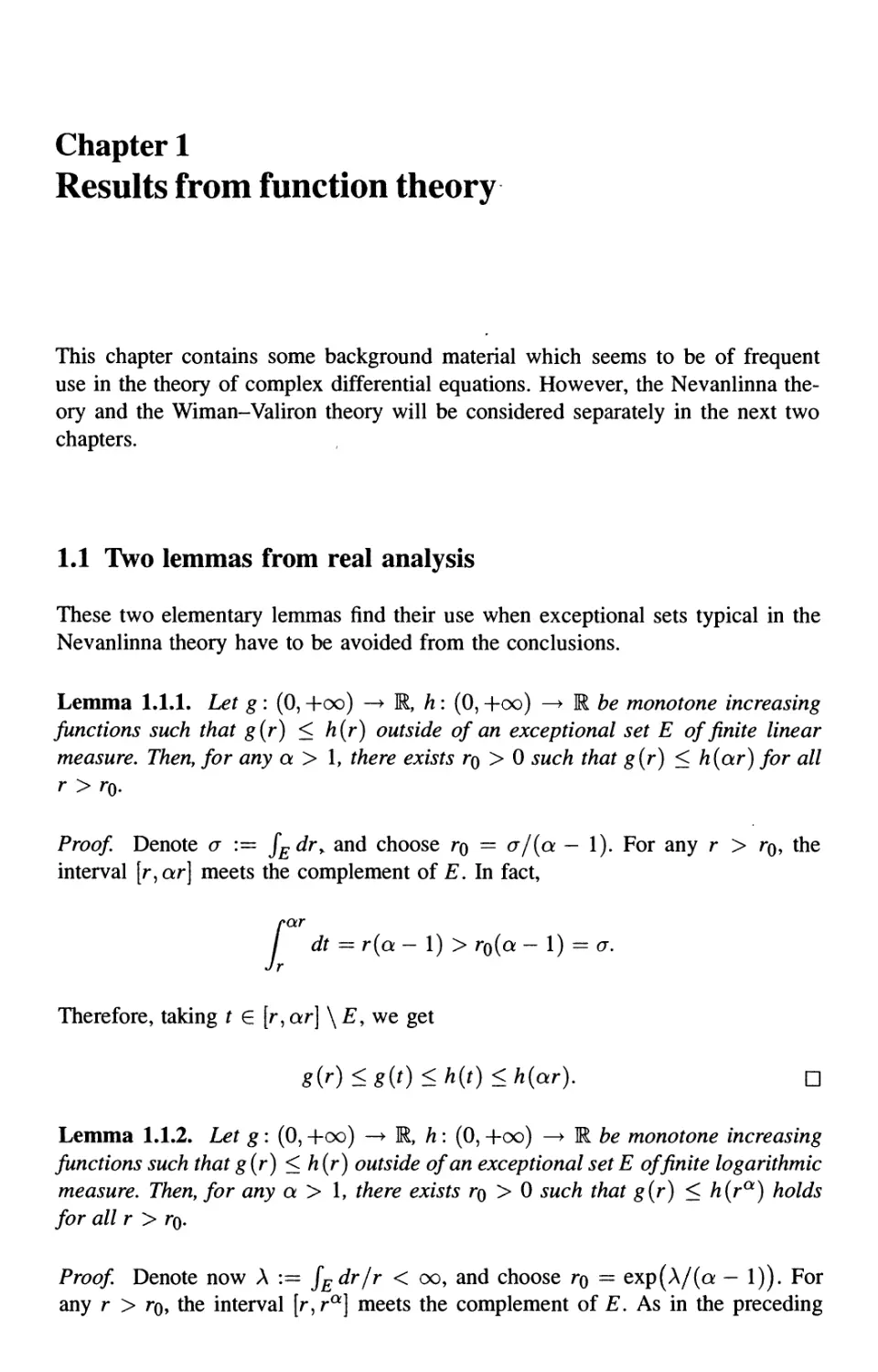
Lemma 1.1.1. Let g : @, -boo) —> R, h: @, -boo) —> R be monotone increasing
functions such that g(r) < h(r) outside of an exceptional set E of finite linear
measure. Then, for any a > 1, there exists r$ > 0 such that g(r) < h(ar) for all
r > r0.
Proof. Denote a := JEdry and choose ro = a/(a - 1). For any r > tq, the
interval [r,ar] meets the complement of E. In fact,
ar
dt = r(a - 1) > ro(a - 1) = a.
r
Therefore, taking t e [r, ar] \ £, we get
g(r)<g(t)<h(t)<h(ar). □
Lemma 1.1.2. Let g: @, -boo) —► R, h: @, -boo) -^ R be monotone increasing
functions such that g(r) < h (r) outside of an exceptional set E of finite logarithmic
measure. Then, for any a > 1, there exists r$ > 0 such that g(r) < h(ra) holds
for all r > ro.
Proof. Denote now Л := $е^г1г < °°> an(* choose ro = exp(A/(a - 1)). For
any r > ro, the interval [r,ra] meets the complement of is. As in the preceding

6 1. Results from function theory
proof,
— = logra-logr =(a- l)logr >(a- I)logr0 = Л.
Therefore, taking now t e [r, ra] \ £, we get
g(r)<g(t)<h(t)<h(ra). П
1.2 Canonical products
Of course, basic knowledge on infinite products of complex numbers, canonical
products, the Weierstrass factorization theorem and the Hadamard factorization
theorem is contained in every course of complex analysis. These notions play a
decisive role in some reasoning of complex differential equations, so we recall the
basic notions and results here. A very readable presentation may be found in the
book of R. Ash [1], p. 131-156.
To begin with, we recall that using the Weierstrass primary factors
Eq(z):=1-z
( z z
Mz) :=(l-z)exp I z + y+ ••• + —
one may prove the following two theorems, see Ash [1], Theorem 4.2.3 and The-
Theorem 4.2.5.
Theorem 1.2.1. Let (an)ne^ be a sequence of non-zero complex numbers (not
necessarily distinct) with limw-^oo|^w| = oo, arranged according to increasing
moduli. Ifmn > n — 1, then the infinite product
defines an entire function f whose sequence of zeros is exactly (an)ne^. □
Since a zero at z — 0 may be handled by multiplying by zw, this means that
we may construct an entire function having zeros precisely at given points, with
prescribed multiplicities.

1.2 Canonical products 7
Definition 1.2.2. Let (an)ne^ be a sequence of non-zero complex numbers (not
necessarily distinct) with limw_+oo \an\ = oo. The exponent of convergence of the
sequence is defined by
Г
X:=infla>0
A-2.1)
Theorem 1.2.3. Lef f/ie sequence (an)ne^ of non-zero complex numbers have a
finite exponent of convergence X and let к be a nonnegative integer > Л — 1. Then
the canonical product
defines an entire function having zeros exactly at the points an, with prescribed
multiplicities. □
The above two theorems may now be combined to obtain the Weierstrass
factorization theorem:
Theorem 1.2.4. Let f be an entire function, with a zero of multiplicity m > 0 at
z = 0. Let the other zeros off be at a\y a^ ... , each zero being repeated as many
times as its multiplicity implies. Thenf has the representation
^) A.2.2)
л=1 V nJ
for some entire function g and some integers mn. If (ап)пещ has a finite exponent
of convergence X, then mn may be taken as k — [Л] > Л — 1 in A.2.2). □
Recall now that
l^^l A.2.3)
where M{rJ) := max|z|=r \f(z)\, defines the order of an entire function. We add
two remarks concerning the above theorem:
A) If an entire function/ has a finite exponent of convergence X(f) for its
zero-sequence (an)ne^, and we write the representation A.2.2) in the form
applying Theorem 1.2.4, then we have X(Q) = a(Q) = X(f), see Ash [1], Theo-
Theorem 4.3.6.

8 1. Results from function theory
B) If the entire function/ in Theorem 1.2.4 is of finite order cr, then g in A.2.2)
is a polynomial of degree < a. This is the essential contents of the Hadamard
factorization theorem.
A couple of other elementary results concerning the exponent of convergence
are frequently used. To this end, consider the sequence (an)ne^ from Defini-
Definition 1.2.2. Denoting now
n(t) := card((aw)wGN П {\z\ < f}), A.2.4)
A.2.5)
we recall, see Hayman [2], Lemma 1.4, that the series Y1T=\ \an\~a in A.2.1) and
the integral f£°(n(t)/ta+l)dt converge simultaneously. Therefore, the exponent
of convergence of (an)ne^ also satisfies
(.2.6)
Moreover, it is easy to prove by the above notions, see Boas [1], Theorem 2.5.8,
that
A = iimsupJ^. A.2.7)
An immediate consequence of A.2.6) is now the following most useful
Lemma 1.2.5. Let {an)ne^ be a non-empty sequence of non-zero complex numbers
(not necessarily distinct) with a finite exponent of convergence Л. Then for every
Proof Given e > 0 and r > 0, we see by A.2.6) that
Therefore, the integrated counting function A.2.5) satisfies
Jo t Jo tx+£+l - Jo tx+£+l -
Let/ be an entire function, or, more generally, meromorphic, and let (an)neN
denote its sequence of zeros, each repeated according to its multiplicity. Denote

1.3 Complex polynomials 9
by X(f) the exponent of convergence of this sequence of complex numbers. Then
it is easy to obtain the following
Lemma 1.2.6. Let f\, /2 be two entire functions with no common zeros. Then for
E =/1/2 we get
A(£) = max(A(fi),A(fc)).
Proof. The inequality max(A(/i), X(f2)) < X(E) is trivial. To prove the converse
inequality, we may assume that A (is) = A > 0. Then, for any e > 0, the integral
r°n{t)dt
diverges, with n(t) being the unintegrated counting function A.2.4) for the zero-
sequence of E. With the corresponding notations n\(t), n2(t) for/i and/2, we
have
Therefore, at least one of the integrals
[°° nx{t)dt [°° n2(t)dt
Jo *A+1-C> JO t^-e
diverges which means that
max(A(/i),A(/a)) > A - e.
Since e is arbitrary, we have the assertion. □
1.3 Complex polynomials
For the convenience of the reader, we recall here two useful results concerning
complex polynomials. The first one is the following self-evident lemma, see Jank
and Volkmann [3], Satz 1.2:
Lemma 1.3.1. LetP(z) = anzn+an_izn~l-\ Ьао with апф0Ье apolynomial.
Then, for every e > 0, there exists r$ > 0 such that for all r — \z\ > tq the
inequalities
hold. П

10 1. Results from function theory
Our second lemma is an easy estimate for the roots of a polynomial, see Marden
[1], Theorem 27.2:
Lemma 1.3.2. LetP(z) — anzn+an-\zn~l4 \-a$withan ф 0 be a polynomial.
Then all zeros ofP(z) lie in the diskD{0, r) of radius
r<l+ max (\ak/an\).
0<k<n-\
Proof. Denote M :— maxo<£<w-i(|tfA:/tfw|)- Assume |z| > 1. Since
\P(z)\ > \an\\z\n-(\ao\ + |e,||z| + ... + k-iHzl"),
we see that
A.3.1)
\z\-l-M
|z|-l
Hence, if |z| > 1 +M, we have \P{z)\ > 0. Therefore all zeros of P(z) in |z| > 1
must satisfy the inequality A.3.1). On the other hand, all zeros of P(z) in jzj < 1
satisfy A.3.1) trivially. □
1.4 The Wronskian determinant
This section contains a number of basic properties of the Wronskian determinants.
However, we don't list properties which are just elementary facts of general deter-
determinants. We shall follow rather closely the presentation given in the thesis of G.
Hennekemper [1], p. 11-19.
Definition 1.4.1. The Wronskian determinant
functions /i, ... , fn is given by
/l
,...,/w) of the meromorphic
fn
Jn
J
J\
n'-l)
J
Jn
n-1)

1.4 The Wronskian determinant 11
Moreover, we denote, for v — 0, ... , n — 1, by
ВД,...,/„)
the determinant which comes from W(f\,... ,fn) by replacing the row
Proposition 1.4.2. Let f\, ..., fn be meromorphic functions. Then
W(/i,... ,fn) vanishes identically if and only iff\, ... , fn are linearly dependent
(over C).
Proof The sufficiency being trivial, let us assume that W(f\,... Jn) = 0. We may
also assume that/i does not vanish identically, hence W(f\) ф 0. Therefore, there
exists i/ € {1,..., л — 1} such that
W(/b.-.,/«/)^0, W(fi,.-.,/i,+i)=0. A.4.1)
Let now a e С be chosen so that f\, ... , fu+\ don't have a pole at a and
that W(/i,... ,/i/)(a) 7^ 0. By A.4.1), the column vectors of W(/i,... Ju+\) are
linearly dependent. Hence, for some constants Q, ... , Cv G C,
fi(a)
Hence, defining
V
we get
Moreover, by A.4.1) and A.4.2),
^ll^l = 0. A.4.3)
Expanding W(/i,... Jv, u) by the last column, we obtain by A.4.3)
^4ти(*)=0. A.4.4)

12 1. Results from function theory
By repeated differentiation of A.4.4), we see that
ц(м)(а) = о for/ieN0.
By the elementary uniqueness theorem of meromorphic functions, и
A.4.2),/i, ... ,/„_!_! are linearly dependent.
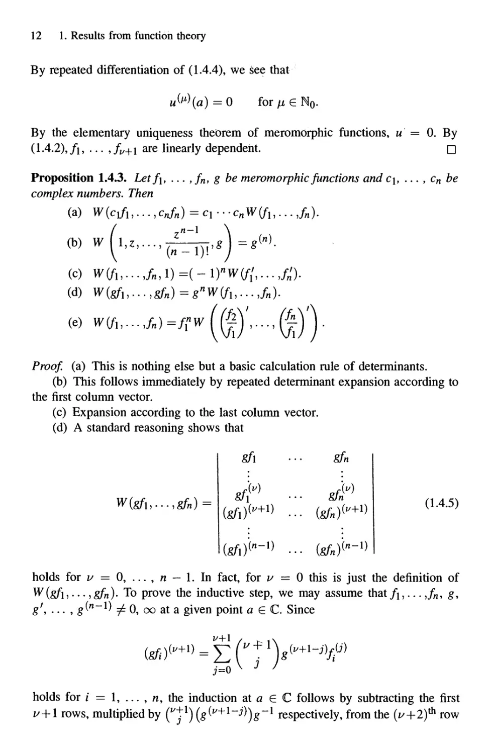
Proposition 1.4.3. Letf\, ... ,fn, g be meromorphic functions and c\,
complex numbers. Then
(a) W(d/i, • •. ,СдГл) = С! • '-cnW(fu... ,/„).
0. By
□
, cn be
l,z,...,-
(b)
(с)
(d)
Proof, (a) This is nothing else but a basic calculation rule of determinants.
(b) This follows immediately by repeated determinant expansion according to
the first column vector.
(c) Expansion according to the last column vector.
(d) A standard reasoning shows that
gf\
gfn
A.4.5)
holds for v = 0, ... , n — 1. In fact, for v — 0 this is just the definition of
i > • • • > gfn)' To prove the inductive step, we may assume that f\,... ,/„, g,
g(n~l) ф 0, oo at a given point aGC. Since
g'
holds for / = 1, ... , n, the induction at a G С follows by subtracting the first
I/+1 rows, multiplied by (^t1) (g(u+l~~fi)g~~l respectively, from the (и+2)^ row

1.4 The Wronskian determinant 13
of A.4.5). The final inductive conclusion now follows by the elementary uniqueness
theorem of meromorphic functions. For v = n — 1 we therefore obtain
W(gfl,...,gfn) =
gfx
gfn
:g"W(fh...,fn).
(e) By the preceding parts,
r r
(т) C^l I- □
Proposition 1.4.4. Letf\, ... ,fn be meromorphic functions. Then
d
Proof. Applying the standard Leibniz formula, see Kowalsky [1], p. 87, to define
a determinant we obtain
E
An~l)
An~l)
/i
fn
fn
Jn-\) Лп-\)
1 • • • Jn
Proposition 1.4.5. Letf\> ..
have
/i
/Г
/л
Jn
fff
Jn
f(n
Jn
/l
/l'
.(Л-2)
fn
fn
A
Jn
n-2)
Jn
(n)
П
,fn be meromorphic functions. Then, for n = 2, we
=/1/2 -Ml

14 1. Results from function theory
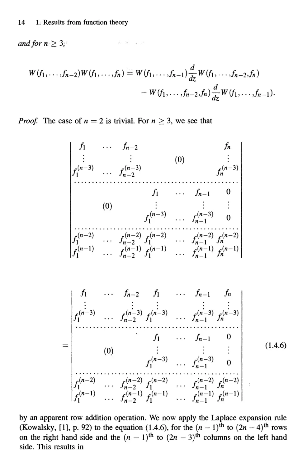
and for n> 3,
Proof. The case of n = 2 is trivial. For n > 3, we see that
/l
(n-2)
(Л-1)
••• fn-2 /l ••• fn-l fn
Лп-Ъ) Jn'-Ъ) Jn-Ъ)
h ••• Jn-2 h
Jn-2) Jn-2)
Jn-2 h
Jn-l) Jn-l)
Jn-2 h
Jn-Ъ) Лп-Ъ)
Jn-\ Jn
Jn-2) Jn-2)
Jn-\ Jn
Jn-l) Jn-l)
Jn-l J"
A.4.6)
by an apparent row addition operation. We now apply the Laplace expansion rule
(Kowalsky, [1], p. 92) to the equation A.4.6), for the (n - l)th to Bn - 4)th rows
on the right hand side and the (n — l)th to {In - 3)th columns on the left hand
side. This results in

/l
fi
(n-3)
fn-2
Jn —
(/1-3)
1.4 The Wronskian determinant 15
/l ... fn
fi
(n-l)
Jn-l)
/l
Jn-2)
Jl
/l
Jn-2)
Jl
••• fn-l
Jn-2)
■ ■ ■ Jn-l
•■■ fn-2
Jn-2)
•■ ■ Jn-2
Jl
An-3)
Jl
Jn-l)
Jl
fn
Jn-2)
Jn
/l
Jn-2
An-3)
Jn-2
Jn-l)
Jn-2
/l"
Jn-l)
/i
Jn
fn
Jn-l)
Jn
fn-l
fn-l
Jn-l)
Jn-l
which is just the assertion. □
Proposition 1.4.6. Letfi, ... , fn be linearly independent meromorphic functions
and define
\-l
Wv(fU...,fn)
A.4.7)
for v = 0, ... , n — 1. Then the meromorphic functions an,v have their poles among
the zeros ofW(f\,...,fn) or the poles off\, ... ,fn. Moreover,
an,n-l=-(W(fu...,fn)) l-^
A.4.8)
Finally, f\, ... , fn satisfy the homogeneous linear differential equation
/i-l
A.4.9)
i/=0
Proof The first assertion is straightforward. Next, A.4.8) follows from A.4.7) by
Proposition 1.4.4. To prove A.4.9), let h be any meromorphic function. Expanding
i,... ,//i, h) according to the last column we get
i/=0
The assertion A.4.9) now follows immediately.
□

16 1. Results from function theory
Proposition 1.4.7. Let f\, ... , fn be linearly independent meromorphic functions
satisfying a homogeneous linear differential equation
/i-l
/(Л)+Х>(*У(|')=О. A.4.11)
i/=0
Then
{..Jn))~lWJ/(fl,...Jn). A.4.12)
Proof Denoting an,n := 1 and an := 1, we may consider A.4.9) and A.4.11) as
linear system of equations to determine an^{z), resp. av(z), at a given z. Since
W(/i, • • • »//i) 7^ 0, such a linear system has a unique solution, and therefore we
get A.4.12) for v = 0, ... , n — 1, at least outside of zeros of W(/j,... ,/„) and
poles of the functions in consideration. By the elementary uniqueness theorem of
meromorphic functions, A.4.12) holds in the whole complex plane. □
Proposition 1.4.8. Let f\, ... , fn be linearly independent meromorphic solutions
of
with meromorphic coefficients. Then the Wronskian determinant W (f\,... Jn) sat-
satisfies the differential equation Wf + an_\(z)W = 0. Specially, if an_\ is an entire
function, then for some С G C, W (f\,... Jn) = С ехр <p where (p is a primitive
function of —an_\.
Proof.
for i -
Since
= 1, ...
с
, n, we see by Proposition
l> ao(z)fi
1.4.4 that
/l
fl
ft2)
f(n)
... fn
••• Л
-(n-2)
Jn
A")
Jn

/l
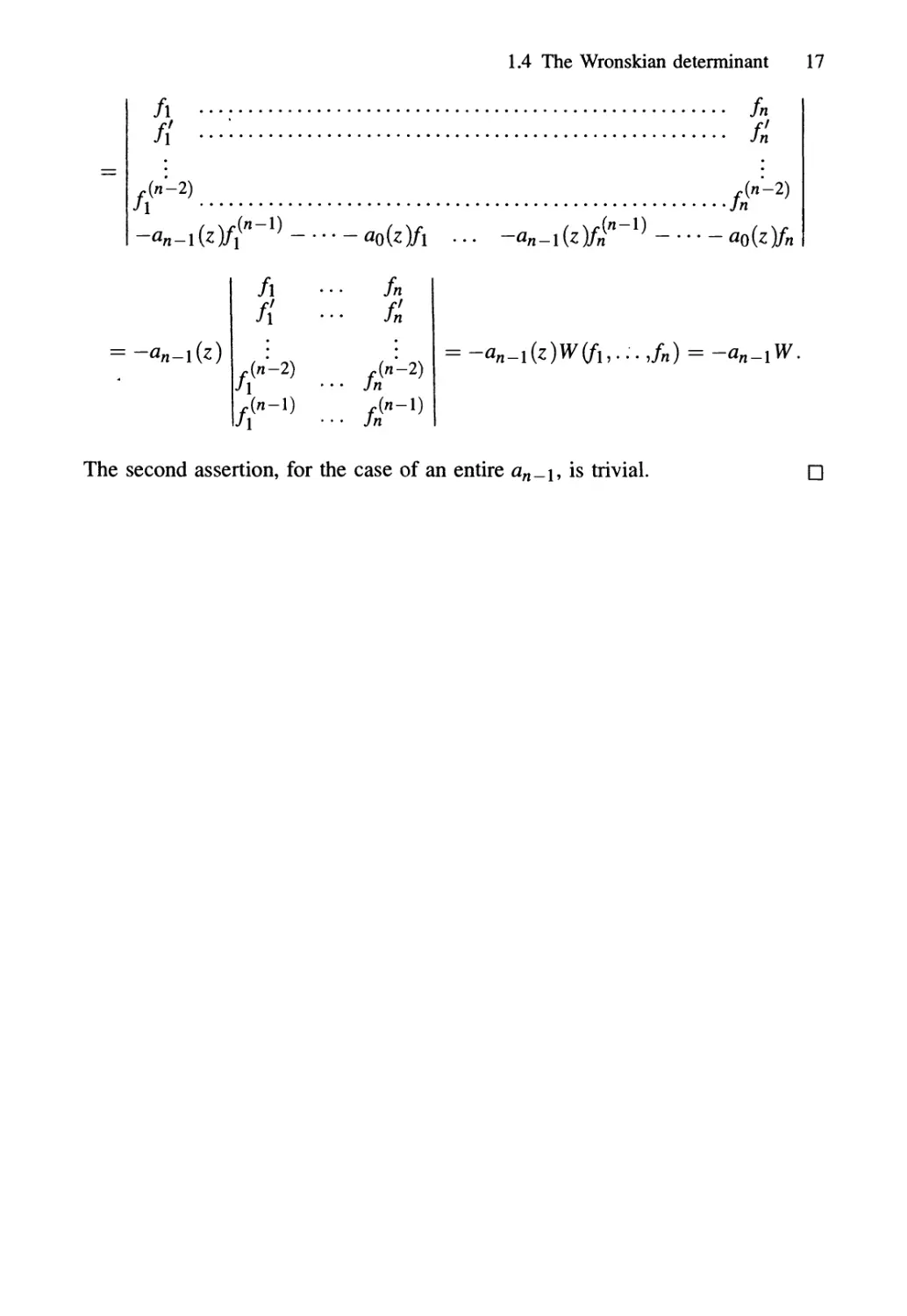
1.4 The Wronskian determinant 17
fn
•л
n-2)
/l ••■ fn
f{ -. /„'
(n-2) -(n-2)
l ■ ■ ■ Jn
n-1) Jn-l)
l ■ ■ ■ Jn
ri"-1) ao(z%
= -an_l(z)W(fl,.:.,fn) = -an_xW.
The second assertion, for the case of an entire an_\, is trivial.
D

Chapter 2
Nevanlinna theory of meromorphic functions
This chapter is not intended to be a complete introduction to the Nevanlinna the-
theory. Although written in a self-contained manner, the selection of the material is
determined by the needs of applications into complex differential equations, and
some technical details will be omitted. An interested reader may consult Nevan-
Nevanlinna [2], Hayman [2], Gross [2] or Jank and Volkmann [3] as well as original
research articles to look for omitted details and to obtain information on those
parts of Nevanlinna theory which are not presented here.
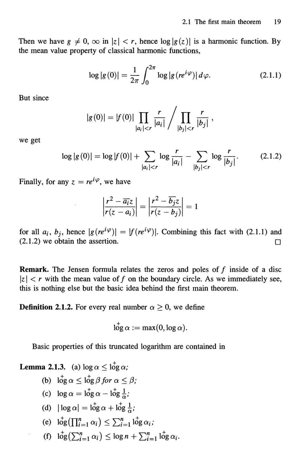
2.1 The first main theorem
The starting point to prove the first main theorem is the Jensen formula which is
a consequence of the elementary fact that log \f{z)\ is harmonic as soon as/(z) is
analytic and Ф 0, combined with the mean value property of harmonic functions.
Theorem 2.1.1 (Jensen). Let f be a meromorphic function such thatf(O) Ф 0, oo
and let a\, п2, ... (resp. b\, &2> • • • ) denote its zeros (resp. poles), each taken into
account according to its multiplicity. Then
E log|fj- E 1о*Щ'
Proof. We give the proof for the case that/ has no zeros or poles on \z \ = r, in
order to recall the essential idea behind the Jensen theorem. For the case where
zeros or poles appear on \z \ = r, we refer to Jank and Volkmann [3], p. 43-47.
Denote

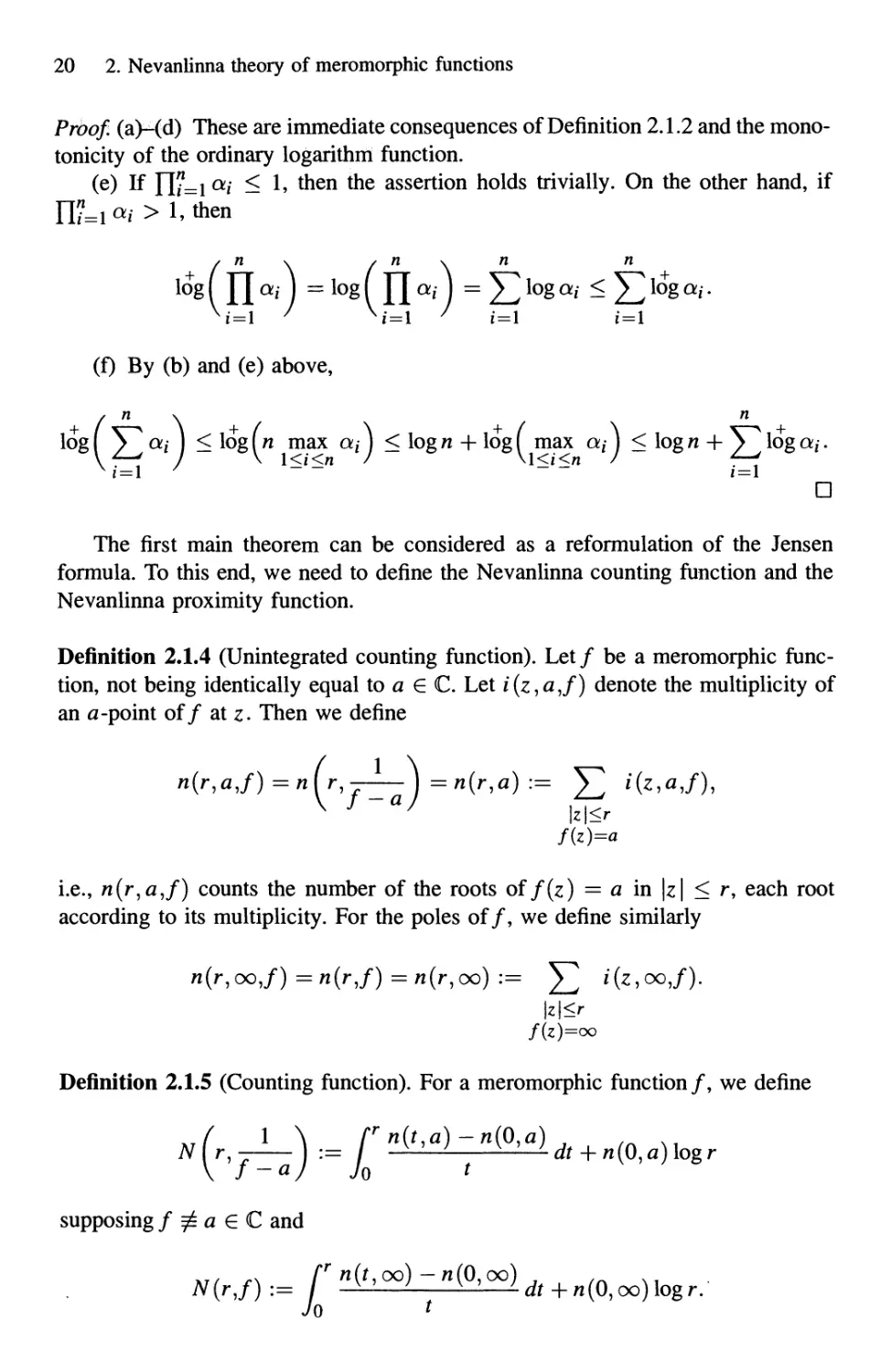
2.1 The first main theorem 19
Then we have g ф 0, oo in \z\ < r, hence log\g{z)\ is a harmonic function. By
the mean value property of classical harmonic functions,
1 f2n
log|g@)| = — / \og\g{rei(p)\d(p. B.1.1)
But since
we get
log|g@)| = log l/*@)| + ^^ l°g]—г~ У^ log tt—r- B.1.2)
Finally, for any z = relip, we have
r2-Jb77
I
r2 - atz
r{z -a()
r ~ bjt
r(z-bj)
for all au ty, hence \g{re^)\ = \f(re^)\. Combining this fact with B.1.1) and
B.1.2) we obtain the assertion. □
Remark. The Jensen formula relates the zeros and poles of/ inside of a disc
\z | < r with the mean value of/ on the boundary circle. As we immediately see,
this is nothing else but the basic idea behind the first main theorem.
Definition 2.1.2. For every real number a > 0, we define
log a := max@, log a).
Basic properties of this truncated logarithm are contained in
Lemma 2.1.3. (a) log a < loga;
(b) loga<log/?/0ra</?;
(c) log a = log a- log ^;
(d) | log a| = log a + log ^;
(e)

20 2. Nevanlinna theory of meromorphic functions
Proof, (a)^(d) These are immediate consequences of Definition 2.1.2 and the mono-
tonicity of the ordinary logarithm function.
(e) If fli=i ai ^ 1' then the assertion holds trivially. On the other hand, if
П?=1а/ > 1. then
(f) By (b) and (e) above,
(П ч П
^2 a/ 1 < log f n max az- J < log л + log f max az- j < log л + ^ log a;.
1 = 1 Z = l
a
The first main theorem can be considered as a reformulation of the Jensen
formula. To this end, we need to define the Nevanlinna counting function and the
Nevanlinna proximity function.
Definition 2.1.4 (Unintegrated counting function). Let/ be a meromorphic func-
function, not being identically equal to a e C. Let i(z,a,f) denote the multiplicity of
an a -point of/ at z. Then we define
J aJ \z\<r
f(z)=a
i.e., n(r,a,f) counts the number of the roots of f(z) = a in \z\ < r, each root
according to its multiplicity. For the poles of/, we define similarly
n(r,oo,/) =n(r,f) = n{r,oo) :=
/(z)=oo
Definition 2.1.5 (Counting function). For a meromorphic function/, we define
supposing / ф а е С and
n(t, oo) — n @,oo)
+n@,oo)logr.

2.1 The first main theorem 21
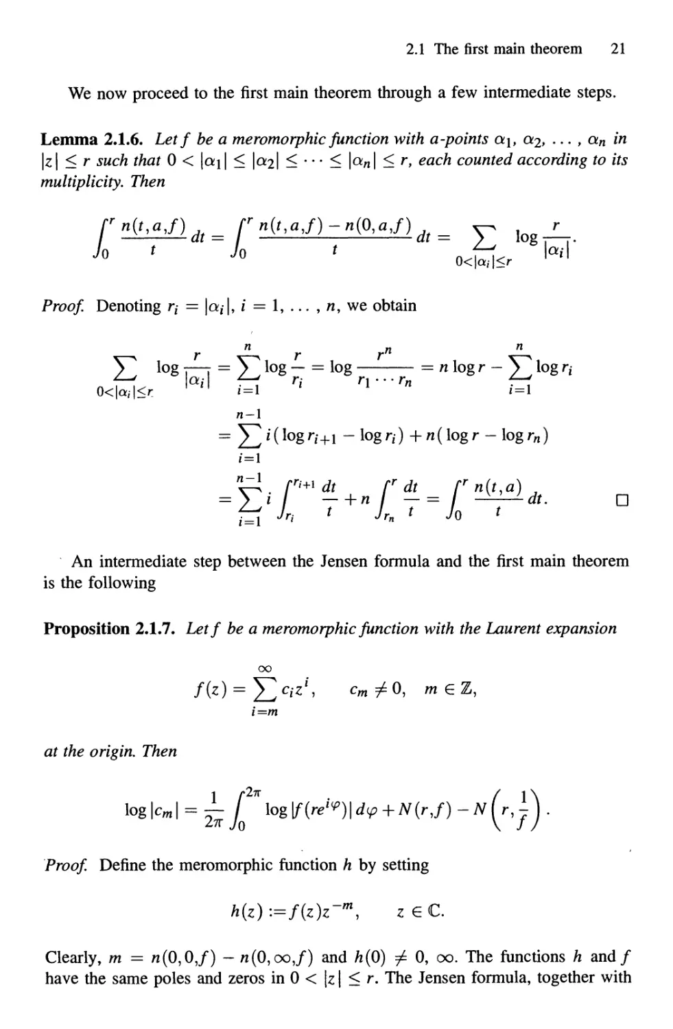
We now proceed to the first main theorem through a few intermediate steps.
Lemma 2.1.6. Let f be a meromorphic function with a-points a\, с*2, ... , an in
\z\ < r such that 0 < |c*i| < \aj\ < • • • < \oin\ < r, each counted according to its
multiplicity. Then
n{t,aj) rn{t,aJ)-«{0,aJ) у _^
Proof Denoting r/ = |a,-|, / = 1, ... , n, we obtain
n
о<Ы<г ' il 1=1 r/ rir/1 1=1
/1-1
= ^/(logr/+1 -logr/)+n(logr-logrw)
1=1
^4 rn+idt rr dt fr n{t,a) J
= }i —+n —= ^—tdt. П
fr[ Jn t Jrn t Jo t
An intermediate step between the Jensen formula and the first main theorem
is the following
Proposition 2.1.7. Letf be a meromorphic function with the Laurent expansion
at the origin. Then
Proof Define the meromorphic function h by setting
h(z):=f(z)z-m, zeC.
Clearly, m = л@,0,/) - л@,оо,/) and h@) ф 0, oo. The functions h and/
have the same poles and zeros in 0 < \z \ < r. The Jensen formula, together with

22 2. Nevanlinna theory of meromorphic functions
Lemma 2.1.6; implies
log|cw| = log|*@)|
1 f2n - _ v^ r v^ r
—— / log \f{r€l^)r m\d(p-\- } log •:—-— у log]—г
2тг Уо ^^/ \bj\ ^^ \ai\
1 r2*
2тг Уо
/%гдг(г оо)-дг(Ооо) Л л(г,0) - л@,0)
+ / Л - / Л
Jo t Jo t
П
Definition 2.1.8 (Proximity function). For a meromorphic function/, we define
m
d(p
supposing / ф а е С and
r2n
2?r Jo
Definition 2.1.9 (Characteristic function). The characteristic function of a mero-
meromorphic function / will be defined as
T(rJ):=m(rJ)+N(r,f).
Theorem 2.1.10 (First main theorem). Letf be a meromorphic function, let a e С
and let
,-z', стф0, тег,
i=m
be the Laurent expansion off — a at the origin. Then
where
r
|v>(r,e)|<log2 + log|a|.

2.1 The first main theorem 23
Proof. Assume first a = 0. By Lemma 2.1.3(c) and Proposition 2.1.7 we obtain
log|cOT| = — I log If (r
+ N(r,f)-fl
-^ J lo+g
1
dip
, =m(rJ)-m{r,j)+N(rJ)-N{r,j),
hence
тГг,^+^Гг,^=т(г,/)+^(г,/)-1оё|сш|, B.1.3)
r(r.7)=:r('-./)-l0S|cm|,
which is the assertion with <p(r,0) = 0.
Proceeding now to the general case а ф 0, we define h :=f — a. Clearly
and
Moreover,
Iog|fc|=loglf-fl|<loglf|+log|fl|+log2,
<log|fc|+log|fl|+log2.
Integrating these inequalities we see that
m(r,h) < m(r,f) +log|a| +log2
m(rj) <m(r,^)+log|a| +log2,
hence
r,a) :=m(r,h)-m(r,f)

24 2. Nevanlinna theory of meromorphic functions
satisfies "
\ф,а)\ <log2 + log|fl|
Applying B.1.3) for h we obtain
= m{rj) + N{r,f) -\og\cm
= T(r,f) - log \cm | + <p(r, a). D
Remark. The first main theorem may be expressed as
B14)
for all a e C. Note that the bounded error term 0A) depends on a e C, hence
some caution is necessary, e.g., in integrating B.1.4).
Proposition 2.1.11. Letf,f\, ... ,fn be meromorphic functions and a, /3, 7, 8 G С
such that a6 — /?7 ф 0. Then
(a) Г(г,/, •••/„)< ELl r(rj$)/<v r > 1,
(b) Г(г,/Л) = пГ(г,/), n € N,
(c) Г (г, YH=\fi) < E?=i Г(г,Л) + log n /or r > 1,
(d) г
assuming/ ф —8
Proof. Follows easily by elementary pole considerations combined with Lemma
2.1.3. The details may be omitted in (a), (c) and (d). For (b), it is enough to observe
that \fn\ = \f\n < 1 if and only if \f\ < 1. □
Remark. The characteristic function offers a natural way to define a measure for
the growth of a meromorphic function:
Definition 2.1.12. The order a(f) of a meromorphic function/ is defined by
For elementary properties of the order a(f), see Nevanlinna [2], p. 217-222.
Specially, we recall that the basic algebraic operations never increase the order.
Moreover, a meromorphic function and its derivative both have the same order, see

2.2 Rational functions and Nevanlinna theory 25
Remark to Corollary 2.3.5 below and Nevanlinna [2], p. 217-222, or Whittaker [1],
p. 82.
Recalling the notion of the exponent of convergence for the zero-sequence of
a meromorphic function/ from Chapter 1, see A.2.6) and A.2.7), we add here the
following elementary
Proposition 2.1.13. For any meromorphic function f\ \(f) < a(f).
Proof. Of course, there is nothing to prove if \(f) = 0 or a(f) = oo. Obviously,
for r > 1,
/ jx Г3гп{*>т)-п(°>т) ( l\
N K-) - /o . *+- Ыlos3r
dt + n @,- )log3r
y\ -n (o,j\) I°g3 + n U,j\ Iog3r
- n (r,-J Iog3 -f n M), -J logr > n (r,-j .
Therefore, by A.2.7) and the first main theorem,
logn(r,i)
X(f) = limsup ^—]-L < limsup
logr
< limsup
logr r^oo logr
log(rCr,/) + O(l)) logrCr,/)
< limsup \— —-—'- = hmsup & v ^
r^oo log 3r - log 3 r^oo log 3r
2.2 Rational functions and Nevanlinna theory
Several inequalities of the Nevanlinna theory depend on an error term whose growth
is of type О (logr). Hence, it is important to characterize meromorphic functions
whose characteristic function has the growth of this type. To this end, we recall
the Poisson-Jensen formula, whose proof can be found in several text-books. Jank
and Volkmann [3], p. 43-47, gives all details.
Theorem 2.2.1. Let f be a meromorphic function such thatf(z) ф 0, oo and let
a\, a2, ... (resp. b\, &2> - - -) denote its zeros (resp. poles), each taken into account

26 2. Nevanlinna theory of meromorphic functions
according to its multiplicity. Suppose z = rei(* and r < R. Then
\a,\<R
An immediate consequence is now
\bj\<R
R2 - bjZ
Proposition 2.2.2. Let g be an entire function and assume that 0 < r < R < oo
and that the maximum modulus M(r,g) — maxui_r \g{z)\ satisfies M(r,g) > 1.
Then
T(r,g) < logM(r,g) < ?-±LT(R,g).
к r
к — r
Proof. The first inequality is trivial:
T(r,g) = m(r,g) =
<\ogM(r,g) = \ogM (r,g).
To prove the second inequality, take zo such that zo = relQ and that \g{zo)\ =
M(r,g). Recall that \R(z -a()/(R2 -aiz)\ < 1 whenever \z\ < R. Therefore, the
Poisson-Jensen formula results in
log|g(,0)| < ±
(R+r){R-r)
{R - rJ + 2Rr A - cosFi - ip))
D
Remark. It is easy to see that by Proposition 2.2.2 the order a(g) given in Defini-
Definition 2.1.12 reduces, in the case of an entire function g, back to the classical order
notion defined by limsup,.^^ log logM(r,g)/ log r, see A.2.3).
We are now ready to give the anticipated characterization of rational functions.
Theorem 2.2.3. A meromorphic function f is rational if and only ifT(r,f) =
O(logr).

2.2 Rational functions and Nevanlinna theory 27
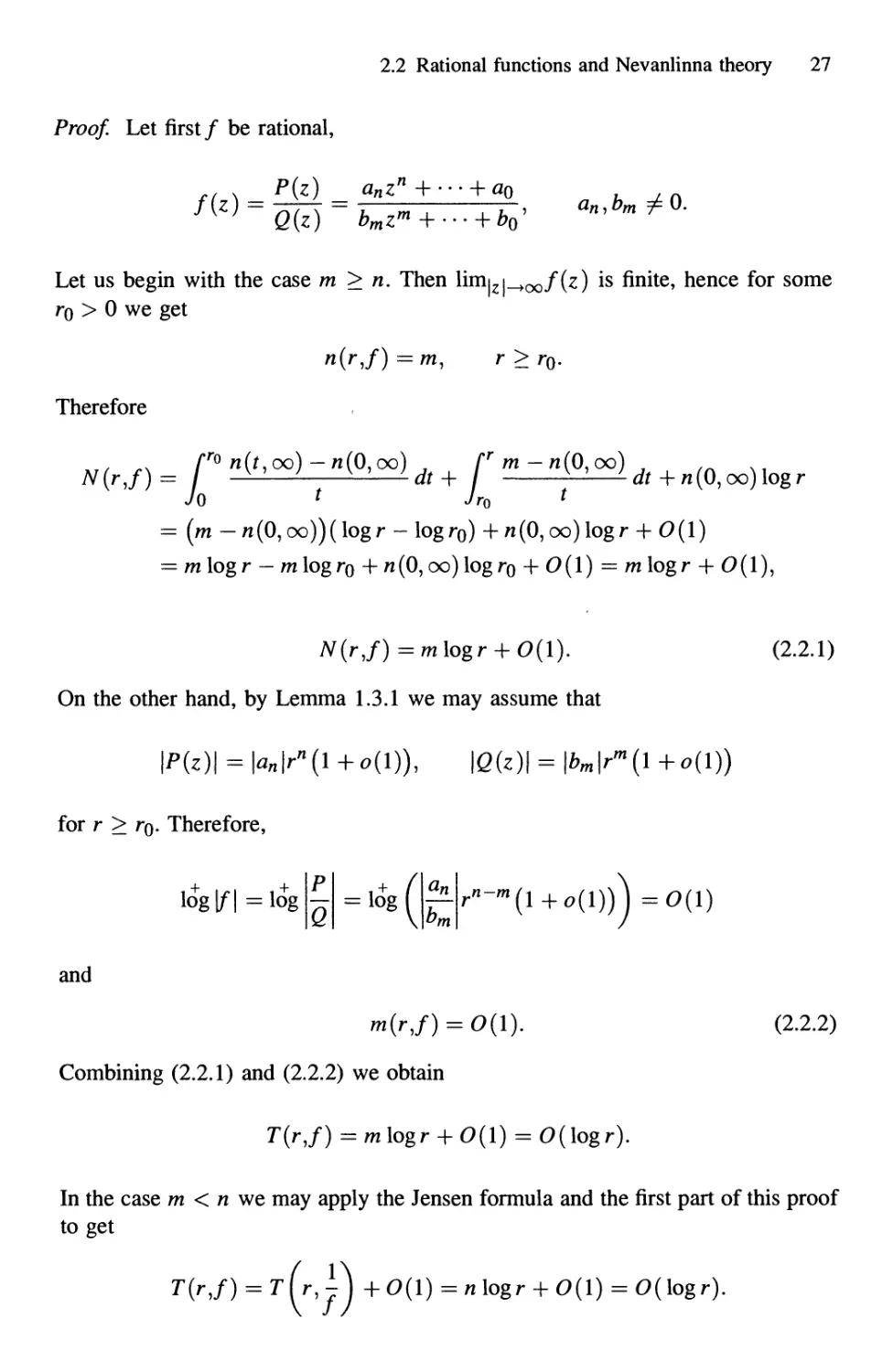
Proof. Let first/ be rational,
Let us begin with the case m > n. Then \\m)[Z^OQf{z) is finite, hence for some
ro > 0 we get
Therefore
n(r,f)=m, r>r0.
>r° n(t, oo) - л@, oo) _ , Г m - л@, оо)
-dt +n@, oo)logr
ro
= (m-n @, oo)) (log r - log r0) + л @, oo) log r + О A)
= mlogr — mlogro +n@, oo)logro -f 0A) = mlogr -f 0A),
N{rJ)=mlogr
On the other hand, by Lemma 1.3.1 we may assume that
\P(z)\ = \an\r"(l +o(l)), \Q(z)\ =
for r > tq. Therefore,
B.2.1)
and
m(r,/) = 0(l). B.2.2)
Combining B.2.1) and B.2.2) we obtain
T(rJ) = mlogr + 0A) - O(logr).
In the case m < n we may apply the Jensen formula and the first part of this proof
to get
T(rJ) = T[^j) + 0A) = n logr + 0A) = O(logr).

28 2. Nevanlinna theory of meromorphic functions
Assume now that/ is a meromorphic function such that T{r,f) — O(logr), i.e.,
for some r0 > 1 and for some ^>0we have
T(rJ)<K\ogr for r>r0. B.2.3)
We may assume that/ is non-constant. By B.2.3),
N{r,f) < К logr forr >r0.
Then for all r > tq, we obtain
(n(r,oo)-n@,oo))logr = (л(г,оо)-л@,оо)) / —
Jr *
< Г2 «(r.oo)- «@,oo) д^ r2^,oo)-»@,oo)^+n@oo)logr2
Jr t JO x
= N(r2J) < К logr2 = 2A: logr.
Therefore
n(r,oo) < 2£+n@,oo)
for all r > tq. This means that/ has at most finitely many poles, say b\, ... , bn,
in the complex plane. Define now an entire function g by
P(z):=(z-bl)-iz-bnI
g(z):=f(z)P(z).
By the first part of the proof we may assume that
r(r,P)<(rt + l)logr, r>r0,
hence
T() <(£+ + l)l Ll r > r0.
By Proposition 2.2.2, with R = 2r, we see that
logM(r,g) < 37Br,g) < 3Llog2r = 3L(logr + log2) < 6Llogr = logr6L
for all r > maxB, r0). For these values of r,
|*(z)| <M(r,g)<r6L

2.2 Rational functions and Nevanlinna theory 29
for \z\ = r. By the Liouville theorem, g must be a polynomial and therefore/ is
a rational function. D
In some parts of the Nevanlinna theory as well as in the theory of complex
differential equations it will be frequent to encounter with quantities which are
of growth o(T(rJ)) as r —> oo outside of a possible exceptional set of finite
linear measure, / being a meromorphic function. Such quantities will be denoted
by S(r,/). Observe that the exceptional set may be different for different quan-
quantities. Moreover, the sum of finitely many quantities of type S(r,f) is again of
type S(r,f). Even more is true:
Proposition 2.2.4. Letf be a meromorphic function. Then the family
s(f) := {# meromorphic \ T(r,g) = S(r,f)}
is a field and an algebra.
Proof. Follows immediately by Proposition 2.1.11. □
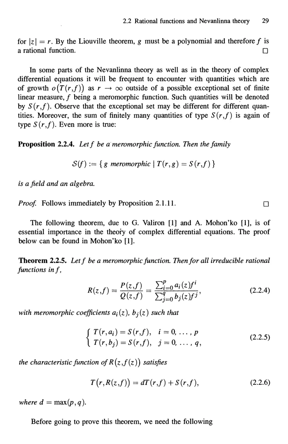
The following theorem, due to G. Valiron [1] and A. Mohon'ko [1], is of
essential importance in the theory of complex differential equations. The proof
below can be found in Mohon'ko [1].
Theorem 2.2.5. Letf be a meromorphic function. Then for all irreducible rational
functions inf,
{224)
with meromorphic coefficients ax (z), bj (z) such that
(T(r,ai)=S(r,f), i=0,
..,p
\T(r,bj)=S(r,f), j=O,...,q, K ■ ■ }
the characteristic function ofR{z,f(z)) satisfies
T(r,R(zJ)) = dT(rJ) +5(r,/), B.2.6)
where d = max(p,q).
Before going to prove this theorem, we need the following

30 2. Nevanlinna theory of meromorphic functions
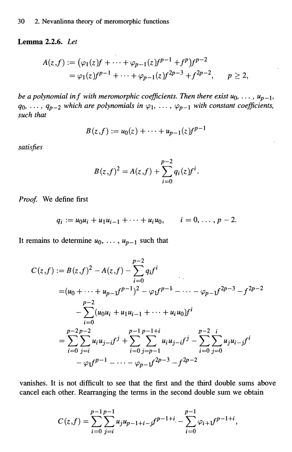
Lemma 2.2.6. Let
A(z,f) := ЫгУ + ---+<pP-l(z)fp-1 +fp)fp~2
P+f2p-2, P>2,
be a polynomial inf with meromorphic coefficients. Then there exist щ, ... , up-\,
Q0> - • > Яр-2 which are polynomials in (p\, ... , <pp-\ with constant coefficients,
such that
satisfies
p-2
/=0
Proof. We define first
qt := щщ + щщ_\ + • • • + щи0, i = 0, ... ,p - 2.
It remains to determine щ, ... , up_\ such that
p-2
C(zJ):=B(zJJ -A(zJ)-^2^f
i=0
p-2
^2 1 + •. • + м;но)/'
p-2p-2 p-lp-l+i p-2 i
/=0 j=i i=0j=p-\ i=0 j=0
vanishes. It is not difficult to see that the first and the third double sums above
cancel each other. Rearranging the terms in the second double sum we obtain
i=0 j=i i=0

2.2 Rational functions and Nevanlinna theory 31
where (pp := 1. Clearly, C(z,f) vanishes, if mq, ... , up-\ are determined recur-
recursively via
p-\
^2^ир_1+(^ = (р1+1, i =p- 1, .., , 0. B.2.7)
3=i
Fixing up_\ := 1, it is easy to see that B.2.7) then determines m^_2, ... , щ
uniquely. D
Proof of Theorem 2.2.5. In this proof, Proposition 2.1.11 will be applied repeatedly,
without pointing out this argument explicitly.
Assume first that q = 0. Clearly, we may assume that b$ = 1. Since
i=0 ^ ^ 1=1
p
an immediate inductive argument results in
" B.2.8)
i=0 7 i=0
By B.2.5),
) ()() B.2.9)
i=0 ^
To prove the inequality converse to B.2.9), assume first that/? = 1. Then
hence
T(r,ao + a]f) = T(r,f)+S(r,f).
Assume next that B.2.6) has been established for all polynomials P (z,/) in / of
type B.2.4) such that degy P(zJ) = s < p - 1, i.e.,
T(r9P{zJ)) =sT(rJ)+S(r,f). B.2.10)

32 2. Nevanlinna theory of meromorphic functions
For the inductive step, we write
We now apply Lemma 2.2.6 to
■(pp_-]fp~
"P
where щ = а(/ар, i = 1, ...,/? — 1. Clearly, T(r,(pi) = S(r,f) for i = 1,
... ,p-l. Moreover, for м0,... , up_\, q$,... , ^_2 determined by Lemma 2.2.6,
we also have Т(г,щ) =5(r,/)f i =0, ... ,p- 1, and Г(г,^-) = S(rJ),j = 0,
... , /? - 2. By Lemma 2.2.6,
/7-2
and degy B(z,f) = p — I. Therefore, our inductive assumption B.2.10) applies to
B{z,f)> whose coefficients are meromorphic functions of type S(r,f). Applying
also B.2.8), we obtain
2(p - \)T(rJ) +S(rJ) = 2T(r,B(z,f)) = T(r,B(z,fJ)
P-2
hence
and we have completed the case q = 0.
We now proceed to the general case q > 0. By the Jensen formula, we may
assume that p > q. Even more, p > q may be assumed. In fact, if p = q, then
S := bpP - ^Q =(^ - apb-l)bp<2,
where degy 5 <p — l.lfS/Qis reducible, i.e., if there exists a non-trivial common
factor Si,S=S\S2,Q= SXQ2, then
S S2 u u P
= =bRa = ba

2.2 Rational functions and Nevanlinna theory 33
and so
P=Sib-l(S2+apQ2).
Therefore S\ is also a common factor of P and Q, a contradiction. Hence S /Q
must be irreducible. Since
and
T(r,R) =т(г,Ьр1^] +S(r,f) = т(г,Ьр^\ +S(r,f),
we see that the case p = q reduces back into p > q.
To prove next the inequality
T(r,R)<pT{rJ)+S{rJ) B.2.11)
for p > q > 0, we first note that the case q = 0 is contained in the first part
of this proof. Assume now that B.2.11) holds for all rational functions R in/ of
type B.2.4) such that degy Q = к < q - 1, degy P =p > k. Since R{zJ) may
be written as
the first part of the proof, together with our inductive assumption, implies that
) +qT(r,f) +S(r,f) =PT(rJ)+S(rJ).
To prove finally
T{r,R)>pT{rJ)+S{r,f) B.2.12)
for/? > q > 0, we may again assume that q > 0. By Cohn [1], Theorem 7.4.2(iii),
there exist two polynomials U and V in/ with meromorphic coefficients in S(r,f),
see Proposition 2.2.4, such that
PU +QV = 1.

34 2. Nevanlinna theory of meromorphic functions
Denoting s := degy U, t := degy V, we see at once that p > q implies t > s.
Clearly,
=(p + t)T(rJ) +S(r,f). B.2.13)
Since t > s, we get by B.2.11)
Combining B.2.13) with this inequality, we obtain the final assertion B.2.12). □
Corollary 2.2.7. Letf be a meromorphic function. Then for all irreducible rational
functions R(z,f) inf, see B.2.4), with meromorphic coefficients ai(z), bj{z), the
characteristic function ofR (z ,/(z )) satisfies
T(r,R(z,/)) = dT{r,f) + О (Щг)) + S (r,f),
where
!?(r)=max{(r(r,fl/),r(r,ftj)}.
ho
Proof In fact, this is the original result due to A. Mohon'ko in [1]; our preceding
proof is nothing else than a simplification of the original one into the case where
the coefficients я/(г), bj(z) are all of type S(r,f). □
2.3 The proximity function of the logarithmic derivative
The second main theorem of the Nevanlinna theory depends essentially on an
estimate of the proximity function of the logarithmic derivative, namely that
m\r,Jj\=S(r,f) B.3.1)
holds for all transcendental meromorphic functions. This is perhaps the deepest
detail of the basic Nevanlinna theory, being most vital for applications to complex

2.3 The proximity function of the logarithmic derivative 35
differential equations at the same time. Despite of this situation, we omit the proof
here, since the proof given by V. Ngoan and I. Ostrovskii [1] could only be repeated
here, see also Jank and Volkmann [3], p. 63-66. Therefore, we just recall
Theorem 2.3.1. Let f be a mewmorphic function such that /@) ^ 0, oo. If
0 < r < R and 0 < a < I, then
т г,- < -
Before getting the estimate B.3.1), we need the following lemma from real
analysis, well-known as the Borel lemma:
Lemma 2.3.2. Let T: [ro,oo) —> [l,oo) be a continuous, increasing function.
Then
т(г+щ)<2Т{г)
outside of a possible exceptional set E С [ tq, oo) with linear measure < 2.
Proof See Hayman [2], p. 38-39, or Jank and Volkmann [3], p. 67-68. □
Theorem 2.3.3. Letf be a transcendental mewmorphic function. Then
and iff is of finite order of growth, then
Proof. Multiplying/ by zm for a suitable m e N, we may assume that/(O) ^ 0, oo.
Let first/ be of finite order, i.e.,
T(rJ) = O(rk) asr->oo
for some k G N. Take a = j, R = 2r, and we obtain from Theorem 2.3.1
m\ r.-r

36 2. Nevanlinna theory of meromorphic functions
for some К > 0 and all sufficiently large values of r. This implies
Suppose next that/ is of infinite order. Taking now R — r — l/T(r,f) and
a = j, we apply Theorem 2.3.1, Bemerkung 8.2 in Jank and Volkmann [3] and
Lemma 2.3.2 to obtain
m (r/j^j < 21og(l + 48A + rT{rJ)f2 ■ 2T(r,f))
outside of a possible exceptional set of finite linear measure. This implies imme-
immediately
Remark 1. The result of Theorem 2.3.3 may be written as
m
(r/j^=O(\ogT(r,f)+\ogr),
outside of a possible exceptional set E of finite linear measure, as one can see
from the above proof. A similar precisement also applies to Corollary 2.3.4 and
Corollary 2.3.5 below. Observe that the standard notation E for such an exceptional
set of finite linear measure will be applied in what follows without explanation.
The set E may be different from orie instance to another. Instead of E, we may
also say that an (in)equality holds n.e. as r —* oo.
Remark 2. In the finite order case, a bit more careful estimate proves the result
due to V. Ngoan and I. Ostrovskii in [1]:
< max@,<т(Л - l).
i
logr
Corollary 2.3.4. Let f be a transcendental meromorphic function and к > 1 be an
integer. Then
m(r/-j-\=S(f,f),

2.3 The proximity function of the logarithmic derivative 37
and iff is of finite order of growth, then
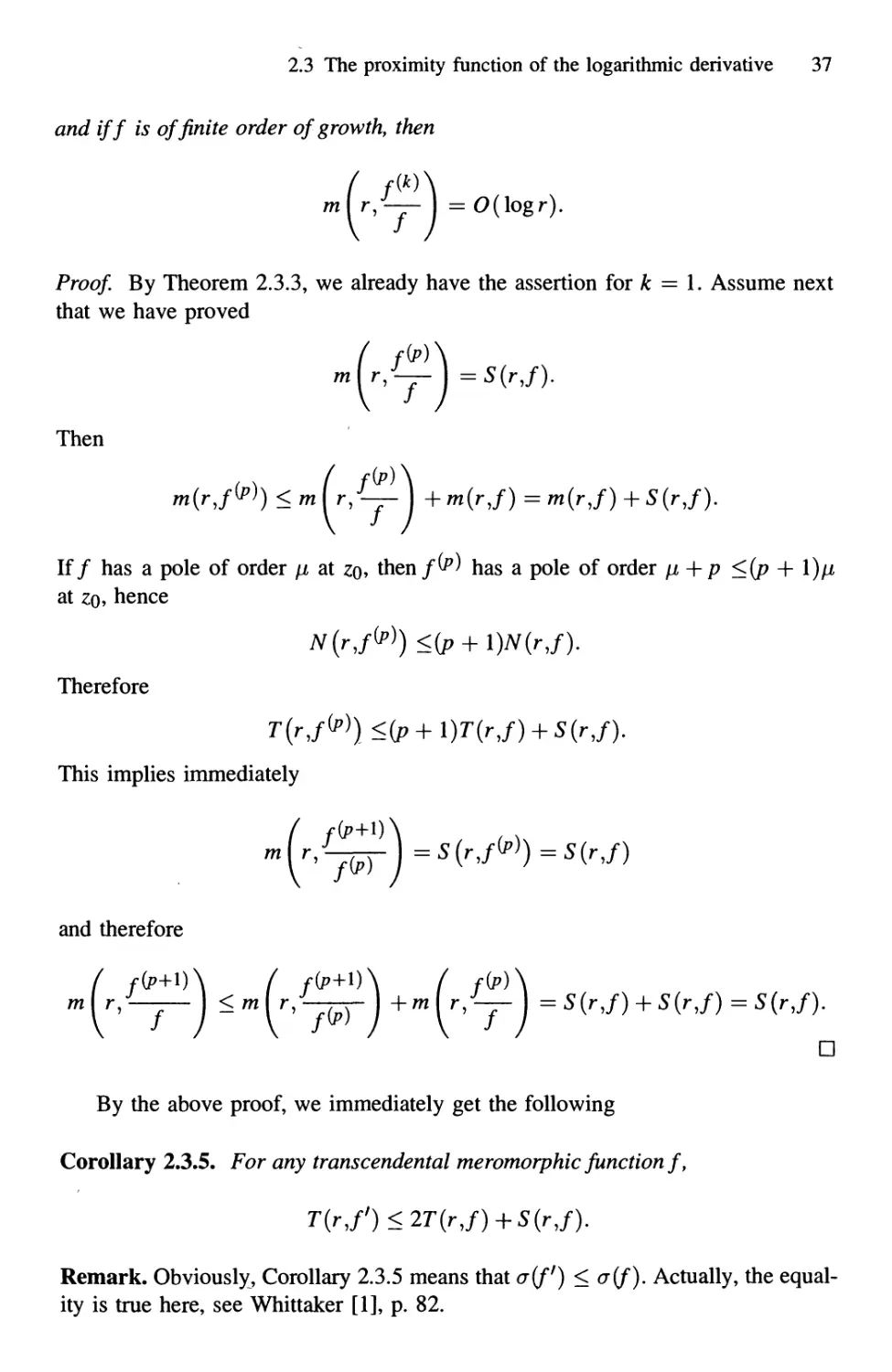
Proof By Theorem 2.3.3, we already have the assertion for к = 1. Assume next
that we have proved
Then
W < m (r/-^-) + m(r,f) = m(r,f) + S(r,f).
If/ has a pole of order д at zq, then /^ has a pole of order /x + p <{p +
at zo, hence
Therefore
This implies immediately
m
and therefore
mlr
/—j—\ <mlr
D
By the above proof, we immediately get the following
Corollary 2.3.5. For any transcendental meromorphic function f,
T(rJf)<2T(rJ) + S(rJ).
Remark. Obviously, Corollary 2.3.5 means that a(ff) < a(f). Actually, the equal-
equality is true here, see Whittaker [1], p. 82.

38 2. Nevanlinna theory of meromorphic functions
To close this section, we include a theorem due to W. Hayman [1], Theorem 4,
which seems to be of interest in the theory of complex differential equations.
Theorem 2.3.6. Let f be a transcendental meromorphic function not of the form
P. Then
Proof. Let us denote (p :=f/ff. Then the zeros of <p, which are all simple, are of
course nothing else than the poles of the logarithmic derivative/7//. Hence
Since
'J-ff"
,^(f'Y-ff"_x ff"
the zeros of cp' - 1 are among the zeros of/ and/". In fact, at a pole zo of/ with
the Laurent expansion
we get for ф := ff"/(f1I by elementary calculation VUo) = 1 + «-1 an(i so
(^'(zo) ф 1. Therefore
Now, Theorem 3.5 in Hayman [2] implies that
^) ^). B.3.4)
Combining now B.3.2) and B.3.3) with B.3.4) we get the assertion. П
Finally, we add an elementary lemma related with the logarithmic derivative
of a meromorphic function frequently needed below. This lemma has nothing to
do immediately with Nevanlinna theory. Concerning its fairly obvious inductive
proof, see Hayman [2], Lemma 3.5.

2.4 Lemmas of Clunie type 39
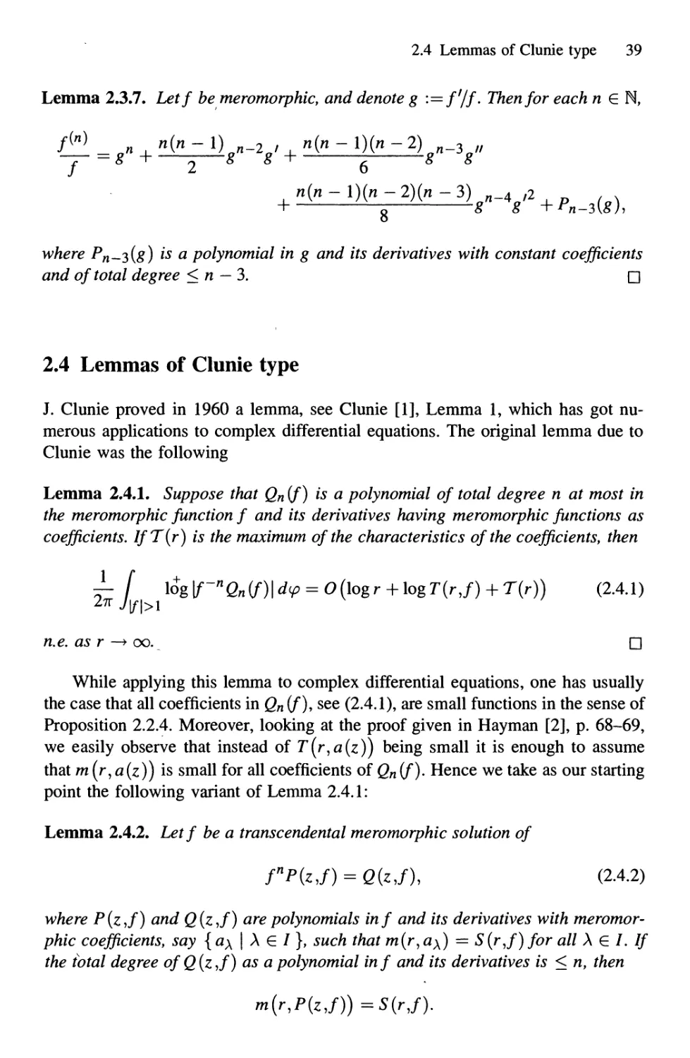
Lemma 2.3.7. Letf be meromorphic, and denote g :=ff/f. Then for each n G N,
where Рп~з{8) ^ fl polynomial in g and its derivatives with constant coefficients
and of total degree < n — 3. □
2.4 Lemmas of Clunie type
J. Clunie proved in 1960 a lemma, see Clunie [1], Lemma 1, which has got nu-
numerous applications to complex differential equations. The original lemma due to
Clunie was the following
Lemma 2.4.1. Suppose that Qn(f) is a polynomial of total degree n at most in
the meromorphic function f and its derivatives having meromorphic functions as
coefficients. IfT(r) is the maximum of the characteristics of the coefficients, then
/ log\f-nQn(f)\dtp = O(logr + logT{rJ) + T{r)) B.4.1)
\f\>\
n.e. as r —» oo. □
While applying this lemma to complex differential equations, one has usually
the case that all coefficients in Qn (f), see B.4.1), are small functions in the sense of
Proposition 2.2.4. Moreover, looking at the proof given in Hayman [2], p. 68-69,
we easily observe that instead of T(r,a(z)) being small it is enough to assume
that m (r, a (z)) is small for all coefficients of Qn (f). Hence we take as our starting
point the following variant of Lemma 2.4.1:
Lemma 2.4.2. Let f be a transcendental meromorphic solution of
f"P(z,f) = Q(z,f), B.4.2)
where P(z,f) and Q(z,f) are polynomials inf and its derivatives with meromor-
meromorphic coefficients, say {a\ \ Л G / }, such that m(r,a\) = S(r,f) for all Л G /. If
the total degree of Q(z,f) as a polynomial inf and its derivatives is < n, then
m(r,P(z,f))=S(r,f).

40 2. Nevanlinna theory of meromorphic functions
Proof, Defining
El:={f€l0M\\f(rei*)\<l},
E2:=[0,2it}\Eu
we may consider the proximity function m(r,P{zJ)) in two parts:
27rm(r,P(z,f))= f log\P\d<p + f l$g\P\dip.
JE\ JE2
Writing, with Л =(/0,..., /Д
Xel
Xel
we have for z £ E\,
\Px(z)\ < Mz)l|j
i=i
llA =s{rj).
/
Therefore, by Corollary 2.3.4,
/ log
J E\
Hence
/ log\P\dcpKY" f log \Px{reiv)\dip + 0A) = S(r,f). B.4.3)
JE\ J^ JE\
To consider E2, write
Q(z,f) =
XeJ
XeJ
By our assumption Iq + • • • + lv < n for all Л =(/o, • • •, lv) ^ J- Therefore,
for z e E2,
XeJ
<YAbx(z)\h\ -
XeJ
T

2.4 Lemmas of Clunie type 41
and, for some К > 0,
f
^ ^(^) =S(rJ). B.4.4)
XeJ j=\ \ J I
Combining B.4.3) and B.4.4), we get the assertion. □
One should perhaps remark that the Clunie lemma appears in numerous variants
in the mathematical literature, all of them being equally well of potential importance
in applications to complex differential equations. Most of these variants follow
through a careful study of the above proof. Examples of such variants are the next
two lemmas:
Lemma 2.4.3. Letf(z) be a transcendental meromorphic solution of finite order a
of B.4.2), where P(z,/) and Q{z,f) are polynomials inf and its derivatives, with
meromorphic coefficients of order at most d < a. If the total degree ofQ(zJ) as
a polynomial inf and its derivatives is at most n, then for any e > 0,
Lemma 2.4.4. Letf(z) be a meromorphic solution of infinite order of B.4.2), where
P(z,f) and Q(z,f) are polynomials inf and its derivatives, with meromorphic
coefficients a\, Л G /, satisfying an estimate of the form
w(r,£iA) = 0(^ +log Г(г,/))
n.e. as r —> oo for some fixed C > 0. If the total degree ofQ(z,f) as a polynomial
inf and its derivatives is at most n, then
m(r,P(z,/))=O(r/4logr(r,/))
n.e. as r —* oo.
Differently formulated is the next lemma, see He and Xiao [5], p. 218-220.
However, this lemma may equally well be considered as a result of Clunie type:
Lemma 2.4.5. Letf(z) be a transcendental meromorphic solution of
Q(zJ)n(z,f) = P(zJ),

42 2. Nevanlinna theory of meromdrphic functions
where
k=0 j=0
are polynomials inf with meromorphic coefficients such that
m(r,ak)=S(r,f), k=O,...,p,
m r
B.4.5)
and O(z,f) is a polynomial in f and its derivatives with meromorphic coeffi-
coefficients a\, Л€/, such that
If q >p, then
Proof. Denote
Clearly,
m(r>a\) = s(r,f), Xe
m(r,n(z,f))=S(r,f).
bq-j(z)
B.4.6)
B.4.7)
B(z) := max \ 1, 2
bq{z)
bq-j(z)
bq{z)
hence
logB(z) < ^ 4 flog |*^(г)| + 1о8 —i->)+21og2 + log*.
j=l 3 \ \Dq\Z)\/
By B.4.5),
Consider now
B.4.8)

2.4 Lemmas of Clunie type 43
Denoting for Л =(i0, ...,!„) e /, |A| := i'q H h in, we get for z G E\(r),
Xel
i\h
An)
f
and
Xel
f
Xel
hence
f
JE
-!- f \og\n(z,f)\d<p =
2* J()
by B.4.5), B.4.6) and B.4.8).
On the other hand, if z € E2(r) := {\z\ = r} \Et(r), then
\f(z)\>B(z)>2
bq{z)
for j = 1, ... , q.
Therefore
and
\f(z)\j>2j
bq{z)
bq(z)
\f(z)\i -V
For z € £г(г) we obtain
q 1 -
bq-l(z)
bq(z)
bo(z)
bq(z)
B.4.9)
\Q(z,f)\ > \bq{z)Mz)\
Since \f(z)\ > 1 for z G £2@. we use ^U,/) = P(zJ)/Q(zJ) to obtain

44 2. Nevanlinna theory of meromorphic functions
and therefore
i- / Iog\f2(zj)\dxp
2тг JEl{r)
Combining B.4.9) with this inequality, we get the assertion B.4.7).
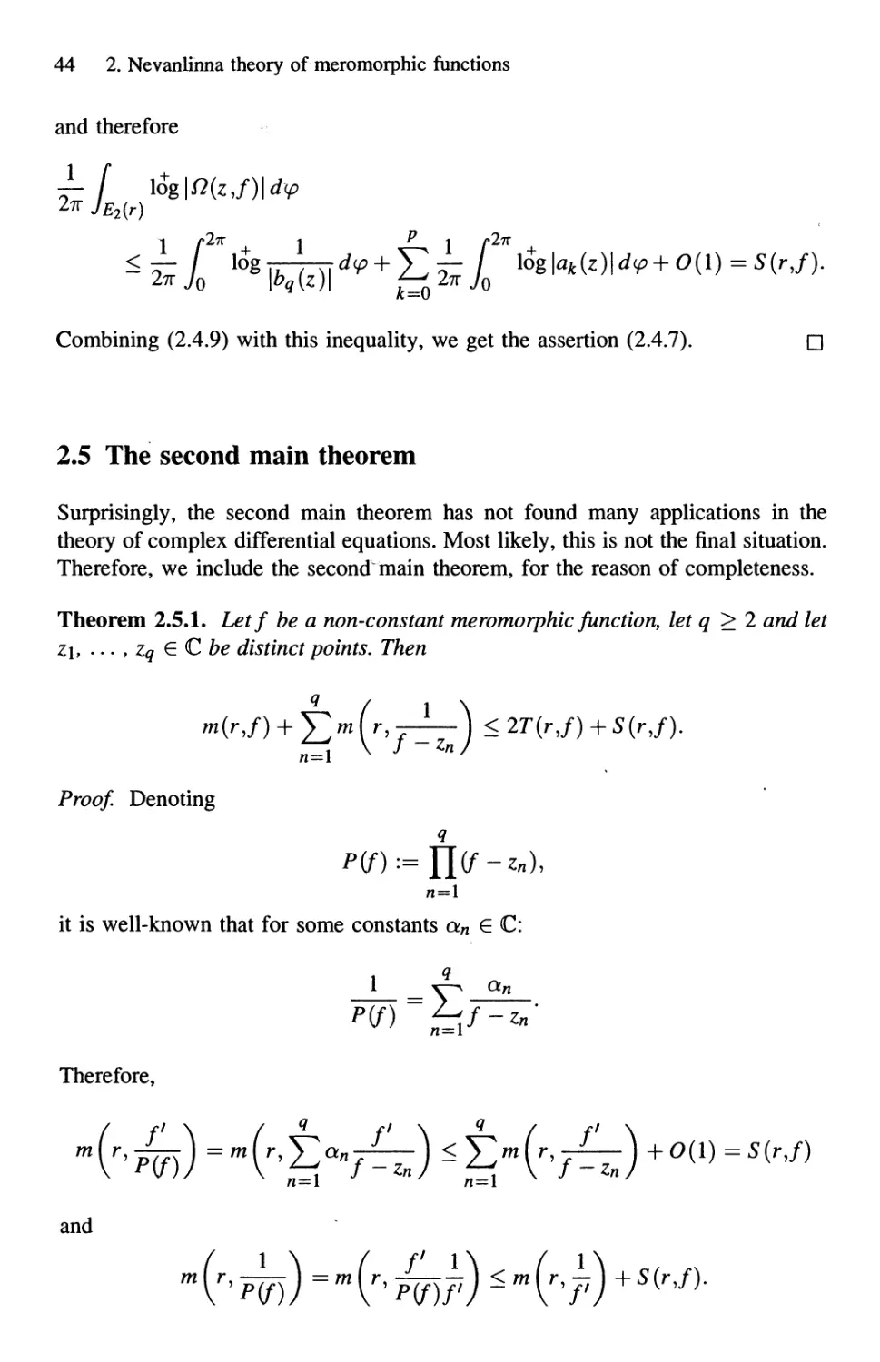
2.5 The second main theorem
Surprisingly, the second main theorem has not found many applications in the
theory of complex differential equations. Most likely, this is not the final situation.
Therefore, we include the second main theorem, for the reason of completeness.
Theorem 2.5.1. Let f be a non-constant meromorphic function, let q > 2 and let
z\, ... , Zq £ С be distinct points. Then
q ( 1 \
Em r'7Z— <
Proof. Denoting
it is well-known that for some constants an G C:
P(f)
Therefore,
m
n = l J ll/ /1 = 1
and
m I r,

2.5 The second main theorem 45
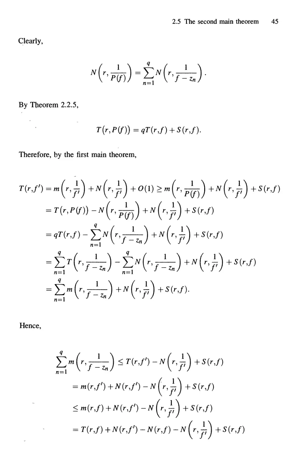
Clearly,
=> N r
By Theorem 2.2.5,
T(r,P(f))=qT{rj)
Therefore, by the first main theorem,
+ N (r,l) + S(r,f)
= T(r,p(f)) -"(г>
= qT(r,f) - £JV (r, _L-) + ^ ^r, i) +S{r,f)
Hence,
('jr^)
Jj) +S(r,f)
< m(rJ)+N(r,f) - N (r, i) + 5(r,/)
= T(r,f)+N(r,f) -N(r,f) - N (r,j^ +S(r,f)

46 2. Nevanlinna theory of meromorphic functions
and
<m(r,f) + T(r,f)+N(r,f) - N(r,f) - N (r,j^j +S(r,f)
= 2T(r,f) - ^N(^,pj+2N(r,f)-N(r,ff)^ +S(r,f).
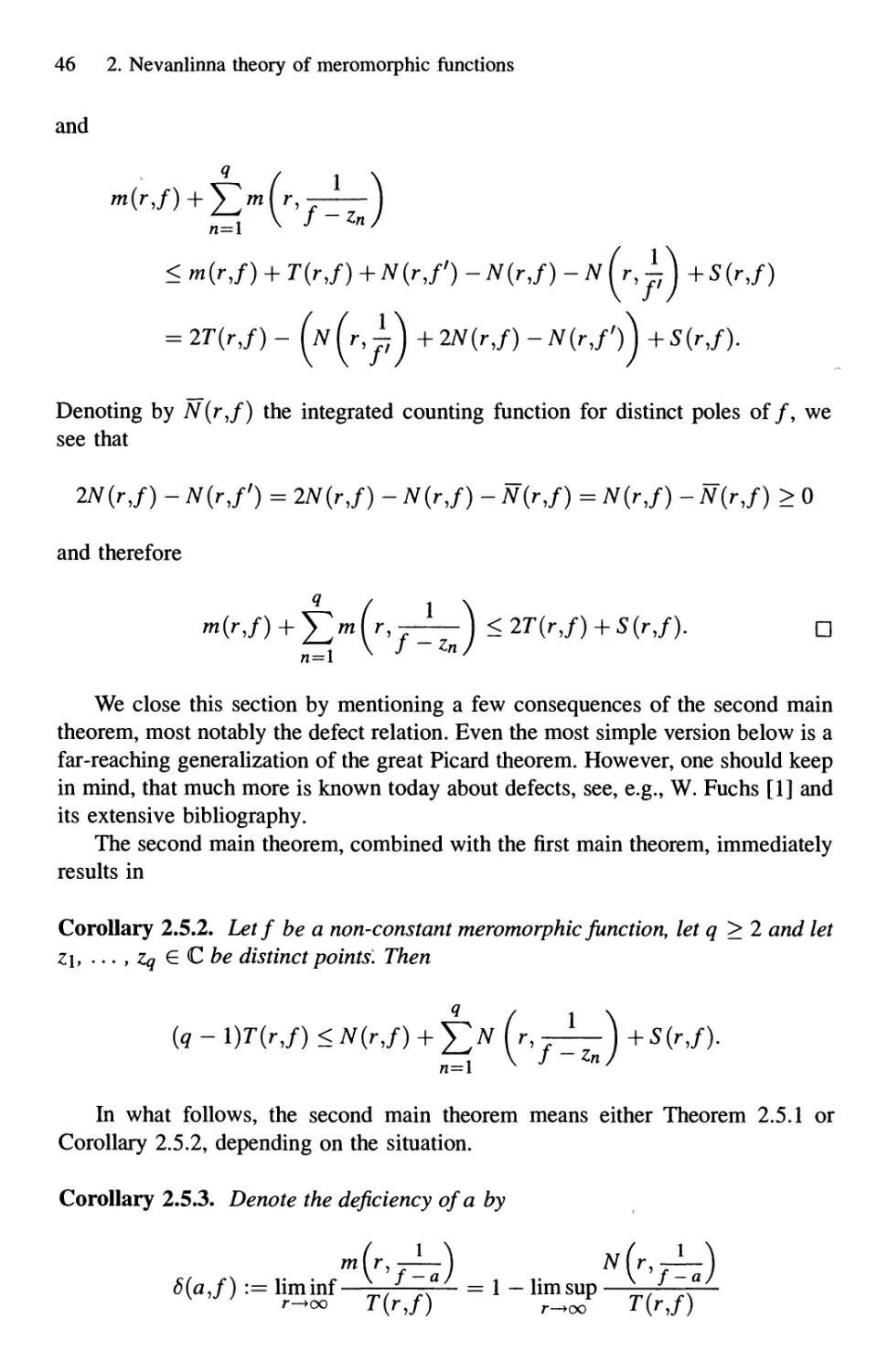
Denoting by N(r,f) the integrated counting function for distinct poles of/, we
see that
2N(rJ) - N(r,f) = 2N(rJ) -N(rJ) - N(rJ) = N(rJ) - N(rJ) > 0
and therefore
q
q ( 1 \
n=\ V J ZnJ
We close this section by mentioning a few consequences of the second main
theorem, most notably the defect relation. Even the most simple version below is a
far-reaching generalization of the great Picard theorem. However, one should keep
in mind, that much more is known today about defects, see, e.g., W. Fuchs [1] and
its extensive bibliography.
The second main theorem, combined with the first main theorem, immediately
results in
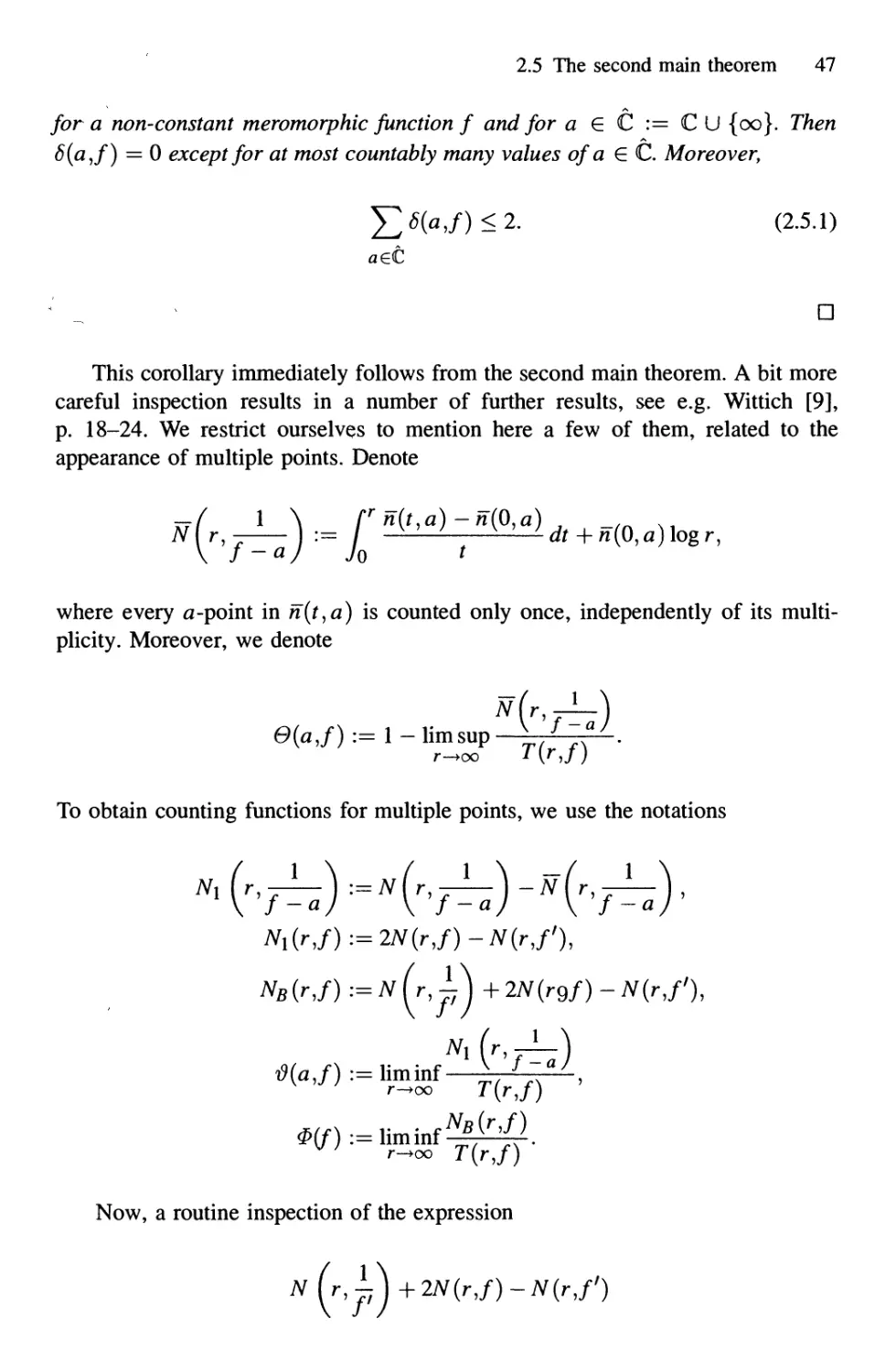
Corollary 2.5.2. Let f be a non-constant meromorphic function, let q > 2 and let
z\, • • • , zq £ С be distinct points. Then
(q - l)T(rJ) < N(rJ) + £> (r, -M + S(rJ).
n=l V J ZnJ
In what follows, the second main theorem means either Theorem 2.5.1 or
Corollary 2.5.2, depending on the situation.
Corollary 2.5.3. Denote the deficiency of a by
ml,') N<r,J-)

2.5 The second main theorem 47
for a non-constant meromorphic function f and for a G С := С U {oo}. Then
8(a,f) = 0 except for at most countably many values of a G C. Moreover,
X) «(*,/)< 2. B.5.1)
aeC
This corollary immediately follows from the second main theorem. A bit more
careful inspection results in a number of further results, see e.g. Wittich [9],
p. 18-24. We restrict ourselves to mention here a few of them, related to the
appearance of multiple points. Denote
where every a -point in n(t,a) is counted only once, independently of its multi-
multiplicity. Moreover, we denote
To obtain counting functions for multiple points, we use the notations
NB(r,f) ~N(r'jj) +2N(rgf)-N(r,f),
Now, a routine inspection of the expression
N(r,j^+2N(r,f)-N(r,f)

48 2. Nevanlinna theory of meromorphic functions
above shows that the following version of the second main theorem is a conse-
consequence of the same proof; the second assertion follows by substituting m(r,f) =
T(rJ) - N(rJ), resp. m (r,^) = T(rJ) - N (r,^) + 0A), into the
first assertion, and observing that N(r,f) = N(r,f) - N\(rJ), N (r, j^J =
Corollary 2.5.4. Letf be a non-constant meromorphic function, let q > 2 and let
Z\, ... , Zq € С be distinct points. Then
J; (m (r,—
и==1 \ \ J ~
and
я
- q — f 1 \
(q - l)T(rJ) < N(rJ) + Y,N(r> 7^—
Corollary 2.5.5. For a non-constant meromorphic function f, the following in-
inequalities hold:
Y, F(a,f) + 0(<i,/)) < J2 в(-а^ ^ 2> <2-5-2>
aet aet
/) ^2-
a
A point a G С is called a completely ramified value of/, if all a-points of/
are at least of multiplicity two. Then of course n(r,a) > 2n(r,a) and therefore
'f-a
hence
0(a,/) = l-limsup
From B.5.2) we immediately conclude

2.6 The Ahlfors-Shimizu characteristic function 49
Corollary 2.5.6. A non-constant meromorphic function f admits at most four com-
completely ramified values. □
2.6 The Ahlfors-Shimizu characteristic function
Iii some order considerations, the Ahlfors-Shimizu characteristic function, mea-
measuring the weight of the image of / on the Riemann sphere, is more suitable
than the usual Nevanlinna characteristic function. Omitting the proofs, which may
be found in Hayman [2], p. 10-13, we just mention the basic definition and the
correspondence between these two characteristic functions.
In fact, the Ahlfors-Shimizu characteristic function will be defined by
where
,2* Г{
1 f* f2
Now, an essentially geometric analysis on the Riemann sphere results in
From this it is rather obvious to see that the difference of 7o(r,/) and T(rJ)
remains bounded (by a constant independent of r), provided/@) ^ oo.

Chapter 3
Wiman-Valiron theory
The Wiman-Valiron theory is an indispensable device while considering the value
distribution theory of entire solutions of complex differential equations. Fortu-
Fortunately, the monograph by G. Jank and L. Volkmann contains an excellent pre-
presentation, see Jank and Volkmann [3], p. 30-38, 187-199. Therefore, we restrict
ourselves to give here just a short review of basic notions and most important
results. The difference of what follows below to [3] is that we consider entire
functions g : С —> С only, while [3] considers vector-valued functions g : С —> С"
whose components g\, ... , gn are entire functions.
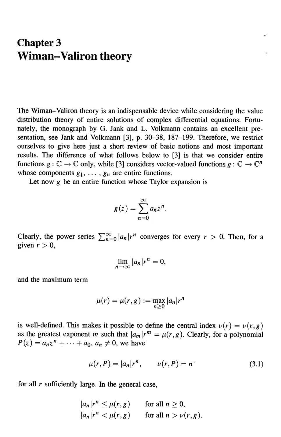
Let now g be an entire function whose Taylor expansion is
Clearly, the power series J2T=o\an\rn converges for every r > 0. Then, for a
given r > 0,
lim
7I-»OO
and the maximum term
»() i(,g)\n\
n>0
is well-defined. This makes it possible to define the central index u(r) = v{r,g)
as the greatest exponent m such that \am\rm — \i{r,g). Clearly, for a polynomial
P(z) = anzn H h a0, an ф 0, we have
/х(г,Р) = ЫЛ v{r,P) = n' C.1)
for all r sufficiently large. In the general case,
\an\rn <»{r,g) foralln>0,
\an\rn < /i(r,g) for all n > v(r,g).

3. Wiman-Valiron theory 51
Because of C.1), we may assume that g is a transcendental entire function while
considering basic properties of the maximum term and the central index. Here it
is enough to recall that
A) ii(r,g) is strictly increasing for all r sufficiently large, is continuous
and tends to +oo as r —■> oo;
B) v(r,g) is increasing, piecewise constant, right-continuous and also
tends to +oo as r —■> oo,
see Jank and Volkmann [3], p. 33-35,
In applications to complex differential equations, two results are of major im-
importance:
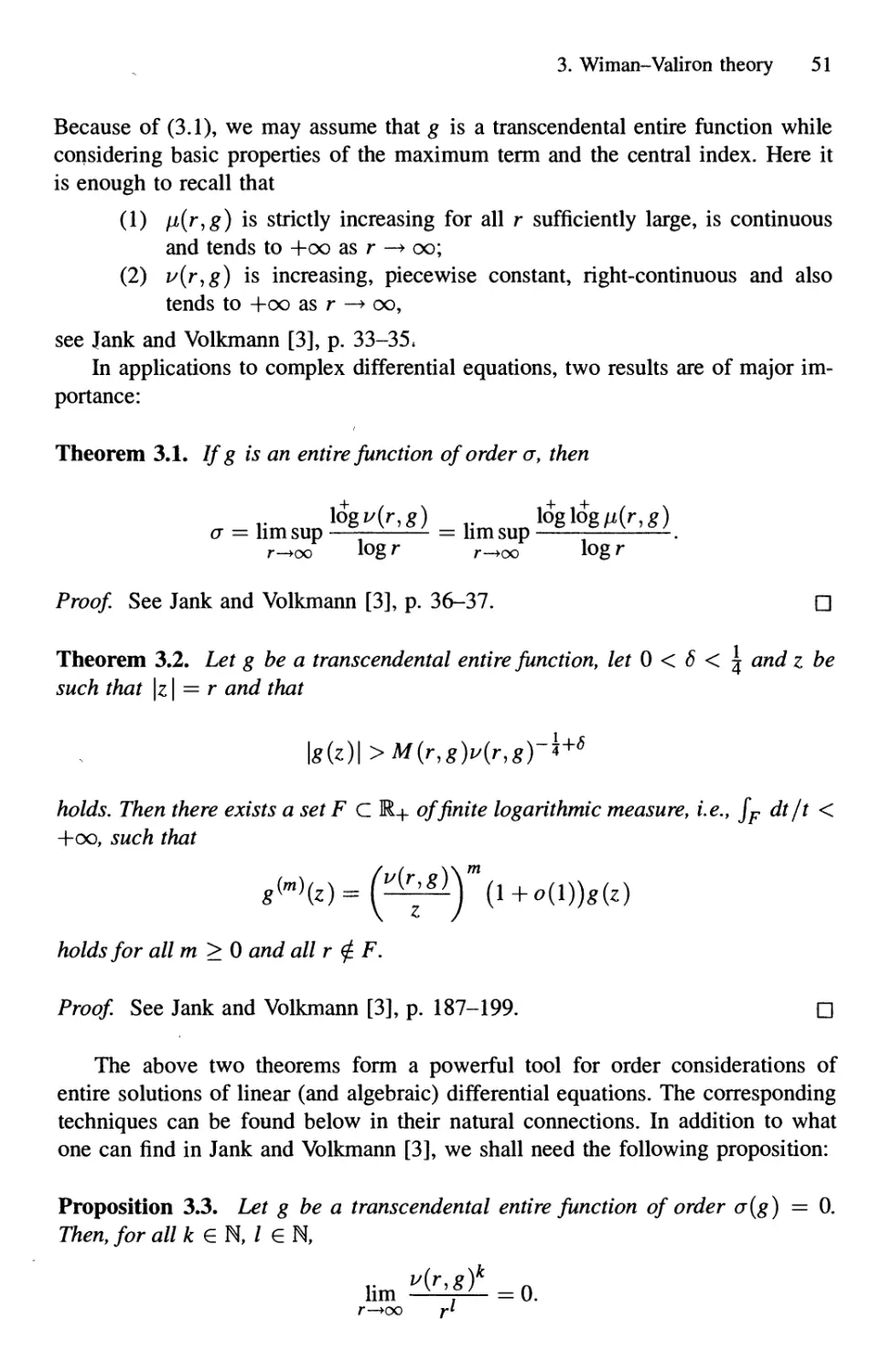
Theorem 3.1. Ifg is an entire function of order a, then
\ogv(r,g) log log ii(r,g)
a = hmsup , = hmsup —— .
r_oo logr r_oo logr
Proof See Jank and Volkmann [3], p. 36-37. D
Theorem 3.2. Let g be a transcendental entire function, let 0 < б < | and z be
such that \z \ = r and that
\g(z)\ >M(r,g)v(r,gr?+s
holds. Then there exists a set F С М+ of finite logarithmic measure, i.e., JF dt/t <
+oo, such that
holds for allm>0 and all r £ F.
Proof. See Jank and Volkmann [3], p. 187-199. □
The above two theorems form a powerful tool for order considerations of
entire solutions of linear (and algebraic) differential equations. The corresponding
techniques can be found below in their natural connections. In addition to what
one can find in Jank and Volkmann [3], we shall need the following proposition:
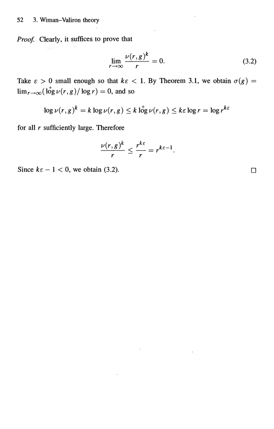
Proposition 3.3. Let g be a transcendental entire function of order cr(g) = 0.
Then, for all k G N, / G N,

52 3. Wiman-Valiron theory
Proof. Clearly, it suffices to prove that
r—xx> r
Take e > 0 small enough so that ke < 1. By Theorem 3.1, we obtain a(g) =
limr_oo(logv{r,g)llog r) = 0, and so
logv(r,g)k =k\ogv(r,g) <k\ogv(r,g) <ke\ogr = \ogrke
for all r sufficiently large. Therefore
r _ ,
Г Г
Since ke - 1 < 0, we obtain C.2).

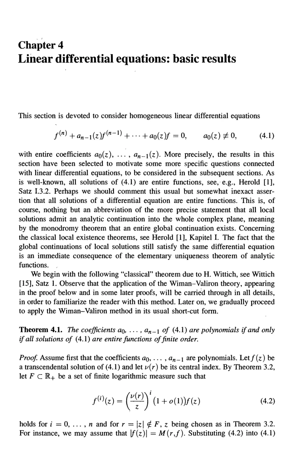
Chapter 4
Linear differential equations: basic results
This section is devoted to consider homogeneous linear differential equations
/<") + an.i{z)f(n-l) + • • • + ao(z)f = 0, ao(z) ф 0, D.1)
with entire coefficients ao(z), ... , an_\(z). More precisely, the results in this
section have been selected to motivate some more specific questions connected
with linear differential equations, to be considered in the subsequent sections. As
is well-known, all solutions of D.1) are entire functions, see, e.g., Herold [1],
Satz 1.3.2. Perhaps we should comment this usual but somewhat inexact asser-
assertion that all solutions of a differential equation are entire functions. This is, of
course, nothing but an abbreviation of the more precise statement that all local
solutions admit an analytic continuation into the whole complex plane, meaning
by the monodromy theorem that an entire global continuation exists. Concerning
the classical local existence theorems, see Herold [1], Kapitel I. The fact that the
global continuations of local solutions still satisfy the same differential equation
is an immediate consequence of the elementary uniqueness theorem of analytic
functions. ,
We begin with the following "classical" theorem due to H. Wittich, see Wittich
[15], Satz 1. Observe that the application of the Wiman-Valiron theory, appearing
in the proof below and in some later proofs, will be carried through in all details,
in order to familiarize the reader with this method. Later on, we gradually proceed
to apply the Wiman-Valiron method in its usual short-cut form.
Theorem 4.1. The coefficients uq, ... , an_\ of D.1) are polynomials if and only
if all solutions of D.1) are entire functions of finite order.
Proof Assume first that the coefficients a$,... , an_\ are polynomials. Let/(z) be
a transcendental solution of D.1) and let u(r) be its central index. By Theorem 3.2,
let F с М+ be a set of finite logarithmic measure such that
D.2)
holds for / = 0, ... , n and for r = \z\ £ F, z being chosen as in Theorem 3.2.
For instance, we may assume that \f{z)\ = M{r,f). Substituting D.2) into D.1)

54 4. Linear differential equations: basic results
we obtain t
+oo(z)(l + o(l)) = 0,
since A + o(l))/(l + 0A)) as well as l/(l + 0A)) are both of type 1 + 0A).
Hence we get
()r) + zna0(z)(l+o(l))=0. D.3)
Denoting
Qn-i{z) := zlan-i{z) =
щ
3=0
we have to consider
»{гу + a,_i(z)(i+осожг)"-1 + • • • + eo(z)(i+o(i)) = o.
If r ^ F is sufficiently large, we may assume, by Lemma 1.3.1, that for these
values of r we have
\Qn-i(z)(l +0A))| < iMf™, i = 1, ... ,n.
By Lemma 1.3.2, we must have
u(r) < 1 + max \Qn_i(z){l+o(l))\ < 1 + 2 max (|clVJr*).
Therefore, there exist a < oo and AT > 1 such that
holds for all г ф F sufficiently large. Given now any a > 1, we see by Lemma 1.1.2
that

4. Linear differential equations: basic results 55
holds for all r sufficiently large. Hence
logi/(r)
hm sup < olg.
r-+oo log Г
Since a > 1 is arbitrary, we see that
1+ ( Л
limsup ——— = a(f) < a < oo.
r-oo logr
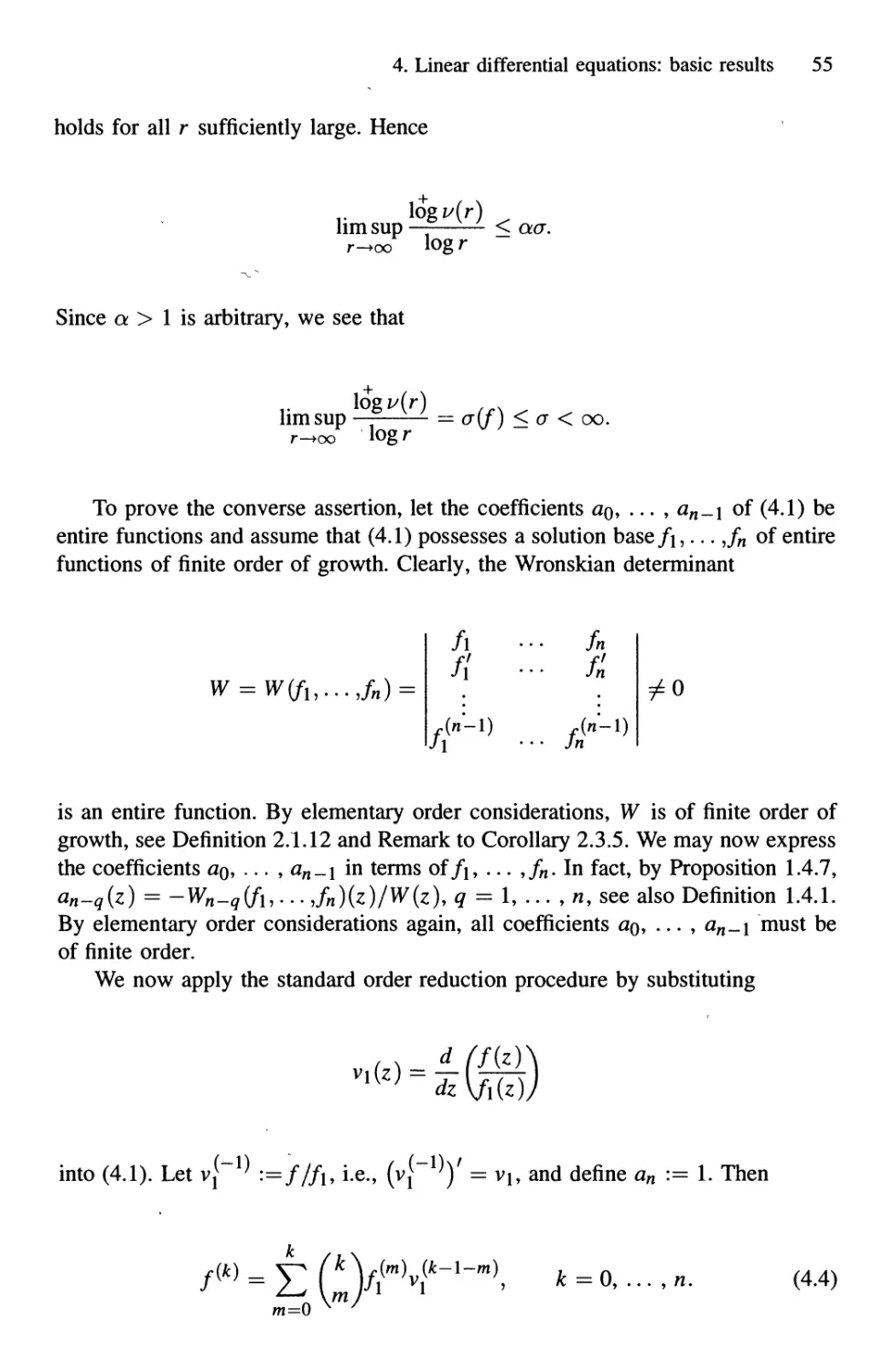
To prove the converse assertion, let the coefficients ciq, ... , an_\ of D.1) be
entire functions and assume that D.1) possesses a solution base/i,...,/« of entire
functions of finite order of growth. Clearly, the Wronskian determinant
/l
fi
(n-l)
fn
fl
Jn
Лп'-l)
is an entire function. By elementary order considerations, W is of finite order of
growth, see Definition 2.1.12 and Remark to Corollary 2.3.5. We may now express
the coefficients a$, ... , an_\ in terms of/i, ...,/„. In fact, by Proposition 1.4.7,
an-q(z) = -Wn-q(fu... Jn)(z)/W(z), q = 1, ... , я, see also Definition 1.4.1.
By elementary order considerations again, all coefficients ciq, ... , an_\ must be
of finite order.
We now apply the standard order reduction procedure by substituting
into
D.1). Let v{ X) :=///b i.e., (vf X))' = vb and define an := 1. Then
f(k) = E
E
m=0
*=o,...,n.
D.4)

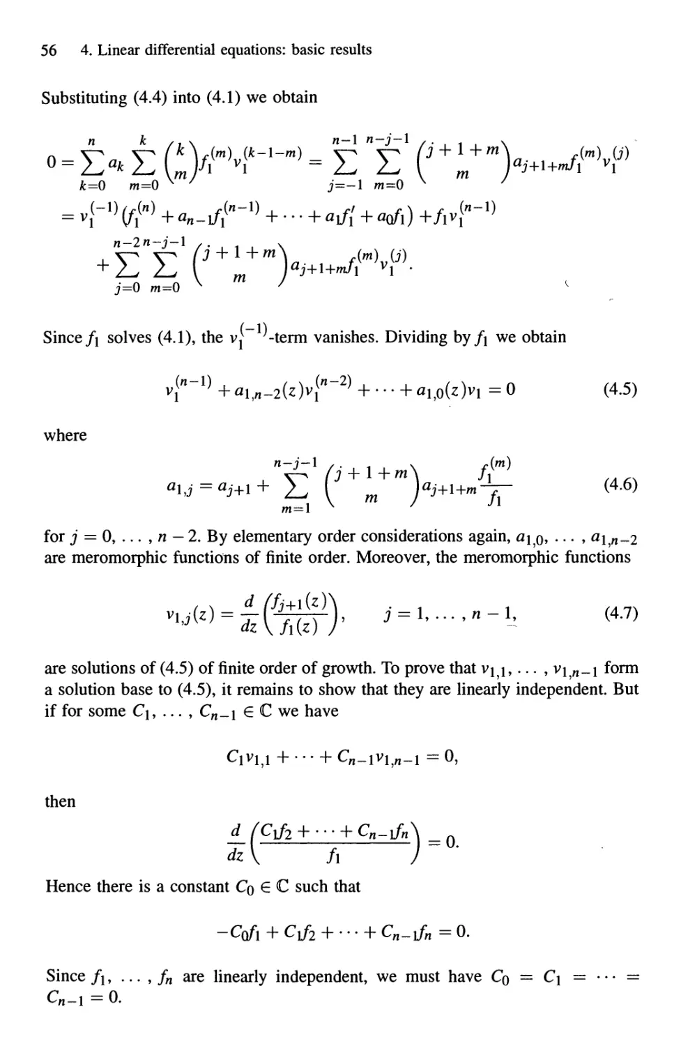
56 4. Linear differential equations: basic results
Substituting D.4) into D.1) we obtain
«—1 n—j—l ,.
к / f x «—1 n—j—l ,. x
m=0 Ч У j=-l m=0 Ч 7
*=0 m
(—1)//•(«) . Лп — 1)
m i •
Since/i solves D.1), the v|~ -term vanishes. Dividing by/i we obtain
vj"-0 +altn_2(z)vln-2) + ---+ah0(z)v1 =0 D.5)
where
-^ /,(m)
m=l
for j = 0, ... , n — 2. By elementary order considerations again, a\Q, ... ,
are meromorphic functions of finite order. Moreover, the meromorphic functions
are solutions of D.5) of finite order of growth. To prove that vii,... , v\n_\ form
a solution base to D.5), it remains to show that they are linearly independent. But
if for some Q, ... , Cn_\ e С we have
then
Hence there is a constant Co € С such that
• • • + с„_л = о.
Since /i, ...,//, are linearly independent, we must have Q = C\ =
Cn-i = 0.

4. Linear differential equations: basic results 57
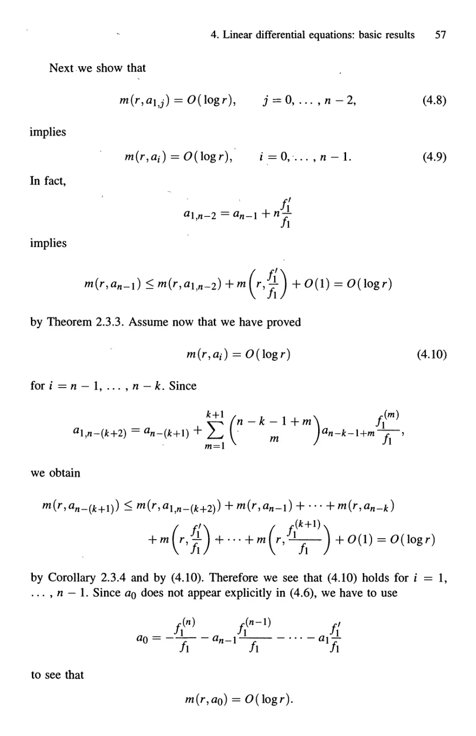
Next we show that
m(r,aij) = O(\ogr), j = 0, ... , л- 2, D.8)
implies
т(г,а() = О (log r), i=0,-... ,л-1. D.9)
In fact,
a^n_2=an-i + nj-
implies
m{r,an_x) <т{г,ах,п_г) +mL/j-\ + O{\) = O{\ogr)
by Theorem 2.3.3. Assume now that we have proved
D.10)
for / = n — 1, ... , n — k. Since
Am)
we obtain
) + ---+т(г,я„_*)
r^~L7
by Corollary 2.3.4 and by D.10). Therefore we see that D.10) holds for i = 1,
... , n — 1. Since ao does not appear explicitly in D.6), we have to use
A») A»-1) ri
/l /l л
to see that
m(r,ao) = O(\ogr).

58 4. Linear differential equations: basic results
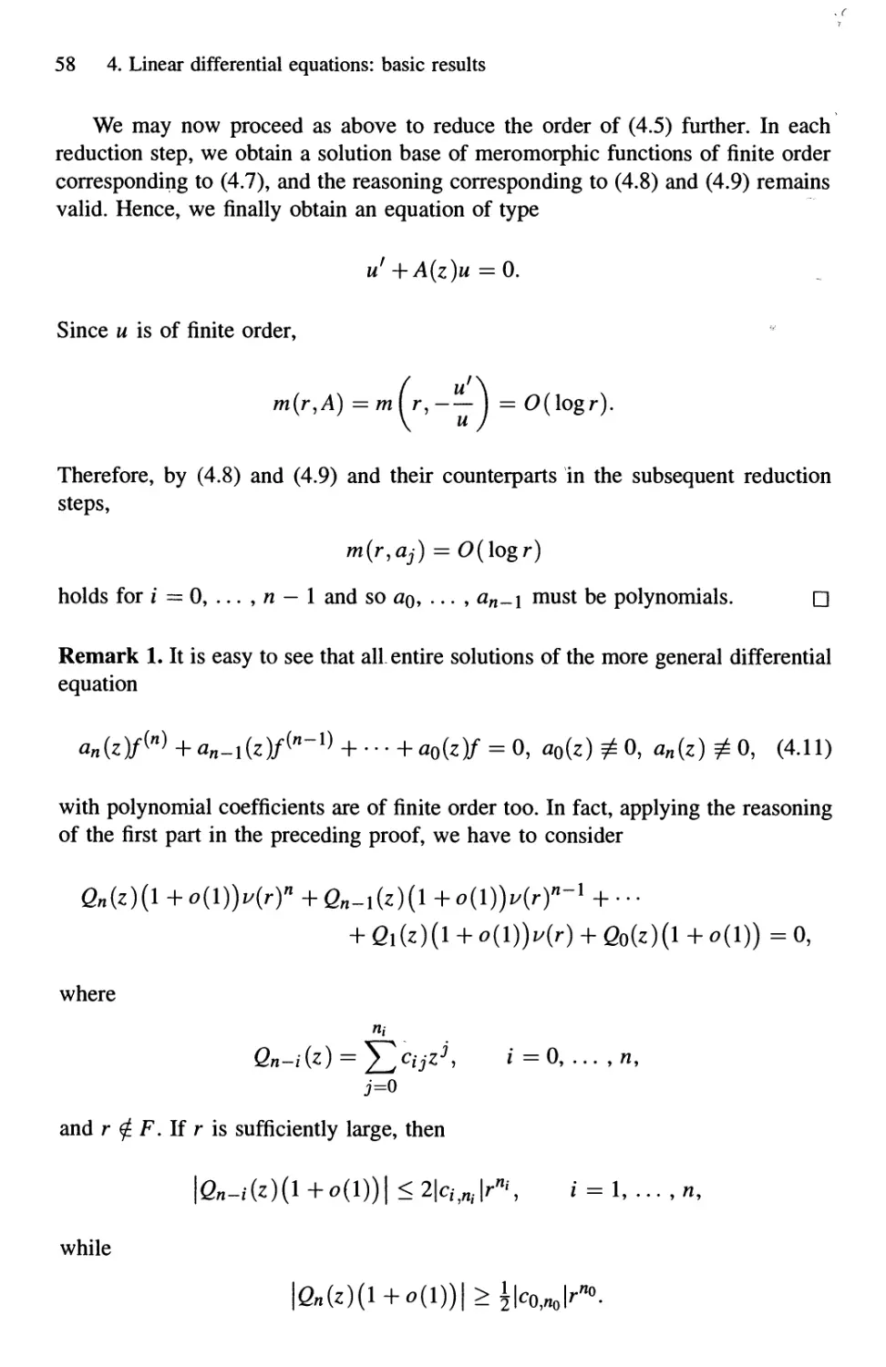
We may now proceed as above to reduce the order of D.5) further. In each
reduction step, we obtain a solution base of meromorphic functions of finite order
corresponding to D.7), and the reasoning corresponding to D.8) and D.9) remains
valid. Hence, we finally obtain an equation of type
u'+A(z)u=0.
Since и is of finite order,
m(r,A)=m\r,--\ = O(logr).
Therefore, by D.8) and D.9) and their counterparts in the subsequent reduction
steps,
m(r,aj) = O(\ogr)
holds for i = 0, ... , и — 1 and so uq, ... , an_\ must be polynomials. □
Remark 1. It is easy to see that all entire solutions of the more general differential
equation
an(z)f{n)+an_l(z)f(n-V + -.-+a0(z)f = 0, ao(z)^O, an(z)^0, D.11)
with polynomial coefficients are of finite order too. In fact, applying the reasoning
of the first part in the preceding proof, we have to consider
where
Щ
Qn-i(z) = Y^cijzJi / =0, ... ,/l,
j=0
and r £ F. If r is sufficiently large, then
|6»-i(z)(l +o(l))| < 2|cM;|r"i, i = 1, ... , n,
while

. 4. Linear differential equations: basic results 59
Lemma 1.3.2 now implies that
v(r) < 1 + max
Qn-i(z){\+o(\))
< 1 + 4 max
11ШЛ I
and we may continue exactly as to above.
Remark 2. From the above reasoning we also conclude that all transcendental
entire solutions/ of D.11) with polynomial coefficients satisfy a(f) > 0. In fact,
assume that a(f) = 0 and consider D.11), written in the form
/=o
D.12)
where \z\ = r <£ F and where z satisfies \f(z)\ = M(r,f). Denote m :=
Considering the powers zJ in D.12), assume that D.12) possesses one term
only with zm, say
azm{l+o(l))v(rM, a^O. D.13)
Dividing D.12) by zw, the term D.13) reduces into
a(l+o(l))u(rY
and so tends to H-oo, if s > 0, and to а ф 0, if s = 0, for r —» oo. On the other
hand, all other terms take, after the division by zm, the form
where к > 0 and / > 0. By Proposition 3.3, all these terms tend to zero for r —> oo,
a contradiction.
Hence, D.12) possesses more than one term of the form D.13), say
i=\
where t > 2. By the above reasoning, Хл=1а/A + o(l))i/(rMi tends to 0 as
r —> oo. This defines, for each r, an algebraic equation for v(r). By Lemma 1.3.2,
v(r) remains bounded, which contradicts the fact that v(r) tends to -boo as r —> oo,
see Chapter 3.

60 4. Linear differential equations: basic results
Remark 3. Actually, the possible orders of growth of the solutions/ of D.1) are
rational numbers, see Wittich [9], p. 65-68. Determining a set of rational numbers
which includes the possible orders, follows by a simple geometric construction,
see Helmrath and Nikolaus [1] as well as Jank and Volkmann [3], p. 199-208. We
omit these considerations here.
The above order reduction procedure may be applied to obtain the following
theorem due to M. Frei [2], p. 207.
Theorem 4.2. Let aj be the last transcendental function in the coefficient sequence
од» • • • > #n-i of coefficients of D.1). Then D.1) possesses at most j linearly inde-
independent solutions of finite order.
Proof By our assumptions, aj is now transcendental entire while а^+\, ... , an-\
are polynomials. Let then/i, ... ,/j+i be linearly independent solutions of D.1),
all having a finite order of growth. If j = n — 1, and so/i, ... ,/„ are all of finite
order of growth, then Theorem 4.1 implies that all coefficients a^ ... , an_\ must
be polynomials, a contradiction. Hence we may assume that j < n - 1.
We now apply the same order reduction procedure as in the proof of Theo-
Theorem 4.1. For convenience, we use the notation vq instead of/ and ao,o> • • • » a0,n-\
instead of «o,... , an_\. Now, for the general reduction step corresponding to D.5)
and D.6) we have after k steps
4"~k) + ak<n-k-l(z)vjin-k-l) + ■ ■ ■ +akfl(z)vk = 0 D.14)
where
1+M\ ft
\ak_ld+l+m—— D.15)
2^ kld+l+m
m=\ Ч ' k \,\
Clearly,
determines at each reduction step a solution base of D.14) in terms of the preced-
preceding solution base. After j reduction steps we may arrange the coefficients in the
equations D.14) for k = 0, .,. , j in the following scheme, where the rows cor-
correspond the equation D.14) for vq, ... , Vj, and the columns from n to 0 give the
coefficients of these equations, while the last column lists those solutions whose

4. Linear differential equations: basic results 61
order is finite.
n - 1
n-2
n-3
0
solutions of
finite order
a0,n-\
fl0,«-2
aO,n-j
aJ~l,n-j
«0,1
«0,0
«1,0
ai,o
>v0J+l
Observe that the boldface coefficient oqj is the first transcendental coefficient
from the left in the first row corresponding to the differential equation for vq, i.e.,
in D.1). By elementary proximity function estimates using D.15), we see that
"*(>*>«*,/) = O(\ogr)
holds in each row for / = n — (k + 1), ... , j + 1 — к, i.e., for all coefficients to the
left from the boldface coefficient а^^_^. On the other hand, D.15) also implies
that
m(r,akJ-k)^O(\ogr) for к = 1, ... , j.
Specially, we obtain
r,ajj) = O(\ogr) for/ =n-(j
while
m(r,ajj0) ^O(logr).
But from the equation D.14) for vj \ we obtain
D.16)
D.17)
(
— • • • — at
and therefore
r^j,o) = O(\ogr)
D.18)
by D.16) and the fact that Vji is of finite order. The contradiction D.17), D.18)
proves the assertion. □
The remaining part of this section is devoted to consider deficiencies of solu-
solutions of D.1). The basic result about deficiencies is

62 4. Linear differential equations: basic results
Theorem 4.3. Letf be an admissible meromorphic solution of D.11) in the sense
that T(r, at) = S(rJ) holds for i = 0, ... , /i. Then
for all а Ф 0, oo. Especially\ this is true for transcendental solutions of D.11) with
polynomial coefficients.
Proof Writing D.11) in the form
an{z)(f -a)(") +aB_1(z)(f - a)*") + • • • + ao(z)(f ~ a) = -
we obtain
f-a aa0
if-a)'
f-a
and therefore
m
{r>fk)=s™
by our assumptions and by Corollary 2.3.4. The assertion follows. □
Since all solutions/ of D.1) are entire functions, Theorem 4.3 therefore means
that a = 0 is the only complex value for admissible solutions of D.1) which may
have problematic deficiencies. Observe, however, that this simple situation does
not remain true, if we consider non-admissible solutions too. In fact, the following
result based on Nikolaus [2], p. 32, shows that any entire function may appear as
a solution of an equation of type D.11) with entire coefficients.
Theorem 4.4. Letf\ be an entire function. Then there exist entire functions а$Уа\> «2
such that ji satisfies the differential equation
/ = 0. D.19)
If all zeros off\ are simple, then 02 = 1-
Proof. Suppose/1 = eh, h entire, has no zeros. Then,
/" _ h'f _ h»f = 0
is the desired differential equation.

4. Linear differential equations: basic results 63
Suppose next that/i has at least one zero, and that all zeros of/i are simple.
By Proposition 1.4.8, we have to determine in this case entire functions p and/2
such that
/1 /2
/,' /2
D.20)
and therefore we must have
We may assume that the zeros of/i have been arranged according to their increasing
moduli:
At the zeros cn of/i, we must have/2(cn) ф 0 by D.20). Since/2 has to be an
entire function, the Laurent expansion of g =/2//! at cn is
-cn)
hence
and therefore
g{z)=l-i(z-cn) l +70 +
^(z) = -7-1 (г-с„Г2 +71+
z —cn
D.21)
at cn. Since f{~ep has double poles only, a simple computation results in
lim f -
z-+cn \ dz
Mi)
[{cn) + \f['{cn){z - cK) + ••■)- (f»(cn)
z "
f/(cB) + ^/1"(c«)(z - с„) + • • • K

64 4. Linear differential equations: basic results
hence
Construct now an entire function (p such that (p(cn) = bn at each cn (Gelfond [1],
p. 170). Since F = (p + gf\, where g is an arbitrary entire function, also satisfies
F(cn) = bn at each cn, we may assume that <p is transcendental. Define now p
as a primitive function of ip. By D.21), f^2ep admits a meromorphic primitive
function яр, see e.g. Narasimhan [1], p. 75-76. Define/2 := ipf\. Then the poles
of яр, which are all simple poles, appear at cn, hence /2 is an entire function.
Finally, define
Then
D.22)
is the required equation D.19), solved by/i and/2. In fact, by D.20),
/l /2
rii fit
h h
Therefore, D.22) may be written as
/l
/2
/2
/1
/,"
/2
/2"
//
/,"
/2'
/2"
which means that
/ /1 /2
/' // /2' =0.
/" /," /2"
This proves the assertion for this case.
In the general case, let (bn)ne^ be a sequence of complex numbers obtained
from the zero-sequence of/1 by repeating fc-fold zeros of f\, к > 2, exactly
k — 1 times, and let /3(г) be an entire function whose sequence of zeros is exactly
(^л)лбН» see Theorem 1.2.1. Then g := /3/! has simple zeros only, and the
assertion follows by applying the preceding part of the proof for g. □
Concerning zero-deficiencies of solutions of D.11), or even of D.1), this is
still a wide area for research. The case of second order in D.1), which is more
thoroughly investigated, will be considered in the next section. For completeness,
we give here the basic result, due to G. Frank (Frank [1], Satz 10), known for the
general case, although this result has a vague connection only with the Nevanlinna

4. Linear differential equations: basic results 65
theory. See also the remark following the proof concerning recent developments.
The proof below is technically complicated, although elementary. If the reader
wants to proceed without studying the proof, no difficulties should appear after-
afterwards.
Theorem 4.5. The linear differential equation D.1) with polynomial coefficients
admits a solution base /j,... ,/„, all of whose members have zero as their Picard
exceptional value in the sense that each fc has at most finitely many zeros, if and
only if there exists a polynomial q such that the transformation
f = equ
results in an equation for и of the form D.1) with constant coefficients.
Proof (first part). Assuming such a transformation exists, it is elementary, see e.g.
Herold [1], Satz III.3.3, that the corresponding equation for и admits a solution
base all of whose members are of the form zre5Z, where r is an integer > 0 and
s G C, hence zero is clearly a Picard value for all members of the corresponding
solution base/j, ...,/„ of D.1).
Assume now that a solution base/i,... ,/„ of D.1) is such that every fj has
zero as its Picard value, i.e.,
/j@ = Pj(z)e^z\ j = 1, .... л, D.23)
holds for some polynomials pj, qj. The case n = 1 is immediate. In fact, from
f'(z)/f(z) — ~ao(z) we see that/ has no zeros. Hence, any polynomial q such
that g=<7i+7Z,7€C\ {0}, gives the desired transformation. To prove the
assertion for n > 2, we consider the Wronskians for/j, ... ,fk-\,fs f°r all s and
к such that 1 < к < s < n. By D.23) we obtain
(..,A-i,/^^/^"^-lH D.24)
and
w'(fi,...,A.ufs) = (PkA<ii + --- + <iic-i+<!,) +PUeqi+'''+qk-l+q° <4-25>
where P^ s is a polynomial. By Proposition 1.4.5, we have
W(fi,...,fk-i)W(fu...,fk,f5)
= W(fl,...,fk)W/(fl,...Jk^,fs)-W{fb...,fk^,fs)W'(fi,...Jk).

66 4. Linear differential equations: basic results
Substituting here the corresponding expressions from D.24) and D.25) we obtain
Pk-l,k-lPM,5 = PtfiPkAd ~ Як) + pkJtP'kj ~ pk,kPk,s D.26)
for к > 2, s — к + 1, ... , n. For к = 1, s — 2, ... , /i, we obtain similarly
Pl,s = PlPs{q's-q[)+ P\p's ~PxPs• D.27)
We denote now:
«l,/ := deg(p,-), / = 1, ... , /i;
/?jfI- :=deg(<7/-<7J), j = 1, ... , л - 1; i=j + l,...,n; D.28)
aj,/ := deg(PJ5/), j = 2, ... , /i; i = j, ... , /i.
After this first part of the proof, we proceed to establish the following
Lemma 4.6. Suppose the sequence q'v...,q'n of derivatives of qi from D.23) con-
contains r distinct functions y r <ny such that each of the distinct functions appears m/
times, while m\ + • • • + mr — n>_ 2. Then
n n-\ n r
an,n = J2a^ + J2 J2 hi - iJ2m^mi - V- D-29)
/=1 j=\ /=j+l i = l
Proof The idea below is to express the degrees a^,s m terms of a\( and Cjj.
The assertion then follows by taking k — s — n. Since we consider the degrees of
polynomials only, we may assume, if needed, that \z | is large enough. The proof
will now be divided in three sections.
A) Assume first that m\ = • • • = mn = 1, i.e., that for all i, j = 1, ... , /2,
i Ф j, we have q'. ф q[. Denoting ao,O = °> D.26), D.27) and D.28) immediately
result in the recursion formula
<**+l,j = ak,k + &k,s + Pk,s ~ ak-l,k-\ D30)
for к > 1, s — к + 1, ... , п. We now assert that
A: — 1 k-2 k-\ k-\
aKs = J2 aM + ]C ]C hi + ahs
i=\ j=i ;=j+i

4. Linear differential equations: basic results 67
for к > 1, s = k, ... , n. Observe here and below that a sum of type Y^=i ls
considered to disappear whenever i\ < /q. For к = s — n, D.31) reduces back
into D.29):
n-\ n-2 n-\ n-\
Otn,n =
Al-1 П
Е Е ftv-
Now, for it = 1, s = 1, ...,«, D.31) holds trivially. For it = 2, s = 2, ...,«,
we obtain
«2,5 = «1,1 + «1,5 + A,5 = «1,1 + «1,5 + A,5 - «0,0
from the recursion formula D.30). But this is nothing else than D.31) in this special
case.
Assume now that we have proved
r-\ r-2 r-\ r-\
r\ r\
Е hi+ам + E
for 1 < r < it — 1, s = r, ... , /i. By the recursion formula D.30) we obtain,
using D.32),

68 4. Linear differential equations: basic results
k,s = ak-\,k-\ + <*k-l,s + /%-l,j - <*k-2,k-2
k-2 k-3 k-2 k-2 k-2 k-3 k-2
i^ + E E
E /^ + *ui + E#*i + EaM + E E
j=i/=j4-i i = i i = l j=\i=j+i
k-2 k-3 k-4 k-3 k-3
Е E /^v-au-2-E#
/C 1 AC J? AC £ fC jC
E /'i.i
| = 1 jz=l 1=7 + 1 / = 1
A:—3 A:—3 A: — 1
j=l 1=1 1=1
k-\ k-2 k-\ jfi A: — 1
м + Е E /?*«•+ai,5 + X>
j=\ i=j+l i = l
which is just D.31).
B) Suppose now that at least one of m\, ... , mr is > 1. We may assume that
the solution base D.23) has been arranged in such a way that all possible repetitions
of a given q[ come immediately after the first occurrence in the sequence, while
all derivatives q[ appearing only once are before repeated derivatives q[. In other
words, derivatives q\ will be grouped in r blocks, each having equal members q[
and different blocks having different derivatives q[, while blocks of length — 1 be-
begin the whole sequence. Moreover, we may assume that the corresponding numbers
d\ ( = deg(p/) form a strictly increasing sequence inside of each block. This may
be achieved, if necessary, by replacing the functions fj by suitable linear combina-
combinations of them, which obviously does not destroy the assumed Picard property. In
fact, if there are several equal degrees ay, we may reduce these degrees by linear
combinations for all but one of these solutions. Continuing down to the lowest
degree we get the desired situation. Let now q'm, ... , q'm+t be the first block of
length > 1. Since q[, ... , q'm are all distinct, Part A) remains valid and we see
that D.31) still holds forl<ife<m,j=ife,...,/i. Observe that this is also true
for m = 1, i.e., in the case that all blocks are of length > 1. Also in this case, we
apply ao,O — 0, if needed.
Proceeding now to compute a^,s for m + 1 < к < m + t + 19 s = k9 ... , n,
the use of D.26), hence of the recursion formula D.30), changes since q's—q'k = 0
for m < s, к < m + t. In this case, the degree of Рк,кР'к s ~ ^k k^k,s nas t0 be

4. Linear differential equations: basic results 69
computed. To do this, we first observe that
m-1 m-2 m-1 m-1
^2 Yl Pit + Y2, &>
j=\ ,"=j+i i = l
m-1 m-2 m-1 m-1
it - Yl
it Yl
j=\ i=j+i i=i
m-1
- m
for s = m + 1, ... , m + r, since a1?I- increases strictly along with i and /3(iS —
deg(^ - q[) = deg(^w - ^/) = AjW for j = m + 1, ... , m + r. Therefore, we
see from
(p \f
LULL]
p /
*m,m/
that
Hence, from D.26) we get
1,5 = am,m + ttm,j ~ «m-l,m-l -1) m + l<S <m + t.
For .y > m + r, we again have q's—q'm Ф 0, meaning that D.30) becomes applicable
and therefore
= am,m + «WjJ +/3w,s - aw_lw_i, m +f + 1 < S < П.
Observing that /?WjJ — 0 for m + 1 < s < m + f, we have therefore
_ f аИ,и + От,5 + Pmi5 ~ «m-l,m-l - 1, m + \<S <m + t
1'5 \ «m,m + «m,5 + Pm,s ~ «w-ijW-l, m + t + 1 < S < П.
Denoting the left hand side of D.30) temporarily by aw+15, we may write the
preceding formula as
am+l s' m + 'l<s <m + t

70 4. Linear differential equations: basic results
To proceed, we have
* a
f or m + 2 < s < m + f, hence we obtain from
p p p p' p' p - p2 (
rr r r r r — rm+l,m+l I
p /
rm + l,m+l/
that
*Ji+lm+l -1 + 
-1 ' -1-2
for m + 2 < s < m + t. Similarly, for m + t < s < n, we get
l,s ~ am,m
= al l ~ 1 + al + /^+l ~ a
~ 1 + a
m+l,s
We assert now that for all 1 < i < t we have
Assume that D.33) holds for all aw+j5j, j < i — 1. Repeating the same reasoning
as above, we obtain
— am
m+i-2

4. Linear differential equations: basic results 71
for m + i < s < m + f, since /?jjS — fi^m+i-\. Hence, from D.26) and D.33) we
obtain for m + i < s < m + t:
a
m+i,s —
= am+i-l,m+i-l ~ 2*0 " !) + am+/-l,5 "
= a
since /3m+I-_i}J = 0 for w + i < .y < m + r. On the other hand, if m + t < s < n,
then we get
/-l,s ~ am+i-2,m+i-2
aiL+i-i,, " l(^' " 1H' " 2)
-2 + lO " 1H " 2)
which proves D.33). To reach the next block, we still need control over aw+f+1 s
for m + t < s < n. But in this case q's - qfm+t ф 0 and we obtain from D.26):
— am+t,m+t + <Xm+t,s + fim+t,s — am+t-\,m+t-\
= <* ~ \t{t + 1) + aXm+tj - \t{t - 1)
= <*
C) The preceding part clarifies the first block of length > 1, proving the first
induction step towards
|_Wjt -f/-i
mx+-+mk+i-\

72 4. Linear differential equations: basic results
for mj + • • • + rrik + i < s < m\ + • • • + т#+1 and
m\-\ |-т*+/ — 1
aWl+...+mjk+I-,J = ]T ahi
i=\ j
i=\ i=\
for mi H Ьт£+1 <s < n. The general induction step may be arranged similarly
as to Part B). Finally, for n —т\Л hmr, we get the assertion of Lemma 4.6. □
We are now ready to continue the proof of Theorem 4.5:
Proof (second part). By D.24) and Proposition 1.4.8, we have
where <p' — —an_\. Hence, the polynomial Pn,n must be a constant and we have
OLn,n = 0.
In the case A) above, m\ = • • • = mr = 1 and we have, from D.29) or D.31),
n — l n
i=\
hence a\\ = • • • = a\n = 0 and Cjj = 0 for j = 1, ...,«- 1 and i = j + 1,
... , л. This means that in D.23) all polynomials pj reduce to constants and
similarly q[ — q1- is a non-zero constant for i ф j. Hence we must have
where q is a polynomial and £,- Ф bj, i ф j, are some constants.
In the cases B) and C), at least one of пц > I. Recall that in each block,
was strictly increasing. Therefore,

4. Linear differential equations: basic results 73
for i = 1, ... , rafc+i- Again, an,n = 0, and we obtain from D.29)
n n — \ n r
E ftri
r—\ n—\ n
k=\ j=\ i=j+i
Therefore, we have /3^ = 0 for j = 1, ...,« — 1; / = j + 1, ... , n and
<*1,т,+...+т* = 0 for к = 1, ... , r - 1. Hence,
r— 1
r— 1 mjt+i-l r— 1
Jk=O i=\ k=0
and therefore
al,mi4--4-mjfe4-i = *"> 1=1,...,
Hence, the solution base D.23) consists of r blocks of functions
Jj,i \Z) — z e , j — l, ... , mM
for i = 1, ... , r. □
Remark. H. Wittich [19], p. 368, already conjectured the assertion of Theorem 4.5
to hold under the weaker assumption that the equation D.1) admits a solution base
/b •••»/«» all of whose members have zero as their Borel exceptional value, i.e.
X(fi) < a(f() for i = 1, ... , и, instead of being Picard exceptional. This has been
recently proved, see Briiggemann [1], Section 5, Briiggemann [2] and Steinmetz
[20]. We omit this result here, since its proof needs the theory of asymptotic
integration, not to be treated in this book. For an extension of these results, see
Briiggemann [3]. Anyway, Theorem 4.4 alone shows that there is still much to be
done concerning deficiencies of solutions of D.1), even in the polynomial case. The
situation becomes much more complicated if some, or all, of the coefficients are
transcendental. Therefore, we continue our study of linear differential equations
in the next chapter by restricting ourselves into the basic case of second order
homogeneous linear differential equations.

Chapter 5
Linear differential equations:
zero distribution in the second order case
To consider the zero distribution of solutions of
S// + ai(z)*/ + fl0(z)*=0, E.1)
where ao, a\ are entire functions, it is elementary to observe that considering of
f"+A(z)f = 0, A(z) entire, E.2)
is sufficient. In fact, if b is a primitive function of —\a\, hence b1 = —\a\, then
the transformation g = /exp(b), applied to E.1), results in
Assume first that A(z) is a polynomial:
f"+P(z)f = 0, E.3)
where
an^0. E.4)
If P(z) = ao is a constant, E.3) may be solved explicitly; hence we may
assume that n > 1 in E.4). This will be done without any more mention. Before
going to consider the zero distribution, we need the following
Proposition 5.1. All non-trivial solutions f of E.3) have the order of growth
o(f)={n+2)/2.
Proof The reasoning here follows the pattern given in Theorem 4.1. Letf(z) be a
non-trivial solution of E.3). Clearly, by E.3),/(z) must be a transcendental entire
function. Let v(r) be its central index. Following Theorem 3.2, let F С R+ be a
set of finite logarithmic measure such that

5. Linear differential equations: zero distribution in the second order case 75
holds for r — \z\ £ F, where z is chosen so that \f(z)\ = M{r,f). Therefore
0. E.5)
By Lemma 1.3.1, we obtain
v{rJ = \v{r)\2 = \anzn+2 + ■■■+ a0z2\\l + o(l)\ > \\an\rn+2
for all r ^ F sufficiently large. Hence
logr - 2 w
and therefore
\ogu(r) n+ 2
hmsup , = a(f) > .
r_oo^ logr v/~ 2
On the other hand, by E.5) and Lemma 1.3.1 again, we have for some К > О,
v(rf < K2rn+1,
outside of a set of r-values of finite logarithmic measure. Hence, given a > 1,
v{r) < Кг*?
implies by Lemma 1.1.2 that
for all r sufficiently large. Therefore
\() n+2
limsup ——— < a-
r-+oo log r 2
Since a > 1 is arbitrary, we get
/r\ ^ n +2
П

76 5. Linear differential equations: zero distribution in the second order case
Before proceeding, we do some general analysis concerning the equation E.2).
One should observe that these formulas remain valid for meromorphic solutions
of E.2) whenever A(z) is a meromorphic function.
Let/i, /2 be two linearly independent meromorphic solutions of E.2), let
E = /1/2 be their product and let W(f\Ji) — /1/2 ~ f\fl be their Wronskian
determinant. Differentiating we obtain by E.2) that
hence W(f\,fi) must be a constant, say W(f\,fi) — c- Therefore
ffl\' _W(fuf2) _ с
W
" /i2 ~/i2
and
/2 f[
h /1 /2//1 hfl Mi E'
In passing, we should perhaps remark here that by the preceding formula all zeros
of E are simple. Now, from E =/1/2 we obtain that
K+K = ~e~'
hence
*' =-|r + ?r. E.6)
/2 E
Using the elementary formula
f"_(f'\'+(fl\
T~\f) \f)
we obtain from E.6) that
On the other hand, by differentiation of E.6) we get

5. Linear differential equations: zero distribution in the second order case 77
Therefore we see that
Finally, writing E.7) in the form
4AE2 =(E'J -с2- 2ЕЕ"
and differentiating once more we get
£'" + 4A(z)Ef + 2A'(z)E = 0. E.8)
Theorem 5.2. Let f\, /2 be two linearly independent solutions of the polynomial
case E.3). Then the order of growth and the exponent of convergence of the zero-
sequence ofE =/1/2 is
Moreover,
Proof By Proposition 5.1, a(f\) = a(f2) =(n + 2)/2 and therefore a(E) <
(n + 2)/2, hence
\'e) =
by Theorem 2.3.3. Rewriting E.7) in the form
and using the trivial fact T(r, P) = O(log r), we get from E.9) by the elementary
Nevanlinna theory and Corollary 2.3.4 that
'\2 E" \
J 1
,^-J -2— -4P
,- )+O(logr),

78 5. Linear differential equations: zero distribution in the second order case
hence
T(r,E) = О Ы(г,^) +logr) . E.10)
Let v{r) be the central index of E. If now a(E) <(n+2)/2, then we may choose a,
1 < a <(n -f 2)/2 so that
u{r) < ra
holds for all sufficiently large r. Applying Theorem 3.2 to
E'\2 fc\2 E"
we see that
\P{z)\<Kr2a~2 E.11)
for a sequence of r-values tending to +oo and for some К > 0. To apply Theo-
Theorem 3.2, we have to assume, of course, that E is transcendental. But E.11) obvi-
obviously holds even if E would be a polynomial since then E'/E —> 0 and E"/E —♦ 0
as r -+ oo. By E.11) and Lemma 1.3.1, we now see that
hence
\an\ <2Kr2a~2-n
for the r-values in question. Since 2a — 2 — n < 0, we obtain by r —♦ oo the
contradiction \an\ = 0. Therefore, a(E) ={n + 2)/2.
If now X(E) <(n+ 2)/2, then we obtain by Lemma 1.2.5
for some /3 <(n H-2)/2, since all zeros of E are simple. By E.10), we would have
and therefore a{E) < C <(n + 2)/2, a contradiction.
Finally, Lemma 1.2.6 immediately implies that
max(A(/a X(f2)) = X(E) = ^

5. Linear differential equations: zero distribution in the second order case 79
Actually, much more refined results about the zero distribution of solutions
of E.3) than the above theorem are known, see, e.g., Gundersen [1], p. 279-292,
Hellerstein and Rossi [1], [2] and Bank [31]. However, these results need some
more sophisticated methods like the asymptotic integration, see e.g. E. Hille [3],
Chapter 7.4, or the Strodt theory (see Strodt [1]). Since the Nevanlinna theory has
no central role in these considerations, we don't go into details in this direction.
However, to give the reader some idea of these results, we state a couple of them
below, omitting the proofs. See Gundersen [1] for details.
Theorem 5.3. Given e > 0, the zeros of any non-trivial solution/ of E.3), apart
from at most finitely many exceptional zeros, are inside of the sectors
Wj(s):= {z eC\ |aigz-0j|<e}, E.12)
where
j = 0, ... , я + L E.13)
□
The rays argz = 0j in E.13) are called critical rays for E.3), while the
corresponding sectors E.12) are called critical e-sectors for E.3).
Theorem 5.4. Let f be a non-trivial solution of E.3) and let p(f) denote the
number of critical e-sectors for E.3) which contain only finitely many zeros off.
Then p(f) is an even number and
W) = P(f)
Finally, given E.3), there always exist two non-trivial solutions f\, /2 such that
P(fl)*p(f2). О
We now return back to
f"+A{z)f = 0, A(z) entire, E.2)
assuming that А (г) is a transcendental function. We first observe the following

80 5. Linear differential equations: zero distribution in the second order case
Proposition 5.5. All non-trivial solutions/ of E.2) are of infinite order of growth.
Proof Since A = -f'/f, a(f) < oo would imply by Corollary 2.3.4 that
hence A would be a polynomial by Theorem 2.2.3, a contradiction. П
Remark. In the case of E.1), non-trivial solutions of finite order may appear. See
e.g. Gundersen [2] and [4] for some results concerning this question.
The basic result about zeros of the solutions is given by
Theorem 5.6. Letf\,f2 denote two linearly independent solutions of E.2), while f
denotes an arbitrary non-trivial solution. Let a denote the order of growth ofA(z)
and let Л (A) denote the exponent of convergence for the distinct zeros ofA(z)* Then
we have:
A) If a e@,+oo) \ N, then max(A(fi), A(fe)) > a.
B) There exist f\, f2 having no zeros in the complex plane, if and only if
A(z) may be represented as
where (p is a non-constant entire function and h is a primitive of e^.
C) // A(A) < a €@, +00], then \(f) > a.
D) // max(A(/i), X(f2)) < 00, then \(f) = +00 holds for allf not being
of the form af\ or af2, a € C.
Remark. Before proving Theorem 5.6, we remark that actually
max(A(/\), \(f2)) = +00, if a < \ and max(A(/>1), \(f2)) > 1 for \ < a < 1.
The case <J < \ was proved in Bank and Laine [3], Theorem 2(A). For the case
a = i, see Shen [2], Theorem 1, and Rossi [1], Theorem 1. The assertion for
\ < a < 1 may be best found in Shen [3], Corollary 2. We omit these results here,
since the methods needed to prove them are, although standard, beyond those ones
we want to apply here. Namely, we would need either some minimum modulus
estimates or the Beurling-Tsuji estimate for harmonic measures, see the references
mentioned in this remark.
Proof of Theorem 5.6. A) Denote E =f\f2 and assume that
X(E) = max(A(/\), A(fc)) < a, E.14)

5. Linear differential equations: zero distribution in the second order case 81
see Lemma 1.2.6. Recall that we already proved
see E.7) and E.9). In the same way as we got E.10), we now obtain
T{r,E) = О ш(г, ^Л + Г(г,А) + log Л n.e. as r -> oo. E.15)
Since E.14) implies N(r,l/E) = O(r&) for some C < a, E.15) immediately
results in <j(E) < a. On the other hand, elementary order considerations applied
to E.7) yield a(E) > a. Therefore, a(E) = a G@,+oo) \ N is not an integer.
The Hadamard factorization theorem, see Theorem 1.2.4 and the remarks to that
theorem, now implies X(E) = a, contradicting E.14).
B) Let first (f be a non-constant entire function and h be a primitive of e^.
Moreover, denote g = —j(<f-\-h). Then, it is an elementary calculation to verify
that the two linearly independent functions f\ = eg,f2 = eg+h both satisfy the
differential equation
On the other hand, assume that E.2) admits two linearly independent solutions
/b/2> both having no zeros in the complex plane. Denote g =/i//2. Clearly, g is
an entire function with no zeros. Since
/_ W(fuf2) _ с
h h
we may calculate the Schwarzian derivative of g to get
On the other hand, since g has no zeros, there exists an entire function h such that
g =eh. Therefore,
and we get easily
A(z) = fa = \Sh - \{h'f. E.17)

82 5. Linear differential equations: zero distribution in the second order case
A zero of h\ with the Taylor expansion h!(z) = ca{z — zo)a-\ around zq, would
be a pole of g"/g\ with the Laurent expansion g (z)/g'(z) = a(z - zo)~l H
around го- By E.16), we obtain Sg(z) — —Ba + a2)(z — zq)~2 H , hence го
would be a pole of A(z), which is impossible. Hence, hf has no zeros and there
exists an entire function (p such that h! = e^. Substituting this into E.17) proves
the assertion.
C) This part could be proved by direct methods relying on Clunie type reason-
reasoning, see, e.g., Bank and Laine [3], Theorem 2(C), where X(A) < a was assumed
instead of A (A) < a, or Bank, Frank and Laine [1], Korollar on p. 356, with a bit
different phrasing of the result. However, we prefer here a short reasoning based
on Theorem 2.3.6 due to W. Hayman. See also Bank and Laine [5], Theorem 5
and its proof.
Since a > 0, the non-trivial solution / of E.2) is transcendental entire and
cannot be of the form eaz+P. Hence, by Theorem 2.3.6,
TVT) =0\N\r^i+N\r^i) ne-
By E.2), we see that
hence n.e. as r —♦ oo,
E.18)
Since A(A) <a, we have N(r, I/A) = O(r^) for some /? < a by Lemma 1.2.5.
Assume now, contrary to our assertion, that \(f) < a. Since all zeros of/ are
simple, we obtain N(r, \/f) = О(г@), changing /3, if needed and so, by E.18),
By E.2), we easily see that

5. Linear differential equations: zero distribution in the second order case 83
hence
a contradiction.
D) Let now f\, /2 be two linearly independent solutions of E.2) such that
A(/i) < 00, Л(/2) < oo, and let/ be a non-trivial solution of E.2) not of the form
afi or o/2, a £ C, such that \(f) < 00. Denote now E =/1/2, F =ff\. Clearly,
X(E) < 00 and X(F) < 00. Since E.15) again holds for E and F, we have for
some P > 0 n.e. as r —♦ 00,
and
Now, there are non-zero constants a\, ai £ С such that/ — a 1/1 + 0:2/^
therefore
F =ffi -
By Corollary 2.3.4, we have n.e. as r —♦ 00,
T{rjx) = O(T(r,A) + г**) = 0(т(г,Л) + r^
= 0 (m(r/j-^j +r^ =0E^)
hence
Г(г,Л) = О(г^) n.e. as r -> 00.
By Lemma 1.1.1, /1 must be of finite order of growth. This is a contradiction to
Proposition 5.5. □
Remark. The case of E.2) with two linearly independent zero-free solutions, i.e.,
the case of
A(z) = -\(e2v(z)+v>'{zJ_2(p»{z)) Eл9)
is of course such that either a (A) = +00 or a (A) is an integer. In fact, by Clunie
[2], Theorem 2,
Вт 1Щ = 0,

84 5. Linear differential equations: zero distribution in the second order case
and therefore, by Corollary 2.3.5, we get from E.19)
T(r,A) =2T(r,e*)+S(r,e<<>) = B +
By the classical P61ya theorem, see Hayman [2], Theorem 2.9, and by Hayman [2],
p. 7, we conclude that a(A) = +oo, if (p is transcendental and a(A) = deg<^ € N,
if (p is a non-constant polynomial.
The above observation gives rise to the conjecture, still remaining open, that
max(A(/j), A(/*2)) = +oo should hold whenever 2a €@, +oo)\N. Actually, many
papers written since 1982 give partial results towards this conclusion.
On the other hand, Theorem 5.6C) proposes that \(f) = +oo might be true
for all non-trivial solutions of E.2) as soon as A(z) admits no zeros. By Theo-
Theorem 5.6C), this is trivial whenever a = +oo. In the finite order case, the assertion
also holds, as described by the next theorem, see Bank and Langley [2], p. 457-458.
Theorem 5.7. All non-trivial solutions/ of
= 0, E.20)
where P(z) is a non-constant polynomial, satisfy X(f) = oo.
A few words are needed before we proceed into the proof. Namely, the method
below seems to be a bit complicated at the first look. In fact, the proof of The-
Theorem 5.7 takes a considerable part of this chapter. The point is that this kind of
reasoning has appeared quite powerful recently, see, e.g., Bank and Langley [4].
Therefore, we give a complete proof despite of its length. What follows is nothing
else than a simplified version of the proof of a more general result due to Bank
and Langley [2], p. 459-469. Namely, Bank and Langley obtain the same conclu-
conclusion in the case of /(*) + (ep^ + Q{z))f = 0 as well, where k > 2, P and Q
are polynomials and their degrees dg, dp satisfy dg + k < kdp. Actually, their
result holds even more generally forfW + (тг^)^*) + Q(z))f = 0 under some
restrictions for n(z).
We need a sequence of preliminary results, which are of some interest on their
own right.
Definition 5.8. An R-set in the complex plane is a countable union of discs whose
radii have finite sum.
Obviously, the union of two fl-sets is again an fl-set. Moreover, we have
Lemma 5.9. The set of angles в for which the ray rel° meets infinitely many discs
of a given R-set has linear measure zero.

5. Linear differential equations: zero distribution in the second order case 85
Proof. Let |J~i B(, Bt =В(ц,п) be a given Д-set, hence Ya^i ri < °°- We таУ
assume that the radii r,- have been ordered decreasingly. Let О denote the set of
angles в such that the ray rel° meets infinitely many discs of the sequence E|)ieN-
Figure 5.1
Now, given e > 0, we take i£ such that
Looking at Figure 5.1, we have
Sin Oi = -r±r.
\zi\
We may assume that for all i > i£, \ц\ > 1 and 0/ < 2sin0j. The latter inequality
of course follows from lim^_,0 0~l sinO = 1. Now, the set Oe of the angles 0 such
that rel° meets at least one of the discs #,-, i > i£, has the linear measure
i=ie i=i£ i=i£
Clearly, О is contained in all sets 6>e, e > 0, hence \9\ = 0.
□

86 5. Linear differential equations: zero distribution in the second order case
Lemma 5.10 (Gronwall). Let u, v be nonnegative integrable functions in [ 1, /
and let с > 0 be a constant If
u(t) <c + I u(s)v(s)ds
holds for all t € [ 1, to], then
u(t) < cexpl / v(s)ds )
holds for all t € [Mo].
Proof Clearly,
<v@-
c + f{u(s)v(s)ds
Integration from 1 to / results in
logfc-f / u(s)v(s)ds) -logс < / v(s)ds
\ J\ J J\
and so
u(t)<c+l u(s)v(s)ds <cexpf / v(s)ds). П
Lemma 5.11. Let f be transcendental meromorphic, and let (cfc)fc€N denote the
sequence of all zeros and poles off, with due account of multiplicity and ordered by
increasing moduli. Then there exists Rq > 0 such that for any z with \z\ = r > /?o»
f [z) ф 0, oo, we have
where
\Ck~Z\
Proof Let (ajt)fceN» resP- (^it)it€N» denote the sequence of all zeros, resp. all
poles, of/. By differentiation of the Poisson-Jensen formula, see Theorem 2.2.1

5. Linear differential equations: zero distribution in the second order case 87
with R = 2r, and Hayman [2], p. 22, we obtain
= nJ0 Brei(P-zJ d(f
1
№
- E
ak
provided/(г) ф 0, oo. Therefore
—
But now, by Lemma 2.1.3(d),
л2тг
1
\Ck\
E.22)
^)\\d^ < 2тт1тBг,/) +mUr,j
< 4nTBrJ) -f 0A) < 5irT{2rJ)
for all r sufficiently large. Moreover, by an elementary application of the triangle
inequality, we also have
4r2 - ckz
~ 4r2 - 2r2
1
The last sum in E.22) contains nBr) terms. Hence, splitting the last sum in two
parts, we get
f(z)
П
\ck\<2r
Proposition 5.12. Letf be a meromorphic function of finite order. Then there exists
N =N(f) >0 such that
f(z)
= 0(r»)
E.23)
holds outside of an R-set.
Remark. By Lemma 5.9, the estimates E.23) and E.26) below hold as z = rew ->
oo along the ray arg z = 0 for all 0 outside a set of angles which is of linear measure
zero.

88 5. Linear differential equations: zero distribution in the second order case
Proof. It suffices to analyze the right-hand side of E.21), under the additional
assumption that/(г) ф 0, oo. An estimate of type TBr,f) = O(rN) clearly
holds, since/ is of finite order. Concerning nBr), we see that for лBг,/),
and similarly for n Br, \ J. Hence,
nBr) < 12_ГDг>/)> E.24)
and the required estimate holds for nBr). It remains to consider
Given r = \z |, we denote by
an annulus such that z € Av. We may assume that v > 1. Denote further
^ := 2-l/ > 0.
Clearly, j- = 2У < r. We now apply the Cartan lemma, see e.g. Veech [1],
p. 185-186, to c\, ... , cmu, whose number is at most nDr). By this lemma, there
exist finitely many closed discs D\v, ... , Dqvj, whose radii have the sum = 2dv
such that for each z ф |jj= i £*;>»mere ^s a permutation 71,... , ^mv of c\,... , cmu
for which
holds for all j = 1, ... , m^. Therefore E.25) satisfies
< mDr)(l+logmI/) < mDr)(l +lognDr))

5. Linear differential equations: zero distribution in the second order case 89
outside of D\u, ... , Dqui1/. By E.24) and the fact that/ is of finite order, the
required estimate follows. Let now v vary over v > 1, and assume that
oo qv
Clearly, £ is a countable union of discs, being an R-set since the sum of the
radii 2dv equals to
□
Corollary 5.13. Letf be a meromorphic function of finite order. Then there exists,
for each к € N, an M^ = M^(f) > 0 such that
f
= 0{rMk)
E.26)
holds for j = 1, ... , к outside of an R-set.
Proof. It suffices to prove E.26)
for/(*V/, k > 1. In fact, from
> provided the assertion already holds
f J + f f
we obtain
/
<
(/(*V/)'
/
+
/
I/
The assertion now follows from Proposition 5.12 (applied to/ and to/(*)//)» the
inductive assumption and the fact that a finite union of R-sets is again an R-set. □
Remark. More precise statements than those in Proposition 5.12 and Corollary 5.13
hold for estimating [C-| outside of an R-set, see G. Gundersen [3]. Moreover,
Gundersen [4] contains a number of other useful logarithmic derivative estimates
applicable to complex differential equations.
For the next lemma, let P(z) ={a + iC)zn4
real, and denote
be a polynomial with a, /3
:=acosn6- CsinnO.

90 5. Linear differential equations: zero distribution in the second order case
Lemma 5.14. Let P(z) be a polynomial of degree dp — n > 1, and consider the
exponential function A(z) := exp(P(z)) on a ray гегв. Then we have:
A) // S(P,0) > 0, there exists an r@) such that \og\A(rei6)\ is increasing
on [r@),-boo) and
\А{гегв)\>^{\8{Р,в)гп)
holds there;
B) if 6(P,6) < 0, there exists an r@) such that log|A(re'^)| is decreasing
on [r@),+oo) and
holds there.
Proof Writing P(z) ={a + iE)zn + Pn-\(z), we see that
where ir(z) := exp(Pn_i(z)), and so
Denoting now
ф(г) := log \A(reie)\ = log \n{reie)\ -f 8{Р,в)гп,
we get
ф'(г):=п6(Р,в)гп-1+О(гп-2),
from which the assertion follows. □
Lemma 5.15. Let P(z), S(z) be two polynomials with degrees p > 1, s respec-
respectively, and let 6q be such that 6(P, Oq) — 0. Consider
where a G С is fixed. Then there is a rational function Q(z) such that for any
0 ф 0q we have
H{reie) = Q{reie) + c{9)e^n^ + 0{r~2) E.28)

5. Linear differential equations: zero distribution in the second order case 91
as r —> oo, where с (в) is a constant, provided 6(P, в) > О, while
H{reie) = Q(reie) + O(r~l) E.29)
holds as r -> oo, if S(P,0) < 0.
Proof We define two sequences (Sj)je^, (Qj)je^ of rational functions inductively
by
SX:=S/P', QX:=S[
and
Sj+xi^Qj/P', Qj+l:=S'j+l forj>\.
Looking at the degrees p, s of the polynomials P(z), S(z), we see immediately
that
\Qm(z)\<Km\z\s-mp E.30)
holds for a constant Km > 0 provided \z\ is sufficiently large, say \z\> rm.
Take now the integral from the right-hand side of E.27). Integration by parts
results, for each m £ N, in
Г S(t)e-l2p^dt = -2 ГSx{t)e-\p^ + 2 Г
= /\-2Sx{t) 2mSm(t))e-ip^+2m Г
la Ja
Select now m large enough so that s — mp < —3. If Qm = 0, we have just to
define
Q:=-2S{-4S2 2mSm.
Otherwise, we have to estimate /flz Qm{t)e~l2P^dt. By E.30), we see that
\Qm(z)\<Km\Z\-3
for all \z\ sufficiently large. If now 6(P,0) > 0, we see by Lemma 5.14 that the
integral
/•o
/
Ja

92 5. Linear differential equations: zero distribution in the second order case
converges. We may fix the path of integration to be along the ray argz = 0 for
all / sufficiently large. Thus we have
Г Qm(t)e'l2p^dt = 2-mc@) - Г
Ja Jz
By Lemma 5.14 again, e~~2PM decreases along the ray argz = 0 for all / suffi-
sufficiently large. Therefore, for \z | large enough,
/o
s~3ds.
E.31)
Defining again
Q:= -2SX-4S2 2mSm,
we see from E.31) that
H(reie) - Q(rew) - с{в)е^п^
must be of type O(r~2).
It remains to look at the case 6(P,6) < 0. Assume r to be sufficiently large,
so that all needed estimates hold at го := y/reie. To estimate /flz Qm{t)e~^p^ dt
again, we may write
Qm(t)e-^')dt= r>Qm{t)e-bpUdt+ f''Qm(t)e-
Ja Jzo
By Lemma 5.14, we may assume that |e2PM| is decreasing, hence
for some constant В while
zo
It is now easy to check that E.29) holds, with the same choice as above for Q. □

5. Linear differential equations: zero distribution in the second order case 93
Lemma 5.16. Suppose a ray arg z = 0 is given such that
Гг\ер^\с1г<<х>.
Then any solution f of
f" + eP(z)f = 0
satisfies
f(reW) = O(r)
as r —> oo.
Proof. Define
G(z):= [Z(z-s)f"(s)ds = - [Z(z-s)ep^f(s)ds.
Jei9 Jei9
By elementary differentiation, G'{z) = - f^e ep^f (s) ds and G"{z) = f"{z),
hence for some constants c\, C2 we obtain
= Cl+c2z- [(z-s)epWf(s)ds. E.32)
ei
Consider now the ray tel° for / > 1. Defining h(z) = n^¥, and dividing E.32)
by \z | = r we see that
and so
h(z)\ < ^ + Ы + \ j\r - t) ■ ф'(*">||Л(гв")| dt
Г t\ep^\h(teie)\dt.
By the Gronwall lemma (Lemma 5.10) we now obtain
A(z)|<O(l)exp I t\ep(te><h>\dt
< 0A)exp Г' t\ep{-teit>\dt = 0A),

94 5. Linear differential equations: zero distribution in the second order case
hence f(rei0) = O(r) as r -> oo. □
Proof of Theorem 5.7. Suppose that/ = ттен is a non-trivial solution of E.20)
and assume тг to be of finite order. From E.20) we obtain
» + 2 -h' + — + ep = 0. E.33)
7Г 7Г
Rewriting E.33) in the form
7Г 7Г
and observing that wfr, ^J = O(logr), wifr, ~j = O(logr) by Corol-
Corollary 2.3.4 and that ep is of finite order of growth, the Clunie lemma (Lemma 2.4.2)
immediately results that <r(hf) = a(h) is finite. Differentiating E.33) and elimi-
eliminating ep from E.33) and the differentiated equation results in
h\2h"-p'h') = -h'"+(p' - 2 ^
A similar Clunie argument shows that the entire function
S(z) :=h" -\P'hf E.34)
must be a polynomial, hence for some V > 0,
\S(z)\<rv,
uniformly in \z | > tq for some ro > 0. Now, an elementary integration of E.34)
gives
E.35)
where
И0 fZpVdt. E.36)
By Lemma 5.15, there exists a rational function Q(z) such that E.28) and E.29)
hold, provided 0q is given such that 6(P,0q) = 0.
Let now a G С be fixed but sufficiently large by modulus and define
CO*

5. Linear differential equations: zero distribution in the second order case 95
We may assume that Q has no poles in \z \ > rg, hence W(z) is analytic in \z \ > r$
and its growth is of finite order as r —> сю. Moreover,
W " тг +4 +Q'
Combining Proposition 5.12 and the reasoning used to prove Corollary 5.13 with
the finiteness of order of тг, we see that for some M > 0,
W(z)
<rM,
W"(z)
W(z)
<r
M
E.37)
both hold outside an R-set E.
Take now 0q such that S(P,во) = 0 and в\, 02 such that
6(p,el)<o, 6(p,e2)>o.
Moreover, we may assume that the rays argz = #i, argz = 02 don't meet E
for |z| >r0.
We first prove that
lim 1
r—>oo
= 0.
E.38)
By Lemma 5.14, j^° r\ep(re' l^\dr < сю, hence we may apply Lemma 5.16 on
the ray argz = 0\ to obtain
E.39)
as r —> oo. Now, combining E.29), E.35) and E.36), we see that
h'(z) =
Q{z)
holds on argz = 0\ as r —> oo. By Lemma 5.14, this implies through integration
from a to rel0] that
?'"')= Г Q(t)dt + O{logr)
Ja

96 5. Linear differential equations: zero distribution in the second order case
as r —» oo. Therefore, for some b > 0,
by E.39). Since 6(Р,вх) < О, this implies E.38).
It remains now to prove that
lim W(rei02)=J E.40)
r—>oo
for some J ф 0, oo. In fact, we may take 0\, 9j sufficiently close to 9. Combining
E.38), E.40) and the finite order of growth of W as r -» oo to apply the Phragmen-
Lindelof principle, see, e.g., Holland [1], Theorem 7.3, we conclude that/ remains
bounded in the sector between the rays argz = #i, argz = 92, provided \z\ > r$.
By Holland [1], Theorem 7.6, E.38) then implies 7=0, which is a contradiction.
To prove E.40), we consider/ in the form/ = WeG, where, by the definition
of W,
G' = -\Pf-Q+hf.
Consider now the rays argz = 9 so close to #2 that 6{P,9) > 0 in the ^-interval
in question. By E.35) and E.28),
G'fciO) = -\P\reie) + Ce№> + с{в)е№> + O(r~2)
= С1@)*И*") - \p'{rei0) + O{r~2). E.41)
Hence,
and so, by Lemma 5.14,
as r —> 00 along the ray argz =9. Since G'e~2p is of finite order of growth
in the ^-interval as r —> 00, we may use the same Phragmen-Lindelof device as
above to conclude that c\ (9) does not depend on 9 in this ^-interval. If c\ (9) = 0,

5. Linear differential equations: zero distribution in the second order case 97
E.41) would result in
\G"(z)\ = O(rbi), j = l,2, E.42)
as r —> oo in the ^-interval we consider. Substituting / = WeG into E.20) we
obtain
^ + 2G'(z)^ + (G"(z) + G'{zf + epV) = 0 E.43)
Using E.42), Proposition 5.12 and Corollary 5.13 we obtain from this
for some 7 > 0 as r —> 00 along the ray argz = #2> contradicting Lemma 5.14.
Therefore we must have c\ := c\F) ^ 0. Now, from E.41) we obtain
Substitution of this and E.41) into E.43) results in
О{г~ъ)
Recalling E.37), and using Lemma 5.14 in the case <S(P,#2) > 0 we see that
c\ + 1 = 0 and we have
where the right-hand side is of polynomial growth along the ray arg z = #2 as
r —> 00. But this implies that
along argz = 62 as r —> 00. By this estimate, we may take a neighbourhood of
argz = #2 with no poles and no zeros of W. Fixing a branch of log W(z), an

98 5. Linear differential equations: zero distribution in the second order case
immediate integration along arg z = #2 results, for some К > 0, in
provided r\, r2 are large enough. Hence, limr_>oolog W(rel°) exists as well as
\imr^oo W(reie*) = limr-.oo^s^^2). To see that E.40) holds for a finite
J Ф 0, it suffices to observe that
for all r large enough. □
By Remarks to Theorem 5.6, both preceding and following the proof, it is
certainly of some interest to determine entire functions A(z) with a (A) G N
such that the equation E.2) admits two linearly independent solutions/i,/2 with
max(A(/\), A(/*2)) < 00. In full generality, this also remains an open problem. To
give some partial results, we first give
Theorem 5.17. Let P be a polynomial of degree deg P = A > 0, and Q be an
entire function of order cr(Q) < A. Suppose that
f+{ep + Q)f = 0 E.44)
admits a non-trivial solution f such that X(f) < A. Then f has no zeros, Q is a
polynomial and
Moreover, E.44) admits in this case two linearly independent zero-free solutions.
Proof The solution / may be written in the form / = He8, where g is entire
transcendental and H is the canonical product formed with the zeros of/, hence
a(H) < A. Substituting/ into E.44) we obtain
-*V = g" + 2^g' + ^-+ep+Q. E.45)
Since m(r,H'/H) = O(logr), the Clunie lemma, see Lemma 2.4.2, applies and
we see that g' has to be of finite order < A. On the other hand, a simple order
consideration implies the reversed inequality, hence a(g) = cr(gf) = A. Differ-
Differentiating E.45) and subtracting E.45), multiplied by Pf, from the differentiated

5. Linear differential equations: zero distribution in the second order case 99
equation, we obtain
g'Bg"-P'g') = -g'"
Applying the Clunie lemma once more, we get
g"-$Pfgf = S{z), • E.46)
where a (S) < A. Writing now E.45) in the form
and substituting E.46) we obtain
-eP ={g'J + B|^ + ^P') 8'+^+S+Q. E.47)
Differentiation of E.47) and substitution of E.46) yields
- P'ep = /"(g'J + (Vf^y + P1^- + \P" + \{P'f + 2s) g'
+ Q'+2S^-+l1P'S. E.48)
Multiplying now E.47) by P' and subtracting then from E.48) implies
Я' //\ f и I и II
\ II 1 / / /
Elementary order considerations now imply a contradiction, unless
^-) - P'jj- + \P" - \{P'J + 2S = 0 E.49)

100 5. Linear differential equations: zero distribution in the second order case
and
I7//\ / rjlf тт/
* -Pf— + 2S—+S' + Q' -P'Q - \PfS =0. E.50)
Since E.49) is a linear differential equation for H'/H with entire coefficients,
Hf/H is an entire function. Hence / admits no zeros and we may assume that
H = 1. Therefore we get from E.49) and E.50)
S = _|/>" + |(P'J E.51)
and
Q' - P'Q + S' - \P'S = 0. E.52)
Substituting E.51) into E.52) we obtain
Immediately,
solves E.53). By the elementary theory of linear differential equations, the corre-
corresponding homogeneous equation is solved by ep and so E.54) is the only solution
of E.53) of order < Л.
It remains to prove that E.44) admits two linearly independent zero-free solu-
solutions. Now, E.44) may be considered as E.2) with
A{z) =ep + \P» - ^(P1J = -\ (ер+^-*1 - P"
Defining now
2ip = P + log 4 — тг/,
we have
By Theorem 5.6B), we get the remaining assertion. □
Remark 1. In the special case of P(z) = z, i.e., in the case of
f+(ez+Q(z))f = 0, E.55)

5. Linear differential equations: zero distribution in the second order case 101
a non-trivial solution/ such that X(f) < 1 exists only, if Q(z) = — j$. In fact,
E.55) has then two linearly independent solutions/i,/2 such that
This observation leads in a natural way to ask when actually the differential
equation
f"+{ez -K)f = 0 E.56)
has a non-trivial solution with X(f) < 00. Before we are able to characterize
this situation, we need some basic analysis about E.2) in the case where A(z) is
periodic. For more details on such periodic equations, see Bank and Laine [4].
Remark 2. The passage from Theorem 5.7 up to Theorem 5.17 as well as the
corresponding references above describe an area of research where new results are
to be expected. For another related reference, see Chiang [1], Chapter 5.
Lemma 5.18. Let G(z) be analytic in 0 < \z\ < 00, with an essential singularity
at z = 00. Then G may be represented as
G(z) = zm<P(z)u(z), E.57)
where m G Z, Ф is analytic in 0 < |z| < 00, Ф(оо) ф 0, and и is entire and
transcendental.
Proof. Let Q be the canonical product formed with the zeros of G. Of course, we
take Q(z) = 1, if G has no zeros. Consider F ={G/Q)'/(G/Q), which is analytic
in 0 < \z\ < 00, since G/Q is analytic and has no zeros in 0 < \z\ < 00. By
Narasimhan [1], p. 37, F possesses a convergent Laurent expansion in 0 < \z\ <
00, which may be split in two parts:
171
Let now D be the domain obtained from 0 < \z \ < 00 by cutting it along the
ray [0, ex)) on the real axis. By Narasimhan [1], p. 75-76, (p admits a primitive
function H on 0 < \z I < 00. Therefore, if zo £ D, we obtain
Г
Jz
F{z)dz=H{z)+m\ogz

102 5. Linear differential equations: zero distribution in the second order case
in D, by incorporating the additive constant in H. On the other hand, log(G/Q)
is an analytic primitive of F in D. Hence we get
E.58)
again changing H(z) by a constant, if needed. Clearly, Я is a converging Laurent
series in 0 < \z \ < oo, which will be split in two parts:
OO -1 ,-ч
H(z) = J2aizi+ ]Г ^=:*(г) + Ф1(-). E.59)
i=0 i=-oo ^ '
Clearly, g is an entire function, while Ф\{\^) is analytic around z = oo, with
Ф\@) = 0. Combining E.58) and E.59) we obtain in D,
which is of the form E.57). It remains to prove that m is an integer. But rewriting
E.57) as
zm = G{z)Wz)u(z))-1 E.60)
we see that the right-hand side of E.60) is single-valued in 0 < \z \ < oo. Hence m
must be an integer and E.57) extends to hold in the whole domain 0 < \z \ < oo. □
Lemma 5.19. Let A(z) be a non-constant entire function of period ш and let f
be a solution of E.2) such that X(f) < oo. Thenf(z) andf(z + 2u) are linearly
dependent.
Proof If f(z) and/(z + a;) are linearly dependent, the conclusion is immediate.
Hence, we may assume that/(z) and/(z + a;) are linearly independent. Then, of
course,/(z + a;) and/(z + Ты) are also linearly independent. Denote now
E3(z):=f(z+w)f(z+2uj)
and assume that the conclusion fails. Clearly, each of /(z), f(z + w), f(z + 2w)
is a solution of E.2) and by Lemma 1.2.6, A(E,-) < oo for i = 1, 2, 3. Therefore,
by E.15),
T(r,Ei) = O(ra + T(r,A)) n.e. as r-> oo E.61)

5. Linear differential equations: zero distribution in the second order case 103
for some a > 0. Since/2 = E\E2{E{)~1, it follows from E.61) that
T{rJ) = O(rQ + T{r,A)) n.e. as r -> oo. E.62)
Since
T(r,A) = m(r,A) = m (r,y) = 5(r,/),
E.62) implies that T(r,f) = O(rQ) n.e. as r —> oo. By Lemma 1.1.1, this means
that/ is of finite order, contradicting Proposition 5.5. □
We now proceed to prove a representation theorem for solutions/ of E.2) in
the case of a periodic A(z), assuming X(f) < oo. We need the following
Lemma 5.20. Let f be an entire function such that the exponent of convergence
X := X(f) > 0, and let exp denote the exponential function ez. Then the exponent
of convergence off о exp satisfies X(f о exp) = oo.
Proof Let/ have MO zeros in the annulus 1 < \w\ < et = M(r,exp), counted
according to their multiplicity. By A.2.7),
l0gn(r) l0g/i(f) ,. log МО л л
hmsup ~ v y = hmsup л *,' = hmsup -—*,к } ч = Л > 0.
r->oo logr r-^oo log(^) ^oo logM(r,exp)
Hence, for some r > 0, and for any k e N, there exists a sequence (tn) tending
to +oo such that
Mb) > (М(г„,ехр))г =(^-)т > tkn. E.63)
Clearly, the exponential function exp takes in \z \ < t2 every complex value w in
the annulus 1 < \w\ < et = M (r,exp), provided t is large enough. Hence,/ о exp
has at least MO zeros ш Ы ^ f2- Making use of E.63), we obtain by A.2.7),
X(f о exp) = limsup > limsup
V) r^ log Г ~ „_>о/
\og ji{tn) logr* k
> hmsup \ > limsup ' = -.
n->oo logr^ n->oo \0gt£ 2
Since к G N is arbitrary, the assertion follows. □
Proposition 5.21. Suppose thatf is a non-trivial solution of
f"+A(z)f = 0

104 5. Linear differential equations: zero distribution in the second order case
where X(f) < oo and A(z) is a non-constant entire function rational in ez. Then
the following hold:
(a) Iff (z) andf (z + 2тг/) are linearly dependent then f(z) has a represen-
representation
where ф is a polynomial, [i and v are integers with [i <vy and d, d^,
... , dv are constants with dj ф 0 for some j ф 0.
(b) If f(z) and f(z + 2тп) are linearly independent then the product
E{z) =f{z)f{z + 2m) satisfies
where ф(д) is rational and is analytic in 0 < \g\ < oo.
Proof (a) We first write A(z) = B(ez), where B(g) is a non-constant rational
function. Observe that/ may be written as
f(z) = ePzU(z), E.64)
where /3 is a suitable complex constant and U is an entire periodic function of
period 2тг/. In fact, defining U(z) := e^zf{z), and making use of f(z + 2тп) =
Kf(z) for some К ф 0, we get
U(z +27Г1) - U(z) = e^zf(z)(Ke~2^ - 1).
Hence, we obtain the desired representation E.64), provided we have chosen /3 G С
so that К = e2*1^. Moreover, by Remmert [1], p. 254-256, U can be written as
U(z) = G(ez\ E.65)
where G(g) is analytic in 0 < \g\ < oo. Substituting now E.64) and E.65)
into E.2) we see that G(g) satisfies the linear differential equation
g2G" + g{2C + \)Gf + (B(g) + /?2)G = 0. E.66)
We next assert that G(g) admits at most finitely many zeros in 0 < \g\ < oo. If this
is not the case, we may arrange the zeros of G(g) in an infinite sequence {gn)neN-
Clearly, a subsequence converging in the extended complex plane exists. Let g*
be such a limit point. Trivially, we have either g* = oo or g* = 0. Assuming

5. Linear differential equations: zero distribution in the second order case 105
first g* = oo, G has an essential singularity at g = oo. From Lemma 5.18, we
recall E.57),
С(д) = дтФ(д)и(д),
where m G Z, Ф is analytic at g = oo, Ф(оо) ф 0, and и is entire and transcen-
transcendental. Substituting E.57) into E.66) we get
о „ / Ф'\ ,
g2u" + g I 2m + 2/3 + 1+ 2g— J и E.67)
+ m(m - l)+B/J+ \)m + 5(^) + /?z+Bm +2/?+ lb—+ £2— ) и = 0.
\ Ф Ф J
Since Ф;/Ф and Ф/;/Ф remain bounded around g = oo, a similar Wiman-Valiron
reasoning as in the first part of Theorem 4.1 results that и is of finite order of
growth. Therefore we may write и = He@, where Q is a polynomial and Я is the
canonical product formed with the zeros of u. From
f(z) = e^zG{ez) = е
we conclude that
A(w oexp) < X(f) < oo,
hence А(м) = Л (Я) = 0 by Lemma 5.20. Therefore Я is a transcendental entire
function of order zero. On the other hand, substituting и = Не® into E.67), we
see that Я satisfies a second order homogeneous linear differential equation with
coefficients of polynomial growth at g = oo. Therefore, a similar reasoning as
in Remark 2 to Theorem 4.1, results in a contradiction a(H) > 0. Therefore,
g* = oo is not possible. Similarly, if we consider F(t) = G(t~l) instead of G(r),
we may apply the above reasoning to see that g* = 0 also cannot hold. This means
that G(g) admits at most finitely many zeros in 0 < \g\ < oo. Since the zeros
of/ are simple, the same is true for the zeros of G, say g\, ... , gq. Denoting
&{o) ={q — Q\)'"{q — Qq)> we таУ consider the function <p(g) = G(g)/&(g)
having no zeros in 0 < |£>| < oo. Therefore <p(ez) is an entire function with no
zeros, hence
where v is entire. Now, ev^ is periodic of period 2тг/, hence also vf(z) has
the same period, since it is the logarithmic derivative of ev^z\ By Remmert [1],
p. 254-256 again,

106 5. Linear differential equations: zero distribution in the second order case
where W(g) is analytic in 0 < \g\ < oo. Therefore we have the representation
f(z) = ePz¥(ezy(z\ E.68)
Differentiating E.68) twice and substituting into/" + B(ez)f = 0 we see that
W(g) satisfies in 0 < \g\ < oo a differential equation
with rational coefficients. Since v' = W(ez) and v" = ezWf(ez) = gW\ we have
R0{ez) + Rx{ezy + v;/+(v'J = 0. E.69)
Writing E.69) in the form
we see that
hence
This means that vf = W(ez) is of finite order of growth, hence W must be a
rational function. Moreover, W does not vanish identically. In fact, E.68) would
then imply a(f) < oo which is impossible by Proposition 5.5. Since W(g) is
analytic in 0 < \g\ < oo, it must be of the form
where n,k > 0 are integers, cq, ... ,cn are constants, cn ф 0, and cq ф 0 provided
к > 0. Therefore we have
j=0

5. Linear differential equations: zero distribution in the second order case 107
Integrating this and substituting into E.68), we obtain the asseited representation.
To ensure that a if) = oo, at least one of the constants d^, ... , dv has to be
non-zero.
(b) By Lemma 5.19, /(z) and f(z + 4тп) are linearly dependent. Denote
E(z) := f{z)f{z + 2tti). Then we must have E(z + 2tti) = KE(z) for some
complex constant К ф 0. This implies that E'/E and EnjE are periodic of pe-
period 2тг/. Since A also has the same period, it follows from E.7) that E2 is periodic
of period 2тп. Again by Remmert [1], p. 254-256,
where ф(д) is analytic in 0 < \g\ < oo. Finally, since \(f) < oo implies X(E) <
oo, we see from E.15) that a(E) < oo. Therefore ф must be rational. □
After these preparations, we are ready to prove our result concerning E.56):
Theorem 5.22. Let К E C, and suppose that E.56),
has a non-trivial solution with \(f) < oo. Then К = q2/l6, where q > 1 is an
odd integer. Conversely, if q is such an integer, then E.56) admits two linearly
independent solutions f\, /2 such that
max(A(/i),A(/2))=0
provided q = 1 and
otherwise.
Proof. Suppose first that/(z), f(z+ 2тп) are linearly dependent. By Proposi-
Proposition 5.21 (a),
where
(yf\ E.70)
where ф is a polynomial and d, /i, v, d^, ... , dv are as in Proposition 5.21(a).
Substitution into E.56) results in
o2G"{Q)+{2d + 1)qG'{q)+{q -K+ d2)G{6) = 0. E.71)

108 5. Linear differential equations: zero distribution in the second order case
By E.70), G'jG is a rational function. Therefore we have, near g = oo, asymptot-
asymptotically
G(Q)
G"(q) 2 2m
G(Q) ав
where m G Z, а ф 0. Substituting these expressions into E.71) we obtain a
contradiction.
Therefore, we may assume that/(z),/(z + 2ni) are linearly independent and,
by Proposition 5.21(b), E(z) =f{z)f{z + 2tti) satisfies
where ф(д) is rational and analytic in 0 < |£>| < oo. Substitution into E.7) results
in
д2фф" - 1д2{ф'J + дфф' + 4{g - К)ф2 + с2ф = 0 E.72)
for some с ф 0. Since ф is rational, E.72) implies that 4(g — К) + с2ф~1 has a
finite limit at g = oo. Therefore, ф(д) must have a simple zero at £ = oo. Hence,
for q > 1 and cjc^ ^ 0, we have
Substituting into E.72) and gathering up powers of g~2q we get
(q + l)q-lq2-q-4K = 0,
hence К = q2/l6. To see that q is odd, observe that, for some ai, ... , a^_i G C,
E(zJe«z = cxe^-^z + • • • + cq = cx{ez - щ) • • \ez - aq_x).
Since the left-hand side has only double zeros, the numbers aj must occur in pairs,
meaning that q — 1 must be even.
To prove the converse, suppose that К =Bn + 1J/16 for n > 0, and define
recursively
m=0

5. Linear differential equations: zero distribution in the second order case 109
where a$ = 1 and
16c(m + l)am+i ={4m2 + 4m - 16K + l)am
holds for m > 0, where с = ±/. Then
W(z) = Q{e~z'2)
satisfies
W"+BcW2 - 5)W;+(^ - K)W = 0
and therefore
/2-|) E.73)
satisfies E.56). For n = 0, we know by Remark 1 to Theorem 5.17 that E.73)
results in max(A(/i), A(/2)) = 0. If n > 1, Q has finitely many zeros in C, hence
Q(e~zl2) defines the zeros of/b/2 to satisfy max(A(fi), А(/2)) = 1. П
Remark. Theorem 5.22 depicts a situation where max(A(/i), A(/2)) < oo for an
equation /" +A(z)/ = 0 implies that max(A(^j), A(^)) = oo is true for all
equations gf/ + B(z)g = 0 such that В ф A is sufficiently close to A in some
sense. It is conjectured that such a behaviour holds in general. However, no such
general result exists, at least to our knowledge. For a related result, indicating that
this conjecture could be valid, see Bank, Laine and Langley [2], Theorem 3.1.

Chapter 6
Complex differential equations and the
Schwarzian derivative
The main part of the preceding chapter was devoted to considering the differential
equation
f"+A(z)f = 0 F.1)
with entire coefficients. Of course, if A(z) is permitted to be general meromor-
meromorphic, the basic difficulty before any considerations concerning the zero (or pole)
distribution of solutions become meaningful is the question about the existence of
global meromorphic solutions. It appears that this is closely connected with the
Schwarzian derivative of meromorphic functions. Actually, our starting point is
the following classical theorem, see, e.g., Herold [1], Satz VII.2.1:
Theorem 6.1. Let A(z) be analytic in a simply connected domain G. Then, for any
two linearly independent solutions f\, j2 of F.1), their quotient g =f\/f2 is locally
injective and satisfies the differential equation
F'2)
Conversely, let g be a locally injective meromorphic function in G and define A(z)
by F.2). Then A(z) is analytic in G and the differential equation F.1) admits two
linearly independent solutions f\, /2 such that g =fi/f2-
Proof The first part of the assertion is nothing more than a straightforward cal-
calculation to see that g satisfies F.2). If g would not be locally injective, say at
z0 e G, then either g\z) = k{z -zO)a + • • •, a > 1, or g{z) = k(z-Zjo)~a + • • •,
a > 2. Computing Sg around z = zo, and recalling that Sg has to be analytic, we
get 2a + a2 = 0, hence a = — 2 in the zero point case and 2(a + 1) =(a + IJ,
hence a = ±1 in the pole case, a contradiction.
Conversely, let g be locally injective and meromorphic in G and define A(z)
by F.2). If g is analytic at zo € G, then A is clearly analytic at zo- If g has a
simple pole at zo, from g(z) = k(z —го) + <Kz), where ф is analytic around zq,

6. Complex differential equations and the Schwarzian derivative 111
we see easily that
g"(Z) 2 2
g'{z) z-zo
hence Sg(z) = 3c\ + O(\z — zo|), and so A has to be analytic around zo- Hence,
A(z) is analytic in G. Take zo € G such that g'(zo) ф оо. Since ^; has no zeros,
we may fix an analytic branch cp of the square root of (gf)~l near zo, i.e., there
is an analytic function ip in a neighbourhood of zo such that <p2 =(gf)~*. An
elementary computation shows that
By Herold [1], Satz 1.5.3, all solutions of F.1) are now analytic in G. Hence, ip
possesses an analytic continuation into G, say/2. Defining/1 := gfi, we see from
/2" +A(z)/2 = 0 and from 2(fj/f2) = -g"/gf that/i also satisfies F.1). П
Remark. In the above locally injective case, Theorem 6.1 has an immediate con-
consequence: If Sg = Sh, then g = а о h, where a is a Mobius-transformation, i.e.
^, ol\Pi - P\OL2 ф 0, and conversely. In fact, denoting
Sg=Sh=:2A{z),
and using Theorem 6.1, there are linearly independent pairs of solutions of F.1),
say mj, м2 and vi, v2 such that
м2 v2
But then, for some constants aj, a2, /?j, /?2,
V2
The condition ai/?2 — /?ia2 ^ 0 follows immediately from the linear independence
of vj, v2. The converse assertion is just a trivial computation.
In order to characterize Schwarzian derivatives, the above theorem is sufficient
for locally injective meromorphic functions only. To get the general result, we
must be able to consider meromorphic functions with branch points. To this end,
we begin by proving the following two lemmas:

112 6. Complex differential equations and the Schwarzian derivative
Lemma 6.2. (a) Let A{z) be meromorphic in a domain D, and assume that F.1)
possesses two linearly independent meromorphic solutions f\, /2 in D. Then g :=
/l Ifl nas tne following properties:
(i) All poles of g in D are of odd multiplicity;
(ii) All zeros of g1 in D are of even multiplicity;
(iii) 2A(z) = Sg(z).
(b) Conversely, let g be a non-constant meromorphic function in a simply con-
connected domain D such that the properties (i) and (ii) hold, and define A(z) by (iii).
Then F.1) possesses two linearly independent meromorphic solutions f\, /2 in D
such that g =/i//2.
Lemma 6.3. (a) Let A{z) be meromorphic in a domain D, and assume that F.1)
possesses two linearly independent meromorphic solutions f\, f2 in D. Set E :=/j/2
and с := W(/i,^). Then E has the following properties:
(i) All zeros ofE in D are simple;
(ii) All poles ofE in D are of even multiplicity;
(iii) At any zero zo ofE in D, the number с /E'(zq) is an odd integer;
(iv) 4AE2={E'J-c2-2EE".
(b) Conversely, let E be a non-vanishing meromorphic function in a simply
connected domain D, and let с ^ 0 be a constant such that (i), (ii) and (iii) above
hold. Then, if A(z) is defined by (iv), the equation F.1) possesses two linearly
independent meromorphic solutions f\, f2 in D such that
(v) £=/ifcc = W(fb/2);
(vi) f[lh = WlE - clE)JHf2 = \(E'IE + c/E).
Proof of Lemma 6.2(a). It is a routine calculation to see that (iii) holds. Denoting
с := W(/i,/2), see Proposition 1.4.8, we get at once gf = -cf^1, from which (i)
and (ii) immediately follow. □
Proof of Lemma 6.3(a). Set g =f\/f2- Then (i), (ii) and (iii) of Lemma 6.2(a) hold.
Moreover,
7 = -tf2~2(/i//l) = -|:. F-3)
Hence, the assertion (i) is immediate. Furthermore, any pole of E of multiplicity m
must be a zero of g1 of multiplicity m, hence m must be even by Lemma 6.2(a)(ii).
To prove (iii), let zo € D be a zero of E. By F.3), g has either a zero (of
multiplicity m) or a pole (of multiplicity n) at zo- Since the zero of E at zo is
simple, we get
Res £■£! = um ((z _ zq)^^ - -c lim , \\ Z°, ч = —=£-^r. F.4)
*=zos(z) z>zoV E(z)J z->zoE{z)-E{zO) E'{z0)

6. Complex differential equations and the Schwarzian derivative 113
If now g has a zero at zo, then either m = 1 or m - 1 is even by Lemma 6.2(a)(ii).
Hence m is odd. Since
we have the conclusion (iii). If g has a pole at zq, then n is odd by Lemma 6.2(a)(i)
and the conclusion (iii) follows from F.4). For (iv), see E.7). □
Proof of Lemma 6.3(b). Let E be a non-vanishing meromorphic function in a
simply connected domain D, satisfying (i), (ii) and (iii) in Lemma 6.3(a). Define
и l(E> c\ н 4E> +
Clearly, any pole zo of H\ or Щ must be either a zero or a pole of E. If E (zo) = 0,
the zero is simple and we obtain around zo
where ф\ is analytic in a neighbourhood of zo- By (iii), either Hi is analytic at zo or
it has a simple pole there with an integer residue. A similar result holds for H2, too.
Next, let zo be a pole of E. Then c/E is analytic at zo and by (ii) Hi and Щ have
simple poles at zo with an integer residue again. Hence, all poles of H\ and #2
in D are simple with integer residues. By Saks and Zygmund [1], p. 193, there are
meromorphic functions/1,/2 in D so that
ft rf
»l=f H2=ff.
/l /2
This proves (vi). From (vi), a routine computation shows that f\, /2 are solutions
of F.1), when A(z) is defined by (iv) of Lemma 6.3(a). Adding now the two
relations in (vi), we get
№)' = e'
№ E'
hence E = Kf]f2 for some К ф 0. Subtracting the same relations, we see that
// /2 _ W(fl,h) _ с _ с
/l /2 /1/2 E Kfif2
and so W(fbf2) = c/K, which implies W(Kfi,f2) - с Hence Kfhf2 are the
asserted solutions of F.1). □

114 6. Complex differential equations and the Schwarzian derivative
Proof of Lemma 6.2(b). Let g be a non-constant meromorphic function in a simply
connected domain D, with the properties (i), (ii) of Lemma 6.2(a), and define A(z)
by (iii). Define now
By this definition, all zeros of E are trivially simple. The poles of E are exactly the
zeros of g', hence of even multiplicity by Lemma 6.2(a)(ii). Finally, if E(zo) = 0,
then g has either a zero or a pole at zo, sav of multiplicity a. By Lemma 6.2(a),
a is odd. By a simple calculation,
= Hm = —а.
E'(z0) ^o g'(zJ - g(z)g"(z)
By a routine computation, Lemma 6.3(a)(iv) defines, with E = —g/gf and с = 1,
the same Л (z) as Lemma 6.2(a)(iii). Hence, by Lemma 6.3(b), F.1) has two linearly
independent solutions/j,/2 such that E =/1/2, ^(/ь/2) = 1- Therefore,
and so
8f Jl /2 =
/l /2 /l//2 '
hence g = С (ft//2) for some С G C. Thus, Cf\ and/2 are the asserted solutions
of F.1). □
The above two lemmas have several interesting consequences, see Bank and
Laine [5]. We give a couple of examples below.
Proposition 6.4. Let E be a non-vanishing entire function. Then E is the product
of two (entire) linearly independent solutions of F.1) with an entire A(z) if and
only if there is a constant с ф 0 such that at every zero zo ofE in D, we have either
Proof. Let A(z) be entire and let/^/2 be two linearly independent solutions of F.1)
such that E =Мг- By Lemma 6.3(a),
4AE2=(E'J-c2-2EE"
with с = WtfiJj) Ф 0- Since A(z) is entire, E'(zoJ = c2 at every zero zo of E
by the above formula.

6. Complex differential equations and the Schwarzian derivative 115
Conversely, let с ^ 0 be such that Ef(zo) = ±c at every zero zo of E. Then (i),
(ii), (iii) of Lemma 6.3(a) are satisfied by E. By Lemma 6.3(b), the equation F.1),
with A given by (iv) of Lemma 6.3(a), admits two linearly independent solutions
/b/2 sucn that E =/1/2. It remains to show that Л is entire. Writing
4AE2 = h :={EfJ - c2 - 2EE"',
we see that h' = —2EE'". Therefore, at every zero of E, the entire function h
has at least a double zero. Therefore, from h = 4AE2 we conclude that A must be
entire. □
Remark. There is an interesting example, due to S. Bank, which shows that the
above property can hold at zeros of E with one exception only. Namely, the
function E(z) = 2^/Jsin y/z is an entire function of order j. Now,
E\z) = (v/F)sinv/F + cosv/F.
At z = 0, we have Ef@) = 2, while at all other zeros of E(z), we have Er(z) =
±1.
Theorem 6.5. (a) Let A(z) be meromorphic, and assume that F.1) possesses two
linearly independent meromorphic solutions f\, /2, each of finite order of growth.
Then g =f\/f2 is a non-constant meromorphic function of finite order such that
(i) all poles of g are of odd multiplicity,
(ii) all zeros of g' are of even multiplicity,
(iii) 2A(z) = Sg(z).
(b) Conversely, suppose that g is a non-constant meromorphic function of finite
order, satisfying (i) and (ii) above. Then, withA(z) defined by (iii), F.1) possesses
two linearly independent meromorphic solutions f\, /2, each of finite order, such
that g= fxi%
Proof. The first part (a) is trivial by Lemma 6.2(a). To prove the second part (b),
we conclude from Lemma 6.2(b) that F.1) possesses two linearly independent
meromorphic solutions/1,/2 such that g =f\/fi- Since gf = —cjf^h must be
of finite order, and by/1 = gfi, the same is true for/j. □
The above results, Lemma 6.2, Lemma 6.3 and Theorem 6.5, have an important
defect, namely that we need to use an auxiliary function before being able to reach
the characterization which is looked for, respectively. The existence of global
meromorphic solutions of F.1) can be settled, resulting in the characterization of
Schwarzian derivatives, see Theorem 6.7 and Corollary 6.9 below. We first need a
lemma from the local theory of linear differential equations. For a more complete
presentation, see Herold [1], p. 115-127.

116 6. Complex differential equations and the Schwarzian derivative
Lemma 6.6. Suppose h is analytic in \z — zq\ < R, R > 0, and consider the
differential equation
,+ f o
(z - zoJ
in the disc \z — zq\ < R. Let p\, p2 be the roots of
p(p-l)+A(zo) = O,
assuming that p\ — p2 G Z \ {0}. Denote by D = D(r) the slit disc
D:={z\\z-zo\<r}\{zo + t\0<t<r}.
F.5)
F.6)
F.7)
Then F.5) admits in some slit disc D = D(r), r < R, two linearly independent
solutions f\, /2 of the form
"о Ф 0,
i=0
- Z0)
i=0
where either к = 0 or k = I.
Proof The idea of the proof is to find correct substitutions of the form
00
f(z) =(z - zo)pJ2ci(z - *>)*> co Ф 0.
F.8)
1=0
To this end, we may use the Taylor expansion
F.9)
/=0
of h in \z - zo| < R- Substituting F.8) and F.9) into F.5), we obtain
(p + n)(p + n
PiCn-i = 0
F.10)
i=0

6. Complex differential equations and the Schwarzian derivative 117
for n = 0, 1, ... . Denote now for convenience
Г <A)(p) := p{p -1) + /% /* 11\
{ / Ч ^ ^т F.П)
]^ ^.(p) :=Д. for/ e N.
Using F.11), one gets from F.10)
coMp) = 0
F.12)
cn<p0{p + n)+ cw_!^i(p + *-!) + ... + cxvn_x(p + 1) + coy>,,(p) = 0
Since cq ф 0, the first equality gives the indicial equation
which is nothing else but F.6) and has therefore the roots Pi, P2- By our assump-
assumption, p\ — P2 is a non-zero integer and we may assume that к := p\ — P2 > 1.
Now, for p = p\, F.12) determines recursively the expansion coefficients c,-, / G N,
for F.8), since </?o(Pi + w) ^ 0 for all n e N, defining a formal power series of the
type required for f\(z). For p = P2 this is not possible in general. In fact, for cK,
we have </?o(P2 + «0 = <A)(Pi) = 0. Therefore, to be able to proceed after having
determined first cq Ф 0, c\, ... , cK_j, we must have
cK-l<Pl(p2 + л - 1) + • • • + ciy?№_i(p2 + 1) + co^K(P2) = 0. F.13)
If this is true, we may determine cK arbitrarily and then proceed normally for
cK+\, ... , defining this way a formal power series of the type required for/2B)
with k = 0. Clearly, f\ and /2 are linearly independent in this case, provided the
convergence of these formal power series has been proved. On the other hand, if
F.13) does not hold, the process cannot be continued for p = P2-
So, depending on whether F.13) holds or not, we get either two or only one
formal power series of type F.8) which formally satisfy F.5). In both cases, we
have to prove that the formal series converges, at least locally around zo- In order to
consider the formal solutions simultaneously, if we have the case of two solutions,
we consider them in the form F.8), i.e.,
1=0

118 6. Complex differential equations and the Schwarzian derivative
If we can prove that for some r €@,/?) and some M > 0,
\сУ <M F.14)
holds for / = 0, 1, 2, ... , we have
and therefore F.8) converges in \z - zo\ < r. Since p satisfies F.6), there clearly
exists an integer p > 0 such that (fo(p +p) = 0 and <po(p + n) > 0 for all n > p.
Since </?o(p) — 0, we therefore obtain
(po(p + n) = </?o(p + n) — <A)(p) —(p + n)(p + n ~ l) + A) — p(p — l) — -
2p-Г
for all n > p. Hence, there is с > 0 such that
ЫР + ")\>сп2 F.15)
for all n > p. Since
oo
mo = £/%(*-zo)f
i=0
is analytic around z = zq, Y^L\Pi{z — zoY represents a continuous function
around z = zq, vanishing at zo- Hence, decreasing r, if needed, we may assume
1=1
Moreover, we define
Af =max(|co|,|ci|r,...,|cp|rP)>O
and assume that F.14) holds for i = 0, 1, ... , n — 1, where n > p. From F.12)
and F.11), we obtain
1=1 1=1

6. Complex differential equations and the Schwarzian derivative 119
Therefore
1=1 1=1
and, by F.15),
\cn\rn < c-ln~2Mc{p + IJ < M.
So, the formal solutions F.8) represent local solutions around z = zo- Hence, if
F.13) holds, we have proved our assertion, having got the case к = 0.
It remains to settle the case where F.13) is not true and we have just one
solution f\ of type F.8), i.e.,
Ml) =(z~ZOr J2a^-Z°y ='^-1о
where a$ ^ 0, and so ф is analytic around z = zo with ф^ъ) ф 0. Hence, we
obviously have
where ip{z) := ф{г)~2 is analytic around z = zo. Since p\ + p2 = 1, we have
-2pi =P2- 1 -pi = -«- 1,
hence
where H(z) is analytic around z = zo- Now, it is obvious that/j possesses a
meromorphic primitive function F\ in a slit disc of type F.7). In fact,
where G(z) is analytic around z = zo- Defining now
we see that

120 6. Complex differential equations and the Schwarzian derivative
and so
fi =fi = Hz)
/2 /1 (z-zoJ'
Hence/2 is a local solution of F.5) in D. Changing f\ by a multiplicative constant,
if needed, we obtain, with к = 1,
where F(z) is analytic in D. By the presence of the logarithm, it is obvious that
/l»/2 are linearly independent. □
We are now ready to characterize equations of type F.1) such that the quotients
of any two local solutions admit global meromorphic continuations. In fact, we have
Theorem 6.7. Let G С С be a simply connected domain, such that A(z) is mero-
meromorphic in G. The quotient of any two local solutions of F.1),
f"+A(z)f = 0,
is meromorphic and admits a meromorphic continuation into the whole G if and
only if at all poles ofA(z), if there are any of them, the Laurent expansion ofA(z)
around zo has the form
where
and
{z -
= 1 — m ,
D(z0) =
1 -m 0
b\ 4-2m
&2 b\
bm-2 bm_3
bm-\ bm_2
z-zo
m integer > 2,
0
@)
(m — 1) —(m — \)m
F.16)
F.17)
b2
h
= 0. F.18)
Moreover, these continuations g of local quotients all satisfy the differential equa-
equation F.2),
Sg=2A(z),
inG.

6. Complex differential equations and the Schwarzian derivative 121
Proof. Suppose first that g is a meromorphic continuation into G of the quotient
of two local solutions f\, /2 of F.1) in a disc D с G, not containing poles
of A(z). A routine calculation, see Theorem 6.1, shows that g satisfies F.2) in D,
hence by the uniqueness properties of meromorphic functions in the whole G. By
Theorem 6.1, g cannot be locally injective at a pole zq of A(z), which means that
its Laurent expansion around zq is of the form
ck{z-zo)k, m/0, ±1,
k=m
кфО
But this implies immediately that
where ф{г) is analytic around zo, hence F.16) and F.17) hold. To prove the
determinant condition F.18), we see from
h(z) :=(z - zoJA(z) =
that h(zo) = \{\ — m2). Therefore the indicial equation for p, see F.6),
p(p - 1) + *(zo) = P(P - 1) + 1A - m2) = 0,
has the roots
1 + m \ — m
P\ = —5—' Pl = —7—'
hence the assumptions of Lemma 6.6 hold. Therefore, in a slit disc D around
see F.7), the following local solution base exists:
'
where ф\, 02 are analytic around zo, ^2(^0) Ф 0 and к = 0 or к = 1. But/i//2 has
to be meromorphic in a neighbourhood of zo, hence the logarithmic term in F.19)
must vanish and so we have к = 0. By the proof of Lemma 6.6, F.13) must
hold. Denoting ц = c//cq, we get from F.12) and F.13) an overdetermined non-

122 6. Complex differential equations and the Schwarzian derivative
homogeneous system of linear equations
(l-m)r,
Ml+D - 2m)t2
b2t\ + Ь^2+(9 - 3m)t3
bm-2h
bm_2t2
bxtm_2 + ((m - lJ-(m -
= -b2
= -b3
F.20)
n-\= -bm-\
which must be uniquely solvable. Since this system contains m — 1 unknowns and
m equations and since the column vectors of the matrix
/1 -m
b\ 4 — 2m
b2 bx
\
@)
Ьщ-2
\ bm-\
Ьт-Ъ
bm-2
.. b\ (m — lJ — (m — \)m
b2 b\ /
F.21)
are linearly independent, the unique solvability of the system of equations above
implies by standard linear algebra, see e.g. Janich [1], p. 116 and 158-159, that
D(zq) = 0.
To prove the converse assertion, we first observe that F.18) and the fact that
the columns of the matrix F.21) are linearly independent, means by Janich [1],
that the system of equations F.20) is uniquely solvable, i.e., that F.13) holds.
Therefore, at all poles of A(z), the local solution base given by Lemma 6.6 does
not contain the logarithmic term. Hence, at every pole zo of A(z), the quotient/i//2
is meromorphic in a disc around zo, since p\ — P2 = m is an integer by F.17).
Let now g be any (non-constant) quotient of two local solutions of F.1)
around some point £ e G, and let D(C,^) with r^ > 0 be a disc where g
is meromorphic. By the local existence theorem of linear differential equations,
see Herold [1], Satz 1.5.3, the local solutions possess analytic continuations into
G \ {£ I C a P°le of A(z)}. Let now £ e G be an arbitrary pole of A(z) and let
D(€ir0' rZ > 0, be a disc around £ such that the local solution base/1,/2 exists
in D(^r^) \'{£ + t \0 <t < r^} and that/i//2 is meromorphic in D(^r^). We
may assume that £ is the only pole of A(z) in D(£, r^). Let Л be a disc contained
in D(£, r^) \ { £ + / I 0 < / < r£ }. Take now a non-selfintersecting path 7 in G
from С into some point in Д such that 7 avoids the poles of A(z), see Figure 6.1.
We may assume that g has a meromorphic continuation along 7 such that the con-
continuation domain contains A. Since Sg =2A(z) holds in Д g is locally injective
in A. Therefore gf has no zeros in A and all possible poles of gf in A must be
double. By Lemma 6.2(b), there aff two linearly independent solutions u\, uj of
F.1) in A such that g = u\/u2. Clearly щ = a^/i + «2/2»  = Pifi + Plfl f°r

6. Complex differential equations and the Schwarzian derivative 123
some ab a2 and /?b /32 such that |ai|2 + \a2\2 > 0, \C\\2 + \C2\2 > 0. From
= Q]/i + Q2/2
^ P\fl+Plf2
we see that g is теготофЫс in D(^,r^), since/1//2 is теготофЫс in D(^r^).
Since this process holds for all poles of A (z) in G, we conclude by the monodromy
theorem that g has а теготофЫс continuation into the whole domain G. □
Figure 6.1
We are now able to give the characterization of the Schwarzian derivatives by
proving
Corollary 6.8. Let G С С be a simply connected domain and letf be a meromorphic
function in G. Thenf is the Schwarzian derivative of a meromorphic function g if
and only if at every pole zo off, the Laurent series of jf is of the form F.16),
satisfying F.17) and F.18).
Proof Suppose first the conditions F.16), F.17) and F.18) hold for the Laurent
series of \f at all poles zo of/. By Theorem 6.7, the теготофЫс continuations g
of any two linearly independent local solutions of
satisfy Sg =/.
Conversely, assume that Sg =f holds for а теготофЫс function g in G. As
in the proof of Theorem 6.7, we see that F.16) and F.17) hold for the Laurent

124 6. Complex differential equations and the Schwarzian derivative
series of \f at all poles zo of/. To prove that F.18) holds for the Laurent series
of \f at zo, let w\, W2 be a local solution base of
defined by Lemnfa 6.6, in a disc А с G. For simplicity, we may assume that
A contains no poles of/. Clearly, Sg = SW{/W2 holds in A. By Remark to The-
Theorem 6.1, there is a Mobius-transformation a such that w\/w2 = <J о g holds
in A Since aog is meromorphic in G, w\/w2 admits a meromorphic continuation
into G. By Theorem 6.7, F.18) holds. □
Remark. Closely related with the Schwarzian derivative is the Schwarzian differ-
differential equation
(Sg)n=R(z,g)
where n G N and R(z,g) is rational in g with meromorphic coefficients. This
differential equation will be considered in Chapters 9 and 10 below.
Our second corollary characterizes those equations F.1), which admit two
linearly independent global meromorphic solutions.
Corollary 6.9. Let G С С be a simply connected domain such that A(z) is mero-
meromorphic in G. The differential equation F.1) admits two linearly independent mero-
meromorphic solutions in G if and only if at all poles zq ofA(z), if there are any of them,
the Laurent expansion of A{z) is of the form F.16), satisfying F.17) with an odd
integer m > 3 and F.18).
Proof Let first/i,/2 be two solutions of F.1) meromorphic in G, and let g be their
quotient. Let zo be a pole of A(z). Clearly, F.16), F.17) and F.18) hold at z0-
By the proof of Theorem 6.7, zo is a branch point of g of order m. Lemma 6.2(a)
implies that m is odd and > 3 by F.17).
Conversely, suppose that F.16), F.17) with an odd m > 3 and F.18) hold at all
poles zo of A(z). By Theorem 6.7, there is a non-constant meromorphic function g
such that F.2) holds. At a pole zo of A(z), g cannot be locally injective, i.e., g
has a branch point at zq. So, g has a Laurent expansion around zq of the form
k=m

6. Complex differential equations and the Schwarzian derivative 125
where cm ф 0 and m ф 0, ±1. As in the proof of Theorem 6.7, it is immediate
that
where ф is analytic at zo, i.e., g has a branch point of order m at zo- The differ-
differential equation F.1) admits two linearly independent meromorphic solutions by
Lemma 6.2(b). □
Fox a number of examples illustrating Theorem 6.7, Corollary 6.8 and Corol-
Corollary 6.9, see Laine and Sorvali [1], p. 124-128.
Remark. In the case of two linearly independent meromorphic solutions of F.1),
say in C, characterized in the above Corollary 6.9, it remains the general open ques-
question about concluding the properties of the solutions from the properties of A(z).
By now, for the corresponding results characterizing properties of solutions, one
needs an auxiliary function, see Theorem 6.5 above, as well as Bank and Laine [5],
Theorems 2A, 2B, ЗА and 3B. To be more precise, Theorems 2A and 2B in Bank
and Laine [5] characterize the situations when all solutions of F.1) are meromor-
meromorphic functions of finite order of growth, while Theorems ЗА and 3B characterize
the situations with two linearly independent zero-free solutions. To be satisfactory,
these characterizations should be given in terms of A(z) only. This remains an
open problem presently.
We close this chapter by the remark that many of the results about the zero-
distribution of solutions given in Chapter 5 for the entire case, seem to have an
analogue in the meromorphic case too, provided we consider the zero-distribution
and the pole-distribution of solutions simultaneously. Another essential difference,
when compared with the entire case, is that the solutions may have multiple zeros
in the meromorphic case. To give an example, we prove the following theorem
from Bank and Laine [5]:
Theorem 6.10. Let A{z) be a transcendental meromorphic function of finite order
a > 0, where a is not a positive integer, and assume thatf\ andfj are two linearly
independent meromorphic solutions of F.1). Then
тах(А(Л)Д(£),АA//,)) > а, F.22)
where A(/j-), i = 1, 2, denotes the exponent of convergence of the sequence of
distinct zeros off.
Proof Assume that F.22) fails to hold. By Lemma 6.3(a)(i), all zeros of E are
simple, hence
A(E) (A(ft)A(fc)) < a.

126 6. Complex differential equations and the Schwarzian derivative
Let now zo be a pole of E, say of order 2k, see Lemma 6.3(a)(ii). Denoting
8 :=hlf\ and с = W(/i,/2), we see from gf/g — c/E and gf = cf^~2, as in the
proof of Lemma 6.3(a), that gf must have a zero of order 2k at zo, hence/i has a
pole of order k at zo- Therefore, by our assumption, we must have \{\/E) < a.
Since X(E) < a, it follows by E.15) that a(E) < a (A) = a. On the other hand,
from 4AE2 ={E'J — с1 — 2ЕЕ" we immediately conclude the reversed inequality.
Thus a(E) = a. Write now E ={G\/G2)eG where G\, G2 are the canonical
products formed with the zeros, resp. poles, of E, and G is a polynomial. Since
a(G\) = \{E) < a and a(G2) = A(l/£) < a, we must have a(eG) = a. This is
a contradiction, since a is not an integer. □
Remark. See Bank and Laine [5], Theorem 5, Theorem 6 and Corollary 7 for
additional results of the same type.

Chapter 7
Higher order linear differential equations
In this chapter, we continue to study the growth and the zero distribution of solu-
solutions of
L(f):=f{n)+an_l(z)f(n-V + --'+al(z)ff + ao(z)f = O, ao(z)^O, G.1)
with entire coefficients. Recall from Chapter 4 that all solutions of G.1) are en-
entire functions. A few classical results were given in Chapter 4. As mentioned in
Remark 3 to Theorem 4.1, the possible orders of growth for solutions of G.1) are
some rational numbers, obtainable by a simple geometric construction, see Jank
and Volkmann [3], p. 199-208. We restrict ourselves here to give a well-known
order estimate, which appears to be useful in later considerations.
Proposition 7.1. Letf be a solution of G.1) with polynomial coefficients
i=0
Then the order a(f) off satisfies
a(f) < 1 + max —3—.
j=0,...,n-\ n - j
Proof We may assume that/ is transcendental of order a := a(f) > 0. Making
use of Theorem 4.1 we conclude that a < +oo. Recall now the asymptotic equality
D.3) for the central index v(r) of/,
v(r)n+zan-i(z){l+o(l))v(r)n-l + ...
+ zn-lal(z){l+o(l))v(r)+zna0(z){l+o(\))=0,
and assume that
<7>l+(degflj-)/(«-i) G-2>
for each j = 0, ... , n — 1. Using Theorem 3.1, we see that
v(r) < ra+e

128 7. Higher order linear differential equations
holds for all sufficiently large values of r, say r > tq, while
holds for a sequence {rm)me^ of r-values tending to +00. By Lemma 1.3.1 and
our assumption G.2) we see for each term with j = 1, ... , n on the left-hand side
of D.3) that
Since j i^j2- + I—04 +(n - j)e < —ne < 0, provided e > 0 is sufficiently
small, we obtain
for j = 1, ... , n whenever m is sufficiently large. But these inequalities mean
that the sum of the terms with j = 1, ... , n is of smaller modulus than \v(rm)\n,
contradicting D.3). □
As a slight improvement of Proposition 7.1, we remark that the assertion ex-
extends easily to the case where the coefficients ao, ... , an_\ in G.1) are rational
functions. To formulate the proposition, consider a rational function R(z) which
behaves asymptotically as cr@, с ф 0, as r —» 00. We define the degree of R(z) at
infinity as deg^R := max@,/3).
Proposition 7.2. Letf be a meromorphic solution of G.1) with rational coefficients
a$, ... , an_\, and let otj denote the degree of aj at infinity, j = 0, ... , n — 1.
Then
rx •
v(f) < 1 + max
j=0,...,n-l П - J
Proof We may assume that/ is transcendental of order a(f) > 0. Obviously all
poles of/ must be situated among the poles of the coefficients, and so there are at
most finitely many of them. Let /?/, i = 1, ... , k, denote the principal parts of/
at each of its poles z\, ... , Zk- Then
i=\

7. Higher order linear differential equations 129
is an entire function and we see that g satisfies a non-homogeneous linear differ-
differential equation
gW+an-l(z)g{n-l) + ---+a0(z)g=R(z) G.3)
with rational coefficients a$, ... , an-\, R. Slightly modifying the reasoning in
Remark 1 to Theorem 4.1, we observe from G.3) that <r(g) = a(f) < oo. A
similar modification in the proof of Proposition 7.1 applies, since the right-hand
side of D.3) now replaces by |#(z)|/|g(z)| which is of type <?A), and therefore it
may be incorporated into the last term on the left-hand side of D.3). □
Another generalization of Proposition 7.1 is to make use of the iterated or-
order of entire functions, see Jank and Volkmann [3], p. 96-113, for an extensive
treatment of this notion. Bernal [1] applied this idea for solutions of linear dif-
differential equations G.1) with entire coefficients. Our treatment below gives, es-
essentially, the main result due to Bernal [1], Theorem 4. Our method of proof is
slightly different. To fix our notations, we define, inductively, expj r := er and
exP/+l r = exp(expj r), / G N. Similarly, for all r sufficiently large, we define
log! r = logr and logI+1 r = log(log; r), / € N. For an entire function /, the
iterated order will be defined by
G.4)
By A.2.3), a\{f) coincides with the usual order a(f) of/. Observe that our defi-
definition G.4) is slightly differently expressed as the corresponding definition in Jank
and Volkmann [3], p. 96-98. Moreover, we define the growth index i (f) of/ by set-
setting i(f) = 0 for a polynomial/, and defining i(f) := min{ j G N | <Jj(f) < +oo },
whenever/ is transcendental and some j £ N with <Jj(f) < +oo exists. In the
case that (Jjif) = +oo for all j e N, we set i(f) = +00. Considering now the
solutions of G.1) with entire coefficients, we define
0} G.5)
for i G N and
6:=sup{i(f)\L(f) = 0}. G.6)
We are now ready to formulate
Theorem 7.3. Consider the linear differential equation G.1) with entire coefficients
ao, ... , aw_i, define p := max{ i(aj) \ j = 0, ... , n - 1 }, and assume that 0 <
p < +00. Then we have 6 < p + 1. Moreover, ^ур+\ < a := max{ap(aj) |

130 7. Higher order linear differential equations
Proof. Recalling again D3), we have for v(r) := i/(r,/), outside of a possible
exceptional set F of finite logarithmic measure,
+ z»-iai(z)(l+o(l))v(r)+zna0(z){l+o(l))=0.
Since gp(aj) < +oo for j = 0,... , n — 1, it is obvious that M (r,aj) < exp^
for any e > 0, provided r is sufficiently large. By Lemma 1.3.2,
u(r) < 1 + max |z"-
U 1
< 1 + max |2rn
outside of possible exceptional set F of finite logarithmic measure. Given C > 1,
Lemma 1.1.2 results in
for all r sufficiently large. By Jank and Volkmann [3], p. 36-37, see the inequali-
inequalities D.12) and D.15), we obtain for each e > 0,
logAf(r,/) < log fi(rj) + log(i/Br,/) +2) < !/(r,/) log г + logBi/Br,/))
log 2 <
Consequently,
(r,/) < /3(a + 4e) log r, G.7)
and therefore, crp+i(/) < oo. Hence /(/) < p + 1 for each solution/ of G.1).
Clearly, by G.6), this means that б < p + 1.
To prove the second assertion, we conclude from G.7) that
hence, by G.5),
7p+l < sup{ap+1(f) | L(f) = 0} < a,
since f5 > 1 and e > 0 were chosen arbitrarily. □
Let us now return back to the value distribution of zeros of solutions of G.1)
with polynomial coefficients. Recalling Theorem 5.3 and Theorem 5.4 from the
second-order case, it is natural to presume that Nevanlinna theory is not the best

7. Higher order linear differential equations 131
device to treat G.1) with polynomial coefficients. In fact, the Strodt theory, see
Strodt [1], [2], is more optimal here. For completeness, we mention the following
recent result due to S. Bank [41], Theorem 1.
Theorem 7.4. The solutions f of G.1) with polynomial coefficients satisfy one
of the following possibilities, called the global oscillation property and the finite
oscillation property, respectively:
(i) For any 9 e( — тг,тг) and any e > 0, there exist 6, 0 < б < min(£,0 +
7Г, 9 — тг), and К > 0, and a non-trivial solution f of G.1) having infinitely many
zeros on the domain
{z eC\ \z\>K, \3igz-0\<6}.
(ii) There exist Л > 0 and a\, ... , <т\ belonging to ( — тг, тг] such that for any
e > 0 and any non-trivial solution f of G.1), all but finitely many zeros off lie in
the union of the sectors | argz - 0>| < e, k = 1, ... , Л. □
Bank [41] gives a detailed analysis to decide whether the sectors in (ii) of
Theorem 7.4 actually possess infinitely many zeros of/. Again, the Strodt theory
plays a decisive role.
We now proceed back into the general case of G.1), assuming that at least
one of the coefficients a0, ... , an_\ is transcendental. By Theorem 4.3, our main
concern is the zero distribution of solutions, although one should keep in mind
Theorem 4.4. Perhaps this is the correct place to remark that the value distribution
of zeros of solutions of G.1) in the general transcendental case is still an area to
be looked forward for more detailed investigations. In fact, Bank and Langley [2],
[3] considered some special cases, while for results of a more general nature, we
have to refer to the very recent papers by Bank and Langley [4], [5], Langley [9]
and the forthcoming article by Hellerstein, Miles and Rossi [2]. We have to make
some restrictions on the results to be presented below. In fact, most of the existing
results rely strongly on asymptotic methods of proof, not to be treated in this book.
Before proceeding into details, we remark that the restriction, if needed, into
the special case of an-\ = 0, i.e.
/to + an_2(z)f{n-2) + • • • + al(z)f' + a0(z)f = 0, ao(z) ф 0, G.8)
means no loss of generality for zero distribution considerations. In fact, if Ф is a
primitive function of an_\, then the standard substitution
г --Ф
which does not change zeros, provided we consider G.1) with entire coefficients,
shows that у satisfies a differential equation of type G.8).

132 7. Higher order linear differential equations
We need the following technical lemma, which may be considered as a com-
completion of Lemma 2.3.7. Concerning the origin of Lemma 7.5, see Frank and
Hellerstein [1], p. 418.
Lemma 7.5. Let f be a meromorphic function. Then, for each j e N, f^/f may
be represented in the form
G.9)
where
where E is a possible exceptional set of finite linear measure.
Proof. By Lemma 2.3.7, we have the representation
G.10)
G.11)
where Pj_i(y) is a differential polynomial, with constant coefficients, of total
degree < j — 1 in/У/ and its derivatives. Each term in P^_iD), written as
ft
where 7 e C, may be rewritten in the form
r
Vn)
Hence, collecting in G.11) all terms with the same power of /'//, we obtain the
representation G.9), where the coefficients bji(z) are some polynomials, with con-
constant coefficients, in (f'/f)f/(ff/f), (ff/f)"/(ff/f), and so on. Now, G.10) is an easy
consequence of Remark 1 to Theorem 2.3.3, combined with Corollary 2.3.4. □

7. Higher order linear differential equations 133
Lemma 7.6. Let f be a meromorphic solution of G.1) with meromorphic coeffi-
coefficients a$, ... , an_i, and define Ф(г) := max(m(r,ao), • •• ^m{r^n-\))- Then
m (г/Л = О (log Г (r/j} +Ф(г) + log Л , г £ £. G.12)
Proof Dividing G.1) first with/, we may apply Lemma 7.5 to conclude the
following reformulation of G.1),
Rearranging terms in this expression according to the powers of /'//, we obtain
i=0
where each q is a finite sum of terms of type —aj (z )bji (z), where we have denoted
an := 1, bjj := 1, %) := 1. Then, we may use a similar inductive argument
by elementary Nevanlinna theory estimates as used to obtain the corresponding
inequality for the characteristic function in B.2.8) to conclude that
/j)+O (
nm r,— <(n-\)m r,— )+0 logT г,— + Ф(г) + \о%г , г Ф E.
\ f J \ f J \ \ f J J
This implies G.12). □
Lemma 7.7 below, see G. Frank and W. Hennekemper [1], Lemma 5 and G.
Hennekemper [1], Lemma 1.4.5, appears to be important while considering non-
homogeneous linear differential equations in the next chapter.
Lemma 7.7. Letf\, ... ,fn be linearly independent meromorphic solutions of a lin-
linear differential equation of type G.1) with meromorphic coefficients aQ, ... , an-\.
Then for each j = 0, ... , n — 1, the following properties hold:
A) the proximity function of aj satisfies
r $ E, G.13)

134 7. Higher order linear differential equations
B) the poles of aj must be among the poles off\, ... , fn and the zeros of the
Wronskian W :=W(fu...Jn),
C) the multiplicity of the poles of aj is < n — j and so
Proof We may apply induction by n. In fact, for n — \,f\ satisfies//+ao(z)f\ = 0
for a meromorphic function a$. But then, by Remark 1 to Theorem 2.3.3,
(r,eo) = m (r/A = O(log7(r,/i) +logr),
The remaining assertions are trivial.
Assume now that we have proved the assertion for linearly independent mero-
meromorphic functions/i, ... ,/„, with ano, ... , ann_\ being the corresponding coef-
coefficients. Observe that the coefficients anQ, ... , an^n_\ in G.1) are uniquely deter-
determined by Proposition 1.4.7. So, consider now/j, ... ,/w+i, being still linearly in-
independent meromorphic functions. Obviously, W(/i,... ,/w+i) and W(/i,... ,fn)
do not vanish identically. Denote now
(d W(fu...,fn+l)\ I (W(fh...Jn+1)\
"+1- \dz W(fu...,fn) ) I \ W(fu...,fn) )•
Now, for an arbitrary meromorphic function g, see Proposition 1.4.6,
^ /_,an+\,v\Z)S — Ur,f t ч
^ W [fu • • ■ Jn+V
W(fu...,fn+i)W(f1,...,fn)W(fu...Jn+l,g)
W(fu..-,fn) (W(fh...,fn+1)J
W(fl,...,fn+l)d
dzW(fi,...,fH+iY

7. Higher order linear differential equations 135
where we have applied Proposition 1.4.5 to obtain the last equality. Proceeding
further, we see that
i/=0
d f W(fi, ...,/„) W(fi,...Jn,g)
d\W(fJ) W(ff)
!,•••,/«) * Wl,---,/n+l) W(fi,...,fn)
dW(fu...Jn,g) W(fu...Jn,g)
•k
71 + 1
dz W(fi,...Jn)
n — 1 \ / n — 1
dz ^ ■ » ' - ,=o
w-1
Comparing the coefficients, we obtain
Now, G.13) for the inductive case,
G.15)
m(r,an+ltV) = О Hog г + log (max (T{r, fx),..., Г(г,/„+1))) V г ^ £,
follows immediately by G.15), the inductive assumption, elementary Nevanlinna
theory estimates, and the fact that,
r £ E.

136 7. Higher order linear differential equations
Moreover, we have to observe that, by Proposition 1.4.6,
m{r,a'nv) <m I r,-^ I +m(r,a/I,I/) = m{r,an^) + O(logr + \ogT(r,an^))
\ an,u I
The second assertion has been proved in Proposition 1.4.6 earlier. The third asser-
assertion G.14) follows immediately by G.15). □
The following two theorems seem to be rather technical at the first sight.
However, these results are likely to be more important than expected today, at
least in considering solutions of G.1), or G.8), with relatively few zeros.
Theorem 7.8. Let a$, ... t an_2 be entire functions of finite order, an_\ be a
polynomial, and assume that G.1) possesses a solution base f\, . . . , fn such that
^(fj)< +oo for j — 1, ... , n. Then the product E :=f\ • • -fn is of finite order of
growth.
Proof. By Proposition 1.4.8, the Wronskian determinant W := W(/\,... ,/„) has
to be of finite order of growth, being a constant / 0, whenever an_\ vanishes
identically. Dividing now
W =
by E =fi • • •/„ we obtain
W
/l
/2
fi
fn
(
h
^-0 £-|>. ,<„-,>
/l /2 ' ' ' fn
By Lemma 7.6, we now have for each / = 1, ... , n,
1
i
■ 1
G.16)
m
"*■

7. Higher order linear differential equations 137
for some /3 > 0. By our hypothesis and by Lemma 1.2.5,
where we have enlarged C, if necessary. Hence,
and now Lemma 1.1.1 implies thatf{/ft must be of finite order of growth for i — 1,
... , n. From G.16) and Lemma 2.3.7, we see that W /E may be written as a
polynomial in/j'/Zb • • • »/«//« ап(* of their derivatives. Hence, from
I - J_ YL
E ~ W "W
we see by Remark to Corollary 2.3.5, and by elementary order considerations that
\/E has to be of finite order of growth. □
Theorem 7.9. Let f, g be two linearly independent solutions of G.8),
where a§ ф 0 is transcendental entire and a\, ... , aw_2 are entire functions of
order < a(ao), resp. polynomials, if cr(ao) = 0. Then и =f /g is of infinite order.
Proof Consider first the case of cr(ao) > 0, and suppose that и is of finite order.
By addition of
fM = ug{n) + m'g{n-l) + . . . + uWg,
with multipliers a$, a\, ... , an_2, 0, 1, respectively, and dividing the resulted
equation by nu' we see that g satisfies a differential equation of the form
g{n-l)+Bn_2(z)g{n-2) + ---+B0(z)g=0, G.17)

138 7. Higher order linear differential equations
where each Bj(z), j = 0, ... , n — 2, is a linear combination of 1, u"/u', ...,
u(n'/uf, with coefficients which are rational multiples of a\, ... , an_\, an := 1.
By Remark 1 to Theorem 2.3.3,
т (г, — j = О (log T(r,g) -flog г), г ^£.
G.18)
To estimate log r(r,g), we apply the Wiman-Valiron method to G.17). Choosing
fj, such that max(cr(ai),... ,cr(aw_2)) < \i < cr{ao), we observe that М{г,щ) <
exp(r^) holds for i = 1, ... , n — 2, provided that r is large enough, and recalling
Corollary 5.13 to make use of the fact that a(uf) = a(u) is of finite order, we may
apply a similar reasoning as in Theorem 4.1, see also the proof of Theorem 7.3,
to conclude that for some К > О
i/(r,g)<£exp(r") G.19)
outside of a possible exceptional set of finite logarithmic measure. By Lemma 1.1.2,
we infer from G.19) that, given a > 1,
i/(r,g)<exp(ra"), r>r0, G.20)
holds for some r$. But now, fixing e > 0, making use of Proposition 2.2.2, and the
estimates for the Wiman-Valiron quantities from Jank and Volkmann [3], p. 36-37,
see again the inequalities D.12) and D.15), we conclude by G.20) that
hence
\ogT(r,g)<ra»+£. G.21)
Now, taking r such /x < r < cr(ao), and selecting a and e to satisfy a/x -f e < r,
we may combine G.18) and G.21) to conclude that
G-22)
Now, making use of Lemma 7.5 and G.21), we see that a similar estimate as G.22)
holds for all m(r,g^')/g), j > 2. By Lemma 1.1.1, enlarging r slightly if needed,

7. Higher order linear differential equations 139
we get
/ n(j)\
m r,^- =0{rT), r>r0, i=l,...,n. G.23)
From G.8), we now obtain
j=i g
and this results with G.23) and the fact that m(r,aj) = O(rr), j = 1, ... , n - 2,
in m(r,a0) = O(rr), hence <r(ao) <r< a(ao), a contradiction.
A similar, but easier reasoning applies, if cr(ao) = 0. □
The above two theorems have their origin in Bank and Langley [4]. Our proof
for Theorem 7.9 is more in the spirit of the Nevanlinna theory. Now, these two
theorems seem to be important devices to penetrate into the value distribution
of higher order linear differential equations. However, up to now at least, some
asymptotic methods have been unavoidable to obtain more specific conclusions.
We refer to Bank and Langley [4], and Langley [9], recalling below three of their
results. The proofs will be omitted.
Theorem 7.10. (Bank and Langley [4], Theorem 2) Suppose that n > 3 and that a§,
... , aw_2 are entire functions such that (i) a§ is transcendental and o{ao) < 1/2,
(ii) if a(a0) > 0, then a(aj) < a(a0) for j = 1, ... , n - 2, while ah ... , я„_2
are polynomials, whenever cr(ao) = 0. Then the differential equation G.8) cannot
have two linearly independent solutions f\, /2 each with \(fj)<-\-oo. □
Theorem 7.11. (Bank and Langley [4], Theorem 3) Suppose that n > 3 and that
ao, ... , aw_2 are entire functions such that cr(aj) < a(ao) < -foo for j = 1,
... , n — 2. Let f\, ... , fn be linearly independent solutions of G.8), each with
X(fj) < сг{ао). Then cr(ao) is an integer and a(f\ ♦••/«) = cr{ao). □
Theorem 7.10 has been modified by Langley [9], who was able to dispense
with the assumption that ao is the dominant coefficient:
Theorem 7.12. (Langley [9], Theorem 2) Suppose that n > 3 and that ao, ... , aw_2
are entire functions of order < 1/2. Suppose further that one of these coefficients,
say aj, is transcendental and dominant in the sense that for each i ф j, either aj
is a polynomial or crfa) < a(aj). Then the differential equation G.8) cannot have
linearly independent solutions f\, ... fn, each with X(fj) < -foo. □
Moreover, a stronger result follows if an_\ in G.1) is dominant, see Langley
[9], Theorem 3. Hellerstein, Miles and Rossi [2], Theorem 1, improved Theo-

140 7. Higher order linear differential equations
rem 7.12 to the following theorem which can be extended to cover some non-
homogeneous situations as well:
Theorem 7.13. Consider the differential equation G.1) with entire coefficients, and
assume that one of the coefficients, say aj, is dominant in the sense that max{ a(a() |
0 < i < n - 1, i Ф j } < a(aj) < \. Then all solutions f of G.1) are of infinite
order.
To close this chapter, we point out that M. Gregus wrote a nice monograph
about third order linear differential equations, mostly considering real domains.
However, much of the material in GreguS [1] seems to be of interest from the
function-theoretic point of view. The first step towards extending these results into
the complex domain has been made recently by K. Ishizaki [9]. We try to give
the reader some idea of this fascinating topics below. For more details, see the
forthcoming paper by Ishizaki. The first two propositions below can be found in
Gregus [1] while the remaining results are due to Ishizaki, see Theorem 1.1 and
Theorem 1.2 in [9].
We now consider a special case of third order linear differential equations
corresponding to G.8) with meromorphic coefficients, i.e. we assume that the co-
coefficient a2{z) vanishes identically. Then, it is just a matter of normalization to
write the equation in the form
/'" + 2A(z)f' + {A'(z) + b(z))f = 0 G.24)
with meromorphic coefficients A(z), b(z). An important role is then played by the
adjoint equation to G.24), namely
/'" + 2A(z)f + (A'(z) - b(z))f = 0. G.25)
The importance of the adjoint equation is immediate by the next proposition.
Proposition 7.14. Iff\,f2 are linearly independent meromorphic solutions of G.24),
then g := W(f\,f2) satisfies G.25). Moreover, iff\,f2>fo ^ a meromorphic solu-
solution base of G.24), then W(fxJiifo) *s a non-zero constant, and g\ := Wfoifo),
£2 := W(/3,/i), £з := W(fi,f2)form a meromorphic solution base of G.25).
Proof This is, in principle, nothing else than an elementary computation, see
GreguS [1], p. 2-3. For the convenience of the reader, we sketch the proof. So, we
know by assumption that
f //" + 2A(z)f{ + (A'{z) + b{z))h = 0,
I fi" + 2A{z)fi + (A'(z) + b{z))f2 =0.

7. Higher order linear differential equations 141
Eliminating/i,/2 from G.26) we obtain
/1/2" -//"/2 + Щг)Шг -flfi) = 0,
/l
/2
fin
h
+:
M(
z)g
Differentiating g = W(f\,f2) twice we get
g" =
/i /2
+
ff\
and so
g" + 2A(z)g =
fi
/1"
Differentiating G.27) once more we obtain
g'" + 2A(z)g' +
2A'|
[z)t
? =
= 0.
/2
/2"
/2
/2"
/l
/Г
fi
fi"
Eliminating next/p/2 from G.26), we find that
(A'(z)+b{z))g =
f[ fi
rill rill
h h
G.27)
G.28)
G.29)
Now, G.28) and G.29) imply the first assertion.
The second assertion results immediately from Proposition 1.4.8. For the last
assertion, it remains to observe that g\, g2, #з are linearly independent. □
Proposition 7.15. Let f\, /2 be linearly independent meromorphic solutions of
G.24), and define f := C]f\ -\-c2f2 for some c\, ci G C, and g := W(f\,f2)- Then
f" f 2'
2
Proof See GreguS [1], Theorem 1.6, observing that g satisfies G.25) by Proposi-
Proposition 7.14. □
Theorem 7.16. Let f\, /2, /3 be a meromorphic solution base of G.24), and let
g\ := W(f2j3), gi := W(f3Ji), g3 := W(f\J2) be a meromorphic solution base
of G.25). If now a(fi) > a(f2), then
cr(f\) =
G.30)

142 7. Higher order linear differential equations
Proof Clearly, (f\/f2)' = W(f2J\)f^2 = ~g?f^2- Since differentiation does not
change the order of growth, see Remark to Corollary 2.3.5, we get
By elementary order properties, see Nevanlinna [2], p. 217-222, a(f\) > a(f2)
implies that cr(f\/f2) = <r{f\). Therefore, G.31) and a(g3) < a(f2) result in
a(f}) < max(a{g3),a(f2)) = a(f2),
a contradiction. Hence, a(g3) > cr(f2), and so a(f\) = тах(сг(£з),сг(/2)) = cr{g3)-
Moreover, by the obvious duality between G.24) and G.25), we see that
Now a(f\) = cr(g3) > a(f2), and so cr(f2/g3) = сг(#з). Similarly as to above, we
obtain cr{g\) = сг(#з). Moreover, cr(f?>/f2) = &{gi/f2) and this implies cr{g\) =
сг(/*з). Finally,
If now a(g2) > cr(g3), then by G.32), a(g2) < ma.x(<j(fi),cr(g3)) = a(g3), a
contradiction. Hence, cr(g2) < cr{g3), and we have got G.30). П
Corollary 7.17. Letf\yf2if3 be a meromorphic solution base of G.24). If a{f\) >
v{fl)> then for anon-trivial solution f of G.24), a(f) = a(f2) if and only iff = /3f2
for some /3^0. For all other non-trivial solutions of G.24), a(f) = <j(f\). □
Theorem 7.18. Let A(z) be a transcendental meromorphic function with finitely
many poles, and letf\, f2 be linearly independent meromorphic solutions of G.24).
Then max(a(fi),a(f2)) = 00.
Proof Define g3 := W(fxJ2). By Proposition 7.15,
ГМ) < . (r.f) + „ (,,£) + я (г, Й) + . (,, f) + O( ,og ,).

7. Higher order linear differential equations 143
Suppose now that max(cr(/i),cr(/2)) < oo. Then also cr(g^) < max(cr(/i),cr(/2)) <
oo, and we see by Theorem 2.3.3 and Corollary 2.3.4 that T(r,A) = O(logr),
hence A is rational, a contradiction. □

Chapter 8
Non-homogeneous linear differential equations
Non-homogeneous linear differential equations present an area of complex dif-
differential equations which is still surprisingly defectively investigated. According
to our main theme, we are mostly looking at growth estimates and at the zero
distribution of solutions of
(8.1)
where we assume, for simplicity, that all coefficients a$ ф 0, a\,... , an_\, F Ф 0
are entire functions. As always in looking at non-homogeneous linear differential
equation (8.1), the corresponding homogeneous equation G.1),
plays a certain role in the reasoning. Moreover, non-homogeneous linear differential
equations always reduce back to homogeneous ones if needed. We give below two
methods to make such a transformation. We believe, in fact, that such ideas could be
more useful than has been realized earlier. As a basic observation, the well-known
fact that all solutions of (8.1) are entire functions goes back into the corresponding
result for homogeneous equations. In fact, we give the following
Proposition 8.1. Suppose all coefficients of (8.1) are entire functions. Then all
solutions of (8.1) are entire functions.
Proof. We may assume that a$ ф 0 and F Ф 0. Recall that all solutions of G.1)
are entire functions, see Chapter 4. So, let/i, ... ,fn be a solution base of G.1).
Recall next Proposition 1.4.8 to infer that the Wronskian of f\, ... , fn satis-
satisfies W(f\y... Jn) — е~ф, where Ф{г) is a primitive function of an-\(z), hence

8. Non-homogeneous linear differential equations 145
W(/\, • • • Jn) has no zeros. Therefore, the system of equations
(8.2)
n-l)
defines uniquely entire functions Afv ... , A'n. In fact, by the classical Cramer rule,
we obtain
where each Gj(f\,... ,/„) is a differential polynomial of f\, ... , fn and of their
derivatives, with constant coefficients. Take now some primitives A\, ... , An of
A\, ... , A'n, and define/o := Aj/i H Ь Anfn. It follows by (8.2) that
+ А^
(8.4)
Multiplying the equations of (8.4) with uq, ... , an_\, 1, respectively, and adding
all these equations, we get/0(w) +an_i(z)f^n~l) +• • - + яо(г)/о = F(z), hence/0 is
an entire solution of (8.1). By the elementary theory of linear differential equations,
all solutions of (8.1) can be represented in the form/ = fo + Cj/l H + Cnfn
for Сi, ... , Cn G C, and the assertion follows. □
Corollary 8.2. If uq ф 0, a\, ... , an_\ are polynomials, and F ф 0 is an entire
function of finite order, then all solutions of (8.1) are of finite order.
Proof By Theorem 4.1, the solution base /j, ...,/„ of the corresponding ho-
homogeneous equation G.1) consists of entire functions of finite order. Moreover,
the Wronskian W(f\,... ,/w) = e~^ is of finite order, since Ф is a polynomial as
a primitive function of an_\. Hence, by (8.3), the entire functions A\, ... , An
needed to form/o are of finite order. □
Remark. Let a be the minimum among the orders of growth of the solutions
of G.1). Then, it is completely elementary that (8.1) may have at most one solu-
solution /o of order cr(/o) < a. Of course, such an exceptional solution may appear. For
example, all non-trivial solutions of/" +A(z)f = 0, A(z) transcendental entire,

146 8. Non-homogeneous linear differential equations
are of infinite order, see Proposition 5.5. But/o(z) = ez is a solution of finite
order of f" + ezf = ez + e2z, while /0(z) = ez\ of order a(f0) = 2, solves
f"+{e-z2 -4z2-2)f = l.
We first give a growth estimate for solutions of (8.1), assuming that the coef-
coefficients ao, ... , aw_i, are polynomials.
Theorem 8.3. Let ao ф 0, a\, ... , aw_i, he polynomials in (8.1), and assume that
F ф 0 am/ cr(F) < 1 + тах^=о,...,л-1 ((^eg«j)/(n — j)). Especially, F may be a
polynomial. Then all solutions of (8.1) a/so satisfy
deg a.,-
cr(/) < 1 -f max —2-±. (8.5)
j=0,...,n-\ n — j
Moreover, if F is a polynomial, then all transcendental solutions of (8.1) satisfy
Proof To prove the growth estimate, recall that all solutions of the corresponding
homogeneous differential equation G.1) satisfy the required estimate (8.5), see
Proposition 7.1. Therefore, it suffices to prove that
cr(fo) < 1 + max -^Щ- =: 7,
j=0,...,w-l n - j
where/o '-= A\f\-\ h Anfn is formed by (8.3) as in the proof of Proposition 8.1.
The assertion follows immediately from (8.3), if we just know that <т{еф) < j.
But clearly,
deg#= 1 -fdegaw_! < 7,
and we have got the assertion (8.5).
To prove the second part of the assertion, write (8.1) in the form
f(n) f{n-l)
By Corollary 2.3.4, we conclude immediately that
m (r,l) <m(r±) +m (r, f ) = O(logr),
since all transcendental solutions of (8.1) are of finite order by the first part of
the proof. Therefore, X(f) = cr(f). Moreover, we see from (8.1) at once that
for any transcendental solution/, there exist at most finitely many zeros of/

8. Non-homogeneous linear differential equations 147
of multiplicity > n -f 1, and so \(f) = \{f). In fact, we have then N(r,f) <
nN(r,f) -f O(logr), and the equality follows by Lemma 1.2.5. □
For a more advanced treatment of (8.1) in the case of polynomial coefficients
ao, ... , an_\, F, we refer to Bank [39] where a detailed analysis concerning
the zero distribution of solutions of (8.1) has been done. Unfortunately, from our
present point of view, the proofs in Bank [39] make strong use of asymptotic
methods, most notably of the Strodt theory. Therefore, we don't go into details
here. For the convenience of the reader, we shortly mention the main result due
to Bank. Observe the essential meaning of the following theorem: In contrast
to the homogeneous case, see Bank [41] and Theorem 7.4 above, a mixture of
the finite oscillation property and the global oscillation property may appear in
the non-homogeneous case. For a concrete example of this type, see Bank [39],
p. 266-267.
Theorem 8.4. (Bank [39], Theorem 1.1) Given a non-homogeneous linear differ-
differential equation (8.1) with polynomial coefficients a$ ф 0, a\y ... , an_\, F ф 0,
there exist a nonnegative integer t and some real numbers sq, ... , st+i satisfying
—7Г = sq < s\ < • • • < st+\ = 7Г, such that for each k G {0,1,...,/} either
(a) for any 0 €(.fyjty+i) and any s > 0, there is a solution f of (8.1) which
has infinitely many zeros in the sector | argz — 9\ < e, or
(b) for any s > 0, any solution f of (8.1) may have at most finitely many zeros
in the closed sector s^ + e < arg z < ty+i — s. □
We next proceed to consider non-homogeneous linear differential equations
(8.1) such that the coefficients a$, ... , an_\ are polynomials while F is transcen-
transcendental. We consider first in some detail the equations of type
(8.6)
where ao ф 0, a\, ... , an_\, Po, P\ ф 0 are polynomials. We may assume that Po
is non-constant. The equation (8.6) has been studied to some extent recently, see
Gao [4], [6], Gao and Chen [1], and Laine [7]. Our presentation below essentially
follows Gao [6].
Lemma 8.5. If the differential equation (8.6) has a solution such that a(f) > C :=
dzgP0, /3>1, then
max
j=0,...,n-i n-j

148 8. Non-homogeneous linear differential equations
Proof. Denote, for convenience, ay := degay for j = 0, ... , n — 1, and assume,
contrary to the assertion, that C > 7. Differentiating (8.6) we get
hence
/(n+1) + M*)/(n) + --- + bo(z)f = O, (8.7)
where
pi
b0 := af0 - a0^- - aoP'o
bj := a'j + ^_i - a^ - fl^, j = 1, ... , n - 1, (8.8)
bn'=an_x--±-P'Q.
Let /3j denote the degree of bj at infinity, j = 0, ... , n. Now, observing that
P[/P\ behaves like z~l as r —> 00, and that ay <(n — j)G — 1), an elementary
inspection of the degrees on the right-hand side of (8.8) implies that
if we just remind that 7 < C. Now, we may apply Proposition 7.2 to (8.7), and
this implies
a(f) < 1 -f max Ц : < {3,
a contradiction. П
Remark. An alternative proof is as follows. Assume again /3 > 7. Let /q be a
solution of (8.6), as constructed in the proof of Proposition 8.1, and let/j, ... ,fn
be a solution base of G.1). Then f = f0 + C\f\ H -f Cnfn for some Cj G C,
j = 1, ... , n. Since (j(C\f\ + • • • + Cnfn) < 7 by Proposition 7.1, we have
a(f0) > p. Looking at (8.3) with F = P\ep°, we have a(F) = /?, <t(Gj) <1<P
and а(еф) = deg# = 1 + degaw_! < 7 < p. Hence сг(Лр <ftj = l,...,n,
and therefore cr(/o) = cr^j/j H +Anfn) < P, a contradiction.
A second auxiliary result before we are able to discuss (8.6) is the following
elementary

8. Non-homogeneous linear differential equations 149
Lemma 8.6. Let Q andh be entire functions and define f := Qeh. Thenf^ may
be represented, for each p G N, in the form
\ (8.9)
\ \ 1 I "I I
where Hj_\(hf) stands for a dijferential polynomial of total degree < j — 1 in h'
and its derivatives, with constant coefficients.
Proof. This is an easy exercise by induction on p. □
Theorem 8.7. Suppose
C:=dtgP0 > 1+ max -^?- =: 7 (8.10)
holds in the equation (8.6). Then all solutions f of (8.6) are of order a(f) = j3,
and (8.6) has at most one solution f which doesn't satisfy
\(f) = J(f) = a(f) = p. (8.11)
If dtgP\ < n(/3 — 1), no such exceptional solution exists. If degP\ > n(/3 — I),
such an exceptional solution /0 may exist, being of the form /0 = Qoep° where Qq
is a polynomial of degree deg Qq = —n(/3— 1) + degPj.
Proof. By (8.6), we see that a(f) > degP0- By Lemma 8.5, a(f) > degP0 would
immediately contradict our assumption (8.10). Hence, a(f) = degPo must hold
for all solutions of (8.6), provided (8.10) is true.
Writing now / = Qep°, we may apply Lemma 8.6 to obtain a differential
equation for Q. A lengthy computation, using (8.9), results in
(8.12)
where the polynomial coefficients bQ, ... , bn-\ may be expressed in the form
bn-\ = an-\ +nPQ
for j = 2, ... , n. Here we have denoted an := 1.

150 8. Non-homogeneous linear differential equations
If B is transcendental, then we conclude from (8.12) by Theorem 8.3 that
= X(Q)=J(Q)=X{f)=X(f).
Hence, to prove (8.11) for all transcendental solutions Q of (8.12), it suffices to
prove that cr(Q) = /3. The assumption (8.10) immediately tells that
an4 := dtgan4 < j{{3 - 1), j = 1, ... , n.
It is then elementary to deduce from (8.13) and (8.14) that
0n4 := dtgbn4 = j{C - 1), j = 1, ... , n.
(8.14)
(8.15)
In fact, the term ^~^Х){Р$ in (8.13) is of degree j(/3 - 1) while all other
terms are of strictly lower degree, due to (8.14). Assume now, for a while, that
a transcendental solution Q of (8.12) is of order cr(Q) < {3. By Theorem 3.1,
for any a such that cr(Q) < a < /3, and for all r sufficiently large, we have
i/(r) := v(r,Q) < r°. To apply the standard Wiman-Valiron reasoning, we write
(8.12) in the form
{*-i)
^
(8.16)
Estimating the terms of (8.16), we may consider for each \z\ = r admissible by
Theorem 3.2 such points where \Q{z)\ = M(r,Q). Let Cj denote the leading
coefficient of bj. Then it is clear that \bo(z)\ > j\co\rnW~l>> by Lemma 1.3.1,
while the transcendentality of Q immediately implies that \P\(z)/Q(z)\ = о (I) as
r —> oo. Using now Theorem 3.2 together with (8.15), we see that
Q{n\z)
Q(z)
and, for j = 1,
bn-j(z)
.. , n - 1,
Therefore it is clear that |^o(^)l alone dominates the modulus of the sum of all other
terms in (8.16), which makes a contradiction. Hence, we must have cr(Q) > /3.
Since a(f) = f3, this results in a(Q) = /3.

8. Non-homogeneous linear differential equations 151
If degPj < n(/3 — 1), a simple term degree comparison in (8.12) implies that
(8.12) doesn't admit polynomial solutions. On the other hand, if degPi > n(/3— 1),
the existence of a polynomial solution Q for (8.12) cannot be eliminated. If such a
polynomial solution Qq exists, it is clear by term degree comparison that deg Qq =
—n(/3 — 1) -f deg Pi. Finally, if Q\, 02 are two such polynomial solutions, then
their difference Q\ — Q2 solves the homogeneous differential equation
G(w) + *л-1 Ш{п~1) + • • • + ЪоШ = 0. (8.17)
Recalling (8.15), and comparing term degrees in (8.17), we get a contradiction.
Hence, (8.12) admits at most one polynomial solution in the case deg Pi >
n{/3-\). n
Example. An exceptional solution in the case deg Pi = n(f3 — 1) may in fact
appear. A simple example is f(z) = exp(z3) which solves the differential equation
/" +/43z2 + 6z)f = 9z4exp(z3).
Theorem 8.8. Suppose
deg aj
/?:=degP0 < 1+ max —^ =: 7
i0,n-l n-j
holds in (8.6). Then all solutions of (8.6) satisfy
P<(j(f)< 7- (8.18)
Moreover, if a(f) > /3, then X(f) = J(f) = a(f).
Proof Again we see by (8.6) that a(f) > /3. If now a(f) > /3, then Lemma 8.5
implies that 7 > f3. We may again differentiate (8.6) exactly as in the proof of
Lemma 8.5, and we get (8.7) with the coefficients (8.8). We have the same degree
estimate for bj at infinity as in the proof of Lemma 8.5. Since /3 < 7, we obtain
fcj <(л - j + 1)G - 1), 3 = 0, • • • , n. (8.19)
By Proposition 7.2 we get, making use of (8.19), that
(f)+. У
and we have proved (8.18).

152 8. Non-homogeneous linear differential equations
To prove the last assertion, suppose that a(f) > /3, and write again/ = Qep°.
Then a(f) = a(Q) > C = a(ep<>), and so X(f) = X(f) = X(Q) = X(Q) =
a(Q)=a(f). n
Remark 1. Concerning the existence of exceptional solutions with a deficient
number of zeros, see Laine [7], Theorem 3.1, for a special case of Theorem 8.8.
Specific examples may be given by/(z) = zez solving/to +z2f =(z3 +z +n)ez
for each n > 2.
Remark 2. The above considerations may be extended to cover some non-homoge-
non-homogeneous linear differential equations of type (8.6) with rational coefficients a0, ... ,
aw_i, P\, or even of type (8.1) with rational coefficients a$, ... , an_\, and a
meromorphic coefficient F of sufficiently small order. Of course, the considerations
must be restricted to deal with meromorphic solutions only. Concerning more
details, see Gao and Chen [1].
The above two theorems contained, in some cases, the possibility that a solution
of a given equation of type (8.6) has a relatively small amount of zeros. This type
of situation, in the case of finitely many zeros, has been analyzed earlier, indirectly,
by G. Frank and S. Hellerstein [1]. In fact, recalling the well-known transformation
g =№~Ф, where Ф is a primitive function of ^aw_b they assume that (8.1) has
been reduced into the special form
/to + an_2(z)f{n-2) + • • • + ao(z)f = F(z). (8.20)
To obtain Theorem 8.12 below, see Frank and Hellerstein [1], Theorem 1, we need
some auxiliary results, also due to Frank and Hellerstein. The importance of these
lemmas should not be underestimated; we believe that their power in investigating
non-homogeneous linear differential equations is still incompletely explored.
Lemma 8.9. Letf\,... ,fnbea solution base of the homogeneous linear differential
equation, corresponding to (8.20),
/(w) + <>n-2{z)f{n~2) + •••+ ao{z)f = 0, a0 ф 0, (8.21)
with polynomial coefficients, n > 2. We may assume that the Wronskian
W (/ь •" Jn) = 1. Let H be a meromorphic function such thatf\H —f[, ..., fnH —
/„' is a solution base of a differential equation
/=0, (8.22)

8. Non-homogeneous linear differential equations 153
see Proposition 1.4.6. Denote An := 1, and define
(8.23)
/or any meromorphic function w. Obviously, Lno(w) = Ln(w). Denote further
Л_1 := 0, a_i := 0, and recall that an_\ = 0. Then
Ln,v(H)-avH =AV_X -Mn-rD + ^-l) (8.24)
for v = 0, ... , n — 1,
An-2 ~ On-2 J~An-l ~ ~^n~An) ^
~ "-^-K-lK-X +An-3 + П-^-а'п_1 - an_3 - ?-Z-A'n_2. (8.25)
Proof. Since Ln is a linear differential operator, it is immediate from (8.22) that
Ln(fiH)=Ln(f!), 1 = 1,...,*. (8.26)
We may apply the Leibniz formula to evaluate the derivatives of the product/;H
on the left-hand side of (8.26). Making use of (8.23), while collecting the terms
according to the increasing derivatives of//, we obtain
/x=0
) = ±fU ±
u=0 V=v
and so
^# i = 1. • • • . n. (8.27)
These equations may be considered as a linear system of equations to determine
1я,1/(Я) for i/ = 0,... , n -1. Since W(/\,... ,fn) = 1, we may apply the Cramer

154 8. Non-homogeneous linear differential equations
rule to solve (8.27) for Ln^{H). Denoting by WJ'(/j,... ,fn) the determinant ob-
obtained from the Wronskian W(f\,■ ■ -Jn) by replacing the row щ ,.. ■ ,/л ) by
(/l , ■ • • Jn: ). we may write the solution !„,„(#) of (8.27) in the following form:
/l
/л
/г
f(
= -я
/l
/n
w
f(n-\)
/l ••■ fn
fi
/l
(v-1)
•• fn
■ ■• /i
... fi
... /i
(v-1)
n-l)
/i=0
The determinants WJ'(/i,... ,/Л) can be easily computed. In fact, W^
= W(/i,...,/n) = 1 trivially. Proposition 1.4.7 implies Wn(ft,...,/Л) =
while
.. ,/„)
= 1, ... , n,
results by an easy computation in Wn+l(f\,...,/«) = -(a^ + аи)- Finally,
i,... ,/„) =0 for other values of j. Hence, we obtain at once that
, =auH v )
and so we have proved (8.24). To obtain (8.25), we just compute
M(H) :=Ln^2(H)-an_2H - rLzl±Ln^ ^

8. Non-homogeneous linear differential equations 155
twice, making first use of (8.23) and then of (8.24). Applying first the defini-
definition (8.23) of Ln,t,(H), we get
M(H) = An_2H+(n - l)An_xHf + n{jl~ l)AnH" - an_2H
- ^-U.-iO^-itf +nAnHf) - izl^An-xH+nAnH')
In 2 az
if we just remind that An — 1. On the other hand, we apply (8.24). Recalling
an_\ = 0, we obtain
1
M(H) = А„_з - an_2An_i-(a'n_2 + ап_ъ) —An_x{An_2 - an_2)
n-\ d
{А)
= Ап_ъ - an_2An_i - a'n_2 - ап_ъ —An_xAn_2
n — 1 n — \ i n — \ i
"• 2n~^n-\an-2 2 «-2 ~\ 2 an-2'
Collecting terms, these two expressions for M(H) result in (8.25). □
Concerning the subsequent part of this chapter, we remind the reader, see
Remark 1 to Theorem 2.3.3, that the possible exceptional set E is of finite linear
measure. The set E may vary from one instance to another.
Lemma 8.10. Letf be a solution of (8.20) with polynomial coefficients a$ Ф 0,
a\, ... , an_2, n > 2, such that F ф 0 is entire. Letf\, ... ,fn be a solution base of
the corresponding homogeneous equation (8.21), assuming that W(f\,...,fn) = 1.
Define
ft
h3 :=fjT~fji j = 1, ... ,n,
and let Aq, ... , An_\ be the meromorphic functions defined by Proposition 1.4.6
so that h\, ... , hn becomes a solution base of
Then
((/-\+]о%Л, r$E, (8.28)

156 8. Non-homogeneous linear differential equations
and
N(r,Aj) <(n-j) (V (r, i) +N (V, i)) , (8.29)
for j = 0, ... , n — 1. Moreover, (8.25) /w/ds w/f/i Я replaced byf'/f.
Proof. We have to prove first that h\, ... , hn are linearly independent. But their
linear dependence would easily imply, by the definition of h\, ... , hn, that/
would be a linear combination of/i, ... ,/«. Hence,/ could not solve (8.20) due
to F Ф 0, a contradiction. Therefore, we deduce that W(h\,... ,hn) ф 0, and the
assertions of the lemma become meaningful.
The last assertion follows immediately by Lemma 8.9.
By Proposition 7.1, /j, ... , fn are of finite order of growth. Therefore, for
some C > 0,
m(r,ft,-) < m ^r,^ + mirjj) + m(r,//) + Iog2 = m (г/Л + O(A
and, clearly,
both for j = 1, ... , n. Hence, we have
T(r,hj) < T (r/j\+O(rP), j = 1, ... , n. (8.30)
By Lemma 7.7A), we get for j = 1, ... , n,
))У г g £. (8.31)
Combining (8.30) and (8.31), we obtain (8.28).
By Lemma 7.7C), we know that the pole multiplicity of Av{z) is bounded
by n — v. By Lemma 7.7B), all poles of Av{z) must be among the poles of/7/
and the zeros of W := W(h\,..., hn). Therefore,
hence
N(r,Av) <{n - v) (n (r, j\ +N(r, ±X\ . (8.32)

8. Non-homogeneous linear differential equations 157
To compute N(r, ^), we use A.4.10) and Proposition 1.4.3 to obtain
?_0
= fW (f/y ~f{,-..,fny-ff) =JW(hb...,hn),
and so
F=fW{hh...,hn)=fW. (8.33)
Since/ is entire,
Combining now (8.32) and (8.34), we conclude that (8.29) holds. □
Lemma 8.11. Letf be a solution of (8.20) with polynomial coefficients a$ ф 0,
a\, ... , an_2f n ^ 2, such thatF ^0 is entire. Then either
m
(r>y) <2N(r,j\+2N(r,^+o(logT(r/-Pj+\ogr), r $ E, (8.35)
orf and F both have no zeros and
F fn + lf n-lF'\n
7 {ьГ7 ^ГТ) • (836)
Proof. Let
A := А„_2 - а„_2 -
be the coefficient of/У/ from (8.25), see Lemma 8.10. By the proof of Lemma 8.10,
all poles of A(z) must be among the zeros of/ and F, see (8.29), and their

158 8. Non-homogeneous linear differential equations
multiplicity is < 2. Therefore,
Suppose now that A does not vanish identically. By (8.28) and (8.37) we
conclude that
m(ryA) = О flog Г (г/Л +log/) , r $ E.
Observe that A'n_^ brings no difficulties while computing m(r,A). In fact,
since
Wn_x{hx,...,hn)
T(r,An_i)=T(r,
for some C > 0 by Proposition 1.4.6 and by (8.30). Hence
Rewriting (8.25) here, we have
J- - n + l л - n~l
r ^ ^n—2.**n — 1 л **n—2,**n-
j 2n 2n
n — 3 , n — 1 .
2
n-2-
W(hu...,hn)
. (8.38)

8. Non-homogeneous linear differential equations 159
Similarly as to compute m(r,A) above, we get
(r,Afy) = О (log Г (r/j\+\ogr\ , r £ E. (8.39)
m (r
By (8.38) and (8.39), we now conclude that
f'\ ( f'\ ( 1
,7- I < m I r,A — ) +*и I r,-
< 2N (r,j\ + 2N (r, j)+O (logГ (r/j\ + \ogr\ , r ^ £,
and so we have proved (8.35), provided А ф 0.
From now on, we assume that A vanishes identically. By (8.37), we now have
By (8.24), since %_i = 0,
(f_\_A _a -IzIa' n ~ lA2
Making use of the definition (8.23), we obtain
n lf 2 я_1+ 2n n-V
This elementary differential equation can be easily integrated locally. By the el-
elementary uniqueness theorem of meromorphic functions, we find a meromorphic
function G such that
j = ^-An_i+G, (8.40)
where j*- = — n~^An-\.
Supposing first G = 0, (8.28) and (8.40) immediately result in
/я г,т =

160 8. Non-homogeneous linear differential equations
Hence, we may now assume that G ф 0. By Proposition 1.4.8, and (8.33), we see
that
On the other hand, since n^- = ^-,we have Gn = CW for some С ф 0. By (8.40)
we obtain
F (fin) f(n-2)
To continue, we may write (8.41) in the form
and assume that С ^ 1. We may now expand the right-hand side of (8.42) by the
binomial formula. Next, using (8.41) and Lemma 7.5, we may represent the left-
hand side of (8.42) as a polynomial in/У/, the coefficients being small functions
in the sense of (8.28) and G.10). Rearranging terms, we obtain from (8.42),
V / j=0 \J /
where
т(г,с,) = О (log Г (r,"M + logrj , r £ £,
for j = 0, ... , n - 1. But now, (8.43) implies that
/ f'\ ( f'\ ( ( f'\ \
nm I r/— J <{n- \)m ( r,— 1 +0 ( log Г I r, — j + logrj , r (£ E,
see the proof of Lemma 7.6. Therefore,
m [r/j\ = О (log Г (г/Л + log Л, г £ E.
It remains to prove that/ and F have no zeros in the case of С = 1. By (8.36),
which follows from (8.41) at once, each zero zq of / is a pole of multiplicity n

8. Non-homogeneous linear differential equations 161
of F/f. In fact, if F/f has no pole at zo, the pole of
n + 1/' n-\F'
f + I F
In f + In F
at zo must cancel, hence F must also have a zero at zo, say of multiplicity /3, while
/ has a zero of multiplicity a at z0- If F/f has no pole at zo,we must have /3 > a.
On the other hand, from the right-hand side of (8.36) the condition for cancelling
a pole at the zeros of/ and F reads as
n + 1 л - 1 Л Л
——a+ ——/3 = 0
2n 2n
which results in n =(/3 — a)/(/3 + a) < 1, and this is not possible. Therefore, each
zero of/ is at least of multiplicity n. If F has a zero of multiplicity /3 at zo, a
similar reasoning shows that / too must have a zero at zq, say of multiplicity a,
and a = n + /3.
To finish the proof, let/ have now a zero of multiplicity a > n at zo- Then F
must have a zero of multiplicity /3 = a — n at zo- By the right-hand side of (8.41),
we may compute the Laurent expansion around zo getting
where g\{z) is holomorphic in a neighbourhood of zo- But we may also apply
(8.36) to obtain the same Laurent expansion, resulting in
/Г (in A- WoiA-in — l^fo! — n\\ 1 Po G \
—-(z) = I -I t г—h 7 ч i , (8.45)
/ V 2n / U - ^o)w U - zo)"
where ^2(^) is again holomorphic in some neighbourhood of zo- Since the expan-
expansions (8.44) and (8.45) must agree, we have
((л + 1)а+(л - 1)(а - n)f ={2n)na{a - 1) • • -(а - л + 1).
We may write this in the form
9 =:-^(а-/:)^(а(а-1)---(а-п + 1)I/п.
But this is a contradiction with the standard inequality between the arithmetic and
geometric mean. D

162 8. Non-homogeneous linear differential equations
Theorem 8.12. Letf — Pe8, where P is a polynomial and g is entire, be a solution
of a non-homogeneous linear differential equation
fW + an-2{z)f[n-Z) + • • • + ao{z)f = Q{z)e^z>, (8.46)
where a$ ф 0, a\, ... , aw_2> л ^ 2, Q 7^ 0 are polynomials and h is an entire
function. Then we have that either
A) h, g are polynomials and h — g is a constant, or
B) P, Q are constants, and there exists a polynomial S such that h — g = nS
and that
g(z)
where uj is an nth root of unity, u/1 = 1.
(8.47)
Proof By assumption, / and F == Qeh both have finitely many zeros. We may
now apply Lemma 8.11. In the first possibility (8.35), we must have Г(г,4) =
O(log r), hence/'// is a rational function. But then, we see from/7/ = P'/P +gf
that g must be a polynomial, and so/ is of finite order of growth. Hence, h has to
be a polynomial. Substituting/ = Pe8 into (8.46), we immediately conclude that
eh~8 is rational, hence a polynomial, and therefore h - g must be a constant.
We may now restrict ourselves to consider the other possibility (8.36) permitted
by Lemma 8.11. Hence,/ and F have no zeros and we may assume that P = Q =
1. In this case, (8.36) takes the form
f - -,«..*■ „.. ■- , • (8-48)
Define now an entire function S by setting nS := h — g. If S reduces to a constant,
then h' — g1. From (8.48) it follows that hf and gf are constants, hence h and g
must be (linear) polynomials. Therefore, we may assume that S is not a constant.
Then (8.48) implies, for some пш root uo of unity, that (8.47) holds. Suppose now,
contrary to the assertion, that S is transcendental. From (8.46) we get
enS = eh-g = e-g(f(n) + a^rfin-2) + ...
An) f(n-2)
= J—+ an^—j- + • • • + oq. (8.49)

8. Non-homogeneous linear differential equations 163
Using Lemma 2.3.7, we obtain by (8.49) that
nS m n{n - 1) tn-2 „ n(n-l)(n-2) ,п-ъ ,„
), (8-50)
where Pn-${gf) is a differential polynomial in gf of total degree < n - 3. Substi-
Substituting now (8.47) into (8.50), we find after a lengthy computation
72-2
Y^Qj(S')ejS =0, (8.51)
i=o
where Qj{Sf) is a differential polynomial in Sf, with polynomial coefficients. More-
Moreover,
я(я1)(я + 1) /|(я1)(у| + 1)р// , ^
Сл-2E ) 24512
If Qn_2{Sf) does not vanish identically, then a standard application of the Valiron-
Mohon'ko theorem to (8.51) results in
T{r,eS) = O(T(r,S')) = О(Г(г,5)), г £ E,
contradicting Clunie [2], Theorem 2(i). Hence, we must have Qn_2{Sf) — 0. But
then, by (8.52), the entire function Sf satisfies a Riccati differential equation
c /2 o c // 24
n(n - !)(„
with polynomial coefficients. By Lemma 2.4.2,
whenever S is transcendental. This is a contradiction, and so S must be a polyno-
polynomial. □
Remark. The complete versions in Frank and Hellerstein [1] for the above results
are slightly more general, see their original article.
As mentioned above, the global theory of non-homogeneous linear differential
equations in the complex plane has not been adequately investigated, and the article
by Frank and Hellerstein [1] is clearly the main reference in this area. Concerning

164 8. Non-homogeneous linear differential equations
(8.1) with polynomial coefficients a$, ... an_\, and with F transcendental entire
being more general than in (8.6) and (8.46), only a few results exist in the literature.
We give here one example only of these results, see Gao [4].
Theorem 8.13. Let F ф 0 be a transcendental entire function of finite order of
growth o-(F) in (8.1) with polynomial coefficients a$ ф 0, a\, ... y an_\. Then
every solution f of (8.1) satisfies \(f) > X(F).
Proof By Corollary 8.2,/ must be of finite order a(f). Substituting the Hadamard
representations/ = Hep, F — Ge@, where P and Q are polynomials, into (8.1),
we see that H must solve a non-homogeneous linear differential equation
Я W + *я_1(г)я(л-1) + • • • + bo(z)H = G{z)e<lM-pM (8.53)
with polynomial coefficients bo,... ,bn-\. Since G has the same zeros as Ge®~p,
we may apply Proposition 2.1.13 and standard order considerations into (8.53) to
conclude that
A(F) - A(G) = \{GeQ'p) < a(Ge^~p) < a{H) = \{H) = X(f). □
To close this chapter, we remark about two forth-coming articles dealing with
non-homogeneous linear differential equations. Both of these articles, due to G.
Gundersen and E. Steinbart [1] and to S. Hellerstein, J. Miles and J. Rossi [2],
extract out situations where all solutions, or at least all transcendental solutions,
of (8.1) with entire coefficients, under certain growth conditions for the coefficients,
are of infinite order.

Chapter 9
Basic non-linear differential equations
Looking at an algebraic differential equation
^(г,/,/;,...,/(л))=0, (9.1)
where P (z, щ,..., un) is a polynomial in the n + 2 variables z, wo* ... , w«, it is
usually not easy to decide, whether (9.1) possesses global meromorphic solutions.
Since Nevanlinna theory, in the first line, is a theory of meromorphic functions, we
restrict our considerations to meromorphic solutions of (9.1) only in the subsequent
chapters. In some special cases, one can prove that all solutions of a given non-
nonlinear differential equation are meromorphic. The basic such cases, the Riccati
differential equation and the Painleve differential equations, will be treated in the
first two sections below. Our third basic non-linear case, the Schwarzian differential
equation which is closely connected with Chapter 6, will be treated in the last
section of this chapter.
9Л The Riccati differential equation
To prove that all solutions of the Riccati differential equation
/' = ao(z) + ax{z)f + a2(z)f2, a2(z) ф 0, (9.1.1)
with entire coefficients are meromorphic, we need two preparatory results:
Proposition 9.1.1. If the Riccati differential equation (9.1.1) with coefficients a$,
a\y a2 meromorphic in a simply connected domain G С С possesses three solutions
f\yflyh meromorphic in G, then (9.1.1) possesses a one-parameter family (fc)ceC
of meromorphic solutions in G with the property that any solution f ^f\ of (9.1.1)
meromorphic in G satisfies f =fc for some CgC.
Proof We first observe that the elementary transformation
f-J—u ai{z) a'2{l) (9 12)

166 9. Basic non-linear differential equations
transforms (9.1.1) into the special case
u' =A(z) + u2 (9.1.3)
with
2 аха' 1 a"
Since (9.1.2) clearly defines a one-to-one correspondence between the solutions of
(9.1.1) and (9.1.3), we may restrict ourselves to consider (9.1.3) only.
Thus, let mj, «2, из be three meromorphic solutions of (9.1.3) in G, and denote
wx :=(щ - u2)~\ w2 :=( ~ «з);
both of these functions satisfy the linear differential equation
w' + 2uxw = l (9.1.4)
in G. Denote further v0 :— w\-W2^ 0. Then of course
Vq + 2mjVo = 0.
Consider now the family of distinct meromorphic functions in G,
we = wi + CVo, С GC.
Obviously, we satisfies (9.1.4), hence wq Ф 0 and so
is meromorphic in G for every С € С. Trivially, uq satisfies (9.1.3) for every
С €C.
On the other hand, let и Ф u\ be any meromorphic solution of (9.1.3) in G.
Then
w :=(u\ — u)
satisfies (9.1.4) and
V=-

9.1 The Riccati differential equation 167
Therefore,
w w\
Vq Vq
for some С € C, and so
w = w>i
resulting in и = uq . П
The following localization principle appears to be useful in proving that the
solutions of (9.1.1) are meromorphic.
Proposition 9.1.2. Let G С С be a simply connected domain and F С G be a sim-
simply connected subdomain. Suppose that the Riccati differential equation (9.1.1) with
coefficients meromorphic in G admits a one-parameter family Q '-—{u\)U(uc)ce€
of meromorphic solutions in G. Then Q\F is the family of meromorphic solutions
of (9.1.1) in F.
Proof. Trivial, by using the preceding proposition. □
Theorem 9.1.3. Suppose that the Riccati differential equation (9.1.1) has entire
coefficients. Then all local solutions of (9.1.1) admit meromorphic continuations
into the whole complex plane.
Remark. Clearly, the meromorphic continuations of local solutions also satisfy
(9.1.1) by the standard uniqueness theorem of meromorphic functions.
Proof. Let c\, c2, сз be three distinct complex numbers, and consider the system
of differential equations
P'= ao(z)Q + ai(z)P
Q> = -a2(z)P. m5)
By the local existence theorem for solutions of systems of linear differential equa-
equations, see Herold [1], Satz 3.1, (9.1.5) admits three solutions {P\,Q\),
(f*3, Q3) of pairs of entire functions such that
Pi@)=ch G/(O) = 1, i = 1,2,3.
Therefore, a routine calculation shows that
Щ := §-, i = 1, 2, 3,
are three meromorphic solutions of (9.1.1) in the complex plane.

168 9. Basic non-linear differential equations
Let now w be a local solution of (9.1.1) in a disc D, satisfying the initial
condition w(zo) = wq G C, zq G D, and defined by the local existence theorem for
solutions of first order differential equations. Observe that also the initial condition
w(zo) = oo defines a unique meromorphic local solution by using the transforma-
transformation и = w. By Proposition 9.1.1, (9.1.1) possesses a one-parameter family of
meromorphic solutions in the complex plane, say Q ={w\)U(wc)ce€- By Propo-
Proposition 9.1.2, w = W\D in D for some W G G- Hence w admits a meromorphic
continuation into the complex plane C. □
By Proposition 9.1.1, the Riccati differential equation (9.1.1) with meromor-
meromorphic coefficients in a simply connected domain G с С possesses either infinitely
many, two, one or no solutions meromorphic in G. In considering these cases,
we may restrict ourselves into the special case (9.1.3), see the proof of Propo-
Proposition 9.1.1. Before going into these questions, we give two lemmas to improve
Proposition 9.1.1 in some sense.
Lemma 9.1.4. Let u\y u^ he two meromorphic solutions of (9.1.3), with A(z)
meromorphic, in a simply connected domain G С С. If all poles of u\ are simple
and the residues of 2u\ are integers at all poles of u\> then (9.1.3) possesses a
one-parameter family (wc)cgC of meromorphic solutions in G with the property
that any meromorphic solution и ф u\ satisfies и = uq for some С G C.
Proof Clearly, wq :=(u\ — i^) satisfies the linear differential equation
wf + 2u{w = 1. (9.1.6)
Since 2m i has integer residues only, there is a meromorphic function у in G such
that 2u\ = y'/y by Saks and Zygmund [1], p. 193. Writing (9.1.6) in the form
wf + y—w = \ (9.1.7)
У
we see that all solutions of (9.1.6) are meromorphic in G. In fact, wq is a particular
solution and the family of solutions of (9.1.7) is
wc:=wo + Cy-\ CeC.
A routine calculation shows that

9.1 The Riccati differential equation 169
satisfies (9.1.3) for all С € С. The meromorphic functions uc, С € С, are distinct,
since the functions we, С € С, are distinct.
On the other hand, let и Ф u\ be any solution of (9.1.3) meromorphic in G.
Clearly, w —{u\ — u)~l satisfies (9.1.6). Hence
for some С € С, resulting in и = uc- □
Lemma 9.1.5. Suppose that the Riccati differential equation (9.1.3) admits a solu-
solution uq meromorphic in a simply connected domain G such that at some pole ofuQ,
the residue of 2щ is not an integer. Then (9.1.3) possesses at most two distinct
meromorphic solutions.
Proof. Suppose (9.1.3) possesses three distinct solutions щ, u\, u2 meromorphic
in G. Following the proof of Proposition 9.1.1, we obtain
^ = -2u0 (9.1.8)
for a meromorphic function vo in G. By (9.1.8), the residues of 2щ would all be
integers and we have a contradiction. □
Before we are able to characterize Riccati equations (9.1.3) with infinitely many
meromorphic solutions, we need the following proposition:
Proposition 9.1.6. If A(z) has a simple pole in a simply connected domain G С
С, then the Riccati differential equation (9.1.3) admits at most one meromorphic
solution in G.
Proof. We may assume that zo is the only pole of A(z) in G. Let и be a mero-
meromorphic solution of (9.1.3); и must have at least one pole in G, namely at zo-
Clearly, all poles of и are simple, with the residue -1. Therefore, и = —g'/g for
an analytic function g in G, hence
g"+A(z)g=0. (9.1.9)
Suppose now that g\, g2 are two linearly independent solutions of (9.1.9) mero-
meromorphic in G and denote h := g2/g\. Obviously, h1 = cg^2 for some constant
с Ф 0. By (9.1.9), g\ and g2 both must have a zero at zo- Let /i > 1 be the mul-
multiplicity of the zero of g\ at z$. Then g^2 (resp. h) has a pole of multiplicity 2\x
(resp. 2\x — 1) at zo- If V> > 1, then g2 — hg\ would have a pole of multiplicity
/i — 1 > 0 at zo- If V> = 1, then g2 would have a regular point at zq such that

170 9. Basic non-linear differential equations
£2(^0) Ф 0- Thus we get a contradiction in both cases. Therefore, all meromorphic
solutions of (9.1.9) must be linearly dependent, hence their logarithmic derivatives
coincide. The assertion follows. □
Theorem 9.1.7. The Riccati differential equation (9.1.3) admits a one-parameter
family (uc)ceC of solutions meromorphic in a simply connected domain G С С
if and only if at all poles zo € G ofA(z) the Laurent expansion ofA(z) around zo
satisfies F.16), F.17) and F.18).
Proof Suppose first that F.16), F.17) and F.18) hold at all poles zq G G of A{z).
By Theorem 6.7, there exists a non-constant meromorphic function g solving
(9.1.10)
in G. Clearly,
solves (9.1.3) in G. Since the Mobius transformations
of g also satisfy (9.1.10), the functions ^(hff/hf) are meromorphic solutions of
(9.1.3) in G. By a straightforward computation,
h" = g" 2jg'
Denoting С := 6/j for 7 ф 0, we see that
is a one-parameter family of solutions of (9.1.3) meromorphic in G.
To prove the converse assertion, let
g:={ux}U{uc\CeC}
be the family of meromorphic solutions of (9.1.3) in G, see Proposition 9.1.1. By
Lemma 9.1.5 and (9.1.8) from its proof, the poles of 2u\ are simple with integer

9.1 The Riccati differential equation 171
residues. Let now zo £ G be an arbitrary pole of A(z) and take m £ Ъ so that
jjiqfcH —1 + 0@
z -zo
where ф is analytic around zo- Then
where ^ is analytic around zo- Clearly, m ф dbl. In fact, if m = ±1, then A(z)
would have a simple pole at го- By Proposition 9.1.6, we could not have the
situation of infinitely many meromorphic solutions of (9.1.3). Thus, we have proved
F.16) and F.17). To prove F.18), we first observe that F.16) and F.17) imply
the indicial equation, see F.6),
By the proof of Theorem 6.7, the linear differential equation F.1) has the local
solution base F.19) in a slit disc F.7), denoted by D, around zo- Since/j, and
therefore/jY/j, is meromorphic in the simply connected domain D с G, and
—f[/f\ satisfies (9.1.3), we must have —f[/f\ — v in D for some v £ G by
Proposition 9.1.2. Since// = —vf\ we get by differentiation in D,
-го)
log(z -zo)+{z -zo)p4i(z)),
and therefore, arranging terms conveniently, multiplying by (z — zo)~P2 and re-
recalling that p\ — P2 = m, we obtain
-p2(z-zorVi(z)-0/1(z). (9.1.11)
Clearly, M admits a meromorphic continuation into the whole disc D(zo,r) by its
definition on the right-hand side of (9.1.11). Since
(z -zo)-n(f{{z) + vfc(z)) =(z -гоГ02(г) (pi(z - гоГ1 + ^|y + v(z)
also is теготофЫс in D(zo,^), we conclude from (9.1.11) that k = 0. By the
proof of Theorem 6.7, the determinant condition F.18) holds. □

172 9. Basic non-linear differential equations
Examples. We give three examples below to show that Riccati equations with two,
one and no meromorphic solutions actually may appear.
A) Consider
u' =
in the complex plane. This equation doesn't admit meromorphic solutions. In fact, if
и is such a solution, clearly its possible poles must be simple, with the residue — 1.
Therefore, there is an entire function g such that и = —gf/g and
<9U2)
By a routine Wiman-Valiron reasoning, v(r, g) remains bounded as r —» oo. Hence
g must be a polynomial, say
g{z)=cnzn + ---+co, cn ^0.
Substituting this into (9.1.12) we obtain
{z2 + z)[n{n - l)cnzn~2+(n - l)(n - 2)cn_izw + •••]+ cnzn + • • • + со = 0.
Collecting terms of degree n we get
n(n- 1L-1=0,
contradicting the fact that n is an integer.
B) The Riccati differential equation
is solved by
z
By Proposition 9.1.6, this is the only possible meromorphic solution.
C) The Riccati differential equation
1
4z6
admits two rational solutions

9.1 The Riccati differential equation 173
"W—5±5i-
By Proposition 9.1.1 and Theorem 9.1.7, these are the only meromorphic solutions.
Remark. By Theorem 9.1.7, in all of the remaining cases, (9.1.3) admits at most
two distinct meromorphic solutions. For more examples of possible cases which
may appear, the reader may consult Bank, Gundersen and Laine [1]. We first
describe these situations through the following three propositions:
Proposition 9.1.8. If A(z) has a double pole zo in a simply connected domain
G С С, such that F.16) and F.17) hold at zo, but F.18) does not hold at zo, then
the Riccati differential equation (9.1.3) admits at most one solution meromorphic
in G.
Proof We may assume that zo is the only pole of A(z) in G. Let u\, w2 be two
meromorphic solutions of (9.1.3) in G. Clearly, their poles in G must all be simple.
By an easy pole consideration, the residues of 2u\ (resp. 2w2) at all of its poles
must be integers. By Lemma 9.1.4, there exists a one-parameter family of solutions
of (9.1.3) meromorphic in G. By Theorem 9.1.7, F.18) holds, a contradiction. □
Proposition 9.1.9. If A(z) has a double pole zo in a simply connected domain
G С С, with the Laurent expansion
then the Riccati differential equation (9.1.3) admits at most one solution meromor-
meromorphic in G.
Proof Let щ, u2 be two solutions of (9.1.3) in G. Clearly, their Laurent expansions
at zo must be of the form
*4(z) = -\(z-zq)-1 + --- , i = 1,2.
Hence щ — w2 is analytic at zo, and we have w(zq) ф 0 for w =(щ — мг)- On
the other hand, by
' w = 1, (9.1.13)
w must have a pole at zo, say of multiplicity /л > 1. Substituting the Laurent
expansion
into (9.1.13) we obtain \x = — 1, a contradiction. □

174 9. Basic non-linear differential equations
Proposition 9.1.10. If' A{z) has a pole zo in a simply connected domain G С С
of odd multiplicity m > 3, then the Riccati differential equation (9.1.3) admits no
meromorphic solutions in G.
Proof. By (9.1.3), a meromorphic solution и of (9.1.3) must have a pole of mul-
multiplicity у at zo, a contradiction. □
We close this section by some remarks about the value distribution of solutions
of (9.1.1). For more extensive considerations, see Wittich [7-9], Mues [1], Laine
[1] and Jank and Volkmann [3].
Proposition 9.1.11. Let a$, a\, a2 he rational functions. Then all meromorphic
solutions f of (9.1.1) are of finite order of growth.
Proof. By (9.1.2), (9.1.1) may be transformed into (9.1.3) with a rational A(z).
Therefore, in r$ < \z\ < oo, all poles of и are simple, with the residue —1. Hence,
for a suitable rational function R, v = и — R has simple poles only, with the
residue —1. Hence, for an entire function g,
u-R-C
8
Substitution into (9.1.3) shows that g satisfies a second order homogeneous linear
differential equation with rational coefficients. Hence, by Remark 1 to Theorem 4.1,
<j(f) = a{u) <a{g) <oo. □
Theorem 9.1.12. Let f be a meromorphic solution of (9.1.1) with meromorphic
coefficients such that T(r,a() — S(r,f) holds for i — 0, 1, 2. Then 6(a,f) — 0
for a = oo and for all a 6 С such that ao(z) + aa\(z) + a2a2(z) Ф 0. If
ao{z) + aax(z) + a2a2{z) = 0, then ©(a,/) = 1.
Proof. Writing (9.1.1) in the form
Ы)/ = -яо - aif +/',
we see by the Clunie argument that
m(r,f)=S(r,f),

9.2 Painleve differential equations 175
hence 6@0,/) = 0. Substituting/ = a + u~l, we get
Hence <5(oo, w) = £(<*,/) = 0, if ao(z) + aai(z) 4- a2a2(z) ф 0.
On the other hand, if a$(z) + aa\(z) + a2a2(z) = 0> then (9.1.1) may be
written in the form
ff=(f-a)(al+aa2+ci2f).
By the standard uniqueness theorem of first order differential equations,/(z) Ф a
except possibly at the poles of coefficients of (9.1.1). Hence, O(aJ) = 1 in this
case. □
9.2 Painleve differential equations
By Painleve differential equations it is usually meant certain types of second order
differential equations fff = R(z,f,ff), whose solutions have some special proper-
properties with respect to their singularities. Three types of these equations, namely
//; = z+6/2, (9.2.1)
f" = C+zf + 2f3, CeC, (9.2.2)
ff" = 1 (/'J + \fA + 4zf3 + 2(z2 - a)f2 +0, a,^C, (9.2.3)
all given in a normalized form, and called usually as the first, second and fourth
Painleve differential equation, see e.g. Hille [3], p. 440, have the remarkable prop-
property that all of their solutions are meromorphic functions, i.e., all local solutions are
meromorphic and have meromorphic continuations into the whole complex plane.
See, e.g., Golubew [1], p. 158-170, for the equations (9.2.1) and (9.2.2).
Theorem 9.2.1. All solutions of (9.2.1) are transcendental meromorphic functions
of finite order of growth.
Proof The Ahlfors-Shimizu characteristic function is the essential device to prove
this theorem. Recall first the definition of the Ahlfors-Shimizu characteristic func-
function, see Chapter 2.6:

176 9. Basic non-linear differential equations
where
Let/(z) be a transcendental meromorphic solution of (9.2.1). A routine calculation
shows that
is a primitive function of f(z). Hence, we get
f'2 = 4/3 + 2zf - IF (9.2.4)
and so
Observing that
\r\n \r\n
\U - \U
< i (9 2 5)
holds for n = 1, ... , 4, we obtain from (9.2.4) and (9.2.5)
wi2
rt rZn iW|2
nA(tJ)= / в —LL—dipdQ
Jo Jo A + \f\)
t r2n
rt r
/ Q
o Jo
rt r2n
rt rt rt r
<87Г/ QdQ + 47T Q2dQ + 2 Q —L±—
Jo Jo Jo Jo A + \f\)
<4^2 + 5^+2 f в [П—)U—
Jo Jo A + \j\ )
1171
L±d<pdQ
To compute the remaining integral, we divide the circle {\z\ = ^} in two parts by
A + I/12J"*"
where
( Al:={\z\ = g\\F'(z)\ = \f(z)\<l\F(z)\}

By (9.2.5) and (9.2.6) we see that
9.2 Painleve differential equations 177
(9.2.7)
Denote now
trivially we have
Уд
If I2)
2J
d<f<L(g).
(9.2.8)
Hence, it suffices to obtain a suitable estimate of growth for L{g). To this end, we
have to differentiate L(g) under the integral sign. Dividing F(z) = u(z) + iv(z)
into its real and imaginary parts, we first observe that
dgl
By the Schwarz inequality,
we obtain
f 9ш f
дь
dg Jax
Therefore
, f ((du\\(dV
<
Integrating this differential inequality we get
L(g)<BL(l)g
(9.2.9)

178 9. Basic non-linear differential equations
for some constant В > 1. Combining (9.2.7), (9.2.8) and (9.2.9), we see that
-— 2 2 dip < Bтг + BL(l))q.
Hence, for some constant A\ > 0,
J\ Jo
\F\
I Q2dg<
Ke3,
for a suitable К > 0, at least for £ > qq > 0. Therefore
It remains to show that rational solutions cannot exist. It is an easy observation
that polynomial solutions are in fact impossible. Obviously, all poles of/ must
be double; so let/(z) = P(z)/Q(zJ be a rational solution with p := deg P,
q := degQ. Substitution into (9.2.1) results in
Q2P" - 2QQ"P - AQQ'P' + 6(Q'JP = zQ4 + 6P2. (9.2.10)
The right-hand side has only one term of maximum degree, since otherwise we
would have 2/7 = Aq + 1, which is clearly impossible. The four terms in the left-
hand side are of degree 2q +/7-2. If now 4q + l > 2/7, then p < 2q and therefore
2q + p — 2 < 4q — 2 < 4# + 1, a contradiction. If then 2/7 > Aq + 1, we have
/7 > 2q +1. On the other hand, comparing the left- and right-hand sides of (9.2.10)
results in 2/7 < 2q + p — 2, hence p < 2q - 2, again a contradiction. □
The value distribution of meromorphic functions satisfying (9.2.1) is extremely
regular. In fact, using notations from Chapter 2.5, we easily get the following
Theorem 9.2.2. Let f be a solution of (9.2.1). Then 6(a,f) = 0 for all a G C.
Moreover, all poles off are double, and
and i?(a,/) < \ holds for all aeC.

9.2 Painleve differential equations 179
Proof. It is an obvious consequence of (9.2.1) that all poles of/ must be double.
Moreover, an easy exercise with Lemma 2.4.2, and the fact that/ is of finite order,
results in m(r,f) = O( log r), hence <5(oo,/) = 0. Consider now a € C. We write
(9.2.1) in the form
f" = 6(f2-a2)+z+6a2,
f"
f-a v ' f-a
An elementary computation, using (9.2.11), gives
m 1 r, 7— )<m[r, —-Т-Ц I + m I r,Z-
(9.2.Ц)
By Corollary 2.3.4 and the fact that m(r,f) = O(log r) we conclude
-.j^y =O(logr), (9.2.12)
hence 6(a,f) = 0 for a € C. To prove the remaining assertions, differentiation
of (9.2.1) gives
fm=l2ff' + l,
- = — -12/,
and therefore
Since
m(r,f')<m(r/j)+m(r,f) =

180 9. Basic non-linear differential equations
we obtain by the first main theorem
r,j^ +2N(r,f)-N(r,f')
= T (r,pj + 2T(r,f) - T(r,f) - m (r,j)j - 2m(r,f) + m(r,f)
and so
«П-*&!%$.г.
Since all poles of/ are double, we have
N^rJ) = 2N{rJ)-N{rj') = 2N(r,f)-N(r,f)-N(r,f)
= N(r,f) -N(r,f) = N(r,f) = iiV(r,/) = \T{rJ) + O(logr),
hence
Further,
N(r,f')=N(rJ)+N(rJ) = \N{r,f) = \T{rJ) + O(logr),
and so
ij = T{rj')-m(r,^\+O{l)=N(rj')+O(logr) =
and we get
It remains to prove that $(a,/) < | for all a G C. Fix a G С and assume that
f(Zo) = a, with multiplicity > 3. By (9.2.1), we obtain
hence we conclude from zq = -6a2 that the a-points of/ are either simple or
double, with at most one exception. Let us now consider a double «-point of/,

9.2 Painleve differential equations 181
denoting it again by zo- Making use of (9.2.4), we have
If z\ ф zo is another double a -point of/, we get
4a3+2azi =
hence
Consider now
G(z):=F(z)-F(zo)-a(z-ZO).
Then G(zi) = G'(zi) = G"(z\) = 0, Gm{z\) Ф 0, i.e., every double «-point of/
is a triple zero of G. Therefore
On the other hand, G' =f — a, hence all poles of G are simple and we have
N(r,G)=11N(r,f)+O(logr).
Since m(r, G) = O( logr), we further obtain
T(r,G) = \T{r,f) + O{ log r).
But now we conclude that
*<„,/> = «
(9.2.13)
To compute $@, G), we see that at multiple zeros £ of G, say of multiplicity > 3,
we have by G'(C) = F'{Q ~ a =/(<) - a = 0, G"(Q = /'(<) = 0, G'"(C) =
/"(£) = 0, a multiple «-point of/ of multiplicity > 2. Hence, there exists at most
one such point and so we have

182 9. Basic non-linear differential equations
Since by (9.2.12)
we obtain
Since $@, G) < (9@,G), which can be seen by an easy computation, we get
0@, G) < 0@, G) - 1 - lim sup ±> £> < \.
T(r,G)
By (9.2.13) we conclude
We complete this section with a few remarks concerning the equation (9.2.3).
Concerning (9.2.2), we just refer to H. Schubart and H. Wittich [1]. The fourth
Painleve equation (9.2.3) has been studied in detail by N. Steinmetz [10]. Before
giving some hints about his investigations, we recall a theorem due to A. Mohon'ko
and V. Mohon'ko [1]. It seems to us that their result may appear to be even more
important than has been realized up to now.
Proposition 9.2.3. Let
P{zJ,f\...JM)=0 (9.2.14)
be an algebraic differential equation, i.e., P(z,uo,u\,... ,un) is a polynomial in all
of its arguments, and let f be a transcendental meromorphic solution of (9.2.14).
If a constant с G С does not solve (9.2.14), then
Proof Clearly, w :~f - с satisfies a similar differential equation. Hence, we may
assume that с = 0, without restricting generality. Obviously, we may write
P{z,f,f,... ,/(n)) = D (z) + Q (z,/,/',... ,/<">),
where

9.2 Painleve differential equations 183
by our assumption and where
Q(z,f,f, ■ ■ ■ ,/(л)) = £ GaWW • • -if {n))j"
is a finite sum of terms with polynomial coefficients Q\(z) such that |A| = jo +
■■■ + jn > 1. To compute m(r, 1//), we first observe that the integral to be
evaluated vanishes on that part of |z| = r, where \f\ > 1. On the other hand, if
If I < 1, then
■ \f\
and so, for each term of Q (z ,/,/',•••,/(")),
(9.2.15)
V Г " I/ I /
Since
Corollary 2.3.4, together with (9.2.15) and the fact that D(z) is a polynomial
implies that
т|г,т1=т|г,--^ <m(r
'j)+mH)
Theorem 9.2.4. Transcendental meromorphic solutions f of (9.2.3) satisfy
A) m(r,/)=S(r,/)f
B) m f r, —!—) = S (rj) for all с еС provided /3^0, and for allc^O
\ f ~ с J
in the case /3 = 0.
Proof To prove A), we may write (9.2.3) in the form
where Q (z, щ, щ, щ) is a polynomial in all of its arguments, of total degree < 3
with respect to uq, u\, щ. By the Clunie lemma (Lemma 2.4.2), the assertion A)
follows immediately.

184 9. Basic non-linear differential equations
The assertion B) follows by Proposition 9.2.3, if we just observe that the
constant function с solves (9.2.3) only in the case /3 = 0 and с = 0. □
Remark. The case /3 = 0, с = 0 may in fact be exceptional. For instance,
'«-(•"'jC'*)"-
for which с = 0 is a Picard value, solves the differential equation
of the form (9.2.3), see Steinmetz [10], p. 555.
Theorem 9.2.5. Let f be a transcendental meromorphic solution of (9.2.3) and let
сi = 0, C2, ... , cp be distinct complex numbers. Then
E m (г'/з^)+ N (r>j>
Proof. By Theorem 2.5.1 and its proof, we have
Em(r'7T^) +N(r'f) + ^('•-/) -^./) < 2T(r,f) + S(r,f).
Let zo be a pole of/. Substituting the corresponding Laurent expansion into (9.2.3)
we conclude that zq is necessarily a simple pole. Hence the second main theorem
takes the reduced form
and therefore
m(r>J)+N[ri77] <2T(r,f)+'S(rJ). (9.2.16)
Since all poles of/ are simple, (9.2.16) may be rewritten as
m{r'l)+N{r'f) " 2N(r^+S(r^ =K{r,ff)+S(rJ) = T(r,f')+S(rJ).
(9.2.17)

9.2 Painleve differential equations 185
On the other hand, if we prove that
/ 1\ / 1\
m r, - > m r, - + S(r,/), (9.2.18)
then
. -^ 1 >
Combining (9.2.17) and (9.2.19), we obtain the assertion. Hence, it suffices to
verify (9.2.18). To this end, we differentiate (9.2.3) to obtain
4/2 = /'" - 14/2/' - 12# - 4a/'.
By Theorem 9.2.4 and Corollary 2.3.4, this equality implies
™(r/y\ =S(r,f). (9.2.20)
If C ф 0, then, by Theorem 9.2.4 again, m(r, \/f) = S(r,f) and so
m г, -г
resulting that (9.2.18) holds. If then /3 = 0, we divide (9.2.3) with ff\ hence we
have
f fff f/ fl rl
4(^2 *) =* 3f 8z ^9221>
Combining Corollary 2.3.4 and Theorem 9.2.4 with (9.2.20) and (9.2.21), we obtain
and therefore
m(r>jn -
which proves (9.2.18). D

186 9. Basic non-linear differential equations
9.3 The Schwarzian differential equation
Obviously, the Schwarzian differential equation
xL v.^ ij )
where R(z,f) is a rational function in/ with polynomial coefficients, is closely re-
related with the considerations made in Chapter 6 above, see Theorem 6.1 and Corol-
Corollary 6.8. In fact, we feel that this connection should be investigated in more details.
Our treatment below is strongly based on Ishizaki [4]. This article, together with
Steinmetz [8], are the main references concerning the differential equation (9.3.1).
Let now P(zJ), resp. Q{zJ), be two irreducible polynomials in/ of degree/?,
resp. q, with polynomial coefficients and denote d := max (/?,#).
Lemma 9.3.1. Letf be a transcendental solution of (9.3.1) with polynomial coef-
coefficients. Then, using the notation Q(z) := Q(z,f(z))> we have
(9.3.2)
fill -} fll ~
Proof. By the representation Sf = V - j(jr) °f tne Schwarzian derivative, we
deduce by Corollary 2.3.4 that
m{r,R)=m(r,(Sf)k)=S(rJJ.
Combining with Theorem 2.2.5, we get
dT(r,f)+S(r,f) = T(r,R)=N(r,R)+S(rJ)
and so
dT(rJ)=N{r,R)+S(rJ). (9.3.3)
If d = p > q, we observe, by inspecting poles of/ outside of zeros and poles of
the coefficients, that
N{r,R) <(p-q)N(r,f)+N (V, £
hence
N(r,R) <{p-q)T(rJ)+N (r,^) +S(r,f). (9.3.4)

9.3 The Schwarzian differential equation 187
Combining (9.3.3) and (9.3.4), we get (9.3.2). Hence, we may assume p <q = d.
Then, similarly as to above,
(9.3.5)
Now, (9.3.2) follows from (9.3.3) and (9.3.5). D
Theorem 9.3.2. Let f be a transcendental solution of (9.3.1) with polynomial
coefficients, and let a\y ... , as be distinct complex constants. Then
(9.3.6)
Proof. It means no restriction to assume that s > 2. Recalling that the Schwarzian
derivative is invariant under Mobius transformations in /, we may assume that
p < q by making a suitable transformation м -(/- 7), 7 ^ C. Moreover,
see the proof of Theorem 6.7, all poles of Sf are double poles. By Jank and
Volkmann [3], Bemerkung 18.3, there are at most finitely many common zeros
of P(z,f) and <2(z,/). Let us consider now a zero zq of Q(z,f) which is not a
zero of P (z,/), and neither a pole nor a zero of any of the coefficients of R(z,/).
Then zo is a double pole of Sf(z), and so a zero of/'. Therefore,
(r,pj =N (V,£) + S(r,/), (9.3.7)
hence
±(i)(l)/). (9.3.8)
We now combine Lemma 9.3.1 and (9.3.8) with an inspection of the proof of the
second main theorem to obtain
(^)
< N (r,i) +m(r,f)+J2m (V,jJ—^ +S(r,f) < 2T(r,f)+S(r,f).

188 9. Basic non-linear differential equations
This implies immediately (9.3.6). □
From now on, we simplify our consideration by assuming that R{z,f) is inde-
independent of z and so P(z,f), Q(zJ) are polynomials in/ with constant complex
coefficients. Hence, we may apply elementary algebra to factorize Q(z,f) = Qif)
in the form
Q(f) = c(f-тху>-.-if-rny», (9.3.9)
where с е С, т\, ... , тп are distinct complex numbers, and fi\ H + \in = q.
Of course, a similar representation holds for P{z,f) = P(f)- By irreducibility
of R(z,f), P(f) and Q{f) don't have common zeros.
Lemma 9.3.3. In the factorization (9.3.9), 2k is divisible by /j,j, j = 1, ... , n.
Moreover, /ij < k for each j = 1, ... , к.
Proof Combining (9.3.9) with Lemma 9.3.1, we get
qT(r,f) + S (r,f) < N (V, I) =
and so
implying m{r,j^r) = S(r,f) and so N(r,j^r) = T(r,f) +S(r,f) for each
j = 1, ... , n. Hence, / must have (infinitely many) tj-points, j = 1, ... , n. At
any such point zo, zo is a double pole of S/(z), and a zero of /'(z). Therefore,
the multiplicity Г of the corresponding tj;-point at zo is > 2. Hence, comparing the
both sides of (9.3.1), we conclude 2k = tfj,j, and the assertion follows. □
Theorem 9.3.4. Suppose the Schwarzian differential equation
(Sf)k=R(f)=P(f)/Q(f) (9.3.10)

9.3 The Schwarzian differential equation 189
with constant coefficients admits a transcendental meromorphic solution. Then Qif)
reduces into one of the following forms:
Qif) =c(f- rx)k(f - r2)k(f - T3)k(f - r4)k, (9.3.11)
Q(f)=c(f-rl)k(f- T2)k(f - r3J*/', (9.3.12)
Qif) =c(f- n)k(f - T2Jkl3if - тгJк1\ (9.3.13)
Qif) =c(f- n)V - r2Jk/3(f - таJ*'4, (9.3.14)
Qif) =c(f- rx)kif - T2Jk^(f - r3J*/5, (9.3.15)
Qif) =c(f- n)k(f - r2Jk^if - тъJк1\ (9.3.16)
Qif) = cif - т,J*% - r2J*/3(f - r3Jk/\ (9.3.17)
Qif)=cif-rx)kif- T2)lkl*if - тъJк>\ (9.3.18)
Qif) = c(f - rjJ*/" if - т2Jк^, (9.3.19)
Qif)=cif-TXJklt, (9.3.20)
Qif)=c, (9.3.21)
where с £ С, с ф 0, т\, т2, tj, T4 are distinct constants and all exponents of
type 2k/t mean that 2k is divisible with t > 2.
Proof. By (9.3.7), and Lemma 9.3.1, we conclude that
qT(r,f)+S(r,f) < 2kN (r,y)j +S(r,f) = N (V, 1
r,—— )+S(r,f) <
hence
2kN U pi = f^VjTirJ) +S(rJ). (9.3.22)
Let zj be a tj:-point of/ of multiplicity tj. Clearly, tj > 2, since zj is necessarily
a zero/' by (9.3.10). Therefore,
2k = tjiij. (9.3.23)
The zero of/' at zj is of multiplicity fj — 1. Let us denote by NTj (r, i) the counting
function of the zeros of/' which come from the tj -points of/ of the above type.

190 9. Basic non-linear differential equations
Similarly defined, we use the notations N\jTj(r, jr) and NTj(r, A), see Chapter 2.5.
Then, see (9.3.7),
Jrzlr( i А и-г„( l
Summing over j, we obtain
and therefore
Nl (r'f)= (n -2Er)r(r>/)+5(r'/)- (9-324)
On the other hand,
Combining now (9.3.22) to (9.3.25), we get
hence
(n
and so
n
2 + Y^—>n. (9.3.26)
By Theorem 9.3.2, YTj=\ VJ = Я < 4А:, and we conclude that n < 4.
If n =4, then Y^j=\ Vj = ^k» an(^ smce Mj ^ ^ by Lemma 9.3.3, we must
have fi\ = [i2 = из = \i\ = k, hence we obtain (9.3.11).

9.3 The Schwarzian differential equation 191
If n = 3, then (9.3.26) and (9.3.23) result in
Ml+^2+W=l + l + l>1 (9327)
2k t\ t2 *3
where tj > 2. Assuming, as we may, that t\ < tj < t^, we find that the only
possible combinations to satisfy (9.3.27) are B,2,/), where t > 2, B,3,3),
B,3,4), B,3,5), B,3,6), B,4,4) and C,3,3). From (9.3.23) we infer that
the corresponding triplets (/ii,/22,^3) must be {к,к, ^г), (к, Щ-, Ц-), (/:, Ц-, Ц-),
(*,f ,f )> (*»T'f )• (*»T»f) and (f 'f 'f )• resulting, respectively, in
(9.3.12M9.3.18).
If then n = 2, then we just conclude that к is divisible with tj, tj > 2,
for j = 1,2, and this results in (9.3.19).
For л = 1, (9.3.20) results immediately, and (9.3.21) follows from the final
case n = 0. □
Remark. Of course, Theorem 9.3.4 is still incomplete; obviously one should in-
investigate the nominator P[f) similarly as Q[f) has been analyzed above. To this
end, we have to use the Malmquist argument, to be presented in the next chapter.
Therefore, Theorem 9.3.4 will be completed in Theorem 10.4 below.

Chapter 10
The Malmquist-Yosida-Steinmetz type theorems
Algebraic differential equations will be treated in the next four chapters, most
results below being of growth estimate type. This chapter concentrates upon results
of Malmquist type thus giving conditions under which meromorphic solutions
growing rapidly with respect to the coefficients may exist.
The celebrated Malmquist theorem, originally published in 1913, see Malm-
Malmquist [1], p. 311, states that a differential equation of the form
/ = *(*,?), (ЮЛ)
where the right-hand side is rational in both arguments, which admits a transcen-
transcendental meromorphic solution, reduces into a Riccati differential equation
/ = oq(z) + a\(z)y + a2(z)y2
with rational coefficients. Of course, the original proof due to Malmquist was
independent of the Nevanlinna theory. The first proof relying on the Nevanlinna
theory was presented by K. Yosida in 1933, see Yosida [1], also restricted to the
birational case. In seventies, a number of papers due to I. Laine [1], C.-C. Yang
[2] and E. Hille [2] were published, where the Malmquist-Yosida theorem was
generalized into the case of R(z,y) rational in у with meromorphic coefficients,
see Theorem 10.2 below. N. Steinmetz characterized in his thesis, Steinmetz [1],
all birational cases of
(y')"=R(z,y) A0.2)
which actually admit transcendental meromorphic solutions. His result was finally
extended to the case of A0.2) with meromorphic coefficients by J. v. Rieth [1] and
by He Yuzan and I. Laine [2], see Remark to Theorem 10.3.
Definition 10.1. Let R(z,y) be rational in у with meromorphic coefficients. A
meromorphic solution у of A0.2) is called admissible, if T(r,a) = S(r,y) holds
for all coefficients a(z) of R(z,y).
Remarks 1. Obviously, if R(z,y) is birational, then a transcendental solution
of A0.2) is admissible, and conversely.

10. The Malmquist-Yosida-Steinmetz type theorems 193
2. Of course, admissibility makes sense relative to any family of meromorphic
functions, without any reference to differential equations.
Theorem 10.2 (Malmquist-Yosida). Let R{z,y) be rational and irreducible in у
with meromorphic coefficients. If the dijferential equation A0.2) admits an admis-
admissible meromorphic solution, then A0.2) reduces into
In
i=0
where at least one of the coefficients a/ (z) does not vanish.
Proof Let d be the degree of R(z,y) with respect to y. By Theorem 2.2.5 and
Theorem 2.3.3, comparison of the characteristic functions of both sides of A0.2)
results in
,y) + S(r,y) = T(r,R(z,y)) = Г(г, (/У) = лГ(г,/)
= nm(r,yf)+nN(r,yf) <nm(r,y—\ + nm{r,y) + 2nN{r,y)
from which we immediately conclude that d <2n.
It remains to prove that R(z,y) reduces to a polynomial in у with meromorphic
coefficients. To this end, write R(z,y) as the quotient of two polynomials in у with
meromorphic coefficients:
where the degree d = max(/?,#) of R{z,y) in у is at most In. Select now 7 e С
such that
f ao(z) + ai(zO + • • • + «/> W Ф 0,
to make the substitution/ :=(y — ^)~l into A0.2). If p -2n>q, we obtain
( - XYif'Y = f2n£toM*)G
Е?^()G
A0.5)

194 10. The Malmquist-Yosida-Steinmetz type theorems
By A0.4), we see that the nominator of A0.5) is of degree p in /, while the
denominator is of degree p-2n. The right-hand side of A0.5) is irreducible, since
otherwise R(z, y) would be reducible. Hence, the first part of our proof applies
to A0.5) and we get
2n >p > q + 2n,
hence q = 0. If then q > p - 2n, we obtain similarly
- i)nif')n =
and therefore q + 2n < 2n, hence q = 0 again. Thus, we must have that the
denominator of R(z, y) is independent of y. Hence R(z, y) is a polynomial in у of
degree < 2л with meromorphic coefficients. □
We now proceed to characterize all cases where transcendental meromorphic
solutions of A0.2) actually may appear, see Steinmetz [1], Satz 2, and Jank and
Volkmann [1], Satz 18.3.
Theorem 10.3 (Steinmetz). Let R(z,y) be rational in both of its arguments. If
A0.2) admits a transcendental meromorphic solution, then after a suitable Mobius
transformation
A0.2) reduces into one of the following types (or an integer power of one of them):
v' = a(z) + b{z)v+c(z)v2, A0.6)
(v'J =a(z)(v -b(z)J(v -n)(v -r2), A0.7)
(v'J = a(z)(v - n)(v - r2)(v - r3)(v - r4), A0.8)
(v'K = a(z)(v - T!J(v - r2J(v - r3J, A0.9)
(v'L = a(z)(v - tO2(v - r2K(v - r3K, A0.10)
(v'N = a(z)(v - nK(v - r2L(v - r3M, A0.11)
where т\, т2, Т3, T4 are complex constants, and the coefficients a(z), b(z), c(z) are
rational functions. Moreover, a(z) ф- 0 in A0.7)—A0.11).
Proof. We follow the proof in Steinmetz [1], p. 27-30, 32-35. By Theorem 10.2,
we know that A0.2) reduces into A0.3), and making a suitable transformation
v =(y — 7)"', we may assume that а2„(г) ф 0.

10. The Malmquist-Yosida-Steinmetz type theorems 195
Consider first the case where the equation A0.3) reduces into
(y')n=ao(z)P(y), A0.12)
where P(y) is a polynomial in у of degree = 2n and ao(z) is rational. Hence
m
- TjY>, £>j = In. A0.13)
An elementary multiplicity consideration at tj-points of у shows that the multiplic-
multiplicity pj must satisfy n(pj — 1) = fijpj, except possibly for finitely many exceptions.
Hence, pj = nj(n — \ij) > 1 and so tj, ... , rm are either Picard-values or com-
completely ramified values of y. By Corollary 2.5.6, we see that m < 4. Next, we show
that the numbers /jLj are all < n. In fact, if \ij > n, then from pj = n/(n — fj,j) we
see that у may have Tj-points only at the zeros or poles of oq(z). Hence, for a suit-
suitable polynomial s(z) = Aza + • • ■ the function и := s/(y - tj) is transcendental
entire. Moreover, substitution into A0.12) results in
uf -
Ц
and the degree 6 of the polynomial P(z, u) in м is < 2n - ^j < n. Applying the
Wiman-Valiron theory we see by Theorem 3.2 that
(v(r,и) - a)n = BZP{1 + o(\))u(zN~n
for some В € С, В ф 0, and C е N, at points z which are admitted by Theo-
Theorem 3.2. Hence, we have v[r■, м) < a-f o(l) which contradicts the fact that v(r) is
unbounded, see Jank and Volkmann [1], Satz 4.1. We now divide our considerations
in three subcases:
A) m = 2 and fJ>\ = fJ>2 = n. Denoting
bo(z) := -rr\—
we see that A0.12) must be the nth power of the Riccati differential equation
У = bo{z)(y-Ti)(y-T2),
i.e., we are in the case A0.6).

196 10. The Malmquist-Yosida-Steinmetz type theorems
B) /xw = n and 1 < /xj < nfor 1 < j < m. In this case, frompj = n/(n-jij)
we obtain
—\
hence m < 3. Since m > 2, we have m = 3 and therefore pi = p2 = 2. This
means that /23 = л, /ii = ^2 — \n aRd so A0.12) must be a power of A0.8), with
r3 = r4.
C) I < Hj <n holds for all 1 < j < m. Then we have
hence either m = 3 or m = 4. If m = 4, A0.14) reduces to the equality
Pi P2 РЪ РА
hence p\ — P2 = ръ = Pa — 2, and so /xj = /x2 = /X3 = /X4 = ^w, i.e., we again
have the case A0.8). Finally, if m = 3, then
3
2и =и'
implies that
But A0.15) results in three possibilities, apart from permutations inside of these:
A) P\ = P2 = РЪ = 3, B) pi =2,p2=P3= 4, C) pi =2, p2 = 3, рз = 6.
Therefore either /xj = /x2 = /хз = |w which reduces into A0.9), or /xj = ^w,
M2 = Мз = I" resulting in A0.10), or /xi = ^w, /X2 = §w, Мз = ^«, and this is
just the case A0.11).
We now proceed to consider the general case. By algebraic factorization, see
Meyberg [1], p. 151, the right-hand side P(z,y) of A0.3) may be written as
«=1

10. The Malmquist-Yosida-Steinmetz type theorems 197
where
and where j%Pj(z,y) Ф 0 for j = 1, ...,/. By Jank and Volkmann [3], Hilfs-
satz 18.6, every function
has infinitely many zeros. Hence we find a zero zo of gj, say, such that ao(zo) Ф
0, oo, and that £Pj{zo,y(zo)) ф 0, Pk{zo,y(zo)) ф 0 for к ф j and y(z0) ф ть
... , rw, see Jank and Volkmann [3], Bemerkung 18.3. Since yf(zo) — 0 by A0.3)
and
we see that gj(zo) ф 0, i.e., zo is a simple zero of gj. Writing
y(z) =y(zo)+(z -zo)pg(z), g(z0) фО, p>2,
and comparing the multiplicities of zeros of both sides of A0.3), we get
n(p — 1) = Xj > n.
Since degy P{z,y) = 2л, we have / < 2. Let us assume first that / = 2. Then
we must have X\ = X2 = n, and A0.3) reduces to a power of a Riccati equation.
Assume next that / = 1. Then either degy P\(z,y) = 2, X\ = n, m = 0, or
degy P\(z,y) = 1, Ai = 2w, m = 0 (and A0.3) reduces to a power of a Riccati
equation in both of these cases), or deg^ P\(z,y) = 1, X\ = n and m > 1. But the
same reasoning as in the first part of the proof results in
m m / 1 ч
V^ V^f 1 \ W
Л=> и;=ПУ 1 ^«ТГ-
/=1 i = \ l
lfm=2, we have p\ = p2 = 2 and fj,\ = ji2 = \n, i.e., A0.3) reduces into A0.7).
Finally, if m = 1 in the last case, we clearly have the case of the лл power of a
Riccati differential equation. □
Remark. If one compares Theorem 10.2 and Theorem 10.3, it is immediate to
ask whether the latter one still holds if we consider admissible solutions in the
same way as in Theorem 10.2. This was partially done by v. Rieth ([1], Satz 4.3);
however, two extra types came into consideration. These were eliminated by He

198 10. The Malmquist-Yosida-Steinmetz type theorems
and Laine [2]. However, we have to omit this result here, since we would need
to understand the non-trivial article by W. Hayman and J. Miles [1] about the
characteristic function of the derivatives of meromorphic functions as well as the
value distribution theory of algebroid functions.
After having now Steinmetz' result, Theorem 10.3 at our disposal, we are able
to return to the Schwarzian differential equation (9.3.10). Recalling Theorem 9.3.4,
we see that (9.3.10) may be written in the form
к _
where с e С, and Q(f) takes one of the forms (9.3.11) to (9.3.21). Moreover, we
may assume for the numerator P(f) =(f - а\)щ •••(/"- <JhYh that degy P(f) =
Sj=i vj — deg/ Q(f)- In fact, since the Schwarzian derivative is invariant under
Mobius transformations, we may achieve the degree equality by doing, if needed,
a preliminary non-singular transformation и :=(af + b)/\cf + d).
Theorem 10.4. Suppose that the Schwarzian differential equation A0.16) with
constant coefficients admits a transcendental meromorphic solution. Then for some
Mobius transformation и :=(af + b)/(cf + d), ad — be ф 0, A0.16) reduces into
one of the following types:
_
— с
гтгг,
(и - Ti)(u - т2)(и - т3)(и - т4)
- г
—с
- с
—С
- -^- -х- -,
{и-т1у(и-т2J(и-г3)
(ц-а1K(ц-а2K
- -у- -у- -=•,
(и - тхJ(и - т2J(и - тъJ
с rj — ,
(и -ri)z(u -т2)(и -r3)
(и - ai)(u - <т2)
П09П
(и -ti)(h -т2)
Su = с, A0.22)
where с € С, and т\, ... , т4, а\, ... , (J4 are complex constants so that т\, ... , r4
are distinct.
Before proceeding into the proof, we observe that each vx in A0.16) is divisible
by k, provided/ takes the corresponding value 07 of a\, ... , o^. In fact, a ap-
appoint zo of/ must be a zero of Sf, hence not a zero of/', and therefore a simple

10. The Malmquist-Yosida-Steinmetz type theorems 199
<j/-point of/. If the multiplicity of Sf at zo is denoted by vs, then vsk — V[. We
now proceed, following Ishizaki [4], to prove a series of lemmas.
Lemma 10.5. Suppose A0.16) has a transcendental meromorphic solution f and
assume that Q(f) is of the form (9.3.20). Then t = 2 in (9.3.20).
Proof Suppose we have t > 3 in (9.3.20). Then h = 1 in A0.16). In fact,
Ik
Supposing/ takes some of the values a\, ... , a^, say a\, we have к < vsk =
Щ < v\ Л \-ь>н — degy P(f) < fc, a contradiction. Therefore, each of a\,... , a^
must be a Picard value of/. Hence, A < 2. If A = 2, we obtain degy Q(f) = 0
by Theorem 9.3.2, which is not the case in (9.3.20). Hence, A = 1 and A0.16)
reduces into
-п\2к/<
By the same argument as above, a is a Picard value of/. Therefore, by the Mobius
transformation и =(f - cr)/(f - r), A0.16) finally reduces into
(Su)k =cu2kl\ A0.23)
and и has no zeros. But from A0.23) we see that m(r, u) = S(r,u) and therefore и
has infinitely many poles, which are all of multiplicity t. Moreover, u1 cannot have
no zeros, since such points would be poles of Su, as seen by a simple computation.
Therefore, u'/u and u"/u' have poles, with residues — t and — (t + 1), respectively,
at the poles of u. Hence,
must be an entire function, and
Denote now h := ^, g := ^, я := *±1. Then h! = hg - h2 and g = ah - ф, and
it is just a simple computation to show that
Su = g' - \g2 = I у - a ) A2 - ф' - \ф2.
A0.24)

200 10. The Malmquist-Yosida-Steinmetz type theorems
Denote further A := £ - a = Ц^- - ^1 ф 0 and we see by A0.23) and A0.24)
that и must satisfy the differential equation
A0.25)
If ip — о, it is an easy exercise to show that и cannot be transcendental. In fact,
we may consider v := £, applying the Wiman-Valiron reasoning. Hence, Ф ф 0.
Consider now the function
F :=Ah2 -Ф = А\— ) -Ф.
w
Obviously, by A0.25), F has no zeros, since и doesn't have. Let us now define
G :=Ah2/&. Hence, F = &(G- 1). Since Т(г,Ф) = S(r,u) = S(r,h), we may
use Corollary 2.5.4 to obtain
= N(r,h) + S(r,h) <T(r,h)+S(r,h)
which is clearly impossible. □
Lemma 10.6. Suppose A0.16) has a transcendental meromorphic solution/. Then
Vj is divisible by k, j = I, ... , h, provided Q(f) is non-constant
Proof. Observe that the case (9.3.21) is not taken into consideration, since in that
case also P(f) reduces into a constant, due to our degree equality above. Therefore,
we have to consider each of the above cases (9.3.11)-(9.3.20). Now, if/ takes the
value <j/, the assertion follows by our preliminary remark before Lemma 10.5.
Therefore, assume that a, is a Picard value of/ for some i = 1, ... , h. By
Theorem 9.3.2, d := degfQ(f) < 2k, if/ has at least one finite Picard value.
Therefore, we get a contradiction in the cases of (9.3.11) to (9.3.15).
Suppose next Q(f) is of type (9.3.16). Looking at the proof of Lemma 9.3.3,
we know that
m

10. The Malmquist-Yosida-Steinmetz type theorems 201
By (9.3.23), all r\-points must be of multiplicity 2. Respectively, T2-points have
multiplicity 3, and тз-points 6. Since N(r,j^r) = T(r,f) + S(r,f), we get
Therefore,
= 3,
a contradiction to Corollary 2.5.5. In a similar way, we deduce a contradiction, if
£(/) is of type (9.3.17) or (9.3.18).
Let us take now the case (9.3.19). If now t\ > 2 or %2 > 2, then similarly as
to the case (9.3.16), we obtain
2,
contradicting Corollary 2.5.5 again. Therefore, t\ = ti = 2. Suppose now A0.16)
has a factor (f — Gi)Vi such that щ is not divisible by k. Since Y%=\ vj — 2k
in (9.3.19), it follows easily, that there must be.at least one more factor, say
(f - Gr)Vr such that vr is not divisible by k. Then O[ and ar must be Picard
values, and d = 0 by Theorem 9.3.2, a contradiction.
It remains to consider the case (9.3.20). By Lemma 10.5, t = 2 and (9.3.20)
implies that d = k. A similar reasoning as in the case (9.3.19) results in a contra-
contradiction. □
Lemma 10.7. Let с ф 0, o\y сг2, &з be complex constants, and let т\, тъ т$ be
distinct complex constants. Then the differential equation
Sf=c(f- ax)(f - o2)(f - aj)/((f - T,)(f - T2)(f - r3)) A0.26)
has no transcendental meromorphic solutions.
Proof. Assume the contrary. By the Mobius transformation и :=(f — тз), we
may reduce A0.26) in the form
Su = c(u - ax){u - a2){u - а3)/{и - ri)(u - r2), A0.27)

202 10. The Malmquist-Yosida-Steinmetz type theorems
with c, <7i, <72, аз, т\, Т2 being changed. By the proof of Lemma 9.3.3 again,
N(r,jr^jr) = T(r,f) + S(r,f), and so/ must have infinitely many тз-points of
multiplicity 2, hence the same holds for the poles of u. Let zo be a pole of w, and
let
u(z) = p(z - го)'2 + a(z - zo) + 0A), p ф 0, A0.28)
be its Laurent expansion at z = zo- By an elementary computation,
On the other hand, from the right-hand side of A0.27), we see that
Su(z) = cC(z - z0) + ca(z - zo)
and therefore с E = —\, с а = Щ, which implies E = -^ and a = 0. Define
now
H :=(и'J/(и-т1)(и-т2). A0.29)
From A0.27), we see immediately that т\- and T2-points of и are all of multiplic-
multiplicity 2, and so u1 has a simple zero at these points. Therefore, H must be regular at
т\- and T2-points of и and so all of the poles zo of H must be f>oles of w, hence
the poles of H are of multiplicity 2. But then, A0.28) implies that
A0.30)
near zo- Defining now
we conclude from A0.28) and A0.30) that <p must be entire. From
T(rJ) + S(rJ) we infer that
f-тз
hence
m(r,cp) < m(r,H) + m(r,u) + 0A)
<m [r,——] +m (r,—-—) +m(r,u) + 0A) = S(r,u).
\ и - Ti / V и~т2/

10. The Malmquist-Yosida-Steinmetz type theorems 203
Hence, from A0.29) we obtain
(u'f = C(n - тОСи - т2){и -ф), Сф О, A0.31)
where Т(г,ф) = т(г,ф) = S(r,u). By Theorem 10.3, A0.31) reduces, after
a suitable non-singular Mobius transformation, into one of the equations A0.6)-
A0.11). But this may happen only, if ф is a constant.
If zo is a zero of u', then zo must be a pole of Su (z), hence either u(zo) = t\
or u(zq) = r2 by A0.27). Therefore, either ф = т\, ф = т2, or ф is a Picard value
of м. If </> = т\, then A0.31) takes the form
By A0.27) and Theorem 9.3.2, if т\ is a Picard value of и, then 3 = J < 2, a
contradiction. If then u(z\) = r\ with multiplicity X\ for some zi € C, then u1 has
a zero of multiplicity X\ — 1 at z\. From
и —т2 (и1J
we see that и — т2 must have double pole at z\, which is impossible. Hence ффт\
and, similarly, ф ф т2. But then ф is a Picard value of w, and we get a contradiction
similarly as to above. □
Lemma 10.8. Let с ф 0, and a, r be complex constants such that афт. Then the
differential equation
Sf=c(f-a)/(f-T) A0.32)
has no transcendental meromorphic solutions.
Proof. Assume again the contrary. By the transformation и := c(f — a)/(f — r),
we get
Su = u, A0.33)
hence m(r,u) = S(r,u). Therefore, и must have infinitely many poles, all of
multiplicity 2. Let zo be a pole of и and let
be its Laurent expansion at z = zo- Similarly as in the preceding lemma, we obtain
/3 = |, a = 0 from A0.34). Denoting g := u"/u', A0.33) takes the form

204 10. The Malmquist-Yosida-Steinmetz type theorems
By A0.33), uf possesses no zeros, hence all poles of g must be poles of w, with
the Laurent expansion
Defining ip := gf — ig2, we see that tp is entire, and
m(r,v)<m(r,Su)+m\rA — \ 1 + 0A) = S(r, u) = S(r,g).
Obviously, и = ip — lg2, and so, after an elementary computation,
u1 = ip' -
9ip — 3cp — g — 4<pg — 3<p g
g = x .
9ip — g^ — 3<pg
Therefore,
<pg + llip g — 9(p + 3(p = 0.
This is a contradiction T(r, g) = S (r, g) by the Valiron-Mohon'ko theorem, unless
ip = 0. But then g, and hence и must be rational, a contradiction. □
Lemma 10.9. Let с ф 0, arcd <7i, 0*2, ri, Г2 be complex constants such that т\ Ф т2.
Then the differential equation
(SfJ = c(f- ax)(f - a2)/((f - n)(f - r2)) A0.35)
has no transcendental meromorphic solutions.
Proof. Let/ be a transcendental meromorphic function solving A0.35). By Lemma
10.6, a\ = a2, and A0.35) takes the form
ФJ = c(f - axJ/((f - n)(f - r2)). A0.36)
Consider the Mobius transformation
и -= (rl + т2 - 2ai)f + airi -
(j\ -T2)(f-G\)

10. The Malmquist-Yosida-Steinmetz type theorems 205
which sends a\, т\, T2 to сю, 1, — 1, respectively. Then we obtain, by the invariance
of the Schwarzian derivative under Mobius transformations, that
- u2 (n - r2J
A0.37)
where /3 ф 1, in general. But taking a such that a4 = /3, and defining ( :=
v(£) := w(z), it follows that A037) reduces into
,(svJ = y^2- (Ю.38)
Denoting now W := 5V, w := 1/A - v2), we have W2 = w. By an elemen-
elementary calculation which relies on the invariance of the Schwarzian derivative under
Mobius transformations, we obtain
hence
/ ./ w/ \2\2
= W2 = w. A0.39)
Applying now Lemma 9.3.1 to A0.38) we infer that 1 - v2 has infinitely many zeros
of multiplicity 4, hence w has infinitely many poles which must be of multiplicity 4.
Let now zo be any such pole of w, with the Laurent expansion
w(z) = p{z -zo)~4 + a(z -zo)~3 + O((z-z0)~2), P Ф °> (Ю.40)
around zo- Obviously, wf/(w(w -1)) is regular at zo, hence Sw defines the Laurent
expansion
around zo- Now, substituting A0.40) and A0.41) into A0.39), we may equate the
coefficients of the resulting two Laurent expansions, and this yields C =(—15/2J,

206 10. The Malmquist-Yosida-Steinmetz type theorems
a = -( - 15/2J|, and therefore /3 = 225/4, a = 0. Define now
w'2 *'
/i := -7 r, 0 := —. A0.42)
w(w — 1) л
To make conclusions about the zeros and poles of A, we have to look at the zeros
of w1 and the zeros, ones and poles of w. If w'{z') = 0, then w is regular at zf, and
so w(z') = 0 or w(z') = 1 by A0.39). If now w(z') = 0, then v must have a pole
at z'. From A0.38), the pole must be simple, and zf is a double zero of w. Thus,
h(z') ф 0, oo. If then w(z') = 1, then v(z') = 0. By A0.38), v'(z') / 0, hence z;
is a simple zero of v, and therefore a double zero of w — 1. Again h(z') ф 0, oo.
The same reasoning shows that A(z') 7^ 0, oo at any point zx such that w(zf) = 0,
resp. w(zf) = 1. Now, at the poles of w, w7(w(w — 1)) is regular, hence h has
a double pole. Therefore, h has no zeros, and has infinitely many double poles
exactly at the poles of w, say zo- Substituting /3 = 225/4, a = 0 into A0.40), we
obtain
around zo- Since ф has poles at the poles of h only, hence at the poles of w only,
we get
Defining
r := ф1 - \ф2, а:=ф'-\к, A0.43)
we see that r and a are regular at any pole of w. Hence, r and a are entire
functions. Now, from A0.43) we conclude
,-±-Г±) ) +2m[r,!f) +O(l)=S(r,h) = S(r,W),
and
By elementary computation, using A0.43), we see that
W = У - \фг -\h = -£h + k(z), A0.44)

10. The Malmquist-Yosida-Steinmetz type theorems 207
where к = \(т + a). On the other hand, combining A0.42) with W2 = w, we get
h = W2(w2-\) = V^T (ia45)
But now, A0.44) and A0.45) result in
W'2 = -^(W - k(z))(W - 1){W + 1). A0.46)
By Theorem 10.3, similarly as in the proof of Lemma 10.7, k(z) reduces to a
constant, say к. Suppose к ф±1. Defining g :=(W - к,), and substituting
into A0.46) we obtain
(K2 - l)g2)
and so
^Д3 '2 fe +2к8). A0.47)
Using the standard Clunie reasoning we see that m(r,g) = S(r,g), hence g has
infinitely many poles, and therefore W has infinitely many /^-points. This is a
contradiction, since A0.44) implies that к is a Picard value of W. In fact, h was
proved to have no zeros.
Therefore, we must have either к = 1 or/^ = -l. Assume that к = 1. Then
A0.46) reduces into
W'2 = -$(W - lJ(W + 1). A0.48)
Now, from W2 = 1/A + v2) we get v2 =(W2 - l)/W2. Therefore,
v1 W 2WW1 2W'
2— = -2— +
W2- 1 W(W2- 1)
and so
Wf
T)v- A049)
Now, differentiating A0.48), we obtain
W" = -^CW2 - 21V - 1). A0.50)
Differentiating then A0.49) twice, and substituting A0.48) and A0.50) into the
differentiated equations, we may compute Sv in terms of W, resulting in Sv =

208 10. The Malmquist-Yosida-Steinmetz type theorems
W — {|. Recalling that W = Sv, we have a contradiction. Similarly, we may
consider the case к = -1. □
Remark. It is possible, using a convenient software package, to solve explicitly
A0.48), and the corresponding differential equation in the case к = ±1. This
procedure would result in a slightly shorter reasoning with respect to the complete
sequence of computations.
Proof of Theorem 10.4. Recall first that we already have, by the preliminary
considerations before Theorem 10.4, the case that degy P(f) = degy Q(f). Assume
now that/ is a transcendental meromorphic solution of A0.16). Therefore, the
case (9.3.21) from Theorem 9.3.4 reduces into A0.22). Hence, we may assume
that Q(f) is non-constant in A0.16), and so each i/j in the nominator of the right-
hand side of A0.16) is divisible by k, hence also degy Q(f) must be divisible
by k. But this implies immediately that (9.3.13), (9.3.14) and (9.3.15) produce a
contradiction. For instance, for (9.3.15) we see that
which is impossible.
Suppose next Q(f) is of type (9.3.12). Then degy Q(f) = 2k + ^, and the
divisibility requirement implies t = 2. But then (9.3.12) reduces into A0.33), hence
a contradiction to Lemma 10.8.
Suppose now Q(f) is of type (9.3.19). Then Lemma 10.6 and the fact that
t\ > 2, t2 > 2 implies that ^ + ^ must be either equal to 2k or to k. In the
former case, t\ = ti = 2, and (9.3.19) reduces into A0.22). In the latter case,
t\ =t2= 4, and we obtain a contradiction to Lemma 10.8.
For the remaining types (9.3.11), (9.3.16), (9.3.17) and (9.3.18), we see imme-
immediately, again using the divisibility of degy Q(f) by k, that these equations reduce
into A0.17), A0.18), A0.19) and A0.20), respectively. D
Another result, also related with Theorem 10.2, proves the non-existence of
admissible solutions of
i=0
This is an easy consequence of the admissible version of Theorem 10.3, see He
and Laine [2], Corollary 2. However, using a reasoning due to K. Ishizaki [6],
p. 272-273, we prove this result directly for n > 3. Under this assumption, the
Ishizaki version below, Theorem 10.11, improves the original non-existence result
due to He and Laine. We first need a preparatory lemma, complementing Theo-
Theorem 2.2.5.

10. The Malmquist-Yosida-Steinmetz type theorems 209
Lemma 10.10. Let у be admissible relative to the coefficients ofP(z, y) =
N(r,P(z,y))=nN{r,y)+S{r,y).
Proof. By Theorem 2.2.5,
T(P{z,y))=nT{r,y) + S(r,y).
On the other hand, an easy inductive argument according to deg^ P(z,y), see the
proof of Lemma 7.6, implies that
m(r,P(z,y)) <nm{r,y)+S(r,y).
Therefore,
N(r,P(z,y))>nN{r,y)+S{r,y).
The converse inequality is immediate by
i=0
Theorem 10.11. The differential equation
P(z,y') = Q(z,y), A0.51)
where P(z,yf), resp. Q(z,y), is a polynomial of degree > 3 iny't resp. a polynomial
in y, with meromorphic coefficients such that 1 < q := deg^ Q(z,y) < p — 1 :=
P(z,yf) — 1, admits no admissible solutions.
Proof. We may denote
Q(z,y) = aq{z)yq + aq_x (z)yq-1 + ■■■ + ao(z), l<q<p-l,
where aq{z) ф 0, and where Г(г,/3,-) =S(r,y), T(r,atj) = S(r,y) holds for all
coefficients of P(z,y') and Q(z,y). By Theorem 2.2.5, we get at once
pT(r,y')=qT(r,y) + S(r,y). A0.52)

210 10. The Malmquist-Yosida-Steinmetz type theorems
Now, writing Q(z,y) = Y^Z\ aj(^)y^ we таУ speak about the coefficients aq+\,
... , OLp-\. Making, if needed, a preliminary transformation
у =u + a(z), a(z) :=-ap_2(z)/((p - l)a>_i(z)),
we may assume below that either ap-\ (z) = 0 or ap_2(z) = 0-
Suppose now, contrary to the assertion, that у is an admissible solution of
A0.51). By Lemma 10.10 and by A0.52), we immediately see that
= N(r,P(z,y'))=pN(r,y')
which is a contradiction unless N(r,y) = S(r,y). Hence,
N(r,y) = S(r,y), N(r,y') =S(r,y). A0.53)
Next, we see that outside of a finite exceptional set of r-values,
v"" A0.54)
hold simultaneously. In fact, substituting у = r + w into A0.51), we get
{aqri + • • • + ахт + ao)«2p = %-l ("), (Ю.55)
where S2p-\ (и) is a differential polynomial in и of total degree at most 2p — 1.
Clearly, и is an admissible solution of A0.55). Choosing r € С to satisfy aqrq +
hajr + ao ф 0, which may fail for finitely many values of r only, the standard
Clunie reasoning implies m(r,u) = S(r,u). Therefore, A0.54) follows.
Take now distinct complex constants т\, ... , rp to satisfy A0.54). The con-
constants r\, ... , rp will be specified later on. It is immediate to deduce, for each
s < p, that
(Ю.56)
In fact, we may write
(y'Y = У У i
=i (У ~Ti) У ~т\ У -ЪУ ~ г5+1

10. The Malmquist-Yosida-Steinmetz type theorems 211
Now, A0.56) follows by A0.54) and by Theorem 2.3.3.
Let us now define
F(z,tj) := (P(zJ) - Q(z,Tj))/(y ~ tj), j = 1, ... ,p. A0.57)
Clearly, P{z,y') - Q(z,tj) = Q(z,y) - Q(z,tj) is divisible by у - tj, and
therefore A0.57) implies
N(rJF(zirj))=S(riy)i j = 1, ... ,p, A0.58)
by Lemma 10.10. We consider
A0.59)
for some complex constants A\, ... , Ap to be specified immediately. By A0.58),
it is clear that N(r,h) = S(r,y), and by A0.54),
A0.60)
3 = 1
Let us now choose the constants A\, ... , Ap to satisfy
A0.61)
\ ■> A n
which results from the elementary partial fractional representation. By A0.61)
and A0.56), it is clear that
-J-)=S(r,y). A0.62)
Combining A0.60) and A0.62), we conclude that m(r,h) = S(r,y) and so

212 10. The Malmquist-Yosida-Steinmetz type theorems
Assuming now that h does not vanish identically, we obtain by A0.59) and
A0.61) that
A0.63)
From A0.63), we conclude by Theorem 2.2.5 that рГ(г,/) =pT(r,y)+S(r,y).
Combining with A0.52), we get the contradiction T(r,y) = S(r,y).
So, we may assume that h vanishes identically. Therefore, using A0.59) and
A0.61) again, we may write
Comparing with the original differential equation A0.16), we get the identity
p \ p~l
i)II^-^)) =ЕМ0^, (Ю.64)
where we have a j (z) = 0 for j > q + 1. We may equate the coefficients on both
sides of A0.64), making use of the fact that either ap-\(z) = 0 or ap_2(z) = 0.
In the case of ap-\(z) = 0, we obtain
.7=1
Selecting now z\, ... , zp and specifying tj, ... , rp so that det,-j \Q(zt, tj)\ / 0,
we obtain A\ = • • • = Ap = 0 from A0.65), a contradiction. If then ap_2(z) = 0,
we get
e 0. A0.66)
A similar reasoning now results the same contradiction A\ = ••• = Ap = 0
from A0.66). □

10. The Malmquist-Yosida-Steinmetz type theorems 213
Remark. Theorem 10.11 remains valid for the case p = 2 too, although the above
method of proof fails. As mentioned above, one may rely on He and Laine [2],
Corollary 2, as shown by Ishizaki [6], Lemma 3.
In the case of first order algebraic differential equations the ultimate goal of
Malmquist type reasoning would be to characterize all differential equations of
type
)n =0 A0.67)
with coefficients rational in z, which admit transcendental meromorphic solutions.
This goal remains far from being achieved presently. We restrict ourselves to
consider here the case n — 2 which may be treated easily by the Nevanlinna theory.
Concerning this result, as well as some related conclusions, see Steinmetz [4].
Theorem 10.12. Letf be a transcendental meromorphic solution of the differential
equation
P(zJj')=A(zJ)+2B(zJ)f' + C(zJ)(f'J = 0, A0.68)
where A(zJ), B(z,f) and C(z,f) are polynomials inf with rational coefficients.
Moreover, P(z,u,v) is supposed to be an irreducible polynomial in u, v. Then
7:=deg/C(z,/)=0, C := deg/*(z,/) < 2, a := deg/A(z,/) < 4.
A0.69)
Before proceeding to prove Theorem 10.12, we need some preparations.
Lemma 10.13. Let/ be a transcendental meromorphic function such that m(r,f) =
S(r,/). Suppose there exist rational functions a(z), b(z) such that the counting
function Ne(r,f) of those poles zv off which don't satisfy
f(z) = —^— +a{zv) + b(zu)(z -*„) + ••-, (Ю.70)
Z Zv
is exceptional in the sense ofNe(rJ) = S (r,/). Thenf satisfies the Riccati differ-
differential equation
/' = -2a1 (z) -a{zJ + 3b(z) + 2a(z)f -f2. A0.71)
Proof We may assume that the poles of/ counted into Ne(r,f) also contain all
such poles where simultaneously a (z) or b (z) has either a zero or a pole. So, let
zv be a pole of/ satisfying A0.70) such that a(zv) / 0, сю and b(zv) Ф 0, сю. А

214 10. The Malmquist-Yosida-Steinmetz type theorems
simple computation shows that F(zv) = 0, where
F(z) :=f'(z) + 2a'(z) + a(zJ - 3b(z) - 2a(z)f(z) +f(zJ.
Therefore, N(r,F) < 2Ne (r,/) + О (log r) = S (rj). Assume now that F doesn't
vanish identically. Then
Hence,
T(r,f) = m(r,f) +N(r,f) < m(r,f) + N (r, j^j + Ne(r,f) = S(r,f),
a contradiction. Therefore, F must vanish identically, and A0.71) follows. □
Lemma 10.14. Let f be a transcendental meromorphic solution of A0.68), and
let т € С be such that A(z,t) doesn't vanish identically. Then
m
Proof Denote now /i := maxG, /3 — 2, a - 4), and
a C 7
A(zJ) = J2^i(z)f\ B{zJ) = YJbi(z)f\ C(zJ) = J2
1=0 i=0 i=0
Substituting/ = r -f y~l into A0.68) we obtain
and so
1=0 \ У/ /=0
1=0

10. The Malmquist-Yosida-Steinmetz type theorems 215
Clearly, A0.72) may be rewritten as
where the total degree of <2/х_|_з(г,у) in у and yr is at most /x + 3. By the Clunie
argument we get m(r,y) = S(r,y), and the assertion follows. П
Lemma 10.15. Let Qq{z,f) be a differential polynomial inf with rational coeffi-
coefficients, of total degree q, letf be transcendental meromorphic, and define
h{z):=Qq{zJ{z))/(f[{f{z)-rj)\ p>q,
where r\, ... , тр are distinct complex numbers. Then
P
j=\ n J T3
Proof. We may consider each of the expressions
* 1—\P (f \
where jo+j\ H \-Jk —: Я\ ^ Я ^ Р» which sum up to h(z), separately. Writing
(f'\jx (f{k)\jk fqx
we may use the standard partial fractional representation to get
P „. _
for some complex constants c\j, not all vanishing. Now, summing up the expres-
expressions A0.73), we obtain
(>
j=\

216 10. The Malmquist-Yosida-Steinmetz type theorems
where m(r,Cj) = S(r,f). The assertion follows immediately. □
Proof of Theorem 10.12. A) Using the earlier notations, see Lemma 10.14, it
suffices to prove that \i — 0. To this end, we define recursively, for4 certain r-values
such that C(z, т) ф 0, A(z, т) ^ 0, a family of auxiliary functions by setting
A0.74)
H (z, r j,..., rs _ i, ra) - H (z, r j,..., rs _ j, r^)
This results, after some computation, in the representation
where Py_i, <2,y_i are polynomials in / with rational coefficients such that
deg/P5_i(z,/,r1,...,r5) < j - 1, deg/e5_i(z,/,ri,...,r5) <s- 1. Writing
we see that H(z, r\,..., rs) may be written as
»(г,ть...,тд) = ^(X^^.^W-^^ (lft76)
Now, from A0.74), we see that K{zJ,r{) = P(z,Thf'(z))/C{z,r) vanishes
at points z such that f(z) = r\. Using A0.76), we see inductively that
K{z,f, rj,..., ts) vanishes at points z such that/(z) = tj for some j = 1, ... , s.
But the assumption that A(z,tj) ф 0, implies by A0.72) that the tj;-points of/
are simple, except possibly at zeros and poles of the coefficients of A0.72), whose
number remains finite. So, the tj -points of/ imply at most finitely many poles of
Я(г,ть...,т5).
B) Assume now that for at least one of the auxiliary functions 7](z) :=
Я(г,Т1,...,т5) with s > 4, we have degyP5_i(z,/, rb... ,r5) < j - 2. Now,
at a pole zo of/ with multiplicity p > 2, it is immediate to see that the pole of
K{z,f, ti, ..., г,) at zo is of multiplicity (j - \)p + 1, while (/ - т\) •••(/- r5)
has a pole of multiplicity 5/7 at zo, these holding at least outside of zeros and poles
of the coefficients of К(z,/,т\,...,rs). Therefore, H{z,t\,. ..,r5) has at most
finitely many poles. Now, it is obvious that Lemma 10.15 applies to A0.75), hence
mir^rn) = S(rJ) and so T(r,r]) = S(rJ). Suppose now \i > 0, contrary to our

10. The Malmquist-Yosida-Steinmetz type theorems 217
assertion. Comparing A0.68) and the equation
(f'J + 2Ps-i(z,f,Th...,Ts)f' + Qs_i(z,f,Th...,Ts)
= v{z)(f~TX)---(f-Ts), A0.77)
which is nothing else than A0.75), we see that (/'J may be eliminated from
A0.68) and A0.77) unless
s-i(z,f,n,.-.,Ts)-r1(z)(f-Ti)---(f~Ts) = u(z)A(z,f)
s-l{z,f,TU...,Ts) = u(z)B(z,f)
= v{z)C{ZJ).
Obviously, this means that degyC(z,/) = 0 and that v{z) is rational. Moreover,
the first equation implies that
,/) = j anddeg/£(z,/) = degfPs_i(z,f,ri,... ,r5) =: r < s - 2.
Therefore, A0.77) may be written in the form
(f'J + 2B0(zJ)f'+A0(zJ) = 0, A0.78)
where degfi40(z,/) = s, degy#o(z,/) = r < .y — 2, .y > 4. By a standard Clunie
reasoning, m{r,f) = 5(r,/). It is immediate to see that all but finitely many of
poles of/, whose total number is infinite, must be simple. Substituting и = \, we
obtain an equation of type
(aous + • • • + as)-{b0us-2 + • • • + brus-r-2)uf + us-4{u'J = 0 A0.79)
with rational coefficients. If s = 4, there is nothing to prove. So, we may assume
that s > 5. Then we cannot have as = 0 and r < s — 2 simultaneously by
irreducibility. If as Ф 0, then at each zero zv of w, r < s — 2 implies as{zv) = 0
and so the number of zeros of м, i.e. the number of poles of/, would be finite,
a contradiction. Hence as = 0 and so r = s - 2. Then we must have uf(zv) =
^s(zi/)/br(zi/) =: ai(zi/). Now, differentiating A0.79) repeatedly, we find rational
functions Q2 (z), «з (z), • • • such that
at the (simple) zeros zv of u. Now, ot\/u satisfies the assumptions of Lemma
10.13, and therefore a\/u, hence also/, solves a Riccati differential equation with
rational coefficients. Substituting into A0.78), we obtain an algebraic equation for/
with rational coefficients. Hence/ is a rational function, a contradiction. Therefore,

218 10. The Malmquist-Yosida-Steinmetz type theorems
(ffJ may be eliminated from A0.68) and A0.77), resulting in
where R{z,f) is rational in/ with coefficients formed by applying rational op-
operations to rj(z) and some rational functions. Defining now Q(w,v) and D(u,v)
as
Г Q(u,v) ~ C(u,v)R(u,v) +B(u,v)
\ D(n,v) := E(W,v)J -A(n,v)C(n,v),
we see by elementary computation that D(z,f(z)) — [Q(z,f{z))j . If now
the identity D(u,v) = (Q(m,v)) doesn't hold, we may find sufficiently many
r-values such that A(z,r) ф 0, D(z,t) ф (<2(z,r)J, to apply Lemma 10.14 and
the fact that T{r,r\) =S(rJ). This results in
1 l+S(rJ)<N[r9——-^——,)+S(r9f)
< T(r,D(z,T))+2T(r,Q(z,T))+S(rJ)=S(rJ),
a contradiction. Therefore, D(u,v) = (Q{u,v)) , but this would contradict the
irreducibility of P (z, и, v).
C) So, we may now assume that all polynomials
S(zJ) := P3(z,/,П,... ,r4) = a3(z)/3 + •
satisfy the condition degy S(z,f) = 3, i.e. that 03B) ф 0. Consider now also
Clearly, a3(z) ф b3(z), since otherwise we would obtain for s = 5 a situation
from Part B). Define now
_/ ч _ H(Z,TI,T2,T3,T4) __ H(z,ThT2,T3,T5)
[Z)'~ a3(z) Ш

10. The Malmquist-Yosida-Steinmetz type theorems 219
after a simple computation,
+ 2B0(zJ)ff + A0(zJ) - s(z)(f - тО •••(/- r5), A0.80)
where Aq(z,/), B${z,f), Cq(z,/) are polynomials in/ with rational coefficients.
Now, comparing A0.80) with A0.68), we obtain the situation at the end of Part B),
unless there is a factor £(z) so that
АоЫ) - s(z)(f -n)...(f- т5) = £{z)A(zJ)
B0{zJ) = ttz)B{zJ)
Co(z,f)=Z(z)C(z,f).
Looking at A0.80), we conclude that ji = 7 = 1, and that C(zJ) = c(z)(f -
q(z)). Dividing A0.68) by c(z) and making, if needed, the transformation/ —>
/ - q(z), we may assume that A0.68) takes the form
P0(z,u,v) :=f(ffJ + 2B(zJ)ff +A(zJ) =0. A0.81)
D) We now divide the reasoning in two final cases. Assume first that A(z,0)
doesn't vanish identically. By Lemma 10.14, m(rA) = S(r,f), and by A0.72)
again, / has at most finitely many multiple zeros. Consider now the simple zeros
of/, say Zi/. Clearly, B(z,0) = 0 implies that/ would have finitely many zeros
only, as we see by inspecting A0.81). Hence, we must have В (z, 0) ф 0. Therefore
A0.81) results in
We denote a\(z) := -jA(z,0)/B(z,0). Differentiating A0.81) repeatedly, we see
similarly as in Part B) that/ would be rational, a contradiction.
E) Assume finally that A(z,0) = 0. By irreducibility of Pq(z,u,v), we must
have B(z,0) Ф 0. Therefore, A0.81) takes the form
f{?J + 2(fco(z) + • • • + h(Z)f3)ff + {ax{z)f + • • • + a5(z)f5) = 0. A0.82)
Inspecting A0.82), or A0.81), we see that/ has at most finitely many zeros.
Hence, v =f~l is a meromorphic function with finitely many poles, satisfying the
differential equation
V(z, v, v') :=(v'J - 2(fco(z)v3 + • • • +b3(z))vf + (a,(z)v4 + • • • +a5(z)) = 0.
A0.83)

220 10. The Malmquist-Yosida-Steinmetz type theorems
Now, we construct similar auxiliary functions as in A0.74), relative to V(z, v,v;).
This results in
«,toi=;::i (.0.84)
(v -ti)(v -r2)
where degv Vi(z,v,rbr2) < 1, degv W\(z, v,ri,r2) < 1. Similarly as to Part A),
we deduce that Hv(z,t\,t2) has at most finitely many poles, while Lemma 10.15
results in m(r,Hv) = S(r,v). Therefore, A0.84) may be written as
(у/J+2У1(г,у,гьг2)у/+1У1(г,у,г1,г2)-Яу(г,гьг2)(у-г1)(у-г2). A0.85)
Similarly as to Part B), eliminating vf from A0.83) and A0.85) yields a contra-
contradiction. Hence, to avoid this, we must have degv (bo(z)v3 H \-b^(z)) < 1. But
this means that bo(z) = 0, hence B(z,0) = 0, a contradiction. □
Remark. The corresponding result for the higher degree case A0.67) has been
proved by A. Eremenko [3], Theorem 6. The proof given by Eremenko relies
strongly on non-trivial algebraic reasoning. It would be interesting to see a purely
function-theoretic proof of this result.

Chapter 11
First order algebraic differential equations
In the preceding chapter we considered some special cases of algebraic differential
equations
^(г,/,/;,...,/(и))=0, A1.1)
where P is a polynomial in the variables/,/7, ... ,/("\ with meromorphic coef-
coefficients. As throughout this presentation, we are interested in solutions/ of A1.1)
which are meromorphic in the complex plane. We write A1.1) in the form
52---(fM)iH=0, A1.2)
Xei
where / is a finite set of multi-indices (i'q, ..., in) = A. Standard notations to be
used below are as follows. The degree |A| of a single term in A1.2) will be defined
by
|A| :=i"oH \-in,
and, correspondingly, its weight by
||A|| := i0 + 2i! 4 h(n + l)iw.
In a natural way, the degree and the weight of the whole equation A1.2) will be
defined by the corresponding maxima as
|/>|:=max|A|, ||P|| := max||A||.
Xei Xei
The first applications of the Nevanlinna theory to algebraic differential equations,
except for the Malmquist-Yosida type of results treated in the preceding chapter,
were due to F. Rellich, see Rellich [1] and H. Wittich, see Wittich [1] and [3]. We
begin this chapter by recalling the classical result from Rellich [1]:
Theorem 11.1. Letf be an entire solution of
P{z,fj',...J{n))=F(f), A1.3)

222 11. First order algebraic differential equations
where the coefficients of P are rational functions and F is transcendental entire.
Thenf is necessarily a constant.
Proof. Clearly, we may assume that / is transcendental. We write the left-hand
side of A1.3) in the form A1.2). Then
iw Aj An)
Xei " *
and we immediately conclude that
T(r,F(f)) =m(r,F(f)) < 52(m{r,ax) + \X\m(rJ)+S(rJ))
xei
for some К > 0. Next, we show that for any k e N, kT(rJ) < T(r,F(f)) +
S(r,f) holds, at least for a sequence of values of r, see Clunie [2], Theorem 2.
Since F is transcendental, there is a complex value b such that F takes b at least
in some points a\, ... , a^^i G C. Then obviously
i = \
Since N(r,f) = 0, the second main theorem, Theorem 2.5.1, implies easily that
Hence
kT(rJ)<KT(rJ)+S(rJ)
must hold at least for a sequence of values of r —> +oo. Since k e N is arbitrary,
we have a contradiction. □
The leading idea, perhaps, in the research of algebraic differential equations
since the pioneering articles by K. Yosida and H. Wittich has been to obtain
growth estimates for solutions in terms of the growth of coefficients. Unfortunately,
completely general results of this type remain inaccessible, see Theorem 11.11

11. First order algebraic differential equations 223
below. The first important result of a growth estimate type was due to A. Gol'dberg
in 1956, see Gol'dberg [1]. We prove this theorem using a method developed by
Bank and Kaufman [1].
Theorem 11.2. Let P (u\, U2, щ) be a polynomial in all of its variables and consider
the first order algebraic differential equation
P(zJJf)=0. A1.4)
Then all meromorphic solutions of A1.4) are of finite order of growth.
The basic idea to prove this theorem is to apply the second main theorem to a
solution of A1.4), while A1.4) will be rewritten in the form
=0, N>1, A1.5)
n=0
where each
P(n)
3=0
is a polynomial in z and/. Theorem 11.2 then follows as a consequence of the
following
Theorem 11.3. Let f be a meromorphic solution of A1.5), and let J be the set
of integers n, 0 < n < N', for which Pn(z,f) does not vanish identically. We may
assume that 0 G J, N G J and that for all n G J', Pp(n)nif) does not vanish
identically. Defining
L := max
fp(j)-p(N)
I N-j
jeJ\{N}
}■
we have
(a) T(r,f) = O(logr)forL<-l,
(b) T(r,f) = O{log2r)forL=~l,
(c) T(r,f) = O{r2L+2)forL> -1.
To prove Theorem 11.3, we denote
E := { w € С | Pjn(w) ф 0 for all Pjn{w)
and we prove first a sequence of four lemmas.

224 11. First order algebraic differential equations
Lemma 11.4. Assume wq G E. Then there exist real numbers b > 0, r\ > 1,
К > 1 and a\ < a2 < — - < aq < L such that for all \<j<s<qwe have
2K\z\ai <K-l\z\as, A1.7)
provided \z\ > r\. Moreover, if \z\ > r\ and \f{z) —щ\ < b, then there exists a
unique j G {1,..., q}, depending on z, such that
K~l\zp<\f'(z)\<K\z\ai. A1.8)
Proof Since each Pjn is a polynomial in / with constant coefficients, it is imme-
immediate to find b > 0, ^2 > d\ > 0 such that for |vv - wq\ < b,
di<\Pjn(w)\<d2
holds for all Pjn{w) not vanishing identically. By A1.6) and Lemma 1.3.1, we
find ro > 1 such that
f-lzF'*'1) < \Pn{zJ{z))\<2d2\z\P^ A1.9)
is true for all Pn(z,f) with n G 7, provided \z\ > ro and \f(z) — wq\ < b. For
simplicity, denote
Q:=y, c2:=2d2, Bn(z) := Pn{zJ(z)).
Assuming now that z satisfies \z\ > tq, \f(z) — wq| < b, we define k = k(z) € J
to be the largest number in J such that
\Bk(z)(f'(z))k\=mzK\Bn(z)(f'(z))"\. A1.10)
Since
N
n=0
пфк
there exists the smallest number m = m(z) € J \{k} such that
\Bm(z)(f'(z))m\ > ^\Bk(z)(f'(z))k\. . A1.11)

11. First order algebraic differential equations 225
The pair (k,m) = (k(z),m(z)) is called the index of z. We define
_P{k)-p(m)
m — к
and
К := max(Wc2cr1I/(j~n).
j,neJ
Then, of course,
j,neJ 2
We next show that the index {k,m) of z satisfies
K~l\z\akm <\ff(z)\<K\z\akm A1.12)
as soon as \z\ > r0 and \f(z) - wo\ < b. In fact, by A1.9) and A1.11),
\ff(z)\m~k > N~~l\Bm(z)\~~l\Bk(z)\ > N~lc~lc\
Suppose now that к <m. Then, by the definition of K,
Moreover, by A1.9) and A1.10),
\f'(z)\k-m > \Bk(z)\-l\Bm(z)\ > c^cx\z\p{
and therefore
\f\z)\ <{c2c~l)l^m^\z\akm <(Nc2cf1I/(m"*)|z|Q!*'fI <K\z\akm,
hence A1.12) holds. Similarly we may proceed if к > т. Now we consider the
set of indices of z, i.e., the set
F := {аы | 3z G C, |z| > r0, \f(z)-wo\ < b, (k,m) the index of z }
and
^ { F \(*km >L)'

226 11. First order algebraic differential equations
Clearly, F is a finite set. Hence, there is Г2 > r$ such that
r^L > K2
holds for all a £ F\. We proceed to show that akm < L holds for akm G F,
provided that the corresponding z satisfies |z| > r^ For k = N we have
p(N)-p(m)
= m_N <L
by the definition of L. Hence, we may assume that k < N. By A1.10),
\Bk(z)(f'(z))k\>\BN(z)(f'(z))N\,
and therefore, by A1.9),
which implies that
Moreover, by A1.12),
|z|a*-~L = |zrL|zr*« < \z\ab"K\f'{zTl <K2.
Since z may be arbitrarily large, we must have akm < L.
We now arrange the points in the finite non-empty set F\F\ according to the
increasing order and denote them as a\ < a^ < • • - < aq. In addition, we may
assume that r\ > r^ is large enough to guarantee that A1.7) holds. The inequalities
A1.12) give us A1.8) as soon as we have chosen aj = akm with (k,m) being the
index of z - □
Definition 11.5. The unique number aj = cij{z) defined by Lemma 11.4 is said to
be associated with z.
Lemma 11.6. Let wq € E, and let b, r\, K, a\, ... , aq be as in Lemma 11.4.
Assume that there exists Rq > r\ and a point zo such that \zq\ > Ro> f(zo) — w0
and that the associated number aj = aj(zo) < — 1- Then/ must be rational.
Proof. Denote first
am := max{^- < -1 | j = 1, ... , q }

11. First order algebraic differential equations 227
and
V = -ат - 1 > 0.
Choose now Rq > r\ large enough to satisfy
R~v < min(br]/4K,b/S'KK). A1.13)
Take zo as in the assertion and write aj = aj(zo) = — 1 — cr; then obviously rj < a.
Writing zo = |zokIV?» we see that
- \f'(re^)\<Krai A1.14)
holds for all r > |zq|- Assume in fact, for a while, that A1.14) does not hold.
By A1.8), the inequality A1.14) is true for r = |zo|. Hence, we find e > 0 and
zi = \z2\ei(p with \Z2\ > \zo\ such that
\f'{z2)\=(K+e)\z2\aj (П.15)
while
\f'(r*iip)\<(K+e)rai
is true for all r, |zo| < r < \z2\- But then
\zo\
[Ы л \7п\~а
<{K + e) / r-l-adr<(K + e)£2±—.
J\zo\ a A1.16)
Hence, A1.13) and A1.16) imply that
\f(z2)-w0\ <(K + e)^ <(K+e)^ < |, A1.17)
assuming e < K, as we may do. Let now as = as(z2) be associated with z2 by
Lemma 11.4. Then, from A1.8) and A1.15) we conclude
K'l\zi\a' < \ff(z2)\ =(K + e)\z2\af<K\z2\a'. (П.18)
The latter inequality immediately tells that aj < as, hence j < s. But then we get
a contradiction
2K\z2\ai <(* + £)№
< Г \f'(O\dr
J\zo\

228 11. First order algebraic differential equations
by A1.7), and so A1.14) must be true. Hence, the same reasoning as used in A1.16)
and A1.17) implies that
A1.19)
for all r > \zo\-
Next, we assert that
\ff(z)\<K\z\ai A1.20)
holds for all z with \z\ = r > Rq. By A1.14), this is true at z\ = rel{p. Assuming
A1.20) is not true, there is an e, 0 < e < K, and zi = re1^ with (p < ф < (p + 2тг
such that
while
\f'{reie)\<(K + e)rai A1.22)
holds for all 0, ip < в < ip. Then integration along the circle from z\ to Z2 results
by A1.22) in \f{z2) ~f{z\)\ < 4irKrl+aJ. By the same reasoning as used above
we obtain from A1.19) and A1.13) that \f(zi) - щ\ < b. Then, using as{z2)
in A1.8), we obtain with A1.21) again A1.18), and we arrive at a contradiction
similarly as to above.
It remains to conclude from A1.19) and A1.20) that/ is necessarily rational.
But this is immediate, since by A1.19) and A1.20), \f\ must be bounded by a
power of r, as soon as r > \zq\- □
Lemma 11.7. Let w$ G E, and let b, r\, K, a\, ... , aq be as in Lemma 11.4
and assume that/ is transcendental. Then there is 6\ with 0 < 6\ < ^ such that if
\zo\ > 2r!,/(zo) = w0> and if the associated number aj := aj(zo) > — 1, then/ is
univalent in the disk \z — zo\ < <$ikol~L-
Proof. Denote Л := max(|a! |, ...,\aq |), choose 6 > 0 such that
and set
Take now zq as in the assertion. Since/ is transcendental, the Picard theorem tells
that
Я:={г||г|>|гь \f(z) - wo\ = b } ф 0.

11. First order algebraic differential equations 229
Clearly, H is closed. Looking at H П { z \ \z \ < kr\ } for some к sufficiently
large, we see that there is z\ € H such that
|zi -zol =dist(zo,//) = mi
\z eH}.
Moreover, an elementary reasoning shows that
\zi-zo\>6\zo\-a>.
In fact, to prove A1.23), we assume for a while that
j <6\zo\-
A1.23)
Consider now the disk Dq := {z | \z - Zq\ < |zi - zol }• Using A1.24) and the
triangle inequality, the assumption |z| < \r\ for some z G Dq implies
\z\ > \\zo\ - \z-zo\\ > \\zq\ - \zi-zo\\ >A -6)\zo\
which is impossible. Thus we must have \z\ > \r\ for all z G Dq. Moreover,
\f(z) - wq\ < b. In fact, if z ф z\, z G £>0, would have \f(z) - wo\ > b,
then the image of the closed line [z,z\] would intersect the circle |£ - wq| =
b, contradicting the definition of z\. Hence, Lemma 11.4 associates a number
ak — ak{z) to each z € Dq. Denote by G^ the subset of Dq with the associated
number ak. By continuity of/7, the sets G^ are closed. Since their union covers Dq
and the sets G^ are distinct, an elementary connectedness argument implies that
ak(z)= aj = flj(zo) for all z G Do. Hence, A1.8) holds for all z G Do. By A1.24)
we see, using the triangle inequality, that ^\zq\ < \z\ < 2\zq\ holds on Dq. Hence
we conclude from A1.8) that
on Dq. But then
2X6K < b = \f(zi) -f(zo)\ =
го
< К
Г |zi - zol < * • 2A • 6 • |zo|e'
i-a7 — 0^
= 2 • 8K,
a contradiction. Therefore A1.23) is true.

230 11. First order algebraic differential equations
Consider now the disk D\ := { z \ \z - zq\ < ФоГ^ }• A similar reasoning
as to above shows that \z\ > \r\, \f(z) - wq\ < b, and
K-l\z\ai<\f'{z)\<K\z\ai
on D\, as well as j\zo\ < \z\ < 2|zo|- Therefore,
K-l.2-M\zo\a> < \f'(z)\<K-2M\zo\a> (П.25)
holds on D\. Denote now
The Cauchy formula applied for the disk D(z,j\zo\~~a') now results by A1.25) in
\f"(z)\<K-21+^\zo\2a>-6-1 A1.26)
on Di- Let finally D3 be the disk
£>3 := { z I |z - zol < «l|zol~ej }•
Since b\ = 6 ■ K~~2 ■ 2~BA+2) < \б, Dj С D-i- Moreover, we see that on £>3,
f'iz) -f'{zo)\ < Г \Г"
< К • 6~l6i • 21+W|zo|e' < К • К'2 • 2"
by A1.25) and A1.26) and the fact that Л > \aj\. Now, if С £ e D3, then
/@ ( f\ J*
-/@ = ff\t)dt = J*(f'(zo) + (f'{t) -/(го))) А,
and we see by A1.25) and A1.26) that/(C) 7^/@- Since aj < L»see Lemma 11.4,
D3 contains the asserted disk \z — zol < 5i|zo|~L. □
Lemma 11.8. Let L, 6\ be real numbers such that L> —1, 0 < 6\ < 1. Let
be a sequence of complex numbers such that each disk \z — Zk \ < #i \zk \~L contains
no other point zm of the sequence. Then as R —► +00, the number v(R) of points

11. First order algebraic differential equations 231
in the annulus 1 < \z\ < R is
forL>-\
u(R) = O(\ogR) forL=-l.
Proof. Let и e N and define
An:={k\2n<\zk\<2n+1}.
For 62 := 2~'Ll<5i we easily deduce
6\\z.k\~L > h ' 2~nL forkeAn. A1.27)
In fact, for L > 0 we get
с i_ \—L \ с ^"L ъ—nL с ъ—nL
and for L < 0,
«1 |z* TL > «1 • 2"nL = «2 • 2|L| • 2""L > E2 • 2"nL,
since 62 = 2~ILI<51 = 2L^j in this case. For k G An, we denote w^ := 2~nZk, thus
1 < кл| < 2. Now, for Л; G А„, the disk
к -Щ\ <rn =62-2-nL-2-n
contains no other wm such that m € An.ln fact, otherwise we deduce from A1.27)
contradicting our assumptions. It follows that the disks \w - wk \ < ^rn for k € An
are all disjoint and inside of \w\ < 3. Hence, denoting by a(n) the number of
these disks, and calculating the disk areas, we obtain
r2
a(n) ■ к-jL < 9тг,
and so
o(n) < 81 • г = 81 • 6Z
Z2 ■ 4"

232 11. First order algebraic differential equations
Now, let R > 2 be given and assume 2m < R < 2m+1. Then,
n=0
If L = -1, then for some К > 0,
v{R) <K+Km < К + K(\og2)-l\ogR = O{\ogR).
Finally, if L > -1, then
m
v{R) < К ]TVA+L) < #A +m)BwA+L)J < O{\ogR)R2L+2 = 0{R2L+2+£).
n=0
By slightly enlarging the disks \w - wk\ < \rn, if needed, we see that v{R) =
O(R2L+2). П
Proof of Theorem 11.3. If L < -1, Lemma 11.6 implies that/ must be rational,
i.e., the assertion (a) is true.
Assume next that L = -1, then take three complex values w\, w2, и>з to apply
Lemma 11.7 and Lemma 11.8. Since
we get by integration
The assertion follows by the second main theorem.
Finally, if L > -1, a similar reasoning results in the conclusion (c). □
Before proceeding, it is perhaps worth giving a couple of more remarks con-
concerning the equation A1.4). It was proved as early as in 1920 by G. Poly a (see
Polya [1], p. 311) the following
Theorem 11.9. Let Р(и\,и2,щ) be a polynomial in all of its variables and let f
be a transcendental entire solution of A1.4). Then a(f) > 0.
Proof Assume on the contrary that a if) — 0. We are going to apply the Wiman-
Valiron theory. Recall first that a(f) = 0 implies
i/(r)
lim -A-i- = 0 A1.28)
r—>oo r

11. First order algebraic differential equations 233
for all k G N, see Proposition 3.3. Let us now write A1.4) in the form
E
E
A1.29)
where Аа^ are complex constants and J is a finite set of triple indices (a, /3,7). Of
course, we assume that each of the indices (a,/?,7) G 7 appears only once in the
left-hand side of A1.29). Next, we observe that the set of triples (/? + 7, a - 7,7)
defines uniquely the corresponding triple (a, /3,7). Hence, a unique term Раъс on
the left-hand side of A1.29) will be defined, if we first consider
then
:= {(«2,/^2,72) €7i I a2-72 = max{ ai -71 |(ab/3b7i) G /1 } }
and finally we take (a,b,c) € /2 sucn mat c = max{72 |(«2»/%»72) ^ ^2 }•
If now (a,/3,7) ^2C 7ь (<*,/? Л) Ф(а,Ъ,с), then clearly /3 + 7 = fc + c,
a — 7 = a - c, but 7 < c. Consider now a sequence zn of points such that
rn = |zw I —* °°» selected so that Theorem 3.2 applies for these points. Then
Z<tf(Zn)bf'(Zn)C
Kbc Z%f{Zn)b
^Q/?7 a—7—(а—с
+ o{\)) -> 0 as n -> 00,
since
00 as n —> 00 and 7 - с < 0.

234 11. First order algebraic differential equations
Assume next that {a, C,7) € УДУ2 meaning /З+7 = b+c, while a—7 <a-c.
Then
PabciZn)
Z%f{Zn)bf'{Zn)
AabcZ°f(Zn)b
Aabc
0
0 as n -* оо
by A1.28) and the fact that a - c-(a - 7) > 1.
Finally, assume that (a, /3,7) G 7 \ 7i, hence /3 + 7 < & + c. Then
PaC-y(zn)
Pabc{Zn)
—
—
Aap-yZ^fiZnrf'iZnI
Aabc
ZmZn)bf'(Zn)C
vir \ч~с
Aa/3-y
1
r(a-c)-{a-j) \f(Zn)\b+c-b
rn \f(Zn)\l
b+c-
ra—a
rn
\f(Zn)\b+C-^+^
f(z»)
f(Zn)
as n
7-c
by A1.28) and by the Liouville theorem. Hence, the term Раъс dominates the left-
hand side of A1.29), at least for the sequence points zn- Letting n —> 00, a simple
application of the triangle inequality results in a contradiction. □
A remark to complete Theorem 11.9 is that transcendental non-entire mero-
morphic solutions/ of A1.4) cannot be excluded, see Bank and Kaufman [1],
p. 298-299. We give their example also here. So, let ш = 1 and J = 2тп be the
primitive periods of a doubly-periodic function, namely the Weierstrass p-function
defined by
p(z) := -2 + >
A1.30)
where o;^ means the non-zero numbers in {m + n • 2тп* | m, n G Z}, arranged
according to their increasing moduli. It easily follows from A1.30) that p is an even
function, see Saks and Zygmund [1], p. 369. Moreover, p satisfies the differential
equation
/2
p = 4(p - ex)(p - e2){p - e3),
A1.31)

11. First order algebraic differential equations 235
where
see Saks and Zygmund [1], p. 371. Since 2тг/ is a period of p, we see at once that
the function w(z) := p( logz) is single-valued on 0 < \z \ < oo. The branch of the
logarithm may be taken arbitrarily. Now, for any С £ С, there corresponds at least
one г 6 С such that z +z~l = C- If zi-hzf"! = Z2+Z21, thenzi-Z2 ={z\—Z2)/z\Z2,
hence either z\ — Z2 or z\ = z^, i.e., logzi = ±logZ2- Since p is an even
function, we have w(z\) = w(z2)- Hence, if we define
M(C) := W(z) for г -hz = С
the definition is unambiguous and w is single-valued in the whole complex plane.
Next, we assert that и is meromorphic. Consider first any point Co Ф ±2. Then,
by solving a quadratic equation, we find MO analytic in a neighbourhood of Co
such that
MO + (МОГ1 =С- (П.32)
Now h(Co) ф 0, hence we may take an analytic branch L(z) of logz, say in
the above neighbourhood of Co- This means that L(h(Q) is analytic and so also
w(C) = p(L(/i(C))) is analytic in some neighbourhood of Co- Consider next Co = 2.
By the above argument, w(C) is meromorphic in some set 0 < |C - Col < Q- Take
a sequence qi —> 0 and denote Ц- := { С | 0 < |C - Col < Qi }• Clearly, the
corresponding г-values from z + z~l — С form a sequence of neighbourhoods
of z = 1. Let L(z) be the analytic branch of log г on \z - 1| < 1 with L(l) =0.
By continuity and the fact that p has a pole at the origin, we see that Co — 2 must
be a pole of w(C). Similarly we can consider Co — —2, hence и is meromorphic.
To obtain a differential equation for u, we may apply A1.31). Namely, from
fc=p'(L(h(O))L'(h(O)h'(O
we get
But from A1.32) we conclude that
■-i'±) =*'.

236 11. First order algebraic differential equations
On the other hand, elementary differentiation of
gives
hence we have the first-order algebraic differential equation
(C2 - 4)(*/J = 4(n - ex){u - ei)(u - e3),
which и satisfies. Clearly, the set of points where p(z) = ej, j = 1, 2, 3, is
{zj +m+n - 2m \m, n eZ},
where z\ = ^, Z2 == ni, Z3 = j + m'. Then, the set of points where и(£) = ej,
j = 1, 2, 3, is
{exp(zj-hm) + exp(-zj-m) \m eZ}. A1.33)
Considering the functions vj :=(м - ^j), which all satisfy, by A1.31), a differ-
differential equation of type
(C2 - 4)(v'J = av3 + bv2 + cv+d, аф О, A1.34)
with constant coefficients on the right-hand side, we see from A1.34) that all
poles of vj have a multiplicity < 2, hence all ej-points of и are at most of
multiplicity 2. Now, from A1.33) we conclude at once that n(r, ej,u) = O{ log r),
hence N(r,ej,u) = O(log2r), j = 1, 2, 3. A standard application of the second
main theorem results in T(r,u) = O( log2 r), hence w is of growth order zero.
Looking at Theorem 11.2, it is natural to ask about its possible generaliza-
generalizations. As we mentioned before Theorem 11.2, it is not possible to go too far in
this direction, see Theorem 11.11 below. In any case, we give a couple of such
generalizations in this and in the next section.
Theorem 11.10. Consider the first order algebraic differential equation
A1.4) such that the coefficients a(z) of P(z,f',/') are entire Junctions of finite
order of growth. Then all entire solutions f of A1.4) satisfy
Г(г,/)=О(ехргЛ),
for some real number A > max{cr(a)}.

11. First order algebraic differential equations 237
Proof. By Proposition 2.2.2, we may consider the maximum modulus M{r,f) and
it is sufficient to find ro > 0 such that
M(r,f) <exp(exprA)
holds for all r > tq. Moreover, we may assume that/ is transcendental. We apply
the Wiman-Valiron theory here, see Chapter 3. In addition to the results there, we
need the fact that outside of a set of r-values of finite logarithmic measure, we
have
z,(r,/)<(logM(r,/)J, A1.35)
see Hayman [4], p. 344. In fact, outside a discrete set of points where ц(г) has no
derivative, we have
see the proof of Satz 4.3 in Jank and Volkmann [3], p. 35. If now E С [tq, -boo)
with ro large enough is the set where
then
f dr Г v{r)dr Г00 v{r)dr
Je r ~ JE r(logn{r)J ~ Jr0 r(logfj,(r
- Г
~Jrn
- (log fj,{r)Y
j-r log (i(r)dr
(log/i(r)J log/4ro)
Hence, outside E and the points where ц(г) has no derivative,
i/(r) - r^ log/i(r) < (log/i(r)J < (logM(r)J.
Let us now write A1.4) in the form
£ Vj = o, (П.36)
where / is a finite index set. Of course, we assume that all entire coefficients akj
are non-vanishing, and we take a number Л such that
\>d:=max{a(akj) \(kj) el}.

238 11. First order algebraic differential equations
Moreover, we define
Then, of course, b > d > 0, E > 0 and b -f 2C < A. Since b > d = y
it is clear that for all sufficiently large values of r,
\akj(z)\<exp(rb) A1.37)
on |z| = r for all (ifc,j) G/.
We now extract a unique term out of the left-hand side of A1.36) in a similar
way as in the proof of Theorem 11.9. Namely, denote
p :=mzx{k+j \(k,j) G
m :=max{j \(p-j,j) G
Let then a\, a2, ... be the zero-points (ф 0) of ap-m,m{z) arranged according to
increasing moduli and define
Now, by the definition of the exponent of convergence, and by Proposition 2.1.13,
converges. Moreover, for all г GD with a sufficiently large modulus,
гь), A1.39)
see Saks and Zygmund [1], Theorem 10.16 on p. 336. Especially, this is true if \z\
is sufficiently large and outside of
л=1
By A1.38), F\ is of finite linear measure, hence also of finite logarithmic measure.
Let F denote the union of all exceptional sets of this proof; clearly F is of finite
logarithmic measure again. We may assume at the same time, that outside of F
the conclusion of Theorem 3.2 is applicable.

11. First order algebraic differential equations 239
We now define
A1.40)
and we proceed to prove that there is rA > 1 such that АП(гА, -foo) С F. In fact,
assume that there is a sequence (rn)ne^ of values in A, tending to -boo, such that
rn <£ F for each n £ N. For the points rn, let zn be a point on \zn\ — rn such that
\f(zn)\ —M{rnJ). Of course, f(zn) ф 0, and we may rewrite A1.36) in the form
j=0
k+j<p
Denote, for simplicity, the left-hand side by &(zn) and the right-hand side by Ф{гп)-
We now assert that
\ФA„)\<М(гп,/)-У2ехр(гьп),
A1.41)
at least for sufficiently large n. Since к + j < p on the right-hand side, we have
p—(k + j) > 1. Since we may assume that M(rn,f) > 1, we have
-\
< M{rn,f)
Moreover, we may assume that the error term о (I) in Theorem 3.2 is < ^ as well
as that rn > 1 and so
^<2v(rn,f),
/Ы
hence
f(Zn)
<2P(u(rn,f))p.
Therefore,
\ФAп)\ <K{v(rn,f))pM(rn,fylexp(rb),
where К > 0 does not depend on rn. By A1.35), we further get
for all n sufficiently large, i.e., A1.41) holds.

240 11. First order algebraic differential equations
Consider next the left-hand side &{zn), assuming first that m = 0, i.e.,
V{zn) = aP-m,m{z) = apfi{z).
Since &{zn) = &(zn), we obtain from A1.39) and A1.41) that
i.e.,
A1.42)
By the definition A1.40) of Л and by A1.35), we have from A1.42) that
rf > {\ogM(rnj)f > v{rnj)
Since b + /3 > 0, we get a contradiction. Therefore АП(гд, -foo) С F in the case
m =0.
Assume now that m > 0 while considering the left-hand side \P(zn)- Assuming
again that the error term о (I) in Theorem 3.2 is < \, we have by A1.40)
f'(Zn)
f(Zn)
We have to prove first that
for all n sufficiently large. To prove A1.44), we prefer to write
A1.43)
A1.44)
where
, m — 1.
Now, from A1.43) we obtain
f'(Zn)
f(Zn)
A1.45)

11. First order algebraic differential equations 241
By A1.39) and the estimate A1.37) holding for all akj(z), we further get
Since 0 < b < b + /3, the right-hand side here tends to 0 as n —► oo. Hence
Wj{zn)\ <{m + I), j = 0, 1, ... , m - 1, A1.46)
for all sufficiently large n. Hence, combining A1.39), A1.45) and A1.46), we have
(W-l
j=o
^тг*+^) > exp(' mrnfc+^)
as soon as n is large enough, since
hm^dm -f l)-!Brn)-w exp(imr£+/3 - r*)) - -f oo.
By A1.41) and A1.44),
i.e.,
as soon as n is large enough. But since/ is transcendental M(rn,f) —> -foo
as n —> oo; so we have a contradiction and our assertion concerning the set A
in A1.40) holds in the general case m > 0.
Since AD(rA, -foo) С F, A is of finite logarithmic measure. Therefore, by
Lemma 1.1.2, and given a > 1,
provided r is large enough. Since a(b + /3) = a(l\ + 3/iA)/10 for some // < 1,
see the definitions of A, J, b and /3, we may choose a such that а(Ь + /3) < 7 < A,
hence
u(rj) < exp(r^), A1.47)
provided r > tq > 1.

242 11. First order algebraic differential equations
Now, from v(r,f) — r— log/x(r,/), which holds outside of the points where
fi(r) has no derivative, we immediately get
log/x(r,/)=logM(r0,/)-h
for r > ro, see Jank and Volkmann [3], p. 35. By A1.47), this implies
log/i(r,/) < logM(r0,/)-h(log r -log ro)exp(r7),
since ^(r,/) is increasing. Therefore, for all r sufficiently large, we have
log/i(r,/)<expBrTr). AL48)
Now, a theorem due to G. Valiron, see Jank and Volkmann [3], Satz 4.4, gives the
estimate
Combining A1.47) and A1.48) we get
M(rJ) < (expexpBr^))B + expB^)) < expexp(rA)
by the fact that 7 < Л, for all sufficiently large values of r. The assertion now
follows immediately by Proposition 2.2.2. □
By Theorem 11.10, one might ask what happens if we consider meromorphic
solutions of A1.4) instead of entire ones. It is convenient to show now that no
general growth estimate in terms of the growth of coefficients only exists. This
will be established by proving the following arbitrary growth theorem due to S.
Bank, see Bank [9], p. 292.
Theorem 11.11. Given any function Ф: @, -boo) —>@, -boo), there exists a mero-
meromorphic function h such that hf/h is of finite order of growth and T(rn,h) > Ф(гп)
fora sequence (rn) tending to -boo.
Remark. Before going to prove Theorem 11.11, it should be perhaps remarked
that by Nevanlinna [2], p. 223-224, there exist two entire functions <p\, <p2 of finite
order of growth such that h'/h = ^1/^2» hence h satisfies a first order algebraic,
in fact linear, differential equation whose coefficients are entire functions of finite
order.
Secondly, we remark that the general idea of the following proof is to construct
h in such a way that all zeros and poles of h lie on a sequence of circles \z\ = rn

11. First order algebraic differential equations 243
whose radii rn —+ oo while the exponent of convergence of the sequence (гп)пещ
remains finite. At the same time, the multiplicities of the zeros and poles are
arranged to grow so fast that the asserted inequality for T(rn,h) follows.
Proof. Choose first a strictly increasing sequence (rn) in A, -foo) whose exponent
of convergence <r is finite. For each nGN, choose \xn G N such that
/in >2ФBг„), A1.49)
and a strictly increasing sequence (pn) of integers > 2 such that
k=\
Define then
<Рп~{(рп\)Рп-2р"У\ п e=N, A1.51)
and take two sequences of complex numbers (zn), (wn) such that
\zn\ = \wn\ = rn, 0 < \zn - wn\ < <Pn A1.52)
holds for all n G N. Using the Weierstrass primary factors, see Section 1.2, we
define
A1.53)
\ ж " \ 7- / /
П = \
By A1.50) and Theorem 1.2.1, A1.53) defines an entire function having its zeros
(of multiplicity ^in) at zn. Immediately, we see that
ff(z) _ v^ .. г/ ч ._ v^ . I 1 ^ , , zPn~l , 1
fG) - ^r>n-Ko^n; -- ^rn ' 2 ] ] 7Pn
J[Z) n = \ n=\ lZn Zn Zn
Similarly, we define (for poles wn),
n=\
hence

244 11. First order algebraic differential equations
Finally, h = f/g will be the asserted meromorphic function.
Now, h has a pole of multiplicity \xm at z — wm, hence
n(rm,h) > fim
for each m G N. Therefore
N(r,h)>
for all r > 0. Hence,
N{2rm,h)>\»m
for each m G N, and so
,/i) > \iim >Ф{2гт)
for each m e N, by A1.49).
It remains to show that h'/h is of finite order of growth. To prove this, let e > 0
and 6 := max(l,cr -f e). We prove that <r(hf/h) < 6, hence a(hf/h) < max(l,cr).
To calculate T(r,hf/h), we consider the domain
D:=C\\J({z\\z-Zn\< 2~Pn } U {z | |z - wn
n=\
From Л'/Л =/У/ - g'/g we get
where ^ sums over those n for which \z\ < \rn while Y^i covers the remaining
terms. We proceed to consider h'/h in D.
In the sum J^, we have obviously
:i/2, |z/wn|<l/2.

11. First order algebraic differential equations 245
Looking at the Maclaurin expansions of (z — zn)~*, resp. (z — wn)~*, we obtain
for L(z,zn) and L(z,wn) the representations
q=pn
A1.54)
Denoting Sq(z,w) := Y^j=oz^wq ^ we ^ave an elementary identity
1 1 z — w „ ,
hence from A1.54)
L(z,zn) -L{z,wn) =
A1.55)
Now, \Sq{zn>Wn)\ <{q + 1L, since |zn| = \wn\ = гл. Therefore, by A1.52)
and A1.55) we obtain
oo
\L(z,Zn)-L(z,wn)\ < ^2 2~q(q + l)V"rn2-
Я=Рп
Computing (YlqD=o2~q) by the Cauchy product rule for converging series, we
see easily that T,™=22~q(<l + 1) = 2. Since rn > 1 and pn > 2, see A1.50), we
get therefore
\L{z,Zn)-L(z,wn)\<2(pn
for all n in the partial sum J^. By A1.51), y,n(pn = ((pn\JPn)~l, hence
n=\
n=\
By A1.50), pn > n -h 1, and so
A1.56)

246 11. First order algebraic differential equations
To consider next the residual sum ^2> we write
L(z,zn) -L(z,wn) =(zn -wn)R(
where
q=0
VW~ (z-Zn)(z-WnY
By the definition of D, \R(z)\ < 2lpn. Since \Sq(zn^n)\ <(q + 1)^ still holds,
we obtain
Pn-i
L(z,Zn)-L(z,wn)\<\zn-wn\\R(z)\+J2\z\q
q=0
Pn-l
Zn ~Wn
\Sq(Zn,Wn)\
9=0
< \zn -wji^ + \z
< \zn ~ *>n
\p--1
q=U
Here the last inequality follows from \z \ > \rn- Since rn > 1 and Y1T=O
= 4, we obtain finally
\L(z,Zn)-L(z,wn)\ < \zn -
By A1.51) and A1.52) we conclude that
oo
1
Pn].
n=l
Pn'-
A1.57)

11. First order algebraic differential equations 247
Combining A1.56) and A1.57), we see that
h'(z)
Hz)
A1.58)
for z G D. Denote now
E:=
n=\
Then the circles |z| = r, where r <£ E, are contained in D, so A1.58) holds on
these circles. Hence, A1.58) implies
m{r,hr/h) <2r + 0(l)
for r £ E.
By the definition of h, h'/h has exactly the poles z\,w\, Z2, W2> • • • which are
all simple. By Lemma 1.2.5,
N{r,h'/h) <Kra+i
for all sufficiently large values of r and some К > 0. Thus,
holds outside of a set of finite linear measure for 6 = max(l, a+e). By Lemma 1.1.1
for all sufficiently large r, hence a(hf/h) < 6 and the assertion follows. □

Chapter 12
Second order algebraic differential equations
Second order algebraic differential equations are more problematic than first order
equations especially to obtain growth estimates for solutions of the type given
in Theorem 11.2, 11.9 and 11.10. In any case, we try to give the reader some
idea of the second order equations by proving the following theorem due to N.
Steinmetz [5].
Theorem 12.1. Let P(u\, W2, из, щ) be a polynomial in all of its arguments, ho-
homogeneous with respect to U2, щ> Щ. Then all meromorphic solutions f of
P(z,fj',f")=0 A2.1)
satisfy
as r —> -boo for some b > 1 depending on the degrees of the polynomial coefficients
of A2.1).
In fact, the assertion is an immediate consequence of a more precise result
proved by Steinmetz in [5], p. 304:
Theorem 12.2. All meromorphic solutions f of the homogeneous differential equa-
equation A2.1) may be represented in the form
A2.2)
where g\, g2, £з are entire functions of finite order of growth.
Proof Substituting у = /'// intoA2.1) we obtain a polynomial G(vi,V2,V3) such
that
Q(z,yJ)=P(z,lJ,y'+y2)=0, A2.3)
since P(u\1U2, щ, щ) was assumed to be homogeneous with respect to U2, щ, щ.
By the Gol'dberg theorem (Theorem 11.2) у is of finite order of growth, i.e., for

12. Second order algebraic differential equations 249
some к > 0 we get
Let (aj), (bj) denote the sequences of distinct zeros (resp. poles) of/, both arranged
according to increasing moduli. Then their exponents of convergence are < k,
hence the series
3=1 3=1
both converge for each e > 0. Now, we proceed to estimate the multiplicities \ij
(resp. Vj) of the zeros aj (resp. poles bj) of/. Of course, the residue of у =ff/f
at the simple pole aj (resp. bj) is equal to [ij (resp. —i^-). To estimate the residues,
we write A2.3) in the form corresponding to A1.5), i.e.,
N
][>n(z,:y)(/)*"=0, A2.5)
л=0
where 0 < qQ < q\ < • • • < qN and
i.e., degyPn(z,y) =pn- Denote now
s := тах{/?„ -f 2^n | n = 0, ... , N
and define
(-1)*"«»(г)С*-9", A2.6)
ч=0 pn+2qn=s
where the coefficients cn (z) are, of course, polynomials and we may assume that
cm(z) Ф 0. Consider now the Laurent-expansion of у at z — aj,
y(z) = -^- -f a0 + a!(z - flj) + • • • .
z aj
Assuming j to be large enough we may assume also that cm(aj) ^ 0. Substituting
the expansion above into A2.5), multiplying the resulting equation by (z — aj)s

250 12. Second order algebraic differential equations
and proceeding to the limit z — aj we obtain for /ij an algebraic equation
m
n(ajtfij) = X)c»(aj)(/ij)" = 0. A2-7)
n=0
making use of A2.6). By A2.7) and Lemma 1.3.2, we get for /zj an estimate
Hj < 1+ max (\cn(aj)/cm(aj)\) = O(\aj\')
\)<n<m — i
for some t > 0 as j —> oo, since the coefficients cn are polynomials in aj here.
Similarly, we get for the poles in y,
But these two inequalities mean that the two series
oo oo
EN
both converge by A2.4). But the series A2.8) represent exactly the sequences of ze-
zeros (resp. poles) of/, with due count of their multiplicity. Hence, by Lemma 1.2.5,
N(r,f) and N(r,l/f) are both of finite order of growth.
Now, we may apply the usual Hadamard method to construct canonical prod-
products g\, g2 with zeros exactly at the zeros (for g\) and poles (for #2) °f/> count-
counting multiplicity. Clearly, gj and #2 are both of finite order. Now, we define #3
via A2.2). Since
we immediately obtain
т{г,8'ъ) < m (r,lp) + O(logr) = O(rk) + O(logr)
as r —> 00, i.e., #3 (and therefore #3) is of finite order of growth. □
Remarks. A) We should perhaps add here that the result corresponding to The-
Theorem 11.9 is also true, i.e., every entire transcendental solution of a second order
algebraic differential equation (even non-homogeneous) with polynomial coeffi-
coefficients is of order > 0, see Zimogljad [1], or Strelitz [7], Theorem 2. However,
both proofs are too lengthy to be presented here.

12. Second order algebraic differential equations 251
B) Secondly, it remains open whether a result similar to Theorem 12.1 holds if
A2.1) is a non-homogeneous differential equation. What is known, gives for T(r,f)
an estimate depending on N(r,f) and N(r, 1//), which is actually not too much.
This will be included in the case of general algebraic differential equations in the
next section.
C) To obtain some Malmquist-Yosida type theorems (see Theorem 10.2) is
no difficulty at all. As was the case in the preceding remark, such results will be
included in the next section. On the other hand, to obtain complete characterization
of second-order equations with admissible solutions in the spirit of the Steinmetz
theorem, Theorem 10.3, remains an open problem. A lot has been made into this
direction, see v. Rieth [1], p. 63-76, and Steinmetz [11]—[13] and [15].
To give the reader an idea of these results, we give an example of this type
below. In fact, what is more or less conjectured is that the existence of a transcen-
transcendental meromorphic solution for a differential equation
f" = R(z,f,f'), A2.9)
where R is rational in z,f and/', forces the equation A2.9) to be of the form
f" = L(z,f)(f'J+M(zJ)f + N(z,f), A2.10)
where L, M, N are birational functions. This conjecture results from classical in-
investigations concerning the algebraic singularities of A2.9). In full generality, the
conjecture remains open. What has been done, is mostly to consider A2.10) to
deduce the specific types of A2.10) which may appear if a transcendental mero-
morphic solution/ exists. Our example below is of this type, see Steinmetz [12],
Satz 1.
Theorem 12.2. Letf be a transcendental meromorphic solution of
f"=N(z,f)+M(z,f)f', A2.11)
where N (z,/), M (z,/) are polynomials inf with rational coefficients. Then either f
satisfies a Riccati differential equation with rational coefficientsy or A2Л I) reduces
into
()()f3 + qo(z)f' + qi(z)ff' A2.12)
with rational coefficients.
Proof Denote к := 6egfN(z,f), I := degfM(zJ) and n := max(Jfc,Z +2). It is
immediate to observe that it suffices to prove that n > 3 forces / to be a solution

252 12. Second order algebraic differential equations
of a Riccati differential equation with rational coefficients. We may write
N(z,f) =Pn{z)fn +Pn-l(z)fn-1 +Pn-2(z,f),
wherepn, qn-2 do not both vanish identically and where degy Pn-2{z,f) < n —2,
deg/Qn_3(z,/) < n - 3. The coefficients of Pn-i{zJ), Qn-3(zJ) are rational
functions. Writing now A2.11) in the form
r(Pn(zl/r4pn-i(zl/r+^-2(zl/r0=///-^n-2(zJ)-Qn-3(zJ^ A2.13)
the standard Clunie reasoning applied to A2.13) results in
m(r,H)=S{rJ), A2.14)
for
H(z)=Pn(z)f2+pn-i(z)f+qn-2(z)ff- A2.15)
Here we assume H ф 0, as we may do, since otherwise there is nothing to prove.
We now divide our reasoning in two parts.
A) Suppose H has finitely many poles. By A2.14) we then have T(r,H)
= S(rJ). If qn_2 vanishes identically, then A2.15) would imply (by pn{z) ф 0)
T(r,f) — S(r,f) which is of course not possible. Hence we may divide A2.15)
by qn-2 and we get a Riccati differential equation
f Я(г) Pni(z)r _ Pn(z) л /12 16ч
) ql{z)
qn-l{z) qn-l{z) qn-l{z)
It remains to prove that H/qn-2 is a rational function. Writing for simplicity
A2.16) as
we substitute this into A2.11). We obtain an algebraic equation
Here the coefficients of the powers of/ on both sides must equal identically, since
otherwise we would again have T(rJ) = S(rJ). Comparing the coefficients of

12. Second order algebraic differential equations 253
fn~2, we have on the right-hand side
Pn-2 + Яп-4а2 + Яп-За\ + Чп-2аЪ,
while on the left-hand side we have
0 for n > 5, 2a\ for n = 5 and я^ + Зя^ for n — A.
Since #„_2 ^ 0, we see in all cases that uq is rational.
B) Suppose now that H has infinitely many poles. By A2.15) we see that
this forces/ to have infinitely many poles. Now, if either pn or qn-2 vanishes
identically, a simple order comparison in A2.13) at a pole of H, outside of poles
and zeros of coefficients, which is then also a pole of/, implies a contradiction.
Hence we must have pn ф 0 and qn-2 Ф 0. Now, from A2.15) and from pn ф 0
we conclude by the Clunie lemma that
m(r,f) = S(rJ).
Next, from
PndT +qn-2(z]f'f"-2 =/" -Pn-2(z,f) ~ Qn-3(z,f]f' -Pn-l(z]f"-1
A2.17)
we conclude that, apart from at most finitely many exceptions, the poles of/ are
simple, say
A2.18)
where ф is analytic around zo- Substituting this into A2.17) we get
A2.19)
since otherwise the pole on the left-hand side of A2.17) would be of higher mul-
multiplicity than on the right-hand side. Denote R := qn-2/Pn-
Let now zo be a pole of multiplicity /i of H, assuming that simultaneously
A2.18) and A2.19) hold. By A2.13) we have n - 2 + /i < maxC,n - 1), hence
/i = 1 and the right-hand side of A2.13) must have a pole of multiplicity n — 1 at
zq. Computing the coefficient of (z - Zo)~^n~1^ on the right-hand side of A2.13),
making use of A2.18) and A2.19), we get -qn-3(zo){R{zo))n~2 + 26R{z0), where
S = 1 for n = 4 and 6 = 0 for n > 5. Denoting

254 12. Second order algebraic differential equations
we get from the. left-hand side of A2.13)
hence
0 = -qn-i(zo) + 26(R(zo)f-n. = g(zo),
where
is a rational function. Clearly, H and gR~lf have the same residues at all points zo
of the above type, i.e.,
K(z) := qn-2(z)f' +Pn(z)f2 +pn-l(z)f ~ f|j/ A2.20)
has at most finitely many poles. But
T(r,K) = m(r,K) + O(logr) = 5(r,/).
Dividing A2.20) with #n_2 we see mat/ satisfies a Riccati equation. A completely
similar reasoning as to the first part shows that K/qn_2 is rational. □
We continue to investigate A2.12) in more details, assuming that q\{z) ф 0.
Then, it is elementary to find two rational functions q\ , £2 such that the substitution
f = g\w + Q2 results in
w" + 2wwf = A(z)+B(z)w -h C{z)w2, A2.21)
ш
C A2.22)
in the case of p^z) ф 0. Of course, the coefficients in A2.21) and A2.22) are
rational functions. We restrict ourselves to consider A2.21) only.
Theorem 12.3. Suppose A2.21) has rational coefficients. Then all transcendental
meromorphic solutions w of A2.21) satisfy a first order linear differential equation
± A2.23)

12. Second order algebraic differential equations 255
with rational coefficients, or else there exists a rational function R(z) such that
B(z) = C(zJ-C'(z), A2.24)
and all transcendental meromorphic solutions w of A2.21) satisfy the following
pair of differential equations:
w> = h(z) + R'(z) + C(z)R(z) + R(zJ - C(z)w - w2
hf = C(z)h + (A(z)+B(z)R{z) + C{z)R(zJ-2R{z)Rf{z)-R"{z)).
Proof Let w be a transcendental meromorphic solution of A2.21). A simple
Laurent expansion substitution into A2.21) shows that the poles of w, up to at
most finitely many exceptions, are simple and with residue one. By Saks and
Zygmund [1], p. 193, there exist a rational function R(z) and an entire function g
with simple zeros only such that
—. A2.26)
g
Substituting A2.26) into A2.21) results in
gg'" ~ g'g" + 2Rgg" =(A - 2RRf + BR + CR2 - Rn)g2
+(B + 2CR - 2R')gg'+{C + 2R)(g'J. A2.27)
Now, outside of poles of A(z)9 B(z)9 C(z) and R(z)9 at the zeros of g(z)9 say
at zq9 we have
Therefore, the meromorphic function
= 8«+(C+2R)g> A228)
g
has at most finitely many poles. Hence,
T(r,h) = m(r,h) + O(\ogr) = S(r,g).
From A2.28), we obtain gn in terms of g, gf and h. Substituting this expression,
and its differentiated form, into A2.27) implies
(/*' - Ch-{A + BR + CR2 - 2RRf - Rff))g ={B - C2 + Cf)gf. A2.29)

256 12. Second order algebraic differential equations
Assume now that A2.24) holds. Then the coefficient of g in A2.29) vanishes
identically, and this is exactly the differential equation for h in A2.25). Rewriting
A2.28) as
(),
8 8
and recalling that w = R+gf/g> we immediately obtain the first equation in A2.25).
So, we may now assume that the coefficients in A2.29) don't vanish identically.
But then A2.29) shows that w — R+g'/g has at most finitely many poles. Rewriting
A2.21) as
wBwf - Cw) =A + Bw -w",
and using the standard Clunie reasoning we see that
m(r,2wf -C(z)w) =S(r,w),
hence
w'=ljC(z)w+A(z),
where
T{r,A) = m(r,A) + O(logr)=S{r,w). A2.30)
To prove that Л is a rational function, we may insert A2.23) into A2.21). This
implies
w{B -2Л- \C' - \C2) +A-A'- \CA = 0.
Since w is transcendental, we may use A2.30) to conclude that T(r, w) = S(r,w),
a contradiction unless 2Л = В - \c* - \C2. □
Remark. Steinmetz [13], Satz 1, gave an extended version of Theorem 12.2 for
equations of type A2.11) such that N{rJ), M{rJ) are birational functions. Our
Theorem 12.3 is a modified version of Steinmetz [12], where A2.21) with polyno-
polynomial coefficients was treated. Finally, we remark that Ishizaki [6] investigated ad-
admissible solutions of A2.12) with meromorphic coefficients. See also Ishizaki [7].

Chapter 13
Algebraic differential equations of
arbitrary order
This is an area investigated rather actively since two decades, see for instance
several articles by S. Bank, A. Z. Mohon'ko, V. D. Mohon'ko, V. Petrenko, N.
Steinmetz and N. Toda, to mention a few names only. Nevertheless, one has to
admit that this area still seems to be unfinished. The things being so, we cannot
do much more than to give a number of more or less scattered results, in the hope
that the reader may get some idea of current results and methods.
Roughly, algebraic differential equations may be divided in two loose classes.
We can conclude in many cases via a Malmquist-Yosida type reasoning, that a
given equation cannot possess admissible solutions. Concerning this class, there
are two main lines of thought in the literature. The first group of results, see notably
the articles of N. Toda, gives estimates for the growth of meromorphic solutions
in terms of the growth of coefficients. Although such estimates are more or less
natural, the technique used to prove them is worthwhile to be studied. Next, one
may try to determine whether such equations at all have meromorphic solutions,
and if they do have, how many.
Concerning then such equations where the existence of admissible solutions
cannot be excluded by using Malmquist-Yosida type conclusions, one may hope to
use some other technique to decide whether admissible solutions exist or not. As
already in the case of second order algebraic differential equations, it seems very
difficult to obtain non-trivial results. So, up to now, the literature mostly contains
growth estimates for admissible solutions, more definite in special cases, and rather
crude generally.
We begin by giving a basic Malmquist-Yosida type result, see Gackstatter and
Laine [1], Satz 5. However, the proof is due to N. Steinmetz, see Steinmetz [1],
p. 21-24. Of course, see Steinmetz [1], his proof actually gives a more general
result. The idea to use the Steinmetz proof is that we avoid this way any reference
to Valiron deficient values.
So, consider now an algebraic differential equation of the type
P(z,f,f',...J{n))=R(z,f), A3.1)

258 13. Algebraic differential equations of arbitrary order
where
рыл', • • • j{nb = 5>A(*yW! - - ¥п)Уп
Xei
is a polynomial in/,/', ... ,/(") with meromorphic coefficients, hence the set /
of multi-indices Л =(/o» • • •>in) 1S finite, and
=0
is rational in /, again with meromoфhic coefficients. We remind here about the
notions of degree and weight, see Chapter 11:
||A|| := i0 + 2/1 4 +(л + 1I'л> А £ /,
|P|:=max|A|, ||P|| := max ||A||.
In the spirit of Definition 10.1, we say that a meromorphic solution/ of A3.1) is
admissible, if Г(г, a) = S(r,f) holds for all a = ад, A € /, and for all а = ао>
... , ap, bo, ... , fc^.
Theorem 13.1. If an algebraic differential equation A3.1) possesses an admissible
meromorphic solution, then R(z,f) reduces to a polynomial inf of degree < \\P\\.
Proof We first observe that for т £ П, where С \ Q is a finite set (consisting
of those points r for which J2rlbi(z) vanishes identically), the function R(z,t)
satisfies T(r,R(z,r)) = S(r,f), provided/ is an admissible solution of A3.1), as
we now assume. Denote next
and define inductively a number of auxiliary functions as follows: Let G7) be a
sequence of distinct points in Q, and define
Ql{z,f,Ti):=R{z,Ti)
Фи Тл ._ Hz)-Qi(z,f,n) A3.2)
for i e N. For the next step we define for / ^ 1,
T\ - Ti

13. Algebraic differential equations of arbitrary order 259
Substituting here the preceding expressions from A3.2) and simplifying we obtain
A3.3)
-Г/
for i ф \. Observe now that the functions Q\ are of type S(r,f), hence the
functions Qi are affine functions in/ with coefficients of type S(r,f). Assume
now, for the inductive step, that we already have defined 0(z,t\, ... ,t5_i,tj)
and Qs{z,f,ti, ...,Ty_i,Tj) for all j > s such that Qs is a polynomial in / of
degree < s — 1 with coefficients of type S (r,/). For all Л: > s + 1, we then define
Substituting now here the expressions from the preceding step, similar to A3.3),
and simplifying, we obtain
~Tk)
A3.4)
Qs JZ , /, Ti, . . . , Ту _!, Tk ) T5 - Q5 (z ,/, Tl, . . . , T5 _ 1, TS ) Tk
By our inductive assumption, Qs+\{zJ,t\, ... ,rs,rk) is a polynomial in/ of
degree < s with coefficients of type S{r,f).
Take now <&(z) := #(z, ti, ..., rs) with 5 = ||P|| + 1, and assume that Ф does
not vanish identically. Denoting \P(z) := Ф(г)(/*(г) — rs) we obtain
To compute т(г,Ф) and m(r, Ф), we first consider
(f(z) - т5_0 (f (z) - n) • • • (f (z) - т5_

260 13. Algebraic differential equations of arbitrary order
Using the elementary partial fractional representations, we first get
r,0+1
1 ( f(z) f(z)
f(z)~rio
r,o+1
5-1
for some constants A\^. Taking plus-logarithms, integrating and keeping in mind
Corollary 2.3.4 and the fact that т(г,сд) = S(r,f), we see now that
^
Fore5(z,/,ri,...,'
5-1
> we таУ write
fit) /(г)
f{z)-Tj
again for some constants Z?j ^ by elementary partial fractional representations. Sim-
Similarly as to above, we get
_
i
hence
^

From Ф{г) = &{z) (f{z) - rs) we get
13. Algebraic differential equations of arbitrary order 261
-1
and therefore
(j)() A3.5)
For the counting functions N(r, Ф), N(r, Ф), we first observe that the poles of Ф
(resp. Ф) appear only in the tj -points of /, j — 1, ... , s — 1 (resp. j = 1,
... , s) and the poles of the coefficients c\, X € I, and the coefficients of Qs.
The coefficients clearly give nothing more than a contribution of type S(rJ).
Let then zo be a Tj-point of/ of multiplicity /л. Then we see from A3.2) that
Q\(zoJ,tj) = R(zo,tj) - h{z0). This implies by A3.3) that
T\ -
Continuing inductively we see by A3.4) that Qk(zJ,r\,... ,rk,Tj) = h(zo) for
k < j and further that Qr(z,/,ri,.. .,rj,.. .,rr) = Ji(zq) for r > j. Especially,
Qs{z,f,r\,...,r5) = h(zo) which means that the pole of Ф (resp. Ф) at zo is at
most of multiplicity \i — 1. This gives us immediately
)() A3.6)
By A3.5) and A3.6) we have
T(rJ) <4J2
Take now nine such sequences of r-values, as we may do, denoting them through
by t\, ... , rgs. Adding the corresponding inequalities A3.7) and using the second

262 13. Algebraic differential equations of arbitrary order
main theorem, see Corollary 2.5.4, we obtain
9T(r,f) <4J2
<ST(r,f) + S(r,f),
a contradiction. Hence at least one of the corresponding Ф-functions, say
#(z,ti,... ,т5), must vanish identically. By A3.4), this means that/ satisfies
the differential equation
Hz) = P(z,f,ff,... ,/W) = G,(z,/,Tb ... ,r5) =: Q{zJ), A3.8)
where Q{zJ) is a polynomial in/ of degree degy Q{z,f) < s — 1 = ||P||, with
coefficients of type S(r,f).
By A3.1) and A3.8),/ is an admissible solution of the algebraic equation
By Theorem 2.2.5 this is not possible unless R(z,f) reduces to Q{zJ). □
We may now proceed to consider such equations where the existence of ad-
admissible solutions can be excluded using Theorem 13.1. So, let us consider again
the equation A3.1), but assume now that R{z,f) is a polynomial in/ of degree
p > \\P\\ with meromorphic coefficients,
i=0
Denote now Л := ||Р|| and
Ф(г) := max{ log г, Г(г, oq), ..., Г(г, ^), T(r, cx) \ X € / }.
Then we get
Theorem 13.2. (Toda [3], p. 118) Consider a differential equation
P
P(zJj',...J{n)) = 'Zfai{z)fi A3.9)
/=0

13. Algebraic differential equations of arbitrary order 263
with meromorphic coefficients and assume that p > A — ||P||. Then all meromor-
meromorphic solutions f of A3.9) satisfy
T(rJ)<Ol?(r))+S{rJ).
Remark. By Theorem 13.1, no one of the meromorphic solutions of A3.9) is
admissible. Therefore, as one can see easily, T(rJ) = О(Ф{г)) holds on a set of
r-values of infinite linear measure. So, the theorem shows that such an estimate
holds nearly everywhere.
Proof By Corollary 2.2.7,
T(r,R(zJ)/(f ~ *)Л) =PT(rJ) + 0(9(r)) + S(r,/), A3.10)
where \P(r) stands for the maximum of the characteristic functions of coefficients
of R(zJ), provided R{z,f)/(f - a)A, a € C, is irreducible.
Next, denoting A(z) := P(zJ{z)J'{z),...J^(z))/(f(z) - а)Л, where
a e C, we prove that
T(r,A{z)) < ЛГ(г,/) + О(Ф(г))+5(г,/). A3.11)
In fact, denoting ip :=(f — a), we may write
A=
if-a)* =^{Z) if-a)*
a V° l (f> V (f{n)t
f-<*
(f{n)
[f-a
where e = ±1. Rearranging terms here we see that
Л
/=0
where m(r,A;) = S(r,tp) = S(r,f) for / = 0, ... , A. Now, an immediate
inductive argument tells that
w(r, A) < Am(r, ip) +S{r,f). A3.12)

264 13. Algebraic differential equations of arbitrary order
Concerning the counting function N (r, Л), poles of Л may appear only at the poles
of coefficients of сд, A € /, and at the a-points of/. In fact, a pole of/ outside
of poles (and zeros) of the сд results either in a zero of A(z) or a regular point of
A(z), since for every term Лд, A € /, of Л, Л = \\P\\ > ||A||. The poles of сд,
A e /, bring a contribution of growth О(Ф(г)) to the poles of A(z). Now, if zo is
an a-point of/ of multiplicity //, then, for every term of Л,
-a
has a pole of multiplicity at most (л{Л—(i\ -\ h in)) + fi(i\ -\ \-in) —
at zo- Altogether this means that
)+5(г,/). A3.13)
Combining A3.12) and A3.13) and using the first main theorem, we obtain A3.11).
Choose now a 6 С such that A(z, a) = a${z) + aa\(z) H \-apap(z) ф 0.
Then / - a is no factor of ТЦ=^1^)Г and so (/ - а)"л YZ^bY is
irreducible. We may now apply A3.10) and A3.11) to the equation
P(z,f,f, ...,f{n)) 1
=
to obtain
i=0
= Г(г, (f - a)-AP{zJj',...,/(»))) < ЛГ(г,/)
and we have our assertion. □
Remark. By Lemma 1.1.1, we have for any given а > 1 and all sufficiently large
values of r,
Т(г,/)<О(Ф(аг)).
Next, we consider the differential equation
(p(Z,/,/',...,/(n)))m = E«,(Z)//,
i=0

13. Algebraic differential equations of arbitrary order 265
where the right-hand side will be written in the form
/=0 j=0
Of course, b = ap-\/pap and bj is a rational expression in uq, ... , ap for j = 0,
... , p — 2. Observe that the following theorem in itself is hardly more than a
special case of Theorem 13.2. However, the method of proof is worthwhile to be
studied for possible further applications.
Theorem 13.3. (Toda [4], Theorem 1) Letf be a meromorphic solution of
p-2
{P(zJJf,... ,/^))m = a(z)(f + b(z))p + J2 biWJ. A3Л4)
if2</?<m — 1 and ifa(z) and at least one of the coefficients b${z), ... , bp_2{z)
does not vanish identicallyy then
where
Ф{г) := max{ log г, Г(г, fl), Г(г, b\ Г(г, *0), • • •, ^(г, ^-2), Г(г, cA) | A G / }.
Before proving the assertion, we need the following
Lemma 13.4. Let g$y g\ be meromorphic functions which are linearly independent
over C. Denoting ф := go + g\, we have
si so
where Nф{г,8\) counts all distinct poles of 8\ which are not poles of ф.
Proof Denote D := ^- - ^. It is easy to check that
g] go g] go

266 13. Algebraic differential equations of arbitrary order
which gives
as well as
The assertion now follows immediately. □
Proof of Theorem 13.3. Write A3.14) in the form
{P{zJ,f, • • • J{n)))m = a{z)(f + b(z))p + ЕВДЯ,
where k is the largest j such that bj does not vanish identically, i.e., we have
О < к < p - 2. Denote further
SO := -a{z)(f+Hz))P, 81 := (P(z,/,/;,... ,/(n))), 0 =
j=0
We may assume that/ is a transcendental meromorphic solution of A3.14).
A) If go vanishes identically, then / = —b(z) and the assertion becomes
trivial.
B) If g\ vanishes identically, then
and the Valiron-Mohon'ko theorem implies
pT(r,f) < kT(r,f) + О{Ф(г)) <{р - 2)T(r,f) + О(Ф(г)),

13. Algebraic differential equations of arbitrary order 267
hence the assertion follows at once.
C) If ф vanishes identically, then
j=0
and we apply the same reasoning as in B).
D) Assume next that no one of gQ, g\, ф vanishes identically, but gQ, g\ are
linearly dependent over C. Then, for some complex constants а ф 0, /3 ф 0, we
have
hence
0=-aa(z)(f+b(z))p+C(P(zJj',...,fW
= -aa(z)(f + b(z))p+p(a(z)(f + b(z))p-
4 j=0
and so
j=o
If a = C, then a(gQ +g\) = 0 implies ф — 0; hence a/C ф 1, and A3.15) implies
PT(rJ) < kT(rJ) + 0{Ф(г)) <{p- 2)T{rJ) + О(Ф(г)).
E) Assume finally that ф does not vanish identically and that gQ, g\ are linearly
independent over C. By Lemma 13.4,
Evidently,
Цг,80)=рЦг,/)
and
Also,
Щг,ф)<Щг,/)+О{Ф(г))

268 13. Algebraic differential equations of arbitrary order
and
Let now zo be a pole of/ outside zeros and poles of the coefficients. Then go as
well as g\= Pm = -go + ф must have a pole of the same multiplicity at zo- This
means that ^- — ^ is regular at zo- Hence
8\ SO
Si 80 J \ 80 J \ 81
Further
and
Consider then a pole zo of / of multiplicity v outside of zeros and poles of the
coefficients. From A3.14) we see that the right-hand side has a pole of multiplic-
multiplicity pv at zo, while the left-hand side must have a pole of multiplicity > mv at zo-
Since m > p, this is not possible and we have
Finally, we see that
S(r,go)<S(r,/) +О
and
Combining now all estimates above, we obtain
f) + O(<P(r))=T(r,g0)
< kT{rJ) + T(r,f) + %T{r,f) + 0{Ф(г)) +S(r,f),

13. Algebraic differential equations of arbitrary order 269
hence
(p - (k + 1 + £)) T(rJ) < О(Ф(г)) +S(rJ).
But
m/ mm
and the assertion follows. □
Remark. Observe that the above theorem does not contain equations of the form
= a(z)(f+b(z))p, A3.16)
provided 0 < p < m — 1, and a(z) ф 0. It remains in doubt generally, whether
A3.16) can admit admissible solutions. If P(z,f,ff, • • • ,/^) = /', then the non-
existence may be proved, see He Yuzan and Laine [2], Corollary 2. See also
Theorem 10.11, originally due to Ishizaki [5], Theorem 1.
Actually, the question which is perhaps more important than to give growth
estimates for solutions in the situations similar Theorem 13.2 and Theorem 13.3,
which may be loosely called as "non-Malmquist" equations, is whether or not
meromorphic solutions at all exist and how many. We next give a couple of results
of this type, see Gundersen and Laine [1], [2] and Wenjun [1].
Consider first the equation
A3Л7)
where n > 3 and the coefficients P^ are polynomials. Of course, we assume that
Pn does not vanish identically. The key idea concerning A3.17) below is to show
that all solutions / actually satisfy an algebraic equation. This gives us
Theorem 13.5. Let d^ := degP^, к = 0, ... , n, denote the degrees ofP^ and set
q:=dn+ max DУ. A3.18)
0<Jt<n-l n — к
Then A3.17) possesses at most (q + \)n — q distinct meromorphic solutions and
at most q + 1 linearly independent meromorphic solutions.
Proof. Let/ be an arbitrary meromorphic solution of A3.17). By the Malmquist-
Yosida theorem (Theorem 10.2)/ is a rational function. Thus, we may write/ =
R/S, where R and S are irreducible polynomials with degrees d#, d$. We denote

270 13. Algebraic differential equations of arbitrary order
d := max(dR,ds). From A3.17), we see that any pole of/ of multiplicity > /j,
has to be a zero of Pn of multiplicity > \i. Therefore Р„/ must be a polynomial,
say <2, and d$ < dn. Of course, Q depends on /. The idea is to give an upper
bound for degQ which-is independent of/.
Suppose first that dR > d$ which implies that \f(z)\ —> oo as \z\ —> oo. We
now write A3.17) in the form
n-\
k A3Л9)
Then, clearly
\Pn(z)f(z)n\
\z\dn+n(dR-ds)
approaches a finite, non-zero limit as \z | —> oo, i.e., Р„/п behaves like zdn+n(dR-ds)
around z — oo. From A3.19), when considering each term on the left-hand side
separately, we see that at least one of the numbers
dR -ds -l,do,di +dR-ds,... , 4-l+(" - !)(<**-*)
must be > dn + n(dR — ds). This means that for one к at least, 0 < к < n — 1,
we must have
and so, by using A3.18),
But this means that
degQ =dR+dn-ds <q.
If now dR < ds, then trivially deg Q < dn < q and we have in all cases
degQ < 4. A3.20)
By A3.20), <2^+1) vanishes identically for all/. Differentiating Q = Pnf repeat-
repeatedly and substituting the original equation A3.17) into the differential identities

13. Algebraic differential equations of arbitrary order 271
gives
Q' =f'Pn +K = Pn £
k=0 k=0
k=0 k=0 k=0
() () n { )
Q{i+1)= E pUk+ E bpk,ifk-lEpxfk= E
k=0 k=0 k=0 k=0
where the coefficients Pfc,j+i are polynomials, and Р(,-+1)„_;?1-_1_1 ^ 0 for every
/. Since Q^+1^ = 0, we see that all rational solutions/ of A3.17) satisfy the
algebraic equation
(q + l)n-q
£ *=0. A3.21)
By the basic field theory, say, e.g., Meyberg [2], Satz 6.5.8, A3.21) has at most
(q + \)n — q distinct solutions in the field of rational functions, proving our first
assertion.
If we then do the differentiation process, without substituting A3.17), we see
that every rational solution/ of A3.17) also satisfies
)f = o,
hence at most q + 1 of them are linearly independent. Q
Remark. Obviously, the bounds given for the number of solutions in Theorem 13.5
are certainly far from being best possible. A slightly better bound for the number
of linearly independent solutions has been found by Gundersen [unpublished]. For
examples related to A3.17), see Gundersen and Laine [2], p. 50-51.
Theorem 13.6. Consider differential equation
where An ф 0, Aq Ф 0, Bm ф 0 and n > m + 3, and where the right-hand side is
irreducible as a rational function inf with meromorphic coefficients. Assume also

272 13. Algebraic differential equations of arbitrary order
that for some q, m + 2 < q < n — 1, the coefficient Aq (z) may be written as Aq —
veh, where v ф 0 is meromorphic, h is nonconstant entire, Г(г, v) = S(r, eh), and
T(r,Ak) = S{r,Aq), T(r,Bj) = S(r,Aq) hold for all к ф q, 0 < к < п, and
all j, 0 < j < m. Then A3.22) does not admit a meromorphic solution.
Proof We write A3.22) in the form
ll Anfn\ 03.23)
J
k=0 J
assuming now that/ is a meromorphic solution of A3.22). By elementary Ne-
vanlinna theory and the assumption that all coefficients on the right-hand side
of A3.23) are of type S(r,Aq), we get
T(r,Aq)<DT(rJ)+S(r,Aq)+S(rJ). A3.24)
Hence, we have
for all Ак ф Aq, 0 < к < n and all Bj, 0 < j < m. Now, writing A3.22) in the
form
4=0 7 *=0
and making use of Lemma 10.10, we obtain
nN(rJ) +S(rJ) < 2N(rJ) + mN(rJ) + S(rJ)
thus
N(rj) = s(rJ). A3.25)
Before proceeding, note that since h in Aq = veh is nonconstant, A3.24) implies
that/ must be transcendental. Secondly, also by A3.24),
Take now logarithmic derivatives from both sides of A3.23), rearrange terms and
observe that n > m + 2. This is an uninteresting manipulation, but the result is

13. Algebraic differential equations of arbitrary order 273
that we get
^^ A3.26)
where Qn is a differential polynomial of total degree < n in / and its derivatives.
Its coefficients are some polynomials in A^, Afk, к ф q, in A'q/Aq and in Bj, Bf-.
Therefore all coefficients c^(z) of Qn satisfy Т(г,Сц) = S(r,f). To finish our
preparations, we define
H :=(n - q)Anff + U^-^M/. A3.27)
Suppose first that H(z) vanishes identically. Since n ф q, A3.27) can be
integrated and we obtain
Aqfq = CAnfn
for a constant С ф 0. Substituting this and the expression for/' from A3.27)
into A3.22) we get
i.e., an algebraic equation for/ with coefficients of type S(rJ). Since Aq Ф 0,
the Valiron-Mohon'ko theorem gives a contradiction T(r,f) — S(rJ).
So, we may assume that H (z) does not vanish identically. We may now apply
the Clunie lemma to A3.26) to obtain m(r,H) = S{rJ). But A3.25) and our
assumptions about coefficients imply that N(r,H) — S(r,f), hence we have
T(r,H) = S(rJ). A3.28)
We may now write A3.27) in the form
and by A3.28) we conclude that
m\r,- =

274 13. Algebraic differential equations of arbitrary order
hence
Ul\S(rJ). A3.29)
We proceed to analyze the zeros of/ more carefully. So, let z\ be a zero of/ of
multiplicity и > 2. Then, from A3.27), H/An must have a zero of multiplicity >
v — 1 at z\. If A^2(r) 1//) means the counting function for multiple zeros of/, with
due count of multiplicity, then
If Ns(r,\/f) means the counting function for simple zeros of/, then we obtain
by A3.29) and the preceding inequality
,f , . ~v,,,- A3.30)
Now, we again take the expression for/' from A3.27) and substitute it into A3.22).
The result is
i.e., we have an algebraic equation for/ of the form
= 0, A3.31)
where Ck = Ak + Dk with T{r,Dk) = 5(r,/). Even more, Djt = 0 for all k > q.
Now, at all simple poles zo of/ which are not poles of the coefficients Q,
we must have Co(zo) = 0. Since Г(г,С0) = S(rJ) and N(r,Ck) = S(rJ) for
Л = 0, ... , n, we have either Cq = 0 or
Ns ^r, i^ < ^V ^r, ^-) + S(rJ) = S(r,/).
By A3.30), we have Co = 0. Therefore, A3.31) reduces into

13. Algebraic differential equations of arbitrary order 275
We may now continue this process up to
n—q n—q
J2 Ck+q{z)fk = ^
k=0 k=0
But now, at the simple zeros zo of/ we see by A3.32) that either A^ has a pole
at zo for some к > q, or A^(zo) = 0. Hence,
a contradiction to A3.30). The proof is now complete. □
Remark. The above proof, originally due to Gundersen, actually gives a more
general result, see Gundersen and Laine [2], Theorem 2.2. The same paper also
contains a number of related examples.
We now return back to the growth estimate results of solutions, see Theo-
Theorem 13.2 and Theorem 13.3. As already shown in Theorem 11.11, a general growth
estimate in terms of the growth of the coefficients only, covering also the admissible
solutions, is necessarily inaccessible. It appears that the counting functions for two
complex values, say e.g. for zeros and poles, are needed to obtain such a growth
estimate. To give the reader some idea of such results, we include here a couple of
typical theorems. Before them, we prove a lemma, see Bank [11], Lemma 7, which
appears to be decisive for such growth results. This lemma estimates the growth
of a meromorphic function in terms of the growth of its logarithmic derivative.
Lemma 13.7. Let у be a meromorphic function not vanishing identically, and
denote w = y'/y. For any a > 1, there exist constants A > 0, В > 0, ro > 1 such
that for all r > г$,
T(r,y) <A(rN(ar,y)+r2exp(BV(ar))), A3.33)
where
9(r) := 7(r,w)log(rr(r,w)). A3.34)
Proof We may assume that w does not vanish identically. For a > 1, we take
a > 1 such that cr3 = a. Let (an), (resp. {bn)) be the sequences of zeros (resp.
poles) of w, each of these sequences arranged according to the increasing moduli.
Let z = rel$ be a point on \z\ = r > 0 outside of zeros and poles of w. For

276 13. Algebraic differential equations of arbitrary order
R = <jr, we apply the Poisson-Jensen formula, see Theorem 2.2.1, and we get
•2* R2 - r2
log|w(z)| = —
f0 R2 - 2Rr cos@ - ip) + r2
log\f(Rel*)\d<p
Clearly,
\an\<R
R2-r2
R{z-an)
\bm\<R
R(z-bm)
R2 - 2Rrcos(9 -
R2-r2
~ (R-rJ'
Next, since \z\ = r < ar = R and \an\ < R, we get \an\ = jr for some 7 such
that 0 < 7 < cr, and therefore
log
R(z-an)
In fact, if z = x + iy and an = a + iC, then
R2
R(z
since
-a-nz
-an)
2
in
a2r2
ar(z
a2r2
r2
-anz
-an)
2
f
-a) +
<J2
(J2zz -anz\2
a2r2\z - an 2
2 -loa- l/3y
- loa - Ipy
cr Z —
*2z-
r2 + \an
an
an
2 .
2
oz--an\
2 \z-an2
-loa- 2j3y
= r2(a2-l+72(a-2-l))=:r2FG)
is a concave parabola such that F@) = a2 - 1 > 0 and F(a) = 0. Therefore, the
Poisson-Jensen formula yields
A3.35)

13. Algebraic differential equations of arbitrary order 277
Obviously, \bm\ < R implies \R2 — bmz\ < 2R2 and, by triangle inequality, \z —
bm\ > \r — \bm\\- Hence, writing R = ar, A3.35) implies
log|w(z)|<-—-m(ar,w) + V Iog2ar + V log -. -—y. A3.36)
Assume now, for a while, that the sequence (bm) of poles of w is infinite. Then,
easy estimates give for m > mQ € N:
N{as,w)= r^w)-n@,w)
Jo , t
rsn(t,W)-n@,W)
jt > 1
~ 2
г
Js
hence
> r
~ Jo
^ n{S,w) [CS J . .G-1
n(s,w) < -^—N(as,w). A3.37)
G—1
For m > щ, we now define
am:=(N{a\bm\,w)y
Since n(\bm\,w) > m> A3.37) implies
m~° >n{\bm\,Y,)-° >
and so
<■ 2°
and the fact that a > 1 results that the series ]CmUno aw converges. Denote now
• OO ч у OO
£ := [0, |Z?mo| + 1] U ( I J \an\) U ( I I [\bm\ - а„
Obviously, E is of finite linear measure. Looking at the last sum in the right-hand
side of A3.36), it is clear that forr^E we have \r - \bm\\ > am provided
m > rriQ and \r — |Z?m|| > 1 for m < rriQ. The sum in question contains at most

278 13. Algebraic differential equations of arbitrary order
n(ar,w) terms, hence
E l08| ТГТГ^ E lQg—^ E
|U \r-\bmW b\ am b\
bm\<ar am bm\<ar
a r,vv) < an(ar, vv)logN(cr r,vv).
The middle sum on the right-hand side of A3.36) is immediately seen to satisfy
for r i E
Iog2ar <n(ar,w)\og2ar, A3.38)
\Ът\«ТГ
since r>\ holds for r £ e. Combining the above considerations, we see that for
log|w(z)| < -m(ar,w) +n(ar,w)\og{2ar) + an(crr,w)\ogN(cr2r,w).
G—1
A3.39)
If the sequence (bm) is empty, we first see from A3.35) that A3.39) holds trivially;
we have just to take E = [0,1] U (U^=i \an\)- If then (bm) is non-empty, say
bh ... , bm, we take E = [0, \bm\ + 1] U (U£Li Kl). Then in A3.36) all terms
in the last sum are < 0 for r £ E. Since A3.38) also holds, we see that A3.39)
remains true for r £ E also in this case.
Define now for simplicity
V(r) := -m(ar,w) +n(ar,w)\ogBar) + an(ar,w)\ogN(cr2r,w),
G—1
and let e > 0 be chosen such that у has no zeros nor poles in 0 < \z\ < e. Denote
b := n@,y)+n@, \/y) and recall that by the first main theorem, or more precisely
by its proof,
for some Л G C.
We next proceed to prove that for \z\ = r £ E we have
\og\y(z)\<B(r), A3.40)

13. Algebraic differential equations of arbitrary order 279
where
B(r) = -Bл(г,у) + rev^) + |A| +b\ogr + 2irrev(r\
We assume that A3.40) does not hold, and so there exists r £ E and zq = rel0°
such that log \y(zo)\ > B(r). Since B(r) > |A| > 0, we may write
\og\y(z0)\>B(r). A3.41)
Let now z\ = ге1в{ be any point on \z\ = r distinct from zo and let Г be the
arc {£ = rezv> | <p g [^ь^о] }• Since r ^ £", w has no poles on \z\ = r and so
there is a simply-connected neighbourhood N of Г such that w is analytic and ф 0
on iV; hence we may take an analytic branch g of logy on N. Since gf = w, we
have
Jr
and, after a simple calculation,
Further,
/•27Г
log |у (зд)| < log
f w(C)dC <logb(zi)|+ j*\w{Q\rdO.
Jr Jo
By A3.39) and A3.41), recalling the definition of V(r), we obtain
log|y(zi)| > log \y(zo)\ -г Г \w(()\dO >B(r) - 2irrevW. A3.42)
Jo
By A3.41), this is true also for z\ = zq, hence we get by integration
m(r,y) > B{r) - 2шеу(г\ A3.43)
By the definition of B(r), we have B(r) - 2тггеу^ > 0, hence \y(z\)\ > 1 for
all z\ on \z | = r. So we also get
m(r,-j =0. A3.44)

280 13. Algebraic differential equations of arbitrary order
Moreover, it is immediate that
/о l
< n(r,y)\og- + n@,;y)logr < -n(r,y) +n@,>')logr
6 £ A3.45)
and similarly
)gr. A3.46)
On the other hand, since |z| = r is free of the zeros and poles of y, the argument
principle gives
and by A3.39) we obtain
"(r.-) <n(r,y) + rev(rK A3.47)
Since T(r, \/y) — T(r,y) + A, we get at once
m(r,y) < N{r,y)+N(r, - J + |A|. A3.48)
Combining now the formulas A3.42) to A3.48) we obtain
^ <m(r,y)
<r-Bn{r,y)+rev^)+blogr + \X\,
wMch contradicts the definition of B(r). Therefore A3.40) holds good. But now
we may integrate A3.40) to obtain
m(r,y)<B(r) A3.49)

13. Algebraic differential equations of arbitrary order 281
for r £ e. By the definition of B(r)9 we get
B(r) < —n{r,y) + — ev^ A3.50)
for all r sufficiently large. By A3.37) and the definition of V(r), we get В > 0
such that
V(r) <BV{a2r) A3.51)
for all sufficiently large values of r, where
Ф(г) = T(r,w)+N(r,w)\ogr+N{r,w)\ogN(r,w). A3.52)
By A3.37), A3.49M13.51) and adding N(r, у) to both sides of A3.49), we further
obtain for some A > 0 that
for all r £ E which are sufficiently large. By Lemma 1.1.1, we see that
T{r,y) < A(rN(a3r,y) + г2
holds for all r sufficiently large. Since a3 = a, we have got A3.33). In fact, A3.34)
and A3.52) are trivially connected by Ф(г) < \P(r) for all r sufficiently large. □
We are now ready to apply Lemma 13.7 to get growth estimates for meromor-
phic solutions of algebraic differential equations. We will consider the differential
equation
P{z,f,f, • • • ,/W) = ^flAfelW'I ' • ¥n)Yn = 0 A3.53)
A€/
as well as its homogeneous parts
Xei
\x\=q
forq < \P\. The important notion we need below is the sum Aq{z) of all coeffi-
coefficients a\{z) in the homogeneous part Pq with multi-indices of maximal weight,

282 13. Algebraic differential equations of arbitrary order
i.e., for k := maxm=^ ||A|| we write
Finally, we define
(P(r):=max(logr,r(r,flA(z))).
After these preparations, we write our next theorem, see Bank [13], Lemma 4, and
Bank and Laine [1], Theorem 4.
Theorem 13.8. Letf be a meromorphic solution of A3.53).
A) If there is q, 0 < q < \P\, such thatf does not satisfy
Pq(zJ,f',...J{n))=0, A3.54)
then for any a > 1, there exist К > 0 and r$ > 1 such that for all r > r$
T(r,f) < KG(ar), A3.55)
where
B) If у satisfies all homogeneous equations A3.54), for q such that 0 <
q < |^|» but we have for some of these q, Aq(z) ф 0, then for any a > 1, there
exist С > 0, D > 0 and r0 > 1 such that for all r > r0,
T(rJ) < C^(ar,/) + r2exp(DG(ar)log(rG(ar)))V A3.56)
Proof A) Using once more Lemma 2.3.7, we may write y(n) in terms of w =ff/f
as
fM = (wn+Pn-i(w))f, A3.57)
where Pn_\{w) is a polynomial in w and its derivatives, of total degree < n — 1
with constant coefficients. It follows that for each q < |P|, the homogeneous part
of total degree q may be written in the form
Pq(z,f,f',...,fM)=Rq(z,w,W',...,W<~n

13. Algebraic differential equations of arbitrary order 283
where Rq(z,w,w',... ,w(n~1)) is a polynomial in w and its derivatives, with
coefficients which are linear combinations (with constant coefficients) of the co-
coefficients of Pq. Let now m be the maximal integer such that / does not satisfy
A3.54) for q = m. Then obviously
By the Valiron-Mohon'ko theorem, see Corollary 2.2.7,
^r(r,^(z,w,w/,...,w("-1))))+O(logr). A3.58)
q=0 J
Since, by Corollary 2.3.5,
T{r,w^) = O(T(r,w)) A3.59)
for j > 1, outside an exceptional set of finite linear measure as r —> oo, and since
T(r,w) =N(rJ)+N(r,j^J +log(r7(r,/)), A3.60)
also outside a possible exceptional set as r —► oo, we may combine A3.58)—A3.60)
to obtain A3.55) with a = 1 outside an exceptional set of finite linear measure.
Lemma 1.1.1 now takes care of the remaining part of the proof.
B) Take now a homogeneous part Pq{zJ J1',...,/(")) such that the corre-
corresponding Aq(z), see above, does not vanish identically. By A3.57), the homoge-
homogeneous equation A3.54) takes the form
where к = maxm=^ ||A|| and where Qjc_\(w) is a differential polynomial in w
of total degree < к — 1 whose coefficients are linear combinations of the original
coefficients a\{z), |A| = q. Clearly we have
Aq(z)wk+Qk_l(w)=0, A3.61)
hence
m(r,Aqw)<Ki<P(r)

284 13. Algebraic differential equations of arbitrary order
for some K\ > 0 by the original Clunie lemma, Lemma 2.4.1, applied to A3.61).
Since
N{r,Aqw) < N{r,Aq) +N{r,w) < К2Ф(г)+n(t,j) +N(rJ)
for some K2 > 0,
and we get
7(r,w) < К (ф(г)
for some К > 0 outside of an exceptional set of finite linear measure. By Lemma
1.1.1,
T(r,w) <KG{/3r) A3.62)
for all r sufficiently large, f3 > 1. Now, we just combine A3.62) with Lemma 13.7,
selecting С > 0, D > 0 conveniently and aC < a> to get the assertion A3.56). □
Remark. A) The result in Part B) of the preceding theorem applies to homoge-
homogeneous linear differential equations with meromorphic coefficients, since then Aq (z),
consisting of one term only, is trivially non-vanishing. In fact, even N(r,f) may be
eliminated, see Bank and Laine [1], Theorem 3. Of course, Part A) above applies
for non-homogeneous linear differential equations, see Bank [13], Theorem 3.
B) By Theorem 13.8, we may determine in all cases the quantities needed
to get a uniform estimate for the growth of meromorphic solutions of A3.53). In
fact, if Theorem 13.8 does not apply, then by A3.61), where now Aq(z) = 0,
w satisfies an algebraic differential equation Pn_i(z,w,w/,... ,w(k~1}) = 0 of
order < n — 1. We now apply Theorem 13.8 to Pn-\ = 0, or descend the order
to n — 2. Eventually, we obtain a first-order equation, but then we see easily that
Theorem 13.8 always applies.

Chapter 14
Algebraic differential equations and
differential fields
The algebraic theory of algebraic differential equations is an extensive field of
research today, see, e.g., Kaplansky [1] and Kolchin [1]. It is not our purpose to
give a survey and even less a complete presentation of this part of mathematics. The
reason why this chapter has been included here is our belief, that a large number of
important and interesting results which could follow by combining the Ritt-Kolchin
theory with function-theoretic reasoning, say the Nevanlinna theory, still remain
undiscovered. So, this chapter contains five parts. For the convenience of the reader,
we first give a quick survey on the algebraic background which is unavoidable in
the subsequent parts. Secondly, we prove a number of results which are of purely
algebraic nature. In the third part, we continue on the algebraic line by proving the
classical Siegel lemma (Siegel [1], p. 60-62), see Lemma 14.3.1 below. In the last
two sections, we present some reasoning where algebraic and function-theoretic
arguments combine. An example here is the celebrated Holder theorem (Holder
[1]) that the gamma function cannot satisfy any algebraic differential equation
with polynomial coefficients, presented here in a generalized form due to Bank
and Kaufman [2]. Sections 14.3 to 14.5 are based, for the most part, to Bank [25],
[26] and to Bank and Kaufman [2].
What we leave aside here is, e.g., the art of reasoning due to Eremenko [l]-[6]
and the still incomplete theory of algebroid solutions of algebraic differential equa-
equations, see He and Xiao [5]. These two areas are not unrelated. However, presenting
them would need an access to the Nevanlinna theory of algebroid functions.
14.1 Some algebraic background
The central notion in what follows is the differential field, i.e., a field К with
an additional additive operator (derivation) D: К —> К such that D(a о b) =
(Da) о b + а о Db. Concerning basic results from the theory of differential fields,
we refer to Kaplansky [1] and Kolchin [1]. Moreover, the reader should keep in
mind below that К always means a subfield of the field of meromorphic functions
in C, unless otherwise specified, and D always means the usual differentiation
in C.

286 14. Algebraic differential equations and differential fields
We begin by recalling some notions from the usual field theory, omitting how-
however all proofs. An interested reader may consult Bourbaki [1], p. 81-100, and
Meyberg [2], p. 12-23, 28-36 and 46-56, for the proofs.
Let К now be a field and LD К a larger field, i.e., a field extension of K. Then
a G L is called algebraic over K, if there exists a nontrivial polynomial P G К[т]
such that P (a) = 0. Of course, a G L is transcendental over K, if it is not algebraic
over K. It is wellknown for the usual field theory, see Meyberg [2], p. 18, that
for every algebraic element a G L there corresponds a unique minimal polynomial
Ma G K[r] such that Ma(a) — 0, i.e., that Ma is of minimal degree in r with
the property Ma{a) = 0 and that its leading coefficient is the unit element 1 G K.
Now, the extension field L of К is called an algebraic extension, if every element
a G L is algebraic over K, otherwise L is called a transcendental extension. It is an
interesting observation, see Bourbaki [1], Proposition V.§3.2.3, that L is algebraic
over К if and only if every ring A such that К С А С L is a field. Moreover, we
recall that if the degree deg(L : K) of the extension L over K, i.e., the dimension
of the vector space L over the coefficient field K, is finite, then L is algebraic, see
Bourbaki [1], Proposition V.§3.2.4. The converse is not true, i.e., there exist, in
general, algebraic extensions whose degree is infinite. However, a G L is algebraic
if and only if deg(^(a) : K) is finite, see Meyberg [2], Satz 6.3.4.
Take now А с L and consider the extension
К (A) := f]{M a field \KcM C.L, AcM}
of К obtained by adjoining all elements of Л into K. We now have the following
proposition, see Bourbaki [1], Proposition V.§3.2.6:
Proposition 14.1.1. Let A be the set of algebraic elements in the field extension L
of K. Then К (A) is algebraic over K.
In addition, we recall that algebraic extensions behave transitively, i.e., if К С
F С £, F is algebraic over К and E algebraic over F, then also E is algebraic
over K.
Definition 14.1.2. The field К is algebraically closed in L, if every element a G L
algebraic over К belongs to K.
An immediate consequence is that the set A of algebraic elements over К in L
is an algebraically closed field.
Definition 14.1.3. A set Л с L is said to be algebraically independent over K,
if for every finite set {jti,... ,xn} С A, the family of monomials x^x!^ • • -x1^ is
linearly independent over K. Otherwise A is said to be algebraically dependent
over K.

14.2 Some purely algebraic results 287
In other words, А С L is algebraically dependent over K, if for some points
x\, ... , xn € A, there is a nontrivial polynomial Р[т\,...,тп] over K, which
vanishes at x\9 ... , *„, i.e.,
• • ,^]r/=X/ = 0,
Xel
where ад € К, A € /, and / is a finite index set. We also call an algebraically
independent set A cLasa transcendental set over K. Now, a set В С L is called a
transcendence base for the field extension L of ДГ, if В is transcendental over К and
L is an algebraic extension of К (В). Via a standard argument using the Zorn lemma
we deduce that every field extension L of К admits a transcendence base, since it
appears that each transcendence base is a maximal element relative to the inclusion
relation as algebraically independent sets over K. Moreover, one can prove that
all transcendence bases are of the same cardinality which will be defined as the
transcendence degree tr(L : K) of L over K. Observe that a transcendence base is
necessarily an empty set, if L is an algebraic extension of K, hence tr(L : К) = О
in this case. Now, similarly as to the usual field extension degrees, if К С М С L
are three fields, then
tr(L : K) = tr(L : M) + tr(M : K). A4.1.1)
Finally, we state the following theorem, see Bourbaki [1], V.§5.2.2.
Theorem 14.1.4. Let L be afield extension of К and let S С L be such that L is an
algebraic extension of K(S). IfD С S is transcendental over K, then there exists
a transcendence base В for L relative to К such that D С В С S.
Obviously, Theorem 14.1.4 is nothing else than a modified form of the exis-
existence theorem for transcendence bases.
For a number of concrete examples of the above notions, see Meyberg [2],
p. 56.
14.2 Some purely algebraic results
Let С denote in what follows a differential subfield of the field of meromorphic
functions M(G) in a domain G С С. Therefore, the constant functions always
belong to С Let у denote a meromorphic function. For n € N, let £(y, n) denote
the field extension C(y,yf,...,yW) and £(у,оо) the field extension C({yW \
n = 0, 1, 2, ... }). We obtain now

288 14. Algebraic differential equations and differential fields
Lemma 14.2.1. Let £ and у be given, and assume that {y,y\ ... ,y^} is alge-
algebraically dependent over £ for some m £ N. Then
tr(£(y,oo) :£) <m. A4.2.1)
Proof Suppose first that yW =y(k) for some 0 < j < k < m. Then it is obvious
that C(y, oo) = C(y,k — 1). If all of y9 yf, ... , y(k~l) are algebraic over £,
then, by transitivity, C(y,oo) is algebraic over £ and tr(C(y,oo) : £) = 0 < m.
Otherwise, some of y, ... , y^) is transcendental over £. By Theorem 14.1.4,
there is a transcendence base of cardinality < к < т.
So, we may assume that y9 yf9 ... , y(m) are distinct. Suppose next that у is
algebraic over £. We then proceed to prove that all derivatives of у are algebraic
over £. Assume the contrary and let q be the smallest natural number such that
y№ is transcendental over £, hence y9 y'9 ... , y^-1) are algebraic over £. Let
Mq-\ € C[t] be the minimal polynomial of y^-1) over £, i.e.,
) + Lq = 0. A4.2.2)
Differentiating A4.2.2) with respect to z, we find that y№ € C(yb~V). Since
-y(^-l) is algebraic over £, this would mean that у ^ is algebraic over £, a contra-
contradiction. But we now have that C(y, oo) is algebraic over С and so tr(C(y,oo) : C)
= 0<m.
Assume now that y9 yr, ... , y(m' are distinct and that у is transcendental
over С Let q then be the maximal natural number such that {y,y',... ,y^} is
transcendental over £, hence q < m - 1 by our original assumption. Let then
Q(uq, ...,Uq+\) be a nontrivial polynomial over £ such that
0. A4.2.3)
We may assume that Q is chosen to be of minimal degree d > 1 in uq+\.
Differentiating A4.2.3) with respect to z and applying the minimality of d, we
see that ;yw+2) becomes a rational function in y, yf9 ... , y^+1), with coeffi-
coefficients in £, hence y^+2) g ^(y,^ + 1). Repeating the same process we see that
yW € C(y,q + 1) for all j > q + 2. Therefore, £{y,oo) = £{y,q + 1). By The-
Theorem 14.1.4, {y,yf,... ,у№} must be a transcendence base of £(y, oo) over £,
resulting in tr(£{y, oo) : £) = q + 1 < m. □
Theorem 14.2.2. Let £ be a differential subfield of M(G), and let A{£) be the
family of meromorphic functions which satisfy an algebraic differential equation
with coefficients in £. Then A{£) is a differential field.

14.2 Some purely algebraic results 289
Proof Take u, v € Л(£), and let T be the field which results by adjoining м, v and
all their derivatives to £. In other words, if C\ := £(и, oo), then T = C\{v, oo).
By Lemma 14.2.1, tr(^* : C\) = tr(£!(v,oo) : C\) < oo and tr^ : £) =
tr(£(w,oo) : £) < oo, hence
tr(.F : £) = tr(^ : £i) + tr(jCi : £) =: p < oo.
Denote now h := м + v, and consider {/г, /г',... ,/г^)}. If h^ = h^ for some
0 < j < к < /?, there is nothing to prove, since £ contains all constant func-
functions. Otherwise, card{h,hf,... ,h^} = p + 1 > /? which means that the set
{/г,h',... >h(P)} must be algebraically dependent, i.e., h € A(C). Similarly, one
may prove that uv9 uf and u~l (for и ф 0) belong to Л(£). П
Theorem 14.2.3. Let С be a differential subfield of M{G), and let again A{C) be
the family of meromorphic functions which satisfy an algebraic differential equation
with coefficients in £. Suppose у € Л(Л(£)). Then у € A(C).
Proof Exactly as above, we may assume that у and all of its derivatives are
distinct functions, since otherwise the assertion is trivial. Assume у satisfies an
algebraic differential equation of order q, with coefficients a\9 ... , aG € A(C).
Hence, for each j, there is an nj such that {aj,af-,... ,a?- } is algebraic over £.
For 1 < j < a, denote by Cj the field extension of £ obtained by adjoining
aj,aj+\y... , аа and all their derivatives to £. For convenience, denote £a+i = £.
Obviously, each Cj is a differential field, and £ С Са с £a-i С ••• С £i-
By A4.1.1),
tr(£i: £) = ][>(£,:£,+!).
J=l
But £j = Cj+\(aj, oo) by the construction; therefore by Lemma 14.2.1,
This means that
tr(Ci : £) < crmax(nb... ,na).
Since {y,yf,... ,y^^} is algebraically dependent over £j, we have
tr(£i(y,oo):£i) <^,
hence
tr(£i(y,oo) : C) <q

290 14. Algebraic differential equations and differential fields
Hence, {y,yf,... ,y^} must be algebraically dependent over £, i.e., у satisfies
an algebraic differential equation of order < p with coefficients in С п
14.3 The Siegel lemma and some related results
The original idea behind the Siegel lemma was to prove that for any complex a
such that 2a is not an odd integer, no nontrivial solution/ of the Bessel differential
equation
z2f" + zf'+(z2-a2)f = 0
can satisfy a first-order algebraic differential equation with rational coefficients.
We are not going deeper into this direction. An interested reader may look at Bank
[27] and Kaufman [1].
Lemma 14.3.1 (Siegel). Let G С С be a domain and let С be a differential field
contained in Ai(G). Suppose that in a domain G\ С G the differential equation
f" + A(z)f'+B(z)f = 0, A4.3.1)
where А, В £ С, possesses a solution/q € A4(G\) such that/o is transcendental
over £, but satisfies a first-order algebraic differential equation over C. Then, at
least in a domain Gi С G\, A4.3.1) admits a nontrivial solution f\ € Л4(G2) such
thatf[jf\ is algebraic over C.
Proof. So, suppose/0 € M(G\) satisfies
P(z,/,/;) = 0, A4.3.2)
where the polynomial P(z,w,v) € £[w,v] may be assumed to be irreducible
over С
Define now a second polynomial P*(z,u, v) € £[m,v] by
Clearly, for all/ € M{G\) which satisfy A4.3.1), we have
^P(z,f(z),f'(z)) =P*(z,f(z),f'(z)). A4.3.4)

14.3 The Siegel lemma and some related results 291
Observe that A4.3.4) holds for any P(z,u,v) € £[m,v], provided only that/ €
M(Gi) solves A4.3.1).
Assume first that P* ф 0. We may consider P(z,u,v) and P*(z,u,v) as
polynomials in (£[m])[v], and compute their resultant polynomial R(z,u), see Cohn
[1], p. 176, for the definition of R(z,u). By Cohn [1], Theorem 7.4.2(iii), there
exist two polynomials Q, Q* £(£["])M such that
R = Q*P + QP*. A4.3.5)
Since P(z,/o(z),/o(z)) = ° and, by A4.3.4), P*(z,/o(z),/o(z)) = °> we must
have R(z,fo(z)) = 0 by A4.3.5). On the other hand, since/q is transcendental
over £, we must have R = 0. By Cohn [1], Theorem 7.4.2(ii), P and P* are not
relatively prime. Since P is irreducible, there exists Я €(£[m])[v] such that
P*(z,u,v)=tf(z,u,v)P(z,u,v). A4.3.6)
By Meyberg [1], p. 148, 155, the total degrees (in и and v) in A4.3.6) must satisfy
degP* = degЯ + degP > degP.
But, as we see from the definition, degP* < degP, hence deg# = 0 and so
Я(г,м,у) reduces to Я € С. Denote now
j=0
where Pj stands for the homogeneous part of P of total degree j and where Pm ф 0,
and use the corresponding notations for P*. The fact H € £ implies that
р;(г,и,у)=Я(г)Р,-(г,и,у) A4.3.7)
for all 0 < j < m.
Since Я is meromorphic, we may solve the linear differential equation
w' = H(z)w A4.3.8)
at least in a subdomain G2 С G\. Let wq € M{G2) be such a nontrivial so-
solution. Let then <p\9 <f2 £ M,(G2) be two linearly independent transcendental
solutions over С of A4.3.1) in G2. The existence can be assumed by changing
G2, if needed. Then, for every a\, a.2 € C, we have, by using the same argument

292 14. Algebraic differential equations and differential fields
which proved A4.3.4), see the remark following A4.3.4),
—
= H {z)Pj{z,
so Pj(z, OL\ip\ + a2^25 ai^i + ^2^2) satisfies A4.3.8) and we have
' A4.3.9)
for some сj @*1,012) € С
If then P* = 0, then each P* = 0 and we have H = 0 in A4.3.7) and A4.3.8).
But then A4.3.9) still holds by choosing wq = 1.
Consider now j = m and fix z € G2 such that <p\9 <p2> Щ a^ have finite,
non-zero values at z. But then the left-hand side of A4.3.9) is a homogeneous
polynomial of degree m in a\, ot2 with constant coefficients, i.e.,
Obviously, we may choose a\, a.2 such that either ol\ ф 0 or a.2 Ф 0 an(i that
cm(oi\,OL2) — 0- Since Pm is homogeneous in м, v, we may denote f\ :=
an(i dividing now A4.3.9) by f™, we obtain
/ f'\
Pm\Z,l,y-J =0,
i-e-> f\/f\ is algebraic over C. □
Theorem 14.3.2. Let G С С be a domain and С С M(G) be a differential field.
Assume that
/"+A(z)/ = 0, A4.3.10)
where A £ £, admits a nontrivial solution /0 € .M(Gi), Gj С G a domain, such
thatfo is transcendental over С while R := —/o7/o € £.
A) Iffi € .M(Gi) /5 a solution of A4.3.10), linearly independent offo, such
that j1 satisfies a first-order algebraic differential equation over C, then
fl=cfo + \fo-\ A4.3.11)

14.3 The Siegel lemma and some related results 293
where с € С and where A £ С satisfies
' cx A4.3.12)
for some q€C\ {0}.
B) Conversely, if for some qEC\ {0}, A4.3.12) has a solution A € £, then
fl — A//o satisfies A4.3.10), /q, /2 are linearly independent andf^/fi € £•
Proof The converse part is easier to prove. In fact, take/2 = A//q. Then
hence, by differentiating once more,
= 0.
Since /2 //2 = —Л + ciA, we see at once that/2'//2 € £. If/0, /2 are linearly
dependent, then for some cl\> oli € C, we would have ct\fo + o^A/q = 0, and
so/o would be algebraic over £, which contradicts our assumptions. Hence/0,/2
must be linearly independent.
To prove the first part of our assertion, we observe that
/1 + R(z)fi = t^t, ci ф 0. A4.3.13)
/oU)
In fact, we have just to check that the derivative of fof( + Rf\fo vanishes, since
c\ Ф 0 by the linear independence of/0,/1.
So, assume that/i solves a first-order algebraic differential equation P{z,f\,f[)
= 0 over С Write the polynomial P(z, u, v) as a finite sum,
P(z,u,v)= J] aijk)uivi> A4.3.14)
where the coefficients a,-j € £, and where the coefficients are ф 0. We assume, as
we may, that P(z,u,v) is irreducible.
Denote d := max^j)e/ j. Making use of A4.3.13), substituting into A4.3.14)
and multiplying by/^, we see that Q(z,f\{z),fo(z)) = 0, where
+cl)j. A4.3.15)

294 14. Algebraic differential equations and differential fields
Clearly, Q(z,u,v) E £[m,v], which we may write
G(z,u,v)= J2 bmn{z)umvn. A4.3.16)
(m,n)eJ
Now, Q(z,u,v) фЪ. In fact
Comparing the coefficients in A4.3.15) and A4.3.16) we obtain b$n =
for 0 < n < d. Hence, if Q(z,u,v) = 0, then bon = 0 for all n and so oqj = 0
for all 0 < j < d. But this means that P(z,u,v) would have a factor of the
form ua, a € N, a contradiction. Moreover, degM Q(z,m,v) > 0, since otherwise
/o would be algebraic over C. Thus, from Q(z,f\{z)Jo(z)) = 0 we conclude that
/l is algebraic over the field extension £(/o) °f £• Since /oV/o ^ ^> ^(/b) is a
differential field.
Let now X^=o aj{z)u^ ^e tne minimal polynomial off\ over C(fo), see Mey-
berg [2], p. 18. Then, of course, q > 1 and aq = \. Since
^)/1(*У=0, A4.3.17)
j=0
we may differentiate A4.3.17). Substituting A4.3.13) into the differentiated equal-
equality, we obtain
0 = J>;-(z)/i(zy +J2^jl(
j=o j=\
я
(a'jiz) - jR(z)aj(z))fi(zY +fo(zy1jciaj(z)f1{z)j~l) = 0. A4.3.18)
Recalling that a^ = 1, a'q = 0, and dividing A4.3.18) by —qR(z)9 we obtain a
normed polynomial of degree q inf\ over £(/b) mt0 &е left-hand side. Therefore,
it must equal with the minimal polynomial above. Comparing coefficients, for the

power/^ , we obtain
14.3 The Siegel lemma and some related results 295
a' ! +R(z)aq-i = -
i.e.,
Adding this to A4.3.13), we see that/i + io^-i solves the differential equation
i.e.,/i + w&q-i = Q/o f°r some Co G C. This means that/i G £(/b), and so we
may write
Л = *jg. A43.1»
where ip, ф are polynomials in /q with coefficients in C. Of course, we assume
that (p, ф are relatively prime as polynomials in/o.
For a polynomial cr G £[x], a(x) = Y^=o^jx^ we now ^е^пе а*(х) —
Sj=o(^j ~ JdjR)xJ- since ^ 6 £, it is clear that we also have a* G C[x].
Moreover, for/o we immediately obtain
±a(fo(z))=a*(fo(z)). A4.3.20)
Defining now ip*, ф* in this way, we obtain by differentiation of A4.3.19), and
making use of A4.3.20) and A4.3.13),
(/Ь) = ,/ = £1 _ „
^(fo) Л /о
hence
() - ^(/Ь)^*(/Ь) +«v(/bWo)) - ^i^(foJ = 0. A4.3.21)
So, /o is a root of
F(x) =х(ф(х)<р*(х) - ф)ф*(х)+Яф)ф(х)) - схф{хJ е С[х]. A4.3.22)

296 14. Algebraic differential equations and differential fields
Since /o is transcendental over C, we must have F = 0. Write now
m
ф(х) = ^tfj*J, ao, ... , am e С, am ф 0.
j=0
Since F = 0, we see from A4.3.22) that ф(хJ is divisible by x, hence we must
have ao = 0. Consider now
If degj V*(*) < m> tnen am = ™amR = -mamfo/fo> hence cimf^1 = c2 for some
C2 G С, С2 ф 0. Since «q = 0 and ф / 0, we have m > 0, i.e.,/o would be algebraic
over С which contradicts our assumption. Hence we have degx ф*(х) =m.
By A4.3.22) again, ф(х) divides хф{х)ф*(х). But (p, ф are relatively prime,
so ф divides хф*(х). But degx ^(дс) = m = degx ^*(л)» hence
where а(дс) = b\x + b$ e C[x] is of degree = 1. But from the expressions given
above for ф, ф*, we obtain through coefficient comparison
Г afm-mamR = bxam A4 3 24)
\ a1- - jajR = b\dj + Mj+Ь J = 0, ... , m - 1.
Since яо = 0, from j = 0 we conclude a\ = 0, provided bo ф 0. By A4.3.24), used
repeatedly, we would get я2 = • • • = am = 0, which is not possible. Thus, we must
have bo = 0. Eliminating now b\ from A4.3.24), and recalling that R = —/o;//o»
we get for j = 0, ... , m — 1,
Integrating A4.3.25), we get aj = KjCimf™'3 for j = 0, ... , m — 1 for some
constants Kj. But this implies that /q is algebraic over £, unless Kq = • • • =
ATw_i = 0, and so uq = -" = am_\ = 0. Therefore,
ф(х) = атхт, ф*(х) = bxamxm. A4.3.26)

14.3 The Siegel lemma and some related results 297
Substituting these expressions back into A4.3.22) we get
(P*{x)-bl(P{x)+R(P{x)-clamxm-1 = 0, cx ф 0. A4.3.27)
Write now
ixi' to,...,tneC, tn^o. A4.3.28)
j=Q
Clearly, we must have и > m -1. Substituting A4.3.28) into A4.3.27), the standard
coefficient comparison results in
-l - cxam = 0
[j- l)R)tj=O, i/m-l. ( •*•*>
Suppose now ip(x) = tm_\xm~l. Defining Л := tm-\/am, we obtain f\ = A//o
by A4.3.19). Since/o,/i are linearly independent, we know that the Wronskian
W(fo,f\) reduces to a non-zero constant, say c\. Then
A' + 2ЯА =fifx
and we have got A4.3.11) with с = 0, and A4.3.12).
Assume now that A4.3.28) contains at least one tj / 0, j / m — 1, j / m + 1.
By A4.3.29), we also have tm_\ ф 0. If now t'- = 0, then bi+(j-l)R = 0 implies
bx =(j - 1)^. Combining the definition of V>* with A4.3.26) we obtain
hence am = c/ow+ \ с ф 0. Since /q is transcendental over £, we have a
contradiction. Therefore, we may assume that tj ф 0, j ф m — 1, j ф m + 1,
implies tf- ф 0.
If there are at least two coefficients Ц ф 0, tj ф 0 in A4.3.28) such that
/ Ф m — 1, j ф m — 1, j' ф m + 1, / ф j, then A4.3.29) implies
\ Ц /о У

298 14. Algebraic differential equations and differential fields
resulting in t(/tj = cf^~l, с ф 0. This contradicts the assumption that/q is
transcendental over C. Hence, A4.3.28) contains exactly one coefficient tj ф 0,
Assume next that A4.3.28) takes the form
where tm_x ф 0, tk ф О, к ф т - 1, к ф т + 1. By A4.3.19),
fx = - + 7/0* ~w, A4.3.30)
where A := tm_\/am G £, 7 := /jt/^w £ £• Differentiating A4.3.30), and invoking
A4.3.13), we get
Cl nr c\ r» / ^ 1 _ гк—m \ *f *■ . \ r» 1 ^irk—m iiT мл\л,оД-/п
/о "■" /о "v/о1 ;=/1'=Ж+л/гл+7'/(^. и-(*-'»ь<"и'
and so
Л' 4- 2XR — ел — \(к — (т 4- l'l'W/? — Vl^~w+1 П4 3 ЗЛ
Since /: / m - 1» A4.3.31) implies that /0 is algebraic over C, unless we have
У + 2XR - cx = 0, and (£-(m + l))jR - 7' = 0. But then ((m + 1) - *)jg- = ^
and so/^" = C7 for some с / 0. This is a contradiction, since /: ф m + 1.
Altogether, we must have
and so by A4.3.19),
/l=7/o + ^, A4.3.32)
/0
where 7 := tm+\/am, Л := tm_\jam. Differentiating A4.3.32) and recalling
A4.3.13) we see that A4.3.31) now takes the form
7'/o2+(A' + 2R\-cx)= 0. A4.3.33)
Since /0 is transcendental over C, we must have 7' = 0. The assertion follows
from A4.3.32) and A4.3.33). □
Proposition 14.3.3. Let С С M{G) be a differential field on a domain G С С. Let
/b/2 £ M(G) be two linearly independent solutions of A4.3.10), wherfA G C, and

14.3 The Siegel lemma and some related results 299
assume thatf[jf\ and f[jf2 are algebraic over С Then all solutions/ of A4.3.10)
in G satisfy a first-order algebraic differential equation over С
Proof We may assume that W(f\,f2) = 1 and so
/l h Ml
hence E :=/i/2 is algebraic over C. Let/ = a\f\ + 0:2/2 be an arbitrary solution
of A4.3.10); clearly we may assume that a\ -ф 0, a2 ф 0. From
/l h
and
fir /lf , /lf
ff = <*lffi + a2ff
Л Л /l
we obtain
Reversing the roles of f\,f2 we also get
ff -y-f = ai (y- - T-)/l- A4.3.35)
Multiplying A4.3.34) and A4.3.35) results in
V /i / V /2 / Ql V/i /2/
Since f{/fi,f2/f2 and £ are algebraic over £, A4.3.36) may be written in the form
/1 1 ^. ■#*' 1 ^. /*2 1 „ r\ /л л 1 ii\
1 a\jj +fl2/ 1 ^3 = ^ A4.J.J/J
where a\, a2, a$ are algebraic over С Denote now by C\ the field extension of С
obtained by adjoining a\, a2, 03, and all their derivatives to C. Clearly, C\ is
an algebraic extension of С and so tr(£j : C) = 0. By A4.3.37), together with
Lemma 14.2.1, tr(£i(/,/') : Cx) < 1. Therefore,
M(Cx(fj') : C) = ti(Cx(fjf) : Ci) + tr(A :£)<!. A4.3.38)

300 14. Algebraic differential equations and differential fields
If/ = /', there is nothing to prove. Otherwise, A4.3.38) combined with Theo-
Theorem 14.1.4, implies that/,/' must be algebraically dependent over C. In fact, if
{/",/'} is transcendental over £, then {/",/'} must be a transcendence base for
the field extension C\(f,ff) of C. This follows, since C\{f ,ff) is an algebraic
extension of C(f,f'). But then
card{A/'} = tr(А(Л/0 :£)<!>
a contradiction. □
Theorem 14.3.4. Let С С M{G) be a differential field on a domain G С С. Let
f\>fl £ M(G) be two linearly independent solutions of A4.3.10), where A G C, and
assume that f\, f2 each satisfy a first-order algebraic differential equation over С
Then all solutions f of A4.3.10) in G satisfy a first-order algebraic differential
equation over C, at least in a domain G\ С G.
Proof A) Suppose that/i,/2 both are algebraic over C. Then so are/j,/^ by the
reasoning given in the proof of Lemma 14.2.1. Hence////1 and/27/2 are algebraic
over С and the assertion follows from Proposition 14.3.3.
B) Assume therefore that/i, say, is transcendental over C. By the Siegel
lemma, Lemma 14.3.1, A4.3.10) admits a nontrivial solution/3 G M{G2), G2 С
G, such that/3/./з is algebraic over С If/1,/3 are linearly dependent, we consider
the linearly independent solutions/2,/3. If/2 is algebraic over C, then so is/^//2,
and the assertion follows from Proposition 14.3.3. In all other cases, we may assume
to have two linearly independent solutions of A4.3.10) in G2, say/1 and/3, so
that /3//3 is algebraic over С while f\ satisfies a first-order algebraic differential
equation over C,f\ being transcendental over C. Suppose P(z,f\,f[) = 0, where
P(z,w,v) G £[w,v] is an irreducible polynomial. If P(z,u,v) is homogeneous in
u, v, then obviously////1 is algebraic over С and the assertion again follows by
Proposition 14.3.3. So, assume that P(z,u,v) is formed by at least two different
homogeneous parts, say P/(z,w,v) and Pj(z,u,v) with / < j. We see that the
assumptions of the Siegel lemma hold. Using the notations and reasoning from its
proof, we see by A4.3.9) that
ol\4>\ +«2^2) = cj(ab«2)^0
for some q (a\, a2) G C, Cj(a\, a2) G C. Let/ be any solution of A4.3.10) in the
domain which is used to obtain A4.3.9). Then/ = ацр\ +a2^f2 f°r some ai, a2.
If Cj(ct\,a.2) ф 0, we may eliminate wq from A4.3.39) and we see that/ satisfies

14.4 Non-algebraic consequences of the Siegel lemma 301
Finally, if Cj(a\, 0:2) = 0, then
Pj{zJj') = 0. □
14.4 Non-algebraic consequences of the Siegel lemma
Recalling the conjecture that max (A(/\), A(/2)) = +00 for two linearly independent
solutions/b/2 of /" + A(z)f = 0 for A(z) entire, provided 2a(A) e@, +00) \ N,
see p. 84, we mention first the following easy
Proposition 14.4.1. Let T denote the differential field of 'meromorphic functions
of finite order of growth. Iff\, /2 are two linearly independent solutions of
f"+A(z)f = 0, A4.4.1)
where A(z) is entire and of finite order cr(A), and if max(A(/j), A(/*2)) < +00,
then all solutions f of A4.4.1) satisfy a first-order algebraic differential equation
over T.
Proof By our assumption,
for some /i > 0. Since
Lemma 2.4.3 immediately tells that
perhaps after a change of /i. Hence, f[jf\ e T and f[lh £ f and our assertion is
a corollary of Theorem 14.3.4. □
Denote now by Cn the differential field of meromorphic functions/ of order <
(n+2)/2.

302 14. Algebraic differential equations and differential fields
Proposition 14.4.2. Let P be a polynomial of degree n>\. Suppose that
f"+P{z)f = 0 A4.4.2)
admits a nontrivial solution f\ such that \(f\) < \{n + 2). Let /2 be another
solution of A4.4.2), linearly independent of f\. Then /2 cannot satisfy any first-
order algebraic differential equation over Cn.
Proof By Proposition 5.1, cr(f) = \{n + 2) holds for all nontrivial solutions
of A4.4.2). By the Valiron-Mohon'ko theorem, Theorem 2.2.5, it is clear that/
must be transcendental over Cn. By the Hadamard factorization theorem, X(f) =
a(f) as soon as \(n -f 2) ^ N, i.e., n is odd. So, our assumptions imply that n
must be even, although this fact is not needed below.
Consider now R := -f[/f\. Since/1 is of finite order, we obtain by Lemma
1.2.5 and Theorem 2.3.3 that
т{г'к)-'Л"л; "Лл
for any s > 0, i.e., R € Cn. Let now/2 be linearly independent of/j, and assume
that /2 satisfies a first-order algebraic differential equation over Cn. By Theo-
Theorem 14.3.2, we have the representation/2 = cf\ + /x/j~ , where // + 2/?/i = cj,
ci ^ 0 and с € С, while /x G £„. Writing
we see that
and so
But this contradicts Theorem 5.2, since /2 — cf\ and f\ are obviously linearly
independent. This proves the assertion. □
Proposition 14.4.3. Let P be again a polynomial of degree n>\. Then at least one
of any two linearly independent solutions of A4.4.2) cannot satisfy any first-order
algebraic differential equation over the field Cn. Moreover, if X(f) = a(f) holds
for all nontrivial solutions f of A4.4.2), then no nontrivial solution of A4.4.2) can
satisfy a first-order algebraic differential equation over Cn.

14.5 The Holder theorem and some related results 303
Proof. We first remark that the latter situation always holds, if n is odd. In fact,
all nontrivial solutions / of A4.4.2) are of order (n + 2)/2 by Proposition 5.1.
If n is odd, then (n + 2)/2 is not an integer and so by the Hadamard theorem
Consider first the latter assertion and let/o / 0 be a solution of A4.4.2) satisfy-
satisfying a first-order algebraic differential equation over Cn. Since a(fo) =(n -f 2)/2,/q
is transcendental over Cn by the Valiron-Mohon'ko argument. By Lemma 14.3.1,
A4.4.2) possesses a solution f\ such that ////i is algebraic over Cn, at least in
a domain G С С. But f\ is entire and the corresponding coefficient functions
in the algebraic equation over Cn, which f[/f\ satisfies, are meromorphic, see
A4.3.2) and the algebraic equation Pm(z,lJ{/fi) = 0 for///ft at the end of
the proof of Lemma 14.3.1. Therefore, the same algebraic equation holds in the
whole of C. By the Valiron-Mohon'ko argument again, (j{f[/f\) <{n + 2)/2 and
so X(fi) < cr(f[/f\) <(n +2)/2, a contradiction.
Consider next the general case, letting/q be a solution of A4.4.2) such that
^(/b) <(w + 2)/2. Let then /\, /2 be any two linearly independent solutions
of A4.4.2). Assume, as we may, that/j is linearly independent of/q. By Propo-
Proposition 14.4.2, /1 cannot satisfy any first-order algebraic differential equation over
Cn. U
14.5 The Holder theorem and some related results
The classical Holder theorem, see Holder [1], asserts that the gamma function F(z)
defined by
пг)-(*~йи+)У»)
where
is the Euler constant, cannot satisfy any algebraic differential equation whose coef-
coefficients belong to the field of rational functions. We will prove the Holder theorem
by using a method due to Bank and Kaufman [4], p. 116, generalizing the original
result.
Theorem 14.5.1. Let С be a differential field of meromorphic functions such that
A) all rational functions belong to £,
B) ifheC, then h\ G £, provided h\ (z) := h(z + 1).

304 14. Algebraic differential equations and differential fields
Then a necessary condition for Г to satisfy an algebraic differential equation over С
is that there exists elements g, /q, ... , fn € £ such thatfo, ... , fn are of period 1,
and not'all of them vanish identicallyy while g is not periodic of period 1, and that
g(z) ~ g(z + 1) = ^/jteX*-1H* A4.5.1)
3=0
holds.
Proof Suppose Г € A(C), see the notations of Theorem 14.2.2. By this theorem,
& = Г'/Г also belongs to A(C). So, consider all polynomials fi(z,u$,... ,un)
■ф 0, with coefficients in С such that
Among these polynomials, we assume that Q has the minimal degree d := \Q\
in щ, ... , un, and minimal number of terms in the homogeneous part Q^ of the
maximal degree d. Moreover, we may assume that at least one term of Q^ has its
coefficient equal to 1.
From the elementary relations r(z + 1) = zF{z), rf(z + 1) = r(z)+zFf{z)
one easily infers that
Therefore, S& satisfies the algebraic differential equation
n(z + l,y + z-1,/+(z-1)/> • • • ,yM+(z-1)^) = 0.
Consider now the polynomial
over С Since S& satisfies
and obviously the terms of maximal degree with the coefficient equal to 1 cancel
each other, Q — Ф must be a zero polynomial, i.e.,
Differentiating, say, the left-hand side of A4.5.2) algebraically with respect to an
uj, which actually appears in A4.5.2), results in a nontrivial polynomial equality

14.5 The Holder theorem and some related results 305
again. Repeating this process we finally obtain a polynomial over C, with degree
equal to 1, say
3=0
where at least one fm may be assumed / 0. Doing the same operation for the
right-hand side of A4.5.2), we obtain by A4.5.3)
j=o j=o
n ( /iVJ^\
iJi * + * [из + [~J )
3=0 ч 7 7 j=0
Since this is a polynomial identity, we see that/j(z) =fj{z + 1), j = 0, ... , n.
Repeating this process we infer that the coefficients /q, ... , fn must be periodic
of period equal to 1. At the same time, the assertion A4.5.1) follows. It remains
to show that g is not periodic of period equal to 1. In fact, if this would be so,
A4.5.1) would imply
з=о
for k = 0, 1, ... , n. But then the Wronskian determinant of the functions z~l,
(z + I), •• • , (z + n)~l would vanish. By Proposition 1.2.4, they would be
linearly dependent over С This is clearly not possible. □
Theorem 14.5.2. The gamma function Г cannot satisfy any algebraic differential
equation over Cq, i.e., the field ofmeromorphic functions f such that T(r,f) = o(r).
Proof. If Г satisfies such an equation, then A4.5.1) holds for g such that T(r,g) =
o(r) and for some complex constants /o, ...,/«. In fact, constants are the only
periodic functions in £q- This is an immediate consequence of T(rJ) > N(r,f) >
cr, с > 0, which holds for any periodic non-constant meromorphic function/. But
the right-hand side of A4.5.1) is rational, so is g, too. The right-hand side has its
only pole at z = 0. By A4.5.1), g must have a pole either at z = 0, or at z = 1 (or
both). In the former case, A4.5.1) implies that g has a pole at all z = —n, n e N.
In the latter case, g must have poles at all z = n € N. Both cases are impossible
for a rational function. □

306 14. Algebraic differential equations and differential fields
Remark. The preceding theorem of course contains the original Holder theo-
theorem. For a more general version of Theorem 14.5.2, see Bank and Kaufman [4],
p. 118-119.
An interesting question which remains open today in its full generality, is
whether the zeros of Г alone define its behavior with respect to algebraic differen-
differential equations, i.e., whether Г <£ A(C) implies Feh £ A(C) for h entire. An easy
result of this type is the following
Proposition 14.5.3. Letf, g be entire functions of finite order with the same zeros,
counting multiplicities. Thenf G A(C) if and only if g G A(C)t for all differential
fields С С М(С).
Proof By our assumptions, g — fe@, where Q is a polynomial. But у = е@
satisfies
where q = degg', which is an algebraic differential equation for у with integer
coefficients. Since integers are contained in С, у G A(C). Since A(C) is a field,
we obtain the assertion. □
Before we are able to get some touch on our question about Feh, we need the
following
Lemma 14.5.4. Let С С Л4(С) be a differential field of me romorphic functions,
and let H be a meromorphic function that does not satisfy any algebraic differential
equation over С Assume that T(r,y) = O(T(r,H'/H)) holds n.e. as r —► oo for
each у G С If now h is entire and Heh G A(C), then for each j = 0, 1, 2, ... ,
A4.5.4)
Proof. Let j be given and define к := max(l, j). Since и = Heh € A{C), then
also u'/u € A{C) as well as all of its derivatives. Since u'/u = h' + H'/H and
so (и'/и)**) = й(*)+(Я'/Я)(*-1), we see that hW+(H'/H)(k-V satisfies an
algebraic differential equation
over С But this means that h^ satisfies an algebraic differential equation

14.5 The Holder theorem and some related results 307
whose coefficients belong to the ring generated by the meromorphic functions
(H'/H)(k-1), ... ,{Н'/Н)(к+т~1) and the coefficients of Q. Obviously, the ho-
homogeneous part Фо °f degree zero of Ф is
Since H'/H ф A(C) as an immediate consequence of our assumption that H £
A(C), Ф$ does not vanish identically. Hence, by Theorem 14.7A), we obtain
T(r,h®) = О (n(t, -±Л + A(r) + log Л , A4.5.5)
n.e. as r —> oo, where A(r) = max{ T(r,a\) \ a\ a coefficient of Ф}. But from
our hypothesis that T(r,y) = O(T(r,H'/H)) holds n.e. as r -» oo for all у G C,
hence
A(r) = o(t (г, ^Л + log Л A4.5.6)
n.e. as r —> oo. Now, the assertion A4.5.4) follows at once from A4.5.5) and
A4.5.6), if we know that Hf/H is a transcendental meromorphic function. In fact,
if H'/H is rational, say H'/H = Р\/Рг for two polynomials P\, P2, then Pb P2
both satisfy an algebraic differential equation with integers as coefficients, i.e., the
coefficients € С trivially. Since A(C) is a field, we must have H'/H G A(C),
which contradicts our assumption that H £ ,Д(£). So, H'/H cannot be a rational
function. □
Theorem 14.5.5. Let h be an entire function such that for some j G Nq and some
aeC,
(h)s{r>hij))- A4-5-7)
Then Feh cannot satisfy any algebraic differential equation over Cq.
Proof Assume, contrary to our assumption that Feh G A(Cq). Define
g := h- —azi.
Then for F := exp(az3'/j\), we have F'/F = azj~l/{j - 1)! G Co, and so F G
Л(£о)- since ^g = F~\reh), we conclude that Г^^ G Д(А))- since ^ is an

308 14. Algebraic differential equations and differential fields
entire function with zeros exactly at { —n \ n G N }, we see at once that
as r —► oo. Hence Lemma 14.5.4 applies for С = Co and H = Г. So,
T(r,gW) = О (м(г, -±r) + r) , A4.5.8)
n.e. as r —► oo. But from g^) = /i^) - a, from A4.5.7) and A4.5.8) we conclude
that
r(r,*tt>) = O(r), A4.5.9)
n.e. as r —> oo. But Lemma 1.1.1 implies that for some K\ > 0, ro > 0 we have
for all r > r0. By A4.5.7), we know that
bmsup ^ ^ J =0
for an exceptional set E of finite linear measure. Hence,
for all r >r\, after having applied Lemma 1.1.1 again, if needed. Hence we have
N(r,l/gti)) = o(r) as r —► oo. By A4.5.9), it is clear that g^i) is an entire
function of finite order (< 1), hence
as г —> oo, by Theorem 2.3.3. But then gti+l)/gki) e Cq which means that
g G A(Co). Then clearly Л G A(C0) and /г' G Л(А))- But h! ={eh)f/eh and
so we get eh G Л(А))'. from Г =(Ген)е~н we now conclude that Г G Л(£о)»
which contradicts Theorem 14.5.2. П
Remark. Bank [25], Proposition 13, gives a list of further properties to h which
imply that Ген <£ A{C0).

14.5 The Holder theorem and some related results 309
We close this chapter by a theorem which is independent of the Holder theorem,
but is anyway of the same spirit as Theorem 14.5.5 above.
Theorem 14.5.6. Let f be a meromorphic function which does not satisfy any
algebraic differential equation over the field
S(f) := {y <E M(C) I T(r,y) =S(rJ) }, A4.5.10)
and let g be meromorphic. If f + g satisfies an algebraic differential equation
over S(f), then
T(rJ) = О (tf(^) +N{r,f) + Г(г,*)) , A4.5.11)
n.e. as r —> oo.
Remark. Obviously, if N{r, \/f) = S(rJ), N{r,f) = S(rJ) and T{r,g) =
S(r,f), then A4.5.11) would result in a contradiction T(rJ) = S(rJ). Hence
we have in this case that/ + g £ A(S(f)y
Proof Suppose/ + g satisfies an algebraic differential equation Q = 0 over S(f).
Then obviously/ satisfies an algebraic differential equation
whose coefficients belong to the ring generated by g, gf, ... , g^m\ and the co-
coefficients of ft. Moreover, for the homogeneous part <Pq of degree zero of Ф we
obtain
*0 = *(z,0,0,...,0) = f2(z,g,g/,...,^w)). A4.5.12)
If the right-hand side of A4.5.12) vanishes, then clearly g € A(S(f)). Since
/ + g e A(S(f)), this would imply a contradiction/ e A(S(f)). Hence Фо / О.
Hence, we may again apply Theorem 14.7A) to infer that
T(rJ) = О (nUj) +ЯЫ) + Д{г)+log Л , A4.5.13)
n.e. as r —> oo, where Д{г) = тах{Г(г,яд) | a\ a coefficient of Ф}. But from
A4.5.10), A4.5.13) and Corollary 2.3.5 we immediately conclude that A4.5.11)
holds, as soon as we know that g is transcendental. But this follows exactly as we
proved the non-rationality of Hf/H at the end of the proof of Theorem 14.5.4. □

Bibliography
Ahmed, S. and Muldoon, M.
[1] Reciprocal power sum of differences of zeros of special functions, SI AM J. Math. Anal.
4 A983), 372-382, MR 84d:33016.
AMEMIYA, I. AND OZAWA, M.
[1] Nonexistence of finite order solutions ofwff + e~zw' + Q(z)w = 0, Hokkaido Math. J.
10 A981), 1-17, Special issue. MR 84b:34007.
Arscott, F. M.
[1] Periodic differential equations, Macmillan, New York, 1964, MR 30 #4006.
Ash, R.
[1] Complex variables, Academic Press, New York-London, 1971, MR 43 #7597.
Bank, S.
[I] On majorants for solutions of algebraic differential equations in regions of the complex
plane, Pacific J. Math. 31 A969), 573-582, MR 41 #542.
[2] On meromorphic solutions of algebraic differential equations, Comment. Math. Helv.
44 A969), 401-^09, MR 41 #7187.
[3] On solutions of algebraic differential equations whose coefficients are entire functions
of finite order, Ann. Mat. Рига Appl. D) 83 A969), 175-183, MR 41 #5686.
[4] Addendum to "On meromorphic solutions of algebraic differential equations", Com-
Comment. Math. Helv. 45 A970), 505, MR 43 #6485.
[5] On the growth of certain meromorphic solutions of arbitrary second order algebraic
differential equations, Proc. Amer. Math. Soc. 25 A970), 791-797, MR 41 #7105.
[6] On the growth of solutions of algebraic differential equations whose coefficients are
arbitrary entire Junctions, Nagoya Math. J. 39 A970), 107-117, MR 42 #3353.
[7] On certain solutions of algebraic differential equations, Analytic theory of differential
equations (Kalamazoo, 1970), Lecture Notes in Math., 183, Springer-Verlag, Berlin,
1971, pp. 165-169, MR 55 #10759.
[8] Л general theorem concerning the growth of solutions of first-order algebraic differential
equations, Compositio Math. 25 A972), 61-70, MR 47 #7093.
[9] Л note on algebraic differential equations whose coefficients are entire functions of finite
order, Ann. Scuola Norm. Sup. Pisa 26 A972), 291-297, MR 51 #10630.
[10] On analytic and meromorphic functions satisfying n:th order algebraic differential equa-
equations in regions of the plane, J. Reine Angew. Math. 253 A972), 87-97, MR 48 #599.
[II] On determining the growth of meromorphic solutions of algebraic differential equations
having arbitrary entire coefficients, Nagoya Math. J. 49 A973), 53-65, MR 47 #8939.
[12] On algebraic differential equations whose coefficients are entire functions of finite order.
Rev. Roumaine Math. Pures. Appl. 20 A975), 511-519, MR 52 #14425.

312 Bibliography
[13] On the growth ofmeromorphic solutions of linear differential equations having arbitrary
entire coefficients, Ann. Mat. Рига Appl. D) 107 A975), 279-289, MR 53 #13687.
[14] Some results on analytic and meromorphic solutions of algebraic differential equations,
Adv. in Math. 15 A975), 41-62, MR 52 #844.
[15] On the existence of meromorphic solutions of differential equations having arbitrarily
rapid growth, J. Reine Angew. Math. 288 A976), 176-182, MR 55 #3376.
[16] Some results on the gamma function and other hypertranscendental functions, Proc.
Roy. Soc. Edinburgh Sect. A 79 A977/78), 335-341, MR 57 #12854.
[17] On the growth of solutions of certain second-order nonlinear differential equations, J.
Math. Anal. Appl. 63 A978), 324-334, MR 58 #17312.
[18] Л general result regarding the growth of solutions of first order differential equations,
Proc. Amer. Math. Soc. 71 A978), 39-45, MR 58 #1373.
[19] On the growth of solutions of algebraic differential equations, Trans. Amer. Math. Soc.
240 A978), 195-212, MR 58 #6419.
[20] An extension of Hardy's theorem on solutions of algebraic differential equations, J.
London Math. Soc. B) 17 A978), 284-290, MR 80c:34028.
[21] On the hypertranscendence ofmeromorphic solutions of certain functional equations,
Proc. Roy. Soc. Edinburgh Sect. A 83 A979), 45-54, MR 80h:39002.
[22] Some representation theorems for solutions of nonlinear second-order differential equa-
equations, J. Differential Equations 34 A979), 84-101, MR 81f:34041.
[23] Some results on hypertranscendental meromorphic functions, Monatsh. Math. 90 A980),
267-289, MR 82b:30030.
[24] On certain canonical products which cannot satisfy algebraic differential equations,
Funkcial. Ekvac. 23 A980), 335-349, MR 82g:30044.
[25] Л note on a theorem of С L. Siegel concerning BesseVs equation, Compositio Math.
46 A982), 15-32, MR 83j:34007.
[26] On certain properties of solutions of second-order linear differential equations,
Monatsh. Math. 94 A982), 179-200, MR 84i:34007.
[27] Л note on zeros of differential polynomials in the Gamma function, Comment. Math.
Univ. St. Paul. 32 A983), 77-84, MR 84h:30007.
[28] On the value distribution theory for entire solutions of second-order linear differential
equations, Proc. London Math. Soc. 50 A985), 505-534, MR 87b:30045.
[29] Three results in the value-distribution theory of solutions of linear differential equations,
Kodai Math. J. 9 A986), 225-240, MR 87h:34004.
[30] On the location of complex zeros of solutions of periodic differential equations, Appl.
Anal. 22 A986), 111-132, MR 87m:34005.
[31] Л note on the zeros of solutions w" -\-P(z)w =0 where P is a polynomial, Appl. Anal.
25 A987), 29-41, MR 88k:34004.
[32] On zero-free regions for solutions ofnth order linear differential equations, Comment.
Math. Univ. St. Paul. 36 A987), 199-213, MR 89b:34008.
[33] On determining the location of complex zeros of solutions of certain linear differential
equations, Ann. Mat. Рига Appl. D) 151 A988), 67-96, MR 89j:34009.
[34] Addendum to: "A note on the zeros of solutions ofw"-\-P(z)w =0 where P is a
polynomial'1, Appl. Anal. 30 A988), 245-248, MR 89j:34010.
[35] A note on the zero-sequences of solutions of linear differential equations, Resultate
Math. 13 A988), 1-11, MR 89b:34009.

Bibliography 313
[36] On complex oscillation theory, Appl. Anal. 29 A988), 209-233, MR 90d:34014.
[37] Л note on the location of complex zeros of solutions of linear differential equations,
Bull. Amer. Math. Soc. (N.S.) 18 A988), 35-38, MR 89a:34010.
[38] Л note on the location of complex zeros of solutions of linear differential equations,
Complex Variables Theory Appl. 12 A989), 159-167, MR 91c:34003.
[39] On the oscillation of solutions of non-homogeneous linear differential equations, Anal-
Analysis 10 A990), 265-293, MR 91j:34008.
[40] On oscillation, continuation, and asymptotic expansions of solutions of linear differential
equations, Rend. Sem. Mat. Univ. Padova 85 A991), 1-25.
[41] On the complex zeros of solutions of linear differential equations, Ann. Mat. Рига Appl.
161 A992), 83-112.
Bank, S. and Frank, G.
[1] Л note on the distribution of zeros of solutions of linear differential equations, Comment.
Math. Univ. St. Paul. 33 A984), 143-151, MR 86h:34005.
Bank, S., Frank, G. and Laine, I.
[1] Uber die Nullstellen von Losungen linearer Differentialgleichungen, Math. Z. 183
A983), 355-364, MR 85j:34054.
Bank, S., Gundersen, G. and Laine, I.
[1] Meromorphic solutions of the Riccati differential equation, Ann. Acad. Sci. Fenn. Ser.
A I Math. 6 A981), 369-398, MR 84b:34008.
Bank, S. and Kaufman, R.
[1] On meromorphic solutions of first-order differential equations, Comment. Math. Helv.
51 A976), 289-299, MR 55 #3375.
[2] An extension of Holder's theorem concerning the Gamma function, Funkcial. Ekvac. 19
A976), 53-63, MR 54 #7880.
[3] On the Weierstrass functions, Sigma, Zeta, Pe, and their functional and differential equa-
equations, Aequationes Math. 16 A977), 149-164, MR 57 #6383.
[4] Л note on Holder's theorem concerning the Gamma function, Math. Ann. 232 A978),
115-120, MR 57 #16721.
[5] On differential equations and functional equations, J. Reine Angew. Math. 311/312
A979), 31-41, MR 81a:10048.
[6] On the order of growth of meromorphic solutions of first-order differential equations,
Math. Ann. 241 A979), 57-67, MR 81d:34003.
[7] On the growth of meromorphic solutions of the differential equation (yf)m = R(z,y),
Acta Math. 144 A980), 223-248, MR 81k:30028.
[8] On Briot-Bouquet differential equations and a question of Einar Hille, Math. Z. 177
(Д981), 549-559, MR 82g:34006.
[9] On the Gamma function and the Nevanlinna characteristic, Analysis 6 A986), i 15-133,
MR 87d:30032.
Bank, S. and Laine, I.
[1] On the growth of meromorphic solutions of linear and algebraic differential equations,
Math. Scand. 40 A977), 119-126, MR 56 #12360.
[2] On the oscillation theory off" -f Af = 0 where A is entire, Bull. Amer. Math. Soc.
(N.S.) 6 A982), 95-98, MR 82m:34005.

314 Bibliography
[3] On the oscillation theory off" + Af = 0 where A is entire, Trans. Amer. Math. Soc.
273 A982), 351-363, MR 83k:34009.
[4] Representation of solutions of periodic second order linear differential equations, J.
Reine Angew. Math. 344 A983), 1-21, MR 85a:34008.
[5] On the zeros of meromorphic solutions of second order linear differential equations,
Comment. Math. Helv. 58 A983), 656-677, MR 86a:34008.
Bank, S., Laine, I. and Langley, J.
[1] On the frequency of zeros of solutions of second-order linear differential equations,
Resultate Math. 10 A986), 8-24, MR 88c:34041.
[2] Oscillation results for solutions of linear differential equations in the complex domain,
Resultate Math. 16 A989), 3-15, MR 90m:34009.
Bank, S. and Langley, J.
[1] On the value distribution theory of elliptic functions, Monatsh. Math. 98 A984), 1-20,
MR 86c:30059.
[2] On the oscillation of solutions of certain linear differential equations in the complex
domain, Proc. Edinburgh Math. Soc. B) 30 A987), 455-469, MR 88i:30045.
[3] On the zeros of the solutions of the equation w^' -\-(Re -f Q)w = 0, Kodai Math. J.
13 A990), 298-309, MR 92a:34009.
[4] Oscillation theory for higher order linear differential equations with entire coefficients,
Complex Variables Theory Appl. 16 A991), 163-175, MR 92g:34003.
[5] Oscillation theorems for higher order linear differential equations with entire periodic
coefficients, Comment. Math. Univ. St. Paul. 41 A992), 65-85.
Barker, G. P. and Singh, A. P.
[1] On differential polynomials, Comment. Math. Univ. St. Paul. 29 A980), 183-191, MR
82j:30038.
Barsegyan, G. A.
[1] Л method for estimating the order of meromorphic solutions of algebraic differential
equations based on the property of "proximity of a-points", Akad. Nauk Armyan. SSR
Dokl. 82:5 A986), 195-197, MR 88f:34006. (Russian)
[2] On estimates for the orders of the meromorphic solutions of second-order algebraic dif-
differential equations, Differentsiarnye Uravneniya 23 A987), 341-344, MR 88m:34003.
(Russian)
Bergweiler, W., Jank, G. and Volkmann, L.
[1] Uber faktorisierbare Lbsungen Riccatischer Differentialgleichungen, Resultate Math. 10
A986), 40-53, MR 88d:34004.
Bernal, L.
[1] On the growth к-order of solutions of a complex homogeneous linear differential equa-
equation, Proc. Amer. Math. Soc. 101 A987), 317-322, MR 89b:34010.
BlEBERBACH, L.
[1] Theorie der gewohnlichen Differentialgleichungen auf funktionentheoretischer Grund-
lage dargestellt, Springer-Verlag, Berlin-New York, 1965, MR 31 #408.
Boas, R. P.
[1] Entire Junctions, Academic Press, New York, 1954, MR 16 #914.

Bibliography 315
Bohmer, К.
[1] Eine verallgemeinerte Fucks'sche Theorie, Manuscripta Math. 3 A970), 343-356, MR
43 #615.
[2] Die moglichen Wachstumsordnungen der Losungen von linearen Differentialgleichun-
Differentialgleichungen, Manuscripta Math. 4 A971), 373-409, MR 44 #7021.
[3] Uber lineare Differentialgleichungen mit Losungen von endlicher Wachstumsordnung,
Arch. Math. 22 A971), 394-400, MR 45 #5442.
[4] Л generalized Fuchsian theory and some applications, International Conference on
Differential Equations, Academic Press, New York-San Francisco-London, 1975,
pp. 800-801, MR 58 #17263.
[5] Charakterisierung von linearen Differentialgleichungen durch Wachstumsbedingungen,
Arch. Math. 26 A975), 64-74; //, ibid. 26 A975), 170-177, MR 53 #918.
[6] Л generalized Fuchsian theory and characterization of special functions, Differential
equations (Third Mexico-U.S. Sympos., Mexico City, 1975), Math. Notes and Sympos.,
Vol. 2, Fondo de Cultura Econom., Mexico City, 1976, pp. 159-170, MR 58 #17263.
(Spanish)
Boiko, S. S.
[1] Asymptotic properties of the solutions of linear differential equations with entire coeffi-
coefficients, Differentsiarnye Uravneniya 14 A978), 1923-1934, MR 80d:34007. (Russian)
Boiko, S. S. and Petrenko, V. P.
[1] Asymptotic properties of the solutions of linear differential equations with entire coeffi-
coefficients, Dokl. Akad. Nauk Ukrain. SSR Ser. A 1977, 99-102, MR 58 #11569. (Russian)
Boutroux, P.
[1] Sur quelques proprietes des fonctions entieres, Acta. Math. 28 A904), 97-224, Jbuch
35,411.
Brannan, D. A. and Hayman, W. K.
[1] Research problems in complex analysis, Bull. London Math. Soc. 21 A989), 1-35, MR
89m:30001.
Bruggemann, F.
[1] Untersuchungen linearer Differentialgleichungen mit rationalen Koejfizienten im Kom-
plexen, Aachen, 1989, Zbl 698.30030.
[2] On the zeros of fundamental systems of linear differential equations with polynomial
coefficients, Complex Variables Theory Appl. 15 A990), 159-166, MR 91j:34009.
[3] On the solutions of linear differential equations with real zeros; proof of a conjecture of
Hellerstein and Rossi, Proc. Amer. Math. Soc. 113 A991), 371-379, MR 91m:34007.
Chalkley, R.
[1] Analytic solutions of algebraic differential equations, SIAM J. Math. Anal. 10 A979),
778-782, MR 81k:34002.
Chiang, Y. M.
[1] Schwarzian derivative and second order differential equations, London, 1991.
Chuang, C.-T. and Yang, C.-C.
[1] Fix-points and factorization of meromorphic functions, World Scientific, Singapore-New
Jersey-London-Hong Kong, 1990, MR 91b:30072.

316 Bibliography
Clunie, J.
[1] On integral and meromorphic functions, J. London Math. Soc. 37 A962), 17-27, MR
26 #1456.
[2] The composition of entire and meromorphic functions, Mathematical Essays Dedicated
to A. J. Macintyre, Ohio Univ. Press, Athens, Ohio, 1970, pp. 75-92, MR 42 #6235.
Clunie, J. and Hayman, W. K.
[1] The spherical derivative of integral and meromorphic functions, Comment. Math. Helv.
40 A966), 117-148, MR 33 #282.
Cohn, P. M.
[1] Algebra, Vol. 1, Wiley, London-New York-Sydney-Toronto, 1974, MR 50 #12496.
Coles, W. J. and Tucker, D. H.
[1] Zeros of solutions of complex differential equations, Bui. Inst. Politehn. Ia§i (N.S.) 14A8)
A968), 61-68, MR 40 #5946.
Dai, C. J. and Yang, C.-C.
[1] On the growth of linear differential polynomials of meromorphic functions, J. Math.
Anal. Appl. 150 A990), 79-84, MR 91h:30051.
Dietrich, V.
[1] Newton-Puiseux-Diagramm fur Systeme linearer Differentialgleichungen, Complex
Variables Theory Appl. 7 A987), 265-296, MR 88g:34003.
Dobrovol'skii, V. A.
[1] Essays on the development of the analytic theory of differential equations, Izdat. Ob'ed.
"ViS6a Skila" pri Kiev.^osudarstv. Univ., Kiev, 1974, MR 56 #12359. (Russian)
DOERINGER, W.
[1] Exceptional values of differential polynomials, Pacific J. Math. 98 A982), 55-62, MR
83a:3OO32.
Drasin, D.
[1] An introduction to potential theory and meromorphic functions, Complex Analysis and
its Applications, Vol I, International Atomic Energy Agency, Vienna, 1976, pp. 1-93,
MR 58 #11455.
[2] Quasiconformal modifications of functions having deficiency sum two, Ann. of Math. B)
114 A981), 493-518, MR 83d:30026.
Droletz, J.
[1] Uber das Wachstum der Losungen linear-homogener Differentialgleichungen mit
Exponentialpolynomen als Koeffizienten, Siegen, 1984, Zbl 566.34005.
Eremenko, A. E.
[1] Meromorphic solutions of algebraic differential equations, Dokl. Akad. Nauk Ukrain.
SSR Ser. A 1982, 14-16, MR 83f:34011. (Russian)
[2] Meromorphic solutions of equations of Briot-Bouquet type, Teor. Funktsil Funktsional.
Anal, i Prilozhen. 38 A982), 48-56, MR 84h:34013. (Russian)
[3] Meromorphic solutions of algebraic differential equations, Uspekhi Mat. Nauk 37:4
A982), 53-82, MR 84h:34014a. (Russian)
[4] Letter to the editors: "Meromorphic solutions of algebraic differential equations", Us-
Uspekhi Mat. Nauk 38:6 A983), 177, MR 84h:34014b. (Russian)

Bibliography 317
[5] Meromorphic solutions of first-order algebraic differential equations, Funktsional. Anal,
i Prilozhen. 18:3 A984), 78-79, MR 85m: 12002. (Russian)
Frank, G.
[1] Picardsche Ausnahmewerte bei Losungen linearer Differentialgleichungen, Karlsruhe,
1969, MR 42 #507.
[2] Picardsche Ausnahmewerte bei Losungen linearer Differentialgleichungen, Manuscripta
Math. 2 A970), 181-190, MR 41 #8756.
[3] Uber ganze Funktionen, die einer linearer Differentialgleichung genugen, Manuscripta
Math. 4 A971), 225-253, MR 44 #5531.
[4] Zur lokalen Werteverteilung der Losungen linearer Differentialgleichungen, Manuscripta
Math. 6 A972), 381-404, MR 46 #2133.
[5] Zur Zerlegung linearer Differentialoperatoren mit ganzen Koeffizienten, J. Reine Angew.
Math. 255 A972), 94-98, MR 47 #7094.
[6] Eine Vermutung von Hayman Uber Nullstellen meromorpher Funktionen, Math. Z. 149
A976), 29-36, MR 54 #10601.
[7] Uber die Nullstellen von linearen Differentialpolynomen mit meromorphen Koeffizien-
Koeffizienten, Complex methods on partial differential equations, 39-48, Math. Res., 53,
Akademie-Verlag, Berlin, 1989, MR 91h:30052.
Frank, G. and Hellerstein, S.
[1] On the meromorphic solutions of nonhomogeneous linear differential equations with
polynomial coefficients, Proc. London Math. Soc. C) 53 A986), 407-428, MR
88k:3OO32.
Frank, G. and Hennekemper, W.
[ 1 ] Einige Ergebnisse Uber die Werteverteilung meromorpher Funktionen und ihrer Ableitun-
gen, Resultate Math. 4 A981), 39-54, MR 83c:30022.
Frank, G., Hennekemper, W. and Polloczek, G.
[1] Uber die Nullstellen meromorpher Funktionen und deren Ableitungen, Math. Ann. 255
A977), 145-154, MR 55 #3257.
Frank, G. and Mues, E.
[1] Uber den Index der Losungen linearer Differentialgleichungen, Manuscripta Math. 5
A971), 155-163, MR 46 #427.
Frank, G. and Nikolaus, J.
[1] Zum Umkehrproblem fur lineare Differentialgleichungen mit Polynomen als Koeffizien-
Koeffizienten, Math. Ann. 189 A970), 169-177, MR 43 #2270.
Frank, G. and Weissenborn, G.
[1] On the zeros of linear differential polynomials of meromorphic functions, Complex Vari-
Variables Theory Appl. 12 A989), 77-81, MR 91a:30028.
Frank, G. and Wittich, H.
[1] Zur Theorie linearer Differentialgleichungen im Komplexen, Math. Z. 130 A973),
363-370, MR 47 #8941.
Frei, M.
[1] Sur I'ordre des solutions entieres d'une equations differentielle lineaire, C. R. Acad. Sci.
Paris 236 A953), 38-40, MR 14, 556.

318 Bibliography
[2] Uber die Losungen linearer Differentialgleichungen mit ganzen Funktionen als Koef-
fizienten, Comment. Math. Helv. 35 A961), 201-222, MR 23 #A3305.
[3] Uber die subnormalen Losungen der Differentialgleichungen w"+e~z wf+konst. -w = 0,
Comment. Math. Helv. 36 A961), 1-8, MR 27 #1641.
Fricke, G. H. and Shah, S. M.
[1] Entire functions satisfying a linear differential equation, Indag. Math. 37 A975), 39-41,
MR 51 #13223.
Fricke, G. H., Roy, R. and Shah, S. M.
[1] Bounded index, entire solutions of ordinary differential equations and summability meth-
methods, Intemat. J. Math. Math. Sci. 4 A981), 417-434, MR 82i:30040.
FUCHS, W. H. J.
[1] The development of the theory of deficient values since Nevanlinna, Ann. Acad. Sci.
Fenn. Ser. A I 7 A982), 33-48, MR 84h:01064.
Gackstatter, F. and Laine, I.
[1] Zur Theorie der gewohnlichen Differentialgleichnungen im Komplexen, Ann. Polon.
Math. 38 A980), 259-287, MR 82g:34007.
Gao, S. A.
[1] On the number of meromorphic solutions of one class of ordinary differential equations,
Kexue Tongbao 31 A986), 1652-1653.
[2] On the number of meromorphic solutions of a class of ordinary differential equations,
Acta Math. Sinica 30 A987), 160-167, MR 88g:34005. (Chinese)
[3] Some results on the complex oscillation theory of periodic second-order linear differen-
differential equations, Kexue Tongbao 33 A988), 1064-1068, MR 89m:34005.
[4] On the complex oscillation of solutions of non-homogeneous linear differential equations
with polynomial coefficients, Comment. Math. Univ. St. Paul. 38 A989), 11-20, MR
90g:34033.
[5] A further result on the complex oscillation theory of periodic second order linear differ-
differential equations, Proc. Edinburgh Math. Soc. B) 33 A990), 143-158, MR 91c:34007.
[6] Two theorems on the complex oscillation theory of non-homogeneous linear differential
equations, J. Math. Anal. Appl. 162 A991), 381-391.
Gao, S. A. and Chen, Z. X.
[1] On the complex oscillation of non-homogeneous linear differential equations with mero-
meromorphic coefficients, Kodai Math. J. 15 A992), 65-78.
Gao, S. A. and He, Y. Z.
[1] On the growth and value distribution of analytic solutions of a class of algebraic differ-
differential equations, Acta Math. Sci. 7 A987), 109-120, MR 89b:34011.
Gao, S. A. and Langley, J. K.
[1] On the zeros of certain linear differential polynomials, J. Math. Anal. Appl. 153 A990),
159-178, MR 91m:30040.
Gelfond, A. O.
[1] Differenzenrechnung, VEB Deutscher Verlag d. Wiss., Berlin, 1958, MR 20 #1121.

Bibliography 319
Gol'dberg, A. A.
[1] On single-valued solutions of first-order differential equations, Ukrain. Mat. Zh. 8
A956), 254-261, MR 19, 32. (Russian)
[2] The growth of meromorphic solutions of second order differential equations, Differ-
entsial'nye Uravneniya 14 A978), 824-829, MR 58 #11412. (Russian)
Gol'dberg, A. A. and Mohon'ko, A. Z.
[ 1 ] The rate of growth of the solutions of algebraic differential equations in angular domains,
Differentsial'nye Uravneniya 11 A975), 1568-1574, MR 57 #16768. (Russian)
Gol'dberg, A. A. and Ostrovskii, I. V.
[1] The distribution of values of meromorphic functions, Moskva, Nauka, 1970, MR 43
#6439. (Russian)
Goldman, L.
[1] Solutions of first order differential equations which are solutions of linear differential
equations of higher order, Proc. Amer. Math. Soc. 10 A959), 936-939, MR 22 #9489.
Golubew, W. W.
[1] Vorlesungen tiber Differentialgleichungen im Komplexen, VEB Deutscher Verlag d.
Wiss., Berlin, 1958, MR 20 #6553.
Gorbuzov, V. N. and Kishkel', S. I.
[1] Apropos a theorem ofWittich, Differentsial'nye Uravneniya 23 A987), 891-893, MR
88f:34007. (Russian)
Gregus, M.
[1] Third order linear differential equations, D. Reidel, Dordrecht, 1987, MR 88a:34002.
Gromak, V. I.
[1] Single-parameter families of solutions of Painleve equations, Differentsial'nye Urav-
Uravneniya 14 A978), 2131-2135, MR81a:34006. (Russian)
[2] Algebraic solutions of the third Painleve equation, Dbkl. Akad. Nauk BSSR 23 A979),
499-502, MR 80i:34004. (Russian)
[3] On the theory of the fourth Painleve equation, Differentsiarnye Uravneniya 23 A987),
716-768, MR 88g:34006. (Russian)
Gromak, V. I. and Lukasevic, N. A.
[1] Special classes of solutions of Painleve's equations, Differentsial'nye Uravneniya 18
A982), 419-429, MR 83e:34012. (Russian)
[2] Analytic properties of solutions of Painleve equations, Universitet-skoe, Minsk, 1990,
MR 92b:34003. (Russian)
Gross, F.
[1] On factorization of elliptic functions, Canad. J. Math. 20 A968), 486-494, MR 37
#1612. •
[2] Factorization of meromorphic functions, Mathematics Research Center, Naval Research
Laboratory, Washington, 1972, MR 53 #11030.
Gross, F. and Osgood, C. F.
[1] On the functional equation fn +gn = hn and a new approach to a certain class of more
general functional equations, Indian J. Math. 23 A981), 17-39, MR 84k:30027.

320 Bibliography
[2] A simpler proof of a theorem of Steinmetz, J. Math. Anal. Appl. 143 A989), 290-294,
MR 90i:30047.
[3] An extension of a theorem of Steinmetz, J. Math. Anal. Appl. 156 A991), 287-292, MR
92h:30052.
Gross, F. and Yang С. С
[1] On the growth of the meromorphic solutions of certain functional-differential equations,
Atti Acad. Naz. Lined (8) 53 A972), 50-55, MR 49 #548.
[2] On meromorphic solutions of a certain class of functional differential equations, Ann.
Polon. Math. 27 A973), 305-311, MR 48#6511.
GUNDERSEN, G.
[1] On the real zeros of solutions off" + A(z)f = 0 where A(z) is entire, Ann. Acad. Sci.
Fenn. Ser. A I Math. 11 A986), 275-294, MR 87j:34013.
[2] On the question ofwhether f" + e~zf + В (z )f = 0 can admit a solution f ф 0 of finite
order, Proc. Roy. Soc. Edinburgh Sect. A 102 A986), 9-17, MR 87f:30067.
[3] Estimates for the logarithmic derivative of a meromorphic function, plus similar esti-
estimates, J. London Math. Soc. B) 37 A988), 88-104, MR 88m:30076.
[4] Finite order solutions of second order linear differential equations, Trans. Amer. Math.
Soc. 305 A988), 415-429, MR 88j:34013.
[5] The deficiencies of meromorphic solutions of certain algebraic differential equations,
Resultate Math. 16 A989), 54-76, MR 90m:34011.
GUNDERSEN, G. AND LAINE, I.
[1] On the meromorphic solutions of some algebraic differential equations, J. Math. Anal.
Appl. Ill A985), 281-300, MR 87a:34007.
[2] Existence of meromorphic solutions of algebraic differential equations, Math. Scand. 67
A990), 35-55, MR 91i:34006.
GUNDERSEN, G. AND STEINBART, E.
[1] Finite order solutions of nonhomogeneous linear differential equations, To appear in
Ann. Acad. Sci. Fenn. Ser. A I.
Hadass, R.
[ 1 ] On the zeros of solutions of the differential equation y(n\z) + P(z)y(z) =0, Pacific J.
Math. 31 A969), 33-46, MR 40 #5974.
Hayman, W. K.
[1] Picard values of meromorphic functions and their derivatives, Arm. of Math. B) 70
A959), 9-42, MR 22 #1675.
[2] Meromorphic functions, Clarendon Press, Oxford, 1964, MR 29 #1337.
[3] Research problems injunction theory, The Athlone Press, London, 1967, MR 36 #359.
[4] The local growth of power series: a survey of the Wiman-Valiron method, Canad. Math.
Bull. 17 A974), 317-358, MR 52 #5965.
Hayman, W. K. and Miles, J.
[1] On the growth of a meromorphic function and its derivatives, Complex Variables Theory
Appl. 12 A989), 245-260, MR 91e:30056.

Bibliography 321
He, Y. Z.
[1] On the algebroid solutions of ordinary differential equations, Acta Math. Sinica 24
A981), 464-471, MR 83f:34012. (Chinese)
[2] Algebroid functions and their applications to ordinary differential equations, Analytic
functions of one complex variable, Contemp. Math., 48, Amer. Math. Soc, Providence,
R.I., 1985, pp. 71-83, MR 87h:30063.
[3] On the meromorphic solutions of a class of ordinary differential equations, Kexue Tong-
bao 32 A987), 80-85, MR 88g:34007.
He, Y. Z. and Gao, S. A.
[1] On the growth and value distribution of analytic solutions of a class of algebraic differ-
differential equations, Acta Math. Sci. 7 A987), 109-120, MR 89b:34011.
He, Y. Z. and Laine, I.
[1] On the growth of algebroid solutions of algebraic differential equations, Math. Scand.
58 A986), 125-138, MR 87j:34014.
[2] The Hayman-Miles theorem and the differential equation {y')n — R(z,y), Analysis 10
A990), 387-396, MR 91m:34008.
He, Y. Z. and Xiao, X. Z.
[1] The applications of value distribution theory to ordinary differential equations, Adv. in
Math. (Beijing) 11 A982), 273-289, MR 84g:34012. (Chinese)
[2] Malmquist's theorem of algebraic differential equations, Kexue Tongbao 28 A983),
165-169, MR 85k:34011. (English)
[3] Admissible solutions of ordinary differential equations, Value distribution theory and its
applications, Contemp. Math., 25, Amer. Math. Soc, Providence, R.I., 1983, pp. 51-61,
MR 86a:34009.
[4] Meromorphic and algebroid solutions of higher-order algebraic differential equations,
Sci. Sinica Ser. A 26 A983), 1034-1043, MR 86b:34015.
[5] Algebroid functions and ordinary differential equations, Beijing, 1988. (Chinese)
He, Y. Z., Zou, X. L. and Lin Y.
[1] Meromorphic solutions of ordinary differential equations, Acta Math. Sinica 34 A991),
289-298, MR 92h:34011. (Chinese)
Hellerstein, S., Miles, J. and Rossi, J.
[1] On the growth of solutions off" + gff + hf = 0, Trans. Amer. Math. Soc. 324 A991),
693-706, MR 91h:30047.
[2] On the growth of solutions of certain linear differential equations of order n, To appear
in Ann. Acad. Sci. Fenn. Ser. A I.
Hellerstein, S. and Rossi, J.
[1] Zeros of meromorphic solutions of second order linear differential equations, Math. Z.
192 A986), 603-612, MR 87m:34006.
[2] On the distribution of zeros of solutions of second-order differential equations, Complex
Variables Theory Appl. 13 A989), 99-109, MR 90k:34035.
Hellerstein, S. and Rubel, L.
[1] Subfields that are algebraically closed in the field of all meromorphic functions, J. Anal-
Analyse Math. 12 A964), 105-111, MR 29 #3636.

322 Bibliography
Hellerstein, S., Shen, L. С and Williamson, J.
[1] Solutions with only real zeros of second order differential equations and zeros of deriva-
derivatives of a meromorphic function, Value distribution theory and its applications, Contemp.
Math., 25, Amer. Math. Soc., Providence, R.I., 1983, pp. 63-67, MR 85d:34004.
[2] Real zeros of derivatives of meromorphic functions and solutions of second order differ-
differential equations, Trans. Amer. Math. Soc. 285 A984), 759-776, MR 85j:30065.
Hellerstein, S. and Yang, C.-C.
[1] Half-plane Tumura-Clunie theorems and the real zeros of successive derivatives, J. Lon-
London Math. Soc. B) 4 A971/72), 469-481, MR 46 #3793,
Helmrath, W. and Nikolaus, J.
[1] Ein elementarer Beweis bei der Anwendung der Zentralindexmethode auf Differential-
gleichungen, Complex Variables Theory Appl. 3 A984), 387-396, MR 86a:30045.
Hennekemper, G.
[1] Uber Fragen zur Werteverteilung von Differentialpolynomen meromorpher Funktionen,
Hagen, 1979, Zbl 445.30024.
Hennekemper, W.
[1] Some results of functions of bounded index, Complex analysis (Joensuu, 1978), Lecture
Notes in Math., 747, Springer-Verlag, Berlin, 1978, pp. 158-160, MR 80j:30032.
[2] Uber die Werteverteilung von (fk+l)(k\ Math. Z. 177 A981), 375-380, MR 82k:30031.
Herold, H.
[1] Differentialgleichungen im Komplexen, Vandenhoeck & Ruprecht, Gottingen, 1975, MR
57 #10051.
[2] Nichteuklidischer Nullstellenabstand der Ldsungen von w" +p(z)w =0, Math. Ann.
287 A990), 637-642, MR 91j:34010.
HlLLE, E.
[ 1 ] Finiteness of the order of meromorphic solutions of some nonlinear ordinary differential
equations, Proc. Roy. Soc. Edinburgh Sect. A 72 A975), 331-336, MR 52 #8540.
[2] On some generalizations of the Malmquist theorem, Math. Scand. 39 A976), 59-79,
MR 56 #12361.
[3] Ordinary differential equations in the complex domain, Wiley, New York-Lon-
York-London-Sydney, 1976, MR 58 #17266.
[4] Non-linear differential equations: questions and some answers, Differential equa-
equations (Proc. Internal. Conf., Uppsala, 1977), Almquist & Wiksell, Stockholm, 1977,
pp. 101-108, MR 57 #16751.
[5] Second-order Briot-Bouquet differential equations, Acta Sci. Math. (Szeged) 40 A978),
63-72, MR 80i:34005.
[6] Remarks on Briot-Bouquet differential equations I, Comment. Math. 1 A978), 119-132,
Special issue. MR 81g:34007.
[7] Some remarks on Briot-Bouquet differential equations П, J. Math. Anal. Appl. 65
A978), 572-585, MR 81i:34003.
[8] Higher order Briot-Bouquet differential equations, Ark. Mat. 16 A978), 271-286, MR
81k:34004.

Bibliography 323
HlNKKANEN, A. AND ROSSI, J.
[1] On a problem of Heller stein, Shen and Williamson, Proc. Amer. Math. Soc. 92 A984),
72-74, MR 86c:30061.
[2] Second order differential equations with rational coefficients, Proc. Amer. Math. Soc.
106 A989), 667-678, MR 89k:34006.
[3] Schwarzian derivatives and zeros of solutions to second order linear differential equa-
equations, Proc. Amer. Math. Soc. 113 A991), 741-746, MR 92b:34046.
Holder, O.
[1] Uber die Eigenschaft der Г-Funktion, keiner algebraischen Differentialgleichung zu
genugen, Math. Ann. 28 A887), 1-13, Jbuch 19, 378.
Holland, A. S. B.
[1] Introduction to the theory of entire functions, Academic Press, New York-London, 1973,
MR 56 #5882.
Horn, J. and Wittich, H.
[1] Gewohnliche Differentialgleichungen, de Gruyter, Berlin, 1960, MR 24 #A268.
Huang, С Z.
[1] Real zeros of solutions of second order linear differential equations, Kodai Math. J. 14
A991), 113-122, MR 92b:34013.
Ichinohe, A.
[ 1 ] Ordre de solutions des equations differentielles algebriques, TRU Math. 5 A969), 85-93,
MR 42 #6323.
Ishizaki, K.
[1] Admissible solutions of higher order differential equations, Proc. Japan Acad. Ser. A
Math. Sci. 65 A989), 4-7, MR 90j:34007.
[2] On some generalizations of theorems ofToda and Weissenborn to differential polynomi-
polynomials, Nagoya Math J. 115 A989), 199-207, MR 90j:30048.
[3] Deficient and ramified small functions for admissible meromorphic solutions of some
differential equations, Complex Variables Theory Appl. 13 A990), 173-183, MR
91b:34007.
[4] Admissible solutions of the Schwarzian differential equations, J. Austral. Math. Soc.
Ser. A 50 A991), 258-278, MR 92c:34005.
[5] On the conjecture of Gackstatter and Lainefor some differential equations, Proc. Japan.
Acad. Ser. A Math. Sci. 67 A991), 270-273.
[6] Admissible solutions of second order differential equations, To appear in Tohoku Math.
J.
[7] Admissible solutions of some second order differential equations II, Preprint.
[8] On the third order differential equations with admissible solutions, Preprint.
[9] On the complex oscillation of linear differential equations of the third order, Preprint.
Ishizaki, K. and Fujita, K.
[ 1 ] Deficient and ramified small functions for admissible solutions of some differential equa-
equations II, Tokyo Jour. Math. 14 A991), 269-276.

324 Bibliography
Jablonskii, A. I.
[1] On differential equations with entire solutions, VescT Acad. Navuk BSSR Ser. Flz.-Tehn.
Navuk 3 A964), 5-10, MR 30 #294. (Russian)
Janich, K.
[1] Lineare Algebra, Springer-Verlag, Berlin-Heidelberg-New York, 1991, Zbl 729.15003.
Jank, G.
[ 1 ] Uber die Nullstellen von Losungen linearer Differentialgleichungen und eine Vermutung
von A. Wiman, Complex methods on partial differential equations, 55-76, Math. Res.,
53, Akademie-Verlag, Berlin, 1989, MR 91f:34005.
Jank, G., Mues, E. and Volkmann, L.
[1] Meromorphe Funktionen, die mit ihrer ersten und zweiten Ableitung einen endlichen
Wert teilen, Complex Variables Theory Appl. 6 A986), 51-71, MR 87k:30052a.
Jank, G. and Volkmann, L.
[ 1 ] Ein elementarer Beweis des Satzes von Malmquist-Yosida-Steinmetz, Complex Variables
Theory Appl. 2 A983), 287-242, MR 85f:34004.
[2] Anwendungen der Werteverteilung auf Funktional- und Funktionaldifferentialgleichun-
gen, Complex Variables Theory Appl. 4 A985), 137-154, MR 87g:30024.
[3] Einfuhrung in die Theorie der ganzen und meromorphen Funktionen mit Anwendungen
auf Differentialgleichungen, Birkhauser, Basel-Boston, 1985, MR 87h:30066.
[4] Eine direkte Methode zur Bestimmung der Wachstumsordnung der Losungen von Dif-
ferentialgleichungssystemen, Complex Variables Theory Appl. 6 A986), 39-49, MR
87j:34015.
Jarnik, V.
[1] Differential equations in the complex domain, Academia, Prague, 1975, MR 57 #751.
(Czech)
JURKAT, W. B.
[1] Meromorphe Differentialgleichungen, Lecture Notes in Math., 637, Springer-Verlag,
Berlin-Heidelberg-New York, MR 82a:34004.
Kaplan, W.
[1] Analytic ordinary differential equations in the large, Proc. U.S.-Japan Seminar on Dif-
Differential and Functional Equations, Benjamin, New York, 1967, pp. 133-151, MR 37
#4304.
[2] Analytic first integrals of ordinary differential equations, Comment. Math. Helv. 47
A972), 205-212, MR 48 #602.
Kaplansky, I.
[1] An introduction to differential algebra, Hermann, Paris, 1957, MR 20 #177.
Kaufman, R.
[1] Riccati equations, zeros and independence, J. Reine Angew. Math. 345 A983), 63-68,
MR 86a:34018.
Kim, W. J.
[1] On the zeros of solutions ofyM + py = 0, J. Math. Anal. Appl. 25 A969), 189-208,
MR 40 #451.

Bibliography 325
[2] The Schwarzian derivative and multivalence, Pacific J. Math. 31 A969), 717-724, MR
40 #5849.
KlMURA, T.
[1] On conditions for an ordinary differential equation of the first order to be reducible to
a Riccati equation by a rational transformation, Funkcial. Ekvac. 9 A966), 251-259,
MR 35 #3110.
Knab, O.
[1] Wachstumsordnung und Index der Losungen linearer Differentialgleichungen mit ratio-
nalen Koeffizienten, Manuscripta Math. 18 A976), 299-316, MR 53 #13688.
[2] Uber das Anwachsen der Losungen linearer Differentialgleichungen mit rationalen Ko-
Koeffizienten in Winkelraumen, Manuscripta Math. 24 A978), 295-322, MR 80a:34004.
[3] Uber Wachstumsordnung und Typus der Losungen linearer Differentialgleichungen mit
rationalen Koeffizienten, Arch. Math. 31 A978/79), 61-69, MR 80b:34004.
[4] Zur Werteverteilung der Losungen linearer Differentialgleichungen, Complex analysis
(Joensuu, 1978), Lecture Notes in Math., 747, Springer-Verlag, Berlin-Heidelberg-New
York, 1979, pp. 189-204, MR 80m:34004.
[5] Eine Bemerkung zur lokalen Werteverteilung der Losungen linearer Differentialgleichun-
Differentialgleichungen, Manuscripta Math. 31 A980), 285-296, MR 81g:34008.
Koch, R. M. and Lowenthal, F.
[I] On the Riccati equation, J. Math. Anal. Appl. 32 A970), 223-234, MR 42 #566.
Kolchin, E. R.
[1] Differential algebra and algebraic groups, Academic Press, New York, 1973, MR 58
#27929.
KOWALSKY, H.-J.
[1] Lineare Algebra, Walter de Gmyter, Berlin-New York, 1972, MR 49 #10706.
KUDRYAVTSEV, D. L.
[1] The monodromy group of a second-order linear differential equation, Differentsiarnye
Uravneniya 22 A986), 1068-1070, MR 87h:34006. (Russian)
Laine, I.
[1] On the behaviour of the solutions of some first order differential equations, Ann. Acad.
Sci. Fenn. Ser. A I 497 A971), MR 52 #8541.
[2] Admissible solutions of Riccati differential equations, Publ. Univ. Joensuu Ser. В 1
A972), Zbl 255.34006.
[3] Admissible solutions of some generalized algebraic differential equations, Publ. Univ.
Joensuu Ser. В 10 A974), Zbl 288.34003.
[4] Complex differential equations and Nevanlinna theory I. Function theoretic methods and
linear differential equations, Arkhimedes 39 A987), 206-223, MR 88k:3OO33. (Finnish)
[5] Complex differential equations and Nevanlinna theory II. Non-linear differential equa-
equations, Arkhimedes 39 A987), 256-267, MR 89c:30074. (Finnish)
[6] Remarks on meromorphic solutions of the Riccati differential equation, Rev. Roumaine
Math. Pures Appl. 33 A988), 83-87, MR 89h:34005.
[7] A note on the complex oscillation theory of non-homogeneous linear differential equa-
equations, Res. Math. 18 A990), 282-285, MR 91m:34009.

326 Bibliography
LAINE, I. AND SORVALI, T.
[1] Local solutions of w" + A(z)w = 0 and branched polymorphic functions, Resultate
Math. 10 A986), 107-129, MR 87j:30109.
Langley, J. K.
[1] The distribution of zeros of certain differential polynomials, J. London Math. Soc. B)
29 A984), 485-498, MR 85k:30040.
[2] On differential polynomials and results ofHayman and Doeringer, Math. Z. 187 A984),
l-ll,MR85h:3OO37.
[3] On complex oscillation and a problem of Ozawa, Kodai Math. J. 9 A986), 430-439,
MR87j:34018.
[4] Exceptional sets for linear differential polynomials, Ann. Acad. Sci. Fenn. Ser. A I
Math. 11 A986), 137-153, MR 87d:30036.
[5] On the zeros of linear differential polynomials with small rational coefficients, J. London
Math. Soc. B) 36 A987), 445-457, MR 89c:30079.
[6] On the zeros of(f" + af)f and a result ofSteinmetz, Proc. Roy. Soc. Edinburgh Sect. A
108 A988), 241-247, MR 89e:30051.
[7] The Tsuji characteristic and zeros of differential polynomials, Analysis 9 A989),
269-282, MR 90k:30056.
[8] On the zeros of second order linear differential polynomials, Proc. Edinburgh Math.
Soc. B) 33 A990), 265-285, MR 91h:30054.
[9] Some oscillation theorems for higher order linear differential equations with entire co-
coefficients of small growth, Resultate Math. 20 A991), 517-529, MR 92g:34004.
Laohakosol, V. and Tantikul, S.
[1] Reciprocal sums of differences of zeros of entire functions satisfying linear differential
equations, Southeast Asian Bull. Math. 9 A985), 72-76, MR 87i:30051.
Lavie, M.
[1] The Schwarzian derivative and disconjugacy of nth order linear differential equations,
Canad. J. Math. 21 A969), 235-249, MR 38 #6153.
[2] Some function-theoretic aspects of disconjugacy of linear-differential systems, Trans.
Amer. Math. Soc. 143 A969), 153-171, MR 40 #2944.
[3] Disconjugacy of linear differential equations in the complex domain, Pacific J. Math. 32
A970), 435-457, MR 41 #2098.
[4] On disconjugacy and interpolation in the complex domain, J. Math. Anal. Appl. 32
A970), 246-263, MR 42 #6347.
[5] Опт — m disconjugacy of differential equations, J. Differential Equations 11 A972),
499-508, MR 46 #448.
Lee, B. and Shah, S. M.
[1] The type of an entire function satisfying a linear differential equation, Arch. Math. 20
A969), 616-622, MR 41 #544.
Lehto, O.
[1] On the birth ofNevanlinna theory, Ann. Acad. Sci. Fenn. Ser. AI Math. 7 A982), 5-23,
MR 84c:01047.
[2] Nevanlinna's value distribution theory, Arkhimedes, Special issue A982), 15-29, MR
85g:01031. (Finnish)

Bibliography 327
Li, J. S.
[1] On entire functions which are solutions of quasialgebraic differential equations of first
order, J. Math. (Wuhan) 2 A982), 93-104, MR 83i:34008. (Chinese)
[2] Meromorphic functions which are solutions of algebraic differential equations, J. Math.
(Wuhan) 3 A983), 175-180, MR 84h:30038. (Chinese)
LOMBET-COFFART, J.
[1] Etude des zeros complexes des solutions des equations differentielles d'Airy, Acad. Roy.
Belg. Bull. Cl. Sci. E) 48 A962), 848-869, MR 26 #6472.
London, D.
[1] On the zeros of the solutions ofw"{z) + P(z)w(z) = 0, Pacific J. Math. 12 A962),
979-991, MR 26 #3958.
London, D. and Schwarz, B.
[1] Disconjugacy of complex differential systems and equations, Trans. Amer. Math. Soc.
135 A969), 487-505, MR 38 #6154.
[2] Strong and quasistrong disconjugacy, Canad. Math. Bull. 25 A982), 435-440, MR
84b:34040.
Lopusans'kii, O. V.
[1] The connection between functions of class HB and the solutions of second order linear
differential equations, Dopovldl Akad. Nauk Ukran. RSR Ser. A 1975, 783-785, MR
53 #3390. (Ukrainian)
Lukasevic, N. A.
[1] The theory of Painleve's fourth equation, Differentsial'nye Uravneniya 3 A967),
771-780, MR 36 #442. (Russian)
[2] On the theory of Painleve's third equation, Differentsial'nye Uravneniya 3 A967),
1913-1923, MR 37 #5451. (Russian)
[3] On the theory of Painleve's second equation, Differentsiarnye Uravneniya 7 A971),
1124-1125, MR 44 #2971. (Russian)
Malmquist, J.
[1] Sur lesfonctions a un nombrefini des branches definies par les equations differentielles
du premier ordre, Acta Math. 36 A913), 297-343, Jbuch 44, 384.
[2] Sur les fonctions a un nombre fini de branches satisfaisant a une equation differentielle
du premier ordre, Acta Math. 42 A920), 317-325, Jbuch 47, 402.
Marden, M.
[1] Geometry of polynomials, 2. ed., Amer. Math. Soc, Providence, R.I., 1966, MR 37
#1562.
Maric, V. and Shah, S. M.
[1] Entire functions defined by gap power series and satisfying a differential equation,
Tohoku Math. J. B) 21 A969), 621-631, MR 41 #3763.
Martynov, I. P.
[1] A generalization of a theorem of H. Wittich, Differentsial'nye Uravneniya 11 A975),
388-389, MR 51 #13323. (Russian)
[2] Analytic properties of solutions of a third-order differential equation, Differentsiarnye
Uravneniya 21 A985), 764-771, MR 87c:34005. (Russian)

328 Bibliography
Matsuda, M.
[1] First order algebraic differential equations, Lecture Notes in Math., 804, Springer-Ver-
lag, Berlin-Heidelberg-New York, 1980, MR 82d:12015.
[2] Liouvillian solutions of second order differential equation without Fuchsian singularities,
Nagoya Math. J. 103 A986), 145-148, MR 87i:34006.
[3] Lectures on algebraic solutions of hypergeometric differential equations, Lectures in
Mathematics, 15, Kinokuniya Co., Ltd., Tokyo, 1985, MR 92a:14007.
Meyberg, K.
[1] Algebra, Teil 1, 2. Auflage, Carl Hanser Verlag, Munchen-Wien, 1980, MR 57 #8a.
[2] Algebra, Teil 2, Carl Hanser Verlag, Munchen-Wien, 1976, MR 57 #8b.
Mocica, Gh.
[ 1 ] On the general solution of a linear differential equation ofBessel type, Bui. Inst. Politehn.
Bucure§ti. Ser. Mec. 49 A987), 3-8, MR 88k:34005. (Romanian)
Mohon'ko, A. Z.
[1] The Nevanlinna characteristics of certain meromorphic functions, Teor. Funktsi! Funk-
tsional. Anal, i Prilozhen. 14 A971), 83-87, MR 45 #7058. (Russian)
[2] Differential and functional equations with factors, Differentsiarnye Uravneniya 15
A979), 1713-1715, MR 80m:34007. (Russian)
[3] Estimates of the growth of branches of algebroid functions and their Nevanlinna char-
characteristics, II, Applications, Teor. Funktsi! Funktsional. Anal, i Prilozhen. 35 A981),
69-73, MR 82j:30041b. (Russian)
[4] Application of a result ofClunie and Hayman to first-order differential equations, Teor.
Funktsi! Funktsional. Anal, i Prilozhen. 35 A981), 74-75, MR 82k:34007. (Russian)
[5] Estimates of Nevanlinna characteristics of algebroidal functions and their applications to
differential equations, Sibirsk. Mat. Zh. 23 A982), 103-113, MR 84e:30040. (Russian)
[6] A class of differential and functional equations, Differentsiarnye Uravneniya 19 A983),
414-419, MR 85d:34006. (Russian)
[7] Existence and properties of complete solutions of a class of differential equations, Dif-
ferentsial'nye Uravneniya 19 A983), 1871-1879, MR 85c:34008. (Russian)
[8] Meromorphic and algebroid solutions of functional equations, Ukrain. Mat. Zh. 36
A984), 780-786, MR 86h:3OO5O. (Russian)
[9] Meromorphic solutions of first-order differential equations, Ukrain. Mat. Zh. 38 A986),
739_744, MR 88j:34014. (Russian)
Mohon'ko, A. Z. and Mohon'ko V. D.
[1] Estimates of the Nevanlinna characteristics of certain classes of meromorphic functions,
and their applications to differential equations, Sibirsk. Mat. Zh. 15 A974), 1305-1322,
MR 53 #8425. (Russian)
Mohon'ko V. D.
[1] Meromorphic solutions of linear differential equations with meromophic coefficients,
Differentsiarnye Uravneniya 9 A973), 1534-1536, MR 48 #11630. (Russian)
[2] Magnitudes of deviations for the transcendental solution of a differential equation, Dif-
Differentsiarnye Uravneniya 14 A978), 1328-1331, MR 81k:34005. (Russian)
[3] Meromorphic solutions of systems of linear differential equations with meromophic coef-
coefficients, Differentsiarnye Uravneniya 16 A980), 1417-1426, MR 81m:34006. (Russian)

Bibliography 329
[4] Algebroidal solutions of differential equations with algebroidal coefficients, Differ-
entsial'nye Uravneniya 20 A984), 417-425, MR 86a:34013. (Russian)
Mues, E.
[1] Uber faktorisierbare Losungen von Riccatischen Differentialgleichungen, Math. Z. 121
A971), 145-156, MR 44 #1806.
[2] Zur Faktorisierung elliptischer Funktionen, Math. Z. 120 A971), 157-164, MR 44
#5455.
[3] Uber lineare Dijferentialgleichungen deren Losungen sich als zusammengesetzte Funk-
tionenf og mit gemeinsamen g darstellen lassen, Arch. Math. 29 A977), 187-192, MR
58 #6424.
[4] Uber die Nullstellen homogener Differentialpolynome, Manuscripta Math. 23 A977/78),
325-341, MR 58 #1154.
[5] Uber ein Problem von Hayman, Math. Z. 164 A979), 239-259, MR 80d:30026.
[6] Zur Wertverteilung von Differentialpolynomen, Arch. Math. 32 A979), 55-67, MR
80j:30039.
[7] Ordinary differential equations in the complex domain, Complex analysis, Akade-
mie-Verlag, Berlin, 1983, pp. 142-149, MR 86h:30001a.
Mues, E. and Redheffer, R.
[1] Uber eine Differentialungleichung m-ter Ordnung im Komplexen, Pacific J. Math. 118
A985), 487-495, MR 86f:34011.
Mues, E. and Steinmetz, N.
[1] Meromorphe Funktionen, die mit ihrer Ableitung Werte teilen, Manuscripta Math. 29
A979), 195-206, MR 8Ok:3OO25.
[2] The theorem of Tumura-Clunie for meromorphic functions, J. London Math. Soc. B)
23 A981), 113-122, MR 82b:30021.
MURATA, Y.
[1] Rational solutions of the second and the fourth Painleve equations, Funkcial. Ekvac. 28
A985), 1-32, MR 87a:34013.
Narasimhan, R.
[1] Complex analysis in one variable, Birkhauser, Boston-Basel-Stuttgart, 1985, MR
87h:30001.
Nehari, Z.
[1] On the zeros of solutions of n-th order linear differential equations, J. London Math.
Soc. 39 A964), 327-332, MR 28 #5206.
[2] Some function-theoretic aspects of linear second-order differential equations, J. Analyse
Math. 18 A967), 259-276, MR 35 #4391.
Nevanlinna, F.
[1] Uber eine Klasse meromorpher Funktionen, Septieme Congres Math. Scand. (Oslo,
1929), Oslo, 1930, pp. 81-83, Jbuch 56, 278.
Nevanlinna, R.
[ 1 ] Uber Riemannschen Fldchen mit endlich vielen Windungspunkten, Acta Math. 58 A932),
295-373, Jbuch 58, 369.

330 Bibliography
[2] Eindeutige analytische Funktionen, 2. Auflage, Grundlehren Math. Wiss., 46, Sprin-
Springer-Verlag, Berlin, 1974, MR 49 #9165.
NGOAN, V. AND OSTROVSKII, I. V.
[1] The logarithmic derivative of a meromorphic function, Akad. Nauk Armyan. SSR Dokl.
41 A965), 272-277, MR 33 #284. (Russian)
NlKOLAUS, J.
[ 1 ] Uber game Losungen linearer Differentialgleichungen, Arch. Math. 18 A967), 618-626,
MR 37 #4307.
[2] Lineare Differentialgleichungen mit gegebener ganzer Lbsung, Math. Z. 103 A968),
30-36, MR 36 #5419.
[3] Konstruktion linearer Differentialgleichungen mit gegebener Struktur des Lbsungsrau-
mes, Ann. Acad. Sci. Fenn. Ser. A I 451 A969), MR 40 #4517.
[4] Uber einige Probleme linearer Differentialgleichungen im Komplexen, Acta. Acad. Xbo.
Ser. В 30:4 A970), MR 54 #5521.
[5] Subnormale Losungen linearer Differentialgleichungen mit transzendenten Koeffizienten,
Arch. Math. 23 A972), 188-191, MR 46 #7610.
[6] Uber die Losungen der Differentialgleichung aw^ + {bz+c)w"+dw' -w =0, Complex
methods on partial differential equations, Proc. Int. Symp. Complex Anal., Graz/Austria
1988, Math. Res., 53, 118-125 A989), Zbl 687.30018.
Ostrowski, A.
[ 1 ] Uber Dirichletsche Reihen und algebraische Differentialgleichungen, Math. Z. 8 A920),
241-298, Jbuch 47, 292.
Ozawa, M.
[1] On a solution ofw" + e~z w'+(az + b)w = 0, Kodai Math. J. 3 A980), 295-309, MR
81k:34006.
[2] On the boundedness of the solutions of a differential equation in the complex domain,
Kodai Math. J. 3 A980), 310-314, MR 81k:34007.
[3] On a conjecture of Gackstatter and Laine, Kodai Math. J. 6 A983), 80-87, MR
84f:30043.
Perron, O.
[ 1 ] Uber lineare Differentialgleichungen mit rationalen Koeffizienten, Acta Math. 34 A911),
139-163, Jbuch 42, 329.
Petrenko, V. P.
[1] Growth of meromorphic functions, Izdat. pri Har'kov. Gos. Univ. Izdat. Ob'ed. "Visca
Skola", Kharkov, 1978, MR 80d:30027. (Russian)
[2] Growth of entire curves and algebroid functions, Dokl. Akad. Nauk SSSR 248 A979),
788-791, MR 81d:30047. (Russian)
[3] Regularity of growth of algebroid solutions of algebraic differential equations, Sibirsk.
Mat. Zh. 21:4 A980), 194-205, MR 82c:34008. (Russian)
[4] On the growth of meromorphic solutions of algebraic differential equations, Differ-
entsial'nye Uravneniya 17 A981), 820-827, MR 82h:34006. (Russian)
[5] Algebraic differential equations and systems that have holomorphic solutions, Dokl.
Akad. Nauk SSSR 262 A982), 34-36, MR 83d:34012. (Russian)

Bibliography 331
[6] Algebraic differential equations that have meromorphic solutions, DifferentsiaTnye
Uravneniya 20 A984), 425-433, MR 85g:30049. (Russian)
Polya, G.
[1] Zur Untersuchung der Grossenordnung ganzer Funktionen, die einer Differentialglei-
chung genugen, Acta Math. 42 A920), 309-316, Jbuch 47, 410.
POSCHL, K.
[1] Zur Frage des Maximalbetrages der Losungen linearer Differentialgleichungen zweiter
Ordnung mit Polynomkoeffizienten, Math. Ann. 125 A953), 344-349, MR 14, 873.
[2] Uber Anwachsen und Nullstellenverteilung der ganzen transzendenten Losungen linearer
Differentialgleichungen, I, J. Reine Angew. Math. 199 A958), 121-138, MR 20 #6561.
[3] Uber Anwachsen und Nullstellenverteilung der ganzen transzendenten Losungen linearer
Differentialgleichungen, II, J. Reine Angew. Math. 200 A958), 129-138, MR 20 #6569.
Rellich, F.
[1] Uber die ganzen Losungen einer gewohnlichen Differentialgleichung erster Ordnung,
Math. Ann. 117 A940), 587-589, MR 2, 50.
[2] Elliptische Funktionen und die ganzen Losungen von yn = f(y), Math. Z. 47 A940),
153-160, MR 3,241.
Remmert, R.
[1] Funktionentheorie I, Springer, Berlin-Heidelberg-New York-Tokyo, 1984, MR
85h:3OOOl.
v. Rieth, J.
[1] Untersuchungen gewisser Klassen gewohnlicher Differentialgleichungen erster und
zweiter Ordnung im Komplexen, Aachen, 1986, Zbl 597.34003.
Ronveaux, A., Dumont-Lepage, M.-C. and Habay, J.
[1] Bounds on the number of poles of the solution of a general Riccati equation, SI AM J.
Math. Anal. 8 A977), 1038-1056, MR 56 #12436.
Rossi, J.
[1] Second order differential equations with transcendental coefficients, Proc. Amer. Math.
Soc. 97 A986), 61-66, MR 87f:30078.
[2] Second order ODE's with transcendental coefficients, Analysis of one complex vari-
variable, World Scientific, Singapore-New Jersey-Hong Kong, 1987, pp. 175-180, MR
88k:30027.
[3] The Tsuji characteristic and real zeros of second order ordinary differential equations,
J. London Math. Soc. B) 36 A987), 490-500, MR 90b:34007.
Roy, R. and Shah, S. M.
[1] Meromorphic functions satisfying a differential equation, Value distribution theory
and its applications, Contemp. Math., 25, Amer. Math. Soc, Providence, R.I., 1983,
pp. 131-139, MR 85c:34009.
[2] Meromorphic solutions of second order differential equations which are not solutions of
first order algebraic differential equations, Illinois J. Math. 30 A986), 429-444, MR
87k:34009.
[3] Vector-valued entire functions satisfying a differential equation, j. Math. Anal. Appl.
116 A986), 349-362, MR 87h:30057.

332 Bibliography
[4] Growth properties of vector entire functions satisfying a differential equation, Indian J.
Math. 28 A986), 25-35, MR 88c:34009.
[5] Sums of functions of bounded index and ordinary differential equations, Complex Vari-
Variables Theory Appl. 12 A989), 95-100, MR 91d:30029.
Rubel, L.
[1] A survey of transcendentally transcendental functions, Amer. Math. Monthly 96 A989),
777-788, MR 91b: 12010.
[2] Quotients of solutions of linear algebraic differential equations, Proc. Amer. Math. Soc.
113 A991), 747-748, MR 92b:34016.
Rubel, L. and Singer, M.
[1] Autonomous Junctions, J. Differential Equations 75 A988), 354-370, MR 89j:34013.
Saks, S. and Zygmund, A.
[1] Analytic functions, Warsaw, 1965, MR 31 #4889.
Schmidt, M. G.
[1] Hinreichende Bedingungen fur die Existenz einer subnormalen Lbsung von einer linea-
ren Differentialgleichung dritter Ordnung mit Polynomkoeffizienten, Complex Variables
Theory Appl. 6 A986), 189-201, MR 88c:34010.
Schubart, H.
[1] Zur Wertverteilung der Painleveschen Transzendenten, Arch. Math. 7 A956), 284-290,
MR 18, 472.
[2] Zur Wertverteilung der elliptischen Funktionen und der Painleveschen Transzenden-
Transzendenten als Lbsungen algebraischer Differentialgleichungen, Rend. Sem. Mat. Torino 17
A957/58), 161-186, MR 21 #2743.
[3] Uber einen Satz von Weierstrass zur p-function, Rend. Sem. Mat. Torino 19 A959/60),
233-236, MR 23 #A2557.
Schubart, H. and Wittich, H.
[1] Uber die Lbsungen der beiden ersten Painleveschen Differentialgleichungen, Math. Z.
66 A957), 364-370, MR 19, 24.
[2] Zur Wachstumsordnung der Lbsungen einer Klasse nichtlinearer Differentialgleichun-
Differentialgleichungen, Arch. Math. 9 A958), 355-359, MR 20 #7108.
[3] Berichtigung zu: Zur Wachstumsordnung der Lbsungen einer Klasse nichtlinearer Dif-
Differentialgleichungen, Arch. Math. 10 A959), 480, MR 23 #A374.
Seda, V.
[1] On the properties of linear differential equation of the second order in the complex
domain, Differential Equations and Their Applications (Proc. Conf., Prague, 1962),
Publ. House Czechoslovak Acad. Sci., Prague, 1963, pp. 179-186, MR 30 #5009.
[2] On some properties of a solution of the Schwarzian differential equation, Czechoslovak
Math. J. 19 A969), 91-98, MR 40 #5965.
Selberg, H. L.
[1] Uber einen Satz von Rellich, Math. Scand. 46 A980), 54-60, MR 81k:34009.
Shah, S. M.
[1] Entire functions satisfying a linear differential equation, J. Math. Mech. 18 A968/69),
131-136, MR 37 #2994.

Bibliography 333
[2] Entire functions of bounded index, Complex analysis (Lexington, 1976), Lecture Notes
in Math., 599, Springer-Verlag, Berlin, 1977, pp. 117-145, MR 56 #15923.
[3] Entire solutions of linear differential equations and bounds for growth and index num-
numbers, Proc. Roy. Soc. Edinburgh Sect. A 94 A983), 49-60, MR 85g:30048.
Shah, S. M. and Wiener, J.
[1] Distributional and entire solutions of ordinary differential and functional-differential
equations, Internat. J. Math. Math. Sci. 6 A983), 243-269, MR 85c:34010.
Shen, L.-C.
[1] Construction of a differential equation y" 4- Ay =0 with solutions having the prescribed
zeros, Proc. Amer. Math. Soc. 95 A985), 544-546, MR 87b:34005.
[2] Solution to a problem of S. Bank regarding the exponent of convergence of the zeros
of the solutions of the differential equation f" + Af = 0, Kexue Tongbao 30 A985),
1579-1585, MR 87j:34020.
[3] Proof of a conjecture of Bank and Laine regarding product of two linearly independent
solutions ofyff+Ay = 0, Proc. Amer. Math. Soc. 100 A987), 301-308, MR 88d:34007.
Sheng, J. W. and Song, G. D.
[1] Some properties of the entire functions extremal for Denjoy's conjecture, Kodai Math.
J. 13 A990), 121-133, MR 91c:30046.
Sibuya, Y.
[1] Global theory of a second order linear ordinary differential equation with a polynomial
coefficient, North-Holland, Amsterdam-Oxford, 1975, MR 58 #6561.
[2] Linear differential equations in the complex domain: problems of analytic continuation,
Amer. Math. Soc., Providence, 1990, MR 92a:34010.
Siegel, C. L.
[1] Transcendental numbers, Princeton Univ. Press, Princeton, 1949, MR 11 #330.
Singh, A. P.
[1] Applications of Nevanlinna theory to differential equations, Indian J. Pure Appl. Math.
14 A983), 1228-1232, MR 85f:34007.
Song, G. D. and Yang, С. С
[1] On pseudoprimality of the combination of meromorphic functions satisfying linear dif-
differential equations, Value distribution theory and its applications, Contemp. Math., 25,
Amer. Math. Soc, Providence, R.I., 1983, pp. 155-162, MR 86c:30046.
Steimels, K.
[ 1 ] Uber ganze transzendente Losungen linearer Differentialgleichungen mit rationalen Ko-
effizienten, Siegen, 1988, Zbl 659.34005.
Steinmetz, N.
[1] Eigenschaften eindeutiger Losungen gewohnlicher Differentialgleichungen im Kom-
plexen, Karlsruhe, 1978, Zbl 427.34008.
[2] Bemerkung zu einen Satz von Yosida, Complex analysis (Joensuu, 1978), Lecture Notes
in Math., 747, Springer-Verlag, Berlin, 1979, pp. 369-377, MR 81a:34007.
[3] Zur Theorie der binomischen Differentialgleichungen, Math. Ann. 244 A979), 263-274,
MR 81a:34008.

334 Bibliography
[4] Ein Malmquistscher Satz fur algebraische Differentialgleichungen erster Ordnung, J.
Reine Angew. Math. 316 A980), 44-53, MR 81m:34007.
[5] Uber das Anwachsen der Losungen homogener algebraischer Differentialgleichungen
zweiter Ordnung, Manuscripta Math. 32 A980), 303-308, MR 82d:34010.
[6] Uber die faktorisierbaren Losungen gewohnlicher Differentialgleichungen, Math. Z. 170
A980), 169-180, MR 83j:34010.
[7] Uber die Nullstellen von Differentialpolynomen, Math. Z. 176 A981), 255-264, MR
82g:3OO53.
[8] On factorization of the solutions of the Schwarzian differential equation {w, z} = q(z),
Funkcial. Ekvac. 24 A981), 307-315, MR 83e:3OO31.
[9] On the primeness of the Painleve transcendents, Factorization theory of meromorphic
functions and related topics, Lecture Notes in Pure and Appl. Math., 78, Dekker, New
York, 1982, pp. 119-128, MR 84b:34009.
[10] Zur Wertverteilung der Losungen der vierten Painleveschen Differentialgleichung,
Math. Z. 181 A982), 553-561, MR 84d:34005.
[11] Uber die eindeutigen Losungen einer homogenen algebraischen Differentialgleichung
zweiter Ordnung, Ann. Acad. Sci. Fenn. Ser. A I Math. 7 A982), 177-188, MR
84f:34009.
[12] Uber eine Klasse von Painleveschen Differentialgleichungen, Arch. Math. 41 A983),
261-266, MR 84k:34015.
[13] Ein Malmquistscher Satz fur algebraische Differentialgleichung zweiter Ordnung, Re-
sultate Math. 10 A986), 152-167, MR 88g:3OO34.
[14] On the zeros of (fW + a^j/^) + • • • + atf)f, Analysis 7 A987), 375-389, MR
89e:34059.
[15] Meromorphe Losungen der Differentialgleichung Q (z, w )d2w/dz 2 = P(z,w) (dw jdz J
Complex Variables Theory Appl. 10 A988), 31-41, MR 89k:34011.
[16] On the zeros of a certain Wronskian, Bull. London Math. Soc. 20 A988), 525-531, MR
89k:30029.
[17] Meromorphic solutions of second-order algebraic differential equations, Complex Vari-
Variables Theory Appl. 13 A989), 75-83, MR 91h:34005.
[18] Algebraische Differentialgleichungen erster und zweiter Ordnung, Complex methods
on partial differential equations, Proc. Int. Symp. Complex Anal., Graz/Austria 1988,
Math. Res., 53, 187-192 A989), Zbl 692.30023.
[19] Exceptional values of solutions of linear differential equations, Math. Z. 201 A989),
317-326, MR 90i:30044.
[20] Linear differential equations with exceptional fundamental sets, Analysis 11 A991),
119-128.
Steinmetz, N. and Yang, C. C.
[ 1 ] On common right factors ofF and F^N\ Factorization theory of meromorphic functions
and related topics, Lecture Notes in Pure and Appl. Math., 78, Dekker, New York, 1982,
pp. 129-138, MR 83j:3OO3O.
Strelitz, Sh.
[ 1 ] On defect values of the meromorphic solutions of ordinary differential equations of the
first order, Litovsk. Mat. Sb. 5 A965), 127-141, MR 32 #7750. (Russian)
[2] The growth of entire transcendental solutions of differential equations, Litovsk. Mat. Sb.
11 A971), 333-341, MR 45 #3822. (Russian)

Bibliography 335
[3] Asymptotic properties of analytic solutions of differential equations, Izdat. "Mintis",
Vilnius, 1972, MR 58 #17268. (Russian)
[4] A remark on meromorphic solutions of differential equations, Proc. Amer. Math. Soc.
65 A977), 255-261, MR 58 #6427.
[5] On meromorphic solutions of algebraic differential equations, Trans. Amer. Math. Soc.
258 A980), 431-440, MR 82a:34006.
[6] Asymptotic properties of entire transcendental solutions of algebraic differential equa-
equations, Value distribution theory and its applications, Contemp. Math., 25, Amer. Math.
Soc, Providence, R.I., 1983, pp. 171-214, MR 85a:30047.
[7] Three theorems on the growth of entire transcendental solutions of algebraic differential
equations, Canad. J. Math. 35 A983), 1110-1128, MR 85e:34006.
Strodt, W.
[1] Contributions to the asymptotic theory of ordinary differential equations in the complex
domain, Mem. Amer. Math. Soc. 13 A954), MR 16, 702.
[2] Principal solutions of ordinary differential equations in the complex domain, Mem.
Amer. Math. Soc. 26 A957), MR 19, 1177.
Toda, N.
[1] On the conjecture of Gackstatter and Laine concerning the differential equation (wf)n =
Y!j=QaAz)w^ Kodai Math- J- 6 A983)> 238-249, MR 85d:34007.
[2] On the growth of non-admissible solutions of the differential equation {w')n = X^fLo aj w
Kodai Math. J. 7 A984), 293-303, MR 86b:34014.
[3] On the growth of meromorphic solutions of an algebraic differential equation, Proc.
Japan Acad. Ser. A Math. Sci. 60 A984), 117-120, MR 86c:34014.
[4] On the growth of meromorphic solutions of some higher order differential equations, J.
Math. Soc. Japan 38 A986), 439-451, MR 87h:34008.
[5] On the growth of meromorphic solutions of some algebraic differential equations,
Tohoku Math. J. B) 38 A986), 599-608, MR 87k:34010.
[6] On algebroid solutions of some binomial differential equations in the complex plane,
Proc. Japan Acad. Ser. A Math. Sci. 64 A988), 61-64, MR 89g:34009.
[7] On algebroid solutions of some algebraic differential equations in the complex plane,
Proc. Japan Acad. Ser. A Math. Sci. 65 A989), 94-97, MR 90j:34012.
[8] On algebroid solutions of algebraic differential equations in the complex plane, Rev.
Roumaine Math. Pures Appl. 36 A991), 457-464.
Toda, N. and Kato, M.
[1] On some algebraic differential equations with admissible algebroid solutions, Proc.
Japan Acad. Ser. A Math. Sci. 61 A985), 325-328, MR 87f:34008.
[2] On algebroid solutions of some algebraic differential equations, Analytic function theory
of one complex variable, Pitman Res. Notes Math. Ser. 212, 1989, pp. 346-355, MR
91b:34010.
Tu, Z. H.
[1] A Malmquist type theorem of some generalized higher order algebraic differential equa-
equations, Complex Variables Theory Appl. 17 A992), 265-275, Zbl 725.30023.

336 Bibliography
Tu, Z. H. and Xiao, X. Z.
[ 1 ] On the meromorphic solutions of system of higher-order algebraic differential equations,
Complex Variables Theory Appl. 15 A990), 197-209, MR 91j:34014.
Urabe, H. and Yang, С. С
[1] On factorization of entire functions satisfying differential equations, Kodai Math. J. 14
A991), 123-133, MR 92g:34007.
Valiron, G.
[1] Sur la derivee des fonctions algebroides, Bull. Soc. Math. France 59 A931), 17-39,
Jbuch57, 371.
Veech, W. A.
[1] A second course in complex analysis, Benjamin, New York-Amsterdam, 1967, MR 36
#3955.
VOLKMANN, L. AND VOLKMANN, P.
[1] Funktional-Differentialgleichungen mit meromorphen Losungen endlicher Wachstums-
ordnung, Complex Variables Theory Appl. 14 A990), 207-210, MR 91b:34011.
Wenjun, Y.
[1] On the number of meromorphic solutions of some first order algebraic differential equa-
equations, J. Math. Anal. Appl. 167 A992), 316-321.
Whittaker, J. M.
[1] The order of the derivative of a meromorphic function, J. London Math. Soc. 11 A936),
82-87, Jbuch 62, 357.
Wittich, H.
[I] Ganze transzendente Lozungen algebraischer Differentialgleichungen, Nachr. Akad.
Wiss. Gottingen. Math.-Phys. Kl. Math.-Phys.-Chem. Abt. 1946, 71-73, MR 9, 145.
[2] Bemerkung zu einer Funktionalgleichung von Poincare, Arch. Math. 2 A950), 90-95,
MR 11,427.
[3] Ganze transzendente Lozungen algebraischer Differentialgleichungen, Math. Ann. 122
A950), 221-234, MR 12, 500.
[4] Uber das Anwachsen der Lozungen linearer Differentialgleichungen, Math. Ann. 124
A952), 277-288, MR 14, 171.
[5] Eindeutige Lozungen der Differentialgleichungen w" = P(z,w), Math. Ann. 125
A953), 355-365, MR 14, 873.
[6] Bemerkung zur Wertverteilung von Exponentialsummen, Arch. Math. 4 A953), 202-209,
MR 15, 208.
[7] Zur Theorie der Riccatischen Differentialgleichung, Math. Ann. 127 A954), 433-440,
MR 16, 36.
[8] Einige Eigenschaften der Losungen von w' — a(z) + b(z)w + c(z)w2, Arch. Math. 5
A954), 226-232, MR 15, 862.
[9] Neuere Untersuchungen Uber eindeutige analytische Funktionen, Springer-Verlag,
Berlin-Gottingen-Heidelberg, 1955, MR 17, 1067.
[10] Defektfreie Losungen linearer Differentialgleichungen, Arch. Math. 7 A957), 459-464,
MR 19, 415.
[II] Uber die Ableitung einer meromorphen Funktion mit maximaler Defektsumme, Math.
Z. 69 A958), 237-238, MR 20 #2448.

Bibliography 337
[12] Defekte Werte eindeutiger analytischer Funktionen, Arch. Math. 9 A958), 65-74, MR
21 #2053.
[13] Eindeutige Losungen der Differentialgleichung w' = R(z,w)9 Math. Z. 74 A960),
278-288, MR 22 #11167.
[14] Uber eine Borelsche ldentitdt, Math. Z. 84 A964), 233-243, MR 29 #4895.
[15] Zur Theorie linearer Differentialgleichungen im Komplexen, Ann. Acad. Sci. Fenn. Ser.
A I 379 A966), MR 33 #5989.
[16] Zur Kennzeichnung linearer Differentialgleichungen mil konstanten Koeffizienten, Fest-
band 70. Geburtstag von Rolf Nevanlinna, Springer-Verlag, Berlin, 1966, pp. 128-134,
MR 37 #5452.
[17] Subnormale Losungen der Differentialgleichung w" +p{ez)wr + q(ez)w = 0, Nagoya
Math. J. 30 A967), 29-37, MR 35 #6897.
[18] Uber einen Satz von G. К Halphen, Math. Z. 101 A967), 83-94, MR 36 #2857.
[19] Bemerkung zur Zerlegung linearer Differentialoperatoren mil ganzen Koeffizienten,
Math. Nachr. 39 A969), 363-372, MR 40 #1622.
[20] Anwendungen der Werteverteilungslehre auf gewohnliche Differentialgleichungen, Ann.
Acad. Sci. Fenn. Ser. A I Math. 7 A982), 89-97, MR 84g:34014.
Xiao, X. Z.
[ 1 ] On a generalization of a theorem ofMalmquistfor a certain type of differential equations,
Acta Math. Sinica 15 A965), 397-405, MR 32 #7813. (Chinese)
[2] On the growth of meromorphic solutions of linear differential equations, Wuhan Daxue
Xuebao 4 A979), 1-10, MR 83b:30029. (Chinese)
[3] A note on the theorem of Fuchs, J. Wuhan Univ. Natur. Sci. Ed. 1 A987), 1-5, MR
88j:34015. (Chinese)
Yanagihara, N.
[1] Meromorphic solutions of some difference equations, Funkcial. Ekvac. 23 A980),
309-326, MR 82m:39006a.
Yang, С. С
[1] On the entire solution of certain class of non-linear differential equations, J. Math. Anal.
Appl. 33 A971), 644-649, MR 43 #5088.
[2] A note on Malmquist's theorem on first-order differential equations, Yokohama Math. J.
20 A972), 115-123, MR 46 #9423.
[3] On meromorphic solutions of generalized algebraic differential equations, Ann. Mat.
Рига Appl. D) 91 A972), 41-52, MR 47 #3679.
[4] Progress in factorization theory of entire and meromorphic functions, Factorization the-
theory of meromorphic functions and related topics, Lecture Notes in Pure and Appl.
Math., 78, Dekker, New York, 1982, pp. 171-192, MR 84a:30043.
Yang, C. C, Song, G. D. and He Y. Z.
[1] Factorization theory of meromorphic functions and research problems, Adv. in Math.
(Beijing) 20 A991), 142-151, MR 92h:30061. (Chinese)
YOSIDA, K.
[1] A generalisation of Malmquist's theorem, J. Math. 9 A933), 253-256, Jbuch 59, 1099.
[2] A note on RiccatVs equation, Proc. Phys.-Math. Soc. Japan C) 15 A933), 227-232,
Jbuch 59, 1099.

338 Bibliography
[3] On the characteristic Junction of a transcendental meromorphic solution of an algebraic
differential equation of the first order and of the first degree, Proc. Phys.-Math. Soc.
Japan C) 15 A933), 337-338, Jbuch 59, 1100.
[4] A remark to a theorem due to Halphen, Japanese J. Math. 9 A933), 231-232, Jbuch 59,
1100.
[5] On algebroid solutions of ordinary differential equations, Japan J. Math. 10 A934),
199-208, Jbuch 60, 389.
[6] A note on Malmquist's theorem on first-order algebraic differential equations, Proc.
Japan Acad. 53 A977), 120-123, MR 55 #12983.
ZlMOGLJAD, V.
[1] The order of growth of entire transcendental solutions of second order algebraic differ-
differential equations, Mat. Sb. 85A27) A971), 286-302, MR 45 #553. (Russian)
Zou, X. L.
[1] The distribution of zeros of solutions of a class of higher-order linear differential equa-
equations, J. Systems Sci. Math. Sci. 8 A988), 56-64, MR 89i:34007. (Chinese)
[2] The distribution of zeros of solutions of a class of linear differential equations, Lectures
on complex analysis, Proc. Symp., Xian/China, 1987, 357-372 A988a), MR 91a:34008.

Index
Л(Л(С)) С Л(С) 289
adjoint differential equation 140
admissible solutions 192, 251, 258
Ahlfors-Shimizu characteristic function
49
A(£) 288
Bank, S. 2, 3, 4, 79, 80, 82, 84, 101,
109, 114, 115, 125, 126, 131, 139,
147, 173, 223, 234, 257, 275, 282,
284, 285, 290, 303, 306, 308
Bank's arbitrary growth theorem 242
Bernal, L. 129
Bessel differential equation 290
Bieberbach, L. 1
Boas, R. P. , 8
Вorel lemma 35
Bniggemann, F. 3, 73
canonical product 6, 7
Cartan lemma 88
central index 50
characteristic function 22, 24
Chen, Z. X. 147, 152
Chiang, Y. M. 101
Chuang, C.-T. 3
Clunie, J. 83, 163, 222
Clunie lemma 39, 41,
completely ramified values 48
complex polynomials 9, 10
counting function 20
— unintegrated 20
defect relations 47
deficiency 46
degree of an algebraic differential
equation 221, 258
differential field 285
Eremenko, A. E. 1, 220, 285
exceptional set 5, 29, 36
exponent of convergence 7
— and the counting function 8
— for product of entire functions 9
= 0 74
— A entire 79
— A = ep 84
— A = ep+Q 98
— A = ez - К 107
— A meromorphic 120
— A periodic 102, 103
— A polynomial 74, 79
— Bank-Laine conjecture 84
— Em + 4A(z)e' + 2A'(z)E = 0 11
— 4AE2=(E'J-c2-2EE" 11
— zeros of solutions 80
finite oscillation property 131, 147
first main theorem 22
f{n)/f = Pn(f'/f) 39
f' = P(zJ) 269
Frank, G. 2, 64, 82, 132, 152, 163
Frank-Hennekemper lemma 133
Frei, M. 60
f' = R(z,f) 271
Fuchs, W. H. J. 46
Gackstatter, F. 257
Gao, S. A. 147, 152, 164
global oscillation property 131, 147
GoFdberg, A. A. 1
Gol'dberg theorem 223
Golubew, W. W. 175
Gregus\ M. 140, 141
Gronwall lemma 86
growth index 129
Gundersen, G. 79, 80, 89, 164, 173,
269, 271, 275

340 Index
Hadamard factorization theorem 8
Hayman, W. K. 38, 39, 49, 82, 198,
237
He, Y. Z. 1, 3, 41, 192, 197, 208, 213,
269, 285
Hellerstein, S. 2, 79, 131, 132, 139,
152, 163, 164
Helmrath, W. 60
Hennekemper, G. 10, 133
Herold, H. 1, 53, 65, 110, 111, 115
Hille, E. 1, 79, 175, 192
Holder theorem 285, 303
indicial equation 117,121
Ishizaki, K. 140, 186, 199, 208, 213,
256, 269
iterated order 129
Jank, G. 1, 2, 25, 35, 36, 50, 51, 60,
129, 174, 187, 194, 197
Jensen formula 18
Jurkat, W. B. 1
Kaplansky, I. 285
Kaufman, R. 223, 234, 285, 290, 303,
306
Kolchin, E. R. 285
Langley, J. K. 2, 3, 84, 109, 131, 139
L(f) = F 144, 155, 157, 164
L(f) = PiePo 147
L(f) = Qeh 162
L(f) = 0 53, 136, 137, 152
— entire coefficients 60, 129
— Frank's theorem 65
— Frei's theorem 60
— polynomial coefficients 53, 127,
130, 131
— reduction of order 55
— Wittich conjecture 73
— Wittich theorem 53
linear measure 5
logarithmic derivative 34, 35, 36, 87,
132, 133, 157, 242, 275
logarithmic measure 5
Malmquist theorem 192
— first order differential equations 213
— second order differential equations
250, 251
Malmquist-Yosida theorem 193
Matsuda, M. 1
maximum modulus 26
maximum term 50
Miles, J. 131, 139, 164, 198
Mohon'ko, A. Z. 29, 34, 182, 257
Mohon'ko V. D. 182, 257
Mohon'ko-Mohon'ko lemma 182
Mues, E. 1, 174
Nevanlinna, F. 1
Nevanlinna, R. 1, 24, 25
Ngoan, V. 35, 36
Nikolaus, J. 1, 60, 62
order of growth 7, 24, 51
Ostrovskii, I. V. 35, 36
Painleve differential equations
— first Painleve differential equation
deficiencies of solutions 178
growth of solutions 175
— fourth Painleve differential
equation 183
— second Painleve differential
equation 182
Petrenko, V. P. 1, 257
Phragmen-Lindelof principle 96
plus-logarithm 19
Poisson-Jensen formula 25, 26
Polya's theorem 232
proximity function 22
P(z,y') = Q(z,y) 209
262,
264, 265
P(z,y,y',y",...,yW) = 0 282
rational functions 26
Rellich theorem 221, 222
Riccati differential equation 165
v. Rieth, J. 192, 197, 251
Rossi, J. 3, 79, 80, 131, 139, 164
Я-set 84

Rubel, L. 3
Schubart, H. 182
Schwarzian derivative 110, 123
Schwarzian differential equation 124,
186
— deficiencies of solutions 187
— existence of transcendental solutions
188, 198
second main theorem 44, 46, 47, 48
Shen, L.-C. 80
Siegel, С L. 285
Siegel lemma 285, 290
— non-algebraic consequences 301
Sorvali, T. 125
S(rJ) 29
Steinbart, E. 164
Steinmetz, N. 3, 73, 182, 184, 186,
192, 198, 213, 248, 251, 256, 257
Steinmetz theorem 194
Strelitz, Sh. 250
Strodt, W. 79, 131, 147
third order linear differential equations
140
Toda, N. 257, 262, 265
transcendence base 287
transcendence degree 287
Index 341
Valiron-Mohon'ko theorem 29, 34
Volkmann, L. 1, 2, 25, 35, 36, 50, 51,
60, 129, 174, 187, 194, 197
Weierstrass factorization theorem 7
Weierstrass p-function 234
weight of an algebraic differential equa-
equation 221, 258
Whittaker, J. M. 25, 37
Wiman-Valiron method 50, 51, 74,
127, 129, 138, 237, 242
Wittich, H. 1, 47, 53, 60, 174, 182,
221, 222
Wronskian determinant 10, 134, 136,
153, 156
— and linear differential equations 15,
16
— derivative 13
-^(Л,...,/„) и
-^(Л,...,/л) 154
Xiao, X. Z. 1, 3, 41, 285
Yang, С. С 3, 192
Yosida, K. 1, 192, 221, 222
Zimogljad, V. 250