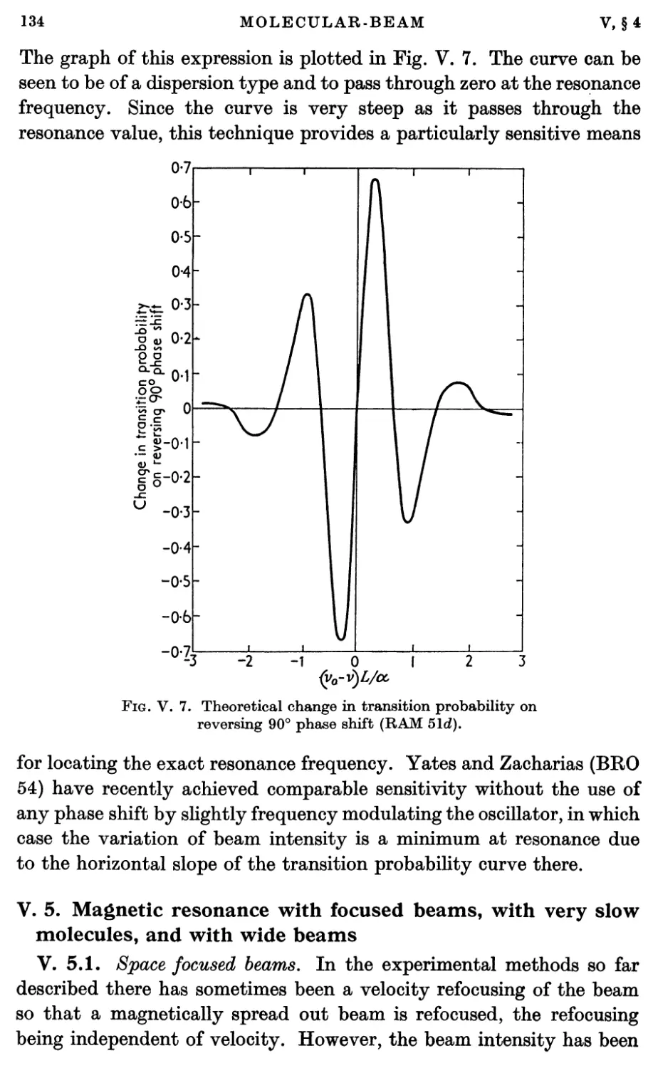
/


Текст
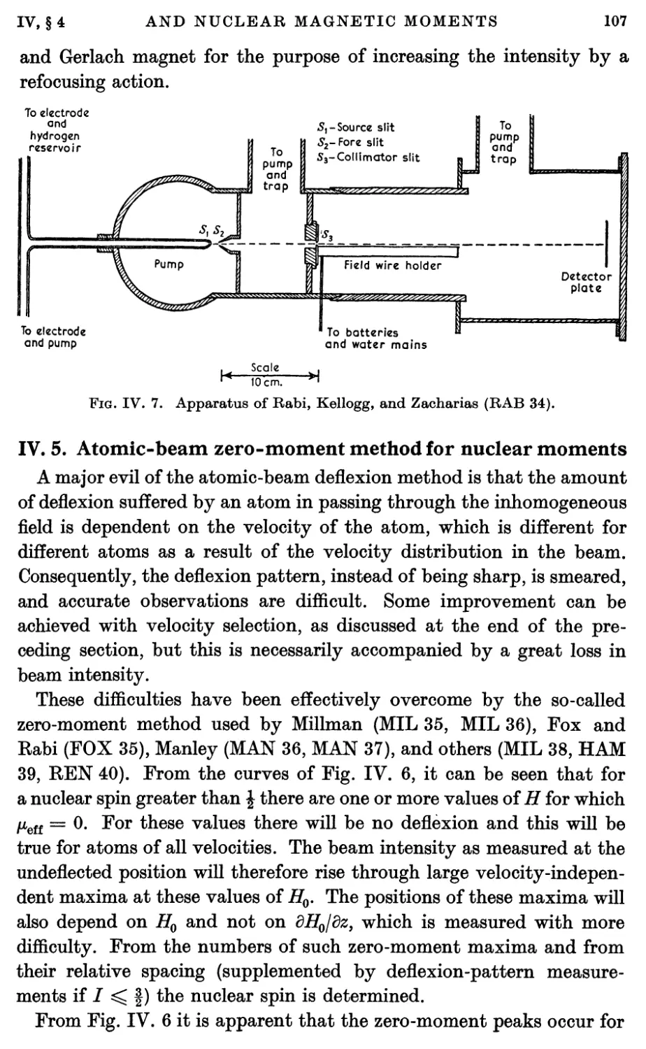
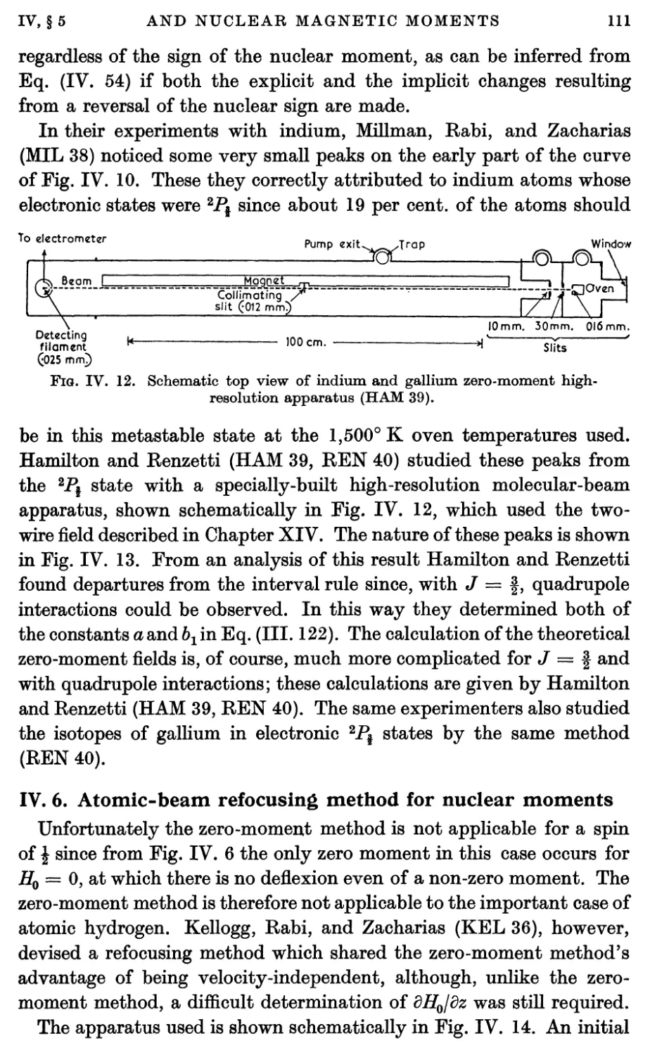
^^i^lWmßl^^m^ssr^^^
THË
INTERNATIONAL SERIES
OF
MONOGRAPHS ON PHYSICS
GENERAL EDITORS
N. F. MOTT E. C. BULLARD
THE INTERNATIONAL SERIES OF
MONOGRAPHS ON PHYSICS
Already Published
THE THEORY OF ELECTRIC AND MAGNETIC SUSCEPTIBILITIES.
By J. h. van vleck. 1932
RELATIVITY, THERMODYNAMICS, AND COSMOLOGY. By b. c.
TOLMAN. 1934
THE PRINCIPLES OF STATISTICAL MECHANICS. By b. c. tolman.
1938
GEOMAGNETISM. By s. chapman and J. babtels. 1940. 2 vols.
THE PRINCIPLES OF QUANTUM MECHANICS. By p. a. m. dibac. Third
edition. 1947
ELECTRONIC PROCESSES IN IONIC CRYSTALS. By n. f. mott and
B. w. gubney. Second edition. 1948
THE THEORY OF ATOMIC COLLISIONS. By n. f. mott and h. s. w.
massey. Second edition. 1948
KINEMATIC RELATIVITY. By e. a. milne. 1948
THE PULSATION THEORY OF VARIABLE STARS. By s. bosseland.
1948
THEORY OF PROBABILITY. By habold jeffbeys. Second edition. 1948
THE SEPARATION OF GASES. By m. buhemann. Second edition. 1949
THEORY OF ATOMIC NUCLEUS AND NUCLEAR ENERGY SOURCES.
By g. gamow and c. l. cbitchfield. 1949. Being the third edition of stbuc-
TUBE OF ATOMIC NUCLEUS AND NUCLEAR TBANSFOBMATIONS
COSMICAL ELECTRODYNAMICS. By h. alfvén. 1950
COSMIC RAYS. By l. jànossy. Second edition. 1950
BASIC METHODS IN TRANSFER PROBLEMS. Radiative Equilibrium
and Neutron Diffusion. By v. koubganoff with the collaboration of I. w.
BUSBBIDGE. 1952
MIXTURES. The Theory of the Equilibrium Properties of some Simple
Classes of Mixtures, Solutions and Alloys. By e. a. Guggenheim. 1952
THE THEORY OF RELATIVITY. By c. molleb. 1952
THE FRICTION AND LUBRICATION OF SOLIDS. By f. p. bowden and
d. tabob. 1952
ELECTRONIC AND IONIC IMPACT PHENOMENA. By h. s. w. massey
and e. h. s. bubhop. 1952
GEOCHEMISTRY. By the late v. m. goldschmidt. Edited by alex muib.
1953
ELECTRICAL BREAKDOWN OF GASES. By J. m. meek and J. d. cbaggs.
1953
DISLOCATIONS AND PLASTIC FLOW IN CRYSTALS. By a. h. cottbell.
1953
THE OUTER LAYERS OF A STAR. By B. v. d. b. woolley and d. w. n.
stibbs. 1953
METEOR ASTRONOMY. By a. c. b. lovell. 1954
DYNAMICAL THEORY OF CRYSTAL LATTICES. By max bobn and
KUN HUANG. 1954
ON THE ORIGIN OF THE SOLAR SYSTEM. By h. alfvén. 1954
THE QUANTUM THEORY OF RADIATION. By w. heitleb. Third
edition. 1954
RECENT ADVANCES IN OPTICS. By e. h. linfoot. 1955
QUANTUM THEORY OF SOLIDS. By b. e. peiebls. 1955
MOLECULAR
BEAMS
BY
NORMAN F. RAMSEY
PBOPESSOB OP PHYSICS AND
JOHN SIMON GUGGENHEIM FELLOW
HABVABD UNIVERSITY
OXFORD
AT THE CLARENDON PRESS
1956
Oxford University Press, Amen House, London E.G.4
GLASGOW NEW YOBK TOBONTO MELBOURNE WELLINGTON
BOMBAY CALCUTTA MADBAS KARACHI CAPE TOWN IBADAN
Geoffrey Gumberlege, Publisher to the University
PRINTED IN GREAT BRITAIN
PREFACE
Molecular-beam experiments have for many years been among the
most fruitful sources of fundamental information about molecules,
atoms, and nuclei. Some of the early experiments provided direct
experimental evidence for spatial quantization and for the spin of the
electron. More recent experiments have led to such important
discoveries as the anomalous magnetic moments of protons and neutrons,
the deuteron quadrupole moment with its implication of a nucléon
tensor interaction, the Lamb shift in the fine structure of atomic
hydrogen with its quantum electrodynamic implications, the anomalous
magnetic moment of the electron, the existence of nuclear octupole
moments, and many others. In addition molecular-beam experiments
have produced a wealth of molecular, atomic, and nuclear data
including an array of nuclear spin, magnetic moment, and quadrupole moment
determinations which, among other things, have provided much of the
initial evidence for nuclear shell models.
Despite the scientific importance of the subject, there have been
remarkably few books on molecular beams. As discussed in Chapter I,
a few review articles and brief monographs have been written but only
one detailed book has been published. That book, by R. Fraser (FRA
31), was written twenty-five years ago, prior to almost all of the
important discoveries listed in the preceding paragraph.
It is my hope that this book will satisfy the need for a detailed,
consistent, and up-to-date discussion of the subject of molecular beams.
Although the entire subject is discussed in the present book,
experiments prior to 1930 are dealt with more briefly since they are described
in greater detail in Fraser's book (FRA 31).
I wish to express my appreciation to the many workers with molecular
beams who have supplied me with information and help in the
preparation of this book. Special thanks are due to Professors I. I. Rabi,
P. Kusch, and J. R. Zacharias and to Drs. H. Kolsky and H. Lew. I
should also like to thank John Wiley & Sons for their permission to
use some material, especially in Chapter III, from my book on Nuclear
Moments published by them, and the John Simon Guggenheim Memorial
Foundation for the fellowship I held at Oxford University during the
VI
PREFACE
completion of this book. Finally, I wish to express special appreciation
to my wife, EKnor Ramsey, for her help in making available the time
during which the book was written, and to my secretary, Phyllis Brown,
for her extensive and excellent help in the preparation of the
manuscript.
K F. R.
Harvard University
Cambridge, Massachusetts
August 1955
CONTENTS
I. MOLECULAR AND ATOMIC BEAMS
1. Introduction 1
2. Typical Molecular-beam Experiment 2
3. Kinds of Molecular-beam Measurements 8
IL GAS KINETICS
1. Molecular Effusion from Sources 11
1.1 Effusion from thin-walled apertures 11
1.2. Effusion from long channels 13
2. Molecular-beam Intensities and Shapes 16
2.1. Beam intensities 16
2.2. Beam shapes 16
3. Velocities in Molecular Beams 19
3.1. Velocity distribution in a volume of gas 19
3.2. Velocity distribution in molecular beams 20
3.3. Characteristic velocities 20
3.4. Experimental measurements of molecular velocities 21
4. Molecular Scattering in Gases 25
4.1. Methods of measurement 25
4.2. Calculation of scattering cross-sections from attenuation
measurements 28
4.3. Cross-section theory 30
4.4. Results of atomic-beam scattering experiments 33
5. Interaction of Molecular Beams with Solid Surfaces 35
5.1. Introduction 35
5.2. Reflection 35
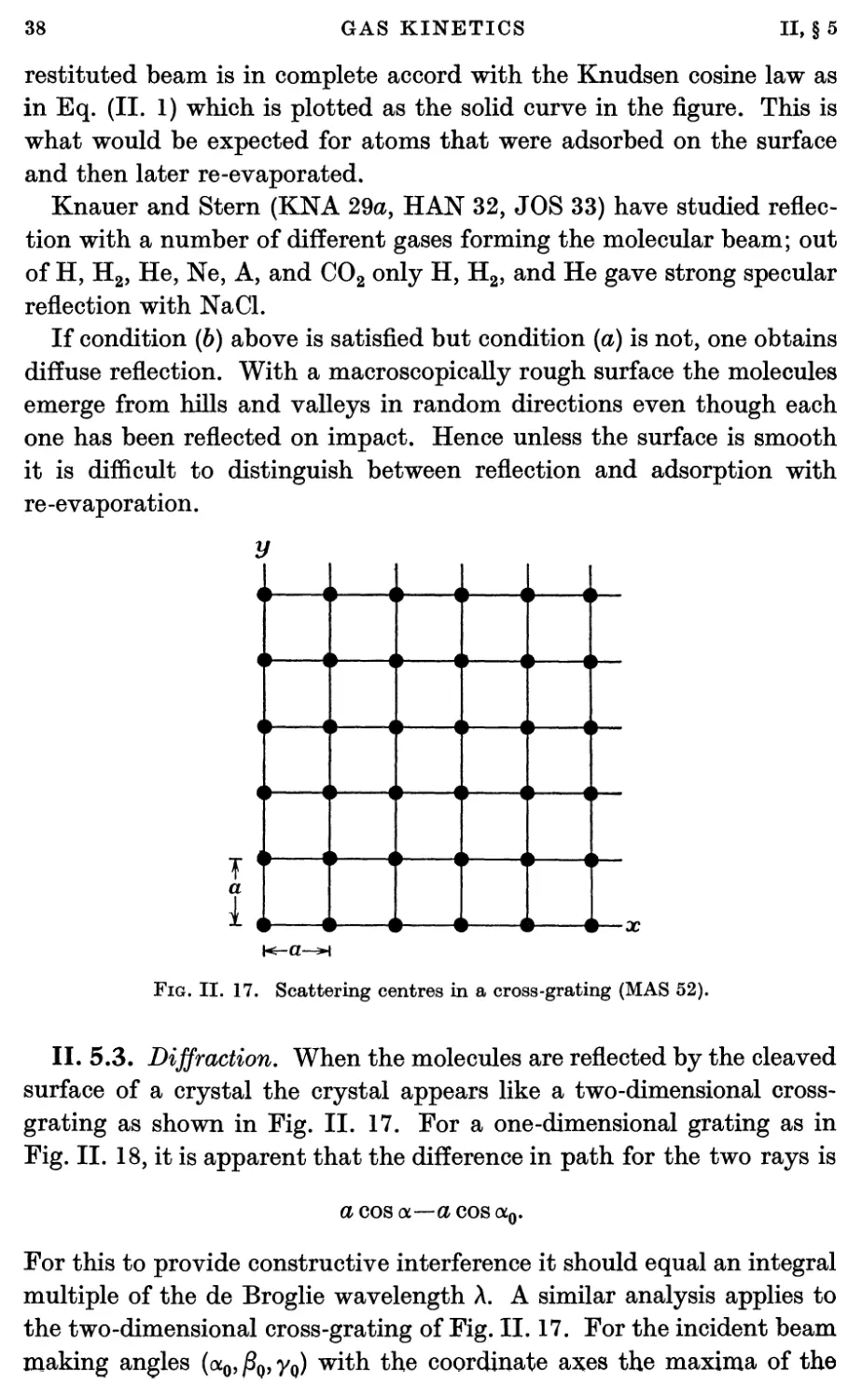
5.3. Diffraction 38
5.4. Inelastic collisions 44
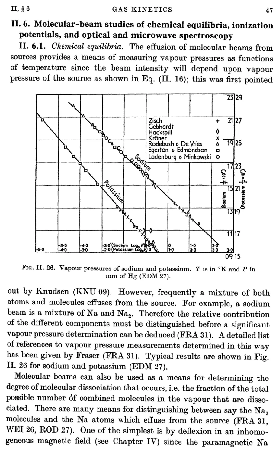
6. Molecular-beam Studies of Chemical Equilibria, Ionization
Potentials, and Optical and Microwave Spectroscopy 47
6.1. Chemical equilibria 47
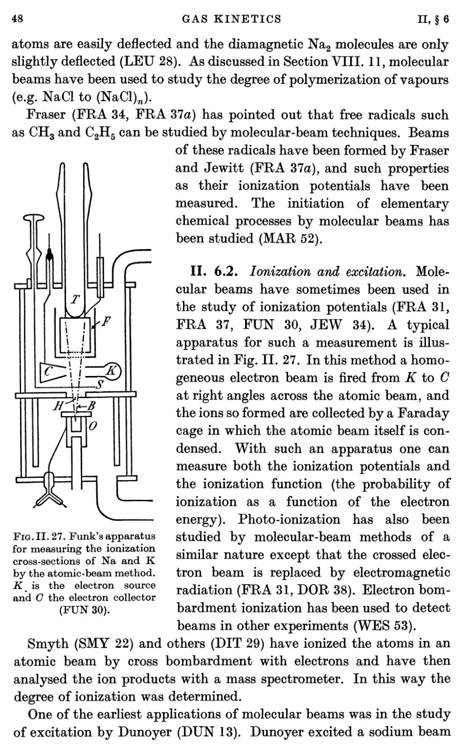
6.2. Ionization and excitation 48
6.3. Optical and microwave absorption spectroscopy 50
III. INTERACTION OF A NUCLEUS WITH ATOMIC AND
MOLECULAR FIELDS
1. Introduction 51
2. Electrostatic Interaction 52
2.1. Multipole expansion 52
2.2. Theoretical restrictions on electric multipole orders 58
2.3. Nuclear electric quadrupole interactions 59
2.4. Multipole moments of arbitrary order 66
CONTENTS
Magnetic Interaction 68
3.1. Magnetic multipoles 68
3.2. Magnetic dipoles 72
3.3. Magnetic dipole interactions with internal and external
magnetic fields 76
3.4. Magnetic interactions in molecules 80
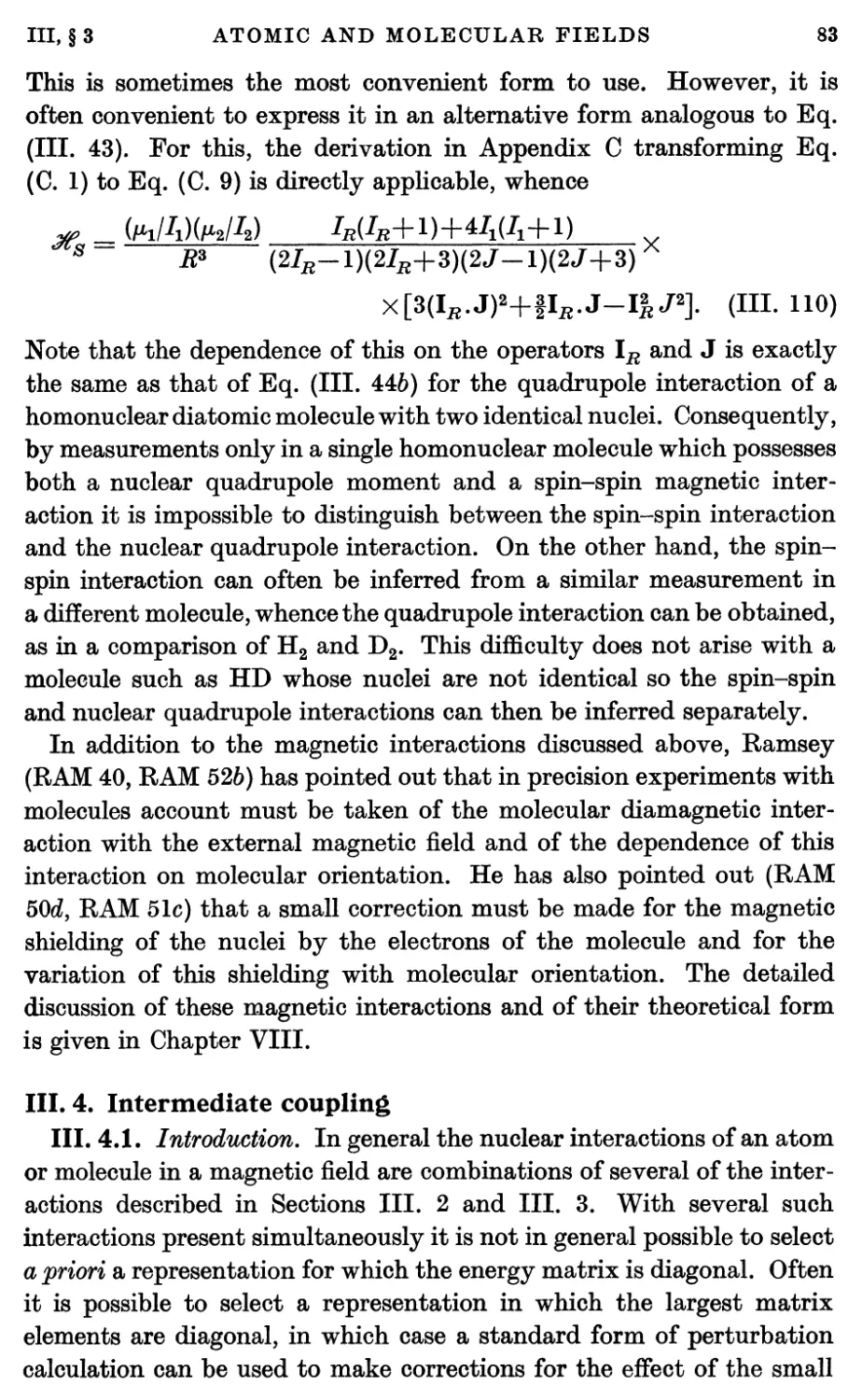
Intermediate Coupling 83
4.1. Introduction 83
4.2. Solution of secular equation 84
4.3. Perturbation theory 87
NON-RESONANCE MEASUREMENTS OF ATOMIC AND
NUCLEAR MAGNETIC MOMENTS
1. Deflexion and Intensity Relations 89
1.1. Effective magnetic moment 89
1.2. Deflexion of molecule by magnetic fields 90
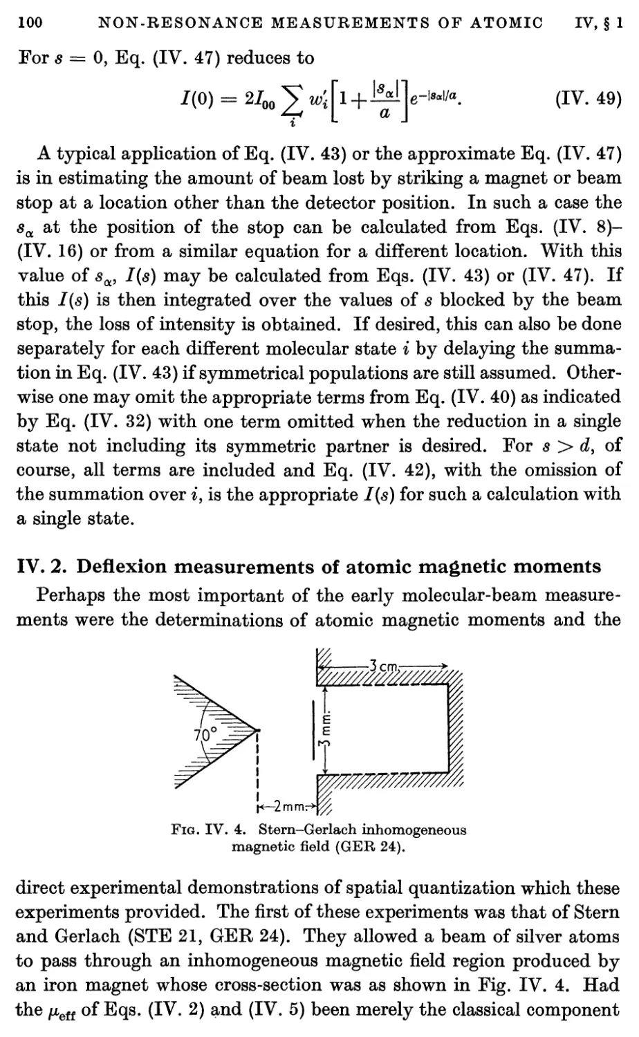
2. Deflexion Measurements of Atomic Magnetic Moments 100
3. Deflexion Measurements of Nuclear and Rotational Magnetic
Moments in Non-paramagnetic Molecules 102
4. Atomic-beam Deflexion Measurements of Nuclear Moments 104
5. Atomic-beam Zero-moment Method for Nuclear Moments 107
6. Atomic-beam Refocusing Method for Nuclear Moments 111
7. Atomic-beam Measurements of Signs of Nuclear Moments 113
8. Atomic-beam Space Focusing Measurements of Nuclear Spins 114
MOLECULAR-BEAM MAGNETIC RESONANCE
METHODS
1. Introduction 115
2. Magnetic Resonance Method 116
3. Transition Probabilities 118
3.1. Transition probability for individual molecules 118
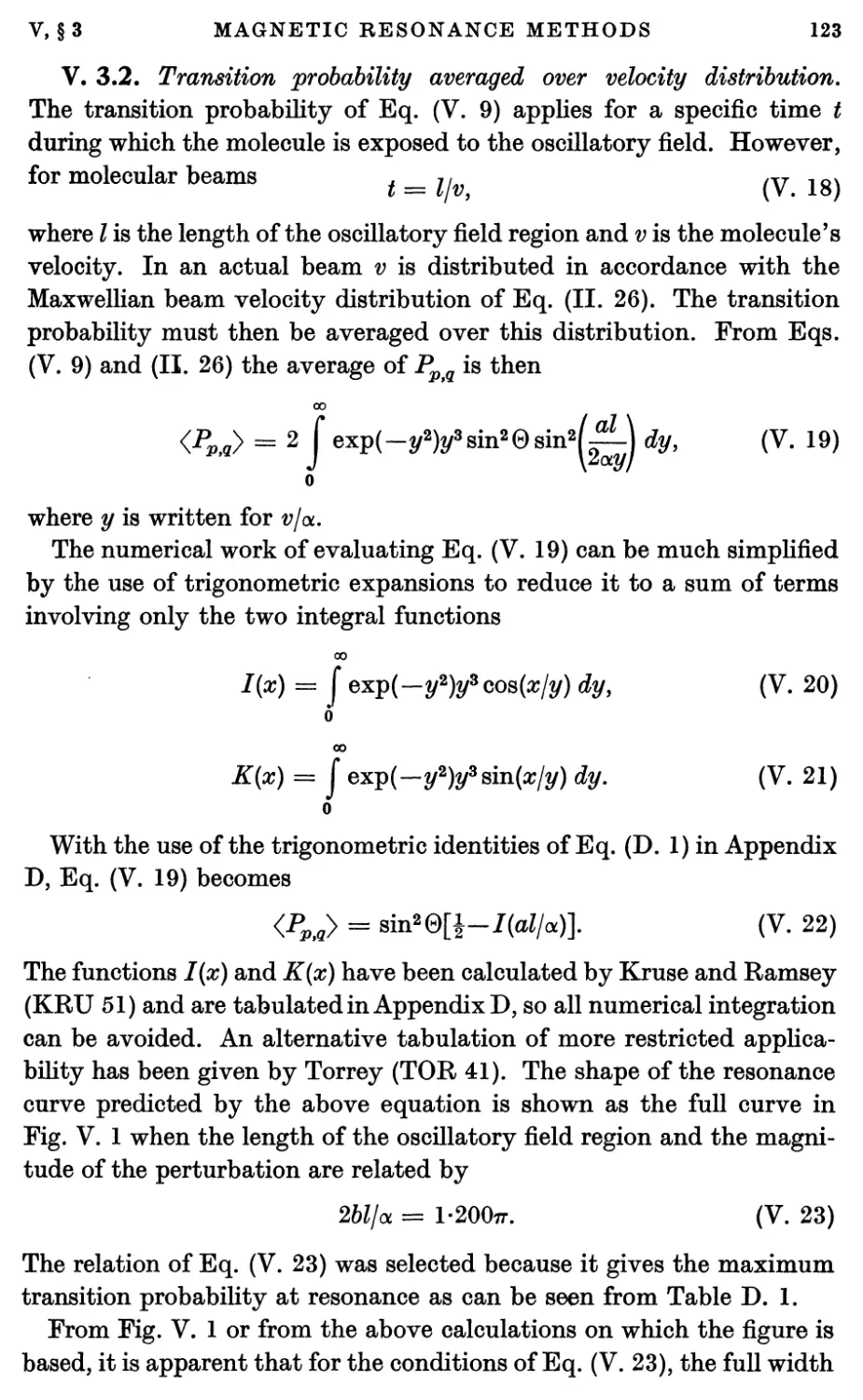
3.2. Transition probability averaged over velocity distribution 123
4. Magnetic Resonance Method with Separated Oscillating Fields 124
4.1. Introduction 124
4.2. Transition probability for individual molecule with separated
oscillating fields 127
4.3. Separated oscillating fields transition probability averaged over
velocity distribution 128
4.4. Phase shifts in the molecular-beam method of separated
oscillating fields 131
5. Magnetic Resonance with Focused Beams, with Very Slow Molecules,
and with Wide Beams 134
5.1. Space focused beams 134
5.2. Beams of very slow molecules. Wide beams 138
6. Distortions of Molecular-beam Resonances 139
CONTENTS
ix
VI. NUCLEAR AND ROTATIONAL MAGNETIC MOMENTS
1. Resonance Measurements of Nuclear Magnetic Moments 145
2. Interpretation with Rotating Coordinate System 146
2.1. Introduction 146
2.2. Classical theory 147
2.3. Quantum theory 151
3. Spins Greater than One-half 153
4. Signs of Nuclear Moments 155
5. Absolute Values of Nuclear Moments 158
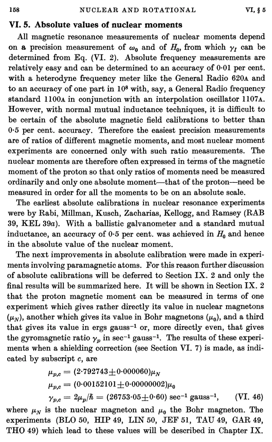
6. Nuclear Magnetic Moment Measurements 159
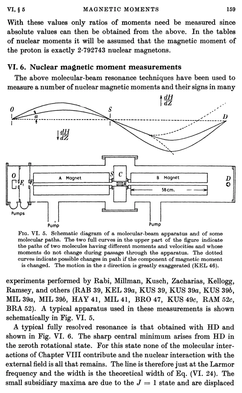
7. Magnetic Shielding 162
8. Molecular Rotational Magnetic Moments 166
8.1. Experimental measurements of rotational magnetic moments 166
8.2. Theory of rotational magnetic moments 169
9. Results of Nuclear Moment Measurements 170
9.1. Introduction 170
9.2. Nuclear moment tables 171
10. Significance of Nuclear Spin and Nuclear Magnetic Moment Results 171
10.1 Introduction 171
10.2. Relations between nuclear statistics, spins, and mass numbers 178
10.3. Nucléon magnetic moments 179
10.4. Deuteron magnetic moment 179
10.5. H8 and He3 magnetic moments 180
10.6. Systematics of nuclear spins and magnetic moments 181
10.7. Nuclear models 184
VII. NEUTRON-BEAM MAGNETIC RESONANCE
1. Introduction 189
2. Polarized Neutron Beams 189
2.1. Neutron beams 189
2.2. Polarization of neutron beams 190
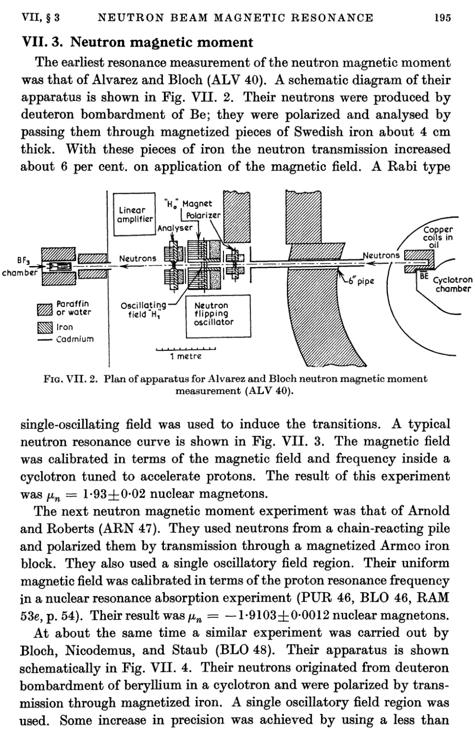
3. Neutron Magnetic Moment 195
VIII. NUCLEAR AND MOLECULAR INTERACTIONS IN
FREE MOLECULES
1. Introduction 202
2. Nuclear and Rotational Magnetic Moments 203
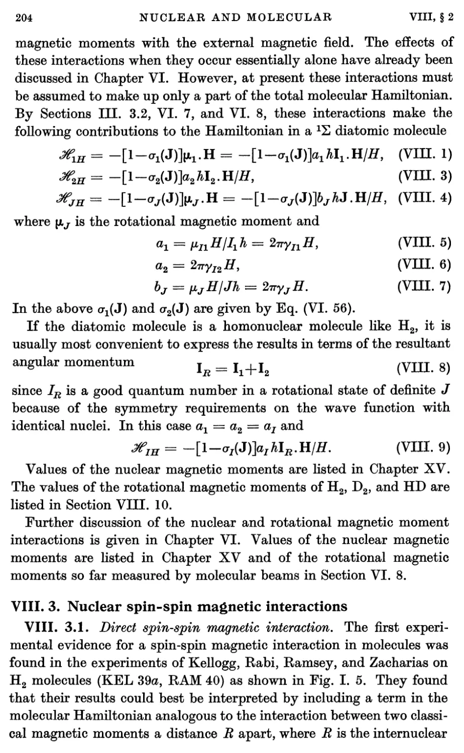
3. Nuclear Spin-Spin Magnetic Interactions 204
3.1. Direct spin-spin magnetic interaction 204
3.2. Electron-coupled interactions between nuclear spins in molecules 206
4. Spin-rotational Magnetic Interactions 208
5. Nuclear Electrical Quadrupole Interaction 213
6. Diamagnetic Interactions 228
7. Effects of Molecular Vibration 230
8. Combined Hamiltonian 233
X
CONTENTS
9. Matrix Elements and Intermediate Couplings 234
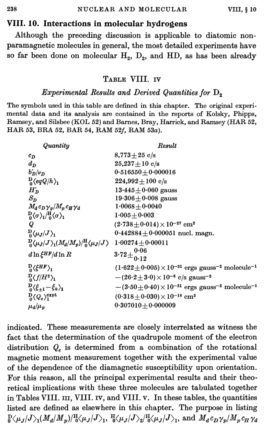
10. Interactions in Molecular Hydrogens 238
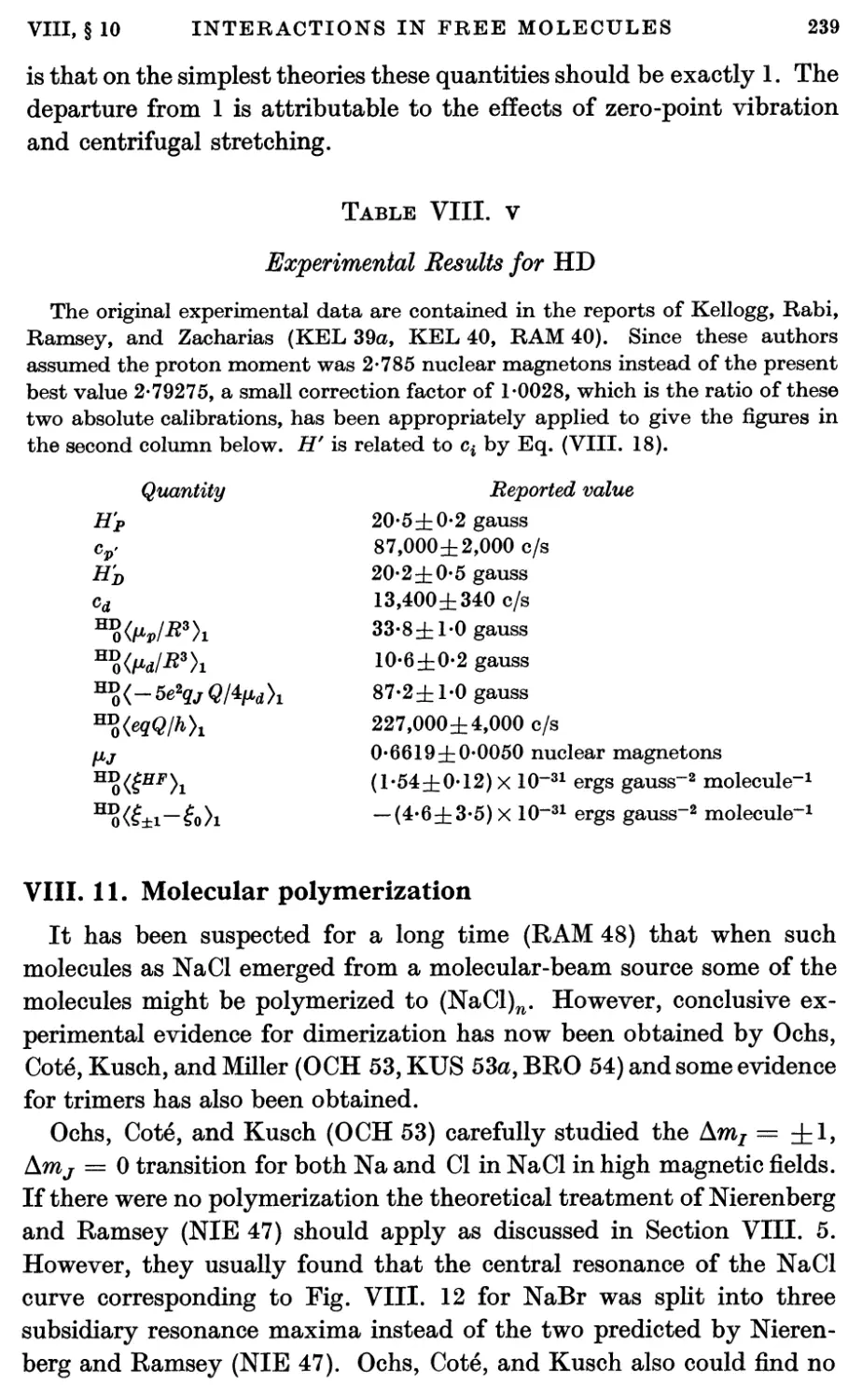
11. Molecular Polymerization 239
IX. ATOMIC MOMENTS AND HYPERFINE STRUCTURES
1. Introduction 241
2. Absolute Scale for Nuclear Moments. The Fundamental Constants 245
3. Nuclear Spins from Atomic Hyperfine Structure 249
4. Atomic Hyperfine Structure Separations for J = J 251
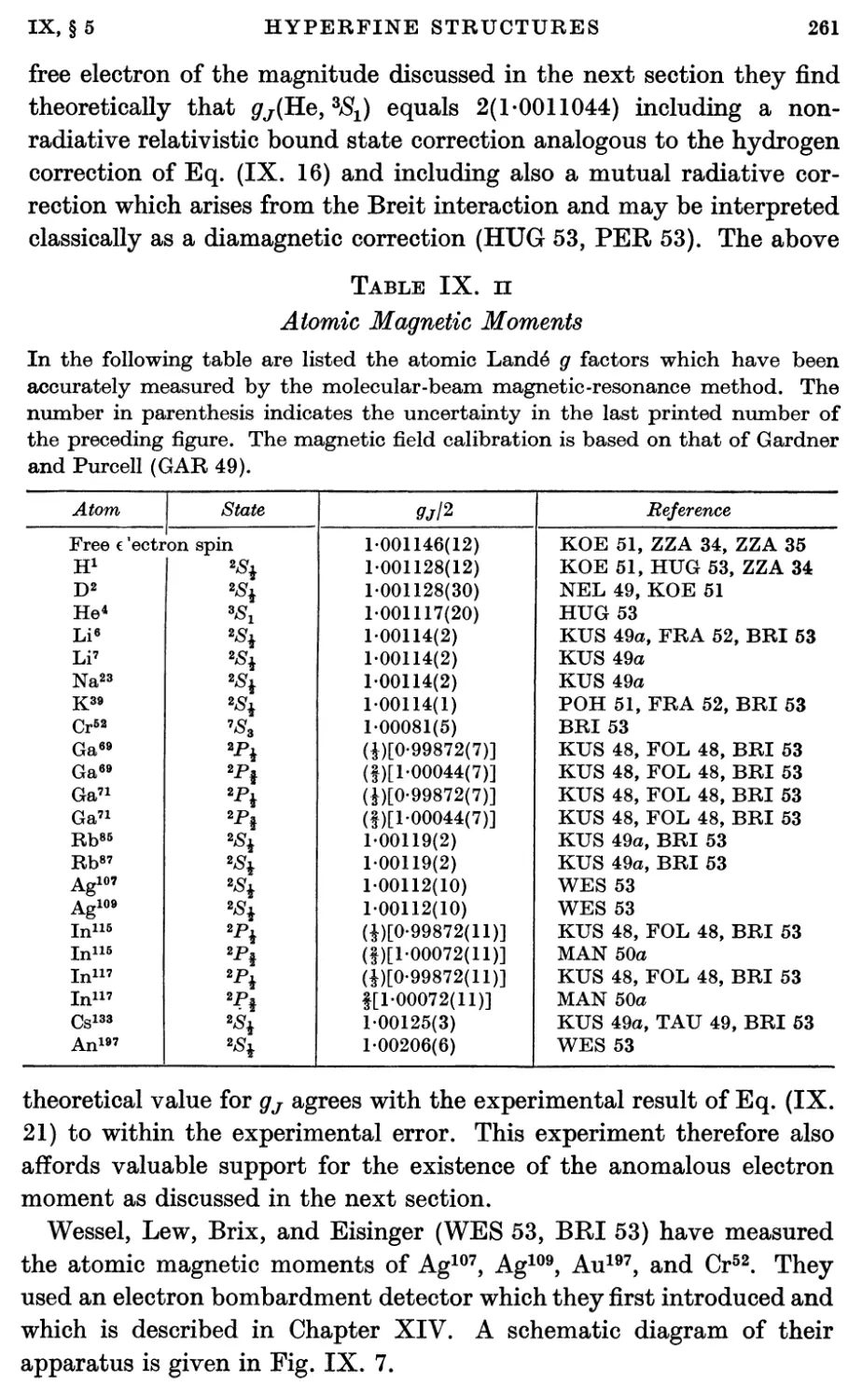
5. Atomic Magnetic Moments ; The Anomalous Electron Moment 256
5.1. Atomic magnetic moments 256
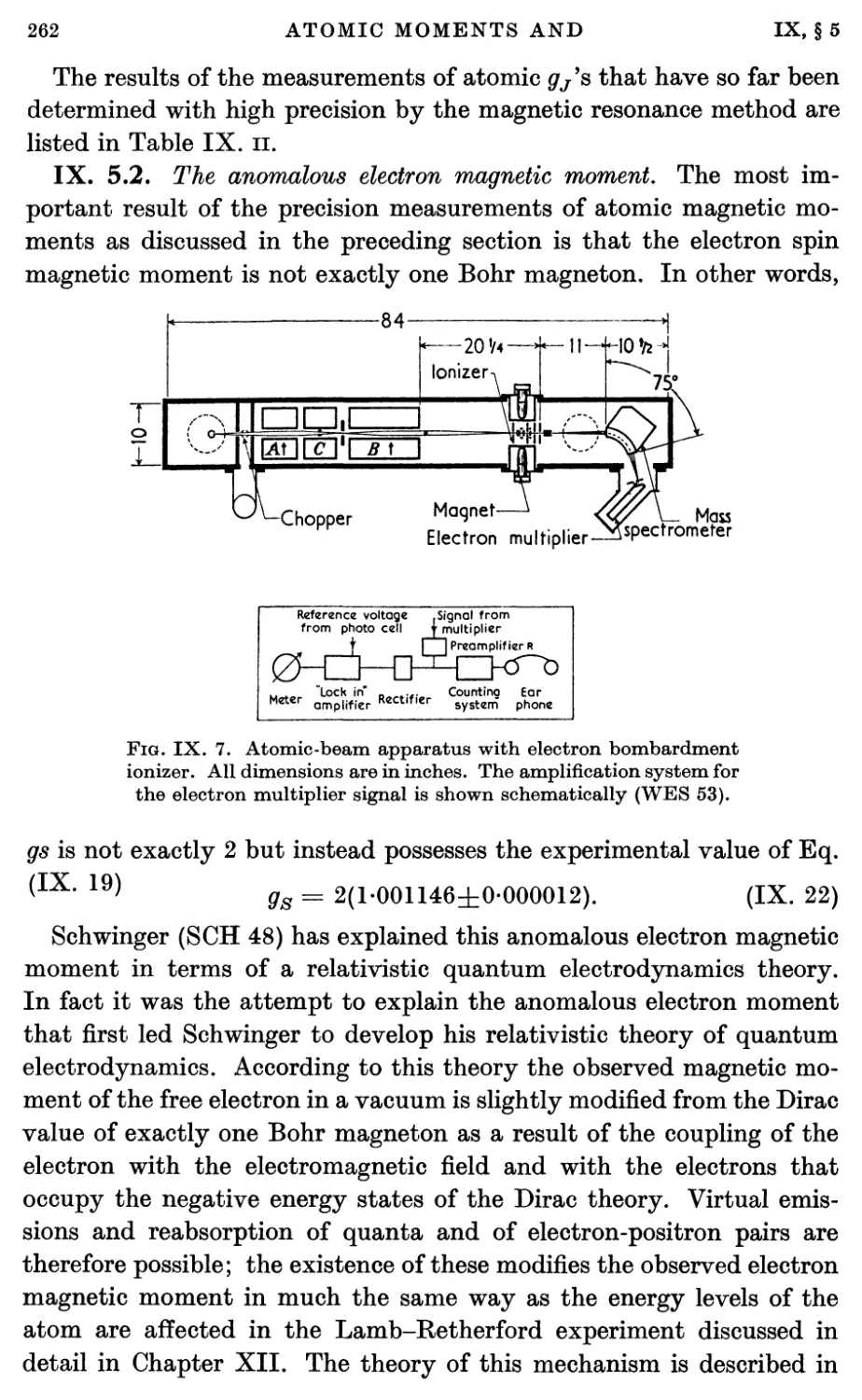
5.2. The anomalous electron magnetic moment 262
6. Hyperfine Structure of Atomic Hydrogen 263
6.1. Atomic hydrogen experiments 263
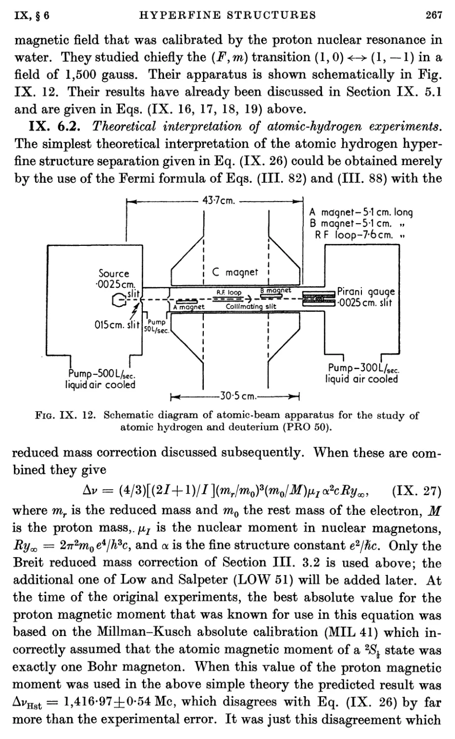
6.2. Theoretical interpretation of atomic-hydrogen experiments 267
7. Direct Nuclear Moment Measurements with Atoms 270
8. Quadrupole Interactions 271
9. Magnetic Octupole Interactions 277
10. Anomalous Hyperfine Structure and Magnetic-moment Ratios for
Isotopes 279
11. Frequency Standards and Atomic Clocks 283
12. Atomic-beam Resonance Method for Excited States 285
X. ELECTRIC DEFLEXION AND RESONANCE
EXPERIMENTS
1. Introduction 287
2. Molecular Interactions in an Electric Field 289
2.1. Molecular Hamiltonian 289
2.2. Energy of vibrating rotator 290
2.3. Stark effect 292
2.4. Hyperfine structure interactions 293
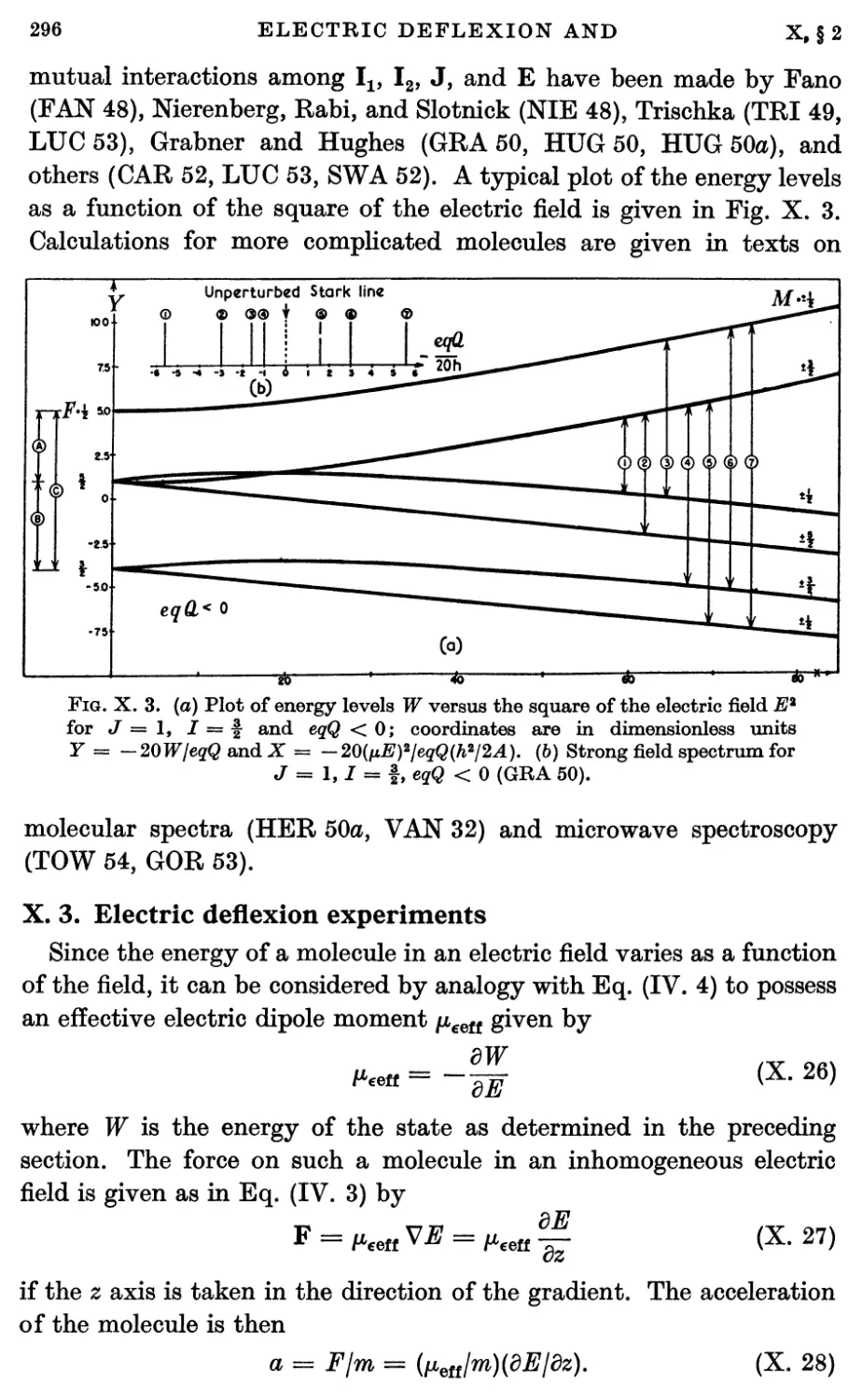
3. Electric Deflexion Experiments 296
4. Electric Resonance Experiments 298
4.1. Introduction 298
4.2. Electric resonance experiments for molecules with negligible
hyperfine structure interactions 301
4.3. Electric resonance experiments with hyperfine structure 303
4.4. Electric resonance experiments with change of J 307
5. Molecular Amplifier 309
XL NUCLEAR ELECTRIC QUADRUPOLE MOMENTS
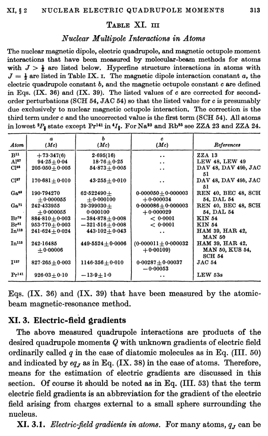
1. Introduction 310
2. Nuclear Electric Quadrupole Interactions 310
2.1. Nuclear quadrupole interactions in molecules 310
2.2. Nuclear quadrupole interactions in atoms 310
CONTENTS
xi
3. Electric-field Gradients 313
3.1. Electric-field gradients in atoms 313
3.2. Electric-field gradients in molecules 315
3.3. Effect of atomic core on nuclear quadrupole interaction 316
4. Nuclear Electric Quadrupole Moments 319
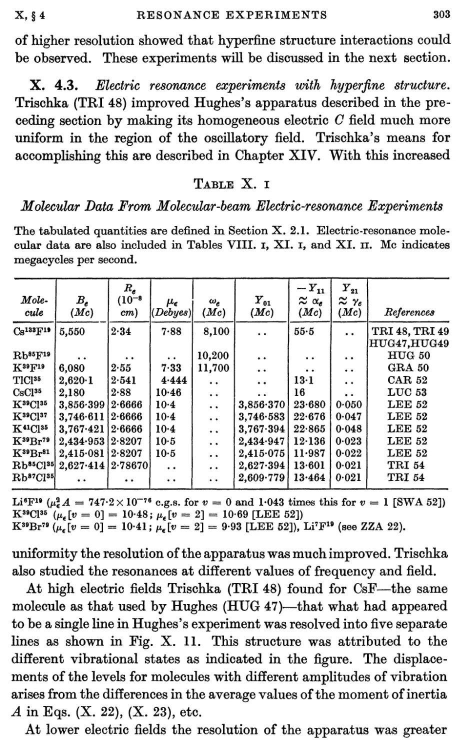
5. Theoretical Interpretation of Nuclear Quadrupole Moments 319
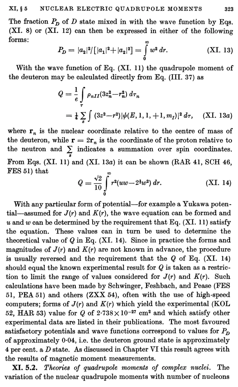
5.1. Theory of deuteron quadrupole moment 319
5.2. Theories of quadrupole moments of complex nuclei 323
XII. ATOMIC FINE STRUCTURE
1. Introduction 327
2. Hydrogen Atomic-beam Method 329
3. Hydrogen and Deuterium Results 331
4. Fine Structure of Singly-ionized Helium 336
5. Theoretical Interpretation 340
XIII. MOLECULAR-BEAM DESIGN PRINCIPLES
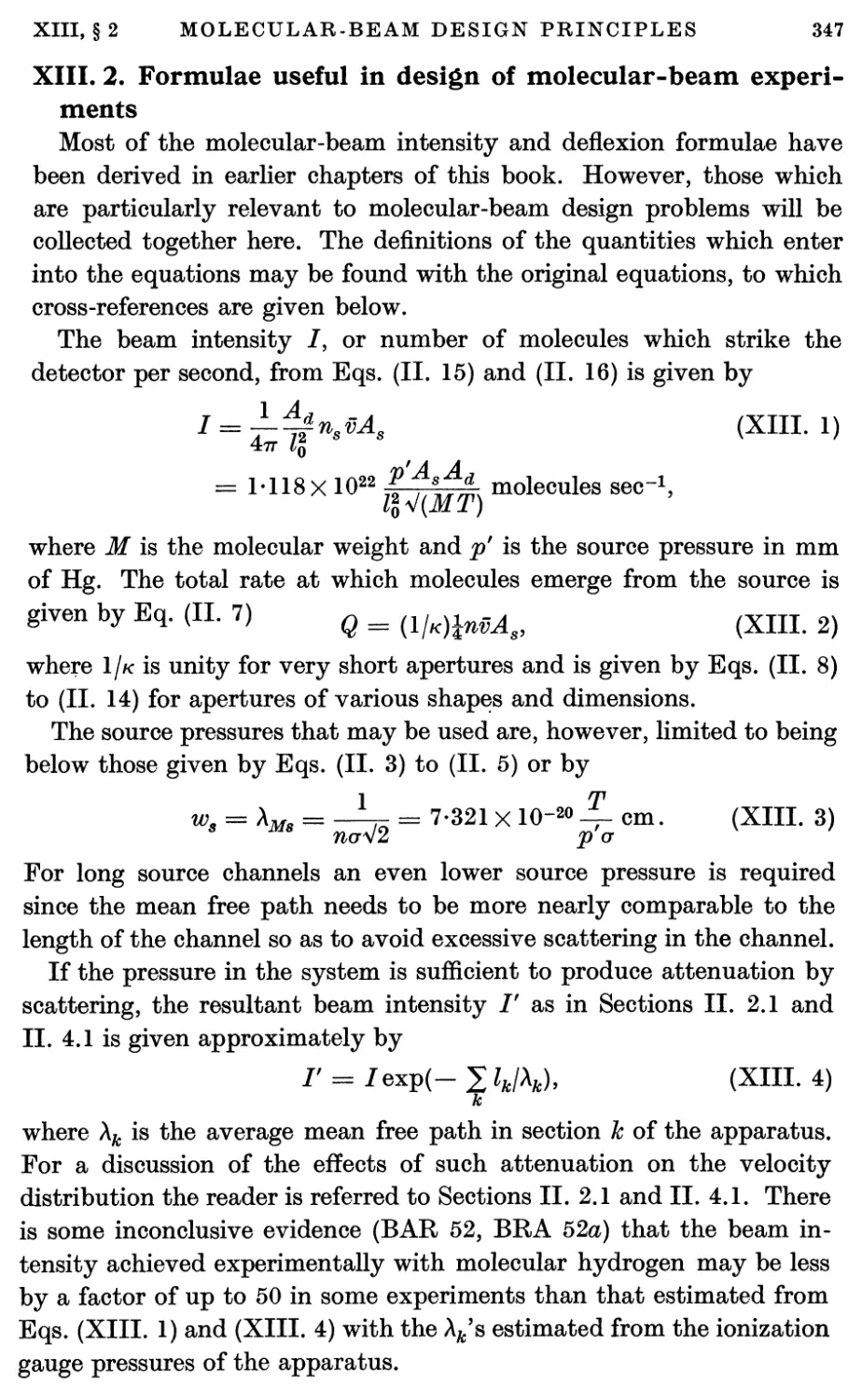
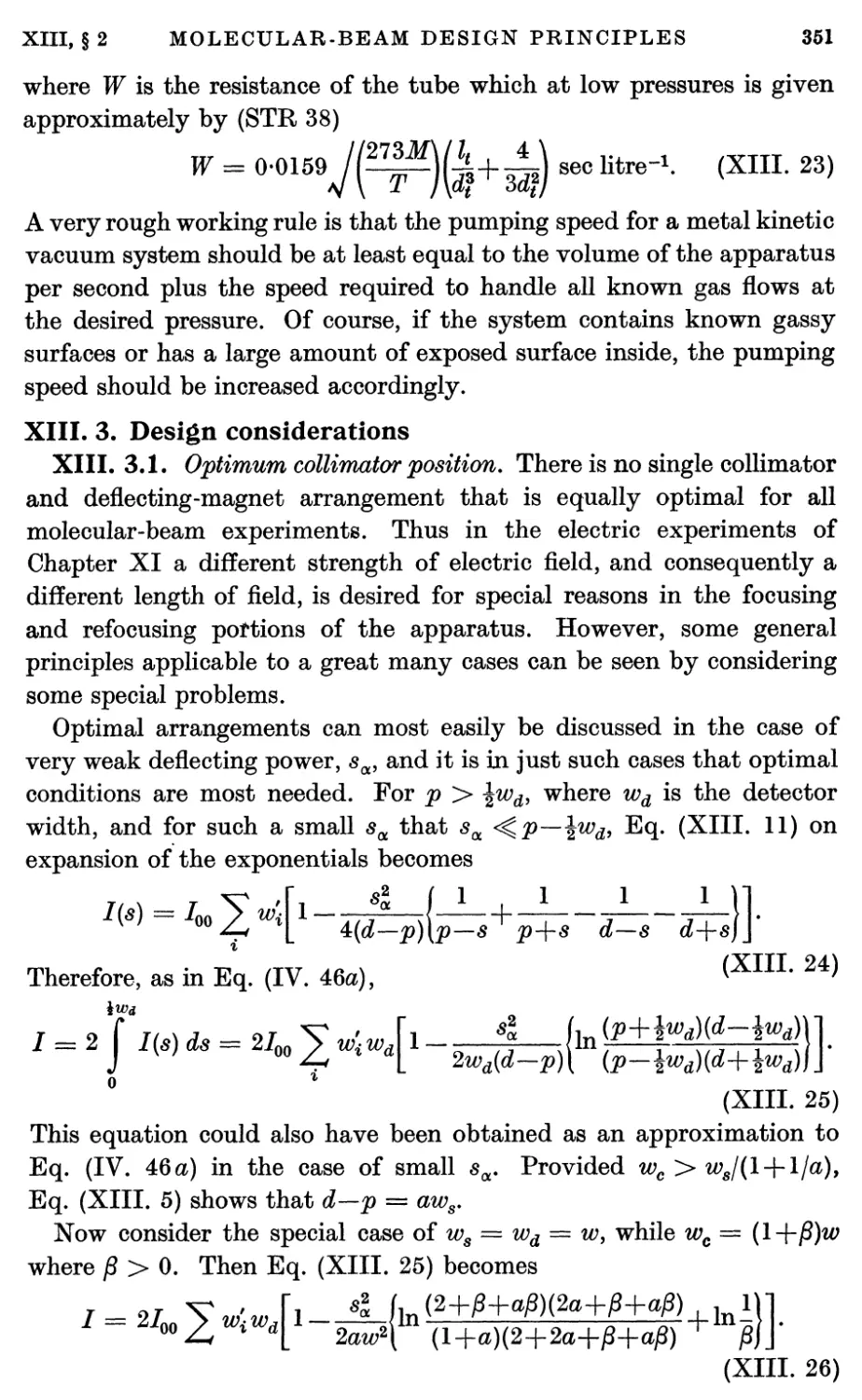
1. Introduction 346
2. Formulae Useful in Design of Molecular-beam Experiments 347
3. Design Considerations 351
3.1. Optimum collimator position 351
3.2. Beam widths, heights, and lengths 352
4. Design Illustration 354
XIV. MOLECULAR-BEAM TECHNIQUES
1. Introduction 361
2. Sources 361
2.1. Sources for non-condensable gases 361
2.2. Heated ovens 364
2.3. Sources for dissociated atoms 372
3. Detectors 374
3.1. Miscellaneous detectors 374
3.2. Surface ionization detectors 379
3.3. Electrometers, mass spectrometers, and electron multiplier
tubes 381
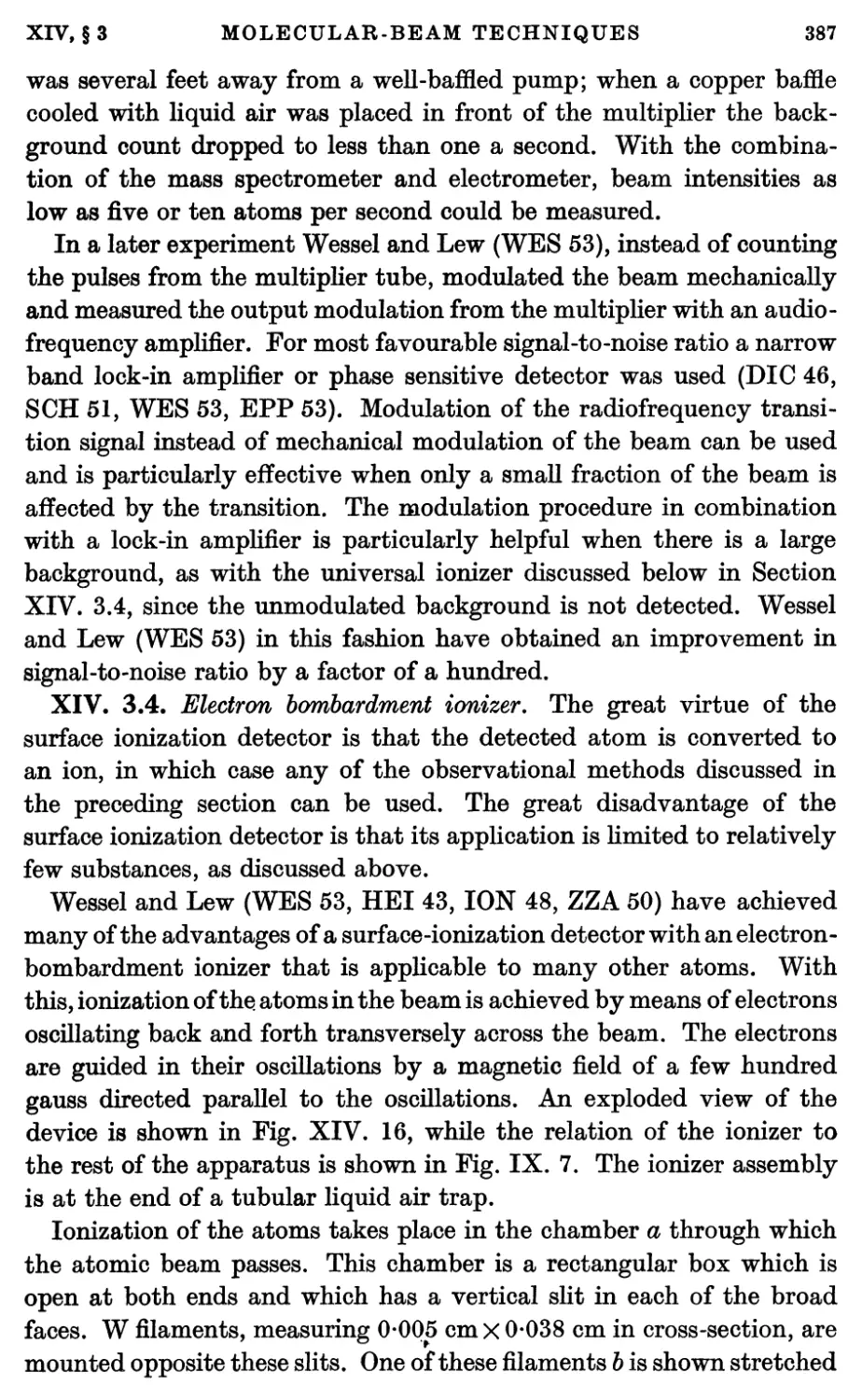
3.4. Electron bombardment ionizer 387
3.5. Stern-Pirani detector 389
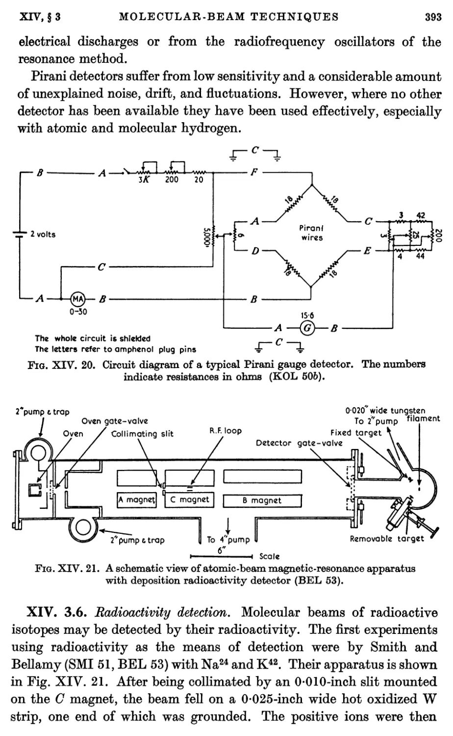
3.6. Radioactivity detection 393
4. Deflecting and Uniform Fields 394
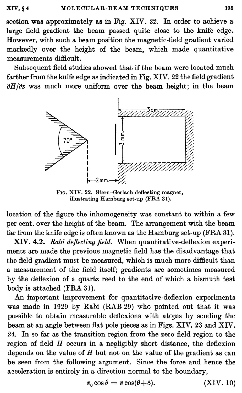
4.1. Stern-Gerlach and Hamburg deflecting fields 394
4.2. The Rabi deflecting field 395
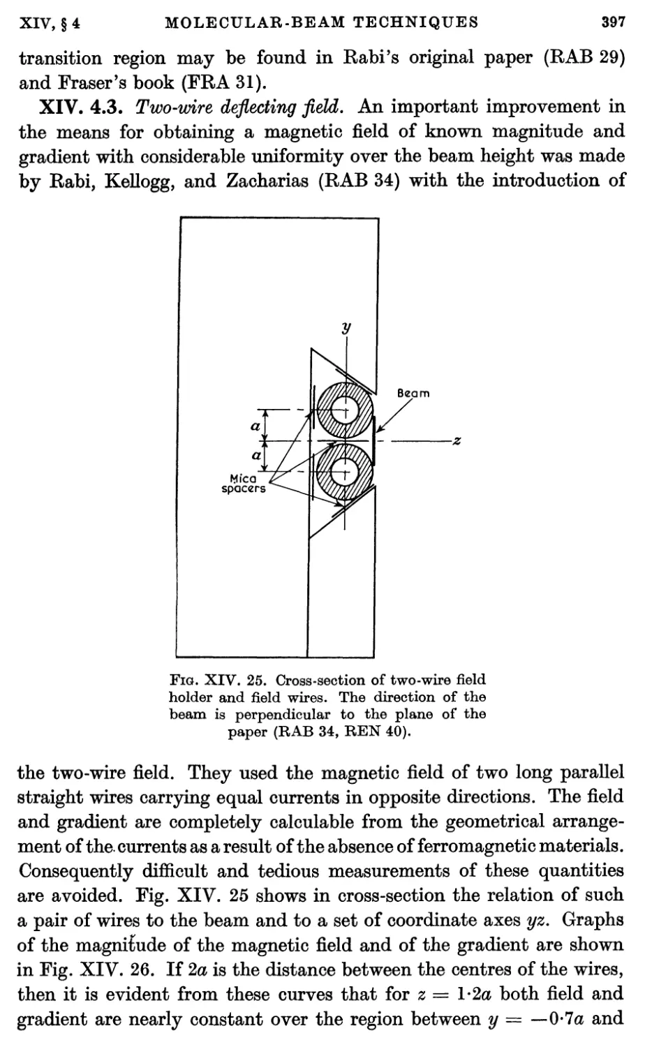
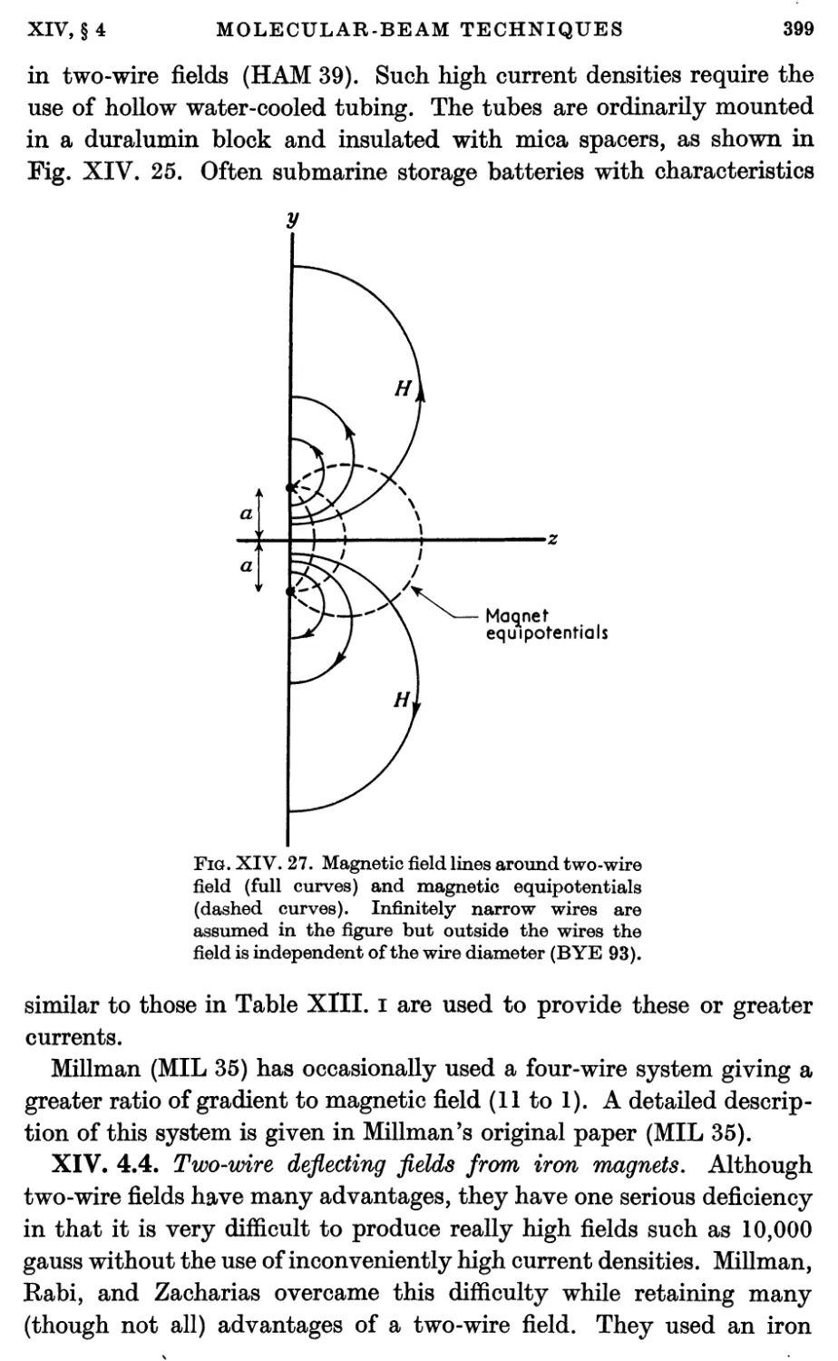
4.3. The two-wire deflecting field 397
4.4. Two-wire deflecting fields from iron magnets 399
4.5. Uniform magnetic fields 401
4.6. Electrostatic fields 402
4.7. Focusing fields 404
XU
CONTENTS
5. Oscillatory Fields 407
5.1. Oscillators 407
5.2. Oscillatory field loops and electrodes 407
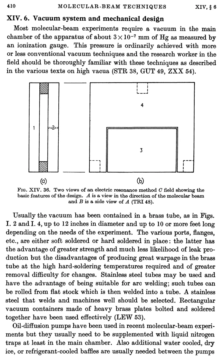
6. Vacuum System and Mechanical Design 410
7. Miscellaneous Components 415
8. Alignment 415
8.1. Optical alignment 415
8.2. Alignment with beam 416
APPENDIXES
a. Fundamental Constants 418
b. Vector and Tensor Relations 419
c. Quadrupole Interaction 421
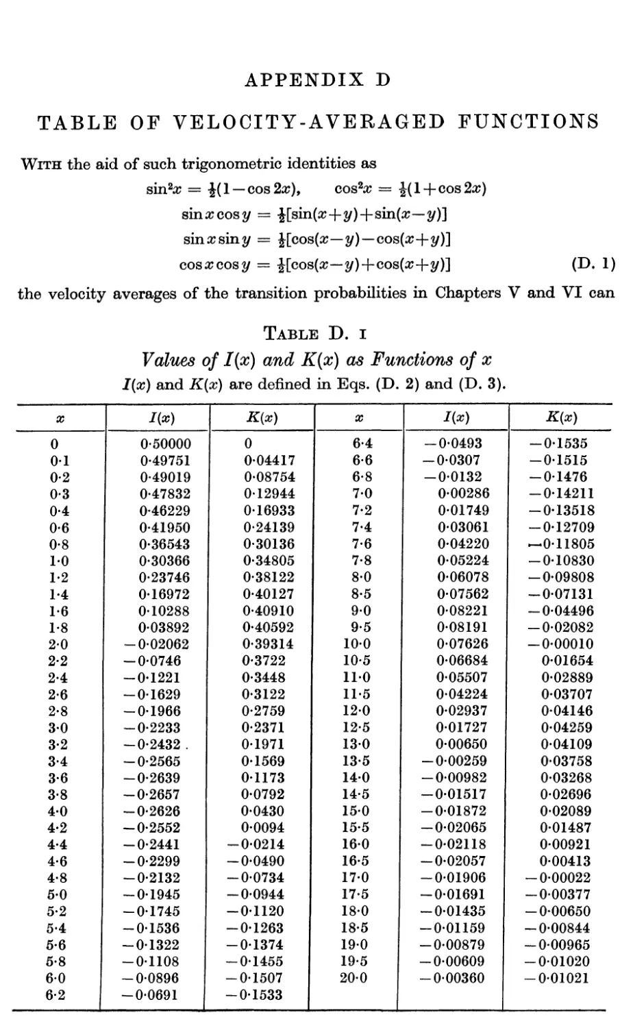
D. Table of Velocity-averaged Functions 425
e. Majorana Formula 427
F. Theory of Two-wire Field 431
G. Notes added in Proof 433
REFERENCES 435
AUTHOR INDEX 455
SUBJECT INDEX
461
I
MOLECULAR AND ATOMIC BEAMS
►To pump
1.1. Introduction
The subject of molecular beams is the study of directed beams of neutral
molecules at such low pressures that the effects of molecular collisions
are for most purposes negligible. The earliest molecular-beam
experiments were those of Dunoyer (DUN 11). He used an apparatus
illustrated in Fig. I. 1. A glass tube 20 cm long was
divided into three separately evacuated
compartments. Some sodium introduced into the first
chamber was heated until it vaporized, whereupon
a deposit of sodium appeared in the third chamber.
The deposit was of the form to be expected on the
assumption that the Na atoms travelled in straight
lines in the evacuated tube.
Subsequent to Dunoyer's pioneering work, many
different experiments based on the molecular-
beam methods have been performed. Particularly
significant from the point of view of the
development of molecular-beam techniques have been the
experiments of Stern and his collaborators at
Hamburg in the nineteen-twenties and early
thirties. The papers of Stern and Knauer in 1926
(STE 26, KNA 26, KNA 29) indeed laid down
many of the principles of molecular-beam
techniques which have been followed even to the
present time.
Precision measurements of nuclear, molecular, and atomic properties
began in 1938 with the introduction of the molecular-beam resonance
method by Rabi and his associates (RAB 38, KEL 39). At first, the
resonance method was applied to the measurement of nuclear magnetic
moments only, but it was soon extended asair ore general technique
of radiofrequency spectroscopy initially by Kellogg, Rabi, Ramsey, and
Zacharias (KEL 39a) in applications to molecules and later by Kusch
and Millman (KUS 40) in the study of atomic states. Since 1938 the
history of molecular beams has dominantly been the history of the
resonance method. As discussed in subsequent chapters, important
►To pump
Na
Fig. I. 1. Schematic
diagram of Dunoyer's
original atomic-beam
apparatus. A is the
source chamber, B the
collimator chamber, and
C the observation
chamber (DUN 11).
3595.91
B
2
MOLECULAR AND ATOMIC BEAMS
Ml
improvements and extensions of the molecular-beam resonance method
have been made by Lamb (LAM 50a), Ramsey (RAM 50c), Kusch
(KÜS51), Rabi (RAB 52), Zacharias (ZAC 53), Lew (WES 53), and
others. However, since 1938, most molecular-beam researches have
been applications of the resonance technique to physical measurements.
The molecular-beam laboratories at Columbia University, Massachusetts
Institute of Technology, and Harvard University have been particularly
effective in measuring with the resonance method many varied
properties of nuclei, atoms, and molecules.
The developments in molecular beams prior to 1937 have been
described in detail by Fraser in two different books (FRA 31, FRA 37).
Since that time no book devoted exclusively to molecular beams has
been published. However, considerable discussion of molecular beams
is given in the nuclear moment books of Kopf ermann (KOP 40) and
Ramsey (RAM 536, RAM 53e) and in various review articles (HAM 41,
BES 42, KEL 46, EST 46, KUS 50, RAM 50, RAM 52). In accordance
with existing conventions as to the scope of the subject molecular
beams, the present book will be limited to beams of electrically neutral
molecules. Ion beam experiments have been discussed extensively by
Massey (MAS 50, MAS 52), Burhop (MAS 52), and others.
I. 2. Typical molecular-beam experiment
Although molecular-beam experiments and apparatus vary greatly
according to their applications, they also have many features in common.
This is especially true of the experiments in recent years, which have
almost exclusively been by the molecular-beam resonance method. For
this reason a general description of a typical molecular-beam resonance
apparatus is given in this section as an introduction to the more detailed
considerations which follow in subsequent chapters.
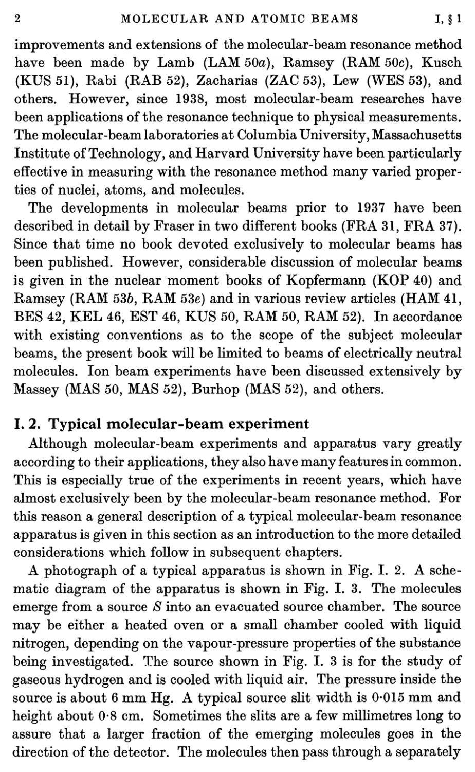
A photograph of a typical apparatus is shown in Fig. I. 2. A
schematic diagram of the apparatus is shown in Fig. I. 3. The molecules
emerge from a source 8 into an evacuated source chamber. The source
may be either a heated oven or a small chamber cooled with liquid
nitrogen, depending on the vapour-pressure properties of the substance
being investigated. The source shown in Fig. I. 3 is for the study of
gaseous hydrogen and is cooled with liquid air. The pressure inside the
source is about 6 mm Hg. A typical source slit width is 0-015 mm and
height about 0-8 cm. Sometimes the slits are a few millimetres long to
assure that a larger fraction of the emerging molecules goes in the
direction of the detector. The molecules then pass through a separately
r: m
■mar^f..
Vt-.V
«SI.*,
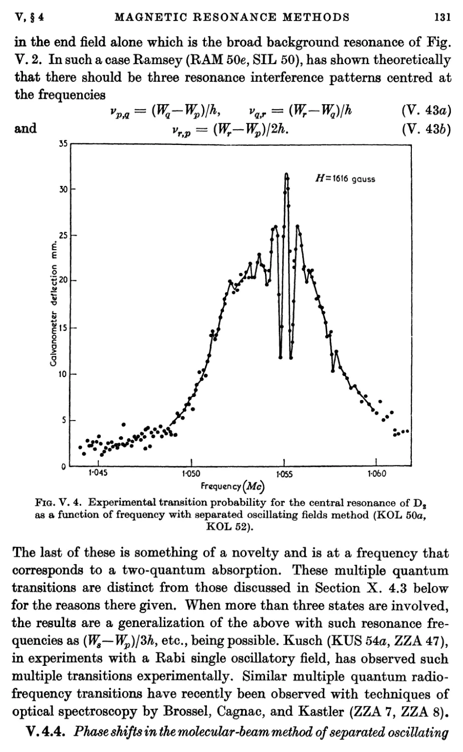
Fig. I. 2. Photograph of a typical molecular beam apparatus (KOL 50).
Fig. I. 4. View of source end of molecular beam apparatus with separating chamber bulkheads removed.
The A deflecting magnet is shown (KOL 50).
I, §2
MOLECULAR AND ATOMIC BEAMS
3
pumped separating chamber and into the main chamber. The purpose
of the separating chamber is to aid in the attainment of a better vacuum
in the main chamber. Typical pressures are 2 x 10~5 mm in the
separating chamber, and 5x 10"7 mm in the main chamber. These pressures
are sufficiently low for most of the molecules to travel the entire
length of the apparatus without being subjected to collisions.
Fig. I. 3. Schematic diagram of a molecular-beam apparatus. The transverse
beam displacements are much exaggerated (KOL 50).
The molecules are detected in the main chamber by any of several
different kinds of detector described in Chapter XIV. Two of the most
frequently used detectors are the surface ionization detector and the
Pirani detector. The former consists of a heated wolfram (tungsten)
wire of about 0-015 mm diameter. If an atom, such as potassium, with
a low ionization potential (4-3 eV for K) strikes the heated tungsten
wire, whose work function is 4-5 eV, the valence electron goes into the
tungsten and the atom evaporates from the wire as a positive ion.
The wire is surrounded by a negatively charged cylinder and the
positive current to the cylinder is determined, thus providing a
measurement of the beam intensity. The Pirani detector, used with
non-condensable gases like H2, consists of a small volume chamber (7-5 cm X 0-5
cm X 0-06 cm in a typical case) along whose length are stretched one or
more thin platinum strips (typically 7-5 cm X 0-05 cm X 0-0001 cm).
The beam is admitted to the Pirani cavity through a long narrow
channel (2-5 cm long, 0-8 cm high, and 0-015 cm wide in a typical case).
4
MOLECULAR AND ATOMIC BEAMS
I, §2
The purpose of the long channel is to make it much easier for the
directed beam molecules from the source to enter the cavity than for
the randomly directed molecules inside the cavity to emerge; in this
way a given number of incident molecules produces a much greater
pressure inside the Pirani cavity than would be the case in the absence
of the channel. A current is passed through the platinum strips to heat
them about 100° C above the temperature of the cavity walls. The
pressure changes in the cavity from the variations of beam intensity
then lead to changes in the thermal conduction of the gas in the cavity
and hence to variations of the temperature of the strips. These
variations can be measured externally by noting the changes in the resistances
of the wires. The resistances are usually measured by including the
Pt strips as one or more arms of a Wheatstone bridge. To minimize
effects from thermal and vacuum fluctuations two identical detectors
are ordinarily used, their strips are placed in opposite arms of the bridge,
and only one of the detectors is exposed to the beam. In this way most
of the undesired fluctuations are partially cancelled. The detector in
Fig. I. 3 is a Pirani detector.
The beam is defined by means of a collimating slit of about the same
width as the source and detector. The collimator is usually placed
approximately in the middle of the apparatus for reasons discussed in
Chapter XIII. When the collimator is in place, the beam is fully defined
and the full beam intensity will be measured by the detector only when
the source, collimator, and detector are in line.
In Fig. I. 3 the molecules pass through two regions of inhomogeneous
magnetic field produced by two magnets usually designated by the
letters A and B and often called the deflecting and refocusing magnets.
Fig. I. 4 is a photograph of a typical one of these magnets for producing
an inhomogeneous magnetic field. Electrically neutral molecules or
atoms which possess magnetic moments will be deflected by such in-
homogeneous magnetic fields (in a uniform magnetic field there would
be no net translational force since the forces on the north and south poles
would be equal and opposite but in an inhomogeneous field one of these
forces exceeds the other). Consequently, the molecules which in the
absence of the field would have gone straight to the detector (as shown
in the straight line of Fig. I. 3) will be deflected by the field so that
they do not even pass through the collimator. On the other hand some
molecules which in the absence of the field would have missed the
detector will be deflected so as to pass through the collimator as shown
by the curved line in Fig. I. 3; the deflexion shown in Fig. I. 3 is, of
I, §2
MOLECULAR AND ATOMIC BEAMS
5
course, highly exaggerated since in practice it is ordinarily only about
0-006 cm. In the absence of a B field these molecules would miss the
detector. On the other hand, if the B field has the direction of its
gradient opposite to that of the A field and has its magnitude suitably
selected, it can refocus the deflected beam on to the detector. This re-
focusing is velocity independent since a slow molecule is deflected more
than a fast one by both the deflecting and the refocusing fields. In
practice, the beam intensity with both the deflecting and refocusing
fields is about 95 per cent, of the value in the absence of all inhomo-
geneous fields.
The refocusing condition given above depends upon the magnitude
and orientation of the net molecular magnetic moment (including the
nuclear contribution) being the same in the refocusing field as in the
deflecting field. As a result if the molecular state changes between
the A and B region the beam intensity will in general be reduced. The
apparatus then serves as a means for determining when a change of
state occurs; it is this use that makes molecular-beam methods of value
in magnetic-resonance experiments.
Ordinarily a uniform magnetic field, often called the G field, is placed
between the two deflecting fields. The presence of the static G field
does not lead to any change in the molecular state or to any consequent
reduction in beam intensity. However, if an oscillatory magnetic field is
also applied in the C field region, molecular transitions will occur when the
oscillator frequency equals one of the Bohr frequencies, vpq, of the system
in the field, where /Tjr „^v,, /T 1X
provided that the transition is an allowed one for the kind of oscillatory
field used. Since the resultant component of the net molecular magnetic
moment is in general, different in the two states, the refocusing will not
occur after the transition has taken place and there will be a reduction
in beam intensity with the minimum occurring at the frequency given
by Eq. (I. 1).
If then the oscillator frequency is varied while the beam intensity is
observed a minimum will occur each time that the frequency is at a
Bohr frequency of Eq. (I. 1) for which a transition is allowed. In this
fashion a radiofrequency spectrum for the molecular system is obtained.
The width of the resonance line is often 300 c/s or 10~8 cm-1 as discussed
in greater detail in Chapter V. Fig. I. 5 is a typical radiofrequency
spectrum, that for molecular H2 in its ground state. The interpretation
of this spectrum will be discussed in Chapter VIII,
MOLECULAR AND ATOMIC BEAMS
I, §2
A particularly simple application of the magnetic-resonance method
occurs when the dominant spin-dependent interaction within the
molecule is that of a nuclear magnetic moment with an external magnetic
field. In this case
W = -i*7.H0 = -tollem:, (I. 2)
Tj UU°o o"^
H\r\H2
Frequency I
6-987Mc
//> =0-5 amp
1600 % 1650
Magnetic field Cgagss)
1700
Fig. I. 5. Radiofrequency spectrum of ortho-H2 molecules arising from
transitions of the resultant nuclear spin (KEL 39a).
where pij is the nuclear magnetic moment, /x7 is the maximum possible
z component of piz, J is the nuclear spin quantum number, and mz is
the magnetic quantum number for the spin orientation. For the
selection rule Am7 = ± 1 then, a resonance will occur at the frequency
v0 = HiH0lhI. (1.3)
Therefore, from a measurement of v0 and H0 and a knowledge of / and
h the magnetic moment may be directly calculated.
The dimensions of the apparatus shown in Figs. I. 2,1. 3, and I. 4 are
appropriate to the study of molecules with no net electronic magnetic
moment, such as 1S diatomic molecules. In this case the observed
interactions are due to such properties as the nuclear magnetic moment,
the molecular rotational magnetic moment, and the nuclear quadrupole
moment as discussed in Chapter VIII. However, such experiments are
by no means the most general ones to which the molecular-beam
resonance method may be applied. Paramagnetic atoms may be studied,
in which case shorter and weaker deflecting fields can be used. A
schematic illustration for such an apparatus is shown in Fig. I. 6. Also in
the foregoing experiment the deflecting fields were adjusted to produce
maximum intensity in the absence of an oscillatory field so that a
resonance provided a reduction in beam intensity (often called a 'flop-
out' experiment). On the other hand, the directions and magnitudes of
I, §2
MOLECULAR AND ATOMIC BEAMS
the grachents of the two deflecting fields can be made such that refocus
m which case the resonance provides an increase rather than a decrease
detector ion source
mass spectrometer
collector
radio frequency
wires
tungsten filament
-cylindrical
electrostatic lens
irL a s!rrtîciSwinz°-beam ?parat- **—*«*».
awe aiagram of the same apparatus is shown in Fig. XIV. 12
tmty. If, for example, » mlus, spectP0Ineter is use(J ^ a ^^
8
MOLECULAR AND ATOMIC BEAMS
I, §2
ionization detector, the wolfram wire of the detector serves as a source
for the mass spectrometer as shown in Fig. I. 6. A still different
modification provides for the use of electric deflecting and oscillatory fields.
These and other modifications of the molecular-beam resonance principle
will be discussed in detail in subsequent chapters.
I. 3. Kinds of molecular-beam measurements
The different kinds of quantities that can be measured with molecular-
beam methods will be described in detail later. However, by way of
introduction and to provide proper perspective, a brief preliminary
survey of these measurements is desirable.
One of the earliest applications of molecular-beam techniques was in
the study of gas kinetics. These applications will be discussed in detail
in Chapter II. They include the experimental measurement of molecular
velocity distributions in gases, the study of molecular effusion from
sources, molecular scattering in gases, the scattering of molecules by
solid surfaces, including reflection and diffraction phenomena, and the
study of chemical equilibria and related ionization and spectroscopic
phenomena.
One of the most important applications of molecular beams has been
in the measurement of the spins and magnetic moments of both atoms
and nuclei by the deflexion of beams of atoms and molecules in inhomo-
geneous magnetic fields. The earliest experiments of this nature by
Stern and Gerlach (GER 24) provided early verification of the reality
of space quantization and evidence for the existence of electron spin.
They also provided measurements of the atomic magnetic moments.
Further development of this technique by Stern (FRI 33c), Rabi (RAB
33), and their associates led to the measurement of nuclear spins and
magnetic moments by the study of the deflexion of atoms and molecules.
These experiments are described in detail in Chapter IV. The
development of the molecular-beam magnetic resonance method by Rabi and
his associates (RAB 39, KEL 39), as discussed in Section I. 2 above and
in Chapter V, made possible high precision measurements of spins and
magnetic moments of nuclei and atoms. The results of these
measurements are discussed in Chapter VI, while Chapter VII discusses the
closely related magnetic moment measurements of the neutron, of
which the first precision experiments were those of Alvarez and Bloch
(ALV 40). Ramsey (RAM 40, HAR 52) and his associates have applied
the magnetic-resonance method to the measurement of rotational
magnetic moments of molecules.
I, §3
MOLECULAR AND ATOMIC BEAMS
9
The magnetic-resonance method may also be used for studying the
radiofrequency spectrum of molecules and atoms which arises from the
various spin-dependent interactions within the molecules themselves as
well as the interactions with an external field. Extensive measurements
on H2, D2, and HD by Rabi (KEL 39a, KEL 40), Ramsey (KEL 39a,
KOL 52, HAR 52), and their associates have provided much
information on the spin-spin magnetic interaction between the two nuclei,
on the spin-rotational magnetic interaction in the molecule, on the
nuclear electrical quadrupole moment, on magnetic shielding of nuclei
by the electrons, on diamagnetic susceptibility and its variation with
molecular orientation, on internuclear spacings in the molecules, on
the effects of zero-point vibration and centrifugal stretching, and on
similar molecular properties. Measurements of some of the preceding
properties in heavier molecules have been made by Nierenberg and
Ramsey (NIE 47) and others (ZEI 52, ZXX 54). Detailed discussions
of these measurements in both light and heavy molecules are given in
Chapters VIII and XI.
The radiofrequency spectra of atoms were first measured by Kusch,
Millman, and Rabi (KUS 40). Such measurements have provided
information on atomic hyperfine structure, on the precision values of the
atomic magnetic moments, and on nuclear quadrupole moment
interactions. One of the most important results of these measurements has
been the determination (KOE 51) that the spin magnetic moment of
the electronis (l'OOlleöiO'OOOOlS) Bohr magnetons rather than exactly
one Bohr magneton as was supposed previously. It has also been found
that the ratios of nuclear magnetic moments of isotopes are not exactly
equal to the ratios of the magnetic hyperfine structure for the same
isotopes. These and related experiments are described in Chapter IX.
When measurements are made with electric deflecting fields and
oscillatory electric fields, as in the experiments of Hughes (HUG 47),
Trischka (TRI 48), and others (CAR 52), quantities are obtained such
as molecular dipole moments, molecular moments of inertia, rotational -
vibrational interactions, nuclear electric quadrupole interactions, spin-
rotational magnetic interactions, and effects of molecular vibration.
A description of such experiments is given in Chapter X. A general
discussion of measurements of nuclear electrical quadrupole moments
is given in Chapter XI.
By a quite different kind of atomic-beam resonance experiment Lamb
and his associates (LAM 50a) have measured the fine structure of atomic
hydrogen. A particularly significant result of these measurements has
10
MOLECULAR AND ATOMIC BEAMS
I, §3
been the discovery that the 2 2S± level of atomic hydrogen is not exactly
degenerate with the 22P^ level, as expected by previous theories, but
instead is higher by 1057-77±(H0 Mc. This fundamental discovery was
the stimulus of most of the advances in quantum electrodynamics and
field theory that have been made in recent years. Chapter XII is
concerned with these measurements.
Molecular-beam design principles and techniques are described in
Chapters XIII and XIV.
II
GAS KINETICS
IL 1. Molecular effusion from sources
II. 1.1. Effusion from thin-walled apertures. The sources of molecules
in practically all molecular-beam experiments consist of small chambers
which contain the molecules in a gas or vapour at a few mm Hg pressure
and which have small apertures or narrow slits about 0-02 mm wide
but up to 1 cm or so high. The width of the slit and the pressure are
adjusted so that there is molecular effusion (KEN 38) as contrasted to
hydrodynamic flow. Under such conditions, the number, dQ, of
molecules which will emerge per second from the source slit travelling in
solid angle dœ at angle 0 relative to a normal to the plane containing
the slit jaws is, by the most elementary kinetic theory arguments
(KEN 38, ROB 33),
dQ = (dœ I ±7r)nv cos 0Asi (II. 1)
where n is the number of molecules per unit volume, v is the mean
molecular velocity inside the source, and As is the area of the source
slit. For an ideal gas of pressure p and absolute temperature T,
p = nhT. (II. 1 a)
The total number Q of molecules that should emerge from the source
in all directions can be found by integrating Eq. (II. 1) over the 2tt
solid angle of the forward direction. In this case and with dœ taken
as 277 sin 0 dd so that the integration goes from 0 equals 0 to \tt, one
immediately obtains from the integration that
Q = lnvAs. (II. 2)
Two assumptions are inherent in Eqs. (II. 1) and (II. 2). One of these
is that every molecule which strikes the aperture passes through it and
does not have its direction changed. This assumption is valid only if
the thickness of the slit jaws is negligible. The effect of the appreciable
thickness of the slit jaws is discussed later in this section. The other
assumption is that the spatial and velocity distributions of the
molecules inside the source are not affected by the effusion of the molecules.
The strict requirement for this condition is that
w<XMs, (IL 3)
12
GAS KINETICS
II, §1
where w is the slit width and XMs the mean free collision path inside the
source. By the usual kinetic theory demonstration,
Ajto==dW (IL4)
where a is the molecular collision cross-section. This relation can be re-
expressed in terms of the source pressure p' in mm of Hg, the absolute
temperature T in °K, and a in cm2 with the following result :
XMs = 7-321 x 10-204^cm. (II. 5)
p a
For air at room temperature \Ms = 0-3 mm at 1 mm of Hg pressure
and XMs = 300 metres at 10-6 mm of Hg. As discussed in Sections II. 2
and II. 4, the mean free paths for the small angle collisions that are
significant with well-defined molecular beams are considerably smaller
than the above.
In actual practice it is found that for most purposes sources are
effective when x /TT v
w~Am, (II. 6)
and w is sometimes taken to be even slightly greater than \Ms. If Eq.
(II. 3) or (II. 6) is not satisfied, a partial hydrodynamic flow results with
the creation of a turbulent gas jet instead of free molecular flow. It is
significant that the above restriction depends only on the width and
not on the height of the slit. With circular apertures, on the other hand,
it depends on the radius of the aperture. Consequently approximately
the same source pressure can be used with a slit whose width equals the
radius of a circular aperture. On the other hand, if the slit is a high
one it will have a much greater area and produce a correspondingly
greater beam intensity. It is for this reason that slits rather than
circular apertures are used in almost all molecular-beam experiments
(FRA 31).
The effects of source pressure in molecular-beam experiments were
first investigated experimentally by Knauer and Stern (KNA 26). They
found that with a well-collimated molecular beam at low source
pressures the beam intensity was indeed proportional to the source pressure.
However, as the pressure reached a value such that Eq. (II. 3) and
(II. 6) were violated, the detected beam intensity increased only slightly
with source pressure. This, they explained (KNA 26, MAY 29, KNA 30,
KRA 35), was due to an increasingly large fraction of the effusing
molecules colliding with each other either in the source slit or immediately
II, § l GAS KINETICS 13
after they emerge. In this way a cloud of molecules is formed in front
of the source slit, and the boundary of the cloud instead of the source
slit serves as the effective source of the molecules. As the source pressure
is further increased, the cloud increases more in size than in intensity.
Consequently the beam is broadened but the ratio of beam intensity to
source pressure is diminished.
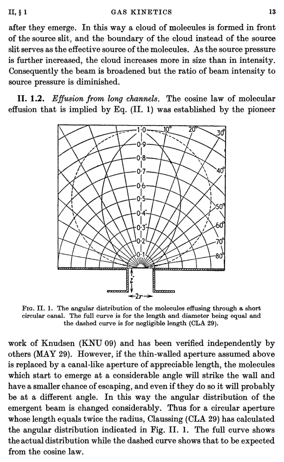
II. 1.2. Effusion from long channels. The cosine law of molecular
effusion that is implied by Eq. (II. 1) was established by the pioneer
Fig. II. 1. The angular distribution of the molecules effusing through a short
circular canal. The full curve is for the length and diameter being equal and
the dashed curve is for negligible length (CLA 29).
work of Knudsen (KNU 09) and has been verified independently by
others (MAY 29). However, if the thin-walled aperture assumed above
is replaced by a canal-like aperture of appreciable length, the molecules
which start to emerge at a considerable angle will strike the wall and
have a smaller chance of escaping, and even if they do so it will probably
be at a different angle. In this way the angular distribution of the
emergent beam is changed considerably. Thus for a circular aperture
whose length equals twice the radius, Claussing (CLA 29) has calculated
the angular distribution indicated in Fig. II. 1. The full curve shows
the actual distribution while the dashed curve shows that to be expected
from the cosine law.
14
GAS KINETICS
II, §1
One consequence of the changed angular distribution with canal-
shaped apertures is that the total amount of gas which emerges from
the source is diminished while that which emerges in the direction of
the canal is undiminished, provided the pressure is sufficiently low for
collisions inside the canal to be negligible, that is, provided XMs >, I,
where I is the canal length. This improvement of beam intensity per
amount of source material consumed is of great value in many molecular-
beam experiments such as those with radioactive isotopes. The
effectiveness of the canal in reducing the total number of molecules that
emerge from the source can be expressed in terms of a factor l//c which
is such that Eq. (II. 2) with a canal-like aperture is replaced by
Q = (l/K)invAs. (II. 7)
Claussing (CLA 29) and others (SMO 10, SIL 50) have calculated the
values of 1/ac for apertures of a number of different shapes. Their results
for slits of various shapes are as follows if w is the width and h the
height of a rectangular slit, r the radius of a circular aperture, and I
the length of the canal.
(a) Any shape aperture of very short length or with 1 = 0:
l//c = 1. (II. 8)
(6) Long circular cylindrical tube with I ;> r:
(c) Long rectangular slit with h ;> I, I ;> w:
1/k == ^ln-. (II. 10)
I w
(d) Long rectangular slit with I > h, I > w:
(P+^)' , l3+w\ (IL n)
O ö J
(e) Long rectangular slit with I > h, I > w, h > w (a special limiting
case of the preceding formula when h ^>w):
l/K = !{l+21nÇ). (II.12)
II, §1
GAS KINETICS
15
Silsbee (SIL 50), with different assumptions, has derived a formula that
agrees with the last one except that the 2 in the denominator is replaced
by 8/3.
If the aperture is of a shape different from any of the above, a poorer
approximation to l/#c can often be obtained for large I from the
expression of Knudsen (KNU 09)
l//c = (16/3)
hi*
dl
(II. 13)
where 0 is the periphery and A the area of a normal cross-section at
position I along the length of the canal. As is present just to cancel
that in Eq. (II. 7). If the cross-section of the canal remains unaltered
along its length, Eq. (II. 13) reduces to
\jK = (ie/3)AllO.
(II. 14)
It should be noted that Eq. (II. 9) is a special case of Eq. (II. 14).
All of the above expressions except Eq. (II. 8) assume that I is much
greater than the narrowest slit dimension. For short canals of infinite
height, Claussing (CLA 29) has calculated and tabulated values of l/#c
for various values of Ijw. His results are given in Table II. i.
Table II. i
Effusion of Gas through Canals of Infinite Height and
Intermediate Length
Values of the factor (l//c) for use in Eq. (II. 7) with canals of intermediate lengths
but infinite height are given in the following table. These values were calculated
by Clausing (CLA 29) and additional tabulated values may be found in his original
paper (CLA 29, FRA 31). The length of canal is designated by I and the width
by w.
l/w
0
01
0-2
0-3
0-4
0-5
0-7
1/k
1
0-9525
0-9096
0-8710
0-8362
0-8048
0-7503
l/w
10
1-5
20
30
40
50
8-0
00
1/k
0-6848
0-6024
0-5417
0-4570
0-3999
0-3582
0-2789
w. 1
Tln-
l w
16
GAS KINETICS
II, §2
II. 2. Molecular-beam intensities and shapes
II. 2.1. Beam intensities. If the pressure in the molecular-beam
apparatus is sufficiently low that no appreciable amount of the beam
is scattered out and if no collimating slit or similar obstruction
intercepts the beam on its way to the detector, the theoretical beam
intensity can readily be calculated from the expressions of the preceding
section.
Let Ad be the area of the detector, l0 be the length of the apparatus
from source to detector, and / be the beam intensity or number of
molecules which strike the detector per second. Then from Eq. (II. 1)
I = i^nMs. (11.15)
If p' is the source pressure in mm Hg, M the molecular weight (not the
weight of the molecule), T the absolute temperature in °K, As and Ad
in cm2, and l0 in cm, the preceding equation can be re-expressed as
J = M18X1022 f 'fjïf* molecules sec"1. (II. 16)
The above expression for the beam intensity assumes that there is
no attenuation of the beam by scattering. If there is such attenuation
in any chamber, such as the separating chamber, through which the
beam passes, the resultant beam intensity can be obtained by
multiplying Eq. (II. 16) by the attenuation factors appropriate to each such
chamber. If Xkv is the mean free path for a beam molecule of velocity
v in passing through the Jcth. chamber whose length is lk, the attenuation
factor for that chamber and that molecular velocity is exp(—lkl\kv).
With the very narrow beams used in molecular-beam experiments,
collisions which deflect a molecule only slightly are sufficient to eliminate
the molecule from the beam. As a result the appropriate value for X^
in molecular-beam experiments is often less than the mean free path
appropriate to other less sensitive experiments. A more detailed
discussion of beam attenuation by gas scattering is given in Section II. 4.
II. 2.2. Beam shapes. If a collimator slit is in position, the apparent
beam intensity measured at a specific location is no longer given by
Eq. (II. 16), but it depends on how much of the beam is intercepted
by the collimator. In general the measured beam intensity depends
on the widths of the source, collimator, and detector slits and on their
II, §2
GAS KINETICS
17
relative positions. However, the beam shape can most easily be
calculated by first considering the dependence of the beam intensity on
detector position in the limit when the detector is infinitely narrow, i.e.
the beam intensity that reaches the detector but is not integrated over
/ x »
1/
/
i\
» \
|w>c+00c-wp a\ =2p
fec+QUc+Wg) a] =2d
Fig. II. 2. Relation of source and collimator
widths to beam shape. In the penumbra region
the intensity varies linearly with
displacement since the amount of exposed source varies
in this way. Consequently the beam is of
trapezoidal shape.
a detector slit of appreciable width. This beam shape can easily be
determined with the aid of Fig. II. 2 to be that given in Fig. II. 3,
where
P = iK+K-w>l> (II. 17)
d = h[wc+(wc+ws)al
a = hdßsc = hdfisc—I = r~ *>
r = hdlhc>
(II. 18)
(II. 19)
(II. 20)
and where lcd is the distance from collimator to detector, lsc the distance
from source to collimator, lsd the distance from source to detector, ws
the width of the source slit, wc the width of the collimator slit, p the
half-width of the top of the trapezoidal beam shape, and d the half-
3595.91 C
18
GAS KINETICS
H, §2
width of the bottom of the trapezoidal beam shape. The absolute value
signs are included to make the result valid in the case when the
collimator slit is so narrow that there is no position at the detector location
for which the source is completely unobscured. A special case, that is
often relevant, is that for which ws = wc — w and a = 1; the preceding
equations then give „ , /TT ^ v
H ë p = \W\ d = fw. (II. 20 a)
The trapezoidal character of the beam is apparent from the fact that
full intensity is received at a detector position for which the source is
completely unobscured. Onthe other hand, if the source is partially
obscured the amount of obscuration varies linearly with position at the
detector. From this linear characteristic it is apparent that the beam
intensity per unit detector width I0(sQ) is given as a function of the
observation position s0 at the detector position by the following:
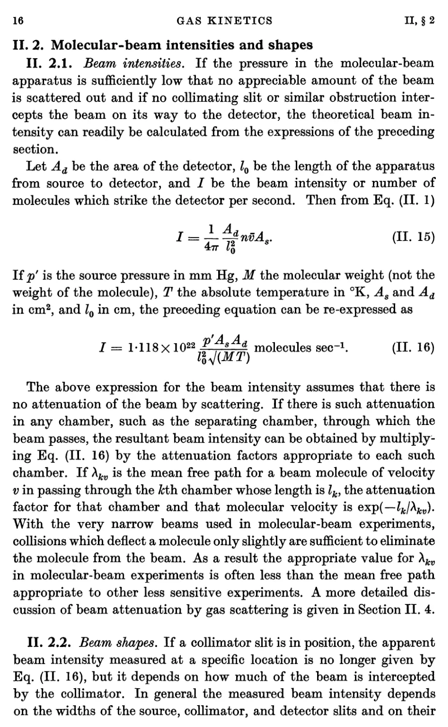
(a) In region AB, where — d < s0 < —p,
W = Joo^°- (H. 21)
(6) In region BC, where — p < s0 < p,
/„(«„) = /„<>• (II- 22)
(c) In region CD, where p < s0 < d,
« = IooP^- (II- 23)
a—p
If the collimator and source widths are such that in the region BC the
source is completely unobscured, 700 is the beam intensity per unit
detector width that would be observed in the absence of a collimator
as in Eq. (II. 15). If on the other hand the source is partially obscured
in this region, 700 is reduced in proportion to the amount of
obscuration.
If the beam is measured with a detector of appreciable width, for any
specific location of the detector the observed total beam intensity is
the integral of all of Fig. II. 3 that is included within the detector slit
width. Consequently, the beam intensity pattern that is observed as
such a detector is moved across the beam is similar to Fig. II. 3 but
the sharp edges are all rounded off by the effect of detector slit width.
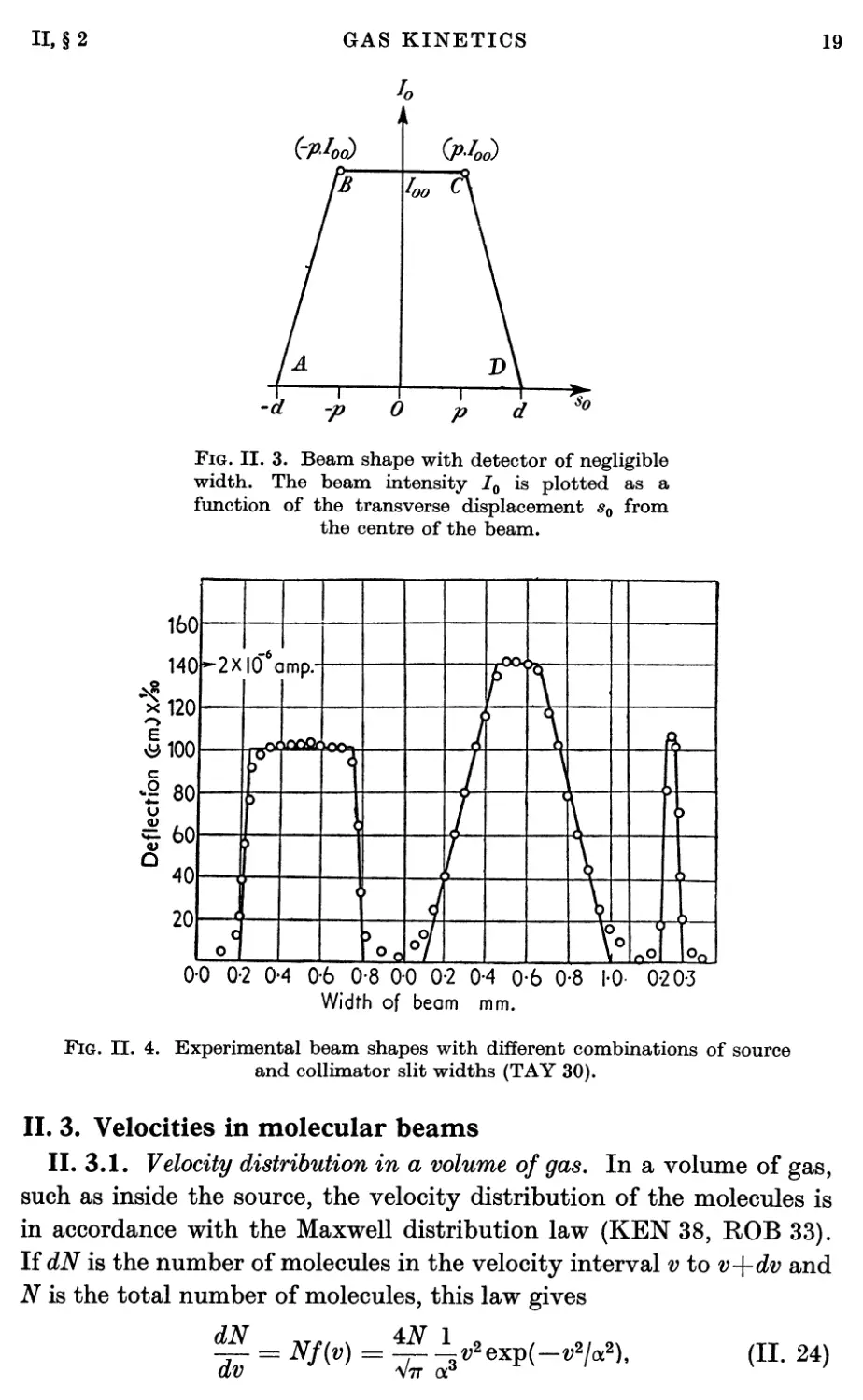
Fig. II. 4 shows typical experimental beam shapes obtained with
sources, detectors, and collimators whose slits are of various widths.
II, §2
GAS KINETICS
19
Mo)
(pW
0
*o
Fig. II. 3. Beam shape with detector of negligible
width. The beam intensity I0 is plotted as a
function of the transverse displacement s0 from
the centre of the beam.
0-0 0-2 04 0-6 0-8 0-0 0-2 0-4 0-6 0-8 1-0 0-20-3
Width of beam mm.
Fig. II. 4. Experimental beam shapes with different combinations of source
and collimator slit widths (TAY 30).
II. 3. Velocities in molecular beams
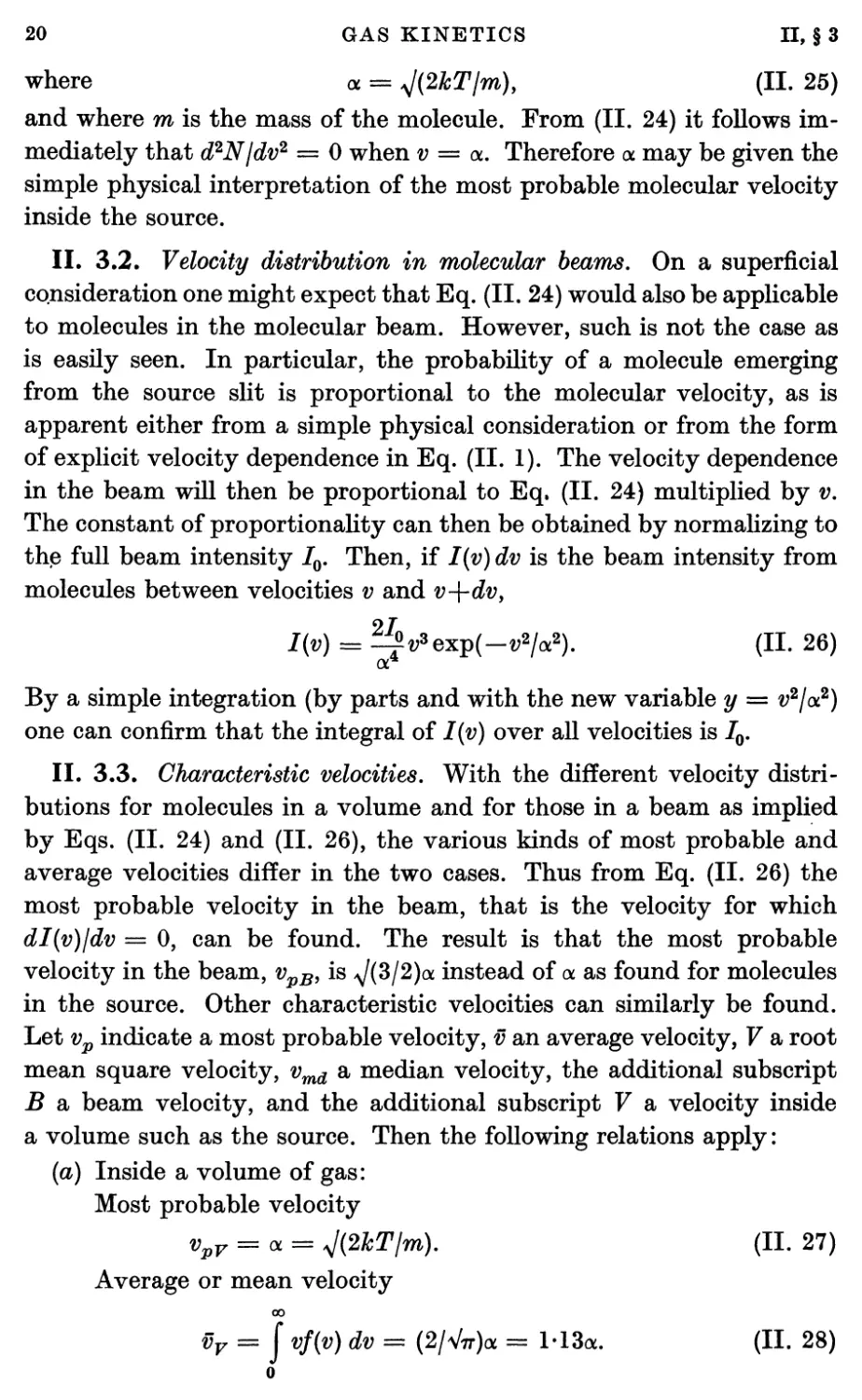
II. 3.1. Velocity distribution in a volume of gas. In a volume of gas,
such as inside the source, the velocity distribution of the molecules is
in accordance with the Maxwell distribution law (KEN 38, ROB 33).
If dN is the number of molecules in the velocity interval v to v-\-dv and
N is the total number of molecules, this law gives
dN A7,, x ±N 1 2 ,
— = Nf(v) = -j- ^2exp(-
-v2l*2)
(II. 24)
20
GAS KINETICS
II, §3
where oc = J(2kTlm)y (II. 25)
and where m is the mass of the molecule. From (II. 24) it follows
immediately that d2N/dv2 = 0 when v = oc. Therefore oc may be given the
simple physical interpretation of the most probable molecular velocity
inside the source.
II. 3.2. Velocity distribution in molecular beams. On a superficial
consideration one might expect that Eq. (II. 24) would also be applicable
to molecules in the molecular beam. However, such is not the case as
is easily seen. In particular, the probability of a molecule emerging
from the source slit is proportional to the molecular velocity, as is
apparent either from a simple physical consideration or from the form
of explicit velocity dependence in Eq. (II. 1). The velocity dependence
in the beam will then be proportional to Eq. (II. 24) multiplied by v.
The constant of proportionality can then be obtained by normalizing to
the full beam intensity IQ. Then, if I(v) dv is the beam intensity from
molecules between velocities v and v-\-dv,
I(v) = ^3exp(-v2/a2). (II. 26)
or
By a simple integration (by parts and with the new variable y = v2/oc2)
one can confirm that the integral of I(v) over all velocities is I0.
II. 3.3. Characteristic velocities. With the different velocity
distributions for molecules in a volume and for those in a beam as implied
by Eqs. (II. 24) and (II. 26), the various kinds of most probable and
average velocities differ in the two cases. Thus from Eq. (II. 26) the
most probable velocity in the beam, that is the velocity for which
dl(v)/dv = 0, can be found. The result is that the most probable
velocity in the beam, vpB, is *J(3/2)oc instead of oc as found for molecules
in the source. Other characteristic velocities can similarly be found.
Let vp indicate a most probable velocity, v an average velocity, V a root
mean square velocity, vmd a median velocity, the additional subscript
B a beam velocity, and the additional subscript V a velocity inside
a volume such as the source. Then the following relations apply:
(a) Inside a volume of gas:
Most probable velocity
VpV=SOL = J(2lcT/m). (II. 27)
Average or mean velocity
00
vv = j vf(v) dv = (2/Vtt)« = 1-13«. (II. 28)
o
II, §3
GAS KINETICS
21
Root mean square velocity
Vv = \jv2f(v) dvV = V(3/2)« = l'22«-
VmdV
Median velocity (such that J [I(v)II0] dv = Ù
(II. 29)
vmdV = i'09*-
(6) In a molecular beam:
Most probable velocity
vpb = V(3/2)<* = x'22a- (II. 30)
Average velocity
vB = (3/4)Vt7cx = 1-33«. (II. 31)
Root mean square velocity
VB= V2a= 1-42«. (II. 32)
Median velocity
vmdB = 1-30«. (II. 33)
The above characteristic velocities can be related to the temperature
of the molecules with the aid of Eq. (II. 25).
II. 3.4. Experimental measurements of molecular velocities. Some of
the earliest molecular-beam research was for the purpose of checking
experimentally the velocity
distribution of the emerging molecules. In
1920 Stern (STE 20, STE 20a) made
a first rough determination with an
apparatus whose principle is
schematically illustrated in Fig. II. 5. When
the apparatus is stationary the beam
atoms deposit at position P. If, on
the other hand, the apparatus is
rotated in the direction indicated by
the arrow, the atoms will follow a
path which will appear curved to an
observer rotating with the apparatus.
The atoms will then deposit at a
different location P\ The separation between P and P' then measures
the velocity of the atoms, and the spread of the deposit indicates the
distribution of velocities. A diagram of the actual apparatus used by
Stern is shown in Fig. II. 6. The cylinder R and its contents were
Fig. II. 5. Schematic diagram
illustrating principle of Stern's molecular-
velocity experiment (STE 20).
22
GAS KINETICS
II, §3
rotated. The source of the beam was silver atoms evaporated from the
silver-sheathed platinum wire L.
Fig. II. 6. Apparatus used by Stern in measuring
molecular velocities (STE 20).
Eldridge (ELD 27) in 1927 made a better determination of the velocity
distribution with the aid of the molecular-beam apparatus shown
schematically in Fig. II. 7. The system of disks was mounted in a large
glass tube, the lowest disk served as the rotor of an induction motor
and rotated the whole system of disks at speeds of up to 7,200
revolutions per minute. The other disks each had a hundred radial slots and
when rotated served as a velocity filter. Cadmium atoms were used
for the beam and they emerged from the slit, which was connected to
the cadmium reservoir which could be heated in a furnace. The spread
of the cadmium deposit then measures the velocity distribution of the
II, §3 GAS KINETICS 23
Fig. II. 7. Eldridge's method for molecular-velocity measurement (ELD 27).
=»- s in mms.
Fig. II. 8. Results of Eldridge's measurements of beam intensity as a function
of displacement. To the left is the undeflected trace with the rotor only in very
slow rotation; to the right is the spectrum at a high rotor velocity. The full
curve at the right is the theoretical distribution on the assumption of negligible
parent beam width. The agreement is in.part fortuitous as can be seen from the
dashed theoretical curve in which allowance is made for the known width of the
parent beam (FRA 31).
atoms. The experimental results are shown by the small circles in Fig.
II. 8. The left portion is obtained when the disks are rotated very
slowly and the right portion is for rapid rotation, The theoretical result
24
GAS KINETICS
II, §3
that would be expected with very narrow slots and the beam velocity
distribution of Eq. (II. 26) is shown by the solid curve in the figure.
However, this excellent agreement is in part fortuitous (FRA 31) since
the predicted result from Eq. (II. 26) is that shown by the dashed curve
when suitable allowance is made for the slit widths.
Lammert (LAM 29) has also used a rotating slotted disk to measure
the velocity distribution of the beam molecules. He obtained even
better agreement with Eq. (II. 26) than did Eldridge.
Some of the early experiments on velocity distributions were inspired
by the hope of finding some kind of a departure from the classical
distribution law due to quantum effects. However, Lenz (LEN 29) and
others (HAL 34) have shown that this hope was not warranted by the
quantum theory which actually developed.
Despite this theoretical result, several more recent experiments have
been made of velocity distributions by Cohen and Ellett (COH 37);
Saski and Fukuda (SAS 38); Estermann, Simpson, and Stern (EST 47);
Knauer (KNA 49); Miller and Kusch (BRO 54), and others (MOO 53,
BEN 54). Cohen and Ellett (COH 37) used a Stern-Gelach experiment
(see Chapter IV) to provide the velocity selection in the beam. At low
oven pressures they found excellent agreement with theory, but at
source pressures of 1-4 mm of Hg and above they found a definite
deficiency of slow atoms. This deficiency they attributed to a greater
scattering of the slower molecules in the vicinity of the oven slit.
Estermann, Simpson, and Stern (EST 47) determined the velocity
distribution by defining the beam with horizontal slits and by observing
the free fall of the molecules under gravity. They, too, found a deficiency
of slower atoms which was worse at high source pressures than at low.
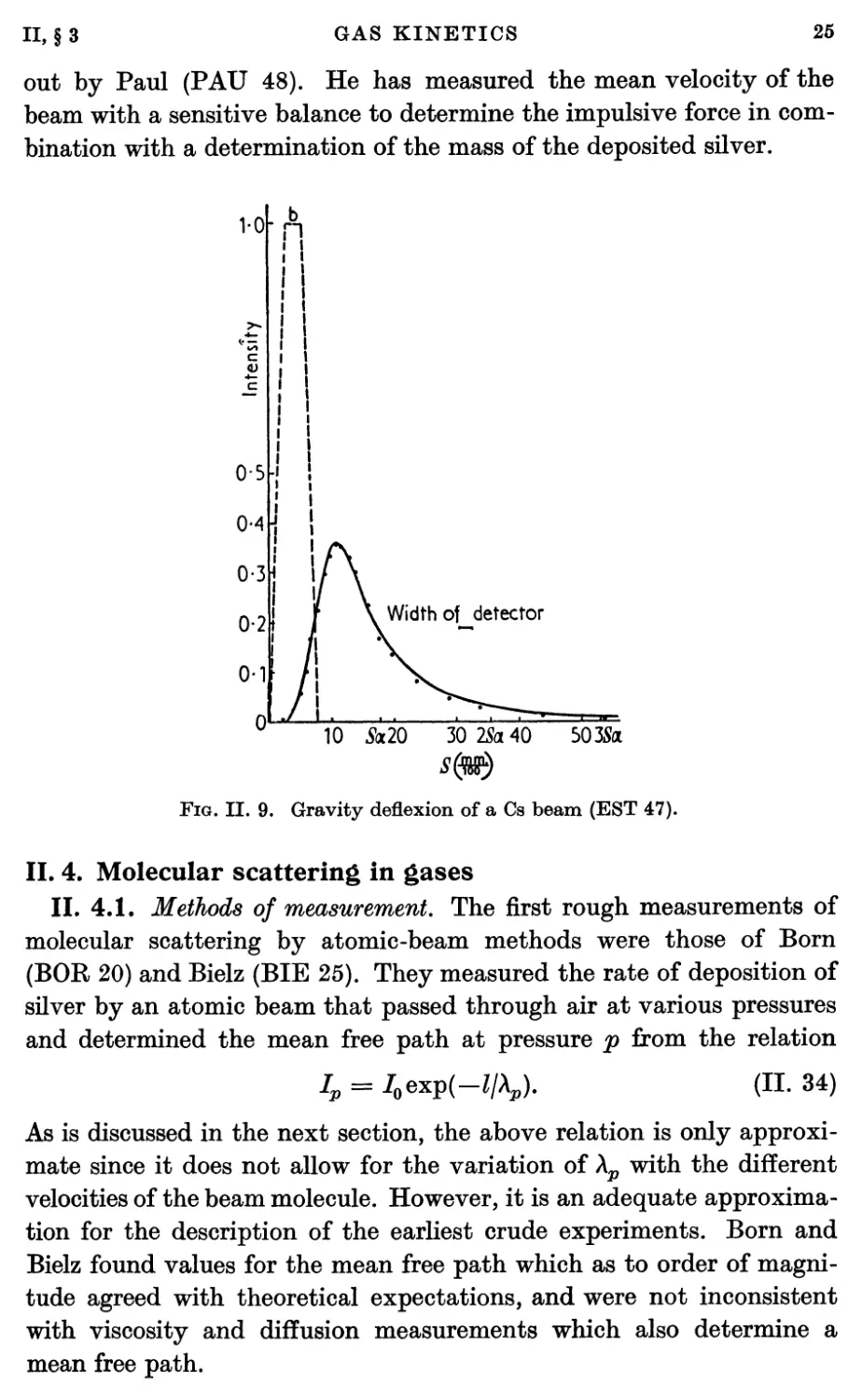
A typical result of their experiment is shown in Fig. II. 9. The curve
indicates the pattern to be expected from the velocity distribution of
Eq. (II. 26). Their results indicated that departures from the
predictions of Eq. (II. 26) occurred at even lower source pressures than found
by Cohen and Ellett. Even at source pressures of 2x 10⁻² mm Hg and
with an oven slit 3 mm X 0-06 mm they found more than a 10 per cent,
deficiency of the slower molecules. Similar results have been obtained
by Knauer (KNA 49a). Knauer determined the velocity distribution
by electronically measuring the time of flight of an interrupted beam.
He agreed with the other observers in attributing the deficiency of slow
molecules to scattering by the cloud in the neighbourhood of the source
slit.
A quite different experiment on molecular velocities has been carried
II, §3
GAS KINETICS
25
out by Paul (PAU 48). He has measured the mean velocity of the
beam with a sensitive balance to determine the impulsive force in
combination with a determination of the mass of the deposited silver.
VO
c
£
0-5
0-4
0-3
0-2
0-1
10 SoclO 30 25a 40 5035a
Fig. II. 9. Gravity deflexion of a Cs beam (EST 47).
II. 4. Molecular scattering in gases
II. 4.1. Methods of measurement. The first rough measurements of
molecular scattering by atomic-beam methods were those of Born
(BOR 20) and Bielz (BIE 25). They measured the rate of deposition of
silver by an atomic beam that passed through air at various pressures
and determined the mean free path at pressure p from the relation
Ip = I0exV(-llXp). (II. 34)
As is discussed in the next section, the above relation is only
approximate since it does not allow for the variation of Xp with the different
velocities of the beam molecule. However, it is an adequate
approximation for the description of the earliest crude experiments. Born and
Bielz found values for the mean free path which as to order of
magnitude agreed with theoretical expectations, and were not inconsistent
with viscosity and diffusion measurements which also determine a
mean free path.
I b
n
•!
i
i
i
i
i
i
i
i
i
t
Li
i
li
]i
u
i
i
i
i
i
li
r j
i
1
!
i
i
i
»
i a.
'A
1/ \
f \ Width of detector
/l \
8. . ^--^
26
GAS KINETICS
II, §4
Knauer and Stern (KNA 26, KNA 29) measured the mean free path
for the non-condensable gas hydrogen by measuring the beam intensity
as a function of source pressure, and by attributing the saturation that
was observed to scattering of the beam by the hydrogen gas in the
apparatus, which increases in proportion to the source pressure for a
non-condensable gas and for a constant pumping speed. The value they
obtained for the mean free path was about 0-4 times that from standard
Fig. II. 10. Rosin and Rabi apparatus for effective collision
cross-sections (ROS 35).
viscosity and diffusion measurements. They attributed this difference
to the fact that a very gentle collision between two molecules which
deflects them only slightly is fully effective in attenuating the well-
collimated molecular beams, whereas such a collision is relatively
ineffective in viscosity or diffusion problems.
Broadway and Fraser (FRA 33, BRO 33, BRO 35, KNA 35) obtained
a higher angular resolution by confining the scattering gas to a limited
region by using a crossed molecular beam, i.e. the normal molecular
beam passed close above the circular opening of an oven from which
mercury was streaming molecularly. Fraser particularly investigated
the scattering at small angles and confirmed, in agreement with
quantum theory (see Section II. 4.4), that the cross-section rose to a high value
for small-angle scattering but that this high value was not infinite.
Some of the most extensive measurements of mean free paths have
been those of Rosin and Rabi (ROS 35). Their apparatus is shown in
Fig. II. 10. In different experiments, beams of neutral atoms of Li,
II, §4
GAS KINETICS
27
Na, K, Rb, and Cs from the oven (1) passed through the scattering
chamber (4) and were detected with a surface ionization detector. H2,
D2, He, Ne, and A were used as scattering gases. Both the change in
beam shape and the attenuation of the beam by the scattering gas
were observed. The beam shapes with and without the scattering gas
are shown in Fig. II. 11. Although the beam intensity is reduced by
the scattering gas there is no appreciable change in beam shape. The
Scattering of
sodium by argon
o Vacuum
O x Gas
o
Width of detector il \\ One minute of arc
^ .^Position of detector
Fig. II. 11. Apparent beam shape with and without argon
scattering of sodium (ROS 35).
absence of such a broadening indicates that only a small fraction of the
atoms are scattered by only a few minutes of arc. This result is in
agreement with the quantum-mechanical interpretation of Section II. 4.4 and
in agreement with Broadway's result discussed in the preceding
paragraph. The inference of scattering cross-sections from the attenuation
measurements of Rosin and Rabi (ROS 35) and of Rosenburg (ROS 39)
by the same method will be discussed in the next section.
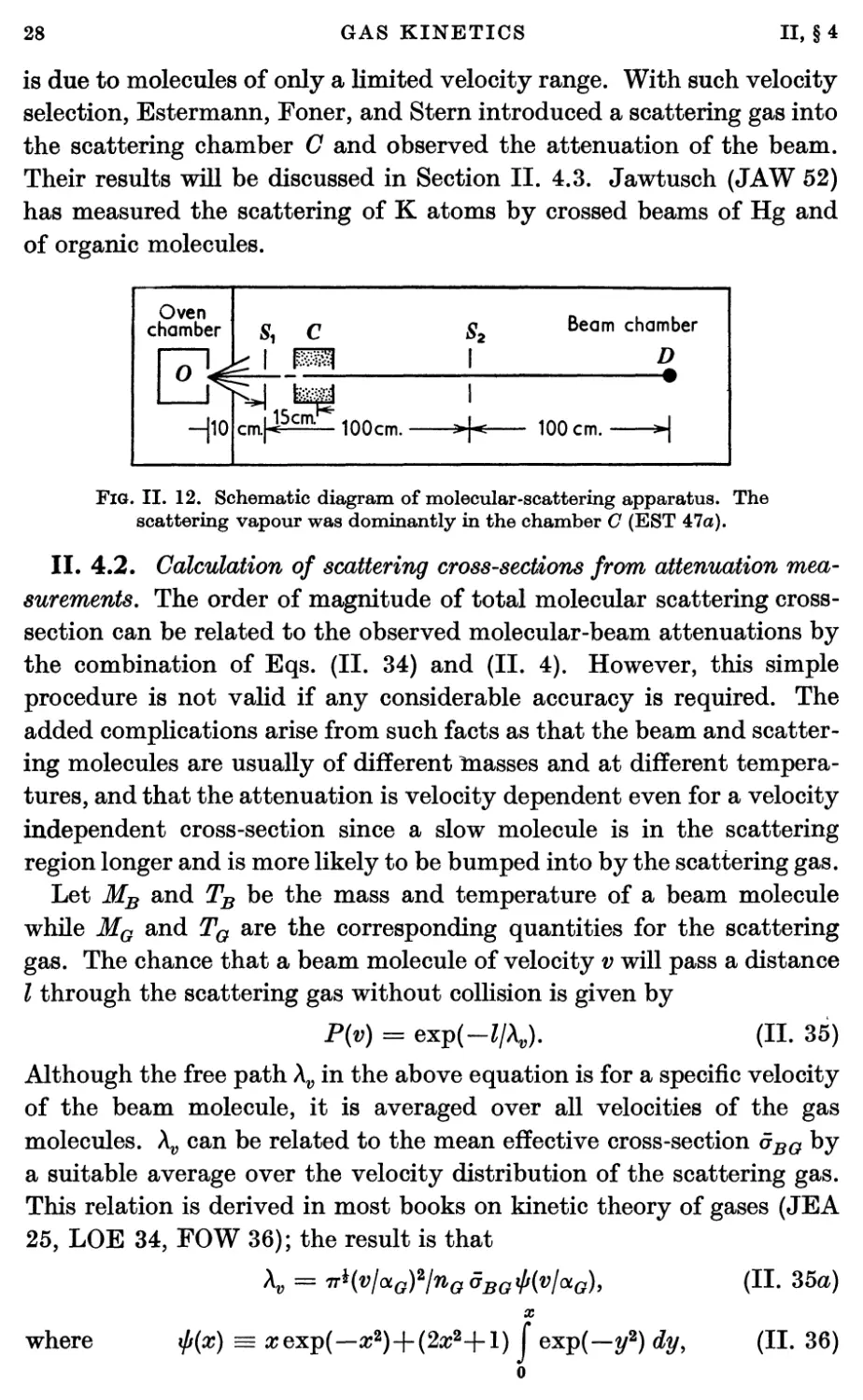
Estermann, Foner, and Stern (EST 47a) measured gas scattering
with the same apparatus they used for measuring velocity distributions
by the free fall of the atoms in a beam as described in Section II. 3.
Their apparatus is schematically represented in Fig. II. 12. The
molecules of different velocities follow different curved trajectories in such
an apparatus as they fall gravitationally in the apparatus.
Consequently when the detector is in a specific position the detected beam
28
GAS KINETICS
II, §4
is due to molecules of only a limited velocity range. With such velocity
selection, Estermann, Foner, and Stern introduced a scattering gas into
the scattering chamber G and observed the attenuation of the beam.
Their results will be discussed in Section II. 4.3. Jawtusch (JAW 52)
has measured the scattering of K atoms by crossed beams of Hg and
of organic molecules.
Fig. II. 12. Schematic diagram of molecular-scattering apparatus. The
scattering vapour was dominantly in the chamber C (EST 47a).
II. 4.2. Calculation of scattering cross-sections from attenuation
measurements. The order of magnitude of total molecular scattering cross-
section can be related to the observed molecular-beam attenuations by
the combination of Eqs. (II. 34) and (II. 4). However, this simple
procedure is not valid if any considerable accuracy is required. The
added complications arise from such facts as that the beam and
scattering molecules are usually of different Masses and at different
temperatures, and that the attenuation is velocity dependent even for a velocity
independent cross-section since a slow molecule is in the scattering
region longer and is more likely to be bumped into by the scattering gas.
Let MB and TB be the mass and temperature of a beam molecule
while MG and TQ are the corresponding quantities for the scattering
gas. The chance that a beam molecule of velocity v will pass a distance
I through the scattering gas without collision is given by
P(v) = expM/A,). (II. 35)
Although the free path Xv in the above equation is for a specific velocity
of the beam molecule, it is averaged over all velocities of the gas
molecules. Xv can be related to the mean effective cross-section 5BQ by
a suitable average over the velocity distribution of the scattering gas.
This relation is derived in most books on kinetic theory of gases (JEA
25, LOE 34, FOW 36); the result is that
K = ^H^hG)2lnGâBGiP(vlocG), (II. 35a)
X
where ifj{x) = xexp(-x*)+(2x2+l) j exp(-*/2) dy, (II. 36)
o
II, § 4 GAS KINETICS 29
and where nQ is the number of gas molecules per cm3 and ocG is defined
by Eq. (II. 25) for the scattering gas molecules. The ratio Ijl0 of the
beam intensities without and with the scattering gas is then equal to
the probability P(v) averaged over all beam velocities with the aid of
Eq. (II. 26). Therefore
7//0 = <P(*)>
00
= 2(%K)4 / exp[-{Znff aBGf(z)lvW}-(aLGl*B)h?]a* dx, (II. 37)
o
where x has been written for v/ocq.
The evaluation of 5BG from Eq. (II. 37) is clearly rather tedious.
An approximation that is often used is obtained by taking
///„ = <P(e)> = <exp(-^)> « exp(-Z/<AB». (II. 38)
(A^) is then determined from the experimental observations and Eq.
(II. 38). However, from Eqs. (II. 35a) and (II. 26),
<AV> = {^l5BQnQ)J{^loc%), (II. 39)
where by definition
oo
J(z) = z2 J [x5li/;(x)]exv(-zx2) dx. (II. 40)
o
Numerical values for J{z) have been calculated by Rosin and Rabi
(ROS 35) and are given in Table II. n. From this table and Eq. (II. 39)
it is apparent that in the special case when ol0Jolb = 1,
<A„> = 0-16laBGnG. (II. 41)
Table II. n
Values of J(z) for a Number of Values of z
>(z) is defined in Eq. (II. 40) (ROS 35)
z
0
005
01
0-2
0-3
J{z)
1/(2Vtt)
0-275
0-265
0-256
0-248
z
0-545
0*8
0-9
10
20
J{z)
0-236
0-221
0-216
0-211
0173
z
30
4-0
5-28
7-0
8-0
J{z)
0155
0-140
0-127
0113
0-107
z
10
15
21
25
30
35
Jiz)
0-094
00813
00714
00643
0-0589
0-0548
Although the calculation of 5BG from Eqs. (II. 38) and (II. 41) is less
accurate than by Eq. (II. 37), Rosin and Rabi have shown that
calculations by the two methods are usually in approximate agreement.
30
GAS KINETICS
II, §4
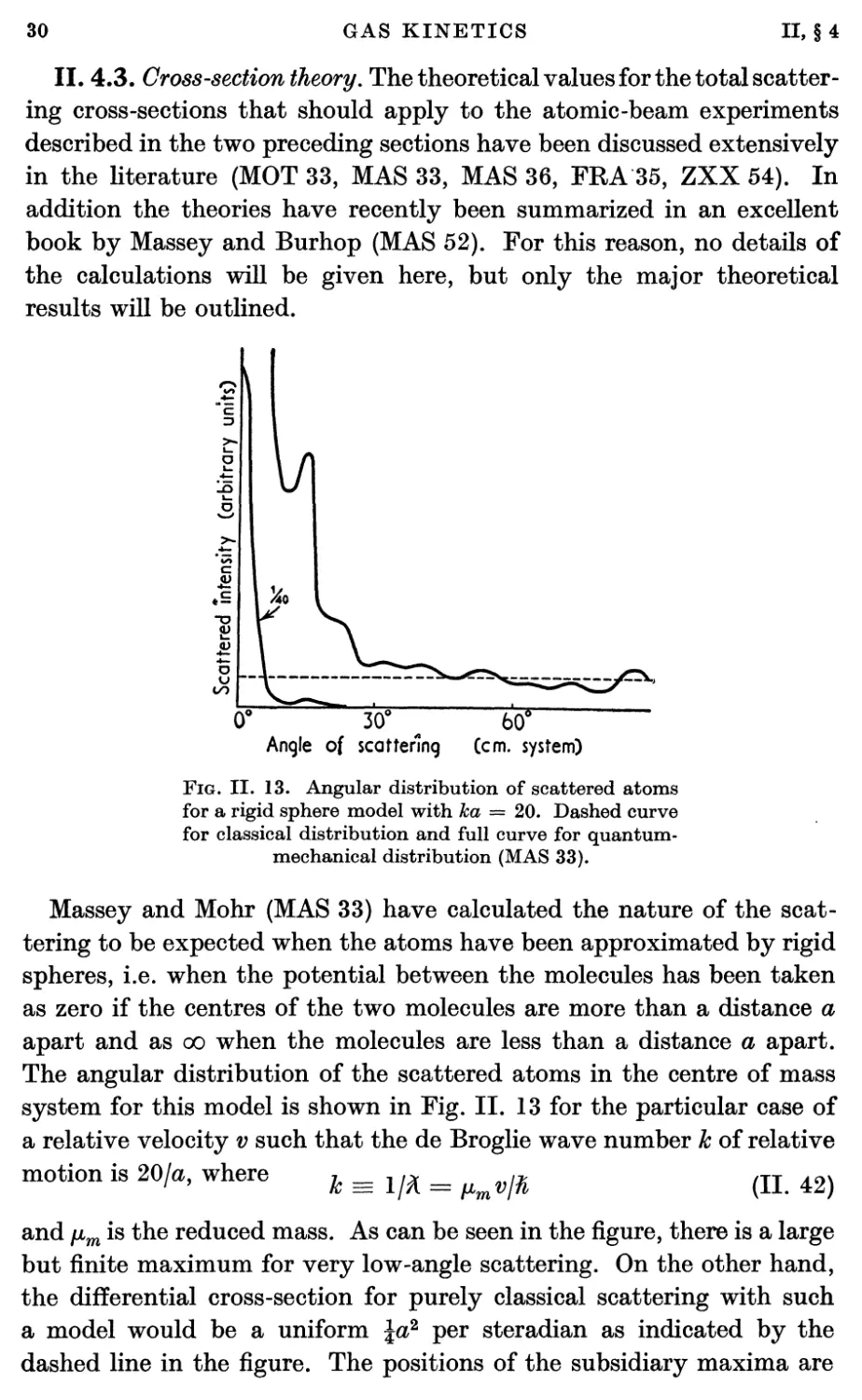
II. 4.3. Gross-section theory. The theoretical values for the total
scattering cross-sections that should apply to the atomic-beam experiments
described in the two preceding sections have been discussed extensively
in the literature (MOT 33, MAS 33, MAS 36, FRA 35, ZXX 54). In
addition the theories have recently been summarized in an excellent
book by Massey and Burhop (MAS 52). For this reason, no details of
the calculations will be given here, but only the major theoretical
results will be outlined.
0° 30°
Angle of scattering
60°
(cm. system)
Fig. II. 13. Angular distribution of scattered atoms
for a rigid sphere model with ka = 20. Dashed curve
for classical distribution and full curve for quantum-
mechanical distribution (MAS 33).
Massey and Mohr (MAS 33) have calculated the nature of the
scattering to be expected when the atoms have been approximated by rigid
spheres, i.e. when the potential between the molecules has been taken
as zero if the centres of the two molecules are more than a distance a
apart and as oo when the molecules are less than a distance a apart.
The angular distribution of the scattered atoms in the centre of mass
system for this model is shown in Fig. II. 13 for the particular case of
a relative velocity v such that the de Broglie wave number k of relative
motion is 201a, where k^1^ = ^ß (n. 42)
and fim is the reduced mass. As can be seen in the figure, there is a large
but finite maximum for very low-angle scattering. On the other hand,
the differential cross-section for purely classical scattering with such
a model would be a uniform \a? per steradian as indicated by the
dashed line in the figure. The positions of the subsidiary maxima are
II, §4
GAS KINETICS
31
in general velocity dependent so that they would be smoothed out by
the velocity distribution of the beam (MIZ 31). For this reason and
because of the very weak intensity of the scattered beam they have
never been observed. As mentioned in the preceding section, almost
all atomic-beam scattering studies have been measurements of total
cross-sections by the attenuation of the beam in passing through a gas-
filled scattering chamber.
1590°
Fig. II. 14. Total collision cross-section as a function
of ka. classical theory, — • — quantum theory
for dissimilar atoms, quantum theory for identical
atoms obeying Bose-Einstein statistics, and
quantum theory for identical atoms obeying Fermi-
Dirac statistics (MAS 33).
One use of the angular distribution curves such as Fig. II. 14 is that
they indicate the angular resolution required in an atomic-beam
experiment if the total cross-section as determined from an attenuation
experiment is to have real meaning and be independent of the resolution
of the apparatus. If a(d) is the differential cross-section and 90 is the
minimum angle of deviation which is counted as a scattering, then the
ratio j8, where
TT j TT
ß = J 0(d)smdd6 j a(6)sm6d6,
(II. 43)
should be as near unity as possible. As shown by Massey and Burhop
(MAS 52), ß will be 0-9 if
60 « 277/a(JfT)*, (II. 44)
32
GAS KINETICS
II, §4
where M is the molecular weight of the incident molecule and where
a is in Â.
The total cross-sections to be expected with the above model at
different velocities are plotted in Fig. II. 14. The temperature scale is
that for which the root mean square velocity of He is the indicated
velocity if \a = 1-05 Â. As indicated in the figure caption the different
curves are for dissimilar atoms, for identical atoms obeying Bose-
Einstein statistics, and for identical atoms obeying Fermi-Dirac
statistics, respectively. It should be noted that the total cross-section at
short wavelengths is double the classically predicted value, as first
pointed out by Massey and Mohr (MAS 33). However, as can be seen
by a comparison with Fig. II. 13, the extra scattering above the classical
prediction all corresponds to small-angle scattering. Consequently,
good angular resolution is required in the total cross-section
measurement if that is to be observed. This doubling of the total cross-section
above the classical value at short wavelengths is the familiar problem of
shadow scattering that arises in diffraction theory and nuclear
scattering as well (BLA 52). It corresponds to the fact that not only is there
scattering of the incident de Broglie wave which strikes the scatterer
but also that a destructive wave of equal amplitude and opposite phase to
the incident one must be postulated immediately behind the scatterer
to provide the necessary shadow. However, this wave at a sufficient
distance from the scatterer spreads out by diffraction, as does any
limited wave, and appears to be a small angle additional scattered wave.
For actual atoms and molecules the above rigid sphere model is a
poor approximation. As an alternative model, Massey and Mohr (MAS
33) have calculated the total cross-section for an interaction potential
which is cut off at small radii but which has the asymptotic form
V~ -Cr-8. (II. 45)
In this case they showed that the total cross-section o was given
approximately by „ «
a = „Ïl^piis-V^CMW'-V, (II. 46)
where v is the velocity of the atoms and
f(s) = ^-.S-^—...-.\n (s even and > 2),
s—2 s—4 2
f(s) = ^=|.^=| — | (« odd and > 3), (II. 47)
f(s) = 1 (s = 3), f{s) = \* (s = 2).
II, §4
GAS KINETICS
33
They showed that the above should be applicable to gas kinetic
collisions at ordinary temperatures between all atoms other than He.
The special case of s = 6, or asymptotically of
V~ -C/r6, (II. 48)
is of particular interest in Eq. (II. 46) since it is what is usually known
as a van der Waals attraction and arises from the dynamic polarization
of one atom by the other. The inverse sixth power law of attraction
arises from the fact that the two electric dipoles interact as r~s but the
polarizability process is one in which the dipoles are not free but must
be induced. As a consequence of this a second-order perturbation
calculation is required so that the dependence is as (r-3)2. Some of the results
to be presented in the next section will be interpreted with the aid of
Eq. (II. 46) in the special case of s = 6.
II. 4.4. Results of atomic-beam scattering experiments. The earliest
important result of atomic-beam scattering experiments was the
demonstration by Born (BOR 20) and Bieler (BIE 25) that cross-sections as
determined from molecular-beam scattering experiments were of the
same order of magnitude as those from other kinetic theory experiments
such as viscosity and diffusion measurements. Knauer and Stern (KNA
29) with the experiment described in Section II. 4.1 showed that the
mean free path in hydrogen-beam scattering experiments was about
0-4 times that to be expected from the measurements of viscosity and
diffusion if the latter were interpreted in terms of a classical rigid-sphere
model. However, the experiments could be reconciled with an angular
distribution, such as that in Fig. II. 13, which provides a large amount
of small-angle scattering since such scattering would be relatively
ineffective in viscosity and diffusion phenomena but would be fully
effective in scattering molecules from the beam. Fig. II. 13 shows that for
a rigid-sphere model the quantum-mechanical distribution is suitable
to account for the molecular-beam results whereas the classical
predictions with the same model are in definite disagreement with experiment.
On the other hand, with an interaction potential as in Eq. (II. 46) a
classical theory predicts a forward scattering peak as required by the
experiment of Knauer and Stern (KNA 29).
In fact, with a potential of the form of Eq. (II. 48), a classical theory
overdoes the prediction of a small-angle scattering peak and predicts
one whose differential cross-section becomes infinite as the angle tends
to zero. On the other hand the experiments of Broadway and Fraser
3595.91
D
34
GAS KINETICS
II, §4
(FRA 33, BRO 33, BRO 35, KNA 35) and of Rosin and Rabi (ROS 35)
show that the forward-scattering cross-section remains finite as
discussed in Section II. 4.1 above. The lack of change in the beam shape
of Fig. II. 11 is a particularly effective demonstration of the finiteness of
the small-angle scattering. The quantum-mechanical prediction is that
for an interaction of the form of Eq. (II. 45) with s > 3 the scattering
should be finite though large at small angles in agreement with
experiment.
A number of effective total cross-sections measured by the atomic-
beam method are given in the literature, particularly in the papers of
Mais (MAI 34), Rosin and Rabi (ROS 35), Rosenberg (ROS 39), Ester-
mann, Foner, and Stern (EST 47a), and others (DOR 38, ZZA 1).
Knauer (KNA 33, KNA 34) and Zabel (ZAB 33, ZAB 34) have observed
the influence of temperature on the scattering of molecular beams. In
Table II. m are given observed collision cross-sections of alkali metal
atoms with rare-gas scattering atoms. The large disagreement between
the measurements of Rosin and Rabi (ROS 35) and Estermann, Foner,
Table II. in
Observed Collision Cross-sections for Alkali Rare-gas Atom Collisions
and derived van der Waals Constants
The van der Waals constant G is defined by Eq. (II. 48). All measurements are
by Rosin and Rabi (ROS 35) except for data marked with a dagger (f) which are
by Rosenberg (ROS 39), with an asterisk (*) by Mais (MAI 34), and with a double
asterisk (**) by Estermann, Foner, and Stern (EST 47a). The calculated values
of G have been given by Massey and Burhop (MAS 52). Ga indicates the value of
G inferred from the listed collision cross-section a while Gv indicates the value of G
inferred from atomic polarizability data (MAS 52).
Alkali
atom
Li
Li
Li
Na
Na
Na
K
K
K
Rb
Rb
Rb
Cs
Cs
Cs
Rare gas
atom
He
Ne
A
He
Ne
A
He
Ne
A
He
Ne
A
He
Ne
A
a
(10-16cm2)
106
120
303
130
213
401
165, 170-8f, 150*
259, 239*
580, 587-lf, 400*
152
268
572
162,(446**)
287
572
Ca
(lO"60 cm6)
14-4
18-7
188
17-8
40-4
192
31-7
50-5
356
25-4
49-0
249
29-4 (370**)
56-7
235
%
(lO"60 cm6)
17
32
125
(26)
(51)
(200)
35
68
260
40
(77)
(290)
44
87
325
II, §4
GAS KINETICS
35
and Stern (EST 47a) in the case where they overlap is both puzzling
and disturbing. If the interaction between the atoms is assumed to be
of the form of Eq. (II. 48), the value of the van der Waals constant G
can be derived from Eq. (II. 46). These constants derived from the
molecular-beam cross-sections are given in Table II. in. However, the
polarizabilities of the alkali atoms have been measured in other
molecular-beam experiments (SCH 34a) and the polarizabilities of the rare-
gas atoms can be deduced from refractivity measurements. Since the van
der Waals interaction is a second-order polarizability effect, the constant
G can be calculated from the polarizability data (MAS 52). The values
of G so determined are listed in Table II. m for comparison with the
values inferred from molecular-beam data. On the whole the
agreement is quite good except for the anomalously large G inferred from
the Cs-He experiment of Estermann et al. (EST 47a).
II. 5. Interaction of molecular beams with solid surfaces
II. 5.1. Introduction. When a molecule strikes a surface it may
suffer an elastic collision and rebound immediately with no loss of
energy or it may suffer an inelastic collision in which case it may either
gain or lose energy. A special case of an inelastic process is for the
molecule to lose so much energy that it remains adsorbed on the surface.
In the case of adsorption the molecule can either remain permanently
on the surface or it may remain there for only short time and then be
restituted to the gas. The molecules which rebound immediately and
elastically can do so in directions that have a direct probability relation
to the direction of incidence. Such molecules are studied in the sections
below entitled Reflection and Diffraction. The remaining cases are
discussed in the section on Inelastic collisions.
II. 5.2. Reflection.. The simplest type of reflection of molecules at
a surface is specular reflection, that is the incident beam, the normal
to the surface at the point of impact, and the reflected beam are all in
the same plane and the angle of incidence equals the angle of reflection
just as in the corresponding optical case.
Two conditions must be satisfied to achieve specular reflection:
(a) The height of the irregularities of the surface when projected on
the direction of the beam must be less than a wavelength. This is just
the familiar requirement for reflection in optical experiments, which is
illustrated by the fact that a piece of smoked glass is a poor reflector
at normal incidence but a good one at glancing incidence. If h is the
average height of irregularities and if <£0 is the glancing angle of the
36
GAS KINETICS
II, §5
incident beam (the complementary angle to the angle of incidence 0O),
this requirement is , . ,
H Asin0o<A. (11.49)
(b) The average time the molecule spends on the surface must be
small. If this is not so the conditions under which re-evaporation of
the molecule will occur will bear no relation to those which prevailed
at condensation. Instead they will be determined by the last stages
of the history of the molecule on the surface.
The irregularities of the best mechanically polished surfaces are of
the order of 10~5 cm, while the de Broglie wavelength for hydrogen at
room temperature is of the order of 10-8 cm. When these values are
substituted in Eq. (II. 49) the condition for reflection becomes <f>0 < 10~3
or the glancing angle must be less than a few minutes of arc.
With polished speculum metal Knauer and Stern (KNA 29a) indeed
observed a 5 per cent, reflecting power for a hydrogen beam at an angle
of 10-3 and at room temperature. The reflecting power is taken as the
maximum intensity of the reflected beam divided by the maximum
intensity of the parent beam. They also found that the reflecting power
was increased if the temperature of the beam was lowered, as would be
expected from Eq. (II. 49).
The smoothest surfaces that are obtainable are the cleaved surfaces
of a crystal. Even these surfaces are not completely smooth because
the ions in the surface are subject to temperature vibrations about their
positions of equilibrium. The amplitudes of these oscillations are of the
order of 10-8 cm. Consequently a roojn-temperature helium beam
should show specular reflection for glancing angles less than 20° or 30°.
The result anticipated above has been found by Estermann and Stern
(EST 30) in the reflection of a helium beam from a cleaved LiF crystal.
Their experimental result is shown in the curve of Fig. II. 15 where
the beam intensity is plotted as a function of the glancing angle. It
will be noted in a comparison of the curves at two different
temperatures that the reflecting power at the lower beam temperature begins
to fall off only at larger glancing angles in agreement with Eq. (II. 49).
Johnson (JOH 28) has found similar effects with atomic hydrogen and
rock salt. The dependence of the reflecting power on the crystal
temperature has been studied (KNA 29a, EST 30, JOH 28) in a number of
experiments. In all cases the reflecting power is increased by a lowering
of the crystal temperature. This is in agreement with previous
assumption that in cleaved crystals the h of Eq. (II. 49) was largely due to thermal
vibrations of the ions in the crystal lattice.
II, §5
GAS KINETICS
37
The importance of the above condition (b) for the production of
specular reflection is clearly indicated in an experiment of Taylor (TAY
30, JOS 33). He searched for a specularly reflected Cs beam from the
Parent beam 290°K : 320cm.
I00°K; 340cm.
100°K
Glancing angle
Fig. II. 15. Reflecting power of LiF for a helium beam at two different
temperatures of the LiF (EST 30).
30
25
£20
Q
5
0° 10° 20° 30° 40° 50° 60° 70° 80° 90° 100° 110°
Angle of reflection
Fig. II. 16. Restitution of Li from cleaved planes of NaCl. The solid curve
represents angular distribution of scattering according to Knudsen's law and
the circles represent the observed intensities. The incident beam was at a
glancing angle of 15° (TAY 30).
cleaved surface of NaCl and LiF. Although the condition of Eq. (II. 49)
was fully satisfied he found no specularly reflected beam for glancing
angles between 2° and 60°. An example of his results for an incident
glancing angle of 15° are shown in Pig. II. 16. No signs of a specularly
reflected beam at 15° can be seen. The angular distribution of the
-HO"
U
3amp
®
A
s
os*
38
GAS KINETICS
II, §5
restituted beam is in complete accord with the Knudsen cosine law as
in Eq. (II. 1) which is plotted as the solid curve in the figure. This is
what would be expected for atoms that were adsorbed on the surface
and then later re-evaporated.
Knauer and Stern (KNA 29a, HAN 32, JOS 33) have studied
reflection with a number of different gases forming the molecular beam; out
of H, H2, He, Ne, A, and C02 only H, H2, and He gave strong specular
reflection with NaCl.
If condition (b) above is satisfied but condition (a) is not, one obtains
diffuse reflection. With a macroscopically rough surface the molecules
emerge from hills and valleys in random directions even though each
one has been reflected on impact. Hence unless the surface is smooth
it is difficult to distinguish between reflection and adsorption with
re-evaporation.
y
t T T T T T—t
1111111
x + + 1 + £ +—x
Fig. II. 17. Scattering centres in a cross-grating (MAS 52).
II. 5.3. Diffraction. When the molecules are reflected by the cleaved
surface of a crystal the crystal appears like a two-dimensional cross-
grating as shown in Fig. II. 17. For a one-dimensional grating as in
Fig. II. 18, it is apparent that the difference in path for the two rays is
a cos oc—a cos a0.
For this to provide constructive interference it should equal an integral
multiple of the de Broglie wavelength A. A similar analysis applies to
the two-dimensional cross-grating of Fig. II. 17. For the incident beam
making angles (a0, ßQ, yQ) with the coordinate axes the maxima of the
II, § 5 GAS KINETICS 39
diffracted beam should be at angles (a, ß, y) with these axes, where
cos oc—cos a0 = n2A/a,
cosjS—cosj80 = n2A/a, (II. 50)
where nx and n2 are any integers, positive or negative. The diffracted
rays are often designated by (nvn2).
man
Fig. II. 18. Diffraction by a one-dimensional grating (FRA 31).
0.-1
Fig. II. 19. Diffraction of a molecular beam by a cross-grating. The positions
of the (0,0) specularly reflected and the (0, ±1) diffracted rays are shown
(MAS 52).
The case of nx = n2 = 0 is just the case of specular reflection that
was discussed in the preceding section.
In most molecular diffraction experiments the crystal is arranged so
that j30 is zero. Fig. II. 19 illustrates the (0,0) reflected and (0, ±1)
diffracted rays.
The first experimental evidence that molecular rays were diffracted
by the cleavage plane of a crystal as from a cross-grating was obtained
40
GAS KINETICS
II, §5
by Stern (STE 29). This work was extended by Estermann and Stern
(EST 30); Estermann, Frisch, and Stern (EST 31, EST 31a); Johnson
(JOH30, JOH31); and others (ELL 29, ELL 37, ZAH 38, ART 42,
COH 37, KEL 32, MIS 51, VES 38, ZAB 32). A typical result is that
of Estermann and Stern (EST 30) as shown in Fig. II. 20. The central
-2cr
-iow ov -1er
Angle of diffraction
•2CT
Fig. II. 20. Diffraction of He at a glancing angle of 18-5° on a cleavage face of
LiF (EST 30).
peak is the specularly reflected (0,0) beam and the side peaks are the
(0, ±1) beams. The broadening of the peaks arises because the beam
is not monochromatic in the de Broglie waves in consequence of the
Maxwell distribution of the molecular velocities.
The most complete investigations of molecular-beam diffraction have
been those of Frisch and Stern (FRI 33a). Their apparatus is shown
schematically in Fig. II. 21. It provided a convenient means for rotating
the crystal about its principal axis OX, i.e. for varying the angle i/j of
Fig. II. 19. Their results for helium on LiF are shown in Fig. II. 22.
The dashed curve gives the theoretically predicted distribution of
intensity for the (0,1) diffracted beam, derived from the Maxwell
distribution of velocity (FRI 33a, LEN 34). The agreement with position
and shape of the experimental distribution is generally quite good but
the two experimental irregularities for f s of 20° and 26° that also
occur for corresponding negative values of i/j are reproducible irregu-
II, §5
GAS KINETICS
41
larities that are smaller than the experimental error. Similar anomalies
were found in specular reflection when the angle rj between the plane
Fig. II. 21. Frisch and Stern's apparatus for studying diffraction of molecular
beams (FRI 33a).
-30° -20° -10° 0° +10° +20° +30°
Fig. II. 22. Observed variation with 0 of reflected intensity for a beam of
helium atoms incident on the cleavage plane of a LiF crystal. Dashed curve is
the theoretical intensity for (0, 1) diffraction (FRI 33a).
of incidence and the principal axis OX of the crystal was varied.
A typical result is shown in Pig. II. 23. Similar anomalies were also
found with He on NaF and H2 on LiF.
42 GAS KINETICS ü, § 5
From an analysis of the conditions under which the anomalous
minima appeared Frisch (FBI 336) was able to show that they arose
when, for the diffracted or reflected beam under observation, the
components^ and py of the molecules' momenta bore certain relations to
Fig. II. 23. Variation of reflected intensity with 17 for a beam of helium atoms
incident on the cleavage plane of a LiF crystal at angles of 65°, 68°, and 70°
(FBI 33a).
each other (see Figs. II. 17 and II. 19 for the specification of the axis
orientation). This relation is demonstrated in Fig. II. 24 where the
values of pz and py which correspond to the minima are plotted. The
analytical relation corresponding to these curves is
(2WA)a-2pya/A==-l-26,
(p8alh)*-2pyalh = 0. (11.51)
Frisch suggested that these anomalies were due to a preferential
adsorption of beam molecules when the condition of Eq. (II. 51) was satisfied.
Lennard-Jones and Devonshire (LEN 36) developed a beautiful
quantum-mechanical mechanism for Frisch's phenomenon, which they called
selective adsorption. They showed that when the conditions of Eq.
(II. 51) were satisfied, a transfer of energy from motion perpendicular
to the surface to motion parallel to the surface may easily take place
because of the periodic nature of the lattice. The molecules then slide
freely over the crystal surface while vibrating with a finite amplitude
in the normal direction. Hence, if the momentum conditions are correct,
this variety of adsorption can take place with a corresponding reduction
II, § 5 GAS KINETICS 43
in the reflected or diffracted intensity. Alternatively, if after collision
the reflected or diffracted beam satisfies the conditions it may be
adsorbed in this way before leaving the crystal.
The details of the analysis of Lennard-Jones and Devonshire may be
found in their original paper (LEN 36) or in the book of Massey and
Burhop (MAS 52). However, the justification of the relations of Eq.
(II. 51) may be seen from a simple qualitative argument. Let unprimed
1-5
10
pzajh
0-5
05 1-0 1-5 2-0
pya/h
Fig. II. 24. Relation between momentum components p%9 py of the diffracted
and specularly reflected molecular beams when anomalous minima occur
(FRI 336).
kx's designate 2tt times de Broglie wave-number components before the
molecules strike the surface and primed k'xs the same things afterwards,
so 1cx = pjh. Let En be the binding energy of the molecule when
occupying an allowed energy level as far as motion normal to the surface
is concerned. Then, from the conservation of energy,
kl+kl+k* = k'*+k'*-2mEnlh\ (II. 52)
From now on let the consideration be limited to transitions for which
1cx = k'x. A transition between two different states in most transition
probability calculations occurs when there is a resonance between the
difference in wave number of the two states and the wave number of
the periodic phenomenon inducing the transition, so it is not
unreasonable that the selection rule for the transition is
rf/oa
/c<0
ky—ky= ±27r/a.
(II. 53)
44
GAS KINETICS
II, §5
A detailed proof of (II. 53) is given in the basic references (LEN 36,
MAS 52), but the essential fact is that in the absence of such a coherency
the integrals involved in the calculation of the transition matrix
integrate to zero owing to the oscillatory character of the integrands. From
Eqs. (II. 52) and (II. 53) with the negative choice of sign and from
the assumed equality of kx and 1c'x, it follows immediately that
k2-2ky(2ix\a) = (2ix\a)2-2mEn\W,
or (Pzalh)2-2(Pvalh) = l-2mEn(a/h)2. (II. 54)
The identity of Eq. (II. 54) with the empirical relation of Frisch in
Eq. (II. 51) gives a beautiful confirmation of the theory of Lennard-
Jones and Devonshire. The existence of two parabolas shows that there
are at least two oscillatory states for an adsorbed. He atom on LiF.
A comparison of Eqs. (II. 54) and (II. 51) provides determinations of
the values of En, which are of value in the theory of surface phenomena.
For He on LiF the values inferred for En are 57-5 and 129 cals, per mole.
II. 5.4. Inelastic collisions. One of the simplest varieties of inelastic
collision of a molecule with a surface is the so-called free-free collision
in which the molecule rebounds immediately but with either a gain or
loss of energy. It is this kind of collision that often largely determines
the rate of interchange of energy between a gas and a solid at a different
temperature. The rate of interchange depends on Knudsen's thermal
accommodation coefficient a', which is defined as follows. Let Ei denote
the average energy brought up to the wall by a molecule, Er the average
energy carried away by the restituted molecule, and Ew the average
energy of the molecule if it were in thermal equilibrium with the wall.
Then the accommodation coefficient oc is defined by
a' = (Et-Er)l(Et-Ev). (II. 55)
Extensive summaries of the experimental studies on accommodation
coefficients and of the theories of free-free inelastic transitions have
been given in the book of Massey and Burhop (MAS 52). Since few of
these measurements have involved molecular-beam techniques such
summaries will not be repeated here. However, it should be noted that
one of the most important molecular-beam detectors—the Stern-Pirani
detector described in Chapters I and XIV—depends on this process.
Inelastic collisions which lead to adsorption can either be followed
by a subsequent restitution of the molecule to the gas or by its perma-
II, §5
GAS KINETICS
45
nently remaining on the surface. Both of these processes have been
studied with molecular-beam techniques. A theory of adsorption has
been developed by Lennard-Jones and Devonshire (LEN 35, LEN 36)
and summarized by Massey and Burhop (MAS 52).
In the case of adsorption and subsequent restitution, the earliest
studies were devoted to a determination of the angular distribution of
the restituted molecules. As discussed in Section II. 5.2, if the molecule
has been adsorbed for an appreciable time the conditions under which
re-evaporation of the molecule will occur bear no relation to those which
prevailed at condensation. Instead they will be determined by the last
stages of the history of the molecule on the surface. Consequently one
would expect the angular distribution to be that for the simple
evaporation of molecules. Knudsen (KNU 15) has pointed out that this angular
distribution should be in accordance with a simple cosine law. If N
molecules, whose directions lie within a solid angle dœ', strike a surface
for which there is no specular reflection or diffraction, then the number
dN of those restituted from the surface within an element of solid angle
dœ making an angle 6 with the normal to the surface is, according to
K*11^11' dN = {l/n)N cos Odœ. (II. 56)
For a gas and a surface in complete equilibrium, it can be shown that
the cosine law for all the molecules that come off the surface is a
necessary consequence of the second law of thermodynamics (GAE 13, EPS
24). However, Knudsen's law is more general in that it is assumed to
apply to evaporated molecules even in the absence of equilibrium.
The earliest molecular-beam studies of the angular distribution of
the restituted molecules were those of Wood (WOO 15). He allowed a
mercury beam to fall on plane glass target at the centre of a bulb and
then examined the thickness of the deposit on the bulb. He later did
the same thing with a cadmium beam. The Knudsen law (Eq. II. 56)
was obeyed to within the experimental error.
Knudsen (KNU 15) performed a similar experiment in which the
restituting surface itself was part of the receiving sphere as in Fig.
II. 25. In that case the mercury deposit on the sphere should be
uniform if Knudsen's law were followed and this was found experimentally
to be true.
One objection to the above experiments was that a cosine law might
result from the roughness of the surface. However, Taylor (TAY 30)
showed that this was not the case by observing the restitution of Li, K,
and Cs atoms from the cleaved planes of NaCl and LiF. As described
46
GAS KINETICS
II, §5
above in Section II. 5.2 and illustrated in Fig. II. 16, Taylor obtained
a complete confirmation of the Knudsen law in these cases (TAY 30,
HUR 54). On the other hand, if He, H2, or H is used with the same
cleaved crystals reflection and diffraction phenomena are observed, as
pointed out in Section II. 5.2 (HAN 32).
c '
Fig. II. 25. Apparatus for confirmation of Knudsen's law
(KNU 15).
Numerous molecular-beam experiments have been made to study
adsorption phenomena. Since these experiments and the corresponding
theories (LEN 36, ZEN 32) have been summarized in books by Fraser
(FRA 31) and Massey and Burhop (MAS 52) they will not be described
in detail here. Some of these experiments have been for the purpose
of measuring the time of adsorption for the restituted molecules, i.e.
the mean time for which they linger on the surface before being
restituted to the gas (CLA 30, ZXX 54). In other experiments the
conditions for permanent adsorption and the migrations of atoms over the
surface while they are adsorbed have been studied (EST 23, COC 28,
FRA 31, DEV52, JOH 33, STA 34, STE 20a, MEL 52, ZXX 54).
Measurements of condensation or sticking coefficients have been made
and tabulated by a number of observers including Fraunfelder (FRA
50), whose paper contains an extensive list of other references, and
Wexler (BRO 54). An important application of these measurements
has been in the selection of suitable collector materials for experiments
in which moments of radioactive nuclei are measured by molecular*
beam methods in which the detection is by the deposition of radioactive
materials as in Section XIV. 3.6. Condensation coefficients may vary
from less than 0*0001 to almost one, depending on the materials,
temperature, surface condition, etc. For example, with Cs on clean W the
condensation coefficient is 0-7.
II, §6
GAS KINETICS
47
IL 6. Molecular-beam studies of chemical equilibria, ionization
potentials, and optical and microwave spectroscopy
II. 6.1. Chemical equilibria. The effusion of molecular beams from
sources provides a means of measuring vapour pressures as functions
of temperature since the beam intensity will depend upon vapour
pressure of the source as shown in Eq. (II. 16); this was first pointed
Nr
H
N
k
25
Zisch + 21
Gebhardt A
Hackspill 0
Kroner x -^
Rodebush 6 De Vries A 19|
Egerton t Edmondson
29
|27
2$
23
Ï321!
19
17
0915
Fig. II. 26. Vapour pressures of sodium and potassium. T is in °K and P in
mm of Hg (EDM 27).
out by Knudsen (KNU 09). However, frequently a mixture of both
atoms and molecules effuses from the source. For example, a sodium
beam is a mixture of Na and Na2. Therefore the relative contribution
of the different components must be distinguished before a significant
vapour pressure determination can be deduced (FR A 31). A detailed list
of references to vapour pressure measurements determined in this way
has been given by Fraser (FRA 31). Typical results are shown in Fig.
II. 26 for sodium and potassium (EDM 27).
Molecular beams can also be used as a means for determining the
degree of molecular dissociation that occurs, i.e. the fraction of the total
possible number of combined molecules in the vapour that are
dissociated. There are many means for distinguishing between say the Na2
molecules and the Na atoms which effuse from the source (FRA 31,
WEI 26, ROD 27). One of the simplest is by deflexion in an inhomo-
geneous magnetic field (see Chapter IV) since the paramagnetic Na
48
GAS KINETICS
II, §6
atoms are easily deflected and the diamagnetic Na2 molecules are only
slightly deflected (LEU 28). As discussed in Section VIII. 11, molecular
beams have been used to study the degree of polymerization of vapours
(e.g. NaCl to (NaCl)J.
eraser (FRA 34, FRA 37a) has pointed out that free radicals such
as CH3 and C2H5 can be studied by molecular-beam techniques. Beams
of these radicals have been formed by Fraser
and Jewitt (FRA 37a), and such properties
as their ionization potentials have been
measured. The initiation of elementary
chemical processes by molecular beams has
I II || | been studied (MAR 52).
|| m I Ç II. 6.2. Ionization and excitation. Mole-
i I Id I imtzj pp cular beams have sometimes been used in
the study of ionization potentials (FRA 31,
FRA 37, FUN 30, JEW 34). A typical
apparatus for such a measurement is
illustrated in Fig. II. 27. In this method a
homogeneous electron beam is fired from K to C
at right angles across the atomic beam, and
the ions so formed are collected by a Faraday
cage in which the atomic beam itself is
condensed. With such an apparatus one can
measure both the ionization potentials and
the ionization function (the probability of
ionization as a function of the electron
energy). Photo-ionization has also been
studied by molecular-beam methods of a
similar nature except that the crossed
electron beam is replaced by electromagnetic
radiation (FRA 31, DOR 38). Electron
bombardment ionization has been used to detect
beams in other experiments (WES 53).
Smyth (SMY 22) and others (DIT 29) have ionized the atoms in an
atomic beam by cross bombardment with electrons and have then
analysed the ion products with a mass spectrometer. In this way the
degree of ionization was determined.
One of the earliest applications of molecular beams was in the study
of excitation by Dunoyer (DUN 13). Dunoyer excited a sodium beam
Fig. II. 27. Funk's apparatus
for measuring the ionization
cross-sections of Na and K
by the atomic-beam method.
K is the electron source
and G the electron collector
(FUN 30).
II, §6
GAS KINETICS
49
to emit resonance radiation and then observed the sharpness with which
the region of emitted radiation fell off. From this he could show that
the duration of the excitation was less than 10~7 sec. Since the atomic
beam travels only about 0-01 cm in such a short time, the atomic beam
method is in general ill adapted to the study of excited electronic states
whose transitions to lower states are allowed. However, as discussed
Fig. II. 28. Typical atomic-beam source for optical hyperfine-structure
measurements. The beam emerges from oven O and is cross-bombarded by the electron
beam from cathode K (PAU 41).
in Chapter IX, even such states as these can be studied to some extent
with a suitable molecular-beam resonance method (RAB 52). Since
metastable excited states ordinarily have lifetimes that are long
compared with the length of time that it takes a molecule to traverse the
apparatus, they are well adapted to almost all molecular-beam methods
and have frequently been studied (HUG 53, ZXY 54). Frisch (FRI
33d) has detected the recoil of Na atoms when an atomic beam of such
atoms is irradiated with resonance radiation; this experiment showed
that the momentum of the absorbed photon was indeed acquired by the
atom.
3595.91
E
50
GAS KINETICS
II, §6
II. 6.3. Optical and microwave absorption spectroscopy. An atomic
beam forms one of the most effective sources for high-resolution optical
spectroscopy. Collision broadening of the spectral lines is eliminated
by the low density of the beam and Doppler broadening is greatly
diminished if the emitted light is viewed in a direction at right angles
to the beam so that the component of velocity in the direction of
observation is small. Such atomic beam sources have been used by
many observers, including Jackson and Kuhn (JAC 34), Minkowski
(MIN 35), Meissner (MEI 37), Paul (PAU 41), and others (DUN 13,
DOB 28, SUR öl, HEY 38). A typical atomic-beam source is shown in
Fig. II. 28. Atomic-beam sources have been particularly effective in
the study of hyperfine structure by means of high-resolution optical
spectroscopy. Descriptions of the optical techniques employed and of
the detailed methods of term analysis are given in books on optical
spectroscopy such as those of Tolansky (TOL 48) and Kopfermann
(KOP 40).
Kastler (ZZA 2, BIT 496), Brossel (ZZA 2, BIT 496), Bitter (BIT
496), Dicke (ZZA 4), Bucka (ZZA 3), and others (ZZA 2, ZZA 4, ZZA 9,
ZZA 10, BIT 496) in some cases have combined the use of polarized
light in optical excitation and detection with the use of oscillatory
radiofrequency fields in such a way that the optical experiments are
quite similar to experiments with the atomic beam magnetic resonance
methods of Chapters I and IX. However, these optical experiments
will not be discussed extensively here since the detection techniques
employed are primarily those of optical spectroscopy.
Molecular beams have been used successfully by Strandberg and
Dreicer (STR ö4) in microwave absorption experiments as a means for
diminishing Doppler broadening. These experiments are to be
distinguished from many of the microwave molecular-beam experiments
discussed below, in that the transitions in Strandberg and Dreicer's
experiments were detected by their effects on the radiation field rather
than by the changed state of the molecule.
Ill
INTERACTION OF A NUCLEUS WITH
ATOMIC AND MOLECULAR FIELDS
III. 1. Introduction
Many of the most important molecular-beam measurements are
determinations of the interactions between a nucleus of a molecule and
the molecular fields at the nucleus from the remainder of the molecule.
For this reason, detailed considerations of molecular-beam
measurements are best preceded by a theoretical discussion of the interaction
of a nucleus with atomic and molecular fields.
The interactions between a nucleus and its atom or molecule may
be studied in various ways, including the methods of optical
spectroscopy, molecular beams, nuclear paramagnetic resonance, microwave
spectroscopy, and paramagnetic resonance as described in the author's
book on Nuclear Moments (RAM 53e). All of these measurements are
consistent with the following assumptions concerning atomic nuclei:
(a) A nucleus has a charge Ze confined to a small region of the order
of lO-12 cm diameter. It is the interaction of this charge with the
electrons of an atom that gives rise to the gross features of optical
atomic spectra.
(6) A nucleus whose mass number A is odd obeys Fermi-Dirac
statistics (the sign of the wave function is reversed if two such identical
nuclei are interchanged), and a nucleus whose mass number A is even
obeys Bose-Einstein statistics (wave function unaltered on interchange).
(c) A nucleus possesses a spin angular momentum capable of being
represented by a quantum-mechanical angular momentum vector a
with all the propertiesf usually associated with such vectors. In nuclear
moment work it is usually most convenient to use a dimensionless
quantity I to measure the angular momentum in units of #, where I is
therefore defined by a _ ^j (HI x)
The spin / of a nucleus is defined as the maximum possible component
of I in any given direction.
(d) The nuclear spin I is half integral if the mass number A is odd
and integral if the mass number is even.
f Good discussions of the properties of angular momentum vectors are given in books
by Condon and Shortley (CON 35), Wigner (WIG 31), Feenberg and Pake (FEE 53),
Racah (RAC 42), Pauli (PAU 32), and Schwinger (SCH 46, SCH 52).
52 INTERACTION OF A NUCLEUS WITH III, § 1
(c) A nucleus has a magnetic moment (PAU 24) \lz which can be
represented as |i, = y,« = fo/%1, (HI. 2)
where yI and gz are defined by the above equation and are called the
nuclear gyromagnetic ratio and the nuclear g factor, respectively. fiN
is the nuclear magneton defined as éHj2Mci where M is the proton mass.|
fjiN has the numerical value of (5-05038±0-00036)x 10~24 erg gauss"1.
The scalar quantity which is a measure of the magnitude of (jlz and
which is called the magnetic moment /x7 is
^ = yiM. (III. 3)
With this Eq. (III. 2) can be written
HZ = fall)l. (III. 4)
(/) Many nuclei with spin equal to or greater than 1 possess an
electrical quadrupole moment, i.e. have electrical charge distributions
which depart from spherical symmetry in a manner appropriate to an
electrical quadrupole moment. (A precise definition of an electrical
quadrupole moment is given in the next section.)
(g) A nucleus with a spin 3/2 or greater may possess a magnetic
octupole moment (JAC 54). (The definition of a magnetic octupole
interaction is given in the next section and in Section IX. 9.)
(h) The nucleus is neither infinitely heavy nor of negligible size, but
instead with certain experiments allowance must be made for the finite
mass and appreciable size of the nucleus (BRE 32, ZXW 54).
(i) The nucleus has a finite polarizability and can be polarized by
a strong electric field (KOP 49, BRE 50, GUN 51, RAM 53/).
III. 2. Electrostatic interaction
III. 2.1. Multivoie expansion. The general electrostatic interaction
3tf*E between a charged nucleus and the charged electrons and nuclei
of the remainder of the molecule is as follows, if the finite extension of
the nucleus is taken into account:
tfB= f [PePndredrn (In 5)
Te T»
t In the literature on the subject of nuclear moments there is considerable confusion
as to notation. In different papers /*0, fin, fxNM represent the nuclear magneton, whereas
Mo» Mi» and ß designate the Bohr magneton. Here /jln will be used for the nuclear
magneton and fi0 for the Bohr magneton. Also in many papers g or gs is written for
fij/IfxNt but in others g represents /^/fyo- In the present book g2 will ordinarily designate
fjLjlIfiN, but in Chapter IX it will designate /xj/J/Xo m order to be consistent with the
literature of molecular-beam hyperfine-structure experiments ; it is clear from the context
which meaning applies.
HI, § 2
ATOMIC AND MOLECULAR FIELDS
53
pe is the charge density of the electrons and of the other nuclei in the
volume element dre at position re relative to the centroid of the nucleus
concerned, so that pe is a function of re. pn is the nuclear charge density
of the nucleus concerned, in the volume
element drn at position rn relative to
the centroid of the nucleus, whence pn is
a function of rn. In addition r is the
magnitude of the radius vector r drawn
from drn to dre as shown in Fig. III. 1.
The definition of pe is such that it is
negative for electrons and positive for
positive charges.
Let 6en be the angle between re and rn
and let re be greater than rn, as may be
ensured by limiting consideration to
electronic charges more distant than the
radius RN of the nucleus (exceptions to
this restriction are discussed in Sections
II. 3.1 and IX. 10). This limitation will
be indicated explicitly by the use of a
superscript e with p% to indicate charges
external to a small sphere of radius BN
surrounding the nucleus and centred on the nuclear centroid. Then
from the cosine law of trigonometry 1/r may be expressed as follows,
using the well-known power series expansion in rjre [cf. MAR 43, p. 96,
MOR 53]:
1/r = (r2e+rl-2rernoosden)^ = 1/^+^ + ^ + ^+..., (III. 6)
where Pk is the Jcth Legendre polynomial of cos 6en, so that
P1 = cos0en,
P2 = K3cos2^-l),
P3=!(5cos306n-3cos06n),
1 dk
From Eqs. (III. 5) and (III. 6), one can write
Fig. III. 1. Electrostatic interactions
of a nucleus in atoms and molecules.
(III. 7)
ÙE
?•
vEk>
(III. 8)
54 INTERACTION OF A NUCLEUS WITH III, § 2
where XEk = j J* ^rlffiP*<cos °en) dredrn. (III. 9)
Te Tn
The «^ term which involves Pk is said to be the interaction energy
from the multipole moment of order 2k. Thus the first term corresponds
to a monopole or single charge, the second to the electric dipole moment,
the third to the electric quadrupole moment, the fourth to the electric
octupole moment, etc.
The direct evaluation of Eq. (III. 9) would necessarily be difficult
since 0en depends upon both the nuclear and the electronic coordinates
and so the double integration is not separated into two integrations each
of which involves only the electron or the nuclear coordinates.
However, such a separation can be achieved by using the spherical harmonic
addition theorem [see CON 35, p. 53 or RAC 42] according to which
Pft(C0SOe„) = ^Zl 2 (-1)4^(COSÖ«'^)F(Ä(COsöe^e)
q=-k
= i (-iy*c™(0n,4>jc®neM (in. io)
f=-k
where C<*>(0, <£) = [4w/(2fc+ l)]*7<*)(oos 0, <£),
6n is the angle between rn and an arbitrary fixed z-axis, <f>n the azimu-
thal angle of drn from the #z-plane, while 0e and <f>e are the
corresponding quantities for dre as shown in Fig. III. 1. Yqk) is the normalized
tesseral harmonic . . j
where ®qk) except for normalization is the associated Legendre polynomial
defined for q > 0 as
and for q < 0 as ©<*> = (-1)*®% (III. 13)
With these expressions, the 2k interaction can be written as
^k=Q(fc)-F<fc>, (III. 14)
where the use of the heavy dot (• ) in Q(fc)#F(fc) for the irreducible (RAC
42) tensors Q(A:) and F(fc) of degree k indicates the tensor scalar product
defined by k
tfEk = Q<*>.F<*> = J (-1W^P (HI. 15)
q=—k
where
(III. 16)
rf (cos e, 4>) = ©»»(cos e) ^3 &*, (in. ii)
Ill, § 2
ATOMIC AND MOLECULAR FIELDS
55
n*> = y (a^ï) J />^,-(Ä+i)nÄ)(eos öef « dre
= J rfre-(*+1>C*»(0e, </>e) dre. (III. 17)
The integrals in Eqs. (III. 16) and (III. 17) have the great advantage
that they separately concern either the electron or the nuclear
coordinates, but not both simultaneously (RAC 42, POU 50).
Although Eqs. (III. 15), (III. 16), and (III. 17) give the general 2*-
pole interaction energy, they are inconvenient to work with in their
most general form. However, the specific expressions applicable for the
three lowest multipoles may easily be derived as in the following
paragraphs.
The monopole interaction is
2tfm = Zeft, (III. 18)
where Ze = Q<») = j Pndrn (III. 19)
and ^ = F^ = f Ê dre. (III. 20)
e
Te
(j>e is the electrostatic potential at the centroid of the nucleus from the
electrical charges external to a small sphere of radius BN centred on the
nuclear centroid and surrounding all the nuclear charge.
In a similar fashion the electric dipole interaction is
•*» = -Pz m-iP+ &--\pJS>+, (111.21)
where pz is the z component of nuclear electrical dipole moment in a
coordinate system whose origin is at the nuclear centroid so that
Pz = QP = / Pnrncosen drn = jPnzn drn (III. 22)
and p± is defined by
p±=px±ipv = ±^Q(£\
= / Pn*nsinencos<f>ndrn±i j Pnrnsin6nsin<f>n drn
Tn
= jpn*n drn±i J Pnyn drn. (III. 23)
Tn
It is then apparent that px is the ^-component of the nuclear electrical
dipole moment. Similarly, E% is the electric field at the nuclear centroid
56 INTERACTION OF A NUCLEUS WITH III, § 2
from the electrical charges external to the small sphere of radius R
surrounding the nucleus so that
^-n^-J^COS^e"/^^-^] (HL
24)
and
E% = E%±iE% = ±F^{ = - (^smdeeoS<l>edTeTi f ^sm6esin<j>edre
' e
Te Tg
(III. 25)
It should be noted that in the derivation of the preceding equations
such differentiations as d/dz with respect to the field point can be
replaced by —d\dzt under the integral sign.
Likewise the electric quadrupole interaction can be written as
-e_x(V^)+1+Ç_2(V^)+2. (III. 26)
In the above Q0 is the zz-component of the nuclear electrical quadrupole
moment tensor. The Qq's are in general denned by
Qo = QP = \ J Pn*î(3oos*dn-1) drn = ij Pn(Zzl-rl) drn,
Tn Tn
Q±l = Q±\ = TVI j PnZn*n± *■»»
Tn
Q±2 = Q% = Vf / Pn 4± drn, (III. 27)
Tn
where xn± is an abbreviation for xn±iyn. The (VÜ7e)'s are components
of the gradient of electric field at the nuclear centroid arising from the
electrical charges external to the sphere of radius RN. They are given
explicitly by
(V2?<% = n« = I j |(3cos^e-l) dre = -I[3^-V.E]
l\dEf\
(VJ0»)±1 = F% = TV! f |f cos0esin0e(cos<k±isin&) dre
' e
Te
V6 dE<L V6
±T^ = ±ir« (IIL28>
HI, § 2
ATOMIC AND MOLECULAR FIELDS
57
(VJB»)±1 = I*& = VI j ^sin^e(cos^±isin^)2 ^ = -^0± E'±,
where a± = £-±i^-. (111.29)
0.0
u —.
0#^ 0y
In the expansions of JfEk in Eqs. (III. 21) and (III. 26), each of the
indicated terms is in general itself a sum of separate terms. As a result,
there is no uniqueness concerning the expansion in the indicated terms :
the individual terms can be recombined into other quite different
indicated terms to yield alternative expansions which superficially appear
to be quite different but which on full expansion are completely
equivalent. One such alternative can be obtained by combining the
expressions -\-q and — q in Eq. (III. 11) so as to make the expansion
in terms of cosg<£ and sin q(f> instead of e±iq4>. Another alternative is to
make the expansion in terms of the Cartesian components of the
tensor. In this case
*m = -p. E« = -Px E%-py Ey-ps E%. (III. 30)
Also tfE2 = -* £ £ G„(VJ0%, (III. 31)
i=x j=x
where Qv = j Pn(Sxnixnj-8y r») drn,
T" Coe (HI. 32)
(V2?%= - (£(3x^-8^*) dre,
Te
and where xnz denotes zn, etc. The equivalence of Eqs. (III. 30) and
(III. 31) to Eqs. (III. 21) and (III. 26) may be shown by a
straightforward expansion of each in Cartesian coordinates. Alternatively, in
the author's book on Nuclear Moments (RAM 53e) the direct calculation
of Eqs. (III. 30) and (III. 31) from Eq. (III. 9) is given.
In quantum-mechanical calculations of the expectation values for
the above expressions, pn should be replaced by its expectation value
(SCH46)
Pn = J ^(rv^,rA)popifj(rv...,rA) dr^^dr^ (III. 32a)
where Pop = £ e, 8(rw-r,). (HI. 326)
i
With this, for example, from Eq. (III. 16),
«%*>> = // r(rv..,rAKC<a">(dn)<f>n)x
Xl«i8(r„-ri)^(r1,...)rA) drv..drAdrn
i
(III. 32c)
58 INTERACTION OF A NUCLEUS WITH III, § 2
III. 2.2. Theoretical restrictions on electric multivoie orders. If a
nuclear multipole moment is associated with a nucleus of definite spin I
whose orientation properties are fully determined by the orientation
of the spin angular momentum /, the possible varieties of nuclear electric
multipole moments are restricted by two general theoretical theorems.
The first theorem arises from a parity consideration and is as follows:
If all nuclear electrical effects arise from electrical charges, if there is
no degeneracy of nuclear states with different parity, and if the nuclear
Hamiltonian is unaltered by an inversion of coordinates (replacement
of r by — r), no odd (Jc odd) electrical multipole can exist. In particular,
a nucleus satisfying the above conditions can have neither an electric
dipole moment nor an electric octupole moment.
The proof of this theorem is given in detail in the author's book on
Nuclear Moments (RAM 53e, p. 23). The essentials of the argument are
that, if the above assumptions apply, then the wave function must be
of either odd or even parity, as discussed in Section XI. 5.1, i.e.
0O*i> yv-, yA, zA) = ±i/j(—xv -yv..., -yA, —zA). (III. 33)
However, with either odd or even parity,
mxv...,zA)\* = m-x,,..., -zA)\\ (in. 34)
On the other hand, for even Jc, the Y(qk) of Eq. (III. 32c) is unaltered for
the same coordinate inversion, whereas for odd Jc the sign is reversed
upon inversion. Therefore with the latter case in Eq. (III. 16) the
integrand is of opposite sign at (—zl9..., — zA) to that at (xv...,zA).
Consequently, when the completed integration is carried out over both
these positions, the net result is zero, which proves the theorem.
In atomic problems, exceptions to the above theorem sometimes arise
owing to degeneracy of states with different parity. On the other hand,
the energy separations of different nuclear energy levels are so large
compared to normal interaction energies with nuclear electric moments
that such degeneracies are very unlikely. Purcell and Ramsey (PUR 50)
have pointed out that the above proof depends on the assumption that
the electrical effects of a nucleus arise only from electric charges, or on
a related parity assumption, and that these assumptions are not
necessarily obvious in the case of little-understood particles like nucléons
and nuclei (DIR 48). Therefore, in an experiment with J. Smith (SMI
51a, SMI 516), they searched with high precision for a possible electric
dipole moment of the neutron. They find, however, that if such a
dipole moment exists its magnitude must be less than the charge of
the electron multiplied by a distance D of 5 x 10~20 cm.
HI, § 2
ATOMIC AND MOLECULAR FIELDS
59
The second theorem is the following: For a nuclear spin J it is
impossible to observe a nuclear electrical multipole moment of order
2k for k greater than 21.
This theorem is also derived in detail in the author's Nuclear Moments
(RAM 53e, p. 24). The essentials of the argument are that if pn in
Eq. (III. 16) is written as ~ 0*0n, the equation can be expressed as
«J,*)~J«r*r<*)^ndTw. (III. 35)
Tn
However, Y(qk) is a possible orbital wave function for an orbital angular
momentum of k (CON 35, p. 52). As ifjn is a wave function of angular
momentum / and by the vector addition of angular momenta (CON 35,
p. 56), the product Yqk) ipn can be considered a wave function of a system
whose angular momentum is between k+I and |&—1\. However, since
0* and hence i/j%rk correspond to angular momentum /, they will be
orthogonal to Yqk) ipn unless they can correspond to the same angular
momentum eigenvalue. Therefore, to prevent Eq. (III. 35) from
vanishing, / must lie between k+I and \k—I | or k < 21, which is the desired
theorem. This restriction is often expressed by saying that /, /, and
k must satisfy the triangle rule, i.e. it must be possible to form a triangle
from three sides proportional to /, /, and k respectively.
Theorems analogous to the above are applicable to the field quantities
F(k) of Eq. (III. 17) when they arise from an atom or molecule whose
angular momentum is J. Thus, Fqk) vanishes unless k < 2 J. Even a
nucleus with a large I and a nuclear quadrupole moment can have no
electric quadrupole interaction energy with an atom whose J = |.
III. 2.3. Nuclear electric quadrupole interactions. The most important
orientation-dependent electrical interaction of a nucleus is that arising
from its electric quadrupole moment. It is therefore desirable to study
in further detail the effect of a nuclear quadrupole interaction upon the
energy levels of an atom or molecule. In general, the calculation of the
energy levels is performed either by a perturbation-theory calculation
or by the solution of the secular equation which results from the matrix
of the Hamiltonian when the quadrupole contributions of Eq. (III. 26)
are included. In either case, the matrix elements of the quadrupole
terms must be calculated for the representation that is used.
The matrix elements may be calculated in a number of different ways.
One procedure is the direct use of a general formula given in the next
section for any order of multipole. Another procedure, the one to be
followed in this section, depends on the observation that one usually
60 INTERACTION OF A NUCLEUS WITH III, § 2
uses a representation based on the angular momentum operators of the
atom, molecule, or nucleus. Matrix elements of functions of the
angular-momentum operators can usually be calculated easily in such
representations from the standard forms (CON 35) for (/mj|I|J'm7),
whose only non-vanishing matrix elements are
{Im^Irrtj) = m7, (III. 35a)
(/m7±l|/±|/m7) = V{(/:pm/)(/±™7+l)},
where I = ^k44^(i-ik)+iJL(i+tk), (III. 356)
where i, j, k are the Cartesian unit vectors. If, therefore, the quadrupole-
moment tensor can be expressed as simply proportional to a tensor in
the angular-momentum variables the calculation of the matrix elements
can be simplified.
The quadrupole moment tensor can be expressed in terms of the
angular momentum variables with the aid of a theorem that is most
simply proved by group theory or by the tensor-commutation rules
(WIG 31, RAC 42, WEY 39, CAS 35, CAS 36, NIE 48). However,
it can also be proved directly from simple matrix multiplications and
from the matrix elements for vectors. Such a proof is straightforward,
though numerically tedious, and is given in the author's book on
Nuclear Moments (RAM 53/, p. 21). By whatever the means of proof,
the theorem applies to all tensors which transform under space rotations
in the same way as does Eq. (III. 11). This will be true of tensors that
are similar in form (including symmetry with respect to commutation)
to Eqs. (III. 11), (III. 16), (III. 17) but which may be based on some
vector A which is other than the space vector r upon which the above
equations depend, provided that A satisfies the same commutation rules
with respect to the total angular momentum operator I as does r (the
dependence of the above equation on the components of r is most
clearly illustrated when they are expressed in forms similar to Eq. (III.
27)). The significance of the phrase in the preceding sentence 'including
symmetry with respect to commutation' is, for example, that one
component of the tensor in Eq. (III. 27) is proportional to znxn±, which is
also equal to xn± zn since the components of r commute among
themselves. On the other hand, a tensor based on the components of the
vector I would not have this characteristic since these components do
not commute among themselves. Consequently, the appropriate form
for the corresponding component of a tensor based on I is
since this expression is symmetric with respect to commutation. The
Ill, § 2
ATOMIC AND MOLECULAR FIELDS
61
theorem which applies to tensors satisfying the above conditions is
that the quantum-mechanical matrix elements diagonal in 7 of all such
tensors have the same orientation dependence, e.g. the same dependence
on the magnetic quantum number mv As discussed and proved in the
author's Nuclear Moments (RAM 53e), a similar theorem applies to
tensors, such as those of Eq. (III. 32), which are symmetric with respect
to the interchanges of any two indices and for which all spurs vanish
(FAL 50). It also applies to tensors based on more than one vector, as
can be shown by the mathematical process of polarization (FAL 50,
WEY 39).
As a result of the above theorem, the calculation of matrix elements
diagonal in 7 can be simplified by writing the tensor components as
proportional to the corresponding expressions in components of I, which
by the above theorem have the same dependence on m7. Thus, from
Eq. (III. 27), one can write
Q0 = i j Pn(3zl-rl) drn = C.£(3/i-P),
Q±i = T^G.UIJ±+I±IZ), (HI. 36)
Q±2 = VfCJ2±.
The value of G in the above equation can be related to the scalar
quantity Q which is conventionally taken as the measure of a nuclear
quadrupole moment. By convention the quantity Q, often called simply
the quadrupole moment, is defined by
Q
= \f Pnii(^l-rl)drn, (III. 37)
where pnII is the charge density when the nucleus is in the orientation
state with m7 = 7. If (7m7|Q0|7m7) designates a matrix element of Q0,
the value of G can be related to Q with the aid of Eqs. (III. 36) and
(III. 37) as foUows
Q = -e(II\Q0\II) = ^[3/2-/(7+1)] = £ 7(21-1).
Therefore, Eq. (III. 36) can be written as
«• = 27#T)[8iî-7(/+1M'
ö±i = T^ ôï7#-mK/±+7±41. (HL 39)
(III. 38)
2 2/(27—1)'
V6 eQ
2 2/(27-1)'
v±2 — Tor/or—r\±m
62 INTERACTION OF A NUCLEUS WITH III, § 2
Since the orientation of the atom or molecule is specified by the
orientation of its angular momentum J, a similar procedure to the above
is applicable in the calculation for matrix elements diagonal in J" of the
tensor components of the gradients of the molecular electric field. Thus,
for such calculations, Eq. (III. 28) can be written as
^=2-ji?^M-J(J+in
(Vi?e)-=46 §m=ï)VJ*+J*Jù (IIL 40)
/VE') - V6 nj J*
{Vjft,±2-T2J(2J-lf±'
where Qj is defined by
1 f3cos20e-l e . 1 [%z\-r\ e , l/dW\
(III. 41)
If qj is due to a single electron, it becomes
qj=_(^-l^ (nL41a)
where the minus sign is due to the negative charge of the electron.
The symbol ( >Jt7 indicates the average potential when the molecule is
in the state with nij = J and peeJJ has a similar meaning for electronic
charge density.
In a similar fashion, when the tensors are written in the form of
Eq. (III. 32), they may be re-expressed for calculations of matrix
elements diagonal in / and J as
(III. 42)
The exact forms for the coefficients are obtained analogously to the
above by considering (II\QZZ\II). Details of this simple calculation
are given in the author's Nuclear Moments (RAM 53e, p. 17).
A third and often useful form for the quadrupole interaction is
*« = 2/(2/-^-l)[3(I-J)2+fI-J~/(/+1)J(J+1)]-
(III. 43)
Ill, § 2 ATOMIC AND MOLECULAR FIELDS 63
A derivation of this equation from Eqs. (III. 31) and (III. 42) is given
in Appendix C. The relation can also be proved by expanding Eq. (III.
43) in terms of the Iz and I± components and comparing it with the
similar expansion of Eqs. (III. 26), (III. 39), and (III. 40). In either
of these two derivations the components of I and J should be
commuted among themselves only in accordance with the usual
commutation rules (CON 35)
[IZ,I±] = IZI±-I±IZ=±I±,
[/+,/_] = 2/„ (III. 44)
The subscript i xj indicates the Cartesian component perpendicular to
the i and j components as in a vector product.
In diatomic molecules with either identical or non-identical nuclei
the quadrupole interaction can be obtained by applying either Eq. (III.
42) or (III. 43) to each nucleus separately. However, in the case of
identical nuclei it is usually more convenient to express the interaction
in terms of the resultant angular momentum IR = Ii+12, since IR is
a good quantum number in a rotational state of definite J because of
the symmetry requirements on the wave function with identical nuclei.
This re-expression is calculated in Appendix C, and two alternative
forms for the calculation of matrix elements diagonal in IR are given.
One of these is that the interaction is as given in Eqs. (III. 31) and
(III. 42), except that Q{j is replaced in the homonuclear diatomic case
by
o = eQ \\ f«(7«+1)+4fi(/i+i)l v
Vi>' ii(22i-l)L (24-1X24+3) JX
x[3/jw/W+Jw^H_8tf7B(/B+l)]. (III. 44a)
The other form derived in Appendix C is that the interaction in the
diatomic homonuclear case for matrix elements diagonal in / is
# e2qjQ [, 4(4+l)+4/1(/1+l)1w
E2 2/1(2/1-l)J(2J-l)L (2IR-l)(2IR+S) JX
x[3(IB.J)«+|IÄ.J-IiJ«]. (III. 446)
Since the values of 1(1+1) and J(J+l) in Eqs. (III. 43) and (III.
446) are independent of the molecular and nuclear orientations, and
since most molecular-beam experiments measure differences in energy
as an orientation is changed, these terms make no net contribution to
the final result and are often omitted (or included in the reference
64 INTERACTION OF A NUCLEUS WITH III, § 2
energy from which the other energies are expressed). With such an
omission the above-mentioned equations can alternatively be written
as #'m = Ä612I.J(2I.J+1). (III. 44c)
The above relations are applicable to the calculation of tensor matrix
elements diagonal in J for both atoms and molecules. For atoms, the
above forms are also those most frequently used. However, in the case
of molecules it is usually convenient to express qj in a form that reduces
the implicit dependence of q3 upon J. Most of this dependence arises
from the definition of qj in Eq. (III. 41) being based on the state with
mj = J. For this reason, q3 would vary with J even if the shape of the
molecule were unaltered by centrifugal stretching since an angular-
momentum vector J in the state mT = J can lie much closer to the
z-axis if J is large than if J is small. This difficulty can be avoided if
qj is expressed in terms of a coordinate system fixed within the molecule.
Consider a symmetric top molecule and let z0 be a coordinate along
the axis of symmetry, while xQ is perpendicular to the axis of symmetry
but in the plane of z and z0, and y0 is mutually perpendicular to x0
and z0. Then, if 0" is the angle between z and z0,
since dWejdzQ dx0 vanishes by symmetry and since dx0jdz = sin 0".
However, from Laplace's equation and from the symmetry between x0 and y0,
•£_•£__"£. ,111.46)
dx% dyl 2 dz%
ld2F«/3cos20
so qj
e
gg/3eoéV-l\ _ (IIL47)
For linear molecules the indicated average can be calculated from the
wave function for a rotating linear molecule in the rotational state with
rrij — J, which wave function is (CON 35, p. 54)
*"<»'«=^ y^irôi*"-«^- <m- 48>
The appropriate integral can be evaluated [PEI 99, Eq. 483] with the
result that t i ^j/p t t
qj~~ ~27+3ë"azf~" ~2J+3e^ ( ' }
where q = (d2Fe/dz§). (III. 49a)
m, §2
ATOMIC AND MOLECULAR FIELDS
65
On the other hand, if the wave function for a symmetric top is used
(TOW 54, KNI 49a), Eq. (III. 47) becomes
*--(,-j?jÇïi)ï&ïï* (m-50)
where K is the quantum number for the projection of J along the axis
of symmetry. For K = 0 Eqs. (III. 49) and (III. 50) agree as they
should since K is necessarily zero for a linear molecule. The forms for
asymmetric tops have been given by Bragg (BRA 48) and others
(KNI 49a).
With the above, Eq. (III. 43), for example, can be written as
*, = eqQ r 3K* ]
E2 2J(2J-1)(2J+3)(2J-1)L J(J+l)\
x[3(I.J)2+fI.J-/(/+l)J(J+l)]. (III. 51)
Unlike qJf the quantity q is independent of J except for such small
effects as centrifugal stretching.f
It is important to realize that Ve in Eq. (III. 49a) is not the same as
the potential V of all electrical charges from the rest of the molecule,
including the electron density of the molecule inside the nuclear radius.
The difference between these two can readily be evaluated. Let px be
the electronic charge density at the nucleus, and assume that in the
immediate vicinity of the nucleus it is spherically symmetric. Then, as
V— Ve arises solely from the spherically symmetric charge distribution
pv from Poisson's equation
(III. 52)
d2Ve d2V 4?r
* = -^ = ^+T*- (IIL53)
Owing to its spherical symmetry, the px term does not affect the
nuclear quadrupole interaction.
When the interaction between the vectors I and J is large compared
f There is much notational confusion in the literature on qj and related quantities.
Kellogg, Rabi, Ramsey, and Zacharias (KEL 40) use the symbol q for what is here
called qJt and Casimir (CAS 36) uses Ce for the same quantity. Feld (FEL 47) and Gordy
(GOR 53) use d2V/dz2 for the quantity here designated as q, and Ramsey (RAM 53e)
uses d2Veldz% for the same quantity. Townes and Bardeen (TOW 54) use q in the same
sense as here but the quantity they call qj is egy in the present notation. Nordsieck
(NOR 40) and Nierenberg (NIE 47) have sometimes used a different quantity q' which
is related to the present notation by q' = (l/2e)q. Although q will be the notation usually
used in the present book, the more explicit d2 V*\dz\ will occasionally be used.
3595.91 F
66 INTERACTION OF A NUCLEUS WITH III, § 2
with the interaction of either with any other field, Eq. (III. 51) can be
expressed in an alternative form. Let F be the vector sum of I and J,
so F = I+J with quantum number F. Then I.J can be evaluated
from F2 = (I+J)2 = I2+J2+2I.J, (III. 54)
so
I.J = J(F«-I«-J») = %[F(F+l)-I(I+l)-J(J+l)] = \0.
(III. 55)
This may be used in Eq. (III. 51), whence the quadrupole energy WE2
(when K = 0) becomes
w» = -7(27=ÏM^W^)[|0(0+1)-*/(7+1W+lîl-
(III. 56)
Magnetic interactions with an external field are often large compared
with the interactions coupling I to J. In such cases a representation
based on the magnetic quantum numbers ml and rrij is often most
suitable. In such a representation <^2 is not diagonal. However, the
appropriate diagonal and non-diagonal matrix elements can be
calculated from Eqs. (III. 39), etc., or from Eq. (III. 51). These matrix
elements are calculated in Eq. (C. 24) of Appendix C by the procedure
used by Kellogg, Rabi, Ramsey, and Zacharias (KEL 40). Their paper
(KEL 40) also gives a detailed example of the application of the above
quadrupole interaction expressions to a practical problem, the
evaluation of the quadrupole moment of the deuteron.
In order that the electrical quadrupole moment Q may be determined
experimentally from the observed interaction energy, an evaluation of
qj or of q is required. Various methods for estimating these quantities
are available. The methods will be discussed in Chapter XI.
III. 2.4. Multivoie moments of arbitrary order. Matrix elements,
diagonal in /, of general multipole moments can be calculated by
rewriting them as proportional to corresponding expressions based on the
angular momentum I with the use of the general theorem given in the
previous section.
On the other hand, it is often more convenient to use direct general
expressions for the matrix elements that have been derived by Racah
(RAC 42) and Wigner (WIG 31). These expressions also give matrix
elements that are non-diagonal in /; they are as follows for the
components of, say, QW in an oclmj representation :
(a/m7|Ç?V/'mj) = (-ly^^ocIllQ^lloc'I^Vill^-mjmjq),
(III. 57)
in, § 2 ATOMIC AND MOLECULAR FIELDS 67
where
V(abc;ocßy) = [(a+b-c)l (a+c-b)l (6+c-a)!/(a+6+c+l)!]*x
Xv{abc;ocßy) (III. 58)
and
v(abc;ocßy) = 8(oc+ß+y,0) 2 (-l^+'X
Z
[(q+«)l (a-«)l (6+j8)l (6-j8)I (c+y)l (c-y)!]»
X-
k z! (a+6-c-z)! (a—a—2)! (6+/?-z)! (c-6+a+z)! (c—a— ß+z)\
(III. 59)
The summation parameter z takes on all integral values consistent with
the factorial notation, the factorial of negative numbers being
meaningless. (ocI\\Qk\\oc'I') indicates the proportionality factor which is
independent of mv Similar expressions are available for matrix elements
of F^ except that J and rrij replace I and mz in the above. The above
formulae can be derived directly from the commutation rules for vectors
(RAC 42).
Alternatively, Racah (RAC 42) has given formulae for the matrix
elements of the tensor scalar products as Eq. (III. 15) in a y J IF m
representation, with the result that
(yJIFm\FW.QW\y'J'rF'm') = 8(^,^,)8(m,m,)(-l)-/+J'-2?,x
X I (yJ\\FM\\y"J')(y"I \\Qf»\\yrr)W{JIJ'r\ Fk), (III. 60)
y"
where W(abcd; ef) is a so-called Racah coefficient defined by
W(abcd;ef)
1*
(a+6-e)! (a+e-6)! (6+e-a)! (c+d-e)\ (c+e-d)! (d+e—c)\ X
X (a+c-f)\ (a+f-c)\ (c+f-a)\(b+d-f)\ (b+f-d)l (d+f-b)\
X
(a+b+e+l)l(c+d+e+l)\(a+c+f+l)\(b+d+f+l)\
Xw(abcd;ef), (III. 61)
with
w(abcd; ef)
^ z (a+b+c+d+l—z)\
" Z(-1)* (a+b-e~z)\ (c+d-e-z)\ (a+c-f-z)\ (b+d-f-z)l X "
Xz\(e+f-a-d+z)\(e+f-b-c+z)\
(III. 62)
Numerical values of the Racah coefficients for different values of the
parameters have been given by several authors (BIE 52, OBI 54, SIM
54, ZZA 5).
68 INTERACTION OF A NUCLEUS WITH III, § 3
III. 3. Magnetic interaction
III. 3.1. Magnetic multivoies. All electronic and nuclear magnetic
effects presumably arise from circulating currents including the various
anomalous moments associated with spins (SCH 37, SCH 48).
Therefore, the mutual potential energy of magnetic interaction between the
nucleus with nuclear current density jn and the electrons with current
density je producing a vector potential Ae at the nucleus may be taken
(CAS 36, CAS 42, ROS 48) as
tfM = -i f j„.Ae drn = -1 f je.An dre. (III. 63)
However, from the equation of continuity for stationary current
distributions, V.j = -p = 0, (III. 64)
whence )n can be derived from a vector potential mn so that
jn = cVxm„ (III. 65)
and mn may be taken as zero outside the nucleus. As a result of this,
the following equation applies since the first term equals zero if the
surface Sn surrounds but lies outside the nucleus :
WM = - J Aexmn.dSn- j (Vnxmn).Aedrn
= - j Vn.(Aexmn)drn- j Ae.(Vnxmn)drn
= - j mn.VwxAe drn= - j mn.Ue drn. (III. 66)
T» T»
The standard vector and tensor relations summarized in Appendix B
are used repeatedly in the preceding and following equations.
For that portion of He which arises exclusively from electron currents
in a region t% external to the nucleus, as indicated by the superscript e
in t\ and H*, one can write, if r equals |re—rj,
C J 7
V>™<dre
Vex^dre- | [Ve^-}xtaedTe
= v»x|- / ^xdSe+J(vnI)xmedr,
(III. 67)
Ill, § 3 ATOMIC AND MOLECULAR FIELDS 69
S'e in the above indicates an inner surface defining the electron-current
distribution, which for H\ is assumed wholly external to the nucleus,
and 8"t an outer surface to the electron distribution. If me vanishes
over both S'e and 81, the first integral on the right in the last of the
above expressions vanishes. Then
m= J VnXVTO^j dre = j (VwVm.-V£) ^dre
= V» J ^n-^ydre = V» j me-V» \ dre
= — V„J me.Ve-dre
K
= -Vn j ™e.dSe+Vnj
V„.m„
*e.dSe+V„ I ^^dr.
(III. 68)
Therefore,
dr„
= - j Vjm* j ^ &r\ drn+ j (Vn.mJT. Ye^t dre.
L ^ T« (III. 69)
If the divergence theorem is applied to the first term on the right, it
vanishes since mn has already been taken equal to zero over a surface
surrounding the nucleus. Therefore,
*%= f j (~V*'mf~V*'me) dre drn. (III.
70)
In the special case of a magnetic 2*-pole interaction for an electron
state in which J = 2>+J—Jfc/2, special care must be taken to avoid
indeterminacy difficulties, like those discussed following Eq. (III. 83)
below for a magnetic dipole interaction in an S$ state (SCH 54, FER 30,
RAM53e, p. 26).
70 INTERACTION OF A NUCLEUS WITH III, § 3
It should be noted that Eq. (III. 70) is exactly the same as the electric
interaction of Eq. (III. 5) except for the correspondence
pe-+ — Ve.me,
Pn^-Vn.mn. (III. 71)
As a result, all the theorems on multipole expansion proved in Section
III. 2 are equally applicable here except for the substitutions of Eq.
(III. 71). The various multipole moments are then defined by a
combination of Eq. (III. 71) with Eqs. (III. 16), (III. 22), and (III. 30).
It should be noted, however, that Eq. (III. 70) is correct only when me
vanishes throughout the nuclear volume as indicated by the superscript
e, whereas Eqs. (III. 5) and (III. 63) apply generally. For the
corrections which enter when the contributions from me inside the nuclear
volume are included, the reader is referred to Section III. 3.2, to
Chapter IX, and to the original papers of Bohr and Weisskopf (BOH
50, BOH 51, BOH 53) and Schwartz (SCH 54).
From the derived correspondence above, the restrictions on multi-
pole order obtained in Section III. 2.2 can be applied to magnetic
multipoles. One important modification, however, arises from the fact
that the electrical charge density pn is normally assumed to be a scalar,
in which case — Vn.mn is a pseudo-scalar (since from Eq. [III. 65] mn
is a pseudo-vector or axial vector). As a result — Vn.mn reverses sign
upon inversion of coordinates while pn does not. Therefore the parity
argument of Section III. 2.2 is exactly reversed and it is even (even k)
magnetic multipoles which cannot exist. The restrictions on magnetic
multipoles therefore are: (a) For a nuclear spin I it is impossible to
observe a nuclear magnetic multipole moment of order 2k greater than
that corresponding to k = 21. (b) No even (k even) magnetic multipole
moment can exist if all nuclear magnetic effects arise from the
circulation of electrical charges, if there is no degeneracy of nuclear states
with different parity, and if the nuclear Hamiltonian is unaltered by
an inversion of coordinates. Corresponding theorems apply to the
atomic field gradients with which the nuclear multipole moments
interact.
Magnetic multipole moments for a definite nuclear spin / can be
expressed in terms of the nuclear angular momentum operators with
the aid of the general theorem given in Section III. 2.3. Alternatively,
matrix elements for magnetic multipole moments or for magnetic
multipole interactions can be evaluated with the general expressions
given in Section III. 2.4.
HI, § 3
ATOMIC AND MOLECULAR FIELDS
71
From the above theorems, the lowest nuclear magnetic multipole
moment is the magnetic dipole moment and the next lowest is the
magnetic octupole moment. Pauli (PAU 24) first suggested that atomic
hyperfine structure might be due to nuclear magnetic dipole moments,
and until recently only magnetic dipole moments have been observed.
For this reason the most detailed discussion of individual magnetic
multipole interactions will be given for magnetic dipoles, as in the next
section. However, Jaccarino, Zacharias, King, Statten, and Stroke
(JAC 54, TOL 13, CAS 42, SCH 54) and others (KUS 54, DAL 54) have
recently found evidence for magnetic octupole interactions in iodine,
indium, and gallium, as discussed in detail in Section IX. 9. The theory
of magnetic octupole interactions has been given in detail by Casimir
and Karreman (CAS 42) and by Schwartz (SCH 54). A summary of
the results of the magnetic octupole theory is given in Section IX. 9.
In the use of an equation such as Eq. (III. 63), an expression for the
electron current density je is required. The electron current density
consists of two parts jel and je2, of which the first is the orbital current
density which non-relativistically is given (PAU 32) as usual by
jel = _i*. (T*VT-YW*). (III. 71a)
The other, je2, is the spin current density and, from Eq. (III. 65), it is
given in a non-relativistic theory (PAU 32) by
je2 = cVxme(
** [*•(«?•) *]
= _^Vx[Y*oY]. (III. 716)
Similar expressions apply to the neutron and proton current densities,
but the value of e in Eq. (III. 71a) must be taken as zero for neutrons
and —e for protons while Eq. (III. 716) must be multiplied by
appropriate factors to allow for the anomalous nucléon magnetic moments.
Relativistically, the current density is given (PAU 32) by
j> = — ec^c^Y} = — ecfyH-i/j
with the usual notation (PAU 32, WEI 54). But Gordon (WEI 54) has
shown that this also may be interpreted as consisting of a convection-
current and spin-current part (PAU 32, SCH 49, WEI 54), with each
part being similar to the non-relativistic expressions except for an
additional factor ß.
72 INTERACTION OF A NUCLEUS WITH III, § 3
III. 3.2. Magnetic dipoles. From Eqs. (III. 22), (III. 30), and (III.
71) an expression for the nuclear magnetic dipole moment is
V-i
= j (-Vn.mn)rndrn. (III. 72)
With the aid of the vector transformation in Appendix B, this can also
be written as
V>I = — J Vn-(mnrJ drn + J (mn^n)rn drn
= jmndrn. (III. 73)
A different expression can be obtained from the relations in Appendix B
since
-rnXj„ = r„x(VnxmJ
= Vn(rn. m n) - (rn. V Jmn- (mn. V Jrn-mn x (V x rn)
= Vn(rn.mJ—(rn.Vn)mn—m*
= Vw(rn.mn)-Vn.(rnmw)+2mn. (III. 74)
Therefore,
V<i = J mndrn = ^\ rnXjn*rw-iJ Vn(rn.mn)drn+
TT T
'n 'n 'n
= YcjrnXindTn (IIL75)
t»
since two of the terms in the penultimate step vanish when transformed
to surface integrals.
From Eqs. (III. 30) and (III. 72), the magnetic dipole interaction
can be taken as JfM1^-^. (Bj+U0), (III. 76)
where H0 is the externally applied magnetic field and Bj the magnetic
induction at the nucleus arising from the rest of the atom or molecule
which has angular momentum J in units of S. As discussed in the
preceding section, the derivation given here of the magnetic interaction
implies the assumption that the electron distribution inside the nucleus
does not contribute appreciably to the interaction energy. However,
HI, § 3
ATOMIC AND MOLECULAR FIELDS
73
by the writing of Bj instead of Hj above, the result also applies to a
point-sized nucleus inside an atom whose electronic magnetization does
not vanish at the nucleus, e.g. in a 2S± state; for a current loop of
negligible dimensions at an induction of BJ} the potential energy is
—yLj.Bj even if the magnetization does not vanish at the loop.
Corrections for the variation of Bj and of the nuclear magnetization over the
finite nuclear volume still remain. However, it can be shown, as
discussed in Chapter IX (CAS 35, BOH 50, BOH 51), that this contribution
is only a few per cent, even in the worst case—heavy nuclei and s
electrons. However, this contribution is responsible for the important
hyperfine-structure anomaly discussed in Chapter IX.
By the general theorem of Section III. 2.3, the magnetic moment
for a nucleus of definite spin / can be written as proportional to I as
already anticipated in Eqs. (III. 2) and (III. 4), so
,1, = 0^/1)1 (III. 77)
with the notation of Section III. 1. From this the magnetic dipole
energy can be written as
^mx = -0*/// )I • (B,+H0). (III. 78)
If Bj is zero as in 1S atomic states or 1S states of non-rotating
molecules, /z7 may readily be evaluated from a measurement of the
energy-level separations, from a knowledge of the applied field H0, and
from Eq. (III. 78). However, in other cases a knowledge of Bj is
required. Just as jx,7 in Eq. (III. 77) could be taken as proportional
to I, so here Bj can be taken as proportional to J for matrix elements
diagonal in J. Therefore if the external field H0 is zero, Eq. (III. 78)
becomes ^ = MlJ> (m 7g)
where a contains all the proportionality constants and is defined by
*•--(¥)?--(9) 5r (m-80>
From Eq. (III. 55), the energy for the above may be written in an Fm
representation as
WM1 = ^[F(F+l)-I(I+l)-J(J+l)] = ^C. (III. 81)
Instead of a, the symbol Ax = I Ja has sometimes been used (SCH 54).
In order that fiz may be determined experimentally from the energy
levels it is necessary according to Eqs. (III. 80) and (III. 81) to have
an estimate for the effective magnetic field at the nucleus due to the
74 INTERACTION OF A NUCLEUS WITH III, § 3
rest of the atom. For hydrogen-like atoms this effective magnetic field
has been calculated quantum-mechanically by Fermi (FER 30), Goud-
smit (GOU 29), and others (KOP 40). The principal results can also be
obtained by simple semi-classical calculations as in the next paragraph.
The procedure is somewhat different for an s electron and an electron
in any other state since the wave function for an s electron does not
vanish at the nucleus.
For a single electron in a 2$j state the value of a may be calculated
as follows. Imagine a sphere drawn about the nucleus at a radius much
larger than the nucleus yet sufficiently small for the electron wave
function to be approximately constant throughout the sphere. Let BJX be
the magnetic induction at the nucleus from the electron density inside
the sphere while BJ2 is due to the electron density outside the sphere.
Then, as a result of the spherical symmetry of the S state, BJ2 = 0.
Therefore, by Eq. (III. 80),
1 «J .«J
But the electron-spin magnetic-moment density, by assumption, is
uniform inside the sphere with a magnetization of
me = — |0ttO(O)|»2/*oS = -l-MOJI^oJ,
where ^n0(0) is the wave function of the s-electron at the position of
zero radius. However, for a uniformly magnetized sphere
BJ1 = ^me=-i|^0hU0)|sj.
Therefore, for an s-electron
*» = -y IH J hU<>)l» = 3 n^Mjm)I, (HI. 82)
where Ry is the Rydberg constant (me4/47rPc cm-1), a is the fine
structure constant e2/Äc, and M\m is the ratio of the proton to the electron
mass.
A semi-classical evaluation of a for non s-states is given in the author's
Nuclear Moments (RAM 53e, p. 25). The result of this calculation for
an electron of orbital angular momentum L ^ 0 is
ha = /x0W7)<r-3>2i(L+l)/J(,7+l)
hcByoPZSgj m
nHL+i)J(J+l)(Mlm)' V * '
Although Eq. (III. 82) is numerically consistent with Eq. (III. 83), the
Ill, § 3
ATOMIC AND MOLECULAR FIELDS
75
former cannot be derived rigorously from the latter since the latter is
indeterminate for L = 0 as its first form shows.
Small corrections to the above have been introduced by Breit (BRE
28, BRE 30, BRE 33, BRE 48, BRE 49) and Margenau (MAR 40) to
allow for the reduced-mass effect of the nucleus and for the relativistic
effects of the atomic electron. The reduced-mass effect introduces an
extra factor of (l+m/M)'3 into Eq. (III. 82). Low and Salpeter (LOW
51) have introduced a small additional reduced-mass correction
corresponding to recoil of the nucleus from the virtual photons that are
interchanged. The correction to Eq. (III. 82) from the anomalous
magnetic moment of the electron is discussed in Chapter IX.
An approximate formula for the calculation of the interaction
constant in alkali metals has been derived by Goudsmit (GOU 33) and is
identical with Eq. (III. 83) except that Zz is replaced by Z% Zi and n
is replaced by n0 where Zi is the effective charge when the valence
electron is inside the core of closed electron shells, Z0 is the effective
charge when it is outside the core, and n0 is the effective principal
quantum number outside the core. Therefore, for alkali atoms
2TThcRyo?ZlZigi
*-^(L+\)J{J+\){MlmY (m-84)
If the fine-structure separation 8 of the same term is known, it can be
used empirically to eliminate the Z0 and n0 dependence, since by atomic
theory s _ 2mhcRyo?Z\Z\
*=*"%*,■> (in- «s)
so ha = L(L+l)8 (in 86)
Various corrections to Eq. (III. 84), including those for mixing, of higher
configurations, have been calculated by Fermi and Segré (FER 33),
Breit and Wills (BRE 30, BRE 33), Casimir (CAS 36), Racah (RAC 31),
Goudsmit and Bacher (GOU 29) and Koster (KOS 52); the results have
been summarized by Kopfermann (KOP 40, SCH 54). In addition to
Eq. (III. 84) applying for alkali atoms with one valence electron, it
can also be used for halogens where just one electron is missing from
the outer shell. It can further be applied approximately to atoms of
the aluminium group, since the first two valence electrons form a more
or less closed shell. More complicated relationships hold for two valence
electrons such as in the alkaline earths. These have been summarized
by Kopfermann (KOP 40, KOS 52, SCH 54).
All the states of a single hyperfine-structure group have the same
76 INTERACTION OF A NUCLEUS WITH III, § 3
values of the quantum numbers / and J in Eq. (III. 81) while F takes
on values from I-\-J to \I— J |. The energy difference between states
with F equal to F and F— 1 is, according to Eq. (III. 81),
WM1(F)-WM1(F-1) = haF. (III. 87)
This regularity is called the interval rule and for this reason a is often
called the interval factor. However, even with magnetic dipole
interactions, exceptions to this rule can occur if two atomic states of different
J are separated by an amount which is not large compared with the
hyperfine structure, in which case J in Eq. (III. 81) is no longer a good
quantum number and second-order perturbations must be taken into
account. Calculations of the effect of perturbations have been made
by Fermi and Segré (FER 33), Casimir (CAS 32), and Goudsmit and
Bacher (GOÜ 33a), Foley (FOL 47a), Ramsey (RAM 53), and others
(KOS 52, SCH 54).
If J = i and F = I-\-\, the separation of the hyperfine-structure
levels is, from Eq. (III. 87),
ATF = W(F)-W(F-l) = haF = ha(I+\) = ha^tl,
Av= \AW\/h. (III. 88)
The quantity Av defined in this way is frequently referred to as the
hyperfine-structure separation, or the hyperfine-structure Av.
Ill* 3.3. Magnetic dipole interactions with internal and external
magnetic fields. So far in the detailed discussion of Eq. (III. 78) it has been
assumed either that there was no intramolecular interaction or that the
external field was zero. However, in many of the practical cases which
arise in molecular-beam measurements, the magnetic interactions of the
electrons and the nuclei with each other and of one or both with the
external field are of comparable importance.
The effect of an external magnetic field on the hyperfine structure
of an atomic energy level illustrates such a combined interaction. In
this case, if the interaction energy with the external field of the electrons
as well as of the nucleus is included and if /xj is the resultant electronic
magnetic moment defined analogously to the definitions in Section III. 1,
Eqs. (III. 78) and (III. 80) become
3tfMX = hal.J-^ J.H0-^I.H0. (III. 88a)
J 1
(a) Weak external field. If the magnetic field is very weak
corresponding to a weak field Zeeman effect, the term Aal.J in the above
is the largest, so that I and J are tightly coupled together to form a
Ill, §3 ATOMIC AND MOLECULAR FIELDS 77
resultant F as in Fig. III. 2 where F = I+J. As a consequence, only
the components of the electron and nuclear magnetic moments along
Ho
-
(F)z;
^ «_,---
< -^ /
V
/ /*
Fig. III. 2. Coupling of nuclear angular
momentum I and electronic angular
momentum J in weak magnetic field H0.
F are effective since the perpendicular components average to zero.
The above then becomes approximately
Ml
hal.J-
■7JmmH'-7lmmH>-<ulm>
But I.I = (F-J).(F-J) = |F|M-|J|2-2J.F, (III. 90)
so the energy for the state specified by quantum numbers F and m,
where m is the magnetic quantum number for F, is
Wm(F,m) = (Fm\^M1\Fm)
= ha(Fm\I.J\Fm)—
_l^ F(F+l)+J{J+l)-I(I+l)
J
ha,
2F(F+1)
^FiF+V+IjI+V-JiJ+l)
I 2F(F+1)
(Fm\F .U0\Fm)—
(Fm | F.H01 Fm)
= '^[F(F+l)-I(I+l)-J(J+l)]-
Hj F(F+l)+J(J+l)-I(I+l)
J
-I
2F(F+1) r
+ 7 2F\F+Ï) J H°m- (m- 91)
78
INTERACTION OF A NUCLEUS
HI, § 3
In the low field limit the term proportional to fjuz can often be neglected
owing to its small size.
(b) Strong external field. In the limit of a very strong magnetic field,
corresponding to a Paschen-Back effect, I and J will each separately
precess rapidly about H0 as in Fig. III. 3, so that F is no longer a good
A
H0
(Dz .
i
(3)z
< ^/*
^/\
\ _
A
Fig. III. 3. Coupling of nuclear angular
momentum I and electronic angular momentum J in
strong magnetic field H0.
quantum number, but instead the good quantum numbers are the
magnetic quantum numbers m1 and nij of I and J respectively. Then,
from Eq. (III. 88a),
WM1(ml9mj) = {m^j^M^m^j)
= MWz^l(IL(J),+ (I)y(J)y+(I).(J)J^/^)--
-jH0mj-
Pi
j #0m7
(III. 92)
since the diagonal elements of (l)x and (l)y are zero.
(c) Intermediate external field. The case of intermediate external field
is of particular importance in molecular-beam research, but it is more
difficult to work out the energy levels since a secular equation must
be solved, as in the corresponding fine-structure case (CON 35). The
1-25 r
75
\*m _.25
-75
-1-25
-175
<^<T^ 10 15
- ^
20 25 30
W
•*•
175
1-25
75
•375|
Wà/i 0
\AW\ _25
-625|
-1-0
-1-5
Fig. III. 4a. Variation of the energy with the magnetic field. Nuclear moment
assumed positive, J = £. The dotted lines are the magnetic levels arising from
the F = I- i state (RAB 36).
1-5
1-0
•625
\AW\ U
-•375
-75
-1-25
•*
-
•5^fo 1-5 2-0 2-5 3-0
IXI
Fig. III. 46. Same as Fig. 4a but with nuclear moment assumed negative
(RAB 36).
80 INTERACTION OF A NUCLEUS WITH III, § 3
procedure for this solution is given below in Section III. 4. The result
of the derivation there given in the case of J = \ but arbitrary / is
jit it? \ ATT llt rj , AW IL , 4m , 9\
(III. 93)
where ,
AW = ™ (21+1), Av=|Aw|/A,
x = (-HjIJ+£iIDHq> (m 94)
and the + is used for F = /+J and the minus for F = I—\. This
energy dependence for the case of / = \ and § is plotted in Fig. III. 4.
In Fig. III. 4a the nuclear moment is assumed positive and in Fig.
III. 46 negative. The quantity Av of Eq. (III. 94) is the hyperfine-
structure separation of Eq. (III. 88). The derivation of Eq. (III. 93) is
given in Section III. 4.
III. 3.4. Magnetic interactions in molecules. Interaction energies in
rotating 1S diatomic molecules depend in general on three different
angular-momentum vectors: Ix of the first nucleus, I2 of the second,
and J of the molecular rotational angular momentum with
corresponding magnetic moments jx^ jx2, and jXj. These vectors can then interact
among themselves in pairs and with an external magnetic field with
interactions of the type included in Eq. (III. 88a). The calculation of
matrix elements for the interaction Hamiltonian and of interaction
energies then proceeds for these in just the same fashion as discussed
above in Section III. 3.3 and subsequently in Section III. 4.
However, in addition, Kellogg, Rabi, Ramsey, and Zacharias (KEL
39a, KEL 40) have pointed out that there is a mutual interaction
between the three angular-momentum vectors which involves all three
of them together. In particular the mutual magnetic interaction J^8
between the two nuclear magnetic moments is just the classical
interaction of two dipoles so
*b = ^3 (l*i • I*«—3(l*i • R)(J*2 • R)/-B2}. (HI. 95)
where R is a vector from nucleus 1 to nucleus 2.
For the calculation of matrix elements of the above interaction, jxx
and fji2 can be written as proportional to Ix and I2 in accordance with
Eqs. (III. 2) and (III. 4). However, the dependence on the angular-
momentum operator J is not immediately apparent. For this reason it
is best to proceed in analogy with the method used in Section III. 2.3
Ill, §3 ATOMIC AND MOLECULAR FIELDS 81
to express the quadrupole interaction in terms of angular-momentum
operators as in Eq. (III. 43).
Eq. (III. 95) can be rewritten as
X>s = - WW4) g [Iu j2,][3Ri R./Bt-Syl (III. 96)
where the subscripts i and j indicate the different Cartesian components.
By the general theorem of Section III. 2.3 in the calculation of matrix
elements diagonal in J. one may write
[3i2,^./i22-Siy] = tf [3 4W4_g.,j2J. (in. 97)
C can then be evaluated by multiplying the preceding equation by Ji
on the left and Jj on the right and summing over i and j. This then
Sives 3(J.R)2/£2-J2 = C[f(J2)2+f 2 JiJjJiJj-(J2)2l (in. 98)
On the left side one may use the fact that J. R vanishes in diatomic
molecules since the angular momentum is always perpendicular to the
intemuclear axis. The right side may be transformed by exactly the
same procedures that in Appendix C transform the right side of Eq.
(C. 12) to the right side of Eq. (C. 19), so
_J2 = %cj2[(2J-l)(2J+3)] (III. 99)
^ °=-{2j-wj+3y <IIL100)
An alternative evaluation of G can be obtained by taking the J, rrij = J
diagonal matrix element of the ^-component of both sides of Eq. (III.
97). The matrix element of the right side is immediately obvious and
that of the left side can be evaluated by integration and from the fact
that the only 0-dependence of ifjjj is as smJ0 (CON 35, p. 5). This
alternative derivation of course also leads to Eq. (III. 100).
From Eqs. (III. 97) and (III. 100),
Wjy»-W_ -{UJ)ßJ+3) [,ü+&5-v]-
(III. 101)
When this is combined with Eq. (III. 96), there results
^=WJyj'' (t,,.;^,, P(vj)<i,j)-(v w
(III. 102)
This expression is applicable to both homonuclear and heteronuclear
diatomic molecules. However, it is the most convenient expression to
8595.91 G
82 INTERACTION OF A NUCLEUS WITH III, § 3
(III. 103)
use only when the two nuclei are not identical, as in the molecule HD.
The matrix elements diagonal in / and J are then obtained directly from
Eq. (III. 102) and the known ways in which the angular-momentum
components operate on the wave functions (CON 35) as in Appendix C.
If, on the other hand, the two nuclei are identical, as in D2, it is
most convenient to use the resultant angular momentum IR = Ii+I2
since IR is a good quantum number in a rotational state of definite J
because of the symmetry requirements on the wave function. For this
purpose, the combination of Eqs. (III. 96) and (III. 101) can be written
in the equivalent form
s R* 3(2J-1)(2J+3)A
ij
Then, if IR is a good quantum number, by the general theorem of
Section III. 2.3 we can write
[aZM/w-8wI1.IJ = D^héEàMsk-S^. (HI. 104)
D can then be evaluated by multiplying both sides of the above by
Im on the left and IRj on the right and summing over i and j. Then,
since the operations on the right side of Eq. (III. 104) are identical
with those on the right side of Eq. (C. 11) in Appendix C, it can be
transformed in the same way to the form of the right side of Eq. (C. 19).
Eq. (III. 104) with these modifications then becomes
[S^.I^.I^-^.yi!] = iDI%(2IR-l)(2IR+3). (III. 105)
But in Eq. (C. 17) of Appendix C it is shown that
1^.1^1^.12 = 11^ (III. 106)
and 1^1, = *[(I1+I2)2-I?-II] = |[I|-2I?] = Pl-I?. (HI. 107)
With these values, Eq. (III. 105) immediately yields
D-2 (2/fl-l)(24+3) • (IIL108)
Therefore Eq. (III. 103) may be written as
s R* 3(2/R-l)(24+3)(2J-l)(2J+3)X
X J |"3 Ir*I™+IvI™-8ijIR] h J*J*+JiJ<-*uV\
(III. 109)
Ill, §3 ATOMIC AND MOLECULAR FIELDS 83
This is sometimes the most convenient form to use. However, it is
often convenient to express it in an alternative form analogous to Eq.
(III. 43). For this, the derivation in Appendix C transforming Eq.
(C. 1) to Eq. (C. 9) is directly applicable, whence
# W/i)W4) JH(VH)+4/i(/i+i)
8 IP (2/ß-l)(2/ie+3)(2J-l)(2J+3)X
x[3(iB.j)«+ii*.J-i!J*]. (in. no)
Note that the dependence of this on the operators 1^ and J is exactly
the same as that of Eq. (III. 446) for the quadrupole interaction of a
homonuclear diatomic molecule with two identical nuclei. Consequently,
by measurements only in a single homonuclear molecule which possesses
both a nuclear quadrupole moment and a spin-spin magnetic
interaction it is impossible to distinguish between the spin-spin interaction
and the nuclear quadrupole interaction. On the other hand, the spin-
spin interaction can often be inferred from a similar measurement in
a different molecule, whence the quadrupole interaction can be obtained,
as in a comparison of H2 and D2. This difficulty does not arise with a
molecule such as HD whose nuclei are not identical so the spin-spin
and nuclear quadrupole interactions can then be inferred separately.
In addition to the magnetic interactions discussed above, Ramsey
(RAM 40, RAM 526) has pointed out that in precision experiments with
molecules account must be taken of the molecular diamagnetic
interaction with the external magnetic field and of the dependence of this
interaction on molecular orientation. He has also pointed out (RAM
5Qd, RAM 51c) that a small correction must be made for the magnetic
shielding of the nuclei by the electrons of the molecule and for the
variation of this shielding with molecular orientation. The detailed
discussion of these magnetic interactions and of their theoretical form
is given in Chapter VIII.
III. 4. Intermediate coupling
III. 4.1. Introduction. In general the nuclear interactions of an atom
or molecule in a magnetic field are combinations of several of the
interactions described in Sections III. 2 and III. 3. With several such
interactions present simultaneously it is not in general possible to select
a priori a representation for which the energy matrix is diagonal. Often
it is possible to select a representation in which the largest matrix
elements are diagonal, in which case a standard form of perturbation
calculation can be used to make corrections for the effect of the small
84 INTERACTION OF A NUCLEUS WITH III, § 4
non-diagonal matrix elements (CON 35). The procedure for such a
calculation is given in Section III. 4.3. In many cases, however, the
non-diagonal matrix elements are comparable to the diagonal ones, in
which case the perturbation procedure is unsatisfactory. In this case
the best procedure is to calculate all the matrix elements from the
interaction Hamiltonian in any convenient representation. The energy levels
of the system may then be obtained by a solution of the corresponding
secular equation.
III. 4.2. Solution of secular equation. An example of the solution of
the secular equation for an intermediate coupling problem is the solution
of the intermediate field problem of Section III. 3.3. In this case and
if the z-axis is taken in the direction of the external field H0, the
Hamiltonian of the system as given in Eq. (III. 88a) is
Jf = — dlz—cJz+haI.J
= -dIz-cJz+haIzJz+%haI+J_+%haI_J+, (III. Ill)
where d = ijiJI)^ and c = (fJLj/J)H0. (III. 112)
As discussed in Section III. 3.3, an Fm representation is most
convenient when H0 is small and an mzmj representation is best when H0
is large. However, in intermediate magnetic fields the matrix is not
even approximately diagonal in either representation, so that the secular
equation must be solved. As a result it makes little difference which
representation is chosen in the calculation of the complete matrix and
the secular equation will, of course, be independent of this choice even
though the matrices are quite different in form. For the present
calculation an mjmj representation will be chosen arbitrarily, so the typical
matrix element will be (mjmjlJ^fajm'j); a calculation with an Fm
representation has been published elsewhere (MIL 38). The calculation
will be limited to atomic states for which J = \ since this greatly
simplifies the arithmetic while retaining an example which illustrates
the important principles and is in fact the specific example needed in
the majority of molecular-beam experiments (BRE 31).
From the commutation rules of Eq. (III. 44), it is easy to show that
Fz = Iz+Jz commutes with the Hamiltonian of Eq. (III. 111).
Therefore, all matrix elements of Jf not diagonal in m = mj-\-mj will
necessarily vanish. Therefore, the total-energy matrix will consist of a number
of submatriees, each corresponding to a different value of m and with
no non-diagonal matrix elements connecting two submatriees of different
m. Since by assumption J = J, these submatriees will, at most, be 2 x 2
Ill, §4 ATOMIC AND MOLECULAR FIELDS 85
corresponding to the two possible states giving the value of ra. In an
mjrrij representation these states are (ra7 = m—J, ntj = J) and
(m7 == m+i, mj = —£).
Let us first consider the submatrix with m = 7+i« In this case the
submatrix is only lxl, since only one state (m7 = /, rrtj = £) can give
the desired m so there are no non-diagonal matrix elements. The same
thing is true of the m = —I—\ submatrix. Since ra7 is completely
determined by m and mj5 let the energy of the level be designated by
WmtTny Then, from Eq. (III. 35a),
JW±* = (±7> ±i\*\±I> ±i) = TdlTic+ihal.
(III. 113)
However, the other submatrices are 2x2. The secular equation is then
of the form
i A—W n i
n it w = °> <m- 114>
I D B—Wm,± I
where, from Eq. (III. 35a),
{^} = (m±i, T\\^\m±h =Fi) = -d(m±\)±^$ta(m±\)
and <IIL 115>
G = D = (m±|, Til^lmTi ±i) = ^(«iil/tNTiKTil^lii)
= iW{U-»+*)(^+"»+i)}V{(H*)(l+i)} = *W{(/+i)*-m*}.
(III. 116)
With the above and by straightforward expansions Eq. (III. 114) can
be written as a'W*iA+b'WmA+c' = 0, (III. 117)
where
o'= 1,
b' = 2dm-\-\ha,
c' = [_rf(«»4.j)+jc_JAa(m+l)][-rf(«»—i)-ic+i»a(»»-i)]-
-JA%2 [(/+|)2-m2]. (III. 118)
Therefore, with some straightforward simplification,
-6'±V{(6'2-4a'c')
"■* ~~ 2a'
= -iha-dm±J{hW(I+%)*+2ha(d-c)m+(d-c)2}.
(III. 119)
When H0 = 0 so that a" and c are also zero the above equation gives Wm+
as equal to the energy of Eq. (III. 91) when F = I-\-\ and Wm„ as
86 INTERACTION OF A NUCLEUS WITH III, § 4
the energy for J7 = I—\. Hence we can use the designation W(F,m)
provided that it is understood that the quantum numbers in this case are
those which apply at the H = 0 limit and that the upper signs are used
for F = 7+1 while the lower ones are used for F = I—\. The
constants a, d, and c can be re-expressed from Eqs. (III. 88) and (III. 112).
With these changes and some elementary rearrangements Eq. (III. 119)
becomes
w/rr x AW Pitt ,AflF /L , 4m , 2\
W^m) = -2(2Ï+ÏT7 °M± ^j(1 + 2T+f + H'
(III. 120)
where x = (-^+fa/^)^ (III. 121)
Air
= (Çj-g^HolàW, (III. 121a)
with gz = —fMj/IfMQ,
where /x0 is the Bohr magneton and a similar definition applies to gj
(see the footnote in Section III. 1). From the nature of the above
derivation, the preceding equation would seem to apply for all values
of m except dz(^+i) f°r which Eq. (III. 113) is the appropriate
expression. However, if the value of Eq. (III. 120) is calculated for the
states of F = I-\-\ [whence the plus sign is used in Eq. (III. 120)] and
m = ±(^+i), the square root becomes the square root of a perfect
square and the resulting linear equation is just the same as Eq. (III.
113). Hence Eq. (III. 120) may be taken to apply to all states. This
is just the relation assumed earlier without proof in Eq. (III. 94). The
energy variation is shown graphically in Fig. III. 4 of Section III.
3.3. In Fig. III. 4a the nuclear moment is assumed positive and in
Fig. III. 46 negative.
With more complicated Hamiltonians, including such features as
quadrupole moment interactions, the procedure is similar except that
additional matrix elements must be computed and if the atomic or
molecular J is greater than half, the secular equation to be solved in
general is of higher degree than quadratic. For example, from Eqs.
(III. 44c) and (III. 88a) the Hamiltonian for an atom with both
magnetic and quadrupole interactions may be written as
jf' = ^/^J + ^lj.Ho+Aal.J+ô^I.^I.J+l).
(III. 122)
Fig. III. 5 illustrates the energy levels of an atom, Ga69, whose nuclear
interactions are those of the above Hamiltonian and which is in a 2Pa
HI, § 4
ATOMIC AND MOLECULAR FIELDS
87
atomic state (BEC 48). Other examples of such calculations will appear
in later chapters, notably Chapter VIII. In Appendix C, Eqs. (C. 24),
(C. 26), and (C. 27), provide useful formulae for the diagonal and
non-diagonal matrix elements needed in such calculations.
12
10
8
6
4
w2
ao
-2
-4
-6
-8
-10
-12
-
F TWp
2 ^2-
- i^DêL
■ ■^_-i~
0
^5
_—=
^s3T
^^_
—
^^-C
^^^
^t—■
^^
^^^^
^r~^_
/
V2 Va
^2!—"
^\^
mjirir
3/2^-"
- - "
.-""" *■
-"""
LV2-«/2 L^ —C
1£ *kJC---^ZLZ "Jl"
^fe-%"
--£.„-%
^*1
^-^
>" **■>.„
^-^
^^^Tr"
'"^""l
Fig. III. 5. The variation with magnetic field of the energy levels of Ga69 in
the 2P| state. For values of x = gj fi0H/ah from 0 to 6, the levels have been
computed with a Hamiltonian including the magnetic dipole and electric
quadrupole interactions. Numerical values for b/a and gt were taken from
Renzetti (REN 40). At x = 10, the calculation was made for a high field
approximation, and the dotted curves join the two solutions smoothly (BEC 48).
III. 4.3. Perturbation theory. Often the energy levels are desired only
in regions in which some terms of the Hamiltonian are much larger
than others. For example, if H0 in Eq. (III. 122) is large, the first term
may be much larger than the last two. Conversely, for small H0 the last
two terms are large compared with the first. In such cases the desired
energy levels can often be obtained more simply by the approximate
methods of perturbation theory than from a complete solution of the
secular equation. This is especially true if the nature of the
Hamiltonian is such that the secular equation is of higher degree than the
second, unlike the example of the preceding section.
88
INTERACTION OF A NUCLEUS
HI, §4
In this case, one can write
JT = ^0+^'> (HI. 123)
where Jf" <^ «^. In the case of large H0i for example, J^ would
correspond to the first term of Eq. (III. 122) and Jf" to the last two. For
simplicity it will be assumed that there is no degeneracy to the problem
with Hamiltonian J^0 (if this assumption is not valid the more
complicated procedure given for example by Condon and Shortly [CON 35,
p. 34] may be followed). Then, as shown in any standard quantum-
mechanics book (CON 35), the energy of the nth level is given by
Wn=Wi+Wi+Wl+...,
where r
W°n = j W^ndr == (n\JT0\n),
Wl=(n\jr\n),
2 V (n\X'\n')(n'\X'\n)
where the 0°/s involved in the matrix elements are the n' eigen-
functions of the unperturbed «^ and where the prime on the last
summation symbol indicates that n' is not to be taken equal to n.
Expressions for the third and higher order perturbations are given by
Condon and Shortley (CON 35, p. 34). In molecular-beam problems it is
sometimes convenient to use as high as third-order perturbation theory
(RAM 52a) but rarely higher. An easy example of the perturbation
procedure can be obtained by applying it to the problem of the
preceding section, in which case the desired matrix elements can be easily
obtained from the appropriate parts of Eqs. (III. 115) and (III. 116),
with the d and c terms being taken as contributing to J^0 while the a
term is part of 3f '.
(III. 124)
(III. 125)
IV
NON-RESONANCE MEASUREMENTS OF
ATOMIC AND NUCLEAR MAGNETIC
MOMENTS
IV. 1. Deflexion and intensity relations
IV. 1.1. Effective magnetic moment. Let W be the effective potential
energy of an atom or molecule in an external magnetic field H0. Then
in the appropriate cases W is given by Eqs. (III. 76), (III. 120), etc.
since W is also equal to the ' spectroscopical energy ' of the molecule
(ZZA 6). However, from the usual relation between force and potential
energy the force on the atom or molecule is given by
F=-VTF=-fjJv#0) (IV. 1)
where it is assumed that the only significant dependence of W on
position is through the spatial variation of the magnetic field H0.
For a simple constant magnetic moment independent of H0, the
energy W by Eq. (III. 76) consists of
W=-V..n0=-t*ettH0, (IV. 2)
where /xeff is the component of fx along H0. Then from Eq. (IV. 1),
F = ~™0 = neaVH0. (IV. 3)
In the general case where the dependence of W on H0 is more
complicated than in Eq. (IV. 2) it is customary to refer to the factors of Eq.
(IV. 1) in the terminology that would apply in the simple constant
magnetic moment case. Thus from a comparison of Eqs. (IV. 1) and
(IV. 3), the —dW/dH0 factor is spoken of as the effective component of
the magnetic moment in the direction of VH0 or
dW /TV a\
^=-Mo- (IV. 4)
The comparison of Eqs. (IV. 1) and (IV. 3) shows that the atom with
a general energy dependence on H0 would be deflected in an inhomo-
geneous magnetic field as if it had a constant magnetic moment whose
component along H0 was given by Eq. (IV. 4).
90 NON-RESONANCE MEASUREMENTS OF ATOMIC IV, § 1
IV. 1.2. Deflexion of molecule by magnetic fields. Consider a molecule
of mass m moving with velocity v in a molecular-beam apparatus such
as that in Fig. I. 3. When the molecule is acted upon by one of the
inhomogeneous magnetic fields, it is accelerated transversely with an
acceleration a which, by Eq. (IV. 3), is given by
a = Flm = (fjL^/mWHJdz), (IV. 5)
where the z-axis is taken in the direction of the gradient of H0.
For many molecular-beam problems it is necessary to calculate the
deflexion of the molecule at various places along its path. This is
necessary, for example, in calculating whether the molecules will clear the
pole faces of the deflecting magnet and in determining the beam
intensity to be expected at the detector. The procedures for such
calculations were developed in the fundamental paper of Stern (STE 27) on
magnetically deflected beams. The sideways displacement of the
molecule is of course dependent on the angle 6 with which it emerges from
the source. However, this angle 6 can be determined for a given
molecule, velocity, and magnetic-field array if the transverse displacement
at the source and at the collimator is taken as zero. This corresponds
to the displacement of a beam defined by an infinitely narrow source
and detector. However, as will be discussed in the next section, this
displacement may also be used to calculate the beam pattern with
appreciable source and collimator widths since it is the displacement
relative to a straight line passing through the same points at the source
and collimator position.
Since the deflexions are small, such approximations as the
replacement of sin 0 by 0 are appropriate in the following calculations.
Likewise, the number of molecules per unit solid angle may be considered
constant for all angles 6 considered. The deflexions are calculated at
the source (S), the entrance to the A magnet (A'), the exit of the A
magnet (A"), the collimator (0), the entrance and exit of the B magnet
(B' and B"), and the detector (D). Various distances are designated
with the notation of Fig. I. 3. In order that the following calculation
may be equally applicable to the molecular-beam electric method, the
transverse acceleration in region A will be taken as aA, in which case a
is given by Eq. (IV. 5) if the deflexion is caused by a transverse magnetic
field gradient and by the corresponding expression of Chapter XI in
the electric case. The transverse displacement relative to a straight line
passing through the same positions at the detector and collimator will
be designated by xsv and the transverse velocity by xvv, where the first
IV, §1 AND NUCLEAR MAGNETIC MOMENTS 91
(IV. 6)
(IV. 7)
so
(IV. 8)
(IV. 9)
(IV. 10)
subscript x indicates the position along the beam and second subscript
v designates the velocity of the molecule concerned; one or both
subscripts will be omitted for simplicity where no clarity is lost thereby.
By definition ss = cs = 0,
sv = A,v = V0m
Now, the time tA that the molecule is in region A is lAjv, etc
A.s = A>s+A,vtA+%aAt2A
= 0(Zi+y+eV>2,
A.v = cv = B,v = A.v+aAtA = ve+aAlAlv,
cs = 0 = A*+AMc,lv = 0(l1+lA+lc.)+laAlA(lA+2lc.)lt>'.
(IV. 11)
Therefore
0 = ~¥a UIa+Mc>Wi+L+Ic>)v2, (IV. 12)
B,s = 0^+^+^+W+k* Ia(Ia+Mc>+Mc)Iv2, (IV. 13)
^ = ö(Z1+^+/C'+^+^) + W^(^+2^+2^+2U/^2+
+W^2, (IV. 14)
pv = Dv = vO+aAlAlv+aBlBlv, (IV. 15)
Ds = 0^+^+^+^+^+^) +
+K ^(^+2^+2^+2^+2^)/^+
+W^(^+2/4)/^2. (IV. 16)
Note that, although 9 appears in the above formulae, it can for any
special case be eliminated with the aid of Eq. (IV. 12).
The most important case of the above formulae is the deflexion at
the detector position as in Eq. (IV. 16). In this case, therefore, the
elimination of the factor 0 from Eq. (IV. 12) will be carried out. If this
is done and the first major term of Eq. (IV. 16) is broken into two
parts to provide cancellation of the denominator in one part, the
resulting expression for the deflexion is
Dsv = -\aAlA{lA+2lc)lv*-\aAlA^
+K^&+2!c+2!c42!5+2yK+|%U!i?+2y/^, (IV. 17)
The first term of the previous equation cancels part of the third term,
the remainder of the third term can be multiplied by
(h+lA+lc-)l(h+lA+l&)>
after which some cancellation with the second term is possible, and use
may be made of the relation from Fig. I. 3 that l5 = ^+^+^ and
92 NON-RESONANCE MEASUREMENTS OF ATOMIC IV, § 1
l6 = ^„-j-^-f-^. With these simplifications the deflexion at the
detector
n», = H*J*Mi+2h)(W+i(«BWB(h+%*)- (IV. 18)
It should be noted that if only this result were desired it could be most
easily obtained by first solving the simple problem that arises when
aA = 0 and consequently 0 = 0. In this case the second term of
Eq. (IV. 18) immediately arises. Then the principle of reversibility of
path could be used to infer from this the deflexion that arises when
the deflecting magnet is placed before instead of after the collimator.
In this way the first term of Eq. (IV. 18) could be found with the l6/l5
factor corresponding to the relative geometrical amplification of the
source and detector displacements.
An alternative expression to the above is often useful, particularly
when dealing with sources and collimators of appreciable width. Let
s0 be the position in the detector plane to which a molecule goes in the
absence of the field, let s be the position to which a molecule with the
same displacement at the source and collimator goes in the presence of
the field so that s—s0 (which will hereafter be called the magnetic
deflexion) corresponds to Dsv, and let sa represent the magnetic deflexion
at the detector position of the molecule with the most probable velocity
a. Then, from Eq. (IV. 18),
«—«0 = «aaa/t>a, (IV. 19)
where 8a = i(a>%^+2y(^y+î(aB/a%(ïA+2ï4). (IV. 20)
In the case of magnetic deflexions we have from Eqs. (IV. 5)
(IV. 21)
Alternatively, from Eq. (II. 25), if T is the absolute temperature of a
source in which a is the most probable velocity,
>> - w(f),W.+«J«A)+3tf(^),WW-«U-
(IV. 22)
IV. 1.3. Deflected beam shape. In Section II. 2 the molecular beam
shape at the detector was discussed in general when the source and
collimator slits provided parallel narrow rectangular apertures for the
beam. It was then shown that the beam shape was in general trapezoidal,
as shown by the undeflected beam intensity I0(s0) in Fig. II. 3 and by
Eqs. (II. 21)-(II. 23). The shape of the beam after being deflected by
an external magnetic field must now be considered. The procedures for
IV, § 1 AND NUCLEAR MAGNETIC MOMENTS 93
calculating the deflected beam shapes were developed in a fundamental
paper by Stern (STE 27).
If all the molecules were in the same molecular state and at the same
velocity, the calculation would be trivial since the beam shape would
then, to the first approximation, be the same as the undeflected shape
and would merely be shifted laterally by an amount equal to the
magnetic deflexion calculated in the previous paragraph. Most of the
complication of the subsequent paragraphs is in allowing adequately
-P v " P
Fig. IV. 1. Beam shape before deflexion with
differential element dsQ.
for the smearing effects of the velocity distribution. In the following,
s will be the transverse distance from the centre of the beam to the
position at which the beam intensity I(s) is being calculated and s0 for
the velocity concerned is the corresponding undeflected position as in
the preceding section and measured from the beam centre, so that s
and 80 are related by Eq. (IV. 19). This notation is shown in Fig. IV. 1.
By Eq. (II. 26) the velocity distribution of the molecules in the
beam is 9T
I(v) dv = ±q v*e~^<* dv. (IV. 23)
or
This may be re-expressed in terms of the magnetic deflexion s—80 by
Eq. (IV. 19), so
v*= -^~oc2 (IV. 24)
8 — 8n
and
2v dv =
—2oc2ds0.
o)
(IV. 25)
94 NON-RESONANCE MEASUREMENTS OF ATOMIC IV, § 1
Therefore, for a fixed s,
dl(s) = I(v) dv = ±Le-8^s~^—^— ds0, (IV. 26)
(ss0f
where the ± is introduced to enable ds0 always to be positive, since in
Eq. (IV. 25) ds0 would be negative for negative sa. The plus is used
for s0L> 0 and the minus for sa < 0. If the beam were initially
infinitely narrow, Eq. (IV. 16) would give the deflected pattern if all
molecules had the same sa. In the next paragraph allowance will be
made for the initial spread of the beam and for different molecular
states.
Let w* be the statistical weight of a particular state whose magnetic
deflexion for velocity oc is sa with the direction of the deflexion being
from s0 to s and where w* is taken as zero for the opposite direction
of deflexion (the asterisk is used to emphasize this unusual
characteristic of the weight function w*). The deflected intensity I(s) then consists
of the sum over all the contributing molecular states i of the integral of
Eq. (IV. 26), where J0 is replaced by w*I0(s0) since the integrand gives
the contribution of a particular velocity to the intensity. Therefore,
the contribution from undeflected intensity I0(s0) between s0 = a and
s0 = b is b
^T1 J \s~so)
1 a
It should be noted that if s lies outside a and b the weight function w*
can be taken out from under the integral sign since it is then a
constant throughout the integration. However, this is not true if s lies
between a and b because w* vanishes for different states when s0 < s
and when s0 > s.
It is convenient to introduce a new variable of integration into Eq.
(IV. 27). Let
x = -?«-, s0 = s-S^, ds0 = %dx. (IV. 28)
S — Sq X X2
SaKs-b)
Then I(s) = £ ± f w%(x)e~xx dx. (IV. 29)
Sal (8-a)
If the sign of sa is retained, the condition for the vanishing of w* is
that it should vanish whenever x is negative.
If s > b > a, the preceding equation can be written as
SaKs-b)
I(s) = J w? f k{x)e~xx dx. (IV. 30)
sj(s-a)
IV, § 1 AND NUCLEAR MAGNETIC MOMENTS 95
If a < s < b the above can be written as
oo Sotl(s-b)
I(s) — % w* f I0(x)e-Xx dx—^ wf f I0(x)e~xx dx.
1 SccKs-a) j oo (iy 31)
Note that, for a given molecular state, w* will be zero in one term of
the preceding equation but not in the other. Also the signs of the
infinite limits need not be correct in the cases when s and s—sQ are
opposite in sign since such terms vanish owing to the vanishing of w*.
In many cases the molecular states have symmetrical populations,
i.e. the statistical weight of the state with sa = |sa| equals that of the
state with sa = — |$a|. For example, this is true of a magnetic moment
if all magnetic quantum numbers are equally populated but is not true
if some of the states are cut off by collisions with an asymmetrical beam
stop. In such symmetrical cases, let w\ be the statistical weight of the
state with positive sa and be zero for negative sa so that 2 w'% = i-
Expressions for w\ are given in Eqs. (XIII. lla)-(XIII. lie). In this
case the definitions of w* and w^ make Eq. (IV. 31) reduce to
[oo -\s<x\l(8-b) -j
j IQ{x')e-*'x' dx' - j I0(x")e-*'x" dx" ,
(IV. 32)
where x'= ^-, x" = Hfstl. (IV. 33)
s s0 s s0
The I0(x') is therefore a different function of x' from I0(x") since for
the latter |sj is replaced by — |sj.
These results may now be applied to the practical case when the
undeflected beam is trapezoidal in shape as in Fig. IV. 1. First the
case of s > d may be considered. Then from Eqs. (II. 21)-(II. 23)
I0(x) = I00(d+s+sjx)l(d-p) for -d < s0 < -p, (IV. 34)
I0(x) = /oo for -p < s0 < P, (IV. 35)
I0(x) = Im(d-s+8jx)l(d-p) for p < s0 < d. (IV. 36)
From Eqs. (IV. 30) and (IV. 34)-(IV. 36)
[SocKs+p) SocliS+p)
dep / ***<*-& j e~xdx+
saKs+d) sj(s+d)
sj(s-p) SocKa-d) sj(s-d)
+ e~xxdx-\--^- e~xxdx+-^- e~x dx
J d-p J d-p J
s<xKs+p) sJis-p) sj(s-p)
(IV. 37)
96 NON-RESONANCE MEASUREMENTS OF ATOMIC IV, § 1
Since the indefinite integral of e~x is — e~x and
j e~xx dx = -e~x(x+l), (IV. 39)
'«•> - '»24ëi{(l+Ä)e~***-(l+ÄKM•">,-
S„
d—p
d
fe-s<xKs+d) e-8<xl(s+p)\ _|_
É(\ 4- S0C \ç-8«I(8+V) (l I _?a_L-Sa/(8-p)l J_
d-
ï_/e-8«/(8-P)_e-8«/(*-<i)j (IV. 40)
-P J
= /M J «4^- [(^+«)e-s«/(s+d)-
— (d-*)e-**-*l. (IV. 41)
Since the two factors in parentheses multiplying sa equal zero as given
above, the equation reduces to
I(s) = J00 V w[^—[(s+d)e-s^s+^+(s-d)e-s^s-^-
— (s-\-p)e-s«K8+rt—(s—p)e-8«K8-rt]. (IV. 42)
It remains to consider the case when s is less than d. The most
interesting case is that for symmetrical populations. Then if s is
between — d and -\-d, one or two of the integrals in Eq. (IV. 37) will be
split into two parts as in Eq. (IV. 32). However, the indefinite integrals
for infinite values of x' or x" vanish so no contributions from these limits
arise. The only other changes from Eq. (IV. 30) are that the sa in the
second part of Eq. (IV. 32) is replaced by — |sa| both in the integrand
and in the limits and that the signs of the terms arising from the upper
limits of the integration are reversed. From Eq. (IV. 42) it is apparent
that these changes are equivalent to putting absolute values around
the sa and the factors such as (s— p) as in the following equation. It is
IV, § 1 AND NUCLEAR MAGNETIC MOMENTS 97
also clear that the resulting expression is appHcable when s is less than
—d since the same changes are made in this case. Therefore for all
values of s the intensity at the detector is given by the following with
the sign of s taken positive:
I(s) = Iwywij^^[(8+d)e^»^^+\8—d\e--^^'d^
i * "'
-.(SJt.p)e-\8cc\K8+p)_^_p^-\8cc\l\8-p\^ (IV. 43)
It should be noted, however, that the preceding equation applies only
in the case of symmetrical populations and that w\ is the statistical
weight of those states with positive sa only and vanishes for states of
negative £a so 2 w\ = h Expressions for w\ are given in Eqs. (XIII.
lla)-(XIII. lie).
From Eqs. (IV. 22) and (IV. 43) the intensity distribution to be
expected at the detector can be calculated for any particular
configuration of the magnetic fields, etc.
For many experiments—such as the one described in Chapter I—the
detector is left at the position of maximum beam for no deflecting
fields. The exact calculation of the intensity to be expected in the
presence of the deflecting fields is then found by integrating Eq. (IV. 43)
over the detector slit. However, a useful approximation can be obtained
from the value of I(s) for s = 0. From Eq. (IV. 43), this result is
7(0) = 2/00 y W'i-T^7 [de~^d-pe-^^l (IV. 44)
i ^
It is apparent from this that 1(0) equals J00 in the limiting case when sa
is zero, as of course it should, provided that use is made of the fact that
2 w\ = J. Typical of the results that can be calculated numerically
i
from Eq. (IV. 44) are the following for wc = wd = w and l8C = lcd so
p = ±w and d = fw as in Eq. (II. 20a).
For 1(0) = i/00: sa = 3-2p = h06s = l-6w. (IV. 45)
For 1(0) = 0-l/00: sa = 8-ty = 2-7d = 4-05w. (IV. 46)
The beam intensity 1(0) as a function of $a for the preceding case is
shown graphically in Fig. IV. 2.
In some cases a more accurate expression than Eq. (IV. 44) is desired
for the theoretical intensity when the detector is centred at the un-
deflected position ; in particular allowance is sometimes made for the finite
3595.91 H
98
NON-RESONANCE MEASUREMENTS OF ATOMIC IV, § 1
width wd of the detector. The expression for this intensity is just twice
the integral of Eq. (IV. 43) from 0 to \wd. The integral is obtained most
1-0
0-9
0-8
07
0-6
0-5
0-4
0-3
0-2
0-1
) 1
y
\
\
\
\
*
:
\
\
\
>
'sa/w
\
\
5 A
^
;
Fig. IV. 2. Dependence of beam intensity at s = 0
upon sjw for detector of negligible width.
easily if \wd < p, in which case one can show with the aid of a simple
integration by parts that
\Wd
I =
= 2 f I(s)ds = 2looywlwd\l-—^ JEif- *" )-
J oo^ t dj_ 2wd{d-p)\ \ d+\wdj
0 *
— Eif— 7 *« \-M ^—U Ei( %—))], (IV. 46a)
00
Ei(a?) = — f — A (IV. 466)
where
is the tabulated exponential integral (JAH 45).
Another interesting limiting case of Eq. (IV. 43) is that for a
rectangular beam, i.e. for p = d = a. At first sight Eq. (IV. 43) is
indeterminate in this case, but the limiting value of Eq. (IV. 43) can be found as p
approaches d. Then, if the first and third (or second and fourth) terms
IV, §1
AND NUCLEAR MAGNETIC MOMENTS
99
of Eq. (IV. 43) are combined together with the common factor lj(d—p),
the combination is of the form
hm -—! - = —xe~Mlx = [l4-l-SLi)eH««i/aj.
Aa^o Aa; dx \ x )
(IV. 46c)
Therefore, with a rectangular beam of half-width a,
1(a) = I00 y w'J(l + ^)e-^°+a)-^^
00 Z, *[[ ^s+aj \8-a\\ ^\8-a\J J
(IV. 47)
The extra factor (s—a)/ \s—a\ is introduced to keep the signs correct
because of the effect of the absolute-value signs in Eq. (IV. 43). Often
Curve iL
Äy=10a
Fig. IV. 3. Deflected beam shape for a rectangular undeflected beam and for
a spin of J. Curve I is for sa = 10a and is on the same scale as the undeflected
curve 0. Curve II is the same as curve I except that the ordinate is multiplied
by a factor often. sm.is the deflexion of the trace maximum while sv is midway
between the two half-maximum positions sx and s2 (FRA 31).
this expression is used instead of Eq. (IV. 43) to obtain approximate
beam shapes with trapezoidal beams by approximating the trapezoid
with a rectangle of equal height and equal area. A beam shape
calculated from Eq. (IV. 47) for a single component of sa = 10a is shown
in Fig. IV. 3. It is apparent from this figure that the maximum of the
deflected trace sm is at a much smaller deflexion than sa. This can also
be seen from Eq. (IV. 47) for sm > a by setting dl(s)jds = 0, whence
2a
-3ln-
o5w
(N. 48)
100 NON-RESONANCE MEASUREMENTS OF ATOMIC IV, § 1
For 5 = 0, Eq. (IV. 47) reduces to
1(0) = 2/00 V Wi\\ + J^lle-ls«!/«. (IV. 49)
A typical application of Eq. (IV. 43) or the approximate Eq. (IV. 47)
is in estimating the amount of beam lost by striking a magnet or beam
stop at a location other than the detector position. In such a case the
5a at the position of the stop can be calculated from Eqs. (IV. 8)-
(IV. 16) or from a similar equation for a different location. With this
value of sa, I(s) may be calculated from Eqs. (IV. 43) or (IV. 47). If
this I(s) is then integrated over the values of s blocked by the beam
stop, the loss of intensity is obtained. If desired, this can also be done
separately for each different molecular state i by delaying the
summation in Eq. (IV. 43) if symmetrical populations are still assumed.
Otherwise one may omit the appropriate terms from Eq. (IV. 40) as indicated
by Eq. (IV. 32) with one term omitted when the reduction in a single
state not including its symmetric partner is desired. For s > d, of
course, all terms are included and Eq. (IV. 42), with the omission of
the summation over i, is the appropriate I(s) for such a calculation with
a single state.
IV. 2. Deflexion measurements of atomic magnetic moments
Perhaps the most important of the early molecular-beam
measurements were the determinations of atomic magnetic moments and the
Fig. IV. 4. Stern-Gerlach inhomogeneous
magnetic field (GER 24).
direct experimental demonstrations of spatial quantization which these
experiments provided. The first of these experiments was that of Stern
and Gerlach (STE 21, GER 24). They allowed a beam of silver atoms
to pass through an inhomogeneous magnetic field region produced by
an iron magnet whose cross-section was as shown in Fig. IV. 4. Had
the jLteff of Eqs. (IV. 2) and (IV. 5) been merely the classical component
IV, §2 AND NUCLEAR MAGNETIC MOMENTS 101
of the atomic magnetic moment, a continuous distribution of values
for fieft would have resulted since all angles of orientation of the
magnetic moment would have been possible classically. Consequently, from
the second term of Eq. (IV. 22) and from Eq. (IV. 43), a continuous
distribution of the intensity at the detector position would have been
expected. Instead of this the pattern of the accumulated silver formed
a double trace as in Fig. XIV. 10.
This result, however, was completely consistent with quantum theory.
According to quantum mechanics (CON 35), if nuclear effects can be
omitted, if the magnetic field is sufficiently weak that the Zeeman
instead of the Paschen-Back limit applies, and if there is Russell-
Saunders coupling, ^ = mg^ (IV 6Q)
where fju0 is the Bohr magneton = eft/2mc, m is the magnetic quantum
number of the atom, and g is the Lande g factor (CON 35)
g=1+^+l)Wl)-X(L+l) (IV61)
m can take on the 2J+1 values
m = -J, -J+l,..., + J, (IV. 52)
where J is the total angular-momentum quantum number of the atom.
The occurrence of a double trace indicates that J = J, as is now known
to be the case since the ground state of the silver atom is 2S±. Actually,
at the time of the original Stern-Gerlach experiment, half-integral
angular-momentum quantum numbers were unknown, so the
experimental results at the same time provided a beautiful confirmation of
the then existing quantum ideas of spatial quantization and an anomaly
for that theory because of the occurrence of two, instead of the
anticipated three, traces.
From the separation of the traces or from the intensity distribution
in comparison with Eqs. (IV. 22), (IV. 43), and (IV. 50), the values of
mg can be inferred. These values are found to agree with Eq. (IV. 51)
for silver, i.e. g = 2, corresponding to L = 0 and J = 8 — |.
Since the time of the first Stern and Gerlach experiment many
different atoms have been studied by similar techniques (TAY 26, TAY
29, KUR 29, LEU 27, PHI 27, SPE 35, STE 37, WRE 27, FRA 26,
SCH 26, MEI 33, MEI 33a). Similar experiments have been performed
with paramagnetic molecules such as 02 (SCH 33). In many of these
experiments improved techniques of detection and deflexion such as
those described in Chapter XIV were used. However, owing to the
velocity distribution, it was difficult to get accurate experimental values
102 NON-RESONANCE MEASUREMENTS OF ATOMIC IV, § 2
for mg, particularly if J were large. In principle this difficulty could be
overcome by using a velocity selector to monochromatize the beam,
but this often reduces the beam intensity too severely. It was found
that, in all cases when there was no reason for the nuclear moment to
confuse the result and when the assumed electronic couplings ought to
apply, the results were in agreement with the theoretical predictions
of the Lande expression of Eq. (IV. 51). A summary of these results
has been given by Fraser (FRA 31). However, the effects of the nuclear
spins can often be quite large; for an intermediate coupling as in Eq.
(III. 93), the nuclear spin affects the orientation of the large electron
magnetic moment, so the effects of the nucleus may be much larger
than would at first sight be expected from the comparative sizes of the
electron and nuclear magnetic moments. The effects of nuclear spins
and magnetic moments in magnetic-deflexion experiments will be
discussed in the remaining sections of this chapter.
IV. 3. Deflexion measurements of nuclear and rotational
magnetic moments in non-paramagnetic molecules
In molecules, such as 1S molecules, for which there is no resultant
electronic magnetic moment, any deflexion in an inhomogeneous
magnetic field must be due to (a) the nuclear magnetic moment, (6) the
rotational magnetic moment which the molecule acquires by virtue of
the rotational angular velocity of the molecule, and (c) any magnetic
moment which may be induced diamagnetically in the molecule by
the application of the external magnetic field. All of these moments
are of the order of nuclear magnetons or less. Since the nuclear
magneton is 1/1836 of a Bohr magneton, the deflexion sensitivity must be
much greater in these experiments than in the experiments with
paramagnetic atoms previously discussed.
By essentially a Stern and Gerlach experiment, of narrower beam and
consequently increased sensitivity, Knauer and Stern (KNA 26a, FRA
31) made an approximate measurement of the rotational magnetic
moment of the H20 molecule by the deflexion method.
Of the 1S molecules in which nuclear effects should be observable,
those that have been most carefully studied by the deflexion method
are H2, D2, and HD. Frisch and Stern (FRI 33c) and Estermann, Stern,
and Simpson (EST 33a, EST 33c, EST 37) in a series of experiments
measured the magnetic moments of the proton and deuteron by the
deflexion of the diatomic hydrogen molecules of a collimated beam which
passed through an inhomogeneous magnetic deflexion field of the Stern
V, § 3 AND NUCLEAR MAGNETIC MOMENTS 103
and Gerlach type. The rotational magnetic moments of these molecules
were also determined approximately. Since these experiments were
with magnetic moments of nuclear instead of Bohr magneton size, they
were necessarily more difficult than those with paramagnetic atoms.
Much longer deflecting fields and larger field gradients were needed.
These were achieved with an apparatus which is schematically
illustrated in Fig. IV. 5.
In experiments with H2, there is no net nuclear magnetic moment in
Fig. IV, 5. Proton magnetic moment apparatus of Estermann, Simpson, and Stern.
St is the source slit, S2 the collimating slit, S3 the foreslit, SA the receiver slit, Ft the gas-
feeding tube, Sh the shutter, and F the magnet pole pieces (EST 37).
para-H2 [the form with antisymmetric spin-wave functions or with
resultant spin angular momentum 1 = 0 (PAU 35, RAM 53e)].
Consequently, the nuclear magnetic moment in para-H2 cannot be measured
and the measurements must be for ortho-H2, for which the spin wave
function is symmetric in the nuclei and for which 7=1. However,
the 1S electronic state is symmetric in the interchange of the two
protons and the protons must satisfy Fermi-Dirac statistics. Consequently,
the orthohydrogen can exist only in odd rotational states for which the
lowest is J = 1. Therefore, the H2 molecules with a resultant nuclear
moment also necessarily possess a rotational magnetic moment. The
net deflexion is then due to the combination of these two moments.
A correction for the contribution of the rotational magnetic moment
to the deflexion was then obtained from some auxiliary experiments.
In these pure parahydrogen, for which there was no nuclear
contribution, was used. From these experiments, the rotational magnetic
moment was calculated. This value could then be used to correct for
the rotational magnetic-moment contribution in the orthohydrogen
experiments. In this way, the nuclear magnetic moments of the proton
and deuteron were obtained as well as the rotational magnetic moment
104 MEASUREMENTS OF MAGNETIC MOMENTS IV, § 3
of the molecule. The results were in general agreement with the much
more accurate later values. The measurement of the proton moment by
this method presumed most accurate, however, was 2-46^0-08 nuclear
magnetons, which was considerably lower than the present best value
2-792743=j=0-000060 nuclear magnetons, as discussed in Chapters VI
and IX.
Deflexions from pure diamagnetic moments have been studied by
Kellogg and Ramsey (KEL 38) in neon and argon, which possess no
electronic, nuclear, or rotational magnetic moment. Their experimental
results were in agreement with Eqs. (IV. 43) and (IV. 22) and with the
assumption that ju,eff is due exclusively to diamagnetism. This result
supported the theoretical expectation that the nuclei concerned had
zero spin.
IV. 4. Atomic-beam deflexion measurements of nuclear moments
Breit and Rabi (BRE 31) first pointed out the possibility of measuring
nuclear spins and magnetic moments by studying the deflexion of beams
of atoms which have electron moments and are consequently much
more easily deflected in an inhomogeneous field (MEI 33, MEI 33a).
Data on nuclear spins and moments are obtainable from such studies
since, as discussed in detail below, the magnitude of the nuclear moment
determines the magnitude of the coupling between the nuclear spin and
the electrons; the nuclear magnetic moment thereby also affects the
strength of the externally-applied magnetic field which is necessary to
produce a given stage of intermediate coupling.
From Eqs. (IV. 22) and (IV. 43), the value /xeff can be obtained from
the observed deflexion pattern. However, from Eq. (IV. 4),
3W
^= m? (IV'53)
where W is the energy of the atom in the magnetic field and is calculated
theoretically by the methods discussed in Section III. 4. Typical
dependencies of W on H0 are given in Figs. (III. 4) and (III. 5). In the
particular case of atoms whose resultant electronic angular-momentum
quantum number J equals | but whose nuclear spin is arbitrary, the
theoretical dependence of W on H0 is given in Eq. (III. 120). From this
and Eq. (IV. 53),
a ~^mT x+2m/(2I+l) ( /*, /*A ay .
rt* - Tm^2{i+(±Mi(2i+i))x+x*y[-^+T)' (iV-54)
1-0
•5
Mo u
-5
-1-0
( 5
\
X
m=
m=
-"'m^O
1-0 1-5
\x\
^m=0
M
2-0 2-5
3-0
^^"^g58*1""*
1-0
•5|
-5
-1-0
Fig. IV. 6a. Variation of effective magnetic moment with magnetic field. The
dotted lines are the moments of the magnetic levels arising from the F = l—\
state. The nuclear moment is assumed positive (RAB 36).
1-0
•5
Mo U
-5
-1-0
*^^-/ ^^^^.
Fig. IV. 66. Same as Fig. 6a except that the nuclear magnetic moment is
assumed negative (RAB 36).
106 NON-RESONANCE MEASUREMENTS OP ATOMIC IV, § 4
where x = ( -pj /J+fij \1 )HJA W (IV. 55)
and ATP = ^=7+1-^=1-1 = h&v = o(/+l). (IV. 56)
Since /x7 <^ jj.j, the above can be written approximately as
^ ~ +2{l + (±rnl(2l+l))x+x*}*\ J J9 ( }
where x = - (-^©^°. (IV. 58)
ATT
This result is shown graphically in Fig. IV. 6 for J = \ and / = J and f.
The dashed lines of Fig. IV. 6a correspond to the F = I—\ state
provided that the magnetic moment is assumed positive (if it is negative
this statement still holds provided that the dashed lines are interchanged
in position with corresponding curved full lines and the straight lines
are unaltered, as in Fig. IV. 66).
The curves for /xeff are dependent in both number and shape on the
value of the nuclear spin. Consequently, the nuclear spin can be
determined from an analysis of the deflexion pattern. Furthermore, the
abscissae of the curves are
m ~ —jSFj— H° WW ( ]
A measurement of the deflexion pattern and its analysis with the aid
of Eqs. (IV. 22), (IV. 43), and Fig. IV. 6 at a suitable intermediate
field then determines \x\ and hence |ATF|. From this value for \LW\
and Eqs. (IV. 56), (III. 82), and (III. 83), fij can be calculated.
In the above fashion, Rabi, Kellogg, and Zacharias (RAB 34, RAB
34a) have measured the hyperfine-structure separations in atomic
hydrogen and deuterium and have inferred therefrom the magnetic
moments of the proton and the deuteron. A schematic diagram of their
experimental apparatus is shown in Fig. IV. 7. The magnetic field used
was of the two-wire variety described in Chapter XIV. In a related
though somewhat different manner Rabi and Cohen (RAB 33, RAB
346, COH 39) have measured the nuclear spins, hyperfine-structure
separations, and nuclear magnetic moments of sodium and caesium.
In order to clarify the spin determination they used a velocity selector
before the principal deflecting field. This velocity selector consisted of
a strong field Stern and Gerlach magnet followed by a selecting slit.
The principal deflecting field was also followed by a strong field Stern
IV, §4 AND NUCLEAR MAGNETIC MOMENTS 107
and Gerlach magnet for the purpose of increasing the intensity by
refocusing action.
5,-Source slit
^2-Fore slit
S3-Collimator slit
^^v^>^>»> » »^ jfci
n
Field wire holder
Detector
plate
To batteries
and water mains
h*-
Scale
10 cm.
Fig. IV. 7. Apparatus of Rabi, Kellogg, and Zacharias (RAB 34).
IV. 5. Atomic-beam zero-moment method for nuclear moments
A major evil of the atomic-beam deflexion method is that the amount
of deflexion suffered by an atom in passing through the inhomogeneous
field is dependent on the velocity of the atom, which is different for
different atoms as a result of the velocity distribution in the beam.
Consequently, the deflexion pattern, instead of being sharp, is smeared,
and accurate observations are difficult. Some improvement can be
achieved with velocity selection, as discussed at the end of the
preceding section, but this is necessarily accompanied by a great loss in
beam intensity.
These difficulties have been effectively overcome by the so-called
zero-moment method used by Millman (MIL 35, MIL 36), Fox and
Rabi (FOX 35), Manley (MAN 36, MAN 37), and others (MIL 38, HAM
39, REN 40). From the curves of Fig. IV. 6, it can be seen that for
a nuclear spin greater than | there are one or more values of H for which
jj,eU = 0. For these values there will be no deflexion and this will be
true for atoms of all velocities. The beam intensity as measured at the
undeflected position will therefore rise through large
velocity-independent maxima at these values of H0. The positions of these maxima will
also depend on H0 and not on 3H0/dz9 which is measured with more
difficulty. From the numbers of such zero-moment maxima and from
their relative spacing (supplemented by deflexion-pattern
measurements if / ^ f ) the nuclear spin is determined.
From Fig. IV. 6 it is apparent that the zero-moment peaks occur for
108
MEASUREMENTS OF MAGNETIC MOMENTS
IV, §5
specific values of \x\. From these values of \x\ and from the values of
#0 at which they occur, |ATT| can be calculated from Eq. (IV. 59).
This method has been applied successfully by the previously-mentioned
workers to a determination of the spins, hyperfine-structure separations,
and nuclear moments for the principal isotopes of lithium, sodium,
potassium, rubidium, caesium, indium, and gallium. A typical apparatus
used in these measurements is shown schematically in Fig. IV. 8. The
To
pump
> lUl
•od iHi
To
Mcleod
Oven
leads
I.
A-Ovsn and-slit
J5-Fore slit
C- Separating slit
Z)-Collimating slit
i? — Field wires
F- Shield
G- Detector filament
//-Collector plate
pump
Fig. IV. 8. Millman's apparatus for the study of potassium by the zero-moment
method (MIL 35).
two-wire field described in Chapter XIV was used in this apparatus.
A typical result with potassium is plotted in Fig. IV. 9 and with indium
and a much higher resolution apparatus in Fig. IV. 10.
In all of the preceding atomic-beam methods the nuclear magnetic
moment was determined from the hyperfine-structure separation and
was therefore uncertain to the extent that the field at the nucleus due
to the electrons was not accurately known but was only approximated
by formulae similar to Eq. (III. 84). However, Millman, Rabi, and
Zacharias (MIL 38) overcame this difficulty in their high-resolution
experiments with indium, whose ground electronic state is 2P^. The success
of their method depended on the difference between the exact Eq. (IV.
54) and the approximate Eq. (IV. 57). According to the approximate
equation or the resulting Fig. IV. 6, the zero moments for states with
the same value of m occur at the same value of \x\. However, with the
exact Eq. (IV. 54), the zero values of ;u.eft are at slightly different values
of \x\ for these states and consequently at slightly different values of
H0. From Eqs. (IV. 54) and (IV. 55), the difference AH0 between the
fields for the two zero moments for J == J is given approximately by
A#0 2/+1 M/
Ä
Hi /2m VI
/vL w+i) J
(IV. 60)
10
20 30 40 50 60 70
Current in field wires-amp.
80 90
Fig. IV. 9. Variation of beam intensity with field at the position of zero deflexion.
1 ampere equals 1-29 gauss. Curve B is the same as part of curve A but is plotted
with an expanded ordinate scale to show the effect of K41 (MIL 35).
_7-5
C
<L>
U
V
ex.
C
>-
** ^n
cJU
£
^c
E
o
00
2-5
5
o o
0
0
0 0
0
0
0
0 0
V
<fi
o
0
0
o
o o
0
0 °
°oooooo<*'
0
z
00
•
o o
o 0
ÜOOOOOOOOOOOO
1
'
%
9 O
s
°o o
°
O
0
0
OOnn«<»M»««nn~.~
60
240
120 180
Magnet current in amperes
Fig. IV. 10. Plot of indium beam intensity against magnet current with detector
fixed at the centre of the beam (MIL 38).
110 NON-RESONANCE MEASUREMENTS OF ATOMIC IV, § 5
Since the electron moment pj is usually known, the value of fij can
be calculated from this equation and such a calculation is independent
of the uncertainties associated with inferring the nuclear moment from
the hyperfine-structure separation. In this manner the magnetic moment
of In115 was found to be 6*40 J^ 0*20 nuclear magnetons with a spin of 9/2.
The overall zero-moment pattern obtained in this experiment is as shown
in Fig. IV. 10. A detail of the fourth peak taken with a beam that was
0-7 mm instead of 2-5 mm high is shown in Fig. IV. 11. The direct
o o
(
o
o
o
o
o
o
o
o
o
o
oo<
°
o o 1
228 231 234 237
Magnet current in amperes
Fig. IV. 11. Detail of fourth indium zero-moment peak (MIL 38).
evaluation of the nuclear magnetic moment depends on the separation
of these doublets.
The difference in intensity between the low and the high field
components of the double peak in Fig. IV. 11 arises from the fact that the
field is necessarily inhomogeneous, and therefore varies across the width
of the beam. The large component represents atoms, the effective
moments of which decrease with increasing field while the small
component comes from atoms for which the reverse is true. In the
inhomogeneous field, this circumstance results in a slight focusing of the beam
in the former case and a spreading in the latter (MIL 38). An
alternative but equivalent means of expressing the difference between the
focusing and non-focusing states in zero-moment experiments is that
for the focusing peaks d2WjdH2 > 0 for H = H0, the zero-moment field,
so the zero-moment plane is a position of minimum energy and the
atom is attracted to it with a force proportional to its displacement y
from the zero-moment plane; on the other hand for the non-focusing
states d2W/dH2 < 0 for H = H0 and the atoms are repelled from
the zero-moment plane with a force proportional to y (HAM 39). In
other words, the focusing states are those which possess minima in Fig.
III. 4 and the non-focusing zero-moment states are those with maxima.
For J = \ the focusing component of the doublet occurs at lower H
IV, §5 AND NUCLEAR MAGNETIC MOMENTS 111
regardless of the sign of the nuclear moment, as can be inferred from
Eq. (IV. 54) if both the explicit and the implicit changes resulting
from a reversal of the nuclear sign are made.
In their experiments with indium, Millman, Rabi, and Zacharias
(MIL 38) noticed some very small peaks on the early part of the curve
of Fig. IV. 10. These they correctly attributed to indium atoms whose
electronic states were 2P$ since about 19 per cent, of the atoms should
To electrometer Pump exit^^Trap Winn™
\ 10mm. 30mm. 016mm.
°Ä « »Oan. H ii£ '
Ç025 mm])
Fig. IV. 12. Schematic top view of indium and gallium zero-moment high-
resolution apparatus (HAM 39).
be in this metastable state at the 1,500° K oven temperatures used.
Hamilton and Renzetti (HAM 39, REN 40) studied these peaks from
the 2P| state with a specially-built high-resolution molecular-beam
apparatus, shown schematically in Fig. IV. 12, which used the two-
wire field described in Chapter XIV. The nature of these peaks is shown
in Fig. IV. 13. From an analysis of this result Hamilton and Renzetti
found departures from the interval rule since, with J = §, quadrupole
interactions could be observed. In this way they determined both of
the constants aand ^in Eq. (III. 122). The calculation of the theoretical
zero-moment fields is, of course, much more complicated for J = § and
with quadrupole interactions; these calculations are given by Hamilton
and Renzetti (HAM 39, REN 40). The same experimenters also studied
the isotopes of gallium in electronic 2Pf states by the same method
(REN 40).
IV. 6. Atomic-beam refocusing method for nuclear moments
Unfortunately the zero-moment method is not applicable for a spin
of \ since from Fig. IV. 6 the only zero moment in this case occurs for
H0 = 0, at which there is no deflexion even of a non-zero moment. The
zero-moment method is therefore not applicable to the important case of
atomic hydrogen. Kellogg, Rabi, and Zacharias (KEL 36), however,
devised a refocusing method which shared the zero-moment method's
advantage of being velocity-independent, although, unlike the zero-
moment method, a difficult determination of dHJdz was still required.
The apparatus used is shown schematically in Fig. IV. 14. An initial
-10-
Dû 5.
V.
•V.. f\
\*.
X
A,M A
&
150 300 450 600
Field current in amperes
750
Fig. IV. 13. Indium beam intensity at position of
zero deflexion as a function of field current. The
small peaks are due to 2P$ atoms and the large
background is due to the first peak of the 2P j atoms.
mJ
To
pump
and
trap
To battery
and water supply
H
Pi rani
gauge
B
Field wires
W
Detail
Iv of
i fie Id I
'leads
Selector
slit Wires
UTo battery and
water supply
Fig. IV. 14. Diagram of apparatus used for the determination of the sign of
the nuclear magnetic moments of hydrogen and deuterium. The permalloy
shield and wires were removed from the apparatus for the measurement of
the magnitudes of the moments (KEL 36).
IV, §6 ATOMIC AND NUCLEAR MAGNETIC MOMENTS 113
deflexion was produced with a weak magnetic field A so fJLeîfl^0 was
approximately \ for the inner states of Fig. IV. 6. The beam was then
allowed to pass into a strong field region B with inhomogeneity reversed.
From Fig. IV. 6, /zeff = jjl0 in this case and hence is known. From the
value of the gradient of the second field required exactly to compensate
the deflexion by the first field and from the gradient of the first field
and the geometrical dimensions of the apparatus, the value of ju,eff
could be calculated by Eq. (IV. 22). From this and Fig. IV. 6, \x\
could be obtained and the value of the H to produce this \x\ in the
first field could be measured; hence |ATT| could be found from Eq. (IV.
59). The value of fiT could then be inferred from Eq. (III. 82). The
wires inside the permalloy shield of Fig. IV. 14 were for the purpose of
measuring the sign of the magnetic moment of the proton as discussed
in the next section.
IV. 7. Atomic-beam measurements of signs of nuclear moments
From Fig. IV. 6 it is apparent that the sign of the nuclear moment
can be determined if it is possible to tell whether fjuett of the state
F = I—\ is positive or negative in strong fields. The identification of
which state has F = I—\ can be made because this state can never
have m = ±(/+|), whereas the state F = I-\-\ can have all possible
values of m. Consequently if one of the intermediate states of Fig. IV. 6
(for example the m = 0 state) is subjected to a low field whose direction
changes rapidly so that non-adiabatic transitions are made to states
of other m values but with the selection rule A.F = 0 being satisfied,
the values of m= ±(i"+£) can be achieved if F = I-\-\ but not if
F = I—\. The experimental determination can then be made in an
apparatus like that in Fig. IV. 14. In the A field the atoms are deflected
by a weak inhomogeneous magnetic field such that \x\ ~ \. The
indicated selector slit then is set to pass only those molecules whose fiGÎÎ in
the A field was, say, positive. The strong inhomogeneous B field is then
set to refocus one of these states, say that with m = 0. Steady current
may then pass through wires inside the permalloy shield to produce
a weak magnetic field whose direction as seen by the moving molecule
seems to change rapidly. By the processes discussed in greater detail
in the next two chapters, this rapid change in direction will induce non-
adiabatic transitions between the states of different m values possible
for the fixed value of F. If F = I—\ for the selected state, all of the
states arising from the non-adiabatic transitions will have the same
value of ji6eff in the strong field by Fig. IV. 6 and the refocusing will be
3595.91 I
114 MEASUREMENTS OF MAGNETIC MOMENTS IV, § 7
as good. On the other hand, if F = I-\-\ for the selected state, one
of the resulting states will have the opposite sign of fiett in the B field,
and the refocusing will be reduced. Therefore, an experimental
determination of whether the transition field current reduces the refocused
beam intensity determines which form of Fig. IV. 6 is applicable and
hence which sign is correct for the nuclear magnetic moment. The
possibility of determining signs of nuclear moments in this manner was
first suggested by Rabi (RAB 36).
In this way Kellogg, Rabi, and Zacharias (KEL 36) measured the
signs of the magnetic moments of the proton and deuteron. In a similar
fashion, Torrey (TOR 37), Gorham (GOR 38), Millman and Zacharias
(MIL 37), and Gorham (GOR 38) determined the signs of the nuclear
magnetic moments of lithium, potassium, rubidium, and caesium.
IV. 8. Atomic-beam space focusing measurements of nuclear
spins
Bennewitz and Paul (ZZA 11) have recently adapted their atomic-
beam space focusing techniques to the measurement of nuclear spins
and hyperfine structure separations of radioactive isotopes. These
focusing techniques are described in Sections V. 5.1 and XIV. 4.7. When
suitable weak focusing fields are applied the atoms are in states of
intermediate coupling between I and J, and the different orientation
states are focused on different concentric rings (ZZA 11). The spins
may be determined by counting the number of rings, while Av is related
to the spacing of the rings.
V
MOLECULAR-BEAM MAGNETIC RESONANCE
METHODS
V. 1. Introduction
The molecular beam magnetic resonance was first introduced by Rabi
and his associates (RAB 38, KEL 39) in 1938. An introductory
description of the method has been given in Chapter I. However, a number
of related experiments were performed prior to 1938. These include
experiments such as those described at the end of the preceding chapter
in which non-adiabatic transitions were induced to allow the
determination of the signs of the nuclear moments.
The first suggestion for the study of non-adiabatic transitions in
molecular beams was made by Darwin (DAR 28) in 1928. His interest
was in the study of the quantum aspects of the non-adiabatic
transitions. In 1931 Phipps and Stern (PHI 31) performed the first
experiments of this nature on paramagnetic atoms which passed through weak
magnetic fields whose direction varied rapidly in space. Güttinger (GUT
31) and Majorana (MAJ 32) discussed the theory of such molecular
beam experiments (the transitions are often called Majorana
transitions). Frisch and Segré (FRI 33) continued the experiments with non-
adiabatic transitions and found, in agreement with Güttinger's and
Majorana's theories, that transitions took place when the rate of change
of the direction of the field was large compared with the Larmor
frequency œ0 = yjH0, or was comparable to it, and did not otherwise.
However, some of the results of Frisch and Segré were not consistent
with theoretical expectations when only the effect of the electronic
moment was included. Rabi (RAB 36) pointed out that this discrepancy
arose from the effects of the nuclear magnetic moment since some of
the transitions were performed in such weak fields that weak or
intermediate coupling between the nuclei and the electrons prevailed, i.e. the
left portions of the curves in Fig. IV. 6 were applicable. The transitions
under such circumstances would be quite different from those where
the effects of the nuclear spins could be neglected. Rabi showed that
the results of Frisch and Segré were consistent with expectations if the
effects of the nuclei were included as in Fig. IV. 6. He also pointed out
that such non-adiabatic transitions could be used to identify the states
and hence to determine the signs of the nuclear magnetic moments as
116
MOLECULAR-BE AM
V,§1
discussed at the end of the preceding chapter. In other papers, Motz
(MOT 36), Rabi (RAB 37), and Schwinger (SCH 37a) discussed theoretical
means for calculating the transition probability for molecules which
passed through a region in which the direction of the field varied rapidly.
In all of the above experiments, however, the direction of the field
varied in space and the only time variation arose as the atom passed
through the region. Since the atoms possessed a Maxwellian
distribution of velocities, the apparent frequencies of the changing field were
different for different molecules. Also, the change ordinarily went
through only a portion of a cycle so no sharp resonance effects could
be expected. The first suggestion that transitions be induced by an
oscillatory field from a radiofrequency oscillator as made in 1936 by
Gorter (GOR 36). He proposed to detect the transitions by the
absorption of the radiofrequency radiation and its reaction on the radio-
frequency circuits. Although Purcell, Torrey, and Pound (PUR 46) and
Bloch, Hansen, and Packard (BLO 46) achieved success with this
method of detection in 1946, Gorter's experiments were unsuccessful in
1936. Rabi (RAB 38, RAB 39, KEL 39a) then proposed the use of such
an oscillator driven magnetic field component as the transition inducing
field of a molecular beam refocusing experiment. With such a radio-
frequency field, the apparent frequency would be almost the same for
all molecules regardless of velocity and each molecule would be exposed
to a large number of cycles. As a result of these two features sharp
resonances are obtained and the transitions occur only in the immediate
neighbourhood of certain discrete frequencies. For this reason the
technique is called the molecular beam resonance method or molecular-
beam radiofrequency spectroscopy.
V. 2. Magnetic resonance method
The basic principles and apparatus for the magnetic resonance method
have already been described in Section I. 2 and need not be repeated
here. In its original conception it was only for measurements of nuclear
magnetic moments (RAB 39, KEL 39a), but it soon became apparent
in the experiments of Kellogg, Rabi, Ramsey, and Zacharias (KEL 40)
that the method was a general technique for radiofrequency
spectroscopy. The nuclear moment measuring application will be discussed
in detail in Chapter VI, but for the sake of suitable generality the
historical order will be reversed and the resonance method will be
discussed in the present chapter in its general radiofrequency
spectroscopy form.
V, §2
MAGNETIC RESONANCE METHODS
117
As pointed out in Chapter I, the oscillator frequency at which a
resonance transition between states of energy Wp and WQ can occur is
v0 = (Wtt-Wp)I2i*. (V. 1)
However, in detailed molecular beam considerations, one is concerned
not only with the frequency of the resonance but also with the width
of the resonance line and the probability of the transition at resonance.
For these reasons a calculation of transition probabilities at, and in the
neighbourhood of, resonance will be given in the next section. Incidental
to this calculation, it will also be shown that the transition probability
is a maximum when the oscillator frequency satisfies Eq. (V. 1).
By way of an introduction to the subsequent quantitative
calculations, a qualitative physical discussion of the resonance process should
be informative. The simplest case is that of a magnetic moment
associated with such a large angular momentum that the problem can be
treated classically. Consider that such a magnetic moment enters a
region of fixed strong homogeneous magnetic field HQ. In this field the
magnetic moment will precess about H0 with the Larmor angular
frequency
w0 = ^H0 = YlH0 (V. la)
as shown in the simple derivation of the precession frequency of a
classical top or gyroscope acted upon by a torque. Consider an added
weak field ü^ perpendicular to H0 whose direction is allowed to rotate
about an axis parallel to H0. At any instant the nuclear moment will
also tend to precess about H± and thereby to change the angle (f> between
fjL7 and H0. However, if the field Hx rotates at a different rate from
that of Eq. (V. la) at which the nucleus precesses, the angle <j> will
sometimes tend to increase and sometimes to decrease and on the
average will not change. On the other hand, if the rate of rotation of
ü?! equals the Larmor frequency, ü^ and the nucleus will precess about
H0 together, so the changes in <f> will be cumulative and a net change
in <f> will be achieved. This process whereby <f> changes is related to
that which leads to the 'sleeping' of a top. The change in <f> can be
detected by a failure of refocusing in the molecular-beam apparatus,
discussed in Chapter I and illustrated schematically in Fig. I. 3. The
minimum in refocused beam intensity then occurs when the oscillator
angular frequency equals the Larmor frequency of Eq. (V. la), which
for this case is equivalent to Eq. (V. 1) as shown in Eq. (I. 3). A
continuation of the discussion of the magnetic moment case will be given
118
MOLECULAR-BEAM
V,§2
in the next chapter; the remainder of this chapter will be devoted to
a discussion of transition probabilities in the general case of radio-
frequency spectroscopy.
V. 3. Transition probabilities
V. 3.1. Transition probability for individual molecules. In the present
section the transition probability between two general states a and b
will be calculated for a molecule subject to a suitable oscillatory
perturbation. As a result, the calculation is necessarily a formal
mathematical one. For a more intuitive and physically interprétable
derivation of a special case of the same problem the reader is referred to
Chapter VI where the magnetic moment case is derived independently.
Theoretical discussions related to molecular beam resonance transition
probabilities have been given by Rabi (RAB 37), Schwinger (SCH 37a),
Bloch and Siegert (BLO 40), Stevenson (STE 40), Torrey (TOR 41),
Ramsey (RAM 50c, RAM bid), Kruse and Ramsey (KRU 51), Rabi,
Ramsey, and Schwinger (RAB 54), and others (CAL 39).
Consider a molecular system which at time t = 0 enters a region
where it is subjected to an oscillatory perturbation that induces
transitions between two molecular energy eigenstates p and q of energies Wp
and Wa for neither of which states can there be appreciable transitions
to any other state while the system is subjected to the perturbing field.
Assume that the perturbation V is of such a form that its matrix
elements are
Vpa = J ft V^ dT = nbeiWt> V™ = m~~iœt> V™ = F*« = °- (V' 2)
As will be shown in the next chapter such a perturbation arises, for
example, if the transitions of a system containing magnetic moments
are induced by a magnetic field rotating with angular velocity œ about
the axis of quantization. It should be noted that for many pairs of
states p and q, the above perturbation will vanish. In particular, if
the perturbation is induced by an oscillatory magnetic field, the b in
Eq. (V. 2) vanishes except for allowed magnetic dipole transitions. For
an atom in an external magnetic field so strong that the nuclear angular
momentum I and the electronic angular momentum J are decoupled
from each other, the selection rules on the corresponding magnetic
quantum numbers are
Am7 = 0, ±1; Anij = 0, ±1. (V. 2a)
If, on the other hand, the external field is weak so that the quantum
V,§3
MAGNETIC RESONANCE METHODS
119
number F of F = 1+J is an approximately good quantum number, the
selection rules are
AF = 0, ±1; Am = 0, ±1. (V. 26)
If the wave function of the system making transitions between the
states p and q is written as
Y(t) = cp(ty/,p+cq(ty/,a (V. 3)
the time-dependent Schrödinger equation is
ihdW/dt = ^W = JT0 W+ FY. (V. 4)
•After multiplication by >pp or ip* and integration over all space these
reduce with the aid of the orthogonality and normality conditions to
M6p(t) = wpcp(t)+fibe^cq(t)
iWa(t) = Me-**Cp(t)+WaCq(t). (V. 5)
Now assume at time t = 0 that
O,(0) = 1, Cs(0) = 0. (V. 6)
Then at time t the solution is
Cp(t) = (icos0sin^+cos^)exp{i[|o;-(W^+^)/2^}
Cq(t) = +ismQsmiatexp{i[-iœ--(Wp+WQ)/2h]t} (V. 7)
where
cos© = (co0—co)/a, sin© = —26/a,
a = [(a,0-co)*+(2br]i, w0 = (Wq-Wp)fi. (V. 8)
The proof of the above is that Eq. (V. 7) clearly satisfies the initial
conditions of Eq. (V. 6) and by substitution in Eq. (V. 5) it can be seen
directly that the differential equations are satisfied.
The probability Ppq of a transition from state p to state q in view
of Eq. (V. 6) is then simply given by
Pp>« = \CM2 = sin20 sin2 iat (V. 9)
or from Eq. (V. 8)
p« = K-l?»+(26y -2fflK-»)2+(26)W (V. io)
It can be seen that the first factor in Eq. (V. 10) does indeed reach
a maximum of unity when
œ = œ0 = (Wq-Wp)l*. (V. 11)
Likewise, the frequency full half-width of this factor is Ao> = 46.
However, the behaviour when both factors of Eq. (V. 10) are taken
into account is less obvious and is dependent on t. This behaviour can
120 MOLECULAR-BEAM V, § 3
be calculated for various choices of t. When t = tt/26 the transition
probability as a function of frequency varies as in the dashed curve of
Fig. V. 1. In the relevant molecular beam problems it is not usually
Eq. (V. 10) that is desired but its average over the velocities in the
beam. The procedures for taking these averages and the results obtain-
Fig. V. 1. Theoretical line shapes. The intensity I is plotted against (œ — a>0)/26.
The dashed curve assumes a uniform velocity and optimum perturbation
(2bl/v = it). The full curve is averaged over the velocity distribution with
optimum perturbation (26Z/a = 1-200?t). The dotted curve is averaged over
the velocity distribution for a large perturbation (2bljoc ^> <n) (TOR 41).
able therefrom are discussed in the next section. One limiting case can,
however, be seen immediately. If bt^>7T the effect of the velocity
distribution will be merely to replace the sin2 factor by its average
<sin2> = J. Therefore, the transition probability is just \ times the
first factor of Eq. (V. 10) so that resonance frequency and half-width
are exactly as discussed at the beginning of this section. The transition
probability in this case is plotted as a function of frequency as the dotted
curve in Fig. V. 1.
It should be noted that the problem discussed above is not the most
general one possible since only two states were assumed to be effective
and since the form of perturbation in Eq. (V. 2) is not the most general
one possible. For this reason some comment about the significance of
the restrictive assumptions is in order.
V,§3
MAGNETIC RESONANCE METHODS
121
One of these restrictions is the omission of spontaneous or other
transitions induced by any perturbations not included in Eq. (V. 2).
For most molecular-beam experiments the omission of spontaneous
transitions is a fully valid approximation. The probability Apq of a
molecule in state p making spontaneous a transition to a lower state q
with the emission of a quantum of frequency vpq = (Ep—EQ)/h is
(CON 35, p. 93) j m^
3ÄC3
AP* = ^SS\(P\V-\<1)\2> (V. 12)
where jji is the dipole moment which leads to the transition. In a typical
molecular-beam experiment [L is the magnetic dipole moment of the
nucleus so the order of magnitude of the matrix element is 1 nuclear
magneton or 5 x 10~24 erg gauss-1 and in a field of 10,000 gauss
vpqtt 5x 10-24X 104X (6-6X 10-27)-1 = 8X 10⁶ c/s.
Therefore,
64tt4 X (8 X 106)3 X (5 X 10~24)2 n_28
A»«~ 3 X 6-6 xl(>-«X (3X10*0)3 -^X10 sec •
(V. 13)
In other words about 1028 seconds is required for a spontaneous
transition, which is vastly longer than the 10-3 seconds that a molecule moving
at 105 cm/sec takes to go the length of a typical molecular-beam
apparatus. Effects of spontaneous radiation have been considered by
Lamb (LAM 50a) in his atomic hydrogen-beam experiments discussed
in Chapter XII.
A second restrictive approximation is the omission of possible
oscillatory diagonal matrix elements in Eq. (V. 2), i.e. the assumption that
Vpp = Vqq = 0 instead of say Heicot. Torrey (TOR 41), however, has
considered such diagonal oscillatory matrix elements and has shown
that, if d <^ œQ, the effects of such oscillatory diagonal elements are
negligible near resonance.
Another approximation has been the inclusion of only two states
p and q above. If these were the only pair of states to which Eq. (V. 11)
applied even approximately then this approximation would indeed be
valid near the resonance of Eq. (V. 11) since transitions to other states
would not be appreciably induced. However, this is not always the
case. A particularly important case is that of a magnetic moment of
spin greater than \ in an external magnetic field, for which the energy
differences of all successive orientation states are the same so if one
transition is near resonance they all are. This case is discussed in detail
in the next chapter and leads to the so-called Majorana formula (MAJ
122
MOLECULAR-BEAM
V, §3
32). The invalidity of this assumption also leads in certain cases to
the possibility of multiple quanta transitions which have been
observed by Kusch (KUS 54a) and which are discussed in greater detail
in Section V. 4.3 (RAM 50e, ZZA 46, ZZA 8, ZZA 47).
A final approximation is the assumption that only a single frequency
œ is present and that the perturbation is of the form of Eq. (V. 2).
Bloch and Siegert (BLO 40) and Stevenson (STE 40) considered the
special case of Eq. (V. 2) being replaced by
Ym = hb^+e-™*), VQP = ûbie-^+e™*) (V. 14)
since this case is the one which arises when transitions of nuclear
moments are induced by an oscillating instead of a rotating magnetic-
field component (an oscillating field can be resolved into two fields
which rotate in opposite directions at the same frequency as in Eq.
(V. 14)). They showed that the effect of the component rotating in
the non-resonant direction was essentially negligible near the resonance
frequency of the other component; the shift œr—œQ of the resonance
frequency œr due to the presence of the non-resonant oppositely rotating
component was shown to be
oir-aj0 = (2&)2/4co0. (V. 15)
For typical values of w0 = 107 cycles see-1 and 26 = 104 cycles sec-1
as in a strong field nuclear resonance experiment, the shift in resonance
frequency is a negligible 2-5 cycles sec-1. However, for low values of
œ0 this correction may become appreciable.
Ramsey (RAM 50e, KOL 52, ZZA 46) has considered the more general
case which also arises frequently in practice of there being present
simultaneously two components whose frequencies and perturbations are
arbitrary. Let Eq. (V. 2) be replaced by
Vm = hbe^+hb^t, VQP = hbe-^+hb^-™1*. (V. 16)
Then for \2b1\ < |a>0—a^l and \2b\ < \œ0—cüJ, Ramsey (RAM 50e)
showed that the transition probability as a function of œ achieves its
maximum at œ = œr where
œr-œ0 = (Wo~Wl)[V{l + (261)2/K-a)1)2}~l]
= J2^\. (V.17)
It should be noted that this result includes Eq. (V. 15) as a special case
applicable when œ1 = — œ0 and b1 = b. It also shows that the effect
in shifting the resonance becomes larger as œ1 approaches œ0.
V, §3
MAGNETIC RESONANCE METHODS
123
V. 3.2. Transition probability averaged over velocity distribution.
The transition probability of Eq. (V. 9) applies for a specific time t
during which the molecule is exposed to the oscillatory field. However,
for molecular beams . _ ,, /y lgv
where I is the length of the oscillatory field region and v is the molecule's
velocity. In an actual beam v is distributed in accordance with the
Maxwellian beam velocity distribution of Eq. (II. 26). The transition
probability must then be averaged over this distribution. From Eqs.
(V. 9) and (II. 26) the average of Ppq is then
00
<PM> = 2 j exp(-y%* sin2 0 SiW|y dy, (V. 19)
0
where y is written for v/oc.
The numerical work of evaluating Eq. (V. 19) can be much simplified
by the use of trigonometric expansions to reduce it to a sum of terms
involving only the two integral functions
00
I(x) = f exp(-i/%3cos(a/y) dy, (V. 20)
ô
00
K{x) = j exp(-2/%3sin(s/y) dy. (V. 21)
o
With the use of the trigonometric identities of Eq. (D. 1) in Appendix
D, Eq. (V. 19) becomes
(PPtq> = sin*0[i-J(aZ/a)]. (V. 22)
The functions I(x) and K(x) have been calculated by Kruse and Ramsey
(KRU 51) and are tabulated in Appendix D, so all numerical integration
can be avoided. An alternative tabulation of more restricted
applicability has been given by Torrey (TOR 41). The shape of the resonance
curve predicted by the above equation is shown as the full curve in
Fig. V. 1 when the length of the oscillatory field region and the
magnitude of the perturbation are related by
2bl/oc = 1-20077. (V. 23)
The relation of Eq. (V. 23) was selected because it gives the maximum
transition probability at resonance as can be seen from Table D. 1.
From Fig. V. 1 or from the above calculations on which the figure is
based, it is apparent that for the conditions of Eq. (V. 23), the full width
124
MOLECULAR-BEAM
V, §3
at half maximum Av of the curve for the averaged transition probability
iS AV = %L = 2b Xo1'787 = 0-284(26). (V.24)
2tt 2tt
Alternatively, from Eq. (V. 23)
Av = l-072«/Z. (V. 25)
Typical experimental resonance curves are shown by the six resonance
lines in Fig. I. 5.
V. 4. Magnetic resonance method with separated oscillating
fields
V. 4.1. Introduction. From Eq. (V. 25) it would appear that an
unrestricted increase in the sharpness of the radiofrequency spectral
lines could be achieved merely by increasing the length I of the region
in which the transitions are induced. However, in practice this unlimited
increase in precision cannot be achieved. One limitation, of course, is
the loss in beam intensity as the apparatus is lengthened. However, in
many cases another limitation often arises first. The molecular energy
is often dependent upon the strength of an external magnetic field in
a major way, e.g. the energy of a simple magnetic moment is directly
proportional to the field strength. It is, however, impossible in practice
to achieve completely uniform magnetic fields over great lengths, so the
resonance frequencies differ along the length of the beam with the
result that the observed resonance pattern is frequently broadened far
beyond the theory of Eq. (V. 25); frequently the resultant resonance
increases rather than decreases in width as the length I of the transition
region is increased.
Ramsey (RAM 49, RAM 50c, RAM 51a, RAM 51d), however, has
recently developed a new molecular-beam resonance method which
overcomes the effect of field inhomogeneities in adding to the resonance
width, and which in addition produces resonances that are 40 per cent,
narrower than those of the old method, even when a perfectly
homogeneous field is available for the latter. Furthermore, the new method
is often more convenient at very high frequencies and reduces Doppler
broadening.
The new method arose from the observation that in Rabi's resonance
method the oscillatory field was of approximately uniform intensity
throughout the regions of the apparatus in which the energy levels of
the molecule were investigated. Ramsey pointed out that this was not
necessarily the most advantageous method of applying the oscillatory
V,§4
MAGNETIC RESONANCE METHODS
125
field since resonance curves of a different and often more useful
character could be obtained if the amplitude and phase of the oscillating field
were varied along the path of the beam. A particular arrangement that
is more advantageous in many cases is one in which the oscillatory field
is confined to a small region at the beginning and another small region
at the end, there being no oscillating field in between.
It is superficially surprising that information can be obtained about
the energy levels of a molecule in a region of space without the
radiation field inducing the transitions being extended throughout that
region. However, by considering the Fourier analysis of an oscillating
field on for a time r, off for a time T, and on again for a time r, one
can see that Ramsey's method of separated oscillating fields produces
transitions at frequencies corresponding to the energy levels in the
intermediate region in which no oscillating field exists. Alternatively,
this can be seen by considering a simple magnetic example as in the
following paragraph.
Consider, as at the end of Section V. 2, a magnetic moment associated
with such a large angular momentum that the problem can be treated
classically. Consider that such a magnetic moment enters a region of
strong homogeneous magnetic field H0 at the entrance and exit ends
of which a weak magnetic field perpendicular to HQ rotates about an
axis parallel to H0. Then, as at the end of Section V. 2, if the angular
momentum is initially parallel to the fixed field so that (f> is equal to
zero initially, it is possible to select the magnitude of the rotating field
to be such that <f> = 90° at the end of the first oscillating region. In
the next region with no oscillating field, the magnetic moment simply
precesses with the Larmor frequency appropriate to the magnetic field
in that region.
When the magnetic moment enters the second oscillating field region
there is again a torque acting to change (f>. If the frequency of the
rotating field is exactly the same as the mean Larmor frequency in the
intermediate region, there is no relative phase shift between the angular
momentum and the rotating field. Consequently, if the magnitude of
the second rotating field and the length of time of its application are
equal to those of the first region, the second rotating field has just the
same effect as the first one, i.e. increases (/> by another 90°, making
(f> — 180°, corresponding to a complete reversal of the direction of the
angular momentum. On the other hand, if the field and the Larmor
frequencies are slightly different, so that the relative phase angle
between the rotating field vector and the precessing angular momentum
126
MOLECULAR-BEAM
V,§4
is changed by 180° while the system is passing through the intermediate
region, the second oscillating field has just the opposite effect to the
first one, with the result that (f> is returned to zero. If the Larmor
frequency and the rotating field frequency differ by just such an amount
that the relative phase shift in the intermediate region is exactly an
integral multiple 360°, <f> will again be left at 180° just as at exact
1-0 r
075
^ê0•5
0-25
-1-5
-1-0
-0-5
0 0-5
(v0-v)L/cl
1-0
1-5
Fig. V. 2. Transition probability averaged over molecular velocity as a function
of frequency near resonance. L = distance between oscillating field regions,
a = most probable molecule velocity, and v = oscillator frequency. The
full curve is the transition probability for the optimum perturbation
(2bl/a. = 0-600it). The dotted curve is for one-third the oscillating field. The
dashed curve is for the Rabi method with the same length of G field (RAM 50c).
resonance. However, in a molecular-beam resonance experiment one
can easily distinguish between exact resonance and the other cases by
the fact that in the former case the condition for no change in the
relative phase of the rotating field and of the precessing angular
momentum is independent of the molecular velocity, whereas in the other
cases the condition for an integral multiple of 360° relative phase shift
is velocity dependent since a slower molecule is in the intermediate
region longer and so experiences a greater shift than a faster molecule.
Consequently, for the molecular beam as a whole, the reorientations
are incomplete in all except the resonance cases. Therefore, one would
expect a resonance curve similar to that shown in Fig. V. 2, in which
the transition probability for a particle of spin f is plotted as a function
of frequency.
V,§4
MAGNETIC RESONANCE METHODS
127
V. 4.2. Transition probability for individual molecule with separated
oscillating fields. The transition probability in the present case can be
calculated with procedures very similar to those used in Section V. 3
for Rabi's method. First, a more general solution to Eqs. (V. 5) can
be obtained by considering the molecule to enter the oscillatory region
at time t± with Cp and Cq having the values C^t^) and C^). Then, if
the molecule remains in that region until time ^H-î7, the solution of
Eqs. (V. 5) at time ^+T for this initial condition is
Cjfh+T) = {[icos@sinlaT+cosiaT]Cp(t1)+
+[*sin08inia2lexp(tcu^)^^
Gq(h+T) = {[isin0siniaTexp(—iwt1)]Cp(t1)+
+[-» cos© sin %aT+cos iaî7]0(Z(^1)}exp{i[-ia>-(T^+TTg)/2A]77},
(V. 26)
where 0, o>0, and a are defined as in Eq. (V. 8). That Eqs. (V. 26) are
solutions of Eqs. (V. 5) can be confirmed readily by substitution. Eqs.
(V. 26) can also easily be seen to satisfy the above initial conditions.
They also reduce to Eqs. (V. 7) obtained earlier in the particular case
then applicable of tx == 0 and initial conditions of Eq. (V. 6). A
particular case of Eqs. (V. 26) occurs when b = 0, in which case
Cp{k+T) = exp[-iWW^n(*i),
Cq{h+T) = exvl-iiWJhmC^). (V. 27)
Now consider a molecule on which the perturbation of Eq. (V. 2) acts
while the molecule goes a distance I in time r, after which it enters a
region of length L and duration T in which b is zero, and after that is
again acted on by the perturbation for a time r. To achieve greater
generaUty, corresponding to the experimental impossibiUty of attaining
completely uniform magnetic fields, assume that the energies of the
states p and q are not constant in the intermediate region where b is
zero, but that the region is divided into a number of sub-regions such
that the Jcth sub-region of duration A^ the energies are Wpk and Wqk.
Then if t is taken to be zero when the first perturbation begins to act,
andif CP(0) = 1, Ce(0) = 0, (V.28)
successive appUcations of (V. 26) and (V. 27) yield
Cp(r) = [icos0sin^ar+cos^ar]exp{i[|cü—(Wp + Wq)l2h}r},
(V. 29)
128 MOLECULAE-BEAM V, § 4
Cq{r) = [ismQsmfrTJexvtfl-fa-lWp+WJfihy}, (V. 30)
Cp(r+T) = IT [exp(-»T»k AW*)]<7p(t)
k
= {exj>[-(ilh)ZWPtkAtk]}Cp(T)
k
= [exP(-iWp Tß)]Cp(r), (V. 31)
Ga(r+ T) = [exp(-iïFg T/ä)]C9(t), (V. 32)
C^+T) = {[Jco80sin|aT+co8^aT]Cp(T+T)+
+[i sin 0 sin \ar exp Ùo(t+ r)]Cg(T+ T)} X
Xexv{i[$œ-(Wp+Wg)l2K}r},
(V. 33)
C4(2T+r) = {[isin0sin|aTexp(-iw(r+T))]CJ)(T+?,)+
+[—i cos0 sin |ar+cos \ar\Cq{T-\- T)} X
Xexp{i[-|w-(^+Tf5)/2Ä]T}. (V.34)
Here Wp = (1/20 | WPJt Atk = (1/X) | Wp>k &Lk
= space mean value of Wp, (V. 35)
with a similar interpretation for WQ.
The elimination of the intermediate values of the C's from Eqs.
(V. 29)-(V. 34) yields for Cq{2t+T),
Cq(2t+T) = — 2isin0[cos0sin2iaTsiniA!T—IsinaTCos^Jx
Xexp{-i[(io> + (^+^)/2Ä)(2r+T) +
+[(^-^+^-Wi)/2Ä]T]}f (V. 36)
where A = [(WQ-Wp)/h]-œ. (V. 36a)
It follows from Eq. (V. 36) that the probability that the system
changes from state p to state q is
Ppq = \CQ\2 = 4 sin20 sin2 ^ar[cos %\Tco$\ar—cos 0sin%\Tsin%ar]2.
(V. 37)
V. 4.3. Separated oscillating fields transition probability averaged over
velocity distribution. The above expression for the transition probability
can be averaged over the molecular velocity distribution as in Section V.
3.2. Without loss of significant generality, this averaging can be carried
out most easily by performing it in only two limiting cases. One of
these is for frequencies so close to resonance that |a>0—œ\ is much less
than |26|,*in which case Eq. (V. 37), when integrated (as in Section
V, §4 MAGNETIC RESONANCE METHODS 129
V. 3.2) over the molecular velocities with the usual molecular beam
weighting factor, becomes
00
<PM> = 2 j exp(-y%38in2Ä0S2/||\ dy. (V. 38)
0
The other interesting limit is that for frequencies so far from exact
resonance that the quantity XL/(2ay) is sufficiently large that in
averaging over the velocities the rapidly varying factor sin2(A£/2ai/)
can be replaced by its average value of £, while sin(A£/2crt/) can be
replaced by its average value of zero. In this case we have
00
<PM> = 4sin20 J exp(-^)2/3sin2/^j|^1_sin20sin2/^L\j dy.
(V. 39)
With the aid of the equations in Appendix D, Eq. (V. 38) becomes
<PP,a> = i-i/(^^-i/p=^)+i/(AZi/«)-l/(4M/«).
(V. 40)
while Eq. (V. 39) becomes
<Pp>g> = sin20(l-|sin20)-Jsin220/(a?/a)-^sin40/(aZ/2a).
(V. 41)
From Eq. (V. 40) and Appendix D it may be seen that the transition
probability is a maximum for À = 0 or for
co = {Wq-Wp)/h. (V. 41a)
Both Eqs. (V. 40) and (V. 41) depend on the value assumed for the
experimentally arbitrary parameter 2bl/oc. Corresponding to Eq. (V. 23),
the maximum transition probability at exact resonance in the present
case is achieved for 2M/a = ^^ ^ 42)
For this choice of 26, the average transition probability in the immediate
vicinity of resonance as given by Eq. (V. 40) has been plotted as the
full line in Fig. V. 2 where the abscissa is (v0—v)L/oc and v = a>/27r.
In contrast to Eq. (V. 25) the full resonance width at half intensity is
8iven by Av = 0-66«/J&. (V. 42a)
For comparative purposes the theoretical transition probability with
the Rabi method and a perfectly uniform field is plotted with dashed
Unes on the same curve. A sharper though weaker resonance can be
3595.91 K
130
MOLECULAR.BEAM
V, §4
obtained by using a smaller value of b than in Eq. (V. 42) since the
slower molecules are then relatively more effective and these are in
the homogeneous field region for a longer time. This is shown by the
dotted curve in Fig. V. 2 which is for
2bljoc = 0-2007T. (V. 43)
0-8-
0-7H
0-6H
0-5-1
0-3H
o-z-
o-H
-H
-(J v)2Z/a = 1-22
trVOlv),Z/a=0-65
V-(Jv)8W* = 1-4
•'' (jfe-T^Z/a^For near resonance) NN
-1 0 1
+
-V0 -0-5 0 ~G?5 ST
(v0-v)Va(For off resonance)
Fig. V. 3. Transition probability as a function of frequency.
The full line is calculated near resonance, the dashed line is
calculated off resonance, and the dotted line is interpolated
between (RAM 50c).
As an indication of the general appearance of the transition
probability over the entire resonance region, the transition probabilities from
Eqs. (V. 40) and (V. 41) are plotted on the same curve in Fig. V. 3.
This can be compared with the experimental result in Fig. V. 4. In
a typical apparatus, such as that in Table XIII. i, the resonance width
is 300 c/s or 10"8 cm-1.
With the method of separated oscillating fields several interesting
possibilities arise when more than two states have to be considered.
In particular, consider three possible states p9 q, and r such that in the
end regions the oscillatory field can induce transitions between p and q
and between q and r, i.e. such that the difference between (WQ—Wp)/h
and (Wr—WQ)/h is appreciable but less than the width of the resonance
V,§4
MAGNETIC RESONANCE METHODS
131
in the end field alone which is the broad background resonance of Fig.
V. 2. In such a case Ramsey (RAM 50e, SIL 50), has shown theoretically
that there should be three resonance interference patterns centred at
the frequencies
"m = Wi-Wp)l*> V = (Wr-WQ)/h (V. 43a)
vr* = (Wr-Wp)l2h. (V. 436)
and
35
30
25
^ 20
'S
115
o
c
I
3
I '
= 1616 gauss
.;<pt*.
.V«*«
J-
J_
1-045
1-060
1-050 J-055
Frequency (Mc)
Fig. V. 4. Experimental transition probability for the central resonance of D2
as a function of frequency with separated oscillating fields method (KOL 50a,
KOL 52).
The last of these is something of a novelty and is at a frequency that
corresponds to a two-quantum absorption. These multiple quantum
transitions are distinct from those discussed in Section X. 4.3 below
for the reasons there given. When more than three states are involved,
the results are a generalization of the above with such resonance
frequencies as {W8—Wp)l3h9 etc., being possible. Kusch (KUS 54a, ZZA 47),
in experiments with a Rabi single oscillatory field, has observed such
multiple transitions experimentally. Similar multiple quantum radio-
frequency transitions have recently been observed with techniques of
optical spectroscopy by Brossel, Cagnac, and Kastler (ZZA 7, ZZA 8).
V. 4.4. Phase shifts in the molecular-beam method of separated oscillating
132 MOLECULAR.BEAM MAGNETIC RESONANCE V, § 4
fields. In all of the preceding sections it has been assumed impKcitly
that the entrance and exit oscillating fields were of the same phase.
Ramsey and Silsbee (RAM 5 Id) have pointed out that it is often
advantageous to introduce a relative phase shift between the two fields.
If the second oscillating field leads the first by a phase angle 8 the Eqs.
(V. 33) and (V. 34) are modified by the replacement of œ(r-\-T) by
œ(r+T)+8. As a result the XT in Eq. (V. 37) is replaced by XT-8
and the probability for transition from state p to state q is
sPPtq = 4sin20sin2 JarfcosKÀÎ7—8)cos|aT—cosOsin^ÀÎ7—8)sin^ar]2.
(V. 44)
Near resonance, where \œ0—œ\ is much less than 26, the Eq. (V. 44)
reduces to gP^ = sin2 26t cos2 j(AT-8). (V. 44a)
This transition probability can be averaged over the velocity
distribution as in the preceding section and can be re-expressed with the aid
of Appendix D as
^pp,qy
= i-i/(46Z/a)+cosS[|/(A^
+sin8[^(Ai/a)-iZ(46Z/a+AL/a)+iZ(46Z/a-AL/a)]. (V. 45)
One of the most useful cases of the introduction of a relative phase
shift 8 is that in which the change in molecular-beam intensity is
measured as 8 is changed from 0 to tt radians. Then
<oPp*>-<*Pp*> = i(XLioc)-^i(mioc+XLioc)-^i(mioc^xLioc).
(V. 46)
This expression is plotted in Fig. V. 5 for 2blj<x = 0-6007T as in Eq.
(V. 42). For comparison purposes an experimental curve of the change
in beam intensity for the nuclear resonance of ortho-D2 is shown in
Fig. V. 6.
The change in the ordinate between maxima and minima in Fig. V. 5
is just double that in Fig. V. 2. Therefore the phase-shifting method
provides the equivalent of an effective doubling of beam intensity over
mere observations of the change in beam intensity as the oscillator is
successively turned off and on. Furthermore, a mere reversal of phase
tends to give less radiofrequency pick-up in other parts of the apparatus
than when the oscillator is turned off and on.
An alternative case of considerable interest is that in which 8 is
changed from ^n to — \tt. Then Eq. (V. 45) becomes
<hr*M>-<-hr 3>.a> = K(XLIa)^K(mioc+XLIoc) + ^K(mioc^XL/oc).
(V. 47)
(v0-v)L/a
Fig. V. 5. Theoretical change in transition probability on removing 180°
phase shift (RAM 51c?).
25 rr
Fig. V. 6. Experimental change in beam intensity on removing 180° phase shift
with ortho-D2 in zeroth rotational state (RAM 51c?).
134
MOLECULAR-BEAM
V,§4
The graph of this expression is plotted in Fig. V. 7. The curve can be
seen to be of a dispersion type and to pass through zero at the resonance
frequency. Since the curve is very steep as it passes through the
resonance value, this technique provides a particularly sensitive means
fva-v)L/cc
Fig. V. 7. Theoretical change in transition probability on
reversing 90° phase shift (RAM 51d).
for locating the exact resonance frequency. Yates and Zacharias (BRO
54) have recently achieved comparable sensitivity without the use of
any phase shift by slightly frequency modulating the oscillator, in which
case the variation of beam intensity is a minimum at resonance due
to the horizontal slope of the transition probability curve there.
V. 5. Magnetic resonance with focused beams, with very slow
molecules, and with wide beams
V. 5.1. Space focused beams. In the experimental methods so far
described there has sometimes been a velocity refocusing of the beam
so that a magnetically spread out beam is refocused, the refocusing
being independent of velocity. However, the beam intensity has been
V,§5
MAGNETIC RESONANCE METHODS
135
no greater than it would have been in the absence of any magnetic
deflexion at all, i.e. it has never been greater than that predicted by
Eq. (II. 15) which assumes a simple diminution of intensity with distance
L as 1/i2.
Vauthier (VAU 49), Friedburg and Paul (FBI 51), and Korsunskii
and Fogel (KOR 51) have suggested the use of inhomogeneous magnetic
fields to produce some genuine focusing of the neutral particles in a
molecular beam.
The focusing magnetic fields used by Friedburg and Paul (FBI 51)
are described in detail in Section XIV. 4.7 and are illustrated
schematically in Fig. XIV. 32. As shown in Eq. (XIV. 14) these fields are
such that the restoring force F on an atom with a constant magnetic
moment is given by f = ^ (y ^
where r± is the projection of the position vector r of the atom on a
plane perpendicular to the dominant beam direction, which is taken
as the z axis. In such a force field the atom undergoes simple harmonic
oscillations with angular frequency œ = ^(DjM). This oscillatory
motion is extended along the z axis because of the velocity component
vz. All atoms which originate from a source point x0 y0 z0 diverging with
arbitrary velocity components vx and vy will converge after half a period
at the point — x0, —y0, zo+(7t/oü)v0. For a single velocity, then, a sharp
real image of the source is formed. As discussed in Section XIV. 4.7,
with practical values of magnetic fields and with a monoenergetic beam,
it is possible at 20 cm from the source to concentrate into a point the
same intensity that would otherwise be distributed over a circular disk
1-4 cm in diameter. Unfortunately, however, molecular beams are not
monoenergetic so there is a large chromatic aberration. Nevertheless,
even with the chromatic aberration the focusing provides a
considerable improvement in beam intensity.
Bennewitz and Paul (ZZA 11) have recently modified their method to
apply to atoms whose magnetic moments depend on the strength of the
external magnetic field. In this way they have measured nuclear spins.
Hamilton, Lemonick, Pipkin, and Reynolds (HAM 53) have partially
overcome the effects of chromatic aberration by the use of one
converging and one diverging lens in series. The optical analogue to their
system is shown in Fig. V. 8. They found that with the use of two lenses
that deviated the atoms equal amounts in opposite directions much of
the chromatic aberration was overcome. Actually, only one type of lens
was constructed, but it was divergent or convergent according to the
136 MOLECULAR-BEAM MAGNETIC RESONANCE V, § 5
orientation of the atomic magnetic moment. Consequently, only atoms
which undergo the desired transition in the C field are unobstructed by
the various stops in the apparatus. The arrangement of stops used is
shown schematically in Fig. V. 9; typical atom paths are shown
Detector -
button
Fig. V. 8. Optical analogue to Hamilton's focusing
atomic-beam apparatus (HAM 53).
1-2
1-1
1-0
0-9
0-8
07
gO-6
0-5
04
0-3'
0-2
0-1
n
c
I
Jvern ^ "
Stop
Stop
/VBV/V
////// *'
/ / / // s
zrf^
1 1 1 1 1
' 1
if
m
,
0 5 10 15 20 25 30 35 40 45 50 55cm.
Fig. V. 9. Stops used in focusing atomic-beam apparatus.
The diagram is distorted by having a much larger vertical
than horizontal scale (HAM 53).
schematically on a distorted scale in Fig. V. 10. Iron magnets were used
to produce the focusing fields as shown in the end view of Fig. V. 11.
The apparatus has been used to measure spins of radioactive isotopes
and the atoms that successfully traversed the maze of stops were
detected by the radioactivity accumulated on the detector. When a
resonance was attained with the oscillatory magnetic field the amount
of collected radioactivity increased.
1-9
1-8
1-7
1-6
1-5
1-4
1-3
1-0
0-9
0-8
0-7
0-6
0-5
0-4
0-3
0-2
0-1
0 5 10 15 20 25 30 35 40 45 50 55 60
cm. —*-
Fig. V. 10. Typical atomic paths in focusing atomic-beam
apparatus. The diagram is distorted by having a much
larger vertical than horizontal scale (HAM 53).
Fig. V. 11. End view of iron focusing magnet. The
marks on the pole tips indicate the varying
aperture with distance along the magnet (HAM 53).
138
MOLECULAR-BEAM
V, §5
Hamilton, Lemonick, Pipkin, and Reynolds (HAM 53, BRO 54) have
measured the spins and hyperfine structure separations of Cu64, Ag111,
Au199, and other radioactive isotopes in this fashion. Hamilton estimates
that his focusing apparatus is about 100 times as sensitive as a
conventional molecular-beam apparatus with non-directive sources. The
results of these measurements are included in Tables VI. I and IX. I.
V. 5.2. Beams of very slow molecules. Wide beams. Zacharias (ZAC
53) has pointed out the possibility of obtaining greatly increased
precision by the use of very slow molecules. In particular he has proposed
the possibility of shooting a molecular beam vertically and then of
observing only those molecules of such very low velocity (~ 600 cm sec-1)
that their direction of flight is reversed by the earth's gravitational
field, so that they may be detected after falling back approximately
to their original position. In this 'fountain' experiment the atoms
would be in the apparatus for approximately one second with the result
that very high precision could be achieved in the measurement
according to Eq. (V. 42a). Zacharias (ZAC 53) has proposed using Ramsey's
method of separated oscillatory fields in this experiment with the first
field acting on the beam as it is on the way up while the second acts
on the falling atoms on the way down.
The obvious objection to the proposed experiment is that the desired
very slow molecules form only a small fraction of the number of
molecules emerging thermally from a source at any reasonable temperature
so that a large loss of beam intensity should be expected. Zacharias
has proposed to compensate for this loss in several ways. One is by
the use of space focusing beams as discussed in Sections V. 5.1 and
XIV. 4.7. The focusing techniques should be particularly well suited
to the proposed experiment since the bad effects of chromatic
aberration in the focusing should be diminished by the limited range of atomic
velocity distributions that are effective in the 'fountain' experiment.
Zacharias also hopes to regain some of the lost intensity by the use
of very wide beams. Since the molecules are going so slowly, large
deflexions are easily obtainable so that magnetic deflexions of the order
of centimetres become possible. Consequently very wide beams of
comparable dimensions can be used. Ordinarily the gain from the use of
wide beams would be considerably compensated by the necessity for
the use of a lower source pressure. However, Zacharias proposes to
overcome this difficulty by subdividing the source slit into many small
parallel channels by the use either of stacked hypodermic needles or
stacked crimped foils so that each individual channel is of smaller
V,§5
MAGNETIC RESONANCE METHODS
139
dimensions. As discussed in Section XIV. 2.2 such sources provide
greater directivity and consequent greater economy of source material.
At the time of writing, the 'fountain' experiment is under
construction but not yet tested. It is, however, a promising new development
in high precision measurements. As discussed in greater detail in
Section IX. 11 such an experiment may provide a frequency standard
accurate to one part in 1013 which should be sufficient to detect changes
of the relativistic gravitational red shift over the surface of the earth.
Collision alignment techniques for wide beams are discussed on page
168 and in Appendix G (ZZA 25).
V. 6. Distortions of molecular-beam resonances
In precision molecular-beam studies one of the most important
problems is the measurement of the frequency of a resonance. However,
although it is ordinarily easy to determine the frequency at which a
peak occurs, it is not so easy to be certain that the experimental peak
is exactly at the Bohr frequency (En—Em)jh for the levels concerned.
In other words, distortions of the resonances may lead to a false result.
In the present section various distortions of nuclear resonances will be
described. These distortions can ordinarily be overcome with sufficient
care, but they must be taken into consideration in the design of
precision experiments if misleading results are to be avoided. Although
some of the distortions that occur with the single oscillatory field method
do not occur with the separated oscillatory field method, almost all of
the distortions with the latter method occur with the former. To avoid
repetition, however, distortions that occur in both methods will be
described only for the separated oscillatory field case since at least
qualitative generalizations to the corresponding distortions in the single
oscillatory field case are apparent. However, from this one should not
infer that there are more distortion difficulties in the separated
oscillatory field case; on the contrary there are fewer and they are more easily
analysed.
One of the earliest observed distortions was the Millman effect (MIL
39), which is a resonance asymmetry that arises if the direction of the
oscillatory field varies along the length of the oscillatory field region.
This asymmetry is discussed in detail in Section VI. 4 so it will not be
described in the present section. The Millman effect can ordinarily be
avoided by the use of suitably designed oscillatory field loops as
discussed in Section XIV. 5.2. It is also less likely to occur with the
separated oscillatory field method.
140
MOLECULAR-BEAM
V, §6
When the wavelength of the oscillatory radiation becomes
comparable to the length of the oscillatory field, a molecular-beam resonance
can become distorted by Doppler effect. This can be seen from the
following discussion if (Av)D represents the Doppler shift for a molecule
of velocity v while (Av)R represents the natural radiation width of the
resonance. Then by the usual Doppler effect discussion (HEI 53),
(Av)Dttv-. (V. 49)
c
On the other hand, from Eq. (V. 25),
(Av)R « v/l, (V. 50)
so (Av)2,/(Av)B « Iv/c = l/\. (V. 51)
This shows that the Doppler distortion becomes serious as the
wavelength of the radiation approaches the length of the oscillatory field.
An alternative explanation of the Doppler effect is to say that if there
are standing waves in the oscillatory field region, the motion of the
molecule along the standing wave pattern will create an apparent
additional oscillatory frequency which must be added to or subtracted
from the applied frequency to obtain the effective frequency. A related
explanation is to say that the standing waves in the oscillatory field
region are due to a superposition of two running waves, one moving in
the same direction as the beam and one in the opposite direction. Then
to the moving molecule the wave going in the same direction will appear
to have a lower frequency and that in the opposite direction a higher
frequency (DAL 53). If both of these waves are of equal amplitude the
Doppler effect will produce a broadening of the resonance and not a
shift in its position. On the other hand if one running wave is of larger
amplitude than the other the resonance will be asymmetrically
distorted. Doppler effect can be most easily overcome by the use of
Ramsey's separated oscillatory field method with each oscillatory field
region being short compared with a wavelength (RAM 50c).
With the single oscillatory field method variations in the value of
H0) the presumed uniform and constant magnetic field, can cause great
distortions to the resonance. If the field changes are so great that the
resonance condition occurs at only a few places along the field, the
apparatus will operate as an accidental, multiple, and somewhat random
separated oscillatory field apparatus ; numerous spurious interference
peaks can then occur. In this way several sharp isolated resonance lines
have been produced where only one should occur, and in some cases a
single sharp resonance has been produced at a position far away from
V,§6
MAGNETIC RESONANCE METHODS
141
that appropriate to the average magnetic field. Fig. V. 12 illustrates
spurious resonances produced by non-uniformities of H0. It should be
noted that the mere fact that a line is apparently of theoretical
narrowness is not proof that it is undistorted by field inhomogeneities since it
may happen that only one of the interference peaks is sufficiently strong
to be easily observable.
25
£ 20
15
10
c
« 51
-o-o- l^. 30 AMP
■ »■* Iw« 1-0 AMP
(VltTH ALL DC FIELDS
REVERSED IN DIRECTION)
f\
I j
_L
1-045
1-055
1-060 2-090
Frequency (Mel
Fig. V. 12. Illustration of multiple peaks produced by non-uniformities of the
constant field H0 with the single oscillatory field method. The transitions are for
nuclear reorientations of the deuteron in ortho-Da in the zeroth rotational state,
for which only a single resonance frequency should be observed, and for which
only a single one is observed with Ramsey's separated oscillatory field method
(PHI 50).
With the separated oscillatory field method the above difficulty is
alleviated. However, it must be remembered in this caseras pointed out
by Ramsey (RAM 50c) and shown in Eq. (V. 41a), that the resonance
occurs for y = [Wq{H)-Wp{H)] \h (V. 52)
and not for [WQ(H)—WP(H)] /A. For energy levels linearly dependent on
H, such as interactions of constant magnetic moments, these are the
same but for energy levels not linearly dependent on H this is not the
case.
As discussed in Section V. 4.3, Ramsey (RAM 50e, SIL 50) has
discussed theoretically and Kusch (KUS 54a) has observed experimentally
142
MOLECULAR-BEAM
V, §6
resonance at frequencies such as (Wr—Wp)/2h. Erroneous results would
be obtained if such a multiple resonance were confused with the normal
single quantum resonance. As discussed in Section V. 4.3 these multiple
transitions occur both with the single and the separated oscillatory field
methods (ZZA 47).
When a greatly excessive oscillatory field is used in the separated
oscillatory field method, Ramsey (RAM 50 e) has shown that two
additional velocity independent resonance minima are produced
symmetrically above and below the principal resonance maxima with a
frequency displacement (Av)^ given by
AvE = 2vTljL, (V. 53)
where vT is the frequency of transitions between the two states in the
oscillatory field region, I is the length of the oscillatory field region,
and L is the distance between the oscillatory field regions. These
resonances can ordinarily be distinguished from the principal one by
their shape and the dependence of their positions upon the oscillatory
field amplitude. The extra resonances can also be avoided by the use
of optimal oscillatory field amplitudes.
If the relative phases of the two oscillatory fields are different from
what is intended the resonance is distorted. Thus, as shown in Section
V. 4.4, for 0° phase shift the resonance corresponds to a transition
probability maximum, for a 180° phase shift a minimum, and for a 90°
phase shift a dispersion-type resonance curve. For intermediate phase
shifts intermediate resonance curves occur. Therefore, if an extraneous
phase shift is present but unknown the resonance frequency will be
incorrectly determined. Consequently, in precision measurements the
relative phases must be carefully measured. This problem is equally
important in the Rabi single oscillatory field method as pointed out by
Ramsey (RAM 49, RAM 50c), since different parts of a relatively long
oscillatory field loop may easily oscillate in different phases thereby
leading to peculiarly shaped resonance curves. Spurious results have
been obtained in this way with a single oscillatory field (DAL 53, KIN
54, JAC 54). Woodgate and Hellworth (ZZA 12) have noted both
theoretically and experimentally that when atomic magnetic
cr-transitions (Am = 0) are observed with a single oscillatory field primarily
designed for ^-transitions (as Pigs. I. 6 and XIV. 34), it is particularly
easy for 180° phase shifts to occur between the beginning and the end
of the oscillatory field region since the necessary component of the
radiofrequency field parallel to H0 can arise from the curvature of the
V,§6
MAGNETIC RESONANCE METHODS
143
radiofrequency field lines and may be oppositely directed at the two
ends.
If the values of H0 in the transition regions of the separated
oscillatory field method are far different from the average value of H0 in the
intermediate region, Ramsey (RAM 50e) has shown that the resonance
is distorted asymmetrically and the position of the resonance maximum
is shifted. If (Aa^ is the difference between the resonance frequency
in the oscillatory region and in the average intermediate region, the
shift Aco0 of the observed resonance is approximately
A<o0 ~ \ (Aa^. (V. 54)
Consequently, this distortion can be eliminated by the use of sufficiently
short oscillatory regions, which has other advantages as well, including
greater ease in locating the resonance.
If the two oscillatory fields in the separated field method have
different amplitudes, Ramsey has shown (RAM 50/) that the shape of
the curve is altered but only in a symmetrical manner. In fact, for
suitable choices of unequal oscillatory field values the resonance can
be changed from a transition probability maximum to a minimum.
This can be seen qualitatively by the fact that if the first oscillatory field
reoriented most of the nuclei about 270° while the second reoriented
them 90°, the exact resonance frequency, at which the two
reorientations would combine to give 360°, would correspond to a transition
probability minimum. Since this distortion is symmetric and has no
dispersion curve character it fortunately leads to no error in the
determination of the resonance frequency. The shape of a single oscillatory
field resonance curve is also modified if the amplitude or direction of
the oscillatory field varies throughout the oscillatory field region (RAM
49, RAM 50e).
In Eq. (V. 17) above it was shown that if two oscillatory fields of
different frequencies were present simultaneously, the one whose
perturbation was 2bx would perturb the resonance curve of the other so
that the resonance maximum instead of occurring at the proper value
œ0 would occur at the angular frequency œr where
"r = "o + 9/26l)2 v (V.55)
There are several ways in which such extraneous oscillatory fields can
occur in practice. One is by virtue of the fact that oscillatory instead
144 MAGNETIC RESONANCE METHODS V, § 6
of rotating fields are ordinarily used and, as discussed in Section V.
3.1, the oppositely rotating component corresponds to a frequency
œ1 = — a>0. This effect was first considered by Bloch and Siegert (BLO
40) and was shown ordinarily to be of negligible importance, as can be
seen from Eq. (V. 55). However, in practice, there are other sources of
oscillatory fields, whose frequencies œ are much closer to a>0, and whose
effects from Eq. (V. 55) may thereby be much greater. For example,
two independent oscillatory fields are sometimes applied simultaneously
in order that two different transitions can be compared. Alternatively,
a second frequency is sometimes unintentionally present when the
desired frequency is produced by frequency multiplication from a
crystal-controlled low-frequency oscillator and when the undesired
frequencies are not adequately filtered out. In either of these cases
the magnitude of the displacement of the desired resonance by the
additional oscillatory field should be estimated from Eq. (V. 55) to eliminate
possible misleading results. An extraneous oscillatory frequency can
also be produced accidentally if an iron magnet is used at low magnetic
fields. Owing to imperfections in the iron, the direction of the field may
then change along the molecular path and to the moving molecule this
will appear to be an oscillatory field. The magnitude of this effect in
any case can then be estimated with the aid of Eq. (V. 55) (RAM 50e
ZZA 46).
VI
NUCLEAR AND ROTATIONAL MAGNETIC
MOMENTS
VI. 1. Resonance measurements of nuclear magnetic moments
The present chapter will be concerned with resonance measurements
of nuclear and rotational magnetic moments from their interactions with
external magnetic fields H0. Resonance measurements of atomic
hyperfine structure and of paramagnetic atoms will be deferred to
Chapter IX even though these experiments yield nuclear moment
information. Therefore, it will be assumed throughout the remainder of
this chapter that all the atoms considered are non-paramagnetic; this
assumption is valid, for example, in XS diatomic molecules.
In the preceding chapter the positions, widths, and shapes of the
molecular-beam resonances were calculated both for Rabi's and for
Ramsey's methods. The corresponding nuclear magnetic moment
expressions can be obtained immediately as special cases of these general
formulae for nuclei of spin J, which thereby can have only two possible
orientation states (magnetic moments with spins greater than J are
discussed in Section VI. 3 below). The energies of the two possible
orientation states of a nucleus of spin \ and gyromagnetic ratio yI in
a magnetic field H0 are from Eqs. (I. 2) and (III. 3)
w±i = ±\y^h0. (vi. i)
From Eq. (V. 11), if state p is taken as that with ra7 = +i> the
resonance frequency is at
"o = YiH0 = WW*, (VI. 2)
i.e. at the Larmor frequency.
In order that the expressions for the resonance shapes of the previous
chapter may apply to magnetic moments, the value of b in Eq. (V. 2)
must be found. Assume that the nucleus is in a fixed external magnetic
field H0 with a weak component Hx that is perpendicular to H0 and
rotating about it with angular velocity to = — cok. Then if the z-axis
is along H0 the resultant magnetic field is
H = #0k+fiicoswÜ—^sinarfj, (VI. 3)
3595.91 L
146
NUCLEAR AND ROTATIONAL
VI, §1
and as in Eq. (III. 356)
tf = —|x7.H = -y7Äl.H
= -yIfiIzHz-\yIM^H1e^-\yIM_H1e-^. (VI. 4)
But from Eq. (V. 2)
»e« = Vpq = (il-T I-*) = -iy/Äi3r1e"(i|/+|-i)
= -\yimxê<»\ (VI. 5)
where the last step follows from Eq. (III. 35a). Therefore
-2b = yiHx = MlWJh = œ0HJH0. (VI. 6)
With these values for œ0 and 26 all the line shape formulae of the
preceding chapter are fully applicable.
The above calculations show that the refocused beam intensity in
a molecular beam resonance experiment as described in Chapter I will
pass through a minimum of intensity at the Larmor frequency of Eq.
(VI. 2) with a resonance shape given by Eqs. (VI. 6) and by Eqs.
(V. 22), (V. 40), or (V. 45). Of course, if the deflecting magnets are
set for refocusing when a transition does occur (so-called 'flop-in'
experiments), the beam intensity minimum will be replaced by a
maximum as described in Section I. 2.
In actual practice an oscillatory field is often used instead of a
rotating field. However, an oscillatory field can always be resolved into two
rotating fields of equal amplitudes and frequencies that rotate in
opposite directions. If H\ is the amphtude of the oscillatory field and
H± the amplitude of one of the rotating components,
Hx = \H\ (VI. 7)
since the two rotating components add together to give the maximum
oscillatory amplitude. Only the component rotating in the correct
direction to give resonance is really effective, so that all the previous
results apply in the oscillatory case provided Hx is determined by Eq.
(VI. 7). The extraneous component introduces a slight shift in the
resonance frequency, but this is ordinarily negligible as shown in Eq.
(V. 15).
VI. 2. Interpretation with rotating coordinate system
VI. 2.1. Introduction. Although the transition probabilities for
nuclear moments have been derived above as special cases of the more
general calculations in the preceding chapter they can also be calculated
directly. Since the methods for the latter calculations are easily
interprétable physically and are often of great help in providing a simplified
VI, §2
MAGNETIC MOMENTS
147
analysis of resonance experiments, they will be given in this section.
These methods utilize a transition to a rotating frame of reference in
which the discussion of the problem is much simplified. In fact on the
rotating coordinate system the problem often becomes so simple that
it can be solved merely by inspection. The extensive and explicit use
of the rotating coordinate system procedures in nuclear resonance
problems was introduced by Bloch, Ramsey, Rabi, and Schwinger; it
has been described in detail by Rabi, Ramsey, and Schwinger (RAB 54).
The rotating coordinate system method is equally applicable to
classical and quantum mechanical systems. Because of the great
simplicity and extensive applicability of the classical description it will be
given as well as the quantum mechanical one.
VI. 2.2. Classical theory. Consider a system consisting of one or
more nuclei or atoms all of which have the same constant gyromagnetic
ratio yv Then the equation of motion of the system in a stationary
coordinate system is
A = èaxH = yjhlxU. (VI. 8)
at
But if d/dt represents differentiation with respect to a coordinate system
that is rotating with angular velocity co,
where I on both sides of the equation is the angular momentum as
measured by the stationary observer, but the dl/dt represents how a
rotating observer would find the stationary observer's I to vary as a
function of time. By rearrangement Eq. (VI. 9) becomes
fidl = yjflx(H+w/yj) = y/HxH, (VI. 10)
at
where Her is the effective field in the rotating coordinate system and is
defined by HCT = H+co/yz. (VI. 11)
In other words, the effect of the rotation of the coordinate system is
merely to change the effective field by the added term co/y7.
This result can readily be applied to interpret the effect of the
rotating magnetic fields used in molecular beam magnetic resonance
experiments. In most of these there is a constant field H0 about which another
(usually much weaker) field Hx perpendicular to H0 rotates with angular
velocity — œ. However, from the point of view of a coordinate system
rotating with Hv none of the magnetic fields are changing as a function
148
NUCLEAR AND ROTATIONAL
VI, §2
of time. Therefore, the axes of the rotating coordinate system can be
selected so that
H0 = H0k, Hi = H±i, co = -cok. (VI. 12)
Then on the rotating coordinate system
Her = (#0-Wy/)k+#ii> (VI. 13)
as is shown schematically in Fig. VI. 1. Since this field is constant in
il
mly--(ükly
VU
>
-(H0-aj/y)k
Fig. VI. 1. Effective magnetic field
in the rotating coordinate system
(RAB 54).
time the solution to the motion of the system is much simpler in the
rotating coordinate system than in the stationary system. From Eq.
(VI. 13) it follows that the magnitude of the effective magnetic field is
\B»\ = V((#o-Wy/)2+#!} = l«/y/l, (VI. 14)
where
<* = V(K-")2+(r/#i)2} = V{K-^)2+(o>0^1/fi0)2}, (VI. 15)
with œ0 by definition being yjH^ Likewise the angle 0 of Her relative
to H0 is given by the following, and is consequently similar to the 0 of
Eq. (V. 8) :
cos© = (œ0—œ)/a9 sin© = yjHJa = (œ^H^H^ja. (VI. 16)
From this it is apparent that when œ = œ0, 0 = 90° and a magnetic
moment initially parallel to H0 can precess about Her until it becomes
antiparallel to H0. In other words, such a moment can have its
orientation relative to H0 changed most completely when œ = œ0, so œ0 can
be considered as the resonance frequency of the system.
If one next goes to a second rotating coordinate system which rotates
about Her with a suitable angular velocity, the effective field Herr in
the doubly rotating system can be reduced to zero. In this doubly
rotating coordinate system the problems become trivial since there is
VI, §2
MAGNETIC MOMENTS
149
then no magnetic field and consequently no change in the orientation
of I. If a is the angular velocity about Her which reduces Herr to zero,
a must be determined by
0 = Hery = Her+-. (VI. 17)
Hence, from (VI. 14) if a is a unit vector parallel to H^
a=-y/Her=-aa, (VI. 18)
where a is the quantity previously defined in Eq. (VI. 15).
As is shown later, the above considerations apply to a quantum
mechanical as well as to a classical system. Consequently, either
classically or quantum mechanically on the doubly rotating coordinate
system with the two rotational angular velocities co and a, there is no
effective resultant field and the state of the system remains constant
in time.
The above can be directly applied to various problems arising in
nuclear resonance experiments. As a first application the method can
be used to demonstrate the criterion for the rate of change of a field
to be 'adiabatic', i.e. to be such that a nuclear moment preserves its
magnetic quantum number (classically its angle) relative to the field
as the field is moved. Let the field be rotated with angular velocity
—œv Then for this problem H0 is zero and Hx is the full field H. On
the rotating coordinate system
Her = {-œjyjk+m. (VI. 19)
The nuclei will then preserve their orientation relative to H provided
Her is approximately equal to Hi or that
Kl < \H7l\, (VI. 20)
which can be written alternatively as
|HxH|//P<|rj#|. (VI. 21)
The use of the rotating coordinate system also provides a simple
pictorial interpretation of the transition process in the molecular beam
magnetic-resonance method. A singly rotating coordinate system
rotating with the oscillator frequency —œ can be used throughout. Prior
to the molecule reaching the rotating field region H± equals zero and
Her has the value (H0—co/y7)k. As the molecule enters the transition
region where the rotating field is being established Her changes.
Conditions are usually such that near resonance the condition of Eq. (VI. 21)
applied to H^ is violated. Consequently the transition under such
circumstances is not adiabatic and the nuclear moments do not follow
150
NUCLEAR AND ROTATIONAL
VI, §2
Her as H± is established. After Ht achieves its full value, Her is
{H0—œ/y^Vi+H^ and the nuclei precess about this effective field.
When the molecules leave the rotating field region Her again changes
too rapidly for the nuclei to follow, and they are left with the
orientation relative to the z axis to which they have precessed in the region
of the rotating field. At exact resonance this precession is about a field
1^ which is perpendicular to the original direction of the field, and
consequently the change of orientation can be large.
The qualitative analysis of the preceding paragraph can also be
expressed quantitatively. Assume the I is initially parallel to H0.
Then in the rotating coordinate system I will precess about Her with
the precession angle 0 and at an angular velocity a. If a is the angle
between H0 and I, the simple geometry of the above precession is such
that after a time interval t2—tx
cos a = cos20+sin20cosa(£2—tx)
= 1-2 sin20 sin2 (%Z^A. (VI. 22)
On the other hand, as shown in the next section, the quantum
mechanical angular momentum operators satisfy the same Eq. (VI. 8).
Since this equation is linear, the expectation values satisfy the same
equation. Therefore, a correspondence between the classical and
quantum mechanical solutions can be established by requiring them to agree
on their predicted average z component and on the total probability.
For a spin of \ these requirements are
Therefore, *»+*.-*=!• (VI. 28,
_ 1—-cosa . „~ . 9a(U—U)
P. i = = sm20 sin2 ————
*•-* 2 2
(œ.HJH^ gin2 a(h-h)m (VL 24)
K-o^+K^/i/o)2 2
This result is in complete agreement with the combination of Eqs.
(V. 10) and (VI. 6).
Likewise the rotating coordinate system analysis procedure is
applicable to Ramsey's resonance method with separated oscillating fields
(RAM 50c). In this case the description through the first oscillating
field is just the same as in the preceding paragraph. After leaving the
oscillating field, with this method, the nucleus enters an intermediate
region where there is only H0, so the magnitude of Hx is zero. Relative
VI, §2
MAGNETIC MOMENTS
151
to the singly rotating coordinate system, the nucleus in this region
precesses about (H0—cü/yj)k until it reaches the second oscillating field.
As a result of this precession the nucleus will in general have a different
orientation relative to Her in the second rotating field region from its
orientation in the first. On the other hand, if the average value of
Hq—co/yj in the intermediate region is zero the orientation of the nucleus
relative to H^ is the same in the second oscillating field region as in
the first. This will be true regardless of the velocity of the molecule.
However, if the average of H0—œ/yj has any value other than zero, the
orientation of the nucleus relative to Her in the second field is in general
different from that in the first and the magnitude of the difference will
depend upon the velocity of the molecule. When the combined effects
of the two rotating field regions are averaged over the velocity of the
molecules, the transition probability is therefore a maximum for œ
equal to the average value of yjH0 in the intermediate region.
VI. 2.3. Quantum theory. Relation (VI. 11) derived above can be
proved equally as well by quantum mechanical as by classical means.
As indicated in the previous section, one procedure is simply to use
the fact that Eq. (VI. 8) applies to the quantum mechanical angular
momentum operators. Eq. (VI. 8) can indeed easily be proved (RAB 54)
to follow from the standard operator relation
(h/i)dl/dt = [jf, I] = JTI-Itf, (VI. 25)
where the Hamiltonian Jf is taken as
^= -y7ÄI.H. (VI. 26)
Alternatively, from a wave mechanical point of view, the Schrödinger
equation for the problem relative to a stationary coordinate system is
MY = MT Y = -yÄI. H Y. (VI. 27)
However, in quantum mechanics the finite rotation operator (KEM 37,
pp. 247, 307, and 532) for the coordinates to be rotated through an
angle SP about an axis along which the system's angular momentum I
has the component J^is the unitary operator exj)(iSPI#,). Let Y and
H be the wave function and field relative to a stationary coordinate
system whereas Yr and Hr are the same quantities relative to
coordinates rotating with angular velocity co. These quantities are related
by the unitary transformation so that
Y = exp(-ico.It)Tr, (VI. 28)
I. Hr = exp(fco. K)I.Hexp(-a>. It). (VI. 29)
152
NUCLEAR AND ROTATIONAL
VI, §2
If Eq. (VI. 28) is substituted in Eq. (VI. 27) and if Eq. (VI. 29) is used
to simplify the resulting expression, one obtains immediately
iWr = -yh\. (H,+a>/y)Yr = -yiil. I«, (VI. 30)
where Her is given by Eq. (VI. 11), with the understanding that H is
to be expressed relative to the rotating coordinate system. This result
justifies the application of the previous discussions to quantum
mechanical as well as classical systems.
The probabilities for transition of the system from a state of one
magnetic quantum number to another can readily be calculated with
the above procedure. Consider the case discussed earlier in which the
magnetic fields are given by Eq. (VI. 12) and assume that up to time
^ the magnitude of Ht is zero after which it is H± until time t2. As use
will be made of the stationary, singly, and doubly rotating coordinate
systems previously discussed, wave functions relative to these three
systems will be designated as T(^), Tr(£), and ^(t), respectively. Since
Herr for the doubly rotating coordinates is zero,
XÀk) = XÀk) = TO)' (VI. 31)
However, as between times t± and t2 the doubly rotating system has
rotated through an angle — a(t2—tj relative to the singly rotating
system one must use the previous finite rotation operator to relate
%r(t2) and Yr(£2), with the result that
%(t2) = exp(m[*2-*Ja.I)Trr(*2). (VI. 32)
Hence from Eq. (VI. 31)
%(t2) = exp^-^a.I)Tr(^). (VI. 33)
In a similar fashion, this can be reduced to a non-rotating coordinate
system with the result
T(£2) = exp(icü£2k.I)exp(ia[£2—^]a.I)exp(—ia^k.IJT^).
(VI. 34)
It should be noted, however, that because the components of / do not
commute one cannot perform all the operations appropriate to
exponentials of ordinary numbers; instead, the exponentials may be taken
as defined by their series expansion.
From the above, the transition probability from a state m to a state
m' can be calculated by taking T(^) = Wm, in which case
= |(m'|exp(îWak. l)exp(ia[t2—<Ja. I)exp(—ico^k. I)|m)|2
= |(m'|exp(iafo—«Ja.I)|m)|*. (VI. 35)
VI, §2
MAGNETIC MOMENTS
153
The last simplifying step is a consequence of Wm and Ym, being eigen-
functions of k.I.
In general, the numerical evaluation of Eq. (VI. 35) is somewhat
cumbersome because of the non-commutativity of the terms in the
exponent. However, a series expansion of the exponential may be used.
In the special case of spin J, it becomes much simplified, for then
I = |<j, where a is the Pauli spin operator. Since, for the Pauli spin
operator, (a.o)2 equals one, the series expansion of the above
exponential together with the series expansion for sine and cosine merely give
exp(^a[£2—Jja.o)
= cos x* 1/ + ^a.asln-^—^
2 ^ 2
= cos ^^+i(axsin®+cxzcos@)sm a(*2~*l}. (VI. 36)
Therefore Pw = sin20 sin2 îfc^î, (VI. 37)
which is the desired transition probability that is applicable to the
conventional molecular beam resonance method. It should be noted
that the above agrees with the classically derived expression in Eq.
(VI. 24). The averaging over the velocity distribution is, of course, the
same as in Chapter V.
The above procedure may also be used to calculate the transition
probability applicable to the molecular beam resonance method with
separated oscillating fields. In this case, Eq. (VI. 34) can be applied
separately to the first oscillating field region, to the intermediate region,
and to the second oscillating field region. The resulting three equations
can then be combined to express the final state of the system in terms
of the initial state and from this the transition probabilities can be
calculated as in Eq. (VI. 35).
VI. 3. Spins greater than one-half
All of the transition probability expressions previously derived have
been limited to spin \. In Chapter V this arose from the limitation to
cases with only two relevant states and in the preceding section a spin
of \ was assumed to simplify the final evaluation. From Eq. (I. 2) it
is apparent that for a magnetic moment of spin one or greater
interacting with a magnetic field the resonance frequencies corresponding
to all the possible Am7 = ± 1 are the same.
The problem of transitions with spin greater than \ was first solved
by Majorana (MAJ 32) by group theoretical methods. He showed that
154
NUCLEAR AND ROTATIONAL
VI, §3
X
the transition probabilities Pm%m* for a general spin J could be related
directly to the probability P±__± calculated above for the transition of
a nucleus of spin \ provided the two nuclei were assumed to have the
same gyromagnetic ratio. Bloch and Rabi (BLO 45) provided a simpler
derivation of the Majorana formula by synthesizing a moment of high
spin from a number of spin \ constituents. A still different derivation
has been given by Hammermesh (HAM 47) from Eq. (VI. 35) but
without restricting the spin to \ in the next step as was done in the above
discussion. Schwinger (SCH 52, ZXZ 54) and Ramsey (RAM 50e)
further simplified the Bloch and Rabi procedure. Such a derivation
of the Majorana formula is given in Appendix E (ZZA 47).
The result of the derivation in Appendix E is that the probability
Pmrn, for the moment starting with magnetic quantum number m to
end with m' after the perturbation is given by
Pmm' = (/-m)!(/+m)!(/-m')!(/+m')!(sin^)^x
[ V (-lHcoHa)"*^ I
[^ (I-m-r)\(I-m'-r)\(m+m'+r)\r\y V ' '
where sin^o: = Pw, (VI. 39)
with i^_t being the transition probability for a nucleus of spin \ and
the same gyromagnetic ratio. The value of P^_j and hence of sin2£a
in Eq. (VI. 39) can be found in the appropriate cases from Eqs. (V. 10),
(V. 37), (V. 44), (VI. 6), or (VI. 24). The summation index r is allowed
to range in the above over all values for which no argument of a factorial
becomes negative. The above equation is frequently written in a
superficially different form with the summation index A = I—m'—r.
However, the form of Eq. (VI. 38) possesses the advantage of
demonstrating explicitly the symmetry in m and m'. From Eq. (VI. 38) and
the restrictions on r it is apparent that
*m,m' *m',m ■*— m,— m'* l***- ^")
In using the Major ana formula to calculate the average probability
over the molecular velocity distribution, one must be careful to calculate
Pmtm> first at a specific velocity and then average over the velocity
distribution to obtain <PmjW->. An incorrect result will be obtained if
<Ph-i> is used in Eq. (VI. 39).
Since Eq. (VI. 38) is not very convenient, it is often useful to consider
the special case which is the probability for spin / of a transition from
m = I to m' — I—I. In this case it is easy to see (RAM 50e) that
^ = (ë=ïy. (l~shl2 *a)2/~x sin2 *a' (VL 41)
VI, §3
MAGNETIC MOMENTS
155
This can be differentiated with respect to a and equated to zero to
obtain the conditions for which PItI-x is a maximum. The result is that
the maximum is for
■iiHa = JU = y(^). (VI-42)
The physical reason that PItI-i does not continue to increase with
increasing i^f-j is, of course, that for too large values of the latter too
many transitions take place from m = /— 1 to m' = I—2, etc. With the
above value for sin £a, Eq. (VI. 41) gives for its maximum possible value
/ 1X21-1
(^,7-l)max=(l-2/) (/>*),
(n,-*)max= 1 (I = *). (VL 43)
The form which Eq. (VI. 38) acquires in a specific case can easily be
worked out, say for a spin of f. If c is written for cos^a and s for
sin \ol, the result is
PM = 4cV-4cV+c6, Ph_k = 4cV-4cV+56. (VI. 44)
All other values of PmiW>> are determined from the above and Eq. (VI.
40). If sin Ja is selected in accordance with Eq. (VI. 42) to maximize
P| j, the numerical values of Pm>m> are
PM = 0-296, Pfi = 0-444, Pf_è = 0-222, Pf_f = 0037,
Pu = 0, P^ = 0. (VI. 45)
VI. 4. Signs of nuclear moments
It is apparent from the above discussion—Eq. (VI. 24) for example—
that the sign of a nuclear magnetic moment can easily be determined
in the molecular-beam magnetic-resonance method. All that is required
is the use of a rotating instead of an oscillatory field, in which case, by
a determination of the direction of rotation (sign of œ) that gives
resonance, the sign of a>0 and hence of yl is determined. The signs are
in fact most easily kept clear by noting that the transition field must
precess in the same direction as a classical magnetic moment with the
same sign as the nuclear moment concerned. The sign of the neutron
magnetic moment, for example, has been determined with a rotating
field (ROG 49).
Millman (MIL 39), however, has pointed out that it is often not
necessary to introduce explicitly a rotating field since the design of the
156
NUCLEAR AND ROTATIONAL
VI, §4
transition field wires is often such as to introduce a slight rotating
component accidentally. The loop carrying the oscillatory current is
often in the form shown in Fig. VI. 2. As the beam approaches the
radiofrequency loop and is at position D the oscillatory field is
approximately in the direction of the beam, but after the molecules are inside
the loop as at F the direction of the oscillatory field is approximately
perpendicular to the beam; in other words, the direction of the
oscillatory field is rotated approximately ninety degrees as the molecule enters
Fig. VI. 2. Schematic perspective diagram of the two-wire
oscillating field. The large arrows indicate the direction of
the constant field and the small arrows the oscillatory fields.
H(N) indicates the magnetic field in its normal direction and
H(R) in the reverse direction (MIL 39).
the loop. For the loop of Fig. VI. 2 it is apparent that the field rotates
another ninety degrees in the same direction as the molecule leaves the
loop. If the transition region on entering the loop is of length AZ, the
apparent increment of angular frequency due to the rotation will be
V7t/2AI; incremental frequencies of 2 x 10⁵ radians sec-1 are often found
in practice. If the basic oscillatory field is resolved into two oppositely
rotating components, the above incremental frequency will increase the
magnitude of the frequency for the component rotating in the same
direction as the rotation from the loop geometry and will decrease the
magnitude of the other component. However, depending on the sign
of the nuclear magnetic moment, only one of these rotating components
is effective in producing transitions. Therefore, transitions are induced
by two oscillatory frequencies, one in the main part of the loop at the
basic oscillator frequency and one in the end regions at a frequency
that is either higher or lower than that of oscillator depending on the
sign of the nuclear moment. These two effective frequencies give rise
VI, §4
MAGNETIC MOMENTS
157
to an asymmetry of the resonance pattern with the direction of the
asymmetry depending on the sign of the nuclear magnetic moment.
Experimental curves demonstrating the Millman effect are shown in
Fig. VI. 3. The curve indicated by N corresponds to the normal direc-
100
80
c
0)
.E 60
E
o
<v
* 40
20l
x \
\ \
/
X
X
Jf~*
-X^O—-O
o o N
x-—-x R
3-068 megacycles
i I
1750
1800
1850 1900
H (gauss)
1950 2000
Fig. VI. 3. Pair of Li7 curves from Li2 molecules. N refers to the normal
direction of the constant field and R the reverse. N corresponds to the positive
Z direction of a right-handed system of axes where the direction of the molecular
velocity determines the positive X axis and the downward direction determines
the positive Y axis (MIL 39).
100
99
98
—O iü o
x-——'—x-»^.
X ^
\
X
\
V.^
X
/
/ 2-155
x
x x R
megacycles
100
99
98
97
3350
3400
3500
3450
H (gauss)
Fig. VI. 4. Pair of Li6 resonance curves from LiCl molecules,
the same meaning as in Fig. VI. 3 (MIL 39).
3550
N and R have
tion of the uniform magnetic field and R to the reversed direction
showing that the direction of the asymmetry is reversed when the
direction of the nuclear precession is reversed. Often the asymmetry
is much less but still detectable as in Fig. VI. 4.
It is, of course, possible to design the radiofrequency current loops
in such a way that Millman effect is avoided. Such designs, as illustrated
in Chapter XIV, are often of value in precision measurements, though
they sacrifice information on signs of nuclear moments.
158
NUCLEAR AND ROTATIONAL
VI, §5
VI. 5. Absolute values of nuclear moments
All magnetic resonance measurements of nuclear moments depend
on a precision measurement of o>0 and of HQ, from which yz can be
determined from Eq. (VI. 2). Absolute frequency measurements are
relatively easy and can be determined to an accuracy of 0-01 per cent,
with a heterodyne frequency meter like the General Radio 620a and
to an accuracy of one part in 108 with, say, a General Radio frequency
standard 1100a in conjunction with an interpolation oscillator 1107a.
However, with normal mutual inductance techniques, it is difficult to
be certain of the absolute magnetic field calibrations to better than
0-5 per cent, accuracy. Therefore the easiest precision measurements
are of ratios of different magnetic moments, and most nuclear moment
experiments are concerned only with such ratio measurements. The
nuclear moments are therefore often expressed in terms of the magnetic
moment of the proton so that only ratios of moments need be measured
ordinarily and only one absolute moment—that of the proton—need be
measured in order for all the moments to be on an absolute scale.
The earliest absolute calibrations in nuclear resonance experiments
were by Rabi, Millman, Kusch, Zacharias, Kellogg, and Ramsey (RAB
39, KEL 39a). With a ballistic galvanometer and a standard mutual
inductance, an accuracy of 0-5 per cent, was achieved in H0 and hence
in the absolute value of the nuclear moment.
The next improvements in absolute calibration were made in
experiments involving paramagnetic atoms. For this reason further discussion
of absolute calibrations will be deferred to Section IX. 2 and only the
final results will be summarized here. It will be shown in Section IX. 2
that the proton magnetic moment can be measured in terms of one
experiment which gives rather directly its value in nuclear magnetons
(fjbN), another which gives its value in Bohr magnetons (/*0), and a third
that gives its value in ergs gauss-1 or, more directly even, that gives
the gyromagnetic ratio yp in sec-1 gauss-1. The results of these
experiments when a shielding correction (see Section VI. 7) is made, as
indicated by subscript c, are
fiPtC = (2-792743± 0-000060)/^
ppfi = (0-00152101 ±0-00000002)/^
7p,c = W* = (26753-05±0-60) sec-1 gauss-1, (VI. 46)
where [an is the nuclear magneton and fx0 the Bohr magneton. The
experiments (BLO 50, HIP 49, LIN 50, JEF 51, TAU 49, GAR 49,
THO 49) which lead to these values will be described in Chapter IX.
VI, §5
MAGNETIC MOMENTS
159
With these values only ratios of moments need be measured since
absolute values can then be obtained from the above. In the tables
of nuclear moments it will be assumed that the magnetic moment of
the proton is exactly 2-792743 nuclear magnetons.
VI. 6. Nuclear magnetic moment measurements
The above molecular-beam resonance techniques have been used to
measure a number of nuclear magnetic moments and their signs in many
kdH
\dZ
IP
0
C!
, 11
1
I
p
J A Magnet
I\At~
Pumps
b
\S
B
n
C
—F*
J B Magnet
lD
*j«
b
TT |
>
IT
Dl
°
"1
Pump
Pump
Fig. VI. 5. Schematic diagram of a molecular-beam apparatus and of some
molecular paths. The two full curves in the upper part of the figure indicate
the paths of two molecules having different moments and velocities and whose
moments do not change during passage through the apparatus. The dotted
curves indicate possible changes in path if the component of magnetic moment
is changed. The motion in the z direction is greatly exaggerated (KEL 46).
experiments performed by Rabi, Millman, Kusch, Zacharias, Kellogg,
Ramsey, and others (RAB 39, KEL 39a, KUS 39, KUS 39a, KUS 396,
MIL 39a, MIL 396, HAY 41, MIL 41, BRO 47, KUS 49c, RAM 52c,
BRA 52). A typical apparatus used in these measurements is shown
schematically in Fig. VI. 5.
A typical fully resolved resonance is that obtained with HD and
shown in Fig. VI. 6. The sharp central minimum arises from HD in
the zeroth rotational state. For this state none of the molecular
interactions of Chapter VIII contribute and the nuclear interaction with the
external field is all that remains. The line is therefore just at the Larmor
frequency and the width is the theoretical width of Eq. (VI. 24). The
small subsidiary maxima are due to the J — 1 state and are displaced
160
NUCLEAR AND ROTATIONAL
VI, §6
from the Larmor frequency as a result of the various molecular
interactions discussed in Chapter VIII. With the separated oscillatory field
such a resolved resonance is of the form shown in Fig. V. 6.
On the other hand, the nuclear moment resonances often have the
appearance of Fig. VI. 7. The width of this resonance is much greater
i
r
0-2% _J[
1 H in HD
Frequency
4-000 mc.
If=0-55amp.
900 950 1000
Magnetic field in qauss
Fig. VI. 6. Resonance curve for HD molecules. The
largest resonance corresponds to the transition of
the proton spin for the zero rotational state (KEL 39a).
than either the theoretical widths of Eq. (VI. 24) or the width to be
expected from possible field inhomogeneities. The explanation of the
width is that there are nuclear quadrupole and spin rotational
interactions in the molecules as discussed in Chapters III and VIII. These
give rise to slight displacements of the individual resonances about the
Larmor frequency as shown in Chapter VIII. However, a large number
of rotational states are excited in many experiments; for NaBr, as an
example, an average value of rotational quantum number J = 40 is
to be expected at the temperature of the molecular-beam oven. Since,
for each of these, 2J-fl different orientation states can occur, there will
be so many closely spaced resonances that a resolution into separate
VI, §6
MAGNETIC MOMENTS
161
lines is impossible and only an average resonance pattern that is much
broadened as in Fig. VI. 7 will be observed. The results of nuclear
moment measurements by molecular-beam methods are given in the
tables of Section VI. 9.2.
Since nuclear quadrupole interactions in a molecule are often
comparable to the interaction with the external magnetic field, a means of
distinguishing that the observed resonance is indeed of the form of
Eq. (VI. 2) is needed. This is ordinarily done by varying the magnetic field
100
.£ 80
E
S
CQ
70
~~3300 3350 3400 3450 3500
(gauss)
Fig. VI. 7. Resonance curve of the Li7 nucleus
observed in LiCl (RAB 39).
by about a factor of two or so and noting whether the frequency changes
proportionally with H0 as implied in Eq. (VI. 2). As a further check,
and as a means of identifying the nucleus, the moment is usually
measured in more than one molecule containing the same nucleus.
Ordinarily the preceding tests are adequate. However, Ramsey
(RAM 48) has pointed out that these tests are not sufficient in certain
cases. In particular, if the molecule possesses a quadrupole interaction
that is large compared with the magnetic interaction with an external
field, a resonance will occur under certain circumstances at just double
the Larmor frequency and with a field and molecule dependence similar
in many ways to a resonance at the Larmor frequency. However, in
such a case, Ramsey (RAM 48) has shown that a double Larmor
frequency resonance can be identified by its shape, its intensity, and its
variation with H0. The predicted twice Larmor frequency resonances
have been observed experimentally by Coté and Kusch (COT 53) at
low magnetic fields with alkali halides. Coté and Kusch have also
extended Ramsey's theory to include the effect of spin-rotational
3595.91 M
5-585 megacycles
i 1
162
NUCLEAR AND ROTATIONAL
VI, §6
magnetic interaction as in Chapter VIII on the shape of the resonance.
The theories of Ramsey and of Coté and Kusch are discussed further
in Section VIII. 5.
A source of error that cannot be eliminated by the preceding tests
is the effect of magnetic shielding, since the resonance frequency for
a magnetically shielded nucleus varies proportionally with H0 just as
for an unshielded one. This correction will be discussed in the next
section.
VI. 7. Magnetic shielding
When an external magnetic field H0 is applied to an atom or molecule,
the electrons acquire an induced diamagnetic circulation which
produces a magnetic field —<jH0 at the position of the nucleus which
partially cancels the initially applied field, where a is called the magnetic
shielding constant. Since this induced diamagnetic field is proportional
to the magnetic field originally applied, it cannot be distinguished from
it by varying the magnitude of the field. Instead, it has the
experimental effect of making a measured nuclear magnetic moment appear
slightly different (usually smaller) than it actually is; the true magnetic
moment will be 1/(1—cr) times the apparent one. Consequently the
magnetic shielding must be calculated theoretically and allowed for in
inferring the magnitude of the nuclear moment from the externally
applied field and the observed resonance frequency.
The first calculations of magnetic shielding were made by Lamb
(LAM 41) who showed that for atoms only
a = ^_j^±ppdT==^_Çpdr (VL47)
where p is the density of electrons. The result is restricted to atoms
only because of the implicit assumption that the nuclear electrostatic
field is spherically symmetric. The preceding equation follows almost
immediately from Larmor's theorem and Ampere's law of electromag-
netism. Values for this correction have been tabulated by Lamb (LAM
41) with Thomas-Fermi, and in a few cases Hartree wave functions, and
by Dickinson (DIC 50a) with Hartree and Hartree-Fock functions.
Although Lamb's theory applies directly only to atoms, most
measurements are made with molecules. Since no better theory was available
VI, §7
MAGNETIC MOMENTS
163
for a long time, all corrections in molecules were made according to
Lamb's theory, the correction being made only for the atom concerned.
However, it was pointed out later by Ramsey (RAM 50a, RAM 50d),
that with the increased accuracy of nuclear moment measurements the
error from this approximate calculation of the diamagnetic correction
was appreciable. For very light molecules, like hydrogen in particular,
the error in Lamb's value of the diamagnetic correction is comparable
to the magnitude of the correction itself. Ramsey (RAM 50c?, RAM 51,
RAM 52e) showed that the average over all molecular orientations of
the magnetic shielding correction could be expressed as
a = cjl+(jhf, (VI. 48)
where aL = -^- f 9- dr = ~ (l l/rk) (VI. 49)
- ~'Ke2 -^—e'I ■<VL50)
n'X'
^rv ^n
The first integral is to be taken over the entire molecule and the origin
of r and rk is the nucleus for which the shielding is desired. Likewise
2 is over all electrons in the molecule. Re denotes the real part only
of the subsequent expression and the prime on the Y' indicates that the
state n' = n is not included in the summation. (nA|2>2|»'A') is the
matrix element between the molecular electronic ground state n and
the electronic excited state n' (with the molecular axis in an orientation
expressed by À) of the orbital angular momentum operator mg for the
ith electron whose z component for example is
<u = -(e»/2met)[**~-Vu^J• (VI. 51)
The aHF of Eq. (VI. 50) corresponds to the second-order paramagnetism
(often called the high frequency term) which enters into the theory of
the ordinary diamagnetic susceptibility of molecules as developed by
Van Vleck (VAN 32, p. 275).
Since the aHF depends on the excited electronic states of the molecule
it is very difficult to evaluate. However, if En—E0 is replaced by the
suitable average energy AE of the excited states it can be extracted
from the summation and the summation evaluated with the aid of the
164
NUCLEAR AND ROTATIONAL
VI, §7
closure property (SCH 49) to give
Nevertheless, even this is difficult to evaluate.
However, Ramsey (RAM 50d, RAM 52/, RAM 53a) has shown that
for linear molecules aHF in Eq. (VI. 50), even before the preceding
approximation, can be evaluated from experimental data on the spin
rotational magnetic interaction discussed in Chapter VIII. In particular
if cw is the spin rotational interaction constant of Chapter VIII for
the nucleus considered and if effects of zero point vibration and
centrifugal stretching are temporarily neglected, Ramsey showed that
TN[Z-R7 3fy7~]' (VL53)
6mc2fjLfr
where {yfR2) is the moment of inertia of the molecule, Ri is the distance
of the nucleus with charge Zi from the nucleus where the shielding is
desired, and M is the mass of the proton. Later, Ramsey (RAM 52/,
RAM 53a, HAR 53) showed that an evaluation of <cr> was also possible
with a suitable allowance for molecular vibration and rotation. The
effects of vibration and centrifugal stretching are discussed in further
detail in Section VIII. 7.
The close relation between spin-rotational interaction and magnetic
interaction might appear at first sight to be a surprising accident.
However, it can be seen to be quite reasonable from the following point
of view. Larmor's theorem states essentially that the application of
a magnetic field H produces a similar effect on the electrons as a rota-
tion of angular velocity w = eH/2mc (VI w)
The electronic contribution to the spin-rotational interaction is
determined by the magnetic field at the nucleus resulting from the electronic
motion which is a consequence of the rotation at angular velocity to.
On the other hand, the magnetic shielding depends on the magnetic
field at the nucleus resulting from the electronic motion which is a
consequence of the application of an external field H. Since to and H
are related by Eq. (VI. 54), the shielding and spin-rotational interaction
constants can be related. This argument can indeed be made
quantitative and Eq. (VI. 53) can be derived in this way (RAM 50d).
With the value of Harrick, Barnes, Bray, and Ramsey (HAR 53) for
cHW and with Newell's theoretical value (NEW 50a, SMA 51) for the
first term, Eq. (VI. 51) yields for the average value of a in the first
VI, §7
MAGNETIC MOMENTS
165
rotational state of H2
a1* = (3-21±0-02)xl0-5,
aHF = -(0-59±0-03)XlO-5,
a = (2-62±0-04) x 10~5. (VI. 55)
In a similar fashion the a for D2 has been found (RAM 52/, RAM 53a,
SMA 51, RAM 52c, and HAR 53) to have almost the same value. It
should be noted that Eq. (VI. 53) comes directly from Eq. (VI. 50)
without the approximations involved in Eq. (VI. 52). As an alternative
to the above evaluation for H2i Hylleraas and Skavlem (HYL 50) and
Ishiguro and Koide (ISH 54) have attempted to calculate the last term
in Eq. (VI. 50) from approximate hydrogen wave functions, but this
procedure should be much less accurate because of the approximations
involved and is best interpreted as a theoretical calculation of the
experimentally measurable spin-rotational magnetic interaction constant.
Because of the difficulty of evaluating the diamagnetic correction in
this manner for molecules other than hydrogen, it is still customary to
approximate the magnetic shielding in heavy molecules by the
correction for the single atom containing the nucleus concerned. This
procedure is relatively fairly accurate for nuclei of large Z, since the
innermost electrons are most effective in producing magnetic shielding owing
to the 1/r factor in Eq. (VI. 47). The validity of this approximation
has been considered theoretically by Ramsey (RAM 52/).
From Eq. (VI. 49) and (VI. 50) one would expect to find differences
in the magnetic shielding in different molecules. Such effects have
indeed been discovered in independent nuclear paramagnetic resonance
experiments by Knight (KNI 49), Dickinson (DIC 50), and Proctor and
Yu (PRO 50). Such shifts of resonance frequency in different chemical
compounds have sometimes been called the chemical effect. As
examples, shifts of 0-015 per cent, and 0-05 per cent, have been found in
different compounds of nitrogen. Similarly shifts of a few parts in a
million have been found in H2, water, and mineral oil so the a in
these should be taken as 2-62 x 10"5, 2-78 X 10~5, and 2-56 X 10~5
respectively (THO 50, GUT 51).
In molecular beam experiments where the molecules are not subject
to frequent collisions, the shielding can be observed in different
orientation states of the molecule and it will not necessarily be the same in
different states. For such cases, Ramsey (RAM 51c, RAM 52a) has
shown that the shielding constant o-(J) of a linear molecule should
166
NUCLEAR AND ROTATIONAL
VI, §7
depend on the rotational angular momentum operator J as
*(j) = R+KK-*j 3(2J_1)(2J+3) [3(j.iw-n
(VI. 56)
where oa is the magnetic shielding of the nucleus when the field H is
perpendicular to the internuclear axis and a^ is the shielding parallel
to the internuclear axis. The above dependence on the operator J can
be proved by averaging over the molecular orientations of the rrij state
concerned as in Eq. (III. 45) ff. or by proceeding analogously to Eq.
(III. 97) (RAM 51c). If xok, yok, zok are Cartesian coordinates fixed in
the molecule of the kth electron with the z0 axis parallel to the
internuclear line,
*v = (e*/2mc*)(n\ J (rE-&)/f*|n),.
°o = è(3<7-orJ, (VI. 57)
where a is given by Eq. (VI. 48). If crJtmr is the value of the shielding
for the rotational state J with magnetic quantum number mj9 the
above gives for example with linear molecules
"i,±i-*i,o = j^i < I (Kk-rl)l4)-la**. (VI. 58)
Since aHF can be evaluated from Eq. (VI. 53), a measurement of the
above difference in shielding yields an experimental value of the quadru-
pole moment of the electron distribution weighted with a \jr\ factor.
So far the molecular beam experiments have not been quite accurate
enough for such a determination, but with some of the new techniques
now under development, as discussed in Chapters V and XIV, such a
measurement should soon be possible.
VI. 8. Molecular rotational magnetic moments
VI. 8.1. Experimental measurements of rotational magnetic moments.
Even non-paramagnetic molecules like those in *Z states can acquire
a small magnetic moment by virtue of the rotation of the molecule.
The order of magnitude to be expected for such a rotational moment
can be seen from the easily calculated result that two protons rotating
about their common centre of mass with an angular momentum h will
possess a magnetic moment of one nuclear magneton. The presence
of the negative electrons and neutral nuclear constituents in general
reduce the magnetic moment below one Bohr magneton.
The first measurements of rotational magnetic moments by the
VI, §8
MAGNETIC MOMENTS
167
magnetic resonance method were those by Ramsey (RAM 40) on H2,
HD, and D2. A typical resonance curve is shown in Fig. VI. 8; the
multiplicity of resonances is due to the molecular interactions discussed
in detail in Chapter VIII. He found the magnetic moments of these
nuclei to be 0-8787±0-0070, 0-6601 ±0-0050, and 0-4406±0-0030 nuclear
magnetons, respectively, with all of the moments positive. To within
the precision of the experiment these values are in the ratio of 4:3:2,
H2 Rotational
Frequency=2*4198 mc.
£=3-5 amps
t t
CLBL
Liquid nitrogen
temperature
f Theoretical
AR position
Dry ice
temperature
t t
Br Cr
3,200
3,400 3,600
Magnetic field in gauss
3,800
4,000
Fig. VI. 8. The radiofrequency spectra of H2 corresponding to transitions in
which the rotational angular momentum changes its orientation. The oscillator
frequency is 2*4198 megacycles and the oscillating field is about 10 gauss
(oscillating current 3-5 amps) (RAM 40).
as would be expected from the relative rotational angular
velocities and as discussed in greater detail in Section VI. 8.2. Likewise the
rotational magnetic moment in the second rotational state was measured
for H2 and it was found to be just twice that for the first rotational
state within the experimental error, as indicated by the location of the
additional peak on the lower curve of Fig. VI. 8.
More recently the rotational magnetic moments \ij of H2 and D2 have
been remeasured with much greater accuracy with the separated
oscillatory field method by Harrick and Ramsey (HAR 52) and by Barnes,
Bray, and Ramsey (BAR 54). A typical resonance curve for one
transition in their experiment is shown in Fig. VI. 9. If H</xJ>1 indicates the
average value of the rotational magnetic moment pj for the H2 molecule
in the zeroth vibrational and first rotational state, their results may be
168 NUCLEAR AND ROTATIONAL
expressed as
*o</v/^>i = 0-88291 ±0-0007 nucl. magns.
^OvAOi = 0-442884±0-000052 nucl. magns.
*o</vM>2 = 0-882265±0-000035 nucl. magns.
^j/JyiiMa/M^/^j/J}, = l-00274±0-00011
HW^>2/HoW^)i = 0-99927±0-00009.
2-0. 1
2-12-52
V6f- DE = 1,108,470 ±30 cps
(uncorrected position)
#=3,507-8 gauss
1-2 h
E 0-8
o
"5 0-4
c
O
| 0
V-o-4
-0-8 h
-1-2
-1-6
\
-U-0
H0-5?
0l
a
3
o-sl
1-0
VI, §8
(VI. 59)
(VI. 60)
(VI. 61)
(VI. 62)
(VI. 63)
800 1,000 1,200 1,400 1.600 1,800 2.000 2,200
Frequency increment to be subtracted from 1,110,000 cps
Fig. VI. 9. Typical D2 rotational resonance for. J = J = 1 (BAR 54).
The above results agree with Ramsey's (RAM 40) earlier values to
well within the experimental error of the earlier experiments. However,
the much greater accuracy of the new experiments provides proof that
the magnetic moment of H2 in the second rotational state is not exactly
double that in the first and that the rotational magnetic moments of
H2 and D2 are not inversely proportional to the nuclear masses as
would be expected on the simplest theory. For example, Eqs. (VI. 62)
and (VI. 63) would equal unity if the simple theory applied. As
discussed in the next section and in Chapter VIII, the failures of the
simple theory can be attributed to the effects of zero point vibrations
and centrifugal stretchings in the molecules. See also Appendix G.
VI, §8
MAGNETIC MOMENTS
169
VI. 8.2. Theory of rotational magnetic moments. An approximate
theory of the rotational magnetic moment of H2 was developed by
Wick (WIC 33, WIC 33a, BRO 41). Ramsey extended this theory to
diatomic molecules in general (RAM 40) and later to general linear
molecules (RAM 52/). The extension of the theories to non-linear
polyatomic molecules has been given by Eshbach and Strandberg (ESH
52) and Schwartz (SCH 53). They have shown that in polyatomic
molecules the rotational gyromagnetic ratio is, in general, a tensor of
the second rank. Ramsey (RAM 52/) has extended the theories to
include the effects of molecular vibrations and centrifugal stretchings on
rotational magnetic moments.
Superficially it might appear that the rotational magnetic moment
could be calculated by supposing that the electronic charge distribution
rotates rigidly with the molecule. However, such an assumption leads
to much too large an electronic contribution. This is well illustrated
by the facts that such a calculation would predict a rotational magnetic
moment of -—2-72 nuclear magnetons for the H2 molecule, which is far
different both in sign and magnitude from the above experimental
result of +0-88291 nuclear magnetons which is fairly close to the
maximum possible positive value of 1 nuclear magneton that would
occur if the electrons made no contribution whatsoever. This result
indicates that there is a large backward slippage of the electrons, as is
confirmed in the discussion of spin-rotational magnetic interactions in
Chapter VIII.
Just as it was shown in Section VI. 7 that there was a close relation
between magnetic shielding and spin-rotational magnetic interaction,
so here there is for the same reason a similar relation between molecular
diamagnetic susceptibility and rotational magnetic moment; the
rotational angular velocity of the molecule and the magnetic field of the
corresponding susceptibility are related by Eq. (VI. 52). As first shown
by Van Vleck (VAN 32, p. 275), the diamagnetic susceptibility of a
single linear molecule is given by
where fHF is the high-frequency term (VAN 32, p. 275) of the
diamagnetic susceptibility and is given by
2 ^, M 2 mgk'A'). (ri\'\ 2 rxénX)
p"=\ y —^—' v ' *—— (vi. es)
3 ici K-K
170
NUCLEAR AND ROTATIONAL
VI, §8
where the quantities concerned are defined as in Eq. (VI. 50). The
close similarity of the above to Eqs. (VI. 48) and (VI. 50) is apparent.
The choice of the origin of coordinates in the present case, however, is
arbitrary (VAN 32, p. 276).
The relation of Wick (WIC 33) and Ramsey (RAM 40, RAM 52/)
mentioned above between the rotational magnetic moment fxR and the
diamagnetic susceptibility of a diatomic molecule in the absence of
vibrational and centrifugal effects is
tHF _ «*& \^Zt D>-d* 2^A
* -ÏWIZH1^ ( * 2' & MJpJl' (V1,bb)
where Zx and Z2 are the two nuclear charges, R is the internuclear
spacing, D is the distance from the centre of mass to the centroid of
nuclear charge, d is the distance from the centre of mass to the centroid
of the electron charge distribution, yj is the reduced mass of the
molecule, and M is the mass of the proton. For molecules with no permanent
dipole moment, like H2, d = D and the second term in the brackets
vanishes. Eq. (VI. 66) is analogous to Eq. (VI. 53) in the magnetic
shielding case. The corrections to Eq. (VI. 66) for molecular vibration
and centrifugal stretching have been given by Ramsey (RAM 52/) and
will be discussed further in Section VIII. 6.
The measured values of pj can be used in the preceding equation to
determine the high frequency terms in the diamagnetic susceptibility
with the result (including vibrational and centrifugal corrections)
^(X^i = WFOi = (0-0978±0-0003)X 10"16 ergs gauss-2 mole-1,
^<XHF>i = (0-1036±0-0005)x 10-16 ergs gauss-2 mole"1,
*o<XHi?>2 = (0-1049±0-0008) x 10~16 ergs gauss"2 mole"1. (VI. 67)
From these values, from the measurements of the ordinary diamagnetic
susceptibility (HAV 33), and from Eq. (VI. 64) the value of < £ r%)
k
can be found. In this way Ramsey (RAM 53c) found that the mean
square distance <r2> of an electron from the mid-point of the H2
molecule is
(r2} = $( 2 rt) = (0-7258±0-0022) x 10"16 cm2. (VI. 68)
VI. 9. Results of nuclear moment measurements
VI. 9.1. Introduction. Although the methods discussed in this
chapter form some of the principal means for the measurement of nuclear
magnetic moments, other molecular beam experiments which yield
VI, §9
MAGNETIC MOMENTS
171
nuclear magnetic-moment data are discussed in Chapters III, IV,
VII, IX, X, and XII. However, the best magnetic moment results by-
all of these methods as well as by non-molecular beam experiments
will be included in the tables of the present chapter. Likewise, for
tabular compactness and convenience the values of the nuclear spins
and nuclear electric quadrupole moments will be included in the same
tables, even though the methods of measuring these quantities are
not discussed in the present chapter but are instead distributed
throughout Chapters III, IV, VIII, IX, X, and XI. A few magnetic
octupole moments have so far been measured, and these have been
included in the tables; the octupole results are discussed in Section
IX. 9.
VI. 9.2. Nuclear moment tables. The nuclear moment values that
have so far been measured for nuclei in their ground states are listed
in Table VI. I. The best known values are listed, regardless of whether
the measurements were by molecular-beam experiments or by other
nuclear moment techniques (RAM 53e). However, explicit references
to original papers are given only for the molecular-beam experiments;
for non-molecular beam measurements, references are merely given to
various printed tables of nuclear moments which in turn Kst the original
publications.
All the magnetic moments in Table VI. i are based on the assumption
that the magnetic moment of the proton is exactly 2*792743, the most
probable value at the time the table was prepared. The magnetic
shielding corrections used in obtaining Table VI. i are listed in Table
VI. ii. Extensive use has been made of the tables of Ramsey (RAM
53e) and Walchli (WAL 53) in the preparation of these tables.
VI. 10. Significance of nuclear spin and nuclear magnetic
moment results
VI. 10.1. Introduction. Although the present chapter is primarily on
nuclear magnetic moments, the theories of nuclear spins and magnetic
moments are so closely related that the significance of both spin and
magnetic moment results will be discussed in the remainder of the
chapter. A further advantage of discussing nuclear spins at this place
is that discussions of the methods of spin measurements are distributed
throughout a number of different chapters, including Chapters III, IV,
VIII, IX, and X; consequently no single chapter is especially
appropriate for the discussion of the significance of the spin results. On the
other hand, nuclear electric quadrupole moments will not be discussed
172
NUCLEAR AND ROTATIONAL
VI, § 10
Table VI. i
Nuclear Moments
The quantities and units of this table are defined as in the text. The asterisk (*)
after a mass number indicates a radioactive isotope and the superscript m
indicates a metastable isomer. All magnetic moments are relative to an assumed
magnetic moment for the proton of 2-792743 and are corrected for magnetic
shielding with the shielding constants of Table VI. n. Moment values marked
with an asterisk (*) were added in proof and were not given consistent shielding
and absolute value adjustments. As the listed experimental errors include no
allowance for the error in the fundamental absolute proton moment calibration,
all magnetic moment errors should be increased to allow for the 0-005 per cent, error
in that calibration if the error in the absolute value of a moment is desired. Almost
all values of Q are subject to a large uncertainty due to lack of knowledge of q.
Quantities in parentheses following a number indicate the uncertainty of the last
printed numeral of the preceding number. Only moments of stable nuclei and
nuclear ground states are listed in the table except in a few cases that are
designated with an asterisk (*) or a superscript m. Moment values calculated
from theory or about which there is considerable uncertainty are enclosed in
brackets [ ]. The present best value of the nuclear magneton fiN is 5-05038(36) X
10~24 erg gauss-1 (DUM 53). Explicit references are given only to molecular-beam
papers; otherwise the reference symbol ZZ is to the tables of Ramsey (RAM 53c)
and Walchli (WAL 53) where the original papers are listed. In most cases data
published after 1 December 1954 are not included in this table, although
molecular beam results up to 15 September 1955 are included.
z
0
1
2
3
4
5
6
7
\Atom
n
H
He
Li
Be
B
C
N
A
1*
1
2
3*
3
4
6
7
9
10
11
12
13
14*
14
15
/
*
\
1
i
0
l
1
*
3
Î
0
0
1
*
ß
(gjy)
-1-913139(45)
+ 2-792743(0)
+0-8574073(2)
+ 2-97884(1)
-2-127544(7)
+0-822008(22)
+ 3-256310(85)
-1-17737(41)
+ 1-80081(49)
+ 2-68852(4)
+0-702381(2)
+0-40371(6)
-0-28313(12)
0
(10-" cm*)
+0-002738(16)
+0-023(2) X
Q(Li7)
[-0-12(15)]
+0-06(4)
2-084(2)Q(B")
+ 00355(2)
-t-0-02
n
(10-** nN cm*)
References
ALV 40, ARN 47, BLO 48, ROG 49,
COR 53, COR 54, ZZ
KEL 39a, MIL 41, TAU 49, THO
49, GAR 49, HIP 49, BRA 52,
SMA 51, RAM 52c, JEF 51, THO
50, RAM 50o\ KOL 52, ZZ
BLO 50, KEL 39a, KOL 52, BRA
52, KEL 39, KEL 40, HAR 53,
NOR 40, NEW 50, ZZ
ZZ
ZZ
ZZ
MAN 37, KUS 49a, KUS 496, KUS
49c, LOG 52, KUS 49, KUS 40,
ZZ
FOX 35, MIL 41, KUS 49a, KUS
49, KUS 40, KUS 49ft, LOG 52,
KUS 49c, MIL 37, STE 53, ZZ
KUS 39, ZZ
MIL 39a, ZZ
MIL 39a, ZZA 13, ZZ
ZZ
HAY 41, ZZ
ZZ
KUS 39a, ZZ
ZAC 40, ZZ
VI, § 10
MAGNETIC MOMENTS
Table VI. i (cont.)
173
z
8
9
10
11
12
13
14
15
16
17
18
19
20
21
22
23
24
25
26
27
28
29
30
Atom
0
F
Ne
Na
Mg
AI
Si
P
S
Cl
A
K
Ca
Sc
Ti
V
Cr
Mn
Fe
Co
Ni
Cu
Zn
A
16
17
18
18*
19
20
21
22
22*
23
24*
24
25
26
26*
27
28
29
30
30*
31
32
33
34
35*
36
34*
35
36*
37
40
38
39
40*
41
42*
40
43
45
47
49
50
51
53
55
57
57*
58*
59
60*
61
63
64*
65
64
66
67
/
0
4
0
[i]
*
[0]
>\
[0]
3
1
4
[0]
i
[0]
[5]
1
[0]
t
[0]
[1]
*
0
*
[0]
f
[0]
3
Î
2
f
[0]
[3]
*
4
f
2
[0]
i
i
1
*
6
l
*
*
Lf]
1
2
i
5
[f]
*
1
I
[0]
[0]
*
ß
<"*)
-1-89370(9)
[+0-8(1)]
+ 2-62850(5)
-0
-0-5(1)
— 0
+ 1-7469(22)
+ 2-21753(10)
+ 1-688(5)
-0
-0-85532(14)
~0
[+2-8(2)]
+ 3-641421(30)
[-10-55525(11)
[+0-6(1)1
+ 1-13162(31)
+0-64342(13)
[ + 1-0(1)1
[ + 1-4(4)1
+0-821808(71)
+ 1-28538(6)
+0-68409(6)
~0
[ + 1-4(4)1
+0-39146(7)
-1-2981(4)
+0-215173(84)
-1-137(5)
~0
-1-317201(12)
+ 4-75631(12)
-0-788130(84)
-1-10377(12)
+ 3-34702(94)*
for NaVO,
+ 5-1470(57)*
for NaVO,
-0-474391(42)
+ 3-46766(14)
|< 005|
4-65(20)
+ 3-5(3)
+ 4-6488(5)
+ 3-5(5)
[ + 0-10(10)]
+ 2-22664(17)
±0-40(5)
+ 2-38473(45)
~0
~0
+0-87571(10)
Q
(10-" cm*)
-0-005(2)
|< 4xl0->|
».
+0 10(6)
+0-155(3)
~0
~0
~0
-0-050
|<2xl0-»l
+0-035
|< 0-011
-0-0782(2)
0-0172(4)
-0-0616(2)
l-220(2)Q(Kr)
-0-157(5)
l-084(7)Q(Cu")
-0-145(5)
Q
(10-" nN cm1)
References
ZZ
zz
ZZ
zz
MIL 41, ZZ
KEL 38, ZZ
ZZ
KEL 38, ZZ
SMI 51, DAV 48a, DAV 486, DAV
49a, DAV 49c, ZZ
KUS 39a, LOG 52, MIL 40, ZZA 23
MIL 41, ZZ
BEL 53, ZZ
ZZ
ZZ
ZZ
ZZ
LEW 48, LEW 49, KOS 52, LEW
53, MIL 396, ZZ
ZZ
ZZ
ZZ
ZZ
ZZ
ZZ
ZZ
ZZ
ZZ
ZZ
ZZ
JAC 51, DAV 48, DAV 496, LIV 51,
KUS 396, LOG 52, SHR 40, ZZ
ZZ
JAC 51, DAV 48, DAV 496, LIV 51,
KUS 396, LOG 52, SHR 40, ZZ
KEL 38
ZZ
KUS 39a, KUS 40, LOG 52, MIL 35,
ZZ
ZAC 42, DAV 49a, DAV 49c, ZZ
KUS 40, MIL 35, LEE 52, ZZ
BEL 53, ZZ
ZZ
ZZ
ZZ
ZZ
ZZ
ZZ
ZZ
BRI 53, ZZ
ZZ
ZZ
ZZ
ZZ
ZZ
ZZ
ZZ
ZZ
HAM 53, BRO 54, ZZ
ZZ
ZZ
ZZ
ZZ
174
NUCLEAR AND ROTATIONAL
Table VI. i (cont.)
vi, § 10
z
31
32
33
34
35
36
37
38
39
40
41
42
43
44
45
46
47
48
49
Atom
Ga
Ge
As
Se
Br
Kr
Rb
Sr
Y
Zr
Nb
Mo
Tc
Ru
Rh
Pd
Ag
Cd
In
A
68
68*
69
71
70
72
73
74
76
75
74
76
77
78
79*
80
82
79
81
82
83
84
86
81*
85
86*
87
86
87
88
89
91
93
92
94
95
96
97
98
100
99
99
101
102
103
105
111*
107
109
111*
110
111
112
113
114
116
111*
I
1ÖT
1
I
I
[0]
[0]
1
[0]
[0]
I
[0]
[0]
*
[0]
0
[0]
*
f
[0]
1
[0]
[0]
f
I
2
f
[0]
t
[0]
*
1
f
[0]
[0]
[0]
[0]
[0]
f
*
*
*
*
[0]
i
[0]
i
[0]
[0]
t
M
("if)
~0
+ 201605(51)
+ 2-56158(26)
-0-87914(12)
+ 1-43896(16)
+0-534058(14)
~0
-1-018(15)
— 0
+ 2-10555(30)
+ 2-26958(3)
~0
-0-969
~0
~0
2-00(1)
+ 1-35268(11)
[-11-67(40)
+ 2-750529(38)
-1-09302(13)
~0
-0-137314(29)
-1-1(3)
+ 6-16713(35)
-0
~0
-0-93270(18)
~0
-0-95229(10)
~0
~0
+ 5-68048(35)
l-09(3)ju(RuM)
[-]0-ll
-0-088512(?)
[-0-6]
-0-113556(14)
0-13053(19)
±0-146(2)*
~0
-0-59499(8)
~0
-0-62243(8)
~0
-0
Q
(10"" em*)
+0-189(3)
+0-1461(15)
| < 7 x 10-»|
|< 7xl0-'|
-0-21(10)
| < 7 x 10"8|
| < 7 x 10⁻⁸|
+0-3(2)
| < 2 x 10⁻⁸|
| < 2 x 10⁻⁸|
|<2xl0-»|
0-7
|< 2xl0-»|
+ 0-33(2)
1-1973(6) x
Q(Br")
+0-28(2)
+0-15
+ 2-0669(5) x
Q(Rb87)
+ 0-14(1)
~0
0-34(17)
a
(10-" ßy cmx)
0-107(4)
0-146(4)
References
ZZ
ZZ
BEC 48, KUS 48, KUS 50a, LOG 51,
FOL 50, REN 40, KOS 52, DAL
54, SCH 54, ZZ
BEC 48, KUS 48, KUS 50a, LOG 51,
FOL 50, REN 40, KOS 52, DAL
54, SCH 54, ZZ
ZZ
ZZ
zz
zz
zz
zz
zz
zz
zz
zz
zz
zz
zz
BRO 47, LEE 52, BRO 54, ZZ
BRO 47, BRO 54, ZZ
ZZ
ZZ
ZZ
ZZ
NIE 54, ZZA 14, ZZ
KUS 39ft, LOG 52, MIL 40, HUG 50,
TRI 54, MIL 36, MIL 37, ZZA 24,
ZZ
BEL 51, BEL 53, ZZ
KUS 39Ô, LOG 52, MIL 40, MIL 36,
MIL 37, ZZA 24, ZZ
ZZ
ZZ
ZZ
ZZ
ZZ
ZZ
ZZ
ZZ
ZZ
ZZ
ZZ
ZZ
ZZ
zz
zz
zz
zz
zz
zz
zz
WES 53, ZZ
WES 53, ZZ
HAM 53, BRO 54, ZZ
ZZ
ZZ
ZZ
ZZ
ZZ
ZZ
ZZ
VI, § 10 MAGNETIC MOMENTS 175
Table VI. i (cont.)
z
50
51
52
53
54
55
56
57
58
59
60
61
62
63
64
65
66
\Atom
Sn
Sb
Te
I
Xe
Ca
Ba
La
Ce*
Pr
Nd
Pm
Sm
Eu
Gd
Tb
Dy
67 Ho 1
A
113
114«
115
111*
115
116
117
118
119
120
121
123
124*
123
125
126
128
130
126*
127
129*
131*
129
131
132
134
136
131*
133
134*
134"»*
135*
137*
134
135
136
137
138
138
139
141
141
143
145
147
147
149
151
153
155 1
157
159
161
163
165
/
i
*
i
*
[0]
*
[0]
*
[0]
*
! i
[3]
*
*
[0]
[0]
[0]
2
*
1
*
i
f
[0]
fO]
[0]
«
i
[4]
8
i
l
[0]
*
[0]
I
[0]
i
[11
*
i
* i
m
*
*
*
*
*
[*,*]
[ft]
Y
ß
M
+ 5-52317(54)
+ 5-53441(66)
-0-917798(76)
~0
-0-99990(19)
~0
-1-04611(84)
— 0
+ 3-35892(19)
+ 2-54653(3)
[ + 3-2(2)]
-0-73587(23)
-0-88716(26)
~0
-0
~0
+ 2-80897(23)
+2-617266(12)
-0-412*
-0-776786(53)
+ 0-690635(85)
~0
-0
— 0
+ 3-48(4)
+ 2-57887(30)
+ 2-95(1)
+ 1-10(1)
+ 2-7382(19)
+ 2-8502(25)
~0
+0-8355(24)
~0
+0-9324(27)
-0 |
+ 2-77807(61)
0-16(6)
+ 3-8(3)
-1-0(2) '
1-6083(12)
M(Nd146)
-0-62(9)
-0-78(37)
-0-65(23)
+ 3-4
2-235(30) x
/x(Eu1M)
+ 1-5
+0-3(2)
+0-3(2)
1-5(4)
1 5
(10-M cm«)
0-820
0-834 "
-0-5
1 1-2751(2) x
1 Q(Sbm)
-0-59(20)
-0-43(15)
0-701213(15) X
KO-lj'
-0-003(2)
0-9(1)"
-0-054
+ 1-2 "
+ 2-5
1
1 ß
klQr^ßycm*
0-31(1)
0-17(3)
[ + 3-0(5)] J .. | .. |
References
HAB, 42, MAN 50, KOS 52, ZZ
ZZ
HAB 42, MAN 50, MIL 38, KOS 52,
SCH 54, KUS 54, ZZ
ZZ
ZZ
ZZ
ZZ
ZZ
ZZ
ZZ
ZZ
ZZ
ZZ
ZZ
ZZ
ZZ
! zz
| ZZ
ZZ
JAC 54, SCH 54, ZZ
ZZ
ZZ
ZZ
ZZ
ZZ
ZZ
ZZ
BEL 53, ZZ
KUS 39a, LOG 52, MIL 37, MIL 40,
ZZ
BEL 53, JAC 52, ZZA 15, ZZA 16, ZZ
COH 54, BRO 54, ZZ
DAV 49a, DAV 49c, ZZ
DAV 49, DAV 49a, DAV 49c, ZZ
ZZ
HAY 41, ZZ
ZZ
HAY 41, ZZ
ZZ
ZZ
ZZ
ZZ
LEW 53a, ZZ
ZZ
ZZ
ZZ
ZZ
ZZ
ZZ
ZZ
ZZ
ZZ
ZZ
ZZ
ZZ
ZZ
176
NUCLEAR AND ROTATIONAL
Table VI. i (cont.)
vi, § 10
z
68
69
70
71
72
73
74
75
76
77
78
79
80
81
82
83
84
89
91
92
93
94
95
Jiom
Er
Tm
Yb
Lu
Hf
Ta
W
Re
Os
Ir
Pt
Au
Hg
Tl
Pb
Bi
Po
Ac
Pa
U
Np
Pu
Am
A
167
169
171
173
175
176*
177
178
179
180
181
182
183
184
186
185
187
187
189
191
193
194
195
196
197
198*
199*
198
199
200
201
202
204
203
205
204
206
207
208
209
210*
(RaE)
214*
(RaC)
209*
227*
231*
233*
235*
237*
239*
239*
241*
241*1
243*
J
*
*
*
*
1
[>7]
r*,t]
[0]
[0]
i
[0]
*
[0]
[0]
4
*
t
f
*
[0]
±
[0]
t
2
*
[0]
i
[0]
I
[0]
[0]
i
*
[0]
[0]
i
[0]
1
1
2
*
t
I
*
sr
*
*
* 1
*
*
p
(»*)
0-50(12)
[+0-8 or-0-15]
+ 0-45
-0-66
+ 2-9(5)
+ 4-2(8)
[+0-6]
-0
~0
+ 21
+0-11846(13)
+ 3-17156(34)
+ 3-17591(34)
+0-655914(78)
+0-2(1)
+ 0-17(3)
~0
+ 0-60596(21)
-0
+0-14(2)
±0-50(4)
±0-24(2)
~0
+0-504117(41)
~0
-0-613(3)
~0
~0
+ 1-6116(14)
+ 1-62734(42)
~0
~0
+0-58943(14)
~0
+ 4-07970(81)
-0-8(2)
60(25)
0-4(2)
1-4(6)
3-53(2)/i(PuMI>)
Q
(10-»4 cm*)
10-2(30)
+ 3-9(4)
+ 5-9
+ 7(1)
+ 6-5
+ 2-8 '
+ 2-6
+ 2-0(8)
+ 1-2(7)
+ 1-0(5)
0-56(10)
+ 0-5
-0-4
~15
*0
Q
(10-" pN cm*)
References
ZZ
ZZ
zz
zz
zz
zz
zz
CS CS
CS CS
ZZ
ZZ
zz
zz
zz
zz
zz
zz
zz
zz
zz
zz
zz
zz
zz
WES 53, ZZ
ZZA56
ZZA56
ZZ
ZZ
ZZ
ZZ
ZZ
ZZ
ZZ
ZZ
zz
zz
zz
zz
zz
SMI 54, PHY 52, ZZ
ZZ
ZZ
zz
zz
zz
zz
CS CS
CS CSJ
ZZ
zz
zz
CS CS
CS CS
VI, §10
MAGNETIC MOMENTS
177
Table VI. n
Magnetic Shielding Corrections
This table lists the magnetic shielding constants o* used in the calculation of
Table VI. I. The effective magnetic field at the nucleus is (1 — <r)H09 where H0 is
the applied magnetic field. The value of cr for Z — 1 comes from the combination
of Ramsey's shielding theory (RAM 50d, RAM 52/, RAM 53a) and the
experiments of Harrick, Barnes, Bray, Ramsey, and Thomas (HAR 53, THO 50).
Values for other Z's are taken from Dickinson's calculations (DIC 50a). Owing
to chemical shifts, the shielding constants actually vary from one compound to
another, but the values below were used for normal corrections.
z
1
2
3
4
5
6
7
8
9
10
11
12
13
14
15
16
17
18
19
20
21
22
23
24
25
26
27
28
29
30
31
or
0-0000278*
0-000060
0-000101
0-000149
0-000199
0-000261
0-000325
0-000395
0-000464
0-000547
0-000629
0-000710
0-000795
0-000881
0-000970
0-00106
000115
0-00124
0-00133
0-00142
0-00151
0-00161
000171
0-00181
0-00191
0-00202
0-00214
0-00226
0-00238
0-00249
0-00261
Z
32
33
34
35
36
37
38
39
40
41
42
43
44
45
46
47
48
49
50
51
52
53
54
55
56
57
58
59
60
61
62
C
0-00273
0-00285
0-00296
0-00308
0-00321
000333
000345
0-00358
0-00371
0-00384
000397
000411
000425
000438
000452
000465
0-00478
0-00491
0-00504
0-00517
0-00531
0-00545
0-00559
0-00573
0-00587
0-00602
0-00616
0-00631
0-00647
0-00662
0-00678
Z
63
64
65
66
67
68
69
70
71
72
73
74
75
76
77
78
79
80
81
82
83
84
85
86
87
88
89
90
91
92
a
0-00693
0-00709
000724
0-00740
0-00756
0-00772
0-00788
0-00804
0-00820
0-00837
0-00853
0-00869
0-00885
0-00901
0-00917
000933
0-00949
0-00965
0-00982
0-00998
0-0101
00103
00105
0-0106
0-0108
00110
00111
00113
00115
00116
* The value of 0-0000278 applies to mineral oil. For H2 a should be 0-0000262 and
for HaO 0-0000256.
3595.91
N
178
NUCLEAR AND ROTATIONAL
VI, § 10
in the remainder of the present chapter since Chapter XI is devoted
to quadrupole moments. Magnetic octupole results are discussed in
Section IX. 9.
Some of the most interesting nuclear magnetic moment results have
been the anomalies in comparisons of the ratios of nuclear magnetic
moments of two isotopes with the ratios of the hyperfine structure
separations of the same two isotopes. These hyperfine structure
anomalies, however, are discussed and interpreted in Chapter IX instead of
the present chapter. Likewise, the important results on the anomalous
electron magnetic moment are discussed in Chapter IX instead of in
the present chapter.
Since the present book is primarily concerned with methods of
molecular beam measurements and not with the theory of nuclear moments,
the interpretations discussed in the remainder of the chapter will be
described only briefly. For more detailed theoretical discussions the
reader should read the original papers referred to below, the author's
Nuclear Moments (RAM 53e), or the standard books on nuclear theory
(BLA 52, SAC 53, ROS 48, ZZA 18).
VI. 10.2. Relations between nuclear statistics, spins, and mass numbers.
A nucleus whose mass number A is odd is found experimentally to
satisfy Fermi-Dirac statistics and a nucleus whose mass number is
even satisfies Bose-Einstein statistics. This is reasonable since the
proton and neutron each separately satisfies Fermi-Dirac statistics;
hence an interchange of two identical nuclei each of which has n such
nucléons will multiply the wave function by ( — \)n as can be seen by
interchanges of the nucléons one at a time. Hence, if n is even, there
is no change in the sign of the wave function, whereas if n is odd the
sign is reversed.
From Table VI. I it is apparent that the nuclear spin is half-integral
if the mass number A is odd and integral if the mass number is even.
A combination of this result with that in the preceding paragraph
implies that Fermi-Dirac statistics is associated with half integral spins
while Bose-Einstein statistics and even spins are associated. Pauli
(PAU 40) from general field theory considerations has shown that this
association must occur for all elementary particles. Pauli's theorem is
reasonable since a particle with spin \ requires a Dirac type of equation
with negative energy states and only with Fermi-Dirac statistics can
these negative energy states be filled so that particles in positive energy
states may be excluded from them.
VI, § 10
MAGNETIC MOMENTS
179
VI. 10.3. Nucléon magnetic moments. The proton magnetic moment
is not exactly one nuclear magneton and the neutron magnetic moment
is not exactly zero, as would be expected from the simplest
considerations based on Dirac's electron theory. It is, however, always possible
to add an additional magnetic moment (PAU 32) to the one that arises
naturally in Dirac's theory. Attempts have been made (ZXW 54,
MAR 52) with partial success to account for the anomalous nucléon
moments on the basis of the meson theory of nuclear forces, since the
resultant magnetic moment is contributed to by the magnetic moment
and currents of the mesons which have a finite probability of existence
within the range of forces of the heavy particle.
VI. 10.4. Deuteron magnetic moment. The magnetic moment of the
proton plus that of the neutron is close to the moment of the deuteron,
but not exactly equal to it; the sum is too high by 0-0225^0-003 nuclear
magnetons. In this case, then, the nucléon moments are nearly but
not exactly additive. That there should be a departure from simple
additivity was predicted by Rarita and Schwinger (RAR 41) on the
basis of their theory of the deuteron electric quadrupole moment. The
theory of the deuteron, especially as concerns its electric quadrupole
moment is discussed in Section XI. 5.1. As shown there, the deuteron
in its ground state is in a mixture of 3SX and 3i>1 states. A departure from
simple additivity of the proton and neutron magnetic moments in the
deuteron then arises from the orbital magnetic moment of the 3i>1 state.
The deuteron magnetic moment, including the effect of the D state,
may be calculated in a straightforward fashion (RAR 41, SCH 46, BLA
52) analogous to the procedure for calculating the Lande g factor of
atoms (CON 35) or to Eq. (III. 91). Since only the components of
magnetic moment parallel to I are effective and since the magnetic
moment by definition is the effective component of fij along the z axis
when mz = /, the magnetic moment is, in general,
f* = Un 2 tin k+9si Si) • II k/I • I> (VI. 69)
i
where gH is the orbital g factor for the ith nucléon with orbital angular
momentum l{ and spin angular momentum st. Then for the proton in
the deuteron lp = ^L with glp = 1 while for the neutron gln = 0.
Therefore, for the deuteron
fti = t*N[iL+g8p sp +gm sw] II k/I I
= /*iv[i(?«i+^)(8p+8j+i(^-0(8p-8n)+iL].n.k/I.I.
(VI. 70)
180
NUCLEAR AND ROTATIONAL
VI, § 10
But (sp—sn) has a zero expectation value in triplet states and in general
sp + sn = S SO
ft = ^[K^+^n)S+iL].II.k/I.I. (VI. 71)
But I = S+L so
ft = Mitom+OI-itofli+^-l)L].II.k/LL (VI. 72)
Then as I .k = m = / and by the analogue to Eq. (III. 90)
m* = My|i(gq,+yw.)^-i(yq.+gw-1) 2(f+i)—^j*
(VI. 73)
Now for either a ^ or a >Z\ state I = S = 1 so 7(7+1) = /S(S+1) = 2.
On the other hand if PD is the fraction of D state as in Section XI. 5.1,
<L(L+l)> = 0(l-PD)+2(2+l)Pi) = 6PD. (VI. 74)
Therefore, ^ = /^+/*n-f(^p+/a»—W)^- (VL 75)
The experimental values of /xp, /xn, and /zd when substituted into the
above equation give about 4 per cent, for PD, which is consistent with
the deuteron quadrupole moment as discussed in Section XI. 5.1.
In the above calculation, relativistic effects have been neglected,
although these are appreciable. Relativistic and other corrections have
been discussed by Sachs (SAC 47), Breit (BRE 47), Primakoff (PRI
47), and others (ZXX 54). These effects also make contributions to
Eq. (VI. 75) of several per cent., so the best that can be inferred from
the experimental magnetic moments is that PD lies between about 2
and 6 per cent.
VI. 10.5. H3 and He3 magnetic moments. The magnetic moments of
H3 and He3 are not exactly equal to the moments of the proton and
neutron; such equality would occur with central forces and an S ground
state for then in XH3 as an example the two neutron moments would
just cancel, leaving the proton moment. Sachs and Schwinger (SAC
46a) and Anderson (AND 49) found that although the existence of
tensor forces easily accounts for an orbital contribution to the moment
and a consequent non-additivity of the intrinsic moments, it is necessary
to make very artificial assumptions to account for the observed results
on this basis alone. A more natural explanation offered by Villars
(VIL 48) and further discussed by Austern, Sachs, and others (AUS 51,
SAC 53, VIL 48) is that, in addition to the above orbital contribution,
a magnetic moment component arises from the exchange currents of
the mesons which, on the meson theory of forces, exchange back and
forth between the particles to give rise to the nuclear forces.
VI, § 10
MAGNETIC MOMENTS
181
VI. 10.6. Systematica of nuclear spins and magnetic moments. Except
for Eu, all measured isotopes whose constitutions differ by just two
neutrons and which have the same spin have magnetic moments which
are the same to within 30 per cent., and in eleven such cases the
agreement is within 12 per cent. The magnetic moment ratio In115/In113
= 1-00224 while the electrical quadrupole moment ratio for the same
two isotopes is 1-0146. It is as if the two added neutrons chiefly
cancelled each other's effect. This tendency of two successive neutrons
just to cancel each other lends support to the various shell theories
of nuclear structure that are discussed in the next section.
Most nuclei with numbers of protons equal to the number of neutrons
and with each of these numbers odd have a spin of 1 like the deuteron.
At one time it was thought that all such nuclei would have a spin of 1.
Now, however, as shown in the tables, it is known that B10 and Na22
depart from this rule.
It has been pointed out by Schmidt (SCH 376) that almost all nuclear
moments of nuclei with odd mass number fall between two limits set
by very simple (too simple) considerations. These assumptions
correspond to assuming that the entire nuclear spin and magnetic moment
arise from the extra nucléon of the type for which there is an odd
number. Then one limit corresponds to the spin and orbital angular
momentum of that nucléon being parallel while for the other Kmit they
are antiparallel.
The Schmidt lines on the above assumptions may easily be evaluated
theoretically. From Eq. (VI. 69) when only a single particle contributes
to the magnetic moment and angular momentum and from the analogue
to Eq. (III. 90),
IM = HN(gLL+gsS).II.klI.I
I(I+1)+L(L+1)-S(S+1) ,
- gLßN 2(7+1) +
, „ „ I(I+1)+S(S+1)-L(L+1) (VJ
+9sH<n 2(7+1) (VI. 76)
since I.k = m1 = I for the state used in defining /x. Since S = \ and
I = £+£, one can eliminate S and L in Eq. (VI. 76) to obtain the
following relations:
(a) for I = L+J,
lil,iN = (I-h)gL+ks (VI. 77)
and (6) for I = L—\,
MK = I^ U-\ j^j 9s- (VI. 78)
Odd-proton nuclei
I
*1
H:
\
Na»-X-Br
O—Mil'
es Uîi-à-co"
o-T<£
%
Spin
%
7*
Fig. VI. 10. Magnetic moment and Schmidt lines as a function of nuclear spin
for nuclei with an odd number of protons and an even number of neutrons
(RAM 53e).
Odd-neutron nuclei
8nT'
ftifc?»-
-JTc'2'
»g^-
Be'—.
Yb"±o
Mg^-o
n' .-
He3-—
Kr'3
Sr'
%
%
%
Spin
%
Fig. VI. 11. Magnetic moment and Schmidt lines as a function of nuclear spin
for nuclei with an odd number of neutrons and an even number of protons
(RAM 53e).
VI, § 10
MAGNETIC MOMENTS
183
For odd proton nuclei gL = 1 and gs = 5-58. For odd neutron nuclei
gL = 0 and gs = -3-83. With these values Eqs. (VI. 77) and (VI. 78)
give the two Schmidt lines for each case.
The two Schmidt lines from the above formulae are plotted in Fig.
VI. 10 for odd proton nuclei and in Fig. VI. 11 for odd neutron nuclei.
The experimental magnetic moments are plotted in the same figures.
They indeed fall well between the Schmidt limits. Theoretical reasons
for the Schmidt lines being significant are discussed in the next section
on nuclear shell models.
Inglis (ING 38) has pointed out that if the orbital g factor is assumed
to be £ for a neutron instead of 0 and J for a proton instead of 1, the
above lines are altered in such a way that they go through the two
main groups of nuclei.
Margenau and Wigner (MAR 40a, ROS 48) have calculated limiting
curves analogous to the Schmidt curves but on the basis of a liquid
drop model of the nucleus. Their results, however, are in less good
agreement with experiment than the simple Schmidt lines.
The experimental significance of the Schmidt lines provides considerable
support to the nuclear shell models discussed in the next section According
to the simplest of these models, as shown in the next section, the nuclear
magnetic moments should fall on, rather than between, the Schmidt lines.
Causes of departure from the Schmidt lines have been extensively
discussed. Foldy (ZXW 54), Townes (ZXW 54), and others have
considered the deviations from the Schmidt lines which can arise from a
less simplified coupling for the nucléons. Schawlow and Townes (SCH
51a, ZZA 19) have pointed out that the departures for odd A nuclei show
the similarity between neutron states and proton states in nuclei. If the
deviations from the Schmidt lines were due to admixtures of the two
states with the same I{L-\-\ and L—\) and if neutron and proton states
were similar, corresponding odd neutron and odd proton nuclei (with
the odd number of neutrons in one equal to the odd number of protons in
the other) should have magnetic moments which lie the same fractional
distance between the £+| and L—\ Schmidt limits. Schawlow and
Townes (SCH 51a, ZZA 19) point out that this is approximately true
experimentally. Miyazowa (MIY51), de Shalit (SHA 51), and Bloch
(BLO 51) suggest that the departures from the Schmidt lines are due at
least in part to a change in the intrinsic magnetic moment of the nucléon
when it is in a nucleus. Such a change might be expected in a meson
theory of the anomalous nucléon moment since the Pauli exclusion
principle will inhibit, say, the dissociation of a proton into a neutron
184
NUCLEAR AND ROTATIONAL
VI, §10
and a meson in dense nuclear matter. Bohr and Mottelson (BOH 53,
BOH 51) have modified the shell model to provide coupling to the
collective motions of the nucleus as a whole; these modifications are
discussed in Section XI. 5.2 and among other things they account for
departures from the Schmidt lines.
The spin measurements of members of various radioactive chains
have been of special value to the theories of the radioactivity concerned.
For detailed discussions of the relations between spin measurements
and radioactivity the reader is referred to recent books on nuclear
theory (BLA 52, SAC 53) and beta radioactivity (PHY 52). The spin
measurements of K40 and Na22, for example, show that their ß decays
are accompanied by large spin changes which confirms the explanation
of their long radioactive half-lives as being due to the forbiddenness of
the transition under the angular momentum selection rules. A very
recent experiment is the molecular beam determination by Smith (SMI
54, PHY 52) that RaE has a spin of 1 and not 0, as previously assumed;
this result has eliminated what was formerly considered to be definite
evidence for a pseudoscalar interaction (SMI 54, PHY 52, PET 52).
VI. 10.7. Nuclear models. For the lighter nuclei, Flowers, Inglis,
Bethe, Feenberg, Wigner, Sachs, and others (ZZA 17, ING 38, SAC 53,
MAR 40a, ZXW 54) have achieved considerable success by interpreting
the nuclear spins and magnetic moments in terms of independent
particle or Hartree models with various types of coupling. These theories
are not described here since they have been summarized in books on
theoretical nuclear physics (SAC 53, ROS 48, BLA 52, ZZA 18).
Sachs (SAC 46) has shown that particularly simple relationships hold
for mirror or conjugate nuclei (isobaric nuclei such that the number of
neutrons in the first equals the number of protons in the second). These
relationships arise from assumptions that there is charge independence
of nuclear forces, that the nuclei are sufficiently light for the asymmetry
from the Coulomb force to be neglected, and that the nuclear moment
is the resultant of the spin and orbital magnetic moments of the
constituent nucléons. Magnetic moment data are available for such a mirror
pair in H3 and He3. The discussion of any self-conjugate nucleus, i.e.
a nucleus for which the number of neutrons equals the number of
protons, is also simplified for the same reasons as are the comparisons
of mirror nuclei (ROS 48, SAC 53).
Although for many nuclear physics calculations—especially at high
nuclear excitation energies—a model of the nucleus analogous to a liquid
drop seems most suitable (WEI 50), there is nevertheless also strong
VI, § 10
MAGNETIC MOMENTS
185
empirical evidence for some form of shell structure in nuclei. Much of
this evidence depends on nuclear spin and magnetic moment data;
some of the spin and moment evidence has already been given in the
preceding section while the remainder depends on a more detailed
development of specific shell models and will be given near the end of
the present section. From other branches of nuclear physics, there is
also now abundant evidence that certain special numbers of neutrons
or of protons in a nucleus form particularly stable configurations even
in heavy nuclei as was first pointed out by Elsasser (ZXW 54), Mayer
(MAY 48), Jensen, Haxel, and Suess (JEN 48), and others (ZXW 54).
The so-called magic numbers for which there is special stability are 2,
8, 20, 28, 50, 82, and 126. Thus the elements with unusually large
numbers of isotopes and with the largest difference of mass number
between the lightest and heaviest isotope are those with 20, 50, or 82
protons. Similar evidence comes from relative abundances, neutron
binding energies, neutron absorption cross-sections, etc., as discussed
in greater detail in Jensen and Mayer's recent book (ZZA 18), in the
author's Nuclear Moments (RAM 53e, p. 137), and elsewhere (BLA
52, SAC 53). Nuclear electrical quadrupole moment results can also be
correlated with the magic numbers, as discussed in Chapter XI and
shown in Fig. XI. 2.
It is somewhat surprising that a shell structure should exist in heavy
nuclei because the interaction between neighbouring particles should
be very strong indeed. The shell structure may be made possible,
however, by the neighbouring potentials blending together to form a roughly
uniform potential and by virtue of the nuclear system being highly
degenerate so that the Pauli exclusion principle reduces the probability
of nucléon collisions (WEI 50).
The high stability, of a system with 2, 8, or 20 like nucléons can easily
be accounted for if the nucléons are assumed to move approximately
independently in a square potential well. For example, 20 like nucléons
would correspond to two Is, six Ip, ten Id, and two 2s like nucléons.
However, the high stability of 28, 50, 82, and 126 does not follow
immediately from such a model. Feenberg (FEE 49), Nordheim (NOR 49),
Mayer (MAY 48), and Jensen, Haxel, and Suess (JEN 48) have shown
that the mean potential can be modified in various ways to produce
the magic numbers. Mayer (MAY 48) and Jensen, Haxel, and Suess
(JEN 48, HAX 48) have accomplished this by a single-particle model
with an assumed strong spin-orbital coupling.
How a suitable spin-orbital coupling can accomplish this can be seen
186
NUCLEAR AND ROTATIONAL
VI, § 10
with the aid of Fig. VI. 12. For an independent particle model in
which each nucléon is assumed to move in the mean potential of the
2
«o4-56-(l68>
uvl-42-(l12K
4-30-(70W
\—-9/2—10—' (SO) V"^^^
420-(40)M l/2_2-^
45 Sd.n 4
/,'*' 211/2Î
.„„^V—ti/2—ia—„ ,''
" ~>—13/2—H—'(Î265">C^
r.—1/2—2—>*'' "-
^-"S — 3/2—4 >
/P'U&l 5/2-6—,
Kit "-x ,—9/2-10-,
44p-6-(l3ÖH"'
L5^_|4.Ço6W
/ "
\—.11/2—12—'(B2l^-'
«. 1/2— 2 — -'*-
-- \ '— 3/2—4 — x,
.->«r--
• 5/2—6—''
/—7/2-8—v
.l3S-2-(92)J
-]-6h-22-(90>|
L4(Z-IO-(68).
~±6-fe)-{f)J--.-
X
-5/2—6 x
\ —7/2—8—'(28) "\
^L ^—3/2—4—>
"—5/2—6«—'
^-^
7^—1/2-2-^
C-—3/2-4—' ^
■5#-18-(58).
3^7-6-(40).
,4/-12-(34).
25—2.(20).
3rf-10-(l8).
'** L2^7-6-(8)4-.
o12-(2)-{ä)1 S 1/2—2 ® Ll5—2—(2)J-0
Fig. VI. 12. Nuclear shells. The energy levels of an infinitely deep rectangular
well are shown on the right and those of a simple harmonic oscillator potential
on the left. The numbers parentheses are the accumulated number of like
nucléons in that shell or lower. The levels in the centre are at energies
intermediate between those of the square well potential and the simple harmonic
oscillator potential. In addition a strong spin-orbital interaction is assumed for
these levels (JEN 48).
nucleus unaffected by the location of other nucléons, one can calculate
the allowed energies of the nucléon for different assumed mean
potentials inside the nucleus. For two forms of this mean potential the
calculations are particularly simple. One of these is a simple three-
dimensional square well potential of infinite depth for which the radial
eigenfunctions are Bessel functions (SCH 49). The energy eigenvalues
for such a system can be calculated readily (SCH 49, JEN 48) and are
VI, § 10
MAGNETIC MOMENTS
187
plotted on the right side of Fig. VI. 12 along with the designation of
the state, the number 2(2Z-f 1) of like nucléons that can exist in each
shell according to the Pauli principle, and the accumulated number
of particles in that shell or lower. The accumulated numbers are in
parentheses. Another potential for which calculations are simple
(SCH 49, JEN 48) is the simple harmonic oscillator potential, for
which the allowed energies and corresponding numbers are plotted on
the left side of Fig. VI. 12. The shape of the mean nuclear potential
well is probably somewhat intermediate between the two models, as
is indicated by the interconnexion of the corresponding states of the
two models by dotted lines. The above postulates alone are not
adequate to give all the magic numbers. Mayer (MAY 48) and Jensen,
Haxel, and Suess (JEN 48, HAX 48) pointed out independently that
the magic numbers would be produced if one assumed the existence of
a strong spin-orbital interaction such that the larger j is lower in energy.
From Fig. VI. 12 it is immediately apparent that such a splitting of
levels of different j can give the magic numbers.
With the aid of suitable rules for the coupling of the different nucléon
angular momenta, one can calculate nuclear spins and magnetic
moments from the above model. If either the number of neutrons or
number of protons is even, Mayer (MAY 48) and Jensen, Haxel, and
Suess (JEN 48) give the coupling rule that an even number of like
nucléons in a shell of the angular momenta just compensate, whereas
an odd number of like nucléons in a shell add up to give the angular
momentum of a single nucléon in the shell. Thus for In113 there are
64 neutrons and 49 protons, so that from Fig. VI. 12 all shells are closed
except for a g9t2 shell; therefore the spin should be 9/2 as it is
experimentally. For both the number of neutrons and the number of protons
being odd, Nordheim (NOR 49) proposes the coupling rule that, if the
spin and orbital angular momenta for one kind of a nucléon are parallel
while they are antiparallel for the other kind of nucléon, the nuclear
spin is ordinarily small, i.e. close to the difference in the two j's of
the two kinds of nucléons; on the other hand the resultant spin is
ordinarily close to the sum of the two j's if the spins and orbital angular
momenta of the two types of nucléons are similarly coupled (both
parallel or both antiparallel). These coupling rules are not completely
inviolate.
For nuclei whose total number of nucléons A is odd, the above model
then predicts that the magnetic moments should fall on the Schmidt
lines calculated in Eqs. (VI. 77) and (VI. 78) and shown in Figs. VI. 10
188 NUCLEAR AND ROTATIONAL MOMENTS VI, § 10
and VI. 11. As shown in the figures the observed moments are closely
correlated with the Schmidt lines, but they fall between the lines rather
than on them. Various reasons that have been suggested for the
observed moments not falling on the lines are discussed at the end of the
preceding section. Extensive applications of nuclear shell principles to
specific nuclei have been given in various review articles (KLI 52,
GOL 52, BOH 53).
Bohr and Mottleson (BOH 53, BOH 51) have modified the nuclear
shell models to provide coupling to the collective motions of the nucleus
as a-whole. These modifications are discussed in Section XI. 5.2 since
they are of particular value in accounting for the observed nuclear
quadrupole moments. When there is strong surface coupling between
the particle motion and the collective motion of the nucleus, the
equivalent of the Schmidt lines are brought closer together in better
agreement with experiment (BOH 53). Detailed calculations of
theoretical nuclear magnetic moments have been made by Bohr and Mottle-
son (BOH 53); their results agree better with experiment than do the
simple shell theories.
VII
NEUTRON BEAM MAGNETIC RESONANCE
VII. 1. Introduction
A neutron beam is essentially a special and particularly simple case
of a neutral molecular beam. As a result, a complete discussion of
neutron-beam experiments both at high and low energies should strictly
be included within the present work. On the other hand, the
experimental techniques and results are ordinarily very different from those
with molecular beams and the subject is such a vast one that its
inclusion would double the size of the book. For this reason all high-
energy neutron experiments and almost all of those at thermal energies
will be omitted. For discussions of the omitted experiments the reader
is referred to the excellent books on various topics of nuclear physics
that have recently appeared (HUG 53a, SEG 53, BLA 52).
The experiments on the neutron magnetic moment are, however, so
closely related to molecular beam resonance experiments both in the
nature of the results and in the resonance techniques employed that
a discussion of them is included. However, even in these experiments
no detailed discussion will be given of the techniques for producing
thermal neutron beams or of detecting them.
Since all neutron moment experiments have utilized polarized neutron
beams, the discussion of the resonance experiments will be preceded by
a discussion of the means for producing polarized neutron beams.
VII. 2. Polarized neutron beams
VII. 2.1. Neutron beams. In the early neutron magnetic moment
experiments the source of neutrons was a beryllium target bombarded
by high-energy deuterons from a cyclotron. In more recent
experiments the source of neutrons has been the fission process in a chain-
reacting pile. In each of these cases the neutrons as they first emerge
from the nucleus are at kinetic energies of several MeV. However, they
can easily be slowed down to low energies by elastic collisions with the
nuclei of a moderator which consists of light nuclei for which the energy
transfer in an elastic collision is relatively large. H, D, Be, and C are
the most common moderating materials. Although hydrogen absorbs
the most energy from the neutron in a single collision because of the
approximate mass equality of neutrons and protons, it also has the
190 NEUTRON BEAM MAGNETIC RESONANCE VII, § 2
largest neutron capture cross-section, so the other materials often
provide the most useful moderators. A 2-MeV neutron after approximately
18 collisions with H and 115 collisions with C will be slowed to thermal
energies (0-025 eV).
The neutrons in such a moderator eventually diffuse to the surface
and emerge to make up the neutron beams of the resonance experiment.
If it is desired, the mean energy of these neutrons can be further reduced
by passing them through a BeO or C filter (HUG 53a) which scatters
out those neutrons whose wavelengths are less than 4-5 Â (BeO) or
6-5 A (C). Such filtering, however, is not ordinarily needed in neutron
magnetic resonance experiments since other means are often available
for eliminating the unwanted fast neutrons. The physical mechanism
of the filtering process is explained in the next section in terms of
Eq. (VII. 4).
The slow neutrons which emerge from either the moderator or the
filter can easily be collimated into a beam by thin sheets of Cd. The
neutron beam may be detected with a BF3 gas-filled proportional counter
(SEG 53). Enriched B10 is preferable in the counter since the 5B10 (not)
3Li7 reaction is the one which makes such counters effective as a result
of its large cross-section (3,990xl0~24 cm2 at the thermal neutron
velocity of 2,200 metres sec-1).
VII. 2.2. Polarization of neutron beams. Four different techniques
have been employed to polarize neutron beams. One of these is
polarization by transmission, which was first suggested theoretically by Bloch
(BLO 36, BLO 37). He pointed out that a neutron beam passing
through a magnetized ferromagnetic substance will become partially
polarized as a result of the interference between the nuclear scattering
and the magnetic scattering caused by the magnetic interaction of the
neutron magnetic moment with the atomic magnetic moment. Thus
if fa is the neutron wave function for the total scattering from a
ferromagnetic microcrystal at the Bragg angle, ifjn for the nuclear scattering,
and ifjm for the magnetic scattering,
W* = I&.+&.I* = l&J2+<A^m+^Ä+l<AJ2- (vu. i)
The last term is ordinarily negligible. However, depending on the
relative orientation of the nuclear moment and the electron moments,
the interference terms above will either add to or subtract from the
dominant nuclear scattering. Hence, if the electron moments of a
material are to a considerable extent aligned, as is the case in strongly
saturated iron, and if a neutron beam is allowed to pass through the
VII, § 2 NEUTRON BEAM MAGNETIC RESONANCE 191
magnetically saturated material, the emerging beam will be polarized
since neutrons of one spin orientation will be scattered more than the
other.
Bloch's original theory of magnetic scattering has been improved by
Schwinger (SCH 37, BLO 37) and by Halpern, Johnson, Holstein, and
Hammermesh (HAL 41). The complete theoretical calculation of the
polarization is quite complicated as it requires detailed knowledge of
the distribution of the magnetic scattering caused by the orbital
electrons (form factor), as well as the calculation of somewhat complicated
crystalline effects in the iron. The net result of these theories is that
the total cross-section a for neutrons in completely saturated iron is
§iven ^ a = a0±p, (VII. 2)
where o-0 is the cross-section for unmagnetized iron, p is a complicated
average of the interference between nuclear and magnetic scattering,
whose sign depends on the orientation of the neutron magnetic field
relative to the magnetic induction.
Polarization by transmission has been studied experimentally by a
number of observers including Powers (POW 38); Bloch, Hammermesh,
and Staub (BLO 43); Bloch, Condit, and Staub (BLO 46a); and Hughes,
Wallace, and Holtzmann (HUG 48), and others (ZXX 54, HUG 53a).
Ordinarily either the above quantity p or the neutron polarization P
defined by
P = n+ , (VII. 3)
has been measured in these experiments. In the preceding equation
n+ is the number of neutrons with spins parallel to the field and n_ is
the number antiparallel.
One of the most significant implications of both the theoretical and
the experimental work is the necessity of a high degree of magnetic
saturation. This is needed because neutrons already polarized in the
initial section of the iron are depolarized when they later encounter
magnetic domains that are not completely aligned with the magnetizing
field, since the neutrons in such a domain will precess magnetically
about an axis not parallel to the magnetizing field. Saturation to
within 0-1 per cent, of complete saturation is necessary in order to
approach the full polarization effect in hot rolled steel 4 cm long. With
magnetizing fields of 10,000 oersted the transmission of neutrons through
a single block 4 cm long is increased by as much as 22 per cent, when
the field is applied.
192 NEUTRON BEAM MAGNETIC RESONANCE VII, § 2
The production of polarized neutrons by transmission involves a
serious loss of intensity because of the large thickness of iron involved.
In addition this method suffers from the inconvenience of very strong
magnetizing fields. A further disadvantage is that neutrons of very
long wavelength (À > 4-04 Â with iron) cannot be polarized in this way
since the iron acts as a pass filter for À > 2dm, where dm is the maximum
d for the crystal in the Bragg relation
n\ = 2dsine (VII. 4)
and 0 is the glancing angle. The neutrons are passed freely for such
A's because there is no possible orientation of the poly crystal for which
the Bragg relation can be satisfied in such a case, so strong Bragg
reflections are not possible. This failure to polarize very slow neutrons
is particularly unfortunate since it is just these neutrons which give
the greatest precision in magnetic resonance experiments.
A second method of polarization involving neutron diffraction from
magnetite (Fe304) has been devised by Shull, Wollan, Koehler, and
Fermi (SHU 51). The magnitude of the Bragg reflection from a single
magnetized ferromagnetic crystal depends on both the nuclear and the
magnetic scattering amplitudes with interference between them being
possible. Shull, Wollan, and Koehler found for Bragg scattering from
the (220) plane of magnetized magnetite that almost complete
destructive interference was achieved for one neutron spin orientation while
a large reflected amplitude could be achieved for the other.
Approximately 100 per cent, polarization was achieved experimentally; the
Bragg reflected polarized neutrons are also monochromatic, which can
be both an advantage and a disadvantage owing to loss of intensity.
This method, like the preceding one, suffers from its inability to polarize
long wavelength neutrons owing to the long wavelength cut off by
possible Bragg reflections.
A third method of polarizing neutron beams has been to collimate
the beam well, then to deflect it in an inhomogeneous magnetic field
similar to those used with molecules in the preceding chapters, and
finally to select the desired part of the beam. This method has been
used by Sherwood and others (SHE 54).
For neutron-beam magnetic-resonance experiments, by far the most
useful of the currently available polarization techniques is that of total
external reflection by magnetized ferromagnetic mirrors. When a
neutron passes through a ferromagnetic domain where the absorption is
small compared with the scattering, its effective wavelength is altered,
VII, § 2 NEUTRON BEAM MAGNETIC RESONANCE 193
i.e. the domain has a net index of refraction. As with an optical index
of refraction the physical basis of the wavelength change is the vector
addition of the amplitudes of the forward scattered waves and the
incident wave. The index of refraction of course depends on the
magnitudes of both the nuclear and the magnetic interactions. Halpern,
Hammermesh, and Johnson (HAL 41), Akheiser and Pomeranchuck
(AKH 48), Eckstein (ECK 49), and Halpern (HAL 49) have indeed
shown for a single domain that
n» = 1 - A Wa/irift, BJE, (VII. 5)
where n is the index of refraction, N the number of nuclei per cm3,
a the amplitude for coherent nuclear scattering (RAM 53gr), Bs the
magnetic induction (assumed at the saturation value inside any single
domain), /xn the neutron magnetic moment, and E the neutron energy.
A simplified derivation of part of this formula is given in a book by
Fermi (FER 50, p. 201).
When the index of refraction is less than unity a total external
reflection can be achieved just as total internal reflection occurs in optics.
The critical glancing angle 6C below which there is total reflection is
determined as in optics by
cos0c = w sin \tt = n. (VII. 6)
Even though a domain size is approximately 10~3 cm in diameter and
the neutron wavelength is 10~8 cm, Snyder (HUG 53a, HUG 51) has
pointed out that in reflection at the glancing angles of critical reflection
experiments the neutron scattering is coherent over an appreciable
number of domains; therefore the average n and consequently the
average B should be used in Eqs. (VII. 5) and (VII. 6). Consequently
cos0c = 1-02 = l-X2Na/7r±fjinBIE,
so 6C = V(ÀWa/7r=F/^ B/E). (VII. 7)
Alternatively, this may be written as
9C = ^XWI^(aTaJ, (VII. 8)
where am is the effective magnetic scattering amplitude
m EX2N h2N ' W ;
Mn being the mass of the neutron.
For cobalt the nuclear scattering amplitude is 3-78 X 10~13 cm and
the saturated magnetic scattering amplitude is ±4-61 x 10-13 cm. From
Eq. (VII. 8), therefore, if B is greater than 82 per cent, of its saturation
3595.91 O
194 NEUTRON BEAM MAGNETIC RESONANCE VII, § 2
value one neutron orientation will be totally reflected and the other
will not. Since the neutrons not totally reflected are reflected to a
negligible extent, virtually 100 per cent, polarization should be produced
in this way.
The polarization of neutrons by total external reflection has been
studied experimentally by Hughes and Burgy (HUG 51). They measured
the polarization by a double reflection effect as illustrated in Fig. VII. 1.
They indeed found that 100 per cent, polarization could be achieved
r Cobalt plated on coppen
Thermal column
^-''v^Counter
-HSs! I ^X-^n"^ Y^-Analyser
b**j A- coils not* shown
^-Polarizer
Fig. VII. 1. Apparatus for the production of neutron
polarization and for measurement of the polarization by
double reflection (HUG 51).
with a high enough B. They found, however, that special care had to
be taken to avoid reorientation transitions (the Majorana transitions of
Section V. 1) in the region between the two magnetic mirrors where
the direction of the field might change rapidly compared with the Larmor
frequency. The neutrons that pass closest to the mirror edges are
particularly susceptible to such Majorana transitions. Also a
magnetically shielded region had to be provided so that the neutron spins
would not merely follow the field as it reversed between one mirror
and the next, i.e. this principal change in field direction had to take
place rapidly compared with the Larmor frequency.
One difficulty with cobalt mirrors is that they are difficult to
magnetize; this is particularly true if the cobalt is hot forged in such a way
as to orient the hexagonal crystals in a direction perpendicular to the
direction of magnetization (COR 54). Corngold, Cohen, Ramsey, and
Hughes (COR 53, COR 54) have found that an alloy of 93 per cent,
cobalt and 7 per cent, iron could be much more easily magnetized since
it forms a face-centred phase at room temperature. Such an alloy easily
gave a 90 per cent, polarization and proved to be very effective as a
polarizer and analyser in a neutron resonance experiment. The mirrors
used in total reflection experiments are ordinarily ground and polished
to optical flatness.
VII, §3 NEUTRON BEAM MAGNETIC RESONANCE 195
VII. 3. Neutron magnetic moment
The earliest resonance measurement of the neutron magnetic moment
was that of Alvarez and Bloch (ALV 40). A schematic diagram of their
apparatus is shown in Fig. VII. 2. Their neutrons were produced by
deuteron bombardment of Be; they were polarized and analysed by
passing them through magnetized pieces of Swedish iron about 4 cm
thick. With these pieces of iron the neutron transmission increased
about 6 per cent, on application of the magnetic field. A Rabi type
Fig. VII. 2. Plan of apparatus for Alvarez and Bloch neutron magnetic moment
measurement (ALV 40).
single-oscillating field was used to induce the transitions. A typical
neutron resonance curve is shown in Fig. VII. 3. The magnetic field
was calibrated in terms of the magnetic field and frequency inside a
cyclotron tuned to accelerate protons. The result of this experiment
was fin = l-93±0-02 nuclear magnetons.
The next neutron magnetic moment experiment was that of Arnold
and Roberts (ARN 47). They used neutrons from a chain-reacting pile
and polarized them by transmission through a magnetized Armco iron
block. They also used a single oscillatory field region. Their uniform
magnetic field was calibrated in terms of the proton resonance frequency
in a nuclear resonance absorption experiment (PUR 46, BLO 46, RAM
53e, p. 54). Their result was fin = —1-9103±0-0012 nuclear magnetons.
At about the same time a similar experiment was carried out by
Bloch, Nicodemus, and Staub (BLO 48). Their apparatus is shown
schematically in Fig. VII. 4. Their neutrons originated from deuteron
bombardment of beryllium in a cyclotron and were polarized by
transmission through magnetized iron. A single oscillatory field region was
used. Some increase in precision was achieved by using a less than
0-5
0-0
0-5
1-0
1-5
-2-0
._ j j j
<
Mm% J
►
" \i\
- f
<
6
- V
i i i
1 n
> J
-j
\
-i
i r
2-0
1-6 1-7 1-8 1-9
Fig. VII. 3. Neutron resonance dip. The magnet current
in arbitrary units is plotted against the fractional change
(AI 11) of the intensity of the neutron beam (ALV 40).
BF3 proportional
counter \
Polarizing
magnet
221/2" ^«r 111/4%
I I I
Precession field Analysing
magnet magnet
Fig. VII. 4. Experimental arrangement for neutron magnetic moment
experiment of Bloch, Nicodemus, and Staub (BLO 48).
VII, § 3 NEUTRON BEAM MAGNETIC RESONANCE 197
normal oscillatory current in which case the resonances were somewhat
narrowed since the slower neutrons were then relatively more effective.
A typical neutron resonance is shown in Fig. VII. 5. The uniform
magnetic field region was calibrated in terms of the Larmor frequency
of the proton moment as measured by the nuclear induction method
(BLO 46) which was developed explicitly for the neutron moment
experiment. The result of this experiment was fijfip = —0-685001±0-000030
t Vp = 7-b7A mc,
2(05 210 215T4vVinkc.
S5
c.
V
8. 205 210 2)5
c 0
-5-
Fig. VII. 5. Neutron resonances observed at 7*674 Mc.
ET = (/on-/off)/(/ofl-Jed) (BLO 48).
with no shielding correction for the proton in H20. Rogers and Staub
(ROG 49) have used a rotating instead of an oscillating magnetic field
to induce the transitions and have thereby determined the sign of the
magnetic moment directly by observing the sense of the Larmor
precession (see Section VI. 4). The neutron moment was negative, as was
to be expected from the approximate additivity of the neutron moment
and the proton moment to give the experimental deuteron moment
within 1 per cent. Further discussion is given in Appendix G.
The most recent and most precise measurement of the neutron
magnetic moment is that of Corngold, Cohen, and Ramsey (COR 53, COR
54). Their experiment employed many techniques not available to
their predecessors. A schematic view of the apparatus is shown in
Fig. VII. 6. The source of neutrons was the fission process in a pile
with the neutrons being slowed down by a graphite moderator. When
^771=4-6 qauss
^(rm^'S gauss
198 NEUTRON BEAM MAGNETIC RESONANCE VII, § 3
desired a BeO filter (HUG 53) could be inserted to reduce the number of
high-energy neutrons and hence to give narrower lines ; the filter, however,
was not ordinarily used since the high-energy neutrons could also be
eliminated by a suitable choice of angles for the polarizing mirrors.
The neutrons were polarized and analysed by total reflection from
mirrors of a 93 per cent, cobalt 7 per cent, iron alloy as discussed in the
previous section. A 90 per cent, polarization as defined by Eq. (VII. 3)
was obtained on a single reflection. The reflection process had the
Fig. VII. 6. Experimental arrangement for neutron magnetic moment
experiment of Corngold, Cohen, and Ramsey (COR 53, COR 54).
advantage of also greatly reducing the average energy of the neutrons
since, from Eq. (VII. 8), only neutrons with a A greater than a certain
minimum value will be totally reflected. This is illustrated in Fig. VII. 7,
where the theoretical beam velocity distribution for room temperature
is drawn and where the cut-off spectrum is indicated for a neutron
glancing angle of 0-005 radians. From this it is apparent that the mean
velocity of the neutrons is reduced by about a factor of four, which leads
to a very desirable fourfold increase in the sharpness of the observed
resonance.
The uniform field was 60 inches long with a gap of 0-7 inches.
Permanent Alnico V magnets supplied both the uniform field and the
fields for the polarizing and analysing mirrors. A typical cross-section
of the C magnet is shown in Fig. VII. 8. The use of permanent magnets
simplified the problem of the constancy of the field in time, though
moderately uniform thermal drifts of 0-2 gauss per day were found at
8,500 gauss. The magnetic fields were hand shimmed for maximum
uniformity as indicated by proton magnetic resonance measurements.
MIRROR CUT-OFF AND EMERGENT BEAM VELOCITY SPECTRUM
SATURATED I RON-COBALT MIRROR
0»O.OQ5 RADIANS M7')
V/Vp, Vp = 2,200
Fig. VII. 7. Neutron velocity spectrum. The curve extending beyond 1*5 is
the theoretical neutron velocity distribution before reflection at a 0-005 radian
glancing angle from a magnetized iron-cobalt mirror. The reflection cuts off the
velocity of even the favourably polarized neutrons at x — v/vp = 0-3 as shown
by the curve at the left, whose vertical scale is multiplied by a factor of 20
(COR 53, COR 54).
Note:
Omitted are
support posts^
(3) extending
from A*-Ä
1
_£
-5"—A
5.450*
] [
Probe carriage
xz^h-and track
Alnico Y.
(25 blocks
x 2-4"= 60)
- i '.
0.7080
Brass spacers (6)
pole faces to remain
parallel to 0-0002
~q
-19.708-
Sae 1010
steel
-5"-H
22.450
- 29.708"-
Fig. VII. 8. Cross-section of the 60 in. long permanent magnet
(COR 53, COR 54).
200 NEUTRON BEAM MAGNETIC RESONANCE VII, § 3
The resonance transitions were induced by Ramsey's method of
separated oscillating fields with two single-turn loops each of which
extended along the beam for l£ inches; the loops were 42 inches apart.
A block diagram of the radiofrequency portions of the experiment are
shown in Fig. VII. 9. Provisions for introducing phase shifts and for
quickly reversing the relative phases of the oscillatory current in the
Overall
heiqht=10
H
Air trimmer
condenser
Coolant
Lucite
vise^
Copper tubinq
flattened to
:-"h'
Pick-up
loop for
oscilloscope
leads
Capacity-1400 jijjif
Q=220 at 25mc/sec.
Fig. VII. 9. Oscillatory field loop (COR 53, COR 54).
two loops were available. A typical resonance curve is shown in Fig.
VII. 10. More subsidiary wiggles occur in these patterns than in the
molecular beam ones in Chapter V. The reason for this is the non-
Maxwellian velocity distribution of the reflected neutron beam as shown
in Fig. VII. 7.
The magnetic field was calibrated with a proton magnetic resonance
probe that is moved along the beam path so that the proton resonance
can be observed at many points and then averaged. Eventually this
averaging may be done automatically by the use of a rapidly flowing
stream of water or of hydrogen gas and a nuclear induction technique
analogous to the use of separated oscillating fields in molecular beam
experiments (PUR 52, COR 54, DIC 54).
The results of this experiment are as follows where the subscript u, w
Out-in
o
aAi
11
,1 1
o 1
!
Ha
'1/
1 1
,J I I I I
470 471 472 473 474
Interpolation oscillator frequency kilocycles
Fig. VII. 10. Neutron magnetic resonance curve. The intensity with loops 180°
out of phase minus the intensity in phase is plotted as a function of frequency.
Additional subsidiary maxima occur as a result of the non-Maxwellian velocity
distribution shown in Fig. VII. 7 (COR 53, COR 54).
Fig. VII. 11. Schematic diagram of apparatus for setting experimental upper
limit to neutron electric dipole moment (SMI 51a, SMI 516).
202 NEUTRON BEAM MAGNETIC RESONANCE VII, § 3
indicates values uncorrected for the magnetic shielding of the protons
in water and c indicates corrected values:
(PnlPp)u,w = (voJvophw = 0-685057±0-000017,
(fjin/fjip)c = 0-685039±0-000017,
fin = — (l-913138±0-000045)(/^MW/2-7926700...) nuclear magnetons,
(VU. 10)
where the last parenthesis above equals (l-00000±0-00005) with the
present best absolute measurements on the proton (WAL 53).
A similar procedure to that in the preceding experiment has been
used by Smith, Purcell, and Ramsey (PUR 50, SMI 51a, SMI 516) in
the experiment, referred to in Section III. 2.2, which set an experimental
upper limit to the electric dipole moment of the neutron. A schematic
view of their apparatuses shown in Fig. VII. 11. The neutron precession
frequency in a weak magnetic field was measured with high precision
by the separated oscillating field technique after which an electric field
of 215 kV/cm was applied and a change in precession frequency was
sought. In this way it was shown that if the neutron possessed an
electric dipole moment it must be less than the charge on the electron
multiplied by a distance D = 5x 10~20 cm.
VIII
NUCLEAR AND MOLECULAR INTERACTIONS
IN FREE MOLECULES
VIII. 1. Introduction
In the two preceding chapters, consideration has been limited to cases
where the only significant interaction energy of the molecule was that
between the external magnetic field and the nuclear and rotational
magnetic moments. However, other interactions such as those of
nuclear quadrupole moments are often of comparable importance. The
theory and experimental results of measurements of the various
interactions which occur in non-paramagnetic molecules will be discussed
in this chapter. Since all of the molecular-beam resonance
measurements of this nature so far have been made on 1S diatomic molecules,
the discussion will be concerned primarily with such molecules;
theoretical discussions of polyatomic molecules and of other states including
paramagnetic ones have been given by Frosch and Foley (FRO 52),
Herzberg (HER 45, HER 50a), and others (TOW 54, VAN 51). Some
of the experimental data of this nature have been obtained by the
molecular-beam electric-resonance method discussed in Chapter X.
Where results obtained by that method are particularly relevant they
will be discussed in the present chapter. However, the present chapter
will emphasize primarily the molecular-beam magnetic-resonance
experiments, Chapter X being reserved for the detailed discussion
of the electric-resonance results.
Historically, in the earliest molecular-beam magnetic-resonance
experiments only the interaction of the nuclear moment with the external
magnetic field was anticipated to be of importance. The interactions
which make up the bulk of the present chapter were added only after
experiments showed the existence of structure and excessive breadth in
the resonance patterns. Although historically the experiments have
thereby preceded the theory at most stages, the historical order will be
reversed for the sake of clarity in the present chapter and the theory of
each interaction will be discussed in advance of the experimental data.
VIII. 2. Nuclear and rotational magnetic moments
In a strong external magnetic field, the largest interactions are often
those of the nuclear magnetic moments and of the molecular rotational
204
NUCLEAR AND MOLECULAR
VIII, § 2
magnetic moments with the external magnetic field. The effects of
these interactions when they occur essentially alone have already been
discussed in Chapter VI. However, at present these interactions must
be assumed to make up only a part of the total molecular Hamiltonian.
By Sections III. 3.2, VI. 7, and VI. 8, these interactions make the
following contributions to the Hamiltonian in a XS diatomic molecule
^k = -[l-°i(J)]l*i-H = -[l-a^Jfia^.H/H, (VIII. 1)
*m = -[l-<r2(J)>2M2.H/#, (VIII. 3)
^jh = -[l-^(J)]fv.H = -[l-oAJftbjhJ.H/H, (VIII. 4)
where jjij is the rotational magnetic moment and
ax = finH/^h = 2iTynH, (VIII. 5)
a2 = 27ryI2H, (VIII. 6)
bj = fLjH/Jh = ZnyjH. (Vni. 7)
In the above ^(J) and cr2(J) are given by Eq. (VI. 56).
If the diatomic molecule is a homonuclear molecule like H2, it is
usually most convenient to express the results in terms of the resultant
angular momentum j — I 4-1 (VIII 8)
since IR is a good quantum number in a rotational state of definite J
because of the symmetry requirements on the wave function with
identical nuclei. In this case ax = a2 = az and
*m = -[l-^JfcM^.H/iï. (VIII. 9)
Values of the nuclear magnetic moments are listed in Chapter XV.
The values of the rotational magnetic moments of H2, D2, and HD are
listed in Section VIII. 10.
Further discussion of the nuclear and rotational magnetic moment
interactions is given in Chapter VI. Values of the nuclear magnetic
moments are listed in Chapter XV and of the rotational magnetic
moments so far measured by molecular beams in Section VI. 8.
VIII. 3. Nuclear spin-spin magnetic interactions
VIII. 3.1. Direct spin-spin magnetic interaction. The first
experimental evidence for a spin-spin magnetic interaction in molecules was
found in the experiments of Kellogg, Rabi, Ramsey, and Zacharias on
H2 molecules (KEL 39a, RAM 40) as shown in Fig. I. 5. They found
that their results could best be interpreted by including a term in the
molecular Hamiltonian analogous to the interaction between two
classical magnetic moments a distance R apart, where R is the internuclear
VIII, §3 INTERACTIONS IN FREE MOLECULES 205
separation. The form of this interaction was discussed in Chapter III
and is given in general by the J^s of Eq. (III. 95). In the case when
the rotational angular momentum quantum number J is a good
quantum number (as it usually is), the interaction ^s can be rewritten as
in Eq. (III. 102) or, with a slight change of notation, as
*' = (27-1^+3) [»(Ii-JXWMIi-Un (VIII. 10)
where d'M = - WJi>W^) <1/Bzy. (VIH. 11)
5 h
If the molecule is homonuclear, the interaction can be rewritten as
Eq. (III. 110), which with a slight change in notation becomes
** = (2y-fx2J+3) [3(I-J)2+fI-J~11 J2]' (VIIL 12)
Where j _ W4)2 /T/ms iRdK+V + tm + l)
d*--5ir<1lR> (24-l)(2/fl+3)
Kolsky, Phipps, Ramsey, Silsbee, and their associates (KOL 50,
KOL 506, KOL 52, HAR 53) have measured the radiofrequency
spectrum of H2 with high precision as shown in Fig. VIII. 1. They find
that the best fit is obtained for a value
?<^m>i = 57,671±24 c/s, (VIII. 14)
where the subscripts and superscripts around the brackets indicate
average values for the molecule H2 in the zeroth vibrational and first
rotational state. Ramsey (RAM 52d, RAM 52/) has compared this
with the theoretical value to be expected from Eq. (VIII. 13) and the
known value of fij. In the calculation of ^(l/i?3)^ suitable allowance
must be made for zero point vibration and centrifugal stretching as
discussed in Section VIII. 7. The theoretical and experimental values
(RAM52d, RAM 52/, HER 50) agree to within the 0-07 per cent,
accuracy of the theoretical calculation. This indicates that, if there is
any long range non-magnetic nuclear tensor interaction [interaction of
the form of Eq. (III. 95)] between two protons 0-74 Â apart, the
interaction potential must be less than 10"19 MeV (RAM 52<Z, RAM 52/).
Alternatively, if it is assumed that the entire interaction is magnetic,
the measurement supplies a precision value for ?<1/-B3>! as fisted in
the tables of Section VIII. 10.
It is of interest to note that Jfs averages to zero over all molecular
206
NUCLEAR AND MOLECULAR
VIII, § 3
orientations. This can be seen either by averaging Eq. (III. 95) over all
directions of R or the equations of this section equally over all molecular
orientation states. For this reason, an interaction of the form of ^fs
cannot be observed in nuclear paramagnetic resonance experiments of the
Purcell (PUR 46) and Bloch (BLO 46) type with gases or liquids such
that frequent collisions provide an averaging over all orientation states.
20%
;16%
-12%
4%
AD
AD
FL
For 2 separated R.F. fields
V = 1-0 amp.
B = 1616*5 gauss
For 1 long R.F. field
1rf = 1-0 amp.-
B = 1611-0 gauss
0%'
6-650 6-700
6750
7000
7050
7-100
6-800 6-850 6-900 6-950
Frequency (Megacycles)
Fig. VIII. 1. Radiofrequency spectrum of ortho-H2 for transitions in which
Ara7 = ±1 and Arrij = 0. The upper curve is with Ramsey's method of
separated oscillating fields while the lower curve is by Rabi's method in the
same apparatus. The relative displacement between the two curves is due
merely to the difference in the magnitude of the uniform fields (KOL 52).
VIII. 3.2. Electron-coupled interactions between nuclear spins in
molecules. Despite the conclusion of the preceding paragraph that no
interaction of the form ^s could be observed in nuclear paramagnetic
resonance experiments, a spin-spin structure has been observed in some
high resolution experiments of this type by Gutowsky, McCall, Slichter,
and McNeil (GUT 51a) and independently by Hahn and Maxwell (HAH
51). They found that their observations could be accounted for if an
interaction of the form h SIX. I2 is assumed to exist between the two
nuclei. If magnetic shielding of the nuclear spin-spin interaction by
the orbital motion of the electron is included, the form of Eq. (III. 95)
is modified in such a way that a residual spin-spin interaction of the
desired form is obtained. However, several attempts to account for the
experimental results in this way led to interactions that were much too
weak (GUT 51a, MCN 51, HAH 51, DRE 52).
The solution to this difficulty was proposed by Ramsey and Purcell
VIII, §3 INTERACTIONS IN FREE MOLECULES 207
(RAM 526, RAM 536), who suggested a mechanism which would give
rise to an Ix. I2 interaction of the magnitude observed. This mechanism
is the magnetic interaction between each nucleus and the electron spin
of its own atom together with the exchange coupling of the electron
spins with each other. The mechanism corresponds to the fact that the
magnetic interaction of one nucleus with the electron of its atom will
make the electron of that atom tend to lie more frequently antiparallel
to the nuclear spin than parallel to it. On the other hand, the two
electron spins in the singlet state must be antiparallel to each other
so that the electron of the other atom will tend to lie more frequently
parallel to the spin of the first nucleus. However, the electron of that
atom interacts magnetically with the second nucleus. The combination
of these interactions therefore provides a spin interaction between the
two nuclei. In terms of perturbation theory the proposed mechanism
corresponds to a second-order perturbation by the higher electronic
triplet states of the molecule, the perturbing interaction being the
magnetic interaction of each nucleus with the electron spins. The
reason why electron spin effects enter here, whereas they are omitted
in ordinary magnetic-shielding calculations, is that here the magnetic
fields from both nuclei vary over the molecule, whereas in the ordinary
magnetic-shielding case one of the perturbing fields is the externally
applied one, which is uniform over the molecule and hence affects both
electron spins alike.
Detailed calculations including both this contribution and that of the
orbital motions of the electrons have been made by Ramsey (RAM 536).
He has shown that in general the electron coupled nuclear spin-spin
interaction in a diatomic molecule is of the form
M>Se = A8Ix. I2+h 2 b<, hi hp (VIII. 15)
ij
where b# is the ij Cartesian component of a traceless tensor of the
second rank (not to be confused with the Kroeneker 8^).
Only when frequent collisions average the molecular orientation
equally over all directions does the interaction reduce to the simpler
A8IX. I2. Hence in the molecular beam case the full expression should
be retained although the tensor term in a case like HD is probably only
about a tenth as large as the simpler A8IX. I2 term.
The general theoretical expressions for 8 and b are quite complicated
and are given in the literature (RAM 536). However, in the case of
HD over 90 per cent, of the interaction is of the form
«HD = («M^AyHyD/ÖAWPaHM), 0™ 16)
208
NUCLEAR AND MOLECULAR
VIII, § 3
where A is a suitable (RAM 536) mean energy of the excited electronic
states of the HD molecule, |^||h&d is the probability density for one
electron to be on the proton and the other on the deuteron. The other
quantities have their earlier meanings.
Following the suggestion of Ramsey and Purcell (RAM 526),
measurements of 8 in HD have been made by Smaller (SMA 52), Carr and Purcell
(CAR 52a), and Wimett (WIM 53) by methods of nuclear paramagnetic
resonance with the result that 8 is 43±0-5 c/s. So far this has not been
Fig. VIII. 2. Proton and deuteron nuclear paramagnetic resonances
with a volume of gaseous HD. The multiplicity of the resonances
is presumably due to electron-coupled nuclear spin interaction
(RAM 526, RAM 53d). The scales for the two curves are indicated
by the fact that the two deuteron resonances are 43 c/s apart,
whereas the outermost proton resonances are each 43 c/s from the
central one (WIM 53).
clearly observed in molecular beam experiments but it should be soon
since its magnitude is just comparable to the present experimental error
in the beam resonance experiments. Fig. VIII. 2 shows nuclear
paramagnetic resonance patterns for HD with the triple proton resonance
and the double deuteron one. Eq. (VIII. 16) can be made to agree
with the experimental value of 8 in HD provided A is assumed to have
the reasonable value of 1-4 Rydbergs.
VIII. 4. Spin-rotational magnetic interactions
The first experimental evidence for a molecular spin-rotational
magnetic interaction was found by Kellogg, Rabi, Ramsey, and Zacha-
rias (KEL 39a, RAM 40) in their molecular-beam study of the radio-
frequency spectrum of H2. To account for their experimental results as
shown in Fig. I. 5, they found that they had to add to the molecular
Hamiltonian of a XS diatomic molecule the two terms
^r=-CiAIi.J,
^=-c2M2.J. (VIII. 17)
These terms could be interpreted as the interaction of the nuclear
VIII, §4 INTERACTIONS IN FREE MOLECULES 209
magnetic moment ^ with the effective magnetic field H\ J due to the
molecular rotation. In this case
c^ihH^K. (VIII. 18)
It should be noted that some confusion in notation exists in this subject,
Table VIII. i
Spin-Rotation Interaction Constants in Diatomic Molecules
The interaction constant ct = —c'Jh is defined by Eq. (VIII. 17). The letter M
under method indicates a measurement by the magnetic resonance method while
the letter E indicates the electric resonance method. Results in cycles per second.
Molecule
~HÏ
HD
HD
D2
LiF
LieF
RbF
Rb85F
Rb87F
CsF
CsF
NaF
NaCl
NaBr
Nal
T1C1
T1C1
T1C1
T1C1
KBr
KBr
RbF
RbCl
CsF
T1C1
Nucleus
(*)
H1
H1
D2
D2
Fi»
F1»
F19
F19
F19
F19
F19
Na28
Na23
Na28
Na23
Cl35
Cl85
Cl87
Cl87
Br79
Br81
Rb87
Rb87
Cs183
Tl
c'i/h = —Ci
1 (cW
-113,904±30
-87,200± 2,000
-13,400±340
-8,788±40
±19,000± 8,000
+ 37,300±700
±9,100±900
±11,000 ±300
±14,000 ±400
+ 16,000±2,000
±12,000±600
~± 1,000
±370 (or-160)
~±670
~± 690 (or-230)
±1,400±100
+ 1,200 ±200
±1,100±100
+ 1,000±200
~±210
-±1,300
±1,100±100
+ 1,000±100
0± 1,000
+ 73,000 ±2,000 j
Method
! M
M
M
M
M
E
M
E
E
E
M
M
M
M
M
M
E
M
E
M
M
M
M,E
E
E
References
KEL 39a, RAM 40, KOL 52,
KEL 39a, RAM 40
KEL 39a, RAM 40
KEL 39a, RAM 40, KOL 52,
NIE 47, WIC 48
SWA 52, ZZA 22
ZZA21
HUG 50
HUG 50
TRI 48
NIE 47, ZZA 21
ZEI 52, COT 53
ZEI 52, COT 53
NIE 47, COT 53
NIE 47, COT 53
ZEI 52
CAR 52
ZEI 52
CAR 52
COT 53
COT 53
BOL 52
BOL 52, TRI 54
TRI 48
CAR 52
HAR52
HAR52
and some authors (ZEI 52, SWA 52) use ci to designate the quantity
called — hci above. To prevent confusion their ci will be called c'i so
cj = -Ac«. (VIII. 18a)
For homonuclear diatomic molecules the above interactions may be
combined as in the preceding sections of this chapter to
tfu = -chIR. J. (VIII. 19)
From the precision measurements of the radiofrequency spectrum
of H2 and D2 by Kolsky, Phipps, Ramsey, Silsbee, and their associates
(KOL 52, HAR 53) as shown in Fig. VIII. 1, values of the
spin-rotational interaction constant c have been derived, as in Table VIII. I.
3595.91 P
210
NUCLEAR AND MOLECULAR
VIII, § 4
Molecules with large moments of inertia like LiF cannot be studied
as easily as H2 because the large number of rotational states excited
leads to a number of closely spaced and unresolvable radiofrequency
spectral lines. However, Nierenberg and Ramsey (NIE 47) have pointed
out that values of the spin rotational interaction constant c can be
inferred from the shape of the resultant resonance pattern which is
Fig. VIII. 3. Comparison of theory and experiment for the radiofrequency
spectrum of LiF. The experimental points are plotted as reduction in beam
intensity (normalized to unity for the maximum) versus the difference in
frequency from the Larmor frequency normalized by the factor hajc— 1 • 91 X 106 sec.
a2 = h2l$TT2IkT = tt/4J2 and c is the parameter of Eq. (VIII. 17). The full line
is the calculated line shape for a total orientation dependent Hamiltonian equal
to -hn9i î H-cI. J (NIE 47).
a statistical superposition of the individual resonances for all the
rotational states that are excited. Some of their theoretical analysis is
summarized in Section VIII. 5. With their statistical theory and
experimental results as shown in Fig. VIII. 3, they measured c in LiF.
These methods have subsequently been extended to T1C1, RbF, RbCl,
NaF, and NaCl by Zeiger, Bolef, and Rabi (ZEI 52, BOL 52, ZEI 50).
They have found an actual splitting of the zero magnetic field nuclear
quadrupole resonance as shown in Fig. VIII. 4. With their analysis,
which is an extension of that of Nierenberg and Ramsey (NIE 47) and
is outlined in Section VIII. 5, c can be determined from the separation
of the peaks, which is approximately 2c J.
Also, by methods that will be discussed in Chapter X, the molecular-
VIII, §4 INTERACTIONS IN FREE MOLECULES 211
beam electric-resonance method has been applied to the determination
of c by Trischka (TRI 48) with CsF, by Hughes and Grabner (HUG 50,
HUG 50a) with RbF, by Swartz and Trischka (SWA 52) with LiF, and
by Carlson, Lee, Fabricand, and Rabi (CAR 52, LEE 52) with T1C1,
KCl, and KBr. The values obtained for the spin-rotational magnetic
l\
V
1
TL Cl35
3-60 3-80 4-00 4-20 4-40
Frequency (mc/sec)
Fig. VIII. 4. Zero field spectrum of CI35 in T1C135. Line intensity (decrease
in beam at the detector) is expressed in cm deflexion on a galvanometer scale.
Peak intensity corresponds to a 0-5 per cent, decrease in total beam. The
radiofrequency current was 12 amperes. The width of the line at half intensity
of each component is 100 kc, considerably greater than the 3 kc resolution half-
width of the apparatus for this molecule (ZEI 52).
interaction parameter c in all of these experiments are listed in Table
VIII. i. See also Appendix G.
The theory of spin-rotational magnetic interaction has been developed
by Wick (WIC 48), Foley (FOL 47a), Brooks (BRO 41), and Ramsey
(RAM 50d, RAM 52e, RAM 52/, RAM 53a). One consequence of these
theories (RAM 50d) is the close relationship between the spin-rotational
magnetic interaction and the high frequency terms <jhf in the magnetic
shielding constant. The justification of this relation has already been
212
NUCLEAR AND MOLECULAR
VIII, § 4
given in Section VI. 7 above, the relationship itself being given in
Eq. (VI. 53). Since this equation expresses the spin rotation interaction
constant c in terms of aHF and since the theory of <jhf is given in Eq.
(VI. 50), the combination of the two equations provides the theoretical
expression for c. As mentioned in Section VI. 7, numerical calculations
with Eq. (VI. 50) are difficult; the chief uses of the theory have been
in indicating reasonable orders of magnitude and in justifying Ramsey's
relation of Eq. (VI. 53) between c and ghf. As pointed out in Section
VI. 7, the values of c for H2 and D2 have been used with Eq. (VI. 53)
to provide an empirical value for aHF from which a can be calculated.
Eq. (VI. 53) is not accurately applicable to any actual molecule
because of the effects of molecular vibration and centrifugal stretching.
Ramsey (RAM 52/) has, however, shown how the equation can be
modified to include these effects. These modifications are discussed in
Section VIII. 7 below.
Recently Ramsey (RAM 53a) has pointed out that the theory as
outlined above is not quite complete. It indeed correctly allows for
the magnetic interaction of the nuclear magnetic moment and the
magnetic field which exists at its location as a result of the motion of the
remainder of the molecule. However, this is not all because there are
also contributions to the spin-rotational interaction from the fact that
the nucleus concerned in general has both a non-vanishing acceleration
and a non-vanishing velocity owing to the combination of the molecular
vibrations and rotations. This results in a contribution to
spin-rotational interaction that is analogous to the entire spin-orbital interaction
of a single valence electron in an atom. As in spin-orbital interactions
in atoms, this contribution consists of two parts: one is due to the
motion of the magnetic dipole moment in the electric field that gives
rise to the nuclear acceleration and the other is the relativistic Thomas
precession. The acceleration and the electric field are of course simply
related by Newton's law
MNdv/dt = ZeE, (VIII. 20)
where MN is the mass of the nucleus concerned.
By a calculation analogous to that in the atomic spin orbital case
Ramsey (RAM 53a) showed that the combination of the simple term
and the Thomas term gave an acceleration contribution cA to the spin-
rotational magnetic-interaction constant c that was given by
%<Ca>j = (yMll-(Ze/2MNcy)]l.(Exv/c)/I.J
= (Y/2n)ß/MNc)[l-Zel2MNcyYv(E/Ryj. (VIII. 21)
Vni, §4 INTERACTIONS IN FREE MOLECULES 213
It is of interest to note that, if y = ZejMNc (as it is for an electron),
the square bracket reduces to \ which is the well-known Thomas factor.
The indicated average has been carried out for the vibrational state
v = 0 and rotational state J = 1 for molecular H2 and D2 with the
result (RAM 53a) ^^ = ^ c/gj
v<cA\ = 30-6 o/s. (VIII. 22)
The experimental quantity c that comes from Eq. (VIII. 19) is then
the combination of the above quantity cA and the cw to which the
preceding theory and Eq. (VI. 53) apply where
c = cA+cw. (VIII. 23)
In deriving values of the shielding constant a as above, the
experimental c must be reduced to cw with (VIII. 23) before Eq. (VI. 53) is
used. Ordinarily this correction is negligible but in the case of H2 it
is large in comparison with the experimental error.
VIII. 5. Nuclear electrical quadrupole interaction
The first and most important nuclear electrical quadrupole
interaction observed in polyatomic molecules was the quadrupole moment
1900 2000 2100
Magnetic field Cgauss)
Fig. VIII. 5. Radiofrequency spectrum of D2 at 80° K arising from transitions
of the resultant nuclear spin. Dotted lines indicate the spectrum predicted
on the assumption of no deuteron electrical quadrupole moment. Arrows
indicate spectrum predicted on assumption of suitable quadrupole moment
(KEL 40).
of the deuteron discovered by Kellogg, Rabi, Ramsey, and Zacharias
(KEL 39, KEL 40) in molecular D2 and HD. They found the radio-
frequency spectrum to be as in Fig. VIII. 5. On the other hand, from
214
NUCLEAR AND MOLECULAR
VIII, § 5
d;Q = - 1^T31 „. (VIII. 26)
the spin-spin and spin-rotational magnetic interactions of the two
preceding sections and from a calibration of the relevant parameters with
the H2 results, the predicted positions of the resonances would be as
shown by the dashed lines. They assumed that the discrepancy was
due to a deuteron quadrupole moment and found in this way that
complete agreement between experiment and theory could be achieved.
From Eq. (III. 43) and (III. 49) with a slight change in nomenclature,
it is apparent that the nuclear quadrupole interaction in a diatomic
molecule can be written as
«*Q = ^Ql + ^08, (VIII. 24)
where JtfQ1 = {2j^^J+3) [S^.J^+R.J-If J2], (VIII. 25)
«3f02 is similarly expressed with subscript 2 replacing subscript 1, and
10A/1(271-1)'
For homonuclear diatomic molecules this can be re-expressed with the
aid of Eq. (III. 446) as
*« = (2J-?K2J+3) [3d«-J)2+I(IB-J)-I|J2], (VU! 27)
d eg& r 7R(ZR+!)+*/!(/!+1)1
0 lOWi^-l) [ (27Ä-l)(27B+3) J
It should be noted that the dependence of J^Q on the operators IR
and J in Eq. (VIII. 27) is exactly the same as the dependence of Jfs
on the same operators in Eq. (VIII. 12). For this reason, in
measurements of a single homonuclear molecule like D2 with a single value of
IR, no experimental distinction can be made between nuclear electrical
quadrupole moment interactions and spin-spin magnetic interactions.
Only the combination of the two are observed with the partial Hamil-
tonian
«*OT = *Q+*a = (2j_?^j+3) t3^-J)2+t(^-J)-^J2]'
(VIII. 29)
where d = dM+dQ. (VIII. 30)
However, from measurements of dM in a molecule like H2 for which
dQ vanishes the value of dM for a structurally similar molecule like D2
where
VIII, §5 INTERACTIONS IN FREE MOLECULES 215
can be inferred from Eq. (VIII. 13); with this and the measured value
of d in D2 the value of dQ can be obtained from Eq. (VIII. 30). In this
calculation, of course, allowance must be made for the differences in
<l/i?3> in Eq. (VIII. 13) because of the different amplitudes of zero
point vibration and centrifugal stretching in the two molecules.
Procedures for making this allowance are discussed in Section VIII. 7 .
It should be noted that in a heteronuclear molecule like HD, the same
formal similarity between Eqs. (VIII. 25) and (VIII. 10) does not occur,
so the value of d'Q1 can be obtained by measurements on the single
molecule HD.
Kolsky, Phipps, Ramsey, Silsbee, and their associates (KOL 50a,
KOL51, KOL 52, PHI 50, SIL 50, HAR 53) have made precision
measurements on the radiofrequency spectrum of D2 and find
*(dQ\ = 25,237±10 c/s. (VIII. 31)
A typical resonance spectral line on which this is based is shown in
Fig. VIII. 6. The apparatus they used is the one shown in Figs. I. 2,
I. 3, and I. 4. From this eqQD can be obtained with the aid of Eq.
(VIII. 28). This result and its implications are given in the tables of
Section VIII. 10 and Chapter XI.
With heavy diatomic molecules like Na|3, too many rotational states
should be excited for separately resolved lines to be observed for each
possible transition. Nevertheless, Kusch, Millman, and Rabi (KUS 39a)
observed a gross structure to the resonance with Naf3 and K|9 as in
Fig. VIII. 7. They suggested that nuclear quadrupole interactions
would give rise to displacements of resonances from the Larmor
frequency, as in the earlier D2 experiments. Although such displaced
resonances might not be separately resolvable owing to the large number
of rotational states excited, they might combine statistically to give
a quadrupole structure of the form observed.
The theory of the magnetic resonance spectra to be expected with
heavy heteronuclear diatomic molecules one of whose nuclei possesses
an electrical quadrupole moment has been developed by Feld and Lamb
(FEL 45). They first calculated the energies of the specific states of
the molecule from a Hamiltonian containing terms like those of Eqs.
(VIII. 1) and (VIII. 25). Such energies could easily be calculated in
either the limits of very strong or very weak magnetic fields since only
diagonal matrix elements are required in these limits and these can be
determined from Eqs. (C. 24), (C. 26), and (C. 27) of Appendix C. The
allowed transition energies w between pairs of these states were then
T 1 1 1 1 1 1 1 1 1 1 1 1 I
DGa = 2.112.270 ±30cps
(Uncorrected position^
H = 3,29724 gauss
E
O
Ç-1
-2
-3
J_
-42
-41
-H s:
4-2
1500 2000 2500 3000
Frequency increment to be added
to 2,110,000 cps
Fig. VIII. 6. D2 nuclear transition in high magnetic
field (HAR 53).
100
| 90
1.80
70
3-017 me
gacycles
2550
2600
2650 2700
H (gauss)
2750 2800
Fig. VIII. 7. Resonance curve for Na23 observed in Na2 with an oscillating
current of about 3 amperes (KUS 39a).
VIII, § 5 INTERACTIONS IN FREE MOLECULES 2*7
found. In general w depends on J and rrtj but in the limit of large J,
to which they limited their consideration, the approximate dependence
is only on m,\J or on z ^ mj/J (Vm 32)
For example, with 1=1 and in the limit of large H, the transition
energies w(ml9mj) for transitions with Ara7 = —-1, Arrij = 0 can easily
be seen to be in this approximation
t*(lfO) = Uij/I)H-ùeqQ(9*-l),
w(0}1) = {lllII)H+&eqQ{W-l). (VIII. 33)
In general, for each possible nuclear transition one may write
w(mj, m'z) = f(z). (VIII. 33a)
For one of these transitions and for any energy interval Aw there
corresponds an interval *
Az = Aw-p. (VIII. 34)
Since the number of values of z or of rrtj within the interval Aw, and
hence the number of transitions within the interval, is proportional to
Az, one may define a 'density of transitions' D given by
D(z) = Az/Aw = l/(dw/dz) = l//'(z). (VIII. 35)
The reciprocal of the slope of the w versus z curve will thus be
proportional to the number of states involved in transitions having a given
energy difference; hence, the depth of the resonance minimum varies
with this quantity. The product of D(z) by the transition probability
P(z) is a measure of the relative strength of the transition, as a function
of the parameter z. D(z)P(z) is therefore called the 'shape function'
S(z) for a transition. However, from Eq. (VIII. 33), or its analogue,
z can be expressed as a function of w and this can be substituted in
S(z) to express the shape function as a function of w, S(w). Clearly
then, 8(w) indicates the shape of the Une as a function of frequency.
This can readily be applied to the above example. In the strong field
case P(z) is independent of molecular orientation so P(z) can be taken
as independent of z\ therefore, except for a constant factor, S equals
D{w). From Eqs. (VIII. 35) and (VIII. 33) for the transition
mj = 1 -> mj = 0
8 = k'D(w) = Jci-lw-im/nHy&eqQ+l}-*, (VIII. 36)
where from Eq. (VIII. 33) w is limited to the range between
(lLZII)H-leqQ and (^/^H+^eqQ
since z must lie between +1 and — 1. It is apparent that this has the
218
NUCLEAR AND MOLECULAR
VIII, § 5
w-fa/OH
Fig. VIII. 8. Theoretical shape of resonance line
for 7=1, corresponding to the transitions
rrij = 1 -> m1 = 0, Amj = 0 in strong magnetic
field as a function of the transition energy. The
ordinate unit is arbitrary, as is the height at which
the line is cut off. The calculation of shape
includes only first-order perturbation terms (FEL 45).
-\eqQ
w<Jii/l)H
+£eqQ
8
Fig. VIII. 9. Theoretical shape of the resonance
line for 7=1, corresponding to the transitions
Am7 = ±1, Amj = 0 in strong magnetic field as
a function of the transition energy. Otherwise the
description of Fig. VIII. 8 applies (FEL 45).
shape shown in Fig. VIII. 8. On the other hand, it is easy to see that
the other state of Eq. (VIII. 33) produces a curve that is just the mirror
image of the preceding one. Consequently, the two states together
should lead to a resonance as shown in Fig. VIII. 9. Of course, the
VIII, §5 INTERACTIONS IN FREE MOLECULES 219
infinite divergence is a theoretical idealization and would not occur in
practice because of the radiation line breadth of Eq. (V. 24), because
of the simultaneous occurrence of spin-rotational interactions as in the
preceding section, and because of the effects of zero point vibration.
With spin f the idealized line shape is predicted by a similar analysis
to be as in Fig. VIII. 10. This is similar to the nature of the
experimental results in Fig. VIII. 7. Feld and Lamb (FEL 45) also extended
-\eqQ
w-t/ij/DH
\eqCL
Fig. VIII. 10. Theoretical shape of the resonance
line for I = f, corresponding to the transitions
Am; = d=l» A% = 0 in a strong magnetic field
as a function of transition energy. Otherwise the
description of Fig. VIII. 8 applies (FEL 45).
their theory to the case of weak magnetic fields. They predicted an
idealized resonance as shown in Fig. VIII. 11 centred at a frequency
determined by the quadrupole interaction. This idealized resonance
would shrink to zero width for H = 0. Although the calculations of
Feld and Lamb were limited to heteronuclear molecules, Foley (FOL
47) extended the theory to homonuclear molecules and showed that
resonances of similar shape were to be expected.
The first extensive experimental study of the quadrupole structure
of the resonance spectra of heavy diatomic molecules was that of
Nierenberg, Ramsey, and Brody (NIE 46, NIE 47) with NaBr, NaCl,
and Nal. Typical experimental resonances which they obtained are
shown in Figs. VIII. 12, VIII. 13, and VIII. 14. The first of these is
at high magnetic fields, the second in weak magnetic fields, and the
third in an essentially zero field. These experiments provided the first
observations of radiofrequency spectra of molecules in the weak and
/=v2
-KjiJÙH 0 +2(fiJnH
w-keqQ
Fig. VIII. 11. Theoretical shape of resonance line,
corresponding to transitions AF = ±1, Am = ±1 in a weak
magnetic field as a function of transition energy. The
shape function includes only first-order perturbation
terms. It is assumed that the nuclear gyromagnetic ratio
is large compared with the rotational gyromagnetic ratio
of the molecule (FEL 45).
100
99
Ü 98 h
E
o
a>
00
97
96
9-5
//=9492 gauss
I L J
r ♦
Br,
; |
_,... Nßa . ,
NaBr
i i 1
10-0 10-5 11-0
Megacycles / second frequency
11-5
12-0
Fig. VIII. 12. Radiofrequency spectrum of NaBr at 9,492 gauss. The middle
arrow indicates the position at which the Na2S resonance would occur if there
were no orientation dependent interactions. The additional arrows indicate
the resonance positions for the two bromine isotopes that are not observed in
this spectrum (NIE 47).
0-50 1-00 1-50
Megacycles / second frequency
200
Fig. VIII. 13. Radiofrequency spectrum of NaBr in a field of 282 gauss.
The spectrum is broadened approximately proportionately to the field and is
approximately centred about the zero-field resonance frequency of Fig. VIII. 14.
Three minima are observed in agreement with theory and with separations
approximately in agreement with the theoretical Fig. VIII. 11 (NIE 47).
0-90
1-00 MO 1-20 1-30
Meqacyc les /second f req uency
1-40
Fig. VIII. 14. Zero-field radiofrequency spectrum of NaBr. The radiofrequency
current is 3 amps. This spectrum is essentially due to the interaction of the
nucleus with the molecule only. Note that the position of the minimum is
almost exactly at a frequency equal to the difference between the frequencies of
of the side minima of Fig. VIII. 12, as expected theoretically. The width is much
larger than the natural width (NIE 47).
222
INTERACTIONS IN FREE MOLECULES VIII, § 5
zero field limits. The general nature of the results at high fields is in
agreement with theory. From the separation of the wings, \eqQ/h\ can
be obtained and is 4-68 Mc. This is in quite good agreement with the
value of 4-88 Mc obtained for the same quantity from the position of
the zero field resonance.
The shape of the weak and zero field spectra, however, were not in
agreement with the above simple theory. In particular, the width of
the zero field resonance was much greater than the radiation width of
Eq. (V. 24). Likewise the width of the central resonance in high fields
was greater than expected and of a surprisingly asymmetrical nature.
Nierenberg and Ramsey (NIE 47) attributed these discrepancies to
the following, (a) Higher order perturbations should be included since
the magnetic interaction in the high-field experiments is not infinitely
great in comparison to the quadrupole interaction. (6) J is not actually
infinite and terms in l/J should be included; these would provide a
broadening effect, (c) A spin-rotational interaction of the form — cI.J
should be included as discussed in the preceding section, (d) Several
molecular vibrational states are excited at the temperatures of the
experiments and these different vibrational states give rise either to
a broadening of a line or to a multiple structure. Likewise centrifugal
expansion of a molecule leads to an added broadening. Nierenberg and
Ramsey (NIE 47) developed theories for most of these effects and
showed that they brought the theory into much closer agreement with
experimental results.
Zeiger, Bolef, and Rabi (ZEI 52, BOL 52) studied the resonance
spectra of TWl, RbCl, and RbF at zero field (the italic nucleus is the
one reoriented in the transition). They observed actual splittings of
the zero field line into two components in the case of T1CZ and into
seven components in the case of RbF as shown in Figs. VIII. 15 and
VIII. 16. The splitting of the T1CZ spectrum into two components
could be accounted for in terms of the spin-rotational interaction (c) of
the preceding paragraph and the asymmetry of the curves could be
attributed to the vibrational and centrifugal effects listed as (d) above.
Fig. VIII. 17 is a comparison between the experiment and the theory
of Zeiger, Bolef, and Rabi when the parameters of the theory were most
favourably selected. In the case of J?6F, where Rb has a spin of §, the
effects of the finiteness of J, as in (6) of the preceding paragraph, are
much more important and the gross splitting is due to the combination
of this and the spin-rotational interaction (c). The widths and shapes of
the resonances are contributed to by the vibrational and centrifugal
Or-
3-00
3-60
3-20 3-40
Frequency (mc./sec.)
Fig. VIII. 15. Zero-field spectrum of CI37 in T1C137. Peak intensity
corresponds to a 0-3 per cent, decrease in the total beam. The width
of the line at half-intensity of each component is 100 kc,
considerably greater than the 3 kc resolution half-width of the apparatus
(ZEI 52).
8-2 8-4 8-6
Frequency (mc/sec.)
Fig. VIII. 16. Zero-field spectrum of Rb87 in Rb87F. Line intensity is
expressed in centimetres deflexion on a galvanometer scale. Peak
intensity corresponds to a 0-2 per cent, change in the total beam.
Radiofrequency current was 15 amps. The widths of the lines at
half-intensity are considerably greater than the 6 kc resolution half-
widths expected for this molecule (BOL 52).
224
NUCLEAR AND MOLECULAR
VIII, § 5
effects (d). The theoretical curve for the resonance to be expected with
the most favourably selected parameters and with six vibrational states
included is shown in Fig. VIII. 18. Zeiger and Bolef (ZEI 52) extended
their analysis to Na2ZGl and Na23F. Coté and Kusch (COT 53) restudied
•2
•4
•6
•8
10
1-2
1-4
-4-20246
z
Fig. VIII. 17. Envelope of the theoretical resonance curves
of the first five vibrational states for T1C1. y =z (JI2ca)eq{J)Q
was taken to be 0*30 for the best agreement with the
experimental resonance curves of T1C185 and T1C137. For purposes
of comparison, the experimental points of the T1C187
resonance in Fig. VIII. 15 are indicated here by crosses (ZEI 52).
NaCl with greater resolution and also made observations on NaF, NaBr,
Nal, and KBr. Zeiger and Bolef, in their analysis, found it convenient
to assume—as they showed to be reasonable—that the quadrupole
interaction depended on the rotational quantum number J and the
vibrational quantum number v as
eqQ = eqQ+etfnQJ(J+l)+eçp»Qv. (VIII. 37)
In this way the analysis of their experiment gave values of the
parameters q, tfJ\ tfv\ and c. The results for the first three of these are given
in Chapter XI while the values of c are given in Section VIII. 4.
1
\
\
X
X 1
1
V7
y
\
\y
y
X
/
/
X
f
/
/
7~
VIII, §5 INTERACTIONS IN FREE MOLECULES 225
Logan, Coté, and Kusch (LOG 52, KUS 49, KUS 496, KUS 53) have
measured the signs of the nuclear quadrupole interactions in molecular-
beam magnetic-resonance experiments with heavy atoms. They
inserted an obstacle in the beam path where the beam was considerably
N(z)
•2
•4
•6
•8
1-0
12-0 8-0 4-0 0 -2-0
z
Fig. VIII. 18. Envelope of the theoretical resonance curves
corresponding to the first six vibrational states of Rb87F,
obtained by selecting y == {Jj2ca)eq{J)Q = 0-30. This
theoretical curve is to be compared with Fig. VIII. 16 (BOL 52).
deflected as shown in Fig. VIII. 19. In this way they could attenuate
the beam due to one sign of components of jx7 without affecting
appreciably the components of opposite sign. From Eq. (VIII. 36) or
from Figs. VIII. 8 and VIII. 9, it can be seen that for one sign of
quadrupole interaction this will reduce the wing on one side of the
high field resonance curve while for the opposite sign the other wing
would be reduced. This is shown clearly in the experimental curves of
Fig. VIII. 20. From these observations, they inferred the signs of a
number of quadrupole interactions. Their results are included in the
tables of Chapter XI.
Van Vleck (KEL 40), Foley (FOL 47a), and Ramsey (RAM 53) have
3595.01 Q
A
___ Oven slit
r — —A 1 +Z
Magnet A [
, Orientation of
-J magnet A pole faces
Magnet C [
-Collimating slit
-r-r
i Obstacle
Magnet B j
tri
£
, Orientation of
magnet B pole faces
^Detector
Fig. VIII. 19. Schematic diagram of apparatus for measuring
signs of nuclear quadrupole interactions (LOG 52).
0 10
Af (kcù
Fig. VIII. 20. Nuclear resonance spectrum of Li7 in Lil. The curve with circles is
obtained with full beam, the curve with squares with molecules of positive total
moment removed from the beam, and the curve with crosses with molecules of
negative total moment removed from the beam (LOG 52).
VIII, §5 INTERACTIONS IN FREE MOLECULES 227
pointed out that second-order magnetic interactions between the nucleus
and either the orbital or spin magnetic field of the electrons can give
rise to pseudo-quadrupole effect in molecules, i.e. to a contribution to
the apparent quadrupole moment interaction in a molecule, which is
not due to a nuclear quadrupole moment at all but to a second-order
magnetic interaction between the nucleus and the electrons. Ramsey
H = 0 gauss H = 49*3 gauss H = 141 -5 gauss
A\
0 ÏOÔ^*lo ÏOÔ 150 200 300 400
Frequency Ckc/sec)
Fig. VIII. 21. Nuclear resonance spectra (J+J) -> (J—J) of Na23 in NaCl at
several magnetic fields. The dotted curve is a theoretical curve using the values
bjh == eqQjSh = -709 kc and c'/ä = -0-16 kc (COT 53).
(RAM 53) showed that in D2 the largest contribution was due to the
electron spin magnetic moment, and even this gave rise to an apparent
quadrupole interaction of only —2-4 c/s in contrast to the experimental
value of 224,992^100 c/s in the same molecule.
As mentioned at the end of Section VI. 6, Ramsey predicted (RAM
48) theoretically a resonance at approximately twice the nuclear Larmor
frequency when the quadrupole interaction was large compared with the
magnetic interaction. This resonance corresponds to transitions
analogous to Eq. (VIII. 33) in which F goes from J+\ to J—\ since the
quadrupole interaction to first order cancels in such a transition. This
resonance has been observed experimentally by Coté and Kusch (COT
53) as shown in Fig. VIII. 21. They have also extended Ramsey's
theory to include the effect of a spin-rotational interaction as in Section
VIII. 4 in modifying the shape of the resonance. Although their
experimental results with NaF, NaCl, NaBr, Nal, and KBr are in general
228
NUCLEAR AND MOLECULAR
VIII, § 5
agreement with theory, the values of the spin-rotational interaction
constant c to yield the best agreement are rather different from the
values of c inferred from other transitions. For this reason the values
of c obtained in this way are placed in parentheses or marked as
approximate in the tables of Section VIII. 4.
A number of quadrupole interactions have been measured with the
molecular-beam electric-resonance method. These experiments are
described in Chapter X and the results are included in the tables of
Chapter XI. Likewise the measurements of quadrupole interactions in
atoms are discussed in Chapter IX and tabulated in Chapter XI. In
Chapter XI methods for evaluating q and hence for obtaining Q will
also be discussed. Measured values of Q are given in Table VI. I.
VIII. 6. Diamagnetic interactions
In studying the radiofrequency spectrum of H2, D2, and HD for
transitions in strong magnetic fields for which the molecular orientation
is changed (Ara^ = ±1), Ramsey (RAM 40) noted slight discrepancies
between his experiments and the theoretical positions of the resonances
with the interactions so far assumed. He attributed these discrepancies
to the diamagnetic susceptibility of the molecule. Since the hydrogen
molecule is not spherically symmetric, its diamagnetic susceptibility
presumably depends on the molecular orientation, i.e. on raj.
Therefore, in a transition with a change of rrij, a contribution to the energy
difference and hence the resonance frequency arises from the dependence
of the diamagnetic susceptibility upon orientation.
In later theoretical discussions, Ramsey developed the theory of this
interaction and the implications of the parameters measurable thereby
(RAM 506, RAM 52a). He showed that if £a is the molecular
diamagnetic susceptibility for a magnetic field applied perpendicular to the
internuclear line of a diatomic molecule and if ^n is the susceptibility
parallel to the internuclear axis, the added terms to the molecular
Hamiltonian from diamagnetic susceptibility could be written in the
form
D (2J-l)(2J+3)
where
-{3(J.H)2/#2-J2}-0A, (VIII. 38)
= (êa-UH2l5h, (VIII. 39)
9 = (Ua+lLW/h. (VIII. 40)
The form of Eq. (VIII. 38) is essentially the same as that of Eq. (VI. 56)
and for the same reasons. Eq. (VIII. 38) can be proved by averaging
VIII, §6 INTERACTIONS IN FREE MOLECULES 229
the diamagnetic susceptibility energy over the molecular orientations
for the state concerned as in Eq. (III. 45) ff. or by proceeding
analogously to Eq. (III. 97) (RAM 52a, RAM 51c). From Eq. (VIII. 38)
it can easily be seen that, in a molecular state with «7=1,
£±x-& = 2A//J5P = M.-t„), (VIII. 41)
where £±1 represents the diamagnetic susceptibility for rrij = ± 1 and
£0 represents the susceptibility for rrij = 0.
The theory of diamagnetism has already been discussed in Section
VI. 8.2. However, in that section the expression given in Eq. (VI. 64)
had already been averaged over all orientations. Prior to the averaging,
the diamagnetic susceptibilities £CT and £w can be written (VAN 32,
p. 275) as g2
^-i^<|<*-+^)> <VIIL42>
where x0y0z0 form a Cartesian system fixed in the molecule with the
zQ axis along the internuclear line as in Section VI. 7. The consistency
of Eqs. (VIII. 42) and (VI. 64) can be seen by the fact that with these
expressions $ = f^+^ (Vm 43)
as should be the case since there are two coordinate axes perpendicular
to the molecular axis and one parallel to it.
From Eq. (VIII. 42) and from the equality of (xlky and <j/oÄ> by
symmetry
ShflH* = $„-*„ = -^ (| (3^-ri))+|F^. (VIII. 44)
This relation was first derived by Ramsey (RAM 506) who pointed out
that it provided an experimental means for determining the quadrupole
moment Qe of the electron distribution in a diatomic molecule since
Qe = (I (3^-ri)) = tf<&5-r-> = -^- [(Zo-U-îèHF]
= __^_ [5A//#2-iF*], (VIII. 45)
where N is the number of electrons in the molecule. The quantity
£a—£„. in the above can be obtained from the experimental
measurement of/ in Eq. (VIII. 38) above and gHF can be found from the
rotational magnetic moment with the aid of Eq. (VI. 66).
230
NUCLEAR AND MOLECULAR
VIII, § 6
Harrick and Ramsey (HAR 52) and Barnes, Bray, and Ramsey
(BAR 54) have measured f/H2 in H2 and D2 and have found
h<//#2>:l = _(27.6±l-5)x 10-6 c/s/gauss-2,
^(flH*\ = _(26-2±3-0) X 10-6 c/s/gauss-2. (VIII. 46)
From these values of ^±1—^0, £a—£w and Qe could be inferred from
the preceding equations, with the results given in the tables of Section
VIII. 10. From the value of Qe, from Eq. (VIII. 45) with N = 2, from
Eq. (VI. 68), and from the symmetry result that <a;g> = <2/o>, the values
of (xf) and (zf) can be found separately. In this way Ramsey (RAM
53c) found that relative to the centre of the H2 molecule the principle
second moments of the electron distribution are
(x\y = <y%y = (0-2144±0-0015)X 10"16 cm2,
<z2> = (0-2969±0-0022) x 10"16 cm.2 (VIII. 47)
VIII. 7. Effects of molecular vibration
Most of the molecular interactions discussed in the preceding sections
depend either directly or indirectly on the internuclear spacing. This
spacing varies with time if the molecule is vibrating. Even when the
molecule is in its lowest vibrational state there is some zero-point
vibration. In addition, molecules in different rotational states will
possess different mean internuclear spacings as a result of centrifugal
stretching. Consequently, the various interactions must be averaged
over the vibration and centrifugal stretching. Thus in Eq. (VIII. 11)
the average value %(1/R*)j must be used, where the symbol J< }j
indicates the expectation value for molecule x in vibrational state v
and rotational state J (x is replaced by H for H2, by D for D2, by HD
for HD, etc.). A typical important vibrational effect is that <1/Ä3>
cannot be replaced by <1/jR2>*.
Allowance for zero-point vibration in magnetic-resonance
experiments was first made in connexion with the nuclear quadrupole
interactions by Nordsieck (NOR 40), Newell (NEW 50), Ramsey (KOL 51,
RAM 52/), and Zeiger and Bolef (ZEI 52). The effect of vibration and
centrifugal stretching in such cases is to replace the q in Eq. (VIII. 26) ff.
by ?<#>,/. Eq. (VIII.37) provides a semi-empirical means for
allowing for vibrational and centrifugal effects (ZEI 52). In the case of H2
the parameters for the J and v dependence of q have been calculated
theoretically (NOR 40, NEW 50).
These procedures have been generalized by Ramsey (RAM 52/) and
extended to the other interactions in the molecule. Ordinarily all the
VIII, §7 INTERACTIONS IN FREE MOLECULES 231
theoretical equations of the preceding sections need to be modified by
merely taking expectation values (£< }j) of both sides of the equation.
Most of the quantities whose expectation values are desired are either
of the form Rn or can be reduced to sums of this form by an expansion
in a series 2 aq(^~^e)q about J?e. For the zeroth vibrational state of
Q
a diatomic molecule, Ramsey (RAM 52/) has shown
X0((R/Rer>j = l+(BJœe)[(aRe)C1l+C2]+
+(Zya^[(aiï!J3^^
(VIII. 48)
where the symbols have their usual molecular significance as in Section
X. 2.2 (HER 50a) and where C± = n,C2 = C^n-l)^, C3 = C2(n-2)/3,
and C4 = C3(n—3)/4. The quantity a is the asymmetry parameter (also
called ß) of the Morse potential (MOR 29). If the molecule is in a low
vibrational state it is most advantageous to use the Morse potential
that best fits the actual potential at its bottom rather than the one
that gives the correct dissociation energy. Thus, the potential can be
fitted to the leading terms of the Dunham (DUN 32, NEW 50) power
series expansion of the potential, in which case
aRe = -aly (VIII. 49)
where ax is the second coefficient of the Dunham series of Eq. (X. 17)
in Section X. 2. Alternatively, it can be determined from the
conventional molecular parameters oce, etc., of Chapter X and the standard
literature (HER 50a) by
aRe=l+*eœe/6Bl (VIII. 50)
For higher vibrational states, approximately the correct result can be
obtained by including only the first two terms of Eq. (VIII. 48) and
by multiplying the second one by 2(v+J) (ZEI 52). Eq. (VIII. 48) is
plotted graphically (RAM 52/) as a function of n in Fig. VIII. 22, where
the parameters are selected to have their best values for H2 (HER 50,
HER 50a) including aRe = 1-608 and Re = 0-74166 A. The ratio of
<(R/Re)n} for D2 to that for H2 is plotted in Fig. VIII. 23.
Although in most cases the desired equations including vibrational
effects can be obtained by merely applying expectation brackets to the
previously derived equations, this is not always true. For example, if
Eqs. (VI. 53) and (VI. 66) are solved for cw and fij respectively and if
the expectation values are taken, the results will involve (aHF/R2} and
(gHFR2}. However, it is <aHF> that is desired in shielding calculations
and <|HF> in diamagnetic theory. To go from the former to the latter,
Fig. VIII. 22. ^<(Ä/Ä«)n>i-1 as a function of n (RAM 52/).
0-010,
0005h
-0025
•For aÄe=1-608
xFor a A, "1-5
5 -4 -3 -2 -1 0
n—►
Fig. VIII. 23. ?<(Ä/ÄÄ)n>i/?<(Ä/Äp)n>i-1 as a function of n (RAM 52/)
VIII, §7 INTERACTIONS IN FREE MOLECULES 233
the dependences of £HF and aHF on R are needed. These can be assumed
to be of the form >HF _ ip/p/o y
„hf = Ge(R/Re)™. (VIII. 51)
With these assumptions, Eqs. (VI. 53) and (VI. 66) are replaced by
X {2Z1 ZJ(Z1+Z2)+2(Z1+Z2) *<(D2-d*)/Rz>j,-
-WIMpx) ^j/J>A (VIII. 52)
and for diatomic molecules
xv<°HF>j = -(*ltonc*iiN)Biï<(BIBer>j$<(B/Rer-*>j.X
X {2Z^N Br' t<(R/Re)-3}j-(2^'IMYN) $<cw}j.}. (Vm. 53)
At first sight this would appear to be no improvement since I and m
are not known. However, Ramsey (RAM 52/, RAM 52c) has pointed
out that it is sometimes possible to determine /xj or cw in two similar
molecules which differ only in rotational state or in isotopic mass. If
one attributes the differences only to changes of reduced mass,
rotational quantum number, centrifugal stretching, and zero-point
vibration, the values of I or m can be determined. With these values, <£HF>
and (aHFy can be found from the preceding equations.
Barnes, Bray, and Ramsey (RAM 526, BAR 54, HAR 53) have
measured various molecular interaction constants in molecular H2 and D2
with sufficient accuracy for the vibration and centrifugal effects to be
important. In this way they have found for these molecules the values
of I and m. The numerical values previously quoted and listed in
Section VIII. 10 for <crHF> and <|Hir> are based on the above theory
and these values of I and m.
Zeiger and Bolef (ZEI 52, BOL 52) have studied quadrupole
interactions by the molecular-beam magnetic-resonance method as discussed
in detail in Section VIII. 5. They find best agreement between theory
and experiment if they assume a vibrational and centrifugal dependence
of the quadrupole interaction as in Eq. (VIII. 37). Their numerical
results are given in the tables of Chapter XI. Hughes and Grabner
(HUG 50, HUG 50a) and Lee, Carlson, Fabricand, and Rabi (LEE 52)
have also studied the dependence of q on v and J by the electric-
resonance method. Their results are discussed in Chapters X and XI.
VIII. 8. Combined Hamiltonian
In the preceding sections we have considered the different interactions
one at a time. In actual practice these occur simultaneously. Therefore,
234 NUCLEAR AND MOLECULAR VIII, § 8
the Hamiltonian for a XS diatomic molecule in a magnetic field is the
sum of the terms of the above type. Thus, for a heteronuclear diatomic
molecule
(VIII. 54)
while for a homonuclear diatomic molecule
jf?= J^IH+J^JH+J^s+J^Se+J^Ij+J^Q+J^D, (VIII. 55)
where the quantities are defined in previous sections.
When this is written out in full in the homonuclear case it becomes
(RAM 52a)
J^= -[l-a^JflajhlR.H/H-ll-GjiJfibhJ .H/H-
-eMJ+(^-^W3(IJ>'+pj-''J']-
(VIII. 56)
with the notation of the earlier parts of the chapter.
VIII. 9. Matrix elements and intermediate couplings
Any theoretical calculation of the energies corresponding to the above
Hamiltonian must be preceded by a calculation of the matrix elements.
The procedures for such calculations have been given in Chapter III
and in Appendix C. By a straightforward application of the formulae
given there one can, for example, easily see that the non-vanishing
matrix elements of Jt? for homonuclear diatomic XS molecules with
/ = J = 1 is as shown in Table VIII. n in an rrtjmj representation
and as Table VIII. in in an Fm representation (RAM 52a).
With these matrix elements the perturbation theory of the energy in
weak and strong magnetic fields can be developed as in Section III. 4.3.
Expressions for the energies in both of these limits to third
perturbation theory have been given by Ramsey (RAM 52a).
For intermediate values of the magnetic field the secular equation
must be solved as in Section III. 4. The secular equation in this case,
however, is more complicated in that it involves a cubic equation. It
has been solved numerically by Ramsey (RAM 52a) for the parameters
most suitable for H2 (a = 4,258# c/s, b = 671-7#, c = 113,904,
d = 57,671) and for D2 (a = 653-6# c/s, b = 336-8#, c = 8,788,
d = 25,237). The energy levels vary as a function of the magnetic field
VIII, §9 INTERACTIONS IN FREE MOLECULES 235
Table VIII. n
Non-vanishing Matrix Elements of ^ in rrtjmj Representation
The quantities a, 6, c, etc., are defined by Eq. (VIII. 56).
mj
±1
±1
0
±1
0
±1
0
0
±1
=F1
mj
±1
0
±1
Tl
0
0
±1
0
Tl
±1
rn'i
±1
±1
0
±1
0
0
±1
±1
0
±1
m'j
±1
0
±1
Tl
0
±1
0
Tl
0
Tl
(mimj\H\mim'j)\h
^(l-ail)aT(l-aJl)b-c + (ll2)d-(ll3)f-g
T(l-ai0)a-d+(2/3)f-g
T(l-ajl)b-d-(llS)f-g
Zf(l-ail)a±(l-aj1)b+c^-(ll2)d-(ll3)f-g
2d+(2/3) f-g
-c + (3/2)d
-c + (3/2)d
-c-(3j2)d
-c-(3j2)d
3d
Table VIII. m
Experimental Results and Derived Quantities for H2
The symbols used in this table are defined in this chapter. The original
experimental data and its analysis are contained in the reports of Kolsky, Phipps,
Ramsey, and Silsbee (KOL 52) and Barnes, Bray, Harrick, and Ramsey (HAR 52,
HAR 53, BRA 52, BAR 54, RAM 2/, RAM 53a).
Quantity
°H
dff
bk/vD
VrIvd
H'h
Hh
H'eH
UoWBF)x
^x
H<Ä(Ä)>fP
H<X(iJ)>f<"»
H<fl-3>-V3
SW-Oi
?W^>2
s0<hj/J>A<hjIJ>i
dln£BF/dlnR = 1
W>1
^<//#2>i
o(b±i~bo)i
^<&>rpt
H<<2e>r>r
<r*>
<*§> = ivl)
(4)
Result
113,904±30 c/s
57,671± 24 c/s
1029766± 0-000040
1029014±0000030
26-752±0-007 gauss
33-862±0-015 gauss
-21-739±0-021 gauss
(-0-59±003)xl0-5
(2-62±0-04)xl0-5
(4-7750±0-0010)x 10~22 ergs
(4-7738±0-0030) x 10"22 ergs
(0-74677±0-00010)x 10~8 cm
0-882910±0-000080 nucl. magn.
0-882265±0-000035 nucl. magn.
0-99927± 0-00009
3-80±0-12
(l-719±0-009)x 10~31 ergs gauss-2 molecule"1
-(27-6± 1-5) X 10"6 c/s gauss"2
— (3-66±0-20) X 10"31 ergs gauss"2 molecule"1
(0-333±0-019)xl0"16cm2
(0-345±0-010) X 10"16 cm2
(0-7258±0-0022) x 10"16 cm2
(0-2144±0-0015) x 10"16 cm2
(0-2969^0-0022) x 10"16 cm2
236
INTERACTIONS IN FREE MOLECULES VIII, § 9
as shown in Figs. VIII. 24 and VIII. 25. These energy levels may be
differenced in accordance with the selection rules of Eqs. (V. 2a) and
(V. 26) to yield the transition frequencies. Typical of these is Fig. VIII.
26 which shows, for H2, the resonances that are allowed in strong
magnetic fields.
Magnetic field (gauss)
Fig. VIII. 24. Energies of H2 states as functions of magnetic
field (RAM 52a).
In the cases of H2 and D2, the radiofrequency spectrum has been
studied with precision by Kolsky, Phipps, Ramsey, and Silsbee (KOL
52, RAM 516) in strong and weak magnetic fields and by Barnes, Bray,
Harrick, and Ramsey (HAR 53) in intermediate fields. The results
have all been found to be consistent with the Hamiltonian for unique
values of the few parameters given above.
For heavier molecules essentially the same procedures can be
followed. However, with larger values of / and J the solutions are in
general more involved and perturbation theory in either the low or
high field limit is ordinarily most suitable. As an added simplification
it is often most convenient to discuss the limit of J;> 1. In this case
the calculations are considerably simplified since the rotational angular
momentum may be treated classically. Examples of such calculations
were given in Section VIII. 5, above.
1000h
500
-S o
1?-500
-1000
D2 Energies
1 1 i i
m.] nijFtn\
1 \ \\\
^H
^JzA
^^ÇM^
E (0 0 2 0)
==£&£uJ
-^^_^ -^ö^3
O^^J
_i i i i
200 400 600 800
Magnetic field (gauss)
1000
Fig. VIII. 25. Energies of D2 states as functions of magnetic
field (RAM 52a).
500
1000
Frequency (kilocycles/second)
Fig. VIII. 26. Frequencies of H2 transitions that are allowed in the strong field
limit (RAM 52a).
238
NUCLEAR AND MOLECULAR
VIII, § 10
VIII. 10. Interactions in molecular hydrogens
Although the preceding discussion is applicable to diatomic non-
paramagnetic molecules in general, the most detailed experiments have
so far been done on molecular H2, D2, and HD, as has been already
Table VIII. iv
Experimental Results and Derived Quantities for D2
The symbols used in this table are defined in this chapter. The original
experimental data and its analysis are contained in the reports of Kolsky, Phipps,
Ramsey, and Silsbee (KOL 52) and Barnes, Bray, Harrick, and Ramsey (HAR 52,
HAR 53, BRA 52, BAR 54, RAM 52/, RAM 53a).
Quantity
cD
dD
Vd/vd
^eqQ/h),
HD
Sd
MdcDyvIMpcHyd
»i/Wi
Q
?W^>i
^j/J^MJM^ifjLj/J)
dhi^/dlnR
?<^>i
?<//#2>i
?<£±i-£o>i
?<^>fpt
Pd/H>p
Result
8,773±25c/s
25,237±10c/s
0-516550±0-000016
224,992 ± 100 c/s
13-445 ±0-060 gauss
19-306±0-008 gauss
1 -0068 ± 0-0040
1-005 ±0003
(2-738±0-014) X 10~27 cm2
0-442884±0-000051 nucl. magn.
1-00274 ±0-00011
3-72+0*06
6 7J±012
(l-622±0-005) X 10~31 ergs gausi
-(26-2±3-0)x 10~6 c/s gauss"2
-(3-50±0-40)x 10-31 ergs gaus
(0-318±0-030)x 10-16 cm2
0-307010± 0-000009
indicated. These measurements are closely interrelated as witness the
fact that the determination of the quadrupole moment of the electron
distribution Qe is determined from a combination of the rotational
magnetic moment measurement together with the experimental value
of the dependence of the diamagnetic susceptibility upon orientation.
For this reason, all the principal experimental results and their
theoretical implications with these three molecules are tabulated together
in Tables VIII. m, VIII. iv, and VIII. v. In these tables, the quantities
listed are defined as elsewhere in this chapter. The purpose in listing
^jlJyi(Md/Mpn^J/J}1, HoW^>2/Ho</vM>i> and MdcDypIMpcHyd
VIII, § 10 INTERACTIONS IN FREE MOLECULES 239
is that on the simplest theories these quantities should be exactly 1. The
departure from 1 is attributable to the effects of zero-point vibration
and centrifugal stretching.
Table VIII. v
Experimental Results for HD
The original experimental data are contained in the reports of Kellogg, Rabi,
Ramsey, and Zacharias (KEL 39a, KEL 40, RAM 40). Since these authors
assumed the proton moment was 2*785 nuclear magnetons instead of the present
best value 2-79275, a small correction factor of 1-0028, which is the ratio of these
two absolute calibrations, has been appropriately applied to give the figures in
the second column below. H' is related to c$ by Eq. (VIII. 18).
Quantity
H'p
V
H'd
Cd
H3W*3>i
H?</W-R3>!
H?<-5eV<2/4^>i
^oieqQ/h),
PJ
H?<^>i
o(f±i—£o)i
Reported value
20-5±0-2 gauss
87,000±2,000 c/s
20-2 ±0-5 gauss
13,400±340c/s
33-8± 1-0 gauss
10-6±0-2 gauss
87-2 ±1*0 gauss
227,000±4,000 c/s
0-6619-b0-0050 nuclear magnetons
(1-54±0-12) X 10~31 ergs gauss-2 molecule-1
— (4-6-L3-5)x 10~31 ergs gauss-2 molecule-1
VIII. 11. Molecular polymerization
It has been suspected for a long time (RAM 48) that when such
molecules as NaCl emerged from a molecular-beam source some of the
molecules might be polymerized to (NaCl)^. However, conclusive
experimental evidence for dimerization has now been obtained by Ochs,
Coté, Kusch, and Miller (OCH 53, KUS 53a, BRO 54) and some evidence
for trimers has also been obtained.
Ochs, Coté, and Kusch (OCH 53) carefully studied the Am7 = ±1,
Amj = 0 transition for both Na and CI in NaCl in high magnetic fields.
If there were no polymerization the theoretical treatment of Nierenberg
and Ramsey (NIE 47) should apply as discussed in Section VIII. 5.
However, they usually found that the central resonance of the NaCl
curve corresponding to Fig. VIII. 12 for NaBr was split into three
subsidiary resonance maxima instead of the two predicted by
Nierenberg and Ramsey (NIE 47). Ochs, Coté, and Kusch also could find no
240 INTERACTIONS IN FREE MOLECULES VIII, § 11
other internal interactions of a diatomic molecule to account for the
third resonance. They therefore suggested that the additional resonance
was due to the existence of dimers (NaCl)2. This suggestion was
supported by the fact that on one occasion an oven condition was found
which produced a resonance in agreement with the theory of Nierenberg
and Ramsey, whereas in other experiments with different oven
conditions the above disagreement occurred. As a confirmation of the dimer
interpretation Ochs, Coté, and Kusch raised the temperature of the
oven slits about 100° C while the temperature of the melt in the main
body of the oven was kept approximately the same. They found in
this case that the peak which did not fit the Nierenberg-Ramsey theory
was diminished in intensity at the higher temperatures, as would be
reasonable since fewer dimers should then occur. Ochs, Coté, and
Kusch (OCH 53) have found similar evidence for the dimerization of
Nal and NaF.
In addition to the above evidence for the dimerization of NaF, Kusch
(KUS 53a) has found independent evidence for this molecule from its
weak field spectrum. As discussed in Section VIII. 5, for a large quadru-
pole interaction and a very weak external magnetic field Ramsey (RAM
48) showed theoretically that with diatomic molecules the resonance
whose frequency is approximately proportional to the external
magnetic field should be at twice the Larmor frequency of the nucleus
concerned instead of at the Larmor frequency. Coté and Kusch indeed
found such a double Larmor frequency resonance but, in addition, with
NaF they also found a resonance at the Larmor frequency which was
difficult to interpret with any simple diatomic molecule theory. Kusch
(KUS 53a) has suggested that the resonance at the Larmor frequency
is due to molecular dimers. From his results he estimates that at his
oven temperature of 950° C approximately 10 per cent, of the beam
consists of dimers or higher polymers.
Miller and Kusch (BRO 54) with a grooved rotating drum velocity
selector have accurately studied the velocity distribution of the
molecules emerging from a molecular-beam oven under different
circumstances. From the analysis of their experimental results they have
inferred the degree of polymerization of various molecular beams. They
have found (BRO 54) approximately no dimerization of CaCl and CsBr,
8 per cent, dimerization with RbCl and Rbl, 13 to 15 per cent,
dimerization of KCl and KI, 20 per cent, dimerization for NaF, 24 per
cent, for NaCl and Nal, and 60 per cent, for Li CI. With Li CI Miller and
Kusch also find evidence for trimers.
IX
ATOMIC MOMENTS AND HYPERFINE
STRUCTURES
IX. 1. Introduction
Although the magnetic resonance method was originally developed
for the study of nuclear magnetic moments in non-paramagnetic
molecules, it was applied by Kusch, Millman, and Rabi (KUS 40) to the
study of paramagnetic atoms in 1940. They used the same apparatus
shown in Fig. VI. 5 that had been applied earlier to the study of
molecules. However, because of the much larger magnetic moments of the
paramagnetic atoms, the deflecting magnets were operated at fields of
50 to 100 gauss instead of their designed rating of 12,000 gauss since
such fields gave adequate deflecting power in the long magnets whose
ratio of gradient to field was about 8. Likewise, a much weaker
oscillatory field could be used since the moment was about 2,000 times as
big. On the other hand, this advantage was compensated by the fact
that much higher frequencies had to be used, since the hyperfine
structure separation of K39 is 462 Mc, for example.
The theoretical variation of the atomic energy levels with external
magnetic field has already been calculated in Chapter III. The original
experiments of Kusch, Millman, and Rabi were with atoms whose
J = i, so Eq. (III. 120) and Fig. III. 4 apply.
One important way in which these experiments differ from most of
those with molecules is that the effective magnetic moment of the atom
in the deflecting field is dependent on the strength of the deflecting
field as can be seen from Eq. (IV. 54) and Fig. IV. 6. As a result, added
versatihty in the experiments can frequently be achieved by the use
of suitably chosen values for the deflecting fields. Two states which
might have approximately the same /xeff at high fields might have quite
different values at a suitable intermediate field so that a transition
between the two states could be detected in the latter circumstance
though not in the former.
Kusch, Millman, and Rabi (KUS 40, MIL 40) studied the radiofre-
quency spectra of Li6, Li7, K39, K41, Na23, Rb85, and Cs133 in this fashion.
They studied these atoms at fields between 0-05 and 4,000 gauss, i.e.
from the ordinary Zeeman region for the hyperfine structure to the
complete Paschen-Back region. They observed a number of different
3595.91 R
242 ATOMIC MOMENTS AND HYPERFINE STRUCTURES IX, § 1
transitions consistent with the selection rules of Eq. (V. 2a) that in
strong fields ^ = ^ ±1; ^ = 0j ±1 (IX 1}
and in weak fields AF = 0, ±1; Am = 0, ±1. (IX. 2)
The transitions with Am = 0 occur only if there is some oscillatory
component parallel to the field. With a simple hairpin a weak
component of this nature ordinarily occurs automatically. However, as
discussed in Chapter XIV the BF field can be designed either to
accentuate or limit this component, as is desired. The transitions in
which m is changed by ±1 are often called tt transitions while those
for which m is unchanged are called a transitions. This is opposite to
the usual assignment in electric dipole transitions since magnetic dipole
transitions are the ones that occur here. The tt lines are induced by
components of the oscillatory field perpendicular to H0 while the a Unes
are produced by components parallel to H0. The selection rules above
may be violated when the multiple quantum transitions discussed in
Chapter V occur.
Typical of the results of Kusch, Millman, and Rabi is the resonance
curve of Fig. IX. 1 at such a weak oscillating field that only the
Am = ± 1 resonances are observed, and the curve of Fig. IX. 2 at a
stronger oscillating field for which the Am = 0 transition occurs as
well. They found that all of their results were in agreement with Eq.
(III. 120). From their results they were able to calculate the atomic
hyperfine structure separations of the atoms concerned. These values
along with those of other atoms are given in a table in the next section.
The hyperfine structure separations can be calculated either from the
low field transitions with |A-P| = 1 or from high field transitions with
Am7 = ±1, Amj = 0 since from Eq. (III. 120) the transition frequency
in such a case for J — | and at high fields is
vmi,mi-x = ±MV/(2l+l)h+glFoHJh, (IX. 3)
where gz is the ordinary Lande g factor for the nucleus in terms of the
Bohr magneton as in Eq. (III. 121) (see the footnote to Section III. 1).
These transitions have the advantage of frequently being at a lower
frequency than the \AF\ = 1 transitions in low fields; for example with
7 = | the Eq. (IX. 3) resonance is approximately at ATF/4A instead
of AW/h. In the early experiments this was particularly necessary since
it removed the need for extremely high frequency oscillators which
were not easily available then. The field dependence of these
transitions at slightly lower fields can be calculated easily from Eq. (III. 120)
and shown to be as in Fig. IX. 3 in the case of Li7.
100
90
80
■VI
« 1
1
1 1 .1
n
1
//= 0-05 gauss
] ii .... J
461-5 4617 461-9
Frequency (megacycles)
462-1
Fig. IX. 1. The Zeeman pattern of the line \AF\ = 1 of R39
observed for very low amplitude of oscillating field. Only tt
components appear (RUS 40).
461-00
461-50 462-00
Frequency (hiegacycles)
462-50
Fig. IX. 2. The Zeeman pattern of the line \&F\ = 1 of R39
with sufficiently large oscillating field to show both a and -n
components (RUS 40).
244
ATOMIC MOMENTS AND
IX, §1
Note that from Eq. (IX. 3) there should be a doublet structure
to the high field resonance. The average of the two Unes is just
AW/(21+ \)h which therefore determines the hyperfine structure
separation AW. On the other hand, the separation of the doublet by Eq.
(IX. 3) is 2gIfjL0H0/h. Hence g2 can be computed from this directly
0-30
0-28
Av
026
0-24
0-22
0-20
i—i—r^n—i—i—\—i—r
i \ i
-r~i—i—rn—r~r
"""■—^=lm^Sr£z}J^-
£=ii2a=9rja^—
£äiSE0~ms^
1.000 2p00
3,000 4,000
H (qauss)
5,000 6,000
Fig. IX. 3. The field dependence of the frequencies of the lines
associated with the spectrum of Li7 resulting from the transitions
Am, = ±1, Amj = 0 (KUS 40).
without the need for knowing the value of the internal atomic field that
enters in the hyperfine structure separation, as is discussed further in
Section IX. 7. This method, however, is in general less accurate than
magnetic moment measurements with 1S molecules since it depends on a
small separation between two very high frequency lines.
It can be seen from Fig. III. 4 that in certain magnetic field regions
the energies of the two states run approximately parallel. This means
that if transitions between the two states are allowed, the transition
frequency, to the first order, will be independent of the magnetic field.
Such field insensitive lines are particularly valuable in the
determination of hyperfine structure separations Av since the results to the first
order are then independent of field fluctuations and of errors in field
calibration.
If sufficient detection sensitivity is available, the deflecting fields of
an atomic apparatus may be made sufficiently long that adequate
IX, §1
HYPERFINE STRUCTURES
245
deflexions for resonance observations can be achieved at the low
deflecting fields corresponding to intermediate coupling. In such cases it is
apparent from Figs. III. 4 and IV. 6 that any allowed transition can
be observed. On the other hand if detection sensitivity is low, the
beam intensity can be greatly increased by the use of short fields with
such low deflecting power that transitions can be detected only in
strong deflecting fields and only if the magnetic moments of the two
states differ by approximately a Bohr magneton. Such transitions in
the strong field limit must then correspond to Am,j = ±1, i.e. they
must be 'across the diagram' transitions in Figs. III. 4 and IV. 6. It
is apparent from the figures that under these conditions only a fraction
of the possible transitions can be observed. Thus, for J = J only one
of the many possible AF = 0, AmF = ± 1 transitions can be observed.
Since the pioneering experiments of Kusch, Millman, and Rabi,
many magnetic resonance studies of atoms have been completed (KUS
51). In any one of these experiments the radiofrequency spectrum could
be observed under a wide variety of circumstances; consequently, many
different results could be obtained from the same experiment, such as
values for /x7, /, Av, etc. This makes the division of the experiments
into categories for clarity of discussion difficult since each experiment
may simultaneously belong to several categories. However, most of
the experiments have had a primary objective with other results being
of secondary importance; this forms the basis of the division of the
remainder of the chapter into sections. These sections in order are (1)
Introduction; (2) Absolute scale for nuclear moments; (3) Nuclear spins
from atomic hyperfine structure; (4) Atomic hyperfine structure
separations for J = J; (5) Atomic magnetic moments and the anomalous
electron moment; (6) Hyperfine structure of atomic hydrogen; (7) Direct
nuclear moment measurements with atoms; (8) Quadrupole
interactions; (9) Magnetic octupole interactions; (10) Anomalous hyperfine
structure and magnetic moment ratios; (11) Frequency standards and
atomic clocks; and (12) Atomic-beam resonance method for excited
states. The experiments on absolute values of nuclear moments are
discussed first because of the dependence of many of the other
experiments upon the absolute calibrations of the magnetic fields.
IX. 2. Absolute scale for nuclear moments. The fundamental
constants
As discussed in Section VI. 5, most nuclear and atomic magnetic
moment measurements involve chiefly the measurement of a frequency
246
ATOMIC MOMENTS AND
IX, §2
and a magnetic field. Although high-precision frequency measurements
are easy, high-precision absolute magnetic field calibrations are very
difficult. However, once a single magnetic moment has been measured
absolutely its resonance frequency can easily be used to calibrate any
other field absolutely. Therefore, the present section will be concerned
with the experiments to fix the magnetic moment of one nucleus—the
proton—in absolute terms.
The first experiment of this nature was that of Millman and Kusch
(MIL 41) using the apparatus and method described in the preceding
section. They calibrated their magnetic field in terms of the spin
magnetic moment of the electron, which they assumed to be exactly
one Bohr magneton. This calibration is possible in an atomic
experiment since, from Eq. (III. 121), the effectiveness of an external magnetic
field in producing a given stage of intermediate coupling in Fig. III. 4
depends on % = (^_fc)/i() jy 2irMV) (IX. 4)
where gj and gz are the ordinary Lande g factors as in Eqs. (III. 121a)
and (IX. 3) and where the second term in the numerator is only a small
correction easily determined with adequate precision by the measured
value of gj with approximately calibrated fields. The value of Av can
be found by observations of field insensitive Unes as in the preceding
section. Observations of the experimental spectrum then determine
experimentally the value of x from which the value of H0 can be inferred
if fx,j is assumed to be exactly one Bohr magneton. The field sensitive
transitions chosen by Kusch and Millman for their field calibrations in
an (F,m) representation were (2, — 2)<->(l, — l)of Na23, (3,—3)<->(2,—2)
of Rb85, and (4, -2)<~>(4, -1) of Cs133. The absolute calibrations
obtained in this way were found to be consistent with each other. Nuclear
magnetic moments of the proton in KOH and other nuclei were then
measured in the' calibrated field to provide what were thought to be
absolute values for the nuclear moments. In these terms, the proton
magnetic moment was found to be 2-7896^0-0008 nuclear magnetons.
This absolute calibration was retained with confidence until the
hyperfine structure separation of atomic hydrogen was measured in
molecular-beam resonance experiments by Nafe, Nelson, and Rabi
(NAF 48) and by Nagle, Julian, and Zacharias (NAG 47). These
experiments are described in detail in Sections IX. 5 and IX. 6. Their result,
as later improved by Prodell and Kusch (PRO 50, ZZA 28) and Wittke
and Dicke (ZZA 29), was
AvH = l,420-40577±0-00005Mc.
IX, §2
HYPERFINE STRUCTURES
247
On the other hand, from the above Kusch and Millman value for fip
and from Eq. (III. 82) with the reduced mass correction there
suggested, one would expect AvH = l,416'97±0-54Mc. Breit (BRE 47a)
suggested that this discrepancy might be due to the electron possessing
a magnetic moment that was slightly different from one Bohr magneton
as implied by Eq. (III. 82). Ramsey (BRE 47a) pointed out that such
an assumed change in the electron moment would also modify the
value of the proton magnetic moment since the magnetic field in the
proton experiment of Millman and Kusch was calibrated in terms
of the electron-magnetic moment. Both of these effects were then
included by Breit (BRE 47a) in considering the atomic hyperfine
structure separation.
Kusch, Foley, Taub, and Mann (KUS 48, FOL 48, KUS 49a, MAN
50a), as described in greater detail in the next section, confirmed the
anomalous electron spin magnetic moment by comparing the values of
the atomic gyromagnetic ratio gj of In and Ga in the 2P| with the
values of gj for the same atoms in 2P^ states and with the gj values of
Na and other alkalis in a 2S± state. The electron spin moment in such
experiments can be measured because in a 2P^ state the resultant electron
magnetic moment is the difference between an orbital and a spin
contribution whereas in a 2P| state it is the sum of the two contributions;
in a 2S± state it is just the electron spin by itself. The orbital magnetic
moment in these experiments was assumed to be exactly one Bohr
magneton. Schwinger (SCH 48) showed that such an anomalous
electron spin moment should be expected on the basis of a suitable rela-
tivistic quantum electrodynamics owing to processes of virtual emission
and reabsorption both of photons and of electron-positron pairs. The
most accurate measurement of the electron magnetic moment is that
due to Koenig, Prodell, and Kusch (KOE 51) using the magnetic field
standardization of Gardner and Purcell (GAR 49) described in the next
paragraph. Koenig, Prodell, and Kusch measured the magnetic moment
of atomic hydrogen in a 2S^ state which has a purer ground state than
the indium, sodium, etc., of the earlier experiments; details of the
experiment will be given in Section IX. 5. Their experimental result
for the magnetic moment of the electron, after a suitable relativistic
correction (KOE 51) was (1-001146±0-000012) Bohr magnetons. This
is in excellent agreement with the theoretical result of 1-0011454 nuclear
magnetons obtained by Karplus and Kroll (KAR 52) in an extension
of Schwinger's theory to the fourth order.
Since by the preceding paragraph the electron moment cannot be
248
ATOMIC MOMENTS AND
IX, §2
assumed to have the simple value of one Bohr magneton, it is not
suitable as the absolute standard in terms of which fields and nuclear
moments are calibrated. The first experiment to calibrate magnetic
fields and nuclear moments in terms of a more suitable standard was
that of Taub and Kusch (TAU 49) who measured the proton resonance
frequency of NaOH in a magnetic field calibrated from the atomic Çj
values of the ground states of Cs133 and In115 which had been determined
in the experiments of the preceding paragraph by Kusch, Foley, and
Taub (KUS 48, FOL 48, KUS 49a). In this way the proton magnetic
moment could be expressed in terms of the orbital magnetic moment
of the electron which was assumed to be one Bohr magneton with the
result that/xp//x0 = 0-00152106±0-00000008. Subsequently Gardner and
Purcell (GAR 49) performed a hydrogen resonance absorption
experiment in a field calibrated by the cyclotron frequency for electrons with
the direct result that
^ = (0-00152101±0-00000002)/x0, (IX. 5)
where the subscript c indicates that the value has been corrected for
diamagnetic shielding (RAM 50d) and u indicates uncorrected values.
The calibration of Eq. (IX. 5) at the time of writing remains the standard
in magnetic field calibrations when atomic or other magnetic moments
are to be expressed in Bohr magnetons.
Magnetic moments may be expressed in terms of the nuclear
magneton as a result of absolute calibrations due to Hippie, Sommer, and
Thomas (HIP 49) and to Bloch and Jeffries (BLO 50, JEF 51). In
these experiments the proton nuclear induction resonance was measured
in a field calibrated in terms of the cyclotron frequency of the proton.
The results were consistent within experimental error; those of Hippie,
Sommer, and Thomas (HIP 49) had the least error. From these
experiments the best value (WAL 53) in mineral oil without diamagnetic
corrections is /jlP}U = (2-792670±0-000060)/xiV. This can be corrected
for magnetic shielding as shown by Ramsey (RAM 50d, HAR 53) and
Thomas (THO 50) with the shielding constant cr=2-78xl0-5 for
mineral oil, which is based on a shielding constant in H2 of 2-62 x 10-5.
The corrected value then is (WAL 53)
fipc = (2-792743±0-000060)/%. (IX. 6)
Yet another calibration has been provided by Thomas, Driscoll,
and Hippie (THO 49) who measured the gyromagnetic ratio yp of the
proton in a magnetic field that was calibrated at the National Bureau
of Standards in terms of the force on a wire carrying a known current.
IX, §2
HYPERFINE STRUCTURES
249
Their uncorrected result was ypu = 2fip/fi = 26,752'3=l=0-6 sec-1 gauss-1
in mineral oil. With the above diamagnetic correction
yPtC = 26,753-05±0-60 sec-1 gauss"1. (IX. 7)
A wealth of fundamental data is provided by the precision values in
Eqs. (IX. 5), (IX. 6), and (IX. 7) together with the above value for
the electron spin magnetic moment and the molecular beam fine-
structure measurements on atomic hydrogen and deuterium discussed
in Chapter XII. One important application of these data has been to
combine them with other measurements to obtain much more accurate
values of the fundamental constants. As a simple illustration, the ratio
of Eq. (IX. 5) to Eq. (IX. 6) provides the ratio Mjm of the proton to
the electron mass directly. Most of the other fundamental constants
depend upon several of the measured data and in a more complex way.
The analysis of the new data to obtain values of the fundamental
constants has been described in detail by DuMond and Cohen (DUM 50,
DUM 53). Greatly improved values of the fundamental constants have
been obtained in this way. The best present values of the fundamental
constants are listed in Appendix A.
IX. 3. Nuclear spins from atomic hyperfine structure
One of the important physical quantities that can be obtained from
magnetic resonance studies of atoms is the spin of a nucleus. This can
be obtained from hyperfine structure observations in many ways since
many of the features of hyperfine structure patterns, e.g. the number
of hnes, depend on the nuclear spin. However, for the reasons discussed
near the end of Section IX. 1, the most convenient means is often to study
transitions between the states of m = — (/—J) and m = — (7+i) for
F = I+\ as in Fig. III. 4a and Eq. (III. 93). In this case, at low
magnetic fields where Eq. (III. 91) applies approximately, the frequency
of the transition is
" = (toj+igMBjV+i) « h9jHoH0l(i+h). (ix. 8)
Since the above is independent of Av and since \ij is ordinarily known
from the nature of the atomic state or from other observations, the
value of / can be inferred directly.
In experiments on isotopes of low relative abundance it has usually
been convenient to adjust the deflecting fields so that the desired
transition is refocused ('flop-in' experiments) since there is then less
background intensity than if everything except the resonance was refocused.
Also short deflecting fields and 'across the diagram' transitions may be
250
ATOMIC MOMENTS AND
IX, §3
used as in Section IX. 1. Additional reduction of background in such
a case can be achieved by the insertion of an obstacle wire as in Fig.
I. 6 to block out atoms of such small moment or high velocity that
they are not appreciably deflected. Some special alignment problems
of 'flop-in' experiments are discussed in Section XIV. 8.2. The use of
a mass spectrometer to analyse the ions which leave the surface ioniza-
6" pump
) 6" pump
Oven
Auxiliary
Mass
spectrometer magnet
\ Rf wires collimator nwrnagwi
C magnet B magnet // /*"***
^Beam flag
!4"pump
Booster
Faraday cage
Electron,
multiplier
Booster
To leak
detector
To Welch
pump
To Kinney
pump
Fig. IX. 4. Schematic diagram to illustrate the atomic-beam apparatus used
to measure K40 (EIS 52).
tion detector reduces unwanted background still further; typical
apparatuses constructed in this fashion are illustrated schematically in
Figs. I. 6 and IX. 4. Electron multipliers are frequently used to increase
the detection sensitivity as in the previous diagrams. The use of mass
spectrometers and electron multipliers in conjunction with molecular
beam experiments is described in greater detail in Chapter XIV. In
this manner radioactive isotopes of alkalis have been detected.
However, Bellamy and Smith (SMI 51, BEL 51, BEL 53) and others (HAM
53, COH 54, BRO 54) have also made measurements on radioactive
isotopes by using the radioactivity as a means of detection. Where
neither a surface ionization detector nor a Pirani gauge was suitable,
as with gold, Wessel and Lew (WES 53) have introduced an electron
bombardment ionizer. These alternative detection means used in hyper-
fine structure measurements are described in Chapter XIV.
Values of / have been measured for a number of isotopes of low
abundance including K40* by Zacharias (ZAC42); Na22* by Davis
(DAV 48a, DAV 486, DAV 49c), and Nagle (NAG 49); Cs134* by
IX, §3
HYPERFINE STRUCTURES
251
Jaccarino, Bederson, and Stroke (JAC 52); Na24*, K42*, Rb86*, Cs131*,
Cs134*, and RaE* by Bellamy and Smith (SMI 51, BEL 53, SMI 54);
Ag111 and Cu64 by Hamilton, Lemonick, Pipkin, and Reynolds; Cs134m*
by Cohen, Gilbert, and Wexler; and Rb81* by Nierenberg, Hobson, and
Silsbee. The results of these spin measurements are included in the
Table VI. i.
IX. 4. Atomic hyperfine structure separations for J = J
The methods of Section IX. 1 have been applied to measurements of
a number of atomic hyperfine structures. In the cases where either /
or J equals \ the theory of the energy levels is particularly simple and
is as given in Eq. (III. 93) and Fig. III. 4; in such cases no
complications from nuclear electric quadrupole interactions can arise, as was
discussed in Chapter III. The values of Av = AW/h can then be
obtained by analysis of the resonance pattern at various values of the
magnetic field as discussed in Section IX. 1.
The use of field insensitive lines to determine Av is particularly
effective since the results are then independent of the field calibration.
Such field insensitive lines may often be found at either low or high
fields as in Section IX. 1. However, Kusch and Taub (KUS 49a) have
pointed out a particularly effective means for observing such lines in
intermediate fields. If the frequency of the transitions is plotted as
a function of H as in Figs. IX. 3 and IX. 5, it is seen that certain of
fjie frequencies pass through a maximum. If this maximum frequency
is measured, Av can be obtained from Eq. (III. 93) without a direct
measurement of x. In particular, the frequency of a line arising from
the transition (I±hm)<~>(Iàzhm~ 1) *s given by
/ = Y{[1+4m*/(2/+1^
±glfi0H0/h, (IX. 9)
where x is given by Eq. (IX. 4). All the lines appear as components
of doublets of frequency separation 2(//,7/1)H0 except when the magnetic
level m = ±(/+J) is involved in the transition. The mean frequency
fm is then as given as in Eq. (IX. 9) without the last term. Kusch and
Taub (KUS 49a) introduce the quantities xx and x2 defined by
xx = -2ra/(2/+l) and x2 = — 2(ra-l)/(2J+l).
In terms of these it is easy to show from Eq. (IX. 9) that fm has its
maximum for
x = (rc1a?a+l)/(»1+a;2)+[(rc1rc2+l)V(a:1+a:2)a--l]*. (IX. 10)
252 ATOMIC MOMENTS AND IX, § 4
The theoretical value of/m/Av may then be determined by Eqs. (IX. 9)
and (IX. 10). It can be shown that a maximum occurs only when
— (7-f) < m < 0, -{!-%) < ra-1 < — 1. In the case of Na23, for
example, where / = § the only line for which a maximum occurs is the
•24
•22
•20
•16
•14
•12
•10
1000 2000 3000 4000 5000
H CqaussD
Fig. IX. 5. The field dependence of the frequencies of the
lines of Rb85 associated with the transitions Am7 = ±1,
Amj = 0 (MIL 40).
line (F, 0) *s—> (F, —1). For Cs where / = |, a maximum will occur for
thelines(i^,-2)^->(JP,-3),(^,-l)<->(^,-2),and(^,0)^->(^,--l).
From an observation of the maximum mean frequency of the doublet
it is thus possible to determine Av with the same precision as that with
which the frequency is measured. This method of determining Av has
a marked advantage over other methods since in the region of field at
which the frequency is a maximum, the line frequencies are almost
entirely field independent. Accordingly small inhomogeneities in the
magnetic field will not affect the width and shape of the lines. A
significant measurement of the line frequency may be made to a precision
(2.-2K3,-3)
C2,-l)-e.-2)
IX, §4
HYPERFINE STRUCTURES
253
limited only by the accuracy of the frequency measuring equipment and
by the natural width of the lines ; the possibility of systematic error arising
from asymmetrical broadening is avoided. It is not necessary to
determine the frequency of the line at the precise maximum since //Av varies
slowly with field in the neighbourhood of the maximum, so corrections
can be made from Eq. (IX. 9) with approximate values for H obtained
from the doublet separation.
Isotopes of very low abundance have been measured by Zacharias
(ZAC 42, DAV 49a), Davis (DAV 486, DAV 49, DAV 49a), Nagle (DAV
49a), Bellamy (SMI 51, BEL 51, BEL 53), Smith (SMI 51, BEL 53),
Electron
collector
R.F.
hairPin Collimator
/
Pirani
detector
Wire
detector B—field
C- field
A-field
Discharge
tube
Fig. IX. 6. Diagram of apparatus used to study He in its metastable triplet
state (HUG 53).
Wessel (WES 53), Lew (WES 53), and others (EIS 52, ZXX 54) with
the various mass spectrometer, electron multiplier, and radioactivity
techniques described in the previous section. In the experiments of
Weinrich, Grosof, and Hughes (WEI 53) the hyperfine structure of the
metastable *SX state of He3 was studied with atoms excited by an
electrical discharge in the source. A schematic diagram of their
apparatus is shown in Fig. IX. 6. Although J = 1 in this state the
interpretation of the experiment is similar to those with J = \ since I = %
whence only two F states are possible.
It should be noted, as pointed out in Chapter III, that the value
of Av deduced from the Breit-Rabi formula, Eq. (III. 93), will not
always be the true hyperfine structure separation. Non-vanishing
matrix elements of the electron-nucleus interaction operator which are not
diagonal in J lead to a perturbation of the levels of the same F. Thus
with a Ph state, as in Berman's (BER 52, SCH 54) studies of Tl, the
F = 1 level will be perturbed by the P% level. Thus if Av' is the true
254
ATOMIC MOMENTS AND
IX, §4
hyperfine structure separation and Ai> that deduced from the Breit-
Rabi formula, then, as shown by Berman (BER 52, SCH 54),
A,' = Av-Ü^M^M, (IX. 11)
where H' is the operator connecting the fine structure levels. The above
correction has been calculated by Frosch (BER 52, SCH 54) for a
number of elements and shown to be 15'2 kc in Tl205, for example, which
is negligible in contrast to the (21,311-48±0-19) Mc for its Av.
Hyperfine structure separations in a number of atoms have been
measured by the above methods by Kusch, Millman, Rabi, Zacharias,
Lew, Foley, Taub, Feld, Nafe, Nelson, Hughes, Eisinger, Bederson,
Jaccarino, Berman, Weinrich, Grasof, Prodell, Ochs, Becker, Mann,
Logan, Wessel, Nagle, Julian, Davis, Zabel, Hardy, Bellamy, Smith,
Hamilton, Cohen, Gilbert, Wexler, and others. Their results and the
appropriate references are given in Table IX. I.
From these values of Av the nuclear moments can be inferred
approximately with the aid of the formulae of Chapter III. However, in most
cases the nuclei whose hyperfine structure can be observed can also
have their magnetic moments measured directly as in Chapter VII,
without the theoretical uncertainty of the hyperfine structure interaction
coefficient. Consequently the measurements of hyperfine structure
separations are now used but rarely to determine nuclear magnetic moments
of abundant isotopes. However, in many cases with isotopes of low
relative abundance (ZAC 42, BEL 53, ZXX 54) atomic beam
experiments are easier than molecular ones because of the greater beam
intensity that is possible with less stringent requirements of deflecting
power. In such cases, the Av's of both the rare and the normal isotopes
are determined and the magnetic moments can be inferred from ratios
of the Fermi-Segré formulae of Eqs. (III. 82), (III. 88), etc. Since
only ratios are involved most of the uncertainties cancel out in isotopic
atoms and the magnetic moment ratio is given by
Some uncertainties due to the phenomena discussed in the next
paragraph remain, but these are very small compared with the uncertainties
of the coefficients that must be calculated in the Fermi-Segré formula
if the magnetic moment of one of the isotopes is not known. Nuclear
moments measured in this way and the corresponding references are
IX, §4
HYPERFINE STRUCTURES
255
Table IX. i
Atomic Hyperfine Structure Separations for J = \
This table lists the accurate data on atomic hyperfine structure separations
in the ground state of atoms with electronic angular momentum J = \. (He3,
which is in the metastable *S1 state but for which / = J, is also included.) The
atom is in *S± except where the state is explicitly given. The number in
parenthesis indicates the uncertainty in the last printed numeral of the preceding listed
value. The figures below can be converted into cm-1 by multiplication with
106/c = 3-335636(9) X lO-5 cm"1 Mc"1. The asterisk (*) indicates a radioactive
isotope and a superscript m indicates a metastable isomer. Additional data for H,
Na, In, and Au in Appendix G. Results for J > % are given in Table XI. 3.
z
1
2
3
5
11
13
17
19
29
31
37
47
49
55
79
81
Atom
H
D
T
He
Li
B2P*
Na
Al
CPPj
K
Cu
Ga
(2n)
Rb
Ag
In
(2^)
Cs
Au
Tl
(V*)
A
1
2
3*
3
6
7
11
22*
23
24*
27
35
37
39
40*
41
42*
64*
69
71
81
85
86*
87
107
109
111*
113
115
131
133
134*
134m*
135*
137*
197
203
205
Av (Mc sec-1)
1,420-40577(5)
327-384302(30)
1,516-702(10)
6,739-71(5)
228-208(5)
803-512(15)
732-4(1)
1,220-64(4)
1,771-631(2)
1,139-35(10)
1,506-14(5)
2074-383(8)
1726-700(15)
461-723(10)
1,285-790(7)
254-018(6)
1,258-9(1)
1,278(20)
2,677-9875(10)
3,402-6946(13)
5,000(125)
3,035-730(5)
3;960(20)
6,834-681(10)
1,712-56(4)
1,976-94(4)
2,180(100)
11,387(4)
11,409-50(10)
13,200(110)
9,192-63183(1)
10,465(12)
3684-594(20)
9,724(8)
10,115-527(15)
6,107-1(10)
21,10606(49)
21,311-48(19)
References
NAF 48, NAG 47, PRO 50, ZZA 28, ZZA 29
NAF 48, NAG 47, PRO 50, ZZA 28
NEL 49
WEI 53, TEU 54
KUS 40, KUS 49a
KUS 40, KUS 49a
ZZA 30
DAV 48a, DAV 486, DAV 49a, DAV 49c
KUS 40, KUS 48, MIL 40, KUS 49a, LOG 51
BEL 53
LEW 48, LEW 53, KOS 52
ZZA 37
ZZA 37
KUS 40, KUS 49a
ZAC 42, EIS 52, DAV 49a, DAV 49c
KUS 40, OCH 50
BEL 53
HAM 53, BRO 54
REN 40, KUS 48, BEC 48, KOS 52, ZZA 57
REN 40, KUS 48, BEC 48, KOS 52, ZZA 57
NIE 54, BRO 54
KUS 40, MIL 40, KUS 49a, OCH 52
BEL 51, BEL 53
KUS 40, MIL 40, KUS 49a, OCH 52
WES 53
WES 53
HAM 53, BRO 54
HAM 39, HAR 42, MAN 50
HAM 39, HAR 42, TAU 49, KUS 48, MAN 50
BEL 53
MIL 40, TAU 49, KUS 49a, SHE 52, ZZA 39
JAC 52, BEL 53
COH 54, BRO 54, ZZA 15, ZZA 16
DAV 49, DAV 49a, DAV 496
DAV 49, DAV 49a, DAV 496, DAV 49c, ZZA55
WES 53
BER 50, BER 52
BER 50, BER 52
256
ATOMIC MOMENTS AND
IX, §4
given in the Table VI. I. An alternative means of obtaining nuclear
magnetic moments from atomic resonance experiments is described in
Section IX. 7.
The signs of the nuclear magnetic moments can be obtained as in
Chapter IV with the oscillatory magnetic field providing the desired
transitions. Alternatively, Hardy and Millman (HAR 42) have
determined the sign of nuclear magnetic moments by identifying the F values
of the focusing zero moment states. In Section IV. 5 it was shown that
the focusing zero-moment states were those for which there are minima
in Fig. III. 4. By showing that for one of these focusing states a
transition to m = — (1+J) could be induced, Hardy and Millman showed
that the configuration in Fig. III. 4 corresponding to a positive magnetic
moment applied.
Another means for determining the signs of nuclear moments has been
used by Zacharias (ZAC 42) and others (DAV 48, BEL 53, ZXX 54).
From Eq. (III. 120) and for the (F,m) transition
(I+i,-I-i)^(I+±,-I+i),
the value of the hyperfine structure Av can be calculated from the
transition frequency v by means of
a = (y—giHoHJh)(gjfi0HJh—v) rIX n„
v-gj^H«l(2I+l)K-2IgiljiQHQl(2l+l)h- K
The resonance may then be observed at a number of different values
of the external field H0 and the sign of gx that leads to a consistent
set of Av's is assumed to be correct. The signs of the nuclear magnetic
moments determined in this way are included in Table VI. I along with
the corresponding references.
The case of the hyperfine structure of hydrogen-like atoms is
particularly important, since for these the hyperfine structure interaction is
amenable to detailed theoretical calculation. Consequently the
experiments with hydrogen atoms are considered separately in Section IX. 6.
IX. 5. Atomic magnetic moments; the anomalous electron
moment
IX. 5.1. Atomic magnetic moments. Essentially the same procedures
as discussed in the previous sections of this chapter can be applied to
the measurement of atomic magnetic moments provided a
field-sensitive rather than a field-insensitive transition is selected. Thus by Eq.
(III. 120) the transition frequency between two states varies in a known
fashion with x if Av has once been determined as in the preceding
IX, §5
HYPERFINE STRUCTURES
257
section. However, x in turn, by Eq. (III. 121), depends on gj^0H0
except for the small and easily made correction term gIfJb0H0.
Therefore, if H0 has been calibrated as by the measurement of a known
moment in the field, gj can be determined.
In the early days of the molecular-beam magnetic-resonance method
there was little interest in the measurement of gj since it was presumed
for the 2S± atoms used in most of the experiments that the atomic
magnetic moment simply had the theoretical value of exactly one Bohr
magneton. However, as discussed in Sections IX. 2 and IX. 6, the
experiments of Nafe, Nelson, and Rabi (NAF 48, KOE 51) and Nagle,
Julian, and Zacharias (NAG 47) on the hyperfine structure separation
in atomic hydrogen first suggested to Breit (BRE 47a) that the spin
magnetic moment of the electron might be slightly different from
exactly one Bohr magneton.
As a result of this suggestion Kusch and Foley (KUS 48) measured
the ratios of various atoms in different atomic states to determine by
a direct experiment the existence of any anomalous moment. They
assumed that the electron spin gs and its orbital gL might depart from
their simple theoretical values in accordance with
fa = 2(1+8*)
9L=I+h- (IX. 12)
From this assumption and that of Russell-Saunders coupling with
atomic Paschen-Back effects neglected, one can easily show (KUS 48)
by procedures analogous to those in the derivation of Eq. (III. 91) that
the ratio of the gj values of two atomic states in the same or different
atoms is
9jJ9ji = (fe«ii+feaÄi)/(flr£ai,+flrÄaÄ,)
= [(2«&+«Zl)/(2«A+«Zl)] +
+2[(«Ä1«^-«il«ÄJ/(2«Ä1+«Zl)^[8Ä-8J^ (IX. 13)
In the above for Russell-Saunders coupling
as = [J(J+1)+S(S+1)-L(L+1)]/2J(J+1) (IX. 14)
and ocL is the same except for the interchange of S and L. It should
be noted that Eq. (IX. 13) depends only on (S#—Sz) and not on each
separately; consequently both of these cannot be determined separately
from the experiments. Therefore 8L is ordinarily assumed equal to zero
and 8S is obtained from the experiments. This assumption has proved
to be consistent with the absolute calibrations of the fields discussed
in Section IX. 2.
3595.91
S
258
ATOMIC MOMENTS AND
IX, §5
Kusch and Foley (KUS 48) then measured gj in the 28^ state of Na,
in the 2Ph state of In, and in the 2P± and 2Pf states of Ga. For the last
of these the J is f instead of \ so the theoretical expression for the
energy levels must be modified from that of Eq. (III. 120) by the use
of a Hamiltonian for the atom as in Eq. (III. 122). Calculations based
on this Hamiltonian have been given by Becker and Kusch (BEC 48)
and by Kusch and Foley (KUS 48); the effects of the nuclear quadrupole
interaction are discussed in greater detail in Section IX. 8. The
theoretical variation of the energy of the atomic levels of Ga with magnetic
field is given in Fig. III. 5. With the aid of this theory the gj for the
2P| of Ga can be inferred as in the above case of J = J. In this way
Kusch and Foley (KUS 48, FOL 48) found experimentally
gj(*PlGB,)lgj(*PtGa,) = 2(l-00172±0-00006),
M8£*Na)/flr,(*PtGa) = 3(l-00242±0-00006),
ört/(2^Na)/ört7(2PiIn) = 3(l-00242±O00010). (IX. 15)
From these and Eq. (IX. 13) with the assumption that 8L = 0, they
found for 8S in the above three cases (0-00114^0-00004), (0-00121 ±
0-00003), and (0-00121 ±0-00005) respectively.
There are possibilities that the assumption of perfect Russell-Saunders
coupling in Eq. (IX. 13) above and in subsequent calculation of Ss may
be invalid. The effects of perturbations which might modify the
coupling slightly as described in Chapter III have been discussed in
detail for these cases by Kusch and Foley (KUS 48) and by Phillips
(PHI 41); relativistic effects have been discussed by Margenau (MAR
40). These calculations show that the approximation of Eq. (IX. 13)
is within the accuracy of the experiment, as is also indicated by the
agreement of the values for 8S. The particularly close agreement
between 2P± measurements on Ga and In would suggest that these states
especially are unaffected by perturbations. The net conclusion of Kusch
and Foley (KUS 48) was that g8 = 2(1-00119±O00005) in agreement
with more accurate values obtained later.
Kusch and Taub (KUS 49a) have measured the ratios of the gj values
of a number of alkali atoms in the manner given above. They find
experimentally that the g/s for Li6, Li7, Na23, and K39 are in agreement
to within 1 part in 40,000. On the other hand, for Cs133 and for either
Rb85 or Rb87 they find ^(CsV^Na) = l-000134±0-000007 and
gj(Rb)/gj{Na,) = l-00005±0-00001. The fact that the g/a of Li, Na,
and K are identical indicates that, within the precision of their
experiment, the gj of these atoms is equal to the spin gyromagnetic ratio, gs.
IX, §5
HYPERFINE STRUCTURES
259
For if perturbations were to affect the value of gj9 they would
presumably affect different atoms by different amounts. The larger gj values
of Rb and Cs presumably arise from some such perturbation (KUS 48,
KUS 49a).
In a similar fashion, Mann and Kusch (MAN 50a) with In in 2Pf and
2Pj states have found gj{2P^)/gj(2P^) = 2(l-00200±0-00006). From this,
from the assumption that gL is exactly unity, and from the assumption
of Russell-Saunders coupling which leads to Eq. (IX. 13), they inferred
that g8 = 2(1-00133±0-000014). This was largely a confirmation of the
earlier experiments of Kusch and Foley; the slight discrepancy was
presumably due to the effects of perturbations on the coupling in the
2P| state.
Nelson and Nafe (NEL 49) have shown for the 2S± ground states of
atomic hydrogen and atomic deuterium that
gj(H)/gj(D) = O999991±O000010,
whence the g value of the electron when bound to the proton differs
from that when bound to the deuteron by less than 0-001 per cent.
Likewise Franken and Koenig (FRA 52, POH51) have shown that
gj(K?9)/gp = 658-2274±0-0023, where gp is the proton g value measured
in a spherical sample of mineral oil. When this is combined with the
value of gj(H.l)/gp obtained by Koenig, Prodell, and Kusch (KOE 51)
in Eq. (IX. 17) below, one obtains ^(K39)/^^1) = l-000016±0-000004.
Although the difference in the g/s of K39 and H1 is small it is none the
less considerably beyond the experimental error. Franken, Koenig, and
Phillips (FRA 52, PHI 41, PHI 52) successfully attribute the discrepancy
to three effects: (a) the relativistic behaviour of the electron, (6) the
diamagnetism of the atomic core, and (c) the perturbation of the
potassium ground state arising from exchange interactions with the excited
states of the electronic core.
The most accurate measurement of an atomic state which should be
free of effects of perturbation is that of Koenig, Prodell, and Kusch
(KOE 51, POH 51, FRA 52, ZZA 34, ZZA 35). They measured the
gj(2Si9 H) of atomic hydrogen in its ground state in a magnetic field
that was calibrated by the proton nuclear resonance in water, as
discussed in greater detail in Section IX. 6.1. Consequently, with the
calibration of the proton magnetic moment in Bohr magnetons by
Gardner and Purcell (GAR 49) as discussed in Section IX. 2, the gj of
atomic hydrogen was obtained directly. Since the ground state of
hydrogen is pure to considerably better than a part in a million, it is
260
ATOMIC MOMENTS AND
IX, §5
apparent that Qj equals g's, the spin value of the bound electron in
atomic hydrogen. Breit (BRE 28) and Margenau (MAR 40) have shown
that the correction for the relativistic mass change due to binding yields
for the g value of the free electron
fa = 0k3(l+2[l-«*|)-i
= ^(l-n^öxio-6)-1. (ix. 16)
Koenig, Prodell, and Kusch (KOE 51) found after making corrections
that -gj(%, B)lg9 = 658-2171±0-0006, (IX. 17)
—gs/gp = 658-2288±0-0006,
where gp is the proton g value measured in a spherical sample of mineral
oil. (See Appendix G.) When this result is combined with that of
Gardner and Purcell (GAR 49), as mentioned aboverand with Eq. (IX.
16), the following experimental results are obtained (KOE 51, HUG 53):
^(H,2^) = 2(l-001128±O000012) (IX. 18)
and g8 = 2(1-001146±0-000012) (IX. 19)
provided that gLi the orbital g for a free electron, is taken as 1.
Measurements similar to the above have been made by Franken and
Koenig (FRA 52) as listed in Table IX. n.
Hughes, Tucker, Rhoderick, and Weinrich (HUG 53) have measured
the magnetic moment of a helium atom in its metastable triplet state
*SV A schematic diagram of their apparatus is shown in Fig. IX. 6.
Atomic hydrogen and atomic helium beams were run successively in
the same magnetic field. The m = ± 1 <-> 0 transition was studied
with He4 (for which 1=0) and the/, m = 1, 0 <-> 1,-1 transition in
atomic hydrogen was studied. The metastable \s2szS1 state of He was
produced in the discharge tube in the fraction of about one metastable
atom for every 2-3 X10⁴ atoms in the ground state. The metastable
helium atoms were detected by the electron emission which results when
they strike a metal surface and become de-excited; the detection
efficiency corresponds to about 0-24 electron per atom (HUG 53, COB 44,
DOR 42, HAG 53). In this way Hughes, Tucker, Rhoderick, and
Weinrich (HUG 53) found experimentally
gjCKe^SJ/gAKSSi) = l-(ll±16)xl<>-«. (IX. 20)
From Eq. (IX. 18) then
^(He,8^) = 2(l-001117±0-000020). (IX. 21)
Perl and Hughes (PER 53, PER 53a) have developed the theory for
the gj of He in a *SX state. For a theoretical anomalous moment of the
IX, §5 HYPERFINE STRUCTURES 261
free electron of the magnitude discussed in the next section they find
theoretically that gjCKe^Sj) equals 2(1-0011044) including a non-
radiative relativistic bound state correction analogous to the hydrogen
correction of Eq. (IX. 16) and including also a mutual radiative
correction which arises from the Breit interaction and may be interpreted
classically as a diamagnetic correction (HUG 53, PER 53). The above
Table IX. n
Atomic Magnetic Moments
In the following table are listed the atomic Lande g factors which have been
accurately measured by the molecular-beam magnetic-resonance method. The
number in parenthesis indicates the uncertainty in the last printed number of
the preceding figure. The magnetic field calibration is based on that of Gardner
and Purcell (GAR 49).
Atom
Free e 'ectr
H1
D2
He4
Li6
Li7
Na23
K39
Cr62
Ga69
Ga69
Ga71
Ga71
Rb85
Rb87
Ag"»
Ag109
In115
In115
In117
In117
Cs133
An197
State
on spin
**
2^
3#i
2^
2<s*
2^
^i
^3
2A
2Pf
2n
2n
2<%
2<%
2<s*
**
2?i
2n
2n
2^f
2^
2<%
gjß _
1-001146(12)
1-001128(12)
1-001128(30)
1-001117(20)
1-00114(2)
1-00114(2)
1-00114(2)
1-00114(1)
1-00081(5)
(i)[0-99872(7)]
(f)[l-00044(7)]
(J)[0-99872(7)]
(f)[l-00044(7)]
1-00119(2)
1-00119(2)
1-00112(10)
1-00112(10)
(J)[0-99872(ll)]
(f)[l-00072(ll)]
(J)[0-99872(ll)]
§[1-00072(11)]
1-00125(3)
1-00206(6)
Reference
KOE 51, ZZA 34, ZZA 35
KOE 51, HUG 53, ZZA 34
NEL 49, KOE 51
HUG 53
KUS 49a, FRA 52, BRI 53
KUS 49a
KUS 49a
POH 51, FRA 52, BRI 53
BRI 53
KUS 48, FOL 48, BRI 53
KUS 48, FOL 48, BRI 53
KUS 48, FOL 48, BRI 53
KUS 48, FOL 48, BRI 53
KUS 49a, BRI 53
KUS 49a, BRI 53
WES 53
WES 53
KUS 48, FOL 48, BRI 53
MAN 50a
KUS 48, FOL 48, BRI 53
MAN 50a
KUS 49a, TAU 49, BRI 53
WES 53
theoretical value for gj agrees with the experimental result of Eq. (IX.
21) to within the experimental error. This experiment therefore also
affords valuable support for the existence of the anomalous electron
moment as discussed in the next section.
Wessel, Lew, Brix, and Eisinger (WES 53, BRI 53) have measured
the atomic magnetic moments of Ag107, Ag109, Au197, and Cr52. They
used an electron bombardment detector which they first introduced and
which is described in Chapter XIV. A schematic diagram of their
apparatus is given in Fig. IX. 7.
262
ATOMIC MOMENTS AND
IX, §5
The results of the measurements of atomic g/s that have so far been
determined with high precision by the magnetic resonance method are
listed in Table IX. n.
IX. 5.2. The anomalous electron magnetic moment. The most
important result of the precision measurements of atomic magnetic
moments as discussed in the preceding section is that the electron spin
magnetic moment is not exactly one Bohr magneton. In other words,
Magnet—» <sat \_ ^ass
Electron mu!tiplier-^sPectromefer
Reference voltage
from photo cell |rr
Signal from
multiplier
Preamplifier R
Oö~t>
M-«. Lock in" d^»;#.» Counting Ear
Meter amplifier Rectifier system- phone
Fig. IX. 7. Atomic-beam apparatus with electron bombardment
ionizer. AH dimensions are in inches. The amplification system for
the electron multiplier signal is shown schematically (WES 53).
gs is not exactly 2 but instead possesses the experimental value of Eq.
(IX. 19) ^ = 2(l.001146±0-000012). (IX. 22)
Schwinger (SCH 48) has explained this anomalous electron magnetic
moment in terms of a relativistic quantum electrodynamics theory.
In fact it was the attempt to explain the anomalous electron moment
that first led Schwinger to develop his relativistic theory of quantum
electrodynamics. According to this theory the observed magnetic
moment of the free electron in a vacuum is slightly modified from the Dirac
value of exactly one Bohr magneton as a result of the coupling of the
electron with the electromagnetic field and with the electrons that
occupy the negative energy states of the Dirac theory. Virtual
emissions and reabsorption of quanta and of electron-positron pairs are
therefore possible; the existence of these modifies the observed electron
magnetic moment in much the same way as the energy levels of the
atom are affected in the Lamb-Retherford experiment discussed in
detail in Chapter XII. The theory of this mechanism is described in
IX, §5
HYPERFINE STRUCTURES
263
greater detail in that chapter. By means of a suitable relativistic second
order calculation Schwinger (SCH 48) showed that the magnetic
moment of the electron should be 1-\-oc/2tt Bohr magnetons, where oc is the
fine structure constant. Karplus and Kroll (KAR 50) extended the
calculation to the fourth order with the result that
gg = 2[l+a/27T-2-973a2/7r2+...] (IX. 23)
or numerically
gs= 2[1-0011454]. (IX. 24)
The above theoretical result is in excellent agreement with the
experimental value in Eq. (IX. 22). As discussed in the next section, a similar
theory also agrees very well with experimental measurements of the
hydrogen atomic hyperfine structure separation.
Perl and Hughes (PER 53, HUG 53) have extended the theory of the
electron magnetic moment to a calculation of the magnetic moment of
He4 in its metastable 3St state with the result
^(He,3^) = 2[l+(x/27r-2-973a2/7r2-<T>/3mc2-<e2/r12>/6mc2]
= 2(1-0011044), (IX. 25)
where <T> is the expectation value for the kinetic energy of the electrons
and <e2//*i2> is the expectation value for the electrostatic interaction
between the two electrons. The first three terms just give the electron
magnetic moment of the free electron along with its anomalous
contribution. The fourth term is the non-radiative relativistic bound-state
correction and is analogous to the relativistic bound-state correction in
atomic hydrogen as in Eq. (IX. 16). The last term is the mutual
radiative correction which arises from the Breit interaction between
the two electrons and may be interpreted classically as a diamagnetic
correction. By a comparison of Eqs. (IX. 25) and (IX. 21) it can be
seen that the agreement between theory and experiment is excellent.
Teutsch and Hughes (TEU 54) have also calculated the theoretical
value for the hyperfine structure separation of He3 in the metastable
*S± state and have found agreement with the experimental results of
Weinrich and Hughes (WEI 53) to within the accuracy of the
calculation.
IX. 6. Hyperfine structure of atomic hydrogen
IX. 6.1. Atomic hydrogen experiments. As a result of the simplicity
of the hydrogen atom and the consequent feasibility of theoretical
interpretations of experimental results with atomic hydrogen,
measurements on this atom have been particularly significant. Consequently,
264 ATOMIC MOMENTS AND HYPERFINE STRUCTURES IX, § 6
the hyperfine structure experiments with atomic hydrogen will be
discussed separately in this section. Although some of the atomic hydrogen
results have already been described in previous sections, the most
detailed discussion of the experiments will be given here.
The first precision hyperfine structure experiments with atomic
hydrogen and deuterium were those of Nafe, Nelson, and Rabi (NAF
/Pump«,
[ and •
\ trap/'
Detector
slit O015mm.
/'Pump\
■ and )
Collimator
slit 005mm,
\trap,.'
B
magnet
C
magnet
UJo
U-6cm.-J it—9 cm.—>J -*J2cmU-
33 cm
'Pump\
and )
■♦.trap./
\Ë
Source
slit 0-04 mm.
Fig. IX. 8. Schematic diagram of atomic-beam apparatus for atomic hydrogen.
Longitudinal dimensions from source to detector are drawn to scale (NAF 48).
48) which were followed shortly by similar experiments by Nagle, Julian,
and Zacharias (NAG 47). A schematic diagram of the apparatus used
by Nafe, Nelson, and Rabi (NAF 48) is shown in Fig. IX. 8.
For atomic hydrogen Nafe and Nelson studied the al9 7Tl9 and rr2
transitions indicated in Fig. IX. 9a for the 2S± ground state. The
frequency of these transitions can be seen to vary with magnetic field as
shown in Fig. IX. 10a. Likewise for atomic deuterium the possible
transitions are as indicated in Figs. IX. 96 and IX. 106. The atomic
hydrogen was produced in a Wood's discharge tube as described in
Chapter XIV. Several different transitions were studied for both
hydrogen and deuterium and at various magnetic fields. Typical
resonances are shown in Fig. IX. 11. All results were consistent with
AvH = l,420-410±0-006 Mc, Avb == 327-384±0-003 Mc,
and
AvH/AvD = 4-33867 ±0-00004.
A similar experiment was performed by Nelson and Nafe (NEL 49)
Fig. IX. 9. The magnetic field dependence of the magnetic levels arising from
the components of a hyperfine structure doublet (a) for the case in which
J — \yI — \ (hydrogen) and (b) for the case in which J = £, I = 1 (deuterium).
Each level is labelled by the quantum numbers F and m that are appropriate
in the region of very weak magnetic fields. The a and it transitions that were
studied are indicated. The two 1=1 lines marked ^ formed an unresolved
doublet (NAF 48).
Fig. IX. 10. The magnetic field dependence of the frequencies of transitions
between magnetic levels arising from the components of the atomic hyperfine
structure doublets for (a) hydrogen and (b) deuterium. The frequencies of
transitions between levels which in high field have the same value of mj have
been omitted since these transitions were not observable with the apparatus
used in the experiments (NAF 48).
266
ATOMIC MOMENTS AND
IX, §6
on tritium. The analysis and results are similar to those with atomic
hydrogen. Their result was AvT = l,516-702±0-010 Mc.
Nelson and Nafe (NEL 49a) with the same apparatus have looked
at field sensitive transitions and thereby confirmed that the magnetic
moments of the electrons in atomic hydrogen and in atomic deuterium
are in agreement to within experimental error of 0-001 per cent., i.e.
(9j)ilI(9j)j> = 0-999991±0-000010.
50
1423
Frequency (megacycles)
Fig. IX. 11. The observed components of the multiplet AF = ± 1
in hydrogen. In order of increasing frequency these are the lines
ax and Wl of Fig. IX. 9 (NAF 48).
Prodell and Kusch (PRO 50) and Kusch (ZZA 28) improved the
precision of the atomic hydrogen hyperfine structure measurements by
designing the oscillatory field so that Doppler effects could not occur
to broaden or shift the lines, by operating at a 0-3 gauss permanent
residual laboratory field so that field stability was assured, and by
similar improvements in technique. The apparatus of Prodell and Kusch
is shown in Fig. IX. 12. They observed the (F,m) transitions for the
a-line (l,0)«->(0,0) and for the two 7r-lines (1, l)«-> (0,0) and
(1,0) «-> (1,-1). The best results were
AvH = l,420-40573±0-00005 Mc/sec,
AvB = 327-384302±0000030 Mc/sec,
(AvH/AvD)exp = 4-33864947±0-00000043. (IX. 26)
Further results are given in Appendix G.
Koenig, Prodell, and Kusch (KOE 51) and others (ZZA 34, ZZA 35)
measured the gj(28h,H) of the ground state of atomic hydrogen in a
IX, §6
HYPERFINE STRUCTURES
267
magnetic field that was calibrated by the proton nuclear resonance in
water. They studied chiefly the (F, m) transition (1,0) ^-> (1, — 1) in a
field of 1,500 gauss. Their apparatus is shown schematically in Fig.
IX. 12. Their results have already been discussed in Section IX. 5.1
and are given in Eqs. (IX. 16, 17, 18, 19) above.
IX. 6.2. Theoretical interpretation of atomic-hydrogen experiments.
The simplest theoretical interpretation of the atomic hydrogen hyper-
fine structure separation given in Eq. (IX. 26) could be obtained merely
by the use of the Fermi formula of Eqs. (III. 82) and (III. 88) with the
• 437cm.
A magnet-5*1 cm. long
B magnet-5-1 cm. .,
R F loop-7-6cm. ».
Pirani gauge
•0025cm. slit
r
Pump-SOOL/sec.
liquid air cooled
Pump-300L/sc
liquid air cooled
Fig. IX. 12. Schematic diagram of atomic-beam apparatus for the study of
atomic hydrogen and deuterium (PRO 50).
reduced mass correction discussed subsequently. When these are
combined they give
Av = (4/3)[(2/+l)//](mr/m0)»(m0/Jf)/i/a?cÄy<X), (IX. 27)
where mr is the reduced mass and m0 the rest mass of the electron, M
is the proton mass,./z7 is the nuclear moment in nuclear magnetons,
Ryœ = 27T2m0e4/Ä3c, and a is the fine structure constant e2/hc. Only the
Breit reduced mass correction of Section III. 3.2 is used above; the
additional one of Low and Salpeter (LOW 51) will be added later. At
the time of the original experiments, the best absolute value for the
proton magnetic moment that was known for use in this equation was
based on the Millman-Kusch absolute calibration (MIL 41) which
incorrectly assumed that the atomic magnetic moment of a 28h state was
exactly one Bohr magneton. When this value of the proton magnetic
moment was used in the above simple theory the predicted result was
AvHst = M16-97±0-54Mc, which disagrees with Eq. (IX. 26) by far
more than the experimental error. It was just this disagreement which
268
ATOMIC MOMENTS AND
IX, §6
first suggested to Breit (BRE 47a) and Schwinger (SCH 48) the
possibility of an anomalous value for the electron magnetic moment; this
suggestion was fully confirmed by the independent experiments
discussed in the preceding section. However, the mere use of the correct
values for the magnetic moments of the electron and of the proton in
the Fermi formula Eqs. (III. 82) and (III. 88) is not adequate for a
complete theoretical discussion, though it does provide a good first
approximation (SCH 48).
Corrections to the Fermi formula arise from interference between the
Coulomb and the magnetic dipole fields of the nucleus. Kroll and
Polluck (KRO 51) and Karplus and Klein (KAR 52, KAR 526) have
carried out a calculation to fourth order of the effects of vacuum
fluctuations of the photon and pair fields in modifying the interaction
of an $-state electron with the Coulomb and magnetic dipole fields of
a proton. They find when all corrections up to fourth order are included
and when only the Breit reduced mass correction is included that the
Fermi formula becomes
Av = (4/3)[(2/+l)//](mr/m0)»(m0/Jf)/i/a?clîy<o X
x{l + a/27r-4Za2(5-2ln2)-2-97a2/7T2}{l+|(Za)2}. (IX. 27a)
With the above expression the agreement between theory and
experiment is excellent; in fact the agreement is better than the accuracy to
which the fine-structure constant a is known. Consequently, the
analysis has been inverted and the experimental results have been
combined with the above theory to provide an experimental evaluation
of the fundamental constant a. Low and Salpeter (LOW 51) and
Arnowitt (ZZA 31) have introduced some small additional corrections
into the above analysis corresponding to the nuclear recoil as photons
are exchanged and to an allowance for the proton not being a point
magnetic dipole. With these corrections the value of a is given by
a-1 = 137-0378±0-0016. (IX. 28)
From Eq. (IX. 27), if only the Breit reduced mass correction were
applied to give the simplest theoretical value for (AvH/AvD)gt, one would
expect that (AvH/AvD)st = (4/3)(mH/mD)3(itt/,/^)> (IX. 29)
where mH and mD are the reduced masses of the electron in hydrogen
and deuterium atoms respectively. With numerical values this then
gives (PRO 50, SMA 51)
(AvH/A»D)st = 4-3393876±0-0000008. (IX. 30)
This disagrees with the experimental results in Eq. (IX. 26) by far
IX, §6
HYPERFINE STRUCTURES
269
more than the experimental error. This discrepancy can most easily
be expressed (LOW 51, PRO 50, ZZA 28) by
A = l-[(yyH = (1'703±0-005)X10-4. (IX. 31)
L (AvD/AvH)8t J
Low and Salpeter (LOW 51) have accounted for some, though not
all, of this discrepancy by introducing an additional reduced mass
correction which allows for the nuclear recoil that occurs when virtual
photons are interchanged. In this manner Low and Salpeter (LOW 51)
can account for a discrepancy of A = (0-3^0-1) X 10-4.
A number of suggestions (HAL 47, BRE 476) have been made about
the source of the remaining disagreement. One of the most fruitful has
been due to A. Bohr (BOH 48, BOH 50, BOH 53) who has pointed out
that the electron charge near the nucleus follows the proton in its
motion in the deuteron. Hence, in a computation of the magnetic
interaction of the neutron with the electrons, the neutron cannot be
considered to be at the exact centre of the atom. Low and Salpeter
(LOW 51) have made quantitative calculations on Bohr's proposal and
find that it leads to A = (l-98±0-10)x 10~4. The combination of this
with the above nuclear recoil correction gives a predicted
A = (2-28±0-20)xl0-4.
Low and Salpeter attribute the discrepancy of (0-58±0-20)x 10~4 to
the structure of the nucléons themselves. Other corrections have been
considered by Greifinger (FOL 54a).
In a comparison of the hyperfine structure separations of hydrogen
and tritium, one would expect, with merely the Breit reduced mass
correction, that from Eq. (IX. 27) in analogy to Eq. (IX. 29) the
following should apply (NEL 49) :
(AvT)Bt = AvH(/x//^)(mT/mH)3
= l,516-709±0-015Mc. (IX. 32)
This result is in excellent agreement with the experimental value of
Nelson and Nafe (NEL 49) which, as listed in the previous section, was
1,516-702^0-010 Mc; the agreement is to one part in 105. At first sight
it is surprising that this excellent agreement should obtain in the case
of tritium, whereas it has just been shown in the preceding paragraphs
that for deuterium there was no such agreement until allowances were
made for nuclear recoil in the exchange of virtual photons and for the
structure of the nucleus. However, by considering the difference in the
interaction between a neutron and a proton with parallel spins and
270
ATOMIC MOMENTS AND
IX, §6
a neutron and a proton with antiparallel spins, Fermi and Teller (FER
48) have calculated the fractional shift in the ratio Ai>T/A*>H and find
it to be between 0-7 X 10~6 and 2-8 X 10~6. This effect would reduce the
value of the hyperfine structure separation of tritium. From a different
point of view and in considering explanations of the triton moment
(e.g. exchange moments or large orbital moments), Avery and Sachs
(AVE 48) estimate that the tritium anomaly would be roughly 5 per
cent, of that in the case of deuterium. Other corrections for tritium
and He3 have been considered by Foley (FOL 54a, ZZA 27) as discussed
in Section IX. 10.
IX. 7. Direct nuclear moment measurements with atoms
As discussed in Section IX. 4, the values of nuclear magnetic moments
can be inferred from the measured values of the hyperfine structure A*>.
Such determinations are particularly effective for the magnetic moment
of a rare isotope of an atom for which the normal isotope's Av and
magnetic moment are both known. In such a case, the magnetic
moment can be inferred from Eq. (IX. 11a) with only a small
uncertainty.
However, in atomic experiments it is also possible to measure the
nuclear magnetic moment from its direct interaction with the external
magnetic field. Thus in strong magnetic fields, if the transition
Ara7 — ±1? kmj = 0 is induced, a doublet structure is observed as in
Eq. (IX. 3), the separation of the doublet being
8v=2glfi0H0/h. (IX. 33)
The value of H0 to be used above can be determined from the mean
frequency of the doublet and the Breit-Rabi formula Eq. (III. 120).
The signs of the magnetic moments can be determined by the methods
of Section IX. 4.
In this way Hardy and Millman (HAR 42) have measured the
magnetic moments of In113 and In115, Becker and Kusch (BEC 48, KUS 50)
have measured Ga69 and Ga71; Kusch and Taub (KUS 49a) have
measured Li6, Li7, Na23, and K39; Ochs, Logan, and Kusch (OCH 50)
have measured K39 and K41, Eisinger and Bederson (EIS 52) have
measured K40; Logan and Kusch (LOG 51) have measured Na23, etc.
(ZXX 54). These results are included in the tables of Chapter XV.
Although the nuclear magnetic moments of Ga were first determined
in this way by Becker and Kusch (BEC 48, KUS 50), they were
subsequently measured by Pound (POU 48) and Bitter (BIT 49) by the
IX, §7
HYPERFINE STRUCTURES
271
nuclear resonance absorption method. The results by the two methods,
however, did not agree. The discrepancy was 0-7 per cent. Thus, by
the above molecular beam method (BEC 48, KUS 50),
^(Ga71)//^1) = 0-9078±0-0015.
^(Ga^J/^H1) = 0-7146±0-0015. (IX. 34)
On the other hand, by the nuclear resonance-absorption method (POU
48, BIT 49) ^(Ga71)//^1) = 0-9148±0-0004,
^(Ga^J/^H1) = 0-7203±0-0006. (IX. 35)
For each isotope the discrepancy is about three times the sum of the
stated uncertainties. A similar discrepancy exists for In113 and In115
(HAR42, LOG 51).
Initially these discrepancies were puzzling since both measurements
presumably depended on the interaction of the nuclear magnetic
moment with the external magnetic field and did not involve the
uncertainties associated with the calculation of jjl from Av. Foley (FOL 50,
SCH 54, ZZA 32), however, has discussed the effect of the partial
decoupling by the applied magnetic field of the L and 8 vectors in the 2P^
state on the nuclear g-value obtained from observational data under the
assumption that decoupling does not occur. He concluded that the
term gjfi0H0lh in Eq. (IX. 3) is modified by a small perturbation term
which is, itself, proportional to the applied magnetic field. For the
cases of gallium and indium the apparent gr-value determined from the
hyperfine structure of atoms is thus greater than the gr-value obtained in
the nuclear resonance experiments. Foley (FOL 50, SCH 54, ZZA 32) has
indicated a satisfactory agreement between the observed and calculated
values for the discrepancy, especially in view of uncertainties in the
theoretical calculations and a rather large experimental error.
A partial confirmation of Foley's theory has been obtained by Logan
and Kusch (LOG 51). Foley's effect cannot occur in an atom in a 2S±
state. Therefore, Logan and Kusch (LOG 51 ) have measured the nuclear
magnetic moment of Na23 by the above method and have found
excellent agreement with the measurements by nuclear resonance
absorption, in agreement with the predictions of Foley's theory (FOL 50).
A similar agreement exists for Cs (KUS 49a).
IX. 8. Quadrupole interactions
In almost all of the experiments so far described in this chapter, the
atoms have been in atomic states of J = \. For all atoms in such states
272 ATOMIC MOMENTS AND HYPERFINE STRUCTURES IX, § 8
nuclear electrical quadrupole moments and other higher nuclear multi-
pole moments cannot be observed for the reasons discussed in Chapter
III. However, for larger J's the observation of such multipole moments
is not precluded.
From Eqs. (III. 43) and (III. 88a) the interaction Hamiltonian may
be written as
^= gJ/xoJ-Ho+Ör7MoI-Ho+^I-J+
+kb 2/(2/-l)J(2J-l) ' (IX-36)
where b is given by Eq. (IX. 38) below. Although the above expression
is in the form ordinarily used by Zacharias, Lew, and their associates
(DAV 496, LEW 49), a slightly different form corresponding to Eq.
(III. 122) was used in the early papers of Hamilton, Kusch, and their
associates (HAM 39, BEC 48, MAN 50). The latters' b (here called 6^
is related to the above quantity b by
&! - 36/[8/(2/-l)J(2J-l)]; (IX. 37)
sometimes the notation A2 = \b is used instead of b (SCH 54).
With such a Hamiltonian the variations of the energy levels with
magnetic field for any choice of the parameters gz, gJy a, and 6 may be
calculated as in Chapter III. The variation of the levels of Ga69 in the
2Pf state for the choice of parameters that agrees most closely with
experiment is shown in Fig. III. 5. It should be noted, as discussed in
detail in Section III. 3.2, that magnetic perturbations from levels of
different J can give rise to apparent electric quadrupole effects.
In experiments on nuclear quadrupole moment interactions in atoms,
a number of different transition frequencies are ordinarily measured.
The parameters gl9 gJf a, and b are then selected by a process of trial
and error to provide the best agreement between theory and
experiment. The parameter a is related to the nuclear magnetic moment and
the atomic properties by the equations of Chapter III. The parameter
b is related to the nuclear quadrupole moment q by the following
relation which follows immediately from Eqs. (III. 43) and (III. 41a)
and which was first given by Casimir (CAS 36)
hb = e2qjQ, (IX. 38)
where qj is defined in Eqs. (III. 41) and (III. 41a). Q is the nuclear
electric quadrupole moment as defined in Chapter III. Means for
evaluating qj will be discussed in detail in Chapter XI.
Becker and Kusch (BEC 48) and Daly, Hollo way, and Schwartz
-M-o
/s
-1-0
^^v.
■^c^ c
^5^
^^
^^j
6, 5 •«
6,4*
6. 3*
6. 2*
►5. 3
►5. 2
6,0«-* 5.-1 \
6,3«-*S, 4/
6,-1 «-*5.-2\
6. 2 «-*S. 3/
6.-2«-* 5,-3!
6. 1 +-* 5, 2/
6,-3«-* 5,-41
6. 0+->5. 1/
6.-4«-* 5.-5
6,-t «-*5, 0
6.-2 +
►5.-1
► 5,-3
J 6.-5 «-> 5,-4
If, gauss
Fig. IX. 13. The theoretical field dependence in the Zeeman
region of the frequencies of the -n lines (AF = ± 1, AmF = ± 1)
in the spectrum of the 2Pf state of In115 (MAN 50).
3595.91 T
274 ATOMIC MOMENTS AND HYPERFINE STRUCTURES IX, § 8
(DAL 54, SCH 54) have measured a and 6 in this way for Ga69 and
Ga71. The theoretical variation of the energy levels for this case is
shown in Fig. III. 5. Mann, Kusch, and Eck (MAN 50, KUS 54) have
made similar measurements for In113 and In115. Since the spins of both
In113 and In115 are 9/2, the spectra are quite complex; this is illustrated
in Fig. IX. 13 in which are plotted the tt transitions for In115 at low
magnetic fields. Davis, Feld, Zabel, Zacharias, Jaccarino, and King
22-60
22-80 23-00 23-20
Frequency in Mqc/sec.
23-40
23-60
Fig. IX. 14. Resonance curves for the two low-frequency resonances of CI35
which fulfil the refocusing condition. The widths of the lines are due to the
inhomogeneity of the steady magnetic field. Similar curves are obtained for Cl37
(DAV 496).
(DAV 48, DAV 496, JAC 51) measured Cl35 and Cl37 by a flop-in type
of experiment as described in Section IX. 3, and King and Jaccarino
(KIN 54) have similarly studied Br79 and Br81; a typical resonance
curve with Cl35 is shown in Fig. IX. 14. Jaccarino, King, Satten, and
Stroke (JAC 54) studied I127; in addition to determining the constants
a and b they also found evidence for a magnetic octupole moment as
discussed in the next section. Lew (LEW 48, LEW 49) has made similar
measurements on Al27; Fig. IX. 15 shows his observed resonance
frequencies at different magnetic fields for transitions between the
F = 3 and the F = 2 levels in comparison with the theoretical curves
which give the best fit by a trial and error process. Lew has also studied
Pr141. The ground electronic state of Pr is 4/36s2 4/| and the nucleus
Pr141 has a spin of §. Consequently the spectrum is much more
complex, as is illustrated in Fig. IX. 16 in which only a few of the many
possible lines are completed.
10 15
UC"field, gauss
Fig. IX. 15. Observed transitions between F = 3 levels and F = 2 levels of the
2Pi state of Al plotted as a function of the external magnetic field (LEW 49).
276
ATOMIC MOMENTS AND
IX, §8
King and Jaccarino (KIN 54) have used what they call a 'flop-out on
flop-in' method to measure a and b for Br79 and Br81. In this method
the inhomogeneous magnetic fields and one oscillating magnetic field
are adjusted as for a 'flop-in' experiment (see Section IX. 3). A second
Fig. IX. 16. Energy levels of an atom with I = f, J = f
in an external magnetic field, calculated for zero quadrupole
interaction. Only those levels which have been observed in
Lew's experiment are shown over the entire range of the
parameter x (LEW 53a).
oscillating magnetic field at a different frequency is then applied to
produce additional transitions which reduce the amount of refocused
'flopped-in' beam. The 'flop-out on flop-in' technique combines the
'flop-in' method's advantage of high discrimination against background
with some of the 'flop-out' method's flexibility and increased number
of fines.
The experimental results for a and 6 determined by the above methods
are given in Table XI. m. In Chapter XI there is a discussion of the
means for determining the nuclear quadrupole moments Q from the
values of 6. Tables of Q determined in this way are given in Chapter VI.
IX, §9
HYPERFINE STRUCTURES
277
IX. 9. Magnetic octupole interactions
Jaccarino, King, Satten, Stroke, and Zacharias (JAC 54) have recently
detected a nuclear magnetic octupole interaction with iodine in an
atomic-beam magnetic-resonance experiment. An octupole moment
interaction in the same atom was earlier reported by Tolansky (TOL 39)
in optical hyperfine structure experiments. However, Casimir and
Karreman (CAS 42) showed that an octupole interaction anywhere near
as large as that reported by Tolansky was very unlikely; the experiment
of Jaccarino and associates indeed confirmed Casimir and Karreman's
theoretical analysis since their observed octupole interaction was much
smaller than that reported by Tolansky. Nevertheless, they did find
a small octupole moment interaction.
The theory of nuclear magnetic octupole interactions is included
implicitly in Chapter III above as can be seen by the combination of
Eqs. (III. 15), (III. 57), and (III. 61). A detailed and explicit discussion
of the theory of nuclear magnetic octupole interactions has been given
by Casimir and Karreman (CAS 42), by Jaccarino, et ah (JAC 54), and
by Schwartz (SCH 54). They show that the octupole interaction can
be written in an F, mF representation as
C*+4C*+IC[-3I(I+1)J(J+1)+
w * 5 +/(/+l)+J(J+l)+3]-4/(/+l)J(J+l)
Ms 4 /(/-l)(2/-l)J(e/-l)(2J-l)
(IX. 39)
where C is defined by Eq. (III. 55) and where c is the nuclear magnetic
octupole constant. The quantity c can be expressed as
hc = QJ r-'Pte(V.nO„dr6 = Q j e ^ °r° (V.ng„dr„
(IX. 40)
where P3e is the Legendre polynomial of degree 3 in the angular
coordinates of the electron charge density and (V. tne)jj is the divergence of the
electron magnetization in the state rrij = J. The quantity Q. is defined
by Û = J* «(V.mJ,, drn = j |(54-32w^)(V.mJJ7 drn
Tn T»
(IX. 41)
and is called the octupole moment. The symbol As = c is sometimes
used instead of c in the octupole expression (SCH 54).
Jaccarino, Zacharias, and their associates (JAC 54) have therefore
analysed their experimental results on atomic I127 with a Hamiltonian
of the form of Eq. (IX. 36) plus Eq. (IX. 39). In this way they obtained
278
ATOMIC MOMENTS AND
IX, §9
values for a, b, and c. However, as discussed in detail by Schwartz
(SCH 54), second order perturbations from nuclear dipole and quadru-
pole interactions also contribute to c. Schwartz has calculated these
second order perturbations both from the 2P^ state and from
configuration interactions. When these corrections are made in c so that the
remaining value of c is presumably due exclusively to a nuclear octu-
pole interaction, the results (SCH 54) are
a = 827-265±0-003 Mc/sec.
b = l,146-356±0-010 Mc/sec.
c = 0-00287±0-00037-0-00053 Mc/sec = 0-00234± 0-00037 Mc/sec.
(IX. 42)
The first term of the first expression for c is the value uncorrected for
perturbations and the last term in the first expression is the theoretical
correction. These values are also listed in Table XI. in. The value of
the octupole moment Q, corresponding to the above value of c is (SCH
54) Q127 = (0-17±0-03) X 10~24 fiN cm2. (IX. 43)
Kusch and Eck (KUS 54) have found evidence for a nuclear
magnetic octupole interaction with In115 while Daly and Holloway (DAL
54) have done likewise with Ga69 and Ga71. Their corrected values for
a, b, and c are tabulated in Table XI. in. The corresponding values of
the nuclear magnetic octupole moments are
Q11B = (0-31±0-01)X 10-24 fiN cm2
Q69 = (0-107±0-004)x 10-24 fiN cm2
£}71 = (0-146±0-004)x 10-24 pN cm2.
The magnitudes of the experimental magnetic octupole interactions
in Eq. (IX. 42) and Table XI. ni are qualitatively very reasonable
as can be seen from the following discussion. The order of magnitude
of the magnetic dipole interaction is WM1 ~ Mo^ivO/7*3)- On ^ne other
hand the order of magnitude of the magnetic octupole interaction is
WM3 ~ Moi^iv ^20/r5)j where R is the nuclear radius. Hence, one would
6XpeCt WMJWM1 ~ R\l/r5)Kllr3) ~ IP/a*,
where a is the effective radius for the electron which provides the
interaction. At first sight one might take for a the Bohr radius a0, but on
further consideration it is apparent that the octupole interaction occurs
chiefly when the electron is close to the nucleus in which region its
orbit is only slightly affected by the shielding of the other electrons;
IX, §9
HYPERFINE STRUCTURES
279
in other words a should be taken to have its approximately unshielded
value a = a0/Z9 so
WM3/WM1~Z*R*la*-10-*
for large Z.
Schwartz (SCH 54) has generalized the calculations of the Schmidt
lines derived in Section VI. 10.6 and has obtained corresponding
expressions for any nuclear multipole moment. In particular he has
obtained theoretical values for nuclear octupole moments as functions
of nuclear spin / on the assumption that the octupole moment is due
to a single odd nucléon. Just as in the case of the Schmidt lines two
predictions are made for each value of / depending on whether
/ = i+| or / = L—\. Schwartz (SCH 54) finds that the experimental
nuclear octupole moments fall between these two theoretical curves in
much the same way that the nuclear magnetic dipole moments fall
between the Schmidt lines.
IX. 10. Anomalous hyperfine structure and magnetic-moment
ratios for isotopes
In Chapter III it was assumed that the entire hyperfine structure
separation in atoms of J = \ was proportional to the nuclear magnetic
moment as in Eq. (III. 82). In such a case if the ratio of the magnetic
moments of two isotopes of the same atom were known, the ratio of
the hyperfine structure separations should be directly calculable from
Eq. (IX. 11a), or from
AvA =to/2(2J1+l)
The above equation is based on the assumption that the nuclei are
sufficiently heavy for the electron reduced mass correction to be
negligible. If this is not so, the right-hand side should be multiplied
by the reduced mass correction factor. For s electrons as in Li it is
presumed in analogy to Eq. (IX. 29) that this correction factor is
(mrl/mr2)3, where mrl is the reduced mass of the 2s electron in Li atom 1,
for example.
However, Nafe, Nelson, and Rabi (NAF 48) and Prodell and Kusch
(PRO 50, SMA 51) have shown that there is a discrepancy between the
experimental and theoretical ratios of the Av's of H and D of 0-017
per cent, as already discussed in detail in Section IX. 6. Likewise,
Bitter (BIT 49a) first pointed out in the case of Rb85 and Rb87 that his
280
ATOMIC MOMENTS AND
IX, § 10
measurements of the ratios of the /x's in a magnetic resonance
absorption experiment were inconsistent with the ratios of the Ai>'s for the
same isotopes as measured earlier by Millman and Kusch (MIL 40),
the discrepancy being ^ per cent. A convenient and conventional
means of expressing the discrepancy between two isotopes of mass
numbers a and ß is as
«A/5 - (Ava/A^)obs~(Av«/A^)calo TX
* - (Av*/Av0)calc ' (iA- 45j
With the later and more accurate measurements of Yasaitis and Smaller
(OCH 52) on the magnetic moment ratio, and of Ochs and Kusch (OCH
52) on the hyperfine structure Av's, the discrepancy for rubidium is
87A85 = 0-003501 ±0-000006. (IX. 46)
Kusch and Mann (KUS 49c) have studied the Li7 and Li6 ratios and
Table IX. in
Magnetic Hyperfine Structure Anomaly
The quantity aA^ listed below is defined by
«Aß = [(A^/A^)obs-(A^/A^)calc]/(A^/A^)calc
See also Appendix G.
Atom
H
H
Li
K
K
Kb
Tl
a
1
1
7
39
39
87
203
ß
2
3
6
41
40
85
205
«A^xlO4
l-703±0-005
0-04±0-14
l-2±0-3
-22-6±10
46-6±l*9
35-01 ±0-06
l-2±0-8
Reference
NAF 48, PRO 50, ZZA 28
NEL 49a
KUS 49c
OCH 50
EIS 52
BIT 49a, MIL 40, OCH 52
BER 50, BER 52
have also found a small anomaly in the ratios. When they include the
reduced mass correction described under Eq. (IX. 44) in (Ai>)calc they
find for lithium 7A6 = 0-00012±0-00003. Berman, Kusch, and Mann
(BER 50, BER 52) with Tl205 and Tl203 in a 2P* state have found
203^205 = o-00012±0-00008. For potassium, Ochs, Logan, and Kusch
(OCH 50) have measured 39A41 and Eisinger, Bederson, and Feld (EIS
52) have determined 39A40. These results are included in Table IX. in.
At one time (DAV 496) it was thought that there was a similar
discrepancy between the ratios of the a's for CI35 and CI37 in 2Pf states
and the ratios of the nuclear magnetic moments. However, this
discrepancy disappeared in a more careful study by Jaccarino and King
(JAC 51).
Casimir (CAS 36), Kopfermann (KOP 40), and Bitter (BIT 49a) have
pointed out that if the finite size of the nucleus is taken into account,
IX, § 10
HYPERFINE STRUCTURES
281
Av will depend on the spatial distribution of the nuclear magnetism.
Bohr and Weisskopf (BOH 50, BOH 51, BOH 53, SCH 54) have shown
how the measurement of aA# leads to information about the structure
of the nuclei involved. Their theory accounts for the hyperfine
structure anomalies between Rb85 and Rb87 and between K39 and K41. Their
theories have been extended to K40 by Eisinger, Bederson, and Feld
(EIS 52). The theories of Bohr (BOH 48, BOH 50) and Low and Salpeter
(LOW 51) for proton-deuteron discrepancy in atomic hydrogen have
already been discussed in detail in Section IX. 6.
It is assumed in the Bohr-Weisskopf theory that the hyperfine
structure anomaly arises from the finite size of the nuclei and from the
difference for the two isotopes involved between the distributions of
the nucléon spins and currents which give rise to the nuclear moments.
The magnetic hyperfine splitting, resulting from the interaction of the
nuclear magnetic moment with an «-electron, is given by the Fermi-
Segré formula of Eqs. (III. 82) and (III. 88). For a nucleus of finite
size, the factor /x7|^n0(0)|2 must be averaged over the nuclear volume,
and the resulting Av depends on the nuclear size, on the nuclear charge,
and on the distribution of the magnetic moment in the nucleus. If
Ai>pt is the Ai> that would occur for the same magnetic moment in a point
nucleus, the quantity e may be defined by
Avob8/A.pt = <Mr)W>-)l2>/MiW0)|2 = l+e. (IX. 47)
The quantity e is related to the previously defined quantity aA# by
«A0 s* e«-eß. (IX. 48)
In particular, a nuclear moment caused by the intrinsic moments of
one or more nucléons will cause a greater anomaly than a moment
caused by orbital motion, since the moment arising from an orbital
current is more strongly concentrated at the centre of the nucleus.
Bohr and Weisskopf (BOH 50, BOH 51) have shown approximately
that « = -<«*>«*-<«!>£. (IX. 49)
where ocs and ocL represent the fractions of the nuclear moment due to
spin moment and orbital moment respectively. By procedures analogous
to those in Eq. (III. 91) one can easily show that
9s 9i~9l „ __ i „ __9l 9s~9i /Tv ~n\
9i 9s~9l 9i 9s~9l
By a direct averaging process in accordance with the above description,
282
ATOMIC MOMENTS AND
IX, § 10
Bohr and Weisskopf (BOH 50, BOH 51) have shown that the quantities
<*£> and (k£) which measure the decrease in hyperfine interaction of
the spin and orbital moments respectively as a consequence of the
deviation of the nuclear magnetization from a point dipole may be
expressed by ^ = (1+0.38C)6(Zf ÄoKÄ,/JB8>f
<KL} = 0-62b(Z, R0)(R*IR%), (IX. 51)
where b(Z, R0) is a parameter dependent only on Z and R0 and
tabulated by Bohr and Weisskopf (Table I of BOH 50) for S± and Pi atomic
states, £ is a constant defined and evaluated by Bohr (BOH 51), R0 is
the radius of the nucleus, often taken as equal to 1-5^4* x 10~13 cm, and
<722> is the mean square radius of the nucléon or nucléons producing
the magnetization (for a uniform distribution over a sphere <J?2/JS§> = f
whereas for a d% proton <722/i?g> ^ 0-66, etc.).
Eisinger, Bederson, and Feld (EIS 52) have applied this theory to
account for the A's of the three K isotopes and the two Rb isotopes
that have been measured. Various models of the nucleus including a
strict single particle model, a model of less extreme independent particle
character, and an asymmetric model due to Bohr (BOH 51, EIS 52)
in which an odd nucléon in the nucleus is assumed to be coupled to
a rotating core which deviates from spherical symmetry (BOH 51, EIS
52). All of these models were found to agree fairly well with the
experimental values for A, though the agreement of the Bohr asymmetric
model was the closest.
Foley (FOL 54a, ZZA 27) has considered theoretically various additional
corrections to the hyperfine structure interaction, especially for light nuclei
such as He3. These include allowances for two protons attracting the
electrons in He3, for failure of adiabatic approximation, for exchange
currents, for effects of two electrons, etc.
In atomic states of L > 0 the electron wave function vanishes at
the position of the nucleus, so the finite nuclear size and the distribution
of spin and moment in the nucleus have negligible effects on the
hyperfine structure. However, owing to relativistic effects, the wave function
of an electron in a 2P% state has, for heavy nuclei, an appreciable 2S±
component and can therefore give rise to a hyperfine structure anomaly
(the above quantity 6 in a 2P% state is of the order of Z2oc2 of that for
a 2Sh state). For an electron of total angular momentum higher than
\H the influence on the hyperfine structure of the finite size of the
nucleus is negligible. For this reason it was puzzling when a hyperfine
structure anomaly was originally reported in the 2Pf state of CI, and
IX, § 10
HYPERFINE STRUCTURES
283
gratifying when the suspected hyperfine structure anomaly was later
shown to be non-existent by Jaccarino (JAC 51, ZZA 37) as mentioned
above.
With Tl203 and Tl205, the Bohr-Weisskopf (BOH 50, BOH 51) theory
predicts the low value of 203A205 = 1-4 x 10"5. The smallness of the
predicted effect results from the great similarity of the magnetic
moments and of the theoretical magnetic distribution in the two isotopic
nuclei and from the fact that the effect in general should be less for P±
states than for S± states. The above predicted value is considerably less
than the experimental value for 203A205 of (12±8) X 10"5. Berman (BER
52) has pointed out that an effect first suggested by Crawford and
Schawlow (CRA 49) can account for the discrepancy by providing a
much larger contribution to A than the Bohr-Weisskopf contribution
which is so small in this case. Rosenthal and Breit (ROS 32) calculated
that in the deduction of nuclear magnetic moments from hyperfine
structure splittings there should be a correction factor due to the
departure of the electronic wave functions from those for a pure
Coulomb field at positions inside the nucleus where there is no longer
a pure Coulomb field from a point nuclear source. Crawford and
Schawlow (CRA 49) have pointed out that for two isotopes of the same
atom a differential correction exists. Crawford and Schawlow have
shown that this differential correction should lead to values for 203^205
of approximately 9-3 X 10⁻⁵ and 10-4 x 10⁻⁵ with nuclei of a uniform
electrical charge and with a spherical shell charge respectively. When
the above Bohr-Weisskopf and Crawford-Schawlow effects are
combined the theoretical value for 203^205 becomes ( 11 ± 1 ) X 10-5 in excellent
agreement with the experimental value of (12 J^B) X 10-5.
IX. 11. Frequency standards and atomic clocks
The field insensitive hyperfine structure transitions in an atomic-beam
magnetic-resonance experiment can be used as frequency and time
standards. For this purpose they possess the advantages over
piezoelectric crystal resonators of being clearly constant in time, of
temperature independence, of obvious reproducibility, and of large Q
where the Q of the resonator is given by v0/Ai>, v0 being the resonance
frequency and Av the full width of the resonance at half intensity.
The atomic-beam standard also possesses the advantages over a
microwave absorption experiment, such as the NH3 clock, of being free of
Doppler broadening and of broadening due to collisions of molecules
either with each other or with the walls of the absorption cell; Dicke
284
ATOMIC MOMENTS AND
IX, § 11
(DIC 54) has, however, succeeded in overcoming Doppler broadening
in some microwave spectroscopy experiments by a 'collision narrowing'
process. Typical feasible Q's for the three methods are 106 for special
piezoelectric crystal resonators, 3x 10⁵ for an NH3 microwave
absorption clock, 106 for an 02 microwave absorption clock, 3x 10⁷ for a Cs
atomic-beam clock at a v0 of 9,192-632 Mc, and 5 X 10⁷ for a Tl atomic-
beam clock at a v0 of 21,368 Mc (LYO 52).
Sherwood, Lyons, McCracken, and Kusch (SHE 52, LYO 52), Zacharias
1 Oven
2 Fore slit
3 Deflecting magnet A
4 RF magnetic field
5 Collimating slit
6 RF magnetic field
7 Deflecting magnet B
8 Stop wire
9 Image slit
io Detector
Note:
Diameter of tank, 12"
Length of tank,5' <
Length of beam, 4
To C magnet
Magnetic field
stabilization
control
Frequency multiplier
and modulator
control chain
ToRF eleçfrodes
Error signal
and control
Region of constant To detector
magnetic field c. ▲
circuit
Quartz
crystal
oscillator
X
Oscillator
control
circuit
Frequency
multiplier
standard
frequency
outputs
Top view of beam apparatus
Frequency standards
wm^
Path of beam showing refocusing
Fig. IX. 17. Schematic diagram of proposed atomic-beam clock (LYO 52).
and Yates (ZZA 38), and Essen, Parry, and Bullard (ZZA 39) have
completed many of the preliminary experiments required for the development
of such a clock. They have used Ramsey's separated oscillatory field
method (RAM 50c, RAM 5 Id) because of its greater precision andits greater
freedom from Doppler broadening. They have used the (F, m) transition
(4,0) <-> (3,0) of Cs. For this transition the resonance frequency is
v = /iv+(9j-9i)2tômiM2kv
= (9,192-63183+0-000427#2) X 106 sec"1. (IX. 52)
If a field of 0-1 gauss is used and held constant only to 10 per cent.,
the frequency will be constant to one part in 1010.
A schematic view of the atomic-beam clock of Sherwood, Lyons,
McCracken, and Kusch (SHE 52) is shown in Fig. IX. 17. With a 50 cm
separation of the separated oscillatory fields in Ramsey's method Q's
of 3 x 10⁷ were achieved with Cs. The precision of an atomic clock can
of course be much greater than that directly indicated by the Q since
the position of a line can be measured to a small fraction of its width,
IX, § 11
HYPERFINE STRUCTURES
285
with the fraction depending in part on the signal-to-noise ratio in the
apparatus. The results with Cs indicated a possible accuracy of one
part in 10*° (LYO 52, ZZA38).
The recent proposals of Zacharias (ZAC 53) discussed in Section V. 5
and in Chapter XIV for the use of very slow molecules to achieve much
greater precision in atomic-beam experiments should be well adapted
to provide an even more accurate frequency and time standard. With
this method, an accuracy of approximately one part in 1013 should
ultimately be attainable (ZAC 53). It is of interest to note that this
accuracy would be sufficient to detect the relativistic gravitational red
shift on the surface of the earth. As shown in any of the standard works
on relativity theory (EDD 30, BER 42), the gravitational frequency
shift 8v at a distance R from the centre a spherical body of mass M
of radius less than R is
8v = (Glc2)(M/R)v,
where 0 is the gravitational constant 6-67 x 10~8 dyne cm2 gm-2, c is
the velocity of light, and v is the frequency observed. On the surface
of the earth hv is 10~V The variation of the shift with a 6-mile difference
in altitude on the earth is 1-5 X 10_12v which should be just detectable
with an accuracy of one part in 1013.
A molecular beam clock with direct detection of molecular oscillations
has recently been employed by Townes (ZZA 36) as described on page
309.
IX. 12. Atomic-beam resonance method for excited states
Most of the experiments described above are on the ground states
of the atoms concerned since the lifetime of an excited state is ordinarily
too short to persist as the atom traverses the length of the beam. In
some cases, however, where metastable atomic states exist whose
lifetimes are greater than the time for the atom to traverse the apparatus,
the resonance spectrum of the metastable states have been studied.
Such experiments are illustrated by the cases of H, He, Ga, CI, and In
discussed above and in Tables IX. i and XI. ni.
Rabi (RAB 52) has proposed experiments on atomic excited states
which are not metastable but for which the excited states are
continuously replenished by absorption of radiation at the appropriate
frequency for excitation, which is quite different from the frequency
of the resonance transitions being studied. In these experiments there
is a necessary loss in precision which arises from the fact that excited
states have lifetimes of the order of 10-8 sec, which brings with it an
286 ATOMIC MOMENTS AND HYPERFINE STRUCTURES IX, § 12
inevitable line width of approximately 10 megacycles. It is difficult
therefore to measure hyperfine-structure intervals to a higher accuracy
than a fraction of a megacycle.
In essence the method is similar to other molecular-beam magnetic-
resonance experiments. However, the C field region in addition to
being illuminated by the radiofrequency field is also illuminated with
optical radiation of the principal series of the atoms under
investigation. This resonance radiation brings a substantial fraction of the atoms
into an upper level in which they have a lifetime of about 10-8 sec.
When they return to the lower state by radiation there is a preference
for the original hyperfine structure state from which they started, as
can be shown by a simple calculation (BIT 496). The application of
a radiofrequency field of sufficient amplitude and of appropriate
resonance frequency causes transitions among the upper hyperfine
structure or magnetic levels. Since the atoms are essentially tagged by the
deflexion which they have suffered in the first deflecting field these
hyperfine transitions in the upper state cause a change in the refocused
beam intensity by the second deflecting field even though the atoms
are then in the lower state.
To reduce the background the deflecting fields are arranged to produce
deflexions that are equal and of the same sign at the detector. In this
way only very few atoms reach the detector. However, when the beam
is illuminated with the optical radiation, some of the atoms which have
absorbed this radiation come down to the ground state with moments
pointing in a direction opposite to the original and are therefore focused
on to the detector by the second deflecting field. When the radio-
frequency field is resonant in the excited state, there is a further change
in the refocused beam intensity. This molecular-beam method is related
to the optical methods of Brossel, Kastler, Bitter, and others (BIT 496)
which use the depolarization of resonance radiation or the so-called
'double resonance' method (BIT 496, ZZA 2, ZZA 9, ZZA 3).
With excitation by the Na D lines from a sodium vapour lamp, Perl
and Rabi (BRO 54, ZZA 23) have studied the 2Pf state of Na23
successfully. The observed radiofrequency resonances were of course quite broad
owing to the short lifetime of the state that was studied. The results
were in general agreement with those of Sagalyn (SAG 54) on Na by
the optical 'double resonance' method. Senitzky, Perl, and Rabi (ZZA 24)
have recently studied the 5Pf atomic excited state of Rb85 in a similar
fashion in order to measure the Rb85 nuclear quadrupole moment, as
listed in Table VI. i.
X
ELECTRIC DEFLEXION AND RESONANCE
EXPERIMENTS
X. 1. Introduction
Molecules consist of positive and negative particles and are
symmetrical to widely varying degrees. The centre of charge of the positive
nuclei may or may nor coincide with the centre of charge of all the
negative electrons, i.e. the molecule may either have a permanent
electric dipole moment or the dipole moment may vanish. A molecule
like 02 for which the electric dipole moment vanishes by symmetry is
called non-polar and one like HCl which possesses a non-vanishing
dipole moment is called a polar molecule. The dipole moment fi€ is of
the order of the electronic charge times a distance of 1 Â or of the order
of 4-8 xlO-18 esu. Consequently electric dipole units are measured
conventionally in Debye units where 1 Debye unit = 10~18 esu. Even
when a molecule possesses no permanent electric dipole moment, its
electronic structure is not completely rigid and it possesses a polariza-
bility, so a dipole moment oceE may be induced proportional to the
strength of the electric field.
The designation of fi€ as a permanent electric dipole moment is
subject to an important qualification; it is the dipole moment that the
molecule possesses relative to a coordinate system which rotates with
the molecule. In the absence of an electric field, the average electric
dipole moment in the laboratory coordinate system is zero. Physically,
this can be seen in the above example of HCl from the fact that the
electric dipole moment is along the internuclear axis, but this axis is
necessarily perpendicular to the molecular angular momentum J about
which the molecule rotates and hence averages its electric dipole
moment to zero. Formally, this can be seen from the general theorem
of Chapter III that a non-degenerate system of a definite angular
momentum J can have no odd electrical multipole moment and hence
in particular no electric dipole moment. An apparent exception to this
theorem can occur for polyatomic molecules: a symmetric top molecule,
for example, in a state of rotation such that the resultant angular
momentum J is along the molecular axis of symmetry, could clearly
have a permanent average value of electric dipole moment. However,
even this case is consistent with the general theorem since the system
288
ELECTRIC DEFLEXION AND
X,§1
is degenerate, as the state with an equal and opposite rate of rotation
about the internuclear axis clearly has the same energy. Indeed if the
electric field is so weak that its interaction energy is small compared
with the A type doubling energy that separates the above two almost
degenerate rotational states, the average electric moment will be zero
even in this case (VAN 32, p. 154).
Although the electric moment of a polar diatomic molecule averages
to zero in the absence of an electric field it does not do so in the presence
of such a field. Consider for example a rotating diatomic molecule with
its angular momentum perpendicular to the electric field. The field
tends to twist the dipole and give it a faster rotation when the dipole
is oriented in the direction of the field and a slower orientation when
it is pointed oppositely to the field. The dipole is consequently oriented
away from the field more often than with it, so that, on the average,
the dipole is directed oppositely to its static tendency. If such a classical
motion is analysed it can easily be shown that the fractional difference
between the time the dipole points in the two directions is proportional
to fji€ Ej^Aœ2, where A is the moment of inertia of the molecule and œ
its rotational angular velocity; this result is indeed the physically
reasonable one. Consequently the change in energy due to the field is
proportional to /x€ E times the above fraction, or
WEoz^€EmAw\ (X. 1)
The change of energy in this case is an increase. On the other hand if
the molecule rotates with its angular momentum either parallel or anti-
parallel to the electric field, the rotating dipole is twisted slightly in
the direction of the field. The energy is thereby decreased; the decrease
can also be shown to be proportional to Eq. (X. 1). In fact it can be
shown quantum mechanically, that the energy change averaged over
random orientations of a rotating molecule gives no net change in
energy since the various positive and negative changes just cancel.« Of
course, for a gas in an electric field the collisions lead to a thermal
relaxation process so that the different orientation states are not equally
occupied but, in accordance with the Boltzmann distribution, the lower
states are more densely populated.
The electric dipole moment, which the above discussion shows that
most molecules possess in an electric field, can be used as the basis of
molecular-beam experiments that are the electric analogue of the
previous magnetic experiments. Thus beam molecules can be deflected by
inhomogeneous electric fields and electric resonance experiments can
X,§1
RESONANCE EXPERIMENTS
289
be performed if oscillatory electric fields induce electric dipole
transitions between different states of the molecule in a uniform electric
field. Much of the analysis of the various possible experiments can be
carried out in strict analogy to the corresponding magnetic experiment.
However, the relevant energy states are those for a molecule in an
electric field. The nature of these states will therefore be summarized
in the next section.
X. 2. Molecular interactions in an electric field
X. 2.1. Molecular Hamiltonian. The theory of molecules in electric
fields, i.e. of the molecular Stark effect, has been discussed by a number
of authors (TOW 54, GOR 53, HER 50a, HER 45). The discussions
related to microwave spectroscopy (TOW 54, GOR 53) are particularly
relevant to the present problem. Molecular beam experiments are
possible not only with diatomic but also with linear, symmetric top, and
asymmetric molecules. However, the high-precision molecular-beam
experiments that have been performed so far have all been on diatomic
1S molecules. For this reason the subsequent discussion will be limited
to such molecules. For a theoretical discussion of polyatomic molecules
in general and for a more detailed discussion of even the diatomic case,
the reader is referred to the books on microwave spectroscopy by
Townes (TOW 54), by Gordy, Smith, and Trambarulo (GOR 53), and
by Herzberg (HER 50a, HER 45).
The Hamiltonian for a vibrating and rotating diatomic molecule in
an electric field can be written as
3fvR *s the component of the Hamiltonian due to the vibration and
rotation of the molecule. It may be written approximately as
where px is the momentum operator for the first nucleus of mass Mx
and U(R) is the potential between the two nuclei. For rigid rotators
Eq. (X. 3) reduces, except for a constant term, to
WviurW = (Ä2/2^)J2, (X. 4)
where J is the rotational angular momenturh in units of h and where
A is the moment of inertia of the molecule. Therefore,
A = fju'B2, (X. 5)
3595.91 U
290
ELECTRIC DEFLEXION AND
X, §2
R being the internuclear spacing and \i! being the reduced mass of the
molecule
II' = M1lttl(M1+M%). (X. 6)
Jf?€ is the component of the Hamiltonian due to the interaction of the
electric dipole moment with an external electric field E and is given by
jr.= -|i,.E. (X.7)
^j and Jf2J are the Hamiltonian components for the spin-rotational
interaction which by Eqs. (VIII. 17) and (VIII. 18a) can be written as
jru+*v = c'iIi.J+c'2I2.J. (X. 8)
JPqi is the component of the Hamiltonian for the quadrupole
interaction of the first nucleus and J^Q2 is that for the second. From Eqs.
(VIII. 25) and (VIII. 26) the first of these, for example, is given as long
as J is a good quantum number by
*qx - ~(eqQ1) 2/1(2/1-l)(2J-l)(2J+3)- (X" 9)
For very large values of fx€ E, so that there is a considerable mixing of
J states, the quadrupole component of the Hamiltonian must be taken
in the more complicated form of Eqs. (III. 26) and (III. 57). 2tf8 is
the spin-spin magnetic interaction component of the Hamiltonian
which by Eqs. (VIII. 10) and (VIII. 11) can be written as
^ __ fyifa /iim\ 3(I1.J)(I2»J)—Ii»I2J2 /v im
^s-IJT<! > (2J-1W+3) ' (X- 10)
Once the parameters and the potential U(B) in the above equation
have been given, the energy levels for any particular electric field can
be obtained by the normal process of diagonalizing the Hamiltonian
matrix as discussed in Chapter III. This process, however, in general
is complicated when all terms are included and it is usually convenient
to consider the effects of the various terms separately.
X. 2.2. Energy of vibrating rotator. The energy levels of a vibrating
and rotating molecule when only the term Jf?VR is included have been
discussed in a number of books (HER 50a, TOW 54, GOR 53). The
potential U(R) may be selected in the form of the Morse potential
(MOR 29) U(B) = D^ _e-a(R-Re)Y. (X. 11)
For such a potential, one can show (HER 50a, TOW 54, GOR 53, JEN
X,§2
KESONANCE EXPERIMENTS
291
53) that the energy Wjv of rotational state J and vibrational state v
may be written approximately as
Wjjhc = We(v+%)--œexe(v+%)*+a>eye(v+ï)*+
+BVJ(J+1)-DVJ*(J+1)*+..., (X. 12)
where Bv = Be-«e(v+%)+ye(v+%)*+... (X. 13)
and Dv = De+ße(v+i)+.... (X. 14)
The first term in Eq. (X. 12) corresponds to simple harmonic vibration,
the second and third terms provide the anharmonic correction, the
fourth term gives the rotational kinetic energy of a vibrating rotator
and the fifth term corresponds to centrifugal stretching.
Ordinarily the energy is merely taken in the above form and the
coefficients are determined empirically. On the other hand, for a Morse
potential, the coefficients can be related to the parameters of Eqs. (X. 3)
and (X. 11) by (HER 50a, TOW 54)
Be = hl8<7T2cAe
Ae = [MiMM+M^R* = rt2
ze = hwecj4D
De= 453/cof = A3/1287rV'H2c3^
_6j(coexeBI) 6-B» _ 3h*a>e (1 1 \
ae~ we coe ~ 16nyB*D \aRe a2i?f/'
(X. 15)
From the above it can be seen that, inversely,
aB, = 4œexJBe) = l+*etoj6B*
Re = (Ä/fcrV-B.)*
D = 2ir*c*co*ti'la2 = Ktoecj4xe. (X. 16)
An alternative development is due to Dunham (DUN 32, HER 50a,
TOW 54). In place of Eq. (X. 11), Dunham assumed a power series for
the potential in the form
U(R) = hca0P{l+a1€+atP+...), (X. 17)
where f = (R-Be)/Be. (X. 18)
Dunham then showed that for this potential the energy could be ex-
pressed by WjJhc = 2Yv(v+tfJi(J+iy, (X. 19)
where I and j are positive integral summation indices. Dunham (DUN
292
ELECTRIC DEFLEXION AND
X, §2
32, TOW 54) has given an extensive table showing the relation between
the first fifteen Yy's and the coefficients a0, al9 etc., of Eq. (X. 17). If
BJœe is small, as it usually is, the IJ/s of Eq. (X. 19) can be related
to the coefficients of Eq. (X. 12) by the following approximate relations:
^lO ~ œe
^01 ~ Be
F02 ~ — De
^20 ~ —°>exe
Tn ~ — oce
T12 ~ — ße.
■*30
Yn
(X. 20)
In experiments on 1S diatomic molecules, the results are expressed
conventionally in an evaluation of the coefficients of either Eq. (X. 12)
or Eq. (X. 19).
X. 2.3. Stark effect. The addition of an electric field may now be
discussed. Initially consideration will be limited to the case of a rigid
rotator for which all terms in Eq. (X. 2) beyond the first two are
assumed to vanish. Then from Eqs. (X. 4) and (X. 7)
JT= (#2/2^)J2-fji€.E. (X. 21)
As long as the electric interaction energy is small compared with the
separation of the energy levels, the energies can be calculated by
perturbation theory. Eqs. (III. 125) may then be used to yield the energy
provided 3fé" is replaced by «?f€. For diatomic XE molecules the first-
order perturbation vanishes for the reasons discussed physically in
Section X. 1. Hence the first non-vanishing term is the second-order
one and it varies as the square of the electric field. The relevant
matrix elements can be calculated from the rotator wave functions
(DEB 29, CON 35, VAN 32) and the second-order perturbation becomes
(VAN 32, TOW 54, SCH 40)
Tf(2)^ A& J(J+l)-3m5 (J
(h*l2A) 2J(J+l)(2J-l)(2J+3) V ^ ;'
W«=wm{-1) (J==0)- (X-22)
It can be noted that this expression is of the quadratic form anticipated
in Eq. (X. 1).
Higher-order perturbation terms for the rigid rotator have been
calculated by Brouwer (BRO 30) and summarized by Hughes (HUG
47, HUG 49). W. E. Lamb has derived an implicit expression for W
in the form of a continued fraction that is applicable even at very
X, §2 RESONANCE EXPERIMENTS 293
strong electric fields. This expression as given by Hughes (HUG 47,
TOW 54) is
W
= mj{mj+l)-
fy2\2A)
tfE*/(h*l2A)*A'T
m j,m j
(mj+l)(mj+2).
W {tfE*l(WlUY}A'mj+ltmj
{W\2A) (mj+2)(mj+3)-{W/(h*l2A)}-...
(X. 23)
-»- ^.-(ffi'jfcr,)- ,x-24>
This equation, like the others discussed here, neglects the distortion
polarizability of the molecule which is quite small. It also, of course,
neglects the quadrupole and other similar terms that are omitted from
Eq. (X. 21). Although J does not appear explicitly in Eq. (X. 23),
different solutions of this implicit equation are obtainable and one of
these corresponds to the desired J. It should be noted that for E = 0
one of the fractions in the continued fraction is indeterminate; for
example, with mj = 1 and J = 2 the first fraction, i.e. the second term
on the right side of Eq. (X. 23) is indeterminate for E = 0. For small
E it is best to rewrite the continued fraction as an expansion about the
numerator of the fraction that becomes indeterminate for E = 0. The
theoretical variation of the energy levels of a rigid rotating polar
molecule as a function of electric field has been calculated by Hughes (HUG
47) to be as shown in Fig. X. 1.
X. 2.4. Hyperfine structure interactions. The calculations are more
complicated when other perturbations are included as in Eq. (X. 2).
When the other perturbations are small compared with the electrical
one, Eq. (X. 22), Eq. (X. 23), or the relation of Brouwer (BRO 30) and
of Lamb and Hughes (HUG 47, HUG 49) can still be applied to calculate
approximately the unperturbed centre of gravity of the split energy
levels (HUG 49) while the displacements of the split levels from the
centre of gravity may be calculated in an m7, rrij representation as in
Chapter III provided p^E2^2 < h2/2A so there is little mixing of
states with different J. In the opposite extreme when the quadrupole
coupling is large compared with the electric perturbation, the
quadrupole displacement of the energy level can be determined in the low-field
limit and then relations such as Eq. (X. 22) can be used to aid in the
calculation of the electrical displacement of energy levels in accordance
with the mixture of states involved therein (HUG 49).
Calculations in the intermediate case when the Stark and hyperfine
294
ELECTRIC DEFLEXION AND
X,§ 2
perturbations are comparable are much more complicated. However,
the procedures for perturbation calculations and for the solution of
secular equations given in Chapter III are applicable. The relevant
matrix elements are given in the literature (DEB 29, CON 35, VAN 32),
in Chapter III, and in Appendix C. For example, if only the spin-
rotational term 3^u is added to Eq. (X. 21), Swartz and Trischka (SWA
Fig. X. 1. Energy levels of a rotating polar linear
molecule with negligible hyperfine structure in an
electric field (HUG 47).
52) have shown the energy variation to be as in Fig. X. 2 for J = 2.
The transition frequencies in a resonance experiment are given in the
same figure.
When both quadrupole and spin rotation interactions are present
simultaneously the calculations are complicated by the fact that there
are four interacting vectors Il9 I2, J, and E to consider. It is ordinarily
convenient to consider various cases each of which can be treated
approximately with greater ease than can the intermediate cases.
Ordinarily if there is a quadrupole moment at all
h2l2A > eqQ > c' (X. 25)
and the contributions of J4?s are so small as to be negligible. In such
circumstances it is conventional to designate fields that are so strong
X,§2
RESONANCE EXPERIMENTS
295
that \k\E2\h2 is comparable to or greater than h2j2A as 'very strong
fields', those with \eqQ\ <^JS?2/£2 <^h2/2A as 'strong fields', those
with \c' |< \i\ E2[h2 <\eqQ\ as 'weak fields', and those with \i\ E2jh2 < \& \
as 'very weak fields'. In all except the very strong field case there is
Fig. X. 2. Theoretical curves showing the variation of energy levels W and
transition frequencies with electric field, assuming the cx Ix. J interaction to be
the only perturbing nuclear-molecular interaction. J — 2, I = J, cx > 0.
y = (lJS4:)fi2E2l(h2l2A). Since the abscissa is proportional to E2, the
unperturbed Stark levels are linear (SWA 52).
a negligible mixing of J states and the expressions such as Eqs. (III.
43) and (X. 9) which assume J is a good quantum number are valid.
In the very strong field case, Eqs. (III. 26) and (III. 57) or their
equivalent would have to be used. If the quadrupole coupling is due
exclusively to nucleus number one as in RbF (HUG 50), the calculation
is simplified in the weak and very weak field cases as a result of there
being a well-defined Fx = Ix+J; consequently a representation based
in part on the quantum number F1 is convenient.
Theoretical calculations of the above nature in the presence of several
296
ELECTRIC DEFLEXION AND
X,§2
mutual interactions among Il9 I2, J, and E have been made by Fano
(FAN 48), Nierenberg, Rabi, and Slotnick (NIE 48), Trischka (TRI 49,
LUC 53), Grabner and Hughes (GRA 50, HUG 50, HUG 50a), and
others (CAR 52, LUC 53, SWA 52). A typical plot of the energy levels
as a function of the square of the electric field is given in Fig. X. 3.
Calculations for more complicated molecules are given in texts on
100
7.5
riçF-t sol
2.5f
Unperturbed Stark line
0 ® 9® I
M-\
•« -a «4 -s -t
eq(L< 0
nfc ' % ' $ ' *r
Fig. X. 3. (a) Plot of energy levels W versus the square of the electric field E*
for J = 1, I — % and eqQ < 0; coordinates are in dimensionless units
Y = -20WleqQtmdX = - 20(/xE')2/eqQ(h2j'2A). (6) Strong field spectrum for
J = 1, / = f, eqQ < 0 (GRA 50).
molecular spectra (HER 50a, VAN 32) and microwave spectroscopy
(TOW 54, GOR 53).
X. 3. Electric deflexion experiments
Since the energy of a molecule in an electric field varies as a function
of the field, it can be considered by analogy with Eq. (IV. 4) to possess
an effective electric dipole moment fi€ett given by
3W
Peett — —
dE
(X. 26)
where W is the energy of the state as determined in the preceding
section. The force on such a molecule in an inhomogeneous electric
field is given as in Eq. (IV. 3) by
F = ^eHV^ = ^eH^ (X.27)
if the z axis is taken in the direction of the gradient. The acceleration
of the molecule is then
a = Flm = (pealm)(dEldz).
(X. 28)
X, §3
RESONANCE EXPERIMENTS
297
With this value for a, the deflexions of the molecule under different
circumstances may be calculated from Eqs. (IV. 9) to (IV. 22). The
deflected beam shape is then given by such relations as Eq. (IV. 43)
with sa determined from Eqs. (IV. 20) and (X. 28).
Typical numerical values of the electric deflexions can easily be
calculated from the above formulae; for example, with [x€ = 10~18 esu,
l(s/Scto)
v 1^
1 1 1
1-0
0-5\
i i i
-2-0 1-5 1-0 0-8 0-5 0-2 0 0*2 0-5 0-8 1-0 1-5 +2-0
s/Sao—►
Fig. X. 4. Calculated intensity distribution in an electrically deflected
beam for a linear rotator at high temperature. The curve is normalized
so jld(slsa0) = 1 (FRA 31).
— CO
large «7, E = 500 esu, (h2l2A)J(J+l) &JcT,T = 300° K, dEjdz = 104
esu cm-1, and I = length of deflecting region = 10 cm there results
^€eff = 3x 10"V€ = 3X 10-21 esu, and s = deflexion = \at2 = 7-5 X
10-2 mm.
A typical theoretical deflexion pattern for polar molecules at high
temperatures, as calculated by Feierabend (FRA 31) for a Rabi type
(RAB 29, RAB 29a) field of Chapter XIV, is shown in Fig. X. 4. At
low temperatures the deflexion pattern is obtained by a separate
calculation for each rotational state which may subsequently be summed
over all rotational states (FRA 31, FRA 37).
Wrede (WRE 27a) early in molecular beam studies, observed a beam
deflexion of KI when the beam was shot parallel to a charged wire as
shown in Fig. X. 5. Estermann and Wohlwill (EST 28, EST 29, WOH 33)
298
ELECTRIC DEFLEXION AND
X, §3
obtained more quantitative data with their apparatus, which possessed
an improved inhomogeneous electric field.
Estermann and Fraser (EST 33) have pointed out that measurements
of electrical dipole moments can be obtained merely by observing the
diminution of beam intensity at the undeflected position as a function
of electric field. In this fashion and also by observations of deflected
beam shapes they studied the molecule Ha (EST 33, SCH 40).
Scheffers (SCH 34), Rodebush, Murray, and Bixler (ROD 36), and
Fraser and Hughes (FRA 36) have studied in this way alkali halides
for which a surface ionization detector could be used. In Debye units
(1 Debye unit = 10~18 esu) the values for fi€ of Scheffers (SCH 34) were
Nal, 4-9; KCl, 6-3; and KI, 6-8, while Rodebush, Murray, and Bixler
(ROD 36, FRA 36) found KCl, 8-0; KBr, 9-06; KI, 9-24; and Csl, 10-2.
Scheffers (SCH 39, SCH 40a) has studied the electric deflexions of
the symmetric top molecules H20 and NH3. He observed large
symmetric deflexions due to the possibility discussed in Section X. 1 of such
molecules possessing a permanent average electric dipole moment.
Originally the NH3 results were difficult to interpret, but Mizushima
(MIZ 48) showed that the experimental results could be explained in
terms of the tunnelling doublets (RAM 53e, GOR 53) of the NH3
molecule.
Scheffers (SCH 34a, SCH 36, SCH 39) has studied the polarizability
of the Cs, K, Li, H, and O atoms by molecular-beam electric-deflexion
techniques. In this case the symmetry of the atom is such that it
possesses no permanent electric dipole moment. However, as discussed
in Section X. 1 the electric polarizability a€ may be measured.
Paul (ZZA 40) has produced focusing electric fields for polar
molecules. Townes (ZZA 36) has made electric focusing molecular
amplifiers and oscillators as described on page 309.
X. 4. Electric resonance experiments
X. 4.1. Introduction. An electric resonance method analogous to the
magnetic resonance method can be applied to polar molecules. A typical
apparatus for such an experiment is shown schematically in Fig. X. 6.
The beam is deflected by an inhomogeneous electric field A and re-
focused with an inhomogeneous electric field B. A stop wire is
introduced in the B field region to eliminate those molecules which have a
small /xeeff. Since the lengths of the deflecting fields are usually different,
a state is ordinarily refocused for different values of electric field E in
deflecting field A and in deflecting field B. However, from Eq. (X. 26)
Fig. X. 5. Trace showing electric deviation of KI beam shot parallel to a charged wire.
The trace is shown at different stages of dry development (see Chap. XIV). The central
portions of the traces show the influence of the electric field around the wire (WRE 27a).
X,§4
RESONANCE EXPERIMENTS
299
and from the equations similar to Eq. (X. 23), the value of fji€ett depends
on E and ordinarily does so differently for different states. Therefore,
the refocusing condition ordinarily applies only to a single state and
no other state will be refocused.
The above selection of a particular state for refocusing is illustrated
in Hughes's experiment on CsF (HUG 47). The energy levels of the
Fig. X. 6. Schematic diagram of molecular-beam electrical-resonance apparatus
for the study KCl (LEE 52).
molecule as a function of E have been given in Fig. X. 1. From Eq.
(X. 26) the values of fji€ett can be calculated from these curves by
differentiation to yield the results shown in Fig. X. 7. From this figure
it is apparent that at low fields molecules in the (J,m) state (1,0) have
a negative moment while at high fields their moment is positive. If
then E and dE/dx point in the same direction in both the A and B
fields and if values of fi€ EI(ft2l2A) are greater and less than 5 (at which
j^eeff = 0) in the A and B fields respectively, (1,0) molecules [and some
(2, i 1) molecules] will be refocused but all others will hit either the wire
stop or some other part of the apparatus. This is indicated schematically
by the sigmoid paths in Fig. X. 8 where the signs of fi€eft in the A and
B fields are listed.
Between the deflecting and refocusing fields a homogeneous electric
field is usually applied and an oscillatory electric field is provided in
0-8
07
0-6
U J
A 04
Î
U\5
Me.eff.
Me 0-2
u z
C\ 1
-ft-l
-00
\J L
-0-3,
3
/
/
r
)
/
/
\ ^
j
7*
f
^
.—^
) <
'
—od
"l.i
2,2
'"lu
—-2,1
?n
7 8
Ä2/2A
Fig. X. 7. Effective electric moments of a rotating polar
linear molecule in an electric field. Hyperfine structure
interactions are neglected (HUG 47).
Oven slit
K/*
A-field
1.<K
[C-field|
B-field
o
E
= Molecules with
E t ji +
dx
K /-Wire stop Detector-*
E t
£
dx
. , £ + (l.±l)
/♦or*
Fig. X. 8. Schematic diagram of electric-resonance apparatus showing
paths of molecules. The transverse scale of the drawing is much larger
than the longitudinal scale (HUG 47).
X,§4
RESONANCE EXPERIMENTS
301
the same region. The detected beam intensity then shows a decrease
when the frequency of the oscillating field is a Bohr frequency as in
Eq. (I. 1) for an allowed electric dipole transition. The selection rules
for allowed electric dipole transitions in the absence of hyperfine struc-
tureare AJ = 0, ±1
AmJ = 0, ±1. (X. 29)
The transitions with Anij = 0 occur when the static and oscillatory
fields are parallel and the Ara^ = ± 1 when they are mutually
perpendicular. On the other hand, if the hyperfine structure is large compared
with the Stark effect splitting, the most suitable quantum numbers for
the specification of the molecular state are I, «7, F, and mF as in Chapter
III. The selection rules for electric dipole transitions are then
AJ = 0, ±1
Ai^ = 0, ±1
AI = 0
Ami, = 0, ±1. (X. 30)
In most of the early experiments the transitions with A J = ± 1 were
not observed because there were no suitable high-frequency generators
(HUG 47, etc.); however, in later experiments after the development
of suitable microwave oscillators, transitions with A J = ±1 were
observed (LEE 52).
X. 4.2. Electric resonance experiments, for molecules with negligible
hyperfine structure interactions. The first experiment by the molecular-
beam electric-resonance method was that of H. K. Hughes (HUG 47)
with CsF. For this molecule the effects of hyperfine structure
interactions proved to.be negligible with his relatively poor resolution.
Hughes's apparatus is shown schematically in Figs. X. 6 and X. 8 with
the horizontal scale in Fig. X. 8 being indicated by the fact that the
length of the A field was 10 cm while the B field length was 18 cm.
For CsF, Hughes studied the (J,mj) transitions (1,0) -> (1, ±1) and
(2, ±1)-> (2, ±2). A typical resonance is shown in Fig. X. 9. The
dependence of the resonance on electric field is shown in Fig. X. 10
where the frequency of the (1,0) -> (1, ±1) resonance is plotted as a
function of E on log-log coordinates. By an analysis of his results,
Hughes was able to infer values of Bei the equilibrium internuclear
distance Re, and fi€. These values are included in Table X. 1.
Trischka (TRI 49) with the same CsF molecule but with an apparatus
250
280
260 270
Field-volts/cm.
Fig. X. 9. Decrease in CsF beam intensity as a function of the homogeneous
electric field intensity at a fixed frequency. The upper and lower curves are for
relatively large and small amplitudes of the oscillating electric field. The width
is due chiefly to field inhomogeneities (HUG 47).
1.000.
100
Field volts cm.
Fig. X. 10. Plot of frequency against field for the (1, 0) -
of CsF (HUG 47).
1000
' (1> ±1) transition
X,§4
RESONANCE EXPERIMENTS
303
of higher resolution showed that hyperfine structure interactions could
be observed. These experiments will be discussed in the next section.
X. 4.3. Electric resonance experiments with hyperfine structure.
Trischka (TRI 48) improved Hughes's apparatus described in the
preceding section by making its homogeneous electric C field much more
uniform in the region of the oscillatory field. Trischka's means for
accomplishing this are described in Chapter XIV. With this increased
Table X. i
Molecular Data From Molecular-beam Electric-resonance Experiments
The tabulated quantities are defined in Section X. 2.1. Electric-resonance
molecular data are also included in Tables VIII. I, XI. I, and XI. n. Mc indicates
megacycles per second.
Mole-
cule
CS133^1»
Rb85F19
K39F19
T1C135
CsCl35
K39C135
K39C137
K41C135
K39Br79
K39Br81
Rb85Cl35
Rb87Cl35
Be
(Mc)
5,550
6,080
2,6201
2,180
3,856-399
3,746-611
3,767-421
2,434-953
2,415-081
2,627-414
••
*.
(io-8
cm)
2-34
2-55
2-541
2-88
2-6666
2-6666
2-6666
2-8207
2-8207
2-78670
••
Me
(Debyes)
7-88
7-33
4-444
10-46
10-4
10-4
10-4
10-5
10-5
°>e
(Mc)
8,100
10,200
11
700
^01
(Mc)
..
3,856-370
3,746-583
3,767-394
2,434-947
2,415075
2,627-394
2,609-779
-^ii
*OLe
(Mc)
55-5
131
16
23-680
22-676
22-865
12136
11-987
13-601
13-464
r2i
£ Ye
(Mc)
••
..
..
0-050
0-047
0-048
0023
0-022
0021
0021
References
TRI 48, TRI 49
HUG47,HUG49
HUG 50
GRA50
CAR 52
LUC 53
LEE 52
LEE 52
LEE 52
LEE 52
LEE 52
TRI 54
TRI 54
Li6F19 {fil A = 747-2 X 10"76 c.g.s. for v = 0 and 1-043 times this for v = 1 [SWA 52])
K39C135 (fi€[v = 0] = 10-48; fi€[v = 2] = 10-69 [LEE 52])
K39Br7fl (fi€[v = 0] = 10-41; /z€[v = 2] = 9-93 [LEE 52]), Li7F19 (see ZZA 22).
uniformity the resolution of the apparatus was much improved. Trischka
also studied the resonances at different values of frequency and field.
At high electric fields Trischka (TRI 48) found for CsF—the same
molecule as that used by Hughes (HUG 47)—that what had appeared
to be a single line in Hughes's experiment was resolved into five separate
lines as shown in Fig. X. 11. This structure was attributed to the
different vibrational states as indicated in the figure. The
displacements of the levels for molecules with different amplitudes of vibration
arises from the differences in the average values of the moment of inertia
A in Eqs. (X. 22), (X. 23), etc.
At lower electric fields the resolution of the apparatus was greater
22
u
v=0
^=94-506 mc/sec.
v = l
Vibrational quantum number v =
v = 3
i/ = 4
A
450
460
Electric field volts cm.
Fig. X. 11. Electric resonance spectrum of CsF in strong electric fields. The
different lines are produced by molecules in five different vibrational states.
The fine structure resulting from nuclear-molecular interactions is not resolved.
The graph in the upper left-hand corner is a semi-log plot showing the variation
of intensity with vibrational quantum number v (TRI 48).
3-80
Frequency - megacycles
Fig. X. 12. Strong electric field spectrum of CsF showing the fine structure
produced by the nuclear-molecular interactions for molecules in several
vibrational states. Arrows at the top of the figure indicate theoretical line positions.
v is the vibrational quantum number (TRI 48).
4-00
X, §4
RESONANCE EXPERIMENTS
305
and a hyperfine structure of the resonance could be observed as shown
in Fig. X. 12. The structure could be attributed to nuclear electric
quadrupole and spin-rotational interaction as in Eq. (X. 2). At even
much lower fields satisfying the 'weak field' conditions of Section X. 2
the resonance spectrum was as shown in Fig. X. 13. Trischka (TRI 48)
11 II
i A ,<v
i h
1
\t\
^\
1 \
i i \
It II
£ = 3-33 volts /cm.
E = 1-84 volts/cm.
J U^Ll \
200 300
Frequency- kilocycles
Fig. X. 13. Weak field spectra of CsF for two different values of the field.
Arrows show the theoretical positions of lines at zero field (TRI 48).
was able to analyse his observations with the Hamiltonian of Eq. (X. 2)
and he thereby determined the hyperfine structure interaction
parameters eqQ and c. These values are included in the tables of Chapters
VIII and XI.
Hughes and Grabner (HUG 50, HUG 50a, GRA 51) have studied the
hyperfine structure of the molecular beam electric resonance spectra of
Rb85F and Rb87F in detail. The observed spectral lines are shown in
Fig. X. 14. They were able to analyse their experiment with the
Hamiltonian of Eq. (X. 2). They obtained values for the Rb nuclear
electric quadrupole interaction parameter eqQ and for the fluorine spin-
rotational interaction constant c. The quadrupole interaction could be
determined separately in each of the first four vibrational states and
showed a 4 per cent, variation between different states. The results
for these parameters are included in the tables of Chapters VIII and
XI. As discussed in Chapter VIII the same molecule has been measured
3595.91 X
306
ELECTRIC DEFLEXION AND
X, §4
with the molecular-beam magnetic resonance method by Bolef and
Zeiger (BOL 52). The results for the quadrupole interaction parameters
as determined by the two methods were in agreement.
In the course of their electric resonance experiments on RbF, Hughes
and Grabner (HUG 50) found an unpredicted line group at exactly one-
half the frequency of an expected line group in the weak field spectrum.
110
E
•8 8
en ü
c
o
U A
n<
n,0
Hit
I Refers to Rb*7F
II Refers to Rb65F
Numbers written above lines are
vibrational quantum numbers
Line group
II
II
l3
l4
ni
n2
H3
n4
Transition
""SUS""!*-/'.'
1 !%-%
1 !%-%
2 i%-ft
1 j%-%
1 !%-%
1 !5/2-*%
1 ;%-%
Half frequency line
3-0 ' fe-0 6-4
4—-r-
■4 1fr
ill"
6-8 ( 8-2 8-Ö ' 14-4 14*8 15-2
Frequency-megacycles
>&
6 21-0
Fig. X. 14. Spectrum observed for Rb86F and Rb87F under low electric field
conditions (fi2E2/h2 <^ |e<Zi#|). Change in beam intensity is expressed in cm of
galvanometer deflexion. All the lines were not taken under comparable
conditions so line intensities cannot be compared indiscriminately. Fine structure
of the lines is not indicated (HUG 50).
They attributed this line group to a two-quantum transition (HUG 50,
HUG 50a) in which two quanta are absorbed in the transition. They
showed (HUG 50a) that such two-quanta transitions should be expected
theoretically for sufficiently intense oscillatory fields (HUG 50a), i.e.
for oscillatory electric fields of amplitude comparable to the static
electric field. In a subsequent report Grabner and Hughes (GRA 51)
confirmed that their extra line group indeed corresponded to a two-
quantum transition by the use of two different oscillatory frequencies
vx and v2 in which case an extra line group was found when
v±+v2 = (En-Em)lh. (X. 31)
These transitions occur between two levels for which a single quantum
transition is also allowed. They are different therefore from the multiple
X,§4
RESONANCE EXPERIMENTS
307
transitions of Sections V. 3.1 and V. 4.3 which are between two states
for which a single quantum transition cannot ordinarily occur. The
intensities of the multiple quantum transitions of Sections V. 3.1 and
V. 4.3 depend greatly on the location of an intermediate state whereas
no additional state is involved here.
Grabner and Hughes (GRA 50) have studied K39F in a fashion similar
to their studies in the preceding paragraph with RbF. The chief
variation of the experiment was that in some experiments they refocused
a specific molecular state by the method described above while in others
they refocused only those molecules which had undergone a non-
adiabatic transition between the A and B fields from the (J,mj) state
(1, ±1) to (1,0) (GRA 50). Their results are included in the tables of
Chapters VIII, X, and XI.
LiF and CsCl have been studied by Swartz, Luce, and Trischka
(SWA 52, LUC 53, GOL 53) and RbCl by Trischka and Braunstein
(TRI 54); their results are included in the tables listed above. One
puzzling result of the LiF experiment is that the value for the spin-
rotational interaction constant c is almost double that inferred for the
same molecule from the molecular-beam magnetic-resonance
experiments of Nierenberg and Ramsey (NIE 47). Swartz and Trischka have
pointed out that a similar discrepancy exists for CsF. This discrepancy
is not yet fully understood but possible explanations include the
dependence of c on the rotational quantum number / and the various
uncertainties discussed on page 211 and in Appendix G.
X. 4.4. Electric resonance experiments with change of J. In all of the
molecular-beam electric-resonance methods so far described the
transitions were such that A J = 0, where / is the rotational quantum number
of the molecule. However, transitions with A J = ± 1 can also be
observed. Thus Carlson, Lee, Fabricand, and Rabi (CAR 52, LEE 52)
have studied in detail the electric resonance spectra of thallium mono-
chloride, potassium chloride, and potassium bromide, utilizing
transitions with AJ = -j-1 as well as transitions with A J = 0. A schematic
view of their apparatus is shown in Fig. X. 15 and a typical set of
resonances is given in Fig. X. 16. The results are included in the tables
of Chapters VIII, X, and XL One of the most surprising results from
this experiment is that the CI quadrupole interaction in KCl increases
by more than 200 per cent, between the first and second molecular
vibrational states whereas the quadrupole interaction of K in the same
molecule changes only 1 per cent, between the same two vibrational
states. From Table X. I it is apparent that more molecular information
t
8V2"
-3-staqe pumps-
V
Oven
D
1-95-1
k-50
Collimator
slit ,- ,. ,,
C-field
A-field \ Ï-7T, B-field Detector
] ^
lI=,l
TOT
2 stage
pumps
1
-12-2-W-6
] A
-13-4
Stop wire ^
3-5
6V
Waveguide
All dimensions in cm.
unless otherwise noted
-25V-
Fig. X. 15. Dimensions of apparatus for electric-resonance studies of KCl
(LEE 52).
30
7687-942
Frequency mc./sec
Fig. X. 16. Variation of the hyperfine structure due to chlorine quadrupole
interaction in KCl with vibrational quantum number v. The transitions are
J = 0 -> J = 1 with the upper state F1 = f (LEE 52).
X,§4
RESONANCE EXPERIMENTS
309
is obtainable from experiments in which transitions with A J = ^ 1 as
well as with A J = 0 are observed.
Trischka and Braunstein (TRI 54) have studied RbCl utilizing both
A J = 0 and A J = ± 1 transitions. Their results are included in the
tables of Chapters VIII, X, and XI.
Molecular-beam electric-resonance experiments with A J = 0, ± 1
should be of great value in future molecular studies.
X. 5. Molecular amplifier
Gordon, Zeiger, and Townes (ZZA 36) have recently used molecular-
beam electric deflexion techniques to make a molecular microwave
amplifier and oscillator. The device, as used on the ammonia inversion
spectrum, depends on the emission of energy inside a high Q cavity by
a beam of ammonia molecules that are mostly in the upper states of
the inversion levels. A beam of molecules passes through a system of
quadrupolar cylindrical electrostatic focusing electrodes similar to the
magnetic six-pole systems of Section XIV. 4.7. Of the inversion levels,
the upper states experience a radial inward (focusing) force, while the
lower states experience an outward force. The molecules arriving at
the cavity are then virtually all in the upper states. If transitions are
induced in the cavity, power is given up by the molecules to the cavity
since stimulated emission exceeds absorption when the high-energy
states are occupied more than the low. If the power emitted from the
beam is enough to maintain the field strength in the cavity at a
sufficiently high level to induce transitions in the following beam, then self-
sustained oscillations will result. Such oscillations have been produced
with an estimated power level of 10-8 watts. The frequency stability
of the oscillation promises to compare well with other 'atomic clocks'.
Under conditions such that oscillations are not maintained, the device
acts like an amplifier of microwave power near a molecular resonance.
Such an amplifier may have a noise figure very near unity. The device
is sometimes called a 'maser', which is an acronym for 'microwave
amplification by stimulated emission of radiation'.
XI
NUCLEAR ELECTRIC QUADRUPOLE
MOMENTS
XI. 1. Introduction
In several of the previous chapters nuclear electric quadrupole
interaction measurements have been discussed in connexion with the
principal topics of the chapters concerned. In the present chapter,
the results of measurements of nuclear quadrupole interactions by
the various molecular-beam methods will be consolidated. Since the
methods of measurement have already been described, they will not
be repeated, although an indication will be given as to whether the
experiment is by the magnetic or the electric-resonance method.
The measured quadrupole interaction is the product of the desired
quadrupole moment Q with an unknown gradient of electric field,
ordinarily indicated as in Eq. (IX. 38) in the case of atoms and usually
called q in the case of diatomic molecules as in Eq. (III. 50). Therefore,
means for the estimation of the electric gradients are discussed in this
chapter. These gradient values when combined with the measured
quadrupole interactions provide values for the nuclear quadrupole
moments. The theoretical interpretations of these quadrupole moments
are discussed in the final section of the chapter.
XI. 2. Nuclear electric quadrupole interactions
XL 2.1. Nuclear quadrupole interactions in molecules. The results of
measurements of nuclear electric quadrupole interactions in molecules
by the various molecular-beam magnetic and electric resonance
experiments are listed in Tables XI. I and XI. n. The symbol M
following a reference indicates experiments by the molecular-beam magnetic-
resonance method whereas E indicates electric resonance experiments.
In Table XI. I are listed the various nuclear quadrupole interaction
constants; where possible the rotational and vibrational states
corresponding to the measurements are designated. In Table XI. n are
listed the empirical coefficients of the quadrupole interaction expansion
of Eq. (VIII. 37) in the cases where such analyses have been made.
XL 2.2. Nuclear quadrupole interactions in atoms. In Table XI. in
are listed the empirical values of the magnetic dipole, electric
quadrupole, and magnetic octupole interaction parameters a, 6, and c of
XI, §2 NUCLEAR ELECTRIC QUADRUPOLE MOMENTS 311
Table XI. i
Nuclear Electric Quadrupole Interactions
Nuclear quadrupole interactions measured in molecular-beam experiments are
listed in this table. Where possible, the molecular rotational and vibrational
state for the measurement is indicated. The asterisk (*) under v and J indicates
average measurements not attributable to a single state. The dagger (f) indicates
eqQ/h of the expansion of Eq. (VIII. 37); the remaining terms in this expansion
are given in Table XI. II. Mc indicates megacyles per second. M under method
indicates magnetic resonance experiments while E indicates electric experiments.
Molecule
HD
I>2
LiCl
Li2
LiF
LiF
LiCl
Lil
LiBr
Na2
NaF
NaF
NaCl
NaCl
NaBr
Nal
KCl
T1C1
T1C1
KCl
T1C1
T1C1
KF
K2
RbF
Rba
RbF
RbF
RbCl
Rb2
CsF
Cs2
K39C136
K39C135
K39C135
K39C135
K39C137
K39C137
Nucleus
D2
D2
Li6
Li7
Li7
Li7
Li7
Li7
Li7
Na23
Na23
Na23
Na23
Na23
Na23
Na23
CI36
CI35
CI36
CI37
CI37
CI37
K39
K39
Rb85
Rb85
Rb87
Rb87
Rb87
Rb87
Cs133
Cs133
K39
K39
K39
K39
K39
K39
V
0
0
*
*
*
0,1
*
*
*
*
*
t
*
t
*
*
*
t
*
*
t
*
f
♦
t
*
t
t
t
*
t
*
0
1
2
3
0
1
J
1
1
*
*
*
1
*
*
*
*
*
t
*
t
*
*
♦
t
*
*
t
*
t
*
t
*
t
t
t
*
t
*
1
1
1
1
1
1
eqQ/h (Mc)
+ 0-227 ±0-004
+ 0-224992
±0000100
+ 00044
+ 0-060
+ 0-408
+ 0-412
+ 0-192
+ 0172
+ 0184
-0-423
-812
-8-40+0-02
-5-40
±5-608±0-02
-4-68
-3-88
-0-420
-15-788±0-02
-15-795±0-040
-0-366
±12-425 + 0-02
-12-446 + 0-003
-7-938± 0-040
-0-158
-70-31 + 0-10
-110
-34-00+0-06
-33-96+0-02
-25-485±0-006
-0-580
+ 1-240+0-008
+ 0-23
-5-656 + 0-006
-5-622 + 0-006
-5-571 + 0-008
-5-511 + 0-008
-5-660+0-006
-5-628 + 0-010
Method
M
M
M
M
M
E
M
M
M
M
M
M
M
M
M
M
M
M
E
M
M
E
E
M
E
M
E
M
M,E
M
E
M
E
E
E
E
E
E
References
KEL 40
KEL 40, KOL 52, HAR 53
KUS 53, KUS 49
KUS 49, KUS 496, LOG 52
KUS 49, KUS 496, LOG 52
ZZA 22
KUS 49, KUS 496, LOG 52
KUS 49, KUS 496, LOG 52
KUS 49, KUS 496, LOG 52
KUS 39a, LOG 52
LOG 52
ZEI 52, LOG 52
NIE 47, LOG 52
ZEI 52
NIE 47, LOG 52
NIE 47, LOG 52
LOG 52
ZEI 52, LOG 52
CAR 52
LOG 52
ZEI 52
CAR 52
GRA50
KUS 39a, LOG 52
HUG 50
LOG 52
HUG 50
BOL 52
BOL 52, TRI 54
LOG 52
TRI 48
KUS 39«, LOG 52
LEE 52
LEE 52
LEE 52
LEE 52
LEE 52
LEE 52
312 NUCLEAE ELECTRIC QUADRUPOLE MOMENTS XI, § 2
Molecule
K41C135
K41C135
K39C135
K39C135
K39C135
K39C135
K39Br79
K39Br79
K39Br79
K39Br79
K39Br79
K39Br79
K39Br81
K39Br81
Rb85Cl35
Rb85C135
Rb85Cl35
Rb85Cl35
Rb85Cl35
Rb85Cl35
Nucleus
K«
K«
CI35
CI35
CI35
CI36
K39
K39
K39
Br79
Br7»
Br79
K3»
Br81
Rb85
Rb85
Rb85
CI35
CI35
CI35
V
0
1
0
1
2
3
0
1
2
0
1
2
0
0
0
1
2
0
1
2
J
eqQ/h (Mc)
- 6-899 ± 0-006
-6-840±0-010
0-040
±0-075±0-010
±0-237±0-010
±0-393±0-010
-5-003 ±0-003
-4-984±0-003
-4-915±0-003
+ 10-244+0-006
+ 11-224 + 0-006
+ 12-204 + 0-006
-5-002+0-003
8-555 + 0-006
-52-675 + 0-005
-52-306 ±0030
-51-903±0-040
+ 0-774±0-009
+ 0-612 + 0-013
+ 0-470+0-010
Method
E
E
E
E
E
E
E
E
E
E
E
E
E
+
E
E
E
E
E
E
References
LEE 52
LEE 52
LEE 52
LEE 52
LEE 52
LEE 52
LEE 52
LEE 52
LEE 52
LEE 52
LEE 52
LEE 52
LEE 52
LEE 52
TRI 54
TRI 54
TRI 54
TRI 54
TRI 54
TRI 54
Table XI. n
Coefficients of Nuclear Quadrupole Interaction Expression
In this table are listed the experimental coefficients of Eq. (VIII. 37) for those
molecules which have been analysed in this fashion. These coefficients are in cycles
per second and are defined by Eq. (VIII. 37) which is as follows:
eqQ/h = eqQ/h+eqWQJ(J+l)/h+eqWQv/h.
The symbol (±) indicates sign unknown; ( + ) indicates the same sign as q; ( — )
indicates the opposite sign to q. Plus or minus signs without parenthesis are used
when the absolute sign is known. The letter M under method indicates magnetic
resonance experiments and E electric resonance experiments.
Molecule
NaF
NaCl
T1C1
T1C1
KF
RbF
RbF
RbCl
CsF
Nucleus
Na23
Na23
CI35
CI37
K"
Rb8S
Rb87
Rb87
Cs133
eqQjh
(els)
-(8-40±0-02)xl0*
(±)(5-608±0-02)xl0«
-(15-788±0-020)xl06
-(12-425±0-020)xl08
-(7-938±0-040)xl06
-(70-31±0-10)xl0«
-(33-96±0-02)xl0«
-(25-485±0-006) X 10«
+ (l-240±0-008)xl0«
eqWQIh
(C{8)
+ 32
(-)24
-18-4
-16-4
~0
~0
+ 26±4
+ 12±2
~o
eqMQlh
(0(8)
+ 80X103
(-)88xl03
-96X103
-76x10*
+ 100x10*
+ 770X103
+ (410±40)
xio3
+ (200+40)
XlO3
< 1%
Method
M
M
E, M
EyM
E
E
M,E
M,E
E
References
ZEI 52, LOG 52
ZEI 52, NIE 47
ZEI 52, CAR 52
ZEI 52, CAR 52
GRA50
HUG 50
BOL 52, HUG 50
BOL 52, TRI 54
TRI 48
XI, § 2 NUCLEAR ELECTRIC QUADRUPOLE MOMENTS 313
Table XI. in
Nuclear Multipole Interactions in Atoms
The nuclear magnetic dipole, electric quadrupole, and magnetic octupole moment
interactions that have been measured by molecular-beam methods for atoms
with J > i are listed below. Hyperfine structure interactions in atoms with
J = J are listed in Table IX. i. The magnetic dipole interaction constant a, the
electric quadrupole constant b, and the magnetic octupole constant c are defined
in Eqs. (IX. 36) and (IX. 39). The listed values of c are corrected for second-
order perturbations (SCH 54, JAC 54) so that the listed value for c is presumably
due exclusively to nuclear magnetic octupole interaction. The correction is the
third term under c and the uncorrected value is the first term (SCH 54). All atoms
in lowest 2Pf state except Pr141 in 4If. For Na23 and Rb85 see ZZA 23 and ZZA 24.
Atom
B11
Al27
CI85
CI87
GaM
Ga71
Br'9
Br81
In118
In115
J127
Pr141
a
(Mc)
+ 73-347(6)
94-25±004
205050+0005
170-681 + 0010
190-794270
±0-000055
242-433955
±0-000055
884-810+0-003
953-770+0-003
241-624+0-024
24216485
±0-00006
827-265 + 0-003
926-03 + 0-10
b
(Mc)
2-695(16)
18-76 + 0-25
54-873 + 0-005
43-255+0-010
62-522490+
±0-000100
39-399030+
0-000100
-384-878+0-008
-321-516 + 0-008
443-102+0-043
449-5524+0-0006
1146-356+0-010
-13-9+1-0
c
(Mc)
0-000050+0-000003
+ 0-000034
0-000086+0-000003
+ 0-000029
< 0-0001
< 0-0001
(0-000011 + 0-000032
+ 0-00109)
0-00287 + 0-00037
-0-00053
References
ZZA 13
LEW 48, LEW 49
DAV 48, DAV 496, JAC
51
DAV 48, DAV 496, JAC
51
REN 40, BEC 48, SCH
54, DAL 54
REN 40, BEC 48, SCH
54, DAL 54
KIN 54
KIN 54
HAM 39, HAR 42,
MAN 50
HAM 39, HAR 42,
MAN 50, KUS 54,
SCH 54
JAC 54
LEW 53a
Eqs. (IX. 36) and (IX. 39) that have been measured by the atomic-
beam magnetic-resonance method.
XL 3. Electric-field gradients
The above measured quadrupole interactions are products of the
desired quadrupole moments Q with unknown gradients of electric field
ordinarily called q in the case of diatomic molecules as in Eq. (III. 50)
and indicated by eqj as in Eq. (IX. 38) in the case of atoms. Therefore,
means for the estimation of electric gradients are discussed in this
section. Of course it should be noted as in Eq. (III. 53) that the term
electric field gradients is an abbreviation for the gradient of the electric
field arising from charges external to a small sphere surrounding the
nucleus.
XI. 3.1. Electric-field gradients in atoms. For many atoms, qj can be
314 NUCLEAR ELECTRIC QUADRUPOLE MOMENTS XI, § 3
attributed dominantly to a single electron, in which case Eq. (III. 41a)
applies. If, furthermore, the angular and electronic wave-functions are
separable for that electron, Eq. (III. 41a) may be written as
1j = -<re-3>^<3 cos20e- 1>jj, (XL 1)
where R provides a small relativistic correction evaluated by Casimir
(CAS 36, DAV 496, KOP 40). The value of <3cos2öe-l>Jt7 may be
directly calculated theoretically from the wave-function of the assumed
electronic state (KOP 40, p. 67). In particular, for 2Si9 2P^, and 2Pt
states it is easy to show that
<3cos»06-l>„=O (2^,2Pè)
<3cos2öe-l>^=-l (2Pf). (XL 2)
Except for the relativistic correction R, all that remains to be evaluated
is <V~3>.
The quantity <r~3> may be evaluated empirically from the
experimental value S of the optical fine (not hyperfine) structure separation 8
since by the theory of optical fine structure (KOP 40, pp. 20 ff., but
note his omission of a factor [2Z+1] on pp. 67 ff.)
<'•->- jmhm- (XL3)
where Zi is the inside effective charge of Section III. 3.2 and À provides
a small relativistic correction (BRE 30, BRE 33, RAC 31, KOP 49).
From the above it is apparent that for a single electron in a 2Pf state
2 8 R
15 f4Zt À
An even better means for evaluating (r~2} is from the measured
magnetic hyperfine structure parameter a of Section III. 3.2 and IX. 8.
This method was first introduced by Davis, Feld, Zabel, and Zacharias
(DAV 496, JAC 51) in their studies of atomic CI. From Eq. (III. 83)
<e y-Miwmwy (XL36)
where IF provides a small relativistic correction that has been calculated
by Casimir (CAS 36, DAV 496). The desired qj is then obtainable
directly from Eqs. (XI. 1, 2, 36). This method is particularly effective
since it does not depend on Zi9 which is estimated only approximately.
In all of the above methods allowance should be made for the mixing
of higher configurations with the ground configuration assumed in the
calculations of the above type (FER 33, KOS 52). Koster (KOS 52)
U = é-h-$ (XL 3a)
XI, §3 NUCLEAR ELECTRIC QUADRUPOLE MOMENTS 315
has discussed the necessary corrections in detail. For Ga, whose ground
configuration is (4s)Hp, Koster has shown that configuration
interaction mixes in enough of the 4s4p5s configuration to provide an
important correction in the above calculation. Koster has tabulated these
corrections for various atomic states. The correction is ordinarily
smaller if (r~zy is determined from the magnetic hyperfine structure of
a 2P^ state instead of a 2Pf state.
Sternheimer (STE 50, STE 54, FOL 54) has pointed out that in
calculations of qj for most atoms by any of the above methods, the
contributions of the inner electron shells are omitted because filled shells
which make up the atomic core are presumed to be spherically
symmetric. Sternheimer, however, showed that the inner atomic shells are
distorted by the nuclear quadrupole moment and that this distorted
core in turn interacts with the valence electrons in a way similar to the
interaction of the nuclear quadrupole moment. Thus the atomic core
depending on the sign of the effect, produces either a shielding or anti-
shielding effect on the nuclear quadrupole interaction. This effect is
discussed in greater detail in Section XI. 3.3.
XI. 3.2. Electric-field gradients in molecules. In the important case
of D2, Nordsieck (NOR 40), Newell (NEW 50), and others (ZXX 54)
have calculated q directly from the molecular wave function. Since
both of the molecular electrons are explicitly included in the
calculation there is no uncertainty due to the shielding phenomena of the
preceding and following sections. Extension of this method to other
molecules, however, is numerically quite difficult.
Townes (TOW 47, TOW 49, TOW 49a) has suggested for heavy atoms
covalently bonded in molecules with ^-orbitals that d*Ve\dz\ can be
calculated from atomic fine structure separations similar to the
calculation of qj in atoms. If the electronic state of the atom were a pure p
state, the calculation would be quite simple and reliable. However, two
uncertainties arise to give difficulty. One uncertainty is that the bond
may be ionic instead of covalent (PAU 41). In such a case the ion
probably has a closed electron shell and the quadrupole interaction is
greatly reduced, because the d*Ve\dz\ from the other ion is much less
than that of a p electron in the atom itself. Thus NaCl and similar
molecules are almost wholly ionically bonded, whereas other molecules
are partially ionic and partially covalent. The percentage of ionic bond
can often be estimated from the electronegativity difference of the
atoms being bonded (PAU 41, TOW 49a). The other uncertainty is
that the bond may not be a pure one with the electron in a pure p
316 NUCLEAR ELECTRIC QUADRUPOLE MOMENTS XI, § 3
state. There may be hybridization of the bond with some 8 as well
as p state, in which case the magnitude of d7kYt\dz\ is decreased. On
the other hand, if the hybridization is with a d state d2VejdzQ is increased.
There is no simple rule to determine the amount of hybridization. In
fact, from a molecular point of view, one of the chief applications of
quadrupole moment interaction measurements is the determination of
the degree of hybridization by measurements of the quadrupole
interactions of the same atom in different molecules (TOW 54).
Except for the case of molecular D2 and HD, the effects of the atomic
cores discussed in the following section modify the quadrupole
interactions in molecules as well as atoms.
In molecules, allowance must be made for the effects upon q of
molecular vibration and centrifugal stretching. These effects have been
discussed in detail by Nordsieck (NOR 40), Newell (NEW 50), Ramsey
(KOL 51, RAM 52/), and Zeiger and Bolef (ZEI 52). Their results are
summarized above in Section, VIII. 7, VIII. 5, and X. 4.
XI. 3.3. Effect of the atomic core on the nuclear quadrupole interaction.
R. M. Sternheimer (STE 50, STE 54) and Foley, Sternheimer, and
Tycko (FOL 54), at the original suggestion of Rabi, have discussed the
effects of the inner filled electron shells in modifying the nuclear electric
quadrupole interaction. Superficially it might appear that this inner
atomic core should not affect the quadrupole interaction due to its
spherical symmetry. However, this spherical symmetry is distorted by
the nuclear quadrupole moment and then interacts with the field
gradients from the valence electrons or remainder of the molecule.
The effect of the atomic core on the nuclear quadrupole coupling can
be represented as the interaction of the valence electron or charges of
the remainder of the molecule with the quadrupole moment induced
in the core by the nuclear quadrupole moment Q. In his original
calculations, Sternheimer (STE 50) used a Fermi-Thomas model and found
a shielding for Q of about 10 per cent., i.e. the quadrupole coupling was
decreased in absolute magnitude by this amount. This effect
corresponds to an angular rearrangement of the electronic charge. For a
positive Q the electrons tend to concentrate along the axis of Q where
the potential energy is a minimum. This angular rearrangement is
due to an excitation of 8 electrons into higher d states, and of p electrons
into / states.
In subsequent calculations Sternheimer (STE 50, STE 54) and others
(FOL 54) showed in addition that the perturbation by the nuclear Q
gives rise to an excitation of p electrons into higher p states and of d
XI, fZ NUCLEAR ELECTRIC QUADRUPOLE MOMENTS 317
electrons into higher d states. This effect corresponds to a radial
redistribution of the charge of the electron core. If Q > 0, then along
the axis of Q the electrons tend to lie closer to the nucleus than in the
unperturbed state, while at right angles to the axis of Q the electrons
are on the average farther away than without the perturbation. The
radial redistribution thus tends to reinforce the effect of the nuclear Q
if the valence electron is sufficiently far outside the core, and for this
reason is referred to as antishielding. This effect depends sensitively
on the principal and azimuthal quantum numbers of the external shells
of the core; it cannot be obtained from the Fermi-Thomas model but
the Hartree-Fock wave-functions are suitable and have usually been
used. The existence of exchange between the valence electron and the
core electrons gives rise to an excitation of the core electrons to higher
states so there are exchange terms due to this and the induced quadru-
pole moment of the core (STE 50, STE 54).
The sign and magnitude of the nuclear quadrupole shielding depends
on the mean distance r from the charge producing the field gradient to
the nucleus which is also the centre of the shell. This can be seen by
considering the quantity y(r) defined by the assumption that in the
presence of the core the quadrupole interaction quantity q for a charge
e at position r from the nucleus is given by
î = (2e/r»)[l-y(r)]. (XL 4)
y(r) then vanishes if there is no atomic core shielding and a negative y
corresponds to antishielding. Foley, Sternheimer, and Tycko (FOL 54)
have calculated the variation of y(r) as a function of r for several typical
ionic "cores with the results shown in Fig. XI. 1.
From this figure it is apparent that for large r, y(r) is large and
negative corresponding to a large antishielding effect. For smaller
distances y(r) becomes much smaller and may be slightly positive.
For polar molecules the charge of the other atom is relatively distant
and y(oo) can be taken as a measure of the quadrupole antishielding.
For CI", Cu+, Rb+, and Cs+ ions -y(oo) is +46-5, +8-7, +50-2, and
+ 86-8. The existence of the negative sign shows that there is
antishielding and the dominant effect is the radial distribution one
discussed above. These results mean, for example, that owing to the
antishielding effect of the core the nuclear quadrupole interaction in
a Cs polar molecule is about 87-8 times bigger than it would have been
with no core antishielding.
In atoms the mean distance r of the valence electron is much less,
318 NUCLEAR ELECTRIC QUADRUPOLE MOMENTS XI, § 3
so for lighter atoms in their ground states the shielding effect from
angular rearrangements often dominate. Since in atoms the valence
electron is at different positions r it is the expectation value (y{re)jrf)
that determines the average quadrupole shielding of the core.
Consequently, the average shielding is measured by the quantity Bs which
80
70
60
| 50
1-740
30
20
10
i
-5
(
-
-
-
-
) 1
;
i ]
; a
^~~—i
"£v
-j
*£!_]
^^^-■"^i
^ci-
\
Cu+ 1
\ 5
Radius (a0)
Fig. XI. 1. [l-y(r)] for CT, Cu+, Rb+, and Cs+. The function
(l-y)eQ{3 cos20-l)/2r3
gives the total quadrupole potential (FOL 54).
is the negative of the ratio of the induced moment interaction energy
to the nuclear Q interaction energy. R is then given by
Bs = <y(re)lrl)Kllr*}. (XL 5)
Theoretical values of Rs for different atoms have been calculated and
tabulated by Sternheimer (STE 50, STE 54) for a number of atoms in
different states. A typical result is that Rs for the 2p ground state of
boron is 0-14, corresponding to a shielding instead of an antishielding
effect.
When the value of (l/rf) is evaluated from the magnetic hyperfine
structure as in Section XI. 3.1, allowance for the core shielding of the
magnetic hyperfine structure interaction must be included as well.
Sternheimer (STE 50, STE 54) has calculated the procedures for making
this correction. One portion of the core effect—part of the exchange
effect—approximately cancels between the magnetic and quadrupole
corrections in this case. However, the other portions remain and require
both the magnetic and electric corrections described by Sternheimer.
XI, §4 NUCLEAR ELECTRIC QUADRUPOLE MOMENTS 319
XI. 4. Nuclear electric quadrupole moments
From the quadrupole interactions tabulated in Section XI. 2 and
from calculations of the electric field gradients by the methods of the
preceding section, a number of nuclear electric quadrupole moments,
Q, have been evaluated. The results of such measurements are included
in Table VI. I. However, many of the quadrupole interaction
measurements in Table XI. I do not contribute usefully to the
knowledge of Q, because we lack a reliable q. Also included in Table VI. I
are values of Q obtained from such non-molecular beam experiments as
microwave spectroscopy. However, almost all the values of Q suffer
from considerable uncertainty since q or eqj are unreliable; this
uncertainty often arises principally from the electric-shielding effects as
discussed in the preceding section.
The quadrupole moment of the deuteron, whose Q = (0-002738^
0-000016) xlO-24 cm2 (KOL 52, HAR 53), is probably the most
important nuclear quadrupole moment for the reasons discussed in the
next section. Also, fortunately, this quadrupole moment suffers least
as a result of uncertainties from the effects of inner closed shells in
shielding the quadrupole interaction.
The theoretical significance of various nuclear electric quadrupole
moments is discussed in the next section.
A small but interesting anomaly has been observed in isotopic ratio
measurements with nuclear quadrupole interactions. Dehmelt and
Krüger (DEH 50, DAV 496) found that the ratio of the nuclear
quadrupole moments of CI35 and CI37 varied in different molecular compounds.
Most of the proposals to account for the original anomalies proved
unsatisfactory. A proposal by Gunther-Mohr, Geschwind, and Townes
(GES 51, GUN 51) that the anomaly was due to the polarizability of
the nucleus appeared feasible. However, recent experiments (JAC 51,
LIV 51, WAN 52) indicate that the anomaly is smaller than was thought
originally but still definite (about 0-02 per cent.). With the diminished
size of the anomaly, it may be due to molecular distortion instead of
nuclear polarizability.
XI. 5. Theoretical interpretation of nuclear quadrupole moments
XI. 5.1. Theory of deuteron quadrupole moment. Since the deuteron
is the simplest nucleus with more than a single nucléon its study has
been particularly revealing as to the nature of nuclear forces. In
particular, prior to the discovery of the electrical quadrupole moment of
the deuteron by Kellogg, Rabi, Ramsey, and Zacharias (KEL 39, KEL
320 NUCLEAR ELECTRIC QUADRUPOLE MOMENTS XI, § 5
40, KOL 52), it was presumed that nuclear forces were central forces,
i.e. that the nuclear potential depended only upon the magnitude of
the nucléon spacing r as in V(r). For such forces the ground state of
the deuteron could easily be shown to be a *S± state (RAM 53g). Since
such a state is spherically symmetric, there should be no deuteron
quadrupole moment.
Therefore, following the experimental discovery of the deuteron
quadrupole moment, Schwinger (RAR 41) introduced a tensor force
which coupled the spin and orbital motion together as a means for
producing a spherically asymmetric state as required by the existence
of the deuteron quadrupole moment. Schwinger assumed the
interaction potential to be proportional to the tensor force operator
8fr.r)(«..r) (XI6)
r*
where gx and a2 are the Pauli spin operators for the proton and neutron,
respectively. It is of interest to note that the angular dependence of
Eq. (XI. 6) is just the same as that for the classical magnetic interaction
of two magnetic dipoles as in Eq. (III. 95). The assumption of this
form of tensor interaction can be justified on quite general grounds,
since it has been proved by Wigner (WIG 41, RAR 41) that, if the
interaction between two particles of spin £ is assumed to be velocity
independent and invariant to the choice of the observer's coordinate
system, the most general interaction can be reduced to the form
V = -\j(r)+L(r)^^f^+K(r)8^. (XL 7)
In quantum theory the constants of motion whose eigenvalues may
be used to specify the eigenstates of the energy must all correspond to
operators which commute with the Hamiltonian and with each other
(CON 35). When the Hamiltonian contains a potential of the form
of Eq. (XI. 7) which couples the spin and orbital angular momenta
together, the operators (CON 35) for L2 and hz no longer commute
with the Hamiltonian. Consequently the eigenstates of the energy can
no longer correspond to definite values of the orbital quantum numbers
L and mL but correspond instead to a mixture of several values, for
example of L = 0 and L = 2 or of S and D orbital states. In a similar
way if S = |(<Xi+a2)> (S)z will not in general commute with the
Hamiltonian so ms will not be a good quantum number either.
However, there are other quantities which are constants of motion
XI, §5 NUCLEAR ELECTRIC QUADRUPOLE MOMENTS 321
even when a tensor force is present. Corresponding to the conservation
of the total angular momentum I = L+S, the quantum numbers 7
and mI may be used along with the energy E. In addition there are
two other valid constants of motion. In the case of only two particles,
if Pa is an operator corresponding to the interchange of ox and cr2, then,
as can be seen by inspection, V is not altered by the application of the
operator Pa, so Pa commutes with the Hamiltonian, whence its
eigenvalues are constants of motion. If xfj is a simultaneous eigenstate of
both the Hamiltonian and Pa, then Paif* = kift, where k is a constant,
and PIi/j = k2if>. However, P\ corresponds to interchanging the two
spins twice, which is equivalent to doing nothing, so k2 = 1 and k = ± 1.
Consequently, even with tensor forces, there is still a sharp split into
symmetrical and antisymmetrical spin functions. However, just as with
two electrons (PAU 35), symmetrical spin functions correspond to
8 = 1 and antisymmetrical to S = 0, therefore in the case of two
particles each having a spin |, S can be used as a good quantum number
even with a tensor force. The remaining constant of motion can be the
eigenvalues of the parity operator Pr, which replaces r by — r. Since
this interchange does not affect Eq. (XI. 7), Pr commutes with the
Hamiltonian and the eigenvalues of Pr are suitable constants. By
exactly the same argument as with Pa above, the only possible
eigenvalues pofPr are ± 1 ; states with +1 are said to have even parity, and
states with —1 odd parity. Therefore a set of constants to specify the
different states is E, 7, S, p, and m7. If there is no degeneracy (other
than spatial) of nuclear states, all these quantities (except mz) are
uniquely determined by a specification of the energy of the state.
Since the effects of the tensor force are small, it is reasonable to
expect that the lowest energy state should be one which is as nearly
similar as possible to the *S± state that exists as the ground state in the
absence of tensor forces. In particular the state with tensor forces
should have the same value of 7, S, and p. Since 7=1 and p = 1 in
a Z8X state, the ground state of the deuteron in the presence of a
relatively weak tensor force can be taken as specified by these same values.
A single value of L will not be associated with the state; however, this
state can be represented as a superposition of eigenstates to the central
force problem since these form a complete set. The contributing
eigenstates are, however, severely limited in number by the fact that they
must have the same value of 7, S, and parity. A value of 7 = 1 when
S = 1 can be achieved only with L = 0, 1, and 2. However, L = 1
has odd parity, so the ground state of the deuteron for which 7=1,
3595.91 Y
322 NUCLEAR ELECTRIC QUADRUPOLE MOMENTS XI, § 5
S = 1, and the parity is even must be a superposition of a 38± state
and a 3Z)1 state. Therefore, we may write
i/j(E, I = 1, S = 1, p = +1, mz) = a^W+a^fA), (XL 8)
where each of the above three i/r's is assumed to be normalized
individually to unity.
Since S = 1 for the ground state of the deuteron,
ax.a2 = 2S*-ia?-iat = 1. (XL 9)
Then Eq. (XL 7) for the ground state of the deuteron becomes
V = -[J(r)+K(r)S12]. (XL 10)
Schwinger (RAR 41, SCH 46, FES 51), Rarita (RAR 41), Feshbach
(FES 51, PEA 51), and others (PEA 51, ZXX 54) have made extensive
calculations on the deuteron ground state. The *S± portion of the wave
function is easily represented as a product of the S orbital wave function
by the spin wave function with S equal 1 and ms equal to the desired
ra7. On the other hand, the 3Z>1 portion is more complicated in that
with L = 2, S = 1, and I = 1 a particular value of m7 can be achieved
in three different ways depending on the relative orientation of L and
S. Therefore, the 3D1 portion is itself a superposition of three states
with different spin and orbital relative orientation. This would make
the writing of the wave function complicated though the procedure is
straightforward with the use of the Clebsch-Gordon or vector addition
coefficients (CON 35, SIM 54). Schwinger (RAR 41, SCH 46, FES 51)
and others, however, have shown that the wave function can be written
much more easily with the aid of the operator S12. This operator acting
on one product of spin and orbital wave functions indeed converts it
into a linear sum of different product combinations. It can be shown
(RAR 41, SCH 46, FES 51) that the linear sums are of exactly the
correct form for the desired ground-state wave functions. In this way
Schwinger and others have shown that the wave function for ground
state of the deuteron can be written as
4,{E, 1,1, +l,mi) = -J_^+2-W12^]Xl(l)mz), (XI. 11)
where x(l>m/) *s ^ne spin wave function of the two nucléons for states
with 8 = 1 and ms = m7, and where u(r) and w(r) are the radial wave
functions of the S and D states, u and w being normalized by
00
j (u2+w2) dr=l. (XI. 12)
o
XI, §5 NUCLEAR ELECTRIC QUADRUPOLE MOMENTS 323
The fraction PD of D state mixed in with the wave function by Eqs.
(XI. 8) or (XI. 12) can then be expressed in either of the following
forms: ^
Pd= l«2l2/[KI2+K|2] = jw*dr. (XI. 13)
o
With the wave function of Eq. (XI. 11) the quadrupole moment of
the deuteron may be calculated directly from Eq. (III. 37) as
Q = ê J Prtlitel-li) dTn
T
= i I f (3z»-f*)|0(tf, 1,1, +l,m/)|2 dr, (XL 13a)
S J
where rn is the nuclear coordinate relative to the centre of mass of
the deuteron, while r = 2rn is the coordinate of the proton relative to
the neutron and 2 indicates a summation over spin coordinates.
s
From Eqs. (XI. 11) and (XI. 13a) it can be shown (RAR 41, SCH 46,
FES 51) that
Q = y= f r2(uw-2*w2) dr. (XI. 14)
o
With any particular form of potential—for example a Yukawa
potential—assumed for J(r) and K(r), the wave equation can be formed and
u and w can be determined by the requirement that Eq. (XI. 11) satisfy
the equation. These values can in turn be used to determine the
theoretical value of Q in Eq. (XI. 14). Since in practice the forms and
magnitudes of J(r) and K(r) are not known in advance, the procedure
is usually reversed and the requirement that the Q of Eq. (XI. 14)
should equal the known experimental result for Q is taken as a
restriction to limit the range of values considered for J(r) and K{r). Such
calculations have been made by Schwinger, Feshbach, and Pease (FES
51, PEA 51) and others (ZXX 54), often with the use of high-speed
computers; forms of J(r) and K(r) which yield the experimental (KOL
52, HAR 53) value for Q of 2-738 X 10"27 cm2 and which satisfy other
experimental data are listed in their publications. The most favoured
satisfactory potentials and wave functions correspond to values for PD
of approximately 0-04, i.e. the deuteron ground state is approximately
4 per cent, a D state. As discussed in Chapter VI this result agrees with
the results of magnetic moment measurements.
XI. 5.2. Theories of quadrupole moments of complex nuclei. The
variation of the nuclear quadrupole moments with number of nucléons
324 NUCLEAR ELECTRIC QUADRUPOLE MOMENTS XI, § 5
in the nucleus has been studied by Kligman (KLI 48); Gordy (GOR 49);
Townes, Foley, and Low (TOW 49); and others (ZXX 54). Townes,
Foley, and Low have plotted the quadrupole moment divided by the
square of the theoretical nuclear radius as a function of the number
10
9
8
LvP<>
$
3h
Of
iTa™
1h äIO £
75
GcpaCßr»
m
Va37?.*. scü»\ .wj
«^^"'vÀf
ff î t
J_
J-
-L
Ge*
J_
oSV
123
:Yb<
Kty2
10 20 30 40
50 60 70 80 90 100 110 120 130
Number of odd nucléons
Fig. XI. 2. The plotted points are quadrupole moments divided by the square
of the nuclear radius (1*5 X 1QT13A^)2. Moments of odd proton nuclei and of odd
proton-odd neutron nuclei (except Li6 and CI36) are plotted as circles against
number of protons. Moments of odd neutron nuclei are plotted as crosses
against number of neutrons. The arrows indicate closing of major nucléon shells.
The solid curve represents regions where quadrupole moment behaviour seems
established. The dashed curve represents more doubtful regions (TOW 49).
of odd nucléons iri the nucleus as in Fig. XI. 2. This figure indeed shows
marked periodicities. The arrows on the curve indicate closing of odd
nucléon shells at the 'magic numbers' of like nucléons—2, 8, 20, 28, 50,
82, or 126.
The signs and magnitudes of many nuclear quadrupole moments can
be accounted for satisfactorily on a simple nuclear shell model (TOW
XI, §5 NUCLEAR ELECTRIC QUADRUPOLE MOMENTS 325
49, RAI 50, BOH 51, BOH 53). However, other nuclear quadrupole
moments do not fit such a simple theory. Thus the sign of the Li7
quadrupole moment seems to be positive, which is opposite to that
expected theoretically (KUS 496, LOG 52). However, this discrepancy
may be due to the theoretical difficulty in the estimation of the sign
of g (STE 53). Moszkowski and Townes (MOS 54) point out that
experimentally there seems to be a natural tendency for the formation of
positive nuclear quadrupole moments. Their examination of the signs
of nuclear quadrupole moments and of the nuclear states which produce
them showed that positive quadrupole moment states tended to lower
energy and positive quadrupole moments dominated beyond normal
expectations for nuclei several particles from closed shells. Such a
tendency for positive quadrupole moments is theoretically reasonable
from the electrostatic and other forces of core deformation (BOH 51,
BOH 53) and from tensor forces (MOS 54).
Some nuclear quadrupole moments are experimentally much too large
to fit a simple nuclear shell theory; this is particularly true of such
nuclei as In113, In115, Sb123, Lu176, etc. Rainwater (RAI 50), Bohr (BOH
51, BOH 53), and others (ZXX 54) have attempted to account for the
large magnitudes of many nuclear quadrupole moments by considering
shell models in which the nucléons moved in fields which were not
spherically symmetrical.
A particularly effective approach to the theory of nuclear quadrupole
moments has been made by Bohr and Mottelson (BOH 53) who attempt
a unified description of nuclear structure which takes into account both
the individual particle aspects of the nuclear shell model as well as the
collective features associated with oscillations of the nucleus as a whole.
The most important of the collective types of motion at low nuclear
excitation energies are oscillations in the nuclear shape, which resemble
surface oscillations. The collective motion is associated with variations
of the average nuclear field, and is therefore strongly coupled to the
particle motion.
The particle-surface coupling implies an interweaving of the two
types of motion, which depends on the particle configuration as well
as on the deformability of the surface. In the immediate vicinity of
major closed shells, the high stability of the spherical nuclear shape
makes the coupling relatively ineffective. In such a weak coupling
situation, the nucleus can be described in terms of approximately free
surface oscillations and the motion of individual nucléons in a spherical
potential.
326 NUCLEAR ELECTRIC QUADRUPOLE MOMENTS XI, § 5
With the addition of particles, the coupling becomes more effective,
and the nucleus acquires a deformed equilibrium shape. For sufficiently
large deformations, a simple limiting coupling scheme is realized, which
bears many analogies with that of linear molecules. In the strong
coupling situation, the nucleus performs small vibrations about an
axially symmetric equilibrium shape. The particles moving in the
deformed field are decoupled from each other and precess rapidly about
the nuclear axis, following adiabatically the slow rotations of the nuclear
shape.
For nuclei with major closed shell configurations, or with a single
extra particle, the expected weak coupling situation is confirmed by
the small quadrupole moments and the approximate validity of simple
shell models.
For configurations with a few particles, the empirical data give
evidence for a major effect of the particle-surface coupling, and in
regions further removed from closed shells, a rather fully developed
strong coupling situation is found. This is indicated, for example, by
the large nuclear quadrupole moments that exist far from closed shells
(BOH 53).
XII
ATOMIC FINE STRUCTURE
XII. 1. Introduction
In the development of quantum mechanics, studies of atomic hydrogen
have always played an important role since only a single electron and
proton are principally involved so that the problem is favourable to
accurate calculations which can be compared with experimental
measurements.
Some of the most informative and most recent studies on hydrogen
have been the atomic-beam experiments of Lamb, Retherford, and
others (LAM 50a, LAM 51, LAM 50) on the atomic fine structure of
hydrogen in its first atomic excited state. As a preliminary to this
experiment a brief introductory review will be given of the state of
knowledge concerning atomic hydrogen prior to the Lamb-Retherford
experiment. In this introductory review the small reduced mass
corrections will not be included and the nucleus will be treated as a fixed
point charge Ze exerting an inverse square law Coulomb force upon the
electron of mass m and charge — e.
According to the Bohr theory of 1913, the electron could be bound
to the nucleus only in certain discrete stationary states of energy
Wn = -Z*hcRyln*y (XII. 1)
where Ry is the Rydberg constant Ry = e4m/47rS3c and n is the principal
quantum number possessing only the values 1, 2, 3,.... According to
the Bohr theory, no fine structure separation was expected for the
energy states of the same n but different degrees of ellipticity. Such
a fine structure for atomic hydrogen had been discovered in 1887 by
Michelson and Morley (LAM 51).
In 1916 Sommerfeld found that the relativistic variation of the
electron mass with velocity could account for a dependence of the energy
on the eccentricity of the orbit. For n = 2 and small atomic number,
there were two possible modes of motion, one circular and one elliptic,
the energy separation of the levels being
ATT2 = (llW)ot2Z*hcRy, (XII. 2)
where a is the fine structure constant e2/fic ~ 1/137. For Z = 1, AW2
is 0-365 cm-1.
When wave mechanics was first applied to atomic hydrogen the
328
ATOMIC FINE STRUCTURE
XII, § 1
same energy levels of Eq. (XII. 1) were predicted as for the simple
Bohr theory. When the relativistic mass variation of the electron was
included in wave mechanics a splitting of otherwise degenerate levels
was obtained, but the separation was 8/3 times the Sommerfeld value
of Eq. (XII. 2). However, when the effects of electron spin and
magnetic moment postulated by Uhlenbeck, Goudsmit, and Thomas were
included the fine structure separation turned out to have the
Sommerfeld value of Eq. (XII. 2). Even so, there was then the difference that
the extra degree of freedom associated with spin increased the number
0-091 cm."*1 2i
0-365 cm"1
%, 1 ÎPW
Fig. XII. 1. Fine structure of n — 2 levels of hydrogen
according to the Dirac theory. The dotted line indicates
the position of the n = 2 level according to the Bohr
theory (LAM 51).
of quantum states; nevertheless the predicted number of spectral fine
structure lines was not altered since degeneracies were also predicted.
Dirac's theory of atomic hydrogen predicted the same level spacings
and the same degeneracies but in a more rigorous fashion than was the
case of the wave mechanical theory to which the electron spin was an
ad hoc addition. The energy levels predicted by the Dirac theory for
n — 2 are shown in Fig. XII. 1, which illustrates the theoretical
degeneracy of the 2 2S± and 2 2Pè states while the 2 2Pf state is 0-365 cm-1
higher. In general, the predicted energy levels according to the Dirac
(DIR 47) theory should be given by the following expansion
Wni = -Z%cRyln2^(oc2Z%cRyln^)[(j+^)-1^(Sl4:n)]+.... (XII. 3)
Extensive spectroscopic studies have been made of the Ha lines (the
hydrogen lines emitted in the transition n = 3 to n = 2) (LAM 51).
The experimental results of Houston and of Williams (LAM 51)
disagreed with the Dirac theory predictions, but the disagreement was not
clearly defined because of the difficulty of the experiment and the small
size of the discrepancy in comparison with the spectral line widths.
Pasternack (PAS 38) pointed out that the results could be interpreted
if the 22S± level were raised about 0-03 cm-1 relative to the 22P^
level. However, Drinkwater, Richardson, and Williams (LAM 50a) later
XII, § 1
ATOMIC FINE STRUCTURE
329
concluded that there was no clear evidence for departures from Dirac's
theory; the predictions of the Dirac theory were therefore generally
believed at the time of the Lamb-Retherford experiment. Attempts
were made between 1932 and 1935 to detect in a Wood's hydrogen
discharge tube the absorption of 2-74 cm microwave radiation,
corresponding to the transition between the 22S± and 22Pa states (LAM 50a).
These attempts, however, were unsuccessful. Subsequent to the
precision Lamb-Retherford experiment described in the next section, much
less accurate but independent confirmations of the Lamb-Retherford
results have been obtained in the optical spectroscopic experiments of
Mack (MAC 47), Kopfermann (KOP 49a), Murakawa (MUR 49), Kuhn
(SER 50), Series (SER 50), and their associates.
XII. 2. Hydrogen atomic-beam method
In the case of atomic hydrogen, the 2P states decay to the IS state
with the emission of a photon of wavelength 1,216 A in 1-6 X 10~9 sec;
the atom could move only 1-3 X 10⁻³ cm in that time, assuming a speed
of 8x 105 cm sec-1. On the other hand the possibility exists that the
2 2S± state would be sufficiently metastable so that a beam of particles
in this state could be used in an atomic beam experiment. If a
transition were then induced by radiofrequency or otherwise to a 2P state,
a decay to 12S± would take place so quickly that the number of excited
atoms in the beam would be reduced. If one could then find a detector
which responded selectively to the excited hydrogen atoms, one would
have the possibility of measuring the energy difference between the
metastable 2 2S± state and the various 2P states.
To carry out this programme, Lamb and Retherford (LAM 50, LAM
50a, LAM 51) had to solve the following problems: (1) production of
a beam of atoms in the 22S± state, (2) stimulation of the desired
microwave transition, and (3) detection of the 22S± atoms by a means which
discriminates between these and the much more abundant ground state
atoms. They accomplished this with the apparatus shown in Fig. XII. 2.
Molecular hydrogen was admitted to a tungsten oven a that was
heated to a temperature of 2,500° K to dissociate the hydrogen
molecules into atoms. A larger scale drawing of the hydrogen dissociator
is shown in Fig. XII. 3. For a pressure of 10-3 atmospheres inside the
oven, the dissociation is 64 per cent, complete. The atoms which
emerge from the oven are all in the atomic ground state and hence not
yet suitable for the radiofrequency resonance.
The hydrogen atoms that emerged from the oven were excited to the
V^Mä^/E2/ZllZ^^ \ electrometer
r_. i' r >/ ( i r-*-* •-wi >■ tube
@® ®©©(D ©
Fig. XII. 2. Cross-section of the second hydrogen fine structure apparatus
showing (a) tungsten oven of hydrogen dissociator, (6) movable slits, (c) electron
bombarder cathode, (d) grid, (e) anode, (/) transmission line, (g) slots for
passage of metastable atoms through interaction space, (h) plate attached to
centre conductor of radiofrequency transmission line, (i) d. c. quenching electrode,
(j),target for metastable atoms, (k) collector for electrons ejected from target,
(I) pole face of magnet, and (m) window for observation of tungsten oven
temperature (LAM 50a).
Stainless
Hydrogen
Inlet *-ff
Water
inlet
Copper •Molybdenum
r^ Tunqsten
tube
Slit -OIOYOSO*
Water
outlet
1 inch
Section A-A
Tungsten tube
Fig. XII. 3. Detail of end of hydrogen dissociator (LAM 50a).
XII, § 2
ATOMIC FINE STRUCTURE
331
n = 2 state by electron bombardment in the region of e in Fig. XII. 2.
The electrons were at 10-8 volts for which the cross-section for 22$i
excitation was approximately 10-17 cm2. It was estimated that
approximately one atom in forty million would be excited to the 2 2S± state.
The beam next passed into the radiofrequency region in which the
transitions were induced. This consisted essentially of an enlarged
coaxial line with apertures for the admission of the beam and with a
molybdenum sheet welded to the central conductor to increase the
effective length of the radiofrequency region and hence to diminish
the line width. An auxiliary electrode i was placed in the same region
to permit quenching of the metastable atoms when desired by the
application of the electric field that arises when 125 volts is applied
to the electrode i. The quenching mechanism is that the Stark effect
from the electric field mixes the 2 2S± and the 2 2P% states whereby the
atom can decay to the ground 12S± state via the P state. The change
in the detected beam when this quenching was induced was very
convenient as a measure of the number of 2 2S± atoms in the beam.
The detector consisted of a tungsten target j and electron collector Jc.
When a metastable hydrogen atom comes close to the target surface
it can undergo an inelastic collision of the second kind in which the atom
returns to the ground state and an electron is liberated from the system
to take up the excess energy (LAM 50a) as discussed in greater detail
in Section XIV. 3.1. The electron current to the collector Jc was then
measured with an FP54 electrometer which used an input resistance
of 7x 10¹⁰ ohms and possessed an overall current sensitivity of about
1-9 X 10-16 amp mm-1 with fluctuations of about 1 mm. The measured
electron current diminished when the microwaves induced transitions
resonantly from the 2 2S± state to a 2P state, since an atom in the latter
state quickly decayed to the ground 12S± state.
As shown in Fig. XII. 2, the excitation, transition, and detection
regions were all in a uniform magnetic field whose value could be varied
from near zero to 4,000 gauss. In this way the Zeeman effect of the
resonance lines could be observed.
Numerous experimental details and necessary precautions are
discussed in detail in the original papers of Lamb, Retherford, Triebwasser,
and Dayhoff (LAM 50a).
XII. 3. Hydrogen and deuterium results
Since the experiments have ordinarily been performed in a magnetic
field, the Zeeman effect on the atomic levels needs to be considered
332
ATOMIC FINE STRUCTURE
XII, § 3
as a preliminary to the discussion of experimental results. According
to the Dirac theory, the Zeeman splitting of the fine structure of the
n = 2 states for hydrogen should be as shown in Fig. XII. 4 in analogy
to the earlier derived Fig. III. 4. However, since the most significant
Fig. XII. 4. Zeeman splitting of the fine structure states
of n = 2 of hydrogen according to the Dirac theory.
x' = Sfi0Hß(WP -WP^)0 « H (in gauss)/5214 and Y is
the energy (LAM 50a).
result of the Lamb-Retherford experiment is the demonstration that
the 2 2S$ and 2 2P± states are not degenerate, a similar theoretical plot
is given in Fig. XII. 5 on the assumption that the 22S± state is raised
1,000 Mc. It should be noted that the scale for Fig. XII. 5 is
somewhat larger than for Fig. XII. 4. The level designations a, ß, a, 6,...
are used in subsequent figures to identify the observed transitions.
The above figures are applicable only when nuclear moment effects are
neglected. When hyperfine structure is included each line becomes
multiple with characteristic structure at its low field end. For atomic
hydrogen in a 2 2S± state this characteristic structure has been derived
in Chapter III and is given in Fig. XII. 6. This structure provides an
0 -2 -4 -6 -8 1-0
jc'tin units of 5124 gauss)
Fig. XII. 5. Zeeman energy levels as in Fig. XII. 4 but
with 22£$ pattern raised by 1,000 Mc/sec. x' and Y are
defined as in Fig. XII. 4 (LAM 50a).
ocf (in units of 63-6 gauss)
Fig. XII. 6. Zeeman splitting of the hyperfine structure of the 2 2S± level.
The zero field separation is taken to be one-eighth that measured for the ground
state by Nafe and Nelson. The dotted lines show the energy levels obtained if
hyperfine structure is ignored, x is as defined in Eq. (III. 120) and Y' is the
energy (LAM 50a).
334
ATOMIC FINE STRUCTURE
XII, § 3
observable splitting of some of the observed lines but for others merely
provides a broadening.
Some typical resonance curves for atomic hydrogen and deuterium
are shown in Figs. XII. 7, XII. 8, and XII. 9. The doublet af of atomic
hydrogen in Fig. XII. 7 corresponds to hyperfine structure, as discussed
in the preceding paragraph. The transitions between states a and ß
400 600 800 1,000 1,200 1,400 1,600
Magnetic field (gauss)
Fig. XII. 7. Observed resonance curves for hydrogen taken at 2195-1 Mc/sec
with power chosen to bring the oce peak to about 31 per cent, quenching. The
hyperfine structure of the transition ocf is clearly resolved, and the separation
is about as expected theoretically if one assumes the hyperfine structure of the
22P$ states is about one-third of that for 22S±. A more accurate test of this
ratio would require fitting of the data to a theoretical formula (LAM 50a).
can be detected by virtue of the fact that at certain magnetic fields
quenching effects are such that the ß state has a short enough lifetime
for the atoms to decay before reaching the detector. On the other hand,
the states are much longer Hved than the P states so the Unes are much
narrower. The multiplicity of the ocß transitions is due to hyperfine
structure effects. The aß transitions provide a convenient calibration
for the magnetic fields used in the experiments.
Numerous theoretical and experimental corrections are required
before accurate values for the relative level locations can be inferred
from the observational data. These include quenching asymmetry,
corrections for line asymmetry, Stark effects, radiative and
non-radiative corrections to line shape, hyperfine structure effects, and damping
400
600
800 1.000 1.200
Magnetic field (gauss)
1.400
1.600
Fig. XII. 8. Observed resonance curves for deuterium, taken at 2195*1
Mc/sec with power chosen to bring the oce peak to about 31 per cent.
Each peak is the composite of three unresolved peaks separated by
about 9 gauss (compared to about 59 gauss for hydrogen) (LAM 50a).
38
36
O
P34
g-32
^301
£
28
26
Deuterium
aß trans if fon'
1613-2 mc/sec;
565 570 575 580
Magnetic field (gauss)
Fig. XII. 9. Sharp resonance curves for transitions ocß in deuterium
at a frequency of 1613-2 Mc/sec, for which the broad resonance oce
overlaps the sharp resonance ocß (LAM 50a).
336
ATOMIC FINE STRUCTURE
XII, § 3
corrections to the Zeeman effect. These corrections are extensively
discussed in the papers of Lamb and his associates (LAM 50a). Lamb
has also discussed the most suitable form of the theory for the hydrogen
atom including reduced mass and anomalous electron magnetic moment
corrections (LAM 50a, KRO 49).
The results on the relative positions of the n = 2 energy levels are
given conventionally in terms of the quantity § representing the
separation of the 22S± level from the 22P^ level and AE representing the
separation of the 22Pf level from the 22P^ level. With this notation,
Lamb, Retherford, Triebwasser, and Dayhoff (LAM 50a) find for
hydrogen (H) and deuterium (D):
cSH = (22£i—22Pi)H = 1057-77±0-10 Mc/sec
§B = (22&-22Pi)D = 1059-00±0-10 Mc/sec
A#D-£D = (22Ps-22Ä)D = 9912-59±0-10 Mc/sec
AEB = (22PA—2aP1)D = 10,971-59±0-20 Mc/sec.
(XII. 4)
As discussed in greater detail by Lamb (LAM 50a), the theoretical
expression for AE in deuterium is
Ai?D/A = £f|5 «■[l+fa*+--^ «»1. (XII. 5)
where RyB is the Rydberg constant for deuterium and a is the fine
structure constant. The leading term of this expression comes from
the energy expansion Eq. (XII. 3) which in turn came from the Dirac
equation; the second term arises from the first omitted term in Eq.
(XII. 3). The third term is due to the spin-orbit interaction associated
with the second order anomalous moment of the electron, and the last
term is due to the fourth order reduction in the anomalous moment
(LAM 50a). From Eq. (XII. 5) and the experimental result in Eq.
(XII. 4) Lamb, Triebwasser, and Dayhoff find for the fine structure
constant a-i = i37-0365±0-0012. (XII. 6)
The quoted uncertainty makes no allowance for errors in Eq. (XII. 5)
or in RyB andc, which were assumed to be 109,707-44 cm-1 and 2-99790 X
1010 cm sec-1, respectively. Results of measurements of the ^-factor and
the hyperfine structure Ai> of the 22S± state are given on pages 260
and 266 and in Appendix G.
XII. 4. Fine structure of singly ionized helium
Lamb and Skinner (LAM 50, LAM 51) have studied the fine structure
of singly ionized helium (He+ or He II) by a microwave method. Since
XII, § 4
ATOMIC FINE STRUCTURE
337
this experiment is not of a molecular beam type, it will not be described
in detail but some description will be given because of the close relation
of this experiment to the atomic hydrogen fine structure experiment
described previously, which was by an atomic-beam method.
The relevant energy levels for He and He+ are shown in Fig. XII. 10.
The resonance transition that was chiefly studied was
2^(m =+!)-> 22Pè(m=-£),
which occurs at approximately 14,000 Mc/sec.
-I 22/>3A
iL-*
Ne+n=2
n=2<
7x10" ev
1 A1 S su
4Qß«/
V/\2
2A-bev\
I 20 ev
HefS, Js L
Fig. XII. 10. Energy levels of He and He+ (LAM 50).
In contrast to the case of hydrogen it is difficult to form a beam of
metastable helium ions. Even if one could do so, the detection scheme
used for hydrogen would not be satisfactory. It is known that ions
may eject electrons from metal surfaces, so that there would be a large
background detector signal due to the helium ions in the ground state
which could not be separated from the much smaller number of
metastable ions.
For this reason Lamb and Skinner (LAM 50) adopted another method.
Helium gas was bombarded by electrons of several hundred volts
energy. The various spontaneous transitions which occur in the
bombardment region are accompanied by the emission of ultraviolet
radiation and may be detected photoelectrically. As can be seen from Fig.
XII. 10, this radiation consists of (a) photons of about 20-24-6 volts
emitted in transitions from excited states of un-ionized helium to its
ground state, (6) radiation of energy 41-54-4 eV emitted in transitions
from excited states to the ground state of the singly ionized He+, and
(c) radiation emitted in other transitions. Of primary interest is the
radiation of 41 eV energy emitted in transitions n = 2 -> n = 1 of the ion.
This may arise either from states 2 2Pè or 2 2Pf. The 2 2S± state, being
metastable with a life of 2x 10~3 sec, would not ordinarily contribute
3595.91 Z
338
ATOMIC FINE STRUCTURE
XII, § 4
to the 41 eV radiation since the atoms in this state would usually diffuse
to the walls or to another part of the chamber where a perturbing
electric field would cause them to decay. If quenching fields are
present or if a microwave field induces a transition from 2S to 2P, an
additional amount of 41 eV radiation is produced. The experiment
consists of a detection of the increase in this radiation when such
transitions are induced by radio waves of a frequency corresponding
to the energy difference 22S% -> 22Ph.
Since the efficiency of photoelectric emission is quite high both for
20 and 41 eV photons, this method necessarily implies a large
background signal. In addition, the metastable atoms 2 ^ of un-ionized He
produced in the bombardment are able to liberate electrons from the
photosensitive surface which are indistinguishable from the photo-
electrons due to the 20 eV radiation. Originally it was hoped to
distinguish between 41 eV and 20 eV photons by a retarding potential placed
between photocathode and anode, but too few of the photoelectrons
had the theoretical maximum energy for this method to succeed.
Instead, the signal to background ratio was increased by inserting
a film of collodion a few hundred Angstroms thick between the
bombardment and detector regions. This completely absorbed the
metastable atoms and, furthermore, absorbed the softer photons
preferentially. Even with the help of the collodion film, however, there was a
background eight times as large as the signal due to the 41 eV radiation
from the 2 2P states of the ion. With this background, nevertheless,
significant resonance curves could be obtained.
A cross-sectional diagram of the apparatus used by Lamb and Skinner
(LAM 50) is shown in Fig. XII. 11. A and B are pole pieces of a magnet,
C is a waveguide, and F is a collodion film. G is a hot filament
maintained at a negative potential, so that electrons of several hundred volts
energy stream across the waveguide into the opposite pole piece and
are collected on a metal plate at H. The photons are detected with a
photoelectric detector, which consists of a copper plate D and an
electron collector E. The current from D to E is measured with an
electrometer tube and a sensitive galvanometer.
As in the experiment with hydrogen the measurements are carried
out in the presence of a magnetic field so that Zeeman splittings are
observed. A typical resonance curve for the ocf transition with
2*Sh(m = ±)->2*Pi(m= -J)
is shown in Fig. XII. 12.
To helium
leak
|«-2cm.-*)
Fig. XII. 11. Cross-sectional diagram of the apparatus. The data reported here were
taken with radiofrequency radiation of about 1-6 cm wavelength transmitted through
the K band waveguide C. This guide could be slipped out of the apparatus, however,
and long wavelengths could be transmitted through the ic-band guide L. J> a disk with
a circular hole, defined the solid angle subtended by the detector plate at the excitation
region. J was maintained at a positive potential with respect to D and E so that
electrons ejected from J would not reach D (LAM 50).
6%
^3
lb
/o
A
A
/ *
\ A=1-
\
\
)98cm.
I
2,000 4,000
H (gauss)
Fig. XI. 12. Experimental fine structure resonance
curve for singly ionized helium (LAM 50).
340
ATOMIC FINE STRUCTURE
XII, § 4
From their experimental results, Lamb and Skinner (LAM 50)
inferred that
£He+ = 22/Si-22Pi == 14,020±100 Mc/sec. (XII. 7)
Lamb and Maiman (ZZA 42) have also shown that
3»?!—38P2 = 658±1 Mc/sec.
XII. 5. Theoretical interpretation
The most obvious interpretation of the Lamb shift S is to attribute
it to short range modifications of Coulomb's law. However, Kemble,
Present, Pasternack, and others (LAM 51) showed that to account for
a 1,000 Mc/sec shift one needed a very large added potential over a
range of 5 X 10~12 cm.
The contribution of the polarization of the vacuum has been discussed
by Uehling and others (LAM 51). This polarization arises from the effect
of charges upon the electrons which fill all the negative energy states
in the Dirac theory (DIR 47). In a straightforward calculation most
of such polarization effects became infinite so that a finite charge
distribution induced an infinite charge density. Uehling showed that
most of these infinities could be eliminated if the charges were 're-
normalized', i.e. if the inducing charge and the polarization charge were
combined together and set equal to the experimental charge. In this
way the charge divergences were attributed to the renormalization of
charge, and the remaining finite polarization charge density could be
taken as physically observable. In this way Uehling showed that the
2 2S± level of atomic hydrogen should be lowered by 27 Mc/sec, which is
far too small and in the wrong direction.
Fröhlich, Heitier, and Kahn (LAM 51) tried to attribute the shift to
the partial dissociation of a proton into a neutron and a meson in
accordance with meson theories, but Lamb and others (LAM 51) showed
that their calculation was invalidated by its divergences.
The interpretation of the major part of the Lamb shift that now
seems most suitable was suggested by Kramers (LAM 51), Bethe (BET
50, BAR 53), Schwinger (SCH 48, KAR 52a), Weisskopf (WEI 49), and
others (KAR 52a, ZXX 54). They realized that quantum
electrodynamics had hidden behind its divergences a physical content which
was in very close agreement with observations. The crucial idea was
renormalization of mass. The quantum theory of radiation predicts
that the electron should have an infinite mass. This arises in part from
the tendency of an electron to emit and reabsorb virtual quanta or
equivalently from the interaction of the electron with the zero point
Xp,§5
ATOMIC FINE STRUCTURE
341
oscillations of the electromagnetic field. Some explanation should
indeed be found for the fact that the observed mass is finite, but Bethe
and others recognized that this was temporarily outside the scope of
the theory and proposed to ignore the electromagnetic mass completely.
For an electron bound in a hydrogen atom, an infinite energy occurs,
but this is merely a manifestation of the infinite electromagnetic mass
which should be eliminated in some future theory. If the mass terms
are properly subtracted, a finite remainder is obtained which would be
zero for a free electron. In the case of a bound electron the force field
which produces the binding ^modifies the effect of the electromagnetic
field and a finite displacement of energy levels results.
The calculation of all the corrections that enter into the theory of
the Lamb shift has been the subject of many papers by Bethe (BET
50), Schwinger (SCH 48, KAR 52a), Weisskopf (WEI 49), Feynman
(KAR 52a), Lamb and Kroll (KRO 49), Salpeter (SAL 53), and others
(ZXX 54). Their principal results will be reviewed at the end of this
section, but a detailed discussion of these calculations would be quite
inappropriate in the present volume. However, Weisskopf and Welton
(WEI 49) have suggested a simple means by which the principal part
of the Lamb shift can be derived and an adaptation of this discussion
is given below.
In quantum electrodynamics (HEI 53, SCH 48) the vector potential
is ordinarily expanded in terms of the normal standing wave modes
inside a large box of volume £i in which the radiation is assumed to be
confined. In such an expansion it is easily shown (HEI 53, SCH 48)
that the coefficients of the expansion satisfy the simple harmonic
oscillator differential equation. Consequently quantization is achieved
by quantizing the amplitudes as simple harmonic oscillators. One
result of this is the existence of zero point oscillations in the
electromagnetic fields.
The fluctuating field strength can contribute to the self energy of an
electron in the hydrogen atom in two ways. One is that it can interact
with it directly regardless of the presence of the proton's Coulomb field.
This interaction turns out theoretically to be infinite in the present
state of the theory. However, it is also of no interest since it only
contributes to the electron's rest mass; this divergence is therefore
ignored in the process of mass renormalization. The second effect of
the fluctuating electric fields is to cause the electron to vibrate in such
a way that its effective charge is smeared out. Consequently the average
electrostatic interaction of the electron with a non-uniform electric
342 ATOMIC FINE STRUCTURE XII, § 5
field is modified. It is this change of the electron's potential energy in
a hydrogen atom that gives rise to most of the Lamb shift.
Consider a stationary state n of the electron in an atom where the
Coulomb potential is F(r) == ^ (Xn 8)
The average potential energy of the electron in this field is
Wn=-ejV\<l,n(r)\*dT, (XII. 9)
where V is the average potential of the electron when at average
position r. When the effects of zero point vibration are then included the
instantaneous position of the electron is at r+8 where 8 is the
displacement due to zero point vibration. Then
V = W+b) = F(r)+W.8+i- J {^fih (XH. 10)
where 8X is the x component of 8, etc. Then as 8^ = 0, 8^8^ = 0 for
i ^j, andSf = S*/3, _
V = F(r)-BV2FS2/3. (XII. 11)
Consequently, the additional electrostatic potential energy due to the
vibration of the electron is
*Wn = -| J" V«F8^B(r)|« dr. (XII. 12)
However, if p0 is the nuclear charge density and if the nucleus is
approximated to a point charge
V27 = -4:7TPo = -47rZeS(r). (XII. 13)
Then 8Wn = -|^Z J S(r)S*|^(r)|» dr
= Ç^|^(0)|*. (XII. 14)
If a free particle whose position is designated by 8 is subject to an
oscillatory field EQ cos cot
mbœ = —eE0cosœt,
a eEo
so 8^, = —~ cos cot
mœ2
p2J?2 p2jp2
and 8«, = ifl corforf = ±%L. (XII. 15)
The amplitude E0 of the zero point oscillation of the electromagnetic
mode can be obtained from the fact that the energy of its oscillation
inside the volume ti, in which it is assumed to be confined, is equal to
XII, § 5
ATOMIC FINE STRUCTURE
343
the normal zero point energy \Km of a simple harmonic oscillator.
Then , ^ ^2
ifUo = ±\ (E2+H2)rfr-pa;
OTT J 077
477
SO El = -^rft<*>
and §l = S-^5- (XU- 16)
12 ra2co3
In a volume Ü, with the inclusion of the two possible polarizations
the number of modes of oscillation between œ and œ+dœ is (PAU 35)
QZ(œ)dœ = ±7T-dv.2.a == °^^a. (XII. 17)
For independent modes of oscillation
6Ü2
Therefore,
J 77 m2c3 J c
CO
CO
= -aihlmcyMœJœJ, (XII. 18)
77
where oc is the fine structure constant e2/fic.
However, the wave function of the hydrogen atom is such that for S
states (PAU 35, CON 35)
1^(0)12=^/77^^ (XII. 19)
where a0 is the Bohr radius &2/me2.
From Eqs. (XII. 14), (XII. 18), and (XII. 19) then
*w«~T'z-H$ini,"'M-^- (XIL20)
The constants in the above expression can be recombined and expressed
in terms of ex and the Rydberg constant Ry = (rae4/2$2)/Ac = (e2/2a0)/Ac.
With the above approximations the shift of the S level in frequency
units is then / 3j
The determination of the limits co2 and cox of the integral in Eq. (XII.
18) is quite complicated and has been discussed extensively by Bethe
and others (BET 50, SAL 53). The upper limit arises from the fact
that for Km > 2mc2 pair creation becomes possible, so as this frequency
is approached one might expect the properties of a vacuum pertaining
8WJh = [^H ^ln^2. (XII. 21)
344
ATOMIC FINE STRUCTURE
XII, § 5
to virtual electron-positron pair creation to affect the results. A
complete calculation (BET 50, SCH 48, KAR 52a, SAL 53, BAR 53, ZXX
54) indeed shows that this is the case and that the effect of virtual pair
creation or of polarization of the vacuum is to induce electron
vibrations that are out of phase with the vibrations caused by the
electromagnetic field in such a way that the integral converges at a frequency
of the order of rac2. For this reason, œ2 may be assumed to be given by
oj2 = mc2lfiK, (XII. 22)
where k is a constant of the order of unity. If now the new parameter
kx is introduced in accordance with kx = hœ1Ky the shift of the S level
may be written as
8".'H^)^ln!?- ,XIL23)
The magnitude of kx can be estimated since the lower integration
limit œ1 arises from the fact that the electron can no longer be regarded
as free when œ is in the neighbourhood of atomic orbital angular
frequencies, 27rRyc. Furthermore, since the electron contributes most
importantly to the Lamb shift when it is nearest to the nucleus, the
effective lower limit œ1 should be considerably larger than 2-nEyo and
in fact Bethe (BET 50) has shown that for this theory kojx should be
17-8(27rJfo/c) whence kx is HSRyhc.
Relativistic treatments of the Lamb shift have been carried out by
Kroll and Lamb (KRO 49, LAM 51), Schwinger (SCH 48), Weisskopf
(WEI 49), Feynman (BAR 53), and others (SAL 53, ZXX 54). The
result to lowest order in both a and Zoc is that the Lamb shift SQ
between the n2S± and n2P% states in a fixed Coulomb potential is
(XII. 24)
where the &0's are average excitation energies evaluated by Bethe,
Brown, and Stehn (BET 50) to have the following values for hydrogen
in its n = 2 state:
fc0(2,0) = (16-646±0-007)ityAc,
Jk0(2,1) = (0-9704±0-0002)ifyAc. (XII. 25)
The first term, in the first square brackets, of Eq. (XII. 24) comes from
the shift of the 2^ level, excluding effects of vacuum polarization.
It is similar in form to the expression derived classically in Eq. (XII.
23). The term involving (—|) is the contribution of vacuum polariza-
XII, § 5
ATOMIC FINE STRUCTURE
345
tion to the 2S± level. The last term, in square brackets, comes from
the shift of the 2Pj level. For Z = 1 and n = 2, <S<J> acquires (SAL 53)
the numerical value 1052-14 Mc/sec. This value of cS(0J) includes a
contribution of —27-13 Mc/sec from the vacuum polarization and of
+ 67-82 Mc/sec from the anomalous magnetic moment of the electron.
The next term in the expansion in powers of Zoc (Coulomb potential
acting twice, etc.) has been calculated by Baranger (BAR 53), by
Karplus and Klein (KAR 52a), and by others to be +7-14 Mc/sec for
Z — 1 and n = 2 (SAL 53, ZZA41). Of the same order in a is the term
corresponding to two virtual photons. This consists of three parts : (a) the
fourth-order anomalous magnetic moment of the electron contributes
—0-94 Mc/sec; (6) the fourth-order vacuum polarization contributes
—0-24 Mc/sec; and (c) the remaining fourth-order radiative correction
terms of -f 0-24 Mc/sec. The sum of the terms of this order in a or Za
is (6-20+0-10) Mc/sec (SAL 53). All of these terms are fourth-order
terms whereas those in Eq. (XII. 24) are second order. When these
are combined with the value of SQ\ the best theoretical value for S^
with the omission of still higher orders is
<§« = 1058-34+0-12 Mc/sec. (XII. 26)
For this to be applied to either hydrogen or deuterium, corrections
of —1-175 Mc/sec must be made for the effect of the nuclear mass on
the level shift in hydrogen, of —0-588 Mc/sec for the same effect in
deuterium, of +0-733 Mc/sec for the effect of the deuteron radius, and
of +0-025 Mc/sec for the effect of electron-nucleon interaction in
hydrogen as discussed by Salpeter (SAL 53). When these are all
combined the theoretical values for the Lamb shift in hydrogen and
deuterium are £H = (1057-19+0-13) Mc,
SB = (1058-49+0-13) Mc. (XII. 27)
A comparison between Eqs. (XII. 4) and (XII. 27) shows that the
experimental values are at present about 0-6 Mc higher than the
theoretical values. This is excellent agreement and confirms not only the
major interpretation of the Lamb shift but also establishes
experimentally such small effects as the vacuum polarization term of —27 Mc.
The 0-6 Mc discrepancy has not as yet been resolved. It might be due
to deviation from the Coulomb field at short distances, but it seems
unlikely that the deviation would produce so large an effect and that
it would be the same in hydrogen and deuterium. The discrepancy may
be due to relativistic corrections of the next order; such corrections
might reasonably be of the required magnitude (BAR 53).
XIII
MOLECULAR-BEAM DESIGN PRINCIPLES
'It's all a matter of intensity.' S. Millman
XIII. 1. Introduction
There is no simple general procedure by which a molecular-beam
experiment can be designed optimally. Each proposed experiment
usually has its own special problems which prevent the rigid
application of general design principles. Thus in some cases only small amounts
of source material may be available while in others there may be
unlimited amounts of source material but the isotopic dilution may be
great. In some cases a small magnetic moment may need to be measured
in a molecule which also possesses a large moment. In some cases a
surface ionization detector can be used, in some a Pirani gauge is
required, while in others the detection may be by nuclear radioactivity.
In some experiments the requirements for narrow resonances and high
precision dominate while in others the dominant design criteria may
be determined by the need for adequate beam intensity for any
observations to be made at all. In each of these cases the design criteria are
quite different.
On the other hand, there are many design relations that apply in
one way or another to most experiments. Therefore, the present chapter
will be devoted to a discussion of these design principles. To prevent
excessive generality, the discussion will primarily be applied to
molecular-beam magnetic-resonance experiments. However, most of the
design criteria can also be adapted to quite different experiments,
such as electric-resonance experiments or molecular-beam scattering
experiments.
Most of the fundamental design principles for molecular-beam
experiments were laid down by Stern and Knauer in their early fundamental
papers (STE 26, KNA 26, KNA 29). What has been added to the
subject since then has in some cases never been published and in many
cases has appeared merely incidentally in various published articles on
molecular-beam experiments. The chief collected discussions of
molecular-beam design principles are contained in Fraser's two books (FRA
31, FRA 37) and in review articles by Estermann (EST 46), Kellogg
and Millman (KEL 46), and Kusch (KUS 50).
XIII, § 2 MOLECULAR-BEAM DESIGN PRINCIPLES
347
XIII. 2. Formulae useful in design of molecular-beam
experiments
Most of the molecular-beam intensity and deflexion formulae have
been derived in earlier chapters of this book. However, those which
are particularly relevant to molecular-beam design problems will be
collected together here. The definitions of the quantities which enter
into the equations may be found with the original equations, to which
cross-references are given below.
The beam intensity /, or number of molecules which strike the
detector per second, from Eqs. (II. 15) and (II. 16) is given by
I = ^nsvAs (XIII. 1)
= 1-118 X 1022 f9 A°f* molecules sec-1,
where M is the molecular weight and p' is the source pressure in mm
of Hg. The total rate at which molecules emerge from the source is
given by Eq. (II. 7) Q = {ljl<)indA^ (XIIL 2)
where 1/k is unity for very short apertures and is given by Eqs. (II. 8)
to (II. 14) for apertures of various shapes and dimensions.
The source pressures that may be used are, however, limited to being
below those given by Eqs. (II. 3) to (II. 5) or by
w*= Xm° = ^2 =7>321 x l0'wfocm • (XIIL 3)
For long source channels an even lower source pressure is required
since the mean free path needs to be more nearly comparable to the
length of the channel so as to avoid excessive scattering in the channel.
If the pressure in the system is sufficient to produce attenuation by
scattering, the resultant beam intensity /' as in Sections II. 2.1 and
II. 4.1 is given approximately by
/' = /exp(-2yAfc), (XIII. 4)
k
where Xk is the average mean free path in section k of the apparatus.
For a discussion of the effects of such attenuation on the velocity
distribution the reader is referred to Sections II. 2.1 and II. 4.1. There
is some inconclusive evidence (BAR 52, BRA 52a) that the beam
intensity achieved experimentally with molecular hydrogen may be less
by a factor of up to 50 in some experiments than that estimated from
Eqs. (XIII. 1) and (XIII. 4) with the AA's estimated from the ionization
gauge pressures of the apparatus.
348 MOLECULAR-BEAM DESIGN PRINCIPLES XIII, § 2
As an indication of the beam intensities required it may be mentioned
that a current of one electron per second equals 1-602 x 10-19 amp.
With a good FP 54 amplifier in conjunction with a surface ionization
detector, current changes as low as about 10-15 amp can be
conveniently observed. With electron multipliers and digital counters the
sensitivity can be increased as discussed in Chapter XIV; on the other
hand with a Pirani detector the sensitivity is much less.
If the beam is defined by a source of slit width w8 and a collimator
of width wc and if it is measured with a very narrow detector, the beam
shape is in the form of a trapezoid whose narrow width is 2p and whose
base width is 2d, where from Eq. (II. 17)
P = i\wc+(wc—ws)a\>
« = Ukc = yj-1 = r-1. (XIII. 5)
If ws = wc = w and if a — 1,
p = %w, d = \w. (XIII. 6)
Analytical expressions for the beam intensity at different parts of the
trapezoid are given in Eqs. (II. 21) to (II. 23).
The velocity distribution in the beam by Eq. (II. 26) is given by
I(v) = ?^3exp(-v2/a2), (XIII. 7)
or
where a is the most probable velocity in a volume of gas and is given
by Eq. (II. 27) a = ^(24r/w)> (Xm 8)
The deflexion $a of a molecule of velocity a at the detector position
of a magnetic resonance type of molecular beam apparatus is given by
Eq. (IV. 22),
s« - w(f)A>Ah+*MtM+e# f£),Mrl-*>.
(XIII. 9)
The corresponding formula for electric deflexions is obtained from Eqs.
(IV. 20) and (X. 28). Deflexions at other positions and other velocities
are given by Eqs. (IV. 9) to (IV. 16). If a molecular transition is
induced between the A and B fields or if these fields are of different
strengths, the values of fietf(dH0ldz) will, of course, be different in the
two deflecting fields.
The value that can be achieved for dHJdz depends of course, on the
magnet design as is discussed in the next chapter. However, as shown
XIII, §2 MOLECULAR-BEAM DESIGN PRINCIPLES 349
there, the maximum value of dHJdz is ordinarily limited by the height
h of the beam since for too large a value of dH0jdz the variation over
the height of the beam is excessive. As shown in Chapter XIV a good
approximate working rule is that the maximum value of dH0jdz is given
by dHJdz = kjh « \-6HJh. (XIII. 10)
The beam shape observable with a very narrow detector in the
presence of a deflecting field that produces a deflexion sa for the
molecule of most probable velocity a is given in Eq. (IV. 43) as
I(s) = 700 V ^^_[(5+i)e^*+d)+|5-û5|e--i8«i/i8-"di---
4* (d—p)
_ (S+p)e-\8a\l(8+p)_\s__p\e-\8a\l\8-p\-]9 (XIII. 11)
It should be noted as in Chapter IV that this relation applies only
when the states are symmetrically populated along the z-axis;
otherwise Eq. (IV. 29) must be used. The effective weight factor w\ of a
state of energy Wt is given by
w\ = c-wW 2 e-w&T for sa > 0, (XIII. 1 la)
' i
w'i = le-W^I 2 *-wikT for *« = 0, (XIII. 116)
' i
w\ = 0 for sa < 0. (XIII. lie)
With atoms, if only a single electronic level of angular momentum J is
appreciably excited and if the nuclear spin is /, Eq. (XIII. 11a) reduces
to 1/[(2J+1)(2/+1)] while Eq. (XIII. 116) is just half as large.
If s = 0, Eq. (XIII. 11) reduces as with Eq. (IV. 44) to
1(0) = 2/00 V w\-J—\de--^d--pe-^^l (XIII. 12)
t-4 d—P
When the conditions of Eq. (XIII. 6) apply, 1(0) equals J/00 when
sa = l-6w as in Eq. (IV. 45) and equals 0-l/00 for
5a = 4-05w. (XIII. 13)
If allowance for the finite width of the detector is desired, Eq. (IV. 46a)
can be used instead of Eq. (XIII. 12). If the contributions of only
certain specific states are desired, the sums in the above equations
should be carried out only over those states.
In Rabi's magnetic resonance method the optimum value for the
perturbation of Eq. (V. 2) which induces the transition is by Eq. (V. 23)
b = O^OOttoc/L (XIII. 14)
In the case of a simple transition of a nucleus with magnetic moment
350 MOLECULAR-BEAM DESIGN PRINCIPLES XIII, § 2
fjij and spin J, the optimal value for the amplitude H[ of the oscillatory-
magnetic field and of Hx for a rotating field are by Eqs. (VI. 6), (VI. 7),
and (XIII. 14) as
H[ = 2HX = 2-±00tt(*IIlü0)H0 = 1 -200(<xllv0)H0, (XIII. 15)
where v0 is the nuclear resonance frequency in a field H0. For such
optimal perturbations the full width of the resonance at half maximum
is by Eq. (V. 25)
Av = 0-5686 = 0-8931/o^/fio = l-072a/Z. (XIII. 16)
In Ramsey's method with separated oscillatory fields the optimal
value for the perturbation by Eq. (V. 42) is
b = 0-300™/?, (XIII. 17)
where I is the length of a single transition field. Alternatively,
therefore, H[ = 2HX = 0-600(oc/lv0)H0. (XIII. 18)
The full resonance width at half maximum in this method is given by
Eq. (V. 42a) Av = 0-65a/L. (XIII. 19)
Optimal transition probabilities for nuclei with higher spins can be
inferred from the above with the aid of Eqs. (VI. 38) ff.
Since vacuum problems play a dpminant role in most molecular-
beam experiments, anyone working in the field should study one of the
good books on vacuum techniques (STR 38, GUT 49) and no attempt
will be made to provide a substitute for such study in the present
book. However, a few particularly useful relations of vacuum
technology will be reproduced here.
If S0 is the pumping speed of a vacuum pump in litres per second at
the low-pressure side of the pump, and if Ap is the area of the throat
of the pump in cm2 (STR 38),
S0 = fApJ(13-2TIM) litres sec"1, (XIII. 20)
where M is the molecular weight, T the absolute temperature, and /
the efficiency factor of the pump, which is unity for a perfect vacuum
at the throat of the pump, is often around 0-5 for a good oil diffusion
pump, and varies between 0-1 and 0-3 for mercury diffusion pumps.
For air at room temperature (STR 38)
S0 = 11-7 fAp litres sec"1. (XIII. 21)
If the pump is at the end of a tube of length lt in cm and diameter
dt, the effective pumping speed S at the other end of the tube is given
4 = i+^ (XIII. 22)
XIII, § 2 MOLECULAR-BEAM DESIGN PRINCIPLES 351
where W is the resistance of the tube which at low pressures is given
approximately by (STR 38)
W = ommJ{S^(k;+ jL) ,*„Mtre-.. (XIII. 23)
A very rough working rule is that the pumping speed for a metal kinetic
vacuum system should be at least equal to the volume of the apparatus
per second plus the speed required to handle all known gas flows at
the desired pressure. Of course, if the system contains known gassy
surfaces or has a large amount of exposed surface inside, the pumping
speed should be increased accordingly.
XIII. 3. Design considerations
XIII. 3.1. Optimum collimator position. There is no single collimator
and deflecting-magnet arrangement that is equally optimal for all
molecular-beam experiments. Thus in the electric experiments of
Chapter XI a different strength of electric field, and consequently a
different length of field, is desired for special reasons in the focusing
and refocusing portions of the apparatus. However, some general
principles applicable to a great many cases can be seen by considering
some special problems.
Optimal arrangements can most easily be discussed in the case of
very weak deflecting power, sa, and it is in just such cases that optimal
conditions are most needed. For p > \wd, where wd is the detector
width, and for such a small sa that sa ^p—\wd, Eq. (XIII. 11) on
expansion of the exponentials becomes
Therefore, as in Eq. (IV. 46a), (XIIL 24)
j oo Z, d[ 2wd(d~p)\ (p-iwd)(d+±wd)j\
(XIII. 25)
This equation could also have been obtained as an approximation to
Eq. (IV. 46a) in the case of small sa. Provided wc > wj(l + lja),
Eq. (XIII. 5) shows that d—p = aws.
Now consider the special case of ws = wd = w, while wc = (\-\-ß)w
where ß > 0. Then Eq. (XIII. 25) becomes
I-21 Vw'wll S« i^+ß+aßm+ß+aß) lnl)l
1 - 2i00 2^^1-^ln {1+a)(2+2a+i3+ai3) +migJJ-
(XIII. 26)
352 MOLECULAR-BEAM DESIGN PRINCIPLES XIII, § 3
For low values of ß
The fractional reduction in beam B by the deflexion field is then given
B = _£L(ln—^L_o+lnii (XIII. 27a)
2aw2\ (1+«)2 ß)
For very small ß the last term dominates and the dependence of B on
sa and a can be taken as
R ~ s2Jaw2. (XIII. 28)
The quantity R should be maximized to provide the best sensitivity
for a deflexion apparatus.
With these criteria, the optimal adjustments for a specific type of
apparatus may be discussed. As a particularly simple example,
consider the case of the deflecting field extending the entire length of the
system so that in Fig. (I. 3) lA — Z5, lB = Z6, lx = Z4 = lc = 0. Then
by Eq. (XIII. 9)
*a = K[l2A(lBßA)+l%] = Kl0lB = Kll" (XIII. 29)
a~\~ I
where K is the constant coefficient of Eq. (XIII. 9). Then, from either
Eq. (XIII. 27) or the approximate (XIII. 28), J? is a maximum when
a/(I +a)2 is a maximum, or when a = 1. Therefore, in this case the most
suitable location for the collimator is midway between the source and
detector as pointed out by Manley (MAN 36). This result is also
reasonable in view of the reversibility of the molecular paths, in which
case if the problem is otherwise symmetrical an extremum would be
expected for the collimator at the mid-point.
XIII. 3.2. Beam widths, heights, and lengths. There is no single
optimum beam width, height, or length for all experiments. Furthermore,
the criteria for the beam width are quite dependent on the nature of
the detector and its noise, and upon the question of whether the
deflecting magnets are the dominant source of the beam length or only
minor contributors thereto. These considerations will be illustrated by
a few examples. To simplify the discussions, a symmetric beam-
deflexion arrangement with the collimator at the mid-point and with
equal length A and B fields will be assumed in all cases. Other less
symmetric problems can be estimated in a similar fashion with the aid
of the formulae of Section XIII. 2.
From Eq. (IV. 46a), a given percentage of reduction in beam
intensity is achieved for a given ratio of sjw. Therefore, in the present
XIII, §3 MOLECULAR.BEAM DESIGN PRINCIPLES 353
comparison it will be assumed that
5a = Jczw. (XIII. 30)
Likewise, from Eq. (XIII. 3),
p' = Jcjw (XIII. 31)
where 1c3 = 7-3 X lO~20T/a mm of Hg cm. From these and from Eqs.
(XIII. 9), (XIII. 10), and (XIII. 1)
I = k^kJw)(hw)2/(2lA+2l1+2l&)2, (XIII. 32)
where &4 = 1-118 X 1022/J(MT) molecules sec"1 cmr2 mm of Hg"1.
From these two equations
'-sJwlw* ,xm33)
When lx+l& <^lA, the above reduces to
I = ik6h. (XIII. 34)
In this case, then, the beam increases in proportion to the beam height.
Of course, if the designed height is increased, according to the first
Eq. (XIII. 32), either the beam width must be decreased or the beam
length must be increased.
A quite different limit of Eq. (XIII. 33) is achieved if l± <^ lA < l&.
Then I = ih(Ulc)2^ (XIII. 35)
This result indicates a rapid increase of intensity with lA and A. Of
course, if these are increased until lA becomes comparable with lc>, the
approximations on which Eq. (XIII. 35) are based cease to be valid
and Eq. (XIII. 33) must be used.
A mere maximization of the above intensities is not the only
important design criterion. In particular, the limitation to most
measurements ordinarily depends on the signal to noise ratio. Therefore, the
source of the detector noise and its dependence on w and h must be
considered in determination of the optimal apparatus design. Thus, if
the chief noise with a surface ionization detector using a circular wire
arose from a random emission of particles of an amount proportional
to the detector area, the noise would increase proportionately with
wd VA. On the other hand, if the limiting noise arose from the input
resistor to the electrometer circuit, the noise would be independent of
h and wd. With a Pirani detector and a constant k factor, on the other
hand, the rate at which the gas leaks from the source is proportional
to wh. Consequently, the equilibrium pressure in a Pirani detector is
proportional to Eq. (XIII. 33) divided by wh. However, the noise
3595.91 A a
354 MOLECULAR-BEAM DESIGN PRINCIPLES XIII, § 3
pressure may be decreased with a larger wh. Detector design problems
will be discussed in greater detail in the next chapter.
Various practical considerations often determine the final design.
Thus the cost and inconvenience of an apparatus ordinarily increases
with its length and these factors often provide the length limitation.
The specific dimensions of an apparatus are often determined by such
practical considerations as the lengths of lathe beds, shapes of
commercially available milling cutters, room dimensions, etc.
If multiple slit sources are used, as in some of Zacharias's (ZAC 53)
experiments discussed in Section V. 5, the design limitation of Eq.
(XIII. 31) is modified. Consequently, the subsequent equations which
are dependent on this are then not applicable. Design problems in
experiments of this type are discussed in Section V. 5.
Once the beam widths, lengths, heights, etc., have been selected, the
anticipated sensitivity and related characteristics of a proposed
experiment can be calculated with the aid of the equations of Section XIII. 2.
Since there is always the danger that an excessive amount of the beam
may be cut off by the magnet or other objects at positions of large
deflexion, the loss to be expected in this fashion may be calculated at
the most critical points by the use of Eqs. (XIII. 9) and (XIII. 11) as
discussed in Section IV. 1.3. Likewise, if a beam stop is introduced to
eliminate the undeflected beam in a flop-in experiment, its effectiveness
can be estimated in the same manner.
XIII. 4. Design illustration
As an illustration of the application of the design procedures, a more
detailed discussion will be given of the molecular-beam apparatus that
has been used in the high resolution studies of molecular hydrogen by
Kolsky, Phipps, Ramsey, and Silsbee (KOL 506, KOL 52).
Certain apparatus parameters in this experiment were selected
somewhat arbitrarily. Thus the resonance width was selected to ensure
adequate precision in the anticipated measurements of molecular dia-
magnetic shifts, of the isotopic mass dependence of the spin-rotational
interaction, and of the nuclear quadrupole interaction as discussed in
Chapter VIII. A full width at half value of 300 c/s with D2 appeared
satisfactory. This precision at high magnetic fields required the use of
Ramsey's separated oscillatory field method. Because of the
inconvenience of a liquid hydrogen cooled source, it was decided to operate
the source at liquid nitrogen temperature or 77-4° K. From Eq. (XIII.
8), öl for D2 is then 5-66 x 104 cm sec"1. From Eq. (XIII. 19) then L
XIII, § 4 MOLECULAR-BEAM DESIGN PRINCIPLES 355
should be at least 121 cm long. A C magnet length of 150 cm was
therefore selected.
A symmetrical apparatus with all slit widths equal was chosen for
lack of any very good reason for doing otherwise. lv l2, Z3, and Z4
were made as small as geometrically convenient with the result that
h = h — 14*3 cm and l2 = Z3 = 6-04 cm. The pumping speed was
chosen to be such that the effect of Eq. (XIII. 4) should have been
negligible, although some effect with small-angle scattering apparently
persisted because the collimated beam intensity proved to be only about
half as great as the uncollimated intensity; in the following calculation
the attenuation by scattering will be omitted.
A Stern-Pirani detector with a single slit channel and a single slit
source were used, so these were made narrow for the reasons discussed
in Sections XIII. 3.2 and XIV. 3.5. On the basis of past experience
and of convenience in construction and alignment this width was
selected to be 0*0015 cm. The deflecting power was determined from
the requirement that 1(0) = 0-l/00 for the Am7 = ±1 transition of the
deuteron. By Eq. (XIII. 13) this required sa = 4-05w = 0-0061 cm
for Ajiceff = 4-33 x 10"24 erg gauss-1.
Permendur pole tips that normally saturate at 23,000 gauss were used
on the A and B magnets, so an assumption of H0 = 14,000 gauss in
Eq. (XIII. 10) appeared to be quite safe. On the basis of viscosity
measurements, the kinetic theory collision cross-section of molecular
D2 was assumed to be a = 4-5 x 10~16 cm2. Finally it was decided on
the basis of experience with previous Stern-Pirani detectors and with
anticipated improvements including a large /c-factor (see Section XIV.
3.5) that a total beam flux density at the detector of I/wd h = 5-12xl013
molecules cm-2 sec-1 should be adequate to make the small peaks due
to the rotational state J — \ usable.
With the above evaluations, the relevant remaining relations from
Eqs. (XIII. 1), (XIII. 3), (XIII. 9), and (XIII. 10) are
/M-MUXl.-jJjj*,.
w= 7-32 xlO"20-^-,
p a
= ISHJh,
dz
l0 = 2^+2^+2^+^ (XIII. 36)
356 MOLECULAR-BEAM DESIGN PRINCIPLES XIII, § 4
Table XIII. i
Characteristics of a High-resolution Molecular Hydrogen-beam
Apparatus
The following characteristics have been determined by Kolsky (KOL 506) to
apply to the apparatus used by Kolsky, Phipps, Ramsey, and Silsbee (KOL 52,
KOL 506) in high-resolution studies of molecular hydrogen. These are listed in
detail because many of them are typical of other molecular-beam experiments as
well. However, many of the parameters vary greatly from one experiment to
another. Illustrations of this apparatus are given in Figs. I. 2,1. 3,1. 4, XIV. 18,
XIV. 19, XIV. 20, XIV. 29, and XIV. 30.
Symbol
A8
Ad
h
w
V
T
Q
I/wh
I
K
*s
Kd I/wh
*«
n
OL =
ê& =
a
l'A = Iß
h
h
Meaning
Area of source slit.
Area of detector slit.
Beam height.
Beam width.
Source pressure.
Temperature of source.
Rate of gas flow from source.
Beam flux density of detector.
Beam to detector.
Kappa factor of detector slit.
Kappa factor of source slit.
—
Lateral deflexion of D2 molecule of
velocity a for A/xeff of 4-33 X 10~24 erg
gauss-1.
Molecular density in source.
*J(2kT/M) = most probable molecule
velocity in source
ForH2
For D2
*J(97rkT/8m) = average velocity of
molecule in beam
For H2
ForD2
Geometrical cross-section for H2
molecule.
Average distance between molecules in
beam at detector.
Lengths of A and B magnets.
Length of G magnet.
Total length of beam.
Value
l-2xl0~3cm2.
l-2xl0-3cm2.
0-8 cm.
0-0015 cm.
3*5 mm Hg.
77-4° K.
1 X 10¹⁹ molecules sec-1.
4*4 x 1013 molecules sec-1
cm .
5-3 x 10¹⁰ molecules sec-1.
302.
10.
1*3 X 1016 molecules sec-1
n-m—2
cm .
0-0068 cm.
4-42 X 1017 molecules
cm .
8-0 X 104 cm sec"1.
5-66x10* cm sec"1.
10-6x10* cm sec"1.
7-5 X 104 cm sec-1.
4-52 X 10-16 cm2.
6-2 X 10"3 cm.
38-2 cm.
150 cm.
269 cm.
xm, § 4
MOLECULAR-BEAM DESIGN PRINCIPLES
357
Symbol
"2> '3
(H0)a\
(H0)Bf
A,B
d
N
IA>i
Ic
NI
Meaning
Distance source to end of A magnet.
Distance between A and G magnets.
Distance source to collimator and
collimator to detector.
Radius of the 'bead' of A and B
magnets.
Radius of the groove of A and B
magnets.
Magnetic field strength for A and B.
Magnetic field strength for C.
Gradient in A and B.
Thickness of iron magnet yokes.
Gap width of G magnet.
Number of turns for each magnet.
Currents in A and B magnets.
Current in G magnet.
Ampere turns.
Total width of magnets.
Total height of magnets.
Centre hole in magnet yoke.
Weight of G magnet iron.
Weight of G magnet copper windings.
Weight of A or B magnet iron.
Weight of A or B magnet copper
windings.
Length of one turn of winding.
Aot B
G
Cross-sectional area of copper windings.
1 turn
16 turns
Cross-sectional area of cooling water per
turn.
Resistance of G winding.
Resistance of A and B winding.
Resistance water-cooled stainless steel
resistors.
Resistance of constantan fixed resistors.
Resistance of constantan shunts for
monitoring G current.
Resistance of all other leads in G circuit.
Voltage across A or B magnet for 400
amps.
Value
14-3 cm.
6-03 cm.
134-5 cm.
0-476 cm (A in.).
0-556 cm (A in.).
About 14,000 gauss
maximum.
About 10,000 gauss
maximum.
About 26,000 gauss cm-1.
5-0 cm (2 in.).
0-728 cm.
16.
75 to 500 amp.
10 to 500 amp.
About 8,000 amp turns
maximum.
17-8 cm.
17-8 cm.
7-62 cm X 7-62 cm (3x3
in.).
662 lb.
145 lb.
178 lb.
46 1b.
99 cm.
320 cm.
1-39 cm2 (| in. x£ in.)
22-25 cm2.
0-312 cm2.
0-0060 ohm.
0-0021 ohm.
0 to 0-25 ohm.
0-1, 0-2, or 0-3 ohm.
0-00462, 0-00117, and
0-000475 ohm.
0-00609 ohm.
0-88 volts.
358
MOLECULAR-BEAM DESIGN PRINCIPLES
XIII, § 4
Symbol Meaning
Voltage across G magnet for 400 amps.
Heat generated in A or B.
Heat generated in C.
Flow rate of cooling water.
Auxiliary field equalizing coils 1 in.
back from magnet gap.
Kind of 2 volt magnet storage batteries
of which 10 are used.
Battery discharge rate.
Normal specific gravity at 80° F.
Normal continuous charging rate from
Lincoln 600 * Shield Arc' welder used
to charge batteries.
Monitoring for G magnet.
Rated pumping speed of Hypervac 20
mechanical pump.
Source chamber National Research
Corp. E-10 type 100 oil-diffusion
pump using Narcoil.
Separating chamber Distillation
Products VMP-260 oil-diffusion pump
using Octoil S.
Main chamber Distillation Products
MCF-700 oil diffusion pump using
Octoil S.
Typical operating vacua:
Foreline measured with National
Research type 501 thermocouple gauge.
Source chamber with Distillation
Products type VG-1A ion gauge.
Separating chamber.
Main chamber (with liquid nitrogen
trap).
Value
2-76 volts.
About 330 watts.
About 1,100 watts.
45 cm3 sec"1.
41 turns of no. 18. wire of
0-368 ohms resistance
each coil normally
carrying about 0*2 amp.
U.S. Navy submarine
Exide storage batteries
of approximately 10,000
ampere hours capacity
per battery.
Normal 400 amps for 10
hrs. Peak 3,400 amps
for £ hr.
1-210.
500 amps at 20 volt.
Leeds and Northrop
potentiometer model 7551
and galvanometer
model 2430 of sensitivity
0-0005 microamp/milli-
meter.
3-3 litres sec-1 with
ultimate vacuum of 10~4
mm Hg.
1,420 litres sec-1 with
ultimate vacuum of
10"5 mm Hg.
250 litres sec-1 with
ultimate vacuum of 4x
10~7 mm Hg.
700 litres sec-1 with
ultimate vacuum of 3x
lO"7 mm of Hg.
2 X 10⁻² mm Hg without
beam and 7 X 10⁻² with.
3 X 10"6 mm Hg without
beam and 2-3 X 10~5
with.
1-4X10"6 without and
5-7 X lO"6 with.
3-5 X10"7 without and
9-6 X 10~7 with.
XIII, § 4
MOLECULAR-BEAM DESIGN PRINCIPLES
359
Symbol Meaning
Volume of system with magnets
removed.
Volume of rest of system with magnets
installed.
Lengths of the different 12-in. diameter
chambers:
Source chamber
Separating chamber
Main chamber
Distance source slit to first separating
chamber slit.
Distance source slit to second
separating chamber slit.
Widths and heights of separating
chamber slits,.
Measured pumping speed at source at
IO-5 mm Hg.
Measured pumping speed of main
chamber at 5 X 10⁻⁷ mm Hg.
Dimensions of each Pirani detector
block (see Fig. XIV. 18).
Dimensions of each cavity in block.
Beam channel.
Dimensions each platinum Pirani strip.
Resistance each strip.
Effective temperature of Pirani strips.
Temperature of Pirani blocks.
Total current through bridge.
Presumed accommodation coefficient
for Pt.
Usual galvanometer deflexion for full
beam.
Sensitivity of detector galvanometer,
Leeds and Northrop HS with 9 ohm
CDRX, 15-6 ohm internal resistance,
and 7*5 sec period.
Observed full width at half maximum
for radiofrequency resonance with D2.
Value
270 litres.
137 litres.
11 in.
1-1 in.
106-1 in.
1-59 cm.
9-52 cm.
0-1 cmx 1-25 cm.
910 litres sec-1.
265 litres sec-1.
8*8 cm high, 7*5 cm long,
and 1*85 cm thick.
7-9 cm high, 0-476 cm in
beam direction, and
0-064 cm across beam.
2-5 cm long, 0-8 cm high,
and 0-0015 cm wide.
7-6 cm long, 0-00010 cm
thick, 0-05 cm wide,
and 0-76 cm2 total
surface area.
11-6 ohms at 195° K and
18-9 ohms at 317° K.
317° K.
195° K (dry ice).
24 milliamps.
i-
31 cm uncollimated and
16 cm collimated or 4-2
microvolt across
galvanometer.
7-32 cm microvolt-1.
285 c/s.
360
MOLECULAR-BEAM DESIGN PRINCIPLES XIII, § 4
where values .for I/wh, w, T, a, sa, A/xeff, HQi lv l2, and lc are given in
the preceding paragraphs; for ~D2, M — 4. Consequently, Eqs. (XIII. 36)
provide five relations among the five unknowns pf, h, l0, dHJdz, and lA.
When the numerical values of the preceding paragraphs are inserted,
the relations reduce to
5-4xlO-5 = /^'/Zg
0-12 = l/p'
6-1X10'= ^1^+28-6)
dHJdz = 2-24xl04/ft
lQ = 2lA+190-7. (XIII. 37)
A solution of the simultaneous Eqs. (XIII. 37) is
lA = 19-6 cm
l0 = 229-9 cm
h == 0-345 cm
pf = 8 mm of Hg
?P = 6-5 X 10⁴ gauss cm-1. (XIII. 38)
oz
Actually h was selected arbitrarily to be 8 mm since the increased beam
height gave an increased beam intensity by the first relation in Eqs.
(XIII. 36) and by the fact that lA contributes only slightly to l0. The
remaining quantities were then determined from this value of h and
the last four of Eqs. (XIII. 37).
As an illustration of the characteristics of a typical molecular beam
apparatus, in Table XIII. 1 are listed a number of properties of the
final apparatus discussed above (KOL 506). This equipment is the one
illustrated in Figs. I. 2, I. 3, I. 4, XIV. 18, XIV. 19, and XIV. 30 that
was used in the high-resolution studies of molecular hydrogen discussed
in Chapter VIII. It should be noted that in different equipments for
different experiments many of these numbers will be greatly changed.
For example, if a surface ionization detector combined with a mass
spectrometer and electron multiplier as in Fig. I. 6 can be used, very
much weaker beams can be detected successfully; the ultimate
limitation being essentially counting statistics. Successful experiments have
been done in such cases with as few as five or ten atoms in appropriate
states striking the detector per second. Likewise, with condensable
vapours much lower source chamber pumping speeds can be used than
with non-condensable gases like H2.
XIV
MOLECULAR-BEAM TECHNIQUES
XIV. 1. Introduction
Each molecular-beam experiment ordinarily incorporates a number of
different techniques, but the combination of techniques chosen for one
experiment is often quite different from that appropriate to another.
Also, the most valuable techniques are frequently not explicitly
molecular-beam ones but they may be common to the general fields of
electronics, high vacua, etc. For these reasons a clear, complete, and
ordered presentation of molecular-beam techniques is not possible.
What will be presented in this chapter will, therefore, be a miscellaneous
array of techniques that are especially applicable to molecular beams.
A reader who plans to undertake active experimental molecular-beam
research should supplement this book with reading of original molecular-
beam research papers (STE 26, STE 27, EST 46, ZZA 58, ZXX 54), and
with study in related fields, notably high vacua (GUT 49), mechanical
design (STR 38), and electronics (TER 37, ELM 49). He would also
be well advised to visit and preferably work in a laboratory already
engaged in molecular-beam research.
In the remainder of this chapter, the various techniques will be
subdivided into sections in accordance with the major molecular-beam
component to which the techniques most contribute: sources, detectors,
deflecting magnets, uniform fields, oscillatory fields, vacuum system,
miscellaneous devices, and alignment.
XIV. 2. Sources
XIV. 2.1. Sources for non-condensable gases. For non-condensable
gases like H2 the source problem is so simple as to be essentially trivial.
A tube carrying gas to a small volume with an adjustable slit opening
for the beam to emerge is all that is required. Ordinarily the source is
attached to a liquid air trap so that it may be cooled. Because of the
thermal contractions on cooling, the source should be made of a single
material (stainless steel is often used) and should not be soft soldered.
The trap walls should be kept thin to diminish liquid air evaporation
by thermal conduction along the walls. A typical non-condensable gas
source is shown at the bottom of the liquid air trap in Fig. XIV. 1.
Often the source slits are made of appreciable thickness so that the
Oil cup-
Wilson seal
Modified crane **440
gate valve 2" I.RS.\ rr->
Handle-
Ad justing nut
Chevron seals
Beam
Fig. XIV. 1. Interchangeable molecular-beam source. Source for non-
condensable gases is shown in position, but this may be replaced by a similar
tube with a heated oven at the bottom. The distance from the handle to the
beam line is 19 inches (RAM 54).
XIV, § 2 MOLECULAR-BEAM TECHNIQUES
363
aperture is sufficiently long in the direction of the beam to diminish the
total amount of gas flow for a given amount of beam intensity in
accordance with Eqs. (II. 7) and (II. 11) (FRA 37, NOL 49). Typical
dimensions for an H2 source aperture are 0-015 mm wide, 3 mm high
and 0-25 mm thick (KEL 39a).
Zacharias and Jaccarino (ZAC 53) have successfully used many small
tubes, such as a stack of hypodermic needles, in parallel in the source to
allow for a greater source pressure with wider beams and to provide
greater directivity to the emerging molecules by an increase in the flow
resistance for those molecules which are incorrectly directed. This
technique is discussed in greater detail in Sections V. 5 and XIV. 2.2.
Kantrowitz and Grey (KAN 51) have also proposed the achievement
of initial directivity by the use of a high velocity jet as the source.
Kistiakowsky and Slichter (KIS 51) have applied the proposal of
Kantrowitz and Grey to an NH3 beam and have obtained an intensity
gain of a factor of 20 but have experienced considerable difficulty from
the large volume of gas flow (ZZA 43).
With H2 an increase in precision could presumably be obtained if
a liquid H2 reservoir were used to cool the source because of the lower
velocities of the emerging gas at the lower temperature. However, so
far no such source has been used. An alternative low-temperature
source which might be more convenient in laboratories with liquid
helium but no liquid hydrogen might be one to use a thermostatically
controlled helium gas flow from a liquid helium reservoir as has been
done in nuclear-scattering experiments by Stahl, Swenson, and Ramsey
(STA 54).
In some cases it may be desirable to change from a non-condensable
gas source to a heated-oven source without loss of the system vacuum.
A mechanism which permits such changes has been designed by Ramsey
and Wanagel (RAM 54) and is illustrated in Fig. XIV. 1.
One complication exists with non-condensable gases that is more
severe than with substances whose vapour pressure is low at room
temperature. Ordinarily much greater pumping speed in the source
chamber is required in the non-condensable gas case since all the gas
which emerges from the source must be pumped away and no effective
addition to the pumping speed is attained by condensation of the
emerging molecules on the walls of the source chamber. In the hydrogen
experiments of Kolsky, Phipps, Ramsey, and Silsbee, for example, a
source-chamber diffusion pump of a rated speed of 1,420 litres per
second was used. Because of the effects of source-chamber pressure there
364 MOLECULAR-BEAM TECHNIQUES XIV, § 2
is an optimal distance between the source slit and the first fore slit to
the separating chamber. If this distance is too great excessive amounts
of scattering will occur in the source chamber and if the distance is too
small the separating chamber pressure will be too great. From Eq.
(XIII. 4) the separation should be such that, if the subscript 1 indicates
the source chamber and 2 the separating chamber, the quantity
(W+(W
should be a minimum. The criteria become more complicated when
effects of molecular reflection on the separating slits and of appreciable
slit thickness are included as discussed by Fraser (FRA 31) and Ester-
man (EST 46).
XIV. 2.2. Heated ovens. Many different designs of heated ovens have
been used in molecular-beam experiments depending on the material
to be vaporized, the length of the run desired, etc.
The choice of material from which the oven is constructed is usually
determined by the criteria that it must not melt at the desired
temperature, that it must not react with the material to be studied, that it will
not alloy with the material, and that excessive creep to the slit jaws
must be avoided. For most molecular-beam substances iron, nickel, or
monel metal have been found to form suitable ovens with iron being
cheaper and more easily machined while nickel may be somewhat more
permanent. A gold-plated iron oven with gold-plated slits often
provides a more stable beam than a plain iron one. Melted hydroxides
react vigorously with iron, but Millman and Kusch (MIL 41, TAU 49)
have found that silver ovens are suitable with hydroxides. Indium and
gallium alloy with iron, but indium beams have been produced
effectively in a pure molybdenum oven at 1,000° C (MIL 38, HAM 39).
A satisfactory beam of gallium cannot be produced in this way, but
Renzetti (REN 40) has shown that graphite ovens are suitable.
Alternatively a graphite insert into a molybdenum oven, with channel, wells,
and slit jaws of graphite has been found suitable (KUS 50a) for gallium.
A graphite insert has also been found to improve the stability of indium
beams, although molybdenum slit jaws have been used in such cases
since they are then less easily broken. An A1203 crucible inside a
graphite oven with the crucible and oven separated by a tantalum foil to
prevent the reduction of the crucible has been found by Lew (LEW 49)
to be especially suitable for atomic aluminium. For praseodymium Lew
(LEW 53a) has used a Th02 crucible inside a molybdenum oven, since
this diminishes the chances of the slits being clogged with molten metal.
XIV, §2 MOLECULAR-BEAM TECHNIQUES 365
The typical design of oven ordinarily used at Columbia by Kusch
and others is shown in Fig. XIV. 2 (KUS 50). It should be noted that
the heating elements are closer to the slit jaws than to the well so that
the slit is at a higher temperature than the rest of the oven. This
diminishes clogging of the slits. The cut under the slit also diminishes
cooling in the slit region. The hole above the well is ordinarily sealed
Fig. XIV. 2. Schematic view of a typical molecular-beam
oven (KUS 50).
with a fitted conical plug that is inserted by pushing it hard in a vice
and that is removed either mechanically or by being bored out. The
slit jaws are usually held in place by four screws made of the same
material as the oven and slit jaws. The slit jaws and the mating oven
surface are lapped to prevent leakage (improved design in ZZA 45). The
channel to the slit is of a diameter slightly greater than the desired
beam height. The oven is usually mounted on three tapered tungsten
pins which fit into the V-shaped notches shown in Fig. XIV. 2. The
thermocouple for measuring the oven temperature is inserted into the
hole indicated. A chromel alumel thermocouple is ordinarily used.
Sometimes it is insulated from the oven with ceramic tubing and
sometimes it is not. In the latter case a small hole may be used and the
thermocouple may be peened into position so that it cannot fall out
accidentally. The heater inserted into each hole of the oven ordinarily
consists of 50 cm of 0-010 in. wolfram (tungsten) wire coiled about a
mandril of 0-075 in. diameter and placed within a Stupakoff ceramic
366 MOLECULAR-BEAM TECHNIQUES XIV, § 2
tube of about 3*5 mm outer diameter. A convenient means of winding
the coil is by the use of a hand-drill with a drill of suitable size serving
as the mandril. Quartz tubing has also been used as an insulator but
it is more expensive and more fragile. The number of heaters used has
varied from two to twenty depending on the desired temperature.
Ordinarily two adjacent coils are wound from a single piece of tungsten
wire. Connexions between the coils are often made mechanically with
nickel connectors possessing set screws. Alternatively, and often with
Heating coil
Baffles
Potassium
Fig. XIV. 3. An oven used for potassium
(EIS 52).
greater reliability, the interconnexions are made by spot welding the
tungsten wires to intermediate nickel wires (tungsten does not weld to
tungsten as effectively as to nickel). Alternating current, controlled
with a variac and stabilized with a saturable reactor in the primary,
is ordinarily used for heating. A one-to-one insulating transformer is
often used to diminish the seriousness of a short of the heater wires to
ground. Tantalum heater wires are superior to wolfram (ZZA 44).
A quite different oven design has been used by Eisinger and Bederson
(EIS 52) as shown in Fig. XIV. 3. The oven was approximately 2|
inches high and f inch in diameter. After being freshly loaded with
2 grammes of K metal, the oven gave large steady beams for
approximately 60 hours. The oven was supplied with a pair of baffles to
counteract any tendency of the charge to spatter the slit jaws (to
'spritz') and thereby clog them. The oven was heated by a tungsten
heating coil near the top of the oven. The 0-006-inch wide slit was
milled with a very thin milling cutter.
XIV, §2 MOLECULAR-BEAM TECHNIQUES 367
A somewhat similar design by Lew (LEW 49) for atomic Al is shown
in Fig. XIV. 4. An aluminium oxide crucible is placed in a thin-walled
graphite jacket. Tantalum foil is wrapped around the crucible to
prevent it from being in contact with the graphite. The aluminium
to be evaporated is placed in the crucible in the form of wire. The
heating of the oven is accomplished by passing alternating current
directly through the graphite jacket. With
a water-cooled radiation shield surrounding
the oven, 800 watts of power is necessary to
raise the temperature in the vicinity of the
slit to the 1,670° K operating temperature.
Above 1,700° K the aluminium oxide begins
to decompose. A charge of 0-17 gramme
lasts about six hours. In some cases ovens
have been heated by electron bombardment
(BER 52).
Graphite
"jacket
Inside diam. 0-63cm.
Outside diam. 0-83 cm.
-Slit
-Aluminum
-Al203 crucible
-Tantalum
foil
For his studies of praseodymium, Lew
(LEW 53a) has used the oven arrangement
shown in Fig. XIV. 5. Two ovens were
mounted on a rotatable platform since he
wished to study two different kinds of beams
interchangeably. The cell used for the
vaporization of Pr was essentially a thin-
walled molybdenum cylinder with a slit cut
longitudinally in the wall. The unit was
machined from a f-inch solid molybdenum
rod to the shape shown in the figure. The
thin-walled section is \ inch inside diameter
and -^ inch outside diameter and the slit is
0-004 inch by \ inch. The unit is clamped
by its lower stem between two blocks of
copper which are in thermal and electrical contact with the bottom of
the water-cooled radiation shield surrounding the unit. The top end
of the cell, i.e. the stem of the cap that closes the cylindrical chamber,
protrudes through the radiation shield and makes contact with a water-
cooled copper block which is electrically insulated from the rest of the
oven assembly. Electrical power is applied between this electrode and
the radiation shield by way of the tubes which lead cooling water to
these parts. The praseodymium metal to be vaporized, instead of being
placed in direct contact with the molybdenum, is contained in a Th02
cm.
Fig. XIV. 4. An oven for
generating a beam of
aluminium atoms (LEW 49).
368
MOLECULAR-BEAM TECHNIQUES XIV, § 2
crucible. This greatly reduces the chances of the oven slit being clogged
by the molten metal. A current of about 240 amps at 10 volts is
required to bring the oven to the operating temperature of 2,000° K
(1,570° C brightness temperature at a wavelength of 0-65/x). The oven
ftotatable
platform
Ball bearings
Water cooling and
current conductor
for Pr oven
Heating coils
Cs atom
Thoria
crucible
Copper clamps
Fig. XIV. 5. Pr and Cs ovens mounted on a rotatable platform for simple and
accurate interchange of positions (LEW 53a).
for the Cs beam consists of an iron cell of square cross-section J in. X
J in. xf in. with a longitudinal slit in one face 0-004 in. x^ in. This
fits into a rectangular hole in a block of iron in which are embedded
some molybdenum heating coils. A charge of Na metal and CsCl in
the cell yields a very steady beam of Cs atoms when the oven is raised
to a temperature of about 200° C.
A different oven has been used by Davis (DAV 486) in his study
of Na22. Since the Na22 was produced by bombardment in a cyclotron,
XIV, §2 MOLECULAR-BEAM TECHNIQUES 369
a maximum of economy of source material was required in this
experiment. Therefore a long narrow canal was used to diminish the number
of molecules emerging in the wrong direction, in accordance with Eqs.
(II. 7) and (II. 11). The oven was constructed of monel metal to
diminish absorption of the sodium by the metal of the oven and a very
small oven cavity of less than 25 cubic millimetres volume was used.
Top plate
Exit slit
Heaters-
Oven blocks
Block holder
Bottom plate
Heaters
Mounting shaft
Source
Fig. XIV. 6. Oven for Na22. Details of the oven
blocks are shown in Fig. XIV. 7 (DAV 486).
The oven assembly is shown in Fig. XIV. 6 while details of the two
oven blocks are shown in Fig. XIV. 7. As illustrated, the oven assembly
consists of simply constructed oven blocks and an oven block holder.
Heaters of molybdenum wire coated with aluminium oxide for
insulation were mounted in the holes of the oven block to permit heating.
The oven block holder was mounted on a horizontal shaft so that the
beam could be directed in a vertical plane to strike the detector, as
the beam was quite directional having a width at half intensity of 1J
degrees which was of the order of the angle of the detector height
subtended at the source. The oven blocks were two monel metal blocks
3595.91 B b
370
MOLECULAR.BEAM TECHNIQUES XIV, § 2
with joining surfaces lapped flat to within 0-00001 inch to prevent
leakage. On the bottom of the upper block was milled a slit 0-010 in, x
0-010 in. x 1-125 in. as shown in Fig. XIV. 7 while a cavity of 25 mm8
capacity was drilled in the lower block. The oven pressure had to be
kept below 3xl0-3 mm of Hg to prevent the mean free path from
becoming less than the length of the canal. Sodium azide (NaN3) was
Top block
Canal
■010 x-OIOxl-125 inches
Mating surfaces lapped
to V2 wavelength
Bottom block
Cavity
25 cu. mm
Ve*diam.
Wdeep
Material: monel metal
Oven blocks
Fig. XIV. 7. Details of oven blocks for Na22 oven shown
in Fig. XIV. 6 (DAV 48).
found to be convenient for handling the Na since it was stable to air
and water at normal temperatures and since it decomposed to yield
free sodium at 320° C.
Means for providing even greater economy of source material have
been suggested by Zacharias and Jaccarino (ZAC 53, ZZA 38) who have
successfully used stacks of hypodermic needles or of channel crimped foil
in the source to provide high directivity. Such sources are also discussed
in Section V. 5.
With materials which require high oven temperatures, it may be
necessary to use cooled radiation shields to prevent excessive heating
of the rest of the apparatus. A typical means for providing such
cooling is illustrated incidentally in Fig. XIV. 5. Similar shields may also
XIV, §2 MOLECULAR-BEAM TECHNIQUES 371
be used for the collection of precious source materials as shown in one
of the details of Fig. I. 6. The bulkhead between the oven and
separating chambers is frequently water cooled.
Many molecular-beam source materials like K, Rb, and Cs react with
water and air with explosive violence, so care must be exercised in
handüng the materials and in opening used ovens that may not be
completely empty. Some materials like Na can be loaded by cleaning
them under a liquid like petroleum ether and then quickly inserting
them in the source before the petroleum ether has evaporated. Such
a procedure, however, is not adequate for Rb and Cs which are usually
distilled in vacuum into a small glass capsule which is broken when
the oven plug of Fig. XIV. 2 is inserted into an oven flushed with
helium, nitrogen, or other inert atmosphere. An alternative procedure
has been used by Millman and Kusch (MIL 41), Lew (LEW 53a), and
others. For example, a mixture of Na metal and CsCl is inserted in
the oven and when this is heated to 200° C a steady beam of Cs atoms
emerges (LEW 53a). Calcium metal and CsCl may also be used (MIL
41) to produce a Cs beam. A Na beam may be produced from a mixture
of NaCl and fresh Ca chips.
When most alkali beams like those of Na, K, etc., are produced,
molecular beams of Na2, etc., are ordinarily present to amounts of
about J per cent. At higher oven temperatures this fraction usually
diminishes. Also with salts such as NaCl and NaF, some
polymerization of the beam occurs and dimers, such as (NaCl)2, are emitted (OCH
53, KUS 53a, RAM 48).
In Table XIV. i are given a list of many of the substances from
which satisfactory beams have been formed, along with the required
oven temperature for a suitable beam (KUS 50). In cases where the oven
temperature is ordinarily measured with a chromel-alumel thermocouple,
the temperature is given in terms of the e.m.f . of such a thermocouple with
the cold junction at room temperature. An e.m.f. of 1 millivolt
corresponds to a temperature difference of about 25° C; exact calibrations
are given in the handbooks (HOD 54). These temperatures are only
approximate and vary with the needs of the experiment. Ovens should
only slowly be brought to their final temperature.
As an alternative to an oven, the surface of a heated filament can
be used as the source for a molecular-beam experiment with a substance
that can be vaporized only at high temperatures (STE 20a, FRA 31,
STA 49). However, owing to the limited amount of material that can
be stored on such a source, filaments are only rarely used now.
372
MOLECULAR-BEAM TECHNIQUES XIV, § 2
Provision for lateral translation of ovens and other sources must be
provided. In the case of ovens similar to that in Fig. XIV. 2, this is
often accomplished by mounting the three pins which support the oven
on an inverted sliding dovetail designed so that the differential
expansion with heating will loosen rather than tighten it.
Table XIV. i
Oven Temperatures
This table lists the oven temperatures that are suitable for the formation of
molecular beams with the listed substances (KUS 50). Since the oven temperatures
are ordinarily measured in millivolts of e.m.f. with a chromel-alumel thermocouple
whose cold junction is at room temperature, the oven temperature is listed in
such units. One millivolt corresponds to a temperature difference of
approximately 25° C; exact calibrations are given in the handbooks (HOD 54). In a few
cases temperatures in degrees Kelvin are listed directly in which case the units
are given explicitly. Temperatures in parentheses are brightness temperatures
as determined with an optical pyrometer at 0-65 jjl.
Substance
Li
Na
K
Rb
Cs
In
Ga
LiF
NaF
KCl
KF
RbF
CsF
LiCl
Temperature
(millivolts)
26-29
14-16
10-11
9
7-8
36-45
40-45
37
35
35
32
28
27
28
Substance
CsCl
Lil
Rbl
Li, Na, and K meta
and tetraborates
NaFBeF2
KFBeFa
NaClAlCl3
KCIAICI3
NaOH
KOH
InCls
Al
Pr
Temperature
(millivolts)
25
22-5
26
35-38
33
33
13
13
25-28
25-28
10
1,670° K
2,000° K (1,840° K)
XIV. 2.3. Sources for dissociated atoms. Often atoms such as H, D,
CI, etc., need to be studied despite the fact that these atoms normally
come combined in molecules such as H2, D2, Cl2, etc. Therefore some
means for dissociating the molecules into atoms is required.
One means for dissociating H2 molecules was discussed in detail in
Chapter XII. This method involves the use of a heated tungsten oven;
from such a source much of the hydrogen emerges in atomic form as
discussed in Chapter XII. Although this method was used in the
Lamb-Retherford experiment, it is not the one that has been most
frequently used in atomic-beam experiments.
In most atomic-beam experiments the atoms have been produced in
XIV, §2 MOLECULAR-BEAM TECHNIQUES 373
a Wood's discharge tube (WOO 20). The chief difficulty with such a
tube is in obtaining a large yield of atoms. Any foreign matter or
contamination such as pieces of metal, dust, wax, sharp or broken edges
of glass, etc., greatly reduces the yield of atomic hydrogen. Even the
electrodes must be kept a long way away from the region in which the
atomic hydrogen is desired.
Water leads
To bottom of
water jacket
Discharge tube
Fig. XIV. 8. Section of atomic hydrogen source chamber
to shoftr construction of Wood's discharge tube and of
eccentric brass adjusting collar (KEL 36).
One discharge tube for the formation of beams of atomic hydrogen
is shown in Fig. XIV. 8. A discharge tube about 4 metres long was
used to keep the electrodes at a distance. The hydrogen reservoir at
atmospheric pressure is saturated with water vapour and is connected
to the discharge tube through a controlled leak near one of the
electrodes. The central portion of the discharge tube is at the beam
source position and is water cooled. An aperture in the discharge tube
at the source position is closed by two microscope cover glasses waxed
to the tube and defining a slit about 0-001 inch wide. The pressure
in the discharge tube is about 1 mm of Hg with approximately
374
MOLECULAR-BEAM TECHNIQUES XIV, § 2
10,000 volts and 50 milliamps being applied to the tube. An atomic
discharge is characterized by a red colour while a blue discharge
characterizes molecular hydrogen. About 80 per cent, of atoms have
been obtained from such a discharge-tube source.
As an alternative source for atomic hydrogen and the halogens,
Zacharias and others (NAG 47, DAV 496) have developed the electrode-
less discharge tube illustrated in Fig. XIV. 9. A glass tube with a
narrow slit at one end was placed at a voltage antinode in a
microwave resonant cavity so that a glow discharge occurs in the gas for a
centimetre or so directly behind the slit. To maintain the discharge
it was necessary to feed into the resonant cavity about 50 watts of
continuous 3,000 megacycle per second radiation. Cooling the outer
wall of the glass tube was provided adequately by an air blast inside
the microwave cavity. In this device no metal was in contact with the
atomic gases and a good ratio of atoms to molecules was obtained in
the beam, as could be checked by a deflexion analysis in the
homogeneous magnetic field. The flow of gas was controlled by a Bourdon
type variable leak to a rate of 1 cm3 at normal temperature and pressure
per minute. A 7-mm tube of type 707 glass was used for the discharge.
The gas pressure in the tube was approximately 0-25 mm of Hg. The
source slit was 0-45 cm high and 0-003 in. wide in a glass of wall 0-010 in.
thick. A beam with 60 per cent, atoms was achieved, though with a
slit 0-001 in. wide and 0-020 in. thick only 30 per cent, atoms were
obtained. The narrow source slit in the glass was achieved by sealing
in a covar ribbon later dissolved in acid or by sawing with a copper wire
charged with emery flour. The glass face was ground gently internally
and externally to obtain a uniform thin wall. The necessary seal between
the glass tube and the microwave cavity was made with Apiezon W
wax. One-inch coaxial arc sources have been found to be even better.
XIV. 3. Detectors
XIV. 3.1. Miscellaneous detectors. The fundamental problem of
molecular beams is the quantitative detection of the molecules in the
beams. For this purpose many different kinds of detectors have been
used. However, of these, four are the chief ones currently used. These
are (a) surface-ionization detector, (6) electron-bombardment ionizer,
(c) Pirani gauge detector, and (d) radioactivity detection. Detection
by either of the first two methods may be supplemented with a mass
spectrometer or an electron multiplier tube. Separate subsections will
be devoted to each of these four methods. The present subsection will
R-F lead
Gas inlet
Cooling air
outlet
Cooling aîr
inlet
Detail of
discharge &>t
tube ' > *"■
Fig. XIV. 9. Cut-away sketch resonant cavity and gas system for producing
atomic CI from Cla (DAV 496).
376 MOLECULAR-BEAM TECHNIQUES XIV, § 3
be briefly devoted to other methods which have occasionally been used.
The discussion of the less frequently used detectors will be quite brief,
and the reader is referred to other references for details (FRA 31,
HUG 53).
One of the earliest molecular-beam detectors was the condensation
target. A glass or metal plate is placed in the path of the beam and
kept at a low enough temperature for a deposit to accumulate on the
surface (DUN 11, FRA 31). For each kind of beam and target material
there exists a transition temperature for the target above which no
permanent deposit is formed. There is also a transition intensity (FRA
31) such that for numbers of atoms per unit area per unit time less
than the transition intensity no permanent deposit is formed no matter
how long the target is exposed (FRA 31). Even if the target is below
the transition temperature, the molecules do not remain in one fixed
position but move at random over the surface to a slight degree. This
lateral motion (Rutscheffekt) makes the edge of the deposit less sharp
and with very narrow beams increases the transition intensity required
for the formation of a permanent deposit at all. The most suitable
target substance varies with the nature of the beam as discussed in
Sections II. 5.4 and XIV. 3.6. Thus sodium adheres strongly to glass,
mercury to silver, bismuth to nickel, and in a lesser degree to copper,
silver, and gold, etc.
If adequate beam intensity is available, the condensation targets can
be exposed long enough to the beam for the formation of a visible
deposit. However, when this is impossible, an otherwise invisible deposit
can often be developed until it is visible. Thus an invisibly light
deposit of Cu, Ag, Au, Ni, etc., on glass may be placed in a not too
fresh 1 to 2 per cent, hydroquinone solution containing gum arabic
as a protective colloid. If a few drops of 1 per cent, silver nitrate
solution are added, atomic silver will be deposited preferentially at
places where a metallic deposit is already present. The trace usually
appears after only a few minutes in the developer (FRA 31, EST 23,
GER 24). An alternative means of development is provided by exposing
the plate with invisible traces to metallic vapour at a low pressure, in
which case the vapour condenses preferentially on the nuclei that have
already been formed. In a system with mercury pumps a suitable
metallic vapour pressure can often be obtained merely by the removal
of liquid air from the mercury traps (FRA 31). This method of
development is usually preferable to the wet method described above (FRA 31,
EST 23, KNA 26). Typical traces obtained in this way are shown in
XIV, §3 MOLECULAR-BEAM TECHNIQUES 377
Fig. XIV. 10. Alternatively the last method can be used to sensitize
the target. If mercury vapour is allowed access to the cooled target
before its exposure to the beam, a visible trace appears in a much
shorter time. The molecules of a molecular-beam deposit are not
distributed uniformly over the area of the deposit but are concentrated
in isolated condensation nuclei, each consisting of many thousands of
molecules. This characteristic makes the condensation target a much
more sensitive detector; in favourable cases a deposit which on the
average is only 2 molecules thick is visible as a result of the
aggregation. The wet method of development may increase the sensitivity by
a factor of ten and the dry metallic vapour method may under
favourable conditions increase the sensitivity by a factor of a thousand. It is
difficult to make quantitative measurements of beam intensity by the
deposit method because of the many factors upon which the trace
visibility depends. The best quantitative success has been achieved by
the use of the time for first appearance of the trace as a measure of the
reciprocal of the beam intensity (FRA 31, EST 23, KNA 26) or by
comparisons of two portions of a trace of equal intensity (RAB 34).
Molecular-beam measurements have also been made with chemical
targets which depend on the impinging molecules reacting chemically
with the target. One of the most important examples of this method
is the use of a Mo03 target to detect atomic hydrogen; the atomic
hydrogen gives a blue Mo02 trace against the pale yellow Mo03
background. Johnson (JOH 29) has shown that if over-exposure is avoided
the darkening as measured with a densitometer is proportional to the
number of atoms striking the target, to within 25 per cent. Quantitative
measurements have also been made by measuring the length of time
for the first appearance of the trace and by taking the beam intensity
as inversely proportional to this time and by comparisons of portions
of a trace of equal intensity (RAB 34). Atomic oxygen may also be
detected chemically by using a litharge target. A brown Pb02 trace is
then formed against the pale-yellow PbO background. Kerschbaum
claims that a Schumann plate makes a sensitive atomic hydrogen
detector as a result of a chemical reaction (FRA 31). Suggestions have
been made for detecting beams by the poisoning of electron emission
or similar surface phenomena by the beam molecules, but no such
detector has as yet been realized in practice (ZXZ 54, MAR 50, MAY
35). Conductivity detectors have been made with semi-conductors like
Cu02(ZZA49).
Sensitive manometers to measure the pressure inside a small receiving
378 MOLECULAR-BEAM TECHNIQUES XIV, § 3
vessel have been used effectively for beam detection. One of these, the
Stern-Pirani detector, is used at the present time for the detection of
non-condensable gases like hydrogen. For this reason, the Pirani
detector will be the subject of the entire Section XIV. 3.5 and the
fundamental principles common to all manometers will be discussed in that
section.
The ionization gauge is a form of manometer detector which has been
used much less extensively than the Pirani gauge. Kingdon (KIN 23),
Johnson (JOH 28a, JOH 29), Knauer and Stern (KNA 29), and others
(COP 35, ELL 31, EST 336, HUN 36, JEW 34, BRA 51), however, have
used the ionization gauge to detect molecular beams. In principle the
ionization gauge can be made quite sensitive for molecules with a low
ionization potential. However, in practice ionization detectors have
proved to be much less stable than Pirani detectors and more subject
to zero drift; consequently, they have only been used occasionally.
Thermopiles and bolometers may be used for the detection of
molecular beams. The kinetic energy of the beam molecules is not sufficient
to be detected, but if atomic hydrogen or oxygen combines chemically
at the surface with the release of about 105 calories per mole the effect
on the thermopile or bolometer can be detected. Wohlwill (WOH 33)
has detected beams in this fashion utilizing merely the heat of
condensation.
Molecular beams can be detected with a radiometer or a sensitive
balance which measures the momentum flux of the beam (FRÂ 31,
COP 37, PAU 48). Paul and Wessel (PAU 48) have in fact measured
the mean velocity of a silver beam by measuring the pressure on a
sensitive balance and also by weighing the mass of silver deposited.
Electron ejection detectors have been used in several important
molecular-beam experiments with atoms in met astable states. Such a
detector as applied to metastable atomic hydrogen by Lamb and
Retherford (LAM 50a) has already been described in Chapter XII.
Hughes, Tucker, Rhoderick, and Weinrich (HUG 53) have used the
same principle in the detection of He atoms in the metastable ls2szSx
state. When a metastable He atom strikes the surface of a cold W
wire, it may make an inelastic collision of the second kind, in which it
may be considered that an electron from the metal goes into the K shell
of the atom, and the L shell electron is ejected and carries off the
excess energy (COB 44). The yield of this process has been measured
to be 0-24 electrons per atom (DOR 42, HAG 53). Detection of
metastable He was then accomplished by the insertion of a movable
a b
Fig. XTV. 10. Typical molecular beam traces by deposition (FRA31).
XIV, §3 MOLECULAR.BEAM TECHNIQUES 379
unheatedW wire surrounded by a nickel electron collector plate attached
to the grid of an FP 54 electrometer tube as in Section XIV. 3.3 with
a 1011 ohm resistance to ground. A schematic view of the apparatus
is shown in Fig. IX. 6; a supplementary Pirani detector is used for
alignment with the unexcited beam. The overall sensitivity of the
electrometer tube and its associated circuit was 10~16 amps per mm.
XIV. 3.2. Surface ionization detectors. One of the most effective and
widely used detectors is the surface ionization detector first developed
for molecular beams by Taylor (TAY 29a, TAY 30) on the basis of the
observation by Langmuir and Kingdon (LAN 25) that every Cs atom
which strikes a heated wolfram wire comes off as a positive ion. Once
the atom is ionized it can be measured in any of several different ways,
including current measurement with a sensitive electrometer, current
measurement with the aid of an electron multiplier tube, and electronic
counting with an electron multiplier tube. The ion may also before it
is counted be passed through a mass spectrometer for purposes of
identification and for reduction of background noise from other
atoms. Details of the various measuring techniques will be given in
the next section while the process of ionization will be discussed in
this section.
If / is the ionization potential of the incident atom and <f> is the work
function of the metal the ratio s+/s° of positive ions to neutral atoms
that emerge from the detector is given in equilibrium by
s+ls° = e-^-^kT. (XIV. 1)
Therefore, if <£ exceeds / by 0*5 volts, all of the atoms will emerge from
the heated wire as ions (KNA 49, FRA 31, KOD 39, STA 49).
Since the work function of pure wolfram (tungsten) is 4-5 volts, a
pure wolfram wire can detect Cs (/ = 3-87 V), Rb (J = 4-16 V), andK
(J == 4*3 V) (HOD 54). It is important that the tungsten be thorium
free since thoriated tungsten has a work function of only 2-6 volts so
that none of the above atoms could be ionized. Ordinarily a tungsten
wire of 0-001 inches diameter has been used which operates at 1,260° K
with a 43 to 50 mA current, at 1,800° K with 100 mA, and 2,600° K
with 200 mA. For Cs, Rb, and K operation at 50 mA is suitable. The
filament may be cleaned by flashing it at 150 mA. The detector wire
is usually surrounded by a copper shield cooled to liquid nitrogen
temperature. Extensive data for wolfram have been tabulated (ZZA 52).
In addition to the detection of the above atoms, a molecule which
contains one of the atoms can also be detected in this way (ROD 32).
380 MOLECULAR-BEAM TECHNIQUES XIV, § 3
Presumably this detection results from the partial dissociation of the
molecule on the hot wire and the surface ionization of the resulting
detectable atom. Although the equilibrium concentration of neutral
atoms may be quite low, as indicated by the non-dissociation in the
oven, the ionized atoms may be relatively abundant since the ionized
atoms are not nearly as effective as neutral atoms in suppressing the
molecular dissociation.
Some elements of higher / can be detected with oxidized W whose
work function is about 6 volts. Na (/ = 5-12 V), Li (I = 5-36 V), In
(/ = 5-76 V), and Ga (I = 5-97 V) (HOD 54) have been detected on
oxidized wolfram; compounds containing one of these atoms can be
detected similarly. The procedure for oxidizing the filament is to flash
it clean at a current of 150 mA. Then it is operated for a while at 85 mA
or 1,500° K in a slight oxygen pressure which may be produced either
by a stream of oxygen flowing directly to the filament or by the
admission of about | a c.c. of oxygen at atmospheric pressure to the
detector chamber of the apparatus. In some cases during actual
observations a stream of oxygen is directed continuously on to the filament
by passing air through a capillary tube from a reservoir at a pressure
(approximately 5x 10~3 mm of Hg) such that the effect on the system
pressure is less than 10~7 mm of Hg; such a continuous coating does
not always seem necessary, however. Even in the absence of a beam
an oxygenated filament provides some ion current. Oxidized filaments
for the detection of indium are ordinarily operated slightly above 50 mA.
With the aid of a mass spectrometer and an electron multiplier, Lew
(LEW 49) has detected an Al beam (I = 5-96 V) by surface ionization
on a W detector wire at 1,780° K, at which temperature the surface
was probably free of oxygen and had a work function of only 4*5 volts
so that the ionization efficiency by Eq. (XIV. 1) should be small. The
oxidized W efficiency was even lower, probably as a result of the
formation of A1203 when the aluminium atoms strike the oxidized wire.
With W at 1,780° K the ionization efficiency was estimated to be 10~6.
Hay (HAY 41) has detected Ba (I = 5-19 V) with a clean filament
operated at a high temperature corresponding to 130 mA or 2,000° K.
Lew (LEW 53a) with considerable difficulty has detected Pr (/ = 5-76 V)
with a Mo ribbon (<f> = 4-27 V) at 2,070° K for which the ionization
efficiency by Eq. (XIV. 1) should be 2xl0~4. The Mo ribbon had
been cleaned before use by prolonged heating in vacuum (12 hours at
2,000° K) to remove impurity ions which would otherwise be emitted
by the detector.
XIV, §3 MOLECULAR-BEAM TECHNIQUES 381
Davis, Feld, Zabel, and Zacharias (DAV 496) have detected CI with
a modified form of surface ionization detector. In this case, CI has an
electron affinity so that it can form Cl~ ions. What is then required is
a high electron density at the filament to enhance the probability of
electron capture. On the other hand the filament must not be too hot
or the electron and CI" backgrounds become excessive. The accelerating
potentials must, of course, be the reverse of that for positive ion
detection. The negative ion current cannot be measured directly as easily as
positive ion current because of confusion with the electron current
which is also emitted from the filament. However, these two negative
currents may easily be separated with a mass spectrometer. About one
CI atom in 104 is ionized to CI" in this method with a clean tungsten
wire, though the detection efficiency varies markedly with the W wire
that is used and is sometimes a hundred times worse. With thoriated
tungsten at 1,200° K to 1,500° K 1 per cent, of the atoms may be
ionized but more background of CI" atoms comes out of the filament.
Atomic I, Br, and F have been detected with thoriated W in this
fashion. Cl2, I2, and Br2 have been detected in this way but the ions
produced have the charge to mass ratio appropriate to CI". Trischka,
Marple, and White (TRI 52) have detected up to 60 per cent, of Cl~
atoms from CsCl, 20 per cent. Br~ from CsBr, and 4 per cent. I" from
Csl. No trace of molecular ions was discovered. These results suggest
that there is dissociation of the caesium halides on the thoriated W
surface (TRI 52, Mas 50, HEN 37).
XIV. 3.3. Electrometers, mass spectrometers, and electron multiplier
tubes. Once charged ions are formed, as in the preceding section, the
ion current may be measured in many different ways. With positive
ions it is frequently adequate to measure the ion current directly with
a sensitive electrometer circuit or D.C. amplifier. AnFP 54 electrometer
tube with an input resistance R0 of 1010 ohms is often used in a Du Bridge
and Brown (DUB 33, STR 38, EST 46) balanced circuit along with a
sensitive galvanometer as in Fig. XIV. 11. A galvanometer of
sensitivity 5xl0_1° amps per mm, 6 sec period, 10,000-ohm CDRX, and
500-ohm coil resistance like the Leeds and Northrup Type R 2500b is
often used.
The procedure for balancing the circuit is as follows. With the
galvanometer shunted to one-tenth or one-hundredth of its full
sensitivity and Rx adjusted so that the galvanometer reads zero when If is
near its rated value, R5 is slowly varied until a deflexion extremum
with R5 is found. If the galvanometer goes off scale before the extremum
382 MOLECULAR.BEAM TECHNIQUES XIV, § 3
is reached it may be brought back with an adjustment of Rv The
extremum adjustment is finally made with the galvanometer at full
sensitivity. The advantage of the circuit is that effects of fluctuations
of the battery voltage or of filament emission balance out to first order.
The sensitivity of such a circuit is often about 3x 10-14 amp/mm but
with special care, a very high input resistor, and with a 10-second time
constant of the amplifying system a usable sensitivity of about 3 x 10~~17
10,000/1
A/W
5 x 10
(S.S. White)
12 volts
storage
bgtteries
5012 R. 50X2
Fig. XIV. 11. Typical Du Bridge-Brown electrometer circuit used in
molecular-beam detection (EST 46).
amp/mm can be obtained (LEW 49). The Ferranti DBM 8a double
electrometer valve has been used instead of an FP 54 to diminish zero
drift. Alternatively a vibrating reed electrometer (APP 54) may be used.
Davis, Nagle, and Zacharias (DAV 486, DAV 49a) introduced the use
of a mass spectrometer following the surface ionizer. Not only does
this identify the atom concerned but also it improves the signal to noise
ratio by eliminating the contributions from other isotopes in the original
beam and from contaminants in the surface-ionization detector or in
the vacuum of the system. A schematic view of their apparatus which
incorporates such a mass spectrometer is shown in Fig. XIV. 12. An
artist's perspective view of the same apparatus is shown in Fig. I. 6.
The ion source they used for the mass spectrometer is shown in Fig.
XIV. 13. It consists of a flat ribbon of W wire 0-015 inches wide
mounted flush with the surface of a plane electrode. The curvature
and spacing of the accelerating electrode is such as to cause ions from
60° wedge
mass spectrometer
magnet pole face
Differential Defini
Oven pumping iht *
chamberN.
\Beam shutten
Wire for
R.F. field
Multistage
beryllium-copper
electron multiplier
Liquid airGro"n15ed Hot wire
• ■ shield ionizer
0 11-5 19-5 21-3 34-8
Distances from oven in cm.
55-6
93-6
Fig. XIV. 12. Schematic diagram of Na22 atomic-beam apparatus showing mass
spectrometer and electron multiplier. A perspective sketch of this apparatus
is shown in Fig. I. 6 (DAV 486).
Spring to hold
Hot tungsten ribbon taut
ribbon ionizer
Focus at 17-5 cm.
Hot wire ionizer
Brass case at
ground potential
+ 1,000 volts
on plane
electrode
Fig. XIV. 13. Hot wire ionizer used with a mass spectrometer
in the detection of Na22 (DAV 486).
384
MOLECULAR-BEAM TECHNIQUES XIV, § 3
the entire length of the used portions of the hot wire to focus at the
centre of the mass spectrometer gap. Such focusing permitted the use
of a gap only one-third the height of the beam. Two slits were cut in
the curved electrode, one to permit the neutral atoms to enter and
strike the hot wire and the other to permit the accelerated ions to escape
and pass through the mass spectrometer. The curved electrode was
grounded while the plane electrode and W wire were at about 1,000
volts positive to accelerate the ions. In front of and behind the box
there was a liquid-air cooled trap to decrease alkali contamination.
The mass spectrometer was a conventional 60-degree, wedge-shaped
electromagnet of Armco magnetic ingot iron with an ion path radius
of 8 cm (DAV 486, DAV 49a, STE 34). The amount of Na23 at the Na22
position is reduced by a factor of 104 with this spectrometer. Jaccarino
and King (JAC 54) have pointed out the importance of shielding all
insulators from the ion beam from its time of ionization until its
detection; otherwise, electrical charges that accumulate on the insulators
may deflect the ion beam erratically. Care must even be taken to avoid
the accumulation of pump oil on metal surfaces. For this reason they
recommend the use either of a metal shielding box that can be heated
or of mercury pumps in the detector chamber. Paul (ZZA 48) has
replaced the magnetic spectrometer by an electric quadrupole mass filter.
Lew (LEW 49, DAV 486) introduced the use of an electron multiplier
following the mass spectrometer. With this the individual ions may be
counted with conventional nuclear counting circuits and counting-rate
meters while the background from the multiplier is less than one count
per second and the time constant is less than a microsecond. When
the counting rate is high, say above 10,000 per second, the ion current
may be measured directly with a D.C. amplifier as discussed above;
in this case the ions may be deflected on to a probe connected directly
to the D.C. amplifier as shown in Fig. XIV. 14.
The construction of the multiplier used by Lew (LEW 49) and others
(DAV 486) is shown in Figs. XIV. 14 and XIV. 15. The geometry of
the plates was copied from the RCA 931-A. Linear electron multiplier
arrays have also been used as in Fig. IX. 4 (EIS 52). The material
of the electrodes was commercial beryllium copper alloy (4 per cent. Be,
96 per cent. Cu) 0-012 cm thick. The two end pieces between which
the dynodes were mounted were of Lavite, though mica templates have
also been used successfully (EIS 52).
Just before the dynodes were mounted in position they were scrubbed
with a fine emery cloth and washed in acetone or alcohol. The assembly
XIV, §3 MOLECULAR.BEAM TECHNIQUES 385
was then placed in a vacuum and heated for about fifteen minutes at
900-1,100° K, as recommended by J. S. Allen (LEW 49); the vacuum
should be about 10"5 mm of Hg and the heating may be by induction
or radiation. Alternatively, heating in a hydrogen furnace may be
substituted (EIS 52). If these temperatures were greatly exceeded it
was found that the Be-Cu deposited metal on the lavite with resulting
-iMountinq
1 tube -3,000
volts
Pulse amp.
:_T i
!r i
I _J
Copper baffle
cooled by
liquid air
10"ohms
D.C amplifier
6 galvanometer
Ä=106ohms
[-Entrance slit
rProbe
Ions
Schematic
Fig. XIV. 14. Electron multiplier and circuit (LEW 49).
electrical leakage. All matter with a higher vapour pressure than Be
or Cu such as solder should be excluded during the heat treatment.
After firing, the multiplier was immediately mounted in its housing
which consisted of a rectangular iron box lined with mica; subsequent
to heat treatment the multiplier should be exposed to air as little as
possible since the multiplier plates deteriorate on exposure.
The housing held, in addition to the multiplier, a bank of eleven
resistors mounted on a piece of Lavite. Ten of the resistors constituted
a voltage divider whereby proper operating voltages for the multiplier
were obtained and the eleventh was the output load resistor as in Fig.
XIV. 14. The resistors were J watt 10 megohm commercial ones with
composition bodies and paint removed. The dynodes were connected
to the resistors by 0-06 cm nickel wire inside glass tubing. A total of
3595.91 C C
386
MOLECULAR.BEAM TECHNIQUES
XIV, § 3
3,000 volts were applied to the voltage divider which thereby provided
300 volts between successive stages of the multiplier. For positive ion
detection the first dynode was at —3,000 volts with respect to the
box or ground so ions entering the front slit of the box from the
^•218 -**,,
^v
All electrodes 1" long
material -005 beryllium-
•093 c°PP€r
Developed length -560
To slide over -030 wire
Developed length -415
Developed length -655
30
tnS\.VeÄ7 *0f7
>04bß
*\rio°
•015 R Deve,°Pe(1 length «600
-453
•372
A
Fig. XIV. 15. Geometry of electron multiplier (LEW 49, DAV 486).
mass spectrometer acquired an additional 3,000 electron volts of energy
before striking the multiplier.
The electron multiplier was found to be 15 per cent, efficient in the
detection of Na and K ions of 3,600 electron volts total energy; Eisinger
and Bederson (EIS 52) subsequently produced multipliers that were
almost 100 per cent, efficient with a background count of less than one
per second even after 450 hours of operation. When the multiplier was
near the part of an oil diffusion pump the background counting rate
was 30 a second, which was ten or twenty times greater than when it
XIV, §3 MOLECULAR-BEAM TECHNIQUES 387
was several feet away from a well-baffled pump; when a copper baffle
cooled with liquid air was placed in front of the multiplier the
background count dropped to less than one a second. With the
combination of the mass spectrometer and electrometer, beam intensities as
low as five or ten atoms per second could be measured.
In a later experiment Wessel and Lew (WES 53), instead of counting
the pulses from the multiplier tube, modulated the beam mechanically
and measured the output modulation from the multiplier with an
audiofrequency amplifier. For most favourable signal-to-noise ratio a narrow
band lock-in amplifier or phase sensitive detector was used (DIC 46,
SCH 51, WES 53, EPP 53). Modulation of the radiofrequency
transition signal instead of mechanical modulation of the beam can be used
and is particularly effective when only a small fraction of the beam is
affected by the transition. The modulation procedure in combination
with a lock-in amplifier is particularly helpful when there is a large
background, as with the universal ionizer discussed below in Section
XIV. 3.4, since the unmodulated background is not detected. Wessel
and Lew (WES 53) in this fashion have obtained an improvement in
signal-to-noise ratio by a factor of a hundred.
XIV. 3.4. Electron bombardment ionizer. The great virtue of the
surface ionization detector is that the detected atom is converted to
an ion, in which case any of the observational methods discussed in
the preceding section can be used. The great disadvantage of the
surface ionization detector is that its application is limited to relatively
few substances, as discussed above.
Wessel and Lew (WES 53, HEI 43, ION 48, ZZA 50) have achieved
many of the advantages of a surface-ionization detector with an electron-
bombardment ionizer that is applicable to many other atoms. With
this, ionization of the atoms in the beam is achieved by means of electrons
oscillating back and forth transversely across the beam. The electrons
are guided in their oscillations by a magnetic field of a few hundred
gauss directed parallel to the oscillations. An exploded view of the
device is shown in Fig. XIV. 16, while the relation of the ionizer to
the rest of the apparatus is shown in Fig. IX. 7. The ionizer assembly
is at the end of a tubular liquid air trap.
Ionization of the atoms takes place in the chamber a through which
the atomic beam passes. This chamber is a rectangular box which is
open at both ends and which has a vertical slit in each of the broad
faces. W filaments, measuring 0-005 cm X 0-038 cm in cross-section, are
mounted opposite these slits. One of these filaments b is shown stretched
388 MOLECULAR-BEAM TECHNIQUES XIV, § 3
between these two stainless-steel clamps c. The lower of these two
clamps can slide up and down in a groove. A coil spring d attached
to the lower clamp keeps the W filament taut. All these parts are
mounted on a fired lava piece I.
Electrons emitted by the heated W filaments are accelerated into
the chamber a at an energy of 30 to 100 electron volts. The total current
Fig. XIV. 16. Electron bombardment ionizer (WES 53).
is usually between 3 and 15 milliamps. The ions that are formed are
pulled out of the ionization region by an electrode e and further
accelerated by electrodes g and A. The potential of e relative to chamber
a is 0 to 20 volts. The potential of chamber a relative to h, which is
necessarily at ground potential, depends on the mass of the ion and
the strength of the magnetic field in the mass spectrometer magnet.
For silver isotopes it is usually around +1,300 volts. The electrode g
is at some intermediate potential adjusted experimentally for maximum
ion intensity. The exit slit in h as well as the entrance slit in m measures
0-038 cm X 1-27 cm. The electrostatic deflecting plates i permit the ion
beam to be directed more accurately at the mass spectrometer magnet.
XIV, § 3 MOLECULAR-BEAM TECHNIQUES
389
The copper tube h is merely a shield between the ions and the stray
fields of the lead-in wires.
Located between the electrodes e and g and at the same potential as
e is a tungsten grid / which can be heated electrically. Its purpose is
to serve as a surface ionization detector for the alkalis. Although it
intercepts only 8 per cent, of the beam, its efficiency of ionization for
alkali atoms which do strike it is so high that the net efficiency for
alkalis is much higher than that of the electron bombardment ionizer.
The efficiency of the electron bombardment ionizer with K39 has been
estimated from a comparison of the relative effectiveness of the W grid
and the bombardment ionizer in the production of ions; from this it is
estimated that the bombardment ionizer ionizes one out of every 3,000
incident K39 atoms. Fricke (ZZA 50) ionizes more with improved design.
Following the ionization, the ions may be accelerated through a mass
spectrometer to an electron multiplier tube as discussed in the
preceding section. The use of a mass spectrometer is essential with the
electron bombardment ionizer to separate out the many undesired ions
that are also produced. The electron multiplier may be fed into a
conventional counting system for aural monitoring or into a rectifier and
narrow band 10 c/s or so amplifier of the lock-in type, as described in
the preceding section. In most cases, despite the selectivity of the
mass spectrometer, the background is so large that the 10 c/s system is
necessary to improve the signal-to-noise ratio. The background, being
unmodulated, does not get through the amplification system. The
improvement in signal-to-noise ratio may be as high as a hundredfold.
Some instabilities have been found with the above ionizer and these
may be due to exposed insulators acquiring electrostatic charges which
deflect the ion beam. For these reasons, a design of ionizer in which
the insulators were electrostatically shielded from a direct view of the
beam and in which oil deposits were prevented would probably be
better, as discussed in the last section.
The atoms which have so far been detected with an electron
bombardment ionizer include Ag, Au, K, etc.
The beam chopper used by Wessel and Lew (WES 53) for beam
modulation consisted of a vertical tube with four vertical slots cut in
it equally spaced around the circumference. It is driven by an external
motor through a shaft which enters the vacuum chamber through a
Garlock 'Klozure' seal.
XIV. 3.5. Stern-Pirani detector. Such gases as molecular and atomic
hydrogen, helium, etc., cannot be ionized with a surface-ionization
390 MOLECULAR.BEAM TECHNIQUES XIV, § 3
detector. However, since these gases are non-condensable they may
be detected with a sensitive pressure manometer. Ordinarily the
manometer is of the hot wirejor Pirani type (PIR 06, HAL 11) and is placed
inside a small volume chamber with a channel to define and admit the
beam. The channel is ordinarily long and narrow to increase the
outward flow resistance of the gas so a higher equilibrium pressure can be
achieved.
The equilibrium pressure that should be attained in a manometer
type of detector may easily be calculated. By Eq. (XIII. 1) the rate
at which gas enters the detector is
I = ±^nsv8A8. (XIV. 2)
On the other hand, from Eq. (XIII. 2) applied to the detector, the rate
of emergence from the detector is
Qa = (llx)lndvdAd. (XIV. 3)
At equilibrium these may be equated. The resulting equation with the
aid of Eqs. (II. 27), (II. 28), and (II. la) reduces to
>—*$M (XIV-4>
Values of k, ordinarily called the kappa factor of the detector, may be
obtained theoretically from Eqs. (II. 8)-(II. 14).
Although the equilibrium pressure rises proportionally with the kappa
factor, there is a disadvantage from too large a kappa factor. The time
constant t of the gauge—the time for the gauge to empty to 1/e of its
initial value with a similar relation applying on filling—increases with
k. In fact, if V is the volume of the manometer detector, from Eqs.
(XIV. 3), (II. 27), and (II. 28)
Consequently if k is greatly increased V must be decreased
correspondingly to prevent a large increase in the filling time constant t of the
gauge. In addition to the time constant for the filling of the gauge
there is a time constant of the associated circuits and a thermal time
constant of the heated wire of the Pirani. There is no need for the
filling time constant to be appreciably less than the other time constants.
An approximate theory of a Pirani gauge sensitivity can be developed
as follows if one assumes that the only cooling of the wire arises from
gaseous conduction or from thermal radiation. Let € be the emissivity
XIV, § 3 MOLECULAR-BEAM TECHNIQUES
391
of the Pirani ribbon, a the radiation constant, Tk the Pirani ribbon
temperature, Td to the temperature of the detector walls, s' the surface
area of the Pirani ribbon per unit length, ot! the thermal accommodation
coefficient of Eq. (II. 55), Cv the specific heat of the gas per mole at
constant volume, and N0 the number of molecules per mole. Then, from Eq.
(II. 2) the energy dissipated by gas conduction per unit length of
ribbon is \ndvdoc\CvjN0){Tp—Td)s' while that from radiation is
e<j(T%— Td)s'. Let e be the electrical energy per unit length supplied
to the wire, regarded as constant over the small pressure range that
occurs. Then for temperature equilibrium
e = €o(T*-T\)8'+al'b(T9--Tdyp, (XIV. 6)
where h=Njhm <XIV-7)
from Eqs. (II. 27), (II. 28), and (II. 1 a). By differentiation one
therefore obtains jm 'hiT m \
dIP _ (*Ö\1P — -Ld) /VTV ON
dp ~ ïeaTl+oc'bp l ;
or in the limit of small p and Tp > Td
*Hp îl_l = *' °* fXIV 9)
dp ~ UqT% 4*<jT% NvJ(27rmkTdy V " J
From this result, from the temperature coefficient of the Pirani ribbon,
and from the sensitivity of the galvanometer circuit one can calculate
directly the beam sensitivity of the Pirani detector. More elaborate
theoretical discussions including such effects as metallic thermal
conductivity along the ribbon have been given by Julian (JUL 47), Kolsky
(KOL 506), and Silsbee (SIL 50, KNU 10).
A horizontal cross-section of one typical form of Pirani detector as
used by Kellogg, Rabi, Ramsey, and Zacharias is shown in Fig. XIV.
17. The nickel ribbons make up four arms of a Wheatstone bridge such
that the two detector ribbons are in two electrically opposite arms
while the same is true of the balancing ribbons. The two detectors are
symmetrically constructed, as shown in the illustration, so that one can
be used to detect the beam while the other balances out vacuum
fluctuations as in Fig. IX. 6. Each set of gauge chambers is formed by
inlaying in solder two 1-6 mm inner diameter copper tubes in a
rectangular trough cut in a brass block. A transverse hole is drilled from
the outside to the inside to interconnect the tubes as shown. The faces
of the block are then surface ground and lapped. The slit jaws are
carefully lapped brass blocks. The slit is formed by forcing these slit
392 MOLECULAR-BEAM TECHNIQUES XIV, § 3
blocks against a 0-015-mm aluminium foil spacer to form a channel
0-015 mm wide, 2 mm high, and 4-5 mm long. The gauge ribbons are
made of nickel ribbon 9 cm long, 0-25 mm wide, and 0-004 mm thick.
The ribbons are kept taut by spiral springs of 6 mil nickel wire formed
on the point of a needle. Nickel leads are brought out through glass
tubes and the ends are sealed with a drop of clear glyptal lacquer.
Finally the gauge is baked at a temperature of 150° C for three days.
Fig. XIV. 17. Horizontal cross-section of a Pirani detector.
The block and tubes are 10 cm long (KEL 39a).
Zacharias and Julian (JUL 47) have introduced a new method of
Pirani gauge construction which permits smaller internal volumes and
consequently greater kappa factors and sensitivity. In this
construction, the Pirani ribbons are mounted in small channels in a flat lapped
block. These channels are then closed with another lapped block and
a gold foil spacer which defines the beam channel. A Pirani detector
of this design used by Kolsky, Phipps, Ramsey, and Silsbee (KOL 506)
is shown photographically in Fig. XIV. 18. The dimensions of the
cavities, ribbons, etc., for this detector are included in Table XIII. I
along with its operating characteristics. The kappa factor of this
gauge is 300. A photograph of the same detector mounted on a movable
trap attached to a porthole cover is shown in Fig. XIV. 19. Pirani
gauges of the same general type have been made from glass blocks
instead of brass ones. A typical Wheatstone bridge circuit used with
a Pirani detector is shown in Fig. XIV. 20. It is important that all
leads be well shielded to avoid electromagnetic pick-up either from
i|i|l|i|i|i|i|i|M»|Mi|MJ|i|im»pM|Mi|,»,|,»,l,l,|,,,,,,M,,,,,,,l,,,*,,,rM,l,,l,,lï,nl
12 3 4 5
Fig. XIV. 18. Interior of a Pirani gauge molecular beam detector. Scale in inches. (KOL 506).
SR
•***>:''
I
Fig. XIV. 19. Assembled Pirani detector in its mount (KOL 506).
XIV, §3 MOLECULAR.BEAM TECHNIQUES 393
electrical discharges or from the radiofrequency oscillators of the
resonance method.
Pirani detectors suffer from low sensitivity and a considerable amount
of unexplained noise, drift, and fluctuations. However, where no other
detector has been available they have been used effectively, especially
with atomic and molecular hydrogen.
r—C—,
-^vXa 1 A*W». 1
The whole circuit is shielded
The letters refer to amphenol plug pins
Fig. XIV. 20. Circuit diagram of a typical Pirani gauge detector. The numbers
indicate resistances in ohms (KOL 506).
2 pump i trap
Oven gate-valve
Oven / Collimating slit
R.F. loop
St
Detector gate-valve
^
0-020" wide tungsten
To 2"pump filament
Fixed target
A magnet
C magnet J | B magnet ]
lojrz: 1 ,i r
^*B^ 2"pumpûtrap y To 4"pump U
6"
Removable target
h Scale
Fig. XIV. 21. A schematic view of atomic-beam magnetic-resonance apparatus
with deposition radioactivity detector (BEL 53).
XIV. 3.6. Radioactivity detection. Molecular beams of radioactive
isotopes may be detected by their radioactivity. The first experiments
using radioactivity as the means of detection were by Smith and
Bellamy (SMI 51, BEL 53) with Na24 and K42. Their apparatus is shown
in Fig. XIV. 21. After being collimated by an 0-010-inch slit mounted
on the C magnet, the beam fell on a 0-025-inch wide hot oxidized W
strip, one end of which was grounded. The positive ions were then
394 MOLECULAR-BEAM TECHNIQUES XIV, § 3
attracted to a 1-cm diameter brass target mounted on an insulated
support which could be removed from the vacuum system through a
gate valve for radioactivity counting. The target, which was 100 volts
negative with respect to ground, was connected to the input of a D.C.
amplifier and integrator. A second similarly situated, normally grounded
collector was mounted in the detector chamber; it could be switched
to the D.C. amplifier input in place of the target which was then
grounded. This collector was used 'when making the C field setting and
other adjustments to avoid unwanted activity being deposited on the
target. The ratio of the activity collected on the removable target
during a run at a particular frequency to the total beam current
integrated over the same period was used as a measure of the active
isotope beam intensity. With Na24 the Na24/Na23 ratio in the source
was about 2xl0-8 and the specific activity was 200 millicuries per
gramme. The target activity at the maximum of the Na24 resonance
was 150 counts per minute after collecting for 20 or 30 minutes.
Cohen, Gilbert, Hamilton, Nierenberg, Wexler, and others (COH 54,
HAM 53, NIE 54, BRO 54) have also used radioactive detection by direct
deposition of the beam on the collector without intermediate ionization.
As discussed in Section II. 5.4 and XIV. 3.1 the condensation or sticking
coefficient varies greatly from one pair of substances to another, so
consideration should be given to the condensation coefficient data
referred to in Section II. 5.4 in the selection of collector materials.
For atoms which can be ionized with a surface ionization detector
there is often no advantage in radioactive detection since the mass-
spectrometer and electron-multiplier techniques that are applicable
with surface ionization detection are very effective, as discussed in
Section XIV. 3.3. Artificially produced radioactive isotopes have been
studied each way. Radioactivity detection is relatively more valuable
in cases where the radioactive isotope is greatly diluted by the stable
isotope as in the Na24 case above. Also the radioactive half life should
not be too great or insufiicient amounts of activity will be produced in
reasonable bombardment times. Radioactive detection should be
particularly valuable with many radioactive isotopes for which the surface
ionization technique is ineffective.
XIV. 4. Deflecting and uniform fields
XIV. 4.1. Stern-Gerlach and Hamburg deflecting fields. The earliest
atomic-beam magnetic-deflexion experiments were done by Stern and
Gerlach (STE 21, GER 24) with iron deflecting magnets whose cross-
XIV, §4 MOLECULAR.BEAM TECHNIQUES 395
section was approximately as in Fig. XIV. 22. In order to achieve a
large field gradient the beam passed quite close to the knife edge.
However, with such a beam position the magnetic-field gradient varied
markedly over the height of the beam, which made quantitative
measurements difficult.
Subsequent field studies showed that if the beam were located much
farther from the knife edge as indicated in Fig. XIV. 22 the field gradient
dH/dz was much more uniform over the beam height; in the beam
Fig. XIV. 22. Stern-Gerlach deflecting magnet,
illustrating Hamburg set-up (FRA 31).
location of the figure the inhomogeneity was constant to within a few
per cent, over the height of the beam. The arrangement with the beam
far from the knife edge is often known as the Hamburg set-up (FRA 31).
XIV. 4.2. Rabi deflecting field. When quantitative-deflexion
experiments are made the previous magnetic field has the disadvantage that
the field gradient must be measured, which is much more difficult than
a measurement of the field itself; gradients are sometimes measured
by the deflexion of a quartz reed to the end of which a bismuth test
body is attached (FRA 31).
An important improvement for quantitative-deflexion experiments
was made in 1929 by Rabi (RAB 29) who pointed out that it was
possible to obtain measurable deflexions with atojpas by sending the
beam at an angle between flat pole pieces as in Figs. XIV. 23 and XIV.
24. In so far as the transition region from the zero field region to the
region of field H occurs in a negligibly short distance, the deflexion
depends on the value of H but not on the value of the gradient as can
be seen from the following argument. Since the force and hence the
acceleration is entirely in a direction normal to the boundary,
v0 cos 0 = v cos(0+S). (XIV. 10)
396 MOLECULAR.BEAM TECHNIQUES XIV, § 4
Therefore, for small 8 and for a fixed magnetic moment whose
component along H is fiv
l-tan0sinS = ^= //—?° \ (XIV in
where T0 is the initial kinetic energy of the atom or molecule. Since
lh.R <€ TQ9 this gives approximately
= K = -£
J5R
2î70tan<9*
(XIV. 12)
Fig. XIV. 23. Illustration of the Rabi deflecting
field (RAB 29a).
*<■
Y
Fig. XIV. 24. Principle of Rabi field (RAB 29a).
The gradient of H does not appear in this as anticipated. Consequently
for interpretation of absolute deflexion measurements, the magnetic-
field data are much more reliable. On the other hand, for comparative
measurements against a standard substance, the Rabi field has no
advantage over the deflexion fields of the previous and subsequent
sections while it suffers from the disadvantage of less deflecting power
for given beam dimensions.
Detailed discussions of the corrections for the finite size of the
XIV, § 4 MOLECULAR-BEAM TECHNIQUES
397
transition region may be found in Rabi's original paper (RAB 29)
and Fraser's book (FRA 31).
XIV. 4.3. Two-mire deflecting field. An important improvement in
the means for obtaining a magnetic field of known magnitude and
gradient with considerable uniformity over the beam height was made
by Rabi, Kellogg, and Zacharias (RAB 34) with the introduction of
Fig. XIV. 25. Cross-section of two-wire field
holder and field wires. The direction of the
beam is perpendicular to the plane of the
paper (RAB 34, REN 40).
the two-wire field. They used the magnetic field of two long parallel
straight wires carrying equal currents in opposite directions. The field
and gradient are completely calculable from the geometrical
arrangement of the. currents as a result of the absence of ferromagnetic materials.
Consequently difficult and tedious measurements of these quantities
are avoided. Fig. XIV. 25 shows in cross-section the relation of such
a pair of wires to the beam and to a set of coordinate axes yz. Graphs
of the magnitude of the magnetic field and of the gradient are shown
in Fig. XIV. 26. If 2a is the distance between the centres of the wires,
then it is evident from these curves that for z = 1 -2a both field and
gradient are nearly constant over the region between y = —- 0-1 a and
398 MOLECULAR-BEAM TECHNIQUES XIV, § 4
+ 0-7a. The curves of Fig. XIV. 26 may be plotted from the following
relations which can be derived in a straightforward though tedious
fashion (RAB 34, DAV 53) as in Appendix F, which gives for the field
and gradient at any point
2a aff
dz ~~
H = 21
r,r,
1'2
(XIV. 13)
1-2
dH'
dz
■^'
z=Ü2^—
* = V2q__
z = 1-3a
1—^J
-5 0 S
Distance along y axis in units of a
Fig. XIV. 26. Plot of the magnetic field and gradient in
the region of the beam with a two-wire field (RAB 34).
where / is one-tenth the current in amperes and r± and r2 are the
distances of the point in question from the centres of the two wires.
In Appendix F it is also shown that the magnetic equipotentials are
circles passing through the centres of the wires as shown for wires of
infinitesimal diameter in Fig. XIV. 27. The field lines form sets of
circles orthogonal to the equipotentials as also shown in Fig. XIV. 27.
With a = 1-23 mm and y = 0 a current of 100 amps in each wire
produces a field of 133 gauss and a gradient of 1,080 gauss per cm
at z = l-2a. In some cases currents up to 800 amps have been used
XIV, §4 MOLECULAR.BEAM TECHNIQUES 399
in two-wire fields (HAM 39). Such high current densities require the
use of hollow water-cooled tubing. The tubes are ordinarily mounted
in a duralumin block and insulated with mica spacers, as shown in
Fig. XIV. 25. Often submarine storage batteries with characteristics
Maqnet
equ i potential s
Fig. XIV. 27. Magnetic field lines around two-wire
field (full curves) and magnetic equipotentials
(dashed curves). Infinitely narrow wires are
assumed in the figure but outside the wires the
field is independent of the wire diameter (BYE 93).
similar to those in Table XIII. I are used to provide these or greater
currents.
Millman (MIL 35) has occasionally used a four-wire system giving a
greater ratio of gradient to magnetic field (11 to 1). A detailed
description of this system is given in Millman's original paper (MIL 35).
XIV. 4.4. Two-wire deflecting fields from iron magnets. Although
two-wire fields have many advantages, they have one serious deficiency
in that it is very difficult to produce really high fields such as 10,000
gauss without the use of inconveniently high current densities. Millman,
Rabi, and Zacharias overcame this difficulty while retaining many
(though not all) advantages of a two-wire field. They used an iron
400 MOLECULAR-BEAM TECHNIQUES XIV, § 4
magnet such that the gap boundaries were the equipotentials
corresponding to the field produced by a two-wire system of Fig. XIV. 27.
Frequently the radius of the convex magnet surface is chosen to equal
the value of the a of the corresponding two-wire field, in which case the
concave surface has a larger radius.
A typical cross-section of the pole pieces for such a magnet is shown
Fig. XIV. 28. Typical cross-section of pole pieces of magnets
effectively producing two-wire fields. The direction of the
beam is perpendicular to the plane of the paper (KEL 46).
in Fig. XIV. 28. As pointed out in the preceding section and illustrated
in Fig. XIV. 27, the magnetic equipotentials are circles which intersect
at positions of the centres of the two equivalent wires. This is fortunate
in that milling cutters to produce circular cross-sections are readily
available.
As long as saturation difficulties are avoided, the field produced by
such an electromagnet is equivalent to that of a two-wire field and
possesses its advantages of uniformity of gradient and field over the
beam height. However, owing to the presence of iron in the magnetic
circuit, the field can no longer be calculated accurately from the exciting
current. The deflecting magnets in most molecular-beam magnetic-
resonance experiments are of this type.
Photographic views of a typical deflecting magnet are shown in Figs.
Fig. XIV. 29. View of molecular beam deflecting magnet. Scale in inches. (KOL 506).
Fig. XIV. 30. The ß and C magnets before installation. The current, cooling water, and radiofrequency connexions
are shown (KOL 50b).
XIV, §4 MOLECULAR-BEAM TECHNIQUES 401
I. 4 and XIV. 29. For higher fields with less current the coils should
be around the portion of the magnet closest to the pole tips. The iron
ordinarily used in such magnets is Armco (American Rolling Mill)
magnet iron. After machining, the iron is ordinarily annealed in
accordance with the Armco procedure B (ARM 45). When especially
high fields are desired the pole tips are made of Western Electric per-
mendur which nominally saturates at 23 kilogauss as compared to 16 kilo-
gauss for Armco iron; the pole tips must be specially heat treated after
machining. The magnets are often wound with water-cooled copper
tubing or bus bar which is insulated with mica sheets or wrapped teflon
tape. The magnets are often excited with several hundred amperes of
current from large storage batteries with the characteristics given in
Table XIII. i; the batteries may be charged by a welding generator
as described in the table. Standard magnet design principles may be
followed in the design of the magnets (POW 46, BOZ 47, ARM 45,
UND 54, IND 54, KOL 506, PHI 50). Brass spacers are often used
above the magnet gap to prevent the pole tips partially drawing together
when the field is applied.
The magnet currents are ordinarily controlled by home-made
rheostats consisting in part of water-cooled stainless-steel resistors for high
currents and in part of constantan resistor strips over which one may
slide clips adapted from battery clips by the insertion of brass inserts
so that a sliding contact may be obtained. The currents are usually
measured with the use of commercial high-current shunts and a Leeds
and Northrup Type K potentiometer.
Although the gradients of the A and B fields may be either in the
same or in the opposite direction, the directions of the A, B, and G
fields are ordinarily in the same direction to diminish the danger of
spontaneous transitions or Majorana flops in the regions between
magnets. In particular, as shown in Chapter IV, it is important that the
direction of a magnetic field as seen by a moving molecule should not
change at a rate comparable to or greater than the Larmor frequencies
of the magnetic moments concerned. As an aid in achieving this, iron
'ears' as shown in Fig. XIV. 29 are sometimes placed on the ends of
the deflecting magnets nearest the G field with a contour to provide
a more gradual transition from the strong deflecting field to the much
weaker fields between magnets.
XIV. 4.5. Uniform magnetic fields. When strong uniform magnetic
fields are desired for the G region, they are usually produced by an
electromagnet constructed and controlled in a fashion similar to the
3595.91 D d
402 MOLECULAR-BEAM TECHNIQUES XIV, § 4
deflecting electromagnets described in the preceding section. A
photographic view of such a magnet is given in Fig. XIV. 30.
When very narrow field dependent resonances are studied the
magnetic field drift with slight changes of cooling water temperature, with
battery discharge, etc., can become very serious with such a magnet.
This difficulty can be alleviated by the use of an electronic control
circuit which will ensure constancy in the position of the photo-
electrically measured spot of the Type K potentiometer galvanometer.
The same circuit can introduce larger corrections when necessary by an
associated servomechanism to adjust the rheostats (SIL 50, KOL 52).
Ferromagnetic electromagnets are not very reliable for the
production of weak magnetic fields of a few gauss or less because of hysteresis
effects which produce field irregularities and uncertainties comparable
to the field itself. In such cases the uniform magnetic field may be
produced by currents in conducting metal strips or coils without the
use of iron; iron electromagnets despite their inherent difficulties at
low fields have nevertheless been used in many experiments, especially
when the resonance frequency has not been very field sensitive. In all
experiments in which an accurately known but weak C field is required,
special care must be taken to compensate or to allow for stray magnetic
fields from the A and B magnets, from neighbouring magnetized bodies
ör current carrying wires, and from the earth's magnetization.
One of the important problems with any magnetic field is its
calibration. Ordinarily this is done in terms of the resonance frequency of
some known magnetic moment as in Chapters VI and IX. Methods
for obtaining absolute calibrations of magnetic fields are discussed in
Section VI. 5.
Occasionally permanent magnets have been used for the C field
because of their great stability and constancy (COR 53, COR 54),
despite the obvious disadvantage that they are not easily adjustable.
Such permanent magnets are usually made of Armco iron and of Alnico
V. The design principles for such magnets are discussed in the literature
(BOZ 47, UND 54) and in the pamphlets obtainable from the
manufacturers (IND 54, UND 54, ARM 45).
XIV. 4.6. Electrostatic fields. Electrostatic fields for electric deflexion
and resonance experiments are usually produced with electrostatic
electrodes of the same shape as the pole faces used in the analogous
magnetic experiments (HUG 47). Fig. XIV. 31, for example, shows a
typical electrostatic deflecting field (LEE 52).
Trischka (TRI 48) has shown that a high degree of uniformity for
XIV, § 4 MOLECULAR-BEAM TECHNIQUES 403
the electrostatic C field is necessary if hyperfine structure effects are to
be observed in electric resonance experiments at other than very low
electrostatic fields. Swartz and Trischka (SWA 52) have achieved the
desired uniformity in some cases with an electrostatic G field formed
from two pieces of J-inch plate glass, coated on adjacent surfaces with
an evaporated metal film and separated by three glass spacers. The
Fig. XIV. 31. Oblique projection of electrostatic deflecting field (LEE 52).
plates were 10 cm long in the beam direction and 6 cm high. These
plates, supported by a brass mount, were clamped together over the
three spacers by adjustable spring brass clamps. For the alignment of
the plates to plane parallelism, light from a Na vapour lamp was
transmitted through the field normal to the coated surfaces, and the
clamping pressure over each spacer was adjusted while the Haidinger fringes
were observed. The physical arrangement and alignment procedure
were thus basically the same as for the Fabry-Perot interferometer.
The metal films were nearly opaque, giving about 1 per cent,
transmission of white light. The segment for the formation of the oscillatory
field was formed by making a narrow scratch in one of the films so as
to isolate electrically a rectangle 8 cm long in the beam direction by
3 cm high at the top centre of the film. The oscillating voltage was then
applied between this rectangle and the rest of the film. Both gold and
aluminium films were used with success, though some difficulty was
404 MOLECULAR-BEAM TECHNIQUES XIV, § 4
experienced in achieving low resistance at each contact with the film.
The contacts were made with silver-plated spring clips and had to be
of low resistance compared with the leakage resistance across the spacers
if the films were to have the same electrostatic potentials as the clips.
Damping resistances in series with the batteries which supplied the
voltages to the clips helped preserve good contacts by preventing
transient charging and discharging currents which apparently removed
the film in the immediate vicinity of the contact (SWA 52).
In some cases it has proved desirable to introduce buffer electric
fields between the deflecting and homogeneous field regions to reduce
spontaneous non-adiabatic transitions from the motion of the molecules
in the beam (LUC 53); the buffer fields are maintained at values
intermediate between those of the deflecting and uniform fields.
XIV. 4.7. Focusing fields. Friedburg and Paul (FRI 51, FRI 50,
ZZA 11), Korsunskii and Fogel (KOR 51), and Vauthier (VAU 49) have
proposed the use of suitable inhomogeneous magnetic fields to produce a
focusing of the beams which emerge at various angles from a source. Such
a focusing magnet should be distinguished from the refocusing magnets
previously described in this chapter in that the refocusing magnets
merely compensate for an earlier deflecting magnet and the resultant
beam intensity at the detector is no more than it would be in the
absence of all magnetic fields. The focusing fields, however, like optical
lenses, were designed to increase the intensity at the detector above
that in the absence of the focusing magnet by bringing together
molecules which emerged from the source at different angles. One difficulty
with all such magnetic focusing lenses so far proposed is that the focal
length is velocity dependent so that the focusing, for a given geometrical
configuration, occurs only for molecules in a limited velocity
distribution. Despite this important limitation, focusing magnets are very
useful in many experiments, including those in which the velocity
distribution is already limited for other reasons.
Friedburg and Paul (FRI 51) have used a focusing magnet designed
on the following considerations. Consider an inhomogeneous magnet
such that the force on a molecule is given by
F = -Dv1 = -D(zl+yl)9 (XIV. 14)
where i^ is the projection of the position vector r on a plane
perpendicular to the dominant beam direction which is taken as the z axis.
In such a force field the molecule will undergo simple harmonic
oscillations with the angular frequency œ = ^(Djm). This oscillatory motion
XIV, § 4 MOLECULAR-BEAM TECHNIQUES
405
is extended along the z-axis because of the velocity component vz. All
molecules which originate from a source point x0, y0i z0 and diverge
with arbitrary velocity components vx and vy will converge after half
a period at the point — xQ, —yQ, Zq+(ttIü))vz. Therefore, for a single
velocity vzi a sharp real image of the source is formed.
For a permanent magnet of spin |, the potential energy may be taken
as one of the two values w — -±-n 1771 (XIV 1^
Hence the force is F = -VW = =F>i V|#|. (XIV. 16)
It is easily seen by substitution that Eqs. (XIV. 15) and (XIV. 16) are
satisfied by ^
\H\ = £-{x*+y*). (XIV. 17)
Furthermore, it is apparent that the following form of H yields Eq.
(XIV. 17) for its absolute value and satisfies V.H = 0 as required by
Maxwell's equations in free space:
H = J^(x*-y*)i-^xyj. (XIV. 18)
The field lines and a set of equipotentials for such a field are plotted
in Fig. XIV. 32.
The angular width cf> of the bundle of emergent particles that is re-
focused may easily be calculated. A molecule with a transverse velocity
vx will go out as far as ii1\H\ = \mvx before starting to return toward
the axis. Therefore, if the typical vz is taken as the most probable
velocity V(2iT/m), ,, H \
*=irlK^n- (XIV'19)
For T ~ 550° K, Hm^x = 104 gauss, and /xx one Bohr magneton, <j> = 1/14
radian. Under these conditions, if the beam is mono-energetic, it is
possible at 20 cm from the source to concentrate the same intensity
into a point as without focusing would be distributed over a circular
disk 1-4 cm in diameter.
The above focusing occurs only for mono-energetic atoms; but in
some experiments only such atoms are used. Alternatively, if the beam
source is pulse modulated, the magnetic field may be varied as a
function of time so that the magnetic field is stronger for the faster atoms
which reach the magnet first and weaker for the slower atoms in just
such a way that all velocities focus at the same position (FRI 51).
Alternatively, the effects of chromatic aberration can be diminished
406 MOLECULAR-BEAM TECHNIQUES XIV, § 4
Fig. XIV. 32. Focusing magnetic field. The field and potential lines for the
magnetic lens are shown. The field lines are dashed. (FRI 51, HAM 53).
Fig. XIV. 33. Schematic view of current bars for
producing desired time variable focusing field (FRI 51).
by using one converging and one diverging lens in series as discussed
in greater detail in Section V. 5.1.
In his first experiments Friedburg (FRI 51) produced the desired
field by currents in six conductors as in Fig. XIV. 33, the currents
XIV, §4 MOLECULAR-BEAM TECHNIQUES 407
in adjacent conductors being oppositely directed. Such a magnetic
field could be conveniently varied with time for use with a modulated
beam as in the preceding paragraph. Alternatively iron pole tips
following the magnetic potential curves of Fig. XIV. 32 may be used
as in Hamilton's experiments (HAM 53) discussed in Section V. 5.1.
XIV. 5. Oscillatory fields
XIV. 5.1. Oscillators. The oscillators used in molecular-beam
resonance experiments are of drastically different designs depending on
the desired frequency range, the required power output, the desired
frequency stability, etc.
In many of the early molecular-beam resonance experiments the
oscillators were simple shunt-fed Hartley oscillators employing an Eimac
250 TL power transmitting tube (TER 37, AME 54, RAB 39, KEL 39a).
These proved to be very convenient and covered a wide frequency
range. Although such oscillators have continued in use to the present
time they have also been supplemented by many other varieties of
oscillators, including surplus aircraft transmitters (KOL 52), crystal
controlled oscillators, lighthouse-tube circuits, and reflex klystrons
(LEE 52) at higher frequencies, etc. Fortunately, in higher frequency
experiments, the magnetic moment with which the oscillatory field
interacts is ordinarily of Bohr magneton size instead of nuclear
magneton size, so much less power is required.
The oscillator design problems for molecular-beam resonance
applications are essentially the same as in other fields such as radio
transmission, radar, television, etc. For this reason no discussion of
oscillator-design principles will be given here. Instead, the reader is
referred to any of the many books on radio-frequency and microwave
oscillators (TER 37, AME 54, BRA 42, TOW 54, RAD 47).
The results of most molecular-beam resonance experiments depend
directly upon a measurement of the oscillator frequency. Ordinarily
these frequencies are measured with such commercially available
frequency-measuring equipment as the General Radio 620a heterodyne
frequency meter good to one part in 104 or the General Radio frequency
standard 1,100a in conjunction with an interpolation oscillator to an
accuracy of one part in 108.
XIV. 5.2. Oscillatory field loops and electrodes. Many different designs
of loops have been used to generate the oscillatory magnetic fields used
in molecular-beam magnetic resonance experiments.
In the earliest experiments a simple hairpin loop was employed
408 MOLECULAR-BEAM TECHNIQUES XIV, § 5
similar to the one in Fig. VI. 2. As discussed in Chapter VI, such a loop
possesses both the advantage and evil of Millman effect.
Millman effect can be reduced with the aid of a loop in the form of
two vertical strips joined at the bottom to form a U as in Fig. XIV. 34.
To R.F current
source „
To R.F current source
I
Fig. XIV. 34. Arrangements for superposing an oscillating magnetic field on a
fixed magnetic field. The orientations of the fixed and alternating fields are
indicated by the arrows, (a) The two-wire arrangement which exhibits marked
Millman effect. (6) The parallel-plane arrangement in which the Millman
effect is suppressed (TAU 49).
In some cases the ribbons have been as Httle as ^ inch wide in the
direction of the beam as in Fig. I. 6 (DAV 486), while in other cases
strips several inches wide in the direction of the beam have been used
as in Figs. IX. 6 and XIV. 34 (HUG 53). For the Ramsey separated
oscillatory-field method, two such loops have usually been used.
The loops may either be fed directly from the oscillator or the loops
may form part of a tuned resonance circuit that is excited by a
transmission line from the oscillator. With the separated oscillatory field,
special care must be taken to ensure that the relative phases of the two
XIV, § 5 MOLECULAR-BEAM TECHNIQUES 409
loops are as desired. The shape of pattern on an oscilloscope trace
when the vertical and horizontal traces are fed from the two loops
through identical circuits may be used for this purpose. An alternative
form of single radiofrequency loop that has been used consists of two
copper ribbons forming a horizontal U; typical dimensions for the
conductors are f inch high, ^ inch apart, and ^ inch thick (EIS 52).
Approx. scale
Fig. XIV. 35. Resonant wave guide source of oscillatory
magnetic field (WEI 53).
At microwave frequencies, tuned wave guide cavities have often been
used to provide the oscillatory magnetic field. A typical wave guide
cavity for use in this fashion at 6,850 Mc/sec is shown schematically in
Fig. XIV. 35.
In the electric-resonance method, the most important criteria for the
oscillatory electric-field electrodes is that they should not distort the
constant uniform electric field for the reasons discussed in Section XIV.
4.6. A means for accomplishing this that was introduced by Trischka
(TRI 48) is shown in Fig. XIV. 36. The oscillatory potential is applied
between sections 3 and 4. An alternative construction utilizing silver-
plated glass blocks has been described in Section XIV. 4.6.
410 MOLECULAR-BEAM TECHNIQUES XIV, § 6
XIV. 6. Vacuum system and mechanical design
Most molecular-beam experiments require a vacuum in the main
chamber of the apparatus of about 3 x 10~7 mm of Hg as measured by
an ionization gauge. This pressure is ordinarily achieved with more
or less conventional vacuum techniques and the research worker in the
field should be thoroughly familiar with these techniques as described
in the various texts on high vacua (STR 38, GUT 49, ZXX 54).
--2H
i—-•
4
3
1 i—
(a) (b)
Fig. XIV. 36. Two views of an electric resonance method C field showing the
basic features of the design. A is a view in the direction of the molecular beam
and B is a side view of A (TRI 48).
Usually the vacuum has been contained in a brass tube, as in Figs.
I. 2 and I. 4, up to 12 inches in diameter and up to 10 or more feet long
depending on the needs of the experiment. The various ports, flanges,
etc., are either soft soldered or hard soldered in place: the latter has
the advantage of greater strength and much less likelihood of leak
production but the disadvantages of producing great warpage in the brass
tube at the high hard-soldering temperatures required and of greater
removal difficulty for changes. Stainless steel tubes may be used and
have the advantage of being suitable for arc welding; such tubes can
be rolled from flat stock which is then welded into a tube. A stainless
steel that welds and machines well should be selected. Rectangular
vacuum containers made of heavy brass plates bolted and soldered
together have been used effectively (LEW 53).
Oil-diffusion pumps have been used in recent molecular-beam
experiments but they usually need to be supplemented with liquid nitrogen
traps at least in the main chamber. Also additional water cooled, dry
ice, or refrigerant-cooled baffles are usually needed between the pumps
XIV, §6 MOLECULAR-BEAM TECHNIQUES 411
and the vacuum chamber to diminish accumulation of oil in the latter.
In Table XIII. I are listed typical pressures, pumping speeds, choices
of pumps, etc. These, of course, vary greatly from experiment to
experiment; for example, with condensable vapours a much lower source-
chamber pumping speed is required. OctoilS, Apiezon diffusion pump oil,
and silicone oils have been used with the oil-diffusion pumps. Narcoil
has been used in source chambers where higher pressures are tolerable.
Standard leak-hunting procedures (STR 38, GUT 49) are applicable
to molecular beams. If a helium leak detector (GUT 49, CON 54, DIS
54) is available, it is very effective for almost all leak hunting. On the
other hand, in the absence of a helium leak detector, effective leak
hunting can be accomplished by the observation of changes in an
ionization gauge reading as the apparatus is painted with water, soap
and water, xylene, alcohol, etc., or is covered with a gas like C02 or
illuminating gas. Many leaks can be repaired temporarily with Apiezon
'Q' putty.
Standard neoprene '0' rings (GAR 54) or similar gaskets can be used
effectively to seal port covers, etc. Typical '0' ring grooves, for example,
are shown in Fig. XIV. 1. Recommended groove dimensions are
specified by the manufacturers, but a slight increase in the '0' ring
compression beyond the normal recommendations is often helpful. If no
helium leak detector is available, two '0' rings per port with a pump-
out hole between, as in Fig. I. 4, may be helpful since a leak through
the inner gasket can immediately be detected by an improvement in
the vacuum when the region between the gaskets is partially exhausted.
If a helium leak detector is available a single '0' ring is adequate and
is less likely to leak.
Often various water leads, etc., have to be introduced into the
apparatus. In such cases, Lew (LEW 53a, ZXZ 54) has found the
fittings of Fig. XIV. 37 to be of great use and wide versatility.
Alternatively, the commercially available Buggie fittings (BUG 54) can be used
effectively.
Often rotary or translatory motions must be provided from the
outside to the inside of a vacuum system. Sylphon or metal bellows are
effective for this purpose, though they are sometimes more difficult to
install than gasket seals; leaks occasionally develop in the soft solder
joints to the bellows and sometimes the bellows themselves develop
cracks. Typical devices using such bellows are described in high vacuum
texts (GUT 49, STR 38). A convenient bellows device for small lateral
motions such as moving sources is shown in Fig. XIV. 38. Alternatively,
fHr
Type N
arnphenol
82-811
Kovar _
glass seal
O-ring
1. With kovar-glass seal
and type N connector
I With garlock
klozure and
movable shaft
U
3. With insulated
water-cooled
conductor
(very reliable')
Knurled
* for simple air
iniet valve in
all purpose hole
Fig. XTV. 37. Typical vacuum fittings (LEW 53a).
Pusher
Bracket
Stud
KAAAAAA
inniiii'iiiiiiiiin
IaaaaaaLI
Bellows V
ÏÏWFFI
Screw
Can
Cap
Fig. XIV. 38. Motion transmitted through metal bellows seal. A typical use
for such a motion is in the adjustment of an oven position (KUS 50).
XIV, §6 MOLECULAR.BEAM TECHNIQUES 413
chevron seals (Garlock Packing Company) may be used for the same
purpose as is illustrated incidentally in Fig. XIV. 1. A still different
seal that has been found to be satisfactory is the Garlock 'Klozure'
seal (LEW 53a, GAR 54, ZXZ 54), asiUustrated in Fig. XIV. 37. A long
tapped hole with a tight-fitting screw that is greased with stop-cock
grease and covered on the outside with Apiezon 'Q' putty has been
found satisfactory for small translatory motions.
Either in this case or with other seals such as sylphons, fine
translatory motions can be obtained with differential screw threads as shown
in Fig. XIV. 38. If the screw on one half has n± threads per inch and
on the other end n2 and if the tapped bracket and cap to which the
screw is threaded are arranged to provide opposite directions of
translation as in Fig. XIV. 37, the net effective number of threads n per inch
is given by Ijn = 1/%— l/n2. Values of 32 and 40 for nx and n2 are
often used, in which case n is 160, corresponding to very fine thread.
Different types of valves suitable for use with vacuum systems are
either commercially available or may be adapted from commercial
valves. A typical adapted valve is included incidentally in Fig. XIV. 1.
Sometimes a gate valve is required to close an aperture without the
consumption of too much space. In such cases a valve similar in
principle to that included in Fig. XIV. 39 can be very effective (LEW
53a, ZXZ 54). Hoke valves, Rockwood ball valves, and modified Crane
valves are often useful (ZZA 53, ZZA 54).
In order that adequate vacuum can be achieved in the main chamber,
most molecular-beam apparatuses are divided into three separately
pumped chambers which open into each other with separating chamber
slits which are sufficiently bigger than the beam dimensions to permit
easy alignment and at the same time are small enough greatly to restrict
the flow of gas between the chambers (0-010 inch separating slit widths
are often used with 0-001 inch wide beams). Typical pressures,
pumping speeds, etc., in the source, separating chamber, and main chamber
are listed in Table XIII. I. In some cases a gate valve is placed between
the source and separating chambers as in Fig. XIV. 39 (LEW 53a,
ZXZ 54) so that the oven may be removed for a refill without loss of
vacuum in the remainder of the apparatus. The use of such a gate
valve is an alternative to the device of Fig. XIV. 1 which also permits
an oven change without a loss of vacuum.
Glass tubes can be attached to metal apparatus by means of kovar
seals which can be soldered directly to the apparatus or to appropriate
metal flanges with '0' ring seals. Kovar seals can also be used to
414 MOLECULAR-BEAM TECHNIQUES XIV, § 6
introduce electrically insulated leads into an apparatus as in Fig. XIV.
37. At lower voltages Buggie fittings (BUG 54) or the equivalent shown
in Fig. XIV. 37 can be used. Micalex plates can be used as easily
machinable and mechanically strong insulating vacuum parts.
Sometimes air leaks occur in the micalex plates, but these can be cured by
painting them with a solution of polystyrene plastic dissolved in benzene.
The relative positions of detector wires, collimator slits, etc., are
sometimes measured with telemicroscopes. However, the use of machinists '
Fig. XIV. 39. Separating chamber bulkheads with gate valve to allow oven
changes without loss of vacuum in the remainder of system. The valve is slid
into position by sliding the rod which passes through the klozure seal, and the
gate valve is sealed by a 90° rotation of the rod which has an elliptical cross-
section near the gates (LEW 53a).
dial gauges for this purpose has proved very convenient. The use of
micrometer screws to provide motions is also satisfactory provided
backlash is avoided by making all final motions in the same direction.
Although some molecular-beam apparatuses have been constructed
with the use of '0' ring seals and very little wax or grease, many have
depended heavily on waxed or greased joints. Thus, seals for the lateral
translations of collimators, etc., have been made by moving ground and
lapped brass plates over similar lapped surfaces which have been greased
with stop-cock grease. The waxes and greases that have been most
extensively used in molecular-beam work include Apiezon N stop-cock
grease which is excellent but very expensive, Cenco stop-cock grease or
Apiezon M which are satisfactory for most purposes, Celvacene, Apiezon
W40 wax, red sealing wax, and Apiezon Q putty.
Pressures inside the different chambers of a molecular-beam
apparatus are ordinarily measured with an ionization gauge such as the
Distillation Products VG-lA gauge (DIS 54). These are suitable from
XIV, §6 MOLECULAR-BEAM TECHNIQUES 415
10~3 mm of Hg down to 10"7 mm. In preliminary leak hunting,
thermocouple gauges such as the one manufactured by the National Research
Corporation (NAT 54) are used for pressures between 1 mm of Hg and
10"3 mm. They are also used to check the pressure in the foreline
between the diffusion and mechanical pumps. As a protection of the
diffusion-pump oil, the foreline thermocouple gauge may be arranged
to turn off the diffusion pumps when the pressure exceeds 0-5 mm of Hg.
XIV. 7. Miscellaneous components
In addition to the above major molecular-beam techniques there are
many minor ones that are of value in some experiments though not in
others.
Deliberately inserted beam obstacles are frequently of value in
determining the signs of various atomic and molecular interactions, since the
states concerned in the resonance can then be identified by the direction
of their deflexion in one of the deflecting fields (LOG 52). Also at
positions of large deflexion, the insertion of selection slits can provide
a considerable amount of velocity selection; velocity selection has also
been obtained with slotted disks and the other means discussed in
Chapter II (FRA 31, p. 73).
Beam flags for mechanically interrupting the beam are often actuated
either by an electromagnet or by a direct mechanical linkage as in
Section XIV. 6; a permanent magnet moving outside a glass housing
containing a ferromagnetic rod inside the housing that is attached to
the beam stop has also been used.
XIV. 8. Alignment
XIV. 8.1. Optical alignment. The preliminary alignment necessary
to locate the molecular beam is usually done optically. Once the
molecular beam has been found most of the final adjustment is done with
the beam itself as the alignment element.
The most important instrument for optical alignment is a telescope
that can focus the length of the apparatus and that retains the
alignment of objects as the focus is changed. The telescope should have
an adjustable vertical cross hair. A good engineer's dumpy level such
as the Keuffel and Esser P5022 tilting dumpy level with 5092 lateral
adjuster has been found to be satisfactory (COH 54). A Gaertner filar
micrometer used with such a level greatly increases its flexibility and
usefulness. A cathetometer style mount is convenient but not essential
(KOL 506).
Frequently the magnets have been aligned optically by sighting with
416 MOLECULAR-BEAM TECHNIQUES XIV, § 8
the telescope along vertical projections that protrude above the magnet,
when the system is open to the air and the separating chamber
bulkheads are removed. However, Ramsey (RAM 54, KOL 506) has found
it convenient to attach a short plumb-bob of stretched B. and S. No. 40
copper wire below a fiducial mark on each end of the magnet and on
similar devices whose locations are critical. Then, with the aid of small
windows in each bulkhead and of projection slit jaws on the source,
collimator, and detector, the alignment can be checked optically under
vacuum and operating conditions.
All slits are made vertical optically with the aid of the telescope
cross-hair which can itself be made vertical by a comparison with a
plumb-bob of B. and S. No. 40 stretched copper wire with a light weight
at one end sitting in a small oil bath to provide damping. Ordinarily,
this can be done with sufficient accuracy by optical means that it need
not be rechecked with the beam.
The vertical alignment of the beam components is much less critical
than the horizontal alignment as a result of the relatively great beam
height, so the vertical alignment is ordinarily done only optically.
However, it must be done with care since a gross mistake will prevent
a good beam.
XIV. 8.2. Alignment with beam. After the alignment has been
completed optically, the system has been evacuated, and the oven has been
raised to an appropriate temperature, the beam hunt can begin. This
is done with the collimator removed, the fore slits either removed or
more widely opened, and all other removable beam obstacles out of
the beam line. If the optical alignment is good, the beam can then
usually be found quickly. However, allowance sometimes needs to be
made for transverse displacement of the oven due to thermal expansion
as it is heated.
Once the beam is found, the remainder of the alignment is done with
the beam itself. As an aid to this alignment with the beam, vertical brass
knife edges are normally placed at the ends of the deflecting magnets at
a known small distance beyond each bead as indicated schematically in
Fig. XIV. 40. With these the locations of the magnet positions can be
determined and the beam can be adjusted as desired relative to the
magnets. Many different geometrical tricks can be used in this
alignment, of which a few are illustrated in the following paragraphs.
The exact locations of the magnets relative to the source and detector
beam scales and the degree of parallelism of the A and B magnets can
be determined as follows. With the collimator removed, the detector
XIV, §8 MOLECULAR.BEAM TECHNIQUES 417
can be moved to position D' of Fig. XIV. 40 where the beam is partially
cut, say to half value, by edge A2. One can confirm that it is edge A2
and not Ax or some other object that is cutting the beam by the fact
that for a given displacement of the source position AS the
compensating detector displacement AD should be given by AD/AS = A2D'/SA2.
The partially cut beam can then be pivoted about A2 until Ax is
partially cut. The transverse position and orientation of the A magnet is
then determined in terms of the scales on the source and detector
Fig. XIV. 40. Schematic diagram illustrating alignment procedure
by use of the molecular beam.
motions. A similar procedure may be applied to the B magnet in which
case its degree of parallelism to the A magnet is determined. With the
above determinations, the molecular beam may be placed at any desired
location relative to the deflecting magnets.
If no good calibration of the source motions is available, a calibration
can be obtained in terms of the detector motion by insertion of the
collimator C. With the collimator in position and held fixed the
transverse displacements of source and detector for maximum beam are
related by ADjAS = CD/SC. In fact no accurate scale at all is required
on the source motion if all displacements of the source are made with
the collimator in position and are followed by the calibrated motion of
the detector so that the source displacement can be inferred from the
above equation. Likewise, the collimator motions can be calibrated in
terms of the detector motions by moving the collimator and detector
together so that the beam is retained while the source is held fixed.
In 'flop-in' experiments, such as those described in Section IX. 3,
an added alignment precaution is required. The force on an atom in
a deflecting field is not completely independent of the transverse
displacement in the field. As a result of this and of the different atomic
trajectories in the A and B fields, the maximum of the refocused beam
is not exactly at the detector position for an undeflected beam.
Consequently the best detector position must be determined empirically after
the 'flopped-in' beam has been produced.
3595.91 E e
APPENDIX A
FUNDAMENTAL CONSTANTS
The following values, with a few exceptions marked by an asterisk (*), are taken
from J. W. M. DuMond and E. R. Cohen, Rev. Mod. Phya. 25, 706 (1953).
Numbers in parentheses indicate the ± for the last figure of the number. All
atomic weights refer to the physical scale. All numerical results in the text are
based on these values of the fundamental constants.
c = 2-997929 (8)x 1010 cm sec"1 ¥' = NQe/c = 9,652-01 (25) emu gm-
e = 4-80288 (21) x 10-10 esu mole"1
m = 9-1085 (6) x 10"28 gm R^ = ehnj^rhH = 109,737-309 (12) cm'1
h = 6-6252 (5) X 10-27 erg sec a"1 = hc/e2 = 137-0377 (16)
h = 1-05444 (9) x 10~27 erg sec e/mc = 1-75888 (5) X 107 emu gm"1
k = 1-38042 (10) x 10"16 erg deg-1 h/e = 1-37943 (5>x 10-17 erg sec esu"1
G = 6-670 (5) x 10-8 dyne cm2 a0 = h2/me2 = 0-529171 (6) x 10-8 cm
gm"2(*) r0 = e*/mc* = 2-81784 (10) X 10"13 cm
N0 = 6-02472 (36) x 1023 gm-mole"1 1 atomic mass unit = 931-162 (24) MeV
R0 = 8-31662 (38) X 107 erg mole"1 proton mass = 938-232 (24) MeV
deg"1 C electron mass = 0-510984 (16) MeV
VQ = 22-4207 (6) x 103 cm3 mole"1
H (atomic wt. of hydrogen) = 1-008142 (3)
H+ (atomic wt. of proton) = H—NQm = 1-007593 (3)
n (atomic wt. of neutron) = 1-008982 (3) (*)
H+/jV0 m (proton mass/electron mass) = 1,836-13 (4)
H+/jV0 (proton mass) = 1-67243 (10) x 10~24 gm
/x0 (Bohr magneton) = eh/2mc = 0-92732 (6) x lO"*20 erg gauss-1
/xe/u0 (electron moment in Bohr magnetons) = l + 5 2-973—5
L 2/TT TT 1
= 1-001145356(13)
fiN = (nuclear magneton) = ehN0/ZR+c = 5-05038 (36) X 10"24 erg gauss-1
Pn/u — 762-295 (35) cycles sec-1 gauss-1 (nuc. res. in 1 gauss for g = 1) (*)
2fjL&+/h = 4,257-83 (15) cycles sec-1 gauss-1 (proton res. freq. in 1 gauss) (*)
/xH+ = 2-79277 (6) fiN [or 2-792743 (60) fxN(*) as used in text]
1 microampere = 6-24192 (30) x 1012 electrons per second (*)
1 curie = 3-7 X 10¹⁰ disintegrations per second (*)
Wavelength associated with 1 electron-volt = 12,397-8 (5)X 10-8 cm
Temperature associated with 1 electron-volt = 11,605-7 (5) ° K
J15 (specific heat H20 at 15° C) = 4-1855 (4) abs-joule gm-1 deg-1 C (*)
A0 = 76/OHgo°cSmHao g0 = 76 x 13-54542 (5) x 0-999972 (2) X 980-665
= 1-013246 (4)x 106 dyne cm-2 atm-1 (*)
77 = 3-14159265 (*) e = 2-71828183 (*)
1 yd = 3,600/3,937 m (*) 1 lb = 0-4535924277 kg (*)
T0 = 273-16(1) °K(*)
APPENDIX B
VECTOR AND TENSOR RELATIONS
The following vector and tensor (dyadic) relations are used in the text. The
derivation of these relations is given in many of the standard books on vector
and tensor analysis (WEA 44, WIL 31). A dyadic is represented by a symbol
such as F.
(B. 1) a.bxc = b.cxa = c.axb
(B. 2) ax(bxc) = (a.c)b-(a.b)c
(B. 3) (axb).(cxd) = a.bx(cxd)
= a.(b.dc—b.cd)
= (a.c)(b.d)-(a.d)(b.c)
(B. 4) (axb)x(cxd) = (axb.d)c-(axb.c)d
(B. 5) V(</>+if>) = V0+V0
(B. 6) V((f>i/j) = 0V0+i/rV0
(B. 7) V.(a-hb) = V.a+V.b
(B. 8) Vx(a+b) = Vxa+Vxb
(B. 9) V.(^a) = a.V<£ + 0V.a
(B. 10) V x (0a) = V(f> x a+0V x a
(B. 11) V(a.b) = (a.V)b+(b.V)a+ax(Vxb) + bx(Vxa)
(B. 12) V.(axb) = b.Vxa-a.Vxb
(B. 13) Vx(axb) = aV.b-bV.a+(b.V)a-(a.V)b
(B. 14) Vx Vxa = VV.a-V.Va = VV.a-V2a
(B. 15) VxV0 = O
(B. 16) V.Vxa = 0
(B. 17) V.r = 3, Vxr = 0, (a.V)r == a
(B. 18) jV<f>dr = j </>dS
V S
(B. 19) jv.adr = Ja.dS
V s
(B. 20) J* Vxadr = jdSxa
v s
(B. 21) jdSxV</> = j cf)ds
s c
(B. 22) J Vxa.dS = Ja.ds
o (7
(B. 23) VxVa = 0
(B. 24) V.VxF = 0
(B. 25) V.Va = Vaa
(B. 26) VxVxF = VV.F-V2F
(B. 27) V(a.b) = (Va).b + (Vbr.a
(B. 28) V(axb) = (Va) xb-(Vb)xa
(B. 29) V(/a) = (V/)a+/Va
(B. 30) V.(/F)== (V/).F+/V.F
(B. 31) Vx(/F) = (V/)xF+/VxF
(B. 32) V.(ab) = (V.a)b+a.Vb
(B. 33) Vx(ab) = (Vxa)b-axVb
420 APPENDIX B
(B. 34) Vx(axb) = V.(ba-ab)
(B. 35) (ab):(cd) =a.cb.d
(B. 36) J dS x Va = f ds a
(B. 37) JdS.VxF = jds.F
(B. 38) J* Va dr = j dS a
V S
(B. 39) jv.¥dr = j dS.F
(B. 40) jVxFdr = jdSxF
V ~ S
APPENDIX C
QUADRUPOLE INTERACTION
From Eqs. (III. 31) and (III. 42),
** = 6 I(2I-l)J(2J-l) Z L3 2 ***1 JL3 2 S«J J*
(C. 1)
Now consider typical terms in this equation. Thus as I and J commute with each
other r -ir t
ZiiijJiJ; = [ J Wjl 2WiJ = (i-J)2- (C 2)
Likewise, 2 -WyJ* = [ 2-^]ja = IaJ2 (c- 3)
ij L i J
and £ 8W I2J2 = 3PJ2. (C. 4)
a
The only complicated terms are
ZijiiJiJ^ZWiJi- (°-5)
a a
In this, from the commutation rules of Eq. (III. 44),
^IiljJjJi = ^IjIiJjJi+i^IixjJjJi
a a a
ij
±5ut JjJi = g == 2 '
So i^IixjJjJi = i*2-^xi[«^«/i+^i«^]—i^IixjJjxi-
ij ij ij
However, the first terms on the right of the above equation are antisymmetric
in i and j so their sum over all i and j vanish. Therefore,
i2,IixjJjJi = —i^IixsJjxi = iS-^ixiJixJ
ij ij ij
= *2a4J» = i.J. (C. 6)
Therefore, 2 Ji4«W = (I.J)2+I.J (C. 7)
and
1 e*qjQ
3t%2 =
6/(2I-l)J(2J
-r(|(I.J)»+|[(I.J)»+I.J]-8PJ«-8FJ«+8PJ«}
*9'Q ro,r »«,*
(C.8)
- Ull/.W-llWJW'^ (C 9)
In diatomic molecules with either identical or non-identical nuclei the quadru-
pole interaction can be obtained by applying either (C. 1) or (C. 9) to each
nucleus separately. However, in the case of identical nuclei it is usually most
convenient to express the result in terms of the resultant angular momentum
IR = Ii+I2 since IR is a good quantum number in a rotational state of definite
J because of the symmetry requirements on the wave function with identical
nuclei. This re-expression is obtained in the following paragraphs.
422 APPENDIX C
From Eq. (III. 42) applied to the two identical nuclei with Ix = I2
Q»=m£=T) Is IiiIuXIisIu-^n+^iIi5XIiihi-^p]. (c. io)
By the general theorem of Section III. 2.3, for calculation of matrix elements
diagonal in IR the symmetric and traceless tensor in the brackets [ ] of the above
equation can be written as proportional to a similar tensor based on 1R. Therefore
(C. 11)
Then E can be evaluated by multiplying both sides on the left by IRi and on
the right by IBi and summing over i and j. This gives
ft f(i*.ii)2+ iiRiiiJiiiiRJ+aR.i2)2+ iim^iiiiR^-^m]
= EU (l\)+% 2 ImIRjIRiIRj- VlA (C 12)
L a J
The typical summation term in the above can be evaluated as follows from the
commutation rules of Eq. (III. 44):
2 Im hj hi Irj = 2 Irî hi hj Irj -\-i%lRi hj x % Irj
ij ij ij
= (ijt-hr+i2ilixiiRiiRj- 2iii,oxi,/w. (C. 13)
ij ij
However, i X (j Xi) = (i. i)j— (i .j)i = j (C. 14)
and in the summation over i this can be achieved twice, once from each non j
Cartesian component, whence an extra factor of two appears in the last term of
the following equation. The penultimate term in Eq. (C. 13) is evaluated by
Eq. (C. 6). Therefore
^IjhIuIuIbs = (IÄ.I1)2+IÄ.Ii-2IÄ.I1
= (Ix.IiP-lB.lv (C. 15)
Eq. (C. 15) and its obvious variants can be used in Eq. (C. 12) with the result
that
[3(IÄ.I1)«+3(IÄ.I1)«-|IÄ.I1-fIÄ.I1-2IiIJ] = E&(PB)*-tVR-(PRn (C 16)
However,
i*-i, = -i[(i*-ii)2-i2Ä-iä = -m-ÏR-m = «, (c. H)
since IJ = I|. Therefore (C. 16) becomes
[•Kq,)»-fli-2qia = lEIR[*IR(IB+l)-3] (C. 18)
or 4IM3JB(/B+l)-3-4/1(/1 + l)] = iM|[(2/B-l)(2JÄ+3)] (C. 19)
E~ l~ (2IR-l)(2IR+Z) • (C- 20)
With this result then, Eqs. (C. 10) and (C. 11) yield
Qi' = 1,(21,-Di1 (2JB-l)(2/fl+3) J I3 2 8wIjsJ- (C-21)
This expression is in the desired form and is dependent on the resultant angular
momentum operator 1R. Since the factor containing the operator 1R in Eq. (C. 21)
is exactly the same as the factor containing the operator I in Eq. (C. 1), precisely
APPENDIX C
423
the same reduction that led to the equation (C. 9) is applicable so that the total
quadrupole interaction energy for a homonuclear diatomic molecule may also be
written as
e*qjQ
rB2:
T)ll (2IR-l)(2IB+3) P{Îr'J) +ïIa-J-IaJ].
2J1(2J1-1)J(2.7-
(C. 22)
From Eqs. (C. 9) and (C. 22) it is apparent that it is important to determine
the matrix elements of the quantity/ defined by
/ = 3(I.J)2+f(I.J)-I2J2. (C. 23)
As discussed in Section III. 4, these matrix elements may be desired in either
an ml9 rrtj representation or in an Fm representation, where F and m are the
total and magnetic quantum numbers of
F = I+J. (C. 24)
The mj mj representation is suitable to perturbation calculations in strong
external magnetic fields while the Fm representation is suitable in the weak field
limit.
In the F, m representation, the calculation is trivial. The quantity (I.J) and
hence the operator/ commutes with F2 and (F)z. Therefore the matrix elements
of/ are diagonal in the Fm representation. As shown in Eq. (III. 56) they are
given by
(Fm\f\Fm) = JC(C+1)-I(I+1)J{J+1) (C. 25)
where G = \[F{F+l)-I(I+\)-J{J+l)] = I.J. (C 26)
In the mj m j representation on the other hand the calculation is more difficult.
However, as shown by Kellogg, Rabi, Ramsey, and Zaeharias (KEL 40) they
can easily be derived by writing / in the equivalent form
/= *[3j;-j(j+i)][3ij-j(/+i)]
+ IIJ.J++J+JML+JLJÜ +
+i[P+Jl+HJll (C 27)
The equivalence of Eqs. (C. 23) and (C. 27) can be seen by expansion and suitable
use of the commutation rules of Eq. (III. 44). With this the desired matrix
elements can be obtained directly with the aid of Eq. (III. 35a). They are
(f*j,**i\f\fnj,nn) = KM-J(/+1)]W-J(J+1)],
(mj,mj|/|mj—l,mj+l) = }(2mj— l)(2mj+l)x
x[(J+mJ)(t/-mJ+l)(J-mI)(/+mI+l)]*,
(mj,mj|/|mj+l,mj-l) = |(2mj4-l)(2mj-l)x
X [(J-mj)(J+mj+1)(J+mjXJ-mj+1)]*,
(mJtmi\f\m -2,m7+2) = |[(J+mJ)(J+mJ-l)(J-mJ+l)(Jr-mJ+2)x
X (7-mj)( J-mj- l)(I+mj+1)( J+mj+2)]*,
(mJ,mI\f\mj+2,mI-2) = i[(J-mj){J-mj-l)(J+mj+l)(J+mj+2)x
X(/+mj)(/+mI-l)(/-mI+l)(/-mJ4-2)]*.
(C. 28)
In calculations of interactions of nuclear magnetic moments with external
magnetic fields it is often desirable to calculate the matrix elements of I in an
424 APPENDIX C
Fm representation. These matrix elements have been tabulated by Feld and
Lamb (FEL 45). The matrix elements diagonal in F are relatively easy to
calculate. For example, this may be done by using the general theorem of
Section III. 2.3 as in Eq. (III. 36). Alternatively by the simple vector addition
argument as used in Eq. (III. 89) it can be seen that the application of the general
theorem will give for matrix elements diagonal in F
1 = 1 F F I(I+l)-J(J+l)+F(F+l)
'|F| |F| 2F(F+1)
-J(J+1)-^)+^+1)[^k+W-.j)+^(l+.j), (C.29)
The desired matrix elements can then be calculated immediately with the aid
of Eq. (III. 35a). They are
<*,m|I|*,m+l) = /(/+1)"^^) + i"(F+1) U(F-rn)(F+m+l)}Hi+ii),
WHl|,im)^
(F9m\I\F,m-l) = /(7+1)-2^) + ^+1) «(^+m)(^m+l)}*(i-ij).
(C. 30)
In the case of matrix elements non-diagonal in F, the calculation is more
difficult. One procedure is with the use of Eq. (III. 57). Alternatively they can be
obtained from the formulae of Condon and Shortley (CON 35, pp. 63, 64, 67).
The results are
(F9m\I\F+l,m+l)
t(F+l-I+J)(F+l + I-J)(I+J+2 + F)x U
= _1 X(I+J-F)(F+m+l)(F+m+2)\
2 I 4(F+l)*(2F+l)(2F+3) J { ~t~^J',
(F9m\I\F+l9m)
f(F+l-I+J)(F+l + I-J)(I+J+2 + F)(I+J-F)[(F+l)*-m^\K
-p
4(2<7+l)2(22<7+l)(2.F+3)
(F9m\l\F+l9m-l)
t(F+l-I+J)(F+l + I-J)(I+J+2 + F)x
= ,1 {i+j-F)(F-m+l)(F-m+2)\
~r2{ 4{F+l)*(2F+l)(2F+3) ' [ nh
(F9m\l\F-l9m+l)
nF-.I+j){F+I-j)(I+j+l + F){I+J+l-F)x
,1 x(F-m)(F-m-l)\
~r2[ 4F2(2F-l)(2F+l) ' I1 **"*■"'
(F9m\l\F-l9m)
f(F-I+J)(F+I-J)(I+J+l + F)(I+J+l-F)(F*-m*)\\
*
(i-*J).
(C. 31)
\ 4F*(2F-l)(2F+l) l k>
(F,m\I\F-l9m-l)
,(F-I+J)(F+I-j)(I+J+l + F)x
1 X(I+J+l-F)(F+m)(F+m-l)
4F2(2F-l)(2F+l)
APPENDIX D
TABLE OF VELOCITY-AVERAGED FUNCTIONS
With the aid of such trigonometric identities as
sin2# = i(l — cos2#), cos2# = J(l+cos2#)
sin x cos y — %[sm.(x-\-y)-\-sm(x—y)]
sin x sin y = J[cos(#—y) — cos(x+y)]
cos x cos y = ^[cos(#—y)-\-cos(x-\-y)~] (D. 1)
the velocity averages of the transition probabilities in Chapters V and VI can
Table D. i
Values of I(x) and K(x) as Functions of x
I(x) and K(x) are defined in Eqs. (D. 2) and (D. 3).
X
0
01
0-2
0-3
0-4
0-6
0-8
10
1-2
1-4
1-6
1-8
2-0
2-2
2-4
2-6
2-8
30
3-2
3-4
3-6
3-8
4-0
4-2
4-4
4-6
4-8
50
5-2
5-4
5-6
5-8
6-0
6-2
11 L
1 U*)
0-50000
0-49751
0-49019
0-47832
0-46229
0-41950
0-36543
0-30366
0-23746
0-16972
0-10288
0-03892
-0-02062
-0-0746
-01221
-01629
-0-1966
-0-2233
-0-2432 .
-0-2565
-0-2639
-0-2657
-0-2626
-0-2552
-0-2441
-0-2299
-0-2132
-0-1945
-01745
-01536
-01322
-0-1108
-0-0896
-0-0691
1 *(*)
0
0-04417
0-08754
0-12944
0-16933
0-24139
0-30136
0-34805
0-38122
0-40127
0-40910
0-40592
0-39314
0-3722
0-3448
0-3122
0-2759
0-2371
0-1971
0-1569
01173
0-0792
0-0430
0-0094
-00214
-0-0490 !
-0-0734
-0-0944
-0-1120
-0-1263
-0-1374
-0-1455
-0-1507
-0-1533
X
6-4
6-6
6-8
7-0
7-2
7-4
7-6
7-8
8-0
I 8-5
9-0
9-5
10-0
10-5
110
11-5
120
12-5
130
13-5
140
14-5
15-0
15-5
160
16-5
17-0
17-5
18-0
18-5
19-0
19-5
20-0
*(*)
-0-0493
-0-0307
-0-0132
0-00286
0-01749
0-03061
0-04220
0-05224
0-06078
! 0-07562
0-08221
0-08191
0-07626
0-06684
0-05507
0-04224
0-02937
0-01727
0-00650
-0-00259
-0-00982
-001517
-0-01872
-0-02065
-0-02118
-0-02057
-0-01906
-0-01691
-0-01435
-0-01159
-0-00879
-0-00609
-0-00360
K{x)
-0-1535
-0-1515
-0-1476
-0-14211
-0-13518
-0-12709
—0-11805
-0-10830
-0-09808
-007131
-0-04496
-0-02082
-0-00010
0-01654
0-02889
003707
0-04146
0-04259
0-04109
0-03758
0-03268
0-02696
0-02089
0-01487
0-00921
0-00413
-0-00022
-0-00377
-0-00650
-0-00844
-0-00965
-0-01020
-001021
426 APPENDIX D
usually be reduced to a sum of terms involving only the two integral functions
oo
I(x) = j exp( -y*)y* cos(x/y) dy, (D. 2)
o
oo
K(x) = j exp( -2/a)2/3 sm(x/y) dy. (D. 3)
o
Tables of these functions have been prepared by Kruse and Ramsey (KRU 51)
and are reproduced in Table D. i.
APPENDIX E
Hence
MAJORANA FORMULA
The derivation in this appendix of the Majorana formula for the transition
probability of a nucleus with general spin is based on analysis of Schwinger
(SCH 52, ZXZ 54) and Bloch and Rabi (BLO 45). In this derivation advantage
is taken of the fact that a resultant angular momentum I can be considered as
composed of the resultant of 21 angular momenta of spin J if
I = 1 \*k, (E. 1)
where a are the Pauli spin operators. If ock is the wave function <f>k for the ifcth
angular momentum of spin J parallel to the z-axis, if ßk is the wave function in
the antiparallel case, and if i/j(II) is the wave function for I, parallel to the axis,
i.e. for m = I, then 2/
0(/J) = n «fc. (E. 2)
k = l
However, we will need ifj(I,m) in general. This can be formed from Eq. (E. 2) by
the application of the lowering operator I_ = Ix—ily.
Since by Eq. (III. 35a)
(m-f-l|I+|m) = (m|J_|m+l) = J{(I-m)(I+m+l)}, (E. 3)
Ijfs(Iym) = <J{(I-m+l)(I+m)}ilj{I,m-l). (E. 4)
I_if,(II) = J{(2I)if>(I,7-1)},
Ili/j(II) = <J{l.2.(2I)(2I-l)}i/j(I,I-2)9
Or if k = I—m
However, this can also be written
#I.n» - Um y^+ff^J (äI_m^(^^)- <E. 6)
From Eqs. (E. 2) and (E. 6) we then have the expression for ifj(Im).
Now suppose that at time t — 0 the state of the complete system with angular
momentum I is 0(0) where i/j(0) is in general a superposition of the above 0(1, m)'s.
Then let a perturbation act for a time t as in Chapter VI and let the
perturbation act the same way on all the spin J's (as it would if all have the same gyro-
magnetic ratio). Let the perturbation be such that, if <f>jc(0) is the initial value
of the wave function of the kth constituent and (j>k(t) is the value at time t. Also
let Uk be the unitary operator which converts one to the other, i.e.
Ab« = CT*(0&(0). (E. 7)
Although Uk will have the same matrix for all cases the k subscript will be
428 APPENDIX E
retained to indicate which function it operates on. Then, with i/j being composed
of a suitable combination of <£fc's
0) = n www- (E- »)
k=l
Now, consider the special case of
^(0) = ifrl.m). (E. 9)
Then II U^(I.m) = 0) = 2 Cm,m.(tty(I,m') (E. 10)
k=l m'
and 2/
<W = W>™')> II Ukftl,m)) (E. 11)
\ k=l *
_ 1 /((/+m)!(7+m/)!| /ri\i-w/rf\i-»»
~ ^Ho (2/)! V l(I-m)!(/-m')!J IdjJ W X
X (etf-0(JJ), n UkeK-il>(II)). (E. 12)
For brevity, the last large parenthesis in Eq. (E. 12) will now be temporarily
designated by (A).
From Eq. (E. 1)
etf- = expfi/x 2 °Ü = n exp(J^cTfc_). (E. 13)
\ k=l I k=\
Hence 2/
(A) = fi (eMV°*-ock, UhefiN*y*-cLh)
k=l
= (6(W2)a_a> C7e(A/2)a_a)2I. (E. 14)
But the meaning of the exponential operators may be defined by their expan-
sion SO eW«)a- = i + (A/2)o-_+i(A/2)2o-2+...
= l + (A/2)cx_, (E. 15)
where the last step arises from the fact that
a2 = G%—G%—i(axay+oyax) = l — l—i(iaz—iaz) = 0. (E. 16)
Therefore (A) = ([1 + (fci)ffj^ t7[1+iA(T_]a)2i
= ([oc+nß], U[oc+\ß])U (E. 17)
since from Eq. (E. 4) a_a == 2s_a = 2ß. Then
(A) = (Uu+XU^+liU^+XiiZL^i)"
= [A(^,_i+/xC7_i,_J) + (^+/xC7.u)]2i. (E. 18)
Consequently
^A-*o \dfj \dXl
^X^oXdfjL/ \d\J y Z-<
= ** ©I_m [(S(*w+*^^^ <K 19>
Ai,A-*0 ^
"■ (27), ,
(I-m)\(I+m)l'
=o
APPENDIX E 429
since only the AI_m term contributes after the differentiation and after the limit
is taken. Hence from Eq. (E. 12)
// (J+mQl \ (d_y~m'
om>m, - mn J\{I_m)l{I+m)l{I_my] \dfJL) X
X [(^,_*+/*tU_j)i-^(U^+fjiU^V-^l (E. 20)
For brevity the square root in the above will be written as V5. Then the above
can be partially expanded and written as
Gmm. = um V5 (*)'-'[ y y <J-™\!
m'm U-+0 \dJ Z, A* (I-m-r)lrl
^ L7—m' r
x Ul~J%-rULh-k
X
(I+m)\
(7+ra- I+m'+r)\ (I-m'-r)\ '
X C7^+^+rc7/-m'-y-m' | # (E> 21)
n'+rTjI-m'-r..I-m'
Since only the \jj~m' term contributes after the differentiation and after the limit
is taken,
(J-ra)!(I+ra)!(J-m')!
(I—m—r)\r\ (m+rn'+r)! (I—m'—r)!
T
X Uf^m,+rUlz^-rUlif-rUr_h-i
= <J{(I-m)\{I+m)\(I-m')\(I+m')\}x
2TTm+m'+rTTl-m~rTTl-m'-rTTr
uhi uh-i u-hi u-h-i /xp 22\
(I-m-r)\(I--m'-r)\(m+m'+r)\r\' v ' '
r
The t^fî), etc., are found in just the same way as the C^'s of Section VI. 2.3
with the Rabi method and Section V. 4.2 with the Ramsey method. In particular,
with the Rabi method from Eqs. (E. 7), (VI. 34), and (VI. 36) and with tx = 0,
£7m\TO = (m'|t7|m) = (m'|exp(£Ja^k.G)exp(£Ja£a.a)|m)
= e^w'(m/|cos(Ja«)+*(o-zcose+aa;sine)sin(4a«)|m). (E. 23)
So Uhi = (cos iat+i cos 0 sin Ja*) x e~i£ü^ = Ae*+
U-l,ï = (t sin 0 sin Ja*) x eiœtt s= 15e**
£4.-* = (^ sin 0 sin J^) x e~i£ü** =s t fie"**
CL*,_* = (cos \at—i cos 0 sin Ja«) x eiû)** =s Aer^. (E. 24)
With these definitions A and J? are real. Since B2 is less than one we can take
B = sin Ja. Then
B2 = sin20sin2 Ja* = P^ = sin2 Ja,
A2 = |cos Ja£+icos0sin Ja£|2 = cos2 Ja£+cos20sin2 \at
= l-(l-cos20)sin2 \at = 1 — sin20 sin2 \at = 1-sin2 Ja = cos2 Ja.
(E. 25)
430 APPENDIX E
With the above
Cm,m> = <J{(I-m)l(I+m)\(I-m')l(I+m')\}X
2eit(m-H»')*+(w-m')0]cosm-H»'+2r ^(i sin ia)2I-wi-m'-2r
(I—m—r)\(I—m'--r)\(m-\-m'-\-r)\r\
r
= J{{I-m)\(I+m)\(I-my.(I+my)i2t-m^eiU''^^
X^^2(/-mJ)T(f-^Cr^+r)»r.- «* 26)
r
Hence
*W = |<Wla = (I-«)!(J+m)!(/-«')!(J+m')lx
/ • i u7 r V ( -1 )r(cot 4a)m+m'+2r 12
X(Sm^)4I[ 2, (J-m-r)l(J-m--:r)l(m+m-+r)lrlJ ' <E-27>
From Eq, (E. 21) it is apparent that the 2 is over all values of r for which no
argument in a factorial is negative. As noted above
sin2£a = Pit_h (E. 28)
where P±t_\ is the transition probability for a moment with the same gyromagnetic
ratio and spin of J; the latter can be evaluated as in Chapter VI.
APPENDIX F
THEORY OF TWO-WIRE FIELD
Consider two wires normal to the yz plane with the wires being at the points
y = ±a, 2 = 0 as in Fig. XIV. 25. Then let rx be a vector in the yz plane
from the point y = —a, z = 0 to an arbitrary point, let r2 be a similar vector
originating at y = +a, z = 0, and let r originate from y = 0, z = 0. Then if
the current / (in abamps) through the wire at ( — a, 0) comes out of the paper
(in the direction of the positive x axis while the other goes in, the field at any
point outside the wires is given (PAG 31) by
H = 2/[i x r^ff+r, x i/r?]. (F. 1)
Between the two wires and in a plane containing them
H = 2/F- + -1. (F. 2)
From Eq. (F. 1) it is apparent that the field is independent of the radii of the
wires provided that the calculation is applied only in the region outside the
wires. Therefore in the remainder of the theoretical discussion the wires, for
simplicity, will be assumed to be of negligibly small radius.
The shapes of the lines of force and magnetic equipotentials can be obtained
as follows. Provided the plane containing and between the two wires is used
as a cut or impenetrable barrier to make the region singly connected and thereby
to avoid multiple values of the potential, the magnetic field may be derived
(PAG 31, WEA 44) from a scalar potential U by
H = -VU, (F. 3)
where U outside the wires and the above plane satisfies
V2L7 = 0. (F. 4)
For infinitely long wires and by symmetry U depends only on the coordinates
y and z. However, as shown in the elementary theory of complex variables
(PAG 31) the real (or imaginary) part of any function of y+iz in a region in
which the function is analytic satisfies Eq. (F. 4) in two dimensions. Thus if
W(y+iz) = U(y,z)+iV(y,z), (F. 5)
where U and V are both real functions, then both U and V satisfy Eq. (F. 4).
U and V are called conjugate functions. It may easily be shown (PAG 31) that
lines of constant U are orthogonal to lines of constant V so that if the former are
considered to be equipotentials the latter represent lines of force, or vice versa.
Now consider the function
W = 2tlln(|±g±^) = 2il]n(r1ei(»/r2e«») = -2I(d1-di)+i2IMr1lri)
(F. 6)
where rx = [(y+a)*+z*]i, rt = [(y-a)*+z*]t,
6t = Uur^zKy+a)], 02 = Um-^z/iy-a)]. (F. 7)
From Eqs. (F. 5) and (F. 6)
U = _2I(*l-01); V = 2Iln(r1/r2). (F. 8)
Between the two wires and in the vicinity of the plane containing them, 0j—92
432
APPENDIX F
is approximately equal to z/r1—(7T—z/r2). Therefore in that plane from Eqs. (F. 3)
and (F. 8), H is exactly the same as in Eq. (F. 2). U also vanishes at infinity.
Consequently, the U of Eq. (F. 8) satisfies the boundary conditions of the two-
wire problem and may be taken as the potential function everywhere. Likewise
the lines of constant V are the lines of force for H in the two-wire problem.
The shapes of the lines of force may then easily be obtained. From Eq. (F. 8)
V is constant if rjr2 equals a constant value, say 1/m. Then
fa+q)2+s2 _i_
(y-a)2+z2 m2 v ' '
and this may easily be reduced to
[2/+a(m2 + l)/(m2-l)]2+z2 = a2[2m/(m2-l)]2. (F. 9)
Therefore the lines of force are circles with centres on the line z = 0 which
passes through the two wires. The circles of smallest radius (m = 0 or oo) are
centred on the two wires. These lines of force are shown in Fig. XIV. 27.
Likewise, from Eq. (F. 8) the magnetic equipotentials correspond to curves
for which 01—62 and hence tan(61—02) are constant, so -
<wfl n \ taugt-tang, z/(y+a)-z/(y-a) 1
and this reduces to y2 + (z—pa)2 = (l+p2)a2. (F. 11)
Therefore, the magnetic equipotentials are circles whose centres lie on the line
y = 0. Since Eq. (F. 11) is always satisfied by the points y = ± a, z = 0, all
the magnetic equipotentials pass through the centres of the wires as shown in
Fig. XIV. 27.
The magnitude of H can be calculated from Eq. (F. 1)
H2 = 4I2 (i+3+-^r[(ixr1/r1).(r1xi/r1)]). (P. 11a)
V71 ~2 rlr2 ;
By Eq. (B. 3) this becomes
2/7
whence H = |H| = 21— (F. 13)
as in Eq. (XIV. 13).
Finally, from Eqs. (F. 13) and (F. 7),
dz
2a T z
= -2jJ|[r?+r22]z (F. 14)
as in Eq. (XIV. 13).
Numerical values of Eqs. (F. 13) and (F. 14) at the point (y = 0, z = l-2a)
can be calculated easily with the result that
ff_H*Z M 14*1 ^/H = 0.983/a. (F.15)
a dz a2 dzl
ZI fiflV1 dz+r% dzl
2a [" z z]
L r2 rxi
APPENDIX G
NOTES ADDED IN PROOF
A number of changes have been made in page proof to include new scientific
developments. Most of these have been incorporated at the appropriate place in
the book, but in a few cases there was insufficient space. In such cases the
additional matter is listed below and a reference to Appendix G is given at the
appropriate place in the book.
Page 168. Recently, Ramsey (ZZA 25) has suggested an entirely new method for
molecular beam resonance measurements of rotational magnetic moments. In
this proposed method the inhomogeneous magnetic deflecting and refocusing
fields would be replaced by scattering gases which could produce collision
alignment of the molecule (ZZA 25). The elimination of the deflecting fields should
make possible the use of broader beams.
Page 197. Stanford, Stephenson, and Bernstein (ZZA 20) have confirmed that
the neutron spin is J by observations of the transition probability as a function
of the oscillatory magnetic field amplitude.
Page 211. As discussed further in Chapter X, the electric resonance and magnetic
resonance values of cx for heavy molecules do not always agree. The
disagreement is probably due to the unreliability of the magnetic measurements with
heavy molecules as a result of these measurements being based on statistical
averages which may be partially confused by the existence of such phenomena as
the molecular polymerization discussed in Section VIII. 11 and vibrational and
centrifugal effects (RAM 48, OCH 53, ZZA 26).
Page 255. In addition to the data listed in Table IX. i, the following data have
recently been obtained.
z
1
11
17
49
79
Atom
H(22^)
Na(32Pè)
Cl(2Pi)
In(2Pi)
Au(2/Sfj)
A
1
23
35
37
114*m
116*m
198*
199*
Av {Mcjsec)
177-5566(3)
188-90(10)
2,074-383(8)
1,726-700(15)
9,700
9,000
22,200(350)
11,180(130)
References
ZZA 33
ZZA 23
ZZA 37
ZZA 37
ZZA 15
ZZA 15
ZZA 56
ZZA 56
Page 260. More recently with microwave paramagnetic absorption techniques
Beringer and Heald (ZZA 34) have found a value of 658-2277±0-002 for —gsjgv.
Likewise White (ZZA 35) has made measurements on the metastable 2S state of
hydrogen and has found 658-231 ±0-008 for —gslgv-
Page 266. Wittke and Dicke (ZZA 29) have studied atomic H by a microwave
absorption technique which utilizes the mechanism of collision reduction of
3595.91 Ff
434
APPENDIX G
Doppler width to provide 3 kc/sec wide resonance lines ; they find
Avu = 1420-40580±0-00005 Mc/sec.
More recently Kusch (ZZA 59) has repeated his earlier atomic hydrogen beam
experiment and has found
AvK = 1420-40573±0-00005 Mc/sec,
in agreement with Dicke, while
AvD = 327-384302±0-000030 Mc/sec.
Heberle, Reich, and Kusch (ZZA 33) have recently measured the Av of atomic
hydrogen in the metastable 2 2S± atomic state and find a value of 177-5566± 0-003
Mc/sec. This result is consistent with the first of Eqs. (IX. 26) and the assumption
that Av(2S) = Av(LS)/(8-5a2).
Page 280. Additional values of «A** have been reported for Cs133-134-135'137 (ZZA 55).
REFERENCES
AKH 48 A. Akheiser and J. Pomeranchuck, J. Exper. and Theor. Phys. USSR,
18, 475 (1948).
ALV 40 L. W. Alvarez and F. Bloch, Phys. Rev. 57, 111 (1940).
AMD 40 I. Amdur and H. Pearlman, J. Chem. Phys. 8, 7 (1940).
AME 54 American Radio Relay League, Radio Amateur's Handbook, West
Hartford, Connecticut.
AND 49 H. L. Anderson, Phys. Rev. 76, 1460 (1949).
APP 54 Applied Physics vibrating reed electrometer, Applied Physics Corp.,
Pasadena, Calif., and Brown Instrument Co.
ARM 45 Armco Magnetic Ingot Iron, American Rolling Mill Co., Middletown,
Ohio (1945).
ARN 47 W. R. Arnold and A. Roberts, Phys. Rev. 71, 878 (1947).
ART 42 K. Artmann, Z. Phys. 118, 624 and 659 (1942) ; 119, 49 and 137 (1942).
AUS 51 N. Austern and R. Sachs, Phys. Rev. 78, 292 (1950) and 81, 705 and
710 (1951).
AVE 48 R. Avery and R. G. Sachs, Phys. Rev. 74, 1320 (1948) ; 433 (1948).
BAR 52 R. G. Barnes, Ph.D. Thesis, Harvard University (1952).
BAR 53 M. Baranger, H. A. Bethe, and R. P. Feynman, Phys. Rev. 92, 482
(1953).
BAR 54 R. G. Barnes, P. J. Bray, and N. F. Ramsey, Phys. Rev. 94, 893 (1954).
BEC 48 G. E. Becker and P. Kusch, Phys. Rev. 73, 584 (1948).
BEL 51 E. H. Bellamy, Nature, 168, 556 (1951).
BEL 53 E. H. Bellamy and K. F. Smith, Phil. Mag. 44, 33 (1953).
BEN 54 A. Bennett, Phys. Rev. 95, 608 (1954).
BER 42 P. G. Bergmann, Introduction to the Theory of Relativity, Prentice-
Hall, Inc., New York (1942).
BER 50 A. Berman, P. Kusch, and A. K. Mann, Phys. Rev. 77, 140 (1950).
BER 52 A. Berman, Phys. Rev. 86, 1005 (1952).
BES 42 W. H. Bessey and O. C. Simpson, Chem. Rev. 30, 234 (1942).
BET 50 H. A. Bethe, L. M. Brown, and J. R. Stehn, Phys. Rev. 72, 339 (1947) ;
77, 370 (1950).
BIE 25 F. Bielz, Zeits.f. Physik, 32, 81 (1925).
BIE 52 L. C. Biedenharn, J. M. Blatt, and M. E. Rose, Rev. Mod. Phys. 24,
249 (1952).
BIT 49 F. Bitter, Phys. Rev. 75, 1326 (1949).
BIT 49a F. Bitter, Phys. Rev. 75, 1326 (1949) ; 76, 150 (1949).
BIT 496 F.Bitter, A. Kastler, and J.Brossel, Comptes Rendus ,229,1213 (1949) ;
Phys. Rev. 46, 583 (1934); 77, 136 (1949); 76, 833 (1949); 79, 196,
225 (1950); 85, 1051 (1952); 86, 308 (1952); 94, 885 (1954); J. Phys.
et Radium, 13, 668 (1952); 11, 255 (1950); Rev. Mod. Phys. 25, 174
(1953).
BLA 52 J. M. Blatt and V. F. Weisskopf, Theoretical Nuclear Physics, John
Wiley and Sons, New York (1952).
BLO 36 F. Bloch, Phys. Rev. 50, 259 (1936).
BLO 37 F. Bloch, Phys. Rev. 51, 994 (1937).
BLO 40 F. Bloch and A. Siegert, Phys. Rev. 57, 522 (1940).
BLO 43 F. Bloch, M. Hammermesh, and H. Staub, Phys. Rev. 64, 47 (1943).
BLO 45 F. Bloch and I. I. Rabi, Rev. Mod. Phys. 17, 237 (1945).
436
REFERENCES
BLO 46 F. Bloch, W. Hansen, and M. E. Packard, Phys. Rev. 69, 127 (1946);
70, 474 (1946).
BLO 46a F. Bloch, R. I. Condit, and H. H. Staub, Phys. Rev. 70, 927 (1946).
BLO 48 F. Bloch, D. Nicodemus, and H. Staub, Phys. Rev. 74, 1025 (1948).
BLO 50 F. Bloch and C. D. Jeffries, Phys. Rev. 80, 305 (1950).
BLO 51 F. Bloch, Phys. Rev. 83, 839 (1951).
BOH 48 A. Bohr, Phys. Rev. 73, 1109 (1948).
BOH 50 A. Bohr and V. F. Weisskopf, Phys. Rev. 77, 94 (1950).
BOH 51 A. Bohr, Phys. Rev. 81, 134 and 331 (1951).
BOH 53 A. Bohr and B. Mottelson, Dan. Mat. Fys. Medd. 27, no. 16 (1953)
and 26, no 14 (1952); Phys. Rev. 89, 316 (1953) and 90, 717 (1953);
Arkivf. Fysik, 4, 455 (1952) ; and A. Bohr, Rotational States of Atomic
Nuclei, Ejnar Munksgaards Forlag, Copenhagen, Denmark (1954).
BOL 52 D. I. Boleff and H. J. Zeiger, Phys. Rev. 85, 799 (1952).
BOR 20 M. Born, Physikal. Zeits. 21, 578 (1920).
BOZ 47 R. M. Bozorth, Rev. Mod. Phys. 19, 29 (1947) and Ferromagnetism,
D. Van Nostrand Co., New York (1951).
BRA 42 J. G. Brainerd, G. Koehler, H. J. Reich, and L. F. Woodruff, Ultra-
High-Frequency Techniques, D. Van Nostrand Co., New York (1942).
BRA 48 J. K. Bragg, Phys. Rev. 74, 533 (1948).
BRA 51 R. Braunstein and J. W. Trischka, Phys. Rev. 82, 319 (1951).
BRA 52 P. J. Bray, R. S. Barnes, N. J. Harrick, and N. F. Ramsey, Phys.
Rev. 87, 220 (1952).
BRA 52a P. J. Bray, Ph.D. Thesis, Harvard University (1952).
BRE 28 G. Breit, Nature, 122, 649 (1928).
BRE 30 G. Breit, Phys. Rev. 35, 1447 (1930).
BRE 31 G. Breit and I. I. Rabi, Phys. Rev. 38, 2082 (1931).
BRE 32 G. Breit and J. Rosenthal, Phys. Rev. 42, 348 (1932) ; 41, 459 (1932).
BRE 33 G. Breit and L. Wills, Phys. Rev. 44, 470 (1933).
BRE 47 G. Breit and F. Bloch, Phys. Rev. 72, 135 (1947).
BRE 47a G. Breit, Phys. Rev. 72, 984 (1947).
BRE 476 G. Breit and R. E.Meyerott, Phys. Rev. 72,1023 ( 1947) ; 75,1447 (1949).
BRE 48 G. Breit and G. E. Brown, Phys. Rev. 74, 1278 (1948).
BRE 49 G. Breit, G. E. Brown, and G. B. Arfken, Phys. Rev. 76, 1299 (1949).
BRE 50 G. Breit, Phys. Rev. 77, 568 (1950) ; 78, 300, 470 (1950) ; 79, 891 (1950).
BRI 53 P. Brix, J. T. Eisinger, H. Lew, and G. Wessel, Phys. Rev. 92, 647
(1953).
BRO 30 F. Brouwer, Dissertation, Amsterdam (1930).
BRO 33 L. F. Broadway, Proc. Roy. Soc. A 141, 626 (1933).
BRO 35 L. F. Broadway, Zeits. f. Physik, 93, 395 (1935).
BRO 41 H. Brooks, Phys. Rev. 59, 925 (1941) and 60, 168 (1941).
BRO 47 S. B. Brody, W. A. Nierenberg, and N. F. Ramsey, Phys. Rev. 72, 258
(1947).
BRO 54 Brookhaven National Laboratory Molecular Beam Conference, August
1954. See also ZZA 45, ZZA 15, ZZA 16, NIE 54, HAM 53.
BUG 54 H. H. Buggie Company, Toledo, Ohio.
BYE 93 W. E. Byerly, Fourier Series and Spherical Harmonics, Ginn and
Company, Boston, Mass. (1893).
CAL 39 P. Caldirola, Nuovo Gimento, 16, 242 (1939).
CAR 52 R. O. Carlson, C. A. Lee, B. P. Fabricand, Phys. Rev. 85, 784 (1952).
CAR 52a H. Y. Carr and E. M. Purcell, Phys. Rev. 88, 415 (1952).
CAS 32 H. B. G. Casimir, Zeits. j. Physik, 77, 811 (1932).
REFERENCES
437
CAS 35 H. B. G. Casimir, Physica, 2, 719 (1935).
CAS 36 H. B. G. Casimir, On the Interaction between Atomic Nuclei and
Electrons, Teylors, Tweede Genootschap, 11, 36 (1936), Haarlem, Holland;
also Arch, du Musie Teylor, iii. 8, 201.
CAS 42 H. B. G. Casimir and G. Karreman, Physica, 9, 494 (1942).
CLA 29 P. Clausing, Physica, 9, 65 (1929), and Zeitsf. Physik, 66, 471 (1931).
CLA 30 P. Clausing, Ann. Physik, 7, 489 (1930), and 8, 289 (1928).
COB 44 A. Cobas and W. E. Lamb, Phys. Rev. 65, 327 (1944).
COC 28 J. D. Cockcroft, Proc. Roy. Soc. 119, 293 (1928), and 119, 306 (1928).
COH 34 V. W. Cohen, Phys. Rev. 46, 713 (1934).
COH 37 V. W. Cohen and A. Ellett, Phys. Rev. 51, 65 (1937) ; 52, 502 and 509
(1937).
COH 54 V. W. Cohen, D. A. Gilbert, S. Wexler, and L. S. Goodman, Phys.
Rev. 95, 569 and 570 (1954). See also ZZA 15 and ZZA 16.
CON 35 E. U. Condon and G. H. Short ley, Theory of Atomic Spectra,
Cambridge University Press, Cambridge, England (1935).
CON 54 Consolidated Engineering Corporation helium leak detector has been
found to be very satisfactory.
COP 35 M. J. Copley, T. E. Phipps, and J. Glasser, Rev. Sei. Inst. 6, 371
(1935).
COP 37 M. J. Copley and V. Deitz, Rev. Sei. Inst. 8, 314 (1937).
COR 53 N. Corngold, V. W. Cohen, and N. F. Ramsey, private communication
(1953).
COR 54 N. Corngold, The Neutron Magnetic Moment, Ph.D. thesis, Harvard
University (1954).
COT 53 R. E. Coté and P. Kusch, Phys. Rev. 90, 103 (1953).
CRA 49 M. F. Crawford and A. L. Schawlow, Phys. Rev. 76, 1310 (1949).
DAL 53 R. T. Daly, Jr., and J. R. Zacharias, Phys. Rev. 91, 476a (1953).
DAL 54 R. T. Daly, Jr., and J. H. Holloway, private communication and
Phys. Rev. (1954).
DAR 28 C. Darwin, Proc. Roy. Soc. 117, 258 (1927).
DAV 48 L. Davis, B. T. Feld, C. W. Zabel, and J. R. Zacharias, Phys. Rev.
73, 525 (1948).
DAV 48a L. Davis, Phys. Rev. 74, 1193 (1948).
DAV 486 L. Davis, Report 88, Research Laboratory of Electronics,
Massachusetts Institute of Technology (1948).
DAV 49 L. Davis, Jr., Phys. Rev. 76, 435 (1949).
DAV 49a L. Davis, D. E. Nagle, and J. R. Zacharias, Phys. Rev. 76,1068 (1949).
DAV 496 L. Davis, B. T. Feld, C. W. Zabel, and J. R. Zacharias, Phys. Rev.
76, 1076 (1949).
DAV 49c L. Davis, D. E. Nagle, and J. R. Zacharias, Phys. Rev. 76, 1068
(1949).
DAV 53 N. Davy and N. H. Langton, Quart. J. Mech. and Applied Math. 6,
115 (1953).
DEB 29 P. Debye, Polar Molecules, Dover Publications, New York (1929 and
1945).
DEH 50 H. G. Dehmelt and H. Krüger, Naturwiss. 37, 111 (1950); Zeits. f.
Phys. 129, 401 (1951); Naturwiss. 37, 398 (1950).
DEV 52 F. M. Devienne, G. R. Acad. Sei. (Paris), 234, 80 (1952), 238, 2397
(1954), and J. Phys. Radium, 13, 53 (1952), and 14, 257 (1953).
DIC 46 R. H. Dicke, Rev. Sei. Inst. 17, 268 (1946).
DJC 50 W. C. Dickinson, Phys. Rev. 76, 1414 (1949).
438
REFERENCES
DIC 50a W. C. Dickinson, Phys. Rev. 80, 563 (1950).
DIC 51 W. C. Dickinson, Phys. Rev. 81, 717 (1951).
DIC 54 R. H. Dicke, Phys. Rev. (1954) and private communication.
DIR 47 P. A. M. Dirac, The Principles of Quantum Mechanics, Oxford
University Press, Oxford, England (1947).
DIR 48 P. A. M. Dirac, Phys. Rev. 74, 817 (1948).
DIS 54 Distillation Products, Inc. and Consolidated Engineering Corporation,
Rochester, New York.
DIT 29 R. W. Ditchburn and F. L. Arnot, Proc. Roy. Soc. 123, 516 (1929).
DOB 28 Dobrezov and Terenin, Naturwiss. 33, 656 (1928).
DOR 38 R. Dorrestein and J. A. Smit, Proc. K. ATcad. Amsterdam, 41, 725 (1938).
DOR 42 R. Dorrestein, Physics, 9, 433 and 447 (1942).
DRE 52 S. Drell, private communication (1952).
DUB 33 L. A. DuBridge and H. Brown, Rev. Sei. Inst. 4, 532 (1933); 4, 665
(1933); 6, 115(1935).
DUM 50 J. W. M. DuMond and E. R. Cohen, Phys. Rev. 77, 411 (1950).
DUM 53 J. W. M. DuMond and E. R. Cohen, Rev. Mod. Phys. 25, 691 (1953).
DUN 11 L.Dunoyer, Comptes Rendus, 152, 594 (1911) ;LeRadium, 8,142(1911).
DUN 13 L. Dunoyer, Comptes Rendus 157, 1068 (1913); Le Radium 10, 400
(1913).
DUN 32 J. L. Dunham, Phys. Rev. 41, 713, 721 (1932) ; 49, 797 (1936) ; 34, 446
(1929).
ECK 49 E. C. Eckstein, Phys. Rev. 76, 1328 (1949) ; 78, 731 (1950).
EDD 30 A. S. Eddington, Mathematical Theory of Relativity, Cambridge
University Press, Cambridge, England (1930).
EDM 27 W. Edmondson and A. Egerton, Proc. Roy. Soc. A 113, 520 (1927).
EIS 52 J. T. Eisinger, B. Bederson, and B. T. Feld, Phys. Rev. 86, 73 (1952),
and Mass. Inst, of Tech. Electronics Laboratory Technical Report
number 212 (28 Jan. 1952).
ELD 27 J. A. Eldridge, Phys. Rev. 30, 931 (1927).
ELL 29 A. Ellett, Olson, and H. A. Zahl, Phys. Rev. 34, 493 (1929) ; 35, 293
(1930); and 36, 893 (1930).
ELL 31 A. Ellett and R. M. Zabel, Phys. Rev. 37, 1112 (1931).
ELL 37 A. Ellett and V. W. Cohen, Phys. Rev. 52, 509 (1937).
ELM 49 W. C. Elmore and M. Sands, Electronics, McGraw-Hill Book Company,
New York City (1949).
EPP 53 Eppley Laboratory, Newport, Rhode Island, commercially
manufactures a lock-in amplifier for the Golay infra-red detector that has
been successfully used in molecular beams (WES 53).
EPS 24 P. S. Epstein, Phys. Rev. 23, 710 (1924).
ESH 52 J. R. Eshbach and M. W. P. Strandberg, Phys. Rev. 85, 24 (1952).
EST 23 L. Estermann and O. Stern, Z. physikal. Chem. 106,399 and 403 (1923).
EST 28 L. Estermann, Z. physikal. Chem. B 1, 161 (1928), and 2, 287 (1929).
EST 29 I. Estermann and M. Wohlwill, Zeits.f. phys. Chem. 2, 287 (1929) and
20, 195 (1933).
EST 30 L. Estermann and O. Stern, Zeits. f. Physik, 61, 95 (1930) U.z.M.15.
EST 31 L. Estermann, O. Frisch, and O. Stern, Zeits f. Physik, 73, 348 (1931).
EST 31a I. Esterman, R. Frisch, and O. Stern, Phys. Zeits. 32, 670 (1931).
EST 33 I. Estermann and R. G. J. Fraser, J. Chem. Phys. 1, 390 (1933).
EST 33a I. Estermann and O. Stern, Zeits.f. Physik, 85, 17 (1933).
EST 336 I. Estermann and O. Stern, Zeits.f. Physik, 85, 135 (1933).
EST 33c L. Estermann and O. Stern, Zeits. f. Physik, 86, 132 (1933).
REFERENCES
439
EST 37 I. Estermann, O. C. Simpson, and O. Stern, Phys. Rev. 52, 535 (1937).
EST 46 I. Estermann, Rev. Mod. Phys. 18, 300 (1946).
EST 47 I. Estermann, O. C. Simpson, and O. Stern, Phys. Rev. 71, 238 (1947).
EST 47a I. Estermann, S. Foner, and O. Stern, Phys. Rev. 71, 250 (1947).
FAL 50 D. L. Falkoff and G. E. Uhlenbeck, Phys. Rev. 79, 323 (1950).
FAN 48 U. Fano, J. Research Nat. Bur. Stand. 40, RP 1866 (1948).
FEE 49 E. Feenberg and K. C. Hammock, Phys. Rev. 75, 1877 (1949).
FEE 53 E. Feenberg and G. E. Pake, Notes on the Quantum Theory of Angular
Momentum, Addison-Wesley Publishing Co., Inc., Cambridge, Mass.
(1953).
FEL 45 B. T. Feld and W. E. Lamb, Phys. Rev. 67, 15 (1945).
FEL 47 B. T. Feld, Phys. Rev. 72, 1116 (1947).
FEL 52 B. T. Feld, Ann. Rev. Nucl. Science (1952).
FER 30 E. Fermi, Zeits.f. Physik, 60, 320 (1930).
FER 33 E. Fermi and E. Segré, Zeits.f. Physik, 82, 729 (1933).
FER 48 E. Fermi and E. Teller, Notes on Pocono Conference of Physics,
sponsored by National Academy of Science, 1 April 1948.
FER 50 E. Fermi, J. Orear, A. H. Rosenfeld, R. H. Schuter, Nuclear Physics,
University of Chicago Press (1950).
FES 51 H. Feshbach and J. Schwinger, Phys. Rev. 84, 194 (1951).
FOL 47 H. M. Foley, Phys. Rev. 71, 747 (1947).
FOL 47a H. M. Foley, Phys. Rev. 72, 504 (1947).
FOL 48 H. M. Foley and P. Kusch, Phys. Rev. 73, 412 (1948).
FOL 50 H. M. Foley, Phys. Rev. 80, 288 (1950).
FOL 54 H. M. Foley, R. M. Sternheimer, D. Tycko, Phys. Rev. 93, 734 (1954).
FOL 54a H. M. Foley, private communication to be published in Phys. Rev.
FOW 36 R. H. Fowler, Statistical Mechanics, Cambridge University Press,
Cambridge, England (1936).
FOX 35 M. Fox and I. I. Rabi, Phys. Rev. 48, 746 (1935).
FRA 26 R. G. J. Fraser, Phil. Mag. 1, 885 (1926), and Proc. Roy.Soc. A114,
212 (1927).
FRA 31 R. G. J. Fraser, Molecular Rays, Cambridge University Press,
Cambridge, England, (1931).
FRA 33 R. G. J. Fraser and L. F. Broadway, Proc. Roy. Soc. A141, 626 (1933).
FRA 34 R. G. J. Fraser, Trans. Faraday Soc. 30, 182 (1934).
FRA 35 R. G. J. Fraser, H. S. W. Massey, and C. B. O. Mohr, Zeits.f. Physik,
97, 740 (1935).
FRA 36 R. G. J. Fraser and J. U. Hughes, J. Ghem. Phys. 4, 730 (1936).
FRA 37 R. G. J. Fraser, Molecular Beams, Methuenand Co., Ltd., London (1937).
FRA 37a R. G. J. Fraser and Jewett, Proc. Roy. Soc. (1937).
FRA 50 H. Frauenfelder, Helv. Phys. Acta, 23, 347 (1950).
FRA 52 P. Franken and S. Koenig, Phys. Rev. 88, 199 (1952).
FRI 33 R. O. Frisch and E. Segré, Zeits.f. Physik, 80, 610 (1933).
FRI 33a R. O. Frisch and O. Stern, Zeits.f. Physik, 84, 430 (1933).
FRI 336 R. O. Frisch, Zeits.f. Physik, 84, 443 (1933).
FRI 33c R. O. Frisch and O. Stern, Zeits.f. Physik, 85, 4 (1933).
FRI 33d R. O. Frisch, Zeits.f. Physik, 86, 42 (1933), U.z.M.30.
FRI 50 H. Friedburg and W. Paul, Naturwissenschaften 37, 20 (1950).
FRI 51 H. Friedburg and W. Paul, Naturwissenschaften, 38, 159 (1951), and
Z. Phys. 130, 493 (1951).
FRO 52 R. A. Frosch and H. M. Foley, Phys. Rev. 88, 1337 (1952).
FUN 30 U. Funk, Ann. der Physik, 4, 149 (1930).
440
REFERENCES
GAE 13 W. Gaede, Ann. Physik, 41, 331 (1913).
GAR 49 J. H. Gardner and E. M. Purcell, Phys. Rev. 76, 1262 (1949).
GAR 54 Garlock Packing Company, Palmyra, New York.
GER 24 Gerlach and O. Stern, Ann. Physik, 74, 673 (1924), and 76, 163 (1925).
GES 51 S. Geschwind, R. Gunther-Mohr, and C. H. Townes, Phys. Rev. 81,
288 (1951).
GOL 52 M. Goldhaber and R. D. Hill, Rev. Mod. Phys. 24, 179 (1952).
GOL 53 J. N. Goldberg, J. W. Trischka, and P. G. Bergmann, Phys. Rev. 89,
278 (1953).
GOR 36 C. J. Gorter, Physica, 3, 503 and 995 (1936).
GOR 38 J. E. Gorham, Phys. Rev. 53, 563 (1938).
GOR 49 W. Gordy, Phys. Rev. 76, 139 (1949).
GOR 53 W. Gordy, W. V. Smith, R. F. Trambarulo, Microwave Spectroscopy,
John Wiley and Sons, Inc., New York (1953).
GOU 29 S. Goudsmit and R. Bacher, Phys. Rev. 34,1499 (1929) ; 37, 663 (1931).
GOU 33 S. Goudsmit, Phys. Rev. 43, 636 (1933).
GOU 33a S. Goudsmit and R. Bacher, Phys. Rev. 43, 894 (1933).
GRA 50 L. Grabner and V. Hughes, Phys. Rev. 79, 819 (1950).
GRA 51 L. Grabner and V. Hughes, Phys. Rev. 82, 561 (1951).
GUN 51 R. Gunther-Mohr, S. Geschwind, and C. H. Townes, Phys. Rev. 81,
289 (1951).
GUT 31 P. Guttinger, Zeits.f. Physik, 73, 169 (1931).
GUT 49 A. Guthrie and R. K. Wakerling, Vacuum Equipment and Techniques,
McGraw-Hill Book Co., New York City (1949).
GUT 51 H. Gutowsky and R. E. McClure, Phys. Rev. 81, 276 (1951).
GUT 51a H. Gutowsky, McCall, C. Slichter, and McNeil, Phys. Rev. 82, 748
(1951), and 84, 589 and 1246 (1951).
HAG 53 H. D. Hagstrum, Phys. Rev. 89, 244 (1953).
HAH 51 E. L. Hahn and D. E. Maxwell, Phys. Rev. 84, 1246 (1951), and 88,
1070 (1952).
HAL 11 Hale, Trans. Amer. Electro. Ghem. Soc. 20, 243 (1911).
HAL 34 Halpem and Wasser, Phys. Rev. 46, 176 (1934).
HAL 41 O. Halpern and L. Holstein, Phys. Rev. 59, 960 (1941); O. Halpern
and M. Johnson, Phys. Rev. 55, 898 (1938) ; O. Halpern, H.
Hammermesh, and M. Johnson, Phys. Rev. 59, 981 (1941); M. Hammermesh,
Phys. Rev. 61, 17 (1942).
HAL 47 O. Halpern, Phys. Rev. 72, 245 (1947).
HAL 49 O. Halpern, Phys. Rev. 76, 1130 (1949).
HAM 39 D. R. Hamilton, Phys. Rev. 56, 30 (1939).
HAM 41 D. R. Hamilton, Am. Joum. of Physics, 9, 319 (1941).
HAM 47 M. Hammermesh, Nuclear Physics Notes, New York University
Physics Department (1947).
HAM 53 D. R. Hamilton, private communication (1953), and Hamilton,
Lemonick, Pipkin, and Reynolds, Phys. Rev. 95, 1356 (1954).
HAN 32 R. R. Hancox, Phys. Rev. 42, 864 (1932).
HAR 42 T. C. Hardy and S. Millman, Phys. Rev. 61, 459 (1942).
HAR 52 N. J. Harrick and N. F. Ramsey, Phys. Rev. 88, 228 (1952).
HAR 53 N. J. Harrick, R. G. Barnes, P. J. Bray, and N. F. Ramsey, Phys. Rev.
90, 260 (1953).
HAV 33 G. G. Havens, Phys. Rev. 43, 992 (1933).
HAX 48 O. Haxel, J. H.D. Jensen, andH. E. Suess, Naturwiss.35,376 (1948);36,
153 (1949) ; Phys. Rev. 75,1766 (1949) ; Zeits.f. Physik, 128, 295 (1950).
REFERENCES
441
HAY 41 R. H. Hay, Phys. Rev. 60, 75 (1941).
HEI 53 W. Heitler, Quantum Theory of Radiation, Oxford University Press,
Oxford, England (1953).
HEI 43 H. Heil, Zeits.f. Physik, 120, 212 (1943).
HEN 37 J. O. Hendricks, T. E. Phipps, and M. J. Copley, J. Chem. Phys. 5,
868 (1937).
HER 45 G. Herzberg, Infra Red and Raman Spectra of Polyatomic Molecules,
D. Van Nostrand Company, New York (1950).
HER 50 G. Herzberg, Can. J. Res. A28, 144 (1950).
HER 50a G. Herzberg, Spectra of Diatomic Molecules, D. Van Nostrand
Company, New York (1950).
HEY 38 M. Heyden and R. Ritschl, Zeits.f. Physik, 108, 739 (1938).
HIB 51 J. W. Hiby and M. Pahl, Z. Phys. 129, 517 (1951), and 130, 348 (1951).
HIP 49 J. A. Hippie, H. Sommer, and H. A. Thomas, Phys. Rev. 76, 1877
(1949), and 80, 487 (1950), and 82, 697 (1951).
HOD 54 CD. Hodgman, Handbook of Chemistry and Physics, Chemical Rubber
Publishing Company, Cleveland, Ohio, U.S.A. (1954).
HUG 47 H. K. Hughes, Phys. Rev. 72, 614 (1947).
HUG 48 D. Hughes, J. R. Wallace, and R. H. Holtzman, Phys. Rev. 73, 1277
(1948).
HUG 49 H. K. Hughes, Phys. Rev. 76, 1675 (1949).
HUG 50 V. Hughes and L. Grabner, Phys. Rev. 79, 314 (1950).
HUG 50a V. Hughes and L. Grabner, Phys. Rev. 79, 829 (1950).
HUG 51 D. J. Hughes and M. T. Burgy, Phys. Rev. 81, 498 (1951).
HUG 53 V. Hughes, G. Tucker, E. Rhoderick, and G. Weinreich, Phys. Rev.
91, 828 (1953).
HUG 53a D. J. Hughes, Pile Neutron Research, Addison-Wesley Publishing Co.,
Cambridge, Mass. (1953).
HUG 536 V. Hughes and G. Weinreich, Phys. Rev. 91, 196 (1953), and 95, 1451
(1954).
HUN 36 R. D. Huntoon and A. Ellett, Phys. Rev. 49, 381 (1936).
HUR 54 F. C. Hurlbut, Phys. Rev. 94, 754 (A) (1954).
HYL 50 E. Hylleraas and P. R. Skavlem, Phys. Rev. 79, 117 (1950).
IND 54 Indiana Permanent Magnet Manual No. 4, The Indiana Steel Products
Co., Valparaiso, Indiana (1954).
ING 38 D. Inglis, Phys. Rev. 53, 470 (1938) ; 53, 880 (1938) ; 55, 329 (1939) ;
60, 837 (1941).
ION 48 N. I. Ionov, Dokl. Akad. Nauk, SSSR, 59, 467 (1948).
ISH 54 E. Ishiguro and S. Koide, Phys. Rev. 94, 350 (1954).
JAC 34 L. Jackson and H. Kuhn, Nature, 134, 25 (1934), and Proc. Roy. Soc.
A 148, 335 (1935).
JAC 51 V. Jaccarino and J. G. King, Phys. Rev. 83, 471 (1951).
JAC 52 V. Jaccarino, B. Bederson, and H. H. Stroke, Phys. Rev. 87, 676 (1952).
JAC 54 V. Jaccarino and J. R. Zacharias, private communication; V.
Jaccarino, J. G. King, R. A. Satten, and H. H. Stroke, Phys. Rev. 94,
1798 (1954).
JAH 45 E. Jahnke and F. Emde, Funktionentafeln, Dover Publications, New
York City (1945).
JAW 52 W. Jawtusch, R. Jaeckel, and G. Schuster, Zeits. f. Physik, 133, 541
(1952) and 141, 146 (1955); Z. Naturforsch. 9a, 475 and 905 (1954).
JE A 25 J. Jeans, The Dynamical Theory of Gases, Cambridge University Press.
Cambridge, England (1925).
442 REFERENCES
JEF 51 C. D. Jeffries, Phys. Rev. 81, 1040 (1951).
JEN 48 J. H. D. Jensen, H. E. Suess, and O. Haxel, Naturwiss. 33, 249 (1946),
35, 376 (1948); 36, 153 (1949); Phys. Rev. 75, 1766 (1949); Zeits.f.
Physik, 128, 295 (1950).
JEN 53 F. A. Jenkins, J. Opt. Soc. Am. 43, 425 (1953).
JEW 34 Jewitt, Phys. Rev. 46, 616 (1934).
JOH 28 T. H. Johnson, J. Franklin Inst. 206, 308 (1928); 207, 635 (1929);
210, 145 (1930).
JOH 28a T. H. Johnson, Phys. Rev. 31, 103 (1928).
JOH 29 T. H. Johnson, J. Franklin Inst. 207, 629 (1929), and 210, 141 (1930).
JOH 30 T. H. Johnson, Phys. Rev. 35, 1299 (1930) ; J. Franklin Inst. 210, 135
(1930).
JOH 31 T. H. Johnson, J. Franklin Inst. 212, 507 (1931).
JOH 33 M. C. Johnson and T. V. Starkey, Proc. Roy. Soc. 140, 126 (1933).
JOS 33 B. Josephy, Zeits.f. Physik, 80, 755 (1933).
JUL 47 R. S. Julian, Ph.D. thesis, Mass. Inst, of Tech., Cambridge, Mass.
(1947).
KAN 51 A. Kantrowitz and J. Grey, Rev. Sei. Instr. 22, 328 (1951).
KAR 50 R. Karplus and N. Kroll, Phys. Rev. 77, 536 (1950).
KAR 52 R. Karplus and A. Klein, Phys. Rev. 85, 972 (1952).
KAR 52a R. Karplus, A. Klein, and J. Schwinger, Phys. Rev. 86, 288 (1952).
KAR 526 R. Karplus and A. Klein, Phys. Rev. 87, 848 (1952).
KEL 32 J. M. B. Kellogg, Phys. Rev. 41, 635 (1932).
KEL 36 J. M. B. Kellogg, I. I. Rabi, and J. R. Zacharias, Phys. Rev. 50, 472
(1936).
KEL 38 J. M. B. Kellogg and N. F. Ramsey, Phys. Rev. 53, 331 (1938).
KEL 39 J. M. B. Kellogg, I. I. Rabi, N. F. Ramsey, and J. R. Zacharias,
Phys. Rev. 55, 728 (1939).
KEL 39a J. M. B. Kellogg, I. I. Rabi, N. F. Ramsey, and J. R. Zacharias,
Phys. Rev. 56, 728 (1939).
KEL 40 J. M. B. Kellogg, I. I. Rabi, N. F. Ramsey, and J. R. Zacharias,
Phys. Rev. 57, 677 (1940).
KEL 46 J. M. B. Kellogg and S. Millman, Rev. Mod. Phys. 18, 323 (1946).
KEM 37 E. C. Kemble, Fundamental Principles of Quantum Mechanics, McGraw-
Hill Publishing Company, New York (1937).
KEN 38 E.H. Kennard, Kinetic Theory of Gases, McGraw-Hill Book Company,
Inc., New York (1938).
KIN 23 K. H. Kingdon, Phys. Rev. 21, 408 (1923).
KIN 54 J. G. King and V. Jaccarino, Phys. Rev. 94,1610 (1954); 95,1706 (1954).
KIS 51 G. B. Kistiakowsky and W. P. Slichter, Rev. Sei. Instr. 22, 333 (1951).
KLI 48 J. Kligman, J. Exp. Theor. Phys. USSR, 18, 346 (1948).
KLI 52 P. F. A. Klinkenberg, Rev. Mod. Phys. 24, 63 (1952).
KNA 26 F. Knauer and O. Stern, Zeits.f. Physik, 39, 764 (1926). U.z.M.2.
KNA 26a F. Knauer and O. Stern, Zeits.f. Physik, 39, 780 (1926). U.z.M.3.
KNA 29 F. Knauer and O. Stern, Zeits.f. Physik, 53, 766 (1929). U.z.M.10.
KNA 29a F. Knauer and O. Stern, Zeits.f. Physik, 53, 799 (1929). U.z.M.ll.
KNA 30 F. Knauer and O. Stern, Zeits.f. Physik, 60, 414 (1930).
KNA 33 F. Knauer, Zeits.f. Physik, 80, 80 (1933) ; see HIB 5L
KNA 34 F. Knauer, Zeits.f. Physik, 90, 559 (1934).
KNA 35 F. Knauer, Zeits. f. Physik, 93, 397 (1935).
KNA 49 F. Knauer, Zeits.f. Physik, 126, 310 (1949).
KNA 49a F. Knauer, Zeits.f. Physik, 126, 319 (1949).
REFERENCES
443
KNI 49 W. D. Knight, Phys. Rev. 76, 1259 (1949).
KNI 49a G. Knight and B. T. Feld, Report 123, Res. Lab. for Electronics,
Mass. Inst, of Tech. (1949).
KNU09 M. Knudsen, Ann. Physik, 28, 76 and 999 (1909); 29, 179 (1909);
48, 1113 (1915).
KNU 10 M. Knudsen, Ann. Physik, 31, 205 (1910) and 34, 593 (1911).
KNU 15 M. Knudsen, Ann. Physik, 48, 1113 (1915).
KOD 39 K. Kodera, Chem. Soc. Japan, Bull. 14, 114 and 141 (1939).
KOE 51 S. Koenig, A. S. Prodell, and P. Kusch, Phys. Rev. 83, 687 (1951);
88, 191 (1952).
KOL 50 H. G. Kolsky, T. E. Phipps, N. F. Ramsey, and H. B. Silsbee, Phys.
Rev. 79, 883 (1950).
KOL 50a H. G. Kolsky, T. E. Phipps, N. F. Ramsey, and H. B. Silsbee, Phys.
Rev. 80, 483 (1950).
KOL 506 H. G. Kolsky, The Radiofrequency Spectrum of H2 in a Magnetic Field,
Ph.D. thesis, Harvard University (1950).
KOL 51 H. G. Kolsky, T. E. Phipps, N. F. Ramsey, and H. B. Silsbee, Phys.
Rev. 81, 1061 (1951).
KOL 52 H. G. Kolsky, T. E. Phipps, N. F. Ramsey, and H. B. Silsbee, Phys.
Rev. 87, 395 (1952).
KOP 40 H. Kopf ermann, Kernmomente, Akademisch Verlagsgesellschaft,
M.B.H., Leipzig, 1940, and Edwards Bros., Ann Arbor, Michigan,
and new editions in German and English (1955).
KOP 49 H. Kopfermann, Zeits.f. Physik, 26, 344 (1949).
KOP 49a H. Kopfermann, H. Krüger, and H. Öhlmann, Zeits.f. Phys. 126, 760
(1949).
KOR 51 M. I. Korsunskii and Ya. M. Fogel, J. Exp. Theor. Phys. (USSR), 21,
25 and 38 (1951).
KOS 52 G. F. Koster, Phys. Rev. 86, 148 (1952).
KRA 35 M. Kratzenstein, Zeits.f. Physik, 93, 279 (1935).
KRO 49 N. M. Kroll and W. E. Lamb, Phys. Rev. 75, 388 (1949).
KRO 51 N. M. Kroll and F. Polluck, Phys. Rev. 84, 594 (1951).
KRU 51 U. E. Kruse and N. F. Ramsey, J. Math. Phys. 30, 40 (1951).
KUR 29 U. Kurt and T. E. Phipps, Phys. Rev. 34, 1357 (1929).
KUS 39 P. Kusch, S. Millman, and I. I. Rabi, Phys. Rev. 55, 666 (1939).
KUS 39a P. Kusch, S. Millman, and I. I. Rabi, Phys. Rev. 55, 1176 (1939).
KUS 396 P. Kusch and S. Millman, Phys. Rev. 56, 527 (1939).
KUS 40 P. Kusch, S. Millman, and I. I. Rabi, Phys. Rev. 57, 765 (1940).
KUS 48 P. Kusch and H. M. Foley, Phys. Rev. 74, 250 (1948) ; 72, 1256 (1947).
KUS 49 P. Kusch, Phys. Rev. 75, 887 (1949).
KUS 49a P. Kusch and H. Taub, Phys. Rev. 75, 1477 (1949).
KUS 496 P. Kusch, Phys. Rev. 76, 138 (1949).
KUS 49c P. Kusch and A. K. Mann, Phys. Rev. 76, 707 (1949).
KUS 49d P. Kusch, Phys. Rev. 76, 161 (1949).
KUS 50 P. Kusch, Lecture Notes on Molecular Beams, Physics Department,
Columbia University (1950).
KUS 50a P. Kusch, Phys. Rev. 78, 615 (1950).
KUS 51 P. Kusch, Physica, 17, 339 (1951).
KUS 53 P. Kusch, Phys. Rev. 92, 268 (1953).
KUS 53a P. Kusch, J. Chem. Phys. 21, 1424 (1953).
KUS 54 P. Kusch, and T. G. Eck, Phys. Rev. 94, 1799 (1954).
KUS 54a P. Kusch, Phys. Rev. 93, 1022 (1954).
444
REFERENCES
LAM 41 W. E. Lamb, Phys. Rev. 60, 817 (1941).
LAM 50 W. E. Lamb and M. Skinner, Phys. Rev. 78, 539 (1950).
LAM 50a W. E. Lamb, R. C. Retherford, S. Triebwasser, and E. S. Dayhoff,
Part I, Phys. Rev. 79, 549 (1950) ; Part II, Phys. Rev. 81, 222 (1951) ;
Part III, Phys. Rev. 85, 259 (1952); Part IV, Phys. Rev. 86, 1014
(1952) ; Part V, Phys. Rev. 89, 98 (1953) ; Part VI, Phys. Rev. 89, 106
(1953) ; and Phys. Rev. 72, 241 (1947).
LAM 51 W. E. Lamb, Reports on Progress in Physics, 14, 19 (1951).
LAM 29 Lammert, Zeits.f. Physik, 56, 244 (1929). U.z.M.13. BF67.
LAN 25 E. Langmuir and K. H. Kingdon, Proc. Roy. Soc. A107, 61 (1925).
LEE 52 C. A. Lee, R. O. Carlson, B. P. Fabricand, and I. I. Rabi, Phys. Rev.
86, 607 (1952); 91, 1395 (1953); 91, 1403 (1953).
LEN 29 W. Lenz, Zeits.f. Physik, 56, 778 (1929).
LEN 34 W. Lenz and E. Brandt, Zeits.f. Physik, 92, 631 and 640 (1934).
LEN 35 J. E. Lennard-Jones and C. Strachan, Proc. Roy. Soc. A150, 442 and
456 (1935).
LEN 36 J. E. Lennard-Jones and A. F. Devonshire, Nature, 137, 1069 (1936),
and Proc. Roy. Soc. A156, 6 (1935).
LEU 27 Leu, Zeits.f. Physik, 41, 551 (1927). U.z.M.4.
LEU 28 Leu and R. Fraser, Zeits.f. Physik, 49, 498 (1928). U.z.M.8.
LEW 48 H. Lew, Phys. Rev. 74, 1550 (1948).
LEW 49 H. Lew, Phys. Rev. 76, 1086 (1949).
LEW 53 H. Lew and G. Wessell, Phys. Rev. 90, 1 (1953).
LEW 53a H. Lew, Phys. Rev. 91, 619 (1953) and private communication.
LIN 50 G. Lindstrom, Phys. Rev. 78, 817 (1950) ; Physica, 17, 412 (1951) ; and
Ark. for Fysik, Stockholm, 4, 1 (1951).
LIV 51 R. Livingston, Phys. Rev. 82, 289 (1951).
LOE 34 L. Loeb, The Kinetic Theory of Gases, McGraw-Hill Book Co., Inc.,
New York (1934).
LOG 51 R. A. Logan and P. Kusch, Phys. Rev. 81, 280 (1951).
LOG 52 R. A. Logan, R. E. Coté, and P. Kusch, Phys. Rev. 86, 280 (1952).
LOW 51 F. Low and E. E. Salpeter, Phys. Rev. 83, 478 (1951) ; 77, 361 (1950).
LUC 53 R. G. Luce and J. W. Trishka, J. Chem. Phys. 21, 105 (1953).
LYO 52 H. Lyons, Annals of New York Academy of Sciences, 55, 831 (1952).
MAC 47 J. E. Mack and N. Austern, Phys. Rev. 72, 972 (1947) ; 77, 745 (1950).
MAI 34 W. H. Mais, Phys. Rev. 45, 773 (1934).
MAJ 32 E. Majorana, Nuovo Gimento, 9, 43 (1932).
MAN 36 J. H. Manley. Phys. Rev. 49, 921 (1936).
MAN 37 J. H. Manley and S. Millman, Phys. Rev. 51, 19 (1937).
MAN 50 A. K. Mann and P. Kusch, Phys. Rev. 77, 427 (1950).
MAN 50a A. K. Mann and P. Kusch, Phys. Rev. 77, 435 (1950).
MAR 40 H. Margenau, Phys. Rev. 57, 383 (1940).
MAR 40a H. Margenau and E. P. Wigner, Phys. Rev. 58, 103 (1940).
MAR 43 H. Margenau and G. M. Murphy, Mathematics of Physics and Chemistry,
D. van Nostrand Company, New York (1943).
MAR 50 A. M. Markus, I. M. Podgomyi, M. I. Korsunskii, and L. I. Pivovar,
J. Exp. Theor. Phys. USSR, 20, 860 (1950), and J. Tech. Phys. USSR,
21, 155 (1951).
MAR 52 H. Martin and M. J. Meyer, Naturwissenschaften, 39, 85 (1952).
MAR 52a R. Marshak, Meson Physics, McGraw-Hill Book Co., Inc. (1952).
MAS 33 H. S. W. Massey and C. B. O. Mohr, Proc. Roy. Soc. A141,434 (1933).
and A141, 188 (1934).
REFERENCES
445
MAS 36 H. S. W. Massey and R. A. Buckingham, Nature, 138, 77 (1936).
MAS 50 H. S. W. Massey, Negative Ions, Cambridge University Press,
Cambridge, England (1950).
MAS 52 H. S. W. Massey and E. H. S. Burhop, Electronic and Ionic Impact
Phenomena, Oxford University Press, Oxford, England (1952).
MAY 29 J. E. Mayer, Zeits. /. Physik, 58, 373 (1929).
MAY 35 J. E. Mayer, Phys. Zeits. 36, 845 (1935).
MAY 40 J. E. Mayer and M. G. Mayer, Statistical Mechanics, John Wiley and
Sons, Inc., New York (1940).
MAY 48 M. Mayer, Phys. Rev. 74, 235 (1948), and 78, 16 (1950).
MCN 51 McNeil, C. Slichter, and H. Gutowsky, Phys. Rev. 84, 589 (1951).
MEI 33 W. Meissner and H. Scheffers, Phys. Zeits. 34, 48 (1933).
MEI 33a W. Meissner and H. Scheffers, Phys. Zeits. 34, 245 (1933).
MEI 37 K. W. Meissner and K. Luft, Ann. Physik, 28, 667 (1937).
MEL 52 N. T. Melnikova, E. D. Shchukin, and M. M. Umonskii, Zh. Eksper.
Teor.Fiz. 22,775 (1952).
MIL 35 S. Millman, Phys. Rev. 47, 739 (1935).
MIL 36 S. Millman and M. Fox, Phys. Rev. 50, 220 (1936).
MIL 37 S. Millman and J. R. Zacharias, Phys. Rev. 51, 1049 (1937).
MIL 38 S. Millman, 1.1. Rabi, and J. R. Zacharias, Phys. Rev. 53, 384 (1938).
MIL 39 S. Millman, Phys. Rev. 55, 628 (1939).
MIL 39a S. Millman, P. Kusch, and I. I. Rabi, Phys. Rev. 56, 165 (1939).
MIL 396 S. Millman and P. Kusch, Phys. Rev. 56, 303 (1939).
MIL 40 S. Millman and P. Kusch, Phys. Rev. 58, 438 (1940).
MIL 41 S. Millman and P. Kusch, Phys. Rev. 60, 91 (1941).
MIN 35 R. Minkowski and Brook, Zeits. f. Physik, 95, 274 and 284 (1935).
MIY 51 H. Miyazawa, Prog. Theor. Phys. 6, 263 (1951).
MIZ 31 S. Mizushima, Phys. Zeits. 32, 798 (1931) ; see HIB 51.
MIZ 48 S. Mizushima, Phys. Rev. 74, 705 (1948).
MOO 53 P. B. Moon, Brit. Journ. Appl. Phys. 4, 97 (1953).
MOR 29 P. M. Morse, Phys. Rev. 34, 57 (1929) ; J. L. Dunham, Phys. Rev. 34,
446 (1929).
MOR 53 P. M. Morse and H. Feshbach, Methods of Theoretical Physics,
McGraw-Hill Book Co., New York (1953).
MOS 54 S. A. Moszkowski and C. H. Townes, Phys. Rev. 93, 306 (1954).
MOT 33 N. F. Mott and H. S. W. Massey, Theory of Atomic Collisions, Oxford
University Press, Oxford, England (1933 and 1949).
MOT 36 L. Motz and M. Rose, Phys. Rev. 50, 348 (1936).
MUR 49 K. Murakawa, S. Suwa, and T. Kamer, Phys. Rev. 76, 1721 (1949).
NAF 48 J. E. Nafe, E. B. Nelson, and I. I. Rabi, Phys. Rev. 71, 914 (1947) ;
73, 718 (1948).
NAG 47 D.E.Nagle,R.S. Julian,and J. R. Zacharias, P%s.i?ev. 72,971 (1947).
NAG 49 D. E. Nagle, Phys. Rev. 76, 847 (1949).
NAT 54 National Research Corporation, Cambridge, Mass.
NEL 49 E. B. Nelson and J. E. Nafe, Phys. Rev. 75, 1194 (1949).
NEL 49a E. B. Nelson and J. E. Nafe, Phys. Rev. 76, 1858 (1949).
NEW 50 G. F. Newell, Phys. Rev. 78, 711 (1950).
NEW 50a G. F. Newell, Phys. Rev. 80, 476 (1950).
NIE 46 W. A. Nierenberg, N. F. Ramsey, and S. B. Brody, Phys. Rev. 70, 773
(1946).
NIE 47 W. A. Nierenberg and N. F. Ramsey, Phys. Rev. 72, 1075 (1947).
NIE 48 W.A.Nierenberg,1.1.Rabi,andM.Slotnick,Phys.Rev.73,1430(1948).
446
REFERENCES
NIE 50 W. A. Nierenberg, Phys. Rev. 80, 1102 (1950).
NIE 54 W. A. Nierenberg, J. C. Hubbs, J. Hobson, and H. Silsbee, Phys. Rev.
96, 1450 (1945).
NOL 49 H. G. Nöller, G. W. Oetjen, and R. Jaeckel, Z. Naturforsch. 4a, 101
(1949).
NOR 40 A. Nordsieck, Phys. Rev. 58, 310 (1940).
NOR 49 L. Nordheim, Phys. Rev. 75, 1894 (1949).
OBI 54 S. Obi, T. Ishidzu, H. Horie, S. Yanagawa, Y. Tanabe, and M. Sato,
Annals of Tokyo Astronomical Observatory, Series 2, vol. iii, no. 3,
Mitaka, Tokyo (1953).
OCH 50 S. A. Ochs, R. A. Logan, and P. Kusch, Phys. Rev. 78, 184 (1950).
OCH 52 S. A. Ochs and P. Kusch, Phys. Rev. 85, 145 (1951).
OCH 53 S. A. Ochs, R. E. Coté, and P. Kusch, J. Chem. Phys. 21, 459 (1953).
PAG 31 See ZZA 51.
PAS 38 S. Pasternack, Phys. Rev. 54, 1113 (1938).
PAU 24 W. Pauli, Naturwiss. 12, 741 (1924).
PAU 32 W. Pauli, Handbuch der Physik, vol. 24, Part 1, Julius Springer,
Berlin, and Edwards Bros., Ann Arbor, Michigan.
PAU 35 L. Pauling and E. B. Wilson, Introduction to Quantum Mechanics,
McGraw-Hill Book Company, New York (1935).
PAU 40 W. Pauli, Phys. Rev. 58, 716 (1940).
PAU 41 W. Paul, Zeits.f. Physik, 117, 774 (1941).
PAU 41a L. Pauling, Nature of the Chemical Bond, Cornell University Press,
Ithaca, New York (1941).
PAU 48 W. Paul and G. Wessell, Z. Phys. 124, 691 (1948).
PEA 51 R. Pease and H. Feshbach, Phys. Rev. 78, 322 (1950) ; 81, 142 (1951).
PEI 99 B. O. Peirce, A Short Table of Integrals, Ginn and Co., Boston (1899).
PER 53 W. Perl and V. Hughes, Phys. Rev. 91, 842 (1953).
PER 53a W. Perl, Phys. Rev. 91, 852 (1953).
PET 52 A. S. Petschek and R. E. Marshak, Phys. Rev. 85, 698 (1952).
PHI 27 T. E. Phipps and J. B. Taylor, Phys. Rev. 29, 309 (1927).
PHI 31 T. E. Phipps and O. Stern, Zeits.f. Physik, 73, 185 (1931). U.z.M.17.
PHI 41 M. Phillips, Phys. Rev. 60, 100 (1941).
PHI 50 T. E. Phipps, Jr., Ph.D. thesis, Harvard University (1950).
PHI 52 M. Phillips, Phys. Rev. 88, 202 (1952).
PHY 52 Physics Report of Symposium on Beta and Gamma Radioactivity,
Physica, 18, 989-1306 (1952).
PIR 06 M. v. Pirani, Deutsch. Phys. Gesell. Verb. 6, 684 (1906).
POH 51 W. B. Pohlman, B. Bederson, and J. T. Eisinger, Phys. Rev. 83, 475
(1951).
POU 48 R. V. Pound, Phys. Rev. 73, 523 (1948), and 74, 228 (1948).
POU 50 R. V. Pound, Phys. Rev. 79, 685 (1950).
POW 38 P. Powers, Phys. Rev. 54, 827 (1938).
POW 46 W. M. Powell, D. G. Magnet Design, pp. 49-55 of Nuclear Physics for
Engineers, Report BP-18, Radiation Laboratory, University of
California (1946).
PRI 47 H. Primakoff, Phys. Rev. 72, 118 (1947).
PRO 50 A. G. Prodell and P. Kusch, Phys. Rev. 79, 1009 (1950); 88, 184
(1952).
PRO 50a W. G. Proctor and F. C. Yu, Phys. Rev. 77, 717 (1950).
PUR 46 E. M. Purcell, H. G. Torrey, and R. V. Pound, Phys. Rev. 69, 37
(1946); 73, 679 (1948).
REFERENCES
447
PUR 50 E. M. Purcell and N. F. Ramsey, Phys. Rev. 78, 699 (1950).
PUR 52 E. M. Purcell and G. Benedek, private communication (1952).
RAB 29 1.1. Rabi, Nature, 123, 163 (1929).
RAB 29a 1.1. Rabi, Zeits.f. Physik, 54, 190 (1929). U.z.M.12.
RAB 33 I. I. Rabi and V. W. Cohen, Phys. Rev. 43, 582 (1933).
RAB 34 I. I. Rabi, J. M. B. Kellogg, and J. R. Zacharias, Phys. Rev. 46, 157
(1934).
RAB 34a I. I. Rabi, J. M. B. Kellogg, and J. R. Zacharias, Phys. Rev. 46, 163
(1934).
RAB 346 I. I. Rabi and V. W. Cohen, Phys. Rev. 46, 707 (1934).
RAB 36 I. I. Rabi, Phys. Rev. 49, 324 (1936).
RAB 37 I. I. Rabi, Phys. Rev. 51, 652 (1937).
RAB 38 I. I. Rabi, J. R. Zacharias, S. Millman, and P. Kusch, Phys. Rev. 53,
318 (1938).
RAB 39 I. I. Rabi, S. Millman, P. Kusch, and J. R. Zacharias, Phys. Rev. 55,
526 (1939).
RAB 52 I. I. Rabi, Phys. Rev. 87, 379 (1952).
RAB 54 1.1. Rabi, N. F. Ramsey, and J. Schwinger, Rev. Mod. Phys. 26, 167
(1954).
RAC 31 G. Racah, Zeits.f. Physik, 76, 431 (1931).
RAC 42 G. Racah, Phys. Rev. 62, 438 (1942).
RAD 47 Radiation Laboratory, Microwave Series, twenty-seven volumes,
especially volumes 7, 8, 11, 15, and 16, McGraw-Hill Book Co., New
York (1947).
RAI 50 J. Rainwater, Phys. Rev. 79, 432 (1950).
RAM 40 N. F. Ramsey, Phys. Rev. 58, 226 (1940).
RAM 48 N. F. Ramsey, Phys. Rev. 74, 286 (1948).
RAM 49 N. F. Ramsey, Phys. Rev. 76, 996 (1949).
RAM 50 N. F. Ramsey, Atomic and Nuclear Moments, Collier's Encyclopedia
(1950).
RAM 50a N. F. Ramsey, Phys. Rev. 77, 567 (1950).
RAM 506 N. F. Ramsey, Phys. Rev. 78, 221 (1950).
RAM 50c N. F. Ramsey, Phys. Rev. 78, 695 (1950).
RAM 50d N. F. Ramsey, Phys. Rev. 78, 699 (1950).
RAM 50e N. F. Ramsey, private communications and lectures (1950) ; see ZZA 60.
RAM 51 N. F. Ramsey, Physica, 17, 303 (1951).
RAM 51a N. F. Ramsey and R. V. Pound, Phys. Rev. 81, 278 (1951).
RAM 516 N. F. Ramsey, Physica, 17, 388 (1951).
RAM 51c N. F. Ramsey, Phys. Rev. 83, 540 (1951).
RAM 51d N. F. Ramsey, and H. B. Silsbee, Phys. Rev. 84, 506 (1951).
RAM 52 N. F. Ramsey, Nuclear Moments, Annual Reviews of Nuclear Science,
i. 97 (1952).
RAM 52a N. F. Ramsey, Phys. Rev. 85, 60 (1952).
RAM 526 N. F. Ramsey and E. M. Purcell, Phys. Rev. 85, 143 (1952).
RAM 52c N. F. Ramsey, Phys. Rev. 85, 688 (1952).
RAM 52d N. F. Ramsey, Phys. Rev. 85, 937 (1952).
RAM 52e N. F. Ramsey, Phys. Rev. 86, 243 (1952).
RAM 52/ N. F. Ramsey, Phys. Rev. 87, 1075 (1952).
RAM 53 N. F. Ramsey, Phys. Rev. 89, 527 (1953).
RAM 53a N. F. Ramsey, Phys. Rev. 90, 232 (1953).
RAM 536 N. F. Ramsey, Nuclear Moments and Statistics, Part III of
Experimental Nuclear Physics, John Wiley and Sons, Inc., New York (1953).
448
REFERENCES
RAM 53c N. F. Ramsey, Science, 117, 470 (1953).
RAM 53d N. F. Ramsey, Phys. Rev. 91, 303 (1953).
RAM 53e N. F. Ramsey, Nuclear Moments, John Wiley and Sons, Inc., New
York (1953).
RAM 53/ N. F. Ramsey, B. J. Malenka, and U. E. Kruse, Phys. Rev. 91, 1162
(1953).
RAM 53<7 N. F. Ramsey, Nuclear Two Body Problems, Part IV of Experimental
Nuclear Physics, John Wiley and Sons, Inc., New York (1953).
RAM 54 N. F. Ramsey, private communication.
RAR 41 W. Rarita and J. Schwinger, Phys. Rev. 59, 436 (1941).
REN 40 N. A. Renzetti, Phys. Rev. 57, 753 (1940).
ROB 33 J. K. Roberts, Heat and Thermodynamics, Blackie and Son, Ltd.,
London (1933).
ROD 27 W. H. Rodebush and de Vries, J. Amer. Ghem. Soc. 49, 656 (1927).
ROD 32 W. H. Rodebush and U. Henry, Phys. Rev. 39, 386 (1932).
ROD 36 W. H. Rodebush, V. Murray, and U. Bixler, J. Ghem. Phys. 4, 372 and
536 (1936).
ROG 49 E. H. Rogers and H. H. Staub, Phys. Rev. 76, 480 (1949).
ROS 32 J. E. Rosenthal and Q. Breit, Phys. Rev. 41, 459 (1932).
ROS 35 S. Rosin and I. I. Rabi, Phys. Rev. 48, 373 (1935).
ROS 39 P. Rosenberg, Phys. Rev. 55, 1267 (1939).
ROS 48 L. Rosenfeld, Nuclear Forces, vols, i and ii, Interscience Publishers,
Inc., New York (1948).
SAC 46 R. Sachs, Phys. Rev. 69 611 (1946).
SAC 46a R. Sachs and J. Schwinger, Phys. Rev. 70, 41 (1946).
SAC 47 R. Sachs, Phys. Rev. 72, 91 (1947).
SAC 53 R. Sachs, Nuclear Theory, Addison-Wesley Press, Cambridge, Mass.
(1953).
SAG 54 P. L. Sagalyn, Phys. Rev. 94, 885 (1954).
SAL 53 E. Salpeter, Phys. Rev. 89, 92 (1953).
SAS 38 N. Saski and M. Fukuda, Proc. Imp. Acad. Tokyo, 14, 166 (1938).
SCH 26 U. Schutz, Zeits. f. Physik, 38, 854 (1926).
SCH 33 R. Schnurmann, Zeits. f. Physik, 85, 212 (1933).
SCH 34 H. Scheffers, Phys. Zeits. 35, 425 (1934).
SCH 34a H. Scheffers and J. Stark, Phys. Zeits. 35, 625 (1934).
SCH 36 H. Scheffers and J. Stark, Phys. Zeits. 37, 217 and 220 (1936).
SCH 37 J. Schwinger, Phys. Rev. 51, 545 (1937).
SCH 37a J. Schwinger, Phys. Rev. 51, 648 (1937).
SCH 376 T. Schmidt, Zeits. f. Physik, 106, 358 (1937).
SCH 39 H. Scheffers, Phys. Zeits. 40, 1 (1939).
SCH 40 H. Scheffers, Phys. Zeits. 41, 89 (1940).
SCH 40a H. Scheffers, Phys. Zeits. 41, 98 (1940).
SCH 46 J. Schwinger and J. Blatt, Lecture Notes on Nuclear Physics, Harvard
University (1946)—reprinted by Boston University Physics
Department (1952).
SCH 48 J. Schwinger, Phys. Rev. 73, 416 (1948) ; 76, 790 (1949).
SCH 49 L. Schiff, Quantum Mechanics, McGraw-Hill Book Co., Inc., New York
(1949).
SCH 51 N. A. Schuster, Rev. Sc. Inst. 22, 254 (1951).
SCH 51a A. L. Schawlow and C. H. Townes, Phys. Rev. 82, 268 (1951).
SCH 52 J. Schwinger, On Angular Momentum, Nuclear Development
Associates (1952).
REFERENCES
449
SCH 53 R. Schwartz, Ph.D. thesis, Harvard University (1953).
SCH 54 C. Schwartz, private communication and Phys. Rev. 97, 380 (1955).
SEG 53 E. Segré, J. Ashkin, H. A. Bethe, K. T. Bainbridge, N. F. Ramsey,
H.H. Staub, B. T. Feld, and P. Morrison, Experimental Nuclear Physics,
vols, i, ii, and iii, John Wiley and Sons, Inc., New York (1953).
SER 50 G. W. Series and H. Kuhn, Proc. Roy. Soc. A 202, 127 (1950) ; A 208,
277 (1951); and Nature, 166, 961 (1950).
SHA 51 A. de Shalit, Helv. Phys. Acta, 24, 296 (1951).
SHE 52 J. E. Sherwood, H. Lyons, R. H. McCracken, and P. Kusch, Bull.
Am. Phys. Soc. 27 (1), 43 (1952).
SHE 54 J. E. Sherwood, T. E. Stephenson, C. P. Stanford, and S. Bernstein,
Phys. Rev. 94, 791 (1954) and 96, 1546 (1954).
SHR 40 E. F. Shrader, S. Millman, and P. Kusch, Phys. Rev. 58, 925 (1940).
SHU 51 C. G. Shull, E. O. Wollan, and J. Koehler, Phys. Rev. 81, 626 (1951) ;
84, 912 (1951).
SIL 50 H. B. Süsbee, Ph.D. thesis, Harvard University (1950).
SIM 54 A. Simon, Numerical Table of Clebsch-Gordon Coefficients, Report
ORNL-1718, Oak Ridge National Laboratory, Tennessee.
SMA 51 B. Smaller, E. Yasaitis, and H. L. Anderson, Phys. Rev. 81, 896 (1951),
and 83, 812(1951).
SMA 52 B. Smaller, E. Yasaitis, E. C. Avery, and D. A. Hutchinson, Phys. Rev.
88, 414 (1952).
SMI 51 K. F. Smith, Nature, 167, 942 (1951).
SMI 51a J. Smith, E. M. Purcell, and N. F. Ramsey, private communication.
SMI 516 J. Smith, Thesis, Harvard University (1951).
SMI 54 K. F. Smith, private communication and report by C. S. Wu in
Glasgow Conference on Nuclear Physics, Pergamon Press, London (1954).
SMO 10 M. v. Smoluchowski, Ann. der Physik u. Chemie, 33, 1567 (1910).
SMY 22 H. D. Smyth, Proc. Roy. Soc. 102, 283 (1922).
SPE 35 O. Specchia, Nuovo Cimento, 12, 541 (1935).
STA 34 T. V. Starkey, Phil. Mag. 18, 241 (1934).
STA 49 S. V. Starodubtsev, J. Exp. Theor. Phys. USSR, 19, 215 (1949).
STA 54 R. H. Stahl, C. Swenson, and N. F. Ramsey, Phys. Rev. 96,1310 (1954)
and Rev. Sei. Inst. 25, 608 (1954).
STE 20 O. Stern, Zeits.f. Physik, 2, 49 (1920), and 3, 417 (1920).
STE 20a O. Stern, Zeits.f. Physik, 3, 418 (1920).
STE 21 O. Stern, Zeits. Physik, 7, 249 (1921).
STE 26 O. Stern, Zeits.f. Physik, 39, 751 (1926) U.z.M.l.
STE 27 O. Stern, Zeits.f. Physik, 41, 563 (1927), U.z.M.5.
STE 29 O. Stern, Naturwiss. 17, 391 (1929).
STE 34 W. E. Stephens, Phys. Rev. 45, 513 (1934).
STE 37 O. Stern, Phys. Rev. 51, 563 (1937).
STE 40 A. F. Stevenson, Phys. Rev. 58, 1061 (1940).
STE 50 R. Sternheimer, Phys. Rev. 80, 102 (1950); 84, 244 (1951); 86, 316
(1952).
STE 53 R. M. Sternheimer and H. M. Foley, Phys. Rev. 92, 1460 (1953).
STE 54 R. M. Sternheimer, Phys. Rev. 95, 736 (1954), and private
communication.
STR 38 J. Strong, Procedures in Experimental Physics, Prentice-Hall Inc.,
New York (1938).
STR 54 M. W. P. Strandberg and H. Dreicer, Phys. Rev. 94, 1393 (1954) and
99, 667(A) (1955).
3595.91 G g
450
REFERENCES
SUR 51 G. Suryan and S. Ramaseshan, Gurr. Sei. 20, 264 (1951).
SWA 52 J. C. Swartz and J. W. Trischka, Phys. Rev. 88, 1085 (1952).
TAU 49 H. Taub and P. Kusch, Phys. Rev. 75, 1481 (1949).
TAY 26 J. B. Taylor, Phys. Rev. 28, 576 (1928).
TAY 29 J. B. Taylor, Zeits.f. Physik, 52, 846 (1929). U.z.M.9.
TAY 29a J. B. Taylor, Zeits.f. Physik, 57, 242 (1929). U.z.M.14.
TAY 30 J. B. Taylor, Phys. Rev. 35, 375 (1930).
TER 37 F. E. Terman, Radio Engineering, McGraw-Hill Book Co., New York
(1937).
TEU 54 W. B. Teutsch and V. W. Hughes, Phys. Rev. 95, 1461 (1954).
THO 49 H. A. Thomas, Driscoll, and J. A. Hippie, Phys. Rev. 75, 902, 922
(1949), and 78, 787 (1950).
THO 50 H. A. Thomas, Phys. Rev. 80, 901 (1950).
TOL 39 S. Tolansky, Proc. Roy. Soc. A 170, 205 (1939).
TOL 48 S. Tolansky, Fine Structure in Line Spectra and Nuclear Spin, Methuen
and Co. Ltd., London (1948).
TOR 37 H. C. Torrey, Phys. Rev. 51, 501 (1937).
TOR 41 H. C. Torrey, Phys. Rev. 59, 293 (1941).
TOR 47 C. H. Townes, Phys. Rev. 71, 909 (1947).
TOW 49 C. H. Townes, H. M. Foley, and F. Low, Phys. Rev. 76, 1415 (1949).
TOW 49a C. H. Townes, and B. P. Dailey, J. Chem. Phys. 17, 782 (1949).
TOW 54 C. H. Townes, Microwave Spectroscopy, McGraw-Hill Book Co., New
York (1955).
TRI 48 J. W. Trischka, Phys. Rev. 74, 718 (1948).
TRI 49 J. W. Trischka, Phys. Rev. 76, 1365 (1949).
TRI 52 J. W. Trischka, D. T. F. Marple, and A. White, Phys. Rev. 85, 136
(1952).
TRI 54 J. W. Trischka and R. Braunstein, private communication and Phys.
Rev. 96, 968 (1954).
UND 54 E. M. Underhill, Electronics Magazine, McGraw-Hill Publ. Co., p. 126,
Dec. 1943; p. 118, Jan. 1944; p. 126, Feb. 1944; Apr. 1944; and
Jan. 1948. Also reprinted by Crucible Steel Co. of America under
title, Permanent Magnet Designs and Alloys.
VAN 32 J. H. Van Vleck, Electric and Magnetic Susceptibilities, Oxford
University Press, Oxford, England (1932).
VAN 51 J. H. Van Vleck, Rev. Mod. Phys. 23, 213 (1951).
VAU 49 R. Vauthier, G.R. Acad. Sei. Paris, 228, 1113 (1949).
VES 38 G. Veszi, Zeits.f. physikal. Ghent. 38, 424 (1938).
VIL 48 F. Villars, Phys. Rev. 72, 256 (1948), and 86, 476 (1952); F. Vülars
and A. TheUung, Phys. Rev. 73, 924 (1948).
WAL 53 H. E. Walchli, Oak Ridge National Laboratory, Report ORNL-1469,
A Table of Nuclear Moment Data.
WAN 52 Wang, Townes, Schawlow, and Holden, Phys. Rev. 86, 809 (1952).
WE A 44 CE. Weatherburn, Vector Analysis (Elementary and Advanced),
G. Bell and Sons, Ltd., London (1944).
WEI 26 Weide and Bichowsky, J. Amer. Chem. Soc. 48, 2529 (1926).
WEI 49 V. W. Weisskopf and T. Welton, Rev. Mod. Phys. 21, 305 (1949);
Phys. Rev. 75, 1240 (1949) ; Phys. Rev. 74, 1157 (1948).
WEI 50 V. Weisskopf, Helv. Phys. Acta, 23, 187 (1950); Science, 113, 101
(1951).
WEI 53 G. Weinrich, G. M. Grosof, and V. W. Hughes, private
communication, and Phys. Rev. 91, 195 (1953), and Phys. Rev. 95, 1451 (1954).
REFERENCES
451
WEI 54 V. W. Weisskopf, Quantum Mechanics Notes, Mass. Inst, of Tech.
(1954).
WES 53 G. Wessel and H. Lew, Phys. Rev. 92, 641 (1953).
WE Y 39 H. Weyl, The Classical Groups, Princeton University Press, Princeton
(1939), pp. 149 ff.
WIC 33 G. C. Wick, Zeits. f. Physik, 85, 25 (1933).
WIC 33a G. C. Wick, Nuovo Cimento, 10, 118 (1933).
WIC 48 G. C. Wick, Phys. Rev. 73, 51 (1948).
WIG 31 E. Wigner, Gruppentheorie und ihre Anwendung auf die
Quantenmechanik der Atomspektren, Friedr. Vieweg und Sohn Akt. Ges.,
Braunschweig, Germany (1931), and Edwards Bros., Ann Arbor,
Michigan (1944).
WIG 41 E. Wigner, Proc. Nat. Acad, of Science, U.S., 27, 282 (1941).
WIL 31 A. P. Wills, Vector and Tensor Analysis, Prentice-Hall, Inc., New
York (1931).
WIM 53 T. F. Wimett, private communication and Phys. Rev. 91, 476a (1953).
WOH 33 M. Wohlwill, Zeits. f. Physik, 80, 67 (1933).
WOO 15 R. W. Wood, Phil. Mag. 30, 300 (1915), and 32, 364 (1916).
WOO 20 R. W. Wood, Proc. Roy. Soc. 97, 455 (1920) ; 102, 1 (1922).
WRE 27 E. Wrede, Zeits. f. Physik, 41, 569 (1927). U.z.M.6.
WRE 27a E. Wrede, Zeits. f. Physik, 44, 261 (1927). U.z.M.7.
ZAB 32 R. M. Zabel, Phys. Rev. 42, 218 (1932).
ZAB 33 R. M. Zabel, Phys. Rev. 44, 53 (1933) ; see HIB 51.
ZAB 34 R. M. Zabel, Phys. Rev. 46, 411 (1934).
ZAC 40 J. R. Zacharias and J. M. B. Kellogg, Phys. Rev. 57, 570 (1940).
ZAC 42 J. R. Zacharias, Phys. Rev. 61, 270 (1942).
ZAC 53 J. R. Zacharias, private communication (1953) and Phys. Rev. 94,
751t (1954).
ZAH 38 H. A. Zahl and A. Ellett, Phys. Rev. 38, 977 (1931).
ZEI 50 H. J. Zeiger, D. I. Bolef, and I. I. Rabi, Phys. Rev. 78, 340a (1950).
ZEI 52 H. J. Zeiger and D. I. Bolef, Phys. Rev. 85, 788 (1952).
ZEN 32 C. Zener, Phys. Rev. 40, 178 (1932).
ZXW 54 No complete or extensive references are here provided for the subject
concerned. Further discussion and additional references are given in
the author's Nuclear Moments (RAM 53e).
ZXX 54 No complete or extensive references are here provided for the subject
concerned. Additional references are listed in the papers explicitly
referred to.
ZXY 54 No complete or extensive references are here provided for the subject
concerned. Further discussion and additional references are given
elsewhere in this book.
ZK.Z 54 Private communication.
ZZ The best known moment value is here recorded, regardless of its
method of measurement, but specific references are given only to the
molecular-beam measurements. For references to the non-molecular-
beam measurement see RAM 53, WAL 53, and Science Abstracts,
A55-A57 (1952-4).
N. Saski and K. Kodera, Mem. Coll. Sei. Kyoto, A 25, 83 (1949).
J. Brossel, B. Cagnac, and A. Kastler, J. Phys. Radium, 15, 6 (1954).
H. Bucka, Zeits. f. Phys. 141, 49 (1955).
W. B. Hawkins and R. H. Dicke, Phys. Rev. 91, 1008 (1953) and 96,
532 (1954).
3595.91 Gg2
452 REFERENCES
ZZA 5 W. T. Sharp, J. M. Kennedy, B. J. Sears, and M. G. Hoyle, Table of
Coefficients for Angular Distribution Analysis, Atomic Energy of
Canada, Ltd., Chalk River, Ontario, Report CRT-556.
ZZA 6 L. J. F. Broer, Physica, 12, 49 (1946).
ZZA 7 J. Brossel, B. Cagnac, and A. Kastler, Compt. Rend. Acad. Sei. Paris,
237, 984 (1953).
ZZA 8 C. Besset, J. Horowitz, A. Messiah, and J. Winter, J. Phys. Radium,
15, 251 (1954).
ZZA 9 K. Althoff, Zeits. f. Physik, 141, 33 (1955).
ZZA 10 U. Meyer-Berkhout, Zeits. f. Physik, 141, 185 (1955).
ZZA 11 G. Bennewitz and W. Paul, Zeits. f. Physik, 139, 489 (1954).
ZZA 12 H. Woodgate and J. Hellworth, private communication.
ZZA 13 G. Wessel, Phys. Rev. 92, 1581 (1953).
ZZA 14 P. Hobson, J. C. Hubbs, W. A. Nierenberg, and H. B. Silsbee, Phys.
Rev. 96, 1450 (1954).
ZZA 15 L. S. Goodman and S. Wexler, Phys. Rev. 95, 570 (1954); 97, 242
(1955) ; 99, 192 (1955) ; and to be published.
ZZA 16 A. Gilbert and V. W. Cohen, Phys. Rev. 95, 569 (1954) and 97, 243
(1955).
ZZA 17 B. H. Flowers, Phil. Mag. 43, 1330 (1952) and Proc. Roy. Soc. A 212,
249 (1952); A 215, 398 (1952); A 214, 515 (1952); and A 215, 120
(1952).
ZZA 18 M. G. Mayer and J. H. D. Jensen, Elementary Theory of Nuclear Shell
Structure, John Wiley and Sons, Inc., New York (1955).
ZZA 19 A. B. Volkov, Phys. Rev. 94, 1664 (1954).
ZZA 20 C. P. Stanford, T. E. Stephenson, and S. Bernstein, Phys. Rev. 96, 983
(1954).
ZZA 21 G. Bemski, W. A. Nierenberg, and H. B. Silsbee, Phys. Rev. 98, 470
(1955).
ZZA 22 R. Braunstein and J. W. Trischka, Phys. Rev. 98, 1092 (1955). This
paper on Li7F19 appeared too late for the results to be included in the
tables.
ZZA 23 L. Perl, 1.1. Rabi, and B. Senitzky, Phys. Rev. 97, 838 (1955) and 98,
611 (1955).
ZZA 24 B. Senitzky, 1.1. Rabi, and M. L. Perl, Phys. Rev. 98, 1537 (A) (1955).
ZZA 25 N. F. Ramsey, Phys. Rev. 98, 1853 (1955).
ZZA 26 R. L. White, Rev. Mod. Phys. 27, 276 (1955).
ZZA 27 A. M. Sessler and H. M. Foley, Phys. Rev. 98, 6 (1955).
ZZA 28 P. Kusch, private communication, to be published in Phys. Rev. ( 1955).
ZZA 29 J. P. Wittke and R. H. Dicke, Phys. Rev. 96, 530 (1954).
ZZA 30 G. Wessel, Phys. Rev. 92, 1581 (1953).
ZZA 31 R. Arnowitt, Phys. Rev. 92, 1002 (1953).
ZZA 32 W. W. Clendenin, Phys. Rev. 94, 1590 (1954).
ZZA 33 J. Heberle, H. Reich, and P. Kusch, Phys. Rev. 98, 1194 (A) (1955).
ZZA 34 R. Beringer and M. A. Heald, Phys. Rev. 95, 1474 (1954).
ZZA 35 L. D. White, Phys. Rev. 98, 1194 (1955).
ZZA 36 J. P. Gordon, H. J. Zeiger, and C. H. Townes, Phys. Rev. 95, 282 (1954)
and 99, 1264 (1955).
ZZA 37 J. G. King and V. Jaccarino, Phys. Rev. 84, 852 (1951).
ZZA 38 J. R. Zacharias, J. G. Yates, and R. D. Haun, Mass. Inst, of Tech. Res.
Lab. for Electronics Quarterly Progress Report, January 1955, p. 30 and
Proc. Inst. Radio Eng. 43, No. 3, 364 (1955).
REFERENCES
453
ZZA 39 L. Essen, J. V. L. Parry, and E. C. Bullard, Nature, 176, 280 and 284
(1955).
ZZA 40 G. Bennewitz, W. Paul, and C. Schlier, Zeits. f. Physik, 141, 6 (1955).
ZZA 41 J. Weneser, R. Bersohn, and N. M. Kroll, Phys. Rev. 91, 1257 (1953).
ZZA 42 T. H. Maiman and W. E. Lamb, Jr., Phys. Rev. 96, 968 (1954).
ZZA 42 E. W. Becker and K. Bier, Z. Naturforsch. 99, 975 (1954).
ZZA 44 W. Nierenberg (private communication) finds that tantalum heater
wires are much less apt to break than wolfram and the same heaters
can be used repeatedly.
ZZA 45 R. C. Miller and P. Kusch, Phys. Rev. 99, 1314 (1955).
ZZA 46 N. F. Ramsey, Phys. Rev. 100, 1191 (1955).
ZZA 47 H. Salwen, Phys. Rev. 99, 1274 (1955).
ZZA 48 W. Paul and H. Steinwedel, Z. Naturforsch. 8 a, 448 (1953), and W.
Paul and M. Raether, Zeits.f. Physik, 140, 262 (1955).
ZZA 49 G. Fricke, Zeits. f. Physik, 141, 171 (1955).
ZZA 50 G. Fricke, Zeits. f. Physik, 141, 166 (1955).
ZZA 51 L. Page and N. A. Adams, Principles of Electricity, D. Van Nostrand
Co., New York (1931) and W. R. Smythe, Static and Dynamic
Electricity, McGraw-Hill Publication Co., New York City (1950).
ZZA 52 H. A. Jones, I. Langmuir, and G. M. Mackay, Phys. Rev. 30, 201 ( 1927)
and C. J. Smithells, Tungsten, D. Van Nostrand Co., New York City
(1940).
ZZA 53 Rockwood ball valves with 'O' ring seals, Rockwood Sprinkler Co.,
Worcester, Mass.
ZZA 54 Hoke globe pattern toggle valves with ' O ' ring seal helium leak
tested and other Hoke valves, Hoke Incorporated, Englewood,
New Jersey.
ZZA 55 H. H. Stroke, Ph.D. Thesis, Mass. Inst, of Tech., and private
communication, J. R. Zacharias.
ZZA 56 J. B. Reynolds, R. L. Christensen, D. R. Hamilton, A. Lemonick,
F. M. Pipkin, and H. H. Stroke, Phys. Rev. 99, 613 (A) (1955).
ZZA 57 A. Lurio and A. G. Prodell, Phys. Rev. 99, 613 (A) (1955).
ZZA 58 J. R. Zacharias, Advances in Electronics (1955).
ZZA 59 P. Kusch, Phys. Rev. 100,1188 (1955).
ZZA 60 N. F. Ramsey, Phys. Rev. 100, 1191 (1955).
AUTHOR INDEX
Adams, N. A., 431.
Akheiser, A., 193.
Althofî, K., 50, 286.
Alvarez, L. W., 8, 172, 195,
196.
Ampere, A. M., 162.
Anderson, H. L., 165, 172,
180, 279.
Arfkin, G. B., 75.
Arnold, W. R„ 172, 195.
Arnot, F. L., 48.
Arnowitt, R., 268.
Artmann, K., 40.
Ashkin, J., 189.
Austern, N., 180.
Avery, E. C, 208.
Avery, R., 208, 270.
Bacher, R., 74, 75, 76.
Back, E., 78.
Bainbridge, K. T., 189.
Baranger, M., 340,344,345.
Bardeen, J., 65.
Barnes, R. S., 159, 164-8,
172, 177, 205, 209, 215,
216, 230, 233, 235, 236,
238, 248, 311, 319, 323,
347.
Becker, E. W., 363.
Becker, G. E., 86, 87, 174,
254, 255, 258, 270, 271,
272, 313.
Bedersen, B., 175, 250, 251,
253, 254, 255, 259, 261,
270, 280, 281, 282, 366,
384-6, 409.
Bellamy, E. H., 173-5, 250,
251, 254-6, 393.
Bemski, G., 209.
Benedek, G., 200.
Bennet, A., 24.
Bennewitz, G., 114, 135,
251, 255, 285, 298, 404.
Bergmann, P. G., 285, 307.
Beringer, R., 259, 260, 261,
266, 433 f.
Berman, A., 253-5, 280,
283, 367.
Bernstein, S., 192, 197,
433 f.
Bersohn, R., 344, 345.
Besset, C, 131.
Bessey, W. H., 2.
Bethe, H. A., 184,189, 340,
341-5.
Bichowsky, J., 47.
Biedenharn, L. C, 67.
Bielz, F., 25, 32.
Bier, K., 363.
Bitter, F., 270, 271, 279,
280, 286.
Bixler, U., 298.
Blatt, J., 32, 51, 67, 178,
179, 184, 185, 189, 322,
323.
Bloch, F., 8, 116, 118, 122,
143, 147, 154, 158, 172,
180, 183, 190,191,195-7,
206, 248, 427.
Bohr, A., 52, 70, 73, 86,
166, 184, 188, 262, 267,
269, 281-3, 325-7, 328,
343.
Bolef, D.I., 9, 209-11,222-
5, 230, 231, 233, 306,
311, 312, 316.
Born, M., 25, 33.
Bose, S. N., 51, 178.
Bozorth, R. M., 401, 402.
Bragg, J. K., 65, 190, 192.
Brainerd, J. G., 407.
Brandt, E., 40.
Braunstein, R., 174, 209,
303, 307, 309, 311, 312,
378, 449 f.
Bray, P. J., 159, 164, 165,
167, 168, 172, 177, 205,
209, 215, 216, 230, 233,
235, 236, 238, 248, 311,
319, 323, 347.
Breit, G., 52, 75, 84, 104,
180, 247, 253, 254, 257,
260, 261, 263, 267-70,
283, 314.
Brix, P., 173, 261.
Broadway, L. F., 26t 34.
Brody, S. B., 159, 174, 219.
Broer, L. J. F., 89.
Brooks, H., 50, 169, 211.
Brossel, J., 50, 131, 286.
Brouwer, F., 26, 292, 293.
Brown, G. E., 75.
Brown, H., 381.
Brown, L. M., 340, 341,
343, 344.
Bucka, H., 50, 286.
Buckingham, R. A., 30.
Bullard, E. C, 255, 284.
Burhop, E. H. S., 2, 30, 31,
34, 35, 38, 39, 43-46.
Burgy, M. T., 193, 194.
Byerly, W. E., 399.
Cagnac, B„ 50, 131, 286.
Caldirola, P., 118.
Carlson, R. O., 9, 173, 174,
209, 211, 238, 296, 299,
301, 303, 307, 308, 311,
312, 402, 403, 407.
Carr, H. Y., 208.
Casimir, H. B. G., 60, 65,
68, 71, 73, 75, 76, 272,
277, 280, 314.
Christensen, R. L., 255.
Claussing, P., 13-15, 46.
Clendenin, W. W., 271.
Cobas, A., 260, 378
Cockcroft, J. D., 46.
Cohen, E.R., 172, 249, 418.
Cohen, V. W., 8, 24, 40,
106, 172, 175, 194, 197-
201, 250, 251, 254, 255,
394, 402, 415.
Condit, R. I., 191.
Condon, E. U., 51, 54, 59,
60, 63, 64, 78, 81, 84, 88,
101, 179, 292, 294, 320,
322, 343, 424.
Copley, M. J., 378, 381.
Corngold, N., 172, 194,
197-201, 402.
Coté, R. E., 161, 162, 172-
5, 209, 211, 224-7, 239,
240, 311, 312, 325, 371,
415, 433 f.
Crawford, M. F., 283.
Dailey, B. P., 315.
Daly, R. F., 71, 140, 142,
174, 272, 278, 313.
Darwin, C, 115.
Davis, L., 7, 173, 175, 250,
253-6,272,274,280,313,
314, 319, 368-70, 374,
375, 381-6, 408.
Davy, N., 398.
Dayhofï, E. S., 2, 9, 121,
327, 329-78.
Debye, P., 292, 294, 298,
456
AUTHOR INDEX
Dehmelt, H. G., 319.
Deitz, V., 378.
Devienne, F. M., 46.
Devonshire, A. F., 42-46.
De Vries, U., 47.
Dicke, R. H., 50, 200, 246,
255, 266t 284, 387, 433 f.
Dickinson, W. C, 162, 165,
175.
Dirac, P. A. M., 51, 59,
178, 179, 262, 328, 329,
332, 336, 340.
Ditchburn, R. W., 48.
Dobrezov, U., 50.
Dorrestein, R., 34, 48, 260,
378.
Dreiser, H., 50.
Drell, S., 206.
Drinkwater, U., 328.
Driscoll, R. L., 158, 172,
248.
Du Bridge, L. A., 381.
Du Mond, J. W. M., 172,
249, 418.
Dunham, J. L., 231, 291.
Dunoyer, L., 1, 48, 50, 376.
Eck, T. G., 71, 175, 274,
278, 313.
Eckstein, E. C, 193.
Eddington, A. S., 285.
Edmondson, W., 47.
Egerton, A., 47.
Einstein, A., 51, 178.
Eisinger, J. T., 173, 250,
253-5, 259, 261, 270,
280-2, 366, 384-6, 409.
Eldridge, J. A., 22, 23.
Ellett, A., 24, 40, 378.
Elmore, W. C, 361.
Elsasser, W. M., 185.
Emde, F., 98.
Epstein, P. S., 45.
Eshbach, J. R., 169.
Essen, L., 255, 284.
Estermann, I., 2, 24, 25,27,
28, 34-37, 40, 46, 102,
103, 297, 298, 346, 361,
364, 376, 377, 378, 381,
382.
Fabricand, B. P., 9, 173,
174, 209, 211, 233, 296,
299, 301, 303, 307, 308,
311, 312, 402, 403, 407.
Falkoff, D. L., 61.
Fano, U., 296.
Feenberg, E., 51, 184, 185.
Feld, B. T., 65, 173, 189,
215, 218-20, 250, 253-6,
270, 272, 274, 280-2,
313, 314, 319, 366, 370,
374,375,381,384-6,409,
423.
Fermi, E., 51, 69, 74-76,
162, 178, 192, 193, 254,
267, 268, 270, 281, 314,
316.
Feshbach, H., 53, 322, 323.
Feynman, R. P., 340, 341,
344, 345.
Flowers, B. H., 184.
Fock, V., 162.
Fogel, Y. M., 135, 404.
Foley, H., 76, 172, 174,
203, 211, 219, 225, 247,
248,254,255,257-9,261,
269-71,282,315-18,324,
325.
Foner, S., 27, 28, 34, 35.
Fowler, R. H., 28.
Fox, M., 107, 172, 174.
Franken, P., 259-61.
Fraser, R., v, 2, 12, 15, 23,
24, 26, 30, 34, 39, 46-48,
99, 101, 102, 297, 298,
346,363,364,371,376-9,
394, 397, 415.
Fraunfelder, H., 46.
Fricke, G., 377, 387, 389.
Friedburg, H., 135, 404-6,
Frisch, R. O., 8, 40-43, 49,
102, 115.
Fröhlich, H., 340.
Frosch, R. A., 203, 254.
Fukuda, U., 24.
Funk, U., 48.
Gaede, W., 45.
Gardner, J. H., 158, 172,
247, 248, 259-61.
Gerlach, W., 8, 100, 376,
394, 395.
Geschwind, S., 52, 319.
Gilbert, A., 175, 250, 251,
254, 255, 394, 415.
Glasser, J., 378.
Goldberg, J. N., 307.
Goldhaber, M., 188.
Goodman, L. S., 174, 175,
250, 255, 394, 415.
Gordon,J.P.,285,298,309.
Gordy, W., 65, 289, 290,
296, 298, 324.
Gorham, J. E., 114.
Gorter, C. J., 116.
Goudsmit, S., 74, 75, 76,
328.
Grabner, L., 174, 209, 210,
233, 295, 296, 303,305-7,
311, 312.
Grey, J., 363.
Grosof, G. M., 253-5, 263,
409.
Gunther-Mohr, R., 52, 319.
Guthrie, A., 350, 361, 410,
411.
Gutlinger, P., 115.
Gutowsky, H., 165, 206.
Hagstrum, H. D., 260, 378.
Hahn, E. L., 206.
Haie, U., 389.
Halpern, O., 24, 191, 193,
269.
Hamilton, D. R., 2, 13,107,
110,111,135-7,173,174,
250, 255, 272, 305, 313,
320, 364, 394, 399, 406,
407.
Hammermesh,M., 154,191,
193.
Hammock, K. C, 185.
Hancox, R. R., 38, 46.
Hansen, W., 116, 195, 197,
206.
Hardy, T. C, 175, 254-6,
270, 271, 313.
Harrick, N. J., 8, 9, 159,
164, 165, 167, 172, 177,
205, 209, 215, 216, 230,
233, 235, 236, 238, 248,
311, 319, 323.
Hartree, D. R., 162, 184.
Haun, R. D., 284, 370.
Havens, G. G., 170.
Hawkins, W. B., 50.
Haxel, O., 185-7.
Hay, R. H., 159, 172, 175,
380.
Heald,M.A.,259,260,261,
266, 433 f.
Heberle, J., 255, 266, 433 f.
Heil, H., 387.
Heitler, W., 340, 341.
Hellworth, U., 142.
Hendricks, J. O., 381.
Henry, U., 379.
Herzberg, G., 203, 205,231,
289-91, 296.
Heyden, M., 50.
Hiby, J. W., 31, 34.
Hill, R. D., 188.
Hippie, J. A., 158,172,248,
AUTHOR INDEX
457
Hirschberg, J. G., 329.
Hobson, J., 174, 251, 255,
394.
Hodgman, C. D., 371, 372,
379, 380.
Holden, A. N., 319.
Holloway, J. H., 71, 272,
278, 313.
Holstein, L., 191, 193.
Holtzmann, R. H., 191.
Horie, H., 67.
Horowitz, J., 131.
Houston, W. V., 328.
Hoyle, M. G., 67.
Hubbs, J. C, Jr., 174, 251,
255, 394.
Hughes, D. J., 189-91,193,
194.
Hughes, H. K., 9, 292-4,
299-303, 402.
Hughes, V. W., 49, 174,
198,209,211,233,253-5,
260, 261, 263, 295, 296,
298,376, 378, 303, 305-7,
311, 312, 408, 409.
Huntoon, R. D., 378.
Hurlbut, F. C, 46.
Hutchinson, D. A., 208.
Hylleraas, E., 165.
Inglis, D., 183, 184.
Ionov, N. I., 387.
Ishidzu, T., 67.
Ishiguro, E., 165.
Jaccarino, V., 52, 71, 142,
173, 175, 251, 254, 255,
274, 276, 277, 280, 283,
313, 314, 319, 363, 370,
384.
Jackson, L., 50.
Jaeckel, R., 98, 363.
Jahnke, E., 98.
Jawtusch, W., 28.
Jeans, J., 28.
Jeffries, C. D., 158, 172,
248.
Jenkins, F. A., 290.
Jensen, J., 178, 184-7.
Jewitt, U., 48, 378.
Johnson, M. C, 46, 191,
193.
Johnson, T. H., 36, 40, 377,
378.
Jones, H. A., 379.
Josephy, B., 37, 38.
Julian, R. S., 246, 254, 255,
257, 264, 374, 391, 392.
Kahn, B., 340.
Kamer, T., 329.
Kantrowitz, A., 363.
Karplus, R., 247, 263, 268,
340, 341, 344, 345.
Karreman, G., 68, 71,
277.
Kastler, A., 50, 131, 286.
Kellogg, J. M. B., 1, 6, 8, 9,
40, 65, 66, 80, 104, 106,
107, 111, 112, 114-16,
158-60, 172, 173, 204,
208, 209, 213, 225, 239,
311, 319, 346, 363, 373,
377, 391, 392, 397, 398,
400, 407, 423.
Kemble, E. C, 151, 340.
Kennard, E. H., 11, 19.
Kennedy, J. M., 67.
King, J. G., 52, 71, 142,
173, 175, 255, 274, 276,
277, 280, 283, 313, 314,
319, 384.
Kingdon, K. H., 378, 379.
Kistiakowsky, G. B., 363.
Klein, A., 268, 340, 341,
344, 345.
Kligman, J., 324.
Klinkenberg, P. F. A., 188.
Knauer, F., 1, 12, 24, 26,
33, 34, 36, 38, 102, 346,
377-9.
Knight, G., 65.
Knight, W. D., 165.
Knudsen,M., 13, 15, 45-47,
391.
Kodera, K., 379.
Koehler, J., 192, 407.
Koenig, S., 9, 247, 257,
259-61, 266.
Koide, S., 165.
Kolsky, H. G., v, 9, 131,
172, 205, 206, 209, 215,
230, 235, 236, 238, 311,
316, 319, 320, 323, 354,
356, 360, 363, 391, 392,
393, 401, 407, 415, 416.
Kopfermann, H., 2, 50, 52,
74, 75, 280, 314, 329.
Korsunskii, M. I., 135, 377,
404.
Koster, G. F., 75,76,173-5,
255, 314, 315.
Kramers, H. A., 340.
Kratzenstein, M., 12.
Kroll, N. M., 247, 263, 268,
336, 341, 344, 345.
Krüger, H., 319, 329.
Kruse, U. E., 52, 60, 118,
123.
Kuhn, H., 50, 329.
Kurt, U., 101.
Kusch, P., v, 1, 2, 8, 9, 24,
71, 86, 87, 115, 116, 122,
131, 141, 158, 159, 161,
162,172-5,209,211,215,
216, 224-7, 239-48, 251,
252, 254, 255, 257-61,
266-74,278-80, 284,311-
13, 325, 346, 364, 365,
371, 372, 407, 408, 412,
416, 433 f.
Lamb, W. E., v, 2, 9, 121,
162, 163, 215, 219, 260,
262, 292, 293, 327, 328,
329, 331-41, 344, 345,
372, 378, 423.
Lammert, U., 24.
Langmuir, I., 379.
Langton, N. H., 398.
Larmor, J., 161, 162, 164.
Lee, CA., 9, 173, 174,209,
211, 233, 296, 299, 301,
303, 307, 308, 311, 312,
402, 403, 407.
Lemonick, A., 13, 135, 136,
251, 255.
Lennard-Jones, J. E., 42-
46.
Lenz, W., 24, 40.
Leu, U., 48, 101.
Lew, H., v, 2, 48, 173-6,
250,253-5,261,262,272,
274-6,313,364,367,368,
371,380,382,384-9,410-
14.
Lindstrom, G., 158.
Livingston, R., 173, 319.
Loeb, L., 28.
Logan, R. A., 172-5, 225,
226, 254, 255, 270, 271,
280, 311, 312, 325, 415.
Low, F., 75, 267-9, 281,
324, 325.
Luce, R. G., 296, 303, 307.
Luft, K., 50.
Lurio, A., 255.
Lyons, H., 255, 284, 285.
Mack, J. E., 329.
Mackay, G. M., 379.
Maiman, T. H., 340.
Mais, W. H., 34.
Majorana, E., 115,121,153,
154, 194.
458
AUTHOR INDEX
Malenka, B. J., 52, 60.
Manley, J.H., 107,172,352.
Mann, A. K., 159, 172, 175,
247, 254, 255, 259, 261,
272-4, 280, 313.
Margenau, H., 53, 75, 183,
184, 258, 260.
Markus, A. M., 377.
Marple, D. T. F., 381.
Marshak, R., 442 f.
Martin, H., 48, 179.
Massey, H. S. W., 2, 30-32,
34, 35, 38, 39, 43, 44-46.
Maxwell, D. E., 206, 405.
Mayer, J. E., 12, 13, 377.
Mayer, M., 53, 178, 179,
184, 185, 187.
McCall, D. W., 206.
McClure, R. E., 165.
McCracken, R. H., 255,284.
McNeil, C. P., 206.
Meissner, W., 50, 101, 104.
Melnikova, N. T., 46.
Messiah, A., 131.
Meyer-Berkhout, U., 50.
Meyerott, R. E., 269.
Michelson, A. A., 327.
Miller, R. C, 24, 240, 365.
Millman, S., 1, 8,9,84,107-
11, 114-16, 139, 155-9,
161,172-5,215,216,241-
6, 252, 254-6, 267, 270,
271, 280, 311, 313, 346,
364, 371, 399, 400, 407,
408.
Minkowski, R., 50.
Miyazawa, H., 183.
Mizushima, S., 31, 298.
Mohr, C. B. O., 30, 31, 32.
Moon, P. B., 24.
Morley, E. W., 327.
Morrison, P., 189.
Morse, P. M., 53, 231, 290
Moszkowski, S. A., 325.
Mott, N. F., 30.
Mottleson, B., 70, 184, 188,
269, 281, 325, 326.
Motz, L., 116.
Murakawa, K., 329.
Murphy, G. M., 53.
Murray, V., 298.
Nafe, J. E., 246, 254, 255,
257,259,261,264-6,269,
279, 280, 333.
Nagle, D.E., 173, 175,246,
250, 253-5, 264, 374,382,
384.
Nelson, E. B., 246, 254,
255,257,259,261,264-6,
269, 279, 280, 333.
Newell, G. F., 164, 172, 230,
231, 315, 316.
Nicodemus, D., 172, 195-7.
Nierenberg, W. A., 9, 60,
65, 159, 174, 209, 210,
219-22, 239, 240, 251,
255, 296, 307, 311, 312,
366, 394.
Nöller, H. G., 363.
Nordheim, L., 185, 187.
Nordsieck, A., 65, 172, 230,
315,316.
Obi, S., 67.
Ochs, S. A., 211, 239, 240,
254, 255, 270, 280, 371,
433 f.
Oetjen, G., 363.
Öhlmann, H., 329.
Olsen, U., 40.
Orear, J., 193.
Packard, M. E., 116, 195,
197, 206.
Page, L., 431.
Pahl, M., 31, 34.
Pake, G. E., 51.
Parry, J. V. L., 255, 284.
Paschen, F., 78.
Pasternack, S., 328, 340.
Paul, W., 25, 49, 50, 114,
135, 298, 315, 378, 384,
404-6.
Pauli, W., 51, 52, 71, 153,
178, 179, 183, 187, 320,
427.
Pauling, L., 103, 321, 343.
Pease, R., 322, 323.
Peirce, B. O., 64.
Perl, M. L., 173, 174, 255,
283, 313.
Perl, W., 260, 261, 263.
Petschek, A. G., 184.
Phillips, M., 258, 259.
Phipps,T.E., 101,115, 378,
381.
Phipps, T. E., Jr., 9, 131,
141, 172, 205, 206, 209,
215, 230, 235, 236, 238,
311, 316, 319, 320, 323,
354, 356, 363, 392, 401,
407.
Pipkin, F. M., 13, 135, 136,
251, 255.
Pirani, M. v., 374, 378, 379,
389-93.
Pivovar, L. I., 377.
Podgomyi, I. M., 377.
Pohlman, W. B., 259, 261.
Polluck, F., 268.
Pomeranchuck, J., 193.
Pound, R. V., 55, 116, 124,
195, 206, 270, 271.
Powell, W. M., 401.
Powers, P., 191.
Present, R., 340.
Primakoff, H., 180.
Proctor, W. G., 165.
Prodell, A. G., 9, 246, 247,
254, 255, 257, 259-61,
266-9, 279, 280.
Purcell, E. M., 58, 83, 116,
158,172,195,200-2,206,
208,233,247,248,259-61.
Râbi, I. I., v, 1, 2, 6, 8, 9,
26, 27, 29, 34, 49, 65, 66,
79, 80, 84, 104-12, 114-
16, 118, 147, 148, 154,
158, 159-61, 172-5, 195,
204, 206-11, 213, 215,
216,225,233,239,241-6,
253-5, 257, 264-6, 270,
279, 280, 285, 286, 296,
297, 299, 301, 303, 307,
308, 311, 312, 313, 316,
319, 349, 363, 364, 373,
377,391,392,395-9,402,
403, 407, 423, 427, 429.
Racah, G., 51, 54, 55, 60,
66, 67, 75, 298, 314.
Raether, M., 384.
Rainwater, J., 325.
Ramaseshan, S., 50.
Ramsey, N. F., 1, 2, 6, 8, 9,
51, 52, 57-62, 65, 66, 69,
74, 76, 80, 83, 88, 103,
104,115,116,118,122-4,
126, 130-4, 140-3, 147,
148, 150, 154, 158-78,
182,185,189,193-5,197-
202, 204-13, 215, 216,
219-22,225,227-40,248,
284, 298, 307, 311, 312,
316, 319, 320, 323, 349,
354, 356, 362, 363, 371,
391, 392, 402, 407, 408,
416, 423, 429, 433 f.
Rarita, W., 179, 320, 322,
323.
Reich, H. J., 255, 266, 407,
433 f.
Renzetti,N.A.,87,107,lll,
174, 255, 313, 364, 397.
AUTHOR INDEX
459
Retherford, S., 2, 9, 262,
327, 329-36, 372, 378.
Reynolds, J. B., 13, 135,
136, 251, 255.
Rhoderick, E., 49,198,253,
260, 261, 263, 376, 378,
408.
Richardson, U., 328.
Ritschel, G., 50.
Roberts, A., 172, 195.
Roberts, J. K., 11, 19.
Rodebush, W. H., 47, 298,
379.
Rogers, E.H., 155,172,197.
Rose, M., 67, 116.
Rosenberg, P., 27, 34.
Rosenfeld, A. H., 193.
Rosenfeld, L., 68, 178, 183,
184.
Rosenthal, J. E., 52, 283.
Rosin, S., 26, 29, 34.
Rydberg, J. R., 74.
Sachs, R., 178, 180, 184,
185, 270.
Sagalyn, P. L., 286.
Salpeter, E., 75,267-9,281,
341, 343-5.
Salwen, H., 122, 131, 142.
Sands, M., 361.
Saski, N., 24, 379.
Sato, M., 67.
Satten, R. A., 52, 70, 142,
175, 274, 277, 313, 384.
Schawlow, A. L., 183, 283,
319.
Schefîers, H., 35, 101, 104,
292, 298.
Schiff, L., 71, 164, 186, 187,
341.
Schlier, C, 298.
Schmidt, T., 181-3, .187,
188.
Schurmann, R., 101.
Schuster, G., 28.
Schuster, N. A., 387.
Schuter, R. H., 193.
Schutz, U., 101.
Schwartz, C, 70, 71, 73, 75,
76, 174, 175, 253, 254,
271,272,277-9,281,313.
Schwartz, R., 169.
Schwinger, J., 51, 68, 69,
116, 118, 147, 148, 154,
179, 180, 184, 191, 247,
262, 263, 268, 320, 322,
323, 340, 341, 344, 345,
427.
Sears, B. J., 67.
Segré, E., 75, 76, 115, 189,
254, 281, 314.
Senitzky, B., 173, 174, 255,
286, 313.
Series, G. W., 329.
Sessler, A. M., 270, 282.
Shalit, A. de, 183.
Sharp, W. T., 67.
Shchukin, E. D., 46.
Sherwood, J. E., 192, 255,
284.
Shortley, G. H., 51, 54, 59,
60, 63, 64, 78, 81, 84, 88,
101, 179, 292, 294, 320,
321, 343, 424.
Shrader, E. F., 173.
Shull, C. G., 192.
Siegert, A., 118, 122, 143.
Silsbee, H. B., 9, 14, 15,
118,124,131-4,141,172,
174, 205, 206, 209, 215,
230, 235, 236, 238, 251,
255, 311, 316, 319, 320,
323, 354, 356, 363, 391,
392, 407.
Simon, A., 67.
Simpson, O. C, 2, 24, 25,
102, 103.
Skavlem, P. R., 165.
Skinner, M., 327, 336-40.
Slichter, C, 206, 363.
Slotnik, M., 296.
Smaller, B., 164, 165, 172,
208, 268, 279, 280.
Smit, J. A., 34, 48.
Smith, J., 58, 201, 202.
Smith, K. F., 173-6, 184,
250,251,253-6,322,393.
Smith, W. V., 65, 289, 290,
296, 298.
Smoluchowski, M. v., 14.
Smyth, H. D., 48.
Smythe, W. R., 431.
Sommer, H., 158, 172, 248.
Sommerfeld, A., 327, 328.
Specchia, O., 101.
Stahl, R. H., 363.
Stanford, C. P., 192, 197,
433 f.
Stark, J., 35, 298, 331, 334.
Starkey, T. V., 46.
Starodubtsev, S. V., 371,
379.
Staub, H. H., 155, 172,189,
191, 195-7.
Stehn, J. R., 340, 341, 343,
344.
I Steinwedel, H., 384.
Stephens, W. E., 384.
Stephenson, T. E., 192, 197,
433 f.
Stern, O., 1, 8, 12, 21, 22,
24-28, 33-38, 40-42, 46,
90, 93, 100-3, 115, 346,
361,371,376-8,389,394,
395.
Sternheimer, R. M., 172,
315-18, 325.
Stevenson, A. F., 118, 122.
Strachman, U., 45.
Strandberg, M. W. P., 50,
169.
Stroke, H. H., 52, 70, 142,
175, 251, 255, 274, 277,
280, 313, 384, 433 f.
Strong, J., 349, 350, 351,
361, 381, 410, 411.
Suess, H. E., 185-7.
Suryan, G., 50.
Suwa, S., 329.
Swartz, J. C, 209,211,294-
6, 303, 307, 403, 404.
Swenson, C, 363.
Tanabe, Y., 67.
Taub, H., 158, 172, 247,
248, 251, 254, 255, 258,
259, 261, 270, 271, 364,
408.
Taylor, J. B., 19, 37, 40, 45,
46, 101, 379.
Teller, E., 270.
Terenin, U., 50.
Terman, F. E., 361, 407.
Teutsch, W. B., 255, 263.
Thomas, H. A. 158, 162,
165, 172, 177, 248, 316,
328.
Thomas, L. H., 212, 213.
Tolansky, S., 50, 71, 277.
Torrey,H.C.,114,116, 118,
120, 121, 123, 195, 206.
Townes, C. H., 52, 65, 183,
203, 285, 289-93, 296,
298, 309, 315, 316, 319,
324, 325.
Trambarulo, R. F., 65, 289,
290, 296, 298.
Triebwasser, S., 2, 9, 121,
327, 329-31, 333-6, 378.
Trischka, J. W., 9, 174,
209,211,294-6,301,303-
5,307,309,311,312,378,
381, 402, 403, 404, 409,
I 410, 449 f.
460
AUTHOR INDEX
Tucker, G., 49, 198, 253,
260, 261, 263, 376, 378,
408.
Tycko, D., 315-18.
Uehling, E. A., 340.
Uhlenbeck, G. E., 61, 328.
Umanskiï, M. M., 46.
Underhill, E. M., 401, 402.
Van Vleck, J. H., 163, 169,
170, 203, 225, 229, 240,
288, 292, 294, 296.
Vauthier, R., 135, 404.
Veszi, G., 40.
Villars, F., 180.
Volkov, A. B., 183.
Wakerling, R. E., 350, 361,
410, 411.
Walchli, H. E., 171, 172 f.,
202, 248.
Wallace, J. R., 191.
Wang, T. C, 319.
Wasser, IL, 24.
Weatherburn, C. E., 419,
431.
Weide, IL, 47.
Weinrich, G., 49, 198, 253-
5, 260, 261, 263, 376, 378,
408, 409.
Weisskopf, V. F., 32,70,71,
73, 178, 179, 184, 185,
189,269,281-3,340,341,
344.
Welton, T., 340, 341, 344.
Weneser, J., 344, 345.
Wessel, G., 2, 25, 48, 172-4,
176, 250, 253, 254, 255,
261,262,313,378,387-9,
410.
Wexler, 255.
Weyl, H., 60, 61.
White, A., 381.
White, L. D., 259, 260, 261,
266, 433 f.
White, R. L., 211, 433 f.
Wick, G. C, 168, 170, 209,
211.
Wigner, E., 51, 60, 66, 183,
184, 320.
Williams, R. C, 328.
Wills, A. P., 75, 314, 419.
Wilson, E. B., 103, 321,
343.
Wimett, T. F., 208.
Winter, J., 131.
Wittke, J. B., 246, 255,
266, 433 f.
Wohlwill, M., 297, 378.
Wollan, E. O., 192.
Wood, R.W., 45, 329,372.
Woodgate, IL, 142.
Woodrull, L. F., 407.
Wrede, E., 101, 297.
Wu, C. S., 322.
Yates, J. G. 284.
Zabel, R. M., 34, 40, 173,
254-6,270,274,280,313,
314, 319, 370, 374, 375,
378, 381.
Zacharias, J. R., v, 1, 2, 6,
8,9,52,65,66,71,80,84,
106-12,114-16,134,138,
140, 142, 158-61, 172-5,
204, 208, 209, 213, 239,
246, 250, 253-7, 264,272,
274, 277, 280, 284, 285,
311, 313, 314, 319, 363,
364,370,373-5,377,381,
382,384,391,392,397-9,
407, 423.
Zahl, H. A., 40.
Zeeman, P., 76, 331, 332,
333, 336, 338.
Zeiger, H. J., 9, 209-11,
222-5,230,231,233,285,
298, 306, 309, 311, 312,
316.
Zener, C, 46.
SUBJECT INDEX
A, 288 f.
a, 73, 119, 290 f., 398.
a0, 291.
.4-magnet, 3.
Absolute values of moments, 158, 245 f.
Acceleration interaction, 212 f.
Accommodation coefficient, 44.
Across diagram transitions, 245.
Adiabatic transitions, 149.
Adsorption, 44 f. ; selective, 42 f.
Alignment: beam, 415 f.; collision, 128,
138 f., 168, 433.
a, 20, 74, 336, 429.
a', 44.
«., 291.
Alpha, 20.
Amplifier, molecular, 298, 309.
Angle, critical, 193.
Angular momentum, 51 f.
Anomalous electron moment, 247 f., 256 f.,
262 f., 268.
Anomalous hyperfine structure, 369 f.,
279 f., 319.
Anomaly quadrupole, 319.
Antishielding, quadrupole, 317 f.
Association, 47 f.
Atomic beams, 1 f.
Atomic clocks, 283 f.
Atomic core, 316 f.
Atomic fields, 51 f.
Atomic hydrogen, 263 f.
Atomic hyperfine structure, 241 f., 251 f.,
254 f., 327 f.
Atomic magnetic moments, 100 f., 241 f.,
256 f.
Atomic states, excited, 285 f.
Atoms, 241 f.
Atoms, dissociated, sources of, 372 f.
Attenuation of beam, 16, 25 f.
Averaged functions, 426.
6, 118, 272.
Be, 291.
JB-magnet, 3.
Bv, 291.
Batteries, storage, 358.
Beam alignment, 416 f.
Beam intensity, 16 f., 94 f., 347, 349 ; shape,
17 f., 92 f., 348 f.
Beams, atomic and molecular, 1 f.
ße, 291.
Bohr frequency, 139.
Bohr magneton, 248.
d, 17.
D, 290 f.
De, 291.
Dvt 291.
S, 207.
*L> 257.
8fi, 257.
AE, 336.
«A**, 269, 280
(VE%, 57.
Av, 76.
Bohr-Mottelson model, 188, 325 f.
Bohr-Weisskopf theory, 281 f.
Bolometer detectors, 378.
Bombardment ionizer, 387 f.
Bonds, chemical, 315 f.
Bose—Einstein statistics, 51.
Bragg reflection, 192.
Breit-Kabi formula, 80, 84 f., 104 f.
C, 73.
c, 277.
clf 208.
&$\ 54.
(7-magnet, 3.
Caesium clock, 284 f.
Centrifugal stretching, 205, 212, 222, 224,
230, 291 f., 316.
Characteristic velocities, 20 f.
Characteristics, apparatus, 356.
Charge renormalization, 340.
Chemical bonds, 315 f.
Chemical detectors, 377; equilibria, 47;
shift, 162 f., 165 f.
Clocks, atomic, 283 f.
Collective nuclear model, 188, 325 f.
Collimator, 4, 417; position, 351 f.
Collision alignment, 128, 138 f., 168, 433.
Collisions, 25 f. ; inelastic, 44.
Complex nuclei, 323 f.
Condensation coefficient, 46.
— detectors, 376.
Conjugate nuclei, 184.
Constants, fundamental, 245 f., 418.
Core, atomic, 316 f.
Coupling, 184 f. ; intermediate, 234.
— rules, 187.
Covalent bonds, 315 f.
Critical angle, 193.
Cross sections, 28 f., 34.
Current density, 71.
Cyclotron frequency, 248.
462
AW, 76.
Debye unit, 288 f.
Deflecting field, electrostatic, 402 f.
Deflecting magnetic fields, 394 f., 431 f.
Deflexion, 348; electric, 288 f., 296 f.
— measurements, 114.
— relations, 89 f.
Defocusing states, 110.
Design: illustration, 354; mechanical,
410 f. ; principles of, 346 f.
Detectors, 3 ; chemical, 377 ; condensation,
376; electron bombardment ionizer,
387 f. ; electron ejection, 378 ; ionization
gauge, 377 ; miscellaneous, 374 f. ; Pirani,
3, 389 f.; radioactivity, 393 f. ;
semiconductor, 377 ; surface ionization, 379 f.
Deuterium, 160, 167 f., 230 f., 235, 238 f.,
259, 264 f., 269 f., 279 f., 331 f.
Deuteron, 160, 179, 319 f.
Diamagnetic correction, 162 f. ;
interactions, 228 f. ; moments, 104 ;
susceptibility, 169 f., 233.
Diamagnetism, 259.
Diatomic molecules, 289 f., 293 f.
Diffraction, 38 f.
Diffusion pumps, 410 f.
Dimers, 240.
Dipole moment: electric, 52, 202, 288 f.,
298 f., 303; magnetic, 52, 195 f., 202,
233, 262 f., 270 f.
Dirac theory, 262, 328.
Direct nuclear moment measurements,
270 f.
Dissociated atoms, sources of, 372 f.
Dissociation, 47.
Distortions of resonances, 139 f., 334 f.
Distribution : electron, 229 f. ; velocity,
240, 348.
Doppler broadening, 50, 140.
Double resonance experiments, 50.
Doublets, 110, 244, 270 f.
Dunham series, 291.
c, 281.
Effective field, 148.
Effective magnetic moment, 89.
Effusion, molecular, 11 f., 47, 347.
Electric deflexion, 288 f., 296 f.
Electric dipole moment, 202, 288 f., 298 f.
Electric field gradients, 62 f., 313.
Electric polarizability, 298 f.
Electric quadrupole interaction, 213 f.,
271 f., 290 f., 293 f., 305 f., 310 f., 319 f.,
421 f.
Electric quadrupole moment, 52, 56 f.,
59 f., 111, 172 f., 310, 313, 319 f.; sign
of, 225.
Electric resonance, 288 f., 298 f.
INDEX
Electrodynamics, quantum, 262 f.
Electrometers, 381 f.
Electron bombardment ionization, 48 f.,
387 f.
Electron coupled interactions, 206 f.
Electron distribution, 170, 229 f.
Electron ejection detectors, 378.
Electron magnetic moment, 247 f., 262 f.,
433 f.
anomalous, 247 f., 256 f., 268.
Electron multipliers, 381 f., 385 f.
Electronegativity, 315.
Electrostatic fields, 402 f.
Electrostatic interaction, 52 f.
Elementary constants, 418.
Elements, matrix, 234.
Emission, stimulated, 298, 309.
Excessive oscillatory fields, 143.
Exchange coupling, 207.
Excitation, 48.
Excited atomic states, 285 f.
Experimental techniques, 361 f.
/, 228.
F, 66.
I*f\ 55.
Fermi-Dirac statistics, 51.
Fermi-Segré formula, 254.
Ferromagnetic mirrors, 192 f.
Field gradients, 313 f.
Field variations, 140, 143.
Fields: atomic and molecular, 51 f.;
electrostatic, 402 f.; focusing, 298, 404 f.;
magnetic, 394 f., 431 f. ; oscillatory, 407.
Filters, 190.
Fine structure, atomic, 327 f.
Fine structure constant, 268, 336.
separation, 75.
Flop-in experiments, 7, 249, 417.
Flop-out experiments, 7.
Flop-out on flop-in, 276 f.
Focusing, 114, 134 f. ; fields, 298, 404 f.;
space, 114; states, 110.
Force, tensor, 320.
Formula, Fermi-Segré, 254.
Formulae, molecular beam, 347 f.
Fountain experiment, 138, 285.
Free electron, 260 f.
Free-free collision, 44.
Free molecules, 203 f.
Free radicals, 48.
Frequency, cyclotron, 248.
— standards, 283 f.
Full half-width, 124, 129.
Fundamental constants, 245 f., 418.
g, 52, 101.
y* 291.
SUBJECT]
SUBJECT INDEX
463
y/, 52.
yM, 317.
Gaskets, rubber, 411.
Gas kinetics, 118.
Gauges, vacuum, 415.
Gradient of electric field, 62 f., 313 f.
Group theory, 60 f.
Gyromagnetic ratio, 52, 72 f., 145 f., 244,
260.
Hlf 146.
H0, 72, 145.
$>Mk> 68 f-
$*80f.
Hamburg deflecting fields, 394 f.
Hamiltonian, 233, 272 f. ; molecular, 289 f.,
293 f.
Hartree model, 184.
Heaters, oven, 366.
Heights, beam, 352 f.
Helium, 260, 336 f.
Heteronuclear molecules, 215.
High frequency terms, 163.
Homonuclear molecules, 82 f., 215.
Hybridization of bonds, 316.
Hydrogen, 158, 160, 167 f., 230 f., 235,
238 f., 246, 259, 263 f., 327 f., 331 f.,
433 f.
Hydrogen deutende, 160, 167 f., 230 f.,
235, 238 f.
Hyperfine structure, 73 f., 241 f., 246,
251 f., 254 f., 293 f., 305 f.
, anomalous, 73, 269 f., 279, 433 f.
of hydrogen, 263 f.
separation, 112 f., 433 f.
J, 16, 51.
Io, 18.
I(s), 96.
I(x), 123.
Inelastic collisions, 44.
Inhomogeneities of field, 140.
Intensity, beam, 16 f., 94 f., 347, 349.
Interaction: acceleration, 212 f.; diamag-
netic, 228 f. ; electric quadrupole, 213 f.,
271 f., 290 f., 293 f., 305 f., 310 f., 319 f.,
421 f. ; molecular, 289 f., 293 f. ; nuclear
and molecular, 203 f., 289 f., 293 f.;
nuclear multipole, 313; nucleus and
atom, 51 f.; pseudo-quadrupole, 227;
spin-rotational, 208 f., 222, 290, 293 f.,
305 f. ; spin-spin, 204 f.
Interchangeable source, 362, 368.
Intermediate coupling, 78 f., 83 f., 104 f.,
234.
Ionic bonds, 315 f.
Ionization, 48 f.
Ionization gauge detectors, 378.
Ionizer, electron bombardment, 387 f.
Iron magnets, 399 f., 431 f.
Isotope shift, 52.
Isotopes, radioactive, 250.
k, 30.
K{x), 123.
k, 14.
Kappa factor, 14.
Kinetics, gas, 11 f.
Knudsen's law, 45 f.
*i, 3.
A, 30.
*, 128.
XMs, 12.
Ap, 25.
Lamb-Retherford experiment, 327 f.
Lamb shift, 336 f.
Lande gr-factor, 101.
Large spins, 153 f.
Larmor frequency, 117.
— theorem, 147 f., 164.
Leak detector, He, 411.
— hunting, 411.
Legendre polynomials, 53 f.
Lengths, beam, 352 f.
Line shapes, 120,127 f., 139 f., 215 f., 334 f.
Lines, Schmidt, 279.
Liquid drop model, 184.
<, 163.
/*', 290.
fiet 287 f.
fies, 89.
M, 52, 72.
fij, 167.
fiN, 52.
Ho, 52.
Magic numbers, 185, 324.
Magnet, permanent, 199.
Magnetic fields, 394 f., 431 f.
Magnetic fields, uniform, 401.
Magnetic moment, 51 f., 68 f., 145 f.
atomic, 256 f., 267 f.; dipole, 52;
electron, 262 f. ; multipole, 68 ; neutron,
195 f., 202 ; nuclear, 102 f., 203 f., 254 f.,
270 f. ; octupole, 52, 172 f., 274 f., 277 f. ;
rotational, 102 f., 166 f., 233.
measurements, 159.
table of, 172 f.
Magnetic resonance methods, 115 f.
Magnetic scattering, 191, 193.
— shielding, 162 f., 177, 233.
Magneton: Bohr, 52, 248 ; nuclear, 52, 246.
Magnets, 4.
464
Magnets, iron, 399 f., 431 f.
Majorana formula, 121, 154, 428 f.
Majorana transitions, 115 f., 401.
Maser, 285, 298, 309.
Mass number, 51.
Mass renormalization, 341.
Mass spectrometers, 381 f.
Matrix elements, 234 f., 421 f.
Mean free path, 12, 25 f., 347.
Mechanical design, 410 f.
Metastable states, 285 f.
Microwave spectroscopy, 50.
Migration, 46.
Millman effect, 139, 155 f.
Mirror nuclei, 184.
Models, nuclear, 184 f.
Moderator, 190.
Molecular amplifier, 298, 309; beam
resonance methods, 1 f. ; beams, 1 f. ;
clocks, 283 f. ; data, 303 ; energy, 289 f.,
293 f. ; fields, 51 f. ; hydrogens, 238 f. ;
interactions, 80 f., 203 f., 289 f., 293 f. ;
oscillator, 285 ; polymerization, 239 f. ;
rotational moments, 166 f. ; scattering,
25; vibration, 205, 212, 222, 224, 230 f.,
291 f., 316.
Molecules, 203 f.
— polar, 287 f.
Moment : absolute scale of, 245 f.
— anomalous, 256 f., 268.
— atomic, 256 f.
— electric dipole, 202 ; electric quadrupole,
52 f., 56 f., 59 f., 213 f., 271 f., 310 f.,
313, 319 f.
— magnetic dipole, 52 f., 72 f., 145 f., 254,
313; magnetic octupole, 52 f., 274 f.,
277 f., 313.
— multipole, 52 f., 66 f., 272.
— neutron, 195 f.
— nuclear magnetic, 51 f., 102 f., 110,
145 f., 170 f., 203 f., 244.
— nuclear, table of, 172 f. ; theory of, 178 f.
— nucléon, 179, 183 f.
— rotational, 203.
— signs of, 256.
— table of, 172 f.
Morse potential, 290 f.
Multiple oscillatory fields, 122, 143.
Multiple quanta transitions, 122, 130, 141,
242, 306 f.
Multiplier, electron, 381 f., 385 f.
Multipole moments, 52 f., 66 f., 272.
n, 11, 193.
vQ, 6, 117.
Neutron: beam, 189 f.; electric dipole
moment, 202 ; magnetic moment, 195 f.,
202; mirror, 193; moderator, 190;
: INDEX
polarization, 190 f., 194 f. ; reflection,
192 f. ; resonance, 201 ; spin, 433.
Non-condensable gas, 361 f.
Non-focusing states, 110.
Non-linearity, 183 f.
Nuclear interactions, see Interaction.
— magneton, 52, 248.
— models, 184 f.
— moments, see Moment.
— polarizability, 319.
— shell models, 181 f., 185 f.
— spins, 114, 249; table of, 172 f.
Nuclear spin-spin interactions, 204 f.
Nucléon moments, see Moment.
o>, 118.
a>e, 291.
œ0, 119.
n, 172, 277.
Octupole moment," 52, 172 f., 274 f., 277 f.
Optical alignment, 415 f.
— spectroscopy, 50.
Optimal designs, 351.
Orientation dependent diamagnetism,
228 f.
Oscillator, 407 f. ; molecular, 285, 298, 309.
Oscillatory fields, 407.
Oven, 47, 364 f.
— materials, 364.
— temperature, 372.
P, 17.
pr, 55.
Pk, 53.
Pp.* HO-
Paramagnetic atoms, 241 f.
Paramagnetism, second order, 163.
Parity, 321.
Perturbations, 222, 253, 258 f., 271 f.
Perturbation theory, 87, 234.
Phase shifts, 131 f., 142.
Photo-ionization, 48.
Physical constants, 245 f., 418.
Pirani detector, 3, 389 f.
Polarizability, electric: molecular, 287,
298; nuclear, 52, 319.
Polarization: collision, 138 f., 168, 433;
neutron, 189 f., 194 f. ; vacuum, 340.
Polar molecules, 287 f.
Polyatomic molecules, 289 f., 298.
Polymerization, 48, 239 f.
Position, collimator, 351 f.
Precession, Thomas, 212 f.
Pressure gauges, 415.
Pressures for molecular beams, 3, 356 f.
Principles, design, 346 f.
Probable velocity, 20.
Proton, 158; magnetic moment of, 248.
SUBJEC
SUBJECT INDEX
465
Pseudo-quadrupole interaction, 225.
Pump speed, 350.
Pumps, vacuum, 358, 410 f.
q, 62 f., 64, 313 f.
Q, 12, 61.
Qe, 229.
^,62, 313 f.
q, 224.
qW, 224.
gW, 224.
Quadrupole anomaly, 319.
Quadrupole interaction, 213 f., 271 f.,
290 f., 305 f., 319 f., 421.
Quadrupole moment, 52, 56 f., 59 f., 310 f.,
313, 319 f.; of electron distribution,
229 f. ; signs of, 225; table of, 172 f.
Quantum electrodynamics, 262 f.
Quenching, 331.
Quenching asymmetry, 334.
Re, 290 f.
Rs, 318.
By, 74.
Rabi deflecting field, 395 f.
— method, 118 f., 349.
Radioactive nuclei, 184 f., 250, 393 f.
Radioactivity detector, 46, 393 f.
Radiometer detectors, 378.
Ramsey method, 124, 350, 354.
Recoil, 49.
Red shift, relativistic, 285.
Reduced mass correction, 268.
Reflection, 35 f.
— neutron, 192 f.
— polarization, 192.
Refocusing, 5.
— electric, 299.
— method, 111 f.
Refraction, neutron, 193.
Relativistic effects, 258 f.
Relativistic red shift, 285.
Renormalization, 340 f.
Representation : F, m, 423 f. ; mIt rrij, 423 f.
Resistance, pumping, 351.
Resonance at twice Larmor frequency,
227.
— electric, 288 f., 298 f.
— for excited states, 285 f.
— frequency, 5.
— line shapes, 215 f., 334 f.
— methods, 1 f., 115 f., 349 f.
— neutron, 201.
Restitution, 45.
Restrictions on multipoles, 58 f.
Rheostats, 401.
Rotating coordinates, 146 f.
Rotation, 291 f., 316.
Rotational magnetic moments, 102 f.,
166 f., 203 f., 233.
Rotational-spin interaction, 208 f., 222.
Rules, selection, 118, 242, 301.
Russell-Saunders coupling, 258.
sa, 92.
S(z), 217.
81%, 320.
SH, 336.
<7, 28, 162.
oBF, 163.
Scattering, 25 f.
— attenuation, 347.
— experiments, 33 f.
— magnetic, 193.
Schmidt lines, 181 f., 279.
Second moments of electron distributions,
230.
Second-order paramagnetism, 163.
Secular equation, 84, 234.
Selection rules, 118, 242, 301.
Selective adsorption, 42 f.
Self-conjugate nuclei, 184.
Semi-conductor detectors, 377.
Separated oscillatory field method, 124.
Shape, beam, 17 f., 92 f., 348, 349 f.
Shapes, resonance lines, 215 f.
Shell models, 181 f., 185 f., 324.
Shielding, magnetic, 177, 162 f., 233;
electric quadrupole, 316 f.
Signs: of nuclear moments, 113 f., 155 f.,
256 ; of quadrupole moments, 225.
Single oscillatory field method, 118 f.
Six pole fields, 135, 406 f.
Slow molecules, 138, 285.
Source, 11 f., 47, 50, 361 f., 369 f.
— of dissociated atoms, 372 f.
— slit, 347.
Space focusing, 114, 134 f.
Spectroscopy, 50.
Specular reflection, 35 f.
Speed, pump, 350.
Spin, 51 f., 114.
— measurement of, 114.
— neutron, 197, 433.
— nuclear, 249.
Spin, table of, 172 f.
Spin-orbital coupling, 185.
Spin-rotational interaction, 164, 208 f.,
222, 290, 293 f., 305 f., 433.
Spin-spin interaction, 80, 204 f.
Standards, frequency, 283 f.
Stark effect, 292 f.
Statistics, 51, 178.
466
SUBJECT INDEX
Stem-Gerlach experiment, 100 f. ; field,
100, 394 f.
Stern-Pirani detector, 3, 389 f.
Sticking coefficient, 46.
Stimulated emission, 298, 309.
Stop wire, 298.
Stretching, centrifugal, 205, 212, 222, 224,
230 f., 291 f., 316.
Structure, hyperfine, 241 f.
Surface ionization detector, 3, 379.
Susceptibility, diamagnetic, 169 f.
Sylphon, 411.
Systematics, 181.
Table of atomic hyperfine structure, 255 ;
atomic magnetic moments, 261 ; collision
cross-section, 34; deuterium molecule,
238 ; effusion through canals, 15 ; electric
resonance, 303 ; fundamental constants,
418 ; hydrogen-deuteride, 239 ; hydrogen
molecule, 235 ; hyperfine anomaly, 280 ;
^(z), 29; magnetic shielding, 177; matrix
elements, 235, 423 f. ; molecular data,
303; nuclear electric quadrupole, 172;
nuclear magnetic dipole, 172, 303;
nuclear magnetic octupole, 172; nuclear
moments, 172; nuclear multipole
interactions, 313; nuclear quadrupole
interactions, 311, 312; nuclear spins, 172;
oven temperatures, 372; physical
constants, 418; spin-rotation interaction,
209 ; typical apparatus, 356 ; vector and
tensor relations, 419 ; velocity averages,
425.
Techniques, 361 f.
Temperatures, oven, 372.
Tensor force, 320.
Tensor relations, 419.
Theory of diamagnetism, 229; hyperfine
structure of hydrogen, 267 f. ; Lamb
shift, 340 f. ; line shapes, 215 f. ; nuclear
interactions in molecules, 51 ; nuclear
moments, 178 f., 319 f.; quadrupole
moments, 319 f.
Thermopile detectors, 378.
0, 119.
Thomas precession, 212 f.
Transition : multiple quanta^ 306 f. ;
probabilities, 118 f., 127 f., 150, 153 f., 428 f. ;
TT and a, 242.
Transmission polarization, 192.
Twice Larmor resonance, 161, 227.
Two-quanta transition, 306 f.
Two-wire deflecting field, 397 f., 431 f.
Typical molecular beam, 3, 354.
Uniform magnetic fields, 401.
Universal detector, 387 f.
v, 391.
Vacuum fluctuations, 268; gauges, 415;
polarization, 340 ; pumps, 358, 410 f. ;
system, 410 f.
Valves, 413.
Vapour pressure, 47.
Variations in field, 140.
Vector relations, 419.
Velocity-averaged functions, 426 ;
distribution, 19 f., 93 f., 123 f., 128 f., 240, 348;
measurements, 21 f.; selection, 415.
Vibrating rotator, 290 f., 316.
Vibration, molecular, 164, 205, 212, 222,
224, 230 f., 291 f., 316.
W, 66.
w\, 95, 349.
WJtV, 291.
van der Waals force, 33.
Weak fields, 219.
Wide beams, 138.
Width, beam, 352 f. ; resonance line, 350.
x, 86.
xe, 291.
£, 169, 291.
&.* 228.
ye> 291.
rw, 29i f.
r<*>, 54.
Zeeman splitting, 332.
Zero-moment method, 107.
Zero-point vibration, 230 f.
PRINTED IN
GREAT BRITAIN
AT THE
UNIVERSITY PRESS
OXFORD
BY
CHARLES BATEY
PRINTER
TO THE
UNIVERSITY
Norman Foster Ramsey Jr
Biography
Borm August27, 1915, Washington, D.C
Died: November 4, 2011, Wayland
çffo'un.an. rfprtet çfîamùeu, Q*l. was an rftmetican physicist
who wo£ awatded the 7989 çffobel(ftize in (p/wSicSfo*
the Invention, of the Separated oscillafolufield method,
which had important application* in the construction of
atomic clocks.
Ramsey was born in Washington, DC on Augusi 27,1915 to Minna Bauer Ramsey;
mathematics 'teacher", and Norman Tosier Ramsey, a West Point graduate and an office
-in the Army Ordinance Corps. He- earned his B.A. in Mathematics^rom Columbia
University in iq^s- Ön his graduation» Columbia awarded h im alCeltett Fellowship
to Cambric
here be carried a second bachelors degree.
physics: His tutor at Cambridge-was Maurice ^oldhaber, who stimulated Ramsey's
interest in molecular beams and in-doing research fora Ph,D with LLRabi at Columbia.
He received his Ph.D. in physics from "Columbia University in iqao.IVi iqao, he
married Elinor Jameson of Brooklyn, New Yor k and moved to the University of
1 llino is with ike: expectation of .spending the rest of his life there. World War 1] wa
howeve'n raging in Europe, and Ramsey-was recruited tc
Radiation Lab where
he spent the next two yêai
ag up the group developing 3 cm wavelength radar
After a stint in Washington, IXC as a radar consu [tant to the Secretary of War, he
went, in 1943, to Lqs_Alamos, to work on the Manhattan Project. At the end of the
war, Kamsey returned to- Columbia University as a processor and research, scientist.
With Rabi, he helped establish the Broohhaven National Laboratory on Long Island,
NY; where he became the-frst head of the Physics-Department In 1947,- he moved
to Harvard University.^] wherehe taught for the riext4ö-yearst except j"or visiting^
processors hips a Middlebury College, Oxford University, Mt. Holyohe College and
the University of Virginia. His Jirst wife, Elinor, :died in ^83, .after which he married
Ellie Welch of Broohline, Massachusetts. Ramsey died on November 4,2011, survived
by his second Wife, seven children and six grandchildren. . t -