Understanding
Molecular Simulation
From Algorithms to Applications
Daan Frenkel
FOM Institute for Atomic and Molecular Physics,
Amsterdam, The Netherlands
Department of Chemical Engineering,
Faculty of Sciences
University of Amsterdam
Amsterdam, The Netherlands
Berend Smit
Department of Chemical Engineering
Faculty of Sciences
University of Amsterdam
Amsterdam, The Netherlands
ACADEMIC PRESS
A Division of Harcourt, Inc.
San Diego San Francisco New York
Boston London Sydney Tokyo

This book is printed on acid-free paper.
Copyright © 2002,1996 by ACADEMIC PRESS
All Rights Reserved.
No part of this publication may be reproduced or transmitted in
any form or by any means, electronic or mechanical, including
photocopying, recording, or any information storage and retrieval
system, without permission in writing from the publisher.
Requests for permission to make copies of any part of the
work should be mailed to the following address: Permissions
department, Harcourt Inc., 6277 Sea Harbor Drive, Orlando,
Florida 32887-6777, USA
Academic Press
A division of Harcourt, Inc.
525 В Street, Suite 1900, San Diego, California 92101-4495, USA
http://www.academicpress.com
Academic Press
A division of Harcourt, Inc.
Harcourt Place, 32 Jamestown Road, London NW1 7BY, UK
http://www.academicpress.com
ISBN 0-12-267351-4
Library of Congress Catalog Number: 2001091477
A catalogue record for this book is available from the British Library
Cover illustration: a 2,5-dimethyloctane molecule inside a
pore of a TON type zeolite (figure by David Dubbeldam)
Typeset by the authors
Printed and bound in Great Britain by MPG Books Ltd, Bodmin, Cornwall
02 03 04 05 06 07 MP 9 8 7 6 5 4 3 2 1

Contents
Preface to the Second Edition xiii
Preface xv
List of Symbols xix
1 Introduction 1
Part I Basics 7
2 Statistical Mechanics 9
2.1 Entropy and Temperature 9
2.2 Classical Statistical Mechanics 13
2.2.1 Ergodicity 15
2.3 Questions and Exercises 17
3 Monte Carlo Simulations 23
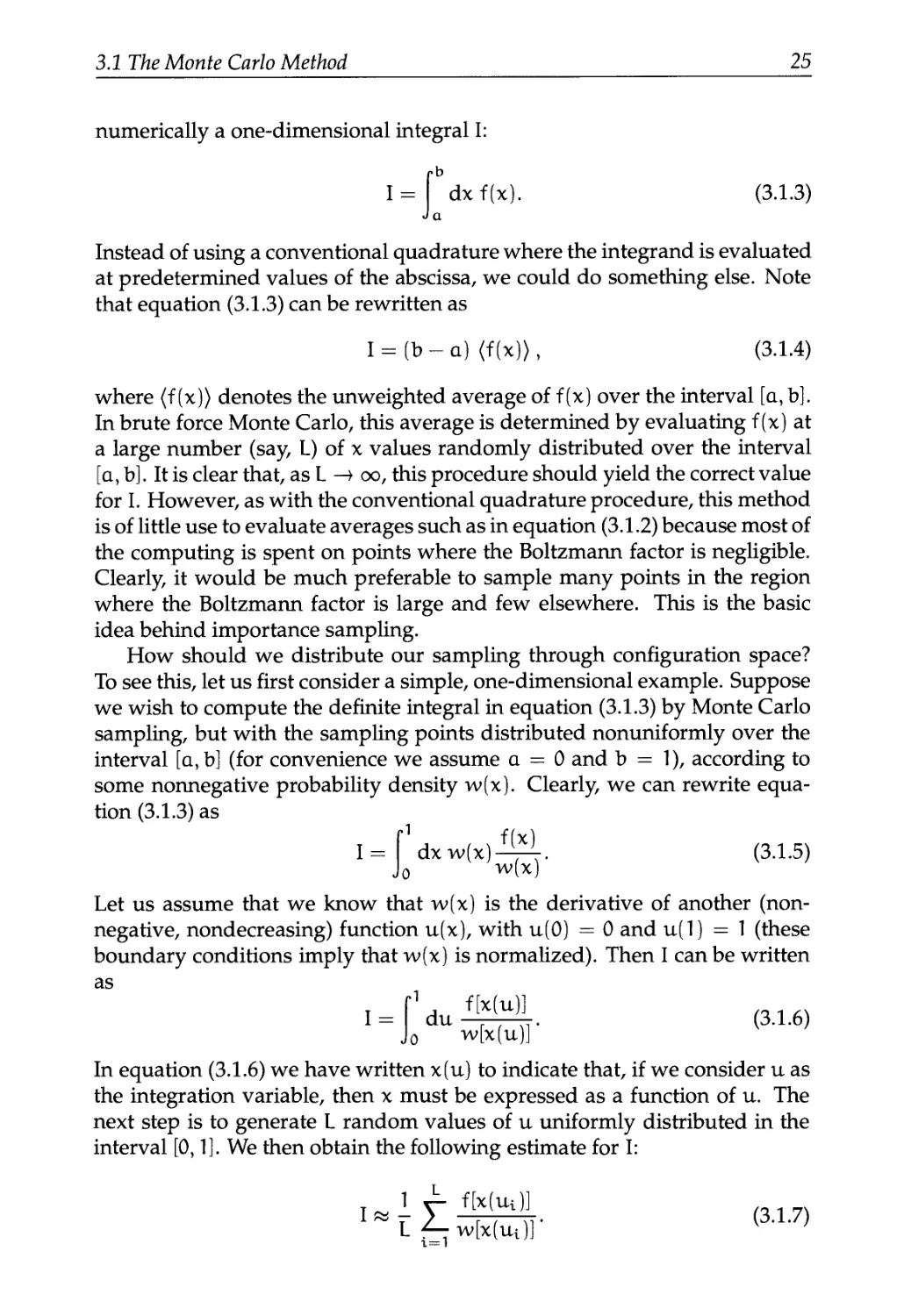
3.1 The Monte Carlo Method 23
3.1.1 Importance Sampling 24
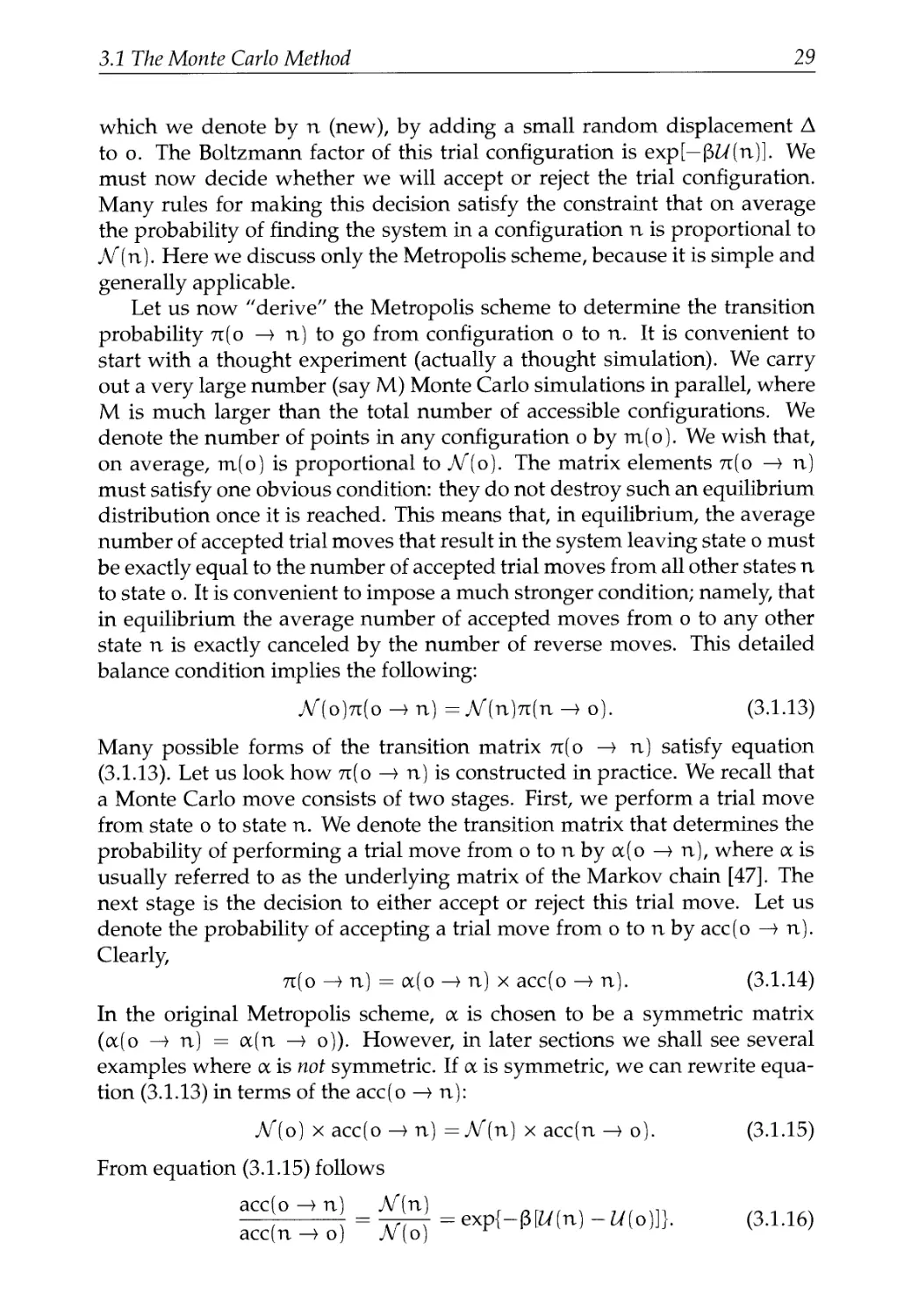
3.1.2 The Metropolis Method 27
3.2 A Basic Monte Carlo Algorithm 31
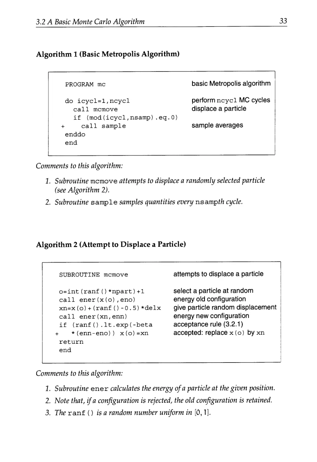
3.2.1 The Algorithm 31
3.2.2 Technical Details 32
3.2.3 Detailed Balance versus Balance 42
3.3 Trial Moves 43
3.3.1 Translational Moves 43
3.3.2 Orientational Moves 48
3.4 Applications 51
3.5 Questions and Exercises 58

vi Contents
4 Molecular Dynamics Simulations 63
4.1 Molecular Dynamics: The Idea 63
4.2 Molecular Dynamics: A Program 64
4.2.1 Initialization 65
4.2.2 The Force Calculation 67
4.2.3 Integrating the Equations of Motion 69
4.3 Equations of Motion 71
4.3.1 Other Algorithms 74
4.3.2 Higher-Order Schemes 77
4.3.3 Liouville Formulation of Time-Reversible Algorithms . 77
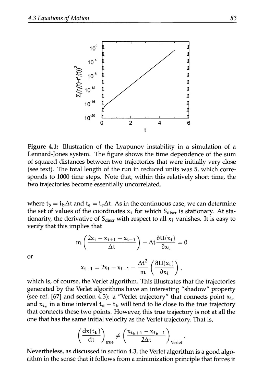
4.3.4 Lyapunov Instability 81
4.3.5 One More Way to Look at the Verlet Algorithm 82
4.4 Computer Experiments 84
4.4.1 Diffusion 87
4.4.2 Order-n Algorithm to Measure Correlations 90
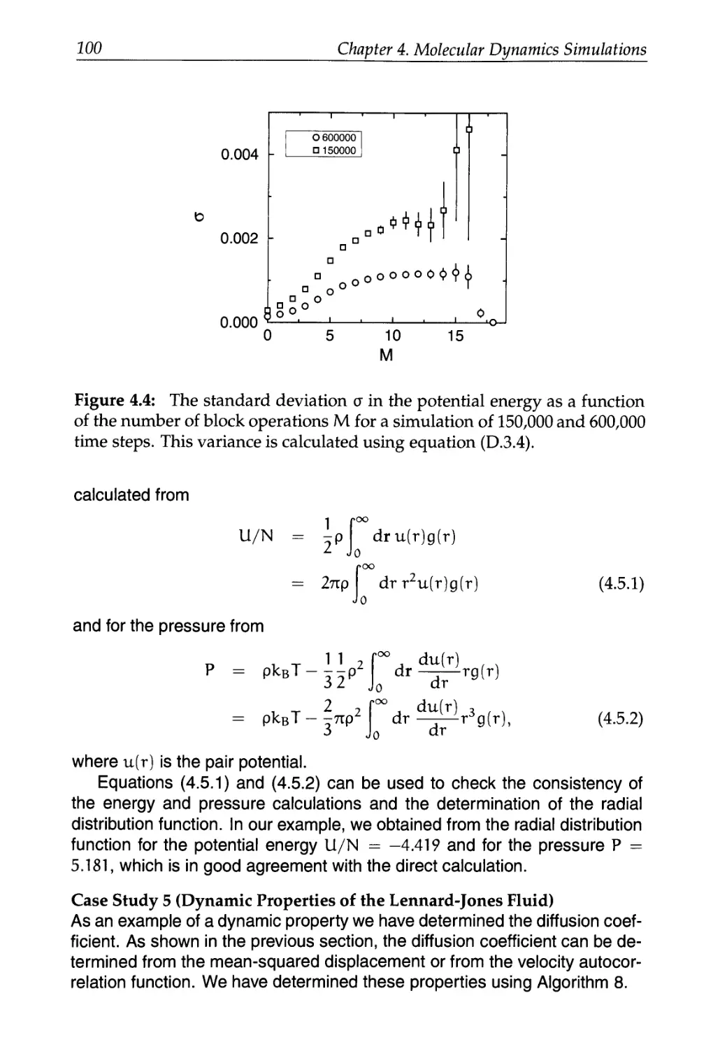
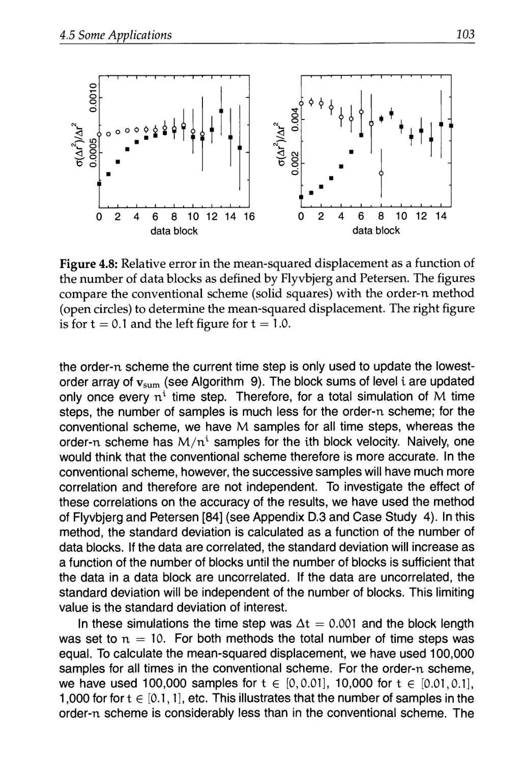
4.5 Some Applications 97
4.6 Questions and Exercises 105
Part II Ensembles 109
5 Monte Carlo Simulations in Various Ensembles 111
5.1 General Approach 112
5.2 Canonical Ensemble 112
5.2.1 Monte Carlo Simulations 113
5.2.2 Justification of the Algorithm 114
5.3 Microcanonical Monte Carlo 114
5.4 Isobaric-Isothermal Ensemble 115
5.4.1 Statistical Mechanical Basis 116
5.4.2 Monte Carlo Simulations 119
5.4.3 Applications 122
5.5 Isotension-Isothermal Ensemble 125
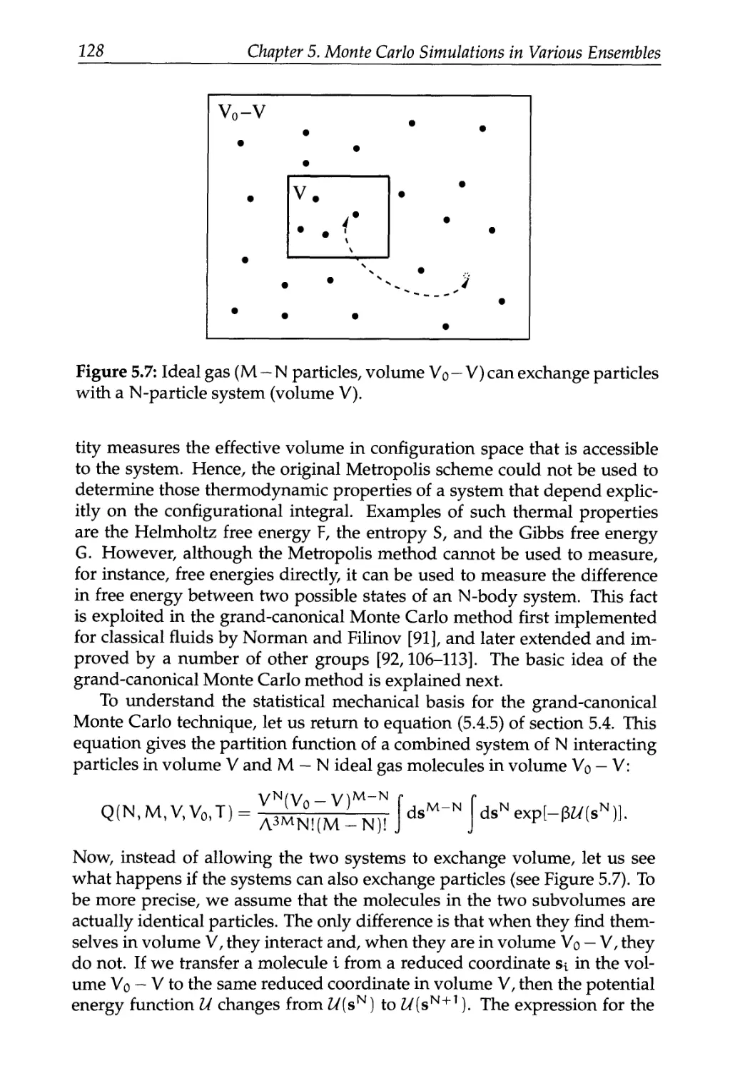
5.6 Grand-Canonical Ensemble 126
5.6.1 Statistical Mechanical Basis 127
5.6.2 Monte Carlo Simulations 130
5.6.3 Justification of the Algorithm 130
5.6.4 Applications 133
5.7 Questions and Exercises 135
6 Molecular Dynamics in Various Ensembles 139
6.1 Molecular Dynamics at Constant Temperature 140
6.1.1 The Andersen Thermostat 141
6.1.2 Nose-Hoover Thermostat 147

Contents vii
6.1.3 Nose-Hoover Chains 155
6.2 Molecular Dynamics at Constant Pressure 158
6.3 Questions and Exercises 160
Part HI Free Energies and Phase Equilibria 165
7 Free Energy Calculations 167
7.1 Thermodynamic Integration 168
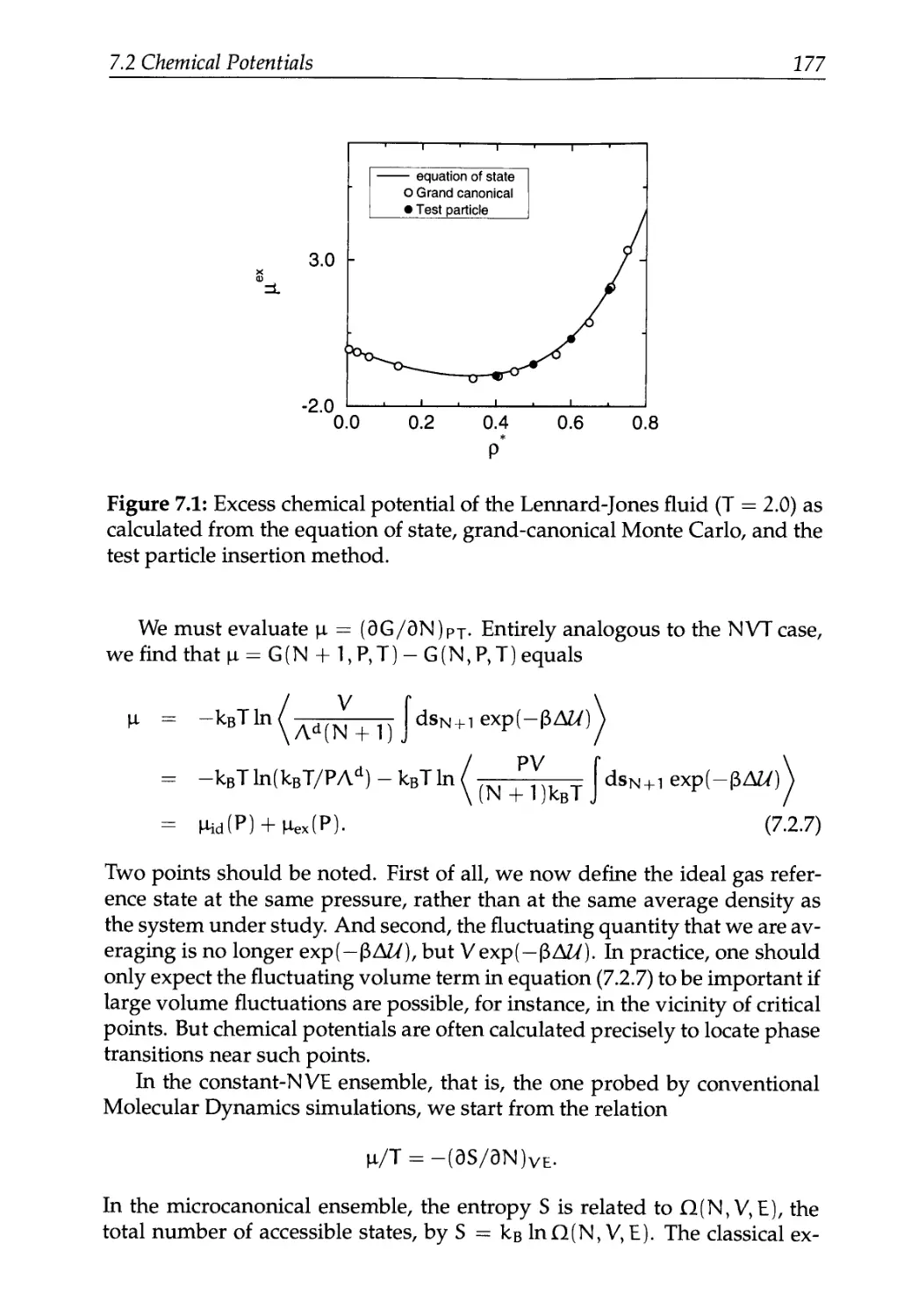
7.2 Chemical Potentials 172
7.2.1 The Particle Insertion Method 173
7.2.2 Other Ensembles 176
7.2.3 Overlapping Distribution Method 179
7.3 Other Free Energy Methods 183
7.3.1 Multiple Histograms 183
7.3.2 Acceptance Ratio Method 189
7.4 Umbrella Sampling 192
7.4.1 Nonequilibrium Free Energy Methods 196
7.5 Questions and Exercises 199
8 The Gibbs Ensemble 201
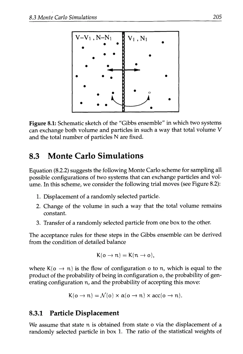
8.1 The Gibbs Ensemble Technique 203
8.2 The Partition Function 204
8.3 Monte Carlo Simulations 205
8.3.1 Particle Displacement 205
8.3.2 Volume Change 206
8.3.3 Particle Exchange 208
8.3.4 Implementation 208
8.3.5 Analyzing the Results 214
8.4 Applications 220
8.5 Questions and Exercises 223
9 Other Methods to Study Coexistence 225
9.1 Semigrand Ensemble 225
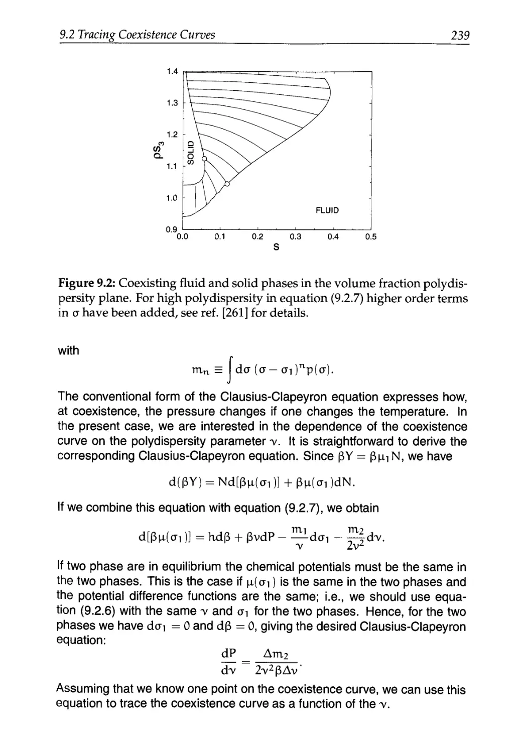
9.2 Tracing Coexistence Curves 233
10 Free Energies of Solids 241
10.1 Thermodynamic Integration 242
10.2 Free Energies of Solids 243
10.2.1 Atomic Solids with Continuous Potentials 244
10.3 Free Energies of Molecular Solids 245
10.3.1 Atomic Solids with Discontinuous Potentials 248
10.3.2 General Implementation Issues 249
10.4 Vacancies and Interstitials 263

viii Contents
10.4.1 Free Energies 263
10.4.2 Numerical Calculations 266
11 Free Energy of Chain Molecules 269
11.1 Chemical Potential as Reversible Work 269
11.2 Rosenbluth Sampling 271
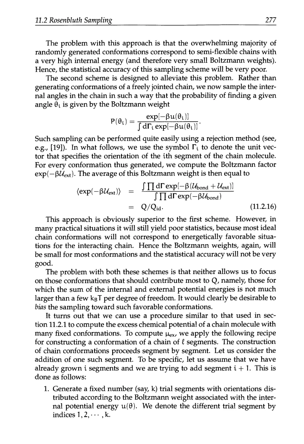
11.2.1 Macromolecules with Discrete Conformations 271
11.2.2 Extension to Continuously Deformable Molecules . . . 276
11.2.3 Overlapping Distribution Rosenbluth Method 282
11.2.4 Recursive Sampling 283
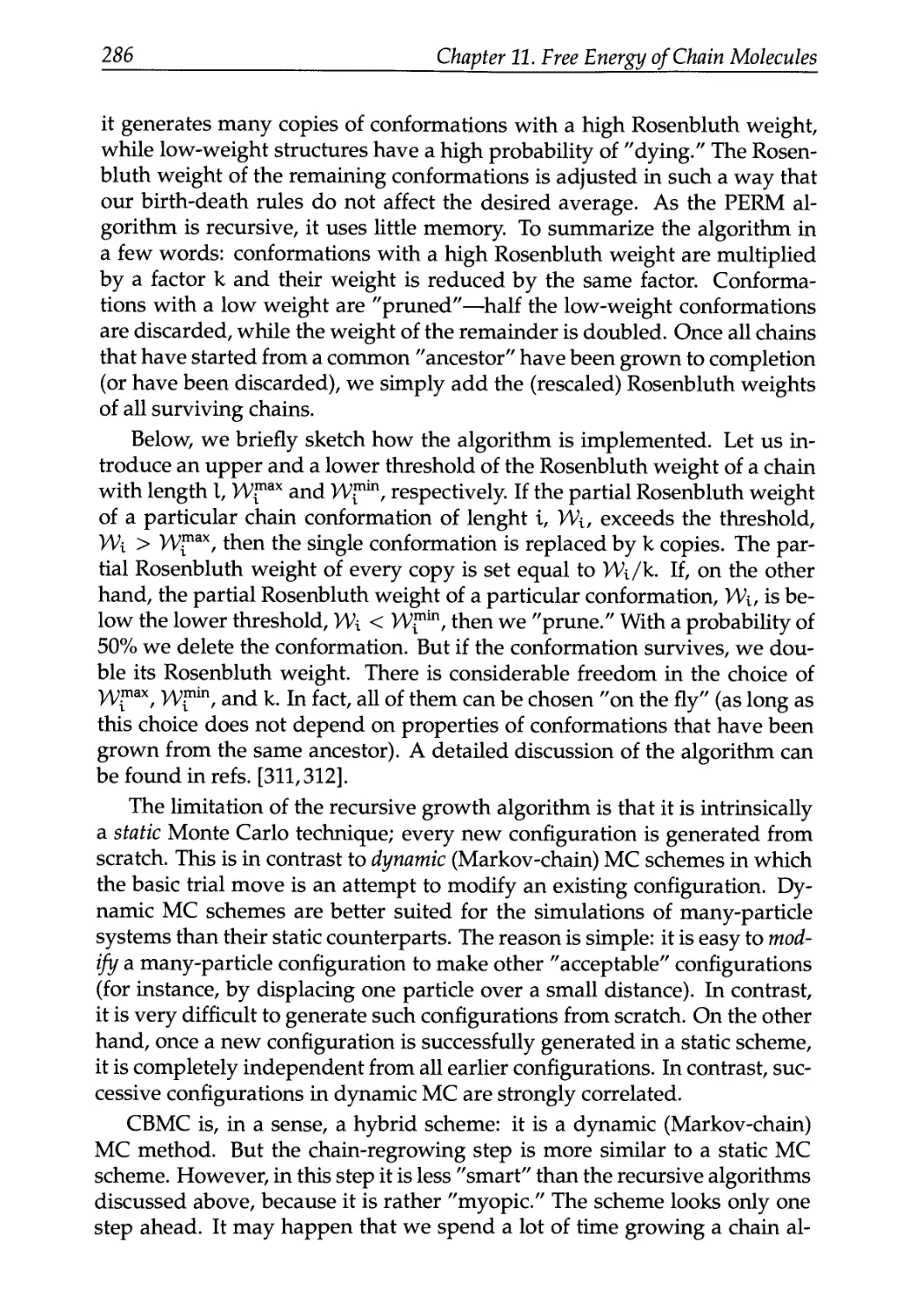
11.2.5 Pruned-Enriched Rosenbluth Method 285
Part IV Advanced Techniques 289
12 Long-Range Interactions 291
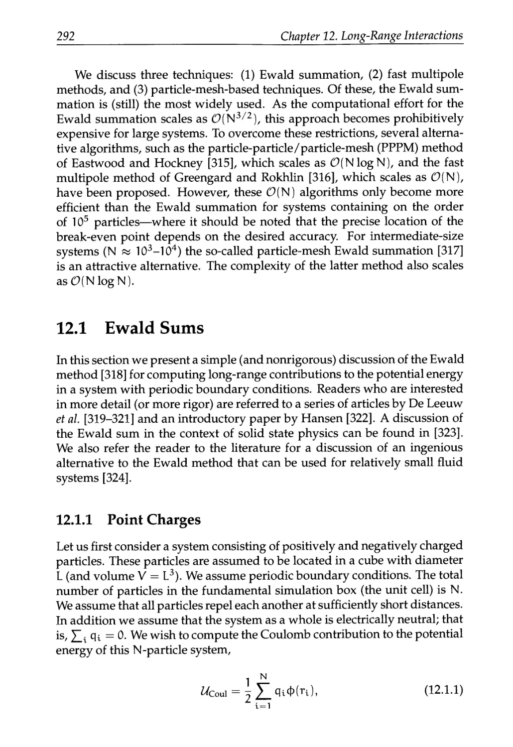
12.1 EwaldSums 292
12.1.1 Point Charges 292
12.1.2 Dipolar Particles 300
12.1.3 Dielectric Constant 301
12.1.4 Boundary Conditions 303
12.1.5 Accuracy and Computational Complexity 304
12.2 Fast Multipole Method 306
12.3 Particle Mesh Approaches 310
12.4 Ewald Summation in a Slab Geometry 316
13 Biased Monte Carlo Schemes 321
13.1 Biased Sampling Techniques 322
13.1.1 Beyond Metropolis 323
13.1.2 Orientational Bias 323
13.2 Chain Molecules 331
13.2.1 Configurational-Bias Monte Carlo 331
13.2.2 Lattice Models 332
13.2.3 Off-lattice Case 336
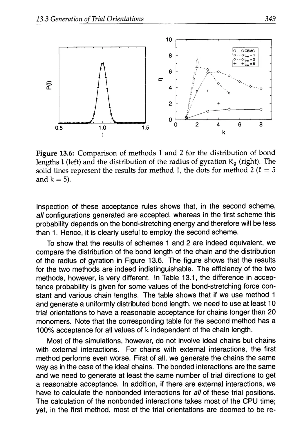
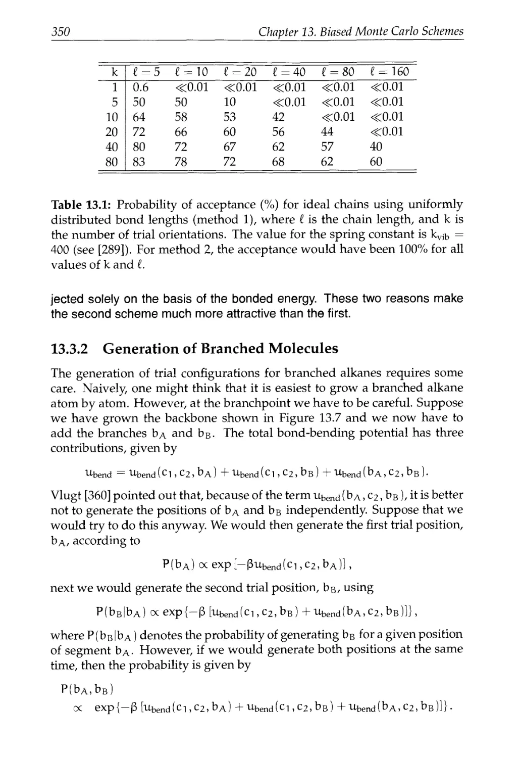
13.3 Generation of Trial Orientations 341
13.3.1 Strong Intramolecular Interactions 342
13.3.2 Generation of Branched Molecules 350
13.4 Fixed Endpoints 353
13.4.1 Lattice Models 353
13.4.2 Fully Flexible Chain 355
13.4.3 Strong Intramolecular Interactions 357
13.4.4 Rebridging Monte Carlo 357
13.5 Beyond Polymers 360
13.6 Other Ensembles 365

Contents ix
13.6.1 Grand-Canonical Ensemble 365
13.6.2 Gibbs Ensemble Simulations 370
13.7 Recoil Growth 374
13.7.1 Algorithm 376
13.7.2 Justification of the Method 379
13.8 Questions and Exercises 383
14 Accelerating Monte Carlo Sampling 389
14.1 Parallel Tempering 389
14.2 Hybrid Monte Carlo 397
14.3 Cluster Moves 399
14.3.1 Clusters 399
14.3.2 Early Rejection Scheme 405
15 Tackling Time-Scale Problems 409
15.1 Constraints 410
15.1.1 Constrained and Unconstrained Averages 415
15.2 On-the-Fly Optimization: Car-Parrinello Approach 421
15.3 Multiple Time Steps 424
16 Rare Events 431
16.1 Theoretical Background 432
16.2 Bennett-Chandler Approach 436
16.2.1 Computational Aspects 438
16.3 Diffusive Barrier Crossing 443
16.4 Transition Path Ensemble 450
16.4.1 Path Ensemble 451
16.4.2 Monte Carlo Simulations 454
16.5 Searching for the Saddle Point 462
17 Dissipative Particle Dynamics 465
17.1 Description of the Technique 466
17.1.1 Justification of the Method 467
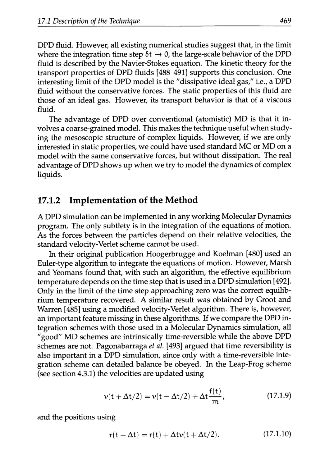
17.1.2 Implementation of the Method 469
17.1.3 DPD and Energy Conservation 473
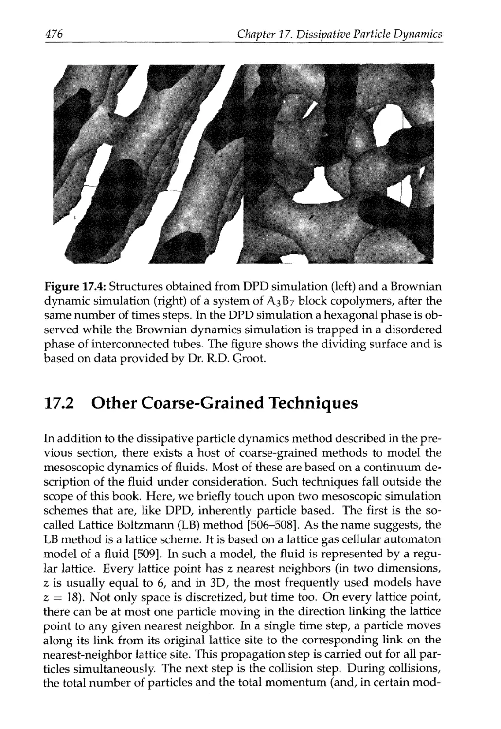
17.2 Other Coarse-Grained Techniques 476
Part V Appendices 479
A Lagrangian and Hamiltonian 481
A.I Lagrangian 483
A.2 Hamiltonian 486
A.3 Hamilton Dynamics and Statistical Mechanics 488

x Contents
A.3.1 Canonical Transformation 489
A.3.2 Symplectic Condition 490
A.3.3 Statistical Mechanics 492
В Non-Hamiltonian Dynamics 495
B.I Theoretical Background 495
B.2 Non-Hamiltonian Simulation of the N,V,T Ensemble 497
B.2.1 The Nose-Hoover Algorithm 498
B.2.2 Nose-Hoover Chains 502
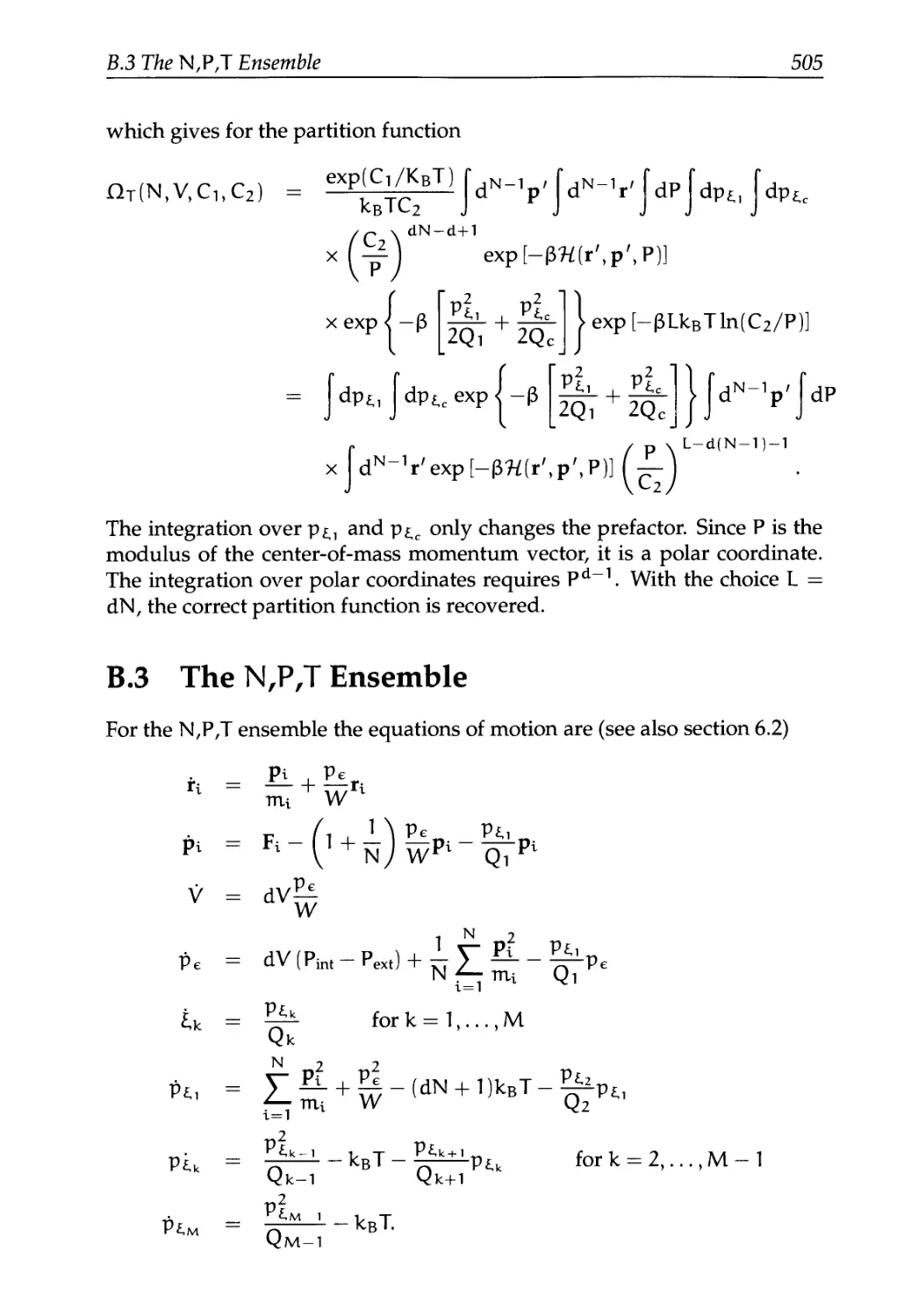
B.3 The N,P,T Ensemble 505
С Linear Response Theory 509
C.I Static Response 509
C.2 Dynamic Response 511
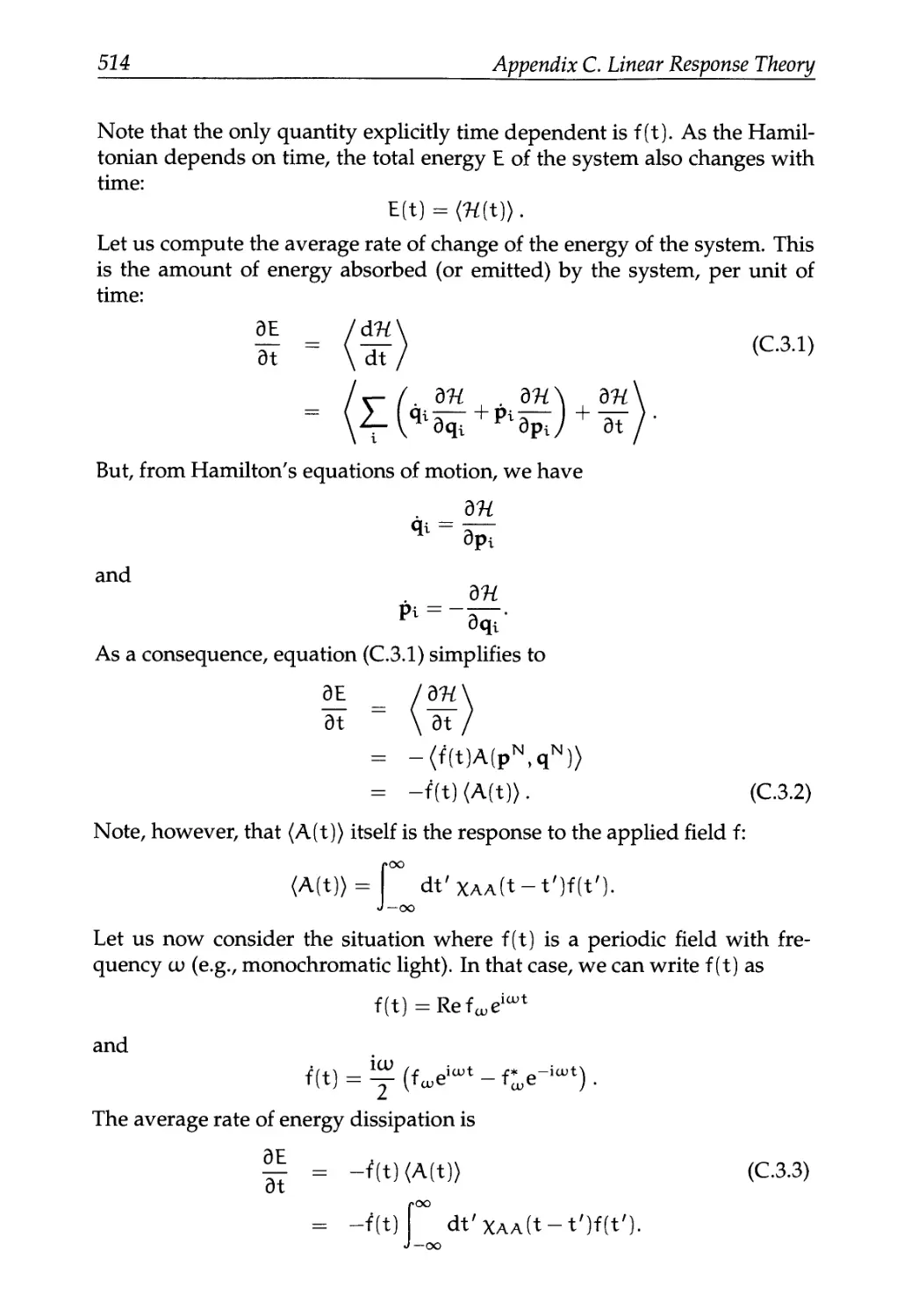
C.3 Dissipation 513
C.3.1 Electrical Conductivity 516
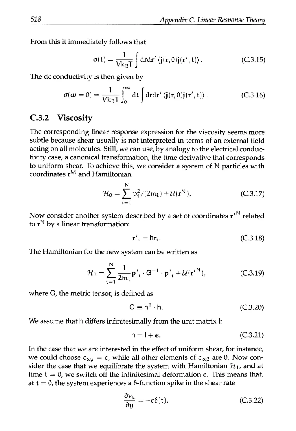
C.3.2 Viscosity 518
C.4 Elastic Constants 519
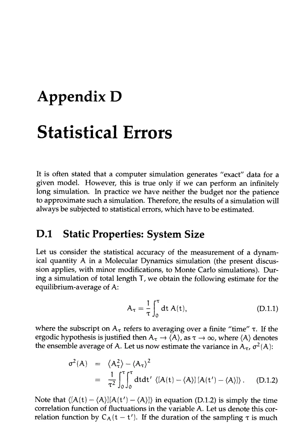
D Statistical Errors 525
D.I Static Properties: System Size 525
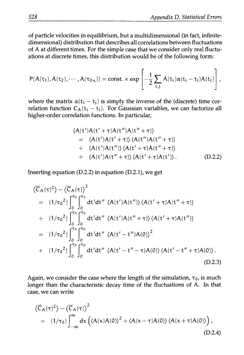
D.2 Correlation Functions 527
D.3 Block Averages 529
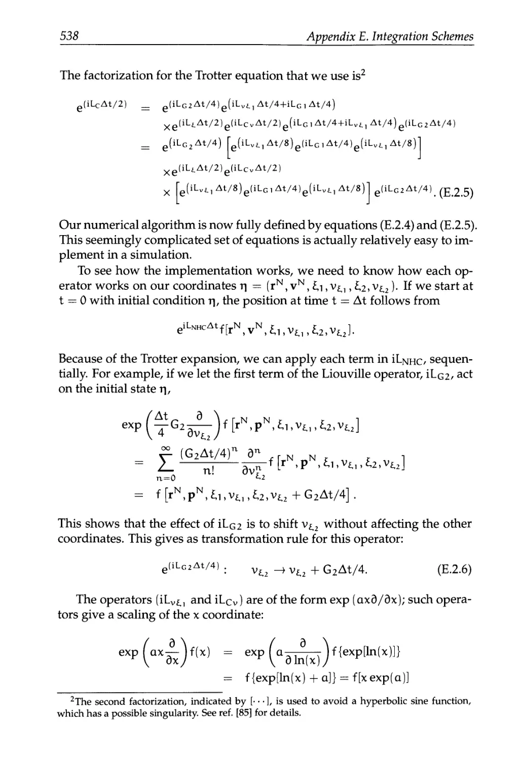
E Integration Schemes 533
E.I Higher-Order Schemes 533
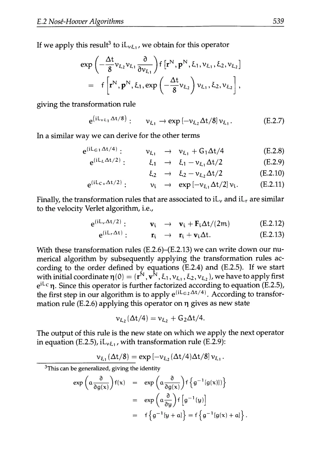
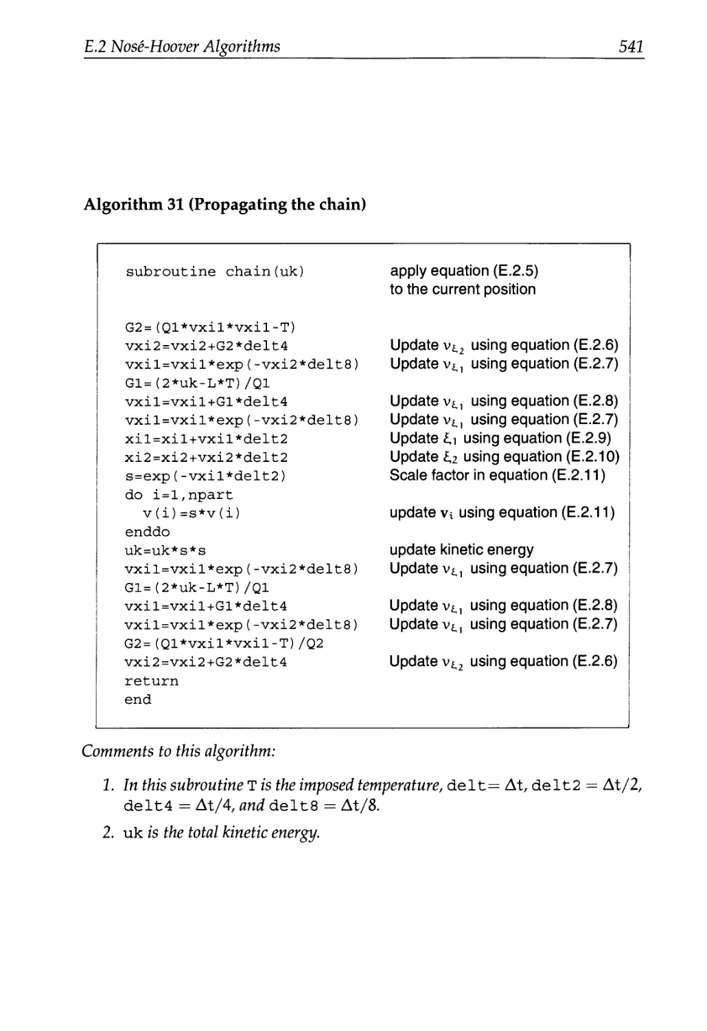
E.2 Nose-Hoover Algorithms 535
E.2.1 Canonical Ensemble 536
E.2.2 The Isothermal-Isobaric Ensemble 540
F Saving CPU Time 545
F.I VerletList 545
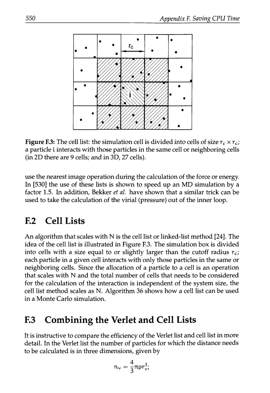
F.2 Cell Lists 550
F.3 Combining the Verlet and Cell Lists 550
F.4 Efficiency 552
G Reference States 559
G.I Grand-Canonical Ensemble Simulation 559
H Statistical Mechanics of the Gibbs "Ensemble" 563
H.I Free Energy of the Gibbs Ensemble 563
H.I.I Basic Definitions 563
H.1.2 Free Energy Density 565
H.2 Chemical Potential in the Gibbs Ensemble 570

Contents xi
I Overlapping Distribution for Polymers 573
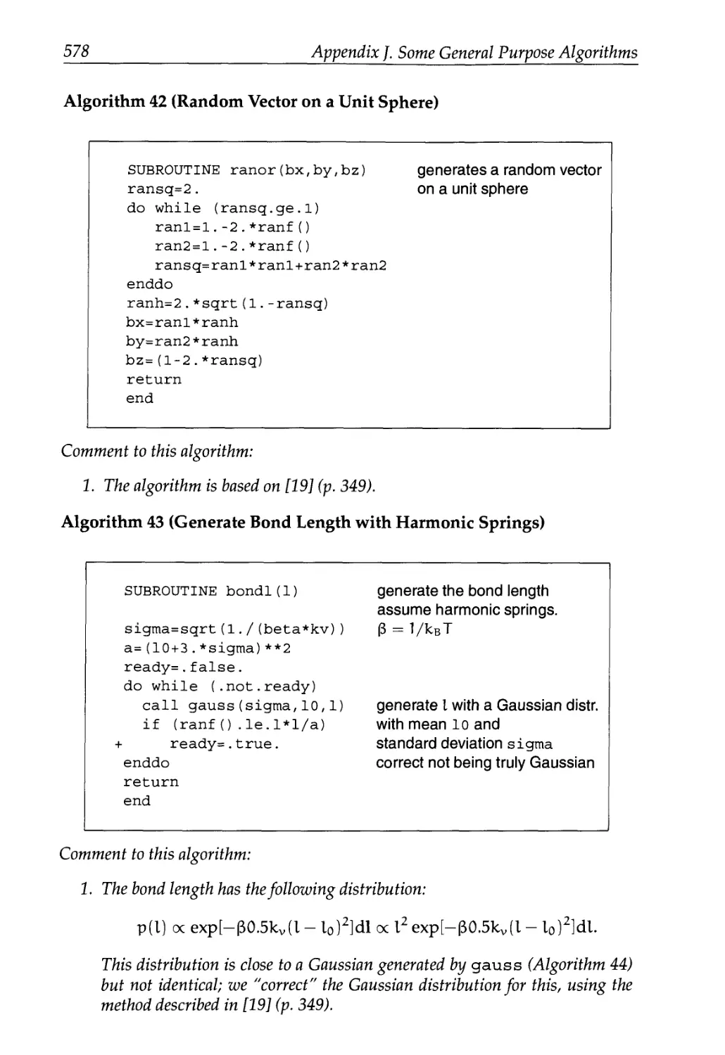
J Some General Purpose Algorithms 577
К Small Research Projects 581
K.I Adsorption in Porous Media 581
K.2 Transport Properties in Liquids 582
K.3 Diffusion in a Porous Media 583
K.4 Multiple-Time-Step Integrators 584
K.5 Thermodynamic Integration 585
L Hints for Programming 587
Bibliography 589
Author Index 619
Index 628

Preface to the Second Edition
Why did we write a second edition? A minor revision of the first edition
would have been adequate to correct the (admittedly many) typographical
mistakes. However, many of the nice comments that we received from stu-
students and colleagues alike, ended with a remark of the type: "unfortunately,
you don't discuss topic x". And indeed, we feel that, after only five years,
the simulation world has changed so much that the title of the book was no
longer covered by the contents.
The first edition was written in 1995 and since then several new tech-
techniques have appeared or matured. Most (but not all) of the major changes
in the second edition deal with these new developments. In particular, we
have included a section on:
• Transition path sampling and diffusive barrier crossing to simulate
rare events
• Dissipative particle dynamic as a course-grained simulation technique
• Novel schemes to compute the long-ranged forces
• Discussion on Hamiltonian and non-Hamiltonian dynamics in the con-
context of constant-temperature and constant-pressure Molecular Dynam-
Dynamics simulations
• Multiple-time-step algorithms as an alternative for constraints
• Defects in solids
• The pruned-enriched Rosenbluth sampling, recoil growth, and con-
concerted rotations for complex molecules
• Parallel tempering for glassy Hamiltonians
We have updated some of the examples to include also recent work. Several
new Examples have been added to illustrate recent applications.
We have taught several courses on Molecular Simulation, based on the
first edition of this book. As part of these courses, Dr. Thijs Vlugt prepared
many Questions, Exercises, and Case Studies, most of which have been in-
included in the present edition. Some additional exercises can be found on

xiv Preface to the Second Edition
the Web. We are very grateful to Thijs Vlugt for the permission to reproduce
this material.
Many of the advanced Molecular Dynamics techniques described in this
book are derived using the Lagrangian or Hamilton formulations of classical
mechanics. However, many chemistry and chemical engineering students
are not familiar with these formalisms. While a full description of classical
mechanics is clearly beyond the scope of the present book, we have added
an Appendix that summarizes the necessary essentials of Lagrangian and
Hamiltonian mechanics.
Special thanks are due to Giovanni Ciccotti, Rob Groot, Gavin Crooks,
Thijs Vlugt, and Peter Bolhuis for their comments on parts of the text. In ad-
addition, we thank everyone who pointed out mistakes and typos, in particular
Drs. J.B. Freund, R. Akkermans, and D. Moroni.

Preface
This book is not a computer simulation cookbook. Our aim is to explain
the physics that is behind the "recipes" of molecular simulation. Of course,
we also give the recipes themselves, because otherwise the book would be
too abstract to be of much practical use. The scope of this book is necessarily
limited: we do not aim to discuss all aspects of computer simulation. Rather,
we intend to give a unified presentation of those computational tools that
are currently used to study the equilibrium properties and, in particular,
the phase behavior of molecular and supramolecular substances. Moreover,
we intentionally restrict the discussion to simulations of classical many-body
systems, even though some of the techniques mentioned can be applied to
quantum systems as well. And, within the context of classical many-body
systems, we restrict our discussion to the modeling of systems at, or near,
equilibrium.
The book is aimed at readers who are active in computer simulation
or are planning to become so. Computer simulators are continuously con-
confronted with questions concerning the choice of technique, because a bewil-
bewildering variety of computational tools is available. We believe that, to make a
rational choice, a good understanding of the physics behind each technique
is essential. Our aim is to provide the reader with this background.
We should state at the outset that we consider some techniques to be
more useful than others, and therefore our presentation is biased. In fact,
we believe that the reader is well served by the fact that we do not present
all techniques as equivalent. However, whenever we express our personal
preference, we try to back it up with arguments based in physics, applied
mathematics, or simply experience. In fact, we mix our presentation with
practical examples that serve a twofold purpose: first, to show how a given
technique works in practice, and second, to give the reader a flavor of the
kind of phenomena that can be studied by numerical simulation.
The reader will also notice that two topics are discussed in great detail,
namely simulation techniques to study first-order phase transitions, and var-
various aspects of the configurational-bias Monte Carlo method. The reason
why we devote so much space to these topics is not that we consider them

xvi Preface
to be more important than other subjects that get less coverage, but rather
because we feel that, at present, the discussion of both topics in the literature
is rather fragmented.
The present introduction is written for the nonexpert. We have done so
on purpose. The community of people who perform computer simulations
is rapidly expanding as computer experiments become a general research
tool. Many of the new simulators will use computer simulation as a tool
and will not be primarily interested in techniques. Yet, we hope to convince
those readers who consider a computer simulation program a black box, that
the inside of the black box is interesting and, more importantly, that a better
understanding of the working of a simulation program may greatly improve
the efficiency with which the black box is used.
In addition to the theoretical framework, we discuss some of the practical
tricks and rules of thumb that have become "common" knowledge in the
simulation community and are routinely used in a simulation. Often, it is
difficult to trace back the original motivation behind these rules. As a result,
some "tricks" can be very useful in one case yet result in inefficient programs
in others. In this book, we discuss the rationale behind the various tricks, in
order to place them in a proper context. In the main text of the book we
describe the theoretical framework of the various techniques. To illustrate
how these ideas are used in practice we provide Algorithms, Case Studies
and Examples.
Algorithms
The description of an algorithm forms an essential part of this book. Such
a description, however, does not provide much information on how to im-
implement the algorithm efficiently. Of course, details about the implementa-
implementation of an algorithm can be obtained from a listing of the complete program.
However, even in a well-structured program, the code contains many lines
that, although necessary to obtain a working program, tend to obscure the
essentials of the algorithm that they express. As a compromise solution, we
provide a pseudo-code for each algorithm. These pseudo-codes contain only
those aspects of the implementation directly related to the particular algo-
algorithm under discussion. This implies that some aspects that are essential for
using this pseudo-code in an actual program have to be added. For exam-
example, the pseudo-codes consider only the x directions; similar lines have to be
added for the у and z direction if the code is going to be used in a simulation.
Furthermore, we have omitted the initialization of most variables.
Case Studies
In the Case Studies, the algorithms discussed in the main text are combined
in a complete program. These programs are used to illustrate some elemen-

Preface xvii
tary aspects of simulations. Some Case Studies focus on the problems that
can occur in a simulation or on the errors that are sometimes made. The com-
complete listing of the FORTRAN codes that we have used for the Case Studies
is accessible to the reader through the Internet.1
Examples
In the Examples, we demonstrate how the techniques discussed in the main
text are used in an application. We have tried to refer as much as possible to
research topics of current interest. In this way, the reader may get some feel-
feeling for the type of systems that can be studied with simulations. In addition,
we have tried to illustrate in these examples how simulations can contribute
to the solution of "real" experimental or theoretical problems.
Many of the topics that we discuss in this book have appeared previ-
previously in the open literature. However, the Examples and Case Studies were
prepared specifically for this book. In writing this material, we could not
resist including a few computational tricks that, to our knowledge, have not
been reported in the literature.
In computer science it is generally assumed that any source code over 200
lines contains at least one error. The source codes of the Case Studies con-
contain over 25,000 lines of code. Assuming we are no worse than the average
programmer this implies that we have made at least 125 errors in the source
code. If you spot these errors and send them to us, we will try to correct
them (we can not promise this!). It also implies that, before you use part of
the code yourself, you should convince yourself that the code is doing what
you expect it to do.
In the light of the previous paragraph, we must add the following dis-
disclaimer:
We make no warranties, express or implied, that the programs
contained in this work are free of error, or that they will meet
your requirements for any particular application. They should
not be relied on for solving problems whose incorrect solution
could result in injury, damage, or loss of property. The authors
and publishers disclaim all liability for direct or consequential
damages resulting from your use of the programs.
Although this book and the included programs are copyrighted, we au-
authorize the readers of this book to use parts of the programs for their own
use, provided that proper acknowledgment is made.
Finally, we gratefully acknowledge the help and collaboration of many
of our colleagues. In fact, many dozens of our colleagues collaborated with
us on topics described in the text. Rather than listing them all here, we men-
mention their names at the appropriate place in the text. Yet, we do wish to
ahttp://molsim.chem.uva.nl/frenkel.smit

xviii Preface
express our gratitude for their input. Moreover, Daan Frenkel should like
to acknowledge numerous stimulating discussions with colleagues at the
FOM Institute for Atomic and Molecular Physics in Amsterdam and at the
van 't Hoff Laboratory of Utrecht University, while Berend Smit gratefully
acknowledges discussions with colleagues at the University of Amsterdam
and Shell. In addition, several colleagues helped us directly with the prepa-
preparation of the manuscript, by reading the text or part thereof. They are Gio-
Giovanni Ciccotti, Mike Deem, Simon de Leeuw, Toine Schlijper, Stefano Ruffo,
Maria-Jose Ruiz, Guy Verbist and Thijs Vlugt. In addition, we thank Klaas
Esselink and Sami Karaborni for the cover figure. We thank them all for
their efforts. In addition we thank the many readers who have drawn our
attention to errors and omissions in the first print. But we stress that the
responsibility for the remainder of errors in the text is ours alone.

List of Symbols
A dynamical variable B.2.6)
acc(o —> n) acceptance probability of a move from о to n
b trial position or orientation
с concentration
Ci concentration of species i
Cy specific heat at constant volume D.4.3)
d dimensionality
D diffusion coefficient
E total energy
f number of degrees of freedom
ft fugacity component i (9.1.9)
fi force on particle i
F Helmholtz free energy B.1.15)
g (r) radial distribution function
G Gibbs free energy E.4.9)
H = 27tfl Planck's constant
M (p, r) Hamiltonian
ji flux of species i
к wave vector
кв Boltzmann's constant
К kinetic energy
K(o —> n) flow of configurations from о to n
L box length
?(q,q) Lagrangian (A.1.2)
t total number of (pseudo-)atoms in a molecule (chain length)
n new configuration or conformation
m mass
M. total number of Monte Carlo samples
N number of particles
Л/"(о) prob. density to find a system in configuration о
A/"n,v,t prob. density for canonical ensemble E.2.2)
Л/n , p,t prob. density for isobaric-isothermal ensemble E.4.8)
Л/"ц.,у,т prob. density for grand-canonical ensemble E.6.6)
о old configuration or conformation
O{xn) terms of order xn or smaller

xx List of Symbols
p
p
p
pi
q
Q
Q(N,V,T)
Q(N,P,T)
Q(H,V,T)
Гг
Гс
Ranf
s
Si
S
t
T
W(o)
Ui
u(r)
Vi
V
vir
Wi
W(o)
W(o)
Z
cx(o —> n)
Э
At
г
e
Л
M-
At
Л
гс(о —> п)
Р
а
ае
0"<х |3
?,
?,г
П(Е)
momentum or a particle
pressure
total linear momentum
electric charge on particle i
generalized coordinates
mass associated with time scaling coordinate s
canonical partition function
isothermal-isobaric partition function
grand-canonical partition function
Cartesian coordinate of particle i
cut-off radius of the potential
random number uniform in [0,1]
time-scaling coordinate in Nose scheme
scaled coordinate of particle i
entropy
time
temperature
potential energy of configuration о
potential energy per particle
pair potential
Cartesian velocity of particle i
volume
virial
Rosenbluth factor of (pseudo-)atom i
total Rosenbluth factor configuration о
normalized total Rosenbluth factor configuration о
configurational part of the partition function
probability of generating conf. n starting from о
reciprocal temperature A /квТ)
Molecular Dynamics time step
coordinate in phase space
characteristic energy in pair potential
shear viscosity
chemical potential
thermal conductivity
thermal de Broglie wavelength
transition probability from о to n
number density
characteristic distance in pair potential
electrical conductivity
cx[3 component of the stress tensor
variance in dynamical variable A
thermodynamic friction coefficient
fugacity coefficient of component i
quantum: degeneracy of energy level E
classical: phase space subvolume with energy E
F.1.3)
E.2.1)
E.4.7)
E.6.5)
F.1.3)
E.4.2)
C.4.2)
C.1.14)
D.4.12)
D.4.14)
E.4.1)
C.1.13)
D.4.16)
D.4.13)
F.1.25)
(9.1.15)
B.1.1)
B.2.9)

List of Symbols xxi
a) orientation of a molecule
(• • •) ensemble average
(• • -)sub average under condition indicated by sub
Super- and subscripts
* reduced units (default, usually omitted)
ra <x component of vector r
Гг vector r associated with particle i
fex excess part of quantity f
fld ideal gas part of quantity f
й unit vector u
Symbol List: Algorithms
b (j ) trial orientation/position j
beta reciprocal temperature A /квТ)
box simulation box length
de 1 x maximum displacement
dt time step in an MD simulation
ell chain length
eni energy of atom i
enn energy of the new configuration
eno energy of the old configuration
etot total energy of the system
f force
к total number of trial orientations/position
kv bond vibration energy constant
1 bond length
n selected trial position
ncycle total number of MC cycles
nhi s number of bins in a histogram
NINT nearest integer
npart total number of particles
nsamp number of MC cycles of MD steps between two samples
о particle number of the old configuration
p pressure
phi bond-bending angle
pi я = 3.14159
r2 distance squared between two atoms
ranf () random number e [0,1]
rho density
re 2 cutoff radius squared (of the potential)
switch = 0 initialization; = 1 sample; = 2 print result

XXII
List of Symbols
t
temp
tempa
theta
tmax
tors
v(i)
vmax
vol
w
wn, wo
x(i)
xm(i)
xn
xn(i)
xo
xt(j)
ubb
utors
•
X
a.le.b
a.lt.b
a.ge.b
a.gt.b
a.and.b
a.or.b
+
*
/
sqrt
time in a MD simulation
temperature
instantaneous temperature, from kinetic energy
torsional angle
maximum simulation time
torsion energy
velocity of atom i
maximum displacement volume
volume simulation box
Rosenbluth factor (new or old)
Rosenbluth factor n(ew)/o(ld) configuration
position of atom i
position of atom i at previous time step
new configuration of a particle
positions of atoms that have been grown
old configuration of a particle
jth trial position for a given atom
bond-bending energy
torsion energy
vector dot product
vector cross product
length of the vector
test: true if a is less than or equal to b
test: true if a is less than b
test: true if a is greater than or equal to b
test: true if a is greater than b
test: true if both a and b are true
test: true if a or b are true
continuation symbol
multiplication
to the power
division
square root

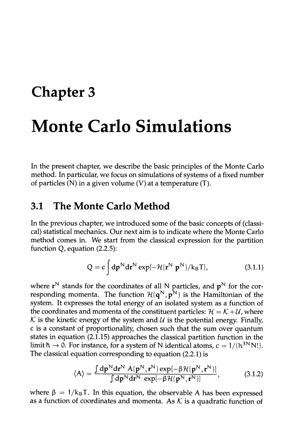
Chapter 1
Introduction
(Pre)history of Computer Simulation
It usually takes decades rather than years before a fundamentally new in-
invention finds widespread application. For computer simulation, the story is
rather different. Computer simulation started as a tool to exploit the elec-
electronic computing machines that had been developed during and after the
Second World War. These machines had been built to perform the very
heavy computation involved in the development of nuclear weapons and
code breaking. In the early 1950s, electronic computers became partly avail-
available for nonmilitary use and this was the beginning of the discipline of com-
computer simulation. W. W Wood [1] recalls: "When the Los Alamos MANIAC
became operational in March 1952, Metropolis was interested in having as
broad a spectrum of problems as possible tried on the machine, in order
to evaluate its logical structure and demonstrate the capabilities of the ma-
machine."
The strange thing about computer simulation is that it is also a discov-
discovery, albeit a delayed discovery that grew slowly after the introduction of the
technique. In fact, discovery is probably not the right word, because it does
not refer to a new insight into the working of the natural world but into our
description of nature. Working with computers has provided us with a new
metaphor for the laws of nature: they carry as much (and as little) infor-
information as algorithms. For any nontrivial algorithm (i.e., loosely speaking,
one that cannot be solved analytically), you cannot predict the outcome of a
computation simply by looking at the program, although it often is possible
to make precise statements about the general nature (e.g., the symmetry) of
the result of the computation. Similarly, the basic laws of nature as we know
them have the unpleasant feature that they are expressed in terms of equa-
equations we cannot solve exactly, except in a few very special cases. If we wish
to study the motion of more than two interacting bodies, even the relatively

Chapter 1. Introduction-
simple laws of Newtonian mechanics become essentially unsolvable. That is
to say, they cannot be solved analytically, using only pencil and the back of
the proverbial envelope. However, using a computer, we can get the answer
to any desired accuracy. Most of materials science deals with the properties
of systems of many atoms or molecules. Many almost always means more
than two; usually, very much more. So if we wish to compute the properties
of a liquid (to take a particularly nasty example), there is no hope of finding
the answer exactly using only pencil and paper.
Before computer simulation appeared on the scene, there was only one
way to predict the properties of a molecular substance, namely by making
use of a theory that provided an approximate description of that material.
Such approximations are inevitable precisely because there are very few sys-
systems for which the equilibrium properties can be computed exactly (exam-
(examples are the ideal gas, the harmonic crystal, and a number of lattice models,
such as the two-dimensional Ising model for ferromagnets). As a result,
most properties of real materials were predicted on the basis of approxi-
approximate theories (examples are the van der Waals equation for dense gases, the
Debye-Huckel theory for electrolytes, and the Boltzmann equation to de-
describe the transport properties of dilute gases). Given sufficient information
about the intermolecular interactions, these theories will provide us with
an estimate of the properties of interest. Unfortunately, our knowledge of
the intermolecular interactions of all but the simplest molecules is also quite
limited. This leads to a problem if we wish to test the validity of a particu-
particular theory by comparing directly to experiment. If we find that theory and
experiment disagree, it may mean that our theory is wrong, or that we have
an incorrect estimate of the intermolecular interactions, or both.
Clearly, it would be very nice if we could obtain essentially exact results
for a given model system without having to rely on approximate theories.
Computer simulations allow us to do precisely that. On the one hand, we
can now compare the calculated properties of a model system with those of
an experimental system: if the two disagree, our model is inadequate; that
is, we have to improve on our estimate of the intermolecular interactions.
On the other hand, we can compare the result of a simulation of a given
model system with the predictions of an approximate analytical theory ap-
applied to the same model. If we now find that theory and simulation disagree,
we know that the theory is flawed. So, in this case, the computer simulation
plays the role of the experiment designed to test the theory. This method of
screening theories before we apply them to the real world is called a com-
computer experiment. This application of computer simulation is of tremendous
importance. It has led to the revision of some very respectable theories, some
of them dating back to Boltzmann. And it has changed the way in which we
construct new theories. Nowadays it is becoming increasingly rare that a
theory is applied to the real world before being tested by computer Simula-

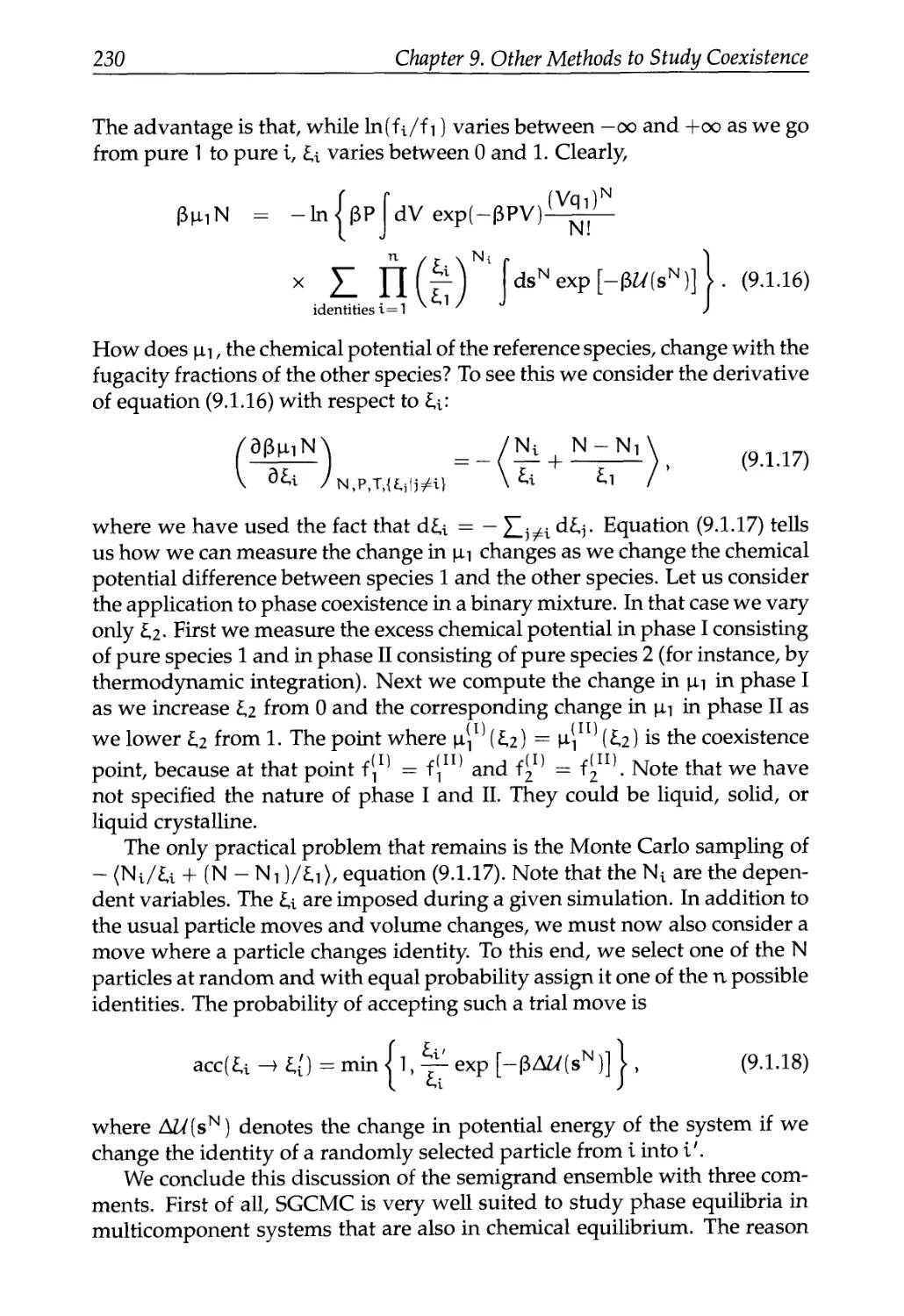
Chapter 1. Introduction
pkBT
1
2
3
4
5
1.03
1.99
2.98
4.04
5.01
Р
±
±
±
±
±
0.04
0.03
0.05
0.03
0.04
Table 1.1: Simulated equation of state of an ideal gas
tion. The simulation then serves a twofold purpose: it gives the theoretician
a feeling for the physics of the problem, and it generates some "exact" results
that can be used to test the quality of the theory to be constructed. Computer
experiments have become standard practice, to the extent that they now pro-
provide the first (and often the last) test of a new theoretical result.
But note that the computer as such offers us no understanding, only
numbers. And, as in a real experiment, these numbers have statistical errors.
So what we get out of a simulation is never directly a theoretical relation. As
in a real experiment, we still have to extract the useful information. To take
a not very realistic example, suppose we were to use the computer to mea-
measure the pressure of an ideal gas as a function of density. This example is
unrealistic because the volume dependence of the ideal-gas pressure has, in
fact, been well known since the work of Boyle and Gay-Lussac. The Boyle-
Gay-Lussac law states that the product of volume and pressure of an ideal
gas is constant. Now suppose we were to measure this product by computer
simulation. We might, for instance, find the set of experimental results in
Table 1.1. The data suggest that P equals pkBT,but no more than that. It is
left to us to infer the conclusions.
The early history of computer simulation (see, e.g., ref. [2]) illustrates this
role of computer simulation. Some areas of physics appeared to have little
need for simulation because very good analytical theories were available
(e.g., to predict the properties of dilute gases or of nearly harmonic crys-
crystalline solids). However, in other areas, few if any exact theoretical results
were known, and progress was much hindered by the lack of unambiguous
tests to assess the quality of approximate theories. A case in point was the
theory of dense liquids. Before the advent of computer simulations, the only
way to model liquids was by mechanical simulation [3-5] of large assem-
assemblies of macroscopic spheres (e.g., ball bearings). Then the main problem be-
becomes how to arrange these balls in the same way as atoms in a liquid. Much
work on this topic was done by the famous British scientist J. D. Bernal, who
built and analyzed such mechanical models for liquids. Actually, it would
be fair to say that the really tedious work of analyzing the resulting three-
dimensional structures was done by his research students, such as the unfor-

Chapter 1. Introduction
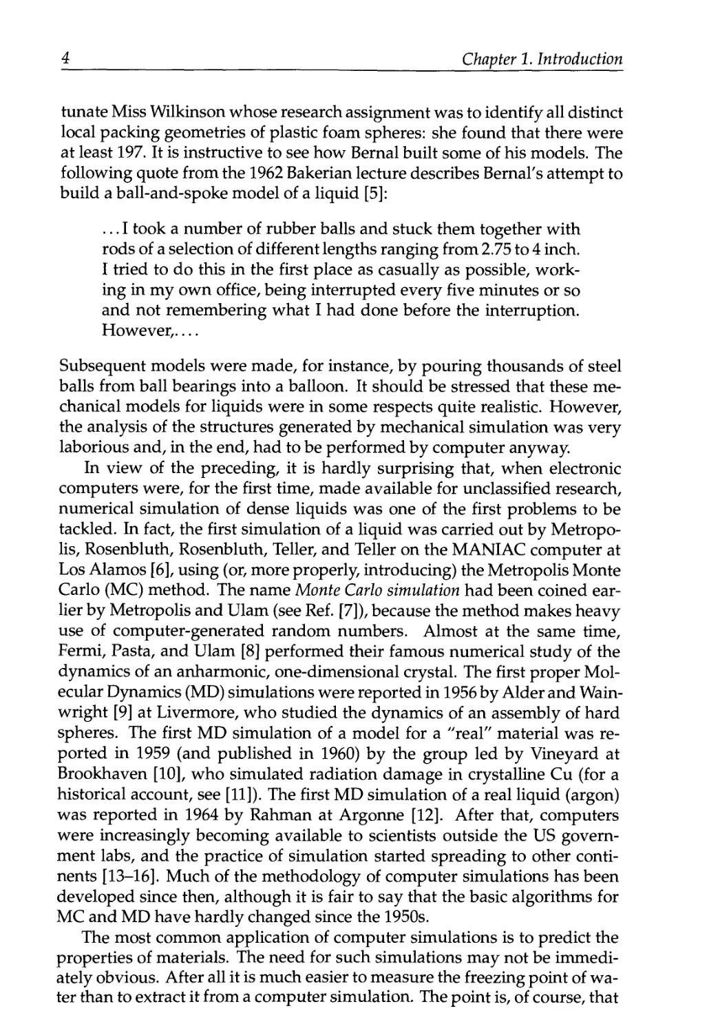
tunate Miss Wilkinson whose research assignment was to identify all distinct
local packing geometries of plastic foam spheres: she found that there were
at least 197. It is instructive to see how Bernal built some of his models. The
following quote from the 1962 Bakerian lecture describes Bernal's attempt to
build a ball-and-spoke model of a liquid [5]:
... I took a number of rubber balls and stuck them together with
rods of a selection of different lengths ranging from 2.75 to 4 inch.
I tried to do this in the first place as casually as possible, work-
working in my own office, being interrupted every five minutes or so
and not remembering what I had done before the interruption.
However,—
Subsequent models were made, for instance, by pouring thousands of steel
balls from ball bearings into a balloon. It should be stressed that these me-
mechanical models for liquids were in some respects quite realistic. However,
the analysis of the structures generated by mechanical simulation was very
laborious and, in the end, had to be performed by computer anyway.
In view of the preceding, it is hardly surprising that, when electronic
computers were, for the first time, made available for unclassified research,
numerical simulation of dense liquids was one of the first problems to be
tackled. In fact, the first simulation of a liquid was carried out by Metropo-
Metropolis, Rosenbluth, Rosenbluth, Teller, and Teller on the MANIAC computer at
Los Alamos [6], using (or, more properly, introducing) the Metropolis Monte
Carlo (MC) method. The name Monte Carlo simulation had been coined ear-
earlier by Metropolis and Ulam (see Ref. [7]), because the method makes heavy
use of computer-generated random numbers. Almost at the same time,
Fermi, Pasta, and Ulam [8] performed their famous numerical study of the
dynamics of an anharmonic, one-dimensional crystal. The first proper Mol-
Molecular Dynamics (MD) simulations were reported in 1956 by Alder and Wain-
wright [9] at Livermore, who studied the dynamics of an assembly of hard
spheres. The first MD simulation of a model for a "real" material was re-
reported in 1959 (and published in 1960) by the group led by Vineyard at
Brookhaven [10], who simulated radiation damage in crystalline Cu (for a
historical account, see [11]). The first MD simulation of a real liquid (argon)
was reported in 1964 by Rahman at Argonne [12]. After that, computers
were increasingly becoming available to scientists outside the US govern-
government labs, and the practice of simulation started spreading to other conti-
continents [13-16]. Much of the methodology of computer simulations has been
developed since then, although it is fair to say that the basic algorithms for
MC and MD have hardly changed since the 1950s.
The most common application of computer simulations is to predict the
properties of materials. The need for such simulations may not be immedi-
immediately obvious. After all it is much easier to measure the freezing point of wa-
water than to extract it from a computer simulation. The point is, of course, that

Chapter 1. Introduction-
it is easy to measure the freezing point of water at 1 atmosphere but often
very difficult and therefore expensive to measure the properties of real ma-
materials at very high pressures or temperatures. The computer does not care:
it does not go up in smoke when you ask it to simulate a system at 10,000 K.
In addition, we can use computer simulation to predict the properties of ma-
materials that have not yet been made. And finally, computer simulations are
increasingly used in data analysis. For instance, a very efficient technique
for obtaining structural information about macromolecules from 2D-NMR
is to feed the experimental data into a Molecular Dynamics simulation and
let the computer find the structure that is both energetically favorable and
compatible with the available NMR data.
Initially, such simulations were received with a certain amount of skep-
skepticism, and understandably so. Simulation did not fit into the existing idea
that whatever was not experiment had to be theory. In fact, many scientists
much preferred to keep things the way they were: theory for the theoreti-
theoreticians and experiments for the experimentalists and no computers to confuse
the issue. However, this position became untenable, as is demonstrated by
the following autobiographical quote of George Vineyard [11], who was the
first to study the dynamics of radiation damage by numerical simulation:
... In the summer of 1957 at the Gordon Conference on Chem-
Chemistry and Physics of Metals, I gave a talk on radiation damage in
metals After the talk there was a lively discussion Some-
Somewhere the idea came up that a computer might be used to follow
in more detail what actually goes on in radiation damage cas-
cascades. We got into quite an argument, some maintaining that it
wasn't possible to do this on a computer, others that it wasn't
necessary. John Fisher insisted that the job could be done well
enough by hand, and was then goaded into promising to demon-
demonstrate. He went off to his room to work. Next morning he asked
for a little more time, promising to send me the results soon after
he got home. After about two weeks, not having heard from him,
I called and he admitted that he had given up. This stimulated
me to think further about how to get a high-speed computer into
the game in place of John Fisher. ...
Finally, computer simulation can be used as a purely exploratory tool.
This sounds strange. One would be inclined to say that one cannot "dis-
"discover" anything by simulation because you can never get out what you have
not put in. Computer discoveries, in this respect, are not unlike mathemat-
mathematical discoveries. In fact, before computers were actually available this kind
of numerical charting of unknown territory was never considered.
The best way to explain it is to give an explicit example. In the mid-
1950s, one of the burning questions in statistical mechanics was this: can
crystals form in a system of spherical particles that have a harsh short-range

Chapter 1. Introduction
repulsion, but no mutual attraction whatsoever? In a very famous computer
simulation, Alder and Wainwright [17] and Wood and Jacobson [18] showed
that such a system does indeed have a first-order freezing transition. This
is now accepted wisdom, but at the time it was greeted with skepticism.
For instance, at a meeting in New Jersey in 1957, a group of some 15 very
distinguished scientists (among whom were 2 Nobel laureates) discussed
the issue. When a vote was taken as to whether hard spheres can form a
stable crystal, it appeared that half the audience simply could not believe
this result. However, the work of the past 30 years has shown that harsh
repulsive forces really determine the structural properties of a simple liquid
and that attractive forces are in a sense of secondary importance.
Suggested Reading
As stated at the outset, the present book does not cover all aspects of com-
computer simulation. Readers who are interested in aspects of computer simu-
simulation not covered in this book are referred to one of the folowing books
• Allen and Tildesley, Computer Simulation of Liquids [19]
• Haile, Molecular Dynamics Simulations: Elementary Methods [20]
• Landau and Binder, A Guide to Monte Carlo Simulations in Statistical
Physics [21]
• Rapaport, The Art of Molecular Dynamics Simulation [22]
• Newman and Barkema, Monte Carlo Methods in Statistical Physics [23]
Also of interest in this context are the books by Hockney and Eastwood [24],
Hoover [25,26], Vesely [27], and Heermann [28] and the book by Evans and
Morriss [29] for the theory and simulation of transport phenomena. The
latter book is out of print and has been made available in electronic form.1
A general discussion of Monte Carlo sampling (with examples) can be
found in Koonin's Computational Physics [30]. As the title indicates, this is
a textbook on computational physics in general, as is the book by Gould
and Tobochnik [31]. In contrast, the book by Kalos and Whitlock [32] fo-
focuses specifically on the Monte Carlo method. A good discussion of (quasi)
random-number generators can be found in Numerical Recipes [33], while
Ref. [32] gives a detailed discussion of tests for random-number generators.
A discussion of Monte Carlo simulations with emphasis on techniques rel-
relevant for atomic and molecular systems may be found in two articles by
Valleau and Whittington in Modern Theoretical Chemistry [34,35]. The books
by Binder [36,37] and Mouritsen [38] emphasize the application of MC simu-
simulations to discrete systems, phase transitions and critical phenomena. In ad-
addition, there exist several very useful proceedings of summer schools [39-42]
on computer simulation.
^ee http://rsc.arm.edu.au/~evans/evansmorrissbook.htm

Parti
Basics

Chapter 2
Statistical Mechanics
The topic of this book is computer simulation. Computer simulation allows
us to study properties of many-particle systems. However, not all properties
can be directly measured in a simulation. Conversely most of the quantities
that can be measured in a simulation do not correspond to properties that
are measured in real experiments. To give a specific example: in a Molecular
Dynamics simulation of liquid water, we could measure the instantaneous
positions and velocities of all molecules in the liquid. However, this kind
of information cannot be compared to experimental data, because no real
experiment provides us with such detailed information. Rather, a typical
experiment measures an average property, averaged over a large number of
particles and, usually, also averaged over the time of the measurement. If
we wish to use computer simulation as the numerical counterpart of exper-
experiments, we must know what kind of averages we should aim to compute.
In order to explain this, we need to introduce the language of statistical me-
mechanics. This we shall do here. We provide the reader with a quick (and
slightly dirty) derivation of the basic expressions of statistical mechanics.
The aim of these derivations is only to show that there is nothing mysterious
about concepts such as phase space, temperature and entropy and many of
the other statistical mechanical objects that will appear time and again in the
remainder of this book.
2.1 Entropy and Temperature
Most of the computer simulations that we discuss are based on the assump-
assumption that classical mechanics can be used to describe the motions of atoms
and molecules. This assumption leads to a great simplification in almost
all calculations, and it is therefore most fortunate that it is justified in many
cases of practical interest. Surprisingly, it turns out to be easier to derive the

10 Chapter 2. Statistical Mechanics
basic laws of statistical mechanics using the language of quantum mechan-
mechanics. We will follow this route of least resistance. In fact, for our derivation,
we need only little quantum mechanics. Specifically, we need the fact that a
quantum mechanical system can be found in different states. For the time be-
being, we limit ourselves to quantum states that are eigenvectors of the Hamil-
tonian V. of the system (i.e., energy eigenstates). For any such state |i >, we
have that %|i > = Ei|i >, where E\ is the energy of state (i >. Most exam-
examples discussed in quantum mechanics textbooks concern systems with only
a few degrees of freedom (e.g., the one-dimensional harmonic oscillator or a
particle in a box). For such systems, the degeneracy of energy levels will be
small. However, for the systems that are of interest to statistical mechanics
(i.e., systems with (9A023) particles), the degeneracy of energy levels is as-
astronomically large. In what follows, we denote by O(E, V, N) the number of
eigenstates with energy E of a system of N particles in a volume V. We now
express the basic assumption of statistical mechanics as follows: a system
with fixed N, V, and E is equally likely to be found in any of its Cl(E) eigen-
eigenstates. Much of statistical mechanics follows from this simple (but highly
nontrivial) assumption.
To see this, let us first consider a system with total energy E that con-
consists of two weakly interacting subsystems. In this context, weakly interacting
means that the subsystems can exchange energy but that we can write the
total energy of the system as the sum of the energies Ei and E2 of the sub-
subsystems. There are many ways in which we can distribute the total energy
over the two subsystems such that Ei + E2 = E. For a given choice of Ei, the
total number of degenerate states of the system is Qi (Ei) x Q2(E2). Note
that the total number of states is not the sum but the product of the number
of states in the individual systems. In what follows, it is convenient to have
a measure of the degeneracy of the subsystems that is additive. A logical
choice is to take the (natural) logarithm of the degeneracy. Hence:
lnn(Ei,E-Ei)=lnQi(Ei)+lnn2(E-Ei). B.1.1)
We assume that subsystems 1 and 2 can exchange energy. What is the most
likely distribution of the energy? We know that every energy state of the total
system is equally likely. But the number of eigenstates that correspond to a
given distribution of the energy over the subsystems depends very strongly
on the value of Ei. We wish to know the most likely value of Ei, that is, the
one that maximizes In Q(Ei, E — Ei). The condition for this maximum is that
/ainQIEbE-EQN =0
V 9E1 /N.V.E
or, in other words,
/аьп2(Е2л
V 9Ei L ,Vi V ЭЕ2 J

2.1 Entropy and Temperature 11
We introduce the shorthand notation
-. niv л/ \n\
B.1.4)
9E /N,V
With this definition, we can write equation B.1.3) as
B.1.5)
Clearly, if initially we put all energy in system 1 (say), there will be energy
transfer from system 1 to system 2 until equation B.1.3) is satisfied. From
that moment on, no net energy flows from one subsystem to the other, and
we say that the two subsystems are in (thermal) equilibrium. When this
equilibrium is reached, In D. of the total system is at a maximum. This sug-
suggests that In O. is somehow related to the thermodynamic entropy S of the
system. After all, the second law of thermodynamics states that the entropy
of a system N, V, and E is at its maximum when the system is in thermal
equilibrium. There are many ways in which the relation between In O. and
entropy can be established. Here we take the simplest route; we simply
define the entropy to be equal to lnO. In fact, for (unfortunate) historical
reasons, entropy is not simply equal to In O; rather we have
S(N, V,E) = kB lnO(N, V,E), B.1.6)
where кв is Boltzmann's constant, which in S.I. units has the value 1.38066
10~23 J/K. With this identification, we see that our assumption that all de-
degenerate eigenstates of a quantum system are equally likely immediately
implies that, in thermal equilibrium, the entropy of a composite system is
at a maximum. It would be a bit premature to refer to this statement as the
second law of thermodynamics, as we have not yet demonstrated that the
present definition of entropy is, indeed, equivalent to the thermodynamic
definition. We simply take an advance on this result.
The next thing to note is that thermal equilibrium between subsystems 1
and 2 implies that |31 = |32- In everyday life, we have another way to express
the same thing: we say that two bodies brought into thermal contact are in
equilibrium if their temperatures are the same. This suggests that |3 must
be related to the absolute temperature. The thermodynamic definition of
temperature is
If we use the same definition here, we find that
|3 = 1/(kBT). B.1.8)
Now that we have defined temperature, we can consider what happens if we
have a system (denoted by A) that is in thermal equilibrium with a large heat

12 Chapter 2. Statistical Mechanics
bath (B). The total system is closed; that is, the total energy E = Ев + Ед is
fixed (we assume that the system and the bath are weakly coupled, so that
we may ignore their interaction energy). Now suppose that the system A is
prepared in one specific quantum state i with energy Ei. The bath then has
an energy Ев = E — Ei and the degeneracy of the bath is given by Ов (Е —
Ei). Clearly, the degeneracy of the bath determines the probability Pi to find
system A in state i:
OB(E-Ei) „1n4
Vi ~ V
To compute Ob (E — EO, we expand lnOB (E — EO around Ei = 0:
^Е B.1.10)
or, using equations B.1.6) and B.1.7),
lnOB(E - Et) = lnOB(E) - Ei/kBT + OA/E). B.1.11)
If we insert this result in equation B.1.9), we get
p.- exp(-Ei/kBT) B112)
This is the well-known Boltzmann distribution for a system at temperature
T. Knowledge of the energy distribution allows us to compute the average
energy (E) of the system at the given temperature T:
(E) = ?EiPi B.1.13)
?.exp(-Ej/kBT)
Э1/квТ
31nQ
ai/kBr
B.1.14)
where, in the last line, we have defined the partition function Q. If we com-
compare equation B.1.13) with the thermodynamic relation
3F/T
Э1/Т'
where F is the Helmholtz free energy, we see that F is related to the partition
function Q:
F = -kBTlnQ = -kBTln | ^exp(-Ei/kBT) j . B.1.15)
\ X /

2.2 Classical Statistical Mechanics 13
Strictly speaking, F is fixed only up to a constant. Or, what amounts to the
same thing, the reference point of the energy can be chosen arbitrarily. In
what follows, we can use equation B.1.15) without loss of generality. The re-
relation between the Helmholtz free energy and the partition function is often
more convenient to use than the relation between In D. and the entropy. As
a consequence, equation B.1.15) is the workhorse of equilibrium statistical
mechanics.
2.2 Classical Statistical Mechanics
Thus far, we have formulated statistical mechanics in purely quantum mech-
mechanical terms. The entropy is related to the density of states of a system with
energy E, volume V, and number of particles N. Similarly, the Helmholtz
free energy is related to the partition function Q, a sum over all quantum
states i of the Boltzmann factor exp(—Ei/kBT). To be specific, let us consider
the average value of some observable A. We know the probability that a
system at temperature T will be found in an energy eigenstate with energy
Ei and we can therefore compute the thermal average of A as
,,,_Liexp(-Ei/lCBT)<t|A|i>
(A> " Е)ехр(-Е,ЛвТ) ' B'2Л)
where < i|A|i > denotes the expectation value of the operator A in quan-
quantum state i. This equation suggests how we should go about computing
thermal averages: first we solve the Schrodinger equation for the (many-
body) system of interest, and next we compute the expectation value of the
operator A for all those quantum states that have a nonnegligible statisti-
statistical weight. Unfortunately, this approach is doomed for all but the simplest
systems. First of all, we cannot hope to solve the Schrodinger equation for
an arbitrary many-body system. And second, even if we could, the number
of quantum states that contribute to the average in equation B.2.1) would
be so astronomically large ((9A010 )) that a numerical evaluation of all ex-
expectation values would be unfeasible. Fortunately, equation B.2.1) can be
simplified to a more workable expression in the classical limit. To this end,
we first rewrite equation B.2.1) in a form that is independent of the specific
basis set. We note that exp(—Ei/kBT) = < i|exp(—%/kBT)|i >, where H is
the Hamiltonian of the system. Using this relation, we can write
=
Trexp(-H/kBT)A
Trexp(-H/kBT) ' K '

24 Chapter 2. Statistical Mechanics
where Tr denotes the trace of the operator. As the value of the trace of an
operator does not depend on the choice of the basis set, we can compute
thermal averages using any basis set we like. Preferably, we use simple
basis sets, such as the set of eigenfunctions of the position or the momen-
momentum operator. Next, we use the fact that the Hamiltonian 1-i is the sum of
a kinetic part /C and a potential part U. The kinetic energy operator is a
quadratic function of the momenta of all particles. As a consequence, mo-
momentum eigenstates are also eigenfunctions of the kinetic energy operator.
Similarly, the potential energy operator is a function of the particle coordi-
coordinates. Matrix elements of U therefore are most conveniently computed in a
basis set of position eigenfunctions. However, H = /C + U itself is not diag-
diagonal in either basis set nor is exp[—C(/C -\-U)}. However, if we could replace
exp(—$H) by exp(—C/C) exp(—$U), then we could simplify equation B.2.2)
considerably. In general, we cannot make this replacement because
exp(-C/C) exp(-|3ZV) = exp{-C[/C + U
where [K,,U] is the commutator of the kinetic and potential energy opera-
operators while O{[ICyU]) is meant to note all terms containing commutators and
higher-order commutators of /C and i/. It is easy to verify that the commuta-
commutator [K,,li\ is of order ft (ft = h/{2n), where H is Planck's constant). Hence, in
the limit ft —» 0, we may ignore the terms of order O{[JC,U]). In that case, we
can write
Trexp(-C^) « Trexp(-|3ZV) exp(-C/C). B.2.3)
If we use the notation |r > for eigenvectors of the position operator and |k >
for eigenvectors of the momentum operator, we can express equation B.2.3)
as
< r\e~fiu\r >< r|k >< k|e~3/c|k >< k|r > . B.2.4)
All matrix elements can be evaluated directly:
< r| exp(-|3ZV)|r >= exp [-
where U{rN) on the right-hand side is no longer an operator but a function
of the coordinates of all N particles. Similarly,
< k| exp(—|3/C)|k >= exp
where pi = ftki, and
<r|k><k|r>=1/V'

2.2 Classical Statistical Mechanics 15
where V is the volume of the system and N the number of particles. Finally,
we can replace the sum over states by an integration over all coordinates and
momenta. The final result is
Trexp(-|3ft) «
~ Qclassical > B.2.5)
where d is the dimensionality of the system and the last line defines the clas-
classical partition function. The factor 1 /N! has been inserted afterward to take
the indistinguishability of identical particles into account. Every N-particle
quantum state corresponds to a volume HdN in classical phase space, but
not all such volumes correspond to distinct quantum states. In particular, all
points in phase space that only differ in the labeling of the particles corre-
correspond to the same quantum state (for more details, see, e.g., [43]).
Similarly, we can derive the classical limit for Trexp(—|3H)A, and finally,
we can write the classical expression for the thermal average of the observ-
observable A as
/;iV_JdpNdrN exp{-|3[i:ipx2/Bmi)+^rN)]}A(pN,qN)
JdpNdr™ exp{-C [?^/{2щ)+и{т™)\}
Equations B.2.5) and B.2.6) are the starting point for virtually all classical
simulations of many-body systems.
2.2.1 Ergodicity
Thus far, we have discussed the average behavior of many-body systems in
a purely static sense: we introduced only the assumption that every quan-
quantum state of a many-body system with energy E is equally likely to be oc-
occupied. Such an average over all possible quantum states of a system is
called an ensemble average. However, this is not the way we usually think
about the average behavior of a system. In most experiments we perform
a series of measurements during a certain time interval and then determine
the average of these measurements. In fact, the idea behind Molecular Dy-
Dynamics simulations is precisely that we can study the average behavior of
a many-particle system simply by computing the natural time evolution of
that system numerically and averaging the quantity of interest over a suf-
sufficiently long time. To take a specific example, let us consider a fluid con-
consisting of atoms. Suppose that we wish to compute the average density of
the fluid at a distance r from a given atom i, pi(r). Clearly, the instanta-
instantaneous density depends on the coordinates r^ of all particles j in the system.
As time progresses, the atomic coordinates will change (according to New-
Newton's equations of motion), and hence the density around atom i will change.

16 Chapter 2. Statistical Mechanics
Provided that we have specified the initial coordinates and momenta of all
atoms (rN@),pN@)) we know, at least in principle, the time evolution of
pt(r; rN @), pN @), t). In a Molecular Dynamics simulation, we measure the
time-averaged density pi(r) of a system of N atoms, in a volume V, at a
constant total energy E:
^)= lim If dt'Pi(r;t'). B.2.7)
*¦ Jo
Note that, in writing down this equation, we have implicitly assumed that,
for t sufficiently long, the time average does not depend on the initial con-
conditions. This is, in fact, a subtle assumption that is not true in general (see,
e.g., [44]). However, we shall disregard subtleties and simply assume that,
once we have specified N, V, and E, time averages do not depend on the
initial coordinates and momenta. If that is so, then we would not change
our result for pi (r) if we average over many different initial conditions; that
is, we consider the hypothetical situation where we run a large number of
Molecular Dynamics simulations at the same values for N, V, and E, but
with different initial coordinates and momenta,
L
initial conditions
i \ initial conditions /о о o\
Pun = . {l.l.o)
number of initial conditions
We now consider the limiting case where we average over all initial condi-
conditions compatible with the imposed values of N, V, and E. In that case, we
can replace the sum over initial conditions by an integral:
Y f(rN@),pN@))
initial tuitions } JEdrNdpNf(rN(O),pN(O)) ^
number of initial conditions O(N,V, E)
where f denotes an arbitrary function of the initial coordinates rN @), pN @),
while O(N, V, E) = JEdrNdpN (we have ignored a constant factor1). The sub-
subscript E on the integral indicates that the integration is restricted to a shell of
constant energy E. Such a "phase space" average, corresponds to the clas-
classical limit of the ensemble average discussed in the previous sections.2 We
JIf we consider a quantum mechanical system, then O(N, V,E) is simply the number of
quantum states of that system, for given N, V, and E. In the classical limit, the number of
quantum states of a d-dimensional system of N distinguishable, structureless particles is given
by Q(N, V, E) = (J dpN drN )/hdN. For N indistinguishable particles, we should divide the latter
expression by a factor N!.
2Here we consider the classical equivalent of the so-called microcanonical ensemble, i.e., the
ensemble of systems with fixed N, V,and E. The classical expression for phase space integrals
in the microcanonical ensemble can be derived from the quantum mechanical expression in-
involving a sum over quantum states in much the same way that we used to derive the classical
constant N, V,T ("canonical") ensemble from the corresponding quantum mechanical expres-

2.3 Questions and Exercises 17
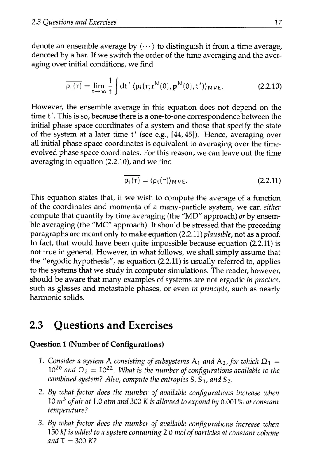
denote an ensemble average by (• • •) to distinguish it from a time average,
denoted by a bar. If we switch the order of the time averaging and the aver-
averaging over initial conditions, we find
Ш= Hm i|dt'(Pi(r;rN@),pN@),t'))NVE. B.2.10)
However, the ensemble average in this equation does not depend on the
time t'. This is so, because there is a one-to-one correspondence between the
initial phase space coordinates of a system and those that specify the state
of the system at a later time t' (see e.g., [44,45]). Hence, averaging over
all initial phase space coordinates is equivalent to averaging over the time-
evolved phase space coordinates. For this reason, we can leave out the time
averaging in equation B.2.10), and we find
Pi(T) = <Pi(r)>NVE. B-2.11)
This equation states that, if we wish to compute the average of a function
of the coordinates and momenta of a many-particle system, we can either
compute that quantity by time averaging (the "MD" approach) or by ensem-
ensemble averaging (the "MC" approach). It should be stressed that the preceding
paragraphs are meant only to make equation B.2.11) plausible, not as a proof.
In fact, that would have been quite impossible because equation B.2.11) is
not true in general. However, in what follows, we shall simply assume that
the "ergodic hypothesis", as equation B.2.11) is usually referred to, applies
to the systems that we study in computer simulations. The reader, however,
should be aware that many examples of systems are not ergodic in practice,
such as glasses and metastable phases, or even in principle, such as nearly
harmonic solids.
2.3 Questions and Exercises
Question 1 (Number of Configurations)
1. Consider a system A consisting of subsystems Ai and Кг, for which D.^ =
1020 and Q.2 = Ю22. What is the number of configurations available to the
combined system? Also, compute the entropies S, Si, and S2.
2. By what factor does the number of available configurations increase when
10 m3 of air at 1.0 aim and 300 К is allowed to expand by 0.001 % at constant
temperature?
3. By what factor does the number of available configurations increase when
150 kj is added to a system containing 2.0 mol of particles at constant volume
and T = 300 K?

18 Chapter 2. Statistical Mechanics
4. A sample consisting of five molecules has a total energy 5e. Each molecule
is able to occupy states of energy ej, with j = 0,1,2, • • • , oo. Draw up a
table with columns by the energy of the states and write beneath them all
configurations that are consistent with the total energy. Identify the type of
configuration that is most probable.
Question 2 (Thermodynamic Variables in the Canonical Ensemble) Start-
Starting with an expression for the Helmholtz free energy (Y) as a function o/N, V, T
-ln[Q(N,V,T)]
Э
one can derive all thermodynamic properties. Show this by deriving equations for
U, p, and S.
Question 3 (Ideal Gas (Part 1)) The canonical partition function of an ideal gas
consisting ofmonoatomic particles is equal to
Q(N.V.T)=
in whichX = h/y/2mn/ft and dP = dqi • • • dqisjd.pi • • • dpisj.
Derive expressions for the following thermodynamic properties:
• F(N,V,T)(Wnf:ln(N!)«Nln(N)-N)
• p (N, V, T) (which leads to the ideal gas law III)
• \i (N, V, T) (which leads to \i = \i0 + RT In p)
• U(N,V,T)andS(N,V,T)
• Cv (heat capacity at constant volume)
• Cp (heat capacity at constant pressure)
Question 4 (Ising Model) Consider a system o/N spins arranged on a lattice. In
the presence of a magnetic field, И, the energy of the system is
N
in which J is called the coupling constant (} > 0) and si = ±1. The second sum-
summation is a summation over all pairs (D x N for a periodic system, D is the dimen-
dimensionality of the system). This system is called the Ising model.
1. Show that for positive }, and H = 0, the lowest energy of the Ising model is
equal to
Uo = -DNJ
in which D is the dimensionality of the system.

2.3 Questions and Exercises 19
2. Show that the free energy per spin of a ID Ising model with zero field is equal
F(|3,N)_ lnBcosh(|3J))
N |3
when N —> oo. The function cosh (x) is defined as
exp [-x] + exp [x] ,.o1,
cosh(x) = —- -—. B.3.1)
3. Derive equations for the energy and heat capacity of this system.
Question 5 (The Photon Gas) An electromagnetic field in thermal equilibrium
can be described as a phonon gas. From the quantum theory of the electromagnetic
field, it is found that the total energy of the system (XX) can be written as the sum of
photon energies:
N N
in which ej is the characteristic energy of a photon with frequency w, j, rij =
0,1,2, • • • , oo is the so-called occupancy number of mode j, and N is the number of
field modes (here we take N to be finite).
1. Show that the canonical partition function of the system can be written as
n 1
i = i
Hint: you will have to use the following identity for | x |< 1:
B.3.3)
i=0
For the product of partition functions of two independent systems A and В
we can write
Qa x QB = Qab B.3.4)
when А П В = 0 and A U В = AB.
2. Show that the average occupancy number of state j, (гц), is equal to
<П>> ЭРИ) = expIPeJ-Г
3. Describe the behavior of (щ) when T —> oo and when T —> 0.

20 Chapter 2. Statistical Mechanics
Question 6 (Ideal Gas (Part 2)) An ideal gas is placed in a constant gravitational
field. The potential energy o/N gas molecules at height z is Mgz, where M. = mN
is the total mass o/N molecules. The temperature in the system is uniform and the
system infinitely large. We assume that the system is locally in equilibrium, so we
are allowed to use a local partition function.
1. Show that the grand-canonical partition function of a system in volume V at
height z is equal to
Q(n,V,T,z) = j~ еХ^У J drexp [-|3 (Ho + Mgz)] B.3.6)
in which Ho is the Hamiltonian of the system at z = 0.
2. Explain that a change in z is equivalent to a change in chemical potential, \i.
Use this to show that the pressure of the gas at height z is equal to
p(z) =p(z = 0) x exp [-|3mgz]. B.3.7)
(Hint: you will need the formula for the chemical potential of an ideal gas.)
Exercise 1 (Distribution of Particles)
Consider an ideal gas of N particles in a volume V at constant energy E.
Let us divide the volume in p identical compartments. Every compartment
contains ni molecules such that
i=p
nt. B.3.8)
An interesting quantity is the distribution of molecules over the p compart-
compartments. Because the energy is constant, every possible eigenstate of the
system will be equally likely. This means that in principle it is possible that
one of the compartments is empty.
1. On the book's website you can find a program that calculates the distri-
distribution of molecules among the p compartments. Run the program
for different numbers of compartments (p) and total number of gas
molecules (N). Note that the code has to be completed first (see the
file distribution./). The output of the program is the probability of find-
finding x particles in a particular compartment as a function of x. This is
printed in the file output.dat.
2. What is the probability that one of the compartments is empty?
3. Consider the case p = 2 and N even. The probability of finding N/2 +
tii molecules in compartment 1 and N/2 —щ molecules in compart-
compartment 2 is given by
N!

2.3 Questions and Exercises 21
Compare your numerical results with the analytical expression for dif-
different values of N. Show that this distribution is a Gaussian for small
ni/N. Hint: Forx > 10, it might be useful to use Stirling's approxima-
approximation:
x! « Bтг)* xx+^ exp [-x]. B.3.10)
Exercise 2 (Boltzmann Distribution)
Consider a system of N energy levels with energies 0, e,2e, • • • , (N - 1) e
and e > 0.
1. Calculate, using the given program, the occupancy of each level for dif-
different values of the temperature. What happens at high temperatures?
2. Change the program in such a way that the degeneracy of energy level
i equals i + 1. What do you see?
3. Modify the program in such a way that the occupation of the energy
levels as well as the partition function (q) is calculated for a hetero
nuclear linear rotor with moment of inertia I. Compare your result with
the approximate result
q = -^2 B.3.И)
for different temperatures. Note that the energy levels of a linear rotor
are
U = J(J + 1M- B.3.12)
with J = 0,1,2, ¦ ¦ • ,oo. The degeneracy of level J equals 2J + 1.
Exercise 3 (Coupled Harmonic Oscillators)
Consider a system of N harmonic oscillators with a total energy U. A single
harmonic oscillator has energy levels 0, e,2e, • • ¦ ,oo (e > 0). All harmonic
oscillators in the system can exchange energy.
1. Invent a computational scheme to update the system at constant total
energy (U). Compare your scheme with the scheme that is incorpo-
incorporated in the computer code that you can find on the book's website
(see the file harmonic./).
2. Make a plot of the energy distribution of the first oscillator as a function
of the number of oscillators for a constant value of U/N (output.dat).
Which distribution is recovered when N becomes large? What is the
function of the other N - 1 harmonic oscillators? Explain.
3. Compare this distribution with the canonical distribution of a single os-
oscillator at the same average energy (use the option NVT).
4. How does this exercise relate to the derivation of the Boltzmann distri-
distribution for a system at temperature T?

22 Chapter 2. Statistical Mechanics
Exercise 4 (Random Walk on a ID Lattice)
Consider the random walk of a single particle on a line. The particle performs
jumps of fixed lengthi. Assuming that the probability for forward or backward
jumps is equal, the mean-squared displacement of a particle after N jumps
is equal to N. The probability that, after N jumps, the net distance covered
by the particle equals n is given by
1. Derive this equation using Stirling's approximation for lnx!.
2. Compare your numerical result for the root mean-squared displace-
displacement with the theoretical prediction (the computed function P(n,N),
see the file output.dat). What is the diffusivity of this system?
3. Modify the program in such a way that the probability to jump in the
forward direction equals 0.8. What happens?
Exercise 5 (Random Walk on a 2D Lattice)
Consider the random walk of N particles on a M x M lattice. Two particles
cannot occupy the same lattice site. On this lattice, periodic boundaries are
used. This means that when a particle leaves the lattices it returns on the
opposite side of the lattice; i.e., the coordinates are given modulo M.
1. What is the fraction of occupied sites @) of the lattice as a function of
MandN?
2. Make a plot of the diffusivity D as a function of 0 for M = 32. For low
values of 0, the diffusivity can be approximated by
D* Do A-9).
Why is this equation reasonable at low densities? Why does it break
down at higher densities?
3. Modify the program in such a way that the probability to jump in one
direction is larger than the probability to jump in the other direction.
Explain the results.
4. Modify the program in such a way that periodic boundary conditions are
used in one direction and reflecting boundary conditions in the other.
What happens?

Chapter 3
Monte Carlo Simulations
In the present chapter, we describe the basic principles of the Monte Carlo
method. In particular, we focus on simulations of systems of a fixed number
of particles (N) in a given volume (V) at a temperature (T).
3.1 The Monte Carlo Method
In the previous chapter, we introduced some of the basic concepts of (classi-
(classical) statistical mechanics. Our next aim is to indicate where the Monte Carlo
method comes in. We start from the classical expression for the partition
function Q, equation B.2.5):
Q = c[dpNdrNexp[-H(rN pN)/kBT], C.1.1)
where rN stands for the coordinates of all N particles, and pN for the cor-
corresponding momenta. The function %(qN,pN) is the Hamiltonian of the
system. It expresses the total energy of an isolated system as a function of
the coordinates and momenta of the constituent particles: H = /C + U, where
/C is the kinetic energy of the system and U is the potential energy. Finally,
с is a constant of proportionality, chosen such that the sum over quantum
states in equation B.1.15) approaches the classical partition function in the
limit Ft —> 0. For instance, for a system of N identical atoms, с = 1/(lx3NlM!).
The classical equation corresponding to equation B.2.1) is
_ JdpNdrN A(p,r)exp[CH(p,r)]
[ ' JdpNdrN exp[|3H(pNrN)] ' K }
where C = 1/квТ. In this equation, the observable A has been expressed
as a function of coordinates and momenta. As /C is a quadratic function of

24 Chapter 3. Monte Carlo Simulations
the momenta the integration over momenta can be carried out analytically.
Hence, averages of functions that depend on momenta only are usually easy
to evaluate.1 The difficult problem is the computation of averages of func-
functions A(rN). Only in a few exceptional cases can the multidimensional in-
integral over particle coordinates be computed analytically; in all other cases
numerical techniques must be used.
Having thus defined the nature of the numerical problem that we must
solve, let us next look at possible solutions. It might appear that the most
straightforward approach would be to evaluate (A) in equation C.1.2) by
numerical quadrature, for instance using Simpson's rule. It is easy to see,
however, that such a method is completely useless even if the number of
independent coordinates DN (D is the dimensionality of the system) is still
very small (9A00). Suppose that we plan to carry out the quadrature by
evaluating the integrand on a mesh of points in the DN-dimensional config-
configuration space. Let us assume that we take m equidistant points along each
coordinate axis. The total number of points at which the integrand must be
evaluated is then equal to mDN. For all but the smallest systems this num-
number becomes astronomically large, even for small values of m. For instance,
if we take 100 particles in three dimensions, and m = 5, then we would have
to evaluate the integrand at 10210 points! Computations of such magnitude
cannot be performed in the known universe. And this is fortunate, because
the answer that would be obtained would have been subject to a large sta-
statistical error. After all, numerical quadratures work best on functions that
are smooth over distances corresponding to the mesh size. But for most in-
termolecular potentials, the Boltzmann factor in equation C.1.2) is a rapidly
varying function of the particle coordinates. Hence an accurate quadrature
requires a small mesh spacing (i.e., a large value of m). Moreover, when
evaluating the integrand for a dense liquid (say), we would find that for the
overwhelming majority of points this Boltzmann factor is vanishingly small.
For instance, for a fluid of 100 hard spheres at the freezing point, the Boltz-
Boltzmann factor would be nonzero for 1 out of every 10260 configurations!
The preceding example clearly demonstrates that better numerical tech-
techniques are needed to compute thermal averages. One such a technique is
the Monte Carlo method or, more precisely, the Monte Carlo importance-
sampling algorithm introduced in 1953 by Metropolis et ah [6]. The applica-
application of this method to the numerical simulation of dense molecular systems
is the subject of the present chapter.
3.1.1 Importance Sampling
Before discussing importance sampling, let us first look at the simplest Mon-
Monte Carlo technique, that is, random sampling. Suppose we wish to evaluate
lrThis is not the case when hard constraints are used, see section 11.2.1.

3.1 The Monte Carlo Method 25
numerically a one-dimensional integral I:
fb
1= dxf(x). C.1.3)
Ja
Instead of using a conventional quadrature where the integrand is evaluated
at predetermined values of the abscissa, we could do something else. Note
that equation C.1.3) can be rewritten as
I = (b-a)<f(x)>, C.1.4)
where (f (x)) denotes the unweighted average of f (x) over the interval [a, b].
In brute force Monte Carlo, this average is determined by evaluating f (x) at
a large number (say, L) of x values randomly distributed over the interval
[a, b]. It is clear that, as L —» oo, this procedure should yield the correct value
for I. However, as with the conventional quadrature procedure, this method
is of little use to evaluate averages such as in equation C.1.2) because most of
the computing is spent on points where the Boltzmann factor is negligible.
Clearly, it would be much preferable to sample many points in the region
where the Boltzmann factor is large and few elsewhere. This is the basic
idea behind importance sampling.
How should we distribute our sampling through configuration space?
To see this, let us first consider a simple, one-dimensional example. Suppose
we wish to compute the definite integral in equation C.1.3) by Monte Carlo
sampling, but with the sampling points distributed nonuniformly over the
interval [a, b] (for convenience we assume a = 0 and b = 1), according to
some nonnegative probability density w(x). Clearly, we can rewrite equa-
equation C.1.3) as
1= [ dxw(x)-^-. C.1.5)
Jo WM
Let us assume that we know that w(x) is the derivative of another (non-
negative, nondecreasing) function u(x), with u@) = 0 and uA) = 1 (these
boundary conditions imply that w(x) is normalized). Then I can be written
as
1= du^p^. C.1.6)
Jo w[x(u)]
In equation C.1.6) we have written x(u) to indicate that, if we consider u as
the integration variable, then x must be expressed as a function of u. The
next step is to generate L random values of u uniformly distributed in the
interval [0,1]. We then obtain the following estimate for I:
(зл.7)

26 Chapter 3. Monte Carlo Simulations
What have we gained by rewriting I in this way? The answer depends cru-
crucially on our choice for w(x). To see this, let us estimate of, the variance in
II, where II denotes the estimate for I obtained from equation C.1.7) with L
random sample points:
~<f/w>) i^mi -<f/w>
where the angular brackets denote the true average, that is, the one that
would be obtained in the limit I —> oo. As different samples i and j are
assumed to be totally independent, all cross terms in equation C.1.8) vanish,
and we are left with
i=1 x v*v[x(Ui)]
= l [((VwJ)-(f/wJ]. C.1.9)
Equation C.1.9) shows that the variance in I still goes as 1/L, but the mag-
magnitude of this variance can be reduced greatly by choosing w(x) such that
f (x)/w(x) is a smooth function of x. Ideally, we should have f (x)/w(x) con-
constant, in which case the variance would vanish altogether. In contrast, if w(x)
is constant, as is the case for the brute force Monte Carlo sampling, then the
relative error in I can become very large. For instance, if we are sampling
in a (multidimensional) configuration space of volume П, of which only a
small fraction f is accessible (for instance, f = 10~~260, see previous section),
then the relative error that results in a brute force MC sampling will be of
order 1/(Lf). As the integrand in equation C.1.2) is nonzero only for those
configurations where the Boltzmann factor is nonzero, it would clearly be
advisable to carry out a nonuniform Monte Carlo sampling of configuration
space, such that the weight function w is approximately proportional to the
Boltzmann factor. Unfortunately, the simple importance sampling scheme
described previously cannot be used to sample multidimensional integrals
over configuration space, such as equation C.1.2). The reason is simply that
we do not know how to construct a transformation such as the one from
equation C.1.5) to equation C.1.6) that would enable us to generate points
in configuration space with a probability density proportional to the Boltz-
Boltzmann factor. In fact, a necessary (but not nearly sufficient) condition for the
solution to the latter problem is that we must be able to compute analytically
the partition function of the system under study. If we could do that for the
systems of interest to us, there would be hardly any need for computer sim-
simulation.

3.1 The Monte Carlo Method 27
3.1.2 The Metropolis Method
The closing lines of the previous section suggest that it is in general not pos-
possible to evaluate an integral, such as /drN exp[— |3ZV(rN)], by direct Monte
Carlo sampling. However, in many cases, we are not interested in the con-
figurational part of the partition function itself but in averages of the type
Hence, we wish to know the ratio of two integrals. What Metropolis et al. [6]
showed is that it is possible to devise an efficient Monte Carlo scheme to
sample such a ratio.2 To understand the Metropolis method, let us first look
more closely at the structure of equation C.1.10). In what follows we denote
the configurational part of the partition function by Z:
Z = [drN exp[-CZY(rN)]. C.1.11)
Note that the ratio exp(—CZY)/Z in equation C.1.10) is the probability den-
density of finding the system in a configuration around rN. Let us denote this
probability density by
Clearly, A/"(rN) is nonnegative.
Suppose now that we are somehow able to randomly generate points in
configuration space according to this probability distribution A/"(rN). This
means that, on average, the number of points ni generated per unit volume
around a point rN is equal to LA/"(rN), where L is the total number of points
that we have generated. In other words,
C.1.12)
By now the reader is almost certainly confused about the difference, if any,
between equation C.1.12) and equation C.1.7) of section 3.1.1. The difference
is that in the case of equation C.1.7) we know a priori the probability of sam-
sampling a point in a (hyper)volume drN around rN. In other words we know
both exp[—CZY(rN)] and Z. In contrast, in equation C.1.12) we know only
exp[— fW(rN)]; that is, we know only the relative but not the absolute prob-
probability of visiting different points in configuration space. This may sound
2 An interesting account of the early history of the Metropolis method may be found in
refs. [1,46].

28
Chapter 3. Monte Carlo Simulations
Nile
Figure 3.1: Measuring the depth of the Nile: a comparison of conventional
quadrature (left), with the Metropolis scheme (right).
rather abstract: let us therefore try to clarify the difference with the help of
a simple example (see Figure 3.1). In this figure, we compare two ways of
measuring the depth of the river Nile, by conventional quadrature (left) and
by Metropolis sampling; that is, the construction of an importance-weighted
random walk (right). In the conventional quadrature scheme, the value of
the integrand is measured at a predetermined set of points. As the choice
of these points does not depend on the value of the integrand, many points
may be located in regions where the integrand vanishes. In contrast, in the
Metropolis scheme, a random walk is constructed through that region of
space where the integrand is nonnegligible (i.e., through the Nile itself). In
this random walk, a trial move is rejected if it takes you out of the water and
is accepted otherwise. After every trial move (accepted or not), the depth of
the water is measured. The (unweighted) average of all these measurements
yields an estimate of the average depth of the Nile. This, then, is the essence
of the Metropolis method. In principle, the conventional quadrature scheme
would also give results for the total area of the Nile. In the importance sam-
sampling scheme, however, information on the total area cannot be obtained
directly, since this quantity is similar to Z.
Let us next consider how to generate points in configuration space with
a relative probability proportional to the Boltzmann factor. The general ap-
approach is first to prepare the system in a configuration rN, which we denote
by о (old), that has a nonvanishing Boltzmann factor exp[— $U{o)\. This
configuration, for example, may correspond to a regular crystalline lattice
with no hard-core overlaps. Next, we generate a new trial configuration r'N,

3.1 The Monte Carlo Method 29_
which we denote by n (new), by adding a small random displacement A
to o. The Boltzmann factor of this trial configuration is exp[— $U{n)]. We
must now decide whether we will accept or reject the trial configuration.
Many rules for making this decision satisfy the constraint that on average
the probability of finding the system in a configuration n is proportional to
jV(n). Here we discuss only the Metropolis scheme, because it is simple and
generally applicable.
Let us now "derive" the Metropolis scheme to determine the transition
probability 7i(o —> n) to go from configuration о to n. It is convenient to
start with a thought experiment (actually a thought simulation). We carry
out a very large number (say M) Monte Carlo simulations in parallel, where
M is much larger than the total number of accessible configurations. We
denote the number of points in any configuration о by m(o). We wish that,
on average, m(o) is proportional to J\f{o). The matrix elements 7i(o —> n)
must satisfy one obvious condition: they do not destroy such an equilibrium
distribution once it is reached. This means that, in equilibrium, the average
number of accepted trial moves that result in the system leaving state о must
be exactly equal to the number of accepted trial moves from all other states rt
to state o. It is convenient to impose a much stronger condition; namely, that
in equilibrium the average number of accepted moves from о to any other
state n is exactly canceled by the number of reverse moves. This detailed
balance condition implies the following:
7V(o)tt(o -> n) = 7V(nOr(n -> o). C.1.13)
Many possible forms of the transition matrix 7i(o —> n) satisfy equation
C.1.13). Let us look how 7i(o —> n) is constructed in practice. We recall that
a Monte Carlo move consists of two stages. First, we perform a trial move
from state о to state n. We denote the transition matrix that determines the
probability of performing a trial move from о to n by cx(o —> n), where ex is
usually referred to as the underlying matrix of the Markov chain [47]. The
next stage is the decision to either accept or reject this trial move. Let us
denote the probability of accepting a trial move from о to n by acc(o —* n).
Clearly,
7г(о —* n) = cx(o —> n) x acc(o —> n). C.1.14)
In the original Metropolis scheme, ex is chosen to be a symmetric matrix
(cx(o —* n) = cx(n —> o)). However, in later sections we shall see several
examples where ex is not symmetric. If ex is symmetric, we can rewrite equa-
equation C.1.13) in terms of the acc(o —> n):
7V(o) x acc(o -» n) =7V(n) x асс(п -» о). C.1.15)
From equation C.1.15) follows
Ш^)-иш- <ЗЛЛ6)

30 Chapter 3. Monte Carlo Simulations
Again, many choices for acc(o —> n) satisfy this condition (and the obvious
condition that the probability acc(o —> n) cannot exceed 1). The choice of
Metropolis et ah is
acc(o^n) = ЛГ(п)/ЛГ(о) if Af(n) < Af(o)
= 1 if7V(n)>7V(o). {6ЛЛ/)
Other choices for acc(o —» n) are possible (for a discussion, see for instance
[19]), but the original choice of Metropolis et ah appears to result in a more
efficient sampling of configuration space than most other strategies that have
been proposed.
In summary, then, in the Metropolis scheme, the transition probability
for going from state о to state n is given by
7r(o —> n) = ct(o —» n) Л/"(п) > Л/"(о)
} ЛГ(п)<ЛГ(о) C.1.18)
Note that we still have not specified the matrix a, except for the fact that it
must be symmetric. This reflects considerable freedom in the choice of our
trial moves. We will come back to this point in subsequent sections.
One thing that we have not yet explained is how to decide whether a
trial move is to be accepted or rejected. The usual procedure is as follows.
Suppose that we have generated a trial move from state о to state n, with
U[n) > U{o). According to equation C.1.16) this trial move should be ac-
accepted with a probability
acc(o -> n) = exp{-|3[ZV(n) - U[o)]} < 1.
In order to decide whether to accept or reject the trial move, we generate
a random number, denoted by Ranf, from a uniform distribution in the in-
interval [0,1]. Clearly, the probability that Ranf is less than acc(o —> n) is
equal to acc(o —> n). We now accept the trial move if Ranf < acc(o —» n)
and reject it otherwise. This rule guarantees that the probability to accept a
trial move from о to n is indeed equal to acc(o —> n). Obviously, it is very
important that our random-number generator does indeed generate num-
numbers uniformly in the interval [0,1]. Otherwise the Monte Carlo sampling
will be biased. The quality of random-number generators should never be
taken for granted. A good discussion of random-number generators can be
found in Numerical Recipes [33] and in Monte Carlo Methods by Kalos and
Whitlock [32].
Thus far, we have not mentioned another condition that n{o —> n) should
satisfy, namely that it is ergodic (i.e., every accessible point in configuration
space can be reached in a finite number of Monte Carlo steps from any other
point). Although some simple MC schemes are guaranteed to be ergodic,

3.2 Л Basic Monte Carlo Algorithm 31
these are often not the most efficient schemes. Conversely, many efficient
Monte Carlo schemes have either not been proven to be ergodic or, worse,
been proven to be nonergodic. The solution is usually to mix the efficient,
nonergodic scheme with an occasional trial move of the less-efficient but
ergodic scheme. The method as a whole will then be ergodic (at least, in
principle).
At this point, we should stress that, in the present book, we focus on
Monte Carlo methods to model phenomena that do not depend on time. In
the literature one can also find dynamic Monte Carlo schemes. In such dy-
dynamic algorithms, Monte Carlo methods are used to generate a numerical
solution of the master equation that is supposed to describe the time evolu-
evolution of the system under study. These dynamic techniques fall outside the
scope of this book. The reader interested in dynamic MC schemes is referred
to the relevant literature, for example Ref. [48] and references therein.
3.2 A Basic Monte Carlo Algorithm
It is difficult to talk about Monte Carlo or Molecular Dynamics programs in
abstract terms. The best way to explain how such programs work is to write
them down. This will be done in the present section.
Most Monte Carlo or Molecular Dynamics programs are only a few hun-
hundred to several thousand lines long. This is very short compared to, for
instance, a typical quantum-chemistry code. For this reason, it is not un-
uncommon that a simulator will write many different programs that are tailor-
made for specific applications. The result is that there is no such thing as a
standard Monte Carlo or Molecular Dynamics program. However, the cores
of most MD/MC programs are, if not identical, at least very similar. Next,
we shall construct such a core. It will be very rudimentary, and efficiency
has been traded for clarity. But it should demonstrate how the Monte Carlo
method works.
3.2.1 The Algorithm
The prime purpose of the kind of Monte Carlo or Molecular Dynamics pro-
program that we shall be discussing is to compute equilibrium properties of
classical many-body systems. From now on, we shall refer to such programs
simply as MC or MD programs, although it should be remembered that there
exist many other applications of the Monte Carlo method (and, to a lesser ex-
extent, of the Molecular Dynamics method). Let us now look at a simple Monte
Carlo program.
In the previous section, the Metropolis method was introduced as a Mar-
Markov process in which a random walk is constructed in such a way that the

32 Chapter 3. Monte Carlo Simulations
probability of visiting a particular point rN is proportional to the Boltzmann
factor exp[—CZY(rN)]. There are many ways to construct such a random walk.
In the approach introduced by Metropolis et ah [6], the following scheme is
proposed:
1. Select a particle at random, and calculate its energy ZY(rN).
2. Give the particle a random displacement, r' = r + Д, and calculate its
new energy U{r'N).
3. Accept the move from rN to r'N with probability
acc(o -> n) = min (i,exp{-[3[ZY(r'N) -ZY(rN)]}) . C.2.1)
An implementation of this basic Metropolis scheme is shown in Algorithms
1 and 2.
3.2.2 Technical Details
In this section, we discuss a number of computational tricks that are of great
practical importance for the design of an efficient simulation program. It
should be stressed that most of these tricks, although undoubtedly very use-
useful, are not unique and have no deep physical significance. But this does not
imply that the use of such computational tools is free of risks or subtleties.
Ideally, schemes to save computer time should not affect the results of a sim-
simulation in a systematic way. Yet, in some cases, time-saving tricks do have
a measurable effect on the outcome of a simulation. This is particularly true
for the different procedures used to avoid explicit calculation of intermolec-
ular interactions between particles that are far apart. Fortunately, once this
is recognized, it is usually possible to estimate the undesirable side effect of
the time-saving scheme and correct for it.
Boundary Conditions
Monte Carlo and Molecular Dynamics simulations of atomic or molecular
systems aim to provide information about the properties of a macroscopic
sample. Yet, the number of degrees of freedom that can be conveniently han-
handled in present-day computers ranges from a few hundred to a few million.
Most simulations probe the structural and thermodynamical properties of a
system of a few hundred to a few thousand particles. Clearly, this number
is still far removed from the thermodynamic limit. To be more precise, for
such small systems it cannot be safely assumed that the choice of the bound-
boundary conditions (e.g., free or hard or periodic) has a negligible effect on the
properties of the system. In fact, in a three-dimensional N-particle system

3.2 A Basic Monte Carlo Algorithm
33
Algorithm 1 (Basic Metropolis Algorithm)
PROGRAM me
do icycl=l,ncycl
call mcmove
if (mod(icycl,nsamp).eq.0)
+ call sample
enddo
end
basic Metropolis algorithm
perform ncycl MC cycles
displace a particle
sample averages
Comments to this algorithm:
1. Subroutine mcmove attempts to displace a randomly selected particle
(see Algorithm 2).
2. Subroutine sample samples quantities every nsampf/z cycle.
Algorithm 2 (Attempt to Displace a Particle)
SUBROUTINE mcmove
o= int(ranf()*npart)+1
call ener(x(o),eno)
xn=x(o)+(ranf()-0.5)*delx
call ener(xn,enn)
if (ranf().It.exp(-beta
+ *(enn-eno)) x(o)=xn
return
end
attempts to displace a particle
select a particle at random
energy old configuration
give particle random displacement
energy new configuration
acceptance rule C.2.1)
accepted: replace x(o) byxn
Comments to this algorithm:
1. Subroutine ener calculates the energy of a particle at the given position.
2. Note that, if a configuration is rejected, the old configuration is retained.
3. The ranf () is a random number uniform in [0,1].

34
Chapter 3. Monte Carlo Simulations
0
•
0
•
о
о
о
о
•о
•
•
•о
•
•
0
•
0
•
о'
о
4
о'
о
•о
ч
»
•
0
ц-
•
4
1
о'
о
•о
•
•о
»
•
0
•
0
•
о
о
о
•о
•
•
•о
•
•
Figure 3.2: Schematic representation of periodic boundary conditions.
with free boundaries, the fraction of all molecules that is at the surface is
proportional to N~1//3. For instance, in a simple cubic crystal of 1000 atoms,
some 49% of all atoms are at the surface, and for 106 atoms this fraction has
decreased to only 6%.
In order to simulate bulk phases it is essential to choose boundary condi-
conditions that mimic the presence of an infinite bulk surrounding our N-particle
model system. This is usually achieved by employing periodic boundary
conditions. The volume containing the N particles is treated as the primitive
cell of an infinite periodic lattice of identical cells (see Figure 3.2). A given
particle (i, say) now interacts with all other particles in this infinite periodic
system, that is, all other particles in the same periodic cell and all particles
(including its own periodic image) in all other cells. For instance, if we as-
assume that all intermolecular interactions are pairwise additive, then the total
potential energy of the N particles in any one periodic box is
<tot
U Гг
where L is the diameter of the periodic box (assumed cubic, for convenience)
and n is an arbitrary vector of three integer numbers, while the prime over
the sum indicates that the term with i = j is to be excluded when n = 0.
In this very general form, periodic boundary conditions are not particularly
useful, because to simulate bulk behavior, we had to rewrite the potential
energy as an infinite sum rather than a finite one.3 In practice, however, we
3In fact, in the first MC simulation of three-dimensional Lennard-Jones particles, Wood and
Parker [49] discuss the use of such infinite sums in relation to the now conventional approach
discussed here.

3.2 A Basic Monte Carlo Algorithm 35
are often dealing with short-range interactions. In that case it is usually per-
permissible to truncate all intermolecular interactions beyond a certain cutoff
distance rc. How this is done in practice is discussed next.
Although the use of periodic boundary conditions proves to be a sur-
surprisingly effective method for simulating homogeneous bulk systems, one
should always be aware that the use of such boundary conditions may lead
to spurious correlations not present in a truly macroscopic bulk system. In
particular, one consequence of the periodicity of the model system is that
only those fluctuations are allowed that have a wavelength compatible with
the periodic lattice: the longest wavelength that still fits in the periodic box
is the one for which Л = L. If long wavelength fluctuations are expected to
be important (as, for instance, in the vicinity of a continuous phase transi-
transition), then one should expect problems with the use of periodic boundary
conditions. Another unphysical effect that is a manifestation of the use of
periodic boundary conditions is that the radial distribution function g(r) of
a dense atomic fluid is found to be not exactly isotropic [50].
Finally, it is useful to point out one common misconception about peri-
periodic boundary conditions, namely, the idea that the boundary of the periodic
box itself has any special significance. It has none. The origin of the periodic
lattice of primitive cells may be chosen anywhere, and this choice will not
affect any property of the model system under study. In contrast, what is
fixed is the shape of the periodic cell and its orientation.
Truncation of Interactions
Let us now consider the case that we perform a simulation of a system with
short-range interactions. In this context, short-ranged means that the total po-
potential energy of a given particle i is dominated by interactions with neigh-
neighboring particles that are closer than some cutoff distance rc. The error that
results when we ignore interactions with particles at larger distances can be
made arbitrarily small by choosing rc sufficiently large. If we use periodic
boundary conditions, the case that rc is less than L/2 (half the diameter of the
periodic box) is of special interest because in that case we need to consider
the interaction of a given particle i only with the nearest periodic image of
any other particles j (see the dotted box in Figure 3.2). If the intermolecular
potential is not rigorously zero for r > rc, truncation of the intermolecular
interactions at rc will result in a systematic error in Utot. If the intermolec-
intermolecular interactions decay rapidly, one may correct for the systematic error by
adding a tail contribution to Utot:
Ыш = }~ uc (rtj) + ^ Г dr и(гLтгг2, C.2.2)

36 Chapter 3. Monte Carlo Simulations
where uc stands for the truncated potential energy function and p is the
average number density. In writing down this expression, it is implicitly
assumed that the radial distribution function g(r) = 1 for r > rc. Clearly, the
nearest periodic image convention can be applied only if the tail correction
is small. From equation C.2.2) it can be seen that the tail correction to the
potential energy is infinite unless the potential energy function u(r) decays
more rapidly than r~3 (in three dimensions). This condition is satisfied if the
long-range interaction between molecules is dominated by dispersion forces.
However, for the very important case of Coulomb and dipolar interactions,
the tail correction diverges and hence the nearest-image convention cannot
be used for such systems. In such cases, the interactions with all periodic
images should be taken into account explicitly. Ways to do this are described
in Chapter 12.1.
Several factors make truncation of the potential a tricky business. First of
all, it should be realized that, although the absolute value of the potential en-
energy function decreases with interparticle separation r, for sufficiently large
r, the number of neighbors is a rapidly increasing function of r. In fact, the
number of particles at a distance r of a given atom increases asymptotically
as rd~1, where d is the dimensionality of the system. As an example, let us
compute the effect of truncating the pair potential for a simple example —
the three-dimensional Lennard-Jones fluid. The pair potential for this rather
popular model system is given by
The average potential energy (in three dimensions) of any given atom i is
given by
where p(r) denotes the average number density at a distance r from a given
atom i. The factor A/2) has been included to correct for double counting of
intermolecular interactions. If we truncate the potential at a distance rc, we
ignore the tail contribution utai1:
foo
dr47tr2p(r)u(r), C.2.4)
where we have dropped the subscript i, because all atoms in the system are
identical. To simplify the calculation of utai1, we assume that for r > rc, the
density p(r) is equal to the average number density p. If u(r) is the Lennard-

3.2 A Basic Monte Carlo Algorithm 37
Jones potential, we find for u
tai1
utail = ]-4np [ drr2u(r)
1
f°° 7 Г/сг\12 /a\6l
drr (~)
Jrc LVr' Vr' J
C.2.5)
9 /ax3
= ^pea3 3Vr
For a cutoff distance rc = 2.5 a the potential has decayed to a value that is
about l/60th of the well depth. This seems to be a very small value, but
in fact the tail correction is usually nonnegligible. For instance, at a density
pa3 = 1, we find utai1 = —0.535e. This number is certainly not negligible
compared to the total potential energy per atom (almost 10% at a typical
liquid density); hence although we can truncate the potential at 2.5 a, we
cannot ignore the effect of this truncation.
There are several ways to truncate potentials in a simulation. Although
the methods are designed to yield similar results, it should be realized that
they yield results that may differ significantly, in particular in the vicinity of
critical points [51-53] (see Figure 3.3). Often used methods to truncate the
potential are
1. Simple truncation
2. Truncation and shift
3. Minimum image convention.
Simple Truncation The simplest method to truncate potentials is to ignore
all interaction beyond rc, the potential that is simulated is
utrunc(r) = j UV) r^Tc {326)
As already explained, this may result in an appreciable error in our estimate
of the potential energy of the true Lennard-Jones potential C.2.3). Moreover,
as the potential changes discontinuously at rc, a truncated potential is not
particularly suitable for a Molecular Dynamics simulation. It can, however,
be used in Monte Carlo simulations. In that case, one should be aware that
there is an "impulsive" contribution to the pressure due to the discontinuous
change of the potential at rc. That contribution can by no means be ignored.

38
Chapter 3. Monte Carlo Simulations
1.3
1.1
0.9
0.7
If
truncated and shifted
tail correction
\
\ '
. A.
0.0 0.2
0.4 0.6
P
0.8 1.0
Figure 3.3: Vapor-liquid coexistence curves of various three-dimensional
Lennard-Jones fluids: effect of the truncation of the potential on the loca-
location of the critical point (large black dots). The upper curve gives the phase
envelope for the full Lennard-Jones potential (i.e., a truncated potential with
tail correction); the lower curve gives the envelope for the potential that is
used in most Molecular Dynamics simulations (truncated and shifted poten-
potential with rc = 2.5a), data from [53].
For instance, for the three-dimensional Lennard-Jones system,
8n 2
tp
3
?<T3
ea3
—
[(?
-
J
—
01
C.2.7)
It is rare, however, to see this impulsive correction to the pressure applied
in simulations of systems with truncated potentials. Usually, it is simply as-
assumed that we can correct for the truncation of the intermolecular potential
by adding the correction given by equation C.2.5) to the potential energy.
The corresponding correction to the pressure is
ДР
tail
= A/2Lтгр2
16 2 3
= —яр ест
¦r-f(r)
C.2.8)
But, as is immediately obvious from a comparison of equations C.2.7) and
C.2.8), the impulsive correction to the pressure is not equivalent to the tail

3.2 Л Basic Monte Carlo Algorithm 39
correction. Rather, the impulsive pressure is the contribution that must be
included if one wishes to compute the true pressure of a system with a trun-
truncated potential, whereas the tail correction should be included to obtain an
estimate of the pressure in a system with untruncated interactions.
Truncated and Shifted In Molecular Dynamics simulations, it is common
to use another procedure: the potential is truncated and shifted, such that
the potential vanishes at the cutoff radius:
""M-^) г<тс C29)
U т > Vq
In this case, there are no discontinuities in the intermolecular potential and
hence no impulsive corrections to the pressure. The advantage of using
such a truncated and shifted potential is that the intermolecular forces are
always finite.4 This is important because impulsive forces cannot be han-
handled in those Molecular Dynamics algorithms to integrate the equations of
motion that are based on a Taylor expansion of the particle positions. Of
course, the potential energy and pressure of a system with a truncated and
shifted potential differ from the corresponding properties of both the mod-
models with untruncated and with truncated but unshifted pair potentials. But,
as before, we can approximately correct for the effect of the modification of
the intermolecular potential on both the potential energy and the pressure.
For the pressure, the tail correction is the same as in equation C.2.8). For the
potential energy, we must add to the long-range correction C.2.5) a contri-
contribution equal to the average number of particles that are within a distance rc
from a given particle, multiplied by half the value of the (untruncated) pair
potential at rc. The factor one-half is included to correct for overcounting
of the intermolecular interactions. One should be extremely careful when
applying truncated and shifted potentials in models with anisotropic inter-
interactions. In that case, truncation should not be carried out at a fixed value of
the distance between the molecular centers of mass but at a point where the
pair potential has a fixed value, because otherwise the potential cannot be
shifted to 0 at the point where it is truncated. For Monte Carlo simulations,
this is not serious, but for Molecular Dynamics simulations this would be
quite disastrous, as the system would no longer conserve energy, unless the
impulsive forces due to the truncating and shifting are taken into account
explicitly.
Minimum Image Convention Sometimes the minimum image convention
is used. The truncation is in this case not at a spherical cutoff; instead the
4The first derivative of the force is discontinuous at the cutoff radius; some authors remove
this discontinuity as well (for more details, see [19]).

40 Chapter 3. Monte Carlo Simulations
interaction with the (nearest image) of all the particles in the simulation box
is calculated. As a consequence, the potential is not a constant on the surface
of a cube around a given particle. Hence, for the same reasons as mentioned
in the previous paragraph, the simple minimum image convention should
never be used in Molecular Dynamics simulations.
In the preceding, we described some details on how the energy should be
calculated. The implementation of a simple, order-N2, algorithm to compute
the energy will be discussed in section 4.2.2 in the context of a Molecular Dy-
Dynamics simulation (see Algorithm 5). More advanced schemes to simulate
large systems efficiently are described in Appendix F.
Initialization
To start the simulation, we should assign initial positions to all particles in
the system. As the equilibrium properties of the system do not (or, at least,
should not) depend on the choice of initial conditions, all reasonable initial
conditions are in principle acceptable. If we wish to simulate the solid state
of a particular model system, it is logical to prepare the system in the crystal
structure of interest. In contrast, if we are interested in the fluid phase, we
simply prepare the system in any convenient crystal structure. This crys-
crystal subsequently melts, because at the temperature and density of a typical
liquid-state point, the solid state is not thermodynamically stable. Actually,
one should be careful here, because the crystal structure may be metastable,
even if it is not absolutely stable. For this reason, it is unwise to use a crystal
structure as the starting configuration of a liquid close to the freezing curve.
In such cases, it is better to use the final (liquid) configuration of a system at
a higher temperature or lower density, where the solid is unstable and has
melted spontaneously. In any event, it is usually preferable to use the final
(well-equilibrated) configuration of an earlier simulation at a nearby state
point as the starting configuration for a new run and adjust the temperature
and density to the desired values.
The equilibrium properties of a system should not depend on the initial
conditions. If such a dependence nevertheless is observed in a simulation,
there are two possibilities. The first is that our results reflect the fact that the
system that we simulate really behaves nonergodically. This is the case, for
instance, in glassy materials or low-temperature, substitutionally disordered
alloys. The second (and much more likely) explanation is the system we
simulate is ergodic but our sampling of configuration space is inadequate;
in other words, we have not yet reached equilibrium.
Reduced Units
In simulations it is often convenient to express quantities such as tempera-
temperature, density, pressure, and the like in reduced units. This means that we
choose a convenient unit of energy, length and mass and then express all

3.2 A Basic Monte Carlo Algorithm 41
other quantities in terms of these basic units. In the example of a Lennard-
Jones system, we use a pair potential that is of the form u(r) = ef (г/ст) (see
equation C.2.3)). A natural (though not unique) choice for our basic units is
the following:
• Unit of length, a
• Unit of energy, e
• Unit of mass, m (the mass of the atoms in the system)
and from these basic units, all other units follow. For instance, our unit of
time is
<j\/m/e
and the unit of temperature is
е/кв.
In terms of these reduced units, denoted with superscript *, the reduced
pair potential u* = u/e is a dimensionless function of the reduced distance
r* = r/a. For instance, the reduced form for the Lennard-Jones potential is
lj
u*J)(r*) = 4
г
1\12
C.2.10)
With these conventions we can define the following reduced units: the po-
potential energy U* = lie, the pressure P* = Po^e, the density p* = per3,
and the temperature T * = квТе^1.
One may wonder why it is convenient to introduce reduced units. The
most important reason is that (infinitely) many combinations of p,T, e, and
a all correspond to the same state in reduced units. This is the law of corre-
corresponding states: the same simulation of a Lennard-Jones model can be used
to study Ar at 60 К and a density of 840 kg/m3 and Xe at 112 К and a density
of 1617 kg/m3. In reduced units, both simulations correspond to the state
point p* = 0.5, T* = 0.5. If we had not used reduced units, we might have
easily missed the equivalence of these two simulations. Another, practical,
reason for using reduced units is the following: when we work with real (SI)
units, we find that the absolute numerical values of the quantities that we
are computing (e.g., the average energy of a particle or its acceleration) are
either much less or much larger than 1. If we multiply several such quanti-
quantities using standard floating-point multiplication, we face a distinct risk that,
at some stage, we will obtain a result that creates an overflow or under-
underflow. Conversely, in reduced units, almost all quantities of interest are of
order 1 (say, between 10~3 and 103). Hence, if we suddenly find a very large
(or very small) number in our simulations (say, 1042), then there is a good
chance that we have made an error somewhere. In other words, reduced

42
Quantity
temperature
density
time
pressure
Reduced units
T* = 1
p* = 1.0
At* = 0.005
P* = 1
Chapter
1 ч T _
\ 7 1 —
<-> P =
<-> At
i~\ p -
\ 7 1 —
' 3. Monte Carlo Simulations
Real units
= 119.8 К
= 1680kg/m3
= 1.09x 10-14s
= 41.9 MPa
Table 3.1: Translation of reduced units to real units for Lennard-Jones argon
(e/kB = 119.8 K, a = 3.405 x lO^V M = 0.03994 kg/mol)
units make it easier to spot errors. Simulation results that are obtained in
reduced units can always be translated back into real units. For instance, if
we wish to compare the results of a simulation on a Lennard-Jones model
at T* = 1 and P* = 1 with experimental data for argon (е/кв = 119.8 К,
ст = 3.405 x 10~10 m, M. = 0.03994 kg/mol), then we can use the translation
given in Table 3.1 to convert our simulation parameters to real SI units.5
3.2.3 Detailed Balance versus Balance
Throughout this book we use the condition of detailed balance as a test
of the validity of a Monte Carlo scheme. However, as stated before, the
detailed-balance condition is sufficient, but not necessary. Manousiouthakis
and Deem [54] have shown that the weaker "balance condition" is a neces-
necessary and sufficient requirement. A consequence of this proof is that one has
more freedom in developing Monte Carlo moves. For example, in the simple
Monte Carlo scheme shown in Algorithm 2 we select a particle at random
and give it a random displacement. During the next trial move, the a pri-
priori probability to select the same particle is the same. Thus the reverse trial
move has the same a priori probability and detailed balance is satisfied. An
alternative scheme is to attempt moving all particles sequentially, i.e., first an
attempt to move particle one, followed by an attempt to move particle two,
etc. In this sequential scheme, the probability that a single-particle move is
followed by its reverse is zero. Hence, this scheme clearly violates detailed
balance. However, Manousiouthakis and Deem have shown that such a se-
sequential updating scheme does obey balance and does therefore (usually —
see Ref. [54]) result in correct MC sampling.
We stress that the detailed-balance condition remains an important guid-
guiding principle in developing novel Monte Carlo schemes. Moreover, most al-
algorithms that do not satisfy detailed balance are simply wrong. This is true
in particular for "composite" algorithms that combine different trial moves.
Therefore, we suggest that it is good practice to impose detailed balance
5In what follows we will always use reduced units, unless explicitly indicated otherwise.
We, therefore, omit the superscript * to denote reduced units.

3.3 Trial Moves 43_
when writing a code. Of course, if subsequently it turns out that the per-
performance of a working program can be improved considerably by using a
"balance-only" algorithm, then it is worth implementing it. At present, we
are not aware of examples in the literature where a "balance-only" algorithm
is shown to be much faster than its "detailed-balance" counterpart.
3.3 Trial Moves
Now that we have specified the general structure of the Metropolis algo-
algorithm, we should consider its implementation. We shall not go into the
problem of selecting intermolecular potentials for the model system under
study. Rather, we shall simply assume that we have an atomic or molecular
model system in a suitable starting configuration and that we have specified
all intermolecular interactions. We must now set up the underlying Markov
chain, that is, the matrix ex. In more down to earth terms: we must decide
how we are going to generate trial moves. We should distinguish between
trial moves that involve only the molecular centers of mass and those that
change the orientation or possibly even the conformation of a molecule.
3.3.1 Translational Moves
We start our discussion with trial moves of the molecular centers of mass.
A perfectly acceptable method for creating a trial displacement is to add
random numbers between — A/2 and +Д/2 to the x,y, and z coordinates of
the molecular center of mass:
x^ -> xt + A (Ranf -0.5)
y[ -> in + A (Ranf - 0.5)
z[ -> zt + A (Ranf -0.5), C.3.1)
where Ranf are random numbers uniformly distributed between 0 and 1.
Clearly, the reverse trial move is equally probable (hence, ex is symmetric).6
We are now faced with two questions: how large should we choose Д? and
should we attempt to move all particles simultaneously or one at a time?
In the latter case we should pick the molecule that is to be moved at ran-
random to ensure that the underlying Markov chain remains symmetric. All
6Although almost all published MC simulations on atomic and molecular systems generate
trial displacements in a cube centered around the original center of mass position, this is by
no means the only possibility. Sometimes, it is more convenient to generate trial moves in a
spherical volume, and it is not even necessary that the distribution of trial moves in such a
volume be uniform, as long as it has inversion symmetry. For an example of a case where
another sampling scheme is preferable, see ref. [55].

44 Chapter 3. Monte Carlo Simulations
other things being equal, we should choose the most efficient sampling pro-
procedure. But, to this end, we must first define what we mean by efficient sam-
sampling. In very vague terms, sampling is efficient if it gives you good value
for money. Good value in a simulation corresponds to high statistical ac-
accuracy, and "money" is simply money: the money that buys your computer
time and even your own time. For the sake of the argument, we assume
the average scientific programmer is poorly paid. In that case we have to
worry only about your computer budget.7 Then we could use the following
definition of an optimal sampling scheme: a Monte Carlo sampling scheme
can be considered optimal if it yields the lowest statistical error in the quan-
quantity to be computed for a given expenditure of computing budget. Usually,
computing budget is equivalent to CPU time.
From this definition it is clear that, in principle, a sampling scheme may
be optimal for one quantity but not for another. Actually, the preceding def-
definition is all but useless in practice (as are most definitions). For instance,
it is just not worth the effort to measure the error estimate in the pressure
for a number of different Monte Carlo sampling schemes in a series of runs
of fixed length. However, it is reasonable to assume that the mean-square
error in the observables is inversely proportional to the number of uncorre-
lated configurations visited in a given amount of CPU time. And the number
of independent configurations visited is a measure for the distance covered
in configuration space. This suggests a more manageable, albeit rather ad
hoc, criterion to estimate the efficiency of a Monte Carlo sampling scheme:
the sum of the squares of all accepted trial displacements divided by com-
computing time. This quantity should be distinguished from the mean-squared
displacement per unit of computing time, because the latter quantity goes to
0 in the absence of diffusion (e.g., in a solid or a glass), whereas the former
does not.
Using this criterion it is easy to show that for simulations of condensed
phases it is usually advisable to perform random displacements of one par-
particle at a time (as we shall see later, the situation is different for correlated
displacements). To see why random single-particle moves are preferred,
consider a system of N spherical particles, interacting through a potential
energy function ?/(rN). Typically, we expect that a trial move will be rejected
if the potential energy of the system changes by much more than квТ. At
the same time, we try to make the Monte Carlo trial steps as large as is pos-
possible without having a very low acceptance. A displacement that would, on
average, give rise to an increase of the potential energy by квТ would still
have a reasonable acceptance. In the case of a single-particle trial move, we
7Still, we should stress that it is not worthwhile to spend a lot of time developing a fancy
computational scheme that will be only marginally better than existing, simpler schemes, unless
your program will run very often and speed is crucial.

3.3 Trial Moves 45
then have
, C.3.2)
where the angle brackets denote averaging over the ensemble and the hori-
horizontal bar denotes averaging over random trial moves. The second deriva-
derivative of U has been absorbed into the function i{U), the precise form of which
does not concern us here. If we now equate (AU) on the left-hand side of
equation C.3.2) to квТ, we find the following expression for Дг2:
kBT/f(W). C.3.3)
If we attempt to move N particles, one at a time, most of the computation
involved is spent on the evaluation of the change in potential energy. As-
Assuming that we use a neighbor list or a similar time-saving device (see Ap-
Appendix F), the total time spent on evaluating the potential energy change is
proportional to nN, where n is the average number of interaction partners
per molecule. The sum of the mean-squared displacements will be propor-
proportional to NAr2 ~ NkeT/f [U]. Hence, the mean-squared displacement per
unit of CPU time will be proportional to kBT/(n f [U)). Now suppose that we
try to move all particles at once. The cost in CPU time will still be propor-
proportional to nN. But, using the same reasoning as in equations C.3.2) and C.3.3),
we estimate that the sum of the mean-squared displacements is smaller by a
factor 1 /N. Hence the total efficiency will be down by this same factor. This
simple argument explains why most simulators use single-particle, rather
than collective trial moves. It is important to note that we have assumed that
a collective MC trial move consists of N independent trial displacements of
the particles. As will be discussed in section 14.2, efficient collective MC
moves can be constructed if the trial displacements of the individual parti-
particles are not chosen independently.
Next, consider the choice of the parameter Д which determines the size
of the trial move. How large should Д be? If it is very large, it is likely
that the resulting configuration will have a high energy and the trial move
will probably be rejected. If it is very small, the change in potential energy
is probably small and most moves will be accepted. In the literature, one
often finds the mysterious statement that an acceptance of approximately
50% should be optimal. This statement is not necessarily true. The opti-
optimum acceptance ratio is the one that leads to the most efficient sampling of
configuration space. If we express efficiency as mean-squared displacement
per CPU time, it is easy to see that different Monte Carlo codes will have
different optimal acceptance ratios. The reason is that it makes a crucial dif-
difference whether the amount of computing required to test whether a trial

46
Chapter 3. Monte Carlo Simulations
CO
о
О
continuous
hard core
Figure 3.4: (left) Typical dependence of the mean-squared displacement of a
particle on the average size Д of the trial move, (right) Typical dependence
of the computational cost of a trial move on the step-size Д. For continuous
potentials, the cost is constant, while for hard-core potentials it decreases
rapidly with the size of the trial move.
move is accepted depends on the magnitude of the move (see Figure 3.4). In
the conventional Metropolis scheme, all continuous interactions have to be
computed before a move can be accepted or rejected. Hence, for continuous
potentials, the amount of computation does not depend on the size of a trial
move. In contrast, for simulations of molecules with hard repulsive cores, a
move can be rejected as soon as overlap with any neighbor is detected. In
that case, a rejected move is cheaper than an accepted one, and hence the av-
average computing time per trial move goes down as the step size is increased.
As a result, the optimal acceptance ratio for hard-core systems is apprecia-
appreciably lower than for systems with continuous interactions. Exactly how much
depends on the nature of the program, in particular on whether it is a scalar
or a vector code (in the latter case, hard-core systems are treated much like
continuous systems), on how the information about neighbor lists is stored,
and even on the computational "cost" of random numbers and exponenti-
exponentiation. The consensus seems to be that for hard-core systems the optimum
acceptance ratio is closer to 20 than to 50%, but this is just another rule of
thumb that should be checked.8
A distinct disadvantage of the efficiency criterion discussed previously
is that it does not allow us to detect whether the sampling of configuration
space is ergodic. To take a specific example, suppose that our system consists
of a number of particles that are trapped in different potential energy min-
8In section 14.3.1, we show how, even in the case of continuous potentials, it is possible to
reject trial moves before all interactions have been evaluated. With such a sampling scheme, the
distinction between the sampling of hard-core and continuous potentials all but disappears.

3.3 Trial Moves 47
ima. Clearly, we can sample the vicinity of these minima quite well and still
have totally inadequate sampling of the whole of the configuration space. A
criterion that would detect such nonergodicity has been proposed by Moun-
Mountain and Thirumalai [56]. These authors consider the difference between the
variance of the time average of the (potential) energy of all particles. Let us
denote the time average of the energy of particle j in time interval t by e, (t):
'о
And the average single-particle energy for this interval is
The variance of interest is
If all particles sample the whole of configuration space, a| (t) will approach
zero as t —> oo:
ai(t)/at@)-)TE/t,
where те is a measure for the characteristic time to obtain uncorrelated sam-
samples. However, if the system is nonergodic, as in a (spin) glass, cte will not
decay to 0. The work of Mountain and Thirumalai suggests that a good
method for optimizing the efficiency of a Monte Carlo scheme is to minimize
the product of те and the computer time per trial move. Using this scheme,
Mountain and Thirumalai concluded that, even for the Lennard-Jones sys-
system, a trial move acceptance of 50% is far from optimal. They found that an
acceptance probability of 20% was twice as efficient.
Of course, a scheme based on the energy fluctuations of a particle is not
very useful to monitor the rate of convergence of simulations of hard-core
systems. But the essence of the method is not that one measures the en-
energy but any quantity that is sensitive to the local environment of a particle.
For instance, a robust criterion would look at the convergence of the time-
averaged Voronoi signature of a particle. Different environments yield dif-
different signatures. Only if every particle samples all environments will the
variance of Voronoi signatures decay to 0.
Of course, in some situations an efficiency criterion based on ergodicity
is not useful. By construction, it cannot be used to optimize simulations of
glasses. But also when studying interfaces (e.g., solid-liquid or liquid-vapor)
the ergodicity criterion would suggest that every particle should have ample

48 Chapter 3. Monte Carlo Simulations
time to explore both coexisting phases. This is clearly unnecessary: ice can
be in equilibrium with water, even though the time of equilibration is far too
short to allow complete exchange of the molecules in the two phases.
3.3.2 Orientational Moves
If we are simulating molecules rather than atoms we must also generate trial
moves that change the molecular orientation. As we discussed already, it
almost requires an effort for generating translational trial moves with a dis-
distribution that does not satisfy the symmetry requirement of the underlying
Markov chain. For rotational moves, the situation is very different. It is
only too easy to introduce a systematic bias in the orientational distribution
function of the molecules by using a nonsymmetrical orientational sampling
scheme. Several different strategies to generate rotational displacements are
discussed in [19]. Here we only mention one possible approach.
Rigid, Linear Molecules
Consider a system consisting of N linear molecules. We specify the orien-
orientation of the ith molecule by a unit vector u\. One possible procedure to
change u4 by a small, random amount is the following. First, we generate a
unit vector v with a random orientation. This is quite easy to achieve (see
Algorithm 42). Next we multiply this random unit vector v by a scale factor
y. The magnitude of у determines the magnitude of the trial rotation. We
now add yv to U4. Let us denote the resulting sum vector by t: t = yv + U4.
Note that t is not a unit vector. Finally, we normalize t, and the result is our
trial orientation vector fi(. We still have to fix y, which determines the ac-
acceptance probability for the orientational trial move. The optimum value of
у is determined by essentially the same criteria as for translational moves.
We have not yet indicated whether the translational and orientational trial
moves should be performed simultaneously. Both procedures are accept-
acceptable. However, if rotation and translation correspond to separate moves,
then the selection of the type of move should be probabilistic rather than
deterministic.
Rigid, Nonlinear Molecules
Only slightly more complex is the case of a nonlinear, rigid molecule. It is
conventional to describe the orientation of nonlinear molecules in terms of
the Eulerian angles (ф,0,ф). However, for most simulations, use of these
angles is less convenient because all rotation operations should then be ex-
expressed in terms of trigonometric functions, and these are computationally
expensive. It is usually better to express the orientation of such a molecule

3.3 Trial Moves 49
in terms of quaternion parameters (for a discussion of quaternions in the
context of computer simulation, see [19]). The rotation of a rigid body can
be specified by a quaternion of unit norm Q. Such a quaternion may be
thought of as a unit vector in four-dimensional space:
Q = (qo,qi,q2,q3) with q§ + q? + q§ + q| = 1. C.3.4)
There is a one-to-one correspondence between the quaternion components
q a and the Eulerian angles,
qo
q,
q2
= cos
= sin
= sin
2
e
2
e
2
cos
COS
sin
9 /ф + ф
cos f 1
Ф-Ф
—-—
q3 = cos|sin^^y^V C.3.5)
and the rotation matrix R, which describes the rotation of the molecule-fixed
vector in the laboratory frame, is given by (see, e.g., [57])
o + qf-ql-fli 2(qiq2-q0q3) 2(q1q3
R= 2(qiq2 + q0q3) qj - q? + q| - q§ 2(q2q3-qoqi)
2(qiq3-qoq2) 2(q2q3 + q0qi) qj - q? - q| + q§
C.3.6)
To generate trial rotations of nonlinear, rigid bodies, we must rotate the vec-
vector (qo,qi,q2)q3)on the four-dimensional DD) unit sphere. The procedure
just described for the rotation of a 3D unit vector is easily generalized to 4D.
An efficient method for generating random vectors uniformly on the 4D unit
sphere has been suggested by Vesely [57].
Nonrigid Molecules
If the molecules under consideration are not rigid then we must also con-
consider Monte Carlo trial moves that change the internal degrees of freedom
of a molecule. In practice, it makes an important difference whether we
have frozen out some of the internal degrees of freedom of a molecule by
imposing rigid constraints on, say, bond lengths and possibly even some
bond angles. If not, the situation is relatively simple: we can carry out nor-
normal trial moves on the Cartesian coordinates of the individual atoms in the
molecule (in addition to center-of-mass moves). If some of the atoms are
strongly bound, it is advisable to carry out small trial moves on those par-
particles (no rule forbids the use of trial moves of different size for different

50 Chapter 3. Monte Carlo Simulations
atoms, as long as the moves for one particular atom are always sampled
from the same distribution).
However, when the bonds between different atoms become very stiff,
this procedure does not sample conformational changes of the molecule effi-
efficiently. In Molecular Dynamics simulations it is common practice to replace
very stiff intramolecular interactions with rigid constraints (see Chapter 15).
For Monte Carlo simulations this is also possible. In fact, elegant techniques
have been developed for this purpose [58]. However, the corresponding MD
techniques [59] are so much easier to use, in particular for large molecules,
that we cannot recommend the use of the Monte Carlo technique for any but
the smallest flexible molecules with internal constraints.
To understand why Monte Carlo simulations of flexible molecules with
a number of stiff (or even rigid) bonds (or bond angles) can become compli-
complicated, let us return to the original expression C.1.2) for a thermal average of
a function A(rN):
_ JdpNdrN A(rN)exph|3-H(pN,rN)]
{ ' JdpNdrN exp[-|3"H(pN,rN)] "
If we are dealing with flexible molecules, it is convenient to perform
Monte Carlo sampling not on the Cartesian coordinates rN but on the gen-
generalized coordinates qN, where q may be, for instance, a bond length or an
internal angle. We must now express the Hamiltonian in equation C.1.2) in
terms of these generalized coordinates and their conjugate momenta. This
is done most conveniently by first considering the Lagrangian С = К — U,
where /C is the kinetic energy of the system {K = J2(l/2)mf2) and U the
potential energy. When we transform from Cartesian coordinates r to gener-
generalized coordinates q, С changes to
2 oq
= lq-G-q-^(qN). C.3.7)
In the second line of equation C.3.7) we have defined the matrix G. The
momenta conjugate to qN are easily derived using
This yields pa = Ga^qp. We can now write down the Hamiltonian Ц in
terms of the generalized coordinates and conjugate momenta:
,q) = \v • G-1 • p + ^(qN). C.3.8)

3.4 Applications 51
If we now insert this form of the Hamiltonian into equation C.1.2), and carry
out the (Gaussian) integration over the momenta, we find that
)]A(qN) J dpN exp(-Cp • G • p/2)
J dqN exp[-[3ZY(qN)]A(qN )|G|* g
The problem with equation C.3.9) is the term |G|?. Although the determi-
determinant |G| can be computed fairly easily for small flexible molecules, its evalu-
evaluation can become quite an unpleasant task in the case of larger molecules.
Thus far we have considered the effect of introducing generalized co-
coordinates only on the form of the expression for thermal averages. If we
are considering a situation where some of the generalized coordinates are
actually constrained to have a fixed value, then the picture changes again,
because such hard constraints are imposed at the level of the Lagrangian
equations of motion. Hard constraints therefore lead to a different form
for the Hamiltonian in equation C.3.8) and to another determinant in equa-
equation C.3.9). Again, all this can be taken into account in the Monte Carlo sam-
sampling (see [58]). An example of such a Monte Carlo scheme is the concerted
rotation algorithm that has been developed by Theodorou and co-workers
[60] to simulate polymer melts and glasses (see section 13.4.4). The idea of
this algorithm is to select a set of adjacent skeletal bonds in a chain (up to
seven bonds). These bonds are given a collective rotation while the rest of
the chain is unaffected. By comparison, Molecular Dynamics simulations
of flexible molecules with hard constraints have the advantage that these
constraints enter directly into the equations of motion (see [59]). The dis-
distinction between Molecular Dynamics and Monte Carlo, however, is more
apparent than real, since it is possible to use MD techniques to generate col-
collective Monte Carlo moves (see section 14.2). In Chapter 13, we shall discuss
other Monte Carlo sampling schemes that are particularly suited for flexible
molecules.
3.4 Applications
In this section we give several case studies using the basic N VT Monte Carlo
algorithm.
Case Study 1 (Equation of State of the Lennard-Jones Fluid)
One of the more important applications of molecular simulation is to com-
compute the phase diagram of a given model system. In fact, in Chapter 8 sev-
several numerical techniques that have been developed specifically to study

52
Chapter 3. Monte Carlo Simulations
phase transitions will be discussed. It may not be immediately obvious to
the reader, however, that there is any need for the sophisticated numerical
schemes presented in Chapter 8. In this Case Study, we illustrate some of
the problems that occur when we use standard Monte Carlo simulation to
determine a phase diagram. As an example, we focus on the vapor-liquid
curve of the Lennard-Jones fluid. Of course, as was already mentioned in
section 3.2.2, the phase behavior is quite sensitive to the detailed form of the
intermolecular potential that is used. In this Case Study, we approximate the
full Lennard-Jones potential as follows:
u r =
0
r < rc
r>rc,
where the cutoff radius rc is set to half the box length. The contribution of
the particles beyond this cutoff is estimated with the usual tail corrections;
that is, for the energy
and for the pressure
utail = °-n9
тлр
1A
з Ue
The equation of state of the Lennard-Jones fluid has been investigated by
many groups using Molecular Dynamics or Monte Carlo simulations starting
with the work of Wood and Parker [49]. A systematic study of the equation of
state of the Lennard-Jones fluid was reported by Verlet [13]. Subsequently,
many more studies have been published. In 1979, the data available at that
time were compiled by Nicolas et al. [61] into an accurate equation of state.
This equation has been refitted by Johnson et al. [62] in the light of more
recent data. In the present study we compare our numerical results with the
equation of state by Johnson et al.
We performed several simulations using Algorithms 1 and 2. During the
simulations we determined the energy per particle and the pressure. The
pressure was calculated using the virial
—
V
where the virial is defined by
C.4.1)
C.4.2)
г )>г

3.4 Applications
53
o.o
0.0 '—°--r • ' ¦ ' ¦ '—¦ ' -0.4
0.0 0.2 0.4 0.6 0.8 1.0 0.0 0.2 0.4 0.6 0.8
Figure 3.5: Equation of state of the Lennard-Jones fluid, (left) Isotherm at
T = 2.0. (right) Isotherm below the critical temperature (T = 0.9); the hori-
horizontal line is the saturated vapor pressure and the filled circles indicate the
densities of the coexisting vapor and liquid phases. The solid curve repre-
represents the equation of state of Johnson et al. [62] and the circles are the results
of the simulations (N = 500). The errors are smaller than the symbol size.
where f (r^) is the intermolecular force. Figure 3.5 (left) compares the pres-
pressure as obtained from a simulation above the critical temperature with the
equation of state of Johnson et al. [62]. The agreement is excellent (as is to
be expected).
Figure 3.5 (right) shows a typical isotherm below the critical tempera-
temperature. If we cool the system below the critical temperature, we should expect
to observe vapor-liquid coexistence. However, conventional Monte Carlo or
Molecular Dynamics simulations of small model systems are not suited to
study the coexistence between two phases. Using the Johnson equation of
state, we predict how the pressure of a macroscopic Lennard-Jones system
would behave in the two-phase region (see Figure 3.5). For densities inside
the coexistence region the pressure is expected to be constant and equal to
the saturated vapor pressure. If we now perform a Monte Carlo simulation
of a finite system E00 LJ particles), we find that the computed pressure is
not at all constant in the coexistence region (see Figure 3.5). In fact we ob-
observe that, over a wide density range, the simulated system is metastable
and may even have a negative pressure. The reason is that, in a finite sys-
system, a relatively important free-energy cost is associated with the creation
of a liquid-vapor interface. So much so that, for sufficiently small systems,
it is favorable for the system not to phase separate at all [63]. Clearly these
problems will be most severe for small systems and in cases where the in-
terfacial free energy is large. For this reason, standard NVT-simulations are
not recommended to determine the vapor-liquid coexistence curve or, for
that matter, any strong first-order phase transition.

54 Chapter 3. Monte Carlo Simulations
To determine the liquid-vapor coexistence curve we should determine the
equation of state for a large number of state points outside the coexistence
region. These data can then be fitted to an analytical equation of state. With
this equation of state we can determine the vapor-liquid curve (this is exactly
the procedure used by Nicolas etal. [61] and Johnson etal. [62]).
Of course, if we simulate a system consisting of a very large number of
particles, it is possible to simulate a liquid phase in coexistence with its vapor.
However, such simulations are quite time consuming, because it takes a long
time to equilibrate a two-phase system.
Case Study 2 (Importance of Detailed Balance)
For a Monte Carlo simulation to sample points in configuration space accord-
according to their correct Boltzmann weight, it is sufficient, but not necessary, to im-
impose the detailed-balance condition on the sampling algorithm. Of course,
as the condition of detailed balance is stronger than strictly necessary, it is
not excluded that correct sampling schemes exist that violate detailed bal-
balance. However, unless one can actually prove that a non-detailed-balance
scheme yields the correct distribution, the use of such schemes is strongly
to be discouraged. Even seemingly reasonable schemes may give rise to
serious, systematic errors.
Here we give an example of such a scheme. Consider an ordinary N,V,T
move; a new position is generated by giving a randomly selected particle,
say i, a random displacement:
xn(i) =xo(i)+Ax(Ranf-0.5),
where Ax is twice the maximum displacement. We now make a small error
and generate a new position using
xn(i) = xo("U + Ax(Ranf- 0.0) wrong!
We give the particles only a positive displacement. With such a move de-
detailed balance is violated, since the reverse move — putting the particle back
at xo — is not possible.
For the Lennard-Jones fluid we can use the program of Case Study 1
to compare the two sampling schemes. The results of these simulations
are shown in Figure 3.6. Note that, at first sight, the results of the incor-
incorrect scheme look reasonable; in fact, at low densities the results of the two
schemes do not show significant differences. But at high densities the wrong
scheme overestimates the pressure. It is important to note that the incorrect
scheme leads to a systematic error that does not disappear when we per-
perform longer simulations.
This example illustrates that one can generate numerical results that look
reasonable, even with an incorrect sampling scheme. For this reason, it is

3.4 Applications
55
ю.о -
0.4
Figure 3.6: Equation of state of the Lennard-Jones fluid (T = 2.0); compari-
comparison of a displacement scheme that obeys detailed balance (circles) and one
that does not (squares). Both simulations have been performed with 500
particles. The solid curve is the equation of state of Johnson et al. [62]. The
figure at the left corresponds to the low-pressure regime. The high-pressure
regime is shown in the right-hand figure.
important always to compare the results obtained with a new Monte Carlo
program with known numerical results or, better still, with exact results that
may be known in some limiting case (dilute vapor, dense solid, etc.).
In the present example, the error due to the neglect of detailed balance is
quite obvious. In many cases, the effects are less clear. The most common
source of non-detailed-balance sampling schemes is the following: in many
programs, we can choose from a repertoire of trial moves (e.g., translation,
rotation, volume changes). It is recommended that these trial moves are not
carried out in fixed order, because then the reverse sequence is impossible
and detailed balance is no longer satisfied.9
In practice one often does not know a priori the optimal maximum dis-
displacement in a Monte Carlo simulation. A practical solution is to adjust during
the simulation the maximum displacement in such a way that the optimum
acceptance probability is obtained. The ideal situation is to determine this
optimum during the equilibration. However, if one would keep adjusting the
maximum step-size during a production run, then one would violate detailed
balance [65]. For example, if from one move to the next, the maximum dis-
displacement is decreased, then the a priori probability for a particle to return
to its previous position could be zero. Hence, if one would change the max-
maximum displacement after every Monte Carlo step serious errors are to be
expected. Of course, if one changes the maximum displacement only a few
9It has been shown [64] that in this case the detailed-balance condition is indeed sufficient
but not necessary to maintain equilibrium.

56 Chapter 3. Monte Carlo Simulations
times during the simulation, then the error will be negligible. Yet, it is better to
stay on the safe side and never change the maximum displacement during
the projection run.
Case Study 3 (Why Count the Old Configuration Again?)
A somewhat counterintuitive feature of the Metropolis sampling scheme is
that, if a trial move is rejected, we should once again count the contributions
of the old configuration to the average that we are computing (see accep-
acceptance rule C.1.18)). The aim of this Case Study is to show that this recount-
recounting is really essential. In the Metropolis scheme the acceptance rule for a
move from о to n is
acc(o->n) = exp{-$[U{n)-U{o)]} U{n)>U{o)
= 1 U[n) <U{o).
These acceptance rules lead to a transition probability
тг(о->п) = ехр{-$[Щп)-К{о)]} Щп)>Що)
= 1 Щп) <U[o).
Note that this transition probability must be normalized:
(О -) Tl) = 1.
From this normalization it follows that the probability that we accept the old
configuration again is by definition
7Г(О —» О) = 1 —
This last equation implies that we should count the contribution of the old
configuration again.
It is instructive to use the Lennard-Jones program from Case Study 1 to
investigate numerically the error that is made when we only include accepted
configurations in our averaging. In essence, this means that in Algorithm 2
we continue attempting to displace the selected particle until a trial move
has been accepted.10 In Figure 3.7 we compare the results of the correct
scheme with those obtained by the scheme in which we continue to displace
a particle until a move is accepted. Again the results look reasonable, but
the figure shows that large, systematic errors are being made.
10It is easy to see that this approach leads to the wrong answer if we try to compute the
average energy of a two-level system with energy levels Eo and Ei. If we include only accepted
trial moves in our averaging, we would find that (E)=(Eq +Ei )/2, independent of temperature.

3.4 Applications
57
ю.о -
0.2
0.4
Figure 3.7: Equation of state of the Lennard-Jones fluid (T = 2.0); compar-
comparison of a scheme in which particles are displaced until a move is accepted
(squares) with the conventional scheme (circles). Both simulations have been
performed with 108 particles. The solid curve is the equation of state of
Johnson et al. [62]. The left figure is at low pressure and the right one at high
pressure.
One of the important disadvantages of the Monte Carlo scheme is that
it does not reproduce the natural dynamics of the particles in the system.
However, sometimes this limitation of the method can be made to work to
our advantage. In Example 1 we show how the equilibration of a Monte
Carlo simulation can be speeded up by many orders of magnitude through
the use of unphysical trial moves.
Example 1 (Mixture of Hard Disks)
In a Molecular Dynamics simulation of, for instance, a binary (A-B) mixture
of hard disks (see Figure 3.8), the efficiency with which configuration space
is sampled is greatly reduced by the fact that concentration fluctuations de-
decay very slowly (typically the relaxation time т ~ DAb/A2, where DAb is the
mutual diffusion coefficient and Л is the wavelength of the concentration fluc-
fluctuation). This implies that very long runs are needed to ensure equilibration
of the local composition of the mixture. In solids, equilibration may not take
place at all (even on time scales accessible in nature). In contrast, in a Monte
Carlo simulation, it is permissible to carry out trial moves that swap the iden-
identities of two particles of species A and B. Such moves, even if they have only
a moderate rate of acceptance (a few percent will do), greatly speed up the
sampling of concentration fluctuations.

58
Chapter 3. Monte Carlo Simulations
Figure 3.8: A mixture of hard disks, where the identities of two particles are
swapped.
3.5 Questions and Exercises
Question 7 (Reduced Units) Typical sets of Lennard-Jones parameters for argon
and krypton are адг = 3.41 А, едгАв = 119.8 К and акг = 3.38 А, еКгАв =
164.0 К [19].
1. At the reduced temperature T* = 2.0, what is the temperature in kelvin of
argon and krypton?
2. A typical time step for MD is At* = 0.001. What is this in SI units for argon
and krypton?
3. If we simulate argon at T = 278 К and density p = 2000 kg/m3 with a
Lennard-Jones potential, for which conditions of krypton can we use the same
data? If we assume ideal gas behavior, compute the pressure in reduced and
normal units.
4. List the main reasons to use reduced units.
Question 8 (Heat Capacity) Heat capacity can also be calculated from fluctua-
fluctuations in the total energy in the canonical ensemble:
(U2) -
kBT
C.5.1)
1. Derive this equation.
2. In a MC NVT simulation, one does not calculate fluctuations in the total
energy but in the potential energy. Is it then still possible to calculate the heat
capacity? Explain.
3. Heat capacity can be also calculated from differentiating the total energy of a
system with respect to temperature. Discuss the advantages or disadvantages
of this approach.

3.5 Questions and Exercises 59
Question 9 (A New Potential) On the planet Krypton, the pair potential between
two Gaia atoms is given by the Lennard-Jones 10-5 potential
Kryptonians are notoriously lazy and it is therefore up to you to derive the tail
corrections for the energy, pressure, and chemical potential. If we use this potential
in an MD simulation in the truncated and shifted form we still have a discontinuity
in the force. Why? If you compare this potential with the Lennard-Jones potential,
will there be any difference in efficiency of the simulation? (Hint: there are two
effects!)
Exercise 6 (Calculation of n)
Consider a circle of diameter d surrounded by a square of length I (I > d).
Random coordinates are generated within the square. The value of n can
be calculated from the fraction of points that fall within the circle.
1. How can я be calculated from the fraction of points that fall in the circle?
Remark: the "exact" value of n can be computed numerically using
я = 4 x arctan A).
2. Complete the small Monte Carlo program to calculate n using this
method.
3. How does the accuracy of the result depend on the ratio l/d and the
number of generated coordinates? Derive a formula to calculate the
relative standard deviation of the estimate of n.
4. Why is this not a very efficient method for computing n accurately?
Exercise 7 (The Photon Gas)
The average occupancy number of state j of the photon gas, <п,>, can be
calculated analytically; see equation B.3.5). It is possible to estimate this
quantity using a Monte Carlo scheme. In this exercise, we will use the fol-
following procedure to calculate (гц):
(i) Start with an arbitrary щ.
(ii) Decide at random to perform a trial move to increase or decrease щ
by 1.
(iii) Accept the trial move with probability
ace (o -> n) = min A,exp [-C (U (n) - U (o))]).
Of course, щ cannot become negative!
1. Does this scheme obey detailed balance when щ = 0?

60 Chapter 3. Monte Carlo Simulations
2. Is the algorithm still correct when trial moves are performed that change
rij with a random integer from the interval [-5,5]? What happens when
only trial moves are performed that change щ with either -3 or +3?
3. Assume that N = 1 and e, = e. Write a small Monte Carlo program
to calculate (щ) as a function of Ce. Compare your result with the
analytical solution.
4. Modify the program in such a way that the averages are not updated
when a trail move is rejected. Why does this lead to erroneous results?
At which values of C does this error become more pronounced?
5. Modify the program in such a way that the distribution of щ is calcu-
calculated as well. Compare this distribution with the analytical expression.
Exercise 8 (Monte Carlo Simulation of a Lennard-Jones System)
In this exercise, we study a 3D Lennard-Jones system. See also Case
Study 1.
1. In the code that you can find on the book's website, the pressure of
the system is not calculated. Modify the code in such a way that the
average pressure can be calculated. You will only have to make some
changes in the subroutine ener.f.
2. Perform a simulation at T = 2.0 and at various densities. Up to what
density is the ideal gas law
(Зр = р C.5.2)
a good approximation?
3. The program produces a sequence of snapshots of the state of the sys-
system. Try to visualize these snapshots using, for example, the program
MOLMOL.
4. For the heat capacity at constant volume one can derive
c =(U2)-(UJ
in which U is the total energy of the system. Derive a formula for the
dimensionless heat capacity. Modify the program (only in mcjivt.f) in
such a way that Cv is calculated.
5. Instead of performing trial moves in which one particle at a time is dis-
displaced, one can make trial moves in which all particles are displaced.
Compare the maximum displacements of these moves when 50% of
all displacements are accepted.
6. Instead of using a uniformly distributed displacement, one can also
use a Gaussian displacement. Does this increase the efficiency of the
simulation?

3.5 Questions and Exercises 61
Exercise 9 (Scaling as a Monte Carlo Move)
Consider a system in which the energy is a function of one variable (x) only,
ехрЫШ(х)] =9(х)9A -х),
in which 9 (x) is the Heaviside step function: Q{x<0) = 0 and 9 (x > 0) = 1.
We wish to calculate the distribution of x in the canonical ensemble. We will
consider two possible algorithms (we will use 6 > 0):
(i) Generate a random change in x between [-6,6]. Accept or reject the new
x according to its energy.
(ii) Generate a random number ф between [1,1 +6]. With a probability of
0.5, invert the value ф thus obtained. The new value of x is obtained
by multiplying x with ф.
1. Derive the correct acceptance/rejection rules for both schemes.
2. Complete the computer code to calculate the probability density of x.
The program writes this distribution to distri.dat.
3. What happens when the acceptance rule of method (i) is used in the
algorithm of method (ii)?

Chapter 4
Molecular Dynamics
Simulations
Molecular Dynamics simulation is a technique for computing the equilib-
equilibrium and transport properties of a classical many-body system. In this con-
context, the word classical means that the nuclear motion of the constituent par-
particles obeys the laws of classical mechanics. This is an excellent approxima-
approximation for a wide range of materials. Only when we consider the translational
or rotational motion of light atoms or molecules (He, H2, D2) or vibrational
motion with a frequency у such that tw > квТ should we worry about quan-
quantum effects.
Of course, our discussion of this vast subject is necessarily incomplete.
Other aspects of the Molecular Dynamics techniques can be found in [19,
39-41].
4.1 Molecular Dynamics: The Idea
Molecular Dynamics simulations are in many respects very similar to real
experiments. When we perform a real experiment, we proceed as follows.
We prepare a sample of the material that we wish to study. We connect this
sample to a measuring instrument (e.g., a thermometer, manometer, or vis-
cosimeter), and we measure the property of interest during a certain time
interval. If our measurements are subject to statistical noise (as most mea-
measurements are), then the longer we average, the more accurate our measure-
measurement becomes. In a Molecular Dynamics simulation, we follow exactly the
same approach. First, we prepare a sample: we select a model system con-
consisting of N particles and we solve Newton's equations of motion for this
system until the properties of the system no longer change with time (we

64 Chapter 4. Molecular Dynamics Simulations
equilibrate the system). After equilibration, we perform the actual measure-
measurement. In fact, some of the most common mistakes that can be made when
performing a computer experiment are very similar to the mistakes that can
be made in real experiments (e.g., the sample is not prepared correctly, the
measurement is too short, the system undergoes an irreversible change dur-
during the experiment, or we do not measure what we think).
To measure an observable quantity in a Molecular Dynamics simulation,
we must first of all be able to express this observable as a function of the posi-
positions and momenta of the particles in the system. For instance, a convenient
definition of the temperature in a (classical) many-body system makes use
of the equipartition of energy over all degrees of freedom that enter quadrat-
ically in the Hamiltonian of the system. In particular for the average kinetic
energy per degree of freedom, we have
^квТ. D.1.1)
In a simulation, we use this equation as an operational definition of the tem-
temperature. In practice, we would measure the total kinetic energy of the sys-
system and divide this by the number of degrees of freedom Nf (= 3N — 3 for
a system of N particles with fixed total momentum1). As the total kinetic
energy of a system fluctuates, so does the instantaneous temperature:
The relative fluctuations in the temperature will be of order 1/-i/N~7. As Nf
is typically on the order of 102-103, the statistical fluctuations in the temper-
temperature are on the order of 5-10%. To get an accurate estimate of the tempera-
temperature, one should average over many fluctuations.
4.2 Molecular Dynamics: A Program
The best introduction to Molecular Dynamics simulations is to consider a
simple program. The program we consider is kept as simple as possible to
illustrate a number of important features of Molecular Dynamics simula-
simulations.
The program is constructed as follows:
1. We read in the parameters that specify the conditions of the run (e.g.,
initial temperature, number of particles, density, time step).
1 Actually, if we define the temperature of a microcanonical ensemble through (квТ) 1 -
C In О/ЭЕ), then we find that, for a d-dimensional system of N atoms with fixed total momen-
momentum, kBT is equal to 2E/(d(N - 1) - 2).

4.2 Molecular Dynamics: A Program 65
Algorithm 3 (A Simple Molecular Dynamics Program)
program md
call init
t = 0
do while (t.lt.tmax)
call force(f,en)
call integrate(f,en)
t=t+delt
call sample
enddo
stop
end
simple MD program
initialization
MD loop
determine the forces
integrate equations of motion
sample averages
Comment to this algorithm:
1. Subroutines init, force, integrate, and sample will be described in
Algorithms 4,5, and 6, respectively. Subroutine sample is used to calculate
averages like pressure or temperature.
2. We initialize the system (i.e., we select initial positions and velocities).
3. We compute the forces on all particles.
4. We integrate Newton's equations of motion. This step and the previ-
previous one make up the core of the simulation. They are repeated until we
have computed the time evolution of the system for the desired length
of time.
5. After completion of the central loop, we compute and print the aver-
averages of measured quantities, and stop.
Algorithm 3 is a short pseudo-algorithm that carries out a Molecular Dy-
Dynamics simulation for a simple atomic system. We discuss the different op-
operations in the program in more detail.
4.2.1 Initialization
To start the simulation, we should assign initial positions and velocities to all
particles in the system. The particle positions should be chosen compatible
with the structure that we are aiming to simulate. In any event, the particles
should not be positioned at positions that result in an appreciable overlap
of the atomic or molecular cores. Often this is achieved by initially placing

66
Chapter 4. Molecular Dynamics Simulations
Algorithm 4 (Initialization of a Molecular Dynamics Program)
subroutine init
sumv=0
sumv2 = 0
do i=l,npart
x (i) =lattice_pos (i)
v(i) = (ranf () -0.5)
sumv=sumv+v(i)
sumv2 = sumv2 +v(i)* * 2
enddo
sumv=sumv/npart
sumv2 = sumv2/npart
fs=sqrtC*temp/sumv2)
do i=l,npart
v (i) = (v (i) -sumv) *f s
xm(i)=x(i)-v(i)*dt
enddo
return
end
initialization of MD program
place the particles on a lattice
give random velocities
velocity center of mass
kinetic energy
velocity center of mass
mean-squared velocity
scale factor of the velocities
set desired kinetic energy and set
velocity center of mass to zero
position previous time step
Comments to this algorithm:
1. Function lattice.pos gives the coordinates of lattice position i and
ranf () gives a uniformly distributed random number. We do not use a
Maxwell-Boltzmann distribution for the velocities; on equilibration it will be-
become a Maxwell-Boltzmann distribution.
2. In computing the number of degrees of freedom, we assume a three-di-
three-dimensional system (in fact, we approximate Nf by 3N).
the particles on a cubic lattice, as described in section 3.2.2 in the context of
Monte Carlo simulations.
In the present case (Algorithm 4), we have chosen to start our run from
a simple cubic lattice. Assume that the values of the density and initial tem-
temperature are chosen such that the simple cubic lattice is mechanically un-
unstable and melts rapidly. First, we put each particle on its lattice site and
then we attribute to each velocity component of every particle a value that
is drawn from a uniform distribution in the interval [—0.5,0.5]. This initial
velocity distribution is Maxwellian neither in shape nor even in width. Sub-
Subsequently, we shift all velocities, such that the. total momentum is zero and
we scale the resulting velocities to adjust the mean kinetic energy to the de-

4.2 Molecular Dynamics: A Program 67
sired value. We know that, in thermal equilibrium, the following relation
should hold:
(v2) = квТ/тп, D.2.1)
where va is the a component of the velocity of a given particle. We can use
this relation to define an instantaneous temperature at time t T (t):
^W. D.2.2)
Clearly, we can adjust the instantaneous temperature T(t) to match the de-
desired temperature T by scaling all velocities with a factor (T/T(t)I/2. This
initial setting of the temperature is not particularly critical, as the tempera-
temperature will change anyway during equilibration.
As will appear later, we do not really use the velocities themselves in
our algorithm to solve Newton's equations of motion. Rather, we use the
positions of all particles at the present (x) and previous (xm) time steps,
combined with our knowledge of the force (f) acting on the particles, to
predict the positions at the next time step. When we start the simulation,
we must bootstrap this procedure by generating approximate previous po-
positions. Without much consideration for any law of mechanics but the con-
conservation of linear momentum, we approximate x for a particle in a direc-
direction by xm (i) = x (i) - v (i) *dt. Of course, we could make a better
estimate of the true previous position of each particle. But as we are only
bootstrapping the simulation, we do not worry about such subtleties.
4.2.2 The Force Calculation
What comes next is the most time-consuming part of almost all Molecular
Dynamics simulations: the calculation of the force acting on every particle.
If we consider a model system with pairwise additive interactions (as we
do in the present case), we have to consider the contribution to the force on
particle i due to all its neighbors. If we consider only the interaction between
a particle and the nearest image of another particle, this implies that, for a
system of N particles, we must evaluate N x (N — 1 )/2 pair distances.
This implies that, if we use no tricks, the time needed for the evaluation of
the forces scales as N2. There exist efficient techniques to speed up the eval-
evaluation of both short-range and long-range forces in such a way that the com-
computing time scales as N, rather than N2. In Appendix F, we describe some
of the more common techniques to speed up the simulations. Although the
examples in this Appendix apply to Monte Carlo simulations, the same tech-
techniques can also be used in a Molecular Dynamics simulation. However, in
the present, simple example (see Algorithm 5) we will not attempt to make

68
Chapter 4. Molecular Dynamics Simulations
Algorithm 5 (Calculation of the Forces)
subroutine force(f,en)
en=0
do i=l,npart
f (i)=0
enddo
do i=l,npart-l
do j=i+l,npart
xr=x(i)-x(j)
xr=xr-box*nint(xr/box)
r2=xr**2
if (r2.lt.rc2) then
r2i=l/r2
r6i=r2i**3
ff=4 8*r2i*r6i*(r6i-0.5)
f (i)=f (i)+ff*xr
f (j)=f (j)-ff*xr
en=en+4*r6i*(r6i-l)-ecut
endif
enddo
enddo
return
end
determine the force
and energy
set forces to zero
loop over all pairs
periodic boundary conditions
test cutoff
Lennard-Jones potential
update force
update energy
Comments to this algorithm:
1. For efficiency reasons the factors 4 and 48 are usually taken out of the force
loop and taken into account at the end of the calculation for the energy.
2. The term ecut is the value of the potential at r — rc;for the Lennard-Jones
potential, we have
ecut =
the program particularly efficient and we shall, in fact, consider all possible
pairs of particles explicitly.
We first compute the current distance in the x, у, and z directions between
each pair of particles i and j. These distances are indicated by xr. As in the
Monte Carlo case, we use periodic boundary conditions (see section 3.2.2). In
the present example, we use a cutoff at a distance rc in the explicit calculation
of intermolecular interactions, where rc is chosen to be less than half the
diameter of the periodic box. In that case we can always limit the evaluation

4.2 Molecular Dynamics: A Program 69
of intermolecular interactions between i and j to the interaction between i
and the nearest periodic image of j.
In the present case, the diameter of the periodic box is denoted by box. If
we use simple cubic periodic boundary conditions, the distance in any direc-
direction between i and the nearest image of j should always be less (in absolute
value) than box/2. A compact way to compute the distance between i and
the nearest periodic image of j uses the nearest integer function (nint (x)
in FORTRAN). The nint function simply rounds a real number to the near-
nearest integer.2 Starting with the x-distance (say) between i and any periodic
image of j, xr, we compute the x-distance between i and the nearest image
of j as xr=xr-box*nint (xr/box). Having thus computed all Cartesian
components of тц, the vector distance between i and the nearest image of
j, we compute r2^ (denoted by r2 in the program). Next we test if r2- is
less than r2, the square of the cutoff radius. If not, we immediately skip to
the next value of j. It perhaps is worth emphasizing that we do not com-
compute |i4j| itself, because this would be both unnecessary and expensive (as it
would involve the evaluation of a square root).
If a given pair of particles is close enough to interact, we must compute
the force between these particles, and the contribution to the potential en-
energy. Suppose that we wish to compute the x-component of the force
Ur) = -au(r)
Эх
Эг
For a Lennard-Jones system (in reduced units),
4.2.3 Integrating the Equations of Motion
Now that we have computed all forces between the particles, we can inte-
integrate Newton's equations of motion. Algorithms have been designed to do
this. Some of these will be discussed in a bit more detail. In the program
(Algorithm 6), we have used the so-called Verlet algorithm. This algorithm
is not only one of the simplest, but also usually the best.
To derive it, we start with a Taylor expansion of the coordinate of a par-
particle, around time t,
r(t + At) = r(t) + v(t)At + ^At2 + %- r +(9(At
/m J!
2Unfortunately, many FORTRAN compilers yield very slow nint functions. It is often
cheaper to write your own code to replace the nint library routine.

70
Chapter 4. Molecular Dynamics Simulations
Algorithm 6 (Integrating the Equations of Motion)
subroutine integrate(f,en)
sumv=0
sumv2=0
do i=l,npart
xx=2*x(i)-xm(i)+delt**2*f(i)
vi=(xx-xm(i))/B*delt)
sumv=sumv+vi
sumv2 = sumv2 +vi * * 2
xm(i)=x(i)
x(i)=xx
enddo
temp=sumv2/C*npart)
etot=(en+0.5*sumv2)/npart
return
end
integrate equations of motion
MD loop
Verlet algorithm D.2.3)
velocity D.2.4)
velocity center of mass
total kinetic energy
update positions previous time
update positions current time
instantaneous temperature
total energy per particle
Comments to this algorithm:
1. The total energy etot should remain approximately constant during the sim-
simulation. A drift of this quantity may signal programming errors. It therefore
is important to monitor this quantity. Similarly, the velocity of the center of
mass sumv should remain zero.
2. In this subroutine we use the Verlet algorithm D.2.3) to integrate the equa-
equations of motion. The velocities are calculated using equation D.2.4).
similarly,
r(t - At) - r(t) - v(t)At
2m
Summing these two equations, we obtain
r(t + At)+r(t-At) =2r(t)
or
3!
m
O{AtA
r(t + At) « 2r(t) - r(t - At) + —At2.
m
D.2.3)
The estimate of the new position contains an error that is of order At4,
where At is the time step in our Molecular Dynamics scheme. Note that the

4.3 Equations of Motion 71
Verlet algorithm does not use the velocity to compute the new position. One,
however, can derive the velocity from knowledge of the trajectory, using
r(t + At) - r(t - At) = 2v(t)At + O{At3)
or
v(t)
This expression for the velocity is only accurate to order At2. However, it
is possible to obtain more accurate estimates of the velocity (and thereby
of the kinetic energy) using a Verlet-like algorithm (i.e., an algorithm that
yields trajectories identical to that given by equation D.2.3)). In our program,
we use the velocities only to compute the kinetic energy and, thereby, the
instantaneous temperature.
Now that we have computed the new positions, we may discard the po-
positions at time t — At. The current positions become the old positions and the
new positions become the current positions.
After each time step, we compute the current temperature (temp), the
current potential energy (en) calculated in the force loop, and the total en-
energy (etot). Note that the total energy should be conserved.
This completes the introduction to the Molecular Dynamics method. The
reader should now be able to write a basic Molecular Dynamics program for
liquids or solids consisting of spherical particles. In what follows, we shall
do two things. First of all, we discuss, in a bit more detail, the methods avail-
available to integrate the equations of motion. Next, we discuss measurements
in Molecular Dynamics simulations. Important extensions of the Molecular
Dynamics technique are discussed in Chapter 6.
4.3 Equations of Motion
It is obvious that a good Molecular Dynamics program requires a good al-
algorithm to integrate Newton's equations of motion. In this sense, the choice
of algorithm is crucial. However, although it is easy to recognize a bad algo-
algorithm, it is not immediately obvious what criteria a good algorithm should
satisfy. Let us look at the different points to consider.
Although, at first sight, speed seems important, it is usually not very rel-
relevant because the fraction of time spent on integrating the equations of mo-
motion (as opposed to computing the interactions) is small, at least for atomic
and simple molecular systems.
Accuracy for large time steps is more important, because the longer the
time step that we can use, the fewer evaluations of the forces are needed per
unit of simulation time. Hence, this would suggest that it is advantageous
to use a sophisticated algorithm that allows use of a long time step.

72 Chapter 4. Molecular Dynamics Simulations
Algorithms that allow the use of a large time step achieve this by storing
information on increasingly higher-order derivatives of the particle coordi-
coordinates. As a consequence, they tend to require more memory storage. For
a typical simulation, this usually is not a serious drawback because, unless
one considers very large systems, the amount of memory needed to store
these derivatives is small compared to the total amount available even on a
normal workstation.
Energy conservation is an important criterion, but actually we should
distinguish two kinds of energy conservation, namely, short time and long
time. The sophisticated higher-order algorithms tend to have very good en-
energy conservation for short times (i.e., during a few time steps). However,
they often have the undesirable feature that the overall energy drifts for long
times. In contrast, Verlet-style algorithms tend to have only moderate short-
term energy conservation but little long-term drift.
It would seem to be most important to have an algorithm that accurately
predicts the trajectory of all particles for both short and long times. In fact,
no such algorithm exists. For essentially all systems that we study by MD
simulations, we are in the regime where the trajectory of the system through
phase space (i.e., the 6N-dimensional space spanned by all particle coor-
coordinates and momenta) depends sensitively on the initial conditions. This
means that two trajectories that are initially very close will diverge expo-
exponentially as time progresses. We can consider the integration error caused by
the algorithm as the source for the initial small difference between the "true"
trajectory of the system and the trajectory generated in our simulation. We
should expect that any integration error, no matter how small, will always
cause our simulated trajectory to diverge exponentially from the true trajec-
trajectory compatible with the same initial conditions. This so-called Lyapunov
instability (see section 4.3.4) would seem to be a devastating blow to the
whole idea of Molecular Dynamics simulations but we have good reasons to
assume that even this problem need not be serious.
Clearly, this statement requires some clarification. First of all, one should
realize that the aim of an MD simulation is not to predict precisely what will
happen to a system that has been prepared in a precisely known initial con-
condition: we are always interested in statistical predictions. We wish to predict
the average behavior of a system that was prepared in an initial state about
which we know something (e.g., the total energy) but by no means every-
everything. In this respect, MD simulations differ fundamentally from numerical
schemes for predicting the trajectory of satellites through space: in the latter
case, we really wish to predict the true trajectory. We cannot afford to launch
an ensemble of satellites and make statistical predictions about their destina-
destination. However, in MD simulations, statistical predictions are good enough.
Still, this would not justify the use of inaccurate trajectories unless the tra-
trajectories obtained numerically, in some sense, are close to true trajectories.
This latter statement is generally believed to be true, although, to our

4.3 Equations of Motion 73
knowledge, it has not been proven for any class of systems that is of in-
interest for MD simulations. However, considerable numerical evidence (see,
e.g., [66]) suggests that there exist so-called shadow orbits. A shadow orbit
is a true trajectory of a many-body system that closely follows the numerical
trajectory for a time that is long compared to the time it takes the Lyapunov
instability to develop. Hence, the results of our simulation are representa-
representative of a true trajectory in phase space, even though we cannot tell a priori
which. Surprisingly (and fortunately), it appears that shadow orbits are bet-
better behaved (i.e., track the numerical trajectories better) for systems in which
small differences in the initial conditions lead to an exponential divergence
of trajectories than for the, seemingly, simpler systems that show no such
divergence [66]. Despite this reassuring evidence (see also section 4.3.5 and
the article by Gillilan and Wilson [67]), it should be emphasized that it is just
evidence and not proof. Hence, our trust in Molecular Dynamics simulation
as a tool to study the time evolution of many-body systems is based largely
on belief. To conclude this discussion, let us say that there is clearly still a
corpse in the closet. We believe this corpse will not haunt us, and we quickly
close the closet. For more details, the reader is referred to [27,67,68].
Newton's equations of motion are time reversible, and so should be our
algorithms. In fact, many algorithms (for instance the predictor-corrector
schemes, see Appendix E, and many of the schemes used to deal with con-
constraints) are not time reversible. That is, future and past phase space coor-
coordinates do not play a symmetric role in such algorithms. As a consequence,
if one were to reverse the momenta of all particles at a given instant, the
system would not trace back its trajectory in phase space, even if the sim-
simulation would be carried out with infinite numerical precision. Only in
the limit of an infinitely short time step will such algorithms become re-
reversible. However, what is more important, many seemingly reasonable al-
algorithms differ in another crucial respect from Hamilton's equation of mo-
motion: true Hamiltonian dynamics leaves the magnitude of any volume ele-
element in phase space unchanged, but many numerical schemes, in particu-
particular those that are not time reversible, do not reproduce this area-preserving
property. This may sound like a very esoteric objection to an algorithm, but
it is not. Again, without attempting to achieve a rigorous formulation of the
problem, let us simply note that all trajectories that correspond to a partic-
particular energy E are contained in a (hyper) volume П in phase space. If we
let Hamilton's equation of motion act on all points in this volume (i.e., we
let the volume evolve in time), then we end up with exactly the same vol-
volume. However, a non-area-preserving algorithm will map the volume Cl
on another (usually larger) volume П'. After sufficiently long times, we ex-
expect that the non-area-preserving algorithm will have greatly expanded the
volume of our system in phase space. This is not compatible with energy
conservation. Hence, it is plausible that nonreversible algorithms will have
serious long-term energy drift problems. Reversible, area-preserving algo-

74 Chapter 4. Molecular Dynamics Simulations
rithms will not change the magnitude of the volume in phase space. This
property is not sufficient to guarantee the absence of long-term energy drift,
but it is at least compatible with it. It is possible to check whether an al-
algorithm is area preserving by computing the Jacobian associated with the
transformation of old to new phase space coordinates.
Finally, it should be noted that even when we integrate a time-reversible
algorithm, we shall find that the numerical implementation is hardly ever
truly time reversible. This is so, because we work on a computer with finite
machine precision using floating-point arithmetic that results in rounding
errors (on the order of the machine precision).
In the remainder of this section, we shall discuss some of these points in
more detail. Before we do so, let us first consider how the Verlet algorithm
scores on these points. First of all, the Verlet algorithm is fast. But we had
argued that this is relatively unimportant. Second, it is not particularly accu-
accurate for long time steps. Hence, we should expect to compute the forces on
all particles rather frequently. Third, it requires about as little memory as is at
all possible. This is useful when we simulate very large systems, but in gen-
general it is not a crucial advantage. Fourth, its short-term energy conservation
is fair (in particular in the versions that use a more accurate expression for
the velocities) but, more important, it exhibits little long-term energy drift.
This is related to the fact that the Verlet algorithm is time reversible and area
preserving. In fact, although the Verlet algorithm does not conserve the total
energy of this system exactly, strong evidence indicates that it does conserve
a pseudo-Hamiltonian approaching the true Hamiltonian in the limit of in-
infinitely short time steps (see section 4.3.3). The accuracy of the trajectories
generated with the Verlet algorithm is not impressive. But then, it would
hardly help to use a better algorithm. Such an algorithm may postpone the
unavoidable exponential growth of the error in the trajectory by a few hun-
hundred time steps (see section 4.3.4), but no algorithm is good enough that it
will keep the trajectories close to the true trajectories for a time comparable
to the duration of a typical Molecular Dynamics run.3
4.3.1 Other Algorithms
Let us now briefly look at some alternatives to the Verlet algorithm. The
most naive algorithm is based simply on a truncated Taylor expansion of the
particle coordinates:
r(t + At) = r(t) + v(t) At + ^ At2 +
Zvn
3 Error-free integration of the equations of motion is possible for certain discrete models, such
as lattice-gas cellular automata. But these models do not follow Newton's equation of motion.

4.3 Equations of Motion 75
If we truncate this expansion beyond the term in At2, we obtain the so-called
Euler algorithm. Although it looks similar to the Verlet algorithm, it is much
worse on virtually all counts. In particular, it is not reversible or area pre-
preserving and suffers from a (catastrophic) energy drift. The Euler algorithm
therefore is not recommended.
Several algorithms are equivalent to the Verlet scheme. The simplest
among these is the so-called Leap Frog algorithm [24]. This algorithm evalu-
evaluates the velocities at half-integer time steps and uses these velocities to com-
compute the new positions. To derive the Leap Frog algorithm from the Verlet
scheme, we start by defining the velocities at half-integer time steps as fol-
follows:
and
From the latter equation we immediately obtain an expression for the new
positions, based on the old positions and velocities:
r(t + At) = r(t) + Atv(t + At/2). D.3.1)
From the Verlet algorithm, we get the following expression for the update of
the velocities:
v(t + At/2) = v(t - At/2) + At—. D.3.2)
m
As the Leap Frog algorithm is derived from the Verlet algorithm, it gives rise
to identical trajectories. Note, however, that the velocities are not defined
at the same time as the positions. As a consequence, kinetic and potential
energy are also not defined at the same time, and hence we cannot directly
compute the total energy in the Leap Frog scheme.
It is, however, possible to cast the Verlet algorithm in a form that uses
positions and velocities computed at equal times. This velocity Verlet algo-
algorithm [69] looks like a Taylor expansion for the coordinates:
r(t + At) = r(t) + v(t)At + ^At2. D.3.3)
2m
However, the update of the velocities is different from the Euler scheme:
v(t + At)=v(t) + f(t + ^t) + f(t)At. D.3.4)
2m
Note that, in this algorithm, we can compute the new velocities only after we
have computed the new positions and, from these, the new forces. It is not

76 Chapter 4. Molecular Dynamics Simulations
immediately obvious that this scheme, indeed, is equivalent to the original
Verlet algorithm. To show this, we note that
r(t + 2At) = r(t + At) + v(t + At) At + f(t + At)At2
2m
and equation D.3.3) can be written as
r(t) = r(t + At) - v(t)At - ^At2.
2m
By addition we get
r(t + 2At) + r(t) = 2r(t + At) + [v(t + At) - v(t)]At + f(t + ^At.
2m
Substitution of equation D.3.4) yields
r(t + 2At) + r(t) - 2r(t + At) + f(t + At)At2,
m
which, indeed, is the coordinate version of the Verlet algorithm.
Let us end the discussion of Verlet-like algorithms by mentioning two
schemes that yield the same trajectories as the Verlet algorithm, but provide
better estimates of the velocity. The first is the so-called Beeman algorithm.
It looks quite different from the Verlet algorithm:
r(t + At) = r(t) + v(t) At + 4f(t)~/(t~At)At2 D.3.5)
6m
f(t-At)At. D.3.6)
However, by eliminating v(t) from equation D.3.5), using equation D.3.6),
it is easy to show that the positions satisfy the Verlet algorithm. However,
the velocities are more accurate than in the original Verlet algorithm. As a
consequence, the total energy conservation looks somewhat better. A dis-
disadvantage of the Beeman algorithm is that the expression for the velocities
does not have time-reversal symmetry. A very simple solution to this prob-
problem is to use the so-called velocity-corrected Verlet algorithm for which the
error both in the positions and in the velocities is of order O{ At4).
The velocity-corrected Verlet algorithm is derived as follows. First write
down a Taylor expansion for r(t + 2At), r(t + At), r(t — At) and r(t — 2At):
r(t + 2At) = r(t)+2v(t)At + v(t)BAtJ/2!+vBAtK/3! + ---
r(t + At) = r(t)+v(t)At + v(t)At2/2!+vAt3/3! + ---
r(t-At) = r(t)-v(t)At + v(t)At2/2!-vAt3/3! + ---
r(t-2At) = r(t)-2v(t)At + v(t)BAtJ/2!-vBAtK/3! + --- .

4.3 Equations of Motion 77
By combining these equations, we can write
12v(t)At = 8[r(t + At) - r(t - At)] - [r(t + 2At) - r(t - 2At)] + O{At4)
or, equivalently,
v(t) = v(t
Note that this velocity can be computed only after the next time step (i.e., we
must know the positions and forces at t + At to compute v(t)).
4.3.2 Higher-Order Schemes
For most Molecular Dynamics applications, Verlet-like algorithms are per-
perfectly adequate. However, sometimes it is convenient to employ a higher-
order algorithm (i.e., an algorithm that employs information about higher-
order derivatives of the particle coordinates). Such an algorithm makes it
possible to use a longer time step without loss of (short-term) accuracy or,
alternatively, to achieve higher accuracy for a given time step. But, as men-
mentioned before, higher-order algorithms require more storage and are, more
often than not, neither reversible nor area preserving. This is true in partic-
particular of the so-called predictor-corrector algorithms, the most popular class
of higher-order algorithms used in Molecular Dynamics simulations. For
the sake of completeness, the predictor-corrector scheme is described in Ap-
Appendix E.I. We refer the reader who wishes to know more about the relative
merits of algorithms for Molecular Dynamics simulations to the excellent
review by Berendsen and van Gunsteren [70].
4.3.3 Liouville Formulation of Time-Reversible Algorithms
Thus far we have considered algorithms for integrating Newton's equations
of motion from the point of view of applied mathematics. However, re-
recently Tuckerman et al. [71] have shown how to systematically derive time-
reversible, area-preserving MD algorithms from the Liouville formulation of
classical mechanics. The same approach has been developed independently
by Sexton and Weingarten [72] in the context of hybrid Monte Carlo simula-
simulations (see section 14.2). As the Liouville formulation provides considerable
insight into what makes an algorithm a good algorithm, we briefly review
the Liouville approach.
Let us consider an arbitrary function f that depends on all the coordi-
coordinates and momenta of the N particles in a classical many-body system. The
term f(pN(t),rN(t)) depends on the time t implicitly, that is, through the

78 Chapter 4. Molecular Dynamics Simulations
dependence of (pN, rN) on t. The time derivative of f is f:
* = *?+>§ D3-8)
= iLf,
where we have used the shorthand notation r for rN and p for pN. The last
line of equation D.3.8) defines the Liouville operator
iL = rfr + p±. D.3.9)
We can formally integrate equation D.3.8) to obtain
f [pN(t),rN(t)] =exp(iLt)f [pN@),rN@)] . D.3.10)
In all cases of practical interest, we cannot do much with this formal solu-
solution, because evaluating the right-hand side is still equivalent to the exact
integration of the classical equations of motion. However, in a few simple
cases the formal solution is known explicitly. In particular, suppose that our
Liouville operator contained only the first term on the right-hand side of
equation D.3.9). We denote this part of iL by iLr:
iLr = t@)^, D.3.11)
where f @) is the value of f at time t = 0. If we insert iLr in equation D.3.10)
and use a Taylor expansion of the exponential on the right-hand side, we get
f(t) = f@)+ iLrtf(O) +-^
= exp (i(O)t^) f @)
n=0
= f[pN(O),(r + r(O)t)N]. D.3.12)
Hence, the effect of exp(iLrt) is a simple shift of coordinates. Similarly, the
effect of exp(iLpt), with iLp defined as
iLp = p@) —, D.3.13)
Эр
is a simple shift of momenta. The total Liouville operator, iL, is equal to iLr
+ iLp. Unfortunately, we cannot replace exp(iLt) by exp(iLrt) x exp(iLpt),

4.3 Equations of Motion 79
because iLr and iLp are noncommuting operators. For noncommuting oper-
operators A and B, we have
exp(A + В) ф exp(A) exp(B). D.3.14)
However, we do have the following Trotter identity:
e(A+B) =
e = Hm eee D315)
P—>oo V /
In the limit P —> oo, this relation is formally correct, but of limited practical
value. However, for large but finite P, we have
JA+B) _ /0A/2P_B/P_A/2P1\P00A/P21
е(А+В) = Л,А/2РеВ/РеА/2Р^ е0A/Р2) D.3.16)
Now let us apply this expression to the formal solution of the Liouville equa-
equation. To this end, we make the identification
and
where At = t/P. The idea is now to replace the formal solution of the Liou-
Liouville equation by the discretized version, equation D.3.16). In this scheme,
one time step corresponds to applying the operator
once. Let us see what the effect is of this operator on the coordinates and
momenta of the particles. First, we apply exp(iLp At/2) to f and obtain
eiLpAt/2f [pN@))rN@I = f
Next, we apply exp(iLrAt) to the result of the previous step
p@) + уp@)| , [r@) + Atr(At/2)]N

80 Chapter 4. Molecular Dynamics Simulations
and finally we apply exp(iLp At/2) once more, to obtain
fp(O) + yP(°) + уP(At)l , [r@) + Atf(At/2)]N 1.
Note that every step in the preceding sequence corresponds to a simple shift
operation in either rN or pN. It is of particular importance to note that the
shift in r is a function of p only (because f = p/m), while the shift in p
is a function of r only (because p = F(rN)). The Jacobian of the transfor-
transformation from {pN @), rN @)} to {pN (At), rN (At)} is simply the product of the
Jacobians of the three elementary transformations. But, as each of these Ja-
cobians.is equal to 1, the overall Jacobian is also equal to 1. In other words,
the algorithm is area preserving.
If we now consider the overall effect of this sequence of operations on
the positions and momenta, we find the following:
p@) -4 p@) + y(F@)+F(At)) D.3.17)
r@) -> r@) + Atf(At/2)
= r@) + Atf(O) + — F(O). D.3.18)
2m
But these are precisely the equations of the Verlet algorithm (in the velocity
form). Hence, we have shown that the Verlet algorithm is area preserving.
That it is reversible follows directly from the fact that past and future coor-
coordinates enter symmetrically in the algorithm.
Finally, let us try to understand the absence of long-term energy drift in
the Verlet algorithm. When we use the Verlet algorithm, we replace the true
Liouville operator exp(iLt) by exp(iLrAt/2) exp(iLP At) exp(iLrAt/2). In do-
doing so, we make an error. If all (nth-order) commutators of Lp and Lr exist
(i.e., if the Hamiltonian is an infinitely differentiable function of pN and rN)
then, at least in principle, we can evaluate the error that is involved in this
replacement:
exp(iLr At/2) exp(iLPAt) exp(iLrAt/2) = exp(iLAt + e), D.3.19)
where e is an operator that can be expressed in terms of the commutators of
Lp and Lr:
oo
? = > (,AtJ C2n+1 > D.O.ZUJ
n=1
where cm denotes a combination of mth-order commutators. For instance,
the leading term is
% ( 1 1
-(AtK 47fiLr. [iLr.iLp]] + тч^р. [iLr>iLp]]

4.3 Equations of Motion 81
Now the interesting thing to note is that, if the expansion in equation D.3.20)
converges, then we can define a pseudo-Liouville operator
it-pseudo = it- + e/At.
This pseudo-Liouville operator corresponds to a pseudo-Hamiltonian, and
the remarkable thing is that this pseudo-Hamiltonian (Hpseud0) is rigorously
conserved by Verlet style (or generalized multi-time-step) algorithms [73-
75]. The difference between the conserved pseudo-Hamiltonian and the true
Hamiltonian of the system is of order (AtJn (where n depends on the order
of the algorithm). Clearly, by choosing At small (and, if necessary, n large),
we can make the difference between the true and the pseudo-Hamiltonian
as small as we like. As the true Hamiltonian is forced to remain close to a
conserved quantity, we can now understand why there is no long-term drift
in the energy with Verlet-style algorithms. In some cases, we can explicitly
compute the commutators (for instance, for a harmonic system) and can ver-
verify that the pseudo-Hamiltonian is indeed conserved [68]. And, even if we
cannot compute the complete series of commutators, the leading term will
give us an improved estimate of the pseudo-Hamiltonian. Toxvaerd [68] has
verified that even for a realistic many-body system, such an approximate
pseudo-Hamiltonian is very nearly a constant of motion.
The Liouville formalism allows us to derive the Verlet algorithm as a
special case of the Trotter expansion of the time-evolution operator. It should
be realized that the decomposition of iL as a sum of iLr and iLp is arbitrary.
Other decompositions are possible and may lead to algorithms that are more
convenient.
4.3.4 Lyapunov Instability
To end this discussion of algorithms, we wish to illustrate the extreme sen-
sensitivity of the trajectories to small differences in initial conditions. Let us
consider the position (rN) of one of the N particles at time t. This position is
a function of the initial positions and momenta at t = 0:
(t)=f[rN@),pN@);t].
Let us now consider the position at time t that would result if we perturbed
the initial conditions (say, some of the momenta) by a small amount e. In
that case, we would obtain a different value for r at time t:
r'(t) = f[rN@),pN@) + e;t].
We denote the difference between r(t) and r'(t) by Ar(t). For sufficiently
short times, Ar(t) is linear in e. However, the coefficient of the linear depen-
dependence diverges exponentially; that is,
|Ar(t)|~eexp(At). D.3.21)

82 Chapter 4. Molecular Dynamics Simulations
This so-called Lyapunov instability of the trajectories is responsible for our
inability to accurately predict a trajectory for all but the shortest simula-
simulations. The exponent Л is called the Lyapunov exponent (more precisely, the
largest Lyapunov exponent; there are more such exponents, 6N in fact, but
the largest dominates the long-time exponential divergence of initially close
trajectories). Suppose that we wish to maintain a certain bound Amax on
|Ar(t)|, in the interval 0 < t < tmax. How large an initial error (e) can we
afford? From equation D.3.21), we deduce
e ~ Amaxexp(-Atmax).
Hence, the acceptable error in our initial conditions decreases exponentially
with tmaX/ the length of the run. To illustrate that this effect is real, we show
the result of two almost identical simulations: the second differs from the
first in that the x components of the velocities of 2 particles (out of 1000)
have been changed by +10~10 and —10~10 (in reduced units). We monitor
the sum of the squares of the differences of the positions of all particles:
As can be seen in Figure 4.1, this measure of the distance does indeed grow
exponentially with time.
After 1000 time steps, the two systems that were initially very close have
become very nearly uncorrelated. It should be stressed that this run was
performed using perfectly normal parameters (density, temperature, time
step). The only unrealistic thing about this simulation is that it is extremely
short. Most Molecular Dynamics simulations do require many thousands of
time steps.
4.3.5 One More Way to Look at the Verlet Algorithm...
In Molecular Dynamics simulations, the Newtonian equations of motion are
integrated approximately. An alternative route would be to first write down
a time-discretized version of the action. (See Appendix A, and then find the
set of coordinates (i.e., the discretized trajectory) that minimizes this action.
This approach is discussed in some detail in a paper by Gillilan and Wil-
Wilson [67].) Let us start with the continuous-time version of the action
Pte
S= dt
and discretize it as follows:
ic-1
1
2 V

4.3 Equations of Motion
83
1OU
10'
10"
10"
10"
Figure 4.1: Illustration of the Lyapunov instability in a simulation of a
Lennard-Jones system. The figure shows the time dependence of the sum
of squared distances between two trajectories that were initially very close
(see text). The total length of the run in reduced units was 5, which corre-
corresponds to 1000 time steps. Note that, within this relatively short time, the
two trajectories become essentially uncorrelated.
where tb = ib At and te = ieAt. As in the continuous case, we can determine
the set of values of the coordinates xi for which Sdiscr is stationary. At sta-
tionarity, the derivative of Sdiscr with respect to all xi vanishes. It is easy to
verify that this implies that
m
At
-At
= 0
or
m
/au(xt;
I 3xt
which is, of course, the Verlet algorithm. This illustrates that the trajectories
generated by the Verlet algorithms have an interesting "shadow" property
(see ref. [67] and section 4.3): a "Verlet trajectory" that connects point xib
and xie in a time interval te — tb will tend to lie close to the true trajectory
that connects these two points. However, this true trajectory is not at all the
one that has the same initial velocity as the Verlet trajectory. That is,
/dx(tb)\
V dt ^rue
2At
Verlet
Nevertheless, as discussed in section 4.3, the Verlet algorithm is a good algo-
algorithm in the sense that it follows from a minimization principle that forces it

84 Chapter 4. Molecular Dynamics Simulations
to approximate a true dynamical trajectory of the system under considera-
consideration.
This attractive feature of algorithms that can be derived from a discretized
action has inspired Elber and co-workers to construct a novel class of MD
algorithms that are designed to yield reasonable long-time dynamics with
very large time steps [76,77]. In fact, Elber and co-workers do not base their
approach on the discretization of the classical action but on the so-called
Onsager-Machlup action [78]. The reason for selecting this more general ac-
action is that the Onsager-Machlup action is a minimum for the true trajectory,
while the Lagrangian action is only an extremum. It would carry too far to
discuss the practical implementation of the algorithm based on the Onsager-
Machlup action. For details, we refer the reader to refs. [76,77].
4.4 Computer Experiments
Now that we have a working Molecular Dynamics program, we wish to use
it to "measure" interesting properties of many-body systems. What proper-
properties are interesting? First of all, of course, those quantities that can be com-
compared with real experiments. Simplest among these are the thermodynamic
properties of the system under consideration, such as the temperature T, the
pressure P, and the heat capacity Cy. As mentioned earlier, the temperature
is measured by computing the average kinetic energy per degree of freedom.
For a system with f degrees of freedom, the temperature T is given by
D.4.1)
i
There are several different (but equivalent) ways to measure the pressure of
a classical N-body system. The most common among these is based on the
virial equation for the pressure. For pairwise additive interactions, we can
write (see, e.g., [79])
1 ' ж " ' ' D.4.2)
where d is the dimensionality of the system, and f {r^) is the force between
particles i and ) at a distance Гц. Note that this expression for the pressure
has been derived for a system at constant N, V, and T, whereas our simula-
simulations are performed at constant N, V, and E. In fact, the expression for the
pressure in the microcanonical ensemble (constant N, V, E) is not identical
to the expression that applies to the canonical (constant N, V, T) ensemble.
Lebowitz et al. [80] have derived a general procedure to convert averages
from one ensemble to another. A more recent (and more accessible) descrip-
description of these interensemble transformations has been given by Allen and

4.4 Computer Experiments 85
Tildesley [41]. An example of a relation derived by such a transformation is
the expression for the heat capacity at constant volume, as obtained from the
fluctuations in the kinetic energy in the microcanonical ensemble:
However, one class of thermodynamic functions cannot be measured di-
directly in a simulation, in the sense that these properties cannot be expressed
as a simple average of some function of the coordinates and momenta of all
the particles in the system. Examples of such properties are the entropy S,
the Helmholtz free energy F, and the Gibbs free energy G. Separate tech-
techniques are required to evaluate such thermal quantities in a computer simu-
simulation. Methods to calculate these properties are discussed in Chapter 7.
A second class of observable properties are the functions that character-
characterize the local structure of a fluid. Most notable among these is the so-called
radial distribution function g(r). The radial distribution function is of in-
interest for two reasons: first of all, neutron and X-ray scattering experiments
on simple fluids, and light-scattering experiments on colloidal suspensions,
yield information about g(r). Second, g(r) plays a central role in theories of
the liquid state. Numerical results for g(r) can be compared with theoretical
predictions and thus serve as a criterion to test a particular theory. In a simu-
simulation, it is straightforward to measure g(r): it is simply the ratio between the
average number density p(r) at a distance r from any given atom (for sim-
simplicity we assume that all atoms are identical) and the density at a distance
r from an atom in an ideal gas at the same overall density. In Algorithm 7
an implementation to compute the radial distribution function is described.
By construction, g(r) = 1 in an ideal gas. Any deviation of g(r) from unity
reflects correlations between the particles due to the intermolecular interac-
interactions.
Both the thermodynamic properties and the structural properties men-
mentioned previously do not depend on the time evolution of the system: they
are static equilibrium averages. Such averages can be obtained by Molecular
Dynamics simulations or equally well by Monte Carlo simulations. How-
However, in addition to the static equilibrium properties, we can also measure
dynamic equilibrium properties in a Molecular Dynamics simulation (but
not with a Monte Carlo simulation). At first sight, a dynamic equilibrium
property appears to be a contradiction: in equilibrium all properties are in-
independent of time; hence any time dependence in the macroscopic prop-
properties of a system seems to be related to nonequilibrium behavior. This
is true, but it turns out that the time-dependent behavior of a system that
is only weakly perturbed is completely described by the dynamic equilib-
equilibrium properties of the system. Later, we shall provide a simple introduc-
introduction to the quantities that play a central role in the theory of time-dependent

86
Chapter 4. Molecular Dynamics Simulations
Algorithm 7 (The Radial Distribution Function)
subroutine gr(switch)
if (switch.eq.0) then
ngr=0
delg=box/B*nhis)
do i=0,nhis
g(i)=0
enddo
else if (switch.eq.1) then
ngr=ngr+l
do i=l,npart-l
do j=i+l,npart
xr=x(i)-x(j)
xr=xr-box*nint(xr/box)
r=sqrt(xr**2)
if (r.It.box/2) then
ig=int(r/delg)
g(ig)=g(ig)+2
endif
enddo
enddo
else if (switch.eq.2) then
do i=l,nhis
r=delg*(i+0.5)
vb=((i+l)**3-i**3)*delg**3
nid=D/3)*pi*vb*rho
g(i)=g(i)/(ngr*npart*nid)
enddo
endif
return
end
radial distribution function
switch = о initialization,
= l sample, and = 2 results
initialization
bin size
nhis total number of bins
sample
loop over all pairs
periodic boundary conditions
only within half the box length
contribution for particle i and j
determine g(r)
distance r
volume between bin i+i and i
number of ideal gas part, in vb
normalize g(r)
Comments to this algorithm:
1. For efficiency reasons the sampling part of this algorithm is usually combined
with the force calculation (for example, Algorithm 5).
2. The factor pi = 3.14159....

4.4 Computer Experiments 87
processes near equilibrium, in particular the so-called time-correlation func-
functions. However, we shall not start with a general description of nonequi-
librium processes. Rather we start with a discussion of a simple specific
example that allows us to introduce most of the necessary concepts.
4.4.1 Diffusion
Diffusion is the process whereby an initially nonuniform concentration pro-
profile (e.g., an ink drop in water) is smoothed in the absence of flow (no stir-
stirring). Diffusion is caused by the molecular motion of the particles in the
fluid. The macroscopic law that describes diffusion is known as Fick's law,
which states that the flux j of the diffusing species is proportional to the
negative gradient in the concentration of that species:
j = -DVc, D.4.4)
where D, the constant of proportionality, is referred to as the diffusion coef-
coefficient. In what follows, we shall be discussing a particularly simple form
of diffusion, namely, the case where the molecules of the diffusing species
are identical to the other molecules but for a label that does not affect the
interaction of the labeled molecules with the others. For instance, this label
could be a particular polarization of the nuclear spin of the diffusing species
or a modified isotopic composition. Diffusion of a labeled species among
otherwise identical solvent molecules is called self-diffusion.
Let us now compute the concentration profile of the tagged species, un-
under the assumption that, at time t = 0, the tagged species was concentrated
at the origin of our coordinate frame. To compute the time evolution of the
concentration profile, we must combine Fick's law with an equation that ex-
expresses conservation of the total amount of labeled material:
5?M V-j(T,t)=0. D.4.5)
+ Vj(T,tH.
Combining equation D.4.5) with equation D.4.4), we obtain
>t) - DV2c(r, t) = 0. D.4.6)
t
at
We can solve equation D.4.6) with the boundary condition
с(т,0)=8(т)
F(r) is the Dirac delta function) to yield
c(r,t) =

Chapter 4. Molecular Dynamics Simulations
As before, d denotes the dimensionality of the system. In fact, for what fol-
follows we do not need c(r, t) itself, but just the time dependence of its second
moment:
(r2(t))=Jdrc(r,t)r2,
where we have used the fact that we have imposed
drc(r,t) = 1.
We can directly obtain an equation for the time evolution of (r2(t)) by mul-
multiplying equation D.4.6) by r2 and integrating over all space. This yields
;M dr r2c(r, t) = D [dr r2V2c(r,t). D.4.7)
The left-hand side of this equation is simply equal to
8(r2(t))
at "
Applying partial integration to the right-hand side, we obtain
drV-(r2Vc(r,t))-D [dr Vr2 ¦ Vc(r,t)
= D [
= D [dS (r2Vc(r,t))-2D [drr- Vc(r,t)
J J
= 0-2D dr(V-rc(r,t)) + 2D dr (V • r)c(r,t)
J J
= 0 + 2dD fdrc(r.t)
= 2dD. D.4.8)
Equation D.4.8) relates the diffusion coefficient D to the width of the con-
concentration profile. This relation was first derived by Einstein. It should be
realized that, whereas D is a macroscopic transport coefficient, (r2(t)) has a
microscopic interpretation: it is the mean-squared distance over which the
labeled molecules have moved in a time interval t. This immediately sug-
suggests how to measure D in a computer simulation. For every particle i, we
measure the distance traveled in time t, Ari(t), and we plot the mean square
of these distances as a function of the time t:

4.4 Computer Experiments 89
This plot would look like the one that will be shown later in Figure 4.6. We
should be more specific about what we mean by the displacement of a par-
particle in a system with periodic boundary conditions. The displacement that
we are interested in is simply the time integral of the velocity of the tagged
particle:
Ar(t) = [ dt'v(t').
Jo
In fact, there is a relation that expresses the diffusion coefficient directly in
terms of the particle velocities. We start with the relation
2D = Um !M, D.4.9)
t—>oo ot
where, for convenience, we consider only one Cartesian component of the
mean-squared displacement. If we write x(t) as the time integral of the x
component of the tagged-particle velocity, we get
t[tdt'dt"(vx(t')vx(t"))
о Jo
= 2 Г Г dt'dt"(vx(t')v,(t")). D.4.10)
Jo Jo
\ [
o Jo
The quantity (vx(t')vx(t")) is called the velocity autocorrelation function. It
measures the correlation between the velocity of a particle at times t' and
t". The velocity autocorrelation function (VACF) is an equilibrium property
of the system, because it describes correlations between velocities at differ-
different times along an equilibrium trajectory. As equilibrium properties are in-
invariant under a change of the time origin, the VACF depends only on the
difference of t' and t". Hence,
(vx(t')vx(t"))=(vx(t'-t")vx@)>.
Inserting equation D.4.10) in equation D.4.9), we obtain
2D = lim 2 [ dt" (vx(t - t")vx@))
t-»oo Jo
foo
dT (vx(t)vx@)>. D.4.11)
In the last line of equation D.4.11) we introduced the coordinate т = t — t".
Hence, we see that we can relate the diffusion coefficient D to the integral

90 Chapter 4. Molecular Dynamics Simulations
of the velocity autocorrelation function. Such a relation between a trans-
transport coefficient and an integral over a time-correlation function is called a
Green-Kubo relation (see Appendix С for some details). Green-Kubo relations
have been derived for many other transport coefficients, such as the shear
viscosity r\,
1 f°°
Л = Т77Г-Р dt (crxy @)crxy (t)> D.4.12)
vkI Jo
with
a*" = f_ ( mivfv}1 + \^XiSy(rn)) ; D.4.13)
the thermal conductivity At,
with
^ L 4 (^ II)DA15)
and electrical conductivity (Te
°e = V^\o dt <j?(O)j?(t)> D.4.16)
with
N
i = 1
For details, see, for example, [79]. Time-correlation functions can easily be
measured in a Molecular Dynamics simulation. It should be emphasized
that for classical systems, the Green-Kubo relation for D and the Einstein
relation are strictly equivalent. There may be practical reasons to prefer
one approach over the other, but the distinction is never fundamental. In
Algorithm 8 an implementation of the calculation of the mean-squared dis-
displacement and velocity autocorrelation function is described.
4.4.2 Order-n Algorithm to Measure Correlations
The calculation of transport coefficients from the integral of a time-correla-
time-correlation function, or from a (generalized) Einstein relation, may require a lot
of memory and CPU time, in particular if fluctuations decay slowly. As
an example, we consider again the calculation of the velocity autocorrela-
autocorrelation function and the measurement of the diffusion coefficient. In a dense

4.4 Computer Experiments
91
Algorithm 8 (Diffusion)
subroutine dif(switch,nsamp)
if (switch.eq.0) then
ntel=0
dtime=dt*nsamp
do i=l,tmax
ntime(i)=0
vacf(i)=0
r2t (i)=0
enddo
else if (switch.eq.1) then
ntel=ntel+l
if (mod(ntel,itO).eq.0) then
to = to + i
tt0=mod(t0-l,tOmax)+1
timeO(ttO)=ntel
do i=,npart
xO(i,ttO)=x(i)
vxO(i,ttO)=vx(i)
enddo
endif
do t=l,min(to,tOmax)
delt=ntel-timeO(t)+1
if (delt.lt.tmax) then
ntime(delt)=ntime(delt)+1
do i=l,npart
vacf(delt)=vacf(delt)+
+ vx(i)*vxO(i,t)
r2t(delt)=r2t(delt)+
+ (x(i)-xO(i,t))**2
enddo
endif
enddo
else if (switch.eq.2) then
do i=l,tmax
time=dtime*(i+0.5)
vacf(i)=vacf(i)
+ /(npart*ntime(i))
r2t(i)=r2t(i)
+ /(npart*ntime(i))
enddo
endif
return
end
diffusion; switch = о init.
= l sample, and = 2 results
Initialization
time counter
time between two samples
tmax total number of time step
number of samples for time i
sample
decide to take a new t = 0
update number of t = 0
see note 1
store the time of t = 0
store position for given t = 0
store velocity for given t = 0
update vacf and r2, for t = 0
actual time minus t = 0
update velocity autocorr.
update mean-squared displ.
determine results
time
volume velocity autocorr.
mean-squared displacement

92 Chapter 4. Molecular Dynamics Simulations
Comments to this algorithm:
1. We define a new t = 0 after each ito times this subroutine has been called.
For each t = 0, we store the current positions and velocities. The term t Omax
is the maximum number oft = Owe can store. If we sample more, the first
t = 0 will be removed and replaced by a new one. This limits the maximum
time we collect data to t0max*it0; this number should not be smaller than
tmax, the total number of time steps we want to sample.
2. Because nsamp gives the frequency at which this subroutine is called, the
time between two calls is nsamp*delt, where delt is the time step.
medium, the velocity autocorrelation function changes rapidly on typically
microscopic time scales. It therefore is important to have an even shorter
time interval between successive samples of the velocity. Yet, when probing
the long-time decay of the velocity autocorrelation function, it is not nec-
necessary to sample with the same frequency. The conventional schemes for
measuring correlation functions do not allow for such adjustable sampling
frequencies. Here, we describe an algorithm that allows us to measure fast
and slow decay simultaneously at minimal numerical cost. This scheme can
be used to measure the correlation function itself, but in the example that we
discuss, we show how it can be used to compute the transport coefficient.
Let us denote by At the time interval between successive measurements
of the velocity of the particles in the system. We can define block sums of the
velocity of a given particle as follows:
D.4.18)
with
D.4.19)
where v(l) is the velocity of a particle at time I. Equation D.4.18) is a re-
recursive relation between block sums of level г and г — 1. The variable n
determines the number of terms in the summation. For example, vC) (j) can

4.4 Computer Experiments
93
vB>(l)
Figure 4.2: Coarse graining the velocities.
be written as
L L Z
dtv(t) =
r(n3j)-r(n3(j-1)
At
Clearly, the block sum of the velocity is related to the displacement of the
particle in a time interval тгг At. In Figure 4.2 the blocking operation is illus-
illustrated. From the preceding block sums, it is straightforward to compute the
velocity autocorrelation function with a resolution that decreases with in-
increasing time. At each level of blocking, we need to store rt x N block sums,
where N is the number of particles (in practice, it will be more convenient to
store the Ыоск-averaged velocities).
The total storage per particle for a simulation of length t = nxAt is г х
n. This should be compared to the conventional approach where, to study
correlations over the same time interval, the storage per particle would be
n\ In the conventional calculation of correlation functions, the number of
floating-point operations scales at t2 (or t In t, if the fast Fourier technique is
used). In contrast, in the present scheme the number of operations scales as t.

94 Chapter 4. Molecular Dynamics Simulations
At each time step we have to update v@) (t) and correlate it with all n entries
in the v@) -array. The next block sum has to be updated and correlated once
every n time steps, the third every every n2 steps, etc. This yields, for the
total number of operations,
t Л 1 1 1 \ t n
1 + + +
At ""Л" ' тг ' п2 ' ' nV ^ AtUn-T
Using this approach, we can quickly and efficiently compute a wide variety
of correlation functions, both temporal and spatial. However, it should be
stressed that each blocking operation leads to more coarse graining. Hence,
any high-frequency modulation of long-time behavior of such correlation
functions will be washed out.
Interestingly enough, even though the velocity autocorrelation function
itself is approximate at long times, we can still compute the integral of the
velocity autocorrelation function (i.e., the diffusion coefficient), with no loss
in numerical accuracy. Next, we discuss in some detail this technique for
computing the diffusion coefficient.
Let us define
j
Af(i) (j) = Y_ v(i) (I)At = r(nl) - r@). D.4.20)
1=0
The square of the displacement of the particle in a time interval тгг At can be
written as
(Af2)(l)(j) = [г(тгг) — r@)] = Af(l)(j) • Af(l)(j). D.4.21)
To compute the diffusion coefficient, we should follow the time dependen-
dependence of the mean-squared displacement. As a first step, we must determine
Af(l)(j) for all г and all j. In fact, to improve the statistics, we wish to use
every sample point as a new time origin. To achieve this, we again create
arrays of length n. However, these arrays do not contain the same block
sums as before, but partial block sums (see Algorithm 9).
1. At every time interval At, the lowest-order blocking operation is per-
performed through the following steps:
(a) We first consider the situation that all lowest-order accumulators
have already been filled at least once (this is true if t > nAt). The
value of the current velocity v(t) is added to
for j = 1, n-l, and
VsumOJ) =v(t)
for j = n.

4.4 Computer Experiments
95
Algorithm 9 (Diffusion: Order-n Algorithm)
subroutine dif(switch,nsamp)
if (switch.eq.0) then
ntel=0
dtime=dt*nsamp
do ib=l,ibmax
ibl(ib)=0
do j =1, n
tel(ib,j)=0
delr2(ib,j)=0
do i=l,npart
vxsum(ib,j,i)=0
enddo
enddo
enddo
else if (switch.eq.2) then
do ib=l,max(ibmax,iblm)
do j=2,min(ibl(ib),n)
time=dtime*j*n**(ib-1)
r2=delr2(ib,j)*dtime**2
enddo
enddo
...(continue)....
diffusion
switch = о initialization,
= l sample, and = 2 results
initialization
time counter for this subroutine
time between two samples
ibmax max. number of blocks
length of current block
n number of steps in a block
counter number of averages
running average mean-sq. displ.
coarse-grained velocity particle i
print results
time
mean-squared displacement
(b) These operations yield
U)=
i=t-n+i
The equation allow us to update the accumulators for the mean-
squared displacement D.4.21) for I = 1,2,..., n:
2. If the current time step is a multiple of n, we perform the first blocking
operation, if it is a multiple of n2 the second, etc. Performing blocking
operation i involves the following steps:

96
Chapter 4. Molecular Dynamics Simulations
... (continue)....
else if (switch.eq.1) then
ntel=ntel+l
iblm=MaxBlock(ntel,n)
do ib=l,iblm
if (mod(ntel,n**(ib-1))
+ .eq.O) then
ibl(ib)=ibl(ib)+l
inm=max(ibl(ib),n)
do i=l,npart
if(ib.eq.l) then
delx=vx(i)
else
delx=vxsum(ib-1,1,i)
endif
do in=l,inm
if (inm.ne.n) then
inp=in
else
inp=in+l
endif
if (in.lt.inm) then
vxsum(ib,in,i)=
+ vxsum(ib,inp,i)+delx
else
vxsum(ib,in,i)=delx
endif
enddo
do in=l,inm
tel(ib,in)=tel(ib,in)+1
delr2(ib,in)=delr2(ib,in)
+ +vxsum(ib,inm-in+1,i)**2
enddo
enddo
endif
enddo
endif
return
end
sample
maximum number of possible
blocking operations
test if ntel is a multiple of nlb
increase current block length
set maximum block length to n
Oth block: ordinary velocity
previous block velocity
test block length equal to n
eqns. D.4.22) or D.4.25)
eqns. D.4.23) or D.4.26)
counter number of updates
update equation D.4.24)
Comment to this algorithm:
1. MaxBlock (ntel,n) gives the maximum number of blocking operations
that can be performed on the current time step ntel.

4.5 Some Applications 97
(a) As before, we first consider the situation that all ith-order accu-
accumulators have already been filled at least once (i.e., t > nxAt).
Using the i — 1th block sum (vsum(i — 1,1)), we update
Vsum(iJ) = vsum(i,j + 1) +vsum(i- 1,1) D.4.22)
for j = l,n-l, and
Vsum(i, j) = vsum(i -1,1) D.4.23)
for j = n.
(b) These operations yield
vsum(i-1,j).
The equations allows us to update the accumulators for the mean-
squared displacement, equation D.4.21), for I = 1,2,..., n:
(Ar2)^(l) = (Ar2)^(l) + vs2um(i,l)At2. D.4.24)
3. Finally, we must consider how to handle arrays that have not yet been
completely filled. Consider the situation that only nmax of the n loca-
locations of the array that contains the ith-level sums have been initialized.
In that case, we should proceed as follows:
(a) Update the current block length: nmax = nmax+1 (nmax < n).
(b) For j = 1, nmax-1
Vsum (i, j) = vsum (i, j) + vsum (i - 1,1). D.4.25)
(c) For j = nmax
vsum(i,j)=vsum(i-1,1). D.4.26)
The update of equation D.4.21) remains the same.
In Case Study 6, a detailed comparison is made between the present al-
algorithm and the conventional algorithm for the diffusion of the Lennard-
Jones fluid.
4.5 Some Applications
Let us illustrate the results of the previous sections with an example. Like in
the section on Monte Carlo simulations we choose the Lennard-Jones fluid

98 Chapter 4. Molecular Dynamics Simulations
as our model system. We use a truncated and shifted potential (see also
section 3.2.2):
0 r > r
r<Tc
c
where uL'(r) is the Lennard-Jones potential and for these simulations rc =
2.5a is used.
Case Study 4 (Static Properties of the Lennard-Jones Fluid)
Let us start a simulation with 108 particles on a simple cubic lattice. We give
the system an initial temperature T = 0.728 and density p = 0.8442, which is
close to the triple (gas-liquid-solid) point of the Lennard-Jones fluid [81-83].
In Figure 4.3 the evolution of the total energy, kinetic energy, and potential
energy is shown. It is important to note that the total energy remains constant
and does not show a (slow) drift during the entire simulation. The kinetic
and potential energies do change initially (the equilibration period) but during
the end of the simulation they oscillate around their equilibrium value. This
figure shows that, for the calculation of the average potential energy or kinetic
energy, we need approx. 1000 time steps to equilibrate the simulation. The
figure also shows significant fluctuations in the potential energy, some of
which may take several A00) time steps before they disappear.
Appendix D shows in detail how to calculate statistical error in the data
of a simulation. In this example, we use the method of Flyvbjerg and Pe-
tersen [84]. The following operations on the set of data points are performed:
we start by calculating the standard deviation of all the data points, then we
group two consecutive data points and determine again the standard devia-
deviation of the new, blocked, data set. This new data set contains half the number
of data points of the original set. The procedure is repeated until there are
not enough data points to compute a standard deviation; the number of times
we perform this operation is called M. What do we learn from this?
First of all, let us assume that the time between two samples is so large
that the data points are uncorrelated. If the data are uncorrelated the stan-
standard deviation (as calculated according to the formula in Appendix D, i.e.,
correcting for the fact we have fewer data points) should be invariant to this
blocking operation and we should get a standard deviation that is indepen-
independent of M. In a simulation, however, the time between two data points is
usually too short to obtain a statistically independent sample; as a conse-
consequence consecutive data points would be (highly) correlated. If we would
calculate a standard deviation using these data, this standard deviation will
be too optimistic. The effect of the block operation will be that after group-
grouping two consecutive data points, the correlation between the two new data
points will be less. This, however, will increase the standard deviation; the
data will have more noise since consecutive data points no longer resemble

4.5 Some Applications
99
-1.0 -
-3.0
time
Figure 4.3: Total, potential, and kinetic energy per particle U/N as a func-
function of the number of time steps Ntime-
each other that closely. This decrease of accuracy as a function of the num-
number of blocking operations will continue until we have grouped so many data
points that two consecutive points are really uncorrelated. This is exactly
the standard deviation we want to determine. It is important to note that we
have to ensure that the standard deviations we are looking at are significant;
therefore, we have to determine the standard deviation of the error at the
same time.
The results of this error calculation for the potential energy are shown
in Figure 4.4, as expected, for a low value of M; the error increases until a
plateau is reached. For high values of M, we have only a few data points,
which results in a large standard deviation in the error. The advantage of this
method is that we have a means of finding out whether we have simulated
enough; if we do not find such a plateau, the simulation must have been too
short. In addition we find a reliable estimate of the standard deviation. The
figure also shows the effect of increasing the total length of the simulation by
a factor of 4; the statistical error in the potential energy has indeed decreased
by a factor of 2.
In this way we obtained the following results. For the potential energy
U = -4.4190 ± 0.0012 and for the kinetic energy К = 2.2564 ± 0.0012, the
latter corresponds to an average temperature of T = 1.5043 ± 0.0008. For the
pressure, we have obtained 5.16 ± 0.02.
In Figure 4.5, the radial distribution function is shown. To determine this
function we used Algorithm 7. This distribution function shows the charac-
characteristics of a dense liquid. We can use the radial distribution function to
calculate the energy and pressure. The potential energy per particle can be

100
Chapter 4. Molecular Dynamics Simulations
0.004
0.002
0.000
О 600000
? 150000
88o°°
10
M
15
Figure 4.4: The standard deviation a in the potential energy as a function
of the number of block operations M. for a simulation of 150,000 and 600,000
time steps. This variance is calculated using equation (D.3.4).
calculated from
U/N =
and for the pressure from
P =
1 f°°
-p dru(r)g(r)
L Jo
Joo
dr r2u(r)g(r)
о
°°. du(r)
dr—rg(r)
D.5.1)
-яр
dr
du(r)
D.5.2)
where u(r) is the pair potential.
Equations D.5.1) and D.5.2) can be used to check the consistency of
the energy and pressure calculations and the determination of the radial
distribution function. In our example, we obtained from the radial distribution
function for the potential energy U/N = -4.419 and for the pressure P =
5.181, which is in good agreement with the direct calculation.
Case Study 5 (Dynamic Properties of the Lennard-Jones Fluid)
As an example of a dynamic property we have determined the diffusion coef-
coefficient. As shown in the previous section, the diffusion coefficient can be de-
determined from the mean-squared displacement or from the velocity autocor-
autocorrelation function. We have determined these properties using Algorithm 8.

4.5 Some Applications
101
0.0 1.0 2.0 3.0
Figure 4.5: Radial distribution function of a Lennard-Jones fluid close to the
triple point: T = 1.5043 ± 0.0008 and p = 0.8442.
In Figure 4.6 the mean-squared displacement is shown as a function of
the simulation time. From the mean-squared displacement we can determine
the diffusion using equation D.4.9). This equation, however, is valid only in
the limit t -» oo. In practice this means that we have to verify that we have
simulated enough that the mean-squared displacement is really proportional
to t and not to another power of t.
The velocity autocorrelation function can be used as an independent
route to test the calculation of the diffusion coefficient. The diffusion co-
coefficient follows from equation D.4.11). In this equation we have to integrate
to t -> oo. Knowing whether we have simulated sufficiently to perform this in-
integration reliably is equivalent to determining the slope in the mean-squared
displacement. A simple trick is to determine the diffusion coefficient as a
function of the truncation of the integration; if a plateau has been reached
over a sufficient number of integration limits, the calculation is probably reli-
reliable.
Case Study 6 (Algorithms to Calculate the Mean-Squared Displacement)
In this case study, a comparison is made between the conventional (Al-
(Algorithm 8) and the order-n methods (Algorithm 9) to determine the mean-
squared displacement. For this comparison we determine the mean-squared
displacement of the Lennard-Jones fluid.
In Figure 4.7 the mean-squared displacement as a function of time as
computed with the conventional method is compared with that obtained from
the order-n scheme. The calculation using the conventional scheme could
not be extended to times longer than t > 10 without increasing the number of

102
Chapter 4. Molecular Dynamics Simulations
Figure 4.6: (left) Mean-squared displacement Ar(tJ as a function of the
simulation time t. Note that for long times, Ar(tJ varies linearly with t.
The slope is then given by 2dD, where d is the dimensionality of the system
and D the self-diffusion coefficient, (right) Velocity autocorrelation function
(v@) • v(t)) as a function of the simulation time t.
10°
10'
10"
10"
— conventional method
О order-n scheme
10'3 10'2 10'1 10° 101 102
Figure 4.7: Mean-squared displacement as a function of time for the
Lennard-Jones fluid (p = 0.844, N = 108, and T = 1.50); comparison of
the conventional method with the order-n scheme .
time steps between two samples because of lack of memory. With the order-
n scheme the calculation could be extended to much longer times with no
difficulty. It is interesting to compare the accuracy of the two schemes. In the
conventional scheme, the velocities of the particles at the current time step
are used to update the mean-squared displacement of all time intervals. In

4.5 Some Applications
103
0 2 4 6 8 10 12 14 16
data block
2 4 6 8 10 12 14
data block
Figure 4.8: Relative error in the mean-squared displacement as a function of
the number of data blocks as defined by Flyvbjerg and Petersen. The figures
compare the conventional scheme (solid squares) with the order-n method
(open circles) to determine the mean-squared displacement. The right figure
is for t = 0.1 and the left figure for t = 1.0.
the order-n scheme the current time step is only used to update the lowest-
order array of vsum (see Algorithm 9). The block sums of level i are updated
only once every nl time step. Therefore, for a total simulation of M time
steps, the number of samples is much less for the order-n scheme; for the
conventional scheme, we have M samples for all time steps, whereas the
order-n scheme has M/nl samples for the ith block velocity. Naively, one
would think that the conventional scheme therefore is more accurate. In the
conventional scheme, however, the successive samples will have much more
correlation and therefore are not independent. To investigate the effect of
these correlations on the accuracy of the results, we have used the method
of Flyvbjerg and Petersen [84] (see Appendix D.3 and Case Study 4). In this
method, the standard deviation is calculated as a function of the number of
data blocks. If the data are correlated, the standard deviation will increase as
a function of the number of blocks until the number of blocks is sufficient that
the data in a data block are uncorrelated. If the data are uncorrelated, the
standard deviation will be independent of the number of blocks. This limiting
value is the standard deviation of interest.
In these simulations the time step was At = 0.001 and the block length
was set to n = 10. For both methods the total number of time steps was
equal. To calculate the mean-squared displacement, we have used 100,000
samples for all times in the conventional scheme. For the order-n scheme,
we have used 100,000 samples for t e [0,0.01], 10,000 for t e [0.01,0.1],
1,000 for for t g [0.1,1], etc. This illustrates that the number of samples in the
order-n scheme is considerably less than in the conventional scheme. The

104
Chapter 4. Molecular Dynamics Simulations
ID
Q_
О
CD
CO
CO
S>
О
100
10
1
1 '
¦ conventional method
О—Oorder-n scheme
1
¦
: ¦ :
¦
O---O- O---O- О
: ¦ :
10'
10'
t
10"
Figure 4.9: Percentage increase of the total CPU time as a function of the total
time for which we determine the mean-squared displacement; comparison
of the conventional scheme with the order-n scheme for the same system as
is considered in Figure 4.7
accuracy of the results, however, turned out to be the same. This is shown
in Figure 4.8 for t = 0.1 and t = 1.0. Since the total number of data blocking
operations that can be performed on the data depends on the total number
of samples, the number of blocking operations is less for the order-n method.
Figure 4.8 shows that for t = 0.1 the order-n scheme yields a standard devi-
deviation that is effectively constant after three data blocking operations, indicat-
indicating the samples are independent, whereas the standard deviation using the
conventional method shows an increase for the first six to eight data blocking
operations. For t = 1.0 the order-n method is independent of the number of
data blocks, the conventional method only after 10 data blocks. This implies
that one has to average over 210 w 1000 successive samples to have two
independent data points. In addition, the figure shows that the plateau value
of the standard deviation is essentially the same for the two methods, which
implies that for this case the two methods are equally accurate.
In Figure 4.9 we compare the CPU requirements of the two algorithms
for simulations with a fixed total number of time steps. This figure shows the
increase of the total CPU time of the simulation as a function of the total time
for which the mean-squared displacement has been calculated. With the
order-n scheme the CPU time should be (nearly) independent of the total
time for which we determine the mean-squared displacement, which is in-
indeed what we observe. For the conventional scheme, however, the required
CPU time increases significantly for longer times. At t = 1.0 the order-n
scheme gives an increase of the total CPU time of 17%, whereas the con-
conventional scheme shows an increase of 130%.

4.6 Questions and Exercises 105
This example illustrates that the saving in memory as well as in CPU time
of the order-n scheme can be significant, especially if we are interested in
the mean-squared displacement at long times.
4.6 Questions and Exercises
Question 10 (Integrating the Equations of Motion)
1. If you do an MD simulation of the Lennard-Jones potential with a time step
that is much too large you will find an energy drift. This drift is towards a
higher energy. Why?
2. Why don't we use Runga-Kutta methods to integrate the equations of motion
of particles in MD?
3. Which of the following quantities are conserved in the MD simulation of Case
Study 4: potential energy, total momentum, position of the center of mass of
the system, or total angular momentum?
4. Show that the Verlet and velocity Verlet algorithms lead to identical trajecto-
trajectories.
5. Derive the Leap-Frog Algorithm by using Taylor expansions for v (t + ^),
v (t - ^), x (t + At), and x (t).
Question 11 (Correlation Functions)
1. The value of the velocity autocorrelation function (vacf) att = O is related to
an observable quantity. Which one?
2. Calculate the limit of the vacf for t —> oo.
3. What is the physical significance of vacf < 0?
4. When you calculate the mean-squared displacement for particles in a system
in which periodic boundary conditions are used and in which particles are
placed back in the box, you should be very careful in calculating the displace-
displacement. Why?
5. What is more difficult to calculate accurately: the self-diffusion coefficient or
the viscosity? Explain.
Exercise 10 (Molecular Dynamics of a Lennard-Jones System)
On the book's website you can find a Molecular Dynamics (MD) program
for a Lennard-Jones fluid in the NVE ensemble. Unfortunately, the program
does not conserve the total energy because it contains three errors.
1. Find the three errors in the code. Hint: there are two errors in integrate.f
and one \nforce.f. See the file system.inc for documentation about some
of the variables used in this code.

106 Chapter 4. Molecular Dynamics Simulations
2. How is one able to control the temperature in this program? After all,
the total energy of the system should be constant (not the tempera-
temperature).
3. To test the energy drift AU of the numerical integration algorithm for a
given time step At after N integration steps, one usually computes [85]
i=N U@)-U(iAt)
1=1
U@)
In this equation, U (x) is the total energy (kinetic + potential) of the
system at time x. Change the program (only in mdloop.f) in such a way
that AU is computed and make a plot of AU as a function of the time
step. How does the time step for a given energy drift change with the
temperature and density?
4. One of the most time-consuming parts of the program is the calculation
of the nearest image of two particles. In the present program, this
calculation is performed using an if-then-else-endif construction. This
works only when the distance between two particles is smaller than
1.5 and larger than -1.5 times the size of the periodic box. A way to
overcome this problem is to use a function that calculates the nearest
integer nint
x = x — box * nint (x * ibox),
in which ibox = 1.0/box. Which expression is faster? (Hint: You only
have to make some modifications in force./.) Which expression will be
faster on a vector computer like a Cray C90? Because the nint func-
function is usually slow, you can write your own nint function. For exam-
example, when x < -998, we can use
nint (x) = int (x + 999.5) - 999. D.6.1)
What happens with the speed of the program when you replace the
standard nint function? Do you have an explanation for this? 4
5. In equation D.6.1), ibox is used instead of 1/box. Why?
6. An important quantity of a liquid or gas is the so-called self-diffusivity
D. There are two methods to calculate D:
(a) by integrating the velocity autocorrelation function:
D = j^ (v(t).v(t + t'
ЭIN
4The result will strongly depend on the computer/compiler that is used.

4.6 Questions and Exercises 107
in which N is the number of particles and v (i, t) is the velocity
of particle i at time t. One should choose t in such a way that
independent time origins are taken, i.e., t = iaAt, i = 1,2, ¦ • • , oo
and (v(t) -v(t + aAt)) «0.
(b) by calculating the mean-squared displacement:
')-x(tJ\
'-. D.6.3)
D = lim
t'-»oo 6t
One should be very careful with calculation of the mean-squared
displacement when periodic boundary conditions are used. Why?
Modify the program in such a way that the self-diffusivity can be calcu-
calculated using both methods. Only modifications in subroutine sampleAiff.f
are needed. Why is it sufficient to use only independent time origins
for the calculation of the means-squared displacement and the velocity
autocorrelation function? What is the unit of D in SI units? How can
one transform D into dimensionless units?
7. For Lennard-Jones liquids, Naghizadeh and Rice [86] report the fol-
following equation for self-diffusivity (dimensionless units, T* < 1.0 and
p* < 3.0):
10log (D*) = 0.05 + 0.07p* - 1'°4^OJP*. D.6.4)
Try to verify this equation with simulations. How can one translate D*
to a diffusivity in SI units?
8. Instead of calculating the average energy (U) directly, one can use the
radial distribution function g(r). Derive an expression for (U) using
g (r). Compare this calculation with a direct calculation of the aver-
average energy. A similar method can be used to compute the average
pressure.
9. In the current version of the code, the equations of motion are inte-
integrated by the Verlet algorithm. Make a plot of the energy drift AU for
the following integration algorithms:
• Verlet
• Velocity Verlet
• Euler (never use this algorithm in real simulations).

Part II
Ensembles

Chapter 5
Monte Carlo Simulations in
Various Ensembles
In a conventional Molecular Dynamics simulation, the total energy E and
the total linear momentum P are constants of motion. Hence, Molecular
Dynamics simulations measure (time) averages in an ensemble that is very
similar to the microcanonical (see [87]); namely, the constant-N VE-P ensem-
ensemble. In contrast, a conventional Monte Carlo simulation probes the canoni-
canonical (i.e., constant-N VT) ensemble. The fact that these ensembles are differ-
different leads to observable differences in the statistical averages computed in
Molecular Dynamics and Monte Carlo simulations. Most of these differ-
differences disappear in the thermodynamic limit and are already relatively small
for systems of a few hundred particles. However, the choice of ensemble
does make a difference when computing the mean-squared value of fluctu-
fluctuations in thermodynamic quantities. Fortunately, techniques exist to relate
fluctuations in different ensembles [80]. Moreover, nowadays it is common
practice to carry out Molecular Dynamics simulations in ensembles other
than the microcanonical. In particular, it is possible to do Molecular Dynam-
Dynamics at constant pressure, at constant stress, and at constant temperature (see
Chapter 6). The choice of ensembles for Monte Carlo simulations is even
wider: isobaric-isothermal, constant-stress-isothermal, grand canonical (i.e.,
constant M-VT), and even microcanonical [88-93]. A more recent addition
to this list is a Monte Carlo method that employs the Gibbs ensemble tech-
technique [94], which was developed to study phase coexistence in moderately
dense (multicomponent) fluids. The Gibbs ensemble method is discussed in
detail in Chapter 8.
As explained in section 3.1 the principal idea of importance sampling is
to use a Monte Carlo procedure to generate a random walk in those regions
of phase space that have an important contribution to the ensemble aver-

222 Chapter 5. Monte Carlo Simulations in Various Ensembles
ages. The acceptance rules are chosen such that these configurations occur
with a frequency prescribed by the desired probability distribution. In sec-
section 3.1 it is shown that such a procedure indeed yields the correct distribu-
distribution of configurations. Essential in the demonstration that our Monte Carlo
scheme samples the desired distribution is the condition of detailed balance.
To be more precise, detailed balance, in fact, is too strong a condition, but
if detailed balance is obeyed we are guaranteed to have a correct sampling
scheme. It may very well be possible that a scheme that does not obey de-
detailed balance still samples the correct distribution. In a Monte Carlo scheme
errors are easily introduced, so one should be extremely careful. We will give
some examples where we can show that detailed balance is not obeyed and
the results show systematic errors. We have found that we could demon-
demonstrate that detailed balance was not obeyed in all cases where we observed
strange results.
5.1 General Approach
In the following sections, we will use the following procedure to demon-
demonstrate the validity of our Monte Carlo algorithms:
1. Decide which distribution we want to sample. This distribution, de-
denoted Л/*; will depend on the details of the ensemble.
2. Impose the condition of detailed balance,
K(o->n) = K(n->o), E.1.1)
where K(o —> n) is the flow of configuration о to n. This flow is given
by the product of the probability of being in configuration o, the prob-
probability of generating configuration n, and the probability of accepting
this move,
K(o -* n) = Л/"(о) x a(o —> n) x acc(o —> n). E.1.2)
3. Determine the probabilities of generating a particular configuration.
4. Derive the condition that needs to be fulfilled by the acceptance rules.
5.2 Canonical Ensemble
It is instructive to apply the preceding recipe to the ordinary Metropolis
scheme. In the canonical ensemble, the number of particles, temperature,
and volume are constant (see Figure 5.1). The partition function is

5.2 Canonical Ensemble
113
Figure 5.1: Canonical ensemble. The number of particles, volume, and tem-
temperature are constant. Shown is a Monte Carlo move in which a particle is
displaced.
Q(N,V,T)=
exp[-pW(r
E.2.1)
where Л = y/\i2/{2птквТ) is the thermal de Broglie wavelength. From the
partition function it follows that the probability of finding configuration rN
is given by
NN)]. E.2.2)
Equations E.2.1) and E.2.2) are the basic equations for a simulation in the
canonical ensemble.
5.2.1 Monte Carlo Simulations
In the canonical ensemble, we have to sample distribution E.2.2). This can
be done using the following scheme:
1. Select a particle at random and calculate the energy of this configura-
configuration U{o).
2. Give this particle a random displacement (see Figure 5.1),
r(o) ->r(o)+A(Ranf-0.5),
where A/2 is the maximum displacement. The value of A should be
chosen such that the sampling scheme is optimal (see section 3.3). The
new configuration is denoted n and its energy U{n).
3. The move is accepted with a probability (see equation C.1.17))
acc(o ->n) =minA,exp{-|3[?/(n) -U{o)
E.2.3)

224 Chapter 5. Monte Carlo Simulations in Various Ensembles
If rejected, the old configuration is kept.
An implementation of this basic Metropolis scheme is shown in Section 3.2
(Algorithms 1 and 2).
5.2.2 Justification of the Algorithm
The probability of generating a particular configuration is constant and in-
independent of the conformation of the system
a(o -»n) = a(n —» o) = a.
Substitution of this equation in the condition of detailed balance E.1.1) and
substitution of the desired distribution E.2.2) gives as condition for the ac-
acceptance rules
аСС!°^П?-^(о)]}. E.2.4)
acc(n —» oj
It is straightforward to demonstrate that acceptance rule E.2.3) obeys this
condition.
5.3 Microcanonical Monte Carlo
Most experimental observations are performed at constant N,P,T; sometimes
at constant ц., V, T; and occasionally at constant N,V,T. Experiments at con-
constant N, V, E are very rare, to say the least. Under what circumstances, then,
would anyone wish to perform Monte Carlo simulations at constant N, V,
and E? We suppose that, if you are interested in the simulation of dense liq-
liquids or solids, the answer would be "hardly ever". Still there are situations
where a microcanonical Monte Carlo method, first suggested by Creutz [93],
may be of use. In particular, you might be worried that a poor random-
number generator may introduce a bias in the sampling of the Boltzmann
distribution or in the unlikely case that the exponentiation of the Boltzmann
factor exp{—C[U(n) — U(o)]} may account for a nonnegligible fraction of the
computing time.
The microcanonical Monte Carlo method uses no random numbers to
determine the acceptance of a move. Rather, it uses the following procedure.
We start with the system in a configuration qN. Denote the potential energy
for this state by U(qN). We now fix the total energy of the system at a value
E > U. To this end, we introduce an additional degree of freedom that carries
the remainder of the energy of the system: Ed =E — U. Ed must always be
nonnegative. Now we start our Monte Carlo run.

5.4 Isobaric-Isothermal Ensemble 115
1. After each trial move we compute the change in potential energy of
the system,
= U(q/N)-U(qN).
2. If AU < 0, we accept the move and increase the energy carried by the
demon by |AU|. If AU > 0, we test if the demon carries enough energy
to make up the difference. Otherwise, we reject the trial move.
Note that no random numbers were used in this decision. Using elementary
statistical mechanics it is easy to see that, after equilibration, the probability
density to find the demon with an energy Ed is given by the Boltzmann
distribution:
A/"(ED) = Ч
Hence, the demon acts as a thermometer. Note that this method does not re-
really simulate the microcanonical ensemble. What is kept (almost) constant is
the total potential energy. We can, however, mimic the real N, V, E ensemble
by introducing a demon for every quadratic term in the kinetic energy. We
then apply the same rules as before, randomly selecting a demon to pay or
accept the potential energy change for every trial move.
Microcanonical Monte Carlo is rarely, if ever, used to simulate molecular
systems.
5.4 Isobaric-Isothermal Ensemble
The isobaric-isothermal (constant-NPT) ensemble is widely used in Monte
Carlo simulations. This is not surprising because most real experiments are
also carried out under conditions of controlled pressure and temperature.
Moreover, constant-NPT simulations can be used to measure the equation of
state of a model system even if the virial expression for the pressure cannot
be readily evaluated. This may be the case, for instance, for certain models
of nonspherical hard-core molecules, but also for the increasingly important
class of models where the (nonpairwise additive) potential energy function
is computed numerically for each new configuration. Finally, it is often con-
convenient to use constant-NPT Monte Carlo to simulate systems in the vicinity
of a first-order phase transition, because at constant pressure the system is
free (given enough time, of course) to transform completely into the state of
lowest (Gibbs) free energy, whereas in a constant-NVT simulation the sys-
system may be kept at a density where it would like to phase separate into two
bulk phases of different density but is prevented from doing so by finite-size
effects.
Monte Carlo simulations at constant pressure were first described by
Wood [88] in the context of a simulation study of two-dimensional hard

226 Chapter 5. Monte Carlo Simulations in Various Ensembles
disks. Although the method introduced by Wood is very elegant, it is not
readily applicable to systems with arbitrary continuous potentials. McDon-
McDonald [89] was the first to apply constant-NPT simulations to a system with con-
continuous intermolecular forces (a Lennard-Jones mixture), and the constant-
pressure method of McDonald is now being used almost universally and
that is discussed next.
5.4.1 Statistical Mechanical Basis
We will derive the basic equations of constant-pressure Monte Carlo in a
way that may appear unnecessarily complicated. However, this derivation
has the advantage that the same framework can be used to introduce some of
the other non-N VT Monte Carlo methods to be discussed later. For the sake
of convenience we shall initially assume that we are dealing with a system
of N identical atoms. The partition function for this system is given by
)]. E.4.1)
It is convenient to rewrite equation E.4.1) in a slightly different way. We
have assumed that the system is contained in a cubic box with diameter
L = V1/3. We now define scaled coordinates sN by
rt = Lsi for i = 1,2, •¦¦ ,N. E.4.2)
If we now insert these scaled coordinates in equation E.4.1), we obtain
Q(N,V,T)= a3Nn, ••• dsNexp[-C^(sN;L)]. E.4.3)
•JO J 0
In equation E.4.3), we have written ^(sN;L) to indicate that U depends on
the real rather than the scaled distances between the particles. The expres-
expression for the Helmholtz free energy of the system is
F(N,V,T) = -kBTlnQ
VN \ f
-kBTln dsNexp[-C^(sN;L)]
= Fid(N,V,T) + Fex(N,V,T). E.4.4)
In the last line of this equation we have identified the two contributions to
the Helmholtz free energy on the previous line as the ideal gas expression
plus an excess part. Let us now assume that the system is separated by a
piston1 from an ideal gas reservoir (see Figure 5.2). The total volume of the
1 Actually, there is no need to assume a real piston. The systems with volume V and Vo — V
may both be isolated systems subject to their individual (periodic) boundary conditions. The
only constraint that we impose is that the sum of the volumes of the two systems equals Vo-

5.4 Isobaric-Isothermal Ensemble
117
Vo-V
•
# • •
•
v. •
* #
Figure 5.2: Ideal gas (m particles, volume Vo—V) can exchange volume with
an N-particle system (volume V).
system plus reservoir is fixed at a value Vo. The total number of particles
is M. Hence, the volume accessible to the M. — N ideal gas molecules is
Vo — V. The partition function of the total system is simply the product of
the partition functions of the constituent subsystems:
Q(N,M,V,V0,T) =
VN(V0-V)
M-N
A3MN!(M-N)!
ds
M-N
|dsNexp[-C^(sN;L)].
E.4.5)
Note that the integral over the sM N scaled coordinates of the ideal gas
yields simply 1. For the sake of compactness, we have assumed that the ther-
thermal wavelength of the ideal gas molecules is also equal to A. The total free
energy of this combined system is Ftot = — keTlnQfN, M, V, Vo,T). Now
let us assume that the piston between the two subsystems is free to move,
so that the volume V of the N-particle subsystem can fluctuate. Of course,
the most probable value of V will be the one that minimizes the free energy
of the combined system. The probability density A/"(V) that the N-particle
subsystem has a volume V is given by 2
^ = VN(Vo-V)M-NJdsNexp[-|3^(sN;L)]
Jo/odV'V'N(Vo-V')M-NJdsNexp[-C^(sN;L/:
E.4.6)
We now consider the limit that the size of the reservoir tends to infinity
2Actually, this step is hard to justify. The reason is that there is no natural "metric" for the
volume integration. Unlike the degeneracy of energy levels or the number of particles in a
system, we cannot count volume. This problem has been addressed by several authors [95,96].
Attard [95] approaches the problem from an information-theory point of view and concludes
that the integration variable should be In V, rather than V. In contrast, Koper and Reiss [96]
aim to reduce the problem to one of counting the number of quantum states compatible with a
give volume. They end up with an expression that is almost identical to the one discussed here.

118 Chapter 5. Monte Carlo Simulations in Various Ensembles
(Vo —> oo, M. —> oo, (M. — N)/Vo —> p). In that limit, a small volume change
of the small system does not change the pressure P of the large system. In
other words, the large system works as a manostat for the small system. In
that case, we can simplify equations E.4.5) and E.4.6). Note that in the limit
V/Vo —> 0, we can write
M-N
-N ->V0M-Nexp(-(M-N)V/V0).
Note that for M. - N -> oo, exp(-(M - N)V/V0) -> exp(-pV). But, as the
reservoir contains an ideal gas, p can be written as CP. With these substitu-
substitutions, the combined partition function E.4.5) can be written as
Q(N,P,T) = x^y|dWNexp(-CPV)|dsNexp[-^(sN;L)], E.4.7)
where we have included a factor |3P to make Q(N, P, T) dimensionless (this
choice is not obvious —see footnote 2). This gives, for equation E.4.6),
VNexp(-CPV)JdsNexp[-C^(sN;L)]
J^° dV V/N exp(-pPV') J dsN exp[-C^(sN; L')]'
In the same limit, the difference in free energy between the combined system
and the ideal gas system in the absence of the N-particle subsystem is the
well-known Gibbs free energy G:
G(N,P,T) = -kBTlnQ(N,P,T). E.4.9)
Equation E.4.8) is the starting point for constant-NPT Monte Carlo sim-
simulations. The idea is that the probability density to find the small system
in a particular configuration of the N atoms (as specified by sN) at a given
volume V is given by
7V(V;sN) oc VNexp(-CPV)exp[-C^(sN;L)]
E.4.10)
We can now carry out Metropolis sampling on the reduced coordinates sN
and the volume V.
In the constant-NPT Monte Carlo method, V is simply treated as an ad-
additional coordinate, and trial moves in V must satisfy the same rules as trial
moves in s (in particular, we should maintain the symmetry of the under-
underlying Markov chain). Let us assume that our trial moves consist of an at-
attempted change of the volume from V to V = V + AV, where AV is a ran-
random number uniformly distributed over the interval [—AVmax, +AVmax]- In
the Metropolis scheme such a random, volume-changing move will be ac-
accepted with the probability
acc(o->n) =
+ P(V - V) - NC-] ln(V'/V)]}). E.4.11)

5.4 Isobaric-Isothermal Ensemble 119
Instead of attempting random changes in the volume itself, one might con-
construct trial moves in the box length L [89] or in the logarithm of the vol-
volume [97]. Such trial moves are equally legitimate, as long as the symmetry
of the underlying Markov chain is maintained. However, such alternative
schemes result in a slightly different form for equation E.4.11). The partition
function E.4.7) can be rewritten as
Q(N,P,T)-^^|d(lnV)VN+1exp(-CPV)|dsNexp[-C^(sN;L)].
E.4.12)
This equation shows that, if we perform a random walk in In V, the proba-
probability of finding volume V is given by
7V(V;sN) oc VN+1 exp(-CPV)exp[-C^(sN;L)]. E.4.13)
This distribution can be sampled with the following acceptance rule:
acc(o->n) =
+ P(V - V) - (N + 1 )C-] ln(V'/V)]}). E.4.14)
5.4.2 Monte Carlo Simulations
The frequency with which trial moves in the volume should be attempted
is dependent on the efficiency with which volume space is sampled. If, as
before, we use as our criterion of efficiency
sum of squares of accepted volume changes
tcpu
then it is obvious that the frequency with which we attempt moves depends
on their cost. In general, a volume trial move will require that we recom-
recompute all intermolecular interactions. It therefore is comparable in cost to
carrying out N trial moves on the molecular positions. In such cases it is
common practice to perform one volume trial move for every cycle of posi-
positional trial moves. Note that, to guarantee the symmetry of the underlying
Markov chain, volume moves should not be attempted periodically after
a fixed number (say N) positional trial moves. Rather, at every step there
should be a probability 1 /N to attempt a volume move instead of a particle
move. The criteria determining the optimal acceptance of volume moves are
no different than those for particle moves.
In one class of potential energy functions, volume trial moves are very
cheap, namely, those for which the total interaction energy can be written as

120 Chapter 5. Monte Carlo Simulations in Various Ensembles
a sum of powers of the interatomic distances,
Un = ?е(а/тч)п
^]n, E.4.15)
or, possibly, a linear combination of such sums (the famous Lennard-Jones
potential is an example of the latter category). Note that Un in equation
E.4.15) changes in a trivial way if the volume is modified such that the linear
dimensions of the system change for L to L':
EA16)
Clearly, in this case, computing the probability of acceptance of a volume-
changing trial move is extremely cheap. Hence such trial moves may be
attempted with high frequency, for example, as frequent as particle moves.
One should be very careful when using the scaling property E.4.16) if at
the same time one uses a cutoff (say rc) on the range of the potential. Use
of equation E.4.16) implicitly assumes that the cutoff radius rc scales with
L, such that r'c = rc(L '/L). The corresponding tail correction to the poten-
potential (and the virial) should also be recomputed to take into account both the
different cutoff radius and the different density of the system.
Algorithms 2, 10, and 11 show the basic structure of a simulation in the
NPT ensemble.
Finally, it is always useful to compute the virial pressure during a con-
constant pressure simulation. On average, the virial pressure should always be
equal to the applied pressure. This is easy to prove as follows. First of all,
note that the virial pressure PV(V) of an N-particle system at volume V is
equal to
(|^) . E.4.17)
In an isothermal-isobaric ensemble, the probability-density V[V) of finding
the system with volume V is equal to exp[-|3(F(V) + PV)]/Q(NPT), where
Q(NPT) = |3P [dV exp[-C(F(V) + PV)].

5.4 Isobaric-Isothermal Ensemble 121
Algorithm 10 (Basic NPT-Ensemble Simulation)
PROGRAM mc_npt
do icycl=l,ncycl
ran=ranf()*(npart+1)+1
if (ran.le.npart) then
call mcmove
else
call mcvol
endif
if (mod(icycl,nsamp).eq.0)
+ call sample
enddo
end
basic NPT ensemble simulation
perform ncycl MC cycles
perform particle displacement
perform volume change
sample averages
Comments to this algorithm:
1. This algorithm ensures that, after each MC step, detailed balance is obeyed and
that per cycle we perform (on average) npart attempts to displace particles
and one attempt to change the volume.
2. Subroutine mcmove attempts to displace a randomly selected particle (Al-
(Algorithm 2), and subroutine mcvol attempts to change the volume (Al-
(Algorithm 11), and subroutine sample updates ensemble averages every
nsampth cycle.
Let us now compute the average value of the virial pressure:
<Pv) = -Q^^JdV(aF(V)/aV)exph|3(F(V) +
^J1 (aexp[-|3F(V)]/aV)exp(-|3PV)
= R E.4.18)
The third line in this equation follows from partial integration.
Thus far we have limited our discussion of Monte Carlo at constant pres-
pressure to pure, atomic systems. Extension of the technique to mixtures is
straightforward. The method is also easily applicable to molecular systems.
However, in the latter case, it is crucial to note that only the center-of-mass

122
Chapter 5. Monte Carlo Simulations in Various Ensembles
Algorithm 11 (Attempt to Change the Volume)
SUBROUTINE mcvol
call toterg(box,eno)
vo=box**3
lnvn=log(vo)+(ranf()-0.5)*vmax
vn=exp(lnvn)
boxn=vn**A/3)
do i=l,npart
x(i)=x(i)*boxn/box
enddo
call toterg(boxn,enn)
arg=-beta*((enn-eno)+p*(vn-vo)
+ -(npart+1)*log(vn/vo)/beta)
if (ranf().gt.exp(arg)) then
do i=l,npart
x(i)=x(i)*box/boxn
enddo
endif
return
end
attempts to change
the volume
total energy old conf.
determine old volume
perform random walk in In V
new box length
rescale center of mass
total energy new conf.
appropriate weight function!
acceptance rule E.2.3)
REJECTED
restore the old positions
Comments to this algorithm:
1. A random walk in In V is performed using acceptance rule E.4.14).
2. The subroutine toterg calculates the total energy. Usually the energy of the
old configuration is known; therefore this subroutine is called only once.
positions of the molecules should be scaled in a volume move, never the
relative positions of the constituent atoms in the molecule. This has one
practical consequence, namely, that the simple scaling relation E.4.16) can
never be used in molecular systems with site-site interactions. The reason
is that, even if the center-of-mass separations between molecules scale as a
simple power of the system size, the site-site separations do not.
5.4.3 Applications
Case Study 7 (Equation of State of the Lennard-Jones Fluid)
Simulations at constant pressure can be used also to determine the equation
of state of a pure component. In such a simulation the density is determined

5.4 Isobaric-Isothermal Ensemble
123
Figure 5.3: Equation of state of the Lennard-Jones fluid as obtained from
N,P,T simulations; isotherms at T = 2.0. The solid line is the equation of
state of Johnson et ah [62] and the squares are the results from the simulations
(N = 108).
as a function of the applied pressure and temperature. Figure 5.3 shows
that, for the Lennard-Jones fluid, the results of an N,P,T simulation compare
very well with those obtained in Case Study 1. In simulations of models
of real molecules one would like to know whether under atmospheric con-
conditions the model fluid has the same density as the real fluid. One would
need to perform several N,V,T simulations to determine the density at which
the pressure is approximately 1 atm. In an N,P,T simulation one would ob-
obtain this result in a single simulation. Furthermore, 1 atm is a relatively low
pressure, and one would need long simulations to determine the pressure
from an N,V,T simulation, whereas the density in general is determined ac-
accurately from an N,P,T simulation.
Case Study 8 (Phase Equilibria from Constant-Pressure Simulations)
In Case Studies 1 and 7 N,V,T or N,P,T simulations are used to determine
the equation of state of a pure component. If these equation-of-state data are
fitted to an analytical equation of state (for example, the van der Waals equa-
equation of state or more sophisticated forms of this equation), the vapor-liquid
coexistence curve can be determined from Maxwell's equal area construc-
construction. Although this way of determining a coexistence curve is guaranteed to
work for all systems, it requires many simulations and, therefore, is a rather
cumbersome route. Alternative routes have been developed to determine
vapor-liquid coexistence from a single simulation. In this case study we in-
investigate one of them: zero pressure simulation.
A zero pressure simulation provides a quick (and dirty) way to obtain an

124
Chapter 5. Monte Carlo Simulations in Various Ensembles
0.4 0.6 0.8 1.0
Figure 5.4: Vapor-liquid coexistence of the Lennard-Jones fluid; for each
temperature the solid lines give at a given temperature the coexisting gas
density (left curve) and the coexisting liquid density (right curve). The cir-
circles are the average densities obtained from N,P,T simulations at zero pres-
pressure. Important to note is that for T = 1.2 the zero pressure method fails to
predict coexistence.
estimate of the liquid coexistence density. If we perform a simulation at zero
pressure and start with a density greater than the liquid density, the average
density obtained from a simulation that is not too long will be close to the
coexistence density. Such a simulation should not be too long because the
probability exists that the system will undergo a large fluctuation in density.
If this fluctuation is towards a lower density the system size can become
infinitely large, since the equilibrium density that corresponds to zero pres-
pressure is exactly zero. Figure 5.4 shows the results for the Lennard-Jones
fluid. Not too close to the critical temperature, a reasonable estimate of the
liquid density can be obtained via a single simulation. Important to note is
that this estimate deviates systematically from the true coexistence densities
and this technique should not be used to determine the coexistence curve.
This technique is very useful for obtaining a first estimate of the coexistence
curve.
As explained below equation E.4.17), V{V), the probability density of
finding a system with volume V is proportional to exp[— C(F(V) + PV)]. This
probability density can be obtained from a constant-pressure simulation by
constructing a histogram of the number of times a certain volume V is ob-
observed during the simulation. Once we know F(V) as a function of V, we
can locate the coexistence points. In contrast to the zero pressure Simula-

5.5 Isotension-Isothermal Ensemble 125
tions used in Case Study 8, this histogram technique does lead to a correct
estimate of the coexistence density. One of the important applications of this
technique is the investigation of finite-size effects. In practice this scheme for
deriving F(V) from V{V) only works near the critical point [98-101] unless
special sampling techniques are used (see section 7.4).
5.5 Isotension-Isothermal Ensemble
The NPT-MC method is perfectly adequate for homogeneous fluids. How-
However, for inhomogeneous systems, in particular crystalline solids, it may not
be sufficient that the simulation box can change size. Often we are interested
in the transformation of a crystal from one structure to another or even in the
change of the shape of the crystalline unit cell with temperature or with ap-
applied stress. In such cases it is essential that the shape of the simulation box
has enough freedom to allow for such changes in crystal structure without
creating grain boundaries or other highly stressed configurations. This prob-
problem was first tackled by Parrinello and Rahman [102,103], who developed
an extension of the constant-pressure Molecular Dynamics technique intro-
introduced by Andersen [104]. The extension of the Parrinello-Rahman method
to Monte Carlo simulations is straightforward (actually, the method is quite
a bit simpler in Monte Carlo than in Molecular Dynamics).
To our knowledge, the first published account of constant-stress Monte
Carlo is a paper by Najafabadi and Yip [90]. At the core of the constant-
stress Monte Carlo method lies the transformation from the scaled coordi-
coordinates s to the real coordinates q. If the simulation box is not cubic and not
orthorhombic, the transformation between s and r is given by a matrix h:
ra = hapsp. The volume of the simulation box V is equal to |det h|. Without
loss of generality we can choose h to be a symmetric matrix. In the constant-
stress Monte Carlo procedure certain moves consist of an attempted change
of one or more of the elements of h. Actually, it would be equally realistic
(but not completely equivalent) to sample the elements of the metric tensor
G = hTh, where hT is the transpose of h. If only hydrostatic external pressure
is applied, the constant-stress Monte Carlo method is almost equivalent to
constant-pressure Monte Carlo.3 Under nonhydrostatic pressure (e.g., uni-
axial stress), there is again some freedom of choice in deciding how to apply
such deforming stresses. Probably the most elegant method (and the method
that reflects most closely the statistical thermodynamics of deformed solids)
3Except that one should never use the constant-stress method for uniform fluids, because
the latter offer no resistance to the deformation of the unit box and very strange (flat, elongated,
etc.) box shapes may result. This may have serious consequences because simulations on sys-
systems that have shrunk considerably in any one dimension tend to exhibit appreciable finite-size
effects.

126
Chapter 5. Monte Carlo Simulations in Various Ensembles
Figure 5.5: Adsorbent (for example, a zeolite) in direct contact with a gas.
is to express all external deforming stresses in terms of the so-called thermo-
dynamic tension (see, e.g., [105]).
5.6 Grand-Canonical Ensemble
The ensembles we have discussed so far have the total number of particles
imposed. For some systems, however, one would like to obtain information
on the average number of particles in a system as a function of the exter-
external conditions. For example, in adsorption studies one would like to know
the amount of material adsorbed as a function of the pressure and temper-
temperature of the reservoir with which the material is in contact. A naive but
theoretically valid approach would be to use the Molecular Dynamics tech-
technique (microcanonical ensemble) and simulate the experimental situation;
an adsorbent in contact with a gas (see Figure 5.5). Such a simulation is pos-
possible for only very simple systems. In real experiments, equilibration may
take minutes or even several hours, depending on the type of gas molecules.
These equilibration times would be reflected in a Molecular Dynamics sim-
simulation, the difference being that a minute of experimental time takes on the
order of 109 seconds on a computer. Furthermore, in most cases, we are
not interested in the properties of the gas phase, yet a significant amount of
CPU time will be spent on the simulation of this phase, and finally, in such
a simulation, there is an interface between the gas phase and the adsorbent.
In the interfacial region the properties of the system are different from the
bulk properties in which we are interested. Since in a simulation the system
is relatively small, we have to simulate a very large system to minimize the

5.6 Grand-Canonical Ensemble
127
Figure 5.6: Adsorbent in contact with a reservoir that imposes constant
chemical potential and temperature by exchanging particles and energy.
influence of this interfacial region.4
Most of these problems can be solved by a careful choice of ensembles.
For adsorption studies, a natural ensemble to use is the grand-canonical en-
ensemble (or (J.,V,T ensemble). In this ensemble, the temperature, volume, and
chemical potential are fixed. In the experimental setup, the adsorbed gas is
in equilibrium with the gas in the reservoir. The equilibrium conditions are
that the temperature and chemical potential of the gas inside and outside
the adsorbent must be equal.5 The gas that is in contact with the adsorbent
can be considered as a reservoir that imposes a temperature and chemical
potential on the adsorbed gas (see Figure 5.6). We therefore have to know
only the temperature and chemical potential of this reservoir to determine
the equilibrium concentration inside the adsorbent. This is exactly what is
mimicked in the grand-canonical ensemble: the temperature and chemical
potential are imposed and the number of particles is allowed to fluctuate
during the simulation. This makes these simulations different from the con-
conventional ensembles, where the number of molecules is fixed.
5.6.1 Statistical Mechanical Basis
In section 3.1.2, we introduced the Metropolis sampling scheme as a method
for computing thermal averages of functions A(rN) that depend explicitly
on the coordinates of the molecules in the N-body system under study. Ex-
Examples of such mechanical properties are the potential energy or the virial
contribution to the pressure. However, the Metropolis method could not be
used to determine the integral JdrN exp[— |3?/(rN)] itself. The latter quan-
4Such a simulation, of course, would be appropriate if the interest is in just this region.
5Note that the pressure is not defined inside the zeolite; therefore, the pressure cannot be an
equilibrium quantity. However, the pressure is related to the chemical potential via an equation
of state, and it is always possible to calculate the pressure of the gas that corresponds to a given
chemical potential and vice versa.

128
Chapter 5. Monte Carlo Simulations in Various Ensembles
Vo-V
•
•
•
•
• •
•
•
•
v.
• .<•
\
N
4
•
•
•
•
•
•
•
•
Figure 5.7: Ideal gas (M — N particles, volume Vo — V) can exchange particles
with a N-particle system (volume V).
tity measures the effective volume in configuration space that is accessible
to the system. Hence, the original Metropolis scheme could not be used to
determine those thermodynamic properties of a system that depend explic-
explicitly on the configurational integral. Examples of such thermal properties
are the Helmholtz free energy F, the entropy S, and the Gibbs free energy
G. However, although the Metropolis method cannot be used to measure,
for instance, free energies directly, it can be used to measure the difference
in free energy between two possible states of an N-body system. This fact
is exploited in the grand-canonical Monte Carlo method first implemented
for classical fluids by Norman and Filinov [91], and later extended and im-
improved by a number of other groups [92,106-113]. The basic idea of the
grand-canonical Monte Carlo method is explained next.
To understand the statistical mechanical basis for the grand-canonical
Monte Carlo technique, let us return to equation E.4.5) of section 5.4. This
equation gives the partition function of a combined system of N interacting
particles in volume V and M — N ideal gas molecules in volume Vo — V:
Q(N,M,V,Vo,T) =
VN(V0-V)M-N
A3MN!(M-N)!
Now, instead of allowing the two systems to exchange volume, let us see
what happens if the systems can also exchange particles (see Figure 5.7). To
be more precise, we assume that the molecules in the two subvolumes are
actually identical particles. The only difference is that when they find them-
themselves in volume V, they interact and, when they are in volume Vo — V, they
do not. If we transfer a molecule i from a reduced coordinate s\ in the vol-
volume Vo — V to the same reduced coordinate in volume V, then the potential
energy function U changes from U{sN) toU{sN+1). The expression for the

5.6 Grand-Canonical Ensemble 129
total partition function of the system, including all possible distributions of
the M particles over the two subvolumes is
Q(M, V, V..T) = ? дз^°, JL N), JdsM~N f de" expHH/(.")].
E.6.1)
Following the approach of section 5.4, we now write the probability den-
density to find a system with M — N particles at reduced coordinates sM~N in
volume V = Vo — V and N particles at reduced coordinates sN in volume V:
— N
Let us now consider a trial move in which a particle is transferred from V
to the same scaled coordinate in V. First we should make sure that we con-
construct an underlying Markov chain that is symmetric. Symmetry, in this case,
implies that the a priori probability to move a particle from V to V should
be equal to the a priori probability of the reverse move. The probability of
acceptance of a trial move in which we move a particle to or from volume V
is determined by the ratio of the corresponding probability densities E.6.2):
) E.6.3)
). E.6.4)
Now let us consider the limit that the ideal gas system is very much larger
than the interacting system: M —» oo, V —> oo, (M/V) —> p. Note that for
an ideal gas the chemical potential ц is related to the particle density p by
]i = квТ1пЛ3р.
Therefore, in the limit (M/N) —> oo, the partition function E.6.1) becomes
Q(H.V.T)= f_ eXPjf3^',VN [dsNexp[-|5W(sN)], E.6.5)
N=0 '
and the corresponding probability density
NN)]. E.6.6)
Equations E.6.5) and E.6.6) are the basic equations for Monte Carlo simu-
simulations in the grand-canonical ensemble. Note that, in these equations, all
explicit reference to the ideal gas system has disappeared.

130 Chapter 5. Monte Carlo Simulations in Various Ensembles
5.6.2 Monte Carlo Simulations
In a grand-canonical simulation, we have to sample the distribution E.6.6).
Acceptable trial moves are
1. Displacement of particles. A particle is selected at random and given a
new conformation (for example, in the case of atoms a random dis-
displacement). This move is accepted with a probability
acc(s -» s') = min (i,exp{-|3[№'N) -^(sN)]}) . E.6.7)
2. Insertion and removal of particles. A particle is inserted at a random po-
position or a randomly selected particle is removed. The creation of a
particle is accepted with a probability
acc(N -» N + 1) =min [l, _Y_exp№-W(N + 1) +W(N)]}
E.6.8)
and the removal of a particle is accepted with a probability
acc(N -»N-1) ^^p
E.6.9)
Appendix G demonstrates how the chemical potential of the reservoir can
be related to the pressure of the reservoir. Algorithm 12 shows the basic
structure of a simulation in the grand-canonical ensemble.
5.6.3 Justification of the Algorithm
It is instructive to demonstrate that the acceptance rules E.6.7)-E.6.9) indeed
lead to a sampling of distribution E.6.6). Consider a move in which we
start with a configuration with N particles and move to a configuration with
N + 1 particles by inserting a particle in the system. Recall than we have to
demonstrate that detailed balance is obeyed:
K(N -»N + 1) =K(N + 1 -»N),
with
K(N -» N + 1) = JV(N) x a(N -> N + 1) x acc(N -» N + 1).
In Algorithm 12 at each Monte Carlo step the probability that an attempt is
made to remove a particle is equal to the probability of attempting to add
one:
agen(N -» N + 1) = agen(N + 1 -» N),

5.6 Grand-Canonical Ensemble 131
Algorithm 12 (Basic Grand-Canonical Ensemble Simulation)
PROGRAM mc.gc
do icycl=l,ncycl
ran=int(ranf()*(npav+nexc))+1
if (ran.le.npart) then
call mcmove
else
call mcexc
endif
if (mod(icycl,nsamp).eq.0)
+ call sample
enddo
end
basic |j.VT ensemble
simulation
perform ncycl MC cycles
displace a particle
exchange a particle
with the reservoir
sample averages
Comments to this algorithm:
1. This algorithm ensures that, after each MC step, detailed balance is obeyed.
Per cycle we perform on average npav attempts6 to displace particles and
nexc attempts to exchange particles with the reservoir.
2. Subroutine mcmove attempts to displace a particle (Algorithm 2), subroutine
mcexc attempts to exchange a particle with a reservoir (Algorithm 13), and
subroutine sample samples quantities every nsamp cycle.
where the subscript "gen" refers to the fact that a measures the probabil-
probability to generate this trial move. Substitution of this equation together with
equation E.6.6) into the condition of detailed balance gives
acc(N->N + 1) _ exp[|3^(N + 1 )]VN + 1 exp[-
A3NN!exp[|3?/(sN
It is straightforward to show that acceptance rules E.6.8) and E.6.9) obey
this condition.
6In the corresponding algorithm in the first edition of this book, we suggested that one could
use the (fluctuating) actual number of particles npart rather than a preset number equal to the
expected average number of particles npav. However, the resulting scheme violates detailed
balance!

132
Chapter 5. Monte Carlo Simulations in Various Ensembles
Algorithm 13 (Attempt to Exchange a Particle with a Reservoir)
SUBROUTINE mcexc
if (ranf().It.0.5) then
if (npart.eq.O) return
o=int(npart*ranf() ) +1
call ener(x(o),eno)
arg=npart*exp(beta*eno)
+ /(zz*vol)
if (ranf().It.arg) then
x(o)=x(npart)
npart=npart-l
endif
else
xn=ranf()*box
call ener(xn,enn)
arg=zz*vol*exp(-beta*enn)
+ /(npart+1)
if (ranf().It.arg) then
x(npart+1)=xn
npart=npart+l
endif
endif
return
end
attempt to exchange a particle
with a reservoir
decide to remove or add a particle
test whether there is a particle
select a particle to be removed
energy particle о
acceptance rule E.6.9)
accepted: remove particle о
new particle at a random position
energy new particle
acceptance rule E.6.8)
accepted: add new particle
Comment to this algorithm:
1. We have defined: zz = ехр((Зц.)/Л3. The subroutine ener calculates the
energy of a particle at a given position.
The most salient feature of the grand-canonical Monte Carlo technique is
that in such simulations the chemical potential u. is imposed, while the num-
number of particles N is a fluctuating quantity. During the simulation we may
measure other thermodynamic quantities, such as the pressure P, the aver-
average density (p), or the internal energy (U). As we know u., we can derive all
other thermal properties, such as the Helmholtz free energy or the entropy.
This may seem surprising. After all, in section 3.1 we stated that Metropolis
sampling cannot be used to sample absolute free energies and related quan-
quantities. Yet, with grand-canonical Monte Carlo we seem to be doing precisely
that. The answer is that, in fact, we do not. What we measure is not an
absolute but a relative free energy. In grand-canonical Monte Carlo, we are
equating the chemical potential of a molecule in an ideal gas at density p (for

5.6 Grand-Canonical Ensemble
133
the ideal gas case we know how to compute \i) and the chemical potential of
the same species in an interacting system at density p'.
Grand-canonical Monte Carlo works best if the acceptance of trial moves
by which particles are added or removed is not too low. For atomic fluids,
this condition effectively limits the maximum density at which the method
can be used to about twice the critical density. Special tricks are needed to
extend the grand-canonical Monte Carlo method to somewhat higher densi-
densities [111]. Grand-canonical Monte Carlo is easily implemented for mixtures
and inhomogeneous systems, such as fluids near interfaces. In fact, some
of the most useful applications of the grand-canonical Monte Carlo method
are precisely in these areas of research. Although the grand-canonical Monte
Carlo technique can be applied to simple models of nonspherical molecules,
special techniques are required since the method converges very poorly for
all but the smallest polyatomic molecules. In section 13.6.1 some of these
techniques are discussed.
5.6.4 Applications
Case Study 9 (Equation of State of the Lennard-Jones Fluid)
In Case Studies 1 and 7, we used N,V,T simulations and N,P,T simulations
to determine the equation of state of the Lennard-Jones fluid. A third way to
determine the equation of state is to impose the temperature and chemical
10.0
о
-5.0
Figure 5.8: Equation of state of the Lennard-Jones fluid; isotherm at T = 2.0.
The solid line is the equation of state of Johnson et ah [62] and the squares
are the results from grand-canonical simulations (with volume V = 250.047).
The dotted line is the excess chemical potential as calculated from the equa-
equation of state of Johnson et ah and the circles are the results of the simulations.

134 Chapter 5. Monte Carlo Simulations in Various Ensembles
potential and calculate the density and pressure. An example of such a
calculation is shown in Figure 5.8. This is not a very convenient method since
both the pressure and density are fluctuating quantities; hence we will have
an error in both quantities, while in the N,P,T ensemble either the pressure or
density is imposed and therefore known without a statistical error. Of course,
a grand-canonical simulation is useful if we want to have information on the
chemical potential of our system.
Example 2 (Adsorption Isotherms of Zeolites)
Zeolites are crystalline inorganic polymers that form a three-dimensional net-
network of micropores (see Figure 5.9). These pores are accessible to various
guest molecules. The large internal surface, the thermal stability, and the
presence of thousands of acid sites make zeolites an important class of cat-
catalytic materials for petrochemical applications. For a rational use of zeolites,
it is essential to have a detailed knowledge of the behavior of the adsorbed
molecules inside the pores of the zeolites. Since this type of information is
very difficult to obtain experimentally, simulations are an attractive alterna-
alternative. One of the first attempts to study the thermodynamic properties of a
molecule adsorbed in a zeolite was made by Stroud et al. [114]. Reviews
of the various applications of computer simulations of zeolites can be found
in [115].
Besides zeolites many other porous materials exist with many interest-
interesting properties. In ref. [116] a review is given of phase separations in these
materials.
Figure 5.9: Example of a zeolite structure (Theta-1), the pore size is approx.
4.4 x 5.5 A2. The Si atoms have four bonds and the О atoms two.

5.7 Questions and Exercises
135
Figure 5.10: Adsorption isotherms of methane in silicalite, showing the
amount of methane adsorbed as a function of the external pressure. The
black symbols are experimental data (see [124] for details). The open squares
are the results of grand-canonical simulations using the model of [119].
For small absorbents such as methane or the noble gases, grand-ca-
grand-canonical Monte Carlo simulations can be applied to calculate the adsorption
isotherms in the various zeolites [117-123]. An example of an adsorption
isotherm of methane in the zeolite silicalite is shown in Figure 5.10. These
calculations are based on the model of Goodbody et al. [119]. The agree-
agreement with the experimental data is very good, which shows that for these
well-characterized systems simulations can give data that are comparable
with experiments.
For long-chain alkanes (butane and longer) it is very difficult to perform a
successful insertion; in almost all attempts one of the atoms of the molecule
will overlap with one of the atoms of the zeolite. As a consequence the
number of attempts has to be astronomically large to have a reasonable
number of successful exchanges with the reservoir. In Chapter 13 we show
how this problem can be solved.
5.7 Questions and Exercises
Question 12 (Trial Moves)
1. If one uses a very large fraction of particle swap trial moves in the grand-
canonical ensemble, one can increase the number of accepted insertions and
deletions. However, is this an efficient approach? (Hint: assume that during

136 Chapter 5. Monte Carlo Simulations in Various Ensembles
these swap moves one has at least a successful deletion of a particle from the
system, before the positions of the other particles are changed.)
2. Which trial move, particle displacement, change of the volume, or particle
insertion or deletion will be computationally most expensive? Why?
3. In a simulation of a molecule that consists of more than one interaction site,
a trial move that rotates the molecule around its center of mass is usually
included. Why? What is the acceptance/rejection rule for this trial move?
4. When a particle is added in the grand-canonical ensemble, the tail corrections
to the potential energy may result in an energy change. Derive an expression
for this energy change when a Lennard-Jones potential is used.
Question 13 (Multicomponent Simulation) We consider developing a grand-
canonical Monte Carlo scheme for a mixture of two components. Assume the tem-
temperature is T and the chemical potential of the components \i\ and \i2-
1. To add or remove particles the following scheme is used:
• Select at random to add or remove a particle.
• Select at random a component.
• Add or remove a particle of this component.
Derive the acceptance rules for these trial moves.
2. An alternative scheme would be:
• Select at random to add or remove a particle.
• Select at random a particle, independent of its identity.
Is this scheme obeying detailed balance if the previous acceptance rules are
used? If not can this be corrected ? Hint: you might want to see ref [125].
Exercise 11 (Monte Carlo in the NPT Ensemble)
On the book's website you can find a program to simulate hard spheres
(diameter 1) in the NPT ensemble using the Monte Carlo technique.
1. What problems would arise if you tried to calculate the virial for this
system directly?
2. In the current code, a random walk is performed in In (V) instead of V.
Change the code in such a way that a random walk in V is performed.
Check that the average densities calculated by both algorithms are
equal.
3. Make a plot of the acceptance probability for volume displacements as
a function of the maximum volume displacement for both algorithms.

5.7 Questions and Exercises 137
Exercise 12 (Ising Model)
In this exercise we consider a 2D Ising model. In this model, N spins s
(±1) are arranged on a square lattice. Every spin (i) has 4 neighbors (j =
1,2,3,4). The total energy of the system equals
i=N
in which si = ±1 and e > 0. The second summation is a summation over
all nearest neighbors of spin i (пгн). The total magnetization M equals the
sum over all spins:
i=N
M = Y si- E.7.1)
The 2D Ising model has a critical point close to |3C « 0.44.
1. Complete the given simulation code for this system (see ising.f).
2. Calculate the distribution of M for N = 32 x 32 and |3 = 0.5 in the
canonical ensemble. This distribution should be symmetrical:
p(M)=p(-M). E.7.2)
The simulation does not appear to yield such a symmetric distribution.
Why not?
3. Instead of a simulation in the canonical ensemble, one can perform a
biased simulation using a distribution function
7rocexp[-CU + W(M)]. E.7.3)
The average value of an observable О in the canonical ensemble is
related to the r-average", through
(OexphWlM)])^
{ ' (exp[-W(M)])n '
in which (•••)„ denotes an ensemble average in the biased system.
Derive this relation.
4. Perform simulations with some given distributions W (M) (for example,
the files zv.typel.dat and zv.type2.dat on the book's website). Explain
your results. How should one choose the function W (M) to obtain the
optimal efficiency?
5. What happens when W (M) is a Gaussian,
/ АЛ \ ^
W(M) =Aexp
with A > 0?
6. What happens when W (M) = W (U) = |3U?

Chapter 6
Molecular Dynamics in
Various Ensembles
The Molecular Dynamics technique discussed in Chapter 4 is a scheme for
studying the natural time evolution of a classical system of N particles in
volume V. In such simulations, the total energy E is a constant of motion. If
we assume that time averages are equivalent to ensemble averages, then the
(time) averages obtained in a conventional MD simulation are equivalent to
ensemble averages in the microcanonical (constant-NVE) ensemble. How-
However, as was discussed in Chapter 5, it is often more convenient to perform
simulations in other ensembles (e.g., N,V,T or N,P,T). At first sight, it would
seem that it is impossible to perform MD simulations in ensembles other
than the microcanonical. Fortunately, it turns out that this is not the case.
Two rather different solutions to this problem have been proposed. One is
based on the idea that dynamical simulation of other ensembles is possible
by mixing Newtonian MD with certain Monte Carlo moves. The second ap-
approach is completely dynamical in origin: it is based on a reformulation of
the Lagrangian equations of motion of the system.
Both approaches occur time and again in many areas of MD simulation,
and we will not attempt to list them all. In particular, the extended La-
Lagrangian method, first introduced by Andersen in the context of constant-
pressure MD simulations [104], has become one of the most important tricks
to extend the applicability of MD simulations. To name but a few of the more
conspicuous examples, the method is used in the Parrinello-Rahman scheme
to simulate crystalline solids under conditions of constant stress [102,103].
In this approach, both the volume and the shape of the crystal unit cell are
allowed to fluctuate. As a consequence, the Parrinello-Rahman scheme is
particularly useful for studying displacive phase transitions in solids.

140 Chapter 6. Molecular Dynamics in Various Ensembles
In this chapter, we do not attempt to give a comprehensive, or even his-
historical, presentation of non-N VE MD simulations. Rather, we have selected a
single (but important) case that will be discussed in detail, namely, constant
temperature simulations. This example allows us to illustrate the main fea-
features of the different approaches. The extension of this method to constant-
pressure and -temperature simulations is discussed in less detail. With this
background, the relevant literature on other applications of these Molecular
Dynamics methods should be more accessible to the reader.
6.1 Molecular Dynamics at Constant Temperature
Before considering different schemes to perform Molecular Dynamics sim-
simulations at constant temperature, we should first specify what we mean by
constant temperature. From a statistical mechanical point of view, there is
no ambiguity: we can impose a temperature on a system by bringing it
into thermal contact with a large heat bath (see section 2.1). Under those
conditions, the probability of finding the system in a given energy state is
given by the Boltzmann distribution and, for a classical system, the Maxwell-
Boltzmann velocity distribution follows:
/ a \3/2
V[V) = (^J exp [-|3p2/Bm)] . F.1.1)
In particular, we then obtain the simple relation between the imposed tem-
temperature T and the (translational) kinetic energy per particle:
kBT = m(v2),
where m is the mass of the particle and va is the ath component of its ve-
velocity. As discussed in Chapter 4, this relation is often used to measure the
temperature in a (microcanonical) MD simulation. However, the condition
of constant temperature is not equivalent to the condition that the kinetic en-
energy per particle is constant. To see this, consider the relative variance of the
kinetic energy per particle in a canonical ensemble. If we constrain the ki-
kinetic energy to be always equal to its average, then the variance vanishes by
construction. Now consider a system that is in thermal equilibrium with a
bath. The relative variance in the kinetic energy of any given particle is sim-
simply related to the second and fourth moments of the Maxwell-Boltzmann
distribution. For the second moment, P2 = ЦаРа/ we have
and for the fourth moment, p4 = (ЦаРа) / we can write

6.1 Molecular Dynamics at Constant Temperature 141
The relative variance of the kinetic energy of that particle is
ffP2 _ (P4) ~ (P2J _ 15(m/CJ - Cm/CJ 2
(p2J ~ (p2J ~ Cm/13J ~3'
If we would use the kinetic energy per particle as a measure of the instan-
instantaneous temperature, then we would find that, in a canonical ensemble, this
temperature (denoted by Tk) fluctuates. Its relative variance is
NVT~ OV
ГЫ2 ~ (ТУ
\'k/NVT x'k/NVT
N (p4) + N(N - 1) (p2) (p2) - N2 (p2):
m2(p2J
1 (p4) - (p2J 2
N (p2J 3N'
So indeed, in a canonical ensemble of a finite system, the instantaneous ki-
kinetic temperature Tk fluctuates. In fact, if we were to keep the average ki-
kinetic energy per particle rigorously constant, as is done in the so-called isoki-
isokinetic MD scheme [29] or the more naive velocity-scaling schemes, then we
would not simulate the true constant-temperature ensemble. In practice, the
difference between isokinetic and canonical schemes is often negligible. But
problems can be expected if isokinetic simulations are used to measure equi-
equilibrium averages that are sensitive to fluctuations. Moreover, one should
distinguish between the isokinetic scheme of [29] and other, more or less ad
hoc velocity-scaling methods. The isokinetic scheme of Evans and Morriss
is well behaved in the sense that it yields the correct canonical ensemble
averages for all properties that depend only on the positions of the parti-
particles [29,126].
The ad hoc methods yield only the desired kinetic energy per particle but
otherwise do not correspond to any known ensemble. Of course, any kind
of temperature regulation, no matter how unphysical, can be used while
preparing the system at a desired temperature (i.e., during equilibration).
But, as efficient MD schemes exist that do generate a true canonical distribu-
distribution, there is little need to use more suspect techniques to fix the temperature.
Here we discuss two of the most widely used canonical MD schemes.
6.1.1 The Andersen Thermostat
In the constant-temperature method proposed by Andersen [104] the system
is coupled to a heat bath that imposes the desired temperature. The coupling
to a heat bath is represented by stochastic impulsive forces that act occasion-
occasionally on randomly selected particles. These stochastic collisions with the heat

142 Chapter 6. Molecular Dynamics in Various Ensembles
bath can be considered as Monte Carlo moves that transport the system from
one constant-energy shell to another. Between stochastic collisions, the sys-
system evolves at constant energy according to the normal Newtonian laws of
motion. The stochastic collisions ensure that all accessible constant-energy
shells are visited according to their Boltzmann weight.
Before starting such a constant-temperature simulation, we should first
select the strength of the coupling to the heat bath. This coupling strength is
determined by the frequency of stochastic collisions. Let us denote this fre-
frequency by y. If successive collisions are uncorrelated, then the distribution
of time intervals between two successive stochastic collisions, P(t;"v), is of
the Poisson form [127,128]
?{t;v)=vexp[-^vt]. F.1.2)
where P(t;"v)dt is the probability that the next collision will take place in the
interval [t,t + dt].
A constant-temperature simulation now consists of the following steps:
1. Start with an initial set of positions and momenta {rN@), pN@)} and
integrate the equations of motion for a time At.
2. A number of particles are selected to undergo a collision with the heat
bath. The probability that a particle is selected in a time step of length
At
3. If particle 1 has been selected to undergo a collision, its new velocity
will be drawn from a Maxwell-Boltzmann distribution corresponding
to the desired temperature T. All other particles are unaffected by this
collision.
The mixing of Newtonian dynamics with stochastic collisions turns the Mo-
Molecular Dynamics simulation into a Markov process [47]. As shown in [104],
a canonical distribution in phase space is invariant under repeated appli-
application of the Andersen algorithm. Combined with the fact that the Markov
chain is also irreducible and aperiodic [104,127,128], this implies that the An-
Andersen algorithm does, indeed, generate a canonical distribution. In Algo-
Algorithms 14 and 15, we show how the Andersen method can be implemented
in a Molecular Dynamics simulation.
Case Study 10 (Lennard-Jones: Andersen Thermostat)
In the present case study, we illustrate some of the strong and weak points of
the Andersen thermostat. The first, and most important, thing to show is that
this thermostat does produce a canonical distribution. Unfortunately, we can
show this only indirectly: we can check whether the Andersen thermostat re-
reproduces known properties of a canonical ensemble. In Figure 6.1 we com-
compare the velocity distribution of a Lennard-Jones fluid as generated by the

6.1 Molecular Dynamics at Constant Temperature
143
Algorithm 14 (Molecular Dynamics: Andersen Thermostat)
program mcLAndersen
call init(temp)
call force(f,en)
t=0
do while (t.lt.tmax)
call integrateA,f,en,temp)
call force(f,en)
call integrateB,f,en,temp)
t=t+dt
call sample
enddo
stop
end
MD at constant temperature
initialization
determine the forces
MD loop
first part of the eqs. of motion
determine the forces
second part of eqs. of motion
sample averages
Comments to this algorithm:
1. This part of the algorithm is very similar to the simple Molecular Dynam-
Dynamics program (Algorithm 3). The difference is that we use the velocity Verlet
algorithm (see section 4.3) for the integration of the equations of motion:
f(t)
r(t + At) = r(t)+v(t)At+-^At
2m
f(t + At) + f(t)
2m
v(t + At) = v(t)
At.
This algorithm is implemented in two steps, in step 1, call inte-
integrate A, f, en, temp), we know the forces and velocities at time t, and
we update r(t) and determine
Then, in call force (f, en) we determine the forces at t+At; and finally
we determine in step 2, call integrate B, f, en, temp), the veloci-
velocities at time t 4- At,
v(t + At)v + , At.
2m
The subroutine integrate is described in Algorithm 15.
2. Subroutines init and force are described in Algorithms 4 and 5, respec-
respectively. Subroutine sample is used to calculate ensemble averages.

144
Chapter 6. Molecular Dynamics in Various Ensembles
Algorithm 15 (Equations of Motion: Andersen Thermostat)
subroutine integrate(switch,f
,en,temp)
if (switch.eq.1) then
do i=l,npart
x(i) =x(i) +dt*v(i) +
+ dt*dt*f(i)/2
v(i)=v(i)+dt*f (i)/2
enddo
else if (switch.eq.2) then
tempa=0
do i=l,npart
v(i)=v(i)+dt*f (i)/2
tempa=tempa+v(i)**2
enddo
tempa=tempa/(s*npart)
sigma=sqrt(temp)
do i=l,npart
if (ranf().It.nu*dt) then
v(i)=gauss(sigma)
endif
enddo
endif
return
end
integrate equations of motion:
with Andersen thermostat
first step velocity Verlet
update positions current time
first update velocity
second step velocity Verlet
second update velocity
instantaneous temperature
Andersen heat bath
test for collision with bath
give particle Gaussian velocity
Comments to this algorithm:
1. In this subroutine we use the velocity Verlet algorithm [69] (see notes to Al-
Algorithm 14).
2. The function gauss (sigma) returns a value taken from a Gaussian distri-
distribution with zero mean and standard deviation sigma (see Algorithm 44);
ranf () is a uniform random number e [0,1].
3. The collisions with the heat bath are Poisson distributed F.1.2). The collision
frequency nu is set at the beginning of the simulation.
4. In this algorithm, neither the total energy nor the total momentum is con-
conserved, s depends on the mass of the particles s = 3/m.

6.1 Molecular Dynamics at Constant Temperature
145
0.4 -
0.2 -
0.0
-5.0
1 ¦ 1
Maxwell-Boltzmann
О v = 0.001
• v =0.01
/
i
¦
-2.5
0.0
V
2.5
5.0
Figure 6.1: Velocity distribution in a Lennard-Jones fluid (T = 2.0, p =
0.8442, and N = 108). The solid line is the Maxwell-Boltzmann distribu-
distribution F.1.1), and the symbols are from a simulation using -v = 0.01 and
-v = 0.001 as collision rates.
Andersen thermostat, with the exact Maxwell-Boltzmann distribution F.1.1).
The figure illustrates that the desired distribution is generated independent
of the value of the collision frequency -v.
The results of constant N.V.T Molecular Dynamics simulations should
be identical to those of canonical Monte Carlo simulations as presented in
Figure 3.5. In making this comparison, we should be a bit careful because
the Monte Carlo simulations were performed on a model with a truncated and
shifted Lennard-Jones potential — the appropriate tail correction was added
afterward. In our Molecular Dynamics program we simulate the Lennard-
Jones model with a truncated and shifted potential. Again, the appropriate
tail correction is added afterward (see section 3.2.2). For the Lennard-Jones
fluid, the tail correction to the pressure is
Ptail = у
tail
In Figure 6.2 the results of the Molecular Dynamics and Monte Carlo simu-
simulations are compared. In addition, we also compare them with the analytical
equation-of-state data of [62]. Clearly, the canonical MD and MC simulations
yield the same answer and agree with the equation-of-state data of [62].
This case study shows that the Andersen thermostat yields good results for
time-independent properties, such as the equation of state. However, as the
method is based on a stochastic scheme, one may wonder whether it can
also be used to determine dynamic properties, such as the diffusion coeffi-

246
Chapter 6. Molecular Dynamics in Various Ensembles
10
8
6
4 -
2 -
0
0.0 0.2 0.4 0.6 0.8 1.0
P
Figure 6.2: Equation of state of the Lennard-Jones fluid (T = 2.0 and
N = 108); comparison of the Molecular Dynamics results using the Ander-
Andersen thermostat (open symbols) with the results of Monte Carlo simulations
(closed symbols) and the equation of state of Johnson et ah [62].
-
\
1
• MC
60S
DMD
i ¦ I ¦ 1 у
/ -
I.I.I.
cient. In general, the answer to this question is no. The stochastic collisions
disturb the dynamics in a way that is not realistic — it leads to sudden random
decorrelation of particle velocities. This effect will result in an enhanced de-
decay of the velocity autocorrelation function, and hence the diffusion constant
(i.e., the time integral of the velocity autocorrelation function) is changed.
Clearly this effect will be more pronounced as the collision frequency -v is
increased. In fact, Tanaka et al. [129] have measured the diffusion coeffi-
coefficient of the Lennard-Jones fluid for various values of the collision frequency
y. They observed that the diffusion coefficient is independent of -v in a rather
narrow frequency range. This effect is also illustrated in Figure 6.3. In practi-
practical cases, у is usually chosen such that the decay rate of energy fluctuations
in the simulation is comparable to that of energy fluctuations in a system
of the same size embedded in an infinite heat bath. Typically, this can be
achieved with relatively small collision rates and hence the effect of colli-
collisions on the dynamics may be small [104]. Nevertheless, one should always
bear in mind that the dynamics generated by the Andersen thermostat is
unphysical. It therefore is risky to use the Andersen method when study-
studying dynamical properties. Figure 6.3 shows that the frequency of stochastic
collisions has a strong effect on the time dependence of the mean-squared
displacement. The mean-squared displacement becomes only independent
of у in the limit of very low stochastic collision rates. Yet, all static properties
such as the pressure or potential energy are rigorously independent of the
stochastic collision frequency.

6.1 Molecular Dynamics at Constant Temperature
147
1.0
0.8
._ 0-6
< 0.4
0.2
0.0
1
v = 0
————— V = 5
v=10
v=20
/
/
i . i i
.0 0.5 1.0 1.5 2.0
t
Figure 6.3: Mean-squared displacement as a function of time for various
values of the collision frequency у of the Lennard-Jones fluid (T = 2.0 and
N = 108).
6.1.2 Nose-Hoover Thermostat
In the Andersen approach to isothermal Molecular Dynamics simulation,
constant temperature is achieved by stochastic collisions with a heat bath.
Nose has shown that one also can perform deterministic Molecular Dynam-
Dynamics at constant temperature [126,130]. The approach of Nose is based on the
clever use of an extended Lagrangian; that is, a Lagrangian that contains ad-
additional, artificial coordinates and velocities. The extended-Lagrangian ap-
approach was introduced by Andersen [104] in the context of constant-pressure
MD simulations. However, at present, extended Lagrangian methods are
widely used not only for simulations in ensembles other than constant N VE,
but also as a stable and efficient approach to perform simulations in which
an expensive optimization has to be carried out at each time step. We discuss
the Nose thermostat as an illustration of an extended-Lagrangian method.
However, for constant-temperature MD simulations, it is now more com-
common to use the Nose scheme in the formulation of Hoover [131,132]. We
therefore also discuss the so-called Nose-Hoover thermostat.
In this section we assume that the reader is familiar with the Lagrangian
and Hamiltonian formulation of classical mechanics. In Appendix A a re-
review of these concepts is given.

148
Chapter 6. Molecular Dynamics in Various Ensembles
Extended-Lagrangian Formulation
To construct isothermal Molecular Dynamics, Nose introduced an additional
coordinate s in the Lagrangian of a classical N-body system:
C
F.1.3)
where L is a parameter that will be fixed later. Q is an effective "mass"
associated to s. The momenta conjugate to 14 and s follow directly from
equation F.1.3):
дС
pi = rr- =
3rt
F.1.4)
F.1.5)
This gives for the Hamiltonian of the extended system of the N particles plus
additional coordinate s:
N 2
= y Pi
2Q+ T'
F.1.6)
We consider a system containing N atoms. The extended system generates a
microcanonical ensemble of 6N + 2 degrees of freedom. The partition func-
function of this ensemble1 is
QNose - ^y
x6
N p\2
L
Li=1
2 т
2Q + ^
in which we have introduced
Let us define
p'=p/s.
N ,2
F.1.7)
F.1.8)
aWe assume implicitly that conservation of energy is the only conservation law; in Ap-
Appendix B.2 the more general case is considered.

6.1 Molecular Dynamics at Constant Temperature 149
For a 6 function of a function H(s), we can write
8[h(s)]=8(s-so)/|h/(so)|,
where H(s) is a function that has a single root at so- If we substitute this
expression into equation F.1.7) and use equation F.1.8), we find, for the
partition function,
1 f oc3N + 1
= nj j dpsdp dr ds —-—
7*(p',r)+pf/BQ)-E
x6 < s — exp — {3-
1 Cexp[ECN
N + l)/L] f . Г a3N + l 2 1
T j dps exp ^-C—_pJ/BQ)j
p^drN exp [-C™±1-Щр',г)] . F.1.9)
If we perform a simulation in this extended ensemble, the average of a quan-
quantity that depends on p', r is given by
A= Hm - fdt A(p(t)/s(t),r(t)) = <A(p/s,r))Nose. F.1.10)
With the choice L = 3N + 1, this ensemble average reduces to the canonical
average:
n = Jdp/NdrNA(p/)r)exp[-CH(p/)r)CN
A/Nl)Jdp/NdrNA(p/>r)exp[-P?{(p/>r)]
Q(NVT)
= <A(p;,r))NVT. F.1.11)
It is instructive to consider the role of the variable s in some detail. In the
ensemble average in equation F.1.11), the phase space is spanned by the co-
coordinates r and the scaled momenta p'. As the scaled momentum is related
most directly to observable properties, we refer to p' as the real momentum,
while p is interpreted as a virtual momentum. We make a similar distinction
between real and virtual for the other variables. Real variables are indicated
by a prime, to distinguish them from their unprimed virtual counterparts.

г'
р'
s'
At'
= г
= P/s
— S
= At/s.
250 Chapter 6. Molecular Dynamics in Various Ensembles
The real and virtual variables are related as follows:
F.1.12)
F.1.13)
F.1.14)
F.1.15)
From equation F.1.15) it follows that s can be interpreted as a scaling
factor of the time step. This implies that the real time step fluctuates during
a simulation. The sampling in equation F.1.10) is done at integer multiples
of the (virtual) time step At, which corresponds to real time steps that are not
constant. It is also possible to sample at equal intervals in real time. In that
case, we measure a slightly different average. Instead of equation F.1.10) we
define
lim - Г dt' A[p(t')/s(t'),r(t')]. F.1.16)
т'-юо т' Jo
Equation F.1.15) shows that the real and virtual measuring times т' and т,
respectively, are related through
t'= fdti/sft).
Jo
This gives, for equation F.1.16),
lim
=
hi
T Jo
lim
т'—>oo
limT_
dt
T
T7
'A
T J,
т J
[p(t
T
dt
D
Tdt
')/s(t'),r(t')
A[p(t)/s(t),
A[p(t)/s(t),
]
r(t)]
r(t)]
/s(t)
/s(t)
= <A(p/s,r)/s)/<1/s>. F.1.17)
If we consider again the partition function F.1.9), we can write for the en-
ensemble average,
f Jdp/NdrN AfpVlexpf]
(A(p/S,r)/S) _ \ Jdp'NdrN exp[-pK(p',rK(N + l)/L] J
exPr-K[K(p',r)]3N/L]
Г
J
Jdp'NdrN A(p/s, r) exp [-|3^(p', rKN/L]
Jdp'NdrN exp[-C[H(p',r)]3N/L]
= (A(p/s,r)>NVT. F.1.18)

6.1 Molecular Dynamics at Constant Temperature 151
In the last step we have assumed that L = 3N. Therefore, if we use a sam-
sampling scheme based on equal time steps in real time, we have to use a differ-
different value for L.
From the Hamiltonian F.1.6), we can derive the equations of motion for
the virtual variables p, r, and t:
= Pi/(miS2)
dt 3pt
dpi _
dt
ds
dt 3ps =^/Q
dps 3%Nose
dt 3s
\ i /
In terms of the real variables, these equations of motion can be written as
^Г = s^=Pi/(mis)=pVmi F.1.19)
dp'i _dpi/s dpi 1 ds
-pi— F.1.20)
dt' dt dt sr'dt
= -^"(.'pi/QJP',
;g - й-wq F.1.21,
d(s'y's/Q) = _s_dps
dt' Q dt
)'2/mi - - /Q. F.1.22)
For these equations of motion, the following quantity is conserved:
Nose = l__ -z—-+U[r JHh L
It should be stressed, however, that this H^ose is not a Hamiltonian, since
the equations of motion cannot be derived from it.
Implementation
In the previous section we showed how the introduction of an additional
dynamical variable (s) in the Lagrangian can be used to perform MD simu-
simulations subject to a constraint (in this case, constant temperature). We stress

152 Chapter 6. Molecular Dynamics in Various Ensembles
once again that the importance of such extended Lagrangian techniques
transcends the specific application. In addition, the problems encountered
in the numerical implementation of the Nose scheme are representative of a
wider class of algorithms (namely, those where forces depend explicitly on
velocities). It is for this reason that we discuss the numerical implementation
of the Nose thermostat in some detail (see also Appendix E.2).
The Nose equations of motion can be written in terms of virtual variables
or real variables. In a simulation it is not convenient to work with fluctuat-
fluctuating time intervals. Therefore the real-variable formulation is recommended.
Hoover [132] has shown that the equations derived by Nose can be further
simplified [133]. In equations F.1.20), F.1.21), and F.1.22), the variables s',
Ps, and Q occur only as s'pg/Q. To simplify these equations, we can intro-
introduce the thermodynamic friction coefficient ?, = s'Pg/Q. The equations of
motion then become (dropping the primes and using dots to denote time
derivatives)
*i = Pi/пи FЛ.24)
FЛ.25)
. dins ., „ __.
s/s = -?- = *>• F-1.27)
Note that the last equation, in fact, is redundant, since equations F.1.24)-
F.1.26) form a closed set. However, if we solve the equations of motion for
s as well, we can use equation F.1.23) as a diagnostic tool, since H' has to be
conserved during the simulation. In terms of the variables used in equations
F.1.24)-F.1.27),H reads
HNose = ? ^~ +№N) + ^ + L^. F.1.28)
As we use the real-variable formulation in this set of equations, we have to
take L = 31M.
An important implication of the Nose equations is that in the Lagrangian
F.1.3) a logarithmic term (In s) is needed to have the correct scaling of time.
Any other scheme that does not have such a logarithmic term will fail to
describe the canonical ensemble correctly.
An important result obtained by Hoover [132] is that the equations of
motion F.1.24)-F.1.26) are unique, in the sense that other equations of the
same form cannot lead to a canonical distribution. In Appendix E.2 we dis-
discuss an efficient way of implementing the Nose-Hoover scheme.

6.1 Molecular Dynamics at Constant Temperature 153
The equations of motion of the Nose-Hoover scheme cannot be derived
from a Hamiltonian. This implies that one cannot use the standard methods
(see Appendix A) to make the connection of the dynamics generated by solv-
solving these equations of motion with Statistical Mechanics. In Appendix В we
discuss how one can analyze such non-Hamiltonian dynamics. The result
of this analysis is that the conventional Nose-Hoover algorithm only gener-
generates the correct distribution if there is a single constant of motion. Normally,
the total energy defined by HNose/ see equation F.1.28), is always conserved.
This implies that one should not have any other conserved quantity. In most
conventional simulations this is the case if the momentum is not conserved,
for example, if their is an external force; i.e., the sum of the forces Y.i *Ч ф 0.
If we simulate a system without external forces, ^t Ft = 0, which implies
we have an additional conservation law, the Nose-Hoover scheme is still
correct provided that the center of mass remains fixed. This condition can
be fulfilled easily if we ensure that during the equilibration the velocity of
the center of mass is set to 0. If we simulate a system using no external field
and in which the center of mass is not fixed or if we have more than one
conservation law, we have to use Nose-Hoover chains to obtain the correct
canonical distribution. This method will be discussed in section 6.1.3.
Application
We illustrate some of the points discussed above in a Nose-Hoover simula-
simulation of the Lennard-Jones fluid.
Case Study 11 (Lennard-Jones: Nose-Hoover Thermostat)
As in Case Study 10, we start by showing that the Nose-Hoover method re-
reproduces the behavior of a system at constant NVT. In Figure 6.4 we com-
compare the velocity distribution generated by the Nose-Hoover thermostat with
the correct Maxwell-Boltzmann distribution for the same temperature F.1.1).
The figure illustrates that the velocity distribution indeed is independent of
the value chosen for the coupling constant Q.
It is instructive to see how the system reacts to a sudden increase in the
imposed temperature. Figure 6.5 shows the evolution of the kinetic temper-
temperature of the system. After 12,000 time steps the imposed temperature is
suddenly increased from T = Ho T = 1.5. The figure illustrates the role of
the coupling constant Q. A small value of Q corresponds to a low inertia of
the heat bath and leads to rapid temperature fluctuations. A large value of Q
leads to a slow, ringing response to the temperature jump.
Next, we consider the effect of the Nose-Hoover coupling constant Q on
the diffusion coefficient. As can be seen in Figure 6.6, the effect is much
smaller than in Andersen's method. However, it would be wrong to conclude
that the diffusion coefficient is independent of Q. The Nose-Hoover method
simply provides a way to keep the temperature constant more gentle than

254
Chapter 6. Molecular Dynamics in Various Ensembles
-5.0
Figure 6.4: Velocity distribution in a Lennard-Jones fluid (T = 1.0, p = 0.75,
and N = 256). The solid line is the Maxwell-Boltzmann distribution F.1.1)
the symbols were obtained in a simulation using the Nose-Hoover thermo-
thermostat.
2.0 -
1.5 -
1.0
0.5
10000
.
ш
\
V
Q = 0.1
Q=1.0
Q=10
20000
time step
Figure 6.5: Response of the system to a sudden increase of the imposed tem-
temperature. The various lines show the actual temperature of the system (a
Lennard-Jones fluid p = 0.75, and N = 256) as a function of the number of
time steps for various values of the Nose-Hoover coupling constant Q.
Andersen's method where particles suddenly get new, random velocities.
For the calculations of transport properties, we prefer simple N.V.E simula-
simulations.

6.1 Molecular Dynamics at Constant Temperature
155
0.08
0.06
S 0.04
0.02 f-
0.00
-
1
Q = 100
Q — 1
Q= 0.01
( ¦ 1
/
I.I.
0.00 0.10
0.20
t
0.30
Figure 6.6: Effect of the coupling constant Q on the mean-squared displace-
displacement for a Lennard-Jones fluid (T = 1.0, p = 0.75, and N = 256).
6.1.3 Nose-Hoover Chains
In the preceding examples, we have applied the Andersen and Nose-Hoover
thermostats to the Lennard-Jones fluid. For the Nose-Hoover thermostat
we have shown that for a system in which there are no external forces and
the center of mass remains fixed, a canonical distribution will be generated.
However, even though for systems with external forces the Nose-Hoover
thermostat generates the desired distribution, there can be exceptional cases
in which we do not find the expected behavior. To illustrate this, we consider
a particularly pathological case, namely, the one-dimensional harmonic os-
oscillator.
Case Study 12 (Harmonic Oscillator (I))
As the equations of motion of the harmonic oscillator can be solved analyt-
analytically, this model system is often used to test algorithms. However, the har-
harmonic oscillator is also a rather atypical dynamical system. This will show
up clearly when we apply our thermostating algorithms to this simple model
system.
The potential energy function of the harmonic oscillator is
The Newtonian equations of motion are
r = v
v = —r.

156
Chapter 6. Molecular Dynamics in Various Ensembles
.0 -2.0 0.0 2 0 4.0
Figure 6.7: Trajectories of the harmonic oscillator: (from left to right) in the
microcanonical ensemble, using the Andersen method, and using the Nose-
Hoover method. The у axis is the velocity and the x axis is the position.
If we solve the equations of motion of the harmonic oscillator for a given set
of initial conditions, we can trace the trajectory of the system in phase space.
Figure 6.7 shows a typical phase space trajectory of the harmonic oscillator,
in a closed loop, which is characteristic of periodic motion. It is straight-
straightforward to simulate a harmonic oscillator at constant temperature using the
Andersen thermostat (see section 6.1.1). A trajectory is shown in Figure 6.7.
In this case the trajectories are points that are not connected by lines. This
is due to the stochastic collisions with the bath. In this example, we allowed
the oscillator to interact with the heat bath at each time step. As a result, the
phase space density is a collection of discrete points. The resulting veloc-
velocity distribution is Gaussian by construction; also for the positions we find a
Gaussian distribution.
We can also perform a constant-temperature Nose-Hoover simulation us-
using the algorithm described in Appendix E.2. A typical trajectory of the har-
harmonic oscillator generated with the Nose-Hoover scheme is shown in Fig-
Figure 6.7. The most striking feature of Figure 6.7 is that, unlike the Andersen
scheme, the Nose-Hoover method does not yield a canonical distribution in
phase space. Even for very long simulations, the entire trajectory would lie
in the same ribbon shown in Figure 6.7. Moreover, this band of trajectories
depends on the initial configuration. This nonergodic behavior of the Nose-
Hoover algorithm was first discovered by Hoover [131]. Toxvaerd and Olson
have shown that similar effects can also be observed in the simulation of a
realistic model for butane [134]. The reason why we do not find a canonical
distribution is that conservation of energy is not the only conservation law.
Tuckerman et al. [135] have shown that an additional conservation law ex-
exists. In Appendix B.2.1 we show that in the presence of such an additional
conservation law the algorithm does not generate the desired distribution.
In the previous section it is argued that the Nose-Hoover algorithm only
generates a correct canonical distribution for molecular systems in which

6.1 Molecular Dynamics at Constant Temperature
157
there in only one conserved quantity or if there are no external forces and the
center of mass remains fixed. The last condition can be obeyed in most prac-
practical systems by initializing the system with a zero center-of-mass velocity.
However, if one is interested in simulating more general systems one cannot
rely on the simple Nose-Hoover algorithm. At this point it is important to
note that the Andersen thermostat does not suffer from such problems, but
its dynamics is less realistic.
To alleviate the restriction for the Nose-Hoover thermostat, Martyna et
al. [136] proposed a scheme in which the Nose-Hoover thermostat is coupled
to another thermostat or, if necessary, to a whole chain of thermostats. As
we show in Appendix B.2.2 these chains take into account additional con-
conservation laws. In [136] it is shown that this generalization of the original
Nose-Hoover method still generates a canonical distribution (provided that
it is ergodic).
The equations of motion for a system of N particles coupled with M
Nose-Hoover chains are given (in real variables, hence L = 3N) by
pi =
F.1.29)
F.1.30)
F.1.31)
F.1.32)
F.1.33)
F.1.34)
For these equations of motion the conserved energy is
M ? M
Hnhc =
F.1.35)
k=2
We can use this conserved quantity to check the integration scheme. It is im-
important to note that the additional M. — 1 equations of motion form a simple
one-dimensional chain and therefore are relatively simple to implement. In
Appendix E.2, we describe an algorithm for a system with a Nose-Hoover
chain thermostat.

158
Chapter 6. Molecular Dynamics in Various Ensembles
> o.o -
-2.0 -
-4.0
-4.0
0.04 -
0.02 -
0.00
-5.0
Figure 6.8: Test of the phase space trajectory of a harmonic oscillator, cou-
coupled to a Nose-Hoover chain thermostat. The left-hand side of the figure
shows part of a trajectory: the dots correspond to consecutive points sepa-
separated by 10,000 time steps. The right-hand side shows the distributions of
velocity and position. Due to our choice of units, both distributions should
be Gaussians of equal width.
Case Study 13 (Harmonic Oscillator (ID)
The harmonic oscillator is the obvious model system on which we test the
Nose-Hoover chain thermostat. If we use a chain of two coupling parame-
parameters, the equations of motion are
V
-r-?,iv
v2-T
^
A typical trajectory generated with the Nose-Hoover chains is shown in Fig-
Figure 6.8. The distribution of the velocity and position of the oscillator are also
shown in Figure 6.8. Comparison with the results obtained using the Ander-
Andersen thermostat (see Case Study 12) shows that the Nose-Hoover chains do
generate a canonical distribution, even for the harmonic oscillator.
6.2 Molecular Dynamics at Constant Pressure
Most experiments are performed at constant pressure instead of constant
volume. If one is interested in simulating the effect of, for example, the com-

6.2 Molecular Dynamics at Constant Pressure 159
position of the solvent on the properties of a system one has to adjust the
volume of an N,V,T simulation to ensure that the pressure remains constant.
For such a system it is therefore much more convenient to simulate at con-
constant pressure. To simulate at constant pressure in a Molecular Dynamics
simulation the volume is considered as a dynamical variable that changes
during the simulation.
In Chapter 5 we have seen that one can perform Monte Carlo simulations
at constant pressure by changing the volume of the simulation box. Here we
consider the equivalent for a Molecular Dynamics simulation. Similar to the
Monte Carlo case, this is an excellent method for homogeneous fluids. For
inhomogeneous systems, however, one may need to change the shape of the
simulation box as well [102,103].
In Appendix В we have shown that the correct thermostating of a Molec-
Molecular Dynamics simulation has many subtleties related to the conservation
laws and whether a simulation is performed with a fixed center of mass.
Similar problems arise with the isothermal-isobaric ensemble. The earlier
scheme of Hoover [132] can only approximate the desired distribution [137].
Since the scheme of Martyna et ah does give the desired distribution, we fo-
focus on this scheme. All these schemes are based on the extended ensemble
approach pioneered by Andersen [104].
The equations of motion proposed by Martyna et al. [138] for the posi-
positions and the momenta are
rt = ? + &* F.2.1)
where N is the number of particles. In these equations of motion we recog-
recognize a thermostat that is introduced via the variables ?,i, p^,, and Qi, similar
to the N,V,T version of the Nose-Hoover chain algorithm. A barostat is in-
introduced via the variables e, pe, and W. e is defined as the logarithm of the
volume V of the system
e = In(V/V@))f
where V@) is the volume at t = 0, W is the mass parameter associated to e,
and pe is the momentum conjugate to e.
The equations of motion F.2.1) and F.2.2) are complemented with an
equation of motion for the volume, which reads in d dimensions
V = ^ F.2.3)
N 2
5~
1
Pe = dV(Pint-Pext) + 7T5— -T^P- F.2.4)
N r—f mi Qi

160 Chapter 6. Molecular Dynamics in Various Ensembles
In these equations Pext is the external pressure, which is imposed (like the
temperature). Pint is the internal pressure, which can be calculated during
the simulation
_
int ~
dv
.зим
av
where U is the potential. This equation differs from the conventional virial
equation for a constant-volume simulation.
The equations of the chain of length M. are2
^ F.2.5)
F-2-6)
M-1 F.2.7)
1Чм т^ F.2.8)
VM-1
The conserved quantity for these equations of motion is
HN,pext,T = ^ ^
Qk
i=1 г
p2
O]< ^
p2
for
1 Vl
W
k-
( A
lQ
P*
Q
= 1,.
k+1
..,M
P?,2
fork
M
7 ^k T- rextv. \O.A.V)
k=1
In Appendix B.3 we demonstrate that this method indeed generates the cor-
correct distribution. The implementation of this algorithm is described in Ap-
Appendix E.2.2.
6.3 Questions and Exercises
Question 14 (Andersen Thermostat)
1. Why is it that the static properties calculated by N VT-MD using the Ander-
Andersen thermostat do not depend on v?
2Here we give the equations of motion in which the particles and the barostat are coupled to
the same Nose-Hoover chain. The more general case is to couple the particle and the barostat
to two different thermostats. The advantage of having two different chains is that they can
be optimized to the different time scales associated with temperature and volume fluctuations.
Since in practice these times scales can be very different it is advised to use two different chains.
The equations of motion can be found in Ref. [137].

6.3 Questions and Exercises 161
2. Why does the diffusivity decrease with increasing y?
Question 15 (Nose-Hoover Thermostat)
1. Explain when do we have to use g = 3N + 1 and g = 3N in the Nose-Hoover
thermostat.
2. Instead of a single Nose-Hoover thermostat, one can also use a chain of ther-
thermostats. Does this lead to a significant increase of the total CPU time for the
simulation of a large system?
3. Another widely used thermostat is the "temperature coupling" ofBerendsen
et ah [139]. This method, however, does not generate the canonical ensem-
ensemble exactly. In this algorithm, the temperature of the system is controlled by
scaling the velocities to every time step with a factor Л
in which To is the desired temperature, T is the actual temperature, At is the
time step of the integration algorithm and ту is a constant.
• Show that this scaling is equivalent to a temperature coupling of the
system with a heat bath at T = To
J = <x(T0-T), F.3.2)
in which J is the heat flux and a is the heat transfer coefficient.
• What is the relation between a and тт ?
Exercise 13 (Barrier Crossing (Part 1))
Consider the movement of a single particle that moves on a 1D potential
energy surface with the following functional form:
{eBx2 x < 0
eA -cosBrrx)) 0<x<l.
eB(x-lJ x>1
The energy, force, and the derivative of the force are continuous functions of
the position x and e > 0.
1. Derive an expression for B. Make a sketch of the potential energy
landscape.
2. You can find a program on the book's website that integrates the equa-
equation of motion of the particle starting at x (t = 0) = 0 using several
methods:

262 Chapter 6. Molecular Dynamics in Various Ensembles
(a) No thermostat (NVE ensemble). What do you expect the phase
space trajectories to look like?
(b) Andersen thermostat. In this method, the velocity of the particle
is coupled to a stochastic heat bath, which leads to a canonical
distribution.
(c) A Nose-Hoover chain. In this method, the motion of the particle
is coupled to a chain of thermostats. The equations of motion are
integrated using an explicit time-reversible algorithm that might
look a little bit complicated at first sight (see Appendix E.2.1), see
integrate.res.f. One can prove that this method yields a canonical
distribution provided that the system is ergodic.
(d) No molecular dynamics, but a simple Monte Carlo scheme.
The Andersen thermostat and the NVE integration algorithm are not
implemented yet, so you will have to do this yourself (see integrate- nve.f
and integrate, and.j). Try to use all methods for a low temperature,
T = 0.05, for which the system behaves like a harmonic oscillator. Pay
special attention to the following:
(a) Why does the distribution of the MC scheme look so much differ-
different at low temperatures?
(b) Why does the phase space distribution of the NVE scheme look
like a circle (or ellipse)?
(c) Compare the phase space distributions of the Nose-Hoover chain
method with distribution generated by the Andersen thermostat.
How long should the Nose-Hoover chain be to generate a canon-
canonical distribution?
3. Investigate at which temperature the probability that the particle cros-
crosses the energy barrier becomes nonnegligible.
4. Another widely used algorithm is the "temperature coupling" of Berend-
sen et al. [139]. This method does not produce a true canonical en-
ensemble. In this algorithm, the temperature of the system is controlled
by scaling the velocities every time step with a factor Л
in which To is the desired temperature, T is the actual temperature,
At is the time step of the integration algorithm, and тт is a constant.
The temperature coupling algorithm can be used in combination with a

6.3 Questions and Exercises 163
Leap-Frog Algorithm
x(t + At) = x(t)+vft+^\At. F.3.4)
Compare the distributions of the Berendsen et al. temperature bath
with the canonical distributions.
5. Modify the program in such a way that the potential energy function
U = e [1 - cos Brrx)] F.3.5)
is used. Calculate the diffusion coefficient as a function of the tempera-
temperature. Why is it impossible to calculate the diffusivity at low temperatures
using ordinary molecular dynamics? Why is the diffusion coefficient
obtained by using the Andersen thermostat a function of the collision
frequency?

Part III
Free Energies and Phase
Equilibria

Chapter 7
Free Energy Calculations
One of the aims of computer simulation is to predict the phase behavior of a
given substance. The techniques that can be used to study phase diagrams
numerically depend on the character of the phase transitions. In particular,
there is quite a difference between the tools used to study first-order phase
transitions and those applied to analyze critical phenomena near continuous
phase transitions. In this chapter, which is devoted to free energy calcula-
calculations, we discuss only first-order phase transitions. Continuous transitions
are, from a computational point of view, no less challenging than first-order
phase transitions (see e.g., [21,36-38,140]). However, the technical problems
are not free energy related.
The most straightforward way to study phase behavior by computer sim-
simulation is to change the temperature or pressure of a given model system and
then to simply wait for a phase transformation to occur. For instance, we can
prepare a system in a stable crystalline phase, and then heat it until it melts.
This approach can be used (and has been, in some cases [82,83,141-145]). But
in general it suffers from a serious drawback: first-order phase transitions
usually exhibit appreciable hysteresis. Hence, the transformation to the new
stable phase, if it happens at all, will proceed irreversibly well beyond the
coexistence point. The reason why hysteresis is common in first-order phase
transitions is that a large free energy barrier separates the two phases at, or
near, coexistence. The height of this barrier is determined by the interfacial
free energy of the interface separating the two coexisting phases. The larger
the area of this interface, the higher is the free energy barrier. Direct simula-
simulations of first-order phase transitions therefore either start with a system that
has been prepared such that the interface is already present or by eliminating
the interface altogether.
There exist several schemes to study phase coexistence without creating
an interface. In fluids, the best-known method is the Gibbs ensemble method

168 Chapter 7. Free Energy Calculations
of Panagiotopoulos [94,146-148], which is discussed in Chapter 8. For what
follows, it is important to point out the main limitation of the Gibbs ensem-
ensemble method: it breaks down when at least one of the two phases becomes
so dense that it becomes effectively impossible to exchange particles. This
happens for instance, when one of the coexisting phases is a dense liquid or,
a fortiori, a solid.
A direct method for studying phase coexistence that does not suffer from
this drawback is the so-called Gibbs-Duhem integration method of Kofke
[149-151] (see section 9.2). This method is designed to trace out a two-phase
coexistence curve, once one point on that curve is known. As a consequence,
the Kofke method can be used only in combination with another method that
generates the initial point on the coexistence curve.
In the early 1980s, Parrinello and Rahman [102,103] designed a powerful
Molecular Dynamics scheme specifically for studying solid-solid transitions
(see section 5.5). This technique can be applied to those transitions that cause
the crystal unit cell to deform without much other rearrangement of the
molecules within the unit cell. Even if these conditions are met, the Parrinel-
lo-Rahman method suffers from some hysteresis. More important, when the
two solids have very different unit cells then the Parrinello-Rahman method
cannot be used.
From this discussion it is clear that there is a great need for robust meth-
methods to compute free energies. In what follows, we shall briefly review sev-
several such techniques. A detailed comparison of the various methods and
their optimization can be found in Ref. [152].
7.1 Thermodynamic Integration
Let us briefly recall why free energies are important when we are interested
in the relative stability of several phases. The second law of thermodynam-
thermodynamics states that for a closed system with energy E, volume V, and number
of particles N, the entropy S is at a maximum when the system is in equi-
equilibrium. From this formulation of the second law it is simple to derive the
corresponding equilibrium conditions for systems that can exchange heat,
particles, or volume with a reservoir. In particular, if a system is in contact
with a heat bath, such that its temperature T, volume V, and number of par-
particles N are fixed, then the Helmholtz free energy F = E — IS is at a minimum
in equilibrium. Analogously, for a system of N particles at constant pressure
P and temperature T, the Gibbs free energy G = F + PV is at a minimum.
If we wish to know which of two phases (denoted by a and C) is stable at
a given temperature and density, we should simply compare the Helmholtz
free energies Fa and Fp of these phases. It would seem that the obvious
thing to do is simply to measure Fa and Fp by computer simulation. Unfor-

7.1 Thermodynamic Integration 169
tunately, it is not possible to measure the free energy (or entropy) directly in
a simulation (see section 3.1.2). Entropy, free energy, and related quantities
are not simply averages of functions of the phase space coordinates of the
system. Rather they are directly related to the volume in phase space that
is accessible to a system. For instance, in classical statistical mechanics, the
Helmholtz free energy F is directly related to the canonical partition function
Q(N, V, T), (see equation B.1.15)):
AdNN!
G.1.1)
where d is the dimensionality of the system. It is clear that Q (N, V, T) is not
of the form of a canonical average over phase space. And this is why F or, for
that matter, S or G cannot be measured directly in a simulation. We call such
quantities that depend directly on the available volume in phase thermal
quantities.
Nothing is strange about the fact that thermal quantities cannot be mea-
measured directly in a simulation: the same problem occurs in the real world
—thermal quantities cannot be measured directly in real experiments either.
When considering numerical schemes to determine the free energy, there-
therefore, it is instructive to see how this problem is solved in the real world.
Experiments always determine a derivative of the free energy, such as the
derivative with respect to volume V or temperature T:
Ш = -p Gл-2)
and
As the pressure P and the energy E are mechanical quantities, they can be
measured in a simulation. To compute the free energy of a system at given
temperature and density, we should find a reversible path in the V-T plane
that links the state under consideration to a state of known free energy. The
change in F along that path can then simply be evaluated by thermodynamic
integration, that is, integration of equations G.1.2) and G.1.3). There are only
very few thermodynamic states for which the free energy of a substance is
known. One state is the ideal gas phase; the other is the low-temperature
harmonic crystal. A well-known example of the thermodynamic integration
method is the calculation of the free energy of a liquid through integration
of the equation of state. In this case the reference state is the ideal gas.
In computer simulations, the situation is quite similar. To compute the
free energy of a dense liquid, one may construct a reversible path to the

270 Chapter 7. Free Energy Calculations
very dilute gas phase. It is not really necessary to go all the way to the
ideal gas. But at least one should reach a state that is sufficiently dilute to
ensure that the free energy can be computed accurately, from knowledge
either of the first few terms in the virial expansion of the compressibility
factor PV/(NkBT) or that the chemical potential can be computed by other
means (see, for example, sections 7.2.1 and 7.2.3). For the solid, the ideal gas
reference state is less useful and another approach is called for. This problem
is discussed in detail in Chapter 10.
In a simulation we are not limited to using a physical thermodynamic
integration path, that is, a path that can also be followed in experiments.
Rather, we can use all parameters in the potential energy function as thermo-
thermodynamic variables. For example, if we know the free energy of the Lennard-
Jones fluid, we can determine the free energy of the Stockmayer fluid1 by
calculating the reversible work required to switch on the dipolar interac-
interactions in the Lennard-Jones fluid [153]. The formalism used to calculate this
free energy difference is Kirkwood's coupling parameter method [154]. Let
us consider an N-particle system with a potential energy function U. We as-
assume that U depends linearly on a coupling parameter Л such that, for Л = 0,
U corresponds to the potential energy of our reference system (denoted by
I), while for Л = 1, we recover the potential energy of the system of interest
(denoted by II):
U{\) = A-AM + AWn
= Ui + МШ-Ш- G.1.4)
In our example, system I corresponds to the Lennard-Jones fluid, while sys-
system II refers to the Stockmayer fluid. In what follows, we assume that the
free energy of system I is known (either analytically or numerically). The
partition function for a system with a potential energy function that corre-
corresponds to a value of Л between 0 and 1 is
The derivative of the Helmholtz free energy F(A) with respect to A can be
written as an ensemble average:
(ЩК)\ _ 1 Э 1 3Q(N,V,T,A)
V ЭА JN>ViT (ЗЭАmW ' ' ' J~ PQ(N,V,T,A) ЭА
J drN
1A Stockmayer fluid consists of Lennard-Jones particles with an embedded point dipole.

7.1 Thermodynamic Integration 171
where (• • -)л denotes an ensemble average for a system with a potential en-
energy function U{\) G.1.4).
The free energy difference between systems II and I can be obtained by
integrating equation G.1.5):
f^ G.1.6)
a=o \ 9Л /л
The importance of this result is that it expresses a free energy difference in
terms of an ensemble average, which, unlike a free energy, can be calculated
directly in a simulation. In principle, we could perform the thermodynamic
integration using any (in general, nonlinear) function U{X), as long as this
function is differentiable and satisfies the boundary condition: U{\ = 0) = U\
and U{\ = 1) = U\\. However, the linear interpolation G.1.4) is particularly
convenient because in that case we know the sign of 92F/9A2. Straightfor-
Straightforward differentiation of equation G.1.5) shows that
N,V,T
In words, (9F/9A) can never increase with increasing A. This (Gibbs-Bogoli-
ubov) inequality can be used to test the validity or accuracy of the simulation
results. In practice, the integration in equation G.1.6) must be carried out nu-
numerically, such as, by Gaussian quadrature. Of course, such a numerical in-
integration will work only if the integrand in equation G.1.6) is a well-behaved
function of A. Occasionally, however, a linear parameterization of U{\) may
lead to a weak (and relatively harmless) singularity in equation G.1.6) for
A —> 0. This point is discussed in more detail in section 10.3.1. Examples
of applications of the thermodynamic integration technique can be found
in [155-168].
Artificial thermodynamic integration is often used to compute the differ-
difference in excess free energy of similar but distinct molecules. Such calcula-
calculations are of particular importance in biomolecular modeling (see e.g., [169]).
For instance, one can thus compute the effect of a chemical substitution on
the binding strength of a molecule to an enzyme. In such calculations, the
thermodynamic integration involves a gradual replacement of part of the
molecule by another building block (for instance, an H could be transformed
into а СНз group).
It should be noted that the thermodynamic integration method based on
equation G.1.6) is intrinsically static; that is, the derivative of the free energy
is obtained in a series of equilibrium simulations (either by the Monte Carlo
technique or by Molecular Dynamics). An intrinsically dynamic scheme for
performing free energy computations was suggested by Watanabe and Rein-
hardt [170]. This method also relies on the existence of a reversible path be-
between the state point of interest and a simple reference system. However,

172 Chapter 7. Free Energy Calculations
the approach of [170] is based on the concept of adiabatic changes. If the
Hamiltonian of a closed system is changed sufficiently slowly (compared
to the slowest natural time scale in the system under consideration), then
the entropy of the system does not change. Actually, the relation between
adiabatic transformations in mechanics and in thermodynamics is subtle.
A time-dependent external perturbation of the Hamiltonian of a classical
many-body system will not change the total volume in phase space that is
occupied by the system. However, if the external perturbation proceeds too
rapidly, then the final energy of the system will depend on the initial con-
conditions. As a consequence, a system that was initially characterized by the
thermodynamic variables N, V, and E ends up in a state that does not cor-
correspond to any known ensemble. In contrast, if the change of the Hamilto-
Hamiltonian is truly adiabatic, then the energy of the system is a unique function of
time (E(t)). The system can then be characterized at every time t by a set
of parameters N, V, E(t), while the entropy of the system remains constant
(because of the conservation of phase space volume).
The requirement that an adiabatic transformation converts a microcano-
nical system characterized by variables N, V, and Ei into another system
characterized by N, V, and E2 can be used as a diagnostic tool in a simu-
simulation. Ideally, different configurations having an energy Ei should on ap-
application of this adiabatic transformation all end up with the same energy
E2. If this condition is not satisfied the transformation has been carried out
too rapidly and the transformation, strictly speaking, is not adiabatic. How-
However, Watanabe and Reinhardt point out that, in practice, this condition is too
strong. Rather one should verify that the average final energy E2 becomes
independent of the switching procedure.
Clearly, the method of Watanabe and Reinhardt is designed for Molec-
Molecular Dynamics, rather than for Monte Carlo, simulations. However, the
method is not limited to the microcanonical ensemble. It can be extended to
other ensembles (e.g., N VT), in which case it becomes a technique for com-
computing free energy changes [170]. It should be noted that several authors
have used Molecular Dynamics simulations with a time-dependent Hamil-
Hamiltonian to compute free energy changes [171]. These simulations are close
in spirit to the Monte Carlo scheme, although, as pointed out in [170], they
can be derived from the adiabatic transformation scheme. All these "slow-
growth" methods can be considered as special cases of the more general
nonequilibrium method for measuring free energy changes that is described
in section 7.4.1.
7.2 Chemical Potentials
In the previous section we discussed several direct, and usually robust, tech-
techniques for computing the thermal properties of a many-body system. How-

7.2 Chemical Potentials 173
ever, in many cases computationally cheaper ways to arrive at the same
result are available. In particular, there exist several techniques for "mea-
"measuring" the chemical potential of a given species in a single Monte Carlo
or Molecular Dynamics simulation. This seems to contradict the statement
made in section 7.1 that thermal properties cannot be measured directly in a
simulation. However, on closer inspection, it will appear that what we mea-
measure is not the chemical potential itself but the excess chemical potential, that
is, the difference between the chemical potential of a given species and that of
an ideal gas under the same conditions.
7.2.1 The Particle Insertion Method
A particularly simple and elegant method for measuring the chemical po-
potential ]x of a species in a pure fluid or in a mixture is the particle insertion
method (often referred to as the Widom method [172]). The statistical me-
mechanics that is the basis for this method is quite simple. Consider the defini-
definition of the chemical potential ]ia of a species a. From thermodynamics, we
know that ]x is defined as
3G
M-Q =
dF
where G, F, and S are the Gibbs free energy, the Helmholtz free energy, and
the entropy, respectively. Here and in the next few paragraphs we focus on
a one-component system; hence we drop the subscript a. Moreover, to keep
the notation compact, we shall initially assume that we deal with a system of
N atoms in a cubic volume with diameter L and volume V= Ld, at constant
temperature T. The classical partition function of such a system is given by
л/N p p
] dN[|3^(NL)] G-2.2)
in which the scaled coordinates sN = rN/L are introduced. In equation
G.2.2), we have written U{sN; L) to indicate that U depends on the real rather
than the scaled distances between the particles. The expression for the Helm-
Helmholtz free energy of the system is
F(N,V,T) = -kBTlnQ
jjdsNexp[-|3ZY(sN;L)]
Fex(N,V,T). G.2.3)

174 Chapter 7. Free Energy Calculations
In the last line of this equation we have identified the two contributions to
the Helmholtz free energy on the previous line as the ideal gas expression
plus an excess part. It is obvious from equation G.2.1) that, for sufficiently
large N, the chemical potential is given by
^ = -kBTln(QN+1/QN).
If we use the explicit form, equation G.2.3) for Qn, we find that
\i = -kBTln(QN+1/QN)
JdsN+1exp[-CZY(sN+1)]|
= Wd(p) + ^x. G.2.4)
In the last line of equation G.2.4), we have separated the chemical potential
in an ideal gas contribution u^ and the excess part Цех- As щ^ (р) can be eval-
evaluated analytically, we focus on ЦеХ- We now separate the potential energy of
the N + 1-particle system into the potential energy function of the N-particle
system, ZY(sN), and the interaction energy of the (N + 1 )th particle with the
rest: NU = ZY(sN+1) — ZV(sN). Using this separation, we can write Цех as
f
Цех = —kBTln dsN-и (exp(—CAZY))N , G.2.5)
where (• • -)N denotes canonical ensemble averaging over the configuration
space of the N-particle system. The important point to note is that equa-
equation G.2.5) expresses Цех as an ensemble average that can be sampled by
the conventional Metropolis scheme [6]. One aspect of the average in equa-
equation G.2.5) makes it different from the quantities usually sampled in a com-
computer simulation: we have to compute the average of an integral over the
position of particle N + 1. This last integral can be sampled by brute force
(unweighted) Monte Carlo sampling. In practice the procedure is as fol-
follows: we carry out a conventional constant-N VT Monte Carlo simulation on
the system of N particles. At frequent intervals during this simulation, we
randomly generate a coordinate Sn+ь uniformly over the unit cube. For
this value of Sn+ь we then compute exp(—CAZY). By averaging the latter
quantity over all generated trial positions, we obtain the average that ap-
appears in equation G.2.5). So, in effect, we are computing the average of the
Boltzmann factor associated with the random insertion of an additional par-
particle in an N-particle system, but we never accept any such trial insertions,
because then we would no longer be sampling the average needed in equa-
equation G.2.5). The Widom method provides us with a very powerful scheme
for computing the chemical potential of (not too dense) atomic and simple
molecular liquids. In Algorithm 16, we demonstrate how this method can
be implemented in a simulation.

7.2 Chemical Potentials 175
Algorithm 16 (Widom Test Particle Insertion)
subroutine Widom
xtest=box*ranf()
call ener(xtest,entest)
wtest=wtest
+ +exp(-beta*entest)
return
end
excess chemical potential
via the addition of test particles
generate a random position
determine energy
update Boltzmann factor in G.2.5)
Comments to this algorithm:
1. This algorithm shows the basic structure of the Wdom test particle method
for the N,V,T ensemble. This subroutine is usually called in the sampling
step of a Monte Carlo simulation, for example, in subroutine sample in
Algorithm 1. Usually, many such test particle insertions are needed to obtain
reliable statistics.
2. The excess chemical potential follows from |3u.ex = — ln(wtest/M), where
M is the total number of test particle insertions. The accuracy of$)±ex can be
estimated using (Jp^ = <Jwtest/wtest.
3. Subroutine ener calculates the energy of the test particle. Note that the test
particle insertion is virtual and is never accepted.
4. For pairwise additive interactions, we can approximately correct for the ef-
effect of the truncation of the intermolecular interactions on the value of the
chemical potential by evaluating a tail correction. This correction turns out
to he a factor of 2 larger than that for the potential energy per particle (see
Case Study 14).
These equations were derived for a spatially homogeneous system. Wid-
Widom [173] also considered the case of a spatially inhomogeneous system. In
that case, Цех depends explicitly on the position r. However, in equilibrium
the chemical potential itself is constant throughout the system. In other
words
is constant.
Case Study 14 (Chemical Potential: Widom Method)
In this case study, we use the Widom test particle insertion method to de-

176 Chapter 7. Free Energy Calculations
termine the excess chemical potential of the Lennard-Jones fluid. The algo-
algorithm we use is a combination of the basic algorithm for performing Monte
Carlo simulations in the NVT ensemble (Algorithms 1 and 2) and determin-
determining the excess chemical potential (Algorithm 16).
We stress that the tail correction for the chemical potential is similar, but
not identical, to that for the potential energy. In the Widom test particle
method we determine the energy difference:
The tail correction is
tail((N + 1)/V) Nutail
- (N + 1)utail((N + 1)/V)- Nutail(N/V)
2N
= 2utail(p). G.2.6)
In Case Study 9, we performed a grand-canonical Monte Carlo simulation
to determine the equation of state of the Lennard-Jones fluid. In the grand-
canonical ensemble the chemical potential and the temperature are imposed
(the density is determined during the simulation). Of course, we can also cal-
calculate the chemical potential during the simulation, using the Widom method.
Figure 7.1 shows a comparison of the imposed and measured chemical po-
potentials.
7.2.2 Other Ensembles
The extension of the Widom method to other ensembles, in particular NPT
and N VE, is relatively straightforward. However, it would be incorrect sim-
simply to apply equation G.2.5) to these other ensembles. As this point is not
always fully appreciated in the literature, we shall briefly discuss the appli-
application of the Widom method to the NPT ensemble (see [174,175]) and to the
N VE ensemble (see [156,176,177]). To derive the expression for the chemical
potential in the NPT ensemble, we start from the expression for the Gibbs
free energy:

7.2 Chemical Potentials
177
3.0 -
-2.0
1 • 1
equation of state
о Grand canonical
• Test particle
i
1
0.0
0.2
0.4
P*
0.6
0.8
Figure 7.1: Excess chemical potential of the Lennard-Jones fluid (T = 2.0) as
calculated from the equation of state, grand-canonical Monte Carlo, and the
test particle insertion method.
We must evaluate ]x = (9G/dN)pj. Entirely analogous to the NVTcase,
we find that \i = G(N + 1,P,T) - G(N,P,T) equals
fj. = -kBT In /
V
dsN + 1
/
= -kBT ln(kBT/PAd) - kBT In / ¦
PV
G.2.7)
Two points should be noted. First of all, we now define the ideal gas refer-
reference state at the same pressure, rather than at the same average density as
the system under study. And second, the fluctuating quantity that we are av-
averaging is no longer exp(—CAZY), but Vexp(—CAZY). In practice, one should
only expect the fluctuating volume term in equation G.2.7) to be important if
large volume fluctuations are possible, for instance, in the vicinity of critical
points. But chemical potentials are often calculated precisely to locate phase
transitions near such points.
In the constant-NVE ensemble, that is, the one probed by conventional
Molecular Dynamics simulations, we start from the relation
In the microcanonical ensemble, the entropy S is related to O(N, V, E), the
total number of accessible states, by S = kB lnO(N, V, E). The classical ex-

178 Chapter 7. Free Energy Calculations
pression for O(N, V, E) is
l|NNN,rN)-E). G.2.8)
Again the derivation proceeds much as before, but that we must now com-
compute O(N +1, V, E)/Q(N, V, E). This is slightly more cumbersome (see [156]),
and we quote only the final result:
C^x = -1п{(ТГ3/2 (T3/2exp(-AZY/kBT))} , G.2.9)
where T is the (fluctuating) temperature (as determined from the instanta-
instantaneous kinetic energy of the particles). Such fluctuations tend to be large
where the heat capacity of the system is large (see [80]).
Extensive numerical studies of the excess chemical potential of finite pe-
periodic systems have shown that this quantity is rather strongly dependent on
the size of the system [92,178]. Computer simulations are typically carried
out for periodic systems in which the fundamental cell contains on order of
102 to 103 particles, and the correction needed to give the infinite system re-
result therefore can be large. Of course, it is possible to estimate the finite-size
correction empirically by carrying out simulations for different values of N
(the number of particles), but this is very time consuming. It clearly would
be much more convenient if the finite-size correction could be estimated di-
directly, since it would then be possible to estimate the chemical potential in
the thermodynamic limit on the basis of results obtained from simulations
of relatively small systems. In fact, Siepmann et al. [179] have derived an
expression for the leading ((9A/N)) system-size dependence of the excess
chemical potential:
(?) [ (f?)i^] („10>
As shown in [179], this expression agrees with the exact result for hard rods
in one dimension and is in excellent agreement with numerical results for
hard disks in two dimensions.
The particle insertion method can be modified to measure the difference
in chemical potential between two species a and C in a mixture. In this case
a trial move consists of an attempt to transform a particle of species a into
species C (without, of course, ever accepting such trial moves). For more
details, the reader is referred to [175,180]. Finally it should be stressed that
particle insertion and swapping techniques are not limited to the measure-
measurement of chemical potentials. In fact, a wide class of partial molar quantities
(such as the partial molar enthalpy ha or the partial molar volume va) can
be measured in this way. For details, see [175,181].

7.2 Chemical Potentials 179
7.2.3 Overlapping Distribution Method
The reader may wonder why, in the previous section, we have been dis-
discussing only a trial move that attempts to add a particle to the system and
not the reverse move. After all, the chemical potential can also be written as
\i = +kBTln(QN/QN+1)
G.2.11)
where NU denotes the interaction energy of particle N + 1 with the remain-
remaining N particles. It would seem that equation G.2.11) can be sampled by
straightforward Metropolis Monte Carlo. In general, however, this is not
true. The reason is that the function exp(|3AZY), in principle, is not bounded.
It can become arbitrarily large, as NU grows. (Incidentally, this is not true
for exp(—CAZY), because one of the conditions that a system must satisfy to
be describable by classical statistical mechanics is that its potential energy
function has a lower bound.) The problem with equation G.2.11) is that very
large values of the integrand coincide with very small values O{exp{—CAZY))
of the Boltzmann factor (which determines how often a configuration is sam-
sampled during a Monte Carlo run). As a consequence, an appreciable con-
contribution to the average in equation G.2.11) comes from a part of config-
configuration space that is hardly ever, or indeed never, sampled during a run.
Hard spheres offer a good illustration. As the potential energy function of
nonoverlapping hard spheres is always zero, a simple Monte Carlo sampling
of equation G.2.11) for a dense fluid of hard spheres would always yield the
nonsensical estimate Цех = О (whereas, in fact, at freezing, ЦеХ/квТ ~ 15).
The correct way to obtain chemical potentials from simulations involving
both particle insertions and particle removals has been indicated by Shing
and Gubbins [182,183]. However, we find it convenient to discuss this prob-
problem in the context of a more general technique for measuring free energy
differences, first introduced by Bennett [184], called the overlapping distribu-
distribution method.
Consider two N-particle systems, labeled 0 and 1 with partition functions
Qo and Qi. For convenience we assume that both systems have the same
volume V, but this is not essential. From equation E.4.4) it follows that the
free energy difference AF = Fi — Fo can be written as
AF = -
Suppose that we are carrying out a (Metropolis) sampling of the configura-
configuration space of system 1. For every configuration visited during this sampling
of system 1 we can compute the potential energy of system 0 (Uq{sn )) for

180 Chapter 7. Free Energy Calculations
the same configuration and, hence, the potential energy difference Ш =
U\ (sN) — ?/o(sN). We use this information to construct a histogram that
measures the probability density for the potential energy difference AU. Let
us denote this probability density by pi [AU]. In the canonical ensemble,
pi [AU) is given by
= Jd.exptp»,)»!»,»,^)
where we have denoted the scaled, configurational part of the partition func-
function by a q (e.g., qi = /dsN exp[—|3ZVi (sN)]). The 6-function in equation
G.2.13) allows us to substitute Uq+AU for U\ in the Boltzmann factor; hence,
-U0-AU)
qocxp(
= ^-exp[-$AU)vo[AU), G.2.14)
qi
where po (AZY) is the probability density of finding a potential energy differ-
difference AU between systems 1 and 0, while Boltzmann sampling the available
configurations of system 0. As the free energy difference between systems 1
and 0 is simply A? = —kBTln(qi /qo), we find from equation G.2.14) that
lnpi [AU) = $[A?-AU)+ lnpo(AZY). G.2.15)
To obtain AY from equation G.2.15) in practical cases, it is convenient to de-
define two functions fo and f i by
and
such that
Suppose that we have measured f о and f i in two separate simulations (one
sampling system 0, the other system 1). We can then obtain A? by fitting
the functions fo and f i to two polynomials in AU that are identical but for
the constant term. The constant offset between the two polynomials yields
our estimate for AF. Note that, to perform such a fit, it is not necessary
that there even exists a range of AU where both fo and f i can be measured.

7.2 Chemical Potentials 181
However, in the absence of such a range of overlap, the statistical accuracy
of the method is usually poor.
Now consider the particle insertion-removal problem. Let us assume
that system 1 is a system with N interacting particles, while system 0 con-
contains N — 1 interacting particles and 1 ideal gas particle. The difference in
free energy between these two systems is obviously equal to m>x- Applying
equation G.2.15) to this particular case, we find that
3Hex = fi(AW)-fo(AW). G.2.16)
Equation G.2.16) is equivalent to the result obtained by Shing and Gubbins.
Using the overlapping distribution method it is possible to combine the re-
results of simulations with trial insertions and trial removals to arrive at a more
accurate estimate for the chemical potential. In section 7.3.1, we discuss the
extension of the Bennett method to multiple histograms and indicate the re-
relation with recent developments in this field [37,185].
Case Study 15 (Chemical Potential: Overlapping Distribution)
In Case Study 14, we used the Widom test particle method to determine the
chemical potential of the Lennard-Jones fluid. This method breaks down at
high densities, where most of the test particles have such a high energy that
the Boltzmann factor in equation G.2.5) is negligible. Once in a while, a
hole in the fluid is found that gives a nonzero contribution to this Boltzmann
factor. However, since these nonzero contributions are only rarely observed,
the statistical accuracy with which we sample the excess chemical potential
will be low. The overlapping distribution method provides a good diagnostic
tool for detecting such sampling problems.
For the overlapping distribution method, we have to perform two simu-
simulations: one simulation using a system of N + 1 particles (system 1) and
a system with N particles and one ideal gas particle (system 0). For each
of these systems we determine the distribution of energy differences, equa-
equations G.2.13) and G.2.14). For system 1, this energy difference Ш is de-
defined as the change of the total energy of the system when one of the par-
particles would be transformed into an ideal gas particle. We have to make a
histogram of the energies of the particles in this system. This can be done
conveniently using Algorithm 2, in which the energy of a randomly selected
particle is calculated before an attempt is made to displace this particle; the
distribution of these energies yields pi [Ш).
For system 0, we have to determine the energy difference AU, which
is the difference in total energy when the ideal gas particle would be turned
into an interacting particle. This energy difference equals the energy of a test
particle in the Widom method (section 7.2.1). When we determine vo{AU),
at the same time we can obtain an estimate of the excess chemical potential
from the Widom particle insertion method.

182
Chapter 7. Free Energy Calculations
Figure 7.2: Comparison of the overlapping distribution function method
and the Widom particle insertion scheme for measuring the chemical po-
potential of the Lennard-Jones fluid at T = 1.2. The solid curve is the particle-
insertion result, the dashed curve was obtained using the overlapping distri-
distribution method (|ЗцеХ = f i — fo)« The units for (ЗцеХ are the same as for ЦШ).
The figure on the left corresponds to a moderately dense liquid (p = 0.7).
In this case, the distributions overlap and the two methods yield identical
results. The right-hand figure corresponds to a dense liquid (p = 1.00). In
this case, the insertion probability is very low. The distributions fo and f i
hardly overlap, and the two different estimates of C ЦеХ do not coincide.
In Figure 7.2 we have plotted the functions fo{AU), U [Ш], and \хек[Ш)
(as defined by equation G.2.16)) as a function of Ш for the Lennard-Jones
fluid at p = 0.7 and p = 1.00. For the sake of comparison, we have also
plotted the results obtained using the Widom particle insertion method. The
figure shows that at p = 0.7 there is a sufficiently large range of energy
differences for which the two functions overlap (-10 < Ш < -5). The
result of the overlapping distribution function therefore is in good agreement
with the results from the Widom method. At p = 1.00, the range of overlap
is limited to the wings of the histograms po and pi, where the statistical
accuracy is low. As a consequence, our estimate for \^Х{Ш) is not constant
(as it should) but appears to depend on Ш. Moreover, the results from
the overlapping distribution method are not consistent with the result of the
Widom particle insertion method.
Note that two separate simulations are needed to determine the excess
chemical potential from the overlapping distribution method. One might think
that the particle addition and particle removal histograms could be measured
in a single simulation of an N-particle system. This would indeed be correct
if there were no difference between the histograms for particle removal from
N and N + 1 particle systems. However, the overlapping distribution method

7.3 Other Free Energy Methods 183
normally is used for systems of only a few hundred particles and at relatively
high densities. Under those conditions, the system-size dependence of (ieX
can be appreciable. Nevertheless, it is useful to keep track of both vo{AU)
and pi [Ш) in a single simulation, simply by checking whether overlap be-
between the two distributions is sufficient.
7.3 Other Free Energy Methods
The present section describes free energy methods of particular importance
for barrier crossing problems (see also Chapter 16). By this we mean either
the computation of the free energy barrier between two states (phases, con-
conformations) or the computation of the free energy of a system that cannot be
equilibrated by conventional means because its free energy landscape con-
consists of many valleys separated by high barriers. The numerical techniques
described in this section therefore are not designed exclusively for free en-
energy calculations but also for equilibration of glassy systems. This is a rather
common problem and deserves special attention. We start, however, with
a simple extension of the overlapping distribution method of section 7.2.3.
In that section, we focused on the application of the technique for comput-
computing the free energy difference between two systems. Now we will discuss the
method, in its generalized form, in a different context, namely, as a technique
for studying high free energy barriers. Such barriers cannot be studied using
conventional Monte Carlo or Molecular Dynamics simulations because the
probability that a spontaneous fluctuation will bring the system to the top of
the barrier is vanishingly small.
7.3.1 Multiple Histograms
As was shown in section 7.2.3, the overlapping distribution function method
can work even if the two distributions do not really overlap. However, they
should not be too far apart. In case there is a large gap between f о and f i, it is
often useful to perform additional simulations for intermediate values of the
Hamiltonian. We thus obtain a sequence of distribution functions fo, fi, ^2,
• • ¦ fn, such that fo overlaps with fi, fi with f2, etc. The free energy differ-
difference between system 0 and system n can then be obtained by adding AFo.i
+ AFi t2 + • • • + AFn_i (TV. The problem with a naive implementation of this
approach is that the statistical errors in the individual free energy differences
AFl)i+i add up quadratically in the final result. Fortunately, techniques exist
that prevent such error propagation. One approach, proposed by Ferren-
berg and Swendsen [185], is based on the idea that it is possible to construct
a self-consistent estimate for the histograms without assuming any specific
functional form.

184 Chapter 7. Free Energy Calculations
For what follows, it is convenient to define the distributions that we are
considering in a slightly more general form. We assume that the original
system that we are studying is characterized by a potential energy function
Uo. We now define a sequence of n related models characterized by a poten-
potential energy function Ui = Uo + Wi (i = 1, • • • , n). For example, Wt could be
At [U-\ —Uo), with 0 < At < 1. Alternatively, Wi could be a function of some
order parameter or reaction coordinate Q(rN). For the sake of generality we
take the latter point of view, because Wi = Ai [U-\ — Uo) can be interpreted
as a function of the order parameter Q(rN) = Ui —Uo. We now consider
histograms Pi(Q) defined as follows:
гги _ Jdr" ехр[-Р(Ц0 + WQ]6[Q - Q(rN)]
PilvJ — ^ >
where Zi is given by
Zi = [drN exp[-C(^0 + Wi)]. G.3.1)
The original system is characterized by an order parameter distribution
JdrNexp(-|3^0N[Q-Q(rN)]
In some cases, we are interested in the ratio Z0/Zn/ because that determines
the free energy difference between systems 0 and n. But, often, the distribu-
distribution function po(Q) itself is of central interest, because it allows us to com-
compute the Landau free energy of the original system as a function of the order
parameter Q:
= -kBTlnp0(Q).
Self-Consistent Histogram Method
In a simulation, the histograms Vi{Q) are estimated by measuring Hi(Q),
the number of times that a system with potential energy function Uo + Wt
has a value on the order of the parameter between Q and Q + AQ. If the total
number of points collected in histogram i is denoted by M.^, then
Pt(Q)AQ = (Hl(Q)>/Ml>
where the <• • •) denotes ensemble averaging. Of course, in a simulation of
finite length, the ratio Hi(Q)//vU will fluctuate around pi(Q)AQ. If we as-
assume that the number of points in bin i is determined by a Poisson distribu-
distribution, then it follows that the variance in pf^fQjAQ, that is, our estimate of

7.3 Other Free Energy Methods 185
Pi(Q)AQ, is given by
Pi(Q)AQ
G.3.2)
In what follows, we shall assume, without loss of generality that our units
are chosen such that AQ = 1. This choice is not essential, of course, but it
simplifies the notation and does not affect the final results. Once we have
measured a set of histograms, we can try to combine this information to
arrive at an estimate of Po(Q) or, equivalently of FLandau(Q)- First of all,
we should note that, in principle, although not in practice, po can be recon-
reconstructed from every individual histogram Pi (Q):
po(Q) = exp(+pWt)|^pt(Q). G.3.3)
Z
In practice, this approach will hardly ever work because the range of Q
values where Po (Q) and Pi(Q) differ significantly from zero need not over-
overlap. Hence the most important contribution to po(Q) would come from a
range of Q values where exp(+|3W0 is very large but Pi(Q) is vanishingly
small. We therefore shall attempt to construct our estimate Post(Q) by a lin-
linear combination of the estimates based on the different histograms:
Vf^Q) = У" wi(Q)exp(+CWi)—1-pft(Q), G.3.4)
^"~Т Zo
г= 1
where Wi(Q) is an as-yet undetermined weight function, subject to the con-
condition
Wi(Q) = l. G.3.5)
Note that, at this stage, the values of the ratios Zt/Zo are also still unknown.
Let us now choose the weights Wi(Q) such that the estimated variance in
Post (Q) is minimized. Using the fact that fluctuations in different simulations

186 Chapter 7. Free Energy Calculations
are uncorrelated, this variance is given by
(peost(QJ) - (vf(Q)J
?t)(|^ (pf(QJ)-(PiSt(Q)J
i)(^) pt(Q)/Mt
= Po(Q) J>2(Q)exp(+|3Wi)^7Mi, G-3.6)
where, in the last line, we have used equations G.3.2) and G.3.3). Next we
must determine the values for "Wt(Q) that minimize the variance of Post(Q).
Differentiating equation G.3.2), under the constraint given by equation G.3.5),
yields
Wi(Q) = aexp(—|3Wi)Mi —-, G.3.7)
where a is an undetermined multiplier, fixed by the condition that Wi(Q) is
normalized:
Inserting equation G.3.7) in equation G.3.4) yields
Finally, we must determine Zi. We do this by inserting equations G.3.9) and
G.3.3) in the definition of Zi (equation G.3.1)):
Zi = jdrNexp[-|3(^o+WO]
= jdQZopo(Q)exp(-|3Wi)
= [dQexp(-pWt)--n ("l{®L /7 ¦ G-3.10)
J Lk=i exp(-|3Wk)Mk/Zk
This is an implicit equation for Zi that must be solved self-consistently. In
fact, we cannot determine the absolute value of all Zt but only their ratio.
Therefore, we can arbitrarily fix one of the Zt (e.g., Zi) at a constant value.
The (nonlinear) set of equations G.3.10) is then solved for the remaining Zi
until self-consistency is reached. The free energy difference between system
n and system 1 then simply can be computed as
AF = -kBTln(Zn/Zi).

7.3 Other Free Energy Methods 187
To give a specific example, assume that we have simulated only two systems
1 and 2, with potential energy functions U-\ and Ыг = U\ + All. Moreover,
let us assume, for the sake of simplicity, that both simulations resulted in the
same number of histogram entries (M = Mi = M2). Then equation G.3.10)
becomes
Z2 = \dAUexp{-fiAU)
Using CAF = — ln(Z2/Zi), we can rewrite equation G.3.11) as
1+exp[-|3(A?/-AF)] J 1+exp[-C(AF-A^)]'
which is equivalent to the equation that must be solved self-consistently
for AF in Bennett's acceptance ratio method [184], to be discussed in sec-
section 7.3.2. This is somewhat surprising because the acceptance ratio method
was devised to minimize the estimated error in the free energy difference
between two systems. In contrast, equation G.3.10) minimizes the error in
our estimate of Po(Q)- If the number of histograms is larger than 2, this
expression is not completely equivalent to the one obtained by minimizing
the error in the free energy difference between system 1 and n (say). But it
is straightforward to derive the equations for the set {Zi} that minimize the
error in the estimate of a particular free energy difference.
Example 3 (Ideal Gas Molecule in an External Field)
To illustrate the self-consistent histogram method, let us consider a trivial
example, namely, the simulation of an ideal gas molecule in an external field:
z z>0
00 z<0 •
For this system, the probability of finding an ideal gas molecule at a position
z is given by the barometric distribution:
Po(z) = Cexp[-|3u(z)].
The Landau free energy as a function of the coordinate z is, in this case,
simply equal to the potential energy:
F(z) = -kBTln[p0(z)] = u(z) = z,
where we have chosen our reference point at z = 0. A direct simulation of
the barometric height distribution yields poor statistics if Cu(z) > 1. This is

188
Chapter 7. Free Energy Calculations
Figure 7.3: The probability of finding an ideal gas particle at position z. The
figure on the left shows the results for the various windows, and the right
figure shows the reconstructed distribution function as obtained from the
self-consistent histogram method.
why we use the self-consistent histogram method. For window i we use the
following window potential:
Wt(z) =
00
0
z<zf
<z<z?
00 Z > Z?
We allow only neighboring windows to overlap:
_max
zi-2
min
Zi+2
Zi
Z?
For each window we perform M samples to estimate the probability ipi{z)
to find an ideal gas particle at a position z. The results of such a simulation
are shown in Figure 7.3. The self-consistent histogram method is used to
reconstruct the desired distribution po(z). According to equations G.3.9)
and G.3.1) this distribution is given by
„es
xn=1 exp(-CWi)Zo/Zi'

7.3 Other Free Energy Methods 189
with
Zt = fdzexp(-pWt) L
lw )/7
=i exp(-CWk)/Zk
=1 exp(-CWk)/Zk
We therefore obtain the following recursive relation for
ZjZi-TAi + lZiA-T+ZiZi
1+1 ZA + lZ+ZJB + fZ
in which At, Bi, and Ci are defined as
г*Гхт
Ai = dz [pi-i(z) +pt(z)]
Jz?1'"
Bi = -1 +J ^'dzpi(z)
czT*
Ci = dz [pi(z)+pi+i(z)].
If we take Zi = 1 and assume that the first window overlaps only with window
2 (Ai =0) then from equation (a) it follows that Z2 can be written as
Bi+СГ
This result can be substituted into equation (a) to give Z3, which can in its
turn be used to calculate Z4, etc. The result of this calculation is shown in
Figure 7.3.
For this example, it is easy to verify that, if we use the analytical expres-
expressions for Ai, Bt, and Ci, we do indeed recover po(z) exactly. In practice, the
histograms (and hence Ai, Bi, and Ci) will be subject to statistical fluctua-
fluctuations. Moreover, more than two windows may be overlapping simultaneously.
In this more general case equation G.3.1) needs to be solved iteratively.
Still, an initial estimate for the various Zi may be obtained with the recursive
scheme just described.
7.3.2 Acceptance Ratio Method
The acceptance ratio method is a scheme, derived by Bennett [184], for esti-
estimating the free energy difference between two systems @ and 1) from two

190 Chapter 7. Free Energy Calculations
simulations: one of system 0 and one of system 1. To derive this scheme,
consider the following identity:
Qo
G.3.12)
Equation G.3.12) is valid for an arbitrary w. The question is this: what choice
of w yields the highest statistical accuracy for |3AF = ln(Qo/Qi)? Let us first
write AF in terms of w:
CAF = ln(wexp(-C^0)I - ln(wexp(-C^ )H . G.3.13)
Next we compute the estimated statistical error in CAF from the variance
in the two terms on the right-hand side of equation G.3.13), divided by the
number of (statistically independent) samples (no and ги, respectively):
=--- -. G.3.14)
Note that the right-hand side of equation G.3.14) does not change if we mul-
multiply w by a constant factor. Therefore, without loss of generality we can
choose the following normalization for w:
f drNwexp[-|3(^0 + Wi)] = constant. G.3.15)
Next, we minimize the statistical error in CAF with respect to w, with the
constraint G.3.15). This is done most conveniently using Lagrange multipli-
multipliers:
0 = [(Qo/o)p(pi) (Qi/i)pCo)]pP(o
G.3.16)
or
constant

7.3 Other Free Energy Methods 191
If we now insert this expression for w in equation G.3.12), we obtain
Q0 <{1
Q, " «1 +exp[P(W, -Uo - С)]}"')
where we have defined exp(CC) = (Qoni )/(Qino). We can express equa-
equation G.3.18) in terms of the Fermi-Dirac function f (x) = 1/A + exp(Cx)):
Note that equation G.3.19) is valid for any choice of C. However, the choice
С = ln[(Qoni)/(Qino)] is optimal.
At first sight this choice of С seems problematic because it presupposes
knowledge of the very quantity we wish to compute, (Qo/Qi )• In practice,
С is determined by a self-consistency requirement, described next.
Suppose that we have obtained numerical estimates for (f [Uo — U-\ + С)) 1
and (f [U-\ — Uo — C))o for a range of values of C:
<f(Wi-W0-C)>0 = —y"fm'(Wi-W0-C), G.3.20)
"П-0 ,
TTl
where 22m (Lm0 stands for the sum over all configurations sampled in
a Monte Carlo simulation of system 1 @). Inserting equations G.3.20) and
G.3.19) in equation G.3.13), we obtain
CAF = In ?1^°+rj - ln(m/no) + PC, G.3.21)
while the optimal choice for С can be rewritten as
CAF = -ln(m/n0) + |3C. G.3.22)
Clearly, equations G.3.21) and G.3.22) are consistent only if
-Uo-C). G.3.23)
In practical situations, С will be treated as an adjustable parameter that is
varied until equation G.3.23) is satisfied. For that value of C, CAF then fol-
follows immediately from equation G.3.22).

192 Chapter 7. Free Energy Calculations
7.4 Umbrella Sampling
In section 7.2.3, the distribution functions ipo(AU) and pi {AU) were intro-
introduced. The functions measure the probability of finding system 0 A) in an
equilibrium configuration sN where the potential energy of system 1 and 0
differ by an amount AU. At first sight it would seem that knowledge of ei-
either po or pi is sufficient for estimating the free energy difference between
systems 0 and 1. After all, equation G.2.15) states that
P1 {AU) = VoiAU) exp[C(AF - AU)].
If we integrate over AU on both sides of this equation, we obtain
JOO pOO
dAUv^{AU) = exp(|3AF) dAU vo{AU)exp{-$AU)
—oo J—oo
1 = exp(|3AF)(exp(-|3A^)>0, G.4.1)
or
Although equation G.4.1) is very useful to estimate free energy differences
between two systems that are not too dissimilar, its applicability is limited.
The problem is that, in many cases of practical interest, the largest contribu-
contributions to the average (exp(—$AU)H come from the region of configuration
space, where ipo{AU) is very small while exp(—$AU) is very large. As a
result, the statistical error in AF is large.
One method to achieve a more accurate estimate of AF is the "umbrella
sampling" scheme suggested by Torrie and Valleau [186]. The basic idea
behind umbrella sampling is that, to obtain an accurate estimate of the free
energy difference between two systems @ and 1), one should sample both
the part of configuration space accessible to system 1 and the part accessible
to 0. To achieve this in a single simulation, one should modify the Markov
chain that governs the sampling of configuration space. This is achieved
by replacing the Boltzmann factor of the system by a nonnegative weight
function 7t(rN). As a result, the probability of visiting a point rN in configu-
configuration space is now proportional to 7t(rN). The expression for (exp(—$AU)H
becomes (see equation G.2.12))
(exp(-
JdrN7l(rN)exp[_^o(rN)]/7l(rN).
or introducing the notation (•• -)n to denote an average over a probability
distribution proportional to 7t(rN),

7Л Umbrella Sampling 193
For both the numerator and the denominator in this equation to be non-
nonzero, 7t(rN) should have an appreciable overlap with both regions of con-
configuration space that are sampled by system 0 and system 1. This bridging
property of w is responsible for the name umbrella sampling.
At first sight, it might seem advantageous to refine the computation of
w in such a way that all relevant configurations can be sampled in one run.
Surprisingly, this is not the case. It is usually better to perform several um-
umbrella sampling runs in (partially overlapping) windows. To see this, let us
define an order parameter Ф that is a measure for the location of a given con-
configuration between systems 0 and 1. For instance, Ф might be the potential
energy or (in constant-pressure simulations) the density. Let us denote the
average value of Ф in system 1 by Фтах and the value in 0 by Фтт- Let us as-
assume that we sample an interval Фтах — Фтт = АФ in n umbrella sampling
simulations. The optimum choice of n is clearly the one that samples the
complete Ф interval in the minimum computing time. To estimate this time,
let us assume that the system performs a random walk in Ф space within the
window АФ/п. Associated with the random walk in Ф space is a diffusion
constant Do. The characteristic time needed to sample one interval АФ/п is
(АФ/пJ
Clearly, the total time to sample all n windows is
(АФJ
= HTn =
The important point to note is that the computing time decreases with in-
increasing n. It would be incorrect, however, to assume that n should be cho-
chosen as large as possible. The actual equilibration time of a run in one of the
Ф windows also depends on the rate at which all coordinates orthogonal to
Ф are sampled. Let us denote this time by t_l. Clearly, once t_l becomes
appreciably larger than xn, the total computation will scale asnxti. This
suggests that the optimum choice of n is the one for which тп « tj_ . For a
more detailed discussion, see [187].
The following simple example is meant to demonstrate the power of the
umbrella sampling technique. Consider a model for n-butane, where all
bond lengths and bond angles are fixed, except the torsional angle ф. Let
us assume that we know the intramolecular energy function ^пй-а(Ф) asso-
associated with changes of the conformation of the molecule. In the dilute gas,
the probability of finding a value of the torsion angle ф is proportional to
exp[— |3?/intraD>)]- For n-butane, this distribution has a maximum at ф = 0°
(the trans conformation) and two lower maxima at ф « 120°, corresponding
to the gauche conformation. Let us suppose that we wish to know what hap-
happens to the probability of finding a molecule at the transition state between

194 Chapter 7. Free Energy Calculations
the two gauche conformations, when the molecule is dissolved in an atomic
liquid. The total potential energy function for the molecule plus solvent is
The probability density Р(ф) of finding a particular value of the angle ф is
given by2
Р(ф) =
Let us now choose the weighting function w equal to exp(+|3Z4itra)- With
this choice, we can rewrite Р(ф) as
-фОДу^г^фт
=
Jexp(-C^tot)ww-1drNdф^
/ехр(-|3^ыег)[6(ф - фт ) expl
J exp (—CZ^inter) exp (—CZ^intra) drN dф i
G.4.4)
(exp(-C^intra))inter
But, as Z^ntra depends only on ф, we can rewrite equation G.4.4) as
Г1ГП ?Tm Pinter (Ф),
where Pinter(Ф) is the probability of finding a conformation with internal an-
angle ф in the absence of the intramolecular torsion barrier. Рыег(Ф) can be
computed accurately, even for values of ф that are very unlikely in the real
system, due to the presence of the internal potential energy barrier U[niTa.
Although umbrella sampling, in principle, is a powerful technique, one
drawback is that the function n is not known a priori. Rather, it must be
constructed using the available information about the Boltzmann weights of
systems 0 and 1. Constructing a good sampling distribution used to require
skill and patience. However, during the past few years, several develop-
developments should have taken some of the black magic out of umbrella sampling.
In fact, a fairly large number of independent papers arrive at similar results.
Next, we briefly review some of these developments.
First of all, Valleau [188-190] has proposed a systematic scheme for com-
computing the weight function n that is needed if umbrella sampling is used to
compute the properties of a system over a wide range of densities and tem-
temperatures. This problem was already considered in 1967 by McDonald and
2 For convenience we ignore that a Jacobian is associated with the transformation from Carte-
Cartesian to generalized coordinates (see Chapter 15).

7.4 Umbrella Sampling 195
Singer [15,191,192], who developed a precursor of the umbrella sampling
scheme.
In the case of temperature scaling alone, the umbrella sampling scheme
is fairly straightforward. Suppose that we wish to gather statistics on the
configurational properties of a system in a temperature range between upper
and lower limits Tu and Ti_. We can then use, as our sampling function, a
linear combination of Boltzmann weights at a discrete set of points in the
temperature interval of interest:
i-u
7t(rN) = Y_ wi exP [-Pi^(rN)] , G.4.5)
i=iL
where |3i = 1 /keTt and wt is a nonnegative weight that remains to be spec-
specified. To get the sampling as uniform as possible, a logical choice for wt
is
because this choice ensures that every term equation G.4.5) yields the same
contribution to the configuration space integral of n. Of course, we do not
know Fex(Tt, V) a priori and hence we have to make a reasonable guess (on
basis of the equation of state). But this is not particularly difficult.
Things become more subtle when we try to apply the same approach to
include sampling over a range of densities. At first sight, it would seem that
we can use almost the same expression as in equation G.4.5) (but for the
need to use scaled coordinates, s = r/V]/d). The weight function n would
then become
iuJu
7T(sN) = Y. WM exP [-|3t^([V.1/ds]N)J , G.4.6)
where Vj is a volume between the limits Vu and Vl- Again, we could choose
but this approach will not always work. The reason is that the sampling
function is too tolerant, in the sense that it allows particles to approach one
another up to a distance that corresponds to a hard-core diameter in the sys-
system with the lowest density. Let us call this distance smin = o-/(Vu/d). If we
sample configuration space with the function given in equation G.4.6), then
for all but the smallest systems, there will be at least one pair of particles with
a separation near smin. For systems with a volume V < Vu, this separation
will correspond to a very high-energy configuration because the real pair
distance would be rmin = a(V/VuI/d. As a consequence, the distribution n
is not really a bridging distribution. Valleau [188] has suggested taking care

196 Chapter 7. Free Energy Calculations
of this problem by making the weight function 7t(rN) depend explicitly on
the shortest pair distance in the system. Although this solution works for
the example discussed by Valleau, it is not a general purpose solution, and
other tricks may be needed in other situations.
Umbrella sampling is a very general technique and, in principle, will
give the correct answer independently of the umbrella potential that is used.
However, the efficiency of this method does depend very much on a clever
choice of this umbrella potential. Here, we describe a class of algorithms that
achieve essentially the same as umbrella sampling but are more robust (i.e.,
require less thought).
7.4.1 Nonequilibrium Free Energy Methods
Above, we discussed a range of techniques for computing free energy dif-
differences. All these techniques assume either that the system under study
is in thermodynamic equilibrium or, at least, that the system is changing
slowly in time. Surprisingly, it is also possible to relate the free energy dif-
difference between two systems to the nonequilibrium work needed to trans-
transform one system into the other in an arbitrarily short "switching" time ts.
In what follows, we briefly describe the nonequilibrium free energy expres-
expression due to Jarzynski [193,194] and some of the generalizations proposed
by Crooks [195-197]. As before, we consider two N-particle systems: one
with a Hamiltonian Но(Г) and the other with a Hamiltonian Hi (Г), where
Г = {pN,rN} represents the phase space coordinates of the system. We as-
assume that we can switch the Hamiltonian of the N-particle system from Ho
to Hi — that is, we introduce a Hamiltonian Нл that is a function of a time-
dependent switching parameter A(t), such that for Л = 0, Нл=о = Но, while
for Л = 1, Нл=1 = Hi. Clearly, we can then write
Hi [r(ts)] = Но[Г@)] + \U dt AdHAi[(t)]. G.4.7)
Jo ал
Clearly,
dtA
о 9Л
is equal to the work W performed on the system due to the switching of the
Hamiltonian. If the switching takes place very slowly, the system remains
in equilibrium during the transformation, and W reduces to the reversible
work needed to transform system 0 into system 1. Hence W(ts —> oo) =
Fi — Fo = AF. However, for a finite switching time, the average amount of
work W that must be expended to transform the system from state 0 to state
1 is larger than the free energy difference AF
W(ts)> AF.

7.4 Umbrella Sampling 197
The work W(ts) depends on the path through phase space and, for a Hamil-
tonian system, this path itself depends on the initial phase space coordinate
Г @) (later we shall consider more general situations where many paths con-
connect Г@) with F(ts)). Let us next consider the average of exp[—CW(ts)]. The
work W(ts) is a function of the initial phase space position Г @). We assume
that at time t = 0, the system is in thermal equilibrium. Then the proba-
probability of finding the system 0 with phase space position Г @) is given by the
canonical distribution
Qo
where Qo is the canonical partition function of the system 0. The average of
exp[— |3W(ts)] is then given by
exp[-CW(ts)]
= [dr@)P0[r@)]exp(-CW[tS)r@)]}
Qo
where we have used the fact that W(ts) = Hi [r(ts)] - Но[Г@)]. Finally, we
use the fact that the Hamiltonian equations of motion are area preserving.
This implies that dV (ts) = dV @). We then obtain Jarzynski's central result
exp[-CW(ts)] = [dr(ts
Qo
= ^=ехр(-(ЗАР). G.4.9)
Qo
This is a surprising result, because it tells us that we can obtain information
about equilibrium free energy differences from a nonequilibrium simulation.
In fact, we already know two limiting cases of this result. First of all, in the
limit of infinitely slow switching, we recover the relation between AF and
the reversible work Ws, written in the form
exp(-C6F)=exp(-CWs).
The other limit is instantaneous switching. In that case, W is simply equal to
Hi[r@)]-Ho[r@)]andweget
exp(-PAF) = (exp(-CAH)).

198 Chapter 7. Free Energy Calculations
Crooks [195] has given a more general derivation of equation G.4.9) that is
not limited to Hamiltonian systems. In fact, Crooks has shown that equa-
equation G.4.9) is valid, provided that the dynamics of the system is Markovian
and microscopically reversible. This implies that equation G.4.9) is also valid
if the "time-evolution" of the system is determined by a Metropolis Monte
Carlo scheme.
Although equation G.4.9) is both surprising and elegant, it would be
wrong to conclude that it necessarily leads to great reductions in the cost
of computing free energy differences. In science, as in life, there is no such
thing as a free lunch. The problem is that, for strongly nonequilibrium trans-
transformations, the statistical accuracy of equation G.4.9) may be poor. This we
already know for the limit of instantaneous switching. The dominant contri-
contribution to the average that we wish to compute may come from initial con-
configurations that are rarely sampled. This was the reason why, for the mea-
measurement of chemical potentials, the "particle-removal" method was not a
viable alternative to the "particle-insertion" scheme. For instance, we could
consider a change in the Hamiltonian of the system that does not change
the free energy of the system. An example would be a Monte Carlo move
that displaces one molecule in a liquid over a distance +X. If X is not small
compared to the typical molecular dimensions, then the displacement of the
particle will most likely require positive work to be performed. The same
holds for the reverse situation where we move the particle back over a dis-
distance —X from its new position to its starting point. However, the free en-
energies of the initial and final situations are the same. Hence, AT should be
zero. This implies that the very small fraction of all configurations for which
the work is negative makes a large contribution to the average of exp(—CW).
In fact, as in the particle-insertion/particle-removal case, the resolution of
the problem lies in a combination of the forward and reverse schemes. We
illustrate this by considering the Hamiltonian system. However, the result
is general. We now consider two nonequilibrium processes: one transforms
the Hamiltonian from Ho to Hi in a time interval ts, and the other process
does the reverse. For both processes, we can make a histogram of the work
that is expended during the transformation. For the forward process, we can
write
G.4.10)
Qo
If we multiply both sides of this equation by exp(—CW) and use the fact that

7.5 Questions and Exercises 199
W(ts) = Hi [Г(ts)] - Н0[Г(О)], we get
exp(-CW)po(W) = [dr@)eXp{~^o[r@)]}exp(-pW)S[W-W(tg)]
Qo
xexp{-pH,[r(ts)]-Ho[r(O)]}5[W-W(ts)]
Qo
= exp(-0AF)pi(-W). G.4.11)
In the last line, we have used the fact that the work that is performed on
going from! toOisequaltoH0[r@)]-Hi[r(ts)] =-W(ts). Hence, just as in
the overlapping distribution method G.2.3), we can obtain AF reliably if the
histograms of the forward and reverse work show some overlap. This illus-
illustrates that the approach of Jarzynski and Crooks provides us not only with
a correct statistical mechanical procedure to determine free energy changes
in nonequilibrium processes, but also with a powerful diagnostic tool for
testing the reliability of the numerical results.
7.5 Questions and Exercises
Question 16 (Free Energy)
1. Why does equation G.2.11) not work for hard spheres?
2. Derive an expression for the error in estimate of the chemical potential ob-
obtained by Widom's test particle method for a system of hard spheres. Assume
that the probability of generating a trail position with at least one overlap is
equal to p.
3. An alternative method for calculating the free energy difference between state
A and state В is to use an expression involving the difference of the two
Hamiltonians:
Derive this equation. What are the limitations of this method? Show that the
Widom's test particle method is just a special case of this equation.

200 Chapter 7. Free Energy Calculations
Question 17 (Ghost Volume) The virial equation is not very convenient for com-
computing the pressure of a hard sphere fluid. Why? It is more convenient to perform
a constant-pressure simulation and compute the density. An alternative way to
compute the pressure of a hard sphere fluid is to use a trial volume change. In this
method, a virtual displacement of the volume is performed and the probability that
such a (virtual) move is accepted has to be computed. Derive that this is indeed a
correct way of calculating the pressure. (Hint: consider the analogy ofWidom's test
particle method.)
Consider now a system of hard-core chain molecules. Can we still use the same
scheme to compute the pressure?

Chapter 8
The Gibbs Ensemble
In many respects, computer simulations resemble experiments. Yet, in the
study of first-order phase transitions, there seems to be a difference. In ex-
experiments, a first-order phase transition is easy to locate: at the right density
and temperature, we will observe that an initially homogeneous system will
separate into two distinct phases, divided by an interface. Measurement of
the properties of the coexisting phases is then quite straightforward. In con-
contrast, in a simulation we often locate a first-order phase transition by com-
computing the thermodynamic properties of the individual phases, then finding
the point where the temperature, pressure, and chemical potential(s) of the
two bulk phases are equal.
The reason we are usually forced to follow this more indirect route in a
simulation is related to the small size of the system studied. If two phases
coexist in such systems, a relatively large fraction of all particles resides in
or near the interface dividing the phases. To estimate this effect, consider
the idealized case that we have a cubic domain of one phase, surrounded
by the other. We assume that the outermost particles in the cube belong to
the interface and that the rest is bulk-like. The fraction of particles in the
interface depends on the system size. As can be seen in Table 8.1, systems
with fewer than 1000 particles are interface dominated. And, even for quite
large systems, the fraction of particles in the interface is nonnegligible. It is
essential therefore to use relatively large systems to calculate reliable coex-
coexistence properties. Unfortunately, for large systems long equilibration times
are needed, not only because the systems contain many particles, but also be-
because equilibration times in two-phase systems tend to be longer than those
in homogeneous systems.

202 Chapter 8. The Gibbs Ensemble
N 125 1,000 64,000 1,000,000
Pint 78% 49% 14% 6%
Table 8.1: Percentage of particles (Pint) in the interface of a cubic domain
containing N particles. Only the outermost particles are assumed to belong
to the interface.
Direct simulations of first-order phase coexistence therefore often are
computationally rather expensive.1 However, in the mid-1980s, Panagioto-
poulos [94] devised a new computational scheme for studying first-order
phase transitions. This scheme has many of the advantages of a direct sim-
simulation of coexistence yet few of its disadvantages. Where applicable, this
scheme (usually referred to as the Gibbs ensemble method) results in a very sig-
significant reduction of the computer time required for phase equilibrium cal-
calculations. With this method, phase equilibria can be studied in a single sim-
simulation. At present, the Gibbs ensemble method has become the technique
par excellence to study vapor-liquid and liquid-liquid equilibria. However,
like simulations in the grand-canonical ensemble, the method does rely on a
reasonable number of successful particle insertions to achieve compositional
equilibrium. As a consequence, the Gibbs ensemble method is not very effi-
efficient for studying equilibria involving very dense phases. However, there is
a technique that greatly facilitates the numerical study of phase equilibria of
dense phases. This is the so-called semigrand ensemble method of Kofke and
Glandt [198], which is discussed in Chapter 9.
The success of the Gibbs ensemble method relies on the possibility of
exchanging particles between the two coexisting phases. If one of the coex-
coexisting phases is a crystal, one would need to find a vacancy in order to insert
a particle. However, the equilibrium concentration of such defects is usually
so low that the conventional Gibbs ensemble method becomes impractical.
Tilwani and Wu [199] suggested an alternative approach in which an atom
is added to the unit box of the solid and this new unit box is used to fill up
(tile) space. In this way particles can be added or removed from the system,
while the crystal structure is maintained. Tilwani and Wu showed that for
the two-dimensional square-well fluid, their method agrees well with the
results from free energy calculations [200].
4t should be pointed out, though, that, as computers become more powerful, the direct
method becomes increasingly attractive because of its simplicity.

8.1 The Gibbs Ensemble Technique 203
8.1 The Gibbs Ensemble Technique
The condition for coexistence of two or more phases I, II, • • • is that the pres-
pressure of all coexisting phases must be equal (Pi = Рц = • • • = P), as must
be the temperature (Ti = Тц = • • • = T) and the chemical potentials of
all species ([if = ц.^ = • • • = м-а). Hence, one might be inclined to think
that the best ensemble for studying would be the "constant-цРТ ensemble".
The quotation marks around the name of this "ensemble" are intentional,
because, strictly speaking, no such ensemble exists. The reason is simple:
if we specify only intensive parameters, such as P, T, and \i, the extensive
variables (such as V) are unbounded. Another way to say the same thing is
that the set P, T, \i is linearly dependent. To get a decent ensemble, we must
fix at least one extensive variable. In the case of constant-pressure Monte
Carlo simulations this variable is the number of particles N, while in grand-
canonical Monte Carlo the volume V of the system is fixed.
After this introduction, it may come as a surprise that the Gibbs ensemble
method of Panagiotopoulos [94,147] comes very close to achieving the im-
impossible: simulating phase equilibria under conditions where the pressure,
temperature, and chemical potential(s) of the coexisting phases are equal.
The reason this method can work is that, although the difference between
chemical potentials in different phases is fixed (namely, at Ац. = О), the abso-
absolute values are still undetermined. Here, we show how the Gibbs ensemble
method can be derived, following the approach developed in the previous
chapters.
At this stage, we focus on the version of the Gibbs ensemble where the
total number of particles and the total volume of the two boxes remain con-
constant; that is, the total system is at N, V, T conditions. The description of the
N,P,T version can be found in [147]. This constant-P method can be ap-
applied only to systems containing two or more components because in a one-
component system, the two-phase region is a line in the P-T plane. Hence,
the probability that any specific choice of P and T will actually be at the phase
transition is vanishingly small. In contrast, for two-component systems, the
two-phase region corresponds to a finite area in the P-T plane.
Note that in either formulation of the Gibbs method, the total number
of particles is fixed. The method can be extended to study inhomogeneous
systems [146] and is particularly suited to study phase equilibria in multi-
component mixtures [147]. A review of applications of the Gibbs ensemble
technique is given in [201]. The great advantage of the Gibbs method over
the conventional techniques for studying phase coexistence is that, in the
Gibbs method, the system spontaneously "finds" the densities and compo-
compositions of the coexisting phases. Hence, there is no need to compute the rel-
relevant chemical potentials as a function of pressure at a number of different

204 Chapter 8. The Gibbs Ensemble
compositions and then construct the coexistence line.
8.2 The Partition Function
In his original article [94], Panagiotopoulos introduced the Gibbs ensemble
as a combination of the N, V, T ensemble, N, P, T ensemble, and ц., V, T en-
ensemble. In the previous section we stated that the Gibbs ensemble is not a
"constant-ц., P, T ensemble", but we did not say what ensemble it actually
corresponds to. This point is considered in detail in Appendix H, where
we demonstrate that, in the thermodynamic limit, the (constant-V) Gibbs
ensemble is rigorously equivalent to the canonical ensemble.
We start our discussion with the expression for the partition function for
a system of N particles distributed over two volumes Vi and V2 = V — Vi,
where the particles interact with each other in volume 1 but behave like an
ideal gas in volume 2 (see equation E.6.1)):
V fV — VilN~
Q(N,Vi,V2.T)= L
п.] =0
To derive the partition function of the grand-canonical ensemble (section
5.6), we assumed that the particles in volume V2 behaved as ideal gas mol-
molecules. Now we consider the case that the particles in both volumes are
subject to the same intermolecular interactions and that the volumes Vi and
V2 can change in such a way that the total volume V = Vi + V2 remains
constant (see Figure 8.1). In this case, we have to integrate over the volume
Vi, which gives, for the partition function [201-203],
1=0
ds?1
(8.2.1)
From the preceding expressions, it follows that the probability of finding a
configuration with rii particles in box 1 with a volume Vi and positions s^1
and s2 ~ni is given by
— Vi)N~n' r iv i
(8.2.2)
We shall use equation (8.2.2) to derive the acceptance rules for trial moves in
Gibbs ensemble simulations.

8.3 Monte Carlo Simulations
205
V-Vi , N-Ni
• •
•
Vi.Ni
•
Figure 8.1: Schematic sketch of the "Gibbs ensemble" in which two systems
can exchange both volume and particles in such a way that total volume V
and the total number of particles N are fixed.
8.3 Monte Carlo Simulations
Equation (8.2.2) suggests the following Monte Carlo scheme for sampling all
possible configurations of two systems that can exchange particles and vol-
volume. In this scheme, we consider the following trial moves (see Figure 8.2):
1. Displacement of a randomly selected particle.
2. Change of the volume in such a way that the total volume remains
constant.
3. Transfer of a randomly selected particle from one box to the other.
The acceptance rules for these steps in the Gibbs ensemble can be derived
from the condition of detailed balance
K(o->n) = K(n->o),
where K(o —» n) is the flow of configuration о to n, which is equal to the
product of the probability of being in configuration o, the probability of gen-
generating configuration n, and the probability of accepting this move:
K(o -> n) =JV(o) x cx(o -> n) x acc(o -> n).
8.3.1 Particle Displacement
We assume that state n is obtained from state о via the displacement of a
randomly selected particle in box 1. The ratio of the statistical weights of

206
Chapter 8. The Gibbs Ensemble
Figure 8.2: Monte Carlo steps in the Gibbs ensemble method: particle dis-
displacement, volume change, and exchange of particles.
these two configurations is given by
Substitution of this ratio into the condition of detailed balance E.1.1) gives,
as an acceptance rule,
acc(o-> n) = mi
(8.3.1)
This acceptance rule is identical to that used in a conventional N,V,T ensem-
ensemble simulation (see section 5.2).
8.3.2 Volume Change
For a change of the volume of box 1 by an amount AV, Vj1 = V° + AV, the
ratio of the statistical weights of the configurations after and before the move

8.3 Monte Carlo Simulations 207
is given by
Imposing the condition of detailed balance gives, as an acceptance rule for
this volume change,
f
(8.3.2)
This way of changing the volume was originally proposed by Panagiotopou-
los et al. [94,147]. A more natural choice for generating a new configuration
in the volume change step is to make a random walk in ln[Vi/( V — Vi)] in-
instead of in Vi (see also Chapter 5 for the N,P,T ensemble). This has the
advantage that the domain of this random walk coincides with all possible
values of Vi. Furthermore, the average step size turns out to be less sensitive
to the density. To adopt this method to the Gibbs ensemble, the acceptance
rule for the volume has to be modified.
If we perform a random walk in ln[Vi/( V — Vi)], it is natural to rewrite
equation (8.2.1) as
" N
x fds?1
^ni exp
The statistical weight of a configuration n with volume Vi is proportional to
^ * L \exp
Vrti!(N — rti)!
Imposing detailed balance for this move leads to the acceptance rule
acc(o^n) = Jl^LJ [)
(8.3.3)
Note that this modification does not affect the acceptance rules for the parti-
particle displacement or particle exchange.

208 Chapter 8. The Gibbs Ensemble
8.3.3 Particle Exchange
Let us assume that we generate configuration n from configuration о (rti
particles in box 1) by removing a particle from box 1 and inserting this par-
particle in box 2. The ratio of statistical weights of the configurations is given
by
Imposing detailed balance for this move leads to the following acceptance
rule:
acc(o -> n) = min A, (^{V^L &&-№{*") - И (<? )]}) . (8.3.4)
8.3.4 Implementation
A convenient method for generating trial configurations is to perform a sim-
simulation in cycles. One cycle consists of (on average) Npart attempts to dis-
displace a (randomly selected) particle in one of the (randomly chosen) boxes,
Nvoi attempts to change the volume of the subsystems, and Nswap attempts to
exchange particles between the boxes. It is important to ensure that at each
step of the simulation the condition of microscopic reversibility is fulfilled.
Possible Gibbs ensemble algorithms are shown in Algorithms 17-19.
In the original implementation of a Gibbs ensemble simulation the calcu-
calculations were performed slightly differently [94]; instead of making a random
choice of the type of trial move (particle displacement, volume change, or
particle exchange) at every Monte Carlo step, the different trial moves were
carried out in a fixed order. First, N attempts were made to move every parti-
particle in succession (the N, V, T part), then one attempt was made to change the
volume (the N,P,T part), and finally Ntry attempts were made to exchange
particles (the \i, V, T part). However, if in a simulation it is possible to choose
from a repertoire of trial moves, random selection of the type of trial move
is recommended, because this way microscopic reversibility is guaranteed.
An additional disadvantage of performing trial moves in a fixed order is that
it may make a difference at what point in the program the measurement of
the physical properties is performed (e.g., after the N, V, T part, the N, P, T
part, or the \i, V, T part). If trial moves are selected at random, all trial moves
are on average equivalent and one can simply perform measurements after
a predetermined number of MC cycles.

8.3 Monte Carlo Simulations 209
Algorithm 17 (Basic Gibbs Ensemble Simulation)
PROGRAM me _Gibbs
do icycl=l,ncycl
ran=ranf()*(npart+nvol+nswap)
if (ran.le.npart) then
call memove
else if (ran.le.(npart+nvol))
call mcvol
else
call meswap
endif
call sample
enddo
end
Gibbs ensemble simulation
perform ncycl MC cycles
attempt to displace a particle
attempt to change the volume
attempt to swap a particle
sample averages
Comments on this algorithm:
1. This algorithm ensures that, in each Monte Carlo step, detailed balance is
obeyed. On average, we perform per cycle npart attempts to displace par-
particles, nvol attempts to change the volume, and nswap attempts to swap
particles between the two boxes.
2. Subroutine memove attempts to displace a randomly selected particle; this
algorithm is very similar to Algorithm 2 (but remember that particles are in
two different boxes). The subroutine mcvol attempts to change the volume
of the two boxes (see Algorithm 18), the subroutine meswap attempts to swap
a particle between the two boxes (see Algorithm 19), and subroutine sample
samples the ensemble averages.
The implementation of trial moves for particle displacement and volume
change in Gibbs ensemble simulations is very similar to that of the corre-
corresponding trial moves in a normal N, V, T or N, P, T simulation. However, the
attempts to exchange particles require some care. To ensure that detailed
balance is obeyed, it is important to first select at random from which box a
particle will be removed and subsequently select a particle at random in this
box. An alternative would be to first select one particle at random (from all
N particles) and then try to move this particle to the other simulation box.
However, in that case, acceptance rule (8.3.4) has to be replaced by a slightly
different one [125].
The number of attempts to exchange a particle will depend on the condi-

220
Chapter 8. The Gibbs Ensemble
Algorithm 18 (Attempt to Change the Volume in the Gibbs Ensemble)
SUBROUTINE mcvol
call toterg(boxl,enlo)
call toterg(box2,en2o)
vol=boxl**3
vo2=v-vol
lnvn=log(vol/vol2)+
+ (ranf 0-0.5) *vmax
vln=v*exp(lnvn)/A+exp(lnvn))
v2n=v-vln
boxln=vln**A/3)
box2n=v2n**A/3)
do i=l,npart
if (ibox(i).eq.1) then
fact=boxln/boxlo
else
fact=box2n/box2o
endif
x(i) =x(i) *fact
enddo
call toterg(boxln,enln)
call toterg(box2n,en2n)
argl=-beta*((enln-enlo)+
+ (npboxA)+1)*log(vln/vlo)/beta)
arg2=-beta*((en2n-en2o)+
+ (npboxB)+1)*log(v2n/v2o)/beta)
if (ranf().gt.exp(argl+arg2)) then
do i=l,npart
if (ibox(i).eq.) then
fact=boxlo/boxln
else
fact=box2o/box2n
endif
x(i)=x(i)*fact
enddo
endif
return
end
attempt to change
the volume
energy old conf. box 1
and 2 (boxl: box length)
old volume box 1 and 2
random walk in In V1/V2
new volume box 1 and 2
new box length box 1
new box length box 2
determine which box
rescale positions
total energy box 1
total energy box 2
appropriate weight function
acceptance rule (8.3.3)
REJECTED
determine which box
restore old configuration

8.3 Monte Carlo Simulations 211
Comments to this algorithm:
1. The term ibox(i) = 1 indicates that particle i is in box 1; npart =
npbox A) + npbox B) where npbox (i) gives the number of particles
in box i.
2. In this algorithm we perform a random walk in In V and we use acceptance
rule (8.3.3).
3. The subroutine tot erg calculates the total energy of one of the two boxes.
In most cases the energy of the old configuration is known, and therefore it is
not necessary to determine this energy at the beginning of the volume step.
tions of the system. For example, it can be expected that close to the critical
temperature, the percentage of accepted exchanges will be higher than close
to the triple point. As a possible check whether the number of attempts is
sufficient, calculate the chemical potential. Since the calculated energy of a
particle that is to be inserted corresponds to just the test particle energy, the
chemical potential can be calculated without additional costs. Appendix H
shows that, in the Gibbs ensemble, the chemical potential can be obtained
from
щ = -kBTln -L /-^- exp [-WAt]) > (8-3-5)
/v \ ni -t- i / Gibbs box 1
where Ш+ is the energy of a (ghost) particle in box 1 and (¦ • ¦)Gibbs, box г
denotes an ensemble average in the Gibbs ensemble restricted to box i. It is
important to note that this ensemble average is valid only if the boxes do not
change identity during a simulation.
Inspection of the partition function (8.2.1) shows that one must allow
for m = 0 (box 1 empty) and щ = N (box 2 empty) to calculate ensem-
ensemble averages correctly. It is important therefore to ensure that the program
can handle the case that one of the boxes is empty. As is clear from equa-
equation (8.3.4), the acceptance rule is constructed such that it indeed rejects trial
moves that would attempt to remove particles from a box already empty.
However, if one also calculates the chemical potential during the exchange
step one should be careful. To calculate the chemical potential correctly (see
Appendix H) one should continue to add test particles when one of the boxes
is full.
Case Study 16 (Phase Equilibria of the Lennard-Jones Fluid)
To illustrate the use of the Gibbs ensemble technique, we determine the
vapor-liquid curve of the Lennard-Jones fluid. In Case Studies 1, 7, and
9 we already determined parts of the equation of state of this fluid and in

212
Chapter 8. The Gibbs Ensemble
Algorithm 19 (Attempt to Swap a Particle between the Two Boxes)
SUBROUTINE meswap
if (ranf().It.0.5) then
in=l
out = 2
else
in=2
out = l
endif
xn=ranf()*box(in)
call ener(xn,enn,in)
w(in)=w(in)+vol(in)*
+ exp(-beta*enn)/(npbox(in)+1)
if (npbox(out).eq.0) return
ido=0
do while (ido.ne.out)
o=int(npart*ranf())+1
ido=ibox(o)
enddo
call ener(x(o),eno,out)
arg=exp(-beta*(enn-eno +
+ log(vol(out)*(npbox(in)+1)/
+ (vol(in)*npbox(out)))/beta) )
if (ranf().It.arg) then
x(o)=xn
ibox(o)=in
nbox(out)=npbox(out)-1
nbox(in)=npbox(in)+1
endif
return
end
attempts to swap a particle
between the two boxes
which box to add or remove
new particle at a random position
energy new particle in box in
update chemical potential (8.3.5)
if box empty return
find a particle to be removed
energy particle о in box out
acceptance rule (8.3.4)
add new particle to box in
Comments to this algorithm:
1. The acceptance rule (8.3.4) is used in this algorithm.
2. The subroutine ener calculates the energy of a particle at the given position
and box.
3. At the end of the simulation, the chemical potential can be calculated from
W (box) USing ЦЬох = - In (Wbox) /Э-

8.3 Monte Carlo Simulations
213
u.o
0.6
Q- 0.4
0.2
n n
box1
box 2
¦Jf
5000
Ncyc,
10000
Figure 8.3: Density of the two boxes of the Gibbs ensemble as a function of
the number of Monte Carlo cycles for a system of Lennard-Jones particles;
the number of particles was N = 256 and temperature T = 1.2.
Case Study 8 we have made an estimate of the liquid coexistence density
from a zero pressure simulation.
In Figure 8.3, the density of the fluid in the two boxes is plotted as a
function of the number of Monte Carlo cycles (as defined in Algorithm 17).
The simulation was started with equal density in both boxes. During the
first 1000 Monte Carlo cycles, the system has not yet "decided" which box
would evolve to a liquid density and which box to a gas density. After 5000
Monte Carlo cycles, the system already has reached equilibrium and the
coexistence properties can be determined.
In Figure 8.4, the phase diagram of the Lennard-Jones as obtained from
Gibbs ensemble simulations is compared with the phase diagram obtained
from the equation of state of Nicolas etal. [61]. The Gibbs ensemble data are
in very good agreement with the equation of state of Nicolas et al. Close to
the critical point the results deviate because Nicolas etal. fitted the equation
of state in such a way that the critical point coincides well with the estimate
of Verlet [13]: Tc = 1.35 and pc = 0.35. The Gibbs ensemble simulations [53]
give as the estimate for the critical point Tc = 1.316 ± 0.006 pc = 0.304 ±
0.006. Lofti et al. [204] used a combination of N,P,T-simulations and test
particle insertion to determine the coexistence curve. The estimate of the
critical point of Lofti etal. (Tc = 1.310 and pc = 0.314) is in good agreement
with the estimate obtained from the Gibbs ensemble. The Gibbs ensemble
simulations and the simulation of Lofti et al. indicate that the estimate of the
critical temperature of Verlet is too high. Johnson et al. [62] used this new
estimate of the critical point together with additional equation-of-state data

214
Chapter 8. The Gibbs Ensemble
1.50
1.25 -
1.00
0.75
1 ¦ 1
г
1 ¦ 1
• critical point
equation of state
Q simulations
1 . In •—
-
0.0 0.2 0.4 0.6 0.8 1.0
Figure 8.4: Phase diagram of the Lennard-Jones fluid as calculated with the
Gibbs ensemble technique (squares) and equation of state of Nicolas et al.
(solid lines). The solid circle gives the estimate of the critical point.
to improve the equation of state of Nicolas et al.
8.3.5 Analyzing the Results
Assuming that we have a working algorithm to perform a simulation in the
Gibbs ensemble, we must now address the question whether the numbers
generated in a simulation are reliable. First of all, the equilibrium conditions
should be fulfilled:
• The pressure in both subsystems must be equal.
• The chemical potential must be equal in both phases.
Unfortunately, both the chemical potential and the pressure of the liquid
phase are subject to relatively large fluctuations. Hence, the observation that
the equilibrium conditions have been fulfilled within the statistical error is not
always sufficient. It is convenient therefore to use additional methods to
analyze the data and judge whether a simulation has been successful.
Graphical Analysis of Simulation Results
In Appendix H, we describe a graphical technique for analyzing the results
of a Gibbs ensemble simulation. In this scheme, the fraction of all particles
(rii/N) in box i is plotted versus the fraction of the total volume (vt/V) taken
up by this box. In the x-y plane, where x = гц/N and у = V\/V, every dot
represents a point sampled in the simulation.

8.3 Monte Carlo Simulations
215
0.0 0.2 0.4 0.6 0.8 1.0
x = n/N
Figure 8.5: Probability plot in the x — у plane of a successful simulation
of a Lennard-Jones fluid well below the critical temperature (T = 1.15 and
N =500).
In the thermodynamic limit, only two points in the x-y plane are sam-
sampled; namely those that correspond to the coexisting liquid and gas density
(see Appendix H). For a finite system, we expect to observe fluctuations
around these points. Figure 8.5 shows an x-y plot for a simulation of two-
phase coexistence well below the critical temperature. The fact that the simu-
simulation results cluster around the two points that correspond to the coexisting
liquid and vapor indicates that the system was well equilibrated. If a simu-
simulation in the Gibbs ensemble is performed far below the critical temperature,
it is in general no problem to analyze the results. After the equilibration, it
becomes clear which of the boxes contains the vapor phase and which the
liquid phase. The densities of the coexisting phases can simply be obtained
by sampling the densities at regular intervals. When estimating the accu-
accuracy of the simulation one should be careful since the "measured" densities
are not sampled independently: in estimating the standard deviations of the
results one should take this into account (this aspect is discussed in more
detail in Appendix A of [205]).
Close to the critical point, however, it is possible that the boxes contin-
continuously change "identity" during a simulation. In Figure 8.6 the evolution
of the density in such a simulation close to the critical point is shown. In
such a system, the average density in any one of the two boxes will tend to
the overall density (N/V). In those circumstances, it is more convenient to
construct a histogram of the probability density P(p) to observe a density p
in either box. Even when the boxes change identity during the simulation,
the maxima of P(p) are still well defined. And, as shown in Appendix H,

216
Chapter 8. The Gibbs Ensemble
10000 20000 30000 40000 50000
Ncyc
0.2
0.4
0.6
Figure 8.6: Density in the two boxes in a Gibbs ensemble simulation close to
the critical temperature. The left figure shows the evolution of the density of
the two boxes during a simulation. The right figure gives the corresponding
probability density. The simulations were performed on a Lennard-Jones
fluid with N = 256 at T = 1.30.
in the thermodynamic limit, the two maxima of P(p) correspond to coexist-
coexisting vapor and liquid densities, except precisely at the critical point. (For a
discussion of the critical behavior of P(p), see the article by Allen and Tildes-
ley [41].) Because P(p) is obtained by sampling the density in both boxes, the
results are not influenced when the boxes change identity. In Figure 8.6 an
example of such a density distribution is shown. In this particular exam-
example, the simulation was carried out rather close to the critical point. Under
those conditions, the interpretation of the density histogram is complicated
because interfaces may form in both boxes. As a consequence, three peaks
are observed; the two outside peaks correspond to the coexisting liquid and
gas phase. A simple model that accounts for the existence of the middle peak
is discussed in [148].
Determining the Critical Point
Close to the critical point, the free energy associated with the formation
of the liquid-vapor interface becomes very small. As a consequence, the
penalty on the creation of an interface in either box becomes small, while the
formation of such interfaces is entropically favorable. For this reason, just
below the critical point, vapor-liquid coexistence can no longer be observed
in a Gibbs ensemble simulation [148]. Therefore, the highest temperature at
which the coexistence can be observed is not a proper estimate of the critical
temperature of the system. To estimate the critical temperature, the results

8.3 Monte Carlo Simulations 217
can be fitted to the law of rectilinear diameters [206]:
Pi±P? Tc)( (8.3.6)
where pi(pg) is the density of the liquid (gas) phase, pc the critical density,
and Tc the critical temperature. Furthermore, the temperature dependence
of the density difference of the coexisting phases is fitted to a scaling law
[207]
Pi-pfl=B(T-Tc)*, (8.3.7)
where C is the critical exponent2 (for three-dimensional systems C « 0.32
and for two-dimensional systems C =0.125 [207]). A and В depend on the
system and are obtained from the fit.
These equations should be used with care. Strictly speaking, they cannot
be used for a simulation of a finite system. The reason is that, at the critical
point, the correlation length that measures the spatial extent of spontaneous
density fluctuations diverges. In a finite system, however, these fluctuations
are constrained by the size of the simulation box. If we suppress long-range
fluctuations, we in fact are modeling a classical system, which has mean field
critical exponents. We therefore can expect to observe a crossover temper-
temperature; below this temperature we sample all relevant fluctuations and we
expect to observe nonclassical behavior. Above this temperature we expect
classical behavior. The crossover temperature will depend on the kind of
ensemble used in the simulation.
For the Lennard-Jones fluid in three and two dimensions the finite-size
effects for the Gibbs ensemble have been analyzed by Panagiotopoulos [208]
(see Example 4). The results of this study indicate that for off-lattice systems
this crossover temperature is very close to the critical temperature. This sug-
suggests that, for applications in which we want to obtain an estimate of the crit-
critical temperature, it is safe to use equations (8.3.6) and (8.3.7). In cases where
finite-size effects are nevertheless thought to be significant, it is always pos-
possible to perform some simulations using different system sizes (although it
seems natural to perform such additional simulations on larger systems, an
estimate of the importance of finite-size effects can usually be obtained with
much less effort from simulations on smaller systems). Of course, if one is
interested specifically in finite-size effects or in the accurate determination
of critical exponents then one has to be more careful and a proper finite-size
scaling analysis should be performed (see, for example, the work of Rovere
et al. [99,101,209] and Wilding and Bruce [100]). For such calculations, the
Gibbs ensemble technique is not particularly well suited.
2Strictly speaking, the use of a scaling law with nonclassical critical exponents is not consis-
consistent with the use of law of rectilinear diameters. However, within the accuracy of the simula-
simulations, deviations from the law of rectilinear diameters will be difficult to observe.

218 Chapter 8. The Gibbs Ensemble
Example 4 (Finite-Size Effects in the Gibbs Ensemble)
Most Gibbs ensemble simulations are performed on relatively small systems
F4 < N < 500). One therefore would expect to see significant finite-size
effects, in particular, close to the critical point. Indeed, in simulations of
a system of 100 Ising spins on a lattice,3 phase coexistence is observed
at temperatures as much as 25% above the critical temperature of the in-
infinite system. In contrast to what is found in lattice gases, the first Gibbs
ensemble studies of the phase diagram of the Lennard-Jones fluid (in two
and three dimensions) [52,94,147,148] did not show significant finite-size
effects. This striking difference with the lattice models motivated Mon and
Binder [210] to investigate the finite-size effects in the Gibbs ensemble for the
two-dimensional Ising model in detail. For the two-dimensional Ising model
the critical exponents and critical temperature are known exactly. Mon and
Binder determined for various system sizes L the order parameter ML(T)
(see equation (8.3.7)):
(
Pc
where pi(T) is the density of the liquid phase, pc and Tc are the critical
density and temperature, respectively, and |3 is the critical exponent.
The results of the simulations of Mon and Binder are shown in Figure 8.7,
in which the order parameter ML(T) is plotted as M.[/|3 (T) versus T/Tc. Such
a plot of the order parameter allows us to determine the effective critical ex-
exponent of the system. If the system behaves classically, the critical exponent
has the mean field value C = 1/2 and we would expect a linear behavior of
Mf (T). On the other hand, if the system shows nonclassical behavior, with
exponent C = 1/8, we would expect a straight line for Mf(T). Figure 8.7
shows that, away from the critical point, the temperature dependence of the
order parameter is best described with an exponent C = 1/8. Closer to the
critical point, the mean field exponent C = 1/2 fits the data better. This
behavior is as expected. Away from the critical point the system can ac-
accommodate all relevant fluctuations and exhibits nonclassical behavior. But
close to the critical point the system is too small to accommodate all fluctu-
fluctuations and, as a consequence, mean field behavior is observed. In addition,
Figure 8.7 shows that we still can observe vapor-liquid coexistence at tem-
temperatures 20% above the critical temperature of the infinite system, which
implies significant finite-size effects. The study of Mon and Binder shows
that, in a lattice model of a fluid, finite-size effects on the liquid-vapor coex-
coexistence curve are very pronounced. It is important to note that, in this lattice
version of the Gibbs ensemble, we do not change the volume and therefore
fewer fluctuations are possible than in the off-lattice version.
3The Ising model is equivalent to a lattice-gas model of a fluid. The latter model is the
simplest that exhibits a liquid-vapor transition.

8.3 Monte Carlo Simulations
219
0.95 1.00
1.05 1.10
T/T
1.15 1.20
Figure 8.7: Finite-size effects in a Gibbs ensemble simulation of the two-
dimensional Ising model. Order parameter M.[/C(T) for L = 10 (i.e., L x
L = 100 spins) versus T/TC/ where Tc is the exact critical temperature for the
infinite system. The lines are fitted through the points. The simulation data
are taken from [210].
The striking differences between the findings of Mon and Binder and the
results of the early simulations of the Lennard-Jones fluid motivated Pana-
giotopoulos to reinvestigate in some detail the finite-size effects of Gibbs en-
ensemble simulations of the two- and three-dimensional Lennard-Jones fluid
[208]. The results of the simulations of Panagiotopoulos are shown in Fig-
Figure 8.8. For the Lennard-Jones fluid, the order parameter is defined as
The results for the two-dimensional Lennard-Jones fluid are qualitatively sim-
similar to the results of Mon and Binder. At low temperatures, Ising-like behavior
is observed and close to the critical point mean-field-like behavior. An impor-
important difference is the magnitude of the finite-size effects. Figure 8.8 shows
that, for the two system sizes, the results are very similar; the finite size
effects are at most 5%. In addition, Figure 8.8 also indicates why the initial
Gibbs ensemble studies on the Lennard-Jones fluids did not show significant
finite-size effects. All these studies used equations (8.3.6) and (8.3.7) to de-
determine the critical point. If we use these equations we implicitly assume
nonclassical behavior up to the critical point. In Figure 8.8, this corresponds
to extrapolating the lines, fitted to the data point, for C = 1 /8. Extrapolation
of these lines to Mf (T) = 0 gives a critical point that is not only independent
of this system size but also very close to the true critical point of the infinite
system.

220
Chapter 8. The Gibbs Ensemble
p 0.4 -
0.80 0.85
0.90 0.95
1.00 1.05
Figure 8.8: Finite-size effects in the liquid-vapor coexistence curve of the
two-dimensional Lennard-Jones fluid (truncated potential rc = 5.0a) stud-
studied by Gibbs ensemble simulation. The order parameter M. corresponds to
the density difference between the coexisting liquid and vapor phases. The
figure shows M.^ (T) versus T/Tc for various system sizes L. Tc is the esti-
estimated critical temperature for the infinite system (Tc = 0.497 ± 0.003). The
simulation data are taken from [208].
For the three-dimensional Lennard-Jones fluid Panagiotopoulos did not
observe a crossover from Ising-like to mean field behavior in the tempera-
temperature regime that could be studied conveniently in the Gibbs ensemble (T <
0.98Tc). Also for liquid-liquid equilibria for the square well fluid, Recht and
Panagiotopoulos [211] and de Miguel et al. [212] did not observe such a
crossover. Moreover, for the three-dimensional Lennard-Jones fluid, the
finite-size effects were negligible away from Tc and very small close to Tc.
8.4 Applications
The Gibbs ensemble technique has been used to study the phase behav-
behavior of a variety of systems. The results of these simulations are reviewed
in [201,213,214]. Here we discuss a few applications of the Gibbs ensem-
ensemble for which the algorithm differs significantly from the one described in
section 8.3.4.
Example 5 (Dense Liquids)
At high densities, the number of exchange steps can become very large and
the simulation requires a significant amount of CPU time. This problem oc-
occurs also in conventional grand-canonical Monte Carlo simulations. Various

8.4 Applications 222
methods, which are used to extend simulations in the grand-canonical en-
ensemble to higher densities, can also be used in the Gibbs ensemble. An ex-
example of such a technique is the so-called excluded volume map sampling.
This technique, based on the ideas of Deitrick et al. [215] and Mezei [111],
has been applied to the Gibbs ensemble by Stapleton and Panagiotopou-
los [216]. Before calculating the energy of the particle that has to be inserted,
a map is made of the receiving subsystem, by dividing this subsystem into
small boxes that can contain at most one particle. Each box carries a label
that indicates whether it is empty or contains a particle. This map can then
be used as a lookup table to check whether there is "space" for the particle
to be inserted. If such a space is not available, the trial configuration can
be rejected immediately. When using the excluded-volume map, some ad-
additional bookkeeping is needed to guarantee detailed balance (see [111] for
further details).
Example 6 (Polar and Ionic Fluids)
Because of the long range of the dipolar and Coulombic interactions, the
dipolar and Coulombic potential cannot simply be truncated. Special tech-
techniques, such as the Ewald summation or reaction field (see Chapter 12.1),
have been developed to take into account the long-range nature of the po-
potential in a simulation. A simple truncation of long-range intermolecular in-
interactions at half the box diameter can lead to an incorrect estimate of the
phase coexistence curve. In addition to the truncation of dipolar or Coulomb
interactions never being admissible, there is a problem if the potential is trun-
truncated at half the diameter of the periodic box. As the size of the simulation
box fluctuates during the simulation, the effective potential is also changing.
As a consequence, a particle in a large simulation box feels a very differ-
different interaction potential than a particle in a small box. The result is that a
Gibbs ensemble simulation with simulation boxes of different sizes may find
apparent phase coexistence between two systems that are described by dif-
different potentials. In fact, this problem is not limited to Coulomb or dipolar
interactions. Even for the relatively short-range Lennard-Jones potential, the
phase diagram is very sensitive to the details of the truncation of the poten-
potential (see section 3.2.2). An example of an application of the Gibbs ensemble
technique to a fluid with Coulomb interactions is the study by Panagiotopou-
los [217] of a simple model for an ionic solution, namely, the restricted prim-
primitive model.4 The estimate of the location of the critical point that follows
from this simulation differed appreciably from an earlier estimate [188,218]
obtained by truncating the Coulomb potential at half the box diameter.
When the Ewald summation method is used to account for Coulomb or
dipolar interactions, then the system size dependence of the results of a
Gibbs ensemble simulation is usually quite small. Such weak system size
4The restricted primitive model is a hard-core potential with a point charge.

222 Chapter 8. The Gibbs Ensemble
dependence, for instance, was found in a Gibbs ensemble simulation of the
liquid-vapor transition in a Stockmayer fluid5 [219,220].
In the case of a closely related system, the dipolar hard-sphere fluid, the
Gibbs ensemble simulations have even resulted in new insights into an old
problem, namely, the location of the liquid-vapor critical point. At first sight,
nothing seems to be special about the liquid-vapor transition in the dipolar
hard-sphere fluid. As the orientationally averaged interaction between two
dipoles results in a van der Waals-like 1/r6 attraction, de Gennes and Pin-
cus conjectured that the vapor-liquid coexistence would be similar to that
of a conventional van der Waals fluid [221]. Kalikmanov [222] used this
conjecture to estimate the critical point. More sophisticated liquid-state the-
theories [223] gave qualitatively similar (though quantitatively different) results.
And, indeed, early constant N,V,T Monte Carlo simulations of Ng etal. [224]
found evidence for such liquid-vapor coexistence, supporting the theoretical
predictions of the existence of liquid-vapor coexistence in a dipolar hard-
sphere fluid.
However, more recent simulations found no evidence for a liquid-vapor
transition [225,226]. To be more precise, these simulations found no ev-
evidence for liquid-vapor coexistence in the temperature range predicted by
the different theories. Even at the lowest temperatures that could be stud-
studied, liquid-vapor coexistence was not observed. Rather, it was found that at
low temperatures the dipoles align nose to tail and form chains [226,227].
These chains make it very difficult to equilibrate the system. Hence, it be-
becomes difficult to distinguish between two possibilities: either the system is in
a thermodynamically stable, homogeneous phase or the system would like
to phase separate into a liquid phase and a vapor phase, but this phase sep-
separation is kinetically inhibited. In either case, the simulations show that the
theoretical description of the liquid-vapor transition in a dipolar hard-sphere
fluid needs to be revised. Camp etal. [228] have performed extensive (NPT
and NVT) Monte Carlo simulations to determine the equation-of-state of
the dipolar hard-sphere fluid. These simulations suggest that, in the dipo-
dipolar hard-sphere system, there is a phase transition between a dilute and a
more concentrated isotropic fluid phase. Both phases appear to consist of
a network of chains of dipolar molecules. A possible explanation for the oc-
occurrence of this phase transition, in terms of a defect-induced critical phase
separation, was suggested by Tlusty and Safran [229]. A normal liquid-gas
transition is driven by the isotropic aggregation of particles. This conven-
conventional mechanism is absent in dipolar hard spheres because it is preempted
by chain formation. In the language of ref. [229], the two coexisting phases
of the dipolar hard-sphere fluid can be thought of as a dilute gas of chain
ends and a high-density liquid of chain branching points. The formation of
branching points in the dipolar chains costs entropy but lowers the energy.
5The Stockmayer potential is a Lennard-Jones potential plus a point dipole.

8.5 Questions and Exercises 223
Which of the two factors dominates depends on the density of the fluid. For
details, we refer the reader to ref. [229].
Example 7 (Mixtures)
An important application of the Gibbs ensemble technique is the simulation
of the phase behavior of mixtures (see, e.g., [147,230,231 ]). One of the main
problems in studying liquid-liquid phase coexistence is that both phases are
usually quite dense. It is difficult therefore to exchange particles between the
two phases. This problem is more serious for the larger of the two species.
Fortunately, it is not necessary to carry out such exchanges for all species,
to impose equality of the chemical potentials in the coexisting phases. It is
sufficient that the chemical potential of only one of the components, label
i, is equal in both phases. For the other components, j, we impose that
щ - M-t should be equal in the two phases. Of course, this implies that, when
m is the same in both phases, then so are all щ. However, the condition
that щ - ц-i is fixed is much easier to impose in a simulation. In practice,
this is achieved by performing Monte Carlo trial moves in which change is
attempted on the identity of a particle (e.g., from i to j). The imposed chem-
chemical; potential difference determines the acceptance probability of such trial
moves. This approach was first applied to Gibbs ensemble simulation of
mixtures by Panagiotopoulos [232]. In these simulations, only the smaller
particles are swapped between the two simulation boxes, while for the larger
particles only identity change moves are attempted.
The situation becomes even simpler when studying symmetric mixtures.
In such systems, the densities of the coexisting phases are equal, while the
molar compositions in boxes I and II are symmetry related (xi = 1 — хц).
As a result, in Gibbs ensemble simulations of such symmetric systems, it is
not necessary to perform volume changes [233,234] or particle exchanges
between the boxes [212].
8.5 Questions and Exercises
Question 18 (Gibbs Ensemble) When one of the boxes in the Gibbs ensemble is
infinitely large and the molecules in this box do not have intermodular interac-
interactions, the acceptance/rejection rule for particle swap becomes identical to the accep-
acceptance/rejection rule for particle swap in the grand-canonical ensemble. Derive this
result.
Question 19 (Scaling of the Potential) When an attempt is made to change the
volume in the Gibbs ensemble, the energy of the new configuration can be calculated
efficiently if scaling properties of the potential can be used. Consider a system of

224 Chapter 8. The Gibbs Ensemble
Lennard-Jones particles. The total energy U of the system is equal to
"^ "^ (8.5.1)
Suppose that the box size of the system is changed from L to L' and s = L'/L
2. W/zy is this scheme so efficient?
2. What is the expression for the total virial of this system?
3. Why does this method only work when the cutoff radius is scaled as well?
4. Derive expressions for the new energy W and new virial V as a function of
s, the old energy (U) and virial (V).
5. How does the tail corrections scale?
Exercise 14 (Vapor-Liquid Equilibrium)
In this exercise, we use Widom's test particle method (see section 7.2.1) to
locate a vapor-liquid equilibrium. The results are compared with a Gibbs
ensemble simulation.
1. Modify the Monte Carlo program of Lennard-Jones particles in the N VT
ensemble (only in the file mcnvt.f) in such a way that the chemical
potential can be calculated using Widom's test particle method:
ln(p-4exp[-PAU+]))
M- = M-0 X , @.5.2)
in which p is the number of particles per volume, U+ is the energy of a
test particle, and
^ (8.5.3)
• Make a plot of the chemical potential and pressure as a function
of the density for T = 0.8.
• Why is it more difficult to calculate the chemical potential at high
densities than at low densities?
• How can you locate the vapor-liquid coexistence densities?
2. Perform a Gibbs ensemble simulation of the system at T = 0.8. In the
Gibbs ensemble, the chemical potential of box i is equal to [203]
(^p[X])
Ш = Ho g , (8-5.4)
in which гц is the number of particles in box i and Vt is the volume of
box i. Do the vapor-liquid density and chemical potential agree with
your previous results?

Chapter 9
Other Methods to Study
Coexistence
The great advantage of the Gibbs ensemble method is that we can study
coexistence between two phases without creating an interface. The present
chapter describes two alternative techniques to study phase coexistence: sem-
igrand ensemble simulations and Gibbs-Duhem integration. These methods
also avoid the creation of an interfaces separating the coexisting phases.
9.1 Semigrand Ensemble
There is an alternative way to study the phase behavior of mixtures. This
method is also based on the observation that, once the chemical potential of
one component in a mixture is fixed, the chemical potential of all other com-
components can be imposed by allowing trial moves that attempt to change the
identity of particles. Such simulations are called semigrand-canonical ensemble
simulations [198].
To explain the basic idea behind semigrand ensemble simulations, it is
useful to recall a result derived in section 7.2.1. There we showed that the
excess chemical potential of a molecule in a fluid is related to the average
Boltzmann factor associated with the random addition of such a molecule to
a fluid with N particles present (equation G.2.5)):
f
= -kBTln ds
N+1
Suppose that we wish to simulate the phase behavior of a binary mixture. In
that case, we must compute the Gibbs free energy per mole of the mixture,

226 Chapter 9. Other Methods to Study Coexistence
as a function of the composition:
G(xA) =xaM-a+xbM-b, (9.1.1)
where хд (= 1 — хв) denotes the mole fraction of species A and \±a (m-b)
denotes the chemical potentials of the component in the mixture. Let us
assume that we have already computed the Gibbs free energy of one of the
pure phases (for instance, by one of the thermodynamic integration methods
described in section 7.1). At first sight it might seem that, to compute G
as a function of хд, we have to repeat such a thermodynamic integration
for a large number of хд values. Fortunately, this is not usually the case.
Rather than recomputing G(x) for a number of compositions, we can study
the change in G (x) with x. In other words, we need to have a "microscopic"
expression for
(nr1) = >*-*• (9Л-2)
V Эх yP)TjN
= (М-А - M-BJid + (М-А - M-BJex-
In the first line of equation (9.1.2), we have used the Gibbs-Duhem rela-
relation. We assume that the ideal gas contributions to the chemical poten-
potential of both A and В are known. The quantity that we must compute is
A Hex = ( m-a — M-b )ex- Naively, we might try to measure this quantity by using
the particle insertion method to obtain щх of species A and В separately and
then subtracting the result. Although such an approach would be correct in
principle, it is time consuming and not very accurate. Fortunately, Ацех can
be obtained much more directly by measuring the Boltzmann factor associ-
associated with a virtual trial move, where a randomly selected particle of type В
is transformed into a particle of type A [174,175,235] (see Figure 9.1). We
leave it as an exercise to the reader to derive that the resulting expression for
is
/^^V (9.1.3)
where AU+~ denotes the change in potential energy of the system if one
particle of type В is changed into type A; —kBTln(NB/[NA + 1]) is simply
the ideal mixing contribution to the chemical potential. The point to note
about equation (9.1.3) is that, for a perfect mixture (i.e., A and В have the
same intermolecular interactions), In (exp(—|3A?/H )) is identically equal to
0. In other words, we may obtain very good statistics on Ащх even when
the direct measurement of the excess chemical potential of the individual
species would yield poor statistics.
The aim of this introduction to the semigrand ensemble is twofold. First
of all, equation (9.1.3) shows that the Boltzmann factor associated with the

9.1 Semigrand Ensemble
227
Figure 9.1: Schematic sketch of the semigrand ensemble, in which Monte
Carlo moves are attempted in which the identity of the molecules can be
interchanged. The figure shows an attempt to transfer the small molecule
into a big one.
change of identity of a particle in a mixture is related to the difference in ex-
excess chemical potential of the two species that take part in the interchange.
Second, we have made it plausible that we can get good statistics on Ац.ех
even when the particle insertion method for measuring the excess chemical
potential of the individual species would fail, for instance, in a crystalline
solid [236]. We recall that the grand-canonical Monte Carlo (GCMC) method
has about the same range of applicability as the particle insertion method.
It is logical therefore to infer that it should be possible to construct a simu-
simulation scheme based on particle interchanges that should work under condi-
conditions where the GCMC scheme fails. The semigrand-canonical Monte Carlo
(SGCMC) method is such a scheme.
How does the SGCMC method work? Let us first consider the expression
for E, the grand-canonical partition function for an n-component mixture:
jjfL
N, ,N2,---
x ]dsN
(9.1.4)
where N = Y_i ^i/ <^(sN) denotes the potential energy function of the n-
component mixture and qi is the "kinetic" contribution to the partition func-
function due to species i. Next, we consider a related partition function Z', iden-
identical to E, except for the constraint that N = 2Zt N^ is fixed. If N is fixed, we
can eliminate one of the Ni, for instance Ni, from the sum in equation (9.1.4),

228 Chapter 9. Other Methods to Study Coexistence
and we obtain
N2,-,Nn 1=1
x [dsN exp[-|3W(sN)]. (9.1.5)
We now multiply this equation on both sides by exp(—(Зц-i N) and we define
a new partition function У = Z' exp(—(Зц-i N):
У= L 'q(r)Nf
N2,--,Nn i=1 ^Ч1 ' i- J
(9.1.6)
The next step is subtle. We shall reinterpret the sum over all Nt in equa-
equations (9.1.4) and (9.1.6). In these equations, we had assumed that, to every
composition Ni, N2, • • • , Nn, there corresponds one term in the sum. Let us
now take a somewhat different point of view: we assume that these differ-
different species are all manifestations of the same "particle". This sounds strange,
so we shall use an analogy to explain what we mean. Let us consider that
we have a group of 100 people, made up of three groups: eaters, drinkers,
and sleepers. In fact, we want to consider all possible combinations of these
groups, with the constraint that the total number is fixed. One such combina-
combination would be 30 eaters, 30 drinkers, and 40 sleepers. We make a discovery:
the same person can be an eater, a drinker, or a sleeper but not simultane-
simultaneously. Now our sum over all combinations becomes different: we have 100
"persons" who can all take on any one out of the three possible identities.
In that case, we have many more ways in which we can make a group of 30
eaters, 30 drinkers, and 40 sleepers, namely 100!/C0!30!40!). If we wish to
have the same total number of terms in our sum as before, we have to divide
by this factor.
Let us now translate this example back to the sum over particles in equa-
equation (9.1.6). We replace the sum over numbers of particles of species i by
a sum over all possible identities of all particles. But then we must correct
for double counting by dividing by N!/(N]! x ••• x Nn!). If we do that,
equation (9.1.6) becomes
identities 1=1 ^Ч1^
(9.1.7)
Finally, it turns out that it is more convenient to consider the corresponding

9.1 Semigrand Ensemble 229
ensemble at constant pressure. In that case, the partition function changes to
л;/ on I JV I лплуЛ 4iJ
(9.1.8)
For cosmetic reasons, we rewrite equation (9.1.8) in terms of the fugacities ft,
rather than the chemical potentials щ. Recall that the fugacity of a species i
is defined by the expression
\ц(?,Т,Ы) = ц?(Т) + квТ1п(Ъ), (9.1.9)
where u.? (T) is the chemical potential of the ideal gas reference state (P = 1)
of species i. Using the expression for the chemical potential of an ideal gas
at pressure P and recalling that, for an ideal gas f = P, it is easy to show that
. (9.1.10)
Inserting equation (9.1.10) in equation (9.1.8), we obtain
G7) l
identities i=1 ^ '
(9.1.11)
What have we achieved by this sequence of transformations from one en-
ensemble to the next? To answer this, it is instructive to look at the characteris-
characteristic thermodynamic function associated with the various partition functions
we have introduced. We started with a grand-canonical ensemble. The link
with thermodynamics is given by
|ЗРУ = 1пЕ(УДЫ). (9.1.12)
The transformation to У, equation (9.1.6), corresponds to a change to the
thermodynamic variable
P(PV-mN)=ln;V(^N,{ln|t?4}). (9.1.13)
Finally, we change to constant pressure, which means that the characteristic
thermodynamic function becomes
PmN = -\пУ [P,T,N,{ln(fi/fi )|i ф 1}]. (9.1.14)
Rather than use ln(fi/f 1) as the independent variable, it is more convenient
to follow [198] and use the fugacity fraction ?,i, defined as
U = nfi . (9.1.15)
2_i=i fi

230 Chapter 9. Other Methods to Study Coexistence
The advantage is that, while ln(ft/f i) varies between —oo and +00 as we go
from pure 1 to pure i, ?,t varies between 0 and 1. Clearly,
V exp(-?PV)
N!
x > I I ( Г1 ) I dsN exp [-C^(sN)l } . (9.1.16)
— V ?,1 / J
identities i=1 N 7
How does ц-i, the chemical potential of the reference species, change with the
fugacity fractions of the other species? To see this we consider the derivative
of equation (9.1.16) with respect to ?,t:
where we have used the fact that d?,i = — Y-^i d?j- Equation (9.1.17) tells
us how we can measure the change in u-i changes as we change the chemical
potential difference between species 1 and the other species. Let us consider
the application to phase coexistence in a binary mixture. In that case we vary
only ?,2. First we measure the excess chemical potential in phase I consisting
of pure species 1 and in phase II consisting of pure species 2 (for instance, by
thermodynamic integration). Next we compute the change in щ in phase I
as we increase ?,2 from 0 and the corresponding change in ц-т in phase II as
we lower ?,2 from 1. The point where \i\ (?,2) = M-i (?2) is the coexistence
point, because at that point i\1] = i[u) and f2!) = f2n). Note that we have
not specified the nature of phase I and II. They could be liquid, solid, or
liquid crystalline.
The only practical problem that remains is the Monte Carlo sampling of
- (Ni/?,i + (N - N] )/?,!), equation (9.1.17). Note that the Nt are the depen-
dependent variables. The ?,t are imposed during a given simulation. In addition to
the usual particle moves and volume changes, we must now also consider a
move where a particle changes identity. To this end, we select one of the N
particles at random and with equal probability assign it one of the n possible
identities. The probability of accepting such a trial move is
acc(?,i -> Ц) = min j 1, j- exp [-CAZY(sN)] j , (9.1.18)
where AZ^(sN) denotes the change in potential energy of the system if we
change the identity of a randomly selected particle from i into i'.
We conclude this discussion of the semigrand ensemble with three com-
comments. First of all, SGCMC is very well suited to study phase equilibria in
multicomponent systems that are also in chemical equilibrium. The reason

9.1 Semigrand Ensemble 231
is that every chemical equilibrium simply imposes a relation between the
fugacities of the reacting species. Hence, the only effect of a chemical equi-
equilibrium is that the number of independent fugacities is reduced by one (see
Example 8). In its simplest form, the semigrand ensemble method can be
used only to study chemical equilibria that involve reactions in which the
total number of molecules is conserved. For reactions in which the total
number of molecules is not conserved one can use the approach described
by Johnson et al. [237] and Smith and Triska [238]. This approach, however,
does require, in addition to identity changes, Monte Carlo moves that in-
involve the insertion and deletion of particles.
Example 8 (Vapor-Liquid Equilibria of Br2-Cl2-BrCl)
The vapor-liquid curve of the ternary system Br2-Cl2-BrCI is an example of
a phase equilibrium problem in which the components are also in chemical
equilibrium. The chemical reaction of interest is
Br2 + Cl2 f-> 2BrCl,
with equilibrium constant
v IT} BrCl f ~ \
т Br2 т Cl2
This equilibrium constant is approximately 10 (at T = 273 K). Since in this
chemical reaction the total number of molecules is conserved, we can use
the standard semigrand ensemble technique to locate the liquid-vapor coex-
coexistence curve.
Let us first consider what the approach would be if we were to perform
ordinary N.P.T simulations to determine the vapor-liquid coexistence curve.
In that case, we would determine the fugacities (chemical potentials) of the
three components in both phases and then find the points for which the fu-
fugacity of each is the same in both phases, subject to the constraint imposed
by equation (a). Kofke and Glandt [198] have shown that the semigrand
ensemble can simplify this procedure significantly.
Let us take Br2 as the reference component. In the constant-pressure
version of the semigrand ensemble, we have as independent variables: the
pressure, the temperature, the total number of particles, and the chemical
potential differences of two of the three components. However, these two
chemical potential differences are not independent, since the fugacities must
satisfy equation (a). Substitution of equation (a) in the normalization of the
fugacity fraction (9.1.15),
yields a quadratic equation that allows us to express both ?,Brci and ?,Ci2 as a
function of ?,вг2. The next step is the calculation of the fugacity of ВГ2 along

232 Chapter 9. Other Methods to Study Coexistence
the path defined by equations (a) and (b) for both the liquid and the vapor
phases. The change in chemical potential of species 1 (in this case, ВГ2)
along an arbitrary path described by the functions U = ?,iM is given by
Using equation (9.1.17), we can write this expression as
(d)
For our system the integration variable у is у = ?,вГ2. Equation (d) can
be used to determine the change in the chemical potential of the reference
compound fugacity along the path defined by equations (a) and (b).
In practice, the simulation proceeds as follows. For the liquid phase the
following steps are performed:
1. We start the integration of equation (d) from a state point where the
chemical potential of the reference compound can be computed rel-
relatively easily. The most natural starting point would be to determine
the fugacity of pure liquid Br2 using one of the methods described in
Chapter 7.
2. Next, we must integrate equation (d) from y{a) = ?,Br2 = 1 to y{b) =
?вг2 = О and evaluate the integrand in equation (d). This integrand is
an ensemble average that is conveniently determined in a semigrand
ensemble simulation. Once ?,вГ2 is specified, ?ci2 and ?,Brci follow. Dur-
During the simulation, a trial move may involve either the attempted dis-
displacement of a particle or an attempt to change its chemical identity.
Attempted identity changes are accepted with a probability given by
equation (9.1.18).
In principle, the same scheme can be used to compute the chemical po-
potential of Br2 in the vapor phase. However, if the vapor phase is dilute, it
is often more convenient to compute the lowest few virial coefficients of the
mixture. The chemical potential of Вг2 can then be computed analytically
from knowledge of these virial coefficients.
Once the dependence of the chemical potential of ВГ2 on the fugacity
fraction ?,вг2 is known for both phases, we can determine the point where ц.вГ2
is equal in the vapor and the liquid. By construction, the chemical potentials
of the other species are then also equal in both phases.
When compared to the Gibbs ensemble technique, the disadvantage of
the semigrand ensemble method is that it is necessary to perform (expen-
(expensive) free energy calculations for (at most) two reference points. The advan-

9.2 Tracing Coexistence Curves 233
tage is that, once this information is known, the semigrand scheme can be
applied to dense phases, such as solids.
The SGCMC scheme can also be used to simulate phase equilibria in con-
continuously polydisperse systems, including polydisperse solids. And finally,
it can be quite advantageous to combine the SGCMC method with the Gibbs
ensemble method for mixtures. In that case the fugacity ratios in both simu-
simulation boxes are kept the same. In other words, we allow particles in either
box to change identity while remaining in the same box. But in addition
we allow trial moves where we attempt to move a particle of the reference
species 1 from one box to the other. Now the selection of the particle to be
swapped goes as follows. First select box I or box II with equal probability.
Next, select any molecule of type 1 in the selected box and try to insert it in
the other box. The acceptance probability of such a move is given by equa-
equation (8.3.2).l The natural choice for the reference species 1 is clearly the one
that can be swapped most efficiently, that is, the smallest molecule in the sys-
system. In Example 10 we describe an application of the semigrand ensemble
for polydisperse systems.
9.2 Tracing Coexistence Curves
Once a single point on the coexistence curve between two phases is known,
the rest of that curve can be computed without further free energy calcu-
calculations. A numerical technique for achieving this has been proposed by
Kofke [149,150]. In its simplest form, Kofke's method is equivalent to the
numerical integration of the Clausius-Clapeyron equation (although Kofke
refers to his approach as Gibbs-Duhem integration). Let us briefly recall the
derivation of the Clausius-Clapeyron equation. When two phases a and C
coexist at a given temperature T and pressure P, their chemical potentials
must be equal. If we change both the pressure and the temperature by in-
infinitesimal amounts dP and dT, respectively, then the difference in chemical
potential of the two phases becomes
= -(sa-sp)dT+ (va-vp)dP. (9.2.1)
Along the coexistence curve \xa = u.^, and hence
dP _ sa-sp _ _ДН
dT va — VC TAv
where we have used the fact that, at coexistence, TAs = AH, where Ha (Hp)
denotes the molar enthalpy of phase a (C). As AH, T, and Av all can be com-
computed directly in a simulation, dP/dT can be computed from equation (9.2.2).
1 We point out that the implementation that we suggest here is slightly different from the one
advocated in [198] and closer to the approach of Stapleton et al. [239].

234 Chapter 9. Other Methods to Study Coexistence
Kofke used a predictor-corrector algorithm to solve equation (9.2.2). If one
of the two coexisting phases is the (dilute) vapor phase, it is convenient to
cast equation (9.2.2) in a slightly different form:
K '
dl/T PAv/Г
Kofke and co-workers have applied this method to locate the vapor-liquid
[149,150] and solid-liquid coexistence curve of the Lennard-Jones fluid [240].
Other applications of the Kofke method can be found in [241-244]. It should
be stressed that Gibbs-Duhem integration is in no way limited to the com-
computation of coexistence curves in the P, T plane. A particularly important
class of problems that can be treated in an analogous fashion is that where
one studies the location of a phase transition as a function of the intermolec-
ular interaction potential. For instance, Agrawal and Kofke have investi-
investigated the effect of a change of the steepness of the intermolecular potential
in atomic systems on the melting point (see Example 9). In the same spirit,
Dijkstra and Frenkel [245,246] studied the effect of a change in flexibility of
rodlike polymers on the location of the isotropic nematic transition, Bolhuis
and Kofke [247] the freezing of poly disperse hard spheres, and Bolhuis and
Frenkel [248] the isotropic-solid coexistence curve of spherocylinders.
Although Gibbs-Duhem integration is potentially a very efficient tech-
technique for tracing a coexistence curve, it is not very robust, as it lacks built-in
diagnostics. By this we mean that the numerical errors in the integration of
equation (9.2.2) may result in large deviations of the computed coexistence
points from the true coexistence curve. Similarly, any error in the location of
the initial coexistence points will lead to an incorrect estimate of the coexis-
coexistence curve. For this reason, it is important to check the numerical stability of
the scheme. This can be achieved by performing additional free energy cal-
calculations to fix two or more points where the two phases are in equilibrium.
Meijer and El Azhar [249] have developed such a scheme in which the esti-
estimates of the coexistence densities are systematically improved by combining
the Gibbs-Duhem scheme with a free energy difference calculation. In addi-
addition, the stability of the integration procedure can be checked by integrating
backward and forward in the same interval. There is some evidence [244]
that other integration schemes may be preferable to the predictor-corrector
method used by Kofke.
In fact, use of the predictor-corrector scheme to estimate phase-coexis-
phase-coexistence curves can lead to unphysical oscillations. These oscillations occur
because of inevitable inaccuracies in our estimate of the initial coexistence
point. This problem can be reduced by exploiting the fact that we know that
the coexistence curve is smooth. For instance, in ref. [244], it was assumed

9.2 Tracing Coexistence Curves 235
that the coexistence curve can be fitted to a polynomial in T, of the form
dlnP Д- .
The Gibbs-Duhem integration is initiated as follows. First we perform the
original Gibbs-Duhem integration to obtain an estimate for the coexistence
curve. At every state point, the right-hand side of equation (9.2.3) is com-
computed. We then fit the coefficients of our polynomial to these numerical data.
This provides us with a new estimate of the coexistence pressures. The old
and the new pressures are mixed together to improve the stability. This pro-
procedure is iterated to convergence.
In some cases, for example, for systems containing long-chain molecules,
percolating systems, or lattice models it is very difficult to perform volume
changes. Escobedo and de Pablo [250] have shown that, under those con-
conditions, it may be preferable to combine Gibbs-Duhem integration with the
grand-canonical ensemble. In this scheme, \i and T are the independent vari-
variables, rather than P and T. The variation in the pressure difference of phases
a and C is given by
dPa - dPo = (Pa - РC )с1ц. + ( — - -^ j dT. (9.2.4)
Along coexistence, we have Pa = Pp, which gives
d|3|0. PocHa — PbHa PaUoc — Pb'U-B /ri ,-, Сч
~Ta~ = —~ ~ = —~ ~ • (9.2.5)
dp pa — PC Pa — Pf3
Implementing this equation in a Gibbs-Duhem integration scheme implies
that the volume changes of the constant pressure simulations are replaced
by particle exchanges and removals.
Escobedo [251] developed extensions of the Gibbs-Duhem integration
technique for multicomponent fluid mixtures.
Example 9 (Freezing of Soft Spheres)
The earliest simulations of freezing were performed by Alder and Wain-
wright [17] and Wood and Jacobson [18]. The exact location of this freezing
transition was first determined by Hoover and Ree [252]. Subsequently, sev-
several authors studied the dependence of the freezing transition on the "soft-
"softness" of the intermolecular potential. This is done most conveniently by con-
considering a class of model systems of variable softness that contains the hard-
sphere model as a limiting case. In this context so-called soft-sphere models
have been studied extensively. The soft-sphere model is characterized by a
pair potential of the form

236 Chapter 9. Other Methods to Study Coexistence
Limiting cases are the hard-sphere model (n -> oo) and the one-component
plasma (n=1). Before the advent of the Gibbs-Duhem integration scheme,
individual simulation studies had been performed to locate the freezing point
for soft spheres with n = 1 [253], n = 4,6,9 [254,255], n = 12 [143,256-
258], and n = oo [252,259]. Actually, the crystal structure at melting changes
from fee (face-centered cubic) (or possibly hep, hexagonal close-packed) for
large n, to bee (body-centered cubic) for small n. Hoover and Ree [252] have
argued that the change from fee to bee takes place around n=6. Agrawal and
Kofke [151,240] showed that the Gibbs-Duhem integration technique can
be used to locate the melting points of all soft-sphere models in one single
simulation. The quantity that is changed in this Gibbs-Duhem integration is
softness parameter s, defined by s = 1/n. We can interpret s as a thermody-
namic variable, on the same footing as the pressure P and the temperature
T. An infinitesimal variation in the thermodynamic variables T, P, and s results
in a variation of the Gibbs free energy G:
where we have defined Л as the thermodynamic "force" conjugate to Л (the
factor N/p has been introduced to keep our notation consistent with that
of [151,240]). We now consider phase coexistence at constant temperature.
If we vary both P and s, the difference in chemical potential of the two phases
will change:
where va (vp) is the molar volume of phase a (C). Along the coexistence
curve, (xa = 13A,3 and hence
ainP\ _ aa
To use this equation in a simulation, we need the statistical mechanical ex-
expression for A. The partition function of a system at constant pressure and
temperature is given by equation E.4.7)
Q(N,P,T) =
The thermodynamic definition of Л is written

9.2 Tracing Coexistence Curves 237
Using G = -kBTlnQ(N,P,T), we obtain
Л = P pQ(N,P,T)l
NQ(N,P,T) [ as JTp
The preceding expression is used to measure Л in the coexisting solid and
liquid phases. This makes it possible to compute the melting curve in the
(P, s) plane. Following this approach, Agrawal and Kofke were able to obtain
the melting pressure of the soft-sphere model for all n between 1 and oo.
They were also able to locate the fluid-fcc-bcc triple point at s w 0.16.
Example 10 (Freezing of Polydisperse Hard Spheres)
One of the early successes of molecular simulation was the discovery that a
hard-sphere fluid has a freezing transition [17,18]. Certain colloidal solutions
can be considered to be excellent experimental realizations of hard-sphere
fluids. However, real colloidal solutions are never perfectly monodisperse.
The polydispersity of colloidal suspensions has a strong effect on the loca-
location of the freezing transition. It is therefore of considerable interest to study
the effect of polydispersity on the location of the freezing transition.
It would seem that the grand-canonical ensemble is the natural one to
study polydisperse systems. In this ensemble we can impose the chemical
potential distribution that generates a continuous size distribution. For the
numerical study of freezing, this approach is not useful, as the probability of
a successful insertion/deletion of a particle in the solid phase is very low. To
avoid this problem, Bolhuis and Kofke [260,261] used the semigrand ensem-
ensemble to study the freezing curve of polydisperse hard spheres. To trace out the
solid-fluid coexistence curve, they combined the semigrand ensemble (see
section 9.1) with the Gibbs-Duhem integration technique (see section 9.2).
In experiments, the polydispersity of a suspension is characterized by the
probability density p(cr), where a is the diameter of a hard sphere. In con-
contrast, in a grand-canonical simulation, one would impose \i{a), i.e., the chem-
chemical potential as a function of sigma. This implies that p(cr) is not imposed a
priori but follows from the simulation. In a semigrand-ensemble simulation
the chemical potentials are fixed with respect to the chemical potential ц-i of
an arbitrarily chosen reference component. A typical semigrand-ensemble
Monte Carlo move is to select a particle at random and change the diame-
diameter of this particle. In this way, the insertion and deletion of entire particles
are avoided. If we simulate in a similar way a second system at the same
pressure and temperature (we use the NPT version for both systems), and
we somehow manage to ensure that the reference chemical potentials are

238 Chapter 9. Other Methods to Study Coexistence
matched, then we know that the two systems are in equilibrium. This makes
this method ideal for phase equilibrium calculations.
To perform a Gibbs-Duhem integration scheme, we need to derive the
equivalent of the Clausius-Clapeyron equation for a polydisperse system.
For an ordinary mixture under isobaric conditions, the Gibbs free energy has
its minimum value at equilibrium. The Gibbs free energy is a natural function
of the temperature, pressure, and number of particles of the various compo-
components: G = G(T,P,N1,N2,...,Nm). In the semigrand ensemble, however,
we keep the total number of particles fixed (N = X.u=} NO, and we impose
the chemical potential differences with respect to a reference chemical po-
potential, say component 1. To find the fundamental thermodynamic function
of state that corresponds to this ensemble, we have to perform a Legendre
transformation to change the Nt dependence into а щ - m dependence for
all components except the reference component 1:
Y = G
For a polydisperse system we have a chemical potential distribution, which
implies that we can replace the summation by an integration over a:
Y = G - N (dap(cr) Mcr) - щ (a)] =
The differential form of this equation gives the fundamental thermodynamic
equation [198]
d(CY) = HdC + CVdP
-NJ
where 6 represents a functional differential.
Bolhuis and Kofke used a quadratic form for the chemical potential to
express the polydispersity:
( — J
|3 [ц(а) - щ (a)] = -[<J J1J ¦ (9.2.6)
In the limit -v -> 0 we recover a system of purely monodisperse hard-spheres
diameter a-\. With this equation for the chemical potential, the fundamental
thermodynamic equation can be written as
d(|3Y) = Hd|3 + pVdPpNn(<n)dN - ^-dcn - ^d^ (9.2.7)

9.2 Tracing Coexistence Curves
239
0.0 0.1 0.2 0.3 0.4 0.5
Figure 9.2: Coexisting fluid and solid phases in the volume fraction polydis-
polydispersity plane. For high polydispersity in equation (9.2.7) higher order terms
in ex have been added, see ref. [261] for details.
with
mT
= dcr (a-
The conventional form of the Clausius-Clapeyron equation expresses how,
at coexistence, the pressure changes if one changes the temperature. In
the present case, we are interested in the dependence of the coexistence
curve on the polydispersity parameter y. It is straightforward to derive the
corresponding Clausius-Clapeyron equation. Since CY = |3ц^, we have
d(|3Y) =
+
)dN.
If we combine this equation with equation (9.2.7), we obtain
d[M<ri)] = HdC + |3vdP - — den - ?|dv.
у 2vL
If two phase are in equilibrium the chemical potentials must be the same in
the two phases. This is the case if u(cti ) is the same in the two phases and
the potential difference functions are the same; i.e., we should use equa-
equation (9.2.6) with the same у and стт for the two phases. Hence, for the two
phases we have dcri = 0 and d|3 = 0, giving the desired Clausius-Clapeyron
equation:
dP Am2
Assuming that we know one point on the coexistence curve, we can use this
equation to trace the coexistence curve as a function of the -v.

240 Chapter 9. Other Methods to Study Coexistence
In Figure 9.2 the solid-fluid coexistence curve is plotted as a function of
the polydispersity s, which is determined during the simulations using
It turns out that the original (fee) hard-sphere crystal structure cannot support
a polydispersity larger than 5.7% of the average sphere diameter.

Chapter 10
Free Energies of Solids
On cooling or compression, almost all liquids undergo a first-order phase
transition to the solid state. It is of considerable practical importance to be
able to predict the location of the freezing point. In this chapter, we describe
various methods for locating solid-liquid coexistence by simulation. The
reader may wonder why a special chapter is devoted to numerical schemes
for locating the solid-liquid coexistence curve. After all, techniques for lo-
locating a first-order coexistence curve were already discussed in Chapter 8
in the context of the liquid-vapor transition. The reason is, of course, that
most of the techniques that work for moderately dense liquids and gases do
not work for solids. Consider, for example, the Gibbs ensemble method. For
this method to work, it is essential that it be possible to exchange particles
between the two coexisting phases. The introduction of a particle into the
solid phase requires the presence of a vacancy in the lattice. Such defects
do occur in real solids, but their concentration is so low (for example, in the
case of a hard-sphere crystal near melting, there is on average one defect in a
system of 8000 particles) that one would need a very large crystal to observe
a reasonable number of holes in a simulation. Hence, the Gibbs ensemble
technique, although still valid in principle, would not be very practical for
the study of solid-liquid or solid-solid coexistence.1
For more details and theoretical background concerning the numerical
study of solid-fluid coexistence, we refer the readers to the review of Monson
and Kofke [262].
'in some special case the method of Tilwani and Wu [199] (see Chapter 8) might make a
d irect Gibbs ensemble simulation feasible.

242 Chapter 10. Free Energies of Solids
10.1 Thermodynamic Integration
Thermodynamic integration is the method most commonly used in the study
of the solid-liquid transition. For the liquid phase, this calculation is straight-
straightforward and was already discussed in section 7.1: the Helmholtz free energy
F of the liquid is determined by integrating this equation of state, starting at
low densities where the fluid behaves effectively as an ideal gas:
Яр) Fd(P) i г' /р(р')-р'квт\ ПП11,
——- = ——- + -—- dp -= , A0.1.1)
NkBT NkBT kBT Jo V P /
where the equation of state as a function of the density (p) is denoted by
P(p), and Fd(p) is the free energy of an ideal gas at density p. An impor-
important condition is that the integration path in equation A0.1.1) should be re-
reversible. If the integration path crosses a strong first-order phase transition,
hysteresis may occur, and equation A0.1.1) can no longer be used. For a liq-
liquid phase, this problem can be avoided by performing the integration in two
steps. Start the simulation at a temperature well above the critical tempera-
temperature and determine the equation of state for compression along an isotherm
to the desired density. In the second step, the system is cooled at constant
density to the desired temperature. The free energy change in this step is
given by
F(T =Tn) F(T =Ti) [T"dA/T)U(T)N)V). AОЛ>2)
кв1ц Kb ii i
The solid-liquid coexistence curve itself does not end in a critical point,
and hence there exists no "natural" reversible path from the solid to the ideal
gas that does not cross a first-order phase transition. It is usually possible,
however, to construct a reversible path to other states of known free energy.
The construction of such paths is the main topic of the present chapter.
Various routes arrive at a state of known free energy. In the mid-1960s,
Hoover and Ree introduced the so-called single-occupancy cell method [252,
263]. In the single-occupancy cell method, the solid is modeled as a lattice
gas; each particle is assigned to a single lattice point and is allowed to move
only in its "cell" around this lattice point. The lattice sites coincide with
the average positions of the atoms of the unconstrained solid. If the density
is sufficiently high—such that the walls of the cells have a negligible influ-
influence on the properties of the system—the free energy of this lattice model
is identical to that of the original solid. The single-occupancy cell model
can be expanded uniformly without melting (or, more precisely, without
loosing its translational order). In this way, we obtain a (presumably re-
reversible) integration path to a dilute lattice gas, the free energy of which can
be calculated analytically. The earliest application of the single-occupancy
cell method was the calculation by Hoover and Ree of the free energy of the
hard-disk [263] and hard-sphere solid [252].

10.2 Free Energies of Solids 243^
An alternative for the single-occupancy cell method was also developed
by Hoover and co-workers [254,256]. In this approach the solid is cooled
to a temperature sufficiently low for it to behave as a harmonic crystal. The
Helmholtz free energy of a harmonic crystal can be calculated analytically,
using lattice dynamics. The free energy of the solid at higher temperatures
then follows from integration of equation A0.1.2).2
In practice, both the single-occupancy cell method and the method using
the harmonic solid have some limitations that make a more general scheme
desirable. For example, there is some evidence that the isothermal expan-
expansion of the single-occupancy cell model may not be completely free of hys-
hysteresis [258]: at the density where the solid would become mechanically un-
unstable in the absence of the artificial cell walls, the equation of state of the
single-occupancy cell model appears to develop a cusp or possibly even a
weak first-order phase transition. This makes the accurate numerical inte-
integration of equation A0.1.1) difficult.
The harmonic-solid method can work only if the solid phase under con-
consideration can be cooled reversibly all the way down to the low tempera-
temperatures where the solid becomes effectively harmonic. However, many molec-
molecular solids undergo one or more first-order phase transitions on cooling.
Even more problematic are model systems for which the particles interact
via a discontinuous (e.g., hard-core) potential. The crystalline phase of such
model systems can never be made to behave like a harmonic solid. For com-
complex molecular systems the problem is of a different nature. Even if these
materials can be cooled to become a harmonic crystal, often it is a highly
nontrivial matter to compute the Helmholtz free energy in this limit.
In the present chapter, we discuss a method that does not suffer from
these limitations and can be applied to arbitrary solids [264]. Although the
method is generally applicable, it is advantageous to make small modifi-
modifications depending on whether we study an atomic solid with a discontin-
discontinuous potential [259], or with a continuous potential [265], or a molecular
solid [155].
10.2 Free Energies of Solids
The method discussed in this section is a thermodynamic integration tech-
technique for computing the Helmholtz free energy of an atomic solid. The basic
idea is to transform the solid under consideration reversibly into an Einstein
crystal. To this end, the atoms are coupled harmonically to their lattice sites.
If the coupling is sufficiently strong, the solid behaves as an Einstein crystal,
2If we use equation A0.1.2) directly, the integration will diverge in for the limit T —> 0. This
divergence can be avoided if we determine the difference in free energy of the solid of interest
and the corresponding harmonic crystal.

244 Chapter 10. Free Energies of Solids
the free energy of which can be calculated exactly. The method was first used
for continuous potentials by Broughton and Gilmer [266], while Frenkel and
Ladd [259] used a slightly different approach to compute the free energy
of the hard-sphere solid. Subsequent applications to atomic and molecular
substances can be found in [155,265].
10.2.1 Atomic Solids with Continuous Potentials
Let us first consider a system that interacts with a continuous potential,
?/(rN). We shall use thermodynamic integration G.1.6) to relate the free en-
energy of this system to that of a solid of known free energy. For our reference
solid, we choose an Einstein crystal, i.e., a solid of noninteracting particles
that are all coupled to their respective lattice sites by harmonic springs. Dur-
During the thermodynamic integration we switch on these spring constants and
switch off the intermolecular interactions. To this end we consider a poten-
potential energy function
ai(rl-r0(iJ, A0.2.1)
where год is the lattice position of atom i and К{г™) is the static contribution
to the potential energy (i.e., the potential energy of a crystal with all atoms at
their lattice positions), Л is the switching parameter, and cti is the Einstein-
crystal spring constant coupling atom i to its lattice site. Note that for Л = 0
we recover the original interactions; for Л = 1, we have switched off the
intramolecular interactions completely (except for the constant static term)
and the system behaves like an ideal (noninteracting) Einstein crystal. The
free energy difference is calculated using equation G.1.6):
F = FEin+ dA(-^) A0.2.2)
Ja=i \ ЭЛ /A
fA=0 / N \
= FEin+ dA (?Q4(ri-ro,iJ-[W(rN)-W(ry)]) .
Ja=1 \i=i /a
The configurational free energy of the noninteracting Einstein crystal is given
by
FEin =^(Го1) — T77 У 1п(я/«Хг|3). A0.2.3)
2C f-^
As we shall see later, it is computationally more convenient to consider
a crystal with fixed center of mass. This will result in a slight modifica-
modification of equation A0.2.3) (see section 10.3.2). The "spring constants" cti can

10.3 Free Energies of Molecular Solids 245
be adjusted to optimize the accuracy of the numerical integration of equa-
equation A0.2.2). It is reasonable to assume that the integration is optimal if the
fluctuations of the quantity XLi=i cci(ri — годJ — U{rN) are minimal, which
implies that the interactions in the pure Einstein crystal should differ as little
as possible from those in the original system. This suggests that cti should
be chosen such that the mean-squared displacements for Л = 1 and Л = 0 are
equal:
i=1 / л=0 U=1 / A = 1
Using the expression for the mean-squared displacement in an Einstein crys-
crystal A0.3.29) we find the following condition for a:
For systems with diverging short-range repulsions (such as, for instance,
the Lennard-Jones potential), the integrand in equation A0.2.2) will exhibit
a weak divergence. This is due to the finite probability that, in an Einstein
crystal, two particles may overlap. In practice, this causes few problems
since the divergence is integrable. Furthermore, the amplitude of the di-
diverging contribution can be strongly suppressed by increasing the value of
the ex's or by truncating the potential for small values of r.
10.3 Free Energies of Molecular Solids
A molecular solid has internal degrees of freedom in addition to the trans-
translation degrees of freedom. These other degrees of freedom can give rise to
a wide variety of crystal structures. For example, a simple molecule such as
nitrogen has at least seven different solid phases [267].
The orientational degrees of freedom of a molecular solid usually compli-
complicate the numerical calculation of the free energy. Although we can still use
an Einstein crystal as reference system, it is often nontrivial to find a path
to this reference system that is free of phase transitions and not plagued by
divergences of the integrand of equation A0.2.2). In such cases it may be
advantageous to use an alternative method that is more robust than the con-
conventional coupling-parameter method described previously.
Let us consider an orientationally disordered molecular solid. We trans-
transform this solid into a state of known free energy in two stages [155,264]. First
we couple the molecules in the solid with harmonic springs to their lattice
sites. But in contrast to the method described earlier, we leave the original
intramolecular interactions unaffected. Subsequently, we expand this "inter-
"interacting Einstein crystal" to zero density (see Figure 10.1). Due to the coupling

246
Chapter 10. Free Energies of Solids
Figure 10.1: Schematic drawing of the lattice-coupling-expansion method
for calculating the free energy of a molecular solid: the first step is the cou-
coupling to an Einstein crystal (denoted by the black dots) and the second step
the expansion to zero density.
to the lattice, the crystal cannot melt on expansion but keeps its original
structure. In the low-density limit, all intermolecular interactions vanish
and the system behaves as an ideal Einstein crystal. This scheme of calcu-
calculating an absolute free energy is referred to as the lattice-coupling-expansion
method [155,264].
During the first stage of the thermodynamic integration, the potential
energy function li\ contains both the original intermolecular potential and
the harmonic coupling to the lattice:
A0.3.1)
where Cli denotes the orientation of particle i, rt its center-of-mass position,
and год the lattice site of particle i. For convenience, we have assumed that
all lattice sites are equivalent. We therefore use the same value of the cou-
coupling constant a for all sites. In most molecular solids, several nonequivalent
molecules may be in a unit cell. In that case different coupling constants may
be chosen for all distinct lattice sites.
The change in free energy associated with switching on the harmonic
springs is given by equation G.1.6):
f1 / N \
AFI=F(A = 1)-Fmolsol= dA ( Г офч-годJ) . A0.3.2)
Jo \t=i /л
It is reasonable to expect that the integrand in equation A0.3.2) is a smooth

10.3 Free Energies of Molecular Solids 247
function of Л, as the mean-squared displacement decreases monotonically
with increasing Л.
During the second stage of the thermodynamic integration, all molecules
remain harmonically coupled to their (Einstein) lattice sites, but this refer-
reference lattice is expanded uniformly to zero density. In what follows, we as-
assume for convenience that the intermolecular potential is pairwise additive:
where r^ = |rt — r,| is the distance between the centers of mass of the
molecules i and j. When we expand the system uniformly with a factor
y, the coordinates of lattice sites are given by угод. When the lattice is ex-
expanded, the intermolecular interactions between the molecules change. This
is best seen by expressing the center-of-mass coordinate of particle i as
П = угод + Arl(
where Art is the position with respect to a lattice site of the expanded Ein-
Einstein crystal. For the distance between two particles, we can write
rij =|y(ro,i-rO(j)+Arl-Arj|. A0.3.3)
In terms of these coordinates, the potential energy of the expanded crystal is
Note that only the intermolecular interactions depend on у (through Гц). The
derivative of the free energy with respect to у is
Only at this stage do we make use of the assumption that the intermolecular
potential is pairwise additive. We stress, however, that the assumption is not
essential—it just yields a simpler form for the final expression.
From equation A0.3.3) it follows that
Эт-jj

248 Chapter 10. Free Energies of Solids
The change in free energy due to the uniform expansion is
A0.3.5)
Note that if, in the preceding equation, we replace Гц by Гц, the expression
in angular brackets reduces to the virial. We therefore refer to the integrand
in equation A0.3.5) as a modified virial.
Finally, we must evaluate the free energy of the reference state: an Ein-
Einstein crystal consisting of noninteracting molecules. As the intramolecular
contribution to the free energy is a constant that depends only on tempera-
temperature, we shall ignore it. The expression for the total free energy of the molec-
molecular solid then becomes
Fmolsol^Ein-^I-AFlI. (Ю.3.6)
For molecular solids with (partial) orientational order, a similar scheme can
be used. We transform the solid by imposing a coupling of the centers of
mass of the molecules together with a coupling of the ordered degrees of free-
freedom. With the combined coupling the solid is expanded. The details of this
scheme depend on the nature of the orientational order.
10.3.1 Atomic Solids with Discontinuous Potentials
Let us finally consider a system of atoms that interact via a hard-core poten-
potential Uq,. As before, we try to construct a reversible path between this system
and a noninteracting Einstein crystal. The problem is that, in this case, it
is not possible to use a linear coupling scheme that simultaneously switches
on the Einstein spring constants and switches off the hard-core interactions.
One solution would be to use the lattice-expansion technique described in
section 10.3. An alternative is to consider a system where we can switch on
the spring constants, while leaving the hard-core interactions between the
particles unaffected:
U{\) =ио + Ш=Ыо+Л^(п- ro,iJ, A0.3.7)
• -i
where N denotes the total number of particles and год the position of the
lattice site to which particle i is assigned. The free energy difference between

10.3 Free Energies of Molecular Solids 249
the system with coupling Л and the hard-sphere fluid is then
J'Amax
dA(^(rN,A)>A. A0.3.8)
о
At sufficiently high values of Amax, the hard particles do not "feel" each
other and the free energy reduces to that of a noninteracting Einstein crys-
crystal. Clearly, the value of the spring constant Л should be sufficiently large
to ensure that the harmonically bound crystal is indeed behaving as an Ein-
Einstein crystal. At the same time, Л should not be too large, because this would
make the numerical integration of equation A0.3.8) less accurate. In general,
the choice of the optimal value for Л depends on the details of the model. In
Case Study 17, we show how to choose Л for a particular model system and
we discuss other practical issues that are specific for hard-core interactions.
10.3.2 General Implementation Issues
If all particles are coupled to the Einstein lattice, the crystal as a whole does
not move. However, in the limit Л —> 0, there is no penalty for moving
the particles away from their "Einstein" lattice position. As a consequence,
the crystal as a whole may start to drift and the mean-squared particle dis-
displacement (r2) becomes on the order L2. If this happens, the integrand in
equation A0.3.8) becomes sharply peaked around Л = 0. This would seem to
imply that the numerical integration of equation A0.3.8) requires many sim-
simulations for low values of Л. This problem can be avoided if we perform the
simulation under the constraint that the center of mass of the solid remains
fixed. In this case, (r2) tends to (т2H, the mean-squared displacement of a
particle from its lattice site in the normal (i.e., interacting) crystal.
To perform a Monte Carlo simulation under the constraint of a fixed cen-
center of mass we have to ensure that, if a particle is given a random displace-
displacement, all particles are subsequently shifted in the opposite direction such
that the center of mass remains fixed. In practice, it is not very convenient to
keep the center of mass in place by moving all particles every time a single-
particle trial move is carried out. Rather, we update the center-of-mass po-
position every time a single-particle trial move is accepted. We need to correct
for the shift of the center of mass only when computing the potential en-
energy of the harmonic springs connecting the particles to their lattice sites. In
contrast, the calculation of the intermolecular potential can be carried out
without knowledge of the position of the center of mass, as a shift of the
center of mass does not change the distance between particles.
It is convenient to distinguish between the "absolute" coordinates (r) of a
particle (i.e., those that have been corrected for center-of-mass motion) and
the uncorrected coordinates (r(u)). When computing the potential energy of
the harmonic springs, we need to know Xlili A4 — годJ- То compute the

250 Chapter 10. Free Energies of Solids
distance of a particle i to its lattice site, 14 — год, we must keep track of the
shift of the center of mass:
Art se 14 - год = r{u) - r$} - ARCM,
where ARcm denotes the accumulated shift of the center of mass of the sys-
system. Every time a particle is moved from r(U) —> r(U) + Ar, ARCm changes
The computation of the change in energy of the harmonic interaction be-
between all particles and their lattice site is quite trivial. Suppose that we at-
attempt to move particle i that is at a distance Art from its lattice site год, by
an amount At. This causes a shift At/N in the center of mass. The change in
the harmonic potential energy is
ri + A-1/N)AlJ-Arf]
A0.3.9)
where, in the last line, we used the fact that Xli=1 Art = 0.
One more caveat should be considered: normally, when a particle moves
out of the periodic box, the particle is put back at the other side of the box.
However, when simulating a system with a fixed center of mass, moving a
particle back into the original simulation box creates a discontinuous change
in the position of the center of mass and hence a sudden change of the en-
energy of the Einstein lattice. Therefore, in a simulation with a fixed center of
mass, particles that move out of the original simulation box should not be
put back in. In any event, the excursion that a harmonically bound particle
can make is small and therefore there is no real need to put the particles back
in the simulation box. Algorithms 20 and 21 sketch how the Einstein-crystal
method is implemented in a Monte Carlo simulation.
Constraints and Finite-Size Effects
The constraint that the center of mass of the system is fixed eliminates a
number of degrees of freedom from the system, and this has an effect on
the free energy. Strictly speaking, the change in free energy due to any hard
constraint is infinite. However, as we shall always consider differences in
free energy, the infinities drop out. The remaining change in the free energy
becomes negligible in the thermodynamic limit. However, as simulations are
necessarily performed on finite systems, it is important to have an estimate

10.3 Free Energies of Molecular Solids
251
Algorithm 20 (Monte Carlo Simulation with Fixed Center of Mass)
subroutine mcmove
call setlat
o=int(ranf()*npart)+1
dis=(ranf()-0.5)*delx
xn=x(o)+dis
dx=x(o)-xO(o)-dxcm
del=lambda*B*dx*dis+
+ dis*dis*(npart-1)/npart)
argl=-beta*del
if (ranf().It.exp(argl)) then
call ener(x(o),eno)
call ener(xn,enn)
arg2=-beta*(enn-eno)
if(ranf().It.exp(arg2)) then
dxcm=dxcm+(xn-x(o))/npart
x(o) =xn
endif
endif
return
end
attempts to move a particle
keeping the center of mass fixed
set up the reference lattice
select particle at random
give particle random displ.
calculate Д14
energy difference with lattice
equation A0.3.9)
energy old configuration
energy new configuration
new shift center of mass
accepted: replace x(o) byxn
Comments on this algorithm:
1. Subroutine setlat sets up the reference lattice and calculates the centers of
mass (Algorithm 21). This subroutine normally is called only once during the
simulation, and ener calculates the energy with the other particles.
2. If a move is accepted, the shift in the center of mass of the system is updated.
3. The term Л (lambda) is the coupling constant as defined in equation A0.3.7)
and dxcm= ARcm is the accumulated shift of the center of mass.
4. For hard-core systems, it is important to compute first the Boltzmann factor
associated with the potential-energy change of the harmonic springs and apply
the Metropolis rule to see if the move should be rejected. Only if this test is
passed should we attempt to perform the more expensive test for overlaps.
of the finite size. Below, we describe in some detail how the free energy of
an unconstrained crystal is computed using simulations of a system with
a fixed center of mass. To keep the discussion general, we will consider a
d-dimensional crystal system of Nmoi molecules composed of a total of N

252
Chapter 10. Free Energies of Solids
Algorithm 21 (Generate an Einstein Crystal)
subroutine setlat(nx,ny,nz)
al=D*vol/(nx*ny*nz))**A/3)
aO=sqrt(al*al/2)
¦i — Л
J_ — U
xcmO=O
xcm=0
do iz=0,nz-l
do iy=0,ny-l
do ix=0,nx-l
xO(i)=aO*ix+(aO/2.)
+ *mod(iz,2)
yO(i)=aO*iy+(aO/2.)
+ *mod(iz,2)
zO(i)=(al/2)*iz
xcmO=xcmO+xO(i)
xcm=xcm+x(i)
enddo
enddo
enddo
xcmO =xcmO/npart
xcm=xcm/npart
dxcm=xcm-xcmO
return
end
generates the reference lattice
3D-fcc structure: nx*ny atoms in
close-packed plane, nz planes
lattice vectors
lattice point of particle i
center of mass of lattice
center of mass of solid
Shift centers of mass
Comments on this algorithm:
1. This algorithm generates an fee (face-centered cubic) lattice and calculates the
centers of mass of the Einstein lattice and the solid.
2. Note that normally the center of mass includes the у and z coordinates as
well.
atoms. The partition function for the unconstrained solid is given by
Q = cN [drdNdpdNexp[-|3ft(ri(Pi)]( A0.3.10)

10.3 Free Energies of Molecular Solids 253
where с N=(HdN mo1 N i! N 2!... N m!) ~], where N i denotes the number of indis-
indistinguishable particles of type 1, N2 the number of particles of type 2, etc.,
and N1 + N2 + ... + Nm = Nmoi. In all calculations of phase equilibria be-
between systems that obey classical statistical mechanics, Planck's constant H
drops out of the result. Hence, in what follows, we omit all factors H. As dis-
discussed in ref. [268], one can write the partition function Qcon of a constrained
system as
x 6[a(r)]6(G-1 -a), A0.3.11)
where cr(r) and cr are the constraints and time derivatives of the constraints,
respectively, and
1
^V*ffk ' Vri(Jl- (Ю.3.12)
In order to constrain the center of mass (CM), we take cr(r) =Hi=i Mali,
thus, cr = Y_iL] (Ma/mi)pi/ where щ = mt/ YLi mi- ^o simplify matters, we
have assumed that there are no additional internal molecular constraints,
such as fixed bond lengths or bond angles.
We first consider the case of an Einstein crystal, which has a potential
energy function given by
1
UEin = -
where год are the equilibrium lattice positions. Note that the particles in a
crystal are associated with specific lattice points and therefore behave as if
they are distinguishable—thus, См = 1 (as we omit the factor 1/Hd(N~1}). It
is easy to show that
QCM 7CMpCM /inaia\
Ein - ^-Ein *Ein у {Ш.ЗЛЗ)
with
A0.3.14)

254 Chapter 10. Free Energies of Solids
and
(
1=1 \i=1
d/2
Рв„ A0.3.15)
where M. = ]Tt mi and Zgin and Реь are the configurational and kinetic
contributions to QEin, the partition function of the unconstrained Einstein
crystal. It then follows that
Q^= VL mV*J C3/47T) QEin- A0-ЗЛ6>
In fact, this expression can be further simplified if we make the specific
choice on = ami. In that case,
Ein ~ (P Л/47Т J vEin- A0.3.1/)
There is a good reason for making this choice for оц: in this case the net force
on the center of mass of the crystal, due to the harmonic springs is always
zero, provided that it is zero when all particles are on their lattice sites. This
makes it easier to perform MD simulations on Einstein crystals with fixed
center of mass. The free energy difference between the constrained and the
unconstrained Einstein crystals is then
A0.3.18)
For an arbitrary crystalline system in the absence of external forces, the par-
partition function subject to the CM constraint is given by
QCM = ZCM(C/27tM)d/2 Y[{2nmi/$)d/2, A0.3.19)
i=1
with
zcm = |drdN exp[-pil(ri)]5 (]~_ щп j , A0.3.20)
while the partition function of the unconstrained crystal is given by
N
d/2 A0.3.21)

10.3 Free Energies of Molecular Solids 255
with
Z = f drdN exp[-CU(rt)]. A0.3.22)
Note that, as far as the kinetic part of the partition function is concerned,
the effect of the fixed center-of-mass constraint is the same for an Einstein
crystal as for an arbitrary "realistic" crystal. Using equations A0.3.19) and
A0.3.21), the Helmholtz free energy difference between the constrained and
unconstrained crystal is given by
FCM = F - kBTln(ZCM/Z) - kBTln {&/2nM)d/2 A0.3.23)
We note that
A0.3.24)
where гсм = Ht М-г'г/ and "Р(гсм) is the probability distribution function of
the center of mass, гсм- То calculate Р(гсм) we exploit the fact that the prob-
probability distribution of the center of mass of the lattice is evenly distributed
over a volume equal to that of the Wigner-Seitz cell3 of the lattice. The rea-
reason the integration over the center-of-mass coordinates is limited to a single
Wigner-Seitz cell is that if the center of mass were to another Wigner-Seitz
cell, we would have created a copy of the crystal that simply corresponds
to another permutation of the particles. Such configurations are not to be
counted as independent. It then follows that 'Р(гсм) = 1/Vws = Nws/V,
where Vws is the volume of a Wigner-Seitz cell, and NWs is the number of
such cells in the system. Thus, ZCM/Z - Р(гСм = 0) = Nws/V. In the case
of one molecule per cell, this implies ZCM/Z = Nmoi/V, where Nmoi is the
number of molecules in the system.
In numerical free energy calculations, the actual simulation involves com-
computing the free energy difference between the Einstein crystal and the nor-
normal crystal, both with constrained centers of mass. We denote this free en-
energy difference by
лгСМ _ rCM rCM
A' = г — rEin.
The free energy per particle of the unconstrained crystal (in units of kBT) is
then
3A Wigner-Seitz cell is constructed by drawing lines to connect a given lattice point to all
nearby lattice points. At the midpoints of these lines, surfaces normal to these lines are con-
constructed. The smallest enclosed volume defines the Wigner-Seitz cell.

256 Chapter 10. Free Energies of Solids
If we consider the special case of a system of identical atomic particles (mi =
m and N = Nmoi), we obtain the following:
3F PAFCM pFEin top d d /ВостгЛ
NT = ~f^ + -N- + TT-2NInN-2Nlnl^rJ- <103'26)
In practice, we usually calculate the excess free energy, Fex = F — Fld, where
Fld is the ideal gas free energy. Let us therefore compute the finite-size cor-
corrections to the latter quantity: Given that
CFid/N = -ln[VNBrcm/|3)dN/2/N!]/N,
we find that
|3Fex = |3AFCM |3FEin lnp d /|3am\
N N N N 2Nn\ 2n J
d+llnN , , 1п27Т .лп _ __.
l + I (m327)
2
where we have used the Stirling approximation:
lnN! «
Hoover has analyzed the system-size dependence of the entropy of a clas-
classical harmonic crystal with periodic boundaries [269]. In this study, it was
established that the leading finite-size correction to the free energy per par-
particle of a harmonic crystal is equal to квТ1п N/N. Assuming that this result
can be generalized to arbitrary crystals, we should expect that |3Fex/N + (d —
1) In N/BN) will scale as N, plus correction terms of order O{1/N2). Fig-
Figure 10.4 shows the N-dependence of CFex/N + (d - 1) lnN/BN) for three-
dimensional hard spheres. The figure clearly suggests that the remaining
system-size dependence scales as 1/N. This is a useful result, because it pro-
provides us with a procedure to extrapolate free energy calculations for a finite
system to the limit N -4 oo. For more details, see ref. [270].
Case Study 17 (Solid-Liquid Equilibrium of Hard Spheres)
In this case study, we locate the solid-liquid coexistence densities of the
hard-sphere model. We determine these densities by equating the chemical
potential and the pressure of the two phases.
For the liquid phase, we use the equation of state of Speedy [271], which
is based on a Pade approximation to simulation data on both the equation of
state and the virial coefficients of hard spheres:
_ PP _ x + 0.076014x2 + 0.019480X3
liquid - ~ - + ] _ 0 54g986x + o.O75647x2 '

10.3 Free Energies of Molecular Solids
257
30
20 -
10 -
0
-
eos: solid
eos: liquid
О Adams: liquid
? Alder et al.: liquid
¦ Alder et al.: solid
^—-^coexistence
¦ NPT: liquid
¦ NPT: solid
• ' ' - /
it.
/¦¦• -
25
20
15
10
5
-
1 ¦ 1
eos: solid
eos: liquid
О Adams
? Smit and Frenkel
¦^---^ coexistence
1 ¦ / 1 /
0.2 0.4
0.6 0.8
P
1.0 1.2
0.3
0.5 0.7
0.9
1.1
Figure 10.2: Pressure P (left) and chemical potential \i (right) as a function of
the density p. The solid curves, showing the pressure and chemical potential
of the liquid phase, are obtained from the equation of state of Speedy [271].
The dashed curve gives the pressure of the solid phase as calculated from
the equation of state of ref. [272]. The open and filled symbols are the results
of computer simulations for the liquid [92,273,274] and solid phases [273],
respectively. The coexistence densities are indicated with horizontal lines.
For the solid phase of the hard-sphere model, Speedy proposed the following
equation of state [272]:
zsolid —
- 0.5921
p* - 0.7072
p*- 0.601
A0.3.28)
where p* = ст3р/\/2. In Figure 10.2, we compare the predictions of this
equation of state for the liquid and solid phases with the results from com-
computer simulations of Alder and Wainwright [273] and Adams [92]. As can be
seen, the empirical equations of state reproduce the simulation data quite
well. To calculate the chemical potential of the liquid phase, we integrate
the equation of state (see A0.1.1)) starting from the dilute gas limit. This
yields the Helmholtz free energy as a function of the density. The chemical
potential then follows from
N N pkBT"
The free energy per particle of the ideal gas is given by

258 Chapter 10. Free Energies of Solids
where Л is the de Broglie thermal wavelength. In what follows we shall write
Cfid(p)=lnp-1.
That is, we shall work with the usual reduced densities and ignore the addi-
additive constant 3 In (Л/ су), as it plays no role in the location of phase equilibria
for classical systems.
Figure 10.2 compares the chemical potential that follows from the Hall
equation of state with some of the available simulation data (namely, grand-
canonical ensemble simulations of [92] and direct calculations of the chemi-
chemical potential, using the Widom test-particle method [274] (see Chapter 7)).
These results show that we have an accurate equation of state for the
liquid phase and the solid phase. Since we know the absolute free energy
of the ideal gas phase, we can calculate the free energy and hence the
chemical potential of the liquid phase. For the solid phase we can use the
equation of state to calculate only free energy differences; to calculate the
absolute free energy we have to determine the free energy at a particular
density. To perform this calculation we use the lattice coupling method.
We must now select the upper limit of the coupling parameter Л (Amax)
and the values of Л for which we perform the simulation. For sufficiently
large values of Л we can calculate ?л=-\ (ъ - годJ analytically, using
2 1 3F(A)
v /л N ЭЛ *
For the noninteracting Einstein crystal, the mean-squared displacement is
given by
{r\ = ±. (Ю.3.29)
For a noninteracting Einstein crystal with fixed center of mass, the free en-
energy is given by equation A0.3.18), which gives
In [259] an analytical expression is derived for the case of an interacting
Einstein crystal, which reads
(r2\ = (r2) _ЁЦ]
W 2 2aB7TpA)(i/2) (l-(p-rlap)J
x {[ста - <j2 - 1/(|ЗЛ)] ехр [-(ЗЛ(а - оJ/2]
+ [ста + а2 - 1/(|ЗЛ)] ехр [-J3A(a + оJ/2}} , A0.3.31)
where a is the separation of two nearest neighbors I and j, а = год - ro.j,
о is the hard-core diameter, and n is the number of nearest neighbors (for

10.3 Free Energies of Molecular Solids
259
0.020 it
0.000
10
10'
0.004 -
0.000
interacting
¦ non interacting
о simulations
i ...
Л
,
10'
10J
Figure 10.3: The mean-squared displacement (г2)л as a function of the cou-
coupling parameter Л for a hard-sphere (fee) solid of 54 particles F layers of 3 x
3 close-packed atoms at a density p = 1.04). The figure on the left shows the
simulation results for low values of A, the figure on the right for high values.
The solid line takes into account nearest-neighbor interactions A0.3.31); the
dashed line assumes a noninteracting Einstein crystal A0.3.30). The open
symbols are the simulation results.
example, n = 12 for fee (face-centered cubic) and hep (hexagonal close-
packed) solids or n = 8 for bec (body-centered cubic)); (P™eriap) 's tne
probability that two nearest neighbors overlap. Such probability is given by
erf[(CA/2I/2(a+a)]+erf[(CA/2I/2((T_a)]
pnn \ _
1 overlap /
exp[-ftA(g - aJ/2] - exp[-|3A(g + aJ/2]
Bтт|ЗАI/2а
A0.3.32)
This equation can also be used to correct the free energy of a noninteracting
Einstein crystal A0.3.18):
|3FEinst(A)
N
N
A0.3.33)
We choose Amax such that, for values of A larger than this maximum value,
(г2)л obeys the analytical expression. Typically, this means that the proba-
probability of overlap of two harmonically bound particles should be considerably
less than 1%. The results of these simulations are presented in Figure 10.3.
This figure shows that if we rely only on the analytical results of the noninter-
noninteracting Einstein crystal we have to take a value for Amax « 1000-2000. If we
use equation A0.3.31) for (г2)л Amax = 500-1000 is sufficient.

260 Chapter 10. Free Energies of Solids
We now should integrate
In practice, this integration is carried out by numerical quadrature. We there-
therefore must specify the values of Л for which we are going to compute (т2)л. То
improve the accuracy of the numerical quadrature, it is convenient to trans-
transform to another integration variable:
where g(A) is an as-yet arbitrary function of Л and G (A) is the primitive of
the function 1/g(A). If we can find a function g(A) such that the integrand,
g(A) (г2)л, is a slowly varying function, we need fewer function evaluations
to arrive at an accurate estimate. To do this we need to have an idea about
the behavior of (r2)x.
For A -4 0, (г2)л -4 (r2H, which is the mean-squared displacement of
an atom around its lattice site in the normal hard-sphere crystal. At high
values of A, where the system behaves like an Einstein crystal, we have
(г2)л —> 3kBT/BA). This leads to the following guess for the functional form
ofg(A):
where с = kBT/ (r2H. Here, (r2H can be estimated from Figure 10.3. The
value of с clearly depends on density (and temperature). For p = 1.04,
extrapolation to A -> 0 gives (r2H « 0.014, which gives с = 70. If we use
this function g(A) the free energy difference is calculated from
N
Г ^ d[ln(A + c)] (A + c)(r2V
Jin с
For the numerical integration we use a n-point Gauss-Legendre quadra-
quadrature [275]. As the integrand is a smooth function, a 10-point quadrature is
usually adequate. As discussed in section 10.3.2, the resulting free energy
still depends (slightly) on the system size. An example of the system-size
dependence of the excess free energy of a hard-sphere crystal is shown in
Figure 10.4 [270]. From this figure, we can estimate the excess free energy
of the infinite system to be Cfex = 5.91889D). This is in good agreement with
the estimate of Frenkel and Ladd, |3fex - 5.9222 [259].
Once we have one value of the absolute free energy of the solid phase at
a given density, we can compute the chemical potential of the solid phase at
any other density, using the equation of state of Speedy (see Figure 10.2).

10.3 Free Energies of Molecular Solids
261
5.88
0.000 0.005 0.010 0.015 0.020
1/N
Figure 10.4: CFex/N + ln(N )/N versus 1 /N for an fee crystal of hard spheres
at a density pa3 = 1.0409. The solid line is a linear fit to the data. The coef-
coefficient of the 1/N term is —6.0B) and the intercept (i.e., the infinite system
limit of CFex/N) is equal to 5.91889D).
The coexistence densities follow from the condition that the chemical poten-
potentials and pressures in the coexisting phases should be equal.
Using the value of 5.91889D) from [270] for the solid at p = 1.04086, we
arrive at a freezing density pi = 0.9391 and a melting density ps = 1.0376.
At coexistence, the pressure is Pcoex = 11.567 and the chemical potential is
ц<:оех = 17.071. In fact, as we shall argue below, the presence of vacancies
in the equilibrium crystal lowers the coexistence pressure slightly: Pcoex =
11.564. These results are in surprisingly good agreement with the original
data of Hoover and Ree [252], who obtained as estimate for the solid-liquid
coexistence densities ps = 1.041 ±0.004 and pi = 0.943 ±0.004 at a pressure
11.70 ±0.18.
The free energy difference between the fee and hep for large hard-sphere
crystals at melting is very close to 0, but the fee structure appears to be the
more stable phase [248,276-278].
Example 11 (Fee or Hep?)
Hard-sphere crystals can occur in different crystal phases. The best known
among these are the face-centered cubic (fee) and hexagonal close-packed
(hep) structures. It is not easy to determine which phase is thermodynam-
ically most stable. The reason is that the free energy differences between
the various structures are on the order of 10~3 kBT per particle, or less. As
a consequence, the earliest numerical studies aimed at computing this free
energy difference [259] were not conclusive. More recent studies [248,278]

262 Chapter 10. Free Energies of Solids
showed conclusively that the fee structure is most stable. While one of the
latter simulations used the Einstein-crystal method of ref. [259], the others
were based on a different approach. Here, we briefly discuss the so-called
lattice-switch Monte Carlo method of Bruce et al. [278].
A close-packed crystal consists of hexagonally close-packed two-dimen-
two-dimensional planes that are stacked up in the vertical direction. Assume that we
construct the crystal by stacking planes. For every new plane there are two
distinct possibilities of stacking it on the previous plane in such a way that
all the atoms fit in the triangular holes between the atoms of the previous
plane. Let us denote these two positions of the new plane by В and C, and
the position of the original plane by Л. With this notation, the fee stacking
obeys the following sequence • • • ABCABCABC- • •, while the hep structure
is characterized by • • • ABABABA- • •. In addition, many hybrid close-packed
structures are possible, as long as we never stack two identical planes on
top of one another (i.e., ВЛЛВ is forbidden).
At any given instant, the atoms in a layer are not exactly on a lattice point.
We can therefore write
where Ri(a) is the ideal reference lattice position of particle i in structure a,
where a labels the crystal structure (e.g., fee or hep). We can now perform a
Monte Carlo simulation where, in addition to the usual particle displacement
moves, we also attempt moves that do not affect the displacement vectors,
ui, but that switch the reference lattice, Ri(a), from fee to hep. In principle,
the free energy difference between these two structures would follow directly
from the relative probabilities of finding the two structures in such a Monte
Carlo simulation:
P(fcc) \
However, in practice, such a lattice switch has a very low acceptance prob-
probability. The usual solution for such a problem is to decompose the large trial
move into many small steps, each of which has a reasonable acceptance
probability. The lattice-switch method of Bruce et al. employs the multi-
canonical method of Berg and Neuhaus [279]. This method is a version of
the umbrella-sampling scheme described in section 7.4. The first step in this
procedure is to define a convenient "order parameter" that connects the two
states. To this end, Bruce et al. defined an overlap order parameter M:
M(uN) - M(uN,fcc) - M(uN,hcp),
where M(uN, a) is the number of pairs of hard spheres that overlap for con-
configuration uN if the a lattice is used as a reference. For example, M(uN, hep)
is zero for a set of displacement vectors, uN, that do not yield a single over-
overlap if we choose an hep reference lattice. Of particular interest are those

10.4 Vacancies and Interstitials 263
configurations for which A4(uN) = 0, since for these configurations lattice
switches are always accepted. Let us define the biased distribution
where P(uN, a) is the unweighted distribution and r\[M(uN)] are the weights
that have to be set. These weights should be chosen such that all relevant
values of M are sampled. From a given simulation one can make an esti-
estimate of these weights and these are then subsequently used and updated
in the next (longer) simulation until the desired accuracy has been achieved.
Bruce et al. [278] used this method to compute the free energy difference
between the hep and the fee structures with a statistical error of 10~5 kBT.
These calculations of Bruce et al. gave further support for the observation
that the fee structure is more stable then the hep structure. Mau and Huse
[280] showed that all hybrids of fee and hep stacking have a free energy
higher than that of a pure fee structure.
10.4 Vacancies and Interstitials
Thus far, we have described crystals as if they were free of imperfections.
However, any real crystal will contain point defects, such as vacancies and
interstitials. In addition, one may find extended defects such as dislocations
and grain boundaries. In equilibrium, point defects are the most common.
Clearly, to have a realistic description of a crystal, it is important to have an
expression for the equilibrium concentration of vacancies and interstitials,
and their contribution to the free energy. This is not completely trivial, as
the concept of a point defect is inextricably linked to that of a lattice site.
And lattice sites lose their meaning in a disordered state. So, we should first
address the question: when is it permissible to count states with a different
number of lattice sites as distinct? The answer is, of course, that this is only
true if these different states can be assigned to distinct volumes in phase
space. This is possible if we impose that every particle in a crystal is con-
confined to its Wigner-Seitz cell. In three-dimensional crystals, this constraint
on the positions of all particles has little effect on the free energy (in con-
contrast, in a liquid it is not at all permissible). Below, we derive an expression
for the vacancy concentration in a crystal, following the approach first given
by Bennett and Alder [281].
10.4.1 Free Energies
The equilibrium concentration of vacancies in a crystal is usually very low.
We shall therefore make the approximation that vacancies do not interact.

264 Chapter 10. Free Energies of Solids
This assumption is not as reasonable as it seems, as the interaction of va-
vacancies through their stress fields is quite long range. The assumption that
vacancies are ideal implies that F(n', the Helmholtz free energy of a crystal
with n vacancies at specified positions, can be written as
F(n) = F@) _ nf 1 = Mf() _ nf i ( A0.4.1)
where M. is the number of lattice sites of the crystal, f о is the free energy per
particle in the defect-free crystal, and —f i is the change in free energy of a
crystal due to the creation of a single vacancy at a specific lattice point. Let
us now consider the effect of vacancies on the Gibbs free energy of a system
of N particles at constant pressure and temperature. First, we define gvac as
the variation in the Gibbs free energy of a crystal of M particles due to the
introduction of a single vacancy at a specific lattice position
gvac = Gm+i,i(NiP,T)-Gm,o(N,P,T)
= Fm+i,i (Vm+i,i) — Fm,o(Vm,o) + P(Vm+i,i — VM,o)-
A0.4.2)
In the above equation, the first subscript refers to the number of lattice sites
in the system, and the second subscript to the number of vacancies. Clearly,
the number of particles N is equal to the difference between the first and
second subscripts. The next step is to write
,i (Vm+i,o)
,i (Vm+i,o) — Fm+i,o(Vm+i,o)
+Fm+i,o(Vm+i,o) ~~ Fm,o(Vm,o)-
A0.4.3)
The first line on the right-hand side of this equation is equal to — PAv, where
Av = vvac — vpart is the difference in the volume of the crystal as one particle
is replaced by a vacancy, at constant pressure and constant number of lattice
sites. The second line on the right-hand side is simply equal to — f i, defined
in equation A0.4.1):
—fi = Fm+i,i (Vm+i,o) — Fm+i,o(Vm+i,o)-
To rewrite the third line on the right-hand side of equation A0.4.3), we note
that the Helmholtz free energy is extensive. We express this by introduc-
introducing fo, the Helmholtz free energy per particle of a defect-free crystal, and
writing Fm,o(Vm,o) = Mfo. Obviously, Fm+i,o(Vm+i,o) —Fm,o(Vm,o) =fo.
Combining these three terms, we find that
A0.4.4)

10.4 Vacancies and Interstitials 265
The volume is also an extensive quantity; hence
It then follows that
P(Vm+i,i — Vm,o) = P(Vm+i,i — Vm+i,o +Vm+i,o —Vm,o)
= P(Av + V/N).
Hence, the Gibbs free energy difference associated with the formation of a
vacancy at a specific lattice site, equation A0.4.2), is then
gvac =
= P(V/N)-f1+fo
= (P/p + fo)-fi
= M-o - f ъ
where we have defined цо = (P/p+fo)- Now we have to include the entropic
contribution due to the distribution of n vacancies over M lattice sites. The
total Gibbs free energy then becomes
G =
« G0(N) + ngvac + nkBTln ^ - nkBT.
If we minimize the Gibbs free energy with respect to n, we find that
<n)«Mexp(-Pgvac),
where we have ignored a small correction due to the variation of In M with
n. If we insert this value in the expression for the total Gibbs free energy, we
find that
G = G0(N) + (n) gvac - (n) gvac - (n) kBT = Go - (n> kBT.
The total number of particles is M — (n). Hence the Gibbs free energy per
particle is
G0-(n)kBT (n)kBT
Ц = N =Ц° N-
fa \io- xvkBT. A0.4.5)
Hence the change in chemical potential of the solid due to the presence of
vacancies is
дц = -XvkBT A0.4.6)
from which it follows that the change in pressure of the solid at fixed chemical
potential is equal to
AP=xvpskBT. A0.4.7)

266 Chapter 10. Free Energies of Solids
10.4.2 Numerical Calculations
Vacancies
Numerically, it is straightforward to compute the equilibrium vacancy con-
concentration. The central quantity that needs to be computed is — f i, the change
in free energy of a crystal due to the creation of a single vacancy at a specific
lattice point. In fact, it is more convenient to consider 4-f i, the change in
free energy due to the removal of a vacancy at a specific lattice point. This
quantity can be computed in several ways. For instance, we could use a
particle-insertion method. We start with a crystal containing one single va-
vacancy and attempt a trial insertion in the Wigner-Seitz cell surrounding that
vacancy Then f i is given by
(Мв), A0.4.8)
where Vws is the volume of the Wigner-Seitz cell, and All is the change in
potential energy associated with the insertion of a trial particle. For hard
particles
fi=-kBTln, лл .
where PQCC (Vws) is the probability that the trial insertion in the Wigner-Seitz
cell will be accepted. As most of the Wigner-Seitz cell is not accessible, it is
more efficient to attempt insertion in a subvolume (typically on the order
of the cell volume in a lattice-gas model of the solid). However, then we
also should consider the reverse move—the removal of a particle from a
subvolume v of the Wigner-Seitz cell, in a crystal without vacancies. The
only thing we need to compute in this case is Prem(v), the probability that a
particle happens to be inside this volume. The expression for f i is then
f1 =-kBTln
Prem(v)Ad
Of course, in the final expression for the vacancy concentration, the factor
Ad drops out (as it should), because it is cancelled by the same term in the
ideal part of the chemical potential. A direct calculation of the vacancy con-
concentration [281,282] suggests that this concentration in a hard-sphere solid
near coexistence is approximately 2.6 x 10~4. Let us assume that the defect-
free crystal is in equilibrium with the liquid at a pressure P and chemical
potential u.. Then it is easy to verify that the shift in the coexistence pressure
due to the presence of vacancies is
-x@)kBT
*p«*<- Vl-vs '

10.4 Vacancies and Interstitials 267
where vi (vs) is the molar volume of the liquid (solid). The corresponding
shift in the chemical potential at coexistence is
<- orcoex
0 Mtoex — •
Pi
Inserting the numerical estimate x@) «2.6x10~4, the decrease in the coexis-
coexistence pressure due to vacancies is 6PCOex ^ —2.57 x 10~3. The corresponding
shift in the chemical potential at coexistence is бц^ех = —2.74 x 10~3. Note
that these shifts are noticeable when compared to the accuracy of absolute
free energy calculations of the crystalline solid.
Interstitials
Thus far, we have ignored interstitials. However, it is not a priori obvious
that these can be ignored. The only new ingredient in the calculation of
the interstitial concentration is the determination of fi. This is best done by
thermodynamic integration. To this end, we first simulate a crystal with
one interstitial. We then determine the excursions of the interstitial from its
average position. Next, we define a volume vo such that the interstitial is
(with overwhelming probability) inside this volume. The probability that a
point particle inserted at random in a Wigner-Seitz cell will be inside this
volume is
Расс = т^-. (Ю.4.9)
Next, we "grow" the particle to the size of the remaining spheres. This will
require a reversible work w. The latter quantity can easily be calculated, be-
because the simulation yields the pressure exerted on the surface of this sphere.
The total free energy change associated with the addition of an interstitial in
a given octahedral hole is then
fi = -kBTln (Pacc^f) + W A0.4.10)
and
xi = exp |-C L - kBTln (Pacc^f) - J } • (Ю.4.11)
As before, the Л3 term drops out of the final result (as it should). For more
details, see refs. [283-287].

Chapter 11
Free Energy of Chain
Molecules
In Chapter 7, we introduced the test particle insertion scheme as an efficient
method for determining the chemical potential. However, this method fails
when the probability of accepting a trial insertion becomes very small. One
consequence is that the simple particle insertion method is less well suited
for molecular than for atomic systems. This is so because the probability of
accepting the random trial insertion of a large molecule in a fluid is usually
extremely small.
Fortunately, it is possible to overcome this problem, at least partially,
by performing nonrandom sampling. Here, we discuss several of the tech-
techniques that have been proposed to compute the chemical potential of chain
molecules. Three different approaches have been proposed to improve the
efficiency of the original Widom scheme. The most direct of these tech-
techniques, in essence, is thermodynamic integration schemes. Next, we dis-
discuss a method based on (generalizations of) the Rosenbluth algorithm for
generating polymer conformations. And, finally, we mention a recursive al-
algorithm.
11.1 Chemical Potential as Reversible Work
The excess chemical potential of a (chain) molecule is simply the reversible
work needed to add such a molecule to a liquid in which N other (possibly
identical) molecules are already present. If we choose to break up the inser-
insertion of the molecule into a number of steps, then clearly the reversible work
needed to insert the whole molecule is equal to the sum of the contributions
of the substeps. At this stage, we are still free to choose the elementary steps,

270 Chapter 11. Free Energy of Chain Molecules
just as we are free to choose whatever reversible path we wish when per-
performing thermodynamic integration. One obvious possibility is to start with
an ideal (noninteracting) chain molecule and then slowly switch on the inter-
interaction of this molecule with the surrounding particles (and the nonbonded
intramolecular interactions). This could be done in the way described in
section 7.1. In fact, this approach was followed by Mtiller and Paul [288],
who performed a simulation in which the polymer interaction is switched
on gradually. Although this simulation could have been performed with
straightforward thermodynamic integration, a multiple-histogram method
(see section 7.3.1) was used instead, but this does not change the overall na-
nature of the calculation. As stated before, the advantage of thermodynamic
integration (and related techniques) is that it is robust. The disadvantage
is that it is no longer possible to measure the excess chemical potential in a
single simulation.
A closely related method for measuring the chemical potential of a chain
molecule was proposed somewhat earlier by Kumar et al. [289,290]. In this
scheme, the chain molecule is built up monomer by monomer. The method
of Kumar et al. resembles the gradual insertion scheme for measuring excess
chemical potentials that had been proposed by Mon and Griffiths [291]. The
reversible work involved in the intermediate steps is measured using the
Widom method; that is, the difference in excess free energy of a chain of
length I and I + 1 is measured by computing Ш{1 —> I + 1), the change in
potential energy associated with the addition of the {I + 1 )th monomer. The
change in free energy is then given by
= -kBTln (ехр[-|ЗД?/(? ->? + !)]). A1.1.1)
This equation defines the incremental excess chemical potential u.j?cr(? —>
i -f 1). The excess chemical potential of the complete chain molecule is sim-
simply the sum of the individual incremental excess chemical potentials. As
the latter contributions are measured using the Widom method, the scheme
of Kumar et al. is referred to as the modified Widom method. This method is
subject to the same limitations as the original Widom method (i.e., the inser-
insertion probability of the individual monomers should be appreciable). In this
respect, it is slightly less general than thermodynamic integration. As with
the multiple-histogram method used by Mtiller and Paul [288], the compu-
computation of the excess chemical potential may require many individual simula-
simulations [290,292].

11.2 Rosenbluth Sampling 271^
11.2 Rosenbluth Sampling
Several proposals for measuring the chemical potential of a chain molecule
in a single simulation have been made. Harris and Rice [293] and Siep-
mann [294] showed how to compute the chemical potential of chain mol-
molecules with discrete conformations using an algorithm to generate polymer
conformations due to Rosenbluth and Rosenbluth [295]. A generalization to
continuously deformable molecules was proposed by Frenkel et ah [296,297]
and by de Pablo et ah [298]. As the extension of the sampling scheme from
molecules with discrete conformations to continuously deformable mole-
molecules is nontrivial, we shall discuss the two cases separately. The approach
followed here, in many respects, is similar to the conformational-bias Monte
Carlo scheme described in section 13.2.1. However, we have attempted to
make the presentation self-contained.
11.2.1 Macromolecules with Discrete Conformations
It is instructive to recall how we compute ЦеХ of a chain molecule with the
Widom technique. To this end, we introduce the following notation: the
position of the first segment of the chain molecule is denoted by q and the
conformation of the molecule is described by Г. The configurational part of
the partition function of a system of chain molecules can be written as1
Udq ? exp[|^(q,r)]. A1.2.1)
The excess chemical potential of a chain molecule is obtained by considering
the ratio
Q(N + l.
where the numerator is the (configurational part of) the partition function
of a system of N + 1 interacting chain molecules while the denominator is
the partition function for a system consisting of N interacting chains and
one chain that does not interact with the others. The latter chain plays the
role of the ideal gas molecule (see section 7.2.1). Note, however, that al-
although this molecule does not interact with any of the other molecules, it
does interact with itself, through both bonded and nonbonded interactions.
Unfortunately, this is not a particularly useful reference state, as we do not
know a priori the configurational part of the partition function of such an
isolated self-avoiding chain. We therefore use another reference state, that of
1We assume that there are no hard constraints on the intramolecular degrees of freedom.

272 Chapter 11. Free Energy of Chain Molecules
the isolated nonself-avoiding chain (i.e., a molecule in which all nonbonded
interactions have been switched off). It should be stressed that the choice of
another reference system makes no difference whatsoever for the computa-
computation of any observable property (see Appendix G).
Let us consider the case of a molecule that consists of I segments. Start-
Starting from segment 1, we can add segment 2 in k2 equivalent directions, and
so on. Clearly, the total number of nonself-avoiding conformations is D.^ —
I~[i=2ki. For convenience, we have assumed that, for a given i, all ki di-
directions are equally likely (i.e., we ignore gauche-trans potential energy dif-
differences and we even allow the ideal chain to fold back on itself). These
limitations are not essential but they simplify the notation. Finally, we as-
assume for convenience that all ki are the same. Hence, for the simple model
that we consider, Oid = k?-1. Using this ideal chain as our reference system,
the expression for the excess chemical potential becomes
"VQfN.VJJQidedn.VJ),
= -ln(exp[-CA^(qN,rN;qN+brN+1)]}, A1.2.2)
where Ш denotes the interaction of the test chain with the N chains already
present in the system and with itself, while (• • •) indicates averaging over all
starting positions and all ideal chain conformations of a randomly inserted
chain.
The problem with the Widom approach to equation A1.2.2) is that almost
all randomly inserted ideal chain conformations will overlap either with par-
particles already present in the system or internally. The most important contri-
contributions to Цех will come from the extremely rare cases, where the trial chain
happens to be in just the right conformation to fit into the available space in
the fluid. Clearly, it would be desirable if we could restrict our sampling to
those conformations that satisfy this condition. If we do that, we introduce a
bias in our computation of the insertion probability and we must somehow
correct for that bias.
The Rosenbluth approach used in [293,294] consists of two steps: in the
first step a chain conformation is generated with a bias that ensures that
"acceptable" conformations are created with a high probability. The next
step corrects for this bias by multiplying with a weight factor. A scheme that
generates acceptable chain conformations with a high probability was devel-
developed by Rosenbluth and Rosenbluth in the early 1950s [295]. In the Rosen-
Rosenbluth scheme, a conformation of a chain molecule is constructed segment by
segment. For every segment, we have a choice of к possible directions. In
the Rosenbluth scheme, this choice is not random but favors the direction
with the largest Boltzmann factor. To be more specific, the following scheme
is used to generate a configuration of one polymer with i monomers:

22.2 Rosenbluth Sampling
273
Figure 11.1: Rosenbluth scheme to insert a polymer segment by segment.
The arrows indicate the trial positions for the next segment.
1. The first monomer is inserted at a random position and its energy is
denoted by uA ^ (n). We define the Rosenbluth weight of this monomer
as-WT =kexp[-|3um(n)].2
2. For all subsequent segments i = 2,3, • • • , I, we consider all к trial posi-
positions adjacent to segment i — 1 (see Figure 11.1). The energy of the jth
trial position is denoted by u(l) (j). From the к possibilities, we select
one, say, n, with a probability
exp[-Cu(iHn)]
A1.2.3)
where wt is defined as
A1.2.4)
The energy u(l) (j) excludes the interactions with the subsequent seg-
segments i + 1 to L Hence, the total energy of the chain is given by
3. Step 2 is repeated until the entire chain is grown, and we can compute
the normalized Rosenbluth factor of configuration n:
A1.2.5)
2The factor к is included in the definition of wj only to keep the notation consistent with
that of section 13.2.1.

274 Chapter 11. Free Energy of Chain Molecules
We use this scheme to generate a large number of configurations, and en-
ensemble averaged properties of these chains are calculated as follows:
,,, Lti W(n)A(n)
where (¦ • -)n indicates that the configurations have been generated by the
Rosenbluth scheme. This label is important, because the Rosenbluth algo-
algorithm does not generate chains with the correct Boltzmann weight. We refer
to the distribution generated with the Rosenbluth procedure as the Rosen-
Rosenbluth distribution. In the Rosenbluth distribution, the probability of gener-
generating a particular conformation n is given by
An important property of this probability is that it is normalized; that is,
where the sum runs over all possible conformations of the polymer. We can
recover canonical averages from the Rosenbluth distribution by attributing
different weights to different chain conformations. And this is precisely
what is done in equation A1.2.6):
Ln>V(n)P(n) •
Substitution of equations A1.2.5) and A1.2.7) gives
... _ LnW(n)k?A(n)exp[-|3^(n)]/>V(n)
\A)n - r=
?nA(n)exp[-pZ/(n)]
Lnexp[-pW(n)]
= (A), A1.2.9)
which shows that equation A1.2.6) indeed yields the correct ensemble aver-
average.
Here, we introduced the Rosenbluth factor as a correction for the bias in
the sampling scheme. The Rosenbluth factor itself is also of interest, since
it can be related to the excess chemical potential. To see this, let us assume
that we use the Rosenbluth scheme to generate a large number of chain con-
conformations while keeping the coordinates of all other particles in the system

22.2 Rosenbluth Sampling 275
fixed. For this set of conformations, we compute the average of the Rosen-
Rosenbluth weight factor W, W. Subsequently, we also perform an ensemble aver-
average over all coordinates and conformations of the N particles in the system,
and we obtain
/ Л
A1.2.10)
where the angular brackets denote the ensemble average over all configura-
configurations of the system {qN, FN} of the solvent. Note that the test polymer does
not form part of the N-particle system. Therefore the probability of find-
finding the remaining particles in a configuration qN does not depend on the
conformation Г of the polymer.
To simplify the expression for the average in equation A1.2.10), we first
consider the average of the Rosenbluth factor for a given configuration {qN,
rN} of the solvent:
,Г })• A1.2.11)
Г
Substitution of equations A1.2.3) and A1.2.5) yields
i=2
П
Li=1
к
i=2
A1.2.12)
where we have dropped all explicit reference to the solvent coordinates {qN,
rN}. Note that equation A1.2.12) can be interpreted as an average over all
ideal chain conformations of the Boltzmann factor exp [— $Uy]. If we now
substitute equation A1.2.12) in equation A1.2.11), we obtain
A1.2.13)
If we compare equation A1.2.13) with equation A1.2.2), we see that the en-
ensemble average of the Rosenbluth factor is directly related to the excess
chemical potential of the chain molecule:
A1.2.14)

276 Chapter 11. Free Energy of Chain Molecules
This completes our demonstration that a measurement of the average Ros-
enbluth factor of a trial chain can indeed be used to estimate the excess chem-
chemical potential of a polymer in a dense fluid. We should stress that the pre-
preceding method for measuring the chemical potential is in no way limited to
chain molecules in a lattice. What is essential is that the number of possible
directions for each segment (k) relative to the previous one be finite.
11.2.2 Extension to Continuously Deformable Molecules
The numerical computation of the (excess) chemical potential of a flexible
chain (with or without elastic forces that counteract bending) is rather dif-
different from the corresponding calculation for a chain molecule that has a
large but fixed number of undeformable conformations.
Here, we consider the case of a flexible molecule with intramolecular
potential energy. Fully flexible chains, of course, are included as a spe-
special case. Consider a semi-flexible chain of I linear segments. Like in the
conformational-bias Monte Carlo scheme (see section 13.2.3), the potential
energy is divided into two contributions: the "internal" potential energy
?4ond/ which includes the bonded intramolecular interactions, and the "ex-
"external" potential energy Uext/ which accounts for the remainder of the inter-
interactions. A chain in the absence of the external interactions is defined as an
ideal chain.
The conformational partition function of the ideal chain is equal to
Qid = с [• • • [ dr, • • -dr? fjexp[-13ubond@i)], A1.2.15)
where с is a numerical constant. We assume that Qid is known. Our aim
is to compute the effect of the external interactions on the conformational
partition function. Hence, we wish to evaluate Q/Qid/ where Q denotes the
partition function of the interacting chain. The excess chemical potential of
the interacting chain is given by
HeX = -kBTln(Q/Qid).
Before considering the "smart" approach to computing \iex, let us briefly
review two not-so-smart methods.
The most naive way to compute the excess chemical potential of the in-
interacting chain is to generate a very large number of completely random con-
conformations of the freely jointed chain. For every conformation we compute
both exp(-|3Z4ond) and exp[-|3(Z4ond + U&a)]. The average of the former
quantity is proportional to Q^, while the average of the latter Boltzmann
factor is proportional to Q. The ratio of these two averages therefore should
yield Q/Qid.

11.2 Rosenbluth Sampling 277_
The problem with this approach is that the overwhelming majority of
randomly generated conformations correspond to semi-flexible chains with
a very high internal energy (and therefore very small Boltzmann weights).
Hence, the statistical accuracy of this sampling scheme will be very poor.
The second scheme is designed to alleviate this problem. Rather than
generating conformations of a freely jointed chain, we now sample the inter-
internal angles in the chain in such a way that the probability of finding a given
angle Эг is given by the Boltzmann weight
Such sampling can be performed quite easily using a rejection method (see,
e.g., [19]). In what follows, we use the symbol Г\ to denote the unit vec-
vector that specifies the orientation of the ith segment of the chain molecule.
For every conformation thus generated, we compute the Boltzmann factor
exp(—|3?4xt)- The average of this Boltzmann weight is then equal to
texpr-ви.п -
<exp( |3Mext)) -
= Q/Qid- A1.2.16)
This approach is obviously superior to the first scheme. However, in
many practical situations it will still yield poor statistics, because most ideal
chain conformations will not correspond to energetically favorable situa-
situations for the interacting chain. Hence the Boltzmann weights, again, will
be small for most conformations and the statistical accuracy will not be very
good.
The problem with both these schemes is that neither allows us to focus
on those conformations that should contribute most to Q, namely, those for
which the sum of the internal and external potential energies is not much
larger than a few квТ per degree of freedom. It would clearly be desirable to
bias the sampling toward such favorable conformations.
It turns out that we can use a procedure similar to that used in sec-
section 11.2.1 to compute the excess chemical potential of a chain molecule with
many fixed conformations. To compute ЦеХ, we apply the following recipe
for constructing a conformation of a chain of i segments. The construction
of chain conformations proceeds segment by segment. Let us consider the
addition of one such segment. To be specific, let us assume that we have
already grown i segments and we are trying to add segment i + 1. This is
done as follows:
1. Generate a fixed number (say, k) trial segments with orientations dis-
distributed according to the Boltzmann weight associated with the inter-
internal potential energy u(9). We denote the different trial segment by
indices 1,2, • • • , k.

278 Chapter 11. Free Energy of Chain Molecules
2. For all к trial segments, we compute the external Boltzmann factor
3. Select one of the trial segments, say, n, with a probability
p(i)(n) = exp[-l3u t(n)]^ (Ц.2.17)
where we have defined
к
4. Add this segment as segment i + 1 to the chain and repeat this proce-
procedure until the entire chain is completed. The normalized Rosenbluth
factor of the entire chain is given by
ext
where, for the first segment, w^xt = kexp — Cu^t A) •
The desired ratio Q/Qid is then equal to the average value (over many trial
chains) of the product of the partial Rosenbluth weights:
Q/Qid = (>Vext>. A1.2.18)
To show that equation A1.2.18) is correct, let us consider the probability with
which we generate a given chain conformation. This probability is the prod-
product of a number of factors. Let us first consider these factors for one segment
and then later extend the result to the complete chain. The probability of
generating a given set of к trial segments with orientations Г] through Г\ is
Ри(П )Pid(r2) • • • PidtrOdr! • • • drk. A1.2.19)
The probability of selecting any one of these trial segments follows from
equation A1.2.17):
for j = 2,3, • • • , L We wish to compute the average of w?xt over all possible
sets of trial segments and all possible choices of the segment. To this end,
we must sum over all j and integrate over all orientations nf=i ^T) (i-e-/we

11.2 Rosenbluth Sampling 279_
average over the normalized probability distribution for the orientation of
segment i+ 1):
•¦,rk)
= [П<1Г,РИ(Г,)?
But the labeling of the trial segments is arbitrary. Hence, all к terms in the
sum in this equation yield the same contribution, and this equation simpli-
simplifies to
() f A1.2.22)
Jdrexp[-Cubond(r)]
(И-2.24)
which is indeed the desired result but for the fact that the expression in equa-
equation A1.2.24) refers to segment i (as indicated by the superscript in Q(г)). The
extension to a chain of I segments is straightforward, although the interme-
intermediate expressions become a little unwieldy.
The final result is a relation between the normalized Rosenbluth factor
and the excess chemical potential:
kr AL225)
where Wfp is the normalized Rosenbluth factor of an isolated chain with
nonbonded intramolecular interactions. This Rosenbluth factor has to be
determined from a separate simulation.
In principle, the results of the Rosenbluth sampling scheme are exact in
the sense that, in the limit of an infinitely long simulation, the results are
identical to those of a Boltzmann sampling. In practice, however, there are
important limitations. In contrast to the conformational-bias Monte Carlo
scheme (see Chapter 13), the Rosenbluth scheme generates an unrepresen-
unrepresentative sample of all polymer conformations as the probability of generating
a given conformation is not proportional to its Boltzmann weight. Accurate
values can be calculated only if these distributions have a sufficient overlap.
If the overlap is small, then the tail of the Rosenbluth distribution makes
the largest contribution to the ensemble average A1.2.6); configurations that

280 Chapter 11. Free Energy of Chain Molecules
have a very low probability of being generated in the Rosenbluth scheme
may have Rosenbluth factors so large that they tend to dominate the en-
ensemble average. Precisely because such conformations are generated very
infrequently, the statistical accuracy may be poor. If the relevant conforma-
conformations are never generated during a simulation, the results will even deviate
systematically from the true ensemble average. This drawback of the Rosen-
Rosenbluth sampling scheme is well known, in fact (see, the article of Batoulis and
Kremer [299,300] and Example 13).
Example 12 (Henry Coefficients in Porous Media)
For many practical applications of porous media, it is important to know the
adsorption isotherm that specifies the dependence of the number of ad-
adsorbed molecules on the external pressure (or chemical potential) at a given
temperature. In Examples 2 and 19, it is demonstrated how to compute
the complete adsorption isotherm via Monte Carlo simulations in the grand-
canonical ensemble. If the external pressures of interest are sufficiently low,
a good estimate of the adsorption isotherm can be obtained from the Henry
coefficient KH. Under these conditions, the number of adsorbed molecules
per unit volume (pQ) is proportional to the Henry coefficient and external
pressure P:
Pa = KHP.
The Henry coefficient is directly related to the excess chemical potential of
the adsorbed molecules. To see this, consider the ensemble average of the
average density in a porous medium. In the grand-canonical ensemble, this
ensemble average is given by (see section 5.6)
NV = 1^q(T,^eXp(P,
/ ^ N=0 '
(q(T)vr-'exp[MN - 1)]/(N - 1)!
N=0
[dsN exp[-pZ/(sN)]
where Ш+ is defined as the energy of a test particle and q (T) has been
defined as in equation A3.6.5). In the limit P -> 0, the reservoir can be
considered an ideal gas
Substitution of this equation and using equation A1.2.2) gives

11.2 Rosenbluth Sampling 282
This gives, for the Henry coefficient,
Maginn etal. [301] and Smit and Siepmann [302,303] used the approach
described in this section to compute the Henry coefficients of linear alkanes
adsorbed in the zeolite silicalite. The potential describing the alkane inter-
interactions is divided into an external potential and an internal potential. The
internal potential includes bond bending and torsion:
U-ln = U-bend + U-tors-
The alkane model uses a fixed bond length. The external interactions include
the remainder of the intramolecular interactions and the interactions with the
zeolite:
UeX = Uintra +Uzeo-
Since the Henry coefficient is calculated at infinite dilution, there are no in-
intramolecular alkane-alkane interactions. Smit and Siepmann use the internal
interactions to generate the trial conformations (see section 13.3) and deter-
determine the normalized Rosenbluth factor using the external interactions only;
this Rosenbluth factor is related to the excess chemical potential according
to
where (Щ?) is the Rosenbluth factor of a molecule in the ideal gas phase
(no interactions with the zeolite) [304]. For an arbitrary alkane, the calcula-
calculation of the Henry coefficient requires two simulations: one in the zeolite and
one in the ideal gas phase. However, for butane and the shorter alkanes, all
isolated (ideal gas) molecules are ideal chains, as there are no nonbonded
interactions. For such chains the Rosenbluth factors in the ideal gas phase
are by definition equal to 1.
In Figure 11.2 the Henry coefficients of the n-alkanes in silicalite as cal-
calculated by Smit and Siepmann are compared with those of Maginn et al. If
we take into account that the models considered by Maginn et al. and Smit
and Siepmann are slightly different, the results of these two independent
studies are in very good agreement.
Example 13 (Rosenbluth Sampling for Polymers)
Batoulis and Kremer [300] have made a detailed analysis of the Rosenbluth
algorithm for self-avoiding walks on a lattice. The Rosenbluth scheme is
used to generate one walk on a lattice. Batoulis and Kremer found that, with
a random insertion scheme, the probability of generating a walk of 100 steps
without overlap is on the order of 0.022% (fcc-lattice). If we use the Rosen-
Rosenbluth scheme, on the other hand, this probability becomes almost 100%.

282
Chapter 11. Free Energy of Chain Molecules
50
40 -
30 -
20 -
10
i . i ¦
О Smit and Siepmann
d Magin et al.
e
g
g
g
g
g
¦
8 10
N..
12
Figure 11.2: Henry coefficients Кн of n-alkanes in the zeolite silicalite as
a function of the number of carbon atoms Nc as calculated by Maginn et
al. [301] and Smit and Siepmann [303].
In Figure 11.3, the distribution of the radius of gyration of the polymer as
calculated with the corrected ensemble average A1.2.6) is compared with
the uncorrected average (i.e., using the Rosenbluth scheme to generate the
schemes and using (A) = A/M) H^=i A(n) instead of equation A1.2.6) to
calculate the ensemble averages). The figure shows that the Rosenbluth
scheme generated chains that are more compact. Batoulis and Kremer
showed that, for longer chain lengths, this difference increases exponen-
exponentially. One therefore should be extremely careful when using such a non-
Boltzmann sampling scheme.
11.2.3 Overlapping Distribution Rosenbluth Method
Although the Rosenbluth particle-insertion scheme described in section 11.2
is correct in principle, it may run into practical problems when the excess
chemical potential becomes large. Fortunately, it is possible to combine the
Rosenbluth scheme with the overlapping distribution method to obtain a
technique with built-in diagnostics. This scheme is explained in Appendix I.
As with the original overlapping distribution method (see section 7.2.3), the
scheme described in Appendix I constructs two histograms (but now as a
function of the logarithm of the Rosenbluth weight rather than the poten-
potential energy difference). If the sampled distributions do not overlap, then
one should expect the estimate of the excess chemical potential of chain
molecules to become unreliable and the Rosenbluth method should not be
used. In fact, recent simulations by Mooij and Frenkel [305], using this over-

22.2 Rosenbluth Sampling
283
D
1 ¦ 1
D Rosenbluth distribution
О Boltzmann distribution
u
D
cPo
D Q О
° О
D
о а °
и °о
п О Dd О
о i D. on rTrfVrtt")
100
200
Figure 11.3: Probability distribution of the radius of gyration Rg • The circles
show the Boltzmann distribution and the squares the Rosenbluth distribu-
distribution. The results are of an fcc-lattice for a walk of 120 steps (data taken from
ref. [300]).
lapping distribution method, show that indeed there is a tendency for the
two distributions to move apart when long chains are inserted into a moder-
moderately dense fluid. Yet, these simulations also show that, at least in this case,
the statistical errors in u«x become important before the systematic errors
due to inadequate sampling show up.
11.2.4 Recursive Sampling
In view of the preceding discussion, it would seem attractive to have un-
unbiased sampling schemes to measure the chemical potential. Of course,
thermodynamic integration methods are unbiased and the modified Widom
scheme, although biased at the level of the insertion of a single monomer
(like the original Widom scheme), is less biased than the Rosenbluth method.
Yet, these methods cannot be used to measure u«x in a single simulation (see
section 11.1).
It turns out that nevertheless it is possible to perform unbiased sampling
of ]ieX in a single simulation. Here, we briefly sketch the basic idea behind
this method. In our description, we follow the approach proposed by Grass-
berger and Hegger [306-308]. Their technique is quite similar to a Monte
Carlo scheme developed a few years earlier by Garel and Orland [309].
Like the Rosenbluth and modified Widom schemes, the recursive sam-
sampling approach is based on a segment-by-segment growth of the polymer.
But that is about where the similarity ends. In recursive sampling the aim is

284 Chapter 11. Free Energy of Chain Molecules
to generate a population of trial conformations. The excess chemical potential
of a chain molecule is directly related to the average number of molecules
that have survived the growth process.
The first step of the procedure is to attempt a trial insertion of a monom-
monomer in the system. Suppose that the Boltzmann factor associated with this
trial insertion is bo = exp[—Cuo(rN)]. We now allow the monomer to make
multiple copies of itself, such that the average number of copies, (no), is
equal to
(no) = 7robo,
where no is a constant multiplicative factor that remains to be specified. A
convenient rule for determining how many copies should be made is the
following. Denote the fractional part of 7robo by fo and the integer part by
io. Our rule is then to generate io (io + 1) copies of the inserted particle with
a probability 1 — f о (f о)- Clearly if io = 0, there is a probability 1 — f о that the
monomer will "die." Assume that we have generated at least one copy of
the monomer. Every copy from now on proceeds independently to generate
offspring. For instance, to generate a dimer population, we add a segment
to every surviving monomer. We denote the Boltzmann weight associated
with these trial additions by bi (i), where the index i indicates that every
surviving monomer will give rise to a different dimer. As before, we have
to decide how many copies of the dimers should survive. This is done in
exactly the same way as for the monomer; that is, the average number of
dimers that descends from monomer i is given by
where n-\, just like no before, is a constant to be specified later. The number
of dimers generated may either be larger or smaller than the original number
of monomers. We now proceed with the same recipe for the next generation
(trimers) and so on. In fact, as with the semi-flexible molecules discussed in
section 11.2.1, it is convenient to include the intramolecular bond-bending,
bond-stretching, and torsional energies in the probability distribution that
determines with what orientation new segments should be added.
The average number of surviving molecules at the end of the ?th step is
<N«>=
where Ut{rN) is the total interaction of the chain molecule with the N sol-
solvent molecules (and the nonbonded intramolecular interactions). The angu-
angular brackets denote a canonical average over the coordinates and over the
intramolecular Boltzmann factors of the ideal (nonself-avoiding) chain. In

22.2 Rosenbluth Sampling 285
other words,
Hence, the excess chemical potential is given by
Ц«с(«) = -квТ1п ( JgNg> ) . A1.2.26)
The constants 7ri should be chosen such that there is neither a population
explosion nor mass extinction. If we have a good guess for m>x(?) then we
can use this to estimate щ. In general, however, щ must be determined by
trial and error.
This recursive algorithm has several nice features. First of all, it is com-
computationally quite efficient (in some cases, more than an order of magnitude
faster than the Rosenbluth scheme, for the same statistical accuracy). In fact,
in actual calculations, the algorithm searches in depth first, rather than in
breadth. That is to say, we try to grow a polymer until it has been completed
(or has died). We then continue from the last branch of the tree from where
we are allowed to grow another trial conformation. In this way, we work
our way back to the root of the tree. The advantage of this scheme is that
the memory requirements are minimal. Moreover, the structure of the pro-
program is very simple indeed (in languages that allow recursive calls). Last
but not least, the recursive scheme generates an unbiased (i.e., Boltzmann)
population of chain conformations [310].
11.2.5 Pruned-Enriched Rosenbluth Method
An important extension of the Rosenbluth scheme has been proposed by
Grassberger [311]. It is called the pruned-enriched Rosenbluth method (PERM).
One of the reasons why the conventional Rosenbluth method fails for long
chains or at high densities is that the distribution of Rosenbluth weights be-
becomes very broad. As a consequence, it can happen that a few conforma-
conformations with a high Rosenbluth weight completely dominate the average. If
this is the case, we should expect to see large statistical fluctuations in the
average. It would, of course, be desirable to focus the simulations on those
classes of conformations that contribute most to the average, and spend little
time on conformations that have a very low Rosenbluth weight. The PERM
algorithm is a generalization of the recursive-sampling scheme discussed
above. It also generates a population of chains with different conformations.
And it shares the advantage that, due to the recursive nature of the algo-
algorithm, we need not keep more than one conformation (plus a set of pointers)
in memory. The "birth" and "death" rules of this algorithm are such that

286 Chapter 11. Free Energy of Chain Molecules
it generates many copies of conformations with a high Rosenbluth weight,
while low-weight structures have a high probability of "dying." The Rosen-
Rosenbluth weight of the remaining conformations is adjusted in such a way that
our birth-death rules do not affect the desired average. As the PERM al-
algorithm is recursive, it uses little memory. To summarize the algorithm in
a few words: conformations with a high Rosenbluth weight are multiplied
by a factor к and their weight is reduced by the same factor. Conforma-
Conformations with a low weight are "pruned"—half the low-weight conformations
are discarded, while the weight of the remainder is doubled. Once all chains
that have started from a common "ancestor" have been grown to completion
(or have been discarded), we simply add the (rescaled) Rosenbluth weights
of all surviving chains.
Below, we briefly sketch how the algorithm is implemented. Let us in-
introduce an upper and a lower threshold of the Rosenbluth weight of a chain
with length I, W^ax and W^in, respectively. If the partial Rosenbluth weight
of a particular chain conformation of lenght i, УЦ., exceeds the threshold,
Wi > W™ax, then the single conformation is replaced by к copies. The par-
partial Rosenbluth weight of every copy is set equal to Wi/k. If, on the other
hand, the partial Rosenbluth weight of a particular conformation, Wi, is be-
below the lower threshold, Wi < W^in, then we "prune." With a probability of
50% we delete the conformation. But if the conformation survives, we dou-
double its Rosenbluth weight. There is considerable freedom in the choice of
W?ax, W?in, and k. In fact, all of them can be chosen "on the fly" (as long as
this choice does not depend on properties of conformations that have been
grown from the same ancestor). A detailed discussion of the algorithm can
be found in refs. [311,312].
The limitation of the recursive growth algorithm is that it is intrinsically
a static Monte Carlo technique; every new configuration is generated from
scratch. This is in contrast to dynamic (Markov-chain) MC schemes in which
the basic trial move is an attempt to modify an existing configuration. Dy-
Dynamic MC schemes are better suited for the simulations of many-particle
systems than their static counterparts. The reason is simple: it is easy to mod-
modify a many-particle configuration to make other "acceptable" configurations
(for instance, by displacing one particle over a small distance). In contrast,
it is very difficult to generate such configurations from scratch. On the other
hand, once a new configuration is successfully generated in a static scheme,
it is completely independent from all earlier configurations. In contrast, suc-
successive configurations in dynamic MC are strongly correlated.
CBMC is, in a sense, a hybrid scheme: it is a dynamic (Markov-chain)
MC method. But the chain-regrowing step is more similar to a static MC
scheme. However, in this step it is less "smart" than the recursive algorithms
discussed above, because it is rather "myopic." The scheme looks only one
step ahead. It may happen that we spend a lot of time growing a chain al-

11.2 Rosenbluth Sampling 287_
most to completion, only to discover that there is simply no space left for
the last few monomers. This problem can be alleviated by using a scan-
scanning method of the type introduced by Meirovitch [313]. This is basically a
static, Rosenbluth-like method for generating polymer configurations. But,
in contrast to the Rosenbluth scheme, the scanning method looks several
steps ahead. If this approach is transferred naively to a conformational-bias
Monte Carlo program, it would yield an enhanced generation of acceptable
trial conformations, but the computational cost would rise steeply (exponen-
(exponentially) with the depth of the scan. This second drawback can be avoided by
incorporating a recursive scanning method that cheaply eliminates doomed
trial configurations, within a dynamic Monte Carlo scheme. In section 13.7
we discuss a dynamic MC algorithm (recoil growth), that is based on this
approach.

Part IV
Advanced Techniques

Chapter 12
Long-Range Interactions
As computing power continues to increase, we can simulate ever larger sys-
systems. For instance, a typical model of a biological system may contain as
many as 105 particles. In such systems it becomes crucial to avoid comput-
computing all pair interactions, as otherwise the computational effort would be pro-
proportional to the square of the number of particles. This issue is particularly
relevant for long-range interactions (e.g., Coulombic and dipolar potentials)
as, for such models, truncation of the potential is never allowed. It then be-
becomes essential to find an efficient technique for computing the long-range
part of the intermolecular interactions. In section 3.2.2, we showed that, if
we truncate the potential at a distance rc, the contribution of the tail of the
potential u(r) can be estimated (in three dimensions) using
where p is the average number density. This equation shows that the tail cor-
correction to the potential energy diverges, unless the potential energy function
u(r) decays faster than r~3. This is why one cannot use truncation plus tail
correction for Coulombic and dipolar interactions.
In the literature, one can find numerous examples where the computa-
computational cost of evaluating long-range interactions is reduced in a rather dras-
drastic way. It is simply assumed that the long-range part of the potential is not
important. The problem of the long-range interactions is then "solved" by
truncation. This gets rid of the expensive part of the calculation, but it gives
rise to serious inaccuracies. A discussion of the artifacts that are introduced
by the various truncation schemes is presented in some detail by Steinbach
and Brooks [314]. In the present chapter we discuss some of the less dra-
conian (and more reliable) techniques for handling long-range interactions.
Such schemes are more expensive than simple truncation, but the advantage
is that they do respect the long-range character of the forces.

292 Chapter 12. Long-Range Interactions
We discuss three techniques: A) Ewald summation, B) fast multipole
methods, and C) particle-mesh-based techniques. Of these, the Ewald sum-
summation is (still) the most widely used. As the computational effort for the
Ewald summation scales as O[N3/2), this approach becomes prohibitively
expensive for large systems. To overcome these restrictions, several alterna-
alternative algorithms, such as the particle-particle/particle-mesh (PPPM) method
of Eastwood and Hockney [315], which scales as 0(N logN), and the fast
multipole method of Greengard and Rokhlin [316], which scales as O[N),
have been proposed. However, these O[N) algorithms only become more
efficient than the Ewald summation for systems containing on the order
of 105 particles—where it should be noted that the precise location of the
break-even point depends on the desired accuracy. For intermediate-size
systems (N « 103-104) the so-called particle-mesh Ewald summation [317]
is an attractive alternative. The complexity of the latter method also scales
asO(NlogN).
12.1 Ewald Sums
In this section we present a simple (and nonrigorous) discussion of the Ewald
method [318] for computing long-range contributions to the potential energy
in a system with periodic boundary conditions. Readers who are interested
in more detail (or more rigor) are referred to a series of articles by De Leeuw
et al. [319-321] and an introductory paper by Hansen [322]. A discussion of
the Ewald sum in the context of solid state physics can be found in [323].
We also refer the reader to the literature for a discussion of an ingenious
alternative to the Ewald method that can be used for relatively small fluid
systems [324].
12.1.1 Point Charges
Let us first consider a system consisting of positively and negatively charged
particles. These particles are assumed to be located in a cube with diameter
L (and volume V = L3). We assume periodic boundary conditions. The total
number of particles in the fundamental simulation box (the unit cell) is N.
We assume that all particles repel each another at sufficiently short distances.
In addition we assume that the system as a whole is electrically neutral; that
is/ Hi Qi = 0- We wish to compute the Coulomb contribution to the potential
energy of this N-particle system,
A2.1.1)

12.1 Ewald SumsШ
where ф(п) is the electrostatic potential at the position of ion i:
where the prime on the summation indicates that the sum is over all periodic
images n and over all particles j, except j = i if n = 0. Note that we assume
that particle i interacts with all its periodic images, but not, of course, with
itself. Here, and in what follows, we use Gaussian units, because it makes
the notation more compact. Equation A2.1.2) cannot be used to compute
the electrostatic energy in a simulation, because it contains a poorly con-
converging sum (in fact, the sum is only conditionally convergent). To improve
the convergence of the expression for the electrostatic potential energy we
rewrite the expression for the charge density. In equation A2.1.2) we have
represented the charge density as a sum of 6-functions. The contribution
to the electrostatic potential due to these point charges decays as 1 /r. Now
consider what happens if we assume that every particle i with charge qi is
surrounded by a diffuse charge distribution of the opposite sign, such that
the total charge of this cloud exactly cancels qi. In that case the electrostatic
potential due to particle i is due exclusively to the fraction of qi that is not
screened. At large distances, this fraction rapidly goes to 0. How rapidly de-
depends on the functional form of the screening charge distribution. In what
follows, we shall assume a Gaussian distribution for the screening charge
cloud.
The contribution to the electrostatic potential at a point n due to a set of
screened charges can be easily computed by direct summation, because the
electrostatic potential due to a screened charge is a rapidly decaying func-
function of r. However, it was not our aim to evaluate the potential due to a
set of screened charges but due to point charges. Hence, we must correct for
the fact that we have added a screening charge cloud to every particle. This
is shown schematically in Figure 12.1. This compensating charge density
varies smoothly in space. We wish to compute the electrostatic energy at the
site of ion i. Of course, we should exclude the electrostatic interaction of the
ion with itself. We have three contributions to the electrostatic potential: first
of all, the one due to the point charge qt, secondly, the one due to the (Gaus-
(Gaussian) screening charge cloud with charge — qi, and finally the one due to the
compensating charge cloud with charge qi. In order to exclude Coulomb self-
interactions, we should not include any of these three contributions to the
electrostatic potential at the position of ion i. However, it turns out that it
is convenient to retain the contribution due to the compensating charge dis-
distribution and correct for the resulting spurious interaction afterwards. The
reason we retain the compensating charge cloud for ion i is that, if we do so,
the compensating charge distribution is not only a smoothly varying func-
function, but it is also periodic. Such a function can be represented by a (rapidly

294
Chapter 12. Long-Range Interactions
Figure 12.1: A set of point charges may be considered a set of screened
charges minus the smoothly varying screening background.
converging) Fourier series, and this will turn out to be essential for the nu-
numerical implementation. Of course, in the end we should correct for the in-
inclusion of a spurious "self" interaction between ion i and the compensating
charge cloud.
After this brief sketch of the method for evaluating the electrostatic con-
contribution to the potential energy, let us now consider the individual terms.
We assume that the compensating charge distribution surrounding an ion i
is a Gaussian with width л/2/ос:
PGauss(r) = -C\i[0t/n)$ exp(-CXT2).
The choice of a will be determined later by considerations of computational
efficiency. We shall first evaluate the contribution to the Coulomb energy
due to the continuous background charge, then the spurious "self" term,
and finally the real-space contribution due to the screened charges.
Fourier Transformation
This chapter relies heavily on the use of the Fourier transformation. It is
therefore instructive to recall some of the basic equations in the context of
electrostatics.
The central problem is to compute the energy of a given charge distribu-
distribution p(r). Formally, this corresponds to solving Poisson's equation for the
electrostatic potential. Using the Gaussian notation,
Л72ф(г) =4тгр(г)
A2.1.3)

12.1 Ewald Sums 235_
where ф(г) is the electrostatic potential at point r. For a single charge z at the
origin the solution of this equation is the Coulomb potential
ф(г) = ^
For a collection of N point charges we can define a charge density
N
pP(r)=^qi6(r-ri)) A2.1.5)
i=1
where xx and qi are the position and charge of particle i, respectively. The
potential in a point r follows from a summation of the contributions of the
particles
A different representation of these equations can be given in Fourier
space. Let us consider a periodic system with a cubic box of length L and
volume V. Any function f (r) that depends on the coordinates of our system
can be represented by a Fourier series:
i °°
f(r) = у Ц f(k)eikr, A2.1.6)
l=-oo
where к = Bn/L)l with 1 = (lx, ly, lz) are the lattice vectors in Fourier space.
The Fourier coefficients f (k) are calculated using
¦l
-ik-r
f(k) = drf(r)e-1Kr. A2.1.7)
Iv
In Fourier space Poisson's equation A2.1.3) has a much simpler form. We
can write for the Poisson equation:
-У2ф(г) = -V2 I-
= ^к2ф(к)е1гк. A2.1.8)
к
For the Fourier transform of the charge density we have
A2.1.9)

296 Chapter 12. Long-Range Interactions
Substitution of equations A2.1.9) and A2.1.8) into equation A2.1.3) yields
the Poisson equation in Fourier space
,21
к^ф(к) = 4тгр(к). A2.1.10)
To find the solution of Poisson's equation for a point charge of strength z at
the origin, we have to perform the Fourier transform of a delta function:
-f,
p(k) = drz6(r)e
lv
= z.
This yields as solution for the Poisson equation
47TZ
-ik-r
The solution for a unit charge is often called the Green's function:
^. A2.1.11)
For a collection of point charges with charge density given by equa-
equation A2.1.5), we can write for the Fourier coefficients of the potential
ф(к) = д(к)рР(к)
with
pP(k) = ^
Jv i=i
N
}~1е-1к1\ A2.1.12)
These equations show that in Fourier space the solution of Poisson's equa-
equation is simply obtained by multiplying p(k) and g(k) for all к vectors.
In the following we will also use another property of the Fourier trans-
transform. If we have a function f i (x), which is the convolution (•) of two other
functions f2(x) and fs(x),
fl(x)=f2(x)*f3(x)=Jdx'f2(x')f3(x-x'),
then the Fourier coefficients of these functions are related by a simple multi-
multiplication:
fi(k)=f2(k)f3(k).

12.1 Ewald Sums 297_
For example, if we have a charge distribution that does not consist of simple
point charges, but a more "smeared out" distribution,
p(r)=2~qiy(r-r0= [dr'y(r')pP(r-r'), A2.1.13)
where y(r) is the "shape" of the charge distribution of a single charge, then
the Poisson equation for this system takes, in Fourier space, the form
Fourier Part of Ewald Sum
We now apply the properties of the Poisson equation in Fourier form to com-
compute the electrostatic potential at a point т\ due to a charge distribution pi (r)
that consists of a periodic sum of Gaussians:
N
Pi (t) = Y_ Y. cG (сх/тг)^ ехр [-<x|r- fa + nL)|2] .
j l
j = l n
To compute the electrostatic potential Ф1 (r) due to this charge distribution,
we use Poisson's equation:
-У2ф1(г) =47tpi(r),
or in Fourier form,
к2ф1(к)=4яр1(к).
Fourier transforming the charge density pi yields
f
pi(k) = dr exp(-ik-r)pi(r)
Jv
N
dr exp(—ik • r) } } qJa/яO exp — a|r — (r< + nL)|
j = 1 n
f N
= dr exp(—ik • г) У" qj(a/7rJ exp —a|r — rj|
J all space • 1 *-
N
= ^q^expl-ik-r^expl-k2^). A2.1.14)
If we now insert this expression in Poisson's equation, we obtain
Ф1 00 = S X. ^ exP(-ik • ri) exp(-k2/4a), A2.1.15)

298 Chapter 12. Long-Range Interactions
where it should be noted that this expression is defined only for к ф 0. This
is a direct consequence of the conditional convergence of the Ewald sum.
For the time being, we shall assume that the term with к = 0 is equal to 0.
As we shall see later, this assumption is consistent with a situation where the
periodic system is embedded in a medium with infinite dielectric constant.
We now compute the contribution to the potential energy due to 4>i, us-
using equation A2.1.1). To this end, we first compute 4>i (r):
) A2.1.16)
k/0
к/Оj=l
and hence,
1
= 2 Y- Y- ^T exP[ik • (* -
k2/4a), A2.1.17)
2V^
k/0
where we have used the definition
N
i). A2.1.18)
Correction for Self-Interaction
The contribution to the potential energy given in equation A2.1.17) includes
a term A /2) qi4>Seif (тч) due to the interaction between a continuous Gaussian
charge cloud of charge qt and a point charge qi located at the center of the
Gaussian. This term is spurious, and we should correct for it. We therefore
must compute the potential energy at the origin of a Gaussian charge cloud.
The charge distribution that we have overcounted is
PGaussM = qdoc/n)i exp(-cxr2).
We can compute the electrostatic potential due to this charge distribution
using Poisson's equation. Using the spherical symmetry of the Gaussian
charge cloud, we can write Poisson's equation as

12.1 Ewald Sums 299
or
Эг2
Partial integration yields
oo
oo
foo
dr exp(—ar )
r
= -2qi(a/n)^exp(-ar2). A2.1.19)
A second partial integration gives
fr
тфсаи88(т) = 2qi[oc/n)^ dr exp(-cxr2)
Jo
= qierf(v^r), A2.1.20)
where, in the last line, we have employed the definition of the error function:
erf (x) = [2/y/n) Jq exp(—u2) du. Hence,
cteauSS(r) = yerf(v^r). A2.1.21)
To compute the spurious self term to the potential energy, we must compute
4>Gauss (t) at r = 0. It is easy to verify that
Hence, the spurious contribution to the potential energy is
A2.1.22)
The spurious self-interaction Useu should be subtracted from the sum of the
real-space and Fourier contributions to the Coulomb energy. Note that equa-
equation A2.1.22) does not depend on the particle positions. Hence, during a sim-
simulation, this term is constant, provided that the values of all (partial) charges
(and particles) in the system remain fixed.

300 Chapter 12. Long-Range Interactions
Real-Space Sum
Finally we must compute the electrostatic energy due to the point charges
screened by oppositely charged Gaussians. Using the results of section 12.1.1,
in particular equation A2.1.21), we can immediately write the (short-range)
electrostatic potential due to a point charge qi surrounded by a Gaussian
with net charge — q^:
<l>short-rangeM = ~ lerf (y/otr)
= —erfc (Var) , A2.1.23)
where the last line defines the complementary error function erfc(x) = 1 —
erf(x). The total contribution of the screened Coulomb interactions to the
potential energy is then given by
1 N
^short-range = J Y. ^iq^rfc (у/аТц) /Гц.
A2.1.24)
The total electrostatic contribution to the potential energy now becomes
the sum of equations A2.1.17), A2.1.22), and A2.1.24):
N
12.1.2 Dipolar Particles
It is straightforward to derive the corresponding expressions for the poten-
potential energy of a system containing dipolar molecules. The only modification
is that we must everywhere replace qi by — щ • Vt. For example, the electro-

12.1 Ewald Sums 301
Figure 12.2: Spherical dielectric surrounded by a sphere,
static energy of a dipolar system becomes
^dipolar = 4^7 2_ vl
A2.1.26)
where
(—ar2
C(r) = 3
and
N
M(k) = ^i^ -kexpfik -n).
Again, this expression applies to a situation where the periodic system is
embedded in a material with infinite dielectric constant.
12.1.3 Dielectric Constant
To derive an expression for the dielectric constant of a polar fluid, we con-
consider the system shown in Figure 12.2: a large spherical dielectric with
radius a and dielectric constant e (region I) surrounded by a much larger

302 Chapter 12. Long-Range Interactions
sphere with radius b and dielectric constant e' (region II). The entire sys-
system is placed in vacuum (region III), and an electric field E is applied. The
potential at a given point in this system follows from the solution of the
Poisson equation with the appropriate boundary conditions (continuity of
the normal component of the displacement D and tangential component of
the electric field E) at the two boundaries between regions I and II, and II
and III. In the limit a —> oo, b —> oo, a/b —> 0, we can write, for the electric
field in region I,
which gives, for the polarization P,
In order to make contact with linear response theory, we should compute
the polarization of the system as a function of the applied external field, i.e.,
the electric field that would be present in the system in the absence of the
particles. Using equation A2.1.27), it is easy to derive that the electrostatic
field E{ that would be present in region I if it were empty is given by equa-
equation A2.1.27) with e = 1:
9e'
1 (?'+2)Be' + 1) "
The field E{ is uniform throughout region I. If we assume that the system
is isotropic and that linear response theory is sufficient, we can write for the
polarization
1 f N
(P) = VQjdrN I>exP
= |^((M2)-(MJ)e{. A2.1.29)
Comparison of equations A2.1.29) and A2.1.28) yields
" !{, A2.1.30)
(P)
where the gk is the Kirkwood factor, which is defined as
1
9k =
((M2) - (MJ) ,
where M is the total dipole moment
N

12.1 Ewald Sums 303^
Combining equations A2.1.28) and A2.1.30) gives
+ Л 4
Be' + e) = 3
For a simulation with conducting boundary conditions (e' —> oo), the ex-
expression for the dielectric constant becomes
e = 1 + ^7грCдк^2. A2.1.31)
This result shows that the fluctuations of the dipole moment depends on the
dielectric constant of the surrounding medium. This, in turn, implies that, for
a polar system, the Hamiltonian itself depends on the dielectric constant e'
of the surrounding medium.
12.1.4 Boundary Conditions
It may appear strange that the form for the potential energy of an infinite pe-
periodic system of ions or dipoles should depend on the nature of the bound-
boundary conditions at infinity. However, for systems of charges or dipoles, this is
a very real effect that has a simple physical interpretation. To see this, con-
consider the system shown in Figure 12.2. The fluctuating dipole moment of
the unit cell M gives rise to a surface charge at the boundary of the sphere,
which, in turn, is responsible for a homogeneous depolarizing field:
2e' + \>
where P = M/V. Now let us consider the reversible work per unit volume
that must be performed against this depolarizing field to create the net po-
polarization P. Using
dw = -EdP = tn PdP,
we find that the total work needed to polarize a system of volume V equals
or, using the explicit expression for the total dipole moment of the periodic
box,
2
2_riC|i

304 Chapter 12. Long-Range Interactions
in the Coulomb case, and
2n
Upol Be'
in the dipolar case. This contribution to the potential energy corresponds to
the к = 0 term that we have neglected thus far. It is permissible to ignore this
term if the depolarizing field vanishes. This is the case if our periodic system
is embedded in a medium with infinite dielectric constant (a conductor, e' —>
oo), which is what we have assumed throughout.
For simulations of ionic systems, it is essential to use such "conducting"
boundary conditions; for polar systems, it is merely advantageous. For a
discussion of these subtle points, see [325].
12.1.5 Accuracy and Computational Complexity
In the Ewald summation, the calculation of the energy is performed in two
parts: the real-space part A2.1.23) and the part in Fourier space A2.1.17).
For a given implementation, we have to choose the parameter a that char-
characterizes the shape of the Gaussian charge distributions, rc the real-space
cutoff distance, and kc the cutoff in Fourier space. In fact, it is common
to write kc as 2n/Lnc, where nc is a positive integer. The total number of
Fourier components within this cutoff value is equal to [Ап/Ъ)п\. The val-
values of these parameters depend on the desired accuracy e, that is, the root
mean-squared difference between the exact Coulombic energy and the re-
results from the Ewald summation. Expressions for the cutoff errors in the
Ewald summation method1 have been derived in [326,327]. For the energy,
the standard deviation of the real-space cutoff error of the total energy is
and for the Fourier part of the total energy
1/2 -,
{nnc/ocL)
where
1/2 -,
6EF » Q^y- -—I exp [- Gtnc/aLJl , A2.1.33)
Note that for both the real-space part and the Fourier part, the strongest
dependence of the estimated error on the parameters a, rc, and nc is through
lrThe accuracy is dependent on whether we focus on the energy (for Monte Carlo) or on the
forces (for Molecular Dynamics).

12.1 Ewald Sums Ш
a function of the form exp (—x2) /x2. We now impose that these two functions
have the same value e. The value of x for which exp(—x2 )/x2 = e we denote
by s. Hence e = exp(—s2)/s2. Then it follows from Equation A2.1.32) that
rc = - A2.1.34)
and from equation A2.1.33) we obtain
7T
A2.1.35)
If we insert these expressions for rc and nc back into the expressions A2.1.32)
and A2.1.33), we find that both errors have the same functional form:
and
Hence, changing s affects both errors in the same way. We now estimate the
computational effort involved in evaluating the Ewald sum. To this end, we
write the total computational time as the sum of the total time in real space
and the total time in Fourier space
t = trNr+tf1Mf, A2.1.36)
where tr is the time needed to evaluate the real part of the potential of a
pair of particles and tf is the time needed to evaluate the Fourier part of the
potential per particle and per к vector. NR and Nf denote the number of
times these terms need to be evaluated to determine the total energy or the
force on the particles. If we assume a uniform distribution of particles, these
two numbers follow from the estimates of rc and nc:
4 s3N2
NR = ттт-т-нг
3
4 s3a3L3N
NF = ~тт = .
3 7T3
The value of a follows from minimization of equation A2.1.36)
which yields for the time
V^3/VC/2) A2-137>

306 Chapter 12. Long-Range Interactions
Note that, with the above expression for a, the parameters rc and nc follow
from equations A2.1.34) and A2.1.35) respectively, once we have specified
the desired accuracy. To optimize the Ewald summation one has to make
an estimate of tr/tf. This ratio depends on the details of the particular
implementation of the Ewald summation and can be obtained from a short
simulation.2
We conclude this section with a few comments concerning the imple-
implementation. First of all, when using equation A2.1.34) to relate rc to oc, one
should make sure that rc < L/2; otherwise the real part of the energy cannot
be restricted to the particles in the box n = 0.
A second practical point is the following: in most simulations, there are
short-range interactions between the particles, in addition to the Coulomb
interaction. Usually, these short-range interactions also have a cutoff ra-
radius. Clearly, it is convenient if the same cutoff radius can be used for the
short-range interactions and for the real-space part of the Ewald summation.
However, if this is done, the parameters of the Ewald summation need not
have their optimum values.
12.2 Fast Multipole Method
An algorithm that is of order O{N) is the fast multipole method. The multi-
pole method is based on the idea that a group of particles at a large distance
can be considered one big cluster, for which it is not necessary to calculate
all particle-particle interactions individually. By clustering the system into
bigger and bigger groups, the interactions can be approximated. This ap-
approach of Appel [329] leads to an order O{N) algorithm [330]. This algo-
algorithm was further refined by Barnes and Hut [331]. In the original algorithm
of Appel, the clusters were approximated as a single charge. Greengard and
Rokhlin [316] developed an algorithm in which the charge distribution in
a cluster is approximated by a multipole expansion. Schmidt and Lee ex-
extended this method to systems with periodic boundary conditions [332].
Algorithm
Next, we give a schematic description of the Greengard and Rokhlin al-
algorithm in three dimensions; a more detailed description can be found in
[328,332,333]. Essential in this algorithm is the use of octal trees and multi-
pole expansions, which are described before we discuss the algorithm.
An octal tree can be constructed in the following way (see Figure 12.3).
The original system is defined to be the unique level-zero cell. Level-one
2 A typical value of this ratio is Tr/tf — 3.6 [328].

12.2 Fast Multipole Method
307
Figure 12.3: Octal tree in two dimensions: the left figure shows the original
level-zero system, the middle figure the level-one cells, and the right figure
the level-two cells.
cells are obtained by dividing the parent cell into eight (four in two dimen-
dimensions) children. This subdivision can be continued till a maximum level, de-
denoted level R, has been obtained. We refer to a cell as Cj , where I denotes
its level and i the index that refers to its position.
In the Greengard and Rokhlin method various multipole expansions are
used. The formula for these expansions are given, for example, in [328];
here we give a short description of the four formulas that are used. In the
description of the algorithm we refer to the operation by the words in italics.
• Multipole expansion of the charges in a cell. Suppose we have a distri-
distribution of к charges at location t\ = A4,0t, Ф0 with charge qi, then the
potential at a point r' = (г',0',ф') sufficiently far away is given by
A2.2.1)
гП+1
n=0 m=—n
M™ =
A2.2.2)
where Ynm are the associated Legendre functions.
Multipole translation. To calculate the multipole expansion of the par-
parent cell, for example, one can use the multipole expansion of its chil-
children. However, for each of these children, the origin of this expan-
expansion A2.2.1) is different for each cell. For example, if multipole expan-
expansions have been made for the children, multipole translations are used to
translate these expansions to a new, common origin, the center of the
parent box. This translated multipole can be used only for sufficiently
far-away positions.
Local expansion. To calculate the potential energy of all particles in a
cell one can determine the potential due to the multipoles in other

308 Chapter 12. Long-Range Interactions
cells. This involves a conversion of the multipole expansions into a
local expansion that converges in the region of interest. Since, in these
multipole expansions, the close-by cells are excluded, within a cell the
potential energy does not change much; therefore it is advantageous
to make a Taylor expansion of the local field in each cell. This field
can then be used to calculate the energy for all atoms in this cell. This
expansion can be used only for positions in the same cell.
• Translation of the local expansion. If we have calculated the local expan-
expansion with respect to a given origin, for example, the local expansion of
the parent box, we can translate this local expansion to, for example,
the center of its children cells.
The Greengard and Rokhlin algorithm consists of the following steps:
1. An octal tree of level R is constructed; the charge distribution in each
of the 8R cells is described with a multipole expansion A2.2.1) about
the center of a box.
2. The multipole expansion of each of the children of a parent is trans-
translated to a multipole expansion around the center of the parent box.
This procedure is repeated until level zero has been reached.
3. The calculation of the energy is done in two steps. Consider a par-
tide in level-R cell C- J. The calculation of the interactions with the
particles in the same cell and in the 26 neighboring level-R cells is per-
performed directly:
close
The interactions with the remainder of the particles are done by cal-
calculating the local field expansion in cell CJ . To calculate this local
field, the following steps are used starting from level two (for levels
zero and one, a local expansion does not exist, and therefore they are
by definition zero, since there are no cells sufficiently far away).
(a) For each cell in level r, transform the local expansion of the parent
cell to the center of the current cell.
(b) Add to the local potentials the transformation of the multipole
potentials of the same level cells that fulfill the following condi-
conditions:
• The cell must be sufficiently far away for the multipole ex-
expansion to be valid; this excludes the neighboring cells.
• The cells must be sufficiently close that their contribution has
not been included in the local field of the parent of the cell;

12.2 Fast Multipole Method
309
>oooo
H^*>0
H000
Figure 12.4: The same level cells (shaded) of which the multipole potentials
are transferred to the current cell to give the local expansion. The current
cell is denoted by C, the neighbors of С do not contribute because they
touch С The white cells of the parent level did not touch the parent cell
of С (indicated with a thick line) and therefore did contribute to the local
expansion of the parent cell.
this excludes the cells that contribute to local potential ini-
initialized in step 3a. In Figure 12.4 these cells are shown. In
three dimensions, 8 x 27 — 27 = 189 of these cells fulfill this
condition.
After level R has been reached the far-way contribution of the
charges in cell C[R] is calculated from the local expansion ULo(Rb
It is important to note that the local expansion ULo(R) can be used for
all particles in the same cell. Therefore in practice the calculation of
this term is usually done after step 2 of this algorithm.
The preceding algorithm is for a finite system of charge. To apply this algo-
algorithm to a system with periodic boundary conditions, the following modifi-
modifications have to be made. In a system with periodic boundary conditions the
level-zero cell is surrounded by periodic images that have the same multi-
pole expansion around their center. In the algorithm we have started step 3a,
assuming that the local field of level zero is 0. For the periodic system, this

310 Chapter 12. Long-Range Interactions
has to be replaced by the local expansion of the potential from all images
except the nearest 26 neighbors. If we have calculated this term, the remain-
remainder of the algorithm remains the same. The summation over all periodic
images is done using an Ewald summation technique (see [332] for details).
Since this involves the multipole expansion of the parent cell (which does
not depend on the number of particles), the overhead in computer time is
very small. However, the timings of Schmidt and Lee do show that to arrive
at the same accuracy as for the nonperiodic system one needs to use a higher
octal tree or more multipole moments.
12.3 Particle Mesh Approaches
The CPU time required for a fully optimized Ewald summation scales with
the number of particles as (9(N3/2). In many applications we not only have
the long-range interactions but short-range interactions as well. For such
systems it may be convenient to use the same cutoff radius for the real-space
sum in the Ewald summation as for the short-range interactions. For a fixed
cutoff, however, the calculation of the Fourier part of the Ewald summation
scales as (9(N2), which makes the Ewald summation inefficient for large sys-
systems. Note that it is only the reciprocal-space part of the Ewald sum that
suffers from this drawback. Clearly, it would be advantageous to have an
approach that handles the Fourier part more efficiently. Several schemes
for solving this problem have been proposed. They all exploit the fact that
the Poisson equation can be solved much more efficiently if the charges are
distributed on a mesh. The efficiency and accuracy of such mesh-based al-
algorithms depend strongly on the way in which the charges are attributed to
mesh points. Below, we briefly discuss the basics of the particle-mesh ap-
approach. However, a full description of the technical details is beyond the
scope of this book.
The earliest particle-mesh scheme for molecular simulations was devel-
developed by Hockney and Eastwood [24]. The charges in the systems were in-
interpolated on a grid to arrive at a discretized Poisson equation. For a regular
grid this equation can be solved efficiently using the Fast Fourier Transform
(FFT) [33]. The computer time associated with the FFT technique scales as
O{N log N), where N denotes the number of points of discrete Fourier trans-
transform. In its simplest implementation, the particle-mesh method is fast, but
not very accurate. The technique was subsequently improved by splitting
the calculation into a short-range and a long-range contribution. In the spirit
of the Ewald method, the short-range part is then calculated directly from
the particle-particle interactions while the particle-mesh technique is used
for the long-range contribution.

12.3 Particle Mesh Approaches
Below, we briefly discuss the particle-mesh methods and their relation to
the Ewald-sum approach. We will not attempt to present an exhaustive de-
description of all existing particle-mesh methods. The reason is twofold: first
of all, a systematic presentation of this subject—as given, for instance, in a
paper by Deserno and Holm [334]—would require a chapter on its own. Sec-
Secondly, Deserno and Holm [334] have shown that most of the "good" alterna-
alternative methods, such as the Particle Mesh Ewald (PME) [317] and Smooth Par-
Particle Mesh Ewald (SPME) [335], are very similar in spirit and can be seen as
variations of the original particle-particle/particle-mesh (PPPM) technique
of Hockney and Eastwood [24]. The choice of the method to use, often de-
depends on the application. For example, Monte Carlo simulations require an
accurate estimate of the energy, while in Molecular Dynamics simulations
we need to compute the forces accurately. Some particle-mesh schemes are
better suited to do one, some to do the other.
The idea of the PPPM method is to split the Coulomb potential into two
parts by using the following (trivial) identity:
1 = М + ЬЛП. A2.3.1)
The idea of using a switching function is similar to the splitting of the Ewald
summation into a short-range and a long-range part. Pollock and Glosli [336]
found that different choices for f (r) yield comparable results, although the
efficiency of the method does depend strongly on a careful choice of this
function. Darden et al. [317] have shown that, if one uses the same Gaus-
Gaussian screening function as in the Ewald summation, the PPPM technique
becomes indeed very similar to the Ewald method.
It is instructive to recall the Fourier-space contribution of the energy:
2^ IT lp(k)|2exp(-k2/4a).
Following Deserno and Holm [334], we write the Fourier-space contribution
as
t=1 V k/0 )
i)' AZ3-2)
where фк(гО can be interpreted as the electrostatic potential due to the sec-
second term in equation A2.3.1):
Фк(г0 = у Y. №)?(k Ф O)P(k) exp(ik • n).
к

312 Chapter 12. Long-Range Interactions
As a product in Fourier space corresponds to a convolution in real space, we
see that the potential фк(г0 is due to the original charge distribution p(x),
convoluted by a smearing function у (r). The Ewald summation is recovered
if we choose a Gaussian smearing function; in which case f (r) is given by an
error function.
In order to evaluate the above expression for the Fourier part of the elec-
electrostatic energy using a discrete fast Fourier transform, we have to perform
the following steps [334,337]:
1. Charge assignment: Up to this point, the charges in the system are not
localized on lattice points. We now need a prescription to assign the
charges to the grid points.
2. Solving Poisson's equation: Via a FFT technique the Poisson equation
for our discrete charge distribution has to be solved (the Poisson equa-
equation on a lattice can also be solved efficiently, using a diffusion algo-
algorithm [338].
3. Force assignment (in the case of MD): Once the electrostatic energy
has been obtained from the solution of the Poisson equation, the forces
have to be calculated and assigned back to the particles in our system.
At every stage, there are several options to choose from. Deserno and Holm
have made a careful study of the relative merits of the various options and
their combinations [334]. Below we give a brief summary of their observa-
observations. For further details the reader is referred to the original article.
To assign the charges of the system to a grid, a charge assignment func-
function, W(r), is introduced. For example, in a one-dimensional system, the
fraction of a unit charge at position x assigned to a grid point at position
xp is given by W(xp — x). Hence, if we have a charge distribution p(x) =
Y_i оцЬ{х — Xi), then the charges at a grid point xp are given by
1 fL
Рм(хр) = - dxW(xp-x)p(x), A2.3.3)
П-JO
where L is the box diameter and h is the mesh spacing. The number of mesh
points in one dimension, M, is equal to L/h. The factor 1 /h. ensures that
Рм is a density. Many choices for the function W(x) are possible. Deserno
and Holm [334] listed the properties that W(x) should have. W(x) should
be an even function and the function should be normalized in such a way
that the sum of the fractional charges equals the total charge of the system.
Since the computational costs is proportional to the number of particles and
the number of mesh points to which the single charge is distributed, a func-
function with a small support decreases the computational cost. In addition, one
would like to reduce the errors due to the discretization as much as possible.
If a particle moves through the system and passes from one grid point to

12.3 Particle Mesh Approaches 313
another, the function W(x) should not yield abrupt changes in the fractional
charges.
A particularly nice way to approach the charge assignment problem was
described by Essmann et al. [335]. These authors argue that the problem of
discretizing the Fourier transform can be viewed as an interpolation prob-
problem. Consider a single term in the (off-lattice) Fourier sum qie~lkr\ This
term cannot be used in a discrete Fourier transform, because r does not, in
general, correspond to a mesh point. However, we can interpolate e~lk fi
in terms of values of the complex exponential at mesh points. For conve-
convenience, consider a one-dimensional system. Moreover, let us assume that x
varies between 0 and L and that there are M equidistant mesh points in this
interval. Clearly, the particle coordinate xt is located between mesh points
[Mxt/L] and [Mxt/L] +1, where [..] denotes the integer part of a real number.
Let us denote the real number Mxt/L by ъц. We can then write an order-2p
interpolation of the exponential as
oo
e-ikxx^ 2" w2p(ui-j)e-ik«4/M,
j = -oo
where the W2p's denote the interpolation coefficients. Strictly speaking the
sum over j contains only M terms. However, to account for the periodic
boundary conditions, we have written it as if —oo < j < oo. For an inter-
interpolation of order 2p, only the 2p mesh point nearest to xt contributes to the
sum. For all other points, the weights W2p vanish. We can now approximate
the Fourier transform of the complete charge density as
N oo
1=1 j=— OO
This can be rewritten as
1=1
We can interpret the above expression as a discrete Fourier transform of a
"meshed" charge density p(j) = Xili ckW^Ui — j). This shows that the
coefficients W2p that were introduced to give a good interpolation of e~ikxXi
end up as the charge-assignment coefficients that attribute off-lattice charges
to a set of lattice points.
While the role of the coefficients W is now clear, there are still several
choices possible. The most straightforward is to use the conventional La-
grange interpolation method to approximate the exponential (see Darden et
al. [317] and Petersen [327]). The Lagrange interpolation scheme is useful for

324 Chapter 12. Long-Range Interactions
Monte Carlo simulations, but less so for the Molecular Dynamics method.
The reason is that although the Lagrangian coefficients are everywhere con-
continuous, their derivative is not. This is problematic when we need to com-
compute the forces acting on charged particles (the solution is that a separate
interpolation must be used to compute the forces). To overcome this draw-
drawback of the Lagrangian interpolation scheme, Essmann et al. suggested the
so-called SPME method [335]. The SPME scheme uses exponential Euler
splines to interpolate complex exponentials. This approach results in weight
functions W2P that are 2p — 2 times continuously differentiable. It should be
stressed that we cannot automatically use the continuum version of Poisson's
equation in all interpolation schemes. In fact equation A2.1.11) is only con-
consistent with the Lagrangian interpolation schemes. To minimize discretiza-
discretization errors, other schemes, such as the SPME method, require other forms of
the Green's function g(k) (see ref. [334]).
In section 12.1.5 we discussed how the parameter a in the conventional
Ewald sum method can be chosen such that it minimizes the numerical error
in the energy (or in the forces). Petersen [327] has derived similar expres-
expressions for the PME method. Expressions that apply to the PPPM method [24]
and the SPME scheme are discussed by Deserno and Holm [339]. In the
case of the force computation, matters are complicated by the fact that, in
a particle-mesh scheme, there are several inequivalent ways to compute the
electrostatic forces acting on the particles. Some such schemes do not con-
conserve momentum, others do—but at a cost. The choice of what is the "best"
method, depends largely on the application [334].
This concludes our discussion of particle-mesh schemes. While we have
tried to convey the spirit of these algorithms, we realize that this description
is not sufficiently detailed to be of any help in the actual implementation of
such an algorithm. We refer readers who are considering implementation
of one of the particle-mesh schemes to the articles of Essmann et al. [335],
Deserno and Holm [334], and, of course, Hockney and Eastwood [24].
Example 14 (Algorithms to Calculate Long-Range Interactions)
A detailed comparison of the various algorithms for determining the long-
range interactions has been performed by Esselink [328]. Esselink consid-
considered an ensemble of cubic systems with a density p = 1. Each system
consists of N randomly distributed particles. The charges were assigned a
random value between -1 and 1 in such a way that the total charge on the
system was made 0. The algorithms compared were the naive approach,
which is a summation of all pairs of particles (PP), the Appel algorithm (AP),
and the Greengard and Rokhlin algorithm (GR); these three methods were
applied to a nonperiodic system. The Ewald summation (EW) was tested on
a periodic version of the system. All algorithms have been optimized for the
accuracy required.

12.3 Particle Mesh Approaches
315
ю1
О OPP
d—а АР
Д-—AGR
V—-VEW
Linear reference
105
103
О OPP
D-—а АР
Д-—AGR
7—-VEW
Linear reference
Figure 12.5: Comparison of algorithms for long-range interactions: the left
figure shows CPU time т as a function of the number of particles N for the
force and the right figure shows that for the energy. PP denotes the summa-
summation over all particle pairs, AP denotes Appel's algorithm, GR the Greengard
and Rokhlin algorithm, and EW the Ewald summation. The data are taken
from [328].
In Figure 12.5 the efficiencies of the various algorithms for the energy
and force calculations are compared.
For nonperiodic systems, for N > 4000 both the AP and GR algorithms
outperform the naive PP algorithm. The GR algorithm for N > 300 is more
efficient than the AP algorithm. However, if the energy alone is sufficient (as
in the case of Monte Carlo simulations), the AP algorithm is more efficient
than the GR algorithm and outperforms the PP algorithm for N > 200. Ding
et al. [333] observed a slightly lower break-even point of the GR and PP
algorithms for N > 300.
For periodic systems it is not possible to use the PP algorithm. For the
force calculation, the EW method is more efficient than the GR algorithm for
N < 100,000. It is important to note that Esselink used a nonperiodic version
for the GR and AP algorithms; for a periodic version this break-even point
will shift to a slightly larger number of particles. Ding et al. [340] observed
a break-even point of the EW and GR methods for only 300 particles, while
Schmidt and Lee [332] obtained a break-even point at several thousand par-
particles. The results of Esselink are supported by Petersen [327]. The reason
for this large difference is not clear, but may very much depend on different
(more efficient) implementations of the Ewald summation.
Esselink did not include the particle-mesh-type methods in his compari-
comparison. Petersen has shown that in the range of N = 104-105 the PME tech-
technique is superior to the Ewald summation and fast multipole methods. Luty
et al. [341] and Pollock and Glosli [336] obtained a conclusion result for

316 Chapter 12. Long-Range Interactions
the PPPM method. Pollock and Glosli even concluded that for any num-
number of particles they have investigated (« 106) the PPPM method, despite
the O(NlogN) complexity, is more efficient than the fast multipole meth-
methods, which have an O{N) complexity. If the fast multipole method is com-
combined with multiple-time step integration (see section 15.3), a more favorable
break-even point is obtained [342]. For a more detailed comparison see
ref. [337].
12.4 Ewald Summation in a Slab Geometry
In the previous sections we discussed the treatment of long-range interac-
interactions in three-dimensional systems. For some applications one is interested
in a system that is finite in one dimension and infinite in the other two di-
dimensions. Examples of such systems are fluids adsorbed in slit-like pores or
monolayers of surfactants.
Special techniques are required to compute long-range interactions in
such inhomogeneous systems. The most straightforward solution would
be to use the same approach as for the three-dimensional Ewald summa-
summation, but restrict the reciprocal-space sum to vectors in the xyy directions
[343,344]. The energy we wish to calculate is
where the summation over n = (Lxnx, Lyny, 0) indicates that periodicity is
only imposed in the xfy directions. As in the ordinary Ewald summation
the prime indicates that for cell @,0,0) the terms i = j should be omitted.
We have a two-dimensional periodicity in the x,y directions for which we
can use the Fourier representation. The resulting expression for the energy
is [345]
1 V r-'erfc(a|i4j +n|) n r-
- 2_ <u<ij 2_ —ir.. +ni— + [Г 2_ cos^h'r^ ^^h)Zii»a^
i,i=i L n ' h>o
м
q2, A2.4.1)
where h = B7tmx/Lx,27rrn.y/Ly ,0) denotes a reciprocal lattice vector, щ is
the distance between two particles in the z direction, and a is the screening
parameter. The function F(h, 24j, oC]
exp(hz)erfc [oz + h/Ba)] + exp(—hz)erfc [—az + h/Ba)]
F(K, z, a) = —^ ^
A2.4.2)

12.4 Ewald Summation in a Slab Geometry 317
corrects for the inhomogeneity in the nonperiodic direction. If the system is
truly two-dimensional, this term takes a simpler form. The function g(z, a)
g(z, a) = z erf(az) + exp [-(zaJ] /{ocy/n) A2.4.3)
is an additional self-term of charge interactions in the central cell that must
be subtracted from the reciprocal-space sum. In a neutral system with all
particles in the plane z = 0 this term disappears. The last term in equa-
equation A2.4.1) is the same self-term that appears in the normal Ewald summa-
summation A2.1.22). The details of the derivation can be found in refs. [343-347].
From a computational point of view equation A2.4.1) is inconvenient.
Unlike the three-dimensional case, the double sum over the particles in the
Fourier part of equation A2.4.1) can, in general, not be expressed in terms of
the square of a single sum. This makes the calculation much more expensive
than its three-dimensional counterpart. Several methods have been devel-
developed to increase the efficiency of the evaluation of the Ewald sum for slab
geometries. Spohr [348] showed that the calculation can be made more effi-
efficient by the use of a look-up table combined with an interpolation scheme
and the long-distance limit given by equation A2.4.6).
Hautman and Klein [349] considered the case in which the deviation of
the charge distribution from a purely two-dimensional system is small. For
such a system one can introduce a Taylor expansion in z, to separate the
in-plane contributions x,y in \/\Jx2 +y2 + z2 from the out-of-plane contri-
contributions. Using this approach, Hautman and Klein derived an expression in
which the Fourier contribution can again be expressed in terms of sums over
single particles. However, unless the ratio z/л/х2 + y2 <C 1, the Taylor ex-
expansion converges very poorly. Therefore the applicability of this method is
limited to systems in which all charges are close to a single plane. An exam-
example of such a system would be a self-assembled monolayer in which only the
head groups carry a charge [349].
An obvious idea would be to use the three-dimensional Ewald summa-
summation by placing a slab of vacuum in between the periodic images (see Fig-
Figure 12.7). Spohr has shown [348], however, that even with a slab that is four
times the distance between the charges one does not obtain the correct lim-
limiting behavior (see Example 15). The reason is that a periodically repeated
slab behaves like a stack of parallel plate capacitors. If the slab has a net
dipole moment, then there will be spurious electric fields between the pe-
periodic images of the slab. More importantly, the usual assumption that the
system is embedded in a conducting sphere does not correctly account for
the depolarizing field that prevails in a system with a (periodic) slab geome-
geometry. Yeh and Berkowitz [350] have shown that one can add a correction term
to obtain the correct limiting behavior in the limit of an infinitely thin slab.
In the limit of an infinitely thin slab in the z direction, the force on a charge

318
Chapter 12. Long-Range Interactions
+q
-q
Figure 12.6: A system containing two point charges at positions @,0,0) and
@,0,z); because of the periodic boundary conditions in the x and у direc-
directions, two oppositely charge "sheets" are formed. There are no periodic
boundary conditions in the z direction.
qt due to the depolarizing field is given by [351]
у "'
and the total electrostatic energy due to this field is
A2.4.4)
A2.4.5)
where Mz is the net dipole moment of the simulation cell in the z direction
If the slab is not infinitely thin compared to the box dimensions, higher-order
correction terms have to be added. However, Yeh and Berkowitz [350] have
shown that the lowest-order correction is sufficient if the spacing between
the periodically repeated slabs is three to five times larger than the thickness
of the slab (see also Crozier et al. [352]).
Example 15 (Ewald in Slab)
To illustrate the difficulties that arise when computing long-range forces in a
slab geometry, Spohr and co-workers [348,352] considered a simple exam-
example of two point charges: a charge +q at @,0, z) and a charge -q at @,0,0).
The system is finite in the z direction and periodic in the x,y directions with
box sizes Lx and Ц (see Figure 12.6). Because of the periodic boundary
conditions the system forms two "sheets" of opposite charge.
In the limit z -> oo, the distance between the periodic images of the
charge is small compared to the distance between the sheets. We can there-
therefore assume a uniform charge density q/(LxLy) on each sheet. In this limit
the force acting between the two particles is given by
2тгд
A2.4.6)

12.4 Ewald Summation in a Slab Geometry
319
Figure 12.7: The system of Figure 12.6 artificially made periodic in the z
direction by adding a slab of vacuum.
It is instructive to compare the various methods to compute the long-range in-
interactions in this geometry. The true forces are given by the two-dimensional
Ewald summation A2.4.1) and we can compare the following methods:
• Two-Dimensional Ewald summation, this solution is given by equa-
equation A2.4.1), which is the "exact" solution to this problem.
• Bare Coulomb Potential, we simple assume that the periodic images
do not exist (or give a zero contribution). The resulting forces follow
Coulomb law.
• Truncated and Shifted Coulomb Potential, in this method it is assumed
that beyond rc = 9 the potential is zero. To remove the discontinuity at
r = Rc the potential is shifted as well (see section 3.2.2).
• Three-Dimensional Ewald Summation, in this approximation a layer of
vacuum is added. The total system (vacuum plus slab) is seen as a
normal periodic three-dimensional system (see Figure 12.7) for which
the three-dimensional Ewald summation (see equation A2.1.25)) is
used. To study the effect of the thickness of the slab of vacuum, two
systems are considered, one with Lz = 3LX and a larger one with
U=3LX.
• 3-Dimensional Ewald Summation with Correction Term, this method
is similar to the previous one; i.e., the normal three-dimensional Ewald
summation is used with an additional slab of vacuum, except that now
we correct for the spurious dipolar interactions, using equation A2.4.4).

320
Chapter 12. Long-Range Interactions
1OU
Ю-
10"
5 a.
О True solution
? Bare Coulomb
Д 3-d Ewald L2=3L,,
V 3-d Ewald L2=5LZ
<3-d Ewald L^S
> Spherical truncations
H n
10
20
z
30
40
Figure 12.8: Comparison of various methods for approximating the long-
range interaction for two charges of the slab geometry shown in Figure 12.6.
In Figure 12.8 we compare the various approximations with the true two-
dimensional solution. The bare Coulomb potential and the shifted and trun-
truncated Coulomb potential both give a zero force in the limit z -» oo and
therefore do not lead to the correct limiting behavior. Although the three-
dimensional Ewald summation gives a better approximation of the correct
solution, it still has the incorrect limiting behavior for both a small and a large
added slab of vacuum. The corrected three-dimensional Ewald summation,
however, does reproduce the correct solution, for both a slab of vacuum of
3LX and that of 5LX.

Chapter 13
Biased Monte Carlo Schemes
Up to this point, we have not addressed a fairly obvious question: what
is the point of using the Monte Carlo technique in simulations? After all,
Molecular Dynamics simulations can be used to study the static properties
of many-body systems and, in addition, MD provides information about
their dynamical behavior. Moreover, a standard MD simulation is computa-
computationally no more expensive than the corresponding MC simulation. Hence,
it would seem tempting to conclude that the MC method is an elegant but
outdated scheme.
As the reader may have guessed, we believe that there are good reasons
to use MC rather than MD in certain cases. But we stress the phrase in cer-
certain cases. All other things being equal, MD is clearly the method of choice.
Hence, if we use the Monte Carlo technique, we should always be prepared
to justify our choice. Of course, the reasons may differ from case to case.
Sometimes it is simply a matter of ease of programming: in MC simulations
there is no need to compute forces. This is irrelevant if we work with pair
potentials, but for many-body potentials, the evaluation of the forces may be
nontrivial. Another possible reason is that we are dealing with a system that
has no natural dynamics. For instance, this is the case in models with dis-
discrete degrees of freedom (e.g., Ising spins). And, indeed, for simulations of
lattice models, MC is almost always the technique of choice. But even in off-
lattice models with continuous degrees of freedom, it is sometimes better, or
even essential, to use Monte Carlo sampling. Usually, the reason to choose
the MC technique is that it allows us to perform unphysical trial moves, that
is, moves that cannot occur in nature (and, therefore, have no counterpart in
Molecular Dynamics) but are essential for the equilibration of the system.
This introduction is meant to place our discussion of Monte Carlo tech-
techniques for simulating complex fluids in a proper perspective: in most pub-
published simulations of complex (often macromolecular) fluids, Molecular Dy-

322 Chapter 13. Biased Monte Carlo Schemes
namics is used, and rightly so. The Monte Carlo techniques that we discuss
here have been developed for situations where either MD cannot be used at
all or the natural dynamics of the system are too slow to allow the system to
equilibrate on the time scale of a simulation.
Examples of such simulations are Gibbs ensemble and grand-canonical
Monte Carlo simulations. Both techniques require the exchange of particles,
either between a reservoir and the simulation box or between the two boxes.
Such particle exchanges are not related to any real dynamics and therefore
require the use of Monte Carlo techniques. But, in the case of complex fluids,
in particular fluids consisting of chain molecules, the conventional Monte
Carlo techniques for grand-canonical or Gibbs ensemble simulations fail.
The reason is that, in the case of large molecules, the probability of accep-
acceptance of a random trial insertion in the simulation box is extremely small
and hence the number of insertion attempts has to be made prohibitively
large. For this reason, the conventional grand-canonical and Gibbs ensem-
ensemble simulations were limited to the study of adsorption and liquid-vapor
phase equilibria of small molecules.
13.1 Biased Sampling Techniques
In this chapter,1 we discuss extensions of the standard Monte Carlo algo-
algorithm that allow us to overcome some of these limitations. The main fea-
feature of these more sophisticated Monte Carlo trial moves is that they are
no longer completely random: the moves are biased in such a way that the
molecule to be inserted has an enhanced probability to "fit" into the existing
configuration. In contrast, no information about the present configuration of
the system is used in the generation of normal (unbiased) MC trial moves:
that information is used only to accept or reject the move (see Chapters 3
and 5). Biasing a Monte Carlo trial move means that we are no longer work-
working with a symmetric a priori transition matrix. To satisfy detailed balance,
we therefore also should change the acceptance rules. This point is discussed
in some detail. Clearly, the price we pay for using configurationally biased
MC trial moves is a greater complexity of our program. However, the re-
reward is that, with the help of these techniques, we can sometimes speed up
a calculation by many orders of magnitude. To illustrate this, we shall dis-
discuss examples of simulations that were made possible only through the use
of bias sampling.
headers who are not familiar with the Rosenbluth scheme are advised to read section 11.2
first.

13.1 Biased Sampling Techniques 323
13.1.1 Beyond Metropolis
The general idea of biased sampling is best explained by considering a sim-
simple example. Let us assume that we have developed a Monte Carlo scheme
that allows us to generate trial configurations with a probability that de-
depends on the potential energy of that configuration:
For the reverse move, we have
Suppose we want to sample the N,V,T ensemble, which implies that we have
to generate configurations with a Boltzmann distribution E.2.2). Imposing
detailed balance (see section 5.1) yields, as a condition for the acceptance
rule,
acc(o->n) i[U[o)] ...
w expj-ft Z/ n -Z/ о }.
1V
асс(п -> о)
A possible acceptance rule that obeys this condition is
A3.1.1)
This derivation shows that we can introduce an arbitrary biasing function
ЦЫ) in the sampling scheme and generate a Boltzmann distribution of con-
configurations, provided that the acceptance rule is modified in such a way that
the bias is removed from the sampling scheme. Ideally, by biasing the prob-
probability to generate a trial conformation in the right way, we could make the
term on the right-hand side of equation A3.1.1) always equal to unity. In
that case, every trial move will be accepted. In Chapter 14.3, we have seen
that it is sometimes possible to achieve this ideal situation. However, in gen-
general, biased generation of trial moves is simply a technique for enhancing
the acceptance of such moves without violating detailed balance.
We now give some examples of the use of non-Metropolis sampling tech-
techniques to demonstrate how they can be used to enhance the efficiency of a
simulation.
13.1.2 Orientational Bias
To perform a Monte Carlo simulation of molecules with an intermolecular
potential that depends strongly on the relative molecular orientation (e.g.,
polar molecules, hydrogen-bond formers, liquid-crystal forming molecules),
it is important to find a position that not only does not overlap with the other
molecule but also has an acceptable orientation. If the probability of finding
a suitable orientation by chance is very low, we can use biased trial moves
to enhance the acceptance.

324 Chapter 13. Biased Monte Carlo Schemes
Algorithm
Let us consider a Monte Carlo trial move in which a randomly selected par-
particle has to be moved and reoriented. We denote the old configuration by
о and the trial configuration by n. We use standard random displacement
for the translational parts of the move, but we bias the generation of trial
orientations, as follows:
1. Move the center of mass of the molecule over a (small) random dis-
distance and determine all those interactions that do not depend on the
orientations. These interactions are denoted by upos(n). In practice,
there may be several ways to separate the potential into orientation-
dependent and orientation-independent parts.
2. Generate к trial orientations {bi, Ьг, • • ¦ , bid and for each of these trial
orientations, calculate the energy uor(bt).
3. We define the Rosenbluth2 factor
W(n) = Ymexp[-fium(bi)]. A3.1.2)
Out of these к orientations, we select one, say, u, with a probability
p(bn)= expl-pu-d,.)]
Г^ехрЬРи-ЧЬ,)]
4. For the old configuration, o, the part of the energy that does not de-
depend on the orientation of the molecules is denoted by upos(o). The
orientation of the molecule in the old position is denoted by bo, and
we generate к — 1 trial orientations denoted by Ьг, • • • , b^. Using these
к orientations, we determine
к
W(o) = exp[-[3uor(bo)] + Y_ ехр[-(Зиог(Ь))]. A3.1.4)
j=2
5. The move is accepted with a probability
acc(o -> n) = min (], ^j exp{-[3[uPos(n) - uP0»] A . A3.1.5)
It is clear that equation A3.1.3) ensures that energetically favorable configu-
configurations are more likely to be generated. An example implementation of this
scheme is shown in Algorithm 22. Next, we should demonstrate that the
sampling scheme is correct.
2 Since this algorithm for biasing the orientation of the molecules is very similar to an algo-
algorithm developed by Rosenbluth and Rosenbluth in 1955 [295] for sampling configurations of
polymers (see section 11.2), we refer to the factor W as the Rosenbluth factor.

13.1 Biased Sampling Techniques
325
Algorithm 22 (Orientational Bias)
PROGRAM orien-bias
o=int(ranf()*npart)+1
xt=ranf()*box
call ener(xt,en)
wn=exp(-beta*en)
sumw= 0
do j=l,k
call ranor(b(j))
call enero(xt,b(j),eno)
w(j)= exp(-beta*eno)
sumw=sumw+w(j)
enddo
call select(w,sum,n)
bn=b(n)
wn=wn*sumw
call ener(x(o),en)
wo=exp(-beta*en)
sumw= 0
do j =1,к
if (j.eq.1) then
b(j)=u(o)
else
call ranor(b(j))
endif
call enero(x(o),b(j),eno)
sumw=sumw+exp(-beta*eno)
enddo
wo=wo*sumw
if (ranf().It.wn/wo)
+ call accept
end
move a particle to a random
position using an orient, bias
select a particle at random
start: generate new configuration
calculate upos
generate к trial orientations
random vector on a sphere
calculate trial orientation j uor(j)
calculate Rosenbluth factor A3.1.2)
select one of the orientations
n is the selected conformation
Rosenbluth factor new configuration
consider the old conformation
calculate upos
consider к trial orientations
use actual orientation of particle о
generate a random orientation
calculate energy of trial orientation j
calculate Rosenbluth factor A3.1.4)
Rosenbluth factor old configuration
acceptance test A3.1.5)
accepted: do bookkeeping
Comments to this algorithm:
1. The subroutine ener calculates the energy associated with the position, the
subroutine enero the energy associated with the orientations.
2. The subroutine ranor generates a random vector on a unit sphere (Algo-
(Algorithm 42), subroutine accept does the bookkeeping associated with the ac-
acceptance of a new configuration, and the subroutine select selects one of
the orientations with probability p(i) = w(i)/ 21. w(j) (see, Algorithm 41).

326
Chapter 13. Biased Monte Carlo Schemes
Figure 13.1: Lattice model in which the molecules can take four orientations
(indicated by arrows, к = 4). The dotted circle indicates the trial position of
the particle that we attempt to move.
Justification of Algorithm
To show that the orientational-bias Monte Carlo scheme just described is cor-
correct, that is, generates configurations according to the desired distribution, it
is convenient to consider lattice models and continuum models separately.
For both cases we assume that we work in the canonical ensemble, for which
the distribution of configurations is given by equation E.2.2)
where U{qN) is the sum of orientational and nonorientational part of the
energy:
?/ = uor + uP°s.
We first consider a lattice model.
Lattice Models
We assume that the molecules in our lattice model can have к discrete orien-
orientations (see Figure 13.1). We impose the condition of detailed balance E.1.1):
K(o->n) = K(n->o).
The flow of configurations о to n is (equation E.1.2))
K(o —> u) = J\f{o) x a(o —> n) x acc(o —> n). A3.1.6)

13.1 Biased Sampling Techniques 327
In the orientational-bias scheme, the probability of selecting conformation n
is (see equation A3.1.3))
. exp[-|3uor(n)]
а@^П)= W(n) •
Imposing detailed balance and substitution of the desired distribution for
Af{n) and Af{o) imposes the following condition on the acceptance rules:
acc(o->n) _ exp[-CW(n)] exp[-Cuor(o)] _ W{n)
асс(п —> о) ехр[— $U{o)} W(o) ехр[—Cuor(u)]
W{n)
w@;
exp{-C[uP°s(n) - uP°s(o)]}. A3.1.7)
Acceptance rule A3.1.5) satisfies this condition. This demonstrates that for a
lattice model detailed balance is fulfilled.
Continuum Model
If the orientation of a molecule is described by a continuous variable, then
there is an essential difference with the previous case. In the lattice model all
the possible orientations can be considered explicitly, and the correspond-
corresponding Rosenbluth factor can be calculated exactly. For the continuum case, we
can never hope to sample all possible orientations. It is impossible to de-
determine the exact Rosenbluth factor since an infinite number of orientations
are possible.3 Hence, the scheme for lattice models, in which the Rosen-
Rosenbluth factor for all orientations is calculated, cannot be used for a continuum
model. A possible solution would be to use a large but finite number of trial
directions. Surprisingly, this is not necessary. It is possible to devise a rig-
rigorous algorithm using an arbitrary subset of all possible trial directions. The
answer we get does not depend on the number of trial directions we choose
but the statistical accuracy does.
Let us consider the case in which we use a set of к trial orientations; this
set is denoted by
{b}k={bbb2l-",bk}.
Conformation bn can be selected only if it belongs to the set {h}^. The set of
all sets {b}ic that includes conformation n is denoted by
Every element of #n can be written as (bn, b*), where b* is the set of к — 1
additional trial orientations. In the flow of configuration о to n, we have to
3In Example 17 we discuss a special case for which the Rosenbluth factor can be calculated
exactly.

328
Chapter 13. Biased Monte Carlo Schemes
Figure 13.2: Continuum model in which the molecule can have an arbitrary
orientation (indicated by arrows). The figure shows two different sets of four
trial orientations that both include orientation bn.
consider the sum over all sets in Bn.
K(o —> n) = J\f{o) ^T a(o
i€Bn
x acc(o
A3.1.8)
in which the probability of generating configuration n and the acceptance
depend on the particular set of trial orientations i.
Similarly, for the reverse move, we define the set Bo
в0={{Ъ}к\ъое{Ъ}к},
for which each element can be written as (bo, b'*). The expression for the
reverse flow then becomes
K(n —> o) = J\f{n) ^ a(n —> o, j) x acc(n —> o, j). A3.1.9)
)ево
It should be stressed that infinitely many different sets of orientations in-
include bn, and the same holds for sets that include bo. Moreover, the prob-
probability of selecting bn from such a set depends on the remainder of the set
b* (see Figure 13.2). Hence, the acceptance probability must also depend on
the sets b* and b'*.
Detailed balance is certainly obeyed if we impose a much stronger condi-
condition, "super-detailed balance," which states that for every particular choice
of the sets b* and b'*, detailed balance should be obeyed,
K(o->u,b*,b'*) = K(u->o,b'*,b*),
jV(o) a(o -> u,b*,b'*) acc(o -> n,b*,b'*)
= jV(n) a(n->o,b'*,b*)acc(n->o,b'*,b*),
A3.1.10)
in which b* and b'* are two sets of к — 1 arbitrary additional trial orienta-
orientations. It may seem strange that the sets b* and b'* show up on both sides of

13.1 Biased Sampling Techniques 329
the equations. However, bear in mind that, to decide on the acceptance of the
forward move, one should generate both the set b* that includes the new ori-
orientation and the set b'* around the old orientation. Hence, the construction
of a trial move includes both sets of trial orientations. As the probabilities
of generating b* and b'* appear on both sides of the equations, they cancel
each other. Moreover, the a priori probability of generating a random orienta-
orientation bn in the forward move is equal to the a priori probability of generating
bo in the reverse move. So these generation probabilities also cancel each
other. This leads to a great simplification of the acceptance criterion. For the
canonical ensemble, substitution of equations A3.1.2) and A3.1.3) yields
асс(о->п,Ь*,Ь'*) _ exp[-(M/(n)] exp[-Cu°r(o)] W(bn,b*)
acc(n->o,b'\b*) ~ exp[-pw(o)] W(bo,b'*) exp[-Cuor(n)]
7
A3.1.11)
As acceptance rule A3.1.5) satisfies this condition, detailed balance is indeed
obeyed.
Note that, in this demonstration, we did not have to assume that the
number of trial orientations к had to be large. In fact, the result is independent
of the number of trial orientations.
Example 16 (Orientational Bias of Water)
Cracknell et al. [353] used an orientational-bias scheme to simulate liquid
water. At ambient temperature, water has a relatively open structure, in
which the water molecules form a network due to the hydrogen bonds. To in-
insert a water molecule successfully, one has not only to place the molecule in
an empty spot but also find a good orientation. The method used by Crack-
Cracknell et al. to find this optimum orientation is similar to the one introduced in
this section, in the sense that a bias in the orientation is introduced and is
subsequently removed by adjusting the acceptance rules. Yet, the philoso-
philosophy behind the approach of Cracknell et al. is fundamentally different.
In the scheme of Cracknell et al., a random position of a water molecule
r is generated and one trial orientation cu is drawn from a distribution f (г, со).
The problem is that the optimum distribution f (r, cu) is not known a priori and
depends on the conformations of the other water molecules. However, as
we have shown, any distribution can be used (as long as detailed balance
and microscopic reversibility are obeyed). Since the construction of the true
orientational distribution requires too much computer time, Cracknell et al.
constructed a distribution that was meant to mimic the true distribution. To
this end, one axis of the water molecule was given a random orientation and,
for the other axis a biasing scheme was used. For this axis, n equidistant
angles \[n were generated
л|ч=27тр/п, р €{!,-•• ,n}.

330 Chapter 13. Biased Monte Carlo Schemes
For each of these, the Boltzmann factor of the energy was calculated
ft = Сехр(-Cифг).
Assuming that the Boltzmann weight varies linearly between test points,
these n points span an approximate orientational distribution f(-ф). For in-
instance, for ф g [27ф/п,2я(р + 1 )/n], the distribution f is given by
f (Ф) = ^ {Bя(р + 1 )/n - T|>)fp + (ф - 27rp/n)fp+1}.
The constant С was fixed by the requirement that the orientational distribu-
distribution be normalized. Using a standard rejection scheme, a trial orientation
is generated according to the distribution specified by f (ф). For liquid water
under ambient conditions, this method gives an improvement of a factor 2-3
over the conventional random insertion.
The main difference between the scheme of Cracknell et al. and the al-
algorithm just discussed is that in Cracknell etal.'s scheme an attempt is made
to construct a continuous distribution that approaches the true distribution in
the limit of large n. In contrast, for the scheme of section 13.1.2, the shape
of the true distribution does not matter. In particular, it is not necessary to
reconstruct the distribution or to calculate a normalization factor.
Example 17 (Dipoles Embedded in Spherical Atoms)
In systems with dipoles, the energy depends on the mutual orientation of
the molecules and a bias in the sampling of the orientation can be useful.
For models of dipoles embedded in an otherwise spherical particle (e.g., the
dipolar hard-sphere fluid) the scheme of section 13.1.2 can be implemented
elegantly as pointed out by Caillol [225]. In equations A3.1.2) and A3.1.4),
the Rosenbluth factor is calculated by sampling к trial orientations. For a
dipolar hard sphere (or any point dipole), we can calculate the Rosenbluth
factors exactly once the electric field (E) at the position of the inserted parti-
particle and that at the position of the old configuration are known:
W(r) = fdbexp[-Pn-E(r)]
sinh[p|n||E(r)|]
where ц is the dipole moment of the molecule.4 A trial orientation can now
4In fact, there is a subtlety with this expression. It assumes that the component of the local
electric field in the direction of the dipole does not depend on the absolute orientation of the
dipole. This seems obvious. But, in the case of an Ewald summation, where the long-range
interaction of a molecule with its periodic images is represented by a Fourier sum, this condition
is not quite satisfied.

13.2 Chain Molecules 331
be drawn directly from the distribution
ехр[-(Зц-Е(г)]
р(г,ш) =
W(r)
13.2 Chain Molecules
The sampling of equilibrium conformations of polymers is usually time con-
consuming. The main reason is that the natural dynamics of polymers are
dominated by topological constraints (for example, chains cannot cross) and
hence any algorithm based on the real motion of macromolecules will suffer
from the same problem. For this reason, many "unphysical" Monte Carlo
trial moves have been proposed to speed up the sampling of polymer con-
conformations (see, e.g., [299]). In this section we introduce the configurational-
bias Monte Carlo scheme [293,297,354,355]. This simulation technique can
be used for systems where it is not possible to change the conformation of a
macromolecule by successive small steps.
13.2.1 Configurational-Bias Monte Carlo
The starting point for the configurational-bias Monte Carlo technique is the
scheme introduced by Rosenbluth and Rosenbluth in 1955 [295]. The Rosen-
bluth scheme itself also was designed as a method to sample polymer con-
conformations.5 A drawback of the Rosenbluth scheme is, however, that it gen-
generates an unrepresentative sample of all polymer conformations; that is, the
probability of generating a particular conformation using this scheme is not
proportional to its Boltzmann weight. Rosenbluth and Rosenbluth corrected
for this bias in the sampling of polymer conformations by introducing a
conformation-dependent weight factor W. However, as was shown in detail
by Batoulis and Kremer [300], this correction procedure, although correct in
principle, in practice works only for relatively short chains (see Example 13).
The solution of this problem is to bias the Rosenbluth sampling in such
a way that the correct (Boltzmann) distribution of chain conformations is
recovered in a Monte Carlo sequence. In the configurational-bias scheme
to be discussed next, the Rosenbluth weight is used to bias the acceptance
of trial conformations generated by the Rosenbluth procedure. As we shall
show, this guarantees that all chain conformations are generated with the
correct Boltzmann weight.
5 The Rosenbluth scheme is discussed in some detail in the context of a free energy calculation
of a chain molecule in Chapter 11.

332
Chapter 13. Biased Monte Carlo Schemes
i. .
r
1 X "
-
1
u
С
J
-
-
J4!
л
u
\
1 X
5
4c
1
_L_
I
Л
X
?
i-C
n
1)
\ ;
Л
n
1
I
1
1
—Г
X
I
Л
ч
b
7
у
L
i
L
j
r
\\ J
[)
0
—
—
Figure 13.3: Sketch of the configurational-bias Monte Carlo scheme. The
left figure shows the generation of a new configuration and the right figure
shows the retracing of the old conformation. The arrows indicate the three
trial positions.
13.2.2 Lattice Models
Algorithm
The configurational-bias Monte Carlo algorithm consists of the following
steps:
1. Generate a trial conformation using the Rosenbluth scheme (see Fig-
Figure 13.3, left) to grow the entire molecule, or part thereof, and compute
its Rosenbluth weight W(n).
2. "Retrace" the old conformation (see Figure 13.3, right) and determine
its Rosenbluth factor.
3. Accept the trial move with a probability
acc(o -) n) = min[l,W(n)/W(o)].
A3.2.1)
The generation of a trial conformation n of a polymer consisting of I mono-
monomers is generated using an algorithm based on the method of Rosenbluth
and Rosenbluth (see Figure 13.3):
1. The first atom is inserted at random, and its energy is denoted by
ui (n), and6 wi(n) = kexp[—Cui (n)], where к is the coordination
number of the lattice, for example, к = 6 for a simple cubic lattice.
2. For the next segment, with index i, there are к possible trial directions.
The energy of trial direction j is denoted by ut(j). From the к possible
6The factor к in the definition of the Rosenbluth weight of the first segment, strictly speaking,
is unnecessary. We introduce it only here to make the subsequent notation more compact.

13.2 Chain Molecules 333
directions, we select one, say, n, with a probability
Pi (n) = 6ХР^л^(П)]. A3-2-2)
where Wi(n) is defined as
к
wl(n)=^exp[-Pul(j)]. A3.2.3)
The interaction energy щ (j) includes all interactions of segment i with
other molecules in the system and with segments 1 through i — 1 of
the same molecule. It does not include the interactions with segments
i+1 to L Hence, the total energy of the chain is given by U{n) =
L-=1Ui(n).
3. Step 2 is repeated until the entire chain is grown and we can determine
the Rosenbluth factor of configuration n:
A3.2.4)
Similarly, to determine the Rosenbluth factor of the old configuration, o, we
use the following steps (see Figure 13.3).
1. One of the chains is selected at random. This chain is denoted by o.
2. We measure the energy of the first monomer ui (о) and compute wi(o)
= kexp[-|3u1(o)].
3. To compute the Rosenbluth weight for the remainder of the chain, we
determine the energy of monomer i at its actual position, and also the
energy it would have had had it been placed in any of the other к — 1
sites neighboring the actual position of monomer i— 1 (see Figure 13.3).
These energies are used to calculate
к
wt(o) = exp[-|3ui(o)] + ^ exp[-Cut(j)].
4. Once the entire chain has been retraced, we determine its Rosenbluth
factor:
?
W(o) = fjwi(o). A3.2.5)

334 Chapter 13. Biased Monte Carlo Schemes
Algorithm 23 (Basic Configurational-Bias Monte Carlo)
PROGRAM CBMC
new.conf= . false.
call grow (new_conf, wo)
new.conf = . true.
call grow (new.conf, wn)
if (ranf().It.wn/wo)
+ call accept
end
configurational-bias Monte Carlo
first retrace (part of) the old conf.
to calculate its Rosenbluth factor
next consider the new configuration
grow (part of) a chain and calculate
the Rosenbluth factor of the new conf.
acceptance test A3.2.6)
accept and do bookkeeping
Comments to this algorithm:
1. This algorithm shows the basic structure of the configurational-bias Monte
Carlo method. The details of the model are considered in the subroutine grow
(see Algorithm 24 for a polymer on a lattice).
2. The subroutine accept takes care of the bookkeeping of the new configura-
configuration.
Finally the trial move from о to n is accepted with a probability given by
acc(o -> n) =min[1,W(n)/W(o)]. A3.2.6)
A schematic example of the implementation of this scheme is given in Al-
Algorithms 23 and 24. We now have to demonstrate that the acceptance rule
A3.2.6) correctly removes the bias of generating new segments in the chain
introduced by using equation A3.2.2).
Justification of the Algorithm
The demonstration that this algorithm samples a Boltzmann distribution is
similar to the one for the orientational-bias algorithm for lattice models (sec-
(section 13.1.2).
The probability of generating a particular conformation n follows from
the repetitive use of equation A3.2.2):
T^-exphftujln)] exp[-C^(n)] M,,«
а о -> n) = I —*- 7—; = ..., , . A3.2.7)
11 win) Wn

13.2 Chain Molecules
335
Algorithm 24 (Growing a Chain on a Lattice)
SUBROUTINE grow(new_conf, w)
if (new.conf) then
xnA)=ranf()*box
else
o=ranf()*npart+l
xn(l)=x(o,l)
endif
call ener(xn(l),en)
w=k*exp(-beta*en)
do i=2,ell
sumw= 0
do j=l,k
xt (j)=xn(i-l)+b(j)
call ener(xt(j),en)
w( j)=exp(-beta*en)
sumw=sumw+w(j)
enddo
if (new.conf) then
call select(w,sumw,n)
xn(i)=xt(n)
else
xn(i)=x(o,i)
endif
w=w*sumw
enddo
return
end
grow an t bead polymer on a lattice
with coordination number к and
calculate its Rosenbluth factor w
insert the first monomer
select old chain at random
calculate energy
Rosenbluth factor first monomer
consider the к trial directions
determine trial position
determine energy trial position j
select one of the trial position
direction n is selected
update Rosenbluth factor
Comments to this algorithm:
1. If new.conf = .true. generate a new configuration, if new_conf =
.false . retrace an old one.
2. In a lattice model we consider all possible trial positions, denoted by b (j ),
therefore, for the old configuration, the actual position is automatically in-
included.
3. The subroutine select (Algorithm 41) selects one of the trial positions with
probability p(i) = w(i)/ ]T. w(j). The subroutine ener calculates the en-
energy of the monomer at the given position with the other polymers and the
monomers of the chain that already have been grown.

336 Chapter 13. Biased Monte Carlo Schemes
Similarly, for the reverse move,
The requirement of detailed balance E.1.1) imposes the following condition
on the acceptance criterion:
acc(o -> n) ^ W{n) m?<»
acc(n-^o) W(o)" { ]
Clearly, the proposed acceptance criterion A3.2.6) satisfies this condition.
It should be stressed that the value of factor W(o) depends on the direc-
direction in which the old configuration is retraced: if we start from monomer 1,
we find a different numerical value for W(o) than if we start from monomer
t As a consequence the probability of such a move depends on the way the
factor W(o) has been calculated. Although such a dependence is at first sight
counterintuitive, both ways of retracing the old conformation—starting with
monomer 1 or with monomer I—result in the correct distribution of states, as
long as both ways occur with equal probability during the simulation. This
is automatically satisfied in the case of linear chains of identical segments
where the labeling of the terminal groups is completely arbitrary.
13.2.3 Off-lattice Case
Next we consider configurational-bias Monte Carlo for off-lattice systems.
As with the orientational moves described in section 13.1.2, some aspects
in a continuum version of configurational-bias Monte Carlo require special
attention. In section 13.1.2 we already showed that it may be possible to de-
develop a configurational-bias sampling scheme even when it is impossible to
calculate the Rosenbluth factor exactly. For chain molecules, we can follow
basically the same approach.
The other important point that we have to consider is the way in which
trial conformations of a chain molecule are generated. In a lattice model,
the number of trial conformations is dictated by the lattice. In an off-lattice
system, one could generate trial segments with orientations distributed uni-
uniformly on a unit sphere. However, for many models of interest this pro-
procedure is not very efficient, in particular when there are strong intramolec-
intramolecular interactions (e.g., bending and torsion potentials). The efficiency of a
configurational-bias Monte Carlo algorithm depends to a large extent on the
method used of generating the trial orientations. For example, an isotropic
distribution of trial directions is well suited for completely flexible chains.
In contrast, for a stiff chain (e.g., liquid-crystal forming polymer), such a
trial position will almost always be rejected because of the intramolecular
interactions.

13.2 Chain Molecules 337
Algorithm
From the preceding discussion, it follows that the intramolecular interac-
interactions should be taken into account in generating the set of trial conforma-
conformations. Here, we consider the case of a flexible molecule with contributions to
the internal energy due to bond bending and torsion. The fully flexible case
then follows trivially. Consider a chain of I linear segments, the potential
energy of a given conformation U has two contributions:
1. The bonded potential energy Ubond is equal to the sum of the contribu-
contributions of the individual joints. A joint between segments i and i + 1
(say) has a potential energy u^ond that depends on the angle 9 between
the successive segments. For instance, u^ond@) could be of the form
u!?ond@)=ke@ — 9oJ. For realistic models for polyatomic molecules,
ubond inciucjes aii local bonded potential energy changes due to the
bending and torsion of the bond from atom i — 1 to atom i.
2. The external potential energy Uext accounts for all interactions with other
molecules and for all the nonbonded intramolecular interactions. In
addition, interactions with any external field that may be present are
also included in UexK.
In what follows we shall denote a chain in the absence of the external inter-
interactions as the ideal chain. Note that this is a purely fictitious concept, as real
chains always have nonbonded intramolecular interactions.
To perform a configurational-bias Monte Carlo move, we apply the fol-
following "recipe" to construct a conformation of a chain of I segments. The
construction of chain conformations proceeds segment by segment. Let us
consider the addition of one such segment. To be specific, let us assume
that we have already grown i — 1 segments and are trying to add segment
i. This is done in two steps. First we generate a trial conformation n, next
we consider the old conformation o. A trial conformation is generated as
follows:
1. Generate a fixed number (say k) trial segments. The orientations of the
trial segments are distributed according to the Boltzmann weight asso-
associated with the bonded interactions of monomer i (u^ond). We denote
this set of к different trial segments by
{b}k={bb..-,bk},
where the probability of generating a trial segment b is given by
A3.2.10)

338 Chapter 13. Biased Monte Carlo Schemes
2. For all к trial segments, we compute the external Boltzmann factors
exp[— |3u|xt(bi)], and out of these, we select one, denoted by n, with a
probability
t _ ехр[-Рир(Ьп)]
where we have defined
к
^ЭиГ*(Ь,)]. A3.2.12)
3. The selected segment n becomes the ith segment of the trial conforma-
conformation of the chain.
4. When the entire chain is grown, we calculate the Rosenbluth factor of
the chain:
t
Wexi{n) = J| wfxt(n), A3.2.13)
where Rosenbluth factor of the first monomer is defined by
wf *(тг) = kexpt-fluf 4(n )], A3.2.14)
where ri is the position of the first monomer.
For the old configuration, a similar procedure to calculate its Rosenbluth
factor is used.
1. One of the chains is selected at random. This chain is denoted o.
2. The external energy of the first monomer is calculated. This energy
involves only the external interactions. The Rosenbluth weight of this
first monomer is given by
wf 4(o) = kexpt-Puf *(о)]. A3.2.15)
3. The Rosenbluth factors of the other I — 1 segments are calculated as fol-
follows. We consider the calculation of the Rosenbluth factor of segment
i. We generate a set of к — 1 orientations with a distribution prescribed
by the bonded interactions A3.2.10). These orientations, together with
the actual bond between segment г — 1 and i, form the set of к orien-
orientations (bo,b'*). These orientations are used to calculate the external
Rosenbluth factor:
A3.2.16)

13.2 Chain Molecules 339
4. For the entire chain the Rosenbluth factor of the old conformation is
defined by
?
Wext(o)= JJwf». A3.2.17)
After the new configuration has been generated and the Rosenbluth factor
of the old configuration has been calculated, the move is accepted with a
probability
acc(o -> n) =min[1,Wext(n)/Wext(o)]. A3.2.18)
We still have to show that this sampling scheme is correct.
Justification of Algorithm
Comparison with the lattice version shows that for the off-lattice case, two
aspects are different. First, for a model with continuous degrees of freedom,
we cannot calculate the Rosenbluth factor exactly. This point has been dis-
discussed in detail in section 13.1.2 for the orientational-bias scheme. As in sec-
section 13.1.2, we impose super-detailed balance. Second, the way in which we
generate trial conformations is different for off-lattice than for lattice mod-
models. In a lattice model there is no need to separate the interactions in bonded
and external ones. We have to show that the way in which we treat bonded
interactions does not perturb the sampling.
The probability of generating a chain of length I is the product of the
probability of generating a trial orientation A3.2.10) and the probability of
selecting this orientation A3.2.11); for all monomers this gives, as a probabil-
probability of generating conformation n,
ot(o -> n) = fjpito -> n) = nPi°nCWiXt(n). A3.2.19)
In the following, we consider the expressions for one of the I segments, to
keep the equations simple. A given set of к trial orientations, which includes
orientation n, is denoted by (bn, b*) (see section 13.1.2). As before, we stress
that the generation of the additional trial orientations (b'*) around the old
segment (bo) is an essential part of the generation of the trial move. We de-
denote the probability of generating the combined set b*, b'* by
7>bond(b*,b'*).

340 Chapter 13. Biased Monte Carlo Schemes
Hence, the flow of configurations is given by
K(o -> п,Ъ*,Ъ'*) = Л/"(о) x ct(o -> n,b*,b'*) x acc(o -> n,b*,b'*)
= exp[-Cu(o)] x Cexp[-Cubo"d(n)] x
xacc(o->n,b*,b'*)Pbond(b*,b/*). A3.2.20)
For the reverse move, we have
K(n->o,b'*,b*) = Af{n) x ct(n-> o,b'*,b*) x acc(n-> o,b'*,b*)
= exp[-pu(n)] x Cexp[-|3ubond(o)] x ^j^!^
xacc(n -> o,b'*,b*)Pbond(b*,b/*). A3.2.21)
Recall that the total energy of a monomer is the sum of the bonded and
external contributions:
u(n) =ubond(n)+uext(n).
We now impose super-detailed balance A3.1.10). The factors Vbond (b*, b '*)
on both sides of the equation cancel each other, and we get the following
simple criterion for the acceptance rule:
acc(o-> п.Ъ'.Ы*) = wext(bn,b*) m 2 221
acc(n->o,b'*,b*) wext(bo,b'*)" К •• )
This demonstration was only for a single segment in a chain. For the entire
chain, the corresponding acceptance criterion is obtained analogously. It is
simply the product of the terms for all segments:
acc[o->n,(bj,---,bj)] nLiwixt(bn,b*) W[n,(b*b-,b(t)]
acc[n -> о, [Ъ'Ъ ¦ • • ,b'J)] П{=1 wf 4(ЬО,Ь'*) W[o, (b'^, ¦ • • ,b'J)] '
A3.2.23)
And, indeed, our acceptance rule A3.2.18) satisfies this condition. The equa-
equation shows that, because the trial orientations are generated with a probabil-
probability A3.2.10) prescribed by the bonded energy, this energy does not appear in
the acceptance rules. In Case Study 19, a detailed discussion is given on the
advantages of this approach. It is important to note that we do not need to
know the normalization constant С of equation A3.2.10).
The basic structure of an algorithm for configurational-bias Monte Carlo
for continuum models is very similar to the lattice version (Algorithm 23);
the main difference is the way in which configurations are generated.

13.3 Generation of Trial Orientations 341
Case Study 18 (Equation of State of Lennard-Jones Chains)
To illustrate the configurational-bias Monte Carlo technique described in this
section, we determine the equation of state of a system consisting of eight-
bead chains of Lennard-Jones particles. The nonbonded interactions are
described by a truncated and shifted Lennard-Jones potential. The potential
is truncated at Rc = 2.5a. The bonded interactions are described with a
harmonic spring
uvib(l)= f 0.5к*ьA- 1J 0.5<l< 1.5
| oo otherwise '
where I is the bond length, the equilibrium bond length has been set to 1,
and kvib = 400.
The simulations are performed in cycles. In each cycle, we perform on
average Ndis attempts to displace a particle, Ncbmc attempts to (partly) re-
grow a chain, and Nvoi attempts to change the volume (only in the case
of N,P,T simulations). If we regrow a chain, the configurational-bias Monte
Carlo scheme is used. In this move we select at random the monomer from
which we start to regrow. If this happens to be the first monomer, the en-
entire molecule is regrown at a random position. For all the simulations, we
used eight trial orientations. The lengths of trial bonds are generated with a
probability prescribed by the bond-stretching potential (see Case Study 19).
In Figure 13.4 the equation of state as obtained from N,V,T simulations
is compared with one obtained from N,P,T simulations. This isotherm is well
above the critical temperature of the corresponding monomeric fluid (Tc =
1.085, see Figure 3.3), but the critical temperature of the chain molecules is
appreciably higher [356].
13.3 Generation of Trial Orientations
The efficient generation of good trial conformations is an essential aspect
of the configurational-bias Monte Carlo scheme for continuum models with
strong intramolecular interactions. For some models (for example, Gaussian
chains) it is possible to generate this distribution directly. For an arbitrary
model we can use the acceptance-rejection technique [33] of generating the
trial orientations.
Here, we show how a rejection technique can be used to generate trial
positions efficiently. The number of trial directions in the CBMC scheme
can be chosen at will. Often, the optimal number of trial directions is deter-
determined empirically. However, more systematic techniques exist to compute
this optimal number [357].

342
Chapter 13. Biased Monte Carlo Schemes
1.1
0.7
0.2
Г» 1
1
ONVT
¦ NPT
-
Г :
-
¦ -9-
-8-
¦ ¦ ¦ 1 .
0.40 0.50
0.60
P
0.70 0.80
Figure 13.4: Equation of state of an eight-bead Lennard-Jones chain as ob-
obtained from N,V,T and N,P,T simulations using the configurational-bias
Monte Carlo scheme. The simulations are performed with 50 chains at a
temperature T = 1.9.
13.3.1 Strong Intramolecular Interactions
Let us consider as an example a model of a molecule in which the bonded
interactions include bond stretching, bond bending, and torsion. The exter-
external interactions are the nonbonded interactions. A united atom model of an
alkane is a typical example of such a molecule.
The probability that we generate a trial configuration b is given by, (see
equation A3.2.10))
P(b)db = Cexp[-Cubond(b)]db. A3.3.1)
It is convenient to represent the position of an atom using the bond length r,
bond angle 0, and torsional angle ф (see Figure 13.5). With these coordinates
the volume element db is given by
db = r2 drd cos 9dc|). A3.3.2)
The bonded energy is the sum of the bond-stretching potential, the bond-
bending potential, and the torsion potential:
.bond
UbOnd(T, 9, ф) =
+
+ "Щогз(Ф)-
A3.3.3)
Substitution of equations A3.3.3) and A3.3.2) into equation A3.3.1) gives
P(b)db = P(r,e,ф)r2drdcosedф
= Cexp[-|3uvib(r)]r2dr x exp[-Cubend@)]dcos9
x ехр[-|ЗиЬгз(Ф)№ф. A3.3.4)

13.3 Generation of Trial Orientations 343
Figure 13.5: Schematic sketch of a part of a molecule.
Many models use a fixed bond length, in which case the first term in equa-
equation A3.3.4) is a constant.
Let us consider the molecule shown in Figure 13.5. The first atom is
placed at a random position and we now have to add the second atom. For
convenience, it is assumed that the model has a fixed bond length. The sec-
second atom has no bonded interactions other than the constraints on the bond
length. The distribution of trial orientations, equation A3.3.4), reduces to
P2(b)dboc dcos9dc|). A3.3.5)
Hence, the trial orientations are randomly distributed on the surface of a
sphere (such a distribution can be generated with Algorithm 42 in Appendix
J).
For the third atom, the bonded energy contains the bond-bending energy
as well. This gives, for the distribution of trial orientations,
P3(b)db oc exp[-Cubend@)] dcos9dc|). A3.3.6)
To generate к trial orientations distributed according to equation A3.3.6), we
again generate a random vector on a unit sphere and determine the angle
0. This vector is accepted with a probability exp[—|3ubend(9)]- W rejected,
this procedure is repeated until a value of 0 has been accepted. In [33], this
acceptance-rejection method is shown to indeed give the desired distribution
of trial orientations. In this way, к (or к — 1, for the old conformation) trial
orientations are generated.
An alternative scheme would be to generate angle 0 uniformly @ e [0,7t])
and to determine the bond-bending energy corresponding to this angle. This
angle 0 is accepted with a probability sin@) exp[-Cubend@)]- If rejected, this
procedure is repeated until a value of 0 has been accepted. The selected
value of 0 is supplemented with a randomly selected angle ф. These two
angles determine a new trial orientation.

344
Chapter 13. Biased Monte Carlo Schemes
Algorithm 25 (Growing an Alkane)
SUBROUTINE grow(new_conf, w)
if (new.conf) then
ib=int(ranf()*ell)+l
ibnewconf=ib
else
ib=ibnewconf
endif
do i=l,ib-l
xn(i)=x(i)
enddo
w=l
do i=ib,ell
if (ib.eq.l) then
if (new.conf) then
xtA)=ranf()*box
else
xt (l)=xn(l)
endif
call enerex(xtA),eni)
w=k*exp(-beta*eni)
else
sumw= 0
do j=l,k
if (.not .new.conf
+ .and. j.eq.l) then
xt(l)=x(i)
else
call next.ci(xt(j),xn,i)
endif
call enerex(xt(j),eni)
wt(j)= exp(-beta*eni)
sumw=sumw+wt(j)
enddo
w=w*sumw
if (new.conf) then
call select(wt,suraw,n)
xn(i)=xt(n)
xstore(i)=xt(n)
else
xn(i)=x(i)
endif
endif
enddo
return
end
grow or retrace an alkane and
calculate its Rosenbluth factor w
new.conf = . true.: new conf.
start to grow from position ib
store starting position
new.conf = . false.: old conf.
same starting position to regrow
as used for the new configuration
store positions that are not regrown
first atom
generate random position
use old position
calculate (external) energy
and Rosenbluth factor
second and higher atoms
actual position as trial orientation
generate trial position
(external) energy of this position
update Rosenbluth factor
select one of the trial orientations
store selected configuration
for bookkeeping

13.3 Generation of Trial Orientations 345
Comments to this algorithm:
1. Subroutine enerex calculates the external energy of an atom at the given
position, and subroutine select selects one of the trial positions with prob-
probability p(i) = w(i)/ Y_j w(j) (Algorithm 41).
2. Subroutine next_ci adds the next atom to the chain as prescribed by the
bonded interactions (Algorithms 26, 27, and 28 are examples for ethane,
propane, and higher alkanes, respectively).
For the fourth and higher atoms, the bonded energy includes both bond-
bending and torsion energy. This gives, for equation A3.3.4),
ptond(b)dbocexp[-Cubend@)]exp[-Cutors(ф)]dcos0dф. A3.3.7)
We again generate a random vector on a sphere and calculate the bond-
bending angle 0 and torsion ф. These angles are accepted with a proba-
probability exp{—C[ubend@) + Tutors(Ф)]}- If these angles are rejected, new vectors
are generated until one gets accepted.
Again an alternative scheme is to determine first a bond-bending angle
0 by generating 0 uniformly on [0,7t] and calculating the bond-bending en-
energy corresponding to this angle. This angle 0 is then accepted with a prob-
probability sin@)exp[—Cubend@)]- This procedure is continued until we have
accepted an angle. Next we generate a torsion angle randomly on [0,2n] and
accept this angle with a probability ехр[—$щОТ5{ф)], again repeating this un-
until a value has been accepted. In this scheme the bond angle and torsion
are generated independently, which can be an advantage in cases where the
corresponding potentials are sharply peaked.
The acceptance-rejection technique is illustrated in Algorithms 25-28 for
different n-alkanes. For all-atom or explicit-hydrogen models of hydrocar-
hydrocarbons, a different strategy is needed for which we refer the reader to the rele-
relevant literature [358,359].
Case Study 19 (Generation of Trial Configurations of Ideal Chains)
In section 13.2.3, we emphasized the importance of efficiently generating
trial segments for molecules with strong intramolecular interactions. In this
case study, we quantify this. We consider the following bead-spring model of
a polymer. The nonbonded interactions are described with a Lennard-Jones
potential and the bonded interactions with a harmonic spring:
uvib(l) = { °-5kvib(l- IJ 0.5 < I < 1.5
\ oo otherwise '
where I is the bond length, the equilibrium bond length has been set to 1,
and kvib = 400. The bonded interaction is only the bond stretching. The
external (nonbonded) interactions are the Lennard-Jones interactions. We
consider the following two schemes of generating a set of trial positions:

346
Chapter 13. Biased Monte Carlo Schemes
Algorithm 26 (Growing Ethane)
SUBROUTINE
call bondl
call ranor
xt(i)=xn(i
return
end
next_c2 (xn, xt, i)
A)
(b)
-l)+l*b
generate a trial position for ethane
position of the first atom is known
generate bond length
generate vector on unit sphere
Comment to this algorithm:
1. The subroutine ranor generates a random vector on a unit sphere (Algo-
(Algorithm 42), and the subroutine bondl (Algorithm 43) generates the bond
length prescribed by the bonded interactions.
Algorithm 27 (Growing Propane)
SUBROUTINE next_c3 (xn,
+ xt,i)
call bondlA)
if (i.eq.2) then
call next_c2 (xn,xt, i)
else if (i.eq.3) then
call bonda(xn,b,i)
xt=xnB)+ l*b
else
STOP 'error'
endif
return
end
generate a trial position for ith atom
position of the (i — 1 )th atom is known
generate bond length
second atom
use Algorithm 26
third atom
generate orientation of the
new position with desired bond angle
Comment to this algorithm:
1. The subroutine ranor generates a random vector on a unit sphere (Algo-
(Algorithm 42), the subroutine bondl (Algorithm 43) generates the bond length
prescribed by the bonded interactions (for the second atom, only bond stretch-
stretching), and the subroutine bonda generates a vector on a unit sphere with bond
angle prescribed by the bond-bending potential (Algorithm 45).

13.3 Generation of Trial Orientations 347
Algorithm 28 (Generating a Trial Position for an Alkane)
SUBROUTINE next_cn(xn,xt, i)
call bondl(l)
if (i.eq.2) then
call next_c2(xn,xt,i)
else if (i.eq.3) then
call next_c3(xn,xt,i)
else if (i.ge.4) then
call tors_bonda (xn,b, i)
xt=xn(i-l)+ l*b
endif
return
end
generate a trial position for ith atom
position of atoms (i — 1) are known
generate bond length
second atom
use Algorithm 26
third atom
use Algorithm 27
fourth and higher atoms
generate vector with prescribed
bond and torsional angles
Comment to this algorithm:
1. The subroutine tors_bonda (Algorithm 46) generates bond bending and a
torsional angle prescribed by the corresponding potentials.
Generate a random orientation with bond length uniformly distributed
in the spherical shell between limits chosen such that they bracket all
acceptable bond lengths. For instance, we could consider limits that
correspond to a 50% stretching or compression of the bond. In that
case, the probability of generating bond length I is given by
Г ocCdlocl2dl 0.5 < I < 1.5
Pi( Ji 0 otherwise
2. Generate a random orientation and the bond length prescribed by the
bond-stretching potential (as described in Algorithm 26). The probabil-
probability of generating bond length I with this scheme is
f ocCexp[-Cuvib(l)]dl = Cexp[-Cuvib(l)]l2dl 0.5 < I < 1.5
V2[ >\ 0 otherwise
Let us consider a case in which the system consists of ideal chains. Ideal
chains are defined (see section 13.2.3) as chains having only bonded inter-
interactions.

348 Chapter 13. Biased Monte Carlo Schemes
Suppose we use method 1 to generate the set of к trial orientations with
bond lengths li, • ¦ • , Ik, then the Rosenbluth factor for atom i is given by
The Rosenbluth factor of the entire chain is
For the old conformation a similar procedure is used to calculate its Rosen-
Rosenbluth factor:
In absence of external interactions the Rosenbluth factor of the first atom is
defined to be wi = k.
In the second scheme, we generate the set of к trial orientations with a
bond length distribution P2(l). If we use this scheme, we have to consider
only the external interaction. Since, for an ideal chain, the external interac-
interactions are by definition 0, the Rosenbluth factor for each atom is given by
and similarly, for the old conformation
wfxt(o)=k.
Hence, the Rosenbluth weight is the same for the new and the old confor-
conformations:
i
Wext(n) =
and
The acceptance rule for the first scheme is
acc(o -> n) = min[1, W(n)/W(o)]
and for the second scheme is
acc(o -> n) = min[l, Wext(n)/Wext(o)] = 1.

13.3 Generation of Trial Orientations
349
10
+
// о' + ^^
о—освмс
o--oi™,= i
О--_
-
-
-о
0 2 4 6 8
к
Figure 13.6: Comparison of methods 1 and 2 for the distribution of bond
lengths I (left) and the distribution of the radius of gyration Rg (right). The
solid lines represent the results for method 1, the dots for method 2 (? = 5
and к = 5).
Inspection of these acceptance rules shows that, in the second scheme,
all configurations generated are accepted, whereas in the first scheme this
probability depends on the bond-stretching energy and therefore will be less
than 1. Hence, it is clearly useful to employ the second scheme.
To show that the results of schemes 1 and 2 are indeed equivalent, we
compare the distribution of the bond length of the chain and the distribution
of the radius of gyration in Figure 13.6. The figure shows that the results
for the two methods are indeed indistinguishable. The efficiency of the two
methods, however, is very different. In Table 13.1, the difference in accep-
acceptance probability is given for some values of the bond-stretching force con-
constant and various chain lengths. The table shows that if we use method 1
and generate a uniformly distributed bond length, we need to use at least 10
trial orientations to have a reasonable acceptance for chains longer than 20
monomers. Note that the corresponding table for the second method has a
100% acceptance for all values of к independent of the chain length.
Most of the simulations, however, do not involve ideal chains but chains
with external interactions. For chains with external interactions, the first
method performs even worse. First of all, we generate the chains the same
way as in the case of the ideal chains. The bonded interactions are the same
and we need to generate at least the same number of trial directions to get
a reasonable acceptance. In addition, if there are external interactions, we
have to calculate the nonbonded interactions for all of these trial positions.
The calculation of the nonbonded interactions takes most of the CPU time;
yet, in the first method, most of the trial orientations are doomed to be re-

350 Chapter 13. Biased Monte Carlo Schemes
к
1
5
10
20
40
80
1 = 5
0.6
50
64
72
80
83
n
i =
«0
50
58
66
72
78
10
.01
1 =
«0
10
53
60
67
72
20
.01
1 =
«0
«0
42
56
62
68
40
.01
.01
? =
«0
«0
«0
44
57
62
80
.01
.01
.01
? = 160
«0.01
«0.01
«0.01
«0.01
40
60
Table 13.1: Probability of acceptance (%) for ideal chains using uniformly
distributed bond lengths (method 1), where t is the chain length, and к is
the number of trial orientations. The value for the spring constant is kvib =
400 (see [289]). For method 2, the acceptance would have been 100% for all
values of к and L
jected solely on the basis of the bonded energy. These two reasons make
the second scheme much more attractive than the first.
13.3.2 Generation of Branched Molecules
The generation of trial configurations for branched alkanes requires some
care. Naively one might think that it is easiest to grow a branched alkane
atom by atom. However, at the branchpoint we have to be careful. Suppose
we have grown the backbone shown in Figure 13.7 and we now have to
add the branches bA and Ьв- The total bond-bending potential has three
contributions, given by
"U-bend =Ubend(c1>C2,bA) + Ubend(Cl , C2, Ьв ) + Ubend(bA, C2, ЬВ ).
Vlugt [360] pointed out that, because of the term Ubend (Ьа , с 2, Ьв), it is better
not to generate the positions of bA and Ьв independently. Suppose that we
would try to do this anyway. We would then generate the first trial position,
bA, according to
P(bA) ocexp[-|3ubend(ci,C2,bA)],
next we would generate the second trial position, Ьв, using
P(bB|bA) OCexp{-
where P (Ьв |bA) denotes the probability of generating Ьв for a given position
of segment bA. However, if we would generate both positions at the same
time, then the probability is given by
P(bA,bB)
ОС ехр{-C [ubend(Cl,C2,bA) +Ubend(Cl,C2,bB) + Ubend(bA, C2,

13.3 Generation of Trial Orientations 351
C,
Figure 13.7: Growth of a banched alkane.
The two schemes are only equivalent if
Р(Ъа,Ъв)=Р(Ъв|Ъа)Р(Ъа).
In general this equality does not hold. To see this, compare the probability
of generating configuration Ьд for the two schemes. This probability is ob-
obtained by integrating over all orientations Ъв- If both chains are inserted at
the same time, we find that
P(bA) =
oc exp[-|3ubend(ci,C2,bA)]
For the sequential scheme, we would have obtained
P(bA) = [dbBP(bB|bA)P(bA)
= P(bA)
oc exp[-|3ubend(ci,C2,bA)]
as, in this scheme, segment Ьа is inserted before segment Ьв- Therefore the
probability Р(Ъа) cannot depend on Ьв.
We can now easily see that if we use a model in which the two branches
are equivalent, for example, isobutane, the sequential scheme does not gen-
generate equivalent a priori distributions for the two branches. Of course, the
generation of trial segments is but one step in the CBMC scheme. Any bias
introduced at this stage can be removed by incorporating the ratio of the true
and the biased distributions in the acceptance criterion. However, the result-
resulting algorithm may be inefficient. Vlugt et al. [361] have shown that simply

352 Chapter 13. Biased Monte Carlo Schemes
ignoring the bias introduced by the "sequential" scheme will result in small,
but noticeable, errors in the distribution of the bond angles.
As the insertion of two segments at the same time is less efficient than
sequential insertion, several strategies have been proposed to increase the
efficiency of the simultaneous generation of branches.
For molecules in which the bond-bending potential has three contribu-
contributions (as in the example above), the simplest scheme is to generate two
random vectors on a sphere and use the conventional rejection scheme to
generate configurations with a probability proportional to their Boltzmann
weight [362]. One can also use this approach for more complex potentials
that include torsion. If the random generation of trial directions becomes
inefficient, it may be replaced by a simple Monte Carlo scheme [361].
For some intramolecular potential it may even be necessary to add more
than two atoms at the same time to ensure a proper a priori distribution of
added segments. In fact, for some molecules that have multiple torsional an-
angles, such as 2,3-dimethylbutane, this approach would imply that all atoms
have to be added at the same time. To avoid such many-particle insertions,
Martin and Siepmann [363] developed a scheme similar to the multiple-first-
bead algorithm (see section 13.5).
The idea is to use a random insertion to generate several trial positions
and to use a CBMC scheme to select acceptable candidates using the internal
energies only. These configurations that are distributed according to the cor-
correct intramolecular Boltzmann weight will subsequently be used in another
CBMC scheme that involves the more expensive external energy calcula-
calculations.
To see how this approach works, assume that we have a model with inter-
internal interactions given by uint. A single segment is added using the following
steps:
1. First generate a set of n^ random trial positions and for each position
compute the internal energy, Umt(i), and calculate the Rosenbluth fac-
factor associated with this internal energy
TVint
A possible orientation is then selected using
pint(j) =
2. Step 1 is repeated to generate к trial positions which are then fed into
the conventional CBMC scheme to compute the Rosenbluth factor us-
using the external potential Wext{n).

13.4 Fixed Endpoints 353_
3. A similar method is used for the old configuration, giving Wint(o) and
Wext(o).
4. A move is accepted using
Wint{n)Wext{n)
acc(o —> n) = min 1,
Wint(o)Wext(o]
Depending on the details of the potential, further refinements are possible.
One can, for instance, separate the bond-bending potential and the torsion
potential. This would imply three nested CBMC steps giving three different
Rosenbluth factors. For more details see [363].
13.4 Fixed Endpoints
A drawback of the conventional configurational-bias Monte Carlo scheme is
that it regrows a chain molecule, either partly or completely, starting from
one of the endpoints. For dense systems, where only relatively short seg-
segments of the molecule can be regrown successfully, the configurational-bias
Monte Carlo scheme reduces to the reptation scheme. This implies that
the equilibration of the middle segments of a chain proceeds very slowly—
for heteropolymers, where reptation moves are forbidden, the situation is
even worse. The same restriction applies to chain molecules that have either
end rigidly anchored to a surface. Finally, conventional configurational-bias
Monte Carlo cannot be applied at all to ring polymers.
In the present section, we discuss how the configurational-bias Monte
Carlo scheme can be extended to include sampling of chain conformations
with fixed endpoints. With such a scheme it is possible to relax the interior of
a chain as efficiently as the endpoints. Ring polymers can be considered spe-
special examples of chain molecules with fixed endpoints. Another interesting
example that can be treated in the same way is the sampling of path inte-
integrals [364], but this falls outside the scope of this book. In addition, we dis-
discuss some alternative Monte Carlo techniques, such as concerted rotations
and end-bridging Monte Carlo, which have been developed by Theodorou
and co-workers [365].
13.4.1 Lattice Models
Let us first consider configurational-bias Monte Carlo between fixed end-
points for a chain molecule on a simple cubic lattice. If we remove n seg-
segments of the molecule between two fixed endpoints ri and гг, we cannot
simply regrow the molecule by the normal Rosenbluth scheme, because this
does not ensure that a trial conformation starting at ri will end at Г2. Clearly,

354 Chapter 13. Biased Monte Carlo Schemes
we must bias our regrowth scheme in such a way that the trial conformation
is forced to terminate at r2. To achieve this, we use the following scheme.
Suppose that we start our regrowth at position ri. On a three-dimensional
lattice, this coordinate is represented by three integer coordinates {ki, li, mi}.
The final position is denoted by {кг, l2, тп.2}. The total number of ideal (i.e.,
nonself-avoiding) random walks of length n between ri and n r2 is denoted
by O(ri, t2\n). We can always compute the number of ideal random walks
between fixed endpoints analytically as it is simply a finite sum of multino-
multinomial coefficients [366,367]. Let us next consider the growth of one segment,
starting at ri. In the original configurational-bias Monte Carlo scheme, we
would consider all к possible trial directions. And we would select one of
these directions, say direction j, with a probability
exp[-Cuext(j)]
L?=1exp[-pu«*(j')]'
where uext(j) denotes the potential energy of trial segment j due to all other
particles already in the system. In the present case, we use a different weight
factor to select the trial segment, namely,
exphPumjflfn +Ar(j),r2;n-1)
In other words, the probability of selecting a given trial direction is propor-
proportional to the number of ideal random walks of length n — 1 that start at the
position of the trial segment and terminate at r2. In this way, we guaran-
guarantee that we generate only conformations that start at ri and terminate at r2.
However, as before, we must correct for the bias that we have introduced.
We do this by constructing a modified Rosenbluth weight W: W = ПГ=1 Wi
with
Lf-i exp[-Cuext(j')]n[ri + Ar(j'),r2;n-i]
-1]
,Г2;п-1]
Q[ri,r2;n-i + 1]
If we now multiply the probability of generating a given trial conformation
Г with the Rosenbluth weight of that conformation, we find that
O[ri,r2;n-i +
Д f exp[-Cuext(j)]Q[rt + Ar(j),r2;n-
~ l\{ Cl\xur2;n-i+l]

13.4 Fixed Endpoints 355
The modified Rosenbluth weight has been chosen such that all but one of
the factors involving the number of ideal conformations cancel each other:
The remaining factor О is the same for all conformations of length n that
start at ri and terminate at r2; hence, it drops out when we compute the
relative probabilities of the old and new conformations. As before, the actual
Monte Carlo scheme involves generating the trial conformation using the
scheme indicated in equation A3.4.1) and accepting the new conformation
with a probability given by
acc(o -> n) = min [1, W(n)/W(o)]. A3.4.5)
A total regrowth of a ring polymer of length i can be accomplished by choos-
choosing ri = r2 and n = L
13.4.2 Fully Flexible Chain
Again, it is possible to extend configurational-bias Monte Carlo to sample
chain conformations between fixed endpoints, using our knowledge of the
exact expression for the number (or, more precisely, the probability density)
of ideal (nonself-avoiding) conformations of n segments between fixed end-
points ri and r2. If we denote the probability density to find segment i + 1
at a distance r from segment i by pi (r), then we have the following recur-
recursion relation between the probability density of the end-to-end separation of
chains of length n and n + 1:
P(rl2;n+1)=[dAP(rl2-A;n)pl(A). A3.4.6)
From equation A3.4.6) and the fact that p 1 (r) is normalized, we immediately
deduce the inverse relation:
P(r12;n)= [dAP(rl2+A;n+1). A3.4.7)
In the special case that all segments are of fixed length a, the expression for
this probability density is [368]
Pfr •«! lKo
Р(Г12'П) =
where 1*12 = In — гг1- This expression is valid for all n > 1. As before,
we wish to modify the configurational-bias Monte Carlo sampling of con-
conformations of a fully flexible chain in such a way that the chain is forced to

356 Chapter 13. Biased Monte Carlo Schemes
terminate at r2. There are two ways to do this. In one approach, we include
the bias in the probability with which we generate trial directions; in the sec-
second, the bias is in the acceptance probability. In either case, our approach
does not depend on the specific form of pi (r), but only on the existence of
the recurrence relation A3.4.7).
In the first approach, we use the following scheme of generating the ith
segment out of I segments to be regrown. We generate к trial segments,
all starting at the current trial position r, such that the a priori probability of
generating a given trial direction (say, Fj) is proportional to the probability of
having an ideal chain conformation of length ? — i between this trial segment
and the final position r2. Let us denote this a priori probability by рьОпа(П).
By construction, PbondlTj) is normalized. Using equation A3.4.7) we can
easily derive an explicit expression for P
Pbondl1 J — г ipi 7J
_ Pi(r)P(i + r-iy,t-t)
Р(Г_ ,.-,;?_ i+1) ' ^4'У'
From here on, we treat the problem just like the sampling of a continuously
deformable chain, described in section 13.2.3. That is, we select one of the к
trial directions with a probability
The contribution to the total Rosenbluth weight of the set of к trial directions
generated in step i is
The overall probability of moving from the old conformation Гоы to a new
conformation rnew is proportional to the product of the probability of gener-
generating the new conformation and the ratio of the new to the old Rosenbluth
weights. The condition of (super-)detailed balance requires that the prod-
product of the probability of generating the new conformation times the Rosen-
Rosenbluth weight of that conformation is (but for a factor that is the same for the
old and new conformations) equal to the product of the Boltzmann weight
of that conformation and the properly normalized probability of generating
the corresponding ideal (i.e., noninteracting) conformation. If we write the

13.4 Fixed Endpoints 357_
expression for this product, we find that
к
exp[-C^ext(rtotal)] Пг-=1 Pi (fi ~ rt-i j пчлт
— к?Р(п2*Л ' U^-iu;
As the last line of this equation shows, the conformations are indeed gener-
generated with the correct statistical weight. In ref. [369] this scheme has been ap-
applied to simulate model homopolymers, random heteropolymers, and ran-
random copolymers consisting of up to 1000 Lennard-Jones beads. For mole-
molecules with strong intramolecular interactions, the present scheme will not
work and other approaches are needed.
13.4.3 Strong Intramolecular Interactions
In the previous section we have shown that we can use the configurational-
bias Monte Carlo scheme to grow a chain of length n between two fixed
endpoints ri and r2 if we know the probability density of conformations of
length n between these points. For the special case of a fully flexible chain
this probability distribution is known analytically. For chains with strong in-
intramolecular interactions such an analytical distribution is not known. Wick
and Siepmann [370] and Chen and Escobedo [371] have show that one can
use an approximated distribution. Chen and Escobedo [371] estimate this
distribution using a simulation of an isolated chain with bonded interactions
only. Wick and Siepmann [370] proposed a scheme in which this estimated
probability distribution is further refined during the simulation.
13.4.4 Rebridging Monte Carlo
If we model a realistic polymer or peptide we have to include bond-bending
and torsional potentials. Suppose that we rotate in the interior of a polymer
a randomly selected torsional angle by an amount Аф. If we would keep all
other torsional angles of the remainder of the chain fixed, a tiny change of
this torsional angle would lead to a large displacement of the last atom of
the chain. If, on the other hand, one would only displace the neighboring

358 Chapter 13. Biased Monte Carlo Schemes
Figure 13.8: Schematic drawing of the rebridging Monte Carlo scheme. Sup-
Suppose we give the atoms 1 and 5 a new position, for example, by rotating
around the —1,0 and 6,7 bonds by angles Афо and АФ7, respectively. If we
would not change the positions of the trimer, consisting of the gray atoms
2, 3, and 4, the intramolecular energy would increase significantly. The re-
bridging problem is to find a new conformation of the trimer with the same
bond length and bond angle as the old conformation that bridges the new
positions 1' and 5'.
atoms, the intramolecular interactions of the chain would increase signifi-
significantly, again limiting the maximum rotation. We would like to ensure that
the rotation affects only a small part of the interior of the chain and that it
results in a redistribution of atoms that does not result in a large increase in
the intramolecular energy. Concerted rotation and rebridging and end-bridging
Monte Carlo are schemes that have been developed by Theodorou and co-
workers [60,365,372] to perform such Monte Carlo moves.
In Figure 13.8 the rebridging problem is sketched schematically. Suppose
we give the atoms 1 and 5 a new position by a random rotation of the driver
angles фо and Ф7. Assume that all bond lengths and bond angles have a
prescribed value, for example, their equilibrium value or any other specified
value. The rebridging problem is to find all possible conformations of the
trimer consisting of the atoms 2, 3, and 4 that rebridge the new positions
of atoms 1 and 5 given the constraints of the prescribed bond lengths and
angles. Wu and Deem [373] have shown that for the rebridging problem
an analytical solution exists and that the maximum number of solutions is
strictly limited to 16. Alternatively, in refs. [365,372] it is shown how to
numerically locate all solutions of the rebridging problem.
Suppose that we have all solutions of the rebridging problem, either
by the analytical solution of Wu and Deem or by the numerical scheme of
Theodorou and co-workers. The next step is to use this in a Monte Carlo
scheme. The scheme that we discuss here is only valid for the interior seg-
segments of a polymer. For the ends of the chains, a slightly different scheme
has to be used [60]:
1. The present conformation of the polymer is denoted by o. We gener-

13.4 Fixed Endpoints 359
ate the new configuration of the polymer, n, by selecting an atom and
a direction (forward or backward) at random. This defines the atoms
pair 1 and 5. These atoms are given new positions 1' and 5' by per-
performing a random rotation around bonds —1,0 and 6,7, respectively
(see Figure 13.8).
2. Solve the rebridging problem to locate all possible conformations of
the trimer that bridge the new positions of atoms 1' and 5'. The total
number of conformations is denoted by Nn and out of these we select
one conformation, say n, at random.7 If no such conformation is found
the move is rejected.
3. For the old conformation, we also locate all possible conformation, i.e.,
we solve the rebridging problem to locate the conformations of the
trimer that bridge the old positions of atoms 1 and 5. This number of
conformation is denoted by N o.
4. In the rebridging scheme, we use a dihedral angle ф to generate a new
configuration. This implies a temporary change of coordinate system;
a Jacobian is associated with this change. In general, this Jacobian is
not equal to 1. This Jacobian has to be taken into account in the ac-
acceptance rules [60]. The equations for this Jacobian can be found in
refs. [60,372,373]. Here, we assume that these determinants for the old
and new conformation have been calculated and are denoted by J(o)
and J(n), respectively.
5. Of the new and old conformations the energies are calculated, U(o)
and U(n), respectively.
6. The new conformation is accepted with a probability
. . / ехр[-|Ш(тгШ(тг)/Ч
acc(o —> n) = mm 1, r
exp[-0U(o)]J(o)/No
In refs. [60,372] the proof is given that this rebridging scheme obeys detailed
balance and samples a Boltzmann distribution.
The reason it is important to find all solutions of the rebridging problem
is to ensure detailed balance. Suppose that the determinants of the Jacobians
are one and the energiegs are zero, then without the terms 1/Nn and 1/NO
the acceptance probability would be one for all possible new conformations.
Suppose that we have a single solution for the new conformation, Nn = 1,
and for the old conformation No = 2. Without the correction we would
violate detailed balance since the a priori probability of the reverse move is
only a half. Pant and Theodorou [372] have developed an alternative scheme
7One could use the configurational-bias Monte Carlo scheme as an alternative for the ran-
random selection.

360 Chapter 13. Biased Monte Carlo Schemes
in which one has to find only a single rebridging conformation, which is the
first solution of their numerical scheme. To ensure detailed balance one has
to check that the old conformation should also be the first solution to which
the numerical scheme converges.
One can also use the rebridging scheme to connect atoms of different
chains. The idea of end-bridging Monte Carlo is to alter the connectivity
of the chain by bridging atoms from different chains. The simplest form
is to rebridge a chain end to an interior segment of another chain with a
trimer. Such an end-bridging Monte Carlo move induces a very large jump
in configuration space. An important aspect of such an end-bridging move
is, however, that it alters the chain lengths of the two chains. Therefore, such
a move cannot be used if it is important to keep the chain length fixed. How-
However, in most practical applications of polymers one does not have a single
chain length but a distribution of chain lengths. Pant and Theodorou [372]
have shown that the resulting chain length distribution resembles a trun-
truncated Gaussian distribution.
One can envision a chain length distribution as a mixture of a very large
number of components, each component characterized by its chain length I.
Imposing the chain length distribution is equivalent to imposing the chemi-
chemical potentials of the various components. This suggests that we could com-
combine these end-bridging moves with the semigrand ensemble simulation tech-
technique (see section 9.1) to determine whether a change of the polymer length
should be accepted.
In principle one can use two rebridging moves for the interior segments
of two chains. This would allow us to perform moves in which the total
chain length remains constant. Whether in practice such a scheme will work
depends on the probability that two segments of different chains with the
same number of end segments connected to it are sufficiently close to each
other.
Tests show that the rebridging method is very efficient for polymer melts
with chain length up to C30. For chains up to C70 rebridging Monte Carlo
still samples the local structure efficiently, but fails to sample chain charac-
characteristics at larger length scales such as the end-to-end vector. End-bridging
Monte Carlo effectively relaxes chains up to C500 [365]. Another important
application of rebridging Monte Carlo is the possibility of simulating cyclic
molecules. This application is illustrated by Wu and Deem in their study of
cis/trans isomerisation of proline-containing cyclic peptides [373,374].
13.5 Beyond Polymers
Thus far, the configurational-bias scheme has been presented exclusively as
a method of generating polymer conformations. The method is more general

13.5 Beyond Polymers 361_
than that. It can be used as a scheme to perform collective rearrangements
of any set of labeled coordinates. In fact, the scheme can be used to carry out
Monte Carlo moves to swap n small particles within a volume AV with one
large particle that occupies the same (excluded) volume. This application
of the CBMC scheme has been exploited by Biben et al. [375,376] to study
mixtures of large and small hard spheres. Gibbs ensemble simulations of
mixtures of spherical colloids and rodlike polymers were performed by Bol-
huis and Frenkel [377] (see Example 18), using CBMC-style particle swaps
and a closely related approach was employed by Dijkstra and co-workers to
study phase separation [366,367] in mixtures of large and small hard-core
particles on a lattice. An application of CBMC for improving the sampling
of ionic solutions has been proposed by Shelley and Patey [378].
A different application of the CBMC ideas is used by Esselink et al. [379]
to develop an algorithm to perform Monte Carlo moves in parallel. Parallel
Monte Carlo appears to be a contradiction in terms, since the Monte Carlo
procedure is an intrinsically sequential process. One has to know whether
the current move is accepted or rejected before one can continue with the
next move. The conventional way of introducing parallelism is to distribute
the energy calculation over various processors or to farm out the calculation
by performing separate simulations over various processors. Although the
last algorithm is extremely efficient and requires minimum skills to use a
parallel computer, it is not a truly parallel algorithm. For example, farming
out a calculation is not very efficient if the equilibration of the system takes
a significant amount of CPU time. In the algorithm of Esselink et al. several
trial positions are generated in parallel, and out of these trial positions the
one with the highest probability of being accepted is selected. This selec-
selection step introduces a bias that is removed by adjusting the acceptance rules.
The generation of each trial move, which includes the calculation of the en-
energy (or Rosenbluth factor in the case of chain molecules), is distributed over
the various processors. Loyens et al. have used this approach to perform
phase equilibrium calculations in parallel using the Gibbs ensemble tech-
technique [380].
An interesting application of this parallel scheme is the multiple-first-
bead algorithm. In a conventional CBMC simulation one would have to
grow an entire chain before one can reject a configuration that is "doomed"
from the start because the very first bead has an unfavorable energy. If the
chains are long this can be inefficient and it becomes advantageous to use a
multiple-first-bead scheme [379]. Instead of generating a single trial position
for the first bead, к trial positions are generated. The energy of these beads,
ui (j) with j = 1,..., k, is calculated, and one of these beads, say j, is selected
using the Rosenbluth criterion:
W]

362 Chapter 13. Biased Monte Carlo Schemes
where
wi (n) = Y_ exp[-Cui (i)].
i=1
Also for the old configuration one should use a similar scheme to compute
wi(o). For some moves the same set of first beads used for the new config-
configuration can be used to compute the Rosenbluth factor for the old configura-
configuration [381]. To ensure detailed balance the Rosenbluth factors associated with
the multiple-first beads should be taken into account in the acceptance rules:
. . / wi(n)W(n)\
асе о -> n) = mm 1, ,
V wi(o)W(o)/
where W[n) and W(o) are the (conventional) Rosenbluth factors of the new
and the old configuration of the chain, respectively, excluding the contribu-
contribution of the first segment. Vlugt et al. [382] have shown that a multiple-first-
bead move can increase the efficiency of simulations of n-alkanes up to a
factor of 3.
Another extension of the CBMC principles is the use of a dual-cutoff ra-
radius [382]. The idea is that usually in a particular trial conformation is ac-
accepted not because it is energetically very favorable, but because its com-
competitors are so unfavorable. This suggests that one can use a much cheaper
potential to perform a prescreening of acceptable trial configurations in a
CBMC move. Let us split the potential into a contribution that is cheap to
compute and the expensive remainder:
U(r) =UcheaP(r)+AU(r).
This can be done, for example, by splitting the potential into a long-range
and short-range part. We can now use the cheap part in our CBMC scheme
to generate trial configurations. The probability of generating a given con-
configuration is then
h = exp[-|3Uche*P(n)]
1 ' WcheaP(n)
and the move is accepted using
/ wcheap(n) \
acc(o -* n) = min M, wchettp p exp{-C[AU(n) - AU(o)]}J .
In ref. [382] it is shown that this scheme obeys detailed balance. The advan-
advantage of this algorithm is that the expensive part of the energy calculation has
to be performed only once and not for every trial segment. A typical appli-
application would be to include the Fourier part of an Ewald summation in All.
Many variations on this theme are possible.

13.5 Beyond Polymers 363
Example 18 (Mixtures of Colloids and Polymers)
Configurational-bias Monte Carlo (CBMC) was presented as a scheme to
sample conformations of chain molecules. In fact, the method is more gen-
general than that. It can be used to perform collective rearrangements of any set
of labeled coordinates. For instance, the scheme can be used to carry out
Monte Carlo moves to swap n small particles within a volume AV with one
large particle that occupies the same (excluded) volume. This application
of the CBMC scheme has been exploited by Biben [375] to study mixtures
of large and small hard spheres. Gibbs ensemble simulations of mixtures
of spherical colloids and rodlike polymers were performed in ref. [377] using
CBMC-style particle swaps, and a closely related approach was employed
by Dijkstra et al. [366,367] to study phase separation of mixtures of large
and small hard-core particles on a lattice.
Below, we briefly discuss an example of such a CBMC scheme, related
to the phase behavior of colloidal suspensions [377]. Examples of colloidal
solutions are milk, paint, and mayonnaise. Since a single colloidal particle
may contain more than 109 atoms, it is not practical to model such a particle
as a collection of atoms. It is better to describe colloidal solutions using
coarse-grained models. For example, a suspension of sterically stabilized
silica spheres in a nonpolar solvent can be described surprisingly accurately
with a hard-sphere potential. Similar to the hard-sphere fluid, such a colloidal
suspension has a "fluid-solid" transition, but not a "liquid-gas" transition. To
be more precise, the colloidal particles undergo a transition from a liquid-
like arrangement to a crystalline structure. But in either case, the solvent
remains liquid. In what follows, we use the terms "crystal," "liquid," and "gas"
to refer to the state of the colloidal particles in suspension. Experimentally,
it is observed that a liquid-gas transition can be induced in a suspension of
hard-sphere colloids by adding nonadsorbing polymers.
The addition of polymers induces an effective attraction between the col-
colloidal particles. This attraction is not related to any change in the internal
energy of the system, but to an increase in the entropy. It is not difficult
to understand the origin of such entropic attractions. Let us assume that
the polymers in solution do not interact with each other. This is never rig-
rigorously true, but for dilute solutions of long, thin molecules, it is a good first
approximation. The translational entropy of N polymers in a volume V is
then equal to that of N ideal-gas molecules occupying the same volume:
StraL = constant + NkB In V, where the constant accounts for all those con-
contributions that do not depend on the volume V. In the absence of colloids,
the volume accessible to the polymers is equal to V<>, the volume of the con-
container. Now suppose that we add one hard colloidal particle with radius Rc.
As the polymers cannot penetrate the colloidal particle, such a colloid ex-
excludes the polymers from a spherical volume with radius Rexci = Rc + RP,
where Rp is the effective radius of the polymer (for flexible polymers, Rp is

364 Chapter 13. Biased Monte Carlo Schemes
on the order of the radius of gyration, and for rigid polymers, Rp is of or-
order O{L), where L is the length of the polymer). Let us denote the volume
excluded by one colloid by v?xcl. Clearly, the entropy of N polymers in the
system that contains one colloid is S^ = constant + NkB ln(V0 - v?xcl).
Now consider what happens if we have two colloidal spheres in the solution.
Naively, one might think that the entropy of the polymer solution is now equal
to s[^ns = constant + NkB ln(Vo - 2v?xcl). However, this is only true if the
two colloids are far apart. If they are touching, their exclusion zones overlap,
and the total excluded volume v^J is less than 2v?xcl. This implies that the
entropy of the polymers is larger when the colloids are touching than when
they are far apart. Therefore, we can lower the free energy of the polymer
solution by bringing the colloids close together. And this is the origin of en-
tropic attraction. The strength of the attraction can be tuned by changing the
polymer concentration and, for sufficiently high polymer concentrations, the
colloidal suspensions may undergo a "liquid-vapor" phase separation.
In the present example, we consider the phase behavior of a mixture of
colloidal hard spheres and thin hard rods [377]. In principle, we can use
Gibbs ensemble simulations to study the "vapor-liquid" coexistence in this
mixture. However, a conventional Gibbs ensemble simulation is likely to fail
as the transfer of a colloidal sphere from one simulation box to the other will,
almost certainly, result in an overlap of the sphere with some of the rodlike
polymers. We can now use the CBMC approach to perform such a trial move
with a higher chance of success. In this scheme, we perform the following
steps:
1. Randomly select a sphere in one of the boxes, and insert this sphere
at a random position in the other box.
2. Remove all the rods that overlap with this sphere. These rods are
inserted in the other box. The positions and orientations of the rods are
chosen such that they intersect with the volume vacated by the colloid
—but apart from that, they are random. Even though we have thus
ensured that the rods are in, or near, the "cavity" left by the colloidal
sphere, they are very likely to overlap with one or more of the remaining
spheres. However, if one tries several orientations and positions of the
rods and selects an acceptable configuration using the configurational-
bias Monte Carlo scheme, one can strongly enhance the acceptance
probability of such particle swaps.
The results of these Gibbs ensemble simulations are presented in Fig-
Figure 13.9. This figure shows that if one increases the fugacity (and thereby
the concentration) of the rods, a demixing into a phase with a low density
of spheres and a phase with a high density of spheres occurs. The longer
the rods, the lower the concentration at which this demixing occurs. We

13.6 Other Ensembles
365
7.0
6.0
5.0
4.0
3.0
2.0
ь
1 '
L/cj=3
i ¦ i
,6
0.00 0.20
o.4q
0.60 0.80
Figure 13.9: Coexistence curves for a mixture of hard spheres and thin rods
[377]. The horizontal axis measures the density and the vertical axis the
fugacity (= exp( C fi)). L/ст is the ratio of the length of the rods to the diameter
of the hard spheres.
stress once again that, in this system, only hard-core interactions between
the particles exist. Therefore this demixing is driven by entropy alone.
13.6 Other Ensembles
13.6.1 Grand-Canonical Ensemble
In Chapter 5, we introduced the grand-canonical ensemble in the context of
simulations of systems in open contact with a reservoir. An essential ingre-
ingredient of Monte Carlo simulations in this ensemble is the random insertion or
removal of particles. Clearly such simulations will be efficient only if there is
a reasonable acceptance probability of particle-insertion moves. In particular
for polyatomic molecules, this is usually a problem. Let us consider the sys-
system mentioned in Example 2, a grand-canonical ensemble simulation of the
adsorption of molecules in the pores of a microporous material such as a ze-
zeolite. For single atoms, the probability that we find an arbitrary position that
does not overlap with one of the atoms in the zeolite lattice is on the order 1
in 103. For dimers, we have to find two positions that do not overlap, and if
we assume that these positions are independent, the probability of success
will be 1 in 106. Clearly, for the long-chain molecules, the probability of a
successful insertion is so low that to obtain a reasonable number of accepted
insertions, the number of attempts needs to be prohibitively large. In the

366 Chapter 13. Biased Monte Carlo Schemes
present section, we demonstrate how configurational-bias Monte Carlo tech-
technique can be used in the grand-canonical ensemble to make the exchange
step of chain molecules more probable.
Algorithm
As in the general scheme of the configurational-bias Monte Carlo technique
for off-lattice systems, we divide the potential energy of a given conforma-
conformation into a bonded potential energy (Ubond), which includes the local in-
intramolecular interactions, and an external potential energy (Uext), which in-
includes the intermolecular interactions and the nonbonded intramolecular
interactions (see section 13.2.3). A chain that has only bonded interactions is
defined as an ideal chain. Let us now consider the Monte Carlo trial moves
for the insertion and removal of particles.
Particle Insertion To insert a particle into the system, we use the following
steps:
1. For the first monomer, a random position is selected, and the energy of
this monomer is calculated. This energy is denoted by u^xt(n) and we
define wf'(n) = kexp[— |3uf *(п)] (as before, the factor к is introduced
only to simplify the subsequent notation).
2. For the following monomers, a set of к trial positions is generated.
We denote these positions by {b}k = (bi >b2, ¦ ¦ ¦ ,b\c). This set of trial
orientations is generated using the bonded part of the potential, which
results in the following distribution for the ith monomer:
p^ond(b)db = Cexp[-Cufnd(b)]db A3.6.1)
with
C = [dbexp[-Cu^ond(b)]. A3.6.2)
Note that the way the trial orientations are generated depends on the
type of monomer being added (see section 13.3). For each of these trial
positions the external energy, u?xt(bj), is calculated, and one of these
positions is selected with a probability
pft(bn) = expl-pupflbn)^ {1363)
in which

13.6 Other Ensembles 367
3. Step 2 is repeated until the entire alkane of length t has been grown,
and the normalized Rosenbluth factor can be calculated:
^. A3.6.4,
1 = 1
4. The new molecule is accepted with a probability
acc(N - N + ,) = min (,, SE»^w«(n)) , A3.6.5)
where fiB is the chemical potential of a reservoir consisting of ideal
chain molecules and q (T) is the kinetic contribution to the molecular
partition function (for atoms, q(T) = 1/Л3).
Particle Removal To remove a particle from the system, we use the follow-
following algorithm:
1. A particle, say, o, is selected at random, the energy of the first monomer
is calculated and is denoted by u^xt(o), and we determine w^xt(o) —
2. For the following segments of the chain, the external energy u?xt(o)
is calculated and a set of k. — 1 trial orientations is generated with a
probability given by equation A3.6.1). Using this set of orientations
and the actual position, we calculate for monomer i:
к
<(o) = exp[-|3uf»]
3. After step 2 is repeated for all i monomers and we compute for the
entire molecule:
4. The selected molecule is removed with a probability
) A3.6.7)

368 Chapter 13. Biased Monte Carlo Schemes
We have defined fiB as the chemical potential of a reservoir consisting of
ideal chains. It is often convenient to use as a reference state the ideal gas
of nonideal chains (i.e., chains that have both bonded and nonbonded in-
intramolecular interactions). This results in a simple, temperature-dependent
shift of the chemical potential:
CЦВ = C^d.chain = CUnonid.chain + In ^-"bonded^ ^ (B 6 g)
where (>vnonbonded) is the average Rosenbluth factor due to the nonbonded
intramolecular interactions. This Rosenbluth factor has to be determined
in a separate simulation of a single chain molecule. For more details about
reference states, see Appendix G. In the same appendix, we also discuss the
relation between the chemical potential and the imposed pressure (the latter
quantity is needed when comparing with real experimental data). To show
that the preceding algorithm does indeed yield the correct distribution, we
have to demonstrate, as before, that detailed balance is satisfied. As the
proof is very similar to those shown before, we will not reproduce it here.
For more details, the reader is referred to [304].
Example 19 (Adsorption of Alkanes in Zeolites)
In Example 2 grand-canonical simulations were used to determine the ad-
adsorption of methane in the zeolite silicalite. Using the scheme described in
the present section, Smit and Maesen computed adsorption isotherms of the
longer alkanes [383]. Adsorption isotherms are of interest since they may
signal phase transitions, such as capillary condensation or wetting, of the
fluid inside the pores [384]. Capillary condensation usually shows up as a
step or rapid variation in the adsorption isotherm. It is often accompanied by
hysteresis, but not always; for instance, experiments on flat substrates [385]
found evidence for steps in the adsorption isotherm without noticeable hys-
hysteresis.
Since the pores of most zeolites are of molecular dimensions, adsorbed
alkane molecules behave like a one-dimensional fluid. In a true one-dimen-
one-dimensional system, phase transitions are not expected to occur. To the extent that
zeolites behave as a one-dimensional medium, one therefore might expect
that the adsorption isotherms of alkanes in zeolites exhibit no steps. If steps
occur, they are usually attributed to capillary condensation in the exterior
secondary pore system formed by the space between different crystals. For
silicalite, adsorption isotherms have been determined for various n-alkanes,
and, indeed, for the short-chain alkanes (methane-pentane) the isotherms
exhibit no steps. The same holds for decane. For hexane and heptane,
however, steplike features are observed (for experimental details, see [383]).
In the simulations of Smit and Maesen [383] the alkane molecules are
modeled with a united atom model; that is, CH3 and CH2 groups are con-
considered as single interaction centers [386]. The zeolite is modeled as a rigid

13.6 Other Ensembles
369
10 10
P [kPa]
10" 10" 10"
P [kPa]
Figure 13.10: Adsorption isotherms of butane (left) and heptane (right); the
closed symbols are experimental data and the open symbols the results from
simulations at T = 298 K.
crystal and the zeolite-alkane interactions are assumed to be dominated by
the interaction with the oxygen atoms and are described by a Lennard-Jones
potential.
Figure 13.10 compares the simulated adsorption isotherms of various
alkanes in silicalite with experimental data. For butane, a smooth isotherm is
observed and the agreement between experiments and simulation is good.
For hexane and heptane, the agreement is good at high pressures but at
low pressures deviations indicate that the zeolite-alkane model may need to
be refined. It is interesting to note that, for heptane, both the experiments
and the simulations show a step at approximately half the loading. Since the
simulations are performed on a perfect single crystal, this behavior must be
due to a transition of the fluid inside the pores and cannot be attributed to
the secondary pore system.
Silicalite has two types of channels, straight and zigzag, which are con-
connected via intersections. It so happens that the length of a hexane molecule
is on the order of the length of the period of the zigzag channel. The simula-
simulations show that, at low chemical potential, the hexane molecules move freely
in these channels and the molecules will spend part of their time at the inter-
intersections. If a fraction of the intersections is occupied, other molecules cannot
reside in the straight channels at the same time. At high pressures, almost all
hexane molecules fit exactly into the zigzag channel. They no longer move
freely and keep their noses and tails out of the intersection. In such a con-
configuration the entire straight channel can now be tightly packed with hexane
molecules. This may explain the plateau in the adsorption isotherm; to fill
the entire zeolite structure neatly, the hexane molecules located in zigzag
channels first have to be "frozen" in these channels. This "freezing" of the

370 Chapter 13. Biased Monte Carlo Schemes
positions of the hexane molecules implies a loss of entropy and therefore will
occur only if the pressure (or chemical potential) is sufficiently high to com-
compensate for this loss. This also makes it clear why we do not observe a step
for molecules shorter or longer than hexane or heptane. If the molecules
are longer, they will always be partly in the intersection and nothing can be
gained by a collective freezing in the zigzag channels. If the molecules are
shorter than one period of the zigzag channel, a single molecule will not oc-
occupy an entire period and a second molecule will enter, which results in a
different type of packing. The interesting aspect is that after the simulations
were published this observation has been confirmed by experiments [387].
Also the adsorption behavior of mixtures of hydrocarbons has many sur-
surprising effects [361,388].
13.6.2 Gibbs Ensemble Simulations
In Chapter 8, the Gibbs ensemble technique was introduced as an efficient
tool for simulating vapor-liquid phase equilibria. One of the Monte Carlo
steps in the Gibbs ensemble technique is the transfer of molecules between
the liquid phase and gas phase. For long-chain molecules, this step, if carried
out completely randomly, results in a prohibitively low acceptance of parti-
particle exchanges. Therefore, the Gibbs ensemble technique used to be limited to
systems containing atoms or small molecules. However, by combining the
Gibbs ensemble method with configurational-bias Monte Carlo, the method
can be made to work for much longer chain molecules.
Algorithm
Let us consider a continuum system with strong intramolecular interactions.
In section 13.2.3 it is shown that for such a system it is convenient to sepa-
separate the potential energy into two contributions: the bonded intramolecu-
intramolecular energy (Ubond) and the "external" energy (Uext) that contains the inter-
molecular interactions and the nonbonded intramolecular interactions. As
in the original implementation of the Gibbs ensemble, we attempt to ex-
exchange a molecule between the two boxes. However, while in section 8.1 the
molecules were inserted at random, we now use the following procedure to
grow a molecule atom by atom in a randomly selected box. Let us assume
this is box 1 with volume Vi. The number of particles in this box is denoted
by tii.
1. The first atom is inserted at a random position, and the (external) en-
energy uf^n) is calculated together with
wf*(n) = kexp[-0uf *(n)]. A3.6.9)

13.6 Other Ensembles 371
2. To insert the next atom i, к trial orientations are generated. The set
of к trial orientations is denoted by {b}i< = bi ,b2, • • • ,bk- These ori-
orientations are not generated at random but with a probability that is a
function of the bonded part of the intramolecular energy:
pbond(bn) = Cexp[-|3u?ond(bn)]. A3.6.10)
Of each of these trial orientations the external energy is calculated
u?xt(bj) together with the factor
wiXt(n) = 21 exp[-|3ufxt(bj )]• A3.6.11)
i=i
Out of these к trial positions, we select one with probability
exp[-p<(bt)]
Pi (bn)~ <^j ' A3.6.12)
3. Step 2 is repeated i — 1 times until the entire molecule is grown and the
Rosenbluth factor of the molecule can be calculated:
i
Wext{n) = [Jwf(n). A3.6.13)
i=i
For the other box, we select a molecule at random and we determine its
Rosenbluth factor, using the following procedure:
1. A particle is selected at random.
2. The (external) energy of the first atom is determined Uixt(o) together
with
w^xt(o) = kexp[-Cu^xt(o)]. A3.6.14)
3. For the next atom, к — 1 trial orientations are generated with a prob-
probability given by equation A3.6.10). These trial orientations, together
with the actual position of atom i (bo), form the set {b '}]< for which we
determine the factor
к
wfxt(o) =exp[-fKxt(o)] + ?exp[-3u|xt(b'j)]. A3.6.15)
1=2
4. Step 2 is repeated t — 1 times until we have retraced the entire chain
and its Rosenbluth factor can be calculated:
f>). A3.6.16)

372 Chapter 13. Biased Monte Carlo Schemes
We then accept this move with probability
The proof of the validity of this algorithm, again, is very similar to those
shown earlier in this chapter. We therefore refer the interested reader to
[356,389,390]. The combination of the Gibbs ensemble technique with the
configurational-bias Monte Carlo method has been used to determine the
vapor-liquid coexistence curve of chains of Lennard-Jones beads [356,389]
and alkanes [386,390-392]. In Example 20, an application of this method is
described.
Example 20 (Critical Properties of Alkanes)
Alkanes are thermally unstable above approximately 650 K, which makes
experimental determination of the critical point of alkanes longer than de-
cane (Сю) extremely difficult. The longer alkanes, however, are present in
mixtures of practical importance for the petrochemical industry. In these mix-
mixtures, the number of components can be so large that it is not practical to
determine all phase diagrams experimentally. One therefore has to rely on
predictions made by equations of state. The parameters of these equations
of state are directly related to the critical properties of the pure components.
Therefore, the critical properties of the long-chain alkanes are used in the
design of petrochemical processes, even if they are unstable close to the
critical point [393]. Unfortunately, experimental data are scarce and con-
contradictory, and one has to rely on semi-empirical methods to estimate the
critical properties [393].
Siepmann et al. [386,390] have used the combination of the Gibbs en-
ensemble technique and configurational-bias Monte Carlo to simulate vapor-
liquid equilibria of the n-alkanes under conditions where experiments are
not (yet) feasible. Phase diagrams are very sensitive to the choice of inter-
interaction potentials. Most available models for alkanes have been obtained by
fitting simulation data to experimental properties of the liquid under standard
conditions. In Figure 13.11 the vapor-liquid curve of octane as predicted
by some of these models is compared with experimental data. This figure
shows that the models of [394,395], which give nearly identical liquid proper-
properties, yield estimates of the critical temperature of octane that differ by 100 K.
Siepmann et al. [386,390] used these vapor-liquid equilibrium data to im-
improve the existing models.
In Figure 13.12 the critical temperatures and densities as predicted by
the model of Siepmann et al. are plotted versus the carbon number. The
simulations reproduce the experimental critical points very well. There is
considerable disagreement, however, between the various experimental es-
estimates of the critical densities. Much of our current knowledge of the critical

13.6 Other Ensembles
373
675
575
475 ftf
375
^ Exp. data
Sim: Siepmann et al.
Sim: Toxvaerd
Sim: OPLS
0.0 0.2 0.4 0.6
P [g/cm3;
Figure 13.11: Vapor-liquid curve of octane: comparison of Gibbs ensemble
simulations using the so-called OPLS model of Jorgensen and co-workers
[394], the model of Toxvaerd [395], and the model of Siepmann et al. [386,
390].
0.24 ¦
0.22 ¦
0.20
0.18
Figure 13.12: Critical temperature Tc (left) and density pc (right) as a func-
function of carbon number Nc. The open symbols are the simulation data and
the closed symbols are experimental data.
properties of the higher alkanes is based on extrapolations of fits of the ex-
experimental data up to Cs. The most commonly used extrapolations assume
that the critical density is a a monotonically increasing function of the carbon
number, approaching a limiting value for the very long alkanes [393,396]. In
contrast to these expectations, the experimental data of Anselme etal. [397]
indicate that the critical density has a maximum for Cs and then decreases

374: Chapter 13. Biased Monte Carlo Schemes
monotonically. The data of Steele (as reported in [396]), however, do not
give any evidence for such a maximum (see Figure 13.12). The simulations
indicate the same trend as that observed by Anselme etal. In this context, it
is interesting to note that Mooij etal. [356], Sheng etal. [398], and Escobedo
and de Pablo [399] used Monte Carlo simulations to study the vapor-liquid
curve of a polymeric bead-spring model for various chain lengths. These
studies also show a decrease of the critical density as a function of chain
length. Such a decrease of the critical density with chain length is a general
feature of long-chain molecules, as was already pointed out by Flory.
The Gibbs ensemble technique makes it possible to compute efficiently
the liquid-vapor coexistence curve of realistic models for molecular fluids.
This makes it possible to optimize the parameters of the model to yield an
accurate description of the entire coexistence curve, rather than of a single
state point. It is likely, but not inevitable, that a model that describes the
phase behavior correctly, will also yield reasonable estimates of other prop-
properties, such as viscosity or diffusivity. Mondello and Grest have shown that
this is indeed true for the diffusion coefficient of linear hydrocarbons [400,
401], while Cochran, Cummings, and co-workers [402,403] found the same
for the viscosity. The hydrocarbon model that was used in these studies had
been optimized to reproduce experimental vapor-liquid coexistence data [386,
390]. Improved force fields have since been proposed for linear alkanes
[358,404,405], branched alkanes [363], alkenes [406,407], alkylbenzenes
[406], and alcohols [408,409].
13.7 Recoil Growth
To find numerical schemes that are more efficient than conformational-bias
Monte Carlo (CBMC), we should first understand why CBMC works better
than a scheme that employs random trial moves. Suppose that we have a
system with hard-core interactions and the probability of successfully in-
inserting a monomer is a. If we assume that the insertion of an m-mer is
equivalent to inserting m independent monomers, then the probability of
a successful random insertion of an n-mer is
^-.random _^ „m
Vm ~ a •
For a dense system, a«1; and therefore random insertion only works for
very short chains. With the CBMC scheme we try к trial orientations and
our growing scheme fails if all of the к trial orientations result in an overlap.
The probability that we grow a chain successfully is therefore
„CBMC ^ Г-i n пчк]т-' _ bm-l

13.7 Recoil Growth
375
Figure 13.13: The conformational-bias Monte Carlo scheme fails if the
molecule is trapped in a dead alley (left); irrespective of the number of trial
orientations the CBMC scheme will never generate an acceptable conforma-
conformation. In the recoil growth scheme (right) the algorithm "recoils" back to a
previous monomer and attempts to regrow from there.
This crude estimate suggests that by increasing k, the number of trial orien-
orientations, we can make b arbitrarily close to 1 and hence obtain a reasonable
insertion probability for any chain length and at any density. In practice,
simply increasing к will not solve the problem. First of all, there is a practical
limitation: increasing к increases the computational cost. More importantly,
the assumption that the probability of a successful insertion of a monomer
is equal and independent for each trial position is not correct. For instance,
if we have grown into a "dead alley" where there is simply no space for an
additional monomer (see Figure 13.13), then no matter how often we try,
the insertion will not be accepted. At high densities such dead alleys are
the main reason the CBMC method becomes inefficient. This suggests that
we need a computational scheme that allows us to escape from these dead
alleys.
The recoil growth (RG) scheme is a dynamic Monte Carlo algorithm that
was developed with the dead-alley problem in mind [410,411]. The algo-
algorithm is related to earlier static MC schemes due to Meirovitch [412] and
Alexandrowicz and Wilding [413]. The basic strategy of the method is that
it allows us to escape from a trap by "recoiling back" a few monomers and
retrying the growth process using another trial orientation. In contrast, the
CBMC scheme looks only one step ahead. Once a trial orientation has been
selected, we cannot "deselect" it, even if it turns out to lead into a dead al-

376 Chapter 13. Biased Monte Carlo Schemes
ley. The recoil growth scheme looks several monomers ahead to see whether
traps are to be expected before a monomer is irrevocably added to the trial
conformation (see Figure 13.13). In this way we can alleviate (but not re-
remove) the dead-alley problem. In principle, one could also do something
similar with CBMC by adding a sequence of I monomers per step. How-
However, as there are к possible directions for every monomer, this would in-
involve computing kl energies per group. Even though many of these trial
monomers do not lead to acceptable conformations, we would still have to
compute all interaction energies.
13.7.1 Algorithm
In order to explain the practical implementation of the RG algorithm, let
us first consider a totally impractical, but conceptually simple scheme that
will turn out to have the same net effect. Consider a chain of I monomers.
We place the first monomer at a random position. Next, we generate к trial
positions for the second monomer. From each of these trial positions, we
generate к trial positions for the third monomer. At this stage, we have gen-
generated k2 "trimer" chains. We continue in the same manner until we have
grown k1 chains of length I. Obviously, most of the conformations thus
generated have a vanishing Boltzmann factor and are, therefore, irrelevant.
However, some may have a reasonable Boltzmann weight and it is these con-
conformations that we should like to find. To simplify this search, we introduce
a concept that plays an important role in the RG algorithm: we shall distin-
distinguish between trial directions that are "open" and thoase that are "closed."
To decide whether a given trial direction, say b, for monomer j is open, we
compute its energy Uj(b). The probability8 that trial position b is open is
given by
p°pen(b) =min(llexp[-Pu,(b)])l A3.7.1)
For hard-core interactions, the decision whether a trial direction is open or
closed is unambiguous, as p?pen(b) is either zero or one. For continuous in-
interactions we compare p°pen(b) with a random number between 0 and 1. If
the random number is less than p°pen(b), the direction is open; otherwise it is
closed. We now have a tree with k1 branches but many of these branches
are "dead," in the sense that they emerge from a "closed" monomer. Clearly,
there is little point in exploring the remainder of a branch if it does not cor-
correspond to an "open" direction. This is where the RG algorithm comes in.
Rather than generating a host of useless conformations, it generates them
"on the fly." In addition, the algorithm uses a cheap test to check if a given
8This probability can be chosen in many alternative ways and may be used to optimize a
simulation. However, the particular choice discussed here appears to work well for Lennard-
Jones and hard-core potentials.

13.7 Recoil Growth 377_
branch will "die" within a specified number of steps (this number is denoted
by Imax)- The algorithm then randomly chooses among the available open
branches. As we have only looked a distance lmax ahead, it may still happen
that we have picked a branch that is doomed. But the probability of ending
up in such a dead alley is much lower than that in the CBMC scheme.
In practice, the recoil growth algorithm consists of two steps. The first
step is to grow a new chain conformation using only "open" directions. The
next step is to compute the weights of the new and the old conformations.
The following steps are involved in the generation of a new conforma-
conformation:
1. The first monomer of a chain is placed at a random position. The en-
energy of this monomer is calculated (ui). The probability that this po-
position is "open" is given by equation A3.7.1). If the position is closed
we cannot continue growing the chain and we reject the trial confor-
conformation. If the first position is open, we continue with the next step.
2. A trial position bi+i for monomer i + 1 is generated starting from
monomer i. We compute the energy of this trial monomer 14+1 (b)
and, using equation A3.7.1), we decide whether this position is open or
closed. If this direction is closed, we try another trial position, up to a
maximum9 of к trial orientations. As soon as we find an open position
we continue with step 3.
If not a single open trial position is found, we make a recoil step. The
chain retracts one step to monomer i — 1 (if this monomer exists), and
the unused directions (if any) from step 2, for i — 1, are explored. If
all directions at level i — 1 are exhausted, we attempt to recoil to i — 2.
The chain is allowed to recoil a total of lmax steps, i.e., down to length
t - lmax + 1 •
If, at the maximum recoil length, all trial directions are closed, the trial
conformation is discarded.
3. We have now found an "open" trial position for monomer i+1. At this
point monomer i—lmax is permanently added in the new conformation;
i.e., a recoil step will not reach this monomer anymore.
4. Steps 2 and 3 are repeated until the entire chain has been grown.
In the naive version of the algorithm sketched above, we can consider the
above steps as a procedure for searching for an open branch on the exist-
existing tree. However, the RG procedure does this by generating the absolute
minimum of trial directions compatible with the chosen recoil distance lmax.
9 The maximum number of trial orientation should be chosen in advance—and may depend
on the index i— but is otherwise arbitrary.

378 Chapter 13. Biased Monte Carlo Schemes
Once we have successfully generated a trial conformation, we have to de-
decide on its acceptance. To this end, we have to compute the weights, W(n)
and W(o), of the new and the old conformations, respectively. This part of
the algorithm is more expensive. However, we only carry it out once we
know for sure that we have successfully generated a trial conformation. In
contrast, in CBMC it may happen that we spend much of our time comput-
computing the weight factor for a conformation that terminates in a dead alley.
In the RG scheme, the following algorithm is used to compute the weight
of the new conformation:
1. Consider that we are at monomer position i (initially, of course, i = 1).
In the previous stage of the algorithm, we have already found that at
least one trial direction is available (namely, the one that is included in
our new conformation). In addition, we may have found that a certain
number of directions (say kc) are closed—these are the ones that we
tried but that died within lmax steps. We still have to test the remaining
krest = к — 1 — kc directions. We randomly generate krest trial positions
for monomer i + 1 and use the recoil growth algorithm to test whether
at least one "feeler" of length lmax can be grown in this direction grown
(unless i+lmax > I; in that case we only continue until we have reached
the end of the chain). Note that, again, we do not explore all possible
branches. We only check if there is at least one open branch of length
lmax in each of the krest directions. If this is the case, we call that di-
direction "available." We denote the total number of available directions
(including the one that corresponds to the direction that we had found
in the first stage of the algorithm) by mi. In the next section we shall
derive that monomer i contributes a factor w^ (n) to the weight of the
chain, where wt(n) is given by
, тти(п)
w(n)
and y°pen[n) is given by equation A3.7.1).
2. Repeat the previous step for all i from 1 to I — 1. The expression for the
partial weight of the final monomer seems ambiguous, as ггц.(п) is not
defined. An easy (and correct) solution is to choose тщ (n) = 1.
3. Next compute the weight for the entire chain:
For the calculation of the weight of the old conformation, we use almost the
same procedure. The difference is that, for the old conformation, we have

13.7 Recoil Growth379
to generate к — 1 additional directions for every monomer i. The weight is
again related to the total number of directions that start from monomer i and
that are "available," i.e., that contain at least one open feeler of length lmax:
n
Finally, the new conformation is accepted with a probability:
acc(o->n)=minA,exp[-3U(n)]W(n)/exp[-3U(o)]W(o)), A3.7.3)
where U(n) and U(o) are the energies of the new and old conformations,
respectively. In the next section, we demonstrate that this scheme generates
a Boltzmann distribution of conformations.
13.7.2 Justification of the Method
The best way to arrive at the acceptance rule for the recoil growth scheme is
to pretend that we actually carry out the naive brute-force calculation where
we first generate the tree of all k1 trial conformations. We denote this tree
by Tn and the a priori probability for generating this tree by Рт(Тп). Next we
test which links are "open" or "closed." The decision whether a monomer
direction is "open" or "closed" is made on the basis of the probabilities equa-
equation A3.7.1) and we denote the probability that we have a particular set On
of "open" monomers (and all others "closed") by Po(On|Tn). Let us note
the number of "open" monomers in this set by N(On) and the number of
"closed" monomers by N (Cn). It is easy to see that the probability of gener-
generating this particular set is given by
N(On) N(Cn)
Po(On|Tn)= П p°pe» П (l-p°kpen(b)).
j=1 k=1
Finally we try to select one completely open conformation by randomly se-
selecting, at every step, one of the "available" trial directions, i.e., a direction
that is connected to (at least) one feeler that does not "die" within lmax steps.
At every step, there are гщ. (n) such directions. Hence the probability of se-
selecting a given direction is simply 1/тти(тг) and the total probability that a
specific conformation will be selected on the previously generated tree of all
possible conformations is

380 Chapter 13. Biased Monte Carlo Schemes
if all mi are nonzero, and
Ps(n|On)=0
otherwise. The fact that the algorithm leaves out many redundant steps (viz.
generating the "doomed" branches or checking if there is more than one
open feeler in a given direction) is irrelevant for the acceptance rule. The
overall probability that we generate a trial conformation n on the set On/
Ps(ti|On), in a tree Tn is
Рт(Тп) x Po(OnlTn) x Ps(n|On). A3.7.4)
In order to compute acceptance probability of a trial move, we should con-
consider the reverse move where the old configuration is generated. By analogy
to the forward case, this probability is given by
Рт(Т0) х Po(Oo|To) x Ps(o|Oo). A3.7.5)
We wish our MC scheme to obey detailed balance. However, just as in the
CBMC case, it is easier to impose the stronger condition of super-detailed bal-
balance. This implies that, in the forward move, we also should consider the
probability of generating a complete tree of possible conformations around
the "old" conformation and the probability that a subset of all monomers
on this tree is "open." We denote the probability of generating this tree by
Pj(Tq), where the prime indicates that this is the probability of generating
all branches of the old tree, except the already existing old conformation.
Clearly
=Р'тГОхР§еп@), A3.7.6)
where Pgen(o) denotes the probability of generating the old conformation.
As in the CBMC scheme, we can include strong intramolecular interactions
in the generation of these trial monomers (see section 13.3). Pgen(o) will then
be of the form (see section 13.3)
pgen(o) = (jlv\ond(boU • A3.7.7)
Similarly, we have to consider the probability P'o (O'o\J'O) that a set O'o on this
tree is "open." Again, the prime indicates that we should not include the old
conformation itself. Again, it is easy to see that
Po(Oo|To) = M]>?Pen(bo) j Р'о@'0ГО. A3.7.8)

13.7 Recoil Growth 382
The a priori probability of generating a trial move from о to n is then given
by
= Рт(Тп) x Po(On|Tn) x Ps(n|On) x PVTO x P'o@o|To).
A3.7.9)
For the reverse move n^o,we can derive a similar expression:
ot(n -> o|Tn)On)T0,
= Pt(To) x Po@o|To) x PG(o|00) x PVTO x Pq(O^IT^).
A3.7.10)
In these equations we have used the notation (o —» n|Tn, 0П)То, 0о) to in-
indicate that we consider a transition from о to n (or vice versa) for a given set
of "embedding" conformations. Clearly, there are many different trees and
sets of open orientations that include the same conformations n and o.
Our super-detailed balance condition now becomes
JV(o) x a(o ->n.|Tn)On)To,Oo)acc(o -» n|TnHn,TOHo)
= JV(ti) x cx(n -> o|Tn)On)T0,Oo)acc(n -> o|Tn)On)T0,Oo).
A3.7.11)
All terms in this equation are known, except the acceptance probabilities. We
now derive an expression for the ratio acc(o —» п|ТП) 0n,To> 0o)/acc(n —»
o|Tn) 0n,TO) Oo). To this end, we insert equations A3.7.6) and A3.7.8) (and
the corresponding expressions for Р^(Т^) and P'o(O^|T^)) into our super-
detailed balance condition equation A3.7.11). This leads to a huge simplifi-
simplification as there is a complete cancellation of all probabilities for generating
"open" or "closed" monomers that do not belong to the new (or the old)
conformation. What remains is
/ I open,, ¦. \
-V(o) x Pgen(n) П Pl ; .nJ acc(o -» n|TnHn,To>0o)
П m.@) ) acc(n^ o|Tn)On)T0H0).
A3.7.12)
In order to simplify the notation, we shall assume that the trial directions
are uniformly distributed, i.e., see equation A3.7.7), pbond= constant. From
equation A3.7.7) it then follows that Pgen(^) and Pgen(o) are identical con-
constants.

382 Chapter 13. Biased Monte Carlo Schemes
Our expression for the ratio of the acceptance probabilities then becomes
acc(o^n) __ Af(n)nl
acc(n-*o) AfMYlLv^inymilny
where we have dropped the indices ТП) On, Using the definitions of
W{n) and W(o) (equation A3.7.2) and below),
acc(o -» n) = Af{n)W{n)
acc(n->o) ~ Af{o)W{o)' к • • )
This is precisely the acceptance rule given by equation A3.7.3). This con-
concludes our "derivation" of the recoil growth scheme. The obvious ques-
question is: how well does it perform? A comparison between CBMC and the
RG algorithm was made by Consta et al. [411], who studied the behavior of
Lennard-Jones chains in solution. The simulations showed that for relatively
short chains (i = 10) at a density of p = 0.2, the recoil growth scheme was
a factor of 1.5 faster than CBMC. For higher densities p = 0.4 and longer
chains N = 40 the gain could be as large as a factor 25. This illustrates the
fact that the recoil scheme is still efficient, under conditions where CBMC is
likely to fail. For still higher densities or still longer chains, the relative ad-
advantage of RG would be even larger. However, the bad news is that, under
those conditions, both schemes become very inefficient.
While the recoil growth scheme is a powerful alternative to CBMC, the
RG strategy is not very useful for computing chemical potentials (see [411]).
More efficient schemes for computing the chemical potential are the recur-
recursive sampling scheme and the Pruning-Enriched Rosenbluth Method (PERM)
(see Chapter 11).
Case Study 20 (Recoil Growth Simulation of Lennard-Jones Chains)
To illustrate the recoil growth (RG) method, we make a comparison be-
between this method and conformational-bias Monte Carlo (CBMC). Consider
20 Lennard-Jones chains of length 15. The monomer density is p = 0.3 at
temperature T = 6.0. Two bonded monomers have a constant bond length
of 1.0, while three successive particles have a constant bond angle of 2.0
radians.
In Figure 13.14 the distribution of the end-to-end vector, RE, of the chain
is plotted. In this figure we compare the results from a CBMC and a RG.
Since both methods generate a Boltzmann distribution of conformations, the
results are identical (as they should be).
For this speficic example, we have compared the efficiency, r\, of the two
methods. The efficiency is defined as the number of accepted trial moves
per amount of CPU time. For CBMC we see that the efficiency increases as
we increase k, the number of trial orientations, from 1 to 4. From 4 to 8 the

13.8 Questions and Exercises
383
0.02 -
0.01
o.oo
\
CBMC
RG
i
\
i . К
8 10
10
8
6
4
2
0
С
i ¦ i ¦
" If + Чч<>
I'/ +
) 2 4
к
1
о—освмс
о - - о imi> = 1
О - - О lma> = 2
6
1
-
-
¦о
-
8
Figure 13.14: Comparison of configurational-bias Monte Carlo (CBMC) with
recoil growth for the simulation of Lennard-Jones chains of length 15. The
left figure gives the distribution of the end-to-end distance (Re). In the right
figure the efficiency (л) is a function of the number of trial directions (k) for
different recoil lengths (lmax) as well as for CBMC.
efficiency is more or less constant, and above 8 a decrease in the efficiency
is observed.
In the RG scheme we have two parameters to optimize: the number of
trial orientations к and the recoil length lmax. If we use only one trial orien-
orientation, recoiling is impossible, since there are no other trial orientations. If
we use a recoil length of 1, the optimum number of trial orientations is 4 and
for larger recoil lengths the optimum is reached with less trial orientations.
Interestingly, the global optimum is 2 trial orientations and a recoil length of
3-5. In this regime, the increase in CPU time associated with a larger recoil
length is compensated by a higher acceptance. In the present study, optimal
RG was a factor 8 more efficient than optimal CBMC.
13.8 Questions and Exercises
Question 20 (Biased CBMC) In a configurational-bias Monte Carlo simulation,
trial positions are selected with a probability that is proportional to the Boltzmann
factor of each trial segment. However, in principle one can use another probability
function [382] to select a trial segment. Suppose that the probability of selecting a
trial segment i is proportional to
Pt a exp [-|3*ut]
in which C* ф C.

384 Chapter 13. Biased Monte Carlo Schemes
1. Derive the correct acceptance/rejection rule for this situation.
2. Derive an expression for the excess chemical potential when this modified
CBMC method is used to generate configurations of test particles.
3. What happens if |3* —» oo and г/C* —> 0?
Exercise 15 (CBMC of a Single Chain)
In this exercise, we will look at the properties of a single chain molecule.
We will compare various sampling schemes. Suppose that we have a chain
molecule of length n in which there are the following interactions between
beads:
• Two successive beads have a fixed bond length I. We will use 1 = 1.
• Three successive beads have a bond-bending interaction
in which 0 is the bond angle, 0o is the equilibrium bond angle, and kt
is a constant. We will use 90 = 2.0 rad (w 114.6°) and kt = 2.0.
• Every pair of beads that is separated by more than two bonds has a
soft repulsive interaction
in which rcut is the cutoff radius (we will use rcut = 1.0 and A > 0).
An interesting property of a chain molecule is the distribution of the end-to-
end distance, which is the distance between the first and the last segments
of the chain. There are several possible schemes for studying this property:
Dynamic Schemes In a dynamic scheme, a Markov chain of states is gen-
generated. The average of a property В is the average of В over the elements of
the Markov chain
i
In the limit N -> oo this expression becomes exact. Every new configuration
is accepted or rejected using an acceptance citerion:
• When unbiased chains are generated:
ace (o -> n) = min A, exp{-C [U (n) - U (o)]}),
in which U is the total energy (soft repulsion and bond bending) of a
chain.

13.8 Questions and Exercises 385
When configurational-bias Monte Carlo is used:
in which
In this equation, к is the number of trial positions and U(iJ) is the
energy of the jth trial position of the ith chain segment. The term U (i, j)
does not contain the bond-bending potential, because that potential
has already been used to generate the trial positions.
Static Schemes In a static scheme, all configurations are generated inde-
independently. To obtain a canonical average, every configuration is weighted
with a factor R
<b>= l=N
2_i=1
For Rt we can write:
• When random chains are generated:
Here, Ui is the total energy of the chain.
• When CBMC is used:
Ri = W. A3.8.1)
1. On the book's website you can find a program for calculating chain
properties using these four methods. However, some additional pro-
programming has to be done in the file grow.f, which is a subroutine for
growing a new chain using either CBMC or random insertion.
2. Compare the end-to-end distance distributions of the four methods.
Which method has the best performance? Investigate how the effi-
efficiency of CBMC depends on the number of trial directions (k).
3. Investigate the influence of chain length on the end-to-end distance
distribution. For which chain lengths do the four methods start to fail?
4. For high temperatures (and for low kt and A), the end-to-end dis-
distance distribution looks like the distribution of a nonself-avoiding ran-
random walk. This means that the chain segments are randomly oriented

386 Chapter 13. Biased Monte Carlo Schemes
and the segments are allowed to overlap. For the mean square end-
to-end distance, we can write
in which (xi,yi,Zi) are the projections of each segment on the (x^
axes
xt — sin (90 cos (Ф0
yi = sin @0 sin (Ф0
Zi = COS @i) .
This set of equations can be reduced to
• Derive equation A3.8.2). Hint: the following equations will be very
useful:
cos2 (90+sin2 (90 = 1
cos(9i-9j) = cos(9i)cos(9j) + sin(9i)sin(9j)
(cosOi-e,)) = o.
The last equation holds because 0t - 0j is uniformly distributed.
• Modify the program in such a way that (r2) is calculated for a
nonself-avoiding random walk. Compare your results with the an-
analytical solution.
• Does
(r2) a n
hold for a chain with a potential energy function described in this
exercise? Investigate the influence of A on the end-to-end dis-
distance distribution.
Exercise 16 (CBMC of a Simple System)
Consider a system with three coordinates (xi,x2,x3) and phase space den-
density
р(хьх2)хз) = exp[-(xf + x| + xf)] =exp[-r2] .
We wish to calculate the average (r2),
/ 2\ = S
using the CBMC algorithm of Falcioni and Deem [414]:

13.8 Questions and Exercises 387
• Generate к sets of new coordinates Bu--- , Bk by adding random vec-
vectors to the old configuration (Ai).
• Select one set (i) with a probability proportional to its Boltzmann factor,
Pt = exp[-rBi].
The corresponding Rosenbluth factor weight is
W(n) =
Starting from the selected configuration Bi, k- 1 configurations (A2>
• • • , Ak) are generated by adding a uniform vector to Bi. Ai is the old
configuration. This leads to the Rosenbluth factor of the old configura-
configuration
• The new configuration Bi is accepted with a probability
acc(o-,n)=min(j,—j.
1. Make a sketch of the configurations Аь ¦ • • , Ak and Bb • • • , Bk. Show
that for к = 1, this algorithm reduces to the standard Metropolis algo-
algorithm for particle displacements.
2. Prove that this algorithm obeys detailed balance.
3. Calculate (r2) analytically using
4. On the book's website you can find a computer program for this CBMC
sampling scheme. This program, however, has to be completed by you
(see the file cbmc.f)\ Make sure that your estimate of (r2) is indepen-
independent of the number of trial directions (k).
5. What happens with the fraction of accepted trial moves when the num-
number of trial directions (k) is increased? Make a plot of the fraction of
accepted trial moves as a function of к for various maximum displace-
displacements. Explain your results.
6. Why is this CBMC method useful when the system is initially far from
equilibrium?

Chapter 14
Accelerating Monte Carlo
Sampling
In this chapter we discuss various advanced Monte Carlo techniques. These
methods illustrate the flexibility the Monte Carlo method gives us to develop
novel ways to sample a system efficiently.
14.1 Parallel Tempering
The method of parallel tempering [415-417] is a Monte Carlo scheme that
has been derived to achieve good sampling of systems that have a free-
energy landscape with many local minima. It resembles the technique of
simulating annealing [418] and is related to several other schemes such as
the extended-ensemble method [415], simulated tempering [416,419], and J-
walking [420]. Closely related schemes had been proposed by Nezbeda and
Kolafa [421] in the context of the Widom particle insertion method, while
Shing and Azadipour and later Vega et ah proposed a (mildly approximate)
version of this method for grand-canonical Monte Carlo [422] and Molecular
Dynamics [423] simulations.
In parallel tempering we consider n-systems. In each of these systems
we perform a simulation in the canonical (N VT) ensemble, but each system
is in a different thermodynamic state. Usually, but not necessarily, these
states differ in temperature. In what follows we assume—for convenience—
that this is the case. Systems with a sufficiently high temperature pass over
the potential. The low-temperature systems, on the other hand, mainly
probe the local free energy minima. The idea of parallel tempering is to
include MC trial moves that attempt to "swap" systems that belong to dif-
different thermodynamic states, e.g., to swap a high-temperature system with

390 Chapter 14. Accelerating Monte Carlo Sampling
a low-temperature system. If the temperature difference between the two
systems is very large, such a swap has a very low probability of being ac-
accepted (see below). This is very similar to particle displacement in ordinary
Monte Carlo, were if one uses a very large maximum displacement a move
has a very low probability of being accepted. The solution to this problem is
to use many small steps. In parallel tempering we use intermediate temper-
temperatures in a similar way. Instead of making attempts to swap between a low
and a high temperature, we swap between ensembles with a small tempera-
temperature difference.
Let us call the temperature of system i, Tt, and the n systems are num-
numbered according to an increasing temperature scale, Ti < T2 < • • • < Tn. We
define an extended ensemble that is the combination of all n subsystems.
The partition function of this extended ensemble is the product of all indi-
individual NVTt ensembles:
Qextended = П QnVT,
where r-41 denotes the positions of the N particles in system i. For the canon-
canonical ensemble the temperature dependence of Л does not play a role since
the total number of particles is constant. However, for extensions to grand-
canonical ensemble simulation this factor should be taken into account. To
sample this extended ensemble it is in principle sufficient to perform NVT
simulations of all individual ensembles. But we can also introduce a Monte
Carlo move, which consists of a swap between two ensembles. The accep-
acceptance rule of a swap between ensembles i and j follows from the condition
of detailed balance. If we denote the configuration of system i by i = г-41,
this condition reads
j, Э,) x ex [(i, Pi), (j, p,) -4 (j, C0, (i, Э,)]
If we perform the simulations in such a way that the a priori probability, ex,
of performing a particular swap move is equal for all conditions, we obtain
as acceptance rules
exp[-ptU(j)-PjU(i)]
exp[-ptU(i)-p,U(j)]
= exp{(P,-Pi)[U(i)-U(j)]}. A4.1.1)

14.1 Parallel Tempering
It is important to note that, as we know the total energy of a configuration
anyway, these swap moves are very inexpensive since they do not involve
additional calculations.
It should be stressed that the swap moves do not disturb the Boltzmann
distribution corresponding to a particular ensemble. Therefore one can de-
determine ensemble averages from every individual ensemble just as we do
for an ordinary Monte Carlo simulations. This is an important improve-
improvement over simulating annealing, since in simulating annealing ensemble av-
averages are not defined. Parallel tempering is a true equilibrium Monte Carlo
scheme.
To see the power of parallel tempering consider a single particle mov-
moving in one dimension. This particle moves in the external potential shown
in Figure 14.1. Depending on the temperature this particle will be able to
cross some of the barriers. A typical probability distribution of an NVTt
simulation of three ensembles is shown in Figure 14.1. These simulations
are done using particle displacements only. As one can expect, only at very
high temperatures is the entire phase space sampled. At low temperatures
the molecule is trapped in a pocket of phase space.
Let us next consider the same three systems and use the extended en-
ensemble and allow for swaps between the ensembles. These swaps are illus-
illustrated in Figure 14.2. In this figure we can trace the history of the various
ensembles and the figure illustrates that exchanges between low and high
temperatures occur via the intermediate temperatures. If we now determine
the probability distribution at the various temperatures we see a striking im-
improvement for the low temperatures. For this system the entire phase space
is being explored. As can be expected, for the high temperatures there are
no differences. In Case Study 21 the details of these simulations are dis-
discussed. Parallel tempering is not restricted to the N VT ensemble and can be
extended to other ensembles as well.
Case Study 21 (Parallel Tempering of a Single Particle)
To demonstrate the parallel tempering technique, we have simulated a single
particle on a simple one-dimensional potential:
U(x) =
00 x < —2
1 x A+sinB7ix)) -2<x<-1.25
2x A+sinB7rx)) -1.25 <x<-0.25
3 x A + sin Bтгх)) -0.25 < x < 0.75.
4 x A + sin Btcx)) 0.75 < x < 1.75
5 x A +sinB7ix)) 1.75 <x< 2
oo x > 2
This function is plotted in Figure 14.1 (left). This potential is caricature of
a glassy material with energy barriers of varying height. This potential is

392
Chapter 14. Accelerating Monte Carlo Sampling
-2.0
1 1 1 ¦ 1
1
J
1
T=0.05
T=0.3
T=2.0
1
1.0 2.0 -2.0 -1.0 0.0
X
1.0
2.0
Figure 14.1: (left) Potential energy (U (x)) as a function of the position
x. (right) Probability (P (x)) of finding a particle at position x for various
temperatures (T) as obtained from ordinary Monte Carlo simulations. The
lower-temperature systems are not able to cross the highest barrier.
constructed in such a way that the equilibrium density at the very minimum
of the potential is very nearly constant.
Clearly, if we perform an ordinary NVT Monte Carlo simulation a par-
particle can only pass a barrier if the temperature is sufficiently high. This is
illustrated in Figure 14.1 (right) in which we have plotted the probability dis-
distributions P (x) for T = 0.05, T = 0.3, and T = 2.0 as obtained from a Monte
Carlo simulation. Apparently, at T = 0.05 and T = 0.3 the particle is not able
to cross all energy barriers, while for T = 2.0 the whole system is sampled.
We now apply the parallel tempering scheme to see whether the sam-
sampling can be improved. In this Monte Carlo algorithm, we have performed
two types of trial moves:
1. Particle displacement. The particle was given a uniformly distributed
random displacement between -0.1 and 0.1. This displacement is ac-
accepted with the conventional acceptance rule for a simulation in the
NVT ensemble
ace (o -> n) = min{l,exp [-C (LI (n) - U (o))]}.
2. Hamiltonian swapping. The Hamiltonians of two randomly selected
neighboring temperatures (i and j) were swapped. This trial move is
accepted with a probability given by equation A4.1.1)
acc(o —> n) =min(l,exp[(f3i — |3j) x (Ц — 1Ц)]).

14.1 Parallel Tempering
393
f
i
/
1 ¦ 1
T=0.05
T=0.3
T=2.0
1 ,
II 1
ii I
1
-2.0 -1.0
0.0
X
1.0
x 0.0 -
2.0
-1.0 -
-20
100000
Figure 14.2: (left) Probability (P (x)) of finding a particle at position x for
various temperatures (T) using parallel tempering, (right) Position (x) as a
function of the number of Monte Carlo trial moves (n) for T = 0.05. For
graphical purposes, we have used 0.05% swap moves here.
During the simulation, it was first decided which system to consider. Next,
it was decided whether to do a displacement or a Hamiltonian swap move.
Following Falcioni and Deem [414], we have used 10% swap moves and 90%
particle displacements.
The results of the parallel tempering simulations are shown in Figure 14.2.
We find a dramatic improvement in the sampling. We now have a constant
equal peak height of the particle to be in any of the wells. The effect of the
swapping moves for the system at the lowest temperature is illustrated in
Figure 14.2 (left). These swapping moves help the particle to cross barriers
during the simulation.
Example 21 (Zeolite Structure Solution)
Falcioni and Deem [414] used simulating tempering as a method to find ze-
zeolite structures. Zeolites are inorganic crystals with a known chemical struc-
structure. The interesting aspect of these materials is that there are about 118
different known zeolite structures. But many more zeolite structures are the-
theoretically possible. If one makes a new zeolite, one often has a powder and
it is much more time consuming, if possible at all, to make a sufficiently large
crystal from which the crystal structure can be determined.
The problem that Falcioni and Deem were interested in was finding the
zeolite structure that corresponds best to an experimental powder diffraction
pattern. Experimentally, it is well known that in zeolites the angles between
three successive T-sites (positions of the Si atoms in an all silica zeolite) are
clustered around 109.5°. Falcioni and Deem assumed that any new zeolite
structure should have angles with a similar distribution. In a similar way

394 Chapter 14. Accelerating Monte Carlo Sampling
rules were deduced for the average bond distance and other properties of
the structures. These rules were translated into a pseudo-Hamiltonian; this
Hamiltonian has a high value for those crystal structures that do not resemble
the characteristics of a zeolite and a low value for those crystals that have
zeolite-like characteristics. An additional term was added to this structural
pseudo-Hamiltonian that indicated the difference between the experimental
and the calculated X-ray powder pattern of the new crystal structure. Falcioni
and Deem then assumed that the unknown zeolite structure corresponds to
the structure that minimizes this combined Hamiltonian. Various Monte Carlo
rules were invented to change the crystal structure, and a new structure was
accepted or rejected by using this pseudo-Hamiltonian. Since this pseudo-
Hamiltonian has many local minima, parallel tempering was used to find the
optimal structure.
To test their method Falcioni and Deem used the information of 32 zeolite
structures to generate the pseudo-Hamiltonian. This information was suffi-
sufficient to solve the structure of the remainder of all known zeolite structures.
Thus far, we have considered examples of the parallel tempering method
in which the systems that are being simulated in parallel differ only in a sin-
single control variable. It is, of course, possible to use more than one variable.
For example, Yan and de Pablo [424] performed a parallel tempering study
of a number of systems that differed both in temperature and in chemical po-
potential. But there is no need to limit the choice of control variable to the usual
"thermodynamic" ones. For example, one may perform parallel simulations
of systems that differ in the parameters characterizing the intermolecular
potential. An example is the parallel tempering simulation that Yan and de
Pablo [425] performed on a number of polymer systems that differed in the
polymer chain length. Bunker and Dtinweg [426] applied parallel tempering
using systems consisting of polymers that have different excluded volume
interactions. In Examples 22 and 23 we discuss these applications.
Another application is to combine parallel tempering with multihisto-
gram umbrella sampling, to map out a free energy landscape (see, e.g., [427]).
As the multihistogram technique requires several simulations anyway, the
sampling efficiency can be increased at no extra cost by integrating these
calculations with the parallel tempering scheme.
Example 22 (Parallel Tempering and Phase Equilibria)
One way to compute the coexistence curve of a Lennard-Jones fluid is to use
grand-canonical Monte Carlo. During such a simulation the density prob-
probability function is monitored. At coexistence two peaks in this distribution
should appear: one corresponding to the gas phase and the other to the
liquid phase. However, in practice, such a simulation is limited to conditions
close to the critical point. The reason is that one needs to sample both the
liquid and the gas phases from a single simulation. Only close to the critical

14.1 Parallel Tempering 395^
point are the density fluctuations sufficiently large that one can observe both
the liquid and the gas. Wilding and Bruce [100,428] used this method to
accurately locate the critical point of a Lennard-Jones fluid using finite-size
scaling techniques.
Far below the critical point, however, the probability of observing a den-
density fluctuation that would spontaneously take the systems from the liquid to
the gas phase or vice versa is so low that the method would become imprac-
impractical. Yan and de Pablo [424] circumvented this problem by using parallel
tempering to ensure that both the liquid and the vapor phases are sampled
in a single simulation. The idea is that fluctuations between the liquid and
the gas phases do occur regularly close to the critical point. The parallel
tempering scheme then ensures that these fluctuations are "transmitted" to
temperatures well below the critical point. Yan and de Pablo call this method
hyper-parallel tempering and simulated 18 different systems with tempera-
temperatures between the triple point and the critical point and chemical potentials
ranging from (Зц. = -6,97 at the triple point to -|3ц- = -2.74 at the critical
temperature.
Suppose that we have a system i, with temperature Tt, excess chemical
potential ц|х, energy lit, and number of particle Ni, and a system j with Tj,
ц!гх, Uj, and Nj. The probability of finding these configurations is
P(a) oc exp(|3«He«xNa - paua).
In a parallel tempering move, we exchange the chemical potential and the
temperature of the two systems without changing the configuration of
either system. The new configuration of system i is then characterized by
i (Ui,Ni,|3j,]^x), while for system ) we have (Uj,Nj, Ct, ц.|х). Such a trial
move is accepted with probability
acc(o -> n) = min (I.exp [(|b^x - Pmf )(Nt - N,) - @, - |3i)(Ut - U,)]) .
Such parallel tempering simulations generate accurate density probability
functions that will contain both the liquid and gas peaks close to coexistence.
The next step is to determine the coexistence properties from these den-
density probability functions. For a given temperature, the value of the chemical
potential at coexistence is fixed. In order to observe liquid-vapor coexis-
coexistence, one should therefore tune the chemical potential such that the density
histogram has peaks of equal area around the liquid and the vapor densities.
Yan and de Pablo showed that one can avoid performing many simulations to
locate the coexistence point in this way. To this end, they used the histogram
reweighting technique as developed by Ferrenberg and Swendsen [185,429]
(see section 7.3.1).
Suppose we perform a simulation at temperature T and chemical poten-
potential ц. The idea of the histogram reweighting technique is that we can use

396 Chapter 14. Accelerating Monte Carlo Sampling
the information of this simulation to estimate the properties at a different
temperature T' and chemical potential ц.'. In a parallel tempering simulation
one should choose the temperatures and chemical potentials of the various
systems in such a way that there is a sufficient overlap of the energy and
density distributions; otherwise the parallel tempering moves would never be
accepted. Such overlap of the different histograms is also required for a suc-
successful application of the histogram reweighting technique. Hence parallel
tempering as used by Yan and de Pablo is ideally suited to be combined with
histogram reweighting (see also ref. [427]).
Yan and de Pablo showed that, provided one has a good set of tem-
temperatures and chemical potentials, the combined parallel temperature and
histogram reweighting technique is very efficient in determining the coex-
coexistence curve of the Lennard-Jones fluid. However, finding a good set of
temperatures and chemical potentials may require some trial and error.
Example 23 (Parallel Tempering and Polymers)
In a parallel tempering simulation one can also perform swaps between
systems that have slightly different Hamiltonians. In some cases, this can
be very useful. Suppose that system i has a temperature T and energy
и{г) = Hk>iu(i)(rki) and system j a temperature T and energy lljj) =
Hk>iu(j)(ria), where u(i) and um are different potentials. As a parallel
tempering move we can swap systems г and j. We take the positions of
the particles in system г and recompute the energy using the intermolecu-
intermolecular potential of system j; this energy is denoted by и|л. In a similar way we
compute for system j the energy using the intermolecular potential of system
i, UJx). The acceptance rule for such a move reads
acc(o -* n) =min (i,exp [-
This type of parallel tempering move can be combined with others involving
the temperature, pressure, or chemical potential.
Bunker and Dunweg used "Hamiltonian" parallel tempering to simulate a
long-chain polymer. The polymer was modeled using a bead-spring model
with a purely repulsive Lennard-Jones interaction between the beads:
r < rPT
r>21/6G
where A and В were chosen such that, for a given value of rPT, the potential
and its first derivative were continuous. We are interested in the properties of
the model system with rPT = 0. The other systems are simply added to facil-
facilitate equilibration. For instance, for tft = 21/6ст, the core repulsion vanishes

14.2 Hybrid Monte Carlo 397_
and polymer chains can pass through each other. In their parallel tempering
scheme, Bunker and Dunweg simulated a number of systems with different
values of rPT. A drawback of this "Hamiltonian" parallel tempering scheme is
that most of the simulation time is spent on systems that are not of physical
interest. After all, we are only interested in the thermodynamic behavior of
the system with гРт = О. However, as is discussed in ref. [426], the gain in
sampling efficiency due to the use of the parallel tempering scheme is still
sufficient to make the scheme competitive.
Yan and de Pablo [425] used a parallel tempering scheme to study phase
coexistence in a polymeric system. In their simulations, each of the subsys-
subsystems contained a tagged chain that has a different chain length. For ex-
example, in box i this chain has a length Mi and in box j a length Mj. In
the last box, k, this chain has the same chain length as the other chains
Mk. This method resembles the expanded ensemble scheme of Escobedo
and de Pablo [399], but in the expanded ensemble scheme only one box
is simulated that switches between states, while in the implementation of
de Pablo all systems are simulated in parallel. To compute the vapor-liquid
coexistence curve of their polymers, Yang and de Pablo performed in ad-
addition parallel tempering moves in the grand-canonical ensemble in which
both the temperature and the chemical potential of each of these subsys-
subsystems changes (see Example 22). Without the parallel tempering moves in
which the chain length is changed, one would have to insert or remove an
entire chain at once. With the parallel tempering this insertion or deletion
can be done very efficiently in those systems for which the tagged chain is
short.
14.2 Hybrid Monte Carlo
In Molecular Dynamics simulations, all particle coordinates are updated si-
simultaneously. In conventional MC simulations, only a few coordinates are
changed in a trial move. As as consequence, collective molecular motions
are not well represented by Monte Carlo, and this may adversely affect the
rate of equilibration. The advantage of Monte Carlo is that, unlike MD, we
can carry out unphysical moves. Moreover, in MC the system is not con-
constrained to move on a hypersurface where some Hamiltonian is conserved.
The time step in Molecular Dynamics is limited by the need to conserve en-
energy. Clearly, no such constraint applies to Monte Carlo. For this reason,
many authors have attempted to combine the natural dynamics of MD with
the large jumps in configuration space possible in MC. The book by Allen
and Tildesley [19] describes a number of such techniques (force-bias MC,
Langevin Dynamics, smart Monte Carlo) that basically work by including
some or all information about the intermolecular forces in the construction
of a collective MC trial move.

398 Chapter 14. Accelerating Monte Carlo Sampling
A technique that has achieved much attention during the past few years
is the hybrid Monte Carlo scheme [430]. The basic idea behind this scheme
is that one can use MD to generate Monte Carlo trial moves. At first sight,
there is no advantage in doing so. However, the criteria for what constitutes
a good Monte Carlo trial move are more tolerant than the specifications of
a good Molecular Dynamics time step. In particular, one can take a time
step that is too long for MD. Energy will not be conserved in such a trial
move. However, as long as one uses an algorithm that is time reversible and
area preserving (i.e., that conserves volume in phase space), such collective
moves can be used as a Monte Carlo trial move. Fortunately, a systematic
way now exists to construct time-reversible, area-preserving MD algorithms,
using the multiple-time-step MD scheme of Tuckerman et al. [71]. The usual
Metropolis algorithm can then be used to decide on the acceptance or re-
rejection of the move (see, e.g., [431,432]). For every trial move, the particle
velocities are chosen at random from a Maxwell distribution. In fact, it is
often advantageous to construct a trial move that consists of a sequence of
MD steps. The reason is that, due to the randomization of the velocities, the
diffusion constant of the system becomes quite low if the velocities are ran-
randomized well before the natural decay of the velocity autocorrelation func-
function.
Yet one cannot make the time step for a single hybrid MC move too long,
because then the acceptance would become very small. As a consequence,
the performance of hybrid MC is not dramatically better than that of the
corresponding Molecular Dynamics. Moreover, the acceptance probability
of hybrid MC moves of constant length decreases with the system size, be-
because the root-mean-square error in the energy increases with N1//2. MD
does not suffer from a similar problem. That is to say, the noise in the to-
total energy increases with N, but the stability of the MD algorithm does not
deteriorate. Hence, for very large systems, MD will always win. For more
normal system sizes, hybrid MC may be advantageous.
It is also interesting to use hybrid MC on models that have an expensive
(many-body) potential energy function that may, to a first approximation, be
modeled using a cheap (pair) potential. We could then perform a sequence
of MD steps, using the cheap potential. At the end of this collective (MD)
trial move, we would accept or reject the resulting configuration by apply-
applying the Metropolis criterion with the true potential energy function. Many
variations of this scheme exist. In any event, the hybrid Monte Carlo method
is a scheme that requires fine tuning [432].
Forrest and Suter [433] have devised a hybrid MC scheme that samples
polymer conformations, using fictitious dynamics of the generalized coordi-
coordinates. This scheme leads to an improved sampling of the polymer confor-
conformations compared to normal MD. The interesting feature of the dynamics
used in ref. [433] is that it uses a Hamiltonian that has the same potential

14.3 Cluster Moves 399
energy function as the original polymer model. In contrast, the kinetic part
of the Hamiltonian is adjusted to speed up conformational changes.
14.3 Cluster Moves
One of the main problems in the simulation of complex liquids is that the
"natural" dynamics of these systems may be quite slow. As a consequence,
normal Molecular Dynamics or Monte Carlo methods may not be adequate
to achieve a good sampling of configuration space. For this reason, various
schemes for speeding up the sampling rate have been proposed. Many of
these techniques rely on the fact that, in Monte Carlo simulations, one has
the freedom to carry out unphysical moves. To give an example: in the sim-
simulation of large (bio)molecules, it is often difficult to explore the different
possible conformations of such molecules, because probable conformations
are often separated by high free energy barriers. A technique for alleviating
this problem is to allow the molecule to explore pathways from one con-
conformation to another that do not cross potential energy barriers but bypass
them. This is achieved by allowing the molecule to make excursions into a
higher "embedding" dimension [434].
14.3.1 Clusters
As explained at the beginning of section 13.2.3, the crucial step in configur-
ational-bias Monte Carlo is that the "bias" in the generation of trial confor-
conformations results in an enhanced acceptance of these trials moves. Ideally, we
would like to bias the generation of trial moves in such a way that every
move is always accepted. Surprisingly, this is sometimes possible. Swend-
sen and Wang [435] (for a review, see [37]) have shown that, at least for
certain classes of lattice problems, it is possible to perform cluster moves
that have an acceptance probability of 100%. In this context, a "cluster" is
a group of particle coordinates (or spins) that are changed collectively in a
Monte Carlo move. That is, the interactions within a cluster do not change
in a cluster move, but the interaction of the cluster with the remainder of the
system may change.
The central idea behind the Swendsen-Wang (SW) scheme and subse-
subsequent extensions and modifications is to generate trial configurations with
a probability that is proportional to the Boltzmann weight of that configura-
configuration. As a result, the subsequent trial moves can be accepted with 100% prob-
probability. We use a somewhat simplified derivation of the Swendsen-Wang for
cluster moves based, again, on the condition for detailed balance. Consider
an "old" configuration (labeled by a superscript o) and a "new" configura-
configuration (denoted by a superscript n). Detailed balance is satisfied if the follow-

400 Chapter 14. Accelerating Monte Carlo Sampling
ing equality holds:
Af(o)P?en({cluster})P{cl}(o -> n)acc(o -> n)
= AT(n)PSen({cluster})P{cl)(n -> o)acc(n -> o), A4.3.1)
where ЛГ(о) is the Boltzmann weight of the old configuration, P?en({cluster})
denotes the probability of generating a specific cluster, starting from the old
configuration of the system. The term Р*с1*(о —» n) is the probability of
transforming the generated cluster from the old to the new situation. Fi-
Finally, acc(o —> n) is that acceptance probability of a given trial move. We
can simplify equation A4.3.1) in two ways. First of all, we require that the
a priori probability P{cl}(o —> n) be the same for the forward and reverse
moves. Moreover, we wish to impose Pacc = 1 for both forward and reverse
moves. This may not always be feasible. However, for the simple case that
we discuss next, this is indeed possible. The detailed balance equation then
becomes
AT(o)Pgen({cluster}) = Af(n)P?en ({cluster}) A4.3.2)
or
p6en«cluster})
Pgen({cluster}) -
where NU is the difference in energy between the new and the old configura-
configurations. The trick is then to find a recipe for cluster generation that will satisfy
equation A4.3.3). To illustrate how this works, consider the Ising model. The
extension to many other models is straightforward.
Ising Model
For the construction of the Ising SW algorithm, the dimensionality of the
model is irrelevant. Consider a given configuration of the spin system, with
Np spin pairs parallel and Na spin pairs antiparallel. The total energy of
that configuration is
where J denotes the strength of the nearest-neighbor interaction. The Boltz-
Boltzmann weight of that configuration is
Aao)=exp[-|3J(Na-Np)]/Z,
where Z is the partition function of the system. In general, Z is unknown,
but that is unimportant. We are concerned only that Z is a constant. Next,
we construct clusters by creating bonds between spin pairs according to the
following recipe:

14.3 Cluster Moves 401
• If nearest neighbors are antiparallel, they are not connected.
• If nearest neighbors are parallel, they are connected with probability p
and disconnected with probability A — p).
Here, it is assumed that J is positive. If J is negative (antiferromagnetic in-
interaction), parallel spins are not connected, while antiparallel spins are con-
connected with a probability p.
In the case that we consider, there are Np parallel spin pairs. The proba-
probability that nc of these are connected and пъ = Np — nc are "broken" is
Pgen({cluster})=pI41-Pr.
Note that this is the probability to connect (or break) a specified subset of all
links between parallel spins. Once the connected bonds have been selected,
we can define the clusters in the system. A cluster is a set of spins that is
at least singly connected by bonds. We now choose our subset of clusters to
flip. After the cluster flipping, the number of parallel and antiparallel spin
pairs will have changed, for example,
Np(n)=Np(o)+A
and (hence)
Na(n)=Na(o)-A.
Therefore, the total energy of the system will have changed by an amount
-2JA:
U{n) =U{o)-2]A.
Let us now consider the probability of making the reverse move. To do this,
we should generate the same cluster structure, but now starting from a sit-
situation where there are Np + A parallel spin pairs and Na — Д antiparallel
pairs. As before, the bonds between antiparallel pairs are assumed to be bro-
broken (this is compatible with the same cluster structure). We also know that
the new number of connected bonds, n'c, must be equal to nc, because the
same number of connected bonds is required to generate the same cluster
structure. The difference appears when we consider how many of the bonds
between parallel spins in the new configuration should be broken (n'b). Us-
Using
Np(n) =n'c +n'b =nc +n'b = Np(o) + A = nc + n
we see that
n'b =nb + A.

402 Chapter 14. Accelerating Monte Carlo Sampling
If we insert this in equation A4.3.3), we obtain
Pgen({cluster})
PSen({cluster})
рПсA -р)Пь
-p)nb+A
Л/7-n)
A4.3.4)
То satisfy this equation, we must have
1-p=exp(-2|3J)
or
p = 1-exp(-2|3J),
which is the Swendsen-Wang rule.
General Cluster Moves
In general, it is not possible to design clusters such that trial moves are al-
always accepted. However, it is often convenient to perform clustering to en-
enhance the acceptance of trial moves. For instance, in molecular systems with
very strong short-range attractions, trial moves that pull apart two neigh-
neighboring particles are very likely to be rejected. It is preferable therefore to
include trial moves that attempt to displace the tightly bound particles as a
single cluster. To do this, we have to specify a rule for generating clusters.
Let us assume that we have such a rule that tells us that particles i and j
belong to a single cluster with probability p(i, j) and are disconnected with
a probability 1 — p(i, j). Here, p(i, j) depends on the state (relative distance,
orientation, spin, etc.) of particles i and j. Moreover, we require that p(i, j)
be unchanged in a cluster move if both i and j belong to the cluster, and also
if neither particle belongs to the cluster. For instance, p (i, j) could depend on
the current distance of i and j only. If we denote the potential energy of the
old (new) configuration by Uo (U-\), the detailed balance condition requires
that
-pf(k,l)]acc(o -» n)
kl
= ехр(-|адП[1-рг(к,1)]асс(п->о), A4.3.5)
kl
where к denotes a particle in the cluster and I a particle outside it. The
superscripts f and r denote forward and reverse moves. In writing equa-
equation A4.3.5), we have assumed that the probability of forming bonds com-
completely within, or completely outside, the cluster is the same for forward and

14.3 Cluster Moves 403
reverse moves. From equation A4.3.5), we derive an expression for the ratio
of the acceptance probabilities:
Clearly, many choices for pki are possible. A particularly simple form was
chosen by Wu et ah [436], who assumed that p(i, j) = 1 for Гц less than a
critical distance rc and p(i, j) = 0 beyond that distance (see Example24).
Note that the acceptance rule in equation A4.3.5) guarantees that two parti-
particles that did not belong to the same cluster in the old configuration will not
end up at a distance less than rc.
Example 24 (Micelle Formation)
Surfactants are amphiphilic molecules that consist of two chemically distinct
parts. If these two parts cannot be connected, then one part will prefer-
preferentially dissolve in another solvent compared to the other part. The most
common case is that one part of the molecule is water soluble and the other
oil soluble. But, as the two parts of the molecule are connected, the dissolu-
dissolution of surfactant molecules in a pure solvent (say, water) causes frustration,
as the oil soluble part of the molecule is dragged along into the water phase.
Beyond a certain critical concentration, the molecules resolve this frustration
by self-assembling into micelles. Micelles are (often spherical) aggregates
of surfactant molecules in which the surfactants are organized in such a way
that the hydrophilic heads point toward the water phase and the hydrophobic
tails toward the interior of the micelle. It is of considerable interest to study
the equilibrium properties of such a micellar solution. However, Molecular
Dynamics simulations on model micelles have shown that the micelles move
on a time scale that is long compared to the time it takes individual surfactant
molecules to move [437]. Using conventional MC, rather than MD, does not
improve the situation: it is relatively easy to move a single surfactant, but it
takes many displacements of single surfactants to achieve an appreciable
rearrangement of the micelles in the system. Yet, to sample the equilibrium
properties of micellar solutions, the micelles must be able to move over dis-
distances that are long compared to their own diameter, they must be able to
exchange surfactant molecules, and they must even be able to merge or
break up. As a consequence, standard simulations of micellar self-assembly
are very slow.
Wu et al. [436] have used cluster moves to speed up the simulation of
micellar solutions. They use a cluster MC scheme that makes it possible to
displace entire micelles with respect to each other. The specific model for
a surfactant solution that Wu et al. studied was based on a lattice model
proposed by Stillinger [438]. In this model, the description of surfactants
is highly simplified: the hydrophilic and hydrophobic groups are considered

404 Chapter 14. Accelerating Monte Carlo Sampling
OO##
•88
Q
Figure 14.3: Snapshot of a typical configuration of the surfactant model of
Wu et al. [436], in which the hydrophilic and hydrophobic parts of surfactant
molecules are represented by charges (black head and white tail). Under
appropriate conditions, the surfactants self-assemble into micelles.
independent (unbonded) particles. The constraint that the head and tail of
a surfactant be physically linked is translated into an electrostatic attraction
between these groups. The magnitude of these effective charges depends
on density and temperature. A typical configuration is shown in Figure 14.3.
In such a system it is natural to cluster the molecules in a micelle and sub-
subsequently move entire micelles. The cluster criterion used by Wu et al. is
= i if щ < rc
= 0 if Гц > rc
Wu et al. used rc = 1, which implies that two particles belong to the same
cluster if they are on neighboring lattice sites.
In the first step of the algorithm, the clusters are constructed using the
preceding criterion. Subsequently, a cluster is selected at random and given
a random displacement. It is instructive to consider the case in which we
would use the ordinary acceptance rules to move the cluster; that is,
acc(o —» n) =min[1,exp(—CAU)].
Figure 14.4 shows such a cluster move. The first step (top) is the construc-
construction of the cluster, followed by a displacement of one of the clusters (middle).
If we accept this move with the probability given by the preceding equation,

14.3 Cluster Moves 405
we would violate microscopic reversibility. Since we have moved the clusters
in such a way that they touch each other, in the next step, these two clusters
would be considered a single cluster. It then will be impossible to separate
them to retrieve the initial configuration.
If we use the correct acceptance rule, equation A4.3.6),
асе о —» n = mm
kl
then this move would be rejected because pnew(k, I) = 1. Since these cluster
moves do not change the configuration of the particles in a cluster and do not
change the total number of particles in a cluster, it is important to combine
these cluster moves with single particle moves, or use a cluster criterion
p(i, j) that allows the number of particles in a cluster to change.
Orkoulas and Panagiotopoulos have used such cluster moves to simulate
the vapor-liquid coexistence curve of the restricted primitive model of an ionic
fluid [439,440].
14.3.2 Early Rejection Scheme
One of the differences of simulations of models with continuous interac-
interactions compared to those of models with hard-core potentials is the way
Monte Carlo moves are optimized. For example, if hard-core interactions
are present, one can reject a move as soon as a single overlap is detected.
For continuous potentials, all interactions must be computed before a trial
move can be accepted or rejected. As a consequence, on average, it is cheaper
to perform a trial move of a hard-core particle that results in rejection than
in acceptance. This leads to the strange situation where it is appreciably
cheaper to perform a MC simulation of a true hard-core model than of a cor-
corresponding model that has very steep but continuous repulsive interactions.
Intuitively, one would expect that, also for continuous potentials, it should
be possible to reject at an early stage those trial moves that are almost cer-
certainly "doomed" because they will result in a large increase of the potential
energy. In practice this is often achieved by assuming that, beyond a certain
critical distance, the continuous potential can be replaced by a hard-core po-
potential. In this section we show that it is not really necessary to make such an
assumption. Rather, we can use the idea behind the Swendsen-Wang scheme
to formulate criteria that allow us to reject at an early stage "doomed" trial
moves for particles with a continuous intermolecular potential [441].
To see how this approach works, consider a trial displacement of particle
i to a new position. We now construct "bonds" between this particle and a
neighboring particle j with a probability
Pbond(U) = max [0,1 - exp(-3Auij)], A4.3.7)

406
Chapter 14. Accelerating Monte Carlo Sampling
Figure 14.4: Violation of detailed balance in a cluster move; the top figure
shows the four clusters in the system; in the middle figure one of the clusters
is given a random displacement, which brings this cluster into contact with
another cluster; and the bottom figure shows that new configuration has
only three clusters if the moves have been accepted.
where Ащу > = un (i, j) — u° (i, j) is change in the interaction energy of parti-
particles i and j caused by the trial displacement of particle i. If j is not connected
to i, we proceed with the next neighbor k, and so on. But as soon as a bond
is found between i and any of its neighbors, we reject the trial move. Only if
particle i is not bonded to any of its neighbors do we accept the trial move.
Before discussing the advantages and disadvantages of this scheme, we
first demonstrate that this scheme satisfies detailed balance (see section 5.2).
The probability that we accept a move from the old to the new position is

14.3 Cluster Moves
407
given by
acc(o
~Pbond(U)] =exp
where the summation is over particles j for which the Au(i, j) is positive. For
the reverse move n —» o, we have
acc(n -> o) =
=exp
The summation is over all particles j for which the reverse move causes an
increase in energy. In addition, we can write
Auij(n —» o) = —Auij(o —» n),
which gives for the probability of accepting the reverse move n —» о
ace n
о) = exp
where the summation is over all particle j for which the energy utj (o —» n)
decreases. Substitution of these two expressions for the acceptance proba-
probabilities under the condition of detailed balance E.1.1), for the ratio of the
acceptance probabilities, gives
асе о
n
ace n
exp
exp
= exp
-3L,viAui.i(°-»n)]
VpE^Auufo-n)]
-Pg^to-n)
=
which demonstrates that detailed balance is indeed obeyed.
It is interesting to compare this scheme with the original Metropolis
algorithm. In the bond formation scheme it is possible that a move is rejected
even when the total energy decreases. Hence, although this scheme yields a
valid Monte Carlo algorithm, it is not equivalent to the Metropolis method.
Equation A4.3.7) ensures that, if a trial displacement puts particle i in a very
unfavorable position where Auij > 0, then it is very likely that a bond will
form between these particles and hence the trial move can be rejected. This
advantage of the early-rejection scheme, at least partly, is offset because for

408 Chapter 14. Accelerating Monte Carlo Sampling
all pair energies that increase due to the trial displacement, a random num-
number must be drawn to test whether a bond will be formed. If a particle inter-
interacts with many other particles, then this scheme requires the calculation of
a large number of random numbers. This can be avoided if we use the early
rejection scheme only for nearest neighbors (i.e., those that are most likely to
contribute to strong repulsive interactions when particle i is moved).1 If this
stage of the trial move is passed, the interaction with the remaining particles
is then computed in the usual way, and accepted or rejected with the con-
conventional Metropolis rule. The early-rejection scheme is not limited to single
particle moves. In fact, it is probably most useful when applied to complex
many-particle moves. For example, in the configurational-bias Monte Carlo
scheme (see Chapter 13), one has to grow an entire molecule to calculate its
Rosenbluth factor before one can reject or accept such a move. If one of the
first segments has been placed at an unfavorable position, such that the new
configuration is "doomed," then the early-rejection scheme could be used to
avoid having to complete the growth of a new polymer configuration.
1Here, too, we must be careful: nearest neighbors are only those particles within a certain
distance before and after the trial displacement of particle i.

Chapter 15
Tackling Time-Scale
Problems
One might argue that it would be sufficient to limit our discussion of Molec-
Molecular Dynamics simulations of atomic systems, because, after all, molecules
are made up of atoms. Hence, if we know how to simulate the dynamics
of nonbonded atoms, we also know how to simulate atoms that belong to
a molecule. Although this statement is correct, as long as it is legitimate to
ignore the quantum nature of intramolecular motions, it is usually not ad-
advisable to employ the same simulation techniques to atoms that belong to a
molecule as to free atoms. The reason is that the characteristic time scales
associated with intramolecular motions are typically a factor 10-50 shorter
than the time over which the translational velocity of a molecule changes
appreciably. In a Molecular Dynamics simulation, the time step should be
chosen such that it is appreciably shorter than the shortest relevant time scale
in the simulation. If we simulate the intramolecular dynamics of molecules
explicitly, this implies that our time step should be shorter than the period of
the highest-frequency intramolecular vibration. This would make the sim-
simulation of molecular substances very expensive. Therefore, techniques for
tackling this problem have been developed. Here, we will discuss three ap-
approaches: constraints, extended Lagrangians, and multiple-time-step simu-
simulations.
Multiple-time-scale Molecular Dynamics [71], is based on the observa-
observation that forces associated with a high-frequency intramolecular vibration
can be integrated efficiently with a time step different than the time step
used for the integration of the intermolecular forces.
An alternative is to treat the bonds (and, sometimes, bond angles) in
molecules as rigid. The Molecular Dynamics equations of motion are then
solved under the constraint that the rigid bonds and bond angles do not

420 Chapter 15. Tackling Time-Scale Problems
change during our simulation. The motion associated with the remaining
degrees of freedom is presumably slower, and hence we can again use a long
time step in our simulations. Here, we briefly explain how such constraints
are implemented in a Molecular Dynamics simulation.
In addition, we illustrate how extended Lagrangians can be used in "on-
the-fly" optimization problems. The first and foremost example of a tech-
technique that uses an extended Lagrangian for this purpose is the Car-Parrinello
"ab-initio" MD method [442]. We shall not discuss this technique because
quantum simulations fall outside the scope of this book. Rather, we shall
illustrate the idea of the Car-Parrinello approach to optimization using a
purely classical example.
15.1 Constraints
To get a feel for the way in which constrained dynamics works, let us first
consider a simple example, namely, a single particle that is constrained to
move on a surface (e.g., a sphere) in space, f(x,y,z) = 0. The (Lagrangian)
equations of motion for the unconstrained particle are (see Appendix A)
РФ = ЬФ- <15-">
As the Lagrangian, C, is equal to /Ckin — ^pot/ the equation of motion for the
unconstrained particle is
ЪЫ
mq = ~a^
Now, suppose that we have the particle initially on the surface f(x,y,z) =
0. Moreover, we impose that, initially, the particle moves tangential to the
constraint plane:
f = q ¦ Vf = 0.
But as the particle moves, its velocity changes such that it is no longer tan-
tangent to the constraint surface. To keep the particle on the constraint surface,
we now apply a fictitious force (the constraint force) in such a way that the
new velocity is again perpendicular to Vf.
In the general case, the dynamics should satisfy many constraints simul-
simultaneously (e.g., many bond lengths). Let us denote the functions describing
these constraints by u-\, gj, • • • • For instance, ai may be a function that is
equal to 0 when atoms i and j are at a fixed distance dtj:
We now introduce a new Lagrangian С that contains all the constraints:

15.1 Constraints 411_
where a denotes the set of constraints and Ла denotes a set of (as yet unde-
undetermined) Lagrange multipliers. The equations of motion that correspond to
this new Lagrangian are
or
A5.1.3)
The last line of this equation defines the constraint force Ga. To solve for
the set Ла, we require that the second derivatives of all сга vanish (our initial
conditions were chosen such that the first derivatives vanished):
Эсга 3qV(Ja
~эГ = at
= qVcra + qq : VVcra
= 0. A5.1.4)
Using equation A5.1.3), we can rewrite this equation as
at
= У —FiViffa - У — У ApViffpVi(Ta + У cnqjViVjCTa
"ГГЦ д ^r
|3 г,)
= 0. A5.1.5)
In the last line of equation A5.1.5), we have written the equation on the pre-
previous line in matrix notation. The formal solution of this equation is
A = M~\F + T). A5.1.6)
This formal solution of the Lagrangian equations of motion in the presence
of constraints, unfortunately, is of little practical use. The reason is that, in a
simulation, we do not solve differential equations but difference equations.
Hence there is little point in going through the (time-consuming) matrix in-
inversion needed for the exact solution of the differential equation, because
this procedure does not guarantee that the constraints also will be accurately
satisfied in the solution of the difference equation.

412 Chapter 15. Tackling Time-Scale Problems
Before we proceed, let us consider a simple example of constrained dy-
dynamics, namely, a particle moving on the surface of a sphere of radius d. In
that case, we can write our constraint function a as
The constraint force G is equal to
G = -AVer = -Ar.
To solve for A, we impose & = 0:
dt<j = 6t(r-r)
= (r • r) + f2 = 0. A5.1.7)
The Lagrangian equation of motion is
r = —(F + G)
m
= l(F-Ar).
m
For convenience, we assume that no external forces are acting on the particle
(F = 0). Combining equations A5.1.7) and A5.1.8), we obtain
-—r2 + f2 = 0. A5.1.8)
m
Hence
mf2
and the constraint force G is equal to
г, л mf2
G = —Ar = =-r.
r2
Recall that, on the surface of a sphere, the velocity r is simply equal to tur.
Hence we can also write the constraint force as
G = —mtu2r,
which is the well-known expression for the centripetal force.
This simple example will help us to understand what goes wrong when
we insert the preceding expression for the constraint force into an MD algo-
algorithm, e.g., the Verlet scheme. In the absence of external forces, we would
get the following algorithm for a particle on the surface of a sphere:
r(t + At) = 2r(t) - r(t - At) - tu2At2r(t).

15.1 Constraints 413
How well is the constraint r2 = d2 satisfied? To get an impression, we work
out the expression for r2 after one time step. Assuming that the constraint
was satisfied at t = 0 and at t = —At, we find that, at t = At,
r2(t + At) = d2{5 + (tuAtL-4(tuAtJ + cos(tuAt)[2(tuAtJ-4]}
At first sight, this looks reasonable, and the constraint violation is of order
A4t, as is to be expected for the Verlet scheme. However, whereas for center-
of-mass motion we do not worry too much about errors of this order in the
trajectories, we should worry in the case of constraints. In the case of trans-
lational motion, we argued that two trajectories that are initially close but
subsequently diverge exponentially still may both be representative of the
true trajectories of the particles in the system. However, if we find that, due
to small errors in the integration of the equations of motion, the numerical
trajectories diverge exponentially from the constraint surface, then we are in
deep trouble. The conclusion is that we should not rely on our algorithm to
satisfy the constraints (although, in fact, for the particle on a sphere, the Ver-
Verlet algorithm performs remarkably well). We should construct our algorithm
such that the constraints are rigorously obeyed.
The most straightforward solution to this problem is not to fix the La-
grange multiplier Л by the condition that the second derivative of the con-
constraint vanishes but by the condition that the constraint is exactly satisfied
after one time step. In the case of the particle on a sphere, this approach
would work as follows. The equation for the position at time t + At in the
presence of the constraint force is given by
r(t + At) = 2r(t) - r(t - At) - — r(t)
m
= ru(t + At) r(t),
m
where ru(t + At) denotes the new position of the particle in the absence of
the constraint force. We now impose that the constraint r2 = d2 is satisfied
at t + At:
d2 = L(t + At)--r(t)
L m
2Л Г Л
= r2(t + At)-—r(t)-ru(t + At)+ -r(t)
m |_m
This expression is a quadratic equation in Л,
^A _ ^r(t) . ru(t + At) + rj(t + At) - d2 = 0,
m / m

414 Chapter 15. Tackling Time-Scale Problems
and the solution is
r(t)-ru(t + At)-x/[r(t)-ru(t + At)]2-d2[r2(t + At)-d2]
d2/m
For the trivial case of a particle on a spherical surface, this approach clearly
will work. However, for a large number of constraints, it will become dif-
difficult, or even impossible, to solve the quadratic constraint equations ana-
analytically. Why this is so can be seen by considering the form of the Verlet
algorithm in the presence of I constraints:
At2 ?
rconstrained(t + д^ = ^constrained^ _ ^_ ?" AkViGk(t). A5.1.9)
If we satisfy the constraints at time t + At, then crk(t + At) = 0. But if
the system would move along the unconstrained trajectory, the constraints
would not be satisfied at t + At. We assume that we can perform a Taylor
expansion of the constraints:
+ O(At4). A5.1.10)
If we insert equation A5.1.9) for r^ — r? in equation A5.1.10), we get
N At2 ?
<%{t + At) = Y_ У Viffk(t + At)Vi(Tk/(t)Ak». A5.1.11)
We note that equation A5.1.11) has the structure of a matrix equation:
cru(t + At) = At2MA. A5.1.12)
By inverting the matrix, we can solve for the vector Л. However, as we had
truncated the Taylor expansion in equation A5.1.10), we should then com-
compute the cr's at the corrected positions, and iterate the preceding equations
until convergence is reached.
Although the approach sketched here will work, it is not computationally
cheap because it requires a matrix inversion at every iteration. In practice,
therefore, often one uses a simpler iterative scheme to satisfy the constraints.
In this scheme, called SHAKE [443], the iterative scheme just sketched is not
applied to all constraints simultaneously but to each constraint in succes-
succession. To be more precise, we use the Taylor expansion of equation A5.1.10)
for die, but then we approximate r? — r^ as
^ A5.1.13)
mi

15.1 Constraints 415
Figure 15.1: Symmetric trimer with bond length d and internal bond angle
ф. (left) Bonds are represented by an infinitely stiff spring; (right) bonds are
represented by hard constraints in the equation of motion of the dimer.
If we insert equation A5.1.13) in equation A5.1.10), we get
1
At) = At2Ak Y_ — Vidk(t + At)Vi<rk(t), A5.1.14)
and hence our estimate for Л к is
In a simulation, we treat all constraints in succession during one cycle of the
iteration and then repeat the process until all constraints have converged
to within the desired accuracy. De Leeuw et ah have shown how one may
cast the problem of constrained dynamics in a Hamiltonian form [444]. The
available evidence seems to indicate that this formalism results in algorithms
used to solve the equations of motion that lead to less drift from the con-
constraint surface than the algorithms used to solve the corresponding Lagrang-
ian equations of motion. Why this should be so is not obvious.
15.1.1 Constrained and Unconstrained Averages
Thus far, we have presented constrained dynamics as a convenient scheme
for modeling the motion of molecules with stiff internal bonds. The advan-
advantage of using constrained dynamics was that we could use a longer time step
in our Molecular Dynamics algorithm when the high-frequency vibrations
associated with the stiff degrees of freedom were eliminated. However, a
hidden danger lies in using constraints: the averages computed in a sys-
system with hard constraints and in a system with arbitrarily stiff but nonrigid
bonds are not the same. To give a well-known specific example, consider a
fully flexible trimer (see Figure 15.1). We wish to fix the bond lengths 7*12 and
Г23. We can do this in two ways. One is to impose the constraints r22 — d2
and Г23 — &2 in tne equations of motion of the trimer. The other is to link the

416 Chapter 15. Tackling Time-Scale Problems
atoms in the trimer by harmonic springs, such that
^Harmonic = J [(^2 ~ dJ + (г23 - dJ] .
Intuitively one might expect that the limit <x —» oo would be equivalent to
dynamics with hard constraints, but this is not so. In fact, if we look at Р(ф),
the distribution of the internal angle ф, we find that
Р(-ф) — csin-ф (Harmonic forces) . .
р(-ф) = csini^i — (cos4>J/4 (Hard constraints).
We shall try to explain the origin for this difference in behavior of "hard"
and "soft" constraints. A convenient way of discussing constraints is to start
with the Lagrangian of the system, С = /С — U. Thus far, we had expressed
the kinetic (K.) and potential (U) energy of the system in terms of the Carte-
Cartesian velocities and coordinates of the atoms. However, when we talk about
bonds and bond angles or, for that matter, any other function of the coordi-
coordinates that has to be kept constant, it is more convenient to use generalized
coordinates, denoted by q. We choose our generalized coordinates such that
every quantity we wish to constrain corresponds to a single generalized co-
coordinate. We denote by qH the set of generalized coordinates that describes
the quantities that are effectively, or rigorously, fixed. The remaining soft
coordinates are denoted by qs- The potential energy function U is a function
of both qn and qs:
If we rigorously fix the hard coordinates such that q н = cr, then the potential
energy is a function of qs, while it depends parametrically on a:
=Z4>ft(cr,qs).
Let us now express the Lagrangian in terms of these generalized coordinates:
1
С = -
1
= iq-G-q-ZY, A5.1.17)
where the last line of equation A5.1.17) defines the mass-weighted metric
tensor G. We can now write the expression for the generalized momentum:
^f A5.1.18)

15.1 Constraints 417
where summation of the repeated index C is implied. Next, we can write the
Hamiltonian as a function of generalized coordinates and momenta:
H pGp
Once we have the Hamiltonian, we can write expressions for the equilib-
equilibrium phase space density that determines all thermal averages. Although
one could write expressions for all averages in the microcanonical ensemble
(constant N, V, E), this is, in fact, not very convenient. Hence, we shall con-
consider canonical averages (constant N, V, T). It is straightforward to write the
expression for the canonical distribution function in terms of the generalized
coordinates and momenta:
p exph^q)]
Qnvt
with
Qnvt= [dpdq exp[-0tt(p,q)]. A5.1.20)
[
The reason we can write equation A5.1.19) in this simple form is that the
Jacobian of the transformation from Cartesian coordinates to generalized
coordinates is 1. Let us now look at the canonical probability distribution
function as a function of q only:
p(q) =
= c'exp[-C^(q)]v^GJ, A5.1.21)
where |G| denotes the (absolute value of the) determinant of G and с and c'
are normalizing constants.
Thus far, we have not mentioned constraints. We have simply trans-
transformed the canonical distribution function from one set of phase space co-
coordinates to another. Clearly, the answers will not depend on our choice of
these coordinates. But now we introduce constraints. That is, in our La-
grangian A5.1.17) we remove the contribution to the kinetic energy due to
the change in the hard coordinates; that is, we set qn = 0, and in the po-
potential energy function, we replace the coordinates qn by the parameters o\
The Lagrangian for the system with constraints is
1 N
CH = -^mit?-W A5.1.22)
= iqs-Gs-qs-W(qs,<7).

418 Chapter 15. Tackling Time-Scale Problems
Note that the number of variables has decreased from 3N to 3N — I, where I
is the number of constraints. The Hamiltonian of the constrained system is
where
vl = ^. A5.1.23)
As before, we can write the phase space density In this case, it is most
convenient to write this density directly as a function of the generalized co-
coordinates and momenta:
VNVT
Let us now write the probability density in coordinate space:
_ f
p(qb) = q dp-
= a'exp[-C^(qs,(r)]x/|Gsl, A5.1.25)
where a and a' are normalizing constants. Now compare this expression
with the result that we would have obtained if we had applied very stiff
springs to impose the constraints. In that case, we would have to use equa-
equation A5.1.21). For qH=(T, equation A5.1.21) predicts
p(qs) = c'exp[-C^(qs,cr)]viGl, A5.1.26)
and this is not the same result as given by equation A5.1.25). Ignoring con-
constant factors, the ratio of the probabilities in the constrained and uncon-
unconstrained system is given by
P(qs)
p(qs,qH = 0"
This implies that, if we do a simulation in a system with hard constraints
and we wish to predict average properties for the system with "stiff-spring"
constraints, then we must compute a weighted average with a weight factor
^/|G|/|Gsl to compensate for the bias in the distribution function of the con-
constrained system. Fortunately, it is usually easier to compute the ratio |G|/|Gs
than to compute |G| and |Gsl individually. To see this, consider the inverse
ofG

15.1 Constraints
419
It is easy to verify that this is indeed the inverse of G:
= > mi
9ri 9ri
ггц
= 6,
'осу
Now, let us write both the matrices G and G 1 in block form
G<
and
AHs
Bss
Ash
Анн
Bsh
Bhs
H
A5.1.27)
A5.1.28)
A5.1.29)
where the subscripts S and H denote soft and hard coordinates, respectively.
The submatrix H is simply that part of G that is quadratic in the deriva-
derivatives of the constraints:
Now we construct a matrix X as follows. We take the first 3N — I columns of
G and we complete it with the last I columns of the unit matrix:
X =
G«
0
A5.1.30)
From the block structure of X, it is obvious that the determinant of X is equal
to the determinant of Gs- Next, we multiply X with GG~\ that is, with the
unit matrix. Straightforward matrix multiplication shows that
G
В
SH
H
A5.1.31)
Hence,
= |GS|
The final result is that
A5.1.32)
A5.1.33)

420
Chapter 15. Tackling Time-Scale Problems
We therefore can write the following relation between the coordinate space
densities of the constrained and unconstrained systems:
1
/ \ I II I -i- /\ /1 С 1 O/1\
Pflexl4J = 'nl Phardiqj- (iD.i.o't)
The advantage of this expression is that we have expressed the ratio of the
determinants of a 3N x 3N matrix and a 3N — t x 3N — t matrix, by the
determinant of an I x I matrix. In many cases, this simplifies the calculation
of the weight factor considerably.
As a practical example, let us consider the case of the flexible trimer, dis-
discussed at the beginning of this section. We have two constraints:
a, = r22 - d2 = 0
(J2 = т2з — d =0.
If all three atoms have the same mass m, we can write
as
m
да] да]
Li
рч рч
Inserting the expressions for cti and a2, we find that
2r22 -г12-г2з
m
-Г12 -
Using the fact that r22 = r23 = d2, we get
8d4
та
1 -
A5.1.35)
Finally, we recover equation A5.1.16) for the ratio of the probability densities
for the constrained and unconstrained systems:
Pflex
Phard
A5.1.36)
This ratio varies between 1 and 0.866, that is, at most some 15%. It should be
noted that, in general, the ratio depends on the masses of the particles that
participate in the constraints. For instance, if the middle atom of our trimer
is much lighter than the two end atoms, then ^/Щ becomes y/1 — cos2 ф
= | sin ф | and the correction due to the presence of hard constraints is not
small. However, to put things in perspective, we should add that, at least for
bond length constraints of the type most often used in Molecular Dynamics

25.2 On-the-Fly Optimization: Car-Parrinello Approach 421
simulations, the effect of the hard constraints on the distribution functions
appears to be relatively small.
Finally, we stress that, although constrained dynamics is discussed in the
context of the simulation of polyatomic molecules, the same technique has
many other applications. For instance, in the Car-Parrinello scheme for "ab
initio" Molecular Dynamics (see, e.g., the articles by Galli in [40,41]), con-
constraints are imposed to keep the Kohn-Sham orbitals orthonormal. In the
simulation of reaction rates (see, for example, Chapter 16 and the article by
Ciccotti [445]), constrained dynamics is used to simulate the system at the
top of the free energy barrier that separates reactants and products. In addi-
addition, it is often possible to compute the free energy difference between two
realizations of a system, by computing the reversible work needed to trans-
transform one system into the other. Again, constrained dynamics simulations
can be used to compute this reversible work.
15.2 On-the-Fly Optimization: Car-Parrinello
Approach
Thus far, we have considered the use of extended Lagrangians only to per-
perform simulations in ensembles other than the microcanonical. However,
another important application of extended Lagrangians is to perform sim-
simulations subject to an expensive variational constraint. Car and Parrinello
[442] pioneered this use of extended Lagrangians to maintain constraints
in the context of the "ab initio" Molecular Dynamics method. The Car-
Parrinello method is a Molecular Dynamics technique in which electronic
density-functional theory (in the local density approximation) is used to
compute the energies and densities of the valence electrons "on the fly"
[442]. It is assumed that the system is in its electronic ground state and
that electrons follow the nuclear motion adiabatically. The condition that
the system is always in its electronic ground state seems to imply that an
electronic energy minimization should be performed at every MD time step.
Typically, this requires an iterative procedure. Moreover, it is important that
this energy minimization is carried out to high accuracy, because a partially
converged electronic density will lag behind the nuclear motion and there-
therefore exert a systematic drag force on the nuclei. What Car and Parrinello
showed is an alternative to this minimization scheme, based on the extended
Lagrangian approach. In the Car-Parrinello method, the electronic density
fluctuates around its optimal (adiabatic) value but, and this is the crucial
point, even though at every step the system is not exactly in its electronic
ground state, the electrons do not exert a systematic drag force on the nu-
nuclei. We discuss in more detail this aspect of the Car-Parrinello method, but
not in the context of electronic structure calculations, as that topic is out-

422 Chapter 15. Tackling Time-Scale Problems
side the scope of this book. For more details on the Car-Parrinello method
for electronic structure calculations, we refer the reader to the excellent re-
reviews of Galli and Pasquarello [446] and Remler and Madden [447]. The
closest classical analogue of "ab initio" Molecular Dynamics is the method
developed by Lowen et al. [448,449] to simulate counterion screening in col-
colloidal suspensions of polyelectrolytes. In the approach of [448], the counter-
ions are described by classical density-functional theory and an extended
Lagrangian method is used to keep the free energy of the counterions close
to its minimum.
Here we consider a somewhat simpler application of the Car-Parrinello
approach to a classical system. As before, the aim of the method is to re-
replace an expensive iterative optimization procedure by a cheap extended
dynamical scheme. As a specific example, we consider a fluid of point-
polarizable molecules. The molecules have a static charge distribution that
we leave unspecified (for instance, we could be dealing with ions, dipoles,
or quadrupoles). We denote the polarizability of the molecules by ex. The
total energy of this system is given by
where Uo is the part of the potential energy that does not involve polariza-
polarization. The induction energy, Upoi, is given by [450]
where Ei is the local electric field acting on particle i and щ. is the dipole
induced on particle i by this electric field. Of course, the local field depends
on the values of all other charges in the system. For instance, in the case of
dipolar molecules,
F- — T- . ntot
where 1ц is the dipole-dipole tensor and |u^ot is the total (i.e., permanent
plus induced) dipole moment of molecule j. We assume that the induced
dipoles follow the nuclear motion adiabatically and that Upoi is always at its
minimum. Minimizing Upoi with respect to the щ yields
Ht - ctEt. A5.2.1)
Hence, to properly account for the molecular polarizability of an N-particle
system, we would have to solve a set of 3N linear equations at every time
step. If we solve this set of equations iteratively, we must make sure that
the solution has fully converged, because otherwise the local field will exert
a systematic drag force on the induced dipoles and the system will fail to
conserve energy.

25.2 On-the-Fly Optimization: Car-Parrinello Approach 423
Now let us consider the Car-Parrinello approach to this optimization
problem. The application of this extended Lagrangian method to polarizable
molecules has been proposed by Rahman and co-workers [451] and by Sprik
and Klein [452]. A closely related approach was subsequently advocated by
Wilson and Madden [453]. The basic idea is to treat the induced dipoles as
additional dynamical variables that are included in the Lagrangian:
Мц? - Ut A5.2.2)
where M is the mass associated with the motion of the dipoles. This La-
Lagrangian yields the following equations of motion for the dipole moments:
The right-hand side of this equation can be considered as a generalized force
that acts on the dipoles. In the limit that this force is exactly zero the iterative
scheme is recovered. If the temperature associated with the kinetic energy of
the dipoles is sufficiently low, the dipoles will fluctuate around their lowest-
energy configuration. More important, there will be no systematic drag force
on the dipoles, and hence the energy of the system will not drift.
To make sure that the induced dipoles are indeed close to their ground-
state configuration, we should keep the temperature of the induced-dipole
degrees of freedom low. Yet, at the same time, the dipoles should be able to
adopt rapidly (adiabatically) to changes in the nuclear coordinates to ensure
that the condition of minimum energy is maintained during the simulation.
This implies that the masses associated with the induced dipoles should be
small. In summary, we require that
M<m,
where the temperature of the induced dipoles is defined as
while the translational temperature is related in the usual way to the kinetic
energy
The condition that the temperature of the induced dipoles should be much
lower than the translational temperature seems to create a problem because,

424 Chapter 15. Tackling Time-Scale Problems
in an ordinary simulation, the coupling between induced-dipole moments
and translational motion leads to heat exchange. This heat exchange will
continue until the temperature of the induced dipoles equals the transla-
translational temperature. Hence, it would seem that we cannot fix the temperature
of the induced dipoles independent of the translational temperature. How-
However, here we can again make use of the Nose-Hoover thermostats. Sprik
and Klein [452] have shown that one can use two separate Nose-Hoover
thermostats to impose the temperature of the positions and to impose the
(low) temperature of the polarization [454]. The mass M associated with the
induced dipoles should be chosen such that the relaxation time of the po-
polarization is on the same order of magnitude as the fastest relaxation in the
liquid.
15.3 Multiple Time Steps
An alternative scheme for dealing with the high-frequency vibrational
modes of polyatomic molecules is based on the Liouville formulation of the
classical equations of motion. We separate the force on a particle into two
parts:
F — Fshort + Flong-
Although this division is arbitrary, for our diatomic molecule we would di-
divide the potential into the short-range interactions that are responisble for
the bond vibration and the long-range attractive forces between the atoms.
The idea is that on the time scale of the vibrations of the atoms, the long-
range part of the potential hardly changes and therefore this "expensive po-
potential" does not need to be updated as often as the "cheap" short-range part
of the potential. This suggests using multiple time steps, a short time step for
the vibration and a much longer one for the remainder of the interactions.
Martyna et ah [85] have used the Liouville formalism to solve the equa-
equations of motion using multiple time steps. Here, we consider the NVE en-
ensemble. For details on how to use multiple time steps in other ensembles,
we refer to [85]. Let us start with the simple case and derive the equations
of motions for a single particle with force F. The Liouville operator for this
system is equation D.3.9):
iL = iLr + iLp
Э F Э
or m ov
The equations of motion follow from applying the Trotter formula D.3.15)
with time step At:
eiLAt ^ ei

15.3 Multiple Time Steps 425_
The position and the velocity at time At follow from applying the Liouville
operator under the initial condition (r@), v@)). As shown in section D.3.3),
iLrt corresponds to a shift in coordinates and iLpt to a shift in momenta. If
we perform these operations in three steps, we obtain
eiLAtf[r(O),r(O)] = eiL*At/2eiUAteiLPAt/2f[r@),r@)]
= eiLpAt/2eiLrAtf [r@) +F@)At/2m,r@)]
= e
iL"A
t/2f [f@) + F@)At/2m,r@) + r(At/2)At]
= f [f@) + F@)At/2m + F(At)At/2m, r@) + r(A/2)At].
The equations of motion that follow are
r(At) = r@) + ^
r(At) = r@)+r(A/2)At,
which the reader wil recognize as the velocity Verlet equations (see sec-
section 4.3.3).
Let us now separate the Liouville operator iLp into two parts:
.T _ F-Fshort Э
long ~
m 3v~ m dv'
We use a Trotter expansion with two time steps: a long time step, At, and a
short one, 6t = At/n. The total Liouville operator then reads
^ eiLiongAt/2ei(Lshort e
We can again apply a Trotter expansion for the terms iLiong and iLr:
_ eiL,ongAt/2
We apply this Liouville operator on the initial position and velocity. We first
make a step using the expensive Fiong
eiLlongAt/2f №@),r@)] = f [r@) + Fiong@)At/2m,r@)] ,
followed by n small steps using the cheap Fshort with the smaller time step,
6t, or
JeiLr6t/neiLshort6t/2njnf [-@) + Flong@)At/2m,r@)] ,

426
Chapter 15. Tackling Time-Scale Problems
Algorithm 29 (Multiple Time Step)
subroutine
+ multi (f.long, f-short)
vx=vx+0. 5*delt*f_long
do it=l,n
vx=vx+0 . 5* (delt/n) *f .short
x=x+(delt/nJ*vx
call force_short (f-short)
vx=vx+0 . 5* (delt/n) *f .short
enddo
call force_all (f.long, f.short)
vx=vx+0. 5*delt*f_long
return
end
Multiple time step, f-long is
the long-range part and f .short
the short-range part of the force
velocity Verlet with time step At
loop for the small time step
velocity Verlet with timestep At/n
short-range forces
all forces
Comments to this algorithm:
1. In the argument list of the subroutine call we have added f -long, f .short
to indicate that in the velocity Verlet algorithm the force has to be known from
the previous time step.
2. Subroutines f orce_short determines to short-range forces. Since this in-
involves a small number of particles, the calculation of these forces is much faster
than f orce_all in which all interactions are computed.
which corresponds to solving the equations of motion using the velocity Ver-
Verlet scheme using the force FshOrt with time step 6t and initial conditions f @) +
Fiong@)A"t/2m,r@). It should be emphasized that this algorithm, by con-
construction, is time reversible. In Algorithm 29 we illustrate how this multiple-
time-step method (MTS) can be implemented.
Two applications of this algorithm are particularly important. One is the
use of MTS algorithms to simulate the dynamics of molecules with stiff in-
internal bonds. In Case Study 22 it is shown that this application of the MTS
method is attractive, since for the case we consider, it is at least as efficient
as constrained dynamics (see section 15.1). The second important area of ap-
application is as a time-saving device in the simulation of systems with com-
computationally "expensive" potential-energy functions. Here the MTS method
offers the possibility of carrying out many time steps with a "cheap" po-
potential energy (e.g., an effective pair potential) and then performing the ex-
expensive correction every nth step. Procacci and co-workers have used this

15.3 Multiple Time Steps 427_
approach to reduce the computational costs associated with the long-range
interactions of Coulombic systems [455,456]. They have used the MTS ideas
in combination with the Ewald summation (see Chapter 12.1) to reduce the
CPU time for the calculation of long-range interactions.
Case Study 22 (Multiple Time Step versus Constraints)
In this Case Study we consider a system of diatomic Lennard-Jones mole-
molecules. We compare two models: the first model uses a fixed bond length
lo between the two atoms of a molecule. In the second model, we use a
bond-stretching potential given by
where I is the distance between the two atoms in a molecule. In the simu-
simulations we used kb = 50000 and l0 = 1. In addition to the bond-stretching
potential, all nonbonded atoms interact via a Lennard-Jones potential. The
total number of diatomics was 125 and the box length 7.0 (in the usual re-
reduced units). The Lennard-Jones potential was truncated at rc = 3.0, while
T = 3.0. The equations of motion are solved using bond constraints for the
first model, while multiple time steps were used for the second model. All
simulations were performed in the NVE ensemble.
It is interesting to compare the maximum time steps that can be used
to solve the equations of motion for these two methods. As a measure of
the accuracy with which the equations of motion are solved, we compute
the average deviation of the initial energy, which is defined by Martyna et
a/. [138] as
N,
itep
«step ._
E (iAt) - E @)
E@)
in which E (i) is the total energy at time i.
For the bond constraints we use the SHAKE algorithm [443] (see also
section 15.1). In the SHAKE algorithm, the bond lengths are exactly fixed
at l0 using an iterative scheme. In Figure 15.2 (left) the energy fluctuations
are shown as a function of the time step. Normally one tolerates a noise
level in E of O{10~5), which would correspond to a time step of 2 x 10~4 for
the first model. This should be compared with a single-time-step Molecular
Dynamics simulation using the second model. A similar energy noise level
can be obtained with a time step of 9 x 10~5, which is a factor 2 smaller.
To apply the multiple-time-step algorithm, we have to separate the inter-
molecular force into a short-range and a long-range part. In the short-range
part we include the bond-stretching potential and the short-range part of the
Lennard-Jones potential. To make a split in the Lennard-Jones potential we

428
Chapter 15. Tackling Time-Scale Problems
10"
10"
10"
ш 10
10-'
10"
10"'
10"
: I ' ' ' '
Г
О—OSHAKE
О—О Normal MD
"¦' ' ' :
1
10"
10 10
At
Figure 15.2: Comparison of the energy fluctuations as a function of the time
step for a normal MD simulation with a harmonic bond potential and a con-
constrained MD simulation with the SHAKE algorithm.
use a simple switching function S (r):
ULj(r) = Ushort(r)+Ulong(r
U
short,
r) = S(r)xULJ(r)
where
and
UlonS(r) = [1 - S (т)] ULj (т),
1 0 < r < rc - Л
S[t) = < 1+Y2By-3) Tm-A<r<rT
0 rm<r <rc
У =
r - rm + Л
A5.3.1)
In fact, there are other ways to split the total potential function [455,456]. We
have chosen Л = 0.3 and rm = 1.7. To save CPU time a list is made of all the
atoms that are close to each other (see Appendix F for details); therefore the
calculation of the short-range forces can be done very efficiently. For a noise
level of 1СГ5, one is able to use 6t = 1СГ4 and n = 10, giving At = 10~~3.
To compare the different algorithms in a consistent way, we compare in
Figure 15.3 the efficiency of the various techniques. The efficiency r\ is de-
defined as the length of the simulation (time step times the number of integra-
integration steps) divided by the amount of CPU time that was used. In the figure,
we have plotted л for all simulations from Figure 15.2. For an energy noise
level of 10~5, the SHAKE algorithm is twice as efficient than normal MD

25.3 Multiple Time Steps
429
10°
10"
PMO"
10"
10"
г
1
D D SHAKE
0 0 Normal MD
ю~6 ю~5
10 10"
10'
1OU -
10"
10"
10"
г
1 1
О Olc-5
D D 5e-5
0 Olc-4
Д Л5е-4
: ^»—*—
-О
I'll
—Л
л :
п
—r\ :
0 2
At
4 6 8 10
П
Figure 15.3: Comparison of the efficiency r\ for bond constraints (SHAKE)
with normal molecular dynamics (left), and multiple times steps (right). The
left figure gives the efficiency as a function of the time step and the right
figure as a function of the number of small time steps n, At = n.6t, where
the value of 6t is given in the symbol legend.
(n = 1). This means that hardly any CPU time is spent in the SHAKE rou-
routine. However, the MTS algorithm is still two times faster (n = 10, 6t = 10~4)
at the same efficiency.

Chapter 16
Rare Events
Molecular Dynamics simulations can be used to probe the natural time evo-
evolution of classical many-body systems on a time scale of 10~14 to 10~8 s (this
upper limit depends of course on the computing power that is at our dis-
disposal). This time window is adequate for studying many structural and dy-
dynamical properties, provided that the relevant fluctuations decay on a time
scale that it is appreciably shorter than 10~8s. This is true for most equilib-
equilibrium properties of simple liquids. It is also usually true for the dynamics
associated with nonhydrodynamic modes. For hydrodynamic modes (typi-
(typically, the modes that describe the diffusion or propagation of quantities that
satisfy a conservation law, such as mass, momentum, or energy), the time
scales can be much longer. But we still can use MD simulations to compute
the transport coefficients that govern the hydrodynamic behavior by making
use of the appropriate Green-Kubo relation. As explained in Appendix C,
Green-Kubo relations allow us to express the hydrodynamic transport coef-
coefficients in terms of a time integral of a correlation function of a dynamical
quantity that fluctuates on a microscopic time scale (e.g., the self-diffusion
coefficient is equal to the integral of the velocity autocorrelation function).
Nevertheless, there are many dynamical phenomena that cannot be stud-
studied in this way. We discuss one particularly important example, namely,
activated processes. Conventional MD simulations cannot be used to study
activated processes. The reason is not that the relevant dynamics is slow, but
rather that it involves a step that involves a rare event. However, if this rare
event does take place, it usually happens quite quickly, i.e., on a time scale
that can be followed by MD simulation. An example is the trans-to-gauche
transition in an alkane: this process is infrequent if the barrier separating the
two conformations is large compared to квТ. Yet, once an unlikely fluctua-
fluctuation has driven the system to the top of the barrier, the actual barrier crossing
is quick.

432 Chapter 16. Rare Events
It turns out that in many cases, MD simulations can be used to compute
the rate of such activated processes. Such calculations were first performed
by Bennett in the context of diffusion in solids [457]. Subsequently, Chan-
Chandler extended and generalized the approach to the calculation of reaction
rates [187,458]. The basic idea behind these MD calculations is that the rate
at which a barrier crossing proceeds is determined by the product of a static
term, namely the probability of finding the system at the top of the barrier,
and a dynamic term that describes the rate at which systems at the top of the
barrier move to the other valley.
16.1 Theoretical Background
As a prototypical example, we consider a unimolecular reaction A f^ B, in
which species A is transformed into species B. If the rate-limiting step of
this reaction is a (classical) barrier crossing, then Molecular Dynamics sim-
simulations can be used to compute the rate constant of such a reaction (the
best explanation of this approach is still to be found in Chandler's original
1978 paper [458]). In contrast, if the rate-limiting step is a tunneling event
or the hopping from one potential-energy surface to another, the classical
approach breaks down, and we should turn to quantum dynamical schemes
that fall outside the scope of this book (see references in [459]). Let us first
look at the phenomenological description of unimolecular reactions. We de-
denote the number density of species A and В by cA and ев, respectively. The
phenomenological rate equations are
dcA(t)
—i = —кд—^вСд (t) + кв—>дСв (t) A6.1.1)
dt
dcB(t)
dt
= +kA-»BCA(t)-lcB-»ACB(t). A6.1.2)
Clearly, as the number of molecules is constant in this conversion reaction,
the total number density is conserved:
B(t)] =
dt
In equilibrium, all concentrations are time independent, i.e., cA = ев = 0.
This implies that
к_^СА2 = кв_1А) А)
where К is the equilibrium constant of the reaction. Let us now consider
what happens if we take a system at equilibrium, and apply a small pertur-
perturbation, AcA, to the concentration of species A (and thereby of species B). We

16.1 Theoretical Background 433
can write the rate equation that determines the decay of this perturbation as
dAcA(t)
dt
- 1cB-»AAcA(t),
where we have used equations A6.1.3) and A6.1.4). The solution to this
equation is
AcA(t) = ДсА@)ехр[-(кА_в +TcB-»A)t] = AcA@)exp(-t/TR), A6.1.5)
where we have defined the reaction time constant
^ A6Л'6)
where we have assumed that the total concentration cA + с в = 1. With this
normalization, cA is simply the probability that a given molecule is in state
A.
Thus far, we have discussed the reaction from a macroscopic, phenome-
nological point of view. Let us now look at the microscopies. We do this in
the framework of linear response theory. First of all, we must have a mi-
microscopic description of the reaction. This means that we need a recipe that
allows us to measure how far the reaction has progressed. In the case of dif-
diffusion over a barrier from one free energy minimum to another, we could
use the fraction of the distance traveled as a reaction coordinate. In general,
reaction coordinates may be complicated, nonlinear functions of the coor-
coordinates of all particles. It is convenient to think of the reaction coordinate
q simply as a generalized coordinate, of the type discussed in the previous
section. In Figure 16.1, we show a schematic drawing of the free energy sur-
surface of the system as a function of the reaction coordinate q. If we wish to
change the equilibrium concentration of species; A, we should apply an ex-
external perturbation that favors all states with q < q* relative to those with
q >q*.
By analogy to the discussion in Appendix C, we consider an external per-
perturbation that changes the relative probabilities of finding species A and B.
To achieve this, we add to the Hamiltonian a term that lowers the potential
energy for q < q*:
H = no-eQA(q-q*), A6.1.7)
where e is a parameter that measures the strength of the perturbation. As we
are interested in the linear response, we shall consider the limit e —> 0. The
function gA(q — q*) is chosen such that it is equal to 1 if the reaction coor-
coordinate q is in the range that corresponds to an equilibrium configuration of
the "reactant," while gA (q - q*) should be equal to 0 for a typical "product"
configuration. The traditional choice for gA is a Heaviside 0-function:
-q*) = 1-9(q-q*)=0(q*-q),

434
Chapter 16. Rare Events
AF
В
Figure 16.1: Schematic drawing of the free energy surface of a many-body
system, as a function of the reaction coordinate q. For q < q*, we have the
reactant species A, for q < q*, we have the product B. As will be discussed
below, the choice of q* is, to some extent, arbitrary. However, it is convenient
to identify the value of the reaction coordinate at the top of the barrier with
where 0(x) = 1 for x > 0 and 0(x) = 0 otherwise. In what follows, we
shall consider the more general case that дд is equal to the 0-function in the
reactant and product domains. However, unlike 0, дд varies smoothly from
1 to 0 in the region of the free energy barrier. For the sake of simplicity, we
refer to the states A and В as "reactants" and "products" in the chemical
sense of the word. However, in general A and В can designate any pair of
initial and final states that can interconvert by a barrier-crossing process.
Let us first consider the effect of a static perturbation of this type on the
probability of finding the system in state A. We note that
Лсд = (cA)e - (cA)o = (9a)e ~ (9aH ¦
Here we have used the fact that g д is equal to 1 in the reactant basin. Hence,
the average value of дд is simply equal to the probability of finding the
system in state A. From equation (C.I.I) of section C.I, we find immediately
that
ЭДсд
Эе
= |з((д2д>о-(дд)о)-
This equation can be simplified by noting that, outside the barrier region,
gA is either 1 or 0 and hence, gA(x) = дд(х). In the barrier region, this
equality need not hold—but those configurations hardly contribute to the

16.1 Theoretical Background 435
equilibrium average. Hence,
^ = 13 [(9A>0 П - <9a>o)] = Э (са> (св> • A6.1.8)
For what follows, it is convenient to define the function дв = 1 — дл- Clearly,
(двH = (П -дл)>0 = (св>0.
Next, consider what happens if we suddenly switch off the perturbation at
time t = 0. The concentration of A will relax to its equilibrium value as
described in equation (C.2.1) and we find that, to first order in e,
л m _ a Jdrexp(-fWo) (9л@) - (gA))exp(iLot) (gA@) - (gA))
A( ] " '
= |Зе(ДдА@)ДдАA)). A6.1.9)
Finally, we can use equation A6.1.8) to eliminate e from the above equation,
and we find the following expression for the relaxation of an initial pertur-
perturbation in the concentration of species A:
ШШ A6л.10)
If we compare this with the phenomenological expression, equation A6.1.5),
we see that
exp,-t/TR) =
Actually, we should be cautious with this identification. For very short
times (i.e., times comparable to the average time that the system spends in
the region of the barrier), we should not expect the autocorrelation func-
function of the concentration fluctuations to decay exponentially. Only at times
that are long compared to the typical barrier-crossing time should we expect
equation A6.1.11) to hold. Let us assume that we are in this regime. Then
we can obtain an expression for tr by differentiating equation A6.1.11):
,-. „, t/l , (9A@)<jA(t)) (9а@)9аМ) ПЛ11.«
-tr exp(-t/TR) = (сд)<св) =" (сд)(св) • A6-1Л2)
where we have dropped the A's, because the time derivative of the equilib-
equilibrium concentration vanishes. Hence, for times that are long compared to
molecular times, but still very much shorter than tr, we can write
T-1 (flA@)9A(t))
Tr - (ca)(cb> A6ЛЛЗ)

436 Chapter 16. Rare Events
or, if we recall equation A6.1.6) for the relation between кд-*в and tr, we
find
i^lMM. A6Л.14)
In this equation, the time dependence of kA-*B(t) is indicated explicitly.
However, we recall that it is only the long-time plateau value of кв->А("Ь)
that enters into the phenomenological rate equation. Finally, we can reex-
press the correlation function in equation A6.1.14) by noting that
= qa9A(aq;q'' = -«Helton=-я(эчдв),
where the last equality defines
Hence,
A6.1.15)
where we have used the fact that (q) = 0. A particularly convenient form of
equation A6.1.15) that we shall use in section 16.3 is
u+n
A6.1.16)
(ca)
But first we establish contact with the conventional "Bennett-Chandler" ex-
expression for the rate constant.
16.2 Bennett-Chandler Approach
If we choose gA = 9(q* — q)—and hence дв = 9(q — q*)—then we can
rewrite equation A6.1.15) in the following way:
(q6(q@)-q*)9(q(t)-q*))
A6.2.1)
—
(ca)
«j6(q*-q@))8(q(t)-q*))
(9(q*-q)>
In this way, we have expressed the rate constant кА-»в exclusively in micro-
microscopic quantities that can be measured in a simulation. Next, we shall see
how this can be done. First, however, we establish the connection between
equation A6.2.1) and the expression for the rate constant that follows from

16.2 Bennett-Chandler Approach 437
Eyring's transition state theory. To this end, consider kA-*B(t) in the limit
t —> 0+:
(q0(q(O+)-q*N(q*-q(O)))
mmq*_-m]1^
where we have used the fact that 0(q(O+) — q*) = 1 , if q < 0, and 0 oth-
otherwise. In other words 0(q(O+) — q*) = 0(q). The expression on the last
line of equation A6.2.2) is the transition state theory prediction for the rate
constant, кд^в •
Now that we have a microscopic expression for the rate constant кд-*в
(equation A6.2.1)), we should consider how to measure it by simulation. It
will turn out that we cannot use conventional Molecular Dynamics simu-
simulations to measure the quantity on the right-hand side of equation A6.2.1).
The reason is the following: what we need to compute is the product of the
probability that the system is at point q* at t = 0, multiplied by the gen-
generalized velocity q at t = 0 and this, in turn, multiplied by 1 if the system
ends up on the product side and by 0 if the system returns to the reactant
side. The problem is that the barrier is usually so high that the probability
that this system will cross the barrier spontaneously is very low (in fact, if
this were not the case, the whole idea of a time-scale separation between
molecular times and times on the order tr would not make sense). Hence, if
we sample equation A6.2.1) by normal Molecular Dynamics, we would get
very poor statistics on кл-»в • The solution of this problem is to constrain the
system such that it is initially always at the top of the barrier. To be more pre-
precise, we equilibrate the system under the constraint q = q* and then we start
a large number of runs in which the system is allowed to cross the barrier
(i.e., without any constraints). But now we must be careful because in the
previous section we argued that constraining the system, such that q = q*,
would affect the equilibrium distribution:
Pun-constrained(q) = \Щ~7 Pconstrained(q) A6.2.3)
with
, .
In the present case, we have one constraint.1 Our constraint is
a= q*-q =
1We assume, for the moment, that there are no other constraints in the system. For a discus-
discussion of the latter case, see e.g., ref. [445].

438 Chapter 16. Rare Events
If q is a linear function of the Cartesian coordinates, there is no need to worry
about the effect of the constraints on the distribution function, because |H|
is a constant. However, in general, q is a nonlinear function of all other
coordinates, and we should consider the effect of |H| on p(q).
16.2.1 Computational Aspects
In practice, the computation of a rate constant consists of two steps. We write
v (q@N(q*-q@))9(q(t)-q*)) w F(q*-q))
kA^B - <S(q*-q(O))> X <e(q*-q)>' {1в2Л)
The first part on the left-hand side of equation A6.2.4) is a conditional aver-
average, namely the average of the product q(OH(q(t) — q*), given that q@) =
q*. It is convenient to compute this conditional average using constraint
Molecular Dynamics. But then we should correct for the fact that the hard
constraint(s) will bias the initial distribution function:
where the subscript с indicates a constrained average over initial configura-
configurations. Note, however, that although the initial coordinates from which the
reaction trajectories are started have been generated from a constrained en-
ensemble, the subsequent time evolution is not in the constrained ensemble.
We still must compute the second term on the right-hand side of equa-
equation A6.2.4), i.e., F(q* - q)) / @(q* - q)). It is the probability density of
finding the system at the top of the barrier, divided by the probability that
the system is on the reactant side of the barrier. This ratio, which we shall
denote by P(q*), cannot be sampled directly with constrained dynamics,
because it is not in the form of a conditional average. We can, however,
compute this probability density indirectly. Let us first look at the statistical
mechanical expression for P(q*). In fact, it is convenient to look at a more
general quantity P(q'), i.e., the probability density of finding the system at
q':
Jdrexp(-pZ/)W-q)
iq ]~ Jdrexp(-|3^H(q*-q) * '
From a direct equilibrium simulation of species A, we can measure P(q')
near the bottom of the free energy, at the reactant side. Below, we derive
an explicit expression for the variation of P(q') with q'. This allows us to
compute the variation of P (q') between the bottom and the top of the barrier,

16.2 Bennett-Chandler Approach 439_
and in this way we can compute P(q*). In fact, rather than computing the
derivative of P(q') with respect to q', we differentiate In P (q'):
dlnP(q') = Jdrexp(-|3^K6(q'-q)/3q'
3q' Jdrexp(-|3?/N(q'-q) " { ' ' }
We can reexpress the integral in the numerator by partial integration. To do
this, we should first transform from the Cartesian coordinates r to a set of
generalized coordinates {Q, q} that includes the reaction coordinate q. We
denote the Jacobian of the transformation from r to {Q, q} by |J|. Now we
carry out the partial integration
dlnP(q') _ JdQdq |J|exp(-|3?Q36(q' - q)/3q'
Эср ~ Jdr exp(-|3?/N(q'-q)
JdQdq 3|J|exp(-|3?Q/3q6(q' - q)
Jdr exp(-|3?/N(q'-q)
_ Jdr
Jdrexp(-C^N(q'-q)
(ЭAп(|Л)-рЦ)/Эд6(д'-д))
where, in the third line, we have transformed back to the original Cartesian
coordinates. It should be noted that the computation of the Jacobian |J| can
be greatly simplified [460].
As the averages both in the numerator and in the denominator contain
6(q — q'), it is natural to express equation A6.2.8) in terms of constrained
averages that can be computed conveniently in a constrained Molecular Dy-
Dynamics simulation. Just as in equation A6.2.5), we must correct for the bias
introduced by the hard constraint:
A6-2.9)
where the subscript с denotes averaging in an ensemble where q is con-
constrained to be equal to q'. If we integrate equation A6.2.9) from the bottom
to the top of the barrier, we get
ln(p, iq J J = dq' ^ -. n U. A6.2.10)
VP(q = q)/ JqA (\h\-i
In practice, this integration has to be carried out numerically.

440
Chapter 16. Rare Events
10
8
6
4
2
0
-2
-4
q' '_
-4.0 -2.0
0.0
q
2.0
4.0
Figure 16.2: Potential-energy barrier for an ideal gas particle; if the particle
has a position to the left of the dividing surface q i the particle is in state A
(reactant). The region to the right of the barrier is designated as product B.
The top of the barrier is denoted by q* (q* =0).
By combining equations A6.2.5), A6.2.6), and A6.2.10), we finally have
an expression for the rate constant кА-*в that can be computed numerically.
It should be noted that, in the above expression, we have assumed that
the reaction coordinate is the only quantity that will be constrained in the
simulation. If there are more constraints, e.g. if we simulate a reaction in a
polyatomic fluid, then the expression for кд-*в becomes a bit more compli-
complicated (see the article by Ciccotti [445], and references therein).
The expression derived above for a unimolecular rate constant is, in no
way, limited to chemical reactions. In fact, the same approach can be used
to study any activated classical process, such as diffusion in solids, crystal
nucleation, or transport through membranes.
Case Study 23 (Ideal Gas Particle over a Barrier)
To illustrate the "Bennett-Chandler" approach for calculating crossing rates,
we consider an ideal gas particle moving in an external field. This particle
is constrained to move on the dimensional potential surface shown in Fig-
Figure 16.2. This example is rather unphysical because the moving particle
cannot dissipate its energy. As a consequence, the motion of the particle
is purely ballistic. We assume that, far away on either side of the barrier,
the particle can exchange energy with a thermal reservoir. Transition state
theory predicts a crossing rate given by equation A6.2.2):
TST
C
exp[-|3u(q*)]
dq exp[-|3u(q)]
exp[-|3u(q*)]
dq exp[-Cu(q)]

16.2 Bennett-Chandler Approach 441
If we choose the dividing surface qi (see Figure 16.2) at the top of the bar-
barrier (qi = q*) none of the particles that start off with a positive velocity will
return to the reactant state. Hence, there is no recrossing of the barrier and
transition state theory is exact for this system.
Note that transition state theory (equation (a)) predicts a rate constant
that depends on the location of the dividing surface. In contrast, the Bennett-
Chandler expression for the crossing rate is independent of location of the
dividing surface (as it should be). To see this, consider the situation that
the dividing surface is chosen to be the left of the top of the barrier (i.e., at
qi < q*). The calculation of the crossing rate according to equation A6.2.4)
proceeds in two steps. First we calculate the relative probability of finding a
particle at the dividing surface. And then we need to compute the probability
that a particle that starts with an initial velocity q from this dividing surface
will, in fact, cross the barrier. The advantage of the present example is that
this probability can be computed explicitly. According to equation A6.2.6),
the relative probability of finding a particle at qi is given by
exp[-|3u(qi)]
If the dividing surface is not at the top of the barrier, then the probability
of finding a particle will be higher at qi than at q*, but the fraction of the
number of particles that actually cross the barrier will be less then predicted
by transition state theory. It is convenient to introduce the time-dependent
transmission coefficient K(t), defined as the ratio
,^_kA-»B(t) _(ci@M(q@)-g1)9(q(t)-q1))
k^ " 0.5(|q@)|) ' iCJ
The behavior of K(t) is shown in Figure 16.3 for various choices of qi. The
figure shows that for t -> 0 K(t) = 1, and that for different values of qi we get
different plateau values. The reason K(t) decays from its initial value is that
particles that start off with too little kinetic energy cannot cross the barrier
and recross the dividing surface (qi). The plateau value of K(t) provides us
with the correction that has to be applied to the crossing rate predicted by
transition state theory. Hence, we see that as we change qi, the probability
of finding a particle at qi goes up, and the transmission coefficient goes
down. But, as can be seen from Figure 16.3, the actual crossing rate (which
is proportional to the product of these two terms) is independent of qi, as it
should be. Now consider the case that qi > q*. In that case, all particles
starting with positive q will continue to the product side. But now there is also
a fraction of the particles with negative q that will proceed to the product side.
These events will give a negative contribution to к. And the net result is that
the transmission coefficient will again be less than predicted by transition

442
Chapter 16. Rare Events
1.0
0.5 -
o.o
V
_ _ f\ Q
q,=-0.4
q,=-0.2
q,= 0
I.I,
0.0
1.0 2.0
t
3.0
10"
10
ю-4
10
10P
Dk
¦ exp(-pu(q))
О transmission rate
¦ ¦ ¦ li
oooooooc
-0.8 -0.6 -0.4 -0.2 0.0
q
Figure 16.3: Barrier recrossing: the left figure gives the transmission coef-
coefficient as a function of time for different values of q i. The right-hand fig-
figure shows, in a single plot, the probability density of finding the system at
q = q i (solid squares), the transmission coefficient к (open squares), and the
overall crossing rate (open circles), all plotted as a function of the location
of the dividing surface. Note that the overall crossing rate is independent of
the choice of the dividing surface.
state theory. Hence, the important thing is not if a trajectory ends up on the
product side, but if it starts on the reactant side and proceeds to the product
side. In a simulation, it is therefore convenient always to compute trajectories
in pairs: for every trajectory starting from a given initial configuration with a
velocity q, we also compute the time-reversed trajectory, i.e., the one starting
from the same configuration with a velocity -q. If both trajectories end up on
the same side of the barrier then their total contribution to the transmission
coefficient is clearly zero. Only if the forward and time-reversed trajectories
end up on different sides of the barrier, do we get a contribution to к. In the
present (ballistic) case, this contribution is always positive. But in general,
this contribution can also be negative (namely, if the initial velocity at the top
of the barrier is not in the direction where the particle ends up).
We chose this simple ballistic barrier-crossing problem because we can
easily show explicitly that the transmission rate is independent2 of the lo-
location of q!. We start with the observation that the sum of the kinetic and
potential energies of a particle that crosses the dividing surface qi is con-
constant. Only those particles that have sufficient kinetic energy can cross the
2The general proof that the long-time limit of the crossing rate is independent of the location
of the dividing surface was given by Miller [461].

26.3 Diffusive Barrier Crossing 443
barrier. We can easily compute the long-time limit of (q(OH(q(t) - qi)):
(<\[0)Ш<х>) - Ъ)) = \^-\ dvvexP(-Cmv2/2)
V 27t L
where ve is the minimum velocity needed to achieve a successful crossing.
ve is given by
-mv2
It then follows that
This term exactly compensates the Boltzmann factor, exp(-|3u(qi)), asso-
associated with the probability of finding a particle at q!. Hence, we have shown
that the overall crossing rate is given by equation (a), independent of the
choice of qi.
The reader may wonder why it is so important to have an expression for
the rate constant that is independent of the precise location of the dividing
surface. The reason is that, although it is straightforward to find the top of
the barrier in a one-dimensional system, the precise location of the saddle
point in a reaction pathway of a many-dimensional system is usually difficult
to determine. With the Bennett-Chandler approach it is not necessary to
know the exact location of the saddle point. Still, it is worth trying to get a
reasonable estimate, as the statistical accuracy of the results is best if the
dividing surface is chosen close to the true saddle point.
The nice feature of the Bennett-Chandler expression for barrier-crossing
rates is that it allows us to compute rate constants under conditions where
barrier recrossings are important, for instance, if the motion over the top of
the barrier is more diffusive than ballistic. Examples of such systems are the
cyclohexane interconversion in a solvent [462] and the diffusion of nitrogen
in an argon crystal [463].
16.3 Diffusive Barrier Crossing
In the previous section we described the Bennett-Chandler expression for
the rate of activated processes. This expression is widely used in numerical
simulation. However, although the expression is correct for arbitrary bar-
barrier crossings (provided that the barrier is much larger than kBT), it is not

444
Chapter 16. Rare Events
и
A
В
x
Figure 16.4: Simple model for a diffuse barrier crossing: a square barrier of
height U and width a) that separates two macroscopic states, A and B.
always computationally efficient. To see this, consider the expression for the
transmission coefficient
_ kA-»B(t) = (q@M(q@) - q*)9(q(t) - q*))
0.5(|q@)|)
A6.3.1)
Clearly, if к —» 1, we can use transition state theory (TST) to compute the
crossing rate, once we know the barrier height. Hence, the only regime
where equation A6.3.1) is of interest is when there are appreciable correc-
corrections to TST, i.e., when к <§; 1. However, precisely in this regime, the numer-
numerical calculation of к, using equation A6.3.1), is plagued by slow transient
behavior and large statistical errors. To illustrate this, let us consider a sim-
simple example: a square barrier of height U and width w that separates two
macroscopic states, A and В (see Figure 16.4). For simplicity, we assume
that, in equilibrium, the two states have the same probability, Peq « 0.5 (the
population of the barrier region is negligible). Moreover, we assume that
the motion in the barrier region is diffusive. For this simple geometry, it is
easy to write down the diffusion equation. This equation follows from the
continuity equation
A6.3.2)
which relates the local density p( q, t) at point q and time t to the flux density
J(q, t). In addition, we have the constitutive equation for the diffusional flux
in an external field
J(q,t)=-D
^P«q,t.
3q
A6.3.3)

16.3 Diffusive Barrier Crossing 445
where U(q) is the external potential. Combining this with the continuity
equation, we obtain the Kramers equation [464],
where D is the diffusion constant of the system. In steady state (p = 0), the
flux density J is constant and hence it follows from equation A6.3.3) that
Jst = -aD, A6.3.5)
where we have used the fact that dli/dq = 0 for —cu/2 < q < cu/2. It then
follows from equation A6.3.3) that the probability distribution at the top of
the barrier is a linear function of the reaction coordinate, q:
pst(q) = aq + b for - w/2 < q < w/2. A6.3.6)
The constants a and b have to be determined from the boundary conditions.
In equilibrium, a = 0 and b = peqexp(—|3U), where peq is the density in
states A and B. Let us suppose now that we increase initially the probability
density in state A from its equilibrium value by an amount 6peq/2, and de-
decrease the probability density of state В by the same amount. If the barrier
is high enough, the flux will be very small and the probabilities of states A
and В will not change. In this case, the stationary probability distribution at
the top of the barrier is
q[^] A6.3.7)
and the flux
jst = D5Pfae-pu A638)
As expected, the flux decreases exponentially with the barrier height. The
probability density at the top of the barrier is given by equation A6.3.7) if,
and only if, the flux has reached its stationary value.
Now consider expression for the rate. We rewrite equation A6.3.1) as
q)>-
Apart from a constant factor, K(t) is the flux through the transition state,
q* (— 0), due to a step function probability profile at t — 0. As this step
function differs from the linear steady-state profile, the resulting flux will
depend on time. We are interested in the plateau value of K(t) after the
initial transient regime. The usual assumption is that this transient regime

446 Chapter 16. Rare Events
extends over typical "molecular" time scales. However, in the present case
it is easy to show that the approach of K(t) to its plateau value can be quite
slow. For times t < w2/D, we can combine equations A6.3.4) and A6.3.2)
to yield
^^, A6.3.10)
with the solution
J(q,t) « eDe-'3uPeqy^exp(-?(q ?) ). A6.3.11)
We then find that J(q*,t) decays as 1/лЛ for times t < w2/D. This means
that the approach to the stationary state is very slow. But, more importantly,
in the case of diffusive barrier crossings, the transmission coefficient к is
typically quite small. And small values of к cannot be determined accu-
accurately using equation A6.3.9). To see this, consider the expression for the
transmission coefficient:
K = uurWWteM - Oq@) = q- • A6.3.12)
\ 141 / eq
In a computer simulation, we put the system initially at q* and let it evolve.
We then compute 9(q(t) — q*) for times that are long enough for equa-
equation A6.3.9) to have reached a plateau value. We repeat this procedure for n
independent trajectories, and then estimate к as
Kest = ^Щ^ШйШ ~ 4*)]i • A6.3.13)
The statistical error in Kest is given by
a2K = ((Kest-<K»2>. A6.3.14)
Taking into account that the trajectories are uncorrelated and assuming that
q and 0(q(t) — q*) are Gaussian variables, we get
« = <«2><82> + ^- A6-ЗЛ5)
If the transmission coefficient is very small, the second contribution in this
expression is negligible, and

16.3 Diffusive Barrier Crossing 447
Moreover,
Finally, @2) = 0.5. Hence,
ст2- ~ -, A6.3.18)
and the relative error is
A6.3.19)
к - ''
This shows that, even for a transmission coefficient as large as 0.1, we would
need to follow about 104 trajectories in order to get an accuracy of only 10%.
The reason the statistical error is so large is that we use the 0-function to
detect transitions from A to B. In a diffusive barrier crossing process, where
recrossings of the transition state are frequent, the time evolution of this 0-
function resembles a random telegraph signal.
In summary, the Bennett-Chandler approach becomes inefficient for sys-
systems with low transmission coefficients because the scheme prepares the
system in a state that is not close to the steady-state situation. In addition,
this scheme employs the "noisy" 0-function to detect whether the system is
in state B.
The obvious question is whether we can do better. Below, we show that
this is indeed possible. First of all, we shall go back to equation A6.1.7) and
try to devise a perturbation that prepares the system immediately close to
the steady state. Secondly, we shall construct a more continuous "detector"
function for measuring the concentration of state B. Below, we shall not dis-
discuss the general case, but explain the basic ideas in the context of our simple
square-barrier model. We refer the reader to the literature [460] for a more
general discussion.
As discussed above, the steady-state probability profile at the top of the
barrier is a linear function of the reaction coordinate. Hence, if we set up a
perturbation that has this shape, rather than a step function, we would elim-
eliminate the problem of the slow, diffusive approach to the steady-state crossing
rate. Let us therefore replace the 0-function perturbation by a function g(q)
chosen such that g(q) = 0(q* — q) outside the barrier region, while inside
the barrier region3 g(q) = 1/2 — q/cu .
The change in the equilibrium concentration profile due to this perturba-
perturbation is
-e-PuPeq^. A6.3.20)
3Note that a perturbation that is everywhere constant does not change the equilibrium
distribution. Hence to compute the change in the concentration profile, we can focus on
g(q) = 1/2-q/cu.

448 Chapter 16. Rare Events
But, with the identification 6 = |3e, this is precisely the (linear) concentra-
concentration profile that corresponds to the steady state. Hence, with this pertur-
perturbation, we have suppressed the initial transient. However, if we still use a
9-function to detect whether the system is in state B, the numerical results
will still be noisy. So the second step is to replace the "detector" function for
state В by 1 — g(q). Note that outside the barrier region g(q) = 9(q* — q).
Hence, replacing 9 with g makes a negligible difference for our estimate of
the concentration of B. Let us next consider the effect of this choice of the
perturbation g on the statistical accuracy for the transmission coefficient к.
We start from equation A6.1.16) for the crossing rate
, Г ,. (q@)OqgB@))q(t)OqgB(t)))
M.->b = at -,—г .
Jo <CA>
Now, дв = 1— 9а = 2 + q/cu inside the barrier, and zero elsewhere. Inside
the barrier region, we have at all times
1
(JO
and hence
(ca)
where the asterisk indicates the condition that both q @) and q (t) should be
within the barrier region. If the velocity correlations decay on a time scale
that is much shorter than the time it takes to diffuse across the barrier, then
we can write
<q@)c|(t)>* » <q@)q(t)> wexp(-|3U)peq.
The transition state theory expression for кд->в is
kTST 0
We then obtain the following expression for the transmission coefficient k:
Making use of the Green-Kubo relation
pOO
D= dt(q@)q(t)>( A6.3.21)
Jo
we obtain
к = -

16.3 Diffusive Barrier Crossing 449
As D is of order 0((|q|) Л), where Л is the mean-free path, we immediately
see that
Л
i.e., the transmission coefficient is approximately equal to the ratio of the
mean-free path to the barrier width.
Next, we consider the statistical accuracy of our estimate for к
-f\ dt'(q@)q(t'))i( A6.3.22)
est cu(|q|)i
where we must remember that in all of the n trajectories considered the sys-
system is initially at the top of the barrier. Following essentially the same rea-
reasoning that led to equation A6.3.15) we now get
((AKestJ) = "
If we assume, as before, that q is a Gaussian variable, then
[<q2)t?dt4q@)q(t')> + D2j . A6.3.23)
We consider the limit t —» со. In that limit D <C (q2)t and hence
2> ^
A6.3.24)
The relative error in the computation of the transmission coefficient is now
—-< v-йг A63-25)
From the Green-Kubo relation equation A6.3.21) we see that the diffusion
constant D is equal to (q2)tc, where тс is the decay time for velocity fluctu-
fluctuations. Hence,
A6.3.26)
Typically, there is not much point in computing the correlation function
(q(O)q(t)) for times much larger than тс. Hence, the relative error in к is

450 Chapter 16. Rare Events
simply 1 /y/n. If we compare this expression for the statistical accuracy in к
with that obtained in the Bennett-Chandler scheme equation A6.3.19)
i K J Bennett-Chandler
we conclude that, by a judicious choice of the scheme to compute к, we have
decreased the statistical error—for a given number of trajectories—by a fac-
factor к. This implies that the present scheme is also applicable in the diffusive
regime where к«1, Moreover, by suppressing the transient behavior, we
have substantially reduced the time to compute a single barrier-crossing tra-
trajectory. The additional gain due to the suppression of transients is of order
Hence, the overall gain in speed is of order 1 /к4. Of course, the present ana-
analysis is based on a highly simplified example. A discussion of the application
of the present method to more realistic diffusive barrier-crossing problems
is discussed in detail in ref. [460].
16.4 Transition Path Ensemble
In the previous sections we have introduced a reaction coordinate as a vari-
variable for characterizing the state of the system. In the discussion we have
implicitly assumed that it is relatively easy to define a proper order param-
parameter. As we have seen in Case Study 23, the result of a simulation should
be independent of this choice of order parameter, but an optimal choice can
make a simulation much more efficient. However, in some practical cases
the choice of reaction coordinate is not as obvious. For example, if the order
parameter involves the complex reorganization of the solvent, the bottleneck
may be quite different from the bottleneck in the system without solvent. In
such a case, if one uses the experience with the system in vaccum one may
end up with a very poor order parameter. As a consequence one has to do
a very time-consuming calculation of the crossing rate. Chandler and co-
workers [465-468] have developed the transition path ensemble, which is
based on earlier ideas of Pratt [469], in which a Monte Carlo method is used
to find the transition paths.

16.4 Transition Path Ensemble 451
16.4.1 Path Ensemble
The starting point is the time correlation function C(t) related to the transi-
transitions between states A and B:
C(t) = <W*o)hB(xt)) и (Нв> (] _ (_Vtr)] t
(па)
where xt are the coordinates and impulses of all particles at time t, and Нд
and h-в are characteristic functions that indicate whether the system is in A
or B, respectively:
f 1 if xin A,B ч
< rt .i . A6.4.2)
[0 otherwise. v '
The correlation function in equation A6.4.1) gives the conditional probability
of finding the system in state В at time t provided it started at t = 0 in state
A. Also here we assume that these transitions are rare events. As a result the
rate constant follows from the plateau of the time derivative:
k(t) = C(t). A6.4.3)
The definitions in this section differ slightly from those introduced in sec-
section 16.1. For example, the correlation functions in equations A6.4.1) and
A6.1.11) differ by a constant. Since this constant does not affect the time
derivative; therefore k(t) in equations A6.4.3) and A6.2.1) are equivalent.
Since the function xt is fully determined by the initial condition xq, the en-
ensemble averages in equation A6.4.1) can be written as an integration over
the initial conditions weighted with the equilibrium distribution jV(xo):
Jdxo-/v'(xo)h-A(xo)HB(xt) 4
)
We can also look at equation A6.4.1) as an ensemble average of Kb (xt):
<C(t)>A>t = (HB(t))A)t
A6.4.5)
J UXoWA.tlXoJ
where the probability of finding a particular "configuration" is given by
Normally we associate a configuration with the position of the particles
in the system. In this ensemble, however, a configuration has a completely
different meaning. The characteristics of this ensemble are that we compute

452 Chapter 16. Rare Events
the average of C(t) over an ensemble of paths that are trajectories that all
have a fixed length t and all start at Л at t = 0. Since we are sampling over
paths this ensemble is called the path ensemble. Since these averages de-
depend on the total length of the path (as measured by the time t) the ensemble
average of Нв depends on t. A procedure for sampling this ensemble would
be to perform a Molecular Dynamics simulation to generate a new path of
length t and subsequently use a Monte Carlo procedure to decide whether to
accept or reject this new path. In this way, we generate an ensemble of paths
that we can use to compute ensemble averages. In the following section we
will discuss the details on how to perform such a simulation.
In principle we could compute C(t) from an "ordinary" path ensemble
simulation. This would imply that we generate an ensemble of paths of
length t that start at A and we would count all the paths that are at time t
in B. However, since the transition from A to В is a rare event, the number
of paths that end in В is so small that such an approach would require very
long simulations. Therefore, we need to help the system explore the regions
of interest.
Let us define an order parameter Л = Л(х) to define the state B. The region
in which the system is in state В is given by
xeB if Amin < A(x) < Amax. A6.4.6)
If we would, for example, consider a particle moving over a potential bar-
barrier, the position of a particle on this barrier could be a choice for A(x). In
Chapter 7 we have seen that we can explore a region of high free energies,
by dividing the order parameters in small windows and imposing that the
system cannot leave such a window. If the window is sufficiently small, the
system will explore all values of A and we can compute the probability distri-
distribution of the order parameter. Combining these probability functions gives
the desired distribution function (this method is also described in Example
3 in section 7.3).
To compute C(t) we can use a similar trick. Let us define P(A, t) as the
probability of finding the system with order parameter A = A(xt) at time t
starting from A at t = 0:
rdxoA/-(xo)HA(xoN[A-A(xt)]
nA'tJ" JdxoA/-(xo)HA(xo) • ( }
From this distribution we can compute C(t) by integrating over those values
of A for which the system is in B, cf., equation A6.4.6):
fAmax
C(t)= dAP(A,t). A6.4.8)
hmin
To compute P(A,t), we divide the order parameter A into windows, and a
given window is defined by A e [Amin[i], Amax[i]]. The window potential,

16.4 Transition Path Ensemble 453
Wi(xt), corresponding to window i is
Г oo A(xt)<Amin[i]
Wi(xt) = < 0 Amin[i]<A(xt)<Amax[i], A6.4.9)
[ oo A(xt) >Amax[i]
where we allow neighboring windows to overlap. The probability of finding
the order parameter in window i is given by
„n + ., J dxp ЛГ(хо)\1А(хо) exp[W(xt)]6[A - A(xt)] n.4im
p л> t: г) = - 7Г-. ^—., ,r . n... .. . A6.4.10)
Jdx0 Af(xo)HA(xo)exp[W(xt)]
This probability distribution can also be written as an ensemble average:
F[A-A(xt)])AW)t = P(A,t:i)
f dxo./V'A,w
The function P(A, t: i) gives the probability that a trajectory of length t that
starts in Л has at time t a value of A in the particular interval. This function
can also be computed from simulations in the path ensemble. The additional
feature is that the window potential A6.4.9) gives an additional constraint
that paths leaving the window will be rejected in the Monte Carlo procedure.
In principle we can use the window approach to compute the correlation
function C(t) for various values of t. The rate constant follows from differ-
differentiating this function using equation A6.4.3). However, this is a relatively
time-consuming procedure. Dellago et al. [468] have developed a more ef-
efficient method to compute this function. The function C(t) can be written
as the product of the probability of finding a particle in В at time t' times a
correction factor:
<HA(xo)>
(HA(xo)HB(xt)) (Ha(xo)Hb(x{))
(Ha(xo)Hb(x()> <Ha(x0)>
A6А12)
The calculation of this correction, which is the ratio of paths that end in В at
time t and t', respectively, is as complex as the calculation of C(t). However,
we can cast this term in a more convenient form. For this, let us define a
slightly different path ensemble, namely the ensemble of paths that have
visited В at least once in the time interval tG [0;T]. An ensemble average in
this ensemble can be written as
(Нв(«.)>л,н.,т,=

454 Chapter 16. Rare Events
where Нв (T) is a characteristic function that has the value 1 if in the interval
[0, T] the path has visited B; otherwise this function is 0. The difference with
the previous ensemble is that a path does not have to end in B. We can use
the fact that for all trajectories with length t G [0; T] we have
HB(xt) = HB(xt)HB(x0,xT).
If at time t the path is in В both sides of the equation are unity and if at
time t the path is not in В both sides are 0. If we substitute this relation into
equation A6.4.12), we obtain
c(t] = (HA(xo)HB(xt)HB(xT)) (HA(xo)HB(xt))
1 j (Ha(xo)Hb(xt)> (Ha(xo)Hb(x()Hb(xt)> l j
ет^хС(П A6А14)
In this equation we have rewritten the correction factor in terms of two en-
ensemble averages. The nice feature of this ensemble average is that both av-
averages can be obtained from a single simulation of paths with length T.
For the rate constant k(t) we have
>b(x())A)Hb(t) dt
= лМ')СA'). A6.4.15)
With this result the calculation of the rate constant is done in two steps. The
first step is the calculation of r|(t, t') using the path ensemble as defined by
equation A6.4.13). The second step is the calculation of C(t') using the win-
window sampling approach in the path ensemble defined by equation A6.4.11).
It is important to note that these two calculations are done in slightly differ-
different path ensembles.
At this point it is important to note that transition path sampling only
requires information on the reactant and product state, and the reaction rate
is a result of the calculation. By definition, the reaction path is also a result
of the simulation. This can be very important for systems in which one does
not have a good idea what to use as an order parameter. Analyzing the
paths that have been generated in a path ensemble simulation might give
indications what could be an appropiate order parameter.
16.4.2 Monte Carlo Simulations
In the previous section we have shown that the calculation of a rate constant
requires the two types of path ensemble simulations. The first ensemble,

16.4 Transition Path Ensemble 455
as defined by equation A6.4.11), uses paths of length t that start in Л. This
ensemble is used to compute the correlation function C(t). The window
potential A6.4.9) gives as additional constraint that at time t the order pa-
parameter A(xt) should have a value in the particular window. The probability
distribution in this ensemble is
JV(A,W) oc JV(xo)HA(Xo)exp[-W(xt)]. A6.4.16)
The second ensemble, as defined by equation A6.4.13), uses paths with a
length T that also start at A. The additional constraint in this ensemble is that
in the interval the path should have been in В (but can leave as well). This
ensemble is used to compute the correction factor r|(t,t'). The probability
distribution in this ensemble is
Л/"(А,НВ) oc/V(x0)HA(xo)Hb(xT). A6.4.17)
Acceptance Rules
Let us start with the derivation of the acceptance rules for a Monte Carlo
simulation in these two ensembles. The old path is denoted by о and the
new path by n. The ratio of the acceptance rules follows from the condition
of detailed balance (see section 5.1):
acc(o -> n) 7V(n)cx(n -> о) П,.1Й,
acc(n —» o) Я(o)a(o —> n)
where a(o —» n) is the a priori probability of generating configuration n
and Я{п) the desired probability distribution, i.e., equations A6.4.16) or
A6.4.17), depending on which path ensemble is used. In the Monte Carlo
moves that are discussed below the a priori probability of generating config-
configuration n is equal to the generation of о and therefore the acceptance rules
reduce to
acc(o -> n) Я(п) A6.4.19)
acc(n —» о) Я {о)
Shooting Moves
We now have to discuss the way we generate a new path. At first sight it may
be logical to make a small change in the initial condition xo and perform a
Molecular Dynamics simulation of length T or t, and to use the acceptance
rule to accept or reject this new path. However, this method will work only
for relatively short paths. In particular for paths that visit B, a small change
in the initial conditions may result in a very large change of the end posi-
position; and a path may not end in B. A better strategy is to make a change in
the position somewhere in the middle of the path and integrate forwards to

456 Chapter 16. Rare Events
compute Xt and backwards in time to compute xo- Since both A and В are
stable states, these points will "attract" paths and therefore such a shooting
move in the middle of a path will not deviate enormously from the initial
path.
Shifting Moves
We have seen that it is very unlikely to obtain an acceptable path by a small
change in the initial positions or velocities. However, we can also change the
initial time by shifting initial time t0 —»t0 + At and the final time t —> t + At,
where At can be positive or negative. Since for this shifting move we do not
have to compute the complete path, but only the increment; i.e., do a Molec-
Molecular Dynamics simulation from t to t + At if At is positive, or backwards in
time from to to to + At if At is negative. One has to be careful: since these
shifting moves are not ergodic one has to combine such moves with shooting
moves. Shifting moves are mostly used to impove the statistics.
Case Study 24 (Ideal Gas Particle in a Two-Dimensional Potential)
To illustrate the path sampling method, consider a system containing a single
particle in the following simple two-dimensional potential [467]:
V(x,y) = ()()(
BJЪб. A6.4.20)
Note that V(x,y) = V(-x,y) = V(x,-y). Figure 16.5 shows that this po-
potential consists of two stable regions around the points (-1,0), which we call
A, and A,0), which we call region B. To be more specific, all points within
a distance of 0.7 from (—1,0) or A,0) are defined to be in region A or B,
respectively. At a temperature of T = 0.1 transitions from A to В are rare
events.
To compute the rate of transitions from A to В we used path ensemble
simulations. The initial distribution N (x0) was chosen to be canonical, i.e.,
N{x0) осехр[-|ЗН(х0)].
A trajectory was generated using standard Molecular Dynamics simulations
(see Chapter 4). The equations of motion were integrated using the velocity-
Verlet algorithm with a time step of 0.002.
The first step was the calculation of the coefficient r\(t, t'). This involves
the computation of the path ensemble averages (HB(xt))A)Hb(T) for various
times t. The result of such a simulation is shown in Figure 16.6 for T = 4.0
and T = 3.6. An important question is whether the time T is long enough.

16.4 Transition Path Ensemble
457
Figure 16.5: Contour plot of the function V(x,y) defined by equa-
equation A6.4.20). The two minima are at (—1,0), A, and @,1), B. These minima
are separated by a potential energy barrier.
Since we are interested in the plateau of k(t), the function (HB(xt))A ,
must have become a straight line for large values of t. If this function does
not show a straight line, the value of T was probably too short, the process is
not a rare event, or the process cannot be described by a single hopping rate.
The consistency of the simulations can be tested by comparing the results
with a simulation using a shorter (or longer, but this is more expensive) T.
Figure 16.6 shows that the results of the two simulations are consistent.
The next step is the calculation of the correlation function C(t). For the
calculation of P (A,t), we have defined the order parameter A as the distance
from point B:
|r-rB|
A6.4.21)
in which гв = A,0). In this way, the region В is defined by 0.65 < A <
1 and the whole phase space is represented by (—oo,l]. In Figure 16.7
(left), we have plotted P (A,i,t = 3.0) as a function of Л for different slices i.
Recombining the slices leads to Figure 16.7 (right). The value of С (t = 3.0)
can be obtained by integrating over region B:
C(t)= dAP(A.t).
'в
A6.4.22)

458
Chapter 16. Rare Events
1.0
0.8
A °-6
m
¦v 0.4
0.2
-
T a 3.6
T = 4.0
/;/
j :
3.0
2.0 -
1.0 -
0.0 ' ¦ ' ¦—**-> ' ¦ ' ¦ ' 0.0
0.0 1.0 2.0 3.0 4.0 5.0 2.0
\
I , 1 .
T = 3.6
T = 4.0
3.0 4.0
t
5.0
Figure 16.6: Нв (t) (left) and T| (t) (right) as a function of time for various
values of the total path length T.
-0.5
Figure 16.7: (left) P (Л, i, t = 3.0) for all slices i. (right) P (Л, t = 3.0) when all
slices i are combined. The units on the у axis are such that J_oo dA P (A, t) =
1.
Combining the results gives for the total crossing rate
k = Ti(t)C(t). A6.4.23)
Using t = 3.0 leads to л B.0) - 1.94, С C.0) = 4.0x10, and к = 8.0x10~6.
Example 25 (Transition Path Sampling with Parallel Tempering)
Transition path sampling (TPS) is a technique that allows us to compute the
rate of a barrier-crossing process without a priori knowledge of the reaction
coordinate or the transition state. However, when there are many distinct
pathways that lead from one stable state to another, then it can be difficult
to sample all possible pathways within the time scale of a single simulation.
Vlugt and Smit [470] have shown that parallel tempering (see section 14.1)

16.4 Transition Path Ensemble 459
Figure 16.8: Schematic representation of two different transition paths from
state Л to state В. Л and В are two stable states, separated by a free energy
barrier. There are two dynamical pathways for the system to go from Л to B,
one path crosses the barrier via saddle point Si while the other path crosses
via saddle point S2. If the (free) energy barrier E between the two paths is
much larger than квТ, it is unlikely that path 1 will evolve to path 2 in a
single transition path simulation. Note that the energy barrier between two
paths (E) is not the same as the energy barrier along the path.
can be used to speed up the sampling of transition pathways that are sepa-
separated by high free energy barriers.
The objective of TPS is to sample all relevant transition paths within a
single simulation. This becomes difficult when different transition paths lead
to distinct saddle points in the free energy surface. To be more precise,
problems arise when the (free) energy barrier between two saddle points is
much higher than kBT (see Figure 16.8). Of course, the sampling problem
would be much less serious if one could work at much higher temperatures
where the transition path can cross the barriers separating the saddle points.
Parallel tempering exploits the possibility of generating "transitions" be-
between different saddle points at high temperatures, to improve the sampling
efficiency at low temperatures. As was already discussed in section 14.1,
parallel tempering can be used to switch between systems at various temper-
temperatures. As an illustration of this combined parallel tempering and transition
path sampling approach, we consider the example discussed in ref. [470]: a
two-dimensional system containing a linear chain of 15 repulsive Lennard-
Jones particles. The nonbonded interactions are given by
+4[1-'2-T-6] Щ-? , A6.4.24)
U T > Trep
in which r is the distance between two particles and rrep = 21/6 (we have
used the Lennard-Jones ст as our unit of length). Neighboring particles i and

460 Chapter 16. Rare Events
j in the chain interact through a double-well potential:
=H
1 -
(Гц - W - Trep)
A6.4.25)
where хц denotes the distance between the neighboring particles i and j.
This potential has two equivalent minima, one for гц = rrep and the other for
14j = Trep + 2w (W > 0).
The chain can have a compact state, Л, if all bonds are in the first mini-
minimum, or an extended state, B, if all bonds are in the second minimum. We
wish to express the transition rate from Л to В as the sum of the rates of the
contributions due to all distinct transition paths. Clearly, there are many (in
this case 14!) distinct pathways that lead from the compact state to the fully
extended state (e.g., first stretch bond 2-3, then 1 - 2, then 6-7, etc.).
Without parallel tempering it would take a prohibitively long time to obtain a
representative sampling of all transition paths at low temperatures. In the
present case, the number of distinct reaction paths is too large to be sam-
sampled even with parallel tempering. However, for many problems the number
of relevant paths is small and the present approach can be used to compute
the rate constant. For more details the reader is referred to ref. [470].
Example 26 (Ion Pair Dissociation)
The dissociation of an Na+СГ pair in water is an example of an activated
process. It is of particular interest to understand the effect of the water
molecules on the dynamics of this process.
As a first guess, one can use the ionic separation as a reaction coordi-
coordinate:
"Поп = |lNa+ — rCl I •
The free energy as a function of this reaction coordinate is shown schemat-
schematically in Figure 16.9. Once we have computed the free energy barrier, we
could, in principle, use the Bennett-Chandler approach to compute the reac-
reaction rate (see section 16.2). However, for this system one would observe a
very small transmission coefficient, which suggests that the chosen reaction
coordinate does not provide an adequate description of the dynamics of this
reaction.
Figure 16.10 explains how an unfortunate choice of the reaction coordi-
coordinate may result in a low transmission coefficient in the Bennett-Chandler ex-
expression for the rate constant. But even if the reaction coordinate is well cho-
chosen, we may still get a low transmission coefficient. If the free energy land-
landscape of the dissociation reaction looks like Figure 16.10(a), the progress
of the reaction would correlate directly with the ionic separation. However,
it could still be that the system exhibits diffusive behavior near the transition

26.4 Transition Path Ensemble
461
F(rlc
Figure 16.9: Free energy as a function of the ionic separation ri(
(b)
Figure 16.10: Two possible scenarios for the ion dissociation; the two figures
show the two-dimensional free energy landscape in a contour plot. A is the
stable associated state and state В the dissociated state, the dotted line corre-
corresponds to the dividing surface as defined by the maximum of the free energy
profile (see Figure 16.9), Г[оп is the reaction coordinate while q represents all
other degrees of freedom. In (a) one sees that the dividing surface nicely
separates the two stable basins, while in (b) a point of r* "belongs" either to
the A basin or to the "B" basin.
state. If this is the case, one would obtain better statistics using the diffusive
barrier crossing method described in section 16.3.
Another possible scenario is shown in Figure 16.10(b). Here, we have

462 Chapter 16. Rare Events
a situation in which the ionic separation is not a good reaction coordinate.
Unlike the situtation in Figure 16.10(a), the dividing surface does not discrim-
discriminate the two stable states. Apparently there is another relevant coordinate
(denoted by q) that is an (as yet unknown) function of positions of the solvent
particles.
Since we do not know what this additional order parameter is, this is an
ideal case to use transition path sampling (TPS), as in TPS we do not have
to make an a priori choice of reaction coordinate.
Geissler et al. [471] used transition path sampling to generate some 103
reaction paths for this process. These paths were subsequently analyzed to
obtain the transition state ensemble. This is the ensemble of configurations
on the reaction paths that have the following "transition-state" property: half
of the trajectories that are initiated at configurations that belong to this en-
ensemble end up on the product side, and the other half on the reactant side.
Although all trajectories originate from the same configuration, they have dif-
different initial velocities (drawn from the appropriate Maxwellian distribution).
In general, Рв, the probability that a trajectory starting from an arbitrary con-
configuration will end up in state В is different from 0.5.
Geissler et al. showed that PB » 0 for most configurations that contained
fivefold-coordinated sodium ions. Conversely, PB « 1, for configurations with
sixfold-coordinated sodium ions. For the Cl~ ion, no such effect was found.
This indicates that, in order to reach the transition state from the associated
state, water molecules have to enter into the first solvation shell of the sodium
ions. The water coordination of the Na+ ion was the order parameter that
was missing in the simple analysis. This example illustrates how TPS can
be used to elucidate unknown "reaction" mechanisms.
16.5 Searching for the Saddle Point
In section 16.4, we described a general procedure for finding barrier-crossing
rates. In principle, this procedure should work even if we have no knowl-
knowledge about the reaction coordinate. However, in practice, the calculations
may become very time consuming. For this reason, a variety of techniques
that aim to identify the relevant reaction coordinate have been proposed.
Below, we briefly describe some of the methods that have been proposed.
More details (and more references) can be found in ref. [459]. The methods
for searching for a reaction path, whihc we discuss, have been designed for
situations where the free energy barrier separating "reactant" and "prod-
"product" is energy-dominated. This is often the case, but certainly not always
(see, e.g., [427]).
One such energy-based scheme is the so-called "nudged elastic band"
(NEB) method proposed by Jonsson and collaborators [472]. This method

26.5 Searching for the Saddle Point 463
aims to find the lowest-energy path to the saddle point that separates the re-
actant basin from the product basin. The NEB method assumes that both the
reactant and product states are known. A number of replicas of the original
system are now prepared. These replicas are initially located equidistantly
along the "linear" path from reactant to product. The position of this orig-
originally linear path is now relaxed to find the reaction path. This is achieved
as follows: the replicas are connected by harmonic springs that tend to keep
them equally spaced—this is the "elastic band." In addition all replicas expe-
experience the gradient of the intermolecular potential that tends to drive them
to a minimum of the potential energy. However, these gradient forces are
only allowed to act perpendicular to the local tangent. Conversely, the elas-
elastic band forces are only allowed to act along the local tangent. As a conse-
consequence, the intermolecular forces move the elastic band laterally until the
tranverse forces vanish (i.e., when it is a minimum energy path) while the
longitudinal forces prevent all replicas from collapsing into the reactant or
product state. For more details and further refinements, see [473-475].
A technique that is similar in spirit, but very different in execution, to the
NEB method is the activation-relaxation technique developed by Barkema
and Mousseau [476]. This method also aims to find the lowest energy path
to the saddle point. Unlike the NEB method, this scheme does not make
use of any a priori knowledge of the product basin. To find the saddle point,
the system is forced to move "uphill" against the potential energy gradient.
However, if we would simply let the system move in a direction opposite to
the force that acts on it, we would reach a potential energy maximum, rather
than a saddle point. Hence, in the method of [476], the force that acts on
the system is only inverted (and then only fractionally) along the vector in
configuration space that connects the position of the initial energy minimum
(i.e., the lowest energy initial state) with the present position of the system.
In all other directions, the original forces keep acting on the system. The
aim of this procedure is to force the system to stay close to the lowest energy
trajectory towards the saddle point. Often there is more than one saddle
point. In that case, the initial displacement of the system from the bottom of
the reactant basin will determine which saddle point will be reached. Note
that we cannot tell a priori whether the saddle point that is found will indeed
be the relevant one. The true transition state can only be found by attempting
many different initial displacements, and by computing the energy and (in
the case of a quasi-harmonic energy landscape) the entropy of the saddle
point.
The only reason special techniques are needed to simulate activated pro-
processes is simply that rare events are ... rare. If, somehow, one could artifi-
artificially increase the frequency of rare events in a controlled way, this would
allow us to use standard simulation techniques to study activated processes.
Voter and collaborators [477,478] have explored this route. The idea behind

464 Chapter 16. Rare Events
the approach of Voter is that the rate of activated processes can be increased
either by artificially lowering the energy difference between the top of the
barrier and the reactant basin ("hyperdynamics" [477]) or by increasing the
temperature ("temperature-accelerated dynamics" [478]). The trick is to ap-
apply these modifications in such a way that it is possible to correct for the
effect that they have on the crossing rate. In both schemes, the essence of
the correction is that the rate kf, at which the system crosses a point i in the
biased system, is higher than the corresponding rate k^1 in the unbiased sys-
system. To recover the unbiased rate, the biased rate should be multiplied by a
factor Pbzmann(i)/PBoltzmannW' where PBdtzmann (PBoltzmann) is the Unbiased
(biased) Boltzmann weight of configuration i. For more details, the reader
is referred to refs. [477,478]. To recover the unbiased rate, the biased rate
should be multiplied by a factor r?hzmaTmd)/P$oltzmamx(i), where P^olt2mann
(P|oltzmann) is the unbiased (biased) Boltzmann weight of configuration i.
An additional "linear" speed-up of the rate calculations can be achieved
by performing n barrier-crossing calculations in parallel [479]. Although this
approach does not reduce the total amount of CPU time required, it does
reduce the wall-clock time of the simulation. For more details, the reader is
referred to refs. [477-479].

Chapter 17
Dissipative Particle
Dynamics
This book focuses on molecular simulation techniques. Thus far, we focused
on those simulation techniques that, if we had infinite computing power at
our disposal, would yield the exact equilibrium properties of the molecu-
molecular model under study. The Dissipative Particle Dynamics (DPD) technique
that we discuss in the present chapter is different in spirit: it is, by construc-
construction, an approximate, coarse-grained scheme. Such models are used when
we need to study the behavior of a system containing very many molecules
for a very long time. For example, colloidal suspensions are dispersions
of mesoscopic A0 nm - 1 ]im) solid particles. These particles themselves
consist of millions, or even billions, of atoms. Furthermore, the number of
solvent molecules per colloid is comparable or even larger. Clearly, a Molec-
Molecular Dynamics simulation that follows the behavior of several thousand col-
colloids over an experimentally relevant time interval (milliseconds to seconds)
would be prohibitively expensive. This is why colloidal suspensions are al-
always modeled using a coarse-grained model. The simplest coarse-grained
model for colloidal suspensions is the hard-sphere fluid. This model can be
used to approximate the static properties of dispersions of uncharged, spher-
spherical colloids with negligible dispersion interactions.1 However, if one is in-
interested in the colloidal dynamics, the solvent cannot be ignored. Colloidal
particles undergo many collisions with the solvent and these collisions are
responsible for the Brownian motion of the colloid. In contrast, in a conven-
conventional MD simulation of hard-sphere dynamics, the motion of the spheres
in between collisions is purely ballistic. This shows that, in order to model
l]n fact, several predictions of the early simulations on hard-sphere fluids have been con-
confirmed with experiments on suspensions of such colloids.

466 Chapter 17. Dissipative Particle Dynamics
colloidal dynamics, we need to account for the effect of the solvent on the
colloidal motion.
However, we know that Brownian motion of uncharged colloids does
not depend on the atomic details of the solvent. The only properties of the
medium that matter are its temperature, density, and viscosity. This suggests
that a fully atomic model is not needed to study colloidal motion. What we
need is a "cheap" model of a solvent that has the following features:
• It exhibits hydrodynamic behavior.
• It has thermal fluctuations that can drive Brownian motion.
• It is cheap to simulate.
The Dissipative Particle Dynamics method was introduced by Hoogerbrug-
ge and Koelman [480,481] with these requirements in mind. It should be
stressed, however, that the DPD method is not unique. Alternative schemes
for achieving the same objective, such as the fluctuating lattice-Boltzmann
method of Ladd [482] and, more recently, a hybrid MD-cellular-automaton
model of Malevanets and Kapral [483], have been proposed in the literature.
Both the DPD approach and the method of ref. [483] bear strong similarities
to Molecular Dynamics. In the DPD approach, the forces due to individ-
individual solvent molecules are lumped together to yield effective friction and a
fluctuating force between moving fluid elements. While this approach does
not provide a correct atomistic description of the molecular motion, it has
the advantage that it does reproduce the correct hydrodynamic behavior on
long length and time scales.
17.1 Description of the Technique
The basic DPD algorithm is very similar to MD: the difference is that, in
addition to the conservative force acting between particles, the total force on
a particle i now also contains a dissipative force and a random force:
C(r4) +fD(ri,,v4) +fR(r4)] . A7.1.1)
The conservative force f ? can, for instance, be derived from a pair potential2
that acts between particles i and j. The dissipative force Щ corresponds to a
frictional force that depends both on the positions and the relative velocities
of the particles:
fD(ri,,v4) = -уш°(тч)(уч .fyftb A7.1.2)
2More recent versions of DPD make use of many-body forces. However, somewhat surpris-
surprisingly, this does not change the structure of the algorithm (see [484]).

27.2 Description of the Technique 467
where Гц = rt — Г) and \ц = vt — Vj, and Ъц is the unit vector in the di-
direction of Гц. у is a coefficient controlling the strength of the frictional force
between the DPD particles. ujd [тц) describes the variation of the friction co-
coefficient with distance. Possible choices for the r-dependence of the friction
coefficient will be discussed later. The random force fR [гц) is of the form:
fR(rtj) = ffu>R(rij)?,ijfrij. A7.1.3)
a determines the magnitude of the random pair force between the DPD par-
particles. ?,ij is a random variable with Gaussian distribution3 and unit variance
and ?,ij = ?,jt, while tuR(rij) describes the variation of the random force with
distance. The functions cuR(r) and cuD(r) cannot be chosen independently.
In order for the configurations of the systems to occur with the proper Boltz-
mann weight, the following relation must be satisfied:
tuD(rij)=[tuR(rij)]2. A7.1.4)
у and a are related to the temperature according to
a2=2kBTy. A7.1.5)
At first sight, the DPD method bears a strong resemblance to the so-called
Brownian dynamics method (see, e.g., [19]); both schemes employ a combi-
combination of random and dissipative forces. However, in Brownian dynamics
the frictional and random forces do not conserve momentum. In fact, the
only property that is conserved in Brownian dynamics is the total number
of particles. In DPD, however, the particular functional forms of the fric-
frictional and random forces ensure that all forces obey action-equals-reaction,
and hence the model conserves momentum. This is essential for recovering
the correct "hydrodynamic" (Navier-Stokes) behavior on sufficiently large
length and time scales.4
17.1.1 Justification of the Method
The first step in the justification of the method is to investigate the rela-
relation between DPD and thermodynamics [487]. The original method was
proposed using heuristic arguments. Espanol and Warren [487] provided a
proper statistical-mechanical basis. Espanol and Warren have shown that
the DPD can be written in the form of a Fokker-Planck equation [47]:
p;t), A7.1.6)
3Groot and Warren [485] found that a uniform distribution with unit variance gave similar
results.
4 An alternative approach for imposing both momentum conservation and proper Boltzmann
sampling has been proposed by Lowe [486].

468
Chapter 17. Dissipative Particle Dynamics
where jCq is the usual Liouville operator of a Hamiltonian system interacting
with conservative forces Fc,
a
m
A7.1.7)
and the operator Co takes into account the effects of the dissipative and the
random forces:
г -V* a
A7.1.8)
The derivation of these equations uses techniques developed for stochastic
differential equations. The importance of casting the DPD equations in a
Fokker-Planck form is that we can use the theory of Markov processes to
prove that the system evolves to an equilibrium distribution; i.e., the steady-
state solution of equation A7.1.6) corresponds to
To make the connection with statistical mechanics, the steady-state solution
should correspond to the canonical distribution:
1
Qnvt
1
Qnvt
exp[-|3-H(r,p)]
exp
where V(r) is the potential that gives rise to the conservative forces, %{t,v)
is the Hamiltonian, and Qnvt is the partition function of the NVT ensemble.
By definition, this equilibrium distribution satisfies
We therefore need to ensure that
This is achieved by imposing that
and
a2 = 2kBTy.
This is precisely the choice made in the previous section.
We still have to show that, on sufficiently large lengths and time scales,
the DPD fluid obeys the Navier-Stokes equation of hydrodynamics. At pres-
present, there exists no rigorous demonstration that this is true for an arbitrary

27.2 Description of the Technique 469
DPD fluid. However, all existing numerical studies suggest that, in the limit
where the integration time step 6t —» 0, the large-scale behavior of the DPD
fluid is described by the Navier-Stokes equation. The kinetic theory for the
transport properties of DPD fluids [488-491] supports this conclusion. One
interesting limit of the DPD model is the "dissipative ideal gas," i.e., a DPD
fluid without the conservative forces. The static properties of this fluid are
those of an ideal gas. However, its transport behavior is that of a viscous
fluid.
The advantage of DPD over conventional (atomistic) MD is that it in-
involves a coarse-grained model. This makes the technique useful when study-
studying the mesoscopic structure of complex liquids. However, if we are only
interested in static properties, we could have used standard MC or MD on a
model with the same conservative forces, but without dissipation. The real
advantage of DPD shows up when we try to model the dynamics of complex
liquids.
17.1.2 Implementation of the Method
A DPD simulation can be implemented in any working Molecular Dynamics
program. The only subtlety is in the integration of the equations of motion.
As the forces between the particles depend on their relative velocities, the
standard velocity-Verlet scheme cannot be used.
In their original publication Hoogerbrugge and Koelman [480] used an
Euler-type algorithm to integrate the equations of motion. However, Marsh
and Yeomans found that, with such an algorithm, the effective equilibrium
temperature depends on the time step that is used in a DPD simulation [492].
Only in the limit of the time step approaching zero was the correct equilib-
equilibrium temperature recovered. A similar result was obtained by Groot and
Warren [485] using a modified velocity-Verlet algorithm. There is, however,
an important feature missing in these algorithms. If we compare the DPD in-
integration schemes with those used in a Molecular Dynamics simulation, all
"good" MD schemes are intrinsically time-reversible while the above DPD
schemes are not. Pagonabarraga et ah [493] argued that time reversibility is
also important in a DPD simulation, since only with a time-reversible inte-
integration scheme can detailed balance be obeyed. In the Leap-Frog scheme
(see section 4.3.1) the velocities are updated using
v(t 4- At/2) = v(t - At/2) + At—, A7.1.9)
m
and the positions using
r(t + At) = r(t) + Atv(t + At/2). A7.1.10)

470 Chapter 17. Dissipative Particle Dynamics
In DPD, the force at time t depends on the velocities at time t. The velocity
at time t is approximated by
= v(t + At/2)+v(t-At/2)
This implies that the term v(t 4- At/2) in equation A7.1.9) appears on both
sides of the equations. In the scheme of Pagonabarraga et al., these equa-
equations were solved self-consistently; i.e., the value for v(t + At/2) calculated
from equation A7.1.9) has to be the same as the value for v(t + At/2) used
to calculate the force at time t. This implies that we have to perform several
iterations before the equations of motion can be solved. This self-consistent
scheme implies that the equations are solved in such a way that time re-
reversibility is preserved.
To see how this time reversibility is related to detailed balance, we con-
consider a single DPD step as a step in a Monte Carlo simulation. If we have
only conservative forces, DPD is identical to standard Monte Carlo. In fact
we can use the hybrid Monte Carlo scheme (see section 14.2) for the DPD
particles. For hybrid Monte Carlo it is essential that a time-reversible al-
algorithm is used to integrate the equations of motion. In the case of hybrid
Monte Carlo detailed balance implies that if we reverse the velocities, the
particles should return to their original positions. If this is not the case de-
detailed balance is not obeyed. If we use a noniterative scheme to solve the
equations of motion in our DPD scheme, the velocity that we calculate at
time t is not consistent with the velocity that is used to compute the force at
this time. Hence, if we reverse the velocities the particles do not return to
their original positions and detailed balance is not obeyed. In Case Study 25
the DPD method is illustrated with a few examples.
Case Study 25 (Dissipative Particle Dynamics)
To illustrate the DPD technique, we have simulated a system of two compo-
components A and 2). The conservative force is a soft repulsive force given by
(C _ I <kj A - Гц ) tij Гц < Гс П 7 1 11 ^
^ U H) i 'c
in which гц = \\гц\\ and rc is the cutoff radius of the potential. The random
forces are given by equation A7.1.3) and the dissipative forces by equa-
equation A7.1.2). The total force on a particle equals the sum of the individual
forces:
fi = ?(?§+*?,+$+«{?). A7-1.12)
To obtain a canonical distribution we use
a2 - 2ykBT

27.2 Description of the Technique
471
2.5
2.0
о- 1.5
1.0
0.5
n n
Г
comp 1
comp2
V ''/
/ \ j \
u./u
0.60
0.50
0.40
0.30
0.20 •
D
a>
ш
n
•
•
»
i
¦ DPD
? Gibbs ensemble (N=384)
о Gibbs ensemble (N=1296)
?
¦
m
D
m ¦
¦ -
•
i
—' S
Figure 17.1: (left) Density profile for квТ = 0.45. (right) Phase diagram
as calculated using DPD and Gibbs ensemble simulations. Both techniques
result in the same phase diagram, but the Gibbs ensemble technique needs
less particles due to the absence of a surface. In the DPD simulations, we
have used a box of 10 x 10 x 20 (in units of r^). The time step of the integration
was At = 0.03.
A simple but useful choice is [485]
\ru) =
A-rtj/rc
0
<rc
'г] С
with rc = 1. The simulations were performed with p = 3.0 and a = 1.5. We
have chosen au = a,, =25 and
= 30. This system will separate
into two phases. In the example shown in Figure 17.1, we have chosen the
z-direction perpendicular to the interface. The left part of Figure 17.1 shows
typical density profiles of the two components. In Figure 17.1 (right), we have
plotted the concentration of one of the components in the coexisting phases.
Since we can write down a Hamiltonian for a DPD system, we can also
perform standard Monte Carlo simulations [494]. For example, we can also
use a Gibbs ensemble simulation (see Chapter 8) to compute the phase
diagram. As expected, Figure 17.1 shows that both techniques give identical
results. Of course, due to the presence ofian interface one needs many more
particles in such a DPD simulation.
Thermodynamic quantities are calculated using only the conservative
force. The pressure of the system is calculated using

472 Chapter 17. Dissipative Particle Dynamics
If we have an interface in our system we can compute the interfacial ten-
tension from the pressure tensor. In a homogeneous system at equilibrium the
thermodynamic pressure is constant and equal in all directions. For an inho-
mogeneous system hydrodynamic equilibrium requires that the component
of the pressure tensor normal to the interface is constant throughout the sys-
system. The components tangential to the interface can vary in the interfacial
region, but must be equal to the normal component in the bulk liquids.
For an inhomogeneous fluid there is no unambiguous way to compute the
normal (pn) and tangential (pt) components of the pressure tensor [495-
497]. Here, we have used the Kirkwood-Buff convention [498]. The system
is divided into Nsl equal slabs parallel to the x,y plane. The local normal
(pn(k)) and tangential (pt(k)) components of the pressure tensor are given
by [207]
= kBT<p(k)> -± /Z^^M\A7ЛЛЗ)
Vsl\TT?V dr /
and
where (p(k)) is the average density in slab k, Vsi = LxLyLz/Nsl is the vol-
volume of a slab, U(r) is the intermolecular potential from which the conser-
conservative forces can be derived. Y.[i\) means tnat tne summation runs over
all pairs of particles i, j for which trie slab к (partially) contains the line that
connects the particles i and j. Slab к gets a contribution 1/NO from a given
pair (i, j), where No is the total number of slabs which intersect this line.
It can be shown that the definition of the interfacial tension (y) is free from
ambiguities [497]. The interfacial tension can be calculated by integrating the
difference of the normal and tangential components of the pressure tensor
across the interface. In the case of our system with two interfaces, у reads
*dz[pn(z)-pt(z)]. A7.1.15)
o
The factor \ corrects the two interfaces we have because of the periodic
boundary conditions.
In Figure 17.2, we have plotted the surface tension of the system as a
function of temperature. Clearly, the surface tension decreases with increas-
increasing temperature. Close to the critical point, the driving force for the formation
of a surface (surface tension) is very low and therefore it is not possible to
form an interface close to the critical point.

27.2 Description of the Technique
473
Figure 17.2: Surface tension as a function of temperature.
17.1.3 DPD and Energy Conservation
The name dissipative particle dynamics implies that during a simulation en-
energy is dissipated. The fact that energy is not conserved in a DPD simulation
can be a disadvantage for some applications. For example, if we have a sys-
system in which there is a temperature gradient, such a temperature gradient
can only be sustained artificially in a DPD simulation [489]. A solution to
this is to introduce an additional variable characterizing the internal energy
in a DPD simulation [499,500].
To this end, we associate with every DPD particle an internal-energy
"reservoir." This reservoir absorbs or releases the energy that would nor-
normally go into the internal degrees of freedom of the group of molecules that
are represented by a single DPD particle. During a collision the energy of
this reservoir can increase or decrease.
The internal energy of a DPD particle is denoted by et. With this vari-
variable we can associate an entropy variable si = s(eO and temperature Tt =
[dst/dei]. The next step is to introduce an equation of motion for this in-
internal energy. There are two processes that can change the internal energy.
The first is "heat conduction" caused by temperature differences between
two particles. The second is "viscous heating" due to the frictional forces.
If the DPD particles are at rest, the time derivative of the internal energy
is given by
= > Ki
1 1
A7.1.16)
where tu(r) is a function determining the range of influence between parti-

474 Chapter 17. Dissipative Particle Dynamics
cles. ?,^ is a random heat flux that occurs spontaneously because of thermal
fluctuations.
We can associate a total mechanical energy to a system of DPD particles:
Emec = Y U() + Y
If we consider the change in mechanical energy, an increase in the potential
energy would be compensated with a decrease in the kinetic energy if there
were no dissipative and random forces. We now impose that the sum of the
internal energy and the mechanical energy is constant:
This implies for the time derivative of the internal energy:
^[TcuD(rij)(virtijJ-(r2(a)R(rij)J]dt
A7.1.17)
The total energy change is a combination of convection A7.1.16) and viscous
heating A7.1.17). For details on the implementation of these methods, the
reader is referred to refs. [499-504].
Example 27 (Hydrodynamics and Phase Separation)
Block copolymers resemble surfactants in the sense that two chemically dif-
different units, say A and B, are linked together by a chemical bond. If the
interactions between these units are very different, the system would phase
separate were it not for the fact that adjacent units are connected by chem-
chemical bonds. However, one often observes microphase separation in such
systems that results in a microscopic texture of alternating A-rich and B-rich
domains. These domains can then arrange into larger-scale structures such
as spheres, rods, sheets, and perforated sheets, or other, more complicated,
sponge-like structures.
The dynamics of the formation of these microstructures has been studied
experimentally and theoretically. However, the effect of the hydrodynamics
on the kinetics of formation of these structures is not fully understood. Groot
et al. [505] compared the formation of these microstructures using dissipa-
dissipative particle dynamics (DPD) and Brownian dynamics. Brownian dynamics

27.2 Description of the Technique
475
10
20
time
Figure 17.3: Order parameter expressing the configurational entropy of the
structure (see ref. [505] for details) as a function of time for a DPD simulation
and a Brownian dynamic simulation. The DPD simulation forms the hexag-
hexagonal structure, while the Brownian dynamic simulation remains trapped in
a phase with interconnecting tubes (see the structures shown in Figure 17.4).
(BD) is a technique that resembles DPD but in which each particle feels a
random force and a drag force relative to a fixed background. The important
difference between BD and DPD is that BD does not satisfy Newton's third
law and hence it does not conserve momentum. As a consequence, BD can
never reproduce hydrodynamic behavior. In contrast, DPD is similar to MD
in that it does conserve momentum. It can therefore be used to model hydro-
dynamic interactions. A comparison of the predictions of a DPD and a BD
simulation for the time evolution of the same model tells us something about
the importance of the hydrodynamics for the process under consideration.
Groot applied the two techniques to study the formation of microstructures
in block copolymers. For such systems, Molecular Dynamics would require
too much CPU time.
Groot et at. [505] studied the formation of the hexagonal phase from an
initially random A3B7 block-copolymer liquid. In Figure 17.3 the evolution of
the order parameter characterizing the various phases is plotted. This figure
shows that in the DPD simulation a hexagonal phase is formed, while the
system modeled by BD remains trapped in a metastable state. Apparently,
hydrodynamic interactions are needed to facilitate the crossing of kinetic bar-
barriers.

476
Chapter 17. Dissipative Particle Dynamics
Figure 17.4: Structures obtained from DPD simulation (left) and a Brownian
dynamic simulation (right) of a system of A3 В 7 block copolymers, after the
same number of times steps. In the DPD simulation a hexagonal phase is ob-
observed while the Brownian dynamics simulation is trapped in a disordered
phase of interconnected tubes. The figure shows the dividing surface and is
based on data provided by Dr. R.D. Groot.
17.2 Other Coarse-Grained Techniques
In addition to the dissipative particle dynamics method described in the pre-
previous section, there exists a host of coarse-grained methods to model the
mesoscopic dynamics of fluids. Most of these are based on a continuum de-
description of the fluid under consideration. Such techniques fall outside the
scope of this book. Here, we briefly touch upon two mesoscopic simulation
schemes that are, like DPD, inherently particle based. The first is the so-
called Lattice Boltzmann (LB) method [506-508]. As the name suggests, the
LB method is a lattice scheme. It is based on a lattice gas cellular automaton
model of a fluid [509]. In such a model, the fluid is represented by a regu-
regular lattice. Every lattice point has z nearest neighbors (in two dimensions,
z is usually equal to 6, and in 3D, the most frequently used models have
z — 18). Not only space is discretized, but time too. On every lattice point,
there can be at most one particle moving in the direction linking the lattice
point to any given nearest neighbor. In a single time step, a particle moves
along its link from its original lattice site to the corresponding link on the
nearest-neighbor lattice site. This propagation step is carried out for all par-
particles simultaneously. The next step is the collision step. During collisions,
the total number of particles and the total momentum (and, in certain mod-

27.2 Other Coarse-Grained Techniques 477
els, the total energy) on a given lattice site is maintained, but apart from this
constraint, particles can change their velocity. There is considerable freedom
in selecting the collision rules, as long as they maintain the full symmetry
of the lattice. With this very simple model, it is possible to mimic hydrody-
namic behavior. However, the cellular automaton method is very "noisy"
and suffers from a number of other practical drawbacks. Moreover, by con-
construction, the lattice model lacks Galilean invariance. The lattice Boltzmann
method was devised to overcome some (but not all) of the problems of lattice
gas cellular automata.
In the most naive version, one can think of the lattice Boltzmann model
as a preaveraged version of a lattice gas cellular automaton [506]. In this
preaveraging, the number of particles on a given link is replaced by the par-
particle density on that link. Note that the particle number is either zero or one,
but the density is a real number. In addition, the resulting equations are
greatly simplified if the collision operator (i.e., the function that described
how the post-collision state of a lattice point depends on the precollision
state) is linearized in the deviation of the particle densities from their (lo-
(local) equilibrium value. Finally, there is no need to restrict the LB collision
operators to forms that can be derived from an underlying cellular automa-
automaton [507,508]. It is, however, essential that the collision operator satisfies the
conservation laws and the symmetries of the original model.
For the simulation of complex flows, the LB method is much more ef-
efficient than the original cellular automaton model. However, one aspect is
missing in the LB approach, namely the intrinsic fluctuations that result from
the discreteness in the number of particles. As a consequence, a normal LB
model does not exhibit "thermal fluctuation." Often this is an advantage.
But if one is interested in Brownian motion of suspended particles [510], or
in the decay of spontaneous stress fluctuations [511], then it is essential to
re-introduce stochastic fluctuations. Such an approach has been proposed
by Ladd [482]. The LB method is very useful for studying flows in com-
complex geometries (e.g., flow in porous media or the dynamics of colloidal sus-
suspensions). The method has also been extended to describe mixtures (see,
e.g., [512]).
The aim of the lattice Boltzmann method and related techniques is to pro-
provide a computationally cheap, particle-based representation of mesoscopic
fluid flows. The LB method that we sketched above achieves this aim by
averaging out essentially all information about individual fluid particles.
There exist other computational techniques that, like DPD, are truly particle-
based. In these models, it becomes essential to make the dynamics of the
fluid particles as cheap as possible. We briefly sketch two closely related
schemes. The first is the so-called Direct Monte Carlo Simulation Method
(DSMC) of Bird [513]. This method was developed to simulate flow of rel-
relatively dilute gases. In the DSMC method, particles move ballistically be-

478 Chapter 17. Dissipative Particle Dynamics
tween collisions. Collisions are carried out stochastically. That is, the num-
number of collisions per time step is fixed by the known collision frequency at the
specified density. The selection of collision partners is stochastic. To this end,
space is divided into cells. Collision partners are then randomly selected
pairs within one cell. The precise collision dynamics depends on the molec-
molecular model that is used. However, in all cases, collisions conserve linear
momentum and energy. An extension of the DSMC method to dense gases
has been proposed by Alexander et ah [514]. For more details on the DSMC
method in general, see the book and review by Bird [513,515], and a tutorial
article by Alexander and Garcia [516]. Recently, Malevanets and Kapral pro-
proposed a particle-based method that is very similar in spirit to DSMC [483].
This method was designed to model the dynamics of macromolecules in an
unstructured solvent. To this end, the forces between the macromolecules
are taken into account explicitly, as is the interaction between solute and sol-
solvent. However, the solvent-solvent interactions are accounted for stochasti-
stochastically. This means that normal Molecular Dynamics is used to update the sol-
solvent and solute positions and momenta, while ignoring the solvent-solvent
interaction. After this normal MD step, the solvent-solvent interaction is
accounted for in a way that is reminiscent of the DMSC scheme: space is
divided into cells and the solvent-solvent collisions take place inside these
cells. Unlike the DSMC scheme, the Malevanets-Kapral method uses many-
body collisions between the solvent particles. The motion of the center of
mass of all particles in a cell is left unchanged, but a uniform, random ro-
rotation is applied to all relative velocities of the particles in the cell. As the
relative velocities do not change in size, the total energy is conserved, while
the conservation of the center-of-mass velocity takes care of the momentum
conservation.

PartV
Appendices

Appendix A
Equations of Motion from
the Lagrangian or
Hamiltonian
Knowledge of Newton's equations of motion is sufficient to understand the
basis of the Molecular Dynamics method. However, many of the more ad-
advanced simulation techniques make use of the Lagrangian and Hamiltonian
formulations of classical mechanics. Here we briefly sketch the relation be-
between these different approaches (see also [517]). For a more detailed, and
more rigorous description of classical mechanics, the reader is referred to the
book by Goldstein [45].
The Lagrangian formulation of classical mechanics is based on a vari-
ational principle. The actual trajectory followed by a classical system in a
time interval {tb, te}, between an initial position хь and a final position xe, is
the one for which the action, S, is an extremum (usually, a minimum). The
classical action S for an arbitrary trajectory is defined as the time integral of
the difference between the kinetic energy K, and the potential energy Uk of
the system, computed along that trajectory:
fte
S= dt \K-U]. (A.0.1)
Jtb
Before considering the general Lagrangian equations of motion that follow
from this extremum principle, let us first consider a few simple examples.
The first case is that of a single particle that moves in the absence of an
external potential, i.e., U — 0. As the particle has to move from хь to xe
in a time interval te — tb, we already know its average velocity: vav. If the
particle would always move with this average velocity, it would follow a

482 Appendix A. Lagrangian and Hamiltonian
straight trajectory that we denote by x(t). Let us denote the true trajectory
of the particle byx(t)=x(t)+r|(t)/ where r|(t) is, as yet, unknown. Then
the velocity of the particle is the sum of the average velocity vav and the
deviation from it, fi(t):
v(t)=Vav+T|(t).
By construction,
f dtfi(t) =0.
In the present example, the potential energy is always zero and hence the
action S is determined by the time integral of the kinetic energy:
S = imjdt [vav +fi(t)]2 = Sav + imfdti]2(t).
Since the last term is always greater than 0, the action has its minimum if
f|(t) = 0 for all t. In other words, we recover the well-known result that,
in the absence of external forces, the particle moves with constant velocity.
This is Newton's first law.
Next, consider a particle moving in a one-dimensional potential U(x). In
this case, the action is
fte
S= dt
Jtb
An arbitrary path, x(t), can be written as the sum of the actual path that a
classical particle will follow, x(t), plus the deviation from this path r\(t):
x(t)=x(t)+T](t).
As before, we impose the initial and final positions of the particle and hence
Tl(tb) = Л^е) = 0. For paths x(t) that are close to the actual path, we can
expand the action in powers of the (small) quantity л (t). Actually, as r|(t) is
itself a function of t, such an expansion is called a functional expansion. The
action is extremal if the leading (linear) terms in this functional expansion
vanish. Let us now consider the functional expansion of the action around

A.I Lagrangian 483
the action of the true path, to linear order in ti (t) :
fte , 1 /dx(t) dл(t)^2
s = Idt 5m (-ЗГ3j
(З
dt -m
'tb
= s
2
dx(t)dri(t)
V dt у dt dt
дЩх)
dx
tb l dt dt
te rU
d2x(t)
where the last step has been obtained via partial integration. Since by def-
definition T|(t) = 0 at the boundaries, the second term on the right-hand side
vanishes. The action has its extremum if the integrand in the last line of the
above equation vanishes for arbitrary r|(t). This condition can be satisfied if
and only if
m dt2 - 8x , (A.0.2)
which is Newton's second law. In other words, Newton's equations of mo-
motion can be derived from the statement that a particle follows a path for
which the action is an extremum.
A.I Lagrangian
There would be little point in introducing this alternative expression of the
laws of classical mechanics, if it did not allow us to do more than simply
rederive F = ma. In fact, the Lagrangian formulation of classical mechan-
mechanics turns out to be very powerful. For one thing, the Lagrangian approach
makes it easy to derive equations of motion in non-Cartesian coordinate
frames. Suppose that we wish to use some generalized coordinates q instead
of the Cartesian coordinate x. For example, consider a pendulum of length
I in a uniform gravitational field. The angle that the pendulum makes with
the vertical (i.e., with the direction of the gravitational field) can be used to
specify its orientation. Since the path that the pendulum follows is clearly
independent of the coordinates that we happen to use to specify its state, the
action should be the same:
S = Jdt?(x,*)=Jdt?(q,<rt, (A.1.1)

484 Appendix A. Lagrangian and Hamiltonian
where the quantity С is called the Lagrangian. The Lagrangian is defined as
the kinetic energy minus the potential energy1:
We again introduce our actual path q (t) and the deviation r|(t) from it:
q(t) = 3A)+лA)
q(t) = q(t)+f|(t).
We can write for the Lagrangian
+ т +
oq oq
As in the previous section, we use the functional expansion of S in powers of
T|(t) to derive an expression for the classical path. To this end, we substitute
the Lagrangian in the expression for the action (A.I.I). Next we write a
possible path of the particle as the sum of the actual path and a correction
T|(t). As before, we use partial integration, and use the fact that rj(t) vanishes
at the boundaries of the integration. It then follows that the action has an
extremum if
which is satisfied for arbitrary r|(t) if and only if
0. (АЛА)
dt \ 9q / dq
This is the Lagrangian equation of motion. To cast this equation of motion in
a more familiar form, we introduce the generalized momentum p associated
with the generalized coordinate q:
dq
Substitution of this expression into equation (A. 1.4) yields
р . (A.1.6)
dq
As the above formulation is valid for any coordinate system, it should
certainly hold for Cartesian coordinates. In these coordinates the Lagrangian
reads
?(x}x)=]-mx2-U(x).
lrThe correct definition is more restrictive; see [45] for more details.

A.I Lagrangian
485
6
Figure A.I: A simple pendulum of length I with mass m.
The momentum associated with x is
3?(x,x)
Px =
dx
and the equation of motion is
mx = —
au(x)
dx '
which is indeed the result we would obtain from Newton's equation of mo-
motion.
Example 28 (A Pendulum in a Gravitational Field)
Consider a simple pendulum of length I with mass m (see Figure A.1). A
uniform gravitational field is acting on the pendulum and the potential energy
is a simple function of the angle 0 that the pendulum makes with the vertical:
U(9) =mgl[1 -cos(9)].
We wish to express the equations of motion in terms of the generalized co-
coordinate 9. The Lagrangian is
С =
The generalized momentum is defined as

486 Appendix A. Lagrangian and Hamiltonian
and the equation of motion follows from equation (A. 1.6)
9U(9)
or
a_ 1 au(9)
mi2 ae •
A.2 Hamiltonian
Using the Lagrangian we have derived the equations of motion in terms of
q and q. Often, it is convenient to express the equations of motion in terms
of q and its conjugate momentum p. To do this we can perform a Legendre
transformation2:
This equation defines the Hamiltonian % of the system. As V. is a function
of q, p and, in general, also of t, it is clear that we can write an infinitesimal
variation of H as
But, using the definition of H, we can also write
dft(q.p) = d(pq)-d?(q,q)
qdp-[-dq + -dq + -
d?
= pdq + qdp— pdq—pdq —--—dt
ot
= qdp-pdq-— dt,
2 In thermodynamics, Legendre transforms are used to derive various thermodynamic po-
potentials. For example, the energy E is a natural function of the entropy S and volume V:
E = E(S, V), i.e., in these variables E is a thermodynamic potential. In most practical applica-
application it is more convenient to have the temperature T rather than the entropy S as independent
variable. Since the temperature is the variable conjugate to the entropy (dE/dS = T), we can
perform a Legendre transform to remove the S dependence:
A = E-TS,
yielding
dA = dE - d(TS) = -SdT - pdV.
For historical reasons the Legendre transform linking the Lagrangian to the Hamiltonian has
the opposite sign.

A.2 Hamiltonian 487
where we have used the definitions of p and p, equations (A. 1.5) and (A. 1.6),
respectively. It then follows directly that
дП
aF = « <A-23>
Щ = ->• <A-2-4>
These are the desired equations of motion in terms of q, p. For most systems
that we consider in this book, the Lagrangian does not explicitly depend on
time. In those circumstances, the Hamiltonian is conserved. This follows
directly from the equations of motion:
dH{qty) _ (УН. дП.
dt ~ 3pP+ dqq
_mm mm
Эр dq dq Эр
= 0.
This conservation law expresses the fact that, in a closed system, the total en-
energy is conserved. In Cartesian coordinates, the Hamiltonian can be written
as
ft(x,Px) = xpx-?(x,x)
= mx2 --mx2+ U(x)
and the Hamiltonian equations of motion reduce to Newton's equations
X —
Px
on
dVm
dx
Px
m
dU(x)
ax
The Hamiltonian equations of motion are two first-order differential equa-
equations—one for p and one for q. In contrast, the Lagrangian formalism yields
a single second-order equation. However, both formalisms yield identical
results. The choice between the two is dictated by considerations of mathe-
mathematical convenience.
Example 29 (A Pendulum in a Gravitational Field: Part II)
We consider again the simple pendulum in a uniform gravitational field, in-
introduced in Example 28:
U(8) =mgl[l -cos(8)],

488 Appendix A. Lagrangian and Hamiltonian
where 9 is the angle that the pendulum makes with the vertical.
In Example 28 we have derived the equations of motion from the La-
Lagrangian in terms of a second-order differential equation in 0. Now we will
use Hamilton's formulation.
The Lagrangian is
The Lagrangian depends on the variables 0 and 0 and in the Hamiltonian
language we want to express the equations of motion in terms of 0 and its
conjugate momentum pe. This conjugate momentum is defined by equa-
equation (A. 1.5)
30
The Hamiltonian follows from the Legendre transformation (A.2.1)
П = реё-
Pe
2ml2
+ U[Q)
which is, of course, equal to the total energy of the pendulum.
The equations of motion follow from equations (A.2.3) and (A.2.4):
9 =
dpe ml2
dU@)
Pe = ~ттг = ~
d0 d0 '
which are the desired equations of motion in terms of two first-order differ-
differential equations.
A.3 Hamilton Dynamics and Statistical Mechan-
Mechanics
The Hamiltonian and Lagrangian formulations of classical mechanics yield
identical results. This is not surprising as the Hamiltonian formulation was
derived from the Lagrangian equations (see section A.2). Yet, the forms of
the Lagrangian and Hamiltonian equations of motion are quite different: the
Hamiltonian equations of motion are first-order differential equations for the
momenta and coordinates of all particles in the system. The Lagrangian

A.3 Hamilton Dynamics and Statistical Mechanics 489
equations of motion are second-order equations of motion for the coordinates
only. The choice of formalism is dictated by considerations of convenience.
For instance, in order to derive the equations of motion of a system with
constraints, the Lagrangian formalism is more convenient (see 15.1). On the
other hand, the Hamiltonian expressions are to be used when establishing
the connection with statistical mechanics (see Chapter 2).
A.3.1 Canonical Transformation
In the Hamiltonian formulation the generalized coordinates and momenta
are independent variables. One can therefore introduce a transformation
of both variables simultaneously. For example, the transformation of the
coordinates q, p to Q, P is denoted by
Q = Q(q,p)
P = P(q,p) (A.3.1)
and the inverse transformation, Q, P into q, p, by
q = q(Q,P)
p = p(Q,P). (A.3.2)
Obviously, the value of any function of the phase-space coordinates is unaf-
unaffected by the coordinate transformation. In the case of the Hamiltonian, this
implies that
ft(q,p) = ft[Q(p,q),P(q,p)] = ft;(Q,P). (A.3.3)
In general, the equations of motion in the new coordinates are not of the
canonical form, unless the coordinate transformation is canonical.3 If the co-
coordinate transformation is canonical, the equations of motion for the new
phase-space coordinates Q, P are
Щ
From equation (A.3.1) and the Hamilton equations of motion for the coordi-
coordinates q, p, it follows that
/dQ(q,p)\ (dH(qyV)\ _ /dQ(q,p)\ /
V Эд A dp ) V dp A
3q
3Since time does not appear explicitly in these equations, we are defining a so-called re-
restricted canonical transformation.

490 Appendix A. Lagrangian and Hamiltonian
Using equation (A.3.3), we can write
(W{Q,P)\ = /ЭТЦд.рЛ /3p(P,Q)\ (дП(дуу)\ /dq(P,Q)\
V ap ) \ эр A ap ) V aq Д эр )'
This equation can only be equal to expression (A.3.4) for Q if
Similarly, we can start with P, and derive two other conditions:
These two equations define the condition for a canonical transformation.
A.3.2 Symplectic Condition
We can express the above conditions for a canonical transformation in a sin-
single equation, by using a matrix notation. Let л be a 2N-dimensional vector
containing the generalized coordinates qt and momenta pi of the N particles
(for the sake of simplicity, we consider a one-dimensional system). Hamil-
Hamilton's equations of motion (A.2.3) and (A.2.4) can be written as
(А.3.8)
where ш is an antisymmetric matrix defined as
0 1
Ш=1 -1 0
In a similar way we can define ?, to be the 2N-dimensional vector contain-
containing the generalized coordinates Qt and P^. Using the matrix notation the
transformation (A.3.1) from Q, P to q,p is written as
For the time derivatives of ?,, we can write
where M is the Jacobian matrix of the transformation. The elements of this
matrix are
M« = |^. (A.3.9)

A3 Hamilton Dynamics and Statistical Mechanics 491
We can write, using equation (A.3.8), for the time derivatives of ?,
? = Мш^. (А.3.10)
on
In a similar way, we can define the inverse transformation (A.3.2)
Since
we can write
If we define the transposed matrix4 of M as defined in equation (A.3.9),
This allows us to rewrite equation (A.3.11) in matrix notation as
?Ш = йд-Ш. (А.3.12)
9л d?,
If we combine equations (A.3.10) and (A.3.12), we have
ot,
This expression for the equations of motion is valid for any set of variables
?, that are being transformed (independently of time) from the set л- Such a
transformation is canonical if the equations of motion in the new coordinates
have the canonical form:
This can only be the case if M satisfies the condition
МшМ = ш. (А.3.13)
This condition is often called the symplectic condition. A matrix M that satis-
satisfies this condition is called a symplectic matrix.5
4One can obtain the transposed matrix of a given matrix A by interchanging rows and
columns, i.e., сц,- — а^.
5To see that this condition is identical to equations (A.3.6) and (A.3.7), we have to multiply
this equation from the right with the inverse matrix of M:
Mcu = cuM.

492 Appendix A. Lagrangian and Hamiltonian
A.3.3 Statistical Mechanics
Using the symplectic notation for a canonical transformation, we consider
the implications for statistical mechanics. In the microcanonical ensemble,
the partition function in a three-dimensional system is defined as
|dpNdqN6 (ft(p, q) - E), (A.3.14)
where H is Planck's constant and the delta-function restricts the integration
to the hypersurface in phase space defined by %(p,q) = E. We can re-
express this integral in terms of other phase-space coordinates, but then we
have to take into account that a volume element in the two coordinate sets
needs not be the same. The volume element associated with ц is
dr| =dqi ...dqNdpi ...dpN
and to ?,
d?, = dQi ...dQNdPi ...dPN.
These two volume elements are related via the Jacobian matrix of the trans-
transformation matrix
dn = |Det(M)|d?,. (A.3.15)
This equation shows that, in general, a coordinate transformation will result
in the appearance of a Jacobian in the partition function:
On.v.e = ^Д^ jdPNdQN |Det(M)| 6 (Я'(Р, Q) - E). (A.3.16)
When computing ensemble averages in coordinate systems other than the
original Cartesian one, the Jacobian of the transformation may be different
from one, and should be taken into account. In what follows, we denote the
Jacobian |Det(M)| by the symbol ш.
For a transformation that is canonical, i.e., obeys condition (A.3.13), the
absolute value of the Jacobian is one. To derive this result we take the deter-
determinant on both sides of the symplectic condition (A.3.13)
Det(McoM) = Det(co)
Det2(M)Det(a>) = Det(co).
This equation can only be true if the determinant of M is ± 1, which implies
that for a canonical transformation the absolute value of the Jacobian associ-
associated with this transformation must be one.
The natural time evolution in phase space of a classical system may be
considered as a coordinate transformation:
n(to)->n(t).

A.3 Hamilton Dynamics and Statistical Mechanics 493
One important property of a Hamiltonian system is that the natural time
evolution corresponds to a symplectic coordinate transformation. We can
consider the transformation from л (to) to л (t) as a sequence of infinitesimal
transformations with time step 6t. Suppose that we define the evolution of
the coordinates during the time interval 6t as transformation of coordinates
from л to ?,:
= n(t)+n(tNt.
The Jacobian of this transformation is
M , |i
Эг|
A c a / эта
= 1+6t— ш—-
9л V 9Л/
= 1 +6UU-
ал an'
where
/ д2П \ д2П
)
\дцдц)ц дщдщ'
Taking into account that ш is an antisymmetric matrix, we can write for the
transpose of the matrix M:
M = 1 cu.
ЭлЭл.
Substitution of this expression for the Jacobian into the symplectic condi-
condition (A.3.13) yields (to first order in 6t)
»л См (л с д2П \ Л с 9^
МшМ = 1 + Ыш-т-^г- ш 1 - 6t—-—ш
V аЭ/ V Эа
. д2П ^ д2П
ш + 6ta>—-г-ш -co6t——— ш
аЭ Эг|Эт|
= ш.
Hence the symplectic condition holds for the evolution of л during an in-
infinitesimal time interval. As we can consider the evolution of л during a
finite interval, as a sequence of canonical transformations of infinitesimal
steps, the total time evolution also satisfies the symplectic condition.
One may view the Hamiltonian as the generator of a canonical transfor-
transformation acting on all points in phase space. As the Jacobian of a canonical

494 Appendix A. Lagrangian and Hamiltonian
transformation is equal to 1, the size of a volume element in phase space
does not change during the natural time evolution of a Hamiltonian system.
Moreover, the density f(q(t),p(t)) around any point in phase space also re-
remains constant during the time evolution. To see this, consider a volume
V in phase space bounded by a surface S. During time evolution, the sur-
surface moves and so do all points inside the surface. However, a point cannot
cross the surface. The reason is simple: if two trajectories in phase space
would cross, it would imply that there are two trajectories that start from
the same phase-space point. But this is impossible, as it would mean that a
trajectory starting from this point is not uniquely specified by its initial con-
conditions. Hence, the number of phase-space points inside any volume does
not change in time. As the volume itself is also constant, this implies that the
phase-space density (i.e., the number of points per unit volume) is constant.
In other words: the phase-space density of a Hamiltonian system behaves
like an incompressible fluid:
^ = 0. (A.3.17)
While the exact solution of Hamilton's equations of motion will satisfy the
incompressibility condition, discrete, numerical schemes will—in general—
violate it. As before, we can consider any numerical MD algorithm (e.g.,
Verlet, velocity Verlet, ...) as a transformation from (q(t),p(t)) to (q(t +
At), q(t + At)). We can then compute the Jacobian of this transformation,
and check whether it is equal to 1 (see sections 4.3 and 4.3.3). For all "good"
algorithms to solve Newton's equations of motion, the Jacobian of the trans-
transformation from (q(t),p(t)) to (q(t + At), q(t +At)) is equal to 1—such algo-
algorithms are said to be "area preserving." It should be noted that the symplec-
tic condition implies more than just the area-preserving properties. Unfor-
Unfortunately, these other consequences do not have such a simple intuitive inter-
interpretation. When we say that it is desirable that an algorithm be symplectic,
we mean more than that it should be area preserving—it should really satisfy
the symplectic condition. Fortunately, in many cases the symplectic nature
of an algorithm is easy to demonstrate by making use of the fact that any set
of classical Hamiltonian equations of motion satisfies the symplectic condi-
condition. An algorithm that can be written as a sequence of exact time evolutions
generated by simple Hamiltonians is therefore necessarily simplectic. An ex-
example is the Verlet algorithm. As discussed in section 4.3.3, this algorithm
can be viewed as a sequence of exact propagations using either the kinetic
part of the Hamiltonian or the potential part. Either propagation satisfies the
symplectic condition. Hence the Verlet algorithm as a whole is symplectic.
For an accessible discussion of symplectic dynamics in general, see ref. [518].
A discussion of symplectic integrators for Molecular Dynamics simulations
can be found in ref. [519].

Appendix В
Non-Hamiltonian Dynamics
The classical Newtonian equations of motion describe the time evolution of
a system of N particles in a volume V, at a total energy E. Often it is more
convenient to keep other thermodynamic variables constant, e.g., the tem-
temperature T or the pressure P. This is easily achieved in a Monte Carlo simu-
simulation, but it is more subtle in the case of Molecular Dynamics simulations.
One way to impose the condition of constant temperature (say) is to make
use of an extended Lagrangian, from which the equations of motion are then
derived (see Chapter 6). While the mechanical consequences of extending
the Lagrangian are straightforward, the effects on the statistical mechanics
of the system are less obvious. The reason is that, in general, these extended
Lagrangians cannot be transformed into a Hamiltonian form. This implies
that we cannot make a connection to statistical mechanics using the meth-
methods introduced in Appendix A.3.3. A systematic procedure for extending the
techniques of classical statistical mechanics to non-Hamiltonian systems was
proposed by Tuckerman et ah [137,520]. In the present Appendix we sketch
the general approach for analyzing extended Lagrangian systems. We will,
however, skip most of the derivations. For a more complete and more rigor-
rigorous derivation, using the mathematical techniques of differential geometry,
the reader is referred to [135].
B.I Theoretical Background
In general, the dynamics that results from solving non-Hamiltonian equa-
equations of motion is not area preserving. As we have seen in Appendix A.3.3,
solving the equations of motion can be considered as a coordinate transfor-
transformation. If the system is Hamiltonian, any volume element in phase space
that is thus transformed may change its shape, but not its volume. In con-

496 Appendix B. Non-Hamiltonian Dynamics
trast, for a non-Hamiltonian system, we have to take into account the Jaco-
bian of the transformation associated with the evolution of n, n(t0) —> nt,
viz. equation (A.3.15),
where the subscript 0 indicates the phase-space volume at t = 0 and J is the
determinant of the Jacobian matrix M of the transformation.
The motion in phase space of a Hamiltonian system is similar to that of an
incompressible liquid: in time the volume of this "liquid" does not change.
In contrast, a non-Hamiltonian system is compressible. This compressibil-
compressibility must be taken into account when considering the generalization of the
Liouville theorem to non-Hamiltonian systems.
The compressibility can be derived from the time dependence of the Ja-
Jacobian
in which K(nt,t), the phase space compressibility of the dynamical system, is
defined:
K(nt)t) = Vn -П. (В.1.2)
Equation (B.I.I) has as formal solution
a1 \
K(ns,s)ds .
о /
If we define w(r|t, t) as the primitive function of K(nt, t), then we can write
n0) = exp[wht>t)--w(Tio,0)]
where the last line defines the quantity ^. Recall that
chit = J(nt;no)dno
д(ло>°)
Hence,
which defines an invariant measure in phase space. This result can be used
to derive the new form of the Liouville equation for non-Hamiltonian sys-
systems. The important point here is that the phase-space distribution, f (n), the
function in which we are interested in, which gives the probability density
in phase space, should be kept separate from the phase-space metric, ^/g,

B.2 Non-Hamiltonian Simulation of the N,V,T Ensemble 497
which ensures that the volume of phase space of a non-Hamiltonian system
is invariant under time evolution,
The expression corresponding to an ensemble average is
(A) = Jdn^nWntfW
Assuming that there are nc conservation laws, Л]< (т|') = С к for к = 1,..., nc/
the partition function of the non-Hamiltonian system is given by
,..., cn) = [v
¦1 k=1
In many applications, one obtains the correct (N VT or NPT) partition func-
function from the above "microcanonical" partition function, by carrying out the
integration over the unphysical variables that have been introduced to rep-
represent the effect of a thermostat or barostat. In order to do this properly, it is
essential to identify all conservation laws. Moreover, it is useful to eliminate
from the analysis all those coordinates that are linearly dependent on other
variables and variables that are "driven." Variables are called "driven" when
they do not influence the time evolution of (and are not coupled through
a conservation law) the physical variables of interest in the system, even
though their own time evolution may depend on these last variables.
B.2 Non-Hamiltonian Simulation of the N,V,T En-
Ensemble
We now apply the methods of non-Hamiltonian dynamics to analyze the
Nose-Hoover algorithm and the Nose-Hoover chains that have been dis-
discussed in sections 6.1.2 and 6.1.3. Our discussion of these algorithms is only
intended as an illustration that there exist systematic techniques for predict-
predicting the phase-space density generated by a particular non-Hamiltonian dy-
dynamics scheme. Such an analysis is essential when one is considering the
use of thermostats or barostats in MD simulations. While we show a few
simple examples, we refer the reader to ref. [135] for a more comprehensive
discussion.

498 Appendix B. Non-Hamiltonian Dynamics
B.2.1 The Nose-Hoover Algorithm
In section 6.1.2 we showed that the Nose-Hoover algorithm generates non-
Hamiltonian dynamics. The Nose-Hoover equations can be written as
Pi = Ft-^iH
Ve, =
where L is a parameter that has to be determined to generate the canonical
distribution.
To analyze the dynamics of this system, we have to determine the con-
conservation laws and the nondriven variables. Let us consider first the case
in which we assume that we only have conservation of energy, viz. equa-
equation F.1.6)
HNose =
where H(r, p) is the physical Hamiltonian. If we use T| = (rN, pN, ?,, p*,), the
phase-space compressibility of this system can be written as
к(п) = Vnf|
= -dN?,-
Hence, it follows that the metric y/g is given by
Г f 1
y/g = exp - Kdt =exp(dN?,).
L J J
Substitution of this metric in the expression for the partition function gives:
nT(N,V,Ci) = jdNpjdNrjdp4jd*
x exp(dN?M (H(r,p) + ^ + LkBT?,- Ci J .

B.2 Non-Hamiltonian Simulation of the N,V,T Ensemble 499
In this expression the integration over ?, and p^ can be performed analyti-
analytically. Because of the 6-function, integration over ?, gives as condition
Substitution of this condition in the partition function gives
1
nT(N,V,Ci) =
LkBT
x exp
dNpfdNrfdpt
LkBT ^ ' v >r; 2Q
exp(dNCi/LkBT) f . 2 ,
= —-—u^j J dpi, exp (-dNp|/2QL)
x fdNpfdNrexp(-pdNft(r,p)/L)
oc Q(N,V,T),
where the last equality only holds provided that we choose L equal to dN.
The integration over p^ yields a constant prefactor that has no physical im-
importance. In section 6.1.2, we derived a similar result for the Nose equa-
equations in terms of its real variables. The present demonstration that the Nose-
Hoover equations lead to a canonical distribution is completely different
from Nose's original argument; yet the end result is the same. Note, how-
however, that we have assumed that there is only a single conservation law, viz.
conservation of HNose- In general, there will be more conserved quantities.
For instance, if we consider a system in the absence of external forces, then
the total linear momentum is also conserved. This will affect the phase-space
distribution. In the Nose-Hoover dynamics, conservation of total momen-
momentum reads
dt
= ^(L(^)+Pt)
= о,
and hence
Pe^ = К, (В.2.1)
where P = 2It pi is the center-of-mass momentum of the system and К is an
arbitrary constant vector.

500 Appendix B. Non-Hamiltonian Dynamics
To continue the analysis, we should eliminate the driven variables from
our system. The center-of-mass position, R, and momentum, P, have no
influence on the other variables. We can eliminate these by considering the
positions and momenta relative to the center of mass of the system, r' and p',
respectively. Note, however, that the magnitude of the center-of-mass mo-
momentum is coupled to the other variables through a conservation law and
cannot be eliminated from the analysis. The components of the center-of-
mass momentum P are linearly dependent.1 Therefore of the d components
only one component can be chosen independently, or we can take as inde-
independent variable P = (?a P*I/2.
We now have to perform a transformation of our systems to the variables
{p'( P, r', R}; the resulting equations of motion are
К =
Q
^ p'2
The equations of motion have two2 conservation laws:
Pexp(?,) = C2.
In the first conservation law we have used
1=1 г
To compute the partition function, we have to determine the metric from the
lrTo see this, consider the components of equation (B.2.1):
which shows that only one of the components is independent.
2 Because we have replaced the d center-of-mass momenta components by a single variable
P only one conservation law for the momenta is left.

B.2 Non-Hamiltonian Simulation of the N,V,T Ensemble 501
compressibility:
N-1 N-1
к = Y_ Vrrrt'+ Y_ Vp^' + Vp-P + V^t + Vp, .p^
i i
= -[d(N-1) + !]?,
From which the metric follows directly:
^/g=exp{[d(N-!) + !]?,}.
The partition function П contains two 6-functions that express the two con-
conservation laws:
aT(N)V,C1)C2)=|dN-1p'|dN-1r'[dp|dpJd?)
x exp{[d(N _ 1) + l] у 8 (Я(г',р\Р) + fe + LkBT^- Ci j 6 (e^P - C2)
The second 6-function imposes that
?, = ln(C2/P).
Hence, integrating over ?, yields
2
й + LkBTln(C2/p)-Ci
The remaining 6-function fixes p^:
pt={2Q[Ci-<W(r/,p/,P)-LkBTln(C2/P)]r*.
Integration over p^ then results in the following expression for П:
f /r ч d(N-1) + 1 ,
x J dP l^j [Ci -H(r',p',P) - LkBTln(C2/P)]-^ .
Note that this is not the partition function for a canonical ensemble. This
problem was first pointed out by Cho et ah [521]. Only in the case that C2 =

502 Appendix B. Non-Hamiltonian Dynamics
0 can the conventional Nose-Hoover generate a canonical distribution. If
C2 — 0 the partition function reads
aT(N)V)CbO)=|dN-1p'|clN-1r'|dp[dp?>|d?)
x exp{[d(N - l) + 1] у 8 IH(r\p\ P) + ^ + LkBT?,- Ci ) 6 (e^P - 0)
The 6-function imposes that P = 0. Integration over P then yields
Пт(ЧУ,С1@) =
xexp{[d(N-1) + 1]?,}exp(-?,)
The other 6-function fixes ?,
and we finally obtain
LkBT
|dptexp[-pd(N-l)p|/BQL)]
[dN-1p'[dN-1r'exp[-C^^:
J J I L
oc
Clearly, if we choose L = d(N — 1), then the correct canonical partition func-
function is recovered. In practice, most conventional Nose-Hoover simulations
are performed with a fixed center of mass and therefore obey the condition
P = 0.
B.2.2 Nose-Hoover Chains
The calculation in the previous section shows that in the case of more than
one conservation law, the Nose-Hoover algorithm does not give us enough
"flexibility" to deal with more than one 6-function in the partition function.

B.2 Non-Hamiltonian Simulation of the N,V,T Ensemble
503
To recover the canonical partition function one needs more that one thermo-
thermostat. This is exactly what the Nose-Hoover chains algorithm of Martyna et
al. [136] is able to do. For M. chains the Nose-Hoover chains equations of
motion are given by (see also section 6.1.3)
Pi =
Р?д
For these equations of motion the conserved energy is
M
Hnhc =
LkBT?,i + Y kBT?,k.
(B.2.2)
k=2
Of these M. chains only ?,1 and the thermostat center, ?,c = Y.k=2 ^ are
independently coupled to the dynamics. The remaining chain variables are
driven. Therefore the M. chains add only two additional degrees of freedom
to the system.
Let us now analyze this method with a chain of two thermostats, M. = 2
and (?,c = ?,2), for a system without external forces, Y.i Fi = 0. In the pre-
previous section we have shown that the conservation laws are the total energy
and one variable of the total momentum:
Pexp(^) = C2,
in which we have again introduced a coordinate system with respect to
the position and momentum of the center of mass {r'( p'} and the indepen-
independent variable of the total center-of-mass momentum P. For the Hamiltonian
H(r'(p'(P),wehave
N-l ,2
Zl
2M

504 Appendix B. Non-Hamiltonian Dynamics
The next step is to determine the compressibility
N-1 N-1
from which the following metric can be derived:
v^ = exp[(dN-d+1)?I + ?,c].
To derive the corresponding partition function this metric and the conser-
conservation laws have to be substituted in the general expression for the partition
function (B.I.5):
x exp [(dN - d + 1 )?,! + ?,c] 6 (e^1 P - C2)
x6 ( H(r'fp'fJ>) + ^l + ^- + LkBT?,i
To obtain the physical important part, we have to integrate over ?,i and ?,c.
The 6-function in the integration over ?,i gives as condition
?,i =ln(C2/P).
Substitution of this expression into the partition function gives
QT(N,V,CbC2) = ^-jdN-y |dN-V jdP jdp,,
dN-d+1
exp(?,c)
x6 ( 7*(r\p\P) + ^r + ^r + LkBTln(C2/P)
The second 6-function gives as condition for ?,c
+ LkBTln(C2/P) -
2Qi 2Q

B.3 The N,P,T Ensemble
505
which gives for the partition function
exp(Ci/KBT)
OT(N,V,Ci,C2) =
kBTC2
C2
dN-d+1
exp[-|3H(r',p',P)]
x exp < —13
pi,
2Qi 2Q(
exp
exp[-|3LkBTln(C2/P)]
2Qi 2Q(
The integration over p^, and p^c only changes the prefactor. Since P is the
modulus of the center-of-mass momentum vector, it is a polar coordinate.
The integration over polar coordinates requires Pd-1. With the choice L =
dN, the correct partition function is recovered.
B.3 The N,P,T Ensemble
For the N,P,T ensemble the equations of motion are (see also section 6.2)
Pi , Pe
TTLi W
Pe =
U =
i=1 l
f or к = 1,..., M
Qk-i
2
Qm-1
1 - kBT -
for к = 2,..., M - 1
kBT.

506 Appendix B. Non-Hamiltonian Dynamics
To analyze the dynamics of this system we have to consider two cases. The
case in which the sum of the forces is zero, Y.i^i = 0, implies that we have
additional conservation forces. The second case, Y-i *Ч ф 0, has only one
conserved quantity; conservation of "energy":
2 M p2
H'-Ci =H(p)r) + ^ + ^^ + (dN + 1)kBT?)i+kBT?)C + PextV-C1 = 0,
where ?,c is defined as the center of the thermostat
м
k=2
We first consider the case Y.i^i Ф 0. To analyze its dynamics we have to
compute the compressibility. The independent variables are3 T| = pN, rN, ?,i,
Qi Qc
which gives as phase-space metric
We can now write for the partition function
|d?,c [dpe exp [(dN + 1 )?,i + ?,c] 6 (H' -
The delta function gives as condition for ?,i
2 M v2
W "
Substitution of this expression into the partition function gives
г г г
dp?,c d?,c dp
J J J
2 M 2
ос JdVexp(-CPextV)[dNpJdNrexp[-CH(p,r)].
3A Nose-Hoover chain of length M. has two independent variables, we use ?,i and ?,c.

B.3 The N,P,T Ensemble 507_
The integration over ?,c gives a constant, which can be infinite but has no
physical importance. This demonstrates that the desired distribution is gen-
generated.
At this point we would like to emphasize that the original Nose-Hoover
algorithm does not generate this distribution. The reason is that the metric
for this algorithm generates an additional 1 /V term in the partition function.
With the algorithm of Martyna et al. this term is removed. This point is
explained in detail in ref. [135].
For the case Y.i Fi = 0, we have as additional conservation laws for the
total momentum P
Similar to the N,V,T ensemble the components of P are linearly dependent
and the center-of-mass coordinates have to be eliminated from the analysis.
This results in a set of equations of motion in coordinates relative to the
center of mass. The details of this proof can be found in ref. [135]. Similar to
the N,V,T ensemble, if we use К = 0, we generate an (N — 1 )PT ensemble.

Appendix С
Linear Response Theory
The Green-Kubo relations presented in section 4.4 are but an example of the
relation between transport phenomena and time-correlation functions. In
fact, Onsager was the first to suggest that a disturbance created in a system
by a weak external perturbation decays in the same way as a spontaneous
fluctuation in equilibrium. The theory that provides this link between corre-
correlation functions and response to weak perturbations is called linear response
theory. In this Appendix, we shall give a very simple introduction to linear
response theory, mainly to illustrate the "mechanical" basis of Onsager's re-
regression hypothesis. For a more detailed discussion, the reader is referred
to any modern textbook on statistical mechanics, such as [44]. A simple in-
introduction (very similar to the one presented here) is given in the book by
Chandler [187], while an extensive discussion of linear response theory in
the context of the theory of liquids is given in [79].
C.I Static Response
First, we consider the static response of a system to a weak applied field.
The field could be an electric field, for instance, and the response might be
the electric current or, for a nonconducting material, the electric polarization.
Suppose that we are interested in the response of a property that can be ex-
expressed as the ensemble average of a dynamical variable A. In the presence
of an external perturbation, the average of A changes from its equilibrium
value (A)o to (A)o + (ДА). Next, we must specify the perturbation. We
assume that the perturbation also can be written as an explicit function of
the coordinates (and, possibly, momenta) of the particles in the system. The
effect of the perturbation is to change the Hamiltonian "Ho of the system, to
V.0 - AB(pN,qN). For instance, in the case of an electric field along the x

510 Appendix C. Linear Response Theory
direction, the change in % would be AH = —ExMx(qN), where Mx is the
x component of the total dipole moment of the system. The electric field Ex
corresponds to the parameter Л. We can immediately write down the general
expression for (AA):
fdrexp[-p(K0-AB)]A
(A)o + ( A) " Jdrexp[-C(^0-AB)] '
where we have used the symbol Г to denote {pN, qN}, the phase-space co-
coordinates of the system. Let us now compute the part of (ДА) that varies
linearly with A. To this end, we compute
Straightforward differentiation shows that
=H(ABH-(AH(BH}.
л=о
To take again the example of the electric polarization, let us compute the
change in dipole moment of a system due to an applied field Ex:
=(,Ej(Mi)-(MxJ}.
Suppose that we wish to compute the electric susceptibility of an ideal gas
of nonpolarizable dipolar molecules with dipole moment ц. In that case,
- <мхJ} =
and hence,
P = Mi - ^2P r
x ~ V 3kBT x>
Of course, this example is special because it can be evaluated exactly. But,
in general, we can compute the expression (C.1.1) only for the susceptibil-
susceptibility, numerically. It should also be noted that, actually, the computation of
the dielectric susceptibility is quite a bit more subtle than suggested in the
preceding example (see, e.g., the discussion in the book of Allen and Tildes-
ley [19] and the article by McDonald in [39]).

C.2 Dynamic Response 511
C.2 Dynamic Response
Thus far, we considered only the static response to a constant perturbation.
Let us now consider a very simple time-dependent perturbation. We begin
by preparing the system in the presence of a very weak, constant pertur-
perturbation (ЛВ). The static response of A to this perturbation is given by equa-
equation (C.I.I). At time t = 0, we discontinuously switch off the external per-
perturbation. The response ДА will now decay to 0. We can write an expression
for the average of AA at time t:
Jdrexp[-C(^0-AB)]A(t)
where A(t) is the value of A at time t if the system started at point Г in
phase space and then evolved according to the natural time evolution of the
unperturbed system. For convenience, we have assumed that the average of
A in the unperturbed system vanishes. In the limit Л —> 0, we can write
- c?Jdr exp[-p-H0]BA(t)
= PA<B@)A(t)>. (C.2.1)
To give a specific example, consider once again a gas of dipolar molecules in
the presence of a weak electric field Ex. The perturbation is equal to —Ex M.x.
At time t = 0, we switch off the electric field. When the field was still on, the
system had a net dipole moment. When the field is switched off, this dipole
moment decays:
(Mx(t)) = Ex|3(Mx@)Mx(t)).
In words, the decay of the macroscopic dipole moment of the system is de-
determined by the dipole correlation function, which describes the decay of
spontaneous fluctuations of the dipole moment in equilibrium. This rela-
relation between the decay of the response to an external perturbation and the
decay of fluctuations in equilibrium is an example of Onsager's regression
hypothesis.
It might seem that the preceding example of a constant perturbation that
is suddenly switched off is of little practical use, because we are interested
in the effect of an arbitrary time-dependent perturbation. Fortunately, in the
linear regime that we are considering, the relation given by equation (C.2.1)
is enough to derive the general response.
To see this, let us consider a time-dependent external field f (t) that cou-
couples to a mechanical property B; that is,
-H(t)=-H0-f(t)B.

512 Appendix C. Linear Response Theory
To linear order in f (t), the most general form of the response of a mechanical
property A to this perturbation is
dt'XAB(t,t')f(t'), (C.2.2)
—oo
where xaB/ the "after-effect" function, describes the linear response. We
know several things about the response of the system that allow us to sim-
simplify equation (C.2.2). First of all, the response must be causal; that is, there
can be no response before the perturbation is applied. As a consequence,
XAB(t,t') = Ofort<t'.
Second, the response at time t to a perturbation at time t' depends only on
the time difference t — t'. Hence,
<AA(t)>= f dt'XAB(t-t')f(t'). (C.2.3)
J— oo
Note that, once we know \, we can compute the linear response of the sys-
system to an arbitrary time-dependent perturbing field f (f). To find an ex-
expression for xab/ let us consider the situation described in equation (C.2.1),
namely, an external perturbation that has a constant value Л until t = 0 and
0 from then on. From equation (C.2.3), it follows that the response to such a
perturbation is
<AA(t)> = [
—oo
OO
= A dTXAB(T). (C.2.4)
If we compare this expression with the result of equation (C.2.1), we see
immediately that
or
for t > 0
To give a specific example, consider the mobility of a molecule in an external
field Fx. The Hamiltonian in the presence of this field is

C.3 Dissipation 513
The phenomenological expression for the steady-state velocity of a molecule
in an external field is
<vx(t)) = iiFx. (C.2.6)
If we derive this relation in terms of correlation functions, we shall find a
microscopic expression for the mobility \i. From equations (C.2.3) through
(C.2.5), we have
<vx(t)> = Fxf dt'Xvxx(t-t':
J—oo
/— oo
foo
0
POO
foo
dT(x@)vx(T))
0
Ioo
dT<vx@)vx(T)>. (C.2.7)
о
In the last line of equation (C.2.7), we used the stationarity property of time-
correlation functions:
A(A(t)B(t + t'))=0.
Carrying out the differentiation, we find that
(A(t)B(t + t')) = -(A(t)B(t + t')>.
Combining equations (C.2.6) and (C.2.7), we find that
POO
dt(vx@)vx(t)>. (C.2.8)
Jo
If we compare this result with the Green-Kubo relation for the self-diffusion
coefficient D.4.11), we recover the Einstein relation, ц = CD.
C.3 Dissipation
Many experimental techniques probe the dynamics of a many-body system
by measuring the absorption of some externally applied field (e.g., visible
light, infrared radiation, microwave radiation). Linear response theory al-
allows us to establish a simple relation between the absorption spectrum and
the Fourier transform of a time-correlation function. To see this, let us again
consider an external field that is coupled to a dynamical variable A(pN, qN).
The time-dependent Hamiltonian of the system is
-H(t)=-Ho-f(t)A(pN,qN).

514 Appendix C. Linear Response Theory
Note that the only quantity explicitly time dependent is f (t). As the Hamil-
tonian depends on time, the total energy E of the system also changes with
time:
ВД = <¦№)>•
Let us compute the average rate of change of the energy of the system. This
is the amount of energy absorbed (or emitted) by the system, per unit of
time:
- - / — \ (C31)
at ~ \dt/ {^Л)
/v- / ъи эта ъи\
\ i V d4i dPi/ dt /
But, from Hamilton's equations of motion, we have
and
ЬП
pi = -т—.
9qi
As a consequence, equation (C.3.1) simplifies to
aE _ 1Ш
at ~ \"aT
= -(f(t)A(pN,qN)>
= -f(t)(A(t)). (C.3.2)
Note, however, that (A(t)) itself is the response to the applied field f:
foo
dt'XAA(t-t')f(t').
—oo
Let us now consider the situation where f (t) is a periodic field with fre-
frequency tu (e.g., monochromatic light). In that case, we can write f (t) as
f(t)=Refa,eia)t
and
The average rate of energy dissipation is
Щ = -f(t)(A(t)> (C.3.3)
pOO
= -f(t) dt'XAA(t-t')f(t').
J—oo

C.3 Dissipation 515
For a periodic field, we have
foo r itut po
dt'XAA(t-t')f(t') = Ь^—
—oo *• J—
oo
* p-itut poo
V
= П [f^^XAAl) LXAAl
(C.3.4)
where
Xaa(cd) ее-Ч dtXAA(t)e-ia)t.
27Г Jo
To compute Ё, the rate of change of the energy, we must average
over one period, T (= 27r/tu), of the field:
-ia't
Ё = Z^[ dt {ia)(fa,eia't-fi,e
*¦ i Jo
x
= -mulfa^ImbcAAM]. (C.3.5)
We use the relation between xaa (t) and the autocorrelation function (C.2.5)
of A:
¦I POO
Xaa(o>) = — j dte-ia)t[-C(A@)A(t)>].
The imaginary part of xaa (cu) is given by
bnbcAAlo))] = ^1 dt sin(tut)(A(O)A(t)>
ft f°°
= --p- dttucos(tut)(A@)A(t)). (C.3.6)
47tJ-oo
Finally, we obtain
о q.2 poo
Ё = Ifj2!^ dt cos(tut) (A(O)A(t)). (C.3.7)
^ J—oo
Hence, from knowledge of the autocorrelation function of the quantity that
couples with the applied field, we can compute the shape of the absorp-
absorption spectrum. This relation was derived assuming classical dynamics and
therefore is valid only if Tltu «С квТ. However, it is also possible to derive a

516 Appendix C. Linear Response Theory
quantum-mechanical version of linear response theory that is valid for arbi-
arbitrary frequencies (see, e.g., [44]).
To give a specific example, let us compute the shape of the absorption
spectrum of a dilute gas of polar molecules. In that case, the relevant corre-
correlation function is the dipole autocorrelation function:
))
For molecules that rotate almost freely (almost, otherwise there would be no
dissipation), ц@) • |u(t) depends on time, because each molecule rotates. For
a molecule with a rotation frequency tu, we have
and for an assembly of molecules with a thermal distribution of rotational
velocities P(tu), we have
= ц2 dtuP(tu)cos(tut).
The rate of absorption of radiation is then given by
For more details about the relation between spectroscopic properties and
time correlation functions, the reader is referred to the article by Madden
in [39].
In the preceding derivation of linear response theory, we assumed that
we prepare the system in an equilibrium state with the perturbation on and
then allow the system to relax to a new equilibrium state with the perturba-
perturbation off. However, this will not always work. Consider, for instance, electri-
electrical conductivity. In that case, the perturbation is an electrical field that will
cause a current to flow in the system. Hence, the state in which we prepared
the system with the field on is not an equilibrium state but a steady nonequi-
librium state. The same holds, for instance, for a system under steady shear.
It would seem that, in such circumstances, one cannot use the framework
of linear response theory in its simplest form to derive transport coefficients
such as the electrical conductivity о or the viscosity r\.
C.3.1 Electrical Conductivity
Fortunately, things are not quite as bad as that. Consider, for example, elec-
electrical conductivity. Indeed, if we put a conducting system in an external
field, we will generate a nonequilibrium steady state. However, what we

С.3 Dissipation 517
can do is to perturb the system by switching on a weak, uniform vector po-
potential A. The Hamiltonian of the system with the vector potential switched
on is
2^G) P (C.3.9)
The system described by this Hamiltonian satisfies the same equations of
motion as the unperturbed system (A is a gauge field) and the system will
be in an equilibrium state at t = 0. We then abruptly switch off the vector
potential. From electrodynamics, we know that a time-dependent vector
potential generates an electric field:
E = --A. (C.3.10)
с
In the present case, the electrical field will be an infinitesimal 6 spike at t = 0:
E(t) = -A6(t). (C.3.11)
с
We can compute the current that results in the standard way. We note that
we can write %' in equation (C.3.9) as
П' =
A f N
По--
с
(C.3.12)
where j (r) denotes the current density at point r. The average current density
at time t due to the perturbation is given by
(t)). (C.3.13)
The phenomenological expression for the current response to an applied 6-
function electric field spike is (see equation (C.2.3))
(j(t)> = Г dt'a(t-t')E(t')
J—oo
= <7(tA (C.3.14)

518 Appendix C. Linear Response Theory
From this it immediately follows that
t)>. (C.3.15)
The dc conductivity is then given by
1 f°° f
<r(<u =0) = yi^Tj dtJ drdr'(J(r,O)j(r',t)). (C.3.16)
C.3.2 Viscosity
The corresponding linear response expression for the viscosity seems more
subtle because shear usually is not interpreted in terms of an external field
acting on all molecules. Still, we can use, by analogy to the electrical conduc-
conductivity case, a canonical transformation, the time derivative that corresponds
to uniform shear. To achieve this, we consider a system of N particles with
coordinates rM and Hamiltonian
). (C.3.17)
Now consider another system described by a set of coordinates r' related
to rN by a linear transformation:
r'i=hri. (C.3.18)
The Hamiltonian for the new system can be written as
' G ' W(r'N), (C3.19)
where G, the metric tensor, is defined as
G = hT • h. (C.3.20)
We assume that h differs infinitesimally from the unit matrix I:
h = I + e. (C.3.21)
In the case that we are interested in the effect of uniform shear, for instance,
we could choose exy = e, while all other elements of ea|3 are 0. Now con-
consider the case that we equilibrate the system with Hamiltonian "Hi, and at
time t = 0, we switch off the infinitesimal deformation e. This means that,
at t = 0, the system experiences a 6-function spike in the shear rate
^e5(t). (C.3.22)
°y

C.4 Elastic Constants 519
We can compute the time-dependent response of the shear stress, <rxy (t), to
the sudden change from Hi to "Ho:
^ W0)<Wt)> • (C.3.23)
By combining equations (C.3.22) and (C.3.23) with equation (C.2.3), we im-
immediately see that the steady-state stress that results from a steady shear is
given by
tfxy = -г± x ттг^р dt (ffxv@)ffxv(t)>, (C.3.24)
ay vKb i Jo
and the resulting expression for the shear viscosity r| is
Л = тттЦ: Г dt (axy @)axy (t)>. (C.3.25)
vkbI Jo
C.4 Elastic Constants
A liquid flows under the influence of shear forces. A solid does not. Rather,
any small deformation of a solid induces an elastic response (stress) that
counteracts it. This elastic stress is proportional to the applied deformation
(strain). The constants of proportionality between stress and strain (to be
defined more precisely below) are called the elastic constants. Below we dis-
discuss how to measure these constants by computer simulation. For the sake
of simplicity, we limit the discussion to crystals on isotropic (hydrostatic)
pressure.
When considering the effect of the strain on the free energy of a solid, it is
essential to introduce the so-called Lagrangian strain tensor (see, e.g., [105]).
The reason is that, on a local scale, all changes in free energy are due to
changes in the distances between the particles that make up the solid. And
the quantity that measures this change is precisely the Lagrangian strain.
We start with the relation between new and old coordinates due to an elastic
deformation:
r' = (l+e)r, (C.4.1)
where
(C.4.2)
is the (conventional) strain tensor. It measures the variation of the displace-
displacement field u with the original coordinate r. Due to the strain, the distance
rtj separating two points i and j in the solid is changed. The new squared

520 Appendix C. Linear Response Theory
distance is then related to the old distance by
rg = гчA+ет)A+е)гч
This defines the Lagrangian strain T|. The new volume V of the system is
related to the original volume Vo by
V' = VodetA + e) (C.4.3)
or
V = V0V/det(TT2^). (C.4.4)
We now expand the Helmholtz free-energy (F) per unit of (undeformed) vol-
volume (V) in powers of the Lagrangian strain parameters r\:
1 ^ ^^ ---. (С.4.5)
This equation defines the (second-order) elastic constants CJ^ 6. To com-
compute the elastic constants numerically, we need a microscopic expression for
the л-dependence of F. To derive such a relation, we must consider in de-
detail what a deformation of the system does to the partition function. Let us
first consider the deformed system. The partition function of this system
(ignoring constants, such as h~3N) is equal to
Qfo) = |dpNdrN exp [-37* (pN,rN)] . (C.4.6)
This partition function depends on the deformation through the boundary
conditions of the integral over the coordinates. This is not very convenient
when computing derivatives with respect to the strain. Therefore, we first
express the partition function of the deformed system in terms of coordi-
coordinates and momenta of the original, undeformed system. We can express the
coordinates A4) and velocities (rt) in this system in terms of the strain tensor
h = A + e), and the original coordinates (год) and velocities (год):
*t = hi-од (C.4.7)
The kinetic energy, /C = ^ rriiif, can be written as
im..2
1 т • _ v !
—TUii'o,i(h И)год = У — ттцгод ¦ G ¦ i"o,i) (C.4.8)

C.4 Elastic Constants 521
where hT = A + eT) is the transverse of h and G = hTh is the metric tensor.
From the definition of h it follows that G = A + 2t|). We can now write
down the generalized momentum род conjugate to the coordinate ro,i (see
section A):
(^|:)miGapf^ (C.4.9)
and hence
/С = 2 ^тг*од • G • год
L^o,i-(^+2r]r'-VOti. (C.4.10)
As
pi =
rt = hro.t, (C.4.11)
the Jacobian of the transformation between {pN, rN} and {p^, r^} is equal to
1. Hence, we can write
Qfo) = |dpNdrNexp[-|3-H(pN,rN)] (C.4.12)
Now the dependence of Q (т|) on r| is only contained in the Hamiltonian. We
can now explicitly carry out the differentiation with respect to r\. Using
/ au \ r-/au\ /Ц \ /аи\ rgvJL
I I = > I I I — I = у I '
¦ \ Эт-- / \ ЭЛосб /
(C.4.13)
and
a|3
(C.4.14)

522 Appendix C. Linear Response Theory
From this it follows immediately that
cL'i = (^-) (C.4.16)
a|3
where
(C.4.17)
denotes the microscopic stress in the deformed system. Note that <j can be
measured in a simulation, while e is fixed by the applied strain. For an
undeformed system CA) is simply equal to —P, where P is the hydrostatic
pressure. From equation (C.4.16), it also follows that the constant of propor-
proportionality between the stress 04 j and the linear strain ers is given by
+ C'2' . (C.4.18)
To determine the second-order elastic constants, Cal 6, we must determine
the initial linear dependence of C^ on цуь- This technique for measur-
measuring the elastic constants is simple and also quite accurate (see, e.g., [522]).
However, several computations are needed to measure the different elastic
constants. The lower the symmetry of the crystal, the more calculations are
needed. This can be avoided by directly considering the microscopic expres-
expression for the С|х2ру6. Such an expression was derived by Squire et al. [523]:
(С.4.19)
Using equation (C.4.19), it takes only a single simulation to measure all elas-
elastic constants. Unfortunately, the statistical errors in the evaluation of this

С.4 Elastic Constants 523
fluctuation expression are usually larger than those obtained when comput-
computing equation (C.4.16). The problems with statistics appear even worse in
constant-stress MD simulations on the same system, where the elastic com-
compliances (rather than the moduli) are determined from fluctuations in the
box shape [524]. Equation (C.4.19) can only be used if the intermolecular
potentials are everywhere continuous. However, a fluctuation expression
that works for hard-core systems has been developed by Farago and Kan-
tor [525]. More details about the numerical evaluation of elastic constants
can be found in [523], [286], [525], and [526], while the general framework
of elastic properties at finite temperature is discussed in [105].

Appendix D
Statistical Errors
It is often stated that a computer simulation generates "exact" data for a
given model. However, this is true only if we can perform an infinitely
long simulation. In practice we have neither the budget nor the patience
to approximate such a simulation. Therefore, the results of a simulation will
always be subjected to statistical errors, which have to be estimated.
D.I Static Properties: System Size
Let us consider the statistical accuracy of the measurement of a dynam-
dynamical quantity A in a Molecular Dynamics simulation (the present discus-
discussion applies, with minor modifications, to Monte Carlo simulations). Dur-
During a simulation of total length T, we obtain the following estimate for the
equilibrium-average of A:
AT = - [ dtA(t), (D.I.I)
where the subscript on AT refers to averaging over a finite "time" т. If the
ergodic hypothesis is justified then AT —» (A), as т —» сю, where (A) denotes
the ensemble average of A. Let us now estimate the variance in AT, a2(A):
a2(A) = (A2)-(ATJ
= -1 Г fdtdt' <[A(t) - (A)] [A(t') - (A)]). (D.1.2)
т Jo Jo
Note that ([A(t) - (A)][A(t') - (A)]) in equation (D.1.2) is simply the time
correlation function of fluctuations in the variable A. Let us denote this cor-
correlation function by Са("Ь — t'). If the duration of the sampling т is much

526 Appendix D. Statistical Errors
larger than the characteristic decay time tA of Сд, then we may rewrite
equation (D.I.2) as
¦I pOO
a2(A) » - dtCA(t)
TJ-oo
(D.1.3)
t
In the last equation we have used the definition of tA as half the integral
from — oo to oo of the normalized correlation function CA(t)/CA@). The
relative variance in AT therefore is given by
^(ад^. (d.i.4)
(АJ Л (АJ '
Equation (D.I.4) clearly shows that the root-mean-square error in AT is pro-
proportional to y/t%/r. This result is hardly surprising. It simply states the
well-known fact the variance in a measured quantity is inversely propor-
proportional to the number of uncorrelated measurements. In the present case, this
number is clearly proportional to i/tA. This result may appear to be trivial,
but it is nevertheless very important, because it shows directly how the life-
lifetime and amplitude of fluctuations in an observable A affect the statistical
accuracy. This is of particular importance in the study of fluctuations as-
associated with hydrodynamical modes or pretransitional fluctuations near a
symmetry-breaking phase transition. Such modes usually have a character-
characteristic lifetime proportional to the square of their wavelengths. To minimize
the effects of the finite system size on such phase transitions, it is prefer-
preferable to study systems with a box size L large compared with all relevant
correlation lengths in the system. However, due to the slow decay of long-
wavelength fluctuations, the length of the simulation needed to keep the
relative error fixed should be proportional to L2. As the CPU time for a run
of fixed length is proportional to the number of particles (at best), the CPU
time needed to maintain constant accuracy increases quite rapidly with the
linear dimensions of the system (e.g., as L5 in three dimensions).
Another aspect of equation (D.I.4) is not immediately obvious; namely,
it makes a difference whether the observable A can be written as a sum of
uncorrelated single-particle properties. If this is the case, then it is easy to
see that the ratio ((A2) — (AJ)/ (AJ is inversely proportional to the number
of particles, N. To see this, consider the expressions for (A) and (A2) — (A)
in this case:
N
(A) = Y_ (at) = N (a) (D.1.5)

D.2 Correlation Functions 527
and
N N
2) (AJ
(A2) - (AI = }_}_ ([at - (a)] [a, - (a)]). (D.1.6)
If the fluctuations in at and щ are uncorrelated, then we find that
(A2>-(AJ 1 (a2)-(aJ
_
(AJ N (a>2
(D.1.7)
From equation (D.1.7) it is clear that the statistical error in a single-particle
property is inversely proportional to л/N. Hence, for single-particle proper-
properties, the accuracy improves as we go to larger systems (at fixed length of the
simulation). In contrast, no such advantage is to be gained when computing
truly collective properties.
D.2 Correlation Functions
We can apply essentially the same arguments to estimate the statistical er-
errors in time correlation functions. Suppose that we wish to measure the
(auto)correlation function1 of the dynamical quantity A. To obtain an esti-
estimate of Ca(t) = (A(O)A(t)), we average the product A(t)A(t + т) over the
initial time t. Suppose that the length of our run is To, then our estimate of
CA(T)is
where the bar over С a denotes the average over a finite time To. Next, we
consider the variance in Ca(t) [527]:
(Ca(tJ)-(Ca(t)>2
= (l/To2)[T°r°dt'dt" (A(t')A(t' + T)A(t")A(t" + T))
Jo Jo
-A/то2) rpdt'dt" (A(t')A(t'+T))(A(t")A(t" + T)).
Jo Jo
(D.2.1)
The first term on the right-hand side of equation (D.2.1) contains a fourth-
order correlation function. To simplify matters, we shall assume that the
fluctuations of A follow a Gaussian distribution. This is not the simple
Gaussian distribution that describes, for instance, the Maxwell distribution
xThe extension to cross-correlation functions of the type (A(t)B(O)} is straightforward and
left as an exercise to the reader.

528 Appendix D. Statistical Errors
of particle velocities in equilibrium, but a multidimensional (in fact, infinite-
dimensional) distribution that describes all correlations between fluctuations
of A at different times. For the simple case that we consider only real fluctu-
fluctuations at discrete times, this distribution would be of the following form:
P(A(ti),A(t2),--- ,А(тОп)) = const, xexp --
where the matrix ct(ti — tj) is simply the inverse of the (discrete) time cor-
correlation function CaIU — tj). For Gaussian variables, we can factorize all
higher-order correlation functions. In particular,
(A(t')A(t' + T)A(t")A(t" + T))
= (A(t')A(t' + t)> (A(t")A(t" + т)>
+ (A(t')A(t")) (A(f + T)A(t" + t)>
+ (A(t')A(t" + t)> (A(t' + T)A(t')). (D.2.2)
Inserting equation (D.2.2) in equation (D.2.1), we get
(Ca(tJ)-(Ca(t)J
= A/то2) Г Г dt'dt" (A(t')A(t")) <A(t'
Jo Jo
+ A/то2) Г Г dt'dt" (A(t')A(t" +
Jo Jo
= A/то2) Г Г° dt'dt" (A(t' - t")A@)J
Jo Jo
+ A/то2) Г Г° dt'dt" (A(t' - t" - t)A(O)) (A(t' - t" + т)А(О)).
Jo Jo
(D.2.3)
Again, we consider the case where the length of the simulation, To, is much
longer than the characteristic decay time of the fluctuations of A. In that
case, we can write
(Ca(tJ)-(Ca(t)J
JOO v
dx ((A(x)A(O)J + (A(x - т)А(О)) (A(x + т)А(О))) ,
—oo
(D.2.4)

D.3 Block Averages 529
where we have defined the variable x as t' — t". Let us now consider two
limiting cases, т = 0 and т —> oo. For т = 0, we can write
- poo
(Ca(tJ)-(Ca(t)J = B/то) dx(A(x)A@)J
J— OO
= 4(A2@)J—. (D.2.5)
The last line of this equation defines the correlation time тс:
(A2@)J
For т —> oo, the product
(A(x-t)A@)>(A(x + t)A@)>
vanishes, and we have
(Ca(tJ) - (Ca(t)J = 2 (A2@)J ^. (D.2.6)
Comparison of equation (D.2.5) with equation (D.2.6) shows that the absolute
error in Ca(t) changes only little with т. As a consequence, the relative error
in time correlation functions increases rapidly as Ca(t) decays to 0. In this
derivation we have assumed that the total number of samples for each т is
equal; in case we have (many) fewer samples for large т, this approach is not
valid. In fact, if we have many fewer samples for large values of т, we may
wonder whether these values are reliable.
It should be stressed that the preceding error estimate is only approx-
approximate, because it relies on the validity of the Gaussian approximation. In
specific cases (e.g., for the fluctuations of particle velocities), it is known that
deviations from the Gaussian approximation occur. However, the deviations
(where they are known) are usually not large, and it seems likely that error
estimates based on the Gaussian approximation are on the correct order of
magnitude. Very little evidence, however, supports or contradicts this belief.
A more detailed discussion of statistical errors in collective and single-
particle time correlation functions can be found in [527] and [528]. Systemat-
Systematical techniques for measuring statistical errors in a simulation are discussed
in [529] and [19].
D.3 Block Averages
The previous section showed that we can estimate the statistical error in time
correlation functions on the basis of our knowledge of the time correlation

530 Appendix D. Statistical Errors
function itself. Hence, no extra work is needed to arrive at an error estimate.
However, as discussed in section D.I, to arrive at an error estimate for a static
quantity, we need to compute the time correlation function of that quantity.
As the computational effort to compute a time correlation function is larger
than that required for a static average, we usually estimate statistical errors
in static quantities by studying the behavior of so-called block averages. A
block average is simply a time average over a finite time te:
tB
dtA(t).
о
During a simulation, we can easily accumulate block averages for a given
block length tB. After the simulation has been completed, we can compute
the block averages for blocks of length n x tB by simply averaging the block
averages of n adjacent blocks of length tB. Let us now consider the variance
in the block averages for a given value of tB:
J_
If tB is much larger than the correlation time t^, we know from section D.I
that
But, as yet, we do not know t^. We therefore compute the product
сг2(Ав)
P(tB) = tB x
(A2) - (A)
2'
In the limit tB > t^, we know that P(tB) must approach t^. Hence, we plot
P(tB) versus tB (or, more conveniently, 1/P(tB) versus 1/tB) and estimate
the limit of P (tB) for tB —> oo. This yields our estimate of t^ and thereby our
error estimate for A. This analysis of block averages is a very powerful tool
to determine whether a simulation is long enough to yield a reliable estimate
of a particular quantity: if we find that P(tB) is still strongly dependent on
tB in the limit tB = т, then we know that our run is too short.
An alternative method for estimating the statistical error in a simulation
has been developed by Flyvbjerg and Petersen [84]. Let Ai, Аг, ..., Al
be L consecutive samples of some fluctuating quantity A of which we want
to calculate its ensemble average and statistical error. We assume that all
L samples are taken after the system has been equilibrated. The ensemble
average is estimated from
i l
<A>«A=-?Ai, (D.3.2)

D.3 Block Averages 531
and we need an estimator of the variance of
, l
cr2(A) = (A2) - (AJ » - Y_ [Ai - A]2 . (D.3.3)
If all L samples were uncorrelated, we could use the standard formulas of
statistics to calculate this variance. However, in a simulation, the samples
are correlated and we have to take this correlation into account.
The idea behind the method of Flyvbjerg and Petersen is to group the
simulation data into consecutive blocks and compute an average for each of
these blocks. These block averages will show less and less correlation be-
between two consecutive blocks if the block size is made larger. In the limit
that there is no detectable correlation between the blocks, the standard sta-
statistical formulas are valid and the standard deviations as a function of the
block size follow these formulas. This procedure leads to a reliable estimate
of the standard deviation.
To see how this method works in practice, consider the following trans-
transformation of our data set Ai, A2,..., Al into a new data set A^, К'г,..., A[_,,
which has half the size of the original set:
A{ = 0.5(A2i-i+A2i)
with
L' - 0.5L.
Note that the average of the new set A' is the same as for the original one.
The variance in A' is given by
cr2(A') = (A'2) - (A'J = p Y. A't -
ii
We can continue to perform this blocking operation, and if we have per-
performed the simulation sufficiently long, the averages A^ will become com-
completely uncorrelated. If this is the case the following relation should hold:
<T2(A'l
——- « Constant.
This constant value is used as an estimate of the variance in the ensemble av-
average. Note that, in a similar way, we can also determine the statistical error
in <T2(A'). This gives as estimate of the variance in our ensemble average
(Л')Х/2а4(А'1 Ш34)

532 Appendix D. Statistical Errors
In Case Study 4, this method was used to compute the standard deviation
of the energy in a Molecular Dynamics simulation. In Figure 4.4 a typical
plot of this estimate of the variance as a function of block size is shown. For
small values of M, the number of blocking operations, the data are correlated
and as a consequence the variance will increase if we perform the blocking
operation. For very high values of M. we have only a few samples, and as a
result, the statistical error in our estimate of <r2 (A) will be large. The plateau
in between gives us the value of <J2(A) we are interested in.

Appendix E
Integration Schemes
E.I Higher-Order Schemes
The basic idea behind the predictor-corrector algorithms is to use informa-
information about the position and its first n derivatives at time t to arrive at a
prediction for the position and its first n derivatives at time t + At. We
then compute the forces (and thereby the accelerations) at the predicted po-
positions. And then we find that these accelerations are not equal to the values
that we had predicted. So we adjust our predictions for the accelerations to
match the facts. But we do more than that. On the basis of the observed
discrepancy between the predicted and observed accelerations, we also try
to improve our estimate of the positions and the remaining n— 1 derivatives.
This is the "corrector" part of the predictor-corrector algorithm. The precise
"recipe" used in applying this correction is a compromise between accuracy
and stability. Here, we shall simply show a specific example of a predictor-
corrector algorithm, without attempting to justify the form of the corrector
part.
Consider the Taylor expansion of the coordinate of a given particle at
time t + At:
Эг At2a2r At3a3r

534 Appendix E. Integration Schemes
Using the notation
xo(t) = r(t)
.. At2 32r
X2(t) = ^Гъ?
At3 a3r
x3(t) = -jj-^j,
we can write the following predictions for xo (t + At) through X3(t + At):
xo(t + At) = xo(t) + xi(t) + x2(t) + x3(t)
X^t + At) = Xi(t) + 2X2 (t) + 3X3 (t)
x2(t + At) = x2(t) + Зхз (t)
x3(t + At) = x3(t).
Now that we have xo(t + At), we can compute the forces at the predicted
position, and thus compute the corrected value for x2 (t + At). We denote the
difference between x2orrected and xPredicted by Ax2:
We now estimate "corrected" values for xo through хз, as follows:
corrected = predicted
where the Cn are constants fixed for a given order algorithm. As indicated,
the values for Cn are such that they yield an optimal compromise between
the accuracy and the stability of the algorithm. For instance, for a fifth-order
predictor-corrector algorithm (i.e., one that uses xo through X4), the values
for Cn are
Co
c2
C3
c4
19
120
= 1
1
1
12'
(of course)

E.2 Nose-Hoover Algorithms 535
One may iterate the predictor and corrector steps to self-consistency. How-
However, there is little point in doing so because A) every iteration requires a
force calculation. One would be better off spending the same computer time
to run with a shorter time step and only one iteration because B) even if we
iterate the predictor-corrector algorithm to convergence, we still do not get
the exact trajectory: the error is still of order Atn for an nth-order algorithm.
This is why we gain more accuracy by going to a shorter time step than by
iterating to convergence at a fixed value of At.
E.2 Nose-Hoover Algorithms
As discussed in section 6.1.2, it is advantageous to implement the Nose ther-
thermostat using the formulation of Hoover, equations F.1.24)-F.1.27). Since
the velocity also appears on the right-hand side of equation F.1.25), this
scheme cannot be implemented directly into the velocity Verlet algorithm
(see also section 4.3). To see this, consider a standard constant-N,V,E simu-
simulation, for which the velocity Verlet algorithm is of the form
r(t + At) = r(t)+v(t)At + f(t)At2/Bm)
When we use this scheme for the Nose-Hoover equations of motion, we ob-
obtain for the positions and velocities
rt(t + At) = ri(t)+v(t)At+[fi(t)/mi-?,(t)vt(t)]At2/2 (E.2.1)
+ fi(t)/iru-?,(t)vi(t)]At/2. (E.2.2)
The first step of the velocity Verlet algorithm can be carried out without dif-
difficulty. In the second step, we first update the velocity, using the old "forces"
to the intermediate value v(t + At/2) = v'. And then we must use the new
"forces" to update v':
vi(t + At) = v't + [ft(t + At)/mt - ?,(t + At)vt(t + At)] At/2. (E.2.3)
In these equations vi (t + At) appears on the right- and left-hand sides; there-
therefore, these equations cannot be integrated exactly.1 For this reason the Nose-
Hoover method is usually implemented using a predictor-corrector scheme
or solved iteratively [138]. This has a disadvantage that the solution is no
longer time reversible. Martyna et ah [85] have developed a set of explicit
reversible integrators using the Liouville approach (see section 4.3.3) for this
type of extended systems.
xFor the harmonic oscillator it is possible to find an analytic solution (see Case Study 12).

536
Appendix E. Integration Schemes
E.2.1 Canonical Ensemble
For M. chains, the Nose-Hoover equations of motion are given by (see also
section 6.1.3)
h = Pi/™.!
4 =
Q
k-1
Qm-i
-kBT
-kRT
Qi
The Liouville operator for the equation of motions is defined as (see sec-
section 4.3.3)
with r| = (rN, pN, ?,M, p^4). Using the equations of motion, pi = mtVi, and
p^k = QkV?,k, we obtain as Liouville operator for the Nose-Hoover chains
iL
NHC =
TTLi
M
k=1
M-1
k=1
dv>
with
Gk = ^(Qk-ivl, ,-квТ).
Vk
As explained in section 4.3.3, the Liouville equation combined with the Trot-
Trotter formula is a powerful technique for deriving a time-reversible algorithm
for solving the equations of motion numerically. Here we will use this tech-
technique to derive such a scheme for the Nose-Hoover thermostats. We use a
simplified version; a more complete description can be found in ref. [85].

E.2 Nose-Hoover Algorithms 537
We have to make an intelligent separation of the Liouville operator. The
first step is to separate the part of the Liouville operator that only involves
the positions (iLr) and the velocities (iLv) from the parts that involve the
Nose-Hoover thermostats (iLc):
iLnhc = iLr + iLv + iLc
with
N
iLr = 5~vt.Vri
1=1
M
k=1
M-1
a a
k=1 ^
There are several ways to factorize iLNHC using the Trotter formula; we fol-
follow the one used by Martyna et ah [85]:
e(iLAt) =e(iLcAt/2)e(iLvAt/2)e(iLrAt)e(iLvAt/2)e(iLcAt/2) + q 1^Ъ\ _ (?.2.4)
The Nose-Hoover chain part Lc has to be further factorized. Here, we will
do this for a chain of length M = 2; the more general case is discussed in ref.
[85]. The Nose-Hoover part of the Liouville operator for this chain length
can be separated into five terms:
iLc = iL?, + iLCv + iLGi + iLv?>1 + iLG2,
where the terms are defined as
iL ^T
N
iLcv = - Y v^.ivi ' ^
iLG1 = Gi^
•т г d
3v^2

538 Appendix E. Integration Schemes
The factorization for the Trotter equation that we use is2
e(iLcAt/2) _ e(iLG2At/4)e(iLvilAt/4+iLG1At/4)
xe(iLtAt/2)e(iLCvAt/2)e(iLG1At/4+iLvil At/4)e(iLG2At/4)
= e(iLG2At/4) ["e(iLvilAt/8)e(iLG1At/4)e(iLvilAt/8)
xe(iLtAt/2)e(iLCvAt/2)
x L(iUtlAt/8)e(iLG1At/4)e(iLvilAt/8)l e(iLG2At/4). (E.2.5)
Our numerical algorithm is now fully defined by equations (E.2.4) and (E.2.5).
This seemingly complicated set of equations is actually relatively easy to im-
implement in a simulation.
To see how the implementation works, we need to know how each op-
operator works on our coordinates rj = (rN, vN, ?,1, v^,, ?,2, v^2). If we start at
t = 0 with initial condition rj, the position at time t = At follows from
Because of the Trotter expansion, we can apply each term in it-NHC/ sequen-
sequentially. For example, if we let the first term of the Liouville operator, iLc2/ act
on the initial state rj,
f (G2At/4)n a- r N N
n=0
This shows that the effect of iLc2 is to shift v^2 without affecting the other
coordinates. This gives as transformation rule for this operator:
e
(iLG2At/4) . v^ ^ v^ + G2At/4. (E.2.6)
The operators (iL^, and iLcv) are of the form exp (axd/dx); such opera-
operators give a scaling of the x coordinate:
= f {exp[ln(x) + a]} = f[xexp(a)]
2The second factorization, indicated by [• • • ], is used to avoid a hyperbolic sine function,
which has a possible singularity. See ref. [85] for details.

E.2 Nose-Hoover Algorithms 539
If we apply this result3 to it-v?j, we obtain for this operator
At d \ г N N
6v
= f lrN,pN,?,i,expf-yV?,2Jv?,1,?,2,v?,J ,
giving the transformation rule
e(iLvtl At/8) . v^ _> exp [_V?p2At/8] V?pl. (E.2.7)
In a similar way we can derive for the other terms
e(iLG1At/4) .
e(iUAt/2) .
e(iLCvAt/2) .
?,1 -
li -
Vi -
4 Vf,, +G!At/4
4 f.T-v^At^
-> ?.2— V?,2At/2
4 exp [—V?_, At/2] vt.
(E.2.8)
(E.2.9)
(E.2.10)
(E.2.11)
Finally, the transformation rules that are associated to iLv and iLr are similar
to the velocity Verlet algorithm, i.e.,
e(iLvAt/2) . v. _> Vi+FiAt/Bm) (E.2.12)
e(iLrAt) . r. ^ n+ViAt. (E.2.13)
With these transformation rules (E.2.6)-(E.2.13) we can write down our nu-
numerical algorithm by subsequently applying the transformation rules ac-
according to the order defined by equations (E.2.4) and (E.2.5). If we start
with initial coordinate rj @) = (rN, vN, ?,i, v^,, ?,2, v^2), we have to apply first
elLcri. Since this operator is further factorized according to equation (E.2.5),
the first step in our algorithm is to apply e(lLG2At/4). According to transfor-
transformation rule (E.2.6) applying this operator on rj gives as new state
V?,2 (At/4) = vl2 +G2At/4.
The output of this rule is the new state on which we apply the next operator
in equation (E.2.5), iLv^,, with transformation rule (E.2.9):
v*,, (At/8) = exp [-v*,2 (At/4)At/8] v*,,.
3This can be generalized, giving the identity

540
Appendix E. Integration Schemes
Algorithm 30 (Equations of Motion: Nose-Hoover)
subroutine integrate
call chain(uk)
call pos.vel (uk)
call chain(uk)
return
end
integrate equations of motion
Nose-Hoover thermostat
Comments to this algorithm:
1. This subroutine solves the equations of motion for a single time step At using
the Trotter equations (E.2.4) and (E.2.5).
2. In the subroutine chain we apply elLcAt/4 to the current state (see
Algorithm 31).
3. In the subroutine pos_vel we apply eflLr+lLp'At to the current state (see
Algorithm 32).
4. uk is the total kinetic energy.
The next step is to apply it-ci, followed by again iLVtl, etc. In this way we
continue to apply all operators on the output of the previous step.
Applying the Nose-Hoover part of the Liouville operator changes ?,ic,
v^k, and vt. The other two Liouville operators change vt and rt. This makes
it convenient to separate the algorithm into two parts in which the posi-
positions and velocities of the particles and the Nose-Hoover chains are con-
considered separately. An example of a possible implementation is shown in
Algorithm 30.
E.2.2 The Isothermal-Isobaric Ensemble
Similar to the canonical ensemble we can derive a time-reversible integration
scheme for simulation in the NPT ensemble. The equations of motions are
given by expressions F.2.1)-F.2.8):
Гг
V = dVpe/W

E.2 Nose-Hoover Algorithms
541
Algorithm 31 (Propagating the chain)
subroutine chain(uk)
G2=(Ql*vxil*vxil-T)
vxi2=vxi2+G2*delt4
vxil=vxil*exp(-vxi2*delt8)
Gl=B*uk-L*T)/Ql
vxil=vxil+Gl*delt4
vxil=vxil*exp(-vxi2*delt8)
xil=xil+vxil*delt2
xi2=xi2+vxi2*delt2
s=exp(-vxil*delt2)
do i=l,npart
v(i) =s*v(i)
enddo
uk=uk*s*s
vxil=vxil*exp(-vxi2*delt8)
Gl=B*uk-L*T)/Ql
vxil=vxil+Gl*delt4
vxil=vxil*exp(-vxi2*delt8)
G2=(Ql*vxil*vxil-T)/Q2
vxi2=vxi2+G2*delt4
return
end
apply equation (E.2.5)
to the current position
Update V?,2 using equation (E.2.6)
Update v*,, using equation (E.2.7)
Update v?,, using equation (E.2.8)
Update v?,, using equation (E.2.7)
Update ?,i using equation (E.2.9)
Update ?.2 using equation (E.2.10)
Scale factor in equation (E.2.11)
update vt using equation (E.2.11)
update kinetic energy
Update v*,, using equation (E.2.7)
Update v?,, using equation (E.2.8)
Update Vf,, using equation (E.2.7)
Update v?,2 using equation (E.2.6)
Comments to this algorithm:
1. In this subroutine T is the imposed temperature, delt= At, delt2 = At/2,
delt4 = At/4, and delt8 = At/8.
2. uk is the total kinetic energy.

542 Appendix E. Integration Schemes
Algorithm 32 (Propagating the Positions and Velocities)
subroutine pos.vel(uk)
uk=0
do i=l,npart
x(i)=x(i) +v(
enddo
call force
do i=l,npart
v(i)=v(i)+f(
x(i)=x(i)+v(
uk=uk+m*v(i)
enddo
return
end
i)*delt2
i)*delt/m
i)*delt2
*v(i)/2
apply equation (E.2.4)
to the current position
update xt using equation (E
calculate the force
update vt using equation (E
update xt using equation (E
update kinetic energy
.2.
.2.
.2.
13)
12)
13)
Comments to this algorithm:
1. In this subroutine delt = At and delt2 = At/2.
2. The subroutine force calculates the force on the particles.
n2_^~ o7P<
^L fOrk=l,...,M
Qk
N 2 2
P?>
ОТ4'
л_1 _ TcBT - J^-p^ for к = 2,..., M - 1
<-1 Qk+1
2
i
To derive a time-reversible numerical integration scheme to solve the equa-
equations of motion we use again the Liouville approach.
A state is characterized by the variables rj = (rN, pN, e, pe, ?,M, p™). The
Liouville operator is defined by
- • d
iL-NPT = Л^~-

E.2 Nose-Hoover Algorithms
543
For a chain of length M = 2, using pt = mtVi(^ тгцгг), р^к =
e = (In V)/d, and pn = Wvn/ the Liouville operator for these equations of
motion can be written as
iLnpt = iU + iLv + iLCp,
in which we define the operators
iLr =
'i+ver0 • Vri + ve —
Fi(r)
mi
iLCp = -
M
k=1
M-1
k=1
with
Gi = 7T
Ge — ——
1_
W
Wv2? - (Nf + 1 )kBT
N
u_dVMbXl-dPexlv
An appropriate Trotter equation for the equations of motion is [85]
e(iLNPTAt) _ e(iLCPAt/2)e(iLvAt/2)e(iLrAt)e(iLvAt/2)e(iLCpAt/2)
The operator iLcp has to be further factorized:
(E.2.14)
iLCp = iLf, + iLCv + iLGe + iLv
4-

544 Appendix E. Integration Schemes
where the terms are defined as
2
iLGe = G(
dN
a
3ve
iLve = -(vtlv.)A
iLGi = Gi-
, a
iLv?>1 = - (v?,,
a
iLG2 = G2-
The Trotter expansion of the term iLc is
e(iLCPAt/2) _ e(iLG2At/4+iLvil At/4)e(iLG i At/4)e(iLGe At/4+iLve At/4)
xe(iLtAt/2)e(iLCvAt/2)
xe(iLVeAt/4+iLGeAt/4)e(iLG1At/4+iLvil At/4)e(iLG2At/4)
iLG2At/4) ["e(iLvilAt/8)e(iLG1At/4)e(iLvilAt/8)l
["e(iLveAt/8)e(iLGeAt/4)e(iLveAt/8)j
,(iLtAt/2)-(iLCvAt/2) L(iLve At/8) „(iLGe At/4) _(iLveAt/8)l
x re(iLvilAt/8)e(iLG,At/4)e(iLvilAt/8)l e(iLG2At/4) (^.2.15)
Similar to the NVT version the transformation rules of the various opera-
operators can be derived and translated into an algorithm. Such an algorithm is
presented in ref. [85].

Appendix F
Saving CPU Time
The energy or force calculation is the most time-consuming part of almost all
Molecular Dynamics and Monte Carlo simulations. If we consider a model
system with pairwise additive interactions (as is done in many molecular
simulations), we have to consider the contribution to the force on particle i,
by all its neighbors. If we do not truncate the interactions, this implies that,
for a system of N particles, we must evaluate N (N — 1 )/2 pair interactions.
And even if we do truncate the potential, we still would have to compute all
N(N — 1 )/2 pair distances to describe which pairs can interact. This implies
that, if we use no tricks, the time needed for the evaluation of the energy
scales as N2. There exist efficient techniques for speeding up the evalua-
evaluation of both short-range and long-range interactions in such a way that the
computing time scales as N3/2, rather than N2. The techniques for the long-
range interactions were discussed in Chapter 12.1; here, we discuss some of
the techniques used for the short-range interactions. These techniques are:
1. Verletlist
2. Cell (or linked) list
3. Combination of Verlet and cell lists
El Verlet List
If we simulate a large system and use a cutoff that is smaller than the simu-
simulation box, many particles do not contribute to the energy of a particle i. It
is advantageous therefore to exclude the particles that do not interact from
the expensive energy calculation. Verlet [13] developed a bookkeeping tech-
technique, commonly referred to as the Verlet list or neighbor list, which is il-
illustrated in Figure F.I. In this method a second cutoff radius rv > rc is in-

546 Appendix F. Saving CPU Time
Figure F.I: The Verlet list: a particle i interacts with those particles within
the cutoff radius rc; the Verlet list contains all the particles within a sphere
with radius rv > rc.
troduced, and before we calculate the interactions, a list is made (the Verlet
list) of all particles within a radius rv of particle i. In the subsequent calcula-
calculation of the interactions, only those particles in this list have to be considered.
Until now we have not saved any CPU time. We gain such time when we
next calculate the interactions; if the maximum displacement of the particles
is less than rv — rc, then we have to consider only the particles in the Verlet
list of particle i. This is a calculation of order N. As soon as one of the par-
particles is displaced more than rv — rc, we have to update the Verlet list. The
latter operation is of order N2, and although this step is not performed each
time an interaction is calculated, it will dominate for a very large number of
particles.
The Verlet list can be used for both Molecular Dynamics and Monte Carlo
simulations. However, there are some small differences in the implemen-
implementation. For example, in a Molecular Dynamics simulation, the force on all
particles is calculated at the same time. It is sufficient therefore to have a
Verlet list with half the number of particles for each particle as long as the
interaction i-j is accounted for in either the list of particle i or that of j. In a
Monte Carlo simulation each particle is considered separately, therefore it is
convenient to have for each particle the complete list. Algorithm 33 shows
the use of the Verlet list in a Monte Carlo simulation.
Bekker et ah have developed an elegant extension of the Verlet list for
systems with periodic boundary conditions [530]. To calculate the force or
potential energy of particle i one has to locate the nearest image of the par-
particles in the Verlet list of particle j (see, Algorithm 34). Bekker et al. have

F.I Verlet List
547
Algorithm 33 (Use of Verlet List in a Monte Carlo Move)
SUBROUTINE mcmove_verlet
o=int(ranf()*npart)+1
if (abs(x(o)-xv(o)).gt.(rv-rc)
+ /2) call new_vlist
call en_vlist (o,x(o) ,eno)
xn=x(o)+(ranf()-0.5)*delx
if (abs(xn-xv(o)).gt.(rv-rc)/2)
+ call new_vlist
call en_vlist(o,xn,enn)
arg=exp(-beta*(enn-eno))
if (ranf().It.arg)
+ x(o)=xn
return
end
attempts to displace a particle
using a Verlet list
select a particle at random
check to make a new list
energy old configuration
random displacement
check to make a new list
energy new configuration
accepted: replace x(o) byxn
Comments to this algorithm:
1. The algorithm is based on Algorithm 2.
2. Subroutine newvlist makes the Verlet list (see Algorithm 34) and subrou-
subroutine en_vlist calculates the energy of a particle at the given position using
the Verlet list (see Algorithm 35).
shown that this nearest image calculation in the inner loop of a MD or MC
simulation can be avoided.
In a periodic system, the total force on particle i can be written as
13
j = 1 k=-13
where the prime denotes that the summation is performed over the nearest
image of particle j in the central box (k = 0) or in one of its 26 periodic
images. Here, (j.k) denotes the periodic image of particle j in box k. Box к is
defined by the integer numbers nx,ny,nz:
к = 9nx + 3n
nz
and
tk =
+ TLyLy + nzLZ(

548 Appendix F. Saving CPU Time
Algorithm 34 (Making a Verlet List)
SUBROUTINE new_vlist
do i=l,npart
nlist(i)=0
xv(i)=x(i)
enddo
do i=l,npart-l
do j=i+l,npart
xr=x(i)-x(j)
if (xr.gt.hbox) then
xr=xr-box
else if (xr.It.-hbox) then
xr=xr+box
end if
if (abs(xr).It.rv) then
nlist(i)=nlist(i)+1
nlist(j)=nlist(j)+1
list(i,nlist(i))=j
end if
enddo
enddo
return
end
makes a new Verlet list
initialize list
store position of particles
nearest image
add to the lists
Comments to this algorithm:
1. Array list (i, itel) is the Verlet list of particle i, the total number of
particles in the Verlet list of particle i is given by nlist (i), and the array
xv (i) contains the position of the particles at the moment the list is made (is
used to see when a new list has to be made).
2. Note that in this algorithm we assume all particles are in the simulation box;
hence x (i) e [0,Ъох].
where tk is the translation vector of the central box to its periodic image k.
A particle in the central box is denoted by (i.0) = i Using this notation, we
can write, for the interaction between particles i and j,

F.I Verlet List
549
Algorithm 35 (Calculating the Energy Using a Verlet List)
SUBROUTINE en_vlist(i
en=0
do jj=l,nlist(i)
j=list (i,jj)
en=en+enij(i,xi,j,:
enddo
return
end
,xi,en)
«(j))
calculates energy using
the Verlet list
loop over the particles in the list
next particle in the list
Comment to this algorithm:
1. Array list (i, itel) and nlist are made in Algorithm 34 and enij
gives the energy between particles i and j at the given positions.
•
•
•
Figure F.2: Verlet lists: (left) conventional approach in which each particle
has a Verlet list; (right) the approach of Bekker et ah in which each periodic
image of a particle has its own Verlet list that contains only those particles in
the central box.
13
We can write
j = 1 k=-13
The importance of this seemingly trivial result is that the summation is over
all particles j in the central box with the nearest image of particle i. The
difference between the two approaches is shown in Figure F.2.
This method is implemented using different Verlet lists for each periodic
image of particle i. These lists contain only those particles that interact with
particle i and are in the central box. If these lists are used, it is not necessary to

550
Appendix F. Saving CPU Time
rc
Figure F.3: The cell list: the simulation cell is divided into cells of size rc x rc;
a particle i interacts with those particles in the same cell or neighboring cells
(in 2D there are 9 cells; and in 3D, 27 cells).
use the nearest image operation during the calculation of the force or energy.
In [530] the use of these lists is shown to speed up an MD simulation by a
factor 1.5. In addition, Bekker et al. have shown that a similar trick can be
used to take the calculation of the virial (pressure) out of the inner loop.
E2 Cell Lists
An algorithm that scales with N is the cell list or linked-list method [24]. The
idea of the cell list is illustrated in Figure F.3. The simulation box is divided
into cells with a size equal to or slightly larger than the cutoff radius rc;
each particle in a given cell interacts with only those particles in the same or
neighboring cells. Since the allocation of a particle to a cell is an operation
that scales with N and the total number of cells that needs to be considered
for the calculation of the interaction is independent of the system size, the
cell list method scales as N. Algorithm 36 shows how a cell list can be used
in a Monte Carlo simulation.
E3 Combining the Verlet and Cell Lists
It is instructive to compare the efficiency of the Verlet list and cell list in more
detail. In the Verlet list the number of particles for which the distance needs
to be calculated is in three dimensions, given by

F.3 Combining the Verlet and Cell Lists 551
Algorithm 36 (Use of Cell List in a Monte Carlo Move)
SUBROUTINE mcmove_neigh
call newnlist(re)
o=int(ranf()*npart)+1
call en_nlist(o,x(o),eno)
xn=x(o) + (ranf 0-0.5) *delx
call en_nlist (o, xn, enn)
arg=exp(-beta*(enn-eno))
if (ranf().It.arg)
+ x(o)=xn
return
end
attempts to displace a particle
using a cell list
make the cell list
select a particle at random
calculate energy old configuration
give particle random displacement
calculate energy new configuration
accepted: replace x (o) by xn
Comments to this algorithm:
1. This algorithm is based on Algorithm 2.
2. Subroutine new_nl i st makes the cell list (see Algorithm 37) and subroutine
en_nlist calculates the energy of a particle at the given position using the
cell list (see Algorithm 38). Note that it is possible, at the expense of some
extra bookkeeping, to update the list once a move is accepted instead of making
a new list every move.
for the cell list the corresponding number is
тц=27рт*.
If we use typical values for the parameters in these equations (Lennard-Jones
potential with rc = 2.5a and rv = 2.7a), we find that гц is five times larger
than nv. As a consequence, in the Verlet scheme, the number of pair dis-
distances that needs to be calculated is 16 times less than in the cell list.
The observation that the Verlet scheme is more efficient in evaluating the
interactions motivated Auerbach et al. [531] to use a combination of the two
lists: use a cell list to construct a Verlet list. The use of the cell list removes
the main disadvantage of the Verlet list for a large number of particles—
scales as N2—but keeps the advantage of an efficient energy calculation. An
implementation of this method in a Monte Carlo simulation is shown in Al-
Algorithm 39.

552 Appendix F. Saving CPU Time
Algorithm 37 (Making a Cell List)
SUBROUTINE new_nlist(rc)
rn=box/int(box/rc)
do icel=O,ncel-l
hoc(icel)=0
enddo
do i=l,npart
icel=int(x(i)/rn)
ll(i)=hoc(icel)
hoc(icel)=i
enddo
return
end
makes a new cell list with cell size rc
using a linked-list algorithm
determine size of cells rn > rc
set head of chain to 0 for each cell
loop over the particles
determine cell number
link list the head of chain of cell icel
make particle i the head of chain
Comment to this algorithm:
1. This algorithm uses the linked-list method. To each cell a particle i is named
head of chain and stored in the array hoc (icel). To this particle the next
particle in the cell (chain) is linked via the linked-list array 11 (i). If the
value of the 11 {i) is 0 no more particles are in the cell (chain). The desired
(optimum) cell size is rc, and rn is the closest size that fits in the box.
F.4 Efficiency
The first question that arises is when to use which method. This depends
very strongly on the details of the systems. In any event, we always start
with a scheme as simple as possible, hence no tricks at all. Although the
algorithm scales as N2, it is straightforward to implement and therefore the
probability of programming errors is relatively small. In addition we should
take into account how often the program will be used.
The use of the Verlet list becomes advantageous if the number of particles
in the list is significantly less than the total number of particles; in three
dimensions this means
If we substitute some typical values for a Lennard-Jones potential (rv = 2.7a
and p = 0.8a~3), we find nv и 66, which means that only if the number of
particles in the box is more than 100 does it make sense to use a Verlet list.
To see when to use one of the other techniques, we have to analyze the
algorithms in somewhat more detail. If we use no tricks, the amount of CPU

F.4 Efficiency
Algorithm 38 (Calculating the Energy Using a Cell List)
553
SUBROUTINE ennlist(i,xi,en)
en=0
icel=int(xi/rn)
do ncel=l,neigh
jcel=neigh(icel,ncel)
j=hoc(jcel)
do while (j.ne.0)
if (i.ne.j)
+ en=en+enij(i,xi,j,x(j))
j=ll(j)
enddo
enddo
return
end
calculates energy using
the cell list
determine the cell number
loop over the neighbor cells
number of the neighbor
head of chain of cell jcel
next particle in the list
Comment to this algorithm:
1. Array 11 (i) and hoc (icel) are constructed in Algorithm 37; enij is
a function that gives the energy between particles i and j at the given posi-
positions, neigh (icel, ncel) gives the location of the ncelf/г neighbor of
cell icel.
time to calculate the total energy is given by
t = cN(N-1)/2.
The constant gives the required CPU time for an energy calculation between
a pair of particles. If we use the Verlet list, the CPU time is
v v (
where the first term arises from the calculation of the interactions and the
second term from the update of the Verlet list, which is done every n* cycle.
The cell list scales with N and the CPU time can be split into two contri-
contributions: one that accounts for the calculation of the energy and the other for
the making of the list,
П = cniN +CiN.
If we use a combination of the two lists, the total CPU time becomes
тс = cnvN + —N.
nu

554
Appendix F. Saving CPU Time
Algorithm 39 (Combination of Verlet and Cell Lists)
SUBROUTINE mcmove_clist
o=int(ranf()*npart)+1
if (abs(x(o)-xv(o)).gt.rv-rc)
+ call new.clist
call en.vlist (o,x(o) , eno)
xn=x(o)+(ranf()-0.5)*delx
if (abs(xn-xv(o)).gt.rv-rc)
+ call new_clist
call en.vlist(o,xn,enn)
arg=exp(-beta*(enn-eno))
if (ranf().It.arg)
+ x(o)=xn
return
end
displace a particle
using a combined list
select a particle at random
check to make a new list
energy old configuration
random displacement
check to make a new list
energy new configuration
accepted: replace x(o) byxn
Comments to this algorithm:
1. The algorithm is based on Algorithm 33.
2. Subroutine newelist makes the Verlet list using a cell list (see Algo-
Algorithm 40) and subroutine en_vlist calculates the energy of a particle at
the given position using the Verlet list (see Algorithm 35).
The way to proceed is to perform some test simulations to estimate the vari-
various constants, and from the equations, it will become clear which technique
is preferred. In Case Study 26, we have made such an estimate for a simu-
simulation of the Lennard-Jones fluid.
Case Study 26 (Comparison of Schemes for the Lennard-Jones Fluid)
It is instructive to make a detailed comparison of the various schemes to save
CPU time for the Lennard-Jones fluid. We compare the following schemes:
1. Verlet list
2. Cell list
3. Combination of Verlet and cell lists
4. Simple N2 algorithm
We have used the program of Case Study 1 as a starting point. At this point it
is important to note that we have not tried to optimize the parameters (such

FA Efficiency
555
Algorithm 40 (Making a Verlet List Using a Cell List)
SUBROUTINE new.clist
call new_nlist (rv)
do i=l,npart
nlist(i)=0
xv(i)=x(i)
enddo
do i=l,npart
icel=int(x(i)/rn)
do ncel=l,neigh
jcel=neigh(icel,ncel)
j=hoc (jcel)
do while (j.ne.0)
if (i.ne.j) then
xr=x(i)-x(j)
if (xr.gt.hbox) then
xr=xr-box
else if(xr.It.-hbox)then
xr=xr+box
endif
if (abs(xr).It.rv) then
nlist(i)=nlist(i)+l
nlist(j)=nlist(j)+1
list(i,nlist(i))=j
list (j ,nlist (j) )=i
endif
endif
j=ll(j)
enddo
enddo
enddo
return
end
makes a new Verlet list
using a cell list
make the cell lists
initialize list
store position of particles
determine cell number
loop over the neighbor cells
number of the neighbor
head of chain of cell jcel
nearest image
add to the Verlet lists
next particle in the cell list
Comments to this algorithm:
1. Array list (i, itel) is the Verlet list of particle i, the number of particles
in the Verlet list of particle i is given by nlist (i), and the array xv (i)
contains the position of the particles at the moment the list is made (is used to
see when a new list has to be made). We assume that all particles are in the
simulation box; hence x (i) e [0,Ъох].
2. Subroutine new_nlist (rv, rn) makes a cell list (Algorithm 37). The de-
desired cell size is rv and the actual cell size is rn.

556 Appendix F. Saving CPU Time
as the Verlet radius) for the various methods; we have simply taken some
reasonable values.
For the Verlet list (and for the combination of Verlet and cell lists) it is
important that the maximum displacement be smaller than twice the differ-
difference between the Verlet radius and cutoff radius. For the cutoff radius we
have used rc = 2.5a, and for the Verlet radius rv = 3.0a. This limits the
maximum displacement to Ax = 0.25a and implies for the Lennard-Jones
fluid that, if we want to use a optimum acceptance of 50%, we can use the
Verlet method only for densities larger than p > 0.6a. For smaller den-
densities, the optimum displacement is larger than 0.25. Note that this density
dependence does not exist in a Molecular Dynamics simulation. In a Molec-
Molecular Dynamics simulation, the maximum displacement is determined by the
integration scheme and therefore is independent of density. This makes the
Verlet method much more appropriate for a Molecular Dynamics simulation
than for a Monte Carlo simulation. Only at high densities does it make sense
to use the Verlet list.
The cell list method is advantageous only if the number of cells is larger
than 3 in at least one direction. For the Lennard-Jones fluid this means that,
if the number of particles is 400, the density should be lower than p < 0.5a.
An important advantage of the cell list over the Verlet list is that this list can
also be used for moves in which a particle is given a random position.
From these arguments it is clear that, if the number of particles is smaller
than 200-500, the simple N2 algorithm is the best choice. If the number of
particles is significantly larger and the density is low, the cell list method is
probably more efficient. At high density, all methods can be efficient and we
have to make a detailed comparison.
To test these conclusions about the N dependence of the CPU time of
the various methods, we have performed several simulations with a fixed
number of Monte Carlo cycles. For the simple N2 algorithm the CPU time
per attempt is
tN2 =cN,
where с is the CPU time required to calculate one interaction. This implies
that the total amount of CPU time is independent of the density. For a calcu-
calculation of the total energy, we have to do this calculation N times, which gives
the scaling of N2. Figure F.4 shows that indeed for the Lennard-Jones fluid,
the tN2 increases linearly with the number of particles.
If we use the cell list, the CPU time will be
where Vi is the total volume of the cells that contribute to the interaction
(in three dimensions, Vi = 27r3), cn is the amount of CPU time required to

F.4 Efficiency
557
4000
2000
О ON'
П—D Neigh. (p=0.2)
O—O Neigh. (p=0.8)
Д---Д Verlet
V—4 Combined
5000
N
10000
Figure F.4: Comparison of various schemes to calculate the energy: т is in
arbitrary units and N is the number of particles. As a test case the Lennard-
Jones fluid is used. The temperature was T* = 2 and per cycle the number of
attempts to displace a particle was set to 100 for all systems. The lines serve
to guide the eye.
make a cell list, and pn is the probability that a new list has to be made.
Figure R4 shows that the use of a cell list reduces the CPU time for 10,000
particles with a factor 18. Interestingly, the CPU time does not increase
with increasing density. We would expect an increase since the number
of particles that contribute to the interaction of a particle i increases with
density. However, the second contribution to TNeigh (pn) is the probability
that a new list has to be made, depends on the maximum displacement,
which decreases when the density increases. Therefore, this last term will
contribute less at higher densities.
For the Verlet scheme the CPU time is
tv = cVvp + cvpvN2,
where Vv is the volume of the Verlet sphere (in three dimensions, Vv =
Anrl/Ъ), cv is the amount of CPU time required to make the Verlet-list, and
pv is the probability that a new list has to be made. Figure F.4 shows that this
scheme is not very efficient. The N2 operation dominates the calculation.
Note that we use a program in which a new list for all particles has to be
made as soon as one of the particles has moved more than (rv - rc)/2;
with some more bookkeeping it is possible to make a much more efficient
program, in which a new list is made for only the particle that has moved out
of the list.

558 Appendix F. Saving CPU Time
The combination of the cell and Verlet lists removes the N2 dependence
of the simple Verlet algorithm. The CPU time is given by
тс = cVvp + cvPvCnN.
Figure F.4 shows that indeed the N2 dependence is removed, but the result-
resulting scheme is not more efficient than the cell list alone.
This case study demonstrates that it is not simple to give a general recipe
for which method to use. Depending on the conditions and number of parti-
particles, different algorithms are optimal. It is important to note that for a Molec-
Molecular Dynamics simulation the conclusions may be different.

Appendix G
Reference States
G.I Grand-Canonical Ensemble Simulation
In a grand-canonical ensemble simulation, we impose the temperature and
chemical potential. Experimentally, however, usually the pressure rather
than the chemical potential of the reservoir is fixed. To compare the experi-
experimental data with the simulation results it is necessary therefore to determine
the pressure that corresponds to a given value of the chemical potential and
temperature of our reservoir.
Preliminaries
The partition function of a system with N atoms in the N, V, T-ensemble is
given by
J)]) (G.I.I)
where sN are the scaled coordinates of the N particles. The free energy is
related to the partition function via
F = -ilnQ(N,V,T),
which gives us for the chemical potential
, V,T)/Q(N, V,T)].

560 Appendix G. Reference States
For a system consisting of N molecules with each molecule having M atoms,
the partition function is
a(T)NVN M f
Q(N, M, V,T) = ^-^ П ds? exp[-C^(svN)]( (G.1.3)
where q(T) is the part of the partition function of a molecule that contains
the integration over momenta (for an atom, q(T) is simply A~3) and the sN
are the Cartesian coordinates of atoms in the molecule. It should be stressed
that, in writing equation (G.1.3), we are making the assumption that there
are no "hard" constraints on these intramolecular coordinates. In the pres-
presence of hard constraints, the integral in equation (G.1.3) would contain a
Jacobian (see section 15.1).
Ideal Gas
In the limit of zero density, any system will behave as an ideal gas. In this
limit only the intramolecular interactions contribute to the total potential
energy
N
1=1
For a system consisting of noninteracting atoms, the partition function (G.I.1)
reduces to
yN
T) (G14)
We can write, for the chemical potential of such an ideal gas of atoms,
^id.gas = HJd.gas + IcbT In p, (G.1.5)
with the chemical potential of the reference state defined by
In case of gas of noninteracting molecules, the partition function (G.1.3) re-
reduces to
Г I
П dsiexp[-|3<7intra(Si)] • (G.1.7)
i=i ) '
Substitution into equation (G.I.2) yields, for the chemical potential,
Wd.gas = ^fd.gas + IcbT In p, (G.1.8)

G.I Grand-Canonical Ensemble Simulation 561
where the reference chemical potential is defined as
PUkLgae = -lnq(T)+CK°ntra
= -lnq(T)-ln
M
Li=1
. (G.1.9)
Note that u.fd depends only on temperature. At any given temperature, it
simply acts as a constant shift of the chemical potential that has no effect on
the observable thermodynamic properties of the system.
Grand-Canonical Simulations
In a grand-canonical simulation, we use the following acceptance rules (see
section 5.6.2). For the addition, we have
acc(N ->N + 1)
= min [1, Vq(T)i7{-^') ехр№в -WN + 1) +ЩЩ}
For the removal of a particle, we have
acc(N ->N-1)
= min f1' N
q(T)exp(-Pu°n
ntra
These equations are based on the idea that particles are exchanged with a
reservoir containing the same molecules at the same chemical potential, the
only difference being that, in the reservoir, the molecules do not interact. In
practical cases (e.g., adsorption), this means that we have a dense phase in
equilibrium with a dilute vapor. And, whereas the absolute chemical po-
potential of the vapor is of little interest, the absolute pressure is clearly an
important quantity. The pressure in the reservoir is related to the chemical
potential through
Substitution of this expression in the acceptance rules yields
acc(N ^ N + 1) =min k^^expi-pg/fN + 1) - W(N)]}1 (G.l.ll)
for the addition of a particle, and a similar expression for particle removal.
In other words, if the experimental conditions are such that the system of

562 Appendix G. Reference States
interest is in equilibrium with a reservoir that behaves like an ideal gas, then
only the pressure of this effectively ideal gas enters into the acceptance rules
for trial moves. All information about the reference state drops out (as ex-
expected).
If the pressure in the reservoir is too high for the ideal gas law to hold,
we have to use an equation of state to relate the chemical potential of the
reservoir to its pressure:
where ф is the fugacity coefficient of the fluid in the reservoir. The fugacity
coefficient can be computed directly from the equation of state of the vapor
in the reservoir. It is important to note that this fugacity coefficient is a func-
function of the temperature and pressure. In summary, for a nonideal gas, we
should replace Pid.gas ш the acceptance rule (G.I.11) by Рф.

Appendix H
Statistical Mechanics of the
Gibbs "Ensemble"
The introduction of a new ensemble brings up the question of whether it is a
"proper ensemble"; that is, does it yield the same results as the conventional
ensembles? To prove it does, we use the partition function (8.2.1) as derived
in section 8.2 to define a free energy. This free energy is used to show that,
in the thermodynamic limit, the Gibbs ensemble and the canonical ensemble
are equivalent. This proof gives considerable insight into why the method
works. Before we proceed, we first list a few basic results for the free energy
in the canonical ensemble.
H.I Free Energy of the Gibbs Ensemble
H.I.I Basic Definitions and Results for the Canonical En-
Ensemble
Consider a system of N particles in a volume V and temperature T (canonical
ensemble). The partition function is defined as (see Ruelle [532])
Q(N,V,T) = дз^у J drN exp[-0W(N)]. (H.I.I)
The free energy density is defined in the thermodynamic limit by
f(p) = lim fv(p) = Hm -—lnQN(V)T,
V->oo V->oo pV
N/V = p

564 Appendix H. Statistical Mechanics of the Gibbs "Ensemble"
where p = N/V is the density of the system. For a finite number of particles
we can write
Q(N,V,T)=exp{-pV[f(p)+o(V)]}, (H.1.2)
where g(V) = o(V) means g(V)/V approaches 0 as V —> oo. With this free
energy, we can derive some interesting properties of a canonical system in
the thermodynamic limit.
For example, it can be shown that this free energy is a convex function of
the density p [532]:
f (xpi + A - X)P2) < Xf (Pl ) + A - X)f (p2), (H.1.3)
for every pi, p2/ and x where 0 < x < 1. The equality holds in the case of a
first-order transition, if pg < pi < P2 < Pi, where pg, pi denote the density
of coexisting gas and liquid phases, respectively.
Another interesting result, which plays a central role on the following
pages, is the well-known saddle point theorem [533] (also called the steepest
descent method). This theorem is based on the observation that, for a macro-
macroscopic system (N very large) in equilibrium, the probability that the free en-
energy density deviates from its minimum value is extremely small. Therefore,
when we calculate for such a system an ensemble average, we have to take
into account only those contributions where the free energy has its minimum
value. Assume that Q(N, V, T) can be written as
Q(N
,V,T)=Jdab---,dam exp [-CV(fm(a1( • • • , a
where ai, • • • , am are variables that characterize the thermodynamic state of
the system. Furthermore, define
f(p) = min fm(ab--- ,am)
,am
and assume that fm(ai, • • • , am) and the term o(V) satisfy a few technical
conditions [533], which hold for most statistical mechanics systems. The
saddle point theorem states that, in the thermodynamic limit, the free energy
of the system is equal to this minimum value f (p) or
V-юо
N/V = p
Moreover, this saddle point theorem can also be used to calculate the
ensemble average of a quantity A:
1 г
-- ,am))v = q(n V T) Jdai)
V T)
x A(ab"-,am)exp{-3V[fm(ab...,am)

H.I Free Energy of the Gibbs Ensemble 565
In the thermodynamic limit, this ensemble average again has contributions
only from those configurations where fm(ai, • • • , am) has its minimum val-
value. Let us define S as the collection of these minima:
, - - - ,Dm
= min fm(a1(--- , aT
We now can state the saddle point theorem in a convenient form by intro-
introducing a function G(ai, • • • , am) > 0 with support on the surface S and
normalization
da1(--- ,damG(ai,-#- ,am) = 1,
s
such that, for an arbitrary function A,
(A(cn, • • • , am)) = lim (A(ai, • • • , am)>v
1(--- ,damG(ab--- ,am)A(ab--- ,a
H.1.2 The Free Energy Density in the Gibbs Ensemble
The Gibbs ensemble is introduced in section 8.2 as an N, V, T ensemble to
which an additional degree of freedom is added: the system is divided into
two subsystems that have no interaction with each other. We can rewrite the
partition function of the canonical ensemble (H.I.1):
Q(N'V'T) = л5ЯШ
п.] =0
— Tli) + interactions between the two volumes]} . (H.I.7)
The difference between this equation and the partition function of the Gibbs
ensemble (8.2.1) is that, in equation (H.I.I), we have interactions between
the subsystems. In the case of short-range interactions, the last term in the
exponent of equation (H.I.7) is proportional to a surface term. This already
suggests that both ensembles should behave similarly in many respects. We
work out these ideas more rigorously in the following pages.
In the usual way, we define, as a free energy in the Gibbs ensemble,
f(p) = lim --—lnQN,v,T. (H.1.8)
V->oo |3V
N/V = p
In the partition function of the Gibbs ensemble (8.2.1), we can substitute
equation (H.I.I):
N -у
Q(N,V,T)= ? j dVi Q(ni,Vi,T)Q(N-m,V-VbT).
щ =

566 Appendix H. Statistical Mechanics of the Gibbs "Ensemble"
Introducing x = Ni/N and у = Vi/V, and assuming that the number of
particles is very large, we can then write
Q(N,V,T)=Nvf dxf dyQN(x,y),
Jo Jo
where
Qn(x,u) = QxN,vV,tQA-x)N,A-u)V,T
Note that, in this equation, f (p) is the free energy of a canonical system. So,
we can apply the saddle point theorem of the previous section (H.I.4) to
calculate the free energy density of the Gibbs ensemble f (p)
f(p)= min Li f^p) + (] -y)i f^p)] = min f(x,y).
0<x<1 [ \У J \1-У )\ 0<x<1
0<y<1 0<y<1
We now have to find the surface S on which the function f(x,y) reaches its
minimum. For this, we can use that f (p) is a convex function of the density
(H.1.3). This gives, for f(x,y),
f(x,y) > f (v^p + (i -у^|з^
We first consider the case where there is only one phase. For this case any
combination of x and у that results in densities pi and p2 in the subsystems
different from p will give a higher free energy. So, the equality in equation
(H.1.9) holds only if
x 1-х
Thus, when there is only one phase, the free energy of the Gibbs ensemble
has its minimum value (in the thermodynamic limit) when both boxes have
a density equal to the equilibrium density of the canonical ensemble. There-
Therefore, the surface S is given by
S ={(x,y)|x = y}.
Second, we consider the case of a first-order phase transition. Let p be
such that pi < p < pg, and let us choose x and у such that
^ j ^
pg < -P = Рз < Pi and pg < т^Р = P4 < Pi- (H.I.10)

H.I Free Energy of the Gibbs Ensemble 567
For this case the equality in equation (H.1.3) holds, and we can write, for
Note that
which gives
f(x,y)=f(p). (H.1.13)
It can be shown that, if x, у do not satisfy equation (H.I.10),
f(x,y)>f(p).
Therefore, the surface S in the case of a first-order phase transition is given
by
S = ((X,V) Pg<-p<Pl, Pg<!^P<Pl}. (H.1.14)
l v * —y )
This result shows that, in the case of a first-order transition, the (bulk) free
energy of the Gibbs ensemble has its minimum value (in the thermodynamic
limit) for all values of x,y where there is vapor-liquid coexistence in both
boxes.
Equations (H.1.9) and (H.1.13) show that, in the thermodynamic limit,
the free energy of the Gibbs ensemble is equal to the free energy of the canon-
canonical ensemble. To calculate an ensemble average, it remains to determine the
function G(x,y) using equation (H.1.6).
In the case of a pure phase G (x, у) needs to be of the form
G(x,y) = g(x) 6(x — y). (H.I.15)
It is shown in the Appendix of [148] that, for an ideal gas, g (x) = 1. We expect
that the same holds for an interacting gas. Figure H.I shows a probability
plot in the x, у plane for a simulation of a finite system at high temperature.
This figure shows that x«i).
In the case of two phases, we will show that the system will split up into
a liquid phase, with density, pi, in one box, and a vapor phase, with density,
pg, in the other box.
Until now we have ignored surface effects, which arise from the presence
of a liquid-vapor interface in the boxes. When the density in one box is
between the vapor and liquid density the system will form droplets of gas
or liquid. The interfacial free energy associated with these droplets has (in
the thermodynamic limit) a negligible contribution to the bulk free energy
of the Gibbs ensemble. Nevertheless, this surface free energy is the driving

568 Appendix H. Statistical Mechanics of the Gibbs "Ensemble"
force that causes the system to separate into a homogeneous liquid in one
box and a homogeneous vapor phase in the other.
These surface effects are taken into account in the next significant term
in the expression for the free energy (H.I.2), which is the term due to the
surface tension. This gives, for the partition function,
Q(N)V)T)=exp{-C[Vf(p) + yA + o(A)]}) (H.1.16)
where A denotes the area of the interface and у denotes the interfacial ten-
tension. For three-dimensional systems, in general this area will be proportional
to V2/3. Using this form of the partition function for the Gibbs ensemble,
equation (H.I.5) can be written as
(A(x,y))v (H.1.17)
Q(N,V,T)
where a(x, у) is a function of the order of unity.
We know from the saddle point theorem that the most important contri-
contribution to the integrals comes from the region S, defined by equation (H.I. 14).
Thus,
<A(x,y))v
JJs dxdV A(x,u) exp {-13 [Vf(x,у) + yV2/3a(x,ij) + o(V2/3)] }
ffSA dxdij А(х,ц)ехр [-|ЗуУ2/3а(х,и) + o(V2/3)]
v » ^ d^ e^ [Cуу2/3а(Х)у) + 0(V2/3)]
JJs dxdy exp {—C [Vf(x,y) + yV2/3a(x,y) + o(V2/3)]}
SJJsdxdyexp{-C[yV2/3a(x)y) + o-—" (НЛЛ8)
and applying the saddle point theorem again
<A(x,y)>
and
lim <A(x,y))v=[[ dxdyG(x,v)A(x,v), (H.1.20)
V—>OO lie
JJi>A
where the surface Sa is now given by
a(x,y) =mina(x,-g)
In the infinite system it is easily seen that the area of the interface is 0, if
box 1 contains only gas (liquid) and box 2 only liquid (gas). Therefore, the

H.I Free Energy of the Gibbs Ensemble
569
0.0 0.2 0.4 0.6 0.8 1.0
X = n/N
Figure H.I: Probability plot in the x,y plane (x = ги/N, у — Vi/V and
x = (N — ni )/N, у = (V — Vi )/V) for a Lennard-Jones fluid at various tem-
temperatures: (left) high temperature (T = 10), (middle) well below the critical
temperature (T = 1.15), and (right) slightly below the critical temperature
(T = 1.30).
surface Sa contains only two points, which correspond to the vapor and
liquid densities:
{(*,
У)
— = pi and
1-х
1 -x
It is straightforward to show that this surface gives, for G (x, у),
Pi
(H.1.22)
P Pl-Pg
Pi Pi - P
P Pi - Pg
b[y-
b(y-
p
pi
Pi
-Pg
-Pg
-P
Pi ~ Pg
(H.1.23)
We have shown more formally that the free energy density for the Gibbs
ensemble, as defined by equation (H.I.8), becomes identical to the free en-
energy density of the canonical ensemble. Furthermore, it is shown that, at
high temperatures, x = y; that is, the densities in the two subsystems of the
Gibbs ensemble are equal and equal to the density in the canonical ensemble
(see Figure H.I).
In the case of a first-order phase transition, if surface terms would be
unimportant, then x and у are restricted to the area defined by equation
(H.1.14):
1-х
1-х
рз < pi and pg < y^-p = P4 < pi
(H.1.24)
If we take surface effects into account, this surface (equation (H.1.24)) re-
reduces to two points in the x,y plane. The densities of these points corre-
correspond to the density of the gas or liquid phase in the canonical ensemble.

570 Appendix H. Statistical Mechanics of the Gibbs "Ensemble"
It is interesting to compare this with the results of an actual simulation
of a finite system. In Figure H.I, the results are shown for a simulation at a
temperature well below the critical point. Under such conditions, the sur-
surface reduces to two points. This should be compared to the results of a sim-
simulation close to the critical point (Figure H.I). Under such conditions the
interfacial tension is very small and we see that the simulation samples the
entire surface S. Note that due to the finite size of this system, fluctuations
are also possible in which the density of a subsystem becomes greater or
smaller than the density of the liquid or gas phase.
H.2 Chemical Potential in the
Gibbs Ensemble
One of the steps in the Gibbs ensemble involves the insertion of a particle
in one of the boxes. During this step, the energy of this particle has to be
calculated (see section 8.3.4). Since this energy corresponds to the energy of
a test particle, we can use the Widom insertion method [172] to calculate the
chemical potential without additional costs [147]. At this point it is impor-
important to note that the Gibbs method requires no computation of the chemical
potentials. However, to test whether the system under consideration has
reached equilibrium or for comparison with other results, it is important
to calculate the chemical potential of the individual phases correctly. The
original Widom expression is valid only in the N, V, T ensemble and can be
modified for applications in other ensembles (see section 7.2.1). Here we
derive an expression for the chemical potential for the Gibbs ensemble. We
restrict ourselves to temperatures sufficiently far below the critical tempera-
temperature that the two boxes, after equilibration, do not change identity. For the
more general case, we refer to [203].
If we rescale the coordinates of the particles with the box length, the par-
partition function for the Gibbs ensemble (8.2.1) becomes
x jds^1 exp [-Щ, (щ )] Ids" ~n' exp [-|%(N - щ )]
n v
= Y dV1V1ni(V-Vi)N-niQi(n1)V1)Q2(N-ni)V-Vi))
л Jo
(H.2.1)
where s = r/L is the scaled coordinates of a particle, L is the box length of

H.2 Chemical Potential in the Gibbs Ensemble 571
the subsystem in which the particle is located, and Qt(rii, Vi) is the partition
of the canonical ensemble (see also section H.I.2).
The chemical potential of box 1 can be defined as
N „y
щ = -kBTln У dViV1ni(V-Vi)N-ni
1 A/'nQ2(N-nbV-Vi). (H.2.2)
Qi(nbVi)
For the ratio of the partition functions of box 1, we can write
Qi(ni+1,Vi) V] f
=
Qi(nbVi) (тц+1)Л3 Jds?1
Vt f ds?1 exp [-I3AZY+] exp [-|3^i (m )]
(щ+1)Л3 Jdsf p
(H.2.3)
in which we have used the notation
where Ш+ is the test particle energy of a (ghost) particle in box 1. We can
write equation (H.2.2) as an ensemble average restricted to box 1:
щ = -kBT In -1 / -^-r exp [-I3AZY+] \ , (H.2.4)
/V \ n1 + ' / Gibbs, box 1
where < • • • >Gibbs, box i denotes an ensemble average in the Gibbs ensemble
restricted to box i (note that this ensemble average is well defined if the
boxes do not change identity during a simulation [203]).

Appendix I
Overlapping Distribution for
Polymers
Let us first consider how the basic idea behind the overlapping distribution
method can be applied to the Rosenbluth insertion scheme. The simplest
approach would be to consider the histogram of the potential energy change
on addition or removal of a chain molecule (see section 7.2.3). However,
for chain molecules, this approach differs from the original Shing-Gubbins
approach in that it has little, if any, diagnostic value. For instance, if we con-
consider the chemical potential of hard-core chain molecules, the distributions
of Ш. will always overlap (namely, at NU = 0), even in the regime where the
method cannot be trusted. Here, we shall describe an overlapping distribu-
distribution method based on histograms of Rosenbluth weights [305]. This method
will prove to be a useful diagnostic tool.
Consider again a model with internal potential energy Uint and external
potential energy UeXt- In what follows, we shall compare two systems. The
first, denoted by 0, contains N chain molecules (N > 0). The second system,
denoted by 1, contains N +1 chain molecules. In addition, both systems may
contain a fixed number of other (solvent) molecules. Let us first consider
system 1. Around every segment j of a particular chain molecule (say, i),
we can generate к — 1 trial directions according to an internal probability
distribution given by equation A1.2.19). Note that the set does not include
the actual orientation of segment j. We denote this set of trial orientations by
k-1
where the subscript rest indicates that this set excludes the actual segment
j. The probability of generating this set of trial directions is given by Prest(j)/

574 Appendix I. Overlapping Distribution for Polymers
given by equation A1.2.19). Having thus constructed an umbrella of trial di-
directions around every segment 1 < j < i, we can compute the Rosenbluth
weight >Vi of molecule i. Clearly, Wi depends on all coordinates of the re-
remaining N molecules (for convenience, we assume that we are dealing with
a neat liquid), on the position rt and conformation Г\ of molecule i, and on
the t sets of к — 1 trial directions:
We now define a quantity x through
x = lnWi(QN+1){rrest}))
where we use Q to denote the translational coordinates r and conformational
coordinates Г of a molecule. Next, consider the expression for the probability
density of x, pi (x):
JdQN+1d{rrest} exp [-|3W(QN+1)] П}=1 Prest(JN(x-ln>Vi)
P1 (x) = >
where
The second line of this equation follows from the fact that all Pint(j) are nor-
normalized. We shall now try to relate pi (x) to an average in system 0 (i.e., the
system containing only N chain molecules). To this end, we write ZY(QN+1)
as ?/(QN) = uex(QN, Qi) + Uint(Qi). Second, we use the fact that
exp [-Cuint(i)] = Zid x
where
f ?
Zid= drilJexpt-PuintU)].
J Hi
Our expression for pi (x) now becomes
pi(x) = ^il_fdQNdrtd{rtrial}exp[-C^(QN)]
Z-N + l J

Appendix I. Overlapping Distribution for Polymers 575
We use the symbol {rtriai} to denote the set of all trial segments, that is, the
"umbrella" of trial directions around all segments of the chain molecule, plus
the segments themselves. Next, every term exp(—Cuex(j)) is multiplied and
divided by Zj, defined as
к
Zj = J^ exp(-|3uext()'))•
This allows us to write, for pi (x),
, л V2id
z
N + 1
x ^_ jdQNdsid{rtrial} exp [-|3^(QN)] Psei(Qi)>Vi6 (x -
trials
trials
where we have transformed from real coordinates ri to scaled coordinates
Si by factoring out V, the volume of the system. Here, Psei(Qi) denotes the
probability of selecting the actual conformation of the molecule from the
given set of trial segments according to the rule given in equation A1.2.20).
Finally, we multiply and divide by Zn and employ the fact that the 6 func-
function ensures that >Vi = exp(x):
J dQNdSid{rtrial}exp(-|3ZY(QN ))Psei(Qi)S(x -
Finally, we obtain
Pi(x) =ex 'd Npo(x)
or
lnpi (x) = X + |3^ex +
Hence, by constructing a histogram of lnw both in system 0 (with N chains)
and in system 1 (with N + 1 chains), we can derive the excess chemical
potential of the chain molecules by studying lnpi (x) — lnpo(x). As in the
original Bennett/Shing-Gubbins scheme [182-184], the method works only
if there is a range of x values where we have good statistics on both p i (x) and
Po(x). The advantage of this overlapping distribution scheme over the sim-
simple Rosenbluth particle insertion method is that, with the present method,
sampling problems for long chains will manifest themselves as a breakdown
of the overlap of po and pi. Figure I.I shows an example of an application
of this overlapping distribution method to hard-sphere polymers.

576
Appendix I. Overlapping Distribution for Polymers
-40 -30 -20 -10
InW
-40 -30 -20 -10
InW
Figure I.I: The functions f (In W) = po(ln>V) + lln>V, g(lnW) = pi(lnW)-
j In W for fully flexible chains of hard sphere of length (left) 1 — 8 and (right)
I = 14 in a hard-sphere fluid at density pa3 = 0.4. Note that the overlap
between the distributions decreases as the chains become longer. The differ-
difference g(ln>V) — f(ln>V) is the overlapping distribution estimated for (Зцех.
For the sake of comparison, we also show the value for (Зцех, obtained using
the Rosenbluth test particle insertion method (dashed lines).

Appendix J
Some General Purpose
Algorithms
This Appendix describes a few algorithms used in the main text.
Algorithm 41 (Selection of Trial Orientations)
SUBROUTINE select(w,sumw,n)
ws=ranf()*sumw
cumw=wA)
n=l
do while (cumw.lt.ws)
n=n+l
cumw=cumw+w(n)
enddo
return
end
selects a trial position with
prob.p(i) =w(i)/?jW(j)
n is the selected trial position
Comments to this algorithm:
1. This subroutine selects a trial position with probability
LJlMj
sumw
2. Note that for large values of к bisection [33] can be more efficient.

578 Appendix J. Some General Purpose Algorithms
Algorithm 42 (Random Vector on a Unit Sphere)
subroutine ranor (bx, by, bz) generates a random vector
ransq=2. on a unit sphere
do while (ransq.ge.l)
ranl=l.-2.*ranf()
ran2=l.-2.*ranf()
ransq=rani*rani+ran2*ran2
enddo
ranh=2.*sqrtA.-ransq)
bx=ranl*ranh
by=ran2*ranh
bz= A-2.*ransq)
return
end
Comment to this algorithm:
1. The algorithm is based on [19] (p. 349).
Algorithm 43 (Generate Bond Length with Harmonic Springs)
SUBROUTINE bondl(l)
sigma=sqrtA./(beta*kv))
a=A0+3.*sigma)**2
ready=.false.
do while (.not.ready)
call gauss(sigma,10,1)
if (ranf().le.l*l/a)
+ ready=.true.
enddo
return
end
generate the bond length
assume harmonic springs.
3 = 1/квТ
generate I with a Gaussian distr.
with mean lo and
standard deviation sigma
correct not being truly Gaussian
Comment to this algorithm:
1. The bond length has the following distribution:
oc exp[-|30.5kv(l - loJ]dl oc I2 exp[-|30.5kv(l - loJ]dl.
This distribution is close to a Gaussian generated by gauss (Algorithm 44)
but not identical; we "correct" the Gaussian distribution for this, using the
method described in [19] (p. 349).

Appendix J. Some General Purpose Algorithms
579
Algorithm 44 (Gaussian Distribution)
SUBROUTINE gauss(sigma,10,1)
r=2.
do while (r.ge.1.)
vl=2.*ranf()-l.
v2=2.*ranf()-1.
r=vl*vl+v2*v2
enddo
l=vl*sqrt(-2.*log(r)/(r))
l=10+sigma*l
return
end
generate I Gaussian distributed
with mean lo and standard
deviation a
I has now zero mean
and unit variance
Comment to this algorithm:
1. This algorithm is based on "numerical recipes" [33] (p. 203).
Algorithm 45 (Generate Bond Angle)
SUBROUTINE bonda(xn,b,i)
ready=.false.
do while (.not.ready)
call ranor(b)
dxlx2=xn(i-l)-xn(i-2)
dxlx2=dxlx2/|dxlx2|
phi=acos(b • dxlx2)
ubb=ubb(phi)
if (ranf().It.exp
+ (-beta*ubb))ready=.true.
enddo
return
end
generate a bond angle pre-
prescribed by the internal inter-
interactions
unit vector on a sphere
Vector Г21 = 14-1 -14-2
normalize vector
calculate the bond angle ф
bond-bending energy
rejection test
Comment to this algorithm:
1. The algorithm uses the "acceptance-rejection" method (see [33]). The subrou-
subroutine ranor generates a random vector on a unit sphere (Algorithm 42), the
function ubb gives the bond-bending energy for the given angle.

580
Appendix J. Some General Purpose Algorithms
Algorithm 46 (Generate Bond and Torsion Angle)
SUBROUTINE tors_bonda(xn,b,i)
ready=.false.
do while (.not.ready)
call ranor(b)
dxlx2=xn(i-l)-xn(i-2)
dxlx2=dxlx2/|dxlx2|
dx2x3=xn(i-2)-xn(i-3)
dx2x3=dx2x3/|dx2x3|
phi=acos(b • dxlx2)
ubb=ubb(phi)
xxl=b x dxlx2
xx2=dxlx2 x dx2x3
theta=acos(xxl • xx2)
utors=utors(theta)
usum=ubb+utors
if (ranf().It.exp
(-beta*usum))ready=.true.
enddo
return
end
generate a vector on unit sphere
with torsional angle and bond-
bending angle prescribed by tor-
torsion and bond-bending potentials
generate unit vector on a sphere
vector Г21 =i4_i -14-2
normalize vector
Vector Г23 = 14-2 - I4_3
normalize vector
calculate the bond angle ф
bond-bending energy
cross product: b and r2i
cross product: r2i and г2з
determine torsion energy
rejection test
Comments to this algorithm:
1. The algorithm uses the "acceptance-rejection" method (see [33]).
2. In the literature, the torsion angle is sometimes defined differently.
3. The subroutine ranor generates a random vector on a unit sphere (Algo-
(Algorithm 42), and the function ubb gives the bond-bending energy for the given
angle ф, and the function utors gives the torsion for the angle 0.

Appendix К
Small Research Projects
In this Appendix we list a few small research projects. These projects in-
involve the development of your own program. A possible strategy is to use
the source code of one of the Case Studies as the starting point. It is our
experience that the completion of such a research project takes about two
weeks, depending on your experience.
K.I Adsorption in Porous Media
In this project we will investigate the adsorption behavior in porous media.
As a model we use a slit-like pore. The interactions with the pore are given
by
U (z) = { ° ° < 2 < L , (K.1.1)
[ oo otherwise v '
where L is the width of the slit. We will investigate the adsorption of methane,
which we model with a Lennard-Jones potential. The starting point is Case
Study 9, which uses a program to simulate the Lennard-Jones fluid in the
grand-canonical ensemble. The project is to develop a program to simulate
an adsorption isotherm of methane in the slit-like pore. Before starting to
program you may want to think about the following points:
1. What is the geometry of the system and how should one apply the
periodic boundary conditions?
2. What is the type of Lennard-Jones potential (truncated, truncated and
shifted, with or without tail corrections)? And what are the parameters
for modeling methane?
3. How is an adsorption isotherm defined thermodynamically?

582 Appendix K. Small Research Projects
With your program, try to answer the following questions:
1. Compute the density profile (density as function on the distance z be-
between the plates) for L = 1,2,5, and 10 for p = 0.7 and T = 2.0. The
total number of particles should be of the order of 100 to 500 for the
widest slit.
2. Compute the excess chemical potential and chemical potential as a
function of the distance between the plates for L = 1,2,5, and 10 for
p = 0.6 and T = 2.0. Try to explain the differences.
3. Compute the adsorption isotherms for L = 2 and 5 for T = 2.0 and 0.8.
Try to explain the results.
K.2 Transport Properties in Liquids
Molecular Dynamics simulations can be used to compute the transport prop-
properties of liquids. Examples of these transport properties are the (self-) diffu-
diffusion coefficient and the viscosity. In Case Study 5 the results for the diffusion
coefficient are shown. In this project we extend these results to mixtures of
Lennard-Jones (LJ) molecules. Before starting to program you may want to
think about the following points:
1. The generalization of the diffusion coefficient from a pure component
to a mixture is not trivial. Try to find in the literature how one should
define a diffusion coefficient of a mixture and how can one compute
this in a simulation. See, for example, refs. [79,534].
2. What is the type of LJ potential (truncated, truncated and shifted, with
or without tail corrections)? And what are the parameters for model-
modeling argon and krypton?
With your program, try to answer the following questions:
1. Compute the pressure, viscosity, and diffusion coefficient of the LJ
fluid at T = 1.0,1.5, and 2.0 for p = 0.7.
2. Compute the diffusion coefficients Di i, D12, and D22 for a mixture of
50% -50% LJ particles in which the components 1 and 2 have the same
interactions (аи = стц = 022 and ei2 = ?ii = ?12) but carry a dif-
different color. This means that the particles are labeled. Experimentally
this could be done by radioactive labeling.
3. Compute the pressure, viscosity, and diffusion coefficient of the LJ
fluid at T = 1.0,1.5, and 2.0 for p = 0.7. Compute the diffusion co-
coefficients Dn, D12/ and D22 for a mixture of 50-50% LJ particles, but
now for a system of 50% argon and 50% krypton (use the parameters of

K.3 Diffusion in a Porous Media 583
argon to compute the reduced temperatures). Does the Einstein equa-
equation for the diffusivity hold for this system?
K.3 Diffusion in a Porous Media
The behavior of liquid in confined geometries is different from the behavior
in the bulk liquid. In the project we investigate the diffusion coefficient in
a cylindrical pore. The starting point is Case Study 5 in which the dynamic
properties of a Lennard-Jones fluid are simulated. This Case Study can be
used as a starting point for our study. The interactions with the walls are
described with a repulsive potential:
U(r) = bteI0 0<r<L _ j
I oo r > L
where L is a radius characterizing the size of the pore and the center of the
cylinder is located at r = 0 and e > 0, a > 0. Some questions that one should
answer before one starts programming are the following:
1. Is the potential for the interactions with the walls appropriate for a
Molecular Dynamics simulation?
2. What is the volume of the pore as a function of the parameter L?
3. What is the dimension of our problem? Do we have diffusion in 1, 2,
or 3 dimensions?
In the first part of the project we study the diffusion in a smooth pore as
defined by the above potential as a function of the pore diameter.
1. Compute the diffusion coefficient of a bulk Lennard-Jones liquid for
p = 0.6 and T = 2.0 and 1.5. Since the program uses an N VE ensem-
ensemble, it is not possible to simulate at exactly the requested temperature.
However, one can ensure to be close to this temperature by an appro-
appropriate equilibration of the system (this is also the case for the following
two questions) during the first part of the MD simulation.
2. Compute the density as a function of the distance from the center of
the pore for p = 0.6 and T = 2.0 and 1.5 and L = 5 and 2. Interpret the
results.
3. Compute the diffusion coefficient for p = 0.6 and T = 2.0 and T = 1.5
and L = 5, 2, and 1. Interpret the results. The interpretation is not
trivial.
4. The above calculations have been performed using the N VE ensemble.
This implies that there is no coupling with the atoms of the walls. In a

584 Appendix K. Small Research Projects
real system the walls are not smooth and can exchange heat with the
adsorbed molecules. A possible way of modeling this is to assume that
we have an Andersen thermostat in the boundary layer with the wall.
Investigate how the results depend on the thickness of the boundary
layer and the constant *v of the Andersen algorithm.
The next step is to model the corrugation caused by the atoms. This
corrugation could be a term:
in2
U (z, r) = A sin2 (nz/aw) exp
г — L
(K.3.2)
where z is the distance to the wall, and crw is a term characterizing the size of
the atoms of the wall and A is the strength of the interaction. The exponential
is added to ensure that the potential is localized close to the walls of the
cylinder. Investigate the diffusion coefficient as a function of the parameters
aw and A both in the N VE and in the Andersen thermostat cases.
K.4 Multiple-Time-Step Integrators
The time step in a Molecular Dynamics simulation strongly depends on the
steepness of the potential energy surface. However, most potentials like
the Lennard-Jones potential are steep at short distances. As short-range
interactions can be computed very fast, it would be interesting to use a
multiple-time-step integration algorithm, in which short-range (computa-
(computationally cheap) interactions are computed every time step and in which long-
range (computationally expensive) interactions are evaluated every n time
steps (n > 1). Recently, there has been a considerable effort to construct
time-reversible multiple-time-step algorithms [71,85].
1. Why is it important to use time-reversible integration schemes in MD?
2. Modify Case Study 4 in such a way that pairwise interactions are cal-
calculated using a Verlet neighbor list. For every particle, a list is made of
neighboring particles within a distance of rcut 4- A. All lists have to be
updated only when the displacement of a single particle is larger than
A/2. Hint: The algorithm on microfiche F.19 of the book of Allen and
Tildesley [19,535] is a good starting point.
3. Investigate how the CPU time per time step depends on the size of A
for various system sizes. Compare your results with Table 5.1 from
ref. [19].
4. Modify the code in such a way that the NVE multiple-time-step algo-
algorithm of ref. [85] is used to integrate the equations of motion. You will

K.5 Thermodynamic Integration 585
have to use separate neighbor lists for the short-range and the long-
range parts of the potential.
5. Why does one have to use a switching function in this algorithm? Why
is it a good idea to use a linear interpolation scheme to compute the
switching function from ref. [85]?
6. Make a detailed comparison between this algorithm and the standard
Leap-Frog integrator (with the use of a neighbor list) at the same en-
energy drift.
K.5 Thermodynamic Integration
The difference in free energy between state A and state В can be calculated
by thermodynamic integration:
A=1
8U(A)
л=о \ ил /л
in which A = 1 in state A and A = 0 in state В. In order to calculate the excess
chemical potential of a Lennard-Jones system, we might use the following
modified potential [536]:
(K.5.2)
Recall that the excess chemical potential is the difference in chemical poten-
potential between a real gas (A = 1) and an ideal gas (A = 0).
1. Make a plot of the modified LJ potential for various values of A.
2. Show that
< 0 (K.5.3)
when
U = U0A + U1 A-A). (K.5.4)
3. Derive equation (K.5.1).
4. Modify the code of Case Study 1 for this modified potential.
5. Perform the thermodynamic integration and compare your results with
the conventional particle insertion method.
6. Calculate the chemical potential as a function of the density by scaling

Appendix L
Hints for Programming
The official rules for writing a program are that it should involve three per-
persons. One for the design, one for the implementation, and one for the testing
of it. Most probably you are doing all steps on your own! The reason there
is a need for three persons is that if you do not realize a certain aspect in the
design phase, it is very likely that you do not think about this either while
implementing or testing a program. The following tips may be useful in
developing a program:
• First try to understand every line of the starting code. If you do not
understand the starting point, it is impossible to make modifications.
• Try to develop a modification plan consisting of the following steps:
1. Make a copy of the program in a new directory.
2. Describe in words why and how a certain subroutine needs to be
modified.
3. Start the programming by writing comment lines describing what
the modifications are and make the modifications according to
your written instructions. If you find during the implementa-
implementations that the original ideas were not correct, describe this in your
notes. This is to ensure that you think before you do. This may
sound obvious and it is, but as you may find out it is a very diffi-
difficult rule to stick to.
4. Do not start modifying the entire program. Try to do it in steps.
Try to test the modifications as soon as possible. For example, if
the program is a Gibbs ensemble simulation you probably have
to modify the particle displacement routine, the volume change,
and the particle exchange. However, there is no need to do this
in all subroutines at the same time. First modify the particle dis-
displacement and make all the tests you can (for example, energy

588 Appendix L. Hints for Programming
conservation) without using the volume displacement and parti-
particle exchange subroutines, before you continue to the next subrou-
subroutine.
5. The first time you run the modified code, you might want to use
array-bound checking (usually, this option is not used by default).
This will slow down the code, but it is very useful for detecting
errors. It is also very useful to use code checkers like, for example,
ftnchek [537].
6. Try to find limiting cases for which your program gives known
results. For example, if you have written a program for a mixture
the results should be identical to the pure component results if
all interaction parameters are taken to be identical. Or does the
program give in the ideal gas limit the same results as the ideal
gas results that can be obtained from theory? This is, of course,
not alway possible, but if it is possible it is a good test case.
7. For a Molecular Dynamics program, it is a good idea to check
the conservation of the total energy. In most systems, the total
impulse should also be conserved (usually zero).
8. In a Monte Carlo program, one has to calculate energy differences
for each trial move. It is a good idea to write a subroutine that
rigorously calculates the total energy of the system without using
any sophisticated tricks. In this way, the sum of the initial energy
and all energy differences of all accepted trial moves should equal
the total energy; any difference should only be due to the limited
accuracy of the computer.
9. Especially for lattice simulations, the result of a MC simulation
might be dependent on the random number generator that is used.
In principle, the perfect random number generator does not ex-
sist, but some are less worse than others. It is always a good idea
to do a MC simulation with two different random number gener-
generators. See, for example, ref. [538] for a discussion about this topic.
• If you see numbers try to understand them and check whether they
are reasonable. Since we use reduced units most properties are in the
range [—1; 1]; this implies that if we find —2.4 it is probably all right,
but if we find 2.4 x 1018 you should be suspicious.
• If you are writing a parallel code, we strongly recommend you make a
detailed workplan before you start programming. A common mistake
is that you forget to pass system variables (for example, temperature
or masses of the particles) to all processors.

Bibliography
[1] W.W. Wood. Early history of computer simulation in statistical mechanics. In
G. Ciccotti and W.G. Hoover, editors, Molecular Dynamics Simulations of Statis-
Statistical Mechanics Systems, pages 2-14. Proceedings of the 97th Int. "Enrico Fermi"
School of Physics, North Holland, Amsterdam, 1986.
[2] G. Ciccotti, D. Frenkel, and I.R. McDonald. Simulation of Liquids and Solids:
Molecular Dynamics and Monte Carlo Methods in Statistical Mechanics. North-
Holland, Amsterdam, 1987.
[3] J.A. Prins. Onze voorstelling omtrent de bouw van de stof. Physica, 8:257-268,
1928.
[4] O.K. Rice. On the statistical mechanics of liquids, and the gas of hard elastic
spheres. /. Chem. Phys., 12:1-18,1944.
[5] J.D. Bernal. The Bakerian lecture, 1962: The structure of liquids. Proc. R. Soc,
280:299-322,1964.
[6] N. Metropolis, A.W. Rosenbluth, M.N. Rosenbluth, A.N. Teller, and E. Teller.
Equation of state calculations by fast computing machines. /. Chem. Phys.,
21:1087-1092, 1953.
[7] N. Metropolis. The begining of the Monte Carlo method. Los Alamos Science,
12:125-130,1987.
[8] E. Fermi, J.G. Pasta, and S.M. Ulam. Studies of non-linear problems. LASL
Report LA-1940,1955.
[9] B.J. Alder and Т.Е. Wainwright. Molecular dynamics by electronic comput-
computers. In I. Progigine, editor, Proc. of the Int. Symp. on Statistical Mechanical Theory
of Transport Processes (Brussels, 1956), pages 97-131. Interscience, Wiley, New
York, 1958.
[10] J.B. Gibson, A.N. Goland, M. Milgram, and G.-H. Vineyard. Dynamics of radi-
radiation damage. Phys. Rev., 120:1229-1253, 1960.
[11] G.-H. Vineyard. Autobiographical remarks of G.-H. Vineyard. In PC. Gehlen,
J.R. Beeler, and R.I. Jaffe, editors, Interatomic Potentials and Simulation of Lattice
Defects, pages xiii-xvi. Plenum, New York, 1972.
[12] A. Rahman. Correlations in the motion of atoms in liquid argon. Phys. Rev.,
136:A405-A411,1964.
[13] L. Verlet. Computer "experiments" on classical fluids. I. Thermodynamical
properties of Lennard-Jones molecules. Phys. Rev., 159:98-103,1967.

590 Bibliography
[14] J.A. Barker and R.O. Watts. Structure of water: A Monte Carlo calculation.
Chem. Phys. Lett., 3:144-145,1969.
[15] I.R. McDonald and K. Singer. Calculation of the thermodynamic properties of
liquid argon from Lennard-Jones parameters by a Monte Carlo method. Dis-
Discuss. Faraday Soc, 43:40-49,1967.
[16] P.N. Vorontsov-Veryaminov, A.M. El'yashevich, and A.K. Kron. Theoretical
investigation of the thermodynamics properties of solutions of strong elec-
electrolytes by the Monte Carlo method. Elektrokhimiya, 2:708-716,1966.
[17] B.J. Alder and Т.Е. Wainwright. Phase transition for a hard sphere system. /.
Chem. Phys., 27:1208-1209,1957.
[18] W.W. Wood and J.D. Jacobson. Preliminary results from a recalculation of the
Monte Carlo equation of state of hard-spheres. /. Chem. Phys., 27:1207-1208,
1957.
[19] M.P. Allen and D.J. Tildesley. Computer Simulation of Liquids. Clarendon Press,
Oxford, 1987.
[20] J.M. Haile. Molecular Dynamics Simulations: Elementary Methods. Wiley, New
York, 1992.
[21] D.P Landau and K. Binder. A Guide to Monte Carlo Simulation in Statistical
Physics. Cambridge University Press, Cambridge, 2000.
[22] D.C. Rapaport. The Art of Molecular Dynamics Simulation. Cambridge Univer-
University Press, Cambridge, 1995.
[23] M.E.J. Newman and G.T. Barkema. Monte Carlo Methods in Statistical Physics.
Oxford University Press, Oxford, 1999.
[24] R.W. Hockney and J.W. Eastwood. Computer Simulations Using Particles.
McGraw-Hill, New York, 1981.
[25] W.G. Hoover. Molecular Dynamics. Springer, Berlin, 1986.
[26] W.G. Hoover. Computational Physics Statistical Mechanics. Elsevier Sci. Publ.,
Amsterdam, 1991.
[27] RJ. Vesely. Computational Physics. An Introduction. Plenum, New York, 1994.
[28] D.W Heermann. Computer Simulation Methods in Theoretical Physics. Springer,
Berlin, 1990.
[29] D.J. Evans and G.P. Morriss. Statistical Mechanics of Non-Equilibrium Liquids.
Academic Press, London, 1990.
[30] S.E. Koonin. Computational Physics. Benjamin/Cummings, Menlo Park, Calif.,
1986.
[31] H. Gould and J. Tobochnik. Computer Simulation Methods, Vols. I and II.
Addison-Wesley, Reading, Mass., 1988.
[32] M.H. Kalos and PA. Whitlock. Monte Carlo Methods. Wiley, New York, 1986.
[33] W.H. Press, B.P. Flannery, S.A. Teukolsky, and W.T. Vetterling. Numerical
Recipes: The Art of Scientific Computing. Cambridge University Press, Cam-
Cambridge, 1986.
[34] J.P. Valleau and S.G. Whittington. A guide to Monte Carlo simulations for
statistical mechanics: 1. Highways. In B.J. Berne, editor, Statistical Mechanics,
Part A, pages 137-168. Plenum, New York, 1977.

Bibliography 592
[35] J.P. Valleau and S.G. Whittington. A guide to Monte Carlo simulations for
statistical mechanics: 2. Byways. In B.J. Berne, editor, Statistical Mechanics, Part
A, pages 169-194. Plenum, New York, 1977.
[36] K. Binder. Applications of the Monte Carlo Method in Statistical Physics. Springer,
Berlin, 1984.
[37] K. Binder. The Monte Carlo Method in Condensed Matter Physics. Springer, Berlin,
1992.
[38] O.G. Mouritsen. Computer Studies of Phase Transitions and Critical Phenomena.
Springer, Berlin, 1984.
[39] G. Ciccotti and W.G. Hoover. Molecular-Dynamics Simulations of Statistical-
Mechanical Systems. Proceedings of the 97th International "Enrico Fermi" School
of Physics. North-Holland, Amsterdam, 1986.
[40] M. Meyer and V. Pontikis. Proceedings of the NATO ASI on Computer Simulation
in Materials Science. Kluwer, Dordrecht, 1991.
[41] M.P Allen and D.J. Tildesley. Proceedings of the NATO ASI on Computer Simula-
Simulation in Chemical Physics. Kluwer, Dordrecht, 1993.
[42] M. Baus, L.K Rull, and J.P. Ryckaert. Observation, Prediction and Simulation of
Phase Transitions. Kluwer, Dordrecht, 1995.
[43] R. Balian. From Microphysics to Macrophysics. Springer, Berlin, 1991.
[44] L.E. Reichl. A Modern Course in Statistical Physics. University of Texas Press,
Austin, 1980.
[45] H. Goldstein. Classical Mechanics. Addison-Wesley, Reading, 2nd edition, 1980.
[46] H.L. Anderson. Scientific uses of the MANIAC. /. Stat. Phys., 43:731-748,1986.
[47] N.G. van Kampen. Stochastic Processes in Physics and Chemistry. North-Holland,
Amsterdam, 1981.
[48] K.A. Fichthorn and W.H. Weinberg. Theoretical foundations of dynamical
Monte Carlo simulations. /. Chem. Phys., 95:1090-1096,1991.
[49] W.W. Wood and F.R. Parker. Monte Carlo equation of state of molecular inter-
interactions with Lennard-Jones potential. I. A supercritical isotherm at about twice
the critical temperature. /. Chem. Phys., 27:720-733,1957.
[50] M.J. Mandel. On the properties of a periodic fluid. /. Stat. Phys., 15:299-305,
1976.
[51] J.G. Powles. The liquid-vapour coexistence line for Lennard-Jones-type fluids.
Physica, 126A:289-299, 1984.
[52] B. Smit and D. Frenkel. Vapour-liquid equilibria of the two dimensional
Lennard-Jones fluid(s). /. Chem. Phys., 94:5663-5668,1991.
[53] B. Smit. Phase diagrams of Lennard-Jones fluids. /. Chem. Phys., 96:8639-8640,
1992.
[54] V.I. Manousiouthakis and M.W. Deem. Strickt detiled balance is unnecessary
in Monte Carlo simulation. /. Chem. Phys., 110:2753-2756,1999.
[55] W.G.T. Kranendonk and D. Frenkel. Simulation of the adhesive-hard-sphere
model. Mol. Phys., 64:403^24,1988.
[56] R.D. Mountain and D. Thirumalai. Quantative measure of efficiency of Monte
Carlo simulations. Physica A, 210:453^60,1994.

592 Bibliography
[57] F.J. Vesely. Angular Monte Carlo integration using quaternion parameters: A
spherical reference potential for CC14. /. Сотр. Phys., 47:291-296,1982.
[58] M. Fixman. Classical statistical mechanics of constraints: A theorem and ap-
application to polymers. Proc. Natl. Acad. Sci. USA, 71:3050-3053,1974.
[59] G. Ciccotti and J.P. Ryckaert. Molecular dynamics simulation of rigid
molecules. Сотр. Phys. Rep., 4:345-392,1986.
[60] L.R. Dodd, T.D. Boone, and D.N. Theodorou. A concerted rotation algorithm
for atomistic Monte Carlo simulation of polymer melts and glasses. Mol. Phys.,
78:961-996,1993.
[61] J.J. Nicolas, K.E. Gubbins, W.B. Streett, and D.J. Tildesley. Equation of state for
the Lennard-Jones fluid. Mol. Phys., 37:1429-1454, 1979.
[62] J.K. Johnson, J.A. Zollweg, and K.E. Gubbins. The Lennard-Jones equation of
state revisited. Mol. Phys., 78:591-618,1993.
[63] Z.W. Salsburg and W.W. Wood. Equation of state of classical hard spheres at
high density. /. Chem. Phys., 37:798-804,1962.
[64] P. Diaconis, S. Holmes, and R.M. Neal. Analysis of a non-reversible Markov
chain sampler. Technical Report BU-1385-M, Biometrics Unit, Cornell Univer-
University, 1997.
[65] M.A. Miller, L.M. Amon, and W.P. Reinhardt. Should one adjust the maximum
step size in a Metropolis Monte Carlo simulation? Chem. Phys. Lett., 331:278-
284, 2000.
[66] G.D. Quinlan and S. Tremaine. On the reliability of gravitational n-body inte-
integrations. Mon. Not. R. Astron. Soc, 259:505-518,1992.
[67] R.E. Gillilan and K.R. Wilson. Shadowing, rare events, and rubber bands - A
variational Verlet algorithm for molecular-dynamics. /. Chem. Phys., 97:1757-
1772,1992.
[68] S. Toxvaerd. Hamiltonians for discrete dynamics. Phys. Rev. E, 50:2271-2274,
1994.
[69] W.C. Swope, H.C. Andersen, P.H. Berens, and K.R. Wilson. A computer sim-
simulation method for the calculation of equilibrium constants for the formation
of physical clusters of molecules: Application to small water clusters. /. Chem.
Phys., 76:637-649,1982.
[70] H.J.C. Berendsen and W.F. van Gunsteren. Practical algorithms for dynamics
simulations. In G. Ciccotti and W. G. Hoover, editors, Molecular Dynamics Sim-
Simulations of Statistical Mechanics Systems, pages 43-65. Proceedings of the 97th
Int. "Enrico Fermi" School of Physics, North Holland, Amsterdam, 1986.
[71] M.E. Tuckerman, B.J. Berne, and G.J. Martyna. Reversible multiple time scale
molecular dynamics. /. Chem. Phys., 97:1990-2001,1992.
[72] J.C. Sexton and D.H. Weingarten. Hamiltonian evolution for the hybrid Monte
Carlo algorithm. Nucl. Phys. B, 380:665-677,1992.
[73] H. Yoshida. Symplectic integrators for hamiltonian systems: Basic theory. In
S. Ferraz-Mello, editor, Chaos, Resonance and Collective Dynamical Phenomena in
the Solar System, pages 407-411. Kluwer, Dordrecht, 1992.
[74] H. Yoshida. Recent progress in the theory and application of symplectic inte-
integrators. Celest. Mech. Dyn. Astron., 56:27-43,1993.

Bibliography 593
[75] P. Saha and S. Tremaine. Symplectic integrators for solar system dynamics.
Astron. J., 104:1633-1640, 1992.
[76] R. Olender and R. Elber. Calculation of classical trajectories with a very large
time step: Formalism and numerical examples. /. Chem. Phys., 105:9299-9315,
1996.
[77] R. Elber, J. Meller, and R. Olender. Stochastic path approach to compute atomi-
cally detailed trajectories: Application to the folding of с peptide. /. Phys. Chem.
B, 103:899-911,1999.
[78] L. Onsager and S. Machlup. Fluctuations and irreversible processes. Phys. Rev.,
91:1505-1512,1953.
[79] J.-P. Hansen and I.R. McDonald. Theory of Simple Liquids. Academic Press,
London, 2nd edition, 1986.
[80] J.L. Lebowitz, J.K. Percus, and L. Verlet. Ensemble dependence of fluctuations
with application to machine computations. Phys. Rev., 153:250-254,1967.
[81] J.-P. Hansen and L. Verlet. Phase transitions of the Lennard-Jones system. Phys.
Rev., 184:151-161,1969.
[82] A.J.C. Ladd and L.V. Woodcock. Triple-point coexistence properties of the
Lennard-Jones system. Chem. Phys. Lett., 51:155-159,1977.
[83] A.J.C. Ladd and L.V. Woodcock. Interfacial and co-existence properties of the
Lennard-Jones system at the triple point. Mol. Phys., 36:611-619,1978.
[84] H. Flyvbjerg and H.G. Petersen. Error estimates on averages of correlated data.
/. Chem. Phys., 91:461-466,1989.
[85] G.J. Martyna, M.E. Tuckerman, D.J. Tobias, and M.L. Klein. Explicit reversible
integrators for extended systems dynamics. Mol. Phys., 87:1117-1157,1996.
[86] J. Naghizadeh and S.A. Rice. Kinetic theory of dense fluids. X. measurement
and interpretation of self-diffusion in liquid ar, kr, xe and сгц. /. Chem. Phys.,
36:2710-2720,1962.
[87] J.J. Erpenbeck and W.W. Wood. Molecular dynamics techniques for hard-core
systems. In B.J. Berne, editor, Statistical Mechanics, Part B, pages 1-40. Plenum,
New York, 1976.
[88] W.W. Wood. Monte Carlo calculations for hard disks in the isothermal-isobaric
ensemble. /. Chem. Phys., 48:415-434,1968.
[89] I.R. McDonald. NpT-ensemble Monte Carlo calculations for binary liquid mix-
mixtures. Mol. Phys., 23:41-58,1972.
[90] R. Najafabadi and S. Yip. Observation of finite-temperature strain transforma-
transformation (f.c.c. <-4 b.c.c.) in Monte Carlo simulation of iron. Scripta Metall, 17:1199-
1204,1983.
[91] G.E. Norman and VS Filinov. Investigation of phase transitions by a Monte-
Carlo method. High Temp. (USSR), 7:216-222,1969.
[92] D.J. Adams. Chemical potential of hard-sphere fluids by Monte Carlo methods.
Mol. Phys., 28:1241-1252,1974.
[93] M. Creutz. Microcanonical Monte Carlo simulation. Phys. Rev. Lett., 50:1411-
1414,1983.

594 Bibliography
[94] A.Z. Panagiotopoulos. Direct determination of phase coexistence properties of
fluids by Monte Carlo simulation in a new ensemble. Mol. Phys., 61:813-826,
1987.
[95] P. Attard. On the density of volume states in the isobaric ensemble. /. Chem.
Phys., 103:9884-9885,1995.
[96] G.J.M. Koper and H. Reiss. Length scale for the constant pressure ensem-
ensemble: Application to small systems and relation to einstein fluctuation theory.
/. Chem. Phys., 100:422^32,1996.
[97] R. Eppinga and D. Frenkel. Monte Carlo study of the isotropic and nematic
phases of infinitely thin hard platelets. Mol. Phys., 52:1303-1334,1984.
[98] K. Binder. Finite size scaling analysis of Ising model block distribution func-
functions. Z. Phys. B, 43:119-140,1981.
[99] M. Rovere, D.W. Hermann, and K. Binder. Block density distribution function
analyses of two-dimensional Lennard-Jones fluids. Europhys. Lett., 6:585-590,
1988.
[100] N.B. Wilding and A.D. Bruce. Density fluctuations and field mixing in the
critical fluid. /. Phys.: Condens. Matter, 4:3087-3108, 1992.
[101] M. Rovere, P. Nielaba, and K. Binder. Simulation studies of gas-liquid transi-
transitions in two dimensions via subsystem-block-density distribution analysis. Z.
Phys., 90:215-228,1993.
[102] M. Parrinello and A. Rahman. Crystal structure and pair potentials: A
molecular-dynamics study. Phys. Rev. Lett., 45:1196-1199,1980.
[103] M. Parrinello and A. Rahman. Polymorphic transitions in single crystals: A
new molecular dynamics method. /. Appl. Phys., 52:7182-7190,1981.
[104] H.C. Andersen. Molecular dynamics at constant pressure and/or temperature.
/. Chem. Phys., 72:2384-2393,1980.
[105] D.C. Wallace. Thermodynamic theory of stressed crystals and higher-order
elastic constants. In H. Ehrenreich, F. Seitz, and D. Turnbull, editors, Solid State
Physics: Advances in Research and Applications, pages 301-404. Academic Press,
New York, 1970.
[106] D.J. Adams. Grand canonical ensemble Monte Carlo for a Lennard-Jones fluid.
Mol. Phys., 29:307-311,1975.
[107] D.J. Adams. Calculating the low temperature vapour line by Monte Carlo. Mol.
Phys., 32:647-657,1976.
[108] D.J. Adams. Calculating the high-temperature vapour line by Monte Carlo.
Mol. Phys., 37:211-221,1979.
[109] L.A. Rowley, D. Nicholson, and N.G. Parsonage. Monte Carlo grand canonical
ensemble calculation in a gas-liquid transition region for 12-6 argon. /. Сотр.
Phys., 17:401-414,1975.
[110] J. Yao, R.A. Greenkorn, and K.C. Chao. Monte Carlo simulation of the grand
canonical ensemble. Mol. Phys., 46:587-594,1982.
[Ill] M. Mezei. A cavity-biased (T,V,n) Monte Carlo method for the computer sim-
simulation of fluids. Mol. Phys., 40:901-906,1980.
[112] J.P Valleau and L.K. Cohen. Primitive model electrolytes. I. Grand canonical
Monte Carlo computations. /. Chem. Phys., 72:5935-5941,1980.

Bibliography 595
[113] W. van Megen and I.K. Snook. The grand canonical ensemble Monte Carlo
method applied to the electrical double layer. /. Chem. Phys., 73:4656-4662,
1980.
[114] H.J.R Stroud, E. Richards, P. Limcharoen, and N.G. Parsonage. Thermody-
namic study of the Linde 5A + methane system. /. Chem. Soc, Faraday Trans. I,
72:942-954,1976.
[115] C.R.A Catlow. Modelling of Structure and Reactivity in Zeolites. Academic Press,
London, 1992.
[116] L.D. Gelb, K.E. Gubbins, R. Radhkrishnan, and M. Sliwinska-Bartkowiak.
Phase separation in confined systems. Rep. Prog. Phys., 62:1573-1659,1999.
[117] J.L. Soto and A.L. Myers. Monte Carlo studies of adsorption in molecular
sieves. Mol. Phys., 42:971-983,1981.
[118] G.B. Wood and J.S. Rowlinson. Computer simulations of fluids in zeolite X and
Y. /. Chem. Soc, Faraday Trans. 2, 85:765-781,1989.
[119] S.J. Goodbody, K. Watanabe, D. MacGowan, J.P.R.B. Walton, and N. Quirke.
Molecular simulations of methane and butane in silicalite. /. Chem. Soc, Faraday
Trans., 87:1951-1958, 1991.
[120] R.Q. Snurr, R.L. June, A.T. Bell, and D.N. Theodorou. Molecular simulations
of methane adsorption in silicalite. Mol. Sim., 8:73-92,1991.
[121] F. Karavias and A.L. Myers. Isosteric heat of multicomponent adsorption:
Thermodynamics and computer simulations. Langmuir, 7:3118-3126,1991.
[122] PR. van Tassel, H.T. Davis, and A.V. McCormick. Open-system Monte Carlo
simulations of Xe in NaA. /. Chem. Phys., 98:8919-8929,1993.
[123] M.W. Maddox and J.S. Rowlinson. Computer simulation of the adsorption of
a fluid mixture in zeolite Y. /. Chem. Soc Faraday Trans., 89:3619-3621,1993.
[124] B. Smit. Simulating the adsorption isotherms of methane, ethane, and propane
in the zeolite silicalite. /. Phys. Chem., 99:5597-5603,1995.
[125] L.F. Rull, G. Jackson, and B. Smit. The condition of microscopic reversibility in
the Gibbs-ensemble Monte Carlo simulations of phase equilibria. Mol. Phys.,
85:435^47,1995.
[126] S. Nose. A unified formulation of the constant temperature molecular dynam-
dynamics method. /. Chem. Phys., 81:511-519,1984.
[127] W Feller. An Introduction to Probability Theory and Its Applications, Vol I. Wiley,
New York, 1957.
[128] W Feller. An Introduction to Probability Theory and Its Applications, Vol II. Wiley,
New York, 1966.
[129] H. Tanaka, K. Nakanishi, and N. Watanabe. Constant temperature molecular
dynamics calculation on Lennard-Jones fluid and its application to water. /.
Chem. Phys., 78:2626-2634,1983.
[130] S. Nose. A molecular dynamics method for simulation in the canonical ensem-
ensemble. Mol. Phys., 52:255-268,1984.
[131] W.G. Hoover. Canonical dynamics: Equilibrium phase-space distributions.
Phys. Rev. A, 31:1695-1697,1985.
[132] W.G. Hoover. Constant pressure equations of motion. Phys. Rev. A, 34:2499-
2500,1986.

596 Bibliography
[133] S. Nose. An extension of the canonical ensemble molecular dynamics method.
Mol. Phys., 57:187-191,1986.
[134] S. Toxvaerd and O.H. Olsen. Canonical molecular dynamics of molecules with
internal degrees of freedom. Ber. Bunsenges. Phys. Chem., 94:274-278,1990.
[135] M.E. Tuckerman, Yi Liu, G. Ciccotti, and G.J. Martyna. Non-Hamiltonian
molecular dynamics: Generalizing Hamilton phase space principles to non-
Hamiltonian systems. /. Chem. Phys., 116:1678, 2001.
[136] G.J. Martyna, M.L. Klein, and M.E. Tuckerman. Nose-Hoover chains: The
canonical ensemble via continuous dynamics. /. Chem. Phys., 97:2635-2645,
1992.
[137] M.E. Tuckerman and G.J. Martyna. Understanding modern molecular dynam-
dynamics: Techniques and applications. /. Phys. Chem. B, 104:159-178, 2000.
[138] G.J. Martyna, D.J. Tobias, and M.L. Klein. Constant-pressure molecular-
dynamics algorithms. /. Chem. Phys., 101:4177-4189,1994.
[139] H.J.C. Berendsen, J.P.M. Postma, W.F. van Gunsteren, A. DiNola, and J.R. Haak.
Molecular dynamics with coupling to an external bath. /. Chem. Phys., 81:3684-
3690,1984.
[140] K. Binder. Monte Carlo Methods in Statistical Physics. Springer, Berlin, 1979.
[141] B.J. Alder and Т.Е. Wainwright. Phase transition in elastic disks. Phys. Rev.,
127:359-361,1962.
[142] S. Toxvaerd and E. Praestgaard. Molecular dynamics calculation of the liquid
structure up to a solid surface. /. Chem. Phys., 67:5291-5295,1977.
[143] J.N. Cape and L. V. Woodcock. Molecular dynamics calculation of phase coexis-
coexistence properties: The soft-sphere melting transition. Chem. Phys. Lett., 59:271-
274,1978.
[144] Y. Hiwatari, E. Stoll, and T. Schneider. Molecular-dynamics investigation of
solid-liquid coexistence. /. Chem. Phys., 68:3401-3404,1978.
[145] A. Ueda, J. Takada, and Y. Hiwatari. Molecular dynamics studies of solid-
liquid interface of soft-core model. /. Phys. Soc. Jpn., 50:307-314,1981.
[146] A.Z. Panagiotopoulos. Adsorption and capillary condensation of fluids in
cylindrical pores by Monte Carlo simulation in the Gibbs ensemble. Mol. Phys.,
62:701,1987.
[147] A.Z. Panagiotopoulos, N. Quirke, M.R. Stapleton, and D.J. Tildesley. Phase
equilibria by simulations in the Gibbs ensemble: Alternative derivation, gen-
generalization and application to mixtures and membrane equilibria. Mol. Phys.,
63:527-545, 1988.
[148] B. Smit, Ph. de Smedt, and D. Frenkel. Computer simulations in the Gibbs
ensemble. Mol. Phys., 68:931-950,1989.
[149] D. A. Kofke. Gibbs-Duhem integration: A new method for direct evaluation of
phase coexistence by molecular simulations. Mol. Phys., 78:1331-1336,1993.
[150] D.A. Kofke. Direct evaluation of phase coexistence by molecular simulation
via integration along the coexistence line. /. Chem. Phys., 98:4149-4162, 1993.
[151] R. Agrawal and D.A. Kofke. Solid-fluid coexistence for inverse-power poten-
potentials. Phys. Rev. Lett, 74:122-125,1995.

Bibliography 597
[152] D.A. Kofke and P.T. Cummings. Quantitative comparison and optimization of
methods for evaluating the chemical potential by molecular simulation. Mol.
Phys., 92:973-996,1997.
[153] S.W. de Leeuw, B. Smit, and C.P. Williams. Molecular dynamics studies of
polar/nonpolar fluid mixtures: I. mixtures of Lennard-Jones and Stockmayer
fluids. /. Chem. Phys., 93:2704-2719,1990.
[154] J.G. Kirkwood. Statistical mechanics of fluid mixtures. /. Chem. Phys., 3:300-
313,1935.
[155] E.J. Meijer, D. Frenkel, R.A. LeSar, and A.J.C. Ladd. Location of melting point
at 300 К of nitrogen by Monte Carlo simulation. /. Chem. Phys., 92:7570-7575,
1990.
[156] D. Frenkel. Free energy computations and first order phase transitions. In
G. Ciccotti and W.G. Hoover, editors, Molecular Dynamics Simulations of Sta-
Statistical Mechanics Systems, pages 151-188. Proceedings of the 97th Int. "Enrico
Fermi" School of Physics, North Holland, Amsterdam, 1986.
[157] E.J. Meijer and D. Frenkel. Melting line of Yukawa system by computer simu-
simulation. /. Chem. Phys., 94:2269-2271,1991.
[158] D. Frenkel and B.M. Mulder. The hard ellipsoid-of-revolution fluid I. Monte
Carlo simulations. Mol. Phys., 55:1171-1192,1985.
[159] A. Stroobants, H.N.W. Lekkerkerker, and D. Frenkel. Evidence for one-, two-
, and three-dimensional order in a system of hard parallel spherocylinders.
Phys. Rev. A, 36:2929-2945,1987.
[160] D. Frenkel, H.N.W. Lekkerkerker, and A. Stroobants. Thermodynamic stability
of a smectic phase in a system of hard rods. Nature, 332:822-823,1988.
[161] J.A.C. Veerman and D. Frenkel. Phase diagram of a system of hard sphero-
spherocylinders by computer simulation. Phys. Rev. A, 41:3237-3244,1990.
[162] J.A.C. Veerman and D. Frenkel. Relative stability of columnar crystalline
phases in a system of parallel hard spherocylinders. Phys. Rev. A, 43:4334-4343,
1991.
[163] J.A.C. Veerman and D. Frenkel. Phase behaviour of disklike hard-core meso-
gens. Phys. Rev. A, 45:5632-5648,1992.
[164] W.G.T. Kranendonk and D. Frenkel. Computer simulation of solid-liquid co-
coexistence in binary hard-sphere mixtures. Mol. Phys., 72:679-697,1991.
[165] W.G.T. Kranendonk and D. Frenkel. Free energy calculations for solid solutions
by computer simulations. Mol. Phys., 72:715-733,1991.
[166] M.D. Eldridge, PA. Madden, and D. Frenkel. Entropy-driven formation of a
superlattice in a hard-sphere binary mixture. Nature, 365:35-37,1993.
[167] M.D. Eldridge, PA. Madden, and D. Frenkel. The stability of the ABi 3 crystal
in a binary hard sphere system. Mol. Phys., 79:105-120,1993.
[168] M.D. Eldridge, PA. Madden, and D. Frenkel. A computer investigation into
the stability of the AB2 superlattice in a binary hard sphere system. Mol. Phys.,
80:987-995,1993.
[169] W.F. van Gunsteren, PK. Weiner, and A. J. Wilkinson. Computer Simulation of
Biomolecular Systems: Theoretical and Experimental Applications. Escom, Leiden,
1993.

598 Bibliography
[170] M. Watanabe and W.P. Reinhardt. Direct dynamical calculation of entropy and
free energy by adiabatic switching. Phys. Rev. Lett., 65:3301-3304,1990.
[171] T.P. Straatsma, H.J.C. Berendsen, and J.P.M. Postma. Free energy of hydropho-
bic hydration: A molecular dynamics study of noble gases in water. /. Chetn.
Phys., 85:6720-6727,1986.
[172] B. Widom. Some topics in the theory of fluids. /. Chem. Phys., 39:2802-2812,
1963.
[173] B. Widom. Structure of interfaces from uniformity of the chemical potential. /.
Stat. Phys., 19:563-574,1978.
[174] K.S. Shing. Infinite-dilution activity coefficients from computer simulation.
Chem. Phys. Lett, 119:149-151, 1985.
[175] P. Sindzingre, G. Ciccotti, C. Massobrio, and D. Frenkel. Partial enthalpies and
related quantities in mixtures from computer simulation. Chem. Phys. Lett.,
136:35-41,1987.
[176] R. Lustig. Statistical mechanics in the classical molecular dynamics ensemble.
I. Fundamentals. /. Chem. Phys., 101:3048-3059,1994.
[177] R. Lustig. Statistical thermodynamics in the classical molecular dynamics en-
ensemble. II. Application to computer simulation. /. Chem. Phys., 101:3060-3067,
1994.
[178] U. Heinbruch and J. Fischer. On the application of Widom's test particle
method to homogeneous and inhomogeneous fluids. Mol. Sim., 1:109-120,
1987.
[179] J.I. Siepmann, I.R. McDonald, and D. Frenkel. Finite-size corrections to the
chemical potential. /. Phys.: Condens. Matter, 4:679-691,1992.
[180] K. Shing and S.T. Chung. Computer simulation methods for the calculation of
the solubility in supercritical extraction systems. /. Phys. Chem., 91:1674-1681,
1987.
[181] P. Sindzingre, C. Massobrio, G. Ciccotti, and D. Frenkel. Calculation of partial
enthalpies of an argon-krypton mixture by NPT molecular dynamics. Chem.
Phys., 129:213-224,1989.
[182] K.S. Shing and K.E. Gubbins. Free energy and vapour-liquid equilibria for a
quadrupolar Lennard-Jones fluid. Mol. Phys., 46:1109-1128,1982.
[183] K.S. Shing and K.E. Gubbins. The chemical potential in non-ideal liquid mix-
mixtures: Computer simulation and theory. Mol. Phys., 49:1121-1138,1983.
[184] C.H. Bennett. Efficient estimation of free energy differences from Monte Carlo
data. /. Сотр. Phys, 22:245-268,1976.
[185] A.M. Ferrenberg and R.H. Swendsen. Optimized Monte Carlo data analysis.
Phys. Rev. Lett, 63:1195-1198,1989.
[186] G.M. Torrie and J.P. Valleau. Nonphysical sampling distributions in Monte
Carlo free-energy estimation: Umbrella sampling. /. Сотр. Phys., 23:187-199,
1977.
[187] D. Chandler. An Introduction to Modern Statistical Mechanics. Oxford University
Press, New York, 1987.
[188] J.P. Valleau. Density-scaling: A new Monte Carlo technique in statistical me-
mechanics. /. Сотр. Phys., 96:193-216,1991.

Bibliography 599
[189] J.P. Valleau. Monte Carlo: Choosing which game to play. In M. Meyer and
V. Pontikis, editors, Proceedings of the NATO ASI on Computer Simulation in Ma-
Materials Science, pages 67-84. Kluwer, Dordrecht, 1991.
[190] J.P. Valleau. Density-scaling Monte Carlo study of subcritical Lennard-
Jonesium. /. Chem. Phys., 99:4718^728, 1977.
[191] I.R. McDonald and K. Singer. Machine calculation of thermodynamic proper-
properties of a simple fluid at supercritical temperatures. /. Chem. Phys., 47-A766-4772,
1967.
[192] I.R. McDonald and K. Singer. Examination of the adequacy of the 12-6 potential
for liquid argon by means of Monte Carlo calculations. /. Chem. Phys., 50:2308-
2315,1969.
[193] C. Jarzynski. Non-equilibrium equality for free energy differences. Phys. Rev.
Lett., 78:2690-2693, 1997.
[194] C. Jarzynski. Equilibrium free-energy differences from non-equilibrium mea-
measurements: A master-equation approach. Phys. Rev. E, 56:5018-5035,1997.
[195] G.E. Crooks. Non-equilibrium measurements of free energy differences for mi-
microscopically reversible markovian systems. /. Stat. Phys., 90:1480-1487,1997.
[196] G.E. Crooks. Entropy production fluctuation theorem and the non-equilibrium
work relation for free-energy differences. Phys. Rev. E, 60:2721-2726,1999.
[197] G.E. Crooks. Path-ensemble averages in systems driven far from equilibrium.
Phys. Rev. E, 61:2361-2366, 2000.
[198] D.A. Kofke and E.D. Glandt. Monte Carlo simulation of multicomponent equi-
equilibria in a semigrand canonical ensemble. Mol. Phys., 64:1105-1131,1988.
[199] P Tilwani and D. Wu. Direct simulation of phase coexistence in solids using
the Gibbs ensemble: Configuration annealing Monte Carlo. Master's thesis,
Department of Chemical Engineering, Colorado School of Mines, Golden, Col-
Colorado, USA, 1999.
[200] P.G. Bolhuis and D. Frenkel. Prediction of an expanded-to-condensed transi-
transition in colloidal crystals. Phys. Rev. Lett., 72:2211-2214,1994.
[201] A.Z. Panagiotopoulos. Direct determination of fluid phase equilibria by simu-
simulation in the Gibbs ensemble: A review. Mol. Sim., 9:1-23,1992.
[202] D. Frenkel. Monte Carlo simulations. In C.R.A. Catlow, editor, Computer Mod-
Modelling of Fluids, Polymers and Solids. NATO ASI, Kluwer, Dordrecht, 1990.
[203] B. Smit and D. Frenkel. Calculation of the chemical potential in the Gibbs
ensemble. Mol. Phys., 68:951-958,1989.
[204] A. Lofti, J. Vrabec, and J. Fischer. Vapour liquid equilibria of the Lennard-Jones
fluid from the NPT plus test particle method. Mol. Phys., 76:1319-1333,1992.
[205] B. Smit. Computer Simulation of Phase Coexistence: from Atoms to Surfactants.
Ph.D. thesis, Rijksuniversiteit Utrecht, The Netherlands, 1990.
[206] J.S. Rowlinson and F.L. Swinton. Liquids and Liquid Mixtures. 3rd edn. Butter-
worth, London, 1982.
[207] J.S. Rowlinson and B. Widom. Molecular Theory of Capillarity. Clarendon Press,
Oxford, 1982.

600 Bibliography
[208] A.Z. Panagiotopoulos. Molecular simulations of phase coexistence: Finite-size
effects and the determination of critical parameters for two- and three dimen-
dimensional Lennard-Jones fluids. Int. f. Thermophys., 15:1057-1072,1994.
[209] M. Rovere, D.W. Hermann, and K. Binder. The gas-liquid transition of the
two-dimensional Lennard-Jones fluid. /. Phys.: Condens. Matter, 2:7009-7032,
1990.
[210] K.K. Mon and K. Binder. Finite size effects for the simulation of phase coexis-
coexistence in the Gibbs ensemble near the critical point. /. Chetn. Phys., 96:6989-6995,
1992.
[211] J.R. Recht and A.Z. Panagiotopoulos. Finite-size effects and approach to criti-
cality in Gibbs ensemble simulations. Mol Phys., 80:843-852,1993.
[212] E. de Miguel, E. Martin del Rio, and M.M. Telo da Gama. Liquid-liquid phase
equilibria of symmetrical mixtures by simulation in the semi-grand canonical
ensemble. /. Chem. Phys., 103:6188-6196,1995.
[213] A.Z. Panagiotopoulos. Molecular simulation of phase equilibria. In E. Kiran
and J.M.H. Levelt Sengers, editors, Supercritical Fluids: Fundamentals for Appli-
Applications, pages 411-437. NATO ASI, Kluwer, Dordrecht, 1994.
[214] A.Z. Panagiotopoulos. Gibbs ensemble techniques. In M. Bauss et al, editor, Ob-
Observation, Prediction, and Simulation of Phase Transitions in Complex Fluids, pages
463-501. NATO ASI, Kluwer, Dordrecht, 1995.
[215] G.L. Deitrick, L.E. Scriven, and H.T. Davis. Efficient molecular simulation of
chemical potentials. /. Chem. Phys., 90:2370,1989.
[216] M.R. Stapleton and A.Z. Panagiotopoulos. Application of the excluded vol-
volume map sampling to phase equilibrium calculations in the Gibbs ensemble. /.
Chem. Phys., 92:1285-1293,1990.
[217] A.Z. Panagiotopoulos. Molecular simulation of phase equilibria: Simple, ionic
and polymeric fluids. Fluid Phase Equilibria, 76:97-112,1992.
[218] J.P. Valleau. The Coulombic phase transition: Density-scaling Monte Carlo. /.
Chem. Phys., 95:584-589,1991.
[219] B. Smit, C.P. Williams, E.M. Hendriks, and S.W. de Leeuw. Vapour-liquid equi-
equilibria for Stockmayer fluids. Mol. Phys., 68:765-769,1989.
[220] M.E. van Leeuwen, B. Smit, and E.M. Hendriks. Vapour-liquid equilibria of
stockmayer fluids: computer simulations and perturbation theory. Mol Phys.,
78:271-283,1993.
[221] P.G. de Gennes and P.G. Pincus. Pair correlations in a ferromagnetic colloid.
Phys. kondens. Materie, 11:189-198, 1970.
[222] V.I. Kalikmanov. Statistical thermodynamics of ferrofluids. Physica A, 183:25-
50,1992.
[223] G.S. Rushbrooke, G. Stell, and J.S. Hoye. Theory of polar liquids I. Dipolar
hard spheres. Mol. Phys., 26:1199-1215, 1973.
[224] K.-C. Ng, J.P. Valleau, G.M. Torrie, and G.N. Patey. Liquid-vapour co-existence
of dipolar hard spheres. Mol Phys., 38:781-788,1979.
[225] J.-M. Caillol. Search of the gas-liquid transition of dipolar hard spheres. /.
Chem. Phys., 98:9835-9849,1993.

Bibliography 601
[226] M.E. van Leeuwen and B. Smit. What makes a polar fluid a liquid? Phys. Rev.
Lett., 71:3991-4994,1993.
[227] J.J. Weis and D. Levesque. Chain formation in low density dipolar hard
spheres: A Monte Carlo study. Phys. Rev. Lett., 71:2729-2732,1993.
[228] P.J. Camp, J.C. Shelley, and G.N. Patey. Isotropic fluid phases of dipolar hard
spheres. Phys. Rev. Lett., 84:115-118, 2000.
[229] T. Tlusty and S.A. Safran. Defect-induced phase separation in dipolar fluids.
Science, 290:1328-1331, 2000.
[230] M.E. van Leeuwen, C.J. Peter, J de Swaan Arons, and A.Z. Panagiotopoulos.
Investigation of the transition to liquid-liquid immiscibility for Lennard-Jones
A2,6) systems, using the Gibbs-ensemble molecular simulations. Fluid Phase
Equilibria, 66:57-75,1991.
[231] V.I. Harismiadis, N.K. Koutras, D.P. Tassios, and A.Z. Panagiotopoulos. How
good is conformal solution theory for phase equilibrium predictions. Fluid
Phase Equilibria, 65:1-18,1991.
[232] A.Z. Panagiotopoulos. Exact calculations of fluid-phase equilibria by Monte
Carlo simulations in a new ensemble. Int. J. Thermophys., 10:447,1989.
[233] J.G. Amar. Application of the Gibbs ensemble to the study of fluid-fluid phase
equilibria in a binary mixture of symmetric non-additive hard-spheres. Mol.
Phys., 4:739-745,1989.
[234] R.D. Mountain and A.H. Harvey. Computer simulation of fluid-fluid phase
equilibria in mixtures of non-additive soft disks. /. Chem. Phys., 94:2238-2243,
1991.
[235] K.S. Shing. Infinite-dilution activity coefficients of quadrupolar Lennard-Jones
mixtures from computer simulation. /. Chem. Phys., 85:4633-4637,1986.
[236] W.G.T. Kranendonk and D. Frenkel. Thermodynamic properties of binary hard
sphere mixtures. Mol. Phys., 72:699-713,1991.
[237] J.K. Johnson, A.Z. Panagiotopoulos, and K.E. Gubbins. Reactive canonical
Monte Carlo: A new simulation technique for reacting or associating fluids.
Mol. Phys., 81:717-733,1994.
[238] W.R. Smith and B. Triska. The reaction ensemble method for the computer sim-
simulation of chemical and phase equilibria. I. Theory and basic examples. Macro-
mol. Symp., 81:343-354,1994.
[239] M.R. Stapleton, D.J. Tildesley, and N. Quirke. Phase equilibria in polydisperse
fluids. /. Chem. Phys., 92:4456^467,1990.
[240] R. Agrawal and D.A. Kofke. Thermodynamic and structural properties of
model systems at solid-fluid coexistence: II. Melting and sublimation of the
Lennard-Jones system. Mol. Phys., 85:43-59,1995.
[241] M.H.J. Hagen, E.J. Meijer, G.C.A.M. Mooij, D. Frenkel, and H.N.W. Lekkerk-
erker. Does C6o have a liquid phase? Nature, 365:425-426, 1993.
[242] E.J. Meijer and D. Frenkel. Colloids dispered in polymer solution. A computer
simulation study. /. Chem. Phys., 100:6873-6887, 1994.
[243] W.O. Haag. Catalysis by zeolites—science and technology. In J. Weitkamp,
H.G. Karge, H. Pfeifer, and W. Holderich, editors, Zeolites and Related Microp-

602 Bibliography
orous Materials: State of the Art 1994, volume 84, pages 1375-1394. Studies in
Surface Science and Catalysis, Elsevier, Amsterdam, 1994.
[244] P.G. Bolhuis, M.H.J. Hagen, and D. Frenkel. Isostructural solid-solid transition
in crystalline systems with short-ranged interactions. Phys. Rev. E, 50:4880-
4890,1994.
[245] M. Dijkstra. The Effect of Entropy on the Stability and Structure of Complex Fluids.
Ph.D. thesis, Rijksuniversiteit Utrecht, The Netherlands, 1994.
[246] M. Dijkstra and D. Frenkel. Simulation study of a two-dimensional system of
semiflexible polymers. Phys. Rev. E, 50:349-357,1994.
[247] P.G. Bolhuis and D.A. Kofke. Numerical study of freezing in polydisperse
colloidal suspensions. /. Phys.: Condens. Matt., 8:9627-9631,1996.
[248] P.G. Bolhuis and D. Frenkel. Tracing the phase boundaries of hard spherocylin-
ders. /. Chem. Phys., 106:666-687,1997.
[249] E.J. Meijer and F.E. Azhar. Novel procedure to determine coexistence lines
by computer simulation. Application to hard-core Yukawa model for charge-
stabilized colloids. /. Chem. Phys., 106:4678-4683,1997.
[250] F.A. Escobedo and J.J. de Pablo. Pseudo-ensemble simulations and Gibbs-
Duhem integrations for polymers. /. Chem. Phys., 106:2911-2923,1997.
[251] F.A. Escobedo. Tracing coexistence lines in multicomponent fluid mixtures by
molecular simulation. /. Chem. Phys., 110:11999-12010, 1999.
[252] W.G. Hoover and F.H. Ree. Melting transition and communal entropy for hard
spheres. /. Chem. Phys., 49:3609-3617,1968.
[253] G.S. Stringfellow, H.E. DeWitt, and W.L. Slattery. Equation of state of the one-
component plasma derived from precision Monte Carlo calculations. Phys. Rev.
A, 41:1105-1111,1990.
[254] W.G. Hoover, S.G. Gray, and K.W. Johnson. Thermodynamic properties of the
fluid and solid phases for the inverse power potentials. /. Chem. Phys., 55:1228-
1136,1971.
[255] B.B. Laird and A.D.J. Haymet. Phase diagram for the inverse sixth power
potential system from molecular dynamics simulations. Mol. Phys., 75:71-80,
1992.
[256] W.G. Hoover, M. Ross, K.W. Johnson, D. Henderson, J.A. Barker, and B.C.
Brown. Soft-sphere equation of state. /. Chem. Phys., 52:4931^941,1970.
[257] J.-P. Hansen. Phase transition of the Lennard-Jones system. II. High-
temperature limit. Phys. Rev. A, 2:221-230,1970.
[258] H. Ogura, H. Matsuda, T. Ogawa, N. Ogita, and A. Ueda. Computer sim-
simulations for the melting curve maximum phenomenon. Prog. Theoret. Phys.,
58:419^33, 1977.
[259] D. Frenkel and A.J.C. Ladd. New Monte Carlo method to compute the free en-
energy of arbitrary solids. Application to the fee and hep phases of hard spheres.
/. Chem. Phys., 81:3188-3194,1984.
[260] P.G. Bolhuis and D.A. Kofke. Monte Carlo study of freezing of polydisperse
hard spheres. Phys. Rev. E, 54:634-643,1996.
[261] D.A. Kofke and P.G. Bolhuis. Freezing of polydisperse hard spheres. Phys. Rev.
E, 59:618-622, 1999.

Bibliography 603
[262] P.A. Monson and D.A. Kofke. Solid-fluid equilibrium: Insights from simple
molecular models. In I. Prigogine and S.A. Rice, editors, Advances in Chemical
Physics, volume 115, pages 113-179. Wiley, New York, 2000.
[263] W.G. Hoover and F.H. Ree. Use of computer experiments to locate the melting
transition and calculate the entropy in the solid phase. /. Chem. Phys., 47:4873-
4878,1967.
[264] E.J. Meijer. Computer Simulations of Molecular Solids and Colloidal Dispersions.
Ph.D. thesis, Rijksuniversiteit Utrecht, The Netherlands, 1993.
[265] D. Frenkel. Stability of the high-pressure body-centered-cubic phase of helium.
Phys. Rev. Lett, 56:858-860,1986.
[266] J.Q. Broughton and G.H. Gilmer. Molecular dynamics investigation of the
crystal-fluid interface. I. Bulk properties. /. Chem. Phys., 79:5095-5104,1983.
[267] J. A. Schouten. Phase equilibria in binary systems at very high pressures. Phys.
Rep., 172:33-92,1989.
[268] J.P. Ryckaert and G. Ciccotti. Introduction of Andersen's demon in the molec-
molecular dynamics of systems with constraints. /. Chem. Phys., 78:7368-7374,1983.
[269] W.G. Hoover. Entropy for small classical crystals. /. Chem. Phys., 49:1981-1982,
1968.
[270] J.M. Poison, E. Trizac, S. Pronk, and D. Frenkel. Finite-size corrections to the
free energies of crystalline solids. /. Chem. Phys., 112:5339-5342, 2000.
[271] R.J. Speedy. Pressure of the metastable hard-sphere fluid. /. Phys.: Condensed
Matter, 9:8591-8599,1997.
[272] R.J. Speedy. Pressure and entropy of hard-sphere crystals. /. Phys.: Condensed
Matter, 10:4387-4391,1998.
[273] B.J. Alder and Т.Е. Wainwright. Studies in molecular dynamics. II. Behavior of
a small number of elastic spheres. /. Chem. Phys., 33:1439-1451,1960.
[274] B. Smit and D. Frenkel. Explicit expression for finite size corrections to the
chemical potential. /. Phys.: Condens. Matt, 1:8659-8665,1989.
[275] M. Abramowitz and I. Stegun. Handbook of Mathematical Functions. Dover, New
York, 1970.
[276] L.V. Woodcock. Entropy difference between the face-centred cubic and hexag-
hexagonal close-packed crystal structures. Nature, 385:141-143,1997.
[277] P.G. Bolhuis, D. Frenkel, S.-C. Mau, and D.A. Huse. Entropy differences be-
between crystal phases. Nature, 388:235-237,1997.
[278] A.D. Bruce, N.B. Wilding, and G.J. Ackland. Free energy of crystalline solids:
A lattice-switch Monte Carlo method. Phys. Rev. Lett., 79:3002-3005,1997.
[279] B.A. Berg and T. Neuhaus. Multicanonical ensemble: A new approach to sim-
simulate first-order phase transitions. Phys. Rev. Lett., 68:9-12,1992.
[280] S.-C. Mau and D.A. Huse. Stacking entropy of hard-sphere crystals. Phys. Rev.
E, 59:4396-4401,1999.
[281] C.H. Bennett and B.J. Alder. Studies in molecular dynamics. IX. Vacancies in
hard sphere crystals. /. Chem. Phys., 54:4796-4808,1970.
[282] R.K. Bowles and R.J. Speedy. Cavities in the hard-sphere crystal and fluid. Mol.
Phys., 83:113-125,1994.

604 Bibliography
[283] W.C. Swope and H.C. Andersen. Thermodynamics, statistical mechanics and
computer simulation of crystals with vacancies and interstitials. Phys. Rev. A,
46:4539^548,1992.
[284] R.J. Speedy and H. Reiss. Cavities in the hard-sphere fluid and crystal and the
equation of state. Mol. Phys., 72:999-1014,1991.
[285] R.J. Speedy and H. Reiss. A computer simulation study of cavities in the hard-
disc fluid and crystal. Mol. Phys., 72:1015-1033,1991.
[286] M.A. Bates and D. Frenkel. Influence of vacancies on the melting transition of
hard disks in two dimensions. Phys. Rev. E, 61:5223-5227, 2000.
[287] S. Pronk and D. Frenkel. Vacancies and interstitials in hard sphere crystals. /.
Phys. Chem. B, 105:6722-6727, 2001.
[288] M. Muller and W. Paul. Measuring the chemical potential of polymer solutions
and melts in computer simulations. /. Chem. Phys., 100:719-724,1994.
[289] S.K. Kumar, I. Szleifer, and A.Z. Panagiotopoulos. Determination of the chem-
chemical potentials of polymeric systems from Monte Carlo simulations. Phys. Rev.
Lett, 66:2935-2938,1991.
[290] S.K. Kumar, I. Szleifer, and A.Z. Panagiotopoulos. Determination of the chem-
chemical potentials of polymeric systems from Monte Carlo simulations. Phys. Rev.
Lett, 68:3658,1992.
[291] K.K. Mon and R.B. Griffiths. Chemical potential by gradual insertion of a par-
particle in Monte Carlo simulation. Phys. Rev. A, 31:956-959,1985.
[292] B. Smit, G.C.A.M. Mooij, and D. Frenkel. Comment on "determination of the
chemical potential of polymeric systems from Monte Carlo simulations". Phys.
Rev. Lett., 68:3657,1992.
[293] J. Harris and S.A. Rice. A lattice model of a supported monolayer of am-
phiphilic molecules: Monte Carlo simulations. /. Chem. Phys., 88:1298-1306,
1988.
[294] J.I. Siepmann. A method for the direct calculation of chemical potentials for
dense chain systems. Mol. Phys., 70:1145-1158,1990.
[295] M.N. Rosenbluth and A.W. Rosenbluth. Monte Carlo simulations of the aver-
average extension of molecular chains. /. Chem. Phys., 23:356-359,1955.
[296] D. Frenkel and B. Smit. Unexpected length dependence of the solubility of
chain molecules. Mol. Phys., 75:983-988,1992.
[297] D. Frenkel, G.C.A.M. Mooij, and B. Smit. Novel scheme to study structural and
thermal properties of continuously deformable molecules. /. Phys.: Condens.
Matter, 4:3053-3076,1992.
[298] J.J. de Pablo, M. Laso, and U.W. Suter. Estimation of the chemical potential of
chain molecules by simulation. /. Chem. Phys., 96:6157-6162,1992.
[299] K. Kremer and K. Binder. Monte Carlo simulations of lattice models for macro-
molecules. Сотр. Phys. Rep., 7:259-310,1988.
[300] J. Batoulis and K. Kremer. Statistical properties of biased sampling methods
for long polymer chains. /. Phys. A: Math. Gen., 21:127-146,1988.
[301] E.J. Maginn, A.T. Bell, and D.N. Theodorou. Sorption thermodynam-
thermodynamics, siting and conformation of long n-alkanes in silicalite as predicted by

Bibliography 605
configurational-bias Monte Carlo integration. /. Phys. Chem., 99:2057-2079,
1995.
[302] B. Smit and J.I. Siepmann. Simulating the adsorption of alkanes in zeolites.
Science, 264:1118-1120,1994.
[303] B. Smit and J.I. Siepmann. Computer simulations of the energetics and siting
of n-alkanes in zeolites. /. Phys. Chem., 98:8442-8452,1994.
[304] B. Smit. Grand-canonical Monte Carlo simulations of chain molecules: Ad-
Adsorption isotherms of alkanes in zeolites. Mol. Phys., 85:153-172,1995.
[305] G.C.A.M. Mooij and D. Frenkel. The overlapping distribution method to com-
compute chemical potentials of chain molecules. /. Phys.: Condens. Matter, 6:3879-
3888,1994.
[306] P. Grassberger. Monte Carlo simulations of 3d self-avoiding walks. /. Phys. A:
Math. Gen., 26:2769-2776,1993.
[307] P. Grassberger and R. Hegger. Monte Carlo simulations of off-lattice polymers.
/. Phys.: Condens. Matt, 7:3089-3097,1993.
[308] P. Grassberger and R. Hegger. Monte Carlo simulations of off-lattice polymers
(corrections and additions). /. Phys.: Condens. Matter, 7:3089-3097,1995.
[309] T. Garel and H. Orland. Guided replication of random chains: a new Monte
Carlo method. /. Phys. A: Math. Gen., 23:L621-L626,1990.
[310] D. Frenkel. Numerical techniques to study complex liquids. In M. Baus et
al., editor, Observation, Prediction and Simulation of Phase Transitions in Complex
Fluids, pages 357-419. NATO ASI, Kluwer, Dordrecht, 1995.
[311] P. Grassberger. Pruned-enriched rosenbluth method: Simulations of theta
polymers of chain length up to 1,000,000. Phys. Rev. E, 56:3682-3693,1997.
[312] H. Frauenkron, U. Bastolla, E. Gerstner, P. Grassberger, and W. Nadler. New
Monte Carlo algorithm for protein folding. Phys. Rev. Lett., 80:3149-3152,1998.
[313] H. Meirovitch. Scanning method as an unbiased simulation technique and its
application to the study of self-attracting random walks. Phys. Rev. A, 32:3699-
3708,1985.
[314] P.J. Steinbach and B.R. Brooks. New spherical-cutoff methods for long-range
forces in macromolecular simulation. /. Сотр. Chem., 15:667-683,1994.
[315] J.W. Eastwood and R.W. Hockney. Shaping the force law in two-dimensional
particle mesh models. /. Сотр. Phys., 16:342-359,1974.
[316] L. Greengard and V. Rokhlin. A fast algorithm for particle simulations. /. Сотр.
Phys., 73:325-348, 1987.
[317] T.A. Darden, D. York, and L. Pedersen. Particle mesh Ewald: An N log(N)
method for Ewald sums in large systems. /. Chem. Phys., 98:10089-10092,1993.
[318] P.P. Ewald. Die Berechnung optischer und elektrostatischer Gitterpotentiale.
Ann. Phys., 64:253-287,1921.
[319] S.W. de Leeuw, J.W. Perram, and E.R. Smith. Simulation of electrostatic systems
in periodic boundary conditions. I. Lattice sums and dielectric constants. Proc.
R. Soc. London A, 373:27-56,1980.
[320] S.W. de Leeuw, J.W. Perram, and E.R. Smith. Simulation of electrostatic systems
in periodic boundary conditions. II. Equivalence of boundary conditions. Proc.
R. Soc. London A, 373:56-66,1980.

606 Bibliography
[321] S.W. de Leeuw, J.W. Perram, and E.R. Smith. Simulation of electrostatic systems
in periodic boundary conditions. III. Further theory and applications. Proc. R.
Soc. London A, 388:177-193,1983.
[322] J.-P. Hansen. Molecular-dynamics simulations of Coulomb systems in two and
three dimensions. In G. Ciccotti and W.G. Hoover, editors, Molecular Dynamics
Simulations of Statistical Mechanics Systems, pages 89-129. Proceedings of the
97th Int. "Enrico Fermi" School of Physics, North Holland, Amsterdam, 1986.
[323] M.P. Tosi. Cohesion of ionic solids in the Born model. In F. Seitz and D. Turn-
bull, editors, Solid State Physics: Advances in Research and Applications, pages
1-120. Academic Press, New York, 1964.
[324] J.-M. Caillol and D. Levesque. Numerical simulations of homogeneous and
inhomogeneous ionic systems: An efficient alternative to the Ewald method. /.
Chem. Phys., 94:597-607,1991.
[325] M. Neumann. Dipole moment fluctuation formulas in computer simulations
of polar systems. Mol. Phys., 50:841-858,1983.
[326] J.A. Kolafa and J.W. Perram. Cutoff errors in the Ewald summation formulae
for point charge systems. Mol. Sim., 9:351-368,1992.
[327] H.G. Petersen. Accuracy and efficiency of the particle mesh Ewald method. /.
Chem. Phys., 103:3668-3679, 1995.
[328] K. Esselink. A comparison of algorithms for long-range interactions. Сотр.
Phys. Comm., 87:375-395,1995.
[329] A.W. Appel. An efficient program for many-body simulation. SIAMJ. Sci. Stat.
Comput, 6:85-103,1985.
[330] K. Esselink. The order of Appel's algorithm. Inf. Proc. Lett, 41:141-147,1992.
[331] J. Barnes and P. Hut. A hierarchical O{N logN) force-calculation algorithm.
Nature, 324:446^49,1986.
[332] K.E. Schmidt and M.A. Lee. Implementing the fast multipole method in three
dimensions. /. Stat. Phys., 63:1223-1235,1991.
[333] H.Q. Ding, N. Karasawa, and W.A. Goddard III. Atomic level simulations
on a million particles: The cell multipole method for Coulombic and London
nonbond interactions. /. Chem. Phys., 97:4309^315,1992.
[334] M. Deserno and С Holm. How to mesh up Ewald sums. I. A theoretical and nu-
numerical comparison of various particle mesh routines. /. Chem. Phys., 109:7678-
7693,1998.
[335] U. Essmann, L. Perera, M.L. Berkowitz, T.A. Darden, H. Lee, and L. Pedersen.
A smooth particle mesh Ewald method. /. Chem. Phys., 103:8577-8593,1995.
[336] E.L. Pollock and J. Glosli. Comments on P3M, FMM, and the Ewald method
for large periodic Coulombic systems. Сотр. Phys. Comm., 95:93-110,1996.
[337] С Sagui and T.A. Darden. Molecular dynamics simulations of biomolecules:
Long-range electrostatic effects. Annu. Rev. Biophys. Biomol. Struc, 28:155-179,
1999.
[338] J.V.L. Beckers, C.P. Lowe, and S.W. de Leeuw. An iterative PPPM method
for simulating Coulombic systems on distributed memory parallel computers.
Mol. Sim., 20:369-383,1998.

Bibliography 607
[339] M. Deserno and С Holm. How to mesh up Ewald sums. II. An accurate er-
error estimate for the particle-particle-particle-mesh algorithm. /. Chem. Phys.,
109:7694-7701,1998.
[340] H.Q. Ding, N. Karasawa, and W.A. Goddard III. The reduced cell multipole
method for coulombic interactions in periodic systems with million-atom unit
cells. Chem. Phys. Lett, 196:6-10,1992.
[341] B.A. Luty, I.G. Tironi, and W.F. van Gunsteren. Lattice-sum methods for calcu-
calculating electrostatic interactions. /. Chem. Phys., 103:3014-3021,1995.
[342] F. Figueirido, R.M. Levy, R. Zhou, and B.J. Berne. Large scale simulation of
macromolecules in solution: Combining the periodic fast multipole method
with multiple time step integrators. /. Chem. Phys., 106:9835-9849,1997.
[343] D.M. Heyes, M. Barber, and J.H.R. Clarke. Molecular dynamics computer sim-
simulation of surface properties of crystalline potassium chloride. /. Chem. Soc.
Faraday Trans. II, 73:1485-1496,1977.
[344] A. Grzybowski, E. Gwozdz, and A. Brodka. Ewald summation of electrostatic
interactions in molecular dynamics of a three-dimensional system with peri-
periodicity in two directions. Phys. Rev. B, 61:6706-6712, 2000.
[345] A.H. Widmann and D.B. Adolf. A comparison of Ewald summation techniques
for planar surfaces. Comput. Phys. Commun., 107:167-186,1997.
[346] S.W. de Leeuw and J.W. Perram. Electrostatic lattice sums for semi-infinite
lattices. Mol. Phys., 37:1313-1322,1979.
[347] E.R. Smith. Electrostatic potentials for simulations of thin layers. Mol. Phys.,
65:1089-1104,1988.
[348] E. Spohr. Effect of boundary conditions and system size on the interfacial prop-
properties of water and aqueous solutions. /. Chem. Phys., 107:6342-6348,1994.
[349] J. Hautman and M.L. Klein. An Ewald summation method for planar surfaces
and interfaces. Mol. Phys., 75:379-395,1992.
[350] I.C. Yeh and M.L. Berkowitz. Ewald summation for systems with slab geome-
geometry. /. Chem. Phys., 111:3155-3162,1999.
[351] E.R. Smith. Electrostatic energy in ionic crystals. Proc. R. Soc. London A,
375:475-505,1981.
[352] P.S. Crozier, R.L. Rowley, E. Spohr, and D. Henderson. Comparison of charged
sheets and corrected 3D Ewald calculations of long-range forces in slab geom-
geometry electrolyte systems with solvent molecules. /. Chem. Phys., 112:9253-9257,
2000.
[353] R.F. Cracknell, D. Nicholson, N.G. Parsonage, and H. Evans. Rotational inser-
insertion bias: A novel method for simulating dense phases of structured particles,
with particular application to water. Mol. Phys., 71:931-943,1990.
[354] J.I. Siepmann and D. Frenkel. Configurational-bias Monte Carlo: A new sam-
sampling scheme for flexible chains. Mol. Phys., 75:59-70,1992.
[355] J.J. de Pablo, M. Laso, and U.W. Suter. Simulation of polyethylene above and
below the melting point. /. Chem. Phys., 96:2395-2403,1992.
[356] G.C.A.M. Mooij, D. Frenkel, and B. Smit. Direct simulation of phase equilibria
of chain molecules. /. Phys.: Condens. Matter, 4:L255-L259,1992.

608 Bibliography
[357] G.C.A.M. Mooij and D. Frenkel. A systematic optimization scheme for config-
urational bias Monte Carlo. Mol. Sim., 17:41-55,1996.
[358] B. Chen and J.I. Siepmann. Transferable potentials for phase equilibria. 3.
Explicit-hydrogen description of normal alkanes. /. Phys. Chem. B, 103:5370-
5379,1999.
[359] M.D. Macedonia and E.J. Maginn. A biased grand canonical Monte Carlo
method for simulating adsorption using all-atom and branched united atom
models. Mol. Phys., 96:1375-1390,1999.
[360] T.J.H. Vlugt. Adsorption and Diffusion in Zeolites: A Computational Study. Ph.D.
thesis, University of Amsterdam, 2000.
[361] T.J.H. Vlugt, R. Krishna, and B. Smit. Molecular simulations of adsorption
isotherms for linear and branched alkanes and their mixtures in silicalite. /.
Phys. Chem. B, 103:1102-1118,1999.
[362] M. Dijkstra. Confined thin films of linear and branched alkanes. /. Chem. Phys.,
107:3277-3288,1997.
[363] M.G. Martin and J.I. Siepmann. Novel configurational-bias Monte Carlo
method for branched molecules. Transferable potentials for phase equilibria.
2. United-atom description of branched alkanes. /. Phys. Chem. B, 103:4508-
4517,1999.
[364] D. Chandler and P.G. Wolynes. Exploiting the isomorphism between quantum
theory and classical statistical mechanics of polyatomic fluids. /. Chem. Phys.,
74:4078-^095,1981.
[365] V.G. Mavrantzas, T.D. Boone, E. Zervopoulou, and D.N. Theodorou. End-
bridging Monte Carlo: A fast algorithm for atomistic simulation of condensed
phases of long polymer chains. Macromolecules, 32:5072-5096,1999.
[366] M. Dijkstra and D. Frenkel. Evidence for entropy-driven demixing in hard-core
fluids. Phys. Rev. Lett, 72:298-300,1994.
[367] M. Dijkstra, D. Frenkel, and J.-P. Hansen. Phase separation in binary hard-core
mixtures. /. Chem. Phys., 101:3179-3189,1994.
[368] H. Yamakawa. Modern Theory of Polymer Solutions. Harper and Row, New York,
1971.
[369] M. Vendruscolo. Modified configurational bias Monte Carlo method for simu-
simulation of polymer systems. /. Chem. Phys., 106:2970-2976,1996.
[370] CD. Wick and J.I. Siepmann. Self-adapting fixed-end-point configurational-
bias Monte Carlo method for the regrowth of interior segments of chain
molecules with strong intramolecular interactions. Macromolecules, 33:7207-
7218, 2000.
[371] Z. Chen and F.A. Escobedo. A configurational-bias approach for the simulation
of inner sections of linear and cyclic molecules. /. Chem. Phys., 113:11382-11392,
2000.
[372] P.V.K. Pant and D.N. Theodorou. Variable connectivity method for the atom-
atomistic Monte Carlo simulation of polydisperse polymer melts. Macromolecules,
28:7224-7234, 1995.

Bibliography 609
[373] M.G. Wu and M.W. Deem. Analytical rebridging Monte Carlo: Application
to cis/trans isomerization in proline-containing, cyclic peptites methods for
cyclic peptides. /. Chem. Phys., 111:6625-6632,1999.
[374] M.G. Wu and M.W. Deem. Efficient Monte Carlo methods for cyclic peptides.
Mol. Phys., 97:559-580,1999.
[375] T. Biben. Structure et stabilite desfluides a deux composants: desfluides atomiques
aux suspensions colloidales. Ph.D. thesis, Universite Claude Bernard, Lyon, 1993.
[376] T. Biben, P. Bladon, and D. Frenkel. Depletion effects in binary hard-sphere
fluids. /. Phys.: Condens. Matt., 8:10799-10821,1996.
[377] PG. Bolhuis and D. Frenkel. Numerical study of the phase diagram of a mix-
mixture of spherical and rodlike colloids. /. Chem. Phys., 101:9869-9875,1995.
[378] J.C. Shelley and G.N. Patey. A configurational bias Monte Carlo method for
ionic solutions. /. Chem. Phys., 100:8265-8270,1994.
[379] K. Esselink, L.D.J.C. Loyens, and B. Smit. Parallel Monte Carlo simulations.
Phys. Rev. E, 51:1560-1568,1995.
[380] L.D.J.C. Loyens, B. Smit, and K. Esselink. Parallel Gibbs-ensemble simulations.
Mol. Phys., 86:171-183,1995.
[381] K. Esselink, P.A.J. Hilbers, S. Karaborni, J.I. Siepmann, and B. Smit. Simulating
complex fluids. Mol. Sim., 14:259-274,1995.
[382] T.J.H. Vlugt, M.G. Martin, B. Smit, J.I. Siepmann, and R. Krishna. Improving
the efficiency of the cbmc algorithm. Mol. Phys., 94:727-733,1998.
[383] B. Smit and T.L.M. Maesen. Commensurate "freezing" of alkanes in the chan-
channels of a zeolite. Nature, 374:42-44,1995.
[384] R. Evans. Microscopic theories of simple fluids and their interfaces. In J. Char-
volin, J.F. Joanny, and J. Zinn-Justin, editors, Liquides aux Interfaces/Liquids at
interfaces, pages 1-98. Les Houches, Session XLVIII, 1988, North Holland, Am-
Amsterdam, 1990.
[385] S.J. Gregg and K.S.W Sing. Adsorption, Surface Area and Porosity. Academic
Press, London, 1982.
[386] J.I. Siepmann, S. Karaborni, and B. Smit. Simulating the critical properties of
complex fluids. Nature, 365:330-332,1993.
[387] W.J.M. van Well, J.P Wolthuizen, B. Smit, J.H.C. van Hooff, and R.A. van San-
ten. Commensurate freezing of n-alkanes in silicalite. Angew. Chem. (Int. Ed.),
34:2543-2544,1995.
[388] R. Krishna, B. Smit, and T.J.H. Vlugt. Sorption-induced diffusion-selective sep-
separation of hydrocarbon isomers using silicalite. /. Phys. Chem. A, 102:7727-7730,
1998.
[389] G.C.A.M. Mooij. Novel Simulation Techniques for the Study of Polymer Phase Equi-
Equilibria. Ph.D. thesis, Rijksuniversiteit Utrecht, The Netherlands, 1993.
[390] B. Smit, S. Karaborni, and J.I. Siepmann. Computer simulations of vapour-
liquid phase equilibria of n-alkanes. /. Chem. Phys., 102:2126-2140, 1995. Erra-
Erratum: /. Chem. Phys. 109:352,1998.
[391] M. Laso, J.J. de Pablo, and U.W Suter. Simulation of phase equilibria for chain
molecules. /. Chem. Phys., 97:2817-2819,1992.

610 Bibliography
[392] J.I. Siepmann, S. Karaborni, and B. Smit. Vapor-liquid equilibria of model alka-
nes. /. Am. Chem. Soc, 115:6454-6455, 1993.
[393] С Tsonopoulos. Critical constant of normal alkanes from methane to polyethy-
polyethylene. AIChE Journal, 33:2080-2083,1987.
[394] W.L. Jorgensen, J.D. Madura, and C.J. Swenson. Optimized intermolecular
potential function for liquid hydrocarbons. /. Am. Chem. Soc, 106:6638-6646,
1984.
[395] S. Toxvaerd. Molecular dynamics calculation of the equation of state of alka-
alkanes. /. Chem. Phys., 93:4290-4295,1990.
[396] C. Tsonopoulos and Z. Tan. Critical constant of normal alkanes from methane
to polyethylene II. Application of the Flory theory. Fluid Phase Equilibria,
83:127-138,1993.
[397] M.J. Anselme, M. Gude, and A.S. Teja. The critical temperatures and densities
of the n-alkanes from pentane to octadecane. Fluid Phase Equilibria, 57:317-326,
1990.
[398] Y.-J. Sheng, A.Z. Panagiotopoulos, S.K. Kumar, and I. Szleifer. Monte Carlo
calculation of phase equilibria for a bead-spring polymeric model. Macro-
molecules, 27:400-406,1994.
[399] F.A. Escobedo and J.J. de Pablo. Simulation and prediction of vapour-liquid
equilibria for chain molecules. Mol. Phys., 87:347-366,1996.
[400] M. Mondello and G.S. Grest. Molecular dynamics of linear and branched alka-
alkanes. /. Chem. Phys., 103:7156-7165, 1995.
[401] M. Mondello, G.S. Grest, E.B. Webb III, and P. Peczak. Dynamics of n-alkanes:
Comparison to Rouse model. /. Chem. Phys., 109:798-805,1998.
[402] J.D. Moore, S.T. Cui, H.D. Cochran, and P.T. Cummings. Rheology of lubri-
lubricant basestocks: A molecular dynamics study of c-30 isomers. /. Chem. Phys.,
113:8833-8840, 2000.
[403] C. McCabe, S.T. Cui, P.T. Cummings, P.A. Gordon, and R.B. Saeger. Examining
the rheology of 9-octylheptadecane to giga-pascal pressures. /. Chem. Phys.,
114:1887-1891, 2001.
[404] M.G. Martin and J.I. Siepmann. Transferable potentials for phase equilibria
(trappe): I. united-atom description of n-alkanes. /. Phys. Chem. B, 102:2569-
2577,1998.
[405] S.K. Nath, F.A. Escobedo, and J.J. de Pablo. On the simulation of vapor-liquid
equilibria for alkanes. /. Chem. Phys., 108:9905-9911,1998.
[406] CD. Wick, M.G. Martin, and J.I. Siepmann. Transferable potentials for phase
equilibria. 4. United-atom description of linear and branched alkenes and
alkylbenzenes. /. Phys. Chem. B, 104:8008-8016, 2000.
[407] S.K. Nath, B.J. Banaszak, and J.J. de Pablo. A new ranted atom force field for
a-olefins. /. Chem. Phys., 1114:3612-3161, 2001.
[408] M.E. van Leeuwen and B. Smit. Molecular simulations of the vapour-liquid
coexistence curve of methanol. /. Phys. Chem., 99:1831-1833,1995.
[409] B. Chen, J.J. Potoff, and J.I. Siepmann. Monte Carlo calculations for alcohols
and their mixtures with alkanes. transferable potentials for phase equilibria. 5.

Bibliography 611
United-atom description of primary, secondary, and tertiary alcohols. /. Phys.
Chem. B, 105:3093-3104, 2001.
[410] S. Consta, N.B. Wilding, D. Frenkel, and Z. Alexandrawicz. Recoil growth:
An efficient simulation method for multi-polymer systems. /. Chem. Phys.,
110:3220-3228,1999.
[411] S. Consta, T.J.H. Vlugt, J. Wichers Hoeth, B. Smit, and D. Frenkel. Recoil
growth algorithm for chain molecules with continuous interactions. Mol. Phys.,
97:1243-1254, 1999.
[412] H. Meirovitch. Statistical properties of the scanning simulation method for
polymer-chains. /. Chem. Phys., 89:2514-2522,1988.
[413] Z. Alexandrowicz and N.B. Wilding. Simulation of polymers with rebound
selection. /. Chem. Phys., 109:5622-5626, 1998.
[414] M. Falcioni and M.W Deem. A biased Monte Carlo scheme for zeolite structure
solution. /. Chem. Phys., 110:1754-1766, 1999.
[415] A.P. Lyubartsev, A.A. Martsinovski, S.V. Shevkunov, and P.N. Vorontsov-
Vel'yaminov. New approach to Monte Carlo calculation of the free energy:
Method of expanded ensembles. /. Chem. Phys., 96:1776-1783,1992.
[416] E. Marinari and G. Parisi. Simulated tempering: A new Monte Carlo scheme.
Europhys. Lett, 19:451-^58,1992.
[417] C.J. Geyer and E.A. Thompson. Annealing markov chain Monte Carlo with
applications to the ancestral inference. /. Am. Stat. Soc, 90:909-920,1995.
[418] S. Kirkpatrick, CD. Gelatt Jr., and M.P. Vecchi. Optimization by simulated
annealing. Science, 220:671-680,1983.
[419] C.J. Geyer. Markov chain Monte Carlo maximum likelihood. In Computing
Science and Statistics, pages 156-163. Proceedings of the 23rd Symposium on
the Interface, 1991.
[420] D.D. Frantz, D.L. Freeman, and J.D. Doll. Reducing quasi-ergodic behaviour in
Monte Carlo simulations by J-walking: Application to atomic clusters. /. Chem.
Phys., 93:2769-2784,1990.
[421] I. Nezbeda and J.A. Kolafa. A new version of the insertion particle method
for determining the chemical potential by Monte Carlo simulation. Mol. Sim.,
5:391-^03,1991.
[422] K. Shing and A.Z. Azadipour. A new simulation method for the grand canon-
canonical ensemble. Chem. Phys. Lett., 190:386-390,1992.
[423] L.F. Vega, K.S. Shing, and L.F. Rull. A new algorithm for molecular dynamics
simulations in the grand canonical ensemble. Mol. Phys., 82:439-^53,1994.
[424] Q.L. Yan and J.J. de Pablo. Hyper-parallel tempering Monte Carlo: Application
to the Lennard-Jones fluid and the restricted primitive model. /. Chem. Phys.,
111:9509-9516,1999.
[425] Q.L. Yan and J.J. de Pablo. Hyperparallel tempering Monte Carlo simulation
of polymeric systems. /. Chem. Phys., 113:1276-1282, 2000.
[426] A. Bunker and B. Diinweg. Parallel excluded volume tempering for polymer
melts. Phys. Rev. E, 63:art. no. 010902, 2001.
[427] S. Auer and D. Frenkel. Prediction of absolute crystal-nucleation rate in hard-
sphere colloids. Nature, 409:1020-1023, 2001.

612 Bibliography
[428] N.B. Wilding. Critical-point and coexistence-curve properties of the Lennard-
Jones fluid: A finite-size scaling study. /. Phys.: Condens. Matter, 4:3087-3108,
1992.
[429] A.M. Ferrenberg and R.H. Swendsen. New Monte Carlo technique for study-
studying phase transitions. Phys. Rev. Lett., 61:2635-2638,1988.
[430] S. Duane, A. Kennedy, B.J. Pendleton, and D. Roweth. Hybrid Monte Carlo.
Phys. Lett. В., 195:216-222,1987.
[431] В. Mehlig, D.W. Heermann, and B.M. Forrest. Exact Langevin algorithms. Mol.
Phys., 76:1347-1357, 1992.
[432] B. Mehlig, D.W. Heermann, and B.M. Forrest. Hybrid Monte Carlo method for
condensed matter systems. Phys. Rev. B, 45:679-685,1992.
[433] B.M. Forrest and U.W. Suter. Generalized coordinate Hybrid Monte Carlo. Mol.
Phys., 82:393-^10,1994.
[434] G.M. Crippen. Conformational analysis by energy embedding. /. Сотр. Chem.,
УЛ71-А76,1982.
[435] R.H. Swendsen and J.-S. Wang. Nonuniversal critical dynamics in Monte Carlo
simulations. Phys. Rev. Lett., 58:86-88,1987.
[436] D. Wu, D. Chandler, and B. Smit. Electrostatic analogy for surfactant assem-
assemblies. /. Phys. Chem., 96:4077-4083,1992.
[437] B. Smit, K. Esselink, P.A.J. Hilbers, N.M. van Os, and I. Szleifer. Computer
simulations of surfactant self-assembly. Langmuir, 9:9-11,1993.
[438] F.H. Stillinger. Variational model for micelle structure. /. Chem. Phys., 78:4654-
4661,1983.
[439] G. Orkoulas and A.Z. Panagiotopoulos. Chemical potentials in ionic sys-
systems from Monte Carlo simulations with distance-biased test particle insertion.
Fluid Phase Equilibria, 93:223-231,1993.
[440] G. Orkoulas and A.Z. Panagiotopoulos. Free energy and phase equilibria for
the restricted primitive model of ionic fluids from Monte Carlo simulations. /.
Chem. Phys., 101:1452-1459, 1994.
[441] D. Frenkel. Advanced Monte Carlo techniques. In M.P. Allen and D.J. Tildes-
ley, editors, Computer Simulation in Chemical Physics, pages 93-152. NATO ASI,
Kluwer, Dordrecht, 1993.
[442] R. Car and M. Parrinello. Unified approach for molecular dynamics and
density-functional theory. Phys. Rev. Lett., 55:2471-2474,1985.
[443] J.P. Ryckaert, G. Ciccotti, and H.J.C. Berendsen. Numerical integration of the
Cartesian equations of motion of a system with constraints: Molecular dynam-
dynamics of n-alkanes. /. Сотр. Phys., 23:237-341, 1977.
[444] S.W de Leeuw, J.W Perram, and H.G. Petersen. Hamilton's equations for con-
constrained dynamical systems. /. Stat. Phys., 61:1203-1222, 1990.
[445] G. Ciccotti. Molecular dynamics simulations of nonequilibrium phenomena
and rare dynamical events. In M. Meyer and V. Pontikis, editors, Proceedings
of the NATO ASI on Computer Simulation in Materials Science, pages 119-137.
Kluwer, Dordrecht, 1991.

Bibliography 613^
[446] G. Galli and A. Pasquarello. First-principle molecular dynamics. In M.P. Allen
and D.J. Tildesley, editors, Computer Simulation in Chemical Physics, pages 261-
313. NATO ASI, Kluwer, Dordrecht, 1993.
[447] D.K. Remler and P.A. Madden. Molecular dynamics without effective poten-
potentials via the Carr-Parrinello approach. Mol. Phys., 70:921-966,1990.
[448] H. Lowen, P.A. Madden, and J.-P. Hansen. Ab initio description of counterion
screening in colloidal suspensions. Phys. Rev. Lett., 68:1081-1084,1992.
[449] H. Lowen, P.A. Madden, and J.-P. Hansen. Nonlinear counterion screening in
colloidal suspensions. /. Chem. Phys., 98:3275-3289,1993.
[450] C.G. Gray and K.E. Gubbins. Theory of Molecular Fluids. 1. Fundamentals.
Clarendon, Oxford, 1984.
[451] M-L. Saboungi, A. Rahman, J.W. Halley, and M. Blander. Molecular dynamics
studies of complexing in binary molten salts with polarizable anions: MAX4.
/. Chem. Phys., 88:5818-5823,1988.
[452] M. Sprik and M.L. Klein. A polarizable model for water using distributed
charge sites. /. Chem. Phys., 89:7556-7560,1988.
[453] M. Wilson and P.A. Madden. Polarization effects in ionic systems from first
principles. /. Phys.: Condens. Matter, 5:2687-2706,1993.
[454] M. Sprik. Computer simulation of the dynamics of induced polarization fluc-
fluctuations in water. /. Chem. Phys., 95:2283-2291,1991.
[455] P. Procacci and M. Marchi. Taming the Ewald sum in molecular dynamics
simulations of solvated proteins via a multiple time step algorithm. /. Chem.
Phys., 104:3003-3012,1996.
[456] P. Procacci, M. Marchi, and G.J. Martyna. Electrostatic calculations and mul-
multiple time scales in molecular dynamics simulation of flexible molecular sys-
systems. /. Chem. Phys., 108:8799-8803,1998.
[457] C.H. Bennett. Exact defect calculations in model substances. In A.S. Nowick
and J.J. Burton, editors, Diffusion in Solids: Recent Developments, pages 73-113.
Academic Press, New York, 1975.
[458] D. Chandler. Statistical mechanics of isomerization dynamics in liquids and
the transition state approximation. /. Chem. Phys., 68:2959-2970,1978.
[459] B.J. Berne, G. Ciccotti, and D.F. Coker. Classical and Quantum Dynamics in Con-
Condensed Phase Simulations. World Scientific, Singapore, 1998.
[460] M.J. Ruiz-Montero, D. Frenkel, and J.J. Brey. Efficient schemes to compute
diffusive barrier crossing rates. Mol. Phys., 90:925-941,1997.
[461] W.H. Miller. Importance of nonseparability in quantum mechanical transition-
state theory. Ace. Chem. Res., 9:306-312,1976.
[462] M.A. Wilson and D. Chandler. Molecular dynamics study of the cyclohexane
interconversion. Chem. Phys., 149:11-20,1990.
[463] M.H. Muser and G. Ciccotti. Two-dimensional orientational motion as a mul-
multichannel reaction. /. Chem. Phys., 103:4273-^278,1995.
[464] H.A. Kramer. Brownian motion in a field of force and the diffusion model of
chemical reactions. Physica, 7:284-304,1940.
[465] P.G. Bolhuis, C. Dellago, and D. Chandler. Sampling ensembles of determinis-
deterministic transition pathways. Faraday Discuss., 110:421-^36,1998.

624 Bibliography
[466] D. Chandler. Finding transition pathways: Throwing ropes of rough mountain
passes, in the dark. In B.J. Berne, G. Ciccotti, and D.F. Coker, editors, Classi-
Classical and Quantum Dynamics in Condensed Phase Simulations, International School
Enrico Fermi, pages 51-66. Italian Physical Society, World Scientific, Singapore,
1998.
[467] С Dellago, P.G. Bolhuis, F.S. Csajka, and D. Chandler. Transition path sam-
sampling and the calculation of rate constants. /. Chem. Phys., 108:1964-1977,1998.
[468] C. Dellago, P.G. Bolhuis, and D. Chandler. On the calcualtion of reaction rate
constants in the transition path ensemble. /. Chem. Phys., 110:6617-6625,1999.
[469] L.R Pratt. A statistical method for identifying transition states in high dimen-
dimensional problems. /. Chem. Phys., 9:5045-5048,1986.
[470] T.J.H. Vlugt and B. Smit. On the efficient sampling of pathways in the transi-
transition path ensemble. Phys. Chem. Comm., 2:3-7, 2001.
[471] PL. Geissler, C. Dellago, and D. Chandler. Kinetic pathways of ion pair disso-
dissociation in water. /. Phys. Chem. B, 103:3706-3710,1999.
[472] G. Mills, H. Jonsson, and G.K. Schenter. Reversible work transition-state
theory—Application to dissociative adsorption of hydrogen. Surface Science,
324:305-337,1995.
[473] G. Henkelman and H. Jonsson. A dimer method for finding saddle points on
high dimensional potential surfaces using only first derivatives. /. Chem. Phys.,
111:7010-7022,1999.
[474] G. Henkelman, B.P. Uberuaga, and H. Jonsson. A climbing image nudged
elastic band method for finding saddle points and minimum energy paths. /.
Chem. Phys., 113:9901-9904, 2000.
[475] G. Henkelman and H. Jonsson. Improved tangent estimate in the nudged elas-
elastic band method for finding minimum energy paths and saddle points. /. Chem.
Phys., 113:9978-9985, 2000.
[476] G.T. Barkema and N. Mousseau. Event-based relaxation of continuous disor-
disordered systems. Phys. Rev. Lett, 77:4358-4361,1996.
[477] A.F. Voter. Hyperdynamics: Accelerated molecular dynamics of infrequent
events. Phys. Rev. Lett, 78:3908-3911,1997.
[478] M.R. Sorensen and A.F. Voter. Temperature-accelerated dynamics for simula-
simulation of infrequent events. /. Chem. Phys., 112:9599-9606, 2000.
[479] A.F. Voter. Parallel replica method for dynamics of infrequent events. Phys.
Rev. B, 57:R13985-R13988, 1998.
[480] P.J. Hoogerbrugge and J.M.V.A. Koelman. Simulating microscopic hydrody-
hydrodynamics phenomena with dissipative particle dynamics. Europhys. Lett., 19:155-
160,1992.
[481] J.M.V.A. Koelman and P.J. Hoogerbrugge. Dynamic simulation of hard-sphere
suspensions under steady shear. Europhys. Lett., 21:363-368,1993.
[482] A.J.C. Ladd. Short-time motion of colloidal particles - numerical-simulation
via a fluctuating lattice-boltzmann equation. Phys. Rev. Lett., 70:1339-1342,
1993.
[483] A. Malevanets and R. Kapral. Solute molecular dynamics in a mesoscale sol-
solvent. /. Chem. Phys., 112:7260-7269, 2000.

Bibliography 615
[484] I. Pagonabarraga and D. Frenkel. Dissipative particle dynamics for interacting
systems. /. Chem. Phys., 115:5015-5026, 2001.
[485] R.D. Groot and P.B. Warren. Dissipative particle dynamics: bridging the gap
between atomistic and mesoscopic simulation. /. Chem. Phys., 107:4423-^435,
1997.
[486] C.P. Lowe. An alternative approach to dissipative particle dynamics. Europhys.
Lett, 47:145-151,1999.
[487] P. Espaftol and P.B. Warren. Statistical mechanics of dissipative particle dy-
dynamics. Europhys. Lett., 30:191-196,1995.
[488] P. Espanol. Hydrodynamics from dissipative particle dynamics. Phys. Rev. E,
52:1734-1742,1995.
[489] C. A. Marsh, G. Backx, and M.H. Ernst. Fokker-Planck-Boltzmann equation for
dissipative particle dynamics. Europhys. Lett., 38:411-415,1997.
[490] C. A. Marsh, G. Backx, and M.H. Ernst. Static and dynamic properties of dissi-
dissipative particle dynamics. Phys. Rev. E, 56:1676-1691,1997.
[491] A.J. Masters and P.B. Warren. Kinetic theory for dissipative particle dynamics:
The importance of collisions. Europhys. Lett., 48:1-7,1999.
[492] C.A. Marsh and J.M. Yeomans. Dissipative particle dynamics: The equilibrium
for finite time steps. Europhys. Lett, 37:511-516,1997.
[493] I. Pagonabarraga, M.H.J. Hagen, and D. Frenkel. Self-consistent dissipative
particle dynamics. Europhys. Lett., 42:377-382,1998.
[494] S.M. Willemsen, T.J.H. Vlugt, H.C.J. Hoefsloot, and B. Smit. Combining dissi-
dissipative particle dynamics and Monte Carlo techniques. /. Сотр. Phys., 147:507-
517,1998.
[495] J.G. Kirkwood and F.P. Buff. . /. Chem. Phys., 17:338,1949.
[496] J.H. Irving and J.G. Kirkwood. . /. Chem. Phys., 18:817,1950.
[497] J.P.R.B. Walton, D.J. Tildesley, and J.S. Rowlinson. The pressure tensor at the
planar surface of a liquid. Mol. Phys., 48:1357-1368,1983.
[498] M.J.P. Nijmeijer, A.E Bakker, C. Bruin, and J.H. Sikkenk. A molecular dynam-
dynamics simulation of the Lennard-Jones liquid-vapour interface. /. Chem. Phys.,
89:3789-3792,1988.
[499] J. Bonet Avalos and A.D. Mackie. Dissipative particle dynamics with energy
conservation. Europhys. Lett., 40:141-146,1997.
[500] P. Espanol. Dissipative particle dynamics with energy conservation. Europhys.
Lett, 40:631-636,1997.
[501] J. Bonet Avalos and A.D. Mackie. Dynamic and transport properties of dissipa-
dissipative particle dynamics with energy conservation. /. Chem. Phys., 111:5267-5276,
1997.
[502] A.D. Mackie, J. Bonet Avalos, and V. Navas. Dissipative particle dynamics
with energy conservation: Modelling of heat flow. Phys. Chem. Chem. Phys.,
1:2039-2049,1999.
[503] S.M. Willemsen, H.C.J. Hoefsloot, D.C. Visser, P.J. Hamersma, and P.D. Iedema.
Modelling phase change with disspative particle dynamics using a consistent
boundary condition. J. Сотр. Phys., 162:385-394, 2000.

616 Bibliography
[504] M. Ripoll, P. Espanol, and M.H. Ernst. Dissipative particle dynamics with en-
energy conservation: Heat conduction. Int. J. Mod. Phys. C, 9:1329-1338,1998.
[505] R.D. Groot, T.J. Madden, and D.J. Tildesley. On the role of hydrodynamic in-
interactions in block copolymer microphase separation. /. Chem. Phys., 110:9739-
9749,1999.
[506] G.R McNamara and G. Zanetti. Use of the Boltzmann-equation to simulate
lattice-gas automata. Phys. Rev. Lett., 61:2332-2335,1988.
[507] R. Benzi, S. Succi, and M. Vergassola. The lattice Boltzmann-equation—Theory
and applications. Phys. Rep., 222:145-197, 1992.
[508] S. Chen and G.D. Doolen. Lattice Boltzmann method for fluid flows. Ann. Rev.
Fluid Mech., 30:329-364, 1998.
[509] U. Frisch, B. Hasslacher, and Y. Pomeau. Lattice-gas automata for the Navier-
Stokes equation. Phys. Rev. Lett., 56:1505-1508, 1986.
[510] A.J.C. Ladd. Numerical simulations of particulate suspensions via a dis-
cretized Boltzmann-equation. 1. Theoretical foundation. /. Fluid Mech.,
271:285-309,1994.
[511] M.H.J. Hagen, C.P. Lowe, and D. Frenkel. Non-Boltzmann behavior from the
Boltzmann equation. Phys. Rev. E, 51:4287-4291,1995.
[512] M.R. Swift, W.M. Osborn, and J.M. Yeomans. Lattice Boltzmann simulation of
nonideal fluids. Phys. Rev. Lett, 75:830-833,1995.
[513] G.A. Bird. Molecular Gas Dynamics and the Direct Simulation of Gas Flows. Claren-
Clarendon, Oxford, 1994.
[514] F.J. Alexander, A.L. Garcia, and B.J. Alder. A consistent Boltzmann algorithm.
Phys. Rev. Lett, 74:5212-5215,1995.
[515] G.A. Bird. Recent advances and current challenges for DSMC. Comput. Math.
Appl, 35:1-14,1998.
[516] F.J. Alexander and A.L. Garcia. The direct simulation Monte Carlo method.
Сотр. Phys., 11:588-593,1997.
[517] R.P. Feynman, R.B. Leighton, and M. Sands. The Feynmann Lectures on Physics.
Addison-Wesley, Reading, Mass., 1965.
[518] J.D. Meiss. Symplectic maps, variational principles, and transport. Rev. Mod.
Phys., 64:795-848,1992.
[519] S.K. Gray, D.W. Noid, and B.Q. Sumpter. Symplectic integrators for large-scale
molecular-dynamics simulations - A comparison of several explicit methods.
/. Chem. Phys., 101:4062-^072,1994.
[520] M.E. Tuckerman, C.J. Mundy, and G.J. Martyna. On the classical statistical
mechanics of non-Hamiltonian systems. Europhys. Lett., 45:149-155, 2000.
[521] K. Cho, J.D. Joannopoulos, and L. Kleinman. Constant temperature molecular
dynamics with momentum conservation. Phys. Rev. E, 47:3145-3151,1993.
[522] D. Frenkel and A.J.C. Ladd. Elastic constants of hard-sphere crystals. Phys.
Rev. Lett, 59:1169,1987.
[523] D.R. Squire, A.C. Holt, and W.G. Hoover. Isothermal elastic constants for ar-
argon. Theory and Monte Carlo simulations. Physica A, 42:388-397,1969.

Bibliography 617
[524] M. Sprik, R.W. Impey, and M.L. Klein. Second-order elastic constants for the
Lennard-Jones solid. Phys. Rev. B, 29:4368-4374,1984.
[525] O. Farago and Y. Kantor. Fluctuation formalism for elastic constants in hard-
spheres-and-tethers systems. Phys. Rev. E, 61:2478-2489, 2000.
[526] S. Sengupta, P. Nielaba, and K. Binder. Elastic moduli, dislocation core energy,
and melting of hard disks in two dimensions. Phys. Rev. E, 61:6294-6301, 2000.
[527] R. Zwanzig and N.K. Ailawadi. Statistical error due to finite averaging in com-
computer experiments. Phys. Rev., 182:280-283,1969.
[528] D. Frenkel. Intermolecular spectroscopy and computer simulations. In J. van
Kranendonk, editor, Intermolecular Spectroscopy and Dynamical Properties of
Dense Systems, International School of Physics "Enrico Fermi", pages 156-201.
Italian Physical Society, North Holland, Amsterdam, 1980.
[529] G. Jacucci and A. Rahman. Comparing the efficiency of Metropolis Monte
Carlo and molecular-dynamics methods for configuration space sampling.
Nuovo Cimento, D4:341-356,1984.
[530] H. Bekker, E.J. Dijkstra, M.K.R. Renardus, and H.J.C. Berendsen. An efficient,
box shape independent non-bonded force and virial algorithm for molecular
dynamics. Mol. Sim., 14:137-151, 1995.
[531] D.J. Auerbach, W. Paul, С Lutz, A.F. Bakker, W.E. Rudge, and F.F. Abraham.
A special purpose parallel computer for molecular dynamics: motivation, de-
design, implementation, and application. /. Phys. Chem., 91:4881-4890,1987.
[532] D. Ruelle. Statistical Mechanics: Rigorous Results. Benjamin, Reading, Mass.,
1969.
[533] R.B. Dingle. Asymptotic Expansions, Their Derivation and Interpretation. Aca-
Academic Press, New York, 1973.
[534] I.M.J.J. van de Ven-Lucassen, T.J.H. Vlugt, A.J.J. van der Zanden, and P.J.A.M.
Kerkhof. Using molecular dynamics to obtain Maxwell-Stefan diffusion coef-
coefficients in liquid systems. Mol. Phys., 94:495-503,1998.
[535] http://www.dl.ac.uk/CCP/CCP5/main.html.
[536] G. Ilario, I.G. Tironi, and W.F. van Gunsteren. A molecular dynamics study of
chloroform. Mol. Phys., 83:381^03,1994.
[537] http://www.dsm.fordham.edu/ ftnchek/.
[538] P. Hellekalek. Good random number generators are (not so) easy to find. Math.
Comput. Sim., 46:485-505,1998.

Author Index
Abraham, KF. 551
Abramowitz, M. 260
Ackland, GJ. 261, 262, 263
Adams, D.J. Ill, 128,178, 257,258
Adolf, D.B. 316,317
Agrawal, R. 168,234,236
Ailawadi, N.K. 527,529
Alder, BJ. 4,6,167,235,237,257,263,
266,478
Alexander, F.J. 478
Alexandrowicz, Z. 375
Allen, M.P. 6,30,39,48,49,58,63,85,
216, 277, 397, 421, 467, 510, 529, 578,
584
Amar,J.G. 223
Amon, L.M. 55
Andersen, H.C. 75,125,139,141,142,
144,146,147,159, 267
Anderson, H.L. 27
Anselme,M.J. 373
Appel,A.W. 306
Attard,P. 117
Auer,S. 394,396,462
Auerbach, D.J. 551
Azadipour, A.Z. 389
Azhar,KE. 234
Backx,G. 469,473
Bakker,A.F. 472,551
Balian, R. 15
Banaszak, BJ. 374
Barber, M. 316,317
Barkema, G.T. 6,463
Barker, J.A. 4,236,243
Barnes, J. 306
Bastolla,U. 286
Bates, M.A. 267,523
Batoulis, J. 280, 281, 283, 331
Baus, M. 6
Beckers, J.V.L. 312
Bekker,H. 546,550
Bell,A.T. 135,281,282
Bennett, C.H. 179, 187, 189, 263, 266,
432, 575
Benzi,R. 476,477
Berendsen, H.J.C. 77,161,162,172,414,
427, 546,550
Berens,P.H. 75,144
Berg,B.A. 262
Berkowitz, M.L. 311,313,314,317,318
Bernal,J.D. 3,4
Berne, BJ. 77, 316, 398, 409, 432, 462,
584
Biben,T. 361,363
Binder, K. 6, 125, 167, 181, 217, 218,
219, 280,331, 399,523
Bird,G.A. 477,478
Bladon,P. 361
Blander, M. 423
Bolhuis, PG. 202, 234, 237, 239, 261,
361, 363, 364, 365,450, 453,456
Bonet Avalos, J. 473,474
Boone, T.D. 51, 353, 358, 359, 360
Bowles, R.K. 266
Brey,JJ. 439,447,450
Brodka,A. 316,317
Brooks, B.R. 291
Broughton, J.Q. 244
Brown, B.C. 236,243
Bruce, A.D. 125,217,261,262,263,395
Bruin, С 472
Buff,F.P 472
Bunker, A. 394,397

620
Author Index
Caillol,J.-M. 222,292,330
Camp,P.J. 222
Cape,J.N. 167,236
Car,R. 410,421
Catlow,C.R.A 134
Chandler, D. 193, 353, 403, 404, 432,
443, 450,453, 456, 462, 509
Chao,K.C. 128
Chen, B. 345,374
Chen,S. 476,477
Chen,Z. 357
Cho,K. 501
Chung, S.T. 178
Ciccotti, G. 3, 6, 50, 51, 63, 156, 176,
178, 226, 253, 414, 421, 427, 432, 437,
440, 443, 462,495, 497, 507, 510, 516
Clarke, J.H.R. 316,317
Cochran,H.D. 374
Cohen, L.K. 128
Coker,D.F. 432,462
Consta, S. 375,382
Cracknell, R.F. 329
Creutz,M. 111,114
Crippen,G.M. 399
Crooks, G.E. 196,198
Crozier,P.S. 318
Csajka,F.S. 450,456
Cui,S.T. 374
Cummings, P.T. 168,374
Darden, T.A. 292, 311, 312, 313, 314,
316
Davis, H.T. 135,221
de Gennes, P.G. 222
de Leeuw, S.W. 170,222,292,312,317,
415
de Miguel, E. 220,223
de Pablo, J.J. 235, 271, 331, 372, 374,
394, 395, 397
de Smedt, Ph. 168, 216, 218,567
de Swaan Arons, J 223
Deem, M.W. 42,358,359,360,386,393
Deitrick, G.L. 221
Dellago, С 450, 453,456,462
Deserno,M. 311,312,314
DeWitt,H.E. 236
Diaconis, P. 55
Dijkstra, E.J. 546,550
Dijkstra, M. 234, 352, 354, 361, 363
Ding,H.Q. 306,315
Dingle, R.B. 564
DiNola,A. 161,162
Dodd,L.R. 51,358,359
DollJ.D. 389
Doolen,G.D. 476,477
Duane, S. 398
Diinweg, B. 394,397
Eastwood, J.W. 6,75,292,310,311,314,
550
Elber,R. 84
Eldridge, M.D. 171
El'yashevich, A.M. 4
Eppinga, R. 119
Ernst, M.H. 469,473,474
Erpenbeck, J.J. Ill
Escobedo, F.A. 235, 357, 374, 397
Espanol, P. 467, 469, 473, 474
Esselink, K. 306,307,314,315,361,362,
403
Essmann,U. 311,313,314
Evans, D.J. 6,141
Evans, H. 329
Evans, R. 368
Ewald,P.P. 292
Falcioni,M. 386,393
Farago,O. 523
Feller, W. 142
Fermi, E. 4
Ferrenberg, A.M. 181,183, 395
Feynman, R.P. 481
Fichthorn, K.A. 31
Figueirido, F. 316
Filinov,V.S 111,128
Fischer, J. 178,213
Fixman, M. 50,51
Flannery, B.P. 6,30,310,341,343,577,
579,580
Flyvbjerg, H. 98,103,530
Forrest, B.M. 398
Frantz,D.D. 389
Frauenkron, H. 286
Freeman, D.L. 389

Author Index
621
Frenkel,D. 3,
178, 202, 204,
234, 236, 243,
258, 260, 261,
285, 331, 341,
372, 374, 375,
447, 450, 462,
529,567, 570,
Frisch,U. 476
37,43,119,168
216, 218, 224,
244, 245, 246,
262, 267, 270,
354, 361, 363,
382, 394, 396,
466, 469, 477,
571, 573
v 171,176,
226, 227,
256, 257,
271, 282,
364, 365,
405, 439,
522, 523,
Galli,G. 422
Garcia, A.L. 478
Garel,T. 283
Geissler, P.L. 462
GelattJr.,C.D. 389
Gelb,L.D. 134
Gerstner, E. 286
Geyer,C.J. 389
Gibson, J.B. 4
Gillilan,R.E. 73,82,83
Gilmer,G.H. 244
Glandt, E.D. 202, 225, 229, 231, 233,
238
Glosli,J. 311,315
Goddard III, W.A. 306,315
Goland,A.N. 4
Goldstein, H. 17, 481, 484
Goodbody, S.J. 135
Gordon, P.A. 374
Gould, H. 6
Grassberger, P. 283, 285,286
Gray,C.G. 422
Gray,S.G. 236,243
Gray,S.K. 494
Greengard,L. 292,306
Greenkorn, R.A. 128
Gregg, S.J. 368
Grest,G.S. 374
Griffiths, R.B. 270
Groot, R.D. 467, 469, 471, 474, 475
Grzybowski, A. 316,317
Gubbins, K.E. 52, 53, 54, 55, 57, 123,
133,134,145,146, 179, 213, 231, 422,
575
Gude,M. 373
Gwozdz, E. 316,317
Haag,W.O. 234
HaakJ.R. 161,162
Hagen, M.H.J. 234,469,477
Haile,J.M. 6
Halley,J.W. 423
Hamersma, P.J. 474
Hansen, J.-P. 84, 90, 98, 236, 292, 354,
361, 363,422, 509, 582
Harismiadis, V.I. 223
Harris, J. 271,272,331
Harvey, A.H. 223
Hasslacher, B. 476
Hautman,J. 317
Haymet, A.D.J. 236
Heermann, D.W. 6,398
Hegger,R. 283
Heinbruch,U. 178
Hellekalek, P. 588
Henderson, D. 236,243, 318
Hendriks, E.M. 222
Henkelman, G. 463
Hermann, D.W. 125,217
Heyes,D.M. 316,317
Hilbers, PAJ. 362,403
Hiwatari, Y. 167
Hockney, R.W. 6,75,292,310,311,314,
550
Hoefsloot, H.C.J. 471,474
Holm, С 311,312,314
Holmes, S. 55
Holt,A.C. 522,523
Hoogerbrugge, P.J. 466, 469
Hoover, W.G. 6,63,147,152,156,159,
235, 236, 242, 243, 256, 261, 510, 516,
522, 523
Hoye,J.S. 222
Huse,D.A. 261,263
Hut, P. 306
Iedema,PD. 474
Ilario,G. 585
Impey,R.W. 523
Irving, J.H. 472
Jackson, G. 136,209
Jacobson, J.D. 6, 235, 237
Jacucci,G. 529
Jarzynski, C. 196

622
Author Index
Joannopoulos, J.D. 501
Johnson, J.K. 52, 53, 54, 55, 57, 123,
133,145,146,213, 231
Johnson, K.W. 236,243
Jonsson, H. 462,463
Jorgensen, W.L. 372,373
June,R.L. 135
Kalikmanov, V.I. 222
Kalos,M.H. 6,30
Kantor,Y. 523
Kapral,R. 466,478
Karaborni, S. 362, 368, 372, 373, 374
Karasawa, N. 306,315
Karavias, F. 135
Kennedy, A. 398
Kerkhof, P.J.A.M. 582
Kirkpatrick, S. 389
Kirkwood,J.G. 170,472
Klein, M.L. 106,157,159,317,423,424,
427, 503, 523, 535, 536, 537, 538, 543,
544, 584, 585
Kleinman, L. 501
Koelman, J.M.V.A. 466,469
Kofke, D.A. 168,202,225,229,231,233,
234, 236,237, 238, 239,241
Kolafa,J.A. 304,389
Koonin, S.E. 6
Koper,G.J.M. 117
Koutras,N.K. 223
Kramer, H.A. 445
Kranendonk, W.G.T. 43,171, 227
Kremer, K. 280, 281,283, 331
Krishna, R. 351, 352, 362, 370, 383
Kron,A.K. 4
Kumar, S.K. 270,350,374
Ladd, A.J.C. 98,167,171,236,243,244,
245, 246, 258, 260, 261, 262, 466, 477,
522
Laird, B.B. 236
Landau, D.P 6,167
Laso,M. 271,331,372
Lebowitz, J.L. 84,111,178
Lee,H. 311,313,314
Lee,M.A. 306,310,315
Leighton, R.B. 481
Lekkerkerker, H.N.W. 171, 234
LeSar, R.A. 171, 243, 244, 245, 246
Levesque,D. 222,292
Levy,R.M. 316
Limcharoen, P. 134
Liu,Yi 156,495,497,507
Lofti,A. 213
Lowe,C.P. 312,467,477
Lowen, H. 422
Loyens, L.D.J.C. 361
Lustig, R. 176
Luty,B.A. 315
Lutz,C. 551
Lyubartsev, A.P. 389
Macedonia, M.D. 345
MacGowan, D. 135
Machlup,S. 84
Mackie,A.D. 473,474
Madden, PA. 171,422, 423
Madden, T.J. 474,475
Maddox,M.W. 135
Madura, J.D. 372,373
Maesen, T.L.M. 368
Maginn,E.J. 281,282,345
Malevanets, A. 466,478
MandeLM.J. 35
Manousiouthakis, V.I. 42
Marchi,M. 427,428
Marinari, E. 389
Marsh, C.A. 469,473
Martin del Rio, E. 220,223
Martin, M.G. 352, 353,362, 374, 383
Martsinovski, A.A. 389
Martyna,G.J. 77, 106, 156, 157, 159,
160, 398, 409, 424, 427, 428, 495, 497,
503, 507, 535, 536, 537, 538, 543, 544,
584, 585
Massobrio, С 176,178, 226
Masters, A.J. 469
Matsuda, H. 236,243
Mau,S.-C. 261,263
Mavrantzas, V.G. 353, 358,360
McCabe,C. 374
McCormick, A.V 135
McDonald, I.R. 3, 4, 84, 90, 111, 116,
119,178,195,509, 582

Author Index
623
McNamara, G.R 476, 477
Mehlig, B. 398
Meijer, E.J. 171,234,243,244,245,246
Meirovitch, H. 287,375
Meiss,J.D. 494
Meller,J. 84
Metropolis, N. 4,24, 27, 32,174
Meyer, M. 6,63,421
Mezei,M. 128,133,221
Milgram, M. 4
Miller, M.A. 55
Miller, W.H. 442
Mills, G. 462
Mon,K.K. 218,219,270
Mondello,M. 374
Monson,P.A. 241
Mooij, G.C.A.M. 234,270,271,282,331,
341, 372, 374, 573
Moore, J.D. 374
Morriss,G.P. 6,141
Mountain, R.D. 47,223
Mouritsen, O.G. 6,167
Mousseau, N. 463
Mulder, B.M. 171
Muller,M. 270
Mundy,C.J. 495
Muser,M.H. 443
Myers, A.L. 135
Nadler,W. 286
Naghizadeh, J. 107
Najafabadi, R. 111,125
Nakanishi,K. 146
Nath,S.K. 374
Navas,V. 474
Neal,R.M. 55
Neuhaus, T. 262
Neumann, M. 304
Newman, M.E.J. 6
Nezbeda,I. 389
Ng,K.-C. 222
Nicholson, D. 128,329
Nicolas, J.J. 52,54,213
Nielaba,P. 125,217,523
Nijmeijer, M.J.P. 472
Noid,D.W. 494
Norman, G.E. 111,128
Nose,S. 141,147,152
Ogawa, T. 236,243
Ogita,N. 236,243
Ogura,H. 236,243
Olender, R. 84
Olsen,O.H. 156
Onsager, L. 84
Orkoulas, G. 405
Orland,H. 283
Osborn,W.M. 477
Pagonabarraga, I. 466, 469
Panagiotopoulos, A.Z. Ill, 168, 202,
203, 204, 207, 208, 217, 218, 219, 220,
221, 223, 231, 270, 350, 374,405, 570
Pant, P.V.K. 358, 359,360
Parisi,G. 389
Parker, F.R. 34,52
Parrinello, M. 125, 139,159, 168, 410,
421
Parsonage, N.G. 128,134, 329
Pasquarello, A. 422
Pasta, J.G. 4
Patey,G.N. 222,361
Paul,W. 270,551
Peczak, P. 374
Pedersen, L. 292, 311, 313, 314
Pendleton, B.J. 398
Percus,J.K. 84,111,178
Perera,L. 311,313,314
Perram, J.W. 292, 304, 317, 415
Peter, C.J. 223
Petersen, H.G. 98, 103, 304, 313, 314,
315, 415, 530
Pincus,P.G. 222
Pollock, E.L. 311,315
Poison, J.M. 256, 260,261
Pomeau,Y. 476
Pontikis,V. 6,63,421
Postma, J.P.M. 161,162,172
Potoff,J.J. 374
Powles,J.G. 37
Praestgaard, E. 167
Pratt, L.R 450
Press, W.H. 6, 30, 310, 341, 343, 577,
579, 580

624
Author Index
Prins,J.A. 3
Procacci, P. 427,428
Pronk, S. 256,260, 261, 267
Quinlan,G.D. 73
Quirke, N. 135,168,203,207,218,223,
233, 570
Radhkrishnan, R. 134
Rahman, A. 4,125,139,159,168, 423,
529
Rapaport, D.C. 6
RechtJ.R. 220
Ree, EH. 235, 236, 242,261
Reichl, L.E. 16,17, 509, 516
Reinhardt, W.P. 55,171,172
Reiss,H. 117,267
Remle^D.K. 422
Renardus, M.K.R. 546, 550
Rice, O.K. 3
Rice, S.A. 107, 271, 272, 331
Richards, E. 134
Ripoll,M. 474
Rokhlin,V. 292,306
Rosenbluth, A.W. 4,24,27,32,174,271,
272, 324, 331
Rosenbluth, M.N. 4, 24, 27, 32, 174,
271, 272,324,331
Ross,M. 236,243
Rovere,M. 125,217
Roweth, D. 398
Rowley, L.A. 128
Rowley, R.L. 318
Rowlinson, J.S. 135, 217, 472
Rudge,W.E. 551
Ruelle,D. 563,564
Ruiz-Montero, M.J. 439, 447,450
Rull, L.F. 6,136, 209, 389
Rushbrooke, G.S. 222
Ryckaert, J.P. 6,50,51, 253,414,427
Saboungi, M-L. 423
Saeger,R.B. 374
Safran,S.A. 222,223
Sagui,C. 312,316
Saha, P. 81
Salsburg, Z.W. 53
Sands, M. 481
Schenter, G.K. 462
Schmidt, K.E. 306, 310,315
Schneider, T. 167
Schouten, J.A. 245
Scriven, L.E. 221
Sengupta, S. 523
Sexton, J.C 77
Shelley, J.C. 222,361
Sheng,Y.-J. 374
Shevkunov, S.V. 389
Shing,K. 178,389
Shing, K.S. 176,179, 226, 389,575
Siepmann, J.I. 178, 271, 272, 281, 282,
331, 345, 352, 353, 357, 362, 368, 372,
373,374, 383
Sikkenk,J.H. 472
Sindzingre, P. 176,178, 226
Sing,K.S.W. 368
Singer, K. 4,195
Slattery, W.L. 236
Sliwinska-Bartkowiak, M. 134
Smit, B. 37,38,135,136,168,170,204,
209, 213, 215, 216, 218, 222, 224, 257,
258, 270, 271, 281, 282, 331, 341, 351,
352, 361, 362, 368, 370, 372, 373, 374,
375, 382, 383, 403, 404, 458, 459, 460,
471, 567, 570, 571
Smith, E.R. 292,317,318
Smith, W.R. 231
Snook, I.K. 128
Snurr, R.Q. 135
Sorensen, M.R. 463,464
Soto,J.L. 135
Speedy, R.J. 256, 257, 266,267
Spohr,E. 317,318
Sprik,M. 423,424,523
Squire, D.R. 522,523
Stapleton, M.R. 168,203,207,218,221,
223, 233, 570
Stegun, I. 260
Steinbach, P.J. 291
Stell,G. 222
Stillinger, F.H. 403
Stoll,E. 167
Straatsma, T.P. 172
Streett,W.B. 52,54,213
Stringfellow, G.S. 236

Author Index
625
Stroobants, A. 171
Stroud, H.J.F. 134
Succi,S. 476,477
Sumpter,B.Q. 494
Suter, U.W. 271, 331, 372, 398
Swendsen, R.H. 181,183, 395, 399
Swenson,C.J. 372,373
Swift, M.R. 477
Swinton, EL. 217
Swope,W.C. 75,144,267
Szleifer, I. 270, 350, 374, 403
Takada,J. 167
Tan,Z. 373,374
Tanaka,H. 146
Tassios,D.P. 223
Teja,A.S. 373
Teller, A.N. 4,24, 27, 32,174
Teller, E. 4, 24, 27, 32,174
Telo da Gama, M.M. 220, 223
Teukolsky, S.A. 6,30,310,341,343,577,
579,580
Theodorou, D.N. 51,135,281,282,353,
358,359, 360
Thirumalai, D. 47
Thompson, E.A. 389
Tildesley, D.J. 6, 30, 39, 48, 49, 52, 54,
58,63,85,168,203,207,213,216,218,
223, 233, 277, 397, 421, 467, 472, 474,
475,510, 529, 570, 578, 584
Tilwani,P 202,241
Tironi,I.G. 315,585
Tlusty,T. 222,223
Tobias, D.J. 106,159,424,427,535,536,
537, 538, 543, 544,584, 585
Tobochnik, J. 6
Torrie,G.M. 192,222
Tosi,M.P. 292
Toxvaerd, S. 73, 81,156,167,372, 373
Tremaine, S. 73,81
Triska,B. 231
Trizac,E. 256,260,261
Tsonopoulos, С 372,373, 374
Tuckerman, M.E. 77,106,156,157,159,
160, 398, 409, 424, 495, 497, 503, 507,
535,536, 537, 538, 543, 544,584, 585
Uberuaga, B.P. 463
Ueda,A. 167,236,243
Ulam,S.M. 4
Valleau, J.P 6,128,192,194,195, 221,
222
van de Ven-Lucassen, I.M.J.J. 582
van der Zanden, A.J.J. 582
van Gunsteren, W.F. 77,161,162,171,
315, 585
vanHooff,J.H.C. 370
van Kampen, N.G. 29,142, 467
van Leeuwen, M.E. 222, 223,374
van Megen, W. 128
vanOs,N.M. 403
van Santen, R.A. 370
van Tassel, P.R. 135
van Well, W.J.M. 370
Vecchi,M.P. 389
Veerman, J.A.C. 171
Vega,L.F. 389
Vendruscolo, M. 357
Vergassola, M. 476,477
Verlet, L. 4, 52, 84, 98, 111, 178, 213,
545
Vesely,FJ. 6,49,73
Vetterling, W.T. 6,30,310,341,343,577,
579, 580
Vineyard, G.-H. 4,5
Visser,D.C. 474
Vlugt, T.J.H. 350, 351, 352, 362, 370,
375, 382, 383, 458,459, 460, 471, 582
Vorontsov-Veryaminov, P.N. 4, 389
Voter, A.E 463,464
VrabecJ. 213
Wainwright, Т.Е. 4, 6, 167, 235, 237,
257
Wallace, D.C. 126,519, 523
Walton, J.P.R.B. 135, 472
Wang,J.-S. 399
Warren, P.B. 467,469,471
Watanabe, K. 135
Watanabe, M. 171,172
Watanabe, N. 146
Watts, R.O. 4
Webb III, E.B. 374
Weinberg,W.H. 31

626 Author Index
Weiner,P.K. 171
Weingarten, D.H. 77
Weis,JJ. 222
Whitlock,P.A. 6,30
Whittington, S.G. 6
Wichers Hoeth, J. 375, 382
Wick, CD. 357,374
Widmann, A.H. 316,317
Widom, B. 173,175, 217,472, 570
Wilding, N.B. 125, 217, 261, 262, 263,
375, 395
Wilkinson, A. J. 171
Willemsen, S.M. 471,474
Williams, C.P. 170,222
Wilson, K.R. 73, 75, 82, 83,144
Wilson, M. 423
Wilson, M.A. 443
Wolthuizen, J.P. 370
Wolynes,P.G. 353
Wood,G.B. 135
Wood, WW. 1, 6, 27, 34, 52, 53, 111,
115,235, 237
Woodcock, L.V. 98,167, 236, 261
Wu,D. 202,241,403,404
Wu,M.G. 358,359,360
Yamakawa, H. 355
Yan,Q.L. 394,395,397
Yao,J. 128
Yeh,I.C 317,318
Yeomans,J.M. 469,477
Yip,S. 111,125
York,D. 292,311,313
Yoshida,H. 81
Zanetti,G. 476,477
Zervopoulou, E. 353, 358,360
Zhou,R. 316
Zollweg, J.A. 52, 53, 54, 55, 57, 123,
133,145,146,213
Zwanzig, R. 527,529

Index
Acceptance rule
biased sampling, 323
canonical ensemble, 29, 32,113
CBMC fixed endpoints, 355
configurational-bias Monte Carlo,
332, 334, 339
Gibbs ensemble, 205
Gibbs ensemble technique, 372
grand-canonical ensemble, 130,367
isobaric-isothermal ensemble, 118
Metropolis scheme, 29
NPT ensemble, 118
orientational bias, 324
parallel tempering, 390
path ensemble, 455
semigrand ensemble, 230
Acceptance-rejection technique, 341
Accepting a trial move, 30
Activation-relaxation technique, 463
Adiabatic transformation, 172
Adsorption
Example, 134
methane in zeolite, 135
Algorithm, xvi
cell lists, 551-553
cell lists and Verlet lists, 554, 555
combined lists, 554, 555
configurational-bias Monte Carlo,
configurational-bias Monte Carlo
(lattice), 334,335
diffusion, 91, 95
equations of motion: Andersen
thermostat, 144
equations of motion: Nose-Hoover
thermostat, 540-542
equations of motion: Verlet algo-
algorithm, 70
exchange of particle, 132
force, calculation of the, 68
Gaussian distribution, 579
generate an Einstein crystal, 252
generate bond and torsion angle,
580
generate bond angle, 579
generate bond length with har-
harmonic springs, 578
Gibbs ensemble technique, 209,
210,212
growing a chain on a lattice, 335
growing an alkane, 344
growing ethane, 346
growing propane, 346
initialization, 66
linked lists, 551-553
mean-squared displacement, 91,
95
Molecular Dynamics: Andersen
thermostat, 143
Molecular Dynamics: Nose-Hoover
thermostat, 540-542
Molecular Dynamics: NVE ensem-
ensemble, 65
Monte Carlo technique (NVT), 251
Monte Carlo technique: ц-VT en-
ensemble, 131,132
Monte Carlo technique: (fixed cen-
center of mass), 251
Monte Carlo technique: NPT en-
ensemble, 121,122
Monte Carlo technique: NVT en-
ensemble, 33
multiple time step, 426

Index
629
orientational bias, 325
particle displacement, 33
particle displacement (fixed cen-
center of mass), 251
particle exchange (Gibbs), 212
particle insertion method, 175
radial distribution function, 86
random vector on a unit sphere,
578
selection of trial orientations, 577
trial position of n-alkane, 347
velocity autocorrelation function,
91,95
Verlet, 82
Verlet lists, 547-549
volume change (Gibbs), 210
volume change (NPT), 122
Widom method, 175
Alkanes^
critical properties, 372
Example, 280,368
generation of trail positions, 342
Andersen thermostat
Algorithm, 143,144
Case Study, 142
Exercise, 161
harmonic oscillator, 155
Lennard-Jones, 142
Antisymmetric matrix, 490
Barrier crossing
Case Study, 440
Beeman algorithm, 76
Bennet-Chandler approach, 436
Bond formation scheme, 405
acceptance rule, 405
Bonded potential energy, 337
Boundary conditions, 32
Branched alkanes
configurational-bias Monte Carlo,
350
Brownian dynamics, 474
Canonical ensemble
Monte Carlo technique, 112
Monte Carlo technique, justifica-
justification of, 114
Canonical transformation
symplectic condition, 491
Case Study, xvi
ц-VT ensemble, 133
Andersen thermostat, 142
barrier crossing, 440
cell lists, 554
chemical potential: Lennard-Jones,
175,181
comparison CPU saving schemes,
554
configurational-bias Monte Carlo,
340, 345
constraints, 427
detailed balance, 54
diffusion, 100,101
Dissipative particle dynamics, 470
dynamic properties of the Lennard-
Jones fluid, 100
Einstein crystal, 256
equation of state: Lennard-Jones,
51,122,133
equation of state: Lennard-Jones
chains, 340
Gibbs ensemble technique, 211
hard spheres, 256
harmonic oscillator, 155,157
keep old configuration, 56
Lennard-Jones, 51,54,56,98,100,
101, 122, 123, 133, 142, 153,
175,181,211
Molecular Dynamics, 98,100,101
Monte Carlo technique, 51,54,56,
122,123,133, 211, 256
multiple time step, 427
Nose-Hoover thermostat, 153
NPT ensemble, 122,123
NVT ensemble, 51
overlapping distribution, 181
parallel tempering, 391
particle insertion method, 175
path ensemble, 456
phase equilibria: Lennard-Jones,
123, 211
rare events, 440, 456
recoil growth, 382
SHAKE, 427

630
Index
solid-liquid phase equilibrium of
hard spheres, 256
static properties of the Lennard-
Jones fluid, 98
trial configurations of ideal chains,
345
Verlet lists, 554
Widom method, 175
Cell lists, 550
Algorithm, 551-553
Case Study, 554
Chain molecules
chemical potential, 270
concerted rotation, 51
Example, 396
Chemical potential
acceptance ratio method, 189
Case Study, 175,181
chain molecules, 270
excess chemical potential, 174,211
finite-size corrections, 178
Gibbs ensemble, 211
ideal gas, 129, 560
incremental, 270
Lennard-Jones, 175,181
mixtures, 226
modified Widom method, 270
multiple-histograms, 183
NPT ensemble, 177
NVE ensemble, 178
NVT ensemble, 174
overlapping distribution, 179,282
particle insertion method, 173,174
recursive sampling, 283
Rosenbluth sampling, 279
self-consistent histogram method,
184
tail correction, 176
thermodynamic integration, 269
umbrella sampling, 192
Widom method, 173,174
Clausius-Clapeyron equation, 233
Cluster moves
Example, 403
Coarse-grained model, 465
Colloids, 465
Example, 363
Compressibility
phase space, 496
Concerted rotation, 51,357
Configurational-bias Monte Carlo
acceptance rule, 332, 334, 339
Algorithm (alkane), 344, 347
Algorithm (ethane), 346
Algorithm (lattice), 334, 335
Algorithm (propane), 346
branched alkanes, 350
Case Study, 340, 345
Exercise, 384, 386
explicit-hydrogen model, 345
fixed endpoints (continuum), 355
fixed endpoints (lattice), 353
Gibbs ensemble technique, 370
justification (lattice), 334
justification (off-lattice), 339
lattice, 332
off-lattice, 336
super-detailed balance, 340
trial orientations, 341
Conformational-bias Monte Carlo
Recoil growth, versus, 374
Constrained dynamics
averages, 415
Case Study, 427
probability density, 418
SHAKE, 427
Coordinate transformation
canonical, 489
Coulomb potential, 292
Critical exponents, 217
Detailed balance, 42,112
biased configurations, 323
canonical ensemble, 114
Case Study, 54
grand-canonical ensemble, 130
Metropolis scheme, 29
super-detailed balance, 328,340
Dielectric constant, 303
Diffusion, 87
Algorithm, 91,95
Andersen thermostat, 147
Case Study, 100,101
Lennard-Jones, 100-102,147,155

Index
631
Nose-Hoover thermostat, 155
NVE simulations, 102
Diffusion coefficient, 88
Diffusive barrier crossing, 443
Diffusivity, 106
Dissipative particle dynamics
Case Study, 470
constant energy, 473
Example, 473,474
Dissipative particle dynamics (DPD),
465
Dynamic Monte Carlo, 31
Early rejection scheme, 405
Einstein crystal
Algorithm, 252
Case Study, 256
free energy, 244
free energy (constrained), 250
partition function, 244
Einstein relation, 88, 513
Elastic constants, 519
Electric susceptibility, 510
Electrical conductivity, 90,516
End-bridging Monte Carlo, 357,360
Ensemble
path ensemble, 452
Ensemble average, 15
canonical ensemble, 23
constrained dynamics, 415
generalized coordinates, 51
Nose-Hoover, 149
path ensemble, 452
Rosenbluth sampling, 274
Entropy
definition, 11
Equation of state
Case Study, 51,122,133, 340
Lennard-Jones, 51,122,133
Lennard-Jones chains, 340
Equations of motion
accuracy, 71, 72
Algorithm, 70, 540-542
Beeman algorithm, 76
energy conservation, 72
Euler algorithm, 75
Example, 485,487
Hamiltonian, 481,487
Lagrangian, 481, 485
Leap Frog algorithm, 75
Lyapunov instability, 81
memory, 72
multiple time step, 424,426
predictor-corrector algorithm, 533
reversibility, 73
speed, 71
velocity Verlet algorithm, 75,426
velocity-corrected Verlet algorithm,
76
Verlet algorithm, 70
Ergodicity, 17
Monte Carlo technique, 30
trial moves, 47
Euler algorithm, 75
Ewald summation, 292
accuracy, 304
boundary conditions, 303
Coulombic interactions, 292
dielectric constant, 301
dipolar interactions, 300
Example, 314, 318
slab geometry, 318
two dimensions, 316
Example, xvii
adsorption in zeolites, 134
adsorption of alkanes in zeolites,
368
alkanes, 280
chain molecules, 396
chemical potential chain molecules,
280
cluster moves, 403
colloids and polymers, 363
critical properties of alkanes, 372
dipolar spheres, 330
dissipative particle dynamics, 474
Ewald summation, 314, 318
finite-size effects (Gibbs), 218
Gibbs ensemble (dense liquids),
220
Gibbs ensemble (ionic fluid), 221
Gibbs ensemble (mixtures), 223
Gibbs ensemble (polar fluid), 221
Gibbs-Duhem integration, 235,237

632
Index
grand-canonical ensemble, 368
Greengard and Rokhlin, 314
Hamiltonian, 487
hard spheres, 237, 261
Henry coefficients in porous me-
media, 280
histogram reweighting technique,
394
hydrodynamics, 474
Lagrangian, 485
methane, 134
mixture of hard disks, 57
orientational bias, 330
orientational bias of water, 329
parallel tempering, 393,394,396,
458
phase equilibria, 394
polydispersity, 237
polymers, 396
Rosenbluth sampling, 281
self-consistent histogram method,
394
semigrand ensemble, 231, 237
transition path sampling, 458,460
vapor-liquid equilibria, 231
zeolite, 134, 280
Exchange of particle
Algorithm, 132
Excluded volume map sampling, 221
Exercise
Andersen thermostat, 161
configurational-bias Monte Carlo,
384,386
free energy, 224
Gibbs ensemble technique, 224
hard spheres, 136
Ising model, 137
Lennard-Jones, 60,105
Molecular Dynamics, 105,161
Monte Carlo, 59-61,136,137
Monte Carlo integration, 59
NPT ensemble, 136
NVT ensemble, 161
phase equilibrium, 224
photon gas, 59
statistical mechanics, 20-22
vapor-liquid equilibrium, 224
Widom method, 224
Extended ensemble, 390
External potential energy, 276, 337
Fee
free energy, 261
Fick's law, 87
Finite-size corrections
chemical potential, 178
Finite-size effects
free energy, 261
Ising model, 219
Lennard-Jones Bd), 220
Force calculation
Algorithm, 68
Free energy
constrained Einstein crystal, 250
Einstein crystal, 244
Exercise, 224
finite-size effects, 261
fixed center of mass, 250
lattice-coupling-expansion method,
246
lattice-switch Monte Carlo, 262
nonequilibrium work, 196
self-consistent histogram method,
187
solid, 261
Fugacity, 229,364
fugacity fraction, 229
Fugacity coefficient, 562
Gauss-Legendre quadrature, 260
Generalized coordinates, 50
ensemble average, 51
Gibbs ensemble
acceptance rule, 205
Gibbs ensemble technique
acceptance rule, 372
Algorithm, 209
analyzing the results, 214
Case Study, 211
chain molecules, 370
chemical potential, 211
configurational-bias Monte Carlo,
370
critical exponents, 217

Index
633
critical point, 216
dense liquids, 220
density evolution, 213
dipolar hard-sphere fluid, 222
Example, 218, 220, 221,223
excluded volume map sampling,
221
Exercise, 224
finite-size effects, 217,218
free energy, 565
free energy density, 563
ionic fluid, 221
law of rectilinear diameters, 217
Lennard-Jones fluid, 214
mixtures, 223
partition function, 204
polar fluid, 221
probability density, 204
restricted primitive model, 221
saddle point theorem, 564
scaling law, 217
schematic sketch, 205
Stockmayer fluid, 222
thermodynamic limit, 564
Gibbs free energy, 118
Gibbs-Duhem integration
Example, 235,237
Grand-canonical ensemble
Case Study, 133
chain molecules, 366
justification of the algorithm, 130
Monte Carlo technique, 126
schematic sketch, 128
Green-Kubo relation, 90, 513
Greengard and Rokhlin
Example, 314
Hamilton formalism
statistical mechanics, 488
Hamiltonian, 23,481
Example, 487
Hamiltonian (non-) system
Liouville theorem, 496
Hard spheres
Case Study, 256
chemical potential, 257
equation of state, 257
Example, 237,261
Exercise, 136
free energy (finite-size effects), 261
free energy solid, 261
freezing, 237
solid-liquid phase equilibrium, 256
Harmonic oscillator
Andersen thermostat, 155
Case Study, 155,157
Nose-Hoover chains, 157
Nose-Hoover thermostat, 155
trajectories, 156,158
Hep
free energy, 261
Heat capacity, 58, 85
Helmholtz free energy, 116
definition, 12
elastic constants, 520
excess, 116
ideal gas, 116
Henry coefficient, 280
Histogram reweighting technique, 395
Example, 394
Hydrodynamics
Example, 474
Hyper-parallel tempering, 395
Hyperdynamics, 464
Ideal chain, 276, 337,366
chemical potential, 368
Importance-sampling scheme, 24
Initialization
Algorithm, 66
Interfacial tension, 472
Internal potential energy, 276
Interstitial
concentration, 263
Ion
Example, 460
Ising
Exercise, 137
Ising model
finite-size effects, 219
Isobaric-isothermal ensemble
Case Study, 122,123
Monte Carlo technique, 115
schematic sketch, 117

634
Index
Isotension-isothermal ensemble
Monte Carlo technique, 125
Jacobian, 490
elastic constant, 521
Jarzynski's identity, 196
Kirkwood g factor, 302
Kirkwood's coupling parameter method,
170
Kirkwood-Buff, 472
Lagrangian, 481
Example, 485
Lagrangian strain tensor, 519
Lattice Boltzmann method, 476
Lattice gas cellular automata, 476
Lattice-coupling-expansion method, 246
Lattice-switch Monte Carlo, 262
Law of rectilinear diameters, 217
Leap Frog algorithm, 75
Lennard-Jones
Algorithm force calculation, 68
Andersen thermostat, 142
Case Study, 51, 54, 56, 98, 100,
101, 122, 123, 133, 142, 153,
175,181, 211
chemical potential, 133,175,177,
181,182
diffusion, 100-102
energies, 99
equation of state, 51, 53, 55, 57,
122,123,133,146
Example, 394
Exercise, 60,105
finite-size effects, 220
force, 69
Gibbs ensemble, 214
mean-squared displacement, 102,
147,155
Molecular Dynamics, 98,100
Nose-Hoover thermostat, 153
phase diagram, 38, 214
phase equilibria, 123
radial distribution function, 101
statistical error, calculation of, 100
truncated and shifted potential,
98
truncation of the potential, effect
of, 38
vapor-liquid coexistence, 124
velocity autocorrelation function,
102
velocity distribution, 145,154
Lennard-Jones chains
Case Study, 340, 382
equation of state, 340, 342
recoil growth, 382
Linear response theory, 509
dissipation, 513
dynamic, 511
static, 509
Linked lists, 550
Algorithm, 551-553
Liouville formulation
multiple time step, 424
Nose-Hoover algorithm, 536
Liouville operator, 78
Liouville theorem
non-Hamiltonian system, 496
Long-range interactions, 36
Example, 314
Lyapunov instability, 81
Markov chain, 29
Matrix
antisymmetric, 490
Jacobian, 490
symplectic, 491
transposed, 491
Maxwell-Boltzmann distribution, 66
Mean-squared displacement
Algorithm, 91,95
Mesoscale dynamics, 476
Mesoscopic model, 465
Methane
adsorption isotherm, 135
Example, 134
Metropolis scheme
schematic sketch, 28
Microcanonical ensemble
Monte Carlo technique, 114
partition function, 492
Minimum image convention, 39
Mobility, 513

Index
635
Model fluid
alkanes, 372
block copolymers, 474
Br2-Cl2-BrCl, 231
dipolar hard-sphere fluid, 222
hard spheres, 237, 256, 261
ideal chains, 345
ions in water, 460
Lennard-Jones, 51,54,56,98,100,
101, 122, 123, 133, 142, 153,
175,181, 211, 394
Lennard-Jones chains, 340
Lennard-Jones dumbbell, 427
methane, 134
point dipoles, 330
polymers, 396
restricted primitive model, 221
soft spheres, 235
Stockmayer fluid, 170,222
water, 329
Molecular Dynamics
Algorithm (NVE), 65, 66, 70
Algorithm (NVT), 143,144
boundary conditions, 32
Case Study, 98,100,101
Exercise, 105,161
initialization, 40
Lennard-Jones, 98,100,101
NPT ensemble, 158
NVE ensemble, 64
NVT ensemble, 140,147,155
potential, truncation of, 35
Monte Carlo
dynamic, 31
end-bridging, 357
Exercise, 59-61,136,137,161
rebridging, 357
Monte Carlo integration
Exercise, 59
Monte Carlo technique
Algorithm (^VT), 131,132
Algorithm (fixed center of mass),
251
Algorithm (Gibbs), 209, 210, 212
Algorithm (NPT), 121,122
Algorithm (NVT), 33
boundary conditions, 32
canonical ensemble, 112
canonical ensemble: justification
of algorithm, 114
Case Study, 51, 54, 56, 122, 123,
133, 211,256
configurational-bias Monte Carlo
(lattice), 334, 335
efficiency, 119
grand-canonical ensemble, 126
initialization, 40
isobaric-isothermal ensemble, 115
isotension-isothermal ensemble, 125
justification, 112
Metropolis scheme, 28
microcanonical ensemble, 114
orientational bias, 325
path ensemble, 454
potential, truncation of, 35
random sampling, 24
Multicanonical method, 262
Multiple time step
Algorithm, 426
Case Study, 427
Liouville formulation, 424
Neighbor list, 545
Nose-Hoover chains
equations of motion, 536
harmonic oscillator, 157
Liouville formulation, 536
Trotter expansion, 536
Nose-Hoover thermostat
Algorithm, 540-542
Case Study, 153
diffusion, 155
harmonic oscillator, 155
Lennard-Jones, 153
NPT ensemble
Exercise, 136
Nudged elastic band, 462
NVE simulations
diffusion, 102
NVT ensemble
Exercise, 161
Overlapping distribution
Case Study, 181

636
Index
chain molecules, 282
chemical potential, 179
polymers, 573
Rosenbluth sampling, 282
Parallel Monte Carlo, 361
Parallel tempering
acceptance rule, 390
Case Study, 391
Example, 393, 394,396,458
Particle displacement
Algorithm, 33, 251
fixed center of mass, 249
Particle exchange
Algorithm, 212
Particle insertion method, 173
Algorithm, 175
Case Study, 175
Partition function, 12
canonical ensemble, 23,112
configurational part, 27
Einstein crystal, 244
elastic constant, 520
Gibbs ensemble, 204
grand-canonical ensemble, 129
grand-canonical ensemble (mix-
(mixture), 227
isobaric-isothermal ensemble, 118
microcanonical ensemble, 492
Nose-Hoover, 148
NPT ensemble, 118
semigrand ensemble, 229
Path ensemble, 452
acceptance rule, 455
Case Study, 456
Monte Carlo technique, 454
shifting moves, 456
shooting moves, 455
Periodic boundary conditions, 34
schematic representation, 34
Phase equilibria
alkanes, 372
Br2-Cl2-BrCl, 231
Case Study, 123, 211, 256
Example, 394
Exercise, 224
freezing soft spheres, 235
Gibbs ensemble technique, 203
Gibbs-Duhem integration, 233
hard spheres, 256
Lennard-Jones, 123, 211
semigrand ensemble, 231
zero pressure, 124
Phase space compressibility
dynamical system, 496
Phenomenological rate equations, 432
Photon gas
Exercise, 59
Poisson's equation, 297
Polarization, 422
Polydispersity
Example, 237
Polymers
block copolymers, 474
Example, 363,396
Potential energy
bonded, 337
external, 276
from radial distribution function,
99
internal, 276
nonbonded, 337
Potential, truncation of, 35
minimum image convention, 39
simple truncation, 37
truncate and shift, 39
Predictor corrector algorithm, 73
Predictor-corrector algorithm, 533
Pressure
from radial distribution function,
100
trail volume method, 200
virial equation, 84
Probability density
canonical ensemble, 113
Gibbs ensemble, 204
grand-canonical ensemble, 129
isobaric-isothermal ensemble, 118
NPT ensemble, 118
Pruned-enriched Rosenbluth method,
285
Radial distribution function
Algorithm, 86

Index
637
potential energy, 99
pressure, 100
Random-number generators, 30
Rare events, 431
Bennet-Chandler approach, 436
Case Study, 440,456
diffusive barrier crossing, 443
transition path ensemble, 450
transition state theory, 437
Rebridging Monte Carlo, 357
Recoil growth
acceptance rule, 379
algorithm, 376
Case Study, 382
Conformational-bias Monte Carlo,
versus, 374
justification of the method, 379
Lennard-Jones chains, 382
super-detailed balance, 380
Recursive sampling
chemical potential, 283
Reduced units, 40,58
Restricted primitive model, 221
Rosenbluth factor, 324, 332
Rosenbluth sampling, 271
chemical potential, 275
continuum model, 276
ensemble average, 274
lattice model, 271
overlapping distribution, 282
pruned-enriched, 285
Saddle point, 462
activation-relaxation technique, 463
hyperdynamics, 464
nudged elastic band, 462
temperature-accelerated dynam-
dynamics, 464
Scaling law, 217
Scanning method, 287
Self-consistent histogram method
Example, 187, 394
Self-diffusion coefficient, 513
Self-diffusivity, 106
Self-interaction, 294
Semigrand ensemble, 225, 360
acceptance rule, 230
Example, 231,237
partition function, 229
Shadow orbit, 73, 83
SHAKE
constrained dynamics, 427
Shear stress, 519
Shear viscosity, 90,519
Shifting moves
path ensemble, 456
Shooting moves
path ensemble, 455
Single-occupancy cell method, 242
Statistical error
block averages, 529
calculation of, 98
correlation functions, 527
static properties, 525
Statistical mechanics, 9
Exercise, 20-22
Hamilton formalism, 488
Steady-state velocity, 513
Stirling approximation, 256
Stockmayer fluid, 170
Gibbs ensemble, 222
Super-detailed balance, 328, 340, 380
Surface tension, 472
Symplectic
canonical transformation, 491
condition, 491
equations of motion, 490
matrix, 491
Tail corrections, 145
chemical potential, 176
energy, 35, 36
Lennard-Jones, 37
pressure, 38
Temperature
instantaneous, 64
kinetic energy, 84
microcanonical ensemble, 64
scaling, 67
thermodynamic definition, 11
Temperature-accelerated dynamics, 464
Thermal conductivity, 90
Thermal quantities, 169
Thermodynamic integration, 168

638
Index
adiabatic transformation, 172
chain molecules, 269
coupling parameter, 170
Transition matrix, 29
Transition path ensemble, 450
Transition path sampling
Example, 458,460
Transition state ensemble, 462
Transition state theory, 437
Transposed matrix, 491
Trial moves
linear rigid molecules, 48
nonlinear rigid molecules, 48
nonrigid molecules, 49
orientational moves, 48
translations, 43
Trotter expansion
Nose-Hoover algorithm, 536
Trotter identity, 79
Umbrella sampling
chemical potential, 192
United-atom model
alcohols, 374
alkenes, 374
alkylbenzenes, 374
branched alkanes, 374
linear alkanes, 374
Units, reduced, 40
Vacancies
concentration, 263
free energy, 263
Vapor-liquid equilibrium
Exercise, 224
Velocity autocorrelation function, 89
Algorithm, 91, 95
Velocity Verlet, 80
Velocity Verlet algorithm, 75
in Andersen thermostat, 143,144
in Nose-Hoover thermostat, 535
Liouville formulation, 425
multiple time step, 426
Velocity-corrected Verlet algorithm, 76
Verlet algorithm, 71, 74, 82
Algorithm, 70
in NVE simulation, 70
Verlet lists, 545
Algorithm, 547-549
Case Study, 554
Virial equation
pressure, 84
Viscosity, 518
Volume change
Algorithm, 122, 210
energy difference, cheap way of
calculating, 120
Gibbs ensemble technique, 206
molecules, 121
Water
Example, 460
orientational bias, 329
Widom method, 173
Algorithm, 175
Case Study, 175
Exercise, 224
mixtures, 226
Wigner-Seitz cell, 255, 263, 266
definition, 255
Zeolite
adsorption isotherm, 135
Example, 134, 368
structure solution, 393
structure, example of a, 134